REPORT DOCUMENTATION PAGE Form Approved

OMB No. 0704-0188

The Dublic reDortina burden for this collection of information is estimated to average 1 hour per response, including the time for reviewing instructions, searching existing data sources aatherina and maintaininq the data needed, and completing and reviewing the collection of information. Send comments regarding th.s burden estimate or any other aspect of this collector of information including suggestions for reducing the burden, to Department of Defense, Washington Headquarters Services, Directorate for Information Operations and Reports (0704-0188) 1215 Jefferson Davis Highway, Suite 1204, Arlington, VA 22202-4302. Respondents should be aware that notwithstanding any other provision of law, no person shall be subject to any penalty for failing to comply with a collection of information if it does not display a currently valid OMB control number.

PLEASE DO NOT RETURN YOUR FORM TO THE ABOVE ADDRESS.

1. REPORT DATE (DD-MM-YYYY) 22/05/2001

REPORT TYPE CONFERENCE PROCEEDINGS

4. TITLE AND SUBTITLE STATISTICAL CHARACTERIZATION OF MULTIBEAM BATHYMETRY DATA

6. AUTHOR(S) Leslie Morgan, Andrew Martinez, Leann Myers and Brian Bourgeois

3. DATES COVERED (From - To)

5a. CONTRACT NUMBER

5b. GRANT NUMBER

5c. PROGRAM ELEMENT NUMBER 62435N

5d. PROJECT NUMBER

5e. TASK NUMBER

5f. WORK UNIT NUMBER

7. PERFORMING ORGANIZATION NAME(S) AND ADDRESS(ES) Naval Research Laboratory Marine Geoscience Division Stennis Space Center, MS 39529-5004

9. SPONSORING/MONITORING AGENCY NAME(S) AND ADDRESS(ES) Office of Naval Research

8. PERFORMING ORGANIZATION REPORT NUMBER

NRL/PP/7440-01-1006

10. SPONSOR/MONITORS ACRONYM(S) ONR

11. SPONSOR/MONITORS REPORT NUMBER(S)

12. DISTRIBUTION/AVAILABILITY STATEMENT Approved for public release, distribution is unlimited.

13. SUPPLEMENTARY NOTES 20010816 031 14. ABSTRACT .,,,_•■ Multibeam sonar systems produce high-density depth data of the ocean floor. Point pattern analysis of the individual depth points is conducted to determine an appropriate parameterized point-to-event distance distribution, F(y). This distribution is needed to quantify the lower bound on the estimated position error of a terrain-based navigation system being developed. The null hypothesis assumes that a Poisson point process produced the two-dimensional pattern. Under the null, F(y) has been shown to follow an exponential distribution where y is the distance from any arbitrary point in the study area to the nearest point in the pattern. Severn tests of the null hypothesis are conducted. These tests lead to a rejection of the null in favor of a regular alternative. Probability plots and likelihood ratio tests arc used to suggest an appropriate distribution, F(y), for the regular point pattern. These tests suggest that a two parameter Weibull distribution with increasing hazard rate may be an appropriate model. Monte Carlo simulations are conducted to determine goodness-of-fit of the Weibull model.

15. SUBJECT TERMS Weibull distribution, Monte Carlo simulations, null hypothesis

16. SECURITY CLASSIFICATION OF: a. REPORT Unclassified

b. ABSTRACT

Unlassified c. THIS PAGE Unclassified

17. LIMITATION OF ABSTRACT

18. NUMBER OF PAGES

17

19a. NAME OF RESPONSIBLE PERSON Leslie Morgan 19b. TELEPHONE NUMBER (Include area code)

228-688-5528

Standard Form 298 (Rev. 8/98) Prescribed by ANSI Std. Z39.18

Statistical Characterization of Multibeam Bathymetry Data

Leslie Morgan, Andrew Martinez, Leann Myers, Brian Bourgeois

Abstract

Multibeam sonar systems produce high-density depth data of the ocean floor. Point pattern analysis of the individual depth points is conducted to determine an appropriate parameterized point-to-event distance distribution, F(y). This distribution is needed to quantify the lower bound on the estimated position error of a terrain-based navigation system being developed. The null hypothesis assumes that a Poisson point process produced the two- dimensional pattern. Under the null, F(y) has been shown to follow an exponential distribution where y is the distance from any arbitrary point in the study area to the nearest point in the pattern. Several tests of the null hypothesis are conducted. These tests lead to a rejection of the null in favor of a regular alternative. Probability plots and likelihood ratio tests are used to suggest an appropriate distribution, F(y), for the regular point pattern. These tests suggest that a two parameter Weibull distribution with increasing hazard rate may be an appropriate model. Monte Carlo simulations are conducted to determine goodness-of-fit of the Weibull model.

I. Introduction

This paper discusses current research on the statistical characterization of multibeam bathymetry data. Multibeam bathymetry provides high-density depth data that is suitable for the generation of a digital terrain map (DTM) of the ocean floor. Specifically, this research is concerned with the characterization of the point pattern of the individual depth points produced by multibeam sonar systems. The goal of this research is to develop a parameterized point-to- event distance model. This model will estimate the mean distance to the nearest bathymetric point from any arbitrary point in the surveyed area, the variance of this distance, and the distribution of this distance. The parameters for this model should be easily and reliably estimated, and the model should be shown to fit the data well.

This research is part of a terrain-based navigation project being conducted by the Naval Research Laboratory at Stennis Space Center, MS. The navigation approach being developed uses multibeam bathymetry in an area to estimate the position of an autonomous underwater vessel (AUV). This approach compares the ocean depth measured by the AUV at its current location with the depths in the bathymetry data. A maximum likelihood procedure is used to find the bathymetry point that is most likely to be the vehicle's current position based upon the vehicle's last estimated position, a state estimator, and the current depth measured [2]. The

1 L. Morgan is with the Naval Research Laboratory at Stennis Space Center, Mississippi and a graduate student in the Department of Biostatistics, Tulane University, New Orleans, Louisiana A. Martinez is with the Department of Electrical Engineering and Computer Science, Tulane University, New Orleans, Louisiana L. Myers is with the Department of Biostatistics, Tulane University, New Orleans, Louisiana B. Bourgeois is with the Naval Research Laboratory at Stennis Space Center, Mississippi

accuracy of this positioning approach is obviously dependent upon the local density and spatial distribution of the bathymetry data. A parameterized model for the point-to-event distance is needed to quantify the lower bound on the estimated position error for the terrain-based navigation system being developed. The vessel that is being navigated will rarely be positioned directly over a bathymetry point. Consequently, the best position estimate that the terrain-based system can provide is the closest bathymetry point to the current location of the vessel. The parameterized model discussed in this paper will ultimately provide confidence intervals for the expected distance to the nearest bathymetry point and give an estimate of the average positioning error that would be observed if the system always picked the nearest bathymetry point from the vessel's true location.

The proposed model is developed by first testing the null hypothesis of complete spatial randomness on a sample bathymetric data set. The null hypothesis of complete spatial randomness, the tests used to evaluate this null hypothesis, and the results of these tests are discussed in the next section. Section 3. describes the process used to select an appropriate parameterized model to estimate the distance to the nearest bathymetric point from any arbitrary point in the dataset. Probability plots and likelihood ratio tests are used to determine an appropriate model and the results of these tests are presented. A two-parameter Weibull distribution is determined to be an appropriate model. This model is found to provide a reasonably good fit to the observed data. The parameters for this model can be easily and reliably estimated, thereby meeting the stated requirements. The last two sections discuss future work and summarize the findings to date.

II. Null Hypothesis Testing

A. Data Description and the Null Hypothesis

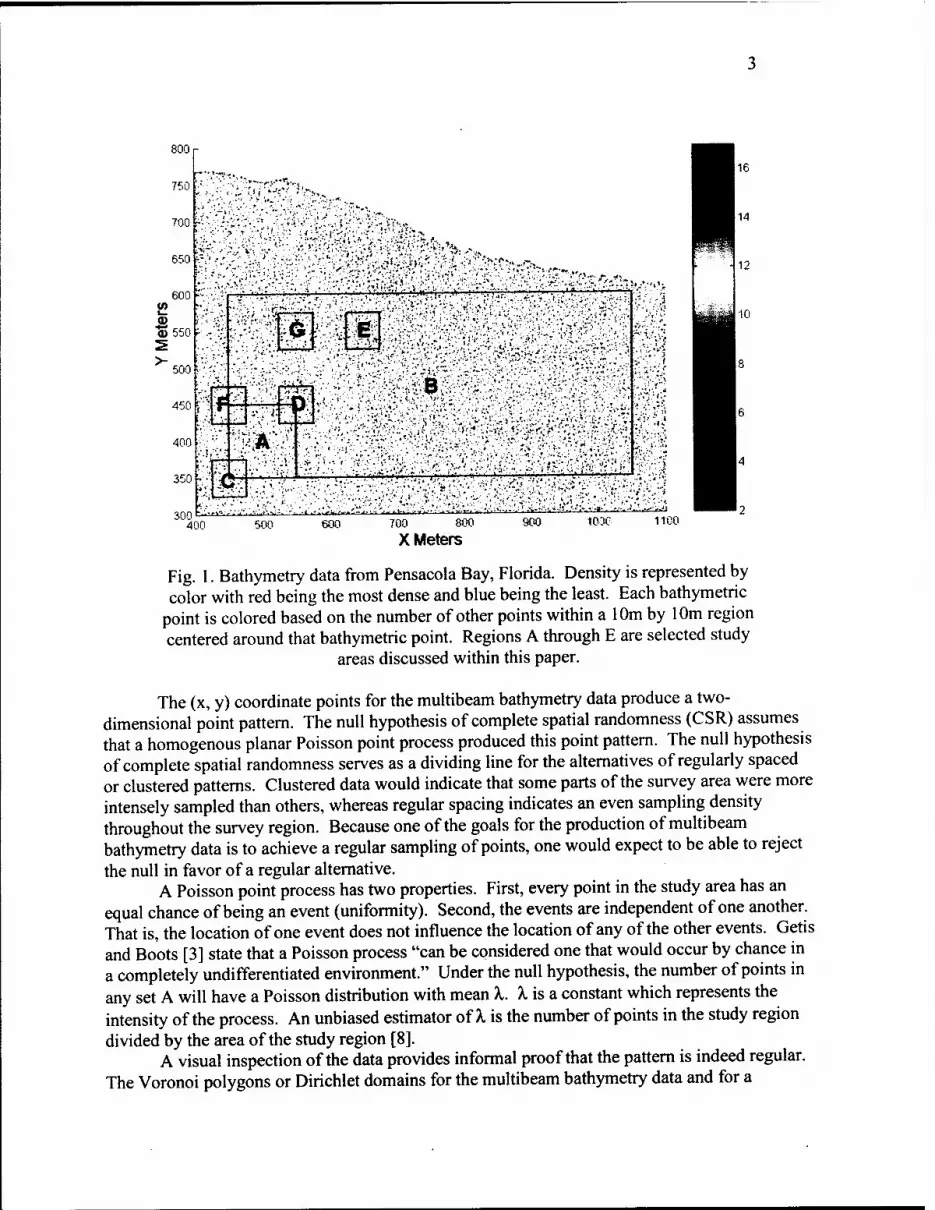
The dataset that is used to develop the parameterized model was obtained from Pensacola Bay, Florida. The data are not gridded and contain (x, y,z) coordinate points in meters. A plot of the entire data set can be seen in Fig. 1. The analysis done in this paper focused on interior regions of the dataset to avoid edge effects. This is a valid restriction in that terrain-based navigation systems should not be used on the edge of available bathymetry data.

800

750

:'. r-.--.y-V- 700 r-\y.:i'i':::-:'\<sii^y

650

600 V) l_

& ©550

500

450

400

350

•>.*.>■ :.-.;•-;~!-,v ;»^.-V .-'it.?'•;-.---i',if'"-^>r,^. „

'.i,-^

14

400 500 600 700 800 900 1030

;'--':J

700 800

X Meters

:.:','f''y * -,i ■'',..'J-V-ii

1100

Fig. 1. Bathymetry data from Pensacola Bay, Florida. Density is represented by color with red being the most dense and blue being the least. Each bathymetric

point is colored based on the number of other points within a 10m by 10m region centered around that bathymetric point. Regions A through E are selected study

areas discussed within this paper.

The (x, y) coordinate points for the multibeam bathymetry data produce a two- dimensional point pattern. The null hypothesis of complete spatial randomness (CSR) assumes that a homogenous planar Poisson point process produced this point pattern. The null hypothesis of complete spatial randomness serves as a dividing line for the alternatives of regularly spaced or clustered patterns. Clustered data would indicate that some parts of the survey area were more intensely sampled than others, whereas regular spacing indicates an even sampling density throughout the survey region. Because one of the goals for the production of multibeam bathymetry data is to achieve a regular sampling of points, one would expect to be able to reject the null in favor of a regular alternative.

A Poisson point process has two properties. First, every point in the study area has an equal chance of being an event (uniformity). Second, the events are independent of one another. That is, the location of one event does not influence the location of any of the other events. Getis and Boots [3] state that a Poisson process "can be considered one that would occur by chance in a completely undifferentiated environment." Under the null hypothesis, the number of points in any set A will have a Poisson distribution with mean X. X is a constant which represents the intensity of the process. An unbiased estimator of X. is the number of points in the study region divided by the area of the study region [8].

A visual inspection of the data provides informal proof that the pattern is indeed regular. The Voronoi polygons or Dirichlet domains for the multibeam bathymetry data and for a

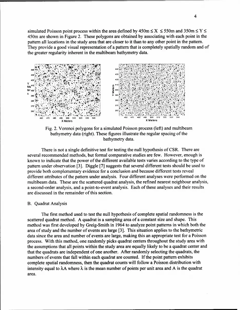
simulated Poisson point process within the area defined by 450m < X < 550m and 350m < Y < 450m are shown in Figure 2. These polygons are obtained by associating with each point in the pattern all locations in the study area that are closer to it than to any other point in the pattern. They provide a good visual representation of a pattern that is completely spatially random and of the greater regularity inherent in the multibeam bathymetry data.

440

430

420

'*<* '■*

• ■ i --».. »VV* "-■'■»

•"•.-äl-vrT.i V.!/ Y • • ■;'

.* '■':** , • - "•0V'»?:^ «k "<"'•; <-*"r:^i>i;",--«i

Me"0 UV *;

•'•'.'' '.^', teuoo V ;-*■;<# -' ■ / V i •!"*'• *.V "''--•." 5*^'". "V;.V:;Vl>.>*-J s

390 .•:•#:;'r.W - V :

■:■■■*:■■ ■ • ':»" ."-"■*■'.':' . r ".-'*.*:•."'■»■'V*fc' 380

370

360 ^.4 >/",":; .-*-:* ... A • . .!..• „•...i»,..u«t" -V»t.'. *•-.-i_iSJL^_i»: i_i

430

»-•-;-V'»::-N-it;.'f-.<.4-"--r. -■»-:,• \*;■-••'••• ■ fV' '• •'..'I

360 ; ':'.",'-v.vv-'i • ■■;•*}; fvv-.*v!,>-<.>.l:r:.i,.7

•l-üi!.'.*i-\l?;.'.t-Lr.,^iii«ir.iiVu-.lA'..tLr i•*.!■! 460 470 480 490 500 510 520 530 540 48° 470 "° 49° 50° 5,° 520 "° 540

X Meters x Meters

Fig. 2. Voronoi polygons for a simulated Poisson process (left) and multibeam bathymetry data (right). These figures illustrate the regular spacing of the

bathymetry data.

There is not a single definitive test for testing the null hypothesis of CSR. There are several recommended methods, but formal comparative studies are few. However, enough is known to indicate that the power of the different available tests varies according to the type of pattern under observation [3]. Diggle [7] suggests that several different tests should be used to provide both complementary evidence for a conclusion and because different tests reveal different attributes of the pattern under analysis. Four different analyses were performed on the multibeam data. These are the scattered quadrat analysis, the refined nearest neighbour analysis, a second-order analysis, and a point-to-event analysis. Each of these analyses and their results are discussed in the remainder of this section.

B. Quadrat Analysis

The first method used to test the null hypothesis of complete spatial randomness is the scattered quadrat method. A quadrat is a sampling area of a constant size and shape. This method was first developed by Greig-Smith in 1964 to analyze point patterns in which both the area of study and the number of events are large [3]. This situation applies to the bathymetric data since the area and number of events are large, making this an appropriate test for a Poisson process. With this method, one randomly picks quadrat centers throughout the study area with the assumptions that all points within the study area are equally likely to be a quadrat center and that the quadrats are independent of one another. After randomly selecting the quadrats, the numbers of events that fall within each quadrat are counted. If the point pattern exhibits complete spatial randomness, then the quadrat counts will follow a Poisson distribution with intensity equal to \A where A. is the mean number of points per unit area and A is the quadrat area.

Quadrats can be any geometric figure, but rectangles are used most often [3]. The choice of quadrat size is somewhat arbitrary. The quadrats should not be so small or so large that one is unable to observe variance in the quadrat counts. There are many suggestions for the appropriate quadrat size. Greig-Smith [9] suggests a quadrat size that provides a mean count of one. Another suggestion is to use square quadrats with the length of a side approximately equal to

2 * Study Area [3].

y Number of Events For the analysis of the multibeam data, 400 quadrat centers are randomly selected within

the region of 450m < X < 1050m and 350m < Y < 600m. This study area avoids quadrats that would extend beyond the sampled bathymetric region. The number of quadrats is selected to provide enough power to detect a departure from a Poisson process while not violating the assumption of independent quadrats. Square quadrats are used. Five separate tests were conducted with quadrat sizes varying from 9 square meters to 49 square meters. Pearson's %2

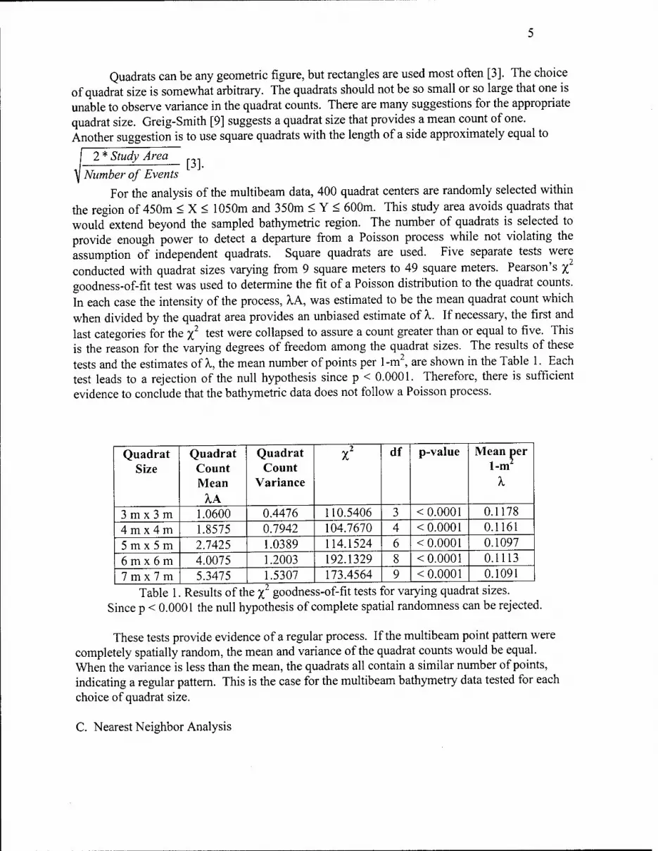
goodness-of-fit test was used to determine the fit of a Poisson distribution to the quadrat counts. In each case the intensity of the process, XA, was estimated to be the mean quadrat count which when divided by the quadrat area provides an unbiased estimate of X. If necessary, the first and last categories for the %2 test were collapsed to assure a count greater than or equal to five. This is the reason for the varying degrees of freedom among the quadrat sizes. The results of these tests and the estimates of X, the mean number of points per 1-m2, are shown in the Table 1. Each test leads to a rejection of the null hypothesis since p < 0.0001. Therefore, there is sufficient evidence to conclude that the bathymetric data does not follow a Poisson process.

Quadrat Size

Quadrat Count Mean

^A

Quadrat Count

Variance

x2 df p-value Mean per 1-m5

X

3 m x 3 m 1.0600 0.4476 110.5406 3 < 0.0001 0.1178

4 m x 4m 1.8575 0.7942 104.7670 4 < 0.0001 0.1161

5 m x 5 m 2.7425 1.0389 114.1524 6 < 0.0001 0.1097

6 m x 6 m 4.0075 1.2003 192.1329 8 < 0.0001 0.1113

7 m x 7 m 5.3475 1.5307 173.4564 9 < 0.0001 0.1091 Table 1. Results of the %2 goodness-of-fit tests for varying quadrat sizes.

Since p < 0.0001 the null hypothesis of complete spatial randomness can be rejected.

These tests provide evidence of a regular process. If the multibeam point pattern were completely spatially random, the mean and variance of the quadrat counts would be equal. When the variance is less than the mean, the quadrats all contain a similar number of points, indicating a regular pattern. This is the case for the multibeam bathymetry data tested for each choice of quadrat size.

C. Nearest Neighbor Analysis

The scattered quadrat test provides strong evidence that the multibeam bathymetry data are not spatially random but instead exhibit regularity of pattern. However, this test does not provide any information about the relationship of events to one another, where an event is the occurrence of a bathymetry point. Nearest neighbor analyses reaffirm that the multibeam data are regularly spaced and provide information on the average distance between events. A nearest neighbor distance for any event is the distance between that event and the nearest other event in the pattern. Two types of nearest neighbor analyses were conducted. The first type involves calculating the mean distance between events. This is used to reaffirm the rejection of the null hypothesis and to provide an estimate of the mean distance between events. The second type, known as refined nearest neighbor analysis, involves comparing the empirical cumulative distribution function (cdf) of all nearest neighbor distances within an area to the cdf expected under CSR. The refined nearest neighbor analysis is also used to reject the null hypothesis and provide an estimate of the inhibition distance. An inhibition distance is a radial distance surrounding an event in a regular point pattern in which it is unlikely to contain a second event.

The first type of nearest neighbor analysis that is done is to randomly select 100 bathymetric points from the study region of 450m < X < 550m and 350m < Y < 450m. This region contains 1114 bathymetric points. One hundred points are chosen to provide adequate power for the test while not violating the assumption of independence of nearest neighbor distances. Nearest neighbor distances as well as second and third nearest neighbor distances are found for the 100 randomly chosen bathymetric points. Second and third nearest neighbor distances are the distances from an event to the second and third nearest events, respectively. The empirical mean distances were calculated and compared to the expected means for the null hypothesis of CSR. Under the null hypothesis, the means of the nearest neighbor distances follow a normal distribution with £(^)and Var(d) as shown in Table 2. [3]. This provides a z

statistic for the null hypothesis of a Poisson process.

d 40 Var{d) z p-value

Nearest Neighbor 1.8944 m 1.4981 .0005504 16.8984 < 0.0001 2nd Nearest Neighbor 3.2961 m 2.2471 .0005971 42.9308 < 0.0001 3 rd Nearest Neighbor 4.5443 m 2.8089 .0006124 70.1294 < 0.0001

Table 2. Comparison of the empirical average nearest neighbor distances d to the expected value, E$) , and variance Varffi) of a CSR process. Since p < 0.0001 the

null hypothesis is rejected.

These tests reaffirm that the null hypothesis of CSR should be rejected. That the average distances, d , between events are greater than those that would be expected under a Poisson process, E(^), provides further evidence that the null should be rejected in favor of a regular alternative [3]. The 1st, 2nd and 3rd nearest neighbor average distances are progressively larger, providing an indication that the data are regularly spaced rather than being composed of regularly spaced clusters of points.

The refined nearest neighbor analysis is the second type of distance analysis that was done. This test involves comparing the cumulative distribution function of all the nearest neighbor distances within the study area with the expected cdf under CSR. Under CSR, the expected cdf is G(r) = 1 - exp(-/\.7tr2 ), r > 0, where r is the distance to the nearest neighbor.

N Lambda is once again defined as the intensity of the process and is estimated by — where N is

the number of points in the study area and A is the size of the study area. For this study area, A

X = 0.1114. The observed and expected cdf s are shown below.

1

0.9 -

i I 1 I

-

0.8 -

C 0 7 - O (

g06

O

a. 0.5

<D > f 04, - E 3 ü 03--

0 2 '•

0 1 >•

1

a 05 1.5 2 25 3 3.5 4 45 5

Distance to Nearest Neighbor (Meters)

Fig. 3. Observed and expected nearest neighbor cumulative distribution functions (cdf)- The blue curve shows the cdf for the multibeam bathymetry data. The pink curve shows the expected

cdf under CSR. The green curve shows the cdf of a simulated CSR process.

The blue cdf is that of the observed nearest neighbor distances for the multibeam bathymetry data in the study region. The pink is the expected cdf under the null hypothesis

A

generated by G(r) with intensity X. The green curve is from a simulated Poisson process of A

intensity X within a 100m by 100m area; simulated data was generated and then used to provide an empirical cdf of a Poisson process. That the observed cdf is less than the expected cdf is further evidence of a regular process [3]. Also, examination of the multibeam bathymetry cdf suggests an inhibition distance of approximately one-meter between points. This is suggested by the observation that the multibeam cdf lags until a radial distance of about one meter between events is reached. After this radial distance of about one meter between events is reached, the multibeam cdf begins to grow exponentially.

Figure 3. clearly shows an empirical difference between the cdf for the multibeam data and the cdf expected under the null hypothesis. A formal test is desired to determine when the observed and expected cdf s differ significantly. However, one cannot conduct the standard two- sample Kolmogorov-Smirnov test because the observed nearest neighbor distances are not mutually independent. Because of this, Diggle [6] suggested finding the maximum absolute horizontal distance between the empirical and expected curves, dr, and then conducting a Monte Carlo test. The Monte Carlo test is conducted by simulating 99 Poisson processes and measuring the maximum horizontal distances between the simulated cdf s and the expected cdf. The results

of the Monte Carlo test on the bathymetry data are shown in Fig. 4. This test provides further evidence that the null hypothesis should be rejected in favor of a regular alternative.

90,

The 99 Simulations of a Homogeneous Poisson Point Process

Max Absolute Difference for Real Data 0.2965

0 0.05 0.1 0.15 0.2 0.25 0.3 0.35

Maximum Absolute Difference in Observed and Expected CDF Fig. 4. Results of the Monte Carlo test. This test provides an indication of the degree to which the empirical cdf differs from the expected cdf. Note that all 99 simulation results cluster closely together with a maximum absolute distance of approximately 0.075. The real data are clearly different, as its maximum absolute difference is a factor of four larger than the simulated data.

D. Second-Order Analysis

Both the scattered quadrat analysis and the nearest neighbor analyses provide strong evidence that the multibeam bathymetry data are not completely spatially random but are instead the result of a regular point process. Since the bathymetry data are an exhaustive map of all the bathymetry points within the study area, second-order analysis can be performed as well. Second-order analysis is the study of inter-event distances, where the events are mapped points. Second-order analysis estimates the K-function. The K-function is closely related to the second- order intensity of a stationary isotropic process, and for this reason, is often called the reduced second moment measure [5]. The advantages of this type of analysis are that it reveals spatial information at all scales of pattern and the exact locations of all events are used in the estimation.

A

The K-function is derived as follows. Let F be the empirical cdf of distances from points A

in a study area A to distinct points in A or a guard area. The expected value of F (d) = the expected number of pairs of points, one in A and the second within d distance of the first. This can be shown to equal AA,2K(d) for d < d0, where K(d) is the aforementioned K function. A is the study area, d0 is the distance that does not allow d to go beyond the guard area, and X2 is

N(N-l) estimated by

A2 where N is the number of points within A. However, it is usual to

consider F (d) to be the sum of all ordered pairs of distinct points in A not more than d distance apart without allowing for a guard area. It can be shown that without the use of a guard area, an

1 is defined as the proportion

A A(Tk(x,y)) unbiased estimator of K is K (d) = —*-' . where

N2 k(x,y) within A of the circumference of the ball centered on x with boundary passing through y [3]. For

2 A 2 a Poisson process, E(K(d)) = 7td . For a regular process, K (d) will be less than 7cd , and for a 2 A

clustering process, it will be greater than Ttd . For simplification, the plot of K(d) for a Poisson

A \K(d) A

process can be linearized by the function L (d) = -i , making E( L (d)) = d. This V K

linearization also has the effect of stabilizing the variances [8]. A

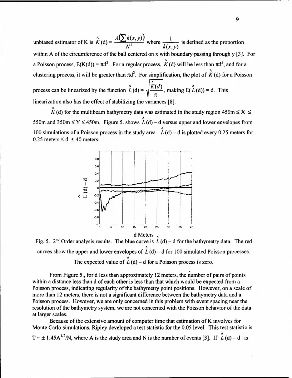
K (d) for the multibeam bathymetry data was estimated in the study region 450m < X < A

550m and 350m < Y < 450m. Figure 5. shows L (d) - d versus upper and lower envelopes from A

100 simulations of a Poisson process in the study area. L (d) - d is plotted every 0.25 meters for 0.25 meters < d < 40 meters.

l

< -J

1

08

06

0.4

02

0

-02

-04

-06

-0 8

-1

" ~r

i

10 15 30 35

,nd d Meters

Fig. 5. 2 Order analysis results. The blue curve is L (d) - d for the bathymetry data. The red A

curves show the upper and lower envelopes of L (d) - d for 100 simulated Poisson processes. A

The expected value of L (d) - d for a Poisson process is zero.

From Figure 5., for d less than approximately 12 meters, the number of pairs of points within a distance less than d of each other is less than that which would be expected from a Poisson process, indicating regularity of the bathymetry point positions. However, on a scale of more than 12 meters, there is not a significant difference between the bathymetry data and a Poisson process. However, we are only concerned in this problem with event spacing near the resolution of the bathymetry system, we are not concerned with the Poisson behavior of the data at larger scales.

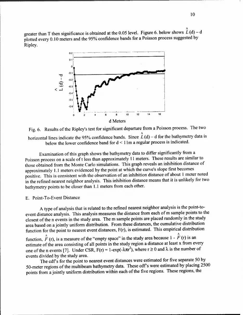
Because of the extensive amount of computer time that estimation of K involves for Monte Carlo simulations, Ripley developed a test statistic for the 0.05 level. This test statistic is

1/2 A

T = ± 1.45A /N, where A is the study area and N is the number of events [3]. If | L (d) - d | is

10

greater than T then significance is obtained at the 0.05 level. Figure 6. below shows L (d) - d plotted every 0.10 meters and the 95% confidence bands for a Poisson process suggested by Ripley.

02

0,

11,11

0 •

-0! T3

1

3 < J

-02

-0 3

•0.4

-0.5

•06 • _1 ^J

d Meters

Fig. 6. Results of the Ripley's test for significant departure from a Poisson process. The two A

horizontal lines indicate the 95% confidence bands. Since L (d) - d for the bathymetry data is below the lower confidence band for d < 1 lm a regular process is indicated.

Examination of this graph shows the bathymetry data to differ significantly from a Poisson process on a scale oft less than approximately 11 meters. These results are similar to those obtained from the Monte Carlo simulations. This graph reveals an inhibition distance of approximately 1.1 meters evidenced by the point at which the curve's slope first becomes positive. This is consistent with the observation of an inhibition distance of about 1 meter noted in the refined nearest neighbor analysis. This inhibition distance means that it is unlikely for two bathymetry points to be closer than 1.1 meters from each other.

E. Point-To-Event Distance

A type of analysis that is related to the refined nearest neighbor analysis is the point-to- event distance analysis. This analysis measures the distance from each of m sample points to the closest of the n events in the study area. The m sample points are placed randomly in the study area based on a jointly uniform distribution. From these distances, the cumulative distribution function for the point to nearest event distances, F(r), is estimated. This empirical distribution

A A

function, F (r), is a measure of the "empty space" in the study area because 1 - F (r) is an estimate of the area consisting of all points in the study region a distance at least x from every one of the n events [7]. Under CSR, F(r) = 1 -expC-toir2), where r > 0 and X is the number of events divided by the study area.

The cdf s for the point to nearest event distances were estimated for five separate 50 by 50-meter regions of the multibeam bathymetry data. These cdf s were estimated by placing 2500 points from a jointly uniform distribution within each of the five regions. These regions, the

11

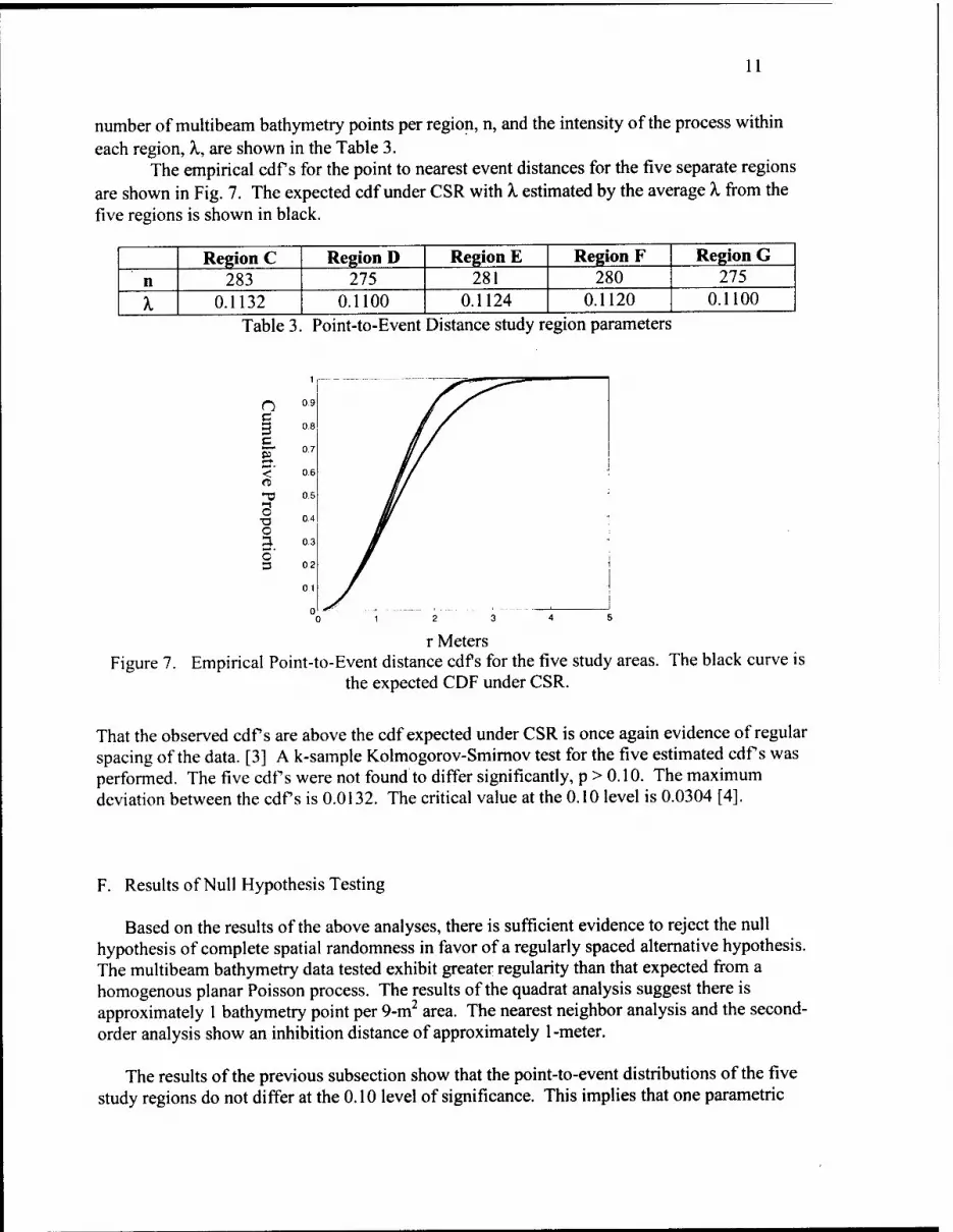
number of multibeam bathymetry points per region, n, and the intensity of the process within each region, X, are shown in the Table 3.

The empirical cdf s for the point to nearest event distances for the five separate regions are shown in Fig. 7. The expected cdf under CSR with A. estimated by the average X from the five regions is shown in black.

Region C Region D Region E Region F Region G n 283 275 281 280 275

X 0.1132 0.1100 0.1124 0.1120 0.1100 Table 3. Point-to-Event Distance study region parameters

o c 3 c 5* *—►

<' a

3 ■o o

o' 3

2 3

r Meters Figure 7. Empirical Point-to-Event distance cdf s for the five study areas. The black curve is

the expected CDF under CSR.

That the observed cdf s are above the cdf expected under CSR is once again evidence of regular spacing of the data. [3] A k-sample Kolmogorov-Smirnov test for the five estimated cdf s was performed. The five cdf s were not found to differ significantly, p > 0.10. The maximum deviation between the cdf s is 0.0132. The critical value at the 0.10 level is 0.0304 [4].

F. Results of Null Hypothesis Testing

Based on the results of the above analyses, there is sufficient evidence to reject the null hypothesis of complete spatial randomness in favor of a regularly spaced alternative hypothesis. The multibeam bathymetry data tested exhibit greater regularity than that expected from a homogenous planar Poisson process. The results of the quadrat analysis suggest there is approximately 1 bathymetry point per 9-m2 area. The nearest neighbor analysis and the second- order analysis show an inhibition distance of approximately 1-meter.

The results of the previous subsection show that the point-to-event distributions of the five study regions do not differ at the 0.10 level of significance. This implies that one parametric

12

model for the point-to-event distance could be used to fit the entire data set. The next section is concerned with the development of an appropriate model.

III. Parameterized Model Development

A parameterized model for the distribution of the point-to-event distances within the multibeam bathymetry data is needed to estimate the lower limit of the positioning error for the terrain-based navigation system being developed. The positioning error is a function of the density and spacing of the bathymetric data. A parameterized model will allow for the estimation of positioning error with confidence intervals. This parameterized distribution should have a lower limit of zero since there will be no negative distances from an arbitrary point to the closest bathymetric point. Transforming the data from linear distances to circular areas is logical because as one moves outward from an arbitrary point in search of the nearest event, one is moving outward along a radius that encloses a circular region around the point.

When the data are completely spatially random, the point-to-event distance distribution is exponential [5]. An exponential distribution is characterized by a constant hazard rate. That is, as one moves outward from an arbitrary point, the probability of encountering an event is the same for all radial distances. The multibeam data exhibits regularity and an inhibition distance, so a distribution with an increasing hazard rate is expected. As one moves outward from an arbitrary point in the multibeam data, the chance of encountering an event may be low at first if the arbitrary point is within the inhibition distance between two points. The observed regular spacing of the events ensures that as one moves out further and further along the radial line, the chance of encountering a multibeam bathymetry point increases.

The five empirical cdf s for the point-to-event distances that were estimated in Section 2 and shown in Fig. 7. are used to determine an appropriate parametric distribution. It is obviously desirable for one distributional type to be appropriate for the entire multibeam data set. The estimated parameters may change in different regions of the data, but the distributional type should not. The k-sample Kolmogorov-Smirnov test showed that these five distributions do not significantly differ at the 0.10 level lending support to the idea that one model could be found to fit throughout the data set.

The first step in determining an appropriate model is to select a group of potential models. As stated above, the distribution should have a lower bound of zero, and an increasing hazard rate is expected. Six standard survival distributions were selected as potential candidates: the generalized gamma, the exponential, the Weibull, the standard gamma, the log-normal, and the log-logistic distributions. Typically survival distributions are used to estimate the time-to- event. These distributions are appropriate because the radial distance-to-event can be thought of as allegorical to time-to-event. The procedure Proc Lifereg in SAS (Statistical Analysis System) was used to determine the log-likelihood for each of the distributional models in each of the five study regions. These log-likelihoods are shown in Table 4. Lower magnitudes correspond to better fits. In all areas assessed, the generalized gamma provides the best fit followed by the Weibull distribution.

Generalized Gamma Weibull Gamma

Region C -3511 -3516 -3528

Region D -3580 -3592 -3604

Region E -3485 -3513 -3534

Region F -3412 -3433 -3458

Region G -3549 -3576 -3594

13

Exponential -3578 -3638 -3583 -3525 -3630

Log-Logistic -3719 -3813 -3765 -3679 -3828

Log-Normal -3826 -3905 -3856 -3806 -3957

Table A L Estimated log-likelihood for each distribution type

The generalized gamma is a three parameter distribution involving the gamma function and the incomplete gamma function. The exponential, Weibull, standard gamma, and log- normal models are all special cases of the generalized gamma distribution. The third parameter of the generalized gamma allows its hazard function to take on a wide variety of shapes. The generalized gamma distribution will fit unless the hazard function has more than one peak [1]. If one of the simpler models can be shown to fit, the generalized gamma is not used for three main reasons. First, the pdf is complicated and the parameters are difficult to interpret. Second, the computer time to estimate the generalized gamma is significantly longer than for the simpler models, and third, the generalized gamma has a reputation for convergence problems [1]. For these reasons, the Weibull distribution was selected as the potential model.

The Weibull model is a slight modification of the exponential model, with the important consequence that the hazard rate is no longer constant. The Weibull cdf incorporating the transformation to radial areas is given by G(r) = l-exp(-?i(7tr2)Y), r > 0, X > 0, and y > 0. A. is a scale parameter and y is a shape parameter. When y < 1 the Weibull distribution has a decreasing hazard rate. When y = 1, the Weibull cdf reduces to the exponential. When 1< y < 2, the hazard rate is increasing at a decreasing rate. When y= 2, the hazard function is an increasing straight line with origin at zero. When y > 2, the hazard function is nonlinearly increasing [ 1 ]. For the

Weibull distribution given above, the expected value of r is given by E(r) 7C I -'Y

and the variance is given by Var(r) = i-l i

7C

Weibull distribution are given by E(rn)

r

l

i + - y)

-r2 i +

-Jn I-12"

V (

_1_ 2y

. The moments of the

. + 2y

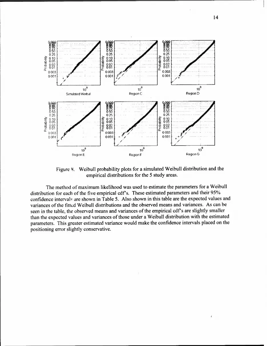
Weibull probability plots are shown in Fig. 8. The plots of the empirical distributions from the five study regions are shown, as well as the plot of a simulated Weibull distribution. The purpose of a Weibull probability plot is to graphically assess whether or not the data come from a Weibull distribution. If the data are Weibull the plot will be linear. Examination of the graphs reveals that while the fits are not ideal, they are nearly linear.

14

Red on F 10

Region G

Figure 8. Weibull probability plots for a simulated Weibull distribution and the empirical distributions for the 5 study areas.

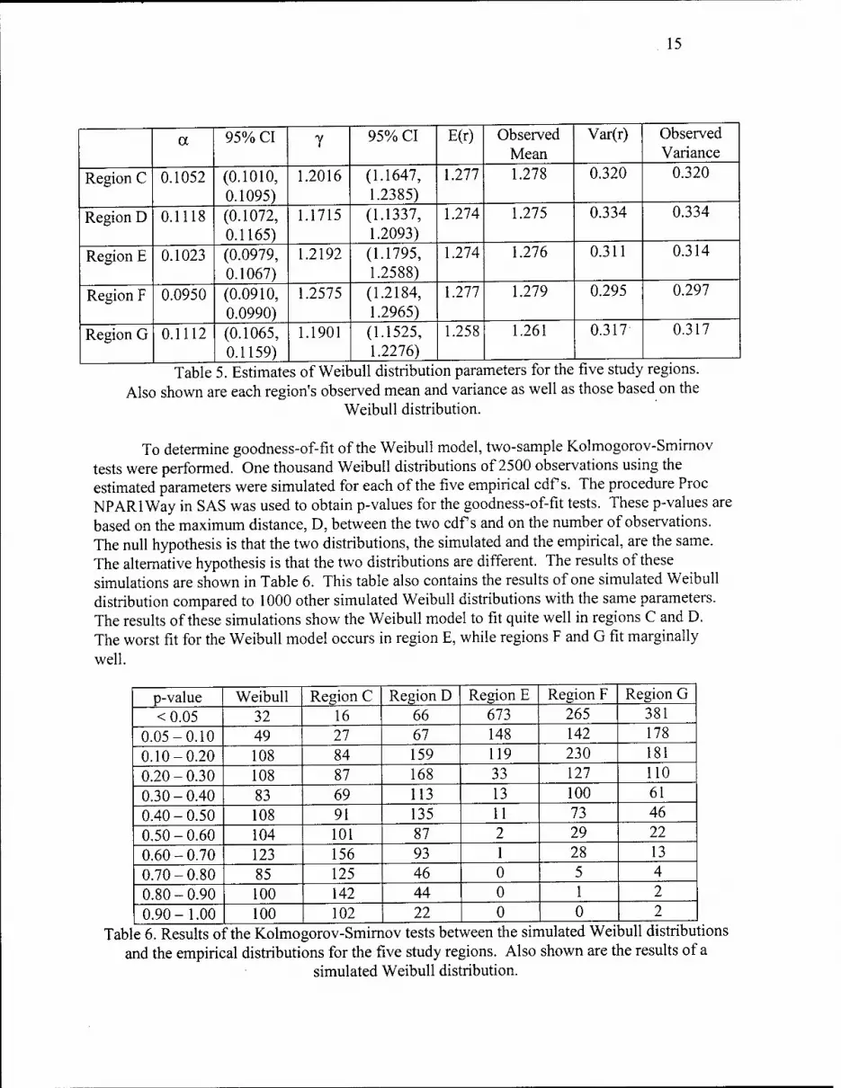
The method of maximum likelihood was used to estimate the parameters for a Weibull distribution for each of the five empirical cdf s. These estimated parameters and their 95% confidence intervals are shown in Table 5. Also shown in this table are the expected values and variances of the fitted Weibull distributions and the observed means and variances. As can be seen in the table, the observed means and variances of the empirical cdf s are slightly smaller than the expected values and variances of those under a Weibull distribution with the estimated parameters. This greater estimated variance would make the confidence intervals placed on the positioning error slightly conservative.

15

a 95% CI y 95% CI E(r) Observed Mean

Var(r) Observed Variance

Region C 0.1052 (0.1010, 0.1095)

1.2016 (1.1647, 1.2385)

1.277 1.278 0.320 0.320

Region D 0.1118 (0.1072, 0.1165)

1.1715 (1.1337, 1.2093)

1.274 1.275 0.334 0.334

Region E 0.1023 (0.0979, 0.1067)

1.2192 (1.1795, 1.2588)

1.274 1.276 0.311 0.314

Region F 0.0950 (0.0910, 0.0990)

1.2575 (1.2184, 1.2965)

1.277 1.279 0.295 0.297

Region G 0.1112 (0.1065, 0.1159)

1.1901 (1.1525, 1.2276)

1.258 1.261 0.317 0.317

Table 5. Estimates of Weibull distribution parameters for the five study regions. Also shown are each region's observed mean and variance as well as those based on the

Weibull distribution.

To determine goodness-of-fit of the Weibull model, two-sample Kolmogorov-Smirnov tests were performed. One thousand Weibull distributions of 2500 observations using the estimated parameters were simulated for each of the five empirical cdf s. The procedure Proc NPARlWay in SAS was used to obtain p-values for the goodness-of-fit tests. These p-values are based on the maximum distance, D, between the two cdf s and on the number of observations. The null hypothesis is that the two distributions, the simulated and the empirical, are the same. The alternative hypothesis is that the two distributions are different. The results of these simulations are shown in Table 6. This table also contains the results of one simulated Weibull distribution compared to 1000 other simulated Weibull distributions with the same parameters. The results of these simulations show the Weibull model to fit quite well in regions C and D. The worst fit for the Weibull model occurs in region E, while regions F and G fit marginally well.

p-value Weibull Region C Region D Region E Region F Region G

<0.05 32 16 66 673 265 381 0.05-0.10 49 27 67 148 142 178

0.10-0.20 108 84 159 119 230 181 0.20-0.30 108 87 168 33 127 110

0.30-0.40 83 69 113 13 100 61 0.40-0.50 108 91 135 11 73 46 0.50-0.60 104 101 87 2 29 22 0.60-0.70 123 156 93 1 28 13 0.70-0.80 85 125 46 0 5 4 0.80-0.90 100 142 44 0 1 2 0.90-1.00 100 102 22 0 0 2

e 6. Results o1 ■theKolmo gorov-Smirr lov tests bet ween the sin lulated Wei 3ull distribul and the empirical distributions for the five study regions. Also shown are the results of a

simulated Weibull distribution.

16

The minimum D, the maximum D, and the mean of D's, for each of the five regions and for the simulated Weibull is shown in Table 7. This table shows that region 3 had an average maximum deviation between the cdf s of 0.0425. This suggests that the fit may not be as bad as the simulations would have it appear and that the small p-values are due to the large sample sizes. The p-values show that in region 3, the distribution is not Weibull. However, the average maximum distance between the cdf s suggests that as a model the Weibull would not be a bad approximation.

Maximum D Minimum D Average D

Weibull 0.0464 0.0100 0.0242

Region C 0.0512 0.0108 0.0227

Region D 0.0600 0.0128 0.0274

Region E 0.0696 0.0212 0.0425

Region F 0.0676 0.0168 0.0339

Region G 0.0772 0.0136 0.0363

Table 7. Range of D values and average D value for the empirical cdf s versus the modeled cdf s. and for the simulated Weibull distribution.

IV. Conclusions and Future Work

For the multibeam data set studied, the null hypothesis of CSR can be rejected in favor of a regular alternative. The average density of the multibeam points is approximately 1 point per 9 square meters. There is an inhibition distance between events of about 1.1 meters. The Weibull distribution was found to provide an adequate model for the point-to-event distance distribution of the data set. The parameters for this model can be easily and reliably estimated, meeting the goals set forth in section 1. The Weibull model will be used to quantify the lower bound on the estimated position error for the terrain-based navigation system being developed.

Future work will involve two parts. First, the analysis of other multibeam data sets is needed to determine if the same regularity of pattern exists and to determine if the Weibull model can be generalized to these data sets. Second, regular point patterns will be simulated to determine for what type of regular patterns a Weibull model is appropriate.

Acknowledgments

This work was funded by the Office of Naval Research through the Naval Research Laboratory under Program Element 62435N.The mention of commercial products or the use of company names does not in any way imply endorsement by the U.S.Navy. Approved for public release; distribution is unlimited. NRL contribution number NRL/PP/7440-01-00XX.

References

[1] Allison, Paul D. (1995), Survival Analysis Using the SAS(R) System: A Practical Guide. Cary. NC: SAS Institute Inc. [2] Beckman, Richard, Martinez, Andrew, and Bourgeois, Brian (2000), "AUV Positioning

17

using Bathymetry Matching," Proceedings of the IEEE Oceans 2000 Conference, 11-15SEP00, Providence, RI. [3] Boots, Barry N., and Getis, Arthur (1988), Scientific Geography Series: Point Pattern Analysis, Vol. 8, Grant Ian Thrall, ed., Newbury Park: Sage Publications. [4] Conover, W. J., (1980), Practical Nonparametric Statistics, 2nd ed., New York: John Wiley and Sons. [5] Cressie, Noel A. (1991), Statistics For Spatial Data, New York: John Wiley and Sons. [6] Diggle, Peter J. (1979), "On Parameter Estimation and Goodness-of-Fit Testing for Spatial Point Patterns," Biometrics, 35, 87-101. [7] Diggle, Peter J. (1983), Statistical Analysis of Spatial Point Patterns, London: Academic Press Inc. [8] Ripley, Brian D. (1981), Spatial Statistics, New York: John Wiley and Sons. [9] Upton, G.; and Fingleton, B. (1985), Spatial Data Analysis by Example: Point Pattern and Quantitative Data, Vol. 1, Chichester: John Wiley and Sons.