spatiotemporal varying effects of built environment on taxi

International Journal of

Geo-Information

Article

Spatiotemporal Varying Effects of Built Environmenton Taxi and Ride-Hailing Ridership in New York City

Xinxin Zhang 1, Bo Huang 2,* and Shunzhi Zhu 1

1 College of Computer and Information Engineering, Xiamen University of Technology, Xiamen 361024, China;[email protected] (X.Z.); [email protected] (S.Z.)

2 Department of Geography and Resource Management and Institute of Space and Earth Information Science,The Chinese University of Hong Kong, Hong Kong 999077, China

* Correspondence: [email protected]

Received: 18 June 2020; Accepted: 27 July 2020; Published: 29 July 2020��

Abstract: The rapid growth of transportation network companies (TNCs) has reshaped the traditionaltaxi market in many modern cities around the world. This study aims to explore the spatiotemporalvariations of built environment on traditional taxis (TTs) and TNC. Considering the heterogeneity ofridership distribution in spatial and temporal aspects, we implemented a geographically andtemporally weighted regression (GTWR) model, which was improved by parallel computingtechnology, to efficiently evaluate the effects of local influencing factors on the monthly ridershipdistribution for both modes at each taxi zone. A case study was implemented in New York City(NYC) using 659 million pick-up points recorded by TT and TNC from 2015 to 2017. Fourteeninfluencing factors from four groups, including weather, land use, socioeconomic and transportation,are selected as independent variables. The modeling results show that the improved parallel-basedGTWR model can achieve better fitting results than the ordinary least squares (OLS) model, and itis more efficient for big datasets. The coefficients of the influencing variables further indicate thatTNC has become more convenient for passengers in snowy weather, while TT is more concentrated atthe locations close to public transportation. Moreover, the socioeconomic properties are the mostimportant factors that caused the difference of spatiotemporal patterns. For example, passengerswith higher education/income are more inclined to select TT in the western of NYC, while vehicleownership promotes the utility of TNC in the middle of NYC. These findings can provide scientificinsights and a basis for transportation departments and companies to make rational and effective useof existing resources.

Keywords: geographically and temporally weighted regression; taxi; Uber; spatiotemporal analysis

1. Introduction

With the popularity of mobile phone usage, transportation network companies (TNCs) that offerapp-based services, such as Uber, DiDi, and Lyft, claim to provide stability and convenience withpeer-to-peer (p2p) processes that connect passengers and private drivers on-line and in real-time [1].As an emerging form of transportation based on network and mobile technology, the analysis of TNCridership has become a hot topic in urban transportation research. Much evidence has shown thatthe rapid development of TNC has had a huge impact on the traditional taxi (TT), leading the taxiindustry to experience significant losses in terms of market share, revenue, labor power and facility [2].This is particularly obvious in large modern cities such as New York City (NYC), where the annual taxiload decreased from 145 million in 2015 to 113 million in 2017, decreasing nearly 23% in three years.In contrast, the ridership by TNCs increased from 37 million to 110 million. The reduction in themarket share of the taxi industry will inevitably cause a decline in the income of taxi drivers and the

ISPRS Int. J. Geo-Inf. 2020, 9, 475; doi:10.3390/ijgi9080475 www.mdpi.com/journal/ijgi

http://www.mdpi.com/journal/ijgi

http://www.mdpi.com

http://www.mdpi.com/2220-9964/9/8/475?type=check_update&version=1

http://dx.doi.org/10.3390/ijgi9080475

http://www.mdpi.com/journal/ijgi

ISPRS Int. J. Geo-Inf. 2020, 9, 475 2 of 23

compression of the taxi business scale, leading to economic difficulties and even the bankruptcy of taxicompanies. In May 2013, although the price of a yellow car’s license plate in NYC had been cut in half,the licenses of many taxi company vehicles were idle because of the lack of new drivers [3].

Nevertheless, many researchers insist that it is premature to announce the inevitable demise of thetaxi industry based on the current success of TNC. For example, Wang et al. reported that the successof TNCs lies in an aggressive but unsustainable price subsidy strategy [4]. Cramer and Krueger’sstudy [5] observed that most trips on TNC are concentrated in daily traffic peak periods. Regardingoff-peak periods, traditional taxis still account for a large proportion of transportation and thus cannotbe replaced. Furthermore, according to the statistical results from [6], the average number of workinghours per week of Uber drivers was approximately half that of many taxi drivers in the U.S.

Regardless of these debates, it is indisputable that the taxi industry is currently facing a hugechallenge and competition from the TNC in many aspects. Therefore, analysis of the differentiation ofthese two modes, such as the characteristics of the target passengers and travel pattern, is conduciveto a better understanding of the competitive relationships between them. However, as all thesedifferentiations are not uniform within a city and are driven by diverse factors, the widely used globalstatistical models are limited to incorporate the significance of spatiotemporal heterogeneity andautocorrelation. The spatiotemporal analysis between taxi/TNC ridership and the built environment isstill an open issue.

This paper presents the results of our research utilizing an improved GTWR model based onparallel computation to efficiently explore the spatiotemporal relationships between TT/TNC and thebuilt environment in NYC, where about 659 million trips occurred from 2015 to 2017. The rest ofthis paper is arranged as follows. Section 2 provides a brief review of the relevant research progress,and Section 3 presents the details of the parallel-based GTWR model adopted in this study. Section 4introduces the related dataset and describes how the data were processed. Section 5 mainly analyzesthe model accuracy and findings. Section 6 discusses the spatiotemporal patterns between taxi andTNC. The last section elaborates upon the conclusions of this paper, as well as future research directions.

2. Related Literature

Taxis have historically comprised a far lower share and geographical coverage of urbantransportation than other transport modes, such as buses and subways; therefore, there are manylesser extensive studies on taxis than on other transport modes. In general, researchers have foundtaxis to be both complements and substitutes for public transit [2]. Despite their small share in urbantransportation, taxis fill a critical gap by providing mobility service and all-day operation, whichare not available in other transportation modes. More importantly, with the popularization of GPSauto-collection devices, the spatiotemporal characteristics of ridership and trajectory by taxis provide avaluable reference for mining the travel patterns of citizens and for traffic optimization [7]. Therefore,the spatiotemporal analysis of taxis has become a research hotspot in recent years.

Early research on taxis mainly focused on market demand components based on the inherentattributes of the taxi industry, such as price, tips, labor costs, and other factors [8]. Because themeasurement of cost, waiting time, and convenience is usually derived from investigations or relevantdepartments, those data are biased and lack objectivity. With the GPS devices carried by taxis,the spatiotemporal data of taxis can be tracked and collected in real-time. These data have theadvantage of spatial-temporal characteristics than previous data and can integrate with externalgeographic factors, such as land use [9] and weather [10,11]. For example, Liu et al. used GPS dataof taxi and urban land use factors to identify ‘source-sink areas’ in Shanghai [12]. Nevertheless,previous studies mostly adopted the ordinary least squares (OLS) method [13,14]. In the OLS model,the aggregated pickup (PU) and drop-off (DO) locations of taxis are used as dependent variables,and the relevant influencing factors, such as weather and land use, are selected as independent variables.Given spatial autocorrelation and heterogeneity exists in the distribution of PU and DO locations for


TT and TNC, the precondition of the OLS model that the observations should be independent of eachother is difficult to satisfy.

To address this issue, Fotheringham et al. proposed a local regression model called GeographicallyWeighted Regression (GWR) [15], which improves the accuracy of regression results by constructing alocal spatial weight matrix for estimating variation in space. Furthermore, the GWR model extends thetraditional regression framework by allowing parameter estimates to vary in space and is thereforecapable to capture local effects. The GWR model has been widely applied in transit ridershipanalysis [16,17]. For example, based on NYC’s taxi data, Qian et al. [18] used the GWR model toanalyze the relationship between taxi locations and urban environmental factors. The results showthat the GWR model can provide better model accuracy and interpretation than the OLS model.One of the remaining problems is that the GWR model only obtains related variable coefficients in thespatial dimension. While dealing with time series datasets, those data often need to be aggregated orseparated based on their timestamps, thereby ignoring the fact that the distribution of taxis or TNCsvaries with different scales of time. Recently, scholars have put forward many improved strategies toaccount for both temporal and spatial variability, such as the GWR-TS [19] and linear mixed effect(LME) + GWR models [20]; still, these models are generally based on the two-stage least squaresregression [21], first fitting the temporal effect using the LME model and then evaluating the spatialheterogeneity effects with the GWR model. Those models cannot simultaneously consider temporaland spatial effects.

To simultaneously model temporal and spatial effects, Huang et al. proposed an improvedGWR-based model, named Geographical and Temporal Weighted Regression (GTWR) [22], which isthought to design simultaneous spatial and temporal weighting. Thus, the GTWR model can reflectcontinuous variations for each location at each time. The initial implementation of the GTWR modelwas carried out for house-price estimation, and the results showed that the accuracy of the GTWRmodel was superior to that of the OLS and GWR models. Recently, the GTWR model has been extendedin many fields, such as air quality [23] and environmental research [24]. Moreover, some scholars haveput forward improved GTWR schemes successively. For example, Wu et al. proposed an improvedmodel, known as the Geographically and Temporally Weighted Autoregressive (GTWAR) model,to estimate spatial autocorrelations [25], and Du et al. proposed a Geographically and circle-TemporallyWeighted regression (GcTWR) model for enhancing the seasonal cycle of long-term observed data [26].

The above research fully shows that the GTWR model has great advantages in spatiotemporalmodeling. Ma et al. applied the GTWR model to public transit and achieved good modelingresults [27]. Zhang et al. also adopted the GTWR model to taxi ridership analysis and achieveda similar conclusion [28]. Nevertheless, due to the fact that the spatiotemporal nonstationarity oftaxis is more complicated than other modes of transit such as buses that have preset routes, previousstudies have generally been limited to taxis or TNC separately, and few studies take into considerationthe difference between taxis and TNC. Research on TNC remains relatively scarce, although its datastructure is similar to that of taxis. Thus, applying the GTWR model for simultaneous analysis of bothtaxis and TNC is still an unsolved issue.

3. Methodology

In this section, we briefly review the basic framework for the GTWR model and how to determinethe parameters of the GTWR model. Then, we propose a parallel computing scheme to improve theefficiency of the GTWR model and apply the model to ridership modeling.

3.1. The Basic Framework of the GTWR Model

The GWR-based model is a local-based spatially varying coefficient regression algorithm thatextends the OLS model by adopting local parameters to be estimated. It is capable of significantlyimproving the estimation accuracy of spatial data, especially for those areas with complex spatialnonstationarity. On this foundation, Huang et al. [22] proposed a GTWR model focusing on


spatiotemporal kernel function definition and spatiotemporal bandwidth optimization, which cansimultaneously address spatial and temporal nonstationarity issues. Assuming that the observation oftaxi ridership is denoted as Yi, where i (I = 1, 2, . . . , n) represents a spatial unit, such as traffic analysiszone (TAZ), thus the GTWR model can be mathematically expressed as follows:

Yi = β0(ui, vi, ti) +∑

k

βk(ui, vi, ti)Xki + εi, (1)

where (ui, vi, ti) represents the center coordinates of TAZ i in a spatial location (ui, vi) at time ti; β0 is theintercept value; βk(ui, vi, ti) denotes the slope for each independent variable Xki; and εi is the randomerror. The variables Xki refer to the influencing factors that improve the associations between ridershipand urban environmental factors, such as weather, land use, socioeconomic, and transport condition.

For a given dataset, a locally weighted least squares method is usually employed to estimate theintercept of β0, as well as the slopes βk for each variable. The GTWR models assume that the closer topoint i in the space-time coordinate system, the greater the weight of the measurements in predictingβk will be. Thus, the coefficients of β̂ = (β0, β1, .., βk)

T can be estimated by:

β̂(ui, vi, ti) = [XTW(ui, vi, ti)X]−1

XTW(ui, vi, ti)Y, (2)

where X is the n×(k+1) matrix of input variables. Y is the n-dimensional vector of the output variables.The space-time weight matrix W(ui, vi, ti) is an n × n weighting matrix to measure the importanceof point i to the estimated point j for both space and time. The Gaussian function is one of the mostcommonly used weight function:

Wi j = exp(−di j

2

h2 ), (3)

where di j denotes a spatiotemporal distance between points i and j, and h is a nonnegative parameterthat presents a decay of influence with distance. By combining the temporal distance dT with thespatial distance dS, the spatiotemporal distance can be expressed as:

dST = ds⊗ dT, (4)

where ‘⊗’ can represent different types of operators. In this study, the ‘+’ as the combination operatorwas selected to calculate the total spatiotemporal distance. With respect to the different scale effectsof space and time, an ellipsoidal coordinate system was constructed to measure the spatiotemporaldistance between each regressive point and the surrounding points [29]. The spatiotemporal distancebetween taxi ridership can thus be expressed as the linear weighting combination indicated below:

(dSTij )

2= λ[(ui − u j)

2 + (vi − v j)2] + µ(ti − t j)

2, (5)

where ti and t j denote the observed time of point i and j. λ and µ are the weights for balancing theinfluences of differing units between space and time variability. The weight matrix is constructed byusing the Gaussian distance decay-based functions and Euclidean distance:

Wi j = exp[−(dST

ij )2

hST2 ]

= exp{−[(ui−u j)

2+(vi−v j)2]+τ(ti−t j)

2

hs2 }

(6)

where the parameter τ stands for the non-negative parameter of scale factor calculated byµ/λ (λ, 0). hSTis a positive parameter named the spatiotemporal bandwidth. Thus, if the spatiotemporal bandwidthand scale factor are determined, the weight matrix W(ui, vi, ti) and β̂(ui, vi, ti) can be obtained.


The adjustment parameters of hST and τ can be acquired either utilizing a cross-validation (CV)process via minimization in terms of the corrected Akaike information criterion (AICc) [30] as follows:

CVRSS(h) =∑

i

[yi − y,1(h)]2, (7)

AICc(h) = n log(RSS(h)

n)+nlog(2π)+n(

n + tr(H(h))n− 2− tr(H(h))

), (8)

where y,1(hs) indicates the predicted value yi from the GTWR model with a bandwidth of h. Therefore,the selection of the optimum h can be acquired through plotting CV(h) against the parameter h.In Equation (8), RSS is the residual sum of squares, and tr(H(h)) is the trace of the hat matrix H(h).

3.2. Implementation of GTWR for Ridership Analysis

Figure 1 presents a flowchart of the implementation using GTWR for ridership analysis. Beforeconstructing the GTWR model for taxi ridership analysis, the observed spatial unit and temporalresolution must be determined first. The spatial unit is generally related to the geographic extent of thestudy area, which can be divided by administrative regions or a regular cell. Due to the limitationof TNC data obtained from NYC, the spatial unit adopted in this study was based on TAZ ratherthan Zip Code Tabulation Areas (ZCTA). In terms of the temporal resolution, different resolutions,such as yearly, monthly, daily, and hourly scales, can be adopted. Since the dataset we adopted wasfrom 2015 to 2017, the month was considered an appropriate minimum unit of time to reduce thecost of computation. Using the same dataset, the OLS and GTWR models were respectively appliedto estimating the globe and local coefficients for both modes and their relationship with the urbanarchitecture environment.ISPRS Int. J. Geo-Inf. 2020, 9, x FOR PEER REVIEW 6 of 24

Figure 1. The flowchart of the implementation using GTWR for ridership analysis.

To quantitatively evaluate the spatiotemporal variation of ridership for taxis and TNC, three variables, including the ridership for two types of TT (yellow + green), the ridership of TNC and the proportion of TNC (PoT = TNC/(TT+TNC)), were selected as dependent variables. With respect to independent variables, we extracted four groups of explanatory variables from multiple open datasets. More details about raw data processing can be found in Section 4.

Several aspects need to be adjusted when applying the GTWR model to taxi ridership analysis. Firstly, compared with the fixed kernel function, the adaptive kernel function can adjust bandwidths according to the density of data points. Thus, it might be a more reasonable way to obtain the weights

ijW for the irregular sharp of TAZs. For simplicity, we use the q-nearest neighbors based on the

following modified bi-square function:

2 2[1 ( / ) ] , if <0, otherwise

ij i ij iij

d h d hW

, (9)

where ih stands for the different bandwidths, which express the q nearest neighbors to consider in the estimation of regression at location i. Thus, the adjustment parameter of fixed bandwidth hST is replaced with the number of nearest neighborhood points q. Note that the q should be constrained to q ≥ 40, otherwise the model will suffer over-fitting problem [25].

The computation of the GTWR model is intensive because each sample uses an adaptive type of bandwidth, which leads to (t*(n − 1)n) combinations of possible values that must be computed for the optimal bandwidth [15]. The computing time will exponentially increase as the number of samples and timestamps increases by, for example, using grid-based data as the spatial unit or constructing the daily GTWR model based on several years of data. An optimized modeling approach is needed to reduce computation consumption. In particular, we employed parallel computing to break down

Figure 1. The flowchart of the implementation using GTWR for ridership analysis.


To quantitatively evaluate the spatiotemporal variation of ridership for taxis and TNC,three variables, including the ridership for two types of TT (yellow + green), the ridership ofTNC and the proportion of TNC (PoT = TNC/(TT+TNC)), were selected as dependent variables. Withrespect to independent variables, we extracted four groups of explanatory variables from multipleopen datasets. More details about raw data processing can be found in Section 4.

Several aspects need to be adjusted when applying the GTWR model to taxi ridership analysis.Firstly, compared with the fixed kernel function, the adaptive kernel function can adjust bandwidthsaccording to the density of data points. Thus, it might be a more reasonable way to obtain the weightsWi j for the irregular sharp of TAZs. For simplicity, we use the q-nearest neighbors based on thefollowing modified bi-square function:

Wi j =

[1− (di j/hi)2]

2, if di j < hi

0, otherwise, (9)

where hi stands for the different bandwidths, which express the q nearest neighbors to consider inthe estimation of regression at location i. Thus, the adjustment parameter of fixed bandwidth hST isreplaced with the number of nearest neighborhood points q. Note that the q should be constrained toq ≥ 40, otherwise the model will suffer over-fitting problem [25].

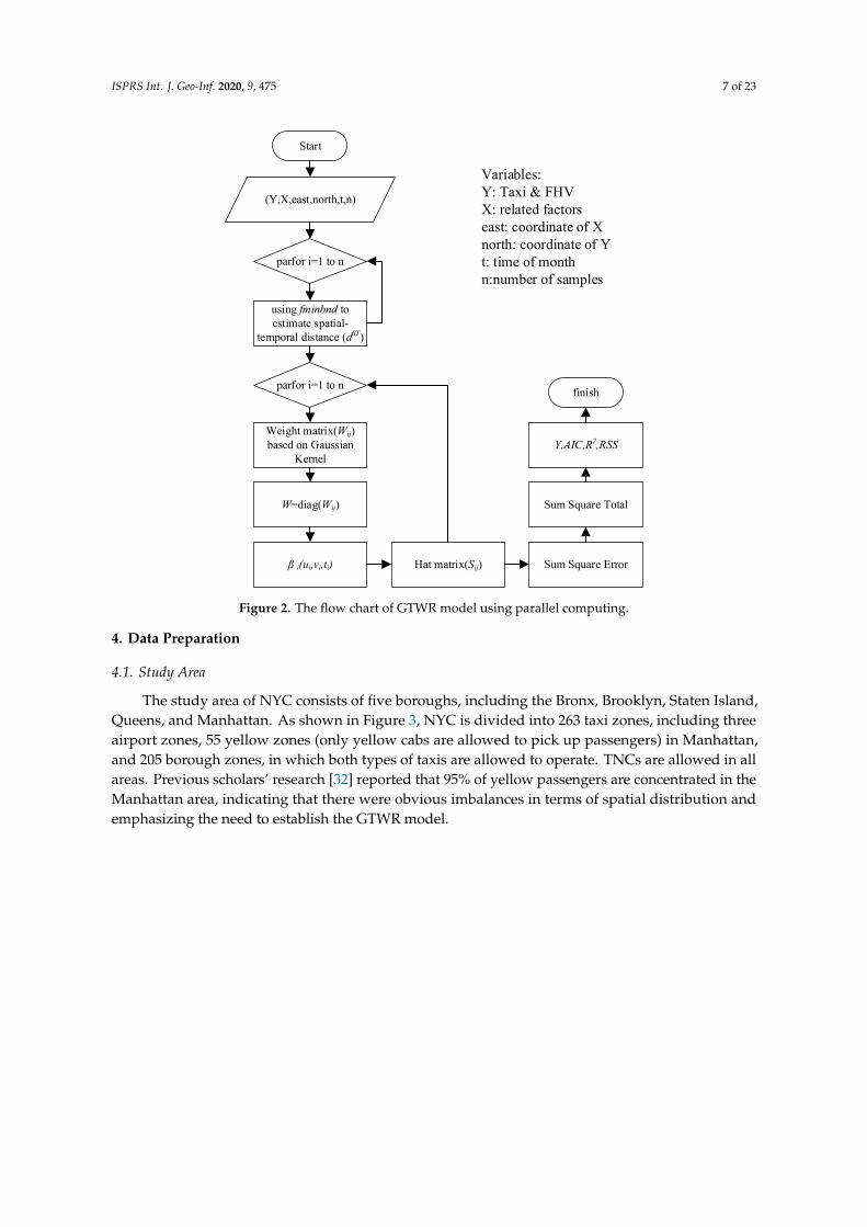
The computation of the GTWR model is intensive because each sample uses an adaptive type ofbandwidth, which leads to (t*(n − 1)n) combinations of possible values that must be computed for theoptimal bandwidth [15]. The computing time will exponentially increase as the number of samplesand timestamps increases by, for example, using grid-based data as the spatial unit or constructingthe daily GTWR model based on several years of data. An optimized modeling approach is neededto reduce computation consumption. In particular, we employed parallel computing to break downthe computational loops of optimal parameter selection into independent parts with different valuesof q and τ. These parts can be executed simultaneously by multiple processors communicating viashared memory, the results of which are combined upon completion as part of the overall algorithm.Thus, the optimal values of q and τ could be efficient found. According to the principle of GTWR,the main computing power is consumed by iteration for obtaining both adjustment parameters.Since the process of finding the optimal adjustment parameters is independent for each iteration,it is suitable for parallel programming. The GTWR algorithm adopted in this study is programmedbased on Matlab®, which provides a function called fminbnd for obtaining the optimal value q andτ. The process of parallel computing can be realized through a loop process, namely parfor [31].The platform for efficiency comparison is based on an Inter® i7-4790 CPU, which has four cores forparallel computing. Figure 2 shows the flow chart of GTWR model using parallel computing. To verifythe robustness of the results, different proportions of training samples were randomly selected for theGTWR model, while the remaining samples were used for verification.


ISPRS Int. J. Geo-Inf. 2020, 9, x FOR PEER REVIEW 7 of 24

the computational loops of optimal parameter selection into independent parts with different values of q and τ. These parts can be executed simultaneously by multiple processors communicating via shared memory, the results of which are combined upon completion as part of the overall algorithm. Thus, the optimal values of q and τ could be efficient found. According to the principle of GTWR, the main computing power is consumed by iteration for obtaining both adjustment parameters. Since the process of finding the optimal adjustment parameters is independent for each iteration, it is suitable for parallel programming. The GTWR algorithm adopted in this study is programmed based on Matlab®, which provides a function called fminbnd for obtaining the optimal value q and τ. The process of parallel computing can be realized through a loop process, namely parfor [31]. The platform for efficiency comparison is based on an Inter® i7-4790 CPU, which has four cores for parallel computing. Figure 2 shows the flow chart of GTWR model using parallel computing. To verify the robustness of the results, different proportions of training samples were randomly selected for the GTWR model, while the remaining samples were used for verification.

Start

(Y,X,east,north,t,n)

using fminbnd to estimate spatial-

temporal distance (dST)

parfor i=1 to n

parfor i=1 to n

Weight matrix(Wij) based on Gaussian

Kernel

W=diag(Wij)

β i(ui,vi,ti) Hat matrix(Sij) Sum Square Error

Sum Square Total

Y,AIC,R2,RSS

finish

Variables:Y: Taxi & FHVX: related factorseast: coordinate of Xnorth: coordinate of Yt: time of monthn:number of samples

Figure 2. The flow chart of GTWR model using parallel computing.

4. Data Preparation

4.1. Study Area

The study area of NYC consists of five boroughs, including the Bronx, Brooklyn, Staten Island, Queens, and Manhattan. As shown in Figure 3, NYC is divided into 263 taxi zones, including three airport zones, 55 yellow zones (only yellow cabs are allowed to pick up passengers) in Manhattan, and 205 borough zones, in which both types of taxis are allowed to operate. TNCs are allowed in all areas. Previous scholars’ research [32] reported that 95% of yellow passengers are concentrated in the Manhattan area, indicating that there were obvious imbalances in terms of spatial distribution and emphasizing the need to establish the GTWR model.

Figure 2. The flow chart of GTWR model using parallel computing.

4. Data Preparation

4.1. Study Area

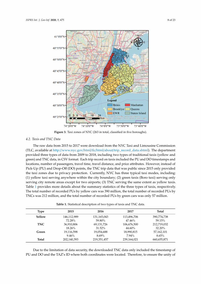
The study area of NYC consists of five boroughs, including the Bronx, Brooklyn, Staten Island,Queens, and Manhattan. As shown in Figure 3, NYC is divided into 263 taxi zones, including threeairport zones, 55 yellow zones (only yellow cabs are allowed to pick up passengers) in Manhattan,and 205 borough zones, in which both types of taxis are allowed to operate. TNCs are allowed in allareas. Previous scholars’ research [32] reported that 95% of yellow passengers are concentrated in theManhattan area, indicating that there were obvious imbalances in terms of spatial distribution andemphasizing the need to establish the GTWR model.

ISPRS Int. J. Geo-Inf. 2020, 9, 475 8 of 23ISPRS Int. J. Geo-Inf. 2020, 9, x FOR PEER REVIEW 8 of 24

Figure 3. Taxi zones of NYC (263 in total, classified in five boroughs).

4.2. Taxis and TNC Data

The raw data from 2015 to 2017 were download from the NYC Taxi and Limousine Commission (TLC, available at http://www.nyc.gov/html/tlc/html/about/trip_record_data.shtml). The department provided three types of data from 2009 to 2018, including two types of traditional taxis (yellow and green) and TNC data, in CSV format. Each trip record on taxis included the PU and DO timestamps and locations, number of passengers, travel time, travel distance, and price attributes. However, instead of Pick-Up (PU) and Drop-Off (DO) points, the TNC trip data that was public since 2015 only provided the taxi zones due to privacy protection. Currently, NYC has three typical taxi modes, including: (1) yellow taxi serving anywhere within the city boundary; (2) green taxis (Boro taxi) serving only serving city remote areas except for two airports; (3) TNC serving the same extent as yellow taxis. Table 1 provides more details about the summary statistics of the three types of taxis, respectively. The total number of recorded PUs by yellow cars was 390 million, the total number of recorded PUs by TNCs was 212 million, and the total number of recorded PUs by green cars was only 57 million.

Table 1. Statistical description of two types of taxis and TNC data.

Type 2015 2016 2017 Total Yellow 146,112,989 131,165,043 113,496,706 390,774,738

72.28% 59.80% 47.46% 59.15% TNC 36,910,806 69,131,726 106,676,500 212,719,032

18.26% 31.52% 44.60% 32.20% Green 19,116,598 19,054,688 18,990,815 57,162,101

9.46% 8.69% 7.94% 8.65% Total 202,140,393 219,351,457 239,164,021 660,655,871

Figure 3. Taxi zones of NYC (263 in total, classified in five boroughs).

4.2. Taxis and TNC Data

The raw data from 2015 to 2017 were download from the NYC Taxi and Limousine Commission(TLC, available at http://www.nyc.gov/html/tlc/html/about/trip_record_data.shtml). The departmentprovided three types of data from 2009 to 2018, including two types of traditional taxis (yellow andgreen) and TNC data, in CSV format. Each trip record on taxis included the PU and DO timestamps andlocations, number of passengers, travel time, travel distance, and price attributes. However, instead ofPick-Up (PU) and Drop-Off (DO) points, the TNC trip data that was public since 2015 only providedthe taxi zones due to privacy protection. Currently, NYC has three typical taxi modes, including:(1) yellow taxi serving anywhere within the city boundary; (2) green taxis (Boro taxi) serving onlyserving city remote areas except for two airports; (3) TNC serving the same extent as yellow taxis.Table 1 provides more details about the summary statistics of the three types of taxis, respectively.The total number of recorded PUs by yellow cars was 390 million, the total number of recorded PUs byTNCs was 212 million, and the total number of recorded PUs by green cars was only 57 million.

Table 1. Statistical description of two types of taxis and TNC data.

Type 2015 2016 2017 Total

Yellow 146,112,989 131,165,043 113,496,706 390,774,73872.28% 59.80% 47.46% 59.15%

TNC 36,910,806 69,131,726 106,676,500 212,719,03218.26% 31.52% 44.60% 32.20%

Green 19,116,598 19,054,688 18,990,815 57,162,1019.46% 8.69% 7.94% 8.65%

Total 202,140,393 219,351,457 239,164,021 660,655,871

Due to the limitation of data security, the downloaded TNC data only included the timestamp ofPU and DO and the TAZ’s ID where both coordinates were located. Therefore, to ensure the unity of

http://www.nyc.gov/html/tlc/html/about/trip_record_data.shtml


spatial reference, the taxi zone defined by TLC was adopted as the basic spatial unit, and number ofmonths was selected as the temporal unit.

After determining the spatiotemporal unit, i.e., each observation represented the total numberof ridership at one taxi zone in a certain month, the dependent variables of monthly ridership werederived based on the spatial and temporal aggregations of each trip. First, the raw data were importedinto the PostGIS spatial database. The data cleansing process was employed to exclude unavailabledata (such as missing coordinates and missing timestamps). Then, all PU geolocations or taxi zone IDwere aggregated into 263 TAZs. Second, we count trips in the same month as monthly ridership forevery TAZ.

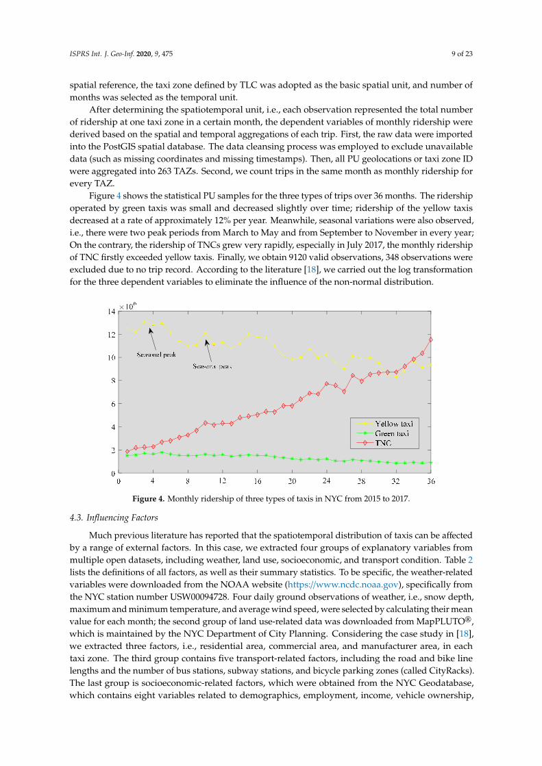
Figure 4 shows the statistical PU samples for the three types of trips over 36 months. The ridershipoperated by green taxis was small and decreased slightly over time; ridership of the yellow taxisdecreased at a rate of approximately 12% per year. Meanwhile, seasonal variations were also observed,i.e., there were two peak periods from March to May and from September to November in every year;On the contrary, the ridership of TNCs grew very rapidly, especially in July 2017, the monthly ridershipof TNC firstly exceeded yellow taxis. Finally, we obtain 9120 valid observations, 348 observations wereexcluded due to no trip record. According to the literature [18], we carried out the log transformationfor the three dependent variables to eliminate the influence of the non-normal distribution.


Due to the limitation of data security, the downloaded TNC data only included the timestamp of PU and DO and the TAZ’s ID where both coordinates were located. Therefore, to ensure the unity of spatial reference, the taxi zone defined by TLC was adopted as the basic spatial unit, and number of months was selected as the temporal unit.

After determining the spatiotemporal unit, i.e., each observation represented the total number of ridership at one taxi zone in a certain month, the dependent variables of monthly ridership were derived based on the spatial and temporal aggregations of each trip. First, the raw data were imported into the PostGIS spatial database. The data cleansing process was employed to exclude unavailable data (such as missing coordinates and missing timestamps). Then, all PU geolocations or taxi zone ID were aggregated into 263 TAZs. Second, we count trips in the same month as monthly ridership for every TAZ.

Figure 4 shows the statistical PU samples for the three types of trips over 36 months. The ridership operated by green taxis was small and decreased slightly over time; ridership of the yellow taxis decreased at a rate of approximately 12% per year. Meanwhile, seasonal variations were also observed, i.e., there were two peak periods from March to May and from September to November in every year; On the contrary, the ridership of TNCs grew very rapidly, especially in July 2017, the monthly ridership of TNC firstly exceeded yellow taxis. Finally, we obtain 9120 valid observations, 348 observations were excluded due to no trip record. According to the literature [18], we carried out the log transformation for the three dependent variables to eliminate the influence of the non-normal distribution.

Figure 4. Monthly ridership of three types of taxis in NYC from 2015 to 2017.

4.3. Influencing Factors

Much previous literature has reported that the spatiotemporal distribution of taxis can be affected by a range of external factors. In this case, we extracted four groups of explanatory variables from multiple open datasets, including weather, land use, socioeconomic, and transport condition. Table 2 lists the definitions of all factors, as well as their summary statistics. To be specific, the weather-related variables were downloaded from the NOAA website (https://www.ncdc.noaa.gov), specifically from the NYC station number USW00094728. Four daily ground observations of weather, i.e., snow depth, maximum and minimum temperature, and average wind speed, were selected by calculating their mean value for each month; the second group of land use-related data was downloaded from MapPLUTO®, which is maintained by the NYC Department of City Planning. Considering the case study in [18], we extracted three factors, i.e., residential area, commercial area, and manufacturer area, in each taxi zone. The third group contains five transport-related factors, including the road and bike line lengths and the number of bus stations, subway stations, and bicycle

Figure 4. Monthly ridership of three types of taxis in NYC from 2015 to 2017.

4.3. Influencing Factors

Much previous literature has reported that the spatiotemporal distribution of taxis can be affectedby a range of external factors. In this case, we extracted four groups of explanatory variables frommultiple open datasets, including weather, land use, socioeconomic, and transport condition. Table 2lists the definitions of all factors, as well as their summary statistics. To be specific, the weather-relatedvariables were downloaded from the NOAA website (https://www.ncdc.noaa.gov), specifically fromthe NYC station number USW00094728. Four daily ground observations of weather, i.e., snow depth,maximum and minimum temperature, and average wind speed, were selected by calculating their meanvalue for each month; the second group of land use-related data was downloaded from MapPLUTO®,which is maintained by the NYC Department of City Planning. Considering the case study in [18],we extracted three factors, i.e., residential area, commercial area, and manufacturer area, in eachtaxi zone. The third group contains five transport-related factors, including the road and bike linelengths and the number of bus stations, subway stations, and bicycle parking zones (called CityRacks).The last group is socioeconomic-related factors, which were obtained from the NYC Geodatabase,which contains eight variables related to demographics, employment, income, vehicle ownership,

https://www.ncdc.noaa.gov


education, and commuting. It is important to note that the minimum values for these factors in Table 2are all zero, because the samples with a default value of zero belong to Central Park, which has taxiridership data but is missing the corresponding socioeconomic data. The log transformation was alsoapplied for factors from SE1 to SE6 to account for differences in size between TAZs.

Table 2. List of influencing factors.

Group Label of Factor Description Min/Max Avg

Weather

W1 Number of snowy days in each month 0/7 1.05W2 Average maximum temperature in each month (◦C) 0.08/30.50 17.78W3 Average minimum temperature in each month (◦C) −8.9/22.10 9.74W4 Average wind speed in each month (km/h) 1.54/3.34 2.36

Land useLU1 Percentage of land use for residential purpose in each TAZ (%) 0/96.81 38.40LU2 Percentage of land use for commercial purpose in each TAZ (%) 0/64.05 11.93LU3 Percentage of land use for manufacturer purpose in each TAZ (%) 0/92.29 9.47

Transport

T1 Length of road per km2 in each TAZ (/km) 0/58.71 26.22T2 Number of subway station per km2 in each TAZ 0/17.09 1.45T3 Number of bus stop per km2 in each TAZ 0/33 7.21T4 Length of bike line per km2 in each TAZ (/km) 0/16.07 3.55T5 Number of CityRacks per km2 in each TAZ 0/389 38.5

Socioeconomic

SE1 Number of residents with at least Bachelors’ degree per km2 in each TAZ 0/35,295 5723SE2 Number of employed residents per km2 in each TAZ 0/32,885 8474SE3 Number of households with more than $75,000 annual income per km2 in each TAZ 0/18,608 3062SE4 Number of vehicle ownership per km2 in each TAZ 0/2680 1379SE5 Number of adults between the ages of 20 and 44 per km2 in each TAZ 0/22,430 7040SE6 Number of employees per km2 in each TAZ 0/47,037 13,894SE7 Average commuting time (minute) in each TAZ 0/60.27 38.83SE8 Percentage of commuting to work by public transportation (excluding taxicab) in each TAZ 0/81.92 53.83

5. Model Estimations and Performance

5.1. Selection of Independent Variables

The multicollinearity of the independent variables will cause bias and affect the credibility ofthe modeling results. To eliminate the collinearity between the factors, we calculate the Pearsoncorrelation coefficient of factors in this study. According to Qian’s suggestion [18], if the pairwisecorrelation coefficients of factors are greater than 0.7, then at most, one of the variables can be includedin the model.

Table 3 shows the test results between every two factors. Most of the pairwise correlationcoefficients were below 0.7. However, for the weather-related group, all four factors (W1-W4) arehighly correlated, so only one of them needs to be retained. Meanwhile, for the socioeconomicfactors, the density of residents with at least a Bachelor’s degree (SE1) is correlated with the densityof employed residents (SE2, 0.92), high income (SE3, 0.99), adults age (SE5, 0.84), and employees(SE6, 0.84), thus these factors (SE2, SE3, SE5 and SE6) need to be removed. Moreover, considering thecomplex situation of flow at airport, we add a dummy factor to denote whether a TAZ has an airport.In this study, three TAZs containing JFK, EWR, and LGA airport were set to 1, the others were set to 0.As a result, fifteen factors, including thirteen independent variables, the number of month (T), and adummy variable of airport (AP) are collected and normalized from the initial set of variables.


Table 3. Pearson correlation coefficient for explanatory variables.

Correlations W1 W2 W3 W4 LU1 LU2 LU3 T1 T2 T3 T4 T5 SE1 SE2 SE3 SE4 SE5 SE6 SE7 SE8

W1 1.00 −0.79 −0.79 0.73 0.00 0.00 0.00 0.01 0.00 0.00 0.00 0.00 0.00 0.01 0.00 0.01 0.01 0.01 0.00 0.01W2 −0.79 1.00 0.99 −0.91 0.00 0.00 0.00 0.00 0.00 0.00 0.00 0.00 0.00 0.00 0.00 0.00 0.00 0.00 0.00 0.00W3 −0.79 0.99 1.00 −0.92 0.00 0.00 0.00 0.00 0.00 0.00 0.00 0.00 0.00 0.00 0.00 0.00 0.00 0.00 0.00 0.00W4 0.73 −0.91 −0.92 1.00 0.00 0.00 0.00 0.00 0.00 0.00 0.00 0.00 0.00 0.00 0.00 0.00 0.00 0.00 0.00 0.00LU1 0.00 0.00 0.00 0.00 1.00 −0.46 −0.46 −0.34 −0.43 −0.16 −0.53 −0.38 −0.32 −0.27 −0.32 0.52 −0.29 −0.21 0.56 −0.08LU2 0.00 0.00 0.00 0.00 −0.46 1.00 −0.16 0.56 0.67 0.52 0.51 0.52 0.58 0.55 0.59 −0.19 0.54 0.49 −0.57 −0.01LU3 0.00 0.00 0.00 0.00 −0.46 −0.16 1.00 −0.10 0.01 −0.19 0.02 0.08 −0.10 −0.14 −0.10 −0.40 −0.11 −0.17 −0.16 0.12T1 0.01 0.00 0.00 0.00 −0.34 0.56 −0.10 1.00 0.47 0.45 0.63 0.38 0.52 0.59 0.52 0.04 0.62 0.57 −0.50 0.28T2 0.00 0.00 0.00 0.00 −0.43 0.67 0.01 0.47 1.00 0.20 0.46 0.49 0.36 0.36 0.36 −0.23 0.40 0.32 −0.47 0.09T3 0.00 0.00 0.00 0.00 −0.16 0.52 −0.19 0.45 0.20 1.00 0.43 0.38 0.63 0.70 0.61 0.13 0.69 0.72 −0.37 0.26T4 0.00 0.00 0.00 0.00 −0.53 0.51 0.02 0.63 0.46 0.43 1.00 0.65 0.61 0.59 0.59 −0.30 0.60 0.55 −0.62 0.24T5 0.00 0.00 0.00 0.00 −0.38 0.52 0.08 0.38 0.49 0.38 0.65 1.00 0.60 0.56 0.59 −0.22 0.56 0.52 −0.56 0.13

SE1 0.00 0.00 0.00 0.00 −0.32 0.58 −0.10 0.52 0.36 0.63 0.61 0.60 1.00 0.92 0.99 0.04 0.84 0.84 −0.62 0.15SE2 0.01 0.00 0.00 0.00 −0.27 0.55 −0.14 0.59 0.36 0.70 0.59 0.56 0.92 1.00 0.90 0.22 0.98 0.98 −0.52 0.36SE3 0.00 0.00 0.00 0.00 −0.32 0.59 −0.10 0.52 0.36 0.61 0.59 0.59 0.99 0.90 1.00 0.05 0.82 0.82 −0.62 0.11SE4 0.01 0.00 0.00 0.00 0.52 −0.19 −0.40 0.04 −0.23 0.13 −0.30 −0.22 0.04 0.22 0.05 1.00 0.19 0.30 0.41 0.13SE5 0.01 0.00 0.00 0.00 −0.29 0.54 −0.11 0.62 0.40 0.69 0.60 0.56 0.84 0.98 0.82 0.19 1.00 0.98 −0.51 0.44SE6 0.01 0.00 0.00 0.00 −0.21 0.49 −0.17 0.57 0.32 0.72 0.55 0.52 0.84 0.98 0.82 0.30 0.98 1.00 −0.44 0.43SE7 0.00 0.00 0.00 0.00 0.56 −0.57 −0.16 −0.50 −0.47 −0.37 −0.62 −0.56 −0.62 −0.52 −0.62 0.41 −0.51 −0.44 1.00 0.13SE8 0.01 0.00 0.00 0.00 −0.08 −0.01 0.12 0.28 0.09 0.26 0.24 0.13 0.15 0.36 0.11 0.13 0.44 0.43 0.13 1.00


5.2. Comparison of Model Accuracy

The OLS model is first calibrated to explore significant factors that influence the three dependentvariables and the results are presented in Table 4. It shows the estimated coefficients and t-probabilityfor each independent variable and indicators for the goodness-of-fit of the model. Most of the factorsare significant at 0.01 level, revealing that these factors are highly related to the ridership for threemodels. However, several factors are not statistically significant, including W1, T2, and AP for TTmodel, T2 for TNC model, and LU2 for PoT model. The variance inflation factor (VIF) values of mostfactors are within a reasonable range (<7.5), indicating that those factors are well selected so that themulticollinearity problem is avoided [33].

Table 4. Estimation results for OLS models.

VariableTT TNC PoT

VIFCoefficient t-prob Coefficient t-prob Coefficient t-prob

Intercept 9.499 0.000 6.633 0.000 0.032 0.067 -W1 −0.090 0.116 −0.248 0.000 −0.047 0.000 1.077LU1 −0.679 0.000 0.553 0.000 0.179 0.000 2.665LU2 3.330 0.000 3.549 0.000 0.029 0.050 3.714LU3 2.955 0.000 3.172 0.000 0.036 0.006 1.971T1 −1.572 0.000 −0.707 0.000 0.120 0.000 2.610T2 0.197 0.184 −0.204 0.134 −0.086 0.000 2.271T3 1.381 0.000 0.528 0.000 −0.150 0.000 2.161T4 0.598 0.000 0.242 0.047 −0.048 0.001 3.513T5 1.360 0.000 2.231 0.000 0.142 0.000 2.336

SE1 1.193 0.000 −1.007 0.000 −0.438 0.000 3.258SE4 3.014 0.000 3.626 0.000 0.123 0.000 2.244SE7 −12.495 0.000 −7.268 0.000 0.789 0.000 3.838SE8 6.752 0.000 3.832 0.000 −0.367 0.000 1.630AP 0.146 0.420 0.440 0.008 0.059 0.004 1.199T −0.717 0.000 2.546 0.000 0.467 0.000 1.077R2 0.8067 0.6729 0.7333

R2adj 0.8064 0.6724 0.7329

RSS 17692.73 14868.11 221.37RMSE 1.2473 1.3680 0.1558

According to the adjusted R2, 80.67%, 67.29% of the variation can be explained for the TTand TNC ridership, and 73.33% for the proportion change of TNC. Based on the coefficient values,most of the factors in our study show an intuitive relation with the taxis and TNC ridership,e.g., three factors, including the number of snowy days (W1), length of roads (T1), and commuting time(SE7), are negatively correlated with variation of ridership in both modes. In addition, eight factors,including LU2, LU3, T3, T4, T5, SE4, SE8 and AP show positive effect on increase of TT and TNCridership. Furthermore, the remaining four factors exhibit different correlations in the two models.For example, the factor of time (T) is negatively correlated with the ridership of TT (−0.721) butpositively correlated with the TNC (2.545), which is consistent with the opposite temporal variationpresented in Figure 2.

However, for those factors that are homogenous over space and time, it is difficult for the OLSmodel to explain. For instance, the negative sign of LU1 in TT and TNC ridership models implies thatlow percentage of residential land use in a TAZ may increase the number of PU points. This situationis contrary to our intuitive understanding. A possible reason is that taxi trips are asymmetric [34]and are more heavily used for trips to residential areas than trips from them. As a result, we conductfurther investigations using GTWR models.

The GTWR model needs to estimate each sample independently to obtain coefficients, resulting involuminous coefficients that vary according to time and place. Table 5 presents the distribution of each


factor for three dependent variables, respectively. The optimal parameter of q is set to 400 and τ is350 (unit: meter/month) through a CV process via minimization in terms of the R2. As shown in Table 5,the adjusted R2 is 0.9787 for TT model and 0.9403 for TNC model and 0.9329 for PoT model, whichcorresponds to 0.1723 (21%), 0.2679 (39%) and 0.20 (27%) improvement in the amount of variationexplained compared to OLS models. Moreover, significant improvements are also achieved for twoindicators of residual sum of squares (RSS) and root mean square error (RMSE). It is evident that,by addressing the spatial–temporal heterogeneities effect, the reduction in the RSS and the RMSEvalues prove the superiority of the GTWR model over the global OLS model in the explanatory powerand the goodness of model fit based on the same dataset.

Table 5. Estimation results for GTWR models.

VariableTT TNC PoT

LQ MED UQ LQ MED UQ LQ MED UQ

Intercept 6.86 12.25 15.81 7.05 10.64 13.80 −0.08 0.17 0.77W1 −0.14 −0.02 0.08 −0.61 −0.09 0.14 −0.09 −0.01 0.01LU1 −3.30 −0.66 1.96 −1.67 0.27 2.84 −0.04 0.14 0.38LU2 −1.79 1.25 6.25 −0.87 1.76 6.44 −0.14 0.08 0.34LU3 −2.27 1.97 6.43 −1.19 2.22 5.68 −0.12 0.08 0.37T1 −5.10 −2.54 1.65 −4.23 −1.77 1.18 −0.07 0.11 0.37T2 −1.08 1.31 6.43 −1.01 0.74 5.50 −0.48 −0.09 0.07T3 −0.63 0.53 3.60 −0.64 0.55 3.24 −0.20 −0.02 0.11T4 −4.33 −0.12 2.97 −2.60 0.06 2.41 −0.21 0.01 0.29T5 −4.63 1.48 8.00 −9.94 0.95 3.61 −1.25 −0.12 0.04

SE1 −6.99 2.09 12.94 −10.30 0.83 6.82 −1.31 −0.19 0.25SE4 −3.17 0.67 3.15 −2.09 0.51 3.15 −0.17 0.06 0.30SE7 −16.35 −5.44 0.94 −10.56 −2.20 3.17 −0.16 0.45 1.37SE8 −2.82 1.07 6.49 −3.73 −0.66 3.36 −0.62 −0.20 0.16AP 0.00 0.00 0.00 0.00 0.00 0.00 0.00 0.00 0.00R2 0.9787 0.9404 0.9430

R2adj 0.9787 0.9403 0.9329

RSS 1948.0 2708.1 47.3015RMSE 0.4531 0.5259 0.0720

Moreover, the GTWR model also provides an in-depth understanding of how influencing factorsvary locally. The coefficients of the regression model can be used to quantitatively analyze therelationship between influencing factors and the dependent variable. To be specific, if the sign of acoefficient is negative, there is a negative correlation between the factor and dependent variable, whichreflects a trend of elimination; otherwise, the factor and dependent variable are positively correlated,indicating a mutually reinforcing relationship. According to the three-column summary, i.e., the lowerquartile (LQ), the median (MED), and the upper quartile (UQ), we observed that the median values ofthe W1, T1, and SE7 are negatively correlated with both TT and TNC ridership, which implies thatsnowy weather, high-density roads, and lengthy commuting time probably decrease the taxi ridership.It is clear that taxi drivers are less willing to operate on snowy days or traffic congestion caused byhigh-density roads, resulting in a drop in ridership. Meanwhile, since the lengthy commuting TAZs aremainly located far from the central city, the correlation coefficients are consistent with the actual spatialdistribution of taxi/TNC ridership decreasing with the increase of distance from the central zone.

The parameter estimation for the number of the subway station (T2) is always positive in TT andTNC models, which suggests that an increase in subway stations will generate more TT and TNCtrips. The positive correlation can be explained in two aspects. First, subway stations are usuallycrowed thus there is a large passenger volume, which will attract and generate more TT and TNC trips.Secondly, the TT and TNC may be widely used for last-mile trips when passengers get off the subwayand commute by TT/TNC to final destinations. Except for these two factors mentioned above, the other


factors show moderate disparity, suggesting that these influencing factors may be positive or negative,which vary significantly over space and time.

6. Discussion

6.1. Temporal Effects of Influencing Factors for TT and TNC Ridership

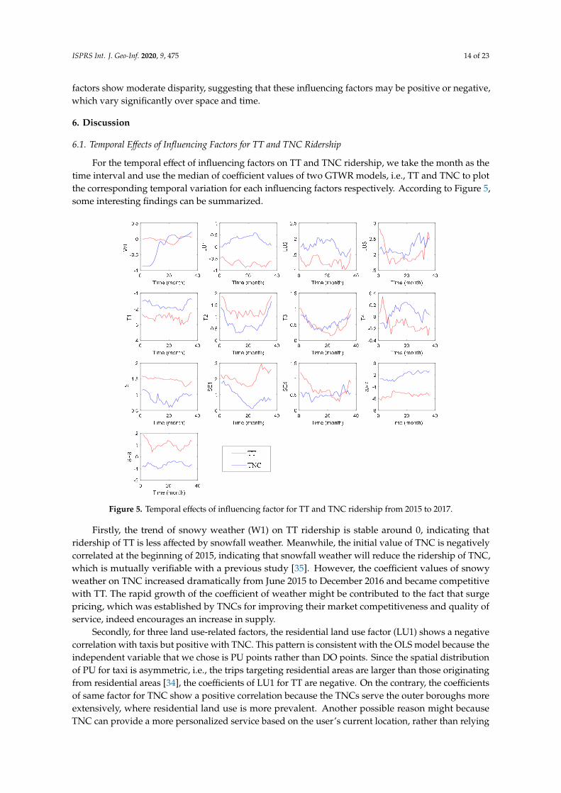
For the temporal effect of influencing factors on TT and TNC ridership, we take the month as thetime interval and use the median of coefficient values of two GTWR models, i.e., TT and TNC to plotthe corresponding temporal variation for each influencing factors respectively. According to Figure 5,some interesting findings can be summarized.


density of vehicle ownership (SE4) due to the fact that TNC platforms allow people to use an assert (their private car) to make an income [36]. Based on the temporal trend of commuting time (SE7) and public transportation usage rate (SE8), the negative correlation with SE7 infers that for those TAZs that are far away from the city center and have lengthy commuting time, both taxi modes are inadequate to cover the travel needs of these areas, and public transportation might be better choices compared with the expensive cost of taxis and TNC. Meanwhile, the positive coefficients of SE8 factor for the TT further verifies that TTs are most prevalent in central cities, such as Manhattan, where the highly developed public transit network has aggregation effects on TTs.

Figure 5. Temporal effects of influencing factor for TT and TNC ridership from 2015 to 2017.

6.2. Spatial Effects of Influencing Factors for TT and TNC Ridership

Another important advantage of the GTWR model is that the local estimated coefficients that denote local relationships can be mappable and thus allow for visual analysis. It is important to note that, similar to the GWR model, many of GTWR’s coefficients might be insignificant, leading to the difficulty to explain heterogeneity in the study area. However, when significance statistics are evaluated and insignificant parameters are removed, the spatiotemporal patterns will become much easier to interpret. In this study, we applied the multiple testing solution proposed by da Silva and Fotheringham [37] to test the significance of local parameter estimates in GTWR to avoid excessive false discoveries. In addition, since the number of local parameter estimates obtained by GTWR at each location corresponds to the valid number of time, it is necessary to assess whether the majority of significant parameters are sufficient to represent the significance of the factor in the TAZ as a whole. In this study, we simply defined an influencing factor in a TAZ as significant when the number of its significant coefficients for all time was greater than 90%. Therefore, we can use the median value of the significant coefficients from GTWR model to produce a spatial variation map for each TAZ.

Taking the coefficients of the PoT model as an example, Figure 6 shows the spatial distribution of coefficients for weather- and land use-influencing factors using graduated colors as rendering

Figure 5. Temporal effects of influencing factor for TT and TNC ridership from 2015 to 2017.

Firstly, the trend of snowy weather (W1) on TT ridership is stable around 0, indicating thatridership of TT is less affected by snowfall weather. Meanwhile, the initial value of TNC is negativelycorrelated at the beginning of 2015, indicating that snowfall weather will reduce the ridership of TNC,which is mutually verifiable with a previous study [35]. However, the coefficient values of snowyweather on TNC increased dramatically from June 2015 to December 2016 and became competitivewith TT. The rapid growth of the coefficient of weather might be contributed to the fact that surgepricing, which was established by TNCs for improving their market competitiveness and quality ofservice, indeed encourages an increase in supply.

Secondly, for three land use-related factors, the residential land use factor (LU1) shows a negativecorrelation with taxis but positive with TNC. This pattern is consistent with the OLS model because theindependent variable that we chose is PU points rather than DO points. Since the spatial distributionof PU for taxi is asymmetric, i.e., the trips targeting residential areas are larger than those originatingfrom residential areas [34], the coefficients of LU1 for TT are negative. On the contrary, the coefficientsof same factor for TNC show a positive correlation because the TNCs serve the outer boroughs moreextensively, where residential land use is more prevalent. Another possible reason might becauseTNC can provide a more personalized service based on the user’s current location, rather than relying


on the taxi driver’s own experience and habits to pick up passengers. For the commercial land-usefactor (LU2) and the manufacturer land-use factor (LU3, mainly refers to the airport, train stations,and external transportation area), the temporal trend of two modes both show significant positivecorrelation, but the coefficient for TNC is higher than for TT in most of the time. The difference oftemporal trends reveals that the increase in the ridership of TNC was more closely related to land usethan TT in 2015–2016, resulting in TNC gaining market share rapidly in TAZs with large commercialand manufacturer areas during this period.

Thirdly, for transport-related factors, it can be seen that except for road density, the rest of thePoints of Interest (POI) factors in the two models are positively correlated. These temporal variationssuggest that taxis and TNC in NYC have mutual promotion effects with other transportation modes,such as buses, subways, and bicycles, reflecting the key role of TT and TNC in meeting the need of thelast mile of trips. Moreover, we found that TT is more attractive than TNC where TAZs have moresubway stations (T2) and CityRacks (T5), but less attractive at TAZs that have more bus stops and higherdensities of bike lines (T4). One possible reason that this pattern occurs is that TT preferred to waitfor passengers on POI, while subway stations and CityRacks exist more often near POI. The oppositehappens with bus stops, which are spread throughout the city where a TT may be not as availableas TNC.

The last group is socioeconomic-related factors, which has an obvious difference between TT andTNC in our case. To be specific, the temporal trend of bachelors’ degree factor (SE1) reveals that TTis more attractive to passengers who have higher education, and this has become more obvious inrecent years. We assume that this phenomenon is because passenger with higher education mighthave better chance to make more incomes (0.98 correlate with SE3 in Table 2), and they will use taxismore often; on the other hand, the rapid growth of TNC is observed to be contributed to by a highdensity of vehicle ownership (SE4) due to the fact that TNC platforms allow people to use an assert(their private car) to make an income [36]. Based on the temporal trend of commuting time (SE7) andpublic transportation usage rate (SE8), the negative correlation with SE7 infers that for those TAZs thatare far away from the city center and have lengthy commuting time, both taxi modes are inadequateto cover the travel needs of these areas, and public transportation might be better choices comparedwith the expensive cost of taxis and TNC. Meanwhile, the positive coefficients of SE8 factor for theTT further verifies that TTs are most prevalent in central cities, such as Manhattan, where the highlydeveloped public transit network has aggregation effects on TTs.

6.2. Spatial Effects of Influencing Factors for TT and TNC Ridership

Another important advantage of the GTWR model is that the local estimated coefficients thatdenote local relationships can be mappable and thus allow for visual analysis. It is important tonote that, similar to the GWR model, many of GTWR’s coefficients might be insignificant, leading tothe difficulty to explain heterogeneity in the study area. However, when significance statistics areevaluated and insignificant parameters are removed, the spatiotemporal patterns will become mucheasier to interpret. In this study, we applied the multiple testing solution proposed by da Silva andFotheringham [37] to test the significance of local parameter estimates in GTWR to avoid excessivefalse discoveries. In addition, since the number of local parameter estimates obtained by GTWR ateach location corresponds to the valid number of time, it is necessary to assess whether the majority ofsignificant parameters are sufficient to represent the significance of the factor in the TAZ as a whole.In this study, we simply defined an influencing factor in a TAZ as significant when the number of itssignificant coefficients for all time was greater than 90%. Therefore, we can use the median value of thesignificant coefficients from GTWR model to produce a spatial variation map for each TAZ.

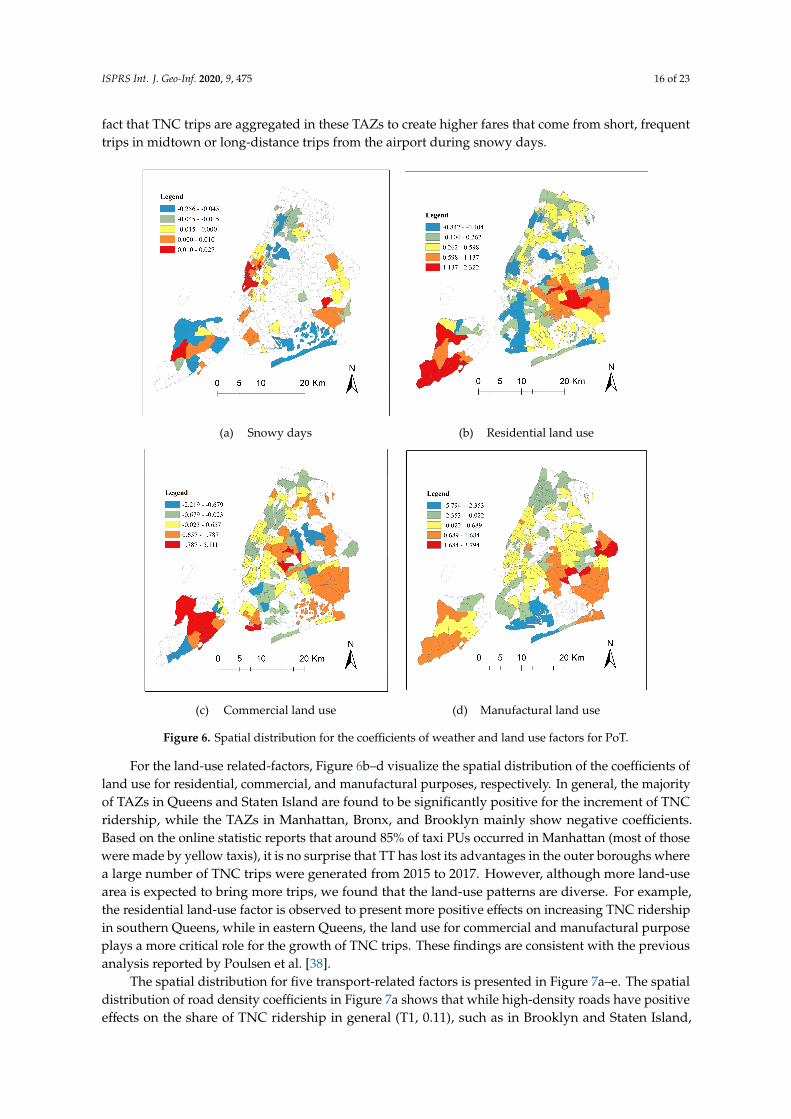
Taking the coefficients of the PoT model as an example, Figure 6 shows the spatial distribution ofcoefficients for weather- and land use-influencing factors using graduated colors as rendering style.Figure 6a shows that the spatial distribution of the coefficients for snowy weather is positive in thesouthern of Manhattan, the central of Staten Island and the JFK airport, which naturally reflects the


fact that TNC trips are aggregated in these TAZs to create higher fares that come from short, frequenttrips in midtown or long-distance trips from the airport during snowy days.


style. Figure 6a shows that the spatial distribution of the coefficients for snowy weather is positive in the southern of Manhattan, the central of Staten Island and the JFK airport, which naturally reflects the fact that TNC trips are aggregated in these TAZs to create higher fares that come from short, frequent trips in midtown or long-distance trips from the airport during snowy days.

For the land-use related-factors, Figure 6b–d visualize the spatial distribution of the coefficients of land use for residential, commercial, and manufactural purposes, respectively. In general, the majority of TAZs in Queens and Staten Island are found to be significantly positive for the increment of TNC ridership, while the TAZs in Manhattan, Bronx, and Brooklyn mainly show negative coefficients. Based on the online statistic reports that around 85% of taxi PUs occurred in Manhattan (most of those were made by yellow taxis), it is no surprise that TT has lost its advantages in the outer boroughs where a large number of TNC trips were generated from 2015 to 2017. However, although more land-use area is expected to bring more trips, we found that the land-use patterns are diverse. For example, the residential land-use factor is observed to present more positive effects on increasing TNC ridership in southern Queens, while in eastern Queens, the land use for commercial and manufactural purpose plays a more critical role for the growth of TNC trips. These findings are consistent with the previous analysis reported by Poulsen et al. [38].

(a) Snowy days

(b) Residential land use

(c) Commercial land use

(d) Manufactural land use

Figure 6. Spatial distribution for the coefficients of weather and land use factors for PoT.

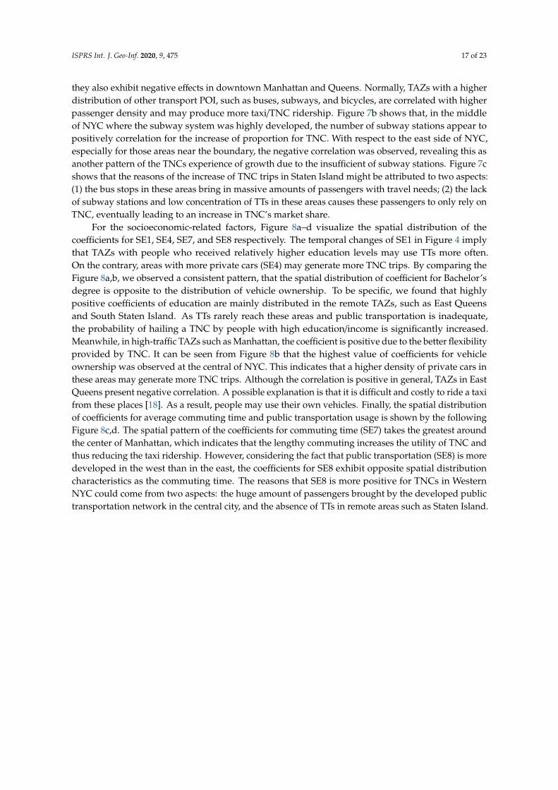
The spatial distribution for five transport-related factors is presented in Figure 7a–e. The spatial distribution of road density coefficients in Figure 7a shows that while high-density roads have positive effects on the share of TNC ridership in general (T1, 0.11), such as in Brooklyn and Staten

Figure 6. Spatial distribution for the coefficients of weather and land use factors for PoT.

For the land-use related-factors, Figure 6b–d visualize the spatial distribution of the coefficients ofland use for residential, commercial, and manufactural purposes, respectively. In general, the majorityof TAZs in Queens and Staten Island are found to be significantly positive for the increment of TNCridership, while the TAZs in Manhattan, Bronx, and Brooklyn mainly show negative coefficients.Based on the online statistic reports that around 85% of taxi PUs occurred in Manhattan (most of thosewere made by yellow taxis), it is no surprise that TT has lost its advantages in the outer boroughs wherea large number of TNC trips were generated from 2015 to 2017. However, although more land-usearea is expected to bring more trips, we found that the land-use patterns are diverse. For example,the residential land-use factor is observed to present more positive effects on increasing TNC ridershipin southern Queens, while in eastern Queens, the land use for commercial and manufactural purposeplays a more critical role for the growth of TNC trips. These findings are consistent with the previousanalysis reported by Poulsen et al. [38].

The spatial distribution for five transport-related factors is presented in Figure 7a–e. The spatialdistribution of road density coefficients in Figure 7a shows that while high-density roads have positiveeffects on the share of TNC ridership in general (T1, 0.11), such as in Brooklyn and Staten Island,


they also exhibit negative effects in downtown Manhattan and Queens. Normally, TAZs with a higherdistribution of other transport POI, such as buses, subways, and bicycles, are correlated with higherpassenger density and may produce more taxi/TNC ridership. Figure 7b shows that, in the middleof NYC where the subway system was highly developed, the number of subway stations appear topositively correlation for the increase of proportion for TNC. With respect to the east side of NYC,especially for those areas near the boundary, the negative correlation was observed, revealing this asanother pattern of the TNCs experience of growth due to the insufficient of subway stations. Figure 7cshows that the reasons of the increase of TNC trips in Staten Island might be attributed to two aspects:(1) the bus stops in these areas bring in massive amounts of passengers with travel needs; (2) the lackof subway stations and low concentration of TTs in these areas causes these passengers to only rely onTNC, eventually leading to an increase in TNC’s market share.

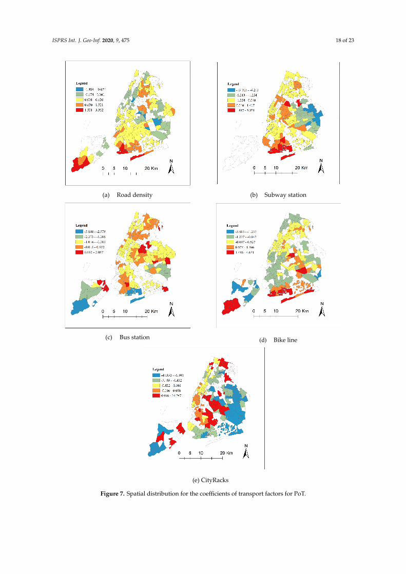
For the socioeconomic-related factors, Figure 8a–d visualize the spatial distribution of thecoefficients for SE1, SE4, SE7, and SE8 respectively. The temporal changes of SE1 in Figure 4 implythat TAZs with people who received relatively higher education levels may use TTs more often.On the contrary, areas with more private cars (SE4) may generate more TNC trips. By comparing theFigure 8a,b, we observed a consistent pattern, that the spatial distribution of coefficient for Bachelor’sdegree is opposite to the distribution of vehicle ownership. To be specific, we found that highlypositive coefficients of education are mainly distributed in the remote TAZs, such as East Queensand South Staten Island. As TTs rarely reach these areas and public transportation is inadequate,the probability of hailing a TNC by people with high education/income is significantly increased.Meanwhile, in high-traffic TAZs such as Manhattan, the coefficient is positive due to the better flexibilityprovided by TNC. It can be seen from Figure 8b that the highest value of coefficients for vehicleownership was observed at the central of NYC. This indicates that a higher density of private cars inthese areas may generate more TNC trips. Although the correlation is positive in general, TAZs in EastQueens present negative correlation. A possible explanation is that it is difficult and costly to ride a taxifrom these places [18]. As a result, people may use their own vehicles. Finally, the spatial distributionof coefficients for average commuting time and public transportation usage is shown by the followingFigure 8c,d. The spatial pattern of the coefficients for commuting time (SE7) takes the greatest aroundthe center of Manhattan, which indicates that the lengthy commuting increases the utility of TNC andthus reducing the taxi ridership. However, considering the fact that public transportation (SE8) is moredeveloped in the west than in the east, the coefficients for SE8 exhibit opposite spatial distributioncharacteristics as the commuting time. The reasons that SE8 is more positive for TNCs in WesternNYC could come from two aspects: the huge amount of passengers brought by the developed publictransportation network in the central city, and the absence of TTs in remote areas such as Staten Island.



Island, they also exhibit negative effects in downtown Manhattan and Queens. Normally, TAZs with a higher distribution of other transport POI, such as buses, subways, and bicycles, are correlated with higher passenger density and may produce more taxi/TNC ridership. Figure 7b shows that, in the middle of NYC where the subway system was highly developed, the number of subway stations appear to positively correlation for the increase of proportion for TNC. With respect to the east side of NYC, especially for those areas near the boundary, the negative correlation was observed, revealing this as another pattern of the TNCs experience of growth due to the insufficient of subway stations. Figure 7c shows that the reasons of the increase of TNC trips in Staten Island might be attributed to two aspects: (1) the bus stops in these areas bring in massive amounts of passengers with travel needs; (2) the lack of subway stations and low concentration of TTs in these areas causes these passengers to only rely on TNC, eventually leading to an increase in TNC’s market share.

(a) Road density

(b) Subway station

(c) Bus station

(d) Bike line ISPRS Int. J. Geo-Inf. 2020, 9, x FOR PEER REVIEW 19 of 24

(e) CityRacks

Figure 7. Spatial distribution for the coefficients of transport factors for PoT.

For the socioeconomic-related factors, Figure 8a–d visualize the spatial distribution of the coefficients for SE1, SE4, SE7, and SE8 respectively. The temporal changes of SE1 in Figure 4 imply that TAZs with people who received relatively higher education levels may use TTs more often. On the contrary, areas with more private cars (SE4) may generate more TNC trips. By comparing the Figure 8a,b, we observed a consistent pattern, that the spatial distribution of coefficient for Bachelor’s degree is opposite to the distribution of vehicle ownership. To be specific, we found that highly positive coefficients of education are mainly distributed in the remote TAZs, such as East Queens and South Staten Island. As TTs rarely reach these areas and public transportation is inadequate, the probability of hailing a TNC by people with high education/income is significantly increased. Meanwhile, in high-traffic TAZs such as Manhattan, the coefficient is positive due to the better flexibility provided by TNC. It can be seen from Figure 8b that the highest value of coefficients for vehicle ownership was observed at the central of NYC. This indicates that a higher density of private cars in these areas may generate more TNC trips. Although the correlation is positive in general, TAZs in East Queens present negative correlation. A possible explanation is that it is difficult and costly to ride a taxi from these places [18]. As a result, people may use their own vehicles. Finally, the spatial distribution of coefficients for average commuting time and public transportation usage is shown by the following Figure 8c,d. The spatial pattern of the coefficients for commuting time (SE7) takes the greatest around the center of Manhattan, which indicates that the lengthy commuting increases the utility of TNC and thus reducing the taxi ridership. However, considering the fact that public transportation (SE8) is more developed in the west than in the east, the coefficients for SE8 exhibit opposite spatial distribution characteristics as the commuting time. The reasons that SE8 is more positive for TNCs in Western NYC could come from two aspects: the huge amount of passengers brought by the developed public transportation network in the central city, and the absence of TTs in remote areas such as Staten Island.

Figure 7. Spatial distribution for the coefficients of transport factors for PoT.



(a) Education

(b) Vehicle ownership

(c) Commuting time

(d) Public transportation usage

Figure 8. Spatial distribution for the coefficients of socioeconomic-related factors for PoT.

6.3. The Efficiency of the Parallel-Based GTWR Model

To test the efficiency of the parallel-based GTWR model, we randomly selected the sample set with different proportions and then recoded the calculation time of the basic GTWR model and the improved model. The same process was repeated 10 times to avoid noisy measures due to other processes that could be running at the same time. Table 6 shows a comparison of the average computation time of both models. With the improvement of parallel computing, we observed that the calculation time was reduced by 49% to 61% based on a four-core CPU. Moreover, we found that a 10% sampling level can guarantee the robustness of the algorithm for modeling in our case. However, random sampling is a simple strategy and may cause some valuable information to be omitted, thus weaken the stability of the model result. A better approach is to use systematic or artificial pre-defined methods, based on time-varying features (e.g., cycles and seasonality) to improve the robustness of the algorithm. Moreover, with the popularity of cloud computing technology, the introduction of distributed computing or cloud computing to the GTWR model is also an effective improvement direction [39].

Figure 8. Spatial distribution for the coefficients of socioeconomic-related factors for PoT.

6.3. The Efficiency of the Parallel-Based GTWR Model

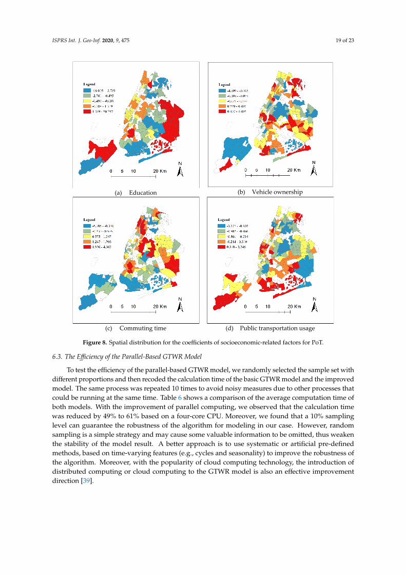
To test the efficiency of the parallel-based GTWR model, we randomly selected the sample set withdifferent proportions and then recoded the calculation time of the basic GTWR model and the improvedmodel. The same process was repeated 10 times to avoid noisy measures due to other processes thatcould be running at the same time. Table 6 shows a comparison of the average computation time ofboth models. With the improvement of parallel computing, we observed that the calculation timewas reduced by 49% to 61% based on a four-core CPU. Moreover, we found that a 10% samplinglevel can guarantee the robustness of the algorithm for modeling in our case. However, randomsampling is a simple strategy and may cause some valuable information to be omitted, thus weakenthe stability of the model result. A better approach is to use systematic or artificial pre-definedmethods, based on time-varying features (e.g., cycles and seasonality) to improve the robustness ofthe algorithm. Moreover, with the popularity of cloud computing technology, the introduction ofdistributed computing or cloud computing to the GTWR model is also an effective improvementdirection [39].


Table 6. Comparison of the efficiency between GTWR and parallel-based GTWR models. (Unit: second).

Percentage ofTraining Samples

Number ofTraining Samples Basic GTWR Parallel-Based

GTWR Time Reduction

10% 913 13.2 5.7 57%30% 2739 88.1 34.5 61%50% 4565 199.6 101.2 49%

100% 9126 1314.4 652.3 50%

7. Conclusions

The rapid development of TNC has been indeed a useful supplement to the traditional taxiindustry in the early development stage, but the growth of the urban demand for taxis has beenrelatively stable. As a result, the relationship between the two modes will inevitably be mutuallycompetitive, and this competitive relationship will demonstrate nonstationarity in time and space.In response to this problem, we select NYC as a case study to illustrate that the GTWR model can bean effective tool for analyzing spatiotemporal heterogeneity. Moreover, the effects of the influencingfactors for the TT and TNC can be quantitatively evaluated in the temporal term, and spatial variationscan also be analyzed by the coefficients at different spatial units (i.e., administrative division-based orgrid-based).

This study compares GTWR with OLS while exploring the relationships between built environmentand the PU ridership. The global coefficients of OLS models are observed to be deficient when dealingwith spatial problem. The GTWR model, on the other hand, shows better performance than theOLS model, especially in the fact that the GTWR model can help to eliminate potential bias fromspatiotemporal heterogeneity and provide localized regression statistics at each location. By visualizingdistributions of median values of coefficients for each factor, the spatiotemporal variations of thefactors could be better interpreted. Our study demonstrates that the relationships between ridershipand influencing factor of built environment vary over space and time in NYC. Moreover, the effectsof influencing factors on TT and TNC are significantly different on both spatial and temporal terms.For example, the model results reveal that the TNC’s surge pricing policy has a significant effect onincreasing TNC trips in snowy conditions, especially in western Manhattan. While TTs have alwaysbeen dominant in downtown Manhattan, the share of TNC has risen significantly in the adjacentneighborhoods due to the availability of transit alternatives, such as subways, buses, and privatecars, which is probably correlated with commuting time (SE7). Meanwhile, the increases of TNCs arealso observed in remote places, which are positively correlated with densities of multiple land use,educated populations, and levels of public transportation usage. Compared to the current saturation ofdemand in the central city, future competition between TT and TNC might be concentrated in remoteareas, such as eastern Queens, which is not adequately covered by public transportation. We believethese findings of spatial variations of taxi demand could provide useful scientific guidelines for thetaxi industry and TNC to optimize their existing resources thus improving efficiency. Furthermore,the basic modeling steps described in this paper, such as data aggregation, factor selection, parameteroptimization, modeling analysis, and visual presentation, can also be applied to other research fieldsfor spatiotemporal modelling. For example, considering the recent outbreak of Coronavirus Disease2019 (COVID-19), the GTWR model might be an appropriate approach to assess the local relationshipsbetween the contagiousness of the virus and the influencing factors of urban environment.

Several challenges remain when applying GTWR models to explore detailed variations inrelationships between taxis and built environment research. As the variation in transportationenvironments in different cities is enormous, the result of GTWR can only be adapted to specificcities. In the follow-up study, we will apply the GTWR model to other large cities for comparisonand evaluation. The model will incorporate with different type of influencing factors, such as POI,real-time population flow, and Internet of Things data, which will help to improve the interpretation ofhow the urban spaces and times result in taxi demand.


We also notice that using a four-core CPU might be insufficient to fully evaluate the performanceof the proposed parallel-based GTWR model. In fact, the optimization of computational performancefor GWR-based models is always a technical bottleneck that plagues the widespread application ofspatiotemporal modeling, especially in the face of a massive spatial and temporal dataset. In this study,the most important thing that we focus on is to apply the GTWR model to evaluate the relationshipbetween the taxi ridership and the influencing factors of built environment. Due to the length limitationof this paper, we only provide a simple technical idea of the design of the parallel-based GTWRmodel and perform it with a small-scale case study (less than 10,000 samples). The efficiency of thecurrent use of a four-core CPU already meets the needs of this study. According to some literature [39],the efficiency of parallel computing is correlated with many factors, such as the structure of thealgorithm, the selection of software, and the size of the data, and in some cases the computation is evenless efficient than serial computation. Therefore, evaluating the efficiency of the parallel-based GTWRmodel could be a complex technical problem, which we believe is necessary to conduct in future.

Another issue that must be considered is that the GTWR model uses statistical local least squaresto estimate the coefficient of variables; therefore, the model’s accuracy depends on the independenceof the observed samples. When there is a strong autocorrelation between the data samples, and thisautocorrelation is not considered well, it will cause the overfitting problem and affect the finalexplanatory results of the model. In this respect, the GTWAR model that can estimate the spatialautocorrelation for each variable might be a better solution. However, the GTWAR model increases thecomputational complexity of the algorithm; therefore, whether this model is necessary for transportationanalysis needs to be further evaluated. Regarding the time dimension, seasonal change might beconsidered. There are more taxis to be operated in summer than in winter, although, in our study,we use weather factors to reflect seasonal changes. The GcTWR model proposed in [26] might be analternative way to improve the general GTWR model. The question is that the definition of the seasonalspan of the GcTWR model is manually preset. In actual situations, periodicity varies. Adopting acertain adaptive method to auto-identify the seasonal span of transportation distribution is anotherproblem that must be considered carefully.

Author Contributions: Conceptualization, Xinxin Zhang and Bo Huang; methodology, Bo Huang; software,Bo Huang; validation, Xinxin Zhang, Bo Huang, and Shunzhi Zhu; data curation, Shunzhi Zhu; writing—originaldraft preparation, Xinxin Zhang; writing—review and editing, Xinxin Zhang and Bo Huang; visualization,Xinxin Zhang; supervision, Bo Huang; and funding acquisition, Shunzhi Zhu. All authors have read and agreedto the published version of the manuscript.

Funding: This work was supported in part by National Nature Science Foundation of China under Grant 61672442,Nature Science Foundation of Fujian Province under Grant 2020J01130815, Science and Technology Project ofQuanzhou (2020C074), and Scientific Climbing Project of Xiamen University of Technology (XPDKT18030).

Acknowledgments: The authors appreciate reviewers for their insightful comments and constructive suggestionson our research work. The authors also want to thank editors for their patient and meticulous work forour manuscript.

Conflicts of Interest: The authors declare no conflict of interest.

References

1. Wallsten, S. The competitive effects of the sharing economy: How is uber changing taxis. Technol. Policy Inst.2015, 22, 1–22.

2. Rayle, L.; Shaheen, S.; Chan, N.; Dai, D.; Cervero, R. App-Based, on-demand Ride Services: Comparing Taxi andRidesourcing Trips and User Characteristics in San Francisco University Of California Transportation Center (UCTC);University of California: Berkeley, CA, USA, 2014.

3. Nie, Y.M. How can the taxi industry survive the tide of ridesourcing? Evidence from shenzhen, China.Transp. Res. Part C Emerg. Technol. 2017, 79, 242–256. [CrossRef]

4. Wang, X.; He, F.; Yang, H.; Gao, H.O. Pricing strategies for a taxi-hailing platform. Transp. Res. Part E Logist.Transp. Rev. 2016, 93, 212–231. [CrossRef]

http://dx.doi.org/10.1016/j.trc.2017.03.017

http://dx.doi.org/10.1016/j.tre.2016.05.011


5. Cramer, J.; Krueger, A.B. Disruptive change in the taxi business: The case of uber. Am. Econ. Rev. 2016, 106,177–182. [CrossRef]

6. Hall, J.V.; Krueger, A.B. An analysis of the labor market for uber’s driver-partners in the united states.ILR Rev. 2018, 71, 705–732. [CrossRef]

7. Li, M.; Dong, L.; Shen, Z.; Lang, W.; Ye, X. Examining the interaction of taxi and subway ridership forsustainable urbanization. Sustainability 2017, 9, 242. [CrossRef]

8. Chen, C.; Varley, D.; Chen, J. What affects transit ridership? A dynamic analysis involving multiple factors,lags and asymmetric behaviour. Urban Stud. 2011, 48, 1893–1908. [CrossRef]

9. Yang, Z.; Franz, M.L.; Zhu, S.; Mahmoudi, J.; Nasri, A.; Zhang, L. Analysis of washington, dc taxi demandusing gps and land-use data. J. Transp. Geogr. 2018, 66, 35–44. [CrossRef]

10. Castro, P.S.; Zhang, D.; Chen, C.; Li, S.; Pan, G. From taxi gps traces to social and community dynamics:A survey. ACM Comput. Surv. (CSUR) 2013, 46, 17. [CrossRef]

11. Chiou, Y.-C.; Jou, R.-C.; Yang, C.-H. Factors affecting public transportation usage rate: Geographicallyweighted regression. Transp. Res. Part A Policy Pract. 2015, 78, 161–177. [CrossRef]

12. Liu, Y.; Wang, F.; Xiao, Y.; Gao, S. Urban land uses and traffic ‘source-sink areas’: Evidence from gps-enabledtaxi data in shanghai. Landsc. Urban Plan. 2012, 106, 73–87. [CrossRef]

13. Sadowsky, N.; Nelson, E. The impact of ride-hailing services on public transportation use: A discontinuityregression analysis. 2017. Economics Department Working Paper Series. 13. Available online: https://digitalcommons.bowdoin.edu/econpapers/13 (accessed on 26 May 2017).

14. Hochmair, H.H. Spatiotemporal pattern analysis of taxi trips in new york city. Transp. Res. Rec. J. Transp.Res. Board 2016, 2542, 45–56. [CrossRef]

15. Fotheringham, A.S.; Crespo, R.; Yao, J. Geographical and temporal weighted regression (gtwr). Geogr. Anal.2015, 47, 431–452. [CrossRef]

16. Chow, L.-F.; Zhao, F.; Liu, X.; Li, M.-T.; Ubaka, I. Transit ridership model based on geographically weightedregression. Transp. Res. Rec. 2006, 1972, 105–114. [CrossRef]

17. Cardozo, O.D.; García-Palomares, J.C.; Gutiérrez, J. Application of geographically weighted regression to thedirect forecasting of transit ridership at station-level. Appl. Geogr. 2012, 34, 548–558. [CrossRef]

18. Qian, X.; Ukkusuri, S.V. Exploring spatial variation of urban taxi ridership using geographically weightedregression. In Proceedings of the Transportation Research Board 94th Annual Meeting, Washington, DC, USA,11–15 January 2015.

19. Fotheringham, A.S.; Crespo, R.; Yao, J. Exploring, modelling and predicting spatiotemporal variations inhouse prices. Ann. Reg. Sci. 2015, 54, 417–436. [CrossRef]

20. Wu, J.; Yao, F.; Li, W.; Si, M. Viirs-based remote sensing estimation of ground-level pm2. 5 concentrationsin beijing–tianjin–hebei: A spatiotemporal statistical model. Remote Sens. Environ. 2016, 184, 316–328.[CrossRef]

21. Taylor, B.D.; Miller, D.; Iseki, H.; Fink, C. Analyzing the Determinants of Transit Ridership Using a Two-Stage LeastSquares Regression on a National Sample of Urbanized Areas; University of California Transportation Center:Berkeley, CA, USA, 2003.

22. Huang, B.; Wu, B.; Barry, M. Geographically and temporally weighted regression for modeling spatio-temporalvariation in house prices. Int. J. Geogr. Inf. Sci. 2010, 24, 383–401. [CrossRef]

23. He, Q.; Huang, B. Satellite-based mapping of daily high-resolution ground pm 2.5 in china via space-timeregression modeling. Remote Sens. Environ. 2018, 206, 72–83. [CrossRef]

24. Chu, H.-J.; Kong, S.-J.; Chang, C.-H. Spatio-temporal water quality mapping from satellite images usinggeographically and temporally weighted regression. Int. J. Appl. Earth Obs. Geoinf. 2018, 65, 1–11. [CrossRef]

25. Wu, B.; Li, R.; Huang, B. A geographically and temporally weighted autoregressive model with applicationto housing prices. Int. J. Geogr. Inf. Sci. 2014, 28, 1186–1204. [CrossRef]

26. Du, Z.; Wu, S.; Zhang, F.; Liu, R.; Zhou, Y. Extending geographically and temporally weighted regression toaccount for both spatiotemporal heterogeneity and seasonal variations in coastal seas. Ecol. Inform. 2018, 43,185–199. [CrossRef]

27. Ma, X.; Zhang, J.; Ding, C.; Wang, Y. A geographically and temporally weighted regression model to explorethe spatiotemporal influence of built environment on transit ridership. Comput. Environ. Urban Syst. 2018,70, 113–124. [CrossRef]

http://dx.doi.org/10.1257/aer.p20161002

http://dx.doi.org/10.1177/0019793917717222

http://dx.doi.org/10.3390/su9020242

http://dx.doi.org/10.1177/0042098010379280

http://dx.doi.org/10.1016/j.jtrangeo.2017.10.021

http://dx.doi.org/10.1145/2543581.2543584

http://dx.doi.org/10.1016/j.tra.2015.05.016

http://dx.doi.org/10.1016/j.landurbplan.2012.02.012

https://digitalcommons.bowdoin.edu/econpapers/13

https://digitalcommons.bowdoin.edu/econpapers/13

http://dx.doi.org/10.3141/2542-06

http://dx.doi.org/10.1111/gean.12071

http://dx.doi.org/10.1177/0361198106197200113

http://dx.doi.org/10.1016/j.apgeog.2012.01.005

http://dx.doi.org/10.1007/s00168-015-0660-6

http://dx.doi.org/10.1016/j.rse.2016.07.015

http://dx.doi.org/10.1080/13658810802672469

http://dx.doi.org/10.1016/j.rse.2017.12.018

http://dx.doi.org/10.1016/j.jag.2017.10.001

http://dx.doi.org/10.1080/13658816.2013.878463

http://dx.doi.org/10.1016/j.ecoinf.2017.12.005

http://dx.doi.org/10.1016/j.compenvurbsys.2018.03.001


28. Zhang, X.; Huang, B.; Zhu, S. Spatiotemporal influence of urban environment on taxi ridership usinggeographically and temporally weighted regression. ISPRS Int. J. Geo-Inf. 2019, 8, 23. [CrossRef]

29. Liu, Y.; Ji, Y.; Shi, Z.; Gao, L. The influence of the built environment on school children’s metro ridership:An exploration using geographically weighted poisson regression models. Sustainability 2018, 10, 4684.[CrossRef]

30. Peruggia, M. Model selection and multimodel inference: A practical information-theoretic approach(2nd ed.).(telegraphic reviews)(book review). J. Wildl. Manag. 2002, 67, 175–196.

31. Sharma, G.; Martin, J. Matlab®: A language for parallel computing. Int. J. Parallel Program. 2009, 37, 3–36.[CrossRef]

32. Yazici, M.A.; Kamga, C.; Singhal, A. A big data driven model for taxi drivers’ airport pick-up decisions inNew York city. In Proceedings of the 2013 IEEE International Conference on Big Data, Silicon Valley, CA,USA, 6–9 October 2013; pp. 37–44.

33. Neter, J.; Kutner, M.H.; Nachtsheim, C.J.; Wasserman, W. Applied Linear Statistical Models; McGraw-Hill Irwin:New York, NY, USA, 1996.

34. King, D.A.; Peters, J.R.; Daus, M.W. Taxicabs for improved urban mobility: Are we missing an opportunity?In Proceedings of the Transportation Research Board 91st Annual Meeting, Washington, DC, USA,22–26 January 2012.

35. Kamga, C.; Yazici, M.A.; Singhal, A. Hailing in the rain: Temporal and weather-related variations in taxiridership and taxi demand-supply equilibrium. In Proceedings of the Transportation Research Board 92ndAnnual Meeting, Washington, DC, USA, 13–17 January 2013.

36. Davidov, G. The status of uber drivers: A purposive approach. Span. Labour Law Employ. Relat. J.Forthcom. (2017) 2016. Forthcoming. [CrossRef]

37. Da Silva, A.R.; Fotheringham, A.S. The multiple testing issue in geographically weighted regression.Geogr. Anal. 2016, 48, 233–247. [CrossRef]

38. Poulsen, L.K.; Dekkers, D.; Wagenaar, N.; Snijders, W.; Lewinsky, B.; Mukkamala, R.R.; Vatrapu, R. Greencabs vs. Uber in New York city. In Proceedings of the 2016 IEEE International Congress on Big Data (BigDataCongress), San Francisco, CA, USA, 27 June–2 July 2016; pp. 222–229.

39. Li, Z.; Fotheringham, A.S.; Li, W.; Oshan, T. Fast geographically weighted regression (fastgwr): A scalablealgorithm to investigate spatial process heterogeneity in millions of observations. Int. J. Geogr. Inf. Sci. 2019,33, 155–175. [CrossRef]

© 2020 by the authors. Licensee MDPI, Basel, Switzerland. This article is an open accessarticle distributed under the terms and conditions of the Creative Commons Attribution(CC BY) license (http://creativecommons.org/licenses/by/4.0/).

http://dx.doi.org/10.3390/ijgi8010023

http://dx.doi.org/10.3390/su10124684

http://dx.doi.org/10.1007/s10766-008-0082-5

http://dx.doi.org/10.20318/sllerj.2017.3921

http://dx.doi.org/10.1111/gean.12084

http://dx.doi.org/10.1080/13658816.2018.1521523

http://creativecommons.org/

http://creativecommons.org/licenses/by/4.0/.

spatiotemporal varying effects of built environment on taxi

Documents