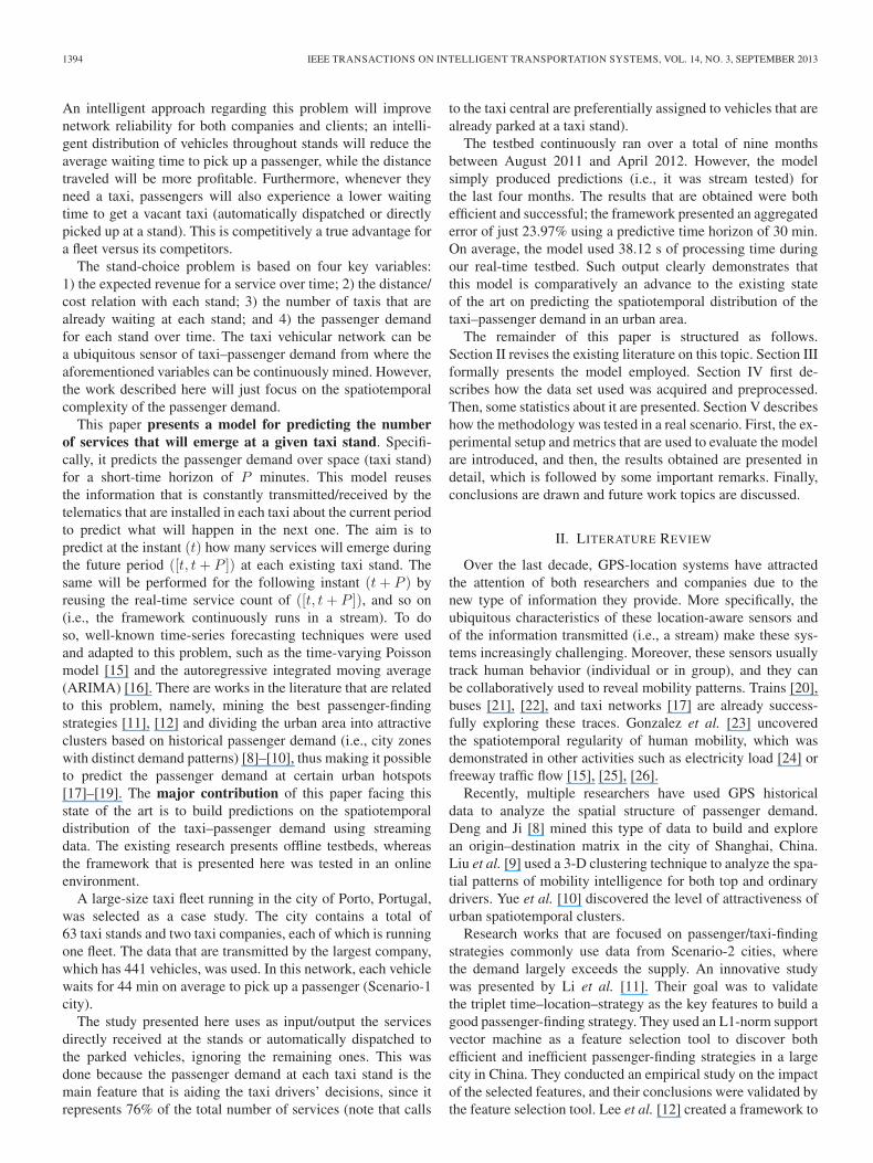
IEEE TRANSACTIONS ON INTELLIGENT TRANSPORTATION SYSTEMS, VOL. 14, NO. 3, SEPTEMBER 2013 1393

Predicting Taxi–Passenger Demand UsingStreaming Data

Luis Moreira-Matias, João Gama, Michel Ferreira, João Mendes-Moreira, and Luis Damas

Abstract—Informed driving is increasingly becoming a key fea-ture for increasing the sustainability of taxi companies. Thesensors that are installed in each vehicle are providing newopportunities for automatically discovering knowledge, which,in return, delivers information for real-time decision making.Intelligent transportation systems for taxi dispatching and forfinding time-saving routes are already exploring these sensingdata. This paper introduces a novel methodology for predict-ing the spatial distribution of taxi–passengers for a short-termtime horizon using streaming data. First, the information wasaggregated into a histogram time series. Then, three time-seriesforecasting techniques were combined to originate a prediction.Experimental tests were conducted using the online data that aretransmitted by 441 vehicles of a fleet running in the city of Porto,Portugal. The results demonstrated that the proposed frameworkcan provide effective insight into the spatiotemporal distributionof taxi–passenger demand for a 30-min horizon.

Index Terms—Autoregressive integrated moving average(ARIMA), data streams, ensemble learning, Global PositioningSystem (GPS) data, mobility intelligence, taxi–passenger demand,time-series forecasting, time-varying Poisson models.

I. INTRODUCTION

ADVANCES in sensor and wireless communications suchas Global Positioning System (GPS), Global System for

Manuscript received August 7, 2012; revised February 22, 2013 and April 20,2013; accepted April 26, 2013. Date of publication June 14, 2013; date ofcurrent version August 28, 2013. This work was supported in part by Projects“Distributed Routing and Infotainment through Vehicular Internet-working”(DRIVE-IN), “Massive Information Scavenging with Intelligent Transporta-tion Systems” (MISC), “Virtual Traffic Lights” (VTL), and “KnowledgeDiscovery from Ubiquitous Data Streams” (KDUS) under Grant CMU-PT/NGN/0052/2008, Grant MITPT/ITS-ITS/0059/2008, Grant PTDC/EIA-CCO/118114/2010, and Grant PTDC/EIA-EIA/098355/2008, respectively; bythe European Regional Development Fund (ERDF) through the COMPETEProgramme (Operational Programme for Competitiveness), and by the Por-tuguese Funds through the Portuguese Foundation for Science and Technology(FCT) within Project FCOMP-01-0124-FEDER-022701. The Associate Editorfor this paper was Dr. M. Brackstone.

L. Moreira-Matias and J. Mendes-Moreira are with the Laboratory forArtificial Intelligence and Decision Support, Tecnologia e Ciência, Institutode Engenharia de Sistemas e Computadores, and also with the Departmentof Informatics Engineering, Faculdade de Engenharia, Universidade do Porto,Porto 4200-465, Portugal (e-mail: luis.matias@fe.up.pt; jmoreira@fe.up.pt).

J. Gama is with the Laboratory for Artificial Intelligence and DecisionSupport, Tecnologia e Ciência, Instituto de Engenharia de Sistemas e Com-putadores, and also with the Faculdade de Economia, Universidade do Porto,Porto 4200-465, Portugal (e-mail: jgama@fep.up.pt).

M. Ferreira is with the Instituto de Telecomunicações, Departamento deCiência de Computadores, Faculdade de Ciências, Universidade do Porto, Porto4169-007, Portugal (e-mail: michel@dcc.fc.up.pt).

L. Damas is with Geolink, Lda., Porto 4050-275, Portugal (e-mail: luis@geolink.pt).

Color versions of one or more of the figures in this paper are available onlineat http://ieeexplore.ieee.org.

Digital Object Identifier 10.1109/TITS.2013.2262376

Mobile Communications (GSM), and WiFi have provided anew way of communicating with running vehicles while col-lecting relevant information on their status and location. Mosttaxi vehicles are now equipped with these kinds of technologies,producing a new source of rich spatiotemporal information.Intelligent transportation systems for efficient taxi dispatching[1], time-saving route finding [2], [3], fuel-saving routing [4],and taxi sharing [5] are already successfully exploring thesekind of data and/or interfaces.

The rising cost of fuel has been reducing the profit forboth taxi companies and drivers. This leads to an unbalancedrelationship between the passenger demand and the number ofrunning taxis, which, in turn, reduces the companies’ profitsand also the levels of passenger satisfaction [6]. Yang et al.presented a relevant mathematical model for expressing thisneed for an equilibrium in distinct contexts [7]. A failure in thisequilibrium may lead to one of the following two scenarios:Scenario 1, i.e., an excess in vacant vehicles and competitionand Scenario 2, i.e., larger waiting times for passengers andlower taxi reliability. However, a question remains open. Is itpossible to guarantee that the taxis’ spatial distribution overtime will always meet the demand, even when the number ofrunning taxis already does that?

Taxi-driver mobility intelligence is an important factor inmaximizing both profit and reliability within every possiblescenario. Knowledge on where the services (transporting a pas-senger from pick-up to drop-off locations) will actually emergecan be an advantage for the driver, particularly when there isno economic viability of adopting random cruising strategiesto find passengers. GPS historical data are one of the mainvariables of this topic because it can reveal underlying runningmobility patterns. Multiple works in the literature have alreadysuccessfully explored this type of data on various applicationssuch as smart driving [3], modeling the spatiotemporal structureof taxi services [8]–[10], building passenger-finding strategies[11], [12], or even predicting taxi location through a passengerperspective [13] (in a Scenario-2 urban area). Despite theiruseful insights, most reported techniques are tested using offlinetestbeds, discarding some of the main advantages of this type ofsignal. In other words, they do not provide any live informationon the location of a passenger or the best route to pick upa passenger at the current specific date/time (i.e., real-timeperformance), while the GPS data are mainly a live data stream(i.e., a time-ordered sequence of instances that are produced inreal-time [14]).

This paper focuses on the real-time choice problem of whichis the best taxi stand to go to after a passenger drop-off (i.e., thestand where another passenger can be picked up more quickly).

1524-9050 © 2013 IEEE

1394 IEEE TRANSACTIONS ON INTELLIGENT TRANSPORTATION SYSTEMS, VOL. 14, NO. 3, SEPTEMBER 2013

An intelligent approach regarding this problem will improvenetwork reliability for both companies and clients; an intelli-gent distribution of vehicles throughout stands will reduce theaverage waiting time to pick up a passenger, while the distancetraveled will be more profitable. Furthermore, whenever theyneed a taxi, passengers will also experience a lower waitingtime to get a vacant taxi (automatically dispatched or directlypicked up at a stand). This is competitively a true advantage fora fleet versus its competitors.

The stand-choice problem is based on four key variables:1) the expected revenue for a service over time; 2) the distance/cost relation with each stand; 3) the number of taxis that arealready waiting at each stand; and 4) the passenger demandfor each stand over time. The taxi vehicular network can bea ubiquitous sensor of taxi–passenger demand from where theaforementioned variables can be continuously mined. However,the work described here will just focus on the spatiotemporalcomplexity of the passenger demand.

This paper presents a model for predicting the numberof services that will emerge at a given taxi stand. Specifi-cally, it predicts the passenger demand over space (taxi stand)for a short-time horizon of P minutes. This model reusesthe information that is constantly transmitted/received by thetelematics that are installed in each taxi about the current periodto predict what will happen in the next one. The aim is topredict at the instant (t) how many services will emerge duringthe future period ([t, t+ P ]) at each existing taxi stand. Thesame will be performed for the following instant (t+ P ) byreusing the real-time service count of ([t, t+ P ]), and so on(i.e., the framework continuously runs in a stream). To doso, well-known time-series forecasting techniques were usedand adapted to this problem, such as the time-varying Poissonmodel [15] and the autoregressive integrated moving average(ARIMA) [16]. There are works in the literature that are relatedto this problem, namely, mining the best passenger-findingstrategies [11], [12] and dividing the urban area into attractiveclusters based on historical passenger demand (i.e., city zoneswith distinct demand patterns) [8]–[10], thus making it possibleto predict the passenger demand at certain urban hotspots[17]–[19]. The major contribution of this paper facing thisstate of the art is to build predictions on the spatiotemporaldistribution of the taxi–passenger demand using streamingdata. The existing research presents offline testbeds, whereasthe framework that is presented here was tested in an onlineenvironment.

A large-size taxi fleet running in the city of Porto, Portugal,was selected as a case study. The city contains a total of63 taxi stands and two taxi companies, each of which is runningone fleet. The data that are transmitted by the largest company,which has 441 vehicles, was used. In this network, each vehiclewaits for 44 min on average to pick up a passenger (Scenario-1city).

The study presented here uses as input/output the servicesdirectly received at the stands or automatically dispatched tothe parked vehicles, ignoring the remaining ones. This wasdone because the passenger demand at each taxi stand is themain feature that is aiding the taxi drivers’ decisions, since itrepresents 76% of the total number of services (note that calls

to the taxi central are preferentially assigned to vehicles that arealready parked at a taxi stand).

The testbed continuously ran over a total of nine monthsbetween August 2011 and April 2012. However, the modelsimply produced predictions (i.e., it was stream tested) forthe last four months. The results that are obtained were bothefficient and successful; the framework presented an aggregatederror of just 23.97% using a predictive time horizon of 30 min.On average, the model used 38.12 s of processing time duringour real-time testbed. Such output clearly demonstrates thatthis model is comparatively an advance to the existing stateof the art on predicting the spatiotemporal distribution of thetaxi–passenger demand in an urban area.

The remainder of this paper is structured as follows.Section II revises the existing literature on this topic. Section IIIformally presents the model employed. Section IV first de-scribes how the data set used was acquired and preprocessed.Then, some statistics about it are presented. Section V describeshow the methodology was tested in a real scenario. First, the ex-perimental setup and metrics that are used to evaluate the modelare introduced, and then, the results obtained are presented indetail, which is followed by some important remarks. Finally,conclusions are drawn and future work topics are discussed.

II. LITERATURE REVIEW

Over the last decade, GPS-location systems have attractedthe attention of both researchers and companies due to thenew type of information they provide. More specifically, theubiquitous characteristics of these location-aware sensors andof the information transmitted (i.e., a stream) make these sys-tems increasingly challenging. Moreover, these sensors usuallytrack human behavior (individual or in group), and they canbe collaboratively used to reveal mobility patterns. Trains [20],buses [21], [22], and taxi networks [17] are already success-fully exploring these traces. Gonzalez et al. [23] uncoveredthe spatiotemporal regularity of human mobility, which wasdemonstrated in other activities such as electricity load [24] orfreeway traffic flow [15], [25], [26].

Recently, multiple researchers have used GPS historicaldata to analyze the spatial structure of passenger demand.Deng and Ji [8] mined this type of data to build and explorean origin–destination matrix in the city of Shanghai, China.Liu et al. [9] used a 3-D clustering technique to analyze the spa-tial patterns of mobility intelligence for both top and ordinarydrivers. Yue et al. [10] discovered the level of attractiveness ofurban spatiotemporal clusters.

Research works that are focused on passenger/taxi-findingstrategies commonly use data from Scenario-2 cities, wherethe demand largely exceeds the supply. An innovative studywas presented by Li et al. [11]. Their goal was to validatethe triplet time–location–strategy as the key features to build agood passenger-finding strategy. They used an L1-norm supportvector machine as a feature selection tool to discover bothefficient and inefficient passenger-finding strategies in a largecity in China. They conducted an empirical study on the impactof the selected features, and their conclusions were validated bythe feature selection tool. Lee et al. [12] created a framework to

MOREIRA-MATIAS et al.: PREDICTING TAXI–PASSENGER DEMAND USING STREAMING DATA 1395

describe the spatiotemporal structure of the passenger demandon Jeju Island, South Korea. A customer-focused approach wasdeveloped by Phithakkitnukoon et al. [13], i.e., to predict whereand when the vacant taxis will be to aid the clients in their dailyscheduling and planning.

Ge et al. [27] provided a cost-efficient route recommendationmodel, which was able to recommend sequences of pick-uplocations. Their goal was to learn from the data that are trans-mitted from the most successful drivers to improve the profitof the remaining ones. Yuan et al. presented in [28] a completework containing methods about the following: 1) how to dividethe urban area into pick-up zones using spatial clustering;2) how a passenger can find a taxi; and 3) which trajectory isthe best to pick up the next passenger. Although their resultsare promising, both approaches are focused on improving thetrajectory of a single driver, disregarding the position of theremaining drivers.

Little research regarding the demand prediction problemexists. Kaltenbrunner et al. [18] detected the geographic andtemporal mobility patterns over data that are acquired froma bicycle network running in Barcelona. This paper also ad-dresses the prediction problem using an autoregressive movingaverage (ARMA) model. The authors’ goal was to forecast thenumber of bicycles at a station to improve the stations’ spatialdeployment. Chang et al. [19] presented a novel insight ondemand prediction; the authors applied clustering to the datathat are extracted from large Asian cities, using other key fea-tures aside from location/time such as the weather. Their outputwas a hotness probability ratio over spatial clusters (i.e., realagglomeration of roads/streets) depending on the driver’s loca-tion. However, the authors disregard the position of other taxis.

ARIMA models are time-series forecasting models that arewidely known for their short-term prediction performance [17]–[19], [26], [29]–[31]. The short-term prediction of traffic flowis addressed by Min and Wynter [26]. The authors use bothhistorical data and spatial correlations between road segmentsto forecast the speed and the volume of traffic in a road network.Although their contribution is useful, the spatial correlationsare difficult to maintain/update in a real-time testbed (theirtestbed was performed offline). The most similar work to ourown is presented by Li et al. [17]. The authors present arecommendation system for improving the drivers’ mobilityintelligence. To do so, data from a taxi network running inHangzhou, China (Scenario 2), was used. First, they calcu-lated the city hotspots, i.e., urban areas where pick-ups morefrequently occur. Second, they used ARIMA to forecast theamount of pick-ups at these hotspots over periods of 60 min.Third, they presented an improved ARIMA depending both ontime and day type. Finally, they proposed a recommendationsystem based on the following variables: 1) the number of taxisthat are already located at each hotspot; 2) the distance fromthe driver’ location to the hotspot in terms of time; and 3) theprediction of the number of services to be demanded in each oneof them. Despite their good results, this approach comparativelyhas the following three weak points to the one presented: 1) itjust uses the most immediate historical data, discarding themid- and long-term memory of the system; 2) in their testbed,the authors use minimum aggregation periods of 60 min over

offline historical data (i.e., the next value prediction task ona time series is easier as long as the aggregation period isincreased), whereas we use short-term periods of 30 min; and3) the work does not clearly describe how the authors updateboth the ARIMA model and the weights that are used by it.

All aforementioned research works (including the last twoapproaches) have a common characteristic, as mainly historicaldata were used and their results were calculated using an offlinetestbed. The framework presented here is a short-term predic-tion model, which uses short-, mid-, and long-term historicaldata as input. It reuses the number of services in real time fromeach stand to calculate the demand for the following period. Itwas tested using an online testbed along a real-time periodof nine months. The main contribution of this paper is thatit produces short-term predictions for the demand at a fixedpoint. This is a computational lightweight process that doesnot disregard the long-term system memory. To the best of ourknowledge, such an approach has no parallel in the literature.The model is presented in the following section.

III. MODEL

This model is an extension of the one that is already pre-sented in [32]. Let S = {s1, s2, . . . , sN} be the set of N taxistands of interest and D = {d1, d2, . . . , dj} be a set of j possi-ble passenger destinations. The idea is to choose the best taxistand at instant t according to the forecast made on passengerdemand distribution over the time stands for period [t, t+ P ].However, this paper (and model) focused only on the predictionproblem.

Consider Xk = {Xk,0, Xk,1, . . . , Xk,t} to be a discrete timeseries (aggregation period of P minutes) for the number ofdemanded services at a taxi stand k. The goal is to build amodel that determines the set of service counts Xk,t+1 forinstant t+ 1 and per taxi stand k ∈ {1, . . . , N}. To do so, threedistinct short-term prediction models are proposed, as well as awell-known data stream ensemble framework to use all models.These models will be described next.

A. Time-Varying Poisson Model

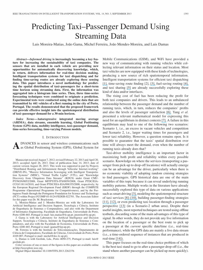
The following section presents a model that was first pro-posed in [15]. The demand for taxi services exhibits, likeother modes of road transportation [21], a daily periodicity thatreflects the patterns of the human activity. As a result, the dataappear to be nonhomogeneous. Fig. 1 shows a one-month taxi-service analysis extracted from our data set that illustrates thisperiodicity (the data set is described in detail in Section IV).

Consider the probability for n taxi assignments to emerge ina certain time period P (n), following a Poisson distribution.It is possible to define it using the following:

P (n;λ) =e−λλn

n!(1)

where λ represents the rate (average demand for taxi services)in a fixed time interval. However, in this specific problem, rateλ is not constant but time variant. Therefore, it was adaptedas a function of time, i.e., λ(t), transforming the Poisson

1396 IEEE TRANSACTIONS ON INTELLIGENT TRANSPORTATION SYSTEMS, VOL. 14, NO. 3, SEPTEMBER 2013

Fig. 1. One-month data analysis (total and per shift).

distribution into a nonhomogeneous one. Let λ0 be the average(i.e., expected) rate of the Poisson process over a full week.Consider λ(t) to be defined as follows:

λ(t) = λ0δd(t)ηd(t),h(t) (2)

where δd(t) is the relative change for weekday d(t) (e.g.,Saturdays have lower day rates than Tuesdays); ηd(t),h(t) isthe relative change for period h(t) in day d(t) (e.g., the peakhours); d(t) represents weekday 1 = Sunday, 2 = Monday, . . .;and h(t) represents the period when time t falls (e.g., the time of00:31 is contained in period 2 if we consider 30-min periods).

Consider λ(t) to be a discrete function (e.g., an histogramtime series of event counts that are aggregated in periodsof P minutes). Equation (2) requires the validity of bothequations, i.e.,

7∑i=1

δi = 7 (3)

I∑i=1

ηd,i = I ∀d (4)

where I is the number of time intervals in a day. The result is adiscrete time series per stand representing the expected demandduring an entire week, i.e., λ(t)k. Each value in this series isan average of all demands that are previously measured in thesame day type and period (i.e., the expected service demand fora Monday from 8:00 to 8:30 is the average of the demand on allpast Mondays from 8:00 to 8:30).

B. Weighted Time-Varying Poisson Model

The model that is previously presented can be seen as a time-dependent average, which produces predictions based on long-term historical data. However, it is not guaranteed that everytaxi stand will have a highly regular passenger demand; in fact,the demand in many stands can be often seasonal. The beachesare a good example of the seasonality demand as taxi demandwill be higher during summer weekends as opposed to otherseasons throughout the year.

To face this specific issue, a weighted average model isproposed based on the one presented before; the goal is toincrease the relevance of the demand pattern observed in the

recent week (e.g., what happened on the previous Tuesdayis more relevant than what happened two or three Tuesdaysago). The weight set ω is calculated using a well-known time-series approach to these type of problems, i.e., the exponentialsmoothing [33]. It is possible to define ω as follows:

ω = α ∗{

1, (1 − α), (1 − α)2, . . . , (1 − α)γ−1}, γ ∈ N

(5)

where γ is the number of historical periods that are considered,and 0 < α < 1 is the smoothing factor (i.e., γ and α are user-defined parameters). Then, based on the previous definition ofλ(t)k, it is possible to define the resulting weighted averageμ(t)k as follows:

μ(t)k =

γ∑i=1

Xt−(θ∗i) ∗ ωi

Ω,Ω =

γ∑i=1

ωi (6)

where θ is the number of time periods contained in a week.

C. ARIMA Model

The two previous models assume the existence of a regular(seasonal or not) periodicity in taxi service passenger demand(i.e., the demand at one taxi stand on a regular Tuesday duringa certain period will be highly similar to the demand verifiedduring the same period on other Tuesdays). However, the de-mand can present distinct periodicities for different stands. Theubiquitous features of this network force us to rapidly decide ifand how the model is evolving so that it is possible to instantlyadapt to these changes.

The ARIMA [16] is a well-known methodology for bothmodeling and forecasting univariate time-series data such astraffic-flow data [26], electricity price [29], and other short-term prediction problems such as the one presented here. Thereare two main advantages to using ARIMA compared with otheralgorithms. First, it is versatile to represent very different typesof time series, i.e., the autoregressive (AR) ones, the movingaverage (MA) ones, and a combination of those two (ARMA).Second, it combines the most recent samples from the series toproduce a forecast and to update itself to changes in the model.A brief presentation of one of the simplest ARIMA models (fornonseasonal stationary time series) is presented next, followingthe existing description in [30] (however, our framework canalso detect both seasonal and nonstationary series). For a moredetailed discussion, the reader should consult a comprehensivetime-series forecasting text such as the one presented in [31].

In an ARIMA model, the future value of a variable isassumed to be a linear function of several past observations andrandom errors. It is possible to formulate the underlying processthat generates the time series (taxi service over time for a givenstand k) as

Rk,t = κ0 + φ1Xk,t−1 + φ2Xk,t−2 + · · ·+ φpXk,t−p

+ εk,t − κ1εk,t−1 − κ2εk,t−2 − · · · − κqεk,t−q (7)

where Rk,t and {εk,t, εk,t−1, εk,t−2, . . .} are the actual valueat time period t and the Gaussian white noise error termsobserved in the past signal, respectively; φl(l = 1, 2, . . . , p) and

MOREIRA-MATIAS et al.: PREDICTING TAXI–PASSENGER DEMAND USING STREAMING DATA 1397

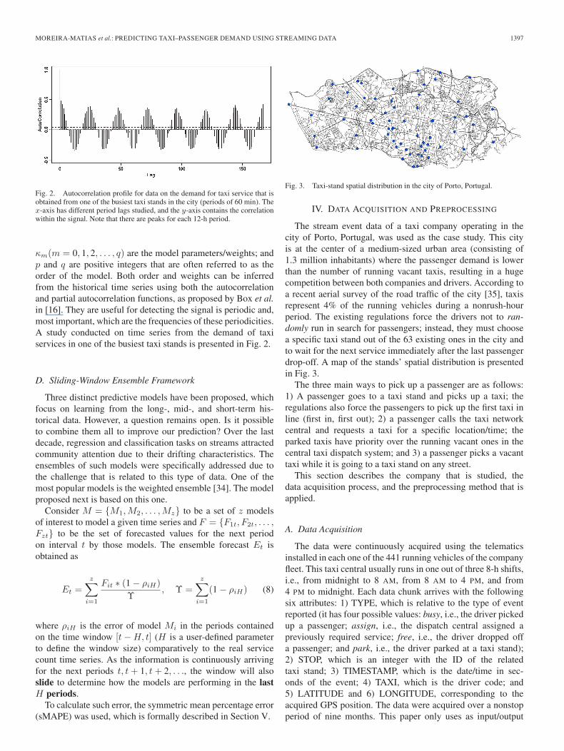
Fig. 2. Autocorrelation profile for data on the demand for taxi service that isobtained from one of the busiest taxi stands in the city (periods of 60 min). Thex-axis has different period lags studied, and the y-axis contains the correlationwithin the signal. Note that there are peaks for each 12-h period.

κm(m = 0, 1, 2, . . . , q) are the model parameters/weights; andp and q are positive integers that are often referred to as theorder of the model. Both order and weights can be inferredfrom the historical time series using both the autocorrelationand partial autocorrelation functions, as proposed by Box et al.in [16]. They are useful for detecting the signal is periodic and,most important, which are the frequencies of these periodicities.A study conducted on time series from the demand of taxiservices in one of the busiest taxi stands is presented in Fig. 2.

D. Sliding-Window Ensemble Framework

Three distinct predictive models have been proposed, whichfocus on learning from the long-, mid-, and short-term his-torical data. However, a question remains open. Is it possibleto combine them all to improve our prediction? Over the lastdecade, regression and classification tasks on streams attractedcommunity attention due to their drifting characteristics. Theensembles of such models were specifically addressed due tothe challenge that is related to this type of data. One of themost popular models is the weighted ensemble [34]. The modelproposed next is based on this one.

Consider M = {M1,M2, . . . ,Mz} to be a set of z modelsof interest to model a given time series and F = {F1t, F2t, . . . ,Fzt} to be the set of forecasted values for the next periodon interval t by those models. The ensemble forecast Et isobtained as

Et =z∑

i=1

Fit ∗ (1 − ρiH)

Υ, Υ =

z∑i=1

(1 − ρiH) (8)

where ρiH is the error of model Mi in the periods containedon the time window [t−H, t] (H is a user-defined parameterto define the window size) comparatively to the real servicecount time series. As the information is continuously arrivingfor the next periods t, t+ 1, t+ 2, . . ., the window will alsoslide to determine how the models are performing in the lastH periods.

To calculate such error, the symmetric mean percentage error(sMAPE) was used, which is formally described in Section V.

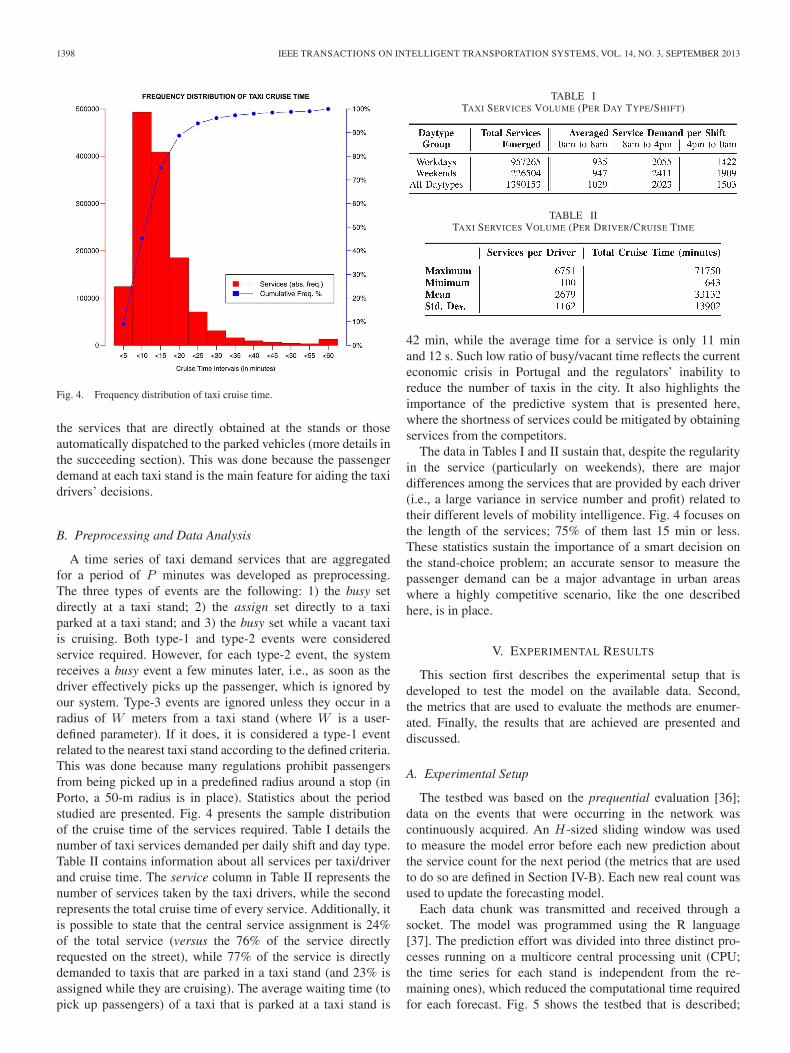
Fig. 3. Taxi-stand spatial distribution in the city of Porto, Portugal.

IV. DATA ACQUISITION AND PREPROCESSING

The stream event data of a taxi company operating in thecity of Porto, Portugal, was used as the case study. This cityis at the center of a medium-sized urban area (consisting of1.3 million inhabitants) where the passenger demand is lowerthan the number of running vacant taxis, resulting in a hugecompetition between both companies and drivers. According toa recent aerial survey of the road traffic of the city [35], taxisrepresent 4% of the running vehicles during a nonrush-hourperiod. The existing regulations force the drivers not to ran-domly run in search for passengers; instead, they must choosea specific taxi stand out of the 63 existing ones in the city andto wait for the next service immediately after the last passengerdrop-off. A map of the stands’ spatial distribution is presentedin Fig. 3.

The three main ways to pick up a passenger are as follows:1) A passenger goes to a taxi stand and picks up a taxi; theregulations also force the passengers to pick up the first taxi inline (first in, first out); 2) a passenger calls the taxi networkcentral and requests a taxi for a specific location/time; theparked taxis have priority over the running vacant ones in thecentral taxi dispatch system; and 3) a passenger picks a vacanttaxi while it is going to a taxi stand on any street.

This section describes the company that is studied, thedata acquisition process, and the preprocessing method that isapplied.

A. Data Acquisition

The data were continuously acquired using the telematicsinstalled in each one of the 441 running vehicles of the companyfleet. This taxi central usually runs in one out of three 8-h shifts,i.e., from midnight to 8 AM, from 8 AM to 4 PM, and from4 PM to midnight. Each data chunk arrives with the followingsix attributes: 1) TYPE, which is relative to the type of eventreported (it has four possible values: busy, i.e., the driver pickedup a passenger; assign, i.e., the dispatch central assigned apreviously required service; free, i.e., the driver dropped offa passenger; and park, i.e., the driver parked at a taxi stand);2) STOP, which is an integer with the ID of the relatedtaxi stand; 3) TIMESTAMP, which is the date/time in sec-onds of the event; 4) TAXI, which is the driver code; and5) LATITUDE and 6) LONGITUDE, corresponding to theacquired GPS position. The data were acquired over a nonstopperiod of nine months. This paper only uses as input/output

1398 IEEE TRANSACTIONS ON INTELLIGENT TRANSPORTATION SYSTEMS, VOL. 14, NO. 3, SEPTEMBER 2013

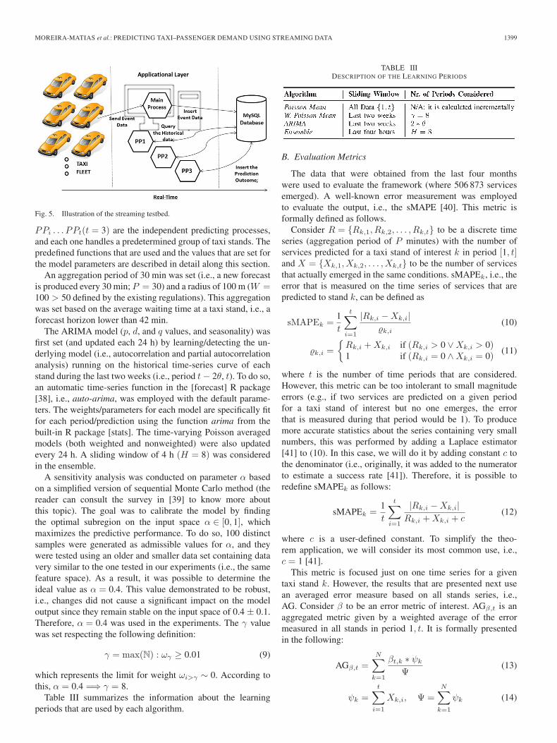
Fig. 4. Frequency distribution of taxi cruise time.

the services that are directly obtained at the stands or thoseautomatically dispatched to the parked vehicles (more details inthe succeeding section). This was done because the passengerdemand at each taxi stand is the main feature for aiding the taxidrivers’ decisions.

B. Preprocessing and Data Analysis

A time series of taxi demand services that are aggregatedfor a period of P minutes was developed as preprocessing.The three types of events are the following: 1) the busy setdirectly at a taxi stand; 2) the assign set directly to a taxiparked at a taxi stand; and 3) the busy set while a vacant taxiis cruising. Both type-1 and type-2 events were consideredservice required. However, for each type-2 event, the systemreceives a busy event a few minutes later, i.e., as soon as thedriver effectively picks up the passenger, which is ignored byour system. Type-3 events are ignored unless they occur in aradius of W meters from a taxi stand (where W is a user-defined parameter). If it does, it is considered a type-1 eventrelated to the nearest taxi stand according to the defined criteria.This was done because many regulations prohibit passengersfrom being picked up in a predefined radius around a stop (inPorto, a 50-m radius is in place). Statistics about the periodstudied are presented. Fig. 4 presents the sample distributionof the cruise time of the services required. Table I details thenumber of taxi services demanded per daily shift and day type.Table II contains information about all services per taxi/driverand cruise time. The service column in Table II represents thenumber of services taken by the taxi drivers, while the secondrepresents the total cruise time of every service. Additionally, itis possible to state that the central service assignment is 24%of the total service (versus the 76% of the service directlyrequested on the street), while 77% of the service is directlydemanded to taxis that are parked in a taxi stand (and 23% isassigned while they are cruising). The average waiting time (topick up passengers) of a taxi that is parked at a taxi stand is

TABLE ITAXI SERVICES VOLUME (PER DAY TYPE/SHIFT)

TABLE IITAXI SERVICES VOLUME (PER DRIVER/CRUISE TIME

42 min, while the average time for a service is only 11 minand 12 s. Such low ratio of busy/vacant time reflects the currenteconomic crisis in Portugal and the regulators’ inability toreduce the number of taxis in the city. It also highlights theimportance of the predictive system that is presented here,where the shortness of services could be mitigated by obtainingservices from the competitors.

The data in Tables I and II sustain that, despite the regularityin the service (particularly on weekends), there are majordifferences among the services that are provided by each driver(i.e., a large variance in service number and profit) related totheir different levels of mobility intelligence. Fig. 4 focuses onthe length of the services; 75% of them last 15 min or less.These statistics sustain the importance of a smart decision onthe stand-choice problem; an accurate sensor to measure thepassenger demand can be a major advantage in urban areaswhere a highly competitive scenario, like the one describedhere, is in place.

V. EXPERIMENTAL RESULTS

This section first describes the experimental setup that isdeveloped to test the model on the available data. Second,the metrics that are used to evaluate the methods are enumer-ated. Finally, the results that are achieved are presented anddiscussed.

A. Experimental Setup

The testbed was based on the prequential evaluation [36];data on the events that were occurring in the network wascontinuously acquired. An H-sized sliding window was usedto measure the model error before each new prediction aboutthe service count for the next period (the metrics that are usedto do so are defined in Section IV-B). Each new real count wasused to update the forecasting model.

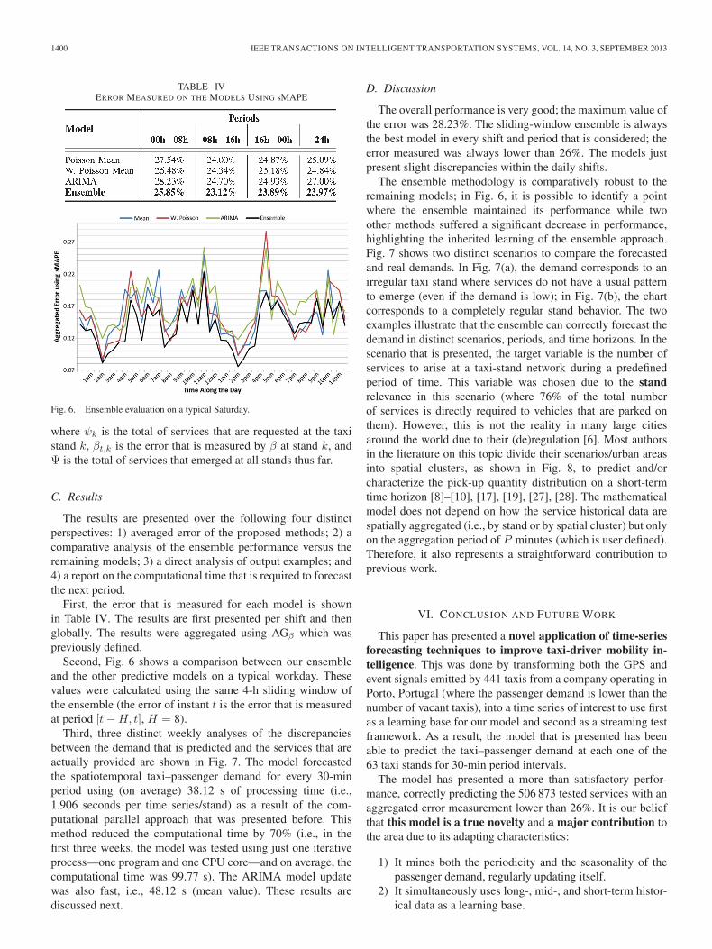
Each data chunk was transmitted and received through asocket. The model was programmed using the R language[37]. The prediction effort was divided into three distinct pro-cesses running on a multicore central processing unit (CPU;the time series for each stand is independent from the re-maining ones), which reduced the computational time requiredfor each forecast. Fig. 5 shows the testbed that is described;

MOREIRA-MATIAS et al.: PREDICTING TAXI–PASSENGER DEMAND USING STREAMING DATA 1399

Fig. 5. Illustration of the streaming testbed.

PPi . . . PPt(t = 3) are the independent predicting processes,and each one handles a predetermined group of taxi stands. Thepredefined functions that are used and the values that are set forthe model parameters are described in detail along this section.

An aggregation period of 30 min was set (i.e., a new forecastis produced every 30 min; P = 30) and a radius of 100 m (W =100 > 50 defined by the existing regulations). This aggregationwas set based on the average waiting time at a taxi stand, i.e., aforecast horizon lower than 42 min.

The ARIMA model (p, d, and q values, and seasonality) wasfirst set (and updated each 24 h) by learning/detecting the un-derlying model (i.e., autocorrelation and partial autocorrelationanalysis) running on the historical time-series curve of eachstand during the last two weeks (i.e., period t− 2θ, t). To do so,an automatic time-series function in the [forecast] R package[38], i.e., auto-arima, was employed with the default parame-ters. The weights/parameters for each model are specifically fitfor each period/prediction using the function arima from thebuilt-in R package [stats]. The time-varying Poisson averagedmodels (both weighted and nonweighted) were also updatedevery 24 h. A sliding window of 4 h (H = 8) was consideredin the ensemble.

A sensitivity analysis was conducted on parameter α basedon a simplified version of sequential Monte Carlo method (thereader can consult the survey in [39] to know more aboutthis topic). The goal was to calibrate the model by findingthe optimal subregion on the input space α ∈ [0, 1], whichmaximizes the predictive performance. To do so, 100 distinctsamples were generated as admissible values for α, and theywere tested using an older and smaller data set containing datavery similar to the one tested in our experiments (i.e., the samefeature space). As a result, it was possible to determine theideal value as α = 0.4. This value demonstrated to be robust,i.e., changes did not cause a significant impact on the modeloutput since they remain stable on the input space of 0.4 ± 0.1.Therefore, α = 0.4 was used in the experiments. The γ valuewas set respecting the following definition:

γ = max(N) : ωγ ≥ 0.01 (9)

which represents the limit for weight ωi>γ ∼ 0. According tothis, α = 0.4 =⇒ γ = 8.

Table III summarizes the information about the learningperiods that are used by each algorithm.

TABLE IIIDESCRIPTION OF THE LEARNING PERIODS

B. Evaluation Metrics

The data that were obtained from the last four monthswere used to evaluate the framework (where 506 873 servicesemerged). A well-known error measurement was employedto evaluate the output, i.e., the sMAPE [40]. This metric isformally defined as follows.

Consider R = {Rk,1, Rk,2, . . . , Rk,t} to be a discrete timeseries (aggregation period of P minutes) with the number ofservices predicted for a taxi stand of interest k in period [1, t]and X = {Xk,1, Xk,2, . . . , Xk,t} to be the number of servicesthat actually emerged in the same conditions. sMAPEk, i.e., theerror that is measured on the time series of services that arepredicted to stand k, can be defined as

sMAPEk =1t

t∑i=1

|Rk,i −Xk,i| k,i

(10)

k,i =

{Rk,i +Xk,i if (Rk,i > 0 ∨Xk,i > 0)1 if (Rk,i = 0 ∧Xk,i = 0)

(11)

where t is the number of time periods that are considered.However, this metric can be too intolerant to small magnitudeerrors (e.g., if two services are predicted on a given periodfor a taxi stand of interest but no one emerges, the errorthat is measured during that period would be 1). To producemore accurate statistics about the series containing very smallnumbers, this was performed by adding a Laplace estimator[41] to (10). In this case, we will do it by adding constant c tothe denominator (i.e., originally, it was added to the numeratorto estimate a success rate [41]). Therefore, it is possible toredefine sMAPEk as follows:

sMAPEk =1t

t∑i=1

|Rk,i −Xk,i|Rk,i +Xk,i + c

(12)

where c is a user-defined constant. To simplify the theo-rem application, we will consider its most common use, i.e.,c = 1 [41].

This metric is focused just on one time series for a giventaxi stand k. However, the results that are presented next usean averaged error measure based on all stands series, i.e.,AG. Consider β to be an error metric of interest. AGβ,t is anaggregated metric given by a weighted average of the errormeasured in all stands in period 1, t. It is formally presentedin the following:

AGβ,t =

N∑k=1

βt,k ∗ ψk

Ψ(13)

ψk =

t∑i=1

Xk,i, Ψ =

N∑k=1

ψk (14)

1400 IEEE TRANSACTIONS ON INTELLIGENT TRANSPORTATION SYSTEMS, VOL. 14, NO. 3, SEPTEMBER 2013

TABLE IVERROR MEASURED ON THE MODELS USING sMAPE

Fig. 6. Ensemble evaluation on a typical Saturday.

where ψk is the total of services that are requested at the taxistand k, βt,k is the error that is measured by β at stand k, andΨ is the total of services that emerged at all stands thus far.

C. Results

The results are presented over the following four distinctperspectives: 1) averaged error of the proposed methods; 2) acomparative analysis of the ensemble performance versus theremaining models; 3) a direct analysis of output examples; and4) a report on the computational time that is required to forecastthe next period.

First, the error that is measured for each model is shownin Table IV. The results are first presented per shift and thenglobally. The results were aggregated using AGβ which waspreviously defined.

Second, Fig. 6 shows a comparison between our ensembleand the other predictive models on a typical workday. Thesevalues were calculated using the same 4-h sliding window ofthe ensemble (the error of instant t is the error that is measuredat period [t−H, t], H = 8).

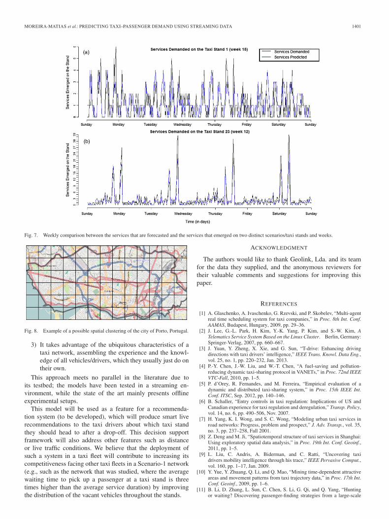
Third, three distinct weekly analyses of the discrepanciesbetween the demand that is predicted and the services that areactually provided are shown in Fig. 7. The model forecastedthe spatiotemporal taxi–passenger demand for every 30-minperiod using (on average) 38.12 s of processing time (i.e.,1.906 seconds per time series/stand) as a result of the com-putational parallel approach that was presented before. Thismethod reduced the computational time by 70% (i.e., in thefirst three weeks, the model was tested using just one iterativeprocess—one program and one CPU core—and on average, thecomputational time was 99.77 s). The ARIMA model updatewas also fast, i.e., 48.12 s (mean value). These results arediscussed next.

D. Discussion

The overall performance is very good; the maximum value ofthe error was 28.23%. The sliding-window ensemble is alwaysthe best model in every shift and period that is considered; theerror measured was always lower than 26%. The models justpresent slight discrepancies within the daily shifts.

The ensemble methodology is comparatively robust to theremaining models; in Fig. 6, it is possible to identify a pointwhere the ensemble maintained its performance while twoother methods suffered a significant decrease in performance,highlighting the inherited learning of the ensemble approach.Fig. 7 shows two distinct scenarios to compare the forecastedand real demands. In Fig. 7(a), the demand corresponds to anirregular taxi stand where services do not have a usual patternto emerge (even if the demand is low); in Fig. 7(b), the chartcorresponds to a completely regular stand behavior. The twoexamples illustrate that the ensemble can correctly forecast thedemand in distinct scenarios, periods, and time horizons. In thescenario that is presented, the target variable is the number ofservices to arise at a taxi-stand network during a predefinedperiod of time. This variable was chosen due to the standrelevance in this scenario (where 76% of the total numberof services is directly required to vehicles that are parked onthem). However, this is not the reality in many large citiesaround the world due to their (de)regulation [6]. Most authorsin the literature on this topic divide their scenarios/urban areasinto spatial clusters, as shown in Fig. 8, to predict and/orcharacterize the pick-up quantity distribution on a short-termtime horizon [8]–[10], [17], [19], [27], [28]. The mathematicalmodel does not depend on how the service historical data arespatially aggregated (i.e., by stand or by spatial cluster) but onlyon the aggregation period of P minutes (which is user defined).Therefore, it also represents a straightforward contribution toprevious work.

VI. CONCLUSION AND FUTURE WORK

This paper has presented a novel application of time-seriesforecasting techniques to improve taxi-driver mobility in-telligence. Thjs was done by transforming both the GPS andevent signals emitted by 441 taxis from a company operating inPorto, Portugal (where the passenger demand is lower than thenumber of vacant taxis), into a time series of interest to use firstas a learning base for our model and second as a streaming testframework. As a result, the model that is presented has beenable to predict the taxi–passenger demand at each one of the63 taxi stands for 30-min period intervals.

The model has presented a more than satisfactory perfor-mance, correctly predicting the 506 873 tested services with anaggregated error measurement lower than 26%. It is our beliefthat this model is a true novelty and a major contribution tothe area due to its adapting characteristics:

1) It mines both the periodicity and the seasonality of thepassenger demand, regularly updating itself.

2) It simultaneously uses long-, mid-, and short-term histor-ical data as a learning base.

MOREIRA-MATIAS et al.: PREDICTING TAXI–PASSENGER DEMAND USING STREAMING DATA 1401

Fig. 7. Weekly comparison between the services that are forecasted and the services that emerged on two distinct scenarios/taxi stands and weeks.

Fig. 8. Example of a possible spatial clustering of the city of Porto, Portugal.

3) It takes advantage of the ubiquitous characteristics of ataxi network, assembling the experience and the knowl-edge of all vehicles/drivers, which they usually just do ontheir own.

This approach meets no parallel in the literature due toits testbed; the models have been tested in a streaming en-vironment, while the state of the art mainly presents offlineexperimental setups.

This model will be used as a feature for a recommenda-tion system (to be developed), which will produce smart liverecommendations to the taxi drivers about which taxi standthey should head to after a drop-off. This decision supportframework will also address other features such as distanceor live traffic conditions. We believe that the deployment ofsuch a system in a taxi fleet will contribute to increasing itscompetitiveness facing other taxi fleets in a Scenario-1 network(e.g., such as the network that was studied, where the averagewaiting time to pick up a passenger at a taxi stand is threetimes higher than the average service duration) by improvingthe distribution of the vacant vehicles throughout the stands.

ACKNOWLEDGMENT

The authors would like to thank Geolink, Lda. and its teamfor the data they supplied, and the anonymous reviewers fortheir valuable comments and suggestions for improving thispaper.

REFERENCES

[1] A. Glaschenko, A. Ivaschenko, G. Rzevski, and P. Skobelev, “Multi-agentreal time scheduling system for taxi companies,” in Proc. 8th Int. Conf.AAMAS, Budapest, Hungary, 2009, pp. 29–36.

[2] J. Lee, G.-L. Park, H. Kim, Y.-K. Yang, P. Kim, and S.-W. Kim, ATelematics Service System Based on the Linux Cluster. Berlin, Germany:Springer-Verlag, 2007, pp. 660–667.

[3] J. Yuan, Y. Zheng, X. Xie, and G. Sun, “T-drive: Enhancing drivingdirections with taxi drivers’ intelligence,” IEEE Trans. Knowl. Data Eng.,vol. 25, no. 1, pp. 220–232, Jan. 2013.

[4] P.-Y. Chen, J.-W. Liu, and W.-T. Chen, “A fuel-saving and pollution-reducing dynamic taxi-sharing protocol in VANETs,” in Proc. 72nd IEEEVTC-Fall, 2010, pp. 1–5.

[5] P. d’Orey, R. Fernandes, and M. Ferreira, “Empirical evaluation of adynamic and distributed taxi-sharing system,” in Proc. 15th IEEE Int.Conf. ITSC, Sep. 2012, pp. 140–146.

[6] B. Schaller, “Entry controls in taxi regulation: Implications of US andCanadian experience for taxi regulation and deregulation,” Transp. Policy,vol. 14, no. 6, pp. 490–506, Nov. 2007.

[7] H. Yang, K. I. Wong, and S. C. Wong, “Modeling urban taxi services inroad networks: Progress, problem and prospect,” J. Adv. Transp., vol. 35,no. 3, pp. 237–258, Fall 2001.

[8] Z. Deng and M. Ji, “Spatiotemporal structure of taxi services in Shanghai:Using exploratory spatial data analysis,” in Proc. 19th Int. Conf. Geoinf.,2011, pp. 1–5.

[9] L. Liu, C. Andris, A. Biderman, and C. Ratti, “Uncovering taxidrivers mobility intelligence through his trace,” IEEE Pervasive Comput.,vol. 160, pp. 1–17, Jan. 2009.

[10] Y. Yue, Y. Zhuang, Q. Li, and Q. Mao, “Mining time-dependent attractiveareas and movement patterns from taxi trajectory data,” in Proc. 17th Int.Conf. Geoinf., 2009, pp. 1–6.

[11] B. Li, D. Zhang, L. Sun, C. Chen, S. Li, G. Qi, and Q. Yang, “Huntingor waiting? Discovering passenger-finding strategies from a large-scale

1402 IEEE TRANSACTIONS ON INTELLIGENT TRANSPORTATION SYSTEMS, VOL. 14, NO. 3, SEPTEMBER 2013

real-world taxi dataset,” in Proc. IEEE Int. Conf. PERCOM Workshops,Mar. 2011, pp. 63–68.

[12] J. Lee, I. Shin, and G. Park, “Analysis of the passenger pick-up patternfor taxi location recommendation,” in Proc. 4th Int. Conf. NCM Adv. Inf.Manage., 2008, vol. 1, pp. 199–204.

[13] S. Phithakkitnukoon, M. Veloso, C. Bento, A. Biderman, and C. Ratti,“Taxi-aware map: Identifying and predicting vacant taxis in the city,” inProc. Ambient Intell., 2010, vol. 6439, pp. 86–95.

[14] J. Gama, Knowledge Discovery From Data Streams. London, U.K.:Chapman & Hall, 2010.

[15] A. Ihler, J. Hutchins, and P. Smyth, “Adaptive event detection with time-varying Poisson processes,” in Proc. 12th Int. Conf. ACM SIGKDD, 2006,pp. 207–216.

[16] G. Box, G. Jenkins, and G. Reinsel, Time Series Analysis. San Francisco,CA, USA: Holden-Day, 1976.

[17] X. Li, G. Pan, Z. Wu, G. Qi, S. Li, D. Zhang, W. Zhang, and Z. Wang,“Prediction of urban human mobility using large-scale taxi traces andits applications,” Front. Comput. Sci. Chin., vol. 6, no. 1, pp. 111–121,Feb. 2012.

[18] A. Kaltenbrunner, R. Meza, J. Grivolla, J. Codina, and R. Banchs, “Urbancycles and mobility patterns: Exploring and predicting trends in a bicycle-based public transport system,” Perv. Mobile Comput., vol. 6, no. 4,pp. 455–466, Aug. 2010.

[19] H. Chang, Y. Tai, and J. Hsu, “Context-aware taxi demand hotspotsprediction,” Int. J. Business Intell. Data Mining, vol. 5, no. 1, pp. 3–18,Dec. 2010.

[20] B. Cule, B. Goethals, S. Tassenoy, and S. Verboven, “Mining train delays,”in Advances in Intelligent Data Analysis X. Berlin, Germany: Springer-Verlag, 2011, ser. LNCS, pp. 113–124.

[21] L. Matias, J. Gama, J. Mendes-Moreira, and J. Freire de Sousa, “Valida-tion of both number and coverage of bus schedules using AVL data,” inProc 13th IEEE Conf. ITSC, 2010, pp. 131–136.

[22] L. Moreira-Matias, C. Ferreira, J. Gama, J. Mendes-Moreira, andJ. de Sousa, “Bus bunching detection by mining sequences of headwaydeviations,” in Advances in Data Mining. Applications and Theoreti-cal Aspects. New York, NY, USA: Springer-Verlag, 2012, ser. LNCS,pp. 77–91.

[23] M. C. Gonzalez, C. A. Hidalgo, and A.-L. Barabasi, “Understandingindividual human mobility patterns,” Nature, vol. 453, no. 7196, pp. 779–782, Jun. 2008.

[24] J. Gama and P. Rodrigues, “Stream-based electricity load forecast,”in Knowledge Discovery in Databases: PKDD. Berlin, Germany:Springer-Verlag, 2007, ser. LNCS, pp. 446–453.

[25] B. Williams and L. Hoel, “Modeling and forecasting vehicular traffic flowas a seasonal ARIMA process: Theoretical basis and empirical results,”J. Transp. Eng., vol. 129, no. 6, pp. 664–672, Nov. 2003.

[26] W. Min and L. Wynter, “Real-time road traffic prediction with spatio-temporal correlations,” Transp. Res. C, Emerg. Technol., vol. 19, no. 4,pp. 606–616, Aug. 2011.

[27] Y. Ge, H. Xiong, A. Tuzhilin, K. Xiao, M. Gruteser, and M. Pazzani,“An energy-efficient mobile recommender system,” in Proc. 16th ACMSIGKDD Int. Conf., 2010, pp. 899–908.

[28] J. Yuan, Y. Zheng, L. Zhang, X. Xie, and G. Sun, “Where to find my nextpassenger?” in Proc. 13th ACM Int. Conf. UbiComp, 2011, pp. 109–118.

[29] J. Contreras, R. Espinola, F. J. Nogales, and A. J. Conejo, “ARIMAmodels to predict next-day electricity prices,” IEEE Trans. Power Syst.,vol. 18, no. 3, pp. 1014–1020, Aug. 2003.

[30] G. Zhang, “Time series forecasting using a hybrid ARIMA and neuralnetwork model,” Neurocomputing, vol. 50, pp. 159–175, Jan. 2003.

[31] J. Cryer and K. Chan, Time Series Analysis With Applications in R.New York, NY, USA: Springer-Verlag, 2008.

[32] L. Moreira-Matias, J. Gama, M. Ferreira, and L. Damas, “A predictivemodel for the passenger demand on a taxi network,” in Proc. 15th IEEEInt. Conf. ITSC, Sep. 2012, pp. 1014–1019.

[33] C. Holt, “Forecasting seasonals and trends by exponentially weightedmoving averages,” Int. J. Forecast., vol. 20, no. 1, pp. 5–10,Jan.–Mar. 2004.

[34] H. Wang, W. Fan, P. Yu, and J. Han, “Mining concept-drifting data streamsusing ensemble classifiers,” in Proc. 9th ACM SIGKDD Int. Conf., 2003,pp. 226–235.

[35] M. Ferreira, H. Conceição, R. Fernandes, and O. Tonguz, “Stereo-scopic aerial photography: An alternative to model-based urban mobilityapproaches,” in Proc. 6th ACM Int. Workshop Veh. InterNetw., 2009,pp. 53–62.

[36] A. Dawid, “Present position and potential developments: Some personalviews: Statistical theory: The prequential approach,” J. Roy. Stat. Soc. A,vol. 47, no. 2, pp. 278–292, Jan. 1984.

[37] R Core Team. (2012). R: A Language and Environment for StatisticalComputing, R Foundation for Statistical Computing, Vienna, Austria.[Online]. Available: http://www.R-project.org

[38] K. Yeasmin and J. H. Rob (2008, Jul.). Automatic Time Series Forecast-ing: The forecast package for R. J. Stat. Softw. [Online]. 27(3), pp. 1–22.Available: http://oai.repec.openlib.org

[39] O. Cappé, S. Godsill, and E. Moulines, “An overview of existing methodsand recent advances in sequential Monte Carlo,” Proc. IEEE, vol. 95,no. 5, pp. 899–924, May 2007.

[40] S. Makridakis and M. Hibon, “The M3-competition: Results, conclusionsand implications,” Int. J. Forecast., vol. 16, no. 4, pp. 451–476, Jan. 2000.

[41] E. Jaynes, Probability Theory: The Logic of Science. Cambridge, U.K.:Cambridge Univ. Press, 2003.

Luis Moreira-Matias received the M.Sc. degreein informatics engineering from the University ofPorto, Porto, Portugal, in 2009, where he is currentlyworking toward the Ph.D. degree in machine learningwith the Faculty of Engineering.

He is also with the Laboratory for Artificial Intel-ligence and Decision Support, Tecnologia e Ciência,Instituto de Engenharia de Sistemas e Computadores,University of Porto. His current research interest islearning from data streams.

João Gama received the Ph.D. degree in computerscience from the University of Porto, Porto, Portugal,in 2000.

He is a Researcher with the Laboratory of Artifi-cial Intelligence and Decision Support, Tecnologiae Ciência, Instituto de Engenharia de Sistemas eComputadores, University of Porto. He has recentlyauthored a book on knowledge discovery from datastreams. His main research interest is learning fromdata streams.

Michel Ferreira received the Ms.c. and Ph.D.degrees in computer science from the Univer-sity of Porto, Porto, Portugal, in 1994 and 2002,respectively.

He is an Assistant Professor with the Faculty ofSciences, University of Porto, where he leads theGeo-Networks group with the Department of Com-puter Science. He has led several research projects inthe areas of logic-based spatial databases, vehicularsensing, and intervehicle communication.

João Mendes-Moreira received the Ph.D. degree inengineering sciences from the University of Porto,Porto, Portugal.

He is an Assistant Professor with the Departmentof Informatics Engineering, Faculty of Sciences,University of Porto, where he is also a Researcherwith the Laboratory for Artificial Intelligence andDecision Support, Tecnologia e Ciência, Institutode Engenharia de Sistemas e Computadores. Hisresearch works focus on applied machine learning.

Luis Damas received the Ph.D. degree in mathemat-ical theory of computation from the University ofEdinburgh, Edinburgh, U.K., in 1984.

He is the creator of one of the most widely usedlogic programming systems, i.e., the YAP Prologcompiler. He is also the Co-founder and the ChiefTechnical Officer with Geolink, Lda., Porto, Portu-gal. His research interests include simulation, dis-tributed systems, and programming languages.