an improved spatiotemporal weighted mean temperature
TRANSCRIPT
Citation: Zhang, B.; Wang, Z.; Li, W.;
Jiang, W.; Shen, Y.; Zhang, Y.; Zhang,
S.; Tian, K. An Improved
Spatiotemporal Weighted Mean
Temperature Model over Europe
Based on the Nonlinear Least Squares
Estimation Method. Remote Sens.
2022, 14, 3609. https://doi.org/
10.3390/rs14153609
Academic Editor: Christopher Kidd
Received: 21 June 2022
Accepted: 26 July 2022
Published: 28 July 2022
Publisher’s Note: MDPI stays neutral
with regard to jurisdictional claims in
published maps and institutional affil-
iations.
Copyright: © 2022 by the authors.
Licensee MDPI, Basel, Switzerland.
This article is an open access article
distributed under the terms and
conditions of the Creative Commons
Attribution (CC BY) license (https://
creativecommons.org/licenses/by/
4.0/).
remote sensing
Article
An Improved Spatiotemporal Weighted Mean TemperatureModel over Europe Based on the Nonlinear Least SquaresEstimation MethodBingbing Zhang 1 , Zhengtao Wang 2 , Wang Li 3, Wei Jiang 1, Yi Shen 1,*, Yan Zhang 1, Shike Zhang 1
and Kunjun Tian 4
1 School of Geographic Sciences, Xinyang Normal University, Xinyang 464000, China;[email protected] (B.Z.); [email protected] (W.J.); [email protected] (Y.Z.);[email protected] (S.Z.)
2 School of Geodesy and Geomatics, Wuhan University, Wuhan 430079, China; [email protected] Faculty of Land Resources Engineering, Kunming University of Science and Technology,
Kunming 650093, China; [email protected] School of Civil and Architectural Engineering, Shandong University of Technology, Zibo 255000, China;
[email protected]* Correspondence: [email protected]; Tel.: +86-15063086165
Abstract: Weighted average temperature (Tm) plays a crucial role in global navigation satellitesystem (GNSS) precipitable water vapor (PWV) retrieval. Aiming at the poor applicability of theexisting Tm models in Europe, in the article, we used observations from 48 radiosonde stations overEurope from 2014 to 2020 to establish a weighted average temperature model in Europe (ETm) bythe nonlinear least squares estimation method. The ETm model takes into account factors such asground temperature, water vapor pressure, latitude, and their annual variation, semiannual variationand diurnal variation. Taking the Tm obtained from the radiosonde data by the integration methodin 2021 as the reference value, the accuracy of the ETm model was evaluated and compared with thecommonly used Bevis model, ETmPoly model, and GPT2w model. The results of the 48 modeledstations showed that the mean bias and root mean square (RMS) values of the ETm model were0.06 and 2.85 K, respectively, which were 21.7%, 11.5%, and 31.8% higher than the Bevis, ETmPoly,and GPT2w-1 (1◦ × 1◦ resolution) models, respectively. In addition, the radiosonde data of 12 non-modeling stations over Europe in 2021 were selected to participate in the model accuracy validation.The mean bias and RMS values of the ETm model were –0.07 and 2.87 K, respectively. Comparedwith the Bevis, ETmPoly, and GPT2w-1 models, the accuracy (in terms of RMS values) increased by20.5%, 10.6%, and 35.2%, respectively. Finally, to further verify the superiority of the ETm model, theETm model, and other Tm models were applied to the GNSS PWV calculation. The ETm model hadmean RMSPWV and RMSPWV/PWV values of 0.17 mm and 1.03%, respectively, which were less thanother Tm models. Therefore, the ETm model has essential applications in GNSS PWV over Europe.
Keywords: weighted average temperature; nonlinear least squares estimation method; GPT2w; Bevis;root mean square
1. Introduction
Water vapor and its variation are the main driving force of weather and climate change,which are important factors in the formation and evolution of disastrous weather. Thechange in atmospheric water vapor is directly related to precipitation and plays an impor-tant role in various meteorological changes such as atmospheric energy transfer, weathersystem evolution, and global climate change. In recent years, with the wide application ofGNSS technology in meteorology [1], compared with conventional meteorological detectiontechnology, GNSS meteorological detection technology has the advantages of high temporal
Remote Sens. 2022, 14, 3609. https://doi.org/10.3390/rs14153609 https://www.mdpi.com/journal/remotesensing

Remote Sens. 2022, 14, 3609 2 of 17
resolution, high precision, and low observation cost. It is an important innovation of mete-orological observation technology, which significantly improves small- and medium-scalenumerical weather observation and forecasting capabilities and effectively makes up forthe limitations of conventional meteorological detection technology [2]. Moreover, it iswidely used in the analysis and imminent prediction of extreme weather such as drought,rainstorms, and typhoons [3]. In the process of GNSS PWV, the water vapor conversioncoefficient is the critical parameter for converting tropospheric zenith wet delay (ZWD)into atmospheric water vapor [2], which is mainly affected by the atmospheric weightedaverage temperature (Tm) [4,5].
Currently, the calculation model of Tm can usually be divided into two categoriesaccording to whether or not in situ meteorological information is needed. The first cate-gory is the empirical model requiring surface meteorological parameters, which generallyrequires the measured surface temperature (Ts) and other meteorological parameters (i.e.,water vapor pressure and atmospheric pressure). Among them, the Bevis model [1] is oneof the most widely used models. It first explores the linear relationship between Ts and Tmand establishes a Bevis model suitable for middle latitude (27◦–65◦N) (Tm = 0.72Ts + 70.2).However, there will be apparent systematic bias when the model is applied to other re-gions [6]. Therefore, many scholars have studied empirical models based on multiyearlocal or global Tm data fitting [6–17] and improved the Bevis model. When surface me-teorological parameters are available, this model will have a good prediction effect. Thesecond type is the Tm model without meteorological parameters [18]. This kind of modelis an empirical model based on multiyear local or global Tm data fitting. It is simple to use,but its accuracy is not very high compared with the Tm model using measured surfacemeteorological information. Representative Tm models include GPT2w and GPT3 modelsproposed by Boehm [18,19], GWMT, GTm-II, GTm-III, and GTrop models proposed byYao [13,20–22] and GGTm model proposed by Huang [23,24]. With the development ofatmospheric science and the progress of detection technology, PWV prediction accuracy isrequired to be higher [25,26]. Therefore, the current Tm model cannot satisfactorily meetthe needs of the prediction accuracy of GNSS PWV over Europe [27]. Consequently, it isnecessary to comprehensively use a variety of meteorological factors and spatiotemporallocation information to establish a high-precision spatiotemporal model of Tm over Europe.
Based on data from 60 radiosonde stations in Europe over seven consecutive years(2014–2020), this paper first analyzed the linear correlation between Tm and ground temper-ature, water vapor pressure, air pressure, latitude, longitude, and elevation. Then, on thisbasis, comprehensively considering the meteorological factors with good linear correlationand spatiotemporal information, the refined ETm model was established using the nonlin-ear least squares method. Taking the Tm calculated by the numerical integration method ofmodeling and non-modeling radiosonde data over Europe in 2021 as the reference values,the accuracy of the ETm model was tested and compared with the Bevis model and GPT2wmodel. The ETm model was comprehensively evaluated by the bias and the root meansquare (RMS) index. This paper is organized as follows: Section 2 shows the materials andmethods used, Section 3 evaluates the ETm model, Bevis model, and GPT2w by the biasand RMS values; finally, Section 4 provides a discussion and the conclusion.
2. Materials and Methods2.1. Study Area
In the article, 60 radiosonde stations in Europe were selected as the research object, ofwhich 48 radiosonde stations were used for modeling, and 12 radiosonde stations were usedfor accuracy validation of non-modeling stations. The 8 year measured data of radiosondestations from 2014 to 2021 (the data sampling interval is 12 h, and the data samplinginterval of individual radiosonde stations is 6 h) were adopted. These data can be obtainedfrom the website, http://weather.uwyo.edu/upperair/seasia.html (accessed on 20 June2022), including the measured radiosonde data from 2014 to 2020 as modeling data and

Remote Sens. 2022, 14, 3609 3 of 17
the measured data from 2021 as reference data for accuracy validation. The geographicaldistribution of the site is shown in Figure 1.
Remote Sens. 2022, 14, x FOR PEER REVIEW 3 of 18
used for accuracy validation of non-modeling stations. The 8 year measured data of radi-osonde stations from 2014 to 2021 (the data sampling interval is 12 h, and the data sam-pling interval of individual radiosonde stations is 6 h) were adopted. These data can be obtained from the website, http://weather.uwyo.edu/upperair/seasia.html, including the measured radiosonde data from 2014 to 2020 as modeling data and the measured data from 2021 as reference data for accuracy validation. The geographical distribution of the site is shown in Figure 1.
Figure 1. Distribution of radiosonde stations over Europe. The red dots denote the positions of the modeling stations, and the blue triangles denote the positions of the non-modeling stations.
2.2. Computing Tm Based on the Numerical Integration Method The radiosonde data were divided into different pressure level data and surface data.
Every pressure level data included meteorological observations such as relative humidity, pressure, temperature, and dew point temperature. The surface data included atmos-pheric precipitable water vapor and the location of the station. According to different pressure levels, the Tm values of the radiosonde stations were calculated by the numerical integration method, which was the most used method with the highest precision recog-nized by scholars at home and abroad. The concrete solution was as follows.
The Tm values were obtained by using measurements of the geopotential height, ab-solute temperature, and relative humidity at each pressure level along the zenith direc-tion. The specific numerical integration method of Tm is shown in formula (1):
2
( / )Tm( / )e T dze T dz=
(1)
where T represents the absolute temperature (K); e is the water vapor pressure (hPa); z stands for the geopotential height along the zenith direction. As radiosonde observations provide the relative humidity (RH) and absolute temperature T (K), which can be used to calculate the e in Equation (2) [25,28]:
7.5( )237.36.11 10
100
TdTdRHe
×+× ×= (2)
In Equation (2), Td stands for the atmospheric temperature in Celsius (T = Td + 273.15). In practice, Equation (1) is discretized using Equation (3):
Figure 1. Distribution of radiosonde stations over Europe. The red dots denote the positions of themodeling stations, and the blue triangles denote the positions of the non-modeling stations.
2.2. Computing Tm Based on the Numerical Integration Method
The radiosonde data were divided into different pressure level data and surfacedata. Every pressure level data included meteorological observations such as relativehumidity, pressure, temperature, and dew point temperature. The surface data includedatmospheric precipitable water vapor and the location of the station. According to differentpressure levels, the Tm values of the radiosonde stations were calculated by the numericalintegration method, which was the most used method with the highest precision recognizedby scholars at home and abroad. The concrete solution was as follows.
The Tm values were obtained by using measurements of the geopotential height, ab-solute temperature, and relative humidity at each pressure level along the zenith direction.The specific numerical integration method of Tm is shown in Formula (1):
Tm =
∫(e/T)dz∫(e/T2)dz
(1)
where T represents the absolute temperature (K); e is the water vapor pressure (hPa); zstands for the geopotential height along the zenith direction. As radiosonde observationsprovide the relative humidity (RH) and absolute temperature T (K), which can be used tocalculate the e in Equation (2) [25,28]:
e =RH × 6.11× 10(
7.5×Td237.3+Td )
100(2)
In Equation (2), Td stands for the atmospheric temperature in Celsius (T = Td + 273.15).In practice, Equation (1) is discretized using Equation (3):
Tm =
n∑1
eiTi
∆zi
n∑1
eiTi
2 ∆zi
(3)
In Equation (3), ∆zi stands for the thickness of the ith atmosphere layer (m); n standsfor the number of the atmosphere layers; Ti, and ei stands for the mean temperature and
Remote Sens. 2022, 14, 3609 4 of 17
water vapor pressure of the ith article were directly and uniformly distributed atmospherelayer, respectively.
2.3. Tm from the Bevis Model
Although the Tm accuracy obtained from the observations of the radiosonde stationsis high, the rare distribution of the radiosonde stations resulted in a limited application.Therefore, the statistical analysis method was generally used to deduce the statisticalrelationship between Tm and Ts. A commonly used empirical equation is the Bevis model,which estimates Tm through the Ts observations. Bevis believed that there was a goodcorrelation between the Tm and Ts. Therefore, radiosonde data of the United States(27◦–65◦N) were used to obtain the following linear regression formula (also known as theBevis empirical formula) through statistical analysis.
Tm = 70.2 + 0.72Ts (4)
The Bevis model was established through two years of the observations at 13 ra-diosonde stations in the United States. The accuracy of the Bevis model was 4.74 K, and therelative error was less than 2%. In addition, the Bevis model has been widely used in theworld due to the fact of its simplicity and practicality.
2.4. Tm from the ETmPoly Model
Baldysz and Nykiel [16] used 24 years (1994–2018) of radiosonde data from 49 ra-diosonde stations over Europe to determine reliable coefficients of the Tm and Ts relation-ship, namely, the ETmPoly model. The Tm values from the ETmPoly model were calculatedthrough the Equation (5):
Tm = a · Ts + b
a = −10.07t5 + 23.95t4 − 19.08t3 + 5.998t2 − 0.7914t + 0.8436
b = 2985t5 − 7200t4 + 5882t3 − 1923t2 + 256.8t + 35.87
(5)
In Equation (5), t = UT/24, UT stands for the universal time of day. In this article, wechose the ETmPoly model for participation in the validation.
2.5. Computing the Tm Based on the GPT2w Model
Bohm et al. [18] added two parameters of the water vapor pressure vertical gradientand atmospheric weighted average temperature into the GPT2 model to obtain the GPT2wmodel, which further improved the accuracy of the GPT2w model. The GPT2w model canprovide Tm values by resolutions of 1◦ × 1◦ and 5◦ × 5◦. Tm of the GPT2w model wascalculated through Equation (6):
TmGPT2w = A0 + A1 cos(DOY
365.252π) + B1 sin(
DOY365.25
2π) + A2 cos(DOY
365.254π) + B2 sin(
DOY365.25
4π) (6)
In Equation (6), DOY stands for the day of year, the coefficients of A0, A1, A2, B1, and B2were determined based on a regular grid of 1◦ × 1◦ and 5◦ × 5◦, namely, the GPT2w-1 andGPT2w-5 models, respectively. In this paper, we chose the GPT2w-1 model to participatein the validation.
2.6. Construction of a New Tm Model (ETm) over Europe
The variation characteristics of Tm mainly include diurnal, seasonal, surface tem-perature, water vapor pressure, and latitude over Europe. Therefore, the ETm model isexpressed as a function of the multiplication of three components, namely, the diurnalvariation, annual and semiannual variations of surface temperature, water vapor pressure,and latitude as shown in Equation (7).
ETm = f (DOY, UT, Ts, es, Latitude) = f1 · f2 · f3 (7)

Remote Sens. 2022, 14, 3609 5 of 17
f1 = 1 + a1 cos(2π
24UT + b1) (8)
f2 = 1 +2
∑i=1
ci cos(i2π
365.25DOY + di) (9)
f3 = e + f · TS + g · ln es + h · Latitude (10)
Because the weighted average temperature will change over time in one day, therefore,the diurnal variation of Tm was considered. See Equation (8), in Equation (7), f1 representsthe diurnal variation component of Tm. UT stands for the universal time of day, and a1and b1 are the coefficient.
The research results show that Tm has noticeable periodic changes (i.e., annual varia-tion and semiannual variation), which were taken into account when modeling Tm. SeeEquation (9), f2 represents the annual and semiannual variation component of Tm. DOYshows day of year, ci and di are the coefficients, and i = 1, 2.
In addition, in Figure 2, Tm had a good linear correlation with Ts and lnes. The corre-lation coefficients were 0.90 and 0.86, respectively. Furthermore, the spatial distributiondiagram between the mean Tm and latitude of each station are shown in Figure 2, and wefound that there was a strong negative linear correlation between the mean Tm values andlatitude, and the correlation coefficient reached −0.94. Thus, the Ts, lnes, and latitude inthe article were regarded as influencing factors [29], and this component is expressed inEquation (10). The four coefficients of e, f, g, and h, were obtained by the nonlinear leastsquares method.
Remote Sens. 2022, 14, x FOR PEER REVIEW 5 of 18
2.6. Construction of a New Tm Model (ETm) over Europe The variation characteristics of Tm mainly include diurnal, seasonal, surface temper-
ature, water vapor pressure, and latitude over Europe. Therefore, the ETm model is ex-pressed as a function of the multiplication of three components, namely, the diurnal var-iation, annual and semiannual variations of surface temperature, water vapor pressure, and latitude as shown in Equation (7).
1 2 3ETm ( , , , , )=sf DOY UT Ts e Latitude f f f= ⋅ ⋅ (7)
1 1 121 cos( )24
f a UT bπ= + + (8)
2
21
21 cos( )365.25i i
if c i DOY dπ
=
= + + (9)
3 lnS sf e f T g e h Latitude= + ⋅ + ⋅ + ⋅ (10)
Because the weighted average temperature will change over time in one day, there-fore, the diurnal variation of Tm was considered. See Equation (8), in Equation (7), 1f rep-resents the diurnal variation component of Tm. UT stands for the universal time of day, and 1a and 1b are the coefficient.
The research results show that Tm has noticeable periodic changes (i.e., annual vari-ation and semiannual variation), which were taken into account when modeling Tm. See Equation (9), 2f represents the annual and semiannual variation component of Tm. DOY shows day of year, ic and id are the coefficients, and i = 1, 2.
In addition, in Figure 2, Tm had a good linear correlation with Ts and lnes. The cor-relation coefficients were 0.90 and 0.86, respectively. Furthermore, the spatial distribution diagram between the mean Tm and latitude of each station are shown in Figure 2, and we found that there was a strong negative linear correlation between the mean Tm values and latitude, and the correlation coefficient reached −0.94. Thus, the Ts, lnes, and latitude in the article were regarded as influencing factors [29], and this component is expressed in Equation (10). The four coefficients of e, f, g, and h, were obtained by the nonlinear least squares method.
(a) (b)
Remote Sens. 2022, 14, x FOR PEER REVIEW 6 of 18
(c)
Figure 2. The linear correlation analysis between Tm with Ts, ln es, and latitude. (a)linear correla-tion between Tm and ln(es), (b)linear correlation between Tm and Ts, (c)linear correlation between Mean of the Tm and latitude.
In order to obtain the optimal solution of the ETm model, we considered the problem of fitting the model coefficients to the observations. The coefficients and observations are related through the nonlinear equations. Our goal was to determine the values of the co-efficients that best fit the observations in the sense of minimizing the sum of the squares of the residual errors. This model cannot be solved directly by analytical methods; there-fore, an iterative approach was used for obtaining the ETm model coefficients. For succes-sive solution steps, a Levenberg–Marquardt method [30,31] was applied. The Levenberg–Marquardt (LM) optimization method is widely used in nonlinear least squares optimal estimation [32]. It is insensitive to over parametric problems and can effectively deal with redundant parameter problems. It has the advantages of both the gradient method and the Gauss Newton method. The algorithm avoids the problem that the Gauss Newton method is not positive definite when solving a Hesse matrix, and it solves the problem when the step size of the gradient descent method is too large [33,34].
For the above consideration, firstly, we selected the observations of 48 radiosonde stations in Europe from 2014 to 2020. Then, the coefficient values of the new ETm model in Europe were obtained by fitting calculation with Equations (7)–(10). See Table 1 for the corresponding reference values of the ETm model coefficients.
Table 1. Coefficients of the ETm model using 48 radiosonde data from 2014–2020 over Europe.
Coefficients Values 1a 0.0052 1b 5.5112 1c 0.0045 1d 2.3179 2c 9.6416 × 10⁻⁴ 2d −0.6483
e 126.0365 f 0.5239 g 3.0680 h −0.1568
35 40 45 50 55 60latitude (°)
270
275
280
Figure 2. The linear correlation analysis between Tm with Ts, lnes, and latitude. (a) linear correlationbetween Tm and ln(es), (b) linear correlation between Tm and Ts, (c) linear correlation between Meanof the Tm and latitude.

Remote Sens. 2022, 14, 3609 6 of 17
In order to obtain the optimal solution of the ETm model, we considered the problemof fitting the model coefficients to the observations. The coefficients and observationsare related through the nonlinear equations. Our goal was to determine the values ofthe coefficients that best fit the observations in the sense of minimizing the sum of thesquares of the residual errors. This model cannot be solved directly by analytical meth-ods; therefore, an iterative approach was used for obtaining the ETm model coefficients.For successive solution steps, a Levenberg–Marquardt method [30,31] was applied. TheLevenberg–Marquardt (LM) optimization method is widely used in nonlinear least squaresoptimal estimation [32]. It is insensitive to over parametric problems and can effectivelydeal with redundant parameter problems. It has the advantages of both the gradientmethod and the Gauss Newton method. The algorithm avoids the problem that the GaussNewton method is not positive definite when solving a Hesse matrix, and it solves theproblem when the step size of the gradient descent method is too large [33,34].
For the above consideration, firstly, we selected the observations of 48 radiosondestations in Europe from 2014 to 2020. Then, the coefficient values of the new ETm modelin Europe were obtained by fitting calculation with Equations (7)–(10). See Table 1 for thecorresponding reference values of the ETm model coefficients.
Table 1. Coefficients of the ETm model using 48 radiosonde data from 2014–2020 over Europe.
Coefficients Values
a1 0.0052b1 5.5112c1 0.0045d1 2.3179c2 9.6416 × 10⁻⁴
d2 −0.6483e 126.0365f 0.5239g 3.0680h −0.1568
2.7. Assessment Methods
We evaluated the performance of the Tm models by calculating the bias and RMSvalues through Equations (11) and (12), respectively.
RMS =
√√√√ 1M
M
∑m=1
(Tmmmodel − Tmm
radiosonde)2 (11)
bias =1M
M
∑m=1
(Tmmmodel − Tmm
radiosonde) (12)
In Equations (11) and (12), M stands for the total number of samples, Tmmmodel stands
for the Tm values calculated by the Tm model, and Tmmradiosonde stands for the high-precision
Tm values calculated by the radiosonde observations with the numerical integration method.
3. Results3.1. Performance Analysis of Different Tm Models at Modeling Stations in 2021
To verify the accuracy and stability of the ETm model, the observations of 48 modelingradiosonde stations over Europe in 2021 were used. The Tm values obtained by thenumerical integration method were used to verify the accuracy of the ETm model. Atthe same time, it was compared and analyzed with the widely used Bevis, GPT2w-1,and ETmPoly models with better performance at present, and the accuracy indexes ofeach model were obtained, respectively. The bias and RMS values are shown in Table 2,Figures 3 and 4.

Remote Sens. 2022, 14, 3609 7 of 17
Table 2. Bias and RMS values of four Tm Models in 2021 using 48 modeling radiosonde stations.
ModelBias/K RMS/K
Max Min Mean Max Min Mean
Bevis 2.42 −2.58 0.83 5.29 2.61 3.64GPT2w-1 0.67 −4.88 −0.35 6.16 2.84 4.18ETmPoly 1.88 −1.64 0.66 4.42 2.49 3.22
ETm 1.63 −1.74 0.06 3.97 2.21 2.85
Remote Sens. 2022, 14, x FOR PEER REVIEW 8 of 18
Figure 3. Bias distribution of the four Tm models at each modeling station in 2021.
Figure 3 shows the bias distribution of the four Tm models at each modeling station in 2021 over Europe. As can be seen from Figure 3, the bias of the Bevis and ETmPoly models showed obvious positive bias in the central and southeast regions, while they showed obvious negative bias in the southwest region. The GPT2w-1 models had appar-ent negative bias in the southern region of Europe. The bias values of the ETm model were more evenly distributed around zero over Europe. The bias values of the ETm model at modeling stations were significantly more stable than that of the other three selected Tm models.
Figure 4. RMS distribution of the four Tm models at each modeling station in 2021.
Figure 3. Bias distribution of the four Tm models at each modeling station in 2021.
Remote Sens. 2022, 14, x FOR PEER REVIEW 8 of 18
Figure 3. Bias distribution of the four Tm models at each modeling station in 2021.
Figure 3 shows the bias distribution of the four Tm models at each modeling station in 2021 over Europe. As can be seen from Figure 3, the bias of the Bevis and ETmPoly models showed obvious positive bias in the central and southeast regions, while they showed obvious negative bias in the southwest region. The GPT2w-1 models had appar-ent negative bias in the southern region of Europe. The bias values of the ETm model were more evenly distributed around zero over Europe. The bias values of the ETm model at modeling stations were significantly more stable than that of the other three selected Tm models.
Figure 4. RMS distribution of the four Tm models at each modeling station in 2021. Figure 4. RMS distribution of the four Tm models at each modeling station in 2021.
Table 2 shows the bias and RMS values of four Tm Models in 2021 using 48 modelingradiosonde stations. It can be seen from Table 2 that the GPT2w-1 model showed a negativebias in Europe, with a mean bias of −0.35 K. The Bevis and ETmPoly models showed a

Remote Sens. 2022, 14, 3609 8 of 17
positive bias, with a mean bias of 0.83 and 0.66 K, respectively. The above results showedthat there were apparent systematic biases in the calculation of the Bevis model, theETmPoly model, and the GPT2w model over Europe. The maximum bias value of the ETmmodel was 1.63 K, the minimum bias value of the ETm model was −1.74 K, and the meanbias values of ETm model was 0.06 K. Compared with other Tm models, the Tm calculatedby the ETm model had no obvious systematic bias. At the same time, the Tm calculated bythe GPT2w-1 model showed the most significant RMS values, with an average RMS valueof 4.18 K. The average RMS values of Tm from the ETmPoly model and the Bevis modelwere 3.22 and 3.64 K, respectively. The accuracy of the Bevis model was better than theGPT2w-1 model, and the ETmPoly model was better than the Bevis model. The mean RMSvalues of the ETm model was 2.85 K, which was 21.7% (0.79 K) higher than the Bevis modeland 31.8% (1.33 K) and 11.5% (0.37 K) higher than the GPT2w-1 model and the ETmPolymodel, respectively. To summarize, the ETm model had the highest prediction accuracycompared with other selected Tm models over Europe.
Figure 3 shows the bias distribution of the four Tm models at each modeling station in2021 over Europe. As can be seen from Figure 3, the bias of the Bevis and ETmPoly modelsshowed obvious positive bias in the central and southeast regions, while they showedobvious negative bias in the southwest region. The GPT2w-1 models had apparent negativebias in the southern region of Europe. The bias values of the ETm model were more evenlydistributed around zero over Europe. The bias values of the ETm model at modelingstations were significantly more stable than that of the other three selected Tm models.
Figure 4 show that the RMS distribution of the four Tm Models at each modelingstations in 2021. In Figure 4, the Bevis and ETmPoly models showed large RMS values inthe northeast and south regions of Europe. In the central and northeast regions of Europe,the RMS values of the GPT2w-1 model were obviously higher than those of other regionsover Europe. The RMS values of the ETm model proposed in the article were directly anduniformly distributed 1–3 cm over Europe, and the overall prediction accuracy was stableand well.
To further verify the prediction performance of the ETm, GPT2w-1, ETmPoly, andBevis models, the histogram of the bias and RMS values at 48 modeling radiosonde stationsover Europe were counted in Figure 5. The Bevis and ETmPoly models showed obviouspositive bias, the GPT2w-1 model showed obvious negative bias, while the bias of the ETmmodel was evenly distributed around zero. The RMS values of the Bevis model, GPT2w-1,ETmPoly, and ETm models were mainly 2–4 cm, 2–5cm, 2–4 cm, and 1–3 cm, respectively.Whether bias or RMS, the overall performance of ETm over Europe was better than theother three selected Tm models.
Remote Sens. 2022, 14, x FOR PEER REVIEW 9 of 18
Figure 4 show that the RMS distribution of the four Tm Models at each modeling stations in 2021. In Figure 4, the Bevis and ETmPoly models showed large RMS values in the northeast and south regions of Europe. In the central and northeast regions of Europe, the RMS values of the GPT2w-1 model were obviously higher than those of other regions over Europe. The RMS values of the ETm model proposed in the article were directly and uniformly distributed 1–3 cm over Europe, and the overall prediction accuracy was stable and well.
To further verify the prediction performance of the ETm, GPT2w-1, ETmPoly, and Bevis models, the histogram of the bias and RMS values at 48 modeling radiosonde sta-tions over Europe were counted in Figure 5. The Bevis and ETmPoly models showed ob-vious positive bias, the GPT2w-1 model showed obvious negative bias, while the bias of the ETm model was evenly distributed around zero. The RMS values of the Bevis model, GPT2w-1, ETmPoly, and ETm models were mainly 2–4 cm, 2–5cm, 2–4 cm, and 1–3 cm, respectively. Whether bias or RMS, the overall performance of ETm over Europe was bet-ter than the other three selected Tm models.
Figure 5. Histogram of bias and RMS values for four Tm models using modeling radiosonde data in 2021.
To test the seasonal performance of four selected models, this paper tested the daily bias and RMS values of four selected Tm models. The results are shown in Figure 6. In Figure 6, we can see that the GPT2w-1 model showed significant negative bias during most days of the year 2021 over Europe, and larger values were observed during spring and winter days, which further indicates that the GPT2w-1 model had a significant sys-tematic bias in calculating Tm. The Bevis and ETmPoly models presented a relatively clear positive bias during the spring and a relatively significant negative bias during the sum-mer. The ETm model showed smaller bias values without obvious seasonal variation dur-ing most days of year 2021. In terms of RMS values, all of these models showed relatively clear seasonal variation, with relatively larger RMS values during spring and winter days and smaller ones during summer days. This was because most of the selected radiosonde stations were located in the middle latitudes where Tm changes less in the summer and more in the winter. In addition, the GPT2w-1 model had a larger RMS value than the other models for most days of the year in 2021 over Europe. In conclusion, the ETm model had more stable and smaller RMS values than the other selected Tm models, because it com-prehensively considered the annual variation, semiannual variation, diurnal variation, etc. The ETm model’s accuracy was less affected by seasonal changes than the other Tm models.
Figure 5. Histogram of bias and RMS values for four Tm models using modeling radiosonde datain 2021.
To test the seasonal performance of four selected models, this paper tested the dailybias and RMS values of four selected Tm models. The results are shown in Figure 6. InFigure 6, we can see that the GPT2w-1 model showed significant negative bias during most

Remote Sens. 2022, 14, 3609 9 of 17
days of the year 2021 over Europe, and larger values were observed during spring andwinter days, which further indicates that the GPT2w-1 model had a significant systematicbias in calculating Tm. The Bevis and ETmPoly models presented a relatively clear positivebias during the spring and a relatively significant negative bias during the summer. TheETm model showed smaller bias values without obvious seasonal variation during mostdays of year 2021. In terms of RMS values, all of these models showed relatively clearseasonal variation, with relatively larger RMS values during spring and winter days andsmaller ones during summer days. This was because most of the selected radiosondestations were located in the middle latitudes where Tm changes less in the summer andmore in the winter. In addition, the GPT2w-1 model had a larger RMS value than theother models for most days of the year in 2021 over Europe. In conclusion, the ETm modelhad more stable and smaller RMS values than the other selected Tm models, because itcomprehensively considered the annual variation, semiannual variation, diurnal variation,etc. The ETm model’s accuracy was less affected by seasonal changes than the otherTm models.
Remote Sens. 2022, 14, x FOR PEER REVIEW 10 of 18
Figure 6. Results of the four Tm models validated using 48 modeling radiosonde data during dif-ferent days of the year 2021.
The above correlation analysis shows that this change had a strong correlation with latitude. In order to analyze the variation relationship between bias, RMS, and latitude calculated by the Bevis model, GPT2w-1 model, and ETmPoly model. The 48 radiosonde stations were classified according to the latitudes 30°−40°N, 40°−50°N, 50°−60°N, and 60°−70°N, and the results are shown in Figure 7. In Figure 7, the Bevis and ETmPoly mod-els showed a significant positive bias in the latitude range greater than 40°, and a negative bias in the latitude range less than 40°. The GPT2w-1 model showed significant negative bias in the latitude range of 30°−50°N and a small positive bias in the latitude range of 50°−70°N. This shows that with the increase in latitude, the systematic error of the Bevis and ETmPoly models became increasingly obvious, which is not suitable for calculation in high-latitude areas. The systematic bias of the GPT2w-1 model in mid-latitudes (30°−50°N) was large. The bias values of the ETm model in different latitudes was rela-tively small or even insignificant. In addition, the RMS values of the ETm model in differ-ent latitudes was smaller than that of the Bevis, ETmPoly, and GPT2w-1 models. Overall, the accuracy of the model was better than the other three Tm models among the different latitudes over Europe.
0 50 100 150 200 250 300 350 400DOY
−5
0
5
10
bias
/K
Bevis GPT2w-1ETmPoly ETm
0 50 100 150 200 250 300 350 400DOY
0
5
10
15
RMS/
K
Bevis GPT2w-1ETmPoly ETm
Figure 6. Results of the four Tm models validated using 48 modeling radiosonde data during differentdays of the year 2021.
The above correlation analysis shows that this change had a strong correlation withlatitude. In order to analyze the variation relationship between bias, RMS, and latitudecalculated by the Bevis model, GPT2w-1 model, and ETmPoly model. The 48 radiosondestations were classified according to the latitudes 30◦−40◦N, 40◦−50◦N, 50◦−60◦N, and60◦−70◦N, and the results are shown in Figure 7. In Figure 7, the Bevis and ETmPolymodels showed a significant positive bias in the latitude range greater than 40◦, and anegative bias in the latitude range less than 40◦. The GPT2w-1 model showed significantnegative bias in the latitude range of 30◦−50◦N and a small positive bias in the latituderange of 50◦−70◦N. This shows that with the increase in latitude, the systematic errorof the Bevis and ETmPoly models became increasingly obvious, which is not suitablefor calculation in high-latitude areas. The systematic bias of the GPT2w-1 model in mid-

Remote Sens. 2022, 14, 3609 10 of 17
latitudes (30◦−50◦N) was large. The bias values of the ETm model in different latitudeswas relatively small or even insignificant. In addition, the RMS values of the ETm modelin different latitudes was smaller than that of the Bevis, ETmPoly, and GPT2w-1 models.Overall, the accuracy of the model was better than the other three Tm models among thedifferent latitudes over Europe.
Remote Sens. 2022, 14, x FOR PEER REVIEW 11 of 18
Figure 7. Results of the bias and RMS of the four Tm models at different latitude ranges.
3.2. Performance Analysis of Different Tm Models at Non-modeling Stations in 2021 In Section 3.1, we analyzed the prediction performance of the observations of 48 mod-
eling stations in 2021, where the ETm model was established and concluded that the ETm model had a good performance at modeling stations. Then, we considered whether other sites over Europe have good generalization in addition to these sites for model construc-tion. In this section, to further verify the accuracy performance of the model at the stations that did not participate in the modeling over Europe, we selected 12 evenly distributed sites over Europe (the non-modeling stations are shown in the blue triangle in Figure 1), which are different from the 48 modeling sites, and used the ETm model to predict their Tm values in 2021. Three traditional models were used to calculate Tm values for com-parison, and their respective bias and RMS values were counted (see Table 3 and Figure 8).
Table 3. RMS and bias values of four Tm Models in 2021 using 12 non-modeling stations.
Model Bias/K RMS/K
Maximum Minimum Mean Maximum Minimum Mean Bevis 2.14 −1.09 0.97 4.89 2.54 3.61
GPT2w-1 0.42 −3.67 −0.57 5.40 3.50 4.43 ETmPoly 1.53 −0.66 0.67 4.38 2.46 3.21
ETm 0.61 −0.81 −0.07 3.54 2.45 2.87
30~40 40~50 50~60 60~70latitude/°
−2
0
2
4
bias
/K
Bevis GPT2w-1ETmPoly ETm
30~40 40~50 50~60 60~70latitude/°
0
2
4
6Bevis GPT2w-1ETmPoly ETm
bias
/KRM
S/K
Figure 7. Results of the bias and RMS of the four Tm models at different latitude ranges.
3.2. Performance Analysis of Different Tm Models at Non-modeling Stations in 2021
In Section 3.1, we analyzed the prediction performance of the observations of 48modeling stations in 2021, where the ETm model was established and concluded that theETm model had a good performance at modeling stations. Then, we considered whetherother sites over Europe have good generalization in addition to these sites for modelconstruction. In this section, to further verify the accuracy performance of the model atthe stations that did not participate in the modeling over Europe, we selected 12 evenlydistributed sites over Europe (the non-modeling stations are shown in the blue trianglein Figure 1), which are different from the 48 modeling sites, and used the ETm model topredict their Tm values in 2021. Three traditional models were used to calculate Tm valuesfor comparison, and their respective bias and RMS values were counted (see Table 3 andFigure 8).
Table 3. RMS and bias values of four Tm Models in 2021 using 12 non-modeling stations.
ModelBias/K RMS/K
Maximum Minimum Mean Maximum Minimum Mean
Bevis 2.14 −1.09 0.97 4.89 2.54 3.61GPT2w-1 0.42 −3.67 −0.57 5.40 3.50 4.43ETmPoly 1.53 −0.66 0.67 4.38 2.46 3.21
ETm 0.61 −0.81 −0.07 3.54 2.45 2.87

Remote Sens. 2022, 14, 3609 11 of 17
Remote Sens. 2022, 14, x FOR PEER REVIEW 11 of 18
Figure 7. Results of the bias and RMS of the four Tm models at different latitude ranges.
3.2. Performance Analysis of Different Tm Models at Non-modeling Stations in 2021 In Section 3.1, we analyzed the prediction performance of the observations of 48 mod-
eling stations in 2021, where the ETm model was established and concluded that the ETm model had a good performance at modeling stations. Then, we considered whether other sites over Europe have good generalization in addition to these sites for model construc-tion. In this section, to further verify the accuracy performance of the model at the stations that did not participate in the modeling over Europe, we selected 12 evenly distributed sites over Europe (the non-modeling stations are shown in the blue triangle in Figure 1), which are different from the 48 modeling sites, and used the ETm model to predict their Tm values in 2021. Three traditional models were used to calculate Tm values for com-parison, and their respective bias and RMS values were counted (see Table 3 and Figure 8).
Table 3. RMS and bias values of four Tm Models in 2021 using 12 non-modeling stations.
Model Bias/K RMS/K
Maximum Minimum Mean Maximum Minimum Mean Bevis 2.14 −1.09 0.97 4.89 2.54 3.61
GPT2w-1 0.42 −3.67 −0.57 5.40 3.50 4.43 ETmPoly 1.53 −0.66 0.67 4.38 2.46 3.21
ETm 0.61 −0.81 −0.07 3.54 2.45 2.87
30~40 40~50 50~60 60~70latitude/°
−2
0
2
4
bias
/K
Bevis GPT2w-1ETmPoly ETm
30~40 40~50 50~60 60~70latitude/°
0
2
4
6Bevis GPT2w-1ETmPoly ETm
bias
/KRM
S/K
Figure 8. Results of the bias and RMS of the four Tm models at 12 non-modeling radiosonde stationsin 2021.
In Table 3, the GPT2w-1 model showed an obvious negative bias, with an average of−0.57 K at the 12 non-modeling radiosonde stations. Both the Bevis and ETmPoly modelsshowed positive bias, and their mean bias values were 0.97 and 0.67 K, respectively; therewas obvious systematic bias in the calculation of the Bevis, ETmPoly, and GPT2w-1 models.The mean bias of the ETm model was−0.07 K, which was smaller than the other threemodels. In term of RMS, the mean RMS values of the Bevis and GPT2w-1 models were3.61 and 4.43 K, respectively. The mean RMS value of the ETmPoly model was 3.21 K. Theaccuracy of the ETmPoly model was better than that of the Bevis and GPT2w-1 models.The mean RMS value of the ETm model was 2.87 K. Compared with the Bevis, ETmPoly,and GPT2w-1 models, the accuracy (in terms of RMS values) increased by 20.5%, 10.6%,and 35.2%, respectively. In conclusion, the prediction accuracy and stability of the ETmmodel are better than the other three selected Tm models.
Figure 8 shows the bias and RMS values of the selected Tm models at 12 non-modelingradiosonde stations in 2021. In Figure 8, the bias values of the Bevis and ETmPoly modelsin most of the radiosonde non-modeling stations were positive, which showed a significantpositive bias. The bias values of the GPT2w-1 model had an obvious negative bias in theradiosonde non-modeling stations. There were several small positive bias values in theGPT2w-1 model. The bias values of the ETm model were evenly distributed. The RMSvalues of the ETmPoly model were smaller than that of the Bevis model in all non-modelingstations. The RMS values of the Bevis model were smaller than that of the GPT2w model inmost non-modeling stations, with the exception of one station. The RMS values of the ETmmodel was the smallest compared to other three selected Tm models. Compared with theother three Tm models, the prediction accuracy and stability of the ETm model was thebest in terms of bias and RMS.
3.3. Impact of Tm on GNSS PWV Using Radiosonde Data in 2021
The purpose of establishing a new Tm model in Europe was to improve the calculationaccuracy of Tm, and its ultimate purpose was to improve the calculation accuracy ofGNSS-PWV. However, GNSS stations and radiosonde stations are usually not at the samelocation, and the elevation system is also different. Moreover, GNSS stations are mainlyused for geodetic studies and are not equipped with meteorological sensors; thus, it isdifficult to comprehensively and reliably study the impact of Tm on GNSS PWV calculation.Therefore, this article used the approximate calculation method to validate the influence

Remote Sens. 2022, 14, 3609 12 of 17
of Tm models on the accuracy of GNSS PWV. The detailed approximate calculation is asfollows [23–25]:
PWV = ΠTm · ZWD (13)
ΠTm =106
ρwRv(k3
Tm + k′2)(14)
ZWD = ZTD− ZHD (15)
Generally, the calculation formula of PWV is shown in Equation (13), where ZWDis zenith wet delay; ΠTm is a conversion factor between PWV and ZWD. The calculationformula of ΠTm is shown in Equation (14). In Equation (14), ρw and Rv are the densityof liquid water and specific gas constant for water vapor, respectively; k′2 and k3 are theatmospheric refractivity constants given in [1]; Tm is the only variable in calculating ΠTm.The precision of PWV is decided by ZWD and ΠTm. The zenith total delay (ZTD) canusually be obtained using undifferenced precision point positioning (PPP) technology, andthe zenith hydrostatic delay (ZHD) can be accurately calculated by using the saastamoneinmodel [35]. Therefore, ZWD with high accuracy can be obtained according to Equation (15),and the PWV error caused by the ZWD error is only approximately 0.7 mm when the ZWDerror is 5 mm [21]. Therefore, we should consider how to improve the prediction accuracyof Tm in this case. According to the law of error propagation; the following approximateformula was obtained by differentiation [36–39].
∆PWVPWV
=∆ΠTm
ΠTm=
1
(1 + k′2k3
Tm)· ∆Tm
Tm(16)
Since k′2k3≈ 5.9× 10⁻⁹ K−1, and Tm is in the range from 230 to 305 K in the article,
Equation (16) can be simplified into Equation (17) [36–39].
∆PWVPWV
=1
(1 + k′2k3
Tm)· ∆Tm
Tm≈ ∆Tm
Tm(17)
Finally, according to the relationship between PWV and Tm in error Equation (17), wecalculate the influence of Tm on GNSS PWV and analyze the calculation results.
RMSPWV
PWV=
1
(1 + k′2k3
Tm)· RMSTm
Tm≈ RMSTm
Tm(18)
In Equation (18), RMSPWV stands for the RMS values of PWV; RMSTm stands for theRMS values of Tm; Tm and PWV are set to annual mean values; RMSPWV/PWV standsfor the relative error of PWV; k′2 and k3 are the atmospheric refractivity constants givenin [1]. Thus, RMSPWV and RMSPWV/PWV were employed to assess the impact of theerrors in Tm on its resultant GNSS PWV. In this section, 60 radiosonde stations were alsoselected throughout Europe, and the distribution of the theoretical results of RMSPWV andRMSPWV/PWV are shown in Figures 9 and 10, and Table 4.
Table 4. Statistical results of RMSPWV and RMSPWV/PWV in 2021 using 60 radiosonde stationsover Europe.
ModelRMSPWV/ mm RMSPWV/PWV/%
Maximum Minimum Mean Maximum Minimum Mean
Bevis 0.36 0.15 0.21 1.83% 0.92% 1.31%GPT2w-1 0.42 0.16 0.25 2.13% 0.99% 1.53%ETmPoly 0.30 0.13 0.19 1.57% 0.89% 1.16%
ETm 0.27 0.11 0.17 1.37% 0.80% 1.03%
Remote Sens. 2022, 14, 3609 13 of 17
Remote Sens. 2022, 14, x FOR PEER REVIEW 14 of 18
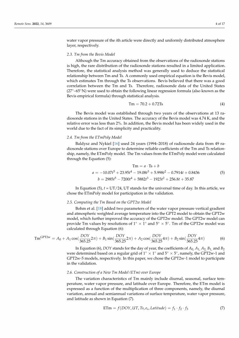
Figure 9. The theoretical RMS of PWV resulting from four different models using radiosonde data in 2021.
Figure 9 shows the distribution of RMSPWV in 2021 over Europe. The ETm model shows a smaller RMSPWV in Europe, where the mean value of RMSPWV was 0.17 mm in the article. According to Equation (18), smaller mean RMSPWV values can be achieved, alt-hough the smaller mean values of Tm were also observed in these regions. For the GPT2w-1 model, the larger RMSPWV values are observed in Europe. In contrast, for the Bevis and ETmPoly models, they showed relatively smaller mean RMSPWV values.
From Figure 10, the results show that the Bevis, GPT2w-1, and ETmPoly models had larger RMSPWV/PWV values at different latitudes over Europe, where the ETm model showed relatively smaller RMSPWV/PWV values than that of the other three Tm models. The ETm showed a relatively stable performance over Europe.
Figure 9. The theoretical RMS of PWV resulting from four different models using radiosonde datain 2021.
Remote Sens. 2022, 14, x FOR PEER REVIEW 14 of 18
Figure 9. The theoretical RMS of PWV resulting from four different models using radiosonde data in 2021.
Figure 9 shows the distribution of RMSPWV in 2021 over Europe. The ETm model shows a smaller RMSPWV in Europe, where the mean value of RMSPWV was 0.17 mm in the article. According to Equation (18), smaller mean RMSPWV values can be achieved, alt-hough the smaller mean values of Tm were also observed in these regions. For the GPT2w-1 model, the larger RMSPWV values are observed in Europe. In contrast, for the Bevis and ETmPoly models, they showed relatively smaller mean RMSPWV values.
From Figure 10, the results show that the Bevis, GPT2w-1, and ETmPoly models had larger RMSPWV/PWV values at different latitudes over Europe, where the ETm model showed relatively smaller RMSPWV/PWV values than that of the other three Tm models. The ETm showed a relatively stable performance over Europe.
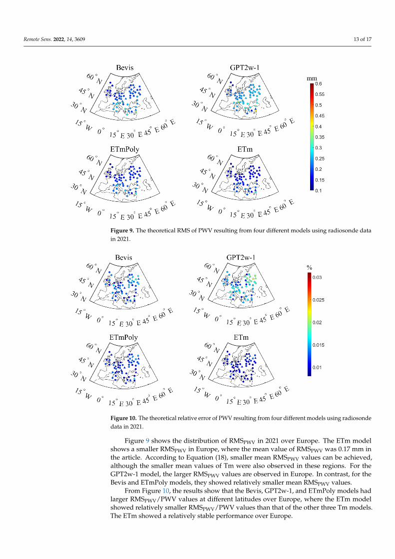
Figure 10. The theoretical relative error of PWV resulting from four different models using radiosondedata in 2021.
Figure 9 shows the distribution of RMSPWV in 2021 over Europe. The ETm modelshows a smaller RMSPWV in Europe, where the mean value of RMSPWV was 0.17 mm inthe article. According to Equation (18), smaller mean RMSPWV values can be achieved,although the smaller mean values of Tm were also observed in these regions. For theGPT2w-1 model, the larger RMSPWV values are observed in Europe. In contrast, for theBevis and ETmPoly models, they showed relatively smaller mean RMSPWV values.
From Figure 10, the results show that the Bevis, GPT2w-1, and ETmPoly models hadlarger RMSPWV/PWV values at different latitudes over Europe, where the ETm modelshowed relatively smaller RMSPWV/PWV values than that of the other three Tm models.The ETm showed a relatively stable performance over Europe.

Remote Sens. 2022, 14, 3609 14 of 17
In Table 4, the RMSPWV values of the ETm were less than 0.27 mm and with a meanRMSPWV value of 0.17 mm over Europe; in terms of RMSPWV/PWV, the ETm model had amean value of 1.03% and ranged from 0.80% to 1.37%. As the ETm can provide accurateTm values for retrieving accurate PWV over Europe. Thus, the ETm model has possibleapplications in the forecasting of severe weather conditions (i.e., typhoon, heavy rainfall,and flood disaster) over Europe.
4. Discussion
In this work, the ETm model was established by considering annual variation, semian-nual variation, diurnal variation, latitude, Ts, and es comprehensively over Europe. TheETm model showed a powerful capability to capture the spatiotemporal variations betweenthe Tm and its associated factors in the development of the ETm models. The ETm andother Tm models proposed in this study were validations; the results presented in Section 3show that the ETm model can be used for high accuracy prediction over Europe. There aremultiple reasons for the improvements of the ETm model over other selected Tm models,as follows.
Firstly, the data for ETm modeling in this study were derived from the atmosphericprofiles measured by the sounding balloons, while the GPT2w-1 model was developedwith the data derived from the ERA-Interim (European Centre for Medium-Range WeatherForecasts Re-Analysis). These two data sources were different somehow, which leads tosome differences between the GTP2w-1 model and the ETm model. What’s more, theGPT2w-1 model takes into account the geographical location of the site and has a goodsimulation of Tm seasonal variation. However, the variation of Tm was strongly correlatedwith meteorological factors, but the GPT2w-1 model did not consider the correlationbetween Tm and meteorological factors, as a result, the Tm prediction accuracy of theGPT2w-1 model in Europe is not high. The ETm model performed better than the GPT2w-1model over Europe.
Secondly, the Bevis model only considers the linear correlation between Tm and Ts,which deviated from reality. Compared with the Bevis model, the ETm model not onlytakes into account Ts, but also takes into account es, latitude, annual variation, semiannualvariation and diurnal variation. This is exactly the reason why the bias and RMS valuesof the Bevis model at the higher latitudes were much larger than the ETm model, just asshown in Figure 7. The ETm model has high accuracy and uniform distribution at differentlatitudes. The results showed that the performance of the ETm model in the differentlatitudes was much better than that of the Bevis model over Europe.
Thirdly, the ETmPoly only considers TS and the coefficients varying with UT, whichdeviated from reality. Compared with the ETmPoly model, the ETm model comprehen-sively considered the annual, semiannual, diurnal, vapor pressure and latitude factors ofTm, It is consistent with the actual situation. This is exactly the reason why the bias andRMS values of the ETmPoly model at the higher latitudes were much larger than the ETmmodel, as shown in Figure 7. The results showed that the performance of the ETm modelin the different latitudes was much better than that of the ETmPoly model.
5. Conclusions
In the article, considering the spatiotemporal information and the surface meteoro-logical factors with good linear correlation with Tm, we applied nonlinear least squareestimation to build a high-precision spatiotemporal Tm model ETm over Europe. We useddata from 48 radiosonde stations over Europe from 2010 to 2020 to train the model andused the 2021 data from these stations to test the ETm model performance at modelingstations over Europe. The bias and RMS values of the ETm model were 0.06 and 2.85 K,respectively. Compared with the widely used Bevis, GPT2w-1, and ETmPoly models,the prediction accuracy was improved by 21.7%, 31.8%, and 11.5%. By comparing theaccuracy of the models in different latitude zones, we observed that ETm model was betterthan traditional empirical models in overcoming the large Tm estimation error caused by

Remote Sens. 2022, 14, 3609 15 of 17
high-latitude factors. In addition, to verify the prediction performance of the ETm modelat non-modeling stations over Europe, we selected the data of another 12 non-modelingradiosonde stations in 2021 to test its accuracy, the bias and RMS values obtained were−0.07 and 2.87 K, respectively. The applicability and accuracy of the model in all positionsin the modeling area were guaranteed. We analyzed the residual time series diagramsof four different Tm models (i.e., Bevis, ETm, GPT2w-1, and ETmPoly models), the ETmmodel alleviated the effect of altitude and seasonal changes on the model accuracy. Sincethe ETm model also have good generalization in non-modeling sites, the models have goodtransferability. Additionally, the impact of Tm on GNSS PWV was analyzed, showing thatthe mean values of RMSPWV and RMSPWV/PWV were 0.17 mm and 1.03% for the ETmmodel, respectively.
The application of the spatiotemporal information and the surface meteorologicalfactors with good linear correlation with the weighted average temperature to Tm modelingis highly advantageous. The reason can be explained by the use of multiparameter inputto build the model. Latitude, time information, surface temperature, and water vaporpressure were all used to simulate the relationship with the output Tm value. Throughthe training of a large amount of data, the model fitted the complex nonlinear relationshipbetween the input and output. Thus, the model had good Tm prediction capability. Anotheradvantage of the model is that it only needs to measure the temperature of the site as ameteorological element to obtain a high-precision Tm value, which is convenient for users.Europe was considered the research area in the article. In future work, we will use deeplearning methods to model Europe data and will not be limited to the Tm prediction on thesurface of the research site.
Author Contributions: Conceptualization, B.Z., Y.S. and Z.W.; methodology, B.Z. and S.Z.; inves-tigation, Y.Z.; formal analysis, W.L.; writing—original draft preparation, W.J.; data curation, K.T.;writing—review and editing. All authors have read and agreed to the published version of themanuscript.
Funding: The Nanhu Scholars Program for Yong Scholars of XYNU. The project was supported bythe National Natural Science Foundation of China (41774019 and 41974007), the Key Laboratory ofGeospace Environment and Geodesy, Ministry of Education, Wuhan University (No.21-01-05). Itwas also supported by the Program for Innovative Research Team (in Science and Technology) at theUniversity of Henan Province (22IRTSTHN010).
Data Availability Statement: Not applicable.
Acknowledgments: We are very grateful to the radiosonde data obtained from the website http://weather.uwyo.edu/upperair/seasia.html (accessed on 7 February 2022). The GPT2w codes can beaccessed at https://vmf.geo.tuwien.ac.at/codes/ (accessed on 5 May 2022).
Conflicts of Interest: The authors declare no conflict of interest.
References1. Bevis, M.; Businger, S.; Herring, A.T.; Rocken, C.; Anthes, R.A.; Ware, R.H. GPS meteorology: Remote sensing of atmospheric
water vapor using the global positioning system. J. Geophys. Res. Atmos. 1992, 97, 15787–15801. [CrossRef]2. Bevis, M.; Businger, S.; Chiswell, S.; Herring, T.A.; Ware, R.H. GPS Meteorology: Mapping Zenith Wet Delays onto Precipitable
Water. J. Appl. Meteorol. 1994, 33, 379–386. [CrossRef]3. Zhao, Q.; Liu, Y.; Ma, X.; Yao, W.; Yao, Y.; Li, X. An improved rainfall forecasting model based on GNSS observations. IEEE Trans.
Geosci. Remote Sens. 2020, 58, 4891–4900. [CrossRef]4. Mendes, V.B.; Langley, R.B. Tropospheric zenith delay prediction accuracy for high-precision GPS positioning and navigation.
Navigation 1999, 46, 25–34. [CrossRef]5. Ross, R.J.; Rosenfeld, S. Estimating mean weighted temperature of the atmosphere for Global Positioning System. J. Geophys. Res.
1997, 102, 21719–21730. [CrossRef]6. Suresh Raju, C.; Saha, K.; Thampi, B.V.; Parameswaran, K. Empirical model for mean temperature for Indian zone and estimation
of precipitable water vapour from ground based GPS measurements. Ann. Geophys. 2007, 25, 1935–1948. [CrossRef]7. Sapucci, L.F. Evaluation of modeling water-vapour-weighted mean tropospheric temperature for GNSS-integrated water vapour
estimates in Brazil. J. Appl. Meteorol. Climatol. 2014, 53, 715–730. [CrossRef]

Remote Sens. 2022, 14, 3609 16 of 17
8. Zhang, B.; Guo, Z.; Lin, F.; Peng, C.; Jiang, D. Establishment and Accuracy Evaluation of Weighted Average Temperature Modelin Guangxi. J. Xinyang Norm. Univ. (Nat. Sci. Ed.) 2022, 35, 85–91.
9. Mekik, C.; Deniz, I. Modelling and validation of the weighted mean temperature for Turkey. Meteorol. Appl. 2017, 24, 92–100.[CrossRef]
10. Emardson, T.R.; Derks, H. On the relation between the wet delay and the integrated precipitable water vapour in the europeanatmosphere. Meteorol. Appl. 2010, 7, 61–68. [CrossRef]
11. Liu, J.; Yao, Y.; Sang, J. A new weighted mean temperature model in China. Adv. Space Res. 2018, 61, 402–412. [CrossRef]12. Zhang, F.; Barriot, J.-P.; Xu, G.; Yeh, T.-K. Metrology Assessment of the Accuracy of Precipitable Water Vapor Estimates from GPS
Data Acquisition in Tropical Areas: The Tahiti Case. Remote Sens. 2018, 10, 758. [CrossRef]13. Yao, Y.; Zhu, S.; Yue, S. A globally applicable, season-specific model for estimating the weighted mean temperature of the
atmosphere. J. Geod. 2012, 86, 1125–1135. [CrossRef]14. Lan, Z.; Zhang, B.; Geng, Y. Establishment and analysis of global gridded Tm–Ts relationship model. Geod. Geodyn. 2016, 7,
101–107. [CrossRef]15. Yao, Y.; Zhang, B.; Xu, C.; Chen, J. Analysis of the global Tm–Ts correlation and establishment of the latitude-related linear model.
Chin. Sci. Bull. 2014, 59, 2340–2347. [CrossRef]16. Baldysz, Z.; Nykiel, G. Improved Empirical Coefficients for Estimating Water Vapor Weighted Mean Temperature over Europe
for GNSS Applications. Remote Sens. 2019, 11, 1995.17. Li, L.; Li, Y.; He, Q.; Wang, X. Weighted Mean Temperature Modelling Using Regional Radiosonde Observations for the Yangtze
River Delta Region in China. Remote Sens. 2022, 14, 1909. [CrossRef]18. Bhm, J.; Mller, G.; Schindelegger, M.; Pain, G.; Weber, R. Development of an improved empirical model for slant delays in the
troposphere (GPT2w). GPS Solut. 2015, 19, 433–441. [CrossRef]19. Landskron, D.; Boehm, J. VMF3/GPT3: Refined discrete and empirical troposphere mapping functions. J. Geod. 2018, 92, 349–360.
[CrossRef]20. Yao, Y.; Zhang, B.; Yue, S.; Xu, C.; Peng, W. Global empirical model for mapping zenith wet delays onto precipitable water. J. Geod.
2013, 87, 439–448.21. Yao, Y.; Xu, C.; Zhang, B.; Cao, N. GTm-III: A new global empirical model for mapping zenith wet delays onto precipitable water
vapour. Geophys. J. Int. 2018, 197, 202–212. [CrossRef]22. Sun, Z.; Zhang, B.; Yao, Y. A Global Model for Estimating Tropospheric Delay and Weighted Mean Temperature Developed with
Atmospheric Reanalysis Data from 1979 to 2017. Remote Sens. 2019, 11, 1893. [CrossRef]23. Huang, L.; Jiang, W.; Liu, L.; Chen, H.; Ye, S. A new global grid model for the determination of atmospheric weighted mean
temperature in GPS precipitable water vapor. J. Geod. 2019, 93, 159–176. [CrossRef]24. Huang, L.; Liu, L.; Chen, H.; Jiang, W. An improved atmospheric weighted mean temperature model and its impact on GNSS
precipitable water vapor estimates for China. GPS Solut. 2019, 23, 51. [CrossRef]25. Wang, X.; Zhang, K.; Wu, S.; Fan, S.; Cheng, Y. Water vapor-weighted mean temperature and its impact on the determination of
precipitable water vapor and its linear trend. J. Geophys. Res. Atmos. 2016, 121, 833–852. [CrossRef]26. Li, H.; Wang, X.; Wu, S.; Zhang, K.; Chen, X.; Qiu, C.; Zhang, S.; Zhang, J.; Xie, M.; Li, L. Development of an Improved Model for
Prediction of Short-Term Heavy Precipitation Based on GNSS-Derived PWV. Remote Sens. 2020, 12, 4101. [CrossRef]27. Guerova, G.; Jones, J.; Douša, J.; Dick, G.; de Haan, S.; Pottiaux, E.; Bock, O.; Pacione, R.; Elgered, G.; Vedel, H.; et al. Review of
the state of the art and future prospects of the ground-based GNSS meteorology in Europe. Atmos. Meas. Tech. 2016, 9, 5385–5406.[CrossRef]
28. Bolton, D. The Computation of Equivalent Potential Temperature. Mon. Weather. Rev. 1980, 108, 1046–1053. [CrossRef]29. Yao, Y.B.; Zhang, B.; Xu, C.Q.; Yan, F. Improved one/multi-parameter models that consider seasonal and geographic variations
for estimating weighted mean temperature in ground-based GPS meteorology. J. Geod. 2014, 88, 273–282. [CrossRef]30. Levenberg, K. A method for the solution of certain problems in least squares. Q. Appl. Math. 1944, 2, 164–168. [CrossRef]31. Marquardt, W. An algorithm for least-squares estimation of nonlinear parameters. J. Soc. Ind. Appl. Math. 1963, 11, 431–441.
[CrossRef]32. Gill, P.R.; Murray, W.; Wright, M.H. The Levenberg-Marquardt Method; Academic Press: London, UK, 1981.33. Bates, D.M.; Watts, D.G. Nonlinear Regression and Its Application; Wiley: New York, NY, USA, 1988.34. Pujol, J. The solution of nonlinear inverse problems and the Levenberg-Marquardt method. Geophysics 2007, 72, W1–W16.
[CrossRef]35. Saastamoinen, J. Atmospheric correction for the troposphere and stratosphere in radio ranging of satellites. Use Artif. Satell. Geod.
Geophys. Monogr. Serv. 1972, 15, 247–251.36. He, C.; Wu, S.; Wang, X.; Hu, A.; Zhang, K. A new voxel-based model for the determination of atmospheric weighted mean
temperature in GPS atmospheric sounding. Atmos. Meas. Tech. 2017, 10, 2045–2060. [CrossRef]37. Li, Q.; Yuan, L.; Chen, P.; Jiang, Z. Global grid-based Tm model with vertical adjustment for GNSS precipitable water retrieval.
GPS Solut. 2020, 24, 73. [CrossRef]

Remote Sens. 2022, 14, 3609 17 of 17
38. Yang, F.; Guo, J.; Meng, X.; Shi, J.; Zhang, D. Determination of Weighted Mean Temperature (Tm) Lapse Rate and Assessment ofIts Impact on Tm Calculation. IEEE Access 2019, 7, 155028–155037. [CrossRef]
39. Long, F.; Hu, W.; Dong, Y.; Wang, J. Neural Network-Based Models for Estimating Weighted Mean Temperature in China andAdjacent Areas. Atmosphere 2021, 12, 169. [CrossRef]