Theoretical Population Biology 79 (2011) 1–11

Contents lists available at ScienceDirect

Theoretical Population Biology

journal homepage: www.elsevier.com/locate/tpb

Spatiotemporal dynamics of viral hepatitis A in ItalyMarco Ajelli a,∗, Laura Fumanelli a,b, Piero Manfredi c, Stefano Merler aa Predictive Models for Biomedicine & Environment, Bruno Kessler Foundation, Italyb Department of Mathematics, University of Trento, Italyc Department of Statistics and Mathematics Applied to Economics, University of Pisa, Italy

a r t i c l e i n f o

Article history:Received 1 July 2009Available online 29 September 2010

Keywords:HAVSpatial contact matrixVaccinationEquilibriaStability

a b s t r a c t

Viral hepatitis A is still common in Italy, especially in Southern regions. In this study, a metapopulationmodel for hepatitis A virus (HAV) transmission is proposed and analyzed. Analytical results on theasymptotic and transient behaviors of the system are carried out. Based on the available Italianmovementdata, a national spatial contact matrix at the regional level, which could be used for new studies on thetransmission dynamics of other infectious diseases, is derived for modeling fluxes of individuals. Despitethe small number of fitted parameters, model simulations are in good agreement with the observedaverage HAV incidence in all regions. Our results suggest that the mass vaccination program introducedin one Italian region only (Puglia, the one with the highest endemicity level) could have played a rolein the decline of HAV incidence in the country as a whole. The only notable exception is representedby Campania, a Southern region showing a high endemicity level, which is not substantially affected byHAV dynamics in Puglia. Finally, our results highlight that the continuation of the vaccination campaignin Puglia would have a relevant impact in decreasing long-term HAV prevalence, especially in SouthernItaly.

© 2010 Elsevier Inc. All rights reserved.

1. Introduction

Viral hepatitis A is an acute liver infectious disease caused bythe hepatitis A virus (HAV). The virus can be transmitted from per-son to person by the oral-fecal route, by ingestion of contaminatedfood or drink or by the use of intravenous drugs (Stapleton andLemon, 1994). Hepatitis A is one of the most common infectiousdiseases worldwide (Das, 2003; Murray and Lopez, 1997), both indeveloping and developed countries (Lucioni et al., 1998). An ef-fective vaccine is available (Averhoff et al., 2001) and many coun-tries recommend vaccination of children (e.g., the United States).For such reasons, various mathematical modeling studies of HAVhave been carried out for evaluating the effectiveness of differentcontrol strategies (Sattenspiel and Simon, 1988; Samandari et al.,2004; Srinivasa Rao et al., 2006; Bauch et al., 2007; Ajelli et al.,2008; Ajelli and Merler, 2009).

In developed countries the two main sources of HAV infectionare represented by direct contacts between individuals andconsumption of infected food/water (Fiore, 2004). In Italy, seafood(such as shellfish and mussels consumed raw) represents the

∗ Corresponding address: Predictive Models for Biomedicine & Environment,Bruno Kessler Foundation, Via Sommarive 18, I–38123 Trento Povo, Italy.

E-mail addresses: ajelli@fbk.eu (M. Ajelli), lfumanelli@fbk.eu (L. Fumanelli),manfredi@ec.unipi.it (P. Manfredi), merler@fbk.eu (S. Merler).

0040-5809/$ – see front matter© 2010 Elsevier Inc. All rights reserved.doi:10.1016/j.tpb.2010.09.003

main source of HAV infections (Mele et al., 2006). For this reason,circulation of HAV in the ‘‘environment’’ was explicitly modeledin two recent studies, focused on the transmission dynamicsof hepatitis A in Southern Italy (Ajelli et al., 2008) and on theevaluation of different strategies for its control (Ajelli and Merler,2009). In Italy, HAV seroprevalence (Ansaldi et al., 2008) andincidence of notified cases are highly variable between regions(see Fig. 1). This study focuses on a metapopulation model (whoseclasses represent different geographical areas) accounting for bothperson-to-person transmission and ingestion of contaminatedfood in order to investigate spatiotemporal dynamics of hepatitisA in Italy.

Metapopulation models have been largely used for studyingendemic (e.g., Hethcote (1978), Koopman et al. (2002) and Amarieiet al. (2008)) and epidemic diseases (e.g., Rvachev and Longini(1985), Sattenspiel and Dietz (1995), Colizza et al. (2007) andBalcan et al. (2009)). A major problemwhen dealing with this kindofmodel is to obtain reliable estimates of themixing level betweenclasses. Here we introduce a spatial contact matrix based on realdata and accounting for both occasional long-distance travels (e.g.,tourism) and daily short-distance (e.g., commuting between placeof residence and of work/study) travels. Such a matrix could alsobe useful for studying the transmission of other infectious diseasesin Italy through metapopulation models. In this study the centralrole of Puglia in determining hepatitis A dynamics is highlightedas well as the effects on other Italian regions of a mass vaccinationprogram implemented in Puglia.

2 M. Ajelli et al. / Theoretical Population Biology 79 (2011) 1–11

Fig. 1. Monthly incidence (notified cases per 100,000 individuals) in Puglia (dashedblack line) and Campania (solid black line). The gray area represents the 95% CI ofthe monthly incidence in Italy.

2. The model

We start by considering the classical SIR model:S ′(t) = −λ(t)S(t)− µS(t)+ bN(t)I ′(t) = λ(t)S(t)− (γ + µ)I(t)R′(t) = γ I(t)− µR(t),

where N(t) = S(t) + I(t) + R(t) represents the total population,composed of susceptible (S), infectious (I) and removed (R)individuals;µ is the mortality rate, b is the fertility rate, 1/γ is theaverage infectious period; λ(t) is the force of infection.

Since the Italian population is experiencing a situation of(about) zero growth (ISTAT, 2007), it is reasonable to assume thatthe mortality and fertility rates coincide (i.e., b = µ) and, conse-quently, the total population remains constant (i.e., N(t) = N).However, this modeling choice is not completely realistic sincewe are not considering immigration and emigration phenomenawhich could be relevant in this context (Iannelli and Manfredi,2007).

The two main sources of HAV infection in Italy are direct con-tacts between individuals and consumption of infected food/water(from now on, we will call the latter the ‘‘indirect’’ contacts com-ponent). Therefore, we may write the overall force of infection attime t as:

λ(t) = λ1(t)+ λ2(t)

where λ1 and λ2 account for direct and indirect transmissionrespectively. As in classical epidemic models, λ1(t) is assumedto be of the form β I(t)

N (where β is the transmission rate). Asregards λ2(t), we take the expression λ2(t) = β

t−∞

I(s)G(t−s)dswhere the delaying kernel G represents the survival probability ofhepatitis A virus in seafood. Assuming that this quantity decaysexponentially over time with decay rate δ, i.e. G(x) = δe−δx withx > 0, δ > 0, as in Ajelli et al. (2008), we derive the followingsystem:

S ′(t) = −λ(t)S(t)− µS(t)+ µNI ′(t) = λ(t)S(t)− (γ + µ)I(t)R′(t) = γ I(t)− µR(t)A′(t) = δ [I(t)− A(t)]

(1)

where λ(t) = β I(t)N + βA(t) and A represents, in a suitable unit,

a proxy for the amount of virus circulating in the environment. Afull discussion of the modeling assumptions can be found in Ajelliet al. (2008).

Model (1) can be easily extended to n classes, each of themrepresenting a geographic area (e.g., in the simulations we will

consider the twenty Italian regions). For simplicity we assumethat the environment of a region can be contaminated only by theindividuals living in the same region. This is not too restrictive,since the average time spent traveling to other regions is shortcompared to the incubation period of HAV (e.g., on average in Italy4.3 days a year are spent away from home for touristic purposes,ISTAT (2002), while the HAV incubation period is 2–4 weeks,Stapleton and Lemon (1994) and CDC (2007)).

Let βkj ≥ 0 be the transmission rate for direct contacts betweenregions k and j, for k, j = 1, . . . , n; we assume that at leastone of the βkj is strictly positive. Likewise, let βkj ≥ 0 be thetransmission rate for indirect contacts between regions k and j, fork, j = 1, . . . , n (with at least one of the βkj strictly positive). Theelements βkj with k = j account for the transmission due to theconsumption of infected food during travels outside the region ofresidence.

Furthermore, we assume that the values of the mortality/fertility rate, the average duration of infection of an individual andthe decay rate of the virus in the environment may vary from re-gion to region: thus we take µk, γk and δk with k = 1, . . . , n. Thisgeneral formulation of the model would allow considering a het-erogeneous population, in terms of both individuals and environ-ments. Interestingly, δk would allow taking into account differentHAV survival probabilities in different areas, which could be vari-able from region to region (e.g., they could depend on the distancebetween the fishing areas and the pipe of the sewage system or theharbors). However, because of the lack of reliable data, the theo-retical analysis of the model will be carried out in the general case.On the other hand, in the simulations we will assume µk = µ andγk = γ , for all k.

Based on these considerations, the extension of system (1) to nclasses is the following 4n-dimensional system:

S ′

k(t) = −Λk(t)Sk(t)− µkSk(t)+ µkNkI ′k(t) = Λk(t)Sk(t)− (γk + µk)Ik(t)R′

k(t) = γkIk(t)− µkRk(t)A′

k(t) = δk [Ik(t)− Ak(t)]

(2)

for k = 1, . . . , n, whereΛk(t) =∑n

j=1 βkjIj(t)Nj

+∑n

j=1 βkjAj(t).In each region the total population size is assumed to be

constant, that is Nk = Sk + Ik + Rk for all k. System (2) can bereformulated in terms of relative frequencies: for k = 1, . . . , n,we define sk(t) =

Sk(t)Nk, ik(t) =

Ik(t)Nk, rk(t) =

Rk(t)Nk

. In addition,for k = 1, . . . , n, let us define the rescaled environment-relatedvariable ak(t) =

Ak(t)Nk

and, for k, j = 1, . . . , n, the rescaled indirect

transmission rate βkj = Nkβkj. System (2) can now be rewritten asfollows:

i′k(t) = λk(t)1 − ik(t)− rk(t)

− (γk + µk)ik(t)

r ′

k(t) = γkik(t)− µkrk(t)

a′

k(t) = δk

ik(t)− ak(t)

(3)

where

λk(t) =

n−j=1

βkjij(t)+

n−j=1

βkjaj(t) (4)

and the fraction of susceptible individuals can be computed assk(t) = 1 − ik(t)− rk(t), for k = 1, . . . , n.

3. Analysis

3.1. Equilibria

System (3) trivially admits the disease-free equilibrium: sk =

1, ik = ak = rk = 0, for k = 1, . . . , n. Next we investigate

M. Ajelli et al. / Theoretical Population Biology 79 (2011) 1–11 3

the existence and uniqueness of the endemic equilibrium. Thefollowing relations must be satisfied:

i∗k = a∗

k

r∗

k =γk

µki∗k . (5)

From the first equation in (3), using (5) and setting λ∗

k =∑n

j=1

(βkj + βkj)i∗j , we get the following expression for i∗k :

i∗k =λ∗

k

γk + µk +γk+µkµk

λ∗

k

=

n∑j=1αkji∗j

1 + ϑk

n∑j=1αkji∗j

. (6)

This is a closed system in the variables i∗k , equivalent to (3)evaluated at the equilibrium, where we have defined ϑk =

γk+µkµk

and αkj =βkj+βkjγk+µk

.Nowwe consider the application F : Rn

→ Rn, i → F(i)where

i = (i1, . . . , in), F(i) = (F1(i), . . . , Fn(i)) and Fk(i) =

∑nj=1 αkjij

1+ϑk∑n

j=1 αkj ij.

Provided that the matrix of direct and indirect transmissionrates

βkj + βkj

is irreducible (which implies that F ′(0) is

irreducible), map F satisfies the hypotheses of the fixed pointtheorem (see Hethcote and Thieme (1985) for its statement andproof).

Thus, if we define R0 as the spectral radius of F ′(0) =αkj, i.e.,

R0 = ρ

βkj + βkj

γk + µk

, (7)

by applying the fixed point theorem to F , we have that a uniqueendemic equilibrium exists whenever R0 > 1. Furthermore, wecan apply

Lemma 3.1 (Thieme, 2003). If the contact matrix is irreducible, thenany endemic equilibrium is strongly endemic, i.e., every component ofthe endemic equilibrium is strictly positive.

Thus we obtain the following result:

Proposition 3.2. If R0 > 1, then system (3) admits a unique stronglyendemic equilibrium.

If the matrix of transmission rates is not irreducible then theendemic equilibrium is not strongly endemic, i.e., ik may be equalto zero for some k.

3.2. Stability of steady states

In order to prove stability properties of the equilibria, we lin-earize system (3) in a neighborhood of the steady state, for boththe disease free and the strongly endemic equilibrium.

First we study the stability of the disease free equilibrium, andin particular we look for conditions such that it is locally unstable,so that the infection is endemic. The following result holds:

Proposition 3.3. The disease free equilibrium of system (3) is locallyasymptotically stable for R0 < 1, unstable for R0 > 1.

As regards the stability of the strongly endemic equilibrium,whose existence and uniqueness are guaranteed when R0 > 1, weare able to state that

Proposition 3.4. Whenever it exists, the strongly endemic equilib-rium (5)–(6) is locally asymptotically stable.

Both propositions are proved in Appendix.

3.3. Transient behavior

In the previous section we proved that the asymptotic behaviorof system (2) is similar to a ‘‘classical’’ (i.e., without indirect trans-mission) SIR model with the same metapopulation structure. Thismeans that the inclusion of indirect transmission in the form of ex-ponentially delayed contacts with people who had been infectiousin the past does not modify the basic qualitative behaviors of themodel. On the other hand, indirect transmissionmight significantlychange the quantitative outcomes of the system.

If the strongly endemic equilibrium exists, then we know thatit is locally asymptotically stable. In the previous section we havenot proved anything about how the trajectories of the system reachthis equilibrium. Here we show, both analytically and numerically,that the transient behavior of this system is quite different fromthe classical SIR model.

For illustrative purposes, let us consider a one-region model, sothat we can compute the equilibrium explicitly; in particular wehave i⋆ =

µ

γ+µ

1 −

1R0

, where R0 =

β+β

γ+µ(see Eq. (7)), r⋆ =

γ

µi⋆,

λ⋆ = (β + β)i⋆.It is well known (Thieme, 2003) that the period of transient

oscillations around an equilibrium is related to the value of theimaginary part of the eigenvalues defining the spectral bound (i.e.,the eigenvalues having the largest real part). In more detail, if suchan eigenvalue is ξ = ρ ± iω ∈ C, then the length of the inter-epidemic period can be suitably approximated by the quasi-periodT = 2π/ω.

Therefore, we compute the characteristic polynomial of theJacobianmatrix evaluated at the endemic equilibrium,which turnsout to be

−ξ 3 +s⋆β − λ⋆ − γ − δ − 2µ

ξ 2 +

δs⋆(β + β)+ µs⋆β

− λ⋆(γ + δ + µ)− (γ + µ)(δ + µ)− δµ

× ξ + δµs⋆(β + β)− λ⋆(γ + µ)− µ(γ + µ)

(where s⋆ = 1 − i⋆ − r⋆), and find its roots.

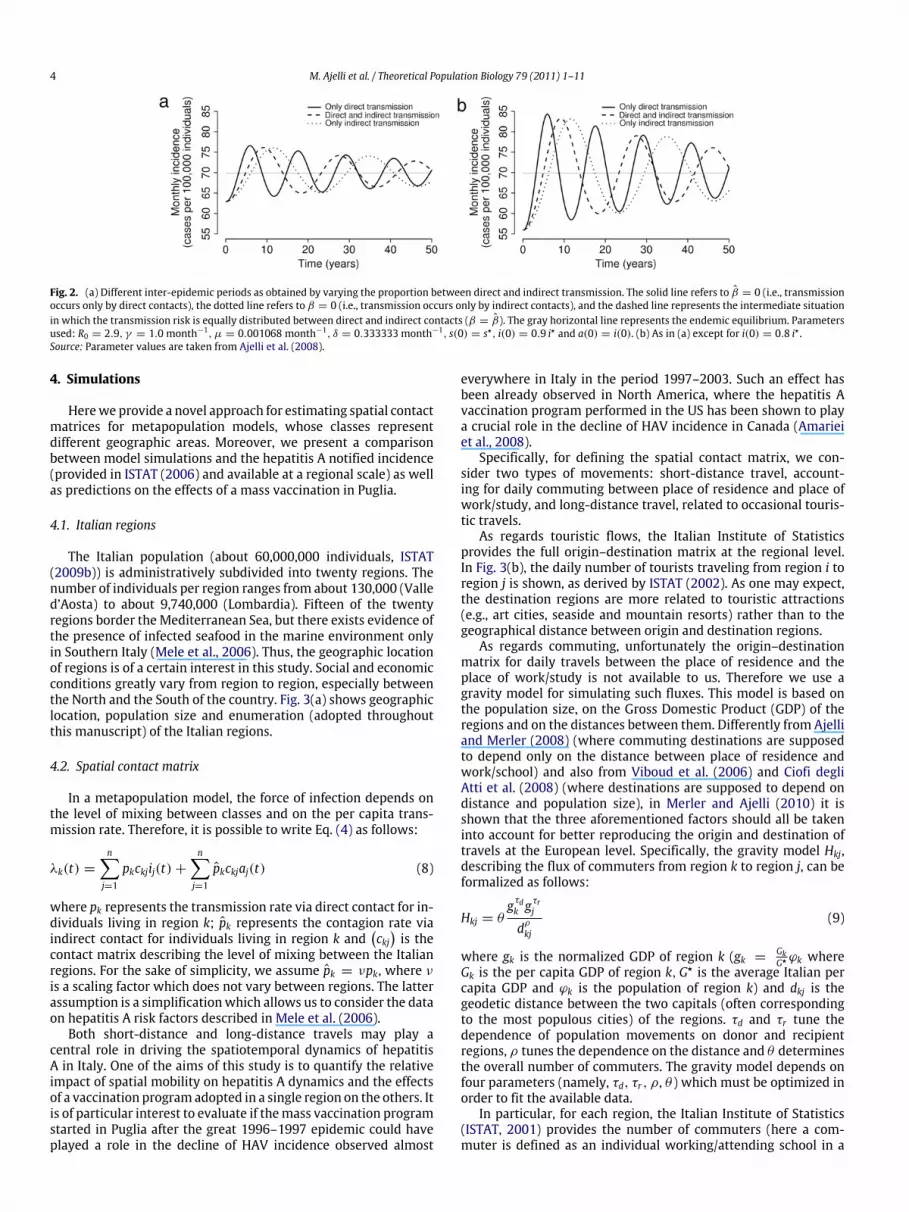
As an example, we take fixed parameter values as in Ajelliet al. (2008) (and in particular we assume R0 = 2.9) and let theproportion between the two sources of infection vary. In particularwe consider three situations: transmission can occur only by directcontact (β = 0), only by indirect contact (β = 0) or equallyby both types of contact (β = β). By computing the roots ofthe characteristic polynomial we are able to find the period oftransient oscillations for the three cases: T = 11.6 years for directtransmission only, T = 23.3 years for indirect transmission onlyand T = 18.4 years for β = β . These results are also confirmedby numerical simulations, whose outcomes are shown in Fig. 2for two different initial conditions. This figure highlights that thepresence of indirect transmission increases the wave period, whilethe initial condition affects only the amplitude of waves withoutaltering their period.

Therefore we are able to conclude that indirect transmissionincreases the inter-epidemic period, and also the duration of asingle epidemic episode. This seems to be consistent with the verylong duration of the HAV epidemic episode observed in Pugliaduring 1996–1997. This makes HAV dynamics in the presenceof indirect transmission potentially very different from otherendemic infections characterized by recurrent epidemics (e.g.,measles, see Grenfell et al. (2001)). The role of the environmentalreservoir in increasing the inter-epidemic period emerges in otherworks on diseases such as cholera (Codeço, 2001), influenza(Rohani et al., 2009; Roche et al., 2009) and scrapie in sheepflocks (Woolhouse et al., 1998). For example, the persistence ofbubonic plague in humans, with long inter-epidemic periods, hasbeen suggested to be possible thanks to the reservoir of infectionrepresented by the rodent population (Keeling and Gilligan, 2000).

4 M. Ajelli et al. / Theoretical Population Biology 79 (2011) 1–11

Fig. 2. (a) Different inter-epidemic periods as obtained by varying the proportion between direct and indirect transmission. The solid line refers to β = 0 (i.e., transmissionoccurs only by direct contacts), the dotted line refers to β = 0 (i.e., transmission occurs only by indirect contacts), and the dashed line represents the intermediate situationin which the transmission risk is equally distributed between direct and indirect contacts (β = β). The gray horizontal line represents the endemic equilibrium. Parametersused: R0 = 2.9, γ = 1.0 month−1, µ = 0.001068 month−1, δ = 0.333333 month−1, s(0) = s⋆, i(0) = 0.9 i⋆ and a(0) = i(0). (b) As in (a) except for i(0) = 0.8 i⋆ .Source: Parameter values are taken from Ajelli et al. (2008).

4. Simulations

Herewe provide a novel approach for estimating spatial contactmatrices for metapopulation models, whose classes representdifferent geographic areas. Moreover, we present a comparisonbetween model simulations and the hepatitis A notified incidence(provided in ISTAT (2006) and available at a regional scale) as wellas predictions on the effects of a mass vaccination in Puglia.

4.1. Italian regions

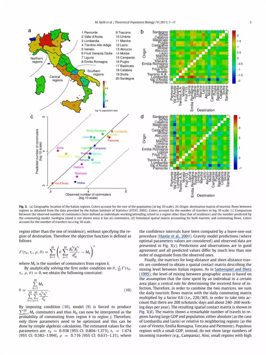
The Italian population (about 60,000,000 individuals, ISTAT(2009b)) is administratively subdivided into twenty regions. Thenumber of individuals per region ranges from about 130,000 (Valled’Aosta) to about 9,740,000 (Lombardia). Fifteen of the twentyregions border the Mediterranean Sea, but there exists evidence ofthe presence of infected seafood in the marine environment onlyin Southern Italy (Mele et al., 2006). Thus, the geographic locationof regions is of a certain interest in this study. Social and economicconditions greatly vary from region to region, especially betweenthe North and the South of the country. Fig. 3(a) shows geographiclocation, population size and enumeration (adopted throughoutthis manuscript) of the Italian regions.

4.2. Spatial contact matrix

In a metapopulation model, the force of infection depends onthe level of mixing between classes and on the per capita trans-mission rate. Therefore, it is possible to write Eq. (4) as follows:

λk(t) =

n−j=1

pkckjij(t)+

n−j=1

pkckjaj(t) (8)

where pk represents the transmission rate via direct contact for in-dividuals living in region k; pk represents the contagion rate viaindirect contact for individuals living in region k and

ckjis the

contact matrix describing the level of mixing between the Italianregions. For the sake of simplicity, we assume pk = νpk, where νis a scaling factor which does not vary between regions. The latterassumption is a simplificationwhich allows us to consider the dataon hepatitis A risk factors described in Mele et al. (2006).

Both short-distance and long-distance travels may play acentral role in driving the spatiotemporal dynamics of hepatitisA in Italy. One of the aims of this study is to quantify the relativeimpact of spatial mobility on hepatitis A dynamics and the effectsof a vaccination program adopted in a single region on the others. Itis of particular interest to evaluate if themass vaccination programstarted in Puglia after the great 1996–1997 epidemic could haveplayed a role in the decline of HAV incidence observed almost

everywhere in Italy in the period 1997–2003. Such an effect hasbeen already observed in North America, where the hepatitis Avaccination program performed in the US has been shown to playa crucial role in the decline of HAV incidence in Canada (Amarieiet al., 2008).

Specifically, for defining the spatial contact matrix, we con-sider two types of movements: short-distance travel, account-ing for daily commuting between place of residence and place ofwork/study, and long-distance travel, related to occasional touris-tic travels.

As regards touristic flows, the Italian Institute of Statisticsprovides the full origin–destination matrix at the regional level.In Fig. 3(b), the daily number of tourists traveling from region i toregion j is shown, as derived by ISTAT (2002). As one may expect,the destination regions are more related to touristic attractions(e.g., art cities, seaside and mountain resorts) rather than to thegeographical distance between origin and destination regions.

As regards commuting, unfortunately the origin–destinationmatrix for daily travels between the place of residence and theplace of work/study is not available to us. Therefore we use agravity model for simulating such fluxes. This model is based onthe population size, on the Gross Domestic Product (GDP) of theregions and on the distances between them. Differently from Ajelliand Merler (2008) (where commuting destinations are supposedto depend only on the distance between place of residence andwork/school) and also from Viboud et al. (2006) and Ciofi degliAtti et al. (2008) (where destinations are supposed to depend ondistance and population size), in Merler and Ajelli (2010) it isshown that the three aforementioned factors should all be takeninto account for better reproducing the origin and destination oftravels at the European level. Specifically, the gravity model Hkj,describing the flux of commuters from region k to region j, can beformalized as follows:

Hkj = θgτdk gτrjdρkj

(9)

where gk is the normalized GDP of region k (gk =GkG⋆ ϕk where

Gk is the per capita GDP of region k,G⋆ is the average Italian percapita GDP and ϕk is the population of region k) and dkj is thegeodetic distance between the two capitals (often correspondingto the most populous cities) of the regions. τd and τr tune thedependence of population movements on donor and recipientregions, ρ tunes the dependence on the distance and θ determinesthe overall number of commuters. The gravity model depends onfour parameters (namely, τd, τr , ρ, θ ) which must be optimized inorder to fit the available data.

In particular, for each region, the Italian Institute of Statistics(ISTAT, 2001) provides the number of commuters (here a com-muter is defined as an individual working/attending school in a

M. Ajelli et al. / Theoretical Population Biology 79 (2011) 1–11 5

Fig. 3. (a) Geographic location of the Italian regions. Colors account for the size of the population (in log 10 scale). (b) Origin–destination matrix of touristic flows betweenregions as obtained from the data provided by the Italian Institute of Statistics (ISTAT, 2002). Colors account for the number of travelers in log 10 scale. (c) Comparisonbetween the observed number of commuters (here defined as individuals working/attending school in a region other than that of residence) and the number predicted bythe commuting model. Sardegna island is not shown since it has no commuters. (d) Simulated spatial matrix accounting for both touristic and commuting flows. Colorsaccount for the number of travelers on a log 10 scale.

region other than the one of residence), without specifying the re-gion of destination. Therefore the objective function is defined asfollows

Γ (τd, τr , ρ, θ) =

20−k=1

θ

20−j=1

gτdk gτrjdρkj

− Mk

2

whereMk is the number of commuters from region k.By analytically solving the first order condition on θ , ∂

∂θΓ (τd,

τr , ρ, θ) = 0, we obtain the following constraint:

θ =

20∑k=1

Mk

20∑k=1

20∑j=1

gτdk gτrjdρkj

. (10)

By imposing condition (10), model (9) is forced to produce∑20k=1 Mk commuters and thus Hkj can now be interpreted as the

probability of commuting from region k to region j. Therefore,only three parameters need to be optimized and this can bedone by simple algebraic calculation. The estimated values for theparameters are: τd = 0.938 (95% CI: 0.804–1.373), τr = 1.674(95% CI: 0.582–1.994), ρ = 0.716 (95% CI: 0.631–1.31), where

the confidence intervals have been computed by a leave-one-outprocedure (Hastie et al., 2001). Gravity model predictions (whereoptimal parameters values are considered) and observed data arepresented in Fig. 3(c). Predictions and observations are in goodagreement and all predicted values differ by much less than oneorder of magnitude from the observed ones.

Finally, the matrices for long-distance and short-distance trav-els are combined to obtain a spatial contact matrix describing themixing level between Italian regions. As in Sattenspiel and Dietz(1995), the level of mixing between geographic areas is based onthe assumption that the time spent by an individual in a certainarea plays a central role for determining the received force of in-fection. Therefore, in order to combine the two matrices, we sumthe daily touristic flows matrix with the daily commuting matrixmultiplied by a factor 0.6 (i.e., 220/365, in order to take into ac-count that there are 200 scholastic days and about 240–260 work-ing days per year). The resulting spatial contact matrix is shown inFig. 3(d). The matrix shows a remarkable number of travels to re-gions having large GDP and population, either absolute (as the caseof Lombardia and Lazio) or relative to neighboring regions (as thecase of Veneto, Emilia Romagna, Toscana and Piemonte). Populousregions with a small GDP, instead, do not show large numbers ofincoming travelers (e.g., Campania). Also, small regions with high

6 M. Ajelli et al. / Theoretical Population Biology 79 (2011) 1–11

Table 1Model parameters kept fixed in the simulations.

Parameter Description Measure unit Value Reference

Nk Number of individuals in region k Dimensionless a (ISTAT, 2009b)1/µ Average life expectancy Years 78 (ISTAT, 2009a)1/γ Average duration of the infectivity period Months 1 (CDC, 2007; Stapleton and Lemon, 1994)1/δk Average survival period of HAV in the

environment for region kMonths 3, 0b (Abad et al., 1994; Biziagos et al., 1988; Mbithi et al., 1991;

Ajelli et al., 2008)ϵ Fraction of notified cases Percentage 3–8c (Ajelli and Merler, 2009)ν Scaling factor for the two sources of infection Dimensionless 2.5 (Mele et al., 2006)V c16 Vaccination coverage at birth Percentage 20d (Lopalco et al., 2005; Ajelli et al., 2008)

V y16 Vaccination rate of 12-years-old individuals Months−1 0.0009d (Lopalco et al., 2005; Ajelli et al., 2008)

a Values reported in Fig. 3(a).b 1/δk = 3 for 14 ≤ k ≤ 19 (i.e., for Southern Italy); 0 otherwise.c Uniformly distributed.d Puglia is the only Italian region which has experienced a vaccination program; for the other regions this parameter is set to 0.

touristic flows do not necessarily have a high number of incomingtravelers (e.g., Trentino Alto Adige). These results suggest that, fordefining the spatial contact matrix at national level for epidemicmodeling, commuting flows aremore relevant than touristic flows.

Finally, it is worth noting that the estimated contact matrix (ckj)is irreducible by construction. Therefore, from the theory above, aunique, strongly endemic equilibrium exists and is stable for theempirical specification of the model.

4.3. Model parameterization, fitting procedure and vaccination

Model parameterization is based on basic demographic infor-mation on the Italian population, hepatitis A natural history andmodel fit to average notification data. Specifically, the populationsize of each region and life expectancy at national level are takenfrom the Italian Institute of Statistics (ISTAT, 2009b,a). The averageinfectivity period for hepatitis A is fixed to 1 month (CDC, 2007;Stapleton and Lemon, 1994). The life expectancy of HAV in the en-vironment is set to three months (Abad et al., 1994; Biziagos et al.,1988; Mbithi et al., 1991; Ajelli et al., 2008). As regards the report-ing factor ϵ, we assume a unique value across the regions. This is asimplifying assumption sincewe expect that regions characterizedby different levels of endemicity, as is the case of Italy, could havevery different proportions of symptomatic cases (due to differencesin the age at which infection is acquired) and reporting rates. Wealso explore the case of two different reporting rates for Northernand Southern Italy. However, given the uncertainty on the report-ing factor, we use a range of plausible values for ϵ taken from pre-vious literature on HAV dynamics in Italy (Ajelli and Merler, 2009)rather than fix it to one specific value. Therefore, conditionally onthe estimated contact matrix, the uncertainty in parameter esti-mates (and thus also in R0) will mainly reflect the uncertainty inthe reporting factor. Model parameter values are summarized inTable 1.

Transmission rates are estimated by fitting the model at its en-demic equilibrium to the actual average HAV incidence of notifiedcases in each region, computed over the pre-vaccination periodJanuary 1992–December 1996. Specifically, the optimization pro-cedure works as follows. First of all, a value of ϵ (the reporting fac-tor, which accounts for both the symptomaticity of HAV infectionand the accuracy of the reporting system) is randomly chosen fromthe uniformdistribution on the range 0.03–0.08 according to previ-ous investigations on hepatitis A in Italy (Ajelli and Merler, 2009);then we compute the corresponding mean square error (MSE) be-tween the number of notified cases simulated by themodel ϵi⋆k andthe actual number of notified cases as follows:

MSE(pk) =

20−k=1

Φk − ϵi⋆k

2where i⋆k is the HAV incidence at the endemic equilibrium in regionk, which depends on the estimated value of the transmission rates

pk, and Φk is the average number ofmonthly notified cases over the5-years period from1992 to 1996 in region k under the assumptionthey reflect the endemic equilibrium. In general, case reports are abettermatch for incidence rather than for prevalence but, since theaverage length of the infectivity period is assumed to be 1 month(i.e., γk = 1 for k = 1, . . . , n), at the endemic equilibriummonthlyincidence and prevalence coincide. For Puglia, Φ16 refers to the pe-riod from January 1992 to December 1995 in order to exclude thelarge 1996 epidemic that could hardly be considered close to theequilibrium value.

Finally, for each choice of the reporting factor, the best trans-mission rates pk are defined as the ones minimizing the resultingMSE. The MSE is optimized by using a random walk stochastic lo-cal search algorithm (Hoos and Stutzle, 2005). In order to keep ourmodel as parsimonious as possible we assume that there are onlyfour distinct pk values (see Eq. (8)), i.e., one for Puglia, one for Cam-pania (the two regions which mostly contribute to HAV endemic-ity in Italy), one for the remaining Southern regions, and one forNorthern and Central Italy and Sardegna, where HAVmay be closeto subcriticality. Therefore, we consider

pk =

p(1) if 1 ≤ k ≤ 13 or k = 20(i.e., Northern and Central

Italy and Sardegna island)p(2) if k = 15 (i.e., Campania)p(3) if k = 16 (i.e., Puglia)p(4) otherwise (i.e., the rest of Southern Italy).

The proportionality factor between indirect and direct transmis-sion rates ν = pk/pk is obtained by survey data (Mele et al., 2006)and it is set to 2.5. Since there does not exist evidence of native in-fected seafood in the Northern, Central and Sardegna marine envi-ronments, we assume that δk and ak(0) are both identically zero for1 ≤ k ≤ 13 or k = 20. Finally, by sampling the distribution of thereporting factor 1000 times, and repeating the optimization proce-dure, the related distribution of the estimates of the transmissionrates pk and of the basic reproduction numbers were found.

For comparing model predictions with notification data on theperiod January 1998–December 2003, the vaccination program(involving both newborns and 12-year-old individuals) started inPuglia in 1997 has to be taken into account. Therefore, we intro-duce the following system:S ′

k(t) = −Λk(t)Sk(t)−µk + V y

k

Sk(t)+ (1 − V c

k )µkNk

I ′k(t) = Λk(t)Sk(t)− (γk + µk) Ik(t)R′

k(t) = γkIk(t)− µkRk(t)+ V ckµkNk + V y

k Sk(t)A′

k(t) = δk [Ik(t)− Ak(t)]

where V ck represents the vaccination coverage of newborns in re-

gion k, and V yk represents the vaccination rate of adolescent indi-

viduals in region k.

M. Ajelli et al. / Theoretical Population Biology 79 (2011) 1–11 7

Fig. 4. (a) Average monthly incidence of notified cases per 100,000 individuals in the twenty Italian regions during the period January 1992–December 1996 (black line),95% CI (gray rectangles) andmodel equilibrium (colored dots). Red dots refer to Northern and Central regions and Sardegna; the green dot refers to Puglia; the blue dot refersto Campania; cyan dots refer to the other Southern regions. For Puglia, the average monthly incidence is computed over the period from January 1992 to December 1995.(b) As in (a), but for the period January 1998–December 2003. Here, a vaccination program involving 20% of newborns and 80% of 12-years-old adolescents is also simulated.(c) Variations (in percentage) between the monthly incidence evaluated at the endemic equilibrium (not considering any vaccination program) and the average monthlyincidence after 5 years from the beginning of the vaccination program in Puglia. Colors as in (a). (d) Variations (in percentage) between the monthly incidence evaluated atthe endemic equilibrium (not considering any vaccination program) and the monthly incidence evaluated at the new endemic equilibrium, as resulting by simulating thevaccination program in Puglia. Colors as in (a).

The vaccination coverage at birth V c16 is kept fixed at 20% and

the monthly vaccination rate of young individuals V y16 is kept fixed

at 0.0009, which corresponds to 80% of the fraction of 12-year-old individuals (≈ 0.013 of the population) divided by 12 (inorder to obtain a monthly rate). Such values are chosen in orderto mimic the vaccination campaign performed in Puglia (Lopalcoet al., 2005).

4.4. Model predictions and empirical epidemiological data

The simulated equilibrium is in good agreement with the aver-age monthly hepatitis A incidence of notified cases computed overthe period from January 1992 to December 1996 (we recall thatfor Puglia the average refers to the period January 1992–December1995). As shown in Fig. 4(a), the model fits all data very well ex-cept for a few regions (namely Basilicata, Liguria and Friuli VeneziaGiulia).

The fitting procedure allows also computing the basic repro-ductive number, as given by Eq. (7). In particular, it is possible toestimate R0 for different Italian areas by restricting the computa-tion of Eq. (7) to the corresponding rows and columns. In Pugliathe estimated R0 is 2.43 (95% CI: 1.47–5.48), where the observedvariability mainly depends on the uncertainty in the HAV report-ing factor. This value is between the estimate given in Martinelliet al. (2010), namely 2.01, and the one given in Ajelli et al. (2008),namely 2.9, which were both computed from the average age atinfection. In Campania we obtain R0 = 1.31 (95% CI: 1.17–1.56),which is noticeably lower than the value estimated in Ajelli et al.(2008), namely 2.2. Therefore, both estimates given here, basedon equilibrium model fit, are lower than the corresponding onesbased on age specific data. As regards the other Italian areas, theestimated R0 values are R0 = 1.07 (95% CI: 1.04–1.11) for South-ern Italy (Puglia and Campania excluded) and R0 = 1.04 (95% CI:

1.02–1.07) for Northern and Central Italy and Sardegna. The latterestimate, close to 1, suggests that hepatitis A is in a situation of ex-tremely low endemicity in Northern and Central Italy. As discussedabove, the reporting factor could be highly variable between theItalian regions: in particular its average value of 5.5% used hereseems a reasonable approximation for Puglia, while the report-ing factor is probably noticeably higher in other Italian regions(e.g., in Northern Italy) and probably lower in other Southern re-gions, especially in Campania: a survey conducted in Campania hashighlighted that only 39% of the interviewed people would visita medical doctor in case of icteric onset (Salamina and D’Argenio,1998).

In order to deepen our understanding of the actual hepatitis Asituation in Italy, we relaxed the assumption of a single reportingfactor for the whole study area by considering a specific valuefor Northern and Central regions and Sardegna, namely ϵ1, andanother one for Southern regions (including Puglia and Campania),namely ϵ2. Since the average age at which infection is acquired isnotably higher in Northern and Central regions than in Southernregions (ISTAT, 2006) and HAV symptoms increase with age(Stapleton and Lemon, 1994; Armstrong and Bell, 2002), we fixϵ1 = 0.2 according to the estimate given in Armstrong and Bell(2002) for the US population agedmore than 14 years. On the otherhand, we continue to sample ϵ2 from the uniform distribution ofrange 0.03–0.08. In this case, the best estimate of the reproductivenumber for Northern and Central Italy and Sardegna results tobe R0 = 1.002, with a corresponding 95% confidence interval of0.992–1.006, while the estimates for the other areas are basicallythe same as obtained by assuming a single reporting factor. Thisconfirms our result that in Northern and Central Italy, hepatitis Ais in a situation of extremely low endemicity and it could possiblybe even non-endemic. From now on results will refer to the case ofa single reporting factor ϵ for the whole country.

8 M. Ajelli et al. / Theoretical Population Biology 79 (2011) 1–11

By keeping the estimated transmission rates fixed, it is possibleto simulate the vaccination program in Puglia and study its effecton the overall hepatitis A dynamics in Italy. Our predictions arein good agreement with observed notification data for the wholeNorthern Italy, while the model overestimates the number ofcases in Southern regions, especially in Puglia and Campania (seeFig. 4(b)). These discrepancies may be due to the simplifyingassumption that the proportion of notified cases does not vary overtime. In fact, it is well known by epidemiologists that the highperceived risk during the 1996 epidemic in Puglia and Campaniainduced a significant increase in the notification rate during thecourse of the epidemic (Ajelli et al., 2008). Since this is not takeninto account in the model fit, the value of the respective fittedtransmission rates may be somewhat overestimated and thusmodel predictions for the period 1998–2003 are higher than theobserved data, especially in Puglia and Campania. As regards theimpact of the vaccination program in Puglia, the model predictsa notable decline in HAV incidence in Puglia, namely about 60%after 5 years from the beginning of vaccination. Moreover, a slightdecline is observable in all other regions, except Campania (seeFig. 4(c)). The difference in the number of notified cases during thepre-vaccination period is larger in Northern and Central Italy thanin Southern regions; this can be explained by the lower R0 valuein the Northern-Central part of the country. Moreover, the limitedeffect on hepatitis A dynamics in Campania strongly suggests thatthis disease is endemic in that region even without contacts withPuglia. Fig. 4(d) shows the effects of the vaccination program inPuglia (by assuming that the vaccination rates do not vary overtime) on the new long-term endemic equilibrium. It is interestingto note that the vaccination program has a significant effect onhepatitis A dynamics in all Southern regions (Campania excluded)and a limited effect on Northern-Central Italian regions. This isa consequence of the spatial contact matrix, which shows highertravel fluxes between Puglia and the other Southern regions ratherthan between Puglia and the rest of Italy (see Fig. 3(d)).

5. Discussion and conclusions

This work extends the model for HAV transmission dynamicswith multiple sources of infection presented in Ajelli et al. (2008).To the best of our knowledge the present manuscript representsthe first instance of a metapopulation model including direct andindirect transmission, of which HAV is perhaps the most notableexample. Our analysis proves that the general form of the pro-posed model shows the qualitative behavior of the classical SIRmodel (considering only the person-to-person source of infection).However, from a quantitative point of view, it shows a differentpattern accounting for longer epidemic and inter-epidemic peri-ods. A spatial contact matrix for Italy at the regional level has beenderived. This matrix takes into account the most relevant humanmovements: daily short-distance travels (e.g., for commuting fromthe place of residence to the place of study/work) and occasionallong-distance travels (e.g., for touristic reasons). A gravity modelfor commuting flows has been developed and specifically parame-terized for the Italian situation. The resulting spatial contactmatrixrepresents a useful starting point for developing Italian metapop-ulation models, with regional spatial resolution, focused on otherinfectious diseases such as, for instance, influenza or measles.

The recent history of hepatitis A in Italy is characterized by alarge heterogeneity, in that althoughHAVmight still be consideredendemic in the nation as a whole, this seems to be true only fora few areas (mainly located in Southern Italy) which are stronglyaffected by HAV, while the others show only few, sporadic casesduring the year. This suggests that in the latter regions HAVhas gone near to, or even below, the critical threshold. This factseems to be appropriately captured by our model which indicates

values of the reproductive numbers slightly greater than one inNorthern and Central Italy or even possibly slightly below oneif heterogeneity in reporting factors, as empirically documented,is considered. This is what can be said by a model like thepresent one, i.e., one which depicts a strongly endemic situationgoverned by constant transmission rates. Further inquiry on theactual patterns of HAV in low endemic Italian areas would requiremore specific approaches. For example the pattern in low endemicItalian areas could also be consistent with ‘‘source/sink’’ dynamicsdriven by seasonal variation in within- or between-subpopulationtransmission, or with a low endemic equilibrium in a discretepopulation, in presence of a low reporting rate. We also feel itwould be important to better investigate the role of internationalimportation, quite substantial in Italy, under situations of sub-criticality.

Model simulations are in good agreement with average notifi-cation values in both the considered periods for most of Italy. Thesimulations highlight that the vaccination program in Puglia couldhave played a role in the observed decline of hepatitis A incidencein several Italian areas. Moreover, the effects of a vaccination pro-gram on the long-term endemic equilibrium is shown and it hasbeen underlined that the strong connection between Puglia andother Southern regions is responsible for a large decrease of HAVprevalence. On the contrary, Campania,which shows a high level ofendemicity by itself, is not substantially affected by HAV dynamicsin Puglia.

The aim of this study is not to evaluate the effectiveness ofspecific control measures or to suggest which kind of vaccinationprogramwould bemore effective. For answering these questions amore structured model is preferable; e.g., an age-structured or anindividual-basedmodel. The latter should be useful also for testingindividually targeted interventions such as closure of day carecenters or kindergartens which are considered as the main sourceof person-to-person transmission for many childhood diseases(Galil et al., 2002), and hepatitis A aswell (Chitambar et al., 1996). Aspecific study on this topic can be found in Ajelli andMerler (2009).

The model proposed here does not take into account eitherthe seasonality of HAV in the marine environment, which maybe an explanation for the seasonal pattern observed in Puglia andCampania, as previously suggested in Ajelli et al. (2008), or anystochastic fluctuation in the transmission rates (e.g., due to humanbehavior, such as different levels of seafood consumption duringthe year, or to climatic changes in the marine environment whichin turn would be responsible for different seafood availability).Therefore, a comparison limited to the average notification dataover two distinct periods, as carried out here, rather than tothe monthly time series seems to represent a better option.Moreover, this choice is also supported by the lack of dynamicalpatterns observed in the time series of notification data (withsome notable exceptions). As regards the reporting factor, weassumed in most of our work a unique value for Italy as awhole. This however certainly represents an oversimplification of acomplex phenomenon involving the endemicity level, the averageage at which individuals acquire infection and the accuracy ofthe reporting system. Indeed, simulations assuming two differentreporting factors have been performed and seem to better capturethe behavior of hepatitis A but at the cost of introducing a furtherparameter whose estimate is uncertain.

Finally, it would certainly be important to improve tools forthe evaluation of the global uncertainty embedded in the mainmodel parameter estimates. In this preliminary effort uncertaintyhas been primarily related to the HAV reporting factor, whichis a well-documented source of uncertainty in HAV notificationdata. However, many other uncertainty sources exist, e.g. in theestimation of transmission rates, in the parameter estimates of themobility model tuning the spatial contact matrix, and so on, which

M. Ajelli et al. / Theoretical Population Biology 79 (2011) 1–11 9

would be important to appropriately take into account in futurework.

Despite some limitations, the proposed model has shown somecapability in explaining some observed hepatitis A patterns bothin pre-vaccination and ongoing vaccination settings and thereforecould represent a reliable starting point for future further analyses.Combining the use of notification, seroprevalence and age-specific data would allow further improvements in understandinghepatitis A dynamics.

Acknowledgments

The authors thank Benjamin M. Bolker (University of Florida),Lorenzo Pellis (Imperial College London), Mimmo Iannelli (Uni-versity of Trento) and Andrea Pugliese (University of Trento) andan anonymous reviewer for their useful comments that certainlyhave contributed to improve this manuscript. MA thanks Alessan-dro Vespignani (Indiana University) for having hosted him at theIndiana University School of Informatics and Computing during hisvisiting period, when part of the presentwork has been carried out.MA, LF and SM thank the European Union FP7 EPIWORK project forresearch funding. MA and PM additionally thank the EPICO projectfor research funding.

Appendix. Details on the stability analysis

Proposition 3.3. The disease-free equilibrium of system (3) is locallyasymptotically stable for R0 < 1, unstable for R0 > 1.

We linearize system (3) in a neighborhood of the disease-freeequilibrium (s, i, a) = (1, 0, 0):x′

y′

z ′

=

J11 J12 J130 J22 J230 J32 J33

xyz

where x, y, z are n-dimensional vectors and the n× n submatricesare defined as follows:

J11 = diag(−µk)k=1,...,n, J12 = (−βkj)k,j=1,...,n,

J13 = (−βkj)k,j=1,...,n,

J22 =

β11 − (γ1 + µ1) β12 · · · β1n

β21 β22 − (γ2 + µ2) · · · β2n...

.... . .

...βn1 βn2 · · · βnn − (γn + µn)

J23 = (βkj)k,j=1,...,n, J32 = diag(δk)k=1,...,n,

J33 = diag(−δk)k=1,...,n.

We notice that the Jacobian matrix is decomposable; therefore itsspectrum is given by the eigenvalues of J11 and of the matrix

L =

J22 J23J32 J33

.

Since the eigenvalues of J11 all have negative real parts, thestability or instability of the disease-free equilibrium comes fromL; so from now on we focus on this matrix. The components ofthe linearized system we consider are therefore those related toinfectious individuals and the amount of virus in the environment:y′

k(t) = λk(t)− (γk + µk)yk(t)

z ′

k(t) = δk

yk(t)− zk(t)

.

(A.1)

First, we prove that the disease-free equilibrium is locally asymp-totically stable for R0 < 1. We set yk = y⋆k exp(ξ t), zk = z⋆kexp(ξ t), with ξ ∈ C, and substitute into (A.1), getting

ξy⋆k =

n−j=1

(βkjy⋆j + βkjz⋆j )− (γk + µk)y⋆k

ξz⋆k = δky⋆k − z⋆k

.

(A.2)

We assume by contradiction that the steady state is not stable, soℜξ ≥ 0, and derive from (A.2)

z⋆k =1

1 + ξ/δky⋆k

(ξ + γk + µk) y⋆k =

n−j=1

(βkjy⋆j + βkjz⋆j ).

Since |1 + ξ |2 = (1 + ℜξ)2 + (ℑξ)2 ≥ 1, we have thatz⋆k ≤y⋆k1 +ξ

γk + µk

y⋆k ≤

n−j=1

βkj + βkj

γk + µk

y⋆j .Let ε = mink=1,...,n ℜ

ξ

γk+µk

> 0; therefore, since1 +

ξ

γk + µk

≥

ℜ1 +ξ

γk + µk

≥ 1 + ε,

we get1 +ξ

γk + µk

y⋆k ≤

n−j=1

βkj + βkj

γk + µk

y⋆j . (A.3)

We can thus apply the following lemma:

Lemma A.1 (Thieme, 2003). Let M be a positive matrix and η ≥ 0such that Mhv ≥ ηv for some natural number h > 0 and some vectorv ∈ Rm such that −v ∈ Rm

+. Then the spectral radius of M, ρ(M), is

such that ρ(M) ≥ η1/h.

We takeM =

βkj+βkjγk+µk

, η = 1+ ε, q = 1, v =

y⋆1 , . . . , y⋆n ∈

Rn: the hypotheses of Lemma A.1 are satisfied thanks to (A.3),consequently

ρ

βkj + βkj

γk + µk

= R0 ≥ 1 + ε > 1;

but this contradicts the hypothesis that R0 < 1. Therefore alleigenvalues of L have a negative real part, and so the disease-freeequilibrium is locally asymptotically stable for R0 < 1.

Now we prove that this steady state is unstable for R0 > 1. Letus write Lmore extensively as given in Box I.

The following lemma turns out to be useful:

Lemma A.2 (Thieme, 2003). Let M be a quasi-positivematrix. If thereexist a positive vector v and η ∈ R such that Mv ≥ ηv, then thespectral bound of M, s(M), satisfies s(M) ≥ η.

We take M = L, η = 0, v = (i∗1, . . . , i∗n, a

∗

1, . . . , a∗n) =

(i∗1, . . . , i∗n, i

∗

1, . . . , i∗n), where i∗k , a

∗

k are the components of theendemic equilibrium; notice that it exists since we are consideringthe case R0 > 1. Then Lv givesn−

j=1

βkj + βkj

i⋆j − (γk + µk) i⋆k

for k = 1, . . . , n (i.e., the first n components), and 0 for thecomponentsn+1, . . . , 2n. This vector is non-negative thanks to Eq.(6); therefore Lemma A.2 guarantees that s(L) ≥ 0, that is, there isat least an eigenvalue of Lwith positive real part, so the disease freeequilibrium is unstable (andhence the infection becomes endemic)for R0 > 1.

10 M. Ajelli et al. / Theoretical Population Biology 79 (2011) 1–11

L =

β11 − (γ1 + µ1) β12 · · · β1n ˆβ11 ˆβ12 · · · ˆβ1n

β21 β22 − (γ2 + µ2) · · · β2n ˆβ21 ˆβ22 · · · ˆβ2n...

.... . .

......

.... . .

...

βn1 βn2 · · · βnn − (γn + µn) ˆβn1 ˆβn2 · · · ˆβnnδ1 0 · · · 0 −δ1 0 · · · 00 δ2 · · · 0 0 −δ2 · · · 0...

.... . .

......

.... . .

...0 0 · · · δn 0 0 · · · −δn

Box I.

Proposition 3.4. Whenever it exists, the strongly endemic equilib-rium (5)–(6) is locally asymptotically stable.

We linearize system (3) in a neighborhood of the stronglyendemic equilibrium (i⋆, r⋆, a⋆), thus obtaining, for k = 1, . . . , n,x′

k =1 − i⋆k − r⋆k

n−j=1

(βkjxj + βkjzj)

−(γk + µk)xk − (xk + yk)λ⋆ky′

k = γkxk − µkykz ′

k = δk (xk − zk) .

Setting xk = x⋆k exp(ξ t), yk = y⋆k exp(ξ t), zk = z⋆k exp(ξ t) (whereξ ∈ C) we getξx⋆k =

1 − i⋆k − r⋆k

n−j=1

(βkjx⋆j + βkjz⋆j )

−(γk + µk)x⋆k − (x⋆k + y⋆k)λ⋆k

ξy⋆k = γkx⋆k − µky⋆kξz⋆k = δk

x⋆k − z⋆k

.

(A.4)

In order to prove local asymptotic stability of the strongly endemicequilibrium, we assume by contradiction that ℜξ ≥ 0 and solvefor y⋆k and z⋆k in (A.4):

y⋆k =γk/µk

1 + ξ/µkx⋆k

z⋆k =1

1 + ξ/δkx⋆k; (A.5)

thereforey⋆k ≤γk

µk

x⋆kz⋆k ≤x⋆k . (A.6)

Now, since from (A.4) we have1 +ξ

γk + µk

x⋆k +

λ⋆k

γk + µk

x⋆k + y⋆k

≤1 − i⋆k − r⋆k

n−j=1

βkjx⋆j + βkj

z⋆j γk + µk

,

substitution of (A.5) and (A.6) into the last inequality yields1 +ξ

γk + µk+

λ⋆k

γk + µkψk(ξ)

x⋆k≤1 − i⋆k − r⋆k

n−j=1

βkj + βkj

γk + µk

x⋆j , (A.7)

where we have defined ψk(ξ) = 1 +γk

ξ+µk.

Let us suppose that the strongly endemic equilibrium is notlocally asymptotically stable: this means that ℜξ ≥ 0.

Notice that, if ℜξ ≥ 0, then also ℜψk(ξ) > 0; in fact,

ℜψk(ξ) = 1 + ℜ

γk

ξ + µk

= 1 +

γk (ℜξ + µk)

(ℜξ + µk)2+ ℑ2ξ

≥ 1 > 0.

Similarly to what has been done in the proof of Proposition 3.3, let

ε = mink=1,...,n

ℜ

ξ

γk + µk+

λ⋆k

γk + µkψk(ξ)

> 0;

since1 +ξ

γk + µk+

λ⋆k

γk + µkψk(ξ)

≥

ℜ1 +ξ

γk + µk+

λ⋆k

γk + µkψk(ξ)

≥ 1 + ε,

from (A.7) we get

(1 + ε)x⋆k ≤

1 − i⋆k − r⋆k

n−j=1

βkj + βkj

γk + µk

x⋆j .Let η = maxk=1,...,n

|x⋆k|wk

, wherew = (w1, . . . , wn) is a solution

to wk =1 − i⋆k − r⋆k

∑nj=1

βkj+βkjγk+µk

w⋆j and wk > 0 for k =

1, . . . , n.The equilibrium is strongly endemic, so at least one of the x⋆k

is strictly positive, and this means that η > 0; moreover, fork = 1, . . . , n,

x⋆k ≤ ηwk and there exists k such thatx⋆k = ηwk.

Consequently,

(1 + ε)x⋆k ≤

1 − i⋆k − r⋆k

n−j=1

βkj + βkj

γk + µk

x⋆j ≤1 − i⋆k − r⋆k

n−j=1

βkj + βkj

γk + µkηwj

= ηwk

=xk ;

but this contradicts the fact that ε > 0. Thus, the strongly endemicequilibrium is locally asymptotically stable.

References

Abad, F.X., Pinto, R.M., Bosch, A., 1994. Survival of enteric viruses on environmentalfomites. Appl. Environ. Microbiol. 60 (10), 3704–3710.

Ajelli, M., Iannelli, M., Manfredi, P., Ciofi degli Atti, M.L., 2008. Basic mathematicalmodels for the temporal dynamics of HAV in medium-endemicity Italian areas.Vaccine 26 (13), 1697–1707.

Ajelli, M., Merler, S., 2008. The impact of the unstructured contacts component ininfluenza pandemic modeling. PLoS One 3 (1), e1519.

Ajelli, M., Merler, S., 2009. An individual-based model of hepatitis A transmission. J.Theor. Biol. 259 (3), 478–488.

M. Ajelli et al. / Theoretical Population Biology 79 (2011) 1–11 11

Amariei, R., Willms, A.R., Bauch, C.T., 2008. The United States and Canada as acoupled epidemiological system: an example from hepatitis A. BMC Infect. Dis.8, 23.

Ansaldi, F., Bruzzone, B., Rota, M.C., Bella, A., Ciofi degli Atti, M.L., Durando,P., Gasparini, R., Icardi, G., 2008. Hepatitis A incidence and hospital-basedseroprevalence in Italy: a nation-wide study. Eur. J. Epidemiol. 23 (1), 45–53.

Armstrong, G.L., Bell, B.P., 2002. Hepatitis A virus infection in the UnitesStates: model-based estimates and implications for childhood immunization.Pediatrics 109, 839–845.

Averhoff, F., Shapiro, C.N., Bell, B.P., Hyams, I., Burd, L., Deladisma, A., Simard, E.P.,Nalin, D., Kuter, B., Ward, C., Lundberg, M., Smith, N., Margolis, H.S., 2001.Control of hepatitis A through routine vaccination of children. J. Am.Med. Assoc.286 (23), 2968–2973.

Balcan, D., Hu, H., Goncalves, B., Bajardi, P., Poletto, C., Ramasco, J., Paolotti, D.,Perra, N., Tizzoni, M., Broeck, W., Colizza, V., Vespignani, A., 2009. Seasonaltransmission potential and activity peaks of the new influenza A(H1N1): aMonte Carlo likelihood analysis based on human mobility. BMC Med. 7, 45.

Bauch, C.T., Srinivasa Rao, A.S., Pham, B.Z., Krahn, M., Gilca, V., Duval, B., Chen,M.H., Tricco, A.C., 2007. A dynamic model for assessing universal hepatitis Avaccination in Canada. Vaccine 25 (10), 1719–1726.

Biziagos, E., Passagot, J., Crance, J.M., Deloince, R., 1988. Long-term survival ofhepatitis A virus and poliovirus type 1 in mineral water. Appl. Environ.Microbiol. 54 (11), 2705–2710.

CDC, 2007. Health information for international travel 2008. Atlanta, US.Department of Health and Human Services, Public Health Service. Centers forDisease Control and Prevention.

Chitambar, S.D., Chadha,M.S., Yeolekar, L.R., Arankalle, V.A., 1996. Hepatitis A in daycare centre. Indian J. Pediatr. 63 (6), 781–783.

Ciofi degli Atti, M.L., Merler, S., Rizzo, C., Ajelli, M., Massari, M., Manfredi, P.,Furlanello, C., Scalia Tomba, G., Iannelli, M., 2008. Mitigation measures forpandemic influenza in Italy: an individual based model considering differentscenarios. PLoS One 3 (3), e1790.

Codeço, C.T., 2001. Endemic and epidemic dynamics of cholera: the role of theaquatic reservoir. BMC Infect. Dis. 1, 1.

Colizza, V., Barrat, A., Barthelemy, M., Vespignani, A., 2007. Predictability andepidemic pathways in global outbreaks of infectious diseases: the SARS casestudy. BMC Med. 5, 34.

Das, A., 2003. An economic analysis of different strategies of immunization againsthepatitis A virus in developed countries. Hepatology 29 (2), 548–552.

Fiore, A.E., 2004. Hepatitis A transmitted by food. Clin. Infect. Dis. 38, 705–715.Galil, K., Lee, B., Strine, T., Carraher, C., Baughman, A.A., Eaton, M., Montero, J.,

Seward, J., 2002. Outbreak of varicella at a day-care center despite vaccination.New Engl. J. Med. 347 (24), 1909–1915.

Grenfell, B.T., Bjørnstad, O.N., Kappey, J., 2001. Travelling waves and spatialhierarchies in measles epidemics. Nature 414 (6865), 716–723.

Hastie, T., Tibshirani, R., Friedman, J., 2001. The Elements of Statistical Learning.Springer.

Hethcote, H.W., 1978. An immunization model for a heterogeneous population.Theor. Popul. Biol. 14 (3), 338–349.

Hethcote, H.W., Thieme,H.R., 1985. Stability of the endemic equilibrium in epidemicmodels with subpopulations. Math. Biosci. 75, 205–227.

Hoos, H.H., Stutzle, T., 2005. Stochastic Local Search: Foundations and Applications.Morgan Kaufmann Publishers.

Iannelli, M., Manfredi, P., 2007. Demographic change and immigration in age-structured epidemic models. Math. Popul. Stud. 14 (3), 169–191.

ISTAT, 2001. XIV censimento generale della popolazione e delle abitazioni. Providedby the Italian Institute of Statistics at: http://dawinci.istat.it/MD/ (in Italian).

ISTAT, 2002. Statistiche del turismo. Provided by the Italian Institute of Statistics at:http://www.istat.it/dati/catalogo/20021009_00/ (in Italian).

ISTAT, 2006. Annuario statistico Italiano. Provided by the Italian Institute ofStatistics. Years 1980–2006 (in Italian).

ISTAT, 2007. Life tables. Provided by the Italian Institute of Statistics at:http://demo.istat.it/unitav/index.html?lingua=eng (Years 1974–2007).

ISTAT, 2009a. Indicatori demografici. Provided by the Italian Institute of Statisticsat: http://demo.istat.it/altridati/indicatori/index.html (in Italian).

ISTAT, 2009b. Popolazione residente. Provided by the Italian Institute of Statisticsat: http://demo.istat.it/pop2009/index.html (in Italian).

Keeling, M.J., Gilligan, C.A., 2000. Metapopulation dynamics of bubonic plague.Nature 407 (6806), 903–906.

Koopman, J.S., Chick, S.E., Simon, C.P., Riolo, C.S., Jacquez, G., 2002. Stochastic effectson endemic infection levels of disseminating versus local contacts. Math. Biosci.180 (1–2), 49–71.

Lopalco, P.L., Malfait, P., Menniti-Ippolito, F., Prato, R., Germinario, C., Chironna,M., Quarto, M., Salmaso, S., 2005. Determinants of acquiring hepatitis A virusdisease in a large Italian region in endemic and epidemic periods. J. ViralHepatitis 12 (3), 315–321.

Lucioni, C., Cipriani, V., Mazzi, S., Panunzio,M., 1998. Cost of an outbreak of hepatitisA in Puglia, Italy. Pharmacoeconomics 13 (2), 257–266.

Martinelli, D., Bitetto, I., Tafuri, S., Lopalco, P.L., Mininni, R.M., Prato, R., 2010. Controlof hepatitis A by universal vaccination of children and adolescents: an achievedgoal or a deferred appointment? Vaccine 28 (41), 6783–6788.

Mbithi, J.N., Springthorpe, V.S., Sattar, S.A., 1991. Effect of relative humidity and airtemperature on survival of hepatitis A virus on environmental surfaces. Appl.Environ. Microbiol. 57 (5), 1394–1399.

Mele, A., Tosti, M.E., Spada, E., Mariano, A., Bianco, E., Group, S.C., 2006.Epidemiology of acute viral hepatitis: twenty years of surveillance throughSEIEVA in Italy and a review of the literature. ISTISAN Rep. 12 (6), 1–39.

Merler, S., Ajelli, M., 2010. The role of population heterogeneity and humanmobilityin the spread of pandemic influenza. Proc. R. Soc. B 277 (1681), 557–565.

Murray, C.J.L., Lopez, A.D., 1997. Mortality by cause for eight regions of the world:global burden of disease study. Lancet 349, 1269–1276.

Roche, B., Lebarbenchon, C., Gauthier-Clerc, M., Chang, C.M., Thomas, F., Renaud,F., van der Werf, S., Guégan, J.F., 2009. Water-borne transmission drives avianinfluenza dynamics in wild birds: the case of the 2005–2006 epidemics in theCamargue area. Infect. Genet. Evol. 9 (5), 800–805.

Rohani, P., Breban, R., Stallknecht, D.E., Drake, J.M., 2009. Environmental trans-mission of low pathogenicity avian influenza viruses and its implications forpathogen invasion. Proc. Natl. Acad. Sci. USA 106 (25), 10365–10369.

Rvachev, L.A., Longini, I.M.J., 1985. A mathematical model for the global spread ofinfluenza. Math. Biosci. 75 (1), 3–22.

Salamina, G., D’Argenio, P., 1998. Shellfish consumption and awareness of risk ofacquiring hepatitis A among Neapolitan families—Italy 1997. Euro Surveill. 3(10).

Samandari, T., Bell, B.P., Armstrong, G.L., 2004. Quantifying the impact of hepatitisA immunization in the United States, 1995–2001. Vaccine 22, 4342–4350.

Sattenspiel, L., Dietz, K., 1995. A structured epidemic model incorporatinggeographic mobility among regions. Math. Biosci. 128, 71–91.

Sattenspiel, L., Simon, C.P., 1988. The spread and persistence of infectious diseasesin structured populations. Math. Biosci. 90, 341–366.

Srinivasa Rao, A.S., Chen, M.H., Pham, B.Z., Tricco, A.C., Gilca, V., Duval, B., Krahn,M.D., Bauch, C.T., 2006. Cohort effects in dynamic models and their impacton vaccination programmes: an example from hepatitis A. BMC Infect. Dis. 6,174.

Stapleton, J.T., Lemon, S.M., 1994. Infectious Diseases. Lippincott Co., Philadelphia,US, pp. 790–797 (Chapter) Hepatitis A and hepatitis E.

Thieme, H.R., 2003. Mathematics in Population Biology. Princeton University Press.Viboud, C., Bjørnstad, O.N., Smith, D.L., Simonsen, L.,Miller,M.A., Grenfell, B.T., 2006.

Synchrony, waves, and spatial hierarchies in the spread of influenza. Science312 (5772), 447–451.

Woolhouse, M.E.J., Stringer, S.M., Matthews, L., Hunter, N., Anderson, R.M., 1998.Epidemiology and control of scrapie within a sheep flock. Proc. R. Soc. B 265,1205–1210.