spatial analysis and land use regression of vocs and no2 in dallas, texas during two seasons

Dynamic Article LinksC<Journal ofEnvironmentalMonitoringCite this: J. Environ. Monit., 2011, 13, 999

www.rsc.org/jem PAPER

Dow

nloa

ded

by U

S E

PA

R

TP

an

d A

WB

ER

C o

n 05

Apr

il 20

11Pu

blis

hed

on 1

5 Fe

brua

ry 2

011

on h

ttp://

pubs

.rsc

.org

| do

i:10.

1039

/C0E

M00

724B

View Online

Spatial analysis and land use regression of VOCs and NO2 in Dallas, Texasduring two seasons†

Luther A. Smith,a Shaibal Mukerjee,*b Kuenja C. Chungc and Jim Afghanic

Received 29th November 2010, Accepted 19th January 2011

DOI: 10.1039/c0em00724b

Passive air sampling for nitrogen dioxide (NO2) and select volatile organic compounds (VOCs) was

conducted at 24 fire stations and a compliance monitoring site in Dallas, Texas, USA during summer

2006 and winter 2008. This ambient air monitoring network was established to assess intra-urban

gradients of air pollutants to evaluate the impact of traffic and urban emissions on air quality. Ambient

air monitoring and GIS data from spatially representative fire station sites were collected to assess

spatial variability. Pairwise comparisons were conducted on the ambient data from the selected sites

based on city section. These weeklong samples yielded NO2 and benzene levels that were generally

higher during the winter than the summer. With respect to the location within the city, the central

section of Dallas was generally higher for NO2 and benzene than north and south. Land use regression

(LUR) results revealed spatial gradients in NO2 and selected VOCs in the central and some northern

areas. The process used to select spatially representative sites for air sampling and the results of analyses

of coarse- and fine-scale spatial variability of air pollutants on a seasonal basis provide insights to guide

future ambient air exposure studies in assessing intra-urban gradients and traffic impacts.

Introduction

The Dallas, Texas metropolitan area, with a population of over

two million, had a growing concern about air quality due to

elevated levels of nitrogen oxides and hazardous air pollutants

potentially influencing ozone nonattainment. To gain a more

complete overview of volatile organic compounds (VOCs) and

nitrogen dioxide (NO2) levels in the City of Dallas, the US

Environmental Protection Agency’s (EPA) Region 6 and Office

aAlion Science and Technology, Inc., Durham, NC, 27713, USAbNational Exposure Research Laboratory, US Environmental ProtectionAgency (E205-03), Research Triangle Park, NC, 27711, USA. E-mail:[email protected]; Fax: +1 919 541 4787; Tel: +1 919 541 1865cUS Environmental Protection Agency, Region 6, 1445 Ross Avenue,Dallas, TX, 75202, USA

† Electronic supplementary information (ESI) available. Tables ofancillary variables considered for use in LUR models, passive methodevaluation, mean concentrations at each site, and maps of measuredNO2 and benzene concentrations. See DOI: 10.1039/c0em00724b

Environmental impact

Passive air sampling for NO2 and select VOCs was conducted in Da

were statistically chosen based on GIS data to be spatially represen

and, thus, able to assess intra-urban gradients of air pollutants. Cit

results revealed spatial gradients of the pollutants with results differ

and statistical approaches employed here may be useful in identifyin

monitoring locations and better inferring pollutant concentrations

This journal is ª The Royal Society of Chemistry 2011

of Research and Development conducted monitoring of air

toxics. These ambient monitoring data were analyzed to examine

differences between sections of the city and combined with

variables calculated in a geographic information system (GIS) to

develop predicted pollutant levels across the city.

A large number of studies assessing spatial differences of

urban air pollutants have employed the exposure prediction

technique known as land use regression (LUR) modeling. In

these studies, monitoring networks are typically established at

a number of sites in an urban area using passive or other field-

portable air monitoring devices. Monitored data combined with

geographic information system (GIS)-derived variables such as

proximity to roadways are used to develop LURs. The LURs can

be used to predict ambient levels at residential locations to aid

spatially based epidemiologic health studies1–5 as well as inform

decisions regarding placement of monitoring sites.

Prior to the current study, EPA conducted air exposure

monitoring studies at elementary schools in El Paso, Texas6 and

llas, Texas during summer and winter seasons. Monitoring sites

tative of air pollution explanatory variables throughout the city

y section comparisons and land use regression (LUR) modeling

ing by season. The combination of passive monitoring and GIS

g local influences on pollutant levels thus helping in evaluating

across city-wide geographic areas.

J. Environ. Monit., 2011, 13, 999–1007 | 999

http://dx.doi.org/10.1039/c0em00724b






Dow

nloa

ded

by U

S E

PA

R

TP

an

d A

WB

ER

C o

n 05

Apr

il 20

11Pu

blis

hed

on 1

5 Fe

brua

ry 2

011

on h

ttp://

pubs

.rsc

.org

| do

i:10.

1039

/C0E

M00

724B

View Online

the Detroit, Michigan area7 and subsequently developed LUR

models to assess intra-urban variability of air pollutants for

children’s asthma studies. Passive air monitors were deployed to

measure ambient levels of VOCs and NO2, and LUR models

were developed. Modeled pollutant concentrations were used to

assess spatial differences in respiratory health effects among

children attending the schools. School sites for monitoring were

selected based on sampling convenience in El Paso and statistical

analysis of GIS data in Detroit. Traffic-related variables, pop-

ulation density, distance to major point sources, and distance

from border crossing, were common explanatory variables in the

regression analyses for VOCs and NO2. Analysis by city section

indicated gradients of pollutant levels in El Paso due to elevation

and limited NO2 gradients in Detroit due to industrial/traffic

influences. Based on this earlier experience, EPA determined that

a similar approach could be applied to examine areas of elevated

ambient VOCs and NO2 in Dallas.

For this study, EPA deployed a passive monitoring network in

Dallas during summer 2006 and winter 2008 to explore intra-

urban variability and seasonality of hazardous air pollutants. As

in the other studies, weeklong sampling periods were used to

monitor NO2 and select VOCs. Monitors were located at City of

Dallas fire stations. Overall spatial analyses on a coarse level are

presented by comparing city sections. As in El Paso and Detroit,

finer scale variability and the influence of different variables on

pollutant levels are assessed through the use of LUR models for

Dallas. Estimates from the LUR models will be used to assess

spatial variation of air quality throughout the city and inform

spatial studies being conducted by EPA in other urban areas.

Methods

Selection of ancillary variables and air monitoring sites

The goal of this project was to gain a more complete overview of

ambient levels of VOCs and NO2 levels in Dallas. The study area

was defined roughly as the interior of the loop formed by

Interstate (I-635) to the north and east, I-20 to the south, State

Highway 408 in the southwest, State Highway 12 to the west, and

I-35 completing the loop in the northwest. In addition, a buffer of

approximately two kilometres was added outside this area. Fig. 1

shows the Dallas fire stations where monitoring was conducted.

The fire station numbers are detailed on the City of Dallas

Fire Department website (http://dallasfirerescue.com/sta_list/

citymap.html). Use of fire stations offered several advantages.

First and foremost, they were well-distributed across the city

from a geographic standpoint and representative of ambient

exposures in the immediate community. Fire stations typically

had enough open accessible physical space to accommodate

samplers and the potential for vandalism of the samplers was low

since they were continuously staffed.

Spatially representative fire station sites were selected and

LUR models developed based on traffic and other urban land-

use variables from GIS databases. Based on previous LUR

studies,1–3,5,6–9 consideration was given to the following types of

ancillary predictor variables: distance to roads carrying certain

volumes of vehicles; traffic intensity; population density and

distance to point sources. Variables were generated using Arc-

View 3 and 9 (ESRI, Redlands, CA) with statistical analyses

1000 | J. Environ. Monit., 2011, 13, 999–1007

implemented in SAS version 9.1.10,11 Data sources for variables

were: (1) fire station location from City of Dallas Fire Depart-

ment; (2) modeled traffic count data for Dallas County from the

Texas Department of Transportation Travel Demand Forecast

Model for 2000; (3) 2000 US Census data; and (4) point source

location and emissions data from the EPA 2002 National

Emission Inventory database. Ancillary variables generated from

these data sources are presented in Tables S1–S4 of the ESI†; see

also Table 1.

From these 51 variables, explanatory variables were selected

by performing separate correlation analyses within four types of

variable groups: distance to road; traffic intensity; housing unit

and population density; and distance from point sources. The

selected variables had Pearson correlation coefficients >0.7 with

some non-selected variables within the same group and were

generally weakly correlated with each other (Table 1). The

philosophy behind selecting variables, within a group that were

weakly correlated, was that adding a highly correlated variable to

one already selected would not contribute much to the predictive

capability. To be useful for predictive purposes, the selected

variables also needed to exhibit a reasonable amount of vari-

ability across the population of fire stations. Based on these

criteria and other considerations such as which data were most

reliable and which variables were thought more likely (within

their group) to influence the pollutants measured, the following

eleven variables were selected as potential explanatory variables:

five road distance variables, traffic intensity within one km of the

site, population density, distance to two size categories of

nitrogen oxide emitters, and distance to one size category each of

benzene and ethylbenzene point sources. Table 1 presents these

variables and the correlation structure among them for moni-

tored and unmonitored fire stations. The selected variables

exhibited a reasonable amount of variability (coefficient of

variation, CV > 30%) across the population of fire stations.

The fire stations were ranked on each of the eleven variables

and divided into six groups of nine based on these rankings. The

groups were designated from 1 (nine lowest ranked sites) to

6 (nine highest ranked sites). These rankings provided the basis

for the selection of monitoring sites. Monitoring locations were

intentionally spread across Dallas but in such a way that high,

medium, and low rankings were present in each part of the city.

See Mukerjee et al.7 for more detail on this approach.

This selection process ensured that the spatial analysis results

would be representative of the Dallas study area. This was

checked in two ways. First, Pearson correlations were calculated

between each of the eleven potential predictors; calculations were

done separately for selected and nonselected sites. Generally,

correlations between variables were weak for both selected and

nonselected groups of sites. More importantly, pairs of variables

had similar correlations for sites chosen versus remaining sites.

Table 1 reports the correlation for both chosen and nonselected

sets of sites. A total of 24 sites were chosen from the pool of 55

potential fire stations (see Fig. 1). Finally, results of an eleven

dimensional cluster analysis confirmed that the chosen sites were

distributed across the various clusters constructed from all 55 fire

stations. This site selection process, coupled with actual site visits

to confirm feasibility, ensured that the subsequent spatial anal-

ysis of ambient data collected would be based on a representative

sample of fire stations for Dallas.



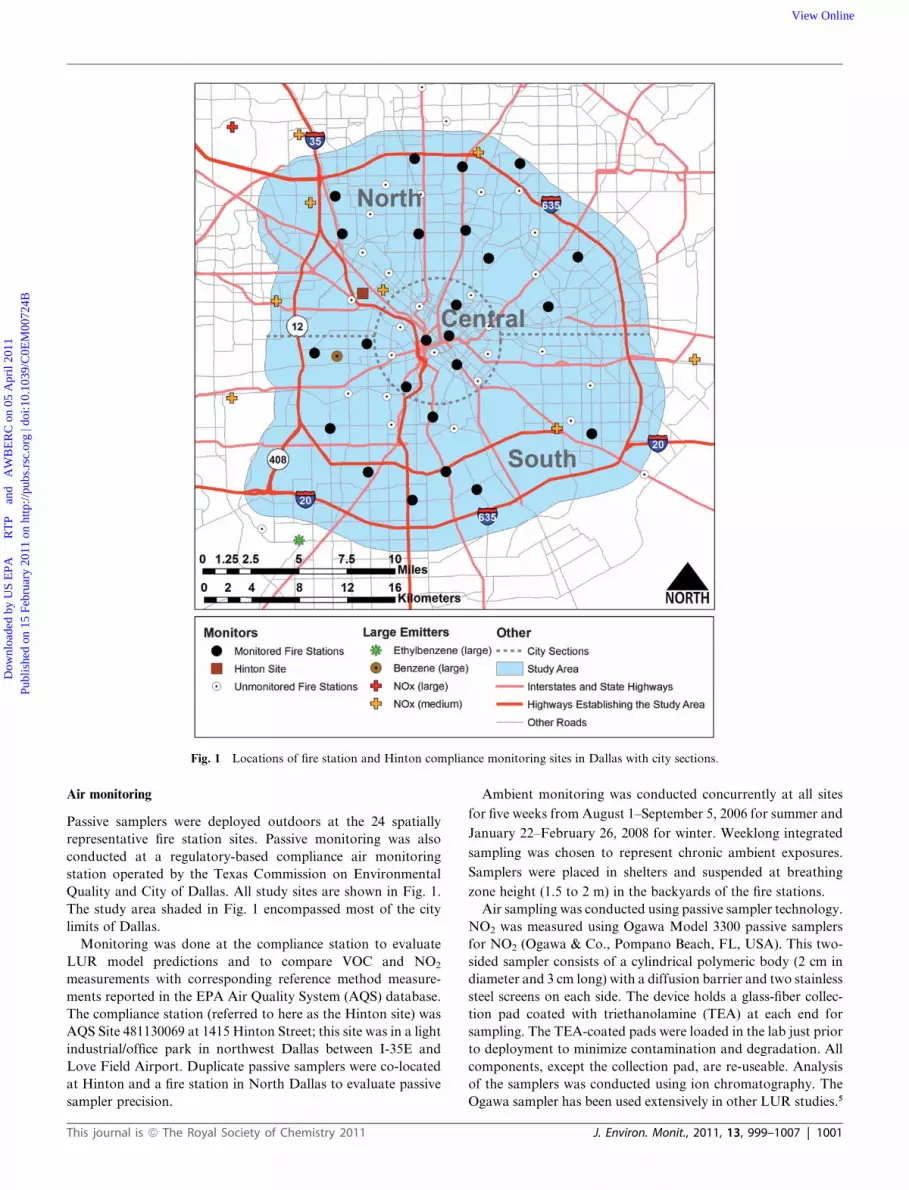
Fig. 1 Locations of fire station and Hinton compliance monitoring sites in Dallas with city sections.

Dow

nloa

ded

by U

S E

PA

R

TP

an

d A

WB

ER

C o

n 05

Apr

il 20

11Pu

blis

hed

on 1

5 Fe

brua

ry 2

011

on h

ttp://

pubs

.rsc

.org

| do

i:10.

1039

/C0E

M00

724B

View Online

Air monitoring

Passive samplers were deployed outdoors at the 24 spatially

representative fire station sites. Passive monitoring was also

conducted at a regulatory-based compliance air monitoring

station operated by the Texas Commission on Environmental

Quality and City of Dallas. All study sites are shown in Fig. 1.

The study area shaded in Fig. 1 encompassed most of the city

limits of Dallas.

Monitoring was done at the compliance station to evaluate

LUR model predictions and to compare VOC and NO2

measurements with corresponding reference method measure-

ments reported in the EPA Air Quality System (AQS) database.

The compliance station (referred to here as the Hinton site) was

AQS Site 481130069 at 1415 Hinton Street; this site was in a light

industrial/office park in northwest Dallas between I-35E and

Love Field Airport. Duplicate passive samplers were co-located

at Hinton and a fire station in North Dallas to evaluate passive

sampler precision.


Ambient monitoring was conducted concurrently at all sites

for five weeks from August 1–September 5, 2006 for summer and

January 22–February 26, 2008 for winter. Weeklong integrated

sampling was chosen to represent chronic ambient exposures.

Samplers were placed in shelters and suspended at breathing

zone height (1.5 to 2 m) in the backyards of the fire stations.

Air sampling was conducted using passive sampler technology.

NO2 was measured using Ogawa Model 3300 passive samplers

for NO2 (Ogawa & Co., Pompano Beach, FL, USA). This two-

sided sampler consists of a cylindrical polymeric body (2 cm in

diameter and 3 cm long) with a diffusion barrier and two stainless

steel screens on each side. The device holds a glass-fiber collec-

tion pad coated with triethanolamine (TEA) at each end for

sampling. The TEA-coated pads were loaded in the lab just prior

to deployment to minimize contamination and degradation. All

components, except the collection pad, are re-useable. Analysis

of the samplers was conducted using ion chromatography. The

Ogawa sampler has been used extensively in other LUR studies.5

J. Environ. Monit., 2011, 13, 999–1007 | 1001


Ta

ble

1P

ears

on

corr

elati

on

sb

etw

een

exp

lan

ato

ryvari

ab

les

con

sid

ered

for

site

sele

ctio

nan

dL

UR

sa

PO

P_

DE

Nb

INT

_10

00

cD

IST

_1

5K

IdD

IST

_4

5K

IeD

IST

_7

5K

IfD

IST

_1

10

KIg

DIS

T_

14

0K

Ph

NO

X1

iN

OX

2j

BE

N1

kE

TH

1l

PO

P_

DE

N1

�0

.20

�0

.30

0.1

00

.04

�0

.23

�0

.09

0.0

20

.15

�0

.02

0.0

4IN

T1

00

0�

0.1

41

�0

.34

�0

.48

�0

.41

�0

.44

�0

.19

�0

.19

�0

.17

�0

.25

0.0

1D

IST

_1

5K

I�

0.2

0�

0.4

81

0.0

3�

0.0

80

.47

0.0

80

.26

0.0

30

.50

0.2

7D

IST

_4

5K

I0

.01

�0

.57

0.3

41

0.3

60

.55

0.6

10

.53

0.1

80

.14

�0

.34

DIS

T_

75

KI

0.1

0�

0.3

50

.36

0.3

41

0.2

6�

0.0

80

.09

0.0

80

.51

0.3

2D

IST

_1

10

KI

�0

.29

�0

.58

0.6

40

.45

0.4

81

0.7

30

.64

0.3

10

.41

�0

.29

DIS

T_

14

0K

P�

0.3

1�

0.4

70

.51

0.5

60

.18

0.8

21

0.7

90

.39

�0

.10

�0

.73

NO

X1

�0

.31

�0

.40

0.3

80

.55

0.3

00

.72

0.7

61

0.3

80

.37

�0

.26

NO

X2

�0

.13

�0

.30

0.0

60

.17

0.3

90

.51

0.5

90

.60

10

.06

�0

.32

BE

N1

0.0

7�

0.1

30

.11

0.0

30

.32

0.1

1�

0.2

70

.26

�0

.09

10

.68

ET

H1

0.2

60

.23

�0

.29

�0

.33

�0

.08

�0

.59

�0

.86

�0

.45

�0

.60

0.6

51

aF

ire

sta

tio

ns

wit

hp

ass

ive

sam

pli

ng

da

ta(n¼

24)

ap

pea

rin

the

up

per

tria

ngu

lar

po

rtio

no

fth

em

atr

ix(i

.e.,

ab

ove

the

dia

go

nalo

f1s)

;co

rrel

ati

on

sw

ith

inth

egro

up

of

un

mo

nit

ore

dfi

rest

ati

on

s(n¼

21

)a

pp

ear

inth

elo

wer

tria

ng

ula

rp

ort

ion

.b

PO

P_D

EN

:p

op

ula

tio

no

fce

nsu

str

act

of

loca

tio

n.

cIN

T1000:

traffi

cin

ten

sity

wit

hin

1000

mo

flo

cati

on

.d

DIS

T_

15

KI:

dis

tan

ceto

nea

rest

road

wit

h1

00

00

<tr

affi

cv

olu

me

#2

00

00

veh

icle

sp

erd

ay.

eD

IST

_4

5K

I:d

ista

nce

ton

eare

stro

ad

wit

h4

00

00

<tr

affi

cv

olu

me

#50

000

veh

icle

sp

erd

ay.

fD

IST

_7

5K

I:d

ista

nce

ton

eare

stro

ad

wit

h7

00

00

<tr

affi

cv

olu

me

#80

000

veh

icle

sp

erd

ay.

gD

IST

_1

10

KI:

dis

tan

ceto

nea

rest

road

wit

h1

00

00

0<

tra

ffic

vo

lum

e#

120

000

veh

icle

sp

erd

ay.

hD

IST

_1

40

KP

:d

ista

nce

ton

eare

stro

ad

wit

htr

affi

cv

olu

me

$1

40

00

0v

ehic

les

per

da

y.

iN

OX

1:

dis

tan

ceto

sou

rce

wit

hN

Ox

emis

sio

ns

>57

00

00

lbs

per

yea

r.j

NO

X2

:d

ista

nce

toso

urc

ew

ith

21

00

0<

NO

xem

issi

on

s<

22

10

00

lbs

per

yea

r.k

BE

N1

:d

ista

nce

toso

urc

ew

ith

ben

zen

eem

issi

on

s>

27

00

00

lbs

per

yea

r.l

ET

H1

:d

ista

nce

toso

urc

ew

ith

eth

ylb

enze

ne

emis

sio

ns

>4

40

0lb

sp

ery

ear.

1002 | J. Environ. Monit., 2011, 13, 999–1007

Dow

nloa

ded

by U

S E

PA

R

TP

an

d A

WB

ER

C o

n 05

Apr

il 20

11Pu

blis

hed

on 1

5 Fe

brua

ry 2

011

on h

ttp://

pubs

.rsc

.org

| do

i:10.

1039

/C0E

M00

724B

View Online

NO2 is an EPA National Ambient Air Quality Standards

(NAAQS) criteria air pollutant and serves as an indicator of

mobile and stationary combustion sources.12 VOCs were

measured using PerkinElmer (PE) thermal desorption diffusion

tubes packed with 40/60 mesh size, unwashed Carbopack X

adsorbent for VOC (Supelco, Inc., Bellefonte, PA, USA). After

the PE tubes were thermally desorbed, they were ready for re-use

and re-deployed in the field. Due to their reusability, the PE tubes

used in Detroit13 were used in this study. Select VOCs such as 1,3-

butadiene and BTEX species (benzene, toluene, ethylbenzene,

o-xylene, and m,p-xylene) are reported in this paper. These

species are classified as air toxics by EPA and the State of

Texas.14,15 BTEX species and 1,3-butadiene are petroleum-

related compounds typically associated with traffic emissions.16

Evaluation of passive samplers for precision and accuracy was

conducted at the Hinton site and a North Dallas fire station (see

Passive method evaluation section in the ESI†). Further details

on the air sampling, analyses, and quality assurance methods are

discussed elsewhere.7,13

Results

Concentrations

Table 2 shows summary statistics of the air pollutants collected

at the fire station sites for each season (ESI†, Table S5 reports

mean concentrations for each site). In general, pollutant levels

were higher during winter than summer. In terms of the means,

this increase was particularly noticeable for benzene and 1,3-

butadiene (67% and 63% increases, respectively) and styrene

which in summer was often below its detection limit. This may

have been due to colder temperatures affecting atmospheric

reaction rates and lower mixing heights resulting in higher

concentrations.17,18

Monitoring methods, sampling time integrals, and analysis

methods in Dallas were the same as those in Detroit7 and similar

to those in El Paso,6 thereby providing an opportunity for

comparison. Median pollutant concentrations from Detroit and

El Paso were comparable to or higher than Dallas. Complex

terrain conditions in El Paso and heavy industrial sources in

Detroit may have been factors in higher pollutant concentrations

encountered in those cities versus Dallas which was dominated by

flat terrain and mobile sources. All data were above method

detection limits; summer and winter NO2 levels were below the

annual NAAQS of 53 ppb12 (Table 2).

Coarse-scale spatial comparisons

Dallas was physically separated by north and south sections and

a central, downtown area (see Fig. 1). The city was divided in this

manner and median pollutant concentrations from fire station

sites in each section were compared. Ten fire stations were

located in the north section, nine in the south, and five in the

central section.

Table 3 reports median values for each city section and the

entire study area for each season and indicates whether the levels

in each section were significantly different (at the 5% level)

between the two seasons. The Wilcoxon rank sum test19 was

utilized for these comparisons. Wintertime levels were higher in

each section for benzene, and for NO2 in the north and south



Table 2 Median pollutant concentrations at Dallas fire stations versus Detroit/Dearborn and El Paso schoolsa

Pollutant

Dallas summer Dallas winter

Dallas seasonaldifference (%)c

Detroit/Dearborn(25 schools; 7/19/2005to 8/30/2005)d

El Paso (22 schools;11/24/1999 to 12/18/1999)d

Concentration(24 fire stations;8/1/2006 to 9/5/2006) MDLb

Concentration(24 fire stations;1/22/2008 to 2/26/2008) MDLb

NO2 12 (4, 25) 2 14 (2, 22) 2 13 16 (11, 24) 22 (11, 37)1,3-Butadiene 72 (38, 149) 30 117 (48, 314) 33 67 74 (50, 128) NMe

Benzene 232 (83, 388) 27 357 (247, 538) 8 63 466 (338, 698) 777 (489, 1531)Toluene 539 (162, 1166) 18 617 (232, 1788) 25 20 1401 (980, 1994) 1473 (772, 3306)Ethylbenzene 86 (31, 190) 11 96 (40, 295) 8 15 186 (126, 360) 250 (152, 558)o-Xylene 86 (30, 218) 13 102 (39, 279) 8 25 200 (120, 338) 298 (177, 672)m,p-Xylene 254 (87, 621) 27 247 (98, 895) 16 10 591 (362, 1228) 838 (474, 1848)

a Medians calculated over all sites and weeks. Units for NO2 in ppbV; VOC in pptV with VOC from El Paso using 3 M organic vapor monitors.Minimum and maximum values in parentheses. b MDL: method detection limit. c (winter � summer)/summer, based on means. d Data summarizedfrom refs. 6 and 7. e NM: not measured.

Table 3 Median pollutant concentrationsa by city section and season based on individual fire stations

Benzene Toluene Ethylbenzene m,p-Xylene o-Xylene NO2

WinterNorth 344b 552 90 250 99 14Central 381 774 136 338 141 16South 345 563 90 238 96 13Entire area 352 568 95 267 103 15SummerNorth 220 594 92 264 87 11Central 283 574 111 317 106 15South 208 411 69 209 71 11Entire area 225 565 89 260 87 12

a VOCs are in pptV and NO2 is in ppbV. b Boldface indicates that the winter values were statistically significantly (5% level) different than thecorresponding summer values.

Table 4 Comparison of pollutants at Dallas city sections within seasons

Benzene Toluene Ethylbenzene m,p-Xylene o-Xylene NO2

South vs. centralSummer C > Sa nsb ns ns ns C > SWinter ns ns ns ns ns C > SSouth vs. northSummer ns ns ns ns ns nsWinter ns ns ns ns ns nsNorth vs. centralSummer C > N ns ns ns ns C > NWinter C > N ns ns ns ns C > N

a C > S means that the central section had statistically significantly (5% level) higher concentrations than the south section. Similarly, C > N means thatthe central section was higher than the north section. b ns: no significant difference at the 5% level.

Dow

nloa

ded

by U

S E

PA

R

TP

an

d A

WB

ER

C o

n 05

Apr

il 20

11Pu

blis

hed

on 1

5 Fe

brua

ry 2

011

on h

ttp://

pubs

.rsc

.org

| do

i:10.

1039

/C0E

M00

724B

View Online

sections. This also held true when looking at the entire city, and

in addition, wintertime o-xylene levels were statistically signifi-

cantly higher when the study area was considered as a whole.

Table 4 reports the results of comparing the city sections to each

other within the summer and winter periods. To guard against false

positives, these comparisons were done with Dunn’s test,19 but

modified as suggested by Hochberg and Tamhane.20 Mukerjee

et al.7 provide details of an application of Dunn’s test to assess

spatial differences. For both summer and winter, the central

section had higher NO2 levels than either the north or south

sections. For benzene, the central section was higher than the north

in both seasons, but higher than the south section only in summer.


LUR modeling

To determine LUR equations, the observed mean values of the

chemicals at each site were plotted against the various potential

predictor variables (Table 1). For each chemical, only those

predictors for which the chemical appeared to have reasonably

consistent behavior were retained for use in developing the

LURs. This suggested the use of multiple linear regression to

estimate the LURs. In most instances, this was applied with the

chemical measurements log-transformed; for the m,p-xylene

LUR, the predictor variable of distance to a large ethylbenzene

source (ETH1) was also log-transformed (see Table 5). For

consistency, the summer predictor variables were applied in the

J. Environ. Monit., 2011, 13, 999–1007 | 1003


Table 5 LUR models for Dallasa

Regression equations R2 (%)

Summer LURsBenzene ¼ 230.9 � 0.028 DIST15KI � 0.0045 DIST75KI +

5.9 � 10�4 DIST110KI + 9.1 � 10�5 INT100072

ln toluene ¼ 6.8 � 3.2 � 10�5 DIST75KI � 8.7 � 10�6

DIST110KI � 1.9 � 10�5 NOX1 + 3.5 � 10�6 NOX241

ln ethylbenzene ¼ 4.9 � 1.1 � 10�5 DIST75KI � 4.0 � 10�5

DIST110KI � 1.8 � 10�7 INT1000 � 2.6 � 10�5 BEN1 +7.9 � 10�6 NOX1 � 1.4 � 10�5 NOX2

63

ln m,p-xylene ¼ �1.6 + 4.1 � 10�5 DIST15KI � 1.3 � 10�5

DIST75KI + 3.8 � 10�6 DIST110KI + 2.5 � 10�7

INT1000 � 5.9 � 10�5 BEN1 + 0.76 ln_ETH1 + 1.4 �10�5 NOX1

71

ln o-xylene ¼ 4.7 � 2.0 � 10�5 DIST75KI � 3.8 � 10�5

DIST110KI � 1.5 � 10�5 BEN1 + 5.1 � 10�6 NOX146

ln 1,3-butadiene ¼ 4.6 � 4.6 � 10�6 DIST75KI � 1.8 � 10�5

DIST110KI � 1.1 � 10�5 BEN1 � 8.2 � 10�6 NOX226

ln NO2 ¼ 2.6 + 4.2 � 10�5 DIST45KI � 2.5 � 10�5

DIST75KI + 1.2 � 10�6 INT1000 � 1.5 � 10�5 BEN134

Winter LURsBenzene ¼ 375.5 + 0.001 DIST15KI � 0.004 DIST75KI �

0.002 DIST110KI + 6.1 � 10�7 INT100049

ln toluene ¼ 7.1 � 2.5 � 10�5 DIST75KI � 8.8 � 10�6

DIST110KI � 2.4 � 10�5 NOX1 � 6.1 � 10�6 NOX241

ln ethylbenzene ¼ 5.0 – 1.2 � 10�5 DIST75KI � 2.3 � 10�5

DIST110KI + 5.0 � 10�8 INT1000 � 2.0 � 10�5 BEN1 +4.2 � 10�6 NOX1 � 1.3 � 10�5 NOX2

40

ln m,p-xylene ¼ 1.1 + 1.4 � 10�5 DIST15KI � 3.3 � 10�5

DIST75KI + 1.3 � 10�5 DIST110KI + 1.2 � 10�7

INT1000 � 5.7 � 10�5 BEN1 + 0.50 ln_ETH1 + 9.4 �10�6 NOX1

40

ln o-xylene ¼ 5.1 � 9.2 � 10�6 DIST75KI � 1.7 � 10�5

DIST110KI � 2.6 � 10�5 BEN1 � 9.8 � 10�7 NOX137

ln 1,3-butadiene ¼ 5.3 � 5.0 � 10�6 DIST75KI � 1.7 � 10�5

DIST110KI � 2.2 � 10�5 BEN1 � 1.2 � 10�5 NOX240

ln NO2 ¼ 2.8 � 2.2 � 10�5 DIST45KI � 1.2 � 10�5

DIST75KI + 6.3 � 10�7 INT1000 � 1.4 � 10�5 BEN148

a Notes: bold indicates regression coefficients significant at the 5% level.log is the natural logarithm. R2 is reported for the original scale, not thelog-transformed scale.23,24

Table 6 Observed and predicted values at the Hinton sitea

Pollutant Measured Predictedb Differencec Percent differenced

SummerBenzene 133 243 (236, 249) 110 83Toluene 494 653 (589, 724) 159 32Ethylbenzene 61 119 (107, 132) 58 94m,p-Xylene 178 357 (324, 393) 179 101o-Xylene 60 109 (105, 114) 49 831,3-Butadiene 48 90 (83, 97) 42 89NO2 12 15 (14, 17) 3 24WinterBenzene 289 371 (360, 382) 82 28Toluene 518 792 (749, 839) 275 53Ethylbenzene 71 133 (112, 157) 61 86m,p-Xylene 194 399 (330, 482) 205 106o-Xylene 67 139 (128, 151) 72 1071,3-Butadiene 84 164 (162, 166) 79 94NO2 14 17 (16, 19) 3 25

a Units are pptV for all VOCs and ppbV for NO2. b 95% confidenceinterval in parentheses. c Difference ¼ predicted � observed. d Percentdifference ¼ (difference/observed) � 100.

Dow

nloa

ded

by U

S E

PA

R

TP

an

d A

WB

ER

C o

n 05

Apr

il 20

11Pu

blis

hed

on 1

5 Fe

brua

ry 2

011

on h

ttp://

pubs

.rsc

.org

| do

i:10.

1039

/C0E

M00

724B

View Online

winter season in each equation. (Since sampling was for week-

long sampling periods, wind direction was not considered in the

LURs.)

When the regressions were first attempted, residual analysis

from initial regression attempts indicated large differences

between the observed and predicted values at a few sites. These

sites varied by chemical. To mitigate this, the regressions were re-

run with each site being weighted by the inverse value of Cook’s

D statistic21 calculated from the unweighted regression. Thus, the

final predictive (LUR) equations downweighted the influence of

those sites which departed from the general pattern established

by the other locations. See Rawlings22 for a discussion of

multivariate regression including influence diagnostics and

weighted regression. In addition to residual analyses, regression

diagnostics included cross-validation.

Table 5 presents results of the LUR models for summer and

winter data. Predictors which were significant at the 5% level are

shown in bold. In each case, the equations show all predictors

used, not just those reported as significant. All R2 values are

reported based on the original (not the log-transformed) scale.

There were similarities and differences between summer and

winter results in terms of which predictors were found to be

1004 | J. Environ. Monit., 2011, 13, 999–1007

significant and performance of the regressions as measured in

terms of R2. Relative to the summer results, benzene and NO2

‘‘lost’’ two predictors (in terms of significance at the 5% level)

while 1,3-butadiene ‘‘gained’’ two. Similarly, toluene and

o-xylene all ‘‘added’’ a significant predictor, while ethylbenzene

and m,p-xylene both ‘‘dropped’’ one.

In terms of the R2 values, benzene, ethylbenzene, and m,p-

xylene all had noticeably higher R2’s in summer than in winter.

On the other hand, NO2 and 1,3-butadiene all had noticeably

lower values in summer. The R2 values for toluene and o-xylene

were approximately the same between summer and winter.

Table 6 displays the respective summer and winter results of

comparing the measured values observed at the Hinton site to the

values predicted there by the regression equations. As an indi-

cator of uncertainty in the predicted values, the table also shows

their 95% confidence intervals. (The Hinton site was withheld

from the LUR estimation to serve as a validation location.)

Relative to summer, the wintertime comparisons at the Hinton

site were better for benzene and o-xylene, and a bit worse for

toluene. Results for m,p-xylene, ethylbenzene, 1,3-butadiene, and

NO2 were similar between seasons.

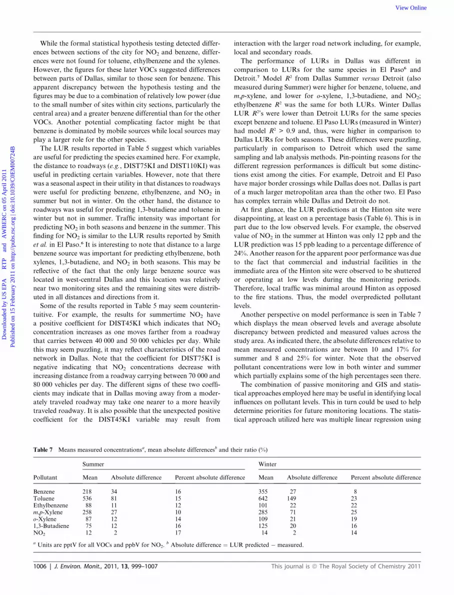
Fig. 2a and b display the LUR predicted pollutant levels in the

summer and winter periods for benzene. Similarly, Fig. 3a and

b present NO2 results. (Figs. S2 and S3 in the ESI† similarly

display the measured concentrations for these pollutants.) Figs. 2

and 3 show generally higher predicted benzene and NO2 levels in

the central section and parts of the north section of Dallas,

echoing the results of the statistical comparisons in Table 4.

Similar figures were obtained for the other BTEX species. This

was expected since the central and north sections of Dallas were

more developed than the south.

Discussion and conclusions

Spatially representative air monitoring sites were established at

fire stations in Dallas during two seasons. Week-long sampling

using passive air samplers at these sites suggested a temporal

difference in concentrations with generally higher levels reported



Fig. 2 LUR predicted benzene concentrations in Dallas: (a) summer and (b) winter.

Fig. 3 LUR predicted NO2 concentrations in Dallas: (a) summer and (b) winter.

Dow

nloa

ded

by U

S E

PA

R

TP

an

d A

WB

ER

C o

n 05

Apr

il 20

11Pu

blis

hed

on 1

5 Fe

brua

ry 2

011

on h

ttp://

pubs

.rsc

.org

| do

i:10.

1039

/C0E

M00

724B

View Online

in winter versus summer. City section was also found to have an

effect for NO2 and benzene with the central section exhibiting

higher pollutant levels than the north or south areas. Though the

concentration differences found here are consistent with the

expectations from higher summertime temperatures and lower


wintertime mixing heights, these results are not definitive since

summer and winter monitoring were conducted more than a year

apart. For example, long-term temporal differences may have

resulted from such influences as urban growth or increased road

construction.

J. Environ. Monit., 2011, 13, 999–1007 | 1005


Dow

nloa

ded

by U

S E

PA

R

TP

an

d A

WB

ER

C o

n 05

Apr

il 20

11Pu

blis

hed

on 1

5 Fe

brua

ry 2

011

on h

ttp://

pubs

.rsc

.org

| do

i:10.

1039

/C0E

M00

724B

View Online

While the formal statistical hypothesis testing detected differ-

ences between sections of the city for NO2 and benzene, differ-

ences were not found for toluene, ethylbenzene and the xylenes.

However, the figures for these later VOCs suggested differences

between parts of Dallas, similar to those seen for benzene. This

apparent discrepancy between the hypothesis testing and the

figures may be due to a combination of relatively low power (due

to the small number of sites within city sections, particularly the

central area) and a greater benzene differential than for the other

VOCs. Another potential complicating factor might be that

benzene is dominated by mobile sources while local sources may

play a larger role for the other species.

The LUR results reported in Table 5 suggest which variables

are useful for predicting the species examined here. For example,

the distance to roadways (e.g., DIST75KI and DIST110KI) was

useful in predicting certain variables. However, note that there

was a seasonal aspect in their utility in that distances to roadways

were useful for predicting benzene, ethylbenzene, and NO2 in

summer but not in winter. On the other hand, the distance to

roadways was useful for predicting 1,3-butadiene and toluene in

winter but not in summer. Traffic intensity was important for

predicting NO2 in both seasons and benzene in the summer. This

finding for NO2 is similar to the LUR results reported by Smith

et al. in El Paso.6 It is interesting to note that distance to a large

benzene source was important for predicting ethylbenzene, both

xylenes, 1,3-butadiene, and NO2 in both seasons. This may be

reflective of the fact that the only large benzene source was

located in west-central Dallas and this location was relatively

near two monitoring sites and the remaining sites were distrib-

uted in all distances and directions from it.

Some of the results reported in Table 5 may seem counterin-

tuitive. For example, the results for summertime NO2 have

a positive coefficient for DIST45KI which indicates that NO2

concentration increases as one moves farther from a roadway

that carries between 40 000 and 50 000 vehicles per day. While

this may seem puzzling, it may reflect characteristics of the road

network in Dallas. Note that the coefficient for DIST75KI is

negative indicating that NO2 concentrations decrease with

increasing distance from a roadway carrying between 70 000 and

80 000 vehicles per day. The different signs of these two coeffi-

cients may indicate that in Dallas moving away from a moder-

ately traveled roadway may take one nearer to a more heavily

traveled roadway. It is also possible that the unexpected positive

coefficient for the DIST45KI variable may result from

Table 7 Means measured concentrationsa, mean absolute differencesb and t

Pollutant

Summer

Mean Absolute difference Percent absolute differ

Benzene 218 34 16Toluene 536 81 15Ethylbenzene 88 11 12m,p-Xylene 258 27 10o-Xylene 87 12 141,3-Butadiene 75 12 16NO2 12 2 17

a Units are pptV for all VOCs and ppbV for NO2. b Absolute difference ¼ L

1006 | J. Environ. Monit., 2011, 13, 999–1007

interaction with the larger road network including, for example,

local and secondary roads.

The performance of LURs in Dallas was different in

comparison to LURs for the same species in El Paso6 and

Detroit.7 Model R2 from Dallas Summer versus Detroit (also

measured during Summer) were higher for benzene, toluene, and

m,p-xylene, and lower for o-xylene, 1,3-butadiene, and NO2;

ethylbenzene R2 was the same for both LURs. Winter Dallas

LUR R2’s were lower than Detroit LURs for the same species

except benzene and toluene. El Paso LURs (measured in Winter)

had model R2 > 0.9 and, thus, were higher in comparison to

Dallas LURs for both seasons. These differences were puzzling,

particularly in comparison to Detroit which used the same

sampling and lab analysis methods. Pin-pointing reasons for the

different regression performances is difficult but some distinc-

tions exist among the cities. For example, Detroit and El Paso

have major border crossings while Dallas does not. Dallas is part

of a much larger metropolitan area than the other two. El Paso

has complex terrain while Dallas and Detroit do not.

At first glance, the LUR predictions at the Hinton site were

disappointing, at least on a percentage basis (Table 6). This is in

part due to the low observed levels. For example, the observed

value of NO2 in the summer at Hinton was only 12 ppb and the

LUR prediction was 15 ppb leading to a percentage difference of

24%. Another reason for the apparent poor performance was due

to the fact that commercial and industrial facilities in the

immediate area of the Hinton site were observed to be shuttered

or operating at low levels during the monitoring periods.

Therefore, local traffic was minimal around Hinton as opposed

to the fire stations. Thus, the model overpredicted pollutant

levels.

Another perspective on model performance is seen in Table 7

which displays the mean observed levels and average absolute

discrepancy between predicted and measured values across the

study area. As indicated there, the absolute differences relative to

mean measured concentrations are between 10 and 17% for

summer and 8 and 25% for winter. Note that the observed

pollutant concentrations were low in both winter and summer

which partially explains some of the high percentages seen there.

The combination of passive monitoring and GIS and statis-

tical approaches employed here may be useful in identifying local

influences on pollutant levels. This in turn could be used to help

determine priorities for future monitoring locations. The statis-

tical approach utilized here was multiple linear regression using

heir ratio (%)

Winter

ence Mean Absolute difference Percent absolute difference

355 27 8642 149 23101 22 22285 71 25109 21 19125 20 1614 2 14

UR predicted � measured.



Dow

nloa

ded

by U

S E

PA

R

TP

an

d A

WB

ER

C o

n 05

Apr

il 20

11Pu

blis

hed

on 1

5 Fe

brua

ry 2

011

on h

ttp://

pubs

.rsc

.org

| do

i:10.

1039

/C0E

M00

724B

View Online

logarithmic transformations, followed by residual analyses and

cross-validation to evaluate adequacy of the models. One might

consider alternative approaches such as kriging or neural

networks but they were not used here because they are quite data

intensive and the limited number of monitoring sites available for

this study would likely not adequately support these spatial

prediction approaches.

Seasonal differences in the LURs and their predictive power

demonstrate the need for caution in developing such models

from annual or multi-year averages without considering seasonal

or other factors. In fact, in their review Hoek et al.5 note that

seasonal aspects have generally been excluded from LUR

modeling efforts either by the nature of the monitoring or

averaging out seasonality during the model fitting process. It is

worth noting that many LUR models are used as part of a health

assessment. If the health issue being studied has a seasonal

aspect, then it would be beneficial for the corresponding LUR to

account for this. The seasonal consideration discovered here is

being further explored in other EPA spatial studies. Thus, the

potential should be available in the future to combine these

results from Dallas with the other LUR efforts mentioned to

obtain a comprehensive analysis of the exposure modeling results

across different US cities and seasons.

Acknowledgements

For their roles in various aspects of the study, we thank the

following: Casson Stallings, Hunter Daughtrey, Karen Oliver,

Dennis Williams, Herb Jacumin, Laura Liao, Mariko Porter,

Chris Fortune, and Mike Wheeler of Alion Science and Tech-

nology; Carry Croghan and Mark Sather of EPA; John Koller

from the City of Dallas. We also thank the City of Dallas Fire

Department for allowing us to use their fire stations. Finally we

thank Davyda Hammond and Gary Norris of EPA for reviewing

the manuscript. This study was an EPA Region 6 Geographic

Initiative (RGI) and Regional Applied Research Effort (RARE)

Project. The US Environmental Protection Agency through its

Office of Research and Development funded and managed the

research described here under contract EP-D-05-065 to Alion.

The paper has been subjected to Agency review and approved for

publication. Mention of trade names or commercial products

does not constitute an endorsement or recommendation for use.


References

1 M. Brauer, G. Hoek, P. van Vliet, K. Meliefste, P. Fischer,U. Gehring, J. Heinrich, J. Cyrys, J. T. Bellander, M. Lewne andB. Brunekreef, Epidemiology, 2003, 14, 228–239.

2 M. Jerrett, A. Arain, P. Kanaroglou, B. Beckerman, D. Potoglou,T. Sahsuvaroglu, J. Morrison and C. Giovis, J. Exposure Anal.Environ. Epidemiol., 2005, 15, 185–204.

3 Z. Ross, P. B. English, R. Scalf, R. Gunier, S. Smorodinsky, S. Walland M. Jerrett, J. Exposure Sci. Environ. Epidemiol., 2006, 16, 106–114.

4 D. K. Moore, M. Jerrett, W. J. Mack and N. K€unzli, J. Environ.Monit., 2007, 9, 246–252.

5 G. Hoek, R. Beelen, K. de Hoogh, D. Vienneau, J. Gulliver,P. Fischer and D. Briggs, Atmos. Environ., 2008, 42, 7561–7578.

6 L. Smith, S. Mukerjee, M. Gonzales, C. Stallings, L. Neas, G. Norrisand H. €Ozkaynak, Atmos. Environ., 2006, 40, 3773–3787.

7 S. Mukerjee, L. A. Smith, M. M. Johnson, L. M. Neas andC. A. Stallings, Sci. Total Environ., 2009, 407, 4642–4651.

8 T. Sahsuvaroglu, A. Arain, P. Kanaroglou, N. Finkelstein,B. Newbold, M. Jerrett, B. Beckerman, J. Brook, M. Finkelsteinand N. L. Gilbert, J. Air Waste Manage. Assoc., 2006, 56, 1059–1069.

9 S. B. Henderson, B. Beckerman, M. Jerrett and M. Brauer, Environ.Sci. Technol., 2007, 41, 2422–2428.

10 SAS Institute, Inc., Base SAS� 9.1.3 Procedures Guide, SAS, Cary,NC, 2004.

11 SAS Institute, Inc., SAS/STAT� 9.1 User’s Guide, SAS, Cary, NC,2004.

12 US EPA Technology Transfer Network National Ambient AirQuality Standards (NAAQS), http://www.epa.gov/ttn/naaqs/accessed 2010.

13 S. Mukerjee, K. D. Oliver, R. L. Seila, H. H. Jacumin, C. Croghan,E. H. Daughtrey, L. M. Neas and L. A. Smith, J. Environ. Monit.,2009, 11, 220–227.

14 US EPA Technology Transfer Network Air Toxics, http://www.epa.gov/ttn/atw/allabout.html, accessed 2010.

15 State of Texas Commission on Environmental Quality Air Toxics, http://www.tceq.state.tx.us/implementation/tox/AirToxics.html, accessed2010.

16 E. M. Fujita, Sci. Total Environ., 2001, 276, 171–184.17 D. H. F. Atkins and D. S. Lee, Atmos. Environ., 1995, 29, 223–239.18 L. Wallace, W. Nelson, R. Ziegenfus, E. Pellizzari, L. Michael,

R. Whitmore, H. Zelon, T. Hartwell and R. Perritt, J. ExposureAnal. Environ. Epidemiol., 1991, 1, 157–192.

19 O. J. Dunn, Technometrics, 1964, 6, 241–252.20 Y. Hochberg and A. C. Tamhane, Multiple Comparison Procedures,

Wiley, NY, 1987.21 R. D. Cook, Technometrics, 1977, 19, 15–18.22 J. O. Rawlings, Applied Regression Analysis: A Research Tool,

Wadsworth and Brooks/Cole, Pacific Grove, CA, 1988.23 T. A. Kv�alseth, Am. Stat., 1985, 39, 279–285.24 A. Scott and C. Wild, Am. Stat., 1991, 45, 127–129.

J. Environ. Monit., 2011, 13, 999–1007 | 1007


spatial analysis and land use regression of vocs and no2 in dallas, texas during two seasons

Documents