some uses of cut elimination
TRANSCRIPT
Some Uses of Cut Elimination
Pedro Francisco Valencia Vizcaıno
Submitted in accordance with the requirements for the degree of
Doctor of Philosophy
The University of Leeds
School of Mathematics
June 2013
The candidate confirms that the work submitted is his own and that appropriatecredit has been given where reference has been made to the work of others.
This copy has been supplied on the understanding that it is copyright materialand that no quotation from the thesis may be published without proper
acknowledgement.
c© 2013 The University of Leeds and Pedro Francisco Valencia Vizcaıno
Abstract
This thesis is mainly about Proof Theory. It can be thought of as ProofTheory in the sense of Hilbert, Gentzen, Schutte, Buchholz, Rathjen, andin general what could be called the German school, but it is also influencedby many other branches, of which the bibliography might give an idea.Intuitionism and other philosophical approaches to mathematics are also animportant part of what is studied, but the Leitmotif of this thesis is CutElimination. The first part of the thesis is concerned with countable codedω-models of Bar Induction. In this part we work from a reverse mathematicspoint of view. A study for an ordinal analysis of the theory of Bar Induction(BI) is carried out, and the equivalence between the statement that everyset is contained in an ω-model of this theory (BI) and the well-orderingprinciple ∀X[WO(X) → WO(ϑX)] which says that if X is a well-ordering,then so is its Bachmann-Howard relativisation, is proven. This is a newresult as far as we know, and, we hope, an important one. In the secondpart of the thesis we shift our viewpoint and consider intuitionistic logicand intuitionistic geometric theories. We show that geometric derivability inclassical infinitary logic implies derivability in intuitionistic infinitary logic.Again, our main tool is Cut Elimination. Next, we present investigationsregarding minimal logic and classical logical principles, and give a preciseclassification of excluded middle, ex falso, and double negation elimination.Other themes and roads are possible and, the author feels, important, buttime limitations as well as a sickly and utterly daft adherence to deadlinesdid not permit him to carry out these studies in full. It is quite shameful.
3

5
Acknowledgements
If I wanted to thank properly all the people that deserve my thanks Iwould need to write at least another PhD. I do apologise for not being ableto express how important the people involved in my studies were, and fornot having thanked them enough, some of them I won’t have a chance toanymore.
I would like to express my great gratitude to Michael Rathjen for su-pervising this thesis and for all his support through many years, and inmany ways. For meetings both in and outside the school, for his hospitalityon many occassions, particularly many nice Christmas gatherings, for hisgenerosity, and also, very importantly, for having had patience with me; afeat not easily accomplished. To me it has been a real honour and a greatpleasure to have been able to discuss mathematical as well as philosophicalissues with him. I hope we have a chance to continue these discussions fora long time to come. Sometimes I did not quite understand his several con-cerns, because as usual he could see a lot deeper into things than I could,even regarding things that had to do with me directly, and I appreciate hisinvolvement and his help. It has been not only a privilege, and a wondefulopportunity but actually a great learning experience, for which I am trulygrateful.
I thank CONACYT for providing me with a scholarship to study in theUK.
I would like to thank the people in the Leeds and Manchester Proof The-ory and Constructivism seminar, and to acknowledge the impact they had onmy views and in my development during my years in England. Many peopleparticipated and I would like to thank them all, in particular Stan Wainer,Peter Schuster, Laura Crosilla, the late John Derrick, Nicola Gambino, Pe-ter Aczel, as well as all my fellow students, in particular Andrew Swan, who,among many other things, was responsible for my going to Japan to JAISTto what was one of the best experiences of my life, Ray-Ming Cheng forbeing an absolutely awesome friend at all times, Matt Hendtlass for all hishelp with many things not only academic, I still owe him a visit to NewZealand, Albert Ziegler for being such a great example and for always beingvery friendly and patient with me, it took him quite a while to explain in-tuitionism to me, but I hope I understand a fraction of what he does, JacobCook for his excellent attitude, his goodwill, for having worked with methrough many ordinal-analytic adventures, and for being so up-beat, andsuch a good influence. Michael Toppel for his candid and refreshing person-ality, as well as his support, encouragement, his innumerable hard questionsand interest in the work in this thesis.
I have to thank Sara Negri for her time, her kindliness, and the help sheoffered me relating to the second part of the thesis.
6
A very very special thank you goes to my external examiner, AntonSetzer, whose understanding, kindness, and positive comments I will notforget. His thoroughness and precision are both exemplary and inspiring.So, really, I am much indebted to him.
My advisory committee, especially S. Barry Cooper and Dugald Macpher-son. I have to thank Barry again in the quality of internal examiner, as wellas for the reading groups and many good conversations, and Dugald for allhis support with my application to go to Munich as a MALOA fellow in thecapacity of early researcher, for all the Christmas dinners, and, of course,for doing an excellent job as an advisor. My heartfelt thanks.
It is only appropriate and a pleasure to thank Prof. Helmut Schwicht-enberg for receiving me in Munich in what was a fantastic learning envi-ronment, and I should thank also the Munich logic group, in particular thepeople whom I shared an office with: Vasileios Karadais, Kenji Miyamoto,Iosif Petrakis, and Davide Rinaldi. Thanks also to Peter Schuster for hissupport in this respect and to Daniel Bembe.
Back in Leeds I need to thank Tim Hainsworth who was there at a vitalmoment to offer invaluable help, and Mrs. Jeanne Shuttleworth, for dealingmarvelously well with all the troubles I have caused her over this long periodof time.
I was very lucky to be able to attend courses by Michael Rathjen, AndyLewis, and Harold Simmons from the University of Manchester via MAGIC,which I am very happy to acknowledge.
To the people who made life in Leeds a good thing, especially MayraMontalvo Ballesteros, whom it will take a while to thank enough, AndresAranda Lopez, Ronnie Nagloo, Simona Leali, Ahmet Cevik, Liliana BadilloSanchez, and Ricardo Bello Aguirre, who proved to be an exceptional friend,gave me a home for a very long time, and all the support anyone could askfor; if you are reading from a hard-bound copy of the thesis it is thanks tohim.
To my old friends, in particular, Mariano Zeron Medina Laris, and JoseLuis Martınez Meyer who always pushed me to do this.
To my parents.
Contents
1 Introduction 9
2 Philosophical Remarks 15
I Ordinal Analysis 19
3 Well Ordering Principles and Bar Induction 21
3.1 Introduction . . . . . . . . . . . . . . . . . . . . . . . . . . . . 21
3.1.1 Bar Induction . . . . . . . . . . . . . . . . . . . . . . . 25
3.2 Relativising the Bachmann-Howard ordinal . . . . . . . . . . 26
3.2.1 Defining OTX(ϑ) in RCA0 . . . . . . . . . . . . . . . 30
3.3 A Well-ordering Proof . . . . . . . . . . . . . . . . . . . . . . 31
3.4 Deduction chains . . . . . . . . . . . . . . . . . . . . . . . . . 34
3.5 Proof of the Main Theorem: The hard direction part 2 . . . . 40
3.5.1 Majorization and Fundamental Functions . . . . . . . 40
3.5.2 The infinitary calculus T ∗Q
. . . . . . . . . . . . . . . . 42
3.5.3 The reduction procedure for T ∗Q
. . . . . . . . . . . . . 47
3.5.4 Embedding DQ into T ∗Q
. . . . . . . . . . . . . . . . . . 50
II Geometric Theories 55
4 The Geometric Fragment 57
4.1 Sequent Calculi . . . . . . . . . . . . . . . . . . . . . . . . . . 59
4.2 Canonical Forms . . . . . . . . . . . . . . . . . . . . . . . . . 66
4.2.1 The key cases for infinitary non-geometric cut elimi-nation . . . . . . . . . . . . . . . . . . . . . . . . . . . 68
4.2.2 Reductions . . . . . . . . . . . . . . . . . . . . . . . . 69
III A Classification of Some Logical Principles 81
5 The formal system ML 83
7
8 CONTENTS
5.1 LJ without weakening-right . . . . . . . . . . . . . . . . . . . 835.2 Negation in Minimal Logic . . . . . . . . . . . . . . . . . . . . 87
5.2.1 Degrees of Negation . . . . . . . . . . . . . . . . . . . 88
6 Classification of the Principles 916.1 A form of ex-falso in minimal logic . . . . . . . . . . . . . . . 916.2 Brief recap of LJ . . . . . . . . . . . . . . . . . . . . . . . . . 916.3 Back to ML . . . . . . . . . . . . . . . . . . . . . . . . . . . . 926.4 Cut Elimination for ML . . . . . . . . . . . . . . . . . . . . . 94
6.4.1 Reductions . . . . . . . . . . . . . . . . . . . . . . . . 946.5 Cut Elimination for ML+ . . . . . . . . . . . . . . . . . . . . 966.6 Principles of Omniscience . . . . . . . . . . . . . . . . . . . . 103
6.6.1 Markov’s Rule . . . . . . . . . . . . . . . . . . . . . . 1036.7 Peirce’s law . . . . . . . . . . . . . . . . . . . . . . . . . . . . 1056.8 Consequentia mirabilis . . . . . . . . . . . . . . . . . . . . . . 1066.9 Godel-Dummet Logic . . . . . . . . . . . . . . . . . . . . . . . 1086.10 Ex falso for atoms . . . . . . . . . . . . . . . . . . . . . . . . 1086.11 Negative Contrapositive . . . . . . . . . . . . . . . . . . . . . 1086.12 Double negation elimination for atoms . . . . . . . . . . . . . 109
Chapter 1
Introduction
Proof theory, as has been noted by some of its leading figures ([6]), is the areaof mathematical logic in which we still care about philosophical problems.It is in this attitude that it becomes meaningful to work with differentkinds of logic, as opposed to working in classical logic only. In this thesiswe will at times work with non-classical logics, like intuitionistic logic andminimal logic. We try to motivate this attitude as best we can throughoutbut perhaps the most appropriate introductions to these topics are [4] andmany of the well-known books on these themes. Some of them can befound in the bibliography at the end of this work. The thesis begins with acouple of philosophical remarks, which we hope help in the aforementionedmotivation, but the overall focus and principal concerns of the thesis aremainly mathematical rather than philosophical.
In the first part proper of the thesis, where we put philosophy on holdand focus on mathematics, we show that the existence of ω-models of barinduction is equivalent to the well-ordering principle which says that ap-plying the Bachmann-Howard operation to any well-ordering yields again awell-ordering, i. e.,
WO(X)→WO(ϑX)
From a broader viewpoint we could say that we are studying a particularinstance of the principle
WOP(f) : ∀X [WO(X)→WO(f(X))]
The study of such principles has become a richer area of research in prooftheory in recent times. Nowadays, several examples of proof theoretic func-tions f for which the statement WOP(f) has turned out to be equivalent toone of the theories of reverse mathematics are known and well understood.We begin this part of the thesis by recalling some of the first and mostfamous examples of such well-ordering principles, and then carry on withour particular one. Not surprisingly, or so it seems to the author, the first
9
10 CHAPTER 1. INTRODUCTION
examples are somewhat implicit in Schutte’s proof of cut elimination for ω-logic [24] and ultimately many of these results can be thought of as havingtheir roots in the work of the great german logician Gerhard Gentzen. Tohim is owed a very great debt (a sentiment no doubt shared by most peo-ple working in the field). The very deep results of Gentzen have motivatedor influenced all the work behind this thesis and it is thanks to his greatachievements that we have in our possession many wonderful tools to workwith. Mostly the work in the thesis is based on Sequent-style calculi, and wehave found this extremely useful. Æsthetic discussions are passed by. Thework of Gentzen has provided us with a great starting point from whichmany new developments can follow, as we hope will be seen in this work.
To get back to a more precise rendering of the contents of the thesis:
Let T be a subsystem of Second Order Arithmetic. We use the formula
P(ω) 4Mω(T )
to express the principle that every set of natural numbers X is containedin a countable coded ω-model of T .
We introduce countably coded ω-models of Second Order Arithmetic andgive some notion of the history of the particular developments in this area aswell as an appropriate background for our new results. We proceed to proveall we require in order to establish our main result of this section, namely,that over RCA0 the following are equivalent:
(i) P(ω) 4Mω(BI)
(ii) ∀X [WO(X)→WO(ϑX)].
We give detailed definitions of bar induction, the Bachmann-Howardordinal representation system, and its relativisations. The objective of thisis to construct from any given well-ordering X, a new well-ordering ϑX ofBachmann-Howard type which incorporates X, in a useful way. Section 3.3proves the direction (i) ⇒ (ii) of the theorem we call our main theorem.With section 3.4 the proof of the other part of the main theorem is begun.The crucial notion of a deduction chain for a given set Q ⊆ N is introducedand some basic facts around these topics are proven. Now, it turns out thatthe set of deduction chains for a set Q is, in fact, a tree DQ. Moreover,it is shown that from an infinite branch of this tree one can construct acountable coded ω-model of BI containing Q (which, the reader might recall,is the principle we wanted to show to be equivalent to our ϑ well-orderingprinciple). As a consequence, one need only consider the case where DQdoes not contain an infinite branch, but this happens precisely when DQ isa well-founded tree. Then the Kleene-Brouwer ordering of DQ, is a well-ordering and, by our well-ordering principle, ϑDQ is a well-ordering too. Itwill then be revealed that DQ can be viewed as a skeleton of a proof D∗ of
11
the empty sequent in an infinitary proof system T ∗Q
that includes Buchholz’sΩ-rule. Transfinite induction over ϑDQ will allow us to show that all cuts inD∗ can actually be removed; but this would yield a cut-free derivation of theempty sequent. As this cannot happen, the final conclusion reached is thatDQ must contain an infinite branch, whence there is a countable coded ω-model of BI containing Q. Some properties of deduction chains were provenin detail by the author, under the guidance of course of his supervisor. Inorder to arrive at the end result we need all the technical lemmas for theinfinitary proof system which can be found in the last sections of this part ofthe thesis. The results relate to a question posed by Montalban in [10] aboutthe ϑ function ordinal notation system for the Bachmann-Howard ordinal.
The second part of the thesis deals with geometric theories in the settingof infinitary logic. Again, we work in a sequent-style calculus in which we caneasily incorporate the infinitary rules that our geometric theories demand.
In this part of the thesis our objective is to prove the conservativity ofinfinitary classical geometric theories over their intuitionistic counterparts.The precise relevant definitions are given in this part, but, intuitively, itis useful to think of a geometric formula as one which is constructed fromatomic formulæ using the connectives ∃,∧ and ∨, and what we mean byconservativity is that if we can derive an infinitary geometric sequent (alldefinitions are below) in the infinitary sequent calculus for classical logic,we can derive this sequent modulo a disjunction in the infinitary intuitionistsystem. This result for infinitary geometric theories is new, to the best ofour knowledge, and was proven by the author under the assignment of hissupervisor. It is important to stress that Prof. Michael Rathjen has donea lot of work around these topics, and that he suggested the work to bedone and guided and supervised the development. Indeed, these are topicswhich have received the attention of many mathematicians, in particular,the finitary version is sometimes referred to as Barr’s theorem. A goodreference for the finitary case is [12]. The author would here like to thankProf. Sara Negri for her kindness, encouragement, and the time she spentanswering many questions he had about topics related to the research inthis part of the thesis.
The outline of this part is as follows: First we define inductively in-finitary geometric formulæ, and try to give some sense of why this shouldbe done carefully. Then we define inductively the infinitary propositionalspectrum of an infinitary formula, which is a simple notion1 that simplifiescertain arguments in the proofs that follow. We go on to set up appropri-ate infinitary sequent calculi (semi)-formal systems for geometric theories(these are defined with precision but one can think of them as axiomatised
1Again, as far as the author is aware it is due to himself. This should not be taken asa claim of the magnificence of the notion or anything like that, but it is required to bevery persnickety when it comes to authorship, hence the clarification.
12 CHAPTER 1. INTRODUCTION
by a certain kind of formulæ, the so-called geometric implications). Wegive a brief discussion of infinitary distributivity, mention its relation to theaxiom of choice and why, therefore we restrict to infinitary disjunctions asopposed to adding infinitary conjunctions as well. A sort of Prenex nor-mal form theorem for infinitary geometric formulas in intuitionistic logicwas proven by the author, because of the approach he chose to follow toprove the main theorem of this part of the thesis. We define the canonicalforms of an infinitary geometric formula, based on the work in [12], ours is astraightforward generalisation from the finitary to the infinitary case. Thesecanonical forms will serve to provide an adequate Axioms-as-rules settingfor our (semi-)formal systems. We then define inductively the non-geometricdegree of an infinitary formula, which we will use to show that we obtain aCut Elimination theorem which shows that non-geometric cuts are dispos-able. This implies that every geometric sequent is derivable from a purelygeometric derivation. As a consequence of this Cut Elimination theorem weprove the aforementioned conservativity result.
The first part of the thesis was done in conjunction with Prof. Rathjen.The second part was carried out mostly by the author but Prof. Rathjenprovided very valuable guidance and assistance. It was Prof. Rathjen whosuggested the problem itself, and he has also thought about it, as well asabout many related issues. The third part ot the thesis which I will nowtry to describe shortly, was, as opposed to the other two, done quite inde-pendently by the author. I want to acknowledge the great debt I owe toMichael Rathjen and I personally believe that he influenced this part of thework a great deal, but he insisted that I made it abundantly clear that hefeels he did not have that much to do with this part of the work; of course,the contents are my responsibility, but I feel it is in order to acknowledgethat at least the genesis of the research is due to him. If it had not beenfor a question he asked in his proof theory course regarding the meaning ofthe inference rule weakening:right as a logical principle, this part of the the-sis would not have been carried out. Some easy Cut Elimination theoremsare proven, and then I venture to call what may follow, a mini research pro-gramme for “reverse logic”. This is because in this “weaker” setting for logicwe can separate classical principles that we normally think of as equivalent.The results obtained include the decomposition of double-negation elimina-tion into ex falso and tertium non datur, in a strict sense: double-negationis not constructively2 equivalent to the law of excluded middle as has beenstated by some constructivists. This new result I found very nice and moti-vating and using the tools developed in this part of the thesis I tried to pushforward to find a crisper classification of logical principles, however timeconstraints prevented me from carrying out as full an analysis as I would
2Of course this depends on what one means by “constructively”. Here we mean in oursetting for minimal logic.
13
have liked to. The proofs are mostly syntactic and original although I wouldlike to acknowledge my indebtedness to Prof. Helmut Schwichtenberg forhis help with these topics while I was an early researcher MALOA fellow atthe University of Munich during the last phase of my PhD studies.
14 CHAPTER 1. INTRODUCTION
Chapter 2
Philosophical Remarks
Sometimes, on a good day, we try to understand ‘the world’. When we1 tryto understand ‘the world’ it seems that we are already taking it for grantedand affecting the world itself. Things that we type and read and actuallyput on paper with our own hands, these are all part of the world we areaiming to understand. So do we already believe in its permanence, solidity,and reliability? And if so, why bother to try to make our claims about itsafe? Why would we want to think about the world if we already know howit functions, what it’s like, and what we can and cannot do in it?
Some faith seems to be of the essence. Not only is it helpful (havingfaith) it seems necessary too.
The purpose of this thesis is to tell you (whatever ‘you’ means) somethingnew, and something interesting.
In the standard model most human endeavours require a great manyassumptions, but it is possible to be aware of this, and, I believe, important.A great many things are unwittingly presupposed and certain ‘philosophical’concerns are deemed a waste of time.
My ideal on the other hand could be expressed more or less by thefollowing thought: To make no assumptions. To concentrate on what wewould in earlier days call facts, or even truth (I think ‘truth’ is an old-fashioned word however2). What I mean by this is that though most of thetime we seem to be forced by language to fall into its claws, there is noreason why this should be so, and we will try our best to free ourselves fromerrors or at least try to be as free from prejudice as we can. Personally Ihate errors, if I could I would eradicate them from the face of the earth;but independently of this personal opinion I think there are grounds thatshow how dangerous errors can be. In this work, in particular, we striveto make no assumptions, i. e.,, the spirit behind everything we do (evenif we fail (involuntarily) to convey it everytime in an explicit manner) is
1I use ‘we’ ambiguously in the hope of making the reading friendlier.2It is, at best, redundant, in a sense to be made precise at some other point.
15
16 CHAPTER 2. PHILOSOPHICAL REMARKS
always something that might be called reductio ad perceptionem, for lack ofa better term, although this already presents us with the problem of typesof judgments (more of this later). We think of two ways of doing things: togo from the world to the symbols we can manipulate, and back of course.Perhaps what we should try to do is not so much to try and fit the worldinto our perception, but rather to expand our perception to encapsulatemore of the world than we normally can (assuming, of course, that this‘more’ makes some sense). I am aware that this already is a problem initself (whether there is a world, or just perception, etc). Naturally thisis related to very deep and serious metaphysical, phenomenological, andepistemological problems which, deep and interesting as they maybe, arenot found to be suitable for a mathematics thesis. For shame!
A favourite thought among certain philosophers is that we can reach anydegree of knowledge we desire by pure thought. It’s an interesting thesis,albeit not thoroughly convincing.
Another of our major concerns is the fact that eventhough there is some‘certainty’ in our perceptions, there is the idea of a deeper reality whichmight contradict these perceptions (or our interpretations of them). So, ina way, eventhough we could perhaps claim (with some certainty) that weare perceiving this or that, it would be sort of rendered valueless if thisperception did not correspond in a fitting way to reality (if such a thingmakes sense). This is a kind of can of worms opened up by metaphysics.
The fight between the ‘there is a beyond’ hypothesis and the solipsisticextreme-perceptual viewpoint is something I find very interesting. Somepeople might find this related to scpeticism, a term they use in a derogatoryway, but it is not at all that. At least not in the way they interpret it.
Could it be that belief is a mysterious thing and that just as you can betoo willing to believe in a mathematical statement, you can, contrariwise,be too willing to doubt or disbelieve something so much that even having avalid proof of the statement you are still not satisfied but for no good reason?Normally you need time or lemmas or something, some sort of “space”,memory, time, the point is you can’t grasp the whole thing in one instant,and even the images it produces are not necessarily clear enough. Thereforeit doesn’t feel completely certain. In actuality this can lead to a study ofvagueness, which is a notion I have found quite intersting and with manypotential applications. Recognising a proof (or its validity) might not be soeasy. It might itself require some Platonism, in practice it does, the pointis how to deal with this situation. It might require you to accept somethingthat isn’t cogital3 (certain according to your thoughts or perceptions) at thatpoint. That is how much of mathematics seems to be (again, in practice,not that it need be so a priori). Things ‘are there’ regardless of whether
3I would like to introduce this neologism in this work. An explanation is not easilyprovided.
17
you can see them. It’s this hypothesis that makes me unsatisfied. Of coursein practice (in the standard model) at some point you will probably exceedthe limits of your brain power and will (again in ‘the real professional wolrd’or ‘in practice’) have to just accept something without cogital evidence forit, but, in my opinion (and I seem to be the only person who thinks so) itshould not be so. One must resist.
Suppose the following line represents the horizon of knowledge.
When we are doing mathematics we pick a starting point, the axioms,and move forward. We get a lot of technical progress and the aim is to goas far as we can but always in the same direction: building up from whatwe already know (or supposed at the offset).
r -On the other hand, when we do philosophy we more or less pick some
point, but we question its origin and we move backward, trying to arrive atthe origin of things.
r
In my opinion, the only way to get a full picture of the horizon of knowl-edge is to keep going backwards and forwards. If we just stick to one disci-pline or direction, we will, at most, cover half the line. If we try to move inone direction, then backtrack and move in the opposite one and then movein the first one again and so on we would, hopefully, eventually cover thewhole line.
Interesting example: If you were given an infinite sequence (say someonewas trying to give you the decimal expansion of a real number) then, theintuition is, that you wouldn’t know it was infinite. By this I mean ifsomeone were to actually give you physically an infinite thing, you probablywouldn’t know it was infinite!
There seems to be a deep-seated belief that one can’t advance unless one‘let’s go’ and has faith in the existence of things beyond one’s ‘perception’.
The symbols, the ‘mental’ objects and the validity of the deduction meth-ods, theorems, etc, are all prone to the same epistemological problem, andcan, therefore, apparently not have the same ‘level’ of certainty as pure per-ception. Incidentally, something very interesting has come up in the lastdays regarding this problem and having to do with judgements and differen-tiation, whether it will prove fruitful, one can only hope. One doesn’t wantto talk about things one thinks, but rather one wants to know.
18 CHAPTER 2. PHILOSOPHICAL REMARKS
Part I
Ordinal Analysis
19

Chapter 3
Well Ordering Principles andBar Induction
Our main objective in this part of the thesis is to show that the existence ofω-models of bar induction is equivalent to the principle saying that apply-ing the Bachmann-Howard operation to any well-ordered set yields again awell-ordered set. In order to do this, several constructions need to be car-ried out. In particular, we require an ordinal notation system of sufficientstrength, and an infinitary (semi-)formal system one of whose distinctivefeatures is its use of Buchholz’s Ω-rule. Let us begin with a brief outlineand introduction to the work ahead.
3.1 Introduction
Definition 3.1.1 Let X be a set of natural numbers. We use X to denotea relational structure with underlying set X, i. e., X = (X,<X) where <X isa relation on X.
We use the formula WO(X) to indicate that <X is a well-ordering rela-tion on X.
We will be concerned with a particular Π12 statement of the form
WOP(f) : ∀X [WO(X)→WO(f(X))] (3.1)
where f is a standard proof-theoretic function from ordinals to ordinals.There are by now several examples of functions f familiar from proof theorywhere the statement WOP(f) has turned out to be equivalent to one of thetheories of reverse mathematics over a weak base theory (usually RCA0).The first explicit example appears to be due to Girard in [6, theorem 5.4.1](see also [8]). However, it is also somewhat implicit in Schutte’s proof of
21
22CHAPTER 3. WELL ORDERING PRINCIPLES AND BAR INDUCTION
cut elimination for ω-logic [24] and can actually be thought of as ultimatelyhaving its roots in the work of Gerhard Gentzen.
Let us state Girard’s result:
Theorem 3.1.2 (RCA0) The following are equivalent:
(i) ∀X [WO(X)→WO(2X)].
(ii) Arithmetical comprehension.
Another characterization from [6], Theorem 6.4.1, shows that arithmeticalcomprehension is equivalent to Gentzen’s Hauptsatz (cut elimination) forω-logic. An important tool for us will be the establishment of connectionsbetween statements of form (3.1) and cut elimination theorems for infinitarylogics.
There are several more recent examples of similar equivalences that havebeen proven by recursion-theoretic as well as proof-theoretic methods. Theseresults give characterizations of the form (3.1) for the theories ACA+
0 andATR0, moreover, the functions appearing in these characterizations arefamiliar proof-theoretic functions. ACA+
0 denotes the theory ACA0 aug-mented by an axiom asserting that for any set X the ω-th jump of X exists.ATR0 asserts the existence of sets constructed by transfinite iterations ofarithmetical comprehension. We use the notation α 7→ εα to denote theusual ε function and ϕ stands for the two-place Veblen function familiarfrom predicative proof theory (cf. [23]). Definitions of the familiar subsys-tems of reverse mathematics can be found in [25].
Let us have a closer look at some of the other theorems.
Theorem 3.1.3 (Afshari, Rathjen [1]; Marcone, Montalban [9]) Over RCA0
the following are equivalent:
(i) ∀X [WO(X)→WO(εX)].
(ii) ACA+0
Theorem 3.1.4 (Friedman [5]; Rathjen, Weiermann [16]; Marcone, Mon-talban [9]) Over RCA0 the following are equivalent:
(i) ∀X [WO(X)→WO(ϕX0)].
(ii) ATR0
There is often another way of characterizing statements of the form (3.1) bymeans of the notion of countable coded ω-model.
3.1. INTRODUCTION 23
Definition 3.1.5 Let T be a theory in the language of second order arith-metic, L2. A countable coded ω-model of T is a set W ⊆ N, viewed asencoding the L2-model
M = (N,S,∈,+, ·, 0, 1, <)
with S = (W )n | n ∈ N such that M |= T when the second order quanti-fiers are interpreted as ranging over S and the first order part is interpretedin the standard way (where (W )n = m | 〈n,m〉 ∈W with 〈 , 〉 being someprimitive recursive coding function).
If T has only finitely many axioms it is obvious how to express M |= Tby just translating the second order quantifiers QX . . .X . . . in the axiomsby Qx . . . (W )x . . .. If T has infinitely many axioms one needs to formalizeTarski’s truth definition for M. This definition can be made in RCA0 as isshown in [25], Definition II.8.3 and Definition VII.2. Some more details willbe provided in Remark 3.1.11.
We write X ∈W if ∃n X = (W )n.
We use the formula
P(ω) 4Mω(T )
to express the principle that every set X is contained in a countablecoded ω-model of T .
The alternative characterizations alluded to above are given in the fol-lowing theorems:
Theorem 3.1.6 (RCA0) The following are equivalent:
(i) ∀X [WO(X)→WO(εX)].
(ii) P(ω) 4Mω(ACA).
Theorem 3.1.7 (RCA0) The following are equivalent:
(i) ∀X [WO(X)→WO(ϕX0)].
(ii) P(ω) 4Mω(∆11-CA)
(iii) P(ω) 4Mω(Σ11-DC)
Proof. See [21, Corollary 1.8]. ut
Whereas Theorems 3.1.6 and 3.1.7 have been established independentlyby recursion-theoretic and proof-theoretic methods, there is also a resultthat has a very involved proof and so far has only been shown by prooftheory. It connects the well-known Γ-function (cf. [23]) with the existenceof countable coded ω-models of ATR0.
24CHAPTER 3. WELL ORDERING PRINCIPLES AND BAR INDUCTION
Theorem 3.1.8 (RCA0) (Rathjen [21, Theorem 1.4]) The following areequivalent:
(i) ∀X [WO(X)→WO(ΓX)].
(ii) P(ω) 4Mω(ATR0).
The tools from proof theory employed in the above theorems involvesearch trees and Gentzen’s cut elimination technique for infinitary logic withordinal bounds. One could perhaps venture a generalisation and say thatevery cut elimination theorem in ordinal-theoretic proof theory encapsulatesa theorem of this type.
The proof-theoretic ordinal functions that figure in the foregoing the-orems are all familiar from so-called predicative or meta-predicative prooftheory. Thus far a function from genuinely impredicative proof theory ismissing. The first such function that comes to mind is of the Bachmann-Howard type. It was conjectured in [20] (Conjecture 7.2) that the pertain-ing principle (3.1) would be equivalent to the existence of countable codedω-models of bar induction. The conjecture is by and large true as will beshown in what follows, however, the relativization of the Bachmann-Howardconstruction allows for two different approaches, yielding principles of dif-ferent strength. As it turned out, only the strongest one is equivalent to theexistence of ω-models of bar induction.
We now proceed to state the main result of this chapter. Unexplainednotions will be defined shortly.
Theorem 3.1.9 (RCA0) The following are equivalent:
(i) ∀X [WO(X)→WO(ϑX)].
(ii) P(ω) 4Mω(BI).
Below we shall refer to Theorem 3.1.9 as the Main Theorem.Perhaps it is in order to clarify the contents of what follows:Subsection 3.1.1 contains a detailed definition of the theory BI. Sec-
tion 3.2 introduces a relativized version of the Bachmann-Howard ordinalrepresentation system, i.e. given a well-ordering X, one defines a new well-ordering ϑX of Bachmann-Howard type which incorporates X. Section 3.3prooves the direction (ii)⇒ (i) of Theorem 3.1.9. With section 3.4 the proofof Theorem 3.1.9 (i) ⇒ (ii) commences. It introduces the crucial notion ofa deduction chain for a given set Q ⊆ N. The set of deduction chains formsa tree DQ. It is shown that from an infinite branch of this tree one canconstruct a countable coded ω-model of BI which contains Q. As a conse-quence, it remains to consider the case when DQ does not contain an infinitebranch, i.e. when DQ is a well-founded tree. Then the Kleene-Brouwer or-dering of DQ, X, is a well-ordering and, by the well-ordering principle (i), ϑX
3.1. INTRODUCTION 25
is a well-ordering, too. It will then be revealed that DQ can be viewed as askeleton of a proof D∗ of the empty sequent in an infinitary proof system T ∗
Q
with Buchholz’s Ω-rule. However, with the help of transfinite induction overϑX it can be shown that all cuts in D∗ can be removed, yielding a cut-freederivation of the empty sequent. As this cannot be, the final conclusionreached is that DQ must indeed contain an infinite branch, whence thereis a countable coded ω-model of BI containing Q, thereby completing theproof of Theorem 3.1.9 (i)⇒ (ii).
3.1.1 Bar Induction
In this subsection we introduce the theory BI of Bar Induction. To set thecontext, we fix some notations. The language of second order arithmetic, L2,consists of free numerical variables a, b, c, d, . . ., bound numerical variablesx, y, z, . . ., free set variables U, V,W, . . . , bound set variables X,Y, Z, . . ., theconstant 0, a symbol for each primitive recursive function, and the symbols =and ∈ for equality in the first sort and the elementhood relation, respectively.The numerical terms of L2 are built up in the usual way; r, s, t, . . . aresyntactic variables for them. Formulas are obtained from atomic formulass = t, s ∈ U and negated atomic formulas ¬ s = t,¬ s ∈ U by closing under∧,∨ and quantification ∀x,∃x,∀X,∃X over both sorts; so we stipulate thatformulas are in negation normal form.
The classes of Π12– and Σ1
n–formulae are defined as usual (with Π10 =
Σ10 = ∪Π0
n : n ∈ N). ¬A is defined by de Morgan’s laws; A → B standsfor ¬A ∨ B. All theories in L2 will be assumed to contain the axiomsand rules of classical two sorted predicate calculus, with equality in thefirst sort. In addition, it will be assumed that they comprise the systemACA0. ACA0 contains all axioms of elementary number theory, i.e. theusual axioms for 0, ′ (successor), the defining equations for the primitiverecursive functions, the induction axiom
∀X [0 ∈ X ∧ ∀x(x ∈ X → x′ ∈ X)→ ∀x(x ∈ X)],
and all instances of arithmetical comprehension
∃Z ∀x[x ∈ Z ↔ F (x)],
where F (a) is an arithmetic formula, i.e. a formula without set quantifiers.For a 2-place relation ≺ and an arbitrary formula F (a) of L2 we define
Prog(≺, F ) := (∀x)[∀y(y ≺ x→ F (y))→ F (x)] (progressiveness)
TI(≺, F ) := Prog(≺, F )→ ∀xF (x) (transfinite induction)
WF(≺) := ∀XTI(≺, X) :=∀X(∀x[∀y(y ≺ x → y ∈ X)) → x ∈ X] → ∀x[x ∈ X]) (well-foundedness).
26CHAPTER 3. WELL ORDERING PRINCIPLES AND BAR INDUCTION
Let F be any collection of formulae of L2. For a 2-place relation ≺ we willwrite ≺∈ F , if ≺ is defined by a formula Q(x, y) of F via x ≺ y := Q(x, y).
Definition 3.1.10 BI denotes the bar induction scheme, i.e. all formulæof the form
WF(≺)→ TI(≺, F ),
where ≺ is an arithmetical relation (set parameters allowed) and F is anarbitrary formula of L2.
By BI we shall refer to the theory ACA0+ BI.
Remark 3.1.11 The statement of the main theorem 3.1.9 uses the notionof a countable coded ω-model of BI. As the stated equivalence is claimedto be provable in RCA0, a few comments on how this is formalized in thisweak base theory are in order. The notion of a countable coded ω-modelcan be formalized in RCA0 according to [25, Definition VII.2.1]. Let M bea countable coded ω-model. Since BI is not finitely axiomatizable we haveto quantify over all axioms of BI to express that M |=BI. The axioms ofBI (or rather their Godel numbers) clearly form a primitive recursive set,Ax(BI). To express M |= φ for φ ∈ Ax(BI) we use the notion of a valuationfor φ from [25, Definition VII.2.1]. A valuation f for φ is a function fromthe set of subformulae of φ into the set 0, 1 obeying the usual Tarski truthconditions. Thus we write M |= φ, if there exists a valuation f for φ suchthat f(φ) = 1. Whence M |=BI is defined by ∀φ ∈ Ax(BI) M |= φ.
3.2 Relativising the Bachmann-Howard ordinal
In this section we show how to relativize the construction that leads tothe Howard-Bachmann ordinal to an arbitrary countable well-ordering. Tobegin with, mainly to foster intuitions, we provide a set-theoretic definitionworking in ZFC. This will then be followed by a purely formal definitionthat can be made in RCA0.
Throughout this section, we fix a countable well-ordering X = (X,<X)without a maximum element, i.e., an ordered pair X = (X,<X), whereX is a set of natural numbers, <X is a well-ordering relation on X, and∀v ∈ X ∃u ∈ X v <X u. We write |X| for X.
Firstly, we need some ordinal-theoretic background. Let ON be the classof ordinals. Let AP := ξ ∈ ON: ∃η ∈ ON[ξ = ωη] be the class of additiveprincipal numbers and let E := ξ ∈ ON: ξ = ωξ be the class of ε–numberswhich is enumerated by the function λξ.εξ.
We write α =NF ωα1 + . . . + ωαn if α = ωα1 + . . . + ωαn and α > α1 ≥. . . αn. Note that by Cantor’s normal form theorem, for every α /∈ E ∪ 0,there are uniquely determined ordinals α1, . . . , αn such that α =NF ωα1 +. . .+ ωαn .
3.2. RELATIVISING THE BACHMANN-HOWARD ORDINAL 27
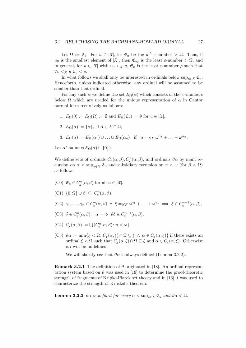
Let Ω := ℵ1. For u ∈ |X|, let Eu be the uth ε-number > Ω. Thus, ifu0 is the smallest element of |X|, then Eu0 is the least ε-number > Ω, andin general, for u ∈ |X| with u0 <X u, Eu is the least ε-number ρ such that∀v <X u Ev < ρ.
In what follows we shall only be interested in ordinals below supu∈X Eu.Henceforth, unless indicated otherwise, any ordinal will be assumed to besmaller than that ordinal.
For any such α we define the set EΩ(α) which consists of the ε–numbersbelow Ω which are needed for the unique representation of α in Cantornormal form recursively as follows:
1. EΩ(0) := EΩ(Ω) := ∅ and EΩ(Eu) := ∅ for u ∈ |X|.
2. EΩ(α) := α, if α ∈ E ∩ Ω,
3. EΩ(α) := EΩ(α1) ∪ . . . ∪ EΩ(αn) if α =NF ωα1 + . . .+ ωαn .
Let α∗ := max(EΩ(α) ∪ 0).
We define sets of ordinals CX(α, β), Cn
X(α, β), and ordinals ϑα by main re-
cursion on α < supu∈X Eu and subsidiary recursion on n < ω (for β < Ω)as follows.
(C0) Eu ∈ CnX (α, β) for all u ∈ |X|.
(C1) 0,Ω ∪ β ⊆ CnX
(α, β),
(C2) γ1, . . . , γn ∈ CnX (α, β) ∧ ξ =NF ωγ1 + . . .+ ωγn =⇒ ξ ∈ Cn+1
X(α, β),
(C3) δ ∈ CnX
(α, β) ∩ α =⇒ ϑδ ∈ Cn+1X
(α, β),
(C4) CX(α, β) :=
⋃Cn
X(α, β) : n < ω,
(C5) ϑα := minξ < Ω: CX(α, ξ)∩Ω ⊆ ξ ∧ α ∈ C
X(α, ξ) if there exists an
ordinal ξ < Ω such that CX(α, ξ)∩Ω ⊆ ξ and α ∈ C
X(α, ξ). Otherwise
ϑα will be undefined.
We will shortly see that ϑα is always defined (Lemma 3.2.2).
Remark 3.2.1 The definition of ϑ originated in [18]. An ordinal represen-tation system based on ϑ was used in [19] to determine the proof-theoreticstrength of fragments of Kripke-Platek set theory and in [16] it was used tocharacterize the strength of Kruskal’s theorem.
Lemma 3.2.2 ϑα is defined for every α < supu∈X Eu and ϑα < Ω.
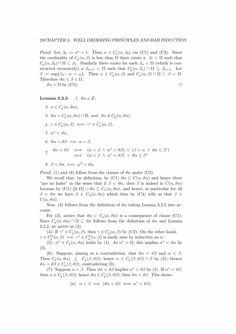
28CHAPTER 3. WELL ORDERING PRINCIPLES AND BAR INDUCTION
Proof: Let β0 := α∗ + 1. Then α ∈ CX(α, β0) via (C1) and (C2). Since
the cardinality of CX(α, β) is less than Ω there exists a β1 < Ω such that
CX(α, β0) ∩ Ω ⊂ β1. Similarly there exists for each βn < Ω (which is con-
structed recursively) a βn+1 < Ω such that CX(α, βn) ∩ Ω ⊆ βn+1. Let
β := supβn : n < ω. Then α ∈ CX(α, β) and C
X(α, β) ∩ Ω ⊂ β < Ω.
Therefore ϑα ≤ β < Ω.ϑα < Ω by (C5). 2
Lemma 3.2.3 1. ϑα ∈ E,
2. α ∈ CX(α, ϑα),
3. ϑα = CX(α, ϑα) ∩ Ω, and ϑα /∈ C
X(α, ϑα),
4. γ ∈ CX(α, β) ⇐⇒ γ∗ ∈ C
X(α, β),
5. α∗ < ϑα,
6. ϑα = ϑβ =⇒ α = β,
7.ϑα < ϑβ ⇐⇒ (α < β ∧ α∗ < ϑβ) ∨ (β < α ∧ ϑα ≤ β∗)
⇐⇒ (α < β ∧ α∗ < ϑβ) ∨ ϑα ≤ β∗
8. β < ϑα ⇐⇒ ωβ < ϑα.
Proof: (1) and (8) follow from the closure of ϑα under (C2).We recall that, by definition, by (C1) ϑα ⊆ C(α, ϑα) and hence there
“are no holes” in the sense that if β < ϑα, then β is indeed in C(α, ϑα)because by (C1) 0,Ω ∪ ϑα ⊆ Cn(α, ϑα), and hence, in particular for allβ ∈ ϑα we have β ∈ Cn(α, ϑα) which then by (C4) tells us that β ∈C(α, ϑα).
Now, (2) follows from the definition of ϑα taking Lemma 3.2.2 into ac-count.
For (3), notice that ϑα ⊂ CX(α, ϑα) is a consequence of clause (C1).
Since CX(α, ϑα) ∩ Ω ⊆ ϑα follows from the definition of ϑα and Lemma
3.2.2, we arrive at (3).(4): If γ∗ ∈ C
X(α, β), then γ ∈ C
X(α, β) by (C2). On the other hand,
γ ∈ CnX
(α, β) =⇒ γ∗ ∈ CnX
(α, β) is easily seen by induction on n.(5): α∗ ∈ C
X(α, ϑα) holds by (4). As α∗ < Ω, this implies α∗ < ϑα by
(3).(6): Suppose, aiming at a contradiction, that ϑα = ϑβ and α < β.
Then CX(α, ϑα) ⊆ C
X(β, ϑβ); hence α ∈ C
X(β, ϑβ) ∩ β by (2); thence
ϑα = ϑβ ∈ CX(β, ϑβ), contradicting (3).
(7): Suppose α < β. Then ϑα < ϑβ implies α∗ < ϑβ by (5). If α∗ < ϑβ,then α ∈ C
X(β, ϑβ); hence ϑα ∈ C
X(β, ϑβ); thus ϑα < ϑβ. This shows
(a) α < β =⇒ (ϑα < ϑβ ⇐⇒ α∗ < ϑβ).
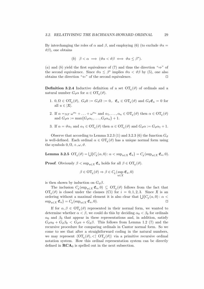
3.2. RELATIVISING THE BACHMANN-HOWARD ORDINAL 29
By interchanging the roles of α and β, and employing (6) (to exclude ϑα =ϑβ), one obtains
(b) β < α =⇒ (ϑα < ϑβ ⇐⇒ ϑα ≤ β∗).
(a) and (b) yield the first equivalence of (7) and thus the direction “⇒” ofthe second equivalence. Since ϑα ≤ β∗ implies ϑα < ϑβ by (5), one alsoobtains the direction “⇐” of the second equivalence. ut
Definition 3.2.4 Inductive definition of a set OTX(ϑ) of ordinals and a
natural number Gϑα for α ∈ OTX(ϑ).
1. 0,Ω ∈ OTX(ϑ), Gϑ0 := GϑΩ := 0,. Eu ∈ OT
X(ϑ) and GϑEu = 0 for
all u ∈ |X|.
2. If α =NF ωα1 + . . .+ ωαn and α1, . . . , αn ∈ OT
X(ϑ) then α ∈ OT
X(ϑ)
and Gϑα := maxGϑα1, . . . , Gϑαn+ 1.
3. If α = ϑα1 and α1 ∈ OTX(ϑ) then α ∈ OT
X(ϑ) and Gϑα := Gϑα1 + 1.
Observe that according to Lemma 3.2.3 (1) and 3.2.3 (6) the function Gϑis well-defined. Each ordinal α ∈ OT
X(ϑ) has a unique normal form using
the symbols 0,Ω,+, ω, ϑ.
Lemma 3.2.5 OTX(ϑ) =
⋃C
X(α, 0) : α < supu∈X Eu = C
X(supu∈X Eu, 0).
Proof. Obviously β < supu∈X Eu holds for all β ∈ OTX(ϑ).
β ∈ OTX(ϑ)⇒ β ∈ C
X(supu∈X
Eu, 0)
is then shown by induction on Gϑβ.
The inclusion CX(supu∈X Eu, 0) ⊆ OT
X(ϑ) follows from the fact that
OTX(ϑ) is closed under the clauses (Ci) for i = 0, 1, 2, 3. Since X is an
ordering without a maximal element it is also clear that⋃C
X(α, 0) : α <
supu∈X Eu = CX(supu∈X Eu, 0). ut
If for α, β ∈ OTX(ϑ) represented in their normal form, we wanted to
determine whether α < β, we could do this by deciding α0 < β0 for ordinalsα0 and β0 that appear in these representations and, in addition, satisfyGϑα0 + Gϑβ0 < Gϑα + Gϑβ. This follows from Lemma 1.2 (7) and therecursive procedure for comparing ordinals in Cantor normal form. So wecome to see that after a straightforward coding in the natural numbers,we may represent 〈OT
X(ϑ), < OT
X(ϑ)〉 via a primitive recursive ordinal
notation system. How this ordinal representation system can be directlydefined in RCA0 is spelled out in the next subsection.
30CHAPTER 3. WELL ORDERING PRINCIPLES AND BAR INDUCTION
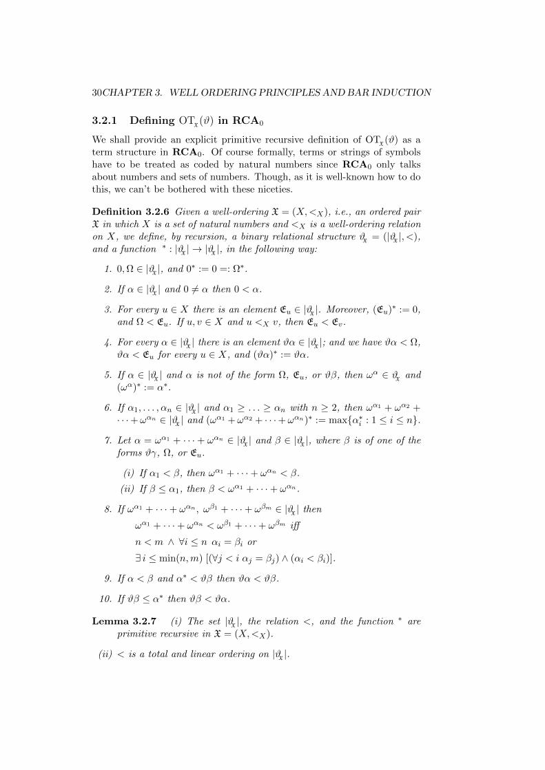
3.2.1 Defining OTX(ϑ) in RCA0
We shall provide an explicit primitive recursive definition of OTX(ϑ) as a
term structure in RCA0. Of course formally, terms or strings of symbolshave to be treated as coded by natural numbers since RCA0 only talksabout numbers and sets of numbers. Though, as it is well-known how to dothis, we can’t be bothered with these niceties.
Definition 3.2.6 Given a well-ordering X = (X,<X), i.e., an ordered pairX in which X is a set of natural numbers and <X is a well-ordering relationon X, we define, by recursion, a binary relational structure ϑ
X= (|ϑ
X|, <),
and a function ∗ : |ϑX| → |ϑ
X|, in the following way:
1. 0,Ω ∈ |ϑX|, and 0∗ := 0 =: Ω∗.
2. If α ∈ |ϑX| and 0 6= α then 0 < α.
3. For every u ∈ X there is an element Eu ∈ |ϑX |. Moreover, (Eu)∗ := 0,and Ω < Eu. If u, v ∈ X and u <X v, then Eu < Ev.
4. For every α ∈ |ϑX| there is an element ϑα ∈ |ϑ
X|; and we have ϑα < Ω,
ϑα < Eu for every u ∈ X, and (ϑα)∗ := ϑα.
5. If α ∈ |ϑX| and α is not of the form Ω, Eu, or ϑβ, then ωα ∈ ϑ
Xand
(ωα)∗ := α∗.
6. If α1, . . . , αn ∈ |ϑX | and α1 ≥ . . . ≥ αn with n ≥ 2, then ωα1 + ωα2 +· · ·+ωαn ∈ |ϑ
X| and (ωα1 +ωα2 + · · ·+ωαn)∗ := maxα∗i : 1 ≤ i ≤ n.
7. Let α = ωα1 + · · · + ωαn ∈ |ϑX| and β ∈ |ϑ
X|, where β is of one of the
forms ϑγ, Ω, or Eu.
(i) If α1 < β, then ωα1 + · · ·+ ωαn < β.
(ii) If β ≤ α1, then β < ωα1 + · · ·+ ωαn.
8. If ωα1 + · · ·+ ωαn , ωβ1 + · · ·+ ωβm ∈ |ϑX| then
ωα1 + · · ·+ ωαn < ωβ1 + · · ·+ ωβm iff
n < m ∧ ∀i ≤ n αi = βi or
∃ i ≤ min(n,m) [(∀j < i αj = βj) ∧ (αi < βi)].
9. If α < β and α∗ < ϑβ then ϑα < ϑβ.
10. If ϑβ ≤ α∗ then ϑβ < ϑα.
Lemma 3.2.7 (i) The set |ϑX|, the relation <, and the function ∗ are
primitive recursive in X = (X,<X).
(ii) < is a total and linear ordering on |ϑX|.
3.3. A WELL-ORDERING PROOF 31
Proof. It is straightforward to see that if we had an oracle for X, then,by the definitions of |ϑ
X|, < and ∗ we could computably decide the ordering
of the terms by their construction. To decode the term we just use thealgorithm basically given by the definition, and then we use the oracle forX to decide what relation the terms stand in, which will of course dependon the well-ordering X. ut
Of course, RCA0 does not prove that < is a well-ordering on |ϑX|.
3.3 A Well-ordering Proof
In this section we work in the background theory
RCA0 + [P(ω) 4Mω(BI)]
and shall prove the following statement
∀X (WO(X)→WO(ϑX)) ,
that is, the part (ii) ⇒ (i) of the main theorem (3.1.9). Some of the proofsare similar to proofs in section 10 of Rathjen and Weiermann’s paper [16].Please note that in this theory we can deduce arithmetical comprehensionand even arithmetical transfinite recursion owing to [6] and [21], respectively.
Let us fix a well-ordering X = (X,<X), an arbitrary set Y and a count-able coded ω-model A of BI which contains both X and Y as elements. Inthe sequel α, β, γ, δ, . . . are supposed to range over ϑX. < will be used to de-note the ordering on ϑX. We are going to work informally in our backgroundtheory. A set U ⊆ N is said to be definable in A if U = n ∈ N | A |= A(n)for some formula A(x) of second order arithmetic which may contain pa-rameters from A.
Definition 3.3.1 1. Acc := α < Ω | A |= WO(< α),
2. M := α : EΩ(α) ⊆ Acc,
3. α <Ω β :⇐⇒ α, β ∈ M ∧ α < β.
Lemma 3.3.2 α, β ∈ Acc =⇒ α+ ωβ ∈ Acc.
Proof. Familiar from Gentzen’s proof in Peano arithmetic. The proof justrequires ACA0. (cf. [23, VIII.§21 Lemma 1]). ut
Lemma 3.3.3 Acc = M ∩ Ω (:= α ∈ M | α < Ω.)
Proof. If α ∈ Acc, then EΩ(α) ⊆ Acc as well; hence α ∈ M∩Ω. If α ∈ M∩Ω,then EΩ(α) ⊆ M ∩ Ω, so α ∈ Acc follows from Lemma 3.3.2. ut
32CHAPTER 3. WELL ORDERING PRINCIPLES AND BAR INDUCTION
Lemma 3.3.4 Let U be A definable. Then
∀α < Ω ∩M [∀β < αβ ∈ U → α ∈ U ]→ Acc ⊆ U .
Proof.This follows readily from the assumption that A is a model of BI. ut
Definition 3.3.5 Let ProgΩ(X) stand for
(∀α ∈ M)[(∀β <Ω α)(β ∈ X) −→ α ∈ X].
Let AccΩ := α ∈ M: ϑα ∈ Acc.
Lemma 3.3.6 If U is A definable, then
ProgΩ(U)→ Ω,Ω + 1 ∈ U .
Proof. This follows from Lemma 3.3.3 and Lemma 3.3.4. ut
Lemma 3.3.7 ProgΩ(AccΩ).
Proof. Assume α ∈ M and (∀β <Ω α)(β ∈ AccΩ). We have to show thatϑα ∈ Acc. It suffices to show
β < ϑα =⇒ β ∈ Acc. (3.2)
We shall employ induction on Gϑ(β), i.e., the length of (the term that repre-sents) β. If β 6∈ E, then (3.2) follows easily by the inductive assumption andLemma 3.3.2. Now suppose β = ϑβ0. According to Lemma 3.2.3 it sufficesto consider the following two cases:Case 1: β ≤ α∗. Since α ∈ M, we have α∗ ∈ EΩ(α) ⊆ Acc; thereforeβ ∈ Acc.Case2: β0 < α and β∗0 < ϑα. As the length of β∗0 is less than the length of β,we get β∗0 ∈ Acc; thus EΩ(β0) ⊆ Acc, therefore β0 ∈ M. By the assumptionat the beginning of the proof, we then get β0 ∈ AccΩ; hence β = ϑβ0 ∈ Acc.
ut
Definition 3.3.8 For every A definable set U we define the “Gentzen jump”
U j := γ | ∀δ [M ∩ δ ⊆ U → M ∩ (δ + ωγ) ⊆ U ].
Lemma 3.3.9 Let U be A definable.
(i) γ ∈ U j ⇒ M ∩ ωγ ⊆ U .
(ii) ProgΩ(U)⇒ ProgΩ(U j).
3.3. A WELL-ORDERING PROOF 33
Proof. (i) is obvious. (ii) M ∩ (δ + ωγ) ⊆ U is to be proved under theassumptions (a) ProgΩ(U), (b) γ ∈ M ∧ M ∩ γ ⊆ U j and (c) M ∩ δ ⊆ U .So let η ∈ M ∩ (δ + ωγ).
1. η < δ: Then η ∈ U is a consequence of (c).
2. η = δ: Then η ∈ U follows from (c) and (a).
3. δ < η < δ + ωγ : Then there exist γ1, . . . , γk < γ such that η =δ+ωγ1 + . . .+ωγk and γ1 ≥ . . . ≥ γk. η ∈ M implies γ1, . . . , γk ∈ M∩γ.Through applying (b) and (c) we obtain M∩(δ+ωγ1) ⊆ U . By iteratingthis procedure we eventually arrive at δ+ωγ1 + . . .+ωγk ∈ U , so η ∈ Uholds.
ut
Corollary 3.3.10 Let I(δ) be the statement that ProgΩ(V ) → δ ∈ M ∧δ ∩M ⊆ V holds for all A definable sets V . Assume I(δ). Let δ0 := δ andδn+1 := ωδn. Then
I(δn)
holds for all n.
Proof. We use induction on n. For n = 0 this is the assumption. Nowsuppose I(δn) holds. Assume ProgΩ(U) for an A definable U . By Lemma3.3.9 we conclude ProgΩ(U j) and hence δn ∈ U j and δn ∩ M ⊆ U j . Asclearly M ∩ 0 ⊆ U we get ωδn ∩M ⊆ U . Since ProgΩ(U) entails δ ∈ M wealso have δn+1 ∈ M. Thus δn+1 ∈ M ∧ δn+1 ∩M ⊆ U , showing I(δn+1). ut
Let ω0(α) := α and ωn+1(α) := ωωn(α).
Proposition 3.3.11 I(Eu) holds for all u ∈ |X|.
Proof. Noting that in our background theory X is a well-ordering, we canuse induction on X. Note also that I(Eu) is a statement about all definablesets in A which is not formalizable in A itself. However, in our backgroundtheory quantification over all these sets is first order expressible and thereforetransfinite induction along <X is available.
First observe that we have I(Ω + 1) by Lemma 3.3.6. Let u0 be the<X -least element of |X|. We have Eu0 ∈ M and for every η < Eu0 thereexists n such that η < ωn(Ω + 1). As a result, using Corollary 3.3.10, wehave
ProgΩ(U)→ Eu0 ∩M ⊆ Ufor every A definable set U .
Now suppose that u ∈ |X| is not the <X -least element and for all v <X uwe have I(Ev). As for every δ < Eu there exists v <X u and n such thatδ < ωn(Ev), the inductive assumption together with Corollary 3.3.10 yields
ProgΩ(U)→ Eu ∩M ⊆ U .
34CHAPTER 3. WELL ORDERING PRINCIPLES AND BAR INDUCTION
Eu ∈ M is obvious. ut
Proposition 3.3.12 For all α < supu∈X Eu we have I(α).
Proof. We proceed by the induction on the term complexity of α. Clearly,I(0). By Lemma 3.3.6 we conclude that I(Ω). Proposition 3.3.11 entailsthat I(Eu) for all u ∈ |X|.
Now let α = ωα1 + · · · + ωαn be in Cantor normal form. Inductivelywe have I(α1), . . . , I(αn). Assume ProgΩ(U). Then ProgΩ(U j) by Lemma3.3.9(ii),and hence α1∩M ⊆ U j , . . . , αn∩M ⊆ U j and α1, . . . , αn ∈ M. Thelatter implies α1 ∈ U j , . . . , αn ∈ U j . Using the definition of U j repeatedlywe conclude α ∩M ⊆ U . Moreover, α ∈ M since α1, . . . , αn ∈ M.
Now suppose that α = ϑβ. Inductively we have I(β). By Lemma 3.3.7we conclude that β ∈ AccΩ, and hence α ∈ Acc. From ProgΩ(U) we obtainby Lemma 3.3.4 that ξ ∈ U for all ξ ≤ α. As a result, I(α). ut
Corollary 3.3.13 ϑX is a well-ordering.
With the previous Corollary, the proof of Theorem 3.1.9 (i)⇒(ii) is finallyaccomplished. Let us summarise the results of this section in the followingtheorem.
Theorem 3.3.14 (RCA0)
[RCA0 + [P(ω) 4Mω(BI)]] ` ∀X [WO(X)→WO(ϑX)].
3.4 Deduction chains
From now on we will be concerned with the part (ii)⇒ (i) of the main theo-rem 3.1.9. An important tool will be the method of deduction chains. Givena sequent Γ and a set Q ⊆ N, deduction chains starting at Γ are built bysystematically decomposing Γ into its subformulas, and adding additionallyat the nth step the formulas ¬An and ¬Q(n), where (An | n ∈ N) is anenumeration of the axioms of the theory BI, and Q(n) is the atom n ∈ U0
if n ∈ Q and n /∈ U0 otherwise. The set of all deduction chains that can bebuilt from the empty sequent with respect to a given set Q forms the treeDQ. There are two scenarios to be considered.
(i) If there is an infinite deduction chain, i.e. DQ is ill-founded, then thisreadily yields a model of BI that contains Q.
(ii) If each deduction chain is finite, then this yields a derivation of theempty sequent, ⊥, in a corresponding infinitary system with an ω-rule. The depth of this derivation is bounded by the order-type α of
3.4. DEDUCTION CHAINS 35
the Kleene-Brouwer ordering of DQ. By the well-ordering principle,transfinite induction up to Eα+1 is available, which allows to transformthis proof into a cut-free proof of ⊥ whose depth is less than ϑEα+1.
As the second alternative is impossible, the first yields the desired model.
Definition 3.4.1 1. We let U0, U1, . . . , Um, . . . be an enumeration of thefree set variables of L2 and, given a closed term t, we write tN for itsnumerical value.
2. Henceforth a sequent will be a finite set of L2-formulae without freenumber variables.
3. A sequent Γ is axiomatic if it satisfies at least one of the followingconditions:
(a) Γ contains a true literal, i.e., a true formula of either of the formsR(t1, . . . , tn) or ¬R(t1, . . . , tn), where R is a predicate symbolin L2 for a primitive recursive relation and t1, . . . , tn are closedterms.
(b) Γ contains the formulae s ∈ U and t /∈ U for some set variable Uand terms s, t with sN = tN.
4. A sequent is reducible if it is not axiomatic and contains a formulawhich is not a literal.
Definition 3.4.2 For Q ⊆ N we define
Q(n)
n ∈ U0 if n ∈ Q,n /∈ U0 otherwise
For some of the following theorems it is convenient to have a finite ax-iomatization of arithmetical comprehension.
Lemma 3.4.3 ACA0 can be axiomatized via a single Π12 sentence ∀XC(X).
Proof. [25, Lemma VIII.1.5]. ut
Definition 3.4.4 In what follows, we fix an enumeration of A1, A2, A3, . . .of all the universal closures of instances of (BI). We also put A0 := ∀X C(X),where the latter is the sentence axiomatises arithmetical comprehension.
Definition 3.4.5 Let Q ⊆ N. A Q-deduction chain is a finite string
Γ0, Γ1, . . . , Γk
of sequents Γi constructed according to the following rules:
36CHAPTER 3. WELL ORDERING PRINCIPLES AND BAR INDUCTION
1. Γ0 = ¬Q(0), ¬A0.
2. Γi is not axiomatic for i < k.
3. If i < k and Γi is not reducible then
Γi+1 = Γi, ¬Q(i+ 1), ¬Ai+1
4. Every reducible Γi with i < k is of the form
Γ′i, E, Γ′′i
where E is not a literal and Γ′i contains only literals. E is said to bethe redex of Γi.
Let i < k and Γi be reducible. Γi+1 is obtained from Γi = Γ′i, E, Γ′′ias follows:
(a) If E ≡ E0 ∨ E1 then
Γi+1 = Γ′i, E0, E1, Γ′′i , ¬Q(i+ 1), ¬Ai+1.
(b) If E ≡ E0 ∧ E1 then
Γi+1 = Γ′i, Ej , Γ′′i , ¬Q(i+ 1), ¬Ai+1
where j = 0 or j = 1.
(c) If E ≡ ∃xF (x) then
Γi+1 = Γ′i, F (m), Γ′′i , ¬Q(i+ 1), ¬Ai+1, E
where m is the first number such that F (m) does not occur inΓ0, . . . , Γi.
(d) If E ≡ ∀xF (x) then
Γi+1 = Γ′i, F (m), Γ′′i , ¬Q(i+ 1), ¬Ai+1
for some m.
(e) If E ≡ ∃XF (X) then
Γi+1 = Γ′i, F (Um), Γ′′i , ¬Q(i+ 1), ¬Ai+1, E
where m is the first number such that F (Um) does not occur inΓ0, . . . , Γi.
(f) If E ≡ ∀XF (X) then
Γi+1 = Γ′i, F (Um), Γ′′i , ¬Q(i+ 1), ¬Ai+1
where m is the first number such that Um does not occur in Γi.
3.4. DEDUCTION CHAINS 37
The set of Q-deduction chains forms a tree DQ labeled with strings of se-quents.
We will now consider two cases.
Case I: DQ is not well-founded. Then DQ contains an infinite path ς . Nowdefine a set M via
(M)i = k | k /∈ Ui occurs in ς.
Set M = (N; (M)i | i ∈ N,∈,+, ·, 0, 1, <).
For a formula F , let F ∈ ς mean that F occurs in ς , i.e. F ∈ Γ for someΓ ∈ ς .
Claim: Under the assignment Ui 7→ (M)i we have
F ∈ ς ⇒ M |= ¬F. (3.3)
The Claim will imply that M is an ω-model of BI. Also note that (M)0 = Q,thus Q is in M. The proof of (3.3) follows by induction on F using Lemma3.4.6 below. The upshot of the foregoing is that we can prove Theorem 3.1.9under the assumption that DQ is ill-founded for all sets Q ⊆ N.
Lemma 3.4.6 Let Q be an arbitrary subset of N and DQ be the correspond-ing deduction tree. Moreover, suppose DQ is not well-founded. Then DQhas an infinite path ς . ς has the following properties:
1. ς does not contain literals which are true in N.
2. ς does not contain formulas s ∈ Ui and t /∈ Ui for constant terms sand t such that sN = tN.
3. If ς contains E0 ∨ E1 then ς contains E0 and E1.
4. If ς contains E0 ∧ E1 then ς contains E0 or E1.
5. If ς contains ∃xF (x) then ς contains F (n) for all n.
6. If ς contains ∀xF (x) then ς contains F (n) for some n.
7. If ς contains ∃XF (X) then ς contains F (Um) for all m.
8. If ς contains ∀XF (X) then ς contains F (Um) for some m.
9. ς contains ¬C(Um) for all m.
10. ς contains ¬Q(m) for all m.
Proof.
38CHAPTER 3. WELL ORDERING PRINCIPLES AND BAR INDUCTION
1. Suppose that ς contained a sequent Γk such that Γk contained a trueliteral. Then Γk would be axiomatic by definition. Rule 2 in theconstruction scheme for deduction chains would imply that there couldbe no sequent after the axiomatic sequent Γk in any deduction chain(which had Γk). Therefore, Γk would have to be the end of the path ς .This cannot happen if ς is infinite. Hence no true literal can belongto a sequent in ς .
2. Let s and t be closed terms such that sN = tN. Suppose that ςcontained a sequent Γi to which the formula s ∈ Un belonged and,furthermore, that ς contained a sequent Γj to which the formula t /∈Un belonged. By inspection of the construction rules for deductionchains we note that any formula of the form x ∈ U (or x /∈ U) whichbelongs to a sequent Γk of a deduction chain necessarily belongs toevery sequent Γm in the chain with m ≥ k. This would imply thatthe sequent Γmax(i,j) contained s ∈ Un and t /∈ Un. Therefore, bydefinition, Γmax(i,j) would be an axiomatic sequent. By Rule 2 of thededuction chains construction scheme, Γmax(i,j) would have to be theend of the path ς . This, however, contradicts the assumption that ςis infinite.
3. Suppose ς contains a sequent Γl+1 such that the formula E ≡ E0∨E1
belongs to Γl+1. Then Γl+1 cannot be an axiomatic sequent becausethis would contradict the hypothesis that ς be an infinite path (as wehave seen in the previous points). Thus, by definition, this sequentmust be reducible given that it is not axiomatic and that it containsthe formula E0 ∨ E1 (which is not a literal). Upon inspection of theconstruction rules for deduction chains we come to the realisation thatif a formula, which isn’t a literal, belongs to a sequent in the path, thenat some point this formula “will be replaced” by one (or two) of lessercomplexity. Since each sequent in the path is finite we know thatfor some number i the formula E will be the first non-literal formula(from left to right) in Γi. Therefore, by the first part of the fourthconstruction rule for deduction chains, Γi+1 = Γ′i, E0, E1, Γ′′i , ¬Q(i+1), ¬Ai+1. So E0 and E1 do indeed belong to a sequent of the infinitepath ς .
4. Suppose ς contains a sequent Γl+1 such that the formula E ≡ E0∧E1
belongs to Γl+1. Then, since Γl+1 cannot be axiomatic, and since itcontains the formula E which is not a literal, it is, by definition, areducible sequent. Because of the rules of construction for deductionchains, we know that at some point i ≥ l + 1 the formula E will bethe first non-literal of the sequent Γi. This means, by rule 4 part (b)of the construction rules, that the next sequent in ς will be Γi+1 =Γ′i, Ej , Γ′′i , ¬Q(i + 1), ¬Ai+1 where j = 0 or j = 1. Therefore ς
3.4. DEDUCTION CHAINS 39
contains either E0 or E1.
5. Suppose ς contains a sequent Γk which contains an occurrence of theformula ∃xF (x). Then, as has already been observed, this occur-rence of the formula ∃xF (x) will “be parsed” at some Γn with n > k.Suppose then, that ∃xF (x) is the first non-literal formula in Γn. Bythe third part of the fourth construction rule for deduction chains,Γn+1 = Γ′n, F (m), Γ′′n, ¬Q(n+ 1),¬An+1, ∃xF (x) where m is the firstnumber such that F (m) does not occur in Γ0, . . . , Γn. As we can see,the fact that for every l > n, Γl contains the formula ∃xF (x) insuresthat F (r) belongs to some sequent in ς for every natural number r.
6. Suppose ς contains a sequent Γk such that the formula ∀xF (x) belongsto Γk. Then, since every non-literal formula is replaced by one (or two)of lesser complexity at some point in the path ς , we know that theformula ∀xF (x) will be the first non-literal formula of the sequent Γnfor some n ≥ k. Suppose then, that ∀xF (x) is the first non-literalformula in Γn. By the fourth part of the fourth construction rule fordeduction chains, Γn+1 = Γ′n, F (m), Γ′′n, ¬Q(n + 1),¬An+1 for somem, in particular, for this m, we have that F (m) appears in the pathς , as we wanted to show.
7. Suppose ς contains a sequent Γk such that the formula ∀XF (X) be-longs to Γk. Then, since every non-literal formula is replaced by one(or two) of lesser complexity at some point in the path ς , we knowthat the formula ∀XF (X) will be the first non-literal formula of thesequent Γn for some n ≥ k. Suppose then, that ∀XF (X) is the firstnon-literal formula in Γn. By the sixth part of the fourth constructionrule for deduction chains, Γn+1 = Γ′n, F (Um), Γ′′n, ¬Q(n + 1),¬An+1,where m is the first number such that m 6= n+ 1 and Um does not oc-cur in Γn. Therefore F (Um) does occur in the path ς for some naturalnumber m.
8. Suppose ς contains a sequent Γk which contains an occurrence of theformula ∃XF (X). Then, this occurrence of the formula ∃XF (X) willbe the first non-literal formula of the sequent Γn for some n ≥ k.Suppose then, that ∃XF (X) is the first non-literal formula in Γn.By the fifth part of the fourth construction rule for deduction chains,Γn+1 = Γ′n, F (Um), Γ′′n, ¬Q(n + 1),¬An+1, ∃XF (X) where m is thefirst number such that F (Um) does not occur in Γ0, . . . , Γn. We cansee that for every l > n, Γl contains the formula ∃XF (X) by theconstruction rules. This insures that F (Ur) will belong to some sequentin ς whatever natural number r is.
9. By direct inspection of the construction rules we can see that ¬Ambelongs to the sequent Γm. Since the path ς is infinite, for every
40CHAPTER 3. WELL ORDERING PRINCIPLES AND BAR INDUCTION
natural number m there is a Γm in ς . Therefore ¬Am is in ς for everynatural number m.
10. By direct inspection of the construction rules we can see that ¬Q(m)belongs to the sequent Γm. Since the path ς is infinite, for everynatural number m there is a Γm in ς . Therefore ¬Q(m) is in ς forevery natural number m.
ut
Corollary 3.4.7 If DQ is ill-founded then there exists a countable codedω-model of BI which contains Q.
For our purposes it is important that Corollary 3.4.7 can be proved inT0 := RCA0 + ∀X (WO(X)→WO(ϑX)). To this end we need to show thatthe semantics of ω-models can be handled in the latter theory, i.e. for everyformula F of L2 there exists a valuation for F in the sense of [25, VII.2.1].It is easily seen that the principle ∀X (WO(X)→WO(ϑX)) implies
∀X (WO(X)→WO(εX))
(see [1, Definition 2.1]) and thus, by [1, Theorem 4.1], T0 proves that everyset is contained in an ω-model of ACA. Now take an ω-model containingDQ and an infinite branch of DQ. In this ω-model we find a valuation forevery formula by [25, VII.2.2]. And hence Corollary 3.4.7 holds in the model,but then it also holds in the world at large by absoluteness.
3.5 Proof of the Main Theorem: The hard direc-tion part 2
The remainder of the chapter will be devoted to ruling out the possibilitythat for some Q, DQ could be a well-founded tree. This is the place wherethe principle ∀X (WO(X)→WO(ϑX)) in the guise of cut elimination for aninfinitary proof system enters the stage. Aiming at a contradiction, supposethat DQ is a well-founded tree. Let X be the Kleene-Brouwer ordering onDQ (see [25, Definition V.1.2]). Then X is a well-ordering. In a nutshell,the idea is that a well-founded DQ gives rise to a derivation of the emptysequent (contradiction) in an infinitary proof system.
3.5.1 Majorization and Fundamental Functions
In this section we introduce the concepts of majorization and fundamen-tal function. They are needed for carrying through the ordinal analysis ofbar induction. More details can be found in [16] section 4 and [3, I.4] towhich we refer for proofs. The missing proofs are actually straightforwardconsequences of Definition 3.2.6.
3.5. PROOF OF THE MAIN THEOREM: THE HARD DIRECTION PART 241
Definition 3.5.1 1. α β means α < β and ϑα < ϑβ.
2. α β :⇐⇒ (α β ∨ α = β).
Lemma 3.5.2 1. α β ∧ β γ =⇒ α γ.
2. 0 < β < ε0 =⇒ α α+ β.
3. α < β < Ω =⇒ α β.
4. α β =⇒ α+ 1 β.
5. α β =⇒ ϑα ϑβ.
6. α = α0 + 1 =⇒ ϑα0 ϑα.
Proof.
1. This follows straightforwardly from the definition: If α β and β γthen, by definition, α < β and ϑα < ϑβ as well as for β and γ, thatis, β < γ and ϑβ < ϑγ. Combining the first and third inequalities weget α < γ, and combining the second and the fourth we get ϑα < ϑγ,and this two are the definition of α γ as we wanted to show.
2. Certainly if 0 < β then α < α+β. Now, by lemma 2.2.3 we have thatif α∗ < ϑ(α + β) then ϑα < ϑ(α + β). Also by lemma 2.2.3 we havethat (α+β)∗ < ϑ(α+β), and, since β < ε0 we have that (α+β)∗ = α∗
and we are done.
3. Since both α and β are less than Ω we have that α∗ < α and β∗ < β.Hence, α∗ < β, and from β < Ω it also follows that β < ϑβ bydefinition of ϑ, therefore ϑα < ϑβ by lemma 2.2.3.
4. Again, since (α + 1)∗ = α∗ < ϑα ≤ β∗ < ϑβ which by lemma 2.2.3gives us that α+ 1 β .
5. If α β, then, by definition, α < β and ϑα < ϑβ. Since the range ofϑ is contained in Ω and since in Ω this function is increasing, we havethat from ϑα < ϑβ (which we have) we obtain (by monotonicity in Ω)ϑϑα < ϑϑβ. These two inequalities show that ϑα ϑβ.
6. From lemma 2.2.3 we have that α∗ < ϑα. Using again that α∗0 =(α0 + 1)∗ we get that (α0)∗ < ϑα and since obviously α0 < α we havethat ϑα0 < ϑα.
Lemma 3.5.3 α β, β < ωγ+1 =⇒ ωγ + α ωγ + β.
Corollary 3.5.4 ωα · n ωα · (n+ 1).
42CHAPTER 3. WELL ORDERING PRINCIPLES AND BAR INDUCTION
Lemma 3.5.5 α β =⇒ ωα · n ωβ.
Definition 3.5.6 Let DΩ := (OTX(ϑ) ∩ Ω) ∪ Ω. A function f : DΩ →
OTX(ϑ) will be called a fundamental function if it is generated by the fol-
lowing clauses:
F1. Id : DΩ → DΩ with Id(α) = α is a fundamental function.
F2. If f is a fundamental function, γ ∈ OTX(ϑ) and f(Ω) < ωγ+1, then
ωγ + f is a fundamental function, where (ωγ + f)(α) := ωγ + f(α) forall α ∈ DΩ.
F3. If f is a fundamental function then so is ωf with (ωf )(α) := ωf(α) forall α ∈ DΩ.
Lemma 3.5.7 Let f be a fundamental function and β ≤ Ω.
(i) If α < β, then f(α) < f(β).
(ii) If α β, then f(α) f(β).
(iii) (f(β))∗ ≤ max((f(0))∗, β∗).
Proof.(i) is obvious by induction on the generation of fundamental func-tions.
(ii) also follows by induction on the generation of fundamental functions,using Lemmata 3.5.3 and 3.5.5.
(iii) as well follows by induction on the generation of fundamental func-tions. ut
Lemma 3.5.8 For every fundamental function f we have f(ϑ(f(0)))
f(Ω).
Proof.Since ϑ(f(0)) < Ω, we clearly have f(ϑ(f(0))) < f(Ω). Since0Ω and f is a fundamental function, we have ϑ(f(0)) < ϑ(f(Ω)) by lemma3.5.7 (ii). Invoking Lemma 3.5.7 (iii), the latter entails that (f(ϑ(f(0))))∗ <ϑ(f(Ω)), so that in conjunction with f(ϑ(f(0))) < f(Ω) it follows thatϑ(f(ϑ(f(0)))) ϑ(f(Ω)). As a result, f(ϑ(f(0))) f(Ω). ut
3.5.2 The infinitary calculus T ∗Q
The calculus T ∗Q
to be introduced stems from [16] section 6. We fix a set
Q ⊆ N. Let LQ2 be the language of second order arithmetic augmented by a
unary predicate Q. The formulas of T ∗Q
arise from LQ2 -formulas by replacing
free numerical variables by numerals, i. e. terms of the form 0, 0′, 0′′, ...Especially, every formula A of T ∗
Qis an LQ2 -formula. We are going to measure
the length of derivations by ordinals. We are going to use the set of ordinalsOT
X(ϑ) of Section 3.
3.5. PROOF OF THE MAIN THEOREM: THE HARD DIRECTION PART 243
Definition 3.5.9 1. A formula B is said to be weak if it belongs toΠ1
0 ∪Π11.
2. Two closed terms s and t are said to be equivalent if they yield thesame value when computed.
3. A formula is called constant if it contains no set variables. The truthor falsity of such a formula is understood with respect to the standardstructure of the integers.
4. 0 := 0, m+ 1 := m′.
In the sequent calculus T ∗Q
below we shall use the following rules of inference:
(∧) ` Γ, A and ` Γ, B =⇒ ` Γ, A ∧B,
(∨) ` Γ, Ai =⇒ ` Γ, A0 ∨A1 if i ∈ 0, 1,
(∀2) ` Γ, F (U) =⇒ ` Γ, ∀XF (X),
(∃1) ` Γ, F (t) =⇒ ` Γ,∃xF (x),
(Cut) ` Γ, A and ` Γ,¬ A =⇒ ` Γ,
where in (∀2) the free variable U is not to occur in the conclusion.
The most important feature of sequent calculi is cut–elimination. To statethis fact concisely, let us introduce a measure of complexity, gr(A), the gradeof a formula A, for LQ2 -formulae.
Definition 3.5.10 1. gr(A) = 0 if A is a prime formula or negated primeformula.
2. gr(∀XF (X)) = gr(∃XF (X)) = ω if F (U) is arithmetic.
3. gr(A ∧B) = gr(A ∨B) = maxgr(A), gr(B)+ 1.
4. gr(∀xH(x)) = gr(∃xH(x)) = gr(H(0)) + 1.
5. gr(∀XG(X)) = gr(∃XG(X)) = gr(G(U)) + 1,if G is not arithmetic.
Definition 3.5.11 Inductive definition of T ∗Q
α
% Γ for α ∈ OTX(ϑ) and
% < ω + ω.
1. If A is a true constant prime formula or negated prime formula andA ∈ Γ, then T ∗
Q
α
% Γ.
44CHAPTER 3. WELL ORDERING PRINCIPLES AND BAR INDUCTION
2. If n ∈ Q and t is a closed term with value n and Q(t) is in Γ, thenT ∗Q
α
% Γ.
3. If n /∈ Q and t is a closed term with value n and ¬Q(t) is in Γ, thenT ∗Q
α
% Γ.
4. If Γ contains formulas A(s1, . . . , sn) and ¬A(t1, . . . , tn) of grade 0 orω, where si and ti (1 ≤ i ≤ n) are equivalent terms, then T ∗
Q
α
% Γ.
5. If T ∗Q
β
% Γi and βα hold for every premiss Γi of an inference (∧), (∨),(∃1), (∀2) or (Cut) with a cut formula having grade < %, and conclu-sion Γ, then T ∗
Q
α
% Γ.
6. If T ∗Q
α0
% Γ, F (U) holds for some α0 α and a non-arithmetic formula
F (U) (i. e., gr(F (U)) ≥ ω), then T ∗Q
α
% Γ, ∃XF (X) .
7. (ω-rule). If T ∗Q
βm% Γ, A(m) is true for every m < ω, ∀xA(x) ∈ Γ, and
βm α, then T ∗Q
α
% Γ .
8. (Ω-rule). Let f be a fundamental function satisfying
(a) f(Ω) α,
(b) T ∗Q
f(0)
% Γ, ∀XF (X) , where ∀XF (X) ∈ Π11, and
(c) T ∗Q
β
0Ξ,∀XF (X) implies T ∗
Q
f(β)
% Ξ,Γ for every set of weak for-mulas Ξ and β < Ω.
Then T ∗Q
α
% Γ holds.
Remark 3.5.12 The derivability relation T ∗Q
α
% Γ is from [16] and is mod-
elled upon the relation PB∗α
n F of [3], the main difference being the sequentcalculus setting instead of P– and N–forms and a different assignment ofcut–degrees. The allowance for transfinite cut–degrees will enable us to dealwith arithmetical comprehension.
Remark 3.5.13 If one ruminates on the definition of the derivability pred-icate T ∗
Q
α
% Ξ the question arises whether it is actually a proper inductivedefinition. The critical point is obviously the condition (c) of the Ω-rule.
Note that T ∗Q
β
0Ξ,∀XF (X) occurs negatively in clause (c). However, since
β < Ω, the pertaining derivation does not contain any applications of the
3.5. PROOF OF THE MAIN THEOREM: THE HARD DIRECTION PART 245
Ω-rule. Thus the definition of T ∗Q
α
% Ξ proceeds via an iterated inductivedefinition. First one defines a derivability predicate without involvement ofthe Ω-rule via an ordinary inductive definition, and in a second step definesT ∗Q
α
% Γ inductively referring to the first derivability predicate in the Ω-rule.
It will actually be a non trivial issue how to handle such inductive defi-nitions in a weak background theory.
Lemma 3.5.14 1. T ∗Q
α
δΓ & Γ ⊆ ∆ & α β & δ ≤ % =⇒ T ∗
Q
β
% ∆ ,
2. T ∗Q
α
% Γ, A ∧B =⇒ T ∗Q
α
% Γ, A & T ∗Q
α
% Γ, B,
3. T ∗Q
α
% Γ, A ∨B =⇒ T ∗Q
α
% Γ, A,B
4. T ∗Q
α
% Γ, F (t) =⇒ T ∗Q
α
% Γ, F (s) if t and s are equivalent,
5. T ∗Q
α
% Γ,∀xF (x) =⇒ T ∗Q
α
% Γ, F (s) for every term s.
6. If T ∗Q
α
% Γ, ∀XG(X) and gr(G(U)) ≥ ω, then T ∗Q
α
% Γ, G(U) .
Proof. Proceed by induction on α. These can be carried out straightfor-wardly. (5) requires (4). As to (6), observe that ∀XG(X) cannot be themain formula of an axiom. 2
Lemma 3.5.15 T ∗Q
2·α0
Γ, A(s1, . . . , sk),¬A(t1, . . . , tk) if α ≥ gr(A(s1, . . . , sk))and si and ti are equivalent terms.
Proof. Proceed by induction on gr(A(s1, . . . , sk)). Crucially note thatif gr(A(s1, . . . , sk)) = ω then Γ, A(s1, . . . , sk),¬A(t1, . . . , tk) is an axiomaccording to Definition 3.5.11 clause (4). ut
Lemma 3.5.16 1. T ∗Q
2m
0¬(0 ∈ U), (∃x)[x ∈ U ∧ ¬(x′ ∈ U)],m ∈ U ,
2. T ∗Q
ω+5
0∀X[0 ∈ X ∧ ∀x(x ∈ X → x′ ∈ X)→ ∀x(x ∈ X)].
Proof. For (1) use induction on m. (2) is an immediate consequence of (1)using Lemma 3.5.14 (1), the ω-rule, (∨), and (∀2).
Definition 3.5.17 For formulas F (U) and A(a), F (A) denotes the resultof replacing each occurrence of the form e ∈ U in F (U) by A(e). Theexpression F (A) is a formula if the bound variables in A(a) are chosen in anappropriate way, in particular, if F (U) and A(a) have no bound variablesin common.
46CHAPTER 3. WELL ORDERING PRINCIPLES AND BAR INDUCTION
Lemma 3.5.18 Suppose α < Ω and let ∆(U) = F1(U), . . . , Fk(U) be aset of weak formulas such that U doesn’t occur in ∀XFi(X) (1 ≤ i ≤ k). Foran arbitrary formula A(a) we then have:
T ∗Q
α
0∆(U) =⇒ T ∗
Q
Ω+α
0∆(A) .
Proof. Proceed by induction on α. Suppose ∆(U) is an axiom. Then
either ∆(A) is an axiom too, or T ∗Q
ω+ω
0∆(A) can be obtained through
use of Lemma 3.5.15. Therefore T ∗Q
Ω+α
0∆(A) by Lemma 3.5.14 (1). If
T ∗Q
α
0∆(U) is the result of an inference, then this inference must be different
from (∃2), (Cut), and the (Ω− rule) since ∆(U) consists of weak formulas,the derivation is cut-free and α < Ω. For the remaining possible inferencerules the assertion follows easily from the induction hypothesis. ut
Lemma 3.5.19 Let Γ, ∀XF (X) be a set of weak formulas. If T ∗Q
α
0Γ, ∀XF (X)
and α < Ω, then T ∗Q
α
0Γ, F (U) .
Proof. Use induction on α. Note that ∀XF (X) cannot be a principalformula of an axiom, since ∃X¬F (X) does not surface in such a derivation.Also, due to α < Ω, the derivation doesn’t involve instances of the Ω-rule.Therefore the proof is straightforward. 2
The role of the Ω-rule in our calculus T ∗Q
is enshrined in the next lemma.
Lemma 3.5.20 T ∗Q
Ω·20∃XF (X),¬F (A) for every arithmetic formula F (U)
and arbitrary formula A(a).
Proof. Let f(α) := Ω + α with dom(f) := α ∈ OT (ψ) : α ≤ Ω. Then
T ∗Q
f(0)
0∀X¬F (X), ∃XF (X),¬F (A) (3.1)
according to Lemma 3.5.15. For α < Ω and every set of weak formulas Θ,we have by Lemmata 3.5.18 and 3.5.19,
T ∗Q
α
0Θ,∀X¬F (X) =⇒ T ∗
Q
f(α)
0Θ,¬F (A).
Therefore, by Lemma 3.5.14 (1),
T ∗Q
α
0Θ,∀X¬F (X) =⇒ T ∗
Q
f(α)
0Θ, ∃XF (X),¬F (A). (3.2)
The assertion now follows from (3.1) and (3.2) by the Ω-rule. 2
Corollary 3.5.21 T ∗Q
Ω·2+1ω ∃X ∀y (y ∈ X ↔ B(y)) for every arithmetic for-
mula B(a).
3.5. PROOF OF THE MAIN THEOREM: THE HARD DIRECTION PART 247
Proof. Owing to Lemma 3.5.20 we have
T ∗Q
Ω·20∃X ∀y (y ∈ X ↔ B(y)), ¬∀y (B(y)↔ B(y)) . (3.3)
As Lemma 3.5.15 yields T ∗Q
k
0∀y (B(y)↔ B(y)) for some k < ω, cutting
with (3.3) yields T ∗Q
Ω·2+1ω ∃X ∀y (y ∈ X ↔ B(x)) . ut
Corollary 3.5.22 For every arithmetic relation ≺ (parameters allowed)
and arbitrary formula A(a) we have T ∗Q
Ω·2+ω
0∀ ~X ∀~x(WF(≺)→ TI(≺, A))
where the quantifiers ∀ ~X ∀~x bind all free variables in WF(≺)→ TI(≺, A).
Proof. By Lemma 3.5.20 we have T ∗Q
Ω·20¬(WF(≺))′, (TI(≺, A))′ where ′
denotes any assignment of free numerical variables to numerals. Hence
T ∗Q
Ω·2+2
0(WF(≺)→ TI(≺, A))′
by two applications of (∨). Applying the ω-rule the right number of timesfollowed by the right number of (∀2) inferences, one arrives at the desiredconclusion. ut
3.5.3 The reduction procedure for T ∗Q
Below we follow [16] section 7.
Lemma 3.5.23 Let C be a formula of grade %. Suppose C is a prime for-mula or of either form ∃XH(X), ∃xG(x) or A∨B. Let α = ωα1 + · · ·+ωαk
with δ ≤ ωαk ≤ . . . ≤ ωα1 . Then we have T ∗Q
α
% ∆,¬C & T ∗Q
δ
% Γ, C =⇒T ∗Q
α+δ% ∆,Γ .
Proof. We proceed by induction on δ.1. Let Γ, C be an axiom. Then there are three cases to consider.
1.1. Γ is an axiom. Then so is ∆,Γ. Hence T ∗Q
α+δ% ∆,Γ .
1.2. C is a true constant prime formula or negated prime formula. A
straightforward induction on α then yields T ∗Q
α
% ∆ , and thus T ∗Q
α+δ% ∆,Γ
by 3.5.14 (1).1.3. C ≡ A(s1, . . . , sn) and Γ contains a formula ¬A(t1, . . . , tn) where si andti are equivalent terms. From T ∗
Q
α
% ∆,¬A(s1, . . . , sn) one receives
T ∗Q
α
% ∆,¬A(t1, . . . , tn) by use of Lemma 3.5.14 (4). Thence T ∗Q
α+δ% ∆,Γ
follows by use of Lemma 3.5.14 (1), since ¬A(t1, . . . , tn) ∈ Γ.
2. Suppose C ≡ A ∨ B and T ∗Q
δ0% Γ, C,A0 with A0 ∈ A,B and δ0 δ.
Inductively we get
T ∗Q
α+δ0% ∆,Γ, A0 . (3.1)
48CHAPTER 3. WELL ORDERING PRINCIPLES AND BAR INDUCTION
Next use Lemma 3.5.14 (2) on T ∗Q
α
% ∆,¬A ∧ ¬B to obtain
T ∗Q
α+δ0% ∆,Γ,¬A0 . (3.2)
Whence use a cut on (3.1) and (3.2) to get the assertion.
3. Suppose C ≡ ∃xG(x) and T ∗Q
δ0% Γ, C,G(t) with δ0 δ. Inductively we
get
T ∗Q
α+δ0% ∆,Γ, G(t) . (3.3)
By Lemma 3.5.14 1), (5), we also get
T ∗Q
α+δ0% ∆,Γ,¬G(t) ; (3.4)
thus (3.3) and (3.4) yield T ∗Q
α+δ% ∆,Γ by (Cut).
4. Suppose the last inference was (∃2) with p. f. C. Then C ≡ ∃XH(X)
and T ∗Q
δ0% Γ, C,H(U) for some δ0 δ and gr(H(U)) ≥ ω. Inductively we
get
T ∗Q
α+δ0% ∆,Γ, H(U). (3.5)
By Lemma 3.5.14 (1), (6) we also get
T ∗Q
α+δ0% ∆,Γ,¬H(U). (3.6)
From (3.5) and (3.6) we obtain
T ∗Q
α+δ% ∆,Γ.
5. Let T ∗Q
δ
% Γ, C be derived by the Ω-rule with fundamental function f .Then the assertion follows from the I. H. by the Ω-rule using the fundamentalfunction α+ f .6. In the remaining cases the assertion follows from the I. H. used on thepremises and by reapplying the same inference. 2
Lemma 3.5.24 T ∗Q
α
η+1Γ =⇒ T ∗
Q
ωα
η Γ.
Proof. We proceed by induction on α. We only treat the crucial case whenT ∗Q
α0
η+1Γ, D and T ∗
Q
α0
η+1Γ,¬D , where α0 α, and gr(D) = η. Inductively
this becomes T ∗Q
ωα0
η Γ, D and T ∗Q
ωα0
η Γ,¬D. Since D or ¬D must be one
of the forms exhibited in Lemma 3.5.23, we obtain T ∗Q
ωα0+ωα0
η Γ by Lemma3.5.23. As ωα0 +ωα0 ωα, we can use Lemma 3.5.14 1.) to get the assertion.
Theorem 3.5.25 (Collapsing Theorem) Let Γ be a set of weak formu-las. We have
T ∗Q
α
ω Γ =⇒ T ∗Q
ϑα
0Γ.
3.5. PROOF OF THE MAIN THEOREM: THE HARD DIRECTION PART 249
Proof. We proceed by induction on α. Observe that for β < δ < Ω, wealways have β δ.1. If Γ is an axiom, then the assertion is trivial.2. Let T ∗
Q
α
ω Γ be the result of an inference other than (Cut) and Ω-rule.
Then we have T ∗Q
α0
ω Γi with α0 α and Γi being the i-th premiss of that
inference. α0α implies ϑα0ϑα. Therefore T ∗Q
ϑα0
0Γ0 by the I. H., hence
T ∗Q
ϑα
0Γ by reapplying the same inference.
3. Suppose T ∗Q
α
ω Γ results by the Ω-rule with respect to a Π11-formula
∀XF (X) and a fundamental function f . Then f(Ω) α and
T ∗Q
f(0)
ω Γ, ∀XF (X), (3.1)
and, for every set of weak formulas Ξ and β < Ω,
T ∗Q
β
0Ξ,∀XF (X) =⇒ T ∗
Q
f(β)
ω Ξ,Γ. (3.2)
The I. H. used on (3.1) supplies us with T ∗Q
ϑ(f(0))
0Γ,∀XF (X) . Hence with
Ξ = Γ we get
T ∗Q
f(ϑ(f(0)))
ω Γ (3.3)
from (3.2). Now Lemma 3.5.8 ensures that f(β)f(Ω), where β = ϑ(f(0)).
So using the I. H. on (3.3), we obtain
T ∗Q
ϑ(f(β))
0Γ , (3.4)
thus T ∗Q
ϑα
0Γ as f(β) α.
4. Suppose T ∗Q
α0
ω Γ, A and T ∗Q
α0
ω Γ,¬A , where α0 α and gr(A) < ω.
Inductively we then get T ∗Q
ϑα0
0Γ, A and T ∗
Q
ϑα0
0Γ,¬A. Let gr(A) = n− 1.
Then (Cut) yields
T ∗Q
β1
n Γ (3.5)
with β1 = (ϑα0) + 1. Applying Lemmma 3.5.24, we get T ∗Q
ωβ1
n−1Γ , and by
repeating this process we arrive at
T ∗Q
βn
0Γ ,
where βk+1 := ωβk (1 ≤ k < n). Since ϑα0 < ϑα, we have βn < ϑα; thus
T ∗Q
ϑα
0Γ. ut
50CHAPTER 3. WELL ORDERING PRINCIPLES AND BAR INDUCTION
3.5.4 Embedding DQ into T ∗Q
.
Assuming that DQ is well-founded tree, the objective of this section is toembed DQ into T ∗
Q, so as to obtain a contradiction. Let X be the Kleene-
Brouwer ordering of DQ. We write DQτ
Γ if Γ is the sequent attached tothe node τ in DQ.
Theorem 3.5.26 DQτ
Ξ ⇒ ∃k < ω T ∗Q
Eτ+k
ω Ξ .
Proof. We proceed by induction on τ , i.e., the Kleene-Brouwer ordering ofDQ.
Suppose τ is an end-node ofDQ. Then Ξ must be axiomatic and therefore
is an axiom of T ∗Q
, and hence T ∗Q
Eτω Ξ .
Now assume that τ is not an end-node of DQ. Then Ξ is not axiomatic.If Ξ is not reducible, then there is a node τ0 immediately above τ in DQ
such that DQτ0
Ξ,¬Q(i),¬Ai for some i. Inductively we have
T ∗Q
Eτ0+k0
ω Ξ,¬Q(i),¬Ai
for some k0 < ω. We also have T ∗Q
0
0Q(i) and, using Corollary 3.5.21 (if
i = 0) and Corollary 3.5.22 (if i > 0), T ∗Q
Ω·2+ωω Ai . Thus, noting that
Ω · 2 + ω Eτ0 + k0, and by employing two cuts we arrive at
T ∗Q
Eτ0+k0+2
ω+nΞ
for some n < ω. By Lemma 3.5.24 we get T ∗Q
ωn(Eτ0+k0+2)
ω Ξ , and hence
T ∗Q
Eτω Ξ since ωn(Eτ0 + k0 + 2) Eτ .Now suppose that Ξ is reducible. Ξ will be of the form
Ξ′, E, Ξ′′
where E is not a literal and Ξ′ contains only literals.First assume E to be of the form ∀xF (x). Then, for each m, there is a
node τm immediately above τ in DQ such that
DQτn
Ξ′, F (m),Ξ′′,¬Q(i),¬Ai
for some i. Inductively we have
T ∗Q
Eτm+km
ω Ξ′, F (m),Ξ′′,¬Q(i),¬Ai
for all m, where km < ω. We also have T ∗Q
0
0Q(i) and, using Lemma 3.5.22,
T ∗Q
Ω·2+ω
0Ai . Thus, noting that Ω · 2 + ω Eτm + km, and by employing
two cuts there is an n such that
T ∗Q
Eτm+km+2
ω+nΞ′, F (m),Ξ′′
3.5. PROOF OF THE MAIN THEOREM: THE HARD DIRECTION PART 251
holds for all m. By Lemma 3.5.24 we get
T ∗Q
ωn(Eτm+km+2)
ω Ξ′, F (m),Ξ′′
for all m. WhenceT ∗Q
Eτω Ξ′, F (m),Ξ′′
since ωn(Eτm + km + 2) Eτ . A final application of the ω-rule yields
T ∗Q
Eτ+1
ω Ξ′,∀xF (x), F (m),Ξ′′
i.e., T ∗Q
Eτ+1
ω Ξ .If E is a redex of another type but not of the form ∃XB(X) with B(U)
arithmetic, then one proceeds in a similar way as in the previous case.Now assume E to be of the form ∃X B(X) with B(U) arithmetic. Then
there is a node τ0 immediately above τ in DQ such that
DQτ0
Ξ′, B(U),Ξ′′,¬Q(i),¬Ai
for some i and set variable U . Inductively we have
T ∗Q
Eτ0+k0
ω Ξ′, B(U),Ξ′′,¬Q(i),¬Ai
for some k0 < ω. We also have T ∗Q
0
0Q(i) and, using Lemma 3.5.22,
T ∗Q
Ω·2+ω
0Ai . Thus, noting that Ω · 2 + ω Eτ0 + k0, and by employing
two cuts there is an n such that
T ∗Q
Eτ0+k0+2
ω+nΞ′, B(U),Ξ′′.
By Lemma 3.5.24 we get
T ∗Q
ωn(Eτ0+k0+2)
ω Ξ′, B(U),Ξ′′. (3.6)
Lemma 3.5.20 yields
T ∗Q
Ω·20∃XB(X),¬B(U). (3.7)
Cutting B(U) and ¬B(U) out of (3.6) and (3.7) we arrive at
T ∗Q
ωn(Eτ0+k0+2)+1
ω Ξ′,∃XB(X),Ξ′′.
Since ωn(Eτ0 +k0 +2)+1Eτ we get T ∗Q
Eτω Ξ′, ∃XB(X),Ξ′′ , i.e., T ∗
Q
Eτω Ξ .ut
Below ∅ stands for the empty sequent and τ0 denotes the bottom nodeof DQ which is the maximum element of the pertaining Kleene-Brouwerordering.
52CHAPTER 3. WELL ORDERING PRINCIPLES AND BAR INDUCTION
Corollary 3.5.27 If DQ is well-founded, then T ∗Q
ϑ(ωn(Eτ0+m))
0∅ for some
n,m < ω.
Proof. We have DQτ0 ¬Q(0),¬A0 . Thus there is a k < ω such that
T ∗Q
Eτ0+k
ω ¬Q(0),¬A0
holds by Theorem 3.5.26. We also have T ∗Q
0
0Q(0) and, using Corollary
3.5.22, T ∗Q
Ω·2+ω
0A0 . Thus, noting that Ω ·2+ωEτ0 +k, and by employing
two cuts we arrive at
T ∗Q
Eτ0+k+2
ω+n∅
for some n < ω. Via Lemma 3.5.24 we deduce T ∗Q
ωn(Eτ0+k+2)
ω ∅ , so that by
Theorem 3.5.25 we conclude T ∗Q
ϑ(ωn(Eτ0+m))
0∅ with m = k + 2. ut
Corollary 3.5.28 DQ is not well-founded.
Proof. If DQ were well-founded we would have
T ∗Q
ϑ(ωn(Eτ0+m))
0∅ (3.8)
for some n,m < ω by Corollary 3.5.27. But a straightforward induction onα < Ω shows that
T ∗Q
α
0Γ ⇒ Γ 6= ∅,
yielding that (3.8) is impossible. ut
It remains to show that the result of Corollary 3.5.28 is provable inACA0 from
∀X (WO(X)→WO(ϑX)) .
Let S be the theory ACA0 plus the latter axiom. The main issue is how toformalize the derivability predicate T ∗
Q
α
ρ Γ in the background theory S. Weelaborated earlier in Remark 3.5.13 that this seems to require an iteratedinductive definition, something apparently not available in S. However, allwe need is a fixed point not a proper inductive definition, i.e., to capture thenotion of derivability in T ∗
Qwithout the Ω-rule it suffices to find a predicate
D of α, ρ,Γ such that
(∗) D(α, ρ,Γ) if and only if α ∈ |ϑX|, ρ ≤ ω+ω, Γ is a sequent, and eitherΓ contains an axiom of T ∗
Qor Γ is the conclusion of an inference of T ∗
Q
other than (Ω) with premisses (Γi)i∈I such that for every i ∈ I thereexists βi α with D(βi, ρ,Γi), and if the inference is a cut it has rank< ρ.
3.5. PROOF OF THE MAIN THEOREM: THE HARD DIRECTION PART 253
(∗) can be viewed as a fixed-point axiom which together with transfiniteinduction for ϑX defines T ∗
Q-derivability (without (Ω)-rule) implicitly.
How can we find a fixed point as described in (∗)? As it turns out, itfollows from [21] that S proves that every set is contained in a countablecoded ω-model of the theory ATR0. It is also known that ATR0 provesthe Σ1
1 axiom of choice, Σ11-AC (see [25, Theorem V.8.3]). Moreover, in
ACA0 + Σ11-AC one can prove for every P -positive arithmetical formula
A(u, P ) that there is a Σ11 formula F (u) such that ∀x[F (x) ↔ A(x, F )],
where A(x, F ) arises from A(x, P ) by replacing every occurrence of the formP (t) in the first formula by F (t). This is known as the Second RecursionTheorem (see [2, V.2.3]). Arguing in S, we find a countable coded ω modelB with X ∈ B such that B is a model of ATR. As a result, there is apredicate D definable in B that satisfies (∗). As a result, D is a set in S.To obtain the full derivability relation T ∗
Q
α
ρ Γ we have to take the Ω-ruleinto account. We do this by taking a countable coded ω-model C of ATRthat contains both X and D. We then define an appropriate fixed pointpredicate DΩ using the clauses for defining T ∗
Q
α
ρ Γ and D for the negativeoccurrences in the Ω-rule.
The upshot is that we can formalize all of this in S.
54CHAPTER 3. WELL ORDERING PRINCIPLES AND BAR INDUCTION
Part II
Geometric Theories
55

Chapter 4
The Geometric Fragment
In this part of the thesis our objective will be to prove the conservativity ofinfinitary classical geometric theories over their intuitionistic counterparts.The precise relevant definitions will be found below, but it is useful to thinkof a geometric formula as one which is constructed from atomic formulæusing the connectives ∃,∧ and ∨, and what we mean by conservativity is thatif we can derive an infinitary geometric sequent (all definitions are below) inthe infinitary sequent calculus for classical logic, we can derive this sequentmodulo a disjunction in the infinitary intuitionistic system. This result forinfinitary geometric theories is new, to the best of our knowledge, and wasproven by the author under the assignment and guidance of his supervisor.The finitary version is sometimes referred to as Barr’s theorem. A goodreference for the finitary case is [12]. The author would here like to thankProf. Sara Negri for her kindness, encouragement, and the time she spentanswering many questions he had about topics related to the research inthis part of the thesis.
The outline of this part is as follows:
1. We define inductively (infinitary) geometric formulæ.
2. We define inductively the infinitary propositional spectrum of an in-finitary formula.
3. We set up infinitary sequent calculi based (semi)-formal systems forgeometric theories.
4. We give a brief discussion on infinitary distributivity of∨
over ∧.
5. We prove a Prenex normal form theorem for infinitary geometric for-mulas in intuitionistic logic. The proof was done by the author thoughhe did not search extensively for a proof in the literature.
6. We define the canonical form of an infinitary geometric formula, basedon the work in [12].
57
58 CHAPTER 4. THE GEOMETRIC FRAGMENT
7. Again based on that work we give the appropriate Axioms-as-rulesapproach for our formal systems through these canonical forms.
8. We define inductively the non-geometric degree of an infinitary for-mula.
9. We prove Cut Elimination.
10. We show that if a geometric sequent is derivable, then there is a (non-geometric-cut)-free proof of this sequent, which is equivalent to sayingthat every derivable geometric sequent can be derived using geometricrules exclusively.
11. We prove our aforementioned conservativity result.
Definition 4.0.29 (Inductive definition of Infinitary Geometric Formulæ)Let L be, as above, a formal language. Let FV (L) denote the set of free vari-ables of L. Then we define a formula as being infinitary geometric by:
1. Any atomic formula A is an infinitary geometric formula.
2. If F1 and F2 are infinitary geometric formulas, then so is F1 ∧ F2.
3. If F (t) is an infinitary geometric formula, then so is ∃xF (x).
4. Let f be a primitive recursive function from the natural numbers tothe natural numbers. We will use ordinals from a notation systemto specify the rank of this function, that is, how the elements of thecodomain should be interpreted from a hierarchy running transfinitelythrough the terms from the notation system. The program for thefunction itself can be used as a symbol and then
∨f is an infinitary
geometric formula.
Definition 4.0.30 A formula is said to be a geometric implication if it isitself geometric or of one of the following forms:
1. ∀~xA with A geometric.
2. ¬A with A geometric.
3. ∀~x¬A with A geometric.
4. ∀~x(F ⊃ G) with F and G geometric formulæ.
A theory is said to be geometric if it can be axiomatised by geometric impli-cations.
Definition 4.0.31 (Inductive definition of Propositional Spectrum)We define the Propostitional Spectrum of a formula by
4.1. SEQUENT CALCULI 59
1. Sp(A) = A for A atomic.
2. Sp(AcB) = Sp(A)cSp(B) where c is a propositional connective.
3. Sp(¬A) = ¬Sp(A).
4. Sp(QxA(x)) = Sp(A(t)) where Q is a quantifier and t is the term usedin the construction of the L-formula QxA(x).
Remark 4.0.32 1. If F is propositional then Sp(F ) = F .
2. As for any other functional definition, equality of Propositional skele-tons is an equivalence relation.
Since in the following chapters we will make strong use of the sequentcalculus we decided to recall the rules here. We can point the reader to[26] for a more detailed exposition of these matters. From the viewpoint offoundations of mathematics these definitions are quite important. We havechosen to include them, but it is not our intention to give a detailed accountof this part of logic at this point. We do need to stress the importanceof keeping a clear distinction between the object language and the metalanguage, the difference between the object theories and the meta-theorywe are dealing with, differences between free and bound variables, and soon. We also feel the need to be very precise with the rules of inference wewill be using and the proof techniques that we will be applying; this willbecome clearer as we move forward.
4.1 Sequent Calculi
Let us begin with the definition of sequent.
Definition 4.1.1 (Sequent) Let L be a formal language (not necessarilyfirst-order). A sequent in this language is a pair of sequences of well-formedL-formulæ separated by a special new symbol →.
We usually denote sequents with Γ→ ∆. Note that either one of Γ and∆ could, in principle, be the empty sequence of formulæ. Please note alsothat the symbol → is a new symbol, i. e., →/∈ L. We want it to behave asa sort of implication, but we will reserve the symbol ⊃ for the implicationsymbol of the language L.
Intuitively sequents are thought of as yielding logically the disjunction ofthe succedent, that is, the sequence on the right of the special new symbol→ from the conjunction of the formulæ in the antecedent (the sequence onthe left of the new symbol →).
Once we have defined our syntactical objects of study, let us introducethe rules we will use for deriving more of them. This was done by the
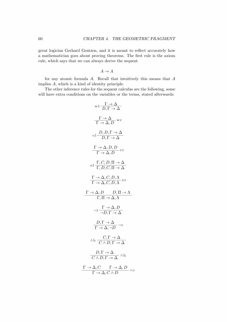
60 CHAPTER 4. THE GEOMETRIC FRAGMENT
great logician Gerhard Gentzen, and it is meant to reflect accurately howa mathematician goes about proving theorems. The first rule is the axiomrule, which says that we can always derive the sequent
A→ A
for any atomic formula A. Recall that intuitively this means that Aimplies A, which is a kind of identity principle.
The other inference rules for the sequent calculus are the following, somewill have extra conditions on the variables or the terms, stated afterwards:
Γ→ ∆w:l
D,Γ→ ∆
Γ→ ∆ w:rΓ→ ∆, D
D,D,Γ→ ∆c:l
D,Γ→ ∆
Γ→ ∆, D,Dc:r
Γ→ ∆, D
Γ, C,D,Π→ ∆e:l
Γ, D,C,Π→ ∆
Γ→ ∆, C,D,Λe:r
Γ→ ∆, C,D,Λ
Γ→ ∆, D D,Π→ Λ
Γ,Π→ ∆,Λ
Γ→ ∆, D¬:l ¬D,Γ→ ∆
D,Γ→ ∆¬:r
Γ→ ∆,¬D
C,Γ→ ∆∧:l1
C ∧D,Γ→ ∆
D,Γ→ ∆∧:l2
C ∧D,Γ→ ∆
Γ→ ∆, C Γ→ ∆, D∧:r
Γ→ ∆, C ∧D

4.1. SEQUENT CALCULI 61
C,Γ→ ∆ D,Γ→ ∆∨:l
C ∨D,Γ→ ∆
Γ→ ∆, C∨:r1
Γ→ ∆, C ∨D
Γ→ ∆, D∨:r2
Γ→ ∆, C ∨D
Γ→ ∆, C D,Π→ Λ⊃:l
C ⊃ D,Γ,Π→ ∆,Λ
C,Γ→ ∆, D⊃:r
Γ→ ∆, C ⊃ D
F (t),Γ→ ∆∀:l ∀xF (x),Γ→ ∆
Γ→ ∆, F (a)∀:r
Γ→ ∆, ∀xF (x)
F (a),Γ→ ∆∃:l ∃xF (x),Γ→ ∆
Γ→ ∆, F (t)∃:r
Γ→ ∆, ∃xF (x)
In the above a is a fully indicated Eigenvariable, for our purposes all thatneed mean to us is that it does not occur in the conclusion of the inferencerule. The term t is arbitrary and we should carefully note that t need notbe fully indicated.
Proposition 4.1.2 The sequent A∨∧
(Bi)→∧
(A∨Bj) is intuitionisticallyprovable.
Proof. The following tree gives a very good idea of what a proof in ourformal system would look like. We consider it sufficient to establish thepropostion.
A→ A
A→ A ∨ B1
A→ A
A→ A ∨ Bm · · ·A→
∧(A ∨ Bj)
B1 → B1∧(Bi)→ B1∧
(Bi)→ A ∨ B1
Bk → Bk∧(Bi)→ Bk∧
(Bi)→ A ∨ Bk · · ·∧(Bi)→
∧(A ∨ Bj)
A ∨∧
(Bi)→∧
(A ∨ Bj)
ut
It seems to be possible, with the appropriate principle of omniscience,to prove infinitary commutativity of
∧and ∨.
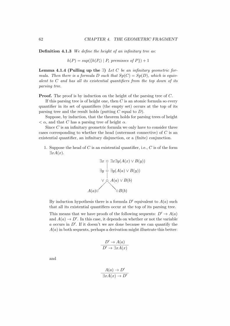
62 CHAPTER 4. THE GEOMETRIC FRAGMENT
Definition 4.1.3 We define the height of an infinitary tree as:
h(P ) = sup(h(Pi) | Pi premisses of P) + 1
Lemma 4.1.4 (Pulling up the ∃) Let C be an infinitary geometric for-mula. Then there is a formula D such that Sp(C) = Sp(D), which is equiv-alent to C and has all its existential quantifiers from the top down of itsparsing tree.
Proof. The proof is by induction on the height of the parsing tree of C.If this parsing tree is of height one, then C is an atomic formula so every
quantifier in its set of quantifiers (the empty set) occurs at the top of itsparsing tree and the result holds (putting C equal to D).
Suppose, by induction, that the theorem holds for parsing trees of height< α, and that C has a parsing tree of height α.
Since C is an infinitary geometric formula we only have to consider threecases corresponding to whether the head (outermost connective) of C is anexistential quantifier, an infinitary disjunction, or a (finite) conjunction.
1. Suppose the head of C is an existential quantifier, i.e., C is of the form∃xA(x).
∃x∃y(A(x) ∨B(y))d∃x
∃y(A(a) ∨B(y))d∃y
∨ d A(a) ∨B(b)
@@@d dA(a) B(b)
By induction hypothesis there is a formula D′ equivalent to A(a) suchthat all its existential quantifiers occur at the top of its parsing tree.
This means that we have proofs of the following sequents: D′ → A(a)and A(a)→ D′. In this case, it depends on whether or not the variablea occurs in D′. If it doesn’t we are done because we can quantify theA(a) in both sequents, perhaps a derivation might illustrate this better:
D′ → A(a)
D′ → ∃xA(x)
and
A(a)→ D′
∃xA(x)→ D′
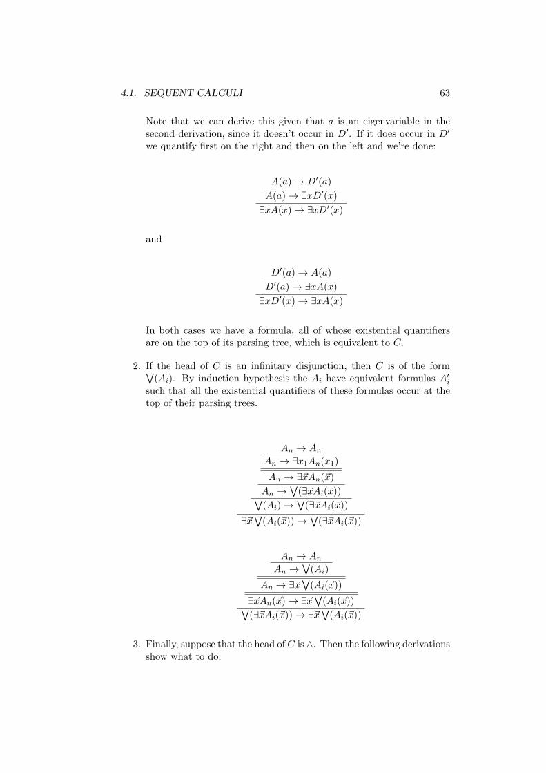
4.1. SEQUENT CALCULI 63
Note that we can derive this given that a is an eigenvariable in thesecond derivation, since it doesn’t occur in D′. If it does occur in D′
we quantify first on the right and then on the left and we’re done:
A(a)→ D′(a)
A(a)→ ∃xD′(x)
∃xA(x)→ ∃xD′(x)
and
D′(a)→ A(a)
D′(a)→ ∃xA(x)
∃xD′(x)→ ∃xA(x)
In both cases we have a formula, all of whose existential quantifiersare on the top of its parsing tree, which is equivalent to C.
2. If the head of C is an infinitary disjunction, then C is of the form∨(Ai). By induction hypothesis the Ai have equivalent formulas A′i
such that all the existential quantifiers of these formulas occur at thetop of their parsing trees.
An → AnAn → ∃x1An(x1)
An → ∃~xAn(~x)
An →∨
(∃~xAi(~x))∨(Ai)→
∨(∃~xAi(~x))
∃~x∨
(Ai(~x))→∨
(∃~xAi(~x))
An → AnAn →
∨(Ai)
An → ∃~x∨
(Ai(~x))
∃~xAn(~x)→ ∃~x∨
(Ai(~x))∨(∃~xAi(~x))→ ∃~x
∨(Ai(~x))
3. Finally, suppose that the head of C is ∧. Then the following derivationsshow what to do:
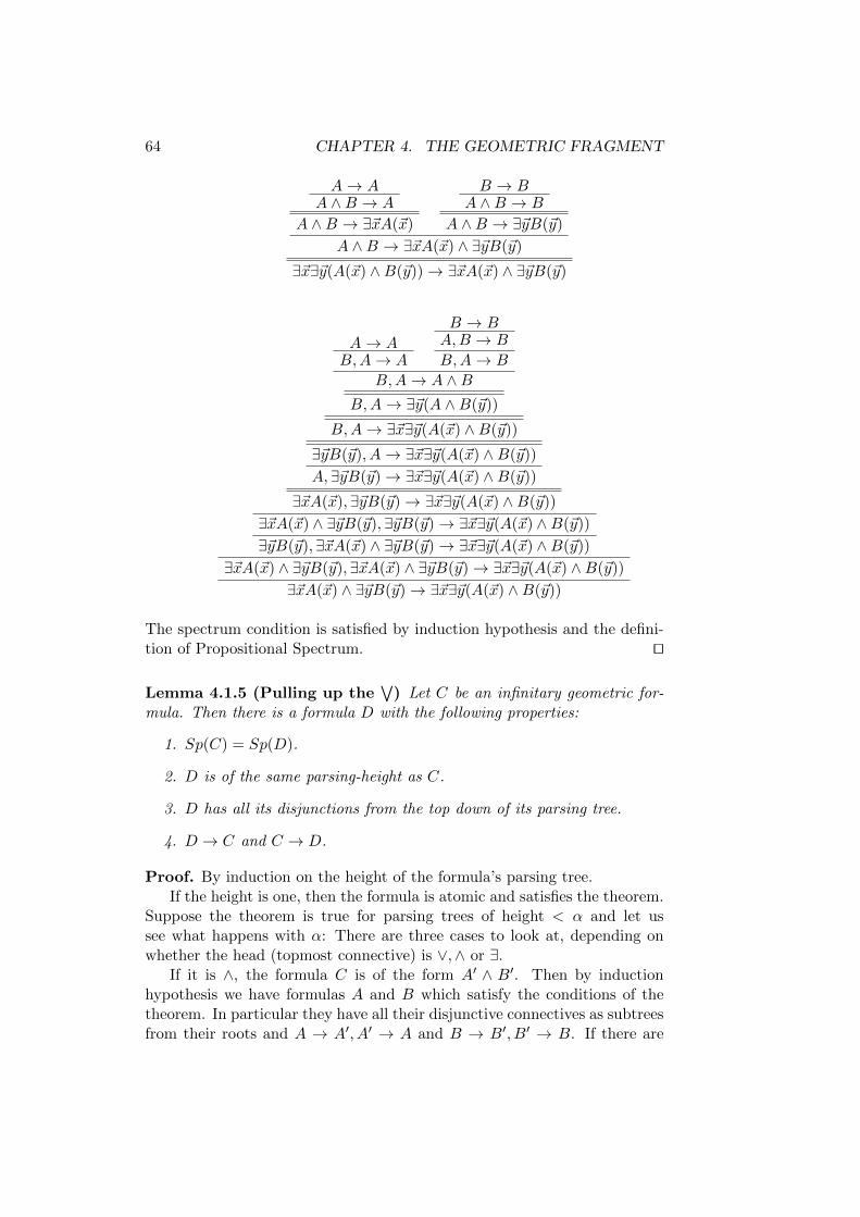
64 CHAPTER 4. THE GEOMETRIC FRAGMENT
A→ AA ∧B → A
A ∧B → ∃~xA(~x)
B → BA ∧B → B
A ∧B → ∃~yB(~y)
A ∧B → ∃~xA(~x) ∧ ∃~yB(~y)
∃~x∃~y(A(~x) ∧B(~y))→ ∃~xA(~x) ∧ ∃~yB(~y)
A→ AB,A→ A
B → BA,B → B
B,A→ B
B,A→ A ∧BB,A→ ∃~y(A ∧B(~y))
B,A→ ∃~x∃~y(A(~x) ∧B(~y))
∃~yB(~y), A→ ∃~x∃~y(A(~x) ∧B(~y))
A,∃~yB(~y)→ ∃~x∃~y(A(~x) ∧B(~y))
∃~xA(~x),∃~yB(~y)→ ∃~x∃~y(A(~x) ∧B(~y))
∃~xA(~x) ∧ ∃~yB(~y), ∃~yB(~y)→ ∃~x∃~y(A(~x) ∧B(~y))
∃~yB(~y), ∃~xA(~x) ∧ ∃~yB(~y)→ ∃~x∃~y(A(~x) ∧B(~y))
∃~xA(~x) ∧ ∃~yB(~y), ∃~xA(~x) ∧ ∃~yB(~y)→ ∃~x∃~y(A(~x) ∧B(~y))
∃~xA(~x) ∧ ∃~yB(~y)→ ∃~x∃~y(A(~x) ∧B(~y))
The spectrum condition is satisfied by induction hypothesis and the defini-tion of Propositional Spectrum. ut
Lemma 4.1.5 (Pulling up the∨
) Let C be an infinitary geometric for-mula. Then there is a formula D with the following properties:
1. Sp(C) = Sp(D).
2. D is of the same parsing-height as C.
3. D has all its disjunctions from the top down of its parsing tree.
4. D → C and C → D.
Proof. By induction on the height of the formula’s parsing tree.If the height is one, then the formula is atomic and satisfies the theorem.
Suppose the theorem is true for parsing trees of height < α and let ussee what happens with α: There are three cases to look at, depending onwhether the head (topmost connective) is ∨,∧ or ∃.
If it is ∧, the formula C is of the form A′ ∧ B′. Then by inductionhypothesis we have formulas A and B which satisfy the conditions of thetheorem. In particular they have all their disjunctive connectives as subtreesfrom their roots and A → A′, A′ → A and B → B′, B′ → B. If there are
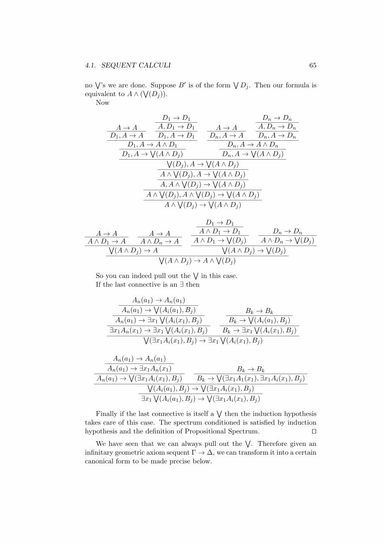
4.1. SEQUENT CALCULI 65
no∨
’s we are done. Suppose B′ is of the form∨Dj . Then our formula is
equivalent to A ∧ (∨
(Dj)).Now
A→ AD1, A→ A
D1 → D1
A,D1 → D1
D1, A→ D1
D1, A→ A ∧D1
D1, A→∨
(A ∧Dj)
A→ ADn, A→ A
Dn → Dn
A,Dn → Dn
Dn, A→ Dn
Dn, A→ A ∧Dn
Dn, A→∨
(A ∧Dj)∨(Dj), A→
∨(A ∧Dj)
A ∧∨
(Dj), A→∨
(A ∧Dj)
A,A ∧∨
(Dj)→∨
(A ∧Dj)
A ∧∨
(Dj), A ∧∨
(Dj)→∨
(A ∧Dj)
A ∧∨
(Dj)→∨
(A ∧Dj)
A→ AA ∧D1 → A
A→ AA ∧Dn → A∨
(A ∧Dj)→ A
D1 → D1
A ∧D1 → D1
A ∧D1 →∨
(Dj)
Dn → Dn
A ∧Dn →∨
(Dj)∨(A ∧Dj)→
∨(Dj)∨
(A ∧Dj)→ A ∧∨
(Dj)
So you can indeed pull out the∨
in this case.If the last connective is an ∃ then
An(a1)→ An(a1)
An(a1)→∨
(Ai(a1), Bj)
An(a1)→ ∃x1∨
(Ai(x1), Bj)
∃x1An(x1)→ ∃x1∨
(Ai(x1), Bj)
Bk → BkBk →
∨(Ai(a1), Bj)
Bk → ∃x1∨
(Ai(x1), Bj)∨(∃x1Ai(x1), Bj)→ ∃x1
∨(Ai(x1), Bj)
An(a1)→ An(a1)
An(a1)→ ∃x1An(x1)
An(a1)→∨
(∃x1Ai(x1), Bj)
Bk → BkBk →
∨(∃x1A1(x1),∃x1Ai(x1), Bj)∨
(Ai(a1), Bj)→∨
(∃x1Ai(x1), Bj)
∃x1∨
(Ai(a1), Bj)→∨
(∃x1Ai(x1), Bj)
Finally if the last connective is itself a∨
then the induction hypothesistakes care of this case. The spectrum conditioned is satisfied by inductionhypothesis and the definition of Propositional Spectrum. ut
We have seen that we can always pull out the∨
. Therefore given aninfinitary geometric axiom sequent Γ→ ∆, we can transform it into a certaincanonical form to be made precise below.
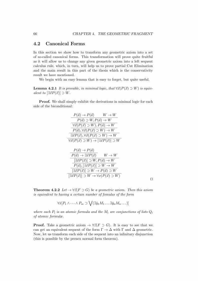
66 CHAPTER 4. THE GEOMETRIC FRAGMENT
4.2 Canonical Forms
In this section we show how to transform any geometric axiom into a setof so-called canonical forms. This transformation will prove quite fruitfulas it will allow us to change any given geometric axiom into a left sequentcalculus rule, which, in turn, will help us to prove partial Cut Eliminationand the main result in this part of the thesis which is the conservativityresult we have mentioned.
We begin with an easy lemma that is easy to forget, but quite useful.
Lemma 4.2.1 It is provable, in minimal logic, that ∀~x(P (~x) ⊃W ) is equiv-alent to [∃~xP (~x)] ⊃W .
Proof. We shall simply exhibit the derivations in minimal logic for eachside of the biconditional:
P (~a)→ P (~a) W →W
P (~a) ⊃W,P (~a)→W
∀~x(P (~x) ⊃W ), P (~a)→W
P (~a),∀~x(P (~x) ⊃W )→W
∃~xP (~x),∀~x(P (~x) ⊃W )→W
∀~x(P (~x) ⊃W )→ [∃~xP (~x)] ⊃W
P (~a)→ P (~a)
P (~a)→ ∃~xP (~x) W →W
[∃~xP (~x)] ⊃W,P (~a)→W
P (~a), [∃~xP (~x)] ⊃W →W
[∃~xP (~x)] ⊃W → P (~a) ⊃W[∃~xP (~x)] ⊃W → ∀x(P (~x) ⊃W )
ut
Theorem 4.2.2 Let → ∀~z(F ⊃ G) be a geometric axiom. Then this axiomis equivalent to having a certain number of fomulas of the form
∀x[P1 ∧ · · · ∧ Pm ⊃∨
(∃y1M1 . . . ∃ynMn . . . )]
where each Pi is an atomic formula and the Mi are conjunctions of lists Qiof atomic formulæ.
Proof. Take a geometric axiom → ∀~z(F ⊃ G). It is easy to see that wecan get an equivalent sequent of the form Γ→ ∆ with Γ and ∆ geometric.Now, let us transform each side of the sequent into an infinitary disjunction(this is possible by the prenex normal form theorem).
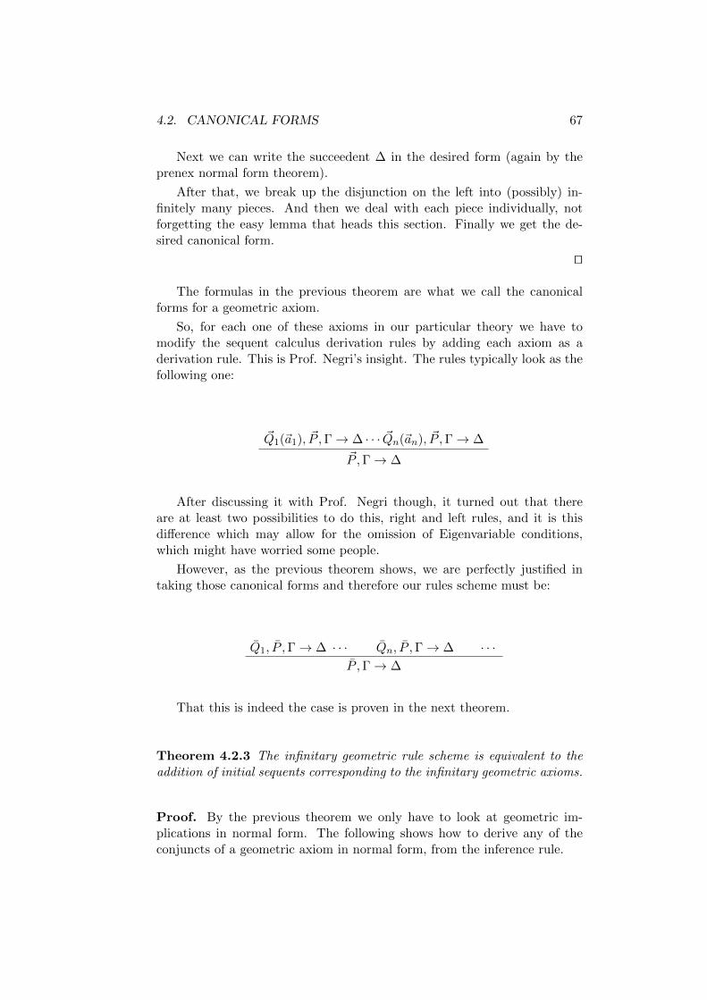
4.2. CANONICAL FORMS 67
Next we can write the succeedent ∆ in the desired form (again by theprenex normal form theorem).
After that, we break up the disjunction on the left into (possibly) in-finitely many pieces. And then we deal with each piece individually, notforgetting the easy lemma that heads this section. Finally we get the de-sired canonical form.
ut
The formulas in the previous theorem are what we call the canonicalforms for a geometric axiom.
So, for each one of these axioms in our particular theory we have tomodify the sequent calculus derivation rules by adding each axiom as aderivation rule. This is Prof. Negri’s insight. The rules typically look as thefollowing one:
~Q1(~a1), ~P ,Γ→ ∆ · · · ~Qn(~an), ~P ,Γ→ ∆
~P ,Γ→ ∆
After discussing it with Prof. Negri though, it turned out that thereare at least two possibilities to do this, right and left rules, and it is thisdifference which may allow for the omission of Eigenvariable conditions,which might have worried some people.
However, as the previous theorem shows, we are perfectly justified intaking those canonical forms and therefore our rules scheme must be:
Q1, P ,Γ→ ∆ · · · Qn, P ,Γ→ ∆ · · ·P ,Γ→ ∆
That this is indeed the case is proven in the next theorem.
Theorem 4.2.3 The infinitary geometric rule scheme is equivalent to theaddition of initial sequents corresponding to the infinitary geometric axioms.
Proof. By the previous theorem we only have to look at geometric im-plications in normal form. The following shows how to derive any of theconjuncts of a geometric axiom in normal form, from the inference rule.
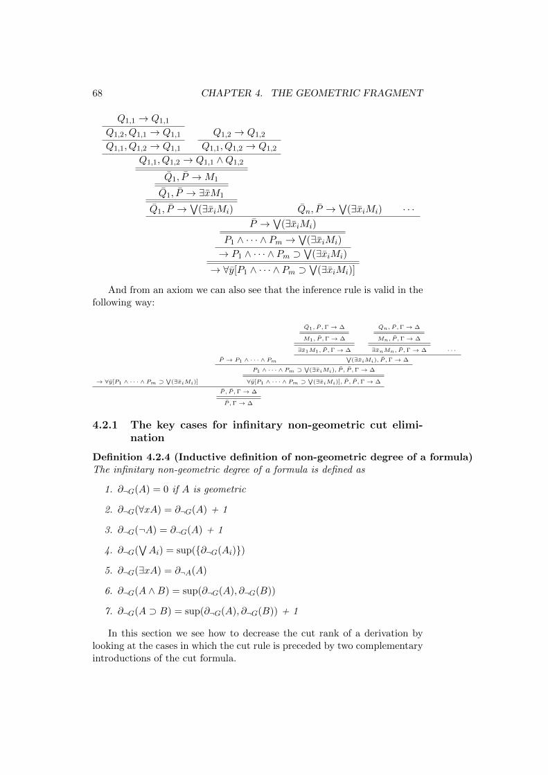
68 CHAPTER 4. THE GEOMETRIC FRAGMENT
Q1,1 → Q1,1
Q1,2, Q1,1 → Q1,1
Q1,1, Q1,2 → Q1,1
Q1,2 → Q1,2
Q1,1, Q1,2 → Q1,2
Q1,1, Q1,2 → Q1,1 ∧Q1,2
Q1, P →M1
Q1, P → ∃xM1
Q1, P →∨
(∃xiMi) Qn, P →∨
(∃xiMi) · · ·P →
∨(∃xiMi)
P1 ∧ · · · ∧ Pm →∨
(∃xiMi)
→ P1 ∧ · · · ∧ Pm ⊃∨
(∃xiMi)
→ ∀y[P1 ∧ · · · ∧ Pm ⊃∨
(∃xiMi)]
And from an axiom we can also see that the inference rule is valid in thefollowing way:
→ ∀y[P1 ∧ · · · ∧ Pm ⊃∨
(∃xiMi)]
P → P1 ∧ · · · ∧ Pm
Q1, P ,Γ→ ∆
M1, P ,Γ→ ∆
∃x1M1, P ,Γ→ ∆
Qn, P ,Γ→ ∆
Mn, P ,Γ→ ∆
∃xnMn, P ,Γ→ ∆ · · ·∨(∃xiMi), P ,Γ→ ∆
P1 ∧ · · · ∧ Pm ⊃∨
(∃xiMi), P , P ,Γ→ ∆
∀y[P1 ∧ · · · ∧ Pm ⊃∨
(∃xiMi)], P , P ,Γ→ ∆
P , P ,Γ→ ∆
P ,Γ→ ∆
4.2.1 The key cases for infinitary non-geometric cut elimi-nation
Definition 4.2.4 (Inductive definition of non-geometric degree of a formula)The infinitary non-geometric degree of a formula is defined as
1. ∂¬G(A) = 0 if A is geometric
2. ∂¬G(∀xA) = ∂¬G(A) + 1
3. ∂¬G(¬A) = ∂¬G(A) + 1
4. ∂¬G(∨Ai) = sup(∂¬G(Ai))
5. ∂¬G(∃xA) = ∂¬A(A)
6. ∂¬G(A ∧B) = sup(∂¬G(A), ∂¬G(B))
7. ∂¬G(A ⊃ B) = sup(∂¬G(A), ∂¬G(B)) + 1
In this section we see how to decrease the cut rank of a derivation bylooking at the cases in which the cut rule is preceded by two complementaryintroductions of the cut formula.
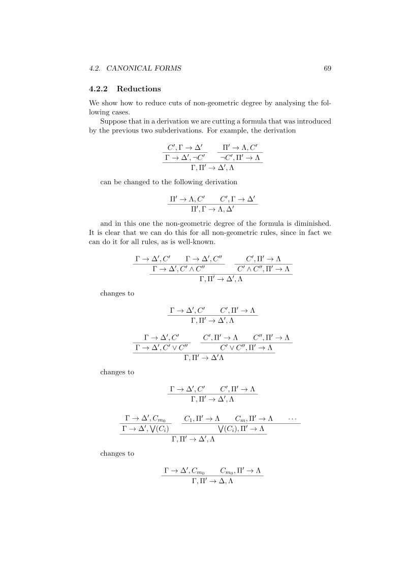
4.2. CANONICAL FORMS 69
4.2.2 Reductions
We show how to reduce cuts of non-geometric degree by analysing the fol-lowing cases.
Suppose that in a derivation we are cutting a formula that was introducedby the previous two subderivations. For example, the derivation
C ′,Γ→ ∆′
Γ→ ∆′,¬C ′Π′ → Λ, C ′
¬C ′,Π′ → Λ
Γ,Π′ → ∆′,Λ
can be changed to the following derivation
Π′ → Λ, C ′ C ′,Γ→ ∆′
Π′,Γ→ Λ,∆′
and in this one the non-geometric degree of the formula is diminished.It is clear that we can do this for all non-geometric rules, since in fact wecan do it for all rules, as is well-known.
Γ→ ∆′, C ′ Γ→ ∆′, C ′′
Γ→ ∆′, C ′ ∧ C ′′C ′,Π′ → Λ
C ′ ∧ C ′′,Π′ → Λ
Γ,Π′ → ∆′,Λ
changes to
Γ→ ∆′, C ′ C ′,Π′ → Λ
Γ,Π′ → ∆′,Λ
Γ→ ∆′, C ′
Γ→ ∆′, C ′ ∨ C ′′C ′,Π′ → Λ C ′′,Π′ → Λ
C ′ ∨ C ′′,Π′ → Λ
Γ,Π′ → ∆′Λ
changes to
Γ→ ∆′, C ′ C ′,Π′ → Λ
Γ,Π′ → ∆′,Λ
Γ→ ∆′, Cm0
Γ→ ∆′,∨
(Ci)
C1,Π′ → Λ Cm,Π
′ → Λ · · ·∨(Ci),Π
′ → Λ
Γ,Π′ → ∆′,Λ
changes to
Γ→ ∆′, Cm0 Cm0 ,Π′ → Λ
Γ,Π′ → ∆,Λ
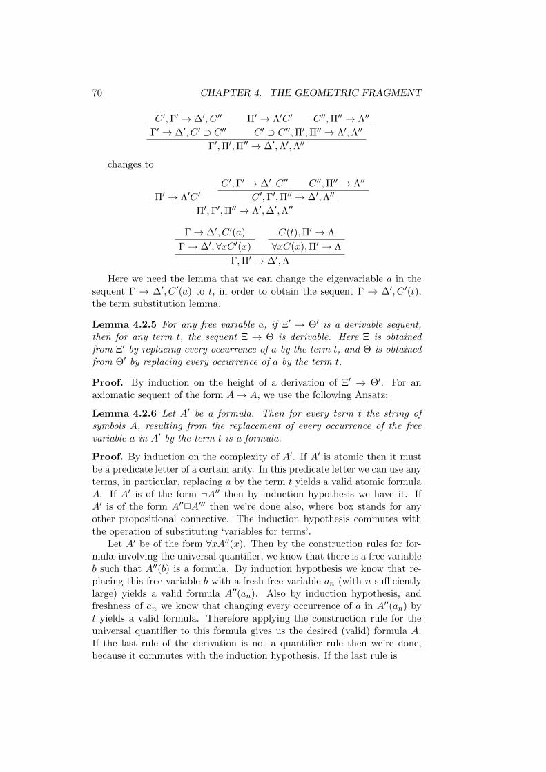
70 CHAPTER 4. THE GEOMETRIC FRAGMENT
C ′,Γ′ → ∆′, C ′′
Γ′ → ∆′, C ′ ⊃ C ′′Π′ → Λ′C ′ C ′′,Π′′ → Λ′′
C ′ ⊃ C ′′,Π′,Π′′ → Λ′,Λ′′
Γ′,Π′,Π′′ → ∆′,Λ′,Λ′′
changes to
Π′ → Λ′C ′C ′,Γ′ → ∆′, C ′′ C ′′,Π′′ → Λ′′
C ′,Γ′,Π′′ → ∆′,Λ′′
Π′,Γ′,Π′′ → Λ′,∆′,Λ′′
Γ→ ∆′, C ′(a)
Γ→ ∆′,∀xC ′(x)
C(t),Π′ → Λ
∀xC(x),Π′ → Λ
Γ,Π′ → ∆′,Λ
Here we need the lemma that we can change the eigenvariable a in thesequent Γ → ∆′, C ′(a) to t, in order to obtain the sequent Γ → ∆′, C ′(t),the term substitution lemma.
Lemma 4.2.5 For any free variable a, if Ξ′ → Θ′ is a derivable sequent,then for any term t, the sequent Ξ → Θ is derivable. Here Ξ is obtainedfrom Ξ′ by replacing every occurrence of a by the term t, and Θ is obtainedfrom Θ′ by replacing every occurrence of a by the term t.
Proof. By induction on the height of a derivation of Ξ′ → Θ′. For anaxiomatic sequent of the form A→ A, we use the following Ansatz:
Lemma 4.2.6 Let A′ be a formula. Then for every term t the string ofsymbols A, resulting from the replacement of every occurrence of the freevariable a in A′ by the term t is a formula.
Proof. By induction on the complexity of A′. If A′ is atomic then it mustbe a predicate letter of a certain arity. In this predicate letter we can use anyterms, in particular, replacing a by the term t yields a valid atomic formulaA. If A′ is of the form ¬A′′ then by induction hypothesis we have it. IfA′ is of the form A′′2A′′′ then we’re done also, where box stands for anyother propositional connective. The induction hypothesis commutes withthe operation of substituting ‘variables for terms’.
Let A′ be of the form ∀xA′′(x). Then by the construction rules for for-mulæ involving the universal quantifier, we know that there is a free variableb such that A′′(b) is a formula. By induction hypothesis we know that re-placing this free variable b with a fresh free variable an (with n sufficientlylarge) yields a valid formula A′′(an). Also by induction hypothesis, andfreshness of an we know that changing every occurrence of a in A′′(an) byt yields a valid formula. Therefore applying the construction rule for theuniversal quantifier to this formula gives us the desired (valid) formula A.If the last rule of the derivation is not a quantifier rule then we’re done,because it commutes with the induction hypothesis. If the last rule is
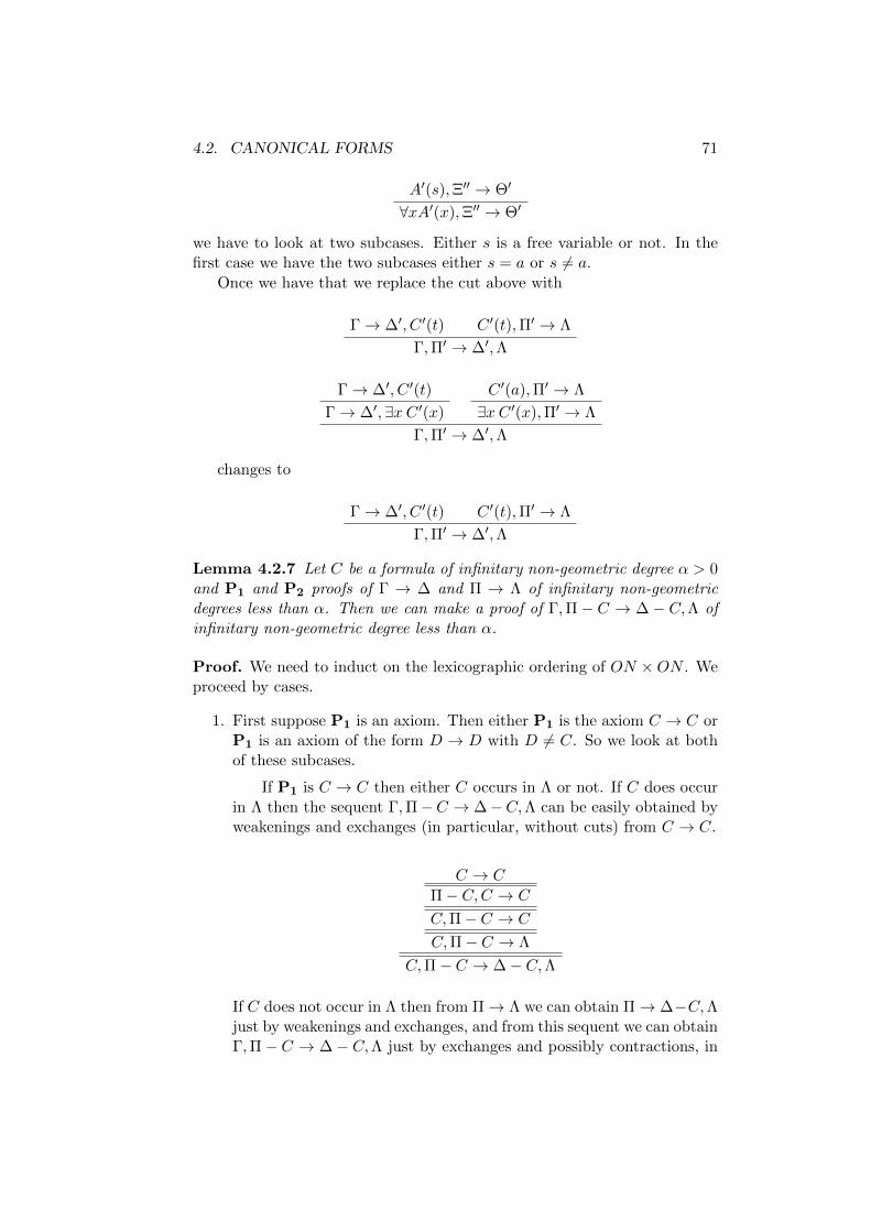
4.2. CANONICAL FORMS 71
A′(s),Ξ′′ → Θ′
∀xA′(x),Ξ′′ → Θ′
we have to look at two subcases. Either s is a free variable or not. In thefirst case we have the two subcases either s = a or s 6= a.
Once we have that we replace the cut above with
Γ→ ∆′, C ′(t) C ′(t),Π′ → Λ
Γ,Π′ → ∆′,Λ
Γ→ ∆′, C ′(t)
Γ→ ∆′, ∃x C ′(x)
C ′(a),Π′ → Λ
∃x C ′(x),Π′ → Λ
Γ,Π′ → ∆′,Λ
changes to
Γ→ ∆′, C ′(t) C ′(t),Π′ → Λ
Γ,Π′ → ∆′,Λ
Lemma 4.2.7 Let C be a formula of infinitary non-geometric degree α > 0and P1 and P2 proofs of Γ → ∆ and Π → Λ of infinitary non-geometricdegrees less than α. Then we can make a proof of Γ,Π − C → ∆ − C,Λ ofinfinitary non-geometric degree less than α.
Proof. We need to induct on the lexicographic ordering of ON ×ON . Weproceed by cases.
1. First suppose P1 is an axiom. Then either P1 is the axiom C → C orP1 is an axiom of the form D → D with D 6= C. So we look at bothof these subcases.
If P1 is C → C then either C occurs in Λ or not. If C does occurin Λ then the sequent Γ,Π−C → ∆−C,Λ can be easily obtained byweakenings and exchanges (in particular, without cuts) from C → C.
C → C
Π− C,C → C
C,Π− C → C
C,Π− C → Λ
C,Π− C → ∆− C,Λ
If C does not occur in Λ then from Π→ Λ we can obtain Π→ ∆−C,Λjust by weakenings and exchanges, and from this sequent we can obtainΓ,Π− C → ∆− C,Λ just by exchanges and possibly contractions, in
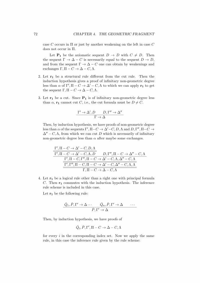
72 CHAPTER 4. THE GEOMETRIC FRAGMENT
case C occurs in Π or just by another weakening on the left in case Cdoes not occur in Π.
Let P1 be the axiomatic sequent D → D with C 6= D. Thenthe sequent Γ → ∆ − C is necessarily equal to the sequent D → D,and from the sequent Γ → ∆ − C one can obtain by weakenings andexchanges Γ,Π− C → ∆− C,Λ.
2. Let r1 be a structural rule different from the cut rule. Then theinduction hypothesis gives a proof of infinitary non-geometric degreeless than α of Γ′,Π− C → ∆′ − C,Λ to which we can apply r1 to getthe sequent Γ,Π− C → ∆− C,Λ.
3. Let r1 be a cut. Since P1 is of infinitary non-geometric degree lessthan α, r1 cannot cut C, i.e., the cut formula must be D 6= C.
Γ′ → ∆′, D D,Γ′′ → ∆′′
Γ→ ∆
Then, by induction hypothesis, we have proofs of non-geometric degreeless than α of the sequents Γ′,Π−C → ∆′−C,D,Λ and D,Γ′′,Π−C →∆′′ −C,Λ, from which we can cut D which is necessarily of infinitarynon-geometric degree less than α after maybe some exchanges.
Γ′,Π− C → ∆′ − C,D,ΛΓ′,Π− C → ∆′ − C,Λ, D D,Γ′′,Π− C → ∆′′ − C,Λ
Γ′,Π− C,Γ′′,Π− C → ∆′ − C,Λ,∆′′ − C,ΛΓ′,Γ′′,Π− C,Π− C → ∆′ − C,∆′′ − C,Λ,Λ
Γ,Π− C → ∆− C,Λ
4. Let r1 be a logical rule other than a right one with principal formulaC. Then r1 commutes with the induction hypothesis. The inferencerule scheme is included in this case.
Let r1 be the following rule:
Q1, P ,Γ′ → ∆ · · · Qn, P ,Γ
′ → ∆ · · ·P ,Γ′ → ∆
Then, by induction hypothesis, we have proofs of
Qi, P ,Γ′,Π− C → ∆− C,Λ
for every i in the corresponding index set. Now we apply the samerule, in this case the inference rule given by the rule scheme:
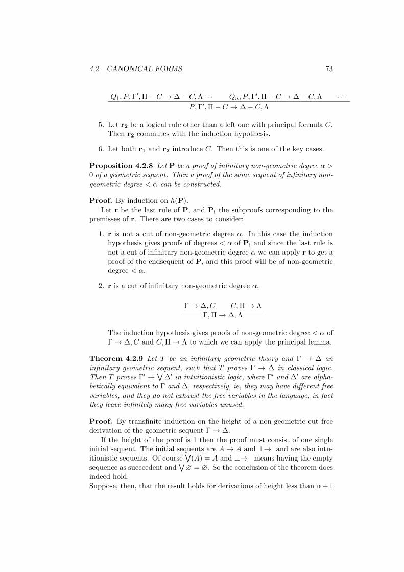
4.2. CANONICAL FORMS 73
Q1, P ,Γ′,Π− C → ∆− C,Λ · · · Qn, P ,Γ
′,Π− C → ∆− C,Λ · · ·P ,Γ′,Π− C → ∆− C,Λ
5. Let r2 be a logical rule other than a left one with principal formula C.Then r2 commutes with the induction hypothesis.
6. Let both r1 and r2 introduce C. Then this is one of the key cases.
Proposition 4.2.8 Let P be a proof of infinitary non-geometric degree α >0 of a geometric sequent. Then a proof of the same sequent of infinitary non-geometric degree < α can be constructed.
Proof. By induction on h(P).Let r be the last rule of P, and Pi the subproofs corresponding to the
premisses of r. There are two cases to consider:
1. r is not a cut of non-geometric degree α. In this case the inductionhypothesis gives proofs of degrees < α of Pi and since the last rule isnot a cut of infinitary non-geometric degree α we can apply r to get aproof of the endsequent of P, and this proof will be of non-geometricdegree < α.
2. r is a cut of infinitary non-geometric degree α.
Γ→ ∆, C C,Π→ Λ
Γ,Π→ ∆,Λ
The induction hypothesis gives proofs of non-geometric degree < α ofΓ→ ∆, C and C,Π→ Λ to which we can apply the principal lemma.
Theorem 4.2.9 Let T be an infinitary geometric theory and Γ → ∆ aninfinitary geometric sequent, such that T proves Γ → ∆ in classical logic.Then T proves Γ′ →
∨∆′ in intuitionistic logic, where Γ′ and ∆′ are alpha-
betically equivalent to Γ and ∆, respectively, ie, they may have different freevariables, and they do not exhaust the free variables in the language, in factthey leave infinitely many free variables unused.
Proof. By transfinite induction on the height of a non-geometric cut freederivation of the geometric sequent Γ→ ∆.
If the height of the proof is 1 then the proof must consist of one singleinitial sequent. The initial sequents are A→ A and ⊥→ and are also intu-itionistic sequents. Of course
∨(A) = A and ⊥→ means having the empty
sequence as succeedent and∨∅ = ∅. So the conclusion of the theorem does
indeed hold.Suppose, then, that the result holds for derivations of height less than α+ 1
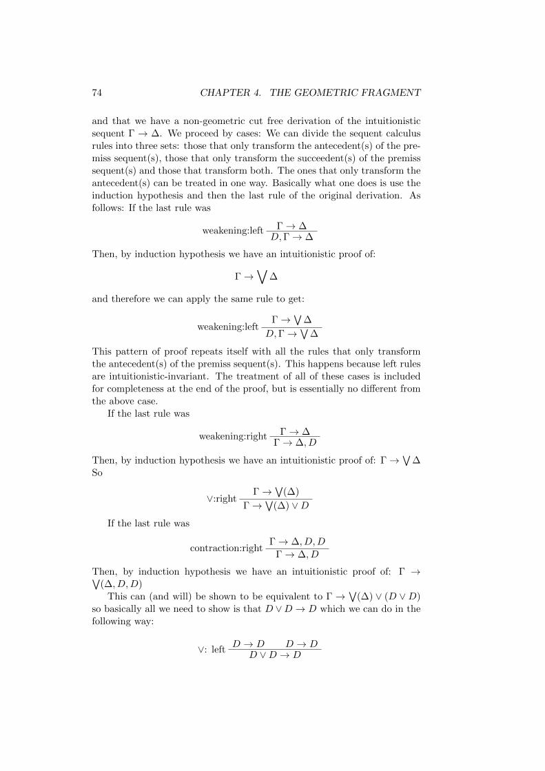
74 CHAPTER 4. THE GEOMETRIC FRAGMENT
and that we have a non-geometric cut free derivation of the intuitionisticsequent Γ → ∆. We proceed by cases: We can divide the sequent calculusrules into three sets: those that only transform the antecedent(s) of the pre-miss sequent(s), those that only transform the succeedent(s) of the premisssequent(s) and those that transform both. The ones that only transform theantecedent(s) can be treated in one way. Basically what one does is use theinduction hypothesis and then the last rule of the original derivation. Asfollows: If the last rule was
Γ→ ∆weakening:leftD,Γ→ ∆
Then, by induction hypothesis we have an intuitionistic proof of:
Γ→∨
∆
and therefore we can apply the same rule to get:
Γ→∨
∆weakening:left
D,Γ→∨
∆
This pattern of proof repeats itself with all the rules that only transformthe antecedent(s) of the premiss sequent(s). This happens because left rulesare intuitionistic-invariant. The treatment of all of these cases is includedfor completeness at the end of the proof, but is essentially no different fromthe above case.
If the last rule was
Γ→ ∆weakening:rightΓ→ ∆, D
Then, by induction hypothesis we have an intuitionistic proof of: Γ→∨
∆So
Γ→∨
(∆)∨:right
Γ→∨
(∆) ∨D
If the last rule was
Γ→ ∆, D,Dcontraction:right
Γ→ ∆, D
Then, by induction hypothesis we have an intuitionistic proof of: Γ →∨(∆, D,D)
This can (and will) be shown to be equivalent to Γ →∨
(∆) ∨ (D ∨D)so basically all we need to show is that D ∨D → D which we can do in thefollowing way:
D → D D → D∨: leftD ∨D → D
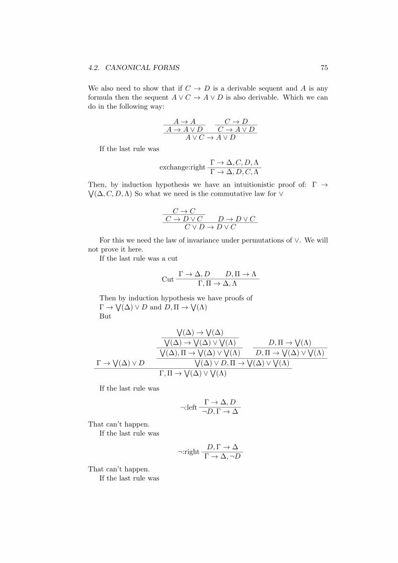
4.2. CANONICAL FORMS 75
We also need to show that if C → D is a derivable sequent and A is anyformula then the sequent A ∨ C → A ∨D is also derivable. Which we cando in the following way:
A→ AA→ A ∨D
C → DC → A ∨D
A ∨ C → A ∨DIf the last rule was
Γ→ ∆, C,D,Λexchange:right
Γ→ ∆, D,C,Λ
Then, by induction hypothesis we have an intuitionistic proof of: Γ →∨(∆, C,D,Λ) So what we need is the commutative law for ∨
C → CC → D ∨ C D → D ∨ C
C ∨D → D ∨ C
For this we need the law of invariance under permutations of ∨. We willnot prove it here.
If the last rule was a cut
Γ→ ∆, D D,Π→ ΛCut
Γ,Π→ ∆,Λ
Then by induction hypothesis we have proofs ofΓ→
∨(∆) ∨D and D,Π→
∨(Λ)
But
Γ→∨
(∆) ∨D
∨(∆)→
∨(∆)∨
(∆)→∨
(∆) ∨∨
(Λ)∨(∆),Π→
∨(∆) ∨
∨(Λ)
D,Π→∨
(Λ)
D,Π→∨
(∆) ∨∨
(Λ)∨(∆) ∨D,Π→
∨(∆) ∨
∨(Λ)
Γ,Π→∨
(∆) ∨∨
(Λ)
If the last rule was
Γ→ ∆, D¬:left ¬D,Γ→ ∆
That can’t happen.If the last rule was
D,Γ→ ∆¬:rightΓ→ ∆,¬D
That can’t happen.If the last rule was
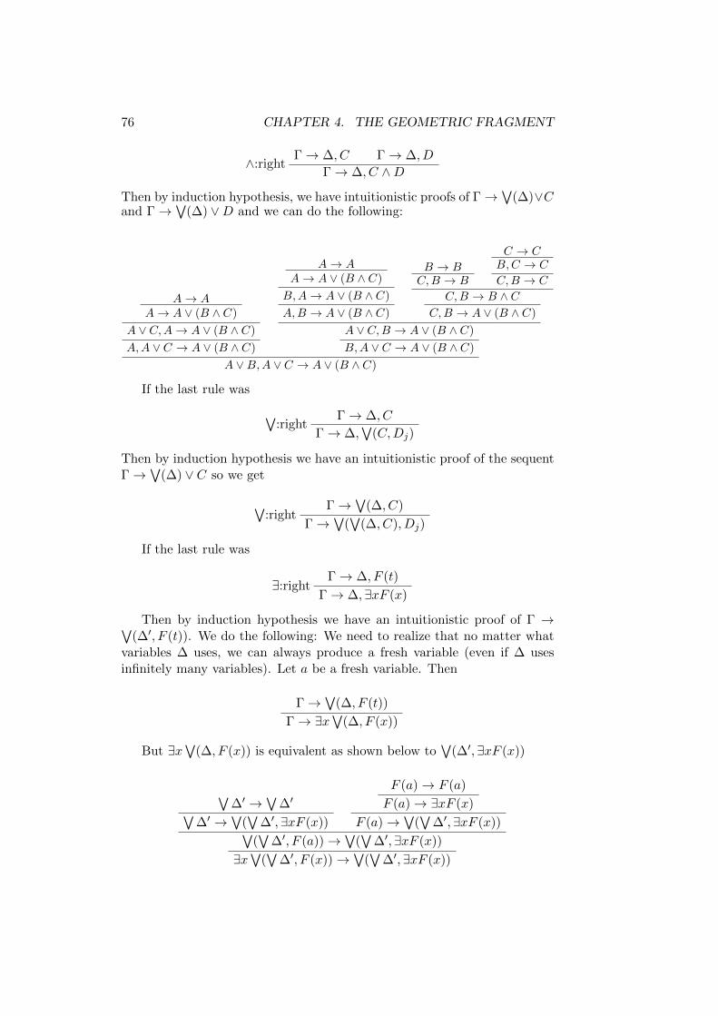
76 CHAPTER 4. THE GEOMETRIC FRAGMENT
Γ→ ∆, C Γ→ ∆, D∧:rightΓ→ ∆, C ∧D
Then by induction hypothesis, we have intuitionistic proofs of Γ→∨
(∆)∨Cand Γ→
∨(∆) ∨D and we can do the following:
A→ AA→ A ∨ (B ∧ C)
A ∨ C,A→ A ∨ (B ∧ C)
A,A ∨ C → A ∨ (B ∧ C)
A→ AA→ A ∨ (B ∧ C)
B,A→ A ∨ (B ∧ C)
A,B → A ∨ (B ∧ C)
B → BC,B → B
C → CB,C → C
C,B → C
C,B → B ∧ CC,B → A ∨ (B ∧ C)
A ∨ C,B → A ∨ (B ∧ C)
B,A ∨ C → A ∨ (B ∧ C)
A ∨B,A ∨ C → A ∨ (B ∧ C)
If the last rule was
Γ→ ∆, C∨:right
Γ→ ∆,∨
(C,Dj)
Then by induction hypothesis we have an intuitionistic proof of the sequentΓ→
∨(∆) ∨ C so we get
Γ→∨
(∆, C)∨:right
Γ→∨
(∨
(∆, C), Dj)
If the last rule was
Γ→ ∆, F (t)∃:right
Γ→ ∆, ∃xF (x)
Then by induction hypothesis we have an intuitionistic proof of Γ →∨(∆′, F (t)). We do the following: We need to realize that no matter what
variables ∆ uses, we can always produce a fresh variable (even if ∆ usesinfinitely many variables). Let a be a fresh variable. Then
Γ→∨
(∆, F (t))
Γ→ ∃x∨
(∆, F (x))
But ∃x∨
(∆, F (x)) is equivalent as shown below to∨
(∆′, ∃xF (x))
∨∆′ →
∨∆′∨
∆′ →∨
(∨
∆′,∃xF (x))
F (a)→ F (a)
F (a)→ ∃xF (x)
F (a)→∨
(∨
∆′,∃xF (x))∨(∨
∆′, F (a))→∨
(∨
∆′,∃xF (x))
∃x∨
(∨
∆′, F (x))→∨
(∨
∆′,∃xF (x))
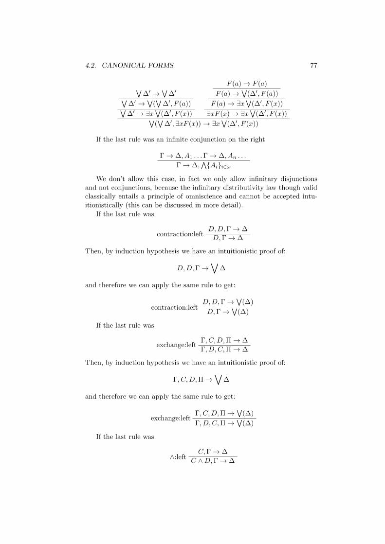
4.2. CANONICAL FORMS 77
∨∆′ →
∨∆′∨
∆′ →∨
(∨
∆′, F (a))∨∆′ → ∃x
∨(∆′, F (x))
F (a)→ F (a)
F (a)→∨
(∆′, F (a))
F (a)→ ∃x∨
(∆′, F (x))
∃xF (x)→ ∃x∨
(∆′, F (x))∨(∨
∆′,∃xF (x))→ ∃x∨
(∆′, F (x))
If the last rule was an infinite conjunction on the right
Γ→ ∆, A1 . . .Γ→ ∆, An . . .
Γ→ ∆,∧Aii∈ω
We don’t allow this case, in fact we only allow infinitary disjunctionsand not conjunctions, because the infinitary distributivity law though validclassically entails a principle of omniscience and cannot be accepted intu-itionistically (this can be discussed in more detail).
If the last rule was
D,D,Γ→ ∆contraction:left
D,Γ→ ∆
Then, by induction hypothesis we have an intuitionistic proof of:
D,D,Γ→∨
∆
and therefore we can apply the same rule to get:
D,D,Γ→∨
(∆)contraction:left
D,Γ→∨
(∆)
If the last rule was
Γ, C,D,Π→ ∆exchange:left
Γ, D,C,Π→ ∆
Then, by induction hypothesis we have an intuitionistic proof of:
Γ, C,D,Π→∨
∆
and therefore we can apply the same rule to get:
Γ, C,D,Π→∨
(∆)exchange:left
Γ, D,C,Π→∨
(∆)
If the last rule was
C,Γ→ ∆∧:left
C ∧D,Γ→ ∆
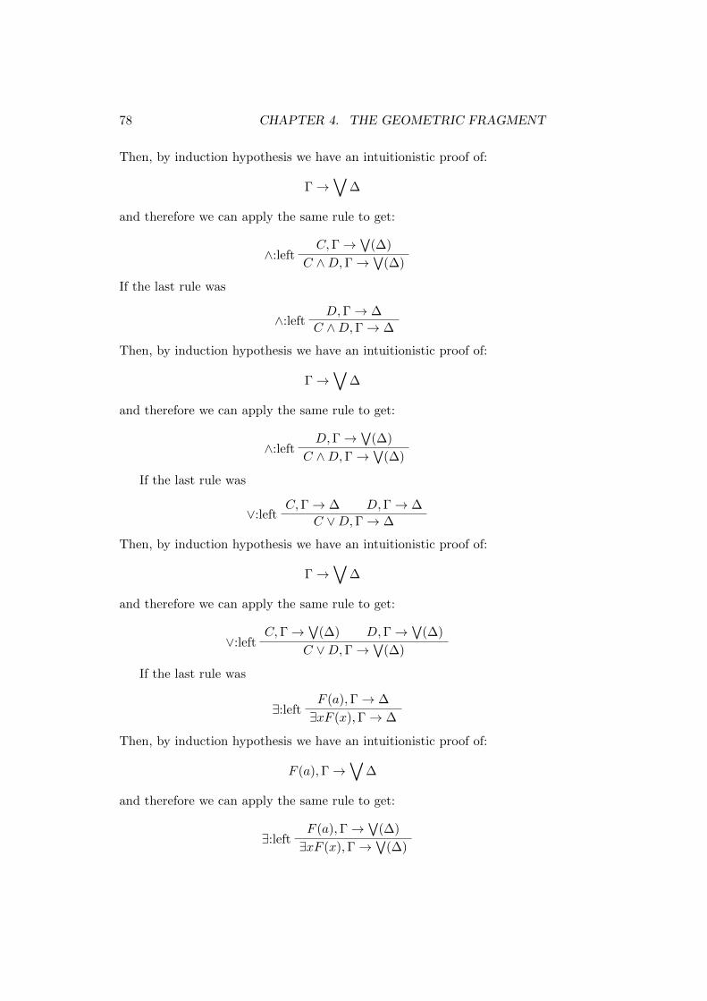
78 CHAPTER 4. THE GEOMETRIC FRAGMENT
Then, by induction hypothesis we have an intuitionistic proof of:
Γ→∨
∆
and therefore we can apply the same rule to get:
C,Γ→∨
(∆)∧:left
C ∧D,Γ→∨
(∆)
If the last rule was
D,Γ→ ∆∧:left
C ∧D,Γ→ ∆
Then, by induction hypothesis we have an intuitionistic proof of:
Γ→∨
∆
and therefore we can apply the same rule to get:
D,Γ→∨
(∆)∧:left
C ∧D,Γ→∨
(∆)
If the last rule was
C,Γ→ ∆ D,Γ→ ∆∨:left
C ∨D,Γ→ ∆
Then, by induction hypothesis we have an intuitionistic proof of:
Γ→∨
∆
and therefore we can apply the same rule to get:
C,Γ→∨
(∆) D,Γ→∨
(∆)∨:left
C ∨D,Γ→∨
(∆)
If the last rule was
F (a),Γ→ ∆∃:left ∃xF (x),Γ→ ∆
Then, by induction hypothesis we have an intuitionistic proof of:
F (a),Γ→∨
∆
and therefore we can apply the same rule to get:
F (a),Γ→∨
(∆)∃:left ∃xF (x),Γ→
∨(∆)
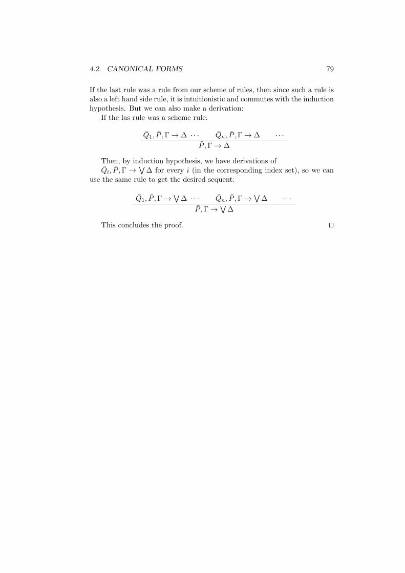
4.2. CANONICAL FORMS 79
If the last rule was a rule from our scheme of rules, then since such a rule isalso a left hand side rule, it is intuitionistic and commutes with the inductionhypothesis. But we can also make a derivation:
If the las rule was a scheme rule:
Q1, P ,Γ→ ∆ · · · Qn, P ,Γ→ ∆ · · ·P ,Γ→ ∆
Then, by induction hypothesis, we have derivations ofQi, P ,Γ →
∨∆ for every i (in the corresponding index set), so we can
use the same rule to get the desired sequent:
Q1, P ,Γ→∨
∆ · · · Qn, P ,Γ→∨
∆ · · ·P ,Γ→
∨∆
This concludes the proof. ut
80 CHAPTER 4. THE GEOMETRIC FRAGMENT
Part III
A Classification of SomeLogical Principles
81

Chapter 5
The formal system ML
This is the next to last part of this work, and though I feel I was veryinfluenced and helped by Michael Rathjen he insists on my making it abun-dantly clear that he feels he had absolutely nothing to do with the work inthis section and that it is entirely my own. In fact it all began because of hisProof Theory course when he asked the students attending what we thoughtthe rule weakening:right was. I ventured a response and said “ex falso” towhich Michael, with a tiny hint of surprise responded that he thought sotoo. After he made this question I started thinking about it more and more.The result is what follows.
We should like to state that to us there is a very important differencethat must be observed when we talk about logical principles. It is one thingto have an instance of a principle, and a very different one to have theprinciple itself.
For example, if A is a particular (concrete) formula then A ∨ ¬A is aninstance of the law of excluded middle. It is not the law of excluded middleitself. The law of excluded middle itself is the principle that allows us toderive all formulæ of that form.
We should keep this in mind in the following.
5.1 LJ without weakening-right
Let ML stand for the formal system obtained from the sequent calculusformal system for intuitionist logic LJ by removing the rule weakening:right.
First let us prove some things in ML:
We recall some logical principlesModus tollens
Theorem 5.1.1 The following hold in minimal logic.
1. P ⊃ Q,¬Q→ ¬P (Modus tollendo tollens)
83
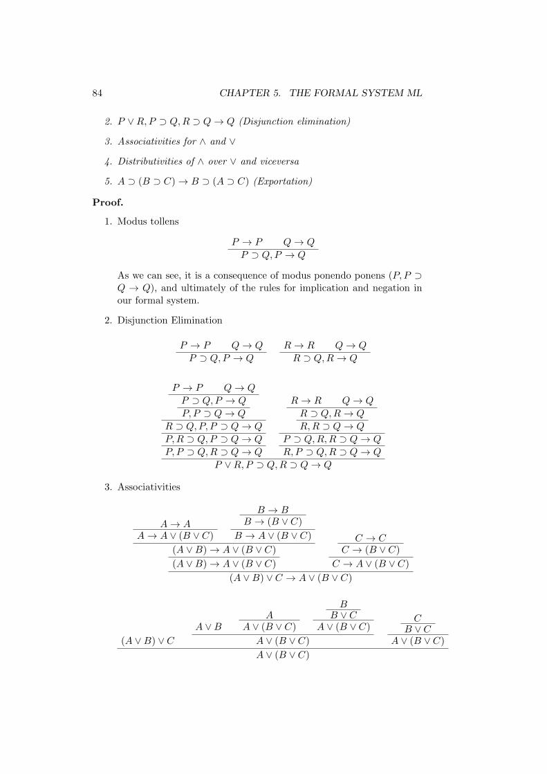
84 CHAPTER 5. THE FORMAL SYSTEM ML
2. P ∨R,P ⊃ Q,R ⊃ Q→ Q (Disjunction elimination)
3. Associativities for ∧ and ∨
4. Distributivities of ∧ over ∨ and viceversa
5. A ⊃ (B ⊃ C)→ B ⊃ (A ⊃ C) (Exportation)
Proof.
1. Modus tollens
P → P Q→ Q
P ⊃ Q,P → Q
As we can see, it is a consequence of modus ponendo ponens (P, P ⊃Q → Q), and ultimately of the rules for implication and negation inour formal system.
2. Disjunction Elimination
P → P Q→ Q
P ⊃ Q,P → Q
R→ R Q→ Q
R ⊃ Q,R→ Q
P → P Q→ Q
P ⊃ Q,P → Q
P,P ⊃ Q→ Q
R ⊃ Q,P, P ⊃ Q→ Q
P,R ⊃ Q,P ⊃ Q→ Q
P,P ⊃ Q,R ⊃ Q→ Q
R→ R Q→ Q
R ⊃ Q,R→ Q
R,R ⊃ Q→ Q
P ⊃ Q,R,R ⊃ Q→ Q
R,P ⊃ Q,R ⊃ Q→ Q
P ∨R,P ⊃ Q,R ⊃ Q→ Q
3. Associativities
A→ AA→ A ∨ (B ∨ C)
B → BB → (B ∨ C)
B → A ∨ (B ∨ C)
(A ∨B)→ A ∨ (B ∨ C)
(A ∨B)→ A ∨ (B ∨ C)
C → CC → (B ∨ C)
C → A ∨ (B ∨ C)
(A ∨B) ∨ C → A ∨ (B ∨ C)
(A ∨B) ∨ CA ∨B
AA ∨ (B ∨ C)
BB ∨ C
A ∨ (B ∨ C)
A ∨ (B ∨ C)
CB ∨ C
A ∨ (B ∨ C)
A ∨ (B ∨ C)
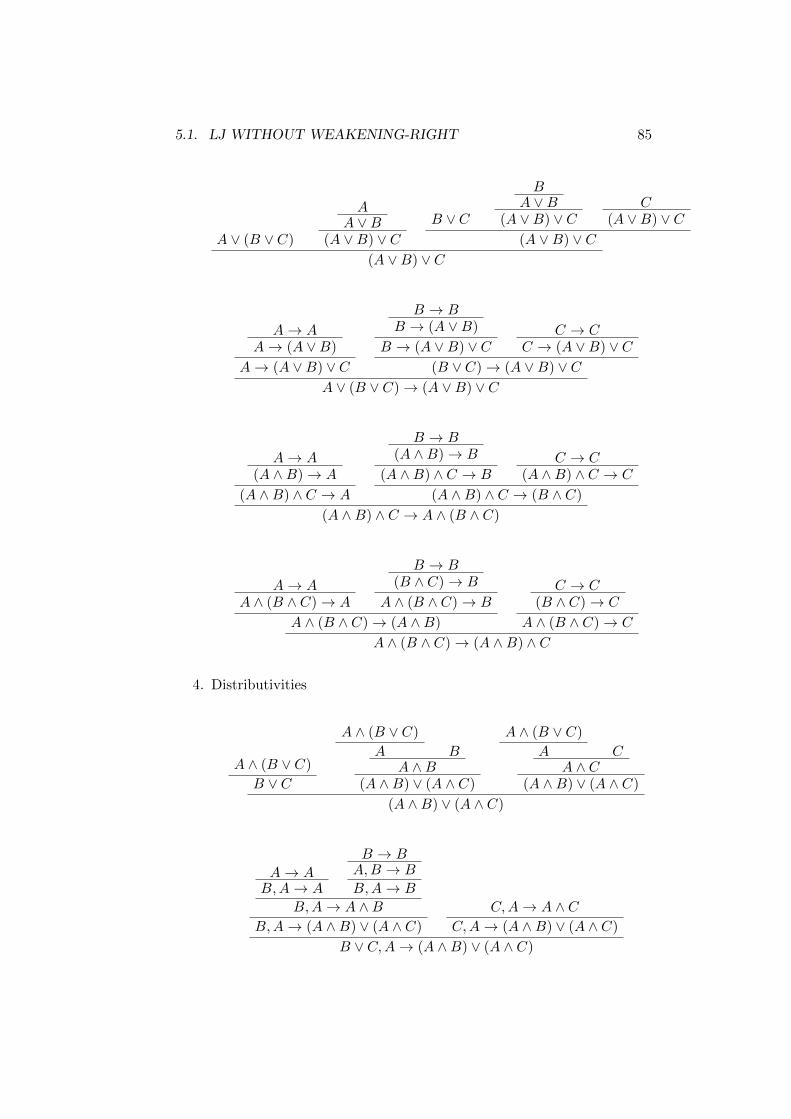
5.1. LJ WITHOUT WEAKENING-RIGHT 85
A ∨ (B ∨ C)
AA ∨B
(A ∨B) ∨ CB ∨ C
BA ∨B
(A ∨B) ∨ CC
(A ∨B) ∨ C(A ∨B) ∨ C
(A ∨B) ∨ C
A→ AA→ (A ∨B)
A→ (A ∨B) ∨ C
B → BB → (A ∨B)
B → (A ∨B) ∨ CC → C
C → (A ∨B) ∨ C(B ∨ C)→ (A ∨B) ∨ C
A ∨ (B ∨ C)→ (A ∨B) ∨ C
A→ A(A ∧B)→ A
(A ∧B) ∧ C → A
B → B(A ∧B)→ B
(A ∧B) ∧ C → BC → C
(A ∧B) ∧ C → C
(A ∧B) ∧ C → (B ∧ C)
(A ∧B) ∧ C → A ∧ (B ∧ C)
A→ AA ∧ (B ∧ C)→ A
B → B(B ∧ C)→ B
A ∧ (B ∧ C)→ B
A ∧ (B ∧ C)→ (A ∧B)
C → C(B ∧ C)→ C
A ∧ (B ∧ C)→ C
A ∧ (B ∧ C)→ (A ∧B) ∧ C
4. Distributivities
A ∧ (B ∨ C)
B ∨ C
A ∧ (B ∨ C)
A BA ∧B
(A ∧B) ∨ (A ∧ C)
A ∧ (B ∨ C)
A CA ∧ C
(A ∧B) ∨ (A ∧ C)
(A ∧B) ∨ (A ∧ C)
A→ AB,A→ A
B → BA,B → B
B,A→ B
B,A→ A ∧BB,A→ (A ∧B) ∨ (A ∧ C)
C,A→ A ∧ CC,A→ (A ∧B) ∨ (A ∧ C)
B ∨ C,A→ (A ∧B) ∨ (A ∧ C)
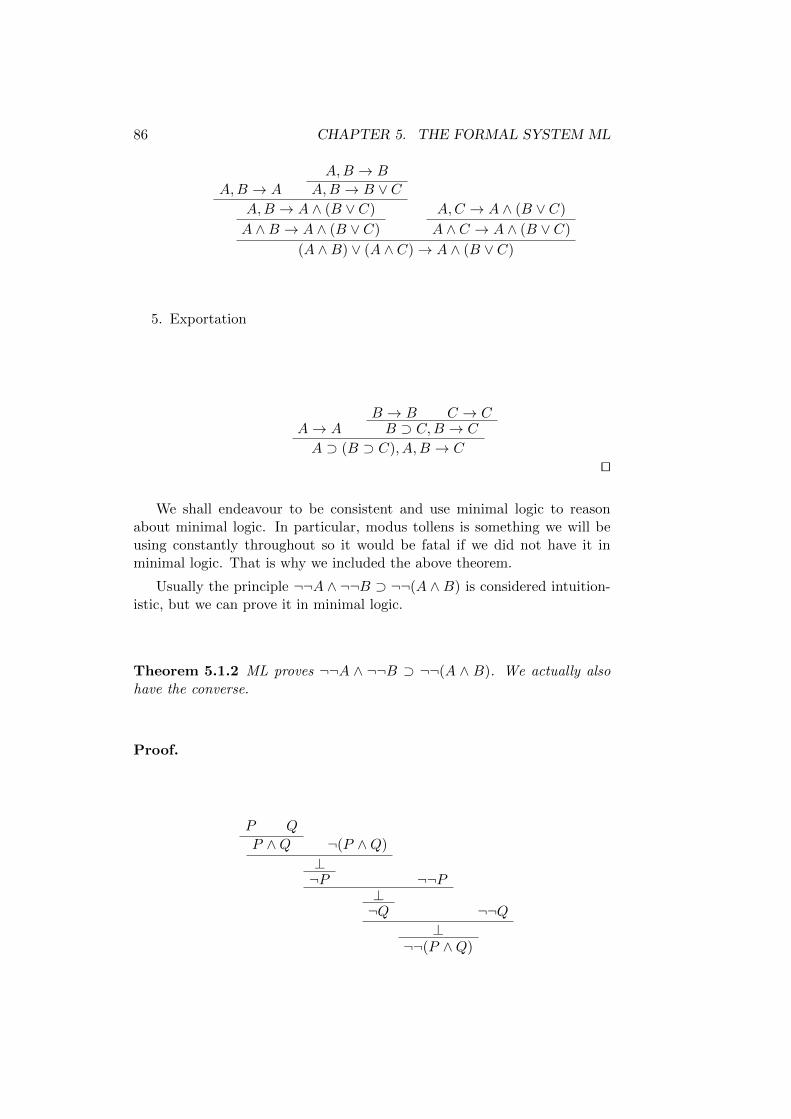
86 CHAPTER 5. THE FORMAL SYSTEM ML
A,B → A
A,B → B
A,B → B ∨ CA,B → A ∧ (B ∨ C)
A ∧B → A ∧ (B ∨ C)
A,C → A ∧ (B ∨ C)
A ∧ C → A ∧ (B ∨ C)
(A ∧B) ∨ (A ∧ C)→ A ∧ (B ∨ C)
5. Exportation
A→ AB → B C → CB ⊃ C,B → C
A ⊃ (B ⊃ C), A,B → C
ut
We shall endeavour to be consistent and use minimal logic to reasonabout minimal logic. In particular, modus tollens is something we will beusing constantly throughout so it would be fatal if we did not have it inminimal logic. That is why we included the above theorem.
Usually the principle ¬¬A ∧ ¬¬B ⊃ ¬¬(A ∧ B) is considered intuition-istic, but we can prove it in minimal logic.
Theorem 5.1.2 ML proves ¬¬A ∧ ¬¬B ⊃ ¬¬(A ∧ B). We actually alsohave the converse.
Proof.
P Q
P ∧Q ¬(P ∧Q)
⊥¬P ¬¬P
⊥¬Q ¬¬Q
⊥¬¬(P ∧Q)
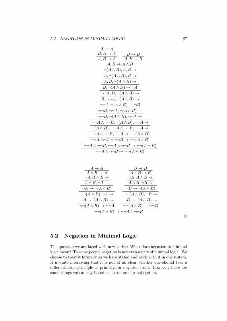
5.2. NEGATION IN MINIMAL LOGIC 87
A→ AB,A→ A
A,B → AB → BA,B → B
A,B → A ∧B¬(A ∧B), A,B →A,¬(A ∧B), B →A,B,¬(A ∧B)→B,¬(A ∧B)→ ¬A¬¬A,B,¬(A ∧B)→B,¬¬A,¬(A ∧B)→¬¬A,¬(A ∧B)→ ¬B¬¬B,¬¬A,¬(A ∧B)→¬¬B,¬(A ∧B),¬¬A→
¬¬A ∧ ¬¬B,¬(A ∧B),¬¬A→¬(A ∧B),¬¬A ∧ ¬¬B,¬¬A→¬¬A ∧ ¬¬B,¬¬A→ ¬¬(A ∧B)
¬¬A,¬¬A ∧ ¬¬B → ¬¬(A ∧B)
¬¬A ∧ ¬¬B,¬¬A ∧ ¬¬B → ¬¬(A ∧B)
¬¬A ∧ ¬¬B → ¬¬(A ∧B)
A→ AA ∧B → A¬A,A ∧B →A ∧B,¬A→¬A→ ¬(A ∧B)
¬¬(A ∧B),¬A→¬A,¬¬(A ∧B)→¬¬(A ∧B)→ ¬¬A
B → BA ∧B → B¬B,A ∧B →A ∧B,¬B →¬B → ¬(A ∧B)
¬¬(A ∧B),¬B →¬B,¬¬(A ∧B)→¬¬(A ∧B)→ ¬¬B
¬¬(A ∧B)→ ¬¬A ∧ ¬¬But
5.2 Negation in Minimal Logic
The question we are faced with now is this: What does negation in minimallogic mean? To some people negation is not even a part of minimal logic. Wechoose to treat it formally as we have stated and work with it in our system.It is quite interesting that it is not at all clear whether one should take adifferentiation principle as primitive or negation itself. However, there aresome things we can say based solely on our formal system.
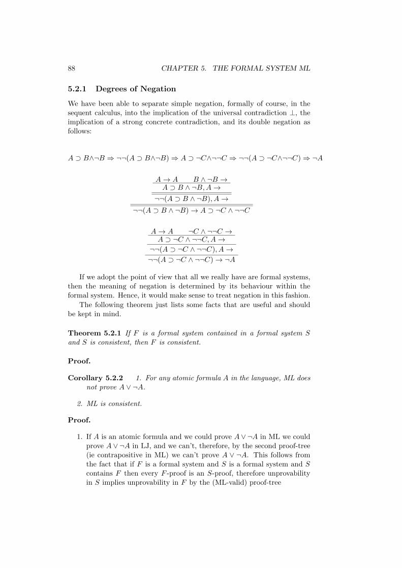
88 CHAPTER 5. THE FORMAL SYSTEM ML
5.2.1 Degrees of Negation
We have been able to separate simple negation, formally of course, in thesequent calculus, into the implication of the universal contradiction ⊥, theimplication of a strong concrete contradiction, and its double negation asfollows:
A ⊃ B∧¬B ⇒ ¬¬(A ⊃ B∧¬B)⇒ A ⊃ ¬C∧¬¬C ⇒ ¬¬(A ⊃ ¬C∧¬¬C)⇒ ¬A
A→ A B ∧ ¬B →A ⊃ B ∧ ¬B,A→
¬¬(A ⊃ B ∧ ¬B), A→¬¬(A ⊃ B ∧ ¬B)→ A ⊃ ¬C ∧ ¬¬C
A→ A ¬C ∧ ¬¬C →A ⊃ ¬C ∧ ¬¬C,A→
¬¬(A ⊃ ¬C ∧ ¬¬C), A→¬¬(A ⊃ ¬C ∧ ¬¬C)→ ¬A
If we adopt the point of view that all we really have are formal systems,then the meaning of negation is determined by its behaviour within theformal system. Hence, it would make sense to treat negation in this fashion.
The following theorem just lists some facts that are useful and shouldbe kept in mind.
Theorem 5.2.1 If F is a formal system contained in a formal system Sand S is consistent, then F is consistent.
Proof.
Corollary 5.2.2 1. For any atomic formula A in the language, ML doesnot prove A ∨ ¬A.
2. ML is consistent.
Proof.
1. If A is an atomic formula and we could prove A∨¬A in ML we couldprove A ∨ ¬A in LJ, and we can’t, therefore, by the second proof-tree(ie contrapositive in ML) we can’t prove A ∨ ¬A. This follows fromthe fact that if F is a formal system and S is a formal system and Scontains F then every F -proof is an S-proof, therefore unprovabilityin S implies unprovability in F by the (ML-valid) proof-tree
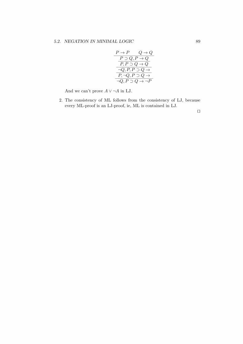
5.2. NEGATION IN MINIMAL LOGIC 89
P → P Q→ Q
P ⊃ Q,P → Q
P,P ⊃ Q→ Q
¬Q,P, P ⊃ Q→P,¬Q,P ⊃ Q→¬Q,P ⊃ Q→ ¬P
And we can’t prove A ∨ ¬A in LJ.
2. The consistency of ML follows from the consistency of LJ, becauseevery ML-proof is an LJ-proof, ie, ML is contained in LJ.
ut
90 CHAPTER 5. THE FORMAL SYSTEM ML
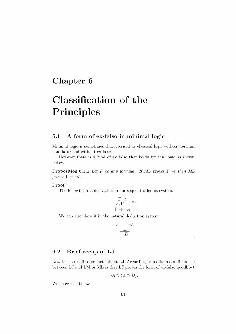
Chapter 6
Classification of thePrinciples
6.1 A form of ex-falso in minimal logic
Minimal logic is sometimes characterised as classical logic without tertiumnon datur and without ex falso.
However there is a kind of ex falso that holds for this logic as shownbelow.
Proposition 6.1.1 Let F be any formula. If ML proves Γ → then MLproves Γ→ ¬F .
Proof.The following is a derivation in our sequent calculus system.
Γ→w:l
A,Γ→Γ→ ¬A
We can also show it in the natural deduction system.
A ¬A⊥¬B ut
6.2 Brief recap of LJ
Now let us recall some facts about LJ. According to us the main differencebetween LJ and LM or ML is that LJ proves the form of ex-falso quodlibet
¬A ⊃ (A ⊃ B).
We show this below.
91
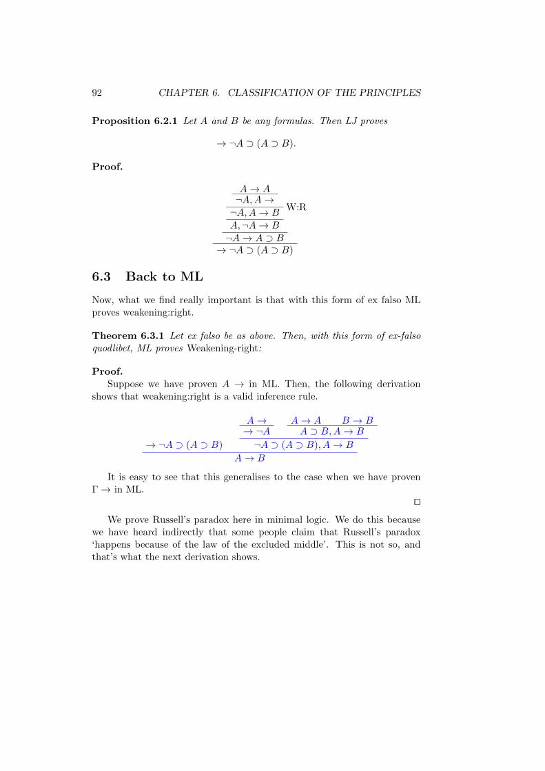
92 CHAPTER 6. CLASSIFICATION OF THE PRINCIPLES
Proposition 6.2.1 Let A and B be any formulas. Then LJ proves
→ ¬A ⊃ (A ⊃ B).
Proof.
A→ A¬A,A→
W:R¬A,A→ B
A,¬A→ B
¬A→ A ⊃ B→ ¬A ⊃ (A ⊃ B)
6.3 Back to ML
Now, what we find really important is that with this form of ex falso MLproves weakening:right.
Theorem 6.3.1 Let ex falso be as above. Then, with this form of ex-falsoquodlibet, ML proves Weakening-right:
Proof.Suppose we have proven A → in ML. Then, the following derivation
shows that weakening:right is a valid inference rule.
→ ¬A ⊃ (A ⊃ B)
A→→ ¬A
A→ A B → BA ⊃ B,A→ B
¬A ⊃ (A ⊃ B), A→ B
A→ B
It is easy to see that this generalises to the case when we have provenΓ→ in ML.
ut
We prove Russell’s paradox here in minimal logic. We do this becausewe have heard indirectly that some people claim that Russell’s paradox‘happens because of the law of the excluded middle’. This is not so, andthat’s what the next derivation shows.
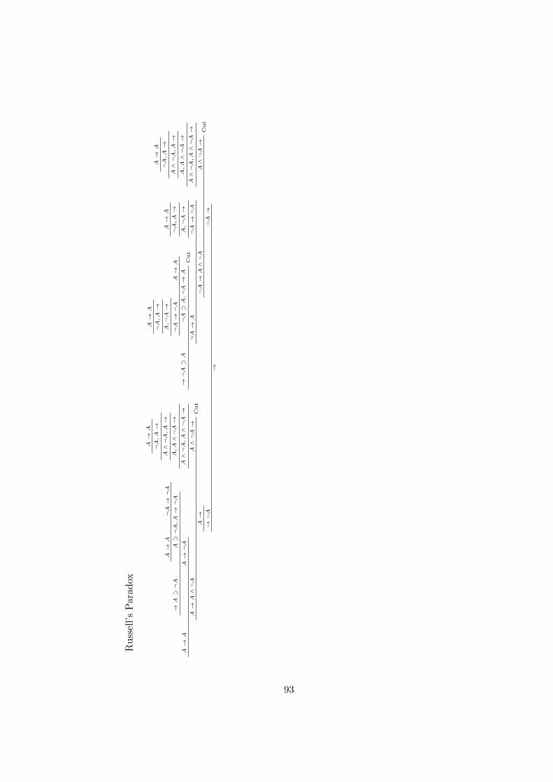
Ru
ssel
l’s
Para
dox
A→A
→A⊃¬A
A→A
¬A→¬A
A⊃¬A,A→¬A
A→¬A
A→A∧¬A
A→A
¬A,A→
A∧¬A,A→
A,A∧¬A→
A∧¬A,A∧¬A→
A∧¬A→
Cut
A→
→¬A
→¬A⊃A
A→A
¬A,A→
A,¬A→
¬A→¬A
A→A
¬A⊃A,¬A→A
Cut
¬A→A
A→A
¬A,A→
A,¬A→
¬A→¬A
¬A→A∧¬A
A→A
¬A,A→
A∧¬A,A→
A,A∧¬A→
A∧¬A,A∧¬A→
A∧¬A→
Cut
¬A→
→
93
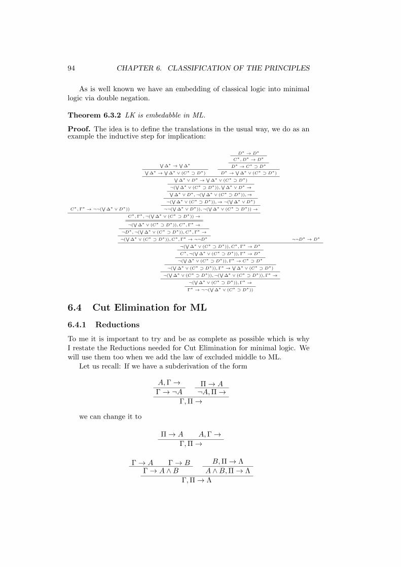
94 CHAPTER 6. CLASSIFICATION OF THE PRINCIPLES
As is well known we have an embedding of classical logic into minimallogic via double negation.
Theorem 6.3.2 LK is embedabble in ML.
Proof. The idea is to define the translations in the usual way, we do as anexample the inductive step for implication:
C∗,Γ∗ → ¬¬(∨
∆∗ ∨D∗))
∨∆∗ →
∨∆∗∨
∆∗ →∨
∆∗ ∨ (C∗ ⊃ D∗)
D∗ → D∗
C∗, D∗ → D∗
D∗ → C∗ ⊃ D∗
D∗ →∨
∆∗ ∨ (C∗ ⊃ D∗)∨∆∗ ∨D∗ →
∨∆∗ ∨ (C∗ ⊃ D∗)
¬(∨
∆∗ ∨ (C∗ ⊃ D∗)),∨
∆∗ ∨D∗ →∨∆∗ ∨D∗,¬(
∨∆∗ ∨ (C∗ ⊃ D∗)),→
¬(∨
∆∗ ∨ (C∗ ⊃ D∗)),→ ¬(∨
∆∗ ∨D∗)
¬¬(∨
∆∗ ∨D∗)),¬(∨
∆∗ ∨ (C∗ ⊃ D∗))→
C∗,Γ∗,¬(∨
∆∗ ∨ (C∗ ⊃ D∗))→
¬(∨
∆∗ ∨ (C∗ ⊃ D∗)), C∗,Γ∗ →
¬D∗,¬(∨
∆∗ ∨ (C∗ ⊃ D∗)), C∗,Γ∗ →
¬(∨
∆∗ ∨ (C∗ ⊃ D∗)), C∗,Γ∗ → ¬¬D∗ ¬¬D∗ → D∗
¬(∨
∆∗ ∨ (C∗ ⊃ D∗)), C∗,Γ∗ → D∗
C∗,¬(∨
∆∗ ∨ (C∗ ⊃ D∗)),Γ∗ → D∗
¬(∨
∆∗ ∨ (C∗ ⊃ D∗)),Γ∗ → C∗ ⊃ D∗
¬(∨
∆∗ ∨ (C∗ ⊃ D∗)),Γ∗ →∨
∆∗ ∨ (C∗ ⊃ D∗)
¬(∨
∆∗ ∨ (C∗ ⊃ D∗)),¬(∨
∆∗ ∨ (C∗ ⊃ D∗)),Γ∗ →
¬(∨
∆∗ ∨ (C∗ ⊃ D∗)),Γ∗ →
Γ∗ → ¬¬(∨
∆∗ ∨ (C∗ ⊃ D∗))
6.4 Cut Elimination for ML
6.4.1 Reductions
To me it is important to try and be as complete as possible which is whyI restate the Reductions needed for Cut Elimination for minimal logic. Wewill use them too when we add the law of excluded middle to ML.
Let us recall: If we have a subderivation of the form
A,Γ→Γ→ ¬A
Π→ A¬A,Π→
Γ,Π→
we can change it to
Π→ A A,Γ→Γ,Π→
Γ→ A Γ→ BΓ→ A ∧B
B,Π→ Λ
A ∧B,Π→ Λ
Γ,Π→ Λ
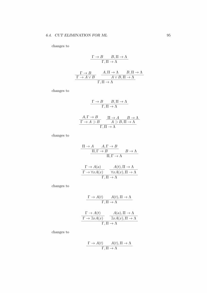
6.4. CUT ELIMINATION FOR ML 95
changes to
Γ→ B B,Π→ Λ
Γ,Π→ Λ
Γ→ BΓ→ A ∨B
A,Π→ Λ B,Π→ Λ
A ∨B,Π→ Λ
Γ,Π→ Λ
changes to
Γ→ B B,Π→ Λ
Γ,Π→ Λ
A,Γ→ B
Γ→ A ⊃ BΠ→ A B → ΛA ⊃ B,Π→ Λ
Γ,Π→ Λ
changes to
Π→ A A,Γ→ B
Π,Γ→ B B → Λ
Π,Γ→ Λ
Γ→ A(a)
Γ→ ∀xA(x)
A(t),Π→ Λ
∀xA(x),Π→ Λ
Γ,Π→ Λ
changes to
Γ→ A(t) A(t),Π→ Λ
Γ,Π→ Λ
Γ→ A(t)
Γ→ ∃xA(x)
A(a),Π→ Λ
∃xA(x),Π→ Λ
Γ,Π→ Λ
changes to
Γ→ A(t) A(t),Π→ Λ
Γ,Π→ Λ
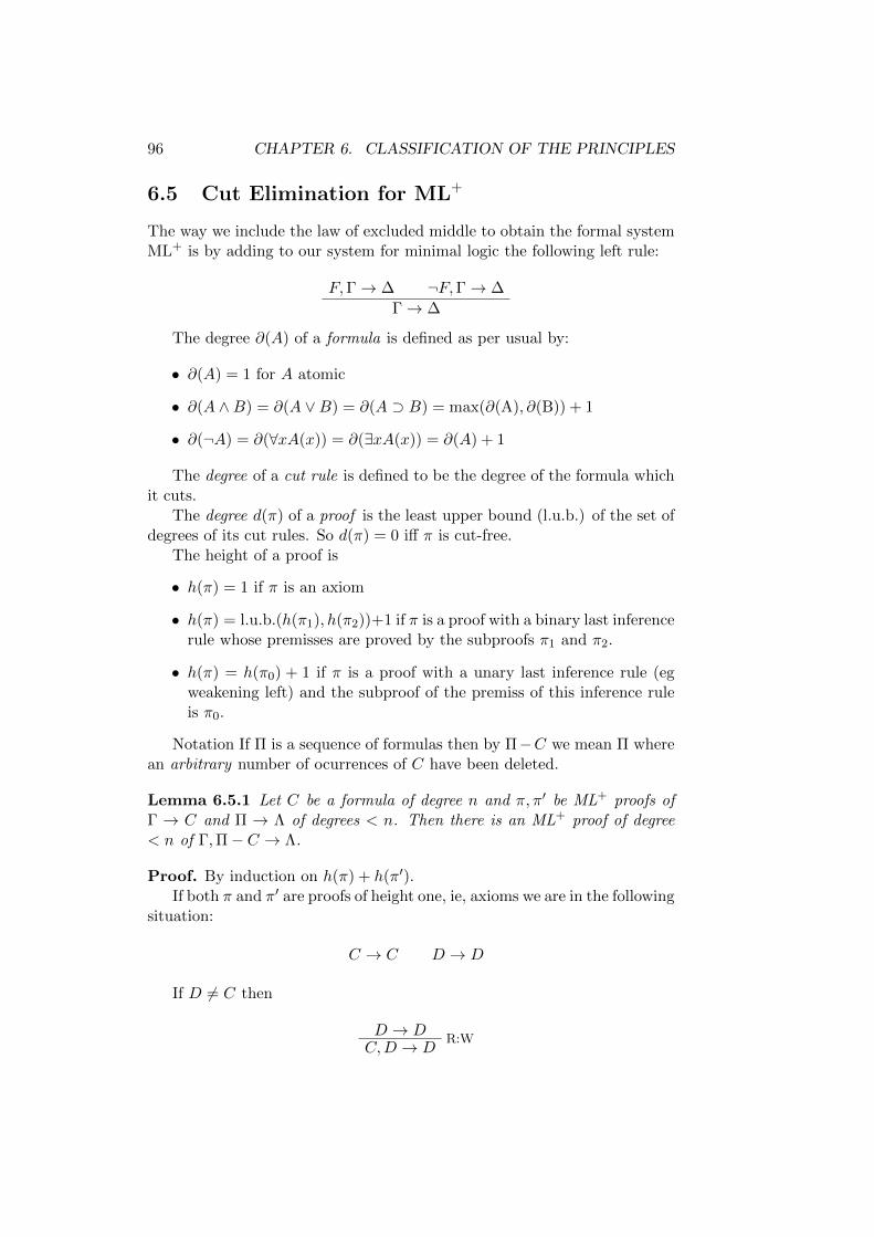
96 CHAPTER 6. CLASSIFICATION OF THE PRINCIPLES
6.5 Cut Elimination for ML+
The way we include the law of excluded middle to obtain the formal systemML+ is by adding to our system for minimal logic the following left rule:
F,Γ→ ∆ ¬F,Γ→ ∆
Γ→ ∆
The degree ∂(A) of a formula is defined as per usual by:
• ∂(A) = 1 for A atomic
• ∂(A ∧B) = ∂(A ∨B) = ∂(A ⊃ B) = max(∂(A), ∂(B)) + 1
• ∂(¬A) = ∂(∀xA(x)) = ∂(∃xA(x)) = ∂(A) + 1
The degree of a cut rule is defined to be the degree of the formula whichit cuts.
The degree d(π) of a proof is the least upper bound (l.u.b.) of the set ofdegrees of its cut rules. So d(π) = 0 iff π is cut-free.
The height of a proof is
• h(π) = 1 if π is an axiom
• h(π) = l.u.b.(h(π1), h(π2))+1 if π is a proof with a binary last inferencerule whose premisses are proved by the subproofs π1 and π2.
• h(π) = h(π0) + 1 if π is a proof with a unary last inference rule (egweakening left) and the subproof of the premiss of this inference ruleis π0.
Notation If Π is a sequence of formulas then by Π−C we mean Π wherean arbitrary number of ocurrences of C have been deleted.
Lemma 6.5.1 Let C be a formula of degree n and π, π′ be ML+ proofs ofΓ → C and Π → Λ of degrees < n. Then there is an ML+ proof of degree< n of Γ,Π− C → Λ.
Proof. By induction on h(π) + h(π′).If both π and π′ are proofs of height one, ie, axioms we are in the following
situation:
C → C D → D
If D 6= C then
D → DR:W
C,D → D
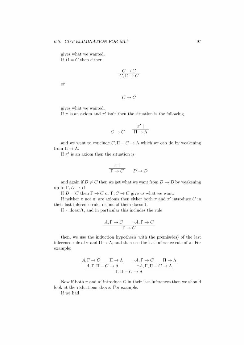
6.5. CUT ELIMINATION FOR ML+ 97
gives what we wanted.
If D = C then either
C → CC,C → C
or
C → C
gives what we wanted.
If π is an axiom and π′ isn’t then the situation is the following
C → C
π′ Π→ Λ
and we want to conclude C,Π− C → Λ which we can do by weakeningfrom Π→ Λ.
If π′ is an axiom then the situation is
π Γ→ C D → D
and again if D 6= C then we get what we want from D → D by weakeningup to Γ, D → D.
If D = C then Γ→ C or Γ, C → C give us what we want.
If neither π nor π′ are axioms then either both π and π′ introduce C intheir last inference rule, or one of them doesn’t.
If π doesn’t, and in particular this includes the rule
A,Γ→ C ¬A,Γ→ C
Γ→ C
then, we use the induction hypothesis with the premiss(es) of the lastinference rule of π and Π→ Λ, and then use the last inference rule of π. Forexample:
A,Γ→ C Π→ Λ
A,Γ,Π− C → Λ
¬A,Γ→ C Π→ Λ
¬A,Γ,Π− C → Λ
Γ,Π− C → Λ
Now if both π and π′ introduce C in their last inferences then we shouldlook at the reductions above. For example:
If we had
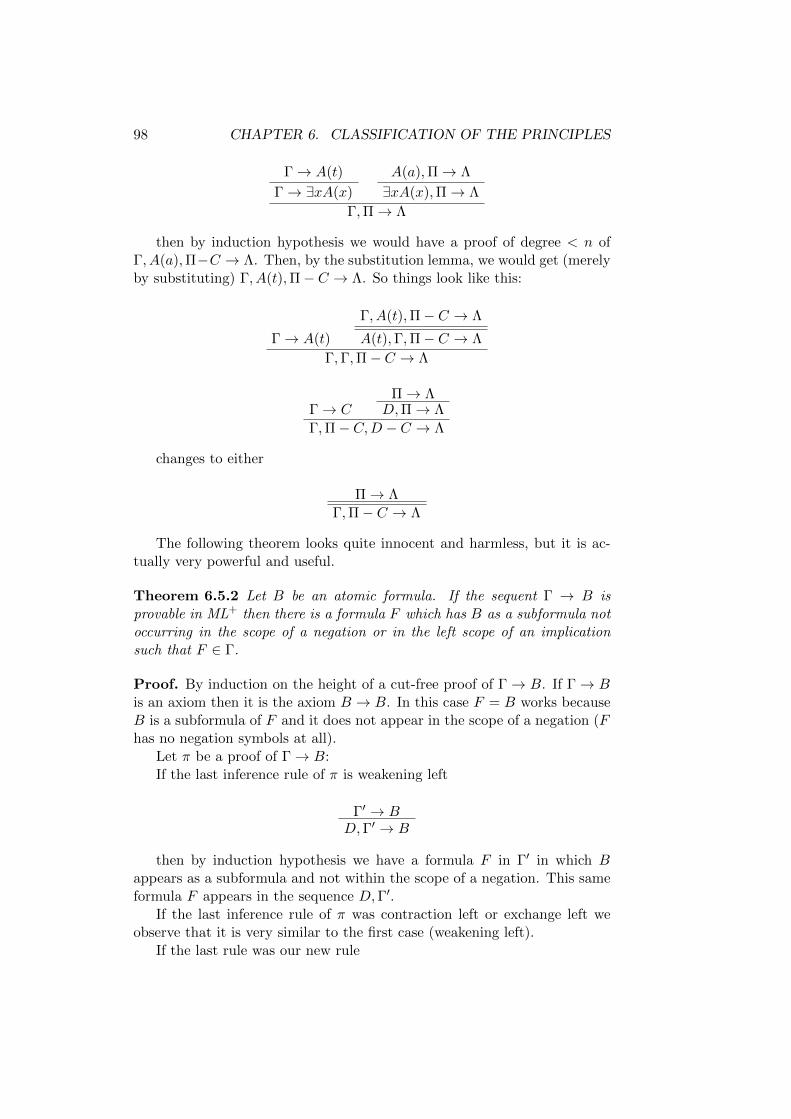
98 CHAPTER 6. CLASSIFICATION OF THE PRINCIPLES
Γ→ A(t)
Γ→ ∃xA(x)
A(a),Π→ Λ
∃xA(x),Π→ Λ
Γ,Π→ Λ
then by induction hypothesis we would have a proof of degree < n ofΓ, A(a),Π−C → Λ. Then, by the substitution lemma, we would get (merelyby substituting) Γ, A(t),Π− C → Λ. So things look like this:
Γ→ A(t)
Γ, A(t),Π− C → Λ
A(t),Γ,Π− C → Λ
Γ,Γ,Π− C → Λ
Γ→ CΠ→ ΛD,Π→ Λ
Γ,Π− C,D − C → Λ
changes to either
Π→ Λ
Γ,Π− C → Λ
The following theorem looks quite innocent and harmless, but it is ac-tually very powerful and useful.
Theorem 6.5.2 Let B be an atomic formula. If the sequent Γ → B isprovable in ML+ then there is a formula F which has B as a subformula notoccurring in the scope of a negation or in the left scope of an implicationsuch that F ∈ Γ.
Proof. By induction on the height of a cut-free proof of Γ→ B. If Γ→ Bis an axiom then it is the axiom B → B. In this case F = B works becauseB is a subformula of F and it does not appear in the scope of a negation (Fhas no negation symbols at all).
Let π be a proof of Γ→ B:If the last inference rule of π is weakening left
Γ′ → BD,Γ′ → B
then by induction hypothesis we have a formula F in Γ′ in which Bappears as a subformula and not within the scope of a negation. This sameformula F appears in the sequence D,Γ′.
If the last inference rule of π was contraction left or exchange left weobserve that it is very similar to the first case (weakening left).
If the last rule was our new rule
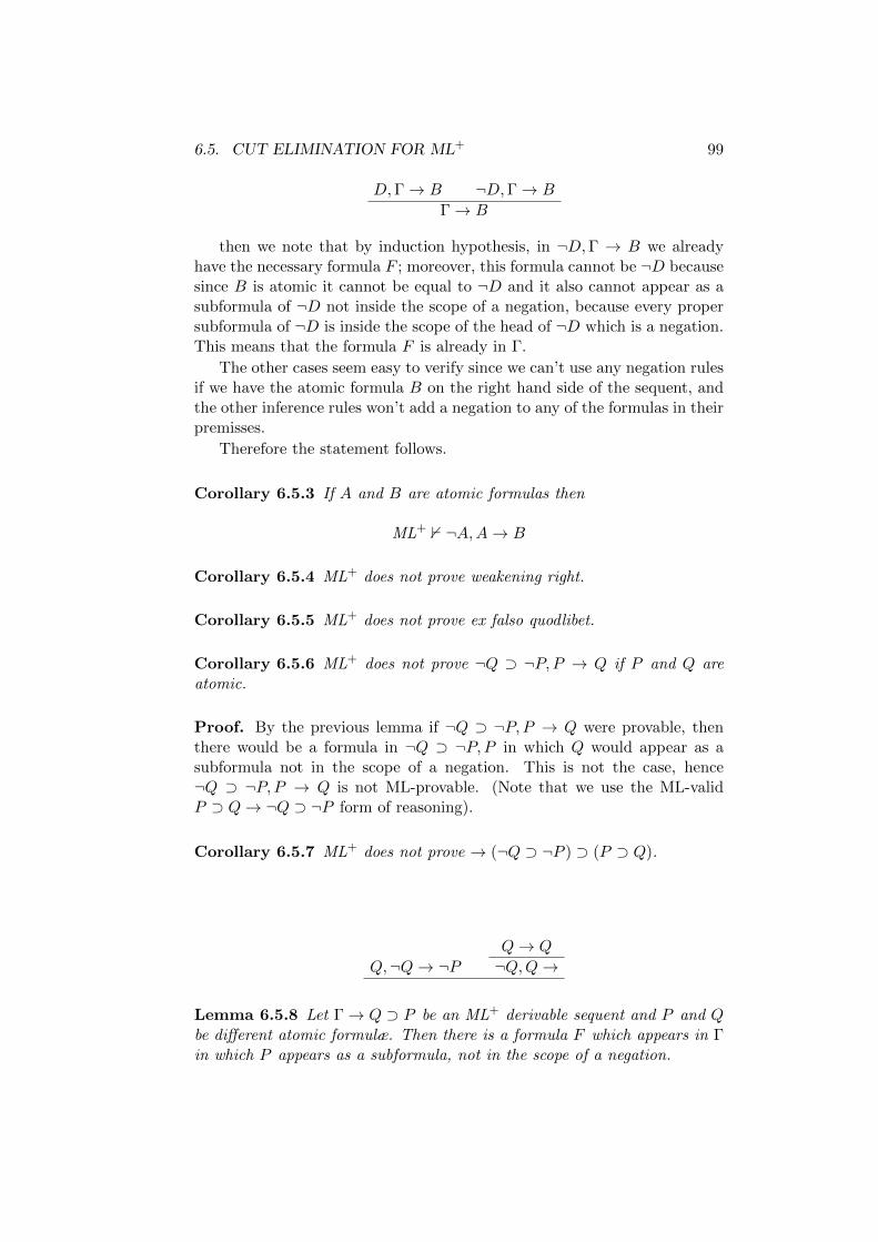
6.5. CUT ELIMINATION FOR ML+ 99
D,Γ→ B ¬D,Γ→ B
Γ→ B
then we note that by induction hypothesis, in ¬D,Γ → B we alreadyhave the necessary formula F ; moreover, this formula cannot be ¬D becausesince B is atomic it cannot be equal to ¬D and it also cannot appear as asubformula of ¬D not inside the scope of a negation, because every propersubformula of ¬D is inside the scope of the head of ¬D which is a negation.This means that the formula F is already in Γ.
The other cases seem easy to verify since we can’t use any negation rulesif we have the atomic formula B on the right hand side of the sequent, andthe other inference rules won’t add a negation to any of the formulas in theirpremisses.
Therefore the statement follows.
Corollary 6.5.3 If A and B are atomic formulas then
ML+ 0 ¬A,A→ B
Corollary 6.5.4 ML+ does not prove weakening right.
Corollary 6.5.5 ML+ does not prove ex falso quodlibet.
Corollary 6.5.6 ML+ does not prove ¬Q ⊃ ¬P, P → Q if P and Q areatomic.
Proof. By the previous lemma if ¬Q ⊃ ¬P, P → Q were provable, thenthere would be a formula in ¬Q ⊃ ¬P, P in which Q would appear as asubformula not in the scope of a negation. This is not the case, hence¬Q ⊃ ¬P, P → Q is not ML-provable. (Note that we use the ML-validP ⊃ Q→ ¬Q ⊃ ¬P form of reasoning).
Corollary 6.5.7 ML+ does not prove → (¬Q ⊃ ¬P ) ⊃ (P ⊃ Q).
Q,¬Q→ ¬PQ→ Q
¬Q,Q→
Lemma 6.5.8 Let Γ→ Q ⊃ P be an ML+ derivable sequent and P and Qbe different atomic formulæ. Then there is a formula F which appears in Γin which P appears as a subformula, not in the scope of a negation.
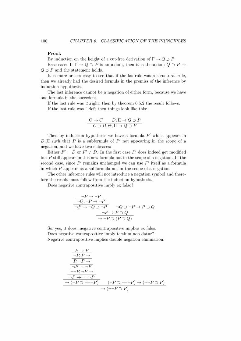
100 CHAPTER 6. CLASSIFICATION OF THE PRINCIPLES
Proof.
By induction on the height of a cut-free derivation of Γ→ Q ⊃ P :
Base case: If Γ → Q ⊃ P is an axiom, then it is the axiom Q ⊃ P →Q ⊃ P and the statement holds.
It is more or less easy to see that if the las rule was a structural rule,then we already had the desired formula in the premiss of the inference byinduction hypothesis.
The last inference cannot be a negation of either form, because we haveone formula in the succedent.
If the last rule was ⊃:right, then by theorem 6.5.2 the result follows.
If the last rule was ⊃:left then things look like this:
Θ→ C D,Π→ Q ⊃ PC ⊃ D,Θ,Π→ Q ⊃ P
Then by induction hypothesis we have a formula F ′ which appears inD,Π such that P is a subformula of F ′ not appearing in the scope of anegation, and we have two subcases:
Either F ′ = D or F ′ 6= D. In the first case F ′ does indeed get modifiedbut P still appears in this new formula not in the scope of a negation. In thesecond case, since F ′ remains unchanged we can use F ′ itself as a formulain which P appears as a subformula not in the scope of a negation.
The other inference rules will not introduce a negation symbol and there-fore the result must follow from the induction hypothesis.
Does negative contrapositive imply ex falso?
¬P → ¬P¬Q,¬P → ¬P¬P → ¬Q ⊃ ¬P ¬Q ⊃ ¬P → P ⊃ Q
¬P → P ⊃ Q→ ¬P ⊃ (P ⊃ Q)
So, yes, it does: negative contrapositive implies ex falso.
Does negative contrapositive imply tertium non datur?
Negative contrapositive implies double negation elimination:
P → P¬P, P →P,¬P →¬P → ¬P¬¬P,¬P →¬P → ¬¬¬P→ (¬P ⊃ ¬¬¬P ) (¬P ⊃ ¬¬¬P )→ (¬¬P ⊃ P )
→ (¬¬P ⊃ P )
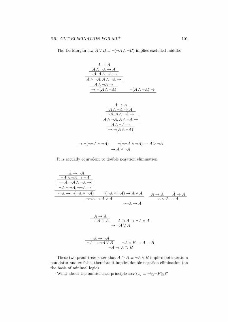
6.5. CUT ELIMINATION FOR ML+ 101
The De Morgan law A ∨B ≡ ¬(¬A ∧ ¬B) implies excluded middle:
A→ AA ∧ ¬A→ A¬A,A ∧ ¬A→
A ∧ ¬A,A ∧ ¬A→A ∧ ¬A→→ ¬(A ∧ ¬A) ¬(A ∧ ¬A)→
A→ AA ∧ ¬A→ A¬A,A ∧ ¬A→
A ∧ ¬A,A ∧ ¬A→A ∧ ¬A→→ ¬(A ∧ ¬A)
→ ¬(¬¬A ∧ ¬A) ¬(¬¬A ∧ ¬A)→ A ∨ ¬A→ A ∨ ¬A
It is actually equivalent to double negation elimination
¬A→ ¬A¬A ∧ ¬A→ ¬A¬¬A,¬A ∧ ¬A→¬A ∧ ¬A,¬¬A→¬¬A→ ¬(¬A ∧ ¬A) ¬(¬A ∧ ¬A)→ A ∨A
¬¬A→ A ∨AA→ A A→ A
A ∨A→ A¬¬A→ A
A→ A→ A ⊃ A A ⊃ A→ ¬A ∨A
→ ¬A ∨A
¬A→ ¬A¬A→ ¬A ∨B ¬A ∨B → A ⊃ B
¬A→ A ⊃ B
These two proof trees show that A ⊃ B ≡ ¬A ∨B implies both tertiumnon datur and ex falso, therefore it implies double negation elimination (onthe basis of minimal logic).
What about the omniscience principle ∃xF (x) ≡ ¬∀y¬F (y)?
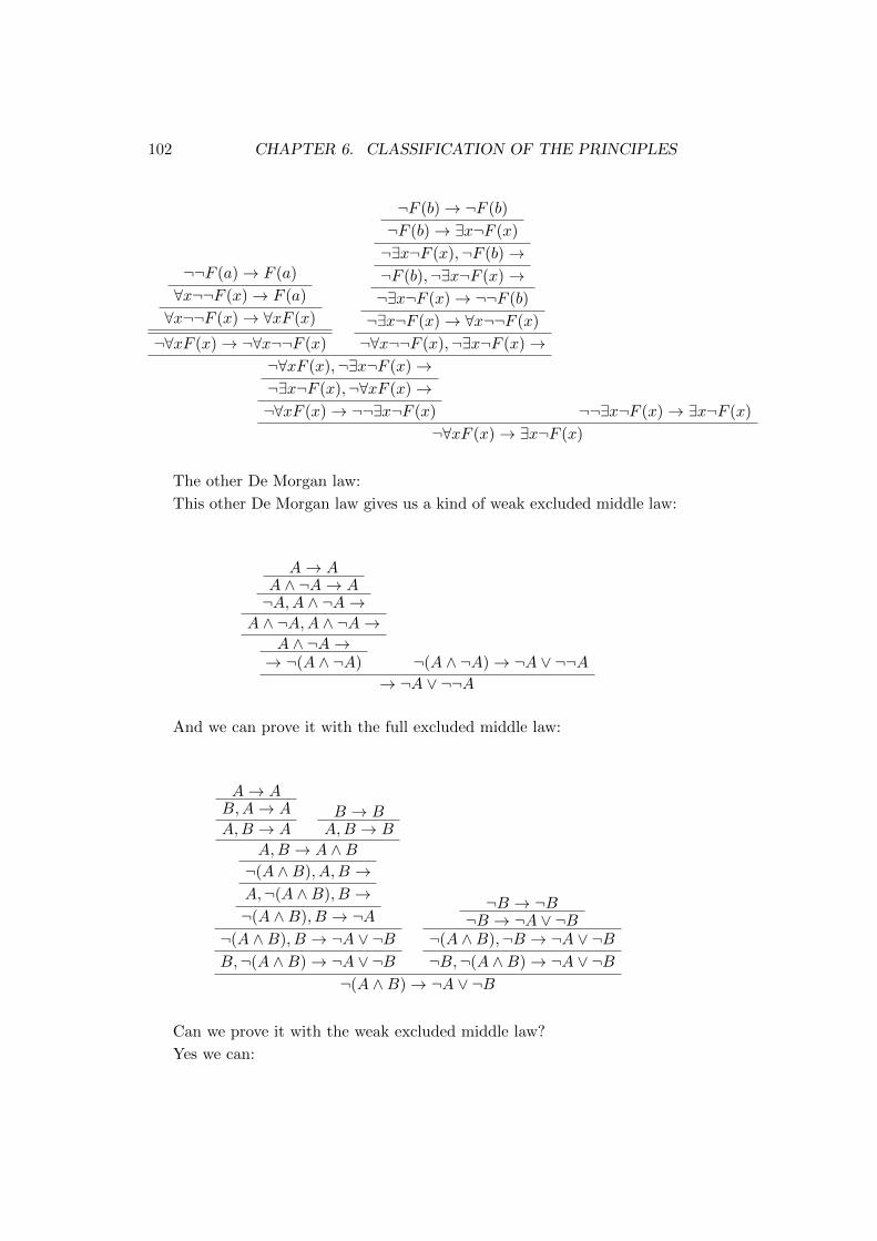
102 CHAPTER 6. CLASSIFICATION OF THE PRINCIPLES
¬¬F (a)→ F (a)
∀x¬¬F (x)→ F (a)
∀x¬¬F (x)→ ∀xF (x)
¬∀xF (x)→ ¬∀x¬¬F (x)
¬F (b)→ ¬F (b)
¬F (b)→ ∃x¬F (x)
¬∃x¬F (x),¬F (b)→¬F (b),¬∃x¬F (x)→¬∃x¬F (x)→ ¬¬F (b)
¬∃x¬F (x)→ ∀x¬¬F (x)
¬∀x¬¬F (x),¬∃x¬F (x)→¬∀xF (x),¬∃x¬F (x)→¬∃x¬F (x),¬∀xF (x)→¬∀xF (x)→ ¬¬∃x¬F (x) ¬¬∃x¬F (x)→ ∃x¬F (x)
¬∀xF (x)→ ∃x¬F (x)
The other De Morgan law:
This other De Morgan law gives us a kind of weak excluded middle law:
A→ AA ∧ ¬A→ A¬A,A ∧ ¬A→
A ∧ ¬A,A ∧ ¬A→A ∧ ¬A→→ ¬(A ∧ ¬A) ¬(A ∧ ¬A)→ ¬A ∨ ¬¬A
→ ¬A ∨ ¬¬A
And we can prove it with the full excluded middle law:
A→ AB,A→ A
A,B → AB → BA,B → B
A,B → A ∧B¬(A ∧B), A,B →A,¬(A ∧B), B →¬(A ∧B), B → ¬A
¬(A ∧B), B → ¬A ∨ ¬BB,¬(A ∧B)→ ¬A ∨ ¬B
¬B → ¬B¬B → ¬A ∨ ¬B
¬(A ∧B),¬B → ¬A ∨ ¬B¬B,¬(A ∧B)→ ¬A ∨ ¬B
¬(A ∧B)→ ¬A ∨ ¬B
Can we prove it with the weak excluded middle law?
Yes we can:
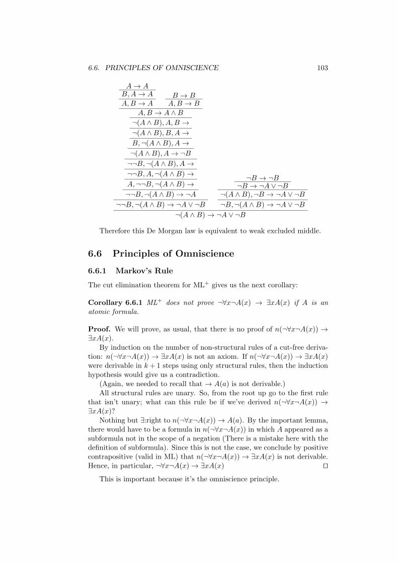
6.6. PRINCIPLES OF OMNISCIENCE 103
A→ AB,A→ A
A,B → AB → BA,B → B
A,B → A ∧B¬(A ∧B), A,B →¬(A ∧B), B,A→B,¬(A ∧B), A→¬(A ∧B), A→ ¬B¬¬B,¬(A ∧B), A→¬¬B,A,¬(A ∧B)→A,¬¬B,¬(A ∧B)→¬¬B,¬(A ∧B)→ ¬A
¬¬B,¬(A ∧B)→ ¬A ∨ ¬B
¬B → ¬B¬B → ¬A ∨ ¬B
¬(A ∧B),¬B → ¬A ∨ ¬B¬B,¬(A ∧B)→ ¬A ∨ ¬B
¬(A ∧B)→ ¬A ∨ ¬B
Therefore this De Morgan law is equivalent to weak excluded middle.
6.6 Principles of Omniscience
6.6.1 Markov’s Rule
The cut elimination theorem for ML+ gives us the next corollary:
Corollary 6.6.1 ML+ does not prove ¬∀x¬A(x) → ∃xA(x) if A is anatomic formula.
Proof. We will prove, as usual, that there is no proof of n(¬∀x¬A(x)) →∃xA(x).
By induction on the number of non-structural rules of a cut-free deriva-tion: n(¬∀x¬A(x))→ ∃xA(x) is not an axiom. If n(¬∀x¬A(x))→ ∃xA(x)were derivable in k+ 1 steps using only structural rules, then the inductionhypothesis would give us a contradiction.
(Again, we needed to recall that → A(a) is not derivable.)
All structural rules are unary. So, from the root up go to the first rulethat isn’t unary; what can this rule be if we’ve derived n(¬∀x¬A(x)) →∃xA(x)?
Nothing but ∃:right to n(¬∀x¬A(x))→ A(a). By the important lemma,there would have to be a formula in n(¬∀x¬A(x)) in which A appeared as asubformula not in the scope of a negation (There is a mistake here with thedefinition of subformula). Since this is not the case, we conclude by positivecontrapositive (valid in ML) that n(¬∀x¬A(x))→ ∃xA(x) is not derivable.Hence, in particular, ¬∀x¬A(x)→ ∃xA(x) ut
This is important because it’s the omniscience principle.
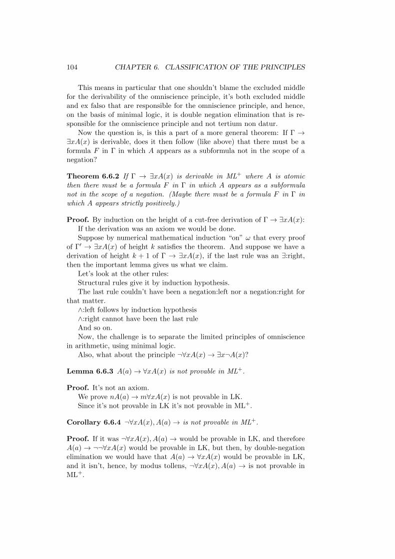
104 CHAPTER 6. CLASSIFICATION OF THE PRINCIPLES
This means in particular that one shouldn’t blame the excluded middlefor the derivability of the omniscience principle, it’s both excluded middleand ex falso that are responsible for the omniscience principle, and hence,on the basis of minimal logic, it is double negation elimination that is re-sponsible for the omniscience principle and not tertium non datur.
Now the question is, is this a part of a more general theorem: If Γ →∃xA(x) is derivable, does it then follow (like above) that there must be aformula F in Γ in which A appears as a subformula not in the scope of anegation?
Theorem 6.6.2 If Γ → ∃xA(x) is derivable in ML+ where A is atomicthen there must be a formula F in Γ in which A appears as a subformulanot in the scope of a negation. (Maybe there must be a formula F in Γ inwhich A appears strictly positively.)
Proof. By induction on the height of a cut-free derivation of Γ→ ∃xA(x):If the derivation was an axiom we would be done.Suppose by numerical mathematical induction “on” ω that every proof
of Γ′ → ∃xA(x) of height k satisfies the theorem. And suppose we have aderivation of height k + 1 of Γ → ∃xA(x), if the last rule was an ∃:right,then the important lemma gives us what we claim.
Let’s look at the other rules:Structural rules give it by induction hypothesis.The last rule couldn’t have been a negation:left nor a negation:right for
that matter.∧:left follows by induction hypothesis∧:right cannot have been the last ruleAnd so on.Now, the challenge is to separate the limited principles of omniscience
in arithmetic, using minimal logic.Also, what about the principle ¬∀xA(x)→ ∃x¬A(x)?
Lemma 6.6.3 A(a)→ ∀xA(x) is not provable in ML+.
Proof. It’s not an axiom.We prove nA(a)→ m∀xA(x) is not provable in LK.Since it’s not provable in LK it’s not provable in ML+.
Corollary 6.6.4 ¬∀xA(x), A(a)→ is not provable in ML+.
Proof. If it was ¬∀xA(x), A(a)→ would be provable in LK, and thereforeA(a) → ¬¬∀xA(x) would be provable in LK, but then, by double-negationelimination we would have that A(a) → ∀xA(x) would be provable in LK,and it isn’t, hence, by modus tollens, ¬∀xA(x), A(a) → is not provable inML+.
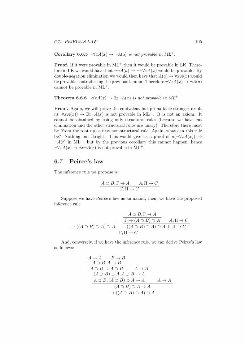
6.7. PEIRCE’S LAW 105
Corollary 6.6.5 ¬∀xA(x)→ ¬A(a) is not provable in ML+.
Proof. If it were provable in ML+ then it would be provable in LK. There-fore in LK we would have that ¬¬A(a)→ ¬¬∀xA(x) would be provable. Bydouble-negation elimination we would then have that A(a)→ ∀xA(x) wouldbe provable contradicting the previous lemma. Therefore ¬∀xA(x)→ ¬A(a)cannot be provable in ML+.
Theorem 6.6.6 ¬∀xA(x)→ ∃x¬A(x) is not provable in ML+.
Proof. Again, we will prove the equivalent but prima facie stronger resultn(¬∀xA(x)) → ∃x¬A(x) is not provable in ML+. It is not an axiom. Itcannot be obtained by using only structural rules (because we have cutelimination and the other structural rules are unary). Therefore there mustbe (from the root up) a first non-structural rule. Again, what can this rulebe? Nothing but ∃:right. This would give us a proof of n(¬∀xA(x)) →¬A(t) in ML+, but by the previous corollary this cannot happen, hence¬∀xA(x)→ ∃x¬A(x) is not provable in ML+.
6.7 Peirce’s law
The inference rule we propose is
A ⊃ B,Γ→ A A,Π→ C
Γ,Π→ C
Suppose we have Peirce’s law as an axiom, then, we have the proposedinference rule
→ ((A ⊃ B) ⊃ A) ⊃ A
A ⊃ B,Γ→ A
Γ→ (A ⊃ B) ⊃ A A,Π→ C
((A ⊃ B) ⊃ A) ⊃ A,Γ,Π→ C
Γ,Π→ C
And, conversely, if we have the inference rule, we can derive Peirce’s lawas follows:
A→ A B → BA ⊃ B,A→ B
A ⊃ B → A ⊃ B A→ A(A ⊃ B) ⊃ A,A ⊃ B → A
A ⊃ B, (A ⊃ B) ⊃ A→ A A→ A
(A ⊃ B) ⊃ A→ A
→ ((A ⊃ B) ⊃ A) ⊃ A
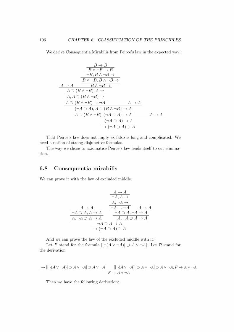
106 CHAPTER 6. CLASSIFICATION OF THE PRINCIPLES
We derive Consequentia Mirabilis from Peirce’s law in the expected way:
A→ A
B → BB ∧ ¬B → B¬B,B ∧ ¬B →
B ∧ ¬B,B ∧ ¬B →B ∧ ¬B →
A ⊃ (B ∧ ¬B), A→A,A ⊃ (B ∧ ¬B)→A ⊃ (B ∧ ¬B)→ ¬A A→ A
(¬A ⊃ A), A ⊃ (B ∧ ¬B)→ A
A ⊃ (B ∧ ¬B), (¬A ⊃ A)→ A A→ A
(¬A ⊃ A)→ A
→ (¬A ⊃ A) ⊃ A
That Peirce’s law does not imply ex falso is long and complicated. Weneed a notion of strong disjunctive formulas.
The way we chose to axiomatise Peirce’s law lends itself to cut elimina-tion.
6.8 Consequentia mirabilis
We can prove it with the law of excluded middle.
A→ A¬A ⊃ A,A→ A
A,¬A ⊃ A→ A
A→ A¬A,A→A,¬A→¬A→ ¬A A→ A¬A ⊃ A,¬A→ A
¬A,¬A ⊃ A→ A
¬A ⊃ A→ A→ (¬A ⊃ A) ⊃ A
And we can prove the law of the excluded middle with it:
Let F stand for the formula [[¬(A ∨ ¬A)] ⊃ A ∨ ¬A]. Let D stand forthe derivation
→ [[¬(A ∨ ¬A)] ⊃ A ∨ ¬A] ⊃ A ∨ ¬A [[¬(A ∨ ¬A)] ⊃ A ∨ ¬A] ⊃ A ∨ ¬A,F → A ∨ ¬AF → A ∨ ¬A
Then we have the following derivation:
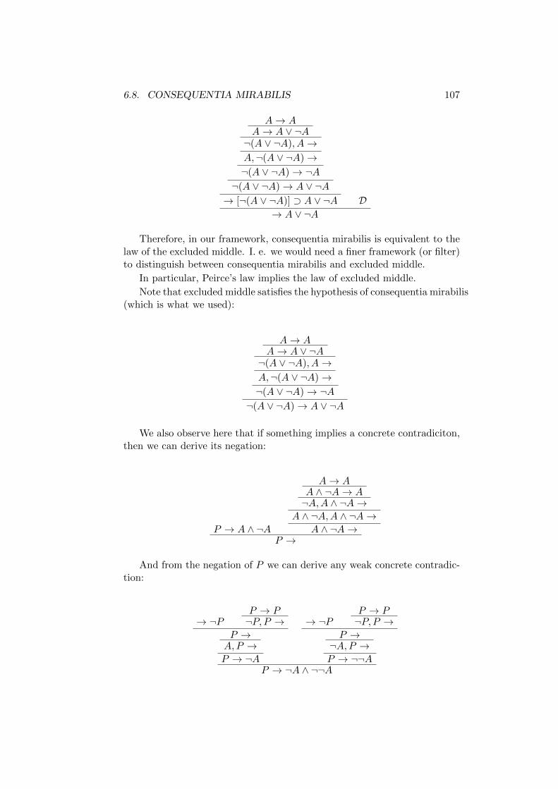
6.8. CONSEQUENTIA MIRABILIS 107
A→ AA→ A ∨ ¬A¬(A ∨ ¬A), A→A,¬(A ∨ ¬A)→¬(A ∨ ¬A)→ ¬A¬(A ∨ ¬A)→ A ∨ ¬A→ [¬(A ∨ ¬A)] ⊃ A ∨ ¬A D
→ A ∨ ¬A
Therefore, in our framework, consequentia mirabilis is equivalent to thelaw of the excluded middle. I. e. we would need a finer framework (or filter)to distinguish between consequentia mirabilis and excluded middle.
In particular, Peirce’s law implies the law of excluded middle.
Note that excluded middle satisfies the hypothesis of consequentia mirabilis(which is what we used):
A→ AA→ A ∨ ¬A¬(A ∨ ¬A), A→A,¬(A ∨ ¬A)→¬(A ∨ ¬A)→ ¬A¬(A ∨ ¬A)→ A ∨ ¬A
We also observe here that if something implies a concrete contradiciton,then we can derive its negation:
P → A ∧ ¬A
A→ AA ∧ ¬A→ A¬A,A ∧ ¬A→
A ∧ ¬A,A ∧ ¬A→A ∧ ¬A→
P →
And from the negation of P we can derive any weak concrete contradic-tion:
→ ¬PP → P¬P, P →
P →A,P →P → ¬A
→ ¬PP → P¬P, P →
P →¬A,P →P → ¬¬A
P → ¬A ∧ ¬¬A
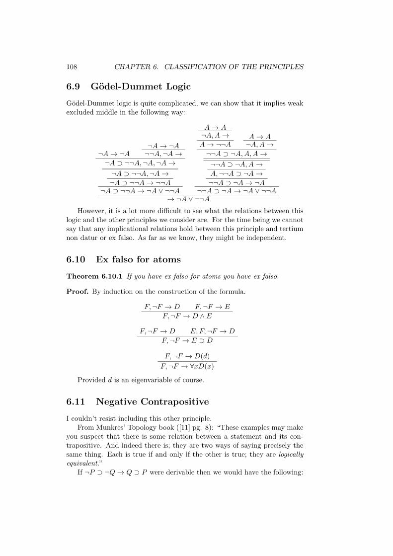
108 CHAPTER 6. CLASSIFICATION OF THE PRINCIPLES
6.9 Godel-Dummet Logic
Godel-Dummet logic is quite complicated, we can show that it implies weakexcluded middle in the following way:
¬A→ ¬A¬A→ ¬A¬¬A,¬A→
¬A ⊃ ¬¬A,¬A,¬A→¬A ⊃ ¬¬A,¬A→¬A ⊃ ¬¬A→ ¬¬A
¬A ⊃ ¬¬A→ ¬A ∨ ¬¬A
A→ A¬A,A→A→ ¬¬A
A→ A¬A,A→
¬¬A ⊃ ¬A,A,A→¬¬A ⊃ ¬A,A→A,¬¬A ⊃ ¬A→¬¬A ⊃ ¬A→ ¬A
¬¬A ⊃ ¬A→ ¬A ∨ ¬¬A→ ¬A ∨ ¬¬A
However, it is a lot more difficult to see what the relations between thislogic and the other principles we consider are. For the time being we cannotsay that any implicational relations hold between this principle and tertiumnon datur or ex falso. As far as we know, they might be independent.
6.10 Ex falso for atoms
Theorem 6.10.1 If you have ex falso for atoms you have ex falso.
Proof. By induction on the construction of the formula.
F,¬F → D F,¬F → E
F,¬F → D ∧ E
F,¬F → D E,F,¬F → D
F,¬F → E ⊃ D
F,¬F → D(d)
F,¬F → ∀xD(x)
Provided d is an eigenvariable of course.
6.11 Negative Contrapositive
I couldn’t resist including this other principle.From Munkres’ Topology book ([11] pg. 8): “These examples may make
you suspect that there is some relation between a statement and its con-trapositive. And indeed there is; they are two ways of saying precisely thesame thing. Each is true if and only if the other is true; they are logicallyequivalent.”
If ¬P ⊃ ¬Q→ Q ⊃ P were derivable then we would have the following:
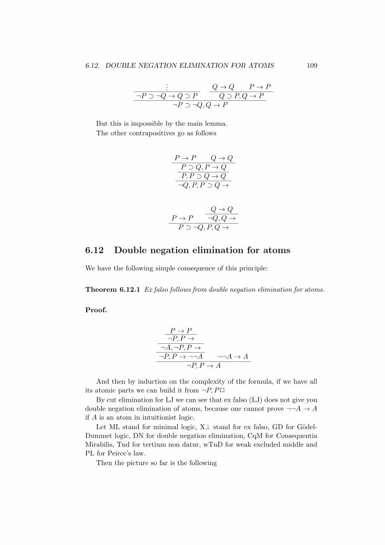
6.12. DOUBLE NEGATION ELIMINATION FOR ATOMS 109
...¬P ⊃ ¬Q→ Q ⊃ P
Q→ Q P → P
Q ⊃ P,Q→ P
¬P ⊃ ¬Q,Q→ P
But this is impossible by the main lemma.
The other contrapositives go as follows
P → P Q→ Q
P ⊃ Q,P → Q
P,P ⊃ Q→ Q
¬Q,P, P ⊃ Q→
P → P
Q→ Q
¬Q,Q→P ⊃ ¬Q,P,Q→
6.12 Double negation elimination for atoms
We have the following simple consequence of this principle:
Theorem 6.12.1 Ex falso follows from double negation elimination for atoms.
Proof.
P → P¬P, P →¬A,¬P, P →¬P, P → ¬¬A ¬¬A→ A
¬P, P → A
And then by induction on the complexity of the formula, if we have allits atomic parts we can build it from ¬P, P2
By cut elimination for LJ we can see that ex falso (LJ) does not give youdouble negation elimination of atoms, because one cannot prove ¬¬A→ Aif A is an atom in intuitionist logic.
Let ML stand for minimal logic, X⊥ stand for ex falso, GD for Godel-Dummet logic, DN for double negation elimination, CqM for ConsequentiaMirabilis, Tnd for tertium non datur, wTnD for weak excluded middle andPL for Peirce’s law.
Then the picture so far is the following
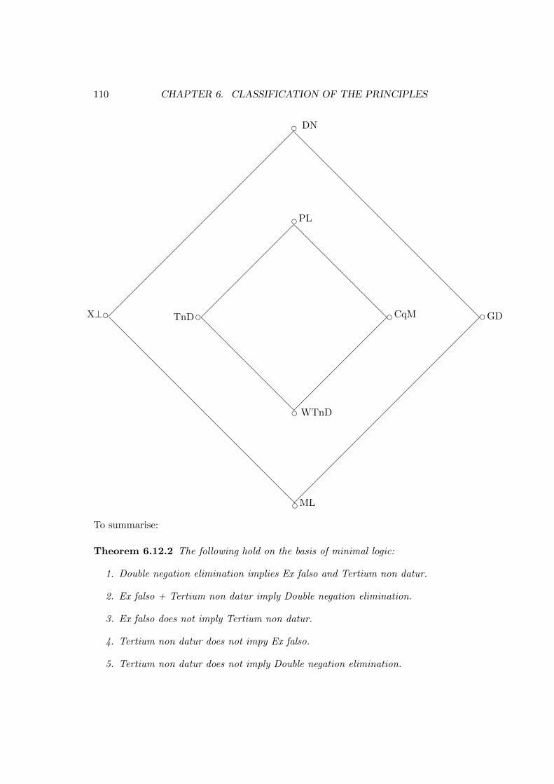
110 CHAPTER 6. CLASSIFICATION OF THE PRINCIPLES
d DN
@@@@@@@@@@@@@@@@@@@@
dPL
@@@@@@@@@@dX⊥
@@@@@@@@@@@@@@@@@@@@
dTnD@@@@@@@@@@
dCqM
dGD
d WTnD
dML
To summarise:
Theorem 6.12.2 The following hold on the basis of minimal logic:
1. Double negation elimination implies Ex falso and Tertium non datur.
2. Ex falso + Tertium non datur imply Double negation elimination.
3. Ex falso does not imply Tertium non datur.
4. Tertium non datur does not impy Ex falso.
5. Tertium non datur does not imply Double negation elimination.
6.12. DOUBLE NEGATION ELIMINATION FOR ATOMS 111
The fifth item in this theorem is new and we hope it sheds some light onwhat the law of excluded middle actually implies on the basis of our formalsystem. It’s possible that the fourth item is also new, but I am not sure,maybe someone else proved it somewhere.
112 CHAPTER 6. CLASSIFICATION OF THE PRINCIPLES
Bibliography
[1] B. Afshari and M. Rathjen: Reverse Mathematics and Well-orderingPrinciples: A pilot study, Annals of Pure and Applied Logic 160 (2009)231-237.
[2] J. Barwise: Admissible Sets and Structures (Springer, Berlin 1975).
[3] W. Buchholz and K. Schutte: Proof Theory of Impredicative Subsys-tems of analysis. Bibliopolis 1988.
[4] Luitzen Egbertus Jan Brouwer, Collected Works, Volume I, North Hol-land, 1975.
[5] Harvey Friedman, Antonio Montalban, Andreas Weiermann: Phi func-tion, draft, 2007.
[6] J.-Y. Girard: Proof Theory and Logical Complexity, vol. 1 (Bibliopolis,Napoli, 1987).
[7] J-Y. Girard: Proofs and Types, Cambridge University Press, 1989.
[8] Jeffry L. Hirst: Reverse mathematics and ordinal exponentiation, An-nals of Pure and Applied Logic 66 (1994) 1–18.
[9] A. Marcone, A. Montalban: The Veblen functions for computabilitytheorists, Journal of Symbolic Logic 76 (2011) 575–602.
[10] A. Montalban: Open Questions in Reverse Mathematics, The Bulletinof Symbolic Logic, Volume 17, Number 3, September 2011, 444–445.
[11] James R. Munkres, Topology, Second Edition, Prentice-Hall, 2000.
[12] S. Negri, J. von Plato Structural Proof Theory
[13] W. Pohlers, Proof Theory
[14] M. Rathjen: Fragments of Kripke-Platek set theory with infinity. In:Leeds Proof Theory 90 (P. Aczel, J. Simmons, S. Wainer, eds.), Cam-bridge University Press.
113
114 BIBLIOGRAPHY
[15] M. Rathjen: ω-models and well-ordering principles. To appear in: NeilTennant (ed.): Foundational Adventures: Essays in Honor of HarveyM. Friedman. Templeton Press (Online); and (College Publications,London, 2013?)
[16] M. Rathjen, A. Weiermann: Proof–theoretic investigations on Kruskal’stheorem. Annals of Pure and Applied Logic 60 (1993) 49–88.
[17] M. Rathjen, A. Weiermann: Reverse Mathematics and Well-orderingPrinciples. In: S. Cooper, A. Sorbi (eds.): Computability in Context:Computation and Logic in the Real World (Imperial College Press,2011) 351–370.
[18] M. Rathjen: Lecture notes: Selected topics in proof theory (MunsterUniversity, 1989)
[19] M. Rathjen: Fragments of Kripke-Platek set theory with infinity. In:Leeds Proof Theory 90 (P. Aczel, H. Simmons, S. Wainer, eds.), Cam-bridge University Press.
[20] M. Rathjen, A. Weiermann: Reverse Mathematics and Well-orderingPrinciples. In: S. Cooper, A. Sorbi (eds.): Computability in Context:Computation and Logic in the Real World (Imperial College Press,2011) 351–370.
[21] M. Rathjen: ω-models and well-ordering principles. To appear in: NeilTennant (ed.): Foundational Adventures: Essays in Honor of HarveyM. Friedman. Templeton Press (Online); and (College Publications,London, 2012)
[22] M. Rathjen Proof Theory Lecture notes, Leeds, 2012.
[23] K.Schutte: Proof Theory. Springer 1977.
[24] K. Schutte: Beweistheoretische Erfassung der unendlichen Induktion inder Zahlentheorie, Mathematische Annalen 122 (1951) 369–389.
[25] S.G. Simpson: Subsystems of Second Order Arithmetic, second edition,(Cambridge University Press, 2009).
[26] G. Takeuti: Proof Theory, second edition, Springer 1975.
[27] Klaus Weich, Improving Proof Search in Propositional IntuitionisticLogic, Logos Verlag Berlin, 2001.