Implementing Restart Model Elimination andTheory Model Elimination on top of SETHEO

Peter BaumgartnerUniversity of Koblenz

Rheinau 156075 Koblenz

Germanypeter@informatik.uni-koblenz.de

Johann SchumannInstitut fur Informatik

Technische Universitat MunchenGermany

80290 Munchenschumann@informatik.tu-muenchen.de

Abstract

This paper presents an implementation for the efficient execution of Theory ModelElimination (TME), TME by Linearizing Completion, and Restart Model Elimination(RME) on top of the automated theorem prover SETHEO. These calculi allow for theoryreasoning using a Model Elimination based theorem prover. They are described indetail and their major properties are shown. Then, a detailed description how TME byLinearizing Completion and RME can be implemented on top of SETHEO’s AbstractMachine (SAM) is given. Due to the flexibility of the Abstract Machine and its inputlanguage LOP, only simple transformations of the input formula are sufficient to obtainan efficient implementation. Only for RME, one machine-instruction of the SAM had tobe modified slightly. We present results of experiments comparing plain SETHEO withan implementation of TME with PTTP (PROTEIN) and the SETHEO implementationpresented here.

1 Introduction

The model elimination calculus (ME calculus) has been developed already in the early days ofautomated theorem proving [Loveland, 1968]. It is a goal-oriented, linear and refutationallycomplete calculus for first order clause logic. Model elimination is the base of numerous proofprocedures for first order deduction. There are high speed theorem provers, like METEOR([Astrachan and Stickel, 1992] or SETHEO ([Letz et al., 1992, Letz et al., 1994]) and there isa whole class of provers, namely Prolog technology theorem proving (PTTP) as introduced in[Stickel, 1988, Stickel, 1989], which rely on model elimination.

This paper deals with several variants of model elimination with an emphasis on theimplementational issue. These variants are called restart model elimination [Baumgartner

1

and Furbach, 1994a] and theory model elimination [Baumgartner, 1992, Baumgartner, 1994].They will be reviewed in the respective sections below. For a more detailed description thereader is referred to the cited literature.

In brief, restart model elimination is a variant which was motivated by taking a logicprogramming view at theorem proving. In logic programming one typically reads a clauseA _ :C _ :Doperationally as a “contrapositive”A C ;Dwhich means, roughly, “in order to prove A it suffices to prove C and D”. However, in(ordinary) model elimination in the presence of non-definite clauses (i.e., clauses with morethan one positive literal) this natural reading has to be given up. For completeness reasons itis required to add the contrapositives:C :A;D:D :A;CIn other words, the “body” literals C and D have to be considered as entry points for the proofsearch, too.

Why should we bother with these contrapositives? Suppose, for example we are given aninput clause1prove(and(X ;Y )) prove(X ) ^ prove(Y )which can be used within a formalization of propositional calculus. A possible contrapositiveis :prove(X ) :prove(and(X ;Y )) ^ prove(Y )The procedural reading of this contrapositive is somewhat strange and leads to an unnecessaryblowing-up of the search space; in order to prove :prove(X ) one has to prove prove(Y ) – agoal which is totally unrelated to :prove(X ) by introducing a new variable.

Now, the question arises whether model elimination can be modified in such a way that theabove “natural” contrapositives suffice. Indeed, this is achieved in restart model elimination(there are also several other calculi achieving this, e.g. Loveland’s NearHorn-Prolog [Loveland,1987], Gabbay’s N-Prolog [Gabbay, 1985] and Plaisted’s problem reduction formats [Plaisted,1988]).

In restart model elimination, for non-definite clauses, likeA _ B _ :C _ :Donly the following contrapositives have to be considered:A :B ;C ;DB :A;C ;D

1Taken from [Plaisted, 1988].

2

It is even possible to restrict to one of those (cf. the selection function below).Of course there is a price to pay. In restart model elimination an additional inference rule

is needed, the restart rule, which allows to begin a completely new proof once a negative bodyliteral, such as :B or :A is encountered.

As mentioned above, restart model elimination is motivated by logic programming. Be-sides that, we think that restart model elimination is also useful in an automated theoremproving context: in proving theorems such as “if x 6= 0 then x 2 > 0” a human typically usescase analysis according to the axiom (X < 0) _ (X = 0) _ (�X < 0). This seems a verynatural way of proving the theorem and leads to a well-understandable proof. Restart modelelimination carries out precisely such a proof by case analysis.

Now let us turn to the other variant, theory model elimination. Theory reasoning wasintroduced by M. Stickel within the general, non-linear resolution calculus [Stickel, 1985]; formodel elimination it is defined and investigated in [Baumgartner, 1992, Baumgartner, 1994].

Theory reasoning means to relieve a calculus from explicit reasoning in some domain(e.g., equality, partial orders, taxonomic reasoning) by taking apart the domain knowledgeand treating it by special inference rules. In an implementation, this results in a universal“foreground” reasoner that calls a specialized “background” reasoner for theory reasoning.The advantages of theory reasoning, when compared with the naive method of supplying thetheories’ axioms as clauses, are the following: for the first, the theory inference system maybe specially tailored for the theory to be reasoned with; thus higher efficiency can be achievedby a clever reasoner that takes advantage of the theories’ properties. For the second, a lotof computation that is not relevant for the overall proof plan is hidden in the background.Thus proofs become shorter and are more compact, leading to better readability (although werecognize that this is a matter of taste).

More technically, in theory reasoning the idea of finding complementary literals is gener-alized to a semantic level. For instance, in the theory of strict orderings, the literals a < b,b < c and c < a may be detected to be inconsistent by the background reasoner. The generalidea is to do the search for complementary literals on this semantical level at every place wheresyntactical reasoning is used in the non-theory version of the calculus.

The question arises how to obtain for a given theory a background calculus. To this end,one of the authors has designed a compilation technique which allows to transform a Horntheory into inference rules which are suitable to be used in conjunction with model elimination.This method, called linearizing completion [Baumgartner, 1995 ] is used throughout all ourexperiments.

Fortunately, theory reasoning can be applied to ordinary model elimination, as well asrestart model elimination in a complete way. Together with various sub-variants of restartmodel elimination we have now a considerable spectrum of different calculi for differentneeds of automated reasoning at hand. It is the purpose of this paper to evaluate some of thesecombinations by using the Setheo theorem prover.

The rest of this paper is structured as follows: after concluding this introduction withsome preliminaries (basic definitions) we will briefly review the model elimination calculus(Section 2). Then we generalize it towards theory model elimination in Section 3. Section 4describes another calculus variant, restart model elimination. Implementation on SETHEO isdiscussed in Section 5. Finally, Section 6 reports on experimental results.

3

1.1 Preliminaries

A clause is a multiset of literals, written as the disjunction L1 _ � � � _Ln . As usual, clauses areconsidered implicitly as being universally quantified, and a clause set is considered logicallyas a conjunction of clauses. Instead of the chains of the original model elimination calculuswe follow [Baumgartner and Furbach, 1993] and work in a branch-set setting. A branch is afinite sequence of literals, written by juxtaposing its constituents L1L2 � � �Ln . A branch set isa finite multiset of branches.

Concerning interpretations we restrict ourselves to Herbrand-Interpretations over a (mosttimes implicitly) given finite signature Σ. Furthermore we suppose Σ to contain the 0-arypredicate symbol F which is to be interpreted by false in every interpretation. We assume atheory to be given by a satisfiable set of universally quantified formulas, e.g. as a clause set(because a Herbrand-theorem holds). In the sequel T always denotes such a theory. As anexample one might think of the theory of equality, given by the usual axioms. A HerbrandT -interpretation I for a formula F is a Herbrand-interpretation over the joint signatures of Tand F that satisfies T , i.e. I j= T . We write I j=T F to indicate that I is a T -interpretationand I satisfies F (i.e. I is a T -model for F ). Furthermore, F is called T -valid, j=T F, iffevery T -interpretation satisfies F , andF is T -(un-)satisfiable iff some (none) T -interpretationsatisfies F . As a consequence of these definition it holds j=T F iff :F is T -unsatisfiable iffT [ f:Fg is unsatisfiable.

2 Review of Model Elimination

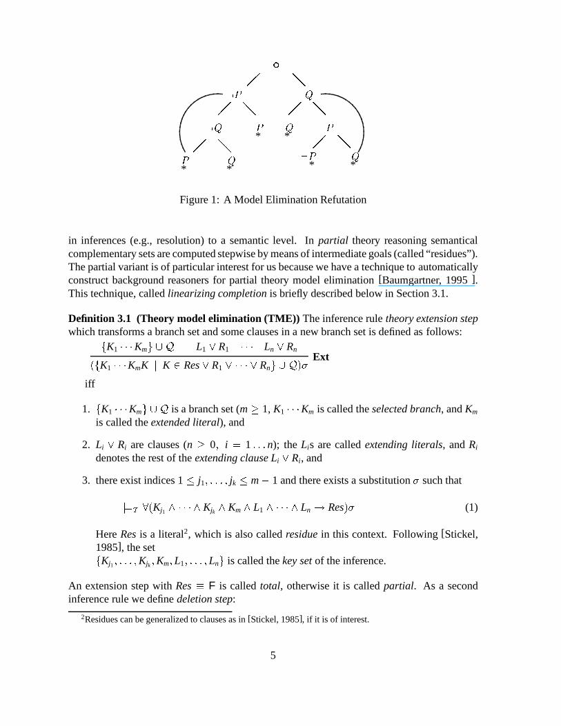
We will briefly and rather informally review our format of model elimination. It differs fromthe original one presented by [Loveland, 1968]; the format we use is described in [Letz et al.,1992] as the base for the prover SETHEO. In [Baumgartner and Furbach, 1993] this calculus isdiscussed in detail and compared to various other calculi. This model elimination manipulatestrees by extension- and reduction-steps. As an example consider the clause setffP ;Qg ; f:P ;Qg ; f:Q ;Pg ; f:P ;:Qgg ;A model-elimination refutation is depicted in Figure 1. It is obtained by successive fanningwith clauses from the input set (extension steps. Additionally, it is required that every innernode (except the root) is complementary to one of its sons. An arc indicates a reduction step,i.e. the closing of a branch due to a path literal complementary to the leaf literal.

We will nor present the inference rules formally, because this is done in a more generalform in the following section.

3 Theory Model Elimination

In this section we will review the extension of model elimination towards theory reasoning.A more thorough treatment can be found in [Baumgartner, 1994].

Theory reasoning comes in two variants [Stickel, 1985]: total and partial theory reasoning.Total theory reasoning directly lifts the idea of finding syntactical complementary literals

4

d�� @@�� �� @@ �� @@�� @@@@:P P:QP Q P:PQ Q

:Q* * * *

**

Figure 1: A Model Elimination Refutation

in inferences (e.g., resolution) to a semantic level. In partial theory reasoning semanticalcomplementary sets are computed stepwise by means of intermediate goals (called “residues”).The partial variant is of particular interest for us because we have a technique to automaticallyconstruct background reasoners for partial theory model elimination [Baumgartner, 1995 ].This technique, called linearizing completion is briefly described below in Section 3.1.

Definition 3.1 (Theory model elimination (TME)) The inference rule theory extension stepwhich transforms a branch set and some clauses in a new branch set is defined as follows:fK1 � � �Kmg [ Q L1 _ R1 � � � Ln _ Rn(fK1 � � �KmK j K 2 Res _ R1 _ � � � _ Rng [ Q)� Ext

iff

1. fK1 � � �Kmg [ Q is a branch set (m � 1, K1 � � �Km is called the selected branch, and Km

is called the extended literal), and

2. Li _ Ri are clauses (n � 0; i = 1 : : :n); the Lis are called extending literals, and Ri

denotes the rest of the extending clause Li _ Ri, and

3. there exist indices 1 � j1; : : : ; jk � m� 1 and there exists a substitution � such thatj=T 8(Kj1 ^ � � � ^ Kjk ^ Km ^ L1 ^ � � � ^ Ln ! Res)� (1)

Here Res is a literal2, which is also called residue in this context. Following [Stickel,1985], the setfKj1 ; : : : ;Kjk ;Km; L1; : : : ; Lng is called the key set of the inference.

An extension step with Res � F is called total, otherwise it is called partial. As a secondinference rule we define deletion step:

2Residues can be generalized to clauses as in [Stickel, 1985], if it is of interest.

5

fK1 � � �KmFg [ QQ Del

Thus the deletion step allows to remove branches which are detected as contradictory (bymeans of a concluding F). The calculus of total theory model elimination (TME) consists ofthe inference rules total theory extension step and deletion step, and partial TME additionallyconsists of partial theory extension step.

A (total, partial) TME derivation of Qn from a clause set M then is defined as a sequence(n � 1) Q1; : : : ;Qn such that

1. Q1 = fL1; : : : ; Lng, i.e., a multiset of branches of length 1, for someL1 _ � � � _ Ln 2 M; this clause is also called the query, and

2. for i = 2; : : : ; n, Qi is obtained (2a) either by applying the Ext inference rule to Qi�1

and some new variants of clauses from M, or else (2b) by applying the Del inferencerule to Qi�1.

A refutation of M is a derivation of the empty branch set fg from M.A branch is called regular iff all the literals occurring in it are pairwise distinct (i.e. the

branch contains no duplicate literals). A branch set is regular iff every of its branches isregular. A derivation is called regular iff every branch set of the derivation is regular. 2Informally, the implication (1) in Definition 3.1 means (roughly) that the residue is a logicalconsequence of some literals along the branch (including the extended literal) and the extendingliterals. This condition is needed to obtain a sound calculus.

As a further refinement, the implication (1) can be required to be minimal (i.e. after deletingany element, (1) would no longer hold). For example, if the theory is “equality”, the selectedbranch isPa Pb and the extending literals are fa = c;:Pcg then a total extension step with keyset fPa;Pb; a = c;:Pcg is possible. However, the implicationPa ^Pb ^a = c^:Pc ! Fis not minimal, as with deleting the extended literal Km = Pb the resulting implicationPa ^ a = c ^ :Pc ! F is still valid. Thus, this proposed extension step would not beallowed. In general, in implementations the local search space can be pruned considerably,as the minimality restriction allows to guide the search for the extending literals around theextended literal Km .

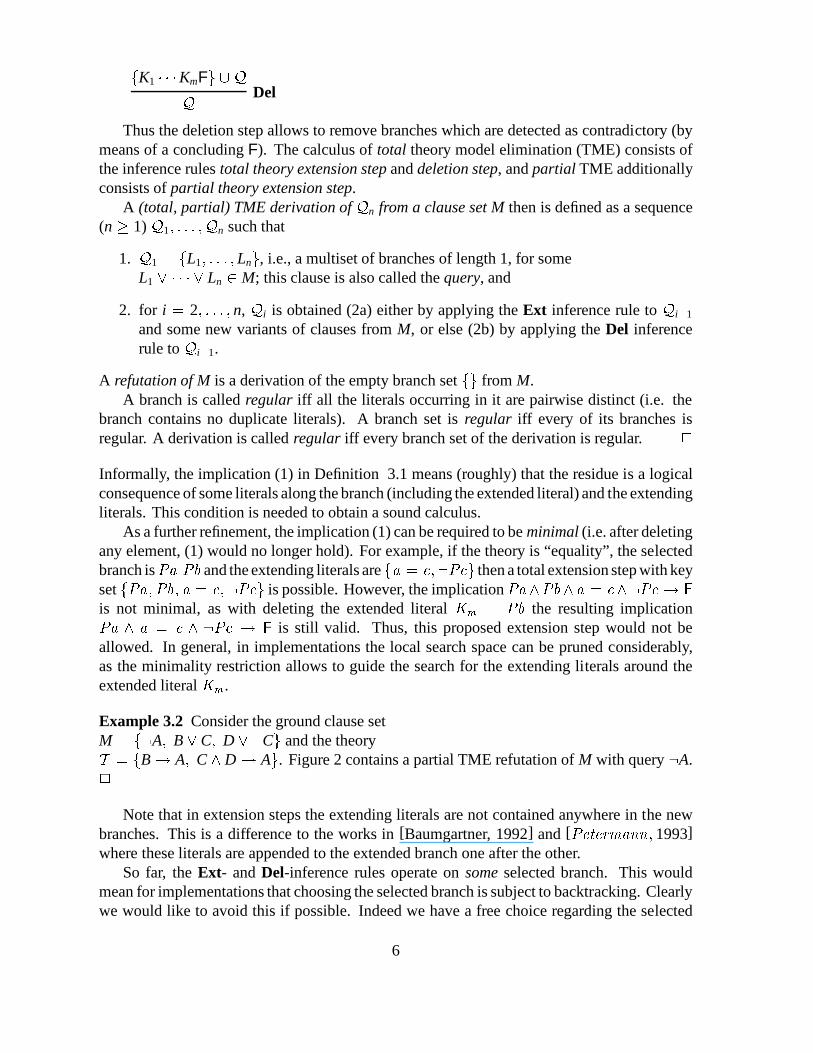
Example 3.2 Consider the ground clause setM = f:A; B _ C; D _ :Cg and the theoryT = fB! A; C ^ D! Ag. Figure 2 contains a partial TME refutation of M with query :A.2

Note that in extension steps the extending literals are not contained anywhere in the newbranches. This is a difference to the works in [Baumgartner, 1992] and [Petermann; 1993]where these literals are appended to the extended branch one after the other.

So far, the Ext- and Del-inference rules operate on some selected branch. This wouldmean for implementations that choosing the selected branch is subject to backtracking. Clearlywe would like to avoid this if possible. Indeed we have a free choice regarding the selected

6

1 ���@@@���@@@���@@@���@@@���@@@ ���@@@���@@@:A

2 3 4 5:A

F C

D

B

:CA

:A

F C

D

B

:CA

:A

C

B

F

F

:A

F C

F

D

B

:CA

F

Figure 2: A TME refutation of M in a tree notation following [Letz et al., 1992]. 1 isthe tree resulting from the query :A. 2 is obtained by a total extension step with B _ C ,making use of the fact that :A ^ B ! F is T -valid (because (:A ^ B ! F) � (B ! A)).In this extension step (and similarly below) we have decorated the edge with the extendingliteral. 3 is obtained by a partial extension step with clause D _ :C , using the T -validity ofC ^ D ! A. 4 is obtained by a total extension step with the ancestor literal :A, which ispossible since :A ^ A! F is valid in every theory. 5 is obtained in a similar way.

branch. As a further advantage of such a result, the selected branch can be chosen heuristically.Occasionally, factoring can be applied more successfully (see [Letz et al., 1994]) if such asubgoal reordering is allowed.

For the formalization, we borrow the notion of a “computation rule” from logic program-ming [Lloyd, 1987]:

Definition 3.3 A computation rule is a function c from the set of branch sets to the set ofbranches such that c(Q) 2 Q. Thus a computation rule can be used in derivations to determinethe selected branch for the next inference step; we say that a derivation is a derivation wrt. ciff the selected branch in every of its inference steps is determined by c. 2For example, if a Prolog-like computation rule is desired, then always some longest branch isto be selected.

The following lemma is crucial; it can be proved for any of the calculi defined in this paper.

Lemma 3.4 (Independence of the computation rule – ground case) Let T be a theory andM be a ground clause set. Suppose there exists a refutation of M with top clause C. Then forevery computation rule c there exists a refutation of M wrt. c.

As a consequence of our completeness proof techniques, which is a traditional ground-proofand lifting technique, it suffices to proof this result for the ground case only. The respective

7

result for the first-order case with variables would be technically much more complicated(cf. [Lloyd, 1987]).

Completeness is stated for the ground case only. Although not quite trivial, lifting to thefirst order case can be carried out by generalizing standard techniques (see e.g. [Chang andLee, 1973, Lloyd, 1987]).

Theorem 3.5 (Ground Completeness of Regular Total TME) Let T be a theory, c be acomputation rule and let M be a T -unsatisfiable ground clause set. Let C 2 M be such thatC is contained in some minimal T -unsatisfiable subset of M. Then there exists a regular totalTME refutation of M wrt. c with query C.

For the ground proof the excess literal parameter technique can be used in a similar way as itis done for the non-theory version in [Baumgartner and Furbach, 1994a]. Regularity is shownby restricting for every branch to be closed the available input clause set to those clauses thatare free of literals occurring in that branch.

An important class of theories are definite theories, i.e., theories that are axiomatized by aset of definite clauses3. For such theories we find a special structure of implications:

Proposition 3.6 For every definite theory T and for every T -valid implication 8(L1 ^ � � � ^Ln ! Ln+1) it holds that either (1) all literals L1; : : : ; Ln and the conclusion Ln+1 are positive,or (2) one single literal Li (1 � i � n) is negative and Ln+1 is either negative or F.

This special structure of implications can immediately be imposed on the correspondingimplications in the definition of extension steps above. If additionally the input clause set is“Horn”, then the ancestor literals of leafs need not to be stored and all extending literals arepositive. This result generalizes a well-known property of ordinary model elimination, whichstates that no reduction steps are required (even possible) in the Horn case.

3.1 Partial Theory Model Elimination by Linearizing Completion

Let us first give some motivation for the linearizing completion technique from the viewpointof partial theory model elimination.

Recall from the definition of theory model elimination (Def. 3.1, in particular condition 3)that we distinguish between total and partial theory model elimination, where the latter differsfrom the former only by the possibility to derive residues (i.e., new subgoals) different fromF. In other words, in total theory model elimination the contradiction must be discovered bythe background reasoner in a single step, while this need not necessarily be so in partial theorymodel elimination.

However, it may be practically difficult or even impossible to design an appropriatebackground calculus for total theory reasoning. Consider e.g. the theory of equality, wherethe background calculus then must be capable to enumerate all solutions for a given rigidE-unification problem [Gallier et al., 1987]. However the decidability of simultaneous rigidE-unification is still open. No matter how this question will eventually be answered, thereare (other) undecidable theories. For undecidable theories we can expect to obtain at most

3A definite clause contains exactly one positive literal.

8

an enumeration procedure for solutions rather than an algorithm. So, the computations inthe background calculus have to be interleaved with the foreground calculus. This makes itdifficult to treat the background calculus as a “black box”.

In order to remedy the situation, partial theory model elimination offers the framework tosplit the one single total extension step into a sequence of partial extension steps, followed bya concluding total step. Take the example of equality again. Then, for instance, a total stepinvolving rigid E-unification can be replaced by a sequence of paramodulation steps whichtransforms an initially given equational goal into :(s = s) which in turn is to be closed by atrivial total step.

However, as defined so far, the difficulty with the partial variant is that it adds possibleinferences, but does not restrict the total inferences. Thus, partial theory model elimination canbe seen only as a framework, and completeness holds vacuously. Furthermore, for efficiencyreasons one would certainly not want to consider all T -valid implications (Condition 3 inDef. 3.1 again) for extension steps. Take again equality: the paramodulation inference ruledoes not compute all equational consequences of the given key set. For example, :(x = y) !:(y = x ) is such a T -valid implication, but paramodulation does not allow to flip the sides ofan equation.

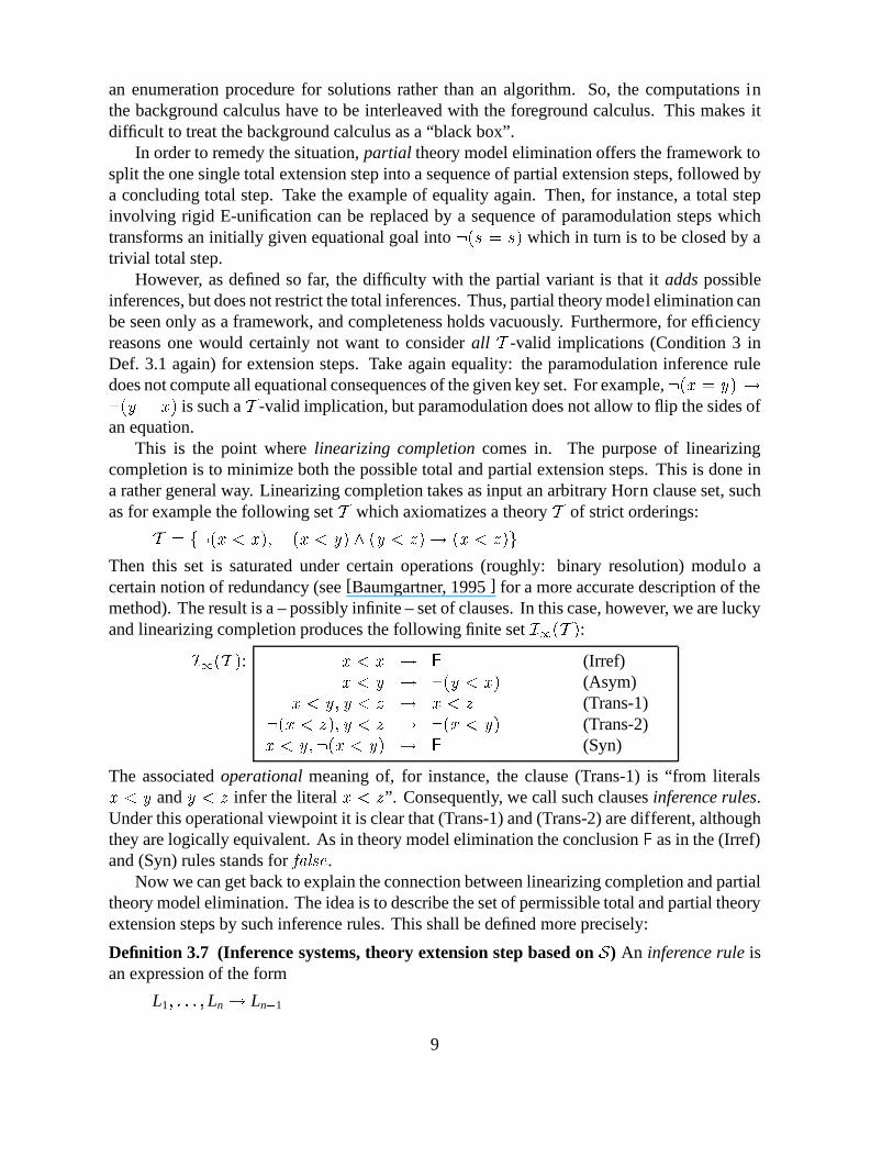
This is the point where linearizing completion comes in. The purpose of linearizingcompletion is to minimize both the possible total and partial extension steps. This is done ina rather general way. Linearizing completion takes as input an arbitrary Horn clause set, suchas for example the following set T which axiomatizes a theory T of strict orderings:T = f:(x < x ); (x < y) ^ (y < z )! (x < z )gThen this set is saturated under certain operations (roughly: binary resolution) modulo acertain notion of redundancy (see [Baumgartner, 1995 ] for a more accurate description of themethod). The result is a – possibly infinite – set of clauses. In this case, however, we are luckyand linearizing completion produces the following finite set I1(T ):I1(T ): x < x ! F (Irref)x < y ! :(y < x ) (Asym)x < y ; y < z ! x < z (Trans-1):(x < z ); y < z ! :(x < y) (Trans-2)x < y ;:(x < y) ! F (Syn)

The associated operational meaning of, for instance, the clause (Trans-1) is “from literalsx < y and y < z infer the literal x < z”. Consequently, we call such clauses inference rules.Under this operational viewpoint it is clear that (Trans-1) and (Trans-2) are different, althoughthey are logically equivalent. As in theory model elimination the conclusion F as in the (Irref)and (Syn) rules stands for false.

Now we can get back to explain the connection between linearizing completion and partialtheory model elimination. The idea is to describe the set of permissible total and partial theoryextension steps by such inference rules. This shall be defined more precisely:

Definition 3.7 (Inference systems, theory extension step based on S) An inference rule isan expression of the form

L1; : : : ; Ln ! Ln+1

9

where all Lis, 1 � i � n, are literals (called premise literals), and Ln+1 is either a literalor F (called conclusion). The declarative meaning of an inference rule is the implication8((L1 ^ : : : ^ Ln)! Ln+1).

An inference system S is a set of inference rules.On modifying the definition of theory extension step (Def. 3.1) we define the inference rule

theory extension step based on S to be defined as theory extension step, except that condition3 is replaced by the following:

3. there exists a new variant

L1; : : : ; Ln ! Res

of an inference rule from S, there exist indices 1 � j1; : : : ; jk � m � 1 and thereexists a substitution � which is a most general unifier for the multisets fL1; : : : ; Lng andfKj1 ; : : : ;Kjk ;Kmg.

A theory model elimination derivation based on S is a derivation where all extension steps arebased on S. 2In words, in order to carry out a theory extension step according to this definition, one has tofind an inference rule from S whose premise literals simultaneously unify with the leaf literaland some literals from the branch to be extended. If this succeeds the instantiated conclusionof the inference rule yields the residue. In case the conclusion is F we have a total step,otherwise a partial step.

It should be clear that by this device the set of possible extension steps can be prunedconsiderably. This holds for instance when using the above inference system I1(T ) for strictorderings.

The soundness of this calculus obviously depends on the soundness ofS. It holds that theorymodel elimination based on S is sound if every inference rule in S is a logical consequence(according to the declarative reading) of the underlying theory.

Completeness is much harder to establish. As a sufficient condition completeness holds ifS is obtained by linearizing completion, as e.g. I1(T ) above.We will leave this presentation of linearizing completion now. Finally, it should be noted

that since linearizing completion is a tedious task if done by hand we have implemented it andused it in the experiments below. In case linearizing completion results in an infinite inferencesystem finite approximations were used.

4 Restart Model Elimination

Let us now modify the theory model elimination calculus (Section 3), such that only a singlecontrapositive per clause is needed. The modifications work for both the total as well as thepartial variant. Hence we will give up the distinction in this section.

For the modifications we have to presuppose definite theories (see the preceeding section).Furthermore, in order to get a complete calculus, we have to assume that there exists only one

10

clause containing only negative literals, which furthermore does not contain variables, and thisclause is to be used as query in refutations4. We note that Theorem 3.5 can be adapted for thisnew setting.

Definition 4.1 (Restart Theory Model Elimination) First, extension steps are restricted tooperate on negative leafs only. For this define a definite theory extension step in the same wayas theory extension step, except that additionally Km is required to be a negative literal and allother key set literals Kj1 ; : : : ;Kjk ; L1; : : : ; Ln are required to be positive literals.

In order to deal with positive leafs Km define the inference rule restart step as follows:fK1 � � �Kmg [ QfK1 � � �KmK1g [ Q Rest

iff Km is a positive literal and Km 6= F.The strict Restart TME calculus consists of the inference rules definite theory extension

step, restart step and deletion step. The non-strict version consists additionally of theoryextension step. 2

If clauses are written in a sequent style A1; � � � ;An B1; � � � ;Bm (where all As and Bsare positive literals) then it is clear that, for syntactical reasons, definite extension steps arepossible only with head literals A’s, but not with B ’s from the body. Thus it is possible torepresent clauses as above without the need of augmenting them with all contrapositives; onlycontrapositives with conclusions (i.e. entry points) stemming from the positive literals arenecessary. The price of the absence of contrapositives is that whenever a path ends with apositive literal, the root of the tree has to be copied. Then, the only inference applicable tothat branch is a definite extension step. Occasionally a shorter refutation exists if non-definiteextension steps are allowed as well; this motivates the need for the non-strict version.

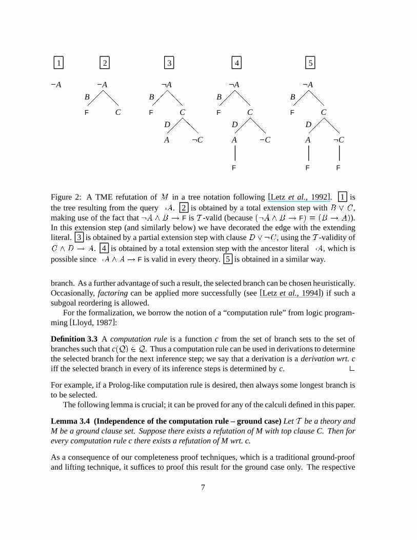
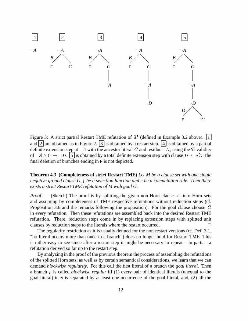
Example 4.2 Consider again the (definite) theory T and ground clause set M of example 3.2(Section 3). In Figure 2 the partial extension step from 2 to 3 is not allowed in RestartTME since the leaf C of the extended branch :AC is positive. A restart step has to take placeinstead. Figure 3 contains a respective strict Restart TME refutation. 2

The restart calculus can further be weakened by introducing a selection function in thefollowing way: a selection function f maps a clause A1; : : : ;An B1; : : : ;Bm with n � 1 toa literal L 2 fA1; : : : ;Ang. Additionally, f is required to be stable under lifting which meansthat if f selects L in the instance of the clause (A1; : : : ;An B1; : : : ;Bm) (for somesubstitution ) then f selects L in A1; : : : ;An B1; : : : ;Bm .5 Now, for (definite) extensionsteps only selected literals may serve as extending literals. Thus, operationally, only one singlecontrapositive per input clause is needed. Notably, all this is complete:

4Without loss of generality this can be achieved by introducing a new clause goal and transforming everypurely negative clause :B1 _ � � � _ :Bm into goal B1 ^ � � � ^Bm .

5This property is needed for the completeness proof; it guarantees for lifting that the selection function willselect on the first order level a literal whose ground instance was selected at the ground level.

11

���@@@:A

F C

B

1

:A:D

���@@@ ���@@@ ���@@@���@@@

:A

2 3 4 5:A

F C

B

:A

F C

B

:A

:A

F C

B

:A:D :C

D

F

Figure 3: A strict partial Restart TME refutation of M (defined in Example 3.2 above). 1and 2 are obtained as in Figure 2. 3 is obtained by a restart step. 4 is obtained by a partialdefinite extension step at :A with the ancestor literal C and residue :D , using the T -validityof :A^C ! :D . 5 is obtained by a total definite extension step with clause D _:C . Thefinal deletion of branches ending in F is not depicted.

Theorem 4.3 (Completeness of strict Restart TME) Let M be a clause set with one singlenegative ground clause G, f be a selection function and c be a computation rule. Then thereexists a strict Restart TME refutation of M with goal G.

Proof. (Sketch) The proof is by splitting the given non-Horn clause set into Horn setsand assuming by completeness of TME respective refutations without reduction steps (cf.Proposition 3.6 and the remarks following the proposition). For the goal clause choose Gin every refutation. Then these refutations are assembled back into the desired Restart TMErefutation. There, reduction steps come in by replacing extension steps with splitted unitclauses by reduction steps to the literals where the restart occurred. 2

The regularity restriction as it is usually defined for the non-restart versions (cf. Def. 3.1,“no literal occurs more than once in a branch”) does no longer hold for Restart TME. Thisis rather easy to see since after a restart step it might be necessary to repeat – in parts – arefutation derived so far up to the restart step.

By analyzing in the proof of the previous theorem the process of assembling the refutationsof the splitted Horn sets, as well as by certain semantical considerations, we learn that we candemand blockwise regularity. For this call the first literal of a branch the goal literal. Thena branch p is called blockwise regular iff (1) every pair of identical literals (unequal to thegoal literal) in p is separated by at least one occurrence of the goal literal, and, (2) all the

12

positive literals occurring in p are pairwise distinct. For example, the refutation in Figure 3 isblockwise regular. Fortunately it holds:

Theorem 4.4 Strict Restart TME with selection function is complete when restricted to block-wise regular refutations.

5 Implementation on top of SETHEO

5.1 Architecture of the System

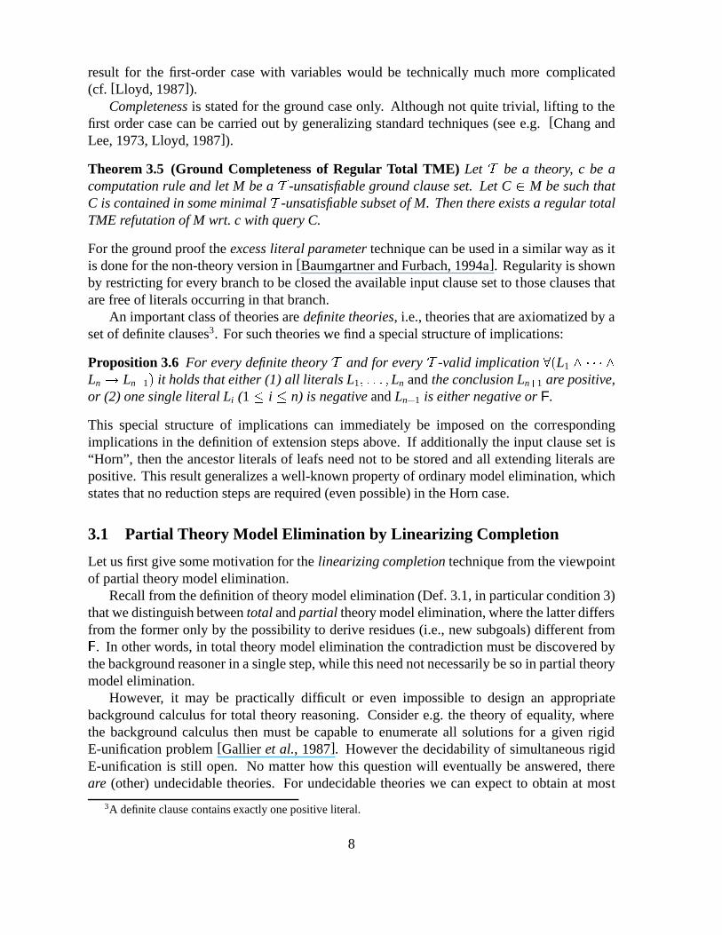
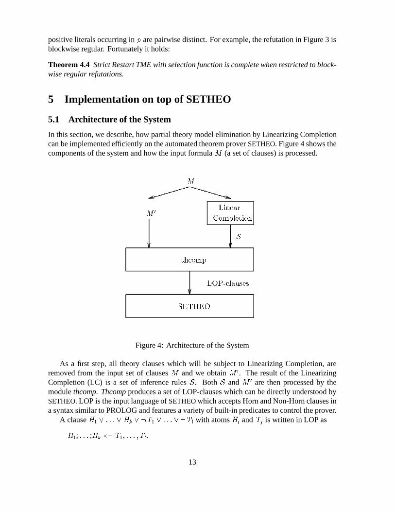
In this section, we describe, how partial theory model elimination by Linearizing Completioncan be implemented efficiently on the automated theorem prover SETHEO. Figure 4 shows thecomponents of the system and how the input formula M (a set of clauses) is processed.�������� XXXXXXXXLinearCompletion

thcompSETHEOLOP-clauses

SMM 0

Figure 4: Architecture of the System

As a first step, all theory clauses which will be subject to Linearizing Completion, areremoved from the input set of clauses M and we obtain M 0. The result of the LinearizingCompletion (LC) is a set of inference rules S. Both S and M 0 are then processed by themodule thcomp. Thcomp produces a set of LOP-clauses which can be directly understood bySETHEO. LOP is the input language of SETHEO which accepts Horn and Non-Horn clauses ina syntax similar to PROLOG and features a variety of built-in predicates to control the prover.

A clause H1 _ : : : _ Hk _ :T1 _ : : : _ :Tl with atoms Hi and Tj is written in LOP asH1; : : : ;Hk <- T1; : : : ;Tl :13

Then, during the compilation phase, k + l contrapositives of the form6Hi:-:H1; : : ::Hi�1;:Hi+1;:Hk ;T1; : : : ;Tl :are generated. If k = 0, the :- is changed to ?-. Such a contrapositive is used – like inPROLOG – as a possible start clause (query). For the following, a contrapositive of a clausec 2 M 0 is labeled ci;j (si;j for an inference rule of S) where i is the number of the clause, andj is the index of the head literal (1 � j � k + l).

A LOP formula can contain a mixture of clauses (with <-, fanned during compilation) andcontrapositives (with :- or ?-, not fanned)7

5.2 Implementation of the theory extension step

In order to implement theory model elimination by Linearizing Completion, the theory exten-sion step based on the given set of inference rules S must be realised within the frameworkof SETHEO. For the following, we drop the condition that the premise literals of a giveninference rule must simultaneously unify with the leaf literal and literals from the branch to beextended (see Definition 3.7). This restriction allows for a much easier implementation on topof SETHEO, since SETHEO’s proof procedure considers exactly one branch to be extended ata time.

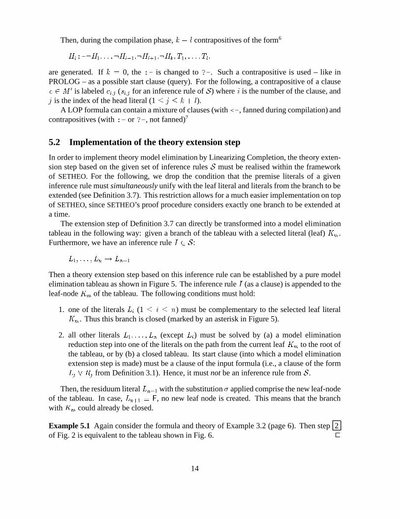
The extension step of Definition 3.7 can directly be transformed into a model eliminationtableau in the following way: given a branch of the tableau with a selected literal (leaf) Km .Furthermore, we have an inference rule I 2 S:L1; : : : ;Ln ! Ln+1

Then a theory extension step based on this inference rule can be established by a pure modelelimination tableau as shown in Figure 5. The inference rule I (as a clause) is appended to theleaf-node Km of the tableau. The following conditions must hold:

1. one of the literals Li (1 � i � n) must be complementary to the selected leaf literalKm . Thus this branch is closed (marked by an asterisk in Figure 5).

2. all other literals L1; : : : ;Ln (except Li ) must be solved by (a) a model eliminationreduction step into one of the literals on the path from the current leaf Km to the root ofthe tableau, or by (b) a closed tableau. Its start clause (into which a model eliminationextension step is made) must be a clause of the input formula (i.e., a clause of the formLj _ Rj from Definition 3.1). Hence, it must not be an inference rule from S.

Then, the residuum literal Ln+1 with the substitution� applied comprise the new leaf-nodeof the tableau. In case, Ln+1 � F, no new leaf node is created. This means that the branchwith Km could already be closed.

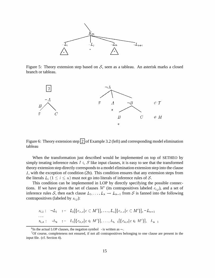
Example 5.1 Again consider the formula and theory of Example 3.2 (page 6). Then step 2of Fig. 2 is equivalent to the tableau shown in Fig. 6. 2

14

��������� PPPPPPPhhhhhhhhhhhhh��� TTTSSS ��� TTTKm

*

:Li:L1 :Ln :Ln+1

* *

Figure 5: Theory extension step based on S, seen as a tableau. An asterisk marks a closedbranch or tableau.

���@@@ ���� DDDaaaaaa���� QQQ2:A CBF

:A*

:B CB*AF 2 M2 TFigure 6: Theory extension step 2 of Example 3.2 (left) and corresponding model eliminationtableau

When the transformation just described would be implemented on top of SETHEO bysimply treating inference rules I 2 S like input clauses, it is easy to see that the transformedtheory extension step directly corresponds to a model elimination extension step into the clauseI , with the exception of condition (2b). This condition ensures that any extension steps fromthe literals Li (1 � i � n) must not go into literals of inference rules of S.

This condition can be implemented in LOP by directly specifying the possible connec-tions. If we have given the set of clauses M 0 (its contrapositives labeled ci;j ), and a set ofinference rules S, then each clause L1; : : : ;Ln ! Ln+1 from S is fanned into the followingcontrapositives (labeled by si;j ):si;1 : :L1 :- L2[fcu;v jc 2 M 0g]; : : : ;Ln [fcu;v jc 2 M 0g];:Ln+1: : :si;n : :Ln :- L1[fcu;v jc 2 M 0g]; : : : ;Ln�1[fcu;v jc 2 M 0g];:Ln+1

6In the actual LOP clauses, the negation symbol : is written as �.7Of course, completeness not ensured, if not all contrapositives belonging to one clause are present in the

input file. (cf. Section 4).

15

A literal L decorated with [fcu;v jc 2 M 0g] means8 that L can only have connections to thehead-literals of the given contrapositives. In our case, it can have a connection to all literalsof our set of clauses M 0. It is obvious that this restriction implements our condition (2b).

5.3 Low-level Implementation

The current version of the language LOP, however, does not support the direct specificationof sets of connections. Therefore, the selection of connections is performed on a lower levelduring the preprocessing and compilation phase in the module thcomp.

In a first step, we duplicate all contrapositives ci;j of M 0, whereby all predicate symbolsof the head-literals of the copy are consistently renamed into new ones (e.g., p now gets p 0).Thus, for a clause H1 _ : : : _ Hk _ :T1 _ : : : _ :Tl from M 0 we get (1 � i � k + l ):Hi :- :H1; : : : ;:Hi�1;:Hi+1; : : : ;:Hk ;T1; : : : ;Tl :H 0i :- :H1; : : : ;:Hi�1;:Hi+1; : : : ;:Hk ;T1; : : : ;Tl :Additionally, each contrapositive si;j of the inference rules of S is processed by renamingall tail literals Li (1 � i � n) which are decorated by [fcu;v jc 2 M 0g] Then, we obtaincontrapositives of the following structure::L1 :- L02; : : : ;L0n ;:Ln+1: : ::Ln :- L01; : : : ;L0n�1;:Ln+1

This duplication of contrapositives and renaming ensures our condition (2b), namely thatan extension step from one of the tail literals L0i (1 � i � n) of an inference rule can bepossibly performed into contrapositives of M 0 only. During the compilation by SETHEO,a graph of all possible connections (“weak unification graph”, [Eder, 1985]) is generated.In order to ensure correct evaluation of model elimination reduction steps, the renaming ofpredicate symbols must be undone before the actual search starts. The graph of all possibleconnections, however, is not changed again.

Furthermore, all methods for pruning the search space which are built into SETHEO (e.g.,constraints, for details see [Letz et al., 1992, Letz et al., 1994]) can be directly applied. Dueto SETHEO’s pure depth-first left-to-right search, the shape of the search space is somewhatdifferent to that of the original theory model elimination. This difficulty, however, can beovercome by assigning different costs for solving the different literals Li of the inference rule.For SETHEO which performs a depth-first search with iterative deepening, the cost is expressedby modifying the currently available resources (number of available levels to the depth bound).For each literal Li of an inference rule, the following costs have been determined empirically:� if Li is solved by a model elimination reduction step, or a unit clause from M 0, then the

cost is 0.� the cost for solving a literal Li (1 � i � n) is 2, and

8This notation is a meta-level construct describing parts of the static graph of possible connections. However,it is only a convenient abbreviation but not part of the the current version of the LOP language.

16

� the cost for solving Ln+1 is 1.

In our implementation, the changes of the resources are performed by using built-inpredicates (getdepth/1, setdepth/1).

5.4 Implementation of Restart TME on top of SETHEO

The implementation of (Strict) Restart TME based on Linearizing Completion can be separatedinto two steps: implementation of restart model elimination (RME) and implementation of thetheory part. Since the second step is almost identical to the transformation described above,we only focus on implementing RME on top of SETHEO. As mentioned in Section 4, there are4 crucial issues wrt. non-restart model elimination:

1. there is only one start clause (clause with negative literals only and without variables),

2. clauses are in general not fanned into contrapositives, and

3. whenever a positive literal in the tail of a clause is found,a restart step must be performed.

4. only blockwise regularity can be demanded.

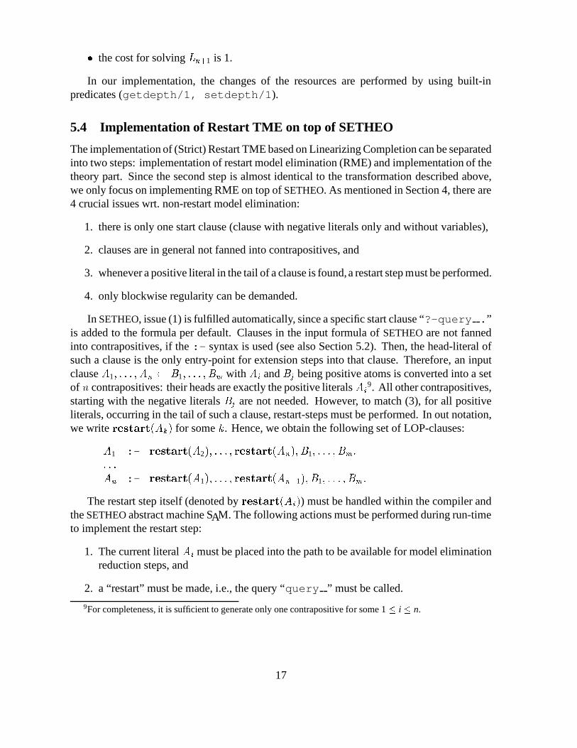
In SETHEO, issue (1) is fulfilled automatically, since a specific start clause “?-query .”is added to the formula per default. Clauses in the input formula of SETHEO are not fannedinto contrapositives, if the :- syntax is used (see also Section 5.2). Then, the head-literal ofsuch a clause is the only entry-point for extension steps into that clause. Therefore, an inputclause A1; : : : ;An B1; : : : ;Bm with Ai and Bj being positive atoms is converted into a setof n contrapositives: their heads are exactly the positive literals Ai 9. All other contrapositives,starting with the negative literals Bj are not needed. However, to match (3), for all positiveliterals, occurring in the tail of such a clause, restart-steps must be performed. In out notation,we write restart(Ak) for some k . Hence, we obtain the following set of LOP-clauses:A1 :- restart(A2); : : : ; restart(An);B1; : : : ;Bm :: : :An :- restart(A1); : : : ; restart(An�1);B1; : : : ;Bm :

The restart step itself (denoted by restart(Ai)) must be handled within the compiler andthe SETHEO abstract machine SAM. The following actions must be performed during run-timeto implement the restart step:

1. The current literal Ai must be placed into the path to be available for model eliminationreduction steps, and

2. a “restart” must be made, i.e., the query “query ” must be called.

9For completeness, it is sufficient to generate only one contrapositive for some 1 � i � n.

17

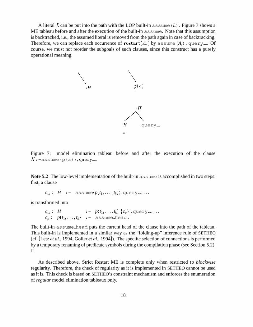
A literal L can be put into the path with the LOP built-in assume(L). Figure 7 shows aME tableau before and after the execution of the built-in assume. Note that this assumptionis backtracked, i.e., the assumed literal is removed from the path again in case of backtracking.Therefore, we can replace each occurrence of restart(Ai) by assume(Ai),query . Ofcourse, we must not reorder the subgoals of such clauses, since this construct has a purelyoperational meaning. JJJ JJJ

,,, eee:H p(a):HH query*

Figure 7: model elimination tableau before and after the execution of the clauseH:-assume(p(a)); query :Note 5.2 The low-level implementation of the built-in assume is accomplished in two steps:first, a clause

ci;j : H :- assume(p(t1; : : : ; tk));query ; : : :is transformed into

ci;j : H :- p(t1; : : : ; tk)[fcpg];query ; : : :cp : p(t1; : : : ; tk) :- assume head.

The built-in assume head puts the current head of the clause into the path of the tableau.This built-in is implemented in a similar way as the “folding-up” inference rule of SETHEO(cf. [Letz et al., 1994, Goller et al., 1994]). The specific selection of connections is performedby a temporary renaming of predicate symbols during the compilation phase (see Section 5.2).2

As described above, Strict Restart ME is complete only when restricted to blockwiseregularity. Therefore, the check of regularity as it is implemented in SETHEO cannot be usedas it is. This check is based on SETHEO’s constraint mechanism and enforces the enumerationof regular model elimination tableaux only.

18

In order to implement the blockwise regularity, the SAM-instruction for regularity (genreg)had to be modified slightly. Instead of proceeding through the entire path (from the currentnode to the root of the tableau) and generating constraints, only a part of the path is checked.This part of the path starts with the current node (environment) and ends at the next restartstep (or at the root of the tableau, if there is none). This condition, however can be detectedvery easily, because at each restart step and at the root of the tableau, the predicate symbol“query ” is present.

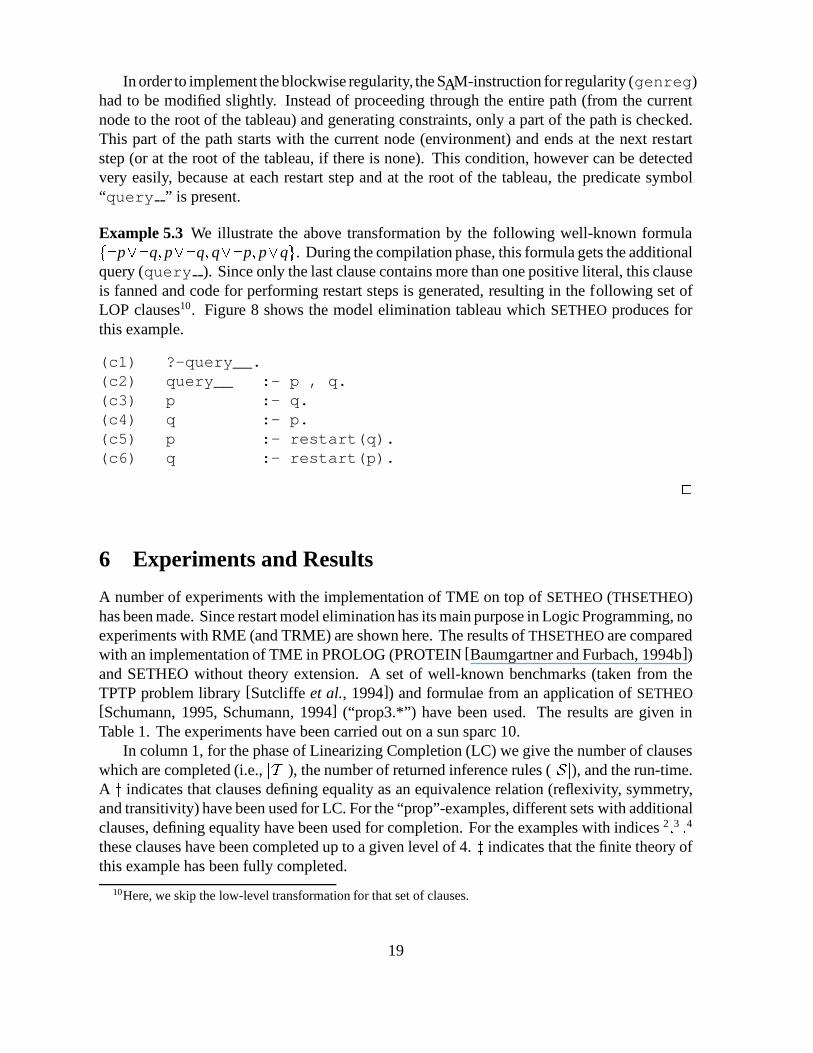
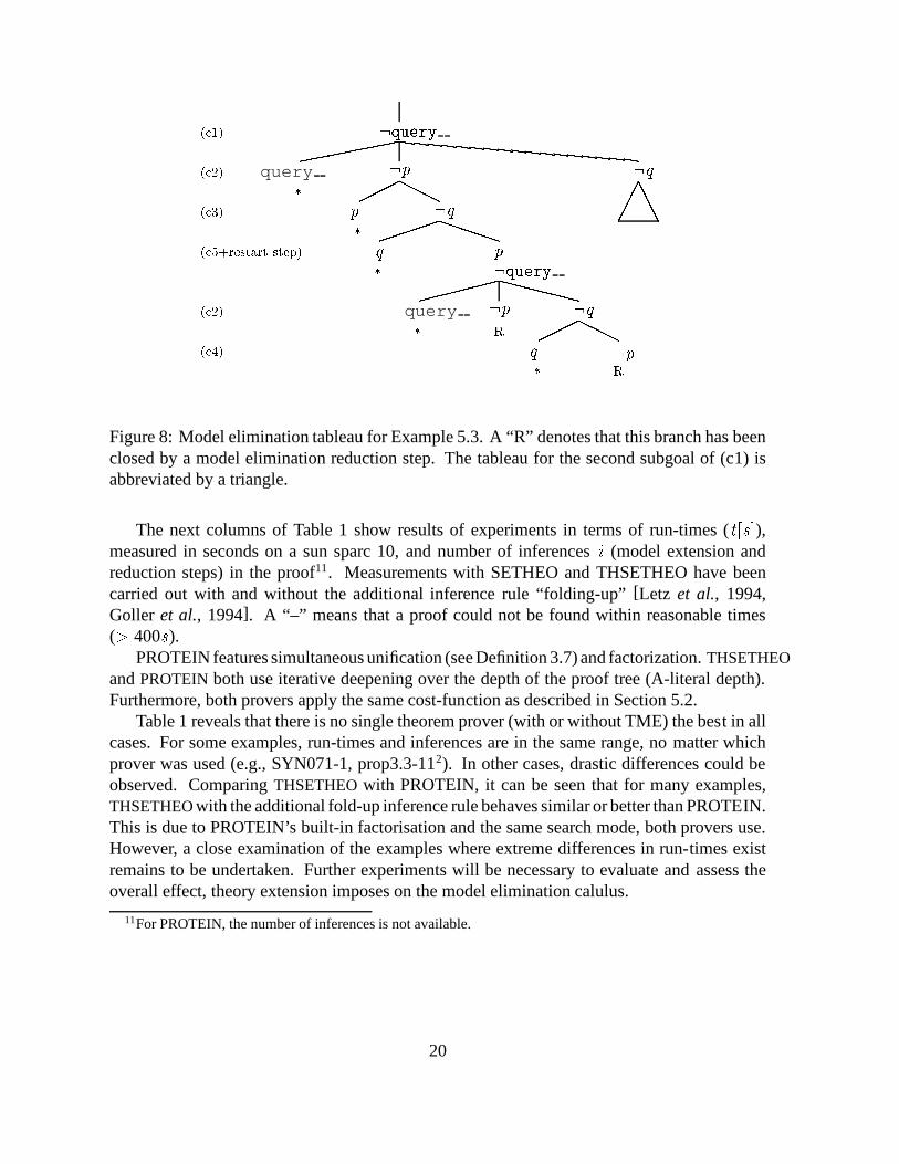
Example 5.3 We illustrate the above transformation by the following well-known formulaf:p_:q; p_:q; q_:p; p_qg. During the compilation phase, this formula gets the additionalquery (query ). Since only the last clause contains more than one positive literal, this clauseis fanned and code for performing restart steps is generated, resulting in the following set ofLOP clauses10. Figure 8 shows the model elimination tableau which SETHEO produces forthis example.

(c1) ?-query__.(c2) query__ :- p , q.(c3) p :- q.(c4) q :- p.(c5) p :- restart(q).(c6) q :- restart(p). 26 Experiments and Results

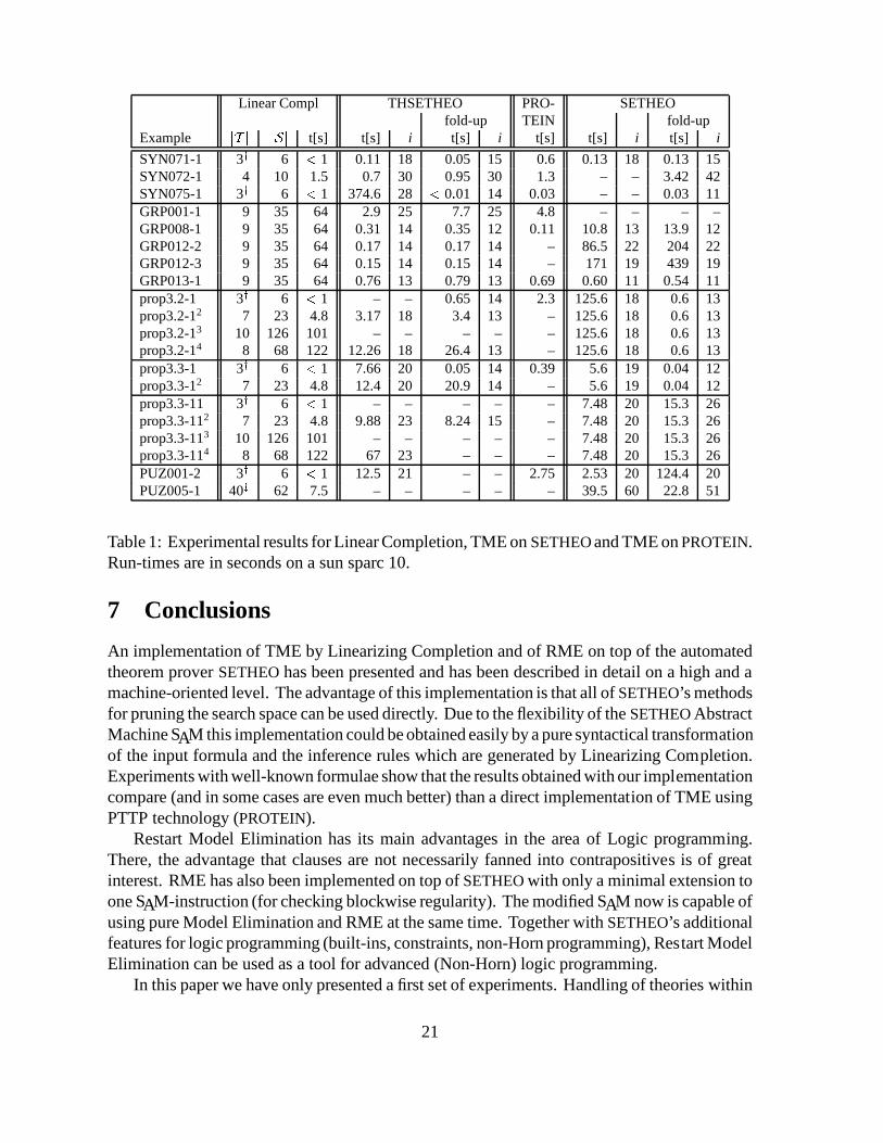
A number of experiments with the implementation of TME on top of SETHEO (THSETHEO)has been made. Since restart model elimination has its main purpose in Logic Programming, noexperiments with RME (and TRME) are shown here. The results of THSETHEO are comparedwith an implementation of TME in PROLOG (PROTEIN [Baumgartner and Furbach, 1994b])and SETHEO without theory extension. A set of well-known benchmarks (taken from theTPTP problem library [Sutcliffe et al., 1994]) and formulae from an application of SETHEO[Schumann, 1995, Schumann, 1994] (“prop3.*”) have been used. The results are given inTable 1. The experiments have been carried out on a sun sparc 10.

In column 1, for the phase of Linearizing Completion (LC) we give the number of clauseswhich are completed (i.e., jT j), the number of returned inference rules (jSj), and the run-time.A y indicates that clauses defining equality as an equivalence relation (reflexivity, symmetry,and transitivity) have been used for LC. For the “prop”-examples, different sets with additionalclauses, defining equality have been used for completion. For the examples with indices 2;3 ;4these clauses have been completed up to a given level of 4. z indicates that the finite theory ofthis example has been fully completed.

10Here, we skip the low-level transformation for that set of clauses.

19

hhhhhhhhhhhhhhhhh��� HHH����� PPPPP������ XXXXXX��� HHH��� AAA:query:p* p* q* p:query* :pR q :p* R

(c2)(c1)(c3)(c5+restart step)(c2)(c4) query

query :q:q

:q

Figure 8: Model elimination tableau for Example 5.3. A “R” denotes that this branch has beenclosed by a model elimination reduction step. The tableau for the second subgoal of (c1) isabbreviated by a triangle.

The next columns of Table 1 show results of experiments in terms of run-times (t [s]),measured in seconds on a sun sparc 10, and number of inferences i (model extension andreduction steps) in the proof11. Measurements with SETHEO and THSETHEO have beencarried out with and without the additional inference rule “folding-up” [Letz et al., 1994,Goller et al., 1994]. A “–” means that a proof could not be found within reasonable times(> 400s).

PROTEIN features simultaneous unification (see Definition 3.7) and factorization. THSETHEOand PROTEIN both use iterative deepening over the depth of the proof tree (A-literal depth).Furthermore, both provers apply the same cost-function as described in Section 5.2.

Table 1 reveals that there is no single theorem prover (with or without TME) the best in allcases. For some examples, run-times and inferences are in the same range, no matter whichprover was used (e.g., SYN071-1, prop3.3-112). In other cases, drastic differences could beobserved. Comparing THSETHEO with PROTEIN, it can be seen that for many examples,THSETHEO with the additional fold-up inference rule behaves similar or better than PROTEIN.This is due to PROTEIN’s built-in factorisation and the same search mode, both provers use.However, a close examination of the examples where extreme differences in run-times existremains to be undertaken. Further experiments will be necessary to evaluate and assess theoverall effect, theory extension imposes on the model elimination calulus.

11For PROTEIN, the number of inferences is not available.

20

Linear Compl THSETHEO PRO- SETHEOfold-up TEIN fold-up

Example jT j jSj t[s] t[s] i t[s] i t[s] t[s] i t[s] i

SYN071-1 3y 6 < 1 0.11 18 0.05 15 0.6 0.13 18 0.13 15SYN072-1 4 10 1.5 0.7 30 0.95 30 1.3 – – 3.42 42SYN075-1 3y 6 < 1 374.6 28 < 0:01 14 0:03 – – 0.03 11GRP001-1 9 35 64 2.9 25 7.7 25 4.8 – – – –GRP008-1 9 35 64 0.31 14 0.35 12 0.11 10.8 13 13.9 12GRP012-2 9 35 64 0.17 14 0.17 14 – 86.5 22 204 22GRP012-3 9 35 64 0.15 14 0.15 14 – 171 19 439 19GRP013-1 9 35 64 0.76 13 0.79 13 0.69 0.60 11 0.54 11prop3.2-1 3y 6 < 1 – – 0.65 14 2.3 125.6 18 0.6 13prop3.2-12 7 23 4.8 3.17 18 3.4 13 – 125.6 18 0.6 13prop3.2-13 10 126 101 – – – – – 125.6 18 0.6 13prop3.2-14 8 68 122 12.26 18 26.4 13 – 125.6 18 0.6 13prop3.3-1 3y 6 < 1 7.66 20 0.05 14 0.39 5.6 19 0.04 12prop3.3-12 7 23 4.8 12.4 20 20.9 14 – 5.6 19 0.04 12prop3.3-11 3y 6 < 1 – – – – – 7.48 20 15.3 26prop3.3-112 7 23 4.8 9.88 23 8.24 15 – 7.48 20 15.3 26prop3.3-113 10 126 101 – – – – – 7.48 20 15.3 26prop3.3-114 8 68 122 67 23 – – – 7.48 20 15.3 26PUZ001-2 3y 6 < 1 12.5 21 – – 2.75 2.53 20 124.4 20PUZ005-1 40z 62 7.5 – – – – – 39.5 60 22.8 51

Table 1: Experimental results for Linear Completion, TME on SETHEO and TME on PROTEIN.Run-times are in seconds on a sun sparc 10.

7 Conclusions

An implementation of TME by Linearizing Completion and of RME on top of the automatedtheorem prover SETHEO has been presented and has been described in detail on a high and amachine-oriented level. The advantage of this implementation is that all of SETHEO’s methodsfor pruning the search space can be used directly. Due to the flexibility of the SETHEO AbstractMachine SAM this implementation could be obtained easily by a pure syntactical transformationof the input formula and the inference rules which are generated by Linearizing Completion.Experiments with well-known formulae show that the results obtained with our implementationcompare (and in some cases are even much better) than a direct implementation of TME usingPTTP technology (PROTEIN).

Restart Model Elimination has its main advantages in the area of Logic programming.There, the advantage that clauses are not necessarily fanned into contrapositives is of greatinterest. RME has also been implemented on top of SETHEO with only a minimal extension toone SAM-instruction (for checking blockwise regularity). The modified SAM now is capable ofusing pure Model Elimination and RME at the same time. Together with SETHEO’s additionalfeatures for logic programming (built-ins, constraints, non-Horn programming), Restart ModelElimination can be used as a tool for advanced (Non-Horn) logic programming.

In this paper we have only presented a first set of experiments. Handling of theories within

21

Model Elimination theorem proving using TME and LC must certainly be further evaluated.In order to make this technique fully automatic, the automatic detection of theory clauses

in the input formula M is necessary. These clauses are removed from the formula and willbe subject to Linearizing Completion. A careful evaluation of experimental results will alsolead to a heuristic control of Linearizing Completion. Control is necessary especially in caseswhere the theory is not finite in order not to generate too many inference rules.

For the TME implementation on top of SETHEO a fine-tuning of the cost-function for anextension step into inference rules can improve the results dramatically. Furthermore, we willevaluate the influence of simultaneous processing of all literals of the inference rules.

This paper has shown techniques for successful combination of Completion methods withtop-down proof search. The straight-forward and efficient implementation on top of SETHEOrevealed that due to its flexibility, SETHEO is ideally suited for implementing different inferencerules and strategies on top of pure Model Elimination.

References

[Astrachan and Stickel, 1992] Owen L. Astrachan and Mark E. Stickel. Caching and Lem-maizing in Model Elimination Theorem Provers. In D. Kapur, editor, Proceedings ofthe 11th International Conference on Automated Deduction (CADE-11), pages 224–238.Springer-Verlag, June 1992. LNAI 607.

[Baumgartner and Furbach, 1993] P. Baumgartner and U. Furbach. Consolution as a Frame-work for Comparing Calculi. Journal of Symbolic Computation, 16(5), 1993. AcademicPress.

[Baumgartner and Furbach, 1994a] P. Baumgartner and U. Furbach. Model Elimination with-out Contrapositives. In A. Bundy, editor, ’Automated Deduction – CADE-12’, volume 814of LNAI, pages 87–101. Springer, 1994.

[Baumgartner and Furbach, 1994b] P. Baumgartner and U. Furbach. PROTEIN: A PROverwith a Theory Extension Interface. In A. Bundy, editor, Automated Deduction – CADE-12,volume 814 of LNAI, pages 769–773. Springer, 1994.

[Baumgartner, 1992] P. Baumgartner. A Model Elimination Calculus with Built-in Theories.In H.-J. Ohlbach, editor, Proceedings of the 16-th German AI-Conference (GWAI-92), pages30–42. Springer, 1992. LNAI 671.

[Baumgartner, 1994] P. Baumgartner. Refinements of Theory Model Elimination and a Variantwithout Contrapositives. In A.G. Cohn, editor, 11th European Conference on ArtificialIntelligence, ECAI 94. Wiley, 1994.

[Baumgartner, 1995 ] P. Baumgartner. Linear and Unit-Resulting Refutations for Horn Theo-ries. Journal of Automated Reasoning, 1995 (?). (To appear, also in: Research Report 9/93,Institute for Computer Science, University of Koblenz, Germany).

22

[Chang and Lee, 1973] C. Chang and R. Lee. Symbolic Logic and Mechanical TheoremProving. Academic Press, 1973.

[Eder, 1985] E. Eder. An Implementation of a Theorem Prover based on the ConnectionMethod. In W. Bibel and B. Petkoff, editors, AIMSA: Artificial Intelligence MethodologySystems Applications, pages 121–128. North–Holland, 1985.

[Gabbay, 1985] D. M. Gabbay. N-Prolog: An extension of Prolog with hypothetical impli-cation II. logical foundations, and negation as failure. Journal of Logic Programming,2(4):251–284, December 1985.

[Gallier et al., 1987] J. H. Gallier, S. Raatz, and W. Snyder. Theorem proving using rigide-unification: Equational matings. In Logics in Computer Science ’87, Ithaca, New York,1987.

[Goller et al., 1994] Chr. Goller, R. Letz, K. Mayr, and J. Schumann. SETHEO V3.2: RecentDevelopments (System Abstract) . In Proc. CADE 12, pages 778–782, June 1994.

[Letz et al., 1992] R. Letz, J. Schumann, S. Bayerl, and W. Bibel. SETHEO: A High-Performance Theorem Prover. Journal of Automated Reasoning, 8(2), 1992.

[Letz et al., 1994] R. Letz, K. Mayr, and C. Goller. Controlled Integrations of the Cut Ruleinto Connection Tableau Calculi. Journal of Automated Reasoning, 13, 1994.

[Lloyd, 1987] J. Lloyd. Foundations of Logic Programming. Symbolic Computation.Springer, second, extended edition, 1987.

[Loveland, 1968] D. Loveland. Mechanical Theorem Proving by Model Elimination. JACM,15(2), 1968.

[Loveland, 1987] D.W. Loveland. Near-Horn Prolog. In J.-L. Lassez, editor, Proc. of the 4thInt. Conf. on Logic Programming, pages 456–469. The MIT Press, 1987.

[Petermann, 1993] U. Petermann. Completeness of the pool calculus with an open built intheory. In Georg Gottlob, Alexander Leitsch, and Daniele Mundici, editors, 3rd KurtGodel Colloquium ’93, number 713 in Lecture Notes in Computer Science, pages 264–277.Springer-Verlag, 1993.

[Plaisted, 1988] D. Plaisted. Non-Horn Clause Logic Programming Without Contrapositives.Journal of Automated Reasoning, 4:287–325, 1988.

[Schumann, 1994] J. Schumann. Using SETHEO for verifying the development of a Com-munication Pro tocol in FOCUS – a case study –. SFB Bericht SFB342/20/94A, TechnischeUniversitat Munchen, 1994. long version.

[Schumann, 1995] J. Schumann. Using SETHEO for Verifying the Development of a Com-munication Pro tocol in FOCUS – A Case Study –. In Proc. Workshop on Theorem Provingwith Analytic Tableaux and Related Methods, Koblenz, Germany, 1995. to appear.

23

[Stickel, 1985] M.E. Stickel. Automated Deduction by Theory Resolution. Journal of Auto-mated Reasoning, 1:333–355, 1985.

[Stickel, 1988] M. Stickel. A Prolog Technology Theorem Prover: Implementation by anExtended Prolog Compiler. Journal of Automated Reasoning, 4:353–380, 1988.

[Stickel, 1989] M. Stickel. A Prolog Technology Theorem Prover: A New Exposition andImplementation in Prolog. Technical note 464, SRI International, 1989.

[Sutcliffe et al., 1994] G. Sutcliffe, C. Suttner, and T. Yemenis. The TPTP problem library.In Proc. CADE-12. Springer, 1994.

24