balancing and elimination of nuisance variables

Volume 6, Issue 2 2010 Article 6

The International Journal ofBiostatistics

CAUSAL INFERENCE

Balancing and Elimination of NuisanceVariables

Siamak Noorbaloochi, Minneapolis VA Medical Center andUniversity of Minnesota

David Nelson, Minneapolis VA Medical Center andUniversity of Minnesota

Masoud Asgharian, McGill University

Recommended Citation:Noorbaloochi, Siamak; Nelson, David; and Asgharian, Masoud (2010) "Balancing andElimination of Nuisance Variables," The International Journal of Biostatistics: Vol. 6: Iss. 2,Article 6.DOI: 10.2202/1557-4679.1209

UnauthenticatedDownload Date | 10/4/16 1:52 PM

Balancing and Elimination of NuisanceVariables

Siamak Noorbaloochi, David Nelson, and Masoud Asgharian

Abstract

Addressing covariate imbalance in causal analysis will be reformulated as an elimination ofthe nuisance variables problem. We show, within a counterfactual balanced setting, howaveraging, conditioning, and marginalization techniques can be used to reduce bias due to apossibly large number of imbalanced baseline confounders. The notions of X-sufficient and X-ancillary quantities are discussed and, as an example, we show how sliced inverse regression andrelated methods from regression theory that estimate a basis for a central sufficient subspaceprovide alternative summaries to propensity based analysis. Examples for exponential families andelliptically symmetric families of distributions are provided.

KEYWORDS: confounding, dimension reduction, sufficient summary, ancillarity

Author Notes: Research supported in part by VAHSR&D Grant IIR 07-229.


1 Introduction

A commonproblemof causalinferencein observationalstudiesis covariateim-balanceor confounding. Covariateimbalanceoccurswhen we are interestedinestimatingtheeffectof avariableof interest,typically aninterventionor treatment,on a responsebut the distributionof the interventionand the outcomeboth varywith the samesetof covariates.In this paper,we studythis problemby treatinginterventionassignmentasa nuisancevariablein thedistributionof thecovariatesandexaminehow to eliminatethis nuisancevariable.Theeliminationof nuisanceparametersin statisticalinferenceis a classic,well studiedarea.We find that,bytreatingtheinterventionvariableasanuisancevariable,weareableto usetheideasunderlyingclassicalmethodsfor eliminatingnuisanceparametersto readilyaddresscovariateimbalance.

Two approacheswe consideraremarginalizationandconditioning. Withmarginalizationwe try to study the effect of the interventionon the outcomebyusingadistributionfor afunctionof thecovariatesthatdoesnotdependupon.Withconditioningwe find a covariate-basedstatistic,called a sufficient summary,forwhichtheconditionaldistributionof thecovariatesgiventhestatisticis independentof the interventionandthenstudy the effect of the interventionon the responsesconditionalon this statistic. Both approachesare basedon a compatiblepair ofconditionalmodels:onefor thecovariatesgiventhe interventionandtheotherfortheinterventiongiventhecovariates.Thecounterpartsof thesetwo methodsin thestatisticaltheoryfor the eliminationof nuisanceparametersareFisher’sclassicalideasof ancillarityandsufficiency.However,in this traditionalstatisticalinference,sufficiencyis usedto marginalizeandancillarity is usedto performa conditionalanalysis.

A critical issuein acausalanalysisis to actuallydefinethecausaleffect. In-deed,for theconditionaleliminationof thecovariateimbalancetheissueof how toaggregateconditionalinferencesis centralto thedefinitionandestimationof causaleffects.RosenbaumandRubin(1983)provideaNeyman-typecounterfactualmodelto givemeaningto theaverageof theconditionaleffects,hereaveragedwith respectto themarginaldistributionof thecovariates.Note,thisspecificaveragingis butonepotentialaveragingproposedby Cochran(1968)for definingunbiasedgroupdif-ferencesin outcomes.In the following sectionwe outline an alternativedecisiontheoreticjustification,usingsquarederrorloss,for usingthis specificform of aver-agingof theconditionaldistributions.Thethird sectionintroducestheconditionalelimination methodwhereinwe definethe notion of sufficient summarieswhichareanalogousto sufficientstatistics. We showthat propensityscoresandrelatedbalancingscoresareall sufficientsummaries.In addition,we showhow theeffec-tive dimensionreductiondirectionsdiscussedby Li (1994)andothersin thetheory

1

Noorbaloochi et al.: Balancing and Elimination of Nuisance Variables


of dimensionreductionfor regressioncanbe usedaslinear sufficientsummaries.Thesesummariesweredevisedchiefly with theaim of reducingthedimensionofthe predictorspace.We discusshow they may be usedto reducebiasdueto co-variateimbalance.In thelastsection,we introduceancillaryquantitiesandprovideconditionsunderwhichthesequantitiescanbeusedfor theeliminationof covariateimbalance.Finally, wedemonstratehowtheseideascanbeappliedto realdatasets.First, however,we needto definethenotationandadditionalconceptswe will usein thesubsequentdiscussion.

Let (Y,T,X) denotea vectorof observablevariableswhereY is a responsevariable,T is a randomvariablewhoseeffecton thedistributionof Y is of interest,andX is asetof p confoundingcovariates.Thesetsof possiblevaluesof Y, T, andX, respectively,will bedenotedby Y , T , andX . For simplicity, we assumethefamiliesof distributionsfor thesemeasuresaredominatedwith respectto Lebesguemeasureor acountingmeasureand,hence,densitiesandprobabilitymassfunctionswill beusedto describethemodels.

Considera family of conditionalcovariatemodelsF = { fθ (x | t) : θ ∈ Θ}anda family of propensitymodelsG = { fβ (t |x) : β ∈ B, t ∈ R, x ∈ Rp}. Weassumethepropensitymodelsandtheconditionalcovariatemodelsarecompatible(Arnold andPress,1989). A pair of conditionaldistributions, fθ (t|x) and fβ (x|t),arecompatibleif thereexistsa joint distribution fβ ,θ (t,x) havingthesepair of dis-tributionsasconditionaldistributions.The family R = { fγ(y| t, x) : γ ∈ Γ} is theregressionmodel.TheindexingsetsΘ, B, andΓ areeithersubsetsof Rd or spec-ify larger semi- or non-parametricfamilies. Let fγ,θ (y, t, x) denotethe densityfor the joint distributionof the randomvector(Y, T, X). The availablesampleis{(yi , ti ,xi), i = 1, . . . ,n} with the observationsdrawn from this joint distributionfγ,θ (y, t, x).

For situationswhereT is a finite set, a commonpracticein propensityanalysisis to assumeaparametricform, suchas

Pr(T = t |X = x) = exp{j=d

∑j=0

βt jhj(x)}{

1+exp{j=d

∑j=0

βt jhj(x)}}−1

for someset of d + 1 known functionshj . However,compatibility requiresthatthis “working” logistic modelyields an equivalentparametricexponentialfamilyconditionalmodelsfor thecovariatesof theform

fθ (x |T = t) = β (θ , x) exp{Q′(θ , t)T(x)}c(θ , t).

Fordetailson thisnecessaryequivalenceseeKay andLittle (1987)andArnold andPress(1989).

2

The International Journal of Biostatistics, Vol. 6 [2010], Iss. 2, Art. 6

DOI: 10.2202/1557-4679.1209


A Counterfactual Setting. Thequestion“If the treatmentandthecovari-ateswereindependent,whatwouldbethedifferencein thedistributionsof Y acrosslevelsof T?” is a basicconditionalquestionin definingandestimatingcausalef-fectsof T on Y. Indeed,to studythe unconfoundedeffect of T on Y onewouldlike theprocessgeneratingtheobserveddatato follow a memberof the family ofdistributions;

J = {(ν(y|x, t), η(x), π(t)) : ν(y|x, t)≥ 0,

η(x)≥ 0, π(t)≥ 0,∫Y ,X

ν(y|x, t)η(x) dxdy= 1, t ∈T },

where,for eachmember,X is independentof T with marginaldistributionsgivenby η and π. Note that we intentionallyusenew notationto denotethe relevantdistributionsin theseunrealizedworlds to put emphasison the fact that were Tand X independent,the datagenerationmechanismwould be different from thecorrespondingmechanismin the realizedworld. The assignmentmechanismTandX aredependentin thefactualworld generatingthedatawith thedistributionsfγ(y|x, t), fθ (x|t)and fβ (t) modeledby R, F andG . Eachchoiceof ν(y|x, t) andη(x) definesa conditionaljoint distributionof theresponseandthecovariatesin acounterfactualsettingwhereT andX areindependent.To studythecausaleffectof T on Y usingsuchcounterfactualmodels,we want to choosea memberof Jwhichis as“close” aspossibleto thefactualworld. Therefore,wemaketheexplicitassumptions:(i) π(t) = f (t), (ii) for eachgivenx andt, theconditionaldistributionof Y is the sameas that for the observedfactual universe,namely,νγ(y|x, t) =fγ(y|x, t). We referto thisassumptionastheregressionassumption.

Under theseassumptions,the derived family of counterfactualresponsemodelsgivenT = t is:

{(νγ,η(y| t) : νγ η(y| t) =∫X

fγ(y|x, t)η(x)dx, η ∈J , γ ∈ Γ}.

Correspondingto eachof thesecounterfactualmodels,whicharedefinedby differ-entchoicesfor η(x), we candefinea setof potentialoutcomes{Yt(γ,η); t ∈ T }.Different functionalsof thesemodelsthencould be usedfor a counterfactualas-sessment.Forexample,for adichotomoustreatmentT, anaveragecausaltreatmenteffectin thecounterfactualsettingindexedby (γ,η) couldbedefinedas

κγ(η) = E(Y1(νγ,η)−Y0(νγ,η)) = Eη [Eγ(Y |X,T = 1)−Eγ(Y|X,T = 0)].

Thereareaninfinite numberof possiblespecificationsfor η(x). Typically,aversionof the ignorability assumptionimplies that thereis just one“true” model,andone“true” causaleffect of the treatment,andthis is the quantitythat causalinferenceproceduresattemptto estimate.Without suchanassumption,we needto considerhow to chooseη in asensible,perhapsoptimal,manner.

3



2 Elimination of NuisanceVariables

Theeffectof confoundingontheestimationof theeffectof T onY canbeaddressedat the designstage(usingrandomization,blocking, etc.) or at the analysisstage.In observationalstudieswe aretypically limited to addressingconfoundingusinganalyticmethods.In doing so, onetacitly acceptsthe regressionassumptionandthenattemptsto controlor eliminatethedependencebetweenX andT. Eliminationof nuisanceparametersis a classicalproblemin statisticalinference.For a reviewof thesemethods,seeBasu(1977)andSeverini(2000). Onepotentialapproachto addressingconfoundingis to treatX asa “nuisance”variablein thepropensitymodel,G , or, equivalently,treatT asa “nuisance”variablein thecovariatemodel,F .

Methodsto eliminatenuisancevariables,whetherexactor approximate,arebasedonfactorizationandsummarizationof thelikelihoodfunction.Classicalsum-marizationmethodsaremarginalization,maximization,andconditioning.Thefac-tual conditionallikelihood is givenby fγ(y|x, t) fθ (x | t). Underthe regressionas-sumption, to constructa counterfactualdistributionfor thepotentialoutcomesoneshouldconcentrateon the forward regressionmodel,F = { fθ (x | t) : θ ∈ Θ}. Inthis model,t is anunwantedindex that is a nuisancein defininga measureof thedirecteffectof T onY. Therefore,onecould look for anoptimalmethodto elimi-natethedependenceof thecovariatesandT, which is very similar to theclassicalmethodsfor eliminationof nuisanceparametersin the developmentof inferenceprocedures.Indeed,this outlook shedslight on a numberof existingmethodsofestimationandopensthedoorto ahostof newproceduresfor causalanalysis.

“Bayesian” Marginalization. BayesianMarginalizationherecouldbede-fined asa methodof eliminatingthe nuisancevariableby averagingover the nui-sancevariableusingawell chosenweightfunction.However,sinceT is anobserv-ablerandomvariable,f (t) is anaturalchoicefor thisweightfunction.Thissuggestsη(x) shouldbe chosento be the marginaldistribution fθ (x) =

∫T fθ (x | t) f (t)dt.

Note that in the factualworld, T andX arenot independentand fθ (x) is indeedacounterfactualchoice.

A nicepropertyof fθ (x) is it yieldsthecounterfactualbalancedmodelclos-estto thefactualworld in thesenseof squarederrorloss,thatis

fθ (x) = argminDET( fθ (x |T = t)−ν(x))2

whereD = {ν(x) : ν(x) ≥ 0∫

ν(x)dx = 1} is theclassof possibledensitiesoverthecovariatespace.Further,

fθ (x) = argminD

∫T

∫Y

fγ(y|x, t)( fθ (x |T = t)−ν(x))2 f (t)dydt

4


DOI: 10.2202/1557-4679.1209


which impliesthefamily of distributions

{νγ,θ (y|T = t) =∫X

fγ(y|x, t) fθ (x)dx, t ∈T ,γ ∈ Γ,θ ∈ Θ} (1)

couldbeusedastheconditionaldistributionsof Y in counterfactualsettingshavingthesameforwardregressionmodelasthefactualworld but with independencebe-tweenT andX with closestresemblanceto thefactualsettinggeneratingthedataasmeasuredby squareddistance.Obviously,othermeasuresof theclosenessof abal-ancedν(x) to theactualcovariatemodelswill resultin a different “counterfactualworking models”.

The well known causalmodeldiscussedby Rubin (1974)andby Rosen-baumand Rubin (1983) providesanotherbasisfor this choiceof η(x). In thismodel,eachunit is associatedwith acollectionof randomvariablescalledpotentialoutcomes,{Yt : t ∈ T }, which aredefinedas“the outcomeif theunit wereto re-ceivetreatmentlevel t”. Considera pair of potentialoutcomesY0 andY1, T = 0,1,andtheobservedresponse,Y = Y0T +Y1(1−T). Fromthis definitionof potentialoutcomesonecanimmediatelydeducethat

νYt (y|x,T = t) = f (y|x,T = t), t = 0,1

which is theregressionassumption.Thestrongignorabilityassumption

νY0,Y1(y0, y1 |X = x, T = 1) = νY0,Y1(y0, y1 |X = x, T = 0)

immediatelyimplies

νYt (y) =∫X

νYt (yt |X = x, T = t) fθ (x)dx

and,hence,a memberof the family of distributionsin (1) forms the basisfor thepotentialoutcomemodelsin thesesettings. Indeed,the main task of the strongignorability assumptionis to justify useof the abovemodel for the conditionalresponses.

Anotherargumentjustifying theuseof this family is basedon thenotionofthe do(x) operatorintroducedby Pearl. The detailsof this argumentaregiven inPearl(2009).Thestratificationmethodsdescribedin Cochran(1968)alsoarebasedonusingthismarginaldistribution.

Conditioning. In the following discussion,ancillarity andsufficiencywillbe highly relevant. Conditioningis basedon finding a U(x1,x2, . . . ,xp) suchthatX andT areconditionally independentgiven U. Hence,inferencecanbe carried

5



out conditionalon thevaluesof U. Theseconditionalinferencescanthenbecom-binedin somesensiblemanner.An importantpoint to be emphasizedis that, forclassicalmethodsof statisticalinference,we useancillarity in conditionalmodel-ing andsufficiencyin informativemarginalization.For creatingbalance,however,weusesufficiencyfor conditioningandancillarity for theresultingnon-informativedistributions.

Notethatin classicalstatisticalinference,whereU is asufficientstatisticfora modelparameter,thesufficiencyprinciple recommendsreplacingthe likelihoodwith thederivedmarginallikelihoodfor theobservedsufficientstatistic.Thecrucialpropertyof U is that,within anyconditionsetdefinedby U, theconditionalmodelsfor X arefreefrom the indexingparameter.That is for all thevaluesof the index,theconditionaldistributionsfor X arethesame.Therefore,whentreatingT asanindexparameter,we canlook for a quantitysufficientfor thefamily indexedby Tandlook within slicesconstructedby thesufficientquantities.

The conditionalityprinciple advocatesrestrictingthe inferencesto condi-tionalmodelsgivenmaximalancillaries.If wetreatT asa“parameter”,themarginaldistributionof theancillarybecomesinvariantwith respectto T. Therefore,to cre-atebalance,onemayidentify situationswhereanancillaryquantityfor T existsandtheoriginalobservedmodelreplacedwith onebasedon thisancillaryquantity.

Usingthenotionof partialsufficiencyfrom CoxandHinkley (1974),wefor-mally definethefollowing notionof a balancingcondition.SeealsoNoorbaloochiandNelson(2008)andNelsonandNoorbaloochi(2009).

Sufficient Summaries.For thecovariatemodelF , thestatisticS(θ , X) isanX-sufficientsummaryfor T if

fθ (x |S(X), T) = fθ (x |S(X)), (2)

that is, the distributionof X over subpopulationsidentifiedby S(X) = s doesnotdependon T. For the compatiblepropensitymodelG , the statisticS(X) is an X-sufficientsummaryif, for any fT in G ,

fT(t |S(X)) = fT(t |X). (3)

If we think of T asa “parameter”andX asthe data,this is similar to the notionof Bayesiansufficiency,whereS(data) is sufficient if f (parameter|S(data)) =f (parameter|data). Note that to identify, or estimate,a sufficientsummary,onedoesnotneedto knowor usethepropensitymodelG . In theabove,weintentionallysuppressedtheparameterθ , (real-valuedor otherwise),assumingit is knownor canbeestimatedvia aconsistentestimatorin anavailablelargesample.

Setsof sufficientcovariatesdiscussedby Dawid (1979),RobinsandMor-genstern(1987),Pearl(2009)andGreenland(2003)arespecialcasesof sufficient

6


DOI: 10.2202/1557-4679.1209


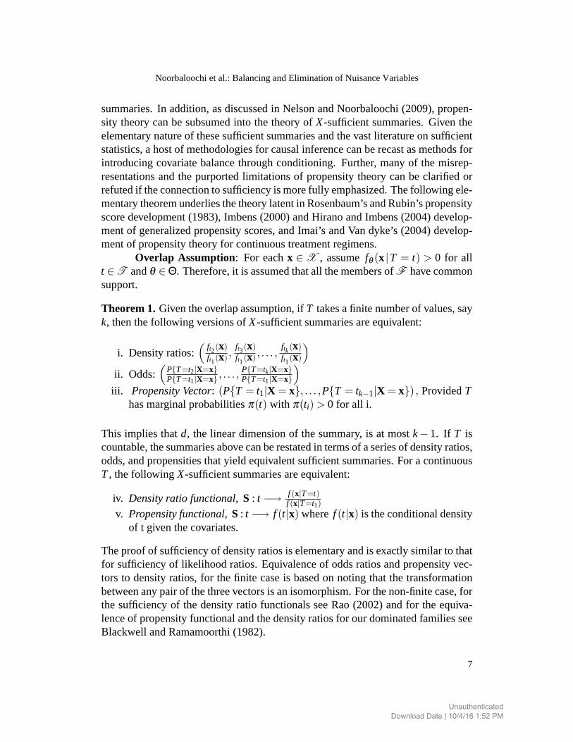
summaries.In addition,asdiscussedin NelsonandNoorbaloochi(2009),propen-sity theorycanbesubsumedinto the theoryof X-sufficientsummaries.Given theelementarynatureof thesesufficientsummariesandthevastliteratureonsufficientstatistics,ahostof methodologiesfor causalinferencecanberecastasmethodsforintroducingcovariatebalancethroughconditioning. Further,manyof themisrep-resentationsandthe purportedlimitations of propensitytheorycanbe clarified orrefutedif theconnectionto sufficiencyis morefully emphasized.Thefollowing ele-mentarytheoremunderliesthetheorylatentin Rosenbaum’sandRubin’spropensityscoredevelopment(1983),Imbens(2000)andHiranoandImbens(2004)develop-mentof generalizedpropensityscores,andImai’s andVan dyke’s(2004)develop-mentof propensitytheoryfor continuoustreatmentregimens.

Overlap Assumption: For eachx ∈ X , assumefθ (x |T = t) > 0 for allt ∈T andθ ∈Θ. Therefore,it is assumedthatall themembersof F havecommonsupport.

Theorem1. Giventheoverlapassumption,if T takesafinite numberof values,sayk, thenthefollowing versionsof X-sufficientsummariesareequivalent:

i. Densityratios:(

ft2(x)ft1(x) ,

ft3(x)ft1(x) , . . . ,

ftk(x)ft1(x)

)ii. Odds:

(P{T=t2|X=x}P{T=t1|X=x} , . . . ,

P{T=tk|X=x}P{T=t1|X=x}

)iii. PropensityVector: (P{T = t1|X = x}, . . . ,P{T = tk−1|X = x}) , ProvidedT

hasmarginalprobabilitiesπ(t) with π(ti) > 0 for all i.

This implies thatd, the lineardimensionof thesummary,is at mostk−1. If T iscountable,thesummariesabovecanberestatedin termsof aseriesof densityratios,odds,andpropensitiesthatyield equivalentsufficientsummaries.For a continuousT, thefollowing X-sufficientsummariesareequivalent:

iv. Densityratio functional, S : t −→ f (x|T=t)f (x|T=t1)

v. Propensityfunctional, S: t −→ f (t|x) where f (t|x) is theconditionaldensityof t giventhecovariates.

Theproofof sufficiencyof densityratiosis elementaryandis exactlysimilar to thatfor sufficiencyof likelihood ratios.Equivalenceof oddsratiosandpropensityvec-tors to densityratios,for thefinite caseis basedon noting that the transformationbetweenanypairof thethreevectorsis anisomorphism.For thenon-finitecase,forthe sufficiencyof thedensityratio functionalsseeRao(2002)andfor theequiva-lenceof propensityfunctionalandthedensityratiosfor ourdominatedfamiliesseeBlackwell andRamamoorthi(1982).

7



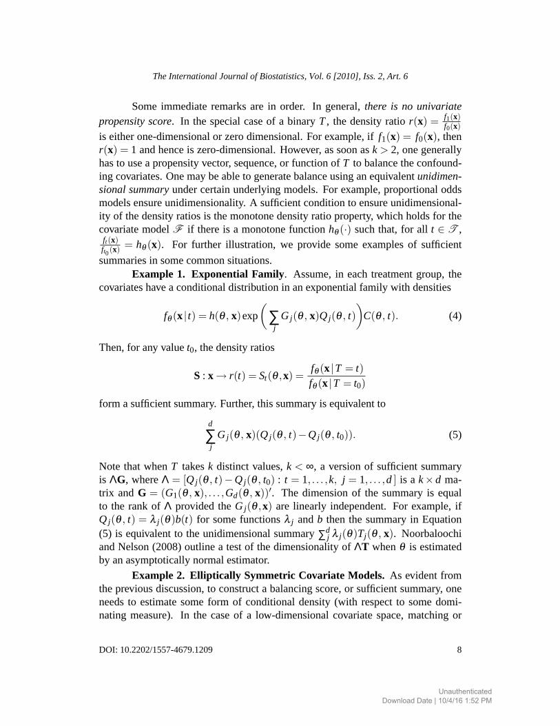
Someimmediateremarksare in order. In general,there is no univariatepropensityscore. In the specialcaseof a binary T, the densityratio r(x) = f1(x)

f0(x)is eitherone-dimensionalor zerodimensional.For example,if f1(x) = f0(x), thenr(x) = 1 andhenceis zero-dimensional.However,assoonask > 2, onegenerallyhasto usea propensityvector,sequence,or functionof T to balancetheconfound-ing covariates.Onemaybeableto generatebalanceusinganequivalentunidimen-sionalsummaryundercertainunderlyingmodels.For example,proportionaloddsmodelsensureunidimensionality.A sufficientconditionto ensureunidimensional-ity of thedensityratiosis themonotonedensityratio property,which holdsfor thecovariatemodelF if thereis a monotonefunctionhθ (·) suchthat, for all t ∈ T ,ft(x)ft0(x) = hθ (x). For further illustration, we provide someexamplesof sufficient

summariesin somecommonsituations.Example 1. Exponential Family. Assume,in eachtreatmentgroup, the

covariateshaveaconditionaldistributionin anexponentialfamily with densities

fθ (x | t) = h(θ , x)exp

(∑

jGj(θ , x)Qj(θ , t)

)C(θ , t). (4)

Then,for anyvaluet0, thedensityratios

S : x → r(t) = St(θ ,x) =fθ (x |T = t)fθ (x |T = t0)

form asufficientsummary.Further,this summaryis equivalentto

d

∑j

Gj(θ , x)(Qj(θ , t)−Qj(θ , t0)). (5)

Note that whenT takesk distinct values,k < ∞, a versionof sufficientsummaryis ΛG, whereΛ = [Qj(θ , t)−Qj(θ , t0) : t = 1, . . . ,k, j = 1, . . . ,d ] is a k×d ma-trix andG = (G1(θ , x), . . . ,Gd(θ , x))′. The dimensionof the summaryis equalto the rank of Λ providedthe Gj(θ ,x) are linearly independent.For example,ifQj(θ , t) = λ j(θ)b(t) for somefunctionsλ j andb thenthe summaryin Equation(5) is equivalentto the unidimensionalsummary∑d

j λ j(θ)Tj(θ , x). NoorbaloochiandNelson(2008)outlinea testof thedimensionalityof ΛT whenθ is estimatedby anasymptoticallynormalestimator.

Example 2. Elliptically Symmetric Covariate Models. As evidentfromthepreviousdiscussion,to constructa balancingscore,or sufficientsummary,oneneedsto estimatesomeform of conditionaldensity(with respectto somedomi-natingmeasure).In the caseof a low-dimensionalcovariatespace,matchingor

8


DOI: 10.2202/1557-4679.1209


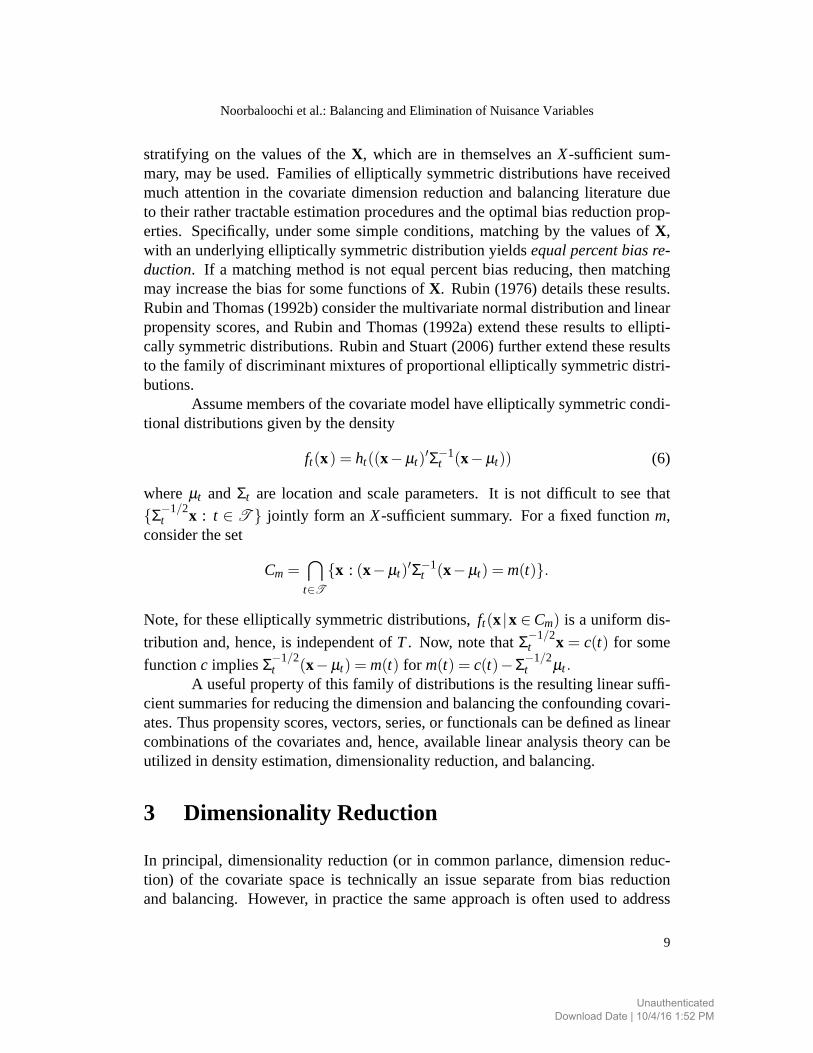
stratifying on the valuesof the X, which are in themselvesan X-sufficient sum-mary,maybeused.Familiesof elliptically symmetricdistributionshavereceivedmuchattentionin the covariatedimensionreductionandbalancingliteraturedueto their rathertractableestimationproceduresandtheoptimalbiasreductionprop-erties. Specifically,undersomesimpleconditions,matchingby the valuesof X,with anunderlyingelliptically symmetricdistributionyieldsequalpercentbiasre-duction. If a matchingmethodis not equalpercentbiasreducing,thenmatchingmay increasethebiasfor somefunctionsof X. Rubin(1976)detailstheseresults.RubinandThomas(1992b)considerthemultivariatenormaldistributionandlinearpropensityscores,andRubin andThomas(1992a)extendtheseresultsto ellipti-cally symmetricdistributions.RubinandStuart(2006)furtherextendtheseresultsto thefamily of discriminantmixturesof proportionalelliptically symmetricdistri-butions.

Assumemembersof thecovariatemodelhaveelliptically symmetriccondi-tionaldistributionsgivenby thedensity

ft(x) = ht((x−µt)′Σ−1t (x−µt)) (6)

whereµt and Σt are locationandscaleparameters.It is not difficult to seethat

{Σ−1/2t x : t ∈ T } jointly form an X-sufficientsummary.For a fixed function m,

considertheset

Cm =⋂

t∈T

{x : (x−µt)′Σ−1t (x−µt) = m(t)}.

Note,for theseelliptically symmetricdistributions,ft(x |x ∈Cm) is a uniform dis-

tribution and,hence,is independentof T. Now, notethat Σ−1/2t x = c(t) for some

functionc impliesΣ−1/2t (x−µt) = m(t) for m(t) = c(t)−Σ−1/2

t µt .A usefulpropertyof this family of distributionsis theresultinglinearsuffi-

cientsummariesfor reducingthedimensionandbalancingtheconfoundingcovari-ates.Thuspropensityscores,vectors,series,or functionalscanbedefinedaslinearcombinationsof the covariatesand,hence,availablelinear analysistheorycanbeutilized in densityestimation,dimensionalityreduction,andbalancing.

3 Dimensionality Reduction

In principal, dimensionalityreduction(or in commonparlance,dimensionreduc-tion) of the covariatespaceis technicallyan issueseparatefrom bias reductionandbalancing. However,in practicethe sameapproachis often usedto address

9



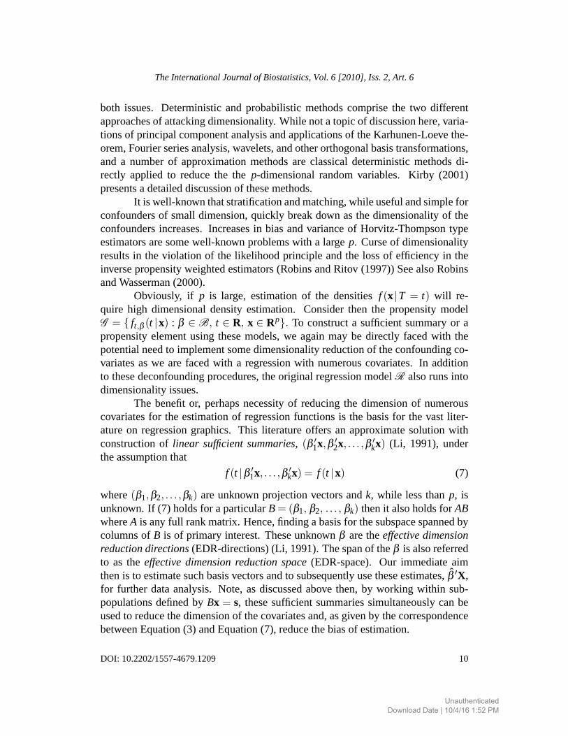
both issues. Deterministicand probabilisticmethodscomprisethe two differentapproachesof attackingdimensionality.While notatopicof discussionhere,varia-tionsof principalcomponentanalysisandapplicationsof theKarhunen-Loevethe-orem,Fourierseriesanalysis,wavelets,andotherorthogonalbasistransformations,and a numberof approximationmethodsare classicaldeterministicmethodsdi-rectly applied to reducethe the p-dimensionalrandomvariables. Kirby (2001)presentsadetaileddiscussionof thesemethods.

It is well-knownthatstratificationandmatching,while usefulandsimpleforconfoundersof small dimension,quickly breakdownasthedimensionalityof theconfoundersincreases.Increasesin biasandvarianceof Horvitz-Thompsontypeestimatorsaresomewell-knownproblemswith a largep. Curseof dimensionalityresultsin the violation of the likelihood principle andthe lossof efficiencyin theinversepropensityweightedestimators(RobinsandRitov (1997))SeealsoRobinsandWasserman(2000).

Obviously, if p is large, estimationof the densities f (x |T = t) will re-quire high dimensionaldensityestimation. Considerthen the propensitymodelG = { ft,β (t |x) : β ∈ B, t ∈ R, x ∈ Rp}. To constructa sufficientsummaryor apropensityelementusing thesemodels,we againmay be directly facedwith thepotentialneedto implementsomedimensionalityreductionof theconfoundingco-variatesaswe arefacedwith a regressionwith numerouscovariates.In additionto thesedeconfoundingprocedures,theoriginal regressionmodelR alsorunsintodimensionalityissues.

The benefitor, perhapsnecessityof reducingthe dimensionof numerouscovariatesfor the estimationof regressionfunctionsis the basisfor the vast liter-atureon regressiongraphics. This literatureoffers an approximatesolutionwithconstructionof linear sufficientsummaries, (β ′

1x,β ′2x, . . . ,β ′

kx) (Li, 1991),undertheassumptionthat

f (t |β ′1x, . . . ,β ′

kx) = f (t |x) (7)

where(β1,β2, . . . ,βk) areunknownprojectionvectorsandk, while lessthan p, isunknown.If (7) holdsfor aparticularB = (β1, β2, . . . , βk) thenit alsoholdsfor ABwhereA is anyfull rankmatrix. Hence,findingabasisfor thesubspacespannedbycolumnsof B is of primary interest.Theseunknownβ aretheeffectivedimensionreductiondirections(EDR-directions)(Li, 1991).Thespanof theβ is alsoreferredto as the effectivedimensionreductionspace(EDR-space).Our immediateaimthenis to estimatesuchbasisvectorsandto subsequentlyusetheseestimates,̂β ′X,for further dataanalysis. Note, asdiscussedabovethen,by working within sub-populationsdefinedby Bx = s, thesesufficientsummariessimultaneouslycanbeusedto reducethedimensionof thecovariatesand,asgivenby thecorrespondencebetweenEquation(3) andEquation(7), reducethebiasof estimation.

10


DOI: 10.2202/1557-4679.1209


Regressiondimensionreductionwas introducedby Li (1991). Li (1997)studiessomeconfoundingissuesfor high-dimensionaldata. Hall and Li (1993)identify problemswherethelinearsufficientsummariesaregoodapproximatesuf-ficient quantities. Carroll and Li (1995) use the dimensionreductionideasfortreatment-controlcomparisons.Cook (1996)andCook andLee (1999)alsocon-siderthebinaryresponsevariable.Thetestof dimensionalityin thesepaperscanbeusedto seeif confoundingis presentandhowto constructlinearpropensityscores.Cook andWeisberg(1994)providea detailedapplicationof sufficientsummariesin regressiongraphicsanda comprehensiveaccountof linearsufficientsummariesanddifferentestimationmethodsfor semi-parametricmodelssatisfyingthe lineardesignconditiondefinedbelow.Chiaromonte,Cook,andLi (2002)addressdimen-sionreductionwhensomeof thecovariatesarecategorical.Cook(2007)providesa nice introductionto the methodologyand Cook and Forzani(2009) developalikelihood-baseddimensionreductionmethod.Fukumizu,Bach,andJordan(2003)andFukumizu,Bach,andJordan(2009)usekernelmethodsto developa method-ology for constructingapproximatelylinearsufficientdirectionsfor modelsthatdonotnecessarilysatisfythis condition.

Sliced inverseregression(SIR) is oneof the oldestestimationproceduresfor constructinglinearsummaries.SIRfindsak-dimensionalbasisfor thesufficientsubspaceof Rp usingthemeanregressionfor membersof F , E(X |T = t), whichis basedon p one-dimensionalregressions.TheconnectionbetweenthemodelFandthemodelgivenbyEquation7 is givenin thefollowing theoremfrom Li (1991).

Theorem2. SupposeEquation( 7) andtheLinearDesignCondition,

∀b∈Rp : E(b′X |β ′x

)= c0 +

k

∑i=1

ciβ′i x, (8)

for asetof constantsci (dependentuponb)hold,thenthecenteredinverseregressioncurveE(X |T = t)−E(X) lies in the linearsubspacespannedby thevectorsΣβi ,i = 1, . . . ,k, whereΣ = Cov(X).

SIR estimatesthe EDR directions,β , using the following simple results.Forasetof vectorsη1, . . . , ηk, definespan(η1, . . . ,ηk) to bethesubspaceof all lin-earcombinations,of theηi andstandardizethecovariates,Z = Σ−1/2{X−E(X)}.Theinverseregressioncurvem1(t) = E(Z |T = t) lies in span(η1, . . . ,ηk) for ηi =Σ1/2βi . With b orthogonalto span(η1, . . . , ηk), it follows thatb′m1(t) = 0 and,fur-ther,thatm1(t)m1(t)′b = Cov{m1(t)}b = 0. As aconsequence,Cov{E(Z |T = t)}is degeneratein all directionsorthogonalto theEDR-directionsηi of Z.

Theseresultssuggestthe following algorithmfor estimatingthe β . First,standardizetheobservedcovariates,slice theobservedvaluesfor T into Sdisjoint

11



ˆ

intervals,andthenwithin slicesfind themeanof thestandardizedcovariates.Con-structtheobservedcovariancematrix of thewithin sliceaveragesasanestimateofCov{m1(t)}. Findtheeigenvectorsfor thismatrix. In general,thisestimatedcovari-ancematrixwill havefull rankbecauseof randomvariability in thedatageneration.Therefore,wecanusetheeigenvectors,̂ηi , of thismatrixwith correspondinglylargeeigenvaluesasestimatesfor theEDR-directionηi . Wecanrescaletheseto estimateβ̂i = Σ̂−1/2ηi for theEDR-directionsof X. SeeLi (1991)for additionaldetails.It isimportantto rememberthatk, thenumberof linearly independentEDR-directions,is theminimumnumberof distinctpropensityscoresoneneedsfor balancingwhenT is multi-valuedor continuous.In thecontinuouscase,k is anapproximationob-tainedbasedon theslicing of T . Thenumberof sliceswill dependon thesamplesizeandtheunderlyingdistribution;however,five slicesseemsto providea goodinitial approximation.

Causal Analysis Using Sufficient Summaries. As discussedin the first section,underthestrongignorabilityassumptionwhenestimatingexpectationsof Yt , andincertainotherscenarios,theindexeddistribution

νγ,θ (y|T = t) =∫

Xfγ(y|x, t) fθ (x) dx

forms a causalresponsedistributionusingmarginalizationwith respectto fθ (x).Let Xs = {x : S(θ ,x) = sθ} whereS(θ ,x) is anX-sufficientsummaryfor T. Foranyfixedsetof parameters

νγ,θ (y|T = t) =∫S

∫Xs

fγ(y|x, t) fθ (x |s)dx fθ (s)ds.

As∫Xs

fγ(y|x, t) fθ (x |s)dx = fγ(y|S = s, T = t) and fθ (x) = fθ (x|S = s) fθ (s),then

νγ,θ (y|T = t) =∫S

fγ(y|S= s, T = t) fθ (S= s)ds (9)

wherefθ (s) =∫T fθ (s|T = t) f (t)dt. Equation(9) showsthatby usingthepossibly

lower-dimensionalsufficientsummaries,onecanderivethe samecausalresponsemodelthat would havebeenconstructedfrom the original covariates.If equation(7) holds,wecanusek linearsummariesestimatedusingSIRor somesimilar tech-niqueto reducethebiasin estimatingtheeffectof T onY. We caninvestigatethisin a numberof differentframeworks.In thefollowing discussion,we will considera standardcounterfactualframeworkfor a binary T. As will be clear,generaliza-tion to multi-valuedandcontinuousinterventionsis not difficult. Again, underthestrongignorabilityassumption,

E(Yt |S= s, T = 1) = E(Yt |S= s, T = 0) = E(Y |S= s, T = t).

12


DOI: 10.2202/1557-4679.1209


ConditionalonS(X) = B′X = s, thetreatmentandthecontrolgroupsarebalanced,that is, X ⊥ T |B′X = s. As discussedabove,an averagetreatmenteffect canbeestimatedusingE(Y1)−E(Y0) = ES

{E(Y1 |S,T = 1)−E(Y0 |S,T = 0)

}Consider

alsothattheaveragetreatmenteffectamongthetreatedcanbeestimatedusingtheresult

E(Y1 |T = 1)−E(Y0 |T = 1) = ES|T=1{E(Y1 |S, T = 1)−E(Y0|S,T = 0)}

wherenowtheouterexpectationis takenovertheconditionaldistributionof SgivenT = 1, namelythe distribution of baselinevariablesin the treatedgroup. Otherinterestingcausalparameterscanbeestimatedin similar fashion.

4 Marginalization: X-ancillary Summaries

Whenbalancein thecovariatesis establishedthroughrandomizationor design,thecausalresponsedistributions,νγ,θ (y|T = t), arethesameasthedistributionsof theresponsein eachtreatmentgroup, fγ,θ (y|T = t). In thiscase,thedistributionof thecovariatesis thesamewithin eachtreatmentgroup.For situationswherethis is notthecase,apotentiallyusefulline of inquiry wouldbeto investigatefunctionsof thecovariates(andpossiblyparameters)thathavethesamedistributionfor all levelsofT.

Recall that an ancillary statisticis onewith a parameter-freedistribution.All informationin the likelihood abouttheparameterslies in theconditionallike-lihood given the ancillary. This is in completecontrastto sufficiencywheretheconditionalmodelshaveno informationabouttheparameters.As discussedin pre-vious sections,propensityscoresand,moregenerally,X-sufficientsummariesaresimilar to sufficientstatisticsin that after conditioningor partitioningthe popula-tion, within partitionsetsthedistributionof thecovariatesis constantacrosslevelsof T.

Definition 2. Within thecovariatemodel,F , thefunctionA(θ ,X) is anX-ancillarysummaryfor theobservableT if, for all (t,θ) ∈T ×Θ :

fθ (x|t) = f (x|A(θ ,x) = a(θ), t) fθ (a)

If T andX areindependentthenX itself is X-ancillary. It is assumedthat T andθ arevariation-independent,that is thedistributionof T doesnot dependon θ andΘ is not definedvia T. In contrastto the useof ancillary statisticsin inferencewherebyconditioningon the observedvalueof the ancillary statisticrestrictsat-tentionto theconditionalpart of the factorizedlikelihood for introducingbalanceof the covariatesacrosslevels of T, the secondfactor is of prime interest. The

13



abovedefinitionparallelsthenotionof partialancillarity,Cox andHinkley (1974);M-ancillarity, Barndorff-Nielsen(1973); and especially,S-ancillarity, Barndorff-NielsenandBlaesild(1975);thenotionof ancillarity proposedby Sandved(1968)andfurtherexploredin Sandved(1972).

For simplicity in the following, we ignoreθ in A(θ ,x). The X-ancillarysummaryA(X) andT areindependent,hence

fγ,θ (y|T = t) =∫A

fγ(y|A(X) = a, T = t) fθ (a)da

In addition,if fγ(y|x, t) = fγ(y|A(x), t), (i.e., if A(x) which is ancillary forT in F and is also an X-sufficient summaryfor Y in the regressionmodel R)then averagingthe usualconditionalregressionmodel resultswill not introduceanyconfoundingdueto imbalancein thecovariates.Note that in this situation,inthe presenceof an X-ancillary andthe dependenceof the regressionmodelon anX-ancillary,theindirecteffectof T onY thatwasexertedthroughX will beblockedby theX ancillaryA(x) andtheconfoundingeffectof X hasbeeneliminatedin theslicesdefinedby A. After characterizingsuchsummaries,the dependenceof theregressionmodelon the ancillary summarymay be empirically investigated.Forexample,if E(Y|x, t) = µ +αt +h(A(x)) holds,then∫

X(µ +αt +h(A(θ ,x)) fθ (x|T = t)dx = µ +αt +

∫A

hθ (a)) fθ (a)da

suggestingthat in orderto find anapproximatelyunbiasedestimatorfor, say,α1−α0, oneshouldfirst slice thepopulationby thevaluesof theancillary, thenwithineachsliceconstructanunbiasedestimatorfor α1−α0. Averagingtheseestimatorswith respectto thet-freedistributionof A givesanapproximateunconfoundedes-timator. In the following example,we providea sufficientconditionunderwhich,for a jointly normalsetof covariates,X-ancillariesexist.

Example 3. Let X|T = t ∼ MVN(µt ,Σt) for t = 0,1. Let (σ tj ,σ

t2, . . . ,σ

tp) denote

the p linearly independentcolumnsof Σt and

M = sp{σ11−σ01,σ12−σ02, . . . ,σ1p−σ0p,µ1−µ0}

bethelinearsubspacegeneratedby thesecolumnvectors.Assume,dim(M ) < p,thenfor anyc in theorthogonalsubspaceof M , c′X is anX-ancillary quantityforT.

NotethatcX givenT = t is distributednormallywith meanc′µt andvariancec′Σtc. But (Σ1−Σ0)c= 0 and,hence,c′Σ1c= c′Σ0c. Thesameholdsfor themeans.That is, the distributionfor c′X is independentof T. It is interestingto notethat,intuitively, M is aspaceof all possibledifferencesbetweenthedistributionsacross

14


DOI: 10.2202/1557-4679.1209


ˆ

the treatmentgroups. Its orthogonalcomplementcharacterizesall linearancillaryquantities. It is not surprisingthat, in this situation,onecanshowthat the linearX-sufficientsummariesspana subspaceof M . For thecommonlyconsideredcasewherethecovariancematricesareequal,Σt = Σ, wehaveM = sp{µt−µ0, t ∈T }and,if thenumberof covariatesis largerthanthenumberof thetreatmentgroups,a linearX-ancillary randomvariableexists.For theusualT = 0,1, whenΣ is fullrank, thereare p−1 linearly independentX-ancillary quantities.In general,thereare p− dim(M ) independentnon-zerovectorsthat spanthe orthogonalcomple-mentof M . Obviously,thelargerp−dim(M ) is themorechoicesof X-ancillariesthereare. The questionof the choiceof an optimal ancillary issuesneedfurtherinvestigations.

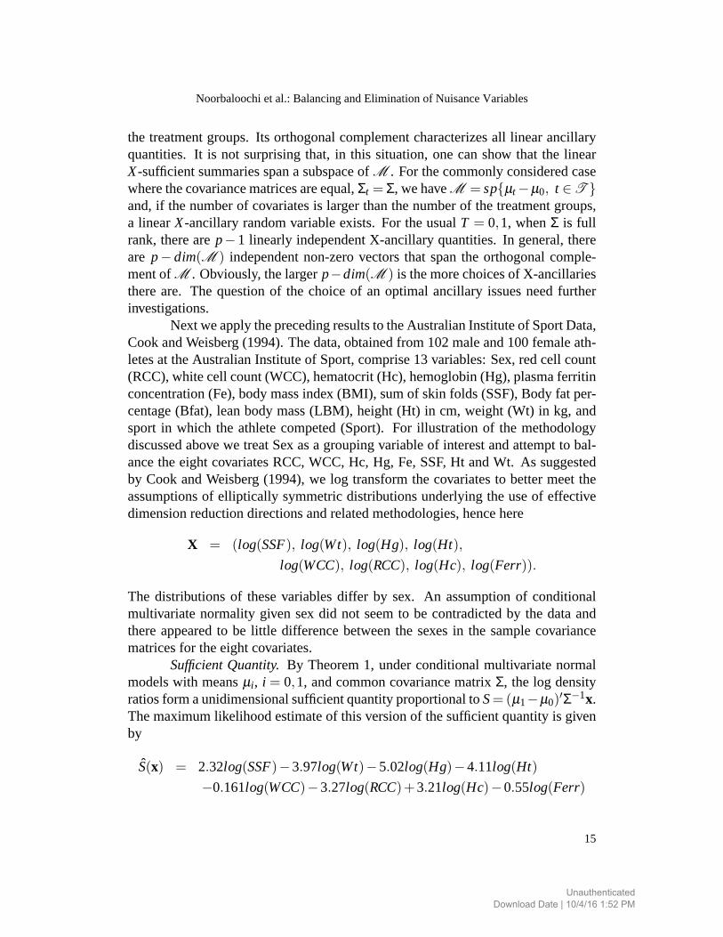
Nextweapplytheprecedingresultsto theAustralianInstituteof SportData,CookandWeisberg(1994).Thedata,obtainedfrom 102maleand100femaleath-letesat theAustralianInstituteof Sport,comprise13 variables:Sex,redcell count(RCC),whitecell count(WCC),hematocrit(Hc), hemoglobin(Hg), plasmaferritinconcentration(Fe),bodymassindex(BMI), sumof skin folds (SSF),Body fat per-centage(Bfat), leanbodymass(LBM), height(Ht) in cm, weight (Wt) in kg, andsport in which the athletecompeted(Sport). For illustration of the methodologydiscussedabovewe treatSexasa groupingvariableof interestandattemptto bal-ancetheeightcovariatesRCC,WCC, Hc, Hg, Fe,SSF,Ht andWt. As suggestedby Cook andWeisberg(1994),we log transformthe covariatesto bettermeettheassumptionsof elliptically symmetricdistributionsunderlyingtheuseof effectivedimensionreductiondirectionsandrelatedmethodologies,hencehere

X = (log(SSF), log(Wt), log(Hg), log(Ht),log(WCC), log(RCC), log(Hc), log(Ferr)).

The distributionsof thesevariablesdiffer by sex. An assumptionof conditionalmultivariatenormality given sexdid not seemto be contradictedby the dataandthereappearedto be little differencebetweenthe sexesin the samplecovariancematricesfor theeightcovariates.

SufficientQuantity. By Theorem1, underconditionalmultivariatenormalmodelswith meansµi , i = 0,1, andcommoncovariancematrix Σ, the log densityratiosform aunidimensionalsufficientquantityproportionalto S= (µ1−µ0)′Σ−1x.Themaximumlikelihood estimateof this versionof thesufficientquantityis givenby

S(x) = 2.32log(SSF)−3.97log(Wt)−5.02log(Hg)−4.11log(Ht)−0.161log(WCC)−3.27log(RCC)+3.21log(Hc)−0.55log(Ferr)

15



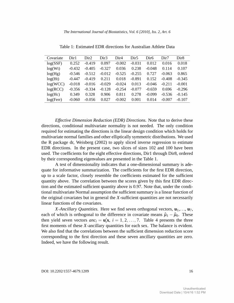
Table1: EstimatedEDRdirectionsfor AustralianAthleteData

Covariate Dir1 Dir2 Dir3 Dir4 Dir5 Dir6 Dir7 Dir8log(SSF) 0.252 -0.419 0.097 -0.002 -0.031 0.012 0.016 0.018log(Wt) -0.432 -0.405 -0.327 0.036 0.238 -0.048 0.114 0.107log(Hg) -0.546 -0.512 -0.012 -0.525 -0.255 0.727 -0.063 0.865log(Ht) -0.447 -0.419 0.211 0.018 -0.891 0.152 -0.408 -0.345log(WCC) -0.018 -0.016 -0.029 -0.024 0.013 -0.046 -0.211 -0.001log(RCC) -0.356 -0.334 -0.128 -0.254 -0.077 -0.659 0.696 -0.296log(Hc) 0.349 0.328 0.906 0.811 0.278 -0.099 -0.536 -0.145log(Ferr) -0.060 -0.056 0.027 -0.002 0.001 0.014 -0.007 -0.107

EffectiveDimensionReduction(EDR)Directions.Notethatto derivethesedirections,conditionalmultivariatenormality is not needed.The only conditionrequiredfor estimatingthedirectionsis thelineardesignconditionwhichholdsformultivariatenormalfamiliesandotherelliptically symmetricdistributions.Weusedthe R packagedr, Weisberg(2002) to apply sliced inverseregressionto estimateEDR directions. In the presentcase,two slicesof sizes102 and100 havebeenused.Thecoefficientsfor theeighteffectivedirections,Dir1 throughDir8, orderedby their correspondingeigenvaluesarepresentedin theTable1.

A testof dimensionalityindicatesthata one-dimensionalsummaryis ade-quatefor informativesummarization.Thecoefficientsfor thefirst EDR direction,up to a scalefactor, closely resemblethe coefficientsestimatedfor the sufficientquantityabove.Thecorrelationbetweenthescoresgivenby this first EDR direc-tion andtheestimatedsufficientquantityaboveis 0.97.Notethat,underthecondi-tionalmultivariateNormalassumptionthesufficientsummaryis alinearfunctionoftheoriginal covariatesbut in generaltheX-sufficientquantitiesarenot necessarilylinearfunctionsof thecovariates.

X-Ancillary Quantities.Herewe find sevenorthogonalvectors,u1,. . ., u7,eachof which is orthogonalto the differencein covariatemeansµ̂1− µ̂0. Thesethen yield sevenvectorsanci = u′ix, i = 1, 2, . . . , 7. Table 4 presentsthe threefirst momentsof theseX-ancillaryquantitiesfor eachsex. Thebalanceis evident.We alsofind thatthecorrelationsbetweenthesufficientdimensionreductionscorecorrespondingto the first directionand thesesevenancillary quantitiesarezero.Indeed,wehavethefollowing result.

16


DOI: 10.2202/1557-4679.1209


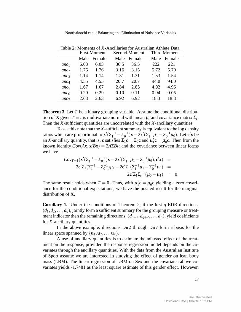
Table2: Momentsof X-Ancillariesfor AustralianAthleteDataFirst Moment SecondMoment Third Moment

anc1

anc2

anc3

anc4

anc5anc6anc7

Male Female6.03 6.031.76 1.761.14 1.144.55 4.551.67 1.670.29 0.292.63 2.63

Male Female36.5 36.53.16 3.151.31 1.3120.7 20.72.84 2.850.10 0.116.92 6.92

Male Female222 2215.72 5.701.53 1.5494.0 94.04.92 4.960.04 0.0518.3 18.3

Theorem 3. Let T bea binarygroupingvariable.Assumetheconditionaldistribu-tion of X givenT = t is multivariatenormalwith meanµt andcovariancematrixΣt .ThentheX-sufficientquantitiesareuncorrelatedwith theX-ancillaryquantities.

ToseethisnotethattheX-sufficientsummaryisequivalentto thelogdensityratioswhich areproportionalto x′(Σ−1

1 −Σ−10 )x−2x′(Σ−1

1 µ1−Σ−10 µ0). Let c′x be

anX-ancillaryquantity,thatis, c satisfiesΣ1c = Σ0c andµ ′1c = µ ′

0c. Thenfrom theknown identityCov(Ax, x′Bx) = 2AΣBµ andthecovariancebetweenlinear formswehave

CovT=1(x′(Σ−11 −Σ−1

0 )x−2x′(Σ−11 µ1−Σ−1

0 µ0),c′x) =

2c′Σ1(Σ−11 −Σ−1

0 )µ1−2c′Σ1(Σ−11 µ1−Σ−1

0 µ0) =

2c′Σ1Σ−10 (µ0−µ1) = 0

ThesameresultholdswhenT = 0. Thus,with µ ′1c = µ ′

0c yielding a zerocovari-ancefor the conditionalexpectations,we havethe positedresult for the marginaldistributionof X.

Corollary 1. Under the conditionsof Theorem2, if the first q EDR directions,(d1,d2, . . . ,dq), jointly form asufficientsummaryfor thegroupingmeasureor treat-mentindicatorthentheremainingdirections,(dq+1,dq+2, . . . ,dp), yield coefficientsfor X-ancillaryquantities.

In the aboveexample,directionsDir2 throughDir7 form a basisfor thelinearspacespannedby {u1,u2, . . . ,u7}.

A useof ancillary quantitiesis to estimatethe adjustedeffect of the treat-menton theresponse,providedtheresponseregressionmodeldependson theco-variatesthroughtheancillaryquantities.With thedatafrom theAustralianInstituteof Sportassumewe are interestedin studyingthe effect of genderon leanbodymass(LBM). The linear regressionof LBM on Sexandthe covariatesaboveco-variatesyields-1.7481astheleastsquareestimateof this gendereffect. However,

17



theestimatedcoefficientfor sexfrom amultiple regressionof LBM onSexandthebalancedancillary measures(anc1, anc2, . . . , anc7) yields -19.762asthe estimateof theeffectof genderonLBM.

More elaborate,sophisticatedanalysisshouldprovide more preciseesti-mates.However,thepurposeof thediscussionshereis simply to illustratetheuseof theconcepts,particularlytheestimationof thesufficientandancillaryquantities.In thissimpleanalysiswedid notusematchingandstratificationtechniques.Thesemethodsareapplicablewhenconditioningmethods,suchaspropensityscore,suf-ficient quantities,andEDR scoresareusedto estimatetreatmenteffects.Here,themain requirementis that the regressionmodelshouldbeexpressibleasa functionof ancillaryquantities.

Thebinaryassumptionontheinterventionvariableandmanyof theworkingassumptionsin theabovediscussionarereally not essential.More generaltheoryfor the constructionof the ancillary andsufficientquantitiesand for their useindevelopingestimatorsfor causalinferenceneedto receivemoreattentionandeffort.In thispaperwehavepresentedsomeinitial resultsin theseareasthatwehopewillattractfurtherdiscussionandresearch.

References

¯

Arnold, B. C. and S. J. Press(1989): “Compatibleconditionaldistributions,” J.Amer.Statist.Assoc., 84,152–156.

Barndorff-Nielsen,O. (1973):“On m-ancillarity,” Biometrika, 60,447–455.Barndorff-Nielsen,O. andP. Blaesild (1975): “S-ancillarity in exponentialfami-

lies,” SankhyaSer.A, 37,354–385.Basu,D. (1977): “On the elimination of nuisanceparameters,”J. Amer.Statist.

Assoc., 72,355–366.Blackwell,D. andR.V. Ramamoorthi(1982):“A bayesbutnotclassicallysufficient

statistic,”Annalsof Statistics, 10,1025–1026.Carroll,R. J.andK.-C. Li (1995):“Binary regressorsin dimensionreductionmod-

els: anewlook at treatmentcomparisons,”Statist.Sinica, 5, 667–688.Chiaromonte,F., R. D. Cook,andB. Li (2002):“Sufficient dimensionreductionin

regressionswith categoricalpredictors,”Ann.Statist., 30,475–497.Cochran,W. G. (1968): “The effectivenessof adjustmentby subclassificationin

removingbiasin observationalstudies,”Biometrics, 24,295–313.Cook, R. D. (1996): “Graphicsfor regressionswith a binary response,”J. Amer.

Statist.Assoc., 91,983–992.Cook, R. D. (2007): “Fisher lecture: Dimensionreductionin regression,”Statist.

Sci., 22,1–26.

18


DOI: 10.2202/1557-4679.1209


Cook,R. D. andL. Forzani(2009): “Likelihood-basedsufficientdimensionreduc-tion,” J. Amer.Statist.Assoc., 104,197–208.

Cook,R. D. andH. Lee (1999): “Dimensionreductionin binary responseregres-sion,” J. Amer.Statist.Assoc., 94,1187–1200.

Cook,R. D. andS.Weisberg(1994):Anintroductionto regressiongraphics, WileySeriesin ProbabilityandMathematicalStatistics:ProbabilityandMathematicalStatistics,New York: JohnWiley & SonsInc., with 2 computerdisks,A Wiley-IntersciencePublication.

Cox,D. R. andD. V. Hinkley (1974):Theoreticalstatistics, London:ChapmanandHall.

Dawid, A. P. (1979): “Conditional independencein statistical theory,” J. Roy.Statist.Soc.Ser.B, 41,1–31.

Fukumizu,K., F. R. Bach, and M. I. Jordan(2003): “Dimensionality reductionfor supervisedlearningwith reproducingkernelHilbert spaces,”J. Mach.Learn.Res., 5, 73–99(electronic).

Fukumizu,K., F. R. Bach,andM. I. Jordan(2009): “Kernel dimensionreductionin regression,”Annalsof Statistics, 37,1871–1905.

Greenland,S. (2003): “Quantifying biasesin causalmodels.”Epidemiology, 14,300–306.

Hall, P. andK.-C. Li (1993): “On almostlinearity of low-dimensionalprojectionsfrom high-dimensionaldata,”Ann.Statist., 21,867–889.

Hirano,K. andG. W. Imbens(2004):“The propensityscorewith continuoustreat-ments,” in Applied Bayesianmodelingand causal inferencefrom incomplete-dataperspectives, Wiley Ser.Probab.Stat.,Chichester:Wiley, 73–84.

Imbens, G. W. (2000): “The role of the propensityscore in estimatingdose-responsefunctions,”Biometrika, 87,706–710.

Kay, R. andS. Little (1987): “Transformationsof theexplanatoryvariablesin thelogistic regressionmodelfor binarydata,”Biometrika, 74,495–501.

Kirby, M. (2001): Geometricdata analysis, New York: Wiley-Interscience[JohnWiley & Sons],anempiricalapproachto dimensionalityreductionandthestudyof patterns.

Li, K.-C. (1991): “Sliced inverseregressionfor dimensionreduction,” J. Amer.Statist.Assoc., 86,316–342,with discussionanda rejoinderby theauthor.

Li, K.-C. (1997): “Nonlinear confoundingin high-dimensionalregression,”Ann.Statist., 25,577–612.

Nelson,D. andS.Noorbaloochi(2009): “Dimensionreductionsummariesfor bal-ancedcontrasts,”J. Statist.Plann.Inference, 139,617–628.

Noorbaloochi,S. andD. Nelson(2008): “Conditionally specifiedmodelsanddi-mensionreductionin theexponentialfamilies,” Journalof MultivariateAnalysis,99,1574–1589.

19



Pearl,J. (2009): Causality, Cambridge:CambridgeUniversityPress,models,rea-soning,andinference.

Rao, C. R. (2002): Linear StatisticalInferenceand its Applications, New York:Wiley.

Robins,J. andL. Wasserman(2000): “Conditioning, likelihood, andcoherence:areviewof somefoundationalconcepts,”J. Amer.Statist.Assoc., 95,1340–1346.

Robins,J. M. and H. Morgenstern(1987): “The foundationsof confoundinginepidemiology,”Comput.Math.Appl., 14,869–916.

Robins,J. M. andY. Ritov (1997): “Toward a curseof dimensionalityappropriate(coda)asymptotictheoryfor semi-parametricmodels.”Statisticsin Medicine, 16,285–319.

Rosenbaum,P.R.andD. B. Rubin(1983):“The centralroleof thepropensityscorein observationalstudiesfor causaleffects,”Biometrika, 70,41–55.

Rubin, D. B. (1974): “Estimatingcausaleffectsof treatmentsin randomizedandnonrandomizedstudies.”J. Edu.Psych., 66,688–701.

Rubin, D. B. (1976): “Multivariate matchingmethodsthat areequalpercentbiasreducing.II. Maximumson biasreductionfor fixed samplesizes,”Biometrics,32,121–132.

Rubin,D. B. andE. A. Stuart(2006): “Affinely invariantmatchingmethodswithdiscriminant mixtures of proportional ellipsoidally symmetric distributions,”Ann.Statist., 34,1814–1826.

Rubin,D. B. andN. Thomas(1992a):“Affinely invariantmatchingmethodswithellipsoidaldistributions,”Ann.Statist., 20,1079–1093.

Rubin,D. B. andN. Thomas(1992b):“Characterizingtheeffectof matchingusinglinearpropensityscoremethodswith normaldistributions,”Biometrika, 79,797–809.

Sandved,E. (1968): “Ancillary statisticsandpredictionof the loss in estimationproblems,”Ann.Math.Statist., 39,1756–1758.

Sandved,E. (1972): “Ancillary statisticsin modelswithout andwith nuisancepa-rameters,”Skand.Aktuarietidskr., 81–91(1973).

Severini,T. A. (2000): Likelihoodmethodsin statistics, OxfordStatisticalScienceSeries, volume22,Oxford: OxfordUniversityPress.

Weisberg,S. (2002): “Dimensionreductionregressionin R,” Journalof StatisticalSoftware(Electronic), 7.

20


DOI: 10.2202/1557-4679.1209


balancing and elimination of nuisance variables

Documents