polar varieties and efficient real elimination

POLAR VARIETIES AND EFFICIENT REAL ELIMINATION

B. BANK, M. GIUSTI, J. HEINTZ, AND G. M. MBAKOP

Dedicated to Steve Smale

Abstract. Let S0 be a smooth and compact real variety given by a reduced reg-ular sequence of polynomials f1, . . . , fp . This paper is devoted to the algorithmicproblem of finding efficiently a representative point for each connected componentof S0 . For this purpose we exhibit explicit polynomial equations that describethe generic polar varieties of S0 . This leads to a procedure which solves our al-gorithmic problem in time that is polynomial in the (extrinsic) description lengthof the input equations f1, . . . , fp and in a suitably introduced, intrinsic geometricparameter, called the degree of the real interpretation of the given equation systemf1, . . . , fp .

Keywords: Real polynomial equation solving, polar variety, geometric degree, arith-metic circuit, arithmetic network, complexity.

1. Introduction

The core of this paper consists in the exhibition of a system of canonical equationswhich describe locally the generic polar varieties of a given semialgebraic completeintersection manifold S0 contained in the real n–dimensional affine space IRn . Thispurely mathematical description of the polar varieties allows the design of a new typeof efficient algorithm (with intrinsic complexity bounds), which computes, in casethat S0 is smooth and compact, at least one representative point for each connectedcomponent of S0 (the algorithm returns each such point in a suitable symbolic codifi-cation). This new algorithm (and, in particular, its complexity) is the main practicaloutcome of the present paper. Let us now briefly describe our results.

Suppose that the real variety S0 is compact and given by polynomial equations ofthe following form:

f1(X1, . . . , Xn) = · · · = fp(X1, . . . , Xn) = 0,

where p, n ∈ IN , p ≤ n and f1, . . . , fp belong to the polynomial ring Q[X1, . . . , Xn]in the indeterminates X1, . . . , Xn over the rational numbers Q . Let d be a givennatural number and assume that for 1 ≤ k ≤ p the total degree deg fk of the poly-nomial fk is bounded by d . Moreover, we suppose that the polynomials f1, . . . , fpform a regular sequence in Q [X1, . . . , Xn] and that they are given by a division-free

Research partially supported by the following German, French, Spanish and Argentinian grants:BA 1257/4-1 (DFG), ARG 018/98 INF (BMBF), UMS 658, ECOS A99E06, DGICYT PB96-0671-C02-02, ANPCyT 03-00000-01593, UBACYT TW 80 and PIP CONICET 4571/96. The first twoauthors wish to thank the MSRI at Berkeley for its hospitality during their stay, fall 1998.

1

2 B. BANK, M. GIUSTI, J. HEINTZ, AND G. M. MBAKOP

arithmetic circuit of size L that evaluates them in any given point of the real (or com-plex) n–dimensional affine space IRn (or Cn ). Further, we assume that the JacobianJ(f1, . . . , fp) of the equation system f1 = · · · = fp = 0 has maximal rank in anypoint of S0 (thus, implicitly, we assume that S0 is smooth). Let W0 := V (f1, . . . , fp)denote the (complex) algebraic variety defined by the polynomials f1, . . . , fp in theaffine space Cn . We denote the singular locus of W0 by SingW0 .

Moreover, let us suppose that the variables X1, . . . , Xn are in generic position withrespect to the equation system f1, . . . , fp . For 1 ≤ i ≤ n − p let Wi be the i–thformal (complex) polar variety associated with W0 (and the variables Xp+i, . . . , Xn ).

Further, let us denote the real counterpart of Wi by Si := Wi ∩ IRn . We call Si thei–th formal real polar variety associated with the real semialgebraic variety S0 (andthe variables Xp+i, . . . , Xn ) . It turns out that the (locally) closed sets Wi \SingW0

and Si are either empty or complex, or real manifolds of dimension n − (p + i) .Moreover, for 1 ≤ i ≤ n− p , one sees easily that

Wi := Wi \ SingW0

is the i–th polar variety (in the usual sense) associated with W0 and the variables

Xp+i, . . . , Xn (here, Wi \ SingW0 denotes the Q-Zariski closure in Cn of the quasi–affine variety Wi \ SingW0 ). For a precise definition of the notion of formal polarvarieties and of polar varieties in the usual sense we refer to Section 2.

Suppose that the real variety S0 is non–empty and satisfies our assumptions. InTheorem 10 of this paper we show that every real polar variety Si = Wi ∩ IRn, 1 ≤i ≤ n − p, is a non–empty, smooth manifold of dimension n − p − i containing atleast one point of each connected component of the real variety S0 . In particular,the real variety Sn−p is a finite set containing at least one representative point ofeach connected component of S0 .

Under the same assumptions we show in Theorem 8 that for 1 ≤ i ≤ n−p the quasi–affine variety Wi\SingW0 is a locally complete intersection that satisfies the Jacobiancriterion. More precisely, the quasi–affine variety Wi \SingW0 is a smooth manifoldof codimension p + i that can be described locally by certain regular sequencesconsisting of the polynomials f1, . . . , fp and i many well–determined p–minors ofthe Jacobian J(f1, . . . , fp) of the f1, . . . , fp . In particular, the quasi–affine variety

Wn−p \ SingW0 is zero-dimensional, whence Wn−p = Wn−p \ SingW0 . Thus Wn−pis a zero-dimensional complex variety that contains a representative point of eachconnected component of the real variety S0 .

The practical outcome of Theorem 8 and Theorem 10 consists in the design of anefficient algorithm (with intrinsic complexity bounds), which adapts the elimina-tion procedure for complex algebraic varieties developed in [30] and [31] to the realcase. Under the additional assumption that, for 1 ≤ k ≤ p , the intermediate ideal(f1, . . . , fk) generated by f1, . . . , fk in Q [X1, . . . , Xn] is radical, we shall applythis procedure to the p

(np−1

)well–determined equation systems of Theorem 8, which

describe the zero-dimensional algebraic variety Wn−p = Wn−p \ SingW0 locally. In

POLAR VARIETIES AND EFFICIENT REAL ELIMINATION 3

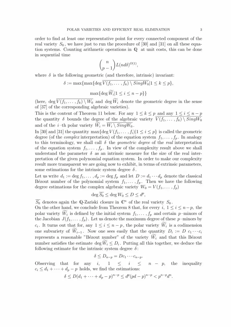
order to find at least one representative point for every connected component of thereal variety S0 , we have just to run the procedure of [30] and [31] on all these equa-tion systems. Counting arithmetic operations in Q at unit costs, this can be donein sequential time (

n

p− 1

)L(ndδ)O(1),

where δ is the following geometric (and therefore, intrinsic) invariant:

δ := maxmaxdeg V (f1, . . . , fk) \ SingW0|1 ≤ k ≤ p,

maxdeg Wi|1 ≤ i ≤ n− p

(here, deg V (f1, . . . , fk) \W0 and deg Wi denote the geometric degree in the senseof [37] of the corresponding algebraic varieties).

This is the content of Theorem 11 below. For any 1 ≤ k ≤ p and any 1 ≤ i ≤ n− pthe quantity δ bounds the degree of the algebraic variety V (f1, . . . , fk) \ SingW0

and of the i–th polar variety Wi = Wi \ SingW0 .

In [30] and [31] the quantity maxdeg V (f1, . . . , fi)|1 ≤ i ≤ p is called the geometricdegree (of the complex interpretation) of the equation system f1, . . . , fp . In analogyto this terminology, we shall call δ the geometric degree of the real interpretationof the equation system f1, . . . , fp . In view of the complexity result above we shallunderstand the parameter δ as an intrinsic measure for the size of the real inter-pretation of the given polynomial equation system. In order to make our complexityresult more transparent we are going now to exhibit, in terms of extrinsic parameters,some estimations for the intrinsic system degree δ .

Let us write d1 := deg f1, . . . , dp := deg fp and let D := d1 · · · dp denote the classicalBezout number of the polynomial system f1, . . . , fp . Then we have the followingdegree estimations for the complex algebraic variety W0 = V (f1, . . . , fp)

degS0 ≤ degW0 ≤ D ≤ dp,

S0 denotes again the Q-Zariski closure in Cn of the real variety S0 .On the other hand, we conclude from Theorem 8 that, for every i, 1 ≤ i ≤ n−p, the

polar variety Wi is defined by the initial system f1, . . . , fp and certain p–minors ofthe Jacobian J(f1, . . . , fp) . Let us denote the maximum degree of these p–minors by

ci . It turns out that for, any 1 ≤ i ≤ n − p , the polar variety Wi is a codimension

one subvariety of Wi−1 . Now one sees easily that the quantity Di := D c1 · · · cirepresents a reasonable ”Bezout number” of the variety Wi and that this Bezout

number satisfies the estimate deg Wi ≤ Di . Putting all this together, we deduce thefollowing estimate for the intrinsic system degree δ :

δ ≤ Dn−p = Dc1 · · · cn−p.Observing that for any i, 1 ≤ i ≤ n − p, the inequalityci ≤ d1 + · · ·+ dp − p holds, we find the estimations:

δ ≤ D(d1 + · · ·+ dp − p)n−p ≤ dp(pd− p)n−p < pn−pdn.


In conclusion, our new real algorithm has a time complexity that is, in worst case,polynomial in the ”Bezout number” Dc1 · · · cn−p of the zero–dimensional polar vari-

ety Wn−p .

Our complexity bound(np−1

)L(ndδ)O(1) depends on the intrinsic (geometric, seman-

tic) parameter δ and on the extrinsic (algebraic) parameters d and n in a polynomialmanner, and it depends on the syntactic parameter L only linearly. In this senseone may consider our complexity bound as intrinsic. Our real algorithm promisestherefore to be practically applicable to special equation systems with low value forthe intrinsic parameter δ .

On the other hand, even in worst case our algorithm improves upon the known dO(n) –time procedures for the algorithmic problem under consideration, also in their mostefficient versions [4], [5] (see also [3], [12], [19], [39], [40], [41], [59], [60], [14], [13]).However, this distinction does not become apparent when we measure complexitiessimply in terms of d and n (all mentioned algorithms have worst–case complexitiesof type dO(n) ), but it becomes clearly visible when we use the ”Bezout number”just introduced as complexity parameter. Only our new algorithm is polynomial inthis quantity. On the other hand, we are only able to reach our goal of algorithmicefficiency by means of a strict limitation to a purely geometric point of view. Forthe moment there is no hope that any of the standard questions of real algebra (e.g.finding generators for the real radical of a polynomial ideal or the formulation of aneffective real Nullstellensatz) can be solved within the complexity framework of thispaper (compare [52], [7] and [8]).

Our (algorithmic and mathematical) methods and results represent a non–obviousgeneralization of the main outcome of [1], where an intrinsic type algorithm wasdesigned for the problem of finding at least one representative point in each connectedcomponent of a real, compact hypersurface given by an n–variate, smooth polynomialequation f of degree d ≥ 2 with rational coefficients (such that f represents a regularequation of that hypersurface). This is the particular case of codimension p = 1 ofthe present paper, and our setting leads to the complexity bound L(ndδ)O(1) provedin [1].

2. Polar Varieties

2.1. Notations, Notions and General Assumptions. Let X1, . . . , Xn be inde-terminates (or variables) over the rational numbers Q and let polynomials f1, . . . , fp ∈Q[X1, . . . , Xn] with 1 ≤ p ≤ n be given. Let Cn and IRn denote the n–dimensionalaffine space over the complex and the real numbers, respectively. We think Cn

to be equipped with the Q -Zariski topology, whereas, on IRn , we consider thestrong topology. For any subset U ⊂ Cn we denote its Q -Zariski–closure byU . By X := (X1, . . . , Xn) we denote the vector of variables X1, . . . , Xn and byx := (x1, . . . , xn) any point of the affine space Cn or IRn . We suppose that thepolynomials f1, . . . , fp form a reduced regular sequence in Q [X1, . . . , Xn] . The


Jacobian of these polynomials is denoted by

J(f1, . . . , fp) :=

[∂fk∂Xj

]1≤k≤p1≤j≤n

.

For any point x ∈ Cn we write

J(f1, . . . , fp)(x) :=

[∂fk∂Xj

(x)

]1≤k≤p1≤j≤n

for the Jacobian of the polynomials f1, . . . , fp at x .

The common complex zeros of the polynomials f1, . . . , fp form an affine, Q-definablesubvariety of Cn , which we denote by

W0 := V (f1, . . . , fp) := x ∈ Cn|f1(x) = . . . = fp(x) = 0.A point x ∈ W0 = V (f1, . . . , fp) is said to be smooth (in W0 ) if the rank of the Jaco-bian of f1, . . . , fp in x satisfies the condition rk J(f1, . . . , fp)(x) = p . Otherwise xis called a singular point of W0 . By SingW0 we denote the set of all singular pointsof W0 .

Remark 1. If x ∈ W0 is smooth, then the hypersurfaces defined by the polynomialsf1, . . . , fp intersect transversally at the pointx .

Definition 2. For every i, 1 ≤ i ≤ n − p, let ∆i denote the set of all commoncomplex zeros of all p -minors of the Jacobian J(f1, . . . , fp) corresponding to thecolumns 1, . . . , p + i − 1 . In other words, ∆i is the determinantal variety de-fined by all p-minors of the submatrix Jp+i−1

1 (f1, . . . , fp) determined by the columns1, . . . , p+ i− 1 of the Jacobian J(f1, . . . , fp) .

We introduce the affine variety

Wi := W0 ∩∆i

associated with the linear subspace of Cn , namely

Xp+i−1 := x ∈ Cn|Xp+i(x) = . . . = Xn(x) = 0and call Wi the i–th formal polar variety of W0 . By

Wi := Wi \ SingW0

we denote the i–th polar variety (in the usual sense) of the variety W0 .

Remark 3. • The index i reflects the expected codimension of the formal polarvariety Wi in W0 . With respect to the ambient space Cn , one has alwayscodim Wi ≥ p+ i.• According to our notation, the common zeros of all p–minors of the JacobianJ(f1, . . . , fp) form the determinantal variety ∆n−p+1 . Obviously, we have Sing W0 =W0 ∩∆n−p+1 = Wn−p+1 .• The formal polar varieties Wi, 1 ≤ i ≤ n − p, form a decreasing sequence. In

particular, we haveW0 ⊃ W1 ⊃ · · · ⊃ Wi ⊃ · · · ⊃ Wn−p ⊃ Wn−p+1 = Sing W0 .


The concept of polar variety goes back to J.–V. Poncelet. Its development has a longhistory: Let us mention among others the contributions of F. Severi, J. A. Todd, S.Kleiman, R. Piene, D. T. Le, B. Teissier, J.–P. Henry, M. Merle ... (see e.g. [58] andthe references quoted there).

2.2. Local Description of the Determinantal Varieties. In this subsection wedevelop a succinct local description of the determinantal varieties ∆i, 1 ≤ i ≤ n−p .The following general Exchange Lemma will be our main tool for this description(this lemma is used in a similar form in [32]). It describes an exchange relationbetween certain minors of a given matrix .

Let A be a given (p×n) -matrix with entries aij from an arbitrary commutative ring.Let l and k be any natural numbers with l ≤ n and k ≤ minp, l . Furthermore,let Ik := (i1, . . . , ik) be an ordered sequence of k different elements from the finiteset of natural numbers 1, . . . , l and let MA (Ik) := MA(i1, . . . , ik) denote the k -minor of the matrix A built up by the first k rows and the columns i1, . . . , ik . Ifit is clear by the context what is the matrix A , we shall just write M(i1, . . . , ik) :=M (Ik) := MA (Ik) .

Lemma 4 (Exchange Lemma). As before let a matrix A and natural numbers land k be given, as well as two intersecting index sets Ik = (i1, . . . , ik) and Ik−1 =(j1, . . . , jk−1) . Then, for suitable numbers εj ∈ 1,−1 with j ∈ Ik \ Ik−1 we havethe following identity:

(∗) M (Ik−1)M (Ik) =∑

j∈Ik\Ik−1

εj M (Ik \ j)M (Ik−1 ∪ j) .

ProofConsider the following ((2k − 1) × (2k − 1)) -matrix L with entries from the givenmatrix A :

L :=

L1(Ik)

O...

Lk−1(Ik)

L1(Ik−1) L1(Ik)...

...

Lk(Ik−1) Lk(Ik)

.

Here, for any 1 ≤ j ≤ k, Lj (Ik) denotes the row vector of length k that we obtainselecting, from the j –th row of the matrix A , the k elements placed in the columnsIk = (i1, . . . , ik) . Similarly, Lj (Ik−1) is obtained from the j –th row of A selectingthe k − 1 elements placed in the columns Ik−1 = (j1, . . . , jk−1) .Now it is not difficult to verify the identity (∗) by calculating the determinant detL


of the quadratic matrix L via Laplace expansion in two different ways. First, by ex-pansion of detL according to the first k− 1 columns of L , we obtain the left–handside of (∗) , disregarding the sign. Expansion of detL according to the first k − 1rows of L leads to the right–hand side of (∗) . This implies the identity (∗) for anappropriate choice of the signs εj , with j ∈ Ik \ Ik−1 . 2

Let m ∈ Q [X1, . . . , Xn] denote the (p − 1)–minor of the JacobianJ(f1, . . . , fp) given by the first (p− 1) rows and columns, i.e., let

m := det

[∂fk∂Xj

]1≤k≤p−11≤j≤p−1

.

We consider the determinantal variety ∆i outside of the hypersurface

V (m) := x ∈ Cn | m(x) = 0and denote this localization by (∆i)m , i.e., we set

(∆i)m := ∆i \ V (m).

¿From now on, for 1 ≤ i1 ≤ · · · ≤ ip ≤ n , let us denote by

M(i1, . . . , ip)

the polynomial in Q[X1, . . . , Xn] defined as the p–minor of the Jacobian J(f1, . . . , fp)built up by its p rows and the columns i1, . . . , ip . As before, we denote by

M(i1, . . . , ip)(x)

the specialization of M(i1, . . . , ip) in a given point x ∈ Cn .

Proposition 5. Let 1 ≤ i ≤ n − p be arbitrarily fixed, and let m be the (p − 1) –minor defined above. Then the determinantal variety ∆i is locally (i.e., outside ofthe hypersurface V (m) ) described by the i polynomials

M(1, . . . , p− 1, p),M(1, . . . , p− 1, p+ 1), . . . ,M(1, . . . , p− 1, p+ i− 1).

In other words, we have

(∆i)m := x ∈ Cn| m(x) 6= 0,M(1, . . . , p− 1, s)(x) = 0, s ∈ p, . . . , p+ i− 1,where M(1, . . . , p−1, s) denotes, as above, the p–minor of the Jacobian J(f1, . . . , fp)built up by the first p− 1 columns and the s–th column.

ProofIt suffices to show that

(∆i)m ⊃ x ∈ Cn| m(x) 6= 0,M(1, . . . , p− 1, s) = 0, s ∈ p, . . . , p+ i− 1holds.Let x∗ ∈ C n be any point satisfying the conditions m(x∗) 6= 0 andM(1, . . . , p − 1, s)(x∗) = 0 for every s ∈ p, . . . , p + i − 1 . We have to verifythat

M(i1, . . . , ip)(x∗) = 0


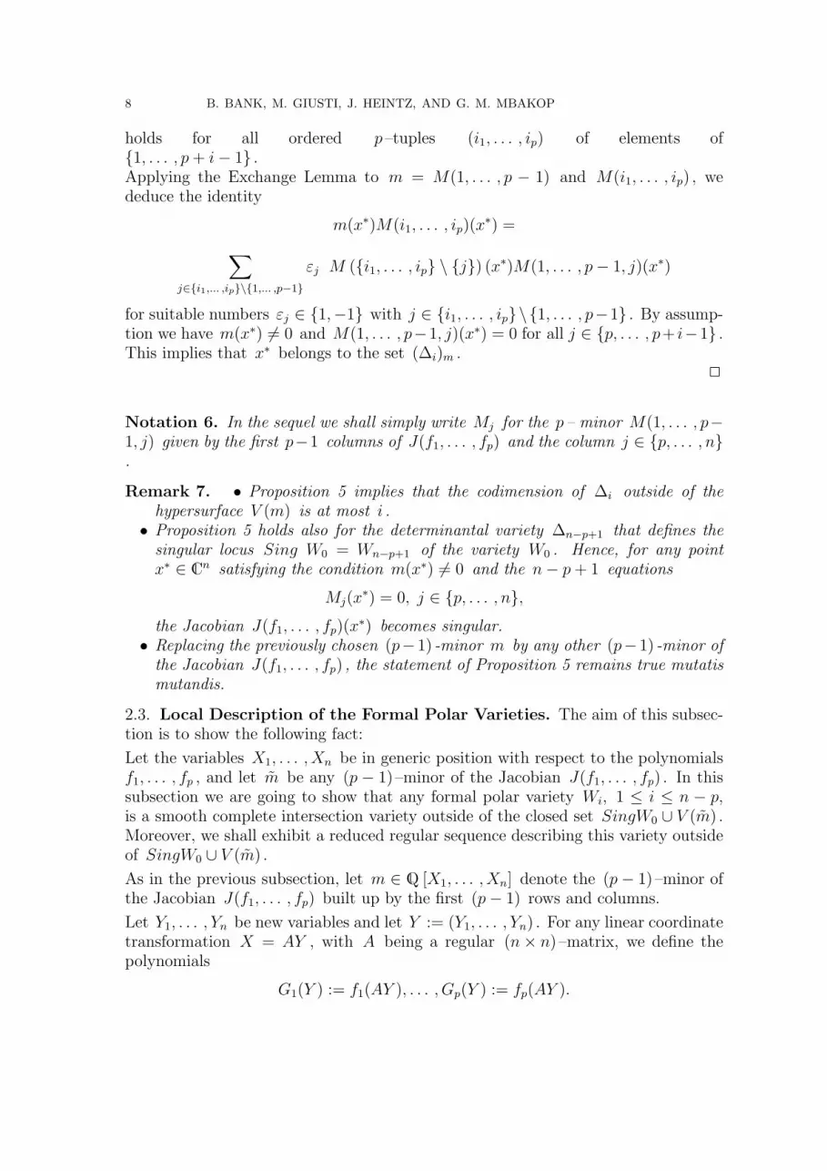
holds for all ordered p–tuples (i1, . . . , ip) of elements of1, . . . , p+ i− 1 .Applying the Exchange Lemma to m = M(1, . . . , p − 1) and M(i1, . . . , ip) , wededuce the identity

m(x∗)M(i1, . . . , ip)(x∗) =∑

j∈i1,... ,ip\1,... ,p−1

εj M (i1, . . . , ip \ j) (x∗)M(1, . . . , p− 1, j)(x∗)

for suitable numbers εj ∈ 1,−1 with j ∈ i1, . . . , ip\1, . . . , p−1 . By assump-tion we have m(x∗) 6= 0 and M(1, . . . , p−1, j)(x∗) = 0 for all j ∈ p, . . . , p+ i−1 .This implies that x∗ belongs to the set (∆i)m .

2

Notation 6. In the sequel we shall simply write Mj for the p– minor M(1, . . . , p−1, j) given by the first p−1 columns of J(f1, . . . , fp) and the column j ∈ p, . . . , n.

Remark 7. • Proposition 5 implies that the codimension of ∆i outside of thehypersurface V (m) is at most i .• Proposition 5 holds also for the determinantal variety ∆n−p+1 that defines the

singular locus Sing W0 = Wn−p+1 of the variety W0 . Hence, for any pointx∗ ∈ Cn satisfying the condition m(x∗) 6= 0 and the n− p+ 1 equations

Mj(x∗) = 0, j ∈ p, . . . , n,

the Jacobian J(f1, . . . , fp)(x∗) becomes singular.

• Replacing the previously chosen (p− 1) -minor m by any other (p− 1) -minor ofthe Jacobian J(f1, . . . , fp) , the statement of Proposition 5 remains true mutatismutandis.

2.3. Local Description of the Formal Polar Varieties. The aim of this subsec-tion is to show the following fact:

Let the variables X1, . . . , Xn be in generic position with respect to the polynomialsf1, . . . , fp , and let m be any (p − 1)–minor of the Jacobian J(f1, . . . , fp) . In thissubsection we are going to show that any formal polar variety Wi, 1 ≤ i ≤ n − p,is a smooth complete intersection variety outside of the closed set SingW0 ∪ V (m) .Moreover, we shall exhibit a reduced regular sequence describing this variety outsideof SingW0 ∪ V (m) .

As in the previous subsection, let m ∈ Q [X1, . . . , Xn] denote the (p− 1)–minor ofthe Jacobian J(f1, . . . , fp) built up by the first (p− 1) rows and columns.

Let Y1, . . . , Yn be new variables and let Y := (Y1, . . . , Yn) . For any linear coordinatetransformation X = AY , with A being a regular (n× n) –matrix, we define thepolynomials

G1(Y ) := f1(AY ), . . . , Gp(Y ) := fp(AY ).


The Jacobian of G1, . . . , Gp has the form

J(G1, . . . , Gp) :=

[∂Gk

∂Yj

]1≤k≤p1≤j≤n

= J(f1, . . . , fp)A.

Using a similar notation as before, we denote by

M(i1, . . . , ip)

the p–minor of the new Jacobian J(G1, . . . , Gp) that corresponds to the columns1 ≤ i1 < · · · < ip ≤ n .

Moreover, we denote by Mj the p– minor M(1, . . . , p−1, j) determined by the fixedfirst p− 1 columns of J(G1, . . . , Gp) and the column j ∈ p, . . . , n .

For p ≤ r, t ≤ n let Zr,t be a new indeterminate. Using the following regular(n− p+ 1)× (n− p+ 1)–parameter matrix

Z :=

1 0 0 · · · 0

Zp+1,p 1

......

. . . O ...

Zp+i−1,p Zp+i−1,p+1 · · · 1

Zp+i,p Zp+i,p+1 · · · Zp+i,p+i−1 1...

......

.... . . 0

Zn,p Zn,p+1 · · · Zn,p+i−1 Zn,p+i Zn,p+i+1 · · · 1

,

we construct an (n × n) –coordinate transformation matrix A := A(Z) , which willenable us to prove the statement at the beginning of this subsection.

For the moment, let us fix an index 1 ≤ i ≤ n − p . We consider the formal polarvariety Wi outside of the hypersurface V (m) . Corresponding to our choice of i , thematrix Z may be subdivided into submatrices as follows:

Z =

Z(i)1 Oi,n−p−i+1

Z(i) Z(i)2

.Here the matrix Z(i) is defined as

Z(i) :=

Zp+i,p . . . Zp+i,p+i−1

. . . . . . . . .

Znp . . . Zn,p+i−1

,


and Z(i)1 and Z

(i)2 denote the quadratic lower triangular matrices bordering Z(i) in

Z , and Oi,n−p−i+1 is the i× (n− p− i+ 1) zero matrix. Let

A := A(Z) :=

Ip−1 Op−1,i Op−1,n−p−i+1

Oi,p−1 Z(i)1 Oi,n−p−i+1

On−p−i+1,p−1 Z(i) Z(i)2

.Here the submatrices Ir and Or,s are unit or zero matrices, respectively, of corre-

sponding size, and Z(i), Z(i)1 , and Z

(i)2 are the submatrices of the parameter matrix

Z introduced before. Thus, A is a regular, parameter dependent (n×n) –coordinatetransformation matrix.

Like the matrix Z , the matrix A contains

s :=(n− p)(n− p+ 1)

2parameters Zr,t which we may specialize into any point z of the affine space Cs .For such a point z ∈ Cs we denote the corresponding specialized matrices by A(z) ,

Z(i)1 (z), Z

(i)2 (z) and Z(i)(z) .

We consider now the coordinate transformation given by X = AY with A = A(Z)and calculate the Jacobian J(G1, . . . , Gp) with respect to the new polynomialsG1, . . . , Gp . Recall that the coordinate transformation matrix A depends on ourprevious choice of the index 1 ≤ i ≤ n− p .

According to the structure of the coordinate transformation matrix A = A(Z) wesubdivide the Jacobian J(f1, . . . , fp) into three submatrices

J(f1, . . . , fp) =[U V W

],

with

U :=

[∂fk∂Xj

]1≤k≤p

1≤j≤p−1

, V :=

[∂fk∂Xj

]1≤k≤p

p≤j≤p+i−1

, W :=

[∂fk∂Xj

]1≤k≤pp+i≤j≤n

.

¿From the identity J(G1, . . . , Gp) = J(f1, . . . , fp) A we deduce that our new Jaco-bian is of the form:

J(G1, . . . , Gp) =

[∂Gk

∂Yj

]1≤k≤p1≤j≤n

=[U V Z

(i)1 +WZ(i) WZ

(i)2

].

We are interested in a local description of the i–th formal polar variety Wi = W0∩∆i

outside of the hypersurface V (m) , where m is the fixed upper left (p − 1)– minorof the Jacobian J(f1, . . . , fp) (and also of its submatrix U ). Since the coordinatetransformation X = AY leaves the submatrix U unchanged, the (p − 1)–minorm remains fixed under this transformation. ¿From Proposition 5 we know that thelocalized determinantal variety (∆i)m is described by the i equations

Mp = 0, . . . ,Mp+i−1 = 0,


and by the condition m 6= 0. The p– minors Mp, . . . ,Mp+i−1 defining these equa-tions are built up by the submatrix [ U V ] of the Jacobian J(f1, . . . , fp) . Under thecoordinate transformation A(Z) the matrix [ U V ] is changed into the submatrix[

U V Z(i)1 +WZ(i)

]of the Jacobian J(G1, . . . , Gp) and the p–minors Mp, . . . ,Mp+i−1 are changed intothe p– minors

Mp, . . . , Mp+i−1

of the matrix[U V Z

(i)1 +WZ(i)

]. This implies the matrix identity

(∗∗)[Mp, . . . , Mp+i−1

]= [Mp, . . . ,Mp+i−1] Z

(i)1 + [Mp+i, . . . ,Mn] Z(i).

For the previously chosen index 1 ≤ i ≤ n − p , the coordinate transformationX = A(Z)Y induces the following morphism of affine spaces:

Φi : Cn × Cs → Cp × Ci,

defined by

(x, z) 7−→ Φi(x, z) :=(f1(x), . . . , fp(x), Mp(x, z), . . . , Mp+i−1(x, z)

).

Consider an arbitrary point z ∈ Cs . We denote by ∆zi the determinantal subvariety of

C n defined by all p–minors of the matrix[U V Z

(i)1 (z) +WZ(i)(z)

](which is a submatrix of the new Jacobian obtained by

specializing the coefficients of the polynomials G1, . . . , Gp into the point z ∈ Cs ).Writing W z

i := W0 ∩ ∆zi , one sees immediately that the zero fiber Φ−1

i (0) of themorphism Φi contains the set

(W zi )m := W0 ∩ (∆z

i )m.

In other words, for any arbitrarily chosen point z ∈ Cs , the zero fiber Φ−1i (0) of

the morphism Φi contains the transformed formal polar variety W zi , localized in the

hypersurface V (m) and expressed in the old coordinates.

We are going now to analyze the rank of the Jacobian of the morphism Φi in anarbitrary point (x, z) ∈ Cn × Cs with x ∈ (W z

i )m . Using the subdivision of the

parameter matrix Z into the parts Z(i), Z(i)1 and Z

(i)2 , the Jacobian J(Φi) of the

morphism Φi can be written symbolically as

J(Φi) =

[∂Φi

∂X

∂Φi

∂Z(i)

∂Φi

∂Z(i)1

∂Φi

∂Z(i)2

].

We have


[∂Φi

∂X

∂Φi

∂Z(i)

]=

=

J(f1, . . . , fp) Op,n−p−i+1 · · · Op,n−p−i+1

∗[

∂fMp

∂Zp+i,p, . . . , ∂

fMp

∂Znp

]· · · O1,n−p−i+1

......

. . ....

∗ O1,n−p−i+1 · · ·[

∂fMp+i−1

∂Zp+i,p+i−1, . . . ,

∂fMp+i−1

∂Zn,p+i−1

]

,

where the columns correspond to the partial derivatives of Φi with respect to thevariables

X1, . . . , Xn, Zp+i,p, . . . , Zn,p, . . . , Zp+i,p+i−1, . . . , Zn,p+i−1

(in this order). The entries Or,t denote here zero matrices of corresponding size andthe row matrices labeled by ”∗” represent the partial derivatives with respect to the

variables X1, . . . , Xn of the minors Mp, . . . , Mp+i−1 . These row matrices will beirrelevant for our considerations.

Furthermore, the third submatrix

[∂Φi

∂Z(i)1

]of J(Φi) can be written as

Op,i−1 Op,i−2 · · · 0[∂fMp

∂Zp+1,p, . . . , ∂fMp

∂Zp+i−1,p

]O1,i−2 · · · 0

O1,i−1

[∂fMp+1

∂Zp+2,p+1, . . . , ∂fMp

∂Zp+i−1,p+1

]· · · 0

......

. . ....

O1,i−1 O1,i−2 · · ·[

∂fMp+i−1

∂Zp+i−1,p+i−2

]O1,i−1 O1,i−2 · · · 0

and the last submatrix

[∂Φi

∂Z(i)2

]of J(Φi) is a zero matrix since the p– minors

Mp, . . . , Mp+i−1 are indepedent of the parameters Zr,t occurring in the submatrix

Z(i)2 of the coordinate transformation matrix A(Z) .

Therefore, the Jacobian J(Φi) is of full rank p+ i wherever the submatrix

J(Φi) :=

[∂Φi

∂X

∂Φi

∂Z(i)

]is of full rank p+ i . On the other hand, considering the i row matrices contained in

J(Φi) for p ≤ j ≤ p+ i− 1 [∂Mj

∂Zp+i,j, . . . ,

∂Mj

∂Zn,j

],


we see that the representation (∗∗) of the transformed p–minors Mj implies theidentity [

∂Mj

∂Zp+i,j, . . . ,

∂Mj

∂Zn,j

]= [ Mp+i, . . . ,Mn] .

Thus, we obtain the representation

J(Φi) =

J(f1, . . . , fp) Op,n−p−i+1 · · · Op,n−p−i+1

∗ [Mp+i, . . . ,Mn] · · · O1,n−p−i+1

......

. . ....

∗ O1,n−p−i+1 · · · [Mp+i, . . . ,Mn]

.

Since all entries of the submatrix J(Φi) of the Jacobian J(Φi) belong to the polyno-mial ring Q [X1, . . . , Xn] , we see that the rank of the matrix J(Φi) in a given point(x, z) ∈ Cn×Cs with x ∈ (W z

i )m depends only on the choice of x . According to ourlocalization outside of the hypersurface V (m) , let us consider an arbitrary smoothpoint x of W0 = V (f1, . . . , fp) satisfying the condition m(x) 6= 0. Suppose that the

submatrix J(Φi)(x) is not of full rank, i.e., that

rk J(Φi)(x) < p+ i

holds. This latter inequality is valid if and only if all p -minorsMp+i, . . . ,Mn of the Jacobian J(f1, . . . , fp) vanish at x . Let z ∈ Cs be any pa-rameter point such that the pair (x, z) belongs to the fiber Φ−1

i (0) of the morphism

Φi . Since the p -minors Mp, . . . , Mp+i−1 of the transformed Jacobian J(G1, . . . , Gp)must vanish at (x, z), we deduce from (∗∗) that

[0, . . . , 0] = [Mp(x), . . . ,Mp+i−1(x)] Z(i)1 (z)

holds (here Z(i)1 (z) denotes again the matrix obtained by specializing the entries of

Z(i)1 into the corresponding coordinates of the point z ∈ Cs ). Because of the lower

triangular form of the regular matrix Z(i)1 , the latter matrix equation holds if and

only if the conditions

Mp+i−1(x) = · · · = Mp(x) = 0.

are satisfyied. Therefore, our assumptions on x and z imply m(x) 6= 0 andMp(x) = · · · = Mn(x) = 0. However, by Remark 7 this means that the Jaco-bian J(f1, . . . , fp)(x) is singular. Hence, x is not a smooth point of W0 , i.e.,x ∈ Sing W0 , which contradicts our assumption on x .

Now, suppose that we are given a point (x, z) ∈ Cn × Cs that belongs to the fiberΦ−1i (0) . Then x belongs to W0 . Further, suppose that x is a smooth point of W0

outside of the hypersurface V (m) . Let us consider the Zariski–open neighbourhood


U of x consisting of all points x ∈ Cn with m(x) 6= 0 and rk J(f1, . . . , fp) = p ,i.e., we consider

U := Cn \ (Sing W0 ∪ V (m)) .

We are going to show that the restricted morphism

Φi : U × Cs → Cp × Ci

is transversal to the origin 0 ∈ Cp × Ci .

In order to see this, consider an arbitrary point (x, z) of U × Cs that satisfies theequation Φi(x, z) = 0 . Thus, x belongs to U ∩W0 and is, therefore, a smooth pointof W0 , which is outside of the hypersurface V (m) . By the preceding considerationson the rank of the Jacobian J(Φi) it is clear that J(Φi) has the maximal rank p+ iat (x, z) . This means that (x, z) is a regular point of Φi . Since (x, z) was anarbitrary point of Φ−1

i (0) ∩ (U × Cs) , the claimed transversality has been shown.

Now, applying the Weak–Transversality–Theorem of Thom–Sard (see e.g. [22]) tothe diagram

Φ−1i (0) ∩ (U × Cs) → Cn × Cs

↓

Cs

one concludes that there is a residual dense set Ωi of parameters z ∈ Cs for whichtransversality holds. This implies that, for every fixed z ∈ Ωi , the transformed andlocalized formal polar variety

W zi \ (Sing W0 ∪ V (m))

is either empty or a smooth variety of codimension p+i . This variety can be describedlocally by the polynomials

(∗ ∗ ∗) f1(X), . . . , fp(X), Mp(X, z), . . . , Mp+i−1(X, z)

that form a regular sequence outside of SingW0 ∪ V (m) . Up to now, our considera-tions concerned only the change of coordinates for an arbitrarily fixed 1 ≤ i ≤ n− p .However, Ω :=

⋂n−pi=1 Ωi is a dense residual parameter set in Cs from which we can

choose a simultaneous change of coordinates for all 1 ≤ i ≤ n− p . For every choicez ∈ Ω and 1 ≤ i ≤ n − p the transformed formal polar variety W z

i is, outside ofthe closed set SingW0 ∪ V (m) , a smooth complete intersection variety described bythe (local) regular sequence (∗ ∗ ∗) . One sees now easily that the affine space IRs

contains a non–empty residual dense set of parameters z such that the conclusionsabove apply to the coordinate transformation X = A(z)Y . Moreover, z can bechosen from Q s .

Taking into account Proposition 5 and Remark 7, we deduce the following result fromour argumentation:


Theorem 8. Let W0 = V (f1, . . . , fp) be a reduced complete intersection varietygiven by polynomials f1, . . . , fp in Q [X1, . . . , Xn] and suppose that the variablesX1, . . . , Xn are in generic position with respect to f1, . . . , fp . Further, let m be theupper left (p − 1) –minor of the Jacobian J(f1, . . . , fp) . Then, every formal polarvariety Wi, 1 ≤ i ≤ n − p, localized with respect to the closed set SingW0 ∪ V (m) ,is either empty or a smooth variety of codimension p+ i that can be decribed by theequations

f1, . . . , fp,Mp, . . . ,Mp+i−1,

where Mj, p ≤ j ≤ p + i − 1, is the p– minor of the Jacobian J(f1, . . . , fp) givenby the columns 1, . . . , p− 1, j . Then the polynomials

f1, . . . , fp,Mp, . . . ,Mp+i−1

form a regular sequence outside of SingW0 ∪ V (m) .

Remark 9. Taking into account that the argumentation on the localization with re-spect to the fixed (p − 1) -minor m remains valid mutatis mutandis for any other(p − 1) -minor m of the Jacobian J(f1, . . . , fp) , Theorem 8 can be restated forany fixed (p − 1) –minor just by reordering of columns and rows of the JacobianJ(f1, . . . , fp) .

2.4. Existence of Real Points in the Polar Varieties. Let f1, . . . , fp be a re-duced regular sequence in Q [X1, . . . , Xn] and let again W0 := V (f1, . . . , fp) be theaffine variety defined by f1, . . . , fp . Consider the real variety S0 := W0 ∩ IRn andsuppose that

(i) S0 is nonempty and bounded (and hence compact),(ii) the Jacobian J(f1, . . . , fp)(x) is of maximal rank in all points x of S0 (i.e., S0

is a smooth subvariety of IRn given by the reduced regular sequence f1, . . . , fp ),(iii) the variables X1, . . . , Xn are in generic position with respect to the polynomials

f1, . . . , fp .

Further, let C be any connected component of the compact set S0 , and let b :=(a1, . . . , ap−1, ap, . . . , an−1, an) ∈ C be a locally maximal point of the last coordinateXn in the non–empty compact set C ⊂ S0 . Without loss of generality we mayassume that the upper left (p− 1)–minor m of the Jacobian J(f1, . . . , fp) does notvanish in b (by our assumptions there must be a (p− 1)–minor of J(f1, . . . , fp) notvanishing at b ). In any local parametrization of S0 at b the variable Xn cannotbe an independent variable, since Xn attains a local maximum in b (an is thislocal maximum). Hence, without loss of generality we may assume that the localparametrization of S0 in b has the following form: there exists an open set U ⊂ IRn−p

containing the point a := (ap, . . . , an−1) , and a continuously differentiable function

ϕ : U → IRp , ϕ := (ϕ1, . . . , ϕp−1, ϕn)

such that

x1 = ϕ1(xp, . . . , xn−1), . . . , xp−1 = ϕp−1(xp, . . . , xn−1),

xn = ϕn(xp, . . . , xn−1)


holds for any x = (xp, . . . , xn−1) ∈ U . With respect to this local parametrization,the polynomials fk, 1 ≤ k ≤ p , induce real valued functions of the form:

fk(Xp, . . . , Xn−1) :=

fk(ϕ1(Xp, . . . , Xn−1), . . . , ϕp−1(Xp, . . . , Xn−1),

Xp, . . . , Xn−1, ϕn(Xp, . . . , Xn−1)).

For every 1 ≤ k ≤ p, and every p ≤ j ≤ n− 1, one has the identity

∂fk∂Xj

=∂fk∂Xj

+∂fk∂X1

∂ϕ1

∂Xj

+ · · ·+ ∂fk∂Xp−1

∂ϕp−1

∂Xj

+∂fk∂Xn

∂ϕn∂Xj

= 0(1)

in the open set U .

Considering the (p× p) –matrix

B :=

∂f1

∂X1

. . .∂f1

∂Xp−1

∂f1

∂Xn

. . . . . . . . . . . . . . . . . . . . . . . . .

∂fp∂X1

. . .∂fp∂Xp−1

∂fp∂Xn

,and observing that B is regular in U , we obtain from (1) that

− detB(x)

∂ϕ1

∂Xj...

∂ϕp−1

∂Xj∂ϕn∂Xj

= (Adj B)(x)

∂f1

∂Xj

(x)

...

∂fp−1

∂Xj

(x)

∂fp∂Xj

(x)

(2)

holds for any x ∈ U (here Adj B denotes the adjoint matrix of the matrix B ). Asb is a locally maximal point of Xn , we have that

∂ϕn∂Xj

(a) = 0

holds for every p ≤ j ≤ n− 1 . Thus, equation (2) implies

B(n, 1) (b)∂f1

∂Xj

(b) + · · ·+B(n, p) (b)∂fp∂Xj

(b) = 0(3)

for every p ≤ j ≤ n − 1 (here for 1 ≤ k ≤ p we denote the entry of the adjointmatrix Adj B at the cross point of the k –th column and the last row by B(n, k) ).Taking into account the particular form of the matrix B , the equation system (3)means that


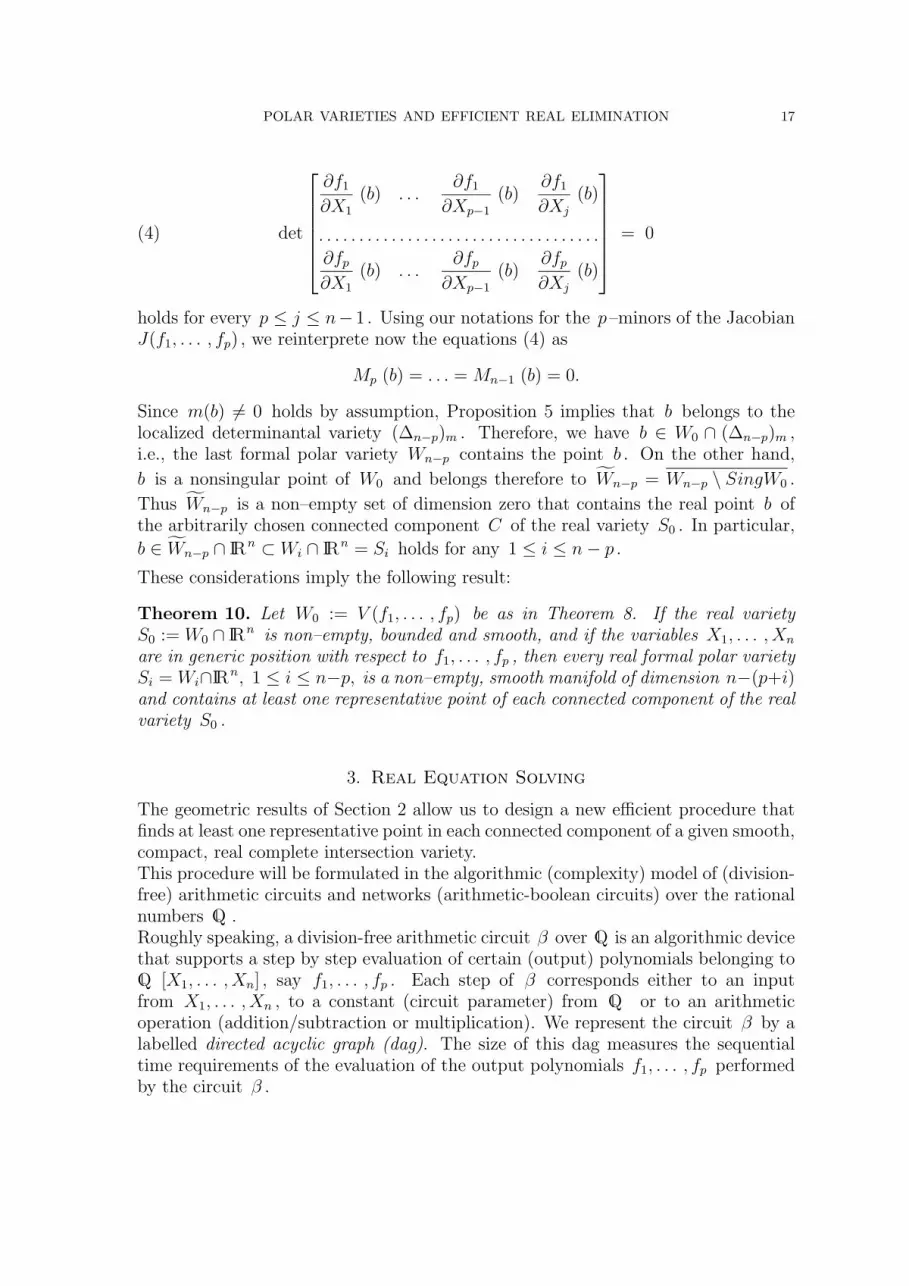
det

∂f1

∂X1

(b) . . .∂f1

∂Xp−1

(b)∂f1

∂Xj

(b)

. . . . . . . . . . . . . . . . . . . . . . . . . . . . . . . . . . .

∂fp∂X1

(b) . . .∂fp∂Xp−1

(b)∂fp∂Xj

(b)

= 0(4)

holds for every p ≤ j ≤ n− 1 . Using our notations for the p–minors of the JacobianJ(f1, . . . , fp) , we reinterprete now the equations (4) as

Mp (b) = . . . = Mn−1 (b) = 0.

Since m(b) 6= 0 holds by assumption, Proposition 5 implies that b belongs to thelocalized determinantal variety (∆n−p)m . Therefore, we have b ∈ W0 ∩ (∆n−p)m ,i.e., the last formal polar variety Wn−p contains the point b . On the other hand,

b is a nonsingular point of W0 and belongs therefore to Wn−p = Wn−p \ SingW0 .

Thus Wn−p is a non–empty set of dimension zero that contains the real point b ofthe arbitrarily chosen connected component C of the real variety S0 . In particular,

b ∈ Wn−p ∩ IRn ⊂ Wi ∩ IRn = Si holds for any 1 ≤ i ≤ n− p .

These considerations imply the following result:

Theorem 10. Let W0 := V (f1, . . . , fp) be as in Theorem 8. If the real varietyS0 := W0 ∩ IRn is non–empty, bounded and smooth, and if the variables X1, . . . , Xn

are in generic position with respect to f1, . . . , fp , then every real formal polar varietySi = Wi∩IRn, 1 ≤ i ≤ n−p, is a non–empty, smooth manifold of dimension n−(p+i)and contains at least one representative point of each connected component of the realvariety S0 .

3. Real Equation Solving

The geometric results of Section 2 allow us to design a new efficient procedure thatfinds at least one representative point in each connected component of a given smooth,compact, real complete intersection variety.This procedure will be formulated in the algorithmic (complexity) model of (division-free) arithmetic circuits and networks (arithmetic-boolean circuits) over the rationalnumbers Q .Roughly speaking, a division-free arithmetic circuit β over Q is an algorithmic devicethat supports a step by step evaluation of certain (output) polynomials belonging toQ [X1, . . . , Xn] , say f1, . . . , fp . Each step of β corresponds either to an inputfrom X1, . . . , Xn , to a constant (circuit parameter) from Q or to an arithmeticoperation (addition/subtraction or multiplication). We represent the circuit β by alabelled directed acyclic graph (dag). The size of this dag measures the sequentialtime requirements of the evaluation of the output polynomials f1, . . . , fp performedby the circuit β .


A (division-free) arithmetic network over Q is nothing else but an arithmetic circuitthat additionally contains decision gates comparing rational values or checking theirequality, and selector gates depending on these decision gates.Arithmetic circuits and networks represent non–uniform algorithms, and the com-plexity of executing a single arithmetic operation is always counted at unit cost.Nevertheless, by means of well known standard procedures our algorithms will al-ways be transposable to the uniform random bit model and they will be practicallyimplementable as well. All this can be done in the spirit of the general asymptoticcomplexity bounds stated in Theorem 11 below.Let us also remark that the depth of an arithmetic circuit (or network) measures theparallel time of its evaluation, whereas its size allows an alternative interpretationas ”number of processors”. In this context we would like to emphasize the partic-ular importance of counting only nonscalar arithmetic operations (i.e.,only essentialmultiplications), taking Q -linear operations (in particular, additions/subtractions)for cost–free. This leads to the notion of nonscalar size and depth of a given arith-metic circuit or network β . It can be easily seen that the nonscalar size determinesessentially the total size of β (which takes into account all operations) and that thenonscalar depth dominates the degree and height of the intermediate results of β .

An arithmetic circuit (or network) becomes a sequential algorithm when we play aso–called pebble game on it. By means of pebble games we are able to introduce anatural space measure in our algorithmic model and along with this, a new, moresubtle sequential time measure. If we play a pebble game on a given arithmeticcircuit, we obtain a so–called straight line program (slp). In the same way we obtain acomputation tree from a given arithmetic network. For more details on our complexitymodel we refer to [11], [25], [26], [45], [53], [38] and especially to [33] (where also theimplementation aspect is treated).

In the next Theorem 11 we are going to consider families of polynomials f1, . . . , fpbelonging to Q [X1, . . . , Xn] , for which we arrange the following assumptions andnotations:

(i) f1, . . . , fp form a regular sequence in Q [X1, . . . , Xn] ,(ii) for every 1 ≤ k ≤ p the ideal (f1, . . . , fk) generated by f1, . . . , fk in

Q [X1, . . . , Xn] is radical and defines a subvariety of Cn of dimension n − kthat we denote by Vk := V (f1, . . . , fk) .

(iii) the variables X1, . . . , Xn are in generic position with respect to the polynomialsf1, . . . , fp .

Let W0 := x ∈ Cn|f1(x) = · · · = fp(x) = 0 and denote by SingW0 the singularlocus of W0 . For 1 ≤ i ≤ n− p let Wi be the i–th formal polar variety associated

with W0 and the variables Xp+i, . . . , Xn , and let Wi := Wi \ SingW0 be the i–thpolar variety of W0 in the usual sense (see Section 2 for precise definitions). Further,

for 1 ≤ k ≤ p we shall write Vk := Vk \ SingW0 . We call

δ := maxmaxdeg Vk|1 ≤ k ≤ p,maxdeg Wi|1 ≤ i ≤ n− pthe degree (of the real interpretation) of the polynomial equation system f1, . . . , fp .Finally, let us make the following assumption:


(iv) the specialized Jacobian J(f1, . . . , fp)(x) has maximal rank in any point x ofS0 := W0 ∩ IRn = x ∈ IRn|f1(x) = · · · = fp(x) = 0 and S0 is a boundedsemialgebraic set (hence, S0 is empty or a smooth, compact real manifold ofdimension n− p ; see Section 2 for details).

Theorem 11. Let n, p, d, δ, L and ` be natural numbers with d ≥ 2 and p ≤ n .There exists an arithmetic network N over Q of size

(np−1

)L(ndδ)O(1) and nonscalar

depth O(n(log nd + `) log δ) with the following property: Let f1, . . . , fp be a familyof n–variate polynomials of a degree at most d and assume that f1, . . . , fp are givenby a division–free arithmetic circuit β in Q [X1, . . . , Xn] of size L and nonscalardepth ` . Suppose that the polynomials f1, . . . , fp satisfy the conditions (i), (ii), (iii)and (iv) above. Further, suppose that the degree of the real interpretation of thepolynomial system f1, . . . , fp is bounded by δ (let us now freely use the notationsjust introduced before).

The algorithm represented by the arithmetic network N starts from the circuit β as

input and decides first whether the complex variety Wn−p is empty. If this is not the

case, then Wn−p is a zero–dimensional complex variety and the network N producesan arithmetic circuit in Q of asymptotically the same size and nonscalar depth as N ,which represents the coefficients of n+1 univariate polynomials q, p1, . . . , pn ∈ Q[Xn]satisfying the following conditions:

deg q = # Wn−p,

maxdeg pk|1 ≤ k ≤ n < deg q,

Wn−p = (p1(u), . . . , pn(u))|u ∈ C, q(u) = 0.Moreover, the algorithm represented by the arithmetic network N decides whether the

set Wn−p∩IRn is empty. If this is not the case, then N produces at most # Wn−p ≤ δsign sequences belonging to the set −1, 0, 1 such that these sign sequences encode thereal zeros of the polynomial q ”a la Thom” ([18]). In this way N describes the finite,

non–empty set Wn−p ∩ IRn , which contains at least one representative point for eachconnected component of the real variety S0 = x ∈ IRn|f1(x) = · · · = fp(x) = 0 .

ProofWe shall freely use the notations of Section 2. Any selection of indices 1 ≤ i1 < · · · <ip ≤ n and 1 ≤ j, k ≤ p determines a p– minor M(i1, . . . , ip) and a (p− 1)– minorm(i1, . . . , ip; j, k) of the Jacobian J(f1, . . . , fp) in the following way: M(i1, . . . , ip)is the determinant of the (p×p) – submatrix of J(f1, . . . , fp) with columns i1, . . . , ip ,and m(i1, . . . , ip; j, k) is the determinant of the matrix obtained from the former onedeleting the row number j and the column number ik . There are p2

(np

)such possible

selections. Let us fix one of them, say i1 := 1, . . . , ip := p; j := p, k := p . Then, usingthe notations of Section 2, we have m(i1, . . . , ip; j, k) = m, M(i1, . . . , ip) = Mp . Letus abbreviate g := mMp . ¿From our assumptions on f1, . . . , fp and Theorem 8 andTheorem 10 of Section 2 we deduce the following facts: For any 1 ≤ i ≤ n − p thepolynomials f1, . . . , fp,Mp, . . . ,Mp+i−1 have degree at most pd . They generate the


trivial ideal or form a regular sequence in the localized Q -algebra Q [X1, . . . , Xn]g .In either case the ideal generated by f1, . . . , fp,Mp, . . . ,Mp+i−1 in Q [X1, . . . , Xn]gis radical and defines a complex variety that is empty or of degree

deg(Wi \ V (g)) ≤ deg(Wi \ SingW0) = deg Wi ≤ δ.

Moreover, by assumption, the polynomials f1, . . . , fp form a regular sequence inQ [X1, . . . , Xn]g and for each 1 ≤ k ≤ p the ideal generated by f1, . . . , fk inQ [X1, . . . , Xn]g is radical and defines a complex variety of degree

deg Vk \ V (g) ≤ deg Vk ≤ δ.

One sees easily that the polynomials f1, . . . , fp,Mp, . . . ,Mn−1 and g can be eval-uated by a division–free arithmetic circuit of size O(L + n5) and nonscalar depthO(log n + `) . Applying now, for each 1 ≤ i ≤ n− p , the algorithm underlying [30],Proposition 18 in its rational version [31], Theorem 19 to the system

f1 = 0, . . . , fp = 0, Mp = 0, . . . ,Mp+i−1 = 0, g 6= 0

we are able to check whether the particular system

f1 = 0, . . . , fp = 0, Mp = 0, . . . ,Mn−1 = 0, g 6= 0

has a solution in Cn . If this is the case, then this system defines a zero–dimensionalalgebraic set, namely Wn−p \V (g) , and the algorithm produces an arithmetic circuitγ in Q that represents the coefficients of n+1 univariate polynomials q, p1, . . . , pn ∈Q [Xn] satisfying the following conditions:

deg q = # (Wn−p \ V (g)),

maxdeg pk|1 ≤ k ≤ n < deg q,

Wn−p \ V (g) = (p1(u), . . . , pn(u))|u ∈ C, q(u) = 0.The algorithm is represented by an arithmetic network of size L(ndδ)O(1) and non-scalar depth O(n(log nd+`) log δ) , and the circuit γ has asymptotically the same sizeand nonscalar depth. Running this procedure for each selection 1 ≤ i1 < · · · < ip ≤ nand 1 ≤ j, k ≤ p we obtain an arithmetic network N0 of size p2

(np

)L(ndδ)O(1) =(

np−1

)L(ndδ)O(1) and nonscalar depth O(n(log nd + `) log δ) , which decides whether

Wn−p = Wn−p \ SingW0 is empty. Suppose that this is not the case. Then N0

describes locally the variety Wn−p , which is now zero-dimensional. Each local de-

scription of Wn−p contains an arithmetic circuit representation of the coefficients ofthe minimal polynomial of the variable Xn with respect to the corresponding local

piece of Wn−p . Moreover, one easily obtains the same type of information for anylinear form Xi + Xn and any variable Xi with 1 ≤ i < n . One multiplies now allminimal polynomials of the variable Xn obtained in this way. Making this productsquarefree (see e.g [45], Lemma 12) one obtains the polynomial q of the statement ofTheorem 11. Doing the same thing for the minimal polynomials of each linear formXi + Xn and each variable Xi with 1 ≤ i < n , yields by means of [45], Lemma 26,the polynomials p1, . . . , pn of the statement of Theorem 11. All this can be done


by means of an arithmetic network N1 , which extends N0 and has asympoticallythe same size and nonscalar depth. The final arithmetic network N is now obtainedfrom N1 in the same way as in the proof [1], Theorem 8. 2

Remark 12. (i) Using the refined algorithmic techniques of [38] or [33] it is not toodifficult to see that for inputs f1, . . . , fp represented by straight–line programsof length T and space S the arithmetic network N can be converted into analgebraic computation tree which solves the algorithmic problem of Theorem 11in time O((Tdn2 + n5)δ3 log3 δ log2 log δ) and space O(Sdnδ2) .

(ii) The smooth, compact hypersurface case (with p := 1 ) of Theorem 11 correspondsexactly to [1], Theorem 8.

(iii) Let J(f1, . . . , fp)T denote the transposed matrix of the Jacobian

J(f1, . . . , fp) of the polynomials f1, . . . , fp in the statement of Theorem 11 andlet

D := det J(f1, . . . , fp)J(f1, . . . , fp)T .

¿From the well–known Cauchy–Binet formula one deduces easily that, with thenotations of Section 2, the identity

D =∑

1≤i1<···<ip≤n

det2 M(i1, . . . , ip)

holds. Replacing now, in the statement and the proof of Theorem 11 for 1 ≤ i ≤n− p , the polar variety Wi by Wi := Wi \ V (D) and the parameter δ by

δ := maxmaxdeg Vk|1 ≤ k ≤ p,maxdeg Wi|1 ≤ i ≤ n− p

one obtains a somewhat improved complexity result, since δ ≤ δ holds.

Let us now suppose that the polynomials f1, . . . , fp ∈ Q[X1, . . . , Xn] satisfy the con-ditions (i), (ii), (iii), (iv) above. Unfortunately, the complexity parameter δ of Theo-

rem 11 is strongly related to the complex degrees of the polar varieties W1, . . . , Wn−pof W0 = x ∈ Cn|f1(x) = · · · = fp(x) = 0 and not to their real degrees. Undersome additional algorithmic assumptions, which we are going to explain below, wemay replace the complexity parameter δ by a smaller one that measures only the

real degrees of the polar varieties W1, . . . , Wn−p . We shall call this new complexityparameter the real degree of the equation system f1, . . . , fp and denote it by δ∗ .

Let 1 ≤ k ≤ p and let us consider the decomposition of the intermediate variety

Vk into irreducible components with respect to the Q -Zariski topology of Cn say

Vk = C1∪ · · · ∪Cs . We call an irreducible component Cr, 1 ≤ r ≤ s , real if Cr ∩ IRn

contains a smooth point of Cr . The union of all real irreducible components of Vkis called the real part of Vk and denoted by V ∗k . We call deg V ∗k the real degree of

the intermediate variety Vk . Similarly, we introduce for every 1 ≤ i ≤ n− p the real

part W ∗i of the polar variety Wi and its real degree degW ∗

i . Finally, we define thereal degree of the equation system f1, . . . , fp as

δ∗ := maxmaxdeg V ∗k |1 ≤ k ≤ p,maxdegW ∗i |1 ≤ i ≤ n− p.


Now, we are going to restate the main outcome of Theorem 11 in terms of the newcomplexity parameter δ∗ . For this purpose we have to include the following twosubroutines in our algorithmic model:

• the first subroutine we need is a factorization algorithm for univariate polynomi-als over Q . In the bit complexity model the problem of factorizing univariatepolynomials over Q is known to be of polynomial time complexity [51], whereasin the arithmetic model we are considering here this question is more intricate[27]. In the extended complexity model we are going to consider here, the cost offactorizing a univariate polynomial of degree D over Q (given by its coefficients)is accounted as DO(1) .• the second subroutine allows us to discard non-real irreducible components of the

occurring complex polar varieties. This second subroutine starts from a straight-line program for a single polynomial in Q [X1, . . . , Xn] as input and decideswhether this polynomial has a real zero (however, without actually exhibiting itif there is one). Again this subroutine is taken into account at polynomial cost.

We call an arithmetic network over Q extended if it contains extra nodes correspond-ing to the first and second subroutine.

Modifying our algorithmic model in this way, we are able to formulate the followingcomplexity result, which generalizes [1], Theorem 12 and improves the complexityoutcome of our previous Theorem 11.

Remark 13. Let n, p, d, δ∗, L and ` be natural numbers with d ≥ 2 and p ≤ n .There exists an extended arithmetic network N ∗ over Q of size

(np−1

)L(ndδ∗)O(1)

with the following property: Let f1, . . . , fp be a family of n–variate polynomials of adegree at most d and assume that f1, . . . , fp are given by a division–free arithmeticcircuit β in Q[X1, . . . , Xn] of size L . Suppose that the polynomials f1, . . . , fp satisfythe conditions (i), (ii), (iii), and (iv) contained in the formulation of Theorem 11.Let us now freely use the notations introduced in the present section. Assume thatthe real variety S0 = x ∈ IRn|f1(x) = · · · = fp(x) = 0 is not empty and thatthe real degree of the polynomial system f1, . . . , fp is bounded by δ∗ . The algorithmrepresented by the arithmetic network N ∗ starts from the circuit β as input anddecides first whether the complex variety W ∗

n−p is empty. If this is not the case,then W ∗

n−p is a zero–dimensional complex variety and the network N ∗ produces anarithmetic circuit in Q of asymptotically the same size as N ∗ ,which represents thecoefficients of n + 1 univariate polynomials q∗, p∗1, . . . , p

∗n ∈ Q [Xn] satisfying the

conditions

deg q∗ = # W ∗n−p,

maxdeg p∗k|1 ≤ k ≤ n < deg q∗,

W ∗n−p = (p∗1(u), . . . , p∗n(u))|u ∈ C, q∗(u) = 0.

Each over Q irreducible component of the complex variety W ∗n−p contains at least one

real point characterized by an irreducible factor of the polynomial q∗ . The algorithm


represented by the network N ∗ returns all these points in a codification ”a la Thom”.Moreover, the non–empty set W ∗

n−p ∩ IRn contains at least one representative pointfor each connected component of the real variety S0 .

The proof of this remark is a straight–forward adaptation of the arguments of theproof of [1], Theorem 12 (which treats only the hypersurface case with p := 1 ) tothe arguments of Theorem 11 above. Therefore, we omit this proof.

References

[1] Bank, B.; Giusti, M.; Heintz, J.; Mbakop, G.M. Polar varieties, real equation solving and datastructures: The hypersurface case. J. Complexity 13, No.1, 5-27, (1997), Best Paper AwardJ. Complexity 1997

[2] Bank, B.; Giusti, M.; Heintz, J.; Mandel, R.; Mbakop, G. M.: Polar Varieties and EfficientReal Equation Solving: The Hypersurface Case. Proceedings of the 3rd Conference Approxi-mation and Optimization in the Caribbean, in: Aportaciones Matematicas, Mexican Societyof Mathematics, J. Bustamante, M. A. Jimenez et al.(eds.) (1998)

[3] A. I. Barvinok: Feasibility testing for systems of real quadratic equations, Manuscript, RoyalInstitute of Technology, Stockholm (1991)

[4] S. Basu, R. Pollack, M.-F. Roy: On the Combinatorial and Algebraic Complexity of QuantifierElimination. J.ACM 43, No. 6, 1002-1045,(1996)

[5] S. Basu, R. Pollack, M.-F. Roy: Complexity of computing semi-algebraic descriptions of theconnected components of a semialgebraic set. Proceedings of ISSAC ’98, Gloor, Oliver (ed.),Rostock, Germany, August 13–15, 1998. New York, NY: ACM Press. 25-29 (1998).

[6] W. Baur, V. Strassen: The complexity of partial derivatives, Theoret. Comput. Sci. 22, 317-330 (1982)

[7] E. Becker, R. Neuhaus: Computation of real radicals of polynomial ideals. Computanial alge-braic geometry (Nice 1992), 1–20, Progr. Math. 109, Birkhauser Boston, Boston MA, (1993)

[8] E. Becker, J. Schmidt: On the real Nullstellensatz. Algorithmic algebra and number theory(Heidelberg, 1997), 173–185, Springer Berlin (1999)

[9] M. Ben-Or, D. Kozen, J. Reif: The complexity of elementary algebra and geometry, J. Comput.Syst. Sci. 32, 251-264 (1986)

[10] B. Buchberger, Ein algorithmisches Kriterium fur die Losbarkeit eines algebraischen Gle-ichungssystems, Aequationes math. 4, 371–383 (1970)

[11] P. Burgisser, M. Clausen, M. A. Shokrollahi Algebraic complexity theory. With the collab-oration of Thomas Lickteig. Grundlehren der Mathematischen Wissenschaften. 315. Berlin:Springer. XXIII, 618 (1997)

[12] L. Blum, F. Cucker, M. Shub, S. Smale, Complexity and real computation. Foreword byRichard M. Karp. New York, NY: Springer. XVI, 453 p. (1997)

[13] J. F. Canny: Some Algebraic and Geometric Computations in PSPACE, Proc. 20th ACMSymp. on Theory of Computing (1988) 460-467

[14] J. F. Canny, I. Z. Emiris: Efficient Incremental Algorithms for the Sparse Resultant and theMixed Volume, J. Symb. Comput. 20, No.2, 117-149 (1995)

[15] L. Caniglia, A. Galligo, J. Heintz: Some new effectivity bounds in computational geometry,Proc. AAECC–6, T. Mora, ed. , Springer LNCS, 357, 131–152 (1989)

[16] A. L. Chistov: Polynomial-time computation of the dimension of components of algebraicvarieties in zero-characteristic, Preprint Universtite Paris XII (1995)

[17] A. L. Chistov, D. J. Grigor’ev: Subexponential time solving systems of algebraic equations ,LOMI Preprints E-9-83, E-10-83, Leningrad (1983)

[18] M. Coste, M.-F. Roy: Thom’s Lemma, the coding of real algebraic numbers and the compu-tation of the topology of semialgebraic sets, J. Symbolic Comput., 5, 121-130 (1988)


[19] F. Cucker, S. Smale: Complexity estimates depending on condition and round-of error, Bilardi,Gianfranco (ed.) et al., Algorithms - ESA ’98. 6th annual European symposium, Venice, Italy,August 24–26, 1998. Proceedings. Berlin: Springer. Lect. Notes Comput. Sci. 1461, 115-126(1998).

[20] J.-P. Dedieu, Estimations for the Separation Number of a Polynomial System, J. SymbolicComp. 24, 683-693 (1997)

[21] J.-P. Dedieu, Approximate Solutions of Numerical Problems, Condition Number Analysis andCondition Number Theorems, Lectures in Applied Mathematics, Vol. 32, 263-283 (1996)

[22] M. Demazure, Catastrophes et bifurcations, Ellipses, Paris (1989)[23] A. Dickenstein, N. Fitchas, M. Giusti, C. Sessa : The membership problem of unmixed ideals

is solvable in single exponential time, Discrete Applied Mathematics, 33, 73–94 (1991) .[24] I. Z. Emiris: On the Complexity of Sparse Elimination, Report No. UCB/CSD-94/840, Univ.

of California (1994)[25] J. von zur Gathen: Parallel arithmetic computations: A survey. Mathematical foundations of

computer science, Proc. 12th Symp., Bratislava/Czech. 1986, Lect. Notes Comput. Sci. 233,93-112 (1986). MSC 1991

[26] J. von zur Gathen: Parallel linear algebra. In J. Reif, editor Synthesis of parallel algorithmns.Morgan Kaufmann (1993)

[27] J. von zur Gathen, G. Seroussi: Boolean circuits versus arithmetic circuits, Information andComputation, 91, (1), 142-154 (1991)

[28] M. Giusti, J. Heintz: La determination des points isoles et de la dimension d’une varietealgebrique peut se faire en temps polynomial, In Computational Algebraic Geometry andCommutative Algebra , Proceedings of the Cortona Conference on Computational AlgebraicGeometry and Commutative Algebra, D. Eisenbud and L. Robbiano, eds., Symposia Matem-atica, vol. XXXIV, Istituto Nazionale di Alta Matematica, Cambridge University Press (1993).

[29] M. Giusti, J. Heintz, J.E. Morais, L.M. Pardo: When polynomial equation systems can be“solved” fast? in Proc. 11th International Symposium Applied Algebra, Algebraic Algorithmsand Error–Correcting Codes, AAECC–11 , Paris 1995, G. Cohen, M.Giusti and T. Mora, eds.,Springer LNCS, 948, 205–231 (1995)

[30] M. Giusti, J. Heintz, J.E. Morais, J. Morgenstern, L.M. Pardo: Straight–line programs inGeometric Elimination Theory, J. Pure Appl. Algebra, 124, No.1-3, 101-146 (1998)

[31] M. Giusti, J. Heintz, K. Hagele, J. E. Morais, J. L. Montana, L. M. Pardo: Lower Bounds forDiophantine Approximations, J. Pure and Applied Alg.,117 & 118, 277–317 (1997)

[32] M. Giusti, J.P. Henry: Minorations de nombres de Milnor, Bull. Soc. Math. Fr.,108, 17-45(1980)

[33] M. Giusti, G. Lecerf, B. Salvy: A Grobner Free Alternative for Polynomial System Solving,submitted to J. of Complexity (1999)

[34] M. Golubitsky, V. Guillemin: Stable Mappings and their Singularities, Springer-Verlag, NewYork (1986)

[35] D. Grigor’ev: Complexity of deciding Tarski Algebra, J. Symbolic Comput.,3, 65-108 (1987)[36] D. Grigor’ev, N. Vorobjov: Solving Systems of Polynomial Inequalities in Subexponential

Time, J. Symbolic Comput. J. Symb. Comput. 5, No.1/2, 37-64 (1988)[37] J. Heintz: Fast quantifier elimination over algebraically closed fields, Theoret. Comp. Sci., 24,

239-277 (1983).[38] J. Heintz, G. Matera, A. Waissbein: On the time–space complexity of geometric elimination

procedures, submitted to AAECC (1999)[39] J. Heintz, M.–F. Roy, P. Solerno: On the complexity of semialgebraic sets, Proc. Information

Processing 89 (IFIP 89) San Francisco 1989, G.X.Ritter, ed., North-Holland (1989) 293–298.[40] J. Heintz, M.–F. Roy, P. Solerno: Complexite du principe de Tarski–Seidenberg, C. R. Acad.

Sci. Paris , t. 309, Serie I, 825–830 (1989)[41] J. Heintz, M–F. Roy and P. Solerno: Sur la complexite du principe de Tarski–Seidenberg,

Bull. Soc. math. France, 18, 101–126 (1990)


[42] J. Heintz, C.P. Schnorr: Testing polynomials which are easy to compute, Proc. 12th Ann.ACM Symp. on Computing (1980) 262–268; also in Logic and Algorithmic. An Interna-tional Symposium held in Honour of Ernst Specker , Monographie No.30,de l’Enseignementde Mathematiques, Geneve, 237–254 (1982)

[43] J. Heintz, R. Wuthrich : An efficient quantifier elimination algorithm for algebraically closedfields of any characteristic, SIGSAM Bull. , vol.,9, No. 4 (1975)

[44] G. Hermann: Die Frage der endlich vielen Schritte in der Theorie der Polynomideale, Math.Ann. 95, 736–788 (1926)

[45] T. Krick, L.M. Pardo: A Computational Method for Diophantine Approximation, in: Algo-rithms in Algebraic Geometry and Applications, MEGA’94 (L. Gonzales-Vega and T. Recio,eds.) Progress in Mathematics, 143, 193-254, Birkhauser, Basel, (1996)

[46] T. Krick, L.M. Pardo: Une approche informatique pour l’approximation diophantienne, C. R.Acad. Sci. Paris, t. 318, Serie I, no. 5, 407–412 (1994)

[47] S. Lang: Diophantine Geometry , Interscience Publishers John Wiley & Sons, New York,London (1962)

[48] D. Lazard: Algebre lineaire sur K[X1, . . . , Xn] et elimination, Bull. Soc. Math. France, 105,165–190 (1977)

[49] D. Lazard : Resolution des systemes d’equations algebriques, Theor. Comp. Sci.,15, 77–110(1981)

[50] D. T. Le, B. Teissier: Varietes polaires locales et classes de Chern des varietes singulieres,Annals of Mathematics, 114, 457-491 (1981)

[51] A. K. Lenstra, H. W. Lenstra Jr., L. Lovasz: Factoring polynomials with rational coefficients,Math. Ann., 261, 534-543 (1982)

[52] H. Lombardi: Une borne sur les degres pour les Theoremes des zeros reel effectif. in M.Coste, L. Mahe and M.–F. Roy (eds) Real Algebraic Geometry, Rennes 1991, Lecture Notesin Mathematics, Vol. 1524, pp 323–345, Springer Berlin, (1992)

[53] G. Matera: Probabilistic algorithms for geometric elimination. Appl. Algebra Eng. Commun.Comput. 9, No.6, 463-520 (1999)

[54] G. M. Mbakop: Effiziente Losung reller polynomialer Gleichungssysteme. Dissertaion, Math.–Nat. Fak.II, Humboldt–Universitat zu Berlin (1999)

[55] M. Milnor: On the Betti numbers of real algebraic varieties, Proc. Amer. Math. Soc.,15,275-280 (1964)

[56] J. Morgenstern: How to compute fast a function and all its derivatives, Prepublication No.49, Universite de Nice (1984)

[57] L.M. Pardo: How lower and upper complexity bounds meet in elimination theory, in Proc.11th International Symposium Applied Algebra, Algebraic Algorithms and Error–CorrectingCodes, AAECC–11, Paris 1995, G. Cohen, M.Giusti and T. Mora, eds., Springer LNCS, 948,33–69 (1995)

[58] R. Piene: Polar classes of singular varieties, Ann. scient. Ec. Norm. Sup. 4. serie, t. 11, 247-276(1978)

[59] J. Renegar: A faster PSPACE algorithm for the existential theory of the reals, Proc. 29thAnnual IEEE Symposium on the Foundation of Computer Science (FOCS), 291-295, (1988)

[60] J. Renegar: On the Computational Complexity and Geometry of the first Order theory of theReals. J. of Symbolic Comput., 13(3), 255-352 (1992)

[61] M.-F. Roy, A. Szpirglas: Complexity of computation with real algebraic numbers, J. SymbolicComputat. 10, 39-51 (1990)

[62] A. Seidenberg: Constructions in Algebra, Transactions Amer. Math. Soc., 197, 273–313 (1974)[63] M. Shub, S. Smale: Complexity of Bezout’s theorem I: Geometric aspects, J. Amer. Math.

Soc., 6, 459-501 (1993)[64] M. Shub, S. Smale: Complexity of Bezout’s theorem II: Volumes and probabilities, in Pro-

ceedings Effective Methods in Algebraic Geometry, MEGA’92 Nice, 1992, F. Eyssette and A.Galligo, eds. Progress in Mathematics, Vol. 109, Birkhauser, Basel, (1993) 267-285


[65] M. Shub, S. Smale: Complexity of Bezout’s theorem III: Condition number and packing, J.of Complexity , 9, 4-14, (1993)

[66] M. Shub, S. Smale: Complexity of Bezout’s theorem IV: Probability of Success, Extensions,SIAM J. Numer. Anal., 33, No.1, 128-148 (1996)

[67] M. Shub, S. Smale: Complexity of Bezout’s theorem V: Polynomial time, Theoretical Comp.Sci., 133 (1994)

[68] P. Solerno: Complejidad de conjuntos semialgebraicos. Thesis Univ. de Buenos Aires (1989)

B. Bank, Institut fur Mathematik, Humboldt-Universitat zu Berlin, Germany

E-mail address: [email protected]

M. Giusti, UMS MEDICIS, Laboratoire GAGE, Ecole Polytechnique, Palaiseau, France


J. Heintz Departamento de Matematicas, Estadıstica y Computacion, Facultad de

Ciencias, Universidad de Cantabria, Santander, Spain


Departamento de Matematica, Universidad de Buenos Aires, Argentina


G. M. Mbakop, Institut fur Mathematik, Humboldt-Universitat zu Berlin, Germany


polar varieties and efficient real elimination

Documents