equations for secant varieties of veronese and other varieties
TRANSCRIPT

arX
iv:1
111.
4567
v1 [
mat
h.A
G]
19
Nov
201
1
EQUATIONS FOR SECANT VARIETIES OF VERONESE AND OTHER
VARIETIES
J.M. LANDSBERG AND GIORGIO OTTAVIANI
Abstract. New classes of modules of equations for secant varieties of Veronese varieties aredefined using representation theory and geometry. Some old modules of equations (catalecticantminors) are revisited to determine when they are sufficient to give scheme-theoretic definingequations. An algorithm to decompose a general ternary quintic as the sum of seven fifthpowers is given as an illustration of our methods. Our new equations and results about themare put into a larger context by introducing vector bundle techniques for finding equations ofsecant varieties in general. We include a few homogeneous examples of this method.
1. Introduction
1.1. Statement of problem and main results. Let SdCn+1 = SdV denote the space ofhomogeneous polynomials of degree d in n + 1 variables, equivalently the space of symmetricd-way tensors over Cn+1. It is an important problem for complexity theory, signal processing,algebraic statistics, and many other areas (see e.g., [7, 11, 41, 27]) to find tests for the border rankof a given tensor. Geometrically, in the symmetric case, this amounts to finding set-theoreticdefining equations for the secant varieties of the Veronese variety vd(PV ) ⊂ PV , the variety ofrank one symmetric tensors.
For an algebraic variety X ⊂ PW , the r-th secant variety σr(X) is defined by
(1) σr(X) =⋃
x1,...,xr∈X
P〈x1, . . . , xr〉 ⊂ PW
where 〈x1, . . . , xr〉 ⊂W denotes the linear span of the points x1, . . . , xr and the overline denotesZariski closure. When X = vd(PV ), σr(X) is the Zariski closure of the set of polynomials thatare the sum of r d-th powers.
When d = 2, S2V may be thought of as the space of (n + 1) × (n + 1) symmetric matricesvia the inclusion S2V ⊂ V ⊗ V and the equations for σr(v2(PV )) are just the size r + 1 minors(these equations even generate the ideal). The first equations found for secant varieties ofhigher Veronese varieties were obtained by imitating this construction, considering the inclusionsSdV ⊂ SaV ⊗ Sd−aV , where 1 ≤ a ≤ ⌊d2⌋: Given φ ∈ SdV , one considers the corresponding
linear map φa,d−a : SaV ∗ → Sd−aV and if φ ∈ σr(vd(PV )), then rank(φa,d−a) ≤ r, see §2.2. Such
equations are called minors of symmetric flattenings or catalecticant minors, and date back atleast to Sylvester who coined the term “catalecticant”. See [20] for a history.
These equations are usually both too numerous and too few, that is, there are redundanciesamong them and even all of them usually will not give enough equations to define σr(vd(PV ))set-theoretically.
In this paper we
• Describe a large class of new sets of equations for σr(vd(PV )), which we call YoungFlattenings, that generalize the classical Aronhold invariant, see Proposition 4.1.1.
First author supported by NSF grants DMS-0805782 and 1006353. Second author is member of GNSAGA-INDAM..
1

2 J.M. LANDSBERG AND GIORGIO OTTAVIANI
• Show a certain Young Flattening, Y Fd,n, provides scheme-theoretic equations for a largeclass of cases where usual flattenings fail, see Theorem 1.2.3.
• Determine cases where flattenings are sufficient to give defining equations (more precisely,scheme-theoretic equations), Theorem 3.2.1. Theorem 3.2.1 is primarily a consequenceof work of A. Iarrobino and V. Kanev [25] and Diesel [12].
• Put our results in a larger context by providing a uniform formulation of all knownequations for secant varieties via vector bundle methods. We use this perspective toprove some of our results, including a key induction Lemma 6.2.1. The discussion ofvector bundle methods is postponed to the latter part of the paper to make the resultson symmetric border rank more accessible to readers outside of algebraic geometry.
Here is a chart summarizing what is known about equations of secant varieties of Veronesevarieties:
case equations cuts out referenceσr(v2(P
n)) size r + 1 minors ideal classicalσr(vd(P
1)) size r + 1 minors of any φs,d−s ideal Gundelfinger, [25]
σ2(vd(Pn))
size 3 minors of anyφ1,d−1 and φ2,d−2
ideal [26]
σ3(v3(Pn)) Aronhold + size 4 minors of φ1,2 ideal Prop. 2.3.1
Aronhold for n = 2[25]σ3(vd(P
n)), d ≥ 4 size 4 minors of φ2,2 and φ1,3 scheme Thm.3.2.1 (1)[46] for n = 2, d = 4
σ4(vd(P2)) size 5 minors of φa,d−a, a = ⌊d
2⌋ scheme Thm. 3.2.1 (2)
[46] for d = 4
σ5(vd(P2)), d ≥ 6 and d = 4 size 6 minors of φa,d−a, a = ⌊d
2⌋ scheme Thm. 3.2.1 (3)
Clebsch for d = 4[25]σr(v5(P
2)), r ≤ 5 size 2r + 2 subPfaffians ofφ31,31 irred.comp. Thm. 4.2.7σ6(v5(P
2)) size 14 subPfaffians ofφ31,31 scheme Thm. 4.2.7
σ6(vd(P2)), d ≥ 6 size 7 minors ofφa,d−a, a = ⌊d
2⌋ scheme Thm. 3.2.1 (4)
σ7(v6(P2)) symm.flat. + Young flat. irred.comp. Thm. 4.2.9
σ8(v6(P2)) symm.flat. + Young flat. irred.comp. Thm. 4.2.9
σ9(v6(P2)) detφ3,3 ideal classical
σj(v7(P2)), j ≤ 10 size 2j + 2 subPfaffians ofφ41,41 irred.comp. Thm. 1.2.3
σj(v2δ(P2)), j ≤
(
δ+1
2
) rankφa,d−a = min(j,(
a+2
2
)
),1 ≤ a ≤ δ
scheme [25], Thm. 4.1A
open and closed conditions
σj(v2δ+1(P2)), j ≤
(
δ+1
2
)
+ 1rankφa,d−a = min(j,
(
a+2
2
)
),1 ≤ a ≤ δ
scheme [25], Thm. 4.5A
open and closed conditions
σj(v2δ(Pn)), j ≤
(
δ+n−1
n
)
size j + 1 minors ofφδ,δ irred.comp. [25] Thm. 4.10A
σj(v2δ+1(Pn)), j ≤
(
δ+nn
) size(
na
)
j + 1 minors of Yd,n,a = ⌊n/2⌋
irred.comp. Thm. 1.2.3
if n = 2a, a odd,(
na
)
j + 2subpfaff. of Yd,n
1.2. Young Flattenings. The simplest case of equations for secant varieties is for the spaceof rank at most r matrices of size p × q, which is the zero set of the minors of size r + 1.Geometrically let A = Cp, B = Cq and let Seg(PA × PB) ⊂ P(A⊗B) denote the Segre varietyof rank one matrices. Then the ideal of σr(Seg(PA× PB)) is generated by the space of minorsof size r + 1, which is ∧r+1A∗⊗ ∧r+1 B∗. Now if X ⊂ PW is a variety, and there is a linear

EQUATIONS FOR SECANT VARIETIES OF VERONESE AND OTHER VARIETIES 3
injection W → A⊗B such that X ⊂ σp(Seg(PA × PB)), then the minors of size pr + 1 furnish
equations for σr(X). Flattenings are a special case of this method where W = SdV , A = SaVand B = Sd−aV .
When a group G acts linearly on W and X is invariant under the group action, then theequations of X and its secant varieties will be G-modules, and one looks for a G-module mapW → A⊗B. Thus one looks for G-modules A,B such that W appears in the G-module decom-position of A⊗B. We discuss this in detail for X = vd(PV ) in §4 and in general in §10 and§11. For now we focus on a special class of Young flattenings that we describe in elementarylanguage. We begin by reviewing the classical Aronhold invariant.
Example 1.2.1. [The Aronhold invariant] The classical Aronhold invariant is the equationfor the hypersurface σ3(v3(P
2)) ⊂ P9. Map S3V → (V⊗ ∧2 V )⊗(V⊗V ∗), by first embeddingS3V ⊂ V⊗V⊗V , then tensoring with IdV ∈ V⊗V ∗, and then skew-symmetrizing. Thus, whenn = 2, φ ∈ S3V gives rise to an element of C9⊗C9. In bases, if we write
φ =φ000x30 + φ111x
31 + φ222x
32 + 3φ001x
20x1 + 3φ011x0x
21 + 3φ002x
20x2
+ 3φ022x0x22 + 3φ112x
21x2 + 3φ122x1x
22 + 6φ012x0x1x2,
the corresponding matrix is:
φ002 φ012 φ022 −φ010 −φ011 −φ012φ012 φ112 φ122 −φ011 −φ111 −φ112φ012 φ112 φ222 −φ012 −φ112 −φ122
−φ002 −φ012 −φ022 φ000 φ001 φ002−φ012 −φ112 −φ122 φ001 φ011 φ012−φ012 −φ112 −φ222 φ001 φ011 φ022φ010 φ011 φ012 −φ000 −φ001 −φ002φ011 φ111 φ112 −φ001 −φ011 −φ012φ012 φ112 φ122 −φ001 −φ011 −φ022
.
All the principal Pfaffians of size 8 of the this matrix coincide, up to scale, with the classi-cal Aronhold invariant. (Redundancy occurs here is because one should really work with thesubmodule S21V ⊂ V⊗ ∧2 V ≃ V⊗V ∗, where the second identification uses a choice of volumeform. The Pfaffian of the map S21 → S21 is the desired equation.)
This construction, slightly different from the one in [40], shows how the Aronhold invariantis analogous to the invariant in S9(C3⊗C3⊗C3) that was discovered by Strassen [48], (see also[39], and the paper [2] by Barth, all in different settings.)
Now consider the inclusion V ⊂ ∧kV ∗⊗∧k+1 V , given by v ∈ V maps to the map ω 7→ v ∧ω.In bases one obtains a matrix whose entries are the coefficients of v or zero. In the special casen+ 1 = 2a+ 1 is odd and k = a, one obtains a square matrix Kn, which is skew-symmetric forodd a and symmetric for even a. For example, when n = 2, the matrix is
K2 =
0 x2 −x1−x2 0 x0x1 −x0 0
and, when n = 4, the matrix is

4 J.M. LANDSBERG AND GIORGIO OTTAVIANI
K4 =
x4 −x3 x2−x4 x3 −x1
x4 −x2 x1−x3 x2 −x1
x4 −x3 x0−x4 x2 −x0x3 −x2 x0
x4 −x1 x0−x3 x1 −x0x2 −x1 x0
.
Finally, consider the following generalization of both the Aronhold invariant and the Kn. Leta = ⌊n2 ⌋ and let d = 2δ+1. Map SdV → (SδV⊗∧a V ∗)⊗(SδV⊗∧a+1 V ) by first performing the
inclusion SdV → SδV⊗SδV⊗V and then using the last factor to obtain a map ∧aV → ∧a+1V .We get:
(2) Y Fd,n(φ) : SδV ∗⊗∧a V → SδV⊗ ∧a+1 V.
If n + 1 is odd, the matrix representing Y Fd,n(φ) is skew-symmetic, so we may take Pfaffiansinstead of minors.
For a decomposable wd ∈ SdV , the map is
αδ⊗v1 ∧ · · · ∧ va 7→ (α(w))δwδ⊗w ∧ v1 ∧ · · · ∧ va.
In bases, one obtains a matrix in block form, where the blocks correspond to the entries of Kn
and the matrices in the blocks are the square catalecticants ±( ∂φ∂xi )δ,δ in the place of ±xi.Let
Y F rd,n := φ ∈ SdV | rank(Y Fd,n(φ)) ≤
(
n
⌊n2 ⌋
)
r.
Two interesting cases are Y F 33,2 = σ3(v3(P
2)) which defines the quartic Aronhold invariant and
Y F 73,4 = σ7(v3(P
4)) which defines the invariant of degree 15 considered in [40].
Remark 1.2.2. Just as with the Aronhold invariant above, there will be redundancies among theminors and Pfaffians of Y Fd,n(φ). See §4 for a description without redundancies.
Theorem 1.2.3. Let n ≥ 2, let a = ⌊n2 ⌋, let V = Cn+1, and let d = 2δ + 1.
If r ≤(δ+nn
)
then σr(vd(Pn)) is an irreducible component of Y F rd,n, the variety given by the
size(na
)
r + 1 minors of Y Fd,n.In the case n = 2a with odd a, Y Fd,n is skew-symmetric (for any d) and one may instead take
the size(
na
)
r + 2 sub-pfaffians of Y Fd,n.In the case n = 2a with even a, Y Fd,n is symmetric.
The bounds given in Theorem 1.2.3 for n = 2 are sharp (see Proposition 4.2.3).
1.3. Vector bundle methods. As mentioned above, the main method for finding equationsof secant varieties for X ⊂ PV is to find a linear embedding V ⊂ A⊗B, where A,B are vectorspaces, such that X ⊂ σq(Seg(PA × PB)), where Seg(PA × PB) denotes the Segre variety ofrank one elements. What follows is a technique to find such inclusions using vector bundles.
Let E be a vector bundle on X of rank e, write L = OX(1), so V = H0(X,L)∗. Let v ∈ Vand consider the linear map
AEv : H0(E) → H0(E∗ ⊗ L)∗(3)
EQUATIONS FOR SECANT VARIETIES OF VERONESE AND OTHER VARIETIES 5
induced by the natural map
A : H0(E)⊗H0(L)∗ → H0(E∗ ⊗ L)∗
where AEv (s) = A(s⊗v). In examples E will be chosen so that both H0(E) and H0(E∗⊗L) arenonzero, otherwise our construction is vacuous. A key observation (Proposition 5.1.1) is thatthe size (re+ 1) minors of AEv give equations for σr(X).
1.4. Overview. In §2 we establish notation and collect standard facts that we will need later.In §3, we first review work of Iarrobino and Kanev [25] and S. Diesel [12], then show how theirresults imply several new cases where σr(vd(PV )) is cut out scheme-theoretically by flattenings(Theorem 3.2.1). In §4 we discuss Young Flattenings for Veronese varieties. The possibleinclusions SdV → SπV⊗SµV follow easily from the Pieri formula, however which of these areuseful is still not understood. In §4.2 we make a detailed study of the n = 2 case. The above-mentioned Proposition 5.1.1 is proved in §5, where we also describe simplifications when (E,L)is a symmetric or skew-symmetric pair. We also give a sufficient criterion for σr(X) to be anirreducible component of the equations given by the (re+ 1) minors of AEv (Theorem 5.4.3). In§6 we prove a downward induction lemma (Lemma 6.2.1). We prove Theorem 1.2.3 in §7, whichincludes Corollary 7.0.10 on linear systems of hypersurfaces, which may be of interest in its ownright. To get explicit models for the maps AEv it is sometimes useful to factor E, as describedin §8. In §9 we explain how to use equations to obtain decompositions of polynomials into sumsof powers, illustrating with an algorithm to decompose a general ternary quintic as the sum ofseven fifth powers. We conclude, in §10-11 with a few brief examples of the construction forhomogeneous varieties beyond Veronese varieties.
Acknowledgments. We thank P. Aluffi, who pointed out the refined Bezout theorem 2.4.1.This paper grew out of questions raised at the 2008 AIM workshop Geometry and representationtheory of tensors for computer science, statistics and other areas, and the authors thank AIMand the conference participants for inspiration.
2. Background
2.1. Notation. We work exclusively over the complex numbers. V,W will generally denote(finite dimensional) complex vector spaces. The dual space of V is denoted V ∗. The projectivespace of lines through the origin of V is denoted by PV . If A ⊂ W is a subspace A⊥ ⊂ W ∗ isits annihilator, the space of f ∈W ∗ such that f(a) = 0 ∀a ∈ A.
For a partition π = (p1, . . . , pr) of d, we write |π| = d and ℓ(π) = r. If V is a vector space,SπV denotes the irreducible GL(V )-module determined by π (assuming dimV ≥ ℓ(π)). Inparticular SdW = S(d)W and ∧aW = S1aW are respectively the d-th symmetric power and
the a-th exterior power of W . SdW = S(d)W is also the space of homogeneous polynomials of
degree d on W ∗. Given φ ∈ SdW , Zeros(φ) ⊂ PW ∗ denotes its zero set.
For a subset Z ⊆ PW , Z ⊆W\0 denotes the affine cone over Z. For a projective variety X ⊂PW , I(X) ⊂ Sym(W ∗) denotes its ideal and IX its ideal sheaf of (regular) functions vanishing
at X. For a smooth point z ∈ X, TzX ⊂ V is the affine tangent space and N∗zX = (TzX)⊥ ⊂ V ∗
the affine conormal space.We make the standard identification of a vector bundle with the corresponding locally free
sheaf. For a sheaf E on X, H i(E) is the i-th cohomology space of E. In particular H0(E) is thespace of global sections of E, and H0(IZ ⊗E) is the space of global sections of E which vanishon a subset Z ⊂ X. According to this notation H0(PV,O(1)) = V ∗.
If G/P is a rational homogeneous variety and E → G/P is an irreducible homogeneous vectorbundle, we write E = Eµ where µ is the highest weight of the irreducible P -module inducing E.We use the conventions of [4] regarding roots and weights of simple Lie algebras.

6 J.M. LANDSBERG AND GIORGIO OTTAVIANI
2.2. Flattenings. Given φ ∈ SdV , write φa,d−a ∈ SaV⊗Sd−aV for the (a, d − a)-polarization
of φ. We often consider φa,d−a as a linear map φa,d−a : SaV ∗ → Sd−aV . This notation iscompatible with the more general one of Young flattenings that we will introduce in §4.
If [φ] ∈ vd(PV ) then for all 1 ≤ a ≤ d − 1, rank(φa,d−a) = 1, and the 2 × 2 minors of φa,d−agenerate the ideal of vd(PV ) for any 1 ≤ a ≤ d− 1. If [φ] ∈ σr(vd(PV )), then rank(φa,d−a) ≤ r,so, the (r + 1)× (r + 1) minors of φa,d−a furnish equations for σr(vd(PV )), i.e.,
∧r+1(SaV ∗)⊗ ∧r+1 (Sd−aV ∗) ⊂ Ir+1(σr(vd(PV ))).
Since Ir(σr(vd(PV ))) = 0, these modules, obtained by symmetric flattenings, also called catalecti-cant homomorphisms, are among the modules generating the ideal of σr(vd(PV )). Geometricallythe symmetric flattenings are the equations for the varieties
Rankra,d−a(SdV ) := σr(Seg(PS
aV × PSd−aV )) ∩ PSdV.
Remark 2.2.1. The equations of σr(v2(PW )) ⊂ PS2W are those of σr(Seg(PW×PW )) restrictedto PS2W . Since S2pV ⊂ S2(SpV ), when d = 2a we may also describe the symmetric flatteningsas the equations for σr(v2(PS
aV )) ∩ PSdV .
2.3. Inheritance. The purpose of this subsection is to explain why it is only necessary toconsider the “primitive” cases of σr(vd(P
n)) for n ≤ r − 1.Let
Subr(SdV ) : = Pφ ∈ SdV | ∃V ′ ⊂ V, dimV ′ = r, φ ∈ SdV ′
= [φ] ∈ PSdV | Zeros(φ) ⊂ PV ∗ is a cone over a linear space of codimension r
denote the subspace variety. The ideal of Subr(SdV ) is generated in degree r+1 by all modules
SπV∗ ⊂ Sr+1(SdV ∗) where ℓ(π) > r+1, see [49, §7.2]. These modules may be realized explicitly
as the (r + 1)× (r + 1) minors of φ1,d−1. Note in particular that σr(vd(PV )) ⊂ Subr(SdV ) and
that equality holds for d ≤ 2 or r = 1. Hence the equations of Subr(SdV ) appear among the
equations of σr(vd(PV )).Let X ⊂ PW be a G-variety for some group G ⊂ GL(W ). We recall that a module M ⊂
Sym(W ∗) defines X set-theoretically if Zeros(M) = X as a set, that it defines X scheme-theoretically if there exists a δ such that the ideal generated by M equals the ideal of X in alldegrees greater than δ, and that M defines X ideal theoretically if the ideal generated by Mequals the ideal of X.
Proposition 2.3.1 (Symmetric Inheritance). Let V be a vector space of dimension greater thanr.
Let M ⊂ Sym((Cr)∗) be a module and let U = [∧r+1V ∗⊗ ∧r+1 (Sd−1V ∗)] ∩ Sr+1(SdV ∗) ⊂Sr+1(SdV ∗) be the module generating the ideal of Subr(S
dV ) given by the (r+1)×(r+1)-minorsof the flattening φ 7→ φ1,d−1.
If M defines σr(vd(Pr−1)) set-theoretically, respectively scheme-theoretically, resp. ideal-
theoretically, let M ⊂ Sym(V ∗) be the module induced by M . Then M +U defines σr(vd(PV ))set-theoretically, resp. scheme-theoretically, resp. ideal-theoretically.
See [32, Chapter 8] for a proof.
2.4. Results related to degree. Sometimes it is possible to conclude global information fromlocal equations if one has information about degrees.
We need the following result about excess intersection.
Theorem 2.4.1. Let Z ⊂ Pn be a variety of codimension e and L ⊂ Pn a linear subspace ofcodimension f . Assume that Z ∩ L has an irreducible component Y of codimension f + e ≤ nsuch that deg Y = degZ. Then Z ∩ L = Y .
EQUATIONS FOR SECANT VARIETIES OF VERONESE AND OTHER VARIETIES 7
Proof. This is an application of the refined Bezout theorem of [16, Thm. 12.3].
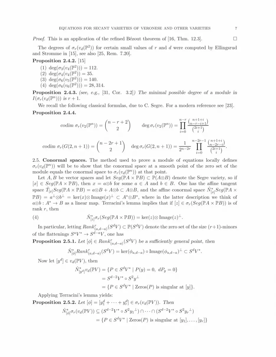
The degrees of σr(vd(P2)) for certain small values of r and d were computed by Ellingsrud
and Stromme in [15], see also [25, Rem. 7.20].
Proposition 2.4.2. [15]
(1) deg(σ3(v4(P2))) = 112.
(2) deg(σ4(v4(P2)) = 35.
(3) deg(σ6(v5(P2))) = 140.
(4) deg(σ6(v6(P2))) = 28, 314.
Proposition 2.4.3. (see, e.g., [31, Cor. 3.2]) The minimal possible degree of a module inI(σr(vd(P
n))) is r + 1.
We recall the following classical formulas, due to C. Segre. For a modern reference see [23].
Proposition 2.4.4.
codim σr(v2(Pn)) =
(
n− r + 2
2
)
degσr(v2(Pn)) =
n−r∏
i=0
( n+1+in−r−i+1
)
(2i+1i
)
codim σr(G(2, n + 1)) =
(
n− 2r + 1
2
)
deg σr(G(2, n + 1)) =1
2n−2r
n−2r−1∏
i=0
( n+1+in−2r−i
)
(2i+1i
) .
2.5. Conormal spaces. The method used to prove a module of equations locally definesσr(vd(P
n)) will be to show that the conormal space at a smooth point of the zero set of themodule equals the conormal space to σr(vd(P
n)) at that point.Let A,B be vector spaces and let Seg(PA × PB) ⊂ P(A⊗B) denote the Segre variety, so if
[x] ∈ Seg(PA × PB), then x = a⊗b for some a ∈ A and b ∈ B. One has the affine tangent
space T[x]Seg(PA × PB) = a⊗B + A⊗b ⊂ A⊗B, and the affine conormal space N∗[x]Seg(PA ×
PB) = a⊥⊗b⊥ = ker(x)⊗ Image(x)⊥ ⊂ A∗⊗B∗, where in the latter description we think ofa⊗b : A∗ → B as a linear map. Terracini’s lemma implies that if [z] ∈ σr(Seg(PA × PB)) is ofrank r, then
(4) N∗[z]σr(Seg(PA× PB)) = ker(z)⊗ Image(z)⊥.
In particular, letting Rankr(a,d−a)(SdV ) ⊂ P(SdV ) denote the zero set of the size (r+1)-minors
of the flattenings SaV ∗ → Sd−aV , one has
Proposition 2.5.1. Let [φ] ∈ Rankr(a,d−a)(SdV ) be a sufficiently general point, then
N∗[φ]Rank
r(a,d−a)(S
dV ) = ker(φa,d−a) Image(φa,d−a)⊥ ⊂ SdV ∗.
Now let [yd] ∈ vd(PV ), then
N∗[yd]vd(PV ) = P ∈ SdV ∗ | P (y) = 0, dPy = 0
= Sd−2V ∗ S2y⊥
= P ∈ SdV ∗ | Zeros(P ) is singular at [y].
Applying Terracini’s lemma yields:
Proposition 2.5.2. Let [φ] = [yd1 + · · ·+ ydr ] ∈ σr(vd(PV )). Then
N∗[φ]σr(vd(PV )) ⊆ (Sd−2V ∗ S2y1
⊥) ∩ · · · ∩ (Sd−2V ∗ S2yr⊥)
= P ∈ SdV ∗ | Zeros(P ) is singular at [y1], . . . , [yr]

8 J.M. LANDSBERG AND GIORGIO OTTAVIANI
and equality holds if φ is sufficiently general.
3. Symmetric Flattenings (catalecticant minors)
3.1. Review of known results. The following result dates back to the work of Sylvester andGundelfinger.
Theorem 3.1.1. (see, e.g., [25, Thm. 1.56]) The ideal of σr(vd(P1)) is generated in degree
r + 1 by the size r + 1 minors of φu,d−u for any r ≤ u ≤ d − r, i.e., by any of the modules
∧r+1SuC2⊗ ∧r+1 Sd−uC2. The variety σr(vd(P1)) is projectively normal and arithmetically
Cohen-Macaulay, its singular locus is σr−1(vd(P1)), and its degree is
(d−r+1r
)
.
Corollary 3.1.2 (Kanev, [26]). The ideal of σ2(vd(Pn)) is generated in degree 3 by the 3 by 3
minors of the (1, d − 1) and (2, d − 2) flattenings.
Proof. Apply Proposition 2.3.1 to Theorem 3.1.1 in the case r = 2.
Remark 3.1.3. C. Raicu [43] recently proved that in Corollary 3.1.2 it is possible to replace the(2, d − 2) flattening with any (i, d− i)-flattening such that 2 ≤ i ≤ d− 2.
Theorem 3.1.4. (see [25, Thms. 4.5A, 4.10A]) Let n ≥ 3, and let V = Cn+1. Let δ = xd2y,
δ′ = pd2q. If r ≤
(
δ−1+nn
)
then σr(vd(PV )) is an irreducible component of σr(Seg(PSδV ×
PSδ′V )) ∩ P(SdV ). In other words, σr(vd(P
n)) is an irreducible component of the size (r + 1)minors of the (δ, δ′)-flattening.
The bound obtained in this theorem is the best we know of for even degree, apart from somecases of small degree listed below. Theorem 1.2.3 is an improvement of this bound in the caseof odd degree.
When dim V = 3 then a Zariski open subset of σr(vd(PV )) can be characterized by openand closed conditions, that is, with the same assumptions of Theorem 3.1.4: If the rank of all(a, d − a)-flattenings computed at φ is equal to min
(
r,(a+2
2
))
then φ ∈ σr(vd(PV )) and thegeneral element of σr(vd(PV )) can be described in this way (see [25, Thm. 4.1A]).
Remark 3.1.5. The statement of Theorem 3.1.4 cannot be improved, in the sense that that thezero locus of the flattenings usually is reducible. Consider the case n = 2, d = 8, r = 10, in thiscase the 10×10 flattenings of φ4,4 define a variety with at least two irreducible components, oneof them is σ10(v8(P
2)) (see [25, Ex. 7.11]).
Proposition 3.1.6. Assume σr(vd(Pn)) is not defective and r < 1
n+1
(
n+dd
)
so that σr(vd(Pn)) is
not the ambient space. Let δ = xd2y, δ
′ = pd2q. There are non-trivial equations from flattenings
iff r <(δ+nδ
)
. (The defective cases where r is allowed to be larger are understood as well.)
Proof. The right hand side is the size of the maximal minors of φδ,δ′ , which give equations forσ(δ+n
δ )−1(vd(P
n)).
For example, when n = 3 and d = 2δ, σr(vd(P3)) is an irreducible component of the zero set
of the flattenings for r ≤(δ+2
3
)
, the flattenings give some equations up to r ≤(δ+3
3
)
, and there
are non-trivial equations up to r ≤ 14
(2δ+33
)
.We will have need of more than one symmetric flattening, so we make the following definitions,
following [25], but modifying the notation:

EQUATIONS FOR SECANT VARIETIES OF VERONESE AND OTHER VARIETIES 9
Definition 3.1.7. Fix a sequence ~r := (r1, . . . , rx d2y) and let
SFlat~r(SdW ) :=φ ∈ SdW | rank(φj,d−j) ≤ rj, j = 1, . . . , x
d
2y
= [
xd2y
⋂
j=1
σrj (Seg(PSjW × PSd−jW ))] ∩ SdW
Call a sequence ~r admissible if there exists φ ∈ SdW such that rank(φj,d−j) = rj for all
j = 1, . . . , xd2y. It is sufficient to consider ~r that are admissible because if ~r is non-admissible,the zero set of SFlat~r will be contained in the union of admissible SFlat’s associated to smaller~r’s in the natural partial order. Note that SFlat~r(S
dW ) ⊆ Subr1(SdW ).
Even if ~r is admissible, it still can be the case that SFlat~r(SdW ) is reducible. For example,
when dimW = 3 and d ≥ 6, the zero set of the size 5 minors of the (2, d− 2)-flattening has twoirreducible components, one of them is σ4(vd(P
2)) and the other has dimension d + 6 [25, Ex.3.6].
To remedy this, let ~r be admissible, and consider
SFlat0~r(SdW ) := φ ∈ SdW | rank(φj,d−j) = rj , j = 1, . . . , x
d
2y
and let
Gor(~r) := SFlat0~r(SdW ).
Remark 3.1.8. In the commutative algebra literature (e.g. [12, 25]), “Gor” is short for Goren-stein, see [25, Def. 1.11] for a history.
Unfortunately, defining equations for Gor(~r) are not known. One can test for membership ofSFlat0~r(S
dW ) by checking the required vanishing and non-vanishing of minors.
Theorem 3.1.9. [12, Thm 1.1] If dimW = 3, and ~r is admissible, then Gor(~r) is irreducible.
Theorem 3.1.9 combined with Theorem 3.1.4 allows one to extend the set of secant varietiesof Veronese varieties defined by flattenings.
3.2. Consequences of Theorems 3.1.9 and 3.1.4.
Theorem 3.2.1. The following varieties are defined scheme-theoretically by minors of flatten-ings:
(1) Let d ≥ 4. The variety σ3(vd(Pn)) is defined scheme-theoretically by the 4× 4 minors of
the (1, d − 1) and (⌊d2⌋, d− ⌊d2⌋) flattenings.(2) For d ≥ 4 the variety σ4(vd(P
2)) is defined scheme-theoretically by the 5 × 5 minors ofthe (⌊d2⌋, d − ⌊d2⌋) flattenings.
(3) For d ≥ 6 the variety σ5(vd(P2)) is defined scheme-theoretically by the 6 × 6 minors of
the (⌊d2⌋, d − ⌊d2⌋) flattenings.(4) Let d ≥ 6. The variety σ6(vd(P
2)) is defined scheme-theoretically by the 7× 7 minors ofthe (⌊d2⌋, d − ⌊d2⌋) flattenings.
Remark 3.2.2. In the recent preprint [6] it is proved that the variety σr(vd(Pn)) is defined set-
theoretically by the (r + 1) × (r + 1) minors of the (i, d − i) flattenings for n ≤ 3, 2r ≤ d andr ≤ i ≤ d− r. Schreyer proved (2) in the case d = 4, [46, Thm. 2.3].
By [47, Thm 4.2], when n ≤ 2, rank(φs,d−s) is nondecreasing in s for 1 ≤ s ≤ ⌊d2⌋. We willuse this fact often in this section.
10 J.M. LANDSBERG AND GIORGIO OTTAVIANI
To prove each case, we simply show the scheme defined by the flattenings in the hypothesescoincides with the scheme of some Gor(~r) with ~r admissible and then Theorem 3.1.4 combinedwith Theorem 3.1.9 implies the result. The first step is to determine which ~r are admissible.
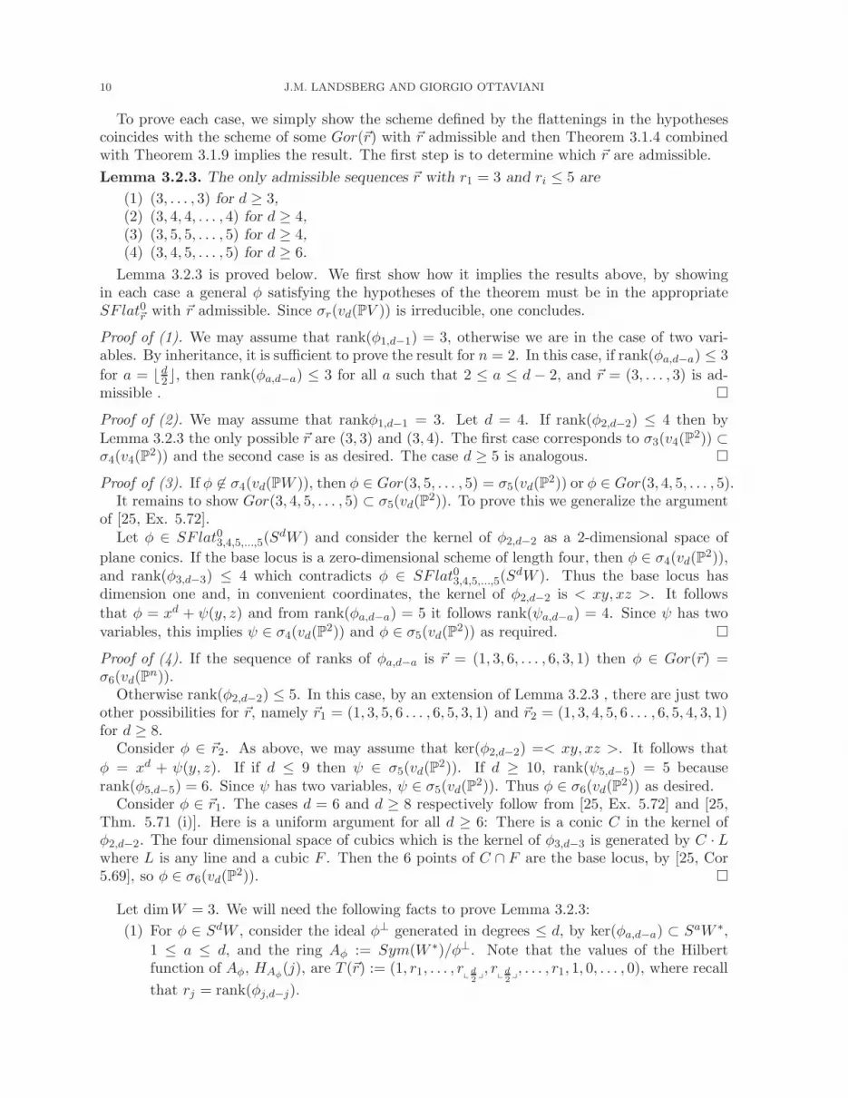
Lemma 3.2.3. The only admissible sequences ~r with r1 = 3 and ri ≤ 5 are
(1) (3, . . . , 3) for d ≥ 3,(2) (3, 4, 4, . . . , 4) for d ≥ 4,(3) (3, 5, 5, . . . , 5) for d ≥ 4,(4) (3, 4, 5, . . . , 5) for d ≥ 6.
Lemma 3.2.3 is proved below. We first show how it implies the results above, by showingin each case a general φ satisfying the hypotheses of the theorem must be in the appropriateSFlat0~r with ~r admissible. Since σr(vd(PV )) is irreducible, one concludes.
Proof of (1). We may assume that rank(φ1,d−1) = 3, otherwise we are in the case of two vari-ables. By inheritance, it is sufficient to prove the result for n = 2. In this case, if rank(φa,d−a) ≤ 3
for a = ⌊d2⌋, then rank(φa,d−a) ≤ 3 for all a such that 2 ≤ a ≤ d − 2, and ~r = (3, . . . , 3) is ad-missible .
Proof of (2). We may assume that rankφ1,d−1 = 3. Let d = 4. If rank(φ2,d−2) ≤ 4 then byLemma 3.2.3 the only possible ~r are (3, 3) and (3, 4). The first case corresponds to σ3(v4(P
2)) ⊂σ4(v4(P
2)) and the second case is as desired. The case d ≥ 5 is analogous.
Proof of (3). If φ 6∈ σ4(vd(PW )), then φ ∈ Gor(3, 5, . . . , 5) = σ5(vd(P2)) or φ ∈ Gor(3, 4, 5, . . . , 5).
It remains to show Gor(3, 4, 5, . . . , 5) ⊂ σ5(vd(P2)). To prove this we generalize the argument
of [25, Ex. 5.72].Let φ ∈ SFlat03,4,5,...,5(S
dW ) and consider the kernel of φ2,d−2 as a 2-dimensional space of
plane conics. If the base locus is a zero-dimensional scheme of length four, then φ ∈ σ4(vd(P2)),
and rank(φ3,d−3) ≤ 4 which contradicts φ ∈ SFlat03,4,5,...,5(SdW ). Thus the base locus has
dimension one and, in convenient coordinates, the kernel of φ2,d−2 is < xy, xz >. It follows
that φ = xd + ψ(y, z) and from rank(φa,d−a) = 5 it follows rank(ψa,d−a) = 4. Since ψ has twovariables, this implies ψ ∈ σ4(vd(P
2)) and φ ∈ σ5(vd(P2)) as required.
Proof of (4). If the sequence of ranks of φa,d−a is ~r = (1, 3, 6, . . . , 6, 3, 1) then φ ∈ Gor(~r) =σ6(vd(P
n)).Otherwise rank(φ2,d−2) ≤ 5. In this case, by an extension of Lemma 3.2.3 , there are just two
other possibilities for ~r, namely ~r1 = (1, 3, 5, 6 . . . , 6, 5, 3, 1) and ~r2 = (1, 3, 4, 5, 6 . . . , 6, 5, 4, 3, 1)for d ≥ 8.
Consider φ ∈ ~r2. As above, we may assume that ker(φ2,d−2) =< xy, xz >. It follows that
φ = xd + ψ(y, z). If if d ≤ 9 then ψ ∈ σ5(vd(P2)). If d ≥ 10, rank(ψ5,d−5) = 5 because
rank(φ5,d−5) = 6. Since ψ has two variables, ψ ∈ σ5(vd(P2)). Thus φ ∈ σ6(vd(P
2)) as desired.Consider φ ∈ ~r1. The cases d = 6 and d ≥ 8 respectively follow from [25, Ex. 5.72] and [25,
Thm. 5.71 (i)]. Here is a uniform argument for all d ≥ 6: There is a conic C in the kernel ofφ2,d−2. The four dimensional space of cubics which is the kernel of φ3,d−3 is generated by C · Lwhere L is any line and a cubic F . Then the 6 points of C ∩ F are the base locus, by [25, Cor5.69], so φ ∈ σ6(vd(P
2)).
Let dimW = 3. We will need the following facts to prove Lemma 3.2.3:
(1) For φ ∈ SdW , consider the ideal φ⊥ generated in degrees ≤ d, by ker(φa,d−a) ⊂ SaW ∗,
1 ≤ a ≤ d, and the ring Aφ := Sym(W ∗)/φ⊥. Note that the values of the Hilbertfunction of Aφ, HAφ
(j), are T (~r) := (1, r1, . . . , rx d2y, r
xd2y, . . . , r1, 1, 0, . . . , 0), where recall
that rj = rank(φj,d−j).

EQUATIONS FOR SECANT VARIETIES OF VERONESE AND OTHER VARIETIES 11
(2) [5, Thm. 2.1] The ring Aφ has a minimal free resolution of the form
0−→Sym(W ∗)(−d− 3)g∗−→⊕u
i=1 Sym(W ∗)(−d+ 3− qi)(5)h
−→⊕ui=1 Sym(W ∗)(−qi)
g−→Sym(W ∗)(0) → Aφ → 0
where the qj are non-decreasing. Here Sym(W ∗)(j) denotes Sym(W ∗) with the labeling
of degrees shifted by j, so dim(Sym(W ∗)(j))d =(d+j+2
2
)
.
(3) Moreover [12, Thm 1.1] there is a unique resolution with the properties q1 ≤ d+32 ,
qi + qu−i+2 = d+ 2, 2 ≤ i ≤ u+12 having T (~r) as the values of its Hilbert function.
(4) Recall that HAφ(j) is also the alternating sum of the dimensions of the degree j term in
(5) (forgetting the last term). Thus the qj determine the ri.(5) [12, Thm. 3.3] Letting j0 be the smallest j such that φj,d−j is not injective, then u =
2j0 + 1 in the resolution above.
Remark 3.2.4. Although we do not need these facts from [5] here, we note that above: h is skew-symmetric, g is defined by the principal sub-Pfaffians of h, Aφ is an Artinian Gorenstein gradedC-algebra and any Artinian Gorenstein graded C-algebra is isomorphic to Aφ for a polynomialφ uniquely determined up to constants. The ring Aφ is called the apolar ring of φ, the resolutionabove is called saturated.
Proof of Lemma 3.2.3. Let ~r be a sequence as in the assumptions. Since dimS2C3 = 6 > 5,u = 5 by Fact 3.2(5). Consider the unique resolution satisfying Fact 3.2(3) having T (~r) asHilbert function. The number of generators in degree 2 is the number of the qi equal to 2. Wemust have q1 = 2, otherwise, by computing the Hilbert function, H(Aφ)(2) = 6 contrary toassumption. The maximal number of generators in degree 2 is three, otherwise we would have2 + 2 = q4 + q5−4+2 = d+ 2, a contradiction.
If there are three generators in degree 2 then qi = (2, 2, 2, d, d), and computing the Hilbertfunction via the Euler characteristic, we are in case (1) of the Lemma.
If there are two generators in degree 2 then there are the two possibilities qi = (2, 2, 3, n−1, n)(case(2)) or qi = (2, 2, 4, n−2, n) (case (4)). Note that qi = (2, 2, 5, n−3, n) for n ≥ 8 is impossiblebecause otherwise ~r = (1, 3, 4, 5, 6, . . .) contrary to assumption. By similar arguments one showsthat there are no other possibilities.
If there is one generator in degree 2 then qi = (2, 3, 3, n − 1, n − 1) (case (3)).
Proposition 3.2.5. Let dimV = 3 and p ≥ 2. If the variety σr(v2p(PV )) is an irreduciblecomponent of σr(v2(PS
pV )) ∩ PS2pV then r ≤ 12p(p+ 1) or (p, r) = (2, 4) or (3, 9).
Proof. Recall that for (p, r) 6= (2, 5)
(6) codimσr(v2p(PV )) =
(
2p+ 2
2
)
− 3r
and from Proposition 2.4.4 every irreducible component X of σr(v2(PSpV )) ∩ PS2pV satisfies
(7) codimX ≤1
2
[(
p+ 2
2
)
− r
] [(
p+ 2
2
)
− r + 1
]
The result follows by solving the inequality.
For the case (p, r) = (2, 4) see Theorem 3.2.1(2) and for the case (p, r) = (3, 9) see Theorem4.2.9.
Corollary 3.2.6. deg σ(p+12 )(v2p(P
2)) ≤∏pi=0
((p+2)(p+1)/2+ip−i+1 )(2i+1
i ).
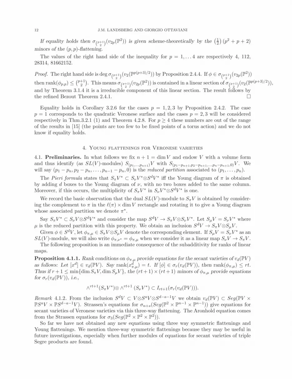
12 J.M. LANDSBERG AND GIORGIO OTTAVIANI
If equality holds then σ(p+12 )(v2p(P
2)) is given scheme-theoretically by the(
12
)
(p2 + p + 2)
minors of the (p, p)-flattening.
The values of the right hand side of the inequality for p = 1, . . . 4 are respectively 4, 112,28314, 81662152.
Proof. The right hand side is deg σ(p+12 )(v2(P
p(p+3)/2)) by Proposition 2.4.4. If φ ∈ σ(p+12 )(v2p(P
2))
then rank(φp,p) ≤(
p+12
)
. This means σ(p+12 )(v2p(P
2)) is contained in a linear section of σ(p+12 )(v2(P
p(p+3)/2)),
and by Theorem 3.1.4 it is a irreducible component of this linear section. The result follows bythe refined Bezout Theorem 2.4.1.
Equality holds in Corollary 3.2.6 for the cases p = 1, 2, 3 by Proposition 2.4.2. The casep = 1 corresponds to the quadratic Veronese surface and the cases p = 2, 3 will be consideredrespectively in Thm.3.2.1 (1) and Theorem 4.2.8. For p ≥ 4 these numbers are out of the rangeof the results in [15] (the points are too few to be fixed points of a torus action) and we do notknow if equality holds.
4. Young flattenings for Veronese varieties
4.1. Preliminaries. In what follows we fix n + 1 = dimV and endow V with a volume formand thus identify (as SL(V )-modules) S(p1,...,pn+1)V with S(p1−pn+1,p2−pn+1,...,pn−pn+1,0)V . Wewill say (p1 − pn, p2 − pn, . . . , pn−1 − pn, 0) is the reduced partition associated to (p1, . . . , pn).
The Pieri formula states that SπV∗ ⊂ SνV
∗⊗SdV ∗ iff the Young diagram of π is obtainedby adding d boxes to the Young diagram of ν, with no two boxes added to the same column.Moreover, if this occurs, the multiplicity of SπV
∗ in SνV∗⊗SdV ∗ is one.
We record the basic observation that the dual SL(V )-module to SπV is obtained by consider-ing the complement to π in the ℓ(π)× dimV rectangle and rotating it to give a Young diagramwhose associated partition we denote π∗.
Say SπV∗ ⊂ SνV⊗SdV ∗ and consider the map SdV → SπV⊗SνV
∗. Let SµV = SνV∗ where
µ is the reduced partition with this property. We obtain an inclusion SdV → SπV⊗SµV .
Given φ ∈ SdV , let φπ,µ ∈ SπV⊗SµV denote the corresponding element. If SµV = SνV∗ as an
SL(V )-module, we will also write φπ,ν∗ = φπ,µ when we consider it as a linear map SνV → SπV .The following proposition is an immediate consequence of the subadditivity for ranks of linear
maps.
Proposition 4.1.1. Rank conditions on φπ,µ provide equations for the secant varieties of vd(PV )
as follows: Let [xd] ∈ vd(PV ). Say rank(xdπ,µ) = t. If [φ] ∈ σr(vd(PV )), then rank(φπ,µ) ≤ rt.Thus if r+1 ≤ mindimSπV,dimSµV , the (rt+1)× (rt+1) minors of φπ,µ provide equationsfor σr(vd(PV )), i.e.,
∧rt+1(SπV∗)⊗ ∧rt+1 (SνV
∗) ⊂ Irt+1(σr(vd(PV ))).
Remark 4.1.2. From the inclusion SdV ⊂ V⊗SaV⊗Sd−a−1V we obtain vd(PV ) ⊂ Seg(PV ×PSaV × PSd−a−1V ). Strassen’s equations for σn+s(Seg(P
2 × Pn−1 × Pn−1)) give equations forsecant varieties of Veronese varieties via this three-way flattening. The Aronhold equation comesfrom the Strassen equations for σ3(Seg(P
2 × P2 × P2)).So far we have not obtained any new equations using three way symmetric flattenings and
Young flattenings. We mention three-way symmetric flattenings because they may be useful infuture investigations, especially when further modules of equations for secant varieties of tripleSegre products are found.

EQUATIONS FOR SECANT VARIETIES OF VERONESE AND OTHER VARIETIES 13
Let
Y F lattπ,µ(SdV ) := φ ∈ SdV | rank(φπ,µ) ≤ t = σt(Seg(PSπV × PSµV )) ∩ PSdV.
Remark 4.1.3. Recall Y F rd,n from §1.2 whose description had redundancies. We can now givean irredundant description of its defining equations:
Y F rd,n = Y F lat( n⌊n2 ⌋)r
((δ+1)a ,δn−a),(δ+1,1a)(SdV ).
This is a consequence of Schur’s Lemma, because the module S(δ+1,1a)V is the only one
appearing in both sides of SdV ⊗ SδV ∗ ⊗ ∧aV → SδV ⊗ ∧a+1V
Note that if SπV ≃ SµV as SL(V )-modules and the map is symmetric, then
Y F lattπ,µ(SdV ) = σt(v2(PSπV )) ∩ PSdV,
and if it is skew-symmetric, then
Y F lattπ,µ(SdV ) = σt(G(2, SπV )) ∩ PSdV.
4.2. The surface case, σr(vd(P2)). In this subsection fix dimV = 3 and a volume form Ω on
V . From the general formula for dimSπV (see, e.g., [17, p78]), we record the special case:
(8) dimSa,bC3 =
1
2(a+ 2)(b+ 1)(a − b+ 1).
Lemma 4.2.1. Let a ≥ b. Write d = α + β + γ with α ≤ b, β ≤ a − b so S(a+γ−α,b+β−α)V ⊂
Sa,bV⊗SdV . For φ ∈ SdV , consider the induced map
(9) φ(a,b),(a+γ−α,b+β−α) : Sa,bV∗ → S(a+γ−α,b+β−α)V.
Let x ∈ V , then
(10) rank((xd)(a,b),(a+γ−α,b+β−α)) =1
2(b− α+ 1)(a − b− β + 1)(a+ β − α+ 2) =: R.
Thus in this situation ∧pR+1(SabV )⊗ ∧pR+1 (Sa+γ−α,b+β−αV ) gives nontrivial degree pR + 1equations for σp(vd(P
2)).
Remark 4.2.2. Note that the right hand sides of equations (8) and (10) are the same whenα = β = 0. To get useful equations one wants R small with respect to dimSa,bC
3.
Proof. In the following picture we label the first row containing a boxes with a and so on.
a a a a ab b b →
a a a a a γ γb b b βα α
Assume we have chosen a weight basis x1, x2, x3 of V and x = x3 is a vector of lowest weight.Consider the image of a weight basis of Sa,bV under (x33)(a,b),(a+γ−α,b+β−α). Namely consider allsemi-standard fillings of the Young diagram corresponding to (a, b), and count how many do notmap to zero. By construction, the images of all the vectors that do not map to zero are linearlyindependent, so this count indeed gives the dimension of the image.
In order to have a vector not in the kernel, the first α boxes of the first row must be filledwith 1’s and the first α boxes of the second row must be filled with 2’s.
Consider the next (b − α, b − α) subdiagram. Let C2ij denote the span of xi, xj and C1
i thespan of xi. The boxes here can be filled with any semi-standard filling using 1’s 2’s and 3’s,but the freedom to fill the rest will depend on the nature of the filling, so split Sb−α,b−αC
3
into two parts, the first part where the entry in the last box in the first row is 1, which has
14 J.M. LANDSBERG AND GIORGIO OTTAVIANI
dimSb−αC223 fillings and second where the entry in the last box in the first row is 2, which has
(dimSb−α,b−αC3 − dimSb−αC
223) fillings.
In the first case, the next β-entries are free to be any semi-standard row filled with 1’s and 2’s,of which there are dimSβC
212 in number, but we split this further into two sub-cases, depending
on whether the last entry is a 1 (of which there is one (= dimSβC11) such), or 2 (of which
there are (dimSβC212 − dimSβC
11) such). In the first sub-case the last a− (b+ β) entries admit
dimSa−(b+β)C3 fillings and in the second sub-case there are dimSa−(b+β)C
223 such. Putting these
together, the total number of fillings for the various paths corresponding to the first part is
dimSb−αC212[(dimSβC
11)(dimSa−b−βC
3) + (dimSβC212 − dimSβC
11)(dimSa−b−βC
223)]
= (b− α+ 1)[(1)
(
a− b− β + 2
2
)
+ (β − 1)(a− b− β + 1)].
For the second part, the next β boxes in the first row must be filled with 2’s (giving 1 =dimSβC
12) and the last a− (b+ β) boxes can be filled with 2’s or 3’s semi-standardly, i.e., there
are dimSa−b−βC223’s worth. So the contribution of the second part is
(dimSb−α,b−αC3 − dimSb−αC
212)(dimSβC
12)(dimSa−b−βC
223)
= (
(
b− α+ 2
b− α
)
− (b− α+ 1))(1)(a − b− β + 1).
Adding up gives the result.
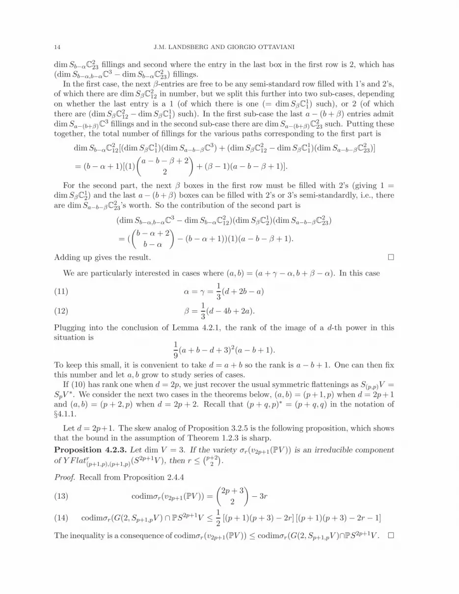
We are particularly interested in cases where (a, b) = (a+ γ − α, b+ β − α). In this case
α = γ =1
3(d+ 2b− a)(11)
β =1
3(d− 4b+ 2a).(12)
Plugging into the conclusion of Lemma 4.2.1, the rank of the image of a d-th power in thissituation is
1
9(a+ b− d+ 3)2(a− b+ 1).
To keep this small, it is convenient to take d = a+ b so the rank is a− b+ 1. One can then fixthis number and let a, b grow to study series of cases.
If (10) has rank one when d = 2p, we just recover the usual symmetric flattenings as S(p,p)V =SpV
∗. We consider the next two cases in the theorems below, (a, b) = (p+1, p) when d = 2p+1and (a, b) = (p + 2, p) when d = 2p + 2. Recall that (p + q, p)∗ = (p + q, q) in the notation of§4.1.1.
Let d = 2p+1. The skew analog of Proposition 3.2.5 is the following proposition, which showsthat the bound in the assumption of Theorem 1.2.3 is sharp.
Proposition 4.2.3. Let dim V = 3. If the variety σr(v2p+1(PV )) is an irreducible component
of Y F latr(p+1,p),(p+1,p)(S2p+1V ), then r ≤
(p+22
)
.
Proof. Recall from Proposition 2.4.4
codimσr(v2p+1(PV )) =
(
2p+ 3
2
)
− 3r(13)
codimσr(G(2, Sp+1,pV ) ∩ PS2p+1V ≤1
2[(p+ 1)(p + 3)− 2r] [(p+ 1)(p + 3)− 2r − 1](14)
The inequality is a consequence of codimσr(v2p+1(PV )) ≤ codimσr(G(2, Sp+1,pV )∩PS2p+1V .

EQUATIONS FOR SECANT VARIETIES OF VERONESE AND OTHER VARIETIES 15
Here is a pictorial description when p = 2 of φ31,31 : S32V → S31V in terms of Young diagrams:
⊗ ∗ ∗ ∗ ∗ ∗ →
∗ ∗∗
∗ ∗ ≃
Corollary 4.2.4. deg σ(p+22 )(v2p+1(P
2)) ≤ 12p
∏p−1i=0
((p+3)(p+1)+ip−i )
(2i+1i )
.
If equality holds then σ(p+22 )(v2p+1(P
2)) is given scheme-theoretically by the size (p + 2)(p +
1) + 2 sub-Pfaffians of φ(p+1,p),(p+1,p).
The values of the right hand side for p = 1, . . . 4 are respectively 4, 140, 65780, 563178924.
Proof. The right hand side is deg σ(p+22 )(G(C
2, S(p+1,p)V ) by Proposition 2.4.4. Now σ(p+12 )(v2p+1(P
2))
is contained in a linear section of σ(p+22 )(G(C
2, S(p+1,p)V )), and by Theorem 1.2.3 it is a irre-
ducible component of this linear section. The result follows by the refined Bezout theorem2.4.1.
In Corollary 4.2.4 equality holds in the cases p = 1, 2 by Proposition 2.4.2. The case p = 1 isjust the Aronhold case and the case p = 2 will be considered in Theorem 4.2.7 (2). For p ≥ 3these numbers are out of the range of [15] and we do not know if equality holds.
Note that the usual symmetric flattenings only give equations for σk−1(v2p+1(P2))for k ≤
12(p
2 + 3p+ 2).
Now let d = 2p + 2 be even, requiring π = µ, the smallest possible rank((xd)π,µ) is three,which we obtain with φ(p+2,p),(p+2,p).
Proposition 4.2.5. Let d = 2p+2. The Young flattening φ(p+2,2),(p+2,2) ∈ Sp+2,2V⊗Sp+2,2V is
symmetric. It is of rank three for φ ∈ vd(P2) and gives degree 3(k+1) equations for σr(v2p+2(P
2))
for r ≤ 12(p
2 + 5p+ 4)− 1. A convenient model for the equations is given in the proof.
A pictorial description when p = 2 is as follows:
⊗ ∗ ∗ ∗ ∗ ∗ ∗ →
∗ ∗∗ ∗
∗ ∗ ≃ .
Proof. Let Ω ∈ ∧3V be dual to the volume form Ω. To prove the symmetry, for φ = x2p+2,consider the map,
Mx2p+2 : SpV ∗⊗S2(∧2V ∗) → SpV⊗S2(∧2V )
α1 · · ·αp⊗(γ1 ∧ δ1) (γ2 ∧ δ2) 7→ α1(x) · · ·αp(x)xp⊗Ω(x γ1 ∧ δ1) Ω(x γ2 ∧ δ2)
and define Mφ for arbitrary φ ∈ S2p+2V by linearity and polarization. If we take bases ofS2V⊗S2(∧2V ) as above, with indices ((i1, . . . , ip), (kl), (k
′l′)), most of the matrix of Me2p+21
is
zero. The upper-right hand 6×6 block, where (i1, . . . , ip) = (1, . . . , 1) in both rows and columnsand the order on the other indices
((12), (12)), ((13), (13)), ((12), (13)), ((12), (23)), ((13), (23)), ((23), (23)),

16 J.M. LANDSBERG AND GIORGIO OTTAVIANI
is
0 1 0 0 0 01 0 0 0 0 00 0 1 0 0 00 0 0 0 0 00 0 0 0 0 00 0 0 0 0 0
showing the symmetry. Now
(SpV⊗S2(∧2V ))⊗2 = (SpV⊗(S22V ⊕ S1111V )⊗2
= Sp+2,2V ⊕ stuff
where all the terms in stuff have partitions with at least three parts. On the other hand, fromthe nature of the image we conclude it is just the first factor and Mφ ∈ S2(Sp+2,2V ).
Note that the usual symmetric flattenings give nontrivial equations for σk−1(v2p+2(P2)) for
k ≤ 12(p
2 + 5p + 6), a larger range than in Proposition 4.2.5. However we show (Theorem
4.2.9) that the symmetric flattenings alone are not enough to cut out σ7(v6(P2)), but with the
((p + 1, 2), (p + 1, 2))-Young flattening they are.Here is a more general Young flattening:
Proposition 4.2.6. Let d = p+ 4q − 1. The Young flattening
φ(p+2q,2q−1),(p+2q,2q−1) ∈ S(p+2q,2q−1)V⊗S(p+2q,2q−1)V,
is skew-symmetric if p is even and symmetric if p is odd.Since it has rank p if φ ∈ vd(P
2), if p is even (resp. odd), the size kp+ 2 sub-Pfaffians (resp.
size kp + 1 minors) of φ(p+2q,2q−1),(p+2q,2q−1) give degree kp2 + 1 (resp. kp + 1) equations for
σk(vp+4q−1(P2)) for
k ≤q(p+ 2q + 2)(p + 2)
p.
Proof. Consider Mφ : Sp−1V ∗⊗Sq(∧2V ∗) → SpV⊗Sq(∧2V ) given for φ = xp+4q−1 by
α1 · · ·αp−1⊗β1 ∧ γ1 · · · βq ∧ γq 7→ Πj(αj(x))xp−1⊗Ω(x β1 ∧ γ1) · · · Ω(x βq ∧ γq)
and argue as above.
Here the usual flattenings give degree k equations for σk−1(vd(P2)) in the generally larger
range k ≤ 18(p + 4q + 2)(p + 4q).
Recall that we have already determined the ideals of σr(vd(P2)) for d ≤ 4, (Thm. 3.2.1 and
the chart in the introduction) so we next consider the case d = 5.Case d = 5: The symmetric flattening given by the size (k+1) minors of φ2,3 define σk(v5(P
2))up to k = 4 by Theorem 3.1.4 (3). Note that the size 6 minors define a subvariety of codimension5, strictly containing σ5(v5(P
2)), which has codimension 6. So, in this case, the bound providedby Theorem 3.1.4 is sharp.
Theorem 4.2.7.
(1) σk(v5(P2)) for k ≤ 5 is an irreducible component of Y F lat2k31,31(S
5C3), the variety given
by the principal size 2k + 2 Pfaffians of the [(31), (31)]-Young flattenings.(2) the principal size 14 Pfaffians of the [(31), (31)]-Young flattenings are scheme-theoretic
defining equations for σ6(v5(P2)), i.e., as schemes, σ6(v5(P
2)) = Y F lat1231,31(S5C3).
(3) σ7(v5(P2)) is the ambient space.

EQUATIONS FOR SECANT VARIETIES OF VERONESE AND OTHER VARIETIES 17
Proof. (1) is a consequence of Theorem 1.2.3.To prove the second assertion, by the Segre formula (Proposition 2.4.4) the subvariety of size
15 skew-symmetric matrices of rank ≤ 12 has codimension 3 and degree 140. By Proposition2.4.2, σ6(v5(P
2)) has codimension 3 and degree 140. We conclude as in the proof of Corollary3.2.6.
Case d = 6: In the case σk(v6(P2)), the symmetric flattening given by the (k + 1) minors of
φ2,4 define σk(v6(P2)) as an irreducible component up to k = 4 (in the case k = 4 S. Diesel [25,
Ex. 3.6] showed that there are two irreducible components) and the symmetric flattening givenby the (k + 1) minors of φ3,3 define σk(v6(P
2)) as an irreducible component up to k = 6.The following is a special case of the Thm. 3.2.1(4), we include this second proof because it
is very short.
Theorem 4.2.8. As schemes, σ6(v6(P2)) = Rank63,3(S
6C3), i.e., the size 7 minors of φ3,3 cut
out σ6(v6(P2)) scheme-theoretically.
Proof. By the Segre formula (Proposition 2.4.4) the subvariety of symmetric 10 × 10 matricesof rank ≤ 6 has codimension 10 and degree 28, 314. By Proposition 2.4.2, σ6(v6(P
2)) hascodimension 10 and degree 28, 314. We conclude as in the proof of Corollary 3.2.6.
The size 8 minors of φ3,3 define a subvariety of codimension 6, strictly containing σ7(v6(P2)),
which has codimension 7. In the same way, the size 9 minors of φ3,3 define a subvariety ofcodimension 3, strictly containing σ8(v6(P
2)), which has codimension 4. Below we constructequations in terms of Young flattenings.
det(φ42,42) is a polynomial of degree 27, which is not the power of a lower degree polynomial.This can be proved by cutting with a random projective line, and using Macaulay2. The twovariable polynomial obtained is not the power of a lower degree polynomial.
If φ is decomposable then rank(φ42,42) = 3 by Lemma 4.2.1, so that when φ ∈ σk(v6(P2))
then rank(φ42,42) ≤ 3k.
Theorem 4.2.9.
(1) σ7(v6(P2)) is an irreducible component of Rank73,3(S
6C3)∩Y F lat2242,42(S6C3), i.e., of the
variety defined by the size 8 minors of the symmetric flattening φ3,3 and by the size 22minors of the [(42), (42)]-Young flattenings.
(2) σ8(v6(P2)) is an irreducible component of Rank83,3(S
6C3)∩Y F lat2442,42(S6C3), i.e., of the
variety defined by the size 9 minors of the symmetric flattening φ3,3 and by the size 25minors of the [(42), (42)]-Young flattenings.
(3) σ9(v6(P2)) is the hypersurface of degree 10 defined by det(φ3,3).
Proof. To prove (2), we picked a polynomial φ which is the sum of 8 random fifth powers oflinear forms, and a submatrix of φ42,42 of order 24 which is invertible. The matrix representingφ42,42 can be constructed explicitly by the package PieriMaps of Macaulay2 [22, 45].
The affine tangent space at φ of Rank83,3(S6C3) has codimension 3 in S6C3. In order to
compute a tangent space, differentiate, as usual, each line of the matrix, substitute φ in theother lines, compute the determinant and then sum over the lines. It is enough to pick oneminor of order 25 of φ42,42 containing the invertible ones of order 24. The tangent space of thisminor at φ is not contained in the subspace of codimension 3, yielding the desired subspace ofcodimension 4.
(1) can be proved in the same way. (3) is well known.
Remark 4.2.10. σ7(v6(P2)) is the first example where the known equations are not of minimal
possible degree.

18 J.M. LANDSBERG AND GIORGIO OTTAVIANI
Case d = 7: In the case of σk(v7(P2)), the symmetric flattening given by the size (k + 1)
minors of φ3,4 define σk(v7(P2)) as an irreducible component up to k = 8.
Theorem 4.2.11.
(1) For k ≤ 10 σk(v7(P2)) is an irreducible component of Y F latk41,41(S
7C3), which is defined
by the size (2k + 2) subpfaffians of of φ41,41.(2) σ11(v7(P
2)) has codimension 3 and it is contained in the hypersurface Y F lat2241,41(S7C3)
of degree 12 defined by Pf(φ41,41).
Proof. (1) follows from Theorem 1.2.3. (2) is obvious.
Remark 4.2.12. We emphasize that σ11(v7(P2)) is the first case where we do not know, even
conjecturally, further equations.
Case d = 8: It is possible that σk(v8(P2)) is an irreducible component of Rankk+1
4,4 (S8C3) upto k = 12, but the bound given in Theorem 3.1.4 is just k ≤ 10. The size 14 minors of φ4,4define a subvariety of codimension 4, which strictly contains σ13(v8(P
2)) which has codimension6. Other equations of degree 40 for σ13(v8(P
2)) are given by the size 40 minors of φ53,52. Itis possible that minors of φ(53),(52) could be used to get a collection of set-theoretic equations
for σ12(v8(P2)) and σ11(v8(P
2)). In the same way, detφ4,4 is just an equation of degree 15 forσ14(v8(P
2)) which has codimension 3.
Case d = 9: It is possible that σk(v9(P2)) is an irreducible component of Rankk+1
4,5 (S9C3) up
to k = 13, but the bound given in Theorem 3.1.4 is just k ≤ 11. Rank144,5(S9C3) strictly contains
σ14(v9(P2)) which has codimension 13. The principal Pfaffians of order 30 of φ54,51 give further
equations for σ14(v9(P2)). In the same way the principal Pfaffians of order 32 (resp. 34) of
φ54,51 give some equations for σ15(v9(P2)) (resp. σ16(v9(P
2))). Another equation for σ15(v9(P2))
is the Pfaffian of the skew-symmetric morphism φ63,63 : S6,3V → S6,3V which can be pictoriallydescribed in terms of Young diagrams, by
⊗ ∗ ∗ ∗ ∗ ∗ ∗ ∗ ∗ ∗ →
∗ ∗ ∗∗ ∗ ∗
∗ ∗ ∗ ≃
We do not know any equations for σk(v9(P2)) when k = 17, 18. The k = 18 case is particularly
interesting because the corresponding secant variety is a hypersurface.
5. Construction of equations from vector bundles
5.1. Main observation. Write e := rank(E) and consider the determinantal varieties or rankvarieties defined by the minors of AEv : H0(E) → H0(E∗ ⊗ L)∗ (defined by equation (3)),
Rankk(E) : = Pv ∈ V |rank(AEv ) ≤ ek
= σek(Seg(PH0(E)∗ × PH0(E∗⊗L)∗)) ∩ PV.
Proposition 5.1.1. Let X ⊂ PV = PH0(L)∗ be a variety, and E a rank e vector bundle on X.Then
σr(X) ⊆ Rankr(E)
i.e., the size (re+ 1) minors of AEv give equations for σr(X).
When E is understood, we will write Av for AEv .
Proof. By (3), if x = [v] ∈ X, then H0(Ix ⊗ E) ⊆ kerAv. The subspace H0(Ix ⊗ E) ⊆ H0(E)has codimension at most e in H0(E), hence the same is true for the subspace kerAx and it

EQUATIONS FOR SECANT VARIETIES OF VERONESE AND OTHER VARIETIES 19
follows rank(Ax) ≤ e. If v ∈ σr(X) is a general point, then it may be expressed as v =∑r
i=1 xi,
with xi ∈ X . Hence
rank(Av) = rank(
r∑
i=1
Axi) ≤r
∑
i=1
rank(Axi) ≤ re
as claimed. Since the inequality is a closed condition, it holds for all v ∈ σr(X).
Example 5.1.2. Let X = vd(PW ), L = O(d), E = O(a) so E∗⊗L = O(d− a), then Rankr(E)is the catalecticant variety of symmetric flattenings in SaW ⊗ Sd−aW of rank at most r.
Example 5.1.3. Let E be a homogeneous bundle on Pn with H0(E)∗ = SµV , H0(E∗ ⊗ L)∗ =SπV . Then Av corresponds to φπ,µ of §4.
The generalization of symmetric flattenings to Young flattenings for Veronese varieties is arepresentation-theoretic version of the generalization from line bundles to higher rank vectorbundles.
Example 5.1.4. A general source of examples is given by curves obtained as determinantalloci. This topic is studied in detail in [14]. In [21], A. Ginensky considers the secant varietiesσk(C) to smooth curves C in their bicanonical embedding. With our notations this correspondsto the symmetric pair (E,L) = (KC ,K
2C). He proves [21, Thm. 2.1] that σk(C) = Rankk(KC)
if k < Cliff(C) and σk(C) ( Rankk(KC) for larger k. Here Cliff(C) denotes the Clifford indexof C.
5.2. The construction in the symmetric and skew-symmetric cases. We say that (E,L)is a symmetric pair if the isomorphism E
α−→E∗ ⊗ L is symmetric, that is the transpose iso-
morphism E ⊗ L∗ αt
−→E∗, after tensoring by L and multiplying the map by 1L equals α, i.e.,α = αt⊗ 1L. In this case S2E contains L as a direct summand, the morphism Av is symmetric,and Rankk(E) is defined by the (ke+ 1)-minors of Av.
Similarly, (E,L) is a skew-symmetric pair if α = −αt⊗1L. In this case e is even, ∧2E containsL as a direct summand, the morphism Av is skew-symmetric, and Rankk(E) is defined by thesize (ke+ 2) subpfaffians of Av, which are equations of degree ke
2 + 1.
Example 5.2.1. Let X = P2×Pn embedded by L = O(1, 2). The equations for σk(X) recentlyconsidered in [8], where they have been called exterior flattenings, fit in this setting. Call p1, p2the two projections. Let Q be the tautological quotient bundle on P2 and let E = p∗1Q⊗p∗2O(1),then (E,L) is a skew-symmetric pair which gives rise to the equations (2) in Theorem 1.1 of [8],while the equations (1) are obtained with E = p∗2O(1).
5.3. The conormal space. The results reviewed in §2.5, restated in the language of vectorbundles, say the affine conormal space of Rankk(E) at [v] ∈ Rankk(E)smooth is the image of themap
kerAv ⊗ Im A⊥v → H0(L) = V ∗.
If (E,L) is a symmetric (resp. skew symmetric) pair, there is a symmetric (resp. skewsymmetric) isomorphism kerAv ≃ Im A⊥
v and the conormal space of Rankk(E) at v is given bythe image of the map S2 (kerAv) → H0(L), (resp. ∧2 (kerAv) → H0(L)).
5.4. A sufficient criterion for σk(X) to be an irreducible component of Rankk(E).
Let v ∈ X, in the proof of Proposition 5.1.1, we saw H0(Iv ⊗ E) ⊆ kerAv. In the same way,H0(Iv ⊗E∗ ⊗L) ⊆ Im A⊥
v , by taking transpose. Equality holds if E is spanned at x = [v]. Thisis generalized by the following Proposition.

20 J.M. LANDSBERG AND GIORGIO OTTAVIANI
Proposition 5.4.1. Let v =∑k
i=1 xi ∈ V , with [xi] ∈ X, and let Z = [x1], . . . , [xk]. Then
H0(IZ ⊗ E) ⊆ kerAv
H0(IZ ⊗ E∗ ⊗ L) ⊆ Im A⊥v .
The first inclusion is an equality if H0(E∗ ⊗ L) → H0(E∗ ⊗ L|Z) is surjective. The second
inclusion is an equality if H0(E) → H0(E|Z) is surjective.
Remark 5.4.2. In [3], a line bundle F → X is defined to be k-spanned if H0(F ) surjects ontoH0(F |Z) for all Z = [x1], . . . , [xk]. In that paper and in subsequent work they study whichline bundles have this property. In particular k-spanned-ness of X ⊂ PH0(F )∗ implies that forall k-tuples of points ([x1], . . . , [xk]) on X, writing Z = [x1], . . . , [xk], then 〈Z〉 = Pk−1, as forexample occurs with Veronese varieties vd(PV ) when k ≤ d+ 1.
Proof. If E∗ ⊗ L is spanned at x = [w] then we claim H0(Ix ⊗ E) = kerAw. To see this, workover an open set where E,L are trivializable and take trivializations. There are tj ∈ H
0(E∗⊗L)such that in a basis ei of the Ce which we identify with the fibers of E on this open subset,〈ei, tj(x)〉 = δij . Take s ∈ ker(Aw). By assumption 〈s(x), tj(x)〉 = 0 for every j, hence, writings =
∑
siei, sj(x) = 0 for every j, i.e., s ∈ H0(Ix ⊗ E).Since
H0(IZ ⊗ E) = ∩ki=1H0(Ixi ⊗ E) ⊆ ∩ki=1 kerAxi ⊆ kerAv,
the inclusion for the kernel follows. To see the equality assertion, if H0(E∗⊗L) → H0(E∗⊗L|Z)
is surjective, for every j = 1, . . . , k we can choose th,j ∈ H0(E∗ ⊗ L), for h = 1, . . . , e, such that
th,j(xi) = 0 for i 6= j, ∀h and th,j span the fiber of E∗ ⊗ L at xj . It follows that if s ∈ ker(Av)then th,j(xj) · s(xj) = 0 for every h, j which implies s(xj) = 0, that is s ∈ H0(IZ ⊗E). The dualstatement is similar.
The following theorem gives a useful criterion to find local equations of secant varieties.
Theorem 5.4.3. Let v =∑r
i=1 xi ∈ V and let Z = [x1], . . . , [xr], where [xj ] ∈ X. If
H0(IZ ⊗E)⊗H0(IZ ⊗ E∗ ⊗ L)−→H0(IZ2 ⊗ L)
is surjective, then σr(X) is an irreducible component of Rankr(E).If (E,L) is a symmetric, resp. skew-symmetric pair, and
S2(
H0(IZ ⊗ E))
→ H0(IZ2 ⊗ L)
resp. ∧2(
H0(IZ ⊗ E))
→ H0(IZ2 ⊗ L)
is surjective, then σr(X) is an irreducible component of Rankr(E).
Proof. Write v = x1 + · · ·+ xr for a smooth point of σr(X). Recall that by Terracini’s Lemma,
PN∗[v]σr(X) is the space of hyperplanes H ∈ PV ∗ such that H ∩ σr(X) is singular at the [xi],
i.e., N∗[v]σr(X) = H0(IZ2 ⊗ L). Consider the commutative diagram
H0(IZ ⊗ E)⊗H0(IZ ⊗ E∗ ⊗ L) −→ H0(IZ2 ⊗ L)
yi
yi
kerAv ⊗ Im A⊥v −→ H0(L)
The surjectivity of the map in the first row implies that the rank of map in the second row isat least dim H0(IZ2 ⊗ L). By Proposition 5.4.1, kerAv ⊗ Im A⊥
v → H0(IZ2 ⊗ L) is surjective,so that the conormal spaces of σk(X) and of Rankk(E) coincide at v, proving the general case.The symmetric and skew-symmetric cases are analogous.

EQUATIONS FOR SECANT VARIETIES OF VERONESE AND OTHER VARIETIES 21
6. The induction Lemma
6.1. Weak defectivity. The notion of weak defectivity, which dates back to Terracini, wasapplied by Ciliberto and Chiantini in [10] to show many cases of tensors and symmetric tensorsadmitted a unique decomposition as a sum of rank one tensors. We review here it as it is usedto prove the promised induction Lemma 6.2.1.
Definition 6.1.1. [10, Def. 1.2] A projective variety X ⊂ PV is k-weakly defective if the generalhyperplane tangent in k general points of X exists and is tangent along a variety of positivedimension.
Notational warning: what we call k-weakly defective is called (k−1)-weakly defective in [10].We shifted the index in order to uniformize to our notion of k-defectivity: by Terracini’s lemma,k-defective varieties (i.e., those where dimσk(X) is less than the expected dimension) are alsok-weakly defective.
The Veronese varieties which are weakly defective have been classified.
Theorem 6.1.2 (Chiantini-Ciliberto-Mella-Ballico). [10, 36, 1] The k-weakly defective varietiesvd(P
n) are the triples (k, d, n):
(i) the k-defective varieties, namely (k, 2, n), k = 2, . . . ,(n+2
2
)
, (5, 4, 2), (9, 4, 3), (14, 4, 4),(7, 3, 4),
and(ii) (9, 6, 2), (8, 4, 3).
Let L be an ample line bundle on a variety X. Recall that the discriminant variety of asubspace V ⊆ H0(L) is given by the elements of PV whose zero sets (as sections of L) aresingular outside the base locus of common zeros of elements of V . When V gives an embeddingof X, then the discriminant variety coincides with the dual variety of X ⊂ PV ∗.
Proposition 6.1.3. Assume that X ⊂ PV = PH0(L)∗ is not k-weakly defective and that σk(X)is a proper subvariety of PV . Then for a general Z ′ of length k′ < k, the discriminant subvarietyin PH0(IZ′2 ⊗ L), given by the hyperplane sections having an additional singular point outsideZ ′, is not contained in any hyperplane.
Proof. If X is not k-weakly defective, then it is not k′-weakly defective for any k′ ≤ k. Hencewe may assume k′ = k − 1. Consider the projection π of X centered at the span of k′ generaltangent spaces at X. The image π(X) is not 1-weakly defective, [10, Prop 3.6] which meansthat the Gauss map of π(X) is nondegenerate [10, Rem. 3.1 (ii)]. Consider the dual variety ofπ(X), which is contained in the discriminant, see [34, p. 810]. If the dual variety of π(X) werecontained in a hyperplane, then π(X) would be a cone (see, e.g. [13, Prop. 1.1]), and thus be1-weakly defective, which is a contradiction. Hence the linear span of the discriminant varietyis the ambient space.
6.2. If X is not k-weakly defective and the criterion of §5.4 works for k, it works fork′ ≤ k.
Lemma 6.2.1. Let X ⊂ PV = PH0(L)∗ be a variety and E → X be a vector bundle on X.Assume that
H0(IZ ⊗E)⊗H0(IZ ⊗ E∗ ⊗ L)−→H0(IZ2 ⊗ L)
is surjective for the general Z of length k, that X is not k-weakly defective, and that σk(X) isa proper subvariety of PV .
Then
H0(IZ′ ⊗ E)⊗H0(IZ′ ⊗ E∗ ⊗ L)−→H0(IZ′2 ⊗ L)
22 J.M. LANDSBERG AND GIORGIO OTTAVIANI
is surjective for general Z ′ of length k′ ≤ k.The analogous results hold in the symmetric and skew-symmetric cases.
Proof. It is enough to prove the case when k′ = k− 1. Let s ∈ H0(I2Z′ ⊗L). By the assumptionand Proposition 6.1.3 there are sections s1, . . . , st, with t at most dimH0(I2Z′ ⊗L), with singular
points respectively p1, . . . , pt outside Z′, such that s =
∑ti=1 si. Let Zi = Z ′∪pi for i = 1, . . . , t.
We may assume that the pi are in general linear position. By assumption si is in the image ofH0(IZi⊗E)⊗H0(IZi⊗E
∗⊗L)−→H0(IZ2i⊗L). So all si come fromH0(IZ′⊗E)⊗H0(IZ′⊗E∗⊗L).
The symmetric and skew-symmetric cases are analogous.
Example 6.2.2 (Examples where downward induction fails). Theorem 6.1.2 (ii) furnishes caseswhere the hypotheses of Lemma 6.2.1 are not satisfied. Let k = 9 and L = OP2(6). Here9 general singular points impose independent conditions on sextics, but for k′ = 8, all thesextics singular at eight general points have an additional singular point, namely the ninth pointgiven by the intersection of all cubics through the eight points, so it is not general. Indeed, inthis case σ9(v6(P
2)) is the catalecticant hypersurface of degree 10 given by the determinant ofφ3,3 ∈ S3C3⊗S3C3, but the 9× 9 minors of φ3,3 define a variety of dimension 24 which strictlycontains σ8(v6(P
2)), which has dimension 23.Similarly, the 9 × 9 minors of φ2,2 ∈ S2C4⊗S2C4 define σ8(v4(P
3)), but the 8 × 8 minors ofφ2,2 define a variety of dimension 28 which strictly contains σ7(v4(P
3)), which has dimension 27.
7. Proof of Theorem 1.2.3
Recall a = ⌊n2 ⌋, d = 2δ + 1, V = Cn+1. By Lemma 6.2.1, it is sufficient to prove the case
t =(δ+nn
)
. Here E = ∧n−aQ(δ)) where Q→ PV is the tautological quotient bundle.By Theorem 5.4.3 it is sufficient to prove the map
(15) H0(IZ ⊗∧aQ(δ)) ⊗H0(IZ ⊗ ∧n−aQ(δ)) → H0(I2Z(2δ + 1))
is surjective. In the case n = 2a, a odd we have to prove that the map
(16) ∧2H0(IZ ⊗ ∧aQ(δ)) → H0(I2Z(2δ + 1))
is surjective. The arguments are similar.We need the following lemma, whose proof is given below:
Lemma 7.0.3. Let Z be a set of(
δ+nn
)
points in Pn obtained as the intersection of δ+n generalhyperplanes H1, . . . ,Hδ+n (δ ≥ 1).
Let hi ∈ V ∗ be an equation for Hi. A basis of the space of polynomials of degree 2δ + 1
which are singular on Z is given by PI,J :=(∏
i∈I hi)
·(
∏
j∈J hj
)
where I, J ⊆ 1, . . . δ+n are
multi-indices (without repetitions) satisfying |I| = δ + 1, |J | = δ, and |I ∩ J | ≤ δ − 1 (that is Jcannot be contained in I).
We prove that the map (15) is surjective for t =(δ+nn
)
by degeneration to the case when the(δ+nn
)
points are the vertices of a configuration given by the union of δ + n general hyperplanesgiven by linear forms h1, . . . , hδ+n ∈ V ∗.
First consider the case n is even. For any multi-index I ⊂ 1, . . . , δ + n with |I| = δ writeqI =
∏
k∈I hk ∈ H0(O(δ)) and for any multi-index H, of length a + 1, let sH be the sectionof ∧aQ represented by the linear subspace of dimension a − 1 given by hH = hi = 0, i ∈ H.Indeed the linear subspace is a decomposable element of ∧aV = H0(∧aQ). The section sH isrepresented by the Plucker coordinates of hH .
The section qIsH ∈ H0(∧aQ(δ)) vanishes on the reducible variety consisting of the linearsubspace hH of dimension a−1 and the degree δ hypersurface qI = 0. In particular, if I∩H = ∅,then qIsH ∈ H0(IZ ⊗ ∧aQ(δ)).

EQUATIONS FOR SECANT VARIETIES OF VERONESE AND OTHER VARIETIES 23
Let I = I0∪u with |I0| = δ, consider |J | = δ such that u /∈ J and |I∩J | ≤ δ−1. It is possibleto choose K1,K2 such that |K1| = |K2| = a and such that K1 ∩K2 = K1 ∩ I = K2 ∩ J = ∅.
We get qI0su∪K1∧ qJsu∪K2
is the degree 2δ + 1 hypersurface qI0qJhu = qIqJ . By Lemma
7.0.3 these hypersurfaces generate H0(I2Z(2δ + 1)). Hence WZ is surjective and the result isproved in the case n is even.
When n is odd, the morphism Aφ is represented by a rectangular matrix, and it induces amap B : H0(∧aQ(δ)) ⊗H0(∧n−aQ(δ)) → H0(O(2δ + 1)).
For any multi-index H, of length n− a+ 1, let sH be the section of ∧aQ represented by thelinear subspace of dimension a − 1 given by hH = hi = 0, i ∈ H. Indeed the linear subspaceis a decomposable element of ∧aV = H0(∧aQ). The section sH is represented by the Pluckercoordinates of hH .
The section qIsH ∈ H0(∧aQ(δ)) vanishes on the reducible variety consisting of the linearsubspace hH of dimension a − 1 and the degree δ hypersurface qI . In particular, if I ∩H = ∅,then qIsH ∈ H0(IZ ⊗ ∧aQ(δ)).
Let I = I0 ∪ u with |I0| = δ, consider |J | = δ such that u /∈ J and |I ∩ J | ≤ δ − 1. Themodification to the above proof is that it is possible to choose K1,K2 such that |K1| = n− a =a+ 1, |K2| = a and such that K1 ∩K2 = K1 ∩ I = K2 ∩ J = ∅.
Then qI0su∪K1∈ H0(∧a+1Q(δ)), qJsu∪K2
∈ H0(∧aQ(δ)),and qI0su∪K1
∧ qJsu∪K2is the degree 2δ+1 hypersurface qI0qJhu = qIqJ . By Lemma 7.0.3
these hypersurfaces generate H0(I2Z(2δ +1)). Hence the map (15) is surjective and the result isproved.
Proof of Lemma 7.0.3. Let Z be a set of(δ+nn
)
points in Pn = PV obtained as the intersectionof δ + n general hyperplanes H1, . . . ,Hδ+n (δ ≥ 1), and hi ∈ V ∗ is an equation for Hi.
We begin by discussing properties of the hypersurfaces through Z, which may be of indepen-dent interest.
Proposition 7.0.4.(i) For d ≥ δ, the products
∏
i∈I hi for every I ⊆ 1, . . . , n + δ such that |I| = d are
independent in SdV ∗.(ii) For d ≤ δ, the products
∏
i∈I hi for every I ⊆ 1, . . . , n+ δ such that |I| = d span SdV ∗.
Proof. Write hI =∏
∈I hi. Consider a linear combination∑
I aIhI = 0. Let d ≥ δ. If d ≥ n+ δthe statement is vacuous, so assume d < n + δ. For each I0 such that |I0| = d there is apoint P0 ∈ V such that hi(P0) = 0 for i /∈ I0 and hi(P0) 6= 0 for i ∈ I0. The equality∑
I aIhI(P0) = 0 implies aI0 = 0, proving (i). For d = δ, (ii) follows as well by counting
dimensions, as dimSδV ∗ =(
δ+nn
)
. For d ≤ δ − 1 pick f ∈ SdV ∗. By the case already proved,there exist coefficients aI , bJ such that
(17) fδ−d∏
i=1
hi =∑
I
aIhI +∑
J
bJhJ
where the first sum is over all I with |I| = δ such that 1, . . . , δ − d ⊆ I and the second sumover all J with |J | = δ such that 1, . . . , δ − d 6⊆ J .
For every J0 such that |J0| = δ and 1, . . . , δ−d 6⊆ J0 there is a (unique) point [P0] such that
hi(P0) = 0 for i /∈ J0 and hi(P0) 6= 0 for i ∈ J0. In particular∏δ−di=1 hi(P0) = 0 and substituting
P0 into (17) shows bJ0 = 0, for each J0. Thus
f
δ−d∏
i=1
hi =∑
I
aIhI

24 J.M. LANDSBERG AND GIORGIO OTTAVIANI
and dividing both sides by∏δ−di=1 hi proves (ii).
Recall that the subspace of SdV ∗ of polynomials which pass through p points and are sin-
gular through q points has codimension ≤ min(
(n+dn
)
, p+ q(n+ 1))
. When equality holds one
says that the conditions imposed by the points are independent and that the subspace has theexpected codimension.
Let IZ denote the ideal sheaf of Z and IZ(d) = IZ ⊗OPn(d). These sheaves have cohomologygroups Hp(IZ(d)), where in particular H0(IZ(d)) = P ∈ SdV ∗ | Z ⊆ Zeros(P ).
Proposition 7.0.5. Let Z be a set of(n+δn
)
points in Pn obtained as above. Then
(i) H0(IZ(d)) = 0 if d ≤ δ.
(ii) H0(IZ(δ + 1)) has dimension(δ+nδ+1
)
and it is generated by the products hI with |I| = δ+1.
(iii) If d ≥ δ + 1 then H0(IZ(d)) is generated in degree δ + 1, that is the natural morphismH0(IZ(δ + 1))⊗H0(OPn(d− δ − 1))−→H0(IZ(d)) is surjective.
Proof. Consider the exact sequence of sheaves
0−→IZ(d)−→OPn(d)−→OZ(d)−→0.
Since Z is finite, dimH0(OZ(d)) =(δ+nn
)
= degZ for every d.
The space H0(OPn(δ)) has dimension(δ+nn
)
and by Proposition 7.0.4, for every I with |I| = δthe element hI vanishes on all the points of Z with just one exception, given by ∩j /∈IHj. Hence
the restriction map H0(OPn(δ))−→H0(OZ(δ)) is an isomorphism. It follows that H0(IZ(δ)) =H1(IZ(δ)) = 0, and thus H0(IZ(d)) = 0 for d < δ proving (i).
Since dim Z = 0, H i(OZ(k)) = 0 for i ≥ 1, and all k. ¿From this it follows that H i(IZ(δ −i+1)) = 0 for i ≥ 2, because H i(OPn(δ− i+1)) = 0. The vanishing for i = 1 was proved above,so that IZ is (δ+1)-regular and by the Castelnuovo-Mumford criterion [37, Chap. 14] IZ(δ+1)is globally generated, H1(IZ(k)) = 0 for k ≥ δ + 1, and part (iii) follows.
In order to prove (ii), consider the products hI with |I| = δ + 1, which are independent by
Proposition 7.0.4.i, so they span a(
δ+nδ+1
)
-dimensional subspace of H0(IZ(δ + 1)).The long exact sequence in cohomology implies
h0(IZ(δ + 1)) = h0(OPn(δ + 1)) − h0(OZ(δ + 1)) + h1(IZ(δ + 1))
=
(
δ + 1 + n
n
)
−
(
δ + n
n
)
+ 0 =
(
δ + n
δ + 1
)
which concludes the proof.
Proposition 7.0.6. Notations as above. Let L0 ⊂ 1, . . . , n+ δ have cardinality n.The space of polynomials of degree δ+1 which pass through the points yL and are singular at
yL0 has a basis given by the products∏
i∈J hi for every J ⊆ 1, . . . , n+ δ such that |J | = δ+1
and #(J ∩ L0) ≥ 2. This space has the expected codimension(
δ+nn
)
+ n.
Proof. Note that if |J | = δ + 1 then # (J ∩ L0) ≥ 1 and equality holds just for the n productshihLc
0for i ∈ L0, where L
c0 = 1, . . . , n + δ\L0. Every linear combination of the hJ which has
a nonzero coefficient in these n products is nonsingular at [yL0 ].Hence the products which are different from these n generate the space of polynomials of
degree δ + 1 which pass through the points [yL] and are singular at [yL0 ].
There are(
δ+nn−1
)
− n such polynomials, which is the expected number(
δ+n+1n
)
− (n + 1) −[
(
δ+nn
)
− 1]
. Since the codimension is always at most the expected one, it follows that these
generators give a basis.

EQUATIONS FOR SECANT VARIETIES OF VERONESE AND OTHER VARIETIES 25
In the remainder of this section, we use products hI where I is a multi-index where repetitions
are allowed. Given such a multi-index I = i1, . . . , i|I|, we write hI = hk11 · · · hkn+δ
n+δ , where jappears kj times in I and we write |I| = k1 + · · · + kn+δ. The support s(I) of a multi-index Iis the set of j ⊂ 1, . . . , n+ δ with kj > 0.
An immediate consequence of (ii) and (iii) of Proposition 7.0.5 is:
Corollary 7.0.7. For d ≥ δ + 1, the vector space H0(IZ(d)) is generated by the monomials hIwith |I| = d and |s(I)| ≥ δ + 1.
Proposition 7.0.8. The space of polynomials of degree 2δ+1 which contain Z is generated byproducts hI with |I| = 2δ + 1, |s(I)| ≥ δ + 1, and all the exponents in hI are at most 2.
Proof. By Corollary 7.0.7, it just remains to prove the statement about the exponents. Let
hI =∏δ+ni=1 h
kii and let nj(I) = #i|ki = j for j = 0, . . . , 2δ + 1. Hence
∑
j≥1 jnj(I) = 2δ + 1
and∑
j≥1 nj(I) ≥ δ + 1.
Assume that γ :=∑
j≥3 nj(I) > 0. It is enough to show that hI =∑
cJhJ where every J
which appears in the sum satisfies |s(J)| ≥ δ + 1, |J | = 2δ + 1 and∑
j≥3 nj(J) < γ.Indeed
2δ+1 = n1(I)+2n2(I)+3n3(I)+ . . . ≥ n1(I)+2n2(I)+3γ ≥ (δ + 1− n2(I)− γ)+2n2(I)+3γ
that is, n2(I)+γ ≤ δ−γ ≤ δ−1. Hence there at least n+1 forms hi which appear with exponentat most one in hI . We can express all the remaining forms hs as linear combinations of thesen+1 forms. By expressing a form with exponent at least 3 as linear combination of these n+1linear forms hi, we get hI =
∑
cJhJ where each summand has the required properties.
To better understand the numbers in the following proposition, recall that∑δ+1
i=1
(δ+n−in−1
)
=(δ+nn
)
as taking E = Cn, F = C1, one has Sn(E+F ) = SnE⊕Sn−1E⊗F ⊕Sn−2E⊗S2F ⊕· · ·⊕SnF .
Proposition 7.0.9. For k = 0, . . . , δ, let Iδ,k,n be the linear system of hypersurfaces of degree
2δ + 1 − k which contain Z and are singular on the points of Z which lie outside ∪ki=1Hi. The
space Iδ,k,n has the expected codimension (n+ 1)(δ+nn
)
− n∑k
i=1
(δ+n−in−1
)
.
Proof. For k = δ the assertion is Proposition 7.0.6 with L0 = δ + 1, . . . , δ + n. We work byinduction on n and by descending induction on k (for fixed δ). We restrict to the last hyperplaneHδ+n.
Let Vδ,k+1,n ⊇ Iδ,k+1,n denote the set of hypersurfaces of degree 2δ − k which pass through
Z \Hδ+n ∩(
∪ki=1Hi
)
and are singular on the points of Z which lie outside(
∪ki=1Hi
)
∪Hδ+n.We have the exact sequence
0−→Vδ,k+1,nψ
−→Iδ,k,nφ
−→Iδ,k,n−1
where φ is the restriction to Cn ⊂ Cn+1, and ψ is the multiplication by hδ+n.Since by induction Iδ,k+1,n has the expected codimension in S2δ−kV ∗ it follows that also
Vδ,k+1,n has the expected codimension
n
[
(
δ + n− 1
n
)
−k
∑
i=1
(
δ + n− 1− i
n− 1
)
]
+
(
δ + n
n
)
−k
∑
i=1
(
δ + n− 1− i
n− 2
)
because the conditions imposed by Vδ,k+1,n are a subset of the conditions imposed by Iδ,k+1,n
and a subset of a set of independent conditions still consists of independent conditions.Since the codimension of Iδ,k,n−1 in S2δ+1−kCn is the expected one, it follows that the codi-
mension of Iδ,k,n in S2δ+1−kV ∗ is at least the expected one, hence equality holds.

26 J.M. LANDSBERG AND GIORGIO OTTAVIANI
The following Corollary proves Lemma 7.0.3.
Corollary 7.0.10. Let Z be a set of(
δ+nn
)
points in Pn = PV obtained as the intersection ofδ+n general hyperplanesH1, . . . ,Hδ+n (δ ≥ 1), and let hi ∈ V ∗ be an equation of Hi. The linearsystem of hypersurfaces of degree 2δ +1 which are singular on Z has the expected codimension(n + 1)
(δ+nn
)
and it is generated by the products hI =∏
i∈I hi with I a multi-index allowingrepetitions such that |I| = 2δ + 1 and the support of I is at least δ + 2 and all the exponentsare at most two.
Proof. The statement about the codimension is the case k = 0 of Proposition 7.0.9. Note thatevery product hI with I such that |I| = 2δ + 1 and s(I) ≥ δ + 2 is singular at any P ∈ Zbecause hI contains at least two factors which vanish at P . Let f be a homogeneous polynomialof degree 2δ + 1 which is singular on Z. By Proposition 7.0.8 we have the decompositionf =
∑
|s(I)|≥δ+2 aIhI +∑
|s(I)|=δ+1 bIhI , where all the exponents are at most 2. Let I0 be in the
second summation with |s(I0)| = δ + 1. There is a unique hi appearing in hI0 with exponent 1and n−1 hyperplanes appearing with exponent 0. Let P0 be the point where these 1+(n−1) = nhyperplanes meet. It follows that hI0 is nonsingular at P0 while, for all the other summands, hIis singular in P0. It follows that bI0 = 0 and f =
∑
|s(I)|≥δ+2 aIhI as we wanted.
8. Construction of AEv via a presentation of E
8.1. Motivating example. Set dimV = n+1, d = 2δ+1 and a = ⌊n2 ⌋. We saw in §4 that the
inclusion SdV ⊂ Sδ+1,1n−aV ∗⊗Sδ+1,1aV yields new modules of equations for σr(vd(PV )). Therelevant vector bundle here is E = Eδω1+ωn−a+1 = ∧aQ(δ) where Q is the tautological quotientbundle. The equations were initially presented without reference to representation theory using(2). Note that rank(Y Fd,n(w
d)) =(na
)
= rank(E).This map between larger, but more elementary, spaces has the same rank properties as the
map Sδ+1,1n−aV ∗ → Sδ+1,1aV , because when one decomposes the spaces in this map as SL(V )-modules, the other module maps are zero.
Observe that
SδV ∗⊗∧a V = H0(O(δ)PV⊗ ∧a V ),
and (SδV⊗ ∧a+1 V )∗ = H0(O(δ)PV⊗ ∧n−a+1 V ).
The vector bundle E= ∧aQ(δ) may be recovered as the image of the map
L1 = O(δ)⊗ ∧aVpE−→O(δ + 1)⊗ ∧a+1V = L0.
8.2. The general case. In the general set-up, in order to factorize E, one begins with a baseline bundleM → X, which is OPW (1) when X = vd(PW ) ⊂ PSdW = PV , and more generally isthe ample generator of the Picard group if X has Picard number one (e.g., rational homogeneousvarieties G/P with P maximal).
The key is to realize E as the image of a map
pE : L1 → L0
where the Li are direct sums of powers of M and
Image(pE) = E.
By construction, for x ∈ X, rank(pE(x)) = e. Let v ∈ V = H0(X,L)∗. Compose the mapH0(L0)⊗H0(L)∗ → H0(L∗
0 ⊗ L)∗ with the map on sections induced from pE, to obtain
PEv : H0(L1) → H0(L∗0 ⊗ L)∗
and observe the linearity PEsv1+tv2 = sPEv1 + tPEv2 for v1, v2 ∈ V , s, t ∈ C.
EQUATIONS FOR SECANT VARIETIES OF VERONESE AND OTHER VARIETIES 27
8.3. Case X = vd(PW ). In the case (X,M) = (PW,O(1)), and L = O(d), this means
Lj = ⊕(O(i))⊕aij
for some finite set of natural numbers ai1, ai2. For the examples in this paper there is just one
term in the summand, e.g., in §8.1, L1 = O(δ)⊕(n+1a ), L0 = O(δ + 1)⊕(
n+1a+1).
When X = vd(PW ), PEv may be written explicitly in bases as follows:Let L1 = ⊕m1
j=1O(bj) and L0 = ⊕m0i=1O(ai). Let pij ∈ Sai−bjW ∗ denote the map O(bj) →
O(ai), given by the composition
O(bj) → L1pE−→L0 → O(ai)
Then, for any φ ∈ SdW , PEv (φ) is obtained by taking a matrix of m1 × m0 blocks withthe (i, j)-th block a matrix representing the catalecticant φbj ,d−ai ∈ SbjW ∗ ⊗ Sd−aiW ∗ ⊗ SdW
contracted by pij so the new matrix is of size h0(L∗0 ⊗ L) × h0(L1) with scalar entries. See
Examples 1.2.1 and 8.4.4 for explicit examples.
8.4. Rank and irreducible component theorems in the presentation setting. Undermild assumptions, the following proposition shows that PEv can be used in place of AEv in thetheorems of §5.
Proposition 8.4.1. Notations as above. Assume thatH0(L1)i
−→H0(E) andH0(L∗0⊗L)
j−→H0(E∗⊗
L) are surjective.Then the rank of AEv equals the rank of PEv , so that the size (ke + 1)-minors of PEv give
equations for σk(X).If (E,L) is a symmetric (resp. skew-symmetric) pair then there exists a symmetric (resp.
skew-symmetric) presentation where L1 ≃ L∗0⊗L and PEv is symmetric (resp. skew-symmetric).
Proof. Consider the commutative diagram
H0(L1)Pv−→ H0(L∗
0 ⊗ L)∗
yi
x
jt
H0(E)Av−→ H0(E∗ ⊗ L)∗
The assumptions i is surjective and jt is injective imply rank(Av) = rank(Pv). The symmetricand skew assertions are clear.
With the assumptions of Proposition 8.4.1, the natural map
H0(L1)⊗H0(L∗0) → H0(E)⊗H0(E∗ ⊗ L)
is surjective and the affine conormal space at v is the image of kerPv ⊗ (Im Pv)⊥ → H0(L).
The following variant of Proposition 5.1.1 is often easy to implement in practice.
Theorem 8.4.2. Notations as above. Let v ∈ σk(X). Assume the maps H0(L1)−→H0(E) andH0(L∗
0 ⊗ L)−→H0(E∗ ⊗ L) are surjective.
(i) If the rank of kerPv ⊗ (Im Pv)⊥ g−→H0(L) at v equals the codimension of σk(X), then
σk(X) is an irreducible component of Rankk(E) passing through v.
(ii) If (E,L) is a symmetric (resp. skew-symmetric) pair, assume that the rank of S2 (kerPv) →H0(L) (resp. of ∧2 (kerPv) → H0(L)) at v coincides with the codimension of σk(X).
Then σk(X) is an irreducible component of Rankk(E) passing through v.
Note that in the skew-symmetric case, Rankk(E) is defined by sub-Pfaffians.

28 J.M. LANDSBERG AND GIORGIO OTTAVIANI
Remark 8.4.3. In Theorem 8.4.2, the rank of the maps is always bounded above by the codi-mension of σk(X), as the rank of the maps is equal to the dimension of the conormal space ofRankk(E) at v.
The previous theorem can be implemented in concrete examples. Indeed the pairing g, ap-
pearing in the theorem, can be described as follows: given f ∈ kerPv ⊂ H0(L1), h ∈ (Im Pv)⊥ ⊂
H0(L∗0⊗L), and φ ∈ H0(L)∗, one has g(f, h)(φ) = h[Pφ(f)].
Example 8.4.4. [Cubic 3-folds revisited] Let dimV = 5, let E = Ω2(4) = ∧2T ∗PV (4) = Eω2
on X = P4, the pair (E,O(3)) is a symmetric pair presented by
L1 = O(1) ⊗ ∧3Vp
−→O(2) ⊗ ∧2V = L0.
Choose a basis x0, . . . , x4 of V , so p is represented by the 10×10 symmetric matrix called K4 inthe introduction. Let L = O(3), for any φ ∈ S3V ∗ the map AEφ is the skew-symmetric morphism
from H0(Ω2(4)) to its dual H0(Ω3(5))∗ where both have dimension 45 and Pφ is represented by
the 50 × 50 block matrix where the entries ±xi in K4 are replaced with ±( ∂φ∂xj )1,1, which are
5 × 5 symmetric catalecticant matrices of the quadric ∂φ∂xj
. In [40] it is shown that a matrix
representing AEφ is obtained from the matrix representing Pφ by deleting five suitably chosen
rows and columns. Here det(Aφ) is the cube of the degree 15 equation of σ7(v3(P4)).
Note that when φ = x30 is a cube, then the rank of AEφ and the rank of Pφ are both equal to
6, which is the rank of Ω2(3).
9. Decomposition of polynomials into a sum of powers
Having a presentation for E enables one to reduce the problem of decomposing a polynomialinto a sum of powers to a problem of solving a system of polynomial equations (sometimes linear)as we explain in this section. We begin with a classical example:
9.1. Catalecticant. Let φ ∈ SdW be a general element of σk(vd(Pn)) so it can be written as
φ =∑k
i=1 ldi . Let Z = l1, . . . , lk, let δ = ⌊d2⌋, and let k ≤
(δ+n−1n
)
. Take E = O(δ) so
AEφ : H0(O(δ)) → H0(O(d− δ))∗. Then kerAφ = H0(IZ(δ)) and kerAφ∩ vδ(PW ) = lδ1, . . . , lδk.
Thus if one can compute the intersection, one can recover Z and the decomposition. For afurther discussion of these ideas see [38].
9.2. Y Fd,n. For φ ∈ SdW , let δ = ⌊d−12 ⌋, a = ⌊n2 ⌋, k ≤
(
δ+nn
)
and take E = ∧aQ(δ), so
Aφ : H0(∧aQ(δ)) → H0(∧n−aQ(d − δ)), then kerAφ = H0(IZ ⊗ ∧aQ(δ)) so that Z can be
recovered as the base locus of kerAφ.
9.3. General quintics in S5C3. A general element φ ∈ S5C3 is a unique sum of seven fifthpowers (realized by Hilbert, Richmond and Palatini [24, 44, 42]), write φ = x51 + · · ·+ x57. Hereis an algorithm to compute the seven summands:
Let E = Q(2) and consider the skew-symmetric morphism AEφ : H0(Q(2)) → H0(Q(2))∗.
(Note that H0(Q(2)) = S3,2V as an SL3-module, and that has dimension 15.) For a generalφ the kernel of Aφ has dimension one and we let s ∈ H0(Q(2)) denote a section spanning it.By Proposition 5.4.1, the seven points where s vanishes correspond to the seven summands.Explicitly, s corresponds to a morphism f : S2W →W such that the set v ∈W |f(v2) ∈< v >consists of the seven points P1, . . . , P7.

EQUATIONS FOR SECANT VARIETIES OF VERONESE AND OTHER VARIETIES 29
One way to describe the seven points is to consider the map
Fφ : PW → P(C2⊗W )
[v] 7→ [v⊗e1 + f(v2)⊗e2]
where C2 has basis e1, e2. Then, the seven points are the intersection Fφ(PW )∩Seg(P1 ×PW ),which is the set of two by two minors of a matrix with linear and quadratic entries. Giving W ∗
the basis x0, x1, x2, the matrix is of the form[
x0 x1 x2q0 q1 q2
]
where the qj are of degree two. In practice this system is easily solved with, e.g. Maple.
10. Grassmannians
10.1. Skew-flattenings. Some natural equations for σr(G(k,W )) ⊂ P∧kW are obtained fromthe inclusions ∧kW ⊂ ∧aW⊗∧k−aW which we will call a skew-flattening. LetW = Cn+1, let ωi,1 ≤ i ≤ n denote the fundamental weights of sl(W ), let Eλ denote the irreducible vector bundleinduced from the P -module of highest weight λ. The skew-flattenings correspond to the bundleEωa → G(k,W ). Note that rank(Eωa) =
(ka
)
, as Eωa is isomorphic to the a-th exterior power of
the dual of the universal sub-bundle of rank k. The map va,k−a = AEv : ∧aW ∗ → ∧k−aW thus
has rank(ka
)
(this is also easy to see directly). Since dim∧aW =(n+1k
)
, one obtains equations
possibly up to the(n+1k
)
/(ka
)
-th secant variety.The case k = 2 is well known, I(σr(G(2,W ))) is generated in degree r+1 by sub-Pfaffians of
size 2r + 2.Let E ∈ G(k,W ) = G(Pk−1,PW ). We slightly abuse notation and also write E ⊂ W for the
corresponding linear subspace. Then
(18) N∗EG(k,W ) = ∧2(E⊥) ∧ (∧k−2W ∗) ⊂ ∧kW ∗.
Now let [E1 + E2] ∈ σ2(G(k,W )). By Terracini’s lemma N∗[E1+E2]
G(k,W ) = N∗E1G(k,W ) ∩
N∗E2G(k,W ). Let U12 = E1
⊥ ∩ E2⊥, and Uj = Ej
⊥. We have
(19)
N∗[E1+E2]
G(k,W ) = (∧2U12) ∧ (∧k−2W ∗) + U12 ∧ U1 ∧ U2 ∧ (∧k−3W ∗) + (∧2U1) ∧ (∧2U2) ∧ (∧k−4W ∗).
To see this, note that each term must contain a ∧2(E1⊥) and a ∧2(E2
⊥). The notation isdesigned so that ∧2(Ej
⊥) will appear if the j index occurs at least twice in the U ’s. Similarlybelow, one takes all combinations of U ’s such that each of 1, 2, 3 appears twice in the expression.
With similar notation,
N∗[E1+E2+E3]
G(k,W ) =(∧2U123) ∧ (∧k−2W ∗)
(20)
+ [U123 ∧ U12 ∧ U3 + U123 ∧ U13 ∧ U2 + U123 ∧ U23 ∧ U1] ∧ (∧k−3W ∗)
+ U12 ∧ U13 ∧ U23 ∧ (∧k−3W ∗) + U123 ∧ U1 ∧ U2 ∧ U3 ∧ (∧k−4W ∗)
+ [(∧2U12) ∧ (∧2U3) + (∧2U13) ∧ (∧2U2) + (∧2U23) ∧ (∧2U1)] ∧ (∧k−4W ∗)
+ (∧2U1) ∧ (∧2U2) ∧ (∧2U3) ∧ (∧k−6W ∗).
30 J.M. LANDSBERG AND GIORGIO OTTAVIANI
We emphasize that with four or more subspaces analogous formulas are much more difficult,because four subspaces have moduli, see [19].
We now determine to what extent the zero sets of the skew-flattenings provide local equationsfor secant varieties of Grassmannians.
The first skew-flattening ∧kW ⊂W⊗∧k−1 W gives rise to the subspace varieties: let
Subp(∧kW ) = [z] ∈ P(∧kW ) | ∃W ′ ⊂W, dimW ′ = p, z ∈ ∧kW ′
it admits a description via a Kempf-Weyman “collapsing” of the vector bundle ∧kSp → G(p,W ),where Sp is the tautological rank p subspace bundle, i.e., the variety is the projectivization of
the image of the total space of ∧kSp in ∧kW . From this description one sees that Subp(∧kW ) is
of dimension p(n+1−p)+(pk
)
and its affine conormal space at a smooth point z ∈ ∧kW ′ ⊂ ∧kWis
N∗zSubp(∧
kW ) = ∧2(W ′⊥)⊗ ∧k−2 W ∗
As a set, Subp(∧kW ) is the zero locus of ∧p+1W ∗⊗∧p+1 (∧k−1W ∗), the size (p+1)-minors of the
skew-flattening. The ideal of Subp(∧kW ) is simply the set of all modules SπW
∗ ⊂ Sym(W ∗)such that ℓ(π) > p. Its generators are known only in very few cases, see [49, §7.3].
Question. In what cases do the minors of the skew-flattenings generate the ideal of Subp(∧kW )?
The most relevant cases for the study of secant varieties of Grassmannians are when p = rk,as σr(G(k,W )) ⊂ Subrk(∧
kW ). Note that in general σr(G(k,W )) is a much smaller subvarietythan Subrk(∧
kW ).
Now we compute ker⊗ Image⊥:For E ∈ G(k,W ), write Ep,k−p : ∧
pW ∗ → ∧k−pW for the flattening. Then
ker(E2,k−2) = ∧2(E⊥)(21)
Image(E2,k−2)⊥ = (∧k−2E)⊥ = E⊥ ∧ (∧k−3W ∗)(22)
and similarly
ker([E1 + E2]2,k−2) = U12 ∧W∗ + U1 ∧ U2(23)
Image([E1 + E2]2,k−2)⊥ = U12 ∧ (∧k−3W ∗) + U1 ∧ U2 ∧ (∧k−4W ∗)(24)
And thus
ker([E1 + E2]2,k−2) ∧ Image([E1 + E2]2,k−2)⊥
= ∧2U12 ∧ (∧k−2W ∗) + U12 ∧ U1 ∧ U2 ∧ (∧k−3W ∗) + ∧2U1 ∧ ∧2U2 ∧ (∧k−4W ∗)
which agrees with (19). (Note that if we had tried the (1, k−1)-flattening, we would have missedthe third term in (19).)
Similarly
ker([E1 + E2 + E3]2,k−2) = U123 ∧W∗ + U12 ∧ U3 + U13 ∧ U2 + U23 ∧ U1
(25)
Image([E1 + E2 + E3]2,k−2)⊥ = U123 ∧ (∧k−3W ∗) + [U12 ∧ U3 + U13 ∧ U2 + U23 ∧ U1] ∧ (∧k−4W ∗)
(26)
+ U1 ∧ U2 ∧ U3 ∧ (∧k−5W ∗)
and ker⊗ Image⊥ does not contain last term in (20) if it is nonzero. However when we considerthe (3, k − 3) flattening we will recover the full conormal space. In general, we obtain:
EQUATIONS FOR SECANT VARIETIES OF VERONESE AND OTHER VARIETIES 31
Theorem 10.1.1. The variety σ3(G(k,W )) ⊂ P ∧k W is an irreducible component of the zeroset of the size 3k + 1 minors of the skew-flattening ∧sW⊗ ∧k−sW , s ≤ k − s, k ≤ dimW − k,as long as s ≥ 3.
This theorem does not extend to σ4(G(k,W )) because there it is possible to have e.g., sumsof vectors in pairwise intersections of spaces that add to a vector in a triple intersection, whichdoes not occur for the third secant variety.
Remark 10.1.2. When dimW is small, the range of Theorem 10.1.1 can be extended. Forexample, when dimW = 8, σ4(G(4, 8)) is an irreducible component of the size 9 minors of∧2C8⊗ ∧6 C8.
We expect the situation to be similar to that of Veronese varieties, where for small secantvarieties skew flattenings provide enough equations to cut out the variety, then for a larger rangeof r the secant variety is an irreducible component of the variety of skew flattenings, and thenfor larger r more equations will be needed.
10.2. Skew-inheritance. If dimW > m, and π is a partition with at most m parts, we say themodule SπW is inherited from the module SπC
m. The following is a straight-forward variant of[30, Prop. 4.4]:
Proposition 10.2.1. Equations (set-theoretic, scheme-theoretic or ideal theoretic) for σr(G(k,W ))for dimW > kr are given by
• the modules inherited from the ideal of σr(G(k, kr)),• and the modules generating the ideal of Subkr(∧
kW ).
11. Homogeneous varieties G/P
Let X = G/P ⊂ PVλ be a homogeneously embedded homogeneous variety, where Vλ denotesthe irreducibleG-module of highest weight λ. In particular, when λ = ωi is fundamental, P is theparabolic obtained by deleting the root spaces corresponding to the negative roots α =
∑
mjαjsuch that mi 6= 0. Let G0 be the Levi-factor of P , if Wµ is an irreducible g0-module given byits highest weight µ, we consider it as a p-module by letting the nilpotent part of p act trivially.We let Eµ → G/P denote the corresponding irreducible homogeneous vector bundle. If µ is alsog-dominant, then H0(Eµ)
∗ = Vµ.
11.1. Example: The usual flattenings for triple Segre products. Let A,B,C be vec-tor spaces, and use ω, η, ψ respectively for the fundamental weights of the corresponding SL-modules. Then take E with highest weight (ω1, η1, 0), so E
∗⊗L has highest weight (0, 0, ψ1).
Note each of these bundles has rank one, as is the rank of Av when v ∈ Seg(PA× PB × PC) asthe theory predicts. We get the usual flattenings as in [28] and [18]. The equations found forthe unbalanced cases in [9, Thm. 2.4] are of this form.
11.2. Example: Strassen’s equations. Let dimA = 3. Taking E with highest weight(ω2, η1, 0) so E
∗⊗L has highest weight (ω2, 0, ψ1), yields Strassen’s equations (see [39] and [29]).
Each of these bundles has rank two, as is the rank of Av when v ∈ Seg(PA × PB × PC).
11.3. Inheritance from usual Grassmannians. Let ω be a fundamental weight for g, andconsider G/P ⊂ PVω. Say the Dynkin diagram of g is such that ω is s-nodes from an end nodewith associated fundamental representation Vη. Then Vω ⊆ ∧sVη and G/P ⊂ G(s, Vη), see, e.g.,[30]. Thus σr(G/P ) ⊂ σr(G(s, Vη)), so any equations for the latter give equations for σr(G/P ).There may be several such ways to consider ω, each will give (usually different) modules ofequations.
For example, in the case Dn/Pn−2, Vωn−2 is a submodule of ∧2Vωn ,∧2Vωn−1 and ∧n−2Vω1 .

32 J.M. LANDSBERG AND GIORGIO OTTAVIANI
In the case of the E series we have inclusions
Vω3 ⊂ ∧2Vω1
Vω4 ⊂ ∧2Vω2
Vωn−1 ⊂ ∧2Vωn
Here, in each case the vector bundle E has rank two, so we obtain minimal degree equationsfor the secant varieties of En/P3, En/P4, En/Pn−1. The dimension of H0(E) for (e6, e7, e8) isrespectively: (27, 133, 3875) for ω3, (78, 912, 147250) for ω4, and (27, 56, 248) for ωn−1.
11.4. Other cases. From the paragraph above, it is clear the essential cases are the fundamentalG/P ⊂ PVω where ω appears at the end of a Dynkin diagram. The primary difficulty infinding equations is locating vector bundles E such that E and E∗⊗L both have sections. If Ecorresponds to a node on the interior of a Dynkin diagram, then E∗ will have a −2 over thenode of ω and E∗⊗L a minus one on the node, and thus no sections. However if E correspondsto a different end of the diagram, one obtains nontrivial equations.
Example 11.4.1. En/Pα1 ⊂ PVω1 for n = 6, 7, 8. Taking E = Eωn , then E∗⊗L = E andH0(Eωn) = Vωn . The rank of E is 2(n − 1) and the fiber is the standard representation ofSO(2n − 2). dimVωn is respectively 27, 56, 248, so one gets equations for σr(En/Pα1) for rrespectively up to 2, 4, 17. Since the matrix is square, it is possible these equations have lowerdegrees than one naively expects. Especially since in the case of E6, the secant variety is knownto be a cubic hypersurface.
Example 11.4.2. Dn/Pn ⊂ PVωn . Here we may take E = Eω1 and then E∗⊗L = Eωn−1 . Thefiber of E is the standard representation of An−1 in particular it is of dimension n, H0(E) = Vω1
which is of dimension 2n and H0(E∗⊗L) = Vωn−1 . Thus these give (high degree) equationsfor the spinor varieties Dn/Pn but no equations for their secant varieties. Some equations forσ2(Dn/Pn) are known, see [35, 33]
References
1. Edoardo Ballico, On the weak non-defectivity of Veronese embeddings of projective spaces, Cent. Eur. J. Math.3 (2005), no. 2, 183–187 (electronic). MR MR2129920 (2005m:14097)
2. W. Barth, Moduli of vector bundles on the projective plane, Invent. Math. 42 (1977), 63–91. MR MR0460330(57 #324)
3. M. Beltrametti, P. Francia, and A. J. Sommese, On Reider’s method and higher order embeddings, DukeMath. J. 58 (1989), no. 2, 425–439. MR MR1016428 (90h:14021)
4. Nicolas Bourbaki, Lie groups and Lie algebras. Chapters 4–6, Elements of Mathematics (Berlin), Springer-Verlag, Berlin, 2002, Translated from the 1968 French original by Andrew Pressley. MR MR1890629(2003a:17001)
5. David A. Buchsbaum and David Eisenbud, Algebra structures for finite free resolutions, and some structure
theorems for ideals of codimension 3, Amer. J. Math. 99 (1977), no. 3, 447–485. MR MR0453723 (56 #11983)6. W. Buczynska and J. Buczynski, Secant varieties to high degree Veronese reembeddings, catalecticant matrices
and smoothable Gorenstein schemes, arXiv:1012.3563.7. Peter Burgisser, Michael Clausen, and M. Amin Shokrollahi, Algebraic complexity theory, Grundlehren
der Mathematischen Wissenschaften [Fundamental Principles of Mathematical Sciences], vol. 315, Springer-Verlag, Berlin, 1997, With the collaboration of Thomas Lickteig. MR 99c:68002
8. D. Cartwright, Erman D., and L. Oeding, Secant varieties of P2×Pn embedded by O(1, 2),, arXiv:1009.1199,
to appear in Journal L.M.S.9. M. V. Catalisano, A. V. Geramita, and A. Gimigliano, On the ideals of secant varieties to certain rational
varieties, J. Algebra 319 (2008), no. 5, 1913–1931. MR MR2392585 (2009g:14068)10. L. Chiantini and C. Ciliberto, Weakly defective varieties, Trans. Amer. Math. Soc. 354 (2002), no. 1, 151–178
(electronic). MR MR1859030 (2003b:14063)11. Pierre Comon, Gene Golub, Lek-Heng Lim, and Bernard Mourrain, Symmetric tensors and symmetric tensor
rank, SIAM J. Matrix Anal. Appl. 30 (2008), no. 3, 1254–1279. MR MR2447451 (2009i:15039)

EQUATIONS FOR SECANT VARIETIES OF VERONESE AND OTHER VARIETIES 33
12. Susan Diesel, Irreducibility and dimension theorems for families of height 3 Gorenstein algebras, Pacific J.Math 172 (1996), 365–396.
13. Lawrence Ein, Varieties with small dual varieties. I, Invent. Math. 86 (1986), no. 1, 63–74. MR 87m:1404714. David Eisenbud, Jee Koh, and Michael Stillman, Determinantal equations for curves of high degree, Amer. J.
Math. 110 (1988), no. 3, 513–539. MR MR944326 (89g:14023)15. Geir Ellingsrud and Stein Arild Stromme, Bott’s formula and enumerative geometry, J. Amer. Math. Soc. 9
(1996), no. 1, 175–193. MR MR1317230 (96j:14039)16. William Fulton, Intersection theory, second ed., Ergebnisse der Mathematik und ihrer Grenzgebiete. 3. Folge.
A Series of Modern Surveys in Mathematics [Results in Mathematics and Related Areas. 3rd Series. A Seriesof Modern Surveys in Mathematics], vol. 2, Springer-Verlag, Berlin, 1998. MR MR1644323 (99d:14003)
17. William Fulton and Joe Harris, Representation theory, Graduate Texts in Mathematics, vol. 129, Springer-Verlag, New York, 1991, A first course, Readings in Mathematics. MR MR1153249 (93a:20069)
18. Luis David Garcia, Michael Stillman, and Bernd Sturmfels, Algebraic geometry of Bayesian networks, J.Symbolic Comput. 39 (2005), no. 3-4, 331–355. MR MR2168286 (2006g:68242)
19. I. M. Gel′fand and V. A. Ponomarev, Problems of linear algebra and classification of quadruples of subspaces in
a finite-dimensional vector space, Hilbert space operators and operator algebras (Proc. Internat. Conf., Tihany,1970), North-Holland, Amsterdam, 1972, pp. 163–237. Colloq. Math. Soc. Janos Bolyai, 5. MR 0357428 (50#9896)
20. Anthony V. Geramita, Catalecticant varieties, Commutative algebra and algebraic geometry (Ferrara), volumededicated to M. Fiorentini, Lecture Notes in Pure and Appl. Math., vol. 206, Dekker, New York, 1999, pp. 143–156.
21. A. Ginensky, A generalization of the Clifford index and determinantal equations for curves and their secant
varieties, PhD. Thesis, arXiv:1002.2023.22. Daniel R. Grayson and Michael E. Stillman, Macaulay 2, a software system for research in algebraic geometry,
Available at http://www.math.uiuc.edu/Macaulay2/.23. Joe Harris and L. Tu, On symmetric and skew-symmetric determinantal varieties, Topology 23 (1984), no. 1,
71–84.24. D. Hilbert, Letter adressee a M. Hermite, Gesam. Abh. vol. II 148-153.25. Anthony Iarrobino and Vassil Kanev, Power sums, Gorenstein algebras, and determinantal loci, Lecture Notes
in Mathematics, vol. 1721, Springer-Verlag, Berlin, 1999, Appendix C by Iarrobino and Steven L. Kleiman.MR MR1735271 (2001d:14056)
26. Vassil Kanev, Chordal varieties of Veronese varieties and catalecticant matrices, J. Math. Sci. (New York) 94(1999), no. 1, 1114–1125, Algebraic geometry, 9. MR MR1703911 (2001b:14078)
27. J. M. Landsberg, Geometry and the complexity of matrix multiplication, Bull. Amer. Math. Soc. (N.S.) 45(2008), no. 2, 247–284. MR MR2383305 (2009b:68055)
28. J. M. Landsberg and L. Manivel, On the ideals of secant varieties of Segre varieties, Found. Comput. Math.4 (2004), no. 4, 397–422. MR MR2097214 (2005m:14101)
29. , Generalizations of Strassen’s equations for secant varieties of Segre varieties, Comm. Algebra 36(2008), no. 2, 405–422. MR MR2387532 (2009f:14109)
30. J. M. Landsberg and Laurent Manivel, On the projective geometry of rational homogeneous varieties, Com-ment. Math. Helv. 78 (2003), no. 1, 65–100. MR 2004a:14050
31. , On the ideals of secant varieties of Segre varieties, Found. Comput. Math. 4 (2004), no. 4, 397–422.MR MR2097214 (2005m:14101)
32. J.M. Landsberg, The geometry of tensors: applications to complexity, statistics and engineering, book inpreparation.
33. J.M. Landsberg and J. Weyman, On secant varieties of compact hermitian symmetric spaces, J. Pure Appl.Algebra 213 (2009), no. 11, 2075–2086.
34. A. Lanteri and R. Munoz, Discriminant loci of ample and spanned line bundles, J. Pure Appl. Algebra 212(2008), no. 4, 808–831. MR MR2363494 (2009c:14012)
35. L. Manivel, On spinor varieties and their secants, SIGMA 5 (2009), volume special ”Elie Cartan and Differ-ential Geometry”.
36. Massimiliano Mella, Singularities of linear systems and the Waring problem, Trans. Amer. Math. Soc. 358(2006), no. 12, 5523–5538 (electronic). MR MR2238925 (2007h:14059)
37. David Mumford, Lectures on curves on an algebraic surface, With a section by G. M. Bergman. Annals ofMathematics Studies, No. 59, Princeton University Press, Princeton, N.J., 1966. MR MR0209285 (35 #187)
38. L. Oeding and G. Ottaviani, Eigenvectors of tensors and algorithms for Waring decomposition,arXiv:1103.0203.

34 J.M. LANDSBERG AND GIORGIO OTTAVIANI
39. Giorgio Ottaviani, Symplectic bundles on the plane, secant varieties and Luroth quartics revisited, Vector Bun-dles and Low Codimensional Subvarieties: State of the Art and Recent Developments (R. Notari G. Casnati,F. Catanese, ed.), Quaderni di Matematica, vol. 21, Dip. di Mat., II Univ. Napoli, 2007, pp. 315–352.
40. , An invariant regarding Waring’s problem for cubic polynomials, Nagoya Math. J. 193 (2009), 95–110.41. Lior Pachter and Bernd Sturmfels (eds.), Algebraic statistics for computational biology, Cambridge University
Press, New York, 2005. MR MR2205865 (2006i:92002)42. F. Palatini, Sulla rappresentazione delle forme ternarie mediante la somma di potenze di forme lineari, Rom.
Acc. L. Rend. 12 (1903), 378–384.43. C. Raicu, 3× 3 minors of Catalecticants, arXiv:1011.1564.44. H.W. Richmond, On canonical forms, Quart. J. Pure Appl. Math. 33 (1904), 967–984.45. Steven V. Sam, Computing inclusions of Schur modules, The J. of Software for Alg. and Geom. 1 (2009),
5–10.46. Frank-Olaf Schreyer, Geometry and algebra of prime Fano 3-folds of genus 12, Compositio Math. 127 (2001),
no. 3, 297–319. MR MR1845040 (2002d:14062)47. Richard P. Stanley, Hilbert functions of graded algebras, Advances in Math. 28 (1978), no. 1, 57–83.
MR MR0485835 (58 #5637)48. V. Strassen, Rank and optimal computation of generic tensors, Linear Algebra Appl. 52/53 (1983), 645–685.
MR 85b:1503949. Jerzy Weyman, Cohomology of vector bundles and syzygies, Cambridge Tracts in Mathematics, vol. 149,
Cambridge University Press, Cambridge, 2003. MR MR1988690 (2004d:13020)
E-mail address: [email protected], [email protected]