the secant line variety to the varieties of reducible plane curves
TRANSCRIPT

THE SECANT LINE VARIETY TO THE VARIETIES OF
REDUCIBLE PLANE CURVES
MARIA VIRGINIA CATALISANO, ANTHONY V. GERAMITA,ALESSANDRO GIMIGLIANO, AND YONG-SU SHIN
Abstract. Let λ = [d1, . . . , dr] be a partition of d. Consider the variety
X2,λ ⊂ PN , N =(d+2
2
)− 1, parameterizing forms F ∈ k[x0, x1, x2]d which are
the product of r ≥ 2 forms F1, . . . , Fr, with degFi = di. We study the secant
line variety σ2(X2,λ), and we determine, for all r and d, whether or not such asecant variety is defective. Defectivity occurs in infinitely many “unbalanced”
cases.
1. Introduction
In 1954 C.Mammana [21] introduced the varieties of reducible plane curves.These varieties can be defined as follows: let R = k[x0, x1, x2] = ⊕i≥0Ri (k = k analgebraically closed field) and let λ = [d1, d2, . . . , dr] be a partition of d =
∑di (we
write λ ` d and usually assume d1 ≥ d2 ≥ · · · ≥ dr ≥ 1).Then, the variety of λ-reducible curves in P2, denoted X2,λ is a subvariety of
P(Rd) = PN (N =(d+22
)− 1) described by:
X2,λ = {[F ] ∈ PN | F = F1 · · ·Fr,degFi = di }.
(The obvious generalization of these varieties to varieties of reducible hypersurfacesin Pn, for n > 2, will be denoted by Xn,λ. In fact, in recent papers these varietiesare often referred to as the varieties of λ-reducible forms.)
Mammana studied various geometric properties of X2,λ such as its degree, orderand singularities.
Not much more was done with these varieties until recently, when they wereseen to be extremely useful in the study of vector bundles on surfaces (see [13, 23]),and in studies related to the classical Noether-Severi-Lefschetz theorem for generalhypersurfaces in Pn (see [8, 9]). In this more modern study of these varieties, secantand join varieties of varieties of λ-reducible forms have played a key role.
Indeed, secant and join varieties (including ”higher” secant varieties, i.e. varietiesof secant t dimensional linear spaces, t > 1) of most classical varieties have beenextensively studied in recent years in part because of their wide-ranging applicationsin Communications Theory, Complexity Theory and Algebraic Statistics as wellas to problems in classical projective geometry and commutative algebra. This isclearly seen in the following books and papers as well as in their ample bibliographies(see [2, 5, 7, 11, 12, 15, 20, 24, 27, 29]).
One of the first things considered about secant varieties (both the secant linevariety and the higher secant varieties) is their dimension. The references mentionedabove show the great progress made in the last few decades on these questions for
1

2 M.V.CATALISANO, A.V. GERAMITA, A.GIMIGLIANO, AND Y.S. SHIN
Segre, Veronese and Grassmann varieties. In the case of the varieties of reducibleforms there is much less known.
The first significant results about the secant varieties of the varieties of λ-reducible forms were obtained by Arrondo and Bernardi in [4] for the case λ =[1, 1, . . . , 1] (where the variety is referred to as the variety of split or completelyreducible forms). They found the dimension of these secant varieties for a veryrestricted, but infinite, class of secant varieties. This was followed by work of Shin[26] who found the dimensions of the secant line varieties to the variety of splitplane curves of any degree. This was generalized by Abo [1], again for split curves,to a determination of the dimensions of all the higher secant varieties. In the samepaper Abo was also able to deal with certain secant varieties for split surfaces in P3
and split cubic hypersurfaces in Pn. In all the cases considered, the secant varietieswere shown to have the expected dimension. Arrondo and Bernardi have speculatedif that would always be the case for the varieties of split forms.
In this paper we consider the case of λ-reducible plane curves of any degree andfor every partition λ. We find the dimensions of all the secant line varieties in thiscase. In sharp contrast to the varieties of split curves, we completely classify thosesecant line varieties which have the expected dimension and exactly what the defectis for those secant line varieties that do not have the expected dimension. Roughlyspeaking we find that the secant line varieties do not have the expected dimensionwhen the partition λ is ”unbalanced”, i.e. if d1 ≥ d2 + · · ·+ dr.
2. Preliminaries
Let R = k[x0, ..., xn], where k is an algebraically closed field, and consider the
variety Xn,λ ⊂ P(Rd) = PN (N =(d+nn
)− 1) of λ-reducible forms, i.e.
Xn,λ = {[F ] ∈ PN | F = F1 · · ·Fr,degFi = di}.
At a general point [F ] ∈ Xn,λ we have that the Fi are general. We can thusassume them to be irreducible, and distinct. In addition, we can assume that thehypersurfaces that the Fi define in Pn meet transversally.
Since the map
P(Rd1)× · · · × P(Rdr ) −→ Xn,λis generically finite, we have that
dimXn,λ =
r∑i=1
[(di + n
n
)− 1
]=
[ r∑i=1
(di + n
n
)]− r.
Quite generally, if X ⊂ Pm is any variety, the (higher) secant varieties to X,denoted σt(X), are defined as follows:
σt(X) = {P ∈ Pm | P ∈ 〈Q1, . . . , Qt〉, Qi ∈ X are distinct},
where the overbar denotes Zariski closure.
Clearly σ1(X) = X, σ2(X) is the closure of the set of points on secant lines toX, . . . , σt(X) is the closure of the set of points on secant Pt−1’s to X.
Since we will mostly be interested in finding dimensions of secant varieties, werecall the following definition:

THE SECANT LINE VARIETY TO THE VARIETIES OF REDUCIBLE PLANE CURVES 3
the expected dimension of σt(X) (obtained by a simple count of parameters) is:
exp.dim σt(X) := min{m, tdimX + (t− 1)}.
It is clear that the actual dimension of σt(X) can never exceed exp.dim σt(X)although it could be smaller. In this latter case we say that σt(X) is defective. Thedifference
exp.dim σt(X)− dimσt(X)
is called the t-defect of X, and denoted by δt. So σt(X) is defective if δt is positive.One of the most fundamental tools needed to calculate dimσt(X) is Terracini’s
Lemma [28]. Roughly speaking, this lemma says that for X ⊂ Pm and P1, . . . , Ptgeneral points on X the position of the tangent spaces to X at these points candetermine the dimension of σt(X). More precisely, if TPi(X) is the (projectivized)tangent space to X at Pi then
dimσt(X) = dim(TP1(X) + · · ·+ TPt(X)).
Inasmuch as our main interest is in calculating dimensions of secant varietiesto varieties of reducible forms, Terracini’s Lemma indicates that we first have tocalculate the tangent spaces at general points of those varieties. This has beendiscussed in other papers (see [1, 8, 26]) and we recall those results here.
If [F ] = [F1F2 · · ·Fr] is a general point of Xn,λ and IF ⊂ k[x0, . . . , xn] = R isthe ideal generated by the r polynomials F/F1, . . . , F/Fr then
TF (Xn,λ) = P((IF )d).
Moreover, IF = ∩1≤i<j≤r(Fi, Fj) (see [22]).
Note that if H(R/IF ,−) is the Hilbert function of the graded ring R/IF , then
dimXn,λ = dimTF (Xn,λ) =
(d+ n
n
)−H(R/IF , d)− 1.
This alternate description of dimXn,λ will be very useful later in this section.
In the special case we will consider in this paper, namely n = 2, the ideal IFdefines a scheme consisting of D =
∑1≤i<j≤r didj distinct points in P2 (which is a
union of several inter-related sets of points which are complete intersections, definedby (Fi, Fj), i, j ∈ {1, . . . , r}).
In case λ = [1, 1, . . . , 1] ` r, n ≥ 2, the codimension 2 subvarieties of Pn definedby ideals of the type I = ∩1≤i<j≤r(Li, Lj) have been studied by several authors.They were first introduced in [19] as extremal points sets with maximal Hilbertfunction and as the support of a family of
(r2
)fat points. The name star configura-
tion was used for such a set of points. Other applications of such star configurationshave figured prominently in the work of [6, 10, 14, 16]. Generalizations to highercodimension varieties and to not necessarily linear forms have been considered in[3, 17, 18, 22].
Continuing with the case n = 2, t = 2, it will be useful to introduce someadditional notation. In this case, the set of D points of P2 defined by the ideal IFwill be denoted by YF . As mentioned before,
TF (X2,λ) = P((IF )d)
and sodimX2,λ = dimTF (X2,λ) = dim(IF )d − 1 (1)
4 M.V.CATALISANO, A.V. GERAMITA, A.GIMIGLIANO, AND Y.S. SHIN
Claim: H(R/IF , d) = D
This is a well known fact and can be found, for example, in [3, 17]. In fact, theentire Hilbert function of the ring R/IF is well known (see the same references).We give a different proof of this here to illustrate how much the ideal IF resemblesa complete intersection ideal (when [F ] is a general point of X2,λ).
Proposition 2.1. Let [F ] be a general point of X2,λ
λ = [d1, . . . , dr], r ≥ 2,
d1 ≥ d2 ≥ · · · ≥ dr ≥ 1,
then(i) For j ≥ d− 2,
H(R/IF , j) = D ;
(ii) For j ≤ d− 1,
H(R/IF , j) =
(j + 2
2
)−
r∑i=1
(max{j − d+ di;−1}+ 2
2
).
Proof. First we will prove the proposition for j = d− 2. Let
v = max{n ∈ N | dn > 1}.We have 0 ≤ v ≤ r and, with this notation,
λ = [d1, . . . , dv, 1, . . . , 1],
where the last r − v entries of the partition are 1.Now recall that the ideal IF is generated by the r polynomials F/F1, . . . , F/Fr,
and observe that, for di = 1, the degree of F/Fi is d − 1. Now we compute thedimension of (IF )d−2.
For v = 0, that is, for λ = [1, . . . , 1], there are no forms in (IF ) of degree d− 2,so we have
(IF )d−2 = (0).
Hence H(R/IF , d−2) = dimRd−2 =(d2
). Since in this case j−d+di = d−2−d+1 =
−1, and D =(d2
), the conclusion follows.
Now let v > 0.We have, in degree d− 2:
(IF )d−2 = {M1 · F/F1 + · · ·+Mv · F/Fv | Mi ∈ Rdi−2}.Hence in (IF )d−2 we have at most
∑vi=1
(di2
), independent forms, that is,
dim(IF )d−2 ≤(d12
)+ · · ·+
(dv2
).
On the other hand, obviously we have (recall that D =∑
1≤i<j≤r didj):
dim(IF )d−2 ≥(d
2
)−D
=
(d1 + · · ·+ dr
2
)−
∑1≤i<j≤r
didj =
(d12
)+ · · ·+
(dr2
)=
(d12
)+ · · ·+
(dv2
).

THE SECANT LINE VARIETY TO THE VARIETIES OF REDUCIBLE PLANE CURVES 5
Hence
dim(IF )d−2 =
(d12
)+ · · ·+
(dv2
)=
(d
2
)−D. (2)
Thus, for j = d− 2, we have
H(R/IF , j) = D .
Since in degree d − 2 the Hilbert function of the ring R/IF is equal to themultiplicity D of the scheme YF , then we also have H(R/IF , j) = D, for j > d− 2,and this completes the proof of (i).
By noticing that for j = d− 2, by (2) we have(j + 2
2
)−
r∑i=1
(max{j − d+ di;−1}+ 2
2
)=
(d
2
)−
v∑i=1
(di2
)= D,
and for j = d− 1, we have(j + 2
2
)−
r∑i=1
(max{j − d+ di;−1}+ 2
2
)=
(d+ 1
2
)−
r∑i=1
(di + 1
2
)
=(d1 + · · ·+ dr + 1)(d1 + · · ·+ dr)
2−
r∑i=1
(di + 1)di2
=∑
1≤i<j≤r
didj = D ,
then in cases j = d− 2 and j = d− 1, we are done also with (ii).Note that since in degree d− 1 the dimension of IF is exactly the sum of what is
generated in degree d − 1 by each of the generators of IF , then the same happensfor all degrees j < d − 1, i.e. H(R/IF , j) grows as much as possible before degreed− 1.
By this observation it follows that the assertion of (ii) also holds for j < d− 2.�
In light of the Claim, we can rewrite (1) as
dimX2,λ =
(d+ 2
2
)−D − 1.
As we noted earlier (Terracini’s Lemma), if [F ] and [G] are two general pointson X2,λ, then
dimσ2(X2,λ) = dim((IF )d + (IG)d)− 1 (3)
By Grassmann’s formula
dim((IF )d + (IG)d) = dim(IF )d + dim(IG)d − dim(IF ∩ IG)d.
Using (3) above, we obtain
dimσ2(X2,λ) = dim(IF )d + dim(IG)d − dim(IF ∩ IG)d − 1
= 2 dimX2,λ + 1− dim(IF ∩ IG)d.
Thus, if exp.dim σ2(X2,λ) = 2 dimX2,λ + 1 then the 2-defect of X2,λ is
(2 dimX2,λ + 1)− (2 dimX2,λ + 1− dim(IF ∩ IG)d) = dim(IF ∩ IG)d.
If, on the other hand, exp.dim σ2(X2,λ) =(d+22
)− 1, then the 2-defect of X2,λ is[(
d+ 2
2
)− 1
]−[2 dimX2,λ + 1− dim(IF ∩ IG)d
]. (4)
6 M.V.CATALISANO, A.V. GERAMITA, A.GIMIGLIANO, AND Y.S. SHIN
But, we noted that dimX2,λ =(d+22
)−D − 1, so (4) becomes(
d+ 2
2
)− 1− 2
((d+ 2
2
)−D − 1
)− 1 + dim(IF ∩ IG)d =
= 2D −(d+ 2
2
)+ dim(IF ∩ IG)d.
So, there is a positive 2-defect in this case if and only if
dim(IF ∩ IG)d >
(d+ 2
2
)− 2D.
We summarize the discussion above as follows:
If exp.dim σ2(X2,λ) = 2 dimX2,λ + 1, i.e. if 2(d+22
)− 2D − 1 ≤ N =
(d+22
)− 1,
that is if(d+22
)− 2D ≤ 0, then the 2-defect of X2,λ is
δ2 := dim(IF ∩ IG)d.
If exp.dim σ2(X2,λ) =(d+22
)− 1, i.e. if
(d+22
)− 2D > 0, then X2,λ has a positive
2-defect if and only if
dim(IF ∩ IG)d >
(d+ 2
2
)− 2D,
and the 2-defect is:
δ2 = dim(IF ∩ IG)d −(d+ 2
2
)+ 2D.
Now, if we consider IF ∩ IG, we have that IF ∩ IG = IYF∪YG , where YF and YGare two sets of D points, both union of related complete intersection: if [F ] =[F1, . . . , Fr], and [G] = [G1, . . . , Gr], then IYF = ∩1≤i<j≤r(Fi, Fj) and IYG =∩1≤i<j≤r(Gi, Gj).
We might expect that YF ∪ YG imposes 2D independent conditions to curves ofdegree d, thus we have that
exp.dim(IYF∪YG)d = max
{(d+ 2
2
)− 2D ; 0
}.
Of course the actual dimension of (IYF∪YG)d can be bigger. We write
δ = dim(IYF∪YG)d − exp.dim(IYF∪YG)d , (δ ≥ 0).
So, when(d+22
)−2D ≤ 0, we have δ2 = dim(IYF∪YG)d = δ, while if
(d+22
)−2D > 0
we have δ2 = dim(IYF∪YG)d −(d+22
)+ 2D = δ.
In conclusion, we get:
Proposition 2.2. Let
δ2 = exp.dim σ2(X2,λ)− dimσ2(X2,λ),
δ = dim(IYF∪YG)d − exp.dim (IYF∪YG)d.
Then we have: δ2 = δ.
In the next section we will exploit Proposition 2.2 in order to prove our mainresult (see Theorem 3.1).
THE SECANT LINE VARIETY TO THE VARIETIES OF REDUCIBLE PLANE CURVES 7
3. The main Theorem
We fix the following notation:
λ = [d1, . . . , dr], r ≥ 2,d1 ≥ d2 ≥ · · · ≥ dr ≥ 1,d = d1 + · · ·+ dr,D =
∑1≤i<j≤r didj .
For any e = 1, . . . , r, let
se =∑i 6=e
di;
pe = D − dese.Note that
pe =
∑
1≤i<j≤ri,j 6=e
didj , for r > 2,
0, for r = 2.
If e = 1, we simplify the notation by writing s for s1 and p for p1. So
s = d2 + · · ·+ dr,
p = D − d1s =
∑
2≤i<j≤r
didj , for r > 2,
0, for r = 2.
If di ≥ ai, for all i, 1 ≤ i ≤ r, ai ∈ N), we will write
[d1, . . . , dr] � [a1, . . . , ar].
Let X2,λ, [F ], [G], YF , YG be as in Section 2. We set
Z = YF ∪ YG,that is, Z is the scheme-theoretic union of two sets of D points of P2 defined,respectively, by the ideals IF and IG (see Section 2) of the two general points [F ]and [G] of X2,λ. In this case we simply say that the scheme Z is associated to thepartition λ.
We will prove the following:
Theorem 3.1. σ2(X2,λ) is defective if and only if d1 ≥ s and 2p− 3s > 0.
Sketch of the proof of Theorem 3.1. First note that in case r = 2 we never have2p− 3s > 0. This case is dealt with in Lemma 4.8, where it is proved that, in thiscase, we always have δ2 = 0.
Given the relationship between the defect of σ2(X2,λ) and the defect of (IZ)destablished in Proposition 2.2, the theorem will be proved by working on δ.
The main point in the Theorem is the importance of the condition d1 ≥ d2+· · ·+dr. What happens is that, by working on the examples, it is easy to realize that inmost of the cases, when d1 = d2 + · · ·+ dr (so d = 2d1), the expected dimension ofIZ is 0, while it is immediate to notice that there is a form of degree d in IZ , henceδ ≥ 1. A few computations show that in this case the condition exp.dim (IZ)d = 0is equivalent to 2p− 3s > 0.
For this reason we will consider the partitions λ = [d1, . . . , dr] with respect tothe hyperplane H = {d1 = d2 + · · ·+ dr}. We have to prove that if λ is “below H”
8 M.V.CATALISANO, A.V. GERAMITA, A.GIMIGLIANO, AND Y.S. SHIN
(with respect to the d1 direction , i.e. if d1 < d2 + · · ·+dr), then δ = 0, while whenwe consider λ “above H” (i.e. with d1 ≥ d2 + · · ·+ dr) we prove that δ = 0 if andonly if 2p− 3s ≤ 0.
We will use a specialization of Z (described in Remark 4.1) which allows us (seeLemmata 4.2 and 4.3) to pass from a point λ to another λ′ � λ and relate thedimensions of the spaces (IZ)d and (IZ′)d′ associated to them. In this way, when λis “below H” we can work our way down to a few “minimal” cases for which we candirectly compute dim(IZ)d (e.g. using CoCoA [25]), and this way we get that δ = 0for all λ “below H” (see Lemmata 4.4, 4.5, 4.6, which we summarize in Proposition4.7).
Eventually, we will work “on H and above” (i.e., for d1 ≥ s), showing, in thatcase, that we have δ > 0 if and only if 2p − 3s > 0. By using Lemma 4.2 again,we will prove that when 2p − 3s ≤ 0 we can “descend” to cases with d1 = s − 1(below the hyperplane H) and get δ = 0 (see Lemma 4.9), while for 2p− 3s > 0 wecan prove that δ > 0 by considering forms in (IZ)d which come from the particularstructure of YF ∪ YG (see Lemma 4.10).
Once we find all the defective σ2(X2,λ) we also get a precise description of thedefect.
Proposition 3.2. When σ2(X2,λ) is defective we have
δ2 =
{2p− 3s if
(d+22
)− 2D > 0,(
d1−s+22
)if(d+22
)− 2D ≤ 0.
Proof. By Proposition 2.2 and Lemma 4.10 (ii) we have that
δ2 = min
{(d1 − s+ 2
2
); 2p− 3s
},
and by a direct computation, we get(d1 − s+ 2
2
)> 2p− 3s ⇔
(d+ 2
2
)− 2D > 0.
�
4. Proof of the main theorem
The next remark describes a specialization we will be using a great deal in whatfollows.
Remark 4.1. For λ 6= [1, . . . , 1] and for any de > 1, (1 ≤ e ≤ r) we construct a
specialization Ze of Z that we will use several times in the sequel. If e is clear from
the context, we will simply write Z instead of Ze.Recall that the ideals IYF and IYG define schemes made of D distinct points
in P2, which are unions of sets of points defined by (Fi, Fj), and by (Gi, Gj),
respectively (i, j ∈ {1, . . . , r}, i 6= j). Consider a curve {Fe = 0} union of a generic
line L = {l = 0} and a generic curve {F ′e = 0} of degree de − 1, so that Fe = l · F ′e.Analogously, let {Ge = 0} be union of the same line L and a generic curve {G′e = 0}of degree de − 1, so Ge = l ·G′e.
THE SECANT LINE VARIETY TO THE VARIETIES OF REDUCIBLE PLANE CURVES 9
Let YF and YG be the schemes associated to the points [F ] = [F1 · · · Fe · · ·Fr] and
[G] = [G1 · · · Ge · · ·Gr] of X2,λ, respectively. Then Ze = YF ∪ YG is a specialization
of Z. Now denote by Y ′F and Y ′G the residual schemes of YF and YG with respectto L, that is, the schemes defined by the ideals IYF : IL and IYG : IL. Observe that
IYF : IL = I[F1···F ′e···Fr] and IYG : IL = I[G1···G′
e···Gr],
so that each of them consists of D′ points, where
D′ = (de − 1)se + pe.
Now set Z ′e (Z ′ if e is clear from the context)
Z ′e = Y ′F ∪ Y ′G.
Observe that [F ′] = [F1 · · ·F ′e · · ·Fr] and [G′] = [G1 · · ·G′e · · ·Gr] are general pointsin X2,λ′ , where λ′e (or simply λ′),
λ′e = [d1, . . . , de − 1, . . . , dr],
is a partition of d′ = d− 1, and note that Y ′F = YF ′ e Y ′G = YG′ .
The next two lemmata make use of the specialization we just described in orderto “work our way” from Z defined by λ to a Z ′ defined by some λ′ � λ.
Lemma 4.2. Let Z ′e be as above. Then(i) For any e = 1, . . . , r, if 1 < de < se, then
dim(IZ)d ≤ dim(IZ′e)d−1.
(ii) Let e = 1. If d1 > 1 and d1 ≥ s− 1, then
dim(IZ)d ≤ dim(IZ′)d−1 + d1 − s+ 1.
Proof. Let Z be the specialization of Z described above, so dim(IZ)d ≤ dim(IZ)d.
(i) Since the degree of the scheme Z∩L is 2∑i6=e di and since d = de+
∑i 6=e di <
2∑i6=e di, by Bezout’s Theorem, L is a fixed component for the curves defined by
the forms of (IZ)d, and the conclusion follows.(ii) Consider a scheme T made of d1−s+1 points on the line L. Since the degree
of the scheme (Z ∪ T ) ∩ L is 2s+ d1 − s+ 1 = d+ 1, then L is a fixed componentfor the curves defined by the forms of (IZ∪T )d, and so dim(IZ∪T )d = dim(IZ′)d−1.Now
dim(IZ∪T )d ≥ dim(IZ)d − (d1 − s+ 1),
hence
dim(IZ)d ≤ dim(IZ)d ≤ dim(IZ∪T )d + d1 − s+ 1 = dim(IZ′)d−1 + d1 − s+ 1.
�
Lemma 4.3. Let r > 2 and, for r = 3, let d3 ≥ 2.Let α = [a1, . . . , ar] be a partition of a, let a1 ≥ · · · ≥ ar ≥ 1, and a1 <
a2 + · · ·+ ar. Consider the variety X2,α. Let Zα be union of the two sets of pointsof P2 defined by the ideals IFα and IGα (see Section 2) of two general points [Fα]and [Gα] in X2,α.
If d1 < s, [d1, . . . , dr] � [a1, . . . , ar], and dim(IZα)a = 0, then dim(IZ)d = 0.

10 M.V.CATALISANO, A.V. GERAMITA, A.GIMIGLIANO, AND Y.S. SHIN
Proof. We prove the lemma by induction on d. Obvious for d = a, so assume d > a.We want to apply Lemma 4.2 (i), with e = min{n ∈ N | dn > an}, hence we have
to check that 1 < de < se. Since de > ae ≥ 1, we get de > 1. The other inequalityis obvious for e = 1. For e > 1 we prove that de < se by contradiction.
If de ≥ se then since d1 < s we have
de ≥ se = d1 + s− de > d1 + d1 − de,and so de > d1, a contradiction. Hence we may apply Lemma 4.2 (i), and we get:
dim(IZ)d ≤ dim(IZ′)d−1,
where Z ′ is the scheme associated to the partition
λ′ = [d1, . . . , de − 1, . . . , dr].
If we prove that λ′ verifies the hypotheses of the lemma, that is
a) every number in λ′ is at least 1;b) the largest number in λ′ is less than the sum of the others;
then, by the induction hypothesis, we get dim(IZ′)d−1 = 0, and we are done.Since de > ae ≥ 1, then de − 1 ≥ 1, and a) is verified. As for b), we split the
proof into two cases.Case 1: d1 > a1. So e = 1, and
λ′ = [d1 − 1, d2, . . . , dr].
For d1 > d2, we have that d1 − 1 is the largest number in λ′, and obviouslyd1 − 1 < s. So, by the induction hypothesis, we get dim(IZ′)d−1 = 0.
Let d1 = d2. In this case d2 is the largest number in λ′ and we need to showthat
d2 < d1 − 1 + d3 + · · ·+ dr = d2 − 1 + d3 + · · ·+ dr.
Since d3 + · · ·+ dr > 1, the inequality above holds.Case 2: d1 = a1. Recall that e = min{n ∈ N | de > ae}, and
λ′ = [d1, . . . , de − 1, . . . , dr].
The largest number in λ′ is still d1, so we have to check that
d1 < d2 + · · ·+ (de − 1) + · · ·+ dr. (5)
If d1 ≥ d2 + · · ·+ (de − 1) + · · ·+ dr, then, since d1 = a1 but a < d, we get
a2 + · · ·+ (ae − 1) + · · ·+ ar < d2 + · · ·+ (de − 1) + · · ·+ dr ≤ d1= a1 ≤ a2 + · · ·+ ar − 1,
a contradiction. Hence (5) holds and, by the induction hypothesis, we are done. �
Lemmata 4.4, 4.5, and 4.6 consider the case d1 < s. We summarize those resultsin Proposition 4.7.
Lemma 4.4. If d1 < s, and we are in one of the following cases:
• [d1, d2, d3] � [4, 3, 3];• [d1, d2, d3] � [6, 6, 2];• [d1, d2, d3, d4] � [4, 4, 1, 1];• [d1, d2, d3, d4] � [2, 2, 2, 1];• [d1, d2, d3, d4, d5] � [2, 1, 1, 1, 1];
THE SECANT LINE VARIETY TO THE VARIETIES OF REDUCIBLE PLANE CURVES 11
• [d1, . . . , dr] � [1, . . . , 1], with r ≥ 6.
then (IZ)d = (0).
Proof. Direct computations using CoCoA ([25]) show that for the following parti-tions we get (IZ)d = (0):
[4, 3, 3], [6, 6, 2]; [4, 4, 1, 1], [2, 2, 2, 1]; [2, 1, 1, 1, 1], and, for r ≥ 6, [1, 1, . . . , 1].Now the conclusion follows immediately from Lemma 4.3 . �
Lemma 4.5. If r = 3, a ≥ 1, and [d1, d2, d3] ∈ {[a, a, 1], [a + 1, a, 1]}, then (IZ)dhas the expected positive dimension.
Proof. By induction on d. For d = 3, that is, for [d1, d2, d3] = [1, 1, 1] see Corollary4.3 in [26] or Theorem 4.1 in [1]. Let d > 3.
By an easy computation we get
exp.dim(IZ)d =
{a+ 3 for [d1, d2, d3] = [a, a, 1],a+ 4 for [d1, d2, d3] = [a+ 1, a, 1].
By Lemma 4.2 (ii) we have that
dim(IZ)d ≤ dim(IZ′)d−1 + d1 − s+ 1,
where Z ′ is associated to the partition
λ′ =
{[a, a− 1, 1] for [d1, d2, d3] = [a, a, 1],[a, a, 1] for [d1, d2, d3] = [a+ 1, a, 1],
and, in both cases, by the induction hypothesis, we get
dim(IZ′)d−1 = a+ 3.
Note that, in case [d1, d2, d3] = [a, a, 1], d > 3 implies a ≥ 2. Hence a − 1 ≥ 1.Thus, for [d1, d2, d3] = [a, a, 1] we have
a+ 3 = exp.dim(IZ)d ≤ dim(IZ)d ≤ a+ 3 + d1 − s+ 1 = a+ 3;
for [d1, d2, d3] = [a+ 1, a, 1] we have
a+ 4 = exp.dim(IZ)d ≤ dim(IZ)d ≤ a+ 3 + d1 − s+ 1 = a+ 4;
and we are done. �
Lemma 4.6. Let d1 < s. If we are in one of the following cases:
• r = 3, [d1, d2, d3] ∈ {[a, a, 1], [2, 2, 2], [3, 2, 2], [3, 3, 2], [4, 3, 2], [4, 4, 2],[5, 4, 2], [5, 5, 2], [6, 5, 2], [3, 3, 3]};
• r = 4, [d1, d2, d3, d4] ∈ {[1, 1, 1, 1], [2, 1, 1, 1], [2, 2, 1, 1], [3, 2, 1, 1], [3, 3, 1, 1],[4, 3, 1, 1]};
• r = 5, [d1, . . . , d5] = [1, 1, 1, 1, 1];
then (IZ)d has the expected positive dimension.
Proof. For d1 = 1, that is if λ = [1, . . . , 1] see Corollary 4.3 in [26] or Theorem 4.1in [1], so let d1 > 1.
For [a, a, 1] see Lemma 4.5.Direct computations using CoCoA (see [25]) (or ad hoc specializations) cover the
cases: [2, 2, 2], [3, 3, 2], [4, 4, 2], [5, 5, 2], [3, 3, 3], [2, 2, 1, 1], and [3, 3, 1, 1].All the other cases follow from the previous ones by applying Lemma 4.2 (ii).
For instance, consider [3, 2, 1, 1]. By Lemma 4.2 (ii) we have
dim(IZ)d ≤ dim(IZ′)d−1 + d1 − s+ 1,
12 M.V.CATALISANO, A.V. GERAMITA, A.GIMIGLIANO, AND Y.S. SHIN
and Z ′ is associated to [2, 2, 1, 1], so
dim(IZ′)d−1 = 28− 26 = 2.
Since exp.dim(IZ)d = 36− 44 = 2, we have
2 ≤ dim(IZ)d ≤ dim(IZ′)d−1 + d1 − s+ 1 = 2 + 3− 4 + 1 = 2,
and the conclusion follows.For the other cases the following table is useful. Note that for these cases d1 =
s− 1.case exp.dim(IZ)d λ′ dim(IZ′)d−1
[3, 2, 2] 4 [2, 2, 2] 4[4, 3, 2] 3 [3, 3, 2] 3[5, 4, 2] 2 [4, 4, 2] 2[6, 5, 2] 1 [5, 5, 2] 1
[2, 1, 1, 1] 3 [1, 1, 1, 1] 3[3, 2, 1, 1] 2 [2, 2, 1, 1] 2[4, 3, 1, 1] 1 [3, 3, 1, 1] 1
�
The following proposition gives a complete picture of what happens “below H”.
Proposition 4.7. Let d1 < s. Then(i) (IZ)d has the expected dimension;(ii) dim(IZ)d = (0) if and only if we are in one of the following cases:
• [d1, d2, d3] � [4, 3, 3];• [d1, d2, d3] � [6, 6, 2];• [d1, d2, d3, d4] � [4, 4, 1, 1];• [d1, d2, d3, d4] � [2, 2, 2, 1];• [d1, d2, d3, d4, d5] � [2, 1, 1, 1, 1];• [d1, . . . , dr] � [1, . . . , 1], with r ≥ 6.
Proof. This follows from Lemmata 4.4 and 4.6, by noticing that the cases listed inLemma 4.6 are the ones left out by Lemma 4.4. �
Lemma 4.8 below, deals with the special case in which r = 2. This was not dealtwith in the preceding lemmata since when r = 2 we never have d1 < s (= d2). It’snot convenient to even consider this case in the successive lemmata since in order tostudy the case d1 ≥ s we actually have to begin with the case in which d1 = s− 1.
Lemma 4.8. For r = 2, (IZ)d has the expected positive dimension.
Proof. In this case the dimension of (IZ)d is always positive, in fact
exp.dim(IZ)d =
(d1 + d2 + 2
2
)− 2d1d2 =
(d1 − d2)2 + 3(d1 + d2) + 2
2.
For d = 2, that is, for [d1, d2] = [1, 1], we trivially have that the dimension of(IZ)d is as expected. For d > 2, by induction on d, by Lemma 4.2 (ii), and easycomputations we get:
dim(IZ)d ≤ dim(IZ′)d−1 + d1 − s+ 1 = exp.dim(IZ)d.
It follows that for r = 2, (IZ)d has the expected dimension. �
THE SECANT LINE VARIETY TO THE VARIETIES OF REDUCIBLE PLANE CURVES 13
The Lemmata 4.9, 4.10 deal with the case d1 ≥ s and complete the proof ofTheorem 3.1.
Lemma 4.9. Let r > 2. If d1 ≥ s−1, and 2p−3s ≤ 0, then (IZ)d has the expecteddimension.
Proof. By induction on d1. If d1 = s− 1, the conclusion follows from Lemma 4.7.Let d1 ≥ s. Observe that if d1 = d2, we have s − d1 ≥ d2 + d3 − d1 > 0, a
contradiction. So d1 > d2.The expected dimension of (IZ)d is
exp.dim(IZ)d =
(d+ 2
2
)− 2d1s− 2p =
(d1 − s+ 2
2
)+ 3s− 2p.
Now let e = 1 and consider the scheme Z ′ associated to the partition [d1 −1, d2, . . . , dr]. Since d1 − 1 ≥ s− 1, by the induction hypothesis and by Lemma 4.2(ii) we have
dim(IZ)d ≤ dim(IZ′)d−1 + d1 − s+ 1 =
(d+ 1
2
)− 2(d1 − 1)s− 2p+ d1 − s+ 1
=
(d1 − s+ 2
2
)+ 3s− 2p = exp.dim(IZ)d,
and the conclusion follows. �
Lemma 4.10. Let r > 2, and 2p− 3s > 0, then(i) for d1 ≥ s− 1,
dim(IZ)d =
(d1 − s+ 2
2
);
(ii) if d1 ≥ s, then (IZ)d is defective with defect
δ = min
{(d1 − s+ 2
2
); 2p− 3s
}.
Proof. (i) By induction on d1. If d1 = s − 1, then, by Lemma 4.7, we have that
dim(IZ)d = exp.dim(IZ)d = max{
0;(d1−s+2
2
)+ 3s− 2p
}= 0 =
(d1−s+2
2
).
Let d1 ≥ s.Now recall that Z = YF ∪ YG is union of two sets of points of P2 defined by the
ideals of two general points [F ] and [G] of X2,λ,
F = F1 · · ·Fr; G = G1 · · ·Gr,and degFi = degGi = di. Hence
F2 · · ·Fr ·G2 · · ·Gr,is a form of degree 2s in the ideal IZ . It follow that there are at least d−2s = d1−sindependent form in (IZ)d, that is,
dim(IZ)d ≥(d1 − s+ 2
2
).
By Lemma 4.2 and by the induction hypothesis we get
dim(IZ)d ≤ dim(I ′Z)d−1 + d1 − s+ 1 =
(d1 − s+ 1
2
)+ d1 − s+ 1 =
(d1 − s+ 2
2
),

14 M.V.CATALISANO, A.V. GERAMITA, A.GIMIGLIANO, AND Y.S. SHIN
and the conclusion follows.(ii) The expected dimension of (IZ)d is
exp.dim(IZ)d = max
{0;
(d1 + s+ 2
2
)− 2d1s− 2p
}= max
{0;
(d1 − s+ 2
2
)+ 3s− 2p
}.
Since, by (i), dim(IZ)d =(d1−s+2
2
)> 0, then (IZ)d is defective with defect
δ =
(d1 − s+ 2
2
)−max
{0;
(d1 − s+ 2
2
)+ 3s− 2p
}= min
{(d1 − s+ 2
2
); 2p− 3s
}.
�
5. A pictorial description of the Main Theorem
As we noticed, Theorem 3.1 directs us to the hyperplane H in Nr defined byx1 = x2 + · · ·+ xr. More precisely, from 3.1 we see that if (d1, . . . , dr) ∈ Nr is suchthat d1 < d2 + · · · + dr, i.e. is “below” H, then σ2(X2,λ), λ = [d1, . . . , dr], is notdefective.
Thus, it only remains to give a more detailed description of defective and non-defective cases “above” H. From Theorem 3.1 we know that δ > 0 if and only if2p− 3s > 0. The next Proposition gives a complete list of the defective cases.
Proposition 5.1. i) We have 2p − 3s > 0 if and only if we are in one of thefollowing cases:
• r = 3, d3 = 2 and d2 ≥ 7;• r = 3, d3 = 3 and d2 ≥ 4;• r = 3, d3 ≥ 4;• r = 4, d3 ≥ 2;• r = 4, d2 ≥ 5;• r = 5, d2 ≥ 2;• r ≥ 6.
ii) If d1 ≥ s and 2p− 3s > 0, then δ > 0 and σ2(X2,λ) is defective if and only ifwe are in one of the cases listed above.
Proof. First note that ii) is immediate from Lemma 4.10.i) Obvious for r = 2, since in this case p = 0.If r = 3, the cases when d3 ≤ 3 follow because we have:
2p− 3s =
−d2 − 3 for d3 = 1,d2 − 6 for d3 = 2,
3d2 − 9 for d3 = 3.
When d3 ≥ 4, since d2 ≥ d3, we get 2p − 3s ≥ 5d2 − 12 > 0. This finishes thecase r = 3.
If r = 4, from the equality
2p− 3s = 2d2(d3 − 1) + 2d3(d4 − 1) + 2d4(d2 − 1)− (d2 + d3 + d4),
THE SECANT LINE VARIETY TO THE VARIETIES OF REDUCIBLE PLANE CURVES 15
it is not hard to check that if d3 = d4 = 1 and d2 ≤ 4 then 2p− 3s ≤ 0, while it ispositive otherwise (i.e. in the cases given in the statement of the proposition).
If r = 5, the conclusion follows from the equality
2p−3s = (2d5+d3)(d2−1)+(2d4+d2)(d3−1)+(2d2+d5)(d4−1)+(2d3+d4)(d5−1).
Which shows that we always have 2p−3s ≥ 0, and 2p−3s = 0 only for [1, 1, 1, 1, 1],i.e. for d2 = 1.
Now let r ≥ 6. We will work by induction on r. We use as our starting pointthe case r = 5, since we just noticed that 2p− 3s ≥ 0 in that case. Now let r > 5and consider the equality
2p− 3s = 2∑
2≤i<j≤r−1
didj − 3(d2 + · · ·+ dr−1) + 2(d2 + · · ·+ dr−1)dr − 3dr.
Since 2(d2 + · · ·+ dr−1)dr − 3dr > 0, and, by the induction hypothesis,
2∑
2≤i<j≤r−1
didj − 3(d2 + · · · dr−1) ≥ 0,
then, for r ≥ 6, 2p− 3s is positive and we are done. �
Remark 5.2. From 5.1 we have 2p − 3s ≤ 0 if and only if we are in the followingcases.
• r = 2;• r = 3, [d2, d3] ∈ {[a, 1], [2, 2], [3, 2], [4, 2], [5, 2], [6, 2], [3, 3]}, where a ≥ 1;• r = 4, [d2, d3, d4] ∈ {[1, 1, 1][2, 1, 1], [3, 1, 1], [4, 1, 1]};• r = 5, [d2, . . . , d5] = [1, 1, 1, 1].
Note that for d1 ≥ s in the cases above, we have δ = 0 and σ2(X2,λ) is notdefective.
From 5.2 we see that to pictorially describe all the non-defective λ above H,there are exactly five cases to consider for λ. Recall that we are only considering
λ = [d1, . . . , dr] with d1 ≥ d2 + · · ·+ dr.
• r = 2: in this case, for every λ, we get that σ2(X2,λ) is non-defective.• r = 3: σ2(X2,λ) is defective except for
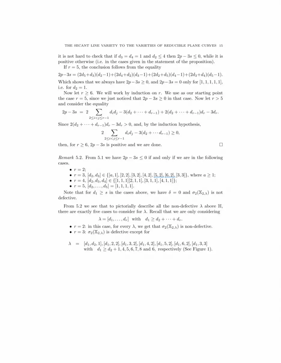
λ = [d1, d2, 1], [d1, 2, 2], [d1, 3, 2], [d1, 4, 2], [d1, 5, 2], [d1, 6, 2], [d1, 3, 3]with d1 ≥ d2 + 1, 4, 5, 6, 7, 8 and 6, respectively (See Figure 1).
16 M.V.CATALISANO, A.V. GERAMITA, A.GIMIGLIANO, AND Y.S. SHIN
d2 = d3
2d2d3 − 3(d2 + d3) = 0
d2, d3 ∈ N+
2d2d3 − 3(d2 + d3) ≤ 0d2 ≥ d3
...
1 2 3 4 5 6 7 8 10 11 12 d3
123456789101112
d2
Figure 1
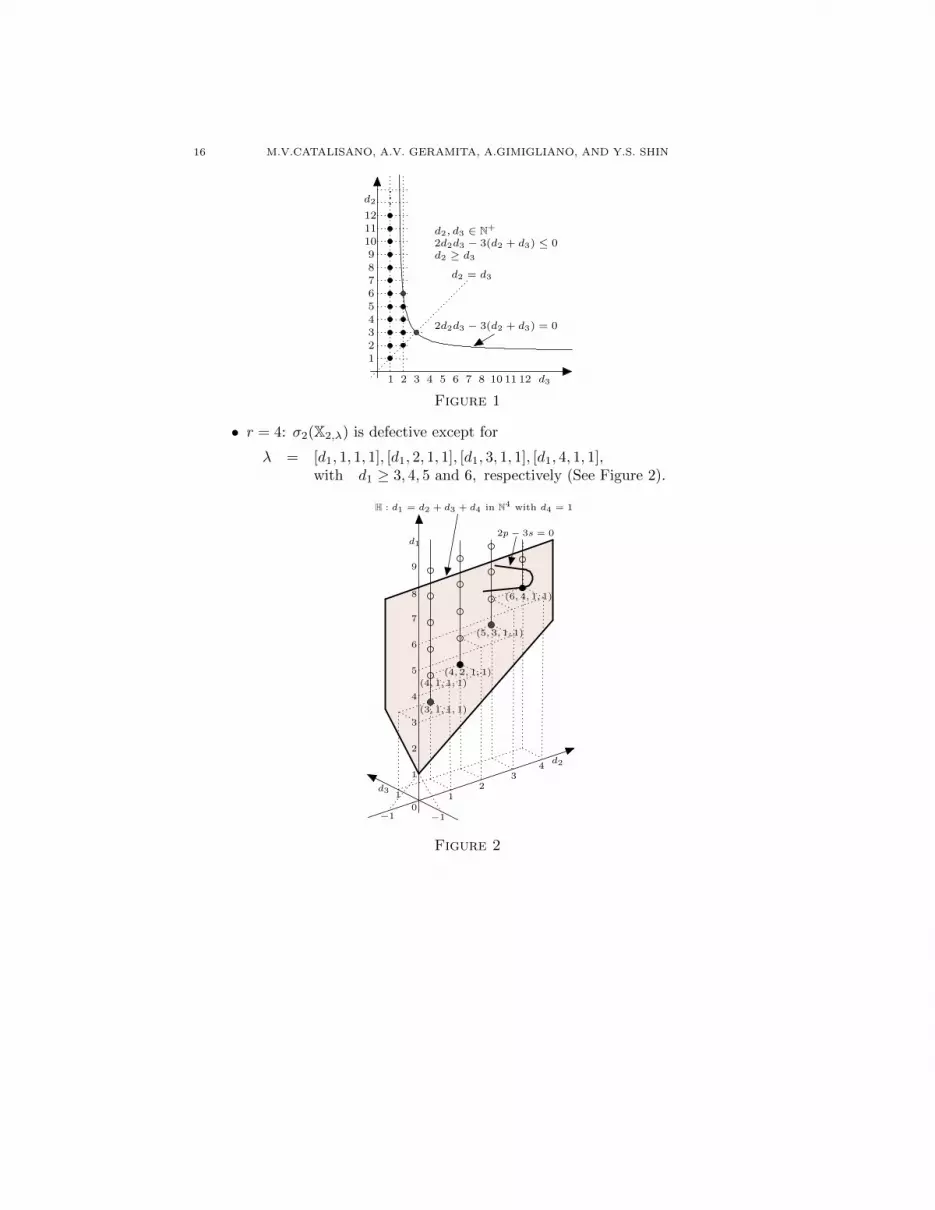
• r = 4: σ2(X2,λ) is defective except for
λ = [d1, 1, 1, 1], [d1, 2, 1, 1], [d1, 3, 1, 1], [d1, 4, 1, 1],with d1 ≥ 3, 4, 5 and 6, respectively (See Figure 2).
12
34
1
1
2
3
4
5
6
7
8
9
−1−1
(3, 1, 1, 1)
(4, 1, 1, 1)(4, 2, 1, 1)
(5, 3, 1, 1)
(6, 4, 1, 1)
d1
d2
d3
0
H : d1 = d2 + d3 + d4 in N4 with d4 = 1
2p− 3s = 0
Figure 2

THE SECANT LINE VARIETY TO THE VARIETIES OF REDUCIBLE PLANE CURVES 17
• r = 5: σ2(X2,λ) is defective except for
λ = [d1, 1, 1, 1, 1], d1 ≥ 4 (See Figure 3).
1
2
1
0
1
2
3
4
5
6
−2−2
d1
d2d3
H : d1 = d2 + d3 + d4 + d5 with d4 = d5 = 1
2p− 3s = 0
(4, 1, 1, 1, 1)
(5, 1, 1, 1, 1)
Figure 3
• r ≥ 6: for every λ, we get that σ2(X2,λ) is defective.
6. Further Remarks and Questions
In light of what we have proved in this paper, the question that puzzles us themost is: What can one say about the dimensions of the higher secant varieties ofX2,λ?
As we have noted, up to now the only results in this direction are due to Abo[1] who gave a complete answer to this question for λ = [1, . . . , 1].
It’s clear that if σ2(X2,λ) fills its ambient space for some λ then σs(X2,λ) has theexpected dimension for that λ and s ≥ 2. Our next goal is to describe all the λsuch that σ2(X2,λ) fills its ambient space, in other words, if λ ` d, the generic formF in degree d can be written as F = F1 + F2, where the Fi belong to X2,λ.
Proposition 6.1. σ2(X2,λ) fills the ambient space PN , (N =(d+22
)− 1), if and
only if either 3s− 2p ≥ 0, or λ = [2, 2, 2, 1].
(Note: A complete description of those λ for which 3s− 2p ≥ 0 is given in 5.1 i). )
Proof. We continue with the notation we have used throughout the paper. Weknow that
dimσ2(X2,λ) = dim((IF )d + (IG)d)− 1 = 2
(d+ 2
2
)− 2D − dim(IZ)d − 1,
hence
dimσ2(X2,λ) = N ⇔ dim(IZ)d =
(d+ 2
2
)− 2D.

18 M.V.CATALISANO, A.V. GERAMITA, A.GIMIGLIANO, AND Y.S. SHIN
Since
dim(IZ)d = max
{(d+ 2
2
)− 2D ; 0
}+ δ,
we get
dimσ2(X2,λ) = N ⇔(d+ 2
2
)− 2D ≥ 0 and δ = 0.
For r = 2, the conclusion follows from Lemma 4.8.
Let r > 2, and d1 ≥ s.In this case from Lemmata 4.9 and 4.10 it follows that δ = 0 ⇔ 3s − 2p ≥ 0.
Since (d+ 2
2
)− 2D =
(d1 − s+ 2
2
)+ 3s− 2p, (6)
hence, for 3s− 2p ≥ 0, we get(d+22
)− 2D > 0. It follows that for d1 ≥ s
dimσ2(X2,λ) = N ⇔ 3s− 2p ≥ 0,
and we are done for r > 2, and d1 ≥ s.Now let r > 2, and d1 < s.In this case we always have δ = 0 (see Proposition 4.7), so we have to check
when (d+ 2
2
)− 2D ≥ 0.
Consider(d+22
)− 2D as a function of d1, say
ϕ(d1) =
(d+ 2
2
)− 2D. (7)
We study this function for d2 ≤ d1 ≤ s− 1. Now, the parabola represented by (7)has its minimum when d1 = s − 3
2 . So for d1 < s − 32 , ϕ is decreasing. Moreover
(see (6)) we haveϕ(s− 1) = ϕ(s− 2) = 3s− 2p.
Hence 3s− 2p ≥ 0 implies ϕ(d1) ≥ 0.It remains to check that if 3s − 2p < 0, then the only case for which d1 is such
that ϕ(d1) = 0, and d2 ≤ d1 < s, is when d1 = 2 and λ = [2, 2, 2, 1].Since the parabola of equation (7) is decreasing in the interval [d2, s − 2] and
ϕ(s− 2) < 0, if we prove that, except for λ = [2, 2, 2, 1], ϕ(d2) < 0, we are done.So now we compute ϕ(d2) for λ 6= [2, 2, 2, 1]. In order to do that, it is useful to
consider the following equality
ϕ(d1) = −r∑i=1
((d1 + · · ·+ dr − 2di)(di − 1))− (r − 5)(d1 + · · ·+ dr) + 2,
which, for d1 = d2, becomes
ϕ(d2) = −2(d3 + · · ·+ dr)(d2 − 1))−r∑i=3
((2d2 + d3 · · ·+ dr − 2di)(di − 1))
−(r − 5)(2d2 + d3 + · · ·+ dr) + 2.
Recall that, since 3s−2p < 0, we have only to consider the cases listed in Proposition5.1, that is,
• r = 3, d3 = 2 and d2 ≥ 7;
THE SECANT LINE VARIETY TO THE VARIETIES OF REDUCIBLE PLANE CURVES 19
• r = 3, d3 = 3 and d2 ≥ 4;• r = 3, d3 ≥ 4;• r = 4, d3 ≥ 2;• r = 4, d2 ≥ 5;• r = 5, d2 ≥ 2;• r ≥ 6.
For r ≥ 6, we get
ϕ(d2) ≤ −(d1 + · · ·+ dr) + 2 < 0.
For r = 5, since d2 ≥ 2, we have
ϕ(d2) ≤ −2(d3 · · ·+ d5) + 2 < 0.
For r = 4 and d3 ≥ 2, and so also d2 ≥ 2, we get
ϕ(d2) ≤ −2d4 − (2d2 + d3 + d4 − 2d4)(d4 − 1) + 2.
Hence, if d4 ≥ 2, then ϕ(d2) < 0.For r = 4, d4 = 1 and λ 6= [2, 2, 2, 1], we have d3 ≥ 3, hence
ϕ(d2) ≤ −4(d3 + d4)− 2(2d2 + d3 + d4 − 2d3) + (2d2 + d3 + d4) + 2 < 0.
It is an easy computation to check that in all the remaining cases we haveϕ(d2) < 0.
�
Other questions which come to mind about the varieties X2,λ and their secantvarieties are:a) Which of these varieties is arithmetically Cohen-Macaulay (aCM)? (we think
that they are all aCM)b) Can one find equations for any of these varieties? So far we know of no
equations satisfied by any of them!c) Assuming that the varieties are aCM, what is their Cohen-Macaulay type?
(This asks about the rank of the last term in a finite free resolution of the definingideal. One can ask about all the ranks and all the graded Betti numbers as well!)
It certainly would be illuminating to have answers to these questions, even forλ = [1, . . . , 1].
Acknowledgments
The first and third authors wish to thank Queens University, in the person ofthe second author, for their kind hospitality during the preparation of this work.The first three authors enjoyed support from NSERC (Canada). The first authorwas also supported by GNSAGA of INDAM and by MIUR funds (Italy). The thirdauthor was also supported by MIUR funds (Italy). The fourth author was supportedby Basic Science Research Program through the National Research Foundationof Korea (NRF) funded by the Ministry of Education, Science, and Technology(2013R1A1A2058240).
References
[1] H. Abo, Varieties of completely decomposable forms and their secants. J. of Algebra 403
(2014) 135–153.
[2] H. Abo, G. Ottaviani, and C. Peterson. Induction for secant varieties of Segre varieties. Trans.Amer. Math. Soc. 361(2), (2009), 767–792.
20 M.V.CATALISANO, A.V. GERAMITA, A.GIMIGLIANO, AND Y.S. SHIN
[3] J. Ahn and Y.S. Shin. The Minimal Free Resolution of A Star-Configuration in Pn and The
weak-Lefschetz Property, J. Korean Math. Soc., 49 (2012), No.2, 405–417.
[4] E. Arrondo and A. Bernardi. On the variety parametrizing completely decomposable poly-nomials. J.Pure and Appl. Alg., 215 (2011), 201-220.
[5] J. Alexander and A. Hirschowitz. Polynomial interpolation in several variables. J. Algebraic
Geom., 4(2), (1995), 201–222.[6] C. Bocci and B. Harbourne. Comparing powers and symbolic powers of ideals. J. Algebraic
Geom. 19 (2010), no. 3, 399–417.
[7] P. Burgisser, M. Clausen, and M.A. Shokrollahi. Algebraic Complexity Theory. SpringerVerlag, Berlin, 1997.
[8] E. Carlini, L. Chiantini, A.V. Geramita, Complete intersections on general hypersurfaces.
Mich. Math. J. 57, (2008), 121–136.[9] E. Carlini, L. Chiantini, A.V. Geramita. Complete Intersection Points on General Surfaces
in P3. Mich. Math. Jo. 59 (2010) 269–281.[10] E. Carlini and A. Van Tuyl. Star Configuration Points and generic plane curves, Proc. AMS
139, (2011) 4181–4192.
[11] M.V. Catalisano, A.V. Geramita, and A. Gimigliano. Secant varieties of Grassmann varieties,Proc. Amer. Math. Soc., 133(3), (2005), 633–642.
[12] M. V. Catalisano, A.V. Geramita, and A. Gimigliano. Secant Varieties of P1 × · · · × P1 (n-
times) are NOT Defective for n ≥ 5, J. of Alg. Geom., 20, (2011), 295-327.[13] L. Chiantini and D. Faenzi. Rank 2 arithmetically Cohen-Macaulay bundles on a general
quintic surface. Math. Nachr. 282 (2009), no. 12, 1691–1708.
[14] S. Cooper, B. Harbourne, and Z. Teitler. Combinatorial bounds on Hilbert functions of fatpoints in projective space. J. Pure Appl. Algebra 215 (2011), no. 9, 2165–2179.
[15] D. Cox and J. Sidman, Secant varieties of toric varieties. J. Pure Appl. Algebra 209 (2007),
no. 3, 651–669.[16] M. Dumnicki, T. Szemberg, J. Szpond, H. Tutaj-Gasinska. Symbolic generic initial systems
of star configurations, ArXiv:1401.4736.[17] A.V. Geramita, B. Harbourne, and J.C. Migliore. Star configurations in Pn, J. of Alg.,376
(2013), 279-299.
[18] A.V. Geramita, B. Harbourne, and J.C. Migliore. d-star configurations and their symbolicpowers (in preparation).
[19] A.V. Geramita, J.C. Migliore, S. Sabourin. On the first infinitesimal neighborhood of a linear
configuration of points in P2. J. of Alg. 298, (2006), 563–611.[20] J.M. Landsberg. Tensors:Geometry and Applications. Graduate Studies in Mathematics. 128.
American Mathematical Society (2011).
[21] C. Mammana. Sulla varieta delle curve algebriche piane spezzate in un dato modo, Ann.Scuola Norm. Super. Pisa (3), 8, (1954), 53–75.
[22] J.P. Park and Y.S. Shin. The Minimal Free Resolution of A Star-configuration in Pn,
arXiv:1404.4724.[23] M. Patnott. The h-vectors of arithmetically Gorenstein sets of points on a general sextic
surface in P3. J. Algebra 403 (2014), 345–362.[24] M. Ravi, Determinantal equations for secant varieties of curves. Comm. Algebra 22 (1994),
3103–3106.
[25] L. Robbiano, J. Abbott, A. Bigatti, M. Caboara, D. Perkinson, V. Augustin, and A. Wills.CoCoA, a system for doing Computations in Commutative Algebra. Available via anonymous
ftp from cocoa.unige.it. 4.7 edition.[26] Y.S. Shin. Secants to The Variety of Completely Reducible Forms and The Union of Star-
Configurations, Journal of Algebra and its Applications, 11, (2012) 109–125.
[27] B. Sturmfels and S. Sullivant. Combinatorial secant varieties. Pure Appl. Math. Q. 2 (2006),
no. 3, part 1, 867–891.[28] A. Terracini. Sulle Vk per cui la varieta degli Sh (h + 1)-seganti ha dimensione minore
dell’ordinario, Rend. Circ. Mat. Palermo, 31, (1911), 392–396.[29] P. Vermeire, Regularity and normality of the secant variety to a projective curve. J. Algebra
319 (2008), 1264–1270.

THE SECANT LINE VARIETY TO THE VARIETIES OF REDUCIBLE PLANE CURVES 21
(M.V.Catalisano) Dipartimento di Ingegneria Meccanica, Energetica, Gestionale e dei
Trasporti, Universita di Genova, Genoa, Italy.
E-mail address: [email protected]
(A.V. Geramita) Department of Mathematics and Statistics, Queen’s University, King-
ston, Ontario, Canada and Dipartimento di Matematica, Universita di Genova, Genoa,Italy
E-mail address: [email protected], [email protected]
(A.Gimigliano) Dipartimento di Matematica, Universita di Bologna, Bologna, ItalyE-mail address: [email protected]
(Y.S. Shin) Department of Mathematics, Sungshin Women’s University, Seoul, 136-742,Republic of Korea
E-mail address: [email protected]