SOME SELECTED NUMERICAL METHODS

FOR SOLVING STIFF ORDINARY

DIFFERENTIAL EQUATION

BY

OGUNNIYE OREOFE S.

MATRIC NO: 100407022

A PROJECT SUBMITTED TO

THE DEPARTMENT OF MATHEMATICAL SCIENCES,

ADEKUNLE AJASIN UNIVERSITY, AKUNGBA AKOKO,

ONDO STATE, NIGERIA.

IN PARTIAL FULFILMENT OF THE REQUIREMENT

FOR THE AWARD OF BACHELOR OF SCIENCE

B.Sc(Hons) DEGREE IN INDUTRIAL MATHEMATICS.

March 2, 2015

CERTIFICATION

This is to certify that this project work was carried out by OGUNNIYE ORE-

OFE S.(100407022) as part of the requirement of the department of MATHE-

MATICAL SCIENCES, for the award of Bachelor of science B.Sc (Hons) degree

in INDUSTRIAL MATHEMATICS.

——————————– ————————————

Mr. A.S Oke Date

Supervisor

——————————– ————————————

External Examinar Date

——————————– ————————————

Prof. O.K koriko Date

Head of Department

DEDICATION

This project is dedicated to Almighty God, the giver of life.

ACKNOWLEGDEMENT

First and foremost, all appreciation goes to the Almighty God for giving me the

strength and making the completion of this research project possible.

Earlier on, when I took the preliminary steps towards my project, I did not forsee

how many individuals would contribute to its completion whom I owe my thanks

and appreciation to. I am particularly grateful to my supervisor, Mr. A.S Oke

for his unlimited support, guidance, thoughtful teachings, objectives comments

and insightful direction. Without his knowlegde this project would never have

been completed.

I will like to extend my sincere appreciation to my loving parent Mr. and Mrs.

Ogunniye, my brothers and sister; Ogunniye Gideon, Ogunniye Sarah, Ogunniye

Victor, and Ogunniye Shola for their continuous support and assistance both fi-

nancially and morally.

Finally, my appreciation goes to my cousins; Gabriel, Elizabeth, Esther, Bless-

ing, Marvellous and Precious and my neighbours; Olubodun Kindness Folajomi,

Olawale, Oluwarotimi, Olufunke, and Oluwapamilerin for their love and care to-

wards me, and to my friends; Fawemimo Oladele, Adeyeye Oluwatobi, Faborode

opeyemi and Fasogbon Ismail for their contribution toward the success of this

project. I love you all.

ABSTRACT

Exponential Time Differencing (ETD1 and ETD2) are used to solve the stiff dif-

ferential equation obtained from the harvesting model and the results are com-

pared with the results obtained from the Euler and the Adam-Bashforth (AB2).

The ETD methods show a high accuracy without much dependence on the choice

of stepsize while the corresponding Euler and AB2 methods become only accurate

as the choice of the stepsize becomes smaller.

Contents

1 INTRODUCTION 3

1.1 Diffrerential equation . . . . . . . . . . . . . . . . . . . . . . . . . 3

1.2 Stiff differential equation . . . . . . . . . . . . . . . . . . . . . . . 4

1.3 Numerical methods for ordinary differential equation . . . . . . . 5

1.3.1 Quality of Numerical method . . . . . . . . . . . . . . . . 6

1.3.2 Stability of Numerical methods . . . . . . . . . . . . . . . 7

1.3.3 Types of Errors in Numerical Analysis . . . . . . . . . . . 8

1.4 Statement of the problem: . . . . . . . . . . . . . . . . . . . . . . 9

1.5 Methodology . . . . . . . . . . . . . . . . . . . . . . . . . . . . . 10

1.6 Justification: . . . . . . . . . . . . . . . . . . . . . . . . . . . . . . 10

2 OVERVIEW 11

2.1 The Concept and Definition of Stiff Differential Equation. . . . . . 12

2.1.1 History of Stiff Differential Equations. . . . . . . . . . . . 13

2.2 Solving Stiff Differential Equations with Exponential Time Differ-

encing methods. (ETD) . . . . . . . . . . . . . . . . . . . . . . . 15

2.3 Solving stiff differential equation with Adam-Bashforth method (AB) 16

2.4 Solving stiff differential equation with Euler method. . . . . . . . 17

1

3 DERIVATION OF METHODS 19

3.1 Euler’s Method . . . . . . . . . . . . . . . . . . . . . . . . . . . . 19

3.1.1 The basic step approximation . . . . . . . . . . . . . . . . 20

3.1.2 Error analysis of Euler’s method . . . . . . . . . . . . . . . 21

3.1.3 Numerical stability of Euler scheme . . . . . . . . . . . . . 23

3.1.4 Rounding off error of Euler’s method . . . . . . . . . . . . 24

3.2 Multistep method . . . . . . . . . . . . . . . . . . . . . . . . . . . 25

3.2.1 Second order Adam-Bashforth method (AB2) . . . . . . . 25

3.2.2 Polynomial Interpolation . . . . . . . . . . . . . . . . . . . 26

3.2.3 Accuracy . . . . . . . . . . . . . . . . . . . . . . . . . . . 28

3.3 Exponential time differencing method . . . . . . . . . . . . . . . . 28

3.3.1 Derivation of ETD1 scheme . . . . . . . . . . . . . . . . . 30

3.3.2 Local truncation error for ETD1 . . . . . . . . . . . . . . . 31

3.3.3 Derivation of ETD2 scheme . . . . . . . . . . . . . . . . . 32

3.3.4 Local truncation error for ETD2 . . . . . . . . . . . . . . . 33

4 NUMERICAL EXPERIMENT 34

4.1 Harvesting Model . . . . . . . . . . . . . . . . . . . . . . . . . . . 34

5 CONCLUSION 42

5.1 Conclusion . . . . . . . . . . . . . . . . . . . . . . . . . . . . . . . 42

2

Chapter 1

INTRODUCTION

1.1 Diffrerential equation

Various problems in the world can be solved when they are modeled and presented

in form of differential equation, Any equation that involves derivatives is said to

be a differential equation. Iin other words, differential equation is an equation

involving derivatives as well as algebraic and transcendental functions, it can be

seen as an equation that contains the derivative(s) of an unknown scalar function.

For more explicitness, a differential equation is very useful and its overwhelm-

ing functions cannot be over-emphasized (especially in the area of modeling our

physical situation across all field of study e.g population, motion of a body etc.)

Examples of differential equations include

d2y

dx2− 5

dy

dx+ 3y = 0 (1.1)

∂u

∂t− ∂2u

∂t2− ∂2u

∂y2− u = 0 (1.2)

3

Differential equations are of two classes

1. Ordinary Differential equation (ODE)

2. Partial Differential equation (PDE)

A differential equation is said to be ordinary if all the derivatives are with respect

to a single independent variable i.e if the unknown function is dependent on one

single variable.

Example

d2y

dx2− 6

dy

dx+ 7y = 0 (1.3)

d3u

dt3− du

dt+ 3u = 0 (1.4)

In contrast, when the unknown function is a function of two or more independent

variables then the differential equation is called partial differential equation. A

partial differential (PDE) is an equation containing partial derivatives of the

independent variables.

Example

∂u

∂t− ∂2u

∂t2− 5

∂2u

∂y2= 0 (1.5)

1.2 Stiff differential equation

The earliest detection of stiffness in differential equationis is in the digital era,

by curtiss et al (1952)[4], was apparently far in advance of its time. He named

the phenomenon and spotted the nature of stiffness. Stiff differential equation

is a differential equation for which certain numerical methods for solving the

equation are numerically unstable, unless the step size is taken to be small. It

4

has proven difficult to formulate a precise definition of stiffness, but the main

idea is that the equation includes some terms that can lead to rapid variation

in the solution. Stiffness is a challenging property of differential equation (DE)

that prevents convectional explicit numerical integrator from handling a problem

efficiently. Stiff differential equations are categorized as those whose solutions (or

different components of a single solution) evolve on a very different time scale

occurring simultaneous i.e the rate of change of the various components of the

solution differ markedly.

Examples of stiff differential equation

du

dt= 3u+ 4u2 (1.6)

dy

dt= ry

(1− y

k

)− β y2

α2 + y2(1.7)

1.3 Numerical methods for ordinary differential

equation

Numerical methods for ordinary differential equations are methods used to find

numerical approximations to the solutions of ordinary differential equations (ODEs).

Their use is also known as ”numerical integration”, although this term is some-

times taken to mean the computation of integrals[8]. Many differential equations

cannot be solved using symbolic computation (”analytic”). For practical pur-

poses however, such as in engineering, a numeric approximation to the solution

is often sufficient. The algorithms studied here can be used to compute such

an approximation. An alternative method is to use techniques from calculus to

obtain a series expansion of the solution. Ordinary differential equations occur

5

in many scientific disciplines, for instance in Physics, Chemistry, Biology, and

Economics. There are many techniques of analytical solution of ordinary differ-

ential equation, but still many problems arising from field work leading to such

equations without analytical solutions or where they exist the problem may be

too cumbersome. Therefore numerical techniques remain the better alternative

methods.

Essentially, the goal of any numerical method is to approximate a solution to the

problem so as to have a close result to the actual solution. Thus, the order of

accuracy of a numerical method is considered of great importance in the analysis

of the basic properties of the method.

1.3.1 Quality of Numerical method

There are two properties by which numerical method is evaluated viz:

1. Accuracy and

2. Efficiency.

Efficiency is normally measured in term of the amount of computer time used

in the execution of a particular method or the number of iterations before the

method will converge. This time is often estimated on the basis of the addition,

subtractions, multiplication and division.

Accuracy of a particular solution to a problem means the closeness of that an-

swer to the exact or analytical solution. The solution of an ordinary differential

equation can never be carried out with complete accuracy because of the require-

ment that number are stored in a computer with a given number of digits. In

general, number have to be ”chopped off” or rounded off and the error due to

this limitation is termed round off errors. The other major cause of inacuracy is

6

truncation errors.

1.3.2 Stability of Numerical methods

In the mathematical subfield of numerical analysis, numerical stability is a gen-

erally desirable property of numerical algorithms. The precise definition of sta-

bility depends on the context. One is numerical linear algebra and the other

is algorithms for solving ordinary and partial differential equations by discrete

approximation[7]. In numerical linear algebra, the principal concern is instabil-

ities caused by proximity to singularities of various kinds, such as very small

or nearly colliding eigenvalues[7]. On the other hand, in numerical algorithms

for differential equations the concern is the growth of round-off errors and/or

initially small fluctuations in initial data which might cause a large deviation

of final answer from the exact solution. Some numerical algorithms may damp

out the small fluctuations (errors) in the input data; others might magnify such

errors. Calculations that can be proven not to magnify approximation errors are

called numerically stable[9]. One of the common tasks of numerical analysis is to

try to select algorithms which are robust that is to say, do not produce a widely

different result for very small change in the input data.

An opposite phenomenon is instability . Typically, an algorithm involves an ap-

proximate method, and in some cases one could prove that the algorithm would

approach the right solution in some limit. Even in this case, there is no guar-

antee that it would converge to the correct solution, because the floating-point,

round-off or truncation errors can be magnified, instead of damped, causing the

deviation from the exact solution to grow exponentially. The above definitions

are particularly relevant in situations where truncation errors are not important.

7

In other contexts, for instance when solving differential equations, a different def-

inition of numerical stability is used.

In numerical ordinary differential equations, various concepts of numerical stabil-

ity exist, for instance A-stability[9]. They are related to some concept of stability

in the dynamical systems sense, often Lyapunov stability. It is important to use

a stable method when solving a stiff equation. Stability is sometimes achieved by

including numerical diffusion. Numerical diffusion is a mathematical term which

ensures that roundoff and other errors in the calculation get spread out and do

not add up to cause the calculation to ”blow up”[7].

1.3.3 Types of Errors in Numerical Analysis

Rounding Off Error:

The round-off error is used because representing every number as a real num-

ber is not possible. So, rounding is introduced to adjust for this situation. A

round-off error represents the numerical amount between what a figure actually

is versus its closest real number value, depending on how the round is applied.

For instance, rounding to the nearest whole number means you round up or down

to what is the closest whole figure. In terms of numerical analysis the round-off

error is an attempt to identify what the rounding distance is when it comes up

in algorithms. It is also known as a quantization error[8].

Truncation Error:

Truncation errors are committed when an iterative method is terminated or a

mathematical procedure is approximated, and the approximate solution differs

from the exact solution.

Discretization Error:

Discretization involves converting or partitioning variables or continuous attributes

8

to nominal attributes, intervals and variables. As a type of truncation error, the

discretization error focuses on how much a discrete math problem is not consis-

tent with a continuous math problem. Evaluating errors provides significantly

useful information, especially when chance and probability are require

1.4 Statement of the problem:

The numerical solution of ordinary differential equations (ODEs) is an old topic.

Various techniques have been adopted over the years to solve differential equa-

tions, and particularly, the old well established method such as Runge-kutta

methods, Euler methods are the still the foundation for the most effective and

widely used code. Nevertheless, there are several kinds of problem which classical

methods like Runge-kutta and Euler do not handle very effectively, problem that

are said to be Stiff. Various author have looked at the solution of stiff differential

equation using some selected time discretization method without comparing the

accuracy of the old well established methods such as Euler scheme, with the time

discretization methods such as Exponential time differencing (ETD) in solving

stiff ordinary differential equation,

This study seeks:

1. To apply this selected numerical scheme in solving stiff ordinary differential

equation.

2. To compare the result of each methods with the exact solution in order to

show their level of accuracy.

9

1.5 Methodology

The method is to evaluate the application of Exponential time differencing (ETD),

Euler and Adam-Bashforth method(AB2). Method employed are ETD1, ETD2,

AB2 and Euler method, which a comprehensive comparison of the results of each

scheme is done, thereby establishing their level of accuracy.

1.6 Justification:

The study would afford students the opportunity to be aware of some key numer-

ical methods for solving stiff differential equation. Information gathered from the

results would educate students on the application and evaluation of these scheme

and which one of these method is much more preferred than the others. In ad-

dition, it could pave the way for more comprehensive reseach on the comparison

of these methods in relation to some specified complex functions which are very

significant in drawing conclusions to a research work.

The study would equally be helpful to various field to understand which of these

numerical scheme would be suitable to solve a modeled problem which turn out

to be a stiff differential equation. The university as a whole will find the study

relevant in keeping track of numerical scheme with respect to their application,

and embark on further research on these scheme to find plausible solution to the

impeding problem pose by stiffness in differential equation.

10

Chapter 2

OVERVIEW

In this section, there is a review of the work of several authors concerning concept,

definitions and various researches done to uncover different numerical methods

used to solve stiff differential equations. Researches, empirical work and authors

opinion are looked at. Below are the focuses of the review.

1. The Concept and Definition of Stiff Differential Equation.

2. History of Stiff Differential Equations.

3. Solving Stiff Differential Equations with Exponential Time Differencing

Methods.

4. Solving stiff differential equation with Adam-Bashforth method.

5. Solving stiff differential equation with Euler method.

11

2.1 The Concept and Definition of Stiff Differ-

ential Equation.

Differential equation of the form y′ = f(t, y) is said to be stiff if its exact solution

y(t) includes a term that decays exponentially to zero as t increases, but whose

derivatives are much greater in magnitude than the term itself[3]. An example of

such a term is e−ct, where c is a large positive constant, because its kth derivative is

cke−ct. Because of the factor of ck, this derivative decays to zero much more slowly

than e−ct as t increases. Garfinkel et al (1977)[15], described stiffness as a property

of differential equation that makes it slow and expensive to solve by numerical

methods. It is a result of the numerical coefficients in the differential equation

(so that there is too wide a spread between the fastest and slowest elements).

According to Moler[16], stiffness is a subtle, difficult, and important concept

in the numerical solution of ordinary differential equations. It depends on the

differential equation, the initial conditions and the numerical method. Dictionary

definitions of the word stiff involve terms like not easily bent, rigid, and stubborn.

We are concerned with a computational version of these properties. An ordinary

differential equation problem is stiff if the solution being sought is varying slowly,

but there are nearby solutions that vary rapidly, so the numerical method must

take small steps to obtain satisfactory results. Stiffness is an efficiency issue. If

we weren’t concerned with how much time a computation takes, we wouldn’t be

concerned about stiffness. Non-stiff methods can solve stiff problems; they just

take a long time to do it.

Dahlquist et al (1973)[17], defined a stiff system as one containing very fast

components as well as very slow components. They represent coupled physical

systems having components varying with very different time scales: that is they

12

are systems having some components varying much more rapidly than the others.

At the moment, even if the old intuitive definition relating stiffness to multi scale

problems survives in most of the authors, the most successful definition seems

to be the one based on particular effects of the phenomenon rather than on the

phenomenon itself, such as for example, the following equivalent definitions.

According to Curtiss, et al (1952)[4], stiff equations are equations where certain

implicit methods perform better, usually tremendous better, than explicit ones;

while Hairer, et al (1996)[18], defined stiff equations as problems for which explicit

methods don’t work. As it usually happens, describing a phenomenon by means

of its effects may not be enough to fully characterize the phenomenon itself. For

example, saying that fire is what produces ash would oblige fire men to wait for

until the end of a fire to see if the ash has been produced. In the same way,

in order to recognize stiffness according to the previous definitions it would be

necessary to apply first explicit methods and see if they work or not.

2.1.1 History of Stiff Differential Equations.

Curtiss et al (1952)[4], detected stiffness in differential equations. They named

the phenomenon and spotted the nature of stiffness (stability requirement dictates

the choice of the step size to be very small). To resolve the problem they recom-

mended time discretization method such as ETD, Integrating factor (IF) meth-

ods. In 1963, Dahlquist, defined the problem and demonstrated the difficulties

that standard differential equation solvers have with stiff differential equations.

At about this time several authors participated in independent research for han-

dling and evading the problems posed by stiff differential equations. For example,

Gear (1968)[15], became one of the most important names in this field. Consid-

erable efforts have gone into developing numerical integration for stiff problems,

13

and hence, the problem of stiffness was brought to the attention of the math-

ematical and computer science community for a comprehensive review of this

phenomenon.

Stiff differential equations are categorized as those whose solutions (or different

components of a single solution) evolve on very different time scales occurring si-

multaneously, i.e. the rates of change of the various components of the solutions

differ markedly. Consider, for example, if one component of the solution has a

term of the form eLt , where L is a large positive constant. This component,

which is called the transient solution, decays to zero much more rapidly, as t

increases, than other slower components of the solutions. Alternatively, consider

a case where a component of the solution oscillates rapidly on a time scale much

shorter than that associated with the other solution components. For a numer-

ical method which makes use of derivative values, the fast component continues

to influence the solution, and as a consequence, the selection of the step size in

the numerical solution is problematic. This is because the required step size is

governed not only by the behavior of the solution as a whole, but also by that of

the rapidly varying transient which does not persist in the solution that we are

monitoring.

In reality, the numerical values occurring in nature are frequently such as to

cause stiffness. Therefore, a realistic representation of a natural system using a

differential equation is likely to encounter this phenomenon. An example is the

field of chemical kinetics, Curtiss, (1952)[4]. Here ordinary differential equations

describe reactions of various chemical species to form other species. The stiffness

in such systems is a consequence of the fact that different reactions take place on

vastly different time scales.

14

2.2 Solving Stiff Differential Equations with Ex-

ponential Time Differencing methods. (ETD)

To provide numerical solution to the problem pose by stiffness, numerous time

discretization methods that are designed to handle stiff systems have been devel-

oped. One example is the family of Exponential time differencing (ETD) scheme

for numerical integration.

Exponential time differencing schemes is a time discretization methods that are

designed to handle stiff system, this class of scheme is especially suited to semi-

linear problem which can be split into a linear part which contains the stiffness

part of the dynamics of the problem, and a non-linear part, which varies more

slowly than the linear part. This method arose originally in the field of electro-

dynamics and since then they have recently received attention.

According to Du(2004)[3], Exponential time differencing schemes are time in-

tegration method that provide effective solution to some linear and non-linear

partial differntial equations.

The basic idea of this method is to replace the spartial derivative in a partial

equation (PDE) with algebraic approximation, thus we have a coupled system of

ODEs with only time remaining as an independent variable.

The formula of the ETD scheme is based on integrating the linear part of the

differential equation exactly, and approximating the non linear term by a polyno-

mial, which is then integrated exactly. The idea of the ETD method is similar to

the method of integrating factor. A clear derivation of the explicit Exact linear

part (ELP) of arbitrary order was giving by cox and mathew where they refer to

these method as the Exponential Time differencing (ETD).

15

2.3 Solving stiff differential equation with Adam-

Bashforth method (AB)

The apparent divergence of the coefficient of ETD2 as L → 0, ETD2 become

the second-order Adams-Bashforth method in this limit.[1] The AdamsBashforth

(AB) and AdamsMoulton (AM) methods are the explicit and implicit method

of Adams respectively. These methods are the basis of some of the most widely

used computer codes for solving the initial value problem of ordinary differential

equation. They are generally more efficient than the RK-methods, especially if

one wishes to find the solution with a high degree of accuracy or if the derivative

function f(t, y) is expensive to evaluate.

Adams methods are based on the idea of approximating the integrand with a

polynomial within the interval (tn, tn+1). Using a kth order polynomial results in

a (k+1)th order method[12]. There are two types of Adams methods, the explicit

and the implicit types. The explicit type is called the Adams-Bashforth (AB)

methods and the implicit type is called the Adams-Moulton (AM) methods.

The first order AB is simply the Euler scheme. The second order versions (ob-

tained by using a linear interpolant) of these methods are quite popular. The

second order Adams-Bashforth (AB2) method is given by

yn+1 = yn +h

2(3f(yn, tn − f(yn−1, tn−1)) (2.1)

The AB2 method is explicit and hence only conditionally stable. Moreover, the

AB2 method requires the solution from the (n − 1)th and the nth steps to find

the solution at the (n+ 1)th step.

16

2.4 Solving stiff differential equation with Euler

method.

For small |L|, ETD1 scheme approaches the forward Euler method.[1]

In mathematics and computational science, the Euler method is a numerical

procedure for solving ordinary differential equations (ODEs) with a given initial

value. It is the most basic explicit method for numerical integration of ordinary

differential equations and is the simplest RungeKutta method. The Euler method

is named after Leonhard Euler, who treated it in his book Institutionum calculi

integralis (published 1768− 70)[11]. The Euler method is a first-order method,

which means that the local error (error per step) is proportional to the square of

the step size, and the global error (error at a given time) is proportional to the

step size. The Euler method often serves as the basis to construct more complex

methods. A method for solving ordinary differential equations using the formula

yn+1 = yn + hf(tn, yn) (2.2)

which advances a solution from tn to tn+1 = tn+h . Note that the method incre-

ments a solution through an interval h while using derivative information from

only the beginning of the interval. As a result, the step’s error is O(h2) . This

method is called simply ”the Euler method” by Press et al. (1992),[14] While

Press et al. (1992) describe the method as neither very accurate nor very sta-

ble when compared to other methods using the same step size, the accuracy is

actually not too bad and the stability turns out to be reasonable as long as the

so-called (Courant-Friedrichs-Lewy condition) is fulfilled.[5] This condition states

that, given a space discretization, a time step bigger than some computable quan-

17

tity should not be taken. In situations where this limitation is acceptable, Euler’s

method becomes quite attractive because of its simplicity of implementation.

18

Chapter 3

DERIVATION OF METHODS

3.1 Euler’s Method

The Euler method is a single step-order numerical procedure for solving ordinary

differential equations (ODEs) with a given initial value. It is the most basic ex-

plicit method for numerical integration of ordinary differential equations and is

the simplest Runge - Kutta method.

The Euler method is a first-order method, which means that the local error (error

per step) is proportional to the square of the step size, and the global error (error

at a given time) is proportional to the step size. The Euler method often serves

as the basis to construct more complex methods.

The Euler method can be derived in a number of ways, the geometrical descrip-

tion, Taylor’s expansion etc.

19

3.1.1 The basic step approximation

Consider the Taylor expansion of the function y around t

y(t+ h) = y(t) + hy′(t) +1

2h2y′′(t) +

1

3!h3y′′′(t) + ...

The differential equation state that y′ = f(t, y) . If this is subtituted in the Taylor

expansion and the quadractic and higher-order terms are ignored, we have

y(t+ h) = y(t) + hy′(t) +O(h2)

arranging this and solve for y′(t)

y′(t) ≈ y(t+ h)− y(t)

h+O(h)

finally integrating the differential equation from t to t + h and apply the funda-

mental theorem of calculus to get

y(t+ h)− y(t) =

∫ t+h

t

f(t, y(t))dt. (3.1)

Now approximating the integral by the left-hand rectangle method (with only

one rectangle): ∫ t+h

t

f(t, y(t))dt ≈ hf(t, y(t)). (3.2)

combining both equation (3.1) and (3.2),

we have

y(t+ h) = y(t) + hf(t, y(t)) (3.3)

This find the Euler method.

20

3.1.2 Error analysis of Euler’s method

The purpose of analysing Euler’s method error is to understand how it works,

to be able to predict the error using it and perhaps accelerate its convergence.

doing this for Euler’s method will also make easier to answer the same question

for other more efficient numerical methods.

Local Truncation error for Euler’s method

Suppose we are solving an initial value problem with differential equation.

y′(t) = f(t, y)

The local truncation error (LTE) of the Euler method is error made in a single

step. It is the difference between the numerical solution after one step, yt and

the exact solution at time tn+1 = tn + h.[6]

The numerical solution is given by

yn+1 = yn + hf(tn, yn)

the LTE in yn+1 is by definition y(tn+h) - yn+1. Taylor expanding y(tn+h) gives

y(tn + h) = y(tn) + hy′(tn) +1

2h2y′′(tn) + ...

21

so that

LTE = y(tn + h)− yn+1 (3.4)

=

(y(tn) + hy′(tn) +

1

2h2y′′(tn) + ...

)− (y(tn) + hy′(tn)) (3.5)

=1

2h2y′′(tn) +O(h3) (3.6)

This conclussion is justifiable if y has a bounded third derivative. This show

that for small h, the local truncation error is approximately proportional to h2.

This make the Euler scheme not very much accurate(for small h) than other

higher numerical sheme such as Exponetial time differencing, and linear multistep

methods, for which the local trucation error is proportionl to a higher power of

the step size.

Global truncation error

suppose once again that we are applying Euler’s method with step size h to the

initial value problem

y′(t) = f(t, y), y(to) = yo (3.7)

Denote by y(t) the exact solution to the initial value problem and by yn the ap-

proximation to y(tn), tn = to + nh, given by n steps of Euler’s method (applied

without roundoff error). The error in yn is y(tn) − yn and is called the Global

truncation error at time tn, the word ”Truncation” is suppoosed to signify that

the error is due solely to Euler’s method and does not include any effects of

roundoff error.[11]

The global truncation error is the cumulative effect of the local truncation errors

committed in each step. The number of steps is easily determined to be (t−to)/h

22

which is proportional to 1/h and the error committed in each step is proportional

to h2. Thus, it is to be expected that the global truncation error will be propor-

tional to h.

This intuitive reasoning can be made precise. If the solution y has a bounded

second derivative and f is Lipschitz continuous in its second argument, then the

global truncation error (GTE).[11] is bounded by

|GTE| ≤ hM

2L(eL(t−to) − 1)

where M is an upper bound on the second derivative of y on the given interval

and L is the Lipschitz constant of f

The precise form of this bound is of little practical importance, as in most cases

the bound vastly overestimates the actual error committed by the Euler method.

What is important is that it shows that the global truncation error is (approxi-

mately) proportional to h. For this reason, the Euler method is said to be first

order.

3.1.3 Numerical stability of Euler scheme

The Euler method can also be numerically unstable, especially for stiff differen-

tial equation, meaning that the numerical solution grows very large for equations

where the exact solution does not. This can be illustrated using the linear equa-

tion

dy

dx= −ay y(0) = 1,

23

The exact solution is y(t) = e−at which decays to zero as t→∞. After n Euler

steps of size h

yn+1 = yn − aynh⇒ yn(1− ah) = (1− ah)n

If h is big, say 1 then the numerical solution is qualitatively wrong: it oscil-

lates and grows. Then this means unstable. Approximate solution will decay

monotonically only if h is small enough:

h ≤ hmax ≡1

a

for a single decaying exponential-like solution (i.e. if there is only one first order

equation) the existence of a stability criterion is not a problem because h has to

be small for the reasons of accuracy.[11]

3.1.4 Rounding off error of Euler’s method

The discussion up to now has ignored the consequences of rounding error. In

step of the Euler method, the rounding error is roughly of the magnitude εyn

where ε is the machine epsilon. Assuming that the rounding errors are all of

approximately the same size, the combined rounding error in N steps is roughly

Nεyo if all errors points in the same direction. Since the number of steps is

inversely proportional to the step size h, the total rounding error is proportional

to ε/h. In reality, however, it is extremely unlikely that all rounding errors point

in the same direction. If instead it is assumed that the rounding errors are

independent rounding variables, then the total rounding error is proportional to

ε/√h .[11]

24

Thus, for extremely small values of the step size, the truncation error will be

small but the effect of rounding error may be big. Most of the effect of rounding

error can be easily avoided if compensated summation is used in the formula for

the Euler method.

3.2 Multistep method

Euler’s methods and Runge-Kutta (RK) methods are known as single-step or

one-step methods, since at a typical step yn+1 is determine solely from yn. As n

increases, that means that there are additional values of the solution, at previous

times, that could be helpful, but are unused.

Multistep methods are time-stepping methods that do use this information. the

two families of the most widely used multistep methods are

1. Adam-Bashforth method

2. Adam-Moulton method.

which are the explicit and implicit Adams method respectively. The method is

initiated by using either a set of known results or from the results of a Euler to

start the initial value problem. The method used during the course of this study

is Adam-bashforth of order 2 (AB2).

3.2.1 Second order Adam-Bashforth method (AB2)

Suppose we have an ordinary differential equation y′ = f(t, y(t)) with an initial

condition y(to) = yo and we want to solve it numerically. If we know y(t) at a

time tn and want to know what y(t) is at a later time tn+1. Reformulate the

25

differential equation.

y′(t) = f(t, y(t))

by integrating over the interval [tn, tn+1], obtaining

∫ tn+1

tn

y′(t)dt =

∫ tn+1

tn

f(t, y(t))dt,

y(tn+1) = y(tn) +

∫ tn+1

tn

f(t, y(t))dt (3.8)

The idea behind any ODE solver is to compute the right hand-side integral for

some numerical approximation of f , the problem is then computed over a series of

steps n = 1, 2, ...N to give a sequence of point yn which approximate y(t) to some

order of accuracy as a function of step size.[12] This method is basis for some of

the most widely used computer codes for solving the initial value problem. They

are generally more efficient than the Euler’s and Runge-kutta methods, especially

if one wishes to find the solution with a higher degree of accuracy.[12] The method

is consistence if the local error (i.e the error from step n to step n + 1) goes to

zero faster than the stepsize (tn+1 − tn) goes to zero.

3.2.2 Polynomial Interpolation

Where the Euler method takes the slope f to be a constant on the interval

[tn, tn+1], the idea behind Adams-Bashforth methods is to approxmiate f by a

Lagrange interpolating polynomial:

P (t) =m∑j=1

Pj(t)

26

where

Pj(t) = yj

m∏k=1k 6=j

t− tktj − tk

Here P (t) is the polynimial of degree ≤ (m − 1) that passes through the

m points (t1, y1 = f(t1)), (t2, y2 = f(t2))...(tm, ym = f(tm)). taking the linear

(m = 2) interpolant on the point tn and an earlier point tn+1, to yield

P (t) = f(tn, yn)t− tn−1tn − tn−1

+ f(tn−1, yn−1)t− tn

tn−1 − tn

Now if we put this approximating polynomial into the integral above, we find

∫ tn+1

tn

f(t, y(t))dt ≈∫ tn+1

tn

P (t)dt (3.9)

=

∫ tn+1

tn

[f(tn, yn)

t− tn−1tn − tn−1

+ f(tn−1, yn−1)t− tn

tn−1 − tn

]dt (3.10)

=(tn − tn+1)

2(tn+1 − tn)

(f(tn, yn)(tn + tn+1 − 2tn−1)− f(tn−1, yn−1)(tn − tn+1)

)

If we let h1 = tn − tn−1 and h2 = tn+1 − tn then

∫ tn+1

tn

P (t)dt =h22h1

((2h1 + h2)f(tn, yn)− h2f(tn−1, yn−1)

). (3.11)

and the sequence of approximation points yn is calculated as

yn+1 = yn +h22h1

[(2h1 + h2)f(tn, yn)− h2f(tn−1, yn−1)] (3.12)

for n = 1, 2, ...N. If the steps are of equal size, i.e h = h1 = h2 then we have

yn+1 = yn +3

2hf(tn, yn)− 1

2hf(tn−1, tn−1), (3.13)

27

which is the standard two-step Adams- Bashforth method.

3.2.3 Accuracy

Replacing f(t, y(t)) with the interpolant P(t) incurs a global error of order O(hm),

so in the case of the two-step method we have O(h2) following the same derivation

with m=1 you get the Euler method so the Euler method is also in fact the one-

step Adams-Bashforth method.[12]

3.3 Exponential time differencing method

Exponential time differencing schemes is a time discretization methods that are

designed to handle stiff system, this class of scheme is especially suited to semi-

linear problem which can be split into a linear part which contains the stiffness

part of the dynamics of the problem, and a non-linear part, which varies more

slowly than the linear part.[2] The basic idea of this method is to replace the spar-

tial derivative in a partial equation (PDE) with algebraic approximation, thus

we have a coupled system of ODEs with only time remaining as an independent

variable.

The formula of the ETD scheme is based on integrating the linear part of the

differential equation exactly, and approximating the non linear term by a poly-

nomial, which is then integrated exactly.

To discribe ETD method in the context of a simple stiff model ODE

du

dt= Lu+ F (u, t) (3.14)

28

where L is a constant and F(u,t) represent non linear and forcing terms.[1] for

the high order Fourier modes, L is large and negative for dissipative PDE i.e the

partial differential in which the determinant of the Jacobian matrix is negatives

or large and imaginary for dispersive PDEs i.e a partial differential equation in

which no boundary condition are imposed, its wave solution spread out in space

as they evolve in time. A suitable time-discretization method for (3.14) should

be able to handle the stiffness caused by the large value of |L| without requiring

time step of order |1/L|. However, since the coefficient L span a wide range of

values when all Fourier modes are considered, the time-discretization methods

method should also be applicable to small value of |L|.

Finally, we require that the term F (u, t) be handled explicitly, since fully implicit

method are too costly for large-scale PDE simulations.

To derive the exponential time differencing (ETD) method, begin by rearranging

(3.14) as

du

dt− Lu = F (u, t), (3.15)

and then multiply throughout equation(3.15) by the integrating factor e−Lt to

have

du

dte−Lt − Lue−Lt = e−LtF (u, t) (3.16)

d

dt

(ue−Lt

)= e−LtF (u, t). (3.17)

29

Then integrating both side of equation (3.17) over a single time step from t = tn

to t = tn+1 = tn + h, we have

∫ tn+1

tn

d

du

(ue−Lt

)dt =

∫ tn+1

tn

e−LtF (u, t)dt (3.18)

u(tn+1)e−Ltn+1 − u(tn)e−Ltn =

∫ tn+1

tn

e−LtF (u, t)dt, (3.19)

u(tn+1)e−Ltn+1 = u(tn)e−Ltn +

∫ tn+1

tn

e−LtF (u, t)dt. (3.20)

Multiply through equation (3.20) by e−Ltn+1

we have

u(tn+1) = u(tn)eL(tn+1−tn) +

∫ tn+1

tn

eL(tn+1−t)F (u, t)dt (3.21)

let h = tn+1− tn, t = tn + τ such that dt = dτ and τ = t− tn, so that τ = 0 when

t = tn and τ = h when t = tn+1

We then have

u(tn+1) = u(tn)eLh +

∫ h

0

eL(h−τ)F (u(tn + τ, tn + τ)dτ (3.22)

u(tn+1) = u(tn)eLh + eLh∫ h

0

e−L(τ)F (u(tn + τ, tn + τ)dτ (3.23)

This formula in equation (3.23) is exact and the various ETD schemes are derived

from the approximation to the integral.

3.3.1 Derivation of ETD1 scheme

We represent the numerical approximation to F (u(tn + τ, tn + τ) as Fn, u(tn) by

un, u(tn+1) by un+1. the simplest approximation to the integral in (3.23) is that

30

F is constant F = Fn + O(h), between t = tn and t = tn+1,[1] so that (3.23)

becomes

un+1 = uneLh +

∫ h

0

e−LτFndτ (3.24)

un+1 = uneLh + Fn

∫ h

0

e−Lτdτ (3.25)

un+1 = uneLh + Fn

[e−Lt

−L

]h0

(3.26)

= uneLh + Fn

[e−Lh

−L− 1

L

](3.27)

= uneLh +

FneLh

L− Fn

L(3.28)

factorizing Fn from the equation (3.28) we have

un+1 = uneLh + Fn

[eLh − 1

]/L (3.29)

which have a local truncation error h2F /2. This version of the exponential time

differencing method has been applied in computational electrodynamics but is

rarely mentioned outside of this field in the numerical analysis literature. For

small |L|, ETD1 scheme approaches the forward Euler method.[1]

3.3.2 Local truncation error for ETD1

given the Taylor’s series expansion of f(x+ h)τ and f(x− h)τ as

f(x+ h)τ = f(x)τ + τhf ′(x) + τh2

2!f ′′(x) +O(h3) + . . . (3.30)

f(x− h)τ = f(x)τ − τhf ′(x) + τh2

2!f ′′(x) +O(h3) + . . . (3.31)

31

from equation (3.30) we have

f(x− h)τ − f(x)τ

h= τf ′ +O(h3),

this is called the forward difference approximation of order1 for τf and the local

truncation error is

e1 =

∫ h

0

τf ′δτ

= f ′∫ h

0

τδτ

= f ′[τ 2

2

]h0

=h2f ′

2= h2F /2

3.3.3 Derivation of ETD2 scheme

If instead of assuming that F is constant over the interval tn ≤ t ≤ tn+1, a higher

order approximation is used.

Such that F = Fn + τ (Fn − Fn−1) /h+O(h2)

un+1 = uneLh + eLh

∫ h

0

e−Lτ [Fn + τ (Fn − Fn−1) /h] dτ

= uneLh +

∫ h

0

eL(h−τ) [Fn + τ (Fn − Fn−1) /h] dτ

= uneLh +

∫ h

0

eL(h−τ)Fn +

∫ h

0

eL(h−τ)Fn − Fn−1

hdτ

= uneLh + Fn

∫ h

0

eL(h−τ)dτ +Fn − Fn−1

h

∫ h

0

τeL(h−τ)dτ

= uneLh + Fn

[eL(h−τ)

−L

]h0

+Fn − Fn−1

h

[−τeL(h−τ)

L− eL(h−τ)

L2

]h0

32

= uneLh + Fn

[1

−L+eLh

L

]+Fn − Fn−1

h

[−hL

+−1

L2+eLh

L2

]= une

Lh +FnL

((1 + Lh)eLh − 1− Lh

Lh

)− Fn−1

hL2

(eLh − 1− Lh

)= une

Lh +FnhL2

((1 + Lh)eLh − 1− Lh

)− Fn−1

hL2

(eLh − 1− Lh

)which have a local truncation error of 5h3F /12. The apparent divergence of the

coefficient of ETD2 as L→ 0, ETD2 become the second-order Adams-Bashforth

method in this limit.[1]

3.3.4 Local truncation error for ETD2

comparing (3.30) and (3.31)

f(x− h)τ − f(x)τ

2h=τ(τ + h)

2+O(h3)

This is called forward difference approximation of order 2 for τ(τ+h)2

f ′′ and the

local truncation error is

e2 =

∫ h

o

τ(τ + h)

2f ′′δτ

=f ′′

2

∫ h

o

τ(τ + h)δτ

=f ′′

2

[τ 3

3+τ 2h

2

]h0

=f ′′

2

[5h3

6

]= 5h3F /12.

33

Chapter 4

NUMERICAL EXPERIMENT

In order to establish the comparison of the ETD methods and the other chosen

methods (i.e Euler and AB2), we pick the harvesting model.

4.1 Harvesting Model

Generally, the harvesting model is of the form

du

dt= (c− βu)u+ f(t, u) (4.1)

where c is the carrying capacity, β is is the growth rate, and f(u, t) is the har-

vesting function.

We shall consider the case where β = 0 and the harvesting function f(u, t) is

directly proportional to time t and square of the population per time so that

f(u, t) = tu2

34

Thus, the model equation becomes

du

dt= cu+ tu2 (4.2)

and assuming u(0) = 1

The exact solution to the model is

u =c2

1− ct+Ke−ctwhere K = c2 − 1 (4.3)

This solution shows that u → 0 as t → ∞. We shall compare the results from

ETD1 with Euler’s scheme and ETD2 with AB2 scheme.

A python code is run to solve this model using the ETD1 and EULER scheme,

and the mean square error from each schemes is computed in order to compare

the accuracy of the schemes.

Below are the graphs from choosing different stepsizes to show the dependence

of the accuracy of the methods on the stepsize.

35

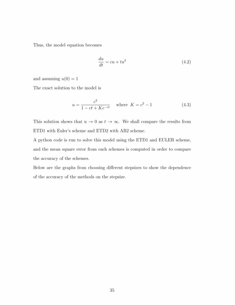
ETD1 and EULER at h = 0.1

Figure 4.1: The graph of the exact solution, ETD1, and Euler at stepsize= 0.1

Figure(4.1) shows the results from ETD1 and Euler as compared with the exact

solution and the mean square error(MSE) are calculated as 1.91399680685 for

ETD1 and 4.15901445216 for Euler.

obviously, Euler scheme show a wide deviation from the exact solution (as can

be seen from the graph and the MSE)

36

ETD1 and EULER at h = 0.01

Figure 4.2: The graph of the Exact solution, ETD1, and EULER atstepsize 0.01

figure(4.2) shows the results from ETD1 and Euler as compared with the exact

solution and the mean square error(MSE) are calculated as 1.69216265131 for

ETD1 and 4.39629251821 for Euler.

Euler scheme show a slight deviation from the exact solution(as can also be seen

from the graph and the MSE)

37

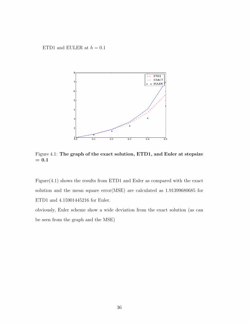
ETD1 and EULER at h = 0.001

Figure 4.3: The graph of the Exact solution, ETD1, and EULER atstepsize 0.001

figure(4.3) shows the results from ETD1 and Euler as compared with the exact

solution and the mean square error(MSE) are calculated as 1.67004541002 for

ETD1 and 4.45859347236 for Euler.

Euler scheme show little or no deviation from the exact solution(as can be seen

from the graph).

It can be observed that as h gets smaller from 0.1 to 0.001, the Euler scheme gets

more accurate. This is due to the stiff nature of the chosen harvesting model.

Hence, if a numerical method of order 1 is needed to compute results for the

harvesting model, ETD1 is preferable to Euler.

A python code is also run to solve thesame harvesting model using the ETD2

and AB2 scheme, and the mean square error from each schemes is computed in

order to compare the accuracy of the schemes.

Below are the graphs from choosing different stepsizes to show the dependence

38

of the accuracy of the methods on the stepsize.

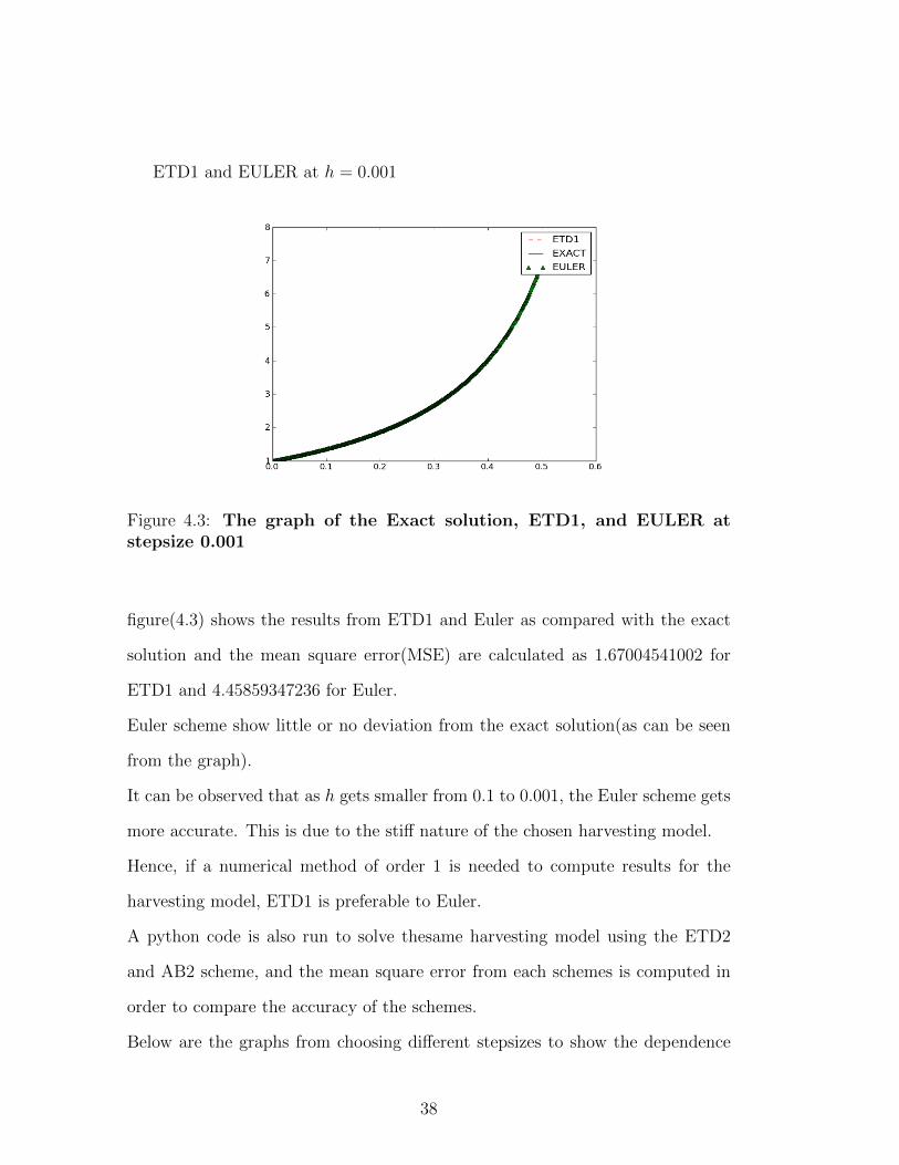
ETD2 and AB2 at h = 0.1

Figure 4.4: The graph of the exact solution, ETD2, and AB2 at stepsize0.1

figure(4.4) shows the results from ETD2 and AB2 as compared with the exact

solution and the mean square error (MSE) are calculated as 2.25091023678 for

ETD2 and 2.73580667268 for AB2.

AB2 shows a wide deviation from the exact solution (as can be seen from the

graph and the MSE)

39

ETD2 and AB2 at h = 0.01

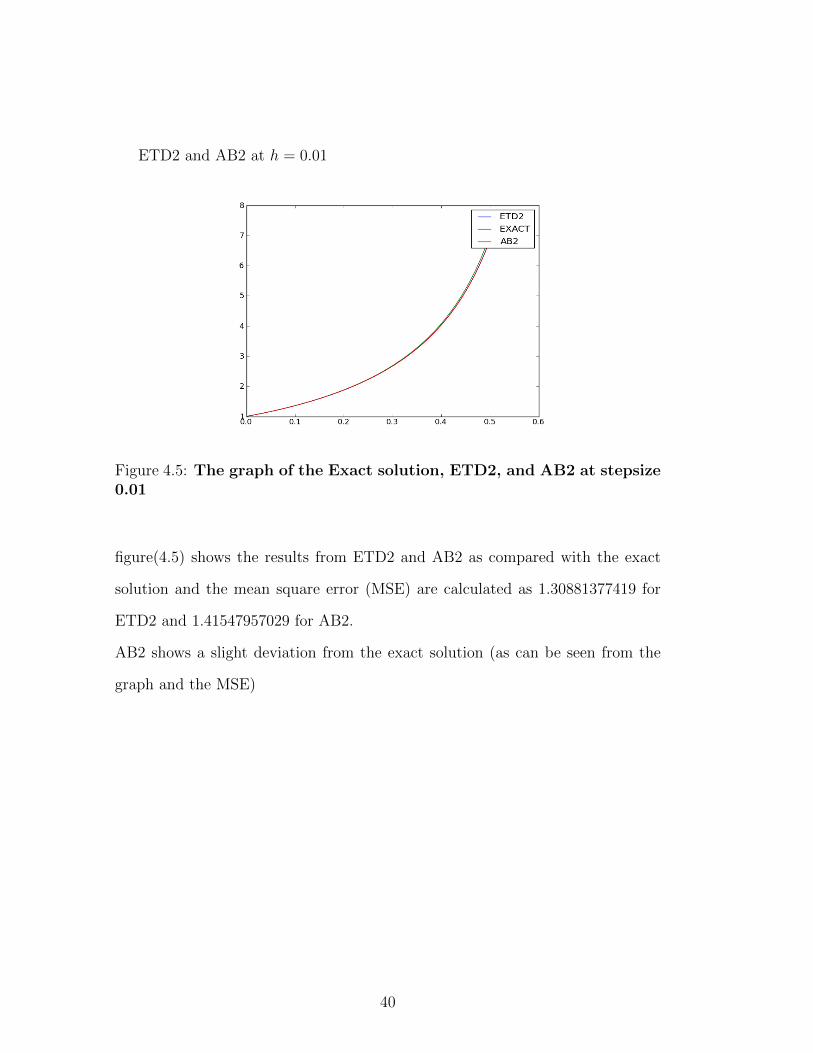
Figure 4.5: The graph of the Exact solution, ETD2, and AB2 at stepsize0.01

figure(4.5) shows the results from ETD2 and AB2 as compared with the exact

solution and the mean square error (MSE) are calculated as 1.30881377419 for

ETD2 and 1.41547957029 for AB2.

AB2 shows a slight deviation from the exact solution (as can be seen from the

graph and the MSE)

40

ETD2 and AB2 at h = 0.001

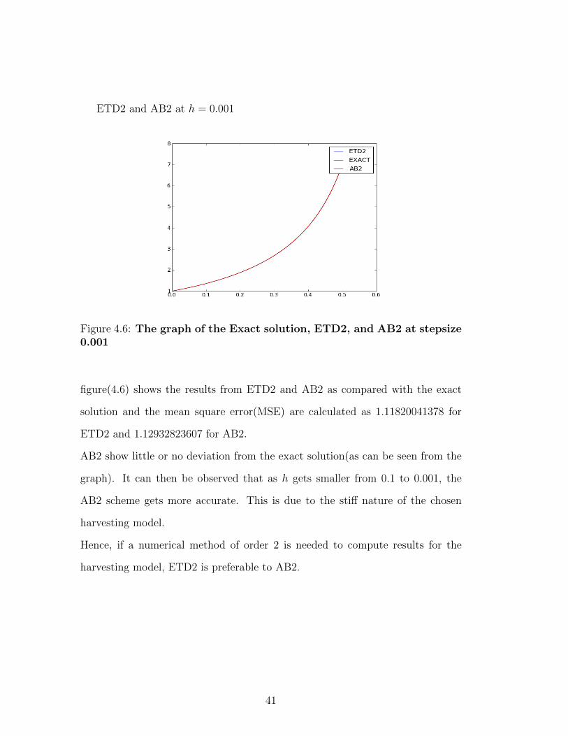
Figure 4.6: The graph of the Exact solution, ETD2, and AB2 at stepsize0.001

figure(4.6) shows the results from ETD2 and AB2 as compared with the exact

solution and the mean square error(MSE) are calculated as 1.11820041378 for

ETD2 and 1.12932823607 for AB2.

AB2 show little or no deviation from the exact solution(as can be seen from the

graph). It can then be observed that as h gets smaller from 0.1 to 0.001, the

AB2 scheme gets more accurate. This is due to the stiff nature of the chosen

harvesting model.

Hence, if a numerical method of order 2 is needed to compute results for the

harvesting model, ETD2 is preferable to AB2.

41

Chapter 5

CONCLUSION

5.1 Conclusion

The pairs of the numerical methods; AB2 and ETD2, EULER and ETD1 were

used to solve the harvesting model and the results of each pair are compared to

investigate their levels of accuray.

The following observations were therefore made from the comparison of the

scheme:

1. Results from Euler and ETD1 shows that as h gets smaller from 0.1 to

0.001, the Euler scheme gets more accurate. This is due to the stiff nature

of the chosen harvesting model. Hence, it can therefore be establish that

ETD1 give a close approximation to the exact solution and it is preferable

when numerical method of order 1 is needed to compute results for the

harvesting model.

2. Results from ETD2 and AB2 shows that as h gets smaller from 0.1 to 0.001,

the AB2 scheme gets more accurate. This is aswell due to the stiff nature

of the chosen harvesting model.

42

Hence, it can also be concluded that ETD2 give a close approximation to the

exact solution and it is preferable when numerical method of order 2 is needed

to compute results for the harvesting model.

43

Bibliography

[1] S.M. Cox and P.C matthews (2001) Exponential Time Differecing for Stiff

Systems, Journal of computational physics vol 176 pg 430-435.

[2] F.de la Hoz, F.valallo: (2008) An exponential time differencing method for

the nonlinear equation, pg 499

[3] Du., Q. and Zhu: Stability Analysis and Application of Exponential time dif-

ferencing schemes, journal of Computational Mathematics, vol 22, No.2

[4] Curtiss,.C.F. and Hirchfelder,.J.O.(1952) ntegration of Stiff Equations. Proc.

Nat. Aca. Sci.vol.48,

[5] Michael Zeltkevic :( 2012 ) International Journal of Engineering and Applied

Sciences,

[6] Weisstein, Eric W: ”Euler Forward Method”, MathWorld–A Wolfram Web

Resource.

[7] Nicholas J. Higham:(1996) Accuracy and Stability of Numerical Algorithms,

Society of Industrial and Applied Mathematics,Philadelphia,

[8] Richard L. Burden and J. Douglas Faires, (2005) : Numerical Analysis, 8th

Edition, Thomson Brooks/Cole, U.S.,

44

[9] Kendall Atkinson, Weimin Han, David Stewart Numerical solution of ordinary

differential equations University of Iowa Iowa City, Iowa pg 16-26, 95 -101

[10] Branislav K. Nikoli Numerical Methods for Ordinary Differential Equations

Department of Physics and Astronomy, University of Delaware, U.S.A. pg 8

[11] Euler method, From Wikipedia, the free encyclopedia

[12] Linear multistep method, From Wikipedia, the free encyclopedia

[13] Lakoba, Taras I.(2012): Simple Euler method and its modifications, (Lecture

notes for MATH334, University of Vermont),

[14] J.H. heinbockei : Numerical methods for scientific computing, pg 191-193.

[15] Garfinkel, .D. and Marbach, .C.B. (1977) Stiff Differential Equations, Ann.

Rev. Biophys, vol. 6, pages 525528

[16] Moler,. C. Stiff Differential Equations,

http://www.mathworks.com/company/.../stiff-differential-equations.html

[17] Dahlquist,.G.(1963). A Stability Problem for Linear Multi-Step. BIT Nu-

mer.Math.vol.131, pages 2743

[18] Hairer,.E. and Wanner,.G. (1996). Solving Ordinary Differential Equations

II. Springer-Verlag, Berlin, second edition, pages 101109

45

Appendix

Algorithm for ETD1 and Euler

from numpy import *

from pylab import *

def f(u,t):

return t*pow(u,2)

def F(u,t):

return c*u + f(u,t)

def ETD1(u,t):

return u*ech + f(u,t)*(ech - 1)/c

def EULER(u,t):

return u + h*F(u,t)

def Exact(t):

return pow(c,2)/(1 - c*t + k*exp(-c*t))

c = 3.0, u0 = 1.0, h = 0.1, t = 0.0

k = (pow(c,2)-u0)/u0

ech = exp(c*h)

tlist = [t]

uETD1list = [u0]

uEULERlist = [u0]

uExactlist = [u0]

ErrorETD1 = 0

ErrorEULER = 0

ErrorETD1 = ErrorETD1 + abs(uETD1list[0]-uExactlist[0])

46

ErrorEULER = ErrorEULER + abs(uEULERlist[0]-uExactlist[0])

i = 1

while t ¡ 0.5:

uETD1 = ETD1(uETD1list[i-1], t)

uETD1list.append(uETD1)

uEULER = EULER(uEULERlist[i-1],t)

uEULERlist.append(uEULER)

t = t + h

tlist.append(t)

uExact = Exact(t)

uExactlist.append(uExact)

ErrorETD1 = ErrorETD1 + abs(uETD1list[i]-uExactlist[i])

ErrorEULER = ErrorEULER + abs(uEULERlist[i]-uExactlist[i])

i = i+1

print ”Mean Squared Error For ETD1 = ”, ErrorETD1

print ”Mean Squared Error For EULER = ”, ErrorEULER

tlist = array(tlist)

uETD1list = array(uETD1list)

uExactlist = array(uExactlist)

uEULERlist = array(uEULERlist)

print uExactlist

print uETD1list

print uEULERlist

figure(0)

plot(tlist,uETD1list, label = ’ETD1’)

plot(tlist,uExactlist, label = ’EXACT’)

47

plot(tlist,uEULERlist, label =’EULER’)

legend()

show()

Algorithm for ETD2 and AB2

from numpy import *

from pylab import *

def f(u,t):

return t*pow(u,2)

def F(u,t):

return c*u + f(u,t)

def ETD1(u,t):

return u*ech + f(u,t)*(ech - 1)/c

def ETD2(u,uprime,t1,t2):

part1 = u*ech

part2 = f(u,t1)*((1+c*h)*ech - 1-2*h*c)/(h*pow(c,2))

part3 = f(uprime,t2)*(-ech + 1 + h*c)/(h*pow(c,2))

return part1 + part2 + part3

def AB2(u1, u0,t1,t2):

return u1 + h*(3*F(u1,t1) - F(u0,t2))/2

def Exact(t):

return pow(c,2)/(1 - c*t + k*exp(-c*t))

c = 3,h = 0.1, u0 = 1, t = 0

k = (pow(c,2)-u0)/u0

48

ech = exp(c*h)

tlist = [t]

uETD1list = [u0]

uETD1 = ETD1(uETD1list[0],t)

t = t + h

tlist.append(t)

uETD1list.append(uETD1)

uExactlist = [Exact(tlist[0]), Exact(tlist[1])]

uETD2list = [uExactlist[0],uExactlist[1]]

AB2list = [uExactlist[0],uExactlist[1]]

print t, uETD2list[0], AB2list[0], uExactlist[0]

print t, uETD2list[1], AB2list[1], uExactlist[1]

ErrorETD2 = 0

ErrorAB2 = 0

ErrorETD2 = ErrorETD2 + abs(uETD2list[1]-uExactlist[1])

ErrorAB2 = ErrorAB2 + abs(AB2list[1]-uExactlist[1])

i = 2

while t¡0.5:

t = t + h

tlist.append(t)

uETD2 = ETD2(uETD2list[i-1], uETD2list[i-2],tlist[i-2],tlist[i-3])

uETD2list.append(uETD2)

AB2val = AB2(AB2list[i-1],AB2list[i-2],tlist[i-2],tlist[i-3])

AB2list.append(AB2val)

uExact = Exact(t)

uExactlist.append(uExact)

49

ErrorETD2 = ErrorETD2 + abs(uETD2list[i]-uExactlist[i])

ErrorAB2 = ErrorAB2 + abs(AB2list[i]-uExactlist[i])

i = i+1

print ”Mean Squared Error For ETD2 = ”, ErrorETD2

print ”Mean Squared Error For AB2 = ”, ErrorAB2

tlist = array(tlist)

uETD2list = array(uETD2list)

uExactlist = array(uExactlist)

AB2list = array(AB2list)

figure(0)

plot(tlist,uETD2list, label = ’ETD2’)

plot(tlist,uExactlist, label = ’EXACT’)

plot(tlist,AB2list, label =’AB2’)

legend()

show()

50