sensitivity analysis of laterally loaded piles embedded in stiff
TRANSCRIPT
University of Windsor University of Windsor
Scholarship at UWindsor Scholarship at UWindsor
Electronic Theses and Dissertations Theses, Dissertations, and Major Papers
2004
Sensitivity analysis of laterally loaded piles embedded in stiff clay Sensitivity analysis of laterally loaded piles embedded in stiff clay
above water table. above water table.
Lebing Liu University of Windsor
Follow this and additional works at: https://scholar.uwindsor.ca/etd
Recommended Citation Recommended Citation Liu, Lebing, "Sensitivity analysis of laterally loaded piles embedded in stiff clay above water table." (2004). Electronic Theses and Dissertations. 3429. https://scholar.uwindsor.ca/etd/3429
This online database contains the full-text of PhD dissertations and Masters’ theses of University of Windsor students from 1954 forward. These documents are made available for personal study and research purposes only, in accordance with the Canadian Copyright Act and the Creative Commons license—CC BY-NC-ND (Attribution, Non-Commercial, No Derivative Works). Under this license, works must always be attributed to the copyright holder (original author), cannot be used for any commercial purposes, and may not be altered. Any other use would require the permission of the copyright holder. Students may inquire about withdrawing their dissertation and/or thesis from this database. For additional inquiries, please contact the repository administrator via email ([email protected]) or by telephone at 519-253-3000ext. 3208.

NOTE TO USERS
This reproduction is the best copy available.
UMI
Reproduced with permission of the copyright owner. Further reproduction prohibited without permission.

Reproduced with permission of the copyright owner. Further reproduction prohibited without permission.
SENSITIVITY ANALYSIS OF LATERALLY LOADED PILES
EMBEDDED IN STIFF CLAY ABOVE WATER TABLE
BY
LEBINGLIU
A Thesis
Submitted to Faculty o f Graduate Studies and Research Through the
Department of Civil and Environmental Engineering
in Partial Fulfillment of the Requirements for the Degree of
Master o f Applied Science
at the
University of Windsor
Windsor, Ontario, Canada
2004
Reproduced with permission of the copyright owner. Further reproduction prohibited without permission.

1 ^ 1National Library of Canada
Acquisitions and Bibliographic Services
395 Wellington Street Ottawa ON K1A 0N4 Canada
Bibliotheque nationals du Canada
Acquisisitons et services bibliographiques
395, rue Wellington Ottawa ON K1A 0N4 Canada
Your file Votre reference ISBN: 0-612-92443-2 Our file Notre reference ISBN: 0-612-92443-2
The author has granted a nonexclusive licence allowing the National Library of Canada to reproduce, loan, distribute or sell copies of this thesis in microform, paper or electronic formats.
The author retains ownership of the copyright in this thesis. Neither the thesis nor substantial extracts from it may be printed or otherwise reproduced without the author's permission.
L'auteur a accorde une licence non exclusive permettant a la Bibliotheque nationale du Canada de reproduire, preter, distribuer ou vendre des copies de cette these sous la forme de microfiche/film, de reproduction sur papier ou sur format electronique.
L'auteur conserve la propriete du droit d'auteur qui protege cette these. Ni la these ni des extraits substantiels de celle-ci ne doivent etre imprimes ou aturement reproduits sans son autorisation.
In compliance with the Canadian Privacy Act some supporting forms may have been removed from this dissertation.
Conformement a la loi canadienne sur la protection de la vie privee, quelques formulaires secondaires ont ete enleves de ce manuscrit.
While these forms may be included in the document page count, their removal does not represent any loss of content from the dissertation.
Bien que ces formulaires aient inclus dans la pagination, il n'y aura aucun contenu manquant.
CanadaReproduced with permission of the copyright owner. Further reproduction prohibited without permission.
ABSTRACT
This study presents the theoretical formulation and numerical investigation of
sensitivity analysis of laterally loaded piles embedded in stiff clay located above the water
table. Single piles with various lengths and boundary conditions subjected to static and
cyclic loadings applied to the pile-head as lateral forces and bending moments are
analyzed. The cyclicity is introduced explicitly to p-y curve. The p-y soil response is of
quasi static type. The pile groups o f 3x3 piles with various spacing (2D, 3D, 4D and 5D)
are also analyzed in the study. For single piles, the pile structure is considered as
one-dimensional beam and the supporting stiff clay is defined by means of p-y
relationship. For groups o f piles, the pile members are considered as one-dimensional
beams and the pile cap is considered as plate. The behaviour of a pile-soil system in the
pile group is simulated also by means o f p-y relationship, which is modified by the fm
factor that is dependent on the spacing o f the piles and the locations o f the piles in the
groups. The pile material parameter and soil physical parameters are taken as the design
variables. The adjoint method for nonlinear system is used to analyze the sensitivity o f the
piles and pile groups. The changes of maximum generalized deflection located at the pile
head o f the pile due to the changes o f the design variables are explored by means of
sensitivity integrands associated with each o f the design variables. The numerical results
in terms of spatial distributions o f sensitivity integrands are presented and discussed in
detail. The sensitivity integrands are integrated and the assessment o f the result is carried
out. The Matlab programmings are used to conduct the numerical investigations o f single
pile and pile groups.
Ill
Reproduced with permission of the copyright owner. Further reproduction prohibited without permission.

Acknowledgements
There are a great number o f people who offered generous help to me in finishing this
research. I specially thank my advisor Dr. B. B. Budkowska for the kind direction,
guidance, insight and financial assistance. My committee members. Dr. Nader G. Zamani
(Mechanical, Automotive and Materials Engineering Department), Dr. Murty K.
Madugula (Civil and Environmental Engineering) and Dr. Faouzi Ghrib also give me
valuable suggestions to improve the thesis. Many people assisted me both in the
analyzing and thesis writing including Deni Priyanto, Deddy Suwano, Zain-Al-Abedin,
Andre Bom, Marcia Mora, Md. Badruzzaman, Dahlia Hafez, and T. I. M. Nazmur
Rahman. Lilian Zhang served as my first audience and commenter of my oral
presentation. Mr. Patrick F. Seguin, Lucian Pop prepared the experimental equipment and
provided technical support for the computer systems. I give thanks to them sincerely.
Without their generous help, this research work cannot be conducted smoothly.
I also would thank my wife, Junying Sun, for her wholehearted support to my study
and research. She has been taking care of my son, Huanhuan, alone for almost 2 years.
She supports me quietly and never complains about the hardship caused by my staying
abroad.
It is my great intention that I would extend great big thanks to my parents. They
tolerated my long time absence from their side with great patience and understanding. I
also want to thank all of my friends and Pastor Lee in my church for their gracious
encouragements and accompany.
This study was supported by Natural Sciences and Engineering Research Council
(NSERC) of Canada awarded to Professor B. B. Budkowska under Grant No. OGP
0110262. The financial assistance is gratefully acknowledged.
IV
Reproduced with permission of the copyright owner. Further reproduction prohibited without permission.
TABLE OF CONTENTS
ABSTRACT.. ...... I ll
ACKNOWLEDGEMENTS ...... IV
LIST OF TABLES................................. ..IX
LIST OF FIGURES............... XI
CHAPTER 1 INTRODUCTION...................... 11.1 Problem statem ent.......................................................... 1
1.2 Objectives ........ 3
1.3 Procedure.................. 4
1.4 Methodology o f sensitivity analysis ......... 5
1.5 Significance o f sensitivity analysis............................................ 5
CHAPTER 2 LITERATURE REVIEW ......... 72.1 Literature review o f the analysis of laterally loaded single p iles .............................7
2.1.1 General ......... 72.1.2 The subgrade-reaction model....................... ......... ............................................ . 82.1.3 The elastic approach ............................................................... 92.1.4 Elastic pile and finite element for soil............... 92.1.5 Rigid pile and plastic soil ............................................ 102.1.6 Characteristic load method........................ .... ........ ............................................... 112.1.7 The p-y curve relationship approach................................... 122.1.8 Field testing and analysis of laterally loaded piles in stiff clay located above
water table................. 14
2.2 Literature review on the analysis of pile groups ..................... 152.2.1 General ........ 152.2.2 Simple static analysis method ....... 162.2.3 Equivalent bent method ......... 172.2.4 Elastic continuum analysis of pile behavior ...... 182.2.5 Group reduction factor method and group amplification method ........ 192.2.6 The p-multipliers method.. ...... 19
2.3 Literature review on the sensitivity analysis of pile foundation ............232.3.1 Definition of the sensitivity analysis........ ............................ 232.3.2 Aim and importance o f the sensitivity analysis ....... .24
Reproduced with permission of the copyright owner. Further reproduction prohibited without permission.
2.3.3 The procedures to conduct sensitivity analysis ...... 252.3.4 Term definitions.......................................................... 262.3.5 The virtual load method for sensitivity analysis of structures................... 262.3.6 The methods of sensitivity analysis ...... 272.3.7 Review of the sensitivity analysis applied to the structures and pile
foundations............................................... 28
CHAPTER 3 THEORETICAL FORMULATION OF SINGLE FILE .......... 333.1 Introduction ......... 33
3.1.1 Soil and deep foundation................................................................... 33
3.2 p-y curve o f stiff clay. ...... 343.2.1 Definition of soil reaction p, deflection y and p-y curve ............................343.2.2 Reese and Welch’s p-y curve theory for stiff clay above water table ...... 35
3.3 Theoretical formulation of sensitivity analysis of laterally loaded piles embeddedin stiff clay above water table....................................................... 40
3.3.1 General.......................................................... 403.3.2 Primary and adjoint structure........................................................................ 403.3.3 Sensitivity operators, sensitivity factors and relative sensitivity factors...........43
CHAPTER 4 THEORETICAL FORMULATION OF THE PILE GROUP 574.1 Introduction.......................................................................... 57
4.2 Laterally loaded pile group effects and p-multipliers.................... 58
4.3 Pile group analysis using p-multipliers .......... 59
CHAPTER 5 NUMERICAL INVESTIGATIONS OF SINGLE PILE ........ 615.1 Introduction.. ......... 61
5.2 Scope........................................................... 62
5.3 The determination of typical design parameters:............. 62
5.4 Determination of relative stiffness factor T .......................... 64
5.5 Short piles and long piles... ....... 72
5.6 Load-deflection relationship... ....... 73
5.7 The stresses and deformations o f adjoint structure ........... 75
5.8 COM624P Program ......... 77
5.9 Results o f sensitivity analysis o f laterally loaded pile. ..................... 78
5.10 Methodology of result verification................................... .78
CHAPTER 6 NUMERICAL INVESTIGATIONS OF THE PILE GROUP......... 816.1 Introduction....................... ....81
6.2 Scope. ................................................................. .......................................... 81
6.3 The determination of Pg for the pile groups under lateral concentrated load ..... 84
VI
Reproduced with permission of the copyright owner. Further reproduction prohibited without permission.
6.4 The determination of the adjoint structure and the unit lateral force Pgi for pilegroups under lateral concentrated load Pg ................................ 86
6.5 The determination o f the Mg of the primary structure for pile groups under pilehead bending moment........................................................... 90
6.6 The determination o f the adjoint structure and the unit lateral force Pgi for pilegroups subjected to bending moment applied to each pile h ead ..... .93
6.7 The results of the sensitivity analysis of laterally loaded pile groups...................94
CHAPTER 7 PROGRAMMING OF SENSITIVITY ANALYSIS FOR SINGLE PILES............................................................... 97
7.1 Introduction.................................................................................. 97
7.2 Preparing and input file generating module........................................... 97
7.3 Calculating module.... ............................................... 100
7.4 Sensitivity integrands analysis module .................................... 101
7.5 Sensitivity factors analysis m odule................................................................ 104
7.6 Result check and error analysis module .................................. 104
CHAPTER 8 PROGRAMMING OF SENSITIVITY ANALYSIS FOR THE PILE GROUPS....................................................... 105
8.1 Introduction .......................................................... 105
8.2 FB-Pier program............................................................................. 109
8.3 A method used to read more precise result from FB-PierV3.................................113
CHAPTER 9 DISCUSSION OF THE RESULTS .............. 1169.1 General................................................................................ 116
9.2 Discussion of the sensitivity analysis results ............................. 1179.2.1 Discussion of the lateral deflections, bending moments o f the primary
structures........................................................................ 1189.2.2 Discussion of the lateral deflections, bending moments and soil resistance of
adjoint structures subjected to unit lateral forces P = 1 ............. 119
9.2.3 Discussion of the sensitivity operators/integrands ........................ 121
9.2.4 Discussion o f the lateral deflections, bending moments and soil resistance of
adj oint structures subj ected to unit bending moments M = 1 ............... 124
9.2.5 Discussion of the sensitivity operators/integrands C™..)........................... 125
9.2.6 Discussion o f sensitivity factors .............................. 1279.2.7 Discussion o f relative sensitivity factors F ........................................... 129
Vll
Reproduced with permission of the copyright owner. Further reproduction prohibited without permission.
9.2.8 Discussion of the sensitivity analysis results of the laterally loaded pilegroups ....... 131
9.3 Verification and error analysis.............................................. 132
9.4 Quantitative assessment of sensitivity factors A ................................... 136
9.5 Assessment of error of lateral deflection based on comparative analysis — exactsolution and sensitivity analysis solution...................... 144
CHAPTER 10 CONCLUSIONS AND SUGGESTIONS FOR FUTURERESEARCH............................................................. 148
10.1 Conclusion.................................................................................................................. 148
10.2 The application o f this study.................................................................................... 156
10.3 Recommendation for future research ........ 156
REFERENCES...................................................... ................. ........................ ................158
APPENDIX A. DERIVATIONS OF FORMULAS OF SENSITIVITYOPERATORS............... 166
APPENDIX B. TYPICAL RESULTS OF THE SENSITIVITY ANALYSIS FOR A FREE HEAD SINGLE LONG PILE EMBEDDED IN THE STIFF CLAY ABOVE WATER TABLE, SUBJECTED TO LATERAL CONCENTRATED FORCES, WITH PILE LENGTH L=10T=13.7M AND NUMBER OF LOAD CYCLES N=1 AND 10000...................... 175
APPENDIX C. TYPICAL RESULTS OF THE SENSITIVITY ANALYSIS FOR PILE B (FIRST TRAILING ROW) IN A PILE GROUP EMBEDDED IN THE STIFF CLAY ABOVE WATER TABLE, SUBJECTED TO LATERAL CONCENTRATED FORCE PG APPLIED TO THE PILE CAP, WITH THE PILES MEMBERS PINNED TO THE PILE CAP, PILE SPACING S= 2D, PILE LENGTH L=10T=13.7M AND NUMBER OF LOAD CYCLES N=1 AND 10000 ........ 204
APPENDIX D. CONTENT OF THE ATTACHED CD ....... 216
VITA AUCTORIS ..... 219
vm
Reproduced with permission of the copyright owner. Further reproduction prohibited without permission.
LIST OF TABLES
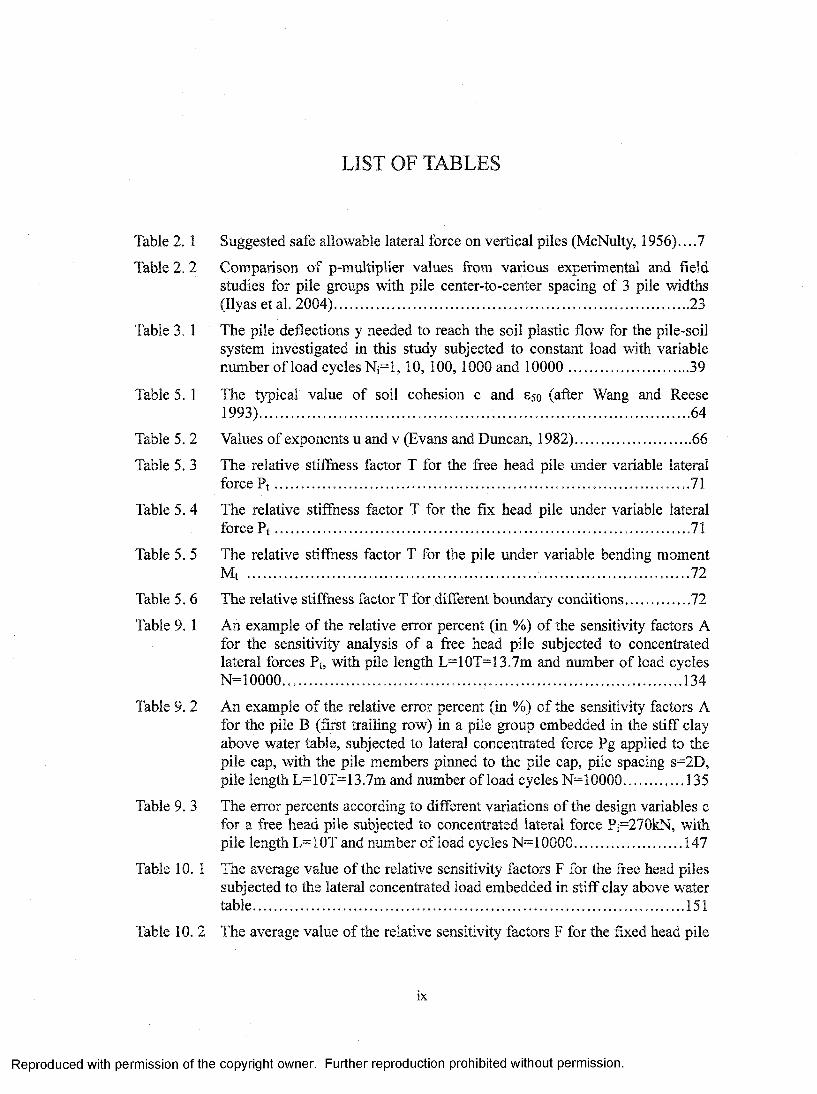
Table 2. 1 Suggested safe allowable lateral force on vertical piles (McNulty, 1956)....7
Table 2. 2 Comparison o f p-multiplier values from various experimental and fieldstudies for pile groups with pile center-to-center spacing of 3 pile widths (Ilyas et al. 2004).. ................................................ 23
Table 3. 1 The pile deflections y needed to reach the soil plastic flow for the pile-soilsystem investigated in this study subjected to constant load with variable number o f load cycles Nj=l, 10,100,1000 and 10000 .................................39
Table 5. 1 The typical value o f soil cohesion c and S50 (after Wang and Reese1993).................................................................. ....64
Table 5. 2 Values of exponents u and v (Evans and Duncan, 1982)......................... 66
Table 5. 3 The relative stiffness factor T for the free head pile under variable lateralforce P t .......................................................... 71
Table 5. 4 The relative stiffness factor T for the fix head pile under variable lateralforce F t ....... 71
Table 5. 5 The relative stiffness factor T for the pile under variable bending momentM, ......................................................... 72
Table 5. 6 The relative stiffness factor T for different boundary conditions.. ..............72
Table 9. 1 An example o f the relative error percent (in %) of the sensitivity factors Afor the sensitivity analysis o f a free head pile subjected to concentrated lateral forces Pt, with pile length L=10T=13.7m and number of load cyclesN=10000.................................. 134
Table 9. 2 An example o f the relative error percent (in %) o f the sensitivity factors Afor the pile B (first trailing row) in a pile group embedded in the stiff clay above water table, subjected to lateral concentrated force Pg applied to the pile cap, with the pile members pinned to the pile cap, pile spacing s=2D, pile length L=10T=13.7m and number o f load cycles N =10000.................135
Table 9. 3 The error percents according to different variations o f the design variables cfor a free head pile subjected to concentrated lateral force Pj=270kN, with pile length L=10T and number o f load cycles N = 10000.. ......................... 147
Table 10. 1 The average value of the relative sensitivity factors F for the free head piles subjected to the lateral concentrated load embedded in stiff clay above water table. ....... 151
Table 10. 2 The average value of the relative sensitivity factors F for the fixed head pile
IX
Reproduced with permission of the copyright owner. Further reproduction prohibited without permission.

subjected to the lateral concentrated load embedded in stiff clay above water table ....... 151
Table 10. 3 The average values of the relative sensitivity factors F for the free head pilesubjected to the bending moment embedded in stiff clay above water tab le .... ....... ....152
Table 10. 4 The average values of the relative sensitivity factors F for all the piles subjected to both the lateral concentrated load and bending moment embedded in stiff clay above water.................................. 152
Reproduced with permission of the copyright owner. Further reproduction prohibited without permission.
LIST OF FIGURES
Figure 2.1 Model for a pile under lateral loading with p-y curves (Reese and Van Impe (2001))...................................................................................................................13
Figure 2. 2 Principle o f equivalent-bent approach ....... 18
Figure 2. 3 The concept of p-multiplier (fm) (Brown et al. 1988)........ 21
Figure 2. 4 The p-y curves for soft clay below water table (Matlock, 1970)....................32
Figure 2. 5 The p-y curves for stiff clay below water table (Reese et al., 1975)............. 32
Figure 3. 1 The graphical definition of p and y (after Reese and et al. (1975)). ............ 34
Figure 3. 2 p-y curves for stiff clay above water table subjected to cyclic loading 36
Figure 3.3 Variability o f ultimate soil resistance p„ along the pile axis........................... 38
Figure 3. 4 Characteristic shape o f p-y curves for cyclic loading in stiff clay above water table for different load cycles Ni, Nj and N 3 (Ni<N2<Ns) (after Welch and Reese, 1972).................................................................................................. 39
Figure 3. 5 A pile element modeled by a beam supported by nonlinear springs 40
Figure 3. 6 A primary structure subjected to a lateral force Ft and the correspondingadjoint structure subjected to a lateral unit force P = 1 applied at the piletop.......................................... 41
Figure 3. 7 A primary structure subjected to a lateral force Pt and the correspondingadjoint structure subjected to a unit bending moment M = 1 applied at the pile top .................................................. ...42
Figure 3.8 A primary structure subjected to a bending moment Mt and thecorresponding adjoint structure subjected to a lateral unit force P = 1 applied at the pile top ............................. 42
Figure 3 .9 A primary structure subjected to a bending moment Mt and thecorresponding adjoint structure subjected to a unit bending moment M = 1 applied at the pile to p .. ........ 43
Figure 3. 10 Physical meaning of normalized sensitivity integrands/operators C(„.) andsensitivity factors A (,„). ................. 48
Figure 3. 11 Convention for the notation o f sensitivity operators/integrands andsensitivity factors. ......................................................52
XI
Reproduced with permission of the copyright owner. Further reproduction prohibited without permission.
Figure 3 .12 Numerical integration using Simpson’s ra le . ........ 54
Figure 4. 1 A 3D view of a typical pile group under lateral load Pg connected by a concrete pile cap ..................... 57
Figure 4. 2 Description of nomenclatures used to describe pile group arrangements. ..58
Figure 4 .3 The p-multiplier design curves proposed by Mokwa and Duncan (2001b).......... 60
Figure 5. 1 Section properties of the pile used in the sensitivity analysis........................63
Figure 5. 2 Load-deformation curves for free-head pile embedded in clay under cyclic lateral load (after Evans and Duncan, 1982)........ 67
Figure 5. 3 Load-deformation curves for fix-head pile embedded in clay under cyclic lateral load (after Evans and Duncan, 1982)........ 68
Figure 5. 4 Load-deformation curves for the pile embedded in clay under cyclic bending moment (after Evans and Duncan, 1982).........................................................69
Figure 5. 5 Pile head deflection yt vs. lateral force Pt applied to the pile head for a free head pile embedded in stiff clay above water table. Pile length L=2T=2.74 m, load cycles N= 10000........................... 73
Figure 5. 6 Pile head deflection yt vs. lateral force Pt applied to the pile head for a fixed head pile embedded in stiff clay above water table. Pile length L=2T=3.58 m, load cycles N =10000.. .......... 74
Figure 5. 7 Pile head deflection yt vs. bending moment Mt applied to the pile head for a free head pile embedded in stiff clay above water table. Pile length L=2T=2.16 m, load cyclesN=10000............................ 74
Figure 5. 8 The method used to calculate various components o f adjoint structure 76
Figure 6. 1 Pile group properties employed in the sensitivity analysis ................83
Figure 6. 2 An example presenting the method to determine the force Pg applied to the pile cap....................................... 85
Figure 6. 3 Force Pgi o f pile A (2nd trailing row), B (1st trailing row), C (Leading row) o f group o f 3x3 piles with the spacing 2D and the length L=10T vs. applied lateral force Pg. Pile pinned to cap, load cycles=l..........................................88
Figure 6 .4 The approach used to determine the force Pgi, the adjoint structure and the temporary structures for the pile groups under lateral concentrated loadPg............................ 89
Figure 6. 5 An example presenting the method to determine the force Mg applied to the head o f the piles in a pile group. ....... ....92
Figure 6. 6 Force Pgi o f pile A (2nd trailing row), B (1st trailing row), C (Leading row) of group of 3x3 piles with the spacing 2D and the length L=10T vs. bending moment Mg applied to the heads o f piles in the pile group. Pile pinned to cap, load cycles=l.................................. ....95
Figure 6. 7 The approach to determine the adjoint structure and the force Pgi for the
XII
Reproduced with permission of the copyright owner. Further reproduction prohibited without permission.

pile groups under bending moment Mg applied at the pile heads in a pile group.................. 96
Figure 7 .1 The programming modules used to analyze the sensitivity of laterally loaded single piles embedded in the stiff clay above the water table........................98
Figure 7. 2 The file name convention for the COM624P input file of the sensitivityanalysis o f single pile ........ 99
Figure 7. 3 A typical input file of COM624P (10201 SO.inp)............................................100
Figure 7. 4 An example o f graphic file o f COM624P....................................... 102
Figure 8.1 The Matlab command line calling FB-Pier program to calculate the laterally loaded piles ............................................................................ .107
Figure 8. 2 A method through which more than 50 nodes can be employed in theFB-PiersV3 ........................................................................... . . .I l l
Figure 8. 3 The executing sequence o f the Matlab files included in the sensitivityanalysis o f laterally loaded pile groups embedded in stiff clay above water table.................................................................................. 112
Figure 8. 4 The file name convention for the FB-Pier input file of the sensitivityanalysis o f the pile group..................................................... 113
Figure 8.5 A Matlab function used to read data from the output files of FB-PiersV3..................................................................... 114
Figure 8. 6 The physical meaning of each column o f the matrix ResultDataM 115
Figure 9. 1 Pile head deflection yt vs. lateral force Pt applied to the pile head for a freehead pile embedded in stiff clay above water table. Pile length L=10T=13.7 m, load cycles N =10000........................................................ 118
Figure 9. 2 The sensitivity o f lateral deflection 8 expressed in (m) caused by changesof the design variables El when applied force Pt have values Pi.. . . . . . . . . . . 138
Figure 9. 3 The relative deflection sensitivity factor 1^ due to the changes of thedesign variables El vs. the relative load factor Ip ........................... 141
Figure 9. 4 The relative deflection sensitivity factor if" due to the changes of thedesign variables c vs. the relative load factor Ip .......................... 141
Figure 9. 5 The relative deflection sensitivity factor I ^ due to the changes o f the
design variables y vs. the relative load factor Ip .................................. 142
Figure 9. 6 The relative deflection sensitivity factor I ^ due to the changes o f the design variables b vs. the relative load factor Ip ....................... 142
Figure 9. 7 The relative deflection sensitivity factor I^^ due to the changes o f thedesign variables S50 vs. the relative load factor Ip ........ 143
Xlll
Reproduced with permission of the copyright owner. Further reproduction prohibited without permission.

Figure 9. 8 The relative deflection sensitivity factor due to the changes of the design variables N vs. the relative load factor Ip ....................................... 143
Figure 9. 9 The relationship A , between Pj. ........ 144
Figure 9. 10 The pile head lateral deflection ytop vs. the ratio (c/co) of design variable c to the initial design variable co, for a free head pile subjected to a pile head lateral concentrated load Ft = 270kN, with pile length L = lOT and number o f load cycles N = 10000................... 145
Figure B. 1 Distributions o f lateral deflections y o f the primary structures for free head piles of length L=10T, loaded by variable lateral force o f discrete variability for the number o f cycles N=1 and 10000........................................... 176
Figure B. 2 Distributions of bending moments o f the primary structures for free head piles of length L=10T, loaded by variable lateral force o f discrete variability for the number o f cycles N= 1 and 10000..................... 177
Figure B. 3 Distributions o f lateral deflections y^(F )o f the adjoint systems subjected to
P = 1 when the primary systems support the lateral concentrated forces ?t o f discrete variability for the number of cycles N=1 and 10000.......... 178
Figure B. 4 Distributions o f bending moments M (F )o f the adjoint systems subjected to
F = 1 when the primary systems support the lateral concentrated forces Ft of discrete variability for the number o f cycles N=1 and 10000.............. .179
Figure B. 5 Distributions of soil resistance p , of the adjoint systems subjected to
F = 1 when the primary systems support the lateral concentrated forces Ft o f discrete variability for the number of cycles N=1 and 10000.................180
Figure B. 6 Distributions o f sensitivity operators C^j affecting the changes of the pilehead lateral deflection 5yt o f the pile of length L=10T due to the changes of bending stiffness El when the pile structures are subjected to a concentrated lateral force Ft o f a discrete variability for the number o f load cycles N = l, 100 and 10000........ 181
Figure B. 7 Distributions o f sensitivity operators affecting the changes of the pilehead lateral deflection 5yt o f the pile o f length L=10T due to the changes of the cohesion c when the pile structures are subjected to a concentrated lateral force Ft o f a discrete variability for the number o f load cycles N=1 and 10000......................................... 182
Figure B. 8 Distributions o f sensitivity operators affecting the changes of the pile
head lateral deflection 6yt o f the pile o f length L=10T due to the changes of the soil unit weight y when the pile structures are subjected to a concentrated lateral force Ft of a discrete variability for the number o f load cycles N=1 and 10000.............. .183
xiv
Reproduced with permission of the copyright owner. Further reproduction prohibited without permission.
Figure B. 9 Distributions o f sensitivity operators affecting the changes of the pilehead lateral deflection 5yt o f the pile of length L=10T due to the changes of the pile’s width b when the pile structures are subjected to a concentrated lateral force Pt o f a discrete variability for the number of load cycles N=1 and 10000....... 184
Figure B. 10 Distributions of sensitivity operators C^o affecting the changes of the pilehead lateral deflection 5yt o f the pile o f length L=10T due to the changes of 850 when the pile structures are subjected to a concentrated lateral force ?t of a discrete variability for the number of load cycles N= 1 and 10000.......... 185
Figure B. 11 Distributions o f sensitivity operators affecting the changes of the pilehead lateral deflection 6yt o f the pile of length L=10T due to the changes of load cycles N when the pile structures are subjected to a concentrated lateral force ?t o f a discrete variability for the number o f load cycles N=100 and N = 10000 186
Figure B. 12 Distributions o f lateral deflections y^(M ) of the adjoint systems subjected
to M = 1 when the primary systems support the lateral concentrated forces Ft of discrete variability for the number of cycles N=1 and 10000....... ............................................... .......................................... ......... ....187
Figure B. 13 Distributions of bending moments M (M )of the adjoint systems subjected
to M = 1 when the primary systems support the lateral concentrated forces ?t of discrete variability for the number of cycles N=1 and 10000. 188
Figure B. 14 Distributions o f soil resistance p , of the adjoint systems subjected to
M = 1 when the primary systems support the lateral concentrated forces Ft o f discrete variability for the number of cycles N=1 and 10000.................189
Figure B. 15 Distributions o f sensitivity operators C™ affecting the changes of the pilehead lateral deflection 5yt o f the pile of length L=10T due to the changes of bending stiffhess El when the pile structures are subjected to a concentrated lateral force Ft o f a discrete variability for the number o f load cycles N=1 and 10000 .......................... 190
Figure B. 16 Distributions o f sensitivity operators Cf® affecting the changes of the pilehead lateral deflection 5yt o f the pile of length L=10T due to the changes of the cohesion c when the pile structures are subjected to a concentrated lateral force Ft o f a discrete variability for the number of load cycles N=1 and 10000................. .191
Figure B. 17 Distributions of sensitivity operators C™ affecting the changes of the pile
head lateral deflection 6yt o f the pile of length L=10T due to the changes of the soil unit weight y when the pile structures are subjected to a concentrated lateral force Ft o f a discrete variability for the number o f load cycles N -1
XV
Reproduced with permission of the copyright owner. Further reproduction prohibited without permission.

and 10000........................... 192
Figure B. 18 Distributions of sensitivity operators affecting the changes of the pilehead lateral deflection 5yt of the pile of length L=10T due to the changes of the pile’s width b when the pile structures are subjected to a concentrated lateral force Pt o f a discrete variability for the number o f load cycles N=1 and 10000............................................................................................... ......... 193
Figure B. 19 Distributions of sensitivity operators affecting the changes of the pilehead lateral deflection 5yt of the pile o f length L=10T due to the changes of 850 when the pile structures are subjected to a concentrated lateral force Ft of a discrete variability for the number o f load cycles N=1 and 10000.......... 194
Figure B. 20 Distributions o f sensitivity operators affecting the changes of the pilehead lateral deflection 8yt of the pile o f length L=10T due to the changes of load cycles N when the pile structures are subjected to a concentrated lateral force Ft of a discrete variability for the number o f load cycles N=100 and N = 10000................................ ......... ................................................................... 195
Figure B. 21 The quantitative assessment o f sensitivity factors A ^ , A ^ , A ^ , A ^
and A^o affecting the top lateral deflection yt o f the free head piles due tothe changes of bending stiffness El, cohesion c, unit weigh y of soil, pile width b and S50, when the pile structures are subject to a concentrated lateral force Ft o f a discrete variability for the number o f load cycles N = 1........ 196
Figure B. 22 The quantitative assessment (in%) o f relative sensitivity factors F ^ , F j^,
F * , F^ and F g affecting the top lateral deflection yt of the free head
piles due to the changes of bending stiffness El, cohesion c, unit weigh y of soil, pile width b and S50, when the pile structures are subject to a concentrated lateral force Ft of a discrete variability for the number o f load cycles N = 1 .................................. 197
Figure B. 23 The quantitative assessment o f sensitivity factors Agf, A™, A™, A™
and A™g affecting the top lateral deflection 0t o f the free head piles due tothe changes o f bending stiffness El, cohesion c, unit weigh y o f soil, pile width b and 850, when the pile structures are subject to a concentrated lateral force Ft o f a discrete variability for the number o f load cycles N = 1........ 198
Figure B. 24 The quantitative assessment (in%) o f relative sensitivity factors F™, F™,
F™, F™ and Fjj® affecting the top angle of flexural rotation 0t of the freehead piles due to the changes of bending stiffness El, cohesion c, unit weigh y of soil, pile width b and 850, when the pile structures are subject to aconcentrated lateral force Ft of a discrete variability for the number of loadcycles N = 1........ 199
Figure B. 25 The quantitative assessment o f sensitivity factors A ^ , A ^ , A ^ , A ^ ,
XVI
Reproduced with permission of the copyright owner. Further reproduction prohibited without permission.
A^o and affecting the top lateral deflection yt o f the free head piles due to the changes o f bending stiffiiess El, cohesion c, unit weigh y of soil, pile width b, S50 and load cycles N, when the pile structures are subject to a concentrated lateral force Pt of a discrete variability for the number o f load cycles N - 10000.......................................................... .200
Figure B. 26 The quantitative assessment (in%) o f relative sensitivity factors , F^^,
pPy pPy and F ^ affecting the top lateral deflection yt of the free
head piles due to the changes of bending stiffiiess El, cohesion c, unit weigh Y of soil, pile width b, S50 and number o f load cycles N, when the pilestructures are subject to a concentrated lateral force Ft of a discretevariability for the number o f load cycles N = 10000...................................201
Figure B. 27 The quantitative assessment o f sensitivity factors A™, A™, A^®, A™,
A™o and A^ affecting the top lateral deflection 0t o f the free head piles due to the changes o f bending stiffness El, cohesion c, unit weigh y of soil, pile width b, 850 and load cycles N, when the pile structures are subjeet to a concentrated lateral force Ft o f a discrete variability for the number of load cycles N = 10000...............................................................................................202
Figure B. 28 The quantitative assessment (in%) o f relative sensitivity factors F™, F™,
F™, F™, Fg o and F™ affecting the top angle of flexural rotation 0t of the free head piles due to the changes of bending stiffness El, cohesion c, unit weigh y of soil, pile width b, 850 and number o f load cycles N, when the pile structures are subject to a concentrated lateral force Ft of a discrete variability for the number of load cycles N = 10000.................. 203
Figure C. 1 The distributions of lateral deflections y of the primary structures for the pile B (first trailing row) in the 3x3 pile group loaded by variable lateral force Fg of discrete variability, piles pinned to the cap, pile spacing=2D, pile length L=10T, load cycles N=1 and 10000........... 205
Figure C. 2 The distributions of bending moments M of the primary structures for the pile B (first trailing row) in the 3x3 pile group loaded by variable lateral force Fg of discrete variability, piles pinned to the cap, pile spacing=2D, pile length L=10T, load cycles N=1 and 10000 ...........................206
Figure C. 3 The distributions of lateral deflections ya of the adjoint struetures for the pile B (first trailing row) in the 3x3 pile group loaded by variable lateral force Fgi o f discrete variability, piles pinned to the cap, pile spacing=2D, pile length L=10T, load cycles N=1 and 10000..................... ....207
Figure C. 4 The distributions of lateral deflections M of the adjoint structures for the pile B (first trailing row) in the 3x3 pile group loaded by variable lateral force Fgi of discrete variability, piles pinned to the cap, pile spacing=2D, pile length L=10T, load cycles N=1 and 10000. .......................208
xvii
Reproduced with permission of the copyright owner. Further reproduction prohibited without permission.
Figure C. 5 The distributions of soil resistance pa of the adjoint structures for the pile B (first trailing row) in the 3x3 pile group loaded by variable lateral force Pgi o f discrete variability, piles pinned to the cap, pile spacing=2D, pile length L=10T, load cycles N -1 and 10000................................................................ 209
Figure C. 6 The distributions o f sensitivity operators affecting the changes o f thepile head lateral deflection Syt due to the changes of bending stiffiiess El for the pile B (first trailing row) in the 3x3 pile group loaded by variable lateral force Pg of discrete variability, piles pinned to the cap, pile spacing=2D, pile length L=10T, load cycles N=1 and 10000.................................... 210
Figure C. 7 The distributions of sensitivity operators affecting the changes o f thepile head lateral deflection 5yt due to the changes of cohesion c of the soil for the pile B (first trailing row) in the 3x3 pile group loaded by variable lateral force Pg of discrete variability, piles pinned to the cap, pile spacing=2D, pile length L= 1OT, load cycles N=1 and 10000....... ....211
Figure C. 8 The distributions of sensitivity operators affecting the changes o f the
pile head lateral deflection 5yt due to the changes of the soil unit weight y for the pile B (first trailing row) in the 3x3 pile group loaded by variable lateral force Pg of discrete variability, piles pinned to the cap, pile spacing=2D, pile length L=10T, load cycles N=1 and 10000. ............212
Figure C. 9 The distributions of sensitivity operators C^’' affecting the changes o f thepile head lateral deflection 5yt due to the changes of the pile width b for the pile B (first trailing row) in the 3x3 pile group loaded by variable lateral force Pg of discrete variability, piles pinned to the cap, pile spacing=2D, pile length L=10T, load cycles N=1 and 10000............. 213
Figure C. 10 The distributions of sensitivity operators affecting the changes o f thepile head lateral deflection 6yt due to the changes of the 850 of soil for the pile B (first trailing row) in the 3x3 pile group loaded by variable lateral force Pg of discrete variability, piles pinned to the cap, pile spacing=2D, pile length L=10T, load cycles N=1 and 10000............................................... ....214
Figure C. 11 The distributions of sensitivity operators affecting the changes o f thepile head lateral deflection 5yt due to the changes o f the number o f load cycles N for the pile B (first trailing row) in the 3x3 pile group loaded by variable lateral force Pg o f discrete variability, piles pinned to the cap, pile spacing=2D, pile length L=10T, load cycles N=1 and 10000.................... 215
Figure D. 1 The structure of the sub-directory system used to hold the sensitivity analysis results of laterally loaded single piles embedded in stiff clay above water table..................... 217
Figure D. 2 The structure of the sub-directory system used to hold the sensitivity analysis results of laterally loaded pile groups embedded in stiff clay above water table.. ....... 218
X V lll
Reproduced with permission of the copyright owner. Further reproduction prohibited without permission.
CHAPTER 1
INTRODUCTION
1.1 Problem statement
Although the piles and pile groups are designed to support vertical load such as the
weight o f buildings, they also frequently need to support the lateral loads or bending
moments. The lateral forces are produced by some of the reasons specified below:
• Wind forces on buildings, bridges, or large billboards.
• Lateral seismic forces.
• Centripetal force produced by the veer o f the vehicles.
• Back fill loads applied to the retaining walls.
• Forces o f ocean waves, water currents applied to the bank or the substructure
of bridges.
• Temperature forces produced by the change of the temperature o f the super
structure.
Unlike the analysis o f axially loaded piles, the analysis o f the laterally loaded piles is
much more complex because o f the highly non-linear property o f the soil and the intricate
pile-soil interactions. The pile soil system should be taken into considerations as
beam-spring system and can be analyzed with more advanced tools — finite element
method or finite difference method. The solution should ensure that equilibrium and
soil-pile interaction compatibilities are satisfied. The problem becomes more complex
because different soils have different physical properties.
Since the laterally loaded piles are used to support the upper structure, designers
Reproduced with permission of the copyright owner. Further reproduction prohibited without permission.
should consider the safety o f the structure, the maintenance services, future rehabilitations,
renovations and replacement activities in overall planning and costing. The sensitivity
analysis is a necessity for us because the following reasons: From the view of safety and
cost control, it is helpful for us to know how the parameters of the system affect the
behaviour of the whole system. It is also important for us to know which parameter is the
most important and the space distributions o f the importance o f the parameters.
Traditionally, sensitivity analysis was carried out as parametric studies where the
parameters o f the system were varied in systematic fashion. The assessment of the
variability o f the system’s parameters on its behavior was achieved by selecting a
representative state variable the performance of which was recorded. One of the
parameters o f the system is changeable while the remaining parameters were maintained
constant. It is necessary to perform hundreds or thousands of times the reanalysis of the
system in order to use this method. This method tacitly assumes that the parameters o f the
system are considered as scalars. So the serious disadvantage of this approach is that it
does not provide any information on the spatial distributions o f the changes the
parameters have on the performance of the system. The sensitivity theory of distributed
parameters provides the legitimate means to find out where and how the changes o f the
system parameters affect the behavior o f the system. Furthermore, it provides the
well-defined theoretical basis to determine the changes o f the performance of the system
due to the changes o f the parameters o f the system simultaneously for all structural
parameters. The key concept o f sensitivity analysis is embodied in the performance
functional based on energy formulation. The adjoint system serves as major assistance
when the sensitivity analysis is shaped. The parameters o f the system are considered to be
the design variables in the form of spatial functions. The sensitivity operators are the
spatial functions, which are gained by the application of virtual work principle with
respect to variations of the design variables. They enable one to show the areas where the
changes of the design variables are o f crucial importance for the performance o f the
Reproduced with permission of the copyright owner. Further reproduction prohibited without permission.
system.
In the study the sensitivity of laterally loaded piles and pile groups embedded in stiff
clay above water table subjected to static and cyclic loading is presented. The pile
structure is modeled as one dimensional beam element. The adjacent soil is simulated by
means o f p-y relationships of Welch and Reese (1972). It is investigated numerically by
means o f the finite differences method program of Wang and Reese (COM624P (1993)).
The physical parameters o f the pile-soil system are taken as the design variables. The
piles and pile groups are subjected to lateral forces and bending moments of discrete
variability. The sensitivity explorations are tackled by means of the adjoint system
method. The spatial distributions of sensitivity integrands affecting the changes o f
maximum generalized deflections or rotations were determined and presented in a
graphical form.
The performance of the pile-soil system is assessed by means of the pile head lateral
deflection yt and the angle of flexural rotation 0t. The design parameters that are used in
the sensitivity analysis o f the laterally loaded pile embedded in stiff clay are the
following:
• The bending stiffiiess o f piles, El
• The cohesion of soil, c
• The unit weight of the soil, y
• The diameter of piles, b
• Strain corresponding to 50% of maximum principal strain difference, S50
• the number of cycles, N
1.2 Objectives
The objectives o f this study are the following:
• To perform the sensitivity analysis o f lateral displacements and angles o f
rotation at the head of the piles embedded in stiff clay located above water
table subjected to lateral loads or bending moments.
Reproduced with permission of the copyright owner. Further reproduction prohibited without permission.
• To understand the behaviour of the laterally loaded piles based on the results
of the sensitivity analysis.
• To determine the distributions o f the sensitivity operators along the depth of
the piles in order to give information for engineers in design/ redesign/
rehabilitation/ strengthen o f the pile/ pile group system.
• To assess the effect o f the changes o f the sensitivity operators on the lateral
deflections and rotations at the pile head.
• To determine the importance that each physical parameter has in the pile group
systems.
1.3 Procedure
The sensitivity analysis is performed through the completion the following steps:
• Determining soil type and soil properties, pile properties, constraint types,
load types, allowable deflections.
• Calculating the relative stiffiiess factor T (the “T” here represents the relative
stiffness factor determined in Section 5.4) of the piles using Characteristic
Load Method (CLM) (Evans and Duncan, 1982)
• Analyzing single piles using COM624P version 2.0 and pile groups using
FB-Piers Version 3.
• Plotting the curves o f the applied force vs. pile head lateral deflection ytop and
determining the values o f loads Pi and M, for sensitivity analysis o f single
piles and pile groups for different pile lengths and boundary conditions.
• Plotting the distributions of lateral deflections y o f primary structure, lateral
deflections ya, bending moments M of primary structure, bending moments Ma
of adjoint structure, soil reaction p o f primary structure and soil reaction pa of
adjoint structure along the length o f the pile.
• Calculating and plotting the distributions of the sensitivity operators for the
single piles and pile groups.
Reproduced with permission of the copyright owner. Further reproduction prohibited without permission.

• Integrating the sensitivity operators to calculate the sensitivity factors using
Simpson’s method.
• Analyzing and comparing the results and interpreting them in graphical form.
• Conclusions.
1.4 Methodology of sensitivity analysis
The method of the sensitivity analysis of laterally loaded piles embedded in
nonlinear soil is based on virtual work theory. It is based on the principle that the virtual
work done by the unit load applied to the pile head of the adjoint structure equals to the
virtual work done by the internal forces o f the pile-soil system. The spatial integrations
are used to calculate the virtual work done by the internal forces o f the pile-soil system.
The integrands used to calculate the virtual work are given a name of “sensitivity
operator”, which is also a spatial function. The sensitivity operators are integrated into a
scalar numbers, which are given a name of “sensitivity factor”. The sensitivity operators
enable us to reveal the spatial distributions o f the influence that the changing of the
design variables have on the generalized pile head deflection. The variations of maximum
generalized deformations at the pile head are established with the aid of sensitivity
operators due to the changes o f the design variables. The sensitivity factors depict
numerically the effects that the design variables have on the generalized lateral pile head
deflections.
The variations o f generalized deflections imposed on the primary structure are
determined with aid o f the physical relations written in a variational form. The
dependence on the state and design variables is taken into account while formulizing the
sensitivity equations.
1.5 Significance of sensitivity analysis
The sensitivity operators and factors are presented in a graphical form, which has
significant practical importance in the standpoint o f the engineering application.
The examination o f the graphical representations allows us to identify the location of
Reproduced with permission of the copyright owner. Further reproduction prohibited without permission.

critical importance in the performance of the system. They also show that variability of
sensitivity operators depends on the magnitude o f the loadings applied to the pile
structure. These features are of crucial importance during the design, rehabilitation,
renovation, improvement and the optimization o f the pile foundations.
The design software and testing techniques currently available in the engineering
area have a common drawback that they are not able to provide any information about
where and how the changes of the parameters of the system (like cohesion of the soil c,
unit weight o f soil y and bending stiffiiess of the pile section El) affect the progressively
changing performance o f an infirastructure system being subjected to lateral cyclic load.
As a supplementary tool to offset this drawback, the sensitivity analysis of distributed
parameters provides quantitative and transparent presentation of the effects that the
changes of the design variables have on the infrastructure system supported by laterally
loaded piles.
It is useful to apply the sensitivity theory to the laterally loaded pile systems because
of the following reasons:
• The spatial distributions of the sensitivity operators make it transparent when
the performance functional of maximum generalized deformations is
formulated in the scope o f variational calculus.
• It can indicate the locations where the deterioration o f material properties of
the infrastructure system is critical to the change of maximum generalized
deformations.
• It is possible to assess quantitatively the impact o f each change of material
properties in the changes o f maximum deformations.
• The sensitivity analysis provides additional information on spatial
distribution of material property contributions.
Reproduced with permission of the copyright owner. Further reproduction prohibited without permission.
CHAPTER 2
LITERATURE REVIEW
2.1 Literature review of the analysis of laterally loaded single piles
2.1.1 General
The pile foimdation is widely used as the media that transfer the load of
superstructure to the ground. Some structures, such as Lugou Bridge (Located in Beijing,
China, built in 1189 A. D., supported by cypress piles) supported by pile foundation stand
steadily for hundreds of years. In the years before 1950s, the design and the construction
of the pile foundations was mainly based on experience, common sense and sometimes
even on intuition. In the later 1950s, the design practice, especially for design o f lateral
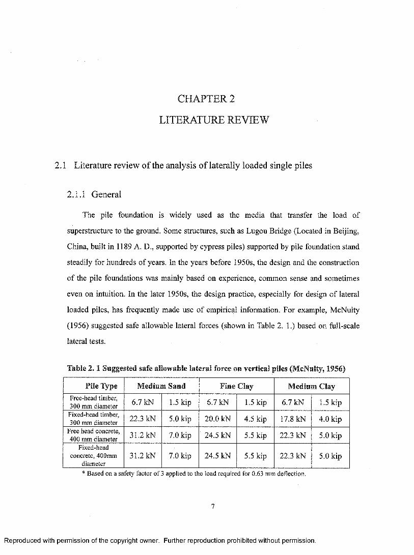
loaded piles, has frequently made use of empirical information. For example, McNulty
(1956) suggested safe allowable lateral forces (shown in Table 2. 1.) based on full-scale
lateral tests.
Table 2.1 Suggested safe allowable lateral force on vertical piles (McNulty, 1956)
Pile Type Medium Sand Fine Clay Medium ClayFree-head timber, 300 mm diameter 6.7 kN 1.5 kip 6.7 kN 1.5 kip 6.7 kN 1.5 kip
Fixed-head timber, 300 mm diameter 22.3 kN 5.0 kip 20.0 kN 4.5 kip 17.8 kN 4.0 kip
Free head concrete, 400 mm diameter 31.2 kN 7.0 kip 24.5 kN 5.5 kip 22.3 kN 5.0 kip
Fixed-head concrete, 400mm
diameter31.2 kN 7.0 kip 24.5 kN 5.5 kip 22.3 kN 5.0 kip
* Based on a safety factor o f 3 applied to the load required for 0.63 mm deflection.
Reproduced with permission of the copyright owner. Further reproduction prohibited without permission.
In past 30 years, however, theoretical approaches for predicting lateral deflections
and bearing capacities o f the pile due to the applied lateral load have been developed
extensively. Two approaches have generally been employed:
1. The subgrade-reaction approach, in which the continuous nature of the soil
medium is ignored and the pile reaction at a point is simply related to the
deflection at that point,
2. The elastic approach, which assumes the soil to be an ideal elastic continuum.
2.1.2 The subgrade-reaction model
The subgrade-reaction model o f soil behavior, which was originally proposed by
Winkler in 1867, characterizes the soil as a series of unconnected linear-elastic springs, so
that deformation occurs only where loading exists. It is the earliest use o f these "springs"
to represent the interaction between soil and the foundations, so the model is thus referred
to as the Winkler method. The one-dimensional representation of this is a "beam on
elastic foundation," thus sometimes it is called the "beam on elastic foundation" method.
In this model, the Coefficient of Subgrade Reaction is used. It is defined as follows:
(2.0 K-lks = coefficient of subgrade reaction (force/length^)
q = bearing pressure (force/length^)
8 = displacement o f foundation component
The obvious disadvantage o f this soil model is the lack of continuity. Real soil is at
least to some extent continuous since the displacement at a point is influenced by stresses
and forces at other points within soil. A further disadvantage is that the spring modulus of
the model (the modulus o f subgrade reaction) is dependent on the size o f the foundation.
In spite of these drawbacks, the subgrade reaction approach has been widely employed in
foundation practice because it provides a relatively simple means o f analysis and enables
Reproduced with permission of the copyright owner. Further reproduction prohibited without permission.

factors such as variation of soil stiffiiess with depth, and layering of the soil profile to be
taken into account readily, although approximately. In addition, despite many difficulties
in determining the modulus o f subgrade reaction of real soil, a considerable amount of
experience has been gained in applying the theory to practical problems, and a number of
empirical correlations (Poulos and Davis 1980, Poulos and Hull 1989) are available for
determining the modulus.
2.1.3 The elastic approach
Poulos and his colleagues contributed to develop the elastic model and several
variations of the model (Poulos and Davis 1980, Poulos and Hull 1989). Solutions have
been presented for variety o f cases of loading of single piles and for the interaction of
piles with close spacing. The elastic solution has gained extensive attention but it is not
suitable for dealing with the problem of large deformation or collapse o f the pile
foundation in highly nonlinear soil.
From a theoretical point o f view, the representation of the soil as a linear elastic
continuum is more satisfactory, as account is taken of the continuous nature of soil. While
the linear elastic model is an idealized representation of real soil, it can be modified to
make allowance for soil yield and can also be used to give approximate solutions for
varying modulus with depth and for layered systems. In addition, it has the important
advantage over the subgrade-reaction approach of enabling analysis to be made of group
action of piles under lateral loads. A further advantage o f the elastic model is that it
enables consistent analysis of both immediate movements and total final movement. The
major drawback to the application of the elastic method to practical problem is the
difficulty of determining the appropriate soil modulus.
2.1.4 Elastic pile and finite element for soil
These models consider the pile as a linear elastic element, which is embedded in a
nonlinear soil modeled by finite element theory. The elements can be fully
Reproduced with permission of the copyright owner. Further reproduction prohibited without permission.
three-dimensional and nonlinear in the physical properties. The elements may be selected
as linear or nonlinear. However, special procedures still are needed to deal with the tensile
stress in the soil, modeling layered soil, accounting for the separation between pile and
soil during repeated loading, the collapse of sand against the back of a pile, accounting
the changes o f the soil characteristic associated with different type of loading. All of these
problems at present have no satisfactory solution.
Yegian and Wright (1973) and Thompson (1977) did their study using
two-dimensional finite element models. Portugal and Seco e Pinto (1993) used the finite
element method based on the p-y curves to obtain a good prediction of the observed
lateral behaviour o f the foundation piles of a Portuguese bridge. Kooijman (1989) and
Brown et al. (1989) used three-dimensional nonlinear fmite elements to develop p-y
curves.
2.1.5 Rigid pile and plastic soil
Broms (1964a, b, 1945) employed the rigid pile and plastic soil model to derive
equations for predicting the loading that develops the ultimate bending moment. The pile
is assumed to be rigid, and a solution is found by use o f the equations of statics for the
distribution o f ultimate resistance o f the soil that puts the pile in equilibrium. After the
ultimate loading is computed for a pile of particular dimensions, the deflection for the
working load may be computed by the equations suggested by the theory. The Broms
method obviously makes use several simplifying assumptions but can be useful for the
initial selection o f a pile.
The engineer can use Broms theory at the beginning o f design if the pile has constant
dimensions and uniform soil characteristics can reasonably considered. Another usage of
the theory is that the solution of the equations will yield the size and length o f the pile for
the expected loading. The pile can then be employed at the starting point for the p-y
method o f analysis.
10
Reproduced with permission of the copyright owner. Further reproduction prohibited without permission.
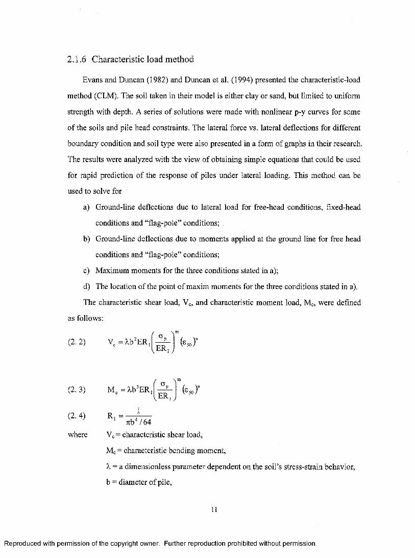
2.1.6 Characteristic load method
Evans and Duncan (1982) and Duncan et al. (1994) presented the characteristic-load
method (CLM). The soil taken in their model is either clay or sand, but limited to uniform
strength with depth. A series of solutions were made with nonlinear p-y curves for some
o f the soils and pile head constraints. The lateral force vs. lateral deflections for different
boimdary condition and soil type were also presented in a form of graphs in their research.
The results were analyzed with the view of obtaining simple equations that could be used
for rapid prediction o f the response o f piles imder lateral loading. This method can be
used to solve for
a) Ground-line deflections due to lateral load for free-head conditions, fixed-head
conditions and “flag-pole” conditions;
b) Ground-line deflections due to moments applied at the ground line for free head
conditions and “flag-pole” conditions;
c) Maximum moments for the three conditions stated in a);
d) The location o f the point of maxim moments for the three conditions stated in a).
The characteristic shear load, Vc, and characteristic moment load. Me, were defmed
as follows:
(2.2) V, =^b"ER,ER, (S50)”
(2. 3) M , = Xh^ER
I
yERi y
(2 .4) R, = ,7ibV64
where Vc = characteristic shear load.
Me = characteristic bending moment,
X = a dimensionless parameter dependent on the soil’s stress-strain behavior,
b = diameter o f pile,
11
Reproduced with permission of the copyright owner. Further reproduction prohibited without permission.

E - modulus o f elasticity o f the pile material,
R i = ratio o f moment o f inertia (dimensionless),
I = moment o f inertia o f pile,
Op = representative passive pressure of soil,
m and n = exponents factors determined by the soil type and force type,
S50 = axial strain at which 50 percent o f the soil strength is mobilized.
The advantage of this method is that the analysis can be obtained quickly and directly. It
can be used to check computer output from more sophisticated analysis and used to
determine the relative stiffiiess factor T.
2.1.7 The p-y curve relationship approach
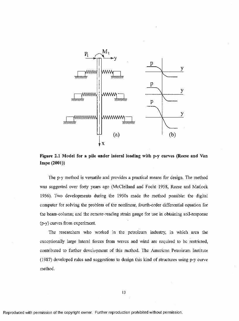
In the late 1940s and 1950s, the model shown in Figure 2.1, which considers the
lateral response of the soil as a function o f the lateral deflection y, was developed. The
solution for beams on an elastic foundation with linear response was presented by
Hetenyi (1946). The numerical solution to a nonlinear differential equation of the pile-soil
system was also presented by Palmer and Thompson (1948). The full-scale tests of
laterally loaded piles were carried out by Gleser (1953), as well as McCammon and
Asherman (1953).
In this approach the pile is considered as a one-dimensional beam embedded in the
soil system. The interaction between the pile and the surrounded soil is modeled by a set
of p-y curves, which denote the relationship between the soil reaction p and the deflection
of pile y. The p-y curves are variable with respect to distance x along the pile and pile
deflection y.
The soil around the pile is replaced by a set of mechanisms that merely indicate that
the soil resistance p is a nonlinear function of pile deflection y. The mechanisms, and the
corresponding curves that represent their behavior, are widely spaced in the sketch but are
considered to be vary continuously with depth. As may be seen, the p-y curves are fully
variable with respect to distance x along the pile and pile deflection y.
12
Reproduced with permission of the copyright owner. Further reproduction prohibited without permission.
7777777777777 im iinitiii
i i / i i m l i i
ywwvwwwTTtmrmtTT wrmimrr
v X
(b )
Figure 2.1 Model for a pile under lateral loading with p-y curves (Reese and Van Impe (2001))
The p-y method is versatile and provides a practical means for design. The method
was suggested over forty years ago (McClelland and Focht 1958, Reese and Matlock
1956). Two developments during the 1950s made the method possible: the digital
computer for solving the problem of the nonlinear, fourth-order differential equation for
the beam-column; and the remote-reading strain gauge for use in obtaining soil-response
(p-y) curves from experiment.
The researchers who worked in the petroleum industry, in which area the
exceptionally large lateral forces from waves and wind are required to be restricted,
contributed to further development of this method. The American Petroleum Institute
(1987) developed rules and suggestions to design this kind o f structures using p-y curve
method.
13
Reproduced with permission of the copyright owner. Further reproduction prohibited without permission.
In other areas, this method has also been broadly used by the engineers since it was
invented. The reason for the popularity o f this model is that the model is based on
full-scale field models and uses the common used soil strength parameters to simulate the
soil resistance-deflection relationships. Further more, this approach takes account of the
complex relationship between the deflection and soil resistance. Different soil phases
such as elastic, nonlinear elastic, softening, and plastic flow were introduced into the p-y
relationship of the pile soil system. Another advantage of this method is that it enables us
to introduce specific p-y relationships according to the on site test results of the soil. This
is very important when new types of soils are subjected to study or more precise results
are required for special projects.
2.1.8 Field testing and analysis of laterally loaded piles in stiff clay located
above water table
It is important to determine the p-y curve in order to model the pile-soil reaction.
Reese and Welch (1972) did a full scale test and provided p-y curve for analysis o f pile
embedded in stiff clay located above water table subjected to cyclic loading. They used a
drilled pier, or shaft, constructed by drilling an open hole, with a diameter of 30 in. (760
mm), to a depth o f 42 ft (13 m) below the ground surface. The instrumented column was a
steel pipe with a wall thickness of % in. (6.4 mm), and an out side diameter of 10 % in.
(270 mm). The site selected for the field test was located in Houston, Tex., near the
intersection o f State Highway 225 and Old South Loop East. The soil profile at the site
consisted of 28 ft (8.5 m) of stiff to very stiif clay, 2 ft (0.6 m) of interspersed silt and clay
layers, and very stiff tan silty clay to a depth o f 42 ft (13 m). At the time of test, the shaft
is above water table. The average undrained shear strength (apparent cohesion) in the
upper 20 ft (6.1 m) is 110 kN/m^. The average value o f the strain at one-half the
maximum stress difference 850 is 0.005 m/m.
14
Reproduced with permission of the copyright owner. Further reproduction prohibited without permission.
The load applied to the shaft was measured by a strain gage load cell in the loading
system and by a pressure transducer connected to hydraulic jack. The shaft was subjected
to repeatable variable loadings. The internal stress and strains and the deformations o f the
shaft were measured.
Reese and Van Impe (2001) also recommended the required soil tests in obtaining the
p-y curves for cyclic loading in stiff clay above water table.
The p-y curve theory will be discussed in details in the CHAPTER 3.
Lutenegger and Dearth (2004) presented series o f static one-way lateral load tests on
prototype-scale drilled shafts installed in a stiff surficial clay crust to investigate the effect
of ground water on lateral load behavior. The paper presents a summary of the testing and
illustrates the influence that groundwater can have on field tests. Tests were conducted
under different ground water conditions at the National Geotechnical Experimentation
Site at the University of Massachusetts, Amherst. The load-displacement results of the
tests are presented in their paper. The results o f the tests show that the load-displacement
behavior was significantly influenced by the ground water regime at the time of testing.
The ultimate lateral load capacity, defmed as the load at a displacement o f 10% of the
shaft diameter, and the initial stiffness increased as the water table dropped. A drop in the
ground water table from 0.4 m to 2.3 m below ground surface increased the ultimate
lateral load from 30 kN to 95 kN.
2.2 Literature review on the analysis of pile groups
2.2.1 General
A pile group is a system made up with 2 or more piles connected with each other at
the end with a pile cap. A pile group may contain battered piles and may be subjected to
simultaneous axial load, lateral load, moment, and possibly, torsional load. There are
varieties of analysis methods to analyze the pile group system. Generally, these methods
may be broken into five categories (which are discussed in section 2 .2.2 to 2.2.6
15
Reproduced with permission of the copyright owner. Further reproduction prohibited without permission.

respectively):
1. Simple static methods that ignore the presence o f the soil and consider the
pile group as a purely structural system.
2. Methods that reduce the pile group to a structural system but take some
account of the effect o f the soil by determining equivalent freestanding
lengths o f the piles.
3. Methods in which the soil is assumed to be an elastic continuum and
interaction between piles can be fully considered.
4. Group Reduction Method and Group Amplification Method, which is based
on single pile analysis with modified modulus.
5. Methods in which the soil is modeled by p-y curve modified according to the
interaction o f the piles in the group.
The first two methods consider interaction between the piles through the pile cap and
not interaction between the soil and piles. The third method allows consideration o f pile
interaction with the soil and the deflections of the piles are calculated together in a group.
The fourth method considers the piles work jointly through the cap and the interaction
between the pile and soil is modeled by modified p-y curves.
2.2.2 Simple static analysis method
Traditional design methods have relied on the consideration o f the pile group as a
simple statically determinate system, ignoring the effect of the soil. This method can be
employed either in an analytical or a graphical way. A graphical solution was presented by
Culmann in 1866 (Terzaghi 1956). A force polygon was used to analyze the equilibrium
state o f the resultant external load and the axial reaction of each pile in the group. The
application of Culmann’s method is limited to the case of a foundation with a group made
of three similar piles. In 1930 Brennecke and Lohmeyer (Terzaghi 1956) presented a
supplemental method to this graphical solution. The vertical component o f the resultant
load is distributed in a trapezoidal shape in such a way that the total area equals the
16
Reproduced with permission of the copyright owner. Further reproduction prohibited without permission.
magnitude of the vertical component. The vertical load is distributed to each pile,
assuming that the trapezoidal load is separated into independent blocks at the top o f a pile,
except at the end piles. The Brennecke and Lohmeyer (Terzaghi 1956) method can handle
more than three similar piles in a group but is restricted to the case where all of the pile
heads are on the same level.
It is worth noting that this method cannot take into account different conditions of
fixity at the pile head, and always assumes zero moment at the head of each pile.
Although methods such as that described above were widely used in design, little is
known as to their reliability. It cannot be expected to be high due to the simplicity o f the
assumptions.
2.2.3 Equivalent bent method
The principle o f this method is illustrated in Figure 2. 2. for a planar group. The
system in Figure 2. 2 (a) is transformed to the equivalent system in Figure 2. 2 (b). Once
the equivalent lengths and areas have been determined, the equivalent bent may be
analyzed by standard structural analysis techniques to determine the deflections, rotations,
and pile stress in the system.
Saul (1968) and Reese et al. (1970) presented matrix analyses in which the above
assumptions are executed in numerical investigations. In Saul’s paper, torsional loading
and dynamic forces are also incorporated. Nair et al. (1969) presented a more convenient
way to compute this system by hand.
17
Reproduced with permission of the copyright owner. Further reproduction prohibited without permission.
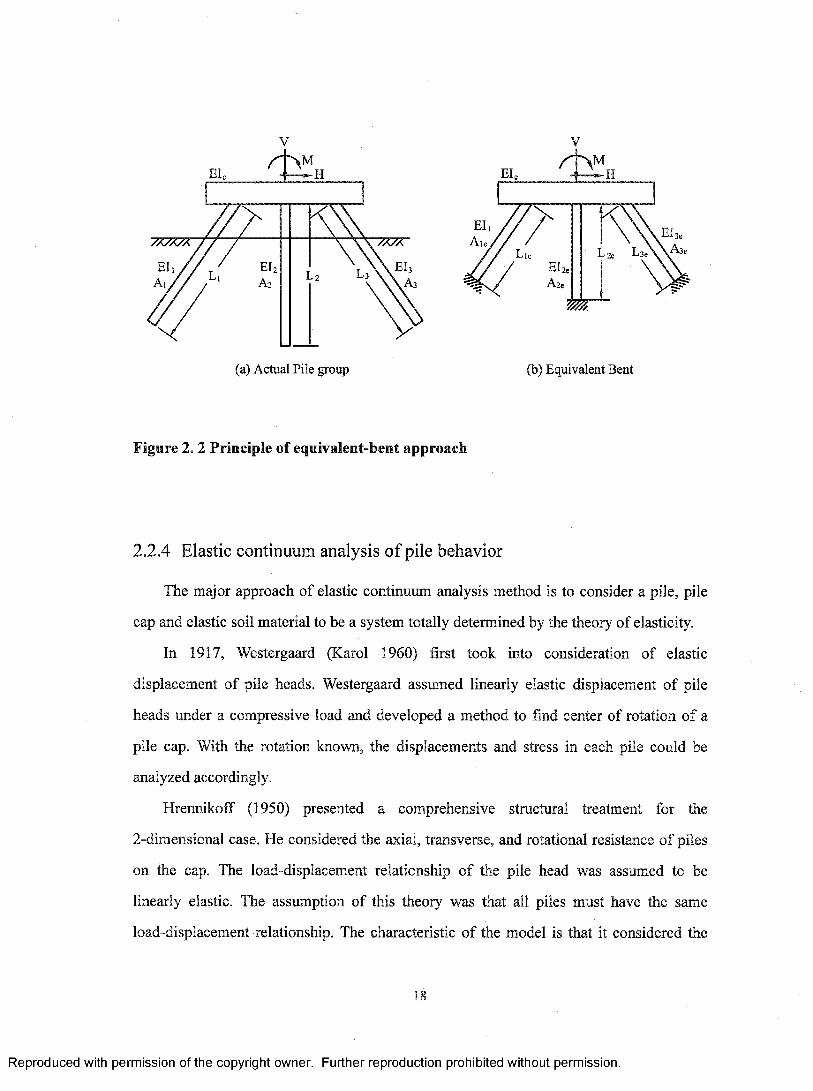
El,
Eh
(a) Actual Pile group
El,
Ale
m
(b) Equivalent Bent
Figure 2. 2 Principle of equivalent-bent approach
2.2.4 Elastic continuum analysis of pile behavior
The major approach o f elastic continuum analysis method is to consider a pile, pile
cap and elastic soil material to be a system totally determined by the theory of elasticity.
In 1917, Westergaard (Karol 1960) first took into consideration of elastic
displacement of pile heads. Westergaard assumed linearly elastic displacement o f pile
heads under a compressive load and developed a method to find center of rotation o f a
pile cap. With the rotation known, the displacements and stress in each pile could be
analyzed accordingly.
Hrennikoff (1950) presented a comprehensive structural treatment for the
2-dimensional case. He considered the axial, transverse, and rotational resistance o f piles
on the cap. The load-displacement relationship o f the pile head was assumed to be
linearly elastic. The assumption of this theory was that all piles must have the same
load-displacement relationship. The characteristic o f the model is that it considered the
18
Reproduced with permission of the copyright owner. Further reproduction prohibited without permission.
laterally loaded pile as an elastic beam on an elastic foundation with uniform stiffness.
The influence factor of the pile group in calculating displacement was defined as the
summation of all the contributions o f single piles. The significance of this method is that
it presents the potential for the analytical treatment of the soil-pile-interaction system.
Asplund (1956) formulated the matrix method for both two-dimensional and
three-dimensional cases. He calculated the stiffness matrix of the pile group and
employed an elastic center method to treat laterally loaded piles. He also considered the
pile arrangement for economical reason. In this model, laterally loaded piles are merely
regarded as elastic beams on an elastic bed with a uniform spring constant.
2.2.5 Group reduction factor method and group amplification method
In this model, the lateral load resistance o f the pile group is determined based on the
single pile analysis but modified according to the pile distance. Prakash (1962) and
Davisson (1970) suggested that the piles would work independently if the pile distances
are more than eight diameters o f piles based on their tests o f piles embedded in sand.
Davisson (1970) also proposed that the pile resistance in a group would equal 75% of a
single pile if the distances between piles were 3 pile diameters. For the piles, which
spaced with a distance o f 3-8 diameters, the soil resistance can be obtained by
interpolation.
Different approach to analyze the laterally loaded pile group was proposed by by Ooi
an Duncim in 1994. It is called Group Amplification Method. This method applies an
amplify coefficient to the lateral deflection bending moment o f piles in the group.
These two methods are highly empirical because they depend on limited test results.
But they provided an effective way to calculate the pile group behaviors through the
analysis of single piles.
2.2.6 The p-multipliers method
The development o f the computer technology made it possible to analyze the
19
Reproduced with permission of the copyright owner. Further reproduction prohibited without permission.
laterally loaded piles using the finite difference and fmite element method. The equations
o f the nonlinear soil-pile interaction can be solved through the finite difference and fmite
element method. So in recent years, more and more research work have been done to
model the soil as a nonlinear material. The p-y curve method is the most commonly used
method in the analysis o f laterally loaded piles and pile groups.
The p-y curve method used to analyze single piles has been explained briefly in the
previous sections. The approach for analyzing the behaviour o f a pile in a group is similar
to the approach used for analysis of a single pile, except that the p-values are reduced
using a p-multiplier to accoimt for the reduced resistance due to the interaction between
piles. The piles and pile cap then can be analyzed as a whole to calculate the deflections
and forces. The computer programs, which are based on the p-multipliers method, are
also readily available in recent years and are in continuous development to incorporate
broader spectrum of variables, such as dynamic effects, that affect the behavior of
laterally loaded pile groups. The p-multipliers method is also used to carry out the
sensitivity analysis o f pile groups in this research.
Brown et al. (1988) firstly proposed the p-multiplier concept. The p-y curves of
single pile are modified to account for the influence o f the interaction between the
different piles in the group. As shown in Figure 2. 3, the p-multiplier fmis the reduction
factor o f soil resistance p for the same deflection of y. The p-y curve is compressed in the
direction of p, so that the soil resistance, p, of piles in-group will be smaller than the soil
resistance o f single piles.
20
Reproduced with permission of the copyright owner. Further reproduction prohibited without permission.
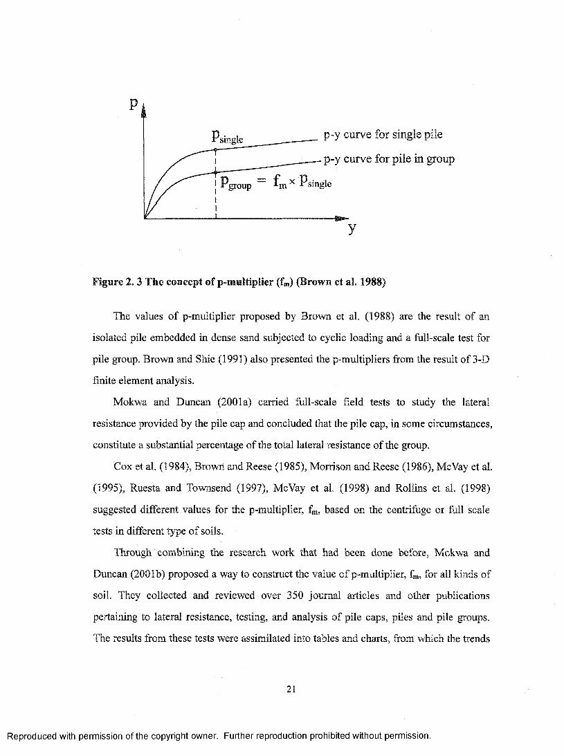
P sin g le — P 'y
p-y curve for pile in group
Pgroup f m ^ P sin g le
y
Figure 2. 3 The concept of p-multiplier (fm) (Brown et al. 1988)
The values o f p-multiplier proposed by Brown et al. (1988) are the result of an
isolated pile embedded in dense sand subjected to cyclic loading and a full-scale test for
pile group. Brown and Shie (1991) also presented the p-multipliers from the result of 3-D
finite element analysis.
Mokwa and Duncan (2001a) carried M l-scale field tests to study the lateral
resistance provided by the pile cap and concluded that the pile cap, in some circumstances,
constitute a substantial percentage of the total lateral resistance of the group.
Cox et al. (1984), Brown and Reese (1985), Morrison and Reese (1986), McVay et al.
(1995), Ruesta and Townsend (1997), McVay et al. (1998) and Rollins et al. (1998)
suggested different values for the p-multiplier, fm, based on the centrifuge or full scale
tests in different type o f soils.
Through combining the research work that had been done before, Mokwa and
Duncan (2001b) proposed a way to construct the value of p-multiplier, fm, for all kinds of
soil. They collected and reviewed over 350 journal articles and other publications
pertaining to lateral resistance, testing, and analysis of pile caps, piles and pile groups.
The results from these tests were assimilated into tables and charts, from which the trends
21
Reproduced with permission of the copyright owner. Further reproduction prohibited without permission.

and similarities can be observed. Their theories are introduce in detail in CHAPTER 4.
Ilyas et al. (2004) proposed a centrifuge model study o f laterally loaded pile groups
in clay. A series o f centrifuge model tests has been conducted in their research to examine
the behavior o f laterally loaded pile groups in normally consolidated and over
consolidated kaolin clay. The pile groups have a symmetrical plan layout consisting of 2,
2x2, 2x3, 3x3 and 4x4 piles with a center-to-center spacing o f three or five times the pile
width. The piles are connected by a solid aluminum pile cap placed just above the ground
level. It is established that the pile group efficiency reduces significantly with increasing
number of piles in a group. The tests also reveal the shadowing effect phenomenon in
which the front piles experience larger load and bending moment than that o f the trailing
piles. The shadowing effect is most significant for the lead row piles and considerably
less significant for subsequent rows of trailing piles. They also pointed out that the
approach adopted by many researchers of taking the average performance of piles in the
same row is found to be inappropriate for the middle rows, o f piles for large pile groups
as the outer piles in the row carry significantly more load and experience considerably
higher bending moment than those of the inner piles. They also compared their
p-multiplier results with those of other researchers as stated in Table 2. 2:
22
Reproduced with permission of the copyright owner. Further reproduction prohibited without permission.

Table 2. 2 Comparison of p-multiplier values from various experimental and field studies for pile groups with pile center-to-center spacing of 3 pile widths (Ilyas et al. 2004)
Size of
pile
group
Average p-multiplier
Leading
row
2nd
trailing trailing
4*
trailingAuthor/soil type and shear strength row row row
Clay
Ilyas et al. (2004) / normally consolidated clay:2x1
2x2
0.8
0.96
0.63
0.78
undrained shear strength = 0-20kPa
3x3 0.65 0.50 0.48
4x4 0.65 0.49 0.42 0.46
Brown et al. (1987) / over consolidated clay:
strength = 70-180kPa3x3 0.7 0.5 0.4
Meimom et al. (1986) / silty clay: strength =2x2 0.9 0.5
25kPa
Rollins et al. (1998) / clayed silt: strength =
50-75kPa3x3 0.6 0.4 0.4
Sand
Brown et al. (1988) / clean medium sand:
friction angle O = 38°3x3 0.8 0.4 0.3
McVay et al. (1995) / medium dense sand 3x3 0.8 0.4 0.3
Mcvay et al. (1998) / medium dense sand 4x3 0.8 0.4 0.4 0.3
Ruesta and Townsend (1997) / loose find sand:
friction angle O = 32°4x4 0.8 0.7 0.3 0.3
2.3 Literature review on the sensitivity analysis of pile foundation
2.3.1 Definition of the sensitivity analysis
Sensitivity Analysis (SA) in this research is defined as the study o f how the
performance of a system (numerical or otherwise) can be affected, qualitatively or
23
Reproduced with permission of the copyright owner. Further reproduction prohibited without permission.
quantitatively, by the change o f the design variables related to the system.
Sensitivity Analysis (SA) aims to ascertain how the model depends upon the
information fed into it, upon its structure and upon the framing assumptions made to build
it. This information can be invaluable, as
• Different level o f acceptance (by the decision-makers and stakeholders) may be
attached to different types o f uncertainty.
• Different uncertainties impact differently on the reliability, the robustness and the
efficiency of the model.
2.3.2 Aim and importance of the sensitivity analysis
A mathematical model is defined by a series o f equations, input factors, parameters,
and variables aimed to characterize the process being investigated. Input is subject to
many sources of uncertainty including errors o f measurement, absence o f information and
poor or partial understanding o f the driving forces and mechanisms. This imposes a limit
on our confidence in the response or output of the model. Further, models may have to
cope with the natural intrinsic variability of the system, such as the occurrence of
stochastic events. Good modeling practice requires that the modeler provides an
evaluation o f the confidence in the model, possibly assessing the uncertainties associated
with the modeling process and with the outcome of the model itself.
Originally, SA was created to deal simply with uncertainties in the input variables
and model parameters. Over the course o f time the ideas have been extended to
incorporate model conceptual uncertainty, i.e. uncertainty in model structures,
assumptions and specifications. As a whole, SA is used to increase the confidence in the
model and its predictions, by providing an understanding of how the model response
variables respond to changes in the inputs, model structures, or factors, i.e. the model
independent variables. SA is thus closely linked to uncertainty analysis (UA), which aims
to quantify the overall uncertainty associated with the response as a result of uncertainties
in the model input.
24
Reproduced with permission of the copyright owner. Further reproduction prohibited without permission.
Many parameters in system models represent quantities that are very difficult, or
even impossible to measure to a great deal o f accuracy in the real world. Also, some
parameter values change in the real world. Therefore, when building a system model, the
modeler is usually at least somewhat uncertain about the parameter values he chooses and
must use estimates. Sensitivity analysis allows him to determine what level o f accuracy is
necessary for a parameter to make the model sufficiently useful and valid. Sensitivity
analysis can also indicate which parameter values are reasonable to use in the model.
Generally speaking, we may conduct sensitivity analysis to determine
(a) the model resemblance with the process imder study,
(b) the quality o f model definition,
(c) factors that mostly contribute to the output variability,
(d) the region in the space of input factors for which the model variation is
maximum,
(e) optimal regions within the space o f factors for use in a subsequent calibration
study,
(f) interactions between factors.
2.3.3 The procedures to conduct sensitivity analysis
There are several possible procedures to perform sensitivity analysis. The most
common sensitivity analysis is sampling-based. A sampling-based sensitivity is one in
which the model is executed repeatedly for combinations o f values sampled from the
distribution (assumed known) of the input factors. In general, SA is performed jointly by
executing the model repeatedly for combination o f factor values sampled with some
probability distribution. The following steps can be listed:
1. specify the target function and select the input o f interest,
2. assign a distribution function to the selected factors,
3. generate a matrix of inputs with that distribution(s) through an appropriate design,
4. evaluate the model and compute the distribution o f the target function,
25
Reproduced with permission of the copyright owner. Further reproduction prohibited without permission.
5. select a method for assessing the influence or relative importance o f each input
factor on the target fimction.
Sensitivity analysis is usually performed as a series of tests in which the modeler sets
different parameter values to see how a change in the parameter causes a change in the
dynamic behavior o f the systems.
2.3.4 Term definitions
The terms used in the sensitivity analysis were defmed by Kohn (2002) as follows:
state variable—the quantities that specify the instantaneous description (state) of the
system
independent variable—the dimension (typically time) over which the state of the
system changes
state equations— equations that specify the state variables as functions of the
independent variable (typically differential equations)
boundary conditions—constraints that specify the particular solution o f the state
equations; e.g. initial values of the state variables or the rate o f input to a process in the
model
transient—the temporal profile o f the state variables after a perturbation in the
boundary conditions
steady state— a solution o f the state equations when the time derivatives of the state
variables are all set to zero; also called a stationary state
parameters— constants (as opposed to variables) in the state equations
sensitivity coefficient—a partial derivative o f a state variable with respect to
variations in a parameter value; these quantities may vary with time.
2.3.5 The virtual load method for sensitivity analysis of structures
Atrek (1996) summarized virtual load methods for sensitivity analysis o f linear
structures. He stated that a response quantity rj can be written as:
26
Reproduced with permission of the copyright owner. Further reproduction prohibited without permission.
(2. 5) r- = p I u
where py is the virtual load vector corresponding to rj, and u is the structural displacement
vector for an applied load vector p.
The virtual method is based on the principle of virtual work. The works o f Toakley
(1968) and Barnett and Hermann (1968) appear to have been among the first to have
employed this hitherto well known concept in order to represent nodal displacements of a
discretized structure explicitly in terms o f the design variables, within the framework of a
systematic approach to structural optimization. It was pointed out in this approach that
each element contribution can be computed separately and the response then computed as
a sum of element contributions. It was also notified that the assumptions made by the
virtual loading consists of a unit load placed at the same node and along the same axis as
the response (deformations) under consideration.
Atrek (1999) extended the application of the virtual load method to the realm of
nonlinear response. The usual nonlinear analysis, handled in a finite element based
solution, is to treat it as a series o f linear analyses. Thus, if rjt is the value of the jth
response quantity at time t during the nonlinear analysis, then
m
(2- 6)k=l
where k = 1, ... , m indicates the series o f linear analyses, the results rjt, of which are
added to arrive at the final result at time t.
2.3.6 The methods of sensitivity analysis
There are two main approaches for estimating the sensitivity o f simulations with
respect to design variables: the forward sensitivity or tangent linear model method, and
the backward or adjoint method.
For models comprised o f ordinary differential equations and/or nonlinear algebraic
equations, the forward sensitivity analysis is normally used. Forward sensitivity methods
27
Reproduced with permission of the copyright owner. Further reproduction prohibited without permission.
can be formulated in terms of an ordinary differential equation, differential-algebraic
equation or algebraic equation (for steady state problems) for the solution sensitivities
with respect to a fixed set of parameters. These new equations can be appended to the
original system, and the resulting augmented system can be solved by the respective
solver code. The additional sensitivity equations contain terms involving Jacobian
matrix-vector products and partial derivatives. Finite differences can be used to estimate
these terms. For some problems, however, this technique does not work. In particular,
difficulties can arise in applications where the solution components are badly scaled. Such
shortcomings motivate researchers to use automatic differentiation (AD) as an efficient
and exact technique for evaluating various terms in the sensitivity equations. AD can also
be used to compute the forward sensitivities in a general simulation code by
differentiating the entire code with respect to a specified set o f parameters. This more
general approach, however, is usually less efficient because it does not exploit the user's
knowledge of the computational requirements o f the simulation.
In cases where the sensitivity o f the solution is needed with respect to a large number
of parameters, adjoint methods may prove more useful. Analogous to the approach for the
forward sensitivities, finite differences or AD can be used to evaluate the adjoint
sensitivity equations within the equation solver. Alternatively, a reverse-mode of AD can
be applied to differentiate a simulation code with respect to the model parameters.
2.3.7 Review of the sensitivity analysis applied to the structures and pile
foundations
The sensitivity analysis is broadly used in many scientific fields, such as computer
science, electronic science and biology etc. Some of the sensitivity analyses applied to the
structures and pile foundations were reviewed in the following sections.
2.3.7.1 Damage assessment by FE model updating using damage functions
Teughels et al. (2002) presented a sensitivity-based finite element (FE) model
28
Reproduced with permission of the copyright owner. Further reproduction prohibited without permission.
updating method using experimental modal data. The procedure employed aimed to
adjust the uncertain properties of the FE model by minimizing iteratively the differences
between the measured modal parameters (natural frequencies and mode shapes) and the
corresponding analytical predictions. In the paper the FE model-updating method was
applied to damage assessment (damage localization and quantification) of structures
whose damage pattern can be represented by a reduction factor o f the element bending
stiffness. But in order to reduce the number o f unknown variables and to obtain a
physically meaningful result, a limited set of damage functions was used to determine the
bending stiffness distribution over the FE model. The updating parameters were the
multiplication factors o f the damage functions. The procedure was illustrated by a modal
test before and after damage application, on a reinforced concrete beam.
2.3.7.2 Sensitivity analysis of elastoplastic structures by using explicit
integration method
Ohsaki (1997) presented an algorithm for sensitivity analysis o f responses o f an
elastoplastic structure. The structure was modeled by the finite element method, and
responses are found by using an explicit integration method incorporating higher-order
differential coefficients with respect to the path parameter. All the governing equations
were differentiated with respect to the design variables, and sensitivity coefficients o f the
responses were updated incrementally at each step.
2.3.7.3 Sensitivity analysis of piles subject to lateral load or bending
moment
Budkowska (1997a) presented the general formulation of the sensitivity analysis of
laterally loaded pile embedded in a homogeneous soil medium. This approach is also
based on the principles o f variational calculus. The central point o f analysis is connected
with the concept o f function with constraints, which is then transformed into augmented
function without constraints, however dependent on the Lagrange multipliers vector. The
29
Reproduced with permission of the copyright owner. Further reproduction prohibited without permission.

other part o f this paper (1997b) investigated the short steel piles subjected to a bending
type load. The pile structures are embedded in homogeneous sand and clayey soil
modeled as a one-dimensional structural element supported by Winkler type foundation.
The modulus of subgrade reaction for clay is constant, while that for sandy soil varies
linearly. The design variables are taken as the bending stiffness o f the pile structure and
modulus of subgrade reaction. Based on the distributions o f sensitivity integration
operators for short piles embedded in clay and sandy soils, some conclusions of
considerable importance for engineering practice are presented.
Budkowska and Cean (1995) presented the sensitivity analysis o f short piles subject
to pile bending moment. First variations of the generalized lateral displacement and
internal forces at the specified cross-section were derived based on the adjoint structure
method combined with the virtual work theorem. The pile was modeled as a
one-dimensional beam element. The response of the soil was simulated by the Winkler
type foundation. The behaviour of the short pile is obtained via the solution of differential
equation of the problem with suitable boundary conditions. The distributions of
sensitivity coefficients o f kinematic quantities at specified cross-sections were also
presented.
Budkowska and Suwamo (2002) presented a sensitivity analysis of lateral
displacements o f long single pile subjected to static horizontal forces applied at the soil
surface. The soil under study is stiff clay below water table that is modeled by means of
the p-y curve. The material characteristics o f the pile-soil system are taken as the design
variables. The sensitivity functional of a nonlinear pile-soil system is formed with the aid
o f the adjoint system that demonstrates the nonlinear features. The determination o f the
first variation o f lateral displacement functional due to the changes o f the design variables
resulted in formulation o f the sensitivity integrands associated with each design variable.
Liu and Budkowska (2004) presented the sensitivity analysis o f short laterally loaded
piles embedded in stiff clay subjected to cyclic loading. The pile structure is modeled as
30
Reproduced with permission of the copyright owner. Further reproduction prohibited without permission.

one dimensional beam element. The adjacent soil is simulated by means of the
constitutive p-y relationship developed by Welch and Reese (1972). The constitutive
parameters o f the pile structure and the soil that are involved in the p-y constitutive
relationships are taken as the design variables. The maximum lateral deflection of the
pile-soil system is subjected to sensitivity analysis. The design variables are considered as
the continuous distributed parameters (Kleiber et al. 1997). The sensitivity investigations
are conducted by means of the adjoint system method that appears to be the most
effective (Dems and Mroz 1983). The sensitivity operators that affect the maximum
lateral deflection of the pile-soil system due to the changes o f the design variables are
determined.
Priyanto (2002) conducted the research work for a thesis leading to a M. A. Sc.
degree about the sensitivity analysis o f piles embedded in soft clay located below the
water table subjected to lateral cyclic loadings. He carried out his sensitivity analysis for
laterally loaded piles and pile groups embedded in the soft clay below water with the p-y
relationship shown in Figure 2. 4. The design variables under investigation are the
saturated unit weight y ' , soil cohesion c, 850, the coefficient of subgrade reaction k and
friction angle <j).
Suwamo (2003) carried out the sensitivity analysis of laterally loaded piles and pile
groups embedded in stiff clay below water table. His research is based on a soil model
shown in Figure 2. 5. In his thesis, the sensitivity analysis is focused on the changes o f the
design variables which are the stif&iess o f the pile section (El), the cohesion of the soil (c),
the modulus of the subgrade reaction (k), the effective unit weight (y ') , the strain at
which 50% soil strength is mobilized (Sj^) and the width o f pile (b). In the thesis both the
theoretical formulations and numerical investigations were presented to conduct the
sensitivity analysis of single piles and pile groups.
31
Reproduced with permission of the copyright owner. Further reproduction prohibited without permission.

0.5
For x>x0.72
0.5
0.72
Figure 2. 4 The p-y curves for soft clay below w ater table (Matlock, 1970)
2.5 \y-0.45y
P = A ,p0.45yAcPc
0.085 p
Yso
1.8y, Deflection, y (m)
Figure 2. 5 The p-y curves for stiff clay below water table (Reese et al., 1975)
32
Reproduced with permission of the copyright owner. Further reproduction prohibited without permission.
CHAPTER 3
THEORETICAL FORMULATION OF SINGLE FILE
3,1 Introduction
3,1.1 Soil and deep foundation
For engineering purpose, soil is defined as an uncemented aggregate o f mineral
grains and decayed organic matter (solid particles) with liquid and gas in the empty
spaces between the solid particles. A foundation is a media used to transfer the load of the
supper structure to the ground. It should meets two kind of safety requirement: enough
strength and deformation of foundation under a certain standard. These two requirements
are called strength ability and serviceability respectively. As one of the mostly used
foundations, the pile foundation is used to transfer the load o f superstructure to soil under
the ground level. It is used very often when the ground is not strong enough to carry the
load above directly.
The pile structure is selected to support mainly vertical load. Also the piles are
designed to carry lateral load in many structures, like bridges, offshore structures, harbor
structures, retaining walls etc. But it was mostly based on the experience while the
engineers design the laterally loaded piles before the development o f new theories of
laterally loaded piles recently. This chapter presents the soil-pile behaviour of stiff clay
above the water table after Reese and Welch (1972) and derivation o f equations for
sensitivity analysis.
33
Reproduced with permission of the copyright owner. Further reproduction prohibited without permission.
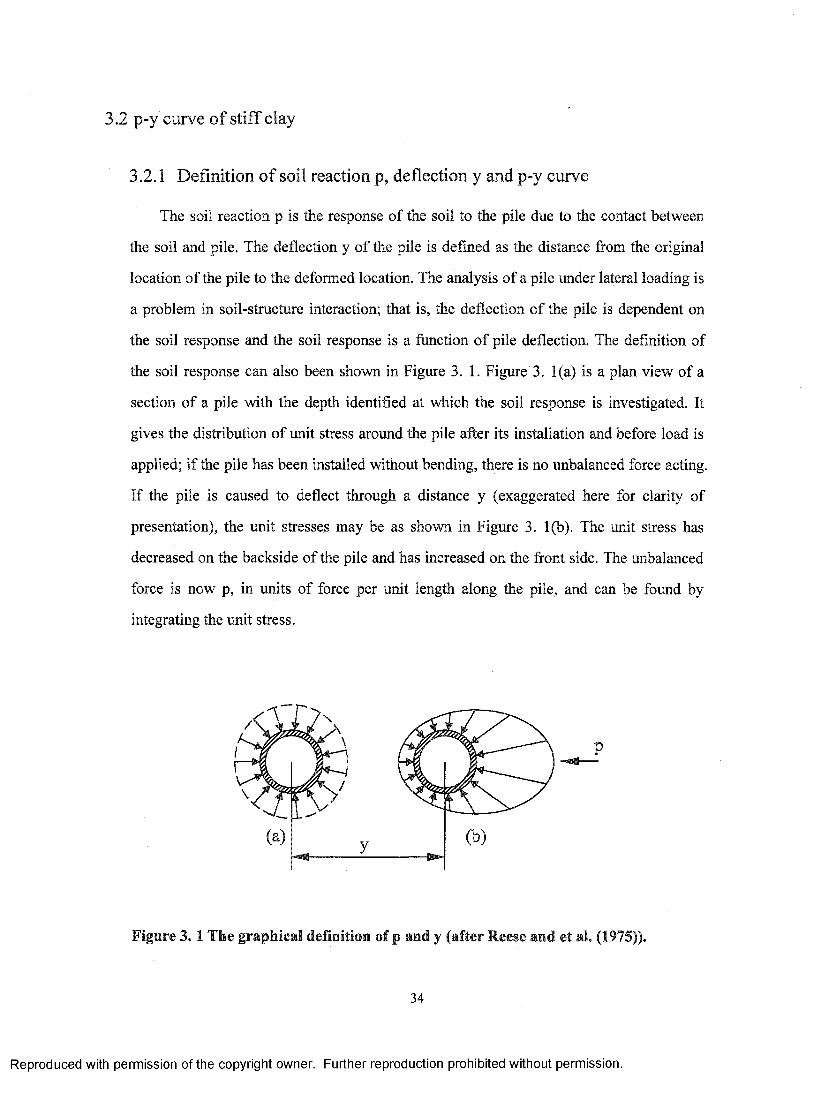
3.2 p-y curve of stiff clay
3.2.1 Definition o f soil reaction p, deflection y and p-y curve
The soil reaction p is the response o f the soil to the pile due to the contact between
the soil and pile. The deflection y of the pile is defined as the distance from the original
location o f the pile to the deformed location. The analysis o f a pile under lateral loading is
a problem in soil-structure interaction; that is, the deflection of the pile is dependent on
the soil response and the soil response is a function of pile deflection. The definition of
the soil response can also been shown in Figure 3. 1. Figure 3. 1(a) is a plan view of a
section o f a pile with the depth identified at which the soil response is investigated. It
gives the distribution o f unit stress around the pile after its installation and before load is
applied; if the pile has been installed without bending, there is no unbalanced force acting.
If the pile is caused to deflect through a distance y (exaggerated here for clarity of
presentation), the unit stresses may be as shown in Figure 3. 1(b). The unit stress has
decreased on the backside of the pile and has increased on the front side. The unbalanced
force is now p, in units of force per unit length along the pile, and can be found by
integrating the unit stress.
Figure 3 . 1 The graphical definition of p and y (after Reese and et al. (1975)).
34
Reproduced with permission of the copyright owner. Further reproduction prohibited without permission.
A nonlinear relationship exists between p and y because, at some deflection y, the
soil response p will reach a limit and remain constant, or perhaps decrease, with further
deflection. The nonlinear curve relating the soil response and the pile deflection is termed
a p-y curve.
There is a method of analysis that is employed in some engineering offices. It starts
with the selection of a depth below the ground line at which the pile is assumed to be
fixed against rotation. No soil is assumed to exist along the pile above that point; thus, the
pile in soil is replaced by a cantilever beam, and solving for deflection and bending
moment proceeds by using the ordinary equations of mechanics. If, by chance, the depth
to the point o f fixity was selected correctly, the computed maximum bending moment
would agree with the actual maximum moment, but the distribution of bending moment
along the pile would certainly be incorrect. Further more, the selection of a point o f fixity
(such that both the maximum deflection and the maximum bending moment both were
computed correctly) would be a virtual impossibility. Thus, no guidelines can be
developed for selecting a point of fixity that would allow the response of a pile to be
calculated accurately. So it is necessary for us to develop a new method—p-y method in
order to get much more accurate results.
3.2.2 Reese and Welch’s p-y curve theory for stiff clay above water table
Based on the research, the shapes o f the typical p-y curves for stiff clay above water
table subjected to static and cyclic loading are shown in Figure 3. 2.
35
Reproduced with permission of the copyright owner. Further reproduction prohibited without permission.

p = p .
p = 0.5p9.6
logN
y
Figure 3.2 p-y curves for stiff clay above w ater table subjected to cyclic loading
The physical relationship between the soil reaction p and the lateral displacement at
an arbitrary depth is presented as follows:
for y<16y5o+9.6y5ologN:
(3. 1) P = 0-5p„1 9.6
'50 1 + — l o g N to
for y> 16y5o+9.6y5ologN:
(3. 2) p = p„
where p = the soil reaction,
Pu = ultimate soil’s resistance.
36
Reproduced with permission of the copyright owner. Further reproduction prohibited without permission.
y = lateral displacement,
N = the number o f load cycles.
The yso is related to the dimensionless parameter 850 by means of the relationship:
(3 .3) Yso = 2 .5850b
where S50 = strain corresponding to 50% of maximum principal strain difference,
b = the width of the pile.
The ultimate soil resistance pu for x <Xr where Xr means the depth of the reduced
resistance, is:
(3. 4) p„ = cbb b
where c = the undrained cohesion,
Y = the soil’s unit weight,
b = the pile’s width,
J = constant, for stiff clay J=0.25.
for X >X r
(3. 5) p„ = 9cb
The depth Xr of the reduced resistance is determined from the continuity o f Eqs.(3. 4)
and (3. 5) that result in:
6cb(3. 6) X, = —— -
yb + Jc
The variability o f ultimate soil resistance p„ along the pile axis is shown graphically
in Figure 3.3.
For different load cycles, the p-y curves come out as a series o f curves shown in
Figure 3. 4, in which the abscissa stands for the pile deflection y and ordinate means the
soil resistance p and different Nj define the different number o f load cycles. The p-y
relationship is consisted of two physical states, which are nonlinear elastic and plastic
flow. It means that if the pile deflection y is less than 16y5o+9.6(y5o)logNi, the physical
37
Reproduced with permission of the copyright owner. Further reproduction prohibited without permission.
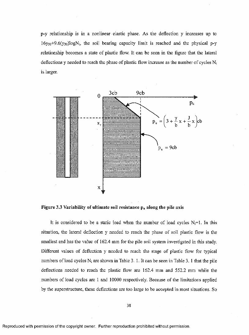
p-y relationship is in a nonlinear elastic phase. As the deflection y increases up to
16y5o+9.6(y5o)logNi, the soil bearing capacity limit is reached and the physical p-y
relationship becomes a state o f plastic flow. It can be seen in the figure that the lateral
deflections y needed to reach the phase of plastic flow increase as the number o f cycles Ni
is larger.
3cb 9cb
Pu
Y J 3 + ^ x + - x cb
Pu = 9cb
Figure 3.3 Variability of ultimate soil resistance p„ along the pile axis
It is considered to be a static load when the number o f load cycles Nj=l. In this
situation, the lateral deflection y needed to reach the phase o f soil plastic flow is the
smallest and has the value o f 162.4 mm for the pile soil system investigated in this study.
Different values o f deflection y needed to reach the stage o f plastic flow for typical
numbers of load cycles Nj are shown in Table 3. 1. It can be seen in Table 3. 1 that the pile
deflections needed to reach the plastic flow are 162.4 mm and 552.2 mm while the
numbers of load cycles are 1 and 10000 respectively. Because o f the limitations applied
by the superstructure, these deflections are too large to be accepted in most situations. So
38
Reproduced with permission of the copyright owner. Further reproduction prohibited without permission.

most o f time the pile-soil system is in the nonlinear elastic phase along the whole pile
length.
P
P = P
P
N 3
9.6
16Y50 +9-6(Y5o)log N 2 9.6(y5o)log Na
Figure 3. 4 Characteristic shape of p-y curves for cyclic loading in stiff clay above w ater table for different load cycles Ni, N2 and N3 (Ni<N2<N3) (after Welch and Reese, 1972)
Table 3 .1 The pile deflections y needed to reach the soil plastic flow for the pile-soil system investigated in this study subjected to constant load with variable number of load cycles Ni=l, 10,100,1000 and 10000
Number o f load cycles Ni
1 10 100 1000 10000
The pile deflections y needed to reach soil plastic
flow.16y5o+9.6(y5o)logNi
162.4 mm 259.8 mm 357.3 mm 454.7 mm 552.2 mm
39
Reproduced with permission of the copyright owner. Further reproduction prohibited without permission.

3.3 Theoretical formulation of sensitivity analysis of laterally loaded piles
embedded in stiff clay above water table
3.3.1 General
In this study, the behavior o f laterally loaded pile embedded in the soil is considered
as a pile-soil interaction system. The pile structure is considered to be a one-dimensional
beam supported by the nonlinear springs, which are simulated by the p-y curves for the
stiff clay above water table subjected to cyclic loading. The concept o f this model can be
shown in Figure 3. 5.
deflected axis y
Nonlinear springs modeled by the p-y curves for the stiff clay above water table subjected to cyclic loading
Figure 3. 5 A pile element modeled by a beam supported by nonlinear springs
3.3.2 Primary and adjoint structure
In this study, the concepts of primary and adjoint structure are widely used. The
primary structure is a “real” structure, in which the actual forces are applied to an actual
existing pile-soil structure system; hence the actual deformations and internal forces are
40
Reproduced with permission of the copyright owner. Further reproduction prohibited without permission.
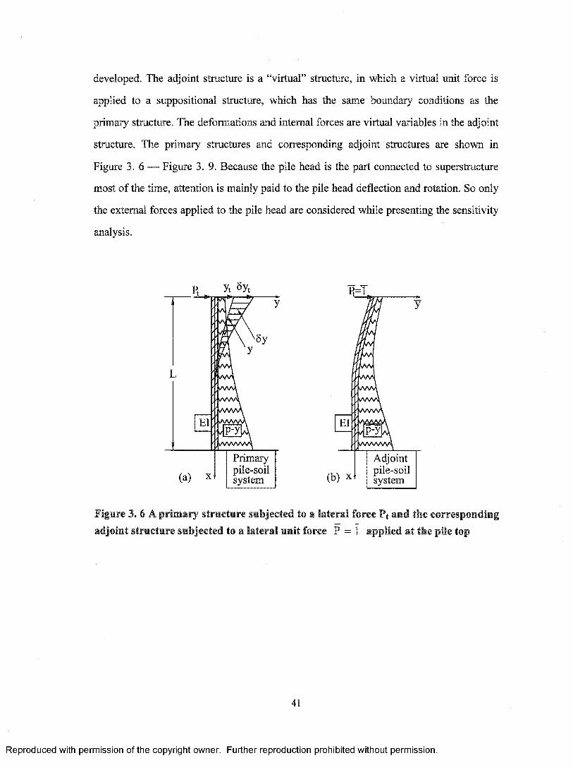
developed. The adjoint structure is a “virtual” structure, in which a virtual unit force is
applied to a suppositional structure, which has the same boundary conditions as the
primary structure. The deformations and internal forces are virtual variables in the adjoint
structure. The primary structures and corresponding adjoint structures are shown in
Figure 3. 6 — Figure 3. 9. Because the pile head is the part connected to superstructure
most o f the time, attention is mainly paid to the pile head deflection and rotation. So only
the external forces applied to the pile head are considered while presenting the sensitivity
analysis.
Primarypile-soilsystem
P t^
Adjointpile-soilsystem(b) X
Figure 3. 6 A primary structure subjected to a lateral force Pj and the corresponding adjoint structure subjected to a lateral unit force P = 1 applied at the pile top
41
Reproduced with permission of the copyright owner. Further reproduction prohibited without permission.
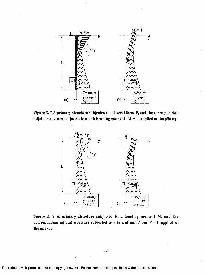
Primarypile-soilsystem
Adjointpile-soilsystem(b) X
Figure 3. 7 A primary structure subjected to a lateral force Ft and the corresponding adjoint structure subjected to a unit bending moment M = 1 applied at the pile top
P-y
Primarypile-soilsystem
P-y
Adjointpile-soilsystem
Figure 3. 8 A primary structure subjected to a bending moment Mt and the corresponding adjoint structure subjected to a lateral unit force P = 1 applied at the pile top
42
Reproduced with permission of the copyright owner. Further reproduction prohibited without permission.
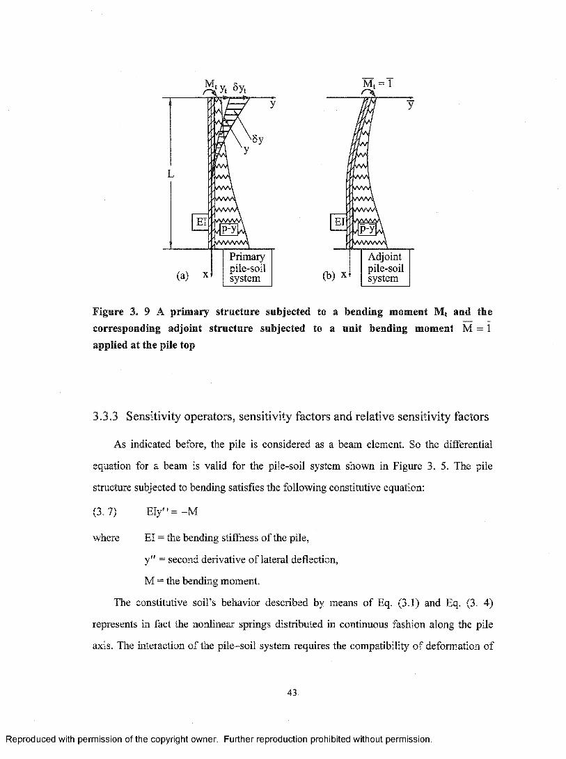
Primarypile-soilsystem
Adjointpile-soilsystem
Figure 3. 9 A primary structure subjected to a bending moment Mt and the corresponding adjoint structure subjected to a unit bending moment M = 1 applied at the pile top
3.3.3 Sensitivity operators, sensitivity factors and relative sensitivity factors
As indicated before, the pile is considered as a beam element. So the differential
equation for a beam is valid for the pile-soil system shown in Figure 3. 5. The pile
structure subjected to bending satisfies the following constitutive equation:
(3. 7) E Iy "= -M
where El = the bending stiffness o f the pile,
y” = second derivative o f lateral deflection,
M = the bending moment.
The constitutive soil’s behavior described by means o f Eq. (3.1) and Eq. (3. 4)
represents in fact the nonlinear springs distributed in continuous fashion along the pile
axis. The interaction of the pile-soil system requires the compatibility o f deformation o f
43
Reproduced with permission of the copyright owner. Further reproduction prohibited without permission.
the pile structure and the adjacent soil. The differential equation that governs the
relationship between the distributed load, which is also the soil reaction p, El and
deflection y is known to all as:
(3. 8) - p = 0
where p = the soil reaction, distribute load along pile axis, kN/m,
= the fourth derivative of y with respect to spatial variables
The physical parameters, which have influences on the lateral resistance capacity,
should be considered and analyzed. It is postulated that all physical parameters of the pile
and the soil that affect the performance o f the pile-soil system are taken as the design
variables. They are arranged in the vector Z of the design variables as follows:
(3 .9) Z = [EI, c , y , b, 8 5 0 , N f
The deformation analysis o f the pile-soil system is conducted for the system being in
the state of static equilibrium. In Figure 3. 6 — Figure 3. 9, for the primary system, the
pile deflections are denoted as y and rotations are denoted as 0 respectively. While at x=0,
the values of deflection y = yt and rotation 0= 0t. On the other hand, if any of the design
variables Z varies, there will be changes occurred to the deflection y and rotation 0 as a
result. These changes are denoted as 5y and 50 respectively.
The variables used in the primary structure shown in Figure 3. 6— Figure 3. 9 can be
divided into to two categories: the state variable (y, y \ y " , y '" , , Pt, Mt, M, p)
and design variable (Z). The deflection y and rotation 0 will change if any o f the state
variables or the design variables changes. The former case means the loads change
whereas the design variables remain constant. This case shows the performance of a
certain pile system under different loads. However, the latter case means the loads keep
constant but the design variables change. The change of the performance associated with
the second case is defined as a sensitivity o f the performance due to the changes of the
design variables. The changes o f the design variables can be arranged in the vector 3Z
44
Reproduced with permission of the copyright owner. Further reproduction prohibited without permission.
defined as:
(3. 10) 8Z = [5EI, 5c, 5y, 5b, 5 N f
where the symbol 6 stands for the variation or change of the variable.
The vector o f the pile head deformation A is consisted of two components, i.e., the
head lateral displacement yx and the angle of rotation Oj. Thus:
(3.11) A = S y „e ,} ’'
the first order o f variation of the deformation of the pile head is:
(3. 12) 6A = {6yT,50Tr
Based on the virtual work theory (Washizu, 1976), for elastic systems, the virtual
work, done by the unit force in the adjoint structure, II is defined as:
(3.13) n = i • A
The first order variation of the virtual work 511 is defined as:
(3. 14) 6n = i®5A
With small variation 5A, the Eq. (3. 14) is valid because the nonlinear elastic system
can be considered linear without unreasonable error in a very small variation area.
Because the nonlinear characteristic of the soil-pile system, our sensitivity analysis in this
research are only restricted to small variations o f design variables. Applying the
sensitivity analysis results to large design variable variations should be carried out with
special caution.
Taking into accoimt vector Z given by the definition (3. 9) together with Eq. (3. 7)
and Eq. (3. 8), the increment of internal forces o f the pile-soil system can be expressed as:
(3. 16) 5p = - ^ 5 y - F - ^ 6 Z 5y dZ
It is interesting to note that Eqs.(3. 15) and (3. 16) are the physical equations that
45
Reproduced with permission of the copyright owner. Further reproduction prohibited without permission.
allow for the variability o f the state variables and the physical parameters as well. For the
primary system subjected to constant load, the condition of state equilibrium implies that:
(3. 17) 5M = 0
(3. 18) 5p = 0
Thus the unknown 5y" and 5y can be determined from Eqs. (3. 17) and (3. 18), that
result in the following:
(3.20) 5y = - - ^ - ^ 5 Z5p dZ
The determination o f 5yt and 50t o f primary structure can be established with aid of
the adjoint system. It is conducted based on the virtual work principle applied with
respect to increments o f generalized deformation of primary structure. Then,
_ L L
(3. 21) 15y, = - jM ^6y"dx + jp^bydx0 0
and
L L— A M(3. 22) 156, = - J M 5 y "d x + Jp 5ydx
where M = the bending moment o f the adjoint structure subjected to F = 1;
_ p „p - the soil reaction of the adjoint structure subjected to P = 1;
---M = the bending moment o f the adjoint structure subjected to M = 1;
“ Mp = the soil reaction of the adjoint structure subjected to concentrated bending
moment M = 1.
5y, 6y" = variations of deformations imposed on the primary system.
The Equation (3. 21) and (3. 22) can be combined into one general equation:
46
Reproduced with permission of the copyright owner. Further reproduction prohibited without permission.
(3. 23) ISA = - j M 6y"dx + JpSydx 0 0
where M = the bending moment o f the adjoint structure subjected to unit force;
p = the soil reaction of the adjoint structure subjected to unit force.
Substituting for 5y" and 5y, the relationships (3. 19) and (3. 20), and incorporating
definition (3. 10), Eq. (3. 23) becomes:
(3. 24) 15A = | mdy" DM DM a(Ei)
5(El)dx
- f v dp dc dp dy dp dh dp SEjq dp SNdx
Equation (3. 24) can be written in another form:
(3. 25) 15A = | m ^ ^ E I ® d x dM a(El) El
- f pdy dp 6c dy dp 5y dy dp 5b dy dp Scjg
• "h ’ '5 0dp dc c dp dy y dp db b dp de^g
Then equation (3. 25) can be written in more compact form as:
50
dy dp - 8N+ - i — —N —apSN N
dx
(3.26) 18A= j c „ ^ d x + J dx
where C ei, Q , C ^ and = the normalized sensitivity integrands/operators
(C(,.,)) affecting changes o f top lateral deflection due to the changes or variations o f the
bending stifftiess El, the cohesion c, the unit soil weight y, the width o f the pile b, the 850
and the number o f cycles N respectively.
The physical meaning of normalized sensitivity integrands/operators C(,..) can be
demonstrated in Figure 3. 10, in which the value of normalized sensitivity integrands C(,„)
for different x along the pile axis are plotted vs. the location x. The values of C(...)
indicate numerically the influences that the changes of the design variables (.„) have on
47
Reproduced with permission of the copyright owner. Further reproduction prohibited without permission.

the pile head deformation. For any point with ordinate x, the greater the value of
the more influence the change of the design variable has on the pile head deformation.
For example, at point a ( x = X a ) , the value o f C(.„) is greater than that at point b (x=Xb).
This means for the same amount of change o f the design variable, the change at point a
will cause more pile head deformation change than at point b. In other words, the pile
head deflection is more sensitive to the change o f the design variable at point a than at
point b. While at point c ( x = X c ) , the value o f C(„.) equals zero. This means the variation
of the design variable at point c will not cause any deformation change at the pile head. In
other words, the lateral deflection at the pile head is not sensitivity to the change o f the
design variable at point c.
O C(-)T
The area o f the hatched part equals
Figure 3. 10 Physical meaning of normalized sensitivity integrands/operators C(.„) and sensitivity factors A(...)
48
Reproduced with permission of the copyright owner. Further reproduction prohibited without permission.
5EI 5c 5y 5b 6S50 ^ +1,and — are scalars. They do not haveThe values o f ----- , — , — , — ,El c Y b s 50 N
units and can be expressed in the form of fractions or percents. From Equation (3. 26), it
is easy to find that the normalized sensitivity integrands (C(,.,)) carry the unit of a force
(kN).
From Figure 3. 4 and Figure 3.3, it is seen that the equations of C ^j,Q ,C ^,C ^,
and fall into three categories according to the value o f deflection y and depth x.
When the deflection y< 16y5o+9.6(y5o)log(N) and x<Xr, the equations of
C ei,Q ,C ^ ,C j,,C^^ and can be presented in Equations (3. 27)~(3. 32); When the
deflection y< 16y5o+9.6(y5o)log(N) and x>Xr, the value o f C(.„) can be presented in
Equations (3. 33)~(3. 38); When y>16yso+9.6(y5o)log(N), the value of C(..,) can be
presented in Eqs. (3. 39) ~ (3. 40). The detail derivations o f the formulas (3. 27) ~ (3. 40)
are presented in Chapter APPENDIX A.
Fory<16y5o+9.6(yso)Iog(N) and x<Xr:
(3.27) C e = - ( y y ) ( E l )
(3. 28)
(3. 29)
(3. 30)
(3. 31)
^ mn(3b + JxXc)
Cy = -^m nbx(Y )
= -m nT ^
1.125c - 0.375yx - 0.125- x c (b)b
C = - m n50 OY J
3 + —X + —Xcb
y -50(^50)
(3. 32) Cy, = mn0.075 In 10
^cb^vN y
1
1 + — logN16 ^ y
/ \3 + ^ x + - x
c b(N)
Fory<16yso+9.6(yso)log(N) and x>Xr:
49
Reproduced with permission of the copyright owner. Further reproduction prohibited without permission.
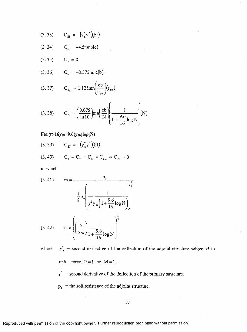
(3.33) Cj. = -(y ly 'X E l)
(3. 34) C, = -4.5mnb(c)
(3. 35) = 0
(3. 36) Cb = -3.375mnc(b)
(3.37) = 1.125mncb
V 50 J(^5o)
(3. 38) Cb, =( 0.675^ f c b lmnt i n 10 J I n J
1
1 + — logN 16 ^ .
(n )
For y>16yso+9.6(y5o)log(N)
(3 .39) Ce, = -(y ly 'X E l)
(3.40) C. = C , = C , = C . „ = C „ = 0
in which
(3.41) m = -------------------- ^ ----------------
:Pu1
yVsoV V
1 + — logN 16 J J
(3. 42) n =
1
f \y 1
y 5o A + — logN16 ^ ,
where y’ = second derivative of the deflection of the adjoint structure subjected to
unit force P = 1 or M = 1,
y" = second derivative o f the deflection o f the primary structure,
P3 = the soil resistance of the adjoint structure,
50
Reproduced with permission of the copyright owner. Further reproduction prohibited without permission.
J = A value determined experimentally, J = 0.25 for stiff clay.
The graphical representations of the sensitivity operators/integrands for single pile
are presented in CHAPTER 4 and for group of piles are presented in CHAPTER 5.
The graphical representations of the sensitivity operators are essential because of the
following reasons:
• The distributions o f sensitivity operators directly give a visual insight of the
distribution o f the influence of the changes of the design variable.
• They form the basis for quantitative assessment of the effect of each design
variable on the change o f the pile head deflection.
They are very usefiil in determining the economical length o f piles subjected to
lateral load. The pile segments along the pile axis can be considered as “effective” in
resisting the lateral load when the sensitivity operator values are not equal zero. On the
other hand, if the sensitivity operator values are equal to zero in some certain segments,
the pile segments are actually not used in resisting the lateral load. Hence, the economical
length of the piles subjected to lateral load can be set as the depth range where the
sensitivity operators have nonzero value.
The notation C(.,.) is suitable to represent the sensitivity operators of all the primary
structures and adjoint structures shown in Figure 3 . 6 - Figure 3. 9. However, in order to
differentiate different load type in the primary and adjoint structure, different notations
C(X.) 5 C™..), C“ .) and C“ ®,) are used to represent the primary and adjoint structures
shown in Figure 3. 6, Figure 3. 7, Figure 3. 8 and Figure 3. 9 respectively. The convention
of these notations is shown in Figure 3. 11.
51
Reproduced with permission of the copyright owner. Further reproduction prohibited without permission.
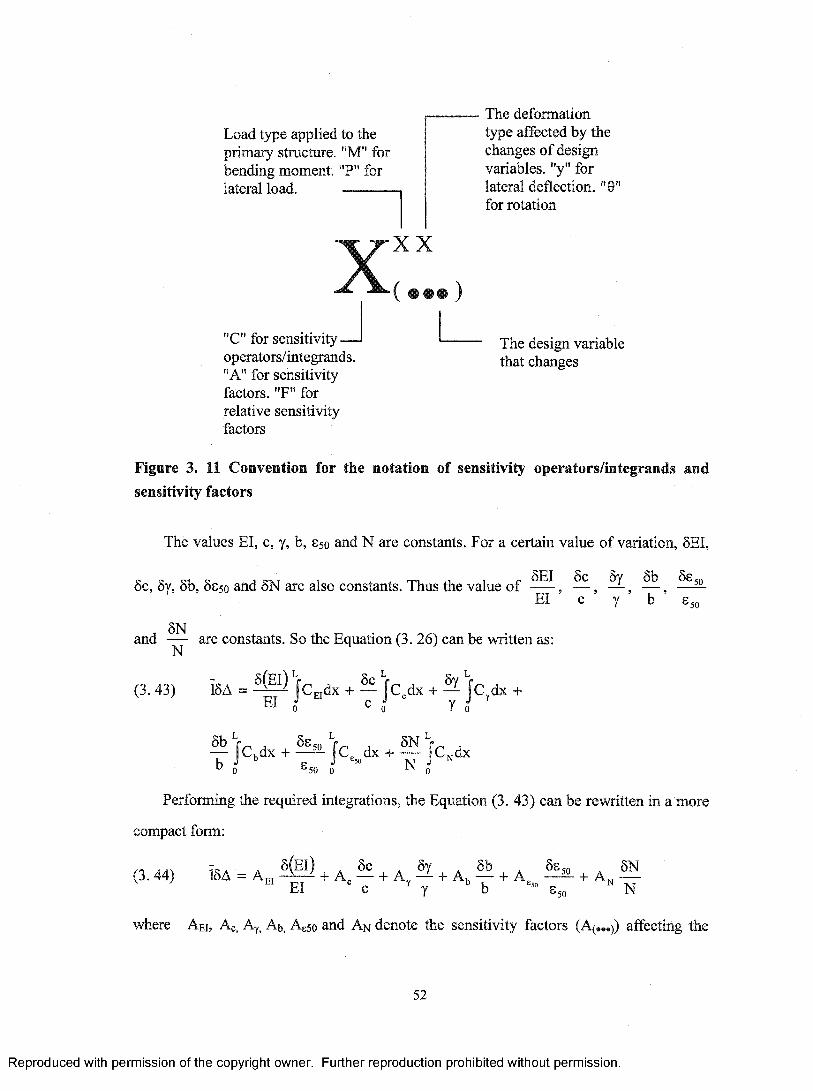
Load type applied to the primary structure. "M" for bending moment. "P" for lateral load. ----------
The deformation type affected by the changes of design variables, "y" for lateral deflection. "0" for rotation
XX X
^ ( • • • )
The design variable that changes
"C" for sensitivity operators/integrands. "A" for sensitivity factors. "F" for relative sensitivity factors
Figure 3. 11 Convention for the notation of sensitivity operators/integrands and sensitivity factors
The values El, c, y, b, S50 and N are constants. For a certain value of variation, 5EI,
5EI 5c 5y 5b 5s 5 05c, 5y, 5b, 5s5o and 5N are also constants. Thus the value o fEl ’ c ’ y ’ b ’ 850
5Nand — are constants. So the Equation (3. 26) can be written as:
(3. 43) 15A = ® jCeidx + — jc ,d x + ^ Jc^dx +El
5cc
5y
b
0 y 0
L
J c , d x + ^ J c .^ d x + ^ J c „ d x'5 0 0 N 0
Performing the required integrations, the Equation (3. 43) can be rewritten in a more
compact form:
(3. 44) 15A = A5(EI) ^ 6c , „ 8t 5b 5e , 5N
El + A „ K A„ —- + A k —— f- A„ — — + A m —El - c ' y " b S50 " N
where Aei, Ac, Ay, Ab, Agso and An denote the sensitivity factors (A(,.,)) affecting the
52
Reproduced with permission of the copyright owner. Further reproduction prohibited without permission.
changes o f the pile head deformation due to the changes or the variations of the bending
stifl&iess El, the cohesion c, the unit soil weight y, the width o f the pile b, the S50 and the
number of cycles N respectively.
(3. 45) A „ = J c „ d x0
(3.46) A , = J c ,d x0
L
(3. 47) = Jc^dx0
(3. 48) A j = J c ,d x0
(3. 49) A ,. = J c . .d x0
L
(3. 50) Aj, = JCj,dx0
The physical meaning of the sensitivity factor A^...^ can be seen in Figure 3. 10, in
which the area o f the hatched part equals the sensitivity factor A (,„ ). From Eq. (3. 44), it
can be easily found that the sensitivity factors A^...^ define the relationship between the
changes o f the design variables and the variations o f the pile head deformations. With the
changes o f the design variables known, the variations o f the pile head deformations can
be obtained conveniently. The values o f A(,.,) imply the magnitude of the influence of
the design variables on the performance of pile head deformations. The greater the value
of A(...) is, the more crucial effect that the design variable has on the variations o f the
deformation.
The sensitivity factors A(„.) carry the unit o f bending moment (kN«m). The
53
Reproduced with permission of the copyright owner. Further reproduction prohibited without permission.
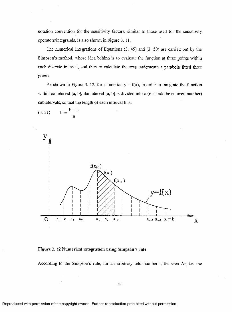
notation convention for the sensitivity factors, similar to those used for the sensitivity
operators/integrands, is also shown in Figure 3. 11.
The numerical integrations o f Equations (3. 45) and (3. 50) are carried out by the
Simpson’s method, whose idea behind is to evaluate the function at three points within
each discrete interval, and then to calculate the area underneath a parabola fitted three
points.
As shown in Figure 3. 12, for a function y = f(x), in order to integrate the function
within an interval [a, b], the interval [a, b] is divided into n (n should be an even number)
subintervals, so that the length of each interval h is:
(3. 51) h =b - a
n
y=f(x)
■i+l
Figure 3.12 Numerical integration using Simpson’s rule
According to the Simpson’s rule, for an arbitrary odd number i, the area Ar, i.e. the
54
Reproduced with permission of the copyright owner. Further reproduction prohibited without permission.
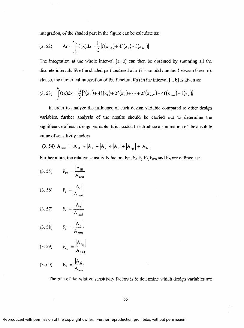
integration, of the shaded part in the figure can be calculate as:
Xi+l 1(3.52) A r= |f (x } d x = -[f(x i_ ,)+ 4 f(x i)+ f(x i,,)]
The integration at the whole interval [a, b] can then be obtained by summing all the
discrete intervals like the shaded part centered at Xi (i is an odd number between 0 and n).
Hence, the numerical integration o f the function f(x) in the interval [a, b] is given as:
(3. 53) J f (x)dx = |[ f ( x o ) + 4 f(x i)+ 2 f (x j) + ■ • • + 2 f )+ 4f(x ,_ ,)+ f(x „ )]
In order to analyze the influence of each design variable compared to other design
variables, further analysis of the results should be carried out to determine the
significance of each design variable. It is needed to introduce a summation of the absolute
value of sensitivity factors:
(3. 54) A total - IA El I + |Ac| + |A^| + |Ab| + A^^ + |A, |
Further more, the relative sensitivity factors Fei, Fc, Fy, Fb, Feso and Fn are defined as:
|A, '(3. 55)
(3. 56)
(3. 57)
(3. 58)
(3. 59)
(3. 60)
Fe, =
F„ =
■■EI
total
Mtotal
Ia J
Fb =
total
^total
Ae50
total
Fn =|A j
total
The role o f the relative sensitivity factors is to determine which design variables are
55
Reproduced with permission of the copyright owner. Further reproduction prohibited without permission.

crucial to the performance o f the pile. Taking into account o f the unit expense to change
each design variable affecting the performance of the pile soil system, the relative
sensitivity factors appear to be the convincing economical measures applicable at the
design stage of a system.
56
Reproduced with permission of the copyright owner. Further reproduction prohibited without permission.
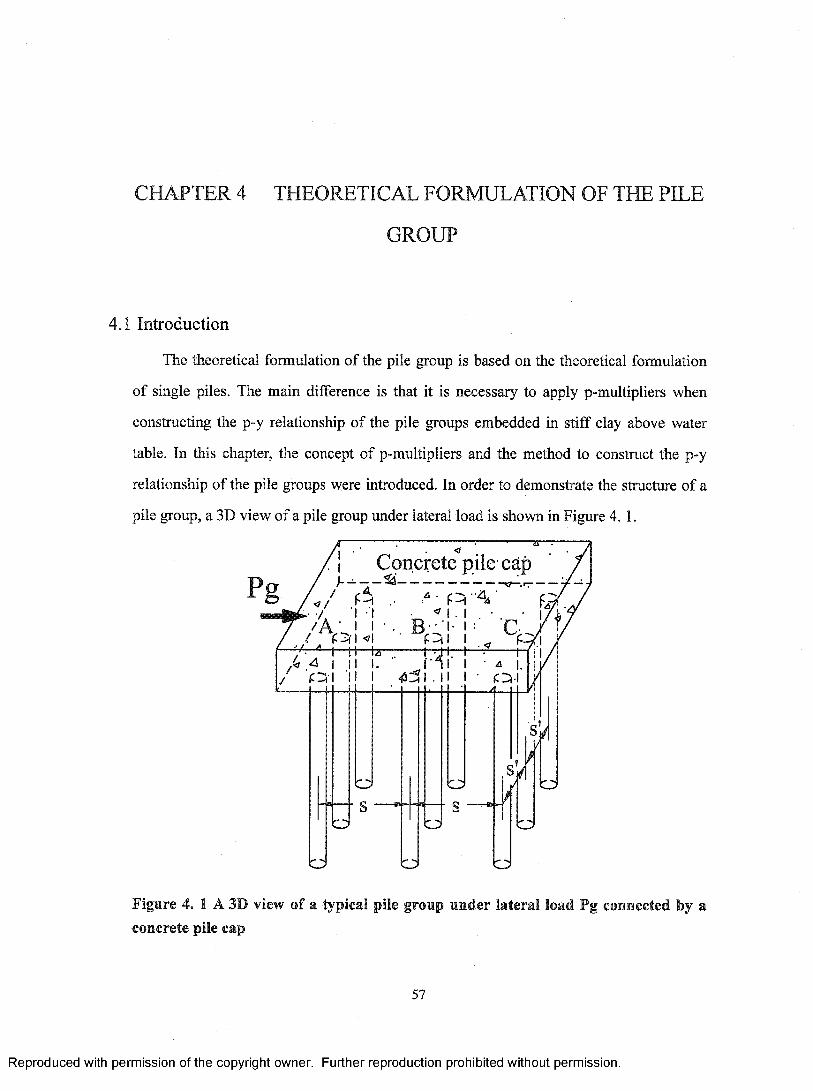
CHAPTER 4 THEORETICAL FORMULATION OF THE PILE
GROUP
4.1 Introduction
The theoretical formulation of the pile group is based on the theoretical formulation
of single piles. The main difference is that it is necessary to apply p-multipliers when
constructing the p-y relationship of the pile groups embedded in stiff clay above water
table. In this chapter, the concept of p-multipliers and the method to construct the p-y
relationship o f the pile groups were introduced. In order to demonstrate the structure o f a
pile group, a 3D view of a pile group under lateral load is shown in Figure 4. 1.
Concrete pile cap
<3 /
Figure 4. 1 A 3D view of a typical pile group under lateral load Pg connected by a concrete pile cap
57
Reproduced with permission of the copyright owner. Further reproduction prohibited without permission.
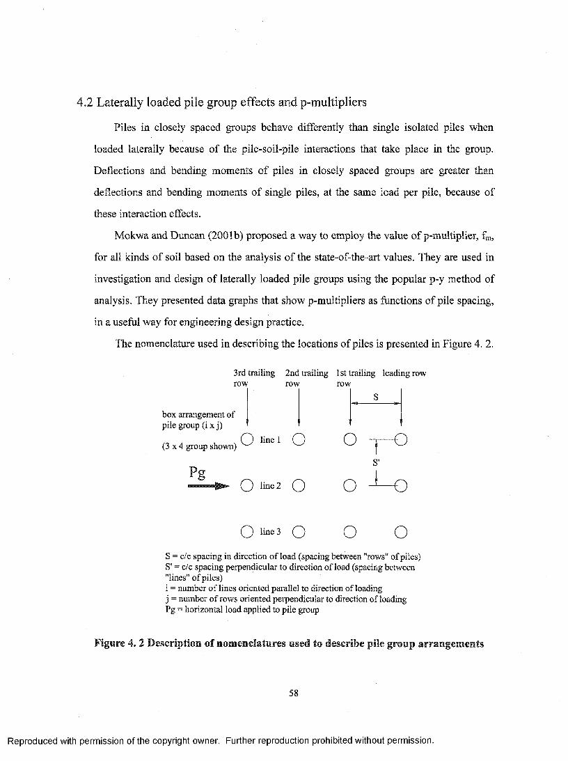
4.2 Laterally loaded pile group effects and p-multipliers
Piles in closely spaced groups behave differently than single isolated piles when
loaded laterally because of the pile-soil-pile interactions that take place in the group.
Deflections and bending moments o f piles in closely spaced groups are greater than
deflections and bending moments o f single piles, at the same load per pile, because of
these interaction effects.
Mokwa and Duncan (2001b) proposed a way to employ the value o f p-multiplier, fm,
for all kinds o f soil based on the analysis o f the state-of-the-art values. They are used in
investigation and design of laterally loaded pile groups using the popular p-y method of
analysis. They presented data graphs that show p-multipliers as functions of pile spacing,
in a useful way for engineering design practice.
The nomenclature used in describing the locations o f piles is presented in Figure 4. 2.
3rd trailing 2nd trailing 1st trailing leading row row row row
' S
box arrangement of pile group (i x j)
( 3 x 4 group shown)
Pg
O hne 1 O O
O line 2 Q Q
S'
-o
-oO line 3 O O o
S = c/c spacing in direction o f load (spacing between "rows" of piles) S' = c/c spacing perpendicular to direction o f load (spacing between "lines" o f piles)i = number o f lines oriented parallel to direction o f loading j = number o f rows oriented perpendicular to direction o f loading Pg = horizontal load applied to pile group
Figure 4. 2 Description of nomenclatures used to describe pile group arrangements
58
Reproduced with permission of the copyright owner. Further reproduction prohibited without permission.
The leading row is the first row on the right, where the lateral load acts from left to right.
The rows following the leading row are labeled as 1®* trailing row, 2"‘ trailing row, and so
on. The spacing between two adjacent piles in a row or line is described by the
center-to-center distance. The spacing parallel to the direction o f load is S, and the
spacing perpendicular to the direction o f loading is S '. Pile spacing is often normalized
by the pile diameter, D. Thus, a spacing indicated as 3D indicates a center-to-center
spacing that is three times the pile diameter.
4,3 Pile group analysis using p-multipliers
The measurements o f deflections and stresses o f the full-scale group indicate that
piles in a group carry unequal lateral loads, depending on their location within the group
and the spacing between piles. The approach for analyzing the behavior of a pile in a
group is similar to the approach used for analysis of a single pile, except that the p-values
are reduced using a p-multiplier (represented by the symbol fm) to accoimt for the reduced
efficiencies caused by pile-soil-pile interactions.
For analysis o f a pile in a group, the lateral load resistance (pgp) is equal to the lateral
load resistance of a single pile (psp) multiplied by a p-multiplier ( fm ):
(4. 1) Pg, = f„p,p
In the past studies (Brown and Reese 1985, Morrison and Reese 1986 and McVay et
al 1955), it is found that little variation exists among the response o f piles in a given row.
So the current state of practice is to associate the value of the p-multiplier ( fm ) with the
row and to use the value o f fm for all piles in the same row. However, the bending
moments for the comer piles in the front row should be adjusted when the piles are very
closely spaced (S'<3D). It is generally assumed that p-multipliers are constant with depth,
even when there are variations in the soil properties with depth.
The results were presented in the form of chart shown in Figure 4. 3, in which the
relationships between the p-multipliers, pile spacing and pile locations are illustrated
59
Reproduced with permission of the copyright owner. Further reproduction prohibited without permission.
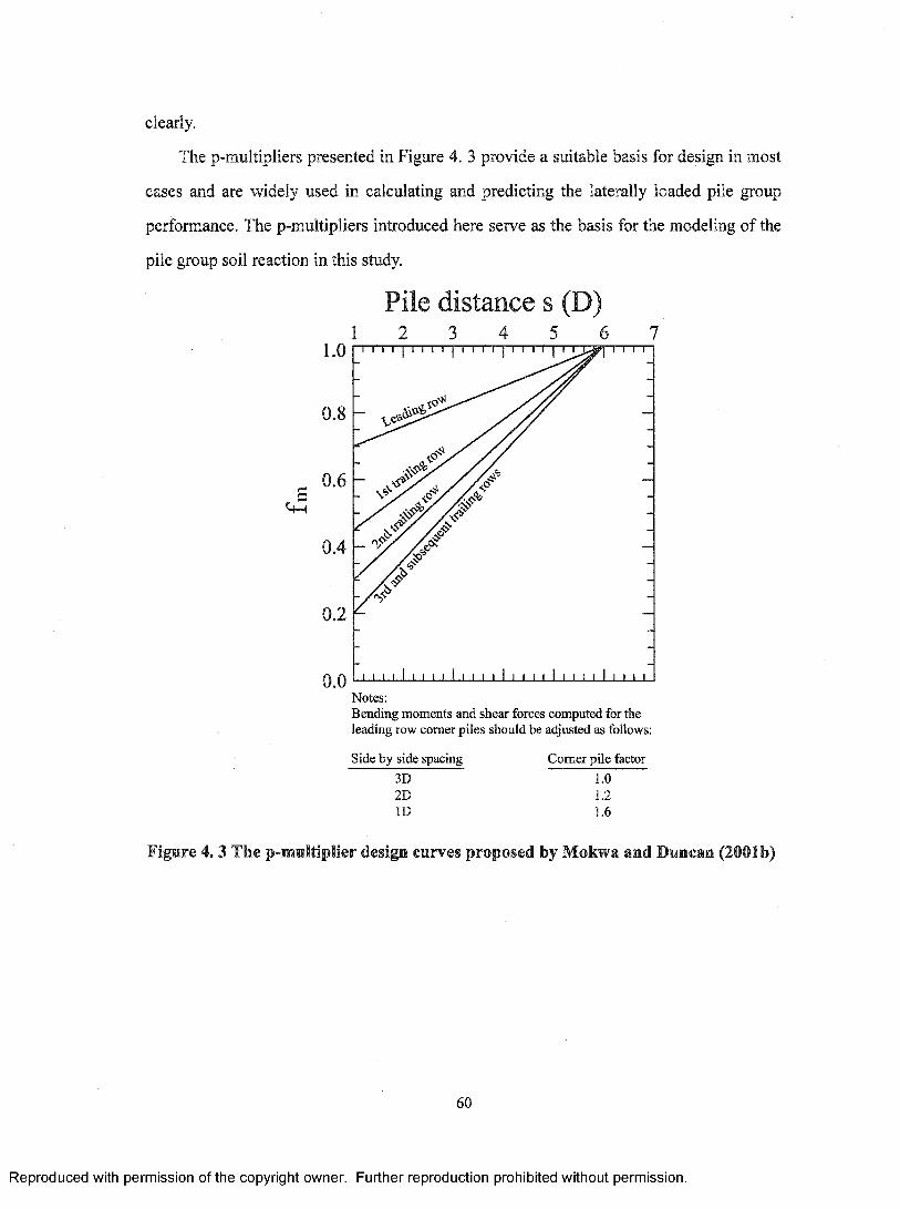
clearly.
The p-multipliers presented in Figure 4. 3 provide a suitable basis for design in most
cases and are widely used in calculating and predicting the laterally loaded pile group
performance. The p-multipliers introduced here serve as the basis for the modeling of the
pile group soil reaction in this study.
Pile distance s (D)1 2 3 4 5 6 7
0.8
0.6
0.4
0.2
0.0Notes;Bending moments and shear forces computed for theleading row comer piles should be adjusted as follows:
Side by side spacing Comer pile factor3D2DID
1.01.21.6
Figure 4. 3 The p-multiplier design curves proposed by Mokwa and Duncan (2001b)
60
Reproduced with permission of the copyright owner. Further reproduction prohibited without permission.
CHAPTER 5 NUMERICAL INVESTIGATIONS OF SINGLE
FILE
5.1 Introduction
In Chapter 3, the theoretical formulations of sensitivity analysis o f laterally loaded
pile are presented by means of equations. Those formulas provide a theoretical approach
in general fashion ready for numerical investigation. Because the formulas are too general,
it is not easy to show the numerical and distributional details of the sensitivity operators
and factors. In order to demonstrate the importance o f each of the design variables and to
find out the distributions of the sensitivity operators with respect to the embedded depth,
the numerical investigations are crucially needed.
In this chapter, the sensitivity analysis o f single piles is carried out in a numerical
fashion. The typical design variables are determined based on the usually used parameters
in reality. The sensitivity operators/integrands o f laterally loaded single piles embedded in
stiff clay above water table are plotted in figures shown in APPENDIX B and the attached
CD. The sensitivity factors of each case are also evaluated in a numerical way. Different
piles with lengths 2T, 3T, 4T, 4.5T, 5T, 6T, 7T, 8T, 9T and lOT (the “T” here represents
the relative stiffness factor determined in Section 5.4) are analyzed in the method
presented in this chapter. The outcomes o f a typical case of the sensitivity analysis are
presented in this chapter. The results for other cases are included into thesis in digital
form saved in the attached CD. The results can be viewed easily with the normally used
picture-viewer software.
61
Reproduced with permission of the copyright owner. Further reproduction prohibited without permission.

5.2 Scope
The sensitivity analysis of single piles, which are conducted in this study, is focused
on the following aspects;
1. Sensitivity analysis of pile head lateral deflection yt for free head piles subjected
to lateral force Pt applied to the head of the pile.
2. Sensitivity analysis of pile head angle of flexural rotation 0t for free head piles
subjected to lateral forces Ft acting at the head of the pile.
3. Sensitivity analysis o f pile head lateral deflection yt for fixed head piles
subjected to lateral forces Pt applied to the head of the pile.
4. Sensitivity analysis of pile head lateral deflection yt for free head piles subjected
to bending moments Mt being applied to the head of pile.
5. Sensitivity analysis o f pile head angle o f flexural rotation 6t for free head piles
subjected to bending moments Mt acting at head of pile.
The pile lengths o f 2T, 3T, 4T, 4.5T, 5T, 6T, 7T, 8T, 9T and lOT are employed in this
analysis. The load cycles of the soil are taken as 1, 10, 100, 1000 and 10000. The p-y
formulation for the stiff clay above water table enables us to include into analysis also a
static loading. This is achieved when number o f load cycles N =l. So in this study, both
the sensitivity analysis o f laterally loaded pile under static and cyclic loading is
performed.
5.3 The determination of typical design parameters:
Pile’s physical properties
The pile used in this study is a standard hollow steel pile HSS 406x13 defined by
“Hollow Structural Sections to ASTM A 500 Grade C”, which is issued by Canadian
Institute of Steel Construction 2000.
The section property o f the pile is calculated in the following steps and presented in
Figure 5. 1:
62
Reproduced with permission of the copyright owner. Further reproduction prohibited without permission.

E = 210GPa
I - 277x10" mm^
El = (210x10® N/m^) x (277x10® mm'*)
= (210xl0®N/m^) X (277x1 O'® m'*)
= 5.817x10'* kN m
. t . t= l l . 43mm
b = 406mm
Pile type: Steel HSS 406x13
Outside diameter b: 406mm Thickness t: 11.43mmArea A:Weight:Y oung's Modulus:
I x = I y :
Allowable stress:Allowable moment: 432.6kN-m Stiffness El:
14161.2mm2
1.112kN/m 210GPa 277x10®mm^ 317MPa
58.17x10^ kN-m^
Figure 5.1 Section properties of the pile used in the sensitivity analysis
Soil cohesion c and 8 5 0 :
The soil cohesion c here is the undrained shear strength and E50 is the strain
corresponding to one-half the maximum principal stress difference. The typical values,
which are present in the manual of COM624P, of c and S50 are given in Table 5. 1.
63
Reproduced with permission of the copyright owner. Further reproduction prohibited without permission.
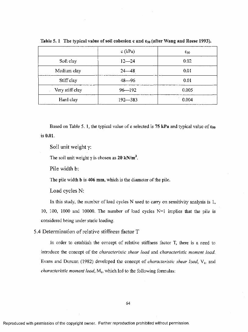
Table 5 .1 The typical value of soil cohesion c and Sjo (after Wang and Reese 1993).
c (kPa) Sso
Soft clay 12— 24 0.02
Medium clay 24—48 0.01
Stiff clay 48— 96 0.01
Very stiff clay 96— 192 0.005
Hard clay 192— 383 0.004
Based on Table 5. 1, the typical value o f c selected is 75 kPa and typical value of 8go
is 0.01.
Soil unit weight y:
The soil unit weight y is chosen as 20 kN/m .
Pile width b:
The pile width b is 406 mm, which is the diameter o f the pile.
Load cycles N:
In this study, the number of load cycles N used to carry on sensitivity analysis is 1,
10, 100, 1000 and 10000. The number of load cycles N=1 implies that the pile is
considered being under static loading.
5.4 Determination of relative stiffness factor T
In order to establish the concept o f relative stiffiiess factor T, there is a need to
introduce the concept o f the characteristic shear load and characteristic moment load.
Evans and Duncan (1982) developed the concept o f characteristic shear load, Vc, and
characteristic moment load. Me, which led to the following formulas;
64
Reproduced with permission of the copyright owner. Further reproduction prohibited without permission.
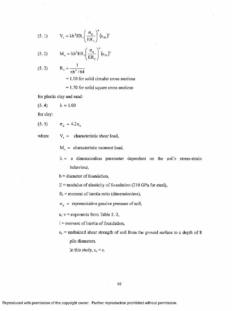
(5. 1) V, = X,b'ER,vER .y
(5. 2) M , = ^b^ER
I
vER iy
i^so f
(bsoX
(5. 3) R , =Tib V 64
= 1.00 for solid circular cross sections
= 1.70 for solid square cross sections
for plastic clay and sand:
(5. 4) X = 1.00
for clay;
(5 .5) o r^= 4 .2 s„
where V , = characteristic shear load,
= characteristic moment load,
X = a dimensionless parameter dependent on the soil’s stress-strain
behaviour,
b = diameter o f foundation,
E = modulus o f elasticity o f foundation (210 GPa for steel),
Ri = moment o f inertia ratio (dimensionless),
CTp = representative passive pressure o f soil,
u, V = exponents from Table 5. 2,
1 = moment o f inertia o f foundation,
Su = undrained shear strength o f soil from the ground surface to a depth o f 8
pile diameters.
In this study, Su = c.
65
Reproduced with permission of the copyright owner. Further reproduction prohibited without permission.
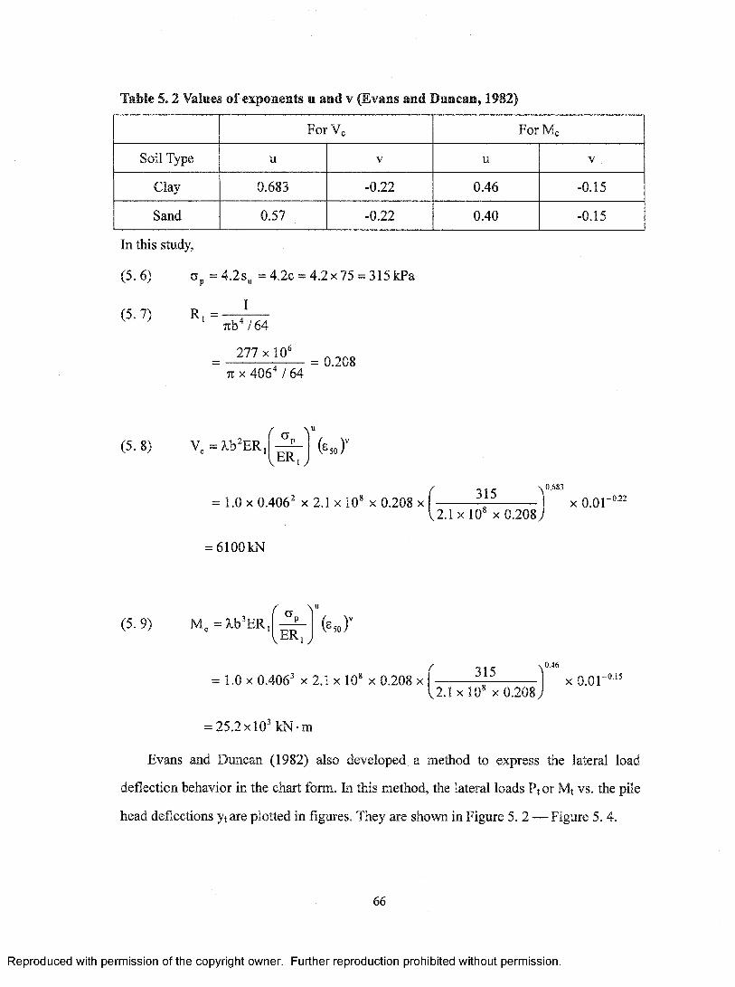
Table 5 .2 Values of exponents u and v (Evans and Duncan, 1982)
For Vc For Me
Soil Type u V u V
Clay 0.683 -0.22 0.46 -0.15
Sand 0.57 -0.22 0.40 -0.15
In this study.
(5 .6) Gp =4.2s„ = 4.2c = 4.2x75 = 315 kPa
(5. 7) R , =I
7Tb V 64
277 X 10^Tz X 406' / 64
= 0.208
(5.8) V =A.b'ER,vE R w
(sso)"
= 1.0 X 0.406^ X 2 .1 x10 ' X 0.208 x
= 6100kN
315 , 0.683
2.1 X 10' X 0.208X 0.01 - 0.22
(5. 9) M , = Xb'ER,v E R , ,
(bsoF
= 1.0 X 0.406' X 2.1 X 10' X 0.208 x
= 2 5 .2 x 1 0 'kN-m
315, 0.46
2.1 X 10' X 0.208X 0.01 - 0.15
Evans and Duncan (1982) also developed a method to express the lateral load
deflection behavior in the chart form. In this method, the lateral loads Pt or Mt vs. the pile
head deflections yt are plotted in figures. They are shown in Figure 5. 2 — Figure 5. 4.
66
Reproduced with permission of the copyright owner. Further reproduction prohibited without permission.

0.048
0.040
Clay
0.032
0.016
0.008
0.05 0.20 0.25 0.30
b
Figure 5. 2 Load-deformation curves for free-head pile embedded in clay under cyclic lateral load (after Evans and Duncan, 1982)
67
Reproduced with permission of the copyright owner. Further reproduction prohibited without permission.

0.048
0.040
Clay
0.032
0.016
0.008
0.01 0.03
yt
0.04 0.05
" F
Figure 5. 3 Load-deformation curves for fix-head pile embedded in clay under cyclic lateral load (after Evans and Duncan, 1982)
68
Reproduced with permission of the copyright owner. Further reproduction prohibited without permission.
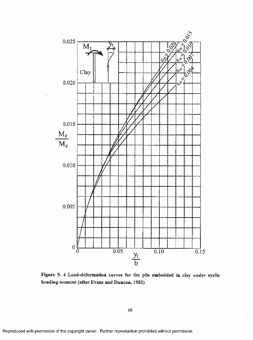
0.025
Clay
0.020
0.015
0.010
0.005
0.05
Figure 5. 4 Load-deformation curves for the pile embedded in clay under cyclic bending moment (after Evans and Duncan, 1982)
69
Reproduced with permission of the copyright owner. Further reproduction prohibited without permission.

The relative s t i f f n e s s factor T is defined as follows:
For free or fixed head pile under lateral loading:
(5. 10) T = y.Ei \ | a , p ,
For pure moment loading:
(5. 11) 1 = 2*
where Ay = 2.43 for a free head pile
Ay = 0.93 for a fixed head pile
B y = 1.62
Based on the relationships shown Figure 5. 2 — Figure 5. 4 and Equations (5. 8), (5.
9), (5. 10) and (5. 11), it is possible to determine the values of the relative stiffness factors
T for different boundary conditions and applied forces. The results obtained in this
fashion are presented in Table 5. 3, Table 5. 4 and Table 5. 5 respectively. Since the T
values change according to the applied force, some approximation is required to be used
in order to find a representative value for all the load applied. The T value corresponding
to Pt = 150 kN or Mt = 150 kN®m used for determination o f the relative stiffness factor is
chosen for further numerical investigations. The relative stiffness factors T determined in
this way are shown in Table 5. 6.
70
Reproduced with permission of the copyright owner. Further reproduction prohibited without permission.
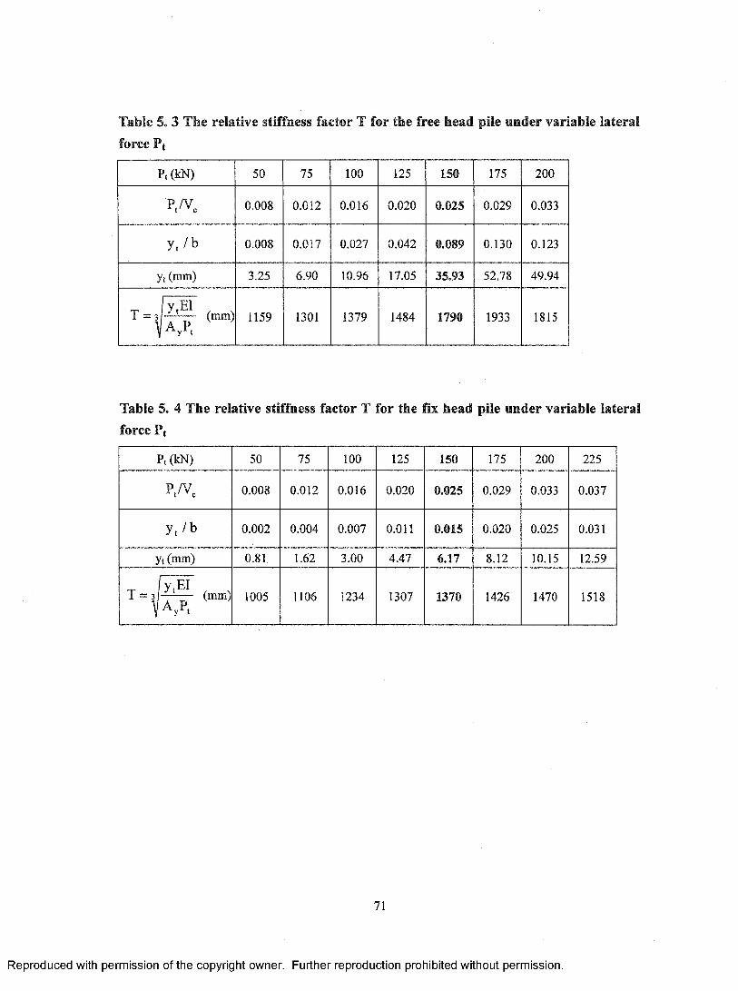
Table 5. 3 The relative stiffness factor T for the free head pile under variable lateral force Pt
P,(kN ) 50 75 100 125 150 175 200
P./v, 0.008 0.012 0.016 0.020 0.025 0.029 0.033
y, / b 0.008 0.017 0.027 0.042 0.089 0.130 0.123
Yt (mm) 3.25 6.90 10.96 17.05 35.93 52.78 49.94
^ 1 y^EI1159 1301 1379 1484 1790 1933 1815
Table 5. 4 The relative stiffness factor T for the fix head pile under variable lateral force Ft
Pt(kN) 50 75 100 125 150 175 200 225
P.A^c 0.008 0.012 0.016 0.020 0.025 0.029 0.033 0.037
y, / b 0.002 0.004 0.007 0.011 0.015 0.020 0.025 0.031
Yt (mm) 0.81 1.62 3.00 4.47 6.17 8.12 10.15 12.59
T = 3y.EI
--------- (mm)A P
1005 1106 1234 1307 1370 1426 1470 1518
71
Reproduced with permission of the copyright owner. Further reproduction prohibited without permission.
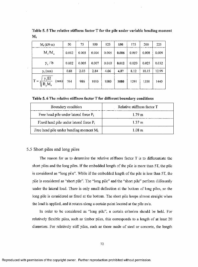
Table 5. 5 The relative stiffness factor T for the pile under variable bending moment Mt
Mt (kN-m) 50 75 100 125 150 175 200 225
M ,/M , 0.002 0.003 0.004 0.005 0.006 0.007 0.008 0.009
y, /b 0.002 0.005 0.007 0.010 0.012 0.020 0.025 0.032
yt (mm) 0.81 2.03 2.84 4.06 4.87 8.12 10.15 12.99
7 = (mm) P y M ,
764 986 1010 1080 1080 1291 1350 1440
Table 5. 6 The relative stiffness factor T for different boundary conditions
Boundary condition Relative stiffness factor T
Free head pile under lateral force Pt 1.79 m
Fixed head pile under lateral force Ft 1.37 m
Free head pile under bending moment Mt 1.08 m
5.5 Short piles and long piles
The reason for us to determine the relative stiffness factor T is to differentiate the
short piles and the long piles. If the embedded length of the pile is more than 5T, the pile
is considered as “long pile”. While if the embedded length of the pile is less than 5T, the
pile is considered as “short pile”. The “long pile” and the “short pile” perform differently
under the lateral load. There is only small deflection at the bottom of long piles, so the
long pile is considered as fixed at the bottom. The short pile keeps almost straight when
the load is applied, and it rotates along a certain point located at the pile axis.
In order to be considered as “long pile”, a certain criterion should be held. For
relatively flexible piles, such as timber piles, this corresponds to a length of at least 20
diameters. For relatively stiff piles, such as those made of steel or concrete, the length
72
Reproduced with permission of the copyright owner. Further reproduction prohibited without permission.

must be at least 35 diameters.
5.6 Load-deflection relationship
The charts o f load-deflection relationship serve for assessment o f nonlinearity o f the
pile soil system and are used to choose the suitable values o f forces Pi or bending
moments Mj in sensitivity analysis. One representative load-deflection relationship
corresponding to each support type is shown from Figure 5. 5 to Figure 5. 7. The
load-deflection relationships for the piles with other boundary conditions and pile lengths
were all included in the attached CD in a digital graphic format.
300
250
200
100
0.05 0.15 0.2y , ( m )
0.1 0.25 0.3 0.35
Figure 5. 5 Pile head deflection yt vs. lateral force Ft applied to the pile head for a free head pile embedded in stiff clay above water table. Pile length L=2T=2.74 m, load cycles N=10000
73
Reproduced with permission of the copyright owner. Further reproduction prohibited without permission.

300
250
200
^ 150
100
y , ( m )
Figure 5. 6 Pile head deflection yt vs. lateral force Ft applied to the pile head for a fixed head pile embedded in stiff clay above water table. Pile length L=2T=3.58 m, load cycles N=10000
350
300
250
■p200
100
0.05 0.1y , ( m )
0.15 0.2
Figure 5. 7 Pile head deflection yt vs. bending moment Mt applied to the pile head for a free head pile embedded in stiff clay above water table. Pile length L=2T=2.16 m, load cycles N=10000
74
Reproduced with permission of the copyright owner. Further reproduction prohibited without permission.
5.7 The stresses and deformations of adjoint structure
The adjoint structure is a virtual structure, which is made of exactly the same
materials and has exactly the same boundary conditions as the corresponding primary
structure but with a virtual unit force applied to the structure.
In this section, the method to calculate various components of the adjoint structure is
presented. It is demonstrated with the aid o f Figure 5. 8, which contains various parts
(“Part i” — “Part iv”) o f primary and adjoint systems. In the Figure 5. 8, the system (p)
denotes the primary structure subjected to a real loading, and the system (a) is the adjoint
structure while the system (b) and (c) are the temporary systems used to calculate the
stresses and deformations o f the adjoint structure. The relationship between (a), (b) and (c)
results in the following outcome:
(5,12) ( a ) = M z W )
where the letters (a), (b) and (c) in parenthesis represent the adjoint pile-soil system,
temporary over-loaded system and temporary under-loaded system shown in Figure 5. 8
respectively.
The temporary over-loaded system (b) and temporary under-loaded system (c) are
also suppositional systems that are used to calculate the adjoint structure shown in (a).
The stresses and deformations of the system (b) and (c) can readily be calculated through
the COM624P program. Hence, the difference o f the system (b) and (c) can be determined
by subtract every item, including lateral deflection, rotation, bending moment and soil
reaction etc., in system (c) from the corresponding item in system (b). The components of
the adjoint system (a) are obtained through dividing the differences between system (b)
and (c) by a number 2.
In order to ensure the result gained from (b) and (c) produces the same physical
status as primary structure, the force Pt or Mt was also applied in addition to the unit force
in the temporary system (b) and (c).
75
Reproduced with permission of the copyright owner. Further reproduction prohibited without permission.
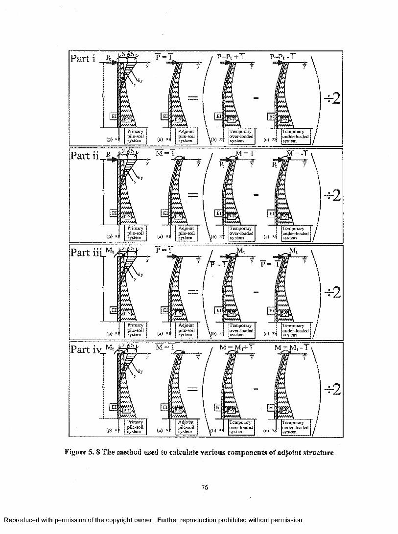
P a r t i p = i
(p)Primarypile-soilsystem
p=Pt + 1
Adjointpile-soilsystem
Temporary over-loaded system
p=Pt - 1
E l
(a) X. (c) X,
Temporaryunder-loadedsystem
- 2
M = 1F a rt M = 1
Pnmarypile-soilsystem
Adjointpile-soilsystem
Temporary ovCT-loaded system(b) x f
M = - l
Pt
(c) X
Temporary undK’-loaded system
Part “1p = 1
Pnmaiy Adjoint temporary over-loaded system
Temporary under-loaded system
pile-soil pile-soilsystem system
Part iv M - i M = Mt+ 1 M = Mt - 1
3 y
«w —
E l a [1
Primarypile-soilsystem (a) X-
Adjointpile-soilsystem \( b ) X
Temporaryover-loadedsystem (c) X.
Temporaryunder-loadedsystem
Figure 5. 8 The method used to calculate various components of adjoint structure
76
Reproduced with permission of the copyright owner. Further reproduction prohibited without permission.
Part i of Figure 5. 8 shows how the stresses and deformations are calculated for the
case when both the primary structure and the adjoint structure are subjected to lateral
loading. In (b) and (c) of Part i, a positive and negative unit force are applied respectively
in addition to the Pt, which is applied to the primary structure. This operation causes the
primary system “temporarily over-loaded or under-loaded”.
Part ii, iii, and iv o f Figure 5. 8 present the ways to calculate the stresses and
deformations of the adjoint structure while the primary and adjoint structure are subjected
to lateral load and bending moment, bending moment and lateral load or bending moment
and bending moment respectively.
The deflection of the adjoint structure y^ , the bending moment M and the soil
resistance p^ are determined in the formulas below:
(5. 13) y,
(5. 14) M = — ^ ^
(5,15) p.
The symbols y(b), M(b) and p(b) are defmed as the pile lateral deflection, bending moment
and soil resistance o f the temporary over-loaded system shown in Figure 5. 8(b), while
y(c), M(c) and p(c) are defmed as the pile lateral deflection, bending moment and soil
resistance of the temporary under-loaded system shown in Figure 5. 8(c).
5.8 COM624P Program
Computer program COM624P was developed (Wang and Reese (1993)) for use in
the analysis o f stresses and deflection o f piles or drilled shafts under lateral loads. The
program is especially written for highway engineers who wish to run the analysis on
microcomputers. The technology on which the program is based is the widely used p-y
77
ReprocJucecJ with permission of the copyright owner. Further reproctuction prohibitect without permission.
method. The program solves the equations giving pile deflection, rotation, bending
moment, and shear by using iterative procedures because of the nonlinear response of the
soil. The beam-column-soil equations are solved by finite difference method.
The program provides a user-friendly/menu-driven input and a graphics output in
microcomputer environment. The version of the Program COM624P for the
microcomputer was developed in 1989. Several new features were included in the
program such as: generating p-y curves for rock, capability o f analysis of piles in sloping
section. The COM624P o f version 2.0 is used to conduct numerical research on sensitivity
analysis o f laterally loaded piles.
5.9 Results of sensitivity analysis of laterally loaded pile
In Chapter 3, the sensitivity analysis of laterally loaded pile is presented in a form of
theoretical formulation. The theoretical formulas provide the basis for numerical
investigations. In this study, the numerical explorations o f the sensitivity analysis of
laterally loaded piles embedded in stiff clay are carried out for different pile boimdary
conditions, pile lengths, load cycles and applied forces. The results of the sensitivity
analysis are presented mostly in the form of graphics saved in the attached CD, whose
content is shown in details in APPENDIX D. A typical example o f the results of the
sensitivity analysis for a free head pile embedded in the stiff clay above water table,
subjected to lateral concentrated load, with pile length L=10T=13.7m and load cycles
N=1 and 10000 is presented in the APPENDIX B. The discussions on the results of the
sensitivity analysis are presented in CHAPTER 9 and the conclusions are presented in
CHAPTER 10.
5.10 Methodology o f result verification
In this section, the results o f the sensitivity analysis are verified and compared with
the results obtained from the numerical calculations of the well-developed software such
as COM624P and FB-Piers.
The results are checked by introducing certain variations in the design variables.
78
Reproduced with permission of the copyright owner. Further reproduction prohibited without permission.
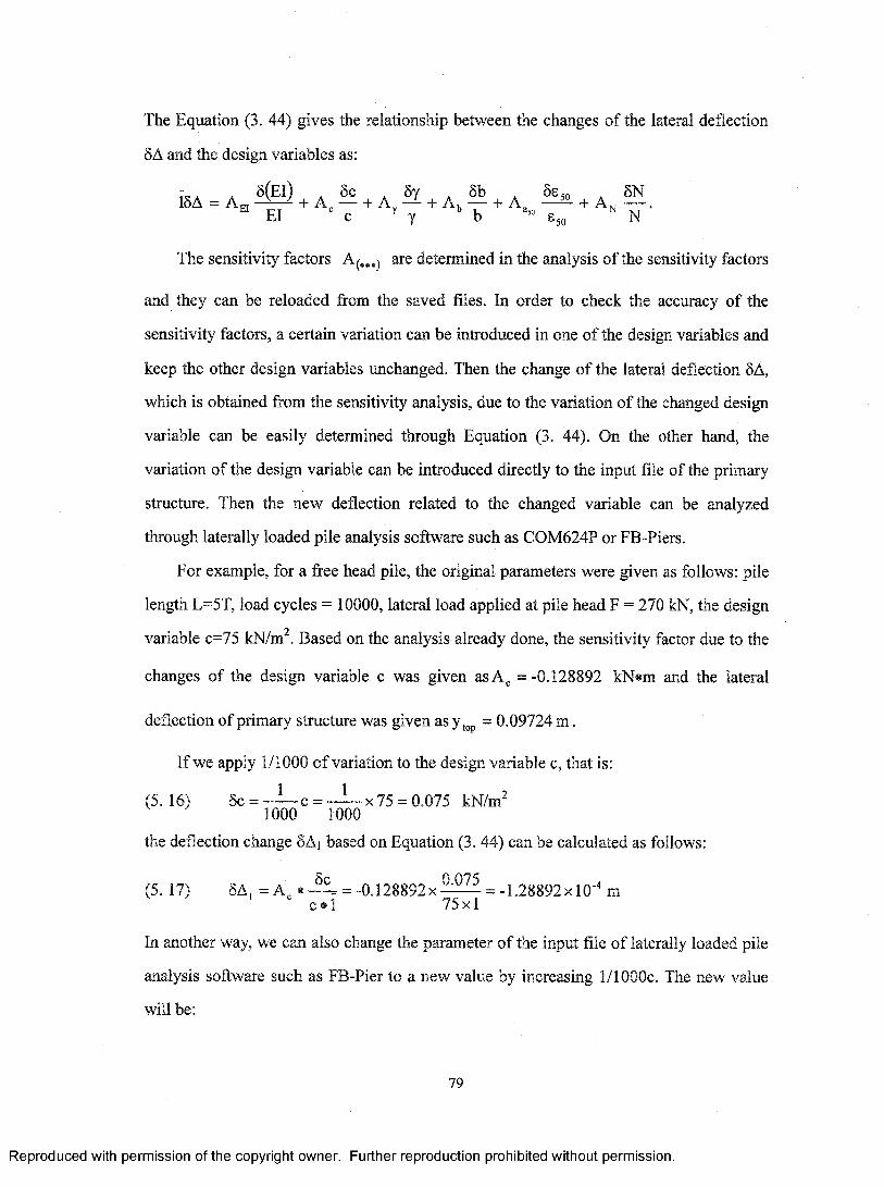
The Equation (3. 44) gives the relationship between the changes o f the lateral deflection
5A and the design variables as:
- . . 5(EI) . 6 c . 5y . 5b . . 6N15A — A ct 1- A 1- A F A t (- A F Am — .
El c ' y b 850 N
The sensitivity factors A(.„) are determined in the analysis of the sensitivity factors
and they can be reloaded from the saved files. In order to check the accuracy of the
sensitivity factors, a certain variation can be introduced in one of the design variables and
keep the other design variables unchanged. Then the change of the lateral deflection 5A,
which is obtained from the sensitivity analysis, due to the variation o f the changed design
variable can be easily determined through Equation (3. 44). On the other hand, the
variation of the design variable can be introduced directly to the input file of the primary
structure. Then the new deflection related to the changed variable can be analyzed
through laterally loaded pile analysis software such as COM624P or FB-Piers.
For example, for a free head pile, the original parameters were given as follows: pile
length L=5T, load cycles = 10000, lateral load applied at pile head F = 270 kN, the design
variable c=75 kN/m^. Based on the analysis already done, the sensitivity factor due to the
changes o f the design variable c was given asA^ = -0.128892 kN«m and the lateral
deflection of primary structure was given as y,gp = 0.09724 m .
If we apply 1/1000 o f variation to the design variable c, that is:
(5. 16) 6c = - ! — c = - ^ x 75 = 0.075 kN/m^1000 1000
the deflection change 5Ai based on Equation (3. 44) can be calculated as follows:
(5. 17) 5A, = A , • - ^ = - 0 . 1 2 8 8 9 2 X = -1.28892x 1 0 'mc • 1 75 X1
In another way, we can also change the parameter o f the input file o f laterally loaded pile
analysis software such as FB-Pier to a new value by increasing 1/1000c. The new value
will be:
79
Reproduced with permission of the copyright owner. Further reproduction prohibited without permission.
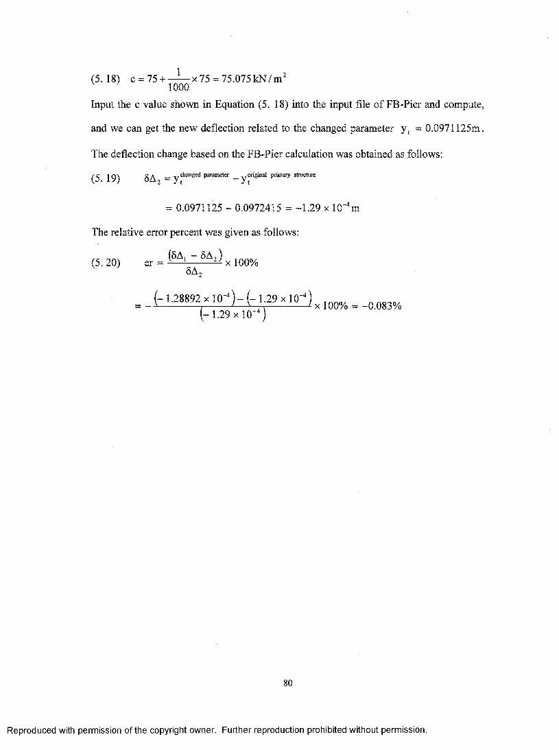
(5. 18) c = 75 + X 75 = 75.075 kN /m ^1000
Input the c value shown in Equation (5. 18) into the input file of FB-Pier and compute,
and we can get the new deflection related to the changed parameter y, = 0.0971125m.
The deflection change based on the FB-Pier calculation was obtained as follows:
1 Q \ S A — parameter original primary structurew- iVj 0ZI2 - Yt “ Yt
= 0.0971125 - 0.0972415 = -1.29 x 1 0 "V
The relative error percent was given as follows:
(5A, - 5 A , )(5. 20) er = ^ ^ x 100%
SAj
^ _ (- 1 .2 8 8 9 2 x l0 ^ ) - ( - 1 2 9 > < 1 0 - ) ^ ^( -1 .2 9 x 1 0 '^ )
80
Reproduced with permission of the copyright owner. Further reproduction prohibited without permission.

CHAPTER 6 NUMERICAL INVESTIGATIONS OF THE PILE
GROUP
6.1 Introduction
In this chapter, the sensitivity analysis o f piles in a pile group is carried out in a
numerical fashion. The pile physical properties are taken the same as for the pile
employed in sensitivity analysis for single isolated piles. But due to the interactions
between the piles in the group, some modifications have been applied to the calculation of
the soil response. The p-multipliers are introduced into the soil-pile reaction model.
6.2 Scope
The groups o f piles employed in this study are shown Figure 6. 1. The sensitivity
analysis of pile groups which is done in the course of this study is consisted of the
following steps:
1. Sensitivity analysis o f top lateral deflection 5yt for pile groups with the piles
pinned to the cap subjected to lateral concentrated force. The analysis is carried
out for the piles located in the center o f the leading row, first trailing row and
second trailing row. The pile spacing s is equal to 2D, 3D, 4D and 5D. The pile
length L is equal to lOT (13.7m). The load cycles cover number o f cycles N =l,
10, 100, 1000 and 10000.
2. Sensitivity analysis o f top lateral deflection 5yt for pile groups with the piles
fixed to the cap subjected to lateral concentrated force. The analysis is carried
out for the piles located in center o f the leading row, first trailing row and second
trailing row. The pile spacing s is equal to 2D, 3D, 4D and 5D. The pile length L
is equal to lOT (17.9m). The load cycles cover number of cycles N = l, 10, 100,
81
Reproduced with permission of the copyright owner. Further reproduction prohibited without permission.
1000 and 10000.Sensitivity analysis of top lateral deflection 5yt for pile groups with the piles
pinned to the cap subjected to bending moment at the pile head. The analysis is
carried out for the piles located in the center of the leading row, first trailing row
and second trailing row. The pile distance s is equal to 2D, 3D, 4D and 5D. The
pile length L is equal to lOT (10.8 m). The load cycles cover number of cycles
N -1, 10, 100, 1000 and 10000.
82
Reproduced with permission of the copyright owner. Further reproduction prohibited without permission.

1050
D=406
1050
Plan view of the pile group
m
trailing trailing rowrow row
Section view m-m
Pile cap, reinforced concrete 1500
■'750;
The pile head is fixed or hinged to the pile cap here lOT
HSS 406x13
Stiff clay above water table
Second First Leading
Figure 6.1 File group properties employed in the sensitivity analysis
83
Reproduced with permission of the copyright owner. Further reproduction prohibited without permission.

6.3 The determination ofPg for the pile groups under lateral concentrated load
The determination of Pg, which is the force applied to the cap of a pile group, is
based on the principle that the pile group will produce the same deflection under the force
Pg as the single pile under lateral force Pt. The reason to adopt this principle is to compare
the sensitivity analysis results o f single pile with the piles in the group when they have
same value of deflection.
An example used to present the method to determine the force Pg is shown in Figure
6. 2. The single pile shown in this example is a free head pile subjected to lateral
concentrated force at the pile head, and the number o f load cycles N is equal 1.
Accordingly, the piles in the pile group are pinned to the pile cap and the pile group is
subjected to lateral concentrated force at the pile cap, and the number o f load cycles N is
also equal 1.
The ordinate in the example represents the external force Pg that the pile group is
subjected to or the pile head concentrated force Pt applied to the pile head of single
isolated pile. The abscissa in the example stands for the lateral deflections produced by
the application o f external force Pg or Pt.
The series of the variable force Pt and the corresponding lateral deflection yjop had
already been determined in the analysis of single piles. The results from previous study of
single piles are retrieved and plotted in a form of Pt vs yxop curve for single pile shown in
Figure 6. 2. It is also possible to obtain the Pg vs yjop curves for pile groups by using the
FB-Pier program to calculate the deflection corresponding to force Pg series and then plot
the result in the same coordinate system with the single pile. The comparison of the Pt vs
yxop curves for single pile and Pg vs yxop curves for pile groups plotted in the same graph
enables one to determine the force Pg required to acquire the same deflection produced by
the force Pt employed in sensitivity analysis of single isolated pile.
The graphs of external force Pg and Pt vs yxop for all the pile groups imder study are saved
in a picture format and are included in the attached CD.
84
Reproduced with permission of the copyright owner. Further reproduction prohibited without permission.
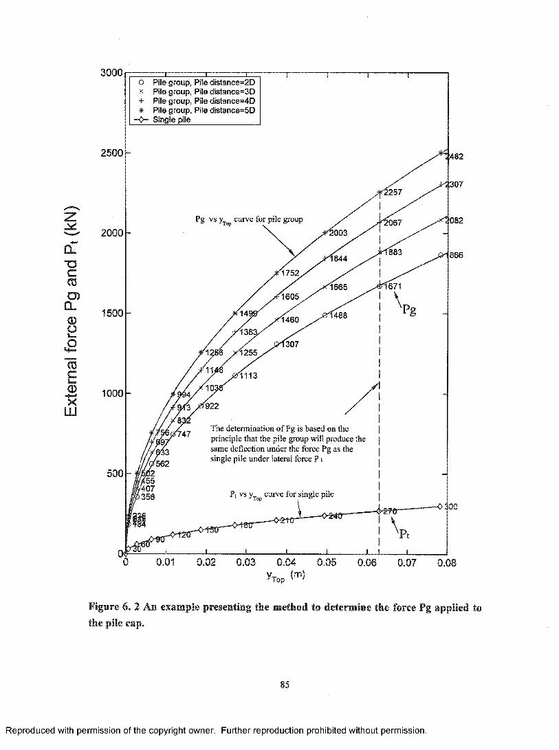
3000
C L
CCD0 5
CL0o
CDc0X
L U
2 5 0 0 -
2000 -
1500
1000
500
0 Pile group, PX Pile group, P+ Pile group, P* Pile group, P
- 0 - Single pile
stance=2Dstance=3Dstance=4Dstance=5D
Pg vs Yj, curve for pile group
The determination of Pg is based on the principle that the pile group will produce the same deflection under the force Pg as the single pile under lateral force P t
Pt vs curve for single pile
:482
3 0 7
082
866
0.01 0.02 0.03 0.04 0.05 0.06 0.07yjop
0.08
Figure 6. 2 An example presenting the method to determine the force Pg applied to the pile cap.
85
Reproduced with permission of the copyright owner. Further reproduction prohibited without permission.
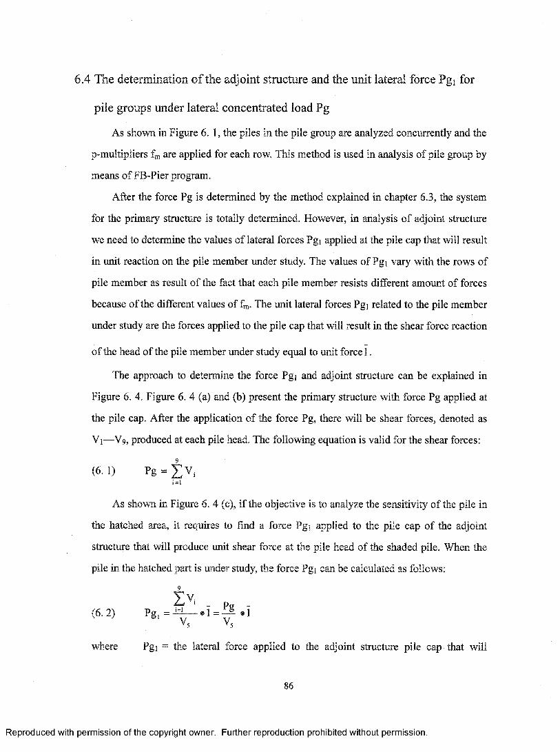
6.4 The determination of the adjoint structure and the unit lateral force Pgi for
pile groups under lateral concentrated load Pg
As shown in Figure 6. 1, the piles in the pile group are analyzed concurrently and the
p-multipliers fm are applied for each row. This method is used in analysis of pile group by
means o f FB-Pier program.
After the force Pg is determined by the method explained in chapter 6.3, the system
for the primary structure is totally determined. However, in analysis o f adjoint structure
we need to determine the values o f lateral forces Pgi applied at the pile cap that will result
in unit reaction on the pile member under study. The values of Pgi vary with the rows of
pile member as result o f the fact that each pile member resists different amount of forces
because o f the different values o f fm- The unit lateral forces Pgi related to the pile member
under study are the forces applied to the pile cap that will result in the shear force reaction
of the head o f the pile member under study equal to unit force 1.
The approach to determine the force Pgi and adjoint structure can be explained in
Figure 6. 4. Figure 6. 4 (a) and (b) present the primary structure with force Pg applied at
the pile cap. After the application o f the force Pg, there will be shear forces, denoted as
V 1—V9, produced at each pile head. The following equation is valid for the shear forces:
(6 .1) Pg = i ; v ,i= l
As shown in Figure 6. 4 (c), if the objective is to analyze the sensitivity o f the pile in
the hatched area, it requires to find a force Pgi applied to the pile cap of the adjoint
structure that will produce unit shear force at the pile head of the shaded pile. When the
pile in the hatched part is under study, the force Pgi can be calculated as follows;
9
V V j‘ - P g -
(6 . 2) =V5 V5
where Pgi = the lateral force applied to the adjoint structure pile cap that will
86
Reproduced with permission of the copyright owner. Further reproduction prohibited without permission.
produce unit shear force at the pile head under analysis,
Vi = the shear forces produced at the pile heads by the application o f the force
Pg at the pile cap of the primary structure,
V5 = the shear force produced at the head of the pile in the shaded area (pile B)
by the application o f the force Pg to the pile cap o f the primary structure.
In general, the force Pgi can be determined through the following equation:
9
T v .^ - ?p -
( 6 . 3 ) Pg , =- i^ . 1 = ^ . 1j j
or
(6.4)1 Vj
where Vj = the shear force produced at the top of pile under consideration by the
application o f the force Pg to the pile cap of the primary structure.
The results o f Pgi for different Pg are presented in the charts o f Pgi vs. Pg in this
study. One typical chart was presented in Figure 6. 3, and all the charts for other cases
were saved in the attach CD in the format o f picture.
Based on the value o f Pgi determined in Equation (6. 3), the required analysis of the
adjoint structure can be executed by means of operating the two temporary structures
shown in Figure 6. 4 according to the following approach:
(6.5) (c) = i [ ( d ) - ( e ) ]
where (c) = the adjoint structure with Pgi applied at the pile cap,
(d) = the over-loaded temporary structure that has the same physical
properties as the primary structure but with force Pg + Pgi applied at the pile
cap,
(e) = the under-loaded temporary structure that has the same physical
properties as the primary structure but subjected to force Pg - Pgi applied at
87
Reproduced with permission of the copyright owner. Further reproduction prohibited without permission.
the pile cap.
11 G—e — e — 0—e — O" o O ' e-
10
z-SC
O)a.OJoou_
7 -
- © - Pile A (Second trailing row) Pile B (First trailing row) Pile C (Leading row)
X, JL J . X. j_ JU184 356 562 747 922 1113 1307 1 488 1 671 1866
lateral force Pg (kN)
Figure 6. 3 Force Pgi of pile A (2nd trailing row), B (1st trailing row), C (Leading row) of group of 3x3 piles with the spacing 2D and the length L=10T vs. applied lateral force Pg. Pile pinned to cap, load cycles=I
88
Reproduced with permission of the copyright owner. Further reproduction prohibited without permission.
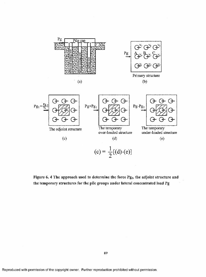
Pile cap
gj S" «V'V “ r : lK “
K,*C M '■'j js ii-
&Pg^
& &
(a)
Primary structure (b)
Pgi = I i-Vs
O O G "
Gpg+pg,
G G G "
G1777^
G G G
The adjoint structure
(c)
Pg-Pgi
G- G- G-The temporary over-loaded structure
(d)
(C) = { [ (d ) - (e ) ]
G- G- G-
G ^ G -
G G G
The temporary under-loaded structure
(e)
Figure 6. 4 The approach used to determine the force Pgi, the adjoint structure and the temporary structures for the pile groups under lateral concentrated load Pg
89
Reproduced with permission of the copyright owner. Further reproduction prohibited without permission.
6.5 The determination of the Mg of the primary structure for pile groups under
pile head bending moment
The primary structure and the bending moment Mg applied to the head of the piles in
a pile group are shown in Figure 6. 7 (a) and (b), in which the piles were pinned to the
pile cap and the bending moment Mg were applied to each head of the piles in the pile
group.
The determination of Mg is based on the principle that the pile group will produce
the same pile head deflection when subjected to the bending moments Mg, which is
applied to the pile heads under the pile cap, as the single isolated pile does when
subjected to bending moment Mt. The reason to adopt this principle is to compare the
sensitivity analysis results o f single pile with the piles in the group when they have same
value of deflection.
An example used to present the method to determine the concentrated bending
moments Mg is shown in Figure 6. 5. The single pile shown in this example is a free head
pile subjected to bending moment at the pile head, and the number o f load cycles N for
this example is equal 1. Accordingly, the piles in the pile group are pinned to the pile cap
and the piles in the pile group are subjected to bending moment at the pile head, and the
number o f load cycles N for this pile group is also equal 1.
The ordinate in the example represents the pile head bending moment Mg applied to
the heads of piles in pile group or the pile head bending moment Mt that the single pile is
subjected to. The abscissa in the example stands for the lateral deflections of a pile head
produced by the application of bending moment Mg or Mt.
The series of the bending moments Mt and the corresponding lateral deflections yxop have
already been determined in the analysis o f single isolated piles. They are retrieved from
previous study and plotted in the form of the Mt vs yxop curves for single pile, as shown in
Figure 6. 5. Similarly, the relationship of the Mg vs yxop curves for pile group can also be
plotted. It is obtained by using the FB-Pier program to calculate the deflections
90
Reproduced with permission of the copyright owner. Further reproduction prohibited without permission.

corresponding to a bending moment Mg series and then plotting the results in the same
coordinate system as which is used for the analysis o f single piles. After the Mt vs yxop
curves for single pile and Mg vs yjop curves for pile group are plotted in the same
coordinate system, it is easy to determine the bending moment Mg required to acquire the
same deflection as that o f the bending moment Mt produced at the head o f single pile.
The graphs o f bending moment Mg and Mt vs yiop for all the other pile groups under
study are saved in a picture format and included in the attached CD.
91
Reproduced with permission of the copyright owner. Further reproduction prohibited without permission.

600o Pile group, Pile distance=2DX Pile group. Pile distance=3D+ Pile group, Pile distanoe=4D♦ Pile group. Pile distance=5D-0- Single pile________________
500
M t vs. y„ curve for single pile 429,
405
M g VS. y curve for pile group■361
'352337
03E^ 300
C3)cT3tz03Jd■aCO03
20003
Mg312
295„
2732'U
234
196
Q-157
The pile deflections produced by M g are equal to the pile deflection produced by M t
117
100
0.005 0.01 0.015 0.02 0.025 0.03 0.035
Figure 6. 5 An example presenting the method to determine the force Mg applied to the head of the piles in a pile group
92
Reproduced with permission of the copyright owner. Further reproduction prohibited without permission.

6.6 The determination of the adjoint stracture and the unit lateral force Pgi for
pile groups subjected to bending moment applied to each pile head
The bending moment Mg is determined in chapter 6.5, hence the primary structure is
determined totally. However, in analysis o f the adjoint structure there is a need to
determine the values of lateral forces Pgi applied at the pile cap that will result in unit
shear force reaction on the pile member subjected to investigation. The method used to
determine the force Pgi for the primary structure shown in Figure 6. 7 is different than the
method deal with the pile group under lateral concentrated force as stated before.
In order to find out the force Pgi, it is necessary to introduce a structure shown in
Figure 6. 7 (c), in which a force 9 is applied in addition to the primary structure shown
in Figure 6. 7 (b). The force 9 is the multiple of 1 and the number of pile members (9)
in the pile group arrangement. The determination o f the force Pgi can be achieved by
subtracting the shear forces produced at the pile heads of structure shown in Figure 6. 7 (b)
from the shear forces produced at the pile heads o f structure shown in Figure 6. 7 (c). The
resultant of the operation “(c)-(b)” can be denoted in Figure 6. 7 (d), in which the shear
force differences AV1-AV9 exist at the heads o f each pile in the pile group. The following
equation is valid for the shear force differences:
(6 .6) 9 = X aV.i=l
As shown in Figure 6. 7 (e), for the sensitivity analysis o f the pile in the hatched area,
the sought force Pgi is required to be applied to the pile cap o f the adjoint structure in
such a way to produce unit shear force at the pile head of the hatched pile. The force Pgi
can be determined through the following equation:
93
Reproduced with permission of the copyright owner. Further reproduction prohibited without permission.
(6. 7) P g i =
E a v ,i = l
AV, AV4
In a general form, the force Pgi for the pile group consisted of 9 piles can be
obtained in the following equation:
E a v ,(6. 8) Pg, = i = l
AV AV.
where Pgi = the lateral force applied to the adjoint structure pile cap that will
produce unit shear force at the pile head under analysis,
A Vi = the shear forces difference produced at the pile head by subtracting the
shear forces produced at the pile heads of structure shown in Figure 6. 7 (b)
from the shear forces produced at the pile heads o f structure shown in Figure
6. 7 (c),
AVj = the shear force difference produced at the top of pile under analysis by
subtracting the shear forces produced at the pile head j o f structure shown in
Figure 6. 7 (b) from the shear forces produced at the pile head j o f structure
shown in Figure 6. 7 (c).
The results of Pgi for different Mg are presented in the charts o f Pgi vs. Mg in this
study. One typical chart is presented in Figure 6. 6, and all the charts for other cases are
saved in the attach disk in the format o f picture.
6.7 The results of the sensitivity analysis o f laterally loaded pile groups
The results o f the sensitivity analysis o f laterally loaded pile groups are presented
mostly in the graphical forms that are saved in the attached CD, whose contents are
presented in details in APPENDIX D. A typical example o f the results of the sensitivity
analysis for pile B (first trailing row) in a pile group embedded in the stiff clay above
water table, subjected to lateral concentrated force Pg applied to the pile cap, with the pile
members pinned to the pile cap, having distance s=2D, whereas pile length L=10T=13.7m
94
Reproduced with permission of the copyright owner. Further reproduction prohibited without permission.
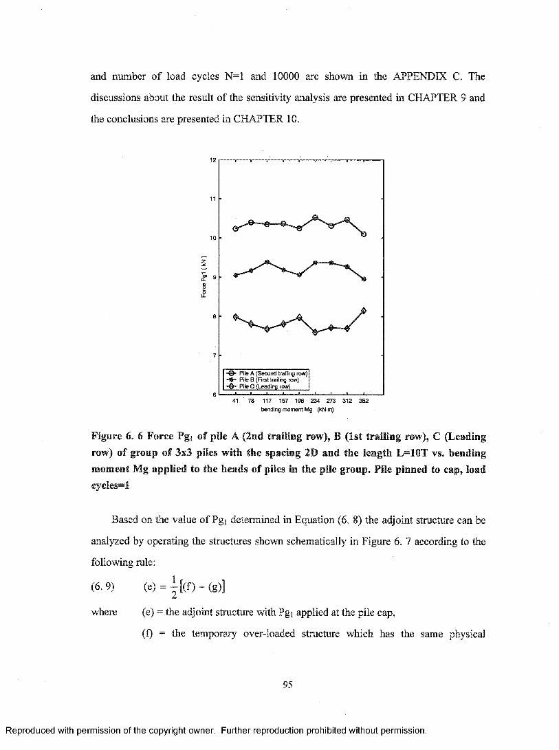
and number o f load cycles N=1 and 10000 are shown in the APPENDIX C. The
discussions about the result of the sensitivity analysis are presented in CHAPTER 9 and
the conclusions are presented in CHAPTER 10.
— ® '10
19
8I
8
" 0 - Pile A (S eco n d trailing row) - m - Pile B (First trailing row)
Pile C (Leading row)
41 78 117 157 196 234 273 312 352bend ing m om ent Mg (kN-m)
Figure 6. 6 Force Pgi of pile A (2nd trailing row), B (1st trailing row), C (Leading row) of group of 3x3 piles with the spacing 2D and the length L=10T vs. bending moment Mg applied to the heads of piles in the pile group. File pinned to cap, load cycles=l
Based on the value o f Pgi determined in Equation (6. 8) the adjoint structure can be
analyzed by operating the structures shown schematically in Figure 6. 7 according to the
following rule:
(6. 9)
where (e) = the adjoint structure with Pgi applied at the pile cap,
(f) = the temporary over-loaded structure which has the same physical
95
Reproduced with permission of the copyright owner. Further reproduction prohibited without permission.
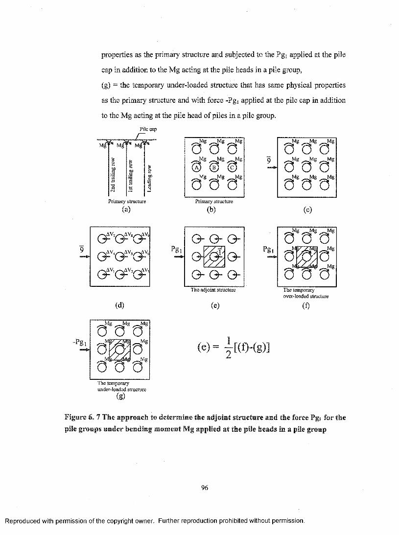
properties as the primary structure and subjected to the Pgi applied at the pile
cap in addition to the Mg acting at the pile heads in a pile group,
(g) - the temporary under-loaded structure that has same physical properties
as the primary structure and with force -Fgi applied at the pile cap in addition
to the Mg acting at the pile head of piles in a pile group.
Pile capr
Mg Mg Mg'
OH•S
0 Q 0..Mg ^ .M g
^ (c
0 0 0
-C#® 0 0 00 0 0^ ^ g —Mg ^Mg0 0 0
Primary structure
(a)Piimaiy structure
( b ) (c)
Pg^G ” G- G “
G - ^ O
G- G- 0 -
P ^
.<-^8 ,-sMg 0 0 0
0 ^ ; 0M g [ ^ y hdg
0 0 0
( d )
The adjoint structure
(e)
The temporary over-loaded structure
( f )
Mg Mg Mg
0 0 0
0 0 0The temporary under-loaded structure
(g)
Figure 6. 7 The approach to determine the adjoint structure and the force Pgi for the pile groups under bending moment Mg applied at the pile heads in a pile group
96
Reproduced with permission of the copyright owner. Further reproduction prohibited without permission.
CHAPTER 7 PROGRAMMING OF SENSITIVITY ANALYSIS
FOR SINGLE PILES
7.1 Introduction
In this study, the Matlab programs are used to prepare the input data for the
COM624P, call COM624P to calculate the deformation and internal forces, read the
output result data o f COM624P for further analysis, to investigate the sensitivity o f single
piles, and to present the sensitivity analysis results. The analysis programs used for
analysis are divided into several modules shown in Figure 7. 1.
7.2 Preparing and input file generating module
The preparing and input file generating module prepares the directory system used to
differentiate different boundary conditions, pile lengths and load cycles o f single piles
embedded in stiff clay above water table. It also generates the input files for COM624P to
calculate the forces and deformations o f the primary and adjoint structures produced by
the applied load. Different file names are assigned to different cases.
97
Reproduced with permission of the copyright owner. Further reproduction prohibited without permission.
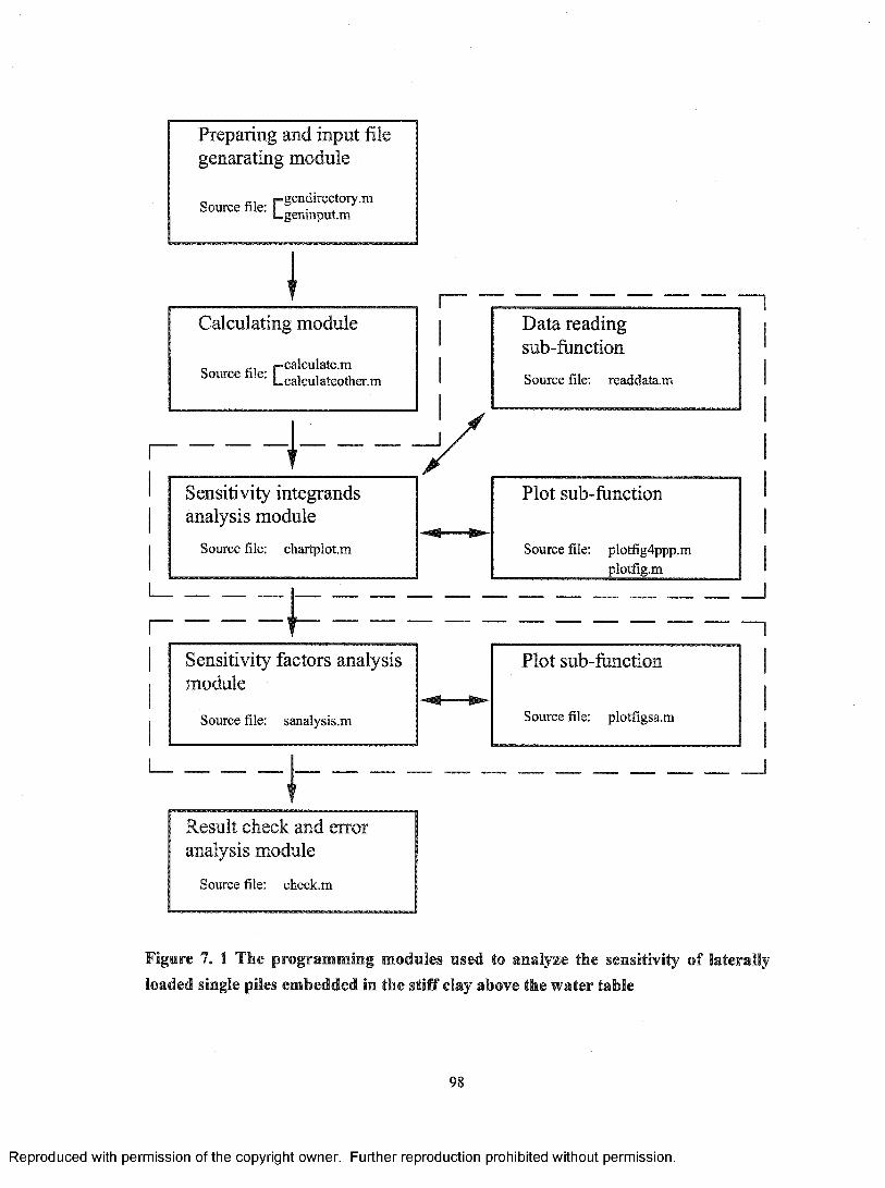
Preparing and input file genarating module
c i-gendirectory.inSource file: I • .L-genmput.m
ICalculating module
„ i-calculate.m Source file: I , , ^Lcalculateother.m
1
Data reading sub-functionSource file: readdata.m
t — - XSensitivity integrands Plot sub-functionanalysis module
Source file: chartplot.m Source file: plotfig4ppp.mplotfig.m
Sensitivity factors analysis module
Source file: sanalysis.m
Plot sub-function
Source file: plotfigsa.m
1 — ------------- _ — ----- ------ —— - — ------ -----
Result check and error analysis module
Source file: check.m
Figure 7. 1 The programming modules used to analyze the sensitivity of laterally loaded single piles embedded in the stiff clay above the water table
98
Reproduced with permission of the copyright owner. Further reproduction prohibited without permission.
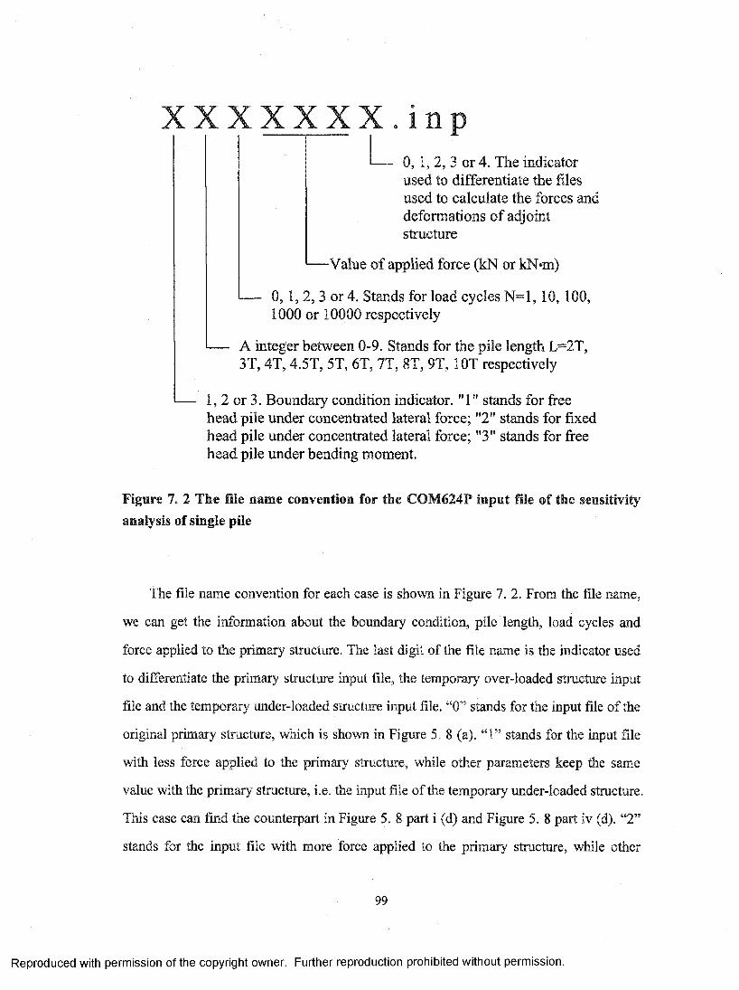
X X X X X X X . i n p0, 1, 2, 3 or 4. The indicatorused to differentiate the files used to calculate the forces and deform ations o f adjointstructure
-Value o f applied force (kN or kN*m)
0, 1 ,2 , 3 or 4. Stands for load cycles N = l, 10, 100, 1000 or 10000 respectively
A integer betw een 0-9. Stands for the pile length L=2T, 3T, 4T, 4.5T, 5T, 6T, 7T, 8T, 9T, lOT respectively
1, 2 or 3. Boundary condition indicator. "1" stands for free head pile under concentrated lateral force; "2" stands for fixed head pile under concentrated lateral force; "3" stands for free head pile under bending moment.
Figure 7. 2 The file name convention for the COM624P input file of the sensitivity analysis of single pile
The file name convention for each case is shown in Figure 7. 2. From the file name,
we can get the information about the boundary condition, pile length, load cycles and
force applied to the primary structure. The last digit of the file name is the indicator used
to differentiate the primary structure input file, the temporary over-loaded structure input
file and the temporary under-loaded structure input file. “0” stands for the input file o f the
original primary structure, which is shown in Figure 5. 8 (a). “ 1” stands for the input file
with less force applied to the primary structure, while other parameters keep the same
value with the primary structure, i.e. the input file of the temporary imder-loaded structure.
This case can find the counterpart in Figure 5. 8 part i (d) and Figure 5. 8 part iv (d). “2”
stands for the input file with more force applied to the primary structure, while other
99
Reproduced with permission of the copyright owner. Further reproduction prohibited without permission.
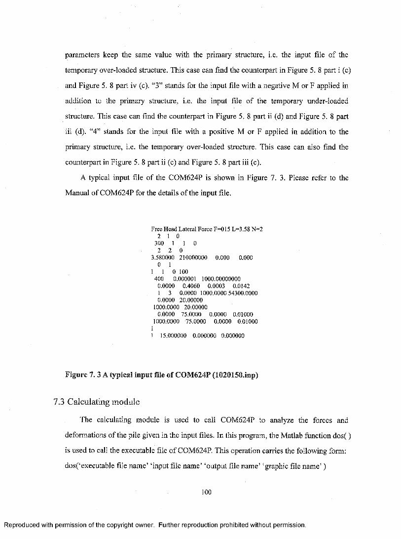
parameters keep the same value with the primary structure, i.e. the input file of the
temporary over-loaded structure. This case can find the counterpart in Figure 5. 8 part i (c)
and Figure 5. 8 part iv (c). “3” stands for the input file with a negative M or F applied in
addition to the primary structure, i.e. the input file o f the temporary under-loaded
structure. This case can find the counterpart in Figure 5. 8 part ii (d) and Figure 5. 8 part
iii (d). “4” stands for the input file with a positive M or F applied in addition to the
primary stmcture, i.e. the temporary over-loaded structure. This case can also find the
counterpart in Figure 5. 8 part ii (c) and Figure 5. 8 part iii (c).
A typical input file of the COM624P is shown in Figure 7. 3. Please refer to the
Manual o f COM624P for the details of the input file.
Free Head Lateral Force F=015 L=3.58 N=2 2 1 0
300 1 1 02 2 0
3.580000 210000000 0.000 0.0000 1
1 1 0 100400 0.000001 1000.00000000
0.0000 0.4060 0.0003 0.01421 3 0.0000 1000.0000 54300.00000.0000 20.00000
1000.0000 20.00000 0.0000 75.0000 0.0000 0.01000
1000.0000 75.0000 0.0000 0.0100011 15.000000 0.000000 0.000000
Figure 7.3 A typical input file of COM624P (1020150.inp)
7.3 Calculating module
The calculating module is used to call COM624P to analyze the forces and
deformations o f the pile given in the input files. In this program, the Matlab function d o s()
is used to call the executable file o f COM624P. This operation carries the following form:
dos(‘executable file name’ ‘input file name’ ‘output file name’ ‘graphic file name’ )
100
Reproduced with permission of the copyright owner. Further reproduction prohibited without permission.
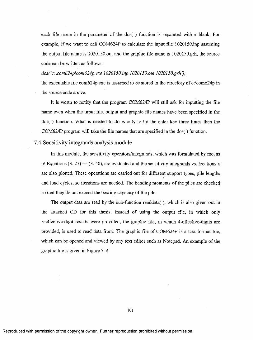
each file name in the parameter o f the dos( ) fimction is separated with a blank. For
example, if we want to call COM624P to calculate the input file 1020150.inp assuming
the output file name is 10201 SO.out and the graphic file name is 1020150.grh, the source
code can be written as follows:
dos( ‘c; \com624p\com624p. exe 10201SO.inp 10201SO.out 1020150.grh’);
the executable file com624p.exe is assumed to be stored in the directory of c:\com624p in
the source code above.
It is worth to notify that the program COM624P will still ask for inputting the file
name even when the input file, output and graphic file names have been specified in the
dos( ) function. What is needed to do is only to hit the enter key three times then the
COM624P program will take the file names that are specified in the dos() function.
7.4 Sensitivity integrands analysis module
In this module, the sensitivity operators/integrands, which was formulated by means
o f Equations (3. 27) — (3. 40), are evaluated and the sensitivity integrands vs. locations x
are also plotted. These operations are carried out for different support types, pile lengths
and load cycles, so iterations are needed. The bending moments o f the piles are checked
so that they do not exceed the bearing capacity of the pile.
The output data are read by the sub-function readdata(), which is also given out in
the attached CD for this thesis. Instead of using the output file, in which only
3-effective-digit results were provided, the graphic file, in which 4-effective-digits are
provided, is used to read data from. The graphic file of COM624P is a text format file,
which can be opened and viewed by any text editor such as Notepad. An example o f the
graphic file is given in Figure 7. 4.
101
Reproduced with permission of the copyright owner. Further reproduction prohibited without permission.
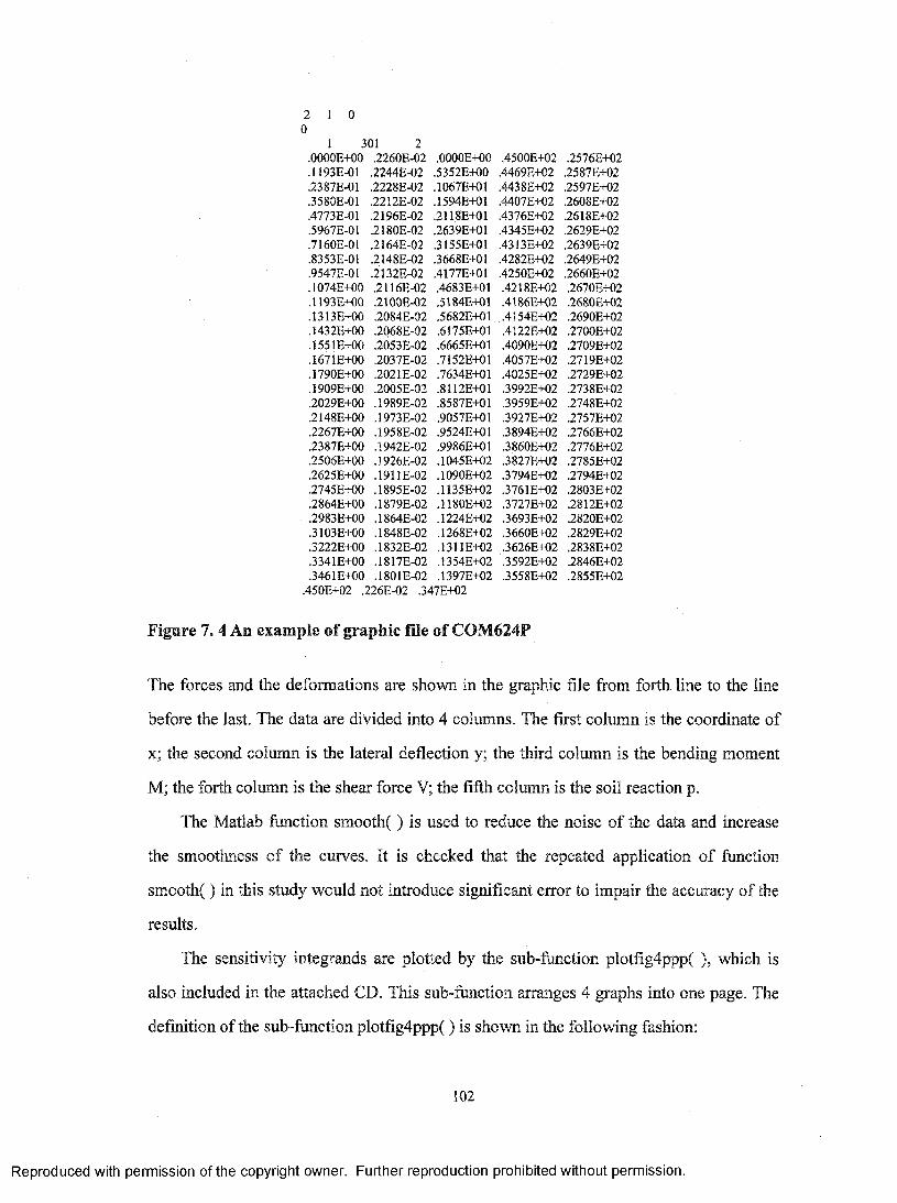
2 1 0 0
1 301 2.OOOOE+00 .2260E-02 .OOOOE+00 ,4500E+02 .2576E+02 .1193E-01 .2244E-02 .5352E+00 .4469E+02 .2587E+02 .2387E-01 .2228E-02 .1067E+01 .4438E+02 .2597E+02 .3580E-01 .2212E-02 .1594E+01 .4407E+02 .2608E+02 .4773E-01 .2196E-02 .2118E+01 .4376E+02 .2618E+02 .5967E-01 .2180E-02 .2639E+01 .4345E+02 .2629E+02 .7160E-0I .2164E-02 .3155E+OI .4313E+02 .2639E+02 .8353E-01 .2148E-02 .3668E+01 ,4282E-K)2 .2649E+02 .9547E-01 .2132E-02 .4177E+01 .425GE+02 .2660E+02 .1074E+00 .2116E-02 .4683E+01 .4218E+02 .2670E+02 .1193E+00 .2100E-02 .5184E+01 .4186E+02 .2680E+02 .1313E+00 .2084E-02 .5682E+01 .4154E+02 .2690E+02 .1432E+00 .2068E-02 .6175E+01 .4122E+02 .2700E+02 .1551E+00 .2053E-02 .6665E+01 .4090E+02 .2709E+02 .1671E+00 .2037E-02 .7152E+01 .4057E+02 .27I9E+02 .1790E+00 .2021E-02 .7634E+01 .4025E+02 .2729E+02 .1909E+00 ,2005E-02 .8112E+01 .3992E+02 .2738E+02 .2029E+00 .1989E-02 .8587E+01 .3959E+02 .2748E+02 .2I48E+00 .1973E-02 .9057E+01 .3927E+02 .2757E+02 .2267E+00 .1958E-02 .9524E+01 .3894E+02 .2766E+02 .2387E+00 .1942E-02 .9986E+01 .3860E+02 .2776E+02 .2506E+00 .1926E-02 .1045E+02 .3827E+02 .2785E+02 .2625E+00 .1911E-02 .1090E+02 .3794E+02 .2794E+02 .2745E+00 .1895E-02 .1135E+02 .3761E+02 .2803E+02 ,2864E-H)0 .1879E-02 .1180E+02 .3727E+02 .2812E+02 .2983E+00 .1864E-02 .1224E+02 .3693E+02 .2820E+02 .3103E+00 .1848E-02 .1268E+02 .3660E+02 .2829E+02 .3222E+00 .1832E-02 .1311E+02 .3626E+02 .2838E+02 .3341E+00 ,1817E-02 .1354E+02 .3592E+02 .2846E+02 .346IE+00 .1801E-02 .1397E+02 ,3558E-K)2 .2855E+02
.450E+02 .226E-02 .347E+02
Figure 7. 4 An example of graphic file of COM624P
The forces and the deformations are shown in the graphic file from forth line to the line
before the last. The data are divided into 4 columns. The first column is the coordinate of
x; the second column is the lateral deflection y; the third column is the bending moment
M; the forth column is the shear force V; the fifth column is the soil reaction p.
The Matlab ftmction smooth( ) is used to reduce the noise o f the data and increase
the smoothness o f the curves. It is checked that the repeated application o f function
smooth() in this study would not introduce significant error to impair the accuracy of the
results.
The sensitivity integrands are plotted by the sub-fimction plotfig4ppp( ), which is
also included in the attached CD. This sub-function arranges 4 graphs into one page. The
definition of the sub-function plotfig4ppp() is shown in the following fashion:
102
Reproduced with permission of the copyright owner. Further reproduction prohibited without permission.

function plotfig4ppp(x, y, nStep, MForce, SupportStyle, LoadCycles, OutFileName,...
NodeNumber, RealLength, FUnit, sTitle, sXLabel, sYLabel, LegendPosition,...
PileLengthInT);
Another sub-fimction plotfig(), which is used to plot one graph per page, was also
created in this study. The definition of plotfig() is shown in the following fashion:
function plotfig(x, y, nStep, MForce, SupportStyle, LoadCycles, OutFileName,...
NodeNumber, RealLength, FUnit, sTitle, sXLabel, sYLabel, LegendPosition,...
PileLengthInT);
The parameters o f sub-function plotfig4ppp( ) and plotfig( ) have the following
meaning:
X — ordinate x.
y — abscissa y; it may stand for sensitivity integrands, lateral deflections or bending
moments etc..
nStep — the number o f force steps, i.e., number o f the curves shown simultaneously
in each graph.
Mforce — matrix of force, i.e., the value o f force series applied to the primary
structure.
SupportStyle — the type of support condition; 1, 2 or 3 as stated before.
LoadCycles — the indicator for load cycles; 0, 1, 2, 3 or 4; represents load cycles 1,
10, 100, 1000 or 10000 respectively.
OutFileName — output file name.
NodeNumber — the number of nodes used to analyze the pile in COM624P.
RealLength — the real length of the pile (m).
FUnit — force unit (kN or kN-m).
sTitle, sXLabel, sYLabel — text represents the title, label o f x axis, label of y axis
respectively.
LegendPosition — the position where the legend was located, pos = -1 places the
103
Reproduced with permission of the copyright owner. Further reproduction prohibited without permission.
legend outside the axes boundary on the right side, pos = 0 places the legend inside the
axes boundary, obscuring as few points as possible, pos = 1 places the legend in the
upper-right comer of the axes (default), pos = 2 places the legend in the upper-left comer
o f the axes, pos = 3 places the legend in the lower-left comer of the axes, pos = 4 places
the legend in the lower-right comer o f the axes.
PileLengthInT— the pile length in the unit o f Relative Stiffiiess factor T.
Through the Matlab function print( ), the graphs are saved to disc in the Ghost Script
Graphical format. The extension name o f the files was .eps and the graphical files can be
opened and viewed through a program GSview [27], whose free trial version can be
downloaded through Intemet.
In the end o f the source code, the Matlab command “save” is used to save the results
into one file for the future use such as calculating the sensitivity factors. The results are
saved into a Matlab format file named “YMC.DAT”. The result can be retrieved by using
the following source code:
load('YMC.DAT','-mat');
Please refer to the manual of Matlab for the details of functions such as plot( ),
prin t(), legend() and load().
7.5 Sensitivity factors analysis module
The sensitivity factors analysis module integrated the sensitivity operators/integrands
to calculate the sensitivity factors. The relative influences are also obtained by calculating
the percentages o f each sensitivity factor to the summation of all the sensitivity factors
related to the pile. The results are printed out as bar charts.
The integrations are obtained by means of the Simpson’s quadrature, which was
accomplished by the sub-function simpsonquad( ).
7.6 Result check and error analysis module
The result check was fulfilled by the source file check, m. The result check method is
stated in detail in Section 5.10.
104
Reproduced with permission of the copyright owner. Further reproduction prohibited without permission.
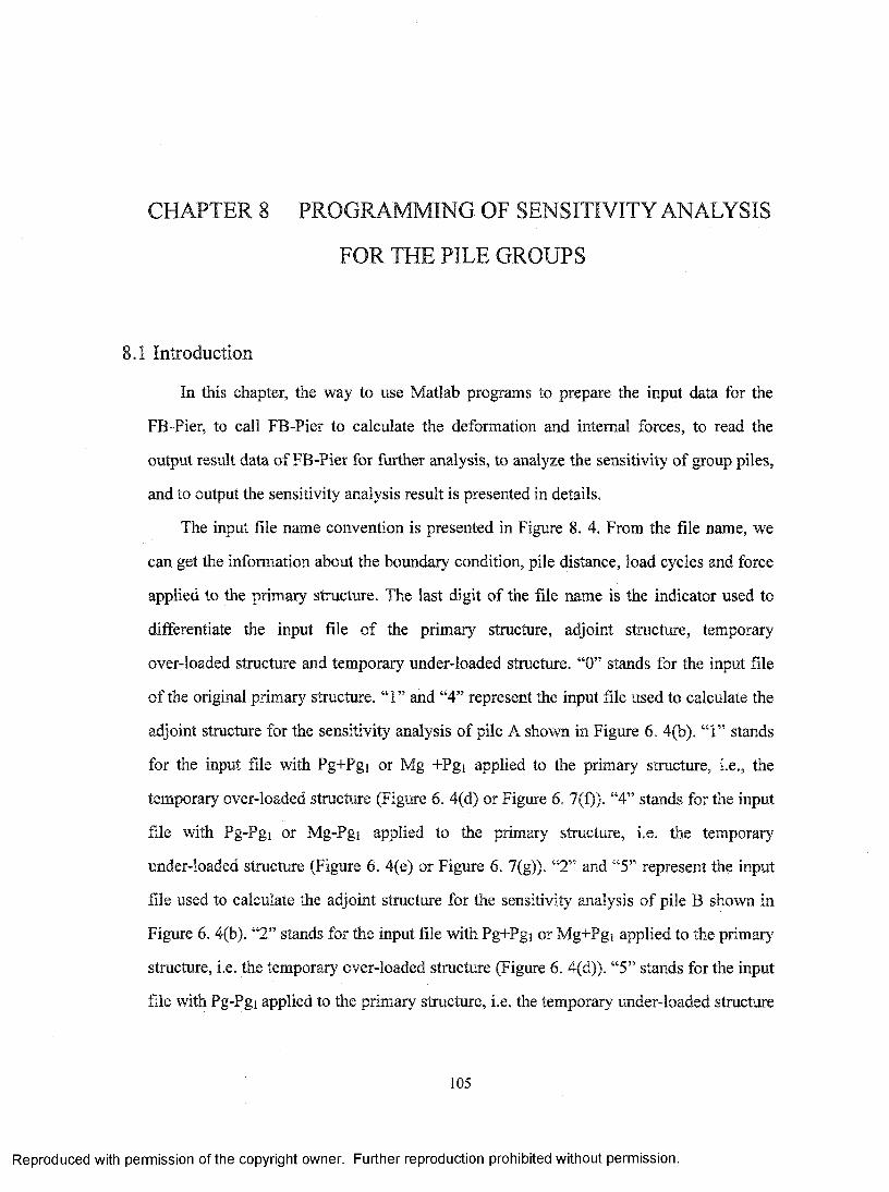
CHAPTER 8 PROGRAMMING OF SENSITIVITY ANALYSIS
FOR THE PILE GROUPS
8.1 Introduction
In this chapter, the way to use Matlab programs to prepare the input data for the
FB-Pier, to call FB-Pier to calculate the deformation and internal forces, to read the
output result data o f FB-Pier for further analysis, to analyze the sensitivity of group piles,
and to output the sensitivity analysis result is presented in details.
The input file name convention is presented in Figure 8. 4. From the file name, we
can get the information about the boundary condition, pile distance, load cycles and force
applied to the primary structure. The last digit o f the file name is the indicator used to
differentiate the input file o f the primary structure, adjoint structure, temporary
over-loaded structure and temporary under-loaded structure. “0” stands for the input file
o f the original primary structure. “1” and “4” represent the input file used to calculate the
adjoint structure for the sensitivity analysis of pile A shown in Figure 6. 4(b). “1” stands
for the input file with Pg+Pgi or Mg +Pgi applied to the primary structure, i.e., the
temporary over-loaded structure (Figure 6. 4(d) or Figure 6. 7(f)). “4” stands for the input
file with Pg-Pgi or Mg-Pgi applied to the primary structure, i.e. the temporary
under-loaded structure (Figure 6. 4(e) or Figure 6. 7(g)). “2” and “5” represent the input
file used to calculate the adjoint structure for the sensitivity analysis o f pile B shown in
Figure 6. 4(b). “2” stands for the input file with Pg+Pgi or Mg+Pgi applied to the primary
structure, i.e. the temporary over-loaded structure (Figure 6. 4(d)). “5” stands for the input
file with Pg-Pgi applied to the primary structure, i.e. the temporary under-loaded structure
105
Reproduced with permission of the copyright owner. Further reproduction prohibited without permission.

(Figure 6. 4(e)). “3” and “6” represent the input file used to calculate the adjoint structure
for the sensitivity analysis o f pile C shown in Figure 6. 4(b). “3” stands for the input file
with Pg+Pgi applied to the primary structure, i.e. the temporary over-loaded structure
(Figure 6. 4(d)). “6” stands for the input file with Pg-Pgi applied to the primary structure,
i.e. the temporary under-loaded structure (Figure 6. 4(e)). “9” stands for the input file of
the temporary structure shown in Figure 6. 7 (c), in which a force 9 , which is 9 times of
a unit force 1, was applied in addition to the primary structure shown in Figure 6. 7 (b).
It is necessary to keep a certain executing sequence o f the Matlab programs included
in the attachment since one o f them depends on the results o f others. The executing
sequence of files is shown in Figure 8. 3. In the following paragraphs, the Matlab
programs are introduced respectively.
Groupgendirectory.m
This program is used to generate the directory system in which the preparing and
result data are saved. There are two directories generated, ‘C:\G’ and ‘C:\GSA’. The
directory ‘C:\G’ is used to hold preparing data and the ‘C:\GSA’ is used to hold the
sensitivity analysis result data.
Groupgeninputproducepdelta.m
This program generates the input files producing the force vs. pile head deflection
graphs, which is also used to find out the force Pg and Mg shown in Figure 6. 2 and
Figure 6. 5. The input files are saved in the fold o f ‘C:\G’.
Groupcalculate.m
This program calculates the input files produced by Groupgeninputproducepdelta.m.
The Matlab command line calling the FB-Pier program to calculate the laterally loaded
piles had the format shown in Figure 8. 1:
106
Reproduced with permission of the copyright owner. Further reproduction prohibited without permission.
String storing Executable file memory size forexecutable file name path calculation,name path 256M used here
nI-------------------FBEXE= C: \progra~l \BSI\FBPier_eng.exe m:256'; dos([FBEXE, ' I:'”,InputFileName, O:'", OutputFileName,
Figure 8. 1 The Matlab command line calling FB-Pier program to calculate the laterally loaded piles
GroupplotPdelta.m
This program calculates the force Pg and Mg determined by the method presented in
Chapter 6.3 and 6.5 and plot the Pg or Mg vs. yxop graphs presented in Figure 6. 2 and
Figure 6. 5.
Groupgenprimaryinput.m
This program generates the input files for FB-Pier to calculate the primary structures
shown in Figure 6. 4 (a) and (b) and Figure 6. 7 (a) and (b). The force Pg and Mg
determined by GroupplotPdelta. m are used as the force series applied at the primary
structure.
Grouptransferresult_primaryonly.m
This program reads the output results o f FB-Piers for the primary structures and
saves them into Matlab format data files.
GroupCalculatePgl_S l_2.m
This program calculates force Pgi, determined by the method shown in Chapter 6.4
and Figure 6. 4, for the pile groups under lateral concentrated load (SupportStyle = 1 and
2). The force Pgi are obtained through the application of Equation (6. 3) and the results of
force Pgi are saved into a Matlab data file named ForcePgl.dat.
GroupGenUnitAppliedF_S3 .m
This program generates the input files for FB-Piers to calculate the structure shown
107
Reproduced with permission of the copyright owner. Further reproduction prohibited without permission.
in Figure 6. 7 (c), in which a force 9 , which is 9 times of a unit force 1, is applied in
addition to the primary structure shown in Figure 6. 7 (b).
GroupCalculateUnitAppliedF_S3 .m
This program calls FB-Pier software to calculate the input files generated in the
program GroupGenUnitAppliedF SS. m.
GroupCalculatePg 1_S3 .m
This program reads the results gained from the program
GroupCalculateUnitAppliedF_S3.m and calculates the Pgi, determined in Section 6.6 and
Figure 6. 7, for the pile groups with bending moments Mg applied at the pile heads
(SupportStyle = 3). The forces Pgi are obtained through the application o f Equation (6. 8).
The results of force Pgi are saved into a Matlab data file named ForcePgl.dat.
Groupplotpg 1 vsPg.m
This program plots the Pgi vs. Pg or Mg charts, whose examples are presented in the
Figure 6. 3 and Figure 6. 6.
Groupgenadjointinput.m
This program generates the input files for FB-Pier to calculate the temporary
over-loaded and temporary under-loaded structures shown in Figure 6. 4 (d) and (e) and
Figure 6. 7 (f) and (g). The results, such as force Pgi, saved in Matlab data file
ForcePgl.dat, which are obtained by the application of GroupCalculatePgl_S1 _2.m and
GroupCalculatePgl S3.m, are loaded and introduced into the input files for the
calculation o f the adjoint structures.
Groupadjointcalculate.m
This program calls FB-Pier to calculate the input files generated through the
application of program Groupgenadjointinput.m.
Grouptransferresult.m
108
Reproduced with permission of the copyright owner. Further reproduction prohibited without permission.

This program reads the output results o f FB-Piers for the adjoint structures and saves
them into Matlab format data files.
groupchartplota.m
In this program, the sensitivity operators/integrands, which are formulated in
Equations (3. 27) — (3. 40), are evaluated and saved in Matlab data files named
“ YM C .D A T”. These operations are carried out for different support types, pile distances,
pile numbers and load cycles, so iterations are needed.
groupchartplotb .m
This program reads the result data gained through groupchartplota.m, and plots the
operators/integrands vs. locations x for piles with different support types, pile distances,
pile numbers and load cycles. The results are saved in the attached CD as the format of
picture format files.
groupsa.m
This program integrates the sensitivity operators/integrands to calculate the
sensitivity factors. The relative sensitivity factors are also obtained by calculating the
percentages o f each sensitivity factor to the summation of all the sensitivity factors
related to the pile. The results are presented as bar charts.
Groupcheck.m
This program is used to check the results of the sensitivity analysis for the pile
groups carried out in this research.
8.2 FB-Pier program
The University of Florida, Bridge Software Institute (BSI), with the support o f the
Florida Department of Transportation and the Federal Highway Administration,
developed FB-Pier program (2001). The program also employs p-y method, but it uses
non-linear fmite element analysis. The program is an integrated program, which both
calculates and designs the structure o f pile/piers. The program has the capability to
109
Reproduced with permission of the copyright owner. Further reproduction prohibited without permission.
analyze and design single piles/piers, pile or shaft groups, piles and pile caps, high mast
signs and retaining walls. The structural model includes both linear and non-linear
(concrete cracking, steel yielding and soil nonlinearity etc.) features. The program can be
downloaded from website http://bsi-web.ce.ufl.edu
In order to obtain preciser results of sensitivity analysis, it may be needed to divide
the piles under study by means of larger number o f nodes, and it may be expected to have
more effective digits in the output results of FB-Piers. This goals are achieved by taking
advantage of advance features o f FB-Piers and writing Matlab programs.
It is considered as an inconvience that the progam of FB-PierV3 has an upper limit
of 50 nodes for each pile when user interface is executed. Other ways are needed to be
found if there is a demand for more nodes. Figure 8. 2 presents one way to modify the
input file to use more than 50 nodes in analyzing pile groups for sensitivity analysis. In
this method, another executable file FBPier_eng.exe, provided together with FB-PierV3
and saved in the same directory where the file FB-Pier exe is saved in, is used.
110
Reproduced with permission of the copyright owner. Further reproduction prohibited without permission.
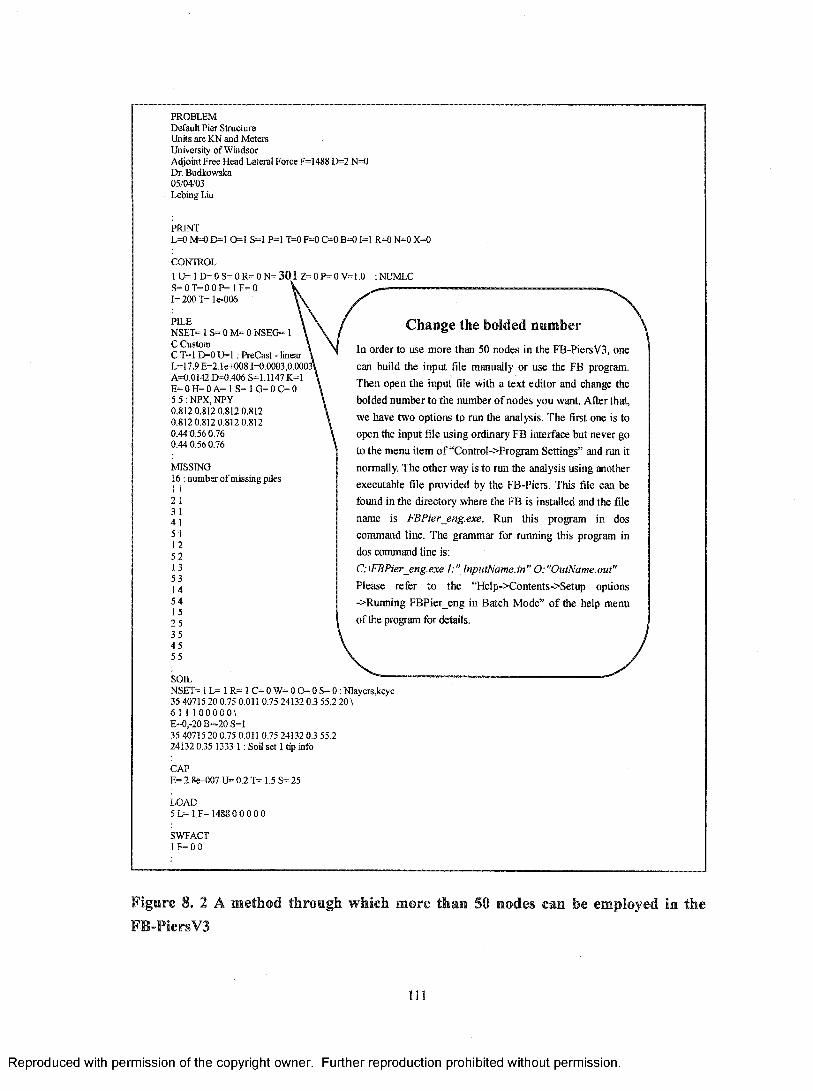
PROBLEM Default Pier Structure Unita are K N and Meters University ofWindsorAdjoint Free Head Lateral Force F=1488 D=2 N=0 Dr. Budkowska 03/04/03 Lebing Liu
PRINTL=0 M =0 D -1 0=1 S=1 P=1 T=0 F=0 C=0 B = 0 1=1 R=0 N=0 X=0
CONTROL
i u = i d = o s = o r = o n = 3 0 1 z = o p = o v = i .o ;N U M LC S=O T=O O P = 1 F = 0 I= 2 0 0 T = le -0 0 6
PILENSET= 1 S= 0 M = 0 NSEG= 1 C CtjstomC T=1 D=0 U=1 : PreCast - linear L=17.9 E=2.1e+0081=0,0003,0.A=0,01421>0.406 S=1.1147 K=1 E = O H = O A = 1 S = I G = 0 C = 0 5 5 : NPX, N PY 0,812 0,812 0.812 0,812 0,812 0.812 0,812 0,812 0.44 0,56 0,76 0,44 0,56 0,76
M ISSING16 : number o f missing piles 1 1 21 3 1 41 5 1 1252 1 353145 415 2 5 3 5 4 555
son.NSET= 1 L = 1 R = 1 C = 0 W = 0 0 = 0 S= 0 : Nlayers,kcyc 35 40715 20 0,75 0.0] 1 0.75 24132 0.3 55,2 20 \6 1 1 1 0 0 0 0 0 \E=0,-20B=-20S=135 40715 20 0,75 0,011 0.75 24132 0.3 55.2 24132 0,35 1333 1 : Soil set 1 tip info
C/kPE= 2,8e+007 U = 0,2 T= 1,5 S= 25
LO AD5 L= 1 F= 1488 0 0 0 0 0
SWFACT1F=00
Change the bolded numberIn order to use more than 50 nodes in the FB-PieisV3, one
can build the input file manually or use the FB program.
Then open the input file with a text editor and change the
bolded number to the number o f nodes you want. After that,
we have two options to run the analysis. The first one is to
open the input file using ordinary FB interface but never go
to the menu item o f “Control->Program Settings” and run it
normally. The other way is to run the analysis using another
executable file provided by the FB-Piers. This file can be
found in the directory where the FB is installed and the file
name is FBPier_eng.exe. Run this program in dos
command line. The grammar for running this program in
dos command line is:
C :\FBPier_eng.exe I :" InputName.in" O:"OutName.out"
Please refer to the “Help->Contents->Setup options
->Running FBPier eng in Batch Mode” o f the help menu
o f the program for details.
Figure 8. 2 A method through which more than 50 nodes can be employed in the FB-Piers V3
111
Reproduced with permission of the copyright owner. Further reproduction prohibited without permission.
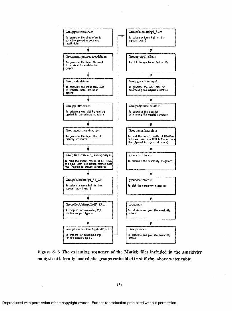
GroupCalculatePgl_S3.m
To colculote force Pgi for the support type 3
Groupadjointcalculate.m
To calculate the files for determining the adjoint structure
Groupgenadjointinputm
To generate the input files for determining the odjoint structure
groupchartplotb.m
To plot the sensitivity integrands
GroupplotpglvsPg.m
To plot the graphs of Pgi vs. Pg
Groupgenprimaryinput.m
To generote the input fiies of primary structures
GroupplotPdelta.m
To calculate and plot Pg and Mg applied to the primary structure
Grouptransfeiresultm
To read the output results of FB-Piers and save them into Matlab formot data files (Applied to adjoint structure)
groupsa.m
To calculate and plot the sensitivity factors
groupcharlplota.m
To calculate the sensitivity Integrands
Groupgeninputproducepdelta.m
To generate the input file used to produce force-defiection grophs
Groupcalculate.m
To calculate the input files used to produce force-deflection graphs
GroupGenUnitAppliedF_S3 .m
To prepare for calculating Pgi for the support type 3
GroupCalculatePgl_Sl_2.m
To calculate force Pgi for the support type 1 and 2
Grouptransferresult_primaryonly.m
To read the output results of FB-Plers and save them into Matlob format data files (Applied to primary structure)
Groupgendirectoiy.m
To generate the directories to save the preporing data and result data
GroupCalculateUnitAppliedF_S3.m
To prepare for calculating Pgi for the support type 3
Groupcheck.m
To coiculate and plot the sensitivityfoctors
Figure 8. 3 The executing sequence of the Matlab files included in the sensitivity analysis of laterally loaded pile groups embedded in stiff clay above water table
112
Reproduced with permission of the copyright owner. Further reproduction prohibited without permission.

X X X X X X X X . i n p L 0, 1, 2, 3 ,4, 5 or 6 . The
indicator used to differentiatethe files used to calculate the forces and deform ations o f adjoint structure
-Value o f applied force (kN or kN*m)
0, 1, 2, 3 or 4. Stands for load cycles N = l, 10, 100, 1000 or 10000 respectively
2, 3, 4 o r 5, stands for pile distance equal 2D, 3D, 4D or 5D respectively
— 1 ,2 or 3. Boundary condition indicator. ”1" stands for a pile pined to a cap under concentrated lateral force; "2" stands for a pile fixed to a cap under concentrated lateral force; "3" stands for a pile pinned to a cap under bending m om ent applied at each pile head.
Figure 8. 4 The file name convention for the FB-Pier input file of the sensitivity analysis of the pile group
8.3 A m eth o d u sed to read m o re p rec ise re su lt from FB-PierV3
In order to read more precise output data (8 effective digits for intemal forces and 16
digits for deflections can be achieved if the results are read from the post processing fiies
of the FB-Piers.), one needs to know something about how to open a binary file and read
data from it. There are several output files for post processing after the running o f the
program. Please refer the menu o f the program “Help->Contents->Post Processing
Formats” for details. Among those files, the file with extension .pil has the information
about the deflection of nodes. The deflections of the pile nodes are stored in double float
point array in this file. And the file with extension .vmd has the information about the
intemal forces of the elements. The file with extension .soi includes the results o f soil
resistance. The Matlab function shown in Figure 8. 5 can read the deflection and force
113
Reproduced with permission of the copyright owner. Further reproduction prohibited without permission.
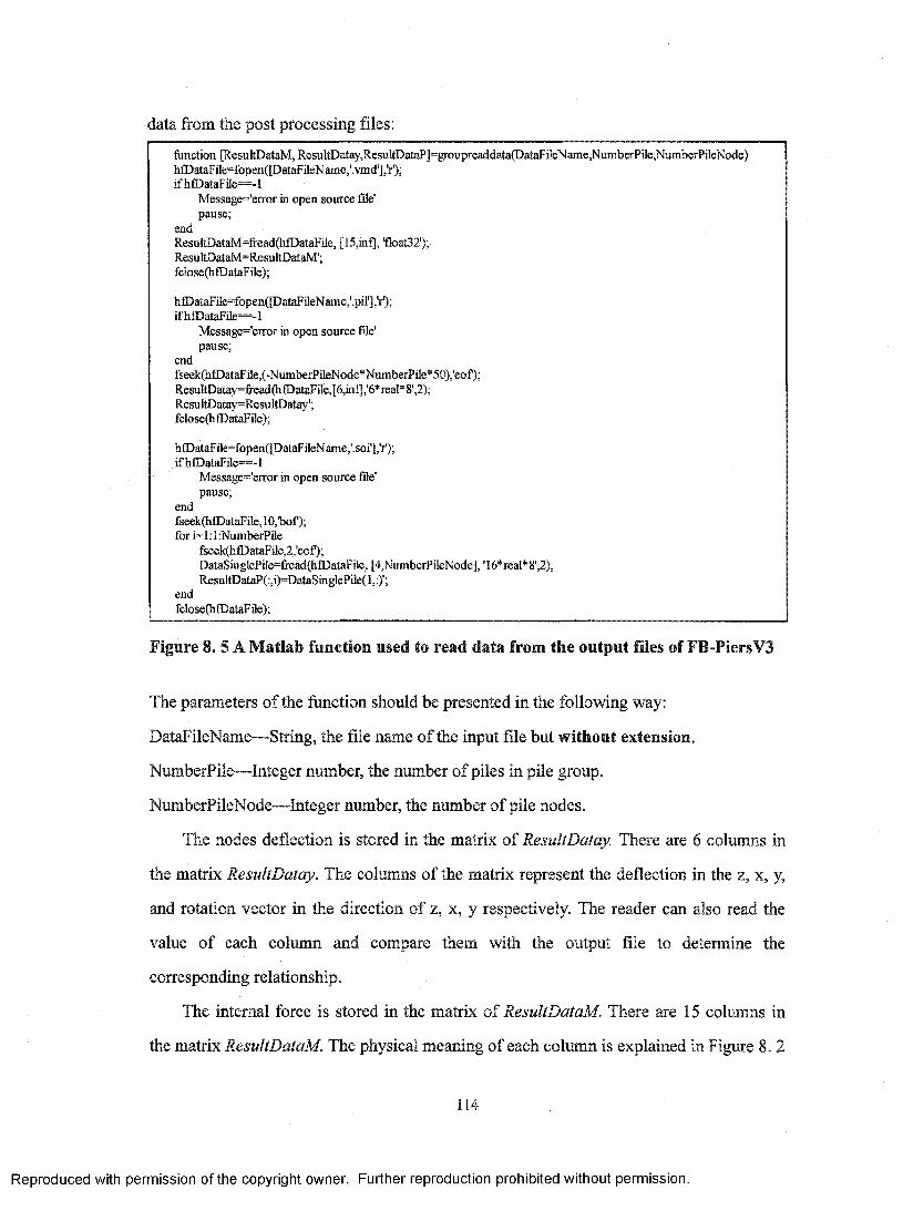
data from the post processing files:function [ResultDataM, ResultDatay,ResultDataP]=groupreaddata(DataFileName,NumberPile,NumberPileNode)hfDataFib=fopen([DataFileName,'.Ymd'],'r');ifhfDataFUe— -1
Message='error in open source file' pause;
endResu!tDataM=ffead(hfDataFile, [15,inf], 'float32');ResultDataM=ResultDataM';fclose(hfDataFile);
hfDataFile=fopen(PataFileName,'.pilX'rO;ifh£DataFile==-l
Message='error in open source file’ pause;
endfseek(hfDataFile,(-NumberPileNode*NumberPile*50),'eof);ResuItDatay=fread(hfDataFile,[6,infj,'6*reaI*8'^);ResultDatay=ResultDatay';fclose(h£DataFile);
hfDataFile=fopen(PataFileName,'.soi'],'r'); if hfDataFile==-1
M essage-error in open source file' pause;
endfseekfhfDataFile, 10,'bof); for i= 1:1 :NumberPile
fseek(hlDataFile,2,'cof);DataSinglePile=fiead(hfDataFile, [4,NumberPileNode], ’16*real*8',2);ResultDataP(;,i)=DataSinglePile(l,:)';
endfclose(h®ataFie);
Figure 8. 5 A M atlab function used to read data from the output files of FB-PiersV3
The parameters o f the function should be presented in the following way:
DataFileName— String, the file name of the input file but without extension.
NumberPile— Integer number, the number o f piles in pile group.
NumberPileNode— Integer number, the number o f pile nodes.
The nodes deflection is stored in the matrix o f ResultDatay. There are 6 columns in
the matrix ResultDatay. The columns o f the matrix represent the deflection in the z, x, y,
and rotation vector in the direction of z, x, y respectively. The reader can also read the
value of each column and compare them with the output file to determine the
corresponding relationship.
The intemal force is stored in the matrix o f ResultDataM. There are 15 columns in
the matrix ResultDataM. The physical meaning of each column is explained in Figure 8. 2
114
Reproduced with permission of the copyright owner. Further reproduction prohibited without permission.
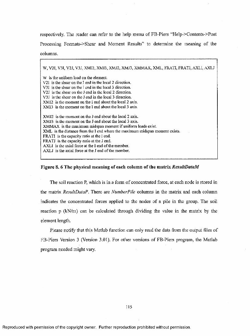
respectively. The reader can refer to the help menu of FB-Piers “Help->Contents->Post
Processing Formats->Shear and Moment Results” to determine the meaning of the
columns.
W, V2I, V3I, V2J, V3J, XMI2, XMI3, XMJ2, XMJ3, XMMAX, XML, FRATI, FRATJ, AXLI, AXLJ
W is the uniform load on the element.V2I is the shear on the I end in the local 2 direction.V3I is the shear on the I end in the local 3 direction.V2J is the shear on the J end in the local 2 direction.V3J is the shear on the J end in the local 3 direction.XMI2 is the moment on the I end about the local 2 axis.XMI3 is the moment on the I end about the local 3 axis.
XMJ2 is the moment on the J end about the local 2 axis.XMJ3 is the moment on the J end about the local 3 axis.XMMAX is the maximum midspan moment if uniform loads exist.XML is the distance from the I end where the maximum midspan moment exists.FRATI is the capacity ratio at the I end.FRATJ is the capacity ratio at the J end.AXLI is the axial force at the I end o f the member.AXLJ is the axial force at the J end o f the member.
Figure 8. 6 The physical meaning of each column of the matrix ResultDataM
The soil reaction P, which is in a form of concentrated force, at each node is stored in
the matrix ResultDataP. There are NumberPile columns in the matrix and each column
indicates the concentrated forces applied to the nodes o f a pile in the group. The soil
reaction p (kN/m) can be calculated through dividing the value in the matrix by the
element length.
Please notify that this Matlab function can only read the data from the output files of
FB-Piers Version 3 (Version 3.01). For other versions o f FB-Piers program, the Matlab
program needed might vary.
115
Reproduced with permission of the copyright owner. Further reproduction prohibited without permission.

CHAPTER 9 DISCUSSION OF THE RESULTS
9.1 General
In this chapter, the sensitivity operators/integrands and sensitivity factors are
discussed and compared. The sensitivity operators are spatial functions with respect to
design variables. They explicitly show the critical locations o f the change that the design
variables have on the maximum deformations. It is worth noting that in variational
formulation the sensitivity operators are integrands, thus the operation o f integrating them
forms the basis for a quantitative assessment of the impact each of the design variables
make on the change of maximum generalized deformations. This aspect of sensitivity
analysis is of key importance in an assessment of laterally loaded single piles. It is due to
the fact that the distributed parameter sensitivity analysis enables one to extract
information of the change of deformations generated by the variation of the material
properties.
The first variation of the performance functional describes a change of pile head
generalized deformation of the primary structure being in the state o f static equilibrium.
In the analysis of the nonlinear adjoint structure, the generalized unit loads are
required to be applied to a state o f deformation corresponding to the primary structure,
whose deflections and intemal forces are depended on the applied force. It causes that the
adjoint structure and hence the sensitivity operators are determined by the load applied to
the primary' structure.
The sensitivity analysis is developed in the vicinity o f the applied load, which at the
time of sensitivity investigations is maintained constant. In the graphical presentations,
the sensitivity analyses based on different values of applied forces are differentiated by
116
Reproduced with permission of the copyright owner. Further reproduction prohibited without permission.
different legends. A specific sensitivity operator distribution along the axis is associated
with one magnitude o f the external load.
The variations o f generalized deflections imposed on the primary structure are
determined with aid o f the physical relations written in a variational form stated in
APPENDIX A. They take into account the dependence on a state and design variables.
The variations of maximum generalized deformations at the pile head are established with
the aid o f sensitivity operators due to the changes o f the design variables.
Comparative analysis of quantitative outcomes resulting from integration of
sensitivity integrands provides a rationale to classify the impact o f the design variables on
the change o f deformations.
The sensitivity analysis of laterally loaded pile-soil systems provides the answer to
the question o f how the changes o f spatially distributed soil parameters involved in a p-y
relationships and bending stiffness o f the pile affect the changes of maximum kinematic
quantities of piles subjected to lateral loadings.
The effect o f the changes of the design variables on the changes o f pile head
deflections is in accordance with the sensitivity operator values. The greater the
sensitivity operator value, the more potential effect the variation o f the design variable
has on the changes of the pile head deflections. For those locations where the sensitivity
operator equals to zero, the variations of the design variables there will not cause any
change of the pile head deflection.
9.2 Discussion of the sensitivity analysis results
The discussion here is based on the case o f the sensitivity analysis of lateral
deflection at the head of the free head pile embedded in stiff clay above water table with
the length L=10T subjected to lateral force Pt. The discussions o f the sensitivity analysis
o f other cases are presented in the next chapter. The sensitivity analysis of the pile under
lateral static load (N =l) and cyclic load, whose typical case is for number o f load cycles
N =10000, are shown and discussed in details.
117
Reproduced with permission of the copyright owner. Further reproduction prohibited without permission.
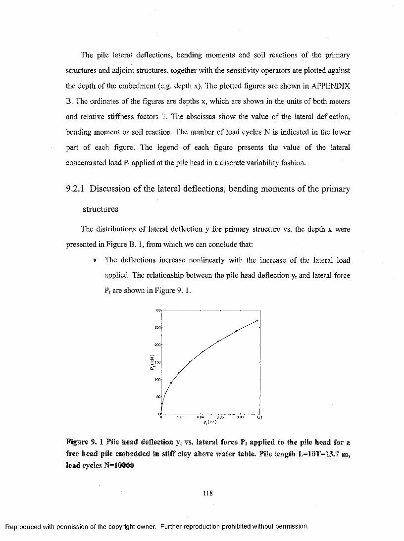
The pile lateral deflections, bending moments and soil reactions of the primary
structures and adjoint structures, together with the sensitivity operators are plotted against
the depth of the embedment (e.g. depth x). The plotted figures are shown in APPENDIX
B. The ordinates o f the figures are depths x, which are shown in the units o f both meters
and relative stiffness factors T. The abscissas show the value of the lateral deflection,
bending moment or soil reaction. The number of load cycles N is indicated in the lower
part o f each figure. The legend o f each figure presents the value of the lateral
concentrated load Pt applied at the pile head in a discrete variability fashion.
9.2.1 Discussion of the lateral deflections, bending moments of the primary
structures
The distributions o f lateral deflection y for primary structure vs. the depth x were
presented in Figure B. 1, from which we can conclude that;
• The deflections increase nonlinearly with the increase of the lateral load
applied. The relationship between the pile head deflection yt and lateral force
Pt are shown in Figure 9. 1.
300
250
200
100
0.02 0.04 0.08 0.1
Figure 9. 1 Pile head deflection yt vs. lateral force Ft applied to the pile head for a free head pile embedded in stiff clay above water table. Pile length L=10T=I3.7 m, load cycles N=10000
118
Reproduced with permission of the copyright owner. Further reproduction prohibited without permission.
• The defections grow larger when the number of load cycles increase for a
certain value of load applied to the pile. For example, for the Pt == 300 kN, the
lateral deflection at the pile head equal 78 mm when load cycle N equal 1,
whereas the deflection has the value o f 98 mm when the load cycle N equal
10000.
• For the long piles embedded in stiff clay above water table, with the depth
increasing, the lateral deflections become smaller. The lateral deflections
almost reach zero at the location x > 3T.
The distributions o f bending moments o f the primary structures vs. the depth x were
presented in Figure B. 2, from which we can find out that:
• The maximum bending moment increase nonlinearly with the increase o f the
applied lateral force.
• The location of the maximum bending moment go deeper as the load cycles
increasing.
9.2.2 Discussion of the lateral deflections, bending moments and soil
resistance of adjoint structures subjected to unit lateral forces P = L
The review of Figure B. 3 entitled distributions of lateral deflections ya(p) of the
adjoint systems subjected to P = 1 when the primary systems support the lateral
concentrated forces Pt of discrete variability for the number of cycles N=1 and 10000,
shows that the deflection of the adjoint structure increase almost linearly with the increase
o f the lateral load applied.
The comparative analysis o f the results presented in Figure B. 3 shows that the major
factor that affects the lateral deflections o f the adjoint structure subjected to the unit
horizontal force P = 1 being in the state of deformation of the primary structure is the
magnitude o f the lateral force Pt that is applied to the primary structure that defines the
119
Reproduced with permission of the copyright owner. Further reproduction prohibited without permission.
deformability o f the pile-soil system.
The soil resistance spring becomes weaker when the lateral deflection increases
because of the larger value o f load applied to the pile head. Thus the constant unit force
applied to the adjoint structure will produce larger deflection when the lateral load applied
to the primary structure become greater.
The review o f distribution of the bending moments M(P) o f the adjoint structure
along the pile axis, Figure B. 4, shows that the bending moments M (P) increase when
the lateral load Pt increase. But for larger Pt, the same increment o f Pt will cause less
M(P) change. For example, when the Pt increase 30kN from 30kN, the maximum M(P)
value will enlarge 0.6 kN-m, whereas the maximum M(P) value increases only O.lkN-m
when the Pt increases 30 kN from 270 kN. As the pile head lateral force Pt increases, the
location of the maximum bending moments goes deeper into the ground.
The load cyclicity N has only slightly effect on the distributions of the bending
moments M(P) of the adjoint structure subjected to P = 1.
The distributions o f the soil resistance pa of the adjoint systems subjected to P = 1
are shown in Figure B. 5. The value o f soil resistance o f the adjoint structure pa increases
as the depth x becomes larger and decreases rapidly after the maximum p* is reached. Soil
resistance pa reaches zero when the lateral deflection y^(P) equal to zero, and changes
sign when the deflection o f ya(P) changes sign. The soil resistance pa has nonzero
value in deep locations even when the deflections of the primary structure are very small.
For example, at a depth of 7T, the pa value is still nonzero although the deflections o f the
primary and adjoint structure become negligible at that depth. This phenomenon exists
because the soil resistance p is very sensitive to the lateral deflections o f the pile and a
very tiny change of the pile deflections will cause the soil resistance p change a certain
amount. Another characteristic that is worth noting is the soil resistance o f the adjoint
120
Reproduced with permission of the copyright owner. Further reproduction prohibited without permission.
stm ctoe pa decrease in a certain location as the lateral forces Pt applied to the primary
structure increases. This phenomenon comes out because the soil becomes weaker when
the deflection, caused by the larger Ft applied to the primary structure, increases and the
soil resistances, which were used to balance the unit force P = 1, are compelled to
distribute in a deeper range.
9.2.3 Discussion of the sensitivity operators/integrands
The characteristic features of operators presented in Figure B. 6 that represent
the sensitivity operators affecting the pile head lateral deflection due to the changes of
bending stiffness El o f the pile when subjected to concentrated lateral force Pt applied to
the pile head can be summarized as follows:
The distributions o f for static loading (N=l) and for cyclic loading (N=10000)
for the same values o f lateral force Pt applied to the primary structure demonstrate very
similar patterns regarding shape as well as the numerical values. These features are
attributed to the relative simplicity o f the p-y soil model, which can develop only a
nonlinear elastic phase followed by the soil plastic flow. We can conclude that yt is
sensitive to the changes o f El in the same fashion for static loading as well as for cyclic
loading.
The patterns of the distribution of are very similar to the patterns of the
corresponding bending moments of the primary structure. The sensitivity operators have
only negative values. This means the increase o f the bending stiffness El at any location
of the pile will causes reduction of the pile head deflection.
For the long piles under service loads, where the load capacity o f the pile sections
should not be exceeded and the lateral deflection of the pile should be within the limit of
serviceability, the sensitivity operators Cgj have nonzero value only at the upper part
ranged from depth 0 to 4T. At the depths o f more than 4T, the sensitivity factors decrease
121
Reproduced with permission of the copyright owner. Further reproduction prohibited without permission.
to zero. Hence the changes o f the pile bending stiffness El at the depths more than 4T
have no influence on the change of the lateral pile head deflection yj. If there is only the
lateral load applied at the pile head, the pile parts, which located at the depth more than
4T is uneconomical.
Figure B. 7 contains the distributions o f sensitivity integrands affecting yt due to
the changes of the cohesion c when the pile is subjected to lateral force Pt o f static type
(N=l) and cyclic type (N=10000). It shows that the sensitivity o f yt due to the changes of
cohesion c slightly increases with an increase o f N for the same values of lateral force Ft
applied. It is worth noting that the sensitivity o f yt due to the changes of c is amplified by
an increase o f lateral loading Ft when the number o f cycles N is maintained constant. The
sensitivity operators achieve maximum value at the up most part o f the pile, where the
soil cohesion c has the highest potential to affect the lateral deflections o f the pile
embedded in the clay. The distributing o f shows that it is more economical to
strengthen only the corresponding part where the sensitivity operators have nonzero value
than strengthen the whole depth of the long pile. This part which is economical to be
strengthened ranges from the ground to the depth of 3T. The sensitivity operators
have only negative values. The physical interpretation o f this fact is the same as the
sensitivity operators .
From the review of Figure B. 8, it is found that the value of the sensitivity operator
equals to zero at the pile head and increases rapidly to the maximum value at the
depth o f IT, then it reduces rapidly to almost zero at the depth o f 3T. At the depth larger
than Xr, the sensitivity operator is equal to zero.
The review of Figure B. 9, enables one to find that the value of sensitivity operator
has maximum value at the pile head and reduces rapidly to zero at the depth of 3T.
When the number of load cycles N increases, the sensitivity operator increases
122
Reproduced with permission of the copyright owner. Further reproduction prohibited without permission.

slightly.
From the review of Figure B. 10, it is found that the maximum value of the
sensitivity operator occurs at the depth o f 0.5T.
Figure B. 11 presents the distributions of sensitivity operators affecting the
changes of the pile head lateral deflection 6y, of the pile of length L=10T due to the
changes of load cycles N for the pile subjected to the cyclic loading (load cycles N>1).
For the case o f number of load cycles N =l, which is considered to be a static case, it
implies that the pile performances is independent of the number of load cycles N.
Therefore the sensitivity operator and sensitivity factor do not exist for the case of
load cycles N =l. Thus, only two typical cases representing the cyclic loading for the
number o f load cycles N=100 and N= 10000 are shown in the figure. The sensitivity
operator increases as the number o f load cycles increase. The values o f sensitivity
operator for the load cycles N =10000 is 2.5 times greater than those for the load
cycles N=100. It is worth remembering that changes of 6N are normalized with respect to
initial input data of the number o f cycles N. Thus, the change o f 6N comes out as the
percentage of the initial input load cycles data.
The sensitivity operators , C f C ^ , C ^ , and presented in Figure
B. 6, Figure B. 7, Figure B. 8, Figure B. 9, Figure B. 10 and Figure B. 11 respectively
have some characteristics in common for the case of free head long pile with pile
length=10T under lateral force Pt o f a discrete variability. They are mainly distributed in
the depth ranging from the ground surface to the depth of 3T. The sensitivity operators
diminish to a negligible value in the locations o f depth more than 3T.
However, their distribution patterns along the pile depth are different. The
distribution pattern of the sensitivity operators is mainly dependent on the decisive
variables that the sensitivity operator is based on. The value of the sensitivity factor
123
Reproduced with permission of the copyright owner. Further reproduction prohibited without permission.
is mainly dependent on the bending moment o f the primary and adjoint structure, so it
shares the distribution pattern with the bending moments. The values of the sensitivity
factors C f , C ^ , and are mainly determined by the deflection y, so the
distribution patterns of theses sensitivity operators have the trends o f the lateral deflection
y. The sensitivity operator is determined mainly by the lateral deflection y and
depth X simultaneously. The combine action o f these two variables makes that the
sensitivity operators have some traits o f the lateral deflection y but being modified
by the depth x. The distribution o f is more complex compared than other sensitivity
operators.
9.2.4 Discussion of the lateral deflections, bending moments and soil
resistance of adjoint structures subjected to unit bending moments
M = i .
The results presented in Figure B. 12 to Figure B. 20 are connected with the
assessment of sensitivity o f the maximum angle o f flexural rotation 6t due to the changes
of the pile-soil strength parameters when the pile is subjected to concentrate lateral force
Pt, a variable in a discrete fashion, which is applied to the pile head.
The distributions o f the deflections o f the adjoint structure y^(M ) when subjected
to a unit bending moment M = 1 applied to the adjoint structure being in the state of
deformation corresponding to primary structure that is loaded by the lateral force Ft are
shown in Figure B. 12. These distributions are very similar to the deflections
y(P) presented in Figure B. 2, that have been already discussed in detail.
The similarities o f the diagrams o f y^fM) and y^(P) are referred to their shapes
as well as numerical values for corresponding magnitudes o f lateral force Pt and the
124
Reproduced with permission of the copyright owner. Further reproduction prohibited without permission.
number o f cycles N.
The distributions of bending moments M(M) developed in the adjoint structure
being loaded by M = 1 applied to the pile head o f the adjoint structure being in the state
of deformation the same as the primary structure when subjected to concentrate lateral
force Pt of discrete variability are shown in Figure B. 13. One of the most distinct
characteristics o f the distribution o f the bending moments M(M) is that it has unit value,
which is also the maximum value, at the pile head. This characteristic can also used to
check if the analysis results are correct.
The distributions of soil resistance p^ of the adjoint systems subjected to M = 1
when the primary systems support the lateral concentrated forces Pt o f discrete variability
for the number o f cycles N=1 and 10000 are shown in Figure B. 14. The distributions of
soil resistance pa for the adjoint structure subjected to M = 1 share some common
characteristics with the distributions of soil resistance pa for the adjoint structure
subjected to P = 1 shown in Figure B. 5. These common characteristics include that the
soil reactions pa o f the adjoint structure are distributed to a deeper depth than the soil
reaction p o f primary structure and the soil reactions pa o f the adjoint structure have
nonzero value at the deep depth even the lateral deflections of the primary structure are
very small at those locations.
9.2.5 Discussion of the sensitivity operators/integrands C™..)
The distributions o f sensitivity operators Cg affecting the changes of the pile head
lateral deflection 5yt o f the pile of length L=10T due to the changes o f bending stiffness
El when the pile structures are subjected to a concentrated lateral force Pt of a discrete
variability for the number o f load cycles N=1 and 10000 are shown in Figure B. 15. The
similarities between o f Figure B. 6 and C™ of Figure B. 15 as far as the shapes of
125
Reproduced with permission of the copyright owner. Further reproduction prohibited without permission.

the integrands are concerned are self-evident. The numerical values o f in reference
to Cgi show that the maximum values of are over 2 times larger than the
appropriate maximum values of C
The sensitivity integrands C™ (presented in Figure B. 16) affecting the changes o f
the pile-head angle of flexural rotation §0t due to the changes of cohesion c resemble the
distributions o f sensitivity integrands o f Figure B. 7. The distribution patterns
corresponding to the same values of external loadings are quite similar for the two cases.
But the maximum numerical values o f the sensitivity operator are almost 4 times as
the numerical value o f the sensitivity operator C™.
The distributions o f sensitivity integrands C™ affecting the changes of the pile
head angle o f flexural rotation 60t due to changes of the pile’s width b are presented in
Figure B. 18. The C™ presented are for the long pile-soil system subjected to lateral
force Pt, variable in discrete fashion, when the number o f cycles N=1 and 10000. The
diagrams of sensitivity operators exhibit high similarity to (shown in Figure B.
9). The small differences in numerical values are observed between the corresponding
and with the former being 2 times larger than the latter.
Distributions of sensitivity operators affecting the changes of the pile head
lateral deflection 5yt of the pile of length L=10T due to the changes o f S50 when the pile
structures are subjected to a concentrated lateral force Pt o f a discrete variability for the
number o f load cycles N=1 and 10000 are very like (shown in Figure B. 10) as far
as the shapes o f integrands and numerical values are concerned. The small differences in
the numerical values o f C^o and C^g are noticed leading to the conclusion that C^g
pee50-are 2 times larger than the corresponding values o f C
126
Reproduced with permission of the copyright owner. Further reproduction prohibited without permission.
Distributions of sensitivity operators C™ affecting the changes o f the pile head
lateral deflection 5yt o f the pile of length L=10T due to the changes o f load cycles N
when the pile structures are subjected to a concentrated lateral force Pt o f a discrete
variability for the number of load cycles N=100 and N = 10000, are shown in Figure B.
20. They have almost the same pattern with the distributions of sensitivity operators
presented in Figure B. 11. But the numerical values of are 2 times larger than those
peof C n
9.2.6 Discussion of sensitivity factors
The value o f the sensitivities factor A is the result of the numerical integration of the
value of sensitivity operator C. In the figures representing the relationship between the
sensitivity factors and the applied lateral force Ft, the ordinates show the sensitivity
factors in the unit o f kN-m and the abscissas standard for the lateral force applied to the
pile head Ft in the unit o f kN.
The quantitative assessment o f sensitivity factors A ^ , A f ', A ^ , A ^ and A ^ q
affecting the top lateral deflection yt o f the free head piles due to the changes o f bending
stiffness El, cohesion c, unit weigh y of soil, pile width b and E50, when the pile structures
are subject to a concentrated lateral force Ft o f a discrete variability for the number of
load cycles N = 1 are shown in Figure B. 21. The sensitivity factors A |[ , A f , A^^,
A ^ and A^^ share the same trend and increase rapidly in clearly nonlinear fashion
when the pile head lateral force Ft increases. For the load cycles N = l, it is considered to
be the static case, so the sensitivity factor A ^ does not exist. The increase o f the
sensitivity factors is not linear. For instance, when the lateral pile head force Ft increases
ten times from 30 kN to 300 kN, the A ^ values increase 260 times. Through the review
of Figure B. 21, it can be concluded that the values of A increase with the increase o f the
127
Reproduced with permission of the copyright owner. Further reproduction prohibited without permission.
load applied to the laterally loaded free head long piles embedded in stiff clay above
water table.
The quantitative assessment o f sensitivity factors A™, A™, A ^ , A™ and A™o
affecting the top lateral deflection 0t of the free head piles due to the changes of bending
stiffness El, cohesion c, unit weigh y o f soil, pile width b and E50, when the pile structures
are subject to a concentrated lateral force Pt of a discrete variability for the number of
load cycles N = 1 were shown in Figure B. 23. The sensitivity factors A™, A™, A^®,
A™ and A^p share the same distribution pattern as the sensitivity factors . But
1 1the values of the former are — ~ — of the value of the latter.
2 5
The quantitative assessment o f sensitivity factors A ^ , A ^ , A ^ , A ^ , A ^ q and
A ^ affecting the top lateral deflection yt of the free head piles due to the changes of
bending stiffiiess El, cohesion c, unit weigh y o f soil, pile width b, E50 and load cycles N,
when the pile structures are subject to a concentrated lateral force ?t of a discrete
variability for the number o f load cycles N = 10000 are shown in Figure B. 25. This case
is considered to be the cyclic type and the number of load cycles N becomes an additional
design variable. The distribution patterns o f the sensitivity factors A[^„) for the load
cycles N =10000 are almost the same as the A|^„) for the static case, except that the
sensitivity factors for the load cycles N =10000 are about 50% larger than those
for static case.
The quantitative assessment of sensitivity factors A™, A™, A™, A™, A™o and
A n affecting the top lateral deflection Ot of the free head piles due to the changes of
bending stiffness El, cohesion c, unit weigh y of soil, pile width b, E50 and load cycles N,
when the pile structures are subject to a concentrated lateral force Pt o f a discrete
variability for the number of load cycles N == 10000 were presented in Figure B. 27. Like
128
Reproduced with permission of the copyright owner. Further reproduction prohibited without permission.
the sensitivity factors , this case is also considered to be cyclic type and an
additional figure was added. The distribution patterns of the sensitivity factors for
the load cycles N - 10000 are almost the same as the for the static case, except that
the sensitivity factors for the load cycles N =10000 are about 35% larger than
those for static case.
9.2.7 Discussion of relative sensitivity factors F
The relative sensitivity factors F, which were introduced in details in Chapter 3.3.3,
are used to compare the relative importance o f the sensitivity factors A. In the figures
representing the relationships between the relative sensitivity factors and the applied
lateral forces Pt, the ordinates show the relative sensitivity factors in the form of
percentage (%) and the abscissas stand for the lateral forces applied to the pile head Pt in
the unit of kN.
The quantitative assessment (in%) of relative sensitivity factors F ^ , F^^, F^^,
F|f and F^q affecting the top lateral deflection yt o f the free head piles due to the
changes of bending stiffness El, cohesion c, unit weigh y of soil, pile width b and Sjo,
when the pile structures are subject to a concentrated lateral force Pt of a discrete
variability for the number of load cycles N = 1 are shown in Figure B. 22. The average
values o f the relative sensitivity factors F ^ , Fj^, F * , F^ and F ^ are 14%, 46%,
4%, 23% and 13% respectively.
The quantitative assessment (in%) of relative sensitivity factors F |f , Ff®, F * ,
F™ and F™g affecting the top angle o f flexural rotation 0t o f the free head piles due to
the changes o f bending stiffness El, cohesion c, unit weigh y o f soil, pile width b and £50,
when the pile structures are subject to a concentrated lateral force Pt of a discrete
variability for the number of load cycles N = 1 are shown in Figure B. 24. The average
129
Reproduced with permission of the copyright owner. Further reproduction prohibited without permission.
values of the relative sensitivity factors F™, F™, F^^, F™ and F™q are 26%, 39%,
3%, 21% and 11% respectively.
The major difference between F^.^ or shown in Figure B. 22 and Figure B.
24 are that the design parameter El take a more important role in F™.j (El accounts for
26%) than in F^ , (El accounts for 14%). This difference is caused by the diversity of
the deformation profile resulted from the two kinds o f boundary conditions of the adjoint
structure.
The quantitative assessment (in%) of relative sensitivity factors F ^ , Ff^, F^^,
, F o and F ^ affecting the top lateral deflection yt o f the free head piles due to the
changes of bending stiffness El, cohesion c, unit weigh y of soil, pile width b, S50 and
number of load cycles N, when the pile structures are subject to a concentrated lateral
force Pt of a discrete variability for the number o f load cycles N = 10000 are shown in
Figure B. 26. The average values o f the relative sensitivity factors F^ , F^^, F * , F * ,
Fg' g and F ^ are 15%, 46%, 4%, 21%, 13% and 1% respectively.
The quantitative assessment (in%) o f relative sensitivity factors F™, FJ®, F™,
F™, F®5® and F™ affecting the top angle o f flexural rotation 0t of the free head piles
due to the changes o f bending stiffness El, cohesion c, unit weigh y o f soil, pile width b,
S50 and number of load cycles N, when the pile structures are subject to a concentrated
lateral force Ft of a discrete variability for the number of load cycles N = 10000 were
shown in Figure B. 28. The average values of the relative sensitivity factors F |f , F™,
F™, F™, F™5 and F™ are 27%, 39%, 3%, 20%, 10% and 1% respectively.
For all the cases analyzing the relative sensitivity factors, some common
characteristics exist.
130
Reproduced with permission of the copyright owner. Further reproduction prohibited without permission.

The design variable El take a more important role as the pile head load Pt applied to
the primary structure increases. This is because the soil becomes weaker when the applied
load Ft increases and the pile bending stiffness has to play a more important role. The
importance o f the design variable c decrease slightly as the concentrated force Ft
increases.
The relative sensitivity factors and increase a certain amount as the
applied load Ft increase.
The relative sensitivity factors F^ and F™ reduce their values as the applied load
Ft increase. The physical explanation of this reduction can be attributed also to the weaker
strength of the soil. The weaker strength o f soil causes soil resistance applied to the unit
area of the pile surface diminish, so the pile width b takes less important role as the
applied load Ft increase and the relative sensitivity factors and F™ decrease.
The relative sensitivity factors F^^g, F™o, F ^ and F™ keep almost constant
value as the applied loads Ft increase. This means that the relative contributions o f the
design variables S50 and N keep the same value while the deflections o f the pile increase.
9.2.8 Discussion of the sensitivity analysis results of the laterally loaded pile
groups
The discussion and comparison o f the sensitivity analysis results o f the pile groups
are based on the precondition that the piles in the pile groups have the same pile head
deflections when compared with single piles correspondingly. The values o f lateral forces
applied to the pile cap are less than the value gained by multiplying the lateral forces
applied to the single pile into the number of piles in the pile group. Bearing this in mind,
it is possible to compare the sensitivity analysis results of the pile groups with the
sensitivity analysis results of single piles when subjected to the same lateral pile head
deflections.
131
Reproduced with permission of the copyright owner. Further reproduction prohibited without permission.
In this chapter, the discussion o f the result is based on a free head single pile, with
length L=10T, subjected to lateral concentrated force Pt and the pile in the first trailing
row (Pile B) o f a pile group with piles pinned to the pile cap, having length L=10T, with
pile spacing = 2D, subjected to lateral force Pg applied to the pile cap. The number of
load cycles N is 1, which stands for static loading, and 10000, which represents the cyclic
loading, respectively. The discussions o f the general characteristics applied to all types of
the laterally loaded piles and pile groups were presented in CHAPTER 10.
Through the comparison o f the sensitivity analysis results o f the pile group presented
in APPENDIX C and the sensitivity analysis of the single pile shown in APPENDIX B, it
can be concluded that the bending moments M, lateral deflections ya of the adjoint
structure, sensitivity operators C and sensitivity factors A o f a pile in the pile group have
the same distribution patterns as a single pile, however, the values o f the those sensitivity
operators and factors are different.
The lateral deflections of the adjoint structure of a pile in a pile group are larger than
those of a single isolated pile. This is because the f-multipliers fm reduce the soil
resistance strengths, resulting the increase of the deflection due to the application o f the
unit force 1.
The magnitudes of sensitivity operators Cei and sensitivity factors Aei for a pile in the
pile group are similar to the magnitudes of a laterally loaded single pile.
The distributions and magnitudes of the soil resistance pa are relatively similar for
both the pile groups and single piles.
The sensitivity operators C(c,y, b,E50,N) and sensitivity factors A(c,y, b, s50,n) of a pile in
the pile group are relatively smaller than those for a single pile.
The relative sensitivity factors F are the same both for the pile group and the single
pile.
9.3 Verification and error analysis
The sensitivity analysis can be verified through the common sense and equivalent
132
Reproduced with permission of the copyright owner. Further reproduction prohibited without permission.

relationships between the variables involved in the stages of the sensitivity analysis
process. They include but are not limited to the rules stated below:
• For single piles, the quantities of the lateral forces applied at the primary
structure are equal to the shear forces at the top of the piles.
• For free head single piles, the quantities of the bending moments applied to
the primary structure are equal to the bending moments at the top o f the piles.
• For pile groups, the loads applied to the pile cap are equal to the summation
o f the shear forces at the top of the pile members.
• The distribution patterns of the sensitivity analysis results follow certain
common characteristics.
• The bending moments M(M) of the adjoint structures subjected to M = 1
have a unit value at the pile head (Figure B. 13).
The most effective method to check the results o f the sensitivity analysis was
presented in Chapter 5.10 entitled Methodology of result verification. The Matlab
programs were developed to check the sensitivity factors o f the single piles and the pile
groups according to the method presented. All the results in this study have been checked
carefully to make sure the correctness of the sensitivity analysis. The error percents,
which are defined in Chapter 5.10, of the sensitivity factors A o f a typical single pile case
are presented in Table 9. 1. And the error percents o f the sensitivity factor A of a typical
pile in a pile group are presented in Table 9. 2. The normalized variation , — , — ,El c y
and — of the design variables are taken as 0.001 in calculating the error5b 5s,o 8N — , — — and — b S50 N
percents presented in Table 9. 1 and Table 9. 2.
133
Reproduced with permission of the copyright owner. Further reproduction prohibited without permission.
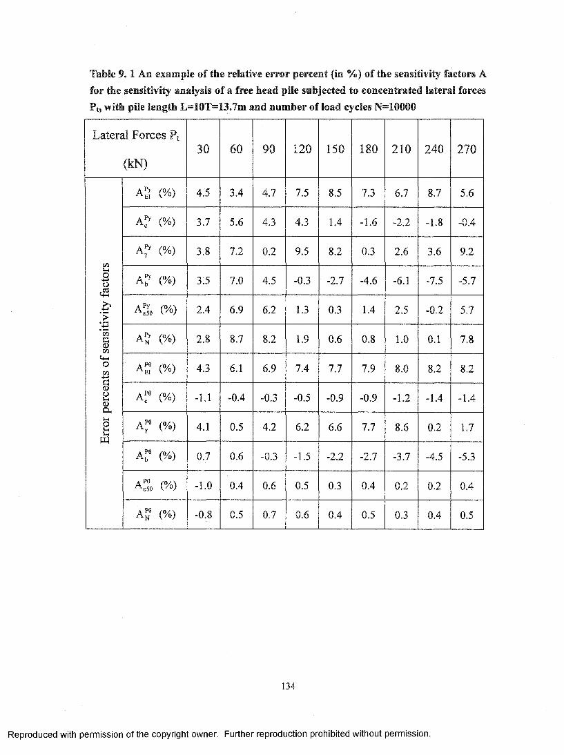
Table 9.1 An example of the relative error percent (in %) of the sensitivity factors A for the sensitivity analysis of a free head pile subjected to concentrated lateral forces Pt, with pile length L=10T=13.7m and number of load cycles N=10000
Lateral Forces Pt
(kN )30 60 90 120 150 180 21 0 240 270
2o+->o
>‘Sa<u
o
f<uoS-4a
§W
(%) 4.5 3.4 4.7 7.5 8.5 7.3 6.7 8.7 5.6
A f (%) 3.7 5.6 4.3 4.3 1.4 -1.6 -2.2 -1.8 -0.4
(%) 3.8 7.2 0.2 9.5 8.2 0.3 2.6 3.6 9.2
A f (%) 3.5 7.0 4.5 -0.3 -2.7 -4.6 -6.1 -7.5 -5.7
A fo (%) 2.4 6.9 6.2 1.3 0.3 1.4 2.5 -0.2 5.7
(%) 2.8 8.7 8.2 1.9 0.6 0.8 1.0 0.1 7.8
A® (%) 4.3 6.1 6.9 7.4 7.7 7.9 8.0 8.2 8.2
A f (%) -1.1 -0.4 -0.3 -0.5 -0.9 -0.9 -1.2 -1.4 -1.4
A™ (%) 4.1 0.5 4.2 6.2 6.6 7.7 8.6 0.2 1.7
A^ (%) 0.7 0.6 -0.3 -1.5 -2.2 -2.7 -3.7 -4.5 -5.3
A:Io (%) -1.0 0.4 0.6 0.5 0.3 0.4 0.2 0.2 0.4
A™ (%) -0.8 0.5 0.7 0.6 0.4 0.5 0.3 0.4 0.5
134
Reproduced with permission of the copyright owner. Further reproduction prohibited without permission.
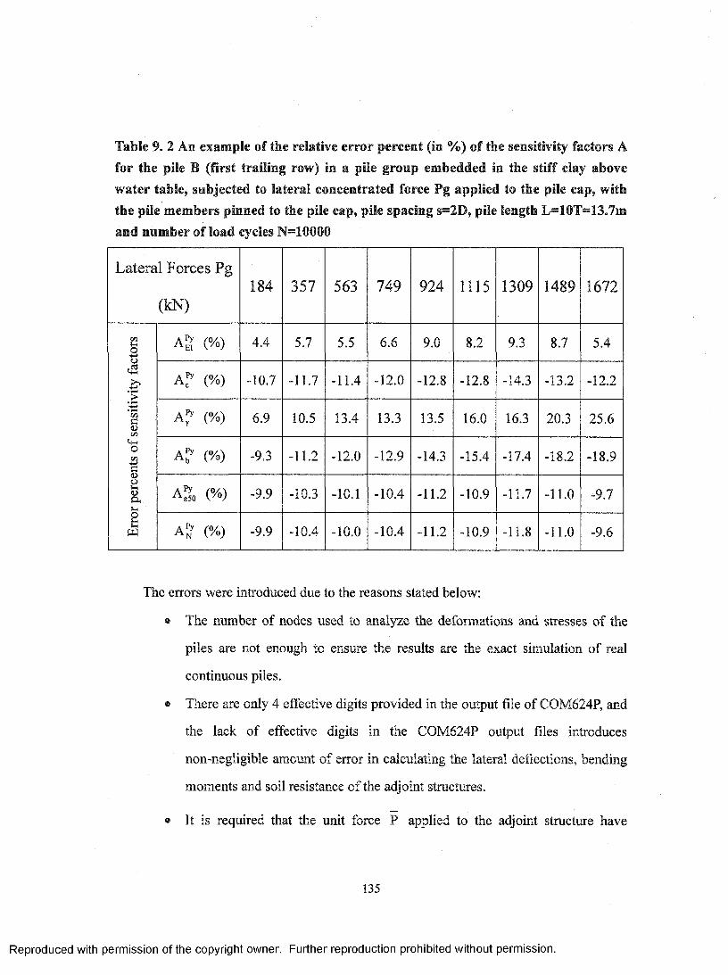
Table 9. 2 An example of the relative error percent (in %) of the sensitivity factors A for the pile B (first trailing row) in a pile group embedded in the stiff clay above w ater table, subjected to lateral concentrated force Pg applied to the pile cap, with the pile members pinned to the pile cap, pile spacing s=2D, pile length L=10T=13.7m and number of load cycles N=10000
Lateral Forces Pg
(kN )184 357 563 749 924 1115 1309 1489 1672
t/5i-io (%) 4.4 5.7 5.5 6.6 9.0 8.2 9.3 8.7 5.4
43(%) -10.7 -11.7 -11.4 -12.0 -12.8 -12.8 -14.3 -13.2 -12.2
COa ;>' (%) 6.9 10.5 13.4 13.3 13.5 16.0 16.3 20.3 25.6
oCO"S
A^ (%) -9.3 -11.2 -12.0 -12.9 -14.3 -15.4 -17.4 -18.2 -18.9
OV4Cu A o (%) -9.9 -10.3 -10.1 -10.4 -11.2 -10.9 -11.7 -11.0 -9.7
§ A^ (%) -9.9 -10.4 -10.0 -10.4 -11.2 -10.9 -11.8 -11.0 -9.6
The errors were introduced due to the reasons stated below:
• The number of nodes used to analyze the deformations and stresses of the
piles are not enough to ensure the results are the exact simulation of real
continuous piles.
• There are only 4 effective digits provided in the output file of COM624P, and
the lack of effective digits in the COM624P output files introduces
non-negligible amount of error in calculating the lateral deflections, bending
moments and soil resistance of the adjoint structures.
• It is required that the unit force P applied to the adjoint structure have
135
Reproduced with permission of the copyright owner. Further reproduction prohibited without permission.
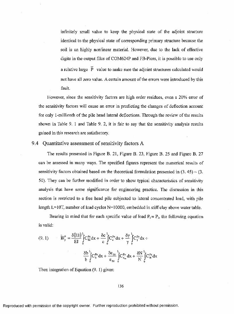
infinitely small value to keep the physical state of the adjoint structure
identical to the physical state of corresponding primary structure because the
soil is an highly nonlinear material. However, due to the lack o f effective
digits in the output files o f COM624P and FB-Piers, it is possible to use only
a relative large P value to make sure the adjoint structures calculated would
not have all zero value. A certain amount of the errors were introduced by this
fault.
However, since the sensitivity factors are high order residues, even a 20% error of
the sensitivity factors will cause an error in predicting the changes o f deflection account
for only 1 -millionth of the pile head lateral deflections. Through the review o f the results
shown in Table 9. 1 and Table 9. 2, it is fair to say that the sensitivity analysis results
gained in this research are satisfactory.
9.4 Quantitative assessment of sensitivity factors A
The results presented in Figure B. 21, Figure B. 23, Figure B. 25 and Figure B. 27
can be assessed in many ways. The specified figures represent the numerical results of
sensitivity factors obtained based on the theoretical formulation presented in (3. 45) ~ (3.
50). They can be further modified in order to show typical characteristics o f sensitivity
analysis that have some significance for engineering practice. The discussion in this
section is restricted to a free head pile subjected to lateral concentrated load, with pile
length L=10T, number o f load cycles N^IOOOO, embedded in stiff clay above water table.
Bearing in mind that for each specific value o f load Pt s Pj, the following equation
is valid:
(9. 1) 18' = - ® j c g d x + — j c » d x + ^ J c f d x +Bi 0 c 0 ^
Then integration o f Equation (9. 1) gives:
136
Reproduced with permission of the copyright owner. Further reproduction prohibited without permission.
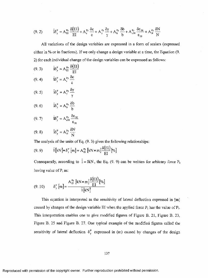
(9.2) i 6 ' = A g ® + A^ — + A ^ ^ + A ? — + A g , ^ + A j — ® El " c Y b S50 N
All variations o f the design variables are expressed in a form of scalars (expressed
either in % or in fractions). If we only change a design variable at a time, the Equation (9.
2) for each individual change of the design variables can be expressed as follows:
(9. 3) 18; = Ag- ®
(9.4) 1 8 ; = A g ^C
(9. 5) 15 = ^y
(9.6) 1 6 > A ^ ^
(9. 7) is; = A g.
5N
50
(9. 8) is; = A g ^
The analysis of the units o f Eq. (9. 3) gives the following relationships:
(9.9) i [k N ] .6;[m ] = A g [ k N . m ] ® [ % ]El
Consequently, according to 1 = IkN , the Eq. (9. 9) can be written for arbitrary force Pt
having value o f ?i as:
A g [ k N .m ] M [ o /„ ](9.10) S ; H = -----------
This equation is interpreted as the sensitivity o f lateral deflection expressed in [m]
caused by changes o f the design variable El when the applied force Pt has the value of Pj.
This interpretation enables one to give modified figures of Figure B. 21, Figure B. 23,
Figure B. 25 and Figure B. 27. One typical example of the modified figures called the
sensitivity of lateral deflection 6 expressed in (m) caused by changes of the design
137
Reproduced with permission of the copyright owner. Further reproduction prohibited without permission.

variables El when applied force Pt have values Pj is shown in Figure 9. 2.
Based on regression analysis of sensitivity o f 6^ [m] due to the changes of the design
variables when the pile structure is subjected to variable P,, the following equation is
obtained:
(9. 11) = -9 .2 3 6 x 1 0 '( P j ' +3 .901xl0-'(pJ-0 .0008013
where Pk = arbitrary lateral load applied to the pile head
The graphical representation of Eq. (9. 11) is shown in Figure 9. 2, in which the
quadratic polynomial curve fit of the sensitivity analysis result is shown. The value
for any arbitrary load value Pk can be obtained through Equation (9. 11) or through the
polynomial fit curve in Figure 9. 2.
8y(m)
-0.07
-0.06
-0.05
-0.04
-0.03
- 0.02
- 0.01
0
Quadratic polynomial curve fit ) (
- 5 = -9.236 X10-’ ( P j ' + 3.901 x 1 O'’ ( p J - 0.0008013
5? value corresponding todiscrete load Pi based on .sensitivity analysis
------- ^ 1--------- 1-------- — 1--------- 1--------- 1_____________
Pk0 30 60 90 120 150 1 80 210 240 270
P i (kN)
Figure 9. 2 The sensitivity of lateral deflection 8 expressed in (m) caused by
changes of the design variables El when applied force Pt have values Pj
The assessment o f sensitivity of lateral deflection due to the change of each design
138
Reproduced with permission of the copyright owner. Further reproduction prohibited without permission.
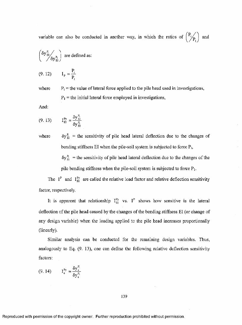
variable can also be conducted in another way, in which the ratios of and
'5 y ’’‘are defined as:
Eiy
(9. 12)
where
And:
(9. 13)
where
I p = -
Pj = the value o f lateral force applied to the pile head used in investigations,
? i = the initial lateral force employed in investigations.
jP y _ ^ Y e i
6y El
by 'j = the sensitivity of pile head lateral deflection due to the changes of
bending stiffness El when the pile-soil system is subjected to force P j,
byg'j = the sensitivity of pile head lateral deflection due to the changes o f the
pile bending stiffiiess when the pile-soil system is subjected to force Pi.
The and are called the relative load factor and relative deflection sensitivity
factor, respectively.
It is apparent that relationship vs. F shows how sensitive is the lateral
deflection of the pile head caused by the changes o f the bending stiffness El (or change of
any design variable) when the loading applied to the pile head increases proportionally
(linearly).
Similar analysis can be conducted for the remaining design variables. Thus,
analogously to Eq. (9. 13), one can define the following relative deflection sensitivity
factors:
(9. 14) jPy syc'5y:
139
Reproduced with permission of the copyright owner. Further reproduction prohibited without permission.
5y^‘(9. 15) 1 ^ = - ^
(9. 16) C
5y?
M .Sy '
(9. 17) 1^0 -5y
e 50
(9.18) i r = ^
They are called relative deflection sensitivity factor due to the changes o f the design
variables c, y , b, 850, and N respectively.
The results of investigations presented in Figure B. 21, Figure B. 23, Figure B. 25
and Figure B. 27 with aid of factors given by formulas (9. 13), (9. 14), (9. 15), (9. 16), (9.
17) and (9. 18) vs. variable Ip given by formula (9. 12) are presented in Figure 9. 3,
Figure 9. 4, Figure 9. 5, Figure 9. 6, Figure 9. 7 and Figure 9. 8 respectively. In these
figures, the points indicated by the asterisks present the l|^„j value corresponding to the
discrete Ip based on the sensitivity analysis, which have been done in CHAPTER 3 and
CHAPTER 5. The curves shown in the figure are the quadratic curve fits o f the discrete
1(7..) value obtained by sensitivity analysis. The curve fit equations are also shown in the
graph.
140
Reproduced with permission of the copyright owner. Further reproduction prohibited without permission.
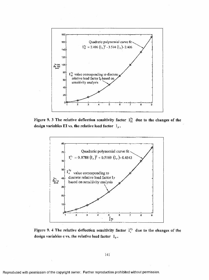
180
Quadratic polynomial curve fit Ig = 2.496 ( I p / -3.514 ( ip ) -2.406
160
140
120
IH value corresponding to discrete relative load factor Ip based on / sensitivity analysis
Figure 9. 3 The relative deflection sensitivity factor due to the changes of thedesign variables El vs. the relative load factor Ip.
Quadratic polynomial curve fit \
I f = 0.8788 ( ip ) '+ 0.5169 ( ip ) -0.4543
c value corresponding to discrete relative load factor Ip based on sensitivity analysist—H
Figure 9. 4 The relative deflection sensitivity factor i f due to the changes of the design variables c vs. the relative load factor Ip.
141
Reproduced with permission of the copyright owner. Further reproduction prohibited without permission.
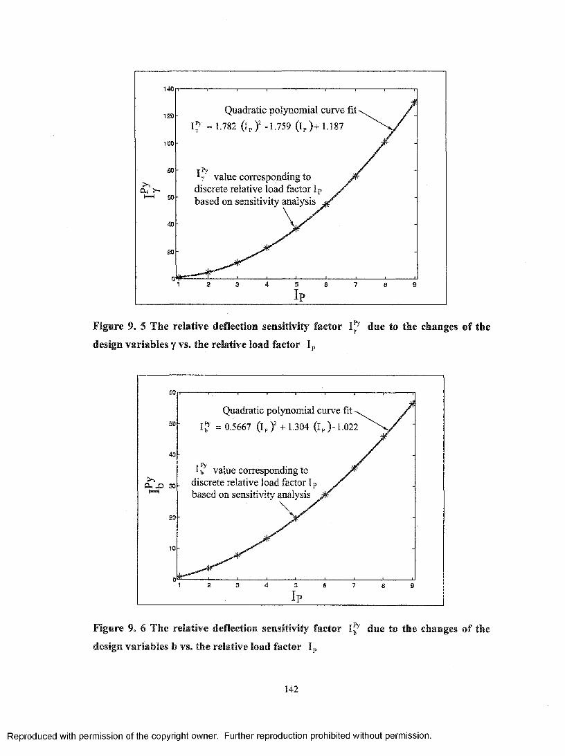
140
Quadratic polynomial curve fit
I f = 1.782 ( I p ) ' -1 .759 (Ip ) + 1 .187120
100
•■■r' value corresponding to discrete relative load factor I based on sensitivity analysis
Figure 9. 5 The relative deflection sensitivity factor i f due to the changes of the
design variables y vs. the relative load factor Ip
Quadratic polynomial curve fit -v I f = 0.5667 ( i p ) ' + 1.304 ( i p ) - 1.022
I b value corresponding to discrete relative load factor I based on sensitivity analysis
Figure 9. 6 The relative deflection sensitivity factor i f due to the changes of the
design variables b vs. the relative load factor Ip
142
Reproduced with permission of the copyright owner. Further reproduction prohibited without permission.
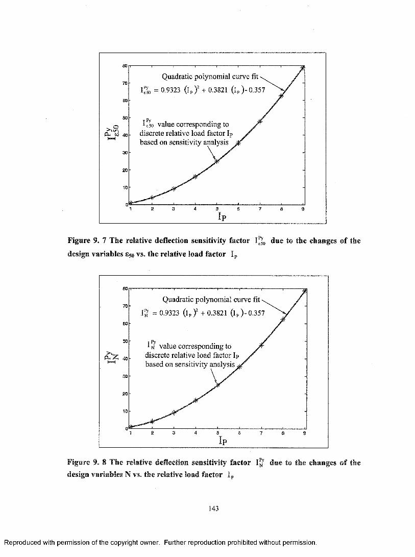
Quadratic polynomial curve fit \
0.9323 (lp)" + 0.3821 ( i p ) - 0.35770
e 50
5016 50 value corresponding to
discrete relative load factor I; based on sensitivity analysis
30
£0
Figure 9. 7 The relative deflection sensitivity factor due to the changes of the
design variables 850 vs. the relative load factor Ip
60Quadratic polynomial curve fit v.
C = 0.9323 ( i p ) ' + 0 .3 8 2 1 ( i p ) - 0.35770
% value corresponding to discrete relative load factor Ip based on sensitivity analysis^
30
2 0 -
Figure 9. 8 The relative deflection sensitivity factor I^ due to the changes of the design variables N vs. the relative load factor Ip
143
Reproduced with permission of the copyright owner. Further reproduction prohibited without permission.
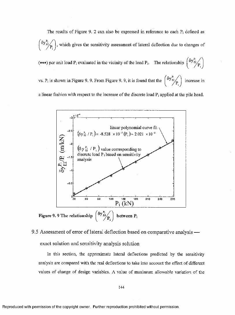
The results of Figure 9. 2 can also be expressed in reference to each P, defined as
, which gives the sensitivity assessment o f lateral deflection due to changes ofV A y
(•••) per unit load Pj evaluated in the vicinity of the load Pi. The relationship 'E l// p
vs. Pi is shown in Figure 9. 9. From Figure 9. 9, it is found that theP,
increase m
a linear fashion with respect to the increase of the discrete load Pi applied at the pile head.
x I O " *
- 2 .5
z
1f t - - 1 . 5
pL, W
CO -I
linear polynomial curve fit \
( S Y f, ! / P i ) = - 8 - 5 2 8 X 1 0 -’ ( P i ) - f 2 . 0 2 1 x l O ' \
(by E l / P i ) value corresponding to discrete load P i based on sensitivity analysis \
- D . 5
30 60 9 0 120 1 5 0 1 8 0 210 240 270P i (kN)
Figure 9. 9 The relationship/ P i
between Pi
9.5 Assessment of error of lateral deflection based on comparative analysis —
exact solution and sensitivity analysis solution
In this section, the approximate lateral deflections predicted by the sensitivity
analysis are compared with the real deflections to take into account the effect of different
values of change o f design variables. A value o f maximum allowable variation o f the
144
Reproduced with permission of the copyright owner. Further reproduction prohibited without permission.
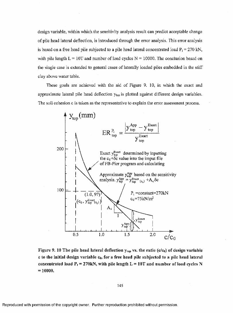
design variable, within which the sensitivity analysis result can predict acceptable change
of pile head lateral deflection, is introduced through the error analysis. This error analysis
is based on a free head pile subjected to a pile head lateral concentrated load Pj = 270 kN,
with pile length L = lOT and number of load cycles N = 10000. The conclusion based on
the single case is extended to general cases of laterally loaded piles embedded in the stiff
clay above water table.
These goals are achieved with the aid of Figure 9. 10, in which the exact and
approximate lateral pile head deflection ytop is plotted against different design variables.
The soil cohesion c is taken as the representative to explain the error assessment process.
, Exact
200
(1.0,97)
(Co. ySrkti
Exact yfop®'* determined by inputting the Co+6c value into the imput file of FB-Pier program and calculating
Approximate based on the sensitivity analysis. yf„^ = yf“ =‘ (c„) +A ^Sc
Pi =constant=270kN Co=75kN/m^
Figure 9.10 The pile head lateral deflection ytop vs. the ratio (c/co) of design variable c to the initial design variable co, for a free head pile subjected to a pile head lateral concentrated load Pt = 270kN, with pile length L = lOT and number of load cycles N = 10000.
145
Reproduced with permission of the copyright owner. Further reproduction prohibited without permission.
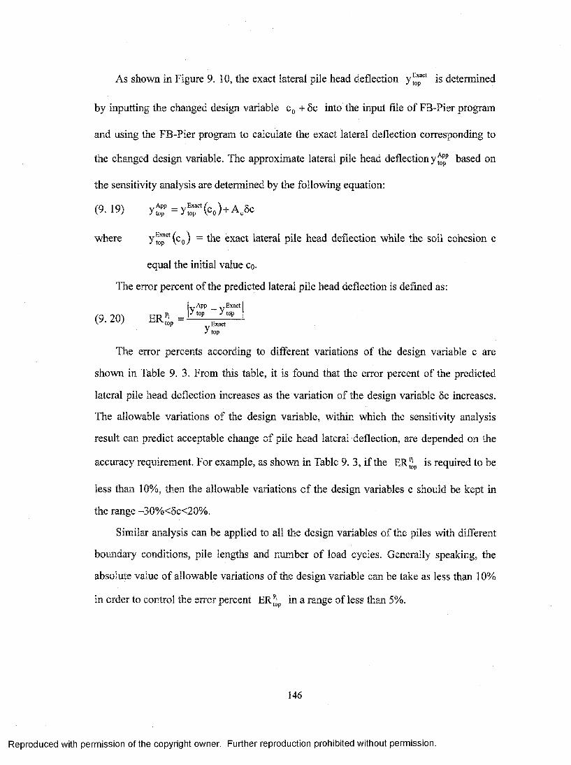
As shown in Figure 9. 10, the exact lateral pile head deflection is determined
by inputting the changed design variable Cq + Sc into the input file of FB-Pier program
and using the FB-Pier program to calculate the exact lateral deflection corresponding to
the changed design variable. The approximate lateral pile head deflection y^^ based on
the sensitivity analysis are determined by the following equation;
(9.19) (<=•)+A.Sc
where y ^ ( c , ) - the exact lateral pile head deflection while the soil cohesion c
equal the initial value cq.
The error percent of the predicted lateral pile head deflection is defined as:
Iy PP _(9. 20) ERf- = '
Exact J top
The error percents according to different variations o f the design variable c are
shown in Table 9. 3. From this table, it is found that the error percent of the predicted
lateral pile head deflection increases as the variation of the design variable Sc increases.
The allowable variations o f the design variable, within which the sensitivity analysis
result can predict acceptable change of pile head lateral deflection, are depended on the
accuracy requirement. For example, as shown in Table 9. 3, if the E R ^ is required to be
less than 10%, then the allowable variations o f the design variables c should be kept in
the range -30%<Sc<20%.
Similar analysis can be applied to all the design variables o f the piles with different
boundary conditions, pile lengths and number o f load cycles. Generally speaking, the
absolute value o f allowable variations of the design variable can be take as less than 10%
in order to control the error percent ER^p in a range of less than 5%.
146
Reproduced with permission of the copyright owner. Further reproduction prohibited without permission.
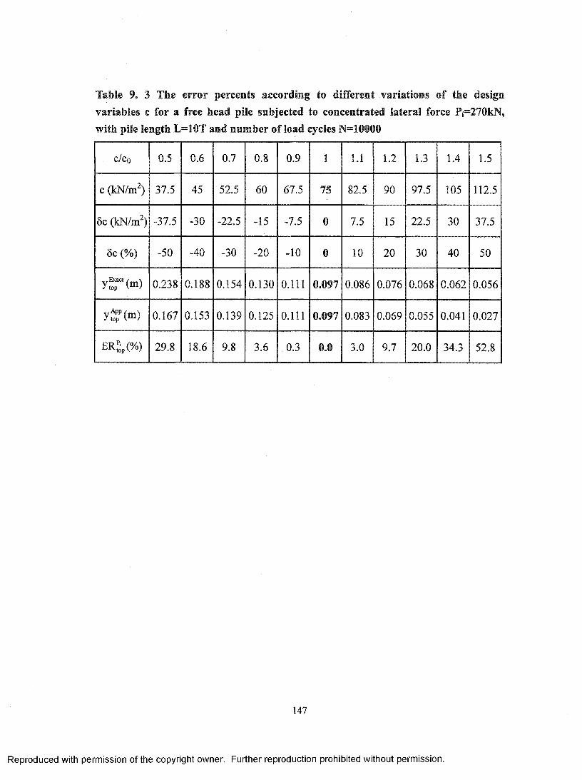
Table 9. 3 The erro r percents according to different variations of the design variables c for a free head pile subjected to concentrated lateral force Pi=270kN, with pile length L=10T and number of load cycles N=10000
c/co 0.5 0.6 0.7 0.8 0.9 1 1.1 1.2 1.3 1.4 1.5
c (kN/m^) 37.5 45 52.5 60 67.5 75 82.5 90 97.5 105 112.5
5c (kN/m^) -37.5 -30 -22.5 -15 -7.5 0 7.5 15 22.5 30 37.5
5c (%) -50 -40 -30 -20 -10 0 10 20 30 40 50
y ^ 7 ‘(m) 0.238 0.188 0.154 0.130 0.111 0.097 0.086 0.076 0.068 0.062 0.056
0.167 0.153 0.139 0.125 0.111 0.097 0.083 0.069 0.055 0.041 0.027
ERf;p(%) 29.8 18.6 9.8 3.6 0.3 0.0 3.0 9.7 20.0 34.3 52.8
147
Reproduced with permission of the copyright owner. Further reproduction prohibited without permission.

CHAPTER 10 CONCLUSIONS AND SUGGESTIONS FOR
FUTURE RESEARCH
10.1 Conclusion
Based on the sensitivity analysis results for the laterally loaded pile embedded in stiff
clay above water table, the common characteristics and conclusions for the piles under
lateral loads and bending moments are presented in this chapter. The conclusions are
based on the following pile and load conditions:
• Free head short and long pile under lateral concentrated load.
• Fixed head short and long pile under lateral concentrated load.
• Free head short and long pile under pile head bending moments.
1. The conclusions about the sensitivity operators are given as follows:
• The design variable El represents the strength of the pile and design variables
c, Y, b, 850 and N represent the effect of the soil. The design variables El, c, y
and b have favorable effect in preventing further pile deflection. Thus, the
sensitivity operator Cgj, and have negative values. Their
integrations, which are the sensitivity factors A ^ , , A^ and Aj, have
negative values accordingly. This means that the increase o f the design
variable El, c, y and b will cause the reduction o f the pile head deflection. The
design variables S50 and N have adverse effects in preventing further pile
deflection. Thus, the sensitivity operator C jq and have positive values.
As a result, their integrations, which is the sensitivity factors A^jg and A^
148
Reproduced with permission of the copyright owner. Further reproduction prohibited without permission.

also have positive values. This means the increase o f the design variable 850
and N will cause the increase o f the pile head deflection.
• The bending moments o f the primary structure and adjoint structure are the
main determinator of the sensitivity operator C e i. Unlike the distributions of
the sensitivity operators C for the other parameters, the distribution o f the
sensitivity operator C e i is not affected by the soil stages.
• The distributions of sensitivity operators C for the design variables increase
their value as the load applied to the pile head increases.
• The depth Xr also affects the sensitivity operator distributions. The sensitivity
operator Cy is equal to zero below the depth Xr.
• For the piles having lengths less than 4T, the sensitivity operators are
distributed along the whole length. For the piles having lengths more than 4T,
the sensitivity operators are mainly distributed at the depth ranged from 0 to
4T. The sensitivity operators distributed in the depths more than 4T have only
a very limited portion. Based on this charaeteristic, it concluded that for the
pile embedded in stiff clay above water table subjected mainly to the lateral
load of cyclic and static type, the most economical pile length can be set as
4T.
• The sensitivity operators C of a pile in the pile group have the same
distribution pattern as the single pile of the same length and boundary
conditions. For a pile in a pile group and a single pile with the same pile head
lateral deflection, the sensitivity operators Cei almost have the same value
both for a pile in a pile group and for a single pile. The pile distance in the
pile group has very small influences on the sensitivity operators C ei- On the
other hand, the sensitivity operators C c, Cy, C b, Ceso and Cn have 1— 3 times
greater value for a single pile than for a pile in a pile group. The closer the
piles in a group are spaced, the smaller the sensitivity operators C c, Cy, C b,
149
Reproduced with permission of the copyright owner. Further reproduction prohibited without permission.
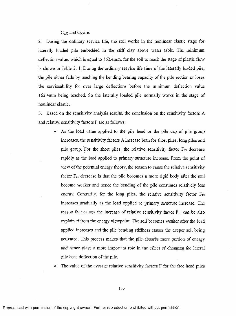
Ce5o and Cm are.
2. During the ordinary service life, the soil works in the nonlinear elastic stage for
laterally loaded pile embedded in the stiff clay above water table. The minimum
deflection value, which is equal to 162.4mm, for the soil to reach the stage o f plastic flow
is shown in Table 3. 1. During the ordinary service life time of the laterally loaded pile,
the pile either fails by reaching the bending bearing capacity o f the pile section or loses
the serviceability for over large deflections before the minimum deflection value
162.4mm being reached. So the laterally loaded pile normally works in the stage of
nonlinear elastic.
3. Based on the sensitivity analysis results, the conclusion on the sensitivity factors A
and relative sensitivity factors F are as follows:
• As the load value applied to the pile head or the pile cap of pile group
increases, the sensitivity factors A increase both for short piles, long piles and
pile group. For the short piles, the relative sensitivity factor Fei decrease
rapidly as the load applied to primary structure increase. From the point of
view of the potential energy theory, the reason to cause the relative sensitivity
factor F e i decrease is that the pile becomes a more rigid body after the soil
become weaker and hence the bending o f the pile consumes relatively less
energy. Contrarily, for the long piles, the relative sensitivity factor Fei
increases gradually as the load applied to primary structure increase. The
reason that causes the increase o f relative sensitivity factor Fei can be also
explained from the energy viewpoint. The soil becomes weaker after the load
applied increases and the pile bending stiffness causes the deeper soil being
activated. This process makes that the pile absorbs more portion of energy
and hence plays a more important role in the effect of changing the lateral
pile head deflection of the pile.
• The value o f the average relative sensitivity factors F for the free head piles
150
Reproduced with permission of the copyright owner. Further reproduction prohibited without permission.
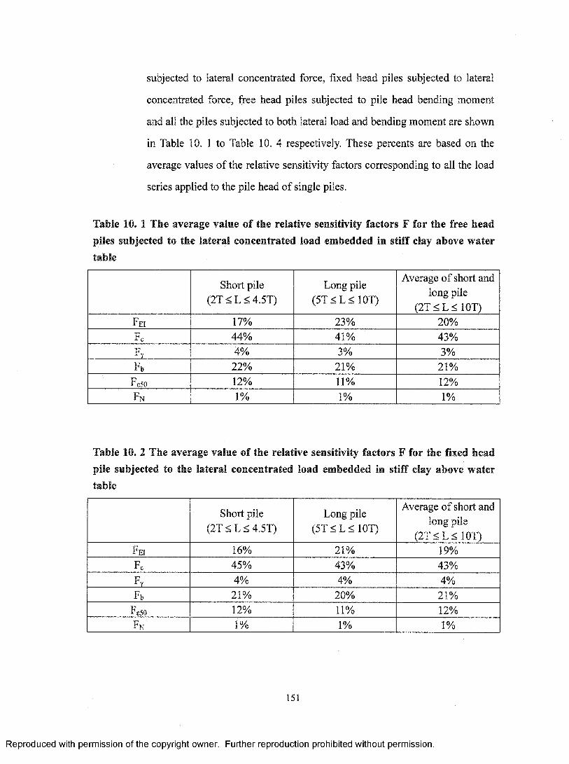
subjected to lateral concentrated force, fixed head piles subjected to lateral
concentrated force, free head piles subjected to pile head bending moment
and all the piles subjected to both lateral load and bending moment are shown
in Table 10. 1 to Table 10. 4 respectively. These percents are based on the
average values o f the relative sensitivity factors corresponding to all the load
series applied to the pile head o f single piles.
Table 10. 1 The average value of the relative sensitivity factors F for the free head piles subjected to the lateral concentrated load embedded in stiff clay above water table
Short pile (2 T < L < 4 .5 T )
Long pile(5 T < L < lOT)
Average o f short and long pile
(2 T < L < 1 0 T )Fei 17% 23% 20%Fc 44% 41% 43%Fv 4% 3% 3%Fb 22% 21% 21%
F e50 12% 11% 12%Fn 1% 1% 1%
Table 10. 2 The average value of the relative sensitivity factors F for the fixed head pile subjected to the lateral concentrated load embedded in stiff clay above water table
Short pile (2T < L < 4.5T)
Long pile (5 T < L < lOT)
Average o f short and long pile
(2 T < L < lOT)Fei 16% 21% 19%Fo 45% 43% 43%F. 4% 4% 4%Fb 21% 20% 21%
Fs50 12% 11% 12%Fn 1% 1% 1%
151
Reproduced with permission of the copyright owner. Further reproduction prohibited without permission.

Table 10. 3 The average values of the relative sensitivity factors F for the free head pile subjected to the bending moment embedded in stiff clay above water table
Short pile (2T < L < 4.5T)
Long pile (5 T < L < lOT)
Average o f short and long pile
(2 T < L < 1 0 T )F ei 22% 44% 35%Fc 42% 30% 35%F , 3% 2% 2%Fb 21% 16% 18%
F s50 11% 7% 9%F n 1% 1% 1%
Table 10. 4 The average values of the relative sensitivity factors F for all the piles subjected to both the lateral concentrated load and bending moment embedded in stiff clay above water
Short pile (2 T < L < 4 .5 T )
Long pile (5 T < L < lOT)
Average of short and long pile
(2 T < L < 1 0 T )F ei 19% 30% 26%Fc 43% 37% 40%Fy 3% 3% 3%Fb 22% 19% 20%
Fe50 12% 10% 10%F n 1% 1% 1%
The average values o f the relative sensitivity factors F for the laterally loaded
pile subjected to both lateral load and bending moment embedded in stiff clay
above water table were shown in Table 10. 4. It is easy to find out that the
design variable c have dominant effect in changing the pile head deflection of
the laterally loaded pile embedded in stiff clay above water tabic. The design
variable El is the second important variable in affecting the lateral deflection
change o f the laterally loaded pile embedded in stiff clay. The design variable
Y and N only have a small portion o f the influence to change the lateral
152
Reproduced with permission of the copyright owner. Further reproduction prohibited without permission.
deflection of the pile.
• The relative sensitivity factors F varies slightly with different support type
and different pile length.
4. The comparison of the short pile and long pile gives us the following conclusion:
• For short piles the changes of the design variables affecting the top
deformations are distributed along the entire length of the pile. The changes
of c, £50, and b at the point of rotation o f a short pile do not affect the changes
o f the top deflection.
• For the long piles, the distributions of sensitivity operators are mainly located
at the depth o f 0-3 T.
• The increase of magnitude o f load acting on the long pile results in the
development of elastic phase that moves deeper and deeper along the pile
axis.
• For the same load applied to the pile head, the numerical values o f the short
piles normally are greater than those of the long piles.
• The short piles fail mainly by the failure o f the soil, while the long piles
mainly fail by reaching the bearing capacity o f the pile section.
5. The major difference of the free head pile and fixed head pile is on the distributions
of the sensitivity operators C ei- For fixed head pile, the maximum value of C e i occurs at
the top o f the pile, while for free head pile C e i has a zero value at the pile head. The
maximum value o f Cei located at the depth 1T-3T where the bending moments of the
primary and adjoint structure have maximum value. The design variable El has more
important effects on the changes o f the lateral deflection of the laterally loaded pile in the
fixed head piles than in the free head piles. The sensitivity operators of other design
variables C c, C y, C b , C eso and C n have the same characteristics for both free head piles and
fixed head piles.
6. The differences o f the sensitivity analysis o f 5yt and 50t are the following:
153
Reproduced with permission of the copyright owner. Further reproduction prohibited without permission.
• For the sensitivity analysis o f 50t for free head pile subjected to bending
moment load at the primary structure, the sensitivity operator C e i has the
maximum value at the top o f the pile, while it has maximum value in the
middle part o f the pile for the sensitivity analysis of 50t for free head piles
subjected to lateral forces and sensitivity analysis of 5yt for free head piles
subjected to bending moments.
• The sensitivity operators C for the other design variables (c, y, b, 850 and N)
of Syt and 50t only vary in magnitude but have similar characteristics. The
values o f the sensitivity operators C affecting the changes of lateral
deflections 5yt are normally larger than the sensitivity operators C affecting
the changes of the pile head rotation 50t.
7. The comparative analysis of the effect o f the piles in a group results in the following
conclusions:
• The piles located in the leading row have the largest bending moment at the
primary structure followed by the piles in the T* trailing row and 2"** trailing
row sequentially. However, the bending moments at the adjoint structure are
ordered oppositely from the largest to smallest as: the pile in the 2"* trailing
row, the F* trailing row, and the leading row.
• The lateral displacement at the top of the piles at the primary structure is even
for each row due to the constraints imposed on the pile cap, but the
distributions of the lateral displacements of the adjoint structure vary for each
row. The piles located in the 2"* trailing row have the largest distribution of
lateral displacements at the adjoint structure followed by the piles in the F*
trailing row and in the leading row sequentially.
• The value and distribution o f the sensitivity operator Cei and the sensitivity
factor Aei o f each row corresponding to the same lateral load applied are
relatively similar.
154
Reproduced with permission of the copyright owner. Further reproduction prohibited without permission.
• The distributions o f C(c, y, b, eso, n ) and A(c, y, b, sso, n ) due to the same applied
load are very similar to each other. However, the value o f C(c,y,b,E50,N) and A(c,
y, b. s50, N ) vary from the largest to the smallest at the leading row, 1^ trailing
row and 2”* trailing row respectively. This means that the leading row is most
sensitive to changes o f the design variables related to soil properties. There
should be more attention paid to the leading row than the other rows when it
is necessary to improve the soil design variables.
• The relative sensitivity factors F are relatively stable and not affected by the
locations of the pile in the group.
8. From the comparative analysis, which takes into account the variability o f spacing s
of the pile groups, the conclusions are given as followings:
• The value of fm for the leading row is greater than that for the trailing rows,
and the fm increase with the increase of spacing s.
• The larger the spacing s o f the groups of piles, the larger the load is required
to produce the same displacement.
• The bending moment at the primary structure increases when the spacing
increase, but the bending moment at the adjoint structure decreases when the
spacing increases. It is found that the bending moment at the primary
structure for group of piles is relatively smaller than that o f the single pile,
but at adjoint structure it is relatively greater than that o f the single pile.
• The load needed to produce the same amount of deflection increases as the
pile distance increases.
• The distributions and magnitudes of sensitivity operators C e i and sensitivity
factors Aei for different pile distances are relatively similar to each other. And
they are also similar to the distributions and magnitudes o f laterally loaded
single piles.
• The closer the piles in a group spaced, the smaller the sensitivity operators
155
Reproduced with permission of the copyright owner. Further reproduction prohibited without permission.
C(c, y, b, e50, n ) and sensitivity factor A(c, y, b, eso, n) are.
• The relative sensitivity factors F are independent o f the pile distance.
10.2 The application of this study
The sensitivity analysis o f the laterally loaded pile embedded in stiff clay above
water table can be applied to the following aspects:
1. Assessing quantitatively the impact of each change of material properties in
the changes of maximum deformations of laterally loaded piles.
2. The determination of the effective depth and economical pile length of
laterally loaded pile embedded in stiff clay above water table.
3. To find a most effective method that reduces the lateral pile head
deformation during the design o f the laterally loaded piles.
4. Predicting the lateral deformations of laterally loaded piles or pile groups
based on the sensitivity analysis results.
5. Assessing the ageing infrastructure system supported by the laterally loaded
piles based on the deterioration rates o f the design variables involved in the
infrastructure system. Including the in-service evaluation, nondestructive
evaluation and monitoring of the infrastructure systems.
6. Directing and planning the maintenances, repairs, rehabilitations,
renovations and replacements of the infrastructures supported by the
laterally loaded piles.
10.3 Recommendation for future research
In order to develop the applicability of the sensitivity analysis in the area o f the
designing and evaluating of the laterally loaded piles, some further studies based on the
sensitivity analysis o f laterally loaded piles can be carried out. These further studies
include following:
1. The sensitivity analysis for the piles embedded in other type of homogenous
soils and combinations of different layered soils.
156
Reproduced with permission of the copyright owner. Further reproduction prohibited without permission.
2. Determining the unit price needed to improve the design variables involved
in the laterally loaded piles. Hence combining the sensitivity analysis results
o f the laterally loaded pile with the economic considerations.
3. Developing computer software to deal with the sensitivity analysis of all
types o f soils, combinations o f layered soils, load conditions and boundary
conditions and to cormect the sensitivity results to the economic
considerations.
4. Finding out the deterioration rates o f the components involved in the
infrastructure systems supported by laterally loaded piles, hence setting up a
method to assess and evaluate the infrastructure systems supported by the
laterally loaded piles.
5. Reviewing and summarizing the sensitivity analysis results based on the
laterally loaded piles to determine the economical lengths of laterally loaded
piles for all types of soils, boundary conditions and load types, hence
recommending the economical pile lengths for laterally loaded piles to the
engineering society.
157
Reproduced with permission of the copyright owner. Further reproduction prohibited without permission.

REFERENCES
1. Alan J. Lutenegger and Amy E. Dearth (2004) “Influence of ground water table
fluctuation on lateral load behavior o f rigid drilled shafts in stiff clay”, Civil
Engineering Database, ASCE 2004, 395-404
2. American Petroleum Institute “Recommended practice for planning, designing and
constructing fixed offshore platforms. API Recommended Practice 2A (RP-2A), 17*
Edition, 1987
3. Asplund, S. O. (1956), “Generalized elastic theory for pile groups”. International
Association for Bridge and Structural Engineering 16: 1-22
4. Atrek E. (1999) 3rd ISSMO/UBCAD/UB/AIAA World Congress of Structural and
Multidisciplinary Optimization WCSMO-3
5. Atrek, E., (1996) “Virtual Loads in Response Sensitivity Analysis”, 6th
AIAA/NAS A/IS SMC Symp. on Multidisciplinary Analysis and Optimization, Part 2,
Bellevue, WA, Sept. 4-6,1996, pp. 1658-1667 (AIAA-96-4173-CP)
6. Barnett, R.L. (1968), Hermann, EC., “High Performance Structures”, NASA
CR-1038.
7. Broms, B. B. (1964a), “Lateral resistance o f piles in cohesive soils”. Journal o f the
soil Mechanics and Foundation Division, ASCE 90(SM2): 27-63
8. Broms, B. B. (1964b), “Lateral resistance o f piles in cohesiveless soils”. Journal of
the soil Mechanics and Foundation Division, ASCE 90(SM3): 123-156
9. Broms, B. B. (1965), “Design o f laterally loaded piles”. Journal o f the Soil
Mechanics and Foundations Division, ASCE 91(SM3): 77-99
10. Brown, D. A. and Shie, C. F. (1991), “Modification of p-y curves to account for
group effects o f laterally loaded piles.” Proceedings of Geotechnical Engineering
158
Reproduced with permission of the copyright owner. Further reproduction prohibited without permission.

Congress 1991, ASCE 1 (Geotechnical Special Publication 27); 479-490
11. Brown, D. A., and Reese, L. C. (1985). “Behavior of a large scale pile group
subjected to cyclic lateral loading” Report to the Minerals Management Service, U.S.
Dept, of Interior, Reston, VA; Dept, of Research, FHWA, Washington DC; and U.S.
Army Engineer Waterways Experiment Station, Vicksburg, Mississippi.
12. Brown, D. A., Morrison, C., and Reese, L. C. (1988), “Lateral load behavior o f pile
group in sand”, J. Geotechnical Engineering, 114(11), 1261-1276
13. Brown, D. A., Reese, L. C., and O’Neil, M. W. (1987), “Cyclic lateral loading of a
large-scale pile group.” Journal o f Geotechnical Engineering, 113(11), 1326-1343
14. Brown, D. A., Shie, C. F. and Kumar, M. (1989) “p-y curves for laterally loaded piles
derived from three dimensional finite element model. Proceedings o f the III
International Symposium, Numerical Models in Geomechanics (NUMOG III),
Niagara Falls, Canada. New York: Elsevier Applied Sciences: 683-690
15. Budkowska, B. B. (1997a), “Sensitivity analysis of short piles subjected to bending in
homogeneous soil. Part I. Theoretical formulation”. Computers and Geotechnics, 21
(2), 87-101
16. Budkowska, B. B. (1997b), “Sensitivity analysis of short piles subjected to bending in
homogeneous soil. Part II. Numerical formulation”, Computers and Geotechnics, 21
(2), 103-119
17. Budkowska, B. B. and Suwamo, D. (2002) “Assessment of horizontal loading o f pile
group penetrating stiff clay below the water table-sensitivity analysis” International
Symposium on Lowland Technology, 2002 (ISLT) Saga, Japan
18. Budkowska, B.B. and Amp Cean, E. (1995), 2.3.7.2 “Sensitivity analysis o f short
piles subject to bending moment”. Fourteenth Australasian Conference on the
Mechanics o f Structures and Materials, University of Tasmania, Hobart, 11-13
December 1995. pp. 357-362.
19. Canadian Geotechnical Society, “Canadian Foundation Engineering Manual”,
159
Reproduced with permission of the copyright owner. Further reproduction prohibited without permission.
Bitech Publishers Ltd., Richmond, B. C. (Third Edition), 1993.
20. Canadian Institute o f Steel Construction (2000), “Hollow Structural Sections to
ASTM A500 Grade C”, ISBN 0-88811-092-8
21. Cox, W. R., Dixon, D. A., and Murphy, B. S. (1984), “Lateral-loaded tests on
25.4-mm diameter piles in very soft clay in side-by-side and in-line groups”.
Laterally Loaded Deep Foundations: Analysis and Performance, ASTM, ST? 835,
122-139
22. Davisson, M. T (1970), “Lateral load capacity o f piles,” Hwy. Res. No. 333.
Transportation Research Board, National Research Council, Washington, D.C.,
104-112
23. Dems, K. and Mroz, Z. (1983), “Variational Approach to Adjoint Systems to
Structural Optimization and Sensitivity Analysis-I”, International Journal of Solids
and Structures, 19, 677-692
24. Duncan, J. M., Evans L. T. (1994), Jr. and P. S. K. Goi, “Lateral load analysis of
single piles and drilled shafts”. Journal of the Geotechnical Engineering Division,
ASCE 120(5): 1018-1033
25. Evans, L. T. and Duncan, Y. M. (1982), “Simplified analysis o f laterally loaded
piles”. Report No. UCB/GT 82-04, Berkeley. Dept. Civil Engineering, University of
California
26. Florida Bridge Software Institute, FB-Pier Version 3.01, Copyright © 2000,
University o f Florida, http://bsi-web.ce.ufl.edu
27. Ghostgum Software Pty Ltd., GSview program. Version 4.6, Copyright © 1993-2002
http://www.ghostgum.com.au/
28. Gleser, S. M. (1953), “Lateral load tests on vertical fixed and free-head piles”.
Symposium on lateral load tests on piles, ASTM Special Technical Publication 154:
75-101
29. Hetenyi, M. (1946), “Beams on elastic foundation”, Ann Arbor: the University of
160
Reproduced with permission of the copyright owner. Further reproduction prohibited without permission.
Michigan Press
30. Hrennikoff, A. (1950), “Analysis o f pile foundation with batter piles”. Transactions,
ASCE; 115(2401)
31. Ilyas, T., Leung, C. F., Chow, Y. K. and Budi, S. S. (2004), “Centrifuge model study
o f laterally loaded pile groups in clay”. Journal of Geotechnical and
Geoenvironmental Engineering, ASCE / March 2004, 274-283
32. Karol, R. H. “Soils and soil engineering”, Englewood Cliffs: Prentice Hall, 1960
33. Kleiber, M., Antunez, H., Hien, T. D. and Kowalczyk, P. (1997), “Parameter
Sensitivity in Nonlinear Mechanics, Theory and Finite Element Computation”, J.
Wiley and Sons, Chichester
34. Kohn M.C. (2002), “Use of Sensitivity Analysis to Assess Reliability o f Metabolic
and Physiological Models”, Risk Analysis, June 2002, vol. 22, no. 3, pp. 623-632(10)
Blackwell Publishers Inc., Boston, USA and Oxford, UK
35. Kooijman, A. P. (1989), “Comparison o f an elastoplastic quasi three-dimensional
model for laterally loaded piles with field tests” . Proceedings of the III International
Symposium, Numerical Models in Geomechanics (NUMOG III), Niagara Falls,
Canada, Elsevier Applied Science: New York: 675-682
36. Liu, L. and Budkowska, B. B. “ Sensitivity investigations of short piles in stiff clay
subjected to cyclic loading”. Eighth Pan-American Congress of Applied Mechanics,
Havana International Conference Center, Cuba, Jan. 5-9, 2004
37. Math Works Inc., Matlab program. Version 6.1.0.450, Release 12.1, Copyright
1984-2001
38. Matlock, H. (1970), “Correlations for design of laterally loaded piles in soft clay”,
Paper No. OTC 1204, Proceedings, Second Annual Offshore Technology Conference,
Houston, Texas, Vol. 1, pp. 577-594
39. Matlock, H., and Reese, L.C. (1960), “Generalized Solutions for laterally Loaded
Piles”, Journal o f the Soil Mechanics and Foimdations Division, ASCE, Vol.86, No
161
Reproduced with permission of the copyright owner. Further reproduction prohibited without permission.

SMS, Proc .Paper 2626, pp.63-91
40. McCammon, G. A. and Asherman, J. C. (1953), “Resistance o f long hollow piles to
lateral load”, Symposium on lateral load tests on piles, ASTM Special Technical
Publication 154: 3-11
41. McClelland, B. and Focht J. A. Jr. (1958), “Soil modulus for laterally loaded piles.
Transactions, ASCE 123: 1049-1086
42. McNulty, J. F. (1956), “Thrust loading on Piles”. J. S. M. F. D., ASCE, Vol. 82, no.
SM4, paper 1081
43. McVay, M., Casper, R., and Shang T. (1995), “Lateral response o f three row groups in
loose to dense sand at 3D and 5D pile spacing”, J. Geotech. Eng., 121(5), 436-441
44. McVay, M., Casper, R., and Shang, T. (1995), “Lateral response of three-row groups
in loose to dense sands at 3D and 5D pile spacing”, ASCE Journal of Geotechnical
and Geoenvironmental Engineering, 121(5), 436-441
45. McVay, M., Zhang, L., Molnit , T. and Lai, P. (1998). “Centrifuge testing of large
laterally loaded pile groups in sand.” ASCE Journal o f Geotechnical and
Geoenvironmental Engineering, 124 (10), 1016-1206
46. Meimom, Y., Baguelin, F., and Jezequel, J. F. (1986), “Pile group behavior under long
time lateral monotonic and cyclic loading.”, Proceedings o f 3'“ international
conference on numerical methods in offshore piling, Instititute Francais Du Petrole,
Nantes, France, 286-302
47. Mokwa R. L., and Duncan, J. M. (2001a), “Experimental evaluation of lateral-load
resistance o f pile caps”, ASCE Journal o f Geotechnical and Geoenvironmental
Engineering, 127(2), 185-192
48. Mokwa, R. L. and Duncan, J. M. (2001), “Laterally loaded Pile Group Effect and p-y
multipliers”, Foundation and Ground Improvement (Proceedings o f speciality
conference: June 9-13, 2001), Blacksburg, Virginia: 728-742
49. Morrison, C. and Reese, L. C. (1986) “A lateral load test of full-scale pile group in
162
Reproduced with permission of the copyright owner. Further reproduction prohibited without permission.
sand”, GR86-1, FHWA, Washington D. C.
50. Nair, K., Gray, H., and Donovan, N. (1969), “Analysis o f Pile Group Behavior,”
ASTM, ST? 444: 229-261
51. Ohsaki M. (1997), “Sensitivity analysis of elastoplastic structures by using explicit
integration method”. Applied Mechanics in the Americas, Proc. 5th Pan American
Congress o f Applied Mechanics, Vol. 5, pp304-306,1997
52. Goi, P. S. K., and Duncan, J. M. (1994), “Lateral load analysis o f groups o f piles and
drilled shafts.”. Journal o f Geotechnical Engineering, Vol. 120, No. 6: 1034-1050
53. Palmer, L. A. and Thompson, J. B. (1948), “The earth pressure and deflection along
the embedded lengths o f piles subjected to lateral thrust”. Proceedings o f the II
International Conference on Soil Mechanics and Foundation Engineering, Rotterdam,
The Netherlands, 5:156
54. Portugal, J. C. and Seco e Pinto, P. S. (1993), “Analysis and design o f piles under
lateral loads.”. Proceedings o f the II International Geotechnical Seminar on Deep
Foundations on Bored and Auger Piles (BAP II), Ghent, Belgium: 309-313
55. Poulos, H G “Series in geotechnical engineering”, TA780.P66, 624.1’54, 80-14658
ISBN 0-471-02084-2
56. Poulos, H. G. and Davis, E. H. (1980), “Pile foundation analysis and design”. New
York: Wiley
57. Poulos, H. G. and Hull, T. S. (1989), “The role of analytical mechanics in foundation
engineering”, Foimdation Engineering, Current Principles and Practices, ASCE 2:
1578-1606
58. Prakash, S. (1962), “Behaviour o f pile groups subjected to lateral loads,” PhD thesis,
Unversity o f Illinois, Urbana, III
59. Priyanto P., Deni G. (2002), “Piles embeded in soft clay located below the water table
subjected to lateral cyclic loadings - sensitivity analysis”. Thesis 2002 .P75,
University o f Windsor Libraries, Windsor, Ontario, Canada
163
Reproduced with permission of the copyright owner. Further reproduction prohibited without permission.
60. Reese, L. C. and Matlock, H. (1956) “Nondimensional solutions for laterally loaded
piles with soil modulus assumed proportional to depth”, Proceedings of VIII Texas
Conference on Soil Mechanics and Foimdation Engineering, 41 PP. University of
Texas, Austin
61. Reese, L. C. and Welch, R. C. (1975), “Lateral loading of deep foundations in stiff
clay”, Journal o f the Geotechnical Engineering Division, Proceedings of the
American Society o f Civil Engineers, Vol. 101, No. G T 7 ,1156 633-649, July, 1975
62. Reese, L. C., and Van Impe, W. F. (2001), “Single piles and groups under lateral
loadings”. Balkema, Rotterdam
63. Reese, L. C., Hudson, B. S. and Smith, R. E. (1970), “Generalized Analysis of Pile
Foundations.” J.S.M.F.D., ASCE, vol. 96, SMI: 235
64. Rollins, K. P., Peterson, K. T., and Weaver, T. J. (1998), “Lateral Load Behavior of
Full-Scale Pile Group in Clay”, ASCE Journal o f Geotechnical and
Geoenvironmental Engineering, 124(6), 468-478
65. Ruesta, P. F. and Townsend, F. C. (1997), “Evaluation o f laterally loaded pile group”,
ASCE Journal o f Geotechnical and Geoenvironmental Engineering, 123(12),
1153-1174
66. Saul, W. E. (1968), “Static and Dynamic Analysis of Pile Foundations.” J. Struct. Div.,
ASCE, Vol. 94, ST5: 1077-1100
67. Suwamo, Deddy (2003), “Nonlinear deformations o f laterally loaded piles embedded
in stiff clay located below the water table - sensitivity analysis”. Thesis 2003 .S89,
University o f Windsor Libraries, Windsor, Ontario, Canada
68. Terzaghi, K. (1956), Theoretical soil mechanics: 363-366. New York: Wiley.
69. Teughels A., Maeck J. and Roeck G D. (2002), “Damage assessment by FE model
updating using damage functions”. Computers and Stractures, Volume 80, Issue 25,
September 2002, Pages 1869-1879
70. Thompson, G. R. (1977), “Application of finite element method to the development
164
Reproduced with permission of the copyright owner. Further reproduction prohibited without permission.

of p-y curves for saturated clays”. Thesis, University o f Texas, Austin
71. Toakley, A.R. (1968), “The Optimum Design of Triangulated Frameworks”, Int. J. of
Mechanical Sciences, V. 10, No. 2,115-127.
72. U. S. Department o f Transportation, Federal Highway Administration, program
“Analysis o f Laterally Loaded Piles and Drilled Shafts”, Version 2.0 (COM624P),
FHWA-SA-91-002 (1993)
73. Wang, S. T. and Reese, L. C. (1993), COM624P— Laterally Loaded Pile Analysis
Program for the Microcomputer, Version 2.0, Report No. FHWA-SA-91-048,
Washington, D. C.
74. Washizu, K. (1976), “Variational method in elasticity and plasticity”, Pergamon Press,
Oxford
75. Washizu, K. (1976), Variational methods in elasticity and plasticity. Oxford:
Pergamon Press.
76. Welch, R. C. and Reese, L. C. (1972), “Lateral Loaded Behavior o f Drilled Shafts”,
Report No. 3-5-65-99, conducted for Texas Highway Department and U.S.
Department o f Transportation, Federal Highway Administration, Bureau of Public
Roads by center for Highway Research
77. Yegian, M. and Wright, S. G. (1973), “Lateral soil resistance-displacement
relationships for pile foundation in soft clays”. Proceedings of the Offshore
Technology Conference, Houston, Texas, 11 (OTC 1893): 663-676
165
Reproduced with permission of the copyright owner. Further reproduction prohibited without permission.
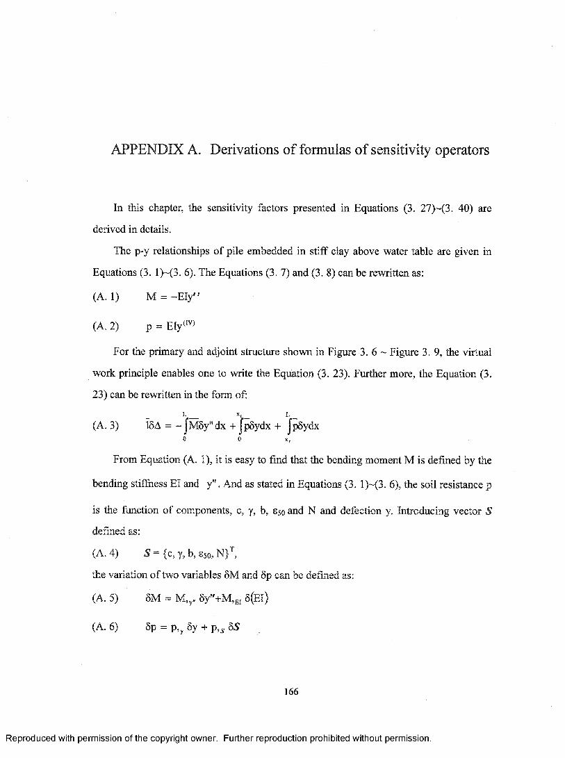
APPENDIX A. Derivations of formulas of sensitivity operators
In this chapter, the sensitivity factors presented in Equations (3. 27)~(3. 40) are
derived in details.
The p-y relationships o f pile embedded in stiff clay above water table are given in
Equations (3. 1)~(3. 6). The Equations (3. 7) and (3. 8) can be rewritten as:
(A. 1) M = -E ly "
(A. 2) p = Ely^’'')
For the primary and adjoint structure shown in Figure 3. 6 ~ Figure 3. 9, the virtual
work principle enables one to write the Equation (3. 23). Further more, the Equation (3.
23) can be rewritten in the form of:
(A. 3) 15A = - |M 5 y "d x + JpSydx + JpSydx
From Equation (A. 1), it is easy to find that the bending moment M is defined by the
bending stif&ess El and y" . And as stated in Equations (3. 1)~(3. 6), the soil resistance p
is the function o f components, c, y, b, 850 and N and defection y. Introducing vector S
defined as:
(A. 4) S = {c,y,b, S50,N } \
the variation o f two variables 5M and 5p can be defined as:
(A. 5) 6M = M,y„ 6y"+M,E, S(E1)
(A. 6) §p = p,^ 5y + p , s 55
166
Reproduced with permission of the copyright owner. Further reproduction prohibited without permission.
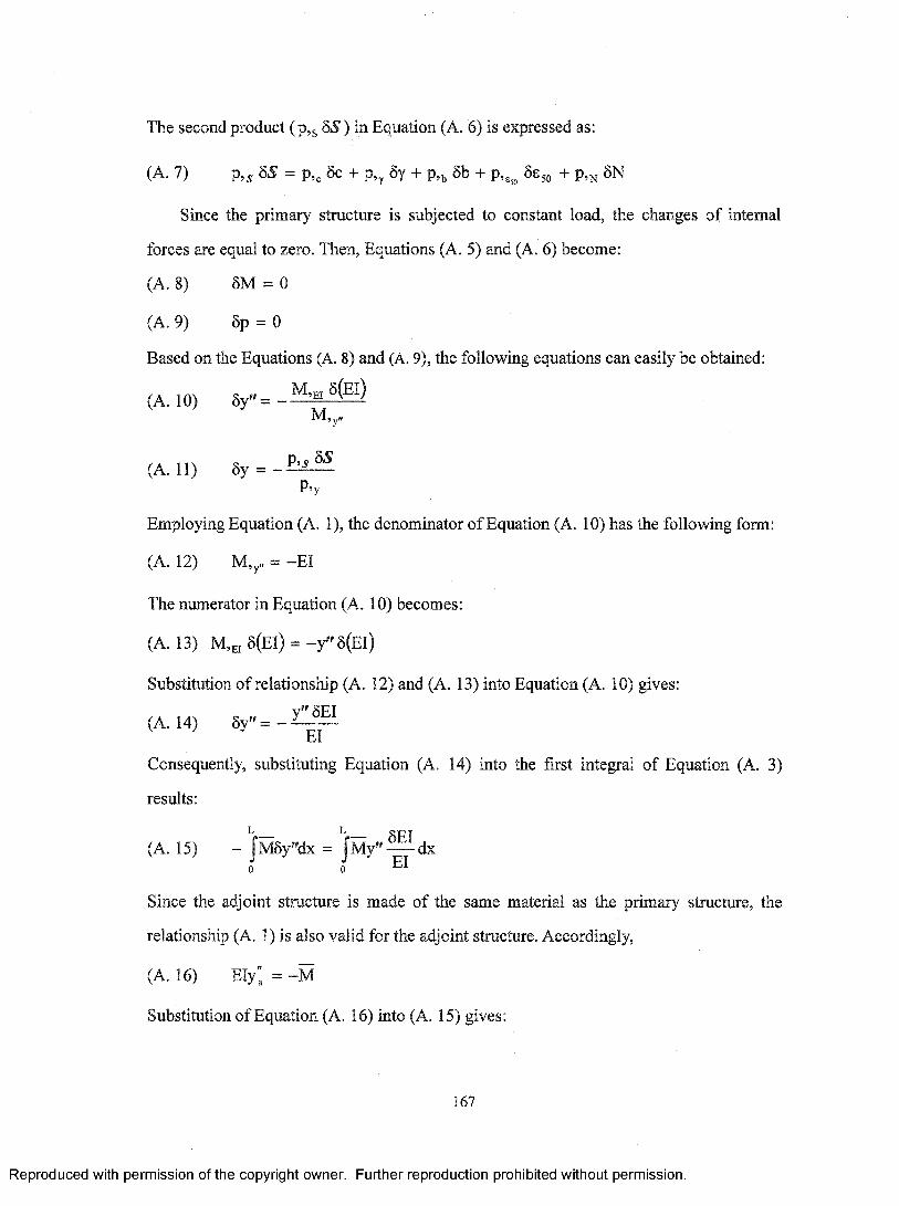
The second product (p,s 6 5 ) in Equation (A. 6) is expressed as:
(A. 7) p,^ 55 = p,, 5c + p,^ 5y + p,^ 5b + p,,^ 5s5o + p,^, 5N
Since the primary structure is subjected to constant load, the changes o f internal
forces are equal to zero. Then, Equations (A. 5) and (A. 6) become:
(A. 8) 5M = 0
(A. 9) 5p = 0
Based on the Equations (A. 8) and (A. 9), the following equations can easily be obtained:
M ,e, 6(EI)(A. 10) 6y"= -
(A. 11) 6y =
M ,,
P,s 55
P ’y
Employing Equation (A. 1), the denominator of Equation (A. 10) has the following form:
(A. 12) M,^„ = -E l
The numerator in Equation (A. 10) becomes:
(A. 13) M ,e 5(EI) = -y "5 (E l)
Substitution o f relationship (A. 12) and (A. 13) into Equation (A. 10) gives:
(A. 14) 6y"=El
Consequently, substituting Equation (A. 14) into the first integral of Equation (A. 3)
results:
6EI(A. 15) - |M 5y"dx = J m / ' — dx
FT0 0
Since the adjoint structure is made o f the same material as the primary structure, the
relationship (A. 1) is also valid for the adjoint structure. Accordingly,
(A. 16) Ely" = -M
Substitution o f Equation (A. 16) into (A. 15) gives:
167
Reproduced with permission of the copyright owner. Further reproduction prohibited without permission.

(A. 17) - jM5y"dx = - J y ”y"5EIdx
The p,y in Equation (A. 11) is determined as follows:
For y<16y5o+9.6(yso)lGg(N):
According to Equation (3. 1):
(A. 18) p = 0.5p„1 9 .6 ,1 + — log N
1650J J
The partial derivative o f p with respect to the lateral deflection y:
(A. 19) p, = 0.5p„ f750
V V1 + — logN
16
1f
7 5 0V V
1 + ^ l o g N 16
81
f7^50
V V1 + — logN
16 J J
Then, the equation (A. 11) then can be rewritten as:
(A. 20) 5y =P,V
1 + — logN 16 ,
In the following paragraphs, the components, which are shown in Equation (A. 7)
p,s 55 = p „ 5c + p,^ 6y + p,^ 5b + p,^^ 5sjo + p,^ 5 N , o f p,^ 55 are derived in
details. Their expressions depend on the value o f x. The following auxiliary designation is
introduced:
168
Reproduced with permission of the copyright owner. Further reproduction prohibited without permission.

(A. 21) n =\J50 J
11 + M io g N
16 ^ ,
For y^l6yso+9.6(y5o)log(N) and x<XrC
(A. 22) p„y J
3 + - X + - Xb b .
cb
Substitution of Equation (A. 22) into (A. 18) produces:
(A. 23) p = i " - Y J3 + —X + —X b b
cb
y
1 9 .6 ,1 H log N16
Based on the Equation (A. 23), the suitable components (A. 7) can be obtained. They are
given as follows:
(A. 24) p,.6c = i(3 b + Jx) ^1 9.61 + — log N
16
5c = ^ (3b + Jx)n5c
(A. 25) p ,, 6y = ^ b x
yy5o
1 9.6 ,1 + — log N16
5y = -^bxnSy
The component p,^ 5b is given by the following equation:
p,b 5b = — (3c + yx)n5b + —[3 + —x + —; cbv4y
^ y ^v2.5S5oby
1
1 + ^ l o g N V 16 ^ .
(-1 ) y * 1
2 .5850b '^ 9.6 ''1 + logN
16
5b
169
Reproduced with permission of the copyright owner. Further reproduction prohibited without permission.
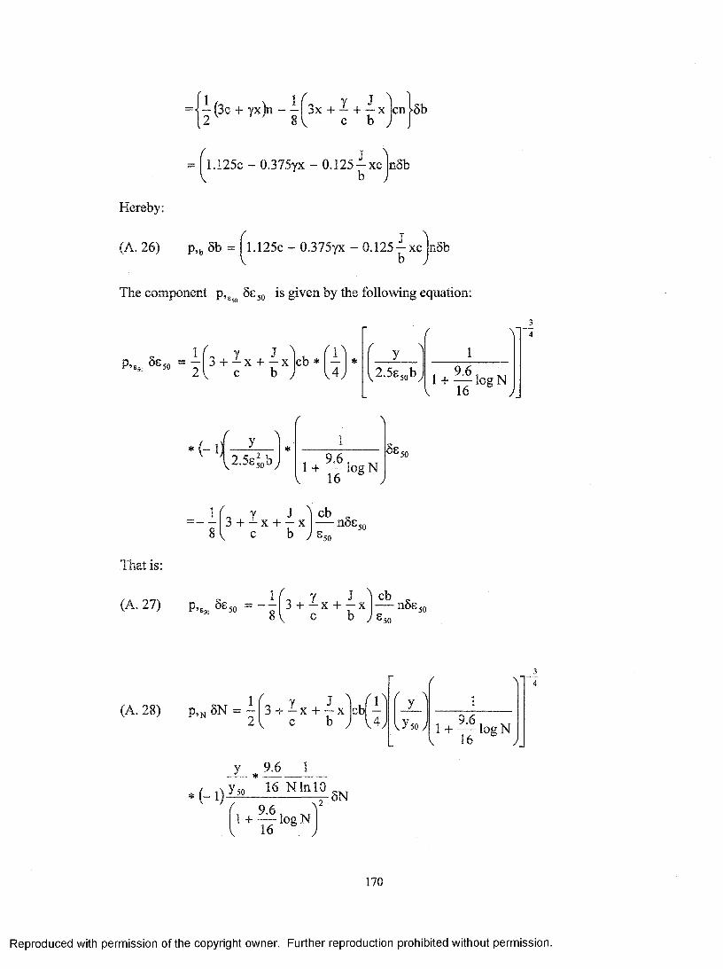
= | —(3c + yx)n - —fs x + — + —8 V c b
cn ^5b
1.125c - 0.375yx - 0.125 ^x c jn S b
Hereby:
(A. 26) p,(, 5b = 1.125c - 0.375yx - 0.125 —xcjn5bi — xclr
The component p,^ SEjq is given by the following equation:
P’B5o ^^50 - 2 3 + —x + —x ]cb * c b J
yv2-5e5oby
1
1 + M i o g N V 16
(-1 )y
2.5z q\) J1
1 9 .6 ,1 + — log NV 16
5s 50
Y J3 + - X + — X
c bcb
n5sy 50
50
That is:
y J3 + - X + —X
c bcb
n5s 50y ^50
(A. 28) p,„ 5N =1 Y J
3 + - X + - X c b
cbr \J L
vysoy
f \
1
1 + — logN 16 ^ ,
y 9.6 1J— * -----------
, 9.6, „1 + — log N . 16
170
Reproduced with permission of the copyright owner. Further reproduction prohibited without permission.
0.075N lnlO
Y J 3 + -^x + - xc b
cbn 11 + — logN
16 ^ .
5N
Fory<16yso+9.6(yso)log(N) and x>Xr:
(A. 29) p„ = 9cb
(A. 30) p = 4.5cbf \yvyso.
1
l + M i o g NV 16
(A. 31) p,, 5c = 4.5b y 11 9.61 + — log N
16 ^ .
5c = 4.5bn5c
(A. 32) p,^ 6y = 0
(A. 33) p,b 5b = 4.5c( j \
vyjoy
1
1 + — logN V 16 ^ ,
6b
+ 4.5cb1
\^2.5Sjob 1 + M i o g NV 16
(-1 )J
11 9.6. . ^1 H log N
16 ^ ,
5b
= (4.5cn - 1.125cn)5b = 3.375cn5b
(A. 34) p, 6850 = 4.5cb/ A
yv2-5S5oby
11 9.6 ,1 + — - log N
16
171
Reproduced with permission of the copyright owner. Further reproduction prohibited without permission.
(-1 )2.5bs^o J
11 9 .6 ,1 + — log N
16 ^ y
6s 50
= - 1.125 — n5g 50'50
(A. 35) p,N 8N = 4.5cbv4y
f \y
v/soy
1
1 + — logN, 16 ^ ,
( -1 )
y
y5o 9.6 1* — * 6N^ 9 6 V 16 NlnlO1 + — logN
16 /
= -0.675cb
NlnlO1
1 + — logN 16 ® .
nSN
By substituting Equations (A. 24)~(A. 28) and (A. 31)~(A. 35) into (A. 20); then
substituting Equations (A. 17) and (A. 20) into Equation (A. 3); taking into account o f the
different expressions for y>6y5o+9.6(y5o)log(N), y<6y5o+9.6(yso)log(N), x<Xr and x>Xr;
and using the expression (3. 41) given as: m = —
following results are obtained:
For y<16y5o+9.6(y5o)log(N):
(A. 36) 18A =
L
+
1
yVso 1 + — logN 16
172
Reproduced with permission of the copyright owner. Further reproduction prohibited without permission.
+ - m n(3b + JxX c)Sc
dx
+ -^ m nbx(Y )Sy
dx
+
+
- mn
-mn
1.125c - 0.375yx - 0.125-^xcVb)5b
dx
- y J 3 + - x + —Xcb
+ J mn' 0.075 Y cb
. I n l o J U .
J 50
1
( 50 )5s 50 dx
'50
A
1 + — logN 16 ^ ,
Y J 3 + ^ x + - x (N)N
dx
+ f[-4.5m nb(c)l— dxi c
+ J [ - 3.375mnc(b)] — dx
+ I 1.125mnC X^\cb
V^50 J( 50 )
5s 50 dx'5 0
+ J( 0.675^ ( cb mn —I In 10 VN,
1
1 + log N 16 ^ .
(N)N
dx
Comparison o f the corresponding terms of Equation (A. 36) and Equation (3. 26)
i8A= J c ^ ^ d x + j c . — + C „ ^ + C . — + c „ ^ + c ,'y ’ 1.y b5b 5s, + r, 50
'50 Ndx leads to
the expressions for the sensitivity operators/integrands given as follows:
Fory<16y5o+9.6(yso)log(N) and x<Xr:
(A. 37) C h = - ( y l y l E i )
173
Reproduced with permission of the copyright owner. Further reproduction prohibited without permission.
(A . 38) C , = - ^ m n(3b + JxX c)
(A. 39) - --^ninbx(Y)
f T A(A. 40) Cb = -m n 1.125c - 0 . 3 7 5 y x - 0.125- x c (b)
b
(A. 41) = - m n 3 + - X + — XV C b , 50
(A. 42) Cj, = mn^ 0 . 0 7 5 ^
V In 10 yv N y1
1 + ^ l o g N 1 6 ^ ,
^3 + ^ x + - x\ n )V c h J
For y<16y5o+9.6(yso)log(N) and x>Xr:
(A. 43) Cei = -(yIy")(Ei)
(A. 44) = -4.5mnb(c)
(A. 45)
(A. 46) Cb = -3.375mnc(b)
(A. 47) C, =1.125mnf^^so „ ( 50 )
(A. 48) = ^0.675^y ln lO y
mnv N y
1
1 + ^ l o g N , 1 6 ^ .
(N)
For y>16y5o+9.6(yso)log(N)
(A. 49) =-(y'.y")(El)
(A. 50) C = C = = C„. = = 0
174
Reproduced with permission of the copyright owner. Further reproduction prohibited without permission.
APPENDIX B. Typical results of the sensitivity analysis for a
free head single long pile embedded in the stiff clay above water
table, subjected to lateral concentrated forces, with pile length
L=10T=13.7m and number of load cycles N=1 and 10000
175
Reproduced with permission of the copyright owner. Further reproduction prohibited without permission.

02
4
6
I 8S§■10Q
12
14
16
£a.
• 30kNo 60kNX 90kN+ 120kN* 150kN□ 180kN0 210kN★ 240kN
270kNA 300kN
-0 .0 2 0 0.02 0.04 0.06Lateral deflections (m) N= 1
2
3
4
5
6
7
8
9
10
I
0.08
• 30kN0 60kNX 90kN+ 120kN* ISOkN□ 180kN❖ 210kN★ 240kN❖ 270kN
5Q .
6 Q
-0 .02 0 0.02 0.04 0.06 0.08Lateral deflections (m) N= 10000
0.110
Figure B. 1 Distributions of lateral deflections y of the primary structures for free head piles of length L=10T, loaded by variable lateral force of discrete variability for the number of cycles N=1 and 10000
176
Reproduced with permission of the copyright owner. Further reproduction prohibited without permission.
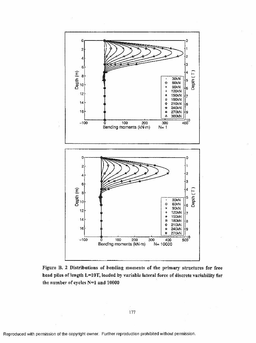
0
2
4
6
l a
§■10Q12
14
16
• 30kNo SOkNX 90kN+ 120kN
ISOkN□ ISOkN❖ 210kN★ 240kN
270kNA 300kN
D.s
-100 0 100 200 300Bending moments (kN m) N= 1
10 400
30kNBOkN90kN120kNISOkN180kN210kN240kN270kN
0 100 200 300 400Bending moments (kN-m) N= 10000
Figure B. 2 Distributions of bending moments of the primary structures for free head piles of length L=10T, loaded by variable lateral force of discrete variability for the number of cycles N=1 and 10000
177
Reproduced with permission of the copyright owner. Further reproduction prohibited without permission.
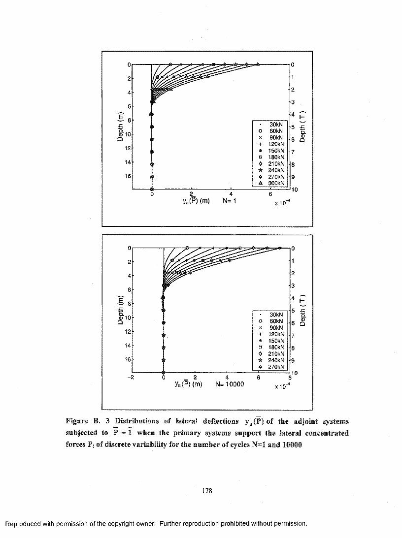
02
4
6
I 8l i oQ
12
14
16
yah) (m) N=^
oX+*□0★
A
SOkN60kN90kN120kNISOkNISOkN210kN240kN270kNSOOkN
01
2
3
4 P5 £
Q.6 Q
7
8
9
10
X 10.-4
SOkNBOkN90kN120kNISOkNISOkN210kN240kN270kN
0 _ 2 Ya (P) (m) N= 10000 x i o
Figure B. 3 Distributions of lateral deflections y ^ (P )o f the adjoint systems subjected to P = 1 when the primary systems support the lateral concentrated forces Pt of discrete variability for the number of cycles N=1 and 10000
178
Reproduced with permission of the copyright owner. Further reproduction prohibited without permission.
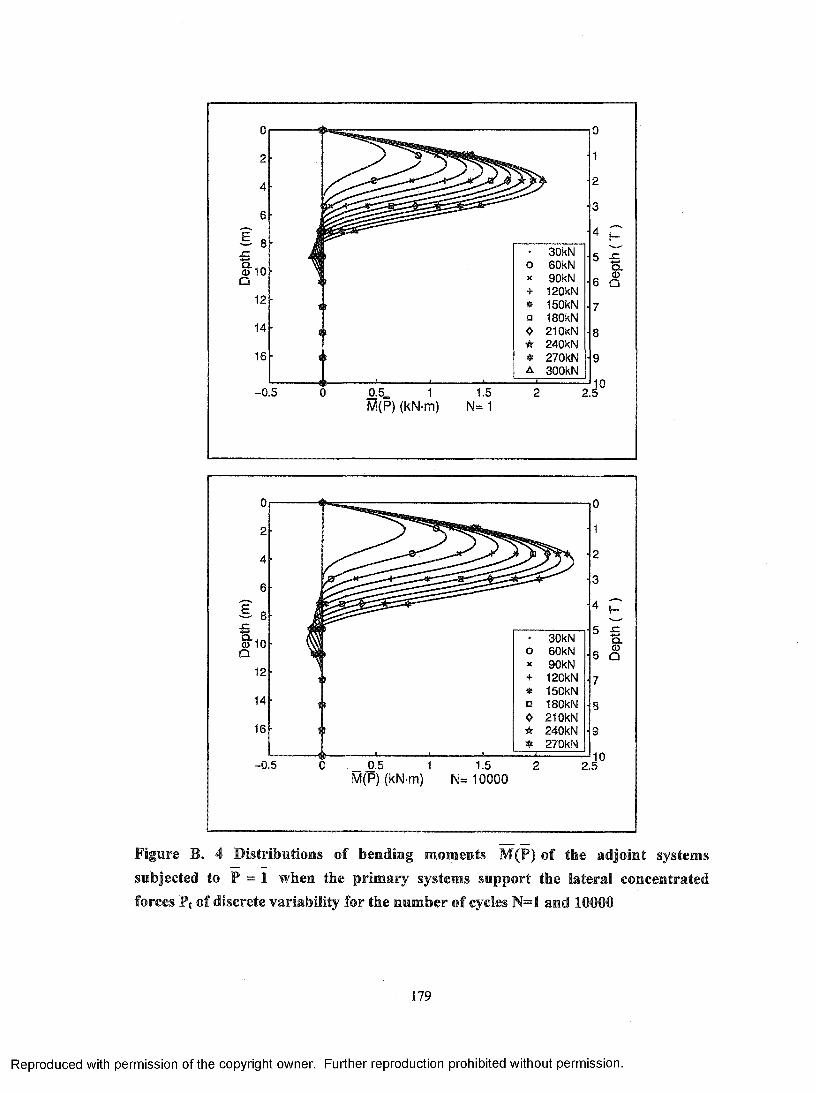
SOkNSOkN90kN120kN150kN180kN210kN240kN270kNSOOkN
1 1.5M(P) (kN-m) N= 1
SOkNBOkN90kN120kNISOkNISOkN210kN240kN270kN
_ JO.5 1M(P) (kN-m)
1.5 N= 10000
7
8
9
105
Figure B. 4 Distributions of bending moments M(P) of the adjoint systems subjected to P = 1 when the primary systems support the lateral concentrated forces Pt of discrete variability for the number of cycles N=1 and 10000
179
Reproduced with permission of the copyright owner. Further reproduction prohibited without permission.
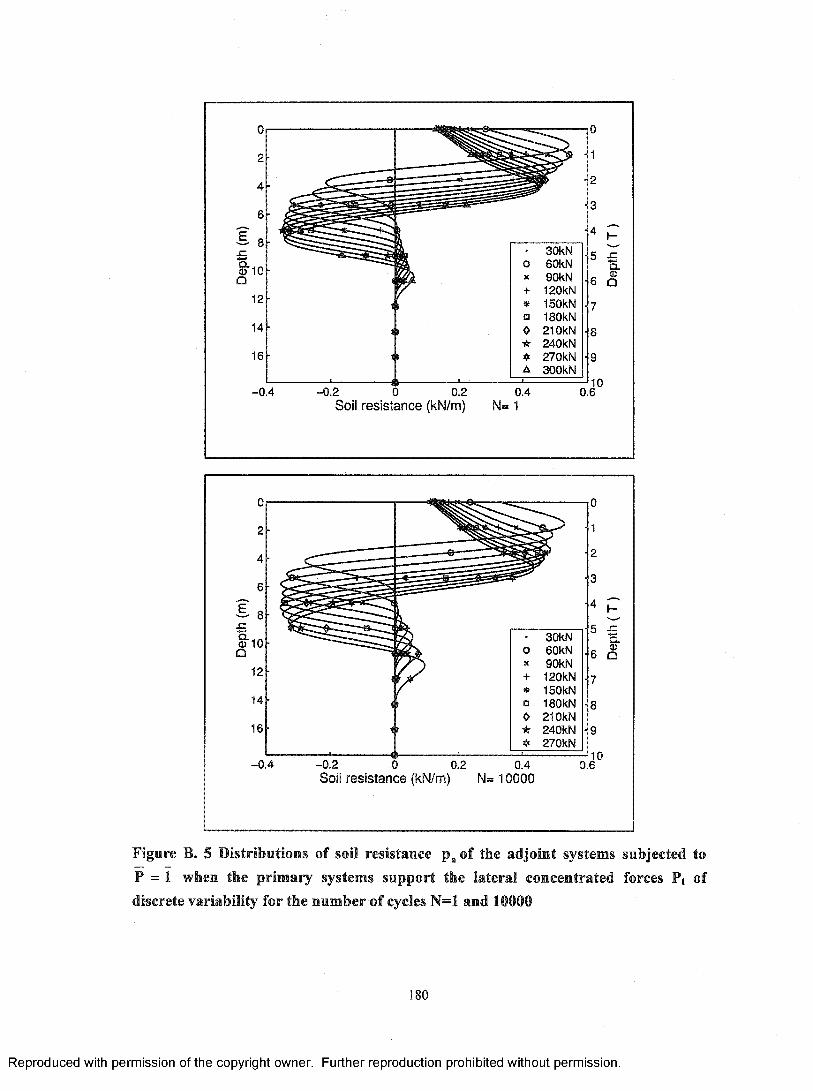
• 30kNo SOkNX 90kN+ 120kN* ISOkN□ ISOkN0 210kN★ 240kN
270kNA 300kN
Q .CDQ
-0 .4 -0 .2 0 0.2 0.4Soil resistance (kN/m) N= 1
o.e
30kN60kN90kN120kN150kN180kN210kN240kN270kN
- 0.2 0 0.2 Soil resistance (kN/m)
0.4N= 10000
Figure B. 5 Distributions of soil resistance p, of the adjoint systems subjected to P = 1 when the primary systems support the lateral concentrated forces Pt of discrete variability for the number of cycles N=1 and 10000
180
Reproduced with permission of the copyright owner. Further reproduction prohibited without permission.
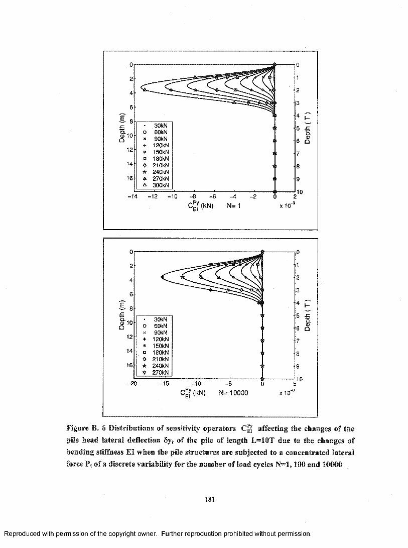
o10 Q12
14
16
+•a0★❖A
30kN60kN90kN120KNISOkNISOkN210kN240kN270kN300kN
-1 4 -1 2 -1 0 - 8 - 6 - 4
(kN) N= 1 X 1 0 '
©10Q12
14
16
30kN60kN90kN120kN150kN180kN210kN240kN270kN
-20 -15 -10C^f(kN)
- 5 0
N= 10000 X 1 0 '
Figure B. 6 Distributions of sensitivity operators affecting the changes of the pile head lateral deflection 6yt of the pile of length L=10T due to the changes of bending stiffness El when the pile structures are subjected to a concentrated lateral force Pt of a discrete variability for the number of load cycles N=l, 100 and 10000
181
Reproduced with permission of the copyright owner. Further reproduction prohibited without permission.

§•10Q12
14
16
+
□
*❖A
30kN60kN90kN120kNISOkNISOkN210kN240kN270kNSOOkN
-0.05 -0.04 -0 .0 3
(kN)- 0,02
N= 1- 0.01
I -
16 £ Ol <1546 Q
17
<6
100
2
4
6
Is£§•10Q
12
14
16
• 30kNo 60kNX 90kN+ 120kN• ISOkN□ ISOkN0 210kN★ 240kN
270kN
-0 .05 -0 .0 4 -0 .0 3
(kN)- 0.02 - 0.01
N= 10000
4 H6 £
Q . <1546 a
17
16
1®
10
Figure B. 7 Distributions of sensitivity operators affecting the changes of the pile head lateral deflection 5yt of the pile of length L=10T due to the changes of the cohesion c when the pile structures are subjected to a concentrated lateral force Pt of a discrete variabiUty for the number of load cycles N=1 and 10000
182
Reproduced with permission of the copyright owner. Further reproduction prohibited without permission.
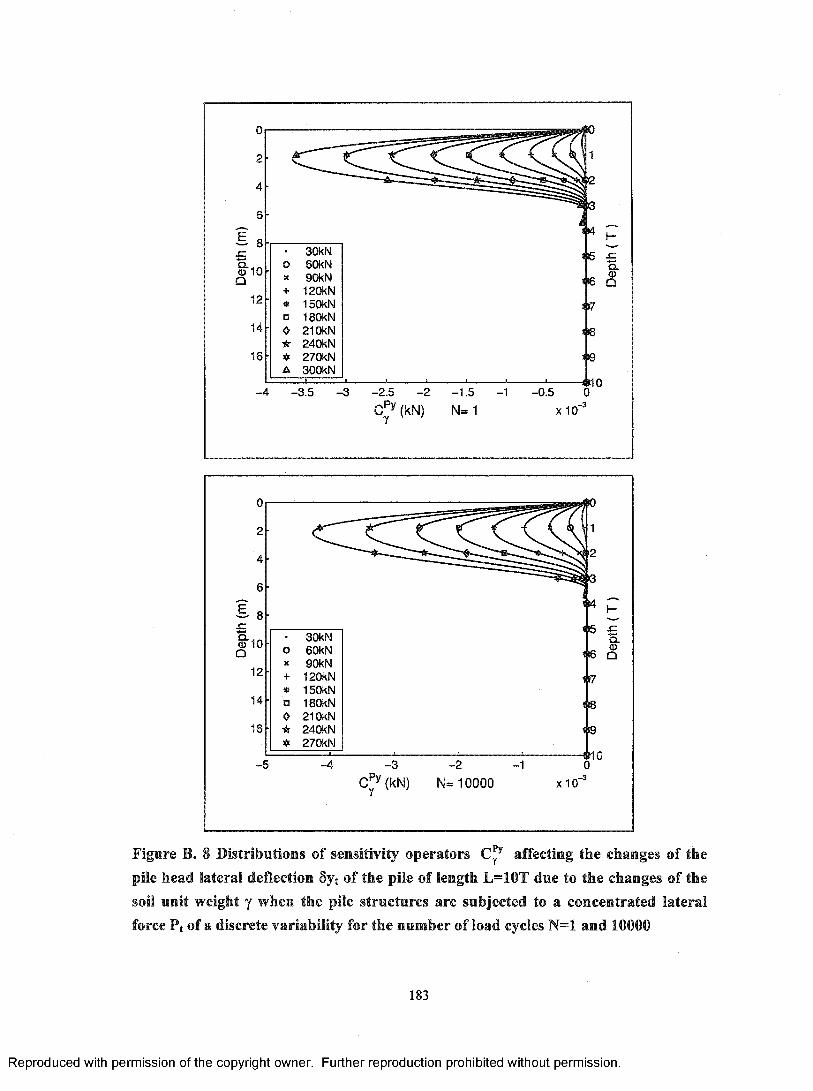
Q) 10 Q12
14
16
o«+*□0ir
A
30kN60kN90kN120kNISOkNISOkN210kN240kN270kNSOOkN
-3 .5 - 3 -2 .5 - 2
(kN)-1 .5
N= 1-1 -0 .5
<6 £ ql
#6 Q
>7
4 6
4r10
X 10,-3
■=- 8
o l OQ12
14
16
+*□0★
30kN60kN90kN120kNISOkNISOkN210kN240kN270kN
- 5 -4 - 3
(kN)-2 -1
N= 10000
16 £ a.
#6 Q
r7
1®1©
4no
X 1 0
0-3
Figure B. 8 Distributions of sensitivity operators affecting the changes of the pile head lateral deflection Syt of the pile of length L=10T due to the changes of the soil unit weight y when the pile structures are subjected to a concentrated lateral force Pt of a discrete variability for the number of load cycles N=1 and 10000
183
Reproduced with permission of the copyright owner. Further reproduction prohibited without permission.
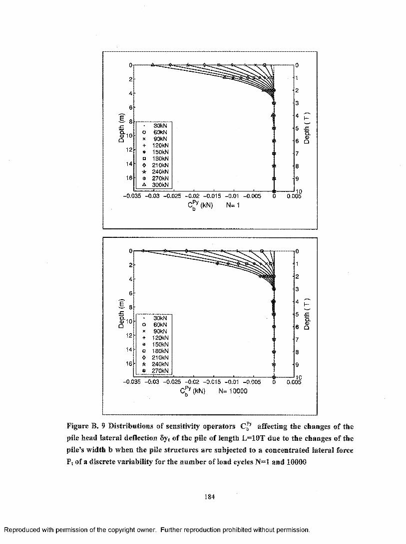
8£<u 10 Q
12
14
16
+*□0★
A
30kN60kN90kN120kNISOkNISOkN210kN240kN270kNSOOkN
-0 .0 3 5 -0 .0 3 -0 .0 2 5 -0 .0 2 -0 .0 1 5 -0.01 -0 .0 0 5
(kN) N= 1
0
2
4
6
I 8so l OQ
12
14
16
+•o0★A
30kN60kN90kN120kNISOkNISOkN210kN240kN270kN
-0 .0 3 5 -0 .0 3 -0 .0 2 5 -0 .0 2 -0 .0 1 5 -0.01 -0 .0 0 5
(kN) N= 10000
5 £ Q.
6 Q
100 0.005
s
5 £ a .
6 Q
100 0.005
Figure B. 9 Distributions of sensitivity operators affecting the changes of the pile head lateral deflection 8yt of the pile of length L=10T due to the changes of the pile’s width b when the pile structures are subjected to a concentrated lateral force Pt of a discrete variability for the number of load cycles N=1 and 10000
184
Reproduced with permission of the copyright owner. Further reproduction prohibited without permission.
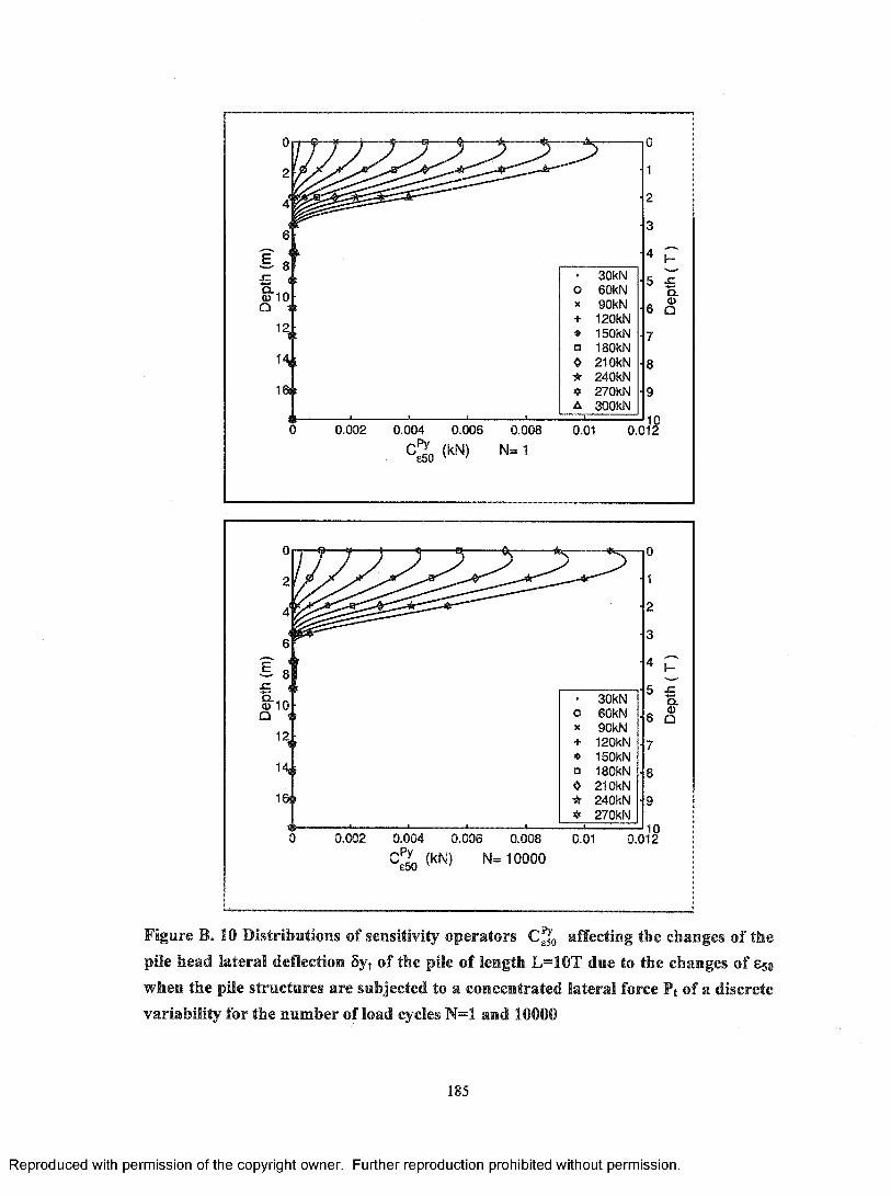
§■10Q 1
H i
16i»
• 30kN0 60kNX 90kN+ 120kN• ISOkNa ISOkN0 210kN★ 240kN❖ 270kNA SOOkN
5 -c Q.
6 Q
0.002 0.004 0.006
C'N)
0.008
N= 10.01 0. 10
012
< r
JCQ.30kN
60kN90kN120kNISOkNISOkN210kN240kN270kN
16ir
0.002 0.004 0.006
(kN) N= 100000.008 0.01 0.012
Figure B. 10 Distributions of sensitivity operators effecting the changes of the pile head lateral deflection 6yt of the pile of length L=10T due to the changes of 850 when the pile structures are subjected to a concentrated lateral force Pt of a discrete variability for the number of load cycles N=1 and 10000
185
Reproduced with permission of the copyright owner. Further reproduction prohibited without permission.
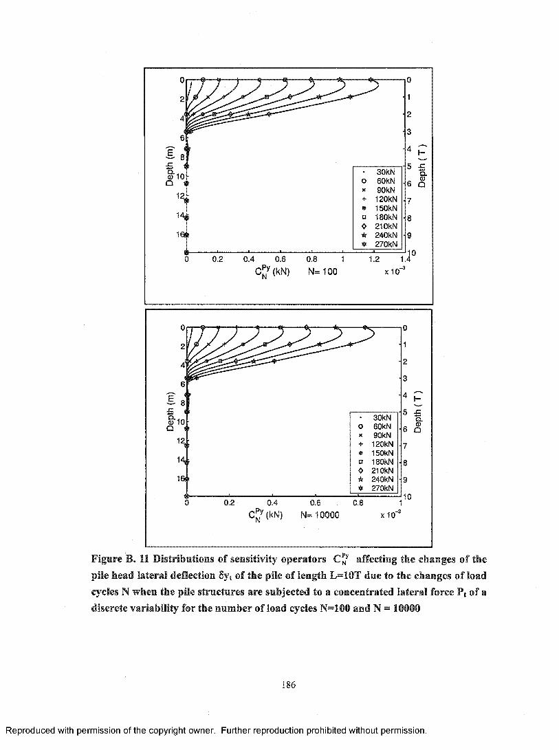
H i
1 Qr
• SOkNo 60kNX 9QkN+ 120kN* ISOkN□ 180kN<> 210kN★ 240kN
270kN
01
2
3
^ h-5 £
a .6 Q
7
8
9
0.2 0.4 0.6 cPy(kN)
0.8 1 N= 100
1.210
1.4
xIO"'
SOkNBOkN90kN120kN150kN180kN210kN240kN270kN
&10 Q.
H i
0.2 0.4
(kN) N= 100000.6 0.8
X 10'
Figure B. 11 Distributions of sensitivity operators affecting the changes of the pile head lateral deflection Syt of the pile of length L=10T due to the changes of load cycles N when the pile structures are subjected to a concentrated lateral force Pt of a discrete variability for the number of load cycles N=100 and N = 10000
186
Reproduced with permission of the copyright owner. Further reproduction prohibited without permission.

02
4
6
I 8£ZQ) 10Q
12
14
16
-0 .5 0.5 _ 1ya(M) (m)
1.5 N= 1
oX+*□0★
A
SOkN60KN90kN120RN150kNISOkN210kN240kN270kNSOOkN
5Q.
6 Q
102.5
X 10’
SOkNSOkN90kN120kN150kNISOkN210kN240kN270kN
0 ^ 1 1.5ya{M) (m) N= 10000 X 10’
Figure B. 12 Distributions of lateral deflections yg(M) of the adjoint systems snbjected to M = 1 when the primary systems support the lateral concentrated forces Pt of discrete variability for the number of cycles N=1 and 10000
187
Reproduced with permission of the copyright owner. Further reproduction prohibited without permission.
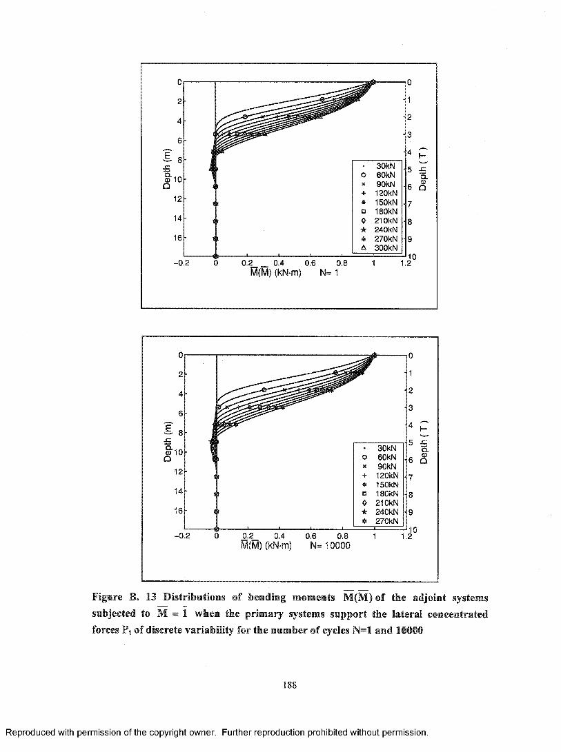
SOkN60kN90kN120kNISOkN180kN210kN240kN270KNSOOkN
0.2____ 0.4 0.6 0.8M(M) (kN m) N= 1
SOkN60kN90kN120kN150kN180kN210kN240kN270kN
£ .2 _ 0.4M(M) (kN m)
0.6 0.8 N= 10000
Figure B. 13 Distributions of bending moments M(M) of the adjoint systems subjected to M = 1 when the primary systems support the lateral concentrated forces Pt of discrete variability for the number of cycles N=1 and 10000
188
Reproduced with permission of the copyright owner. Further reproduction prohibited without permission.
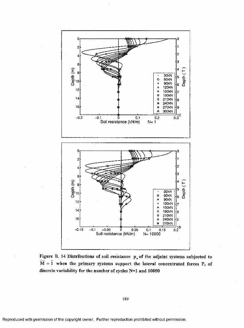
• 30kNo 60kNX 90kN+ 120kN* ISOkN□ ISOkN<> 210kN★ 240kN
270kNA SOOkN
01
2
3
4 P5 -c ■S.6 Q
7
8
9
- 0.2 - 0.1 0 0.1 0.2 Soil resistance (kN/m) N= 1
100.3
30kN60kN90kN120kNISOkN180kN210kN240kN270kN
-0.1 -0 .0 5 0 0.05Soil resistance (kN/m)
0.1 0.15N= 10000
Figure B. 14 Distributions of soil resistance of the adjoint systems subjected to M = 1 when the primary systems support the lateral concentrated forces Pt of discrete variability for the number of cycles N=1 and 10000
189
Reproduced with permission of the copyright owner. Further reproduction prohibited without permission.
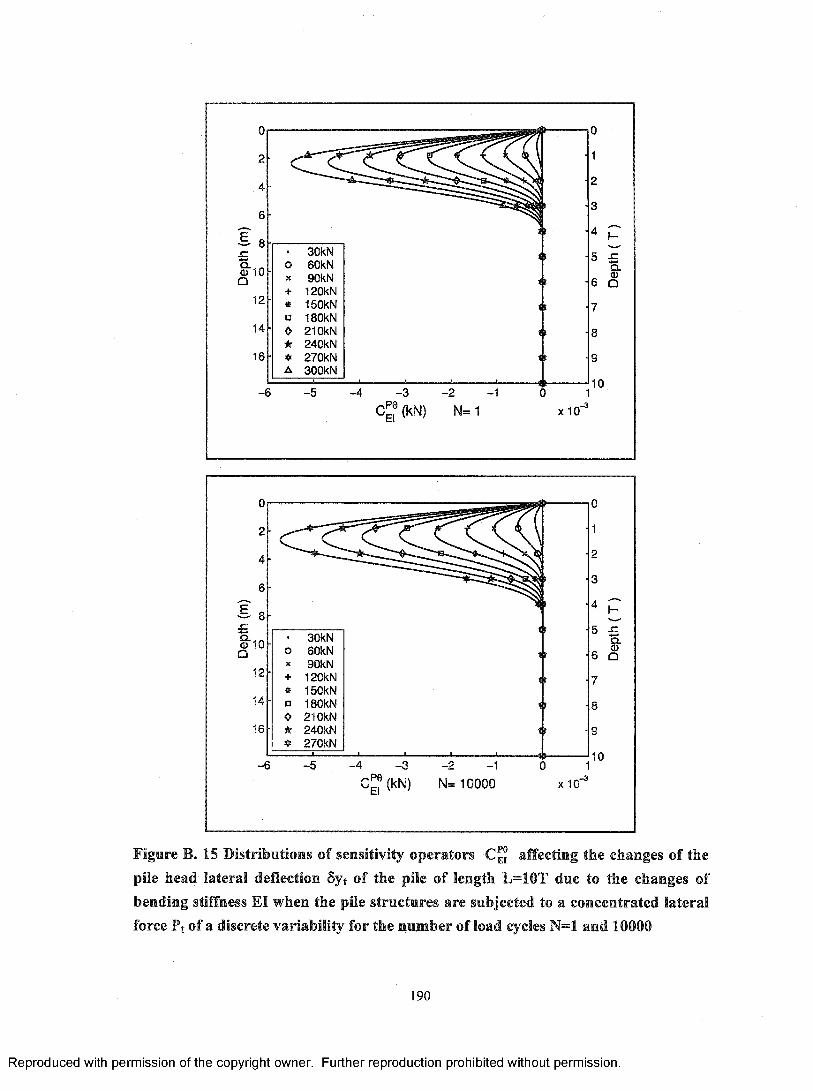
szs.<uQ§•10
SOkNSOkN90kN120kN150kN180kN210kN240kN270kNSOOkN
(kN) N= 1 x10
SOkN SOkN 90kN 120kN 150kN
o 180kN 0 210kN
240kN 270kN
(kN)-2 -1
N= 10000 xIO ’'
Figure B. 15 Distributions of sensitivity operators C , affecting the changes of the pile head lateral deflection Syt of the pile of length L=10T due to the changes of bending stiffness El when the pile structures are subjected to a concentrated lateral force Pt of a discrete variability for the number of load cycles N=1 and 10000
190
Reproduced with permission of the copyright owner. Further reproduction prohibited without permission.

8
§■10Q12
14
16
+
□0★♦A
30kNSOkN90kN120kNISOkNISOkN210kN240kN270kN300kN
-0.012 -0.01 -0 .008
(kN)0.006 -0 .004
N= 1-0.002
Or^
iz. 8 £Q- . <D 10 Q
12
14
16
• 30kN o 60kN « 90kN + 120kN• 1SOkN o ISOkN0★
210kN240kN270kN
-0.012 -0 .01 -0 .0 0 8 -0 .0 0 6 -0 .0 0 4 -0 .0 0 2
(kN) N= 10000
< 6 SQ.
46 Q
(7
<8
♦10
’ b6 :£
Q. 0516 Q
r7
18
1©
100
Figure B. 16 Distributions of sensitivity operators affecting the changes of the pile head lateral deflection 5yt of the pile of length L=10T due to the changes of the cohesion c when the pile structures are subjected to a concentrated lateral force Pt of a discrete variability for the number of load cycles N=1 and 10000
191
Reproduced with permission of the copyright owner. Further reproduction prohibited without permission.
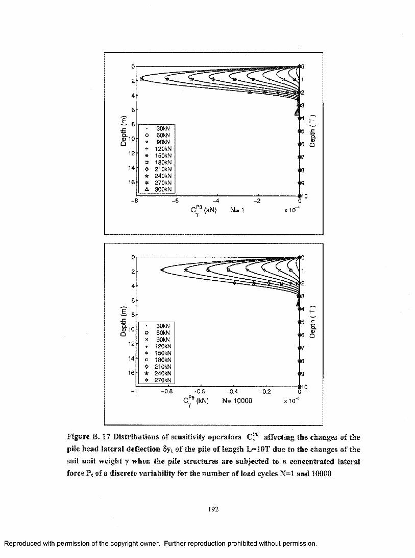
6 -
E 8sz
o l O -Q
1 2 -
1 4 -
16
- 8
oit+•a0★
A
30kN60kN90kN120kN150kNISOkN210kN240kN270kNSOOkN
C^®{kN) N= 1
C™ (kN)-0 .4
N= 10000
#5 -c Q.O’#6 Q
i f f
I©
10
Jno
X 10
SOkNSOkN90kN120kNISOkNISOkN210kN240KN270kN
1 6 Q
X 10
Figure B. 17 Distributions of sensitivity operators C™ affecting the changes of the pile head lateral deflection 6yt of the pile of length L=10T due to the changes of the soil unit weight y when the pile structures are subjected to a concentrated lateral force Pt of a discrete variability for the number of load cycles N=1 and 10000
192
Reproduced with permission of the copyright owner. Further reproduction prohibited without permission.
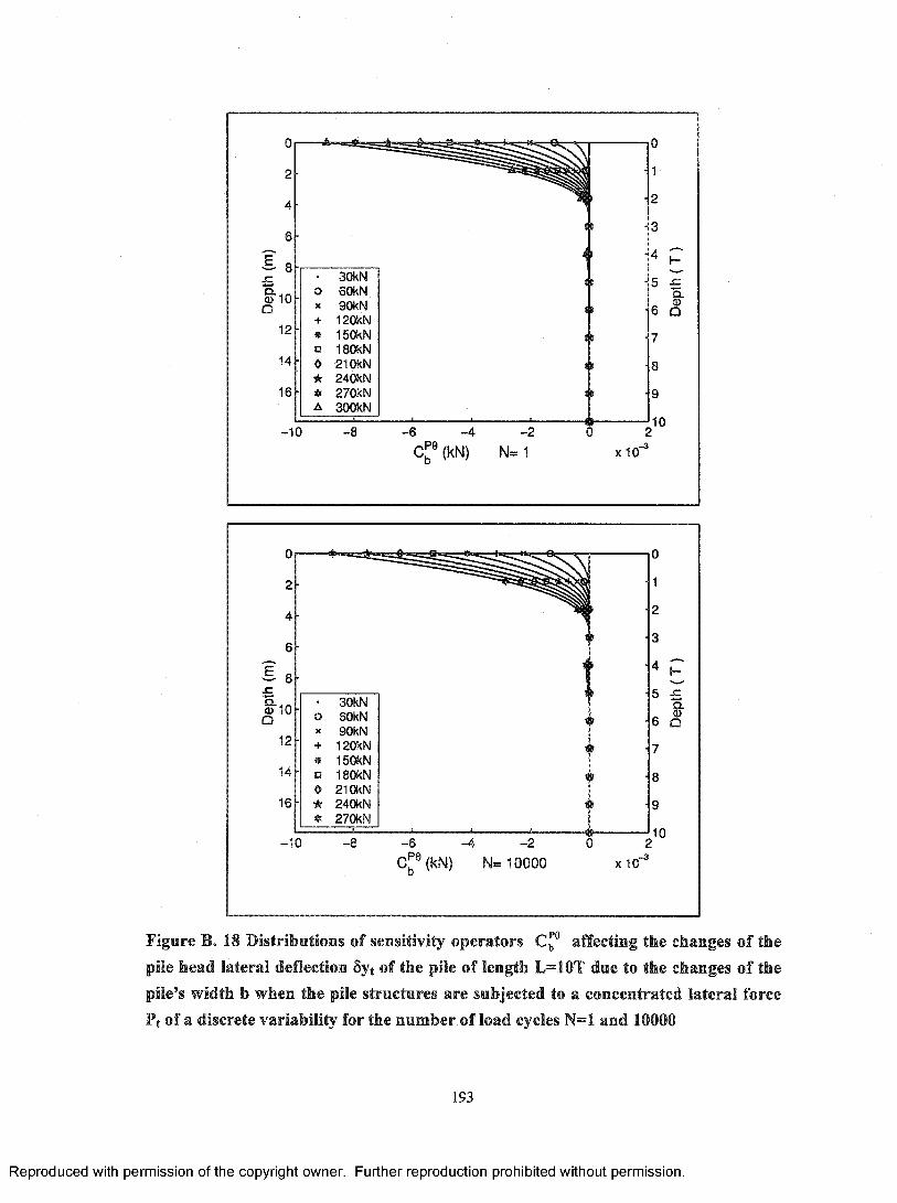
0
2
4
6
I s£ZO10Q
12
14
16
. SOkNo SOkNX 90kN+ 120kN* ISOkNO ISOkN0 210kN★ 240kN❖ 270kNA SOOkN
-10
I-5 -c
Q.6 Q
7
8
9
10
C (kN) N= 1 X 10"
0
2
4
6
S 8
o l OQ
12
14
16
+
□0★
SOkN60kN90kN120kNISOkN180kN210kN240kN270kN
-10 -8 -6
"bcr® (kN)- 4 - 2
N= 10000 X 10'
2-3
0
1
2
3
4 P5 £
Ql
6 Q
7
8
9
10
Figure B. 18 Distributions of sensitivity operators affecting the changes of the pile head lateral deflection Syt of the pile of length L=10T due to the changes of the pile’s width b when the pile structures are subjected to a concentrated lateral force Pt of a discrete variability for the number of load cycles N=1 and 10000
193
Reproduced with permission of the copyright owner. Further reproduction prohibited without permission.
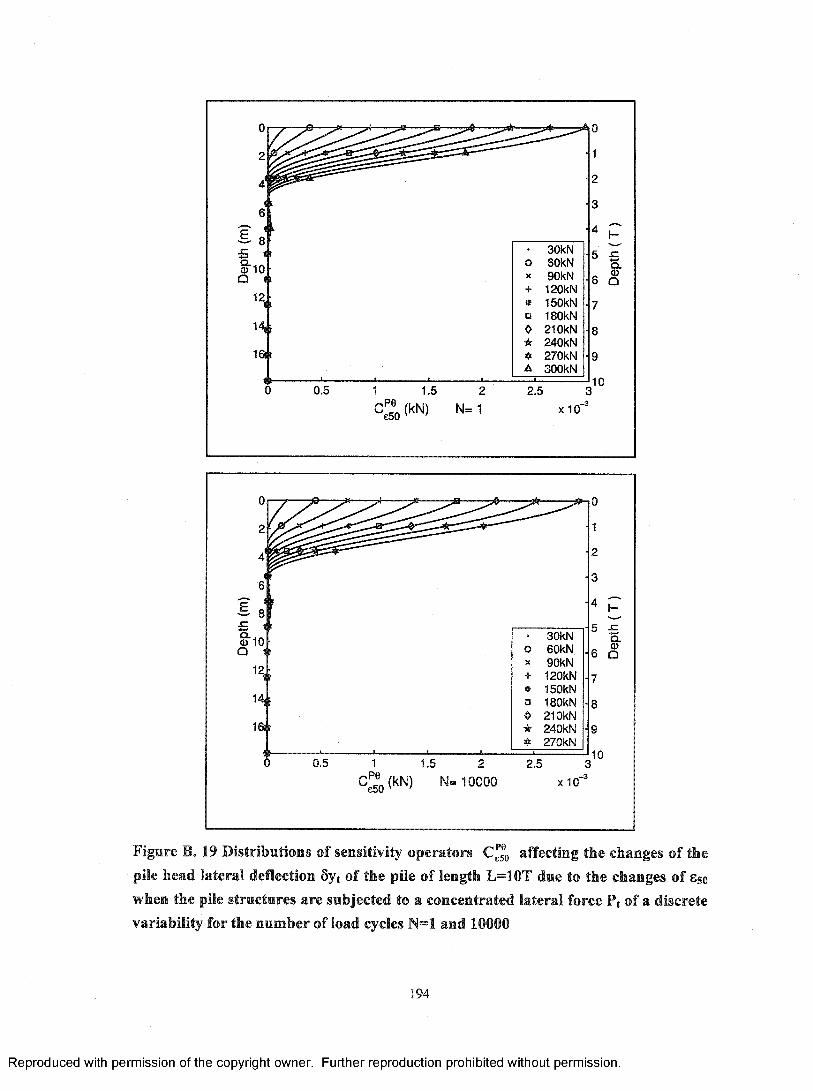
o10Q 1
H r
16ir
0.5 1.5
(kN) N= 1
oX
+*□0★
A
SOkN60kN90kN120kN150kNISOkN210kN240kN270kNSOOkN
2.5
X 10'
3,—3
01
2
3
^ 1-5 £
Q.6 Q
7
8
9
10
<u 10 SOkN60kN90kN120kN150kNISOkN210kN240kN270RN
Q.
H i
0.5 2.5,-3N= 10000 X I f f
Figure B. 19 Distributions of sensitivity operators affecting the changes of the pile head lateral deflection Sy, of the pile of length L=10T due to the changes of Sso when the pile structures are subjected to a concentrated lateral force P, of a discrete variability for the number of load cycles N=1 and 10000
194
Reproduced with permission of the copyright owner. Further reproduction prohibited without permission.
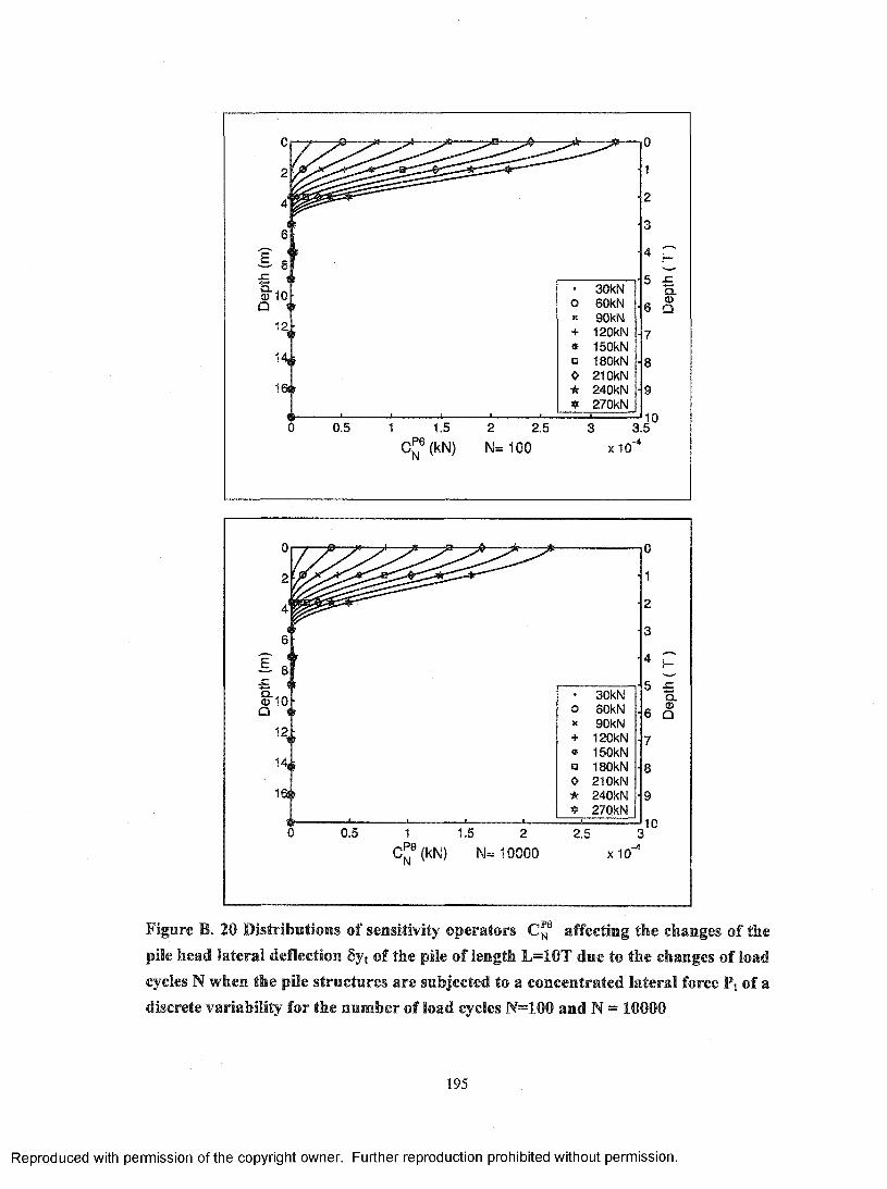
'2,
H r
iar
• 30kNo SOkNX 90kN+ 120kN* 150kN□ IBOkN0 210kN★ 240kN
270kN
0.5 1.5
C^®(kN)2 2.5
N= 100 X 1 0
7
8
9
sz szQ.30kN
60kN90kN120kN150kNISOkN210kN240kN270kN
0.5 2.5.-4(kN) N= 10000 x10‘
Figure B. 20 Distributions of sensitivity operators C™ affecting the changes of the pile head lateral deflection Syt of the pile of length L=10T due to the changes of load cycles N when the pile structures are subjected to a concentrated lateral force Pt of a discrete variability for the number of load cycles N=1G0 and N = 10000
195
Reproduced with permission of the copyright owner. Further reproduction prohibited without permission.
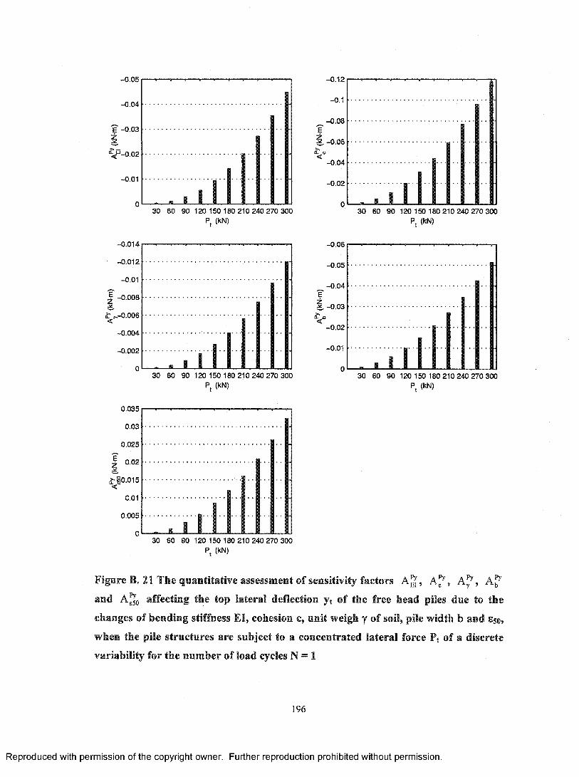
- 0.05
-0 .04
"e -0 .03
'-0.02
-0.01
30 60 90 120 150 180 210 240 270 300
- 0.12
-0.1
-0 .08
^ -0 .06
-0 .04
-0.02
30 60 90 120 150 180 210 240 270 300P, (kN) Pj (kN)
•0.014
-0.012
-0.01
g -0.008
-0.004
-0.002
30 60 90 120 150 180 210 240 270 300
-0.06
-0 .05
-0 .0 4
-0.03
-0.02
-0.01
30 60 90 120 150 180 210 240 270 300P( (kN) P, (kN)
0.035
0.03
0.025
r0.015
0.01
0.005
30 60 90 120 150 180 210 240 270 300Pj (kN)
PyFigure B. 21 The quantitative assessment of sensitivity factors A ^ , A f', Ai^, A
and A^o affecting the top lateral deflection yt of the free head piles due to the
changes of bending stiffness El, cohesion c, unit weigh y of soil, pile width b and Eso,
when the pile structures are subject to a concentrated lateral force Pt of a discrete
variability for the number of load cycles N = 1
196
Reproduced with permission of the copyright owner. Further reproduction prohibited without permission.
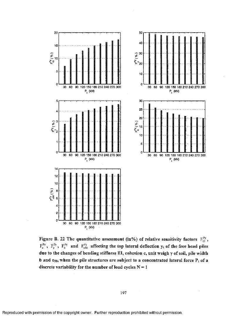
20 50
15
■ 10
40
^30
' -“20
10
a. f- u- 2
14
12
10
8
I 6
4
2
0
30 60 90 120 150 180 210 240 270 300 P, (kN)
30 60 90 120 150 180 210 240 270 300 P, (kN)
30 60 90 120 150 180 210 240 270 300 Pj (kN)
30
25
20
15
10
5
30 60 90 120 150 180 210 240 270 300 P, (kN)
30 60 90 120 150 180 210 240 270 300 P, (kN)
Figure B. 22 The quantitative assessment (in%) of relative sensitivity factors , pPy pPy pPy ^nd affecting the top lateral deflection yt of the free head piles due to the changes of bending stiffness El, cohesion c, unit weigh y of soil, pile width b and Sso, when the pile structures are subject to a concentrated lateral force Ft of a discrete variability for the number of load cycles N = 1
197
Reproduced with permission of the copyright owner. Further reproduction prohibited without permission.
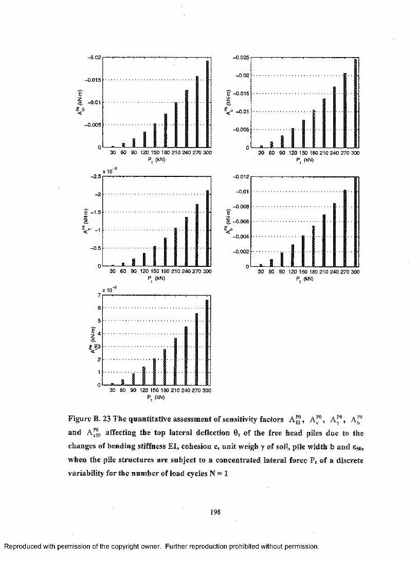
-0.02
-0 ,015
e -0.01
-0 .005
30 60 90 120 150 180 210 240 270 300P, (kN)
X 10-2 .5
-2
E '-1 .5
-0 .5
30 60 90 120 150 180 210 240 270 300P, (kN)
X 107
6
5
E"4
|3<2
1
030 60 90 120 150 180 210 240 270 300
- 0.025
-0.02
f -0 .015
-0.01
-0 .005
30 60 90 120 150 180 210 240 270 300
-0.012
-0.01
-0 .008'i1 . -0 .006
V-0 .004
-0.002
0
P, (kN)
....................1
. ■ I I30 60 90 120 150 180 210 240 270 300
P, (kN)
p, (kN)
Figure B. 23 The quantitative assessment of sensitivity factors A P0 El 5
P0 A™ A™
and affecting the top lateral deflection 0t of the free head piles due to the
changes of bending stiffness El, cohesion c, unit weigh y of soil, pile width b and 850,
when the pile structures are subject to a concentrated lateral force Pt of a discrete
variability for the number of load cycles N = 1
198
Reproduced with permission of the copyright owner. Further reproduction prohibited without permission.
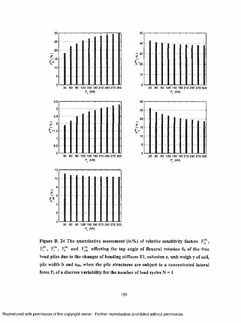
3.5
3
2.5
? 2 1^1.5
1
0.5
0
12
10
8
^ 6 £ § u_
4
2
0
30 60 90 120 150 180 210 240 270 300 P, (kN)
30 60 90 120 150 180 210 240 270 300 P, (kN)
30 60 90 120 150 180 210 240 270 300 P (kN)
50
40
30
‘ “20
10
30
25
20
— 15
10
5
30 60 90 120 150 180 210 240 270 300 P, (kN)
30 60 90 120 150 180 210 240 270 300 P, (kN)
peFigure B. 24 The quantitative assessment (in%) of relative sensitivity factors Fgj ,
F™, F™, F™ and F™ affecting the top angle of flexural rotation 0t of the free
head piles due to the changes of bending stiffness El, cohesion c, unit weigh y of soil,
pile width b and Sgo, when the pile structures are subject to a concentrated lateral
force Pt of a discrete variability for the number of load cycles N = 1
199
Reproduced with permission of the copyright owner. Further reproduction prohibited without permission.
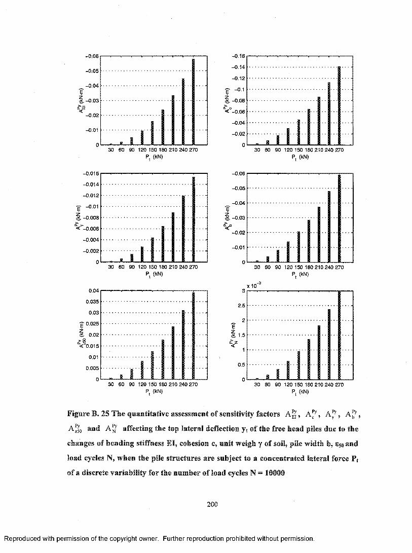
- 0.06
-0.05
-0.04
-0.01
30 60 90 120 150 180 210 240 270R (kN)
-0.016
-0.014
-0.012-0.01
^ -0.008
< -0.006
-0.004
-0.002
30 60 90 120 150 180 210 240 270P( (kN)
0.04
0.035
0.03
■p 0.025
it 0.02<0 . 01 5
0.010.005
30 60 90 120 150 180 210 240 270Pt (kN)
- 0.16
-0.14
-0.12-P -0.1^ -0.08
< -0.06
-0.04
-0.02
30 60 90 120 150 180 210 240 270P, (kN)
-0.06
-0.05
-0.04f1 . -0.03
-0.02
-0.01
0
3
2.5
2
..............................1
■ . 1 130 60 90 120 150 180 210 240 270
P, (kN)
xIO
1. 1.5S: 2 < 1
0.5
030 60 90 120 150 180 210 240 270
p, (kN)
Figure B. 25 The quantitative assessment of sensitivity factors , A ^ , A ^ ,
A^o and A^ affecting the top lateral deflection yt of the free head piles due to the
changes of bending stiffness El, cohesion c, unit weigh y of soil, pile width h, 850 and
load cycles N, when the pile structures are subject to a concentrated lateral force Pt
of a discrete variability for the number of load cycles N = 10000
200
Reproduced with permission of the copyright owner. Further reproduction prohibited without permission.
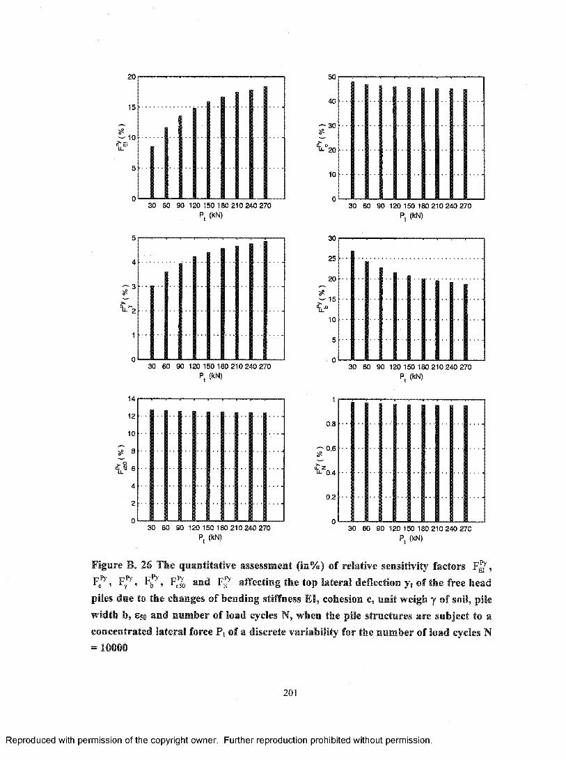
20 50
15
10
40
30
1 “20
10
LL 2
14
12
10
? 8
30 60 90 120 150 180 210 240 270 P, (kN)
30 60 90 120 150 180 210 240 270 Pt (kN)
30 60 90 120 150 180 210 240 270 P, (kN)
30
25
20
^ 15V
10
5
0
0.8
■0.6
0.4
0.2
30 60 90 120 150 180 210 240 270 p, (kN)
30 60 90 120 150 180 210 240 270P, (kN)
30 60 90 120 150 180 210 240 270 P, (kN)
Figure B. 26 The quantitative assessment (in%) of relative sensitivity factors , FJ , F. , F o and F^ affecting the top lateral deflection yt of the free head piles due to the changes of hending stiffness E l, cohesion c, unit weigh y of soil, pile width b, Sso and number of load cycles N, when the pile structures are subject to a concentrated lateral force Pt of a discrete variability for the number of load cycles N =10000
201
Reproduced with permission of the copyright owner. Further reproduction prohibited without permission.
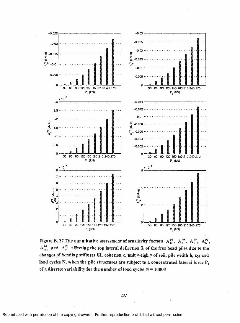
- 0.025
-0.02
f -0 .015 ±
-0 .005
jJ lIX 10
30 60 90 120 150 180 210 240 270 P, (kN)
-3
-3
-2.5
_ -2 Ei - 1 . 5
-1
-0.5
0
87
6
E 5z
< 3
210
l lxIO
30 60 90 120 150 180 210 240 270 P, (kN)
-3
............. , . 1 . ,■ 1 1 1
- 0.03
-0.025
-0.02
1 ,-0 .015
-0.01
-0.005
0
-0.014
-0.012
-0.01
-0.008
,-0.006
-0.004
-0.002
0
....................1
__■__1__i—■__30 60 90 120 150 180 210 240 270
P, (kN)
, 1. , ^ 1 1
30 60 90 120 150 180 210 240 270
xiO"P, (kN)
z
il30 60 90 120 150 180 210 240 270
Pj (kN)30 60 90 120 150 180 210 240 270
Pj (kN)
Figure B. 27 The quantitative assessment of sensitivity factors A™, A™, A™, A™, Agjo and A ® affecting the top lateral deflection 0t of the free head piles due to the changes of hending stiffness El, cohesion c, unit weigh y of soil, pile width b, 850 and load cycles N, when the pile structures are subject to a concentrated lateral force Pt of a discrete variability for the number of load cycles N = 10000
202
Reproduced with permission of the copyright owner. Further reproduction prohibited without permission.
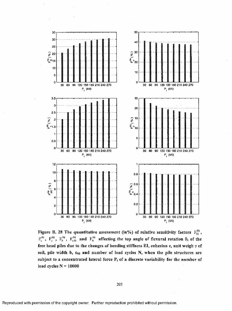
35
30
25
?20
V“1510
5
0
3.5
3
2.5
? 2 1^1.5
1
0.5
0
12
10
8
LL
4
2
0
30 60 90 120 150 180 210 240 270Pj (kN)
30 60 90 120 150 180 210 240 270P, (KN)
50
40
:; 30
1l“20
10
25
20
15
10
0.8
0.6
Q. Zu- 0.4
0.2
30 60 90 120 150 180 210 240 270 P, (KN)
30 60 90 120 150 180 210 240 270 P, (KN)
30 60 90 120 150 180 210 240 270 P, (kN)
30 60 90 120 150 180 210 240 270 P, (kN)
Figure B. 28 The quantitative assessment (in%) of relative sensitivity factors F,P0 El ’:P6
b ’ Fs50P0 affecting the top angle of flexural rotation 0t of the
free head piles due to the changes of bending stiffness El, cohesion c, unit weigh y of soil, pile width b, 850 and number of load cycles N, when the pile structures are subject to a concentrated lateral force Pt of a discrete variability for the number of load cycles N = 10000
203
Reproduced with permission of the copyright owner. Further reproduction prohibited without permission.
APPENDIX C. Typical results of the sensitivity analysis for
pile B (first trailing row) in a pile group embedded in the stiff clay
above water table, subjected to lateral concentrated force Pg
applied to the pile cap, with the piles members pinned to the pile
cap, pile spacing s= 2D, pile length L=10T= 13.7m and number of
load cycles N=1 and 10000
204
Reproduced with permission of the copyright owner. Further reproduction prohibited without permission.
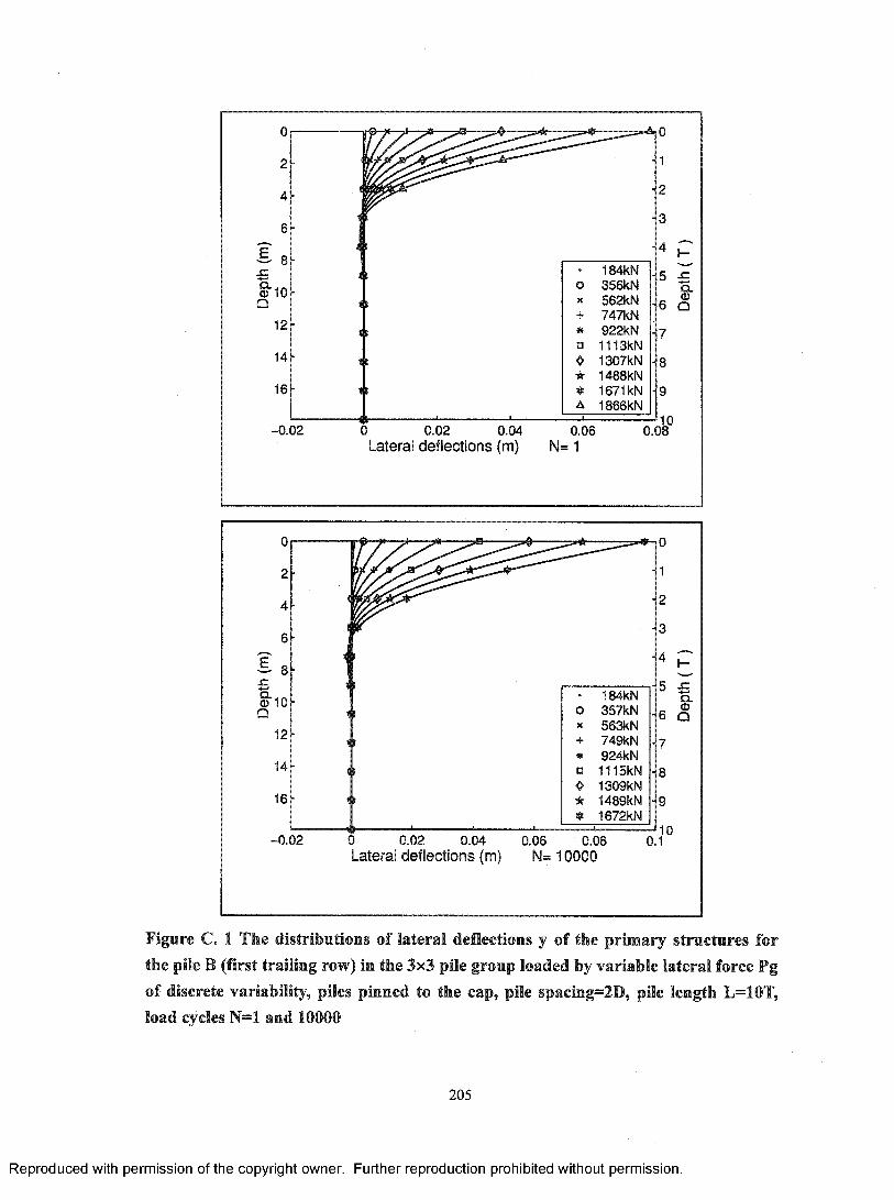
■£Q.
0
2
4
6
I 8m10Q
12
14
16
• 184KNo 356kNX 562KN+ 747KN• 922kN□ 1113kN0 1307kN★ 1488kN
1671kNA 1866kN
^ h-5 -E
6 Q
7
8
9
-0 .02 0 0 .02 0 .04 0.06Lateral deflections (m) N= 1
MO 0 .08
Z
• 184kN11 0 357kN
X 563kNr + 749kN
• 924kNt 0 1115kN
0 1309kNt ★ 1489kN
>........ 1 ■ ■—...........1____« 1672kN
0
1
2
3
h-5 ^
6 Q
7
8
9
-0 .0 2 0 0 .02 0 .04 0.06 0.08Lateral deflections (m) N= 10000
0.110
Figure C. 1 The distributions of lateral deflections y of the primary structures for the pile B (first trailing row) in the 3x3 pile group loaded by variable lateral force Pg of discrete variability, piles pinned to the cap, pile spacing=2D, pile length L=10T, load cycles N=1 and 10000
205
Reproduced with permission of the copyright owner. Further reproduction prohibited without permission.
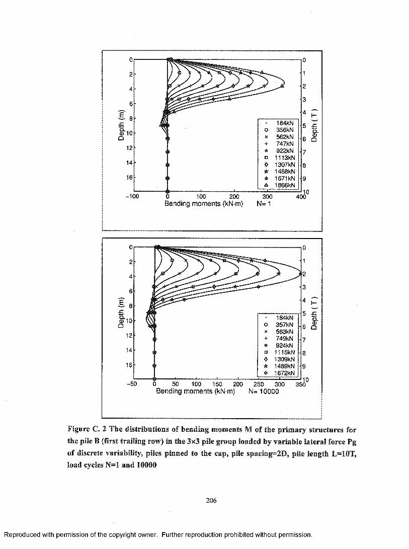
02
4
6
I 8 €o l OQ
12
14
16
0
2
4
6
I 8 £o l OQ
12
14
16
. 184KNo 356KN
562RN+ 747KN• 922KN□ 1113kN0 1307kN★ 1488kNif 1671kNA 1866kN
01
2
3
4 P5 -c
6 Q
7
8
9
-100 0 100 200 300 400Bending moments (kN-m) N= 1
• 184kNo 357kNX 563kN+ 749kN* 924kNa IIIS k N❖ 1309kN★ 1489kN
1672kN
1-
- 5 0 0 50 100 150 200 25 0 300 350Bending moments (kN-m) N= 10000
Figure C. 2 The distributions of bending moments M of the primary struetures for the pile B (first trailing row) in the 3x3 pile group loaded by variable lateral force Pg of discrete variability, piles pinned to the cap, pile spacing=2D, pile length L=10T, load cycles N=1 and 10000
206
Reproduced with permission of the copyright owner. Further reproduction prohibited without permission.

184KN 356KN 562KN 747KN 922KN
o 1113kN 0 1307kN ★ 1488kN « 1671kN A 1866kN
Q .
6 Q
0 2 4 6Lateral deflections (m) N= 1
1010X 10“
184kN357kN563kN749kN924kNIIISkN1309kN1489kN1672kN
0 2 4 6Lateral deflections (m) N= 10000 X10“
Figure C. 3 The distributions of lateral deflections y, of the adjoint structures for the pile B (first trailing row) in the 3x3 pile group loaded by variable lateral force Pgi of discrete variability, piles pinned to the cap, pile spacing=2D, pile length L=10T, load cycles N=1 and 10000
207
Reproduced with permission of the copyright owner. Further reproduction prohibited without permission.
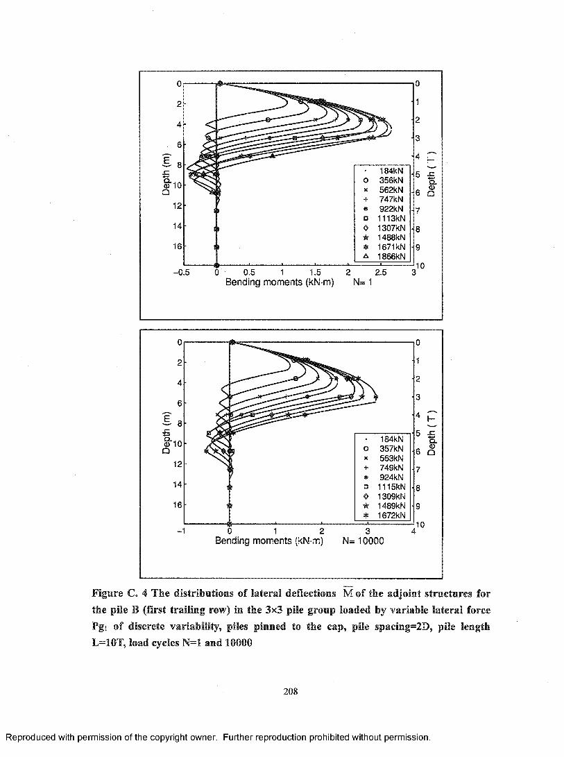
0
2
4
6
I 8£S’ 10Q
12
14
16
. 184KNo 356kNX 562kN+ 747kN• 922kN□ 1113kN<> 1307kN•A 1488kN
1671kNA 1866kN
- 0 ,5 0 0 .5 1 1.5 2 2.5Bending moments (kN-m) N= 1
01
2
3
4 P5 ^
Q .
6 Q
7
8
9
10
• 184kNo 357kNX 563kN
749kN* 924kN□ 1115kN0 1309kN★ 1489kNA 1672kN
0 1 2 Bending moments (kN-m)
0
1
2
3
h-5 -c
6 Q
7
8
9
10N = 10000
Figure C. 4 The distributions of lateral deflections M of the adjoint structures for the pile B (first trailing row) in the 3x3 pile group loaded by variable lateral force Pgi of discrete variability, piles pinned to the cap, pile spacing=2D, pile length L=10T, load cycles N=1 and 10000
208
Reproduced with permission of the copyright owner. Further reproduction prohibited without permission.
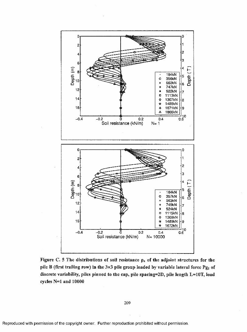
02
4
6
I 8 £o10Q
12
14
16
0
2
4
6
I 8£§■10Q
12
14
16
• 184RNo 356KNK 562RN+ 747KN• 922KN□ 1113kN0 1307RN★ 1488RN❖ 1671RNA 1866RN
- l O
• 1
■2
• 3
•4
• 5
■ 6
■ 7
■8
■9
a .s
-0 .4 -0 .2 0 0.2 0.4Soil resistance (kN/m) N= 1
100.6
ir
• 184RNO 357RNX 563RN+ 749RN* 924RN□ 1115RN0 1309RN★ 1489RN
1672RN
Q.s
-0 .4 -0 .2 0 0 .2 0.4Soil resistance (kN/m) N= 10000
o.€
Figure C. 5 The distributions of soil resistance pa of the adjoint structures for the pile B (first trailing row) in the 3x3 pile group loaded by variable lateral force Pgi of discrete variability, piles pinned to the cap, pile spacing=2D, pile length L=10T, load cycles N=1 and 10000
209
Reproduced with permission of the copyright owner. Further reproduction prohibited without permission.
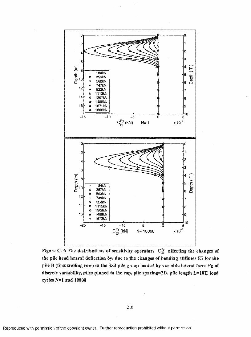
• 184KNo 356kNK 562KN+ 747KN• 922KN□ 1113kN❖ 1307kN★ 1488kN
■ A 1671kNA 1866kN
-15 -1 0
C^f(kN) N= 1
10
12
14
16
■ 184kNo 357kNX 563kN+ 749kN* 924kN
■ a IIISkN0 1309kN
■ ★ 1489kN1672kN
-20 -15 -10C^f(kN) N= 10000
0
1
2
3
4
5
6
7
8
9
10
X 10'
X 1 0 '
5,-3
0
1
2
3
4 P5 £
Q.6 Q
7
8
9
10
Figure C. 6 The distributions of sensitivity operators affecting the changes of the pile head lateral deflection 8yt due to the changes of bending stiffness El for the pile B (first trailing row) in the 3x3 pile group loaded by variable lateral force Pg of discrete variability, piles pinned to the cap, pile spacing=2D, pile length L=10T, load cycles N=1 and 10000
210
Reproduced with permission of the copyright owner. Further reproduction prohibited without permission.

8
o10Q12
14
16
oX+
□0★
A
184kN356kN562kN747kN922kN1113kN1307kN1488kN1671kN1866kN
- 0.02 -0 .015 - 0.01
cr'(kN)-0 .005
Q .
46 Q
r7
(8
Jno
N = 1
£a0)Q§■10 &
12
14
16
+
□0★
184kN357kN563kN749kN924kN1115kN1309RN1489kN1672kN
-0.025 - 0.02 -0 .015
cPy(kN)-0.01 -0 .005
N= 10000
>7
18
1Q
4no
Figure C. 7 The distributions of sensitivity operators Cf’' affecting the changes of the pile head lateral deflection 8yt due to the changes of cohesion c of the soil for the pile B (first trailing row) in the 3x3 pile group loaded by variable lateral force Pg of discrete variability, piles pinned to the c a p , pile spacing=2D, pile length L=10T, load cycles N=1 and 10000
211
Reproduced with permission of the copyright owner. Further reproduction prohibited without permission.
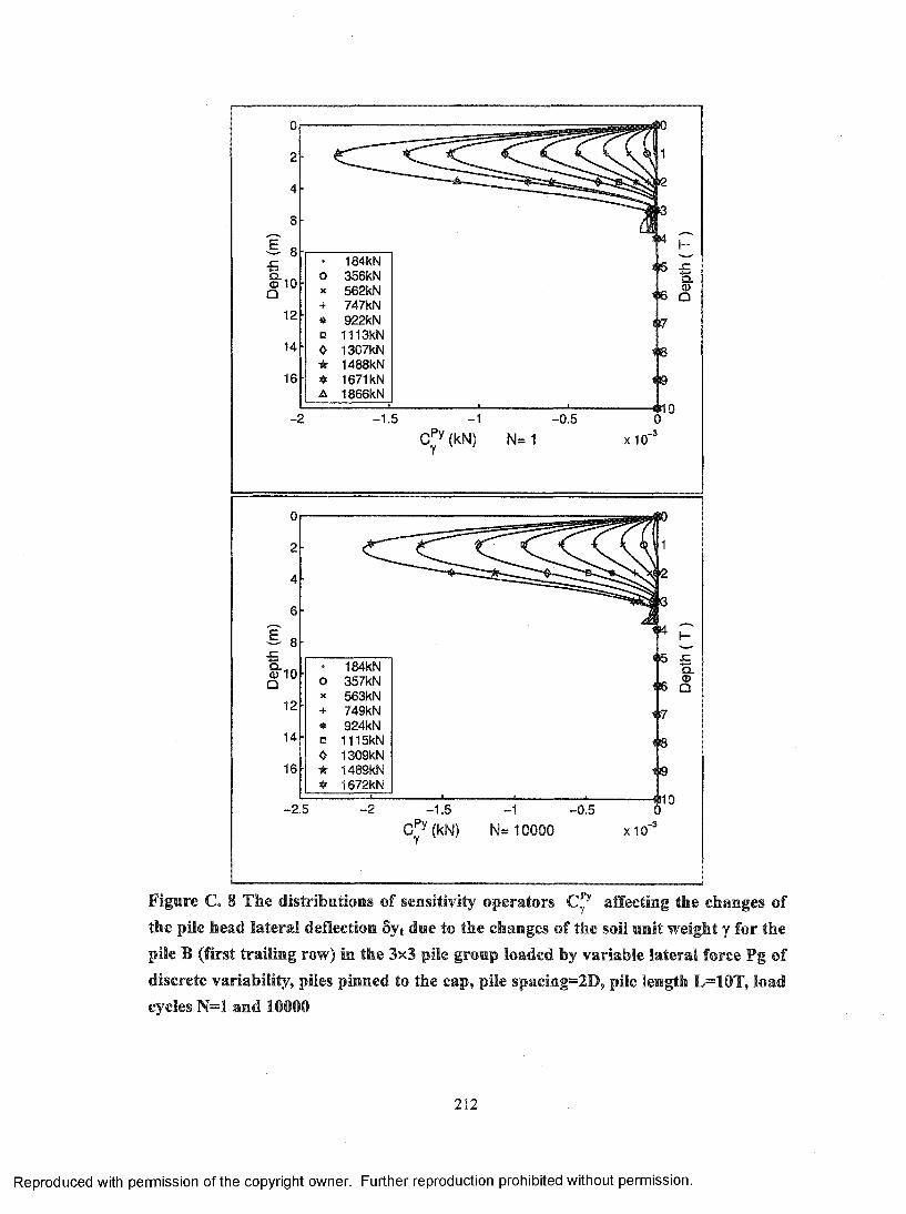
12
14
16
+
□0★
A
184KN356kN562kN747kN922kN1113kN1307kN1488kN1671kN1866kN
cPy(kN) N=1
8
§"10Q12
14
16
o+
□❖★
184kN357kN563kN749kN924kNIIISkN1309kN1489kN1672kN
-2 .5 -2 -1 .5
cPy(kN)-1 -0 .5
N= 10000
X 1 0 '
♦5 £ Q.
1 6
17
18
10
1(10
X 1 0 "
Figure C. 8 The distributions of sensitivity operators affecting the changes of the pile head lateral deflection 6yt due to the changes of the soil unit weight y for the pile B (first trailing row) in the 3x3 pile group loaded by variable lateral force Pg of discrete variability, piles pinned to the cap, pile spaeing=2D, pile length L=10T, load cycles N=1 and 10000
212
Reproduced with permission of the copyright owner. Further reproduction prohibited without permission.

8
§■10Q12
14
16
-15
• 184kNo 356KNX 562kN 11+ 747kN• 922kN (►0 IIISkN❖ 1307kN★ 1488RN« 1671kN tA 1866kN
11-10
cPy(kN) N= 1
6
I 8£§"10Q
12
14
16
-1 5
• 184kNO 357kNX 563kN+ 749kN• 924kNa 1115kN❖ 1309kN★ 1489kNV 1672kN .
-10cPy(kN)
-5 0
N= 10000
j—
X 10
5 J=
6 Q
7
8
9
10
0
1
2
3
4 P5 -c
6 Q
7
8
9
10
X 1 0 '
Figure C. 9 The distributions of sensitivity operators affecting the changes of the pile head lateral deflection 5yt due to the changes of the pile width b for the pile B (first trailing row) in the 3x3 pile group loaded by variable lateral force Pg of discrete variability, piles pinned to the cap, pile spacing=2D, pile length L=10T, load cycles N=1 and 10000
213
Reproduced with permission of the copyright owner. Further reproduction prohibited without permission.
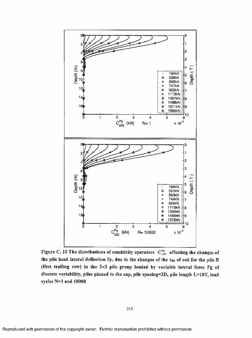
§ ■ 1Q
• 184kNo 356kN
11 * 562kN+ 747kN
i > • 922kND 1113kN
n 0 1307kN★ 1488kN
i t « 1671kN
n ■ ■ ■ ■A 1866kN
C S, (I'N)
4
N=1
- 0
■ 1
•2
■3
■4
• 5
■ 6
■ 7
•8
•9
10
X 10
6-3
I • 184kNi r O 357kN
X 563kN1 + 749kN
• 924kNi i o IIISkN
0 1309kNi t ★ 1489kN
>------------- i-------------- 1-------------- 1_________ 1____A 1672kN
2 3 4
(kN) N= 10000 X 10'
6.-3
Figure C. 10 The distributions of sensitivity operators affecting the changes of the pile head lateral deflection 5yt due to the changes of the Ss§ of soil for the pile B (first trailing ro w ) in the 3x3 pile group loaded by variable lateral force Pg of discrete variability, piles pinned to the cap, pile spacing=2D, pile length L=10T, load cycles N=1 and 10000
214
Reproduced with permission of the copyright owner. Further reproduction prohibited without permission.
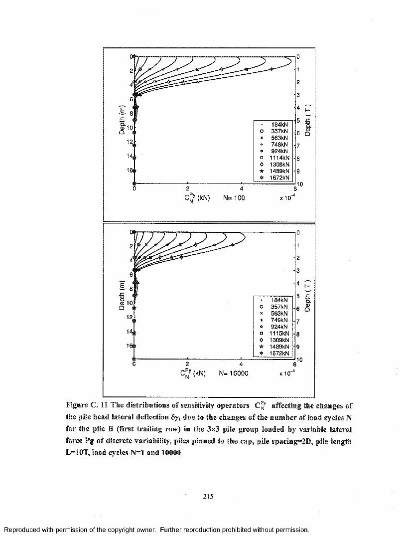
'2,
H r
i ar
• 184kNir o 357kN
X 563kNir + 748kN
* 924kNir □ 1114kN
0 1308kNir ★ 1489kN
ir1672kN
2C ( k N )
4
N= 100 X 1 0 '
oX
+
□0★
184KN357kN563KN749kN924kNIIISkN1309kN1489kN1672kN
2C ( k N ) N= 10000 x10
6-4
7
8
9
10
Figure C. 11 The distributions of sensitivity operators affecting the changes of the pile head lateral deflection 6yt due to the changes of the number of load cycles N for the pile B (first trailing row) in the 3x3 pile group loaded by variable lateral force Pg of discrete variability, piles pinned to the cap, pile spacing=2D, pile length L=10T, load cycles N=1 and 10000
215
Reproduced with permission of the copyright owner. Further reproduction prohibited without permission.
APPENDIX D. Content of the attached CD
The Matlab programs used to conduct the sensitivity analysis of laterally loaded
single piles and pile groups, the sensitivity analysis results in the digital graphical format,
and a shared program GSView used to view the sensitivity analysis results are included in
the CD (Compact Disc) attached to this study.
The Matlab programs used to conduct the sensitivity analysis are saved in the
directory “M atlab”. The files included in this directory are the Matlab source files, which
should be opened with the Matlab software and executed in the Matlab command
windows. Please refer to the manual or the help menu of the Matlab program for the
details about how to open, edit, execute and save the Matlab source files. The source files
should be executed in a certain sequence because the execution of one file might depend
on the results o f another. The execution sequences o f the source files for the sensitivity
analysis of single piles and pile groups are presented in details in CHAPTER 7 and
CHAPTER 8 respectively.
The sensitivity analysis results o f the laterally loaded single piles are saved in the
directory “\TCH”. The sensitivity analysis results for different boundary conditions, pile
lengths and load cycles are saved in different sub-directories. The structure o f the
sub-directory system used to hold the sensitivity analysis results o f the laterally loaded
piles embedded in stiff clay are presented in Figure D. 1.
The sensitivity analysis results are presented in the graphical pictures, which are
saved in the subdirectories in the Ghostscript format that has an extension name “.eps”.
The Ghostscript files can be viewed by the GSView program provided in the directory
named “\GSView”. It is needed to be installed to the computer before the GSView
program can be used. The installation can be finished simply by run both o f the
216
Reproduced with permission of the copyright owner. Further reproduction prohibited without permission.
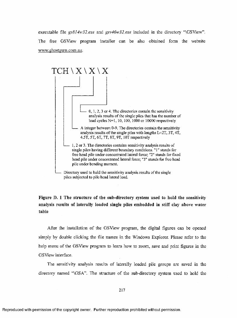
executable file gs814w32.exe and gsv46w32.exe included in the directory “\GSView”.
The free GSView program installer can be also obtained form the website
www.ghostgum.com.au.
T C H \ X \ X \ X
- 0, 1, 2, 3 or 4. The directories contain the sensitivity analysis results o f the single piles that has the number o f load cycles N = l, 10, 100,1000 or 10000 respectively
A integer between 0-9. The directories contain the sensitivity analysis results o f the single piles with lengths L=2T, 3T, 4T, 4.5T, 5T, 6T, 7T, 8T, 9T, lOT respectively
1, 2 or 3. The directories contains sensitivity analysis results o f single piles having different boundary conditions. "1" stands for free head pile under concentrated lateral force; "2" stands for fixed head pile under concentrated lateral force; "3" stands for free head pile under bending moment.
Directory used to hold the sensitivity analysis results o f the single piles subjected to pile head lateral load.
Figure D. 1 The structure of the sub-directory system used to hold the sensitivity analysis results of laterally loaded single piles embedded in stiff clay above water table
After the installation o f the GSView program, the digital figures can be opened
simply by double clicking the file names in the Windows Explorer. Please refer to the
help menu of the GSView program to learn how to zoom, save and print figures in the
GSView interface.
The sensitivity analysis results o f laterally loaded pile groups are saved in the
directory named “\GSA”. The structure of the sub-directory system used to hold the
217
Reproduced with permission of the copyright owner. Further reproduction prohibited without permission.
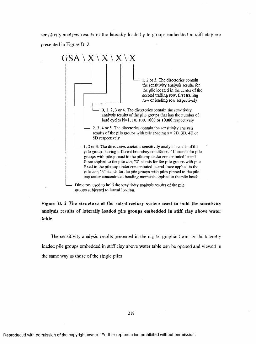
sensitivity analysis results o f the laterally loaded pile groups embedded in stiff clay are
presented in Figure D. 2.
G S A \ X \ X \ X \ X
1, 2 or 3. The directories contain the sensitivity analysis results for the pile located in the center o f the second trailing row, first trailing row or leading row respectively
- 0 , 1 , 2, 3 or 4. The directories contain the sensitivity analysis results o f the pile groups that has the number o f load cycles N = l, 10, 100, 1000 or 10000 respectively
2, 3, 4 or 5. The directories contain the sensitivity analysis results o f the pile groups with pile spacing s = 2D, 3D, 4D or 5D respectively
1, 2 or 3. The directories contains sensitivity analysis results o f the pile groups having different boundary conditions. "1" stands for pile groups with pile pinned to the pile cap under concentrated lateral force applied to the pile cap; "2" stands for the pile groups with pile fixed to the pile cap under concentrated lateral force applied to the pile cap; "3" stands for the pile groups with piles pinned to the pile cap under concentrated bending moments applied to the pile heads.
Directory used to hold the sensitivity analysis results o f the pile groups subjected to lateral loading.
Figure D. 2 The structure of the sub-directory system used to hold the sensitivity analysis results of laterally loaded pile groups embedded in stiff clay above water table
The sensitivity analysis results presented in the digital graphic form for the laterally
loaded pile groups embedded in stiff clay above water table can be opened and viewed in
the same way as those of the single piles.
218
Reproduced with permission of the copyright owner. Further reproduction prohibited without permission.

VITAAUCTORIS
Name:
Place o f birth:
Date of birth:
Education:
Lebing Liu
Yiyang, Hunan Province, P. R. China
December 21, 1974
High school of Yiyang County, Yiyang, Hunan Province, P. R. China 1990-1993
Civil and Environmental Engineering Department,Tianjin University, Tianjin, P. R. China 1993-1997
University of Windsor, Windsor, Ontario, Canada 2002-2004
219
Reproduced with permission of the copyright owner. Further reproduction prohibited without permission.