Solving Computational and Memory Requirements of Feature Based Simultaneous Localization and Map Building Algorithms

Jose Guivant and Eduardo Nebot

Australian Centre for Field Robotics Department of Mechanical and Mechatronic Engineering

The University of Sydney, NSW 2006, Australia jguivant/nebot @acfr.usyd.edu.au

Abstract

This paper presents new algorithms to implement simultaneous localisation and map building (SLAM)

in environments with very large number of features. The algorithms present an efficient solution to the

full update required by the Compressed Extended Kalman Filter algorithm (CEKF). It makes uses of

the Relative Landmark Representation (RLR) to develop very close to optimal de-correlation solutions.

With this approach the memory and computational requirements are reduced from ~O(N2) to

~O(N*Nb), being N and Nb proportional to the number of features in the map and features close to the

vehicle respectively. Experimental results are presented to verify the operation of the system when

working in large outdoor environments.

1 Introduction

Autonomous navigation in outdoor environments present significant challenges due to the lack of reli-

able sensors and perceptions algorithms to extract navigation information from unstructured environ-

ments. In [1], the problem of navigation in complex outdoor natural environments based on multi-

sensor information was introduced presenting different type of terrain representations that were used

for planning operations. New perception algorithms were also presented to facilitate the interpretation

of the sensor information [2], [3], [4]. Nevertheless the solution of “Simultaneous Localization and

Mapping” (SLAM) [7],[8] or “Concurrent Map and Localisation” (CML) [9] problem in large and to-

tally unstructured environments presents formidable problems still unresolved.

The solution of SLAM has been addressed with approaches based on Bayesian filtering [10]. These

techniques approximate the probability representation using samples of the probability density distri-

bution. Although they are still computationally expensive for real time implementation they present

significant advantages such as the inherent solution of the data association problem. There are several

optimal and sub-optimal techniques that are attractive to solve SLAM in real time [5], [7], [9], [12],

most of them based on the Extended Kalman Filter (EKF) framework, These techniques assume Gaus-

sian or at least uni-modal probability density distributions.

It is well known that one of the major problems of EKF SLAM algorithms is the computational re-

quirements that is of order ~O(N2), being N the states used to represent the landmarks and vehicle pose.

In [7], a Compressed EKF (CEKF) algorithm is presented that dramatically reduces the computational

requirements of SLAM. This algorithm is very efficient when the vehicle remains in local areas for

significant period of time or when high frequency external information is incorporated [6]. Still a full

SLAM update is required when a transition to a different area is performed. Another important imple-

mentation aspect is the memory requirement of the SLAM algorithms to store the state covariance er-

ror matrix. A system with 10000 states will require up to 800 MB of RAM to maintain this matrix.

Both memory and global update calculation have a cost of order ~O(N2) as stated before. When using

the CEKF the cost in the global update evaluation is not critical provided the transitions between local

areas are not frequent but the memory requirements remain similar to the full SLAM implementation.

This is due to the need of maintaining cross-covariance terms between all the states that have to be pre-

served. This implies that the complete covariance matrix has to be maintained in fast processing mem-

ory (RAM). We argue that the maintenance of the complete covariance matrix is important in cases

where the cross-correlation between states is strong or at least not negligible. Any attempt to conserva-

tively de-correlate a subset of states implies an increase in the value of some diagonal sub-matrixes. If

subsets of lightly correlated states are present then de-correlation of these states can be done with a

small loss in the predicted estimation quality. This paper makes use of RLR (Relative Landmark Rep-

resentation) to generate close to optimal results that will significantly reduce the computational and

memory requirement of SLAM when working in large environments.

This work is organized as follows. Section 2 presents a brief introduction to the CEKF filter. The de-

correlation algorithm is presented in section 3 and the integration with the CEKF in SLAM applica-

tions is described in section 4. Finally experimental results are presented in section 5 with conclusions

given in section 6.

1. Optimal Compressed Extended Kalman Filter (CEKF).

This section presents a brief summary of the CEKF algorithm. A full description is presented in [7].

Assume that for a period of time 1 2/k k k kW = £ £ , the model and observations of the system can be

expressed in the following form:

( )( )

( ) ( )( ) ( )( ) ( )

( ) ( )( ) ( )( )

, , ,

, ,1

1

,

, , /

a ba N Na b

b

a a aa

b b b

a h

XX X R X R

X

f X k u k k kX k

X k X k k

y k h X k k k

X u k k

nn

n

È ˘= Œ ŒÍ ˙Î ˚

È ˘+È ˘+= Í ˙Í ˙+ +Í ˙Î ˚ Î ˚= +

" ŒW (1)

Where Xa and Xb are active and passive states respectively and the model and observation noises

( ) ( ) ( ), ,a b hk k kn n n are Gaussian and uncorrelated. In this system the observations during the interval

Ω are only function of the states Xa. In this case the states Xa can be estimated in a very efficient form

using the CEKF algorithm as shown bellow. At the beginning of the periodW , k = k1, a set of auxiliary

matrices are initialized:

( )1 1 1 1

*,, 0, 0, 0

, ,a a a

k k k bb k

N xN Nk k k

I Q

R R

f y q

f y q

= = = =

ΠΠ(2)

At every prediction or update stage, during the time period W , a normal EKF algorithm is run with the

subsystem Paa, Xa., where Paa is the covariance matrix error for the states Xa. An additional set of ma-

trices is maintained to store the information gathered to be transfered to the rest of the system when the

full update stage is executed. During the period 1 2k k k£ £ the prediction step is implemented using the

standard EKF prediction for the sub-system Paa, Xa and the update of the auxiliary matrices:

)1 1 1

* *, ,( 1) ,

, ,k aa k k k k k

Aaa

A

bb k bb k bb k

J

fJ X

Q Q Q

f f y y q q- - -

-

= ◊ = =∂Ê = ∂Ë

= +

(3)

A new observation is processed with a standard EKF update equations for the sub-system Paa, Xa and the update of the auxiliary matrices as follows:

( ),

11, ,

1 1 1

,

11 2 , 1 1 1

a ka

k k k Tk a k k a kT

k k k k k

k aa k k

T Tk k k a k k k

hH XI

H S H

P

H S z

f m fb

y y f b fm b

q q f

--

- - -

-- - - - -

∂Ï = ∂Ô= - ◊ Ô = ◊ ◊Ì= + ◊ ◊ Ô = ◊ÔÓ

= + ◊ ◊ ◊

(4)

At the end of the intervalW , k = k2, the update of all the states in the system and covariance matrix is performed. This step is called global or full update:

( ) ( ) ( )

( ) ( ) ( ) ( ) ( )

( ) ( ) ( )

2 2 1

22 1 1 2 1

22 1 1

, ,

*,, , , ,

, , ,

ab k k ab k

bb kbb k bb k ba k k ab k

kb k b k ba k

P P

P P P P Q

X X P

f

y

q

= ◊

= - ◊ ◊ +

= - ◊

(5)

It can be seen that the knowledge of ( ) ( ) ( ) ( ), , ,b bb ab baX k P k P k P k is only explicit at times k = k1 and k

= k2. No explicit information about this family of states and their related covariance and cross-

covariance matrices is required at times k / k1 < k < k2. This information is implicitly contained (at any

instant k) in the matrixes , ,k k kf y q . The matrices ,k kf y have dimensions Na * Na and the vector kq is of

order Na. All the information (covariance and cross-covariance values) related to the states Xb(k) re-

mains compressed in these three auxiliary matrices. It is important to note that the CEKF estimation is

optimal and generates the same results as the full EKF algorithm. Although these results are used here

in a SLAM application the CEKF algorithm can be applied to any system where the observations re-

main function of a set of states for a period of time as shown in equation (1).

2 De-correlation algorithm

The maintenance of the complete covariance matrix is essential in cases where the cross-correlation

between states is strong or at least not negligible. Any attempt to conservatively de-correlate a subset

of states implies an increase in the value of some diagonal sub-matrixes. If subsets of weakly corre-

lated states are present then de-correlation of these states can be done with a small loss in the predicted

estimated quality. Unfortunately when a map represents the landmarks in absolute form with respect to

a single global frame, all the states are or tend to be strongly correlated. In this case most of the state’s

high correlation coefficients are due to the map representation and not due to map estimation problem

itself. This correlation is important when a conservative de-correlation procedure is desired.

An appropriate map representation that avoids this problem is the Relative Landmark Representation

(RLR). This representation divides the map into sub-regions where the landmarks are defined respect

to local coordinate frames [15]. For the 2-D case each local frame is defined based on two local land-

marks represented in global coordinates. The high correlation characteristic persists but only between

the frame base landmarks and the vehicle states. These landmarks represent a small subset of the total

landmark population.

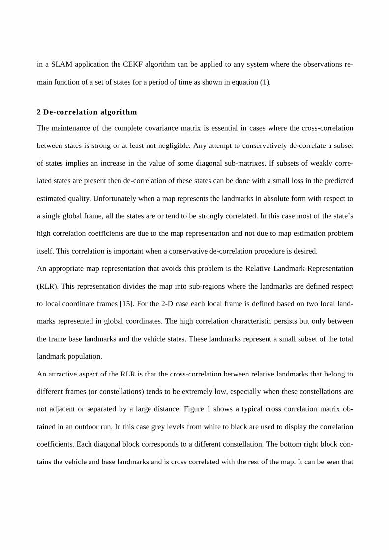
An attractive aspect of the RLR is that the cross-correlation between relative landmarks that belong to

different frames (or constellations) tends to be extremely low, especially when these constellations are

not adjacent or separated by a large distance. Figure 1 shows a typical cross correlation matrix ob-

tained in an outdoor run. In this case grey levels from white to black are used to display the correlation

coefficients. Each diagonal block corresponds to a different constellation. The bottom right block con-

tains the vehicle and base landmarks and is cross correlated with the rest of the map. It can be seen that

the cross-correlation terms between adjacent constellations are very weak and almost non-existent for

distant constellation.

covariance coefficients (states ordered by constellation)

states

stat

es

20 40 60 80 100 120 140 160 180 200 220

20

40

60

80

100

120

140

160

180

200

220

Figure 1 Correlation coefficients using a Relative Landmark Representation (RLR). The bottom right block has the vehicle state and all the absolute base landmarks. The other blocks have the relative states in each constellation.

Cross-correlation is significant between the absolute states and the relative states and between relative states in the same constellation.

Although the off-diagonal terms are very close to zero they can not be eliminated without any modifi-

cation of the diagonal blocks. Depending on the number of blocks a de-correlation approach can be

designed by multiplying the diagonal terms by a factor greater than two. As will be seen later in this

paper this approach will generate unnecessarily conservative results.

The previous discussion suggests that a much less conservative approach can be designed based on the

off-diagonal terms. This approach will be very close to optimal since these terms are very close to zero

making the increment of the diagonal terms very small as shown later in this section.

The algorithm to cancel the weakly cross-correlation terms in a consistent manner is now presented.

Given a symmetric nonnegative definite matrix 2 20, xP P R≥ Œ , it is possible to obtain a de-

correlated (diagonal) matrix D P≥ according to:

11 12

21 22

11 12 12 12

12 1222 12

11 12

1222

0

0

0

0

0

p pP

p p

p p p p

p pp p

p p

D Dpp

k k

k kk

tk

k

È ˘= =Í ˙Î ˚

È ˘ È ˘+ ◊ ◊ -Í ˙ Í ˙= - =Í ˙ Í ˙+ -Í ˙ Í ˙Î ˚ Î ˚

È ˘+ ◊Í ˙= - £ =Í ˙+Í ˙Î ˚

" >

(6)

This is true since t is a nonnegative definite matrix:

12 12

12 12

0 01

p p

p p

kt k

k

È ˘◊ -Í ˙= ≥ " >Í ˙- ◊Í ˙Î ˚

(7)

It is always possible to de-correlate the covariance matrices corresponding to two groups of states α and β using a similar technique. Assuming a generic block matrix P represented as follow:

11 1

1

, , , ,...

.. ..

.. .. .. ..

.. .. .. ..

.. ..

T

T T

n x n m xm l xl n xm

m

n nm

C D

P C E

D E

R R R C R

c c

C

c c

ab

ga b g

È ˘Í ˙= Í ˙Í ˙Î ˚

Œ Œ Œ Œ

È ˘Í ˙Í ˙=Í ˙Í ˙Í ˙Î ˚

(8)

It can be partially de-correlated as

00

00

0 0

0 0

, / 0

0

0

T T

T

T

T

T T T T

CC

C C

C

C

C

C

DC D

P C E E

D E D E

% %

% %

% % %

% % %

%%%

%

%

%

a aa ab b bb

a a a a ab b b b b

aa b

b

a aab b b

g g

È ˘ -È ˘ È ˘È ˘Í ˙= - + =Í ˙ Í ˙Í ˙ -Í ˙Î ˚ Î ˚ Î ˚Î ˚

+ - +È ˘ È ˘ È ˘= - £Í ˙ Í ˙ Í ˙

+ - +Î ˚ Î ˚ Î ˚-È ˘

≥Í ˙-Î ˚fl

È ˘+È ˘ Í ˙Í ˙ Í ˙= £ +Í ˙ Í ˙Í ˙Î ˚ Í ˙Î ˚

(9)

The matrix P will be nonnegative definite if the matrices a% and b% are formed with the following ex-

pressions:

, ,1,

, , ,1 1 ,,

,

,/

0 ,

1,

/

0 ,

0 ,

m

i k i kki j

n n

i k i k k ik k k ii j

i k

c i j

i j

c c i j

i j

i k

ka a

kkb b

k

=

= =

Ï◊ =Ô= Ì

Ô πÓÏ

◊ = ◊ =Ô= ÌÔ πÓ

> "

Â

 Â

% %

% %% % (10)

Equation 10 guarantees that the matrix P will be, at least, nonnegative definite.

Selecting , , 1i k k ik k= =% the coefficients α and β becomes:

, , , ,1 1

,m n

i i i k j j k jk k

c ca b= =

= =Â Â%% (11)

A less conservative selection of the family ,i kk can be done considering the cross-correlations coef-

ficients:

, ,,

, , ,

, ,,

, , , ,

1

i i i ii k

k k i i k k

k k k kk i

i k i i i i k k

a ak

b a b

b bk

k a a b

= =◊

= = =◊

%

(12)

Then α and β are evaluated:

, , , , ,1 1 , ,

,, , , ,

1 1 , ,

, ,1 , ,

1

1

m m

i i i k i k i i i kk k i i k k

n nj j

j j j k j k k jk k k k j j

n

j j k jk k k j j

c c

c c

c

a k aa bb

b ka b

ba b

= =

= =

=

= ◊ = ◊ ◊◊

= ◊ = ◊ =◊

= ◊ ◊◊

 Â

 Â

Â

%

% %% (13)

Finally the diagonal coefficients are updated:

, , , ,1

, , , ,1

1

1

m

i i i i i i i kk

n

i i i i i i k ik

a a a m

b b b m

=

=

Ê ˆ+ = ◊ +Á ˜Ë ¯

Ê ˆ+ = ◊ +Á ˜Ë ¯

Â

Â

%

% (14)

with ,,

, ,

i ki k

i i k k

c

a bm =

◊ (15)

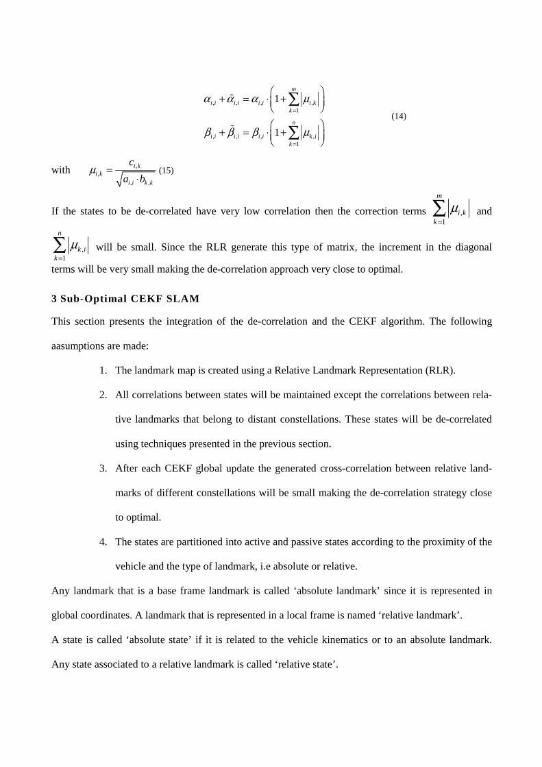
If the states to be de-correlated have very low correlation then the correction terms ,1

m

i kk

m=Â and

,1

n

k ik

m=Â will be small. Since the RLR generate this type of matrix, the increment in the diagonal

terms will be very small making the de-correlation approach very close to optimal.

3 Sub-Optimal CEKF SLAM

This section presents the integration of the de-correlation and the CEKF algorithm. The following

aasumptions are made:

1. The landmark map is created using a Relative Landmark Representation (RLR).

2. All correlations between states will be maintained except the correlations between rela-

tive landmarks that belong to distant constellations. These states will be de-correlated

using techniques presented in the previous section.

3. After each CEKF global update the generated cross-correlation between relative land-

marks of different constellations will be small making the de-correlation strategy close

to optimal.

4. The states are partitioned into active and passive states according to the proximity of the

vehicle and the type of landmark, i.e absolute or relative.

Any landmark that is a base frame landmark is called ‘absolute landmark’ since it is represented in

global coordinates. A landmark that is represented in a local frame is named ‘relative landmark’.

A state is called ‘absolute state’ if it is related to the vehicle kinematics or to an absolute landmark.

Any state associated to a relative landmark is called ‘relative state’.

The assumptions (1) and (3) are strictly related. If the RLR map representation is used then the correla-

tion between the states representing the relative landmarks that belong to different constellations tends

to be very small. Conversely, the correlation between absolute states tends to be strong especially be-

tween states representing close absolute landmarks. It is then possible to design an algorithm to pre-

serve the cross-correlation of any absolute state with any other state (relative or absolute) and to ignore

(de-correlate) any cross-correlation between two relative states associated to two relative landmarks

that belong to different constellations (defined in different local frames). The approach proposed also

preserves the cross-correlation terms between relative landmarks of the same constellation (or close

constellations).

A normal EKF full SLAM performing this de-correlation in each update will result in excessively con-

servative results since over-bounding will be required in each update to de-correlate. Conversely, a

CEKF will only require the full update after many local updates rendering in a less conservative over-

bounding strategy. In the CEKF algorithm a global update is required only when the vehicle abandons

a sub-region.

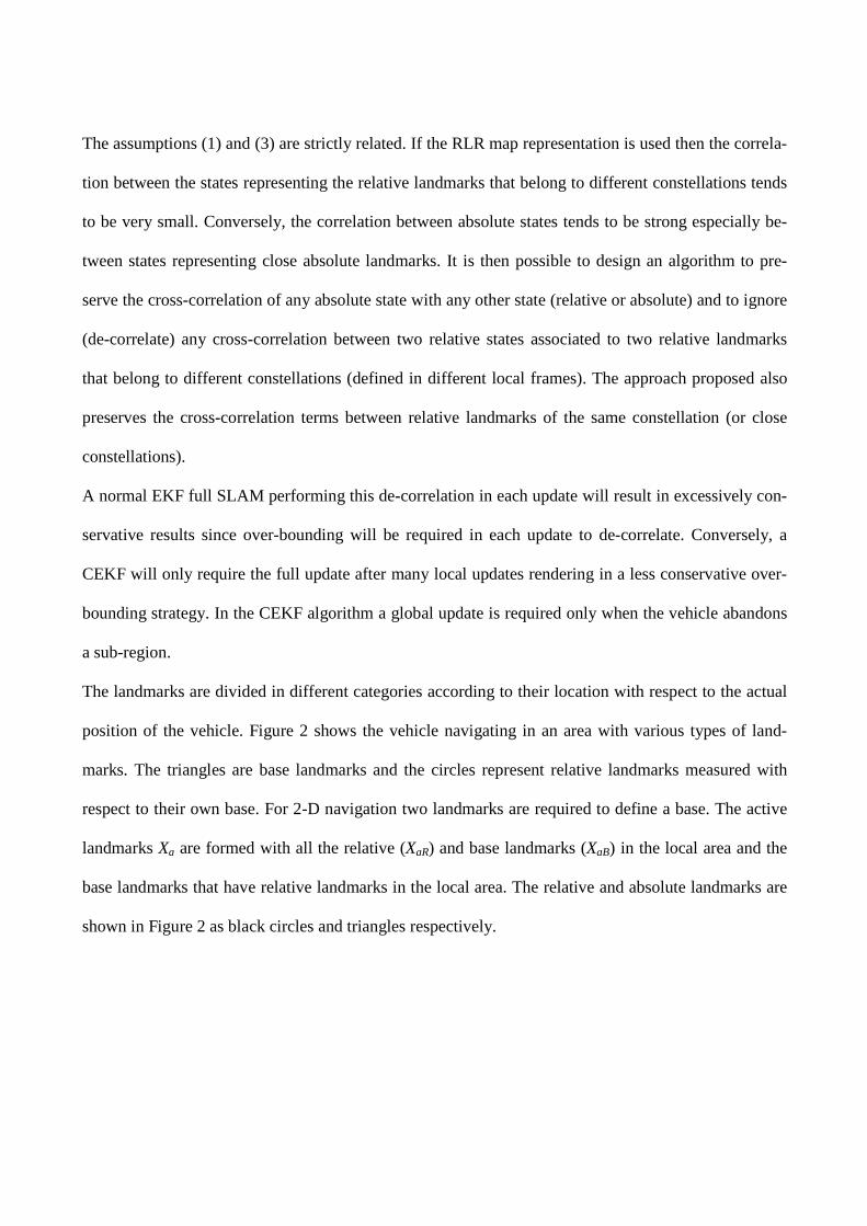
The landmarks are divided in different categories according to their location with respect to the actual

position of the vehicle. Figure 2 shows the vehicle navigating in an area with various types of land-

marks. The triangles are base landmarks and the circles represent relative landmarks measured with

respect to their own base. For 2-D navigation two landmarks are required to define a base. The active

landmarks Xa are formed with all the relative (XaR) and base landmarks (XaB) in the local area and the

base landmarks that have relative landmarks in the local area. The relative and absolute landmarks are

shown in Figure 2 as black circles and triangles respectively.

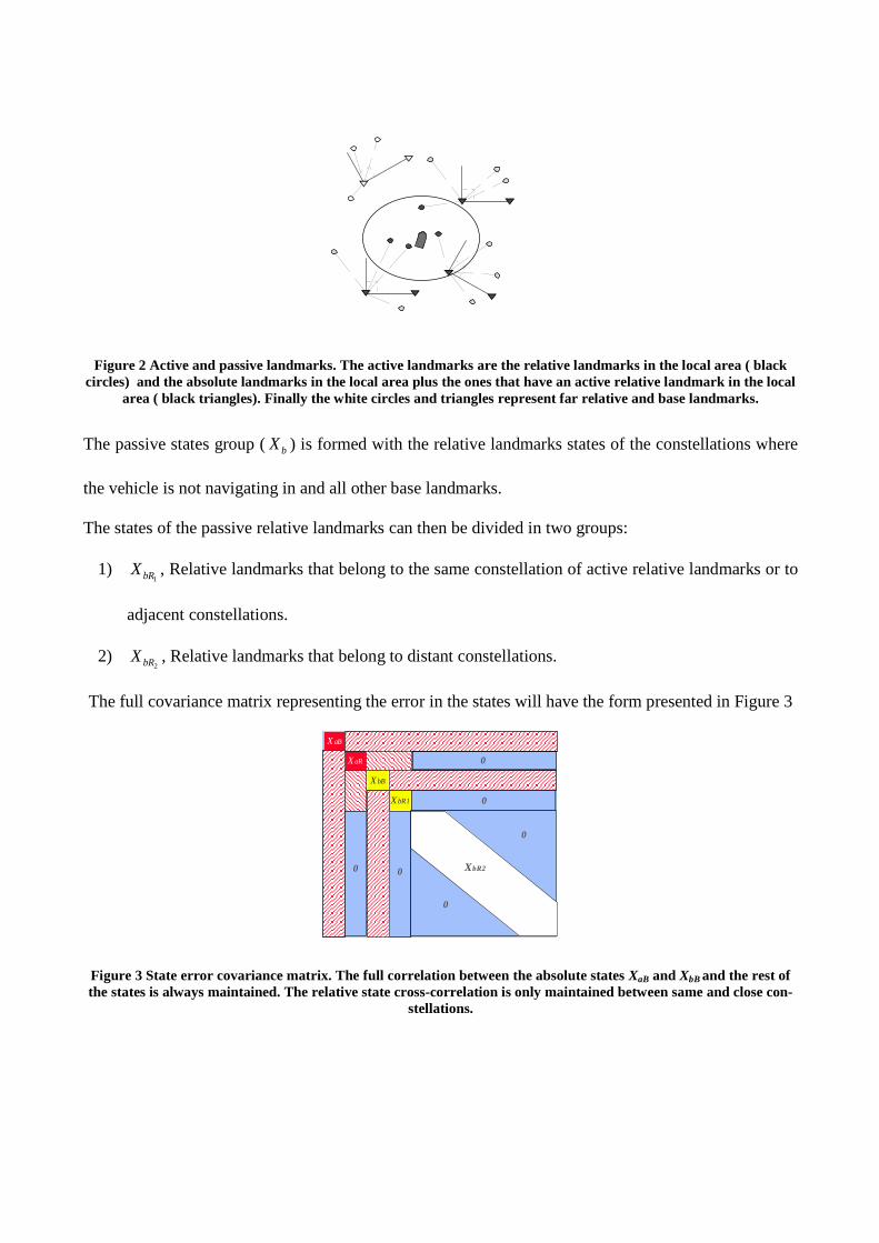
Figure 2 Active and passive landmarks. The active landmarks are the relative landmarks in the local area ( black circles) and the absolute landmarks in the local area plus the ones that have an active relative landmark in the local

area ( black triangles). Finally the white circles and triangles represent far relative and base landmarks.

The passive states group ( bX ) is formed with the relative landmarks states of the constellations where

the vehicle is not navigating in and all other base landmarks.

The states of the passive relative landmarks can then be divided in two groups:

1) 1bRX , Relative landmarks that belong to the same constellation of active relative landmarks or to

adjacent constellations.

2) 2bRX , Relative landmarks that belong to distant constellations.

The full covariance matrix representing the error in the states will have the form presented in Figure 3

State Covariance

Matrix

XaB

XaR

XaB

XaR

XbB

XbR1

XbB

XbR1

C C

C

C

C C

C

C

0

0

XbR200

0

0

00

0

0

Figure 3 State error covariance matrix. The full correlation between the absolute states XaB and XbB and the rest of the states is always maintained. The relative state cross-correlation is only maintained between same and close con-

stellations.

The cross-correlations between states 1bRX with

2bRX and aRX with 2bRX are set to zero with appropri-

ate modification of the terms in 1bRX and aRX according to the de-correlation procedures presented in

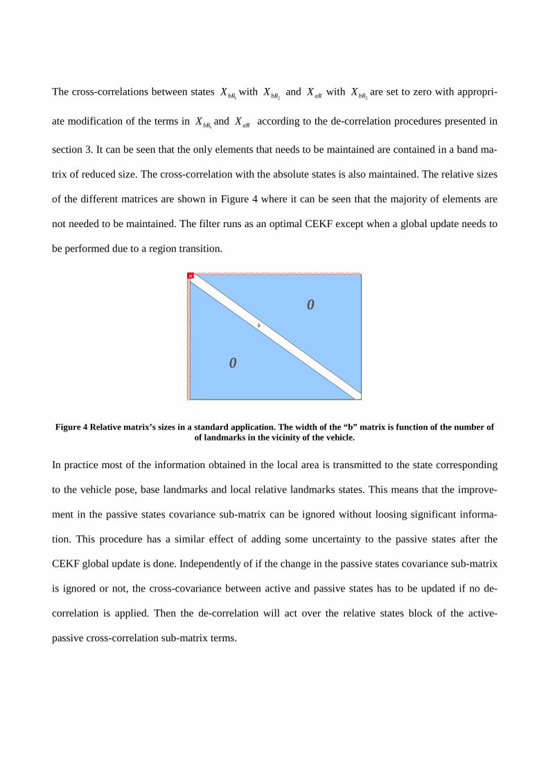
section 3. It can be seen that the only elements that needs to be maintained are contained in a band ma-

trix of reduced size. The cross-correlation with the absolute states is also maintained. The relative sizes

of the different matrices are shown in Figure 4 where it can be seen that the majority of elements are

not needed to be maintained. The filter runs as an optimal CEKF except when a global update needs to

be performed due to a region transition.

a

b

0

0

Figure 4 Relative matrix’s sizes in a standard application. The width of the “b” matrix is function of the number of of landmarks in the vicinity of the vehicle.

In practice most of the information obtained in the local area is transmitted to the state corresponding

to the vehicle pose, base landmarks and local relative landmarks states. This means that the improve-

ment in the passive states covariance sub-matrix can be ignored without loosing significant informa-

tion. This procedure has a similar effect of adding some uncertainty to the passive states after the

CEKF global update is done. Independently of if the change in the passive states covariance sub-matrix

is ignored or not, the cross-covariance between active and passive states has to be updated if no de-

correlation is applied. Then the de-correlation will act over the relative states block of the active-

passive cross-correlation sub-matrix terms.

With this approach the memory and computation requirements will be ~O(N*Nb), assuming a constant

number of landmarks Nb is used. Since Nb is << N the computation and memory requirements of the

algorithm are dramatically reduced.

The implementation of the strategy proceeds as follows: The complete optimal global update of the

passive states is done after r CEKF internal steps:

( ) ( ) ( )

( ) ( ) ( ) ( ) ( )

( ) ( ) ( )

2 2 1

2 1 1 2 1

22 1 1

2 1

, ,

, , , ,

, , ,

ab k k ab k

bb k bb k ba k k ab k

kb k b k ba k

k k r

P P

P P P P

X X P

f

y

q

= += ◊

= - ◊ ◊

= - ◊

(16)

With the sub-optimal CEKF approach most of the improvement of bbP is ignored. The CEKF auxiliary

matrixy is still needed to evaluate the part of Pbb not ignored. The objective is to transfer the new in-

formation to the states representing the vehicle pose, absolute landmarks and local relative landmarks,

ignoring completely the covariance changes in the non-local relative landmarks states. From the view-

point of the non-local relative landmarks, no change in their quality is obtained.

In practical SLAM applications it can be observed that the cross-correlation factors between relative

landmarks of different constellations have values of order 10-4 or smaller. This value becomes much

smaller for distant constellations. This characteristic makes the conservative de-correlation close to op-

timal since very small virtual noise has to be added to the relative landmarks covariances to obtain the

de-correlated matrix bounds.

A less aggressive de-correlation strategy can be implemented by accepting the existence of cross-

correlation between relative landmarks of different constellations provided that these constellations are

geographically close. Then de-correlation is implemented only between distant constellations. This

will increase the width of the band matrix in Figure 4 . In the particular case when a cross-correlation

factor is not small enough one of the involved states can be degraded to quality zero.

A final comment on the consistency of the method is noteworthy. It is well known that any Kalman

Filter based system is prone to catastrophic failures under a data association problem. This could be

due to failure in the feature extraction algorithm, or in the observation or prediction models. Under this

situation it is very difficult to guarantee the consistency of the algorithm. These types of problems are

common in difficult environments such as underwater [9],[14], where vehicle, models and sensor in-

formation have significant uncertainty. In many other applications, such as the ones related to land ve-

hicles, it is possible to have combinations of vehicle models and sensors to provide the level of integ-

rity required to detect any possible data association problem if ever occurs. In such cases the EKF be-

come the most efficient tool to solve the SLAM problem. This work presents consistent and close to

optimal solutions that are applicable to these common types of applications.

4 Results

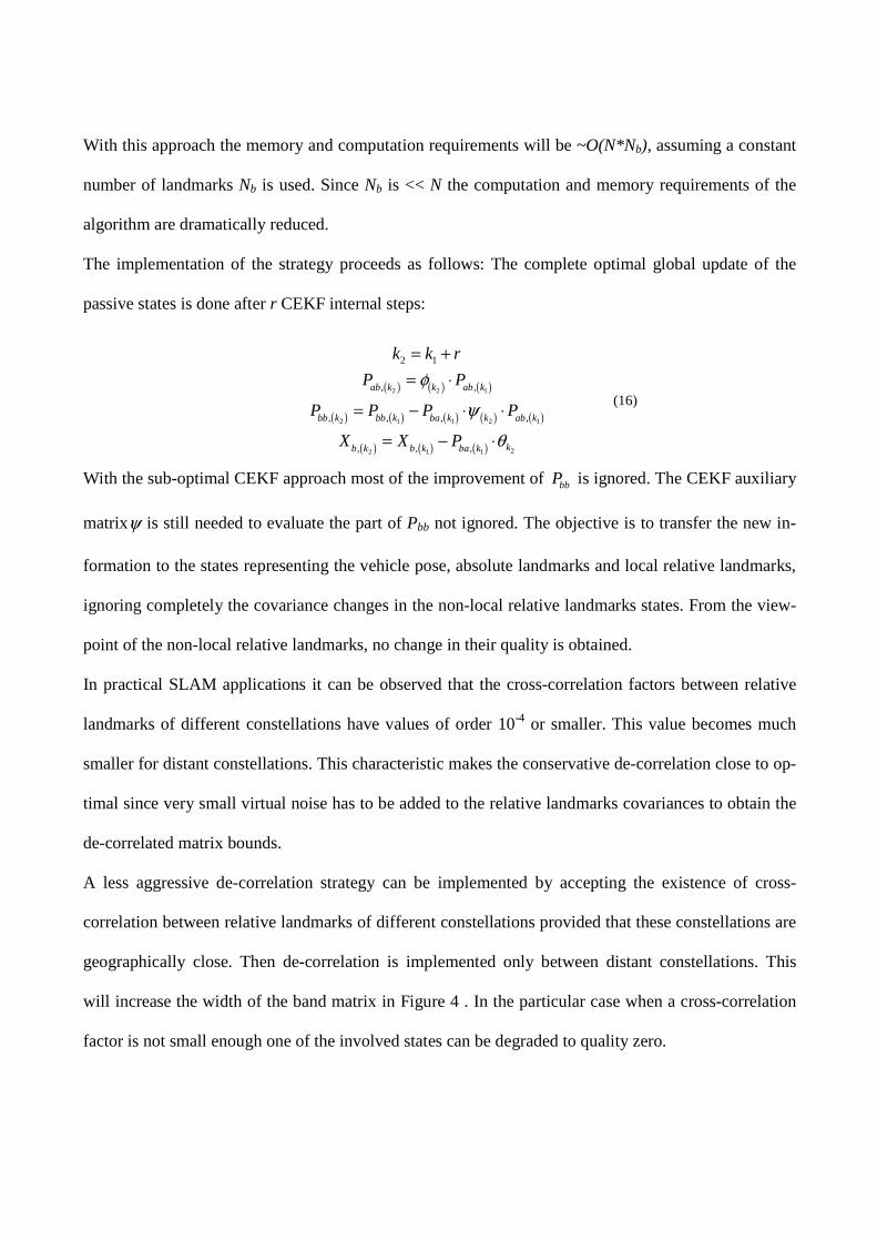
The algorithm was implemented using a data set logged with the utility vehicle shown in Figure 5. The

vehicle is retrofitted with velocity and steering encoders, two lasers range sensors and GPS. A Com-

pass sensor was not used since the density of landmark in the environment was enough to maintain low

heading errors. The GPS is used to obtain ground truth. The vehicle operated in a large outdoor un-

structured environment similar to the one shown in Figure 5.

Figure 5. Utility vehicle and outdoor environment. The vehicle is equipped with laser range sensors, steering and velocity encoders.

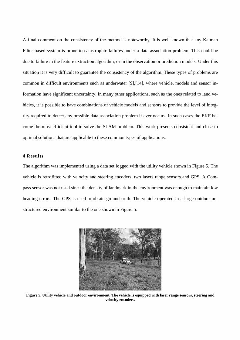
The final trajectory and map using the Full SLAM and the sub-optimal CEKF are superimposed in

Figure 6. In this case an aggressive de-correlation policy was used. The filter conservatively ignores

the cross-correlation between relative states that belong to different constellations. In this case a band

matrix of approximate size of N*Na will be maintained. Na is the maximum number of landmarks in a

local area. For this particular case the covariance matrix has a total size of approximately 250000 ele-

ments. With the algorithm proposed the memory required is less than 15000 elements. A less conserva-

tive approach will consider more than one consecutive constellation to maintain the cross-correlation

between relative landmarks of adjacent constellations. This will require additional memory to maintain

the relevant coefficients but will still will be significant smaller that maintaining the full covariance

matrix. For larger system the improvement will be more significant.

−150 −100 −50 0 50 100 150−100

−50

0

50

100

150

200

250Map and Path

longitude (metres)

lati

tud

e (m

etre

s)

Figure 6. Final Trajectory and Map. The figure presents the superposition of the final trajectory generated by the full EKF and the CEKF with the de-correlation techniques presented in this paper. All the landmarks that belong to a constellation are joined with lines to a base. Although an aggressive de-correlation was utilized (elimination of

cross-correlations of adjacent constellation) the difference with the full EKF is not noticeable using this scale.

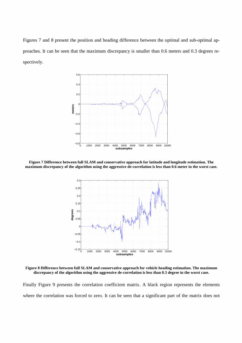
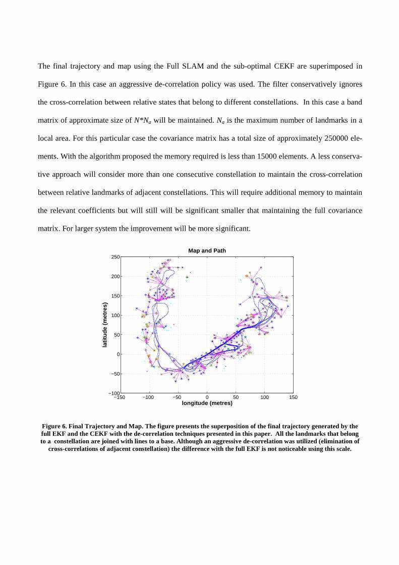
Figures 7 and 8 present the position and heading difference between the optimal and sub-optimal ap-

proaches. It can be seen that the maximum discrepancy is smaller than 0.6 meters and 0.3 degrees re-

spectively.

0 1000 2000 3000 4000 5000 6000 7000 8000 9000 10000−0.8

−0.6

−0.4

−0.2

0

0.2

0.4

0.6

subsamples

met

ers

Figure 7 Difference between full SLAM and conservative approach for latitude and longitude estimation. The maximum discrepancy of the algorithm using the aggressive de-correlation is less than 0.6 meter in the worst case.

0 1000 2000 3000 4000 5000 6000 7000 8000 9000 10000−0.15

−0.1

−0.05

0

0.05

0.1

0.15

0.2

0.25

0.3

subsamples

deg

rees

Figure 8 Difference between full SLAM and conservative approach for vehicle heading estimation. The maximum discrepancy of the algorithm using the aggressive de-correlation is less than 0.3 degree in the worst case.

Finally Figure 9 presents the correlation coefficient matrix. A black region represents the elements

where the correlation was forced to zero. It can be seen that a significant part of the matrix does not

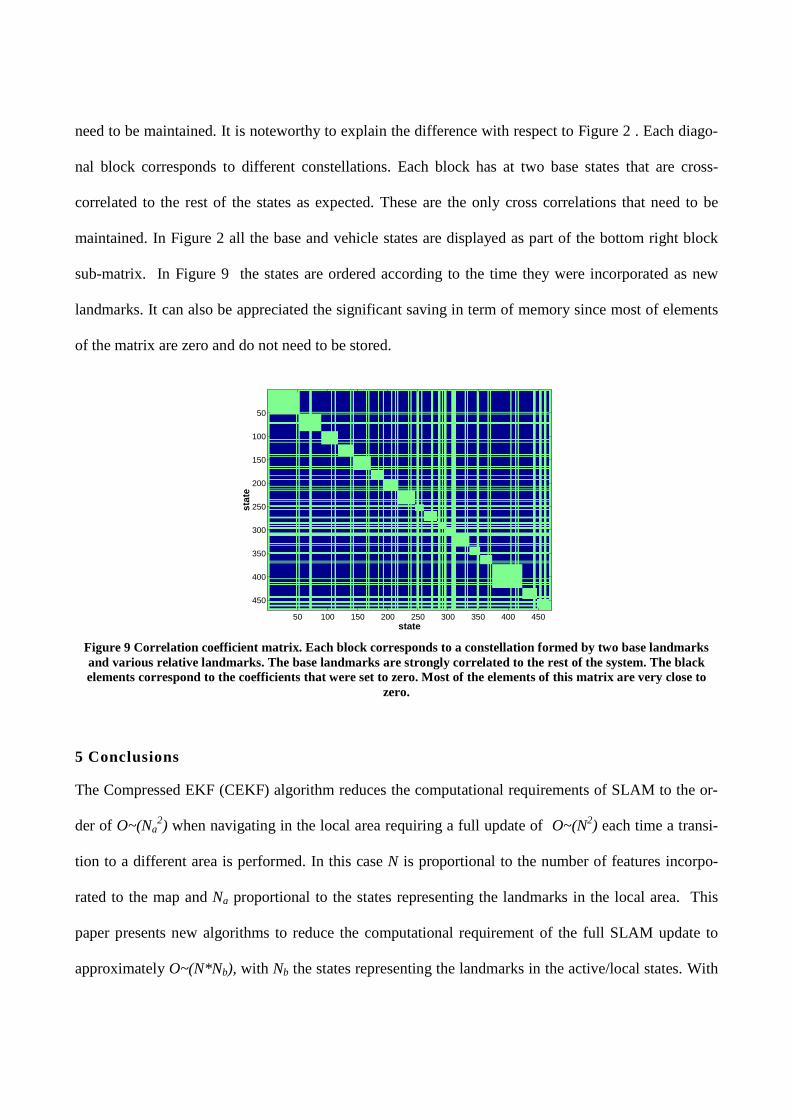
need to be maintained. It is noteworthy to explain the difference with respect to Figure 2 . Each diago-

nal block corresponds to different constellations. Each block has at two base states that are cross-

correlated to the rest of the states as expected. These are the only cross correlations that need to be

maintained. In Figure 2 all the base and vehicle states are displayed as part of the bottom right block

sub-matrix. In Figure 9 the states are ordered according to the time they were incorporated as new

landmarks. It can also be appreciated the significant saving in term of memory since most of elements

of the matrix are zero and do not need to be stored.

state

stat

e

50 100 150 200 250 300 350 400 450

50

100

150

200

250

300

350

400

450

Figure 9 Correlation coefficient matrix. Each block corresponds to a constellation formed by two base landmarks and various relative landmarks. The base landmarks are strongly correlated to the rest of the system. The black elements correspond to the coefficients that were set to zero. Most of the elements of this matrix are very close to

zero.

5 Conclusions

The Compressed EKF (CEKF) algorithm reduces the computational requirements of SLAM to the or-

der of O~(Na2) when navigating in the local area requiring a full update of O~(N2) each time a transi-

tion to a different area is performed. In this case N is proportional to the number of features incorpo-

rated to the map and Na proportional to the states representing the landmarks in the local area. This

paper presents new algorithms to reduce the computational requirement of the full SLAM update to

approximately O~(N*Nb), with Nb the states representing the landmarks in the active/local states. With

this implementation the memory requirements are also reduced to order N*Nb. Since Nb is << N the

computation and memory requirements of the algorithm are dramatically reduced. The experimental

results have also demonstrated that by using the appropriate map representation the results obtained are

very close to optimal as expected from the derivation presented in section 3.

6 References

[1] R. Chatila, “Autonomous Navigation in Natural Environments”, Robotics and Autonomous Sys-

tems, 16(2-4) (1995) pp.197-211.

[2] Y. Takeuchi and M. Hebert, "Finding Images of Landmarks in Video Sequences," Proceedings of

the IEEE Conference on Computer Vision and Pattern Recognition (CVPR '98), June, 1998.

[3] J Leonard, P. Neuman, R. Rikoski, “Towards Robust Data Association and Feature Modelling for

Condurrent Mapping and Localization”, ISRR, Lorne, Australia, November 2001.

[4] C.-C. Wang and C. Thorpe, "Simultaneous Localization and Mapping with Detection and Track-

ing of Moving Objects", Submitted to IEEE ICRA '02, 2002 , pp 2918-2923.

[5] S. Julier AND J. Uhlmann, “Building a Million Beacon Map”, Sensor Fision and Decentralized

Control in Robotic System. Proceeding of SPIE, 2001, pp 10-21.

[6] A. Davidson, “Mobile Robot Navigation Using Active Vision”, PhD Thesis, University of Oxford,

1999.

[7] J. Guivant and E. Nebot, “Optimization of the Simultaneous Localization and Map-Building Al-

gorithm for Real-Time Implementation”, IEEE Trans. on Robotics and Automation, Vol 17, No 3., June

2001, pp 242-257.

[8] J. Castellanos, M. Devy and J. Tardos, “Simultaneous localization and map building for mobile

robots: a landmark based approach”, Presented at IEEE conference on Robotic and Automation, Work-

shop W4, San Francisco , USA, April 2000.

[9] J. Leonard and H. J. S. Feder, “A computationally efficient method for large-scale concurrent

mapping and localization”, In Proc of the Ninth Int. Symposium on Robotics Research, Utah, USA, Oc-

tober 1999, pp. 316-321.

[10] M. Montemerlo AND S. Thrun AND D. Koller AND B. Wegbreit, “FastSLAM: A Factored Solu-

tion to the Simultaneous Localization and Mapping Problem, March 2002.

[11] J. Guivant, E. Nebot and H. Durrant-Whyte, "Simultaneous localization and map building using

natural features in outdoor environments", In Proc of IAS-6 Intelligent Autonomous Systems, Italy, Jul.

2000, pp. 581-586.

[12] Knight J., Davison A., “Constant Time SLAM using Postponement”, IROS 2001, Hawaii, USA,

Nov. 2001, pp 406-411

[13] Masson F., Guivant J, Nebot E, “Hybrid Architecture for Simultaneous Localization and Map

Building in large outdoor areas”, In Press IROS 2002.

[14] Williams SB, G Dissanayake, H Durrant-Whyte "Constrained Initialisation of the Simultaneous

Localisation and Mapping Algorithm". 3rd International Conference on Field and Service Robotics

(FSR 2001) June 10-13, Espoo, Finland, pp 315-320.

[15] J. Guivant, “Efficient Simultaneous Localisation and Mapping in Large Environments”, PhD the-

sis, Univesrsity of Sydney, 2002.