Available online at www.sciencedirect.com

ScienceDirect

Nuclear Physics B 916 (2017) 117–131

www.elsevier.com/locate/nuclphysb

Solution of the classical Yang–Baxter equation with

an exotic symmetry, and integrability of a multi-species

boson tunnelling model

Jon Links

School of Mathematics and Physics, The University of Queensland, Brisbane, QLD 4072, Australia

Received 20 October 2016; received in revised form 5 January 2017; accepted 7 January 2017

Available online 10 January 2017

Editor: Hubert Saleur

Abstract

Solutions of the classical Yang–Baxter equation provide a systematic method to construct integrable quantum systems in an algebraic manner. A Lie algebra can be associated with any solution of the classical Yang–Baxter equation, from which commuting transfer matrices may be constructed. This procedure is re-viewed, specifically for solutions without skew-symmetry. A particular solution with an exotic symmetry is identified, which is not obtained as a limiting expansion of the usual Yang–Baxter equation. This solution facilitates the construction of commuting transfer matrices which will be used to establish the integrability of a multi-species boson tunnelling model. The model generalises the well-known two-site Bose–Hubbard model, to which it reduces in the one-species limit. Due to the lack of an apparent reference state, applica-tion of the algebraic Bethe Ansatz to solve the model is prohibitive. Instead, the Bethe Ansatz solution is obtained by the use of operator identities and tensor product decompositions.© 2017 The Author. Published by Elsevier B.V. This is an open access article under the CC BY license (http://creativecommons.org/licenses/by/4.0/). Funded by SCOAP3.

1. Introduction

The Yang–Baxter equation is a cornerstone in the theory of integrable quantum systems. It facilitates the construction of commuting transfer matrices which generate sets of conserved op-erators. A limiting procedure may be performed to obtain the classical Yang–Baxter equation [3].

E-mail address: jrl@maths.uq.edu.au.

http://dx.doi.org/10.1016/j.nuclphysb.2017.01.0050550-3213/© 2017 The Author. Published by Elsevier B.V. This is an open access article under the CC BY license (http://creativecommons.org/licenses/by/4.0/). Funded by SCOAP3.

118 J. Links / Nuclear Physics B 916 (2017) 117–131

Despite the name, this equation also has a long history in the study of integrable quantum systems [11,15,16]. In some cases these models have been formulated through the notion of a Gaudin al-gebra [2,12,21], which turns out to be an essentially equivalent approach up to generalisation of the classical Yang–Baxter equation [1]. Below, the use of a non-standard form of the classical Yang–Baxter equation will be employed, which affords solutions that do not have the property of being skew-symmetric. This formulation first appeared in [27,28]. A particular case will be identified within a class of solutions of this equation, and analysed in detail.

The motivation for this study arises from a recent construction of an integrable generalisation, and Bethe Ansatz solution, of the p + ip-pairing Hamiltonian [19]. With the benefit of some hindsight, it will be shown below that this result can be re-derived in a more direct manner. Not only does this provide a clearer understanding of the integrability of the model derived in [19], it also opens up new avenues of applications. As an example, an integrable, multi-species, bo-son tunnelling model will be derived. Following the experimental realisation of a two-species Bose–Einstein condensate in 2008 [36], there has been considerable effort to study such sys-tems. Tunnelling models for two-species systems were quickly formulated [8,22,25,35], and the general area of research continues to attract significant activity [6,7,20,38,40]. Having an inte-grable model for multi-species tunnelling offers an opportunity for a different perspective on tunnelling phenomena.

The integrable model which will be derived below is described in terms of 2L mutually commuting sets of canonical boson operators, representing 2L degrees of freedom for the sys-tem. These operators are labelled by two indices, j = 1, ..., L denoting the boson species, and X = A, B denoting the two potential wells between which tunnelling occurs. The operators sat-isfy the relations

[bj,X, bk,Y ] = 0,

[b†j,X, b

†k,Y ] = 0,

[bj,X, b†k,Y ] = δjkδXY I.

Number operators for each species in each well are given by

Nj,X = b†j,Xbj,X.

Set

NX =L∑

j=1

Nj,X,

Nj = Nj,A + Nj,B.

The Hamiltonian is given by

H = U(NA − NB)2 + μ(NA − NB) +L∑

j=1

Ej

(b

†j,Abj,B + b

†j,Bbj,A

). (1)

The coupling parameter U characterising the inter-boson interactions is positive for repulsive in-teractions and negative for attractive interactions. The well bias, such as that due to the presence of an applied external field, is parametrised by μ. The parameters Ej are the amplitudes associ-ated with each species for tunnelling between the wells. The signs of Ej are not important, as they can be changed by a unitary transformation bj,X �→ −bj,X . There are no constraints imposed on any of the coupling parameters, they are all free, real variables.

J. Links / Nuclear Physics B 916 (2017) 117–131 119

When L = 1 (1) reduces to the two-site Bose–Hubbard model, which endures as the subject of widespread investigation, e.g. [4,5,13,24,26,41]. Thus (1) represents an L-species generalisa-tion. This Hamiltonian commutes with each of the operators Nj , j = 1, .., L, indicating that the number of particles for each species is conserved. The main objective below is to construct an additional L conserved operators, establishing that the model is integrable.

In Sect. 2 a general Lie-algebraic approach will be taken to construct a family of commuting transfer matrices. It will be seen that the classical Yang–Baxter equation emerges in a natural way, in a form that does not assume skew-symmetry. This form has been promoted by Skrypnyk in a series of works [27–34]. Relationship to the usual form of the Yang–Baxter equation will be discussed. A study of some provisional elements of the associated representation theory will lead to the identification of a distinguished solution of the classical Yang–Baxter equation with an exotic symmetry, in a sense which will be defined. In Sect 3 attention turns to the construction of the model, and its solution. Due to the lack of an apparent reference state, application of the algebraic Bethe Ansatz to solve the model in general is prohibitive. Instead the Bethe Ansatz solution will first be derived in the limiting, but non-trivial, case when Nj = 1 for all j = 1, ..., L. Based on this result the general solution will be obtained through a tensor product construction. Concluding remarks are offered in Sect. 4.

2. Commuting transfer matrices from the classical Yang–Baxter equation

Let {ejk : j, k = 1, ..., n} denote the standard basis elements for End(Cn). Introduce an ab-

stract, infinite-dimensional complex Lie algebra G with generating functions

{T jk (u) =

∞∑l=−∞

tjk [l]ul : u ∈C, j, k = 1, ..., n}

and set

T (u) =n∑

j,k=1

Tjk (u)ek

j .

For u, v ∈C, let r(u, v) ∈ End(Cn ⊗Cn), which is expressible as

r(u, v) =n∑

j,k,l,p=1

rjlkp(u, v)ek

j ⊗ epl .

The symmetry properties

[r12(u, v), r21(v,u)] = 0, (2)

[r12(u, v)t2 , r21(v,u)t2 ] = 0, (3)

where t2 denotes the partial transpose taken in the second component of the tensor product, are assumed. These assumptions provide for a different approach than those followed in [27–34]. The commutation relations imposed on G are compactly given by

[T1(u), T2(v)] = [T2(v), r12(u, v)] − [T1(u), r21(v,u)] (4)

where the subscripts denote the actions on tensor components of Cn ⊗ Cn. Assuming that the

Jacobi identity holds, such that an associative enveloping algebra can be constructed in the usual way, it follows from the commutation relations (4) that the transfer matrix

120 J. Links / Nuclear Physics B 916 (2017) 117–131

t (u) = tr((T (u))2

)=

n∑j,k=1

Tjk (u)T k

j (u) (5)

satisfies

[t (u), t (v)] = 0 ∀u, v ∈ C.

This result does not depend on any properties of r(u, v) other than (2), (3), as well as (4) being compatible with the Jacobi identity. It can be shown that a sufficient condition for the Jacobi identity to hold is the imposition that the non-standard classical Yang–Baxter equation (CYBE)

[r12(u, v), r23(v,w)] − [r21(v,u), r13(u,w)] + [r13(u,w), r23(v,w)] = 0 (6)

holds. Recall that for the complex vector space Cm, a Lie algebra representation π : G →End(Cm) is required to preserve the commutator in the sense

π([

Tjk (u), T

pl (v)

])=

[π(T

jk (u)), π(T

pl (v))

]. (7)

The imposition of the CYBE also provides the notion of an adjoint representation πad : G →End(Cn). The identification

πad(Tjk (u)) =

n∑l,p=1

rjlkp(u, v)e

pl (8)

satisfies (7) as a consequence of (4) and (6).The above construction is non-standard in the sense that there is no assumption that the solu-

tion of (6) possesses the skew-symmetry property

r12(u, v) = −r21(v,u).

Consequently such solutions lie outside the Belavin–Drinfel’d classification of solutions [3]. The skew-symmetry property arises naturally in cases where a solution of (6) is obtained from a solution R(u, v) ∈ End(Cn ⊗C

n) of the Yang–Baxter equation

R12(u, v)R13(u,w)R23(v,w) = R23(v,w)R13(u,w)R12(u, v)

with the unitarity condition

R12(u, v)R21(v,u) = I ⊗ I, (9)

where I is the identity operator. If R(u, v) depends on some parameter η, and admits an expan-sion R(u, v) ∼ I ⊗ I + η r(u, v) + O(η2) as η → 0, then r(u, v) satisfies

[r12(u, v), r23(v,w)] + [r12(u, v), r13(u,w)] + [r13(u,w), r23(v,w)] = 0 (10)

while it follows from (9) that

r12(u, v) + r21(v,u) = 0. (11)

It is then seen that (10) and (11) combined are equivalent to (6).As an example, let P : Cn ⊗C

n → Cn ⊗C

n denote the permutation operator with the action

P(x ⊗ y) = (y ⊗ x) ∀x, y ∈ Cn.

J. Links / Nuclear Physics B 916 (2017) 117–131 121

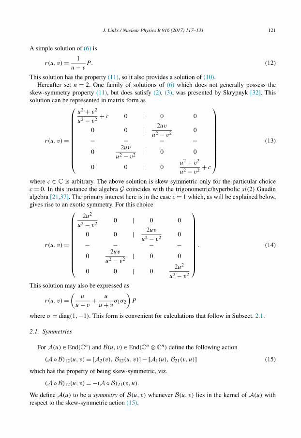
A simple solution of (6) is

r(u, v) = 1

u − vP. (12)

This solution has the property (11), so it also provides a solution of (10).Hereafter set n = 2. One family of solutions of (6) which does not generally possess the

skew-symmetry property (11), but does satisfy (2), (3), was presented by Skrypnyk [32]. This solution can be represented in matrix form as

r(u, v) =

⎛⎜⎜⎜⎜⎜⎜⎜⎜⎜⎜⎜⎝

u2 + v2

u2 − v2+ c 0 | 0 0

0 0 | 2uv

u2 − v20

− − − −0

2uv

u2 − v2| 0 0

0 0 | 0u2 + v2

u2 − v2+ c

⎞⎟⎟⎟⎟⎟⎟⎟⎟⎟⎟⎟⎠

(13)

where c ∈ C is arbitrary. The above solution is skew-symmetric only for the particular choice c = 0. In this instance the algebra G coincides with the trigonometric/hyperbolic sl(2) Gaudin algebra [21,37]. The primary interest here is in the case c = 1 which, as will be explained below, gives rise to an exotic symmetry. For this choice

r(u, v) =

⎛⎜⎜⎜⎜⎜⎜⎜⎜⎜⎜⎜⎝

2u2

u2 − v20 | 0 0

0 0 | 2uv

u2 − v20

− − − −0

2uv

u2 − v2| 0 0

0 0 | 02u2

u2 − v2

⎞⎟⎟⎟⎟⎟⎟⎟⎟⎟⎟⎟⎠

. (14)

This solution may also be expressed as

r(u, v) =(

u

u − v+ u

u + vσ1σ2

)P

where σ = diag(1, −1). This form is convenient for calculations that follow in Subsect. 2.1.

2.1. Symmetries

For A(u) ∈ End(Cn) and B(u, v) ∈ End(Cn ⊗Cn) define the following action

(A ◦B)12(u, v) = [A2(v), B12(u, v)] − [A1(u), B21(v,u)] (15)

which has the property of being skew-symmetric, viz.

(A ◦B)12(u, v) = −(A ◦B)21(v,u).

We define A(u) to be a symmetry of B(u, v) whenever B(u, v) lies in the kernel of A(u) with respect to the skew-symmetric action (15).

122 J. Links / Nuclear Physics B 916 (2017) 117–131

The above definition gives rise to a generalised notion of symmetries for solutions of (6). It turns out that these are characterised in terms of the one-dimensional representations π0 of their associated Lie algebra G, i.e. π0 : G → C. From (7) it is seen that for any one-dimensional representation

π0

([T

jk (u), T

pl (v)

])= 0.

Equivalently, it follows from (4) that a one-dimensional representation may be expressed as a mapping ρ(T (u)) = J (u) ∈ End(C2) satisfying

0 = [J2(v), r12(u, v)] − [J1(u), r21(v,u)] , (16)

which is precisely the statement that J (u) is a symmetry of r(u, v) with respect to the skew-symmetric action (15). In [31,33] such a solution J (u) is termed a generalised shift element of r(u, v).

Note that solutions J (u) of (16) necessarily close under commutation to form a Lie algebra in cases where the skew-symmetry property (11) holds. In general they do not close, however examples of this are rare. For the case of the solution (12), it is seen that all constant elements of End(C2) satisfy (16). It is therefore natural to identify the symmetry of (12) as gl(2). On the other hand for generic values of c in (13), solutions of (16) are given by constant diagonal elements of End(C2). In this instance the symmetry of (13) is identified as u(1). For the specific choice c = 1 in (13) leading to (14) an exotic symmetry emerges, which does not form a Lie algebra.

Setting

J (u) =D + uO (17)

where D is diagonal and O is off-diagonal it is found that (16) is satisfied by J (u). First

[J2(v), r12(u, v)] − [J1(u), r21(v,u)]

= u(D2 + vO2)

(1

u − v+ 1

u + vσ1σ2

)P

− u

(1

u − v+ 1

u + vσ1σ2

)P(D2 + vO2)

− v(D1 + uO1)

(1

v − u+ 1

u + vσ1σ2

)P

+ v

(1

v − u+ 1

u + vσ1σ2

)P(D1 + uO1)

= (D2 −D1)P + σ1σ2(D2 −D1)P

where simplification to the final expression has relied on the fact that σO = −Oσ . Now every diagonal operator on C2 may be expressed as D = aI + bσ for some a, b ∈ C. It then follows that

[J2(v), r12(u, v)] − [J1(u), r21(v,u)] = b(σ2 − σ1)P + bσ1σ2(σ2 − σ1)P

= b(σ2 − σ1)P + b(σ1 − σ2)P

= 0.

Because this solution for J (u) has an explicit dependence on the parameter u, it is quite distinct compared to the gl(2) symmetry of (12) and the u(1) symmetry of (13). Observe also that while

J. Links / Nuclear Physics B 916 (2017) 117–131 123

explicit spectral-parameter dependent forms of J (u) have been presented in [31], there are of a diagonal form and therefore form a commutative Lie algebra. The solution (17) provides a simple, concrete example where the symmetries are not of a Lie algebraic type.

For later use, the notation G will be adopted for the Lie algebra associated with the case of the solution (14).

2.2. General representations

General representations of G are first obtained by an evaluation homomorphism ρz to the enveloping algebra U(sl(2)) of sl(2). Adopting the convention for the sl(2) generators {Sz, S+, S−} to satisfy the commutation relations

[Sz, S±] = ±S±, [S+, S−] = 2Sz,

ρz has the action

ρz(T1

1 (u)) = u2

u2 − z2(I + 2Sz),

ρz(T1

2 (u)) = uz

u2 − z2S+,

ρz(T2

1 (u)) = uz

u2 − z2S−,

ρz(T2

2 (u)) = 2u2

u2 − z2(I − 2Sz),

preserving the commutation relations (4) for the solution (14). Every representation of sl(2) then affords a representation of G. For the choice of the spin-1/2 representation of sl(2) this coincides with the adjoint representation (8).

A second evaluation homomorphism to the enveloping algebra U(sl(2)), denoted ρ(0), is de-duced from the one-dimensional representation. Specifically,

ρ(0)(T11 (u)) = αI,

ρ(0)(T12 (u)) = uβI,

ρ(0)(T21 (u)) = uγ I,

ρ(0)(T22 (u)) = δI,

where α, β, γ, δ ∈ C are arbitrary, which again preserves the commutation relations (4) for the solution (14). Taking the tensor product of these evaluation homomorphisms provides evaluation homomorphisms acting on tensor product of copies of U(sl(2)). The general map

ρ⊗L = ρ(0) ⊗ ρz1 ⊗ ρz2 ⊗ ... ⊗ ρzL

has the form

ρ⊗L(T 11 (u)) = αI +

L∑j=1

u2

u2 − z2j

(I + 2Szj ),

ρ⊗L(T 12 (u)) = uβI +

L∑ 2uzj

u2 − z2j

S+j ,

j=1

124 J. Links / Nuclear Physics B 916 (2017) 117–131

ρ⊗L(T 21 (u)) = uγ I +

L∑j=1

2uzj

u2 − z2j

S−j ,

ρ⊗L(T 22 (u)) = δI +

L∑j=1

u2

u2 − z2j

(I − 2Szj ).

It then follows that τ(u) = ρ⊗L(t (u)) ∈ U(sl(2))⊗L satisfying

[τ(u), τ (v)] = 0, ∀u, v ∈ C

is a transfer matrix expressed in terms of spin operators.Hereafter set δ = −α, and γ = β with α, β ∈ R, giving

τ(u) =⎛⎝αI +

L∑j=1

u2

u2 − z2j

(I + 2Szj )

⎞⎠

2

+⎛⎝−αI +

L∑j=1

u2

u2 − z2j

(I − 2Szj )

⎞⎠

2

+⎛⎝uβI +

L∑j=1

2uzj

u2 − z2j

S+j

⎞⎠(

uβI +L∑

k=1

2uzk

u2 − z2k

S−k

)

+⎛⎝uβI +

L∑j=1

2uzj

u2 − z2j

S−j

⎞⎠(

uβI +L∑

k=1

2uzk

u2 − z2k

S+k

)

= 2(α2 + β2u2)I + 2u4

⎛⎝ L∑

j=1

1

u2 − z2j

⎞⎠

2

I

+ 4u2L∑

j=1

z2j

(u2 − z2j )

2Cj + 4

L∑j=1

u2

u2 − z2j

Tj ,

where C = 2(Sz)2 + S+S− + S−S+ is the sl(2) Casimir element and

Tj = 2(Szj )

2 + 2αSzj + βzj (S

+j + S−

j )

+L∑

k =j

(4z2

j

z2j − z2

k

SzjS

zk + 2zj zk

z2j − z2

k

(S+j S−

k + S−j S+

k )

). (18)

With the restriction zj ∈ R, j = 1, ..., L, which is imposed from now on, the {Tj : j = 1, ..., L}form a set of mutually commuting, self-adjoint operators. Consequently they are simultaneously diagonalisable. It is seen that the union of this set, the identity operator, and the set of Casimir elements {Cj : j = 1, ..., L} is the full set of functionally independent operators that can be extracted from the transfer matrix.

Matrix forms of transfer matrix are obtained by choosing a representation of sl(2) for each copy in the tensor product U(sl(2))⊗L. It should be noted that these representations need not be isomorphic, and throughout the parameters α, β, z1, z2, ..., zL are arbitrary real parameters. This provides a range of potential applications for constructing integrable models.

J. Links / Nuclear Physics B 916 (2017) 117–131 125

3. Integrable, multi-species, boson tunnelling model

Having identified the exotic symmetry of the solution (14), and outlined the construction of representations of G, attention turns towards an application through the construction of an integrable, multi-species, boson tunnelling model. The Hamiltonian is defined as

H = 2U

L∑j=1

Tj = 4U

⎛⎝ L∑

j=1

Szj

⎞⎠

2

+ 4Uα

L∑j=1

Szj + 2Uβ

L∑j=1

zj (S+j + S−

j ). (19)

Next the spin operators are represented in terms of boson operators through the Jordan–Schwinger map

Szj = 1

2(Nj,A − Nj,B),

S+j = b

†j,Abj,B,

S−j = b

†j,Bbj,A

where the spin sj of each representation is determined by 2sj = Nj . This maps (19) to (1) with the identification μ = 2Uα and Ej = 2Uβzj . For simplicity it will be assumed hereafter that the zj , and consequently the Ej , are distinct parameters.

Since the operators (18) commute with (19), application of the Jordan–Schwinger map to the Tj yields a set of L operators which necessarily commute with (1). Along with the Nj , which also commute with (1), the construction for the model is one which establishes that it is integrable since the number of independent conserved operators is the same as the number of degrees of freedom. Closely related to the property of integrability is the notion of an exact solution. The next step is to derive an explicit form for such a solution.

3.1. Bethe Ansatz solution

Below it will be shown that the eigenvalues �j of the conserved operators (18) have the form

�j = 2s2j + 2αsj +

L∑k =j

4sj skz2j

z2j − z2

k

− 2N∑

n=1

sj z2j

z2j − vn

(20)

such that the parameters {vn : l = 1, ..., N}, known as the Bethe roots, satisfy the Bethe Ansatz equations

α − 1 +L∑

l=1

2vnsl

vn − z2l

=N∑

m =n

2vn

vn − vm

+β2

L∏l=1

(vn − z2l )

2sl

4N∏

m =n

(vn − vm)

. (21)

Consequently, the energy eigenvalues E for the Hamiltonian (1) have the form

E = 2U

L∑j=1

�j = UN2 + μN − 4U

L∑j=1

N∑n=1

sj z2j

z2j − vn

.

126 J. Links / Nuclear Physics B 916 (2017) 117–131

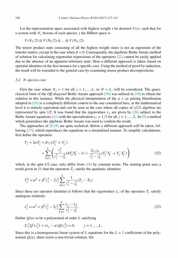
Let the representation space associated with highest weight s be denoted V (s), such that for a system with Nj bosons of each species j the Hilbert space is

V (N1/2) ⊗ V (N2/2) ⊗ ... ⊗ V (NL/2)

The tensor product state consisting of all the highest weight states is not an eigenstate of the transfer matrix, except in the case when β = 0. Consequently, the algebraic Bethe Ansatz method of solution for calculating eigenvalue expressions of the operators (22) cannot be easily applied due to the absence of an apparent reference state. Here a different approach is taken, based on operator identities in the first instance for a specific case. Using the method of proof by induction, the result will be extended to the general case by examining tensor product decompositions.

3.2. N -species case

First the case where Nj = 1 for all j = 1, ..., L, so N = L, will be considered. The quasi-classical limit of the Off-diagonal Bethe Ansatz approach [39] was utilised in [19] to obtain the solution in this instance. While the physical interpretation of the p + ip pairing Hamiltonian adopted in [19] is a completely different context to the one considered here, at the mathematical level it is entirely equivalent and can be seen as the case where all copies of sl(2) algebras are represented by spin 1/2. It was found that the eigenvalues λj are given by (20) subject to the Bethe Ansatz equations (21) with the specialisation sj = 1/2 for all j = 1, ..., L. In [9] a method which generalises the algebraic Bethe Ansatz was used to confirm the result.

The approaches of [9,19] are quite technical. Below a different approach will be taken, fol-lowing [17], which reproduces the equations in a streamlined manner. To simplify calculations, first define the operators

Tj = 2αSzj + βzj (S

+j + S−

j )

+L∑

k =j

(z2j

z2j − z2

k

(4SzjS

zk − I ) + 2zj zk

z2j − z2

k

(S+j S−

k + S−j S+

k )

)(22)

which, in the spin-1/2 case, only differ from (18) by constant terms. The starting point uses a result given in [9] that the operators Tj satisfy the quadratic identities

T 2j = α2 + β2z2

j − 2z2j

L∑k =j

1

z2j − z2

k

(Tj − Tk).

Since these are operator identities it follows that the eigenvalues λj of the operators Tj satisfy analogous relations:

λ2j = α2 + β2z2

j − 2z2j

L∑k =j

λj − λk

z2j − z2

k

. (23)

Define Q(u) to be a polynomial of order L satisfying

2z2jQ

′(z2j ) + (λj − α)Q(z2

j ) = 0, j = 1, ...,L.

Since this is a homogeneous linear system of L equations for the L + 1 coefficients of the poly-nomial Q(u), there exists a non-trivial solution. Set

J. Links / Nuclear Physics B 916 (2017) 117–131 127

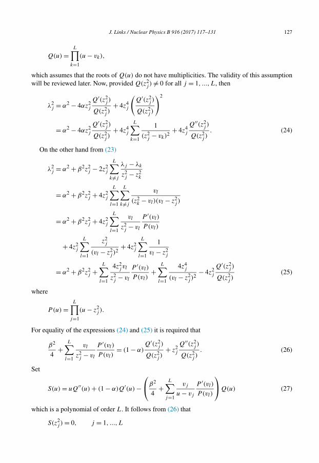
Q(u) =L∏

k=1

(u − vk),

which assumes that the roots of Q(u) do not have multiplicities. The validity of this assumption will be reviewed later. Now, provided Q(z2

j ) = 0 for all j = 1, ..., L, then

λ2j = α2 − 4αz2

j

Q′(z2j )

Q(z2j )

+ 4z4j

(Q′(z2

j )

Q(z2j )

)2

= α2 − 4αz2j

Q′(z2j )

Q(z2j )

+ 4z4j

L∑k=1

1

(z2j − vk)2

+ 4z4j

Q′′(z2j )

Q(z2j )

. (24)

On the other hand from (23)

λ2j = α2 + β2z2

j − 2z2j

L∑k =j

λj − λk

z2j − z2

k

= α2 + β2z2j + 4z2

j

L∑l=1

L∑k =j

vl

(z2k − vl)(vl − z2

j )

= α2 + β2z2j + 4z2

j

L∑l=1

vl

z2j − vl

P ′(vl)

P (vl)

+ 4z2j

L∑l=1

z2j

(vl − z2j )

2+ 4z2

j

L∑l=1

1

vl − z2j

= α2 + β2z2j +

L∑l=1

4z2j vl

z2j − vl

P ′(vl)

P (vl)+

L∑l=1

4z4j

(vl − z2j )

2− 4z2

j

Q′(z2j )

Q(z2j )

(25)

where

P(u) =L∏

j=1

(u − z2j ).

For equality of the expressions (24) and (25) it is required that

β2

4+

L∑l=1

vl

z2j − vl

P ′(vl)

P (vl)= (1 − α)

Q′(z2j )

Q(z2j )

+ z2j

Q′′(z2j )

Q(z2j )

. (26)

Set

S(u) = uQ′′(u) + (1 − α)Q′(u) −⎛⎝β2

4+

L∑j=1

vj

u − vj

P ′(vl)

P (vl)

⎞⎠Q(u) (27)

which is a polynomial of order L. It follows from (26) that

S(z2j ) = 0, j = 1, ...,L

128 J. Links / Nuclear Physics B 916 (2017) 117–131

which, along with the consideration of the asymptotic behaviour of (27) as u → ∞, establishes that

S(u) = −β2

4P(u). (28)

Evaluating S(vn) through (27) and (28) and equating these expressions then yields the Bethe Ansatz equations

α − 1 + vn

P ′(vn)

P (vn)= vn

Q′′(vn)

Q′(vn)+ β2

4

P(vn)

Q′(vn), n = 1, ...,L (29)

which are equivalent to (21). It can be verified that (20) holds.It needs addressing at this point that the assumptions that the roots of Q(u) do not have

multiplicities, and that Q(z2j ) = 0, are not always valid. In the β = 0 limit numerical solutions of

the Bethe Ansatz equations confirm that both of these situations occur [10,14,18,23]. Two Bethe roots may coalesce at a point z2

j through which they transition between being real-valued and a complex-conjugate pair. Moreover in this limit some of the L Bethe roots must be seen as being infinite-valued, and there are well-identified points at which several additional roots collapse to be zero-valued or infinite-valued. All of these instances may be interpreted as singular solutions of (21), but can be simply regularised by expressing (29) in a polynomial form

(α − 1)P (vn)Q′(vn) + vnP

′(vn)Q′(vn) = vnQ

′′(vn)P (vn) + β2

4P(vn)

2.

So, while the above derivation of the Bethe Ansatz equations breaks down when the roots of Q(u) have multiplicities, or Q(z2

j ) = 0, indicators from available numerical studies [10,14,18,23] suggest that the equations are nonetheless valid.

3.3. The general case

The validity of the formulae (20), (21) in general follows by an inductive argument on each of the species number labels Nj , starting with the case Nj = 1 for all j = 1, ..., N which has been established above. Every finite-dimensional irreducible sl(2) module is contained in some tensor product of spin-1/2 modules, and in particular

V (N1/2) ⊗ ...V (NL/2) ⊆ V (1/2)⊗N

where N = N1 + ... + NL as before. Now consider a system of M ≥ L species, for which it is determined that for j = M − 1, M

limzM→zM−1

Tj =2(Szj )

2 + 2αSzj + βzj (S

+j + S−

j )

+M−2∑k =j

(4z2

j

z2j − z2

k

SzjS

zk + 2zj zk

z2j − z2

k

(S+j S−

k + S−j S+

k )

)

+ 4z2j

z2j − z2

M−1

Szj (S

zM−1 + Sz

M)

+ 2zj zM−1

z2j − z2

M−1

(S+j (S−

M−1 + S−M) + S−

j (S+M−1 + S+

M)) (30)

while

J. Links / Nuclear Physics B 916 (2017) 117–131 129

limzM→zM−1

(TM−1 + TM) =2(SzM−1 + Sz

M)2 + 2α(SzM−1 + Sz

M)

+ βzj (S+M−1 + S+

M + S−M−1 + S−

M)

+M−2∑k=1

2zM−1zk

z2M−1 − z2

k

(S+M−1 + S+

M)S−k

+M−2∑k=1

2zM−1zk

z2M−1 − z2

k

(S−M−1 + S−

M)S+k

+M−2∑k=1

4z2M−1

z2M−1 − z2

k

(SzM−1 + Sz

M)Szk . (31)

Noting the result

V (sM−1 + sM) ⊆ V (sM−1) ⊗ V (sM),

let PM denote the projection onto the component V (sM−1 + sM). The above expressions (30), (31) show that the general form of the conserved operators (18) is preserved via

Tj = limzM→zM−1

PMTjPM, j = 1, ...,M − 2,

TM−1 = limzM→zM−1

PM(TM−1 + TM)PM

whereby the tilded notation refers to a new system of N particles of M − 1 species, such that NM−1 = NM−1 +NM and Nj = Nj otherwise. It should be noted that a projection onto any other irreducible component of the tensor product V (sM−1) ⊗ V (sM) gives rise to a system where the number of particles is strictly less that N . This is not an appropriate step for establishing the desired result, since it requires a change in the number of Bethe roots.

Suppose that (20), (21) hold for the M-species system. Letting �j denote the eigenvalues for Tj , it is required to show that (20), (21) hold for the new system of M − 1 species with the tilded notation. For (21) the result follows simply from the relations

limzM→zM−1

M∑l=1

2sl

vn − z2l

= 2(sM−1 + sM)

vn − z2M−1

+M−2∑l=1

2sl

vn − z2l

,

limzM→zM−1

M∏l=1

(vn − z2l )

2sl = (vn − zM−1)2sM−1+2sM

M−2∏l=1

(vn − z2l )

2sl .

In a similar manner it follows that (20) holds with the observations

�j = limzM→zM−1

�j,

�M−1 = limzM→zM−1

(�M−1 + �M).

Finally note that at each step the labels Nj can be reordered without loss of generality, such that limits (30), (31) can be taken. It therefore follows by induction on each Nj = 2sj that (20), (21)hold in general.

130 J. Links / Nuclear Physics B 916 (2017) 117–131

4. Conclusion

This work first identified a particular solution of a non-standard form of the classical Yang–Baxter equation. This solution is unusual in that it admits a symmetry which does not close to form a Lie algebra. The solution was used for the construction of an integrable, multi-species, boson tunnelling model, and the Bethe Ansatz equations characterising the spectrum were de-rived.

Having obtained the exact solution, there are several avenues for ongoing work to take place. One promising course is to adapt integral equation techniques [10,23] to investigate ground-state properties in the limit of large particle numbers. This will be the subject of a future study.

Acknowledgements

This work was supported by the Australian Research Council through Discovery Project DP150101294. I thank Taras Skrypnyk for helpful comments.

References

[1] A.B. Balantekin, T. Dereli, Y. Pehlivan, Solutions of the Gaudin equation and Gaudin algebras, J. Phys. A, Math. Gen. 38 (2005) 5697–5707.

[2] O. Babelon, D. Talalaev, On the Bethe ansatz for the Jaynes–Cummings–Gaudin model, J. Stat. Mech. Theory Exp. (2007) P06013.

[3] A.A. Belavin, V.G. Drinfel’d, Solutions of the classical Yang–Baxter equation for simple Lie algebras, Funct. Anal. Appl. 16 (1982) 159–180.

[4] N.M. Bogoliubov, Time-dependent correlation functions for the bimodal Bose–Hubbard model, J. Math. Sci. 213 (2016) 662–670.

[5] S. Campbell, G. De Chiara, M. Paternostro, Equilibration and nonclassicality of a double-well potential, Sci. Rep. 6 (2016) 19730.

[6] G. Ceccarelli, J. Nespolo, A. Pelissetto, E. Vicari, Bose–Einstein condensation and critical behavior of two-component bosonic gases, Phys. Rev. A 92 (2015) 043613.

[7] R. Cipolatti, L. Villegas-Lelovsky, M.C. Chung, C. Trallero-Giner, Two-species Bose–Einstein condensate in an optical lattice: analytical approximate formulae, arXiv:1508.04341.

[8] R. Citro, A. Naddeo, E. Orignac, Quantum dynamics of a binary mixture of BECs in a double-well potential: a Holstein–Primakoff approach, J. Phys. B, At. Mol. Opt. Phys. 44 (2011) 115306.

[9] P.W. Claeys, S. De Baerdemacker, D. Van Neck, Read–Green resonances in a topological superconductor coupled to a bath, Phys. Rev. B 93 (2016) 220503(R).

[10] C. Dunning, M. Ibañez, J. Links, G. Sierra, S.-Y. Zhao, Exact solution of the p + ip pairing Hamiltonian and a hierarchy of integrable models, J. Stat. Mech. Theory Exp. (2010) P08025.

[11] V.Z. Enol’skii, V.B. Kuznetsov, M. Salerno, On the quantum inverse scattering method for the DST dimer, Physica D 68 (1993) 138–152.

[12] M. Gaudin, Diagonalisation d’une classe d’Hamiltoniens de spin, J. Phys. (Paris) 37 (1976) 1087–1098.[13] E.-M. Graefe, H.J. Korsch, M.P. Strzys, Bose–Hubbard dimers, Viviani’s windows and pendulum dynamics, J. Phys.

A, Math. Theor. 47 (2014) 085304.[14] M. Ibañez, J. Links, G. Sierra, S.-Y. Zhao, Exactly solvable pairing model for superconductors with px + ipy -wave

symmetry, Phys. Rev. B 79 (2009) 180501.[15] B. Jurco, Classical Yang–Baxter equations and quantum integrable systems, J. Math. Phys. 30 (1989) 1289–1293.[16] B. Jurco, On quantum integrable models related to nonlinear quantum optics. An algebraic Bethe ansatz approach,

J. Math. Phys. 30 (1989) 1739–1743.[17] J. Links, Completeness of the Bethe Ansatz solution for the rational, spin-1/2 Richardson–Gaudin system,

arXiv:1603.03542.[18] J. Links, I. Marquette, A. Moghaddam, Exact solution of the p+ ip model revisited: duality relations in the hole-pair

picture, J. Phys. A, Math. Theor. 48 (2015) 374001.

J. Links / Nuclear Physics B 916 (2017) 117–131 131

[19] I. Lukyanenko, P.S. Isaac, J. Links, An integrable case of the p + ip pairing Hamiltonian interacting with its envi-ronment, J. Phys. A, Math. Theor. 49 (2016) 084001.

[20] J.-P. Lv, Q.-H. Chen, Y. Deng, Two-species hard-core bosons on the triangular lattice: a quantum Monte Carlo study, Phys. Rev. A 89 (2014) 013628.

[21] G. Ortiz, R. Somma, J. Dukelsky, S. Rombouts, Exactly-solvable models derived from a generalized Gaudin algebra, Nucl. Phys. B 707 (2005) 421–457.

[22] H. Qiu, J. Tian, L.-B. Fu, Collective dynamics of two-species Bose–Einstein-condensate mixtures in a double-well potential, Phys. Rev. A 81 (2010) 043613.

[23] S.M.A. Rombouts, J. Dukelsky, G. Ortiz, Quantum phase diagram of the integrable px + ipy fermionic superfluid, Phys. Rev. B 82 (2010) 224510.

[24] G. Santos, C. Ahn, A. Foerster, I. Roditi, Bethe states for the two-site Bose–Hubbard model: a binomial approach, Phys. Lett. B 746 (2015) 186–189.

[25] I.I. Satija, R. Balakrishnan, P. Naudus, J. Heward, M. Edwards, C.W. Clark, Symmetry-breaking and symmetry-restoring dynamics of a mixture of Bose–Einstein condensates in a double well, Phys. Rev. A 79 (2009) 033616.

[26] K.V.S. Shiv Chaitanya, Sibasish Ghosh, V. Srinivasan, Entanglement in two-site Bose–Hubbard model with non-linear dissipation, J. Mod. Opt. 61 (2014) 1409–1417.

[27] T. Skrypnyk, Integrable quantum spin chains, non-skew symmetric r-matrices and quasigraded Lie algebras, J. Geom. Phys. 57 (2006) 53–67.

[28] T. Skrypnyk, Generalized quantum Gaudin spin chains, involutive automorphisms and “twisted” classical r-matrices, J. Math. Phys. 47 (2006) 033511.

[29] T. Skrypnyk, Quantum integrable systems, non-skew-symmetric r-matrices and algebraic Bethe ansatz, J. Math. Phys. 48 (2007) 023506.

[30] T. Skrypnyk, Generalized Gaudin spin chains, nonskew symmetric r-matrices, and reflection equation algebras, J. Math. Phys. 48 (2007) 113521.

[31] T. Skrypnyk, Generalized Gaudin systems in a magnetic field and non-skew-symmetric r-matrices, J. Phys. A, Math. Theor. 40 (2007) 13337–13352.

[32] T. Skrypnyk, Non-skew-symmetric classical r-matrices and integrable cases of the reduced BCS model, J. Phys. A, Math. Theor. 42 (2009) 472004.

[33] T. Skrypnyk, Generalized shift elements and classical r-matrices: construction and applications, J. Geom. Phys. 80 (2014) 71–87.

[34] T. Skrypnyk, Quantum integrable models of interacting bosons and classical r-matrices with spectral parameters, J. Geom. Phys. 97 (2015) 133–155.

[35] B. Sun, M.S. Pindzola, Dynamics of a two-species Bose–Einstein condensate in a double well, Phys. Rev. A 80 (2009) 033616.

[36] G. Thalhammer, G. Barontini, L. De Sarlo, J. Catani, F. Minardi, M. Inguscio, Double species Bose–Einstein con-densate with tunable interspecies interactions, Phys. Rev. Lett. 100 (2008) 210402.

[37] M. Van Raemdonck, S. De Baerdemacker, D. Van Neck, Exact solution of the px + ipy pairing Hamiltonian by deforming the pairing algebra, Phys. Rev. B 89 (2014) 155136.

[38] W. Wang, V. Penna, B. Capogrosso-Sansone, Inter-species entanglement of Bose–Bose mixtures trapped in optical lattices, New J. Phys. 18 (2016) 063002.

[39] Y. Wang, W.-L. Yang, J. Cao, K. Shi, Off-Diagonal Bethe Ansatz for Exactly Solvable Models, Springer-Verlag, 2015.

[40] Y.-H. Wu, T. Shi, Topological phases of two-component bosons in species-dependent artificial gauge potential, arXiv:1508.05139.

[41] S.-Y. Wu, H.-H. Zhong, J.-H. Huang, X.-Z. Qin, C.-H. Lee, Dynamic fragmentation in a quenched two-mode Bose–Einstein condensate, Front. Phys. 11 (2016) 110301.