arX

iv:1

003.

5506

v1 [

gr-q

c] 2

9 M

ar 2

010

Exotic Smoothness and Quantum Gravity

T. Asselmeyer-Maluga

German Aerospace Center, Berlin andLoyola University, New Orleans, LA, USA

E-mail: torsten.asselmeyer-maluga@dlr.de

Abstract. Since the first work on exotic smoothness in physics, it was folkloreto assume a direct influence of exotic smoothness to quantum gravity. Thus,the negative result of Duston [1] was a surprise. A closer look into thesemi-classical approach uncovered the implicit assumption of a close connectionbetween geometry and smoothness structure. But both structures, geometry andsmoothness, are independent of each other.

In this paper we calculate the “smoothness structure” part of the path integralin quantum gravity assuming that the “sum over geometries” is already given. Forthat purpose we use the knot surgery of Fintushel and Stern applied to the classE(n) of elliptic surfaces. We mainly focus our attention to the K3 surfaces E(2).Then we assume that every exotic smoothness structure of the K3 surface can begenerated by knot or link surgery a la Fintushel and Stern. The results are appliedto the calculation of expectation values. Here we discuss the two observables,volume and Wilson loop, for the construction of an exotic 4-manifold using theknot 52 and the Whitehead link Wh. By using Mostow rigidity, we obtain atopological contribution to the expectation value of the volume. Furthermore weobtain a justification of area quantization.

PACS numbers: 04.60.Gw, 02.40.Ma, 04.60.Rt

Submitted to: Class. Quantum Grav.

Exotic Smoothness and Quantum Gravity 2

1. Introduction

One of the outstanding problems in physics is the unification of the quantum andgeneral relativity theory. In the case of the quantization of gravity one works on thespace of (pseudo-)Riemannian metrics or better on the space of connections (Levi-Civita or more general). The diffeomorphism group of the corresponding manifold isthe gauge group of this theory. Knowing more about the structure of this group meansknowing more about quantum gravity. An explicit expression for this correspondenceis given by General Relativity Theory (GRT). In this theory we start with a manifold,choose a smooth structure and write down the field equation. The beginning and theend of this procedure can be motivated by physics but the choice of the smoothnessstructure is not obvious. The reason for this ambiguity is given by the existenceof distinct, i.e. non-diffeomorphic, smoothness structures (exotic smoothness) indimension four (see [2] for an overview). The first examples of exotic 7-spheres werediscovered by Milnor in 1956 [3]. Then it was shown that there are only a finitenumber of smoothness structures in dimensions greater than 4 [4, 5]. In contrast thereare countable infinite many (distinct) exotic smoothness structures for some compact4-manifolds (see the knot surgery below) and uncountable infinite many for some non-compact manifolds (see [6] in case of M×R with M a compact, close 3-manifold, or theoverview in [7]) including the exotic R4[8, 9, 10]. Usually such a variety of structureshas a meaning in physics. The first relation between quantum field theory and exoticsmoothness was found by Witten [11]. He constructed a topological field theory havingthe Donaldson polynomials as ground state. Sładkowski [12, 13, 14] discussed theinfluence of differential structures on the algebra C(M) of functions over the manifoldM with methods known as non-commutative geometry. Especially in [13, 14] he stateda remarkable connection between the spectra of differential operators and differentialstructures. For example, the eta-invariant η(RP 4, g, φ) (measuring the asymmetry ofthe spectrum) of a twisted Dirac-operator is different from the eta-invariant of theexotic RP 4 for all metrics g and all spin structures φ [15]. Thus the most interestingdimension for physics has the richest structure. Now the questions are: What isthe physical relevance of the differential structure? How does the observable or itsexpectation value depend on the smoothness structure? In the case of the exotic R4 thefirst question was discussed by Brans and Randall [16] and later by Brans [17, 18] aloneto guess, that exotic smoothness can be a source of non-standard solutions of Einsteinsequation. The author published an article [19] to show the influence of the differentialstructure to GRT for compact manifolds of simple type. Finally Sładkowski showedin [20] that the exotic R4 can act as the source of the gravitational field. As shownin [21, 22] the existence of exotic smoothness has a tremendous impact on cosmology,further explored in [23]. Beginning with the work of Krol [24, 25, 26, 27, 28, 29] onthe relation between categorical constructions and exotic smoothness, the focus inthe topic is shifted to show a direct relation between exotic smoothness and quantumgravity [30, 31, 32].

In the first section of chapter 10 in [2], the meaning of exotic smoothness forgeneral relativity was discussed on general grounds. Since the first papers aboutexotic smoothness it was folklore to state an influence of exotic smoothness to thestate sum (or path integral) for quantum gravity. Then the negative result of the firstpaper written by Duston [1] was a surprise. He was able to calculate semi-classicalresults using exotic smoothness. The reason for the negative result is the loose relationbetween differential topology and differential geometry for 4-manifolds (in contrast to

Exotic Smoothness and Quantum Gravity 3

the strong relation for 3-manifolds known as the geometrization conjecture of Thurston[33]). But the smoothness structure is rather independent of the geometry whereasDuston assumed a coupling between geometry and topology because of its semi-classical approach. Of course, there are some restrictions induced by the smoothnessstructure like the existence of a Ricci-flat metric but nothing more.

In this paper we use a different approach to overcome this problem by dividingthe measure in the path integral into two parts: the geometrical part (sum overgeometries) and the differential topological part (sum over exotic smoothness). Bothparts are more or less independent of each other. If one assume the existence of thepath integral for the geometrical part (state sum Z0 see below) then the state sum ischanged by exotic smoothness according to (13). The paper is organized as follows.First we will give a physical motivation for exotic smoothness structures and presentthe model assumptions. Then we study the construction of the special class of ellipticsurfaces and the exotic smoothness structures using knot surgery. In section 4 wediscuss the splitting of the action functional (using the diffeomorphism invariance ofthe Einstein-Hilbert action) according to the knot surgery to get the relation (5). Thenin section 6 we will discuss the calculation of the functional integral to get (13). Thenwe discuss the expectation value of two observables: the volume and the Wilson loop.The calculation of the examples of the knot 52 and the Whitehead link Wh togetherwith some concluding remarks close the paper.

2. Physical Motivation and model assumptions

Einsteins insight that gravity is the manifestation of geometry leads to a new viewon the structure of spacetime. From the mathematical point of view, spacetime isa smooth 4-manifold endowed with a (smooth) metric as basic variable for generalrelativity. Later on, the existence question for Lorentz structure and causalityproblems (see Hawking and Ellis [34]) gave further restrictions on the 4-manifold:causality implies noncompactness, Lorentz structure needs a codimension-1 foliation.Usually, one starts with a globally foliated, noncompact 4-manifold Σ×R fulfilling allrestrictions where Σ is a smooth 3-manifold representing the spatial part. But othernoncompact 4-manifolds are also possible, i.e. it is enough to assume a noncompact,smooth 4-manifold endowed with a codimension-1 foliation.

All these restrictions on the representation of spacetime by the manifold conceptare clearly motivated by physical questions. Among the properties there is onedistinguished element: the smoothness. Usually one assumes a smooth, unique atlasof charts covering the manifold where the smoothness is induced by the unique smoothstructure on R. But as discussed in the introduction, that is not the full story. Evenin dimension 4, there are an infinity of possible other smoothness structures (i.e. asmooth atlas) non-diffeomorphic to each other.

If two manifolds are homeomorphic but non-diffeomorphic, they are exotic toeach other. The smoothness structure is called an exotic smoothness structure.

The implications for physics are obvious because we rely on the smooth calculusto formulate field theories. Thus different smoothness structures have to representdifferent physical situations leading to different measurable results. But it shouldbe stressed that exotic smoothness is not exotic physics! Exotic smoothness is amathematical possibility which should be further explored to understand its physicalrelevance.

In this paper we use a special class of the 4-manifold. Currently, there are

Exotic Smoothness and Quantum Gravity 4

(uncountable) many examples of exotic, noncompact 4-manifolds which are hard todescribe. Thus we will restrict to the class of compact 4-manifolds where we havepowerful invariants like Seiberg-Witten invariants [35, 36] or Donaldson polynomials[37, 38] to distinguish between different smoothness structures. Secondly we willnot discuss the definition of the path integral and all problems connected withrenormalization, definiteness etc. Third, we don’t discuss the Euclidean and/orLorentzian signature of the metric. Clearly the compactness of the 4-manifold impliesthe Euclidean metric on the 4-manifold but smoothness question are independent of themetric. Thus, without loss of generality one can remove one point from the compact4-manifold to get a noncompact 4-manifold with Lorentz signature. Forth, we use theknot surgery of Fintushel and Stern [39] to construct the exotic smoothness structure.This approach assumes a special class of 4-manifolds (“complicated-enough”) whichcontains the class of elliptic surfaces among them the important K3 surface. Thus wesummarize the assumptions

(i) The 4-manifold is the compact and simple-connected elliptic surface E(n) whereE(2) is the K3 surface.

(ii) All problems with the definition and calculation of the path integral are ignored.

(iii) The signature of the metric is not discussed, i.e. the calculations are the samefor Euclidean or Lorentzian metric.

(iv) The exotic smoothness structures of the 4-manifold E(n) are constructed byFintushel-Stern knot surgery.

3. Elliptic surfaces and exotic smoothness

In this section we will give some information about elliptic surfaces and itsconstruction. First we will give a short overview of the construction of elliptic surfacesand a special class of elliptic surfaces denoted by E(n) in the literature. Then wepresent the construction of exotic E(n) by using the knot surgery of Fintushel andStern.

3.1. Elliptic surfaces

A complex surfaces S is a 2-dimensional complex manifold which is compact andconnected. A special complex surface is the elliptic surface, i.e. a complex surfaces Stogether with a map π : S → C (C complex curve, i.e. Riemannian surface), so thatfor nearly every point p ∈ S the reversed map F = π−1(p) is an elliptic curve i.e. atorus‡. Now we will construct the special class of elliptic surfaces E(n).

The first step is the construction of E(1) by the unfolding of singularities for twocubic polynomials intersecting each other. The resulting manifold E(1) is the manifold

CP 2#9CP2

but equipped with an elliptic fibration. Then we use the method of fibersum to produce the surfaces E(n) for every number n ∈ N. For that purpose wecut out a neighborhood N(F ) of one fiber π−1(p) of E(1). Now we sew together twocopies of E(1) \N(F ) along the boundary of N(F ) to get E(2) i.e we define the fibersum E(2) = E(1)#fE(1). Especially we note that E(2) is also known as K3-surfacewidely used in physics. Thus we get the recursive definition E(n) = E(n− 1)#fE(1).The details of the construction can be found in the paper [40].

‡ We denote this map π as elliptic fibration. Thus every complex surface which is equipped with aelliptic fibration is an elliptic surface.

Exotic Smoothness and Quantum Gravity 5

3.2. Knot surgery and exotic elliptic surface

The main technique to construct an exotic elliptic surface was introduced by Fintusheland Stern [39], called knot surgery. In short, given a simple-connected, compact4-manifold M with an embedded torus T 2 (having special properties, see below),cut out M \ N(T 2) a neighborhood N(T 2) = D2 × T 2 of the torus and glue inS1 × S3 \N(K), with the knot complement S3 \N(K) (see appendix Appendix A).Thus the construction depends on a knot, i.e. an embedding of the circle S1 into R3

or S3. Then we obtain the new 4-manifold

MK = (M \N(T )) ∪T 3 (S1 × (S3 \N(K)))

from a given 4-manifold M by gluing M \ N(T 2) and S1 × S3 \ N(K) along thecommon boundary, the 3-torus T 3. It is the remarkable result of Fintushel and Stern[39] for a non-trivial knot K that MK is non-diffeomorphic to M . We remark thatthe construction can be easily generalized to links, i.e. the embedding of the disjointunion of circles S1 ⊔ · · · ⊔ S1 into R3 or S3. The reader not interested in the detailsof the construction can now jump to the next section.

The precise definition can be given in the following way for elliptic surface: Letπ:S → C be an elliptic surface and π−1(t) = F a smooth fiber (t ∈ C). As usual,N(F ) denotes a neighborhood of the regular fiber F in S (which is diffeomorphicto D2 × T 2). Deleting N(F ) from S to get a manifold S \ N(F ) with boundary∂(S \N(F )) = ∂(D2 × F ) = S1 × F = T 3, the 3-torus. Then we take the 4-manifoldS1 × (S3 \N(K)), K a knot, with boundary ∂(S1 × (S3 \N(K))) = T 3 and regluingit along the common boundary T 3. The resulting 4-manifold

SK = (S \N(F )) ∪T 3 (S1 × (S3 \N(K)))

is obtained from S via knot surgery using the knot K. The regular fiber F in theelliptic surface S has two properties which are essential for the whole construction:

(i) In a larger neighborhood Nc(F ) of the regular fiber F there is a cups fiber c,i.e. an embedded 2-sphere of self-intersection 0 with a single nonlocally flat pointwhose neighborhood is the cone over the right-hand trefoil knot.

(ii) The complement S \ F of the regular fiber is simple-connected π1(S \ F ) = 1.

Then as shown in [39], SK is not diffeomorphic to S. The whole procedure canbe generalized to any 4-manifold with an embedded torus of self-intersection 0 in aneighborhood of a cusp.

Before we proceed with the physical interpretation, we will discuss the questionwhen two exotic SK and SK′ for two knots K,K ′ are diffeomorphic to each other.Currently there are two invariants to distinguish non-diffeomorphic smoothnessstructures: Donaldson polynomials and Seiberg-Witten invariants. Fintushel andStern [39] calculated the invariants for SK and SK′ to show that SK differs from SK′

if the Alexander polynomials of the two knots differ. Unfortunately the invariantsare not complete. Thus we cannot say anything about SK and SK′ for two knotswith the same Alexander polynomial. But Fintushel and Stern [41, 42] constructedcounterexamples of two knots K,K ′ with the same Alexander polynomial but withdifferent SK and SK′ . Furthermore Akbulut [43] showed that the knot K and itsmirror K̄ induce diffeomorphic 4-manifold SK = SK̄ .

Exotic Smoothness and Quantum Gravity 6

4. The action functional

In this section we will discuss the Einstein-Hilbert action functional of the exotic 4-manifold. The main part of our argumentation is additional contribution to the actionfunctional coming from exotic smoothness. Here it is enough to consider the exoticsmoothness generated by knot surgery.

We start with an elliptic surface, the K3 surface M = E(2). In this paper weconsider the Einstein-Hilbert action

SEH(g) =

∫

M

R√g d4x (1)

and fix the Ricci-flat metric g as solution of the vacuum field equations. Now we studythe effect to vary the differential structure by a knot surgery. This procedure effectedonly a submanifold N(T 2) ⊂ M and we consider a decomposition of the 4-manifold

M = (M \N(T 2)) ∪T 3 N(T 2)

with N(T 2) = D2 × T 2 leading to a sum in the action

SEH(M) =

∫

M\N(T 2)

R√g d4x+

∫

N(T 2)

R√g d4x .

Because of diffeomorphism invariance of the Einstein-Hilbert action, this decomposi-tion don’t depend on the concrete realization with respect to any coordinate system.Now we construct a new smoothness structure MK

MK = (M \N(T 2)) ∪T 3 (S1 × (S3 \N(K)))

by using a knot K, i.e. an embedding K : S1 → S3. Then the 4-manifold M \N(T 2)with boundary a 3-torus T 3 appears in both 4-manifolds M and MK . Thus we canfix it and its action

SEH(M \N(T 2)) =

∫

M\N(T 2)

R√g d4x

by using a fixed metric g in the interior int(M \N(T 2)). Furthermore we can ignorea possible boundary term because the 3-torus T 3 = ∂(M \N(T 2)) is a flat, compact3-manifold. Thus we obtain

SEH(MK) = SEH(M \N(T 2)) +

∫

S1×(S3\N(K))

RK

√gK d4x (2)

with a metric gK and scalar curvature RK for the 4-manifold S1 × (S3 \N(K)). Nowwe consider the integral

SEH(N(T 2)) =

∫

N(T 2)=D2×T 2

R√g d4x

over N(T 2) = D2×T 2 w.r.t. a suitable product metric. The torus T 2 is a flat manifoldand the disk D2 can be chosen to embed flat in N(T 2). Thus, this integral vanishesSEH(N(T 2)) = 0 and

SEH(M \N(T 2)) = SEH(M) .

Exotic Smoothness and Quantum Gravity 7

Using this relation and (2), we obtain the following relation

SEH(MK) = SEH(M) +

∫

S1×(S3\N(K))

RK

√gK d4x (3)

between the Einstein-Hilbert action on M with and without knot surgery. Next wewill evaluate the integral

∫

S1×(S3\N(K))

RK

√gK d4x

by using a product metric gK

ds2 = dθ2 + hikdxidxk

with periodic coordinate θ on S1 and metric hik on the knot complement S3 \N(K).We are using the ADM formalism with the lapse N and shift function N i to get arelation between the 4-dimensional R and the 3-dimensional scalar curvature R(3) (see[44] (21.86) p. 520)

√gK R d4x = N

√h(

R(3) + ||n||2((trK)2 − trK2))

dθ d3x

with the normal vector n and the extrinsic curvature K. Without loss of generality,using the product metric in S1 × (S3 \N(K)) we can embed S3 \N(K) →֒ S1 × (S3 \N(K)) in such a manner that the extrinsic curvature has a fixed value or vanishesK = 0 (parallel transport of the normal vector). Then one obtains

∫

S1×(S3\N(K))

RK

√gK d4x = LS1 ·

∫

(S3\N(K))

R(3)

√hN d3x

with the length LS1 =∫

S1 dθ of the circle S1. Thus the integral on the right side is the3-dimensional Einstein-Hilbert action. As shown by Witten [45, 46, 47], this action

∫

(S3\N(K))

R(3)

√hN d3x = L · CS(S3 \N(K),Γ)

is related to the Chern-Simons action CS(S3 \ N(K),Γ) (defined in the appendixAppendix B)

∫

S1×(S3\N(K))

RK√gK d4x = LS1 · L · CS(S3 \N(K),Γ)

with respect to the (Levi-Civita) connection Γ and a second length L. At least for theclass of prime knots, the knot complements S3 \ N(K) have constant curvature andthe length has the order of the volume, i.e. L = 3

√

V ol(S3 \N(K)). Finally we havethe relation (2)

SEH(MK) = SEH(M)+LS1 · 3

√

V ol(S3 \N(K))·CS(S3\N(K),Γ)(4)

as the correction to the action SEH(M) after the knot surgery. Finally we will writethis relation in the usual units

1

~SEH(MK) =

1

~SEH(M)+

LS1 · 3

√

V ol(S3 \N(K))

L2P

·π·CS(S3\N(K),Γ)(5)

Exotic Smoothness and Quantum Gravity 8

5. The functional integral

Now we will discuss the (formal) path integral

Z =

∫

Dg exp

(

i

~S[g]

)

(6)

and its conjectured dependence on the choice of the smoothness structure. In thefollowing we will using frames e instead of the metric g. Furthermore we will ignoreall problems (ill-definiteness, singularities etc.) of the path integral approach. Theninstead of (6) we have

Z =

∫

De exp

(

i

~SEH [e,M ]

)

with the action

SEH [e,M ] =

∫

M

tr(e ∧ e ∧R)

where e is a 1-form (coframe), R is the curvature 2-form R and M is the 4-manifold.Next we have to discuss the measure De of the path integral. Currently there is norigorous definition of this measure and as usual we assume a product measure. Thenwe have two possible parts which are more or less independent from each other:

(i) integration DeG over geometries

(ii) integration DeK over different differential structures parametrized by knots K.

We assume that the first integration can be done to get formally

Z0(M) =

∫

Geometries

DeG exp

(

i

~SEH [e,M ]

)

and we are left with the second integration∫

Knots

DeK exp

(

i

~SEH [e,MK ]

)

by varying the differential structure using the knot surgery. But the set of differentdifferential structures on a compact 4-manifold has countable infinite cardinality. Thenthe integral changes to a sum

∫

Knots

DeK exp

(

i

~SEH [e,MK ]

)

=∑

Knots K

exp

(

i

~SEH [e,MK ]

)

Now we made the following main conjecture:

Conjecture 5.1. All distinct exotic smoothness structures) of the compact 4-manifoldM = E(2) can be generated by knots and links.

As mentioned above, Akbulut [43] showed that the pair of a knot and its mirrorknot (same for links) induces diffeomorphic smoothness structures. Thus assuming theconjecture 5.1 and the relation (5) for knot surgery, we obtain for the path integral

Z = Z0 ·∑

K

exp

(

iLS1 · 3

√

V ol(S3 \N(K))

L2P

· CS(S3 \N(K),Γ)

)

(7)

where the connection Γ is chosen to be the Levi-Civita connection. Finally exoticsmoothness contributes to the state sum of quantum gravity.

Exotic Smoothness and Quantum Gravity 9

6. Observables

Any consideration of quantum gravity is incomplete without considering observablesand its expectation values. Here we consider two kind observables:

(i) Volume

(ii) holonomy along open and closed path (Wilson loop)

The expectation value for the volume can be calculated via the decomposition of the4-manifold MK , i.e.

MK = (M \N(T 2)) ∪T 3 (S1 × (S3 \N(K)))

leading to

V ol(MK) = V ol(M) + (V ol(S1 × S3 \N(K))− V ol(N(T 2))

= V ol(M) + (LS1 · V ol(S3 \N(K))− V ol(N(T 2))

Let

〈V ol(M)〉0 =

∫

DeG V ol(M, eG) exp(

i~SEH [e,M ]

)

∫

DeG exp(

i~SEH [e,M ]

)

be the expectation value of the volume w.r.t. the geometry. Using the linearity of theexpectation value, we obtain

〈V ol(MK)〉0 = 〈V ol(M)〉0 +⟨

V ol(S1 × S3 \N(K))⟩

0−⟨

V ol(N(T 2))⟩

and be choosing a unit length scale for the circle in S1 × (S3 \N(K)) as well for thetorus T 2in N(T 2) we have

〈V ol(MK)〉0 = 〈V ol(M)〉0 +⟨

V ol(S3 \N(K))⟩

− 1 . (8)

Thus the volume depends on the volume of the knot complement S3 \ N(K) only.This result seems not satisfactory because one may choose the scale of the volumeV ol(S3 \ N(K)). Surprisingly, that is not true! As Thurston [48] showed there aretwo classes of knots: hyperbolic knots and non-hyperbolic knots. The (interior ofthe) knot complement of a hyperbolic knot admits a homogeneous metric of constantnegative curvature (normalized to −1). In contrast, the knot complement of non-hyperbolic knots admits no such metric. As Mostow [49] showed, every hyperbolic3-manifold is rigid, i.e. the volume is a topological invariant. Thus we can scale theknot complement for non-hyperbolic knots in such a manner that

V ol(MK) ≈ V ol(M) non-hyperbolic knot K

whereas

V ol(MK) = V ol(M) + V ol(S3 \N(K))− 1 hyperbolic knot K .

Finally we can claim

Proposition 6.1. The expectation value of the volume for the 4-manifold M dependson the choice of the smoothness structure if this structure is generated by knot surgeryalong a hyperbolic knot or link.

Exotic Smoothness and Quantum Gravity 10

It is known that most knots or links are hyperbolic knots or links among themthe figure-8 knot, the Whitehead link and the Borromean rings. The class of non-hyperbolic knots contains the torus knots among them the trefoil knot.

Now we discuss the holonomy

hol(γ,Γ) = Tr

exp

i

∫

γ

Γ

along a path γ w.r.t. the connection Γ, as another possible observable. Then thereare two cases:

(i) the path γ lies in M \N(T 2), i.e.it is not affected by knot surgery, or

(ii) the path γ lies in N(T 2) as well as in S1 × (S3 \N(K)).

Obviously, the expectation value of the holonomy for the first case does not dependon the choice of the differential structure and we will ignore it. In the second casewe choose a path in the knot complement S3 \ N(K). As stated above, the actionis identical to the Chern-Simons action. Furthermore it is known that there is animportant subclass among all paths, the closed paths§ . Thus we will concentrate onthe closed paths, i.e. we consider the Wilson observable

W (γ) = Tr

exp

i

∫

γ

Γ

with the expectation value

〈W (γ)〉 =∫

DΓW (γ) exp(

i ℓ · CS(S3 \N(K),Γ)

∫

DΓ exp (i ℓ · CS(S3 \N(K),Γ)(9)

w.r.t. the setting

LS1 · 3

√

V ol(S3 \N(K)) = L2P · ℓ .

The Wilson loop depends on the connection only. Thus we switch to the path integralover the connections instead using the frames. As discussed by Witten in the landmarkpaper [50], the expectation value 〈W (γ)〉 for a knot γ is a knot invariant dependingon ℓ, now called the colored Jones polynomial. If γ is the unknot then 〈W (γ)〉 is aninvariant of the 3-manifold in which the unknot embeds. Reshtetikhin and Turaev [51]constructed this invariant (the RT-invariant) using quantum groups. Thus,

Proposition 6.2. The expectation value for the Wilson loop 〈W (γ)〉 is a knotinvariant of the knot γ in S3 \N(K). The knot γ represents a non-contractable loop,i.e. an element in π1(S

3 \N(K)). If γ is the unknot then 〈W (γ)〉 is the RT-invariant.

But that is not the full story. First consider a closed, contractable curve γin N(T 2) = D2 × T 2 = S1 × (D2 × S1) representing a knot. The knot surgerychanged N(T 2) to S1 × S3 \N(K) but the knot γ is untouched. Thus, the knot γ inS1 ×S3 \N(K) can be approximated by a knot in S3. Then we have the Wilson loopW0(γ) for that special case and obtain [50]

〈W0(γ)〉 = Jones polynomial Jγ(q) (10)

§ It is known that the path space is fibered over the closed paths by constant paths.

Exotic Smoothness and Quantum Gravity 11

where we have

q = exp

(

2πi

2 + ℓ

)

with the variable ℓ defined in (9). For this result we assumed the holonomy groupSU(2) or SL(2,C) for the connection, which will be discussed below.

Secondly consider a closed curve, the unknot, in N(T 2) = D2 × T 2 = S1 ×(D2 × S1) going around the non-trivial loop in the solid torus D2 × S1. Again, theknot surgery changed N(T 2) to S1 × S3 \ N(K). Then the unknot in N(T 2) is thegenerator of π1(D

2×S1) = Z which can be mapped to the group π1(S3\N(K)), the so-

called knot group. Now we will concentrate on the semi-classical approach around theclassical solution, i.e. the extrema of the Chern-Simons functional CS(S3 \N(K),Γ)in (7). The extrema of the Chern-Simons action are the flat connections (see appendixAppendix B). Then the Wilson loop W (γ) is a homomorphism

W (γ) : π1(S3 \N(K)) → G

from the fundamental group π1(S3 \ N(K)) into the structure group G of the

connection (usually called gauge group). From the physical point of view one can arguethat the connection Γ is induced by a 4-dimensional connection in S1×S3\N(K). Thusone has SO(3, 1) or SO(4) (remember we don’t discuss the signature). Interestinglythis setting is supported by mathematics too. Above we divide the knots K into twoclasses: hyperbolic knots (= knot complement S3 \N(K) with hyperbolic geometry)and non-hyperbolic knots. According to Thurston [33] (see Scott [52] for an overview)a hyperbolic geometry is given by the homomorphism

π1(S3 \N(K)) → SO(3, 1) = PSL(2,C) (11)

into the Lorentz group isomorphic to the projective, linear group as isometry groupIsom(H3) of the 3-dimensional hyperbolic space H

3. Thus a natural choice of thestructure group for the connection in the knot complement of a hyperbolic knot is theLorentz group!

Next we remark that the structure group gauges via conjugation the Wilson loop.Denote by Hom(π1(S

3 \N(K)), SO(3, 1)) the set of homomorphisms (11) and by

Rep(S3 \N(K), SO(3, 1)) = Hom(π1(S3 \N(K)), SO(3, 1))/SO(3, 1)

the representation variety of gauge invariant, flat connections. Usually this varietyhas singularities but as shown in [53] one can construct a substitute, the charactervariety, which has the structure of a manifold. This variety (as shown by Gukov[54]) represents the classical solutions. Turaev [55, 56] introduced a deformationquantization procedure to construct a quantum version of Rep(S3 \N(K), SO(3, 1)).It works in the neighborhood of boundary, i.e. in ∂(S3 \ N(K)) × [0, 1]. Then onearrives at the so-called skein space (see [32] for a discussion). Then the expectationvalue of Wilson loop observables are given by integrals over some skein space. We willcome back to this point in a forthcoming paper.

7. Examples

In this section we will present some concrete calculations based on the relation (7),i.e. we consider the relation

Z(MK)

Z0(MK)= exp

(

iLS1 · 3

√

V ol(S3 \N(K))

L2P

· CS(S3 \N(K),Γ)

)

Exotic Smoothness and Quantum Gravity 12

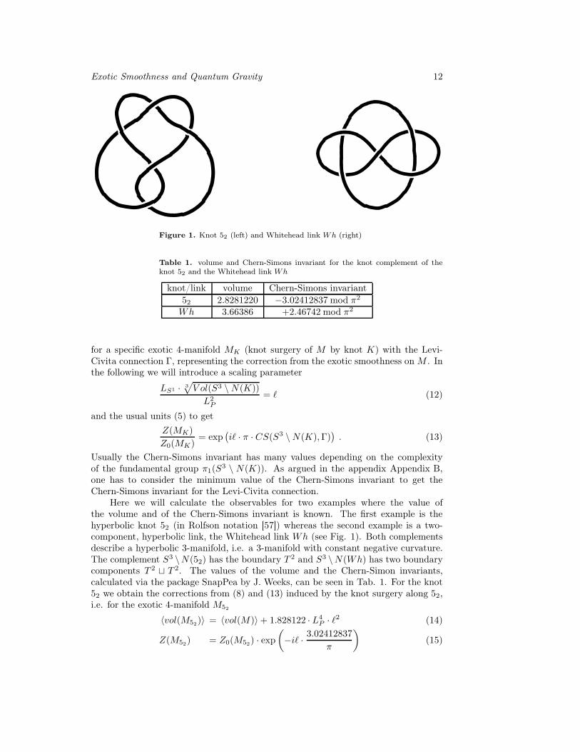
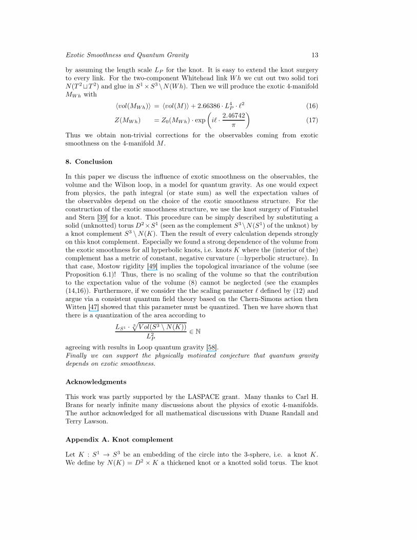
Figure 1. Knot 52 (left) and Whitehead link Wh (right)

Table 1. volume and Chern-Simons invariant for the knot complement of theknot 52 and the Whitehead link Wh

knot/link volume Chern-Simons invariant

52 2.8281220 −3.02412837 mod π2

Wh 3.66386 +2.46742 mod π2

for a specific exotic 4-manifold MK (knot surgery of M by knot K) with the Levi-Civita connection Γ, representing the correction from the exotic smoothness on M . Inthe following we will introduce a scaling parameter

LS1 · 3

√

V ol(S3 \N(K))

L2P

= ℓ (12)

and the usual units (5) to get

Z(MK)

Z0(MK)= exp

(

iℓ · π · CS(S3 \N(K),Γ))

. (13)

Usually the Chern-Simons invariant has many values depending on the complexityof the fundamental group π1(S

3 \ N(K)). As argued in the appendix Appendix B,one has to consider the minimum value of the Chern-Simons invariant to get theChern-Simons invariant for the Levi-Civita connection.

Here we will calculate the observables for two examples where the value ofthe volume and of the Chern-Simons invariant is known. The first example is thehyperbolic knot 52 (in Rolfson notation [57]) whereas the second example is a two-component, hyperbolic link, the Whitehead link Wh (see Fig. 1). Both complementsdescribe a hyperbolic 3-manifold, i.e. a 3-manifold with constant negative curvature.The complement S3 \N(52) has the boundary T 2 and S3 \N(Wh) has two boundarycomponents T 2 ⊔ T 2. The values of the volume and the Chern-Simon invariants,calculated via the package SnapPea by J. Weeks, can be seen in Tab. 1. For the knot52 we obtain the corrections from (8) and (13) induced by the knot surgery along 52,i.e. for the exotic 4-manifold M52

〈vol(M52)〉 = 〈vol(M)〉+ 1.828122 · L4P · ℓ2 (14)

Z(M52) = Z0(M52) · exp(

−iℓ · 3.02412837π

)

(15)

Exotic Smoothness and Quantum Gravity 13

by assuming the length scale LP for the knot. It is easy to extend the knot surgeryto every link. For the two-component Whitehead link Wh we cut out two solid toriN(T 2⊔T 2) and glue in S1×S3 \N(Wh). Then we will produce the exotic 4-manifoldMWh with

〈vol(MWh)〉 = 〈vol(M)〉+ 2.66386 · L4P · ℓ2 (16)

Z(MWh) = Z0(MWh) · exp(

iℓ · 2.46742π

)

(17)

Thus we obtain non-trivial corrections for the observables coming from exoticsmoothness on the 4-manifold M .

8. Conclusion

In this paper we discuss the influence of exotic smoothness on the observables, thevolume and the Wilson loop, in a model for quantum gravity. As one would expectfrom physics, the path integral (or state sum) as well the expectation values ofthe observables depend on the choice of the exotic smoothness structure. For theconstruction of the exotic smoothness structure, we use the knot surgery of Fintusheland Stern [39] for a knot. This procedure can be simply described by substituting asolid (unknotted) torus D2×S1 (seen as the complement S3\N(S1) of the unknot) bya knot complement S3 \N(K). Then the result of every calculation depends stronglyon this knot complement. Especially we found a strong dependence of the volume fromthe exotic smoothness for all hyperbolic knots, i.e. knots K where the (interior of the)complement has a metric of constant, negative curvature (=hyperbolic structure). Inthat case, Mostow rigidity [49] implies the topological invariance of the volume (seeProposition 6.1)! Thus, there is no scaling of the volume so that the contributionto the expectation value of the volume (8) cannot be neglected (see the examples(14,16)). Furthermore, if we consider the the scaling parameter ℓ defined by (12) andargue via a consistent quantum field theory based on the Chern-Simons action thenWitten [47] showed that this parameter must be quantized. Then we have shown thatthere is a quantization of the area according to

LS1 · 3

√

V ol(S3 \N(K))

L2P

∈ N

agreeing with results in Loop quantum gravity [58].Finally we can support the physically motivated conjecture that quantum gravitydepends on exotic smoothness.

Acknowledgments

This work was partly supported by the LASPACE grant. Many thanks to Carl H.Brans for nearly infinite many discussions about the physics of exotic 4-manifolds.The author acknowledged for all mathematical discussions with Duane Randall andTerry Lawson.

Appendix A. Knot complement

Let K : S1 → S3 be an embedding of the circle into the 3-sphere, i.e. a knot K.We define by N(K) = D2 ×K a thickened knot or a knotted solid torus. The knot

Exotic Smoothness and Quantum Gravity 14

complement S3 \ N(K) results in cutting N(K) off from the 3-sphere S3. Then oneobtains a 3-manifold with boundary ∂(S3 \N(K)) = T 2. The properties of the knotcomplement depend strongly on the properties of the knot K. So, the fundamentalgroup π1(S

3 \N(K)) is also denoted as knot group. In contrast, the homology groupH1(S

3 \N(K)) = Z don’t depend on the knot.

Appendix B. Chern-Simons invariant

Let P be a principal G bundle over the 4-manifold M with ∂M 6= 0. Furthermore letA be a connection in P with the curvature

FA = dA+A ∧ A

and Chern class

C2 =1

8π2

∫

M

tr(FA ∧ FA)

for the classification of the bundle P . By using the Stokes theorem we obtain∫

M

tr(FA ∧ FA) =

∫

∂M

tr(A ∧ dA+2

3A ∧ A ∧A)

with the Chern-Simons invariant

CS(A, ∂M) =1

8π2

∫

∂M

tr(A ∧ dA+2

3A ∧A ∧ A) . (B.1)

Now we consider the gauge transformation A → g−1Ag + g−1dg and obtain

CS(g−1Ag + g−1dg, ∂M) = CS(A, ∂M) + k

with the winding number

k =1

24π2

∫

∂M

(g−1dg)3 ∈ Z

of the map g : M → G. Thus the expression

CS(A, ∂M) mod 1

is an invariant, the Chern-Simons invariant. Now we will calculate this invariant. Forthat purpose we consider the functional (B.1) and its first variation vanishes

δCS(A, ∂M) = 0

because of the topological invariance. Then one obtains the equation

dA+A ∧A = 0 ,

i.e. the extrema of the functional are the connections of vanishing curvature. The set ofthese connections up to gauge transformations is equal to the set of homomorphismsπ1(∂M) → SU(2) up to conjugation. Thus the calculation of the Chern-Simonsinvariant reduces to the representation theory of the fundamental group into SU(2).In [59] the authors define a further invariant

τ(Σ) = min {CS(α)| α : π1(Σ) → SU(2)}

Exotic Smoothness and Quantum Gravity 15

for the 3-manifold Σ. This invariants fulfills the relation

τ(Σ) =1

8π2

∫

Σ×R

tr(FA ∧ FA)

which is the minimum of the Yang-Mills action∣

∣

∣

∣

∣

∣

1

8π2

∫

Σ×R

tr(FA ∧ FA)

∣

∣

∣

∣

∣

∣

≤ 1

8π2

∫

Σ×R

tr(FA ∧ ∗FA)

i.e. the solutions of the equation FA = ± ∗ FA. Thus the invariant τ(Σ) of Σcorresponds to the self-dual and anti-self-dual solutions on Σ×R, respectively. Or theinvariant τ(Σ) is the Chern-Simons invariant for the Levi-Civita connection.

References

[1] C. Duston. Exotic smoothness in 4 dimensions and semiclassical Euclidean quantum gravity.arXiv: 0911.4068, 2009.

[2] T. Asselmeyer-Maluga and C.H. Brans. Exotic Smoothness and Physics. WorldScientific Publ.,Singapore, 2007.

[3] J. Milnor. On manifolds homeomorphic to the 7-sphere. Ann. Math., 64:399 – 405, 1956.[4] M.A. Kervaire and J. Milnor. Groups of homotopy spheres: I. Ann. Math., 77:504 – 537, 1963.[5] R. Kirby and L.C. Siebenmann. Foundational essays on topological manifolds, smoothings, and

triangulations. Ann. Math. Studies. Princeton University Press, Princeton, 1977.[6] Ž. Bižaca and J. Etnyre. Smooth structures on collarable end of 4-manifolds. Topology, 37:461–

467, 1998.[7] R.E. Gompf and A.I. Stipsicz. 4-manifolds and Kirby Calculus. American Mathematical Society,

1999.[8] R Gompf. An infinite set of exotic R4’s. J. Diff. Geom., 21:283–300, 1985.[9] M.H. Freedman and L.R. Taylor. A universal smoothing of four-space. J. Diff. Geom., 24:69–78,

1986.[10] C.H. Taubes. Gauge theory on asymptotically periodic 4-manifolds. J. Diff. Geom., 25:363–430,

1987.[11] E. Witten. Topological quantum field theory. Comm. Math. Phys., 117:353–386, 1988.[12] J. Sładkowski. Exotic smoothness, noncommutative geometry and particle physics. Int. J.

Theor. Phys., 35:2075–2083, 1996.[13] J. Sładkowski. Exotic smoothness and particle physics. Acta Phys. Polon., B 27:1649–1652,

1996.[14] J. Sładkowski. Exotic smoothness, fundamental interactions and noncommutative geometry.

hep-th/9610093, 1996.[15] S. Stolz. Exotic structures on 4-manifolds detected by spectral invariants. Inv. Math., 94:147–

162, 1988.[16] C.H. Brans and D. Randall. Exotic differentiable structures and general relativity. Gen. Rel.

Grav., 25:205, 1993.[17] C.H. Brans. Localized exotic smoothness. Class. Quant. Grav., 11:1785–1792, 1994.[18] C.H. Brans. Exotic smoothness and physics. J. Math. Phys., 35:5494–5506, 1994.[19] T. Asselmeyer. Generation of source terms in general relativity by differential structures. Class.

Quant. Grav., 14:749 – 758, 1996.[20] J. Sładkowski. Gravity on exotic R4 with few symmetries. Int.J. Mod. Phys. D, 10:311–313,

2001.[21] T. Asselmeyer-Maluga and C.H. Brans. Cosmological anomalies and exotic smoothness

structures. Gen. Rel. Grav., 34:1767–1771, 2002.[22] J. Sładkowski. Exotic smoothness and astrophysics. Act. Phys. Polon. B, 40:3157–3163, 2009.[23] T. Asselmeyer-Maluga and H. Rosé. Dark energy and 3-manifold topology. Act. Phys. Pol.,

38:3633–3639, 2007.[24] J. Krol. Background independence in quantum gravity and forcing constructions. Found. of

Physics, 34:361–403, 2004.[25] J. Krol. Exotic smoothness and non-commutative spaces.the model-theoretic approach. Found.

of Physics, 34:843–869, 2004.

Exotic Smoothness and Quantum Gravity 16

[26] J. Król. Model theory and the ads/cft correspondence. presented at the IPM String School andWorkshop, Queshm Island, Iran, 05-14. 01. 2005, arXiv:hep-th/0506003.

[27] J. Król. A model for spacetime: The role of interpretation in some grothendieck topoi. Found.Phys., 36:1070, 2006.

[28] J. Król. A model for spacetime ii. the emergence of higher dimensions and field theory/stringsdualities. Found. Phys., 36:1778, 2006.

[29] J. Król. (quantum) gravity effects via exotic R4. Ann. Phys. (Berlin), 2010.[30] T. Asselmeyer-Maluga and J. Król. Gerbes, SU(2) WZW models and exotic smooth R4.

submitted to Comm. Math. Phys., arXiv: 0904.1276.[31] T. Asselmeyer-Maluga and J. Król. Gerbes on orbifolds and exotic smooth R4. subm. to Comm.

Math. Phys., arXiv: 0911.0271.[32] T. Asselmeyer-Maluga and J. Król. Exotic smooth R4, noncommutative algebras and

quantization. submitted to Comm. Math. Phys., arXiv: 1001.0882.[33] W. Thurston. Three-dimensional manifolds, Kleinian groups and hyperbolic geometry. Bull.

Amer. Math. Soc. (N.S.), 6:357–381, 1982.[34] S.W Hawking and G.F.R. Ellis. The Large Scale Structure of Space-Time. Cambridge University

Press, 1994.[35] E. Witten. Monopoles and four-manifolds. Math. Research Letters, 1:769–796, 1994.[36] S. Akbulut. Lectures on Seiberg-Witten invariants. Turkish J. Math., 20:95–119, 1996.[37] S. Donaldson. Polynomial invariants for smooth four manifolds. Topology, 29:257–315, 1990.[38] S. Donaldson and P. Kronheimer. The Geometry of Four-Manifolds. Oxford Univ. Press,

Oxford, 1990.[39] R. Fintushel and R. Stern. Knots, links, and 4-manifolds. Inv. Math., 134:363–400, 1998.

(dg-ga/9612014).[40] R Gompf. Sums of elliptic surfaces. J. Diff. Geom., 34:93–114, 1991.[41] R. Fintushel and R.J. Stern. Nondiffeomorphic symplectic 4-manifolds with the same Seiberg-

Witten invariants. Geom. Topol. Monogr., 2:103–111, 1999. arXiv:math/9811019.[42] R. Fintushel and R.J Stern. Families of simply connected 4-manifolds with the same Seiberg-

Witten invariants. aXiv:math/0210206, 2002.[43] S. Akbulut. A fake cusp and a fishtail. Turk. J. of Math., 23:19–31, 1999.[44] C. Misner, K. Thorne, and J. Wheeler. Gravitation. Freeman, San Francisco, 1973.[45] E. Witten. 2+1 dimensional gravity as an exactly soluble system. Nucl. Phys., B311:46–78,

1988/89.[46] E. Witten. Topology-changing amplitudes in 2+1 dimensional gravity. Nucl. Phys., B323:113–

140, 1989.[47] E. Witten. Quantization of Chern-Simons gauge theory with complex gauge group. Comm.

Math. Phys., 137:29–66, 1991.[48] W. Thurston. Three-Dimensional Geometry and Topology. Princeton University Press,

Princeton, first edition, 1997.[49] G.D. Mostow. Quasi-conformal mappings in n-space and the rigidity of hyperbolic space forms.

Publ. Math. IHÉS, 34:53–104, 1968.[50] E. Witten. Quantum field theory and the jones polynomial. Comm. Math. Phys., 121:351–400,

1989.[51] N.Y. Reshetikhin and V. Turaev. Invariants of three-manifolds via link polynomials and

quantum groups. Inv. Math., 103:547–597, 1991.[52] P. Scott. The geometries of 3-manifolds. Bull. London Math. Soc., 15:401–487, 1983.[53] M. Culler and P.B. Shalen. Varieties of group representations and splittings of 3-manifolds.

Ann. of Math., 117:109–146, 1983.[54] S. Gukov. Three-dimensional quantum gravity, chern-simons theory, and the A-polynomial.

Comm. Math. Phys., 255:577–627, 2005. arXiv: hep-th/0306165.[55] V. Turaev. Algebras of loops on surfaces, algebras of knots, and quantization. Adv. Ser. Math.

Phys., 9:59–95, 1989.[56] V.G. Turaev. Skein quantization of poisson algebras of loops on surfaces. Ann. Sci. de l’ENS,

24:635–704, 1991.[57] D. Rolfson. Knots and Links. Publish or Prish, Berkeley, 1976.[58] C. Rovelli and L. Smolin. Discreteness of area and volume in quantum gravity. Nucl. Phys.,

B442:593–622, 1995. Erratum-ibid. B456 (1995) 753.[59] R. Fintushel and R.J. Stern. Instanton homology of Seifert fibred homology three spheres. Proc.

London Math. Soc., 61:109–137, 1990.