The measurement of surface gravity

This article has been downloaded from IOPscience. Please scroll down to see the full text article.

2013 Rep. Prog. Phys. 76 046101

(http://iopscience.iop.org/0034-4885/76/4/046101)

Download details:

IP Address: 165.134.144.37

The article was downloaded on 19/03/2013 at 13:49

Please note that terms and conditions apply.

View the table of contents for this issue, or go to the journal homepage for more

Home Search Collections Journals About Contact us My IOPscience

IOP PUBLISHING REPORTS ON PROGRESS IN PHYSICS

Rep. Prog. Phys. 76 (2013) 046101 (47pp) doi:10.1088/0034-4885/76/4/046101

The measurement of surface gravityDavid Crossley1, Jacques Hinderer2 and Umberto Riccardi3

1 Department of Earth and Atmospheric Sciences, Saint Louis University, 3642 Lindell Blvd., St LouisMO 63108, USA2 Ecole et Observatoire des Sciences de la Terre, University of Strasbourg, CNRS, France3 Dipartimento di Scienze della Terra, dell’Ambiente e delle Risorse (DiSTAR) Universita ‘Federico II’di Napoli, L.go S Marcellino 10, 80138 Naples, Italy

E-mail: crossley@eas.slu.edu

Received 17 September 2012, in final form 3 December 2012Published 18 March 2013Online at stacks.iop.org/RoPP/76/046101

AbstractThis review covers basic theory and techniques behind the use of ground-based gravimetry atthe Earth’s surface. The orientation is toward modern instrumentation, data processing andinterpretation for observing surface, land-based, time-variable changes to the geopotential.The instrumentation side is covered in some detail, with specifications and performance of themost widely used models of the three main types: the absolute gravimeters (FG5, A10 fromMicro-g LaCoste), superconducting gravimeters (OSG, iGrav from GWR instruments), andthe new generation of spring instruments (Micro-g LaCoste gPhone, Scintrex CG5 and BurrisZLS). A wide range of applications is covered, with selected examples from tides and oceanloading, atmospheric effects on gravity, local and global hydrology, seismology and normalmodes, long period and tectonics, volcanology, exploration gravimetry, and some examples ofgravimetry connected to fundamental physics. We show that there are only a modest numberof very large signals, i.e. hundreds of µGal (10−8 m s−2), that are easy to see with allgravimeters (e.g. tides, volcanic eruptions, large earthquakes, seasonal hydrology). Themajority of signals of interest are in the range 0.1–5.0 µGal and occur at a wide range of timescales (minutes to years) and spatial extent (a few meters to global). Here the competingeffects require a careful combination of different gravimeter types and measurement strategiesto efficiently characterize and distinguish the signals. Gravimeters are sophisticatedinstruments, with substantial up-front costs, and they place demands on the operators tomaximize the results. Nevertheless their performance characteristics such as drift andprecision have improved dramatically in recent years, and their data recording ability andruggedness have seen similar advances. Many subtle signals are now routinely connected withknown geophysical effects such as coseismic earthquake displacements, post-glacial rebound,local hydrological mass balances, and detection of non-steric sea level changes.

(Some figures may appear in colour only in the online journal)

This article was invited by George T Gillies

Contents

1. Introduction 21.1. Short history 2

2. What is measured in gravity 32.1. Gravitational acceleration 32.2. The static field 42.3. Anomalies and corrections 52.4. Gravity and height variations 62.5. Gravity from Earth rotation 62.6. Time-variable gravity 7

3. Instrumentation 73.1. Absolute gravimeters 93.2. Spring gravimeters 103.3. Superconducting gravimeters 133.4. Gravimeter noise and precision 14

4. Applications of gravimetry 164.1. Tides 164.2. The atmosphere 194.3. Hydrology 21

0034-4885/13/046101+47$88.00 1 © 2013 IOP Publishing Ltd Printed in the UK & the USA

Rep. Prog. Phys. 76 (2013) 046101 D Crossley et al

4.4. Long periods and tectonics 244.5. Sea level and ocean circulation 254.6. Ground-satellite comparisons 264.7. Earthquakes and normal modes 284.8. Volcanology 32

4.9. Exploration gravimetry 344.10. Exotic gravimetry 38

5. Conclusions 39Acknowledgments 39References 39

1. Introduction

When a house sits on a slope, the owner knows the floors arenot parallel to the ground but horizontal, and the walls arevertical. To ensure this the builders use a bubble level for thefloors and a plumb line for the walls; in a well built house thewalls should be exactly 90 to the floors. If a constructionworker on the roof were to time the swing of his plumb line, orto drop an object to the ground and time its fall, he could alsofind an approximation to the local gravitational acceleration.Such ideas are central to gravimetry and geodesy—to definethe level surface for the instrument and to measure accelerationalong the plumb line. In absolute gravimeters (AGs) the objectis a falling corner cube, and in relative gravimeters the objectis a mass is supported against falling by either a spring or amagnetic field.

Our title emphasizes measurement because gravity isan area of physics where instrumentation has driven thedevelopment of data analysis techniques and theoreticalmodels. The new generation of AGs and superconductinggravimeters (SGs) now dominate the measurement of gravityat geodetic observatories and fundamental reference stations.Even for field deployment, the latest and more portableversions of AGs and SGs are becoming feasible to deployalongside the traditional spring instruments, though generallythe cost factor is still important in many applications.

A relatively new application is hydrology, which wasnot considered a useful signal 20 years ago, but today isan important research area, not least because it is connectedto global change. Of the many effects at a gravity station,hydrological mass transport due to variations in soil moistureand groundwater levels are the most widespread and least easilymodeled. The complete picture involves not only precipitationthat drives the system, and air properties that affect evaporation(temperature, pressure, humidity), but the complex pathwaysof runoff and infiltration involves multiple time and distancescales. In the past it was considered sufficient to removethe tidal and atmospheric signals from a gravity series beforeinterpreting the residuals, but today it is recognized thathydrology must frequently be dealt with before some of theweaker signals of interest (e.g. from seismic precursors orvolcanic unrest) can be clearly identified.

Newtonian gravity, based on classical physics, applies toall the examples here, and we refer to gravity as measuredon the surface of the Earth, this being the only astronomicalbody on which observations have been taken. Althoughgravity measurements using space techniques are not covered,we make an exception to discuss the comparison of groundgravity with satellite gravity from the gravity recovery andclimate experiment (GRACE) mission that has substantiallyimproved our knowledge of large-scale hydrological processes

on Earth. We do not treat several important areas ofgravity measurements, namely airborne, ocean, and boreholeapplications, as these each have their special instrumentationand processing requirements. The review is oriented towardtime-varying gravity rather than the static field, though thelatter has been considerably improved due to the inclusion ofdata from the GRACE and gravity field and ocean circulationexplorer (GOCE) missions. A section on gravity involvingfundamental physics concludes the coverage. We also notehere that Melchior (2008) gave an expert review (originallypublished about 1999) on the measurement of gravity just aboutthe time that SGs were becoming established (1997), and sincethen many other reviews of different aspects of gravimetry haveappeared (as mentioned later).

The SI unit appropriate to our topic is the nm s−2

(10−9 m s−2), but much of the gravity community still usesthe mGal (10−5 m s−2) and µGal (10−8 m s−2), the latter beingespecially useful for the small signals in this review. Withg ≈ 10 m s−2, a mGal is 1 part in 10−6 (1 ppm) and a µGalis 1 part in 10−9. At the limit of precision for SGs is thenanogal or nGal (10−11 m s−2), or 1 part in 10−12. Suchratios are sometimes loosely called ’accuracies’. Resolutionis determined by the number of meaningful digits that can beread by the electronics; it is related to the quantization level ofthe recorder (# bits) and can be as small as 0.1 nGal for SGs.

1.1. Short history

The first issue of the Bulletin d’Information des MareesTerrestres (BIM) in December 1956 is a convenient pointto connect with the history of gravimetry. It contained justtwo contributions, both on versions of a new instrument, thetidal gravimeter. The first (Woollard 1956) noted that a newLaCoste-Romberg (LR) gravimeter had just been completed,and contained an offer to construct further gravimeters, eachweighing about 120 kg (with all components) at a cost of $25keach. In the second paper on the installation of a gravimeterin Strasbourg, Lecolazet (1956) described his modifications toa field instrument for tidal purposes. The stimulus for suchmeasurements was the upcoming International GeophysicalYear (July 1957–December 1958). Lecolazet also referred toearly tidal recordings in a number of countries that had begunin 1954. BIM was to become the foremost publication in tidalstudies, extending to gravimetry in general, and it was thescientific journal of the International Center of Earth Tides(ICET) that was also started in 1956.

In the second issue of BIM, a short note from LaCosteto Melchior on the merits of two new tidal meters states‘... the comparison indicates an accuracy of better than 1microgal ...’. This was a notable achievement as the typicalfield gravimeter at that time had an accuracy of about 0.1 mGalor 100 µGal. Such accuracy was to remain the standard for

2

Rep. Prog. Phys. 76 (2013) 046101 D Crossley et al

most field gravimeters up to the introduction of the SG in themid 1980s. The most serious limitation of spring gravimetersfor periods longer than the main tides (1 day) remains theirinherent and unpredictable drift, though it is much reduced inrecent models. As we will see, there was a parallel historybetween 1960 and 1990 in the development of AGs and SGsin their respective domains of measurement.

2. What is measured in gravity

2.1. Gravitational acceleration

Classical theory defines the gravitational acceleration, or forceper unit mass, g as the gradient of the geopotential (here weuse a positive potential as in geodesy):

g = −gn = ∇W, g = |∇W |; (1)

where the direction n is the outward normal to the localequipotential surfaces (the level surfaces). Let us considersome of the contributions to this potential. The Newtonianattraction V is due to all masses (solid Earth, oceans,atmosphere) that act on the gravimeter. It is frequentlyexpressed as a spherical harmonic expansion over degree

and order m of the fully normalized associated Legendrefunctions Pm

V (r, θ, φ) = GM

r

max∑=0

∑m=0

(re

r

)

Pm(cosθ)

×[Cmcos(mφ) + Smsin(mφ)

](2)

where Cm and Sm are known in this context as Stokescoefficients (e.g. Torge 2012). We use a geocentric sphericalcoordinate system where (r, θ, φ) are radius, colatitude, andlongitude of a measurement point. Here re is a reference radius(e.g. the equatorial radiusa of an ellipsoid, or the mean radiusR

of the equivalent spherical Earth), G is Newton’s gravitationalconstant (6.674 × 10−11 m3 kg−1 s−2), and M is Earth’s mass(5.974 × 1024 kg). Note that the shortest half wavelengththat can be resolved at r = re with such an expansion isλ1/2 = πre/max, yielding 56 km for max = 360, and 9 kmfor max = 2190 (see table 2).

Because gravity is invariably measured on (or near) thesurface of a rotating planet, W has to include the centrifugalpotential

= 12

[r22 − (r.Ω)2

]= 122r2sin2θ, (3)

where = e3 is the rotation angular velocity of the Earth inthe space fixed direction e3. The Earth also experiences a tidalforce from the Moon, Sun and planets (out to Saturn). Thetidal force is a differential force appearing between a point Pon the surface of the Earth and its center of mass O, and it isthe gradient of the tidal potential WT. For the simple case ofthe Moon it is shown (e.g. Stacey (1992, p 116)) that the totalpotential WM at P can be expressed as

WM = Gm

R

(1 +

m

2(M + m)

)+

Gma2

2R3

(3cos2ψ − 1

)

+1

2ω2

La2sin2θ. (4)

where m is the Moon’s mass, ψ the angle between the line OP(radius a) and the Earth–Moon distance R, θ the colatitude ofP and ωL is the orbital angular velocity of the Earth about theEarth–Moon barycenter. The first term is a simplified formof the static potential V slightly modified by the lunar mass,and the second term is the tidal potential of degree 2, W2. Thethird term is the centrifugal potential of the Earth about thebarycenter of the Earth–Moon system. Because this has thesame form as in (3), we can regard ωL as a small additionto (ωL ). The more general tidal potential including alldegrees can be written in this geometry (e.g. Agnew (2007)) as

WT(a, ψ) = GM

R

∞∑n=2

(a

R

)n

Pn(cos ψ), (5)

where we switch to degree n for tides rather than to avoidlater confusion with Love numbers. Equations (2)–(5) give themost important contributions to the potential W = V ++WT.

Ideally a gravimeter should have the axis of its sensoraligned with the plumb line n, but if tilted through a smallangle β the measured gravity will have an apparent reductionof δβ = gcosβ − g ≈ g(β)2/2. This amounts to −0.49 ×10−3 µGal µrad−2, so a gravity meter must be leveled to about9 arcsec (∼45 µrad) to achieve a precision of 1 µGal. Allgravimeters therefore require at least a very precise initialadjustment to reach this tilt minimum, and some (the SGs) havea built-in tilt measurement and feedback system to dynamicallymaintain a true level (Hinderer et al 2007, Riccardi et al 2009).Most of the contributions to time-variable gravity, apart fromtheir direct effects (such as mass or height changes), will alsoperturb the level equipotential surfaces. If not corrected in realtime, this effect gives an unwanted tilt contribution (gravityreduction) to the measurement.

Relative gravimeters are essentially no different inprinciple from seismometers (or accelerometers), andtherefore they measure exactly the same contributions toacceleration. To emphasize this point, we use an expression forthe total acceleration measured by a seismometer on a sphericalEarth in response to a harmonic deformation of frequency ω

and spherical harmonic degree (e.g. Dahlen and Tromp (1998p 238)) that has a true vertical displacement u1

g(R) = ω2u1 + 2g0u1/R + ( + 1)ψ/R. (6)

The inertial term (ω2u1) gives the ground acceleration,the second term (2g0u1/R) gives the effect of verticaldisplacement u1 of the instrument through a surfacegravitational field g0 (at radius R), and the final term indicatesthe redistribution of surface potential ψ . Seismometersrespond predominantly at high frequencies (e.g. ω2 ∼ 1–100 Hz) so the first term in equation (6) dominates, and to agood approximation g = ω2u where u is the effective grounddisplacement. A gravimeter, on the other hand, operates atfrequencies below 1 Hz, where the inertial term in (6) is muchsmaller and so

g(R) ≈ 2g0u1/R + ( + 1)ψ/R. (7)

3

Rep. Prog. Phys. 76 (2013) 046101 D Crossley et al

Table 1. The World Geodetic System WGS84.

Parameter Symbol Value

Equatorial radius (m) a 6 378 137.0Flattening (b-a)/a f 1/298.257 223 563 1Equatorial gravity (m s−2) γa 9.780 322 677 14Normal gravitational constant k 0.001 931 851 386 39(First numerical ellipticity)2 e2 0.006 694 379 990 13

2.2. The static field

Geodesy is a complex subject with a long history and wewill outline only essential concepts; many textbooks (e.g.Torge (2012)) are available for the details. We start witha Geodetic Reference System (GRS) model that defines areference ellipsoid that is the best fit to the actual gravityfield of the Earth; this is the basis of all geodetic calculations.WGS84 is one such model defined by two parameters for thegeometry (a,f) and 3 parameters for the gravity field on theellipsoid (γe, k, e2), as in table 1 (NIMA 2000, Jekeli 2012).There are slight variations in these parameters depending onthe application, e.g. satellite altimetry.

It can be seen that the constants are defined to highprecision. The differences between WGS84 and previousversions are very small, for example the polar radius haschanged by only 0.1 mm. WGS84 is an Earth-based (or body)reference frame that coincides with the International TerrestrialReference (ITRF94)—a spatial reference frame co-rotatingwith the Earth and defined by space geodetic measurements—to an accuracy of about 2 cm (NIMA 2000), or about 6 µGalin surface gravity/height equivalence. The geocenter (of theEarth’s mass) is known to depart from the center of the ITRFby a motion of several mm/yr (Swenson et al 2008).

The appropriate coordinate system on the oblate Earthis ellipsoidal, and given by geodetic coordinates (h, φ, λ)—(ellipsoidal height, ellipsoidal latitude, longitude). From theparameters in table 1, the gravity on the level ellipsoid (h = 0),i.e. the gradient of the normal potential U, becomes

γ0(φ) = |∇U0| = γa(1 + k sin2φ)(1 − e2sin2φ)−1/2 (8)

which is an exact representation, and should be the preferredformula for the variation of gravity with latitude, as arguedby Featherstone and Dentith (1997). Various versions of theInternational Gravity Formula—long used in gravity surveys(e.g. Telford et al (1990))—are simplified versions of thisexpression, but have older constants and are inadequate forprecise work. The normal gravity at height h above theellipsoid can also be expressed in terms of the referencemodel as

γ (h, φ) = |∇U |= γ0

[(1 − 2

a(1 + f + m − 2f sin2φ)h +

3

a2h2

], (9)

where m = (2a2b2/GM) is the ratio of centrifugalacceleration to gravity at the equator. It is also convenientto express the normal potential as a sum of zonal spherical

harmonics (r, θ ) (there is no longitudinal variation)

U(r, θ) = GM

r

[1 −

∞∑=1

(a

r

)2

J2P2(cosθ)

]+ (r, θ)

(10)

with the coefficients J2 given as simple functions of f, e, C −A (the difference in polar-equatorial moments of inertia), andM; see e.g. Torge (2012). A geodetic model (WGS84) isderived for different purposes than a seismic Earth modelsuch as PREM (Dziewonski and Anderson 1981), but theyare connected by the constraint of a compatible Earth mass M

and polar moment of inertia C. PREM is a radial model withR = 6371 km and surface gravity g0 = 9.81557 m s−2.

There have been substantial improvements to the actualmeasured global (static) gravity field of the Earth in the lastdecade since the launch of the GRACE twin satellites in2002 (Tapley et al 2004). Table 2 shows the parametersand statistics of some recent models generated with thehelp of GRACE data, extracted from the ICGEM websitehttp://icgem.gfz-potsdam.de/ICGEM/ICGEM.html. Note thatall the models in table 2 are a combination of satellite data withground gravity, but many other satellite-only models are alsoavailable. It is now standard practise to use the geoid heightN to compare such global field models. Denoting by H theorthometric height (classical leveling) of a station above meansea level, and by h the ellipsoidal height in (9), the geoid heightN is the difference

N = h − H (11)

(e.g. Barthelmes (2009)). These quantities are properly definedin ellipsoidal coordinates (φ, λ), not the spherical coordinatesused in equation (2). Equivalent quantities in sphericalcoordinates can also be derived, albeit with some error. Intable 2 the final columns of geoid height differences fromground GPS sites agree with global gravity models at about the20 cm level. But note that satellite solutions have much betteraccuracy at long wavelengths; for example at scales 200 kmthe geoid height error is about 3 cm, which is similar to thedifference between WGS84 and ITRF94, noted above.

EGM2008 is the highest resolution gravity and geoidmodel currently available, at http://earth-info.nga.mil/GandG/wgs84/gravitymod/egm2008/egm08 wgs84.html. Here thesatellite data provide reliable information up to about degree115, thereafter the higher degrees are based on traditionalground-based gravity surveys. Gravity anomalies arecomputed from the ground surveys on a 5′ ×5′ grid and requireextensive processing to remove regional bias and processinginconsistencies between different eras, surveys, and nationaldatabases.

A notable feature of the model EIGEN-6C (table 2) isthat it includes time variations of the harmonic coefficients,to allow for drift and secular variation due to mass motions;this is important especially for satellite gravimetry (Forsteet al 2011). This approach (maybe unfortunately) blurs thedistinction between the classical (static) gravity field, and thetreatment of time-variable gravity, though as in geomagnetismthe idea of a constant field is a myth.

4

Rep. Prog. Phys. 76 (2013) 046101 D Crossley et al

Table 2. Some recent global gravity models.

Model Year max Data sourcea Reference USAb Europeb

EIGEN-6C 2011 1420 S(GR,GO,LA),G,A Forste et al 2011 0.247 0.214EIGEN-51C 2010 360 S(GR,CH),G,A Bruinsma et al (2010) 0.335 0.289EIGEN-5C 2008 360 S(GR,LA),G,A Forste et al (2011) 0.341 0.303EGM2008 2008 2190 S(GR),G Pavlis et al (2008) 0.248 0.208

a S=satellite (GRACE, CHAMP, LAGEOS, GOCE), G=ground gravity, A=altimeter.b rms geoid height differences (m) between GPS/leveling and the gravity field model.

2.3. Anomalies and corrections

Geoid heights are of primary interest to any activity usingelevation, and especially national geodetic grids, because theyallow the conversion of GPS ellipsoidal heights to orthometricheights (equation (11)). Gravity anomalies (associated withthe static field) and gravity residuals (associated with time-variable gravity) are the difference between a measured valueand a reference or a model value, that can be chosen accordingto the purpose. For the static field, the various geodeticanomalies are defined on the ICGM website, under functionsof the geopotential (Barthelmes 2009). Assuming quantitiesare computed at the same ellipsoidal coordinates (λ, φ), themost direct estimate of gravity is called in geodesy the gravitydisturbance

δg(h) = gobs(h) − γ (h), (12)

where gobs(h) is the observed gravity at a station, and γ (h) isgiven by equation (9). This is very different from the classicalgravity anomaly, that is the difference between the gravity onthe geoid minus normal gravity on the ellipsoid, at the samestation coordinates, which is difficult to determine without ageoid model. In modern geodesy the preferred gravity anomalyis given by

δg(h) = gobs(h) − γ (h − ζ ), (13)

where ζ is the height anomaly defined indirectly through thepotential

W(h) = U(h − ζ ) (14)

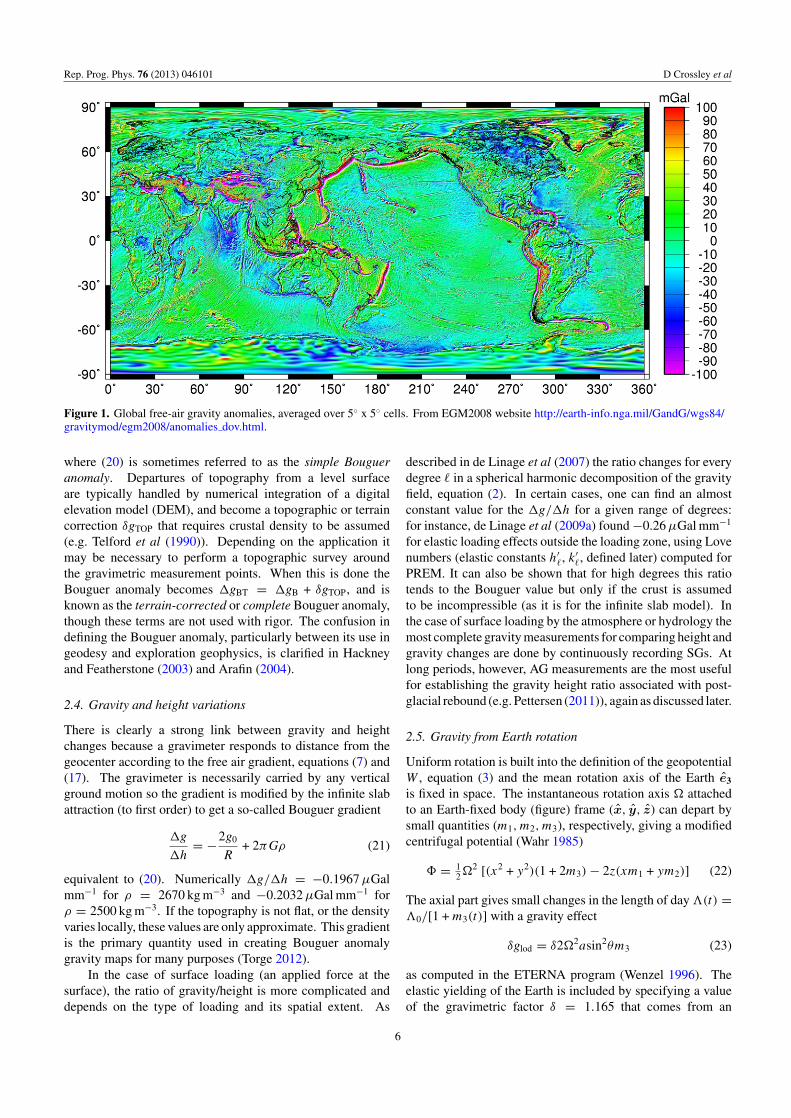
i.e. the height for which the ellipsoid equipotential has thesame value as the station equipotential. The reason for thischoice is that equation (13) can be evaluated using sphericalharmonic expansions of the potentials (U, W ) using formulaesuch as (2) and (10), and is thus useful for satellite as well assurface fields. To give an example, figure 1 shows the globalfree air gravity anomalies (13) computed for EGM2008. Therange is approximately ±100 mGal and clearly shows majorplate tectonic features such as plate boundaries.

The differences between the various types of gravityanomalies introduced above (and their spherical earthequivalents) can reach 20–30 mGal, and therefore cannotbe ignored for modern geodetic and geophysical purposes,especially at long wavelengths. To capture detailed crustalstructure requires anomalies at the mGal level over hundredsof km, and processing for geophysical exploration requiresanomalies at sub-mGal accuracy at scale of a km or less.

For a geodesist it is important to know that models suchas WGS84 include the atmosphere as part of the total Earth

mass enclosed by the reference ellipsoid; hence variationsin atmospheric density are not part of the normal gravity.For ground-based stations, the gravity disturbance may becorrected for the atmosphere above the station to get surfacegravity

gS = δg(h) + δgA (15)

where the atmospheric correction can be approximated by

δgA = 0.87e−0.116H 1.047mGal (16)

and H is the orthometric height in km. For station Ghuttu at1880 m in the Himalayas (part of the Global GeodynamicsProject SG network; Arora et al (2008)) the correction is0.695 mGal compared to 0.87 mGal at mean sea level. Thedifference of 175 µGal is important for geodetic purposes, butwould not be included for geophysical surveys, nor does itenter the time variations at a single station.

The traditional gravity reductions used in geophysics cannow be summarized. We start with the surface gravity gS inequations (12) and (15), and note the latitude effect need notbe treated separately as it is included in the definition of γ0

equation (8). The free air effect can be obtained from thederivative of equations (9) and (10):

δgFA = ∂γ

∂h≈ −2g0

RH, (17)

where H is the datum height (that can be freely chosen)in m. The numerical value is −3.086 µm s−2 m−1 or−0.3086 µGal mm−1. In addition, corrections for topographyare extremely important for computing the geoid and necessaryfor gravity surveys in hilly terrain. In practice the correctionis done first by computing the effect of an infinite horizontallayer of density ρ and thickness H (the Bouguer slab or plate):

δgB = 2πGρ H. (18)

Using ρ = 2670 kg m−3 as an average crustal density givesan effect of 1.11873 µm s−2 m−1 or 0.11873 µGal mm−1. Asometimes-forgotten technique for estimating ρ is that ofminimizing the cross correlation between topography and theresulting Bouguer anomaly (Nettleton 1976, p 91). Applyingthese corrections (note that corrections are the negative of theeffects) to surface gravity gS gives the traditional geophysicalanomalies as:

Free air anomalygFA = gS − δgFA (19)

Bouguer anomalygB = gS − δgFA − δgB, (20)

5

Rep. Prog. Phys. 76 (2013) 046101 D Crossley et al

Figure 1. Global free-air gravity anomalies, averaged over 5 x 5 cells. From EGM2008 website http://earth-info.nga.mil/GandG/wgs84/gravitymod/egm2008/anomalies dov.html.

where (20) is sometimes referred to as the simple Bougueranomaly. Departures of topography from a level surfaceare typically handled by numerical integration of a digitalelevation model (DEM), and become a topographic or terraincorrection δgTOP that requires crustal density to be assumed(e.g. Telford et al (1990)). Depending on the application itmay be necessary to perform a topographic survey aroundthe gravimetric measurement points. When this is done theBouguer anomaly becomes gBT = gB + δgTOP, and isknown as the terrain-corrected or complete Bouguer anomaly,though these terms are not used with rigor. The confusion indefining the Bouguer anomaly, particularly between its use ingeodesy and exploration geophysics, is clarified in Hackneyand Featherstone (2003) and Arafin (2004).

2.4. Gravity and height variations

There is clearly a strong link between gravity and heightchanges because a gravimeter responds to distance from thegeocenter according to the free air gradient, equations (7) and(17). The gravimeter is necessarily carried by any verticalground motion so the gradient is modified by the infinite slabattraction (to first order) to get a so-called Bouguer gradient

g

h= −2g0

R+ 2πGρ (21)

equivalent to (20). Numerically g/h = −0.1967 µGalmm−1 for ρ = 2670 kg m−3 and −0.2032 µGal mm−1 forρ = 2500 kg m−3. If the topography is not flat, or the densityvaries locally, these values are only approximate. This gradientis the primary quantity used in creating Bouguer anomalygravity maps for many purposes (Torge 2012).

In the case of surface loading (an applied force at thesurface), the ratio of gravity/height is more complicated anddepends on the type of loading and its spatial extent. As

described in de Linage et al (2007) the ratio changes for everydegree in a spherical harmonic decomposition of the gravityfield, equation (2). In certain cases, one can find an almostconstant value for the g/h for a given range of degrees:for instance, de Linage et al (2009a) found −0.26 µGal mm−1

for elastic loading effects outside the loading zone, using Lovenumbers (elastic constants h′

, k′, defined later) computed for

PREM. It can also be shown that for high degrees this ratiotends to the Bouguer value but only if the crust is assumedto be incompressible (as it is for the infinite slab model). Inthe case of surface loading by the atmosphere or hydrology themost complete gravity measurements for comparing height andgravity changes are done by continuously recording SGs. Atlong periods, however, AG measurements are the most usefulfor establishing the gravity height ratio associated with post-glacial rebound (e.g. Pettersen (2011)), again as discussed later.

2.5. Gravity from Earth rotation

Uniform rotation is built into the definition of the geopotentialW , equation (3) and the mean rotation axis of the Earth e3

is fixed in space. The instantaneous rotation axis attachedto an Earth-fixed body (figure) frame (x, y, z) can depart bysmall quantities (m1, m2, m3), respectively, giving a modifiedcentrifugal potential (Wahr 1985)

= 122 [(x2 + y2)(1 + 2m3) − 2z(xm1 + ym2)] (22)

The axial part gives small changes in the length of day (t) =0/[1 + m3(t)] with a gravity effect

δglod = δ22asin2θm3 (23)

as computed in the ETERNA program (Wenzel 1996). Theelastic yielding of the Earth is included by specifying a valueof the gravimetric factor δ = 1.165 that comes from an

6

Rep. Prog. Phys. 76 (2013) 046101 D Crossley et al

Earth model such as PREM. Replacing m3 by δ/0 (0 =86 400 s) we find at the equator δglod = 0.091 µGal ms−1. Thelargest contribution to δ are decadal fluctuations at about5 ms amplitude, and smaller fluctuations of 1–2 ms due tothe atmosphere at various timescales (Hide and Dickey 1991).The LOD effect is therefore less than 0.5 µGal and frequentlyneglected.

The gravity effect of the polar motion, due to the (x, y)components of (22), is much larger and determined from

δgpm = −δ2asin2θ(m1cos λ + m2sin λ). (24)

At mid-latitudes δgpm = 3.96 µGal rad−1, with m1 and m2

in radians, giving at most a variation of about 15 µGal ingravity that is easily detected in SG records. Using IERSdata for (m1, m2), the polar motion correction has now becomestandard for all SG and AG data processing, and extremely welldefined by space geodetic data (e.g. VLBI). All SG stationshave been able to detect periodic polar motion that consistsmainly of an annual term (365 days), due to the atmosphere andhydrosphere, and a 435-day component due to the Chandlerwobble (CW) of the Earth’s rotation axis e3 about the figureaxis z (as seen in the body frame).

2.6. Time-variable gravity

In the same way that gravity surveys are corrected for knowneffects to produce spatial gravity anomalies, there are a numberof steps to reducing time-variable gravity observations (see e.g.Hinderer et al (2007)). A gravity time series g(obs) can bedecomposed into a series of additive effects:

g(obs) = g(disturbances – instrument and site origin,

earthquakes)

+g(tides – solid Earth, ocean)

+g(atmosphere – nominal admittance correction)

+g(polar motion – annual and Chandler)

+g(drift – instrument)

+g(hydro – rainfall, soil moisture, groundwater,

surface water, ice)

+g(other – ocean currents, tectonics, slow

earthquakes, GIA, .......) (25)

where g(other) includes all other possible signals. Theprocedure for all instruments (particularly AGs and SGs)is to subtract contributions that can be modeled with someconfidence, and then to subject the residual to more detailedrefinement or interpretation. The corrections most easily dealtwith are the first five (disturbances - drift) and they can besummed to yield a g(model). The residual consists of effectsthat are the topic of current research: g(res) = g(obs) - g(model)= g(hydro) + g(other).

The corrections depend somewhat on the instrument.For AGs, the disturbances are minimized by the rejectionof noisy ‘set values’ (see later) and although there is noinstrument drift, other subtle effects such as the instrumentheight and the gravity gradient need to be specified. SGsare influenced by all the effects noted above because of their

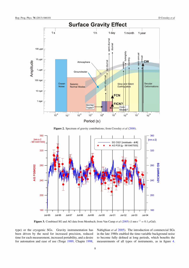
broad spectrum; this makes them extremely useful, but requiresmuch care in the processing to separate the contributions. Oneway to visualize the various contributions is to show themschematically (figure 2) in terms of amplitude (µGal) versusperiod. We divide the contributions into two types of signal:

(a) Periodic: tides, polar motion, wobbles and nutations, andseismic elastic normal modes

(b) Aperiodic: atmospheric pressure, hydrology, volcanic,non-tidal ocean circulation, and general earth deformationas above.

The periodic signals are discrete vertical lines, except forseismic normal modes that are shown as a block because thereare many close-spaced modes visible after a large earthquake.The aperiodic constituents each form a continuous spectrum,for which we convert the power spectral density to a normalizedequivalent time-domain amplitude. Figure 2 is based on a largenumber of papers from SG recordings dating back to the late1980s. Station quality and sampling was not standardized untilabout 1997 when the Global Geodynamics Project (GGP) waslaunched as part of the SEDI Deep Earth initiative (Crossleyet al 1999), so the best data begin at about that time.

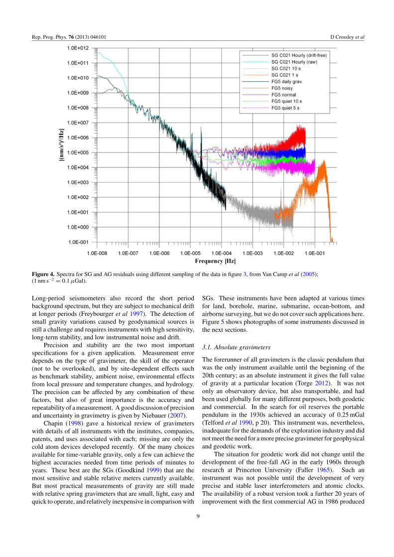
We show in figure 3 two series of gravity data from SGand AG instruments, based on 9 years of data from Membach,Belgium (Van Camp et al 2005). The SG data have beencorrected for the standard model (tides, atmospheric pressure,polar motion, and instrument drift), while the AG data havebeen processed identically except no drift is removed but aconstant value is subtracted. It can be seen there is generallyexcellent agreement within the error bars of the AG data(±20 nm s−2) or 2.0 µGal. The residual is dominated byseasonal (annual) hydrology variations of amplitude ±4 µGalwith some of the other signals in (22) undoubtedly present. Infigure 4, again from Van Camp et al (2005) we see a compositespectrum obtained by processing different forms of the datausing specialized criteria.

The long-period part of the spectrum shows the hourlySG residuals with and without drift removed, compared to theFG5 daily estimates. Between f = 10−7 Hz (100 days) and10−5 Hz (1 day) the three spectra are remarkably consistentand a period of 1 day represents the cross-over where the AGnoise level flattens out with decreasing period but the SG noisecontinues to fall. Further discussion of figure 4 will be givenin the appropriate sections below.

3. Instrumentation

Static gravity anomalies range from several 100 mGalassociated with tectonic and crustal features of 10’s–100’s km,to surveys requiring accuracies of 0.1 mGal for environmentalstudies or mineral exploration. Many signals in time-variable gravity are in the range 0.1–10 µGal, and someof these require monitoring over several years to achievesuccess; this poses much more stringent requirements thanspatial surveys. In gravimetry we have two complimentarydomains—absolute measurements that use almost exclusivelyAGs with a free-fall test mass, and relative measurementsusing either spring gravimeters (exploration type, or geodetic

7

Rep. Prog. Phys. 76 (2013) 046101 D Crossley et al

Figure 2. Spectrum of gravity contributions; from Crossley et al (2008).

Figure 3. Combined SG and AG data from Membach; from Van Camp et al (2005) (1 nm s−2 = 0.1 µGal).

type) or the cryogenic SGs. Gravity instrumentation hasbeen driven by the need for increased precision, reducedtime for each measurement, increased portability, and a desirefor automation and ease of use (Torge 1989, Chapin 1998,

Nabighian et al 2005). The introduction of commercial SGsin the late 1980s enabled the time-variable background noiseto become fully defined at long periods, which benefits themeasurements of all types of instruments, as in figure 4.

8

Rep. Prog. Phys. 76 (2013) 046101 D Crossley et al

Figure 4. Spectra for SG and AG residuals using different sampling of the data in figure 3, from Van Camp et al (2005);(1 nm s−2 = 0.1 µGal).

Long-period seismometers also record the short periodbackground spectrum, but they are subject to mechanical driftat longer periods (Freybourger et al 1997). The detection ofsmall gravity variations caused by geodynamical sources isstill a challenge and requires instruments with high sensitivity,long-term stability, and low instrumental noise and drift.

Precision and stability are the two most importantspecifications for a given application. Measurement errordepends on the type of gravimeter, the skill of the operator(not to be overlooked), and by site-dependent effects suchas benchmark stability, ambient noise, environmental effectsfrom local pressure and temperature changes, and hydrology.The precision can be affected by any combination of thesefactors, but also of great importance is the accuracy andrepeatability of a measurement. A good discussion of precisionand uncertainty in gravimetry is given by Niebauer (2007).

Chapin (1998) gave a historical review of gravimeterswith details of all instruments with the institutes, companies,patents, and uses associated with each; missing are only thecold atom devices developed recently. Of the many choicesavailable for time-variable gravity, only a few can achieve thehighest accuracies needed from time periods of minutes toyears. These best are the SGs (Goodkind 1999) that are themost sensitive and stable relative meters currently available.But most practical measurements of gravity are still madewith relative spring gravimeters that are small, light, easy andquick to operate, and relatively inexpensive in comparison with

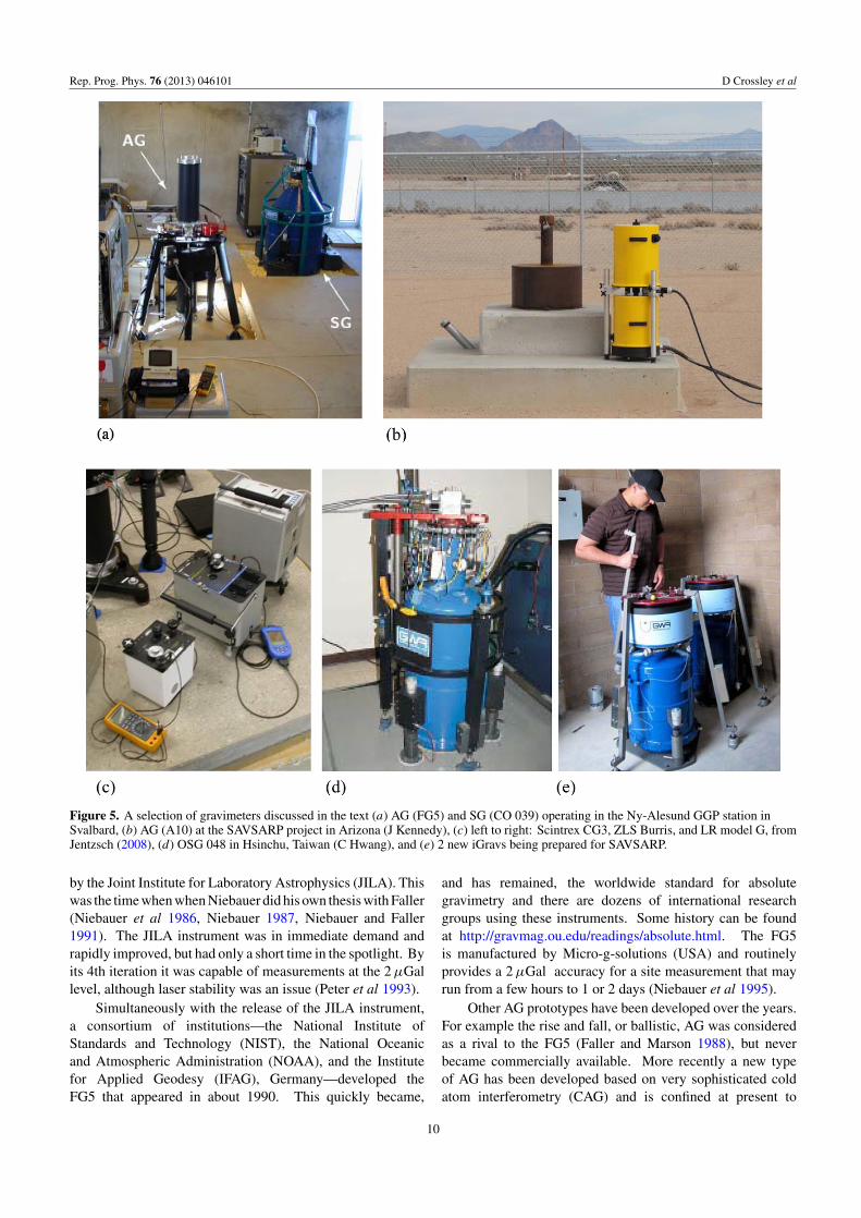
SGs. These instruments have been adapted at various timesfor land, borehole, marine, submarine, ocean-bottom, andairborne surveying, but we do not cover such applications here.Figure 5 shows photographs of some instruments discussed inthe next sections.

3.1. Absolute gravimeters

The forerunner of all gravimeters is the classic pendulum thatwas the only instrument available until the beginning of the20th century; as an absolute instrument it gives the full valueof gravity at a particular location (Torge 2012). It was notonly an observatory device, but also transportable, and hadbeen used globally for many different purposes, both geodeticand commercial. In the search for oil reserves the portablependulum in the 1930s achieved an accuracy of 0.25 mGal(Telford et al 1990, p 20). This instrument was, nevertheless,inadequate for the demands of the exploration industry and didnot meet the need for a more precise gravimeter for geophysicaland geodetic work.

The situation for geodetic work did not change until thedevelopment of the free-fall AG in the early 1960s throughresearch at Princeton University (Faller 1965). Such aninstrument was not possible until the development of veryprecise and stable laser interferometers and atomic clocks.The availability of a robust version took a further 20 years ofimprovement with the first commercial AG in 1986 produced

9

Rep. Prog. Phys. 76 (2013) 046101 D Crossley et al

Figure 5. A selection of gravimeters discussed in the text (a) AG (FG5) and SG (CO 039) operating in the Ny-Alesund GGP station inSvalbard, (b) AG (A10) at the SAVSARP project in Arizona (J Kennedy), (c) left to right: Scintrex CG3, ZLS Burris, and LR model G, fromJentzsch (2008), (d) OSG 048 in Hsinchu, Taiwan (C Hwang), and (e) 2 new iGravs being prepared for SAVSARP.

by the Joint Institute for Laboratory Astrophysics (JILA). Thiswas the time when when Niebauer did his own thesis with Faller(Niebauer et al 1986, Niebauer 1987, Niebauer and Faller1991). The JILA instrument was in immediate demand andrapidly improved, but had only a short time in the spotlight. Byits 4th iteration it was capable of measurements at the 2 µGallevel, although laser stability was an issue (Peter et al 1993).

Simultaneously with the release of the JILA instrument,a consortium of institutions—the National Institute ofStandards and Technology (NIST), the National Oceanicand Atmospheric Administration (NOAA), and the Institutefor Applied Geodesy (IFAG), Germany—developed theFG5 that appeared in about 1990. This quickly became,

and has remained, the worldwide standard for absolutegravimetry and there are dozens of international researchgroups using these instruments. Some history can be foundat http://gravmag.ou.edu/readings/absolute.html. The FG5is manufactured by Micro-g-solutions (USA) and routinelyprovides a 2 µGal accuracy for a site measurement that mayrun from a few hours to 1 or 2 days (Niebauer et al 1995).

Other AG prototypes have been developed over the years.For example the rise and fall, or ballistic, AG was consideredas a rival to the FG5 (Faller and Marson 1988), but neverbecame commercially available. More recently a new typeof AG has been developed based on very sophisticated coldatom interferometry (CAG) and is confined at present to

10

Rep. Prog. Phys. 76 (2013) 046101 D Crossley et al

research laboratories. Initial results are extremely promising incomparison with the optical FG5, achieving agreement withinabout 5 µGal (Merlet et al 2010). Portability will be the nextchallenge but the CAG has some advantages as it can measuremore frequently (several times a sec) than the FG5 and becauseof lack of mechanical wear. An improved version of theballistic AG (the IMGC-02) improves on the portability andaccuracy of the original instrument (Agostino et al 2008). Itcompares well with the FG5 and CAG at the 5–10 µGal level(Louchet-Chauvet et al 2010).

For a review of the operation of the FG5 we recommendNiebauer (2007). The instrument automatically drops andcatches a falling corner cube and measures drop length andtime using a laser interferometer and an atomic clock. Eachdrop cycle takes about 10 s, and about 100 drops are addedtogether to make a set value (these times are adjustable).After corrections for the tides, polar motion, and atmosphericpressure the set value has about a 2 µGal uncertainty. Usuallyone records for 1–2 days to get a site value with an estimatederror also in the 1–2 µGal range. The AG is a fundamentalmeasurement and the error budget is exhaustively analyzed toarrive at estimates of formal error, accuracy, and uncertainty,including all known instrument effects (Niebauer 2007, VanCamp et al 2005).

The AG data shown in figure 3 are taken with great care foraccuracy, recording for periods of up to 8 days continuouslyfor each value, which is longer than at most of the highquality geodetic sites in the GGP network. If one considersthe SG data, here with disturbances and instrumental offsetsremoved, to be essentially ‘error-free’, then some AG valuesdepart significantly from the SG curve. This is an indication(but not proof) of possible AG instrumental problems. Alltypes of AG have been regularly compared every 4 years,dating back to the 1st International Comparison of AbsoluteGravimeters (ICAG) held at the Bureau International desPoids et Mesures (BIPM) in Paris in 1981 (e.g. Vitushkinet al (2002)). The intercomparisons are used to assess thereliability of each AG compared to the mean group value,but offsets are not applied to past or future measurements.The Paris venue has been retired, but comparisons continueelsewhere (e.g. Francis and Van Dam (2006)). Jiang et al(2009) reported on two relative gravimeters (CG5 and Burris)that were included in (ICAG-2009) to monitor the relativedifference between the various instrument locations the AGcampaign. After about 16 repetitions of the gravity differencesbetween two locations, it was possible to reach an accuracy of1–2 µGal with such instruments, sufficient to track possibleerrors between different AGs.

Small AG offsets do occur in controlled experiments; forexample, Van Camp et al (2003) compared 4 well-performingAGs in Europe and determined systematic differences of 1.3–6.8 µGal. After extensive analysis they concluded that actualuncertainties in the AG are probably closer to 3–4 µGal ratherthan the more usual error of 1–2 µGal. This uncertainty wasconfirmed in a different way by Wziontek et al (2006) whofound that offsets between five different AGs, again measuringfrequently, of 1–4 µGal had occurred (intermittently) andrequired correction to bring agreement in line with a reference

SG series. Imanishi et al (2002) found similar behavior inthe AG calibration of an SG. Despite these minor problemsAGs are widely considered to be ‘drift-free’, simply by thefundamental nature of their operation.

Recent modifications of the FG5 have been introduced byMicro-g LaCoste, such as the smaller FG5-L and extended FG-X, but the most popular alternative is the A10 that has been usedas a less expensive (but somewhat less accurate) observatoryalternative to the FG5 (Liard and Gagnon 2002). It functionsalso as a high quality survey instrument for critical applicationsthat rivals the accuracy of the best spring gravimeters, but doesnot suffer any of the drift problems. Faller (2005) also refersto a micro-version of the FG5 AG meter using a special camto automate the dropping, but this instrument seems to haveremained a prototype (Vitushkin and Faller 2002).

3.2. Spring gravimeters

Relative gravimeters are suitable for either spatial surveysor time-variable gravity. They can be either mechanical(where a gravity change is compensated by the length changeof a spring) or magnetic (where the gravity change iscompensated by the levitation of a superconducting sphere).All spring gravimeters contain one or more mechanical springssupporting a mass in a temperature sealed container. Despiteshielding, mechanical changes (creep) in the spring leads toan unavoidable instrumental drift that appears as long-termgravity changes. It was not until Prothero and Goodkind(1968) developed the first SG that relative instruments becameessentially free of drift.

Spring field gravimeters were introduced in theearly 1930s, when O. H. Truman of Humble Oilused a rather large instrument to find salt domes (seehttp://www.eas.slu.edu/eqc/eqc instruments/fr grav.html for aphoto). Subsequently there was a rapid development towardsmore portable models that could be used for oil and mineralexploration, for example the Worden gravimeter (1940) thatbecame a standard that is essentially unchanged and stillavailable today as an analog instrument. The famous LaCosteand Romberg company started in 1939, and their highlyregarded, and still current, model G (geodetic) instrument forworldwide surveys was launched in 1959.

A mass-spring device senses gravity differences thatcause extension or contraction of an internal spring. Thereare significant hysteresis and phase lag effects, the latterbeing reduced by applying an electronic nulling (feedback)system (Harrison and LaCoste 1978, Harrison and Sato 1984,Van Ruymbeke 1989). These meters have traditionallybeen analog, requiring manual/optical readings with resultingprecision of tens to hundreds of µGal and low observationrates. The advent of instruments equipped with capacitiveor electrostatic feedback with µGal resolution (e.g. Bonvalotet al (1998)) has substantially increased our ability to conducthigh-precision discrete and continuous gravity surveys overextended periods of time.

Instrument drift complicates the analysis of subtle changesinduced by true geodynamical sources. It is much easier tomeasure gravity signals varying over a few hours (e.g. tides)

11

Rep. Prog. Phys. 76 (2013) 046101 D Crossley et al

Figure 6. Geometry of the Zero Length Spring, LR instruments.

than to measure slowly varying signals over periods of monthsor years. As seen in figure 4, gravity noise from essentiallydrift-free instruments such as SGs and AGs typically has ared spectrum, i.e. rising at low frequencies (Agnew 1992, VanCamp et al 2010); an additional contribution is the mechanicaldrift of spring instruments. Worse is the often non-lineardrift and offsets that are sometimes difficult to model in post-processing.

The length of the spring and the mass must be controlledvery precisely, which is challenging even with currenttechnology. The length of a 1 cm spring must be controlledto 10−11 cm (=0.1 Å) to achieve a precision of 1 µGal. Asignificant breakthrough came with an ‘inclined zero-lengthspring’ (figure 6) designed by LaCoste and Romberg (2004),and available just after World War II. The mass is at the end of alever arm with an inclined metal zero-length spring suspension,which allows it to be both linear and sensitive to small changesin gravity (Ander et al 1999).

For this type of sensor with a 10 cm spring, a 10 µGalchange in gravity is only 10−7 m, which can be measuredoptically, and this revolutionized the geophysics industry byproviding highly accurate small instruments. To minimizeenvironmental effects gravity meters are sealed so air pressuredoes not directly influence the buoyancy of the mass (butatmospheric attraction and pressure loading of the groundcannot be prevented). The temperature dependence of themetal spring constant is about 10−3 C−1, so to make a10 µGal measurement, the temperature must be held to within±10 µ C. For better thermostatic control of the sensor, theinterior is heated to a higher temperature than the expectedambient environment; even so, fluctuations from the specifiedoperating temperature will result in substantial instrumentaldrift (LaCoste and Romberg 2004).

To reduce mechanical creep, LR developed Earth Tide(ET) gravimeters with the sensor housed in a double oven

chamber for improved thermal insulation and more efficientair-tight sealing; this gives an extremely low and linear driftand a coherent response to atmospheric pressure changes. Butthe larger volume casing hinders their portability and restrictsthem more to permanent gravity stations. The standard LRfield gravimeters are available in two versions. Model modelG is primarily used for prospecting and crustal surveys witha worldwide range (up to 7000 mGal) and an accuracy of10 µGal (equivalent to a resolution of about 1 part in 108).Model D has a limited range (about 200 mGal) with higherresolution and mainly devoted to high-precision measurementsfor studies in volcanology and geodesy.

Scintrex Ltd. developed a gravity sensor made of fusedquartz with electrostatic feedback, and the CG-3 and later theCG-5 gravimeters were the first instruments with a levellingcorrection. As a result of their success, Scintrex gravimetersbecame a major competitor for LR meters, although todaythey are also marketed by Micro-g LaCoste. The advantageof the quartz sensors is their rugged reliability when in anunclamped condition. By contrast, the metal spring sensorsneed a clamping mechanism to avoid major damage duringtransit which customarily results in drift and offsets (or tares)in the sensor output. Quartz springs are made in a glass blowingprocess, and are generally easier to manufacture than the metalones. But quartz is a low-density material compared to metalsensors, so it is difficult to have a large proof mass (typicallyonly 5 mg). This keeps the sensor small which limits theiraccuracy as compared with metal sensors where a relativelyheavy (15 g) proof mass can be packaged in a robust andcompact design.

Metal sensors require magnetic shielding, whereas quartzdevelops static charges which introduces spurious electrostaticforces (though Scintrex developed technology to minimizethis problem). Moreover, quartz has notoriously sensitivethermal properties so differential expansion and contractionof elements of the sensor can produce large effects. As quartzsensors are basically glass, they flow like a liquid over time.The thermal and viscous effects then give larger drift thaninstruments with metal spring sensors. Most commercialrelative gravimeters employ a zero-length spring made eitherof metal (LR, Zero Length Spring Inc., and ZLS Corp.) orquartz (Scintrex Ltd., Worden Gravity Meter Company, andSoden Ltd.); for a review we recommend Torge (2012).

A typical linear drift rate of about 600 µGal day−1 hasbeen observed for the Scintrex CG3/3M at the operatingtemperature of 60 C (Scintrex Limited 1995). A drift higherthan 700 µGal day−1 is reported by Merlet et al (2008) for thefirst releases of the Scintrex CG5 (Scintrex Limited, 2006)and a drift of about 300 µGal day−1 has been observed byRiccardi et al (2011). The zero-length metal spring sensorsusually have smaller drift rates in the order of some tens ofµGal day−1. A drift rate varying from 5 to 15 µGal day−1 isreported by Berrino et al (2006) for a LR model D gravimeteroperating in an underground laboratory. For the Burris gravitymeter, manufactured by the ZLS Corporation (zlscopr.com/),a drift rate lower than 20 µGal day−1 was found by Jentzsch(2008). Extremely low-drift rates (5 µGal day−1), thebest ever reached in spring sensors, have been reported

12

Rep. Prog. Phys. 76 (2013) 046101 D Crossley et al

by Riccardi et al (2011) for the newest generation of ETgravimeters, the Micro-g LaCoste gPhone (#54).

The gPhone core sensor is the LR zero-length metalspring system, based on the LR ET meter, with significantupgrades including an improved thermal system (a doubleoven) for increased temperature stability. This results insubstantial noise reduction and a much lower and more lineardrift. Some studies from this new sensor are beginningto appear. For example, Kang et al (2011) describe clearcontributions (10–15 µGal) from hydrological changes atseasonal timescales in the data from seven gPhones installedfor geodetic purposes in a gravity network in China. To achievesuch identifications, however, high-degree polynomials weresubtracted for instrument drift, which raises concern over thereliability of the subsequent residuals.

Unlike the SGs, spring meters are not provided with anactive tilt feedback system to automatically keep the meteraligned to the vertical. Nevertheless, the Scintrex CG5 andother meters (gPhone; LCR models G and D; Burris ZLS) areequipped with an (X,Y) pair of internal electronic tiltmetersthat monitor tilt changes with time. The tilt output signalsprovide a theoretical correction that can be applied in thesoftware that controls the meter. Setup errors and tilt changescan also introduce small jumps or changes in sensitivity. Thetilt effect is more critical when permanent recording gravitystations are installed, hence the use of autolevelling platforms.

The precision of the gravimeter, together with all thepitfalls (drift, offsets, and setup errors), will strongly limitthe repeatability of measurements with a spring sensor. Todeal with this problem, spring gravimeter surveys are alwaysconducted in a looping fashion, with one or more base stationsbeing re-occupied as frequently as possible to define the drift.In shorter, low precision, surveys the drift also includes the tidalsignal, but for high quality surveys the tides can be modeledand removed early in the reduction process, so the remainingdrift is mostly mechanical.

The calibration of spring gravimeters is always done by themanufacturer on accurate calibration lines and in the laboratoryusing a device based on reference masses or a moving platform,so that an operating value or a calibration table is provided forconverting the measured quantity (counter units) to a gravityunit. Prior to the advent of AGs, it also became commonfor users to establish their own calibration line that had agravity spread of at least 100 mGal which acted as a smallnetwork of reference sites for repeat surveys. Gravity valueson the line were established from previously well-calibratedinstruments (e.g. direct from the manufacturer) and could berefined in a bootstrap operation. Vertical lines have alsoestablished, sometimes on different floors in a building, toprovide a relatively large local gravity difference arising fromthe free air effect. Regular measurements on a calibration lineare recommended for checking the manufacturer’s scale factorwhich can change over time. More recently the use of AGs hasbecome the preferred method of calibrating spring instruments,similar to the calibration of SGs, e.g. Palinkas (2006). Dueto a spring gravimeter’s small size, the use of a calibrationplatform that induces a precise acceleration was also widelyused in some laboratories (e.g. Van Ruymbeke 1989).

Test results on the gPhone ET drift and sensitivity havebeen completed by Riccardi et al (2011, 2012) in comparisonwith an SG and CG5. These studies began with the idea ofpossibly calibrating SGs using a gPhone as a reference (aswell as an AG), but ended up as an investigation of the timevariability of the gPhone calibration itself. The stability of theircalibration factors clearly needs to be further investigated.

3.3. Superconducting gravimeters

The early history of the SG (e.g. Hinderer et al (2007))started at about the same time as the Faller–Niebauercollaboration for the AG. John Goodkind pioneered theinstrument, and Prothero completed a thesis on a functioningprototype (Prothero and Goodkind 1968), though he neverworked with SGs again. His role was taken by RichardWarburton who received his PhD from Cornell U in appliedphysics and came as a postdoc to UCSD (University ofCalifornia, San Diego). Yet it was to take another decadeor so of development until GWR (Goodkind, Warburton,and Reineman) was formed in 1979 to manufacture the SGcommercially (http://www.gwrinstruments.com/about.html).The Goodkind–Warburton collaboration resulted in severallandmark papers demonstrating the merits of the newinstrument, on ocean tide loading (or OTL) (Warburton et al1975), air pressure reductions (Warburton and Goodkind1977), and the gravity tide spectrum (Warburton and Goodkind1978). To this day GWR Instruments is the only manufacturerof SGs, commercial or otherwise.

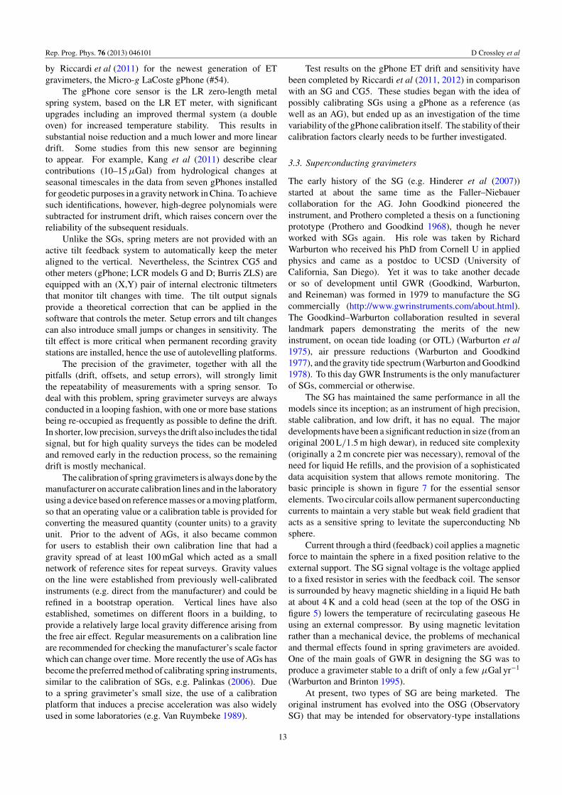
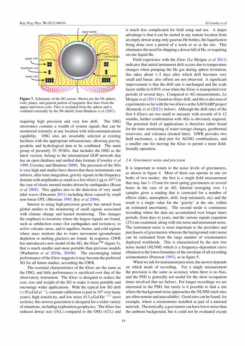
The SG has maintained the same performance in all themodels since its inception; as an instrument of high precision,stable calibration, and low drift, it has no equal. The majordevelopments have been a significant reduction in size (from anoriginal 200 L/1.5 m high dewar), in reduced site complexity(originally a 2 m concrete pier was necessary), removal of theneed for liquid He refills, and the provision of a sophisticateddata acquisition system that allows remote monitoring. Thebasic principle is shown in figure 7 for the essential sensorelements. Two circular coils allow permanent superconductingcurrents to maintain a very stable but weak field gradient thatacts as a sensitive spring to levitate the superconducting Nbsphere.

Current through a third (feedback) coil applies a magneticforce to maintain the sphere in a fixed position relative to theexternal support. The SG signal voltage is the voltage appliedto a fixed resistor in series with the feedback coil. The sensoris surrounded by heavy magnetic shielding in a liquid He bathat about 4 K and a cold head (seen at the top of the OSG infigure 5) lowers the temperature of recirculating gaseous Heusing an external compressor. By using magnetic levitationrather than a mechanical device, the problems of mechanicaland thermal effects found in spring gravimeters are avoided.One of the main goals of GWR in designing the SG was toproduce a gravimeter stable to a drift of only a few µGal yr−1

(Warburton and Brinton 1995).At present, two types of SG are being marketed. The

original instrument has evolved into the OSG (ObservatorySG) that may be intended for observatory-type installations

13

Rep. Prog. Phys. 76 (2013) 046101 D Crossley et al

Figure 7. Schematic of the SG sensor. Shown are the Nb sphere,coils, plates, and general pattern of magnetic flux lines from theupper and lower coils. Flux is excluded from the sphere and isconfined externally by the Nb shield; from Hinderer et al (2007).

requiring high precision and very low drift. The OSGelectronics contains a wealth of system signals that can bemonitored remotely at any location with telecommunicationscapability. OSG sites are invariably selected at existingfacilities with the appropriate infrastructure, allowing gravity,geodetic and hydrological data to be combined. The maingroup of presently 25–30 SGs, that includes the OSG as thelatest version, belong to the international GGP network thathas an open database and unified data formats (Crossley et al1999, Crossley and Hinderer 2009). The precision of the SGsis very high and studies have shown that these instruments canretrieve, after time integration, gravity signals in the frequencydomain with amplitudes as small as a few nGal (1 pg or 1012) inthe case of elastic normal modes driven by earthquakes (Rosatet al 2005). This applies also to the detection of very smalltidal waves (Ducarme 2011) including those caused by smallnon-linear OTL (Merriam 1995, Boy et al 2004).

Interest in using high-precision gravity has turned fromglobal studies to the monitoring of small signals associatedwith climate change and hazard monitoring. This changesthe emphasis to locations where the largest signals are found,such as subduction zones (for earthquakes and tectonics), toactive volcanic areas, and to aquifers, basins, and cold regionswhere mass motions due to water movement (groundwaterdepletion or melting glaciers) are found. In response, GWRhas introduced a new model of the SG, the iGravTM (figure 5),that is much smaller and more portable than previous models(Warburton et al 2010a, 2010b). The encouraging initialperformance of the iGrav suggests it may become the preferredSG for all future studies, according the GWR.

The essential characteristics of the iGrav are the same asthe OSG, and little performance is sacrificed over that of theobservatory instrument. The iGrav is designed to reduce thecost, size and weight of the SG to make it more portable andencourage wider applications. With the typical low SG drift(10 µGal yr−1), constant calibration (a part in 104 over manyyears), high sensitivity, and low noise (0.3 µGal Hz−1/2 (nextsection), this newest generation is designed for a wider varietyof situations, including exploration geophysics. The iGrav hasreduced dewar size (16 L) compared to the OSG (42 L) and

is much less complicated for field setup and use. A majoradvantage is that it can be started in any remote location froman empty dewar using only gaseous He bottles, the liquefactionbeing done over a period of a week or so at the site. Thiseliminates the need for shipping a dewar full of He, or requiringon-site liquid He.

Field experience with the iGrav (Le Moigne et al 2011)indicates that initial instrument drift occurs due to temperaturechanges when pumping the He gas during sphere levitation;this takes about 1–2 days after which drift becomes verysmall and linear; also offsets are not observed. A significantimprovement is that the drift rate is unchanged and the scalefactor stable to 0.05% even when the iGrav is transported overperiods of several days. Compared to AG measurements, LeMoigne et al (2011) found no iGrav drift, and this is also true ofexperiments so far with the two iGravs at the SAVSARP project(Kennedy et al (2012); below). Although the drift rates of thefirst 4 iGravs are too small to measure with records of 6–12months, further confirmation with AGs is obviously required.The potential field of applications is therefore rather broadfor the time monitoring of water-storage changes, geothermalreservoirs, and volcanos (treated later). GWR provides twofield enclosures, a dual pier for AG/SG combinations, anda smaller one for moving the iGrav to permit a more field-friendly operation.

3.4. Gravimeter noise and precision

It is important to return to the noise levels of gravimeters,as shown in figure 4. Most of them can operate in one (orboth) of two modes: the first is a single field measurementthat may last 1–15 min for most spring gravimeters or severalhours in the case of an AG. Internal averaging over 1 ssamples gives a reading that is corrected for a number ofeffects (tides, atmosphere, drift, loop mismatch, etc) and theresult is a single value for the ‘gravity’ at the site, withinan estimated uncertainty. The second mode is continuousrecording where the data are accumulated over longer timesperiods, from days to years, and the various signals (equation(25)) are examined, along with site noise and instrument noise.The instrument noise is most important to the providers andpurchasers of gravimeters whereas the background (site) noisecan be estimated from the large number of seismometersdeployed worldwide. This is characterized by the new lownoise model (NLNM) which is a frequency-dependent curveobtained as the lower boundary of the envelope of all recordingseismometers (Peterson 1993), as in figure 9.

When we ask for instrument precision, the answer dependson which mode of recording. For a single measurementthe precision is the same as accuracy when there is no bias,and the PSD is generally not useful for the short occupationtimes involved (but see below). For longer recordings we areinterested in the PSD, but rarely is it possible to find a sitewhere the background noise approaches the NLNM (such sitesare often remote and unavailable). Good sites can be found, forexample, where a seismometer installed as part of a nationalnetwork. Theoretically, a gravimeter can have lower noise thanthe ambient background, but it could not be evaluated except

14

Rep. Prog. Phys. 76 (2013) 046101 D Crossley et al

in a laboratory environment with anti-vibration facilities (butthis still would not shield against changes in the gravitationalpotential). All current gravimeters have instrumental noiseabove the NLNM, at least for periods 1000 s.

Nevertheless, SGs routinely have lower noise at periods1000 s due to their inherent stability and superior pressurecorrection compared to seismometers. A methodology hasarisen for characterizing the noise of SGs by computing aquantity known as the Seismic Noise Magnitude (SNM), asintroduced by Banka et al (1998) and Banka and Crossley(1999) and extended in Rosat et al (2004) and Rosat andHinderer (2011). The method is straightforward: (a) assemblea length of raw data (e.g. 1 month, 1 year), (b) subtracttheoretical tides and nominal atmospheric pressure, (c) subtracta degree 9 polynomial to remove any residual tides, (d) selectthe 5 quietest days with smallest daily variance, and (e)compute the power spectral density (PSD) and its mean value〈PSD〉 between periods of 340–600 s. Then we can estimate:

PDB(f ) = 10log10(PSD) − 160,

SNA =√

〈PSD〉,SNM = log10 (〈PSD〉) + 2.5, (26)

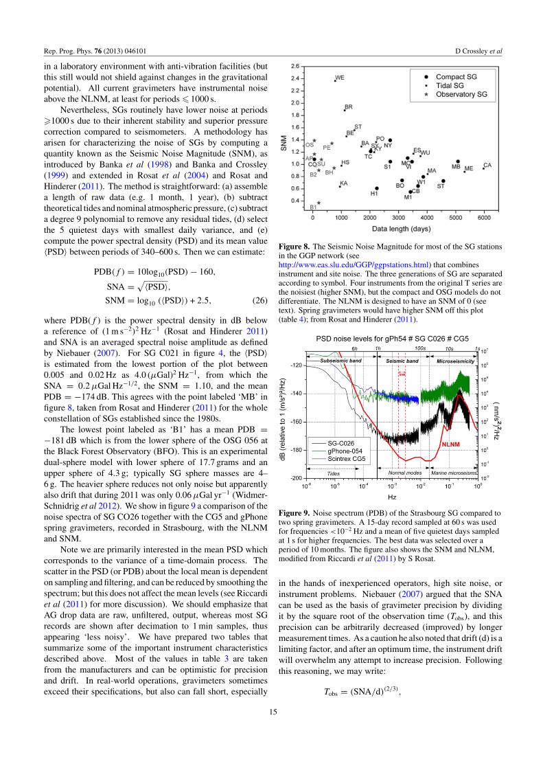
where PDB(f ) is the power spectral density in dB belowa reference of (1 m s−2)2 Hz−1 (Rosat and Hinderer 2011)and SNA is an averaged spectral noise amplitude as definedby Niebauer (2007). For SG C021 in figure 4, the 〈PSD〉is estimated from the lowest portion of the plot between0.005 and 0.02 Hz as 4.0 (µGal)2 Hz−1, from which theSNA = 0.2 µGal Hz−1/2, the SNM = 1.10, and the meanPDB = −174 dB. This agrees with the point labeled ‘MB’ infigure 8, taken from Rosat and Hinderer (2011) for the wholeconstellation of SGs established since the 1980s.

The lowest point labeled as ‘B1’ has a mean PDB =−181 dB which is from the lower sphere of the OSG 056 atthe Black Forest Observatory (BFO). This is an experimentaldual-sphere model with lower sphere of 17.7 grams and anupper sphere of 4.3 g; typically SG sphere masses are 4–6 g. The heavier sphere reduces not only noise but apparentlyalso drift that during 2011 was only 0.06 µGal yr−1 (Widmer-Schnidrig et al 2012). We show in figure 9 a comparison of thenoise spectra of SG CO26 together with the CG5 and gPhonespring gravimeters, recorded in Strasbourg, with the NLNMand SNM.

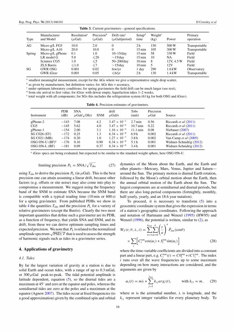
Note we are primarily interested in the mean PSD whichcorresponds to the variance of a time-domain process. Thescatter in the PSD (or PDB) about the local mean is dependenton sampling and filtering, and can be reduced by smoothing thespectrum; but this does not affect the mean levels (see Riccardiet al (2011) for more discussion). We should emphasize thatAG drop data are raw, unfiltered, output, whereas most SGrecords are shown after decimation to 1 min samples, thusappearing ‘less noisy’. We have prepared two tables thatsummarize some of the important instrument characteristicsdescribed above. Most of the values in table 3 are takenfrom the manufacturers and can be optimistic for precisionand drift. In real-world operations, gravimeters sometimesexceed their specifications, but also can fall short, especially

Figure 8. The Seismic Noise Magnitude for most of the SG stationsin the GGP network (seehttp://www.eas.slu.edu/GGP/ggpstations.html) that combinesinstrument and site noise. The three generations of SG are separatedaccording to symbol. Four instruments from the original T series arethe noisiest (higher SNM), but the compact and OSG models do notdifferentiate. The NLNM is designed to have an SNM of 0 (seetext). Spring gravimeters would have higher SNM off this plot(table 4); from Rosat and Hinderer (2011).

Figure 9. Noise spectrum (PDB) of the Strasbourg SG compared totwo spring gravimeters. A 15-day record sampled at 60 s was usedfor frequencies <10−2 Hz and a mean of five quietest days sampledat 1 s for higher frequencies. The best data was selected over aperiod of 10 months. The figure also shows the SNM and NLNM,modified from Riccardi et al (2011) by S Rosat.

in the hands of inexperienced operators, high site noise, orinstrument problems. Niebauer (2007) argued that the SNAcan be used as the basis of gravimeter precision by dividingit by the square root of the observation time (Tobs), and thisprecision can be arbitrarily decreased (improved) by longermeasurement times. As a caution he also noted that drift (d) is alimiting factor, and after an optimum time, the instrument driftwill overwhelm any attempt to increase precision. Followingthis reasoning, we may write:

Tobs = (SNA/d)(2/3),

15

Rep. Prog. Phys. 76 (2013) 046101 D Crossley et al

Table 3. Current gravimeters—general specifications.

Manufacturer Resolutiona Precisionb Drift ratec Setupd Weighte PrimaryType and Model (µGal) (µGal) (µGal/period) time (kg) Power operation

AG Micro-g/L FG5 10.0 2.0 0 2 h 150 500 W TransportableMicro-g/L A10 20.0 10.0 0 15 min 105 300 W Transportable

Spring Micro-g/L gPhone 0.1 1.0 10–15/day 15 min 58 330 W FieldLR model G 5.0 20 ∼15/day 15 min 10 NA FieldScintrex CG5 1.0 5 50–200/day 10 min 8 12V, 4.5 W FieldZLS Burris 1.0 7 ∼15/day 10 min 5 12V Field

SG GWR OSG 0.001 0.02 few/yr 1 day 290 1.6 kW ObservatoryGWR iGrav 0.001 0.05 6/yr 2 h 130 1.4 kW Transportable

a smallest meaningful measurement, except for the AGs where we give a representative single drop scatter,b as given by manufacturer, but definition varies; for AGs this = accuracy,c under optimum laboratory conditions; for spring gravimeters the field drift can be much larger (see text),d from site arrival to first value; for iGrav with dewar empty, liquefaction takes 1–2 weeks,e total weight with all components; for SGs this includes the refrigeration system (61 kg for both OSG and iGrav).

Table 4. Precision estimates of gravimeters.

PDB SNA drift Tobs PrecisionInstrument (dB) µGal/

√(Hz) SNM µGal/s (unit) µGal Source

gPhone-2 −143 7.08 4.2 3.47 × 10−3 2.7 min 0.56 Riccardi et al (2011)CG5 −145 5.62 4.0 3.47 × 10−4 10.7 min 0.22 Riccardi et al (2011)gPhone-1 −154 2.00 3.1 1.16 × 10−4 11.1 min 0.08 Niebauer (2007)SG C026 (ST) −172 0.25 1.3 6.34 × 10−8 6.9 h 0.002 Riccardi et al (2011)SG C021 (MB) −174 0.20 1.0 1.27 × 10−7 3.8 h 0.002 Van Camp et al (2005)OSG 056-U (BF)a −176 0.16 0.90 6.34 × 10−8 5.1 h 0.001 Widmer-Schnidrig (2012)OSG 056-L (BF) −181 0.09 0.37 6.34 × 10−8 3.4 h 0.001 Widmer-Schnidrig (2012)

a iGrav specs are being evaluated, but expected to be similar to the standard weight sphere, here OSG 056-U.

limiting precision PL = SNA/√

Tobs (27)

using Tobs to derive the precision PL (in µGal). This is the bestprecision one can attain assuming a linear drift, because otherfactors (e.g. offsets or site noise) may also come into play tocompromise a measurement. We suggest using the frequencyband of the SNM to estimate SNA because the SNM bandis compatible with a typical reading time (10 min or 600 s)for a spring gravimeter. From published PDBs we show intable 4 the quantities Tobs and the precision PL for a variety ofrelative gravimeters (except the Burris). Clearly the two mostimportant quantities that define such a gravimeter are its PDB,as a function of frequency, that yields SNA and SNM, and itsdrift; from these we can derive optimum sampling times andexpected precision. We note thatPL is related to the normalizedamplitude spectrum

√PSD/T that is used to assess the strength

of harmonic signals such as tides in a gravimeter series.

4. Applications of gravimetry

4.1. Tides

By far the largest variation of gravity at a station is due tosolid Earth and ocean tides, with a range of up to 0.3 mGal,or 300 µGal peak-to-peak. The tidal potential amplitude islatitude dependent, equation (5), so the diurnal tides are amaximum at 45 and zero at the equator and poles, whereas thesemidiurnal tides are zero at the poles and a maximum at theequator (Agnew 2007). The tides occur at fixed frequencies (toa good approximation) given by the combined spin and orbital

dynamics of the Moon about the Earth, and the Earth andother planets—Mercury, Mars, Venus, Jupiter and Saturn—around the Sun. The primary motion is diurnal Earth rotation,followed by the Moon’s orbital motion about the Earth, thenthe annual orbital motion of the Earth about the Sun. Thelargest components are at semidiurnal and diurnal periods, butthere are also long-period components (fortnightly, monthly,half-yearly, yearly, and an 18.6 year nutation).

To proceed, it is necessary to transform (5) into ageocentric coordinate system that gives the expression in termsof a station’s geographic coordinates. Following the approachand notation of Hartmann and Wenzel (1995) (HW95) andWenzel (1996), the potential is written, similar to (2), as

WT (r, θ, λ, t) =nmax∑n=1

n∑m=0

(r

a

)n

Pnm(cosθ)

×∑

i

[Cnm

i cos(αi) + Snmi sin(αi)

](28)

where the time-variable coefficients are divided into a constantpart and a linear part, e.g. Cnm

i (t) = C0nmi + tC1nm

i . The indexi runs over all the wave frequencies up to some maximumdepending on how many interactions are considered, and thearguments are given by

αi(t) = mλ +jmax∑j=1

kij argi(t), with ki1 = m, (29)

where m is the azimuthal number, λ is longitude, and thekij represent integer variables for every planetary body. To

16

Rep. Prog. Phys. 76 (2013) 046101 D Crossley et al

include all interactions to a specified accuracy, the maximumdegree nmax changes for each astronomical body, e.g. up to 7for the Moon and up to 2 for the major planets. In HW95there are 11 (jmax) astronomical arguments. Catalogs of thetide generating potential (TGP) have been produced sinceDoodson (1921) and generally give a table of every wave,with its frequency, coefficients kij , and amplitudes Cnm

i , Snmi ,

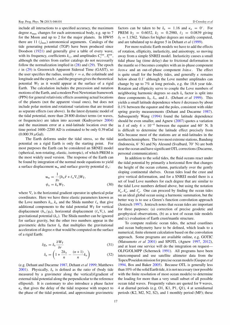
although the entries from earlier catalogs do not necessarilyfollow the normalization implied in (28) and (29). The epocht in (29) is Greenwich Apparent Sidereal Time (GAST), sothe user specifies the radius, usually r = a, the colatitude andlongitude and the epoch t , and the program gives the theoreticalpotential WT as it would appear at the surface of a rigidEarth. The calculation includes the precession and nutationmotions of the Earth, and a modern Post Newtonian framework(PPN) for general relativistic effects assuming actual locationsof the planets (not the apparent visual ones), but does notinclude polar motion and rotational variations that are treatedas separate effects (see above). In the latest dynamic model ofthe tidal potential, more than 28 800 distinct terms (or waves,or frequencies) are taken into account (Kudryavtsev 2004)and the maximum error at a mid-latitude location over thetime period 1600–2200 AD is estimated to be only 0.39 nGal(0.000 39 µGal).

The Earth deforms under the tidal stress, so the tidalpotential on a rigid Earth is only the starting point. Formost purposes the Earth can be considered an SRNEI model(spherical, non-rotating, elastic, isotropic), of which PREM isthe most widely used version. The response of the Earth canbe found by integration of the normal mode equations to yielda surface displacement un and surface gravity potential ψn:

un = 1

g0[hnr + n∇s]WT,

ψn = knWT, (30)

where ∇s is the horizontal gradient operator in spherical polarcoordinates. Here we have three elastic parameters known asthe Love numbers hn, kn and the Shida number n that giveadditional components to the tidal potential WT for verticaldisplacement (hn/g0), horizontal displacement (n∇s), andgravitational potential (kn). The Shida number can be ignoredfor surface gravity, but the other two numbers appear in thegravimetric delta factor δn that multiplies the gravitationalacceleration of degree n that would be computed on the surfaceof a rigid Earth:

δgn = δn

∂WT

∂r(31)

δn =(

1 +2hn

n− (n + 1)

nkn

)(32)

(e.g. Dehant and Ducarme 1987, Dehant et al 1999; Matthews2001). Physically, δn is defined as the ratio of (body tidemeasured by a gravimeter along the vertical)/(gradient ofexternal tidal potential along the perpendicular to the referenceellipsoid). It is customary to also introduce a phase factorκn that gives the delay of the tidal response with respect tothe phase of the tidal potential, and approximate gravimetric

factors can be taken to be δn = 1.16 and κn = 0. ForPREM h2 = 0.6032, k2 = 0.2980, 2 = 0.0839 givingδ2 = 1.1562. Values for higher degrees are readily computed,and are tabulated up to degree 5 in Dehant et al (1999).

For more realistic Earth models we have to add the effectsof rotation, ellipticity, inelasticity, and anisotropy, so movingaway from a simple SNREI model. Inelasticity causes a smalltidal phase lag (time delay) due to frictional deformation inthe mantle so δ becomes complex with an in-phase componentδcos κ and an out-of-phase component δsin κ . The effectis quite small for the bodily tides, and generally κ remainsbelow about 0.1 although the Love number amplitudes canchange by up to 7% at long periods, e.g. the 18.6 year tide.Rotation and ellipticity serve to couple the Love numbers ofneighboring harmonic degrees so each δn factor is split intothree components δ0, δ+, and δ− (Dehant et al 1999). Thisyields a small latitude dependence where δ decreases by about0.1% between the equator and the poles, consistent with olderspring gravity measurements (Dehant and Ducarme 1987).Subsequently Wang (1994) found the latitude dependenceshould be even smaller, and Agnew (2007) quotes a variationin δ of only 4 × 10−4 between the equator and 60 N. Itis difficult to determine the latitude effect precisely fromSGs because most of the stations are at mid-latitudes in thenorthern hemisphere. The two most extreme stations, Bandung(Indonesia, 6 N) and Ny Alesund (Svalbard, 70 N) are bothnear the ocean and have significant OTL corrections (Ducarme,personal communication).

In addition to the solid tides, the fluid oceans react underthe tidal potential by primarily a horizontal flow that changesthe height of the ocean column, particularly over the gentlysloping continental shelves. Ocean tides load the crust andgive vertical deformation, and for a SNREI model there is aset of load Love numbers for each degree that are similar tothe tidal Love numbers defined above, but using the notationh′

n, k′n, and ′

n. One can proceed by finding the ocean tideson an ideal global ocean using a harmonic summation, but thebetter way is to use a Green’s function convolution approach(Jentzsch 1997). Jentzsch notes that ocean tides are importantfor three purposes: (a) correction of precise geodetic andgeophysical observations, (b) as a test of ocean tide modelsand (c) evaluation of Earth crust/mantle structure.

To compute realistic ocean tides, the actual coastlinesand ocean bathymetry have to be defined, which leads to anumerical, finite element calculation based on the convolutionapproach. Some programs are available online, e.g. GOTIC(Matsumoto et al 2001) and SPOTL (Agnew 1997, 2012),and at least one service will do the integration on request—OLFG/OLMPP (Scherneck 1991). All programs have beenintercompared and use satellite altimeter data from theTopex/Poseidon mission for precise ocean models (Gaspar et al1994, Bos and Baker 2005). Because OTL is generally lessthan 10% of the solid Earth tide, it is not necessary (nor possiblewith the finite resolution of most ocean models) to determinethe loading for more than a very small subset of all possibleocean tidal waves. Frequently values are quoted for 9 waves,4 at diurnal periods (e.g. O1, K1, P1, Q1), 4 at semidiurnalperiods (K2, M2, N2, S2), and 1 monthly period (MF); these

17

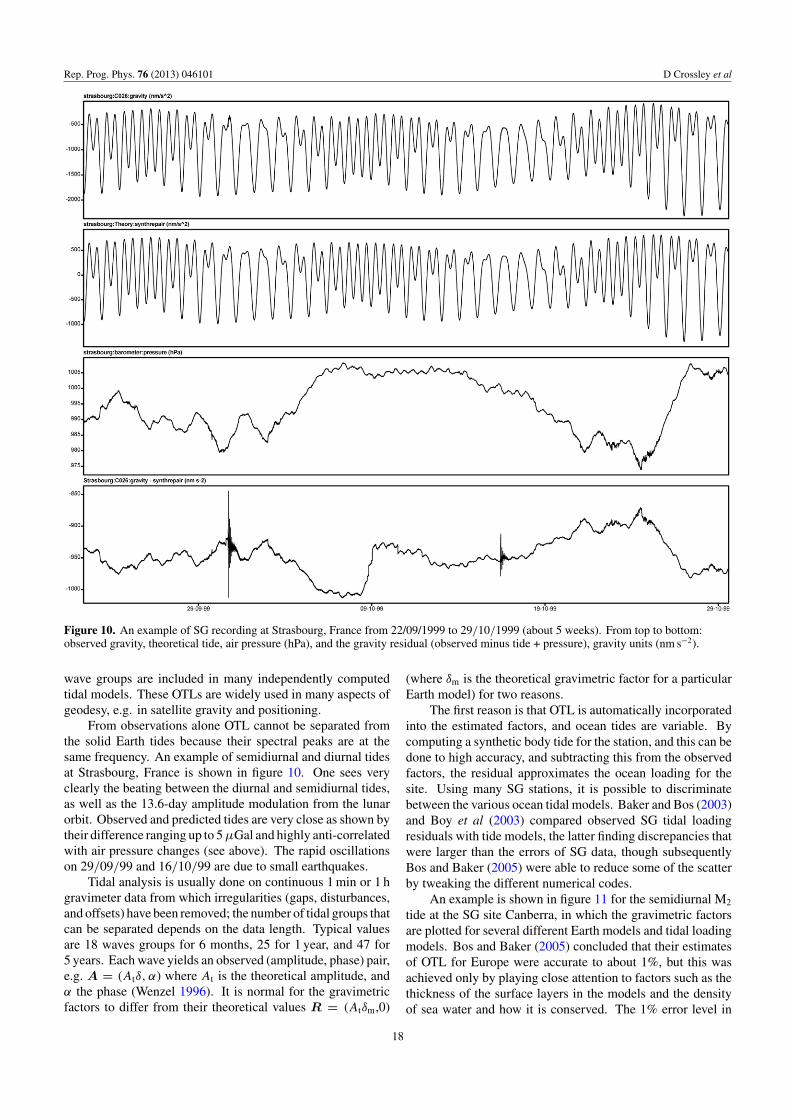
Rep. Prog. Phys. 76 (2013) 046101 D Crossley et al

Figure 10. An example of SG recording at Strasbourg, France from 22/09/1999 to 29/10/1999 (about 5 weeks). From top to bottom:observed gravity, theoretical tide, air pressure (hPa), and the gravity residual (observed minus tide + pressure), gravity units (nm s−2).

wave groups are included in many independently computedtidal models. These OTLs are widely used in many aspects ofgeodesy, e.g. in satellite gravity and positioning.

From observations alone OTL cannot be separated fromthe solid Earth tides because their spectral peaks are at thesame frequency. An example of semidiurnal and diurnal tidesat Strasbourg, France is shown in figure 10. One sees veryclearly the beating between the diurnal and semidiurnal tides,as well as the 13.6-day amplitude modulation from the lunarorbit. Observed and predicted tides are very close as shown bytheir difference ranging up to 5 µGal and highly anti-correlatedwith air pressure changes (see above). The rapid oscillationson 29/09/99 and 16/10/99 are due to small earthquakes.

Tidal analysis is usually done on continuous 1 min or 1 hgravimeter data from which irregularities (gaps, disturbances,and offsets) have been removed; the number of tidal groups thatcan be separated depends on the data length. Typical valuesare 18 waves groups for 6 months, 25 for 1 year, and 47 for5 years. Each wave yields an observed (amplitude, phase) pair,e.g. A = (Atδ, α) where At is the theoretical amplitude, andα the phase (Wenzel 1996). It is normal for the gravimetricfactors to differ from their theoretical values R = (Atδm,0)

(where δm is the theoretical gravimetric factor for a particularEarth model) for two reasons.

The first reason is that OTL is automatically incorporatedinto the estimated factors, and ocean tides are variable. Bycomputing a synthetic body tide for the station, and this can bedone to high accuracy, and subtracting this from the observedfactors, the residual approximates the ocean loading for thesite. Using many SG stations, it is possible to discriminatebetween the various ocean tidal models. Baker and Bos (2003)and Boy et al (2003) compared observed SG tidal loadingresiduals with tide models, the latter finding discrepancies thatwere larger than the errors of SG data, though subsequentlyBos and Baker (2005) were able to reduce some of the scatterby tweaking the different numerical codes.

An example is shown in figure 11 for the semidiurnal M2

tide at the SG site Canberra, in which the gravimetric factorsare plotted for several different Earth models and tidal loadingmodels. Bos and Baker (2005) concluded that their estimatesof OTL for Europe were accurate to about 1%, but this wasachieved only by playing close attention to factors such as thethickness of the surface layers in the models and the densityof sea water and how it is conserved. The 1% error level in

18

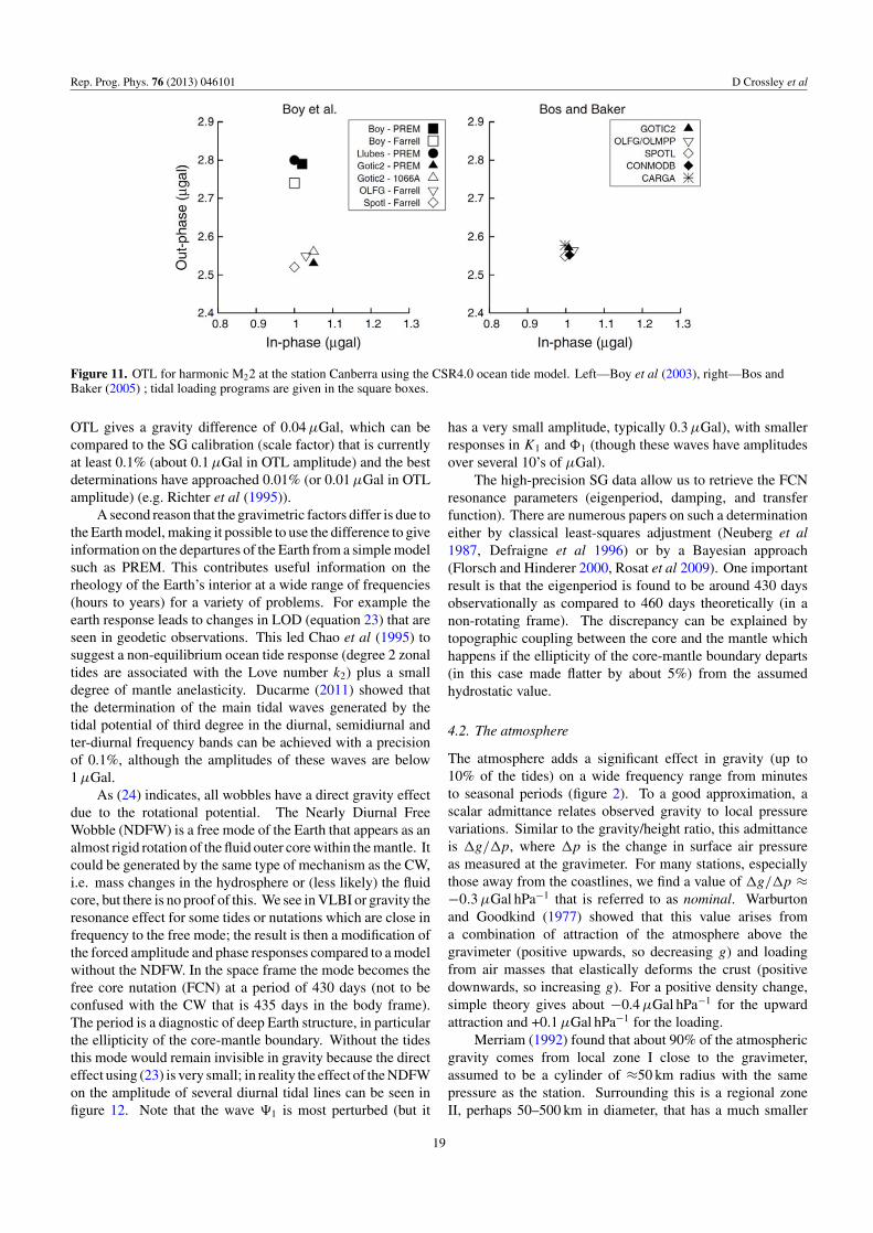
Rep. Prog. Phys. 76 (2013) 046101 D Crossley et al

Figure 11. OTL for harmonic M22 at the station Canberra using the CSR4.0 ocean tide model. Left—Boy et al (2003), right—Bos andBaker (2005) ; tidal loading programs are given in the square boxes.

OTL gives a gravity difference of 0.04 µGal, which can becompared to the SG calibration (scale factor) that is currentlyat least 0.1% (about 0.1 µGal in OTL amplitude) and the bestdeterminations have approached 0.01% (or 0.01 µGal in OTLamplitude) (e.g. Richter et al (1995)).

A second reason that the gravimetric factors differ is due tothe Earth model, making it possible to use the difference to giveinformation on the departures of the Earth from a simple modelsuch as PREM. This contributes useful information on therheology of the Earth’s interior at a wide range of frequencies(hours to years) for a variety of problems. For example theearth response leads to changes in LOD (equation 23) that areseen in geodetic observations. This led Chao et al (1995) tosuggest a non-equilibrium ocean tide response (degree 2 zonaltides are associated with the Love number k2) plus a smalldegree of mantle anelasticity. Ducarme (2011) showed thatthe determination of the main tidal waves generated by thetidal potential of third degree in the diurnal, semidiurnal andter-diurnal frequency bands can be achieved with a precisionof 0.1%, although the amplitudes of these waves are below1 µGal.

As (24) indicates, all wobbles have a direct gravity effectdue to the rotational potential. The Nearly Diurnal FreeWobble (NDFW) is a free mode of the Earth that appears as analmost rigid rotation of the fluid outer core within the mantle. Itcould be generated by the same type of mechanism as the CW,i.e. mass changes in the hydrosphere or (less likely) the fluidcore, but there is no proof of this. We see in VLBI or gravity theresonance effect for some tides or nutations which are close infrequency to the free mode; the result is then a modification ofthe forced amplitude and phase responses compared to a modelwithout the NDFW. In the space frame the mode becomes thefree core nutation (FCN) at a period of 430 days (not to beconfused with the CW that is 435 days in the body frame).The period is a diagnostic of deep Earth structure, in particularthe ellipticity of the core-mantle boundary. Without the tidesthis mode would remain invisible in gravity because the directeffect using (23) is very small; in reality the effect of the NDFWon the amplitude of several diurnal tidal lines can be seen infigure 12. Note that the wave 1 is most perturbed (but it

has a very small amplitude, typically 0.3 µGal), with smallerresponses in K1 and 1 (though these waves have amplitudesover several 10’s of µGal).

The high-precision SG data allow us to retrieve the FCNresonance parameters (eigenperiod, damping, and transferfunction). There are numerous papers on such a determinationeither by classical least-squares adjustment (Neuberg et al1987, Defraigne et al 1996) or by a Bayesian approach(Florsch and Hinderer 2000, Rosat et al 2009). One importantresult is that the eigenperiod is found to be around 430 daysobservationally as compared to 460 days theoretically (in anon-rotating frame). The discrepancy can be explained bytopographic coupling between the core and the mantle whichhappens if the ellipticity of the core-mantle boundary departs(in this case made flatter by about 5%) from the assumedhydrostatic value.

4.2. The atmosphere

The atmosphere adds a significant effect in gravity (up to10% of the tides) on a wide frequency range from minutesto seasonal periods (figure 2). To a good approximation, ascalar admittance relates observed gravity to local pressurevariations. Similar to the gravity/height ratio, this admittanceis g/p, where p is the change in surface air pressureas measured at the gravimeter. For many stations, especiallythose away from the coastlines, we find a value of g/p ≈−0.3 µGal hPa−1 that is referred to as nominal. Warburtonand Goodkind (1977) showed that this value arises froma combination of attraction of the atmosphere above thegravimeter (positive upwards, so decreasing g) and loadingfrom air masses that elastically deforms the crust (positivedownwards, so increasing g). For a positive density change,simple theory gives about −0.4 µGal hPa−1 for the upwardattraction and +0.1 µGal hPa−1 for the loading.

Merriam (1992) found that about 90% of the atmosphericgravity comes from local zone I close to the gravimeter,assumed to be a cylinder of ≈50 km radius with the samepressure as the station. Surrounding this is a regional zoneII, perhaps 50–500 km in diameter, that has a much smaller

19

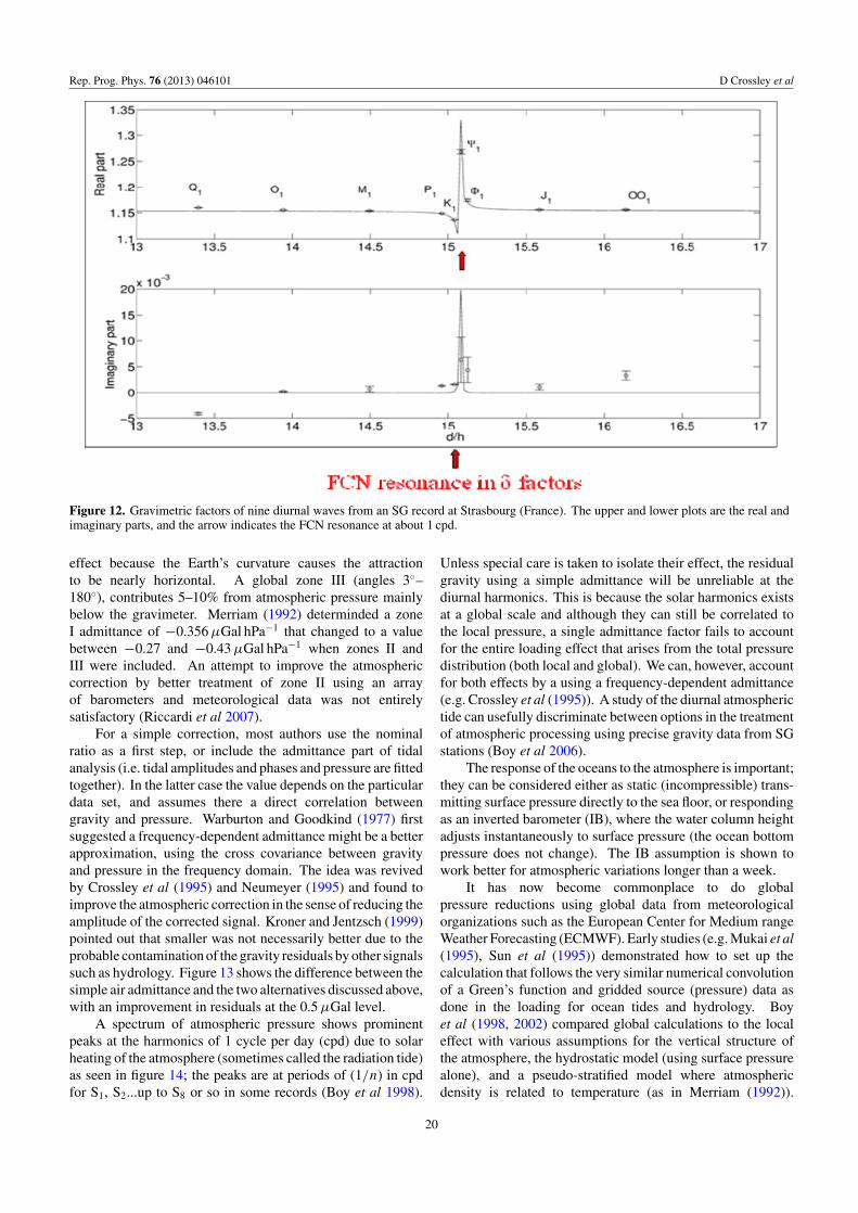
Rep. Prog. Phys. 76 (2013) 046101 D Crossley et al

Figure 12. Gravimetric factors of nine diurnal waves from an SG record at Strasbourg (France). The upper and lower plots are the real andimaginary parts, and the arrow indicates the FCN resonance at about 1 cpd.

effect because the Earth’s curvature causes the attractionto be nearly horizontal. A global zone III (angles 3–180), contributes 5–10% from atmospheric pressure mainlybelow the gravimeter. Merriam (1992) determinded a zoneI admittance of −0.356 µGal hPa−1 that changed to a valuebetween −0.27 and −0.43 µGal hPa−1 when zones II andIII were included. An attempt to improve the atmosphericcorrection by better treatment of zone II using an arrayof barometers and meteorological data was not entirelysatisfactory (Riccardi et al 2007).

For a simple correction, most authors use the nominalratio as a first step, or include the admittance part of tidalanalysis (i.e. tidal amplitudes and phases and pressure are fittedtogether). In the latter case the value depends on the particulardata set, and assumes there a direct correlation betweengravity and pressure. Warburton and Goodkind (1977) firstsuggested a frequency-dependent admittance might be a betterapproximation, using the cross covariance between gravityand pressure in the frequency domain. The idea was revivedby Crossley et al (1995) and Neumeyer (1995) and found toimprove the atmospheric correction in the sense of reducing theamplitude of the corrected signal. Kroner and Jentzsch (1999)pointed out that smaller was not necessarily better due to theprobable contamination of the gravity residuals by other signalssuch as hydrology. Figure 13 shows the difference between thesimple air admittance and the two alternatives discussed above,with an improvement in residuals at the 0.5 µGal level.

A spectrum of atmospheric pressure shows prominentpeaks at the harmonics of 1 cycle per day (cpd) due to solarheating of the atmosphere (sometimes called the radiation tide)as seen in figure 14; the peaks are at periods of (1/n) in cpdfor S1, S2...up to S8 or so in some records (Boy et al 1998).

Unless special care is taken to isolate their effect, the residualgravity using a simple admittance will be unreliable at thediurnal harmonics. This is because the solar harmonics existsat a global scale and although they can still be correlated tothe local pressure, a single admittance factor fails to accountfor the entire loading effect that arises from the total pressuredistribution (both local and global). We can, however, accountfor both effects by a using a frequency-dependent admittance(e.g. Crossley et al (1995)). A study of the diurnal atmospherictide can usefully discriminate between options in the treatmentof atmospheric processing using precise gravity data from SGstations (Boy et al 2006).

The response of the oceans to the atmosphere is important;they can be considered either as static (incompressible) trans-mitting surface pressure directly to the sea floor, or respondingas an inverted barometer (IB), where the water column heightadjusts instantaneously to surface pressure (the ocean bottompressure does not change). The IB assumption is shown towork better for atmospheric variations longer than a week.

It has now become commonplace to do globalpressure reductions using global data from meteorologicalorganizations such as the European Center for Medium rangeWeather Forecasting (ECMWF). Early studies (e.g. Mukai et al(1995), Sun et al (1995)) demonstrated how to set up thecalculation that follows the very similar numerical convolutionof a Green’s function and gridded source (pressure) data asdone in the loading for ocean tides and hydrology. Boyet al (1998, 2002) compared global calculations to the localeffect with various assumptions for the vertical structure ofthe atmosphere, the hydrostatic model (using surface pressurealone), and a pseudo-stratified model where atmosphericdensity is related to temperature (as in Merriam (1992)).

20

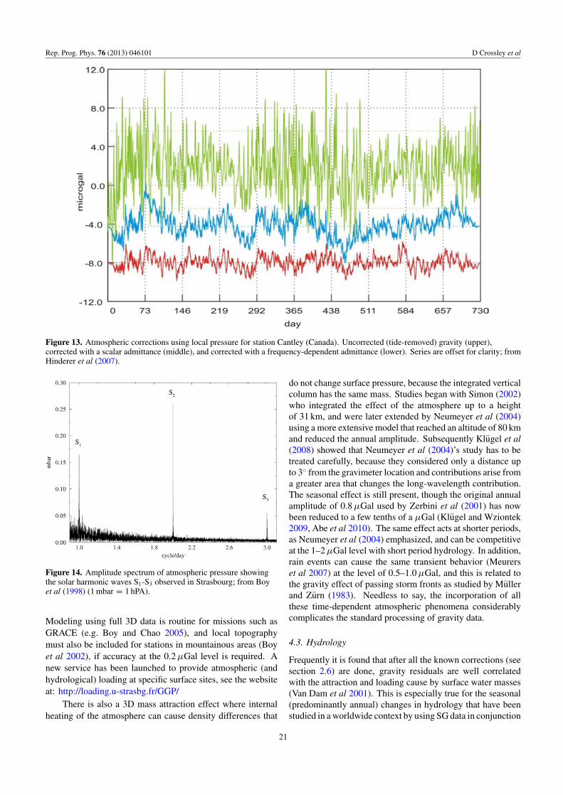
Rep. Prog. Phys. 76 (2013) 046101 D Crossley et al

Figure 13. Atmospheric corrections using local pressure for station Cantley (Canada). Uncorrected (tide-removed) gravity (upper),corrected with a scalar admittance (middle), and corrected with a frequency-dependent admittance (lower). Series are offset for clarity; fromHinderer et al (2007).

Figure 14. Amplitude spectrum of atmospheric pressure showingthe solar harmonic waves S1-S3 observed in Strasbourg; from Boyet al (1998) (1 mbar = 1 hPA).

Modeling using full 3D data is routine for missions such asGRACE (e.g. Boy and Chao 2005), and local topographymust also be included for stations in mountainous areas (Boyet al 2002), if accuracy at the 0.2 µGal level is required. Anew service has been launched to provide atmospheric (andhydrological) loading at specific surface sites, see the websiteat: http://loading.u-strasbg.fr/GGP/

There is also a 3D mass attraction effect where internalheating of the atmosphere can cause density differences that

do not change surface pressure, because the integrated verticalcolumn has the same mass. Studies began with Simon (2002)who integrated the effect of the atmosphere up to a heightof 31 km, and were later extended by Neumeyer et al (2004)using a more extensive model that reached an altitude of 80 kmand reduced the annual amplitude. Subsequently Klugel et al(2008) showed that Neumeyer et al (2004)’s study has to betreated carefully, because they considered only a distance upto 3 from the gravimeter location and contributions arise froma greater area that changes the long-wavelength contribution.The seasonal effect is still present, though the original annualamplitude of 0.8 µGal used by Zerbini et al (2001) has nowbeen reduced to a few tenths of a µGal (Klugel and Wziontek2009, Abe et al 2010). The same effect acts at shorter periods,as Neumeyer et al (2004) emphasized, and can be competitiveat the 1–2 µGal level with short period hydrology. In addition,rain events can cause the same transient behavior (Meurerset al 2007) at the level of 0.5–1.0 µGal, and this is related tothe gravity effect of passing storm fronts as studied by Mullerand Zurn (1983). Needless to say, the incorporation of allthese time-dependent atmospheric phenomena considerablycomplicates the standard processing of gravity data.

4.3. Hydrology

Frequently it is found that after all the known corrections (seesection 2.6) are done, gravity residuals are well correlatedwith the attraction and loading cause by surface water masses(Van Dam et al 2001). This is especially true for the seasonal(predominantly annual) changes in hydrology that have beenstudied in a worldwide context by using SG data in conjunction

21

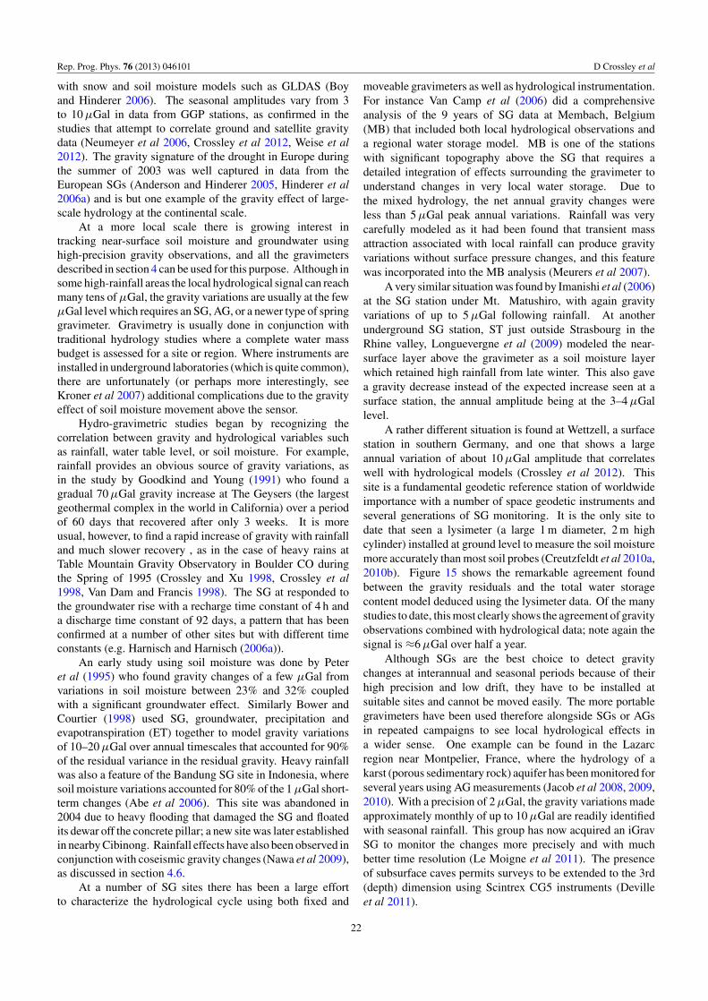
Rep. Prog. Phys. 76 (2013) 046101 D Crossley et al

with snow and soil moisture models such as GLDAS (Boyand Hinderer 2006). The seasonal amplitudes vary from 3to 10 µGal in data from GGP stations, as confirmed in thestudies that attempt to correlate ground and satellite gravitydata (Neumeyer et al 2006, Crossley et al 2012, Weise et al2012). The gravity signature of the drought in Europe duringthe summer of 2003 was well captured in data from theEuropean SGs (Anderson and Hinderer 2005, Hinderer et al2006a) and is but one example of the gravity effect of large-scale hydrology at the continental scale.

At a more local scale there is growing interest intracking near-surface soil moisture and groundwater usinghigh-precision gravity observations, and all the gravimetersdescribed in section 4 can be used for this purpose. Although insome high-rainfall areas the local hydrological signal can reachmany tens of µGal, the gravity variations are usually at the fewµGal level which requires an SG, AG, or a newer type of springgravimeter. Gravimetry is usually done in conjunction withtraditional hydrology studies where a complete water massbudget is assessed for a site or region. Where instruments areinstalled in underground laboratories (which is quite common),there are unfortunately (or perhaps more interestingly, seeKroner et al 2007) additional complications due to the gravityeffect of soil moisture movement above the sensor.

Hydro-gravimetric studies began by recognizing thecorrelation between gravity and hydrological variables suchas rainfall, water table level, or soil moisture. For example,rainfall provides an obvious source of gravity variations, asin the study by Goodkind and Young (1991) who found agradual 70 µGal gravity increase at The Geysers (the largestgeothermal complex in the world in California) over a periodof 60 days that recovered after only 3 weeks. It is moreusual, however, to find a rapid increase of gravity with rainfalland much slower recovery , as in the case of heavy rains atTable Mountain Gravity Observatory in Boulder CO duringthe Spring of 1995 (Crossley and Xu 1998, Crossley et al1998, Van Dam and Francis 1998). The SG at responded tothe groundwater rise with a recharge time constant of 4 h anda discharge time constant of 92 days, a pattern that has beenconfirmed at a number of other sites but with different timeconstants (e.g. Harnisch and Harnisch (2006a)).

An early study using soil moisture was done by Peteret al (1995) who found gravity changes of a few µGal fromvariations in soil moisture between 23% and 32% coupledwith a significant groundwater effect. Similarly Bower andCourtier (1998) used SG, groundwater, precipitation andevapotranspiration (ET) together to model gravity variationsof 10–20 µGal over annual timescales that accounted for 90%of the residual variance in the residual gravity. Heavy rainfallwas also a feature of the Bandung SG site in Indonesia, wheresoil moisture variations accounted for 80% of the 1 µGal short-term changes (Abe et al 2006). This site was abandoned in2004 due to heavy flooding that damaged the SG and floatedits dewar off the concrete pillar; a new site was later establishedin nearby Cibinong. Rainfall effects have also been observed inconjunction with coseismic gravity changes (Nawa et al 2009),as discussed in section 4.6.

At a number of SG sites there has been a large effortto characterize the hydrological cycle using both fixed and

moveable gravimeters as well as hydrological instrumentation.For instance Van Camp et al (2006) did a comprehensiveanalysis of the 9 years of SG data at Membach, Belgium(MB) that included both local hydrological observations anda regional water storage model. MB is one of the stationswith significant topography above the SG that requires adetailed integration of effects surrounding the gravimeter tounderstand changes in very local water storage. Due tothe mixed hydrology, the net annual gravity changes wereless than 5 µGal peak annual variations. Rainfall was verycarefully modeled as it had been found that transient massattraction associated with local rainfall can produce gravityvariations without surface pressure changes, and this featurewas incorporated into the MB analysis (Meurers et al 2007).

A very similar situation was found by Imanishi et al (2006)at the SG station under Mt. Matushiro, with again gravityvariations of up to 5 µGal following rainfall. At anotherunderground SG station, ST just outside Strasbourg in theRhine valley, Longuevergne et al (2009) modeled the near-surface layer above the gravimeter as a soil moisture layerwhich retained high rainfall from late winter. This also gavea gravity decrease instead of the expected increase seen at asurface station, the annual amplitude being at the 3–4 µGallevel.

A rather different situation is found at Wettzell, a surfacestation in southern Germany, and one that shows a largeannual variation of about 10 µGal amplitude that correlateswell with hydrological models (Crossley et al 2012). Thissite is a fundamental geodetic reference station of worldwideimportance with a number of space geodetic instruments andseveral generations of SG monitoring. It is the only site todate that seen a lysimeter (a large 1 m diameter, 2 m highcylinder) installed at ground level to measure the soil moisturemore accurately than most soil probes (Creutzfeldt et al 2010a,2010b). Figure 15 shows the remarkable agreement foundbetween the gravity residuals and the total water storagecontent model deduced using the lysimeter data. Of the manystudies to date, this most clearly shows the agreement of gravityobservations combined with hydrological data; note again thesignal is ≈6 µGal over half a year.

Although SGs are the best choice to detect gravitychanges at interannual and seasonal periods because of theirhigh precision and low drift, they have to be installed atsuitable sites and cannot be moved easily. The more portablegravimeters have been used therefore alongside SGs or AGsin repeated campaigns to see local hydrological effects ina wider sense. One example can be found in the Lazarcregion near Montpelier, France, where the hydrology of akarst (porous sedimentary rock) aquifer has been monitored forseveral years using AG measurements (Jacob et al 2008, 2009,2010). With a precision of 2 µGal, the gravity variations madeapproximately monthly of up to 10 µGal are readily identifiedwith seasonal rainfall. This group has now acquired an iGravSG to monitor the changes more precisely and with muchbetter time resolution (Le Moigne et al 2011). The presenceof subsurface caves permits surveys to be extended to the 3rd(depth) dimension using Scintrex CG5 instruments (Devilleet al 2011).

22

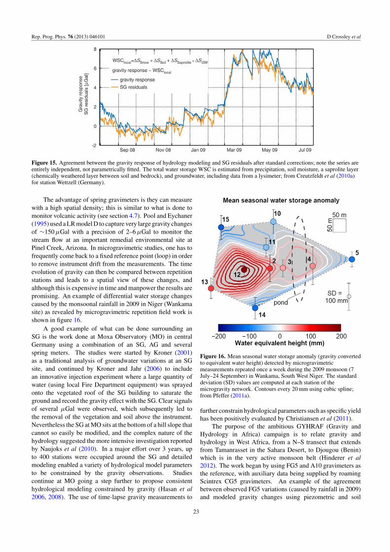
Rep. Prog. Phys. 76 (2013) 046101 D Crossley et al

Figure 15. Agreement between the gravity response of hydrology modeling and SG residuals after standard corrections; note the series areentirely independent, not parametrically fitted. The total water storage WSC is estimated from precipitation, soil moisture, a saprolite layer(chemically weathered layer between soil and bedrock), and groundwater, including data from a lysimeter; from Creutzfeldt et al (2010a)for station Wettzell (Germany).

The advantage of spring gravimeters is they can measurewith a high spatial density; this is similar to what is done tomonitor volcanic activity (see section 4.7). Pool and Eychaner(1995) used a LR model D to capture very large gravity changesof ∼150 µGal with a precision of 2–6 µGal to monitor thestream flow at an important remedial environmental site atPinel Creek, Arizona. In microgravimetric studies, one has tofrequently come back to a fixed reference point (loop) in orderto remove instrument drift from the measurements. The timeevolution of gravity can then be compared between repetitionstations and leads to a spatial view of these changes, andalthough this is expensive in time and manpower the results arepromising. An example of differential water storage changescaused by the monsoonal rainfall in 2009 in Niger (Wankamasite) as revealed by microgravimetric repetition field work isshown in figure 16.

A good example of what can be done surrounding anSG is the work done at Moxa Observatory (MO) in centralGermany using a combination of an SG, AG and severalspring meters. The studies were started by Kroner (2001)as a traditional analysis of groundwater variations at an SGsite, and continued by Kroner and Jahr (2006) to includean innovative injection experiment where a large quantity ofwater (using local Fire Department equipment) was sprayedonto the vegetated roof of the SG building to saturate theground and record the gravity effect with the SG. Clear signalsof several µGal were observed, which subsequently led tothe removal of the vegetation and soil above the instrument.Nevertheless the SG at MO sits at the bottom of a hill slope thatcannot so easily be modified, and the complex nature of thehydrology suggested the more intensive investigation reportedby Naujoks et al (2010). In a major effort over 3 years, upto 400 stations were occupied around the SG and detailedmodeling enabled a variety of hydrological model parametersto be constrained by the gravity observations. Studiescontinue at MO going a step further to propose consistenthydrological modeling constrained by gravity (Hasan et al2006, 2008). The use of time-lapse gravity measurements to

Figure 16. Mean seasonal water storage anomaly (gravity convertedto equivalent water height) detected by microgravimetricmeasurements repeated once a week during the 2009 monsoon (7July–24 September) in Wankama, South West Niger. The standarddeviation (SD) values are computed at each station of themicrogravity network. Contours every 20 mm using cubic spline;from Pfeffer (2011a).

further constrain hydrological parameters such as specific yieldhas been positively evaluated by Christiansen et al (2011).

The purpose of the ambitious GYHRAF (Gravity andHydrology in Africa) campaign is to relate gravity andhydrology in West Africa, from a N–S transect that extendsfrom Tamanrasset in the Sahara Desert, to Djougou (Benin)which is in the very active monsoon belt (Hinderer et al2012). The work began by using FG5 and A10 gravimeters asthe reference, with auxiliary data being supplied by roamingScintrex CG5 gravimeters. An example of the agreementbetween observed FG5 variations (caused by rainfall in 2009)and modeled gravity changes using piezometric and soil

23

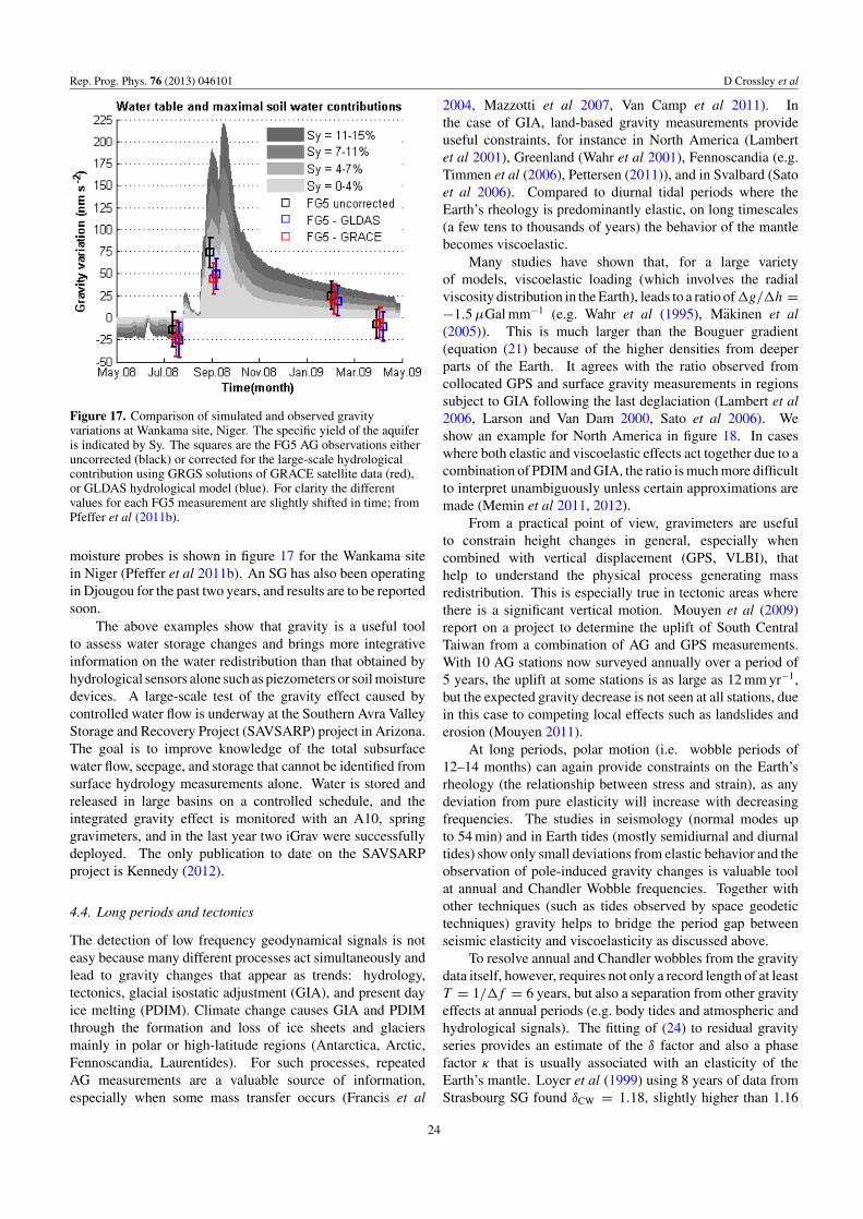
Rep. Prog. Phys. 76 (2013) 046101 D Crossley et al

Figure 17. Comparison of simulated and observed gravityvariations at Wankama site, Niger. The specific yield of the aquiferis indicated by Sy. The squares are the FG5 AG observations eitheruncorrected (black) or corrected for the large-scale hydrologicalcontribution using GRGS solutions of GRACE satellite data (red),or GLDAS hydrological model (blue). For clarity the differentvalues for each FG5 measurement are slightly shifted in time; fromPfeffer et al (2011b).

moisture probes is shown in figure 17 for the Wankama sitein Niger (Pfeffer et al 2011b). An SG has also been operatingin Djougou for the past two years, and results are to be reportedsoon.

The above examples show that gravity is a useful toolto assess water storage changes and brings more integrativeinformation on the water redistribution than that obtained byhydrological sensors alone such as piezometers or soil moisturedevices. A large-scale test of the gravity effect caused bycontrolled water flow is underway at the Southern Avra ValleyStorage and Recovery Project (SAVSARP) project in Arizona.The goal is to improve knowledge of the total subsurfacewater flow, seepage, and storage that cannot be identified fromsurface hydrology measurements alone. Water is stored andreleased in large basins on a controlled schedule, and theintegrated gravity effect is monitored with an A10, springgravimeters, and in the last year two iGrav were successfullydeployed. The only publication to date on the SAVSARPproject is Kennedy (2012).

4.4. Long periods and tectonics

The detection of low frequency geodynamical signals is noteasy because many different processes act simultaneously andlead to gravity changes that appear as trends: hydrology,tectonics, glacial isostatic adjustment (GIA), and present dayice melting (PDIM). Climate change causes GIA and PDIMthrough the formation and loss of ice sheets and glaciersmainly in polar or high-latitude regions (Antarctica, Arctic,Fennoscandia, Laurentides). For such processes, repeatedAG measurements are a valuable source of information,especially when some mass transfer occurs (Francis et al

2004, Mazzotti et al 2007, Van Camp et al 2011). Inthe case of GIA, land-based gravity measurements provideuseful constraints, for instance in North America (Lambertet al 2001), Greenland (Wahr et al 2001), Fennoscandia (e.g.Timmen et al (2006), Pettersen (2011)), and in Svalbard (Satoet al 2006). Compared to diurnal tidal periods where theEarth’s rheology is predominantly elastic, on long timescales(a few tens to thousands of years) the behavior of the mantlebecomes viscoelastic.

Many studies have shown that, for a large varietyof models, viscoelastic loading (which involves the radialviscosity distribution in the Earth), leads to a ratio of g/h =−1.5 µGal mm−1 (e.g. Wahr et al (1995), Makinen et al(2005)). This is much larger than the Bouguer gradient(equation (21) because of the higher densities from deeperparts of the Earth. It agrees with the ratio observed fromcollocated GPS and surface gravity measurements in regionssubject to GIA following the last deglaciation (Lambert et al2006, Larson and Van Dam 2000, Sato et al 2006). Weshow an example for North America in figure 18. In caseswhere both elastic and viscoelastic effects act together due to acombination of PDIM and GIA, the ratio is much more difficultto interpret unambiguously unless certain approximations aremade (Memin et al 2011, 2012).

From a practical point of view, gravimeters are usefulto constrain height changes in general, especially whencombined with vertical displacement (GPS, VLBI), thathelp to understand the physical process generating massredistribution. This is especially true in tectonic areas wherethere is a significant vertical motion. Mouyen et al (2009)report on a project to determine the uplift of South CentralTaiwan from a combination of AG and GPS measurements.With 10 AG stations now surveyed annually over a period of5 years, the uplift at some stations is as large as 12 mm yr−1,but the expected gravity decrease is not seen at all stations, duein this case to competing local effects such as landslides anderosion (Mouyen 2011).

At long periods, polar motion (i.e. wobble periods of12–14 months) can again provide constraints on the Earth’srheology (the relationship between stress and strain), as anydeviation from pure elasticity will increase with decreasingfrequencies. The studies in seismology (normal modes upto 54 min) and in Earth tides (mostly semidiurnal and diurnaltides) show only small deviations from elastic behavior and theobservation of pole-induced gravity changes is valuable toolat annual and Chandler Wobble frequencies. Together withother techniques (such as tides observed by space geodetictechniques) gravity helps to bridge the period gap betweenseismic elasticity and viscoelasticity as discussed above.

To resolve annual and Chandler wobbles from the gravitydata itself, however, requires not only a record length of at leastT = 1/f = 6 years, but also a separation from other gravityeffects at annual periods (e.g. body tides and atmospheric andhydrological signals). The fitting of (24) to residual gravityseries provides an estimate of the δ factor and also a phasefactor κ that is usually associated with an elasticity of theEarth’s mantle. Loyer et al (1999) using 8 years of data fromStrasbourg SG found δCW = 1.18, slightly higher than 1.16

24

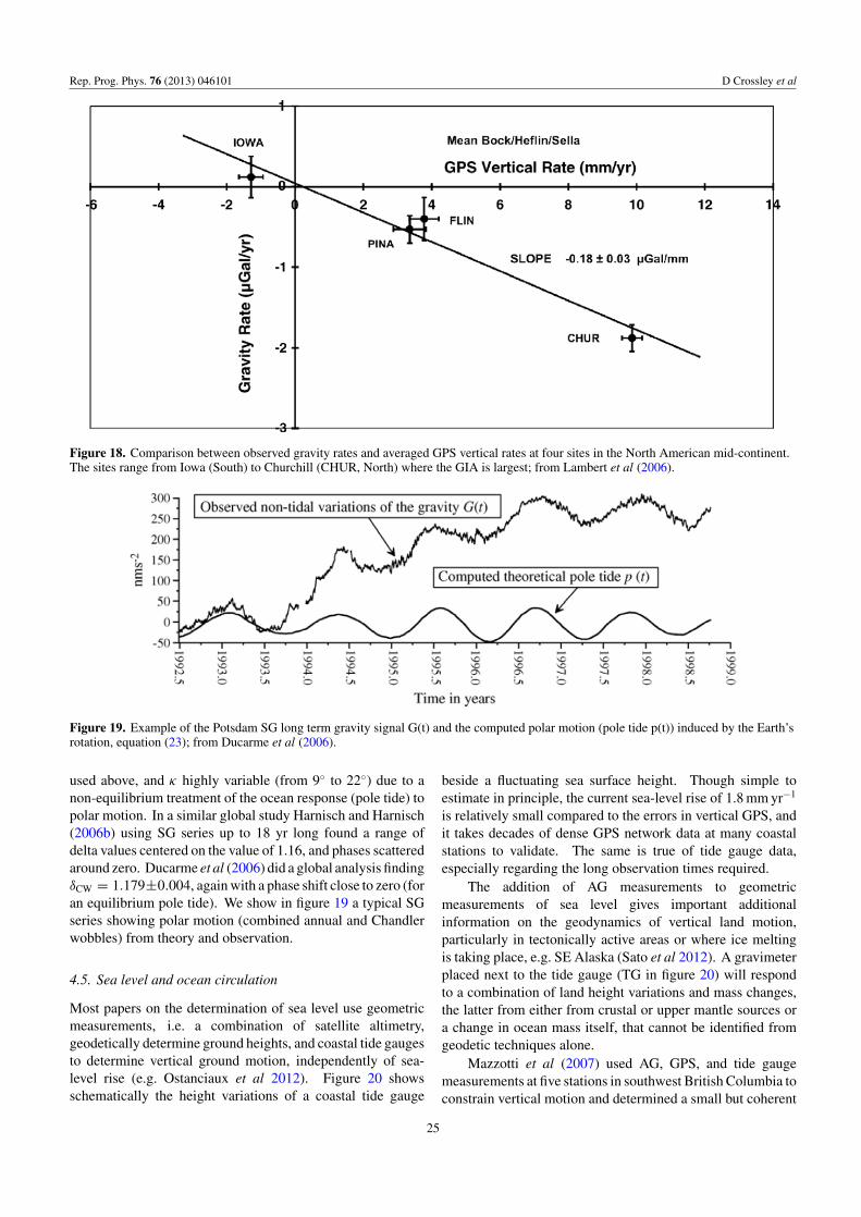
Rep. Prog. Phys. 76 (2013) 046101 D Crossley et al

Figure 18. Comparison between observed gravity rates and averaged GPS vertical rates at four sites in the North American mid-continent.The sites range from Iowa (South) to Churchill (CHUR, North) where the GIA is largest; from Lambert et al (2006).

Figure 19. Example of the Potsdam SG long term gravity signal G(t) and the computed polar motion (pole tide p(t)) induced by the Earth’srotation, equation (23); from Ducarme et al (2006).

used above, and κ highly variable (from 9 to 22) due to anon-equilibrium treatment of the ocean response (pole tide) topolar motion. In a similar global study Harnisch and Harnisch(2006b) using SG series up to 18 yr long found a range ofdelta values centered on the value of 1.16, and phases scatteredaround zero. Ducarme et al (2006) did a global analysis findingδCW = 1.179±0.004, again with a phase shift close to zero (foran equilibrium pole tide). We show in figure 19 a typical SGseries showing polar motion (combined annual and Chandlerwobbles) from theory and observation.

4.5. Sea level and ocean circulation

Most papers on the determination of sea level use geometricmeasurements, i.e. a combination of satellite altimetry,geodetically determine ground heights, and coastal tide gaugesto determine vertical ground motion, independently of sea-level rise (e.g. Ostanciaux et al 2012). Figure 20 showsschematically the height variations of a coastal tide gauge

beside a fluctuating sea surface height. Though simple toestimate in principle, the current sea-level rise of 1.8 mm yr−1

is relatively small compared to the errors in vertical GPS, andit takes decades of dense GPS network data at many coastalstations to validate. The same is true of tide gauge data,especially regarding the long observation times required.

The addition of AG measurements to geometricmeasurements of sea level gives important additionalinformation on the geodynamics of vertical land motion,particularly in tectonically active areas or where ice meltingis taking place, e.g. SE Alaska (Sato et al 2012). A gravimeterplaced next to the tide gauge (TG in figure 20) will respondto a combination of land height variations and mass changes,the latter from either from crustal or upper mantle sources ora change in ocean mass itself, that cannot be identified fromgeodetic techniques alone.

Mazzotti et al (2007) used AG, GPS, and tide gaugemeasurements at five stations in southwest British Columbia toconstrain vertical motion and determined a small but coherent

25

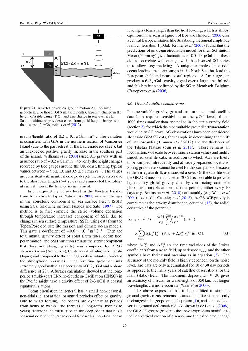
Rep. Prog. Phys. 76 (2013) 046101 D Crossley et al

Figure 20. A sketch of vertical ground motion G (obtainedgeodetically, or though GPS measurements), apparent change in theheight of a tide gauge (T.G), and true change in sea level SL.Satellite altimetry provides a check from geoid height change overthe oceans; after Ostanciaux et al (2012).

gravity/height ratio of 0.2 ± 0.1 µGal mm−1. The variationis consistent with GIA in the northern section of VancouverIsland (due to the past retreat of the Laurentide ice sheet), butan unexpected positive gravity increase in the southern partof the island. Williams et al (2001) used AG gravity with anassumed ratio of −0.2 µGal mm−1 to verify the height changesrecorded by tide gauges around the UK coast, finding typicalvalues between −3.8±1.6 and 0.9±3.1 mm yr−1. The valuesare consistent with mantle rheology, despite the large errors dueto the short data length (3–4 years) and unmodeled hydrologyat each station at the time of measurement.

In a unique study of sea level in the Western Pacific,from Antarctica to Japan, Sato et al (2001) verified changesin the non-steric component of sea surface height (SSH)using SGs, following on from Fukuda and Sato (1997). Themethod is to first compute the steric (volume expansionthrough temperature increase) component of SSH due tochanges in sea surface temperature (SST), using data from theTopex/Poseidon satellite mission and climate ocean models.This gave a coefficient of −0.6 × 10−2 m C−1. Then thetotal annual gravity effect of solid Earth tides, ocean tide,polar motion, and SSH variation (minus the steric componentthat does not change gravity) was computed for 3 SGstations Syowa (Antarctica), Canberra (Australia), and Esashi(Japan) and compared to the actual gravity residuals (correctedfor atmospheric pressure). The resulting agreement wasextremely good within an uncertainty of 0.2 µGal and a phasedifference of 20. A further calculation showed that the long-period (multi-year) El-Nino-Southern-Oscillation (ENSO) inthe Pacific might have a gravity effect of 2–3 µGal at coastalequatorial stations.

Ocean circulation in general has a small non-seasonal,non-tidal (i.e. not at tidal or annual periods) effect on gravity.Due to wind forcing, the oceans are dynamic at periodsfrom hours to weeks, and there is a long-term (months toyears) thermohaline circulation in the deep ocean that has aseasonal component. At seasonal timescales, non-tidal ocean

loading is clearly larger than the tidal loading, which is almostequilibrium, as seen in figure 1 of Boy and Hinderer (2006); fora central European station like Strasbourg the annual amplitudeis much less than 1 µGal. Kroner et al (2009) found that thepredictions of an ocean circulation model for their SG stationMoxa (Germany) give fluctuations of 0.5–1.0 µGal, but thesedid not correlate well enough with the observed SG seriesto to allow easy modeling. A unique example of non-tidalocean loading are storm surges in the North Sea that load theEuropean shelf and near-coastal regions. A 2 m surge canproduce a 6–8 µGal gravity signal over a large area inland,and this has been confirmed by the SG in Membach, Belgium(Fratepietro et al (2006).

4.6. Ground-satellite comparisons

In time-variable gravity, ground measurements and satellitedata both requires sensitivities at the µGal level, almost1000 times smaller than anomalies in the static gravity field(section 2), for which the most suitable ground instrumentationwould be an SG array. AG observations have been consideredalongside GRACE data, for example in determining the upliftof Fennoscandia (Timmen et al 2012) and the thickness ofthe Tibetan Plateau (Sun et al 2011). There remains aninconsistency of scale between single station values and highlysmoothed satellite data, in addition to which AGs are likelyto be sampled infrequently and at widely separated locations.Spring gravimeters cannot be used for this comparison becauseof their irregular drift, as discussed above. On the satellite sidethe GRACE mission launched in 2002 has been able to providehigh quality global gravity data, by constructing completeglobal field models at specific time periods, either every 10days (e.g. Bruinsma et al (2010)) or monthly (e.g. Wahr et al2004). As used in Crossley et al (2012), the GRACE gravity iscomputed as the gravity disturbance, equation (12), the radialderivative of the potential:

gSAT(r, θ, λ) = GM

ra

nmax∑n=2

(a

r

)n+1(n + 1)

×n∑

m=0

[Cmn Ym,c

n (θ, λ) + Smn Ym,s

n (θ, λ)], (33)

where Cmn and Sm

n are the time variations of the Stokescoefficients from a mean field, up to degree nmax, and the othersymbols have their usual meaning as in equation (2). Theaccuracy of the monthly field is highly dependent on the noiselevel, and data are only accumulated for 10 or 30 day periodsas opposed to the many years of satellite observations for themain (static) field. The maximum degree nmax ≈ 30 givesan accuracy of 1 µGal for wavelengths of 350 km, but longerwavelengths are more accurate (Wahr et al 2006).

The above expression has to be modified to simulateground gravity measurements because a satellite responds onlyto changes in the geopotential (equation (1)), and cannot detectvertical ground deformation h. As shown in de Linage (2008),the GRACE ground gravity is the above expression modified toinclude vertical motion of a sensor and the associated change

26

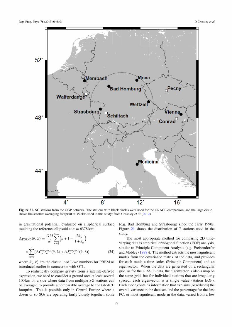
Rep. Prog. Phys. 76 (2013) 046101 D Crossley et al

Figure 21. SG stations from the GGP network. The stations with black circles were used for the GRACE comparison, and the large circleshows the satellite averaging footprint at 350 km used in this study; from Crossley et al (2012).

in gravitational potential, evaluated on a spherical surfacetouching the reference ellipsoid at a = 6378 km:

gGRND(θ, λ) = GM

a2

nmax∑n=2

(n + 1 − 2h′

n

1 + k′n

)

×n∑

m=0

[Cmn Ym,c

n (θ, λ) + Smn Ym,s

n (θ, λ)] (34)

where h′n, k

′n are the elastic load Love numbers for PREM as

introduced earlier in connection with OTL.To realistically compare gravity from a satellite-derived

expression, we need to consider a ground area at least several100 km on a side where data from multiple SG stations canbe averaged to provide a comparable average to the GRACEfootprint. This is possible only in Central Europe where adozen or so SGs are operating fairly closely together, some

(e.g. Bad Homburg and Strasbourg) since the early 1990s.Figure 21 shows the distribution of 7 stations used in thestudy.

The most appropriate method for comparing 2D time-varying data is empirical orthogonal function (EOF) analysis,similar to Principle Component Analysis (e.g. Preisendorferand Mobley (1988)). The method extracts the most significantmodes from the covariance matrix of the data, and providesfor each mode a time series (Principle Component) and aneigenvector. When the data are generated on a rectangulargrid, as for the GRACE data, the eigenvector is also a map onthe same grid, but for individual stations that are irregularlyspaced, each eigenvector is a single value (station EOF).Each mode contains information that explains (or reduces) theoverall variance in the data set, and the percentage for the firstPC, or most significant mode in the data, varied from a low

27

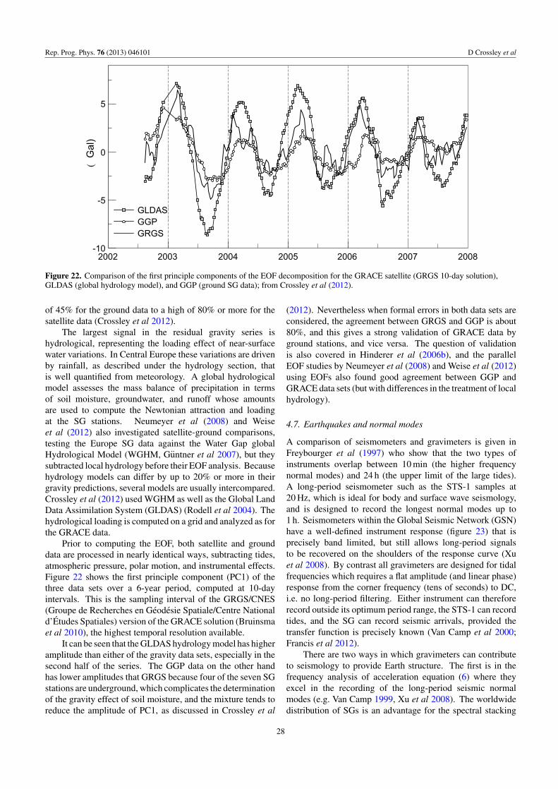
Rep. Prog. Phys. 76 (2013) 046101 D Crossley et al

2002 2003 2004 2005 2006 2007 2008

(µGal)

-10

-5

0

5

GLDAS

GGP

GRGS

Figure 22. Comparison of the first principle components of the EOF decomposition for the GRACE satellite (GRGS 10-day solution),GLDAS (global hydrology model), and GGP (ground SG data); from Crossley et al (2012).

of 45% for the ground data to a high of 80% or more for thesatellite data (Crossley et al 2012).

The largest signal in the residual gravity series ishydrological, representing the loading effect of near-surfacewater variations. In Central Europe these variations are drivenby rainfall, as described under the hydrology section, thatis well quantified from meteorology. A global hydrologicalmodel assesses the mass balance of precipitation in termsof soil moisture, groundwater, and runoff whose amountsare used to compute the Newtonian attraction and loadingat the SG stations. Neumeyer et al (2008) and Weiseet al (2012) also investigated satellite-ground comparisons,testing the Europe SG data against the Water Gap globalHydrological Model (WGHM, Guntner et al 2007), but theysubtracted local hydrology before their EOF analysis. Becausehydrology models can differ by up to 20% or more in theirgravity predictions, several models are usually intercompared.Crossley et al (2012) used WGHM as well as the Global LandData Assimilation System (GLDAS) (Rodell et al 2004). Thehydrological loading is computed on a grid and analyzed as forthe GRACE data.

Prior to computing the EOF, both satellite and grounddata are processed in nearly identical ways, subtracting tides,atmospheric pressure, polar motion, and instrumental effects.Figure 22 shows the first principle component (PC1) of thethree data sets over a 6-year period, computed at 10-dayintervals. This is the sampling interval of the GRGS/CNES(Groupe de Recherches en Geodesie Spatiale/Centre Nationald’Etudes Spatiales) version of the GRACE solution (Bruinsmaet al 2010), the highest temporal resolution available.

It can be seen that the GLDAS hydrology model has higheramplitude than either of the gravity data sets, especially in thesecond half of the series. The GGP data on the other handhas lower amplitudes that GRGS because four of the seven SGstations are underground, which complicates the determinationof the gravity effect of soil moisture, and the mixture tends toreduce the amplitude of PC1, as discussed in Crossley et al

(2012). Nevertheless when formal errors in both data sets areconsidered, the agreement between GRGS and GGP is about80%, and this gives a strong validation of GRACE data byground stations, and vice versa. The question of validationis also covered in Hinderer et al (2006b), and the parallelEOF studies by Neumeyer et al (2008) and Weise et al (2012)using EOFs also found good agreement between GGP andGRACE data sets (but with differences in the treatment of localhydrology).

4.7. Earthquakes and normal modes

A comparison of seismometers and gravimeters is given inFreybourger et al (1997) who show that the two types ofinstruments overlap between 10 min (the higher frequencynormal modes) and 24 h (the upper limit of the large tides).A long-period seismometer such as the STS-1 samples at20 Hz, which is ideal for body and surface wave seismology,and is designed to record the longest normal modes up to1 h. Seismometers within the Global Seismic Network (GSN)have a well-defined instrument response (figure 23) that isprecisely band limited, but still allows long-period signalsto be recovered on the shoulders of the response curve (Xuet al 2008). By contrast all gravimeters are designed for tidalfrequencies which requires a flat amplitude (and linear phase)response from the corner frequency (tens of seconds) to DC,i.e. no long-period filtering. Either instrument can thereforerecord outside its optimum period range, the STS-1 can recordtides, and the SG can record seismic arrivals, provided thetransfer function is precisely known (Van Camp et al 2000;Francis et al 2012).

There are two ways in which gravimeters can contributeto seismology to provide Earth structure. The first is in thefrequency analysis of acceleration equation (6) where theyexcel in the recording of the long-period seismic normalmodes (e.g. Van Camp 1999, Xu et al 2008). The worldwidedistribution of SGs is an advantage for the spectral stacking

28

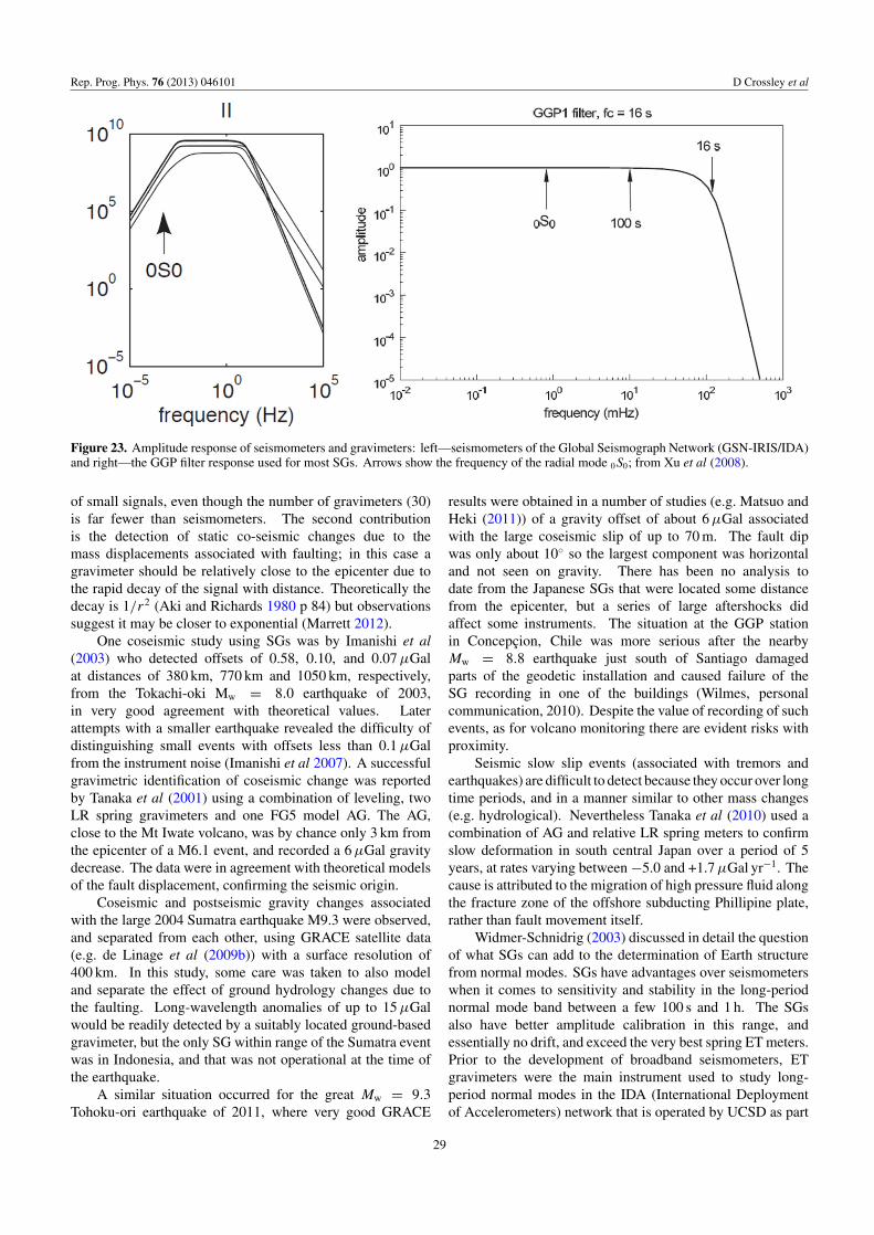
Rep. Prog. Phys. 76 (2013) 046101 D Crossley et al

Figure 23. Amplitude response of seismometers and gravimeters: left—seismometers of the Global Seismograph Network (GSN-IRIS/IDA)and right—the GGP filter response used for most SGs. Arrows show the frequency of the radial mode 0S0; from Xu et al (2008).

of small signals, even though the number of gravimeters (30)is far fewer than seismometers. The second contributionis the detection of static co-seismic changes due to themass displacements associated with faulting; in this case agravimeter should be relatively close to the epicenter due tothe rapid decay of the signal with distance. Theoretically thedecay is 1/r2 (Aki and Richards 1980 p 84) but observationssuggest it may be closer to exponential (Marrett 2012).

One coseismic study using SGs was by Imanishi et al(2003) who detected offsets of 0.58, 0.10, and 0.07 µGalat distances of 380 km, 770 km and 1050 km, respectively,from the Tokachi-oki Mw = 8.0 earthquake of 2003,in very good agreement with theoretical values. Laterattempts with a smaller earthquake revealed the difficulty ofdistinguishing small events with offsets less than 0.1 µGalfrom the instrument noise (Imanishi et al 2007). A successfulgravimetric identification of coseismic change was reportedby Tanaka et al (2001) using a combination of leveling, twoLR spring gravimeters and one FG5 model AG. The AG,close to the Mt Iwate volcano, was by chance only 3 km fromthe epicenter of a M6.1 event, and recorded a 6 µGal gravitydecrease. The data were in agreement with theoretical modelsof the fault displacement, confirming the seismic origin.

Coseismic and postseismic gravity changes associatedwith the large 2004 Sumatra earthquake M9.3 were observed,and separated from each other, using GRACE satellite data(e.g. de Linage et al (2009b)) with a surface resolution of400 km. In this study, some care was taken to also modeland separate the effect of ground hydrology changes due tothe faulting. Long-wavelength anomalies of up to 15 µGalwould be readily detected by a suitably located ground-basedgravimeter, but the only SG within range of the Sumatra eventwas in Indonesia, and that was not operational at the time ofthe earthquake.

A similar situation occurred for the great Mw = 9.3Tohoku-ori earthquake of 2011, where very good GRACE

results were obtained in a number of studies (e.g. Matsuo andHeki (2011)) of a gravity offset of about 6 µGal associatedwith the large coseismic slip of up to 70 m. The fault dipwas only about 10 so the largest component was horizontaland not seen on gravity. There has been no analysis todate from the Japanese SGs that were located some distancefrom the epicenter, but a series of large aftershocks didaffect some instruments. The situation at the GGP stationin Concepcion, Chile was more serious after the nearbyMw = 8.8 earthquake just south of Santiago damagedparts of the geodetic installation and caused failure of theSG recording in one of the buildings (Wilmes, personalcommunication, 2010). Despite the value of recording of suchevents, as for volcano monitoring there are evident risks withproximity.

Seismic slow slip events (associated with tremors andearthquakes) are difficult to detect because they occur over longtime periods, and in a manner similar to other mass changes(e.g. hydrological). Nevertheless Tanaka et al (2010) used acombination of AG and relative LR spring meters to confirmslow deformation in south central Japan over a period of 5years, at rates varying between −5.0 and +1.7 µGal yr−1. Thecause is attributed to the migration of high pressure fluid alongthe fracture zone of the offshore subducting Phillipine plate,rather than fault movement itself.

Widmer-Schnidrig (2003) discussed in detail the questionof what SGs can add to the determination of Earth structurefrom normal modes. SGs have advantages over seismometerswhen it comes to sensitivity and stability in the long-periodnormal mode band between a few 100 s and 1 h. The SGsalso have better amplitude calibration in this range, andessentially no drift, and exceed the very best spring ET meters.Prior to the development of broadband seismometers, ETgravimeters were the main instrument used to study long-period normal modes in the IDA (International Deploymentof Accelerometers) network that is operated by UCSD as part

29

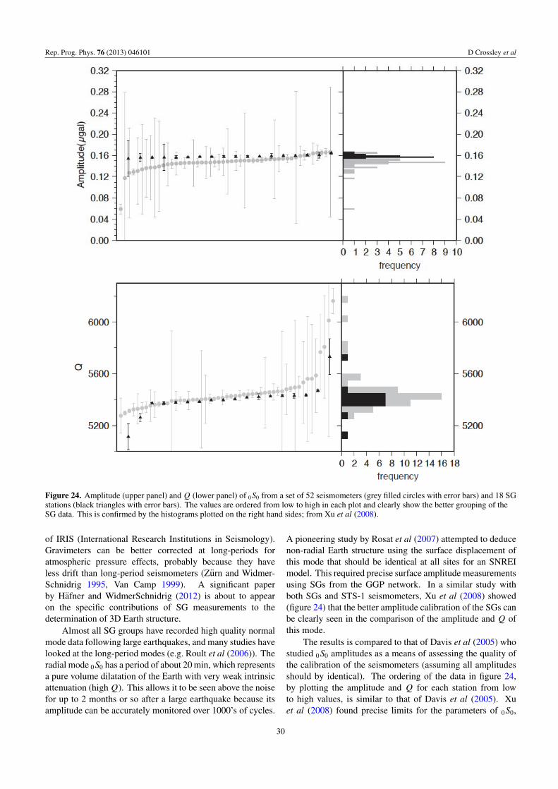
Rep. Prog. Phys. 76 (2013) 046101 D Crossley et al

Figure 24. Amplitude (upper panel) and Q (lower panel) of 0S0 from a set of 52 seismometers (grey filled circles with error bars) and 18 SGstations (black triangles with error bars). The values are ordered from low to high in each plot and clearly show the better grouping of theSG data. This is confirmed by the histograms plotted on the right hand sides; from Xu et al (2008).

of IRIS (International Research Institutions in Seismology).Gravimeters can be better corrected at long-periods foratmospheric pressure effects, probably because they haveless drift than long-period seismometers (Zurn and Widmer-Schnidrig 1995, Van Camp 1999). A significant paperby Hafner and WidmerSchnidrig (2012) is about to appearon the specific contributions of SG measurements to thedetermination of 3D Earth structure.

Almost all SG groups have recorded high quality normalmode data following large earthquakes, and many studies havelooked at the long-period modes (e.g. Roult et al (2006)). Theradial mode 0S0 has a period of about 20 min, which representsa pure volume dilatation of the Earth with very weak intrinsicattenuation (high Q). This allows it to be seen above the noisefor up to 2 months or so after a large earthquake because itsamplitude can be accurately monitored over 1000’s of cycles.

A pioneering study by Rosat et al (2007) attempted to deducenon-radial Earth structure using the surface displacement ofthis mode that should be identical at all sites for an SNREImodel. This required precise surface amplitude measurementsusing SGs from the GGP network. In a similar study withboth SGs and STS-1 seismometers, Xu et al (2008) showed(figure 24) that the better amplitude calibration of the SGs canbe clearly seen in the comparison of the amplitude and Q ofthis mode.

The results is compared to that of Davis et al (2005) whostudied 0S0 amplitudes as a means of assessing the quality ofthe calibration of the seismometers (assuming all amplitudesshould by identical). The ordering of the data in figure 24,by plotting the amplitude and Q for each station from lowto high values, is similar to that of Davis et al (2005). Xuet al (2008) found precise limits for the parameters of 0S0,

30

Rep. Prog. Phys. 76 (2013) 046101 D Crossley et al

Figure 25. The long period normal mode spectrum following the Balleny Island earthquake of 1998, Mw = 8.1; record length = 80 h. TheSG C021 is installed at the underground observatory at Membach, Belgium, along with an STS1-V seismometer. Cross spectrum improvesthe S/N; from Van Camp et al (1999).

confirming the results of Rosat et al (2007) for the SGs. For theSumatra (2004) earthquake the best frequency determinationis 0.814 656 5 ± 1.2 × 10−6 mHz, the amplitude was 0.1582 ±0.054 µGal—equivalent to a vertical displacement of 60 µm—and the Q is 5400.94 ± 22.5.

In a more general sense, figure 25 shows the very closeagreement in recording a Mw = 8.1 event using the C012 SG

and STS1-V in Membach. Qualitatively the records are verysimilar but differences are seen in the lower frequencies wherethe SG has a lower noise level. Thus the better-sited SGs canindeed contribute to long-period seismology, the only difficultyhas been calibrating the SG electronics, as required for all databefore it can be uploaded to the IRIS global seismic database.This involves measuring the complete transfer functions of all

31

Rep. Prog. Phys. 76 (2013) 046101 D Crossley et al

the SGs that requires a separate electronic laboratory procedure(Van Camp et al 2000, Francis et al 2012).

Even during the rare absence of large earthquakes (Mw >

5.5), the background spectrum of free oscillations can bedetected as a continuous ‘hum’ of the Earth, as first discoveredby the SG recording at Syowa station, Antarctica (Nawa et al1998). The phenomenon has since been confirmed by manyother instruments, i.e. LR tidal gravimeters, STS1, and STS2seismometers, and early suggestions for the source favoredexcitation by the earth’s atmosphere (Lognonne et al 1998,Tanimoto 2001). The seasonal variation in the hum signalclearly identifies atmospheric and oceanic sources for theenergy source (e.g. Kurrle and Widmer-Schnidrig (2006)),and in a recent review Nishida (2013) points to the probableconnection with oceanic infragravity waves (low frequencysurface gravity waves excited by wind shear).

A long-sought mode of the Earth is a modeled translationalmotion of the inner core within the fluid outer core, knownas the Slichter Triplet whose single mode frequency is splitinto three components by the Earth’s ellipticity and rotation.Conventional seismic theory predicts the periods for PREM as[4.78, 5.320 and 5.96] h (e.g. Crossley et al (1992), Hindereret al (1995), Rogister (2003), Rosat et al (2006)), which makesit an ideal target for SGs that have low noise in the tidalband. Despite a great deal of searching, using innovative signalenhancement techniques, detection has remained elusive, savefor Courtier et al (2000) who claim to have seen the mode insome early SG recordings, and a claim for Slichter spectralpeaks proposed by Sun et al (2006). This failure probablycomes from the weakness of earthquake excitation, as themost reliable theoretical prediction is a signal of only 1 nGalfrom the largest earthquake ever recorded, the 1960 Chileanevent of Mw = 9.5. Probably nothing short of a ratherlarge extraterrestrial impact would be sufficient (Rosat andRogister 2012).

4.8. Volcanology

The challenge in volcano monitoring is to forecast magmaticactivity before any eruption. Identifying the source ofunrest (the term used for disturbances in volcanology) is not,however, straightforward because of the complexity of bothmagma dynamics and the geometry of subsurface structuresbeneath active volcanoes. Repeated and continuous gravitymeasurements are effective tools to address such problems,because gravity changes reflect mass-transport processes atdepth (Dzurisin 2003). High-precision gravity measurements(both relative and absolute, vertical gradient, and continuousrecording) are able to determine magma and/or gas migrationwithin a magmatic system, and volcanic edifice, in the periodleading up to an eruption (e.g. Berrino et al (1984), Eggers(1987), Yokoyama (1989), Brown et al (1991), Gottsmann et al(2003), Carbone and Greco (2007)). Geodesy and volcanologyhave both benefited in the search for precursor signals ofvolcanic eruptions.

Volcano monitoring requires, like hydrology, essentiallytime-lapse surveys, or 4D data, through the repetition ofhigh-precision gravity measurements. Observations at a

number of benchmark or network locations are tied to areference or base station that is optimally outside the areaof interest, thus avoiding mass/density changes that wouldaffect gravity at both the reference and network stations.This problem can arise on small volcanic islands where itmight be difficult to find a reference outside the zone ofinterest (Furuya et al 2003); in all cases the geometry of thenetwork and station spacing (Davis et al 2008) are designedto maximize information about the target. The new portableAGs (especially the A10) are well suited to make time-lapseabsolute measurements (Ferguson et al 2008). Where difficultenvironmental conditions limit the use of AGs to only a fewselected sites, a combination of AG measurements and relativegravity measurements (hybrid gravimetry) is recommended(Berrino 2000). Hybrid gravimetry is especially importantwhere gravity at the reference site might change.

The dynamics of magmatic masses beneath a volcanousually leads to both ground deformation and gravity changes(see e.g. Johnsen et al 1980, Berrino et al 1984). Even if4D gravity and height data is well characterized by diversegeodetic techniques, the physical mechanisms responsiblefor deformation can still be ambiguous. For example,episodes of ground uplift and subsidence at the Yellowstonecaldera (Wyoming-USA), and Campi Flegrei (Italy) have beendocumented by repeated leveling and GPS surveys and by anInSAR study. In many cases the geodetic data alone may notbe able to discriminate between possible source models.

Ambiguity is a fundamental and well studied feature ofall gravity surveys. For volcanos, the time-variable gravityfield might be due to episodic intrusions of magma beneath thecaldera, or by pressurization/depressurization cycles occurringin the deep hydrothermal system (Smith et al 1997, Wickset al 1998, Dzurisin et al 1999, Battaglia et al 2006). Theconfusion between mass changes and elastic deformation canbe partially addressed if they are jointly analyzed. The twomechanisms predict different gravity/height changes, hencemass changes (gravity) and deformation changes (height)can determine the subsurface mass/volume variation. Such4D gravity surveying goes back at least four decades, withmeasurements in the Wairakei geothermal field on the NorthIsland of New Zealand as early as 1961 (Allis and Hunt 1986).The Campi Flegrei caldera (Italy) has been surveyed using tidegauges observations, leveling and gravity measurements since1870s and 1880s (Corrado et al 1976; Berrino et al 1984).Yellowstone Caldera in Wyoming has been studied throughgravity measurements since 1977 (Arnet et al 1997), and theLong Valley Caldera has been surveyed using gravity since1982 (Battaglia et al 2003).

Subsurface structures are usually modeled in terms ofsimple bodies that are mathematically easy to treat (Mogi1958, Okubo and Watanabe 1989, Okada 1992); a magmareservoir for example can be approximated as a sphericalbody. If its depth is large compared to its radius, onecan model the deformation as dilation of a point source ina homogeneous elastic half-space (Mogi 1958). Changesin gravity and elevation are normally inversely correlated,using, as a first approximation, the free air gradient (FAG)of −0.3086 µGal mm−1 (as in equation (17)). The FAG has

32

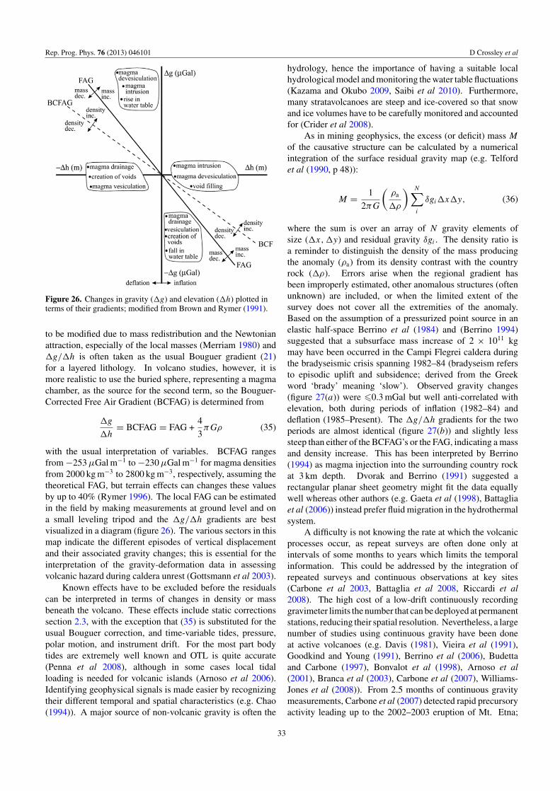
Rep. Prog. Phys. 76 (2013) 046101 D Crossley et al

Figure 26. Changes in gravity (g) and elevation (h) plotted interms of their gradients; modified from Brown and Rymer (1991).

to be modified due to mass redistribution and the Newtonianattraction, especially of the local masses (Merriam 1980) andg/h is often taken as the usual Bouguer gradient (21)for a layered lithology. In volcano studies, however, it ismore realistic to use the buried sphere, representing a magmachamber, as the source for the second term, so the Bouguer-Corrected Free Air Gradient (BCFAG) is determined from

g

h= BCFAG = FAG +

4

3πGρ (35)

with the usual interpretation of variables. BCFAG rangesfrom −253 µGal m−1 to −230 µGal m−1 for magma densitiesfrom 2000 kg m−3 to 2800 kg m−3, respectively, assuming thetheoretical FAG, but terrain effects can changes these valuesby up to 40% (Rymer 1996). The local FAG can be estimatedin the field by making measurements at ground level and ona small leveling tripod and the g/h gradients are bestvisualized in a diagram (figure 26). The various sectors in thismap indicate the different episodes of vertical displacementand their associated gravity changes; this is essential for theinterpretation of the gravity-deformation data in assessingvolcanic hazard during caldera unrest (Gottsmann et al 2003).

Known effects have to be excluded before the residualscan be interpreted in terms of changes in density or massbeneath the volcano. These effects include static correctionssection 2.3, with the exception that (35) is substituted for theusual Bouguer correction, and time-variable tides, pressure,polar motion, and instrument drift. For the most part bodytides are extremely well known and OTL is quite accurate(Penna et al 2008), although in some cases local tidalloading is needed for volcanic islands (Arnoso et al 2006).Identifying geophysical signals is made easier by recognizingtheir different temporal and spatial characteristics (e.g. Chao(1994)). A major source of non-volcanic gravity is often the

hydrology, hence the importance of having a suitable localhydrological model and monitoring the water table fluctuations(Kazama and Okubo 2009, Saibi et al 2010). Furthermore,many stratavolcanoes are steep and ice-covered so that snowand ice volumes have to be carefully monitored and accountedfor (Crider et al 2008).

As in mining geophysics, the excess (or deficit) mass M

of the causative structure can be calculated by a numericalintegration of the surface residual gravity map (e.g. Telfordet al (1990, p 48)):

M = 1

2πG

(ρa

ρ

) N∑i

δgixy, (36)

where the sum is over an array of N gravity elements ofsize (x, y) and residual gravity δgi . The density ratio isa reminder to distinguish the density of the mass producingthe anomaly (ρa) from its density contrast with the countryrock (ρ). Errors arise when the regional gradient hasbeen improperly estimated, other anomalous structures (oftenunknown) are included, or when the limited extent of thesurvey does not cover all the extremities of the anomaly.Based on the assumption of a pressurized point source in anelastic half-space Berrino et al (1984) and (Berrino 1994)suggested that a subsurface mass increase of 2 × 1011 kgmay have been occurred in the Campi Flegrei caldera duringthe bradyseismic crisis spanning 1982–84 (bradyseism refersto episodic uplift and subsidence; derived from the Greekword ‘brady’ meaning ‘slow’). Observed gravity changes(figure 27(a)) were 0.3 mGal but well anti-correlated withelevation, both during periods of inflation (1982–84) anddeflation (1985–Present). The g/h gradients for the twoperiods are almost identical (figure 27(b)) and slightly lesssteep than either of the BCFAG’s or the FAG, indicating a massand density increase. This has been interpreted by Berrino(1994) as magma injection into the surrounding country rockat 3 km depth. Dvorak and Berrino (1991) suggested arectangular planar sheet geometry might fit the data equallywell whereas other authors (e.g. Gaeta et al (1998), Battagliaet al (2006)) instead prefer fluid migration in the hydrothermalsystem.

A difficulty is not knowing the rate at which the volcanicprocesses occur, as repeat surveys are often done only atintervals of some months to years which limits the temporalinformation. This could be addressed by the integration ofrepeated surveys and continuous observations at key sites(Carbone et al 2003, Battaglia et al 2008, Riccardi et al2008). The high cost of a low-drift continuously recordinggravimeter limits the number that can be deployed at permanentstations, reducing their spatial resolution. Nevertheless, a largenumber of studies using continuous gravity have been doneat active volcanoes (e.g. Davis (1981), Vieira et al (1991),Goodkind and Young (1991), Berrino et al (2006), Budettaand Carbone (1997), Bonvalot et al (1998), Arnoso et al(2001), Branca et al (2003), Carbone et al (2007), Williams-Jones et al (2008)). From 2.5 months of continuous gravitymeasurements, Carbone et al (2007) detected rapid precursoryactivity leading up to the 2002–2003 eruption of Mt. Etna;

33

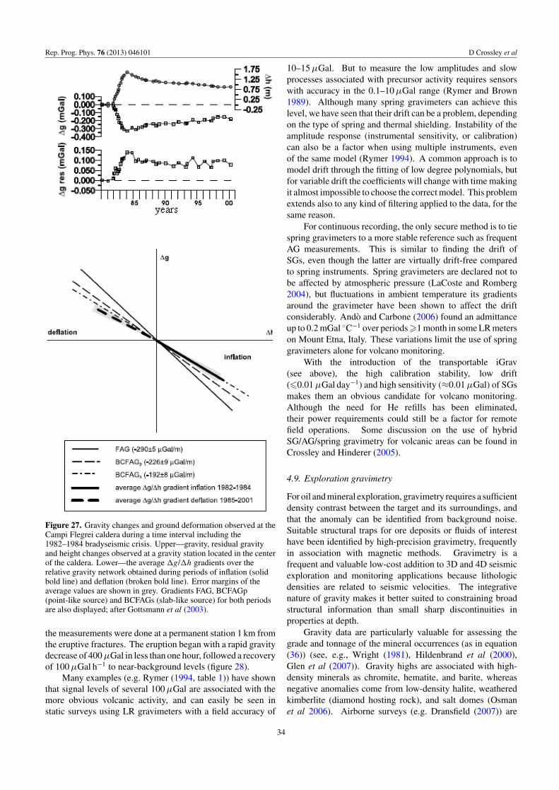
Rep. Prog. Phys. 76 (2013) 046101 D Crossley et al

Figure 27. Gravity changes and ground deformation observed at theCampi Flegrei caldera during a time interval including the1982–1984 bradyseismic crisis. Upper—gravity, residual gravityand height changes observed at a gravity station located in the centerof the caldera. Lower—the average g/h gradients over therelative gravity network obtained during periods of inflation (solidbold line) and deflation (broken bold line). Error margins of theaverage values are shown in grey. Gradients FAG, BCFAGp(point-like source) and BCFAGs (slab-like source) for both periodsare also displayed; after Gottsmann et al (2003).

the measurements were done at a permanent station 1 km fromthe eruptive fractures. The eruption began with a rapid gravitydecrease of 400 µGal in less than one hour, followed a recoveryof 100 µGal h−1 to near-background levels (figure 28).

Many examples (e.g. Rymer (1994, table 1)) have shownthat signal levels of several 100 µGal are associated with themore obvious volcanic activity, and can easily be seen instatic surveys using LR gravimeters with a field accuracy of

10–15 µGal. But to measure the low amplitudes and slowprocesses associated with precursor activity requires sensorswith accuracy in the 0.1–10 µGal range (Rymer and Brown1989). Although many spring gravimeters can achieve thislevel, we have seen that their drift can be a problem, dependingon the type of spring and thermal shielding. Instability of theamplitude response (instrumental sensitivity, or calibration)can also be a factor when using multiple instruments, evenof the same model (Rymer 1994). A common approach is tomodel drift through the fitting of low degree polynomials, butfor variable drift the coefficients will change with time makingit almost impossible to choose the correct model. This problemextends also to any kind of filtering applied to the data, for thesame reason.

For continuous recording, the only secure method is to tiespring gravimeters to a more stable reference such as frequentAG measurements. This is similar to finding the drift ofSGs, even though the latter are virtually drift-free comparedto spring instruments. Spring gravimeters are declared not tobe affected by atmospheric pressure (LaCoste and Romberg2004), but fluctuations in ambient temperature its gradientsaround the gravimeter have been shown to affect the driftconsiderably. Ando and Carbone (2006) found an admittanceup to 0.2 mGal C−1 over periods 1 month in some LR meterson Mount Etna, Italy. These variations limit the use of springgravimeters alone for volcano monitoring.

With the introduction of the transportable iGrav(see above), the high calibration stability, low drift(0.01 µGal day−1) and high sensitivity (≈0.01 µGal) of SGsmakes them an obvious candidate for volcano monitoring.Although the need for He refills has been eliminated,their power requirements could still be a factor for remotefield operations. Some discussion on the use of hybridSG/AG/spring gravimetry for volcanic areas can be found inCrossley and Hinderer (2005).

4.9. Exploration gravimetry

For oil and mineral exploration, gravimetry requires a sufficientdensity contrast between the target and its surroundings, andthat the anomaly can be identified from background noise.Suitable structural traps for ore deposits or fluids of interesthave been identified by high-precision gravimetry, frequentlyin association with magnetic methods. Gravimetry is afrequent and valuable low-cost addition to 3D and 4D seismicexploration and monitoring applications because lithologicdensities are related to seismic velocities. The integrativenature of gravity makes it better suited to constraining broadstructural information than small sharp discontinuities inproperties at depth.

Gravity data are particularly valuable for assessing thegrade and tonnage of the mineral occurrences (as in equation(36)) (see, e.g., Wright (1981), Hildenbrand et al (2000),Glen et al (2007)). Gravity highs are associated with high-density minerals as chromite, hematite, and barite, whereasnegative anomalies come from low-density halite, weatheredkimberlite (diamond hosting rock), and salt domes (Osmanet al 2006). Airborne surveys (e.g. Dransfield (2007)) are

34

Rep. Prog. Phys. 76 (2013) 046101 D Crossley et al

Figure 28. Residual gravity signal at Mount Etna encompassing the 2002–2003 eruption; after Williams-Jones et al (2008).

Figure 29. (a) Western United States cordillera showing ore deposits superimposed on major tectonic elements and main igneous zones,sedimentary basins, and metamorphic belts. (b) Filtered isostatic residual gravity anomalies. Small black triangles are maxima of thehorizontal gradient at intermediate wavelength, interpreted as main density boundaries. BH is the Bingham porphyry copper deposit; fromHildenbrand et al (2000).

widely used to map the total anomalous mass, equation (36),responsible for the anomaly. To do so requires a separationof the anomaly from the regional gradient, as in the review oflinear and spectral methods by Mantovani et al (2008). Othermathematical methods, e.g. analytical downward continuation,regression, modeling, and filtering techniques can beused, but all require some subjective evaluation (Blakeley(1995 p 311)).

Using filtered isostatic gravity anomaly maps, Hilden-brand et al (2000) identified regional crustal structures thatguided the emplacement of large metallic ore deposits in thewestern US. Figure 29 shows the structural setting and filteredgravity data, with a range of about 30 mGal, that are interpretedas regional mass anomalies extending to substantial crustaldepths. The heavy white line (figure 29(b)) shows a frontalthrust belt separating thin-skinned thrust faults on the east from

35

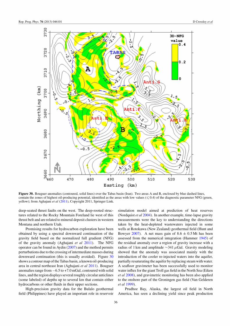
Rep. Prog. Phys. 76 (2013) 046101 D Crossley et al

Figure 30. Bouguer anomalies (contoured, solid lines) over the Tabas basin (Iran). Two areas A and B, enclosed by blue dashed lines,contain the zones of highest oil-producing potential, identified as the areas with low values ( 0.4) of the diagnostic parameter NFG (green,yellow); from Aghajani et al (2011), Copyright 2011, Springer Link.

deep-seated thrust faults on the west. The deep-rooted struc-tures related to the Rocky Mountain Foreland lie west of thisthrust belt and are related to mineral deposit clusters in westernMontana and northern Utah.

Promising results for hydrocarbon exploration have beenobtained by using a spectral downward continuation of thegravity field based on the normalized full gradient (NFG)of the gravity anomaly (Aghajani et al 2011). The NFGoperator can be found in Aydin (2007) and the method permitsperturbations due to the crossing of intermediate masses duringdownward continuation (this is usually avoided). Figure 30shows a contour map of the Tabas basin, a known oil-producingarea in central northeast Iran (Aghajani et al 2011). Bougueranomalies range from −6.5 to +7.0 mGal, contoured with solidlines, and the region displays several roughly circular anticlines(some labeled) of depths up to several km that contain eitherhydrocarbons or other fluids in their upper sections.

High-precision gravity data for the Bulalo geothermalfield (Philippines) have played an important role in reservoir

simulation model aimed at prediction of heat reserves(Nordquist et al 2004). In another example, time-lapse gravitymeasurements were the key to understanding the directionstaken by the heat-depleted wastewaters injected in somewells at Rotokawa (New Zealand) geothermal field (Hunt andBowyer 2007). A net mass gain of 8.6 ± 0.5 Mt has beenassessed from the numerical integration (Hammer 1945) ofthe residual anomaly over a region of gravity increase with aradius of 1 km and amplitude ∼341 µGal. Gravity modelingshowed that the anomaly was associated mainly with theintroduction of the cooler re-injected waters into the aquifer,partially resaturating the aquifer by replacing steam with water.A seafloor gravimeter has been successfully used to monitorwater influx for the giant Troll gas field in the North Sea (Eikenet al 2008), and gravimetric monitoring has been also appliedto the onshore part of the Groningen gas field (Van Gelderenet al 1999).

Prudhoe Bay, Alaska, the largest oil field in NorthAmerica, has seen a declining yield since peak production

36

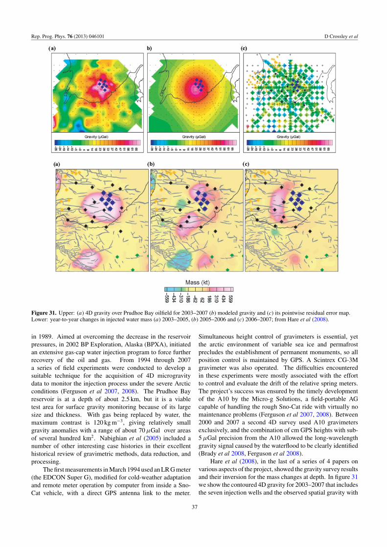
Rep. Prog. Phys. 76 (2013) 046101 D Crossley et al

Figure 31. Upper: (a) 4D gravity over Prudhoe Bay oilfield for 2003–2007 (b) modeled gravity and (c) its pointwise residual error map.Lower: year-to-year changes in injected water mass (a) 2003–2005, (b) 2005–2006 and (c) 2006–2007; from Hare et al (2008).

in 1989. Aimed at overcoming the decrease in the reservoirpressures, in 2002 BP Exploration, Alaska (BPXA), initiatedan extensive gas-cap water injection program to force furtherrecovery of the oil and gas. From 1994 through 2007a series of field experiments were conducted to develop asuitable technique for the acquisition of 4D microgravitydata to monitor the injection process under the severe Arcticconditions (Ferguson et al 2007, 2008). The Prudhoe Bayreservoir is at a depth of about 2.5 km, but it is a viabletest area for surface gravity monitoring because of its largesize and thickness. With gas being replaced by water, themaximum contrast is 120 kg m−3, giving relatively smallgravity anomalies with a range of about 70 µGal over areasof several hundred km2. Nabighian et al (2005) included anumber of other interesting case histories in their excellenthistorical review of gravimetric methods, data reduction, andprocessing.

The first measurements in March 1994 used an LR G meter(the EDCON Super G), modified for cold-weather adaptationand remote meter operation by computer from inside a Sno-Cat vehicle, with a direct GPS antenna link to the meter.

Simultaneous height control of gravimeters is essential, yetthe arctic environment of variable sea ice and permafrostprecludes the establishment of permanent monuments, so allposition control is maintained by GPS. A Scintrex CG-3Mgravimeter was also operated. The difficulties encounteredin these experiments were mostly associated with the effortto control and evaluate the drift of the relative spring meters.The project’s success was ensured by the timely developmentof the A10 by the Micro-g Solutions, a field-portable AGcapable of handling the rough Sno-Cat ride with virtually nomaintenance problems (Ferguson et al 2007, 2008). Between2000 and 2007 a second 4D survey used A10 gravimetersexclusively, and the combination of cm GPS heights with sub-5 µGal precision from the A10 allowed the long-wavelengthgravity signal caused by the waterflood to be clearly identified(Brady et al 2008, Ferguson et al 2008).

Hare et al (2008), in the last of a series of 4 papers onvarious aspects of the project, showed the gravity survey resultsand their inversion for the mass changes at depth. In figure 31we show the contoured 4D gravity for 2003–2007 that includesthe seven injection wells and the observed spatial gravity with

37

Rep. Prog. Phys. 76 (2013) 046101 D Crossley et al

a positive water anomaly of about 65 µGal. The other twosections show the modeled gravity and its error map at aboutthe 11 µGal level. The year-to-year mass changes obtainedfrom inverse modeling in the lower panels of figure 31 showsignificant blocking of the waterflood by faults at the depth ofthe reservoir.

4.10. Exotic gravimetry

Gravimetry is governed by the laws of Newton and Einstein,and implicated in the development of new theories ongravitation and gravitational waves. The assumptionsof conventional gravimetry (e.g. that G is constant andgravitational waves propagate at light speed) are the topic ofwide-ranging speculation by physicists, and of key importanceis observational verification. One of the very first uses of anSG was the suggestion by Warburton and Goodkind (1976)that observations of tidal phases could detect the presence ofa universal preferred reference frame. Using an 18-monthrecord at Pinon Flat, they focussed on one of the semidiurnaltides (R2) as the most likely to show evidence of tidal-likedeformations of the Earth from rotation and orbital motionin a preferred reference frame. Tidal analysis at this levelrequires precise corrections for OTL and atmospheric pressure,and this ultimately limited their ability to make a definitivedetermination; for a Newtonian tide of amplitude 24.274 µGaltheir error level was about 0.02 µGal and with a phase error of−90 (up to which a preferred frame was not indicated).

The long-term stability of SGs was suggested by Shiomi(2008a) as beneficial to test theories of the anisotropy in G,indicating the possibility of accuracies rivaling lunar laserranging (LLR). Shiomi (2008b) also suggested other possiblesignals that could be tested by high-precision gravimetry:(a) preferred frame effects (as in Warburton and Goodkind(1976)), (b) scalar and gravitational waves through theexcitation of the seismic normal modes 0S0 and 0S2 at periodsof 20 min and 54 min respectively, and the presence of dilatonicwaves associated with translational motions of the inner coreat periods of 6 h (Slichter triplet) and 24 h. As in the preferredframe analysis, the important factor for such studies is theaccuracy with which the competing effects from OTL and theatmospheric can be assessed.

The Apache Point Observatory Lunar Laser-rangingOperation (APOLLO) began ranging to the Moon in 2006,and is currently one of the leading installations in this field. Interms of fundamental physics, LLR currently provides the besttests of the strong equivalence principle, the time variation ofthe strength of gravity, gravitomagnetism, geodetic precession,and the inverse-square law (e.g. Muller and Biskupek (2007),Murphy (2009)). A major effort is underway within APOLLOto reduce the lunar distance uncertainty from the cm level tothe mm range, as a further improvement to tighten the tests ofgeneral relativity that are underway. To this end an SG wasinstalled at the telescope site in 2008 for two purposes (a) togive improved tidal models for the site through the analysis oflocal tides and atmospheric pressure effects, and (b) to monitorthe gravity/height ratio to further model site motion. TheSG is located almost immediately under the telescope that is

used nightly for astronomical experiments, and the azimuthalswings of the dome can be seen as small offsets in the SG seriesat about the 0.1–0.5 µGal level, but they can be removed bycross correlating with the dome azimuth.

A total solar eclipse is an opportunity to study thegravitational shielding effect of the Moon. This was first triedin 1997 in China using a LR D meter, with apparent gravitysignals of about 5 µGal (Wang et al 2000). Subsequently twogroups analyzed data from an eclipse over northern Europein 1999, when the shadow path passed almost directly overtwo SG stations, and close to two other SGs, with a suite ofLR ET meters specifically deployed along the path. Mansinhaet al (2001) reported the attempt to identify gravity signalsbetween the leading and trailing edges of the transit. From thethree best stations, they estimated that any eclipse signal above0.05 × 10−9 m s−2, or 0.005 µGal, would have been detected.

Using other gravity data during the same eclipse, VanRuymbeke et al (2003) claimed that, due to the higher noisein his data, no eclipse effects above a threshold of 0.2 µGal(significantly higher than Mansinha et al 2001) could havebeen detected in the experiment. The noise in the data isnot just instrumental but incorporates other effects such asincomplete modeling of the atmosphere. In any case these twogravity studies concluded that the upper bound of the universalconstant of gravitational absorption (the so-called Majoranavalue) is of the order of 10−16 m2 kg−1 while the analysis ofLLR data (Dickey et al 2004) was able to provide a much lowerbound of 10−22 m2 kg−1. There is hence no confirmation of anygravitational shielding or absorption effect.

The question of precisely defining a single value of grav-ity in the absolute sense (using AGs), is at the heart of an im-portant problem in fundamental physics—how to redefine thekilogram (e.g. Marson (2012)). The kilogram has, since 1889,been related to an international prototype made of platinum–iridium at Bureau International des Poids et Mesures (BIPM,Paris)—this is the only remaining fundamental reference as-sociated with a unique physical entity. The goal is to replacethis standard by a more fundamental connection and so far itis not clear which will be successful. One of two approachesis to define the kilogram using Avagadro’s constant (Hill et al2011). The other is to make a Watt balance measurement thatcan link Planck’s constant h to a weight defined though mg; themass m can be defined, providing the measurement of g (usingan AG) is completely reliable and unbiased. To ensure that g isbe free of systematic effects, this is best achieved by compar-ing observations made by instruments with different principles(i.e. free-fall, rise and fall, or cold atom) such as attemptedby Louchet-Chauvet et al (2010). The original project to dothis was the e-MASS Euramet Joint Research Project betweenthe National Metrology Institutes of Switzerland (METAS,now EJPD), Italy (INRIM) and France (LNE) (Marson 2012)and this was one reason that AG instruments other than theFG5 have continued to be developed. There is currently afollow-on project ‘Realisation of the awaited definition of thekilogram—resolving the discrepancies’ to remeasure Planck’sconstant and Avagadro’s number prior to the finalization of thenew kilogram (details can be found on the EURAMET web-site at http://www.euramet.org/index.php?id=emrp call 2011#c10996).

38

Rep. Prog. Phys. 76 (2013) 046101 D Crossley et al

It is within the scope of this review to rememberthe experiments, predominantly done in the 1980s, todetermine if gravity follows precisely the inverse-square law,or alternatively if equivalence was violated, or there exists a‘fifth force’. In one of the most accurate tests, Niebauer et al(1987) used a version of the commercial JILA AG (modifiedto have two dropping chambers) to determine an agreement inacceleration of uranium and copper test masses to an accuracyof 5 × 10−10 (Faller 2005). Carussotto et al (1996) repeatedthe experiment with different apparatus and also found nodetectable violation of standard theory.

A unique free-fall AG measurement of G itself wasreported by Schwarz et al (1998) using a standard FG5gravimeter surrounded by a 500 kg ring-shaped test mass thatcould be located vertically at various positions with respectto the internal falling cube. As stated by the authors, ‘thisexperiment is the only laboratory determination of gravity thatdoes not suspend the test mass from a support system. Itis therefore free of many systematic errors associated withsupports’. Their value of G was a rather high (6.6873 ±0.0094) × 10−11 in SI units. More recently the apparentconvergence of measurements of G, towards the current valueof (6.67428 ± 0.000 67) × 10−11, was challenged by a recentdual pendulum measurement (Parks and Faller 2010) thatyielded a significantly lower value (6.67234 ± 0.000 14) ×10−11, close to a prior value established in 1986. The aboveestimates give an accuracy in G of 0.01%, or 1 part in 104,which is less than a typical calibration error for SGs (0.1%),but is far short of the precision of AG measurements of g itself(1 part in 109).

5. Conclusions

It seems appropriate to conclude such a lengthy review withonly brief conclusions. In essence we have tried to indicatethat gravimetry is, like most fields of science, searching forvery small and subtle signals buried in a broad range of effectsof the same size and timescale. In this case the effects arisemostly from Earth’s environment, from internal processes suchas earthquakes, magmatic activity, tectonics, and hydrology, toexternal effects from the oceans, soil moisture, tides, and theatmosphere. Many studies dwell on the importance of one ofthese sources, arguing that the others can be modeled decently;but what is signal and what is noise is relative, as always.

Modern instruments complement each other to providethe necessary time resolution and precision at the sub-µGallevel for a single location (SGs), with long-term control at the1–2 µGal level (AGs), and the necessary spatial coverage fromspring gravimeters at the 5 µGal level (Scintrex CG5, BurrisZLS, and gPhone). As we have seen in almost all cases it isonly the combination of all three types that provides an idealstrategy for the most of the problems we have discussed. Thepracticalities of doing 4D gravity surveys, however, are alwaysgoing to be limited by the cost of instruments, manpower andlogistics, and inevitably steered towards current goals such asglobal change, hazard monitoring, and commercial interest.Nevertheless the effort required has been shown to pay offwith impressive results in fields like hydrology that a decadeago were only just beginning to be researched.

Acknowledgments

We thank Severine Rosat for help with some figures andRichard Warburton (GWR Instruments) and Tim Niebauer(Micro-g LaCoste) for checking the accuracy of statementsin the Instrumentation section. The journal editors were verygenerous in allowing our submission delays. Support for DCrossley is acknowledged through NASA/10-APRA10-0045and NSF/PHY-1068879 grants (Gravitational Tests via LunarLaser Ranging: APOLLO Analysis and Acquisition).

References

Abe M, Takemoto S, Fukuda Y, Higashi T, Imanishi Y, Iwano S,Ogasawara S, Kobayashi Y, Dwipa A and Kusuma D S 2006Hydrological effects on the superconducting gravimeterobservation in Bandung J. Geodyn. 41 288–95

Abe M, Kroner C, Neumeyer J and Chen X D 2010 Assessment ofatmospheric reductions for terrestrial gravity observations Bull.d’Inf. Marees Terr. 146 11817–38

Aghajani H, Moradzadeh A and Zeng H 2011 Detection ofhigh-potential oil and gas fields using normalized full gradientof gravity anomalies: a case study in the Tabas Basin, EasternIran Pure Appl. Geophys. 168 1851–63

Agnew D C 1997 NLOADF: a program for computing ocean-tideloading J. Geophys. Res. 102 5109–10

Agnew D 1992 The time domain behavior of power law noisesGeophys. Res. Lett. 19 333–6

Agnew D 2007 Earth tides Treatise on Geophysics vol 3 edT Herring, Gen ed. G Schubert (Amsterdam: Elsevier)pp 163–95

Agnew D C 2012 SPOTL: Some programs for ocean-tide loadingSIO Technical Report Scripps Institution of Oceanography andhttp://escholarship.org/uc/item/954322pg

Agostino G, Desogus S, Germak A, Origlia C, Quagliotto D,Berrino G, Corrado G, d’Errico V and Ricciardi G 2008 Thenew IMGC-02 transportable absolute gravimeter:measurement apparatus and applications in geophysics andvolcanology Ann. Geophys. 51 39–49

Aki K and Richards P 1980 Quantitative Seismology, Theory andMethods (San Francisco: Freeman Price) vol 1, 557pp; vol 2353pp

Allis R G and Hunt T M 1986 Analysis of exploitation-inducedgravity changes at Wairakei geothermal field Geophysics51 1647–60

Anderson O and Hinderer J 2005 Global inter-annual gravitychanges from GRACE: early results Geophys. Res. Lett.32 L01402

Ando B and Carbone D 2006 A new computational approach toreduce the signal from continuously recording gravimeters forthe effect of atmospheric temperature Phys. Earth Planet. Int.159 247–56

Arafin S 2004 Relative Bouguer anomaly The Leading Edge23 850–1

Ander M E, Summers T and Gruchalla M 1999 The LaCoste &Romberg gravity meter: system analysis and instrumentalerrors Geophysics 64 1708–819

Arnet F, Kahle H G, Klingele E, Smith R B and Meertens C M 1997Temporal gravity and height changes of the Yellowstonecaldera Geophys. Res. Lett. 24 2741–4

Arnoso J, Fernandez J and Vieira R 2001 Interpretation of tidalgravity anomalies in Lanzarote, Canary Islands J. Geodyn.31 341–54

Arnoso J, Benavent M, Ducarme B and Montesinos F G 2006 A newocean tide loading model in the Canary Islands region J.Geodyn. 41 100–11

39

Rep. Prog. Phys. 76 (2013) 046101 D Crossley et al

Arora B, Kamal Kumar A, Rawat G, Kumar N and Choubey V M2008 First observations of free oscillations of the earth fromIndian superconducting gravimeter in Himalaya Curr. Sci. 951611–7

Aydin A 2007 Interpretation of gravity anomalies with thenormalized full gradient (NFG) method and an example PureAppl. Geophys. 64 2329–44

Baker T F and Bos M S 2003 Validating Earth and oceanmodels using tidal gravity measurements Geophys. J. Int.152 468–85

Banka D, Crossley D and Jentzsch G 1998 Investigations ofsuperconducting gravimeter records in the frequency range ofthe free oscillations of the Earth: the noise magnitude Proc.13th Int. Sympon. Earth Tides (Observatoire Royal deBelgique, Brussels) pp 641–9

Banka D and Crossley D 1999 Noise levels of superconductinggravimeters at seismic frequencies Geophys. J. Int.139 87–97

Battaglia M, Segall P and Roberts C 2003 The mechanics of unrestat Long Valley caldera, California: II. Constraining the natureof the source using geodetic and micro-gravity data J. Volcan.Geotherm. Res. 127 219–45

Battaglia M, Troise C, Obrizzo F, Pingue F and De Natale G 2006Evidence for fluid migration as the source of deformation atCampi Flegrei caldera (Italy) Geophys. Res. Lett.33 L01307

Battaglia M, Gottsmann J, Carbone D and Fernandez J 2008 4DVolcano gravimetry Geophysics 73-6 WA3–18

Barthelmes F 2009 Definition of functionals of the geopotential andtheir calculation from spherical harmonic models: theory andformulas used by the calculation service of the InternationalCentre for Global Earth Models (ICGEM),http://icgem.gfz-potsdam.de Scientific Technical Report 09/02,Deutsches Geo-ForschungsZentrum GFZ

Berrino G, Corrado G, Luongo G and Toro B 1984 Grounddeformation and gravity changes accompanying the 1982Pozzuoli uplift Bull. Volcanol. 47 187–200

Berrino G 1994 Gravity changes induced by height-mass variationsat the Campi Flegrei caldera J. Volcanol. Geotherm. Res.61 293–309

Berrino G 2000 Combined gravimetry in the observationof volcanic processes in Southern Italy J. Geodyn.30 371–88

Berrino G, Corrado G and Riccardi U 2006 On the capability ofrecording gravity stations to detect signals coming fromvolcanic activity: the case of Mt. Vesuvius J. Volcan.Geotherm. Res. 150 270–82

Blakeley R J 1995 Potential Theory in Gravity and MagneticApplications (Cambridge: Cambridge University Press)

Bonvalot S, Diament M and Gabalda G 1998 Continuous gravityrecording with Scintrex CG-3M meters: a promising tool formonitoring active zones Geophys. J. Int. 135 470–94

Bos M S and Baker T F 2005 An estimate of the errors in gravityocean tide loading computations J.Geodyn. 79 50–63

Bower D R and Courtier N 1998 Precipitation effects on gravitymeasurements at the Canadian absolute gravity site Phys. EarthPlanet. Int. 106 353–69

Boy J-P, Hinderer J and Gegout P 1998 Global atmospheric loadingand gravity Phys. Earth Planet. Int. 109 161–77

Boy J-P, Gegout P and Hinderer J 2002 Reduction of surface gravitydata from global atmospheric pressure loading Geophys. J. Int.149 534–45

Boy J-P, Llubes M, Hinderer J and Florsch N 2003 A comparison oftidal ocean loading models using superconducting gravimeterdata J. Geophys. Res. 108 2193

Boy J-P, Llubes M, Ray R D, Hinderer J, Florsch N, Rosat S,Lyard F and Letellier T 2004 Non-linear oceanic tidesobserved by superconducting gravimeters in EuropeJ. Geodyn. 38 391–405

Boy J-P and Chao B 2005 Precise evaluation of atmospheric loadingeffects on Earth’s time-variable gravity field J. Geophys. Res.110 B08412

Boy J-P and Hinderer J 2006 Study of the seasonal gravity signal insuperconducting gravimeter data J. Geodyn. 41 227–33

Boy J-P, Ray R and Hinderer J 2006 Diurnal atmospheric tide andinduced gravity variations J. Geodyn. 41 253–8

Brady J L, Ferguson J F, Hare J L, Seibert J E, Klopping F J, Chen Tand Niebauer T 2008 Results of the World’s First 4DMicrogravity Surveillance of a Waterflood–Prudhoe Bay,Alaska SPE Reservoir Eval. Eng. 11 824–31 (SPE-101762-PA)

Branca S, Carbone D and Greco F 2003 Intrusive mechanism of the2002 NE-Rift eruption at Mt. Etna (Italy) inferred throughcontinuous microgravity data and volcanological evidencesGeoph. Res. Lett. 30 SDE 14 1–4

Brown G C, Rymer H and Stevenson D 1991 Volcano monitoring bymicrogravity and energy budget analysis J. Geol. Soc. Lond.148 585–93

Bruinsma S, Lemoine J M, Biancale R and Vales N 2010CNES/GRGS 10-day gravity field models (release 2) and theirevaluation Adv. Space Res. 45 587–601

Budetta G and Carbone D 1997 Potential application of the ScintrexCG-3M Gravimeter for monitoring volcanic activity: results offield trials on Mt. Etna, Sicily J. Volcanol. Geotherm. Res.76 199–214

Carbone D, Budetta G, Greco F and Rymer H 2003 Combineddiscrete and continuous gravity observations at Mt. EtnaJ. Volcanol. Geotherm. Res. 123 123–35

Carbone D, Budetta G, Greco F and Zuccarello L 2007 A datasequence acquired at Mt. Etna during the 2002–2003 eruptionhighlights the potential of continuous gravity observations as atool to monitor and study active volcanoes J. Geodyn. 43 320–9

Carbone D and Greco F 2007 Review of microgravity observationsat Mt. Etna: a powerful tool to monitor and study activevolcanoes Pure Appl. Geophys. 164 769–90

Carussotto S, Cavasinni V, Perrone F, Polacco E, Iacopini E andStefanini G 1996 g-universality test with a Galileo’s typeexperiment Nuovo Cimento 111B 1259–75

Chao B F 1994 The geoid and Earth rotation GeophysicalInterpretations of Geoid. ed P Vanicek and N Christou(Boca Raton, FC: CRC Press) pp 285–98

Chao B F, Merriam J B and Tamura Y 1995 Geophysical analysisof zonal tidal signals in length of day Geophys. J. Int.122 765–75

Chapin D 1998 Gravity instruments: past, present, future LeadingEdge 17 100–12

Christiansen L, Binning P J, Rosbjerg D, Andersen O B and BauerGottwein P 2011 Using time lapse gravity for groundwatermodel calibration: an application to alluvial aquifer storageWater Resources Res. 47 W06503

Corrado G, Guerra I, Bascio L A, Luongo G and Rampoldi R 1976Inflation and microearthquakes activity of Phlegraean FieldsItaly Bull. Volcanol. 40 (3) 169–88

Courtier N, Ducarme B, Goodkind J, Hinderer J, Imanishi Y, SeamaN, Sun H, Merriam J, Bengert B and Smylie D E 2000 Globalsuperconducting gravimeter observations and the search for thetranslational modes of the inner core Phys. Earth Planet. Int.117 3–20

Creutzfeldt B, Guntner A, Wziontek H and Merz B 2010a Reducinglocal hydrology from high precision gravity measurements: alysimeter-based approach Geophys. J. Int. 183 178–87

Creutzfeldt B, Guntner A, Thoss H, Merz B and Wziontek H 2010bMeasuring the effect of local water storage changes on in situgravity observations: case study of the Geodetic ObservatoryWettzell, Germany Water Resources Res. 46 W08531

Crider J G, Hill Johnsen K and Williams-Jones G 2008 Thirty-yeargravity change at Mount Baker Volcano, Washington, USA:extracting the signal from under the ice Geophys. Res. Let35 L20304

40

Rep. Prog. Phys. 76 (2013) 046101 D Crossley et al

Crossley D J, Rochester M G and Peng Z R 1992 Slichtermodes and Love numbers Geophys. Res. Lett.19 1679–82

Crossley D, Jensen O Hinderer J 1995 Effective barometricadmittance and gravity residuals Phys. Earth Planet Int.90 221–41

Crossley D and Xu H 1998 Analysis of superconducting gravimeterdata, from Table Mountain, Colorado Geophys. J. Int.135 835–44

Crossley D, Xu H and Van Dam T 1998 Comprehensive analysis of2 years of SG data from Table Mountain, Colorado Proc. 13thSymp. Earth Tides, Brussels 1997 (Observatoire Royal deBelgique) pp 659–68

Crossley D et al 1999 Network of superconducting gravimetersbenefits a number of disciplines EOS. Trans. Am. Geophys.Union 80 121–6

Crossley D J and Hinderer J 2005 Using SG arrays for hydrology incomparison with GRACE satellite data, with extension toseismic and volcanic hazards Korean J. Remote Sensing 2131–49

Crossley D and Hinderer J 2008 The contribution of GGPSuperconducting gravimeters to GGOS Observing ourChanging Earth (IAG Sympo. vol 133) (Berlin: Springer)pp 841–52

Crossley D and Hinderer J 2009 A review of the GGP network andscientific challenges J. Geodyn. 48 299–304

Crossley D, de Linage C, Boy J-P, Hinderer J and Famiglietti J2012 A comparison of the gravity field over Central Europefrom superconducting gravimeters, GRACE and globalhydrological models, using EOF analysis Geophys. J. Int.189 877–97

Dahlen F A and Tromp J 1998 Theoretical Global Seismology(Princeton, NJ: Princeton University Press)

Davis J P, Ishii M and Masters G 2005 An assessment of theaccuracy of GSN sensor response information Seismol. Res.Lett. 76 678–83

Davis P M 1981 Gravity and Earth tides measured on an activevolcano, Mt Etna, Sicily J. Volcanol. Geotherm. Res.11 213–23

Davis K, Kass M A, Krahenbuhl R A and Li Y 2008 Survey designand model appraisal based on resolution analysis for 4Dgravity monitoring SEG Expanded Abstr. 27 731

Defraigne P, Dehant V and Hinderer J 1994 Stacking gravity tidemeasurements and nutation observations in order to determinethe complex eigenfrequency of the Nearly Diurnal FreeWobble J. Geophys. Res. 99 9203–13

Defraigne P, Dehant V and Wahr J M 1996 Internal loading of aninhomogeneous compressible Earth with phase boundariesGeophys. J. Int. 125 173–92

Dehant V and Ducarme B 1987 Comparison between the theoreticaland observed tidal gravimetric factors Phys. Earth Planet. Int.49 192–212

Dehant V, Defraigne P and Wahr J M 1999 Tides for a convectiveEarth J. Geophys. Res. 104 1035–58

de Linage C, Hinderer J and Rogister Y 2007 A search for the ratiobetween gravity variation and vertical displacement due to asurface load Geophys. J. Int. 171 986–94

de Linage C 2008 Mesures gravimetriques absolues et relatives enco-localisation avec des techniques geodesiques depositionnement precis: quel lien entre les variations depesanteur et les mouvements verticaux? PhD Thesis Ecole etObservatoires des Sciences de la Terre, Universite LouisPasteur Strasbourg

de Linage C, Hinderer J and Boy J-P 2009a Variability of thegravity-to-height ratio due to surface loads Pure Appl.Geophys. 166 1217–45

de Linage C, Rivera L, Hinderer J, Boy J-P, Rogister Y, Lambotte Sand Biancale R 2009b Separation of coseismic and postseismicgravity changes for the 2004 Sumatra—Andaman earthquake

from 4.6 yr of GRACE observations and modelling of thecoseismic change by normal-modes summation Geophys. J.Int. 176 695–714

Deville S, Champollion C, Chery J, Doerflinger E, Le Moigne N,Bayer R and Vernant P 2011 Studying unsaturated epikarstwater storage properties by time lapse surface to depth gravitymeasurements Abstract G43C-07 Presented at 2011 FallMeeting, AGU (San Francisco, CA: 5–9 December)

Dickey J O et al 2004 Lunar laser ranging: a continued legacy of theApollo program Science 265 482–90

Doodson A 1921 The harmonic development of the tide-generatingpotential Proc. R. Soc. Lond. A 100 305–29

Dransfield M 2007 Airborne gravity gradiometry in the search formineral deposits Proc. Exploration 07: 5th Decennial Int.Conf. on Mineral Exploration (Toronto, Canada)ed B Milkereit pp 341–54

Ducarme B, Venedikov A, Arnoso J, Chen X-D, Sun H-P andVieira R 2006 Global analysis of the GGP superconductinggravimeters network for the estimation of the pole tidegravimetric amplitude factor J. Geodyn. 41 334–44

Ducarme B 2011 Determination of the main Lunar waves generatedby the third degree tidal potential and validity of thecorresponding body tides models J. Geodyn. 86 65–75

Dvorak J and Berrino G 1991 Recent ground movements andseismic activity in Campi Flegri, southern Italy: episodicgrowth of a resurgent dome J. Geophys. Res. 96 2309–23

Dziewonski A M and Anderson D L 1981 Preliminary referenceEarth model Phys. Earth Planet Int. 25 297–356

Dzurisin D, Wicks C Jr and Thatcher W 1999 Renewed uplift at theYellowstone Caldera measured by leveling surveys and satelliteradar interferometry Bull. Volcanol. 61 349–55

Dzurisin D 2003 A comprehensive approach to monitoring volcanodeformation as a window on the eruptive cycle Rev. Geophys.41 1009

Eggers A A 1987 Residual gravity changes and eruption magnitudesJ. Volcanol. Geotherm. Res. 33 201–16

Eiken O, Stenvold T, Zumberge M, Aines H and Sasegawa G 2008Gravimetric monitoring of gas production from the Troll fieldGeophys. 73 (6) WA149–WA154

Faller J E 1965 Results of an absolute determination of theacceleration of gravity J. Geophys. Res. 70 4035–8

Faller J, Guo Y, Gschwind J, Niebauer T, Rinker R L and Xue J1983 The JILA (Joint Institute for Laboratory Astrophysics)portable absolute gravity apparatus, Defense TechnicalInformation Center

Faller J E and Marson I 1988 Ballistic methods of measuring g—thedirect free fall and symmetric rise and fall methods comparedMetrologia 25 49–55

Faller J E 2005 The measurement of little g: a fertile ground forprecision measurement J. Res. Natl Inst. Stand. Technol.110 559–81

Featherstone W E and Dentith M C 1997 A Geodetic approach togravity data reduction for geophysics Comput. Geosci.23 1063–70

Ferguson J F, Chen T, Brady J, Aiken C L V and Seibert J 2007 The4D microgravity method for waterflood surveillance: II.Gravity measurements for the Prudhoe Bay reservoir, AlaskaGeophysics 72 I33–43

Ferguson J F, Klopping F J, Chen T, Seibert J E, Hare J L andBrady J L 2008 The 4D microgravity method for waterfloodsurveillance: III. 4D absolute microgravity surveys at PrudhoeBay, Alaska Geophysics 73-6 WA163–71

Florsch N and Hinderer J 2000 Bayesian estimation of the Free CoreNutation parameters from the analysis of precise tidal gravitydata Phys. Earth Planet. Int. 117 21–35

Forste C et al 2008 EIGEN-5C A new global combinedhigh-resolution GRACE-based gravity field model of theGFZ-GRGS cooperation EGU General Assembly 2008 (13–18April, Vienna, Austria) EGU2008-A-03426

41

Rep. Prog. Phys. 76 (2013) 046101 D Crossley et al

Forste C et al 2011 EIGEN-6A new combined global gravity fieldmodel including GOCE data from the collaboration ofGFZ-Potsdam and GRGS-Toulouse, EGU2011-3242 EGUGeneral Assembly 2011, 3–8 April 2011, Vienna, Austria

Francis O, Van Camp M, Van Dam T, Warnant T and Hendrickx M2004 Indication of the uplift of the Ardenne in long termgravity variations in Membach (Belgium) Geophys. J. Int.158 346–52

Francis O and Van Dam T 2006 Analysis of results of theinternational comparison of absolute gravimeters inWalferdange (Luxembourg) of November 2003 Cahiers CentreEur. Geodyn. Seismol. Lux. 26 1–24

Francis O, Lampitelli C, Klein G, Van Camp M and Palinkas V2012 Comparison between the transfer functions of threesuperconducting gravimeters Bull. d’Inf. Marees Terr.147 11857–68

Fratepietro F, Baker T F, Williams S D P and Van Camp M2006 Ocean loading deformations caused by storm surgeson the northwest European shelf, Geophys. Res. Lett.33 L06317

Freybourger M, Hinderer J and Trampert J 1997 Comparative studyof superconducting gravimeters and broadband seismometersSTS-1/Z in seismic and subseismic frequency bands Phys.Earth Planet. Sci. 101 203–217

Fukuda Y and Sato T 1997 Gravity effects of sea level variation atthe Superconducting Gravimeter sites, estimated from ERS-1and Topex-Poseidon altimeter data Gravity, Geoid, and MarineGeodesy (IAG Sympo. vol 117) ed J Segawa et al (Berlin:Springer)

Furuya M, Okubo S, Sun W, Tanaka T, Oikawa J, Watanabe H andMaekawa T 2003 Spatiotemporal gravity changes atMiyakejima volcano: Japan: Caldera collapse, explosiveeruptions and magma movement J. Geophys. Res. 108 2219

Glen J M G, Schmidt J and Morin R 2007 Gravity and magneticcharacter of south-central Alaska: Constraints on geologic andtectonic interpretations, and implications for mineralexploration Geol. Soc. Am. Special Papers 431 593-622

Gaeta F, De Natale G, Peluso F, Mastrolorenzo G, Castagnolo D,Troise C, Pingue F, Mita D G and Rossano S 1998 Genesis andevolution of unrest episodes at Campi Flegrei caldera: The roleof thermal fluid-dynamical processes in the geothermal systemJ. Geophys. Res. 103 20921–34

Gaspar P, Ogor P, Le-Traon Y and Zanife O Z 1994 Estimating thesea state bias of the TOPEX and POSEIDON altimeters fromcrossover differences J. Geophys. Res. 99 24981–94

Goodkind J M and Young C 1991 Gravity and hydrology at KilaueaVolcano, the Geysers and Miami Proc. Workshop: Non TidalGravity Changes Intercomparison Between Absolute andSuperconducting Gravimeters Cahiers Centre Eur. Geodyn.Seismol. Lux. 3 163–7

Goodkind J M 1999 The superconducting gravimeter Rev. Sci.Instrum. 70 4131–52

Gottsmann J, Berrino G, Rymer H and Williams-Jones G 2003Hazard assessment during caldera unrest at the Campi Flegrei,Italy: a contribution from gravity–height gradients EarthPlanet. Sci. Lett. 211 295–309

Guntner A, Stuck J, Werth S, Doll P, Verzano K and Merz B 2007 Aglobal analysis of temporal and spatial variations in continentalwater storage Water Resources Res. 43 W05416

Hackney R I and Featherstone W E 2003 Geodetic versusgeophysical perspectives of the ‘gravity anomaly’ Geophys. J.Int. 154 35–43

Hafner R and Widmer-Schnidrig R 2012 Signature of 3-D densitystructure in spectra of the spheroidal free oscillation 0S2,Geophys. J. Int. 192 285–94

Hammer S 1945 Estimating ore masses in gravity prospectingGeophysics 10 50–62

Hare J L, Ferguson J F and Brady J L 2008 The 4D microgravitymethod for waterflood surveillance: IV. Modeling and

interpretation of early epoch 4D gravity surveys at PrudhoeBay, Alaska Geophysics 73-6 WA173–80

Harnisch G and Harnisch M 2006a Hydrological influences in longgravimetric data series J. Geodyn. 41 276–87

Harnisch M and Harnisch G 2006b Study of long-term gravityvariations, based on data of the GGP co-operation J. Geodyn.41 318–25

Harrison J C and LaCoste L J B 1978 The measurement of surfacegravity ed I I Mueller Applications of Geodesy toGeodynamics: Ninth GEOP Conf. (Ohio State University,Columbus, OH) ed II Mueller Report No 280

Harrison J C and Sato T 1984 Implementation of electrostaticfeedback with a LaCoste-Romberg model G gravity meterJ. Geophys. Res. 89 7957–61

Hartmann T and Wenzel H-G 1995 The HW95 tidal potentialcatalogue Geophys. Res. Lett. 22 3553–6

Hasan S, Troch P A, Boll J and Kroner C 2006 Modeling thehydrological effect in local gravity at Moxa, GermanyJ. Hydrometeorol. 7 346–54

Hasan S, Troch P A, Bogaart P W and Kroner C 2008 Evaluatingcatchment-scale hydrological modeling by means ofterrestrial gravity observations Water Resources Res.44 W08416

Hide R and Dickey J 1991 Earth’s variable rotation Science253 629–37

Hildenbrand T G, Berger B, Jachen R C and Ludington S 2000Regional crustal structures and their relationship to thedistribution of ore deposits in the Western United States, basedon magnetic and gravity data Econ. Geol. 95 1583–603

Hill T P, Miller J and Censullo A C 2011 Towards a better definitionof the kilogram Metrologia 48 83–6

Hinderer J, Crossley D and Jensen O 1995 A search for the Slichtertriplet in superconducting gravimeter data Phys. Earth Planet.Int. 90 183–95

Hinderer J, Pfeffer J, Boucher M, Nahmani S, de Linage C, Boy J-P,Genthon P, Seguis L, Favreau G and Bock O 2012 Land waterstorage changes from ground and space geodesy: first resultsfrom the GHYRAF (Gravity and Hydrology in Africa)experiment Pageoph 169 1391–410

Hinderer J, Crossley D and Warburton R J 2007 Superconductinggravimetry Treatise on Geophysics vol 3 (Geodesy) edT Herring, Gen. ed G Schubert (Amsterdam: Elsevier) pp65–122

Hinderer J, Ole Andersen O, Lemoine F, Crossley D and Boy J-P2006a Seasonal changes in the European gravity field fromGRACE: a comparison with superconducting gravimeters andhydrology model predictions J. Geodyn. 41 59–68

Hinderer J, de Linage C and Boy J-P 2006b How to validatesatellite-derived gravity observations with gravimeters at theground? Bull. d’Inf. Marées Terr. 142 11433–42

Hunt T and Bowyer D 2007 Reinjection and gravity changes atRotokawa geothermal field, New Zealand Geothermics36 421–35

Imanishi Y, Higashi T and Fukuda Y 2002 Calibration of thesuperconducting gravimeter T011 by parallel observation withthe absolute gravimeter FG5 210- a Bayesian approachGeophys. J. Int. 151 867–78

Imanishi Y, Sato T, Higashi T, Sun W and Okubo S 2003 A networkof superconducting gravimeters detects submicrogal coseismicgravity changes Science 306 476–8

Imanishi Y, Kokubo K and Tatehata H 2006 Effect of undergroundwater on gravity observation at Matsushiro, Japan J. Geodyn.41 221–6

Imanishi Y, Tamura Y, Ikeda H and Okubo S 2007 Permanentgravity changes recorded on superconducting gravimeters fromearthquakes in central Japan—the Noto Hantou and NiigatakenChuetsu-oki events in 2007 J. Geodyn. 48 260–8

Jacob T, Bayer R, Chery J, Jourde H, Le Moigne N, Boy J-P,Hinderer J, Luck B and Brunet P 2008 Absolute gravity

42

Rep. Prog. Phys. 76 (2013) 046101 D Crossley et al

monitoring of water storage variation in a karst aquifer on thelarzac plateau (Southern France) J. Hydrology 359 105–17

Jacob T, Chery J, Bayer R, Le Moigne N, Boy J-P, Vernant P andBoudin F 2009 Time-lapse surface to depth gravitymeasurements on a karst system reveal the dominant role ofthe epikarst as a water storage entity Geophys. J. Int.177 347–60

Jacob T, Bayer R, Chery J and Le Moigne N 2010 Time-lapsemicrogravity surveys reveal water storage heterogeneity of akarst aquifer J. Geophys. Res. 115 B06402

Jekeli C 2012 Geometric reference systems in geodesy, LectureNotes, Ohio State University http://hdl.handle.net/1811/51274

Jentzsch G 1997 Earth tides and ocean loading Tidal Phenomena edH Wilhem et al (Berlin: Springer) pp 145–71

Jentzsch G 2008 The automated Burris gravity meter—a newinstrument using an old principle Proc. Symp. on TerrestrialGravimetry: Static and Mobile Measurements (St Petersburg,Russia, 20–23 August 2007)

Jiang Z et al 2009 Relative gravity measurement campaign duringthe 8th International Comparison of Absolute Gravimeters(2009) Metrologia 49 95–107

Johnsen G V, Bjornsson A and Sigurdsson A 1980 Gravity andelevation changes caused by magma movement beneath theKrafla caldera, northeast Iceland J. Geophys. 47 132–40

Kang K, Li H, Peng P, Hao H and Wie J 2011 Seasonal variations inhydrological influences on gravity measurements usinggPhones Terr. Atmos. Ocean. Sci. 22 157–68

Kazama T and Okubo S 2009 Hydrological modeling ofgroundwater disturbances to observed gravity: theory andapplication to Asama Volcano, Central Japan J. Geophys. Res.114 B08402

Kennedy J, Ferre T, Creutzfeldt B and Gunter A 2012Gravity-measured water storage change and subsurfacehydraulic properties at a Managed Recharge Facility in Tucson,USA SAGEEP 25 18 (http://dx.doi.org/10.4133/1.4721694)

Klugel T, Wziontek H, Abe M and Kroner C 2008 Computation ofatmospheric gravity changes from 3-dimensional numericalweather models Geophys. Res. Abs. 10 EGU2008-A-06120,SRef-ID: 1607-7962/gra/EGU2008-A-06120 EGU GeneralAssembly, 2008

Klugel T and Wziontek H 2009 Correcting gravimeters andtiltmeters for atmospheric mass attraction using operationalweather models J. Geodyn. 48 204–10

Kroner C and Jentzsch G 1999 Comparison of different pressurereductions for gravity data and resulting consequences Phys.Earth Planet. Int. 115 205–18

Kroner C 2001 Hydrological effects on gravity data of theGeodynamic Observatory Moxa J. Geodyn. Soc. Japan47 353–8

Kroner C and Jahr T 2006 Hydrological experiments around thesuperconducting gravimeter at Moxa Observatory J. Geodyn.41 268–75

Kroner C, Jahr T, Naujoks M and Weise A 2007 Hydrologicalsignals in gravity—foe or friend? IAG Symposia DynamicPlanet (IAG Symposia vol 130) (Berlin: Springer)pp 504–10

Kroner C, Dobslaw H, Thomas M, Janssen F and Weise A 2009Non-tidal oceanic mass shifts and their impact on terrestrialgravity observations Geophys. Res. Abs. 11 EGU2009-4079

Kudryavtsev S M 2004 Improved harmonic development of theEarth tide generating potential J. Geodyn. 77 829–38

Kurrle D and Widmer-Schnidrig R 2006 Spatiotemporal features ofthe Earth’s background oscillations observed in central EuropeGeophys. Res. Lett. 33 L24304

LaCoste L J B and Romberg 2004 Instruction manual, Model G andD gravity meters: http://www.gravity-meta-repair.com/images/gdmanual.pdf (last accessed 5 August 2008)

Lambert A, Courtier N, Sasagawa G, Klopping F, Winester D,James T and Liard J 2001 New constraints on Laurentide

postglacial rebound from absolute gravity measurementsGeophys. Res. Lett. 28 2109–12

Lambert A, Courtier N and James T S 2006 Long-term monitoringby absolute gravimetry: Tides to postglacial rebound J.Geodyn. 41 307–17

Larson K M and Van Dam T 2000 Measuring postglacial reboundwith GPS and absolute gravity Geophys. Res. Lett. 27 3925–8

Lecolazet R 1956 L’enregistrement de la maree gravimetrique avecun gravimetre North-American Bull. d’Inf. Marees Terr. 1 4–16

Le Moigne N, Champollion C, Warburton R, Bayer R, Deville S,Doerflinger E, Chery J, Vernant P, Boudin F and Collard P2011 New iGrav superconducting gravimeter: accuracy, driftand first results Abstract G31B-0955 Presented at 2011 FallMeeting, AGU (San Francisco, CA 5–9 December)

Liard J and Gagnon C 2002 The new A-10 Absolute gravimeter atthe 2001 international comparison of absolute gravimetersMetrologia 39 477–83

Lognonne P, Clevede E and Kanamori H 1998 Computation ofseismograms and atmospheric oscillations by normal-modesummation for a spherical earth model with realisticatmosphere Geophys. J. Int. 135 388–406

Longuevergne L, Boy J-P, Florsch N, Viville D, Ferhat G, Ulrich P,Luck B and Hinderer J 2009 Local and global hydrologicalcontributions to gravity variations observed in Strasbourg J.Geodyn. 48 189–94

Louchet-Chauvet A, Merlet S, Bodart Q, Landragin A, Dos Santos FP, Baumann H, D’Agostino G and Origlia C 2010 Comparisonof 3 absolute gravimeters based on different methods for thee-MASS project (arXiv:1008.2884v2 [physics.atom-ph])

Loyer S, Hinderer J and Boy J-P 1999 Determination of thegravimetric factor at the Chandler period from Earth’sorientation data and superconducting gravimetry observationsGeophys. J. Int. 136 1–7

Makinen J, Engfeldt A and Harsson B G 2005 The Fennoscandianland uplift gravity lines 1966–2003 Gravity, Geoid and SpaceMissions ed C Jekeli et al (IAG Symposium 129) (Berlin:Springer) pp 328–32

Mansinha L, Ducarme B, Hinderer J, Meurers B and Van RuymbekeM 2001 Search for the Gravitational absorption effect usingsuperconducting gravimeters during the eclipse of August 11,1999 J. Geodyn. Soc. Japan 47 387–91

Mantovani M S M, Shukowsky W, de Brito Neves B B and RugenskiA 2008 Gravimetric study of a potential mineral deposit in theItapororoca region, Brazil Geophys. Prospect. 56 751–60

Marrett R 2012 Radial decay of coseismic displacement amplitudesfrom thrust earthquakes (Abstract) Seismol. Res. Lett. 83 382

Marson I 2012 A short walk along the gravimeters path Int. J.Geophys. 2012 687813

Matsumoto K, Sato T, Takanezawa T and Ooe M 2001 GOTIC2: aprogram for computation of oceanic tidal loading effect J.Geodyn. Soc. Japan 47 243–8

Matsuo K and Heki K 2011 Coseismic gravity changes of the 2011Tohoku-oki earthquake from satellite gravimetry Geophys. Res.Lett. 38 L00G12

Matthews P M 2001 Love numbers and gravimetric factors fordiurnal tides J. Geodyn. Soc. Japan 46 231–6

Mazzotti S, Lambert A, Courtier N, Nykolaishen L and Dragert H2007 Crustal uplift and sea level rise in northern Cascadia fromGPS, absolute gravity, and tide gauge data Geophys. Res. Lett.34 L15306

Melchior P 2008 Gravimetric measuring techniques PhysicalMethods, Instruments and Measurements (Encyclopedia of LifeSupport Systems (EOLSS)) ed vol II Y M Tsipenyuk pp 259–90(Developed under the Auspices of the UNESCO, EolssPublishers, Oxford, UK http://www.eolss.net)

Memin A, Rogister Y, Hinderer J, Omang O C and Luck B 2011Secular gravity variation at Svalbard (Norway) from groundobservations and GRACE satellite data Geophys. J. Int.184 1119–30

43

Rep. Prog. Phys. 76 (2013) 046101 D Crossley et al

Memin A, Hinderer J and Rogister Y 2012 Separation of thegeodetic consequences of past and present ice-mass change:influence of topography with application to Svalbard (Norway)Pure Appl. Geophys. 169 1357–72

Merlet S, Kopaev A, Diament M, Geneves G, Landragin A and DosSantos F P 2008 Micro-gravity investigations for the LNE wattbalance project Metrologia 45 265–74

Merlet S, Bodart Q, Malossi N, Landragin A, Pereira F, Dos SantosF P, Gitlein O and Timmen L 2010 Comparison between twomobile absolute gravimeters: optical versus atomicinterferometers Metrologia 47 L9

Merriam J B 1980 The series computation of the gravitationalperturbation due to an ocean tide Phys. Earth Planet. Int.23 81–6

Merriam J 1992 Atmospheric pressure and gravity Geophys. J. Int.109 488–500

Merriam J 1995 Non-linear tides observed with thesuperconducting gravimeter at Cantley, Quebec Geophys. J.Int. 123 529–40

Meurers B, Van Camp M and Petermans T 2007 Correctingsuperconducting gravity time-series using rainfall modelling atthe Vienna and Membach stations and application to Earth tideanalysis J. Geodyn. doi:10.1007/s00190-007-0137-1

Mogi K 1958 Relations between the eruptions of various volcanoesand the deformations of the ground surfaces around them Bull.Earth. Res. Inst. 36 99–134

Mouyen M, Masson F, Hwang C, Cheng C C, Cattin R, Lee C W, LeMoigne N, Hinderer J, Malavieille J, Bayer R and Luck B 2009Expected temporal absolute gravity change across theTaiwanese Orogen, a modeling approach J. Geodyn. 48 284

Mouyen M 2011 Contribution of gravimetry to the Taiwaneseorogeny study PhD Thesis defense, June 16,eost.u-strasbg.fr/semipgs/these mouyen.pdf

Mukai A, Higashi T, Takemoto S, Nakagawa I and Naito I 1995Accurate estimation of atmospheric effects on gravityobservations made with a superconducting gravimeter at KyotoPhys. Earth Planet. Int. 91 149–59

Muller J and Biskupek L 2007 Variations of the gravitationalconstant from lunar laser ranging data Class. Quant. Grav.24 4533–8

Muller T and Zurn W 1983 Observation of gravity changes duringthe passage of cold fronts J. Geophys. 53 155–62

Murphy T W Jr 2009 Lunar Ranging, Gravitomagnetism, andAPOLLO Space Sci. Rev. 148 217–23

Nabighian M N, Ander M E, Grauch V J S, Hansen R O, LaFehr TR, Li Y, Pearson W C, Peirce J W, Phillips J D and Ruder M E2005 Historical development of the gravity method inexploration Geophysics 70 63–89

Naujoks M, Kroner C, Weise W, Jahr T, Krause P and Eisner S 2010Evaluating local hydrological modelling by temporal gravityobservations and a gravimetric three-dimensional modelGeophys. J. Int. 182 233–49

Nawa K, Suda N, Fukao Y, Sato T, Aoyama Y and Shibaya K 1998Incessant excitation of the Earth’s free oscillations EarthPlanets Space 50 3–8

Nawa K, Suda N, Yamada I, Miyajima R and Okubo S 2009Coseismic change and precipitation effect in temporal gravityvariation at Inuyama, Japan: a case of the 2004 off the Kiipeninsula earthquakes observed with a superconductinggravimeter J. Geodyn. 48 1–5

Nettleton L L 1976 Gravity and Magnetics In Oil Prospecting(New York: McGraw-Hill) 464pp

Neuberg J, Hinderer J and Zurn W 1987 Stacking gravity tideobservations in Central Europe for the retrieval of the complexeigenfrequency of the nearly diurnal free wobble Geophys. J.R. Astron. Soc. 91 853–68

Neumeyer J 1995 Frequency-dependent atmospheric pressurecorrection on gravity variations by means of cross-spectralanalysis Bull. Inf. Mar. Terr. 122 9212–20

Neumeyer J, Hagedoorn J, Leitloff J and Schmidt T 2004 Gravityreduction with three-dimensional atmospheric pressuredata for precise ground gravity measurements J. Geodyn.38 437–50

Neumeyer J et al 2006 Combination of temporal gravity variationsresulting from Superconducting Gravimeter (SG) recordings,GRACE satellite observations and global hydrology modelsJ. Geodyn. 79 573–85

Neumeyer J, Barthelmes B, Kroner C, Petrovic S, Schmidt R,Virtanen H and Wilmes H 2008 Analysis of gravity fieldvariations derived from superconducting gravimeterrecordings, the GRACE satellite and hydrological models atselected European sites Earth Planets Space 60 505–18

Niebauer T M, Hoskins J K and Faller J E 1986 Absolute gravity: Areconnaissance tool for studying vertical crustal motionsJ. Geophys. Res. 91 9145–9

Niebauer T M 1987 New absolute gravity instruments for physicsand geophysics PhD Dissertation University of Colorado,Boulder, 155pp

Niebauer T M, McHugh M P and Faller J E 1987 Galilean test forthe fifth force Phys. Rev. Lett. 59 609–12

Niebauer T M and Faller J E 1991 Absolute gravimetry:environmental noise limits Workshop Proc., Non-tidal gravitychanges, Walferdange (Luxembourg) Cahiers du Centre Eur.Geodyn. Seismol. 3 39–45

Niebauer T M, Sasagawa G S, Faller J E, Hilt R and Klopping F1995 A new generation of absolute gravimeters Metrologia32 159

Niebauer T 2007 Gravimetric methods—absolute gravimeter:instruments concepts and implementation Treatise onGeophysics vol 3, Gen. ed G Schubert (Amsterdam: Elsevier)pp 43–64

NIMA 2000 Department of defense world geodetic system 1984,3rd edn Technical Report NIMA TR8350.2

Nishida K 2013 Earth’s Background Free Oscillations Annu. Rev.Earth Planet. Sci. 41 at press

Nordquist G, Protacio J A P and Acuna J A 2004 Precision gravitymonitoring of the Bulalo geothermal field, Philippines:independent checks and constraints on numerical simulationGeothermics 33 37–56

Okada Y 1992 Internal deformation due to shear and tensile faults ina halfspace Bull. Seismol. Soc. Am. 82 1018–40

Okubo S and Watanabe H 1989 Gravity change caused by a fissureeruption Geophys. Res. Lett. 16 445–8

Osman O, Albora A M and Osman N U 2006 A new approach forresidual gravity anomaly profile interpretations: Forced NeuralNetwork (FNN) Ann. Geophys. 49 1201–8

Ostanciaux E, Husson L, Choblet G, Robin C and Pedoja K 2012Present-day trends of vertical ground motion along the coastlines Earth-Sci. Rev. 110 74–92

Palinkas V 2006 Precise tidal measurements by spring gravimetersat the station Pecny J. Geodyn. 41 14–22

Parks H V and Faller J E 2010 Simple pendulum determination ofthe gravitational constant Phys. Rev. Lett. 105 110801

Pavlis N K, Holmes S A, Kenyon S C and Factor J K 2008 An Earthgravitational model to degree 2160:EGM2008 EGU GeneralAssembly 2008 (13–18 April, Vienna, Austria)EGU2008-A-01891

Penna N T, Bos M S, Baker T F and Scherneck H-G 2008 Assessingthe accuracy of predicted ocean tide loading displacementvalues J. Geodyn. 82 893–907

Peter G, Klopping F, Sasagawa G, Faller J and Niebauer T 1993Short- and long-term stability of the JILAG-4 absolutegravimeter J. Geophys. Res. 98 4619–26

Peter G, Klopping F and Berstis K A 1995 Observing and modelinggravity changes caused by soil moisture and groundwater tablevariations with superconducting gravimeters in Richmond,Florida Cahiers Centre Eur. Geodyn. Seismol. Lux.11 147–59

44

Rep. Prog. Phys. 76 (2013) 046101 D Crossley et al

Peterson J 1993 Observations and modeling of seismic backgroundnoise Open-File Report 93-332 US Department of Interior,Geological Survey, Albuquerque, NM

Pettersen B R 2011 The postglacial rebound signal of Fennoscandiaobserved by absolute gravimetry, GPS, and Tide Gauges, Int. J.Geophys. 2011 957329

Pfeffer J 2011a Etude du cycle de l’eau en Afrique sahelienne :Approche multidisciplinaire et apport de la gravimetrie terrestreet spatiale These de Doctorat Universite de Strasbourg, France

Pfeffer J, Boucher M, Hinderer J, Favreau G, Boy J-P, de Linage C,Luck B, Oi M and Le Moigne N 2011b Hydrologicalcontribution to time-variable gravity: influence of the WestAfrican Monsoon in Southwest Niger Geophys. J. Int.184 661–72

Pool D R and Eychaner JH 1995 Measurements of aquifer-storagechange and specific yield using gravity Surveys Ground Water33 425–32

Preisendorfer R W and Mobley C D 1988 Principal ComponentAnalysis in Meteorology and Oceanography (Amsterdam:Elsevier)

Prothero W A Jr and Goodkind J M 1968 A superconductinggravimeter Rev. Sci. Instr. 39 1257–62

Riccardi U, Hinderer J and Boy J-P 2007 On the efficiency ofbarometric arrays to improve the reduction of atmosphericeffects on gravity data Phys. Earth Planet. Int. 161 224–42

Riccardi U, Berrino G, Corrado G and Hinderer J 2008 Strategies inthe processing and analysis of continuous gravity record inactive volcanic areas: the case of Mt. Vesuvius AnnalsGeophys. 51 67–85

Riccardi U, Hinderer J, Boy J-P and Rogister Y 2009 Tilteffects on GWR superconducting gravimeters J. Geodyn.48 316–24

Riccardi U, Rosat S and Hinderer J 2011 Comparison of theMicro-g LaCoste gPhone-054 spring gravimeter and theGWR-C026 superconducting gravimeter in Strasbourg(France) using a 300-day time series Metrologia48 28–39

Riccardi U, Rosat S and Hinderer J 2012 On the accuracy of thecalibration of superconducting gravimeters using absolute andspring sensors: A critical comparison Pure Appl. Geophys.169 1343–56

Richter B, Wilmes H and Nowak I 1995 The Frankfurt calibrationsystem for relative gravimeters Metrologia 32 217–23

Rodell M et al 2004 The global land data assimilation system Bull.Am. Meteorol. Soc. 85 381–94 [Available online athttp://disc.gsfc.nasa.gov/services/grads-gds/gldas.shtml.]

Rogister Y 2003 Splitting of seismic-free oscillations and of theSlichter triplet using the normal mode theory of a rotating,ellipsoidal earth Phys. Earth Planet. Int. 140 169–82

Rosat S, Hinderer J, Crossley D and Boy J-P 2004 Performance ofsuperconducting gravimeters from long-period seismology totides J. Geodyn 38 461–76

Rosat S, Sato T, Imanishi Y, Hinderer J, Tamura Y, McQueen H andOhashi M 2005 High resolution analysis of the gravest seismicnormal modes after the 2004 Mw = 9 Sumatra earthquakeusing superconducting gravimeter data Geophys. Res. Lett.32 L13304

Rosat S, Rogister Y, Crossley D and Hinderer J 2006 A search forthe Slichter triplet with superconducting gravimeters: impacton the density jump at the inner core boundary J. Geodyn.41 296–306

Rosat S, Watada S and Sato T 2007 Geographical variations of the0S0 normal mode amplitude: predictions and observations afterthe Sumatra–Andaman earthquake Earth Planets Space 59307–11

Rosat S, Florsch N, Hinderer J and Llubes M 2009 Estimation of thefree core nutation parameters from SG data: sensitivity studyand comparative analysis using linearized least-squares andBayesian methods J. Geodyn. 48 331–9

Rosat S and Hinderer J 2011 Noise levels of superconductinggravimeters: updated comparison and time stability Bull.Seismol. Soc. Am. 101 1233–41

Rosat S and Rogister Y 2012 Excitation of the Slichter mode bycollision with a meteoroid or pressure variations at thesurface and core boundaries Phys. Earth Planet. Int.190-191 25–33

Roult G, Rosat S, Clevede E, Millot-Langet R and Hinderer J 2006New determinations of Q quality factors and eigenfrequenciesfor the whole set of singlets of the Earth’s normal modes 0S0,0S2, 0S3 and 2S1 using superconducting gravimeter data fromthe GGP network J. Geodyn. 41 345–57

Rymer H and Brown G C 1989 Gravity changes as a precursor tovolcanic eruptions at Poás volcano, Costa Rica Nature342 902–5

Rymer H 1994 Microgravity changes as a precursor to volcanicactivity J. Volcanol. Geotherm. Res. 61 311–28

Rymer H 1996 Microgravity monitoring Monitoring and Mitigationof Volcano Hazards ed R Scarpa and R Tilling (Berlin:Springer) pp 169–97

Saibi H, Gottsmann J and Ehara S 2010 Post-eruptive gravitychanges from 1999 to 2004 at Unzen volcano (Japan): awindow into shallow aquifer and hydrothermal dynamics J.Volcanol. Geotherm. Res. 191 137–47

Sato T, Fukuda Y, Aoyama Y, McQueen H, Shibuya K, Tamura Y,Asari K and Ooe M 2001 On the observed annual gravityvariation and the effect of sea surface height variations Phys.Earth Planet. Int. 123 45–63

Sato T, Miura S, Sun W, Sugano T, Freymueller J T, Larsen C F,Ohta Y, Fujimoto H, Inazu D and Motyka R J 2012 Gravity anduplift rates observed in southeast Alaska and their comparisonwith GIA model predictions J. Geophys. Res. 117 B01401

Sato T, Okuno J, Hinderer J, MacMillan D, Plag H-P, Francis O,Falk R and Fukuda Y 2006 A geophysical interpretation of thesecular displacement and gravity rates observed atNy-Ålesund, Svalbard in the Arctic—effects of post-glacialrebound and present-day ice melting Geophs. J. Int.165 729–43

Scherneck H-G 1991 A parameterized solid Earth tide model andocean loading effects for global geodetic base-linemeasurements Geophys. J. Int. 106 677–94

Schwarz J P, Robertson D S, Niebauer T M and Faller J E 1998 Afree-fall determination of the Newtonian constant of gravitationScience 282 2230–4

Scintrex Limited 1995 CG-3/3M Autograv automated gravity meteroperator manual and http://scintrexltd.com/downloads/CG3.pdf

Scintrex Limited 2006 CG5 Autograv automated gravity meteroperator manual (Rev. 4). 308pp at http://www.scintrexltd.com/gravity.html

Shiomi S 2008a Proposal for a geophysical search for dilatonicwaves Phys. Rev. D 78 042001

Shiomi S 2008b Testing gravitational physics with superconductinggravimeters Prog. Theor. Phys. Suppl. 172 61–70

Simon D 2002 Modeling of the field of gravity variations induced bythe seasonal air mass warming during 1998–2000 Bull. d’Inf.Marees Terrestres 136 10821–36

Smith R B, Meertens C M, Lowry A R, Palmer R and Ribe N M1997 The Yellowstone Hotspot: Evolution and its topographic,deformation and earthquake signatures Geol. Soc. Am. Abstr.Programs 29 166

Stacey F 1992 Physics of the Earth 3rd edn (Brisbane, Australia:Brookfield Press) 513pp

Sun H-P, Ducarme B and Dehant V 1995 Correction of theatmospheric pressure on gravity measurements recorded by asuperconducting gravimeter at Brussels Proc. 12th Int. Symp.Earth Tides (Beijing, China, August 1993) (Beijing: SciencePress) pp 317–30

Sun H-P, Zheng D, Ding X, Chen W and Chen X 2006Detection of the special gravity signals in sub-tidal

45

Rep. Prog. Phys. 76 (2013) 046101 D Crossley et al

band by using wavelet technique Chinese Sci. Bull.51 713–22

Sun W, Wang Q, Li H, Wang Y and Okubo S 2011 A reinvestigationof crustal thickness in the Tibetan Plateau using absolutegravity, GPS and GRACE data Terr. Atmos. Ocean. Sci.22 109–19

Swenson S, Chambers D and Wahr J 2008 Estimating geocentervariations from a combination of GRACE and ocean modeloutput J. Geophys. Res. 113 B08410

Tanaka Y, Okubo S, Makida M, Kimura I and Kosuge T 2001 Firstdetection of absolute gravity change caused by earthquakeGeophys. Res. Lett. 28 2979–81

Tanaka Y et al 2010 Gravity changes observed between 2004 and2009 near the Tokai slow-slip area and prospects for detectingfluid flow during future slow-slip events Earth Planets Space62 905–13

Tanimoto T 2001 Continuous free oscillations: atmosphere-solidEarth coupling Ann. Rev. Earth Planet Sci. 29 563–84

Tapley B D, Bettadpur S, Watkins M M and Reigber C 2004 Thegravity recovery and climate experiment: Mission overviewand early results Geophys. Res. Lett. 31 019920

Telford W M Geldart L P and Sheriff R E 1990 AppliedGeophysics 2nd ed (New York: Cambridge University Press)770pp

Timmen L, Gitlein O, Klemann V and Wolf D 2012 Observinggravity change in the Fennoscandian uplift area with theHanover absolute gravimeter Pure App. Geophys.169 13311342

Timmen L et al 2006 Observing Fennoscandian gravity change byabsolute gravimetry Geodetic Deformation Monitoring: FromGeophysical to Engineering Roles IAG Symp. vol 131, ed FSansò and A J Gil (Heidelberg: Springer) pp 193–9

Torge W 1989 Gravimetry (Berlin: Walter de Gruyter)Torge W 2012 Geodesy 4th ed (Berlin: Walter de Gruyter)Van Camp M 1999 Measuring seismic normal modes with the GWR

C021 superconducting gravimeter Phys. Earth Planet. Int.116 81–92

Van Camp M, Wenzel H-G, Schott P, Vauterin P and Francis O 2000Accurate transfer function determination for superconductinggravimeters Geophys. Res. Lett. 27 37–40

Van Camp M, Hendrickx M, Richard P, Thies S, Hinderer J,Amalvict M, Luck B and Falk R 2003 Comparisons of theFG5#101, #202, #206 and #209 absolute gravimeters at fourdifferent European sites Proc. Workshop on Instrumentationand Metrology in Gravimetry (Muschsbach Castle,Luxembourg, 28–30 October 2002) ed P Francis and T VanDam Cahiers Cent. Eur. Geodyn. Seismol. 22 65–73

Van Camp M, Williams SDP and Francis O 2005 Uncertainty ofabsolute gravity measurements J. Geophys. Res. 110 B05406

Van Camp M, Vanclooster M, Crommen O, Petermans T,Verbeeck K, Meurers B, Van Dam T and Dassargues A 2006Hydrogeological investigations at the Membach station,Belgium, and application to correct long periodic gravityvariations J. Geophys. Res. 111 B10403

Van Camp M, Metivier L, de Viron O, Meurers B and Williams S DP 2010 Characterizing long-time scale hydrological effects ongravity for improved distinction of tectonic signals J. Geophys.Res. 115 B07407

Van Camp M, de Viron O, Scherneck H-G, Hinzen K-G, Williams SD P, Lecocq Quinif Y and Camelbeeck T 2011 Repeatedabsolute gravity measurements for monitoring slow intraplatevertical deformation in western Europe J. Geophys. Res.116 B08402

Van Dam T M and Francis O 1998 2 years of continuousmeasurement of tidal and nontidal variations of gravity inBoulder, Colorado. Geophys. Res. Lett. 25 393–6

Van Dam T, Wahr J, Milly P and Francis O 2001 Gravity changesdue to continental water storage J. Geodyn. Soc. Japan47 249–1254

Van Gelderen M, Haagermans R and Bilker M, 1999 Gravitychanges and natural gas extraction in Groningen Geophys.Prospect. 57 979–93

Van Ruymbeke M 1989 New developments of feedback electronicsBull. d’Inf. Marees Terr. 104 7292–8

Van Ruymbeke M, Shaoming L, Mansinha L and Meurers B2003 Search for the gravitational absorption effect usingspring and superconducting gravimeters during the totalsolar eclipse of August 11, 1999 Bull. d’Inf. Marees Terr.138 10967–76

Van Ruymbeke M 1989 A Calibration system for gravimeters usinga sinusoidal acceleration resulting from a vertical periodicmovement. Bull. Geodyn. 63 223–35

Vieira R, Van Ruymbeke M, Fernández J, Arnoso J and de Toro C1991 The Lanzarote underground laboratory Cahiers CentreEur. Geodyn. Seismol. Lux. 4 71–86

Vitushkin L et al 2002 Results of the 6th InternationalComparison of Absolute Gravimeters ICAG-2001 Metrologia39 407–24

Vitushkin A L and Faller J E 2002 Measurement results witha small cam-driven absolute gravimeter Metrologia39 465

Wahr J 1985 Deformation induced by polar motion J. Geophys. Res.90 9363–8

Wahr J M, Dazhong H and Trupin A 1995 Prediction of verticaluplift caused by changing polar ice volumes on viscoelasticEarth Geophys. Res. Lett. 22 977–80

Wahr J M, Van Dam T, Larson K and Francis O 2001 Geodeticmeasurements in Greenland and their implications J. Geophys.Res. 106 16567–81

Wahr J, Swenson S, Zlotnicki V and Velicogna I 2004 Time-variablegravity from GRACE: first results Geophys. Res. Lett.31 L1150110

Wahr J, Swenson S and Velicogna I 2006 Accuracy of GRACE massestimates Geophys. Res. Lett. 33 L06401

Wang R 1994 Effect of rotation and ellipticity on earth tidesGeophys. J. Int. 117 562–5

Wang Q, Yang X, Wu C, Guo H, Liu H and Hua C 2000 Precisemeasurement of gravity variation during a total solar eclipsePhys. Rev. D 62 41101–3

Warburton R J and Goodkind J M 1978 Detailed gravity-tidespectrum between one and four cycles per day Geophys. J. R.Astron. Soc. 52 117–36

Warburton R J, Beaumont C and Goodkind J M 1975 The effect ofocean tide loading on tides of the solid earth observed with thesuperconducting gravimeter Geophys. J. R. Astron. Soc.43 707–20

Warburton R and Goodkind J 1976 Search for evidence of apreferred reference frame Astrophys. J. 208 881–6

Warburton R J and Brinton E W 1995 Recent developmentsin GWR Instruments’ superconducting gravimetersProc. 2nd Workshop: Non-tidal gravity changesIntercomparison between absolute and superconductinggravimeters Cahiers Centre Eur. Geodyn. Seismol. Lux.11 23–56

Warburton R J Pillai H and Reineman R C 2010a Initial results withthe new GWR iGravTM superconducting gravity meterExtended Abstract Presented at 2nd Asia Workshop onSuperconducting Gravimetry Taipei, Taiwan, (20-22 June2010)

Warburton R, Pillai H and Reineman R 2010b Initial results with thenew iGravTM superconducting gravity meter IAG Symposiumon Terrestrial Gravimetry: Static and Mobile Measurements(TG-SMM2010) (Published in International Association ofGeodesy (IAG) Symposium Proceedings Russia, St Petersburg22–25 June 2010)

Warburton R J and Goodkind J M 1977 The influence ofbarometric-pressure variations on gravity Geophys. J. R.Astron. Soc. 48 281–92

46

Rep. Prog. Phys. 76 (2013) 046101 D Crossley et al

Weise A et al 2012 Tackling mass redistribution phenomena bytime-dependent GRACE and terrestrial gravity observationsJ. Geodyn. 59-60 82–91

Wenzel H-G 1996 The nanogal software: tide data processingpackage ETERNA 3.3 Bull. d’Inf. Marees Terr. 1249425–39

Wicks CW Thatcher W R and Dzurisin D 1998 Migration of fluidsbeneath Yellowstone caldera inferred from satellite radarinterferometry Science 282 458–62

Widmer-Schnidrig R 2003 What can superconducting gravimeterscontribute to normal-mode seismology? Bull. Seismol. Soc. Am93 1370–80

Widmer-Schnidrig R, Zurn W, Duffner P, and Forbriger T 2012 Thedual-sphere superconducting gravimeter at BFO—long periodsignals and instrument drift, poster GRAV-P.136 at DGG Conf.(Universitat Hamburg 5–8 March)

Williams-Jones G, Rymer H, Mauri G, Gottsmann J, Poland M andCarbone D 2008 Toward continuous 4D microgravitymonitoring of volcanoes Geophysics 73 WA19–28

Williams S D P, Baker T F and Jeffries G 2001 Absolute gravitymeasurements at UK tide gauges Geophys. Res. Lett.28 2317–20

Woollard G P 1956 Data on LaCoste and Romberg Tidal GravityMeters Bull. d’Inf. Marees Terr. 1 2–3

Wright P M 1981 Gravity and magnetic methods in mineralexploration Economic Geology ed B J Skinner 75thAnniversary volume pp 829–39

Wziontek H, Falk R, Wilmes H and Wolf P 2006 Rigorouscombination of superconducting and absolute gravitymeasurements with respect to instrumental properties Bull.d’Inf. Marees Terr. 142 11417–22

Xu Y, Crossley D and Herrmann R B 2008 Amplitude and Q of 0S0

from the Sumatra earthquake as recorded on superconductinggravimeters and seismometers Seismol. Res. Lett. 79 797–805

Yokoyama I 1989 Microgravity and height changes caused byvolcanic activity: four Japanese examples Bull. Volcanol.51 333–45

Zerbini S, Richter B, Negusini M, Romagnoli C, Simon D,Domenichini F, Schwahn W 2001 Height and gravity variousby continuous GPS, gravity and environmental parameterobservations in the southern Po Plain, near Bologna, ItalyEarth Planet. Sci. Lett. 192 267–79

Zurn W and Widmer-Schnidrig R 1995 On noise reduction invertical seismic records below 2 mHz using local barometricpressure Geophys. Res. Lett. 22 3537–40

Zurn W and Widmer-Schnidrig R 2006 0S0: gravity, and strain andEarth radius (abstract) Bull. d’Inf. des Marees Terrest.142 11463–4

47