Side payments and international cooperation in a

regionalised integrated assessment model for

climate change1

Marc Germain2, Philippe Tulkens3, Henry Tulkens4

and Jean-Pascal van Ypersele5

March 2002

1This research is part of the CLIMNEG/CLIMBEL projects

(http://www.core.ucl.ac.be/climneg) �nanced by the Federal OÆce for Scienti�c, Tech-

nical and Cultural A�airs (contrats SSTC/DWTC CG/DD/241 et CG/10/27A). The

authors wish to thank Johan Eyckmans and Vincent van Steenberghe for careful read-

ing and valuable comments and suggestions.2Center for Operational Research and Econometrics, Universit�e catholique de Lou-

vain, Louvain-la-Neuve, Belgium.3Bureau f�ed�eral du Plan, Brussels, Belgium.4Center for Operational Research and Econometrics, Universit�e catholique de Lou-

vain, Louvain-la-Neuve, and Facult�es Universitaires Saint-Louis, Brussels, Belgium.5Institut d'Astronomie et de G�eophysique G. Lema�tre, Universit�e catholique de

Louvain, Louvain-la-Neuve, Belgium.

Abstract

Human induced climate change is a global concern but climate impacts and pos-

sibilities for greenhouse gases (GHG) emissions reductions exhibit strong regional

contrasts. This paper presents a modi�ed version of the economic-climatic RICE

model that computes regional temperature changes and discusses the impact of

this regionalisation with respect to simulations using the global temperature trend

only.

Financial transfers between countries are a possible mechanism to sustain a bind-

ing emission reduction international treaty. With respect to other contributions,

this study reevaluates the possible gains from a voluntary worldwide coalitionally

stable agreement on GHG emissions reductions in the context of a more re�ned

division (in 13 regions) of the world.

The improved geographical representation highlights some contrasted interests

to cooperate between countries otherwise aggregated in the "Rest of the World".

The regional temperature change representation allows for more emission reduc-

tions in all scenarios as greater regional damages appear. In terms of transfers

and welfare, the overall picture remains similar to previous results published with

this model but greater contrasts appear between the regions considered.

1

Introduction

Human induced climate change is a global concern but climate impacts and pos-

sibilities for greenhouse gases (GHG) emissions reductions exhibit strong regional

contrasts. Indeed, GHG emissions are not evenly distributed and predicted re-

gional climate change impacts vary considerably from one area to another. Some

areas could "bene�t" from slight changes on their climate, but others could be

seriously negatively a�ected. Moreover, the potential for emissions reductions

also di�er, in terms of mitigation cost for instance.

Integrated assessment modeling studies attempting to consider regional as-

pects of the economical cost and climatic impact of GHG emissions reductions

have appeared in the recent years (see a.o. Energy Modeling Forum, 1999). In

Nordhaus and Boyer (1999, 2000) (RICE98 and RICE99 models), depollution and

climate damage cost functions are de�ned per country or region considered but

a single climate variable, the global mean atmosphere temperature, is considered

to compute climate damage costs. As a �rst aim, this study presents a modi�ed

version of the RICE98 model that computes regional temperature changes and

discusses the impact of this regionalisation with respect to simulations using the

global temperature trend only.

On the economical and political side, reaching a global agreement on GHG

emission reductions requires that countries (potentially) slightly a�ected by cli-

mate damages could bene�t from incentives in order to consent to reduce signi�-

cantly their GHG emissions. One of the possible mechanisms could be to organize

international �nancial transfers in order to bring all countries to sign a binding

emission reduction treaty. In this scope, Eyckmans and Tulkens (1999) have

investigated the application of �nancial transfer mechanisms within the climate

change framework using a model that considers six regions. Based on previ-

ous theoretical studies (Chander and Tulkens, 1995, 1997; Germain, Toint and

Tulkens, 1997) the transfer schemes proposed renders international cooperation

not only individually rational but also rational in terms of coalitions, in the sense

that no country or group of countries can do better by itself than what it would

obtain at the international optimum with transfers.

As an alternative to international cooperation, Eyckmans and Tulkens (1999)

consider the non-cooperative Nash equilibrium, where each region de�nes its emis-

sions taking into account the cost of potential climate damage on itself but not

on the other regions. However, with the limited number of regions taken into

account (Europe, USA, Japan, China, former Soviet Union and the Rest of the

world), one may consider that the regionalisation of the world is too coarse, in

particular in the case of the "Rest of the world" region. The second aim of this

study is to reexamine the results from these authors using a model that consid-

ers 13 regions in order to reevaluate the possible gains from cooperation and the

bene�ts from �nancial transfers that could bring the regions towards a worldwide

voluntary agreement on GHG emissions reductions.

2

This paper is organized as follows: the �rst section describes the IAM used. A

Ramsey type optimization model based on RICE98 (Nordhaus and Boyer, 1999)

provides the economic component. The climatic component uses a single equa-

tion for the global temperature evolution and Global Circulation Model (GCM)

outputs to compute regional temperature variations. Section 2 describes the four

cases investigated. The �rst one is the international optimum (IO) where coun-

tries are supposed to internalize the impact of climatic change in an optimal way.

The second case is the business as usual (BAU) scenario where no mitigation

measure is taken. The third case simulates the Nash equilibrium (NE) where

each country considers the climate damages on itself only and the last case is an

intermediate possibility between IO and NE where a coalition of regions jointly

de�ne their decision variables in order to maximize the coalition's objective. All

of these scenarios are computed with a system of non-linear equations (based on

�rst order optimality conditions) that allows to compute the economies trajec-

tory. Section 3 presents and discusses the results for each scenario. Section 4

applies the transfer function from Eyckmans and Tulkens (1999) in our model.

The results con�rm that such transfers make the international optimum scenario

not only individually rational but also rational in the sense of coalitions. In sec-

tion 5, we �rst proceed to a sensitivity analysis of the results to changes in the

time horizon and to the discount rate. We then compare the results obtained in

section 4 with those obtained when the atmospheric temperature is not region-

alised. It appears that when temperature is regionalised, abatement of emissions

is higher and the average temperature change simulated is smaller. Section 6

summarizes the main results.

1 The model

The model is what is called in the literature an Integrated Assessment Model,

i.e. a model aimed at analyzing climate change from an economic point of view.

This model holds in two main parts : an economic model component and a

climate model component. The economic component is similar to the RICE-

98 model developed by Nordhaus and Boyer (1999) : it is written as a simple

optimal growth model �a la Ramsey, with economic and climatic constraints. If

the economic submodel is close to RICE-98 1, the climatic submodel is somewhat

developed as air-surface temperature are being regionalised.

1With respect to RICE-98, the only di�erence is that we do not introduce a backstop energy

technology supposed to appear during the 21th century and which does not emit CO2.

3

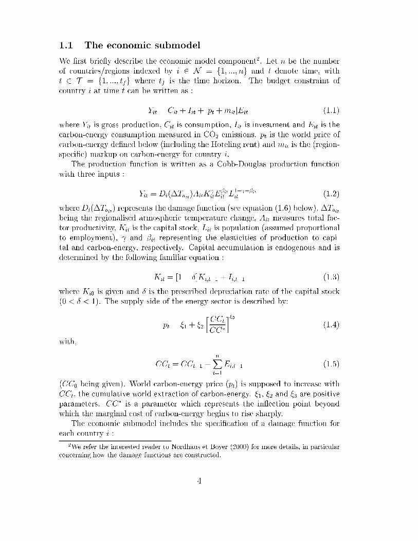
1.1 The economic submodel

We �rst brie y describe the economic model component2. Let n be the number

of countries/regions indexed by i 2 N = f1; :::; ng and t denote time, with

t 2 T = f1; :::; tfg where tf is the time horizon. The budget constraint of

country i at time t can be written as :

Yit = Cit + Iit + [pt +mit]Eit (1:1)

where Yit is gross production, Cit is consumption, Iit is investment and Eit is the

carbon-energy consumption measured in CO2 emissions. pt is the world price of

carbon-energy de�ned below (including the Hoteling rent) and mit is the (region-

speci�c) markup on carbon-energy for country i.

The production function is written as a Cobb-Douglas production function

with three inputs :

Yit = Di(�Tait)AitK itE

�itit L

1� ��itit (1:2)

where Di(�Tait) represents the damage function (see equation (1.6) below), �Taitbeing the regionalised atmospheric temperature change, Ait measures total fac-

tor productivity, Kit is the capital stock, Lit is population (assumed proportional

to employment), and �it representing the elasticities of production to capi-

tal and carbon-energy, respectively. Capital accumulation is endogenous and is

determined by the following familiar equation :

Kit = [1� Æ]Ki;t�1 + Ii;t�1 (1:3)

where Ki0 is given and Æ is the prescribed depreciation rate of the capital stock

(0 < Æ < 1). The supply side of the energy sector is described by:

pt = �1 + �2

�CCt

CC�

��3(1:4)

with,

CCt = CCt�1 +nXi=1

Ei;t�1 (1:5)

(CC0 being given). World carbon-energy price (pt) is supposed to increase with

CCt, the cumulative world extraction of carbon-energy. �1, �2 and �3 are positive

parameters. CC� is a parameter which represents the in ection point beyond

which the marginal cost of carbon-energy begins to rise sharply.

The economic submodel includes the speci�cation of a damage function for

each country i :

2We refer the interested reader to Nordhaus et Boyer (2000) for more details, in particular

concerning how the damage functions are constructed.

4

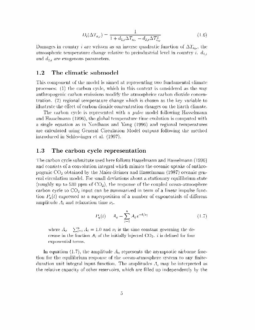
Di(�Tait) =1

1 + d1;i�Tait + d2;i�T 2ait

(1:6)

Damages in country i are written as an inverse quadratic function of �Tait , the

atmospheric temperature change relative to preindustrial level in country i. d1;iand d2;i are exogenous parameters.

1.2 The climatic submodel

This component of the model is aimed at representing two fundamental climate

processes: (1) the carbon cycle, which in this context is considered as the way

anthropogenic carbon emissions modify the atmospheice carbon dioxide concen-

tration. (2) regional temperature change which is chosen as the key variable to

illustrate the e�ect of carbon dioxide concentration changes on the Earth climate.

The carbon cycle is represented with a pulse model following Hasselmann

and Hasselmann (1996), the global temperature time evolution is computed with

a single equation as in Nordhaus and Yang (1996) and regional temperatures

are calculated using General Circulation Model outputs following the method

introduced in Schlessinger et al. (1997).

1.3 The carbon cycle representation

The carbon cycle substitute used here follows Hasselmann and Hasselmann (1996)

and consists of a convolution integral which mimics the oceanic uptake of anthro-

pogenic CO2 obtained by the Maier-Reimer and Hasselmann (1987) oceanic gen-

eral circulation model. For small deviations about a stationary equilibrium state

(roughly up to 530 ppm of CO2), the response of the coupled ocean-atmosphere

carbon cycle to CO2 input can be summarized in term of a linear impulse func-

tion Pa(t) expressed as a superposition of a number of exponentials of di�erent

amplitude Ai and relaxation time �i.

Pa(t) = Ao +nXi=1

Ai e�t=�i (1:7)

where Ao +Pn

i=1Ai = 1:0 and �i is the time constant governing the de-

crease in the fraction Ai of the initially injected CO2. i is de�ned for four

exponential terms.

In equation (1.7), the amplitude Ao represents the asymptotic airborne frac-

tion for the equilibrium response of the ocean-atmosphere system to any �nite-

duration unit integral input function. The amplitudes Ai may be interpreted as

the relative capacity of other reservoirs, which are �lled up independently by the

5

atmospheric input at rates characterized by the relaxation time scales �i (Maier-

Reimer and Hasselmann, 1987). Ai and �i are given in the parameter list of the

appendix.

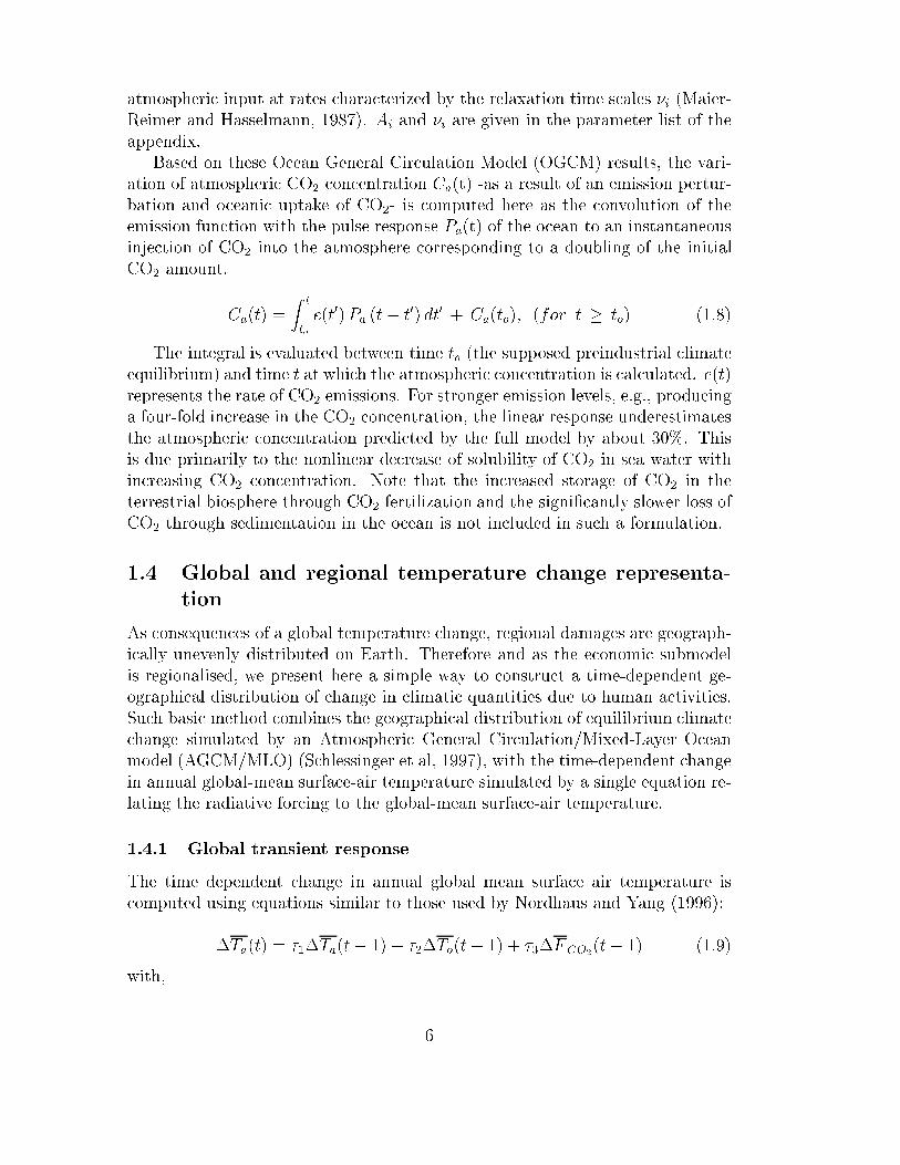
Based on these Ocean General Circulation Model (OGCM) results, the vari-

ation of atmospheric CO2 concentration Ca(t) -as a result of an emission pertur-

bation and oceanic uptake of CO2- is computed here as the convolution of the

emission function with the pulse response Pa(t) of the ocean to an instantaneous

injection of CO2 into the atmosphere corresponding to a doubling of the initial

CO2 amount.

Ca(t) =

Z t

toe(t0)Pa (t� t

0) dt0 + Ca(to); (for t � to) (1:8)

The integral is evaluated between time to (the supposed preindustrial climate

equilibrium) and time t at which the atmospheric concentration is calculated. e(t)

represents the rate of CO2 emissions. For stronger emission levels, e.g., producing

a four-fold increase in the CO2 concentration, the linear response underestimates

the atmospheric concentration predicted by the full model by about 30%. This

is due primarily to the nonlinear decrease of solubility of CO2 in sea water with

increasing CO2 concentration. Note that the increased storage of CO2 in the

terrestrial biosphere through CO2 fertilization and the signi�cantly slower loss of

CO2 through sedimentation in the ocean is not included in such a formulation.

1.4 Global and regional temperature change representa-

tion

As consequences of a global temperature change, regional damages are geograph-

ically unevenly distributed on Earth. Therefore and as the economic submodel

is regionalised, we present here a simple way to construct a time-dependent ge-

ographical distribution of change in climatic quantities due to human activities.

Such basic method combines the geographical distribution of equilibrium climate

change simulated by an Atmospheric General Circulation/Mixed-Layer Ocean

model (AGCM/MLO) (Schlessinger et al, 1997), with the time-dependent change

in annual global-mean surface-air temperature simulated by a single equation re-

lating the radiative forcing to the global-mean surface-air temperature.

1.4.1 Global transient response

The time dependent change in annual global mean surface air temperature is

computed using equations similar to those used by Nordhaus and Yang (1996):

�Ta(t) = �1�Ta(t� 1) + �2�To(t� 1) + �3�FCO2(t� 1) (1:9)

with,

6

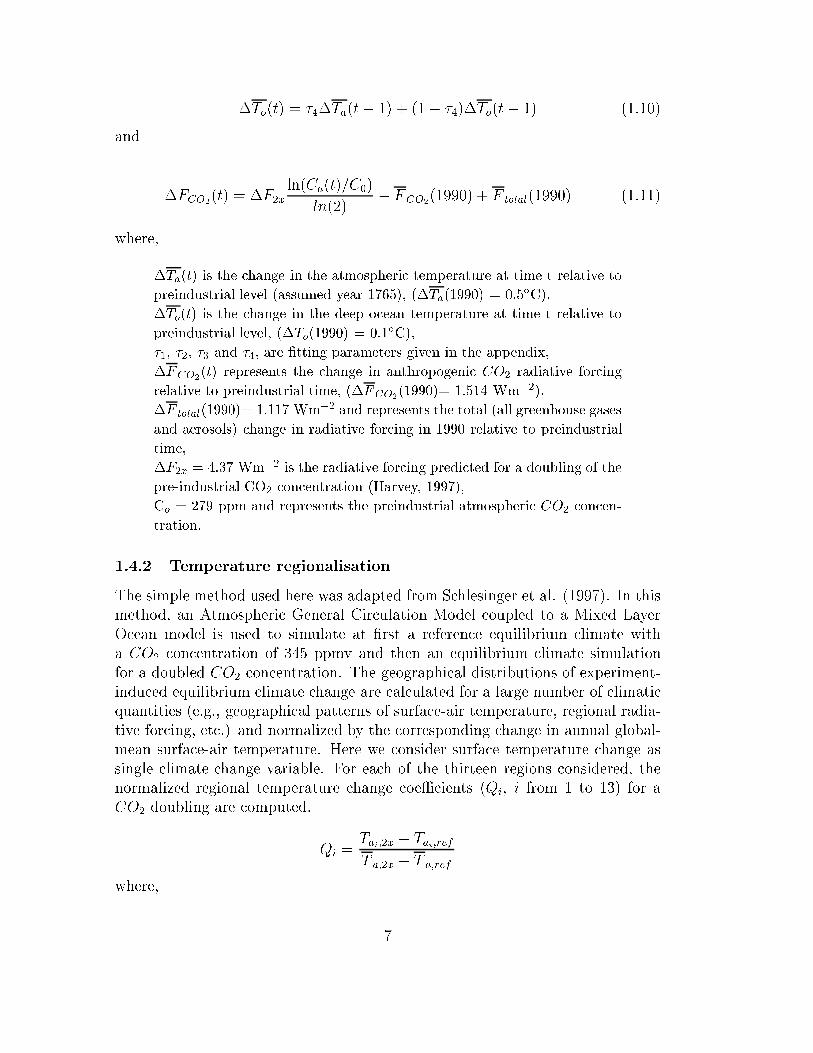
�To(t) = �4�Ta(t� 1) + (1� �4)�To(t� 1) (1:10)

and

�FCO2(t) = �F2x

ln(Ca(t)=C0)

ln(2)� FCO2

(1990) + F total(1990) (1:11)

where,

�Ta(t) is the change in the atmospheric temperature at time t relative to

preindustrial level (assumed year 1765), (�Ta(1990) = 0.5ÆC),

�To(t) is the change in the deep ocean temperature at time t relative to

preindustrial level, (�To(1990) = 0.1ÆC),

�1, �2, �3 and �4, are �tting parameters given in the appendix,

�FCO2(t) represents the change in anthropogenic CO2 radiative forcing

relative to preindustrial time, (�FCO2(1990)= 1.514 Wm�2),

�F total(1990)= 1.117 Wm�2 and represents the total (all greenhouse gases

and aerosols) change in radiative forcing in 1990 relative to preindustrial

time,

�F2x = 4.37 Wm�2 is the radiative forcing predicted for a doubling of the

pre-industrial CO2 concentration (Harvey, 1997),

Co = 279 ppm and represents the preindustrial atmospheric CO2 concen-

tration.

1.4.2 Temperature regionalisation

The simple method used here was adapted from Schlesinger et al. (1997). In this

method, an Atmospheric General Circulation Model coupled to a Mixed Layer

Ocean model is used to simulate at �rst a reference equilibrium climate with

a CO2 concentration of 345 ppmv and then an equilibrium climate simulation

for a doubled CO2 concentration. The geographical distributions of experiment-

induced equilibrium climate change are calculated for a large number of climatic

quantities (e.g., geographical patterns of surface-air temperature, regional radia-

tive forcing, etc.) and normalized by the corresponding change in annual global-

mean surface-air temperature. Here we consider surface temperature change as

single climate change variable. For each of the thirteen regions considered, the

normalized regional temperature change coeÆcients (Qi, i from 1 to 13) for a

CO2 doubling are computed.

Qi =Tai;2x � Tai;ref

T a;2x � T a;ref

where,

7

Tai corresponds to the GCM air-surface temperature output averaged over

the area covered by country i. The subscripts 2x and ref refer to the

doubled CO2 and reference simulation respectively,

T a, represents the global air-surface temperature.

As the transient global surface temperature �T a(t) change is computed fol-

lowing equation (1.9), the annual mean regional temperature change at time t

relative to an arbitrary reference year are then calculated using Qi:

Tai(t) = Qi (�Ta(t)��Ta(1990)) (1:12)

where Tai(t) is the regional temperature change relative to preindustial time on

region i.

2 Cooperative and non-cooperative solutions

To endogenise the regions' carbon-energy and investment time paths, we present

hereafter four di�erent modes of behaviour: (1) the cooperative solution or in-

ternational optimum, (2) the Nash equilibrium where countries optimize indi-

vidually, (3) the partial agreement Nash equilibrium where a single coalition of

countries is allowed to form, and (4) the business-as-usual scenario where coun-

tries ignore impacts of climate change.

2.1 The international optimum

In the international optimum (also called cooperative) scenario, a social planner is

assumed to choose investment and carbon-energy consumption so as to maximize

the world's total welfare de�ned as the sum of all countries' discounted utilities

over the planning period. The problem to be solved is :

maxfIit;Eitgi2N ;t2T

W =nXi=1

tfXt=1

�itUi(Cit); (2:1)

subject to constraints (1.1) to (1.12) for all t 2 T and i 2 N , all variables (emis-

sions, investment, CO2 concentration,...) being positive. Cit is the aggregate

consumption for country i during period t. Ui is the utility function for country

i. It is assumed to be a strictly increasing and concave function of consumption.

Damages do not directly enter the utility function but cause a 'loss' of produc-

tion (recall equation (1.2)). � is the (time and country varying) discounting factor

(0 < �it � 1) obtained by integration of the social rate of time preference onwards.

First-order conditions for an interior maximum are given by3:

3Prime indicates the function derivative.

8

@W

@Eit

= �itU0

i(Cit)@Cit

@Eit

+

tfX�=t+1

nXj=1

�j�U0

j(Cj�)

"@Cj�

@�Taj�

@�Taj�@Eit

+@Cj�

@p�

@p�

@Eit

#= 0

(2:2)

@W

@Iit= ��itU

0

i(Cit) +

tfX�=t+1

�j�U0

j(Cj�)@Cj�

@Kj�

@Kj�

@Iit= 0 (2:3)

8t 2 T ; 8i 2 N . Equation (2.2) (known as Samuelson's optimal condition for

public goods) states that the marginal gain of utility from current consumption

in country i obtained by the emission of one extra ton of carbon today must

be equal to the sum of future marginal losses of utility from consumption in

all countries. As shown by the terms between square brackets in (2.2), these

losses have two components. The �rst term is the loss of consumption due to

the negative impact on production of the increase of atmospheric temperature

in the future. The second is the loss of consumption due to the increase of the

price of carbon-energy in the future induced by the extraction of one more ton

of carbon-energy today.

Equation (2.3) states that the current marginal loss of utility in country i

due to an additional unit of investment must be equal to the sum of the future

gains in utility from consumption obtained through the future higher capital

stock induced by that extra unit of investment. (2.3) shows that country i's

investment policy doesn't have any direct impact on the utility of other regions.

In the �eld of energy on the contrary, country i's policy in uences the welfare

of other regions both through the price of carbon-energy and through climate

change (the environmental externality).

2.2 The non-cooperative Nash equilibrium

In the non-cooperative open-loop Nash equilibrium, each player (country) is sup-

posed to choose investment and carbon-energy consumption so as to maximize

his total welfare de�ned as the sum of its discounted utilities over the planning

period, given the strategies of all other players. Country i solves the following

problem :

maxfIit;Eitgt2T

Ni =

tfXt=1

�itUi(Cit); (2:4)

subject to constraints (1.1) to (1.12) for all t 2 T , and given the other countries's

energy and investment time paths.

Concerning carbon-energy, the �rst-order conditions for an interior maximum

are given by:

9

@Ni

@Eit

= �itU0

i(Cit)@Cit

@Eit

+

tfX�=t+1

�j�U0

j(Cj� )

"@Cj�

@�Taj�

@�Taj�@Eit

+@Cj�

@p�

@p�

@Eit

#= 0

(2:5)

8t 2 T . On the other hand, the optimal condition obtained by derivating Ni

with respect to investment is the same as in (2.3). Equation (2.5) states that the

marginal gain of utility from current consumption in country i obtained by the

emission of one extra ton of carbon today must be equal to the sum of future

marginal losses of country i utility from consumption. Contrary to what happens

at the international optimum (see equation 2.2), country i takes only account

of the impact of its marginal carbon emission (through the future increase of

atmospheric temperature and world price of energy) on itself and ignores the

impact on the others.

Solving the system of equations (1.1) to (1.12), (2.3), (2.5) 8i leads to the

Nash equilibrium. It is an equilibrium in the sense that no country has interest

to deviate from its trajectory if all other countries stick to their trajectory. Due

to the fact that the players do not take account of the impact of their strategy

on others, the Nash equilibrium is clearly suboptimal with respect to the interna-

tional optimum. Formally, if W is the world's total welfare at the international

optimum, and Ni country's total welfare at the Nash equilibrium, one must verify

thatPn

i=1Ni � W .

2.3 The partial agreement Nash equilibrium w.r.t. a coali-

tion

We introduce now a situation of partial cooperation, i.e. an intermediate case

between the full cooperation situation illustrated by the international optimum,

and the no cooperation case characterizing the Nash equilibrium. For doing so,

we call upon the concept of partial agreement Nash equilibrium w.r.t. a coalition

(PANE) introduced by Chander and Tulkens (1995, 1997). Suppose that the

coalition S � N forms. Then the PANE w.r.t. to S is an equilibrium where the

members of S maximize jointly the sum of their utilities, while the regions outside

S act individually. Formally, the PANE w.r.t. to coalition S is the combination

of strategies that solves simultaneously the following problems:

a) for S :

maxfIit;Eitgi2S;t2T

Xi2S

tfXt=1

�itUi(Cit); (2:6)

given the emissions and investment paths of non-members of S and subject to

constraints (1.1) to (1.12) for all t 2 T and i 2 S;

b) for each region j outside of S :

10

maxfIjt;Ejtgt2T

tfXt=1

�jtUj(Cjt); (2:7)

subject to constraints (1.1) to (1.12) for all t 2 T , and given the other countries's

energy and investment time paths.

Two remarks must be made about equations (2.6) and (2.7). First, they may

be reinterpreted as describing a Nash equilibrium between a coalition S and the

non-members of S. Secondly, the PANE appears clearly as a generalization both

of the cooperative solution (where S = f1; :::; ng) and of the Nash equilibrium

(where S is reduced to a singleton).

With respect to carbon-energy, the �rst order conditions associated with in-

terior solutions of problems (2.6) and (2.7) are :

�itU0

i(Cit)@Cit

@Eit

+Xk2S

tfX�=t+1

�k�U0

k(Ck�)

"@Ck�

@�Tak�

@�Tak�@Eit

+@Ck�

@p�

@p�

@Eit

#= 0; i 2 S

(2:8)

�jtU0

j(Cjt)@Cjt

@Ejt

+

tfX�=t+1

�j�U0

j(Cj�)

"@Cj�

@�Taj�

@�Taj�@Ejt

+@Cj�

@p�

@p�

@Ejt

#= 0; j 2 NnS

(2:9)

As far as investment is concerned, the �rst order optimal conditions remain the

same as in (2.3).

2.4 The business-as-usual scenario

The business-as-usual (BAU) scenario is like the Nash equilibrium, except that

countries are assumed to ignore the impact of climate change on their future

welfare. In the BAU scenario, each player (country) is supposed to choose in-

vestment and carbon-energy consumption in order to maximise its total welfare

de�ned as the sum of its discounted utilities over the planning period, given the

strategies of all other players and ignoring future damages due to climate change.

Formally, country i solves the following problem :

maxfIit;Eitgt2T

Bi =

tfXt=1

�itUi(Cit); (2:10)

subject to constraints (1.1) to (1.12) for all t 2 T , given the other countries

energy and investment time paths, and assuming that the time evolution for

atmospheric temperature in country i, (�Tait), is exogenous4 . In other words,

country i is supposed to ignore the in uence of Eit on �Tai� ; � � t.

4So that the damages appearing in the production function are also exogenous (recall (1.2).

11

Concerning carbon-energy, the �rst-order conditions for an interior maximum

are given by:

@Bi

@Eit

= �itU0

i(Cit)@Cit

@Eit

+

tfX�=t+1

�j�U0

j(Cj� )@Cj�

@p�

@p�

@Eit

= 0 (2:11)

8t 2 T . On the other hand, the optimal condition obtained by derivating Bi

with respect to investment is the same as in (2.3). Contrary to what happens

under Nash equilibrium conditions (equation 2.5), country i takes account for the

impact of its marginal carbon emission on itself only through the future increase

world price of energy.

Solving the system of equations (1.1) to (1.12), (2.11), (2.5) leads to the BAU

scenario. Due to the fact that the players do not take account for the impact of

climate change, even on themselves, BAU is clearly suboptimal with respect to

NE. Formally, if Bi and Ni are respectively country i's total welfare at BAU and

NE, one must verify that Bi � Ni; 8i 2 N .

3 Simulations

3.1 Foreword

We now discuss some numerical simulations made with the model described in

the preceding sections. In this section, we wish to illustrate the gains from

international cooperation with respect to the Nash equilibrium and with respect

to a business-as-usual (BAU) scenario. Whatever the type of behaviour chosen

(cooperation, PANE, NE or BAU), the algorithm (written in Matlab) calculates

the trajectories of the economies by solving the associated system of �rst order

conditions. Its main advantage is its speed5, which will appear to be very helpful

in the next section when testing for coalitional rationality. Its main drawback

comes from what makes its specialization : it is only suited to compute interior

solutions and thus would not easily be adapted to integrate inequality constraints

on some variables (for example a ceiling on temperature increase).

The "game" framework is the same as in RICE-98 (Nordhaus and Boyer,

1999). The world is divided in 13 regions or countries, which are European

Union (Europe), Japan, USA, China, Russia, India, high-income OPEC (HIO)6,

Eastern Europe (EE), other high income (OHI)7, middle income (MI)8, lower

5A run, for example the calculation of the IO, takes around 25 seconds on a PC Pentium

III 450mhz. This is to be compared to the 15-30 minutes necessary to solve the full RICE-99

model on a 500 mhz machine (Nordhaus and Boyer, 2000, chapter 6).6Saudi Arabia, Lybia,...7Canada, Australia,...8Brazil, Corea,...

12

middle income (LMI)9, low income (LI)10, Sub-Saharian Africa (Africa). Except

for the climate module, almost all data were borrowed from RICE-98. A complete

table of the parameters used is given in the appendix. Contrary to Nordhaus and

Boyer (1999) who take a value of 3%, we have set the initial annual rate of time

preference in the base case to 1%. It is indeed well known that climate change

isq a long period phenomenon (compared to usual economic horizons). We thus

give more weight to the future, in particular to the damages that will follow

from climate change. As it will appear from the sensitivity analysis on the time

preference parameter, choosing a rather low value for this parameter enhances

the interest of international cooperation w.r.t. non-cooperative scenarios.

3.2 Numerical results

Results are shown for a time horizon of 160 years (i.e. until 2150), but to avoid

boundary e�ects associated to this �nite horizon problem, computations were

made for a planning horizon of 300 years11. Periods are taken to be decades. The

model considers only CO2 emissions, i.e. other GHG are ignored. Figure 1 gives

the average annual world carbon emissions for three scenarios : international

optimum (IO), Nash equilibrium (NE) and business-as-usual (BAU).

9Mexico, Turkey,...10Indonesia, Pakistan,...11In a �nite horizon problem, the weight of damages due to climate change diminishes as

one approaches the end of the planning period. Thus, at that time, emissions increase and lose

their signi�cance.

13

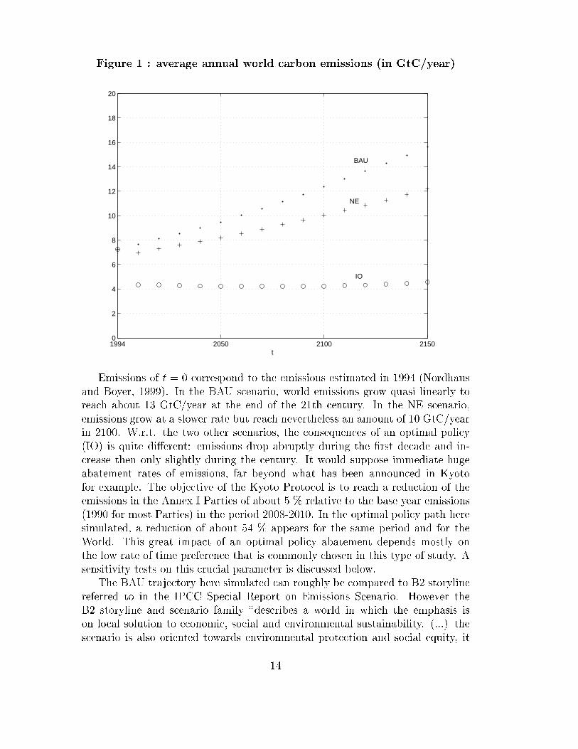
Figure 1 : average annual world carbon emissions (in GtC/year)

1994 2050 2100 21500

2

4

6

8

10

12

14

16

18

20

BAU

NE

IO

t

Emissions of t = 0 correspond to the emissions estimated in 1994 (Nordhaus

and Boyer, 1999). In the BAU scenario, world emissions grow quasi linearly to

reach about 13 GtC/year at the end of the 21th century. In the NE scenario,

emissions grow at a slower rate but reach nevertheless an amount of 10 GtC/year

in 2100. W.r.t. the two other scenarios, the consequences of an optimal policy

(IO) is quite di�erent: emissions drop abruptly during the �rst decade and in-

crease then only slightly during the century. It would suppose immediate huge

abatement rates of emissions, far beyond what has been announced in Kyoto

for example. The objective of the Kyoto Protocol is to reach a reduction of the

emissions in the Annex I Parties of about 5 % relative to the base year emissions

(1990 for most Parties) in the period 2008-2010. In the optimal policy path here

simulated, a reduction of about 54 % appears for the same period and for the

World. This great impact of an optimal policy abatement depends mostly on

the low rate of time preference that is commonly chosen in this type of study. A

sensitivity tests on this crucial parameter is discussed below.

The BAU trajectory here simulated can roughly be compared to B2 storyline

referred to in the IPCC Special Report on Emissions Scenario. However the

B2 storyline and scenario family "describes a world in which the emphasis is

on local solution to economic, social and environmental sustainability. (...) the

scenario is also oriented towards environmental protection and social equity, it

14

focuses on local and regional levels" (IPCC, 2000). Therefore, it seems that the

BAU scenario here simulated does not represent a scenario with growth rate of

emissions that are compatible with the IPCC estimates. All scenarios in the

IPCC report that could be associated to the BAU situation belong to the A1

or A2 category and show a much greater increase of the emissions in the �rst

half of the 21st century. The quasi-linear trend here simulated in the BAU case

is associated to the hypothesis chosen in the model construction and tend to

underestimate the emission growth relative to other reviewed scenarios. Because

the BAU scenario used here is "optimistic", the potential bene�ts of cooperation

w.r.t. the "do nothing" hypothesis as measured hereafter will be underestimated.

On the other hand, the model did not show any trajectory that allows a

growth of emissions followed by a decrease. Such path is simulated with other

types of economic models but does not seem in the scope of the model of the

"RICE type" as used here. Our goal here is not to provide with realistic emission

scenarios as we rather concentrate on cooperation interests. The limitation shown

here does not a�ect the nature of our results but it remains relevant to �x the

limit of the scope of the results interpretation.

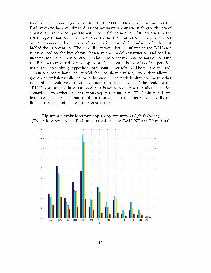
Figure 2 : emissions per capita by country (tC/hab/year)

(For each region, col. 1: BAU in 1990; col. 2, 3, 4: BAU, NE and IO in 2100)

JAP USA EU OHI HIO MI RUS LMI EE LI CHI IND AFR0

1

2

3

4

5

6

7

8

9

i

15

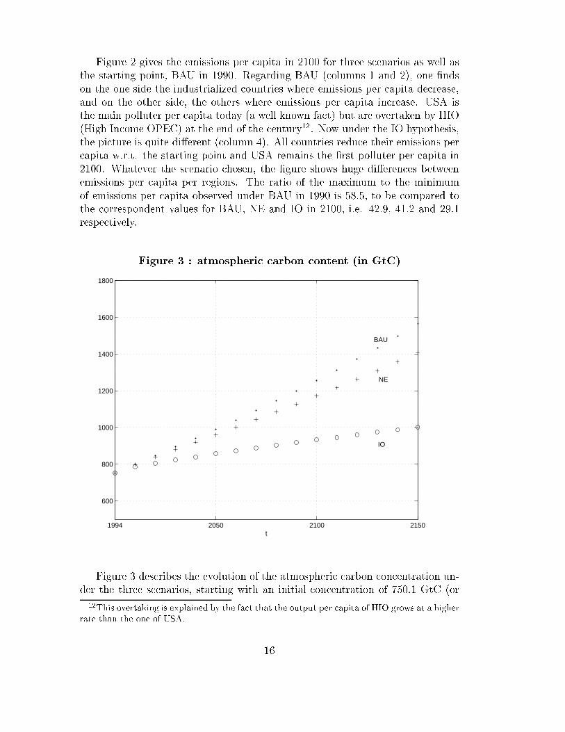
Figure 2 gives the emissions per capita in 2100 for three scenarios as well as

the starting point, BAU in 1990. Regarding BAU (columns 1 and 2), one �nds

on the one side the industrialized countries where emissions per capita decrease,

and on the other side, the others where emissions per capita increase. USA is

the main polluter per capita today (a well known fact) but are overtaken by HIO

(High Income OPEC) at the end of the century12. Now under the IO hypothesis,

the picture is quite di�erent (column 4). All countries reduce their emissions per

capita w.r.t. the starting point and USA remains the �rst polluter per capita in

2100. Whatever the scenario chosen, the �gure shows huge di�erences between

emissions per capita per regions. The ratio of the maximum to the minimum

of emissions per capita observed under BAU in 1990 is 58.5, to be compared to

the correspondent values for BAU, NE and IO in 2100, i.e. 42.9, 41.2 and 29.1

respectively.

Figure 3 : atmospheric carbon content (in GtC)

1994 2050 2100 2150

600

800

1000

1200

1400

1600

1800

t

BAU

NE

IO

Figure 3 describes the evolution of the atmospheric carbon concentration un-

der the three scenarios, starting with an initial concentration of 750.1 GtC (or

12This overtaking is explained by the fact that the output per capita of HIO grows at a higher

rate than the one of USA.

16

equivalently 352 ppm (part per million 13). It grows steadily in the three scenar-

ios, reaching values around 1300 GtC (610 ppm) in 2100 for BAU. The increase

is much weaker for IO, where the atmospheric concentration reaches a level of

960 GtC (451 ppm) around 2100. Note that even under the IO hypothesis, one

may not speak of a stabilization of the atmospheric carbon concentration in the

next two centuries.

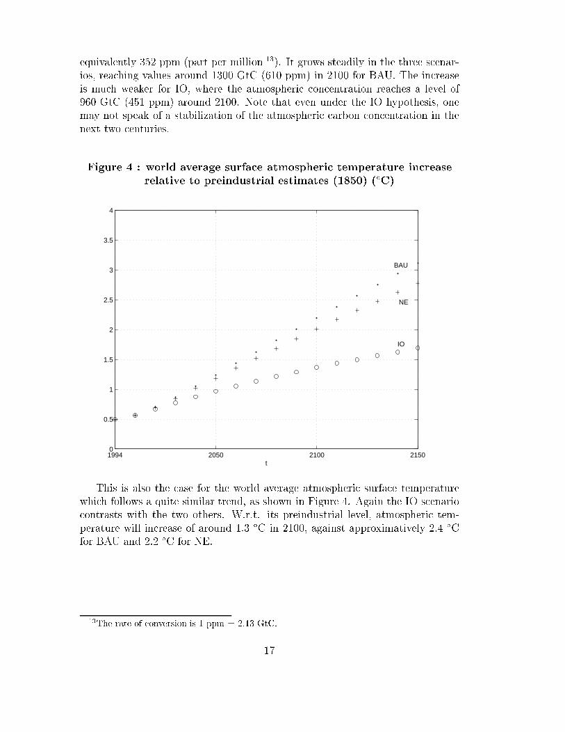
Figure 4 : world average surface atmospheric temperature increase

relative to preindustrial estimates (1850) (ÆC)

1994 2050 2100 21500

0.5

1

1.5

2

2.5

3

3.5

4

t

BAU

NE

IO

This is also the case for the world average atmospheric surface temperature

which follows a quite similar trend, as shown in Figure 4. Again the IO scenario

contrasts with the two others. W.r.t. its preindustrial level, atmospheric tem-

perature will increase of around 1.3 ÆC in 2100, against approximatively 2.4 ÆC

for BAU and 2.2 ÆC for NE.

13The rate of conversion is 1 ppm = 2.13 GtC.

17

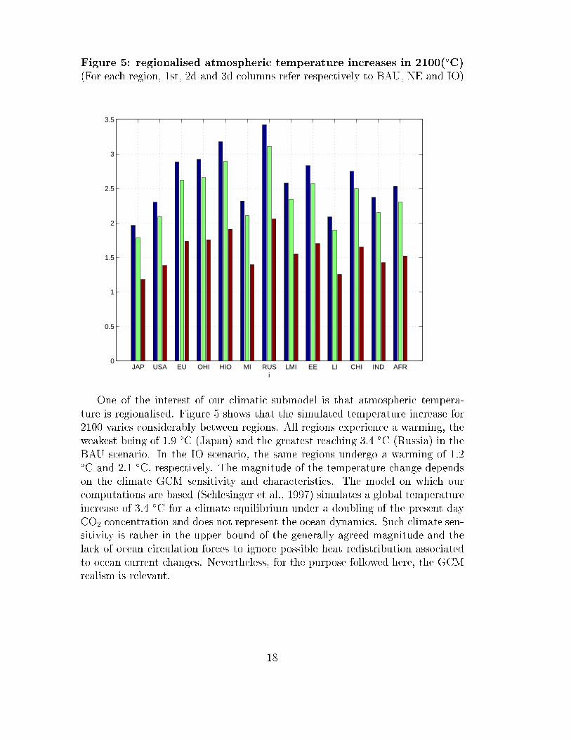
Figure 5: regionalised atmospheric temperature increases in 2100(ÆC)

(For each region, 1st, 2d and 3d columns refer respectively to BAU, NE and IO)

JAP USA EU OHI HIO MI RUS LMI EE LI CHI IND AFR0

0.5

1

1.5

2

2.5

3

3.5

i

One of the interest of our climatic submodel is that atmospheric tempera-

ture is regionalised. Figure 5 shows that the simulated temperature increase for

2100 varies considerably between regions. All regions experience a warming, the

weakest being of 1.9 ÆC (Japan) and the greatest reaching 3.4 ÆC (Russia) in the

BAU scenario. In the IO scenario, the same regions undergo a warming of 1.2ÆC and 2.1 ÆC, respectively. The magnitude of the temperature change depends

on the climate GCM sensitivity and characteristics. The model on which our

computations are based (Schlesinger et al., 1997) simulates a global temperature

increase of 3.4 ÆC for a climate equilibrium under a doubling of the present day

CO2 concentration and does not represent the ocean dynamics. Such climate sen-

sitivity is rather in the upper bound of the generally agreed magnitude and the

lack of ocean circulation forces to ignore possible heat redistribution associated

to ocean current changes. Nevertheless, for the purpose followed here, the GCM

realism is relevant.

18

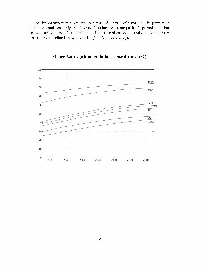
An important result concerns the rate of control of emissions, in particular

in the optimal case. Figures 6.a and 6.b show the time path of optimal emission

control per country. Formally, the optimal rate of control of emissions of country

i at time t is de�ned by �IO;it = 100(1� EIO;it=EBAU;it)).

Figure 6.a : optimal emission control rates (%)

2020 2040 2060 2080 2100 2120 21400

10

20

30

40

50

60

70

80

90

100

t

JAP

EU

US

MIOHI

HIO

RUS

19

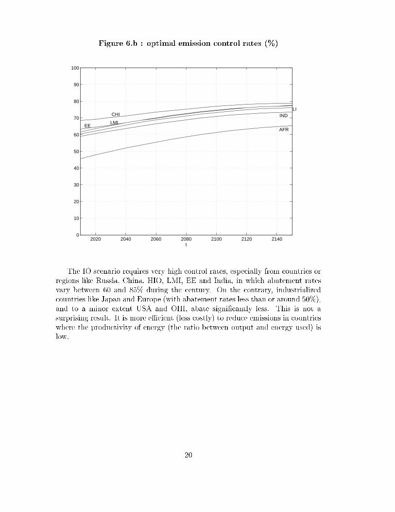
Figure 6.b : optimal emission control rates (%)

2020 2040 2060 2080 2100 2120 21400

10

20

30

40

50

60

70

80

90

100

t

AFR

INDLI

LMIEE

CHI

The IO scenario requires very high control rates, especially from countries or

regions like Russia, China, HIO, LMI, EE and India, in which abatement rates

vary between 60 and 85% during the century. On the contrary, industrialized

countries like Japan and Europe (with abatement rates less than or around 50%),

and to a minor extent USA and OHI, abate signi�cantly less. This is not a

surprising result. It is more eÆcient (less costly) to reduce emissions in countries

where the productivity of energy (the ratio between output and energy used) is

low.

20

Figure 7 : relative welfare gains w.r.t. BAU (%)

(For each region, 1st and 2d columns refer respectively to NE and IO)

JAP USA EU OHI HIO MI RUS LMI EE LI CHI IND AFR0

1

2

3

4

5

6

7

i

Figure 7 illustrates the relative welfare gains of NE and IO w.r.t. BAU. If

everybody gets a positive gain at the NE w.r.t. BAU (recall subsection 3.4),

this is not true for IO w.r.t. NE. Indeed, if the world as a whole gains from an

optimal policy, Figure 7.b shows that the bene�ts are very unevenly distributed.

W.r.t. BAU, the impact of applying an optimal policy appears to pro�t mainly

to Europe and India (the two most vulnerable regions to climate change14). The

problem is that a few regions (USA, HIO, EE) are better under NE than under IO.

These countries have to abate a lot under IO (especially HIO and EE), while they

su�er relatively little from climate change. So if there are no obstacle to move

from BAU to NE (all countries have interest to do so), this does not hold when

moving from NE to IO. The losing countries would ask for �nancial compensation

if one hopes their voluntary collaboration to an international optimal policy. One

way consists of �nancial sidepayments, and we turn now to them in the following

section.

14Recall that the damage functions are written as inverse quadratic functions of atmospheric

temperature change (cfr. equation 1.6). Europe and India have the highest values for the

parameter d2;i multiplying the quadratic term.

21

4 Financial transfers

4.1 The transfer formula

We make use of a theoretical transfer scheme proposed by Germain, Toint and

Tulkens (1997) for stock pollution problems. This transfer scheme has been

adapted and applied to the climate change problem by Eyckmans and Tulkens

(1999) in the context of a partition of the world in 6 regions. The formula used

by these authors is:

�i = �[Wi �Ni] +�iPn

k=1 �k

nXj=1

[Wj �Nj]; i = 1; :::; n (3:1)

where �i is the �nancial transfer received or given by country i, Wi and Ni are

the total welfares obtained by country i at the international optimum and at

the Nash equilibrium respectively15. A positive (negative) transfer represents a

sum received (payed). The transfers are de�ned as lump-sum quantities (i.e. for

the whole planning period) and appear to be the sum of two terms. The �rst

one corresponds to the opposite of what the country gains or loses between IO

and NE. The second term assigns a share of the global surplus generated by

international cooperation w.r.t. NE. With a transfer limited to the �rst term,

region i would be indi�erent between IO with transfers (IOT) and NE. Note that

from equation (3.1) the bigger �i, the larger the fraction attributed to i. The

weights �i are de�ned by

�i =

tfXt=1

�itD0

i(�T�

ait)Y �

it ; i = 1; :::; n (3:2)

D0

i(�T�

ait) is the marginal damage cost in relative terms a�ecting country i at

time t along the optimal trajectory. D0

i(�T�

ait)Y �

it is the same in absolute terms.

Then �i is the discounted sum of country i's marginal damage costs over the

planning period and is thus a positive quantity.

From (3.1), it is clear that the sidepayments are balanced, i.e.P

i �i = 0.

Moreover, they make cooperation individually rational in the sense that

WTi4

= Wi + �i � Ni; 8i = 1; :::; n (3:3)

At the optimum with transfers, all regions are better o� than at the Nash equi-

librium.

4.2 Computation of the transfers

The principal results are summarized in the following �gures.

15In other words, Wiis the share obtained by region i of the world's total welfare given by

the solution of problem (2.1), while Niis the solution of problem (2.4).

22

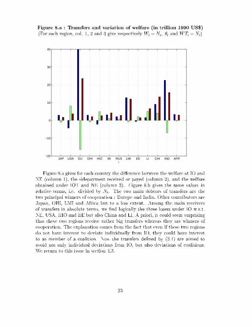
Figure 8.a : Transfers and variation of welfare (in trillion 1990 US$)

(For each region, col. 1, 2 and 3 give respectively Wi �Ni; �i and WTi �Ni)

JAP USA EU OHI HIO MI RUS LMI EE LI CHI IND AFR−20

−10

0

10

20

30

40

i

Figure 8.a gives for each country the di�erence between the welfare at IO and

NE (column 1), the sidepayment received or payed (column 2), and the welfare

obtained under IOT and NE (column 3). Figure 8.b gives the same values in

relative terms, i.e. divided by Ni. The two main debtors of transfers are the

two principal winners of cooperation : Europe and India. Other contributors are

Japan, OHI, LMI and Africa but to a less extent. Among the main receivers

of transfers in absolute terms, we �nd logically the three losers under IO w.r.t.

NE, USA, HIO and EE but also China and LI. A priori, it could seem surprising

that these two regions receive rather big transfers whereas they are winners of

cooperation. The explanation comes from the fact that even if these two regions

do not have interest to deviate individually from IO, they could have interest

to as member of a coalition. Now the transfers de�ned by (3.1) are aimed to

avoid not only individual deviations from IO, but also deviations of coalitions.

We return to this issue in section 4.3.

23

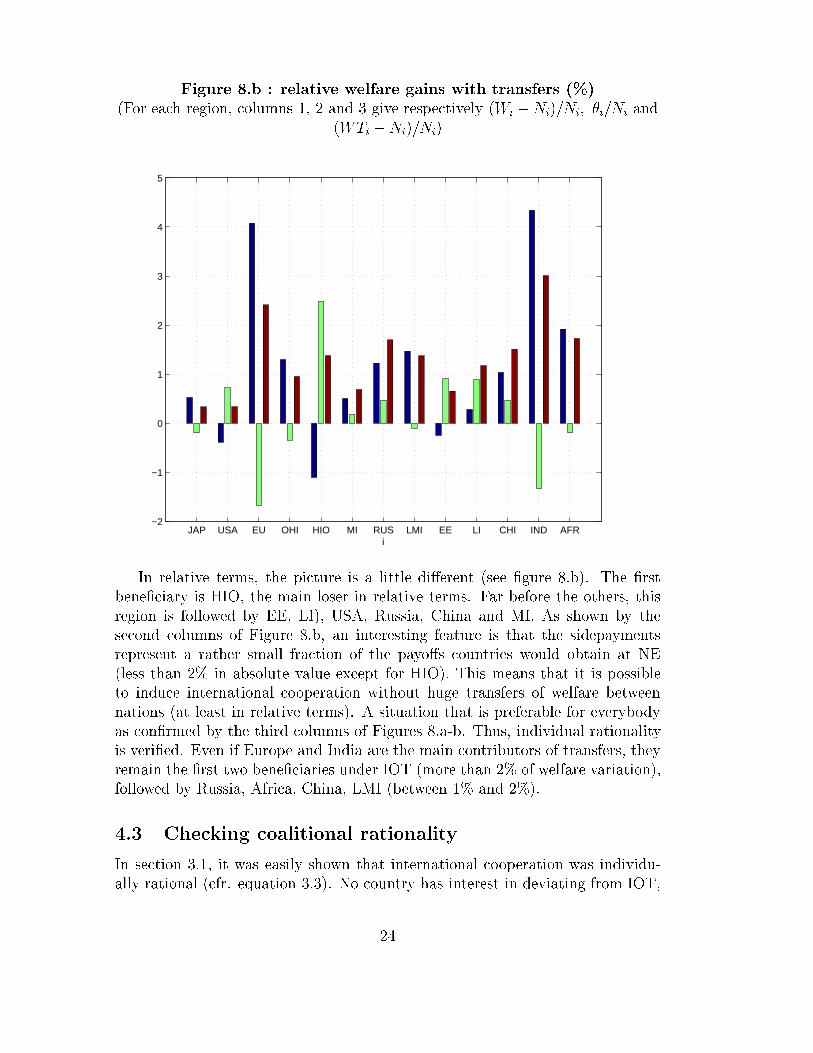
Figure 8.b : relative welfare gains with transfers (%)

(For each region, columns 1, 2 and 3 give respectively (Wi �Ni)=Ni; �i=Ni and

(WTi �Ni)=Ni)

JAP USA EU OHI HIO MI RUS LMI EE LI CHI IND AFR−2

−1

0

1

2

3

4

5

i

In relative terms, the picture is a little di�erent (see �gure 8.b). The �rst

bene�ciary is HIO, the main loser in relative terms. Far before the others, this

region is followed by EE, LI), USA, Russia, China and MI. As shown by the

second columns of Figure 8.b, an interesting feature is that the sidepayments

represent a rather small fraction of the payo�s countries would obtain at NE

(less than 2% in absolute value except for HIO). This means that it is possible

to induce international cooperation without huge transfers of welfare between

nations (at least in relative terms). A situation that is preferable for everybody

as con�rmed by the third columns of Figures 8.a-b. Thus, individual rationality

is veri�ed. Even if Europe and India are the main contributors of transfers, they

remain the �rst two bene�ciaries under IOT (more than 2% of welfare variation),

followed by Russia, Africa, China, LMI (between 1% and 2%).

4.3 Checking coalitional rationality

In section 3.1, it was easily shown that international cooperation was individu-

ally rational (cfr. equation 3.3). No country has interest in deviating from IOT,

24

because if it does, the other regions will react by returning to NE, where every-

body (including the country that originally deviated) loses w.r.t to IOT. However

there are no theoretical results that guarantee that this is also true for all subset

(coalition) of regions.

We thus want to verify numerically if the subsequent conjecture is true :

Assume that if a coalition S forms, then a partial agreement Nash equilibrium

(PANE) w.r.t. S such as described by (2.6-7) prevails. Then with the sidepay-

ments de�ned by (3.1-2), no coalition has as a whole interest to deviate from the

international optimum with transfers.

Formally, what should be veri�ed to guarantee that this conjecture is true is that

w(S) �Xi2S

WTi; 8S � N ; S 6= N ; jSj � 2 (3:4)

where w(S) is by de�nition the total welfare obtained by coalition S at the PANE

w.r.t. S, i.e. the solution of problem (2.6).

Considering one after the other each of the 8177 possible coalitions16, we

checked if inequality (3.4) was true. The conclusion is that (3.4) is always true.

Thus with such transfers as de�ned by (3.1) and (3.2), international cooperation

is indeed rational in the sense of coalitions.

5 Sensitivity analysis

In this section, we will test the impact of regionalising the atmospheric temper-

ature w.r.t. the situation where temperature is not regionalised. We will also

proceed to a sensitivity analysis on our simulations results to variations of the

time horizon (tf ) and of the rate of time preference (�).

5.1 Regionalisation vs. no-regionalisation of temperature

The main originality of this model w.r.t. other Integrated Assessment Models

is that atmospheric temperature is regionalised. It is interesting to analyze to

which extent regionalisation of temperature modi�es the results from the situation

where temperature is assumed to be uniform around the world. In the reference

case (RC), atmospheric temperature in region i is related to world temperature

by (1.12), where Qi is the ith component of the vector of exogenous parameters

Q = [0:82 0:96 1:21 1:23 1:33 0:97 1:44 1:08 1:19 0:88 1:15 0:99 1:06]. In the

alternative case (AC), all the components of Q are equal to one.

Table 1 summarizes the main results. As shown by column 3 and 4 which

give respectively for RC and AC the values observed in 2100 of the emissions

16Indeed, there are 213 � 15 = 8177 possible subsets S of f1; :::; ng, such that S 6=

f1; :::; ng; jSj � 2. The 15 cases that are dropped correspond to S = f1; :::; ng (IO), the

13 singletons (which each corresponds to NE) and the case where S is empty.

25

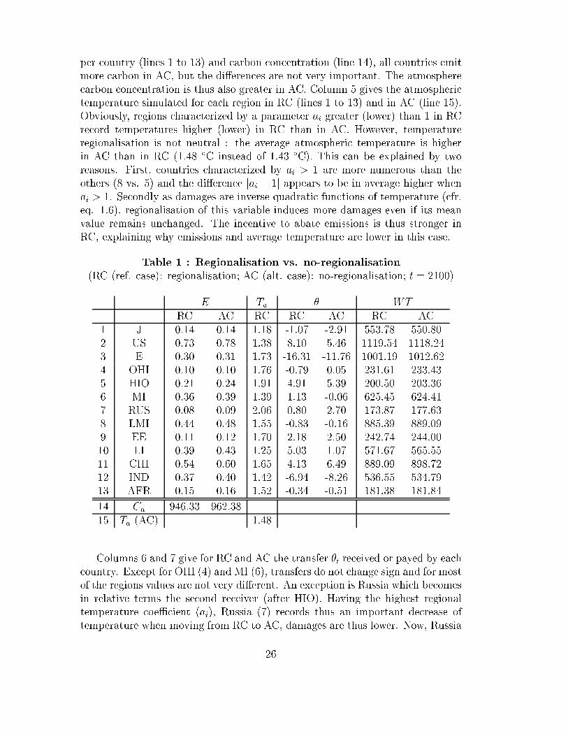
per country (lines 1 to 13) and carbon concentration (line 14), all countries emit

more carbon in AC, but the di�erences are not very important. The atmosphere

carbon concentration is thus also greater in AC. Column 5 gives the atmospheric

temperature simulated for each region in RC (lines 1 to 13) and in AC (line 15).

Obviously, regions characterized by a parameter ai greater (lower) than 1 in RC

record temperatures higher (lower) in RC than in AC. However, temperature

regionalisation is not neutral : the average atmospheric temperature is higher

in AC than in RC (1.48 ÆC instead of 1.43 ÆC). This can be explained by two

reasons. First, countries characterized by ai > 1 are more numerous than the

others (8 vs. 5) and the di�erence jai � 1j appears to be in average higher when

ai > 1. Secondly as damages are inverse quadratic functions of temperature (cfr.

eq. 1.6), regionalisation of this variable induces more damages even if its mean

value remains unchanged. The incentive to abate emissions is thus stronger in

RC, explaining why emissions and average temperature are lower in this case.

Table 1 : Regionalisation vs. no-regionalisation

(RC (ref. case): regionalisation; AC (alt. case): no-regionalisation; t = 2100)

E Ta � WT

RC AC RC RC AC RC AC

1 J 0.14 0.14 1.18 -1.07 -2.91 553.78 550.80

2 US 0.73 0.78 1.38 8.10 5.46 1119.54 1118.24

3 E 0.30 0.31 1.73 -16.31 -11.76 1001.19 1012.62

4 OHI 0.10 0.10 1.76 -0.79 0.05 231.61 233.43

5 HIO 0.21 0.24 1.91 4.91 5.39 200.50 203.36

6 MI 0.36 0.39 1.39 1.13 -0.06 625.45 624.41

7 RUS 0.08 0.09 2.06 0.80 2.70 173.87 177.63

8 LMI 0.44 0.48 1.55 -0.83 -0.16 885.39 889.09

9 EE 0.11 0.12 1.70 2.18 2.50 242.74 244.00

10 LI 0.39 0.43 1.25 5.03 1.07 571.67 565.55

11 CHI 0.54 0.60 1.65 4.13 6.49 889.09 898.72

12 IND 0.37 0.40 1.42 -6.94 -8.26 536.55 534.79

13 AFR 0.15 0.16 1.52 -0.34 -0.51 181.38 181.84

14 Ca 946.33 962.38

15 Ta (AC) 1.48

Columns 6 and 7 give for RC and AC the transfer �i received or payed by each

country. Except for OHI (4) and MI (6), transfers do not change sign and for most

of the regions values are not very di�erent. An exception is Russia which becomes

in relative terms the second receiver (after HIO). Having the highest regional

temperature coeÆcient (ai), Russia (7) records thus an important decrease of

temperature when moving from RC to AC, damages are thus lower. Now, Russia

26

is called to a big e�ort of abatement at the international optimum (which is the

assumption made for both RC and AC). Russia being less vulnerable to climate

change in AC, it is therefore logical that higher transfers are needed to convince

that country to adhere to IO. The same story holds for China (11).

In terms of welfare (see columns 8 and 9) which give for RC and AC the

welfare obtained at the optimum with transfers WTi, the picture remains similar

even if there are visible di�erences. These di�erences follow from the value of ai: if ai is smaller (greater) than 1, country i obtains a smaller (higher) welfare

in AC than in RC because it is in that case more (less) vulnerable to climate

change.

5.2 Change of the time horizon

For evident computational reasons, the model is solved for a �nite time horizon.

In the above simulations, tf is set to 300 years17. Even if this time horizon value

seems already long, it is �nite and thus the model ignores what happens after

the year 2300, in particular in terms of damages. It is thus interesting to see how

results are a�ected if tf changes, in particular when the rate of time preference

has been chosen to a low value.

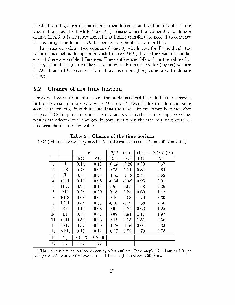
Table 2 : Change of the time horizon

(RC (reference case) : tf = 300; AC (alternative case) : tf = 400; t = 2100)

E �=W (%) (WT �N)=N (%)

RC AC RC AC RC AC

1 J 0.14 0.12 -0.19 -0.28 0.33 0.67

2 US 0.73 0.61 0.73 1.11 0.34 0.64

3 E 0.30 0.25 -1.60 -1.78 2.41 4.62

4 OHI 0.10 0.08 -0.34 -0.49 0.95 2.01

5 HIO 0.21 0.16 2.51 3.65 1.38 2.26

6 MI 0.36 0.30 0.18 0.55 0.69 1.12

7 RUS 0.08 0.06 0.46 0.03 1.70 3.39

8 LMI 0.44 0.35 -0.09 -0.21 1.38 2.36

9 EE 0.11 0.08 0.91 0.84 0.66 1.25

10 LI 0.39 0.31 0.89 0.91 1.17 1.97

11 CHI 0.54 0.43 0.47 0.15 1.51 2.56

12 IND 0.37 0.29 -1.28 -1.64 3.01 5.33

13 AFR 0.15 0.12 -0.19 0.22 1.73 2.73

14 Ca 946.33 912.66

15 Ta 1.43 1.33

17This value is similar to those chosen by other authors. For example, Nordhaus and Boyer

(2000) take 350 years, while Eyckmans and Tulkens (1999) choose 320 years.

27

(E : emissions (GtC/year); Ca : atmospheric carbon content (GtC); Ta : atmo-

spheric temperature change (ÆC); � : transfers; W , WT , N : welfare levels at the

IO with and without transfers and at the Nash equilibrium)

Table 2 summarizes the comparison between the reference case (RC) where

tf = 300 and the alternative case (AC) where tf = 400. The two cases assume

international cooperation (IO). Columns 3 and 4 give respectively for RC and

AC the values observed in 2100 of the emissions per country (lines 1 to 13),

carbon concentration (line 14) and average atmospheric temperature (line 15).

Because future damages are taken account on a longer horizon, emissions of all

countries decline. A 3.7% decrease in the carbon concentration is associated with

a 7.5% temperature change from RC to AC. Such an important variation from a

model parameter that should not in uence signi�cantly the result reveals another

limitation on the signi�cance of the absolute results. Some trends and general

insights can be drawn, but before extensive sensitivity analysis is performed great

caution remains necessary in the model results interpretation.

In terms of welfare, one observes that the picture remains globally the same

in the two cases. The principal winners of cooperation are still Europe and India

and the two main losers remain USA and HIO. A di�erence is that now EE

is a bene�ciary. Because welfare levels and transfers are lump-sum quantities

calculated on unequal planning periods in the two cases, it is meaningless to

compare them in absolute terms. Columns 5 and 6 give respectively for RC and

AC the ratio �i=Wi (in %) characterizing each country. Although the di�erences

are visible, the picture remains similar for the principal donors (Europe and

India) and the principal receivers (USA and HIO). Except for Africa, the sign

of the transfers remains unchanged (Africa becomes a receiver of transfers under

AC). Columns 7 and 8 give respectively for RC and AC the gain in relative terms

between IOT and NE (i.e. (WTi � Ni)=Ni; in %) characterizing each country.

Here the di�erences appear to be more signi�cant. The relative gains obtained by

the countries are nearly multiplied by 2 when moving from RC to AC. So, even

if it does not change fundamentally the results, one can conclude that choosing

a longer planning period increases signi�cantly the interest of cooperation w.r.t

non-cooperation because future damages are taken account on a longer horizon.

5.3 Change of the rate of time preference

It is well known in the climate change literature that results can be very sensitive

to the rate of time preference. In the reference case (RC), this parameter is �xed

to a rather low value (1%) at the beginning of the planning period, and following

Nordhaus et Boyer (1999, 2000), it is assumed to decrease slowly after18. In the

alternative case (AC), we take for the initial value of the rate of time preference

18The annual rate of decrease of the discount rate is equal to .226%. The values observed in

RC for t = 2100; 2200; 2300 are then respectively .79, .61 and .47 %.

28

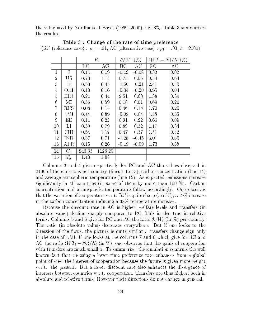
the value used by Nordhaus et Boyer (1999, 2000), i.e. 3%. Table 3 summarizes

the results.

Table 3 : Change of the rate of time preference

(RC (reference case) : �1 = :01; AC (alternative case) : �1 = :03; t = 2100)

E �=W (%) (WT �N)=N (%)

RC AC RC AC RC AC

1 J 0.14 0.19 -0.19 -0.08 0.33 0.02

2 US 0.73 1.15 0.73 0.05 0.34 0.64

3 E 0.30 0.43 -1.60 -0.21 2.41 0.40

4 OHI 0.10 0.16 -0.34 -0.20 0.95 0.04

5 HIO 0.21 0.44 2.51 0.68 1.38 0.39

6 MI 0.36 0.59 0.18 0.01 0.69 0.20

7 RUS 0.08 0.18 0.46 0.18 1.70 0.20

8 LMI 0.44 0.89 -0.09 0.04 1.38 0.35

9 EE 0.11 0.22 0.91 0.22 0.66 0.09

10 LI 0.39 0.79 0.89 0.32 1.17 0.34

11 CHI 0.54 1.12 0.47 0.37 1.51 0.42

12 IND 0.37 0.71 -1.28 -0.45 3.01 0.80

13 AFR 0.15 0.26 -0.19 -0.09 1.73 0.58

14 Ca 946.33 1126.29

15 Ta 1.43 1.98

Columns 3 and 4 give respectively for RC and AC the values observed in

2100 of the emissions per country (lines 1 to 13), carbon concentration (line 14)

and average atmospheric temperature (line 15). As expected, emissions increase

signi�cantly in all countries (in some of them by more than 100 %). Carbon

concentration and atmospheric temperature follow accordingly. One observes

that the variation of temperature w.r.t. RC is quite sharp (.55 ÆC), a 19% increase

in the carbon concentration inducing a 38% temperature increase.

Because the discount rate in AC is higher, welfare levels and transfers (in

absolute value) decline sharply compared to RC. This is also true in relative

terms. Columns 5 and 6 give for RC and AC the ratio �i=Wi (in %) per country.

The ratio (in absolute value) decreases everywhere. But if one looks to the

direction of the ows, the picture is quite similar : transfers change sign only

in the case of LMI. If one looks at the columns 7 and 8 which give for RC and

AC the ratio (WTi � Ni)=Ni (in %), one observes that the gains of cooperation

with transfers are much smaller. To summarize, the simulation con�rms the well

known fact that choosing a lower time preference rate enhances from a global

point of view the interest of cooperation because the future is given more weight

w.r.t. the present. But a lower discount rate also enhances the divergence of

interests between countries w.r.t. cooperation. Transfers are thus higher, both in

absolute and relative terms. However their directions do not change in general.

29

6 Conclusion

This paper describes an economic model of climate change that includes a rep-

resentation of the regional temperature changes on the 13 geographical regions

considered. Using �nancial transfers mechanisms as de�ned in Eyckmans and

Tulkens (1999), we check the interest of countries or group of countries to deviate

from the theoretical international optimal policy by �nancial transfer opportuni-

ties. These results obtained here with a more developed version of the model con-

�rm the outcome of the previous analysis performed with the world represented

with 6 regions and no regional temperature variation. However, we observe here

some contrasted interests to cooperate between countries within the "Rest of the

World" category of countries. India and the high-income OPEC countries have

divergent interests and the improved but still insuÆcient geographical represen-

tation allows to taking such divergence into account.

The regional temperature change representation adds a little more realism to

the crude physical representation of the climate system in this model. Under these

hypotheses, more emission reductions are simulated in all scenarios as greater

regional damages appear. In terms of transfers and welfare, the overall picture

remains similar as previous results but more contrasts appear between the regions

considered.

The sensitivity test on the choice of the time horizon showed an important

limitation of this type of model. From a theoretical point of view, the time horizon

has to be chosen in order to avoid any spurious e�ect on the results within the

period studied. It is shown here that choosing a longer period for the time

horizon signi�cantly a�ects the results and increases the interest of international

cooperation versus non-cooperation. Such bias reveals a model drawback.

The sensitivity to the choice of the discount rate is great and is a well-known

limitation. Therefore, here as in any interpretation of the results with this model,

the results will be closely linked to the value of this parameter.

The trajectories simulated in the di�erent scenarios computed showed that

the model in its present state does not simulate emissions trend that peak before

the end of the period considered (except for the international optimal case. The

BAU scenario under estimates emission growth relative to the IPCC. This char-

acteristic is linked to the hypothesis underlying the model buildup and need to be

investigated in depth but the underestimation of the BAU emissions growth rate

has the consequence of underestimating the potential damage e�ect and therefore

the potential bene�ts of international cooperation.

This leads us to conclude that beyond the analysis that con�rms the interest

of �nancial transfers to prevent free-riding and coalition formation, the model of

the RICE type used here reveals some characteristics which all tend to reduce the

impact of climate change and the interest to reduce the emissions in comparison

with other economical models.

30

Bibliography

Boyer J. and W. Nordhaus (1999). "Requiem for Kyoto : an economic analysis of

the Kyoto Protocol". In "The costs of the Kyoto Protocol : a multi-model

evaluation", The Energy Journal, 131-156.

Boyer J. and W. Nordhaus (2000). Warming the World. Economic Models of

Global Warming, MIT Press.

Chander P. and H. Tulkens (1995). "A core-theoretic solution for the design of

cooperative agreements on transfrontier pollution", International Tax and

Public Finance, 2, 279-293.

Chander P. and H. Tulkens (1997). "The core of an economy with multilateral

environmental externalities", International Journal of Game Theory, 26,

379-401.

Eyckmans J. and H. Tulkens (1999). "Simulating with RICE coalitionally sta-

ble burden sharing agreements for the climate change problem", CORE

discussion paper no 9926.

Energy Modeling Forum (1999). Economic and energy system impacts of the

Kyoto Protocol : Results from the Energy Modeling Forum study, The EMF

16 Working Group, Stanford Energy Modeling Forum, Stanford University,

july.

Germain M., Ph. Toint and H. Tulkens (1998). "Financial transfers to ensure co-

operative international optimality in stock pollutant abatement". In Duchin

F., Faucheux S., Gowdy J. and Nicola�i I. (eds.), Sustainability and Firms:

Technological Change and the Changing Regulatory Environment, Edward

Elgar, Cheltenham.

Hasselmann, K. and S. Hasselmann (1996). "Multi-actor optimization of green-

house gas emissions paths using coupled integral climate response and eco-

nomic models",Max Planck Institut f�ur Meteorologie Report, 209, Hamburg,

Germany.

Harvey, L.D.D., J. Gregory, M. Ho�ert, A. Jain, M. Lal, R. Leemans, S.B.C.

Raper, T.M.L. Wigley and J. de Wolde, (1997). "An introduction to sim-

ple climate models used in the IPCC Second Assessment Report", IPCC

Technical paper II, Intergovernmental Panelaon Climate Change, Bracknell,

U.K.

Kverndokk S. (1994). "Coalitions and side payments in international CO2 treaties".

In Van Ierland (ed.), International Environmental Economics, Theories,

31

Models and Application to Climate Change, International Trade and Acid-

i�cation, Developments in Environmental Economics, vol. 4, Elsevier, Am-

sterdam.

Maier-Reimer, E. and K. Hasselman (1987). "Transport and storage of CO2 in

the ocean -an inorganic ocean - circulation carbon cycle model", Climate

Dynamics, 2, 63-90.

Nordhaus W. and Z. Yang (1996). "A regional dynamic general-equilibrium

model of alternative climate-change strategies", American Economic Re-

view, 86, 741-765.

Schlessinger, M.E., N. Andronova, A. Ghanem, S. Malyshev, T. Reichler, E.

Rozanov, W.Wang and F. Yangi (1997). "Geophysical scenarios of Greenhouse-

Gas and Anthropogenic-Sulfate-Aerosol Induced Climate Changes." Cli-

mate Research Group Report, Department of Atmospheric Sciences, Uni-

versity of Illinois at Urbana-Champain, Urbana, USA.

7 Appendix

7.1 List of variables

Yit: gross production of country i

Cit: consumption of country i

Iit: investment of country i

Kit: capital stock of country i

Lit: population of country i (exogenous)

Eit: carbon-energy consumption of country i (measured in CO2 emissions)

Ait: total factor productivity of country i (exogenous)

pt: world price of carbon-energy

mit: markup on carbon-energy of country i

Di(�Tait) : damage due to temperature change on country i

CCt: cumulative world extraction of carbon-energy

Pa(t): linear atmospheric CO2 impulse function [GTC]

t: time [years]

e(t): rate of CO2 emissions into the atmosphere [GTC/year]

�Ta(t): change in the atmospheric temperature at time t relative to preindustrial

level (assumed year 1765) [ÆC)]

�To(t): change in the deep ocean temperature at time t relative to preindustrial

level [ÆC)]

�FCO2(t): change in anthropogenic CO2 radiative forcing relative to preindus-

trial time [Wm�2]

Tai : GCM air-surface temperature output averaged over the area covered by

32

country i.

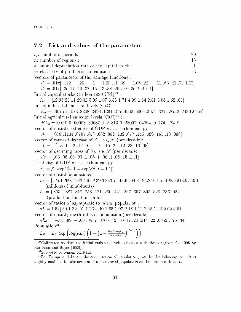
7.2 List and values of the parameters

tf : number of periods : 30

n: number of regions : 13

Æ: annual depreciation rate of the capital stock : .1

: elasticity of production to capital : .3

Vectors of parameters of the damage functions :

d1 = :01x[�:42 � :26 � :1 � 1:08 :41 :39 � 1:08 :22 � :52 :63 :41 :74 1:57]

d2 = :01x[:25 :17 :49 :37 :15 :13 :33 :26 :19 :25 :2 :49 :1]

Initial capital stocks (trillion 1990 US$)19 :

K0 = [12:93 25:11 29:32 5:09 1:07 5:86 1:71 4:99 1:84 2:51 3:08 1:62 :63]

Initial industrial emission levels (GtC) :

E0 = [:3075 1:4073 :8208 :2493 :1294 :277 :4962 :5606 :3677 :3274 :8713 :2480 :0454]

Initial agricultural emission levels (GtC)20 :

EL0 = [0 0 0 0 :00008 :39637 0 :21813 0 :28007 :04094 :01774 :17419]

Vector of initial elasticities of GDP w.r.t. carbon energy :

�0 = [:078 :1134 :0707 :077 :082 :082 :132 :077 :146 :099 :165 :13 :098]

Vector of rates of decrease of �i0; i 2 N (per decade):

�0 = �[:13 :1 :12 :12 :07 :1 :25 :15 :25 :12 :28 :16 :08]

Vector of declining rates of �it; i 2 N (per decade):

d� = [:06 :06 :06 :06 :1 :08 :1 :08 :1 :08 :15 :1 :1]

Elasticity of GDP w.r.t. carbon energy :

�it = �i0 exp(�i0d�i

[1� exp(d�i[t� 1])])

Vector of initial populations :

L0 = [125:1 260:7 383:4 65:8 29:3 283:7 148:0 564:8 194:2 911:5 1198:5 918:6 549:1]

(millions of inhabitants)

L0 = [:303 1:387 :818 :253 :121 :280 :441 :567 :357 :308 :828 :236 :054]

(production function units)

Vector of ratios of asymptotic to initial population :

aL = 1:5x[:89 1:32 :91 1:26 4:40 1:65 1:07 2:18 1:12 2:48 1:40 2:02 4:51]

Vector of initial growth rates of population (per decade) :

gL0 = [�:07 :09 � :06 :0977 :3705 :125 :0117 :20 :014 :22 :0852 :175 :34]

Population21:

Lit = Li0 exp

�log(aLi)

�1�

�1� log(1+gLi)

log(aLi)

�(t�1)��

19Calibrated so that the initial emission levels coincides with the one given for 1995 by

Nordhaus and Boyer (1999).20Supposed to remain constant.21For Europe and Japan, the computation of population given by the following formula is

slightly modi�ed to take account of a decrease of population on the �rst four decades.

33

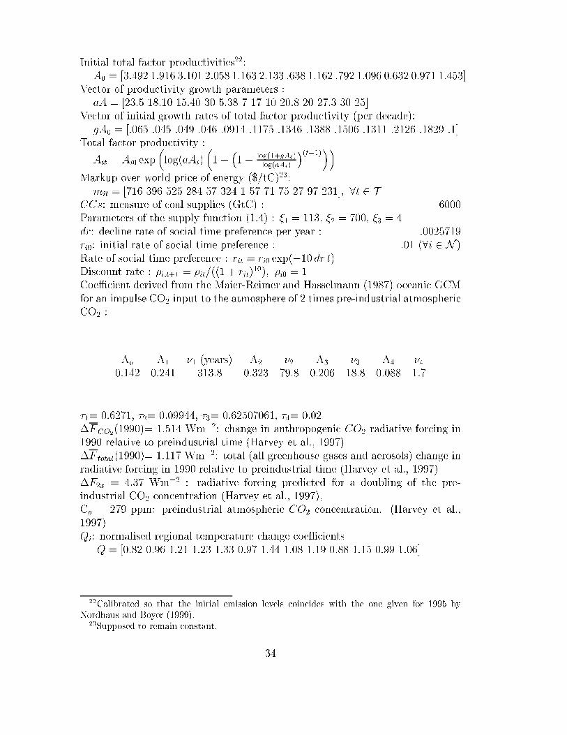
Initial total factor productivities22:

A0 = [3:492 1:916 3:101 2:058 1:163 2:133 :638 1:162 :792 1:096 0:632 0:971 1:453]

Vector of productivity growth parameters :

aA = [23:5 18:10 15:40 30 5:38 7 17 10 20:8 20 27:3 30 25]

Vector of initial growth rates of total factor productivity (per decade):

gA0 = [:065 :045 :049 :046 :0914 :1175 :1346 :1388 :1506 :1311 :2126 :1829 :1]

Total factor productivity :

Ait = Ai0 exp

�log(aAi)

�1�

�1� log(1+gAi)

log(aAi)

�(t�1)��

Markup over world price of energy ($/tC)23:

mit = [716 396 525 284 57 324 1 57 71 75 27 97 231]; 8t 2 T

CCs: measure of coal supplies (GtC) : 6000

Parameters of the supply function (1.4) : �1 = 113, �2 = 700, �3 = 4

dr: decline rate of social time preference per year : .0025719

ri0: initial rate of social time preference : .01 (8i 2 N )

Rate of social time preference : rit = ri0 exp(�10 dr t)

Discount rate : �i;t+1 = �it=((1 + rit)10); �i0 = 1

CoeÆcient derived from the Maier-Reimer and Hasselmann (1987) oceanic GCM

for an impulse CO2 input to the atmosphere of 2 times pre-industrial atmospheric

CO2 :

Ao A1 �1 (years) A2 �2 A3 �3 A4 �4

0.142 0.241 313.8 0.323 79.8 0.206 18.8 0.088 1.7

�1= 0.6271, �2= 0.09944, �3= 0.62507061, �4= 0.02

�FCO2(1990)= 1.514 Wm�2: change in anthropogenic CO2 radiative forcing in

1990 relative to preindustrial time (Harvey et al., 1997)

�F total(1990)= 1.117 Wm�2: total (all greenhouse gases and aerosols) change in

radiative forcing in 1990 relative to preindustrial time (Harvey et al., 1997)

�F2x = 4.37 Wm�2 : radiative forcing predicted for a doubling of the pre-

industrial CO2 concentration (Harvey et al., 1997),

Co = 279 ppm: preindustrial atmospheric CO2 concentration. (Harvey et al.,

1997)

Qi: normalised regional temperature change coeÆcients

Q = [0:82 0:96 1:21 1:23 1:33 0:97 1:44 1:08 1:19 0:88 1:15 0:99 1:06]

22Calibrated so that the initial emission levels coincides with the one given for 1995 by

Nordhaus and Boyer (1999).23Supposed to remain constant.

34