shoreline instability under low-angle wave incidence

, , , /,

Shoreline instability under low-angle wave incidence1

D. Idier

BRGM, 3 Avenue C. Guillemin, BP 6009, 45060 Orleans Cedex 2, France2

A. Falques

UPC, C/ Jordi Girona 1-3, Modul B4/B5, despatx 103 - E-08034, Barcelona,3

Catalonia, Spain4

B.G. Ruessink

Utrecht University, Institute for Marine and Atmospheric Research Utrecht,5

Faculty of Geosciences, Department of Physical Geography, P.O. box 80115,6

3508 TC Utrecht, The Netherlands7

R. Garnier

Instituto de Hidraulica Ambiental IH Cantabria, Universidad de Cantabria,8

ETSI Caminos Canales y Puertos, Avda. los Castros s/n, 39005 Santander,9

Cantabria, Spain10

D. Idier, BRGM, 3 Avenue C. Guillemin, BP 6009, 45060 Orleans Cedex 2, France.

([email protected])

A. Falques, UPC, C/ Jordi Girona 1-3, Modul B4/B5, despatx 103 - E-08034, Barcelona,

Catalonia, Spain. ([email protected])

D R A F T September 27, 2011, 5:50pm D R A F T

hal-0

0635

211,

ver

sion

1 -

24 O

ct 2

011

Author manuscript, published in "Journal of Geophysical Research Earth Surface (2011) 45 p." DOI : 10.1029/2010JF001894

http://dx.doi.org/10.1029/2010JF001894

http://hal-brgm.archives-ouvertes.fr/hal-00635211

http://hal.archives-ouvertes.fr

, Q ,

Abstract.11

The growth of megacusps as shoreline instabilities is investigated by ex-12

amining the coupling between wave transformation in the shoaling zone, long-13

shore transport in the surf zone, cross-shore transport, and morphological14

evolution. This coupling is known to drive a potential positive feedback in15

case of very oblique wave incidence, leading to an unstable shoreline and the16

consequent formation of shoreline sandwaves. Here, using a linear stability17

model based on the one-line concept, we demonstrate that such instabilities18

can also develop in case of low-angle or shore-normal incidence, under cer-19

tain conditions (small enough wave height and/or large enough beach slope).20

The wavelength and growth time scales are much smaller than those of high-21

angle wave instabilities and are nearly in the range of those of surf zone rhyth-22

mic bars, O(102 − 103 m) and O(1 − 10 days), respectively. The feedback23

mechanism is based on: (1) wave refraction by a shoal (defined as a cross-24

shore extension of the shoreline perturbation) leading to wave convergence25

shoreward of it, (2) longshore sediment flux convergence between the shoal26

and the shoreline, resulting in megacusp formation, and (3) cross-shore sed-27

B.G. Ruessink, Utrecht University, Institute for Marine and Atmospheric Research Utrecht,

Faculty of Geosciences, Department of Physical Geography, P.O. box 80115, 3508 TC Utrecht,

The Netherlands. ([email protected])

R. Garnier, IH Cantabria, Universidad de Cantabria, Avda. los Castros s/n, 39005 Santander,

Cantabria, Spain. ([email protected])


hal-0

0635

211,

ver

sion

1 -

24 O

ct 2

011

, Q ,

iment flux from the surf to the shoaling zone, feeding the shoal. Even though28

the present model is based on a crude representation of nearshore dynam-29

ics, a comparison of model results with existing 2DH model output and lab-30

oratory experiments suggests that the instability mechanism is plausible. Ad-31

ditional work is required to fully assess whether and under which conditions32

this mechanism exists in nature.33


hal-0

0635

211,

ver

sion

1 -

24 O

ct 2

011

, Q ,

1. Introduction

Rhythmic shorelines featuring planview undulations with a relatively regular spacing or34

wavelength are quite common on sandy coasts. In the present study, we focus on undu-35

lations that are linked to submerged bars or shoals and are generally known as shoreline36

sandwaves [Komar , 1998; Bruun, 1954]. These sandwaves can be classified according to37

their length scale as short and long sandwaves (see, e.g., Stewart and Davidson-Arnott38

[1988]).39

The spacing of short sandwaves ranges from several tens to several hundreds of meters40

and their seaward perturbations are known as megacusps. Observations show that these41

megacusps can develop shoreward of crescentic bar systems during the typical “Rhythmic42

Bar and Beach” morphological beach state or can develop from the shore attachment43

of transverse bars that characterise the “Transverse Bar and Beach” state [Wright and44

Short , 1984]. These transverse bars can appear where the horns of a previous crescentic45

bar approach the shoreline [Wright and Short , 1984; Sonu, 1973; Ranasinghe et al., 2004;46

Lafon et al., 2004; Castelle et al., 2007]. On the other hand, transverse bars can also47

develop freely, independently of any offshore rhythmic system (e.g. the “transverse finger48

bars” [Sonu, 1968, 1973; Ribas and Kroon, 2007]). The formation of rhythmic surf zone49

bars and associated megacusps is believed to be due primarily to an instability of the50

coupling between the evolving bathymetry and the distribution of wave breaking (bed-51

surf coupling) [Falques et al., 2000]. The developing shoals and channels cause changes in52

wave breaking, which in turn cause gradients in radiation stresses and thereby horizontal53

circulation with rip currents. If the sediment fluxes carried by this circulation converge54


hal-0

0635

211,

ver

sion

1 -

24 O

ct 2

011

https://www.researchgate.net/publication/240568892_Three-Dimensional_Beach_Changes?el=1_x_8&enrichId=rgreq-6938d9245f913a0fb206b164837734cf-XXX&enrichSource=Y292ZXJQYWdlOzI0MTg4MTQ3NztBUzo5OTcxMDcxMDg0NTQ1OUAxNDAwNzg0Mjk0OTc2

https://www.researchgate.net/publication/50209056_Migrating_sand_waves_or_sand_humps_with_special_reference_to_investigations_carried_out_on_the_Danish_North_Sea_Coast?el=1_x_8&enrichId=rgreq-6938d9245f913a0fb206b164837734cf-XXX&enrichSource=Y292ZXJQYWdlOzI0MTg4MTQ3NztBUzo5OTcxMDcxMDg0NTQ1OUAxNDAwNzg0Mjk0OTc2

https://www.researchgate.net/publication/46725427_Characteristics_and_dynamics_of_surfzone_transverse_finger_bars?el=1_x_8&enrichId=rgreq-6938d9245f913a0fb206b164837734cf-XXX&enrichSource=Y292ZXJQYWdlOzI0MTg4MTQ3NztBUzo5OTcxMDcxMDg0NTQ1OUAxNDAwNzg0Mjk0OTc2

, Q ,

over the shoals and diverge over the channels, a positive feedback arises and the coupled55

system self-organizes to produce certain patterns, both morphological and hydrodynamic56

(see, e.g., Reniers et al. [2004]; Garnier et al. [2008]). In the case of oblique wave inci-57

dence, a meandering of the longshore current is also essential to the instability process58

[Garnier et al., 2006]. Two important characteristics of all available models of the self-59

organized formation of rhythmic surf zone bars are that they (1) are essentially based60

on sediment transport driven by the longshore current and rip currents only, i.e. ignore61

cross-shore transport induced by undertow and wave non-linearity and (2) do not consider62

morphological changes beyond the offshore reach of the rip-current circulation.63

Rhythmic shorelines can also develop as a result of an instability not related to bed-64

surf coupling. Ashton et al. [2001] and Ashton and Murray [2006a, b] have shown that65

sandy shorelines are unstable for wave angles (angle between wave fronts and the local66

shoreline orientation) larger than about 42◦ in deep water, leading to the formation of67

shoreline sandwaves, cuspate features and spits. Falques and Calvete [2005] have found68

that the initial characteristic wavelength of the emerging sandwaves is in the range of 3 to69

15 km, i.e., much larger than that of surf zone rhythmic bars. This instability caused by70

high-angle waves will henceforth be referred to as HAWI (High-Angle Wave Instability).71

The physical mechanism can be explained as follows. For oblique wave incidence, there72

are essentially two counteracting effects. On one hand, the angle relative to the local73

shoreline is larger on the lee of a cuspate feature than on the updrift side. This tends to74

cause larger alongshore sediment flux at the lee and thereby divergence of sediment flux75

along the bump, which therefore tends to erode. On the other hand, since the refractive76

wave ray turning is stronger at the lee than at the updrift flank, there is more wave energy77


hal-0

0635

211,

ver

sion

1 -

24 O

ct 2

011

, Q ,

spreading due to crest stretching at the lee causing smaller waves and smaller alongshore78

sediment flux. This produces convergence of sediment flux at the bump, which therefore79

tends to grow. For high angle waves the latter effect dominates and, if the bathymetric80

perturbation associated with the shoreline feature extends far enough offshore, it leads to81

the development of the cuspate feature. In contrast to the bed-surf instability for rhythmic82

surf zone bars, this instability mechanism depends essentially on the coupling between the83

surf and shoaling zones. Indeed, the gradients in alongshore sediment flux that induce84

bathymetric changes in the surf zone occur because of wave field perturbations induced by85

bathymetric features in the shoaling zone. Thus, in order to achieve a positive feedback,86

the shoals (or the bed depressions) in the surf zone must extend into the shoaling zone.87

This is achieved by the cross-shore sediment fluxes induced, for instance, by wave non-88

linearity, gravity and undertow, which force the cross-shore shoreface profile to reach an89

equilibrium profile. HAWI may provide an explanation for the self-organized formation90

of some long shoreline sand waves which are reported in the literature [Verhagen, 1989;91

Inman et al., 1992; Thevenot and Kraus , 1995; Ruessink and Jeuken, 2002; Davidson-92

Arnott and van Heyningen, 2003].93

On the other hand, some observations for low incidence angles show that longshore94

currents can converge on megacusps because of wave refraction [Komar , 1998]. Such cur-95

rent convergence may lead to longshore sediment flux convergence and hence to megacusp96

growth. If the submerged part of the megacusp grows and extends far enough into the97

shoaling zone (due to the cross-shore transport leading to an equilibrium profile), wave98

refraction would be enhanced and a positive feedback would arise. This might provide a99

mechanism for shoreline instability formation under low-angle wave incidence that bears100


hal-0

0635

211,

ver

sion

1 -

24 O

ct 2

011

, Q ,

some similitude with HAWI in the sense that the coupling between the surf and shoaling101

zones is essential, in contrast to the bed-surf instability. We will refer to this potential102

mechanism as Low-Angle Wave Instability (LAWI). The aim of the present contribution103

is to investigate this new morphodynamic instability mechanism and discuss whether the104

resulting shoreline instability may be found in nature.105

The lay-out of this paper is as follows. First (Section 2), we introduce the 1D-morfo106

model [Falques and Calvete, 2005] that we used to investigate LAWI. Numerical experi-107

ments of idealized cases are presented and analyzed in Section 3. We find that shoreline108

sandwaves can indeed develop because of LAWI, with a length scale comparable to those109

of megacusps and rhythmic surf zone bars. In Section 4, we analyze the physics of the110

instability mechanism. We conclude our paper with a discussion and a summary of the111

main results.112

2. The shoreline stability model: 1D-morfo

Owing to the similitude with HAWI [Ashton et al., 2001; Falques and Calvete, 2005], the113

LAWI mechanism is assumed to be un-related to surf zone processes like rip or longshore114

meandering currents. Thus, the engineering simplification of one-line modeling [Dean115

and Dalrymple, 2002] is used, where the shoreline dynamics are based on alongshore116

gradients in the total alongshore transport rate, Q (i.e., the total volume of sand carried117

by the wave-driven longshore current that crosses a cross-section of the surf zone area118

for unit of time (m3/s)). Using such a simple model, which neglects numerous aspects119

of surf zone dynamics, including rip current circulation, longshore current meandering,120

and thus the bed-surf coupling phenomena, allows to investigate properly whether the121

LAWI mechanism is supported by the governing equations. Furthermore, the consistency122


hal-0

0635

211,

ver

sion

1 -

24 O

ct 2

011

, Q ,

of the sediment transport patterns from the one-line modelling has been confirmed by123

using a 2DH model (delft3D) [List and Ashton, 2007], at least in case of HAWI. These124

reasons, in addition to the fact that HAWI has been studied and reproduced with a linear125

stability model called 1D-morfo based on the one-line concept, lead us to use the same126

model to investigate LAWI and its differences with HAWI. A very brief description of the127

1D-morfo model is given here. The reader is referred to Falques and Calvete [2005] for128

further details.129

The model describes the dynamics of small amplitude perturbations of an otherwise rec-130

tilinear coastline. Following the one-line concept, the dynamics are governed by gradients131

in the total alongshore wave-driven transport rate Q:132

D∂xs

∂t= −∂Q

∂y(1)

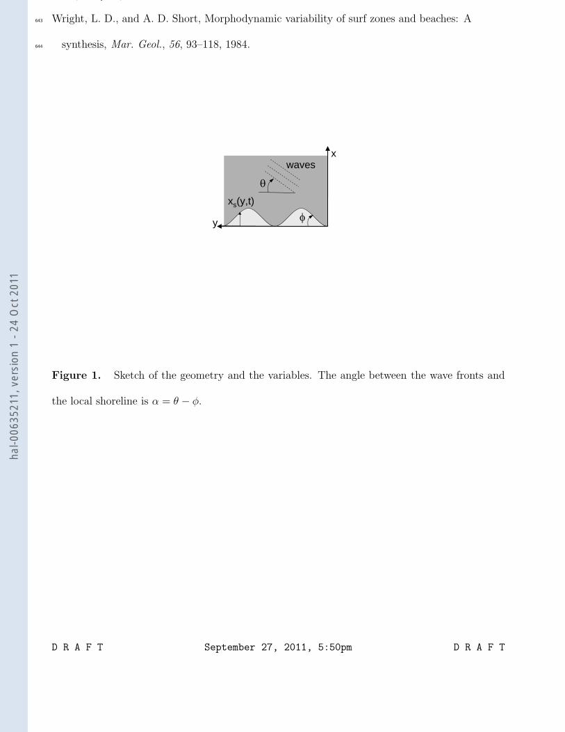
A Cartesian coordinate system is used, with x increasing seaward in the unperturbed133

cross-shore direction and y running alongshore (Figure 1). The position of the shoreline Figure 1134

is given by x = xs(y, t), where t is time and D is the active water depth (as defined by135

Falques and Calvete [2005]), which is of the order of the depth of closure. This active136

water depth is directly related to the one-line model concept, for more details, see Falques137

and Calvete [2005]. The transport rate Q is computed according to the longshore sediment138

transport equation of Ozasa and Brampton [1980]. In this formulation, Q is the sum of139

two terms: the first one (Q1) is driven by waves approaching the shore at an angle and140

is equivalent to the CERC formula [USACE , 1984], and the second one (Q2) takes into141

account the influence of wave set-up induced currents related to the alongshore gradient142

in the wave height.143


hal-0

0635

211,

ver

sion

1 -

24 O

ct 2

011

, Q ,

The equation of the sediment transport rate Q can be written as follows:144

Q = Q1 +Q2 Q = μH5/2b

(sin(2(θb − φ))− r

2

βcos(θb − φ)

∂Hb

∂y

)(2)

where Hb is the (rms) wave height at breaking (index b), θb is the angle between wave145

fronts and the unperturbed coastline at breaking, and φ = tan−1(∂xs/∂y) is the local146

orientation of the perturbed shoreline. β is the beach slope at the instantaneous shoreline147

(i.e. the waterline). The constant μ is proportional to the empirical parameter K1 of148

the original CERC formula and is ∼ 0.1 − 0.2 m1/2s−1. For the reference case of this149

paper, a value, μ = 0.15 m1/2s−1, was chosen, which corresponds to K1 = 0.525. The150

nondimensional parameter r is equal to K2/K1, where K2 is the empirical parameter of151

Ozasa and Brampton [1980]. According to Horikawa [1988], r ranges between 0.5 and 1.5,152

whereas Ozasa and Brampton [1980] suggest a value of 1.62. The value r = 1 is used for153

the present reference case, which is equivalent to K2 = K1 and has been used in several154

earlier studies on shoreline instabilities [Bender and Dean, 2004; List et al., 2008; van den155

Berg et al., 2011]. However, the term Q2 is not always taken into account, and its validity156

and application range are uncertain. In section 3.2, we will study the sensitivity of our157

results to the value of r.158

Some discussion exists about the capacity of the CERC formula (Q1) to predict correctly159

gradients in alongshore sediment transport in the presence of bathymetric perturbations160

[List et al., 2006, 2008; van den Berg et al., 2011]. The results of List and Ashton [2007]161

suggest that the CERC formula predicts qualitatively correct transport gradients for large162

scale shoreline undulations (alongshore lengths of 1-8 km). The term Q2 was introduced to163

describe the sediment transport resulting from alongshore variations in the breaker wave164

height induced by diffraction near coastal structures. These breaker-height variations in-165


hal-0

0635

211,

ver

sion

1 -

24 O

ct 2

011

, Q ,

duce alongshore gradients in set-up, which drive longshore currents and hence sediment166

transport. In our work, alongshore variability in breaker heights is related to wave re-167

fraction rather than to wave diffraction, but the subsequent mechanism for alongshore168

sediment transport remains the same.169

To compute the sediment transport rate according to eq. 2, Hb(y, t) and θb(y, t) are170

needed. The procedure to determine them is as follows. It is assumed that the wave171

height and wave angle are alongshore uniform in deep water. Then, wave transformation,172

including refraction and shoaling, is performed from deep water up to the breaking point173

so that Hb(y, t) and θb(y, t) are determined and Q can be computed. To do the wave174

transformation, a perturbed nearshore bathymetry coupled to the shoreline changes is175

assumed:176

D(x, y, t) = D0(x)− β f(x) xs(y, t) (3)

where D(x, y, t) and D0(x) are the perturbed and unperturbed water depth, respectively,177

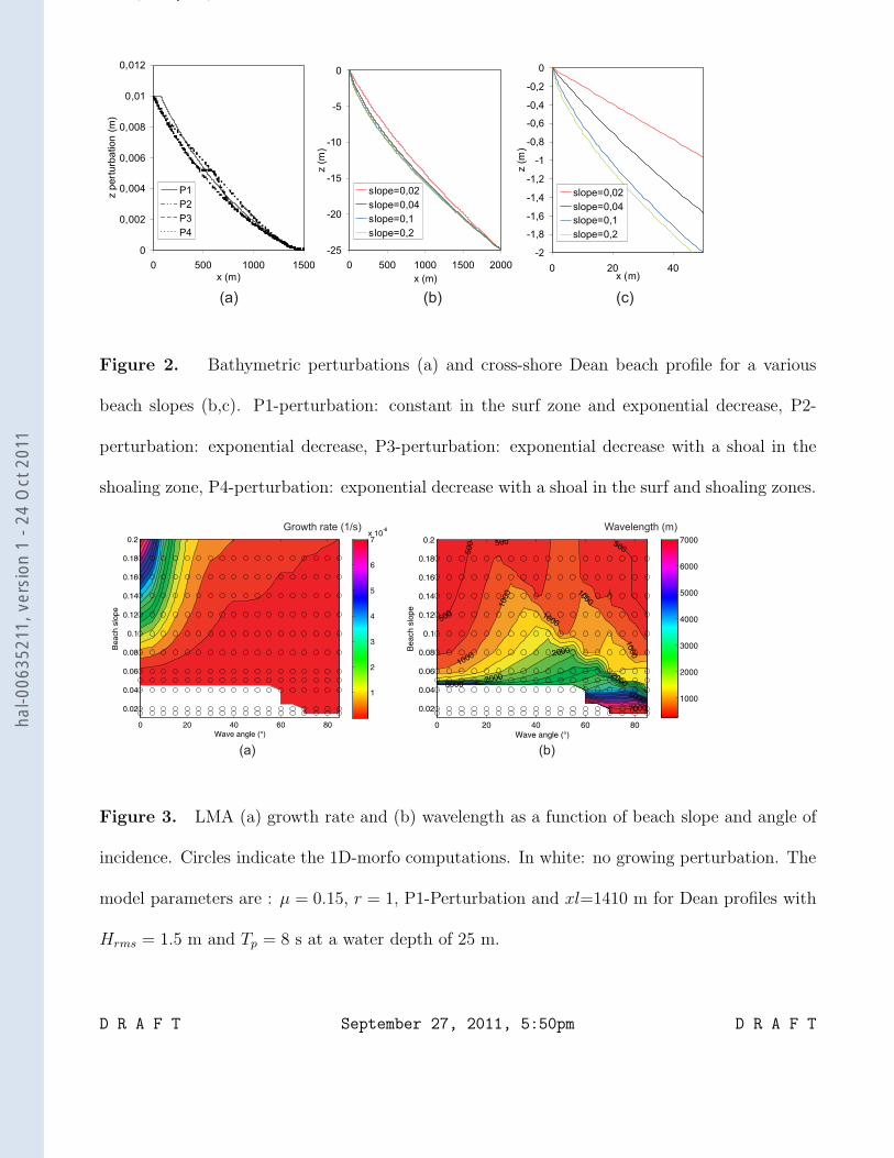
and f(x) is a shape function. Figure 2a shows some examples of possible perturbation Figure 2178

profiles: constant bed perturbation in the surf zone and decreasing exponentially in the179

offshore direction (P1), bed perturbation decreasing exponentially in the offshore direction180

from the coast (P2), and bed perturbation similar to a shoal (P3 and P4).181

The offshore extension of the bathymetric perturbation is controlled by its “charac-182

teristic” length, xl, which is a free parameter in the model. It was shown by Falques183

and Calvete [2005] that the coupling between the surf and shoaling zones is crucial for184

HAWI. This is accomplished only if xl is at least a couple of times larger than the surf185

zone width. The parameter xl can be seen as a way to parameterise cross-shore sediment186

transport, especially between the surf and shoaling zones. This makes HAWI essentially187


hal-0

0635

211,

ver

sion

1 -

24 O

ct 2

011

, Q ,

different from the surf zone morphodynamic instabilities that lead to rhythmic bars and188

rip channels. The changes in the shoreline cause changes in the bathymetry (both in the189

surf and shoaling zones), which in turn cause changes in the wave field. The changes in190

the wave field affect the sediment transport that drives shoreline evolution. Therefore,191

the shoreline, the bathymetry and the wave field are fully coupled.192

Following the linear stability concept, the perturbation of the shoreline is assumed to193

be194

xs(y, t) = aeσt+iKy + c.c. (4)

where a is a small amplitude. For each given (real) wavenumber, K, this expression is195

inserted into the governing equation (eq. 1), and into the perturbed bathymetry equation196

(eq. 3). By computing the perturbed wave field and inserting Hb and θb in eq. 1, the197

complex growth rate, σ(K) = σr + iσi, is determined. All of the equations are linearized198

with respect to the amplitude, a. Then, for those K such that σr(K) > 0 a sandwave with199

wavelength λ = 2π/K tends to emerge from a positive feedback between the morphology200

and the wave field. The pattern that has the maximum growth rate is called the Linearly201

Most Amplified mode (LMA mode).202

3. Numerical experiments on idealised cases

To investigate the possible mechanism causing shoreline instabilities under low wave203

incidence angles, numerical experiments on idealised cases are performed. First, numerical204

experiments and results are given. Then, a sensitivity study is done to assess better the205

results.206


hal-0

0635

211,

ver

sion

1 -

24 O

ct 2

011

, Q ,

3.1. Instabilities versus beach slope and wave incidence angle

3.1.1. Configuration207

A Dean profile (Figure 2b) is chosen as the equilibrium profile, using various beach208

slopes (Figures 2b and c). The adopted profile is given by:209

D0(x) = b((x+ x0)

2/3 − x2/30

)(5)

which has been modified from the original Dean profile to avoid an infinite slope at the210

shoreline. The constants b and x0 are determined from the prescribed slope β at the211

coastline and the prescribed distance xc from the coastline to the location of the closure212

depth Dc (see Falques and Calvete [2005] for details). The forcing conditions are waves213

with Hrms = 1.5 m and Tp = 8 s at a water depth of 25 m. The wave direction ranges214

from 0◦ to 85◦ in increments of 5◦. A closure depth D = 20 m is chosen. To perform the215

linear stability analysis, the shape function for the bathymetric perturbations is assumed216

to be constant in the surf zone and to decrease exponentially seaward. Its cross-shore217

extent is given by the characteristic distance xl corresponding to the closure depth of 20218

m, i.e. xl = 1410 m for the present case (P1-perturbation in Figure 2a).219

3.1.2. Results220

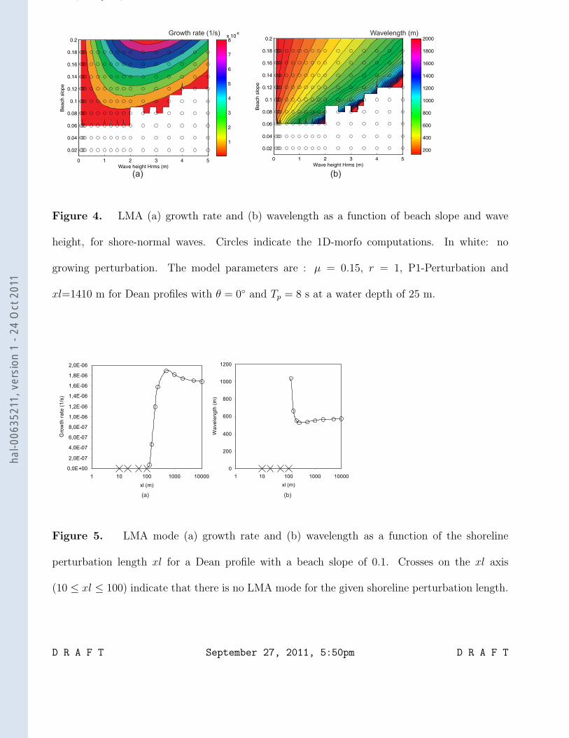
Figure 3a shows the growth rate of the LMA mode versus the wave angle and the beach Figure 3221

slope. The wave angle is given for a water depth of 25 m. The beach slope is defined as222

the beach slope at the shoreline. For small beach slopes (< 0.04) the coast behaves as223

expected: it is unstable only if the wave incidence angle is large enough. In this case, the224

shoreline instabilities clearly correspond to HAWI. For instance, for a beach slope of 0.02,225


hal-0

0635

211,

ver

sion

1 -

24 O

ct 2

011

, Q ,

a wave incidence of 70◦ leads to the largest growth rate (3.13× 10−9 s −1) , corresponding226

to a wavelength of 7000 m (Figure 3b).227

However, for larger beach slopes, instabilities occur for all wave directions, and espe-228

cially for low wave incidence angles. These instabilities correspond to what will be called229

LAWI in the present paper. Furthermore, among all the wave incidence angles, the most230

amplified mode is for shore-normal wave incidence. For a beach slope of 0.1, an angle of231

0◦ leads to the largest growth rate (1.82 × 10−6 s −1), corresponding to a wavelength of232

571 m (Figure 3b).233

3.2. Sensitivity analysis

The sensitivity analysis is performed using a planar beach, as the aim is to focus on the234

mechanisms. However, simulations with other (e.g. barred) profiles also lead to LAWI235

(not shown).236

3.2.1. Wave height and beach slope237

Keeping the same reference configuration as above and focusing on shore-normal wave238

incidence, we investigate the sensitivity of the instability to the wave height for a range239

of beach slopes. For normally incident waves, instabilities develop only for a beach slope240

that exceeds 0.04 (Figure 4). In this case, there is an optimum in the wave height for Figure 4241

which the growth rate is largest. This wave height increases with the beach slope. For242

instance, for a beach slope of 0.1 and 0.18), the optimal wave height Hrms is 1.75 m and243

2.5 m, respectively. A wave height increase also leads to an increase in the LMA mode244

wavelength, which is due to the corresponding increase in surf zone width.245

3.2.2. Bathymetric perturbation length246


hal-0

0635

211,

ver

sion

1 -

24 O

ct 2

011

, Q ,

The influence of the parameter xl was previously investigated by Falques and Calvete247

[2005], who showed that xl must exceed a threshold to initiate HAWI (the perturbation248

must extend across both the surf and shoaling zones). Similar behaviour is found here249

by exploring the range between xl = 10 and xl = 104 m. Figure 5 shows that there is a Figure 5250

threshold, xl > 100 m, above which shoreline instabilities may occur. This value appears251

physically reasonable since the width of the surf zone in the reference case is about 73252

m. For 125 ≤ xl ≤ 250 m, the shoreline instability wavelength decreases significantly253

(from 1040 to 530 m) with increasing perturbation length, whereas for xl ≥ 250 m, the254

wavelength increases only slightly until reaching a nearly constant value of 574 m. The255

growth rate increases with increasing xl for values below 500 m but decreases for xl256

exceeding 500 m, reaching a nearly constant value for large perturbation length scales.257

The main conclusion is that instabilities occur only if the perturbation extends far enough258

into the shoaling zone. When the perturbation length is about the width of the surf zone,259

it influences the wavelength and growth rate of the LMA mode strongly, whereas for larger260

perturbation length values, this influence is negligible.261

3.2.3. Initial perturbation shape262

To evaluate the influence of the bathymetric perturbation shape function on the results263

we have presented so far, several shapes were investigated using the same wave-boundary264

conditions and a perturbation length xl of 2000 m. The shape functions we consider are265

(Figure 2a):266

• Perturbation P1: bed perturbation constant in the surf zone and decreasing expo-267

nentially in the offshore direction268


hal-0

0635

211,

ver

sion

1 -

24 O

ct 2

011

, Q ,

• Perturbation P2: bed perturbation decreasing exponentially from the coast in the269

offshore direction270

• Perturbation P3: P2 perturbation with a shoal located only in the shoaling zone,271

from 400 to 800 m, with a maximum height at x1 = 600 m.272

• Perturbation P4: P2 perturbation with a shoal located in both the surf and shoaling273

zones, from 0 to 1400 m, with a maximum height at x1 = 600 m.274

The reference configuration is still the same (Hrms=1.5 m, T = 8 s, θ = 0◦). The four275

shape functions result in LMA mode wavelengths of 571, 571, 608 and 608 m, respectively,276

and growth rates of 1.7, 1.5, 1.7, 1.7 ×10−6 s −1, respectively. Thus, the results are277

slightly sensitive (mean wavelength of 598 m and a standard deviation of 18 m) to the278

bed perturbation type, but all perturbation types cause LAWI with similar growth rates.279

3.2.4. Sediment transport equation280

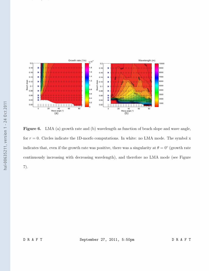
To investigate the sensitivity of the results to the sediment transport equation, compu-281

tations were carried out with r = 0, which reduces eq. 2 to the CERC equation. This282

sensitivity study is done in beach slope - wave angle space. The LMA characteristics are283

quite similar with r = 1 (Figure 3) and r = 0 (Figure 6), except for the case of normal Figure 6284

wave incidence. In this case (r = 0), for small beach slopes, all of the perturbations are285

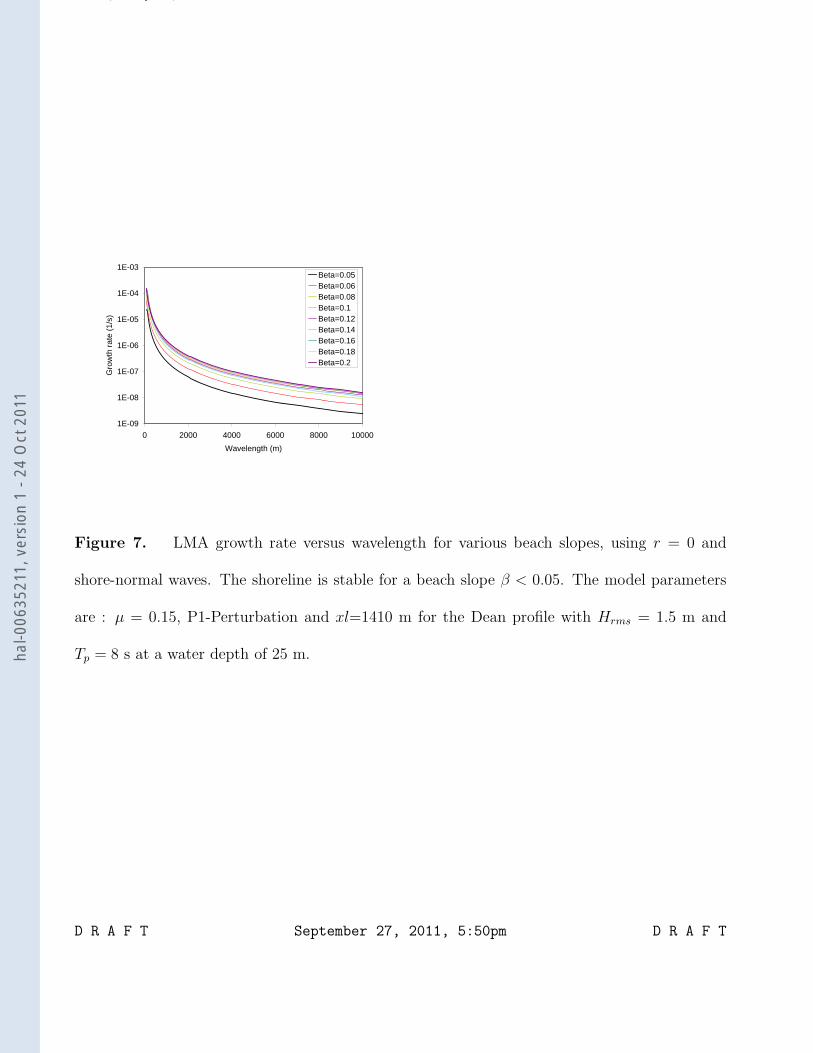
damped, as for r = 1. For larger beach slopes, the growth rate increases with decreasing286

perturbation wavelength without reaching a local maximum (Figure 7). Thus there is no Figure 7287

LMA mode for shore-normal wave incidence (X symbol on Figure 6). This specific case for288

shore-normal wave incidence will be discussed in section 4. To summarize, the previous289

results are not highly sensitive to the second term of the sediment transport equation,290

except for the case of shore-normal wave incidence.291


hal-0

0635

211,

ver

sion

1 -

24 O

ct 2

011

, Q ,

4. The physical mechanism

Here we investigate the physics behind the model prediction of shoreline instabilities292

caused by low wave incidence angles. The physical processes are analysed based on the293

study of the growth rate components, and the hydrodynamic and sediment transport294

patterns, before identifying the main mechanisms.295

4.1. Growth rate analysis

In the perturbed situation where the shoreline position is given by eq. 4, the wave296

height and wave angle at breaking are given by:297

Hb(y, t) = H0b + (H ′

br + iH ′bi)e

σt+iKy + c.c.

θb(y, t) = θ0b + (θ′br + iθ′bi)eσt+iKy + c.c. (6)

where H0b , θ

0b are the wave height and angle for the unperturbed situation. Then, according298

to Falques and Calvete [2005], the growth rate (the real part of the complex growth rate)299

is:300

σr = 2μ

DH0

bK2 cos

(2θ0b

)︸︷︷︸

e0

⎛⎜⎜⎜⎜⎝−1︸︷︷︸

e1

+θ′biaK︸︷︷︸e2

+5H ′

bi

4aKH0b

tan(2θ0b

)︸︷︷︸

e3

−rH ′

br

aβ

cos (θ0b )

cos (2θ0b )︸︷︷︸e4

⎞⎟⎟⎟⎟⎠ (7)

A clue to the physical mechanism is provided by a careful analysis of the meaning and301

behaviour of each term:302

• e0: common to all terms. It does not contribute to the stability/instability since it303

is positive. This is because we can assume that θ0b < 45 ◦ due to wave refraction. It is the304

magnitude of the growth rate.305

• e1: always negative. It represents the contribution due to the changes in shoreline306

orientation when there is no perturbation in the wave field. This is the only term arising307


hal-0

0635

211,

ver

sion

1 -

24 O

ct 2

011

, Q ,

in case of the classical analytical one-line modeling (Pelnard-Considere equation) [Dean308

and Dalrymple, 2002]. It is a damping term describing the shoreline diffusivity in that309

approach.310

• e2: its sign depends on θ′bi. Numerical computations [Falques and Calvete, 2005]311

demonstrates that it is always positive. This results from the fact that refracted wave312

rays tend to rotate in the same direction as the shoreline. Thus e2 is a growing term.313

• e3: its sign depends on H ′bi. Numerical computations [Falques and Calvete, 2005]314

show that H ′bi > 0 for long sandwaves and < 0 for short sandwaves. This term is related315

to energy spreading due to wave crest stretching as waves refract. Thus e3 is a growing or316

damping term, depending on the sandwave wavelength, 2π/K. Moreover, its magnitude317

increases with an increasing incident wave angle. These two properties explain that e3 is318

an essential growing term for HAWI formation Falques and Calvete [2005], whereas, for319

LAWI, its magnitude is smaller and it is, most of the time, negative.320

• e4: this term stems from the alongshore gradients in Hb in the sediment transport321

equation (eq. 2). Its sign is the opposite to that of H ′br, which is numerically found to be322

always positive. This is related to the fact that the maximum in wave energy is always323

located close to the sandwave crest (wave focusing). Thus e4 is a damping term.324

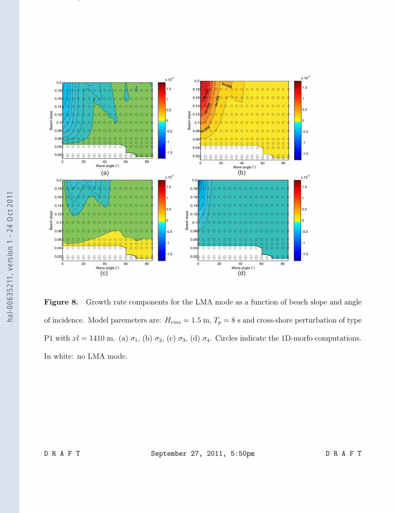
The corresponding growth rate contributions, σ1 = e0e1, σ2 = e0e2, ... are plotted in325

Figure 8. It can be seen that σ2 is always positive leading to the development of shoreline Figure 8326

sandwaves, whereas σ1 and σ4 are always negative, leading to the damping of the sand-327

waves. The term σ3 can be either positive, for small beach slope (eg smaller than 0.05328

to 0.08), or negative, for larger beach slopes. Even if the behaviour of this term is not329

monotonous, σ3 generally increases with the wave angle. It is remarkable that σ2 becomes330


hal-0

0635

211,

ver

sion

1 -

24 O

ct 2

011

, Q ,

very large for large beach slopes and for small wave angles. For normal wave incidence331

(θ0b = 0), σ3 = 0 and σ2 is the only contribution leading to the instability. We therefore332

conclude that wave refraction is responsible for LAWI in the case of very steep beach333

slopes.334

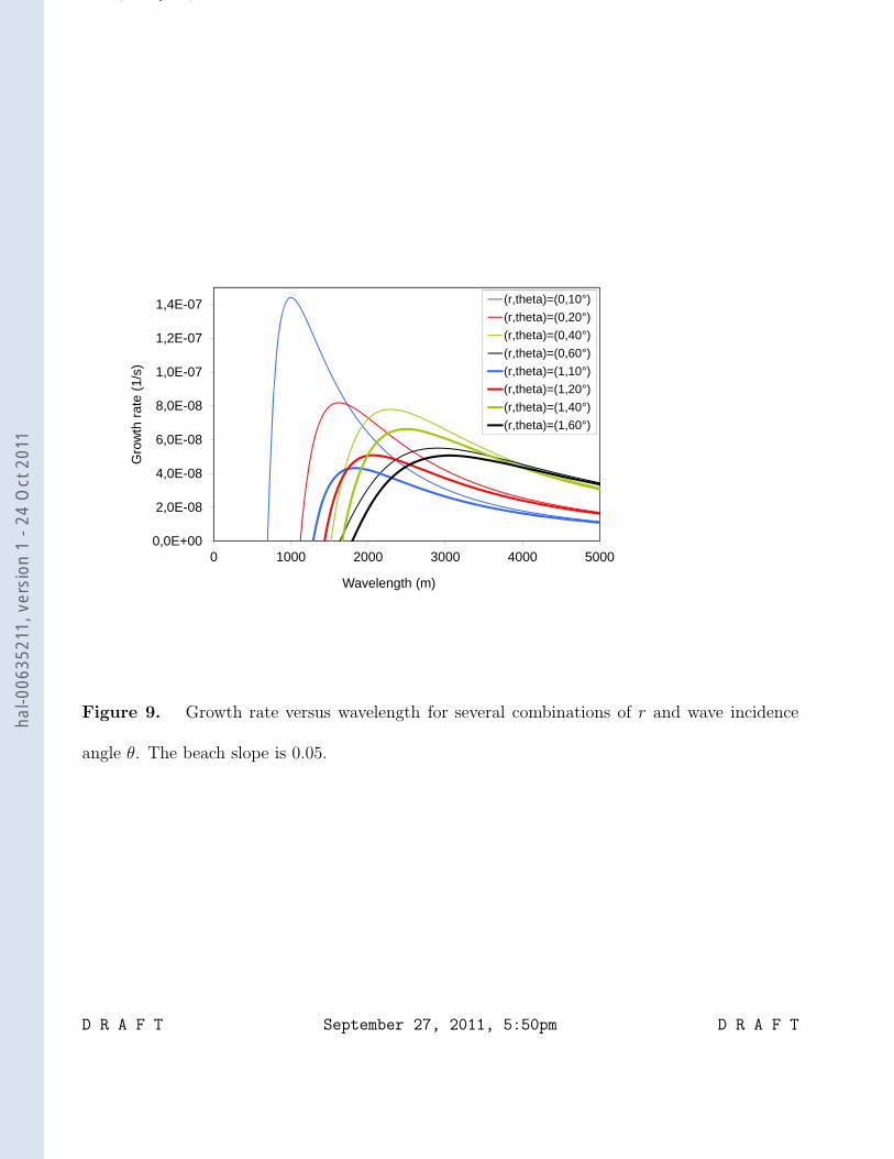
Based on the growth rate results, it is also possible to analyse the relative influence335

of the wave incidence induced Q1 and wave set-up induced Q2 sediment transport. The336

analysis of the growth rate versus the perturbation wavelength for r = 0 or r = 1 and337

several wave incidence angles θ (Figure 9) shows that the relative influence of Q2 decreases Figure 9338

with increasing the wave incidence angle. In other words, wave height gradients (wave set-339

up induced sediment fluxes) largely influence (damp) the shoreline instability for low wave340

angle incidence (LAWI), whereas their impact is almost negligible for large wave incidence341

angles (HAWI). The main driving term of the LAWI is due to the wave incidence induced342

sediment transport flux Q1. This means that the use of the CERC equation alone, taking343

into account wave refraction in the shoaling zone, can cause LAWI. The Q2 term influences344

this instability by changing the growth rate and the favored wavelength. This influence345

increases with decreasing wave incidence until the case of perfectly shore-normal waves,346

for which there is a prefered wavelength (LMA mode) only if the Q2 term is taken into347

account (Figure 6).348

4.2. Model results analysis: Hydrodynamic and sediment transport

To understand better how wave refraction causes shoreline instabilities, hydrodynamic349

and sediment transport model results are analysed next. Here, we focus on the case350

of shore-normal wave incidence, considering the LMA mode obtained for a beach slope351

equal to 0.1 (case a). The model results are compared with the same wave incidence, but352


hal-0

0635

211,

ver

sion

1 -

24 O

ct 2

011

, Q ,

a smaller beach slope (0.02) for which the shoreline is stable (case b). The perturbation353

wavelength (571 m) is the same for both cases, corresponding to the LMA mode of case354

(a). Although the linear stability analysis is strictly valid only in the limit a → 0 we355

choose a shoreline sandwave amplitude a = 10 m (for visualization and comparison of356

the different sources of sediment transport). In addition, to make the analysis simpler,357

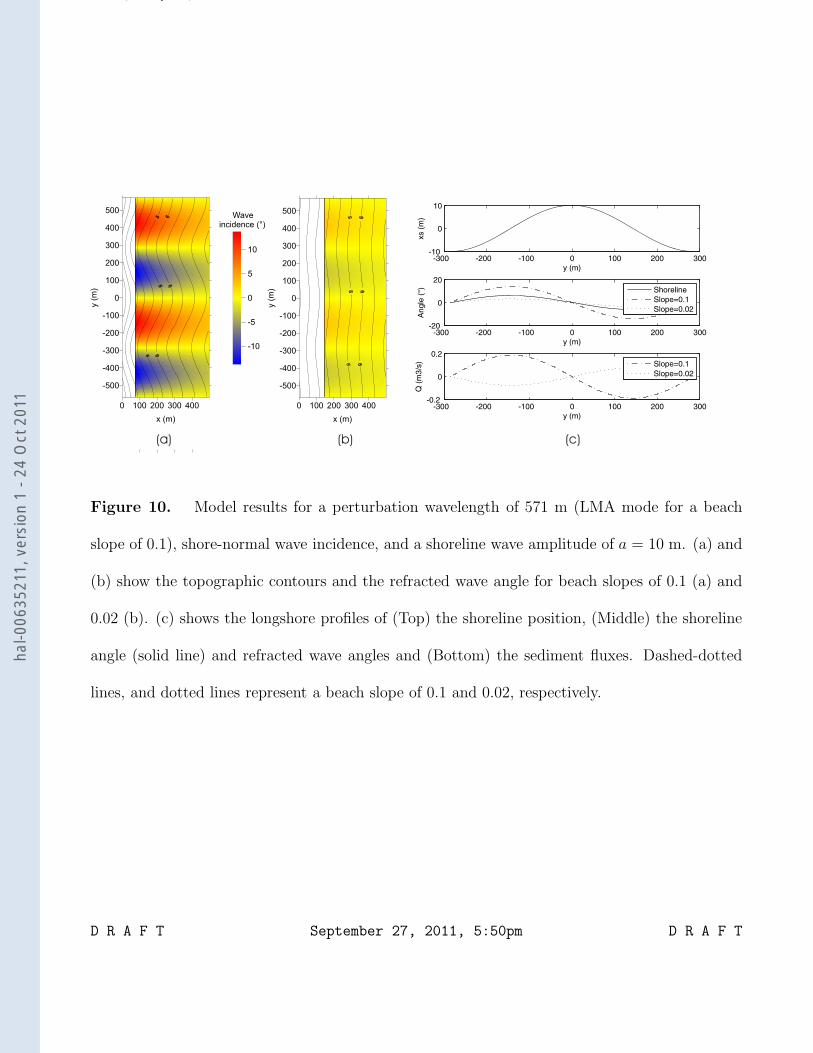
we assume shore-normal waves and r = 0. Figures 10a and b show planviews of the

Figures 10

358

wave angle, as well as a longshore cross-section of several quantities along the breaking359

line. First, it can be noted that the breaking line is much farther offshore in case (b)360

because of the shallower bathymetry. This is directly linked with the bathymetry. These361

planviews illustrate the wave focussing on the cusp, which implies increasing wave height362

and converging waves at the cusps.363

Looking at the alongshore cross-section (Figure 10c), the wave angle amplitude is much364

larger for case (a) than for case (b), about 14◦ versus 3.2◦, indicating a stronger refraction365

up to the breaking line in case (a). The corresponding amplitude of the oscillation in366

the shoreline angle is about 6.3◦, and is thus within the range of those two values. This367

means that the angle of the wave fronts with respect to the local shoreline reverses when368

passing from case (a) to (b), implying a reversal in the direction of sediment transport.369

This can be traced back to equation 6. The wave angle amplitude is much larger for case370

(a). Coming back to equation 6, in the case of shore-normal waves and r = 0, there are371

only two terms left: e1, which is the contribution due to shoreline change only, and e2,372

which represents the wave refraction-induced sediment flux. The analytical computation373

for the present case leads to: e1 = −1 for both cases, whereas e2 = 2.23 for case (a) and374

e2 = 0.507 (case b), consistent with the different amplitudes of alongshore wave angle375


hal-0

0635

211,

ver

sion

1 -

24 O

ct 2

011

, Q ,

oscillation. This clearly shows that the growth rate is positive for case (a) and negative376

for case (b). The alongshore cross-section of the resulting sediment flux Q (Figure 10c)377

illustrates the opposite behaviour for the two cases. Our sign convention is that positive378

Q represents sediment transport directed in the direction of the increasing y coordinate379

(i.e. to the right on the cross-sections). A positive (negative) longshore gradient indicates380

a convergence (divergence), assumed to cause shoreline accretion (erosion). Thus Figure381

10c shows that Q for case (a) has a spatial phase-lag compared to the shoreline such that382

the shoreline perturbation should be amplified, whereas Q for case (b) has an opposite383

phase-lag, leading to the damping of the perturbation. This spatial phase-lag change384

results from the continuous amplitude changes of the terms e1 and e2: the phase-lag385

between shoreline and longshore sediment fluxes is either 90◦ or −90◦, implying that386

there is no migration and either amplification or damping of the shoreline perturbation.387

Thus, for shore-normal waves and neglecting the damping term related with wave set-388

up induced sediment flux (second term in eq. 2), the instability of the shoreline results389

from an alongshore oscillation in the angle of wave refraction, which is stronger than the390

oscillation in the angle of shoreline orientation.391

4.3. Mechanism

From the above, we can draw the following conclusion: the main growing term is re-392

lated to the wave refraction toward the cusp, leading to wave incidence induced sediment393

transport converging at the cusp. This term strongly increases with beach slope. The394

damping is due to three components: (1) longshore sediment transport due to the shore-395

line orientation only (and not refraction, term e1), (2) wave energy spreading (term e3),396


hal-0

0635

211,

ver

sion

1 -

24 O

ct 2

011

, Q ,

and (3) wave height gradients (set-up) (term e4), the second component having a smaller397

damping effect than the two others.398

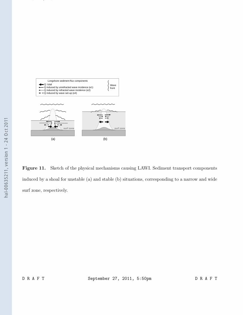
Now we can figure out how LAWI works (Figure 11). Let us consider shore-normal Figure 11399

wave incidence. In this case, the wave energy spreading has no influence on the instability400

(e3 = 0). If a cuspate feature with an associated shoal develops on a coastline, wave401

refraction bends wave rays towards the tip of the feature. Depending on the orientation402

of the refracted wave fronts with respect to the local shoreline along the cuspate feature,403

the alongshore sediment flux can be directed towards the tip, reinforcing it and leading to404

a positive feedback between flow and morphology. Whether the transport is directed to405

the tip, depends on the bathymetry and wave conditions. For a given offshore extent, xl,406

of the associated shoal and a given wave height, the surf zone will become narrower if the407

beach slope increases. Then, the shoal will extend a longer distance beyond the surf zone,408

and the waves will be refracted strongly when they reach the breaking point, increasing409

the wave incidence related sediment flux (e2) convergence whereas the divergence term410

(e1) is constant. As shown by the model results (Figure 10), the contribution of the411

refracted wave angle (e2) can exceed the contribution of the shoreline orientation to the412

sediment flux (e1), such that Q1 (resulting from e1 and e2) converges near the cusp. This413

leads to the development of the cusp. If the beach slope is mild, the surf zone will be414

wider, and wave refraction over the shoal before breaking will be less intense, leading to415

smaller wave incidence angle induced sediment fluxes, which are dominated instead by the416

diverging sediment flux induced by shoreline orientation changes. In this case, as shown417

in the model results (Figure 10c), the sediment flux is directed away from the tip of the418

cusp.419


hal-0

0635

211,

ver

sion

1 -

24 O

ct 2

011

, Q ,

5. Discussion

5.1. Linear stability analysis validity

The 1D-morfo model has been applied to investigate HAWI and to study the sandwaves420

generation along the Dutch coast [Falques , 2006], El Puntal beach - Spain [Medellın et al.,421

2008, 2009]. The results indicated similarities with the wavelengths observed in nature.422

This supports the use of this linear stability model to investigate the mechanisms of shore-423

line sandwave formation. In the present paper, it is clear that LAWI is a robust output424

of the 1D-morfo model, and the physical mechanism causing instabilities is wave refrac-425

tion induced by an offshore shoal associated with a cuspate feature. This wave refraction426

leads to two counter-acting phenomena: sediment transport induced by converging waves427

counteracted by diverging wave height gradients. The present paper investigates the lin-428

ear generation only. The pros and cons of linear stability analysis have been discussed429

extensively in [Blondeaux , 2001; Dodd et al., 2003; Falques et al., 2008; Tiessen et al.,430

2010]. In any case, the fundamental assumption of infinitesimal amplitude growth makes431

comparisons to field data questionable. Nonlinear model studies for other rhythmic fea-432

tures, such as crescentic sandbars and sand ridges [Calvete, 1999; Damgaard et al., 2002],433

have sometimes shown the finite-amplitude dynamics to be dominated by the LMA mode434

; in other cases, modes other than the LMA became dominant. We leave the nonlinear435

modeling of LAWI, including the study on cessation of the growth, to future work.436

5.2. Analogy with megacusps: growth rates and circulation patterns

Although the model results are given for a planar beach, LAWI is also found in the437

presence of a shore-parallel bar (not shown). Thus, for intermediate morphological beach438

state where crescentic bars and associated megacusp systems usually develop, the model439


hal-0

0635

211,

ver

sion

1 -

24 O

ct 2

011

, Q ,

predicts LAWI. To survive in the finite amplitude domain, the LAWI must grow at a440

rate comparable to that of co-existing instabilities. Our sensitivity studies indicate LAWI441

growth rates to range from 10−6s−1 (for a beach slope of 0.05) to 10−5s−1 (for a beach442

slope of 0.2). The typical generation time scale thus ranges from 1.5 to 11.5 days. These443

time scales were obtained for shore-normal waves having a moderate wave height of 1.5444

m and wave period of 8 s. A typical time scale for the LMA mode of crescentic bars is445

several days [Damgaard et al., 2002; Garnier et al., 2010]. Thus, for specific beach slope446

and wave conditions, the LMA shoreline instabilities have comparable initial growth rates447

as those of crescentic bar patterns.448

Computations for the idealized cases gives LAWI wavelengths of the same order of449

magnitude as the observed spacing of crescentic bars and associated megacusps. The450

distinction between these two kinds of instabilities is therefore difficult and the validation451

of the presence of LAWI in a Rhythmic Bar and Beach morphological environment is not452

straightforward. More generally, a proper validation of the present results would need453

dataset of shoreline evolution, together with bathymetric, wave and current data, starting454

from an initial longshore uniform beach. To our knowledge, such data do not exist.455

Although we cannot validate the model results with wavelengths observed in the field,456

it is possible to discuss whether the type of nearshore circulation linked to LAWI, that is,457

a longshore sediment flux pointing toward the cuspate feature at both sides, is realistic or458

not in nature and in the framework of 2DH modeling. According to Komar [1998], both459

types of longshore current patterns, either converging or diverging at a megacusp, are460

observed in nature. Another example showing that this type of circulation is realistic is461

the case of a submerged breakwater. Both observations and numerical modelling indicate462


hal-0

0635

211,

ver

sion

1 -

24 O

ct 2

011

, Q ,

that if the breakwater is beyond the breaker line, the waves drive longshore currents that463

converge at the lee of the breakwater to build a salient [Ranasinghe et al., 2006]. This464

converging type of circulation at a megacusp was also observed by Haller et al. [2002] in465

laboratory experiments on barred beaches with rip channels. One of their six experimental466

configurations may be quite close to a LAWI configuration. This configuration had the467

largest average water depth at the bar crest and the smallest rip velocity at the rip neck,468

such that, in addition to the rip current circulation, they found a secondary circulation469

system near the shoreline, likely forced by the breaking of the larger waves that propagated470

through the channel. As these waves are breaking close to the shoreline, they drove471

longshore currents away from the rip channels into the shallowest area. This experiment472

shows that breaking close to the shoreline counteracts the rip-induced circulation, leading473

to current convergence in the shallowest area.474

The studies of Calvete et al. [2005] and Orzech et al. [2011] give other elements to475

investigate the plausibility of the LAWI mechanism, in rip channels configurations. For476

the case of a barred-beach, Calvete et al. [2005] developed a 2DH linear stability model,477

having a fixed shoreline, that describes the formation of rip channels from an initially478

straight shore-parallel bar. For shore-normal waves, the circulation linked to rip channel479

formation is offshore through the channels and onshore over the shoals or horns of the480

developing crescentic bar as is clearly observed in nature (e.g. [MacMahan et al., 2006]).481

However, they also noticed small secondary circulation cells near the shoreline flowing in482

the opposite direction, leading to presence of megacusp formed in front of the horns of483

the crescentic bar; therefore, the shoreline undulations were out of phase (spatial phase-484

lag of 180◦) with the crescentic bars, meaning that the amplitude of the wave-refracted485


hal-0

0635

211,

ver

sion

1 -

24 O

ct 2

011

, Q ,

terms should dominate the amplitude of the wave set-up terms (Eq. 2). The formation of486

those megacusps was not part of the instability leading to the crescentic bar development487

but was forced by the hydrodynamics associated with it. More importantly, the small488

secondary circulation cells were essentially related to wave refraction: if wave refraction489

from the model was eliminated, they did not develop. Thus, wave refraction by offshore490

shoals (those of the crescentic bar in this case) can induce a circulation that may move491

sediment toward a developing cuspate feature. A recent study, based on both observation492

(video images) and non-linear morphodynamic modeling [Orzech et al., 2011] also showed493

the occurence of two types of megacusp (shoreward of the shoal or shoreward of the494

rip), and the associated converging sediment fluxes toward the megacusps. This tends to495

support our mechanism analysis of LAWI formation.496

The similarity between LAWI and megacusps in both wavelength and growth time497

is certainly intriguing given the fact that 1D-morfo is mainly based on the gradients498

in longshore sediment transport and wave set-up induced sediment transport (damping499

term), but neglects many surf zone processes like rip current circulation, which is known500

to be essential to crescentic bar dynamics [Calvete et al., 2005; Garnier et al., 2008].501

However, the analysis above tends to show that there could be configurations, where the502

processes taken into account in 1D-morfo are dominant in the system, at the initial stage.503

This could explain why similarities are observed with the various numerical experiments504

done with more sophisticated models. Furthermore, we should keep in mind the fact that505

the LAWI mechanism is not related to any longshore bar, and thus that short shoreline506

sandwaves such as megacusps could develop without a bar, whereas it was thought that,507

for barred beaches, short shoreline sandwaves develop due to surf zone sand bar variability.508


hal-0

0635

211,

ver

sion

1 -

24 O

ct 2

011

, Q ,

6. Conclusions

A one-line linear stability model, which was initially created to describe the formation of509

shoreline sandwaves under high-angle wave incidence, has revealed shoreline instabilities510

for low to shore-normal wave incidence (LAWI). The most amplified mode has wavelengths511

of ∼ 500 m and characteristic growth time scales of a few days, which are smaller than512

those of the high angle wave instabilities. Sensitivity analyses focusing on wave height,513

wave incidence angle, beach slope, beach profile, model free parameters and the sediment514

transport equation show that, for low to shore-normal wave incidence, instabilities develop515

for sufficiently large beach slopes (e.g. 0.06) and for sufficiently small wave heights (smaller516

than 2 m for a beach slope of 0.06).517

The main process causing the instabilities for low to shore-normal wave incidence is wave518

refraction on a shoal in the shoaling zone, which focuses wave fronts onshore of it, leading519

to wave incidence induced sediment transport converging at the cusp. This effect strongly520

increases with beach slope. The damping is due to three longshore transport components:521

(1) that caused by shoreline orientation only (and not refraction), (2) that caused by522

wave energy spreading (minor effect for low-angle wave incidence), (3) that caused by523

wave height gradients (set-up). Whether LAWI develops or not depends on the balance524

between these growing and damping terms. If this shoreline sand accumulation can feed525

the initial shoal through cross-shore sediment transport, a positive feedback arises.526

Acknowledgments. The authors thank the reviewers (including A. Ashton) for their527

comments and suggestions, D. Calvete for fruitful discussions, J. Thiebot for his comments528

on this paper. M. Yates-Michelin is also acknowledged for her careful English corrections.529

Funding from the ANR VMC 2006 - project VULSACO n◦ANR-06-VULN-009, the Span-530


hal-0

0635

211,

ver

sion

1 -

24 O

ct 2

011

, Q ,

ish Government (CTM2009-11892/IMNOBE project and TM2006-08875/MAR project),531

the Netherlands Organisation for Scientific Research (NWO) project 818.01.009, the Uni-532

versity of Nottingham and the Juan de la Cierva program are also acknowledged.533

References

Ashton, A., and A. B. Murray, High-angle wave instability and emergent shoreline534

shapes: 1. modeling of sand waves, flying spits, and capes, J.Geophys.Res., 111,535

F04,011,doi:10.1029/2005JF000,422, 2006a.536

Ashton, A., and A. B. Murray, High-angle wave instability and emergent shoreline537

shapes: 2. wave climate analysis and comparisons to nature, J.Geophys.Res., 111,538

F04,012,doi:10.1029/2005JF000,423, 2006b.539

Ashton, A., A. B. Murray, and O. Arnault, Formation of coastline features by large-scale540

instabilities induced by high-angle waves, Nature, 414, 296–300, 2001.541

Bender, C., and R. Dean, Potential shoreline changes induced by three-dimentional bathy-542

metric anomalies with gradual transitions in depth, Coast. Eng., 51, 1143–1161, 2004.543

Blondeaux, P., Mechanics of coastal forms, Ann. Rev. Fluid Mech., 33, 339–370, 2001.544

Bruun, P., Migrating sand waves or sand humps, with special reference to investigations545

carried out on the Danish North Sea Coast, in Coastal Eng. 1954, pp. 269–295, Am.546

Soc. of Civ. Eng., 1954.547

Calvete, D., Morphological stability models: Shoreface-connected sand ridges, Ph.D. the-548

sis, Appl. Physics Dept., Univ. Politecnica de Catalunya, Barcelona, Spain, 1999.549

Calvete, D., N. Dodd, A. Falques, and S. M. van Leeuwen, Morphological development550

of rip channel systems: Normal and near normal wave incidence, J. Geophys. Res.,551


hal-0

0635

211,

ver

sion

1 -

24 O

ct 2

011

, Q ,

110 (C10006), doi:10.1029/2004JC002803, 2005.552

Castelle, B., P. Bonneton, H. Dupuis, and N. Senechal, Double bar beach dynamics on553

the high-energy meso-macrotidal french aquitanian coast : a review, Mar. Geol., 245,554

141–159, 2007.555

Damgaard, J., N. Dodd, L. Hall, and T. Chesher, Morphodynamic modelling of rip channel556

growth, Coastal Eng., 45, 199–221, 2002.557

Davidson-Arnott, R. G. D., and A. van Heyningen, Migration and sedimentology of long-558

shore sandwaves, Long Point, Lake Erie, Canada, Sedimentology, 50, 1123–1137, 2003.559

Dean, R. G., and R. A. Dalrymple, Coastal Processes, Cambridge University Press, Cam-560

bridge, 2002.561

Dodd, N., P. Blondeaux, D. Calvete, H. E. de Swart, A. Falques, S. J. M. H. Hulscher,562

G. Rozynski, and G. Vittori, The use of stability methods in understanding the mor-563

phodynamical behavior of coastal systems, J. Coastal Res., 19 (4), 849–865, 2003.564

Falques, A., Wave driven alongshore sediment transport and stability of the Dutch coast-565

line, Coastal Eng., 53, 243–254, 2006.566

Falques, A., and D. Calvete, Large scale dynamics of sandy coastlines. Diffusivity and567

instability, J. Geophys. Res., 110 (C03007), doi:10.1029/2004JC002587, 2005.568

Falques, A., G. Coco, and D. A. Huntley, A mechanism for the generation of wave-driven569

rhythmic patterns in the surf zone, J. Geophys. Res., 105 (C10), 24,071–24,088, 2000.570

Falques, A., N. Dodd, R. Garnier, F. Ribas, L. MacHardy, P. Larroud, D. Calvete, and571

F. Sancho, Rhythmic surf zone bars and morphodynamic self-organization, Coastal Eng.,572

55, 622–641, doi:10.1016/j.coastaleng.2007.11.012, 2008.573


hal-0

0635

211,

ver

sion

1 -

24 O

ct 2

011

, Q ,

Garnier, R., D. Calvete, A. Falques, and M. Caballeria, Generation and nonlinear evolu-574

tion of shore-oblique/transverse sand bars, J. Fluid Mech., 567, 327–360, 2006.575

Garnier, R., D. Calvete, A. Falques, and N. Dodd, Modelling the formation and the576

long-term behavior of rip channel systems from the deformation of a longshore bar, J.577

Geophys. Res., 113 (C07053), doi:10.1029/2007JC004632, 2008.578

Garnier, R., N. Dodd, A. Falques, and D. Calvete, Mechanisms controlling crescentic bar579

amplitude, J. Geophys. Res., 115, doi:10.1029/2009JF001407, 2010.580

Haller, M. C., R. A. Dalrymple, and I. A. Svendsen, Experimental study of581

nearshore dynamics on a barred beach with rip channels, J. Geophys. Res., 107 (C6),582

10.1029/2001JC000,955, 2002.583

Horikawa, K., Nearshore Dynamics and Coastal Processes, University of Tokio Press,584

Tokio, Japan, 1988.585

Inman, D. L., M. H. S. Elwany, A. A. Khafagy, and A. Golik, Nile delta profiles and586

migrating sand blankets, in Coastal Eng. 1992, pp. 3273–3284, Am. Soc. of Civ. Eng.,587

1992.588

Komar, P. D., Beach Processes and Sedimentation, second ed., Prentice Hall, Englewood589

Cliffs, N.J., 1998.590

Lafon, V., D. D. M. Apoluceno, H. Dupuis, D. Michel, H. Howa, and J. M. Froidefond,591

Morphodynamics of nearshore rhythmic sandbars in a mixed-energy environment (SW592

France): I. Mapping beach changes using visible satellite imagery, Estuarine, Coastal593

and Shelf Science, 61, 289–299, 2004.594

List, J. H., and A. D. Ashton, A circulation modeling approach for evaluating the condi-595

tions for shoreline instabilities, in Coastal Sediments 2007, pp. 327–340, ASCE, 2007.596


hal-0

0635

211,

ver

sion

1 -

24 O

ct 2

011

, Q ,

List, J. H., D. M. Hanes, and P. Ruggiero, Predicting longshore gradients in alongshore597

transport: comparing the cerc formula to delft3d, in Coastal Eng. 2006, pp. 3370–3380,598

World Scientific, 2006.599

List, J. H., L. Benedet, D. M. Hanes, and P. Ruggiero, Understanding differences between600

delft3d and emperical predictions of alongshore sediment transport gradients, in Coastal601

Eng. 2008, pp. 1864–1875, World Scientific, 2008.602

MacMahan, J. H., E. B. Thornton, and A. J. H. M. Reniers, Rip current review, Coastal603

Eng., 53, 191–208, 2006.604

Medellın, G., R. Medina, A. Falques, and M. Gonzalez, Coastline sand waves on a low605

energy beach at ’El Puntal’ spit, Spain, Mar. Geol., 250, 143–156, 2008.606

Medellın, G., A. Falques, R. Medina, and M. Gonzalez, Sand waves on a low-energy beach607

at el ’puntal’ spit, Spain: Linear Stability Analysis, J. Geophys. Res., 114 (C03022),608

doi:10.1029/2007JC004426, 2009.609

Orzech, M., A. Reniers, E. Thornton, and J. MacMahan, Megacusps on610

rip channel bathymetry: Observations and modeling, Coastal Eng., p.611

doi:10.1016/j.coastaleng.2011.05.001, 2011.612

Ozasa, H., and A. H. Brampton, Mathematical modelling of beaches backed by seawalls,613

Coastal Eng., 4, 47–63, 1980.614

Ranasinghe, R., G. Symonds, K. Black, and R. Holman, Morphodynamics of intermediate615

beaches: A video imaging and numerical modelling study, Coastal Eng., 51, 629–655,616

2004.617

Ranasinghe, R., I. L. Turner, and G. Symonds, Shoreline response to multi-functional618

artificial surfing reefs: A numerical and physical modelling study, Coastal Eng., 53,619


hal-0

0635

211,

ver

sion

1 -

24 O

ct 2

011

, Q ,

589–611, 2006.620

Reniers, A. J. H. M., J. A. Roelvink, and E. B. Thornton, Morphodynamic model-621

ing of an embayed beach under wave group forcing, J. Geophys. Res., 109 (C01030),622

doi:10.1029/2002JC001586, 2004.623

Ribas, F., and A. Kroon, Characteristics and dynamics of surfzone transverse finger bars,624

J. Geophys. Res., 112 (F03028), doi:10.1029/2006JF000685, 2007.625

Ruessink, B. G., and M. C. J. L. Jeuken, Dunefoot dynamics along the dutch coast, Earth626

Surface Processes and Landforms, 27, 1043–1056, 2002.627

Sonu, C. J., Collective movement of sediment in littoral environment, in Coastal Eng.628

1968, pp. 373–400, Am. Soc. of Civ. Eng., 1968.629

Sonu, C. J., Three-dimensional beach changes, J. Geology, 81, 42–64, 1973.630

Stewart, C. J., and R. G. D. Davidson-Arnott, Morphology, formation and migration of631

longshore sandwaves; long point, lake erie, canada, Mar. Geol., 81, 63–77, 1988.632

Thevenot, M. M., and N. C. Kraus, Longshore sandwaves at Southampton Beach, New633

York: observations and numerical simulation of their movement, Mar. Geology, 126,634

249–269, 1995.635

Tiessen, M. C. H., S. M. V. Leeuwen, D. Calvete, and N. Dodd, A field test of a linear636

stability model for crescentic bars, Coastal Engineering, 57, 41–51, 2010.637

USACE, Shore protection manual, Tech. Rep. 4th ed., 2 Vol., USACE, U.S. Government638

Printing Office, Washington, D.C., 1984.639

van den Berg, N., A. Falques, and R. Ribas, Long-term evolution of nourished beaches640

under high angle wave conditions, Journal of Marine Systems, to appear, 2011.641

Verhagen, H. J., Sand waves along the dutch coast, Coastal Eng., 13, 129–147, 1989.642


hal-0

0635

211,

ver

sion

1 -

24 O

ct 2

011

, Q ,

Wright, L. D., and A. D. Short, Morphodynamic variability of surf zones and beaches: A643

synthesis, Mar. Geol., 56, 93–118, 1984.644

x

y

xs(y,t)

waves

Figure 1. Sketch of the geometry and the variables. The angle between the wave fronts and

the local shoreline is α = θ − φ.


hal-0

0635

211,

ver

sion

1 -

24 O

ct 2

011

, Q ,

(a) (b) (c)

0

0,002

0,004

0,006

0,008

0,01

0,012

0 500 1000 1500x (m)

zpert

urb

ation

(m)

P1

P2

P3

P4

-25

-20

-15

-10

-5

0

0 500 1000 1500 2000

x (m)

z(m

)

slope=0,02

slope=0,04

slope=0,1

slope=0,2

-2

-1,8

-1,6

-1,4

-1,2

-1

-0,8

-0,6

-0,4

-0,2

0

0 20 40x (m)

z(m

)

slope=0,02

slope=0,04

slope=0,1

slope=0,2

Figure 2. Bathymetric perturbations (a) and cross-shore Dean beach profile for a various

beach slopes (b,c). P1-perturbation: constant in the surf zone and exponential decrease, P2-

perturbation: exponential decrease, P3-perturbation: exponential decrease with a shoal in the

shoaling zone, P4-perturbation: exponential decrease with a shoal in the surf and shoaling zones.

(a) (b)

Growth rate (1/s) Wavelength (m)

Figure 3. LMA (a) growth rate and (b) wavelength as a function of beach slope and angle of

incidence. Circles indicate the 1D-morfo computations. In white: no growing perturbation. The

model parameters are : μ = 0.15, r = 1, P1-Perturbation and xl=1410 m for Dean profiles with

Hrms = 1.5 m and Tp = 8 s at a water depth of 25 m.


hal-0

0635

211,

ver

sion

1 -

24 O

ct 2

011

, Q ,

(a) (b)


Figure 4. LMA (a) growth rate and (b) wavelength as a function of beach slope and wave

height, for shore-normal waves. Circles indicate the 1D-morfo computations. In white: no

growing perturbation. The model parameters are : μ = 0.15, r = 1, P1-Perturbation and

xl=1410 m for Dean profiles with θ = 0◦ and Tp = 8 s at a water depth of 25 m.

0

200

400

600

800

1000

1200

1 10 100 1000 10000

xl (m)

Wa

ve

len

gth

(m)

0,0E+00

2,0E-07

4,0E-07

6,0E-07

8,0E-07

1,0E-06

1,2E-06

1,4E-06

1,6E-06

1,8E-06

2,0E-06

1 10 100 1000 10000

xl (m)

Gro

wth

rate

(1/s

)

(a) (b)

Figure 5. LMA mode (a) growth rate and (b) wavelength as a function of the shoreline

perturbation length xl for a Dean profile with a beach slope of 0.1. Crosses on the xl axis

(10 ≤ xl ≤ 100) indicate that there is no LMA mode for the given shoreline perturbation length.


hal-0

0635

211,

ver

sion

1 -

24 O

ct 2

011

, Q ,


(a) (b)

Figure 6. LMA (a) growth rate and (b) wavelength as function of beach slope and wave angle,

for r = 0. Circles indicate the 1D-morfo computations. In white: no LMA mode. The symbol x

indicates that, even if the growth rate was positive, there was a singularity at θ = 0◦ (growth rate

continuously increasing with decreasing wavelength), and therefore no LMA mode (see Figure

7).


hal-0

0635

211,

ver

sion

1 -

24 O

ct 2

011

, Q ,

1E-09

1E-08

1E-07

1E-06

1E-05

1E-04

1E-03

0 2000 4000 6000 8000 10000Wavelength (m)

Gro

wth

rate

(1/s

)

Beta=0.05Beta=0.06Beta=0.08Beta=0.1Beta=0.12Beta=0.14Beta=0.16Beta=0.18Beta=0.2

Figure 7. LMA growth rate versus wavelength for various beach slopes, using r = 0 and

shore-normal waves. The shoreline is stable for a beach slope β < 0.05. The model parameters

are : μ = 0.15, P1-Perturbation and xl=1410 m for the Dean profile with Hrms = 1.5 m and

Tp = 8 s at a water depth of 25 m.


hal-0

0635

211,

ver

sion

1 -

24 O

ct 2

011

, Q ,

(a) (b)

(c) (d)

Figure 8. Growth rate components for the LMA mode as a function of beach slope and angle

of incidence. Model paremeters are: Hrms = 1.5 m, Tp = 8 s and cross-shore perturbation of type

P1 with xl = 1410 m. (a) σ1, (b) σ2, (c) σ3, (d) σ4. Circles indicate the 1D-morfo computations.

In white: no LMA mode.


hal-0

0635

211,

ver

sion

1 -

24 O

ct 2

011

, Q ,

0,0E+00

2,0E-08

4,0E-08

6,0E-08

8,0E-08

1,0E-07

1,2E-07

1,4E-07

0 1000 2000 3000 4000 5000

Gro

wth

rate

(1/s

)

Wavelength (m)

(r,theta)=(0,10°)(r,theta)=(0,20°)(r,theta)=(0,40°)(r,theta)=(0,60°)(r,theta)=(1,10°)(r,theta)=(1,20°)(r,theta)=(1,40°)(r,theta)=(1,60°)

Figure 9. Growth rate versus wavelength for several combinations of r and wave incidence

angle θ. The beach slope is 0.05.


hal-0

0635

211,

ver

sion

1 -

24 O

ct 2

011

, Q ,

(a) (b)

0 100 200 300 400

x (m)

-500

-400

-300

-200

-100

0

100

200

300

400

500

y(m

)

-10

-5

0

5

10

Waveincidence (°)

0 100 200 300 400

x (m)

-500

-400

-300

-200

-100

0

100

200

300

400

500

y(m

)

(c)

Figure 10. Model results for a perturbation wavelength of 571 m (LMA mode for a beach

slope of 0.1), shore-normal wave incidence, and a shoreline wave amplitude of a = 10 m. (a) and

(b) show the topographic contours and the refracted wave angle for beach slopes of 0.1 (a) and

0.02 (b). (c) shows the longshore profiles of (Top) the shoreline position, (Middle) the shoreline

angle (solid line) and refracted wave angles and (Bottom) the sediment fluxes. Dashed-dotted

lines, and dotted lines represent a beach slope of 0.1 and 0.02, respectively.


hal-0

0635

211,

ver

sion

1 -

24 O

ct 2

011

, Q ,

surf zone surf zone

(a) (b)

Q: totalQ induced by unrefracted wave incidence (e1)Q induced by refracted wave incidence (e2)Q induced by wave set-up (e4)

Longshore sediment flux components

Wave front

Figure 11. Sketch of the physical mechanisms causing LAWI. Sediment transport components

induced by a shoal for unstable (a) and stable (b) situations, corresponding to a narrow and wide

surf zone, respectively.


hal-0

0635

211,

ver

sion

1 -

24 O

ct 2

011

shoreline instability under low-angle wave incidence

Documents