shao, 2008 - geophysical sciences
TRANSCRIPT


Physics and Modelling of Wind Erosion

ATMOSPHERIC AND OCEANOGRAPHIC SCIENCES LIBRARYVOLUME 3
Editors
Lawrence A. Mysak, Department of Atmospheric and Oceanographic Sciences,McGill University, Montreal, Canada
Kevin Hamilton, International Pacific Research Center, University of Hawaii,Honolulu, HI, U.S.A.
Editorial Advisory Board
L. Bengtsson Max-Planck-Institut für Meteorologie, Hamburg, GermanyA. Berger Université Catholique, Louvain, BelgiumJ.R. Garratt CSIRO, Aspendale, Victoria, AustraliaG. Geernaert DMU-FOLU, Roskilde, DenmarkJ. Hansen MIT, Cambridge, MA, U.S.A.M. Hantel Universität Wien, AustriaH. Kelder KNMI (Royal Netherlands Meteorological Institute),
De Bilt, The NetherlandsT.N. Krishnamurti The Florida State University, Tallahassee, FL, U.S.A.P. Lemke Alfred-Wegener-Institute for Polar and Marine Research,
Bremerhaven, GermanyP. Malanotte-Rizzoli MIT, Cambridge, MA, U.S.A.D. Randall Colorado State University, Fort Collins, CO, U.S.A.J.-L. Redelsperger METEO-FRANCE, Centre National de Recherches
Météorologiques, Toulouse, FranceA. Robock Rutgers University, New Brunswick, NJ, U.S.A.S.H. Schneider Stanford University, CA, U.S.A.G.E. Swaters University of Alberta, Edmonton, CanadaJ.C. Wyngaard Pennsylvania State University, University Park, PA, U.S.A.
7
Fwor other titles published in this seires, go toww.springer.com/series/5669
Physics and Modelling of Wind Erosion
Y aping ShaoUniversity of Cologne, Germany
by
ABC

Dr. Yaping Shao
ISBN 978-1-4020-88 - e-ISBN 978-1-4020-88 -
Library of Congress Control Number: 2008932207
All Rights Reservedc© 2008 Springer Science + Business Media B.V.
No part of this work may be reproduced, stored in a retrieval system, or transmitted in any form or byany means, electronic, mechanical, photocopying, microfilming, recording or otherwise, without writtenpermission from the Publisher, with the exception of any material supplied specifically for the purposeof being entered and executed on a computer system, for exclusive use by the purchaser of the work.
Printed on acid-free paper
9 8 7 6 5 4 3 2 1
springer.com
University of [email protected]
94 0 95 7
Preface 1
Wind erosion occurs in many arid, semiarid and agricultural areas of theworld. It is an environmental process influenced by geological and climaticvariations as well as human activities. In general, wind erosion leads to landdegradation in agricultural areas and has a negative impact on air quality.Dust emission generated by wind erosion is the largest source of aerosols whichdirectly or indirectly influence the atmospheric radiation balance and henceglobal climatic variations. Strong wind-erosion events, such as severe duststorms, may threaten human lives and cause substantial economic damage.
The physics of wind erosion is complex, as it involves atmospheric, soiland land-surface processes. The research on wind erosion is multidisciplinary,covering meteorology, fluid dynamics, soil physics, colloidal science, surfacesoil hydrology, ecology, etc. Several excellent books have already been writtenabout the topic, for instance, by Bagnold (1941, The Physics of Blown Sandand Desert Dunes), Greeley and Iversen (1985, Wind as a Geological Pro-cess on Earth, Mars, Venus and Titan), Pye (1987, Aeolian Dust and DustDeposits), Pye and Tsoar (1990, Aeolian Sand and Sand Dunes). However,considerable progress has been made in wind-erosion research in recent yearsand there is a need to systematically document this progress in a new book.There are three other reasons which motivated me to write this book. Firstly,in most existing books, there is a general lack of rigor in the description ofwind-erosion dynamics; secondly, the emphasis of the existing books appearsto be placed primarily on sand-particle motion, while topics related to themodelling of dust entrainment, transport and deposition have not been pre-sented in great detail and thirdly, the results presented in the existing booksappear to be mainly experimental and lacking in documentation of the com-putational modelling effort involved.
My intention is to provide a summary of the existing knowledge of winderosion and recent progress in that research field. The basic contents of thebook include the physics of particle entrainment, transport and depositionand the environmental processes that control wind erosion. It is intended totreat the physics of wind erosion as rigorously as possible, from the viewpoint
v
vi Preface 1
of fluid dynamics and soil physics. A considerable proportion of the bookis devoted to the computational modelling of wind erosion. I hope that thisbook can be used as a reference point for both wind-erosion researchers andpostgraduate students. My basic consideration is that wind erosion can onlybe understood from a multidisciplinary viewpoint and the computationalmodelling of wind erosion should focus on the development of integrated sim-ulation systems. Such a system should tightly couple dynamic models, suchas atmospheric prediction models and wind-erosion schemes, with real datathat characterises soil and surface conditions. In the introductory chapter ofthe book, this basic concept is reiterated, while in Chapter 9 examples of theadvocated modelling approach are given. Chapter 2 provides a summary ofwind-erosion climatology in the world and selected regions. Chapters 3 and4 are devoted to the description of atmospheric modelling and land-surfacemodelling, as these are the prerequisite for the modelling of wind erosion.Chapter 5 is a description of the basic aspects of wind-erosion theory, whileChapters 6, 7 and 8 are dedicated to the entrainment, transport and depo-sition of sand and dust particles. In Chapter 9, the integrated wind-erosionmodelling system and the data requirement are described. The concludingremarks are given in Chapter 12.
Cologne, Germany Yaping ShaoNovember 1999
Preface 2
Since the publication of the first edition of this book in 1999, much progresshas been made in the field of wind-erosion research, especially on dust. Thisis mainly due to the strong interests in understanding the impacts of mineralaerosol on climate change and the role of dust in bio-geochemistry. In thisedition, I have updated the contents of the book to reflect the new develop-ments and corrected the mistakes known to me in the first edition. I have alsoimproved the text and the illustrations.
Many colleagues have helped with the preparation of this edition. Inparticular, I wish to thank Drs Masao Mikami, Irina Sokolik, Karl-HeinzWyrwoll, Qingcun Zeng, Gongbing Peng, Chaohua Dong, Zhaohui Lin,Masaru Chiba, Naoko Seino, Taichu Y. Tanaka, Masahide Ishizuka, EunjooJung and Youngsin Chun for their support. I also wish to thank Ms. DagmarJansen for her careful proofreading of the manuscript and Ms. Martina Klosefor helping with the manuscript preparation using LaTeX.
Cologne, Germany Yaping ShaoMarch 2008
vii
Acknowledgements
About 10 years ago, Dr. M. R. Raupach introduced me to the research ofwind erosion. I have ever since maintained a strong interest in this field.During these years, I came to know many colleagues, including ProfessorL. M. Leslie, Dr. J. F. Leys, Dr. G. H. McTainsh, Mr. P. A. Findlater,Professor W. G. Nickling, Dr. D. A. Gillette, Professor H. Nagashima,Dr. B. Marticorena, Dr. G. Bergametti and Dr. I. Tegen among manyothers, who helped me to develop a understanding of the topics presentedin this book. I am grateful to them for the valuable discussions and argu-ments during the years and to many of them for providing me with theirresearch results for inclusion in this book. In the wind-erosion research com-munity, there prevails truly a collaborative spirit. The development of theintegrated wind-erosion modelling system described in Chapter 9 has beena team effort, and I acknowledge explicitly the significant contributions tothe project made by my colleagues and friends, especially, Dr. H. Lu, Dr.P. Irannejad, Dr. R. K. Munro, Dr. C. Werner and Mr. R. Morison. The as-sistance of Dr. P. Irannejad and Mr. H. X. Zhuang in preparing the graphsand the manuscript has been very helpful. The painstaking final correctionsby Dr. R. A. Byron-Scott have resulted in improvements to a text whichhas been written uncomfortably in my second language. Several chapters ofthe book were drafted during my stay at the Institute for Geophysics andMeteorology, University of Cologne, in 1999 when I was an Alexander vonHumboldt Research Fellow. My stay in Germany has been a happy one, and Ithank Professor Dr. M. Kerschgens and the Humboldt Foundation for makingthat possible. My thanks also go to Dr. M. de Jong from Kluwer AcademicPublishers for her enthusiastic and patient approach toward publishing thisbook. Finally, I would like to take this opportunity to express my gratitudeto Professor P. Schwerdtfeger, Dr. J. M. Hacker and Dr. T. H. Chen for theircontinuous encouragements throughout my scientific career.
ix
Contents
Preface 1 . . . . . . . . . . . . . . . . . . . . . . . . . . . . . . . . . . . . . . . . . . . . . . . . . . . . . . v
Preface 2 . . . . . . . . . . . . . . . . . . . . . . . . . . . . . . . . . . . . . . . . . . . . . . . . . . . . . . vii
Acknowledgements . . . . . . . . . . . . . . . . . . . . . . . . . . . . . . . . . . . . . . . . . . . . ix
1 Wind Erosion and Wind-Erosion Research . . . . . . . . . . . . . . . . . 11.1 Wind-Erosion Phenomenon . . . . . . . . . . . . . . . . . . . . . . . . . . . . . . . 11.2 Wind-Erosion Research . . . . . . . . . . . . . . . . . . . . . . . . . . . . . . . . . . 71.3 Integrated Wind-Erosion Modelling . . . . . . . . . . . . . . . . . . . . . . . . 9
2 Wind-Erosion Climatology . . . . . . . . . . . . . . . . . . . . . . . . . . . . . . . . . 132.1 Climatic Background for Wind Erosion . . . . . . . . . . . . . . . . . . . . . 132.2 Geographic Background for Wind Erosion . . . . . . . . . . . . . . . . . . 182.3 Atmospheric Systems . . . . . . . . . . . . . . . . . . . . . . . . . . . . . . . . . . . . 20
2.3.1 Monsoon Winds . . . . . . . . . . . . . . . . . . . . . . . . . . . . . . . . . . . 212.3.2 Cyclones and Frontal Systems . . . . . . . . . . . . . . . . . . . . . . . 232.3.3 Squall Lines . . . . . . . . . . . . . . . . . . . . . . . . . . . . . . . . . . . . . . 24
2.4 Global Wind-Erosion Patterns . . . . . . . . . . . . . . . . . . . . . . . . . . . . 262.5 Major Wind-Erosion Regions . . . . . . . . . . . . . . . . . . . . . . . . . . . . . 29
2.5.1 Dust Weather Records and Satellite RemoteSensing . . . . . . . . . . . . . . . . . . . . . . . . . . . . . . . . . . . . . . . . . . 29
2.5.2 North Africa . . . . . . . . . . . . . . . . . . . . . . . . . . . . . . . . . . . . . . 302.5.3 The Middle East . . . . . . . . . . . . . . . . . . . . . . . . . . . . . . . . . . 342.5.4 Central Asia . . . . . . . . . . . . . . . . . . . . . . . . . . . . . . . . . . . . . . 362.5.5 Southwest Asia . . . . . . . . . . . . . . . . . . . . . . . . . . . . . . . . . . . 372.5.6 Northeast Asia . . . . . . . . . . . . . . . . . . . . . . . . . . . . . . . . . . . . 392.5.7 The United States . . . . . . . . . . . . . . . . . . . . . . . . . . . . . . . . . 442.5.8 Australia . . . . . . . . . . . . . . . . . . . . . . . . . . . . . . . . . . . . . . . . . 45
xi
xii Contents
3 Atmospheric Boundary Layer and AtmosphericModelling . . . . . . . . . . . . . . . . . . . . . . . . . . . . . . . . . . . . . . . . . . . . . . . . . 493.1 Atmospheric Boundary Layer . . . . . . . . . . . . . . . . . . . . . . . . . . . . . 493.2 Governing Equations for Atmospheric Boundary-Layer Flows . 523.3 Reynolds Averaging and Turbulent Flux . . . . . . . . . . . . . . . . . . . . 563.4 Equations for Mean Flows . . . . . . . . . . . . . . . . . . . . . . . . . . . . . . . . 593.5 Equations for Turbulent Fluxes and Variances . . . . . . . . . . . . . . . 60
3.5.1 Turbulent Dust Flux and Dust ConcentrationVariance . . . . . . . . . . . . . . . . . . . . . . . . . . . . . . . . . . . . . . . . . 60
3.5.2 Turbulent Kinetic Energy . . . . . . . . . . . . . . . . . . . . . . . . . . 613.5.3 Features of Different Atmospheric Boundary Layers . . . . 63
3.6 Surface Layer . . . . . . . . . . . . . . . . . . . . . . . . . . . . . . . . . . . . . . . . . . . 673.6.1 Flux-Gradient Relationship . . . . . . . . . . . . . . . . . . . . . . . . . 673.6.2 Friction Velocity . . . . . . . . . . . . . . . . . . . . . . . . . . . . . . . . . . 683.6.3 Logarithmic Wind Profile and Roughness Length . . . . . . 713.6.4 Stability Measures . . . . . . . . . . . . . . . . . . . . . . . . . . . . . . . . . 72
3.7 Similarity Theories . . . . . . . . . . . . . . . . . . . . . . . . . . . . . . . . . . . . . . 743.7.1 Monin–Obukhov Similarity Theory . . . . . . . . . . . . . . . . . . 753.7.2 Mixed–Layer Similarity Theory . . . . . . . . . . . . . . . . . . . . . 78
3.8 Turbulent Flow Models . . . . . . . . . . . . . . . . . . . . . . . . . . . . . . . . . . . 793.9 Meso-scale, Regional and Global Atmospheric Models . . . . . . . . 85
4 Land-Surface Modelling . . . . . . . . . . . . . . . . . . . . . . . . . . . . . . . . . . . 914.1 General Aspects . . . . . . . . . . . . . . . . . . . . . . . . . . . . . . . . . . . . . . . . . 924.2 Surface Energy Balance . . . . . . . . . . . . . . . . . . . . . . . . . . . . . . . . . . 944.3 Soil Moisture . . . . . . . . . . . . . . . . . . . . . . . . . . . . . . . . . . . . . . . . . . . 964.4 Soil Temperature . . . . . . . . . . . . . . . . . . . . . . . . . . . . . . . . . . . . . . . . 1014.5 Calculation of Surface Fluxes . . . . . . . . . . . . . . . . . . . . . . . . . . . . . 1014.6 Land-Surface Parameters . . . . . . . . . . . . . . . . . . . . . . . . . . . . . . . . . 1064.7 Examples of Land-Surface Simulation . . . . . . . . . . . . . . . . . . . . . . 1104.8 Treatment of Heterogeneous Surfaces . . . . . . . . . . . . . . . . . . . . . . 112
5 Basic Aspects of Wind Erosion . . . . . . . . . . . . . . . . . . . . . . . . . . . . 1175.1 Soil-Particle Characteristics . . . . . . . . . . . . . . . . . . . . . . . . . . . . . . . 1175.2 Forces on an Airborne Particle . . . . . . . . . . . . . . . . . . . . . . . . . . . . 1245.3 Particle Terminal Velocity . . . . . . . . . . . . . . . . . . . . . . . . . . . . . . . . 1295.4 Modes of Particle Motion . . . . . . . . . . . . . . . . . . . . . . . . . . . . . . . . . 1315.5 Threshold Friction Velocity for Sand Particles . . . . . . . . . . . . . . . 134
5.5.1 The Bagnold Scheme . . . . . . . . . . . . . . . . . . . . . . . . . . . . . . 1355.5.2 The Greeley-Iversen Scheme . . . . . . . . . . . . . . . . . . . . . . . . 1385.5.3 The Shao–Lu Scheme and the McKenna Neuman
Scheme . . . . . . . . . . . . . . . . . . . . . . . . . . . . . . . . . . . . . . . . . . 1395.6 Threshold Friction Velocity for Dust Particles . . . . . . . . . . . . . . . 142
5.6.1 Relative Importance of Forces . . . . . . . . . . . . . . . . . . . . . . . 1425.6.2 Stochastic Nature of Threshold Friction Velocity . . . . . . 145
Contents xiii
6 The Dynamics and Modelling of Saltation . . . . . . . . . . . . . . . . . 1496.1 Equations of Particle Motion . . . . . . . . . . . . . . . . . . . . . . . . . . . . . . 1506.2 Uniform Saltation . . . . . . . . . . . . . . . . . . . . . . . . . . . . . . . . . . . . . . . 1526.3 Non-Uniform Saltation . . . . . . . . . . . . . . . . . . . . . . . . . . . . . . . . . . . 1546.4 Streamwise Saltation Flux . . . . . . . . . . . . . . . . . . . . . . . . . . . . . . . . 1566.5 The Bagnold-Owen Saltation Equation . . . . . . . . . . . . . . . . . . . . . 157
6.5.1 The Bagnold Model . . . . . . . . . . . . . . . . . . . . . . . . . . . . . . . 1576.5.2 The Owen Model . . . . . . . . . . . . . . . . . . . . . . . . . . . . . . . . . . 158
6.6 Other Saltation Equations . . . . . . . . . . . . . . . . . . . . . . . . . . . . . . . . 1636.7 The Owen Effect . . . . . . . . . . . . . . . . . . . . . . . . . . . . . . . . . . . . . . . . 165
6.7.1 The Formulation of Owen . . . . . . . . . . . . . . . . . . . . . . . . . . 1656.7.2 The Formulation of Raupach . . . . . . . . . . . . . . . . . . . . . . . . 1666.7.3 Other Formulations . . . . . . . . . . . . . . . . . . . . . . . . . . . . . . . . 1716.7.4 Profile of Saltation Flux . . . . . . . . . . . . . . . . . . . . . . . . . . . . 171
6.8 Independent Saltation . . . . . . . . . . . . . . . . . . . . . . . . . . . . . . . . . . . . 1726.9 Supply-Limited Saltation . . . . . . . . . . . . . . . . . . . . . . . . . . . . . . . . . 1756.10 Evolution of Streamwise Sand Transport with Distance . . . . . . . 1766.11 Splash Entrainment . . . . . . . . . . . . . . . . . . . . . . . . . . . . . . . . . . . . . . 178
6.11.1 Wind-Tunnel Observations . . . . . . . . . . . . . . . . . . . . . . . . . 1786.11.2 Numerical Simulations . . . . . . . . . . . . . . . . . . . . . . . . . . . . . 179
6.12 Numerical Modelling of Saltation . . . . . . . . . . . . . . . . . . . . . . . . . . 1866.12.1 Simple Flow Model . . . . . . . . . . . . . . . . . . . . . . . . . . . . . . . . 1866.12.2 Large-Eddy Simulation Model . . . . . . . . . . . . . . . . . . . . . . . 1876.12.3 Particle Motion . . . . . . . . . . . . . . . . . . . . . . . . . . . . . . . . . . . 1886.12.4 Aerodynamic Entrainment . . . . . . . . . . . . . . . . . . . . . . . . . . 1906.12.5 Splash Scheme . . . . . . . . . . . . . . . . . . . . . . . . . . . . . . . . . . . . 191
6.13 Understanding of Saltation from NumericalSimulations . . . . . . . . . . . . . . . . . . . . . . . . . . . . . . . . . . . . . . . . . . . . . 1946.13.1 Importance of Splash Entrainment . . . . . . . . . . . . . . . . . . . 1946.13.2 Particle-Momentum Flux, Saltation Flux
and Roughness Length . . . . . . . . . . . . . . . . . . . . . . . . . . . . . 1976.14 Saltation in Turbulence . . . . . . . . . . . . . . . . . . . . . . . . . . . . . . . . . . 199
6.14.1 Intermittency of Saltation . . . . . . . . . . . . . . . . . . . . . . . . . . 2016.14.2 Aeolian Streamers . . . . . . . . . . . . . . . . . . . . . . . . . . . . . . . . . 2056.14.3 Dynamical Similarity of Saltation . . . . . . . . . . . . . . . . . . . 206
7 Dust Emission . . . . . . . . . . . . . . . . . . . . . . . . . . . . . . . . . . . . . . . . . . . . . 2117.1 Dust Flux and Friction Velocity . . . . . . . . . . . . . . . . . . . . . . . . . . . 2117.2 Mechanisms for Dust Emission . . . . . . . . . . . . . . . . . . . . . . . . . . . . 2167.3 Aerodynamic Dust Entrainment . . . . . . . . . . . . . . . . . . . . . . . . . . . 2227.4 Energy-Based Dust-Emission Scheme . . . . . . . . . . . . . . . . . . . . . . 2227.5 Volume-Removal-Based Dust-Emission Scheme . . . . . . . . . . . . . . 226
7.5.1 Motion of Ploughing Particle and VolumeRemoval . . . . . . . . . . . . . . . . . . . . . . . . . . . . . . . . . . . . . . . . . 230
7.5.2 Vertical Dust Flux . . . . . . . . . . . . . . . . . . . . . . . . . . . . . . . . . 232
xiv Contents
7.6 Comparison of Dust Schemes . . . . . . . . . . . . . . . . . . . . . . . . . . . . . 2337.7 Spectral Dust-Emission Scheme . . . . . . . . . . . . . . . . . . . . . . . . . . . 2357.8 Discussions on Dust Schemes . . . . . . . . . . . . . . . . . . . . . . . . . . . . . 245
8 Dust Transport and Deposition . . . . . . . . . . . . . . . . . . . . . . . . . . . . 2478.1 Evidence of Dust Transport and Deposition . . . . . . . . . . . . . . . . . 2478.2 Lagrangian Dust-Transport Model . . . . . . . . . . . . . . . . . . . . . . . . . 2528.3 Eulerian Dust-Transport Model . . . . . . . . . . . . . . . . . . . . . . . . . . . 2558.4 Vertical Dust Transport by Diffusion . . . . . . . . . . . . . . . . . . . . . . . 2618.5 Vertical Dust Transport by Convection . . . . . . . . . . . . . . . . . . . . . 273
8.5.1 Convective Adjustment . . . . . . . . . . . . . . . . . . . . . . . . . . . . 2738.5.2 Cumulus Parameterisation . . . . . . . . . . . . . . . . . . . . . . . . . . 275
8.6 Dry Deposition . . . . . . . . . . . . . . . . . . . . . . . . . . . . . . . . . . . . . . . . . . 2778.6.1 Two-Layer Dry-Deposition Model: Smooth
Surface . . . . . . . . . . . . . . . . . . . . . . . . . . . . . . . . . . . . . . . . . . . 2788.6.2 Two-Layer Dry-Deposition Model:
Vegetation . . . . . . . . . . . . . . . . . . . . . . . . . . . . . . . . . . . . . . . . 2828.6.3 Single-Layer Dry-Deposition Model . . . . . . . . . . . . . . . . . . 286
8.7 Wet Deposition . . . . . . . . . . . . . . . . . . . . . . . . . . . . . . . . . . . . . . . . . 2888.7.1 The Theory of Slinn . . . . . . . . . . . . . . . . . . . . . . . . . . . . . . . 2898.7.2 Scavenging Rate . . . . . . . . . . . . . . . . . . . . . . . . . . . . . . . . . . 2958.7.3 Scavenging Ratio . . . . . . . . . . . . . . . . . . . . . . . . . . . . . . . . . . 299
9 Integrated Wind-Erosion Modelling . . . . . . . . . . . . . . . . . . . . . . . 3039.1 System Structure . . . . . . . . . . . . . . . . . . . . . . . . . . . . . . . . . . . . . . . . 3049.2 Wind-Erosion Parameterisation Scheme . . . . . . . . . . . . . . . . . . . . 3079.3 Threshold Friction Velocity for Natural Surfaces . . . . . . . . . . . . . 308
9.3.1 Drag Partition: Approach I . . . . . . . . . . . . . . . . . . . . . . . . . 3109.3.2 Drag Partition: Approach II . . . . . . . . . . . . . . . . . . . . . . . . 3169.3.3 Relationship of λ and z0 . . . . . . . . . . . . . . . . . . . . . . . . . . . 3179.3.4 Double Drag Partition . . . . . . . . . . . . . . . . . . . . . . . . . . . . . 3219.3.5 Soil Moisture . . . . . . . . . . . . . . . . . . . . . . . . . . . . . . . . . . . . . 3239.3.6 Chemical Binding and Crust . . . . . . . . . . . . . . . . . . . . . . . . 327
9.4 Sand Drift and Dust Emission of Soils with MultipleParticle Sizes . . . . . . . . . . . . . . . . . . . . . . . . . . . . . . . . . . . . . . . . . . . 328
9.5 Climatic Constraints on Dust Emission . . . . . . . . . . . . . . . . . . . . . 3339.5.1 Erodibility Derived from Synoptic Data . . . . . . . . . . . . . . 3339.5.2 Erodibility Derived from Satellite Data . . . . . . . . . . . . . . . 3369.5.3 Wind-Erosion Hot Spots . . . . . . . . . . . . . . . . . . . . . . . . . . . 336
9.6 Land-Surface Parameters . . . . . . . . . . . . . . . . . . . . . . . . . . . . . . . . . 3369.6.1 Soil Particle-Size Distribution . . . . . . . . . . . . . . . . . . . . . . . 3379.6.2 Soil-Binding Strength . . . . . . . . . . . . . . . . . . . . . . . . . . . . . . 3429.6.3 Frontal-Area Index . . . . . . . . . . . . . . . . . . . . . . . . . . . . . . . . 3449.6.4 Soil Moisture . . . . . . . . . . . . . . . . . . . . . . . . . . . . . . . . . . . . . 347
9.7 Manipulation of GIS Data . . . . . . . . . . . . . . . . . . . . . . . . . . . . . . . . 347
Contents xv
9.8 Examples of Integrated Wind-Erosion Modelling . . . . . . . . . . . . . 3509.8.1 Wind-Erosion Time Series . . . . . . . . . . . . . . . . . . . . . . . . . . 3509.8.2 Wind-Erosion Predictions on Global, Regional
and Local Scales . . . . . . . . . . . . . . . . . . . . . . . . . . . . . . . . . . 3519.9 Data Assimilation . . . . . . . . . . . . . . . . . . . . . . . . . . . . . . . . . . . . . . . 359
10 Sand Dunes, Dynamics and Modelling . . . . . . . . . . . . . . . . . . . . . 36110.1 Classification of Sand Dunes . . . . . . . . . . . . . . . . . . . . . . . . . . . . . . 36310.2 Migration Speed of Transverse Dunes . . . . . . . . . . . . . . . . . . . . . . 37010.3 Basic Features of Flow over a Sand Dune . . . . . . . . . . . . . . . . . . . 37310.4 Sand Transport . . . . . . . . . . . . . . . . . . . . . . . . . . . . . . . . . . . . . . . . . 37710.5 Computational Fluid Dynamic Simulation . . . . . . . . . . . . . . . . . . 381
10.5.1 Flow-Model Implementation: Non-hydrostatic Model . . . 38210.5.2 Flow-Model Implementation: Large-Eddy Model . . . . . . . 38410.5.3 Computation of Erosion and Deposition Rates . . . . . . . . 385
10.6 Discrete Lattice Simulation . . . . . . . . . . . . . . . . . . . . . . . . . . . . . . . 388
11 Techniques for Wind-Erosion Measurements . . . . . . . . . . . . . . . 39111.1 Wind-Tunnel Measurements . . . . . . . . . . . . . . . . . . . . . . . . . . . . . . 39111.2 Sand Measurements . . . . . . . . . . . . . . . . . . . . . . . . . . . . . . . . . . . . . . 393
11.2.1 Passive Samplers . . . . . . . . . . . . . . . . . . . . . . . . . . . . . . . . . . 39311.2.2 Active Samplers . . . . . . . . . . . . . . . . . . . . . . . . . . . . . . . . . . . 39611.2.3 Impact Sensors: Sensit, Saltiphone and Safire . . . . . . . . . 39711.2.4 Sand Particle Counter . . . . . . . . . . . . . . . . . . . . . . . . . . . . . 399
11.3 Dust Measurements . . . . . . . . . . . . . . . . . . . . . . . . . . . . . . . . . . . . . . 40011.3.1 High- and Low-Volume Air Samplers . . . . . . . . . . . . . . . . . 40011.3.2 Optical Particle Counter . . . . . . . . . . . . . . . . . . . . . . . . . . . 402
11.4 Deposition Collectors . . . . . . . . . . . . . . . . . . . . . . . . . . . . . . . . . . . . 40311.5 Field Measurements . . . . . . . . . . . . . . . . . . . . . . . . . . . . . . . . . . . . . 40411.6 Particle-Size Analysis . . . . . . . . . . . . . . . . . . . . . . . . . . . . . . . . . . . . 407
11.6.1 Dry Sieving . . . . . . . . . . . . . . . . . . . . . . . . . . . . . . . . . . . . . . . 40711.6.2 Settling Tube and Elutriator . . . . . . . . . . . . . . . . . . . . . . . . 40811.6.3 Electro-Sensing Methods . . . . . . . . . . . . . . . . . . . . . . . . . . . 41011.6.4 Laser Granulometry . . . . . . . . . . . . . . . . . . . . . . . . . . . . . . . 412
11.7 Abrasion Emitter . . . . . . . . . . . . . . . . . . . . . . . . . . . . . . . . . . . . . . . . 412
12 Concluding Remarks . . . . . . . . . . . . . . . . . . . . . . . . . . . . . . . . . . . . . . 41512.1 Current Research Topics . . . . . . . . . . . . . . . . . . . . . . . . . . . . . . . . . 41512.2 Dust Cycle in the Earth System . . . . . . . . . . . . . . . . . . . . . . . . . . . 419
References . . . . . . . . . . . . . . . . . . . . . . . . . . . . . . . . . . . . . . . . . . . . . . . . . . . . . 421
Index . . . . . . . . . . . . . . . . . . . . . . . . . . . . . . . . . . . . . . . . . . . . . . . . . . . . . . . . . . 447
1
Wind Erosion and Wind-Erosion Research
1.1 Wind-Erosion Phenomenon
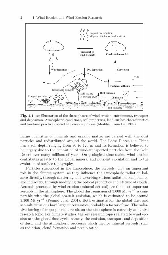
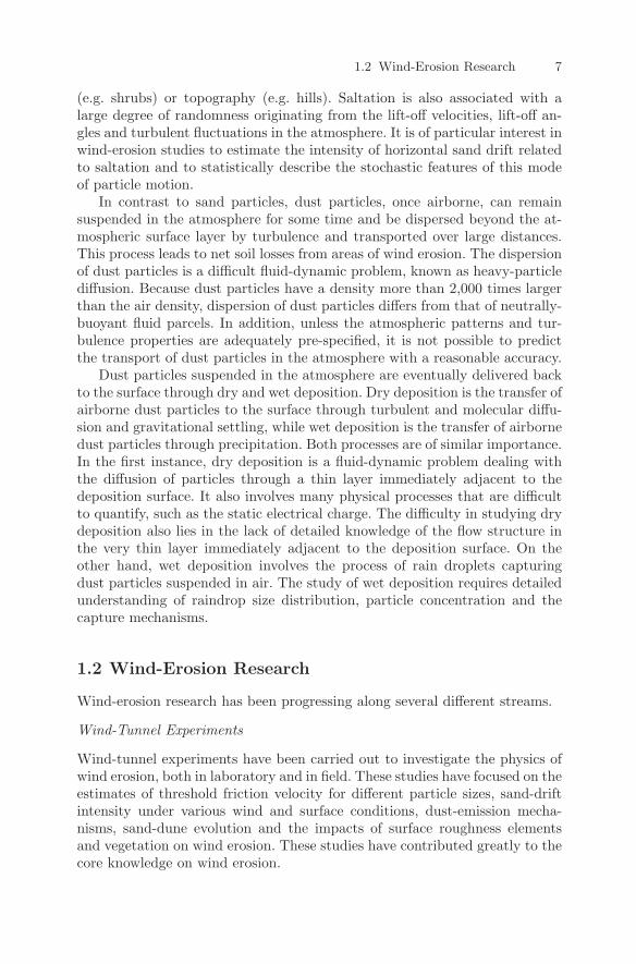
Wind erosion is a process of wind-forced movement of soil particles. This pro-cess has the distinct phases of particle entrainment, transport and deposition(Fig. 1.1). It is a complex process because it is affected by many factors whichinclude atmospheric conditions (e.g. wind, precipitation and temperature), soilproperties (e.g. soil texture, composition and aggregation), land-surface char-acteristics (e.g. topography, moisture, aerodynamic roughness length, vegeta-tion and non-erodible elements) and land-use practice (e.g. farming, grazingand mining). During a wind-erosion event, these factors interact with eachother and, as erosion progresses, the properties of the eroded surface can besignificantly modified.
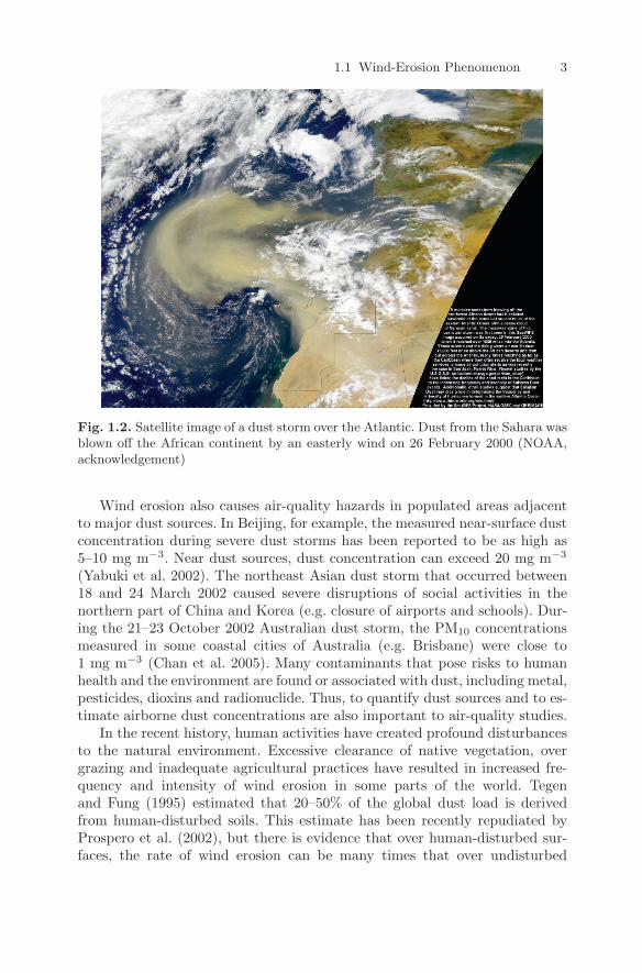
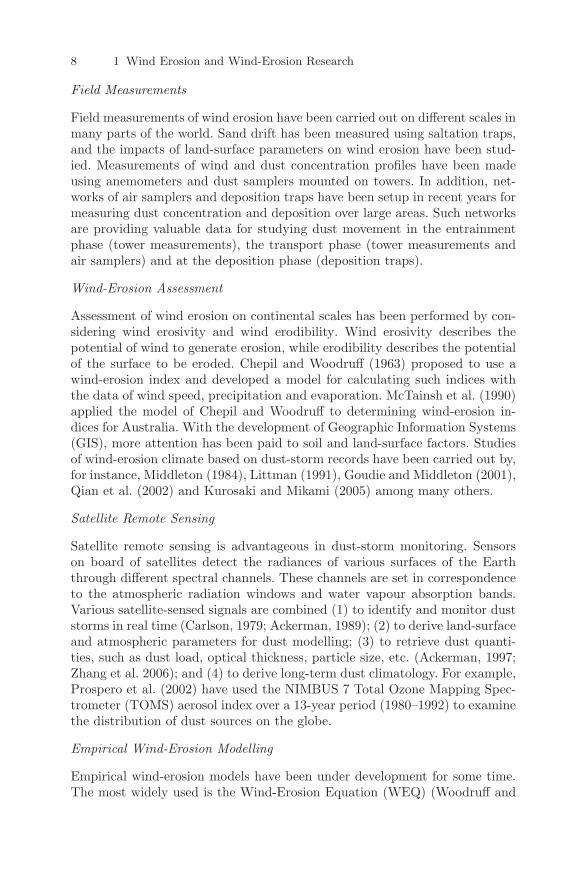
In the first instance, wind erosion is a geological and climatic phenomenonwhich takes place over long periods of time in deserts and arid regions. Most ofthe time, wind-erosion events proceed unnoticed but sometimes they are mostspectacular. Figure 1.2 shows the satellite image of a massive dust storm overthe Atlantic on 26 February 2000. During this event, dust from the SaharaDesert was lifted to up to 5,000 m above ground and blown off the African con-tinent by an easterly wind. Dust storms of this magnitude have been observedelsewhere in the world, for instance in the Middle East, China and Australia(Figs. 1.3, 2.4). Between 15 and 19 April 1998, severe dust storms developedover the Gobi Desert in Mongolia and China. In the following days, the dust-storm front moved across China and, by April 20, the elongated dusty beltcovered a 2,000-km stretch of the east coast of China. The dust clouds weremoving across the Pacific on 23 and 24 April and arrived in North Americaby 27 April (Husar et al. 2001).
Wind erosion is the main mechanism for the formation and evolution ofsand seas in the world and the long-range transport of sediments from conti-nent to ocean. Recent studies suggest that the global dust emission amounts to3,000 Mt yr−1 (estimates vary between 1,000 and 10,000 Mt yr−1), and a con-siderable proportion of this dust is deposited in the ocean (Duce et al. 1991).
Y. Shao, Physics and Modelling of Wind Erosion, 1c© Springer Science+Business Media B.V. 2008
2 1 Wind Erosion and Wind-Erosion Research
Wind
Soil moisture
Condensation nuclei
Dry deposition
Transport bywind & clouds
Wet deposition
Saltation
Impact on radiation(Optical thickness, backscatter)
Roughness elements
Trapped particlesSoil texture& surface crust
Dust emission
Turbulent diffusion
Convection
Fig. 1.1. An illustration of the three phases of wind erosion: entrainment, transportand deposition. Atmospheric conditions, soil properties, land-surface characteristicsand land-use practice control the erosion process (Modified from Lu, 1999)
Large quantities of minerals and organic matter are carried with the dustparticles and redistributed around the world. The Loess Plateau in Chinahas a soil depth ranging from 30 to 120 m and its formation is believed tobe largely due to the deposition of wind-transported particles from the GobiDesert over many millions of years. On geological time scales, wind erosioncontributes greatly to the global mineral and nutrient circulation and to theevolution of surface topography.
Particles suspended in the atmosphere, the aerosols, play an importantrole in the climate system, as they influence the atmospheric radiation bal-ance directly, through scattering and absorbing various radiation components,and indirectly, through modifying the optical properties and lifetime of clouds.Aerosols generated by wind erosion (mineral aerosol) are the most importantaerosols in the atmosphere. The global dust emission of 3,000 Mt yr−1 is com-parable with the global sea-salt emission, which is estimated to be around3,300 Mt yr−1 (Penner et al. 2001). Both estimates for the global dust andsea-salt emissions have large uncertainties, probably a factor of two. The radia-tive forcing of tropospheric aerosols on the atmosphere is currently an activeresearch topic. For climate studies, the key research topics related to wind ero-sion are the global dust cycle, namely, the emission, transport and depositionof dust, and the atmospheric processes which involve mineral aerosols, suchas radiation, cloud formation and precipitation.
1.1 Wind-Erosion Phenomenon 3
Fig. 1.2. Satellite image of a dust storm over the Atlantic. Dust from the Sahara wasblown off the African continent by an easterly wind on 26 February 2000 (NOAA,acknowledgement)
Wind erosion also causes air-quality hazards in populated areas adjacentto major dust sources. In Beijing, for example, the measured near-surface dustconcentration during severe dust storms has been reported to be as high as5–10 mg m−3. Near dust sources, dust concentration can exceed 20 mg m−3
(Yabuki et al. 2002). The northeast Asian dust storm that occurred between18 and 24 March 2002 caused severe disruptions of social activities in thenorthern part of China and Korea (e.g. closure of airports and schools). Dur-ing the 21–23 October 2002 Australian dust storm, the PM10 concentrationsmeasured in some coastal cities of Australia (e.g. Brisbane) were close to1 mg m−3 (Chan et al. 2005). Many contaminants that pose risks to humanhealth and the environment are found or associated with dust, including metal,pesticides, dioxins and radionuclide. Thus, to quantify dust sources and to es-timate airborne dust concentrations are also important to air-quality studies.
In the recent history, human activities have created profound disturbancesto the natural environment. Excessive clearance of native vegetation, overgrazing and inadequate agricultural practices have resulted in increased fre-quency and intensity of wind erosion in some parts of the world. Tegenand Fung (1995) estimated that 20–50% of the global dust load is derivedfrom human-disturbed soils. This estimate has been recently repudiated byProspero et al. (2002), but there is evidence that over human-disturbed sur-faces, the rate of wind erosion can be many times that over undisturbed
4 1 Wind Erosion and Wind-Erosion Research
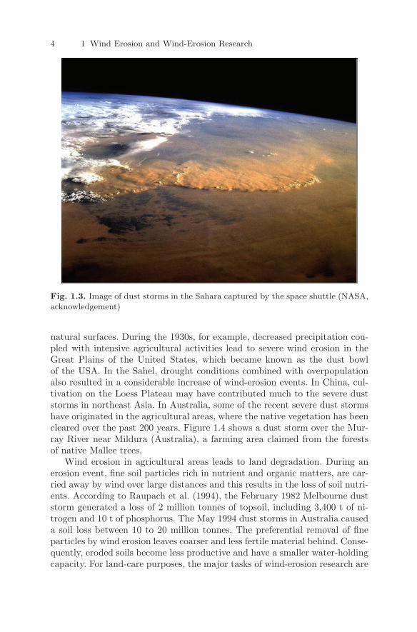
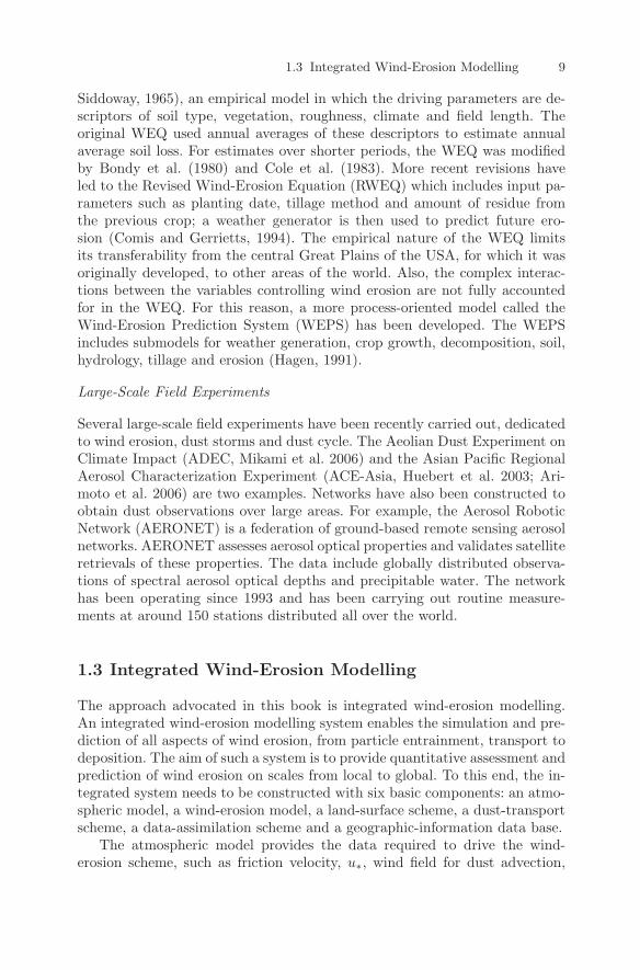
Fig. 1.3. Image of dust storms in the Sahara captured by the space shuttle (NASA,acknowledgement)
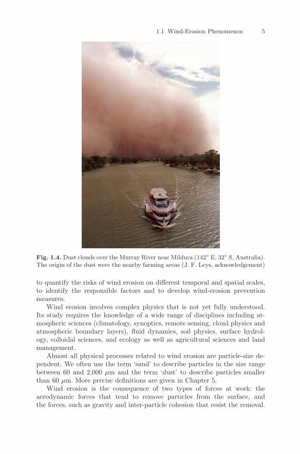
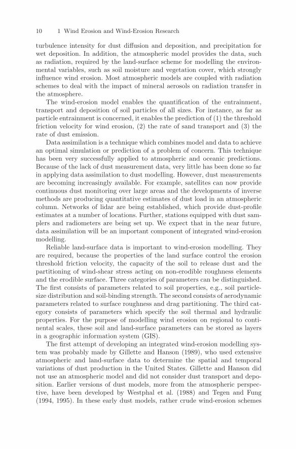
natural surfaces. During the 1930s, for example, decreased precipitation cou-pled with intensive agricultural activities lead to severe wind erosion in theGreat Plains of the United States, which became known as the dust bowlof the USA. In the Sahel, drought conditions combined with overpopulationalso resulted in a considerable increase of wind-erosion events. In China, cul-tivation on the Loess Plateau may have contributed much to the severe duststorms in northeast Asia. In Australia, some of the recent severe dust stormshave originated in the agricultural areas, where the native vegetation has beencleared over the past 200 years. Figure 1.4 shows a dust storm over the Mur-ray River near Mildura (Australia), a farming area claimed from the forestsof native Mallee trees.
Wind erosion in agricultural areas leads to land degradation. During anerosion event, fine soil particles rich in nutrient and organic matters, are car-ried away by wind over large distances and this results in the loss of soil nutri-ents. According to Raupach et al. (1994), the February 1982 Melbourne duststorm generated a loss of 2 million tonnes of topsoil, including 3,400 t of ni-trogen and 10 t of phosphorus. The May 1994 dust storms in Australia causeda soil loss between 10 to 20 million tonnes. The preferential removal of fineparticles by wind erosion leaves coarser and less fertile material behind. Conse-quently, eroded soils become less productive and have a smaller water-holdingcapacity. For land-care purposes, the major tasks of wind-erosion research are
1.1 Wind-Erosion Phenomenon 5
Fig. 1.4. Dust clouds over the Murray River near Mildura (142 E, 32 S, Australia).The origin of the dust were the nearby farming areas (J. F. Leys, acknowledgement)
to quantify the risks of wind erosion on different temporal and spatial scales,to identify the responsible factors and to develop wind-erosion preventionmeasures.
Wind erosion involves complex physics that is not yet fully understood.Its study requires the knowledge of a wide range of disciplines including at-mospheric sciences (climatology, synoptics, remote sensing, cloud physics andatmospheric boundary layers), fluid dynamics, soil physics, surface hydrol-ogy, colloidal sciences, and ecology as well as agricultural sciences and landmanagement.
Almost all physical processes related to wind erosion are particle-size de-pendent. We often use the term ‘sand’ to describe particles in the size rangebetween 60 and 2,000 µm and the term ‘dust’ to describe particles smallerthan 60 µm. More precise definitions are given in Chapter 5.
Wind erosion is the consequence of two types of forces at work: theaerodynamic forces that tend to remove particles from the surface, andthe forces, such as gravity and inter-particle cohesion that resist the removal.
6 1 Wind Erosion and Wind-Erosion Research
The former can be quantified by the friction velocity, u∗, a measure of windshear at the surface, and the latter by the threshold friction velocity, u∗t,which defines the minimum friction velocity required for wind erosion to oc-cur. While u∗ is related to atmospheric flow conditions and surface aerody-namic properties, u∗t is related to a range of surface properties, such as soiltexture, soil moisture and vegetation cover. For dry and bare sandy soil sur-faces, u∗t is small, and therefore it is not surprising that wind erosion occursmainly under such conditions. The balance between u∗ and u∗t is governedby, and is sensitive to, a number of environmental factors, namely, (1) weather(wind, temperature, rainfall, etc.); (2) soil type (soil texture, hydraulic proper-ties, etc.); (3) soil state (wetness, compactness, aggregation, etc.); (4) surfacemicroscopic conditions (aerodynamic roughness length, vegetation coverage,etc.) and (5) surface macroscopic conditions (landforms, windbreaks, etc.). Asa consequence, wind erosion is strongly variable in space and intermittent intime. The sporadic nature of wind-erosion events makes the modelling andprediction of wind erosion, even in a qualitative sense, a formidable task.
For soil particles to become airborne, lift forces associated with wind shearnear the surface or caused by particle impacts must overcome the gravitationaland cohesive forces acting upon them. We call the entrainment of particlesaerodynamic entrainment if it is dominated by aerodynamic forces, and re-fer to it as splash or bombardment entrainment if it is mainly caused bythe impact of other moving particles. In either situation, the forces involvedin the entrainment process vary strongly from case to case, depending on arange of factors, but in particular on particle size. Consequently, the domi-nant mechanism for particle entrainment also depends on particle size. Forsand particles, the entrainment is essentially aerodynamic, while for dust par-ticles the entrainment is primarily due to the impact of saltating sand grains,a phenomenon known as saltation bombardment (Gillette et al. 1982; Shaoet al. 1993b).
The motion of airborne particles in the atmosphere has two modes, knownas saltation and suspension. Saltation refers to the small hopping motion ofsand-sized particles in the direction of the wind, while suspension refers tothe floating motion of dust-sized particles in the atmosphere.
Through saltation, soil particles are transported in the direction of windduring an erosion event. Saltation is the mechanism for the evolution of sandseas on regional scales and the development of sand dunes and fence-line driftson local scales. It is an interesting dynamic problem which involves the in-teractions between the fluid phase, the particulate phase and the surface. Asparticles saltate through the atmospheric surface layer with a strong windshear, they absorb momentum from the airflow and generate a momentumtransport in the vertical direction. During the impact on the surface, thesaltating particles may splash more particles into the atmosphere. The de-position of saltating particles is of great significance to the evolution of theland surface. Particles in saltation may be deposited as wind speed reducesdue to changes in atmospheric conditions or changes in surface roughness
1.2 Wind-Erosion Research 7
(e.g. shrubs) or topography (e.g. hills). Saltation is also associated with alarge degree of randomness originating from the lift-off velocities, lift-off an-gles and turbulent fluctuations in the atmosphere. It is of particular interest inwind-erosion studies to estimate the intensity of horizontal sand drift relatedto saltation and to statistically describe the stochastic features of this modeof particle motion.
In contrast to sand particles, dust particles, once airborne, can remainsuspended in the atmosphere for some time and be dispersed beyond the at-mospheric surface layer by turbulence and transported over large distances.This process leads to net soil losses from areas of wind erosion. The dispersionof dust particles is a difficult fluid-dynamic problem, known as heavy-particlediffusion. Because dust particles have a density more than 2,000 times largerthan the air density, dispersion of dust particles differs from that of neutrally-buoyant fluid parcels. In addition, unless the atmospheric patterns and tur-bulence properties are adequately pre-specified, it is not possible to predictthe transport of dust particles in the atmosphere with a reasonable accuracy.
Dust particles suspended in the atmosphere are eventually delivered backto the surface through dry and wet deposition. Dry deposition is the transfer ofairborne dust particles to the surface through turbulent and molecular diffu-sion and gravitational settling, while wet deposition is the transfer of airbornedust particles through precipitation. Both processes are of similar importance.In the first instance, dry deposition is a fluid-dynamic problem dealing withthe diffusion of particles through a thin layer immediately adjacent to thedeposition surface. It also involves many physical processes that are difficultto quantify, such as the static electrical charge. The difficulty in studying drydeposition also lies in the lack of detailed knowledge of the flow structure inthe very thin layer immediately adjacent to the deposition surface. On theother hand, wet deposition involves the process of rain droplets capturingdust particles suspended in air. The study of wet deposition requires detailedunderstanding of raindrop size distribution, particle concentration and thecapture mechanisms.
1.2 Wind-Erosion Research
Wind-erosion research has been progressing along several different streams.
Wind-Tunnel Experiments
Wind-tunnel experiments have been carried out to investigate the physics ofwind erosion, both in laboratory and in field. These studies have focused on theestimates of threshold friction velocity for different particle sizes, sand-driftintensity under various wind and surface conditions, dust-emission mecha-nisms, sand-dune evolution and the impacts of surface roughness elementsand vegetation on wind erosion. These studies have contributed greatly to thecore knowledge on wind erosion.
8 1 Wind Erosion and Wind-Erosion Research
Field Measurements
Field measurements of wind erosion have been carried out on different scales inmany parts of the world. Sand drift has been measured using saltation traps,and the impacts of land-surface parameters on wind erosion have been stud-ied. Measurements of wind and dust concentration profiles have been madeusing anemometers and dust samplers mounted on towers. In addition, net-works of air samplers and deposition traps have been setup in recent years formeasuring dust concentration and deposition over large areas. Such networksare providing valuable data for studying dust movement in the entrainmentphase (tower measurements), the transport phase (tower measurements andair samplers) and at the deposition phase (deposition traps).
Wind-Erosion Assessment
Assessment of wind erosion on continental scales has been performed by con-sidering wind erosivity and wind erodibility. Wind erosivity describes thepotential of wind to generate erosion, while erodibility describes the potentialof the surface to be eroded. Chepil and Woodruff (1963) proposed to use awind-erosion index and developed a model for calculating such indices withthe data of wind speed, precipitation and evaporation. McTainsh et al. (1990)applied the model of Chepil and Woodruff to determining wind-erosion in-dices for Australia. With the development of Geographic Information Systems(GIS), more attention has been paid to soil and land-surface factors. Studiesof wind-erosion climate based on dust-storm records have been carried out by,for instance, Middleton (1984), Littman (1991), Goudie and Middleton (2001),Qian et al. (2002) and Kurosaki and Mikami (2005) among many others.
Satellite Remote Sensing
Satellite remote sensing is advantageous in dust-storm monitoring. Sensorson board of satellites detect the radiances of various surfaces of the Earththrough different spectral channels. These channels are set in correspondenceto the atmospheric radiation windows and water vapour absorption bands.Various satellite-sensed signals are combined (1) to identify and monitor duststorms in real time (Carlson, 1979; Ackerman, 1989); (2) to derive land-surfaceand atmospheric parameters for dust modelling; (3) to retrieve dust quanti-ties, such as dust load, optical thickness, particle size, etc. (Ackerman, 1997;Zhang et al. 2006); and (4) to derive long-term dust climatology. For example,Prospero et al. (2002) have used the NIMBUS 7 Total Ozone Mapping Spec-trometer (TOMS) aerosol index over a 13-year period (1980–1992) to examinethe distribution of dust sources on the globe.
Empirical Wind-Erosion Modelling
Empirical wind-erosion models have been under development for some time.The most widely used is the Wind-Erosion Equation (WEQ) (Woodruff and
1.3 Integrated Wind-Erosion Modelling 9
Siddoway, 1965), an empirical model in which the driving parameters are de-scriptors of soil type, vegetation, roughness, climate and field length. Theoriginal WEQ used annual averages of these descriptors to estimate annualaverage soil loss. For estimates over shorter periods, the WEQ was modifiedby Bondy et al. (1980) and Cole et al. (1983). More recent revisions haveled to the Revised Wind-Erosion Equation (RWEQ) which includes input pa-rameters such as planting date, tillage method and amount of residue fromthe previous crop; a weather generator is then used to predict future ero-sion (Comis and Gerrietts, 1994). The empirical nature of the WEQ limitsits transferability from the central Great Plains of the USA, for which it wasoriginally developed, to other areas of the world. Also, the complex interac-tions between the variables controlling wind erosion are not fully accountedfor in the WEQ. For this reason, a more process-oriented model called theWind-Erosion Prediction System (WEPS) has been developed. The WEPSincludes submodels for weather generation, crop growth, decomposition, soil,hydrology, tillage and erosion (Hagen, 1991).
Large-Scale Field Experiments
Several large-scale field experiments have been recently carried out, dedicatedto wind erosion, dust storms and dust cycle. The Aeolian Dust Experiment onClimate Impact (ADEC, Mikami et al. 2006) and the Asian Pacific RegionalAerosol Characterization Experiment (ACE-Asia, Huebert et al. 2003; Ari-moto et al. 2006) are two examples. Networks have also been constructed toobtain dust observations over large areas. For example, the Aerosol RoboticNetwork (AERONET) is a federation of ground-based remote sensing aerosolnetworks. AERONET assesses aerosol optical properties and validates satelliteretrievals of these properties. The data include globally distributed observa-tions of spectral aerosol optical depths and precipitable water. The networkhas been operating since 1993 and has been carrying out routine measure-ments at around 150 stations distributed all over the world.
1.3 Integrated Wind-Erosion Modelling
The approach advocated in this book is integrated wind-erosion modelling.An integrated wind-erosion modelling system enables the simulation and pre-diction of all aspects of wind erosion, from particle entrainment, transport todeposition. The aim of such a system is to provide quantitative assessment andprediction of wind erosion on scales from local to global. To this end, the in-tegrated system needs to be constructed with six basic components: an atmo-spheric model, a wind-erosion model, a land-surface scheme, a dust-transportscheme, a data-assimilation scheme and a geographic-information data base.
The atmospheric model provides the data required to drive the wind-erosion scheme, such as friction velocity, u∗, wind field for dust advection,
10 1 Wind Erosion and Wind-Erosion Research
turbulence intensity for dust diffusion and deposition, and precipitation forwet deposition. In addition, the atmospheric model provides the data, suchas radiation, required by the land-surface scheme for modelling the environ-mental variables, such as soil moisture and vegetation cover, which stronglyinfluence wind erosion. Most atmospheric models are coupled with radiationschemes to deal with the impact of mineral aerosols on radiation transfer inthe atmosphere.
The wind-erosion model enables the quantification of the entrainment,transport and deposition of soil particles of all sizes. For instance, as far asparticle entrainment is concerned, it enables the prediction of (1) the thresholdfriction velocity for wind erosion, (2) the rate of sand transport and (3) therate of dust emission.
Data assimilation is a technique which combines model and data to achievean optimal simulation or prediction of a problem of concern. This techniquehas been very successfully applied to atmospheric and oceanic predictions.Because of the lack of dust measurement data, very little has been done so farin applying data assimilation to dust modelling. However, dust measurementsare becoming increasingly available. For example, satellites can now providecontinuous dust monitoring over large areas and the developments of inversemethods are producing quantitative estimates of dust load in an atmosphericcolumn. Networks of lidar are being established, which provide dust-profileestimates at a number of locations. Further, stations equipped with dust sam-plers and radiometers are being set up. We expect that in the near future,data assimilation will be an important component of integrated wind-erosionmodelling.
Reliable land-surface data is important to wind-erosion modelling. Theyare required, because the properties of the land surface control the erosionthreshold friction velocity, the capacity of the soil to release dust and thepartitioning of wind-shear stress acting on non-erodible roughness elementsand the erodible surface. Three categories of parameters can be distinguished.The first consists of parameters related to soil properties, e.g., soil particle-size distribution and soil-binding strength. The second consists of aerodynamicparameters related to surface roughness and drag partitioning. The third cat-egory consists of parameters which specify the soil thermal and hydraulicproperties. For the purpose of modelling wind erosion on regional to conti-nental scales, these soil and land-surface parameters can be stored as layersin a geographic information system (GIS).
The first attempt of developing an integrated wind-erosion modelling sys-tem was probably made by Gillette and Hanson (1989), who used extensiveatmospheric and land-surface data to determine the spatial and temporalvariations of dust production in the United States. Gillette and Hanson didnot use an atmospheric model and did not consider dust transport and depo-sition. Earlier versions of dust models, more from the atmospheric perspec-tive, have been developed by Westphal et al. (1988) and Tegen and Fung(1994, 1995). In these early dust models, rather crude wind-erosion schemes
1.3 Integrated Wind-Erosion Modelling 11
and land-surface data were used. Marticorena and Bergametti (1995), Shaoet al. (1996) and Marticorena et al. (1997) developed physics-based wind-erosion models and applied them to improve the simulations of wind erosion.Shao and Leslie (1997) and Lu (1999) developed an almost fully integratedwind-erosion modelling system which couples a physics-based wind-erosionscheme with an atmospheric model, a land-surface scheme and a geographic-information database. They have implemented the system for the prediction ofdust storms in Australia. Since the late 1990s, a number of dust storm modelsfor global, regional and local dust problems have been developed. Examples ofglobal dust models include those of Zender et al. (2003), Ginoux et al. (2004)and Tanaka and Chiba (2006). Examples of regional dust models include thestudies of Nickovic et al. (2001), Liu et al. (2001), Shao et al. (2003) and Unoet al. (2005). Seino et al. (2005) simulated dust storms in the Tarim Basinusing a meso-scale dust model.
Integrated modelling is a new approach to studying wind erosion. It takesthe advantage of the recent rapid expansion in computing power, develop-ments in atmospheric and land-surface modelling, and the increasing avail-ability of land-surface and remote-sensing data. This approach is a majorstep forward in the quantitative prediction of wind erosion, the comprehen-sive analysis of wind-erosion processes and the identification of the naturaland human factors that affect wind erosion. However, integrated systems arecomplex. As will become evident in this book, nearly all wind erosion processesare sensitive to parameters which cannot be derived with great certainty. Forexample, threshold friction velocity is sensitive to soil moisture and vege-tation cover. As a consequence, it is difficult to predict wind erosion withgreat accuracy. Nevertheless, recent studies have demonstrated that integratedwind-erosion modelling systems can produce results (sand-drift intensity, dustemission, dust concentration, etc.) which are comparable in magnitude withobserved data, and the uncertainties embedded in the modelling systems arecomparable with the uncertainties of observations.
2
Wind-Erosion Climatology
In this chapter, we describe the climatology of wind erosion. We are inter-ested in the spatial patterns and temporal variations of wind erosion and thegeographic, climatic and synoptic conditions which determine them.
The understanding of wind-erosion climatology is largely based on thevarious measurements obtained through the techniques of remote sensing,comparison of aerosol samples with soil samples, monitoring air mass trajec-tories, analysis of dust weather records and numerical modelling. Among thesetechniques, the analysis of dust weather records and the analysis of remotesensing data are the most popular (Kurosaki and Mikami, 2005; Prosperoet al. 2002). Although weather records are relatively scarce for desert areasand the weather-station network is not dense enough in non-desert areas toprovide an accurate picture, the basic climatic features of wind erosion on theglobe are now quite well known. Earth-observing satellites are now providinga huge amount of data for studying large-scale dust activities. By examiningthe aerosol optical thickness (Legrand et al. 1994; Moulin et al. 1998) and theabsorbing aerosol index (Herman et al. 1997), which can be retrieved fromsatellite signals, much about large-scale dust activities has been learned.
2.1 Climatic Background for Wind Erosion
The global pattern of wind erosion is closely related to the general circulationof the atmosphere. The distributions of solar radiation and albedo over theglobe determine that there is a surplus of available energy (net radiation)in the region of low latitudes and a deficit in the region of high latitudes.This distribution of available energy leads to the general circulation of theatmosphere.
As the Earth rotates around its axis, an apparent force acts continuouslyon a moving air stream if it is studied in a coordinate system which follows theEarth’s rotation. This apparent force, known as the Coriolis force, is −2Ω×vfor a unit mass of fluid moving with speed v. Ω is the angular velocity vector
Y. Shao, Physics and Modelling of Wind Erosion, 13c© Springer Science+Business Media B.V. 2008
14 2 Wind-Erosion Climatology
of the Earth’s rotation. The Coriolis force is proportional to the magnitude ofv but acts in the direction perpendicular to v (right hand side in the north-ern hemisphere, and left hand side in the southern hemisphere). In the freeatmosphere, the pressure-gradient force and the Coriolis force dominate thebehaviour of the flow. The wind at the balance between the two forces is knownas the geostrophic wind. In a local coordinate system (with the origin posi-tioned at a specified location on the earth surface), (x, y, z), with x pointingeastward, y northward and z upward, the geostrophic wind is vg = (ug, vg, 0),where ug and vg are given by
fug = −1ρ
∂p
∂y(2.1)
fvg =1ρ
∂p
∂x(2.2)
where ρ is air density, p is pressure and f = 2Ω sin φ is the Coriolis param-eter with φ being latitude and Ω =| Ω |. Wind in the free atmosphere isquasi-geostrophic, flowing parallel to the isobars. The situation in the at-mospheric boundary layer is somewhat different. Here, in addition to thepressure-gradient and Coriolis forces, the airflow is also influenced by fric-tion. As a consequence, wind in the atmospheric boundary layer flows acrossisobars from the high-pressure region to the low-pressure region.
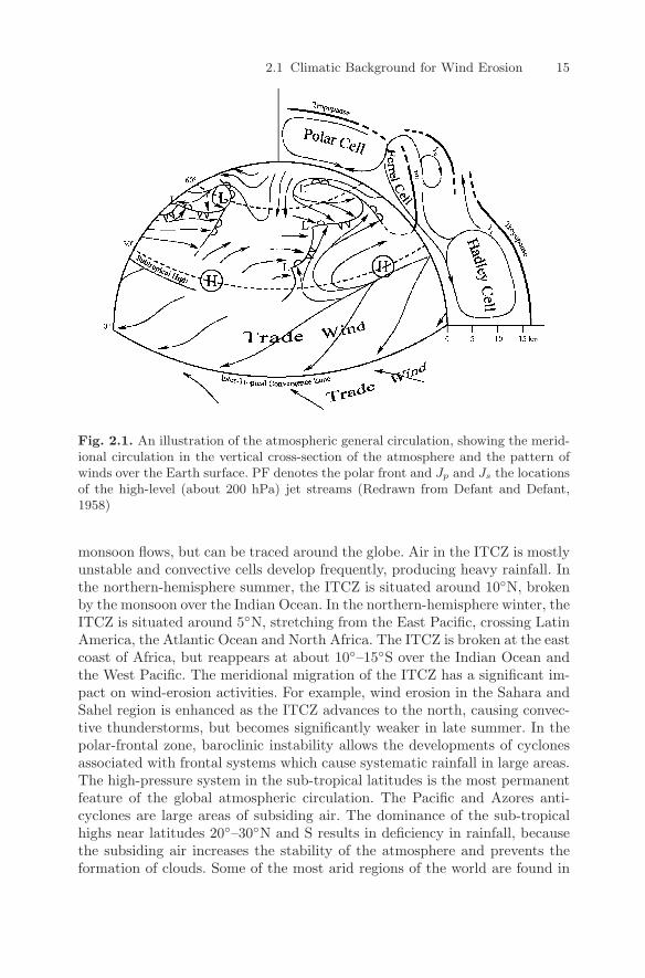
The basic features of the atmospheric general circulation are as illustratedin Fig. 2.1. In the meridional direction, the circulation is characterised by threecirculation cells, the Hadley, the Ferrel and the polar cells. Near the equator,warm air rises and flows to the poles in the upper atmosphere. Under theinfluence of the Coriolis force, the poleward-moving air obtains the westerlymomentum and forms westerly flows at around 30N and 30S. At these lati-tudes, air converges at high levels and subsides, leading to the developments ofthe sub-tropical highs. The higher pressure in the sub-tropical region leads toflows in the lower atmosphere toward the equator, which complete the Hadleycell. Again, due to the Coriolis force, the airflows moving toward the equa-tor acquire an easterly component and are known as the trade wind. Thesub-tropical high also generates poleward flows in the lower atmosphere. Inthe polar regions, the situation is the opposite, where strong surface coolingcauses air to sink and to flow towards the equator in the lower atmosphere.The air moving towards the equator converges at about 50N and 50S withthe air originating from the sub-tropical high, forming the polar-front zone.
The three meridional circulation cells give rise to three surface windregimes in each hemisphere: the trade winds of low latitudes, the midlati-tude westerly and the polar easterlies. This general circulation pattern hasmajor implications to the distributions of wind, precipitation, temperatureand hence wind erosion. The trade winds from the two hemispheres form theinter-tropical convergence zone (ITCZ), which can be clearly identified overthe ocean and less so over the land, where it is modified and suppressed byother atmospheric systems. The ITCZ may be broken at several locations by
2.1 Climatic Background for Wind Erosion 15
Fig. 2.1. An illustration of the atmospheric general circulation, showing the merid-ional circulation in the vertical cross-section of the atmosphere and the pattern ofwinds over the Earth surface. PF denotes the polar front and Jp and Js the locationsof the high-level (about 200 hPa) jet streams (Redrawn from Defant and Defant,1958)
monsoon flows, but can be traced around the globe. Air in the ITCZ is mostlyunstable and convective cells develop frequently, producing heavy rainfall. Inthe northern-hemisphere summer, the ITCZ is situated around 10N, brokenby the monsoon over the Indian Ocean. In the northern-hemisphere winter, theITCZ is situated around 5N, stretching from the East Pacific, crossing LatinAmerica, the Atlantic Ocean and North Africa. The ITCZ is broken at the eastcoast of Africa, but reappears at about 10–15S over the Indian Ocean andthe West Pacific. The meridional migration of the ITCZ has a significant im-pact on wind-erosion activities. For example, wind erosion in the Sahara andSahel region is enhanced as the ITCZ advances to the north, causing convec-tive thunderstorms, but becomes significantly weaker in late summer. In thepolar-frontal zone, baroclinic instability allows the developments of cyclonesassociated with frontal systems which cause systematic rainfall in large areas.The high-pressure system in the sub-tropical latitudes is the most permanentfeature of the global atmospheric circulation. The Pacific and Azores anti-cyclones are large areas of subsiding air. The dominance of the sub-tropicalhighs near latitudes 20–30N and S results in deficiency in rainfall, becausethe subsiding air increases the stability of the atmosphere and prevents theformation of clouds. Some of the most arid regions of the world are found in
16 2 Wind-Erosion Climatology
such places, including the Sahara Desert, the Kalahari and Namib Deserts,the Middle East, the Thar Desert, the coastal deserts of northern Chile, Peru,southern California and large areas of western and central Australia.
The idealised global circulation pattern as depicted in Fig. 2.1 is signifi-cantly modified by the irregular distribution of continents, oceans and moun-tain ranges which have different thermal and dynamic properties as well asdifferent seasonal variations. The continents have a smaller heat capacity thanthe ocean and hence undergo stronger annual temperature variations. Thethermal contrasts between the continents and the ocean lead to the devel-opments of monsoons which profoundly affect the distributions of wind andprecipitation.
Monsoons constitute a major component of the global circulation and playa major role in the sub-tropical and tropical regions of Asia and Africa. West,east and middle Africa, north Indian Ocean, India, South China Sea, thesouthern parts and north-eastern parts of China, Japan, west Pacific Indonesiaand the northern part of Australia are areas under the influence of monsoons.The Asian monsoon system is the most prominent in the world and consistsof the north-east winter monsoon and the south-west summer monsoon. Mon-soons greatly affect the patterns of precipitation in many parts of the world.In India, for instance, there is little precipitation during the winter monsoonbetween November and March, while rainfall is plentiful during the summermonsoon between June and October. In China, the movement of the precipi-tation zone from south to north between spring and autumn is closely relatedto the propagation of the southeast Asian summer monsoon. In April andMay, the rain zone is normally situated in south China and, in early summer,in the Changjiang valley before moving further north in late summer. Thesummer monsoon that produces rainfall, cannot penetrate to the inland areasof China. This results in a diminished precipitation and increased wind ero-sion in these areas. In addition, the Tibetan Plateau and the high mountainsin western China block the moisture from the Indian Ocean in the southwest.As a consequence, north-western and northern China, parts of north-easternChina and Mongolia, suffer deficiencies in rainfall. The Taklimakan Desert sit-uated between the Tian and Kunlun mountain ranges receives no more than100 mm of rainfall per year, and the Gobi Desert situated along the borderof China and Mongolia receives no more than 200 mm of rainfall per year.The Taklimakan and the Gobi Deserts are the largest deserts in the temperateclimate zone.
In general, wind erosion is more active in dry years. Littman (1991) stud-ied dust-storm frequencies in Asia and found that the occurrence of duststorms not only shows seasonal fluctuations, but also inter-annual variationsbetween 3.6 and 5.5 years. In Australia, severe dust storms mostly occur dur-ing drought years, such as 1982 and 1983, 1991, 1994 and 2002. During thesummer of 1982–1983, the eastern regions of Australia were transformed intoa near desert. Inland of the Dividing Range, there were vast areas of failedcropland and bared grazing land from which topsoil began to erode. Dust
2.1 Climatic Background for Wind Erosion 17
storms started in the spring and were widespread during the summer, withparticularly severe dust storms occurring in January and February of 1983(Garratt, 1997).
The underlying mechanism for extensive drought in Australia is the ElNino which represents the sea surface temperature variations in the equatorialPacific. During the El Nino years, warm waters occur in the eastern Pacificalong the tropical coast of South America. The El Nino phenomenon is coupledwith the Southern Oscillation in the tropical atmosphere, which represents thevariations of the Walker circulation. El Nino and Southern Oscillation (ENSO)are two closely related processes, the former taking place in the Pacific Oceanand the latter in the tropical atmosphere.
The Walker circulation (Fig. 2.2) is a longitudinal circulation in low-latitude atmosphere, arising from the variations of sea surface temperatureacross the ocean. Air rises at longitudes of relative heating and sinks at otherlongitudes of relative cooling. Under the normal state of the ocean and atmo-sphere across the Pacific Ocean, in the tropical latitudes off the west coast ofSouth America, the south or south-east trade winds generate a surface cur-rent of cold water from the south, and this is deflected towards the west bythe Coriolis force. The surface water drifting away is replaced by up-wellingof cold deep-ocean water. Consequently, there develops a strong gradient insea surface temperature from this area across the Pacific to the warm wa-ters of the Indonesian archipelago. This temperature contrast drives an east-west circulation cell in the atmosphere – the Walker circulation. Over theIndonesian region, the relatively warm and humid air rises to produce cloudsand rainfall. Over the eastern Pacific, the relatively cool air sinks and thus,the rainfall is scanty by tropical standards. This is accompanied by easterlywinds across the Pacific at the surface and westerlies in the upper atmo-sphere.
On occasions, the easterlies of the tropical Pacific weaken and therebyreduce the wind stress, resulting in warm water flowing eastward across thePacific to displace the cold water off the South American coast. With theappearance of warm surface waters in the central to eastern Pacific, the dif-ference in temperature across the Pacific is reduced. The Walker circulationbecomes weak or breaks down altogether, and a more complicated circulationcell structure develops in its place. As a result, cloud formation and rainfallis reduced in the Australian/Indonesian region but increased in the central toeastern Pacific. There is also evidence that these warm waters in the centralPacific can induce a series of atmospheric waves propagating into the North-ern Hemisphere. For some El Nino events these atmospheric disturbances canbe the cause of severe weather events over the entire globe. Areas consis-tently affected by the El Nino include Australia, Southeast Asia, large areasof China and the United States as well as certain areas in South America andAfrica.
18 2 Wind-Erosion Climatology
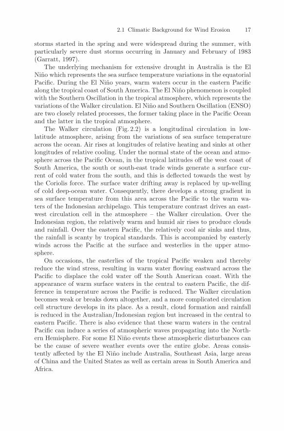
Fig. 2.2. An illustration of the atmospheric circulations over the tropical Pacific.During El Nino years, warm surface-ocean waters appear in the tropical East Pacific,accompanied by a weak Walker circulation. El Nino years are associated with lowerrainfall and greater wind-erosion risks in eastern Australia (top). During La Ninayears, warm surface-ocean waters appear in the tropical West Pacific, accompaniedby a strong Walker circulation. La Nina years are associated with higher rainfall andsmaller wind-erosion risks in eastern Australia (bottom)
2.2 Geographic Background for Wind Erosion
Wind erosion can only happen in areas where there is supply of sand anddust. However, the formations of sand and dust sources are determined by,apart from aeolian transport, weathering and fluvial (including glaciofluvial)processes. Prospero et al. (2002) pointed out that almost all major present-daydust sources are located in arid topographic depressions where fluvial actionis evident.
2.2 Geographic Background for Wind Erosion 19
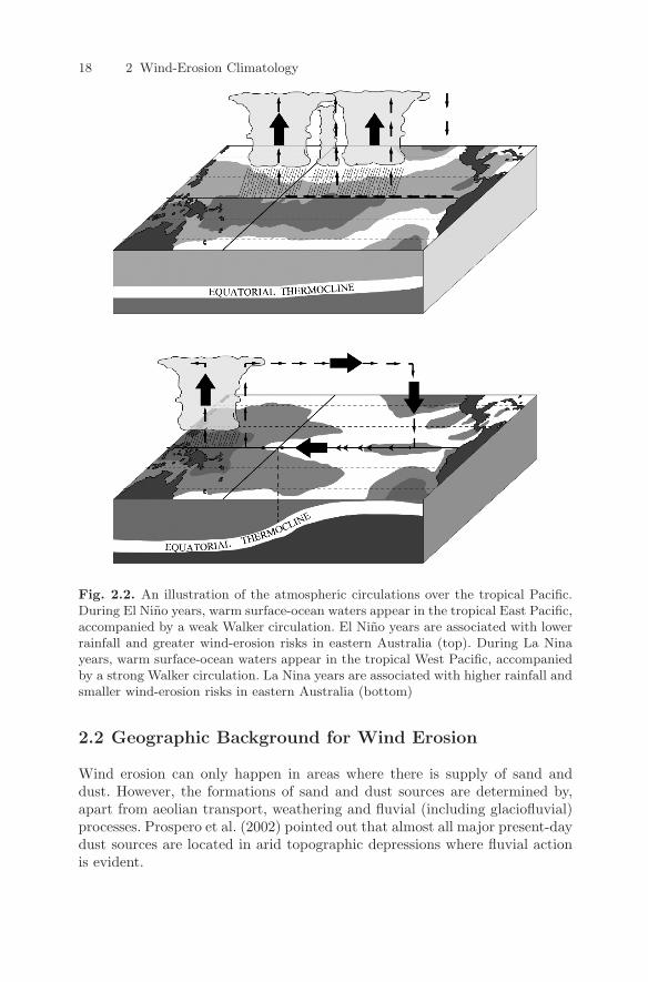
Fig. 2.3. Implications of fluvial actions to the formation of present-day dust sources
Fluvial actions are of paramount importance to the formation of thepresent-day dust sources, such as the Bodele Depression (North Africa), theTarim Basin (China) and the Lake Eyre Basin (Australia). These sources arelocated in arid regions centred over topographic lows or on lands adjacent totopographic highs. Fluvial processes are efficient in producing fine particles byseparating them from the soil matrix and carrying them to deposition basinsor alluvial plains (Fig. 2.3). Fluvial action is evident in the dust source regionsby the presence of ephemeral rivers and streams, alluvial fans, playas and saltlakes. Alluvial fans form at the base of mountains where water erosion sup-plies the sediment. The upper part of the alluvial fan is characterized by coarsesediment, and the lower part by fine sediment. The development of alluvialfans over geologic time may extend to large areas to form alluvial basins, orin areas of gentle slopes alluvial plains. Playa, also known as alkali flat, isa flat-bottomed dry lakebed which consists of fine-grained sediments infusedwith alkali salts. A consistent association of dust sources with playas has beenfound (Gill, 1996). While playas may be not dust sources themselves, strongdust emission may occur in the alluvial fans that ring the basins in which theplayas are found (Reheis et al. 1995).
Most prudent-day dust source regions have deep and extensive alluvialdeposits resulting from a relatively recent pluvial history. During the pluvialphases, these regions were flooded and thick layers of sediment were depositedand are now exposed to wind erosion. Many of the dust sources were floodedduring the Pleistocene (roughly 2 million to 10,000 years ago, e.g., the LakeChad Basin).
20 2 Wind-Erosion Climatology
Most of the present-day sand and dust sources are confined to regionswith annual rainfall below 250 mm. While the global pattern of aridity isdetermined by the general circulation of the atmosphere, the interferences oflandforms on the atmospheric flow field can significantly modify the climatein a region. The most arid places in the world are basins situated in thewake of high mountains. For example, the Great Basin (USA) in the wake ofthe Sierra Nevada receives less than 120 mm annual rainfall, and the TarimBasin (China) surrounded by the Tian and Kunlun mountains and the PamirPlateau receives less than 100 mm annual rainfall. As air approaches themountain ranges, it is either diverted to flow around them or forced to rise.The adiabatic cooling associated with the upward motion promotes conden-sation and precipitation and thereby depletes the moisture in the airflow.Further down wind, air descends over the mountains. The adiabatic heatingassociated with the downward motion suppresses condensation and precipita-tion and thereby generates hot and dry airflows, known as foehn. In connectionto wind erosion, this process has three important consequences. First, an aridshadow develops in the mountain wake. Second, precipitation increases onmountain slopes which leads to fluvial activity and sediment transport fromthe mountain slopes to the adjacent depressions. Third, complex flow patternsdevelop in regions around the mountain ranges, which affect dust transport,e.g., dust may be transported along preferred paths or allowed to accumulatein certain areas. Preferred routes of dust transport have been identified onsatellite images of dust events. For example, dust is often seen to elongatefrom south-eastern Iran into the Indus Delta along the southern flanks ofthe Makran mountains (Prospero et al. 2002). Dust from the Gobi Desert ispreferentially transported south-eastwards along the north-western boundaryof the Tibetan Plateau and dust from the Thar Desert eastwards along thesouthern boundary of the Tibetan Plateau (Shao and Dong, 2006). Dust orig-inating from the northeast Tarim Basin is often advected to the southwest ofthe basin causing high dust concentrations over there (Shao and Wang, 2003).
2.3 Atmospheric Systems
Severe dust storms are mostly generated by vigorous weather systems, such asmonsoon winds, cyclones and fronts, squall lines and thunderstorms. In thesesystems, the necessary meteorological conditions for the formation of a sub-stantial dust storm are present, including (i) strong near-surface wind to liftsand and dust particles from the surface; (ii) strong turbulence or convectionto disperse particles to high levels; and (iii) strong winds to transport particlesover large distances horizontally. Despite these common features, the atmo-spheric systems which generate dust storms in different parts of the world canbe quite different.
2.3 Atmospheric Systems 21
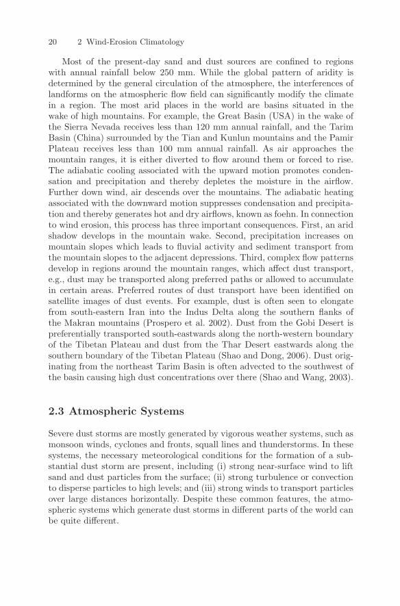
Fig. 2.4. The structure of the atmospheric circulation over North Africa in August.A: Location of the monsoon trough and the low-level easterly jet over the Sahara. Tothe north of the monsoon trough at about 20N blows the north-easterly Harmattan(hot and dry) and to the south the south-westerly monsoon wind (warm and moist).B: Vertical structure of the atmosphere along the dashed line in A. Strong windsassociated with the convections in the monsoon trough may generate dust storms(Redrawn from Barry and Chorley, 2003)
2.3.1 Monsoon Winds
In North Africa, Southeast Asia and the Middle East, dust storms are of-ten generated by monsoon winds or monsoon-related convective disturbances.The Harmattan (low-level hot and dry north-easterly) of North Africa and theShamal (low-level hot and dry northerly) of the Middle East are well-knownexamples. The patterns of wind and precipitation in North Africa are very
22 2 Wind-Erosion Climatology
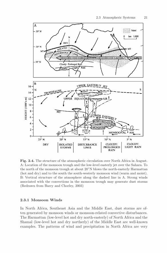
Fig. 2.5. Satellite image of the dust storm originating in the Gobi Desert of north-west China on 14 April 1998. The image, from 16 April 1998, shows the dust cloudsbehind the cold front and near the centre of the storm (SeaWiFS image by NormanKuring, NASA GSFC, acknowledgment)
much determined by the regular and continuous migration of the monsoontrough between the annual extreme locations of about 2N in January and25N in August. South of the trough is a shallow south-westerly airflow of c.a.1,000 m deep, and overriding the south-westerly is an easterly of around 3,000m deep, known as the midlevel easterly jet. North of the monsoon trough blowsthe Harmattan from the sub-tropic high pressure center (Fig. 2.4). Along themonsoon trough, shallow easterly waves develop, accompanied by surface cy-clones. The cyclones generate strong near-surface winds which entrain largeamounts of dust into the atmosphere (Westphal et al. 1988). Isolated stormsand a broad zone of disturbances also occur just below the midlevel easterlyjet. Another mechanism for the outbreaks of the Saharan dust are the dryconvections which mix momentum from the midlevel easterly jet down to thesurface where dust is mobilized (Prospero and Carlson, 1981). In the Harmat-tan affected regions, wide spread dust haze occurs in light wind conditions,known as the Harmattan haze.
The Shamal blows almost daily in the Middle East between June andSeptember. It may generate dust storms across Iraq, Kuwait and the Arabian
2.3 Atmospheric Systems 23
Peninsula. The synoptic situation responsible for the Shamal is a zoneof convergence between the subtropical ridge extending into the northernArabian Peninsula and Iraq from the Mediterranean Sea and the Mon-soon Trough across southern Iran and the Southern Arabian Peninsula. Thenortherly flow associated with this synoptic situation is further accelerateddue to the channelling effect exerted by the Iranian and the Arabian Plateaus.As the Shamal blows over the Tigris and Euphrates alluvial plains, a tremen-dous amount of dust may be lifted into the atmosphere to create dust plumeswhich stretch southward across Kuwait and the northern Persian Gulf. TheShamal dust storms move into an area like a dust wall of 1,000–2,500 m talland 100–200 km thick. In the dust wall, the visibility drops to near zero.
2.3.2 Cyclones and Frontal Systems
Frontal systems associated with cyclones and depressions also generate large-scale dust storms. For example, in spring in Northeast Asia, up to 15 Mon-golian cyclones (midlatitude cyclones initiating from baroclinic disturbancesover the Mongolian Plateau) travel from northwest to southeast along the EastAsian trough over the east coast of the Eurasian continent. Mongolian cyclonesare accompanied by rigorous cold fronts and post-frontal north-westerly windsreaching up to 20 m s−1. The cyclones move over the Gobi Desert and gener-ate dust storms in Northeast Asia. Figure 2.5 shows a satellite image of the16 April 1998 dust storm originating in the Gobi Desert. During this event,dust was transported to as far as the west coast of the United States.
Intense wind-erosion events in Australia are mostly associated with South-ern Ocean cold fronts propagating from southwest to northeast (Garratt, 1984;Garratt et al. 1989). The 8 February 1983 Melbourne dust storm, for instance,was generated by a dry cold front which represented a sharp demarcation be-tween a hot northwest flow ahead of it and a west-south-west cooler flowbehind it (Fig. 2.6). The structure of the front was typical of the summer coolchanges in southern Australia, which can be described as propagating gravitycurrents (horizontal flows of a fluid that is denser than its surroundings). Thecold front consists of an advancing wedge of cooler air marked in this case bya wall of dust, which undercuts the warm air mass ahead of the front. Thedepth of the gravity current at the head was about 300 m. The propagationspeed of the gravity current exceeded 20 m s−1.
Figure 2.7 depicts the typical weather pattern that generates dust stormsin Australia. A dust episode in Australia lasts two to three days. Initially,a low is positioned over the Southern Oceans and a high to the south-west of Australia. A cold front extends from the low pressure centre tothe Great Australia Bight. Strong post-frontal southerly airflows are di-rected onto the southern coast of the continent, and a strong hot dry north-westerly wind blows over the south-eastern parts of Australia. Then, the lowmoves rapidly eastward, accompanied by the north-eastward propagation ofthe cold front. Strong south-westerly wind (12–15 ms−1) prevails behind the
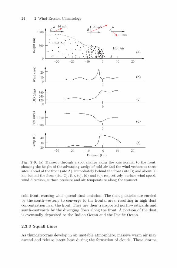
24 2 Wind-Erosion Climatology
0
0
0
(a)
(b)
(c)
(d)
(e)
Distance (km)
DD
(de
g)H
eigh
t (m
)Pre
s (h
Pa)
ABC
C ABW
ind
(m/s
)T
emp
(C)
Hot AirDust
Cold Air
20 m/s
10 m/s
14 m/s
30
240
0120
360
1000
1010
20
40
010
20
0
500
1000
−10−20−30 10 200
10 20−10−20 0−30
Fig. 2.6. (a) Transect through a cool change along the axis normal to the front,showing the height of the advancing wedge of cold air and the wind vectors at threesites: ahead of the front (site A), immediately behind the front (site B) and about 30km behind the front (site C); (b), (c), (d) and (e): respectively, surface wind speed,wind direction, surface pressure and air temperature along the transect
cold front, causing wide-spread dust emission. The dust particles are carriedby the south-westerly to converge to the frontal area, resulting in high dustconcentration near the front. They are then transported north-westwards andsouth-eastwards by the diverging flows along the front. A portion of the dustis eventually deposited to the Indian Ocean and the Pacific Ocean.
2.3.3 Squall Lines
As thunderstorms develop in an unstable atmosphere, massive warm air mayascend and release latent heat during the formation of clouds. These storms
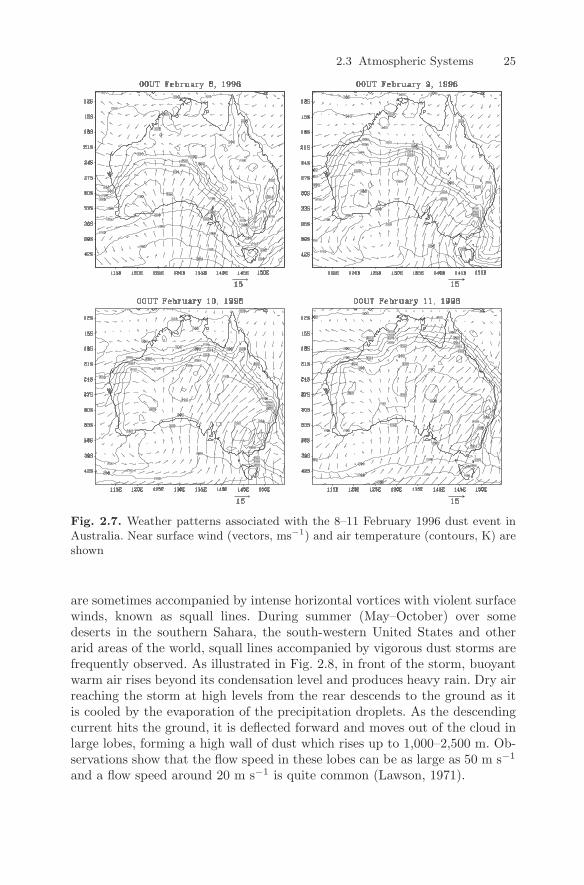
2.3 Atmospheric Systems 25
Fig. 2.7. Weather patterns associated with the 8–11 February 1996 dust event inAustralia. Near surface wind (vectors, ms−1) and air temperature (contours, K) areshown
are sometimes accompanied by intense horizontal vortices with violent surfacewinds, known as squall lines. During summer (May–October) over somedeserts in the southern Sahara, the south-western United States and otherarid areas of the world, squall lines accompanied by vigorous dust storms arefrequently observed. As illustrated in Fig. 2.8, in front of the storm, buoyantwarm air rises beyond its condensation level and produces heavy rain. Dry airreaching the storm at high levels from the rear descends to the ground as itis cooled by the evaporation of the precipitation droplets. As the descendingcurrent hits the ground, it is deflected forward and moves out of the cloud inlarge lobes, forming a high wall of dust which rises up to 1,000–2,500 m. Ob-servations show that the flow speed in these lobes can be as large as 50 m s−1
and a flow speed around 20 m s−1 is quite common (Lawson, 1971).
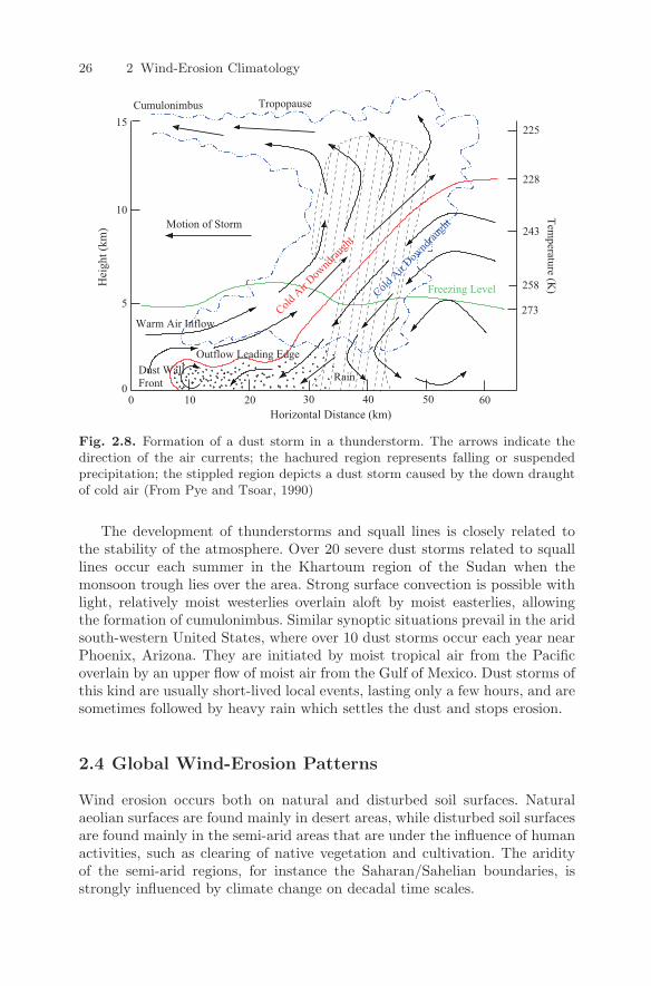
26 2 Wind-Erosion Climatology
0
Freezing Level
Motion of Storm
Cold A
ir Dow
ndrau
ght
Cold A
ir Dow
ndrau
ght
Outflow Leading EdgeDust WallFront
Tropopause
258
273
243
228
225
10 20 30 40 50 60
Hei
ght (
km)
Temperature (K
)Cumulonimbus
Warm Air Inflow
Rain
Horizontal Distance (km)
10
15
5
0
Fig. 2.8. Formation of a dust storm in a thunderstorm. The arrows indicate thedirection of the air currents; the hachured region represents falling or suspendedprecipitation; the stippled region depicts a dust storm caused by the down draughtof cold air (From Pye and Tsoar, 1990)
The development of thunderstorms and squall lines is closely related tothe stability of the atmosphere. Over 20 severe dust storms related to squalllines occur each summer in the Khartoum region of the Sudan when themonsoon trough lies over the area. Strong surface convection is possible withlight, relatively moist westerlies overlain aloft by moist easterlies, allowingthe formation of cumulonimbus. Similar synoptic situations prevail in the aridsouth-western United States, where over 10 dust storms occur each year nearPhoenix, Arizona. They are initiated by moist tropical air from the Pacificoverlain by an upper flow of moist air from the Gulf of Mexico. Dust storms ofthis kind are usually short-lived local events, lasting only a few hours, and aresometimes followed by heavy rain which settles the dust and stops erosion.
2.4 Global Wind-Erosion Patterns
Wind erosion occurs both on natural and disturbed soil surfaces. Naturalaeolian surfaces are found mainly in desert areas, while disturbed soil surfacesare found mainly in the semi-arid areas that are under the influence of humanactivities, such as clearing of native vegetation and cultivation. The aridityof the semi-arid regions, for instance the Saharan/Sahelian boundaries, isstrongly influenced by climate change on decadal time scales.
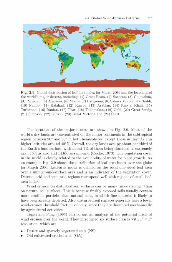
2.4 Global Wind-Erosion Patterns 27
Fig. 2.9. Global distribution of leaf-area index for March 2004 and the locations ofthe world’s major deserts, including: (1) Great Basin, (2) Sonoran, (3) Chihuahua,(4) Peruvian, (5) Atacama, (6) Monte, (7) Patagonia, (8) Sahara, (9) Somali-Chabli,(10) Namib, (11) Kalahari, (12) Karroo, (13) Arabian, (14) Rub al Khali, (15)Turkestan, (16) Iranian, (17) Thar, (18) Taklimakan, (19) Gobi, (20) Great Sandy,(21) Simpson, (22) Gibson, (23) Great Victoria and (24) Sturt
The locations of the major deserts are shown in Fig. 2.9. Most of theworld’s dry lands are concentrated on the major continents in the subtropicalregion between 20 and 30 in both hemispheres, except those in East Asia inhigher latitudes around 40N. Overall, the dry lands occupy about one third ofthe Earth’s land surface, with about 4% of them being classified as extremelyarid, 15% as arid and 14.6% as semi-arid (Cooke, 1973). The vegetation coverin the world is closely related to the availability of water for plant growth. Asan example, Fig. 2.9 shows the distribution of leaf-area index over the globefor March 2004. Leaf-area index is defined as the total one-sided leaf areaover a unit ground-surface area and is an indicator of the vegetation cover.Deserts, arid and semi-arid regions correspond well with regions of small leaf-area index.
Wind erosion on disturbed soil surfaces can be many times stronger thanon natural soil surfaces. This is because freshly exposed soils usually containmore erodible particles than natural soils, in which fine material is likely tohave been already depleted. Also, disturbed soil surfaces generally have a lowerwind-erosion threshold friction velocity, since they are disrupted mechanicallyby agricultural activities.
Tegen and Fung (1995) carried out an analysis of the potential areas ofwind erosion over the world. They introduced six surface classes with 1 × 1
resolution, which are
• Desert and sparsely vegetated soils (NS)• Old cultivated eroded soils (OA)
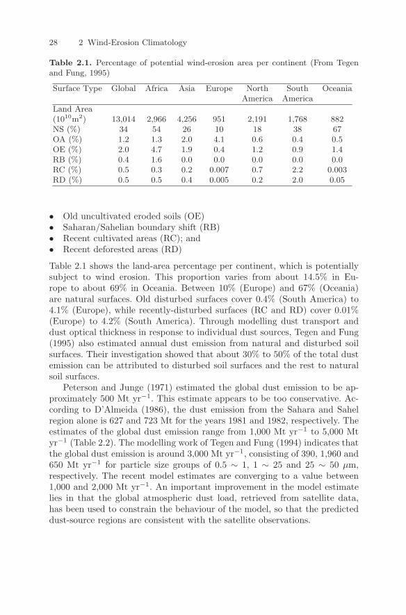
28 2 Wind-Erosion Climatology
Table 2.1. Percentage of potential wind-erosion area per continent (From Tegenand Fung, 1995)
Surface Type Global Africa Asia Europe North South OceaniaAmerica America
Land Area(1010m2) 13,014 2,966 4,256 951 2,191 1,768 882NS (%) 34 54 26 10 18 38 67OA (%) 1.2 1.3 2.0 4.1 0.6 0.4 0.5OE (%) 2.0 4.7 1.9 0.4 1.2 0.9 1.4RB (%) 0.4 1.6 0.0 0.0 0.0 0.0 0.0RC (%) 0.5 0.3 0.2 0.007 0.7 2.2 0.003RD (%) 0.5 0.5 0.4 0.005 0.2 2.0 0.05
• Old uncultivated eroded soils (OE)• Saharan/Sahelian boundary shift (RB)• Recent cultivated areas (RC); and• Recent deforested areas (RD)
Table 2.1 shows the land-area percentage per continent, which is potentiallysubject to wind erosion. This proportion varies from about 14.5% in Eu-rope to about 69% in Oceania. Between 10% (Europe) and 67% (Oceania)are natural surfaces. Old disturbed surfaces cover 0.4% (South America) to4.1% (Europe), while recently-disturbed surfaces (RC and RD) cover 0.01%(Europe) to 4.2% (South America). Through modelling dust transport anddust optical thickness in response to individual dust sources, Tegen and Fung(1995) also estimated annual dust emission from natural and disturbed soilsurfaces. Their investigation showed that about 30% to 50% of the total dustemission can be attributed to disturbed soil surfaces and the rest to naturalsoil surfaces.
Peterson and Junge (1971) estimated the global dust emission to be ap-proximately 500 Mt yr−1. This estimate appears to be too conservative. Ac-cording to D’Almeida (1986), the dust emission from the Sahara and Sahelregion alone is 627 and 723 Mt for the years 1981 and 1982, respectively. Theestimates of the global dust emission range from 1,000 Mt yr−1 to 5,000 Mtyr−1 (Table 2.2). The modelling work of Tegen and Fung (1994) indicates thatthe global dust emission is around 3,000 Mt yr−1, consisting of 390, 1,960 and650 Mt yr−1 for particle size groups of 0.5 ∼ 1, 1 ∼ 25 and 25 ∼ 50 µm,respectively. The recent model estimates are converging to a value between1,000 and 2,000 Mt yr−1. An important improvement in the model estimatelies in that the global atmospheric dust load, retrieved from satellite data,has been used to constrain the behaviour of the model, so that the predicteddust-source regions are consistent with the satellite observations.
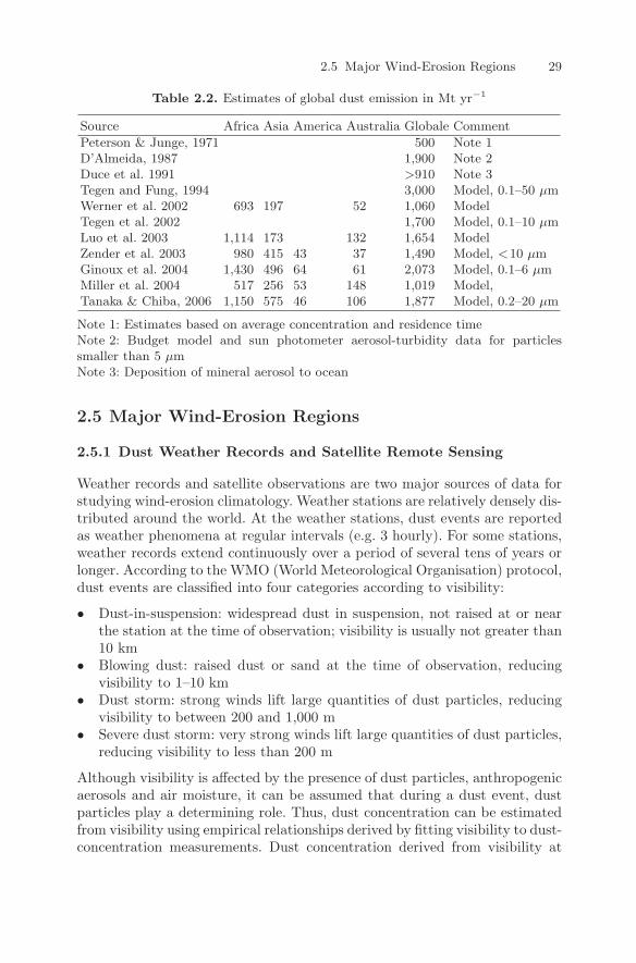
2.5 Major Wind-Erosion Regions 29
Table 2.2. Estimates of global dust emission in Mt yr−1
Source Africa Asia America Australia Globale Comment
Peterson & Junge, 1971 500 Note 1D’Almeida, 1987 1,900 Note 2Duce et al. 1991 >910 Note 3Tegen and Fung, 1994 3,000 Model, 0.1–50 µmWerner et al. 2002 693 197 52 1,060 ModelTegen et al. 2002 1,700 Model, 0.1–10 µmLuo et al. 2003 1,114 173 132 1,654 ModelZender et al. 2003 980 415 43 37 1,490 Model, <10 µmGinoux et al. 2004 1,430 496 64 61 2,073 Model, 0.1–6 µmMiller et al. 2004 517 256 53 148 1,019 Model,Tanaka & Chiba, 2006 1,150 575 46 106 1,877 Model, 0.2–20 µm
Note 1: Estimates based on average concentration and residence timeNote 2: Budget model and sun photometer aerosol-turbidity data for particlessmaller than 5 µmNote 3: Deposition of mineral aerosol to ocean
2.5 Major Wind-Erosion Regions
2.5.1 Dust Weather Records and Satellite Remote Sensing
Weather records and satellite observations are two major sources of data forstudying wind-erosion climatology. Weather stations are relatively densely dis-tributed around the world. At the weather stations, dust events are reportedas weather phenomena at regular intervals (e.g. 3 hourly). For some stations,weather records extend continuously over a period of several tens of years orlonger. According to the WMO (World Meteorological Organisation) protocol,dust events are classified into four categories according to visibility:
• Dust-in-suspension: widespread dust in suspension, not raised at or nearthe station at the time of observation; visibility is usually not greater than10 km
• Blowing dust: raised dust or sand at the time of observation, reducingvisibility to 1–10 km
• Dust storm: strong winds lift large quantities of dust particles, reducingvisibility to between 200 and 1,000 m
• Severe dust storm: very strong winds lift large quantities of dust particles,reducing visibility to less than 200 m
Although visibility is affected by the presence of dust particles, anthropogenicaerosols and air moisture, it can be assumed that during a dust event, dustparticles play a determining role. Thus, dust concentration can be estimatedfrom visibility using empirical relationships derived by fitting visibility to dust-concentration measurements. Dust concentration derived from visibility at
30 2 Wind-Erosion Climatology
individual weather stations can then be used to generate a dust-concentrationfield through spatial interpolation (Shao and Dong, 2006).
Satellite remote sensing is advantageous in monitoring dust events becauseof its excellent spatial and temporal coverages. Satellite sensors can detect ra-diation signals from aerosol and various surfaces of the Earth through differentspectral channels. The channels are commonly set in correspondence of theatmospheric radiation windows. The main ones are VL (visible light, 0.65–0.85 µm), NIR (near infrared, 1.6 µm), MIR (middle infrared, 3.7 µm), WV(water vapour, 6.7 µm) and TIR (thermal infrared, 11 and 12 µm). Signalsfrom the various channels can be combined to detect dust events from satelliteimagery and to derive variables for quantifying dust load and dust particlesize (Ackerman, 1997).
The TOMS (Total Ozone Mapping Spectrometer, Nimbus 7 Satellite) datahave been shown to be very useful for mapping the distribution of absorbingaerosols (largely comprised of dust and black carbon). The radiative effect ofaerosols is measured in terms of an aerosol index defined as
AI = −100 log10
[(I340
I380
)ms
−(
I340
I380
)cl
]
where (I340/I380)ms is the measured ratio of the backscattered radiance at340 nm to that at 380 nm, and (I340/I380)cl is the calculated ratio by a radi-ation transfer model that assumes a pure gaseous atmosphere. The differencebetween the measured and calculated ratios is attributed to the presence ofaerosols. Absorbing aerosols, clouds and non-absorbing aerosols yield positive,near-zero and negative AI values, respectively. The positive AI is the absorb-ing aerosol index which normally varies between 0 and 30. The TOMS datahave been used to identify areas of high dust concentration (e.g. Goudie andMiddleton, 2001).
2.5.2 North Africa
The Sahara is the largest arid region on Earth. It occupies nearly all of NorthAfrica, extending in length for approximately 5,600 km from the Atlanticcoast to the shores of the Red Sea. In the north–south direction, it spanssome 2,000 km or 20 degrees of latitude from about 35N in the Atlas regionof Algeria to about 15N in the thorn shrub and grassland region, known asSudan. The semi-arid region around 12N to the south of the Sahara is theSahel. The Sahel runs from the Atlantic Ocean to the Horn of Africa, changingfrom semi-arid grassland to thorn savanna. The Sahel countries today includeSenegal, Cape Verde, Mauritania, Mali, Burkina Faso, Nigeria, Chad andSudan. The Sahel receives 150–500 mm of rainfall a year, primarily in themonsoon season. The amount of rainfall is subject to significant variationsdue to climate change. While it is widely accepted that the Sahara is thelargest dust source in the world, the estimates of the source strength varyover a wide range (Table 2.3).
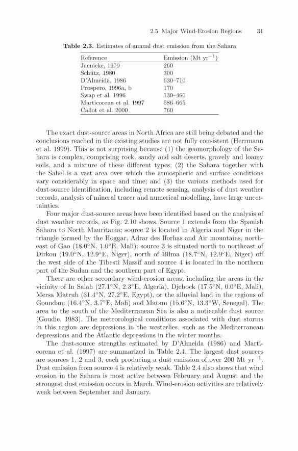
2.5 Major Wind-Erosion Regions 31
Table 2.3. Estimates of annual dust emission from the Sahara
Reference Emission (Mt yr−1)
Jaenicke, 1979 260Schutz, 1980 300D’Almeida, 1986 630–710Prospero, 1996a, b 170Swap et al. 1996 130–460Marticorena et al. 1997 586–665Callot et al. 2000 760
The exact dust-source areas in North Africa are still being debated and theconclusions reached in the existing studies are not fully consistent (Herrmannet al. 1999). This is not surprising because (1) the geomorphology of the Sa-hara is complex, comprising rock, sandy and salt deserts, gravely and loamysoils, and a mixture of these different types; (2) the Sahara together withthe Sahel is a vast area over which the atmospheric and surface conditionsvary considerably in space and time; and (3) the various methods used fordust-source identification, including remote sensing, analysis of dust weatherrecords, analysis of mineral tracer and numerical modelling, have large uncer-tainties.
Four major dust-source areas have been identified based on the analysis ofdust weather records, as Fig. 2.10 shows. Source 1 extends from the SpanishSahara to North Mauritania; source 2 is located in Algeria and Niger in thetriangle formed by the Hoggar, Adrar des Iforhas and Air mountains, north-east of Gao (18.0N, 1.0E, Mali); source 3 is situated north to northeast ofDirkou (19.0N, 12.9E, Niger), north of Bilma (18.7N, 12.9E, Niger) offthe west side of the Tibesti Massif and source 4 is located in the northernpart of the Sudan and the southern part of Egypt.
There are other secondary wind-erosion areas, including the areas in thevicinity of In Salah (27.1N, 2.3E, Algeria), Djebock (17.5N, 0.0E, Mali),Mersa Matruh (31.4N, 27.2E, Egypt), or the alluvial land in the regions ofGoundam (16.4N, 3.7E, Mali) and Matam (15.6N, 13.3W, Senegal). Thearea to the south of the Mediterranean Sea is also a noticeable dust source(Goudie, 1983). The meteorological conditions associated with dust stormsin this region are depressions in the westerlies, such as the Mediterraneandepressions and the Atlantic depressions in the winter months.
The dust-source strengths estimated by D’Almeida (1986) and Marti-corena et al. (1997) are summarized in Table 2.4. The largest dust sourcesare sources 1, 2 and 3, each producing a dust emission of over 200 Mt yr−1.Dust emission from source 4 is relatively weak. Table 2.4 also shows that winderosion in the Sahara is most active between February and August and thestrongest dust emission occurs in March. Wind-erosion activities are relativelyweak between September and January.
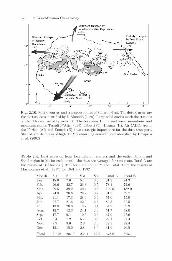
32 2 Wind-Erosion Climatology
Fig. 2.10. Major sources and transport routes of Saharan dust. The dotted areas arethe dust sources identified by D’Almeida (1986). Large solid circles mark the stationsof the African turbidity network. The locations Bilma and some mountains andmountain chains Tassali N’Ajjer (TN), Tibesti (T), Hoggar (H), Air (AIR), Adrardes Iforhas (AI) and Ennedi (E) have strategic importance for the dust transport.Shaded are the areas of high TOMS absorbing aerosol index identified by Prosperoet al. (2002)
Table 2.4. Dust emission from four different sources and the entire Sahara andSahel region in Mt for each month, the data are averaged for two years. Total A arethe results of D’Almeida (1986) for 1981 and 1982 and Total B are the results ofMarticorena et al. (1997) for 1991 and 1992
Month S 1 S 2 S 3 S 4 Total A Total B
Jan. 18.6 7.0 5.1 0.6 31.3 24.3Feb. 26.6 22.7 23.3 0.5 73.1 72.6Mar. 29.5 39.2 40.4 0.5 109.6 132.0Apr. 24.8 26.6 29.2 0.7 81.3 59.7May 21.1 17.3 28.6 0.6 67.6 75.0Jun. 22.7 21.6 42.9 2.3 89.5 52.5Jul. 13.8 20.3 19.7 0.4 54.2 62.9Aug. 12.7 12.3 24.1 2.6 51.7 48.0Sep. 17.7 9.1 10.5 0.6 37.9 27.6Oct. 8.4 7.2 5.7 0.8 22.1 21.4Nov. 8.9 9.6 2.8 2.3 22.3 22.4Dec. 13.1 15.0 2.8 1.0 31.9 26.5
Total 217.9 207.9 235.1 12.9 673.8 625.7
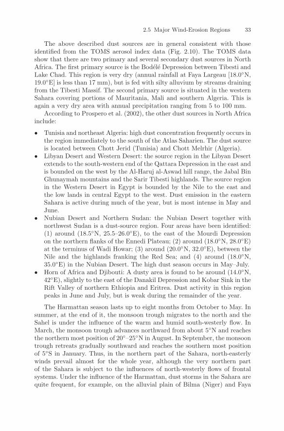
2.5 Major Wind-Erosion Regions 33
The above described dust sources are in general consistent with thoseidentified from the TOMS aerosol index data (Fig. 2.10). The TOMS datashow that there are two primary and several secondary dust sources in NorthAfrica. The first primary source is the Bodele Depression between Tibesti andLake Chad. This region is very dry (annual rainfall at Faya Largeau [18.0N,19.0E] is less than 17 mm), but is fed with silty alluvium by streams drainingfrom the Tibesti Massif. The second primary source is situated in the westernSahara covering portions of Mauritania, Mali and southern Algeria. This isagain a very dry area with annual precipitation ranging from 5 to 100 mm.
According to Prospero et al. (2002), the other dust sources in North Africainclude:
• Tunisia and northeast Algeria: high dust concentration frequently occurs inthe region immediately to the south of the Atlas Saharien. The dust sourceis located between Chott Jerid (Tunisia) and Chott Melrhir (Algeria).
• Libyan Desert and Western Desert: the source region in the Libyan Desertextends to the south-western end of the Qattara Depression in the east andis bounded on the west by the Al-Haruj al-Aswad hill range, the Jabal BinGhunaymah mountains and the Sarir Tibesti highlands. The source regionin the Western Desert in Egypt is bounded by the Nile to the east andthe low lands in central Egypt to the west. Dust emission in the easternSahara is active during much of the year, but is most intense in May andJune.
• Nubian Desert and Northern Sudan: the Nubian Desert together withnorthwest Sudan is a dust-source region. Four areas have been identified:(1) around (18.5N, 25.5–26.0E), to the east of the Mourdi Depressionon the northern flanks of the Ennedi Plateau; (2) around (18.0N, 28.0E)at the terminus of Wadi Howar; (3) around (20.0N, 32.0E), between theNile and the highlands franking the Red Sea; and (4) around (18.0N,35.0E) in the Nubian Desert. The high dust season occurs in May–July.
• Horn of Africa and Djibouti: A dusty area is found to be around (14.0N,42E), slightly to the east of the Danakil Depression and Kobar Sink in theRift Valley of northern Ethiopia and Eritrea. Dust activity in this regionpeaks in June and July, but is weak during the remainder of the year.
The Harmattan season lasts up to eight months from October to May. Insummer, at the end of it, the monsoon trough migrates to the north and theSahel is under the influence of the warm and humid south-westerly flow. InMarch, the monsoon trough advances northward from about 5N and reachesthe northern most position of 20–25N in August. In September, the monsoontrough retreats gradually southward and reaches the southern most positionof 5S in January. Thus, in the northern part of the Sahara, north-easterlywinds prevail almost for the whole year, although the very northern partof the Sahara is subject to the influences of north-westerly flows of frontalsystems. Under the influence of the Harmattan, dust storms in the Sahara arequite frequent, for example, on the alluvial plain of Bilma (Niger) and Faya
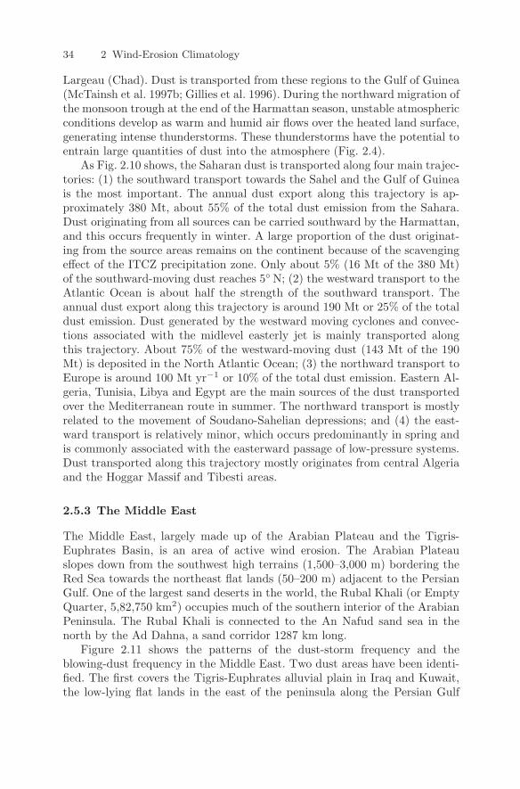
34 2 Wind-Erosion Climatology
Largeau (Chad). Dust is transported from these regions to the Gulf of Guinea(McTainsh et al. 1997b; Gillies et al. 1996). During the northward migration ofthe monsoon trough at the end of the Harmattan season, unstable atmosphericconditions develop as warm and humid air flows over the heated land surface,generating intense thunderstorms. These thunderstorms have the potential toentrain large quantities of dust into the atmosphere (Fig. 2.4).
As Fig. 2.10 shows, the Saharan dust is transported along four main trajec-tories: (1) the southward transport towards the Sahel and the Gulf of Guineais the most important. The annual dust export along this trajectory is ap-proximately 380 Mt, about 55% of the total dust emission from the Sahara.Dust originating from all sources can be carried southward by the Harmattan,and this occurs frequently in winter. A large proportion of the dust originat-ing from the source areas remains on the continent because of the scavengingeffect of the ITCZ precipitation zone. Only about 5% (16 Mt of the 380 Mt)of the southward-moving dust reaches 5 N; (2) the westward transport to theAtlantic Ocean is about half the strength of the southward transport. Theannual dust export along this trajectory is around 190 Mt or 25% of the totaldust emission. Dust generated by the westward moving cyclones and convec-tions associated with the midlevel easterly jet is mainly transported alongthis trajectory. About 75% of the westward-moving dust (143 Mt of the 190Mt) is deposited in the North Atlantic Ocean; (3) the northward transport toEurope is around 100 Mt yr−1 or 10% of the total dust emission. Eastern Al-geria, Tunisia, Libya and Egypt are the main sources of the dust transportedover the Mediterranean route in summer. The northward transport is mostlyrelated to the movement of Soudano-Sahelian depressions; and (4) the east-ward transport is relatively minor, which occurs predominantly in spring andis commonly associated with the easterward passage of low-pressure systems.Dust transported along this trajectory mostly originates from central Algeriaand the Hoggar Massif and Tibesti areas.
2.5.3 The Middle East
The Middle East, largely made up of the Arabian Plateau and the Tigris-Euphrates Basin, is an area of active wind erosion. The Arabian Plateauslopes down from the southwest high terrains (1,500–3,000 m) bordering theRed Sea towards the northeast flat lands (50–200 m) adjacent to the PersianGulf. One of the largest sand deserts in the world, the Rubal Khali (or EmptyQuarter, 5,82,750 km2) occupies much of the southern interior of the ArabianPeninsula. The Rubal Khali is connected to the An Nafud sand sea in thenorth by the Ad Dahna, a sand corridor 1287 km long.
Figure 2.11 shows the patterns of the dust-storm frequency and theblowing-dust frequency in the Middle East. Two dust areas have been identi-fied. The first covers the Tigris-Euphrates alluvial plain in Iraq and Kuwait,the low-lying flat lands in the east of the peninsula along the Persian Gulf
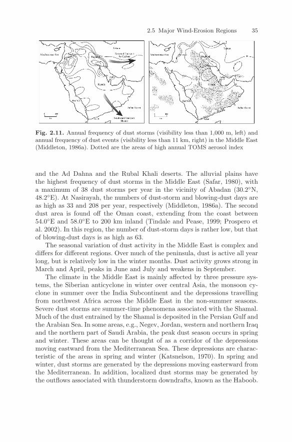
2.5 Major Wind-Erosion Regions 35
Fig. 2.11. Annual frequency of dust storms (visibility less than 1,000 m, left) andannual frequency of dust events (visibility less than 11 km, right) in the Middle East(Middleton, 1986a). Dotted are the areas of high annual TOMS aerosol index
and the Ad Dahna and the Rubal Khali deserts. The alluvial plains havethe highest frequency of dust storms in the Middle East (Safar, 1980), witha maximum of 38 dust storms per year in the vicinity of Abadan (30.2N,48.2E). At Nasirayah, the numbers of dust-storm and blowing-dust days areas high as 33 and 208 per year, respectively (Middleton, 1986a). The seconddust area is found off the Oman coast, extending from the coast between54.0E and 58.0E to 200 km inland (Tindale and Pease, 1999; Prospero etal. 2002). In this region, the number of dust-storm days is rather low, but thatof blowing-dust days is as high as 63.
The seasonal variation of dust activity in the Middle East is complex anddiffers for different regions. Over much of the peninsula, dust is active all yearlong, but is relatively low in the winter months. Dust activity grows strong inMarch and April, peaks in June and July and weakens in September.
The climate in the Middle East is mainly affected by three pressure sys-tems, the Siberian anticyclone in winter over central Asia, the monsoon cy-clone in summer over the India Subcontinent and the depressions travellingfrom northwest Africa across the Middle East in the non-summer seasons.Severe dust storms are summer-time phenomena associated with the Shamal.Much of the dust entrained by the Shamal is deposited in the Persian Gulf andthe Arabian Sea. In some areas, e.g., Negev, Jordan, western and northern Iraqand the northern part of Saudi Arabia, the peak dust season occurs in springand winter. These areas can be thought of as a corridor of the depressionsmoving eastward from the Mediterranean Sea. These depressions are charac-teristic of the areas in spring and winter (Katsnelson, 1970). In spring andwinter, dust storms are generated by the depressions moving easterward fromthe Mediterranean. In addition, localized dust storms may be generated bythe outflows associated with thunderstorm downdrafts, known as the Haboob.
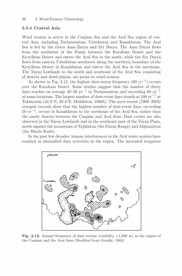
36 2 Wind-Erosion Climatology
2.5.4 Central Asia
Wind erosion is active in the Caspian Sea and the Aral Sea region of cen-tral Asia, including Turkmenistan, Uzbekistan and Kasakhstan. The AralSea is fed by the rivers Amu Darya and Syr Darya. The Amu Darya flowsfrom the northwest of the Pamir between the Karakum Desert and theKyzylkum Desert and enters the Aral Sea in the south, while the Syr Daryaflows from eastern Uzbekistan northwest along the northern boundary of theKyzylkum Desert in Kazakhstan and enters the Aral Sea in the northeast.The Turan Lowlands to the south and southeast of the Aral Sea, consistingof deserts and dried playas, are prone to wind erosion.
As shown in Fig. 2.12, the highest dust-storm frequency (60 yr−1) occursover the Karakum Desert. Some studies suggest that the number of dustydays reaches on average 40–50 yr−1 in Turkmenistan and exceeding 80 yr−1
at some locations. The largest number of dust-event days stands at 108 yr−1 atTakhiyatas (42.8N, 59.4E, Middleton, 1986b). The more recent (1998–2003)synoptic records show that the highest number of dust-event days, exceeding50 yr−1, occurs in Kasakhstan to the northeast of the Aral Sea, rather thanthe sandy deserts between the Caspian and Aral Seas. Dust events are alsoobserved in the Turan Lowlands and in the southeast part of the Turan Plain,nestle against the mountains of Tajikistan (the Gissar Range) and Afghanistan(the Hindu Kush).
In the past few decades, human interferences in the Aral water system haveresulted in intensified dust activities in the region. The increased irrigation
Fig. 2.12. Annual frequency of dust storms (visibility <1,000 m) in the region ofthe Caspian and the Aral Seas (Modified from Goudie, 1983)
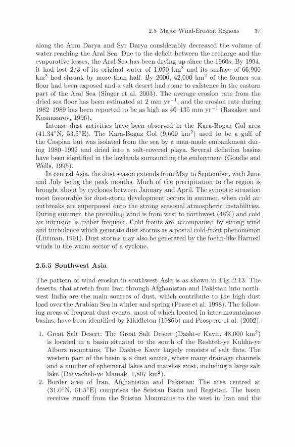
2.5 Major Wind-Erosion Regions 37
along the Amu Darya and Syr Darya considerably decreased the volume ofwater reaching the Aral Sea. Due to the deficit between the recharge and theevaporative losses, the Aral Sea has been drying up since the 1960s. By 1994,it had lost 2/3 of its original water of 1,090 km3 and its surface of 66,900km2 had shrunk by more than half. By 2000, 42,000 km2 of the former seafloor had been exposed and a salt desert had come to existence in the easternpart of the Aral Sea (Singer et al. 2003). The average erosion rate from thedried sea floor has been estimated at 2 mm yr−1, and the erosion rate during1982–1989 has been reported to be as high as 40–135 mm yr−1 (Razakov andKosnazarov, 1996).
Intense dust activities have been observed in the Kara-Bogaz Gol area(41.34N, 53.5E). The Kara-Bogaz Gol (9,600 km2) used to be a gulf ofthe Caspian but was isolated from the sea by a man-made embankment dur-ing 1980–1992 and dried into a salt-covered playa. Several deflation basinshave been identified in the lowlands surrounding the embayment (Goudie andWells, 1995).
In central Asia, the dust season extends from May to September, with Juneand July being the peak months. Much of the precipitation to the region isbrought about by cyclones between January and April. The synoptic situationmost favourable for dust-storm development occurs in summer, when cold airoutbreaks are superposed onto the strong seasonal atmospheric instabilities.During summer, the prevailing wind is from west to northwest (48%) and coldair intrusion is rather frequent. Cold fronts are accompanied by strong windand turbulence which generate dust storms as a postal cold-front phenomenon(Littman, 1991). Dust storms may also be generated by the foehn-like Harmsilwinds in the warm sector of a cyclone.
2.5.5 Southwest Asia
The pattern of wind erosion in southwest Asia is as shown in Fig. 2.13. Thedeserts, that stretch from Iran through Afghanistan and Pakistan into north-west India are the main sources of dust, which contribute to the high dustload over the Arabian Sea in winter and spring (Pease et al. 1998). The follow-ing areas of frequent dust events, most of which located in inter-mountainousbasins, have been identified by Middleton (1986b) and Prospero et al. (2002):
1. Great Salt Desert: The Great Salt Desert (Dasht-e Kavir, 48,000 km2)is located in a basin situated to the south of the Reshteh-ye Kuhha-yeAlborz mountains. The Dasht-e Kavir largely consists of salt flats. Thewestern part of the basin is a dust source, where many drainage channelsand a number of ephemeral lakes and marshes exist, including a large saltlake (Daryacheh-ye Mamak, 1,807 km2).
2. Border area of Iran, Afghanistan and Pakistan: The area centred at(31.0N, 61.5E) comprises the Seistan Basin and Registan. The basinreceives runoff from the Seistan Mountains to the west in Iran and the
38 2 Wind-Erosion Climatology
Fig. 2.13. Annual frequency of dust storms in southwest Asia and the main routesof dust transport (Modified from Washington et al. 2003)
mountains to the east in Afghanistan. Ephemeral lakes and swamps arewidespread in this area. Dust plumes have been seen to rise from theslat lakes in the northern part, e.g., Hamun-e Saberi (31.5N, 61.3E),Hamum-e Puzak (31.5N, 61.1E) and Daryacheh-ye-Hamun (31.7N,61.1E) and from the Gowd-e Zereh depression (29.8N, 61.8E). On aver-age, the number of dust days in the Seistan Basin is 80 yr−1. The northwestof Baluchistan in Pakistan, where a large dry lake (the Hamun-i-Mashkel,1,950 km2, 28.2N, 63.0E) is situated, has also been considered to be adust source.
3. Makran coastal area: High dust concentration has been observed to elon-gate from south-eastern Iran into the Indus Delta along the southernflanks of the Makran mountain chain. The dust plumes are believed to berelated to a dry salt lake, Humum-e Jaz Murian (1,087 km2).
4. Thar Desert: The Thar Desert (212,000 km2) centred in eastern Pakistanand western India, together with the arid regions of the Indian Rajasthan
2.5 Major Wind-Erosion Regions 39
Desert, is a major dust source of long wind-erosion history (Thomas et al.1999). The Himalayas and the Hindu Kush impart a strong control onthe dust sources and dust transport. This region receives large amountsof runoff from the mountains; these waters feed the Indus and Gangesriver systems, producing over time deep sediment deposits. Loess depositsderived from large-scale Pleistocene glaciofluvial outwash also serve aspresent-day dust sources. The desert was probably a much more intensesource of dust in the recent past and over time, aeolian processes hadselectively transported silt away, leaving behind coarse sands (Tripathiand Rajmani, 1999).
The seasonal variations of dust activities in southwest Asia are very muchdetermined by the Indian monsoon system. The onset of the Indian south-westerly summer monsoon occurs in mid June. By mid May, south-easterlywinds are active to the south of Bay of Bengal, which then progress rapidlytowards northwest, reaching Bay of Bengal in late May. In June, the Indiansummer monsoon breaks out over the subcontinent and in July advances toPakistan. The summer monsoon begins to retreat in September, and thenorth-westerly winter monsoon starts to dominate in December. The rainseason of the subcontinent falls between June and August.
In Iran, Afghanistan and Pakistan, dust activity starts in April–May, peaksin June–July, and greatly weakens by September. In northwest India, dustactivity starts in March–April and peaks in the pre-monsoon season of May–June. By July, when the Indian monsoon becomes established, dust activity isconfined to northwest India. Large dust storms in northwest India are usuallyassociated with the low-pressure systems, which usually last for several daysand produce dust storms over a wide area of northwest India and Pakistan.In the pre-monsoon season, the dust is generally transported to the northeastand east along the southern franks of the Tibetan Plateau, down the GangeticPlain by the southwest jet stream to as far as Myanmar. During winter, dustis transport to the Arabian Sea.
2.5.6 Northeast Asia
The sources of northeast Asian dust are the desert regions in China and Mon-golia. In China, arid and semiarid areas occupy 3.57 million km2, consistingof 0.25, 1.43, 1.14 and 0.75 million km2 hyper-arid, arid, semiarid and drysub-humid lands, respectively. Distributed from west to east are the Takli-makan (32.74 × 10⁴ km2), Gurbantunggut (4.73 × 10⁴ km2), Tsaidam Basin(3.31×10⁴ km2), Kumutage (1.95×10⁴ km2), Badain Juran (4.71×10⁴ km2),Tengger (3.67×10⁴ km2), Ulan Buh (1.03×10⁴ km2), Hobq (1.61×10⁴ km2),Mu Us (2.5 × 10⁴ km2), Small Tengger (2.33 × 10⁴ km2) and Keerxing(2.46 × 10⁴ km2). A considerable portion of Mongolia is occupied by desertplains, and southeast Mongolia is part of the Gobi.
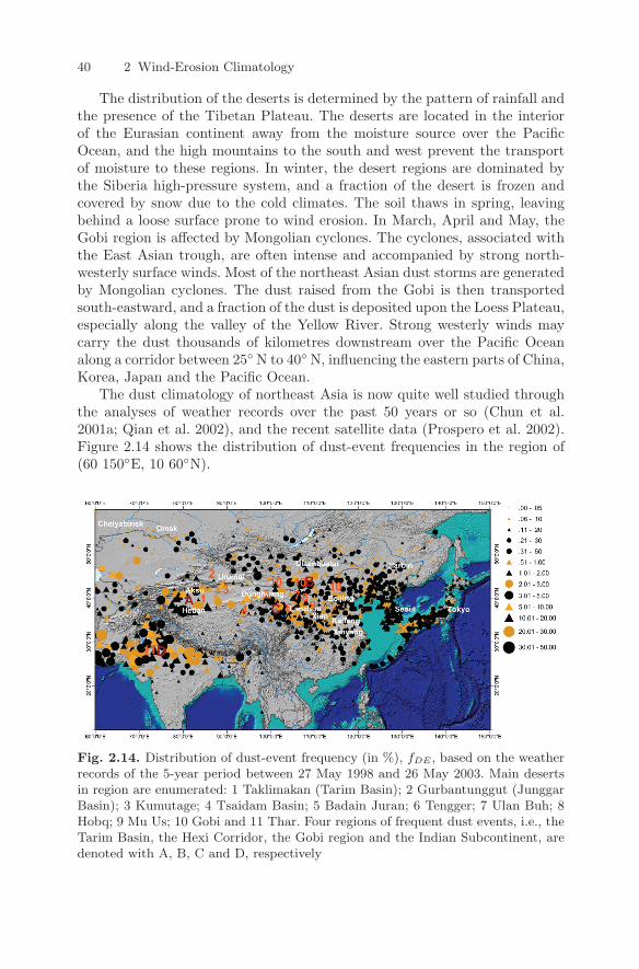
40 2 Wind-Erosion Climatology
The distribution of the deserts is determined by the pattern of rainfall andthe presence of the Tibetan Plateau. The deserts are located in the interiorof the Eurasian continent away from the moisture source over the PacificOcean, and the high mountains to the south and west prevent the transportof moisture to these regions. In winter, the desert regions are dominated bythe Siberia high-pressure system, and a fraction of the desert is frozen andcovered by snow due to the cold climates. The soil thaws in spring, leavingbehind a loose surface prone to wind erosion. In March, April and May, theGobi region is affected by Mongolian cyclones. The cyclones, associated withthe East Asian trough, are often intense and accompanied by strong north-westerly surface winds. Most of the northeast Asian dust storms are generatedby Mongolian cyclones. The dust raised from the Gobi is then transportedsouth-eastward, and a fraction of the dust is deposited upon the Loess Plateau,especially along the valley of the Yellow River. Strong westerly winds maycarry the dust thousands of kilometres downstream over the Pacific Oceanalong a corridor between 25 N to 40 N, influencing the eastern parts of China,Korea, Japan and the Pacific Ocean.
The dust climatology of northeast Asia is now quite well studied throughthe analyses of weather records over the past 50 years or so (Chun et al.2001a; Qian et al. 2002), and the recent satellite data (Prospero et al. 2002).Figure 2.14 shows the distribution of dust-event frequencies in the region of(60 150E, 10 60N).
Fig. 2.14. Distribution of dust-event frequency (in %), fDE , based on the weatherrecords of the 5-year period between 27 May 1998 and 26 May 2003. Main desertsin region are enumerated: 1 Taklimakan (Tarim Basin); 2 Gurbantunggut (JunggarBasin); 3 Kumutage; 4 Tsaidam Basin; 5 Badain Juran; 6 Tengger; 7 Ulan Buh; 8Hobq; 9 Mu Us; 10 Gobi and 11 Thar. Four regions of frequent dust events, i.e., theTarim Basin, the Hexi Corridor, the Gobi region and the Indian Subcontinent, aredenoted with A, B, C and D, respectively
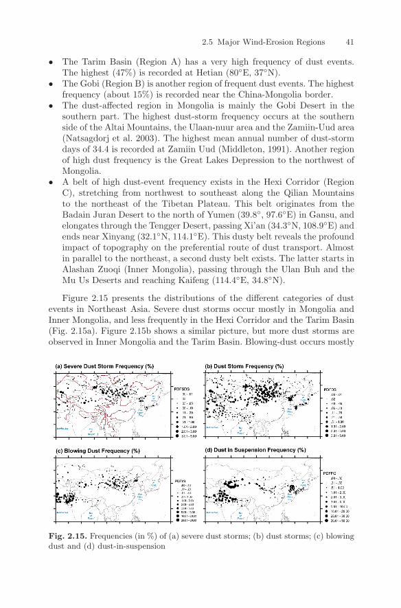
2.5 Major Wind-Erosion Regions 41
• The Tarim Basin (Region A) has a very high frequency of dust events.The highest (47%) is recorded at Hetian (80E, 37N).
• The Gobi (Region B) is another region of frequent dust events. The highestfrequency (about 15%) is recorded near the China-Mongolia border.
• The dust-affected region in Mongolia is mainly the Gobi Desert in thesouthern part. The highest dust-storm frequency occurs at the southernside of the Altai Mountains, the Ulaan-nuur area and the Zamiin-Uud area(Natsagdorj et al. 2003). The highest mean annual number of dust-stormdays of 34.4 is recorded at Zamiin Uud (Middleton, 1991). Another regionof high dust frequency is the Great Lakes Depression to the northwest ofMongolia.
• A belt of high dust-event frequency exists in the Hexi Corridor (RegionC), stretching from northwest to southeast along the Qilian Mountainsto the northeast of the Tibetan Plateau. This belt originates from theBadain Juran Desert to the north of Yumen (39.8, 97.6E) in Gansu, andelongates through the Tengger Desert, passing Xi’an (34.3N, 108.9E) andends near Xinyang (32.1N, 114.1E). This dusty belt reveals the profoundimpact of topography on the preferential route of dust transport. Almostin parallel to the northeast, a second dusty belt exists. The latter starts inAlashan Zuoqi (Inner Mongolia), passing through the Ulan Buh and theMu Us Deserts and reaching Kaifeng (114.4E, 34.8N).
Figure 2.15 presents the distributions of the different categories of dustevents in Northeast Asia. Severe dust storms occur mostly in Mongolia andInner Mongolia, and less frequently in the Hexi Corridor and the Tarim Basin(Fig. 2.15a). Figure 2.15b shows a similar picture, but more dust storms areobserved in Inner Mongolia and the Tarim Basin. Blowing-dust occurs mostly
Fig. 2.15. Frequencies (in %) of (a) severe dust storms; (b) dust storms; (c) blowingdust and (d) dust-in-suspension
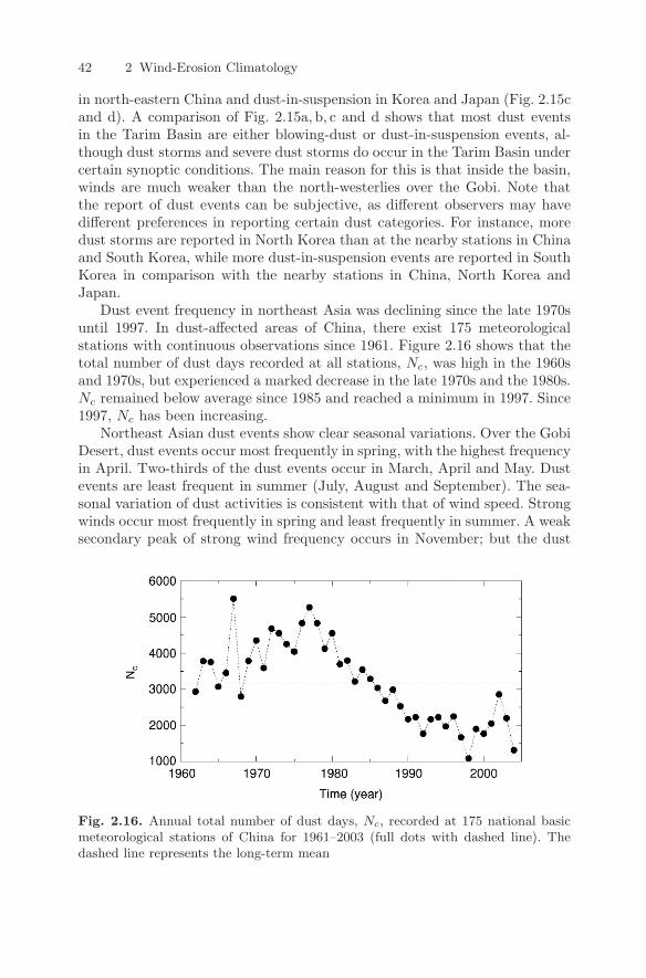
42 2 Wind-Erosion Climatology
in north-eastern China and dust-in-suspension in Korea and Japan (Fig. 2.15cand d). A comparison of Fig. 2.15a, b, c and d shows that most dust eventsin the Tarim Basin are either blowing-dust or dust-in-suspension events, al-though dust storms and severe dust storms do occur in the Tarim Basin undercertain synoptic conditions. The main reason for this is that inside the basin,winds are much weaker than the north-westerlies over the Gobi. Note thatthe report of dust events can be subjective, as different observers may havedifferent preferences in reporting certain dust categories. For instance, moredust storms are reported in North Korea than at the nearby stations in Chinaand South Korea, while more dust-in-suspension events are reported in SouthKorea in comparison with the nearby stations in China, North Korea andJapan.
Dust event frequency in northeast Asia was declining since the late 1970suntil 1997. In dust-affected areas of China, there exist 175 meteorologicalstations with continuous observations since 1961. Figure 2.16 shows that thetotal number of dust days recorded at all stations, Nc, was high in the 1960sand 1970s, but experienced a marked decrease in the late 1970s and the 1980s.Nc remained below average since 1985 and reached a minimum in 1997. Since1997, Nc has been increasing.
Northeast Asian dust events show clear seasonal variations. Over the GobiDesert, dust events occur most frequently in spring, with the highest frequencyin April. Two-thirds of the dust events occur in March, April and May. Dustevents are least frequent in summer (July, August and September). The sea-sonal variation of dust activities is consistent with that of wind speed. Strongwinds occur most frequently in spring and least frequently in summer. A weaksecondary peak of strong wind frequency occurs in November; but the dust
Fig. 2.16. Annual total number of dust days, Nc, recorded at 175 national basicmeteorological stations of China for 1961–2003 (full dots with dashed line). Thedashed line represents the long-term mean
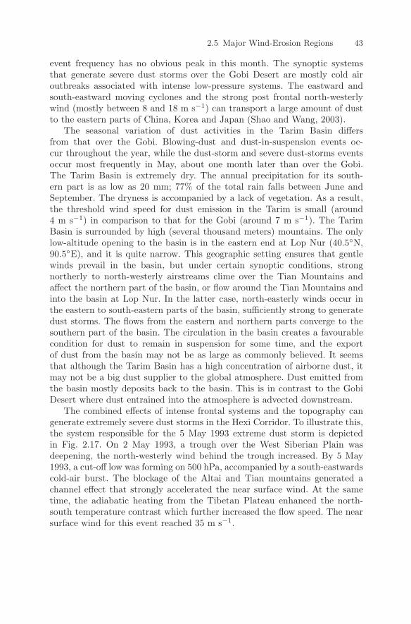
2.5 Major Wind-Erosion Regions 43
event frequency has no obvious peak in this month. The synoptic systemsthat generate severe dust storms over the Gobi Desert are mostly cold airoutbreaks associated with intense low-pressure systems. The eastward andsouth-eastward moving cyclones and the strong post frontal north-westerlywind (mostly between 8 and 18 m s−1) can transport a large amount of dustto the eastern parts of China, Korea and Japan (Shao and Wang, 2003).
The seasonal variation of dust activities in the Tarim Basin differsfrom that over the Gobi. Blowing-dust and dust-in-suspension events oc-cur throughout the year, while the dust-storm and severe dust-storms eventsoccur most frequently in May, about one month later than over the Gobi.The Tarim Basin is extremely dry. The annual precipitation for its south-ern part is as low as 20 mm; 77% of the total rain falls between June andSeptember. The dryness is accompanied by a lack of vegetation. As a result,the threshold wind speed for dust emission in the Tarim is small (around4 m s−1) in comparison to that for the Gobi (around 7 m s−1). The TarimBasin is surrounded by high (several thousand meters) mountains. The onlylow-altitude opening to the basin is in the eastern end at Lop Nur (40.5N,90.5E), and it is quite narrow. This geographic setting ensures that gentlewinds prevail in the basin, but under certain synoptic conditions, strongnortherly to north-westerly airstreams clime over the Tian Mountains andaffect the northern part of the basin, or flow around the Tian Mountains andinto the basin at Lop Nur. In the latter case, north-easterly winds occur inthe eastern to south-eastern parts of the basin, sufficiently strong to generatedust storms. The flows from the eastern and northern parts converge to thesouthern part of the basin. The circulation in the basin creates a favourablecondition for dust to remain in suspension for some time, and the exportof dust from the basin may not be as large as commonly believed. It seemsthat although the Tarim Basin has a high concentration of airborne dust, itmay not be a big dust supplier to the global atmosphere. Dust emitted fromthe basin mostly deposits back to the basin. This is in contrast to the GobiDesert where dust entrained into the atmosphere is advected downstream.
The combined effects of intense frontal systems and the topography cangenerate extremely severe dust storms in the Hexi Corridor. To illustrate this,the system responsible for the 5 May 1993 extreme dust storm is depictedin Fig. 2.17. On 2 May 1993, a trough over the West Siberian Plain wasdeepening, the north-westerly wind behind the trough increased. By 5 May1993, a cut-off low was forming on 500 hPa, accompanied by a south-eastwardscold-air burst. The blockage of the Altai and Tian mountains generated achannel effect that strongly accelerated the near surface wind. At the sametime, the adiabatic heating from the Tibetan Plateau enhanced the north-south temperature contrast which further increased the flow speed. The nearsurface wind for this event reached 35 m s−1.
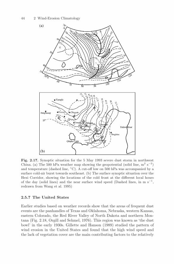
44 2 Wind-Erosion Climatology
Fig. 2.17. Synoptic situation for the 5 May 1993 severe dust storm in northwestChina. (a) The 500 hPa weather map showing the geopotential (solid line, m2 s−2)and temperature (dashed line, C). A cut-off low on 500 hPa was accompanied by asurface cold-air burst towards southeast. (b) The surface synoptic situation over theHexi Corridor, showing the locations of the cold front at the different local hoursof the day (solid lines) and the near surface wind speed (Dashed lines, in m s−1,redrawn from Wang et al. 1995)
2.5.7 The United States
Earlier studies based on weather records show that the areas of frequent dustevents are the panhandles of Texas and Oklahoma, Nebraska, western Kansas,eastern Colorado, the Red River Valley of North Dakota and northern Mon-tana (Fig. 2.18, Orgill and Sehmel, 1976). This region was known as ‘the dustbowl’ in the early 1930s. Gillette and Hanson (1989) studied the pattern ofwind erosion in the United States and found that the high wind speed andthe lack of vegetation cover are the main contributing factors to the relatively
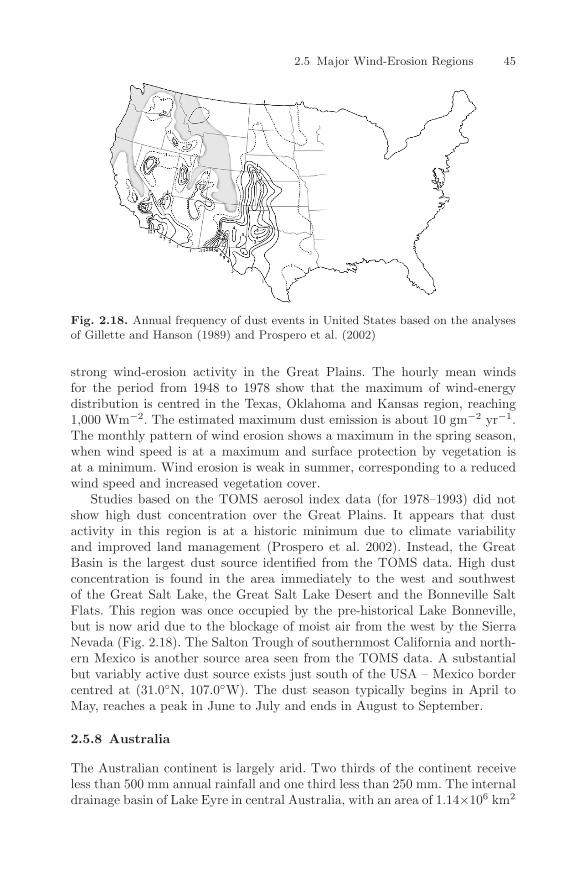
2.5 Major Wind-Erosion Regions 45
Fig. 2.18. Annual frequency of dust events in United States based on the analysesof Gillette and Hanson (1989) and Prospero et al. (2002)
strong wind-erosion activity in the Great Plains. The hourly mean windsfor the period from 1948 to 1978 show that the maximum of wind-energydistribution is centred in the Texas, Oklahoma and Kansas region, reaching1,000 Wm−2. The estimated maximum dust emission is about 10 gm−2 yr−1.The monthly pattern of wind erosion shows a maximum in the spring season,when wind speed is at a maximum and surface protection by vegetation isat a minimum. Wind erosion is weak in summer, corresponding to a reducedwind speed and increased vegetation cover.
Studies based on the TOMS aerosol index data (for 1978–1993) did notshow high dust concentration over the Great Plains. It appears that dustactivity in this region is at a historic minimum due to climate variabilityand improved land management (Prospero et al. 2002). Instead, the GreatBasin is the largest dust source identified from the TOMS data. High dustconcentration is found in the area immediately to the west and southwestof the Great Salt Lake, the Great Salt Lake Desert and the Bonneville SaltFlats. This region was once occupied by the pre-historical Lake Bonneville,but is now arid due to the blockage of moist air from the west by the SierraNevada (Fig. 2.18). The Salton Trough of southernmost California and north-ern Mexico is another source area seen from the TOMS data. A substantialbut variably active dust source exists just south of the USA – Mexico bordercentred at (31.0N, 107.0W). The dust season typically begins in April toMay, reaches a peak in June to July and ends in August to September.
2.5.8 Australia
The Australian continent is largely arid. Two thirds of the continent receiveless than 500 mm annual rainfall and one third less than 250 mm. The internaldrainage basin of Lake Eyre in central Australia, with an area of 1.14×10⁶ km2
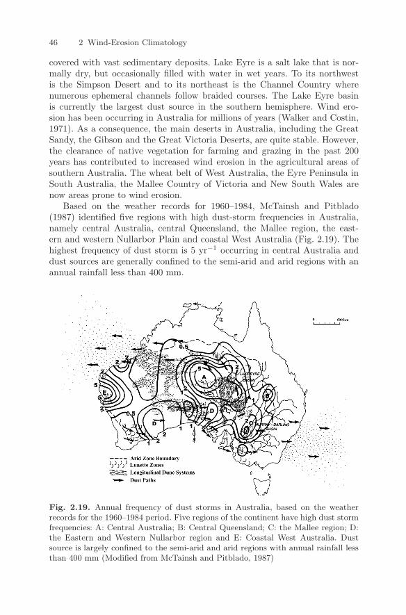
46 2 Wind-Erosion Climatology
covered with vast sedimentary deposits. Lake Eyre is a salt lake that is nor-mally dry, but occasionally filled with water in wet years. To its northwestis the Simpson Desert and to its northeast is the Channel Country wherenumerous ephemeral channels follow braided courses. The Lake Eyre basinis currently the largest dust source in the southern hemisphere. Wind ero-sion has been occurring in Australia for millions of years (Walker and Costin,1971). As a consequence, the main deserts in Australia, including the GreatSandy, the Gibson and the Great Victoria Deserts, are quite stable. However,the clearance of native vegetation for farming and grazing in the past 200years has contributed to increased wind erosion in the agricultural areas ofsouthern Australia. The wheat belt of West Australia, the Eyre Peninsula inSouth Australia, the Mallee Country of Victoria and New South Wales arenow areas prone to wind erosion.
Based on the weather records for 1960–1984, McTainsh and Pitblado(1987) identified five regions with high dust-storm frequencies in Australia,namely central Australia, central Queensland, the Mallee region, the east-ern and western Nullarbor Plain and coastal West Australia (Fig. 2.19). Thehighest frequency of dust storm is 5 yr−1 occurring in central Australia anddust sources are generally confined to the semi-arid and arid regions with anannual rainfall less than 400 mm.
Fig. 2.19. Annual frequency of dust storms in Australia, based on the weatherrecords for the 1960–1984 period. Five regions of the continent have high dust stormfrequencies: A: Central Australia; B: Central Queensland; C: the Mallee region; D:the Eastern and Western Nullarbor region and E: Coastal West Australia. Dustsource is largely confined to the semi-arid and arid regions with annual rainfall lessthan 400 mm (Modified from McTainsh and Pitblado, 1987)
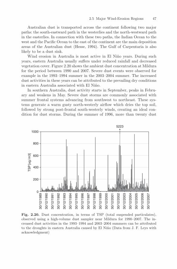
2.5 Major Wind-Erosion Regions 47
Australian dust is transported across the continent following two majorpaths: the south-eastward path in the westerlies and the north-westward pathin the easterlies. In connection with these two paths, the Indian Ocean to thewest and the Pacific Ocean to the east of the continent are the main depositionareas of the Australian dust (Hesse, 1994). The Gulf of Carpentaria is alsolikely to be a dust sink.
Wind erosion in Australia is most active in El Nino years. During suchyears, eastern Australia usually suffers under reduced rainfall and decreasedvegetation cover. Figure 2.20 shows the ambient dust concentration at Mildurafor the period between 1990 and 2007. Severe dust events were observed forexample in the 1993–1994 summer in the 2003–2004 summer. The increaseddust activities in these years can be attributed to the prevailing dry conditionsin eastern Australia associated with El Nino.
In southern Australia, dust activity starts in September, peaks in Febru-ary and weakens in May. Severe dust storms are commonly associated withsummer frontal systems advancing from southwest to northeast. These sys-tems generate a warm gusty north-westerly airflow which dries the top soil,followed by strong post-frontal south-westerly winds, creating an ideal con-dition for dust storms. During the summer of 1996, more than twenty dust
TS
P[u
g/m
3]
5223
1000
800
600
400
200
0
30/1
2/19
89
30/1
2/19
90
30/1
2/19
91
30/1
2/19
92
30/1
2/19
93
30/1
2/19
94
30/1
2/19
95
30/1
2/19
96
30/1
2/19
97
30/1
2/19
98
30/1
2/19
99
30/1
2/20
00
30/1
2/20
01
30/1
2/20
02
30/1
2/20
03
30/1
2/20
04
30/1
2/20
05
30/1
2/20
06
30/1
2/20
07
Fig. 2.20. Dust concentration, in terms of TSP (total suspended particulates),observed using a high-volume dust sampler near Mildura for 1990–2007. The in-creased dust activities in the 1993–1994 and 2003–2004 summers can be attributedto the droughts in eastern Australia caused by El Nino (Data from J. F. Leys withacknowledgment)

48 2 Wind-Erosion Climatology
events were recorded in Australia, with the 8–11 February storm being themost severe. The weather pattern which produced this storm, as shown inFig. 2.7, is typical for the region.
In northern Australia, wind erosion occurs mostly during the spring toearly summer. Winds are strongest and dust-storm frequency is highest inSeptember, October and November (McTainsh et al. 1998). As northernAustralia is influenced by summer rainfall, dust storms peak during Septem-ber to November at the end of the dry season, and then decrease with theonset of summer rains.
3
Atmospheric Boundary Layer and AtmosphericModelling
Atmospheric systems of various scales, from global circulation to boundary-layer turbulence, play an essential role in wind erosion. The general circulationof the atmosphere determines the global patterns of wind, precipitation, soilmoisture, vegetation cover etc. and hence the global pattern of wind erosion,as discussed in Chapter 2. For individual wind-erosion events, wind shear nearthe surface is responsible for particle entrainment into the atmosphere, andturbulence in the atmospheric boundary layer is important for particle dif-fusion and deposition. Severe dust storms are mostly generated by intensemeso-scale to synoptic-scale atmospheric systems, and the long-range trans-port of dust is dependent on the large-scale flow field. In this Chapter, wedescribe the basic aspects of the atmosphere that are relevant to wind erosionand give an outline of atmospheric modelling. The emphasis of the discussionis on the atmospheric boundary layer where the most important wind-erosionprocesses take place.
3.1 Atmospheric Boundary Layer
Based on its temperature profile, the atmosphere is divided into the tropo-sphere, the stratosphere, the mesosphere and the thermosphere (Fig. 3.1). Thetroposphere is about 10 km (polar region) to 15 km (tropics) deep, in whichtemperature decreases monotonically with height except at inversions. Mostsynoptic events take place in the troposphere. The atmospheric boundary layeris the layer of air of 1–2 km depth directly above the Earth’s surface, which isstrongly affected by the atmosphere-surface exchanges of momentum, energyand mass on time scales less than a day. The rest of the troposphere is thefree atmosphere. The atmospheric boundary layer has the following features:
• Flows are predominately turbulent, and the vertical transports of momen-tum, energy and mass are mainly accomplished by turbulence of scalessimilar to the boundary-layer depth or smaller
Y. Shao, Physics and Modelling of Wind Erosion, 49c© Springer Science+Business Media B.V. 2008
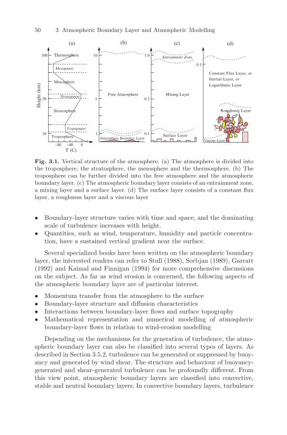
50 3 Atmospheric Boundary Layer and Atmospheric Modelling
100
50
10
T (C)
Hei
ght
(km
)
10
5
1
0.1
Surface Layer
0.5
1.0
0.1
−40 0
Tropopause
Mesopause
Roughness Layer
Constant Flux Layer, orInertial Layer, or
Logarithmic Layer
(a) (b) (c) (d)
Viscous Layer
Free Atmosphere Mixing Layer
Mesosphere
Thermosphere
Stratosphere
Troposphere Atmospheric Boundary Layer
Entrainment Zone
Stratopause
−80
Fig. 3.1. Vertical structure of the atmosphere. (a) The atmosphere is divided intothe troposphere, the stratosphere, the mesosphere and the thermosphere. (b) Thetroposphere can be further divided into the free atmosphere and the atmosphericboundary layer. (c) The atmospheric boundary layer consists of an entrainment zone,a mixing layer and a surface layer. (d) The surface layer consists of a constant fluxlayer, a roughness layer and a viscous layer
• Boundary-layer structure varies with time and space, and the dominatingscale of turbulence increases with height.
• Quantities, such as wind, temperature, humidity and particle concentra-tion, have a sustained vertical gradient near the surface.
Several specialized books have been written on the atmospheric boundarylayer, the interested readers can refer to Stull (1988), Sorbjan (1989), Garratt(1992) and Kaimal and Finnigan (1994) for more comprehensive discussionson the subject. As far as wind erosion is concerned, the following aspects ofthe atmospheric boundary layer are of particular interest.
• Momentum transfer from the atmosphere to the surface• Boundary-layer structure and diffusion characteristics• Interactions between boundary-layer flows and surface topography• Mathematical representation and numerical modelling of atmospheric
boundary-layer flows in relation to wind-erosion modelling
Depending on the mechanisms for the generation of turbulence, the atmo-spheric boundary layer can also be classified into several types of layers. Asdescribed in Section 3.5.2, turbulence can be generated or suppressed by buoy-ancy and generated by wind shear. The structure and behaviour of buoyancy-generated and shear-generated turbulence can be profoundly different. Fromthis view point, atmospheric boundary layers are classified into convective,stable and neutral boundary layers. In convective boundary layers, turbulence
3.1 Atmospheric Boundary Layer 51
is generated by buoyancy; in stable boundary layers, turbulence is suppressedby buoyancy, and in neutral boundary layers, turbulence is generated by windshear.
In a layer close to the surface, known as the surface layer, atmosphericquantities (e.g. wind speed, temperature and aerosol concentration) varyrapidly with height, and turbulence is predominantly generated by wind shearand the buoyancy effects are secondary although they may still be significant.The surface layer has several outstanding features which lead to its differentnames:
• Inertial Layer: Turbulent kinetic energy is generated mainly by wind shearand dissipated through a cascade process from large to small eddies andeventually to molecular motion.
• Constant Flux Layer: The vertical transfer of atmospheric quantities (e.g.momentum) is dominated by turbulent diffusion and the fluxes (e.g. mo-mentum flux) are almost constant with height.
• Logarithmic Layer: The vertical profiles of atmospheric quantities (e.g.wind speed) are approximately logarithmic.
The understanding of the surface layer is important to wind-erosion studiesbecause the entrainment of soil particles is determined by the momentumtransfer from this layer to the surface and the motion of sand-sized particlesis confined to this layer.
The surface is usually rough, because it consists of various roughness ele-ments such as plants, rocks and buildings. A criterion for determining whetherthe surface is smooth or rough is the Reynolds number defined by Equa-tion (3.35). The well-established theories for the surface layer mostly dealwith the bulk effects of the roughness elements on the flow. The depth of thesurface layer varies considerably, depending not only on the thermal stabilityof the surface layer but also on the types and arrangements of the roughnesselements. Over a moderately rough surface, e.g., a grass land, the depth ofthe surface layer may be several metres to several tens of metres. Over a veryrough surface, e.g., an urban surface, the depth of the surface layer may beseveral tens to several hundreds of metres.
Further, over a rough surface, a layer can be identified in which the flowis strongly affected by the presence of individual roughness elements. Thislayer is known as the roughness layer. The roughness layer is usually ex-tremely complex, and we do not yet have a general framework for describingits behaviour. The lack of understanding of the roughness layer poses a majorchallenge to the studies of wind erosion, because the fluid dynamic aspects ofwind erosion are essentially problems of the roughness layer. Most roughnesselements are non-erodible, such as the pebbles over the Gobi Desert and thethorn shrubs over the Sahel savanna. However, the presence of the roughnesselements can significantly alter the near-surface flow field and the distributionof shear stress on the surface which itself may be erodible. It is of particular
52 3 Atmospheric Boundary Layer and Atmospheric Modelling
interest in wind erosion studies to estimate the shear stress on the erodiblefraction of an aeolian surface, a problem known as drag partition, as discussedin Chapter 9.
In a layer very close to the smooth surface (i.e. the roughness elements aresufficiently small), say a few millimetres, turbulence is generally very weak dueto the very strong effect of viscous dissipation. Here, the transfer processesare dominated by molecular diffusion. This layer is called the viscous layer.
3.2 Governing Equations for AtmosphericBoundary-Layer Flows
We consider the atmospheric boundary layer in a local Cartesian coordinatesystem (x, y, z) with x pointing to east, y to north and z upward. To fa-cilitate the use of the Cartesian-tensor indicial notation, we shall also setx ≡ x1, y ≡ x2 and z ≡ x3. The atmospheric boundary-layer flow is com-pletely described by the temporal evolution of the velocity field (u ≡ u1,v ≡ u2, w ≡ u3) and the fields of pressure, p, density, ρ, temperature, T ,specific humidity, q, and a concentration, c. Since our main interest is winderosion, c represents the concentration of airborne dust. The quantities q andc are mixing ratios, defined respectively as the mass of water vapour and thatof soil particles per unit mass of air and have the dimensions of [M M−1].The corresponding governing equations for atmospheric boundary-layer floware consisted of the equations of motion, an equation of state, the continuityequation and the equations for temperature, moisture and dust concentration.These equations form a closed system which fully describes the spatial andtemporal dependence of u, v, w, p, ρ, T , q and c. For most purposes of at-mospheric boundary-layer studies and wind-erosion modelling, the governingequations are simplified using the Boussinesq approximations (Stull, 1988).
The continuity equation describes the conservation of mass (as well asinsuring that the atmosphere behaves as a physical continuum) and may bewritten as
∂ρ
∂t+
∂ρuj
∂xj= 0 (3.1)
where t is time and uj is the jth component of flow speed. Under the assump-tion that atmospheric boundary-layer flows are incompressible, the continuityequation becomes
∂uj
∂xj= 0 (3.2)
The equations of motion can be written as
dui
dt= −δi3g − 2εijkΩjuk − 1
ρ
∂p
∂xi+
1ρ
∂τij
∂xj(3.3)
3.2 Governing Equations for Atmospheric Boundary-Layer Flows 53
The inertial term can also be written as
dui
dt=
∂ui
∂t+ uj
∂ui
∂xj
The Kronecker and Alternating tensors are respectively defined by
δij =
1 for i = j0 for i = j
and
εijk =
⎧⎨⎩
1 for cases 123, 231, 312−1 for cases 321, 213, 1320 otherwise
Terms 1, 2, 3 and 5 in Equation (3.3) represent momentum storage, advection,gravity force and pressure-gradient force, respectively. Term 4 is the Coriolisforce arising from the Earth’s rotation. Ωj is the jth component of the Earth’srotation vector Ω = [0, Ω cos φ,Ω sinφ], with Ω = 7.27 × 10⁻⁵ s−1 being theangular speed of the Earth’s rotation and φ being the latitude. Since thevertical velocity component of the atmosphere is small, the Coriolis term canbe simplified to fεij3uj with f = 2Ω sin φ. Term 6 is the divergence of viscousshear stress, τij , which causes the fluid to deform due to intermolecular forces.
We can interpret τij as the force per unit area in the xi direction actingon the face that is normal to the xj direction. The viscous shear stress is asymmetric tensor of nine components with six independent ones, as τij = τji.Using the Boussinesq approximations that the dynamic viscosity (a propertyof the fluid), µ, is constant and the flow is incompressible, the viscous shear-stress term can be simplified to
1ρ
∂τij
∂xj= ν
∂2ui
∂x2j
where ν = µ/ρ is the kinematical molecular viscosity. For atmosphericboundary-layer flows, ν is approximately 1.5×10⁻⁵ m2 s−1. Finally, the equa-tions of motion are simplified to
dui
dt= −δi3g + fεij3uj −
1ρ
∂p
∂xi+ ν
∂2ui
∂x2j
(3.4)
For the x-component of the flow, we can write Equation (3.4) explicitly as
du
dt= fv − 1
ρ
∂p
∂x+ ν
(∂2u
∂x2+
∂2u
∂y2+
∂2u
∂z2
)
The Reynolds number is the ratio of the magnitude of the inertial term tothe viscous term,
Re =du
dt/ν
∂2u
∂x2

54 3 Atmospheric Boundary Layer and Atmospheric Modelling
The larger the Reynolds Number, the less important is the viscous term inthe equations of motion. In order to estimate the magnitude of Re, we intro-duce a typical velocity scale V and a typical length scale L for the flow anduse them to normalise the corresponding variables. The dimensionless velocity,time and length are then u∗ ≈ u/V , t∗ ≈ tV/L and x∗ ≈ x/L, respectively. Itfollows that the Reynolds Number can be expressed as
Re =du∗
dt∗V 2L−1/ν
∂2u∗
∂x∗2 V L−2
If the characteristic scales V and L are correctly chosen for a particular fluiddynamic problem, then
du∗
dt∗/∂2u∗
∂x∗2 ≈ O(1)
and we obtain an approximation to the Reynolds Number
Re ≈ V L/ν (3.5)
For atmospheric boundary-layer flows, V ≈ 5 ms−1 and L ≈ 100 m, it fol-lows that Re ≈ 3 × 10⁷. Hence, atmospheric boundary-layer flows have largeReynolds Numbers and are almost always turbulent. So it follows that theviscous shear-stress term is often neglected from the equations of motion forflows in the body of the atmospheric boundary layer. However, very close tothe surface (where L is small), the Reynolds Number reduces and the flowbecomes laminar. The viscous layer (or laminar layer) close to the surface hasa thickness of only a few millimetres.
The equation of state describes the relationship between pressure, temper-ature and density
p = ρRaT (3.6)
where Ra is the specific gas constant of air. If air is dry, Ra = R/Md = 287 Jkg−1K−1, with R being the universal gas constant and Md being the molecularweight of dry air. For humid air, Ra = (1 + 0.61q)R/Md.
If an air parcel is subject to heating, its temperature and density willchange according to the first law of thermodynamics
cvdT
dt+ p
dα
dt= se (3.7)
where se is the heating rate per unit mass, α = 1/ρ, cv is the specific heat atconstant volume. If se is zero, the process is adiabatic. Using the equation ofstate and the relationship cp = cv + Ra, where cp is specific heat at constantpressure, we obtain for adiabatic processes
cpd(ln T ) − Rad(ln p) = 0 (3.8)
The potential temperature, θ, is the temperature an air parcel at pressurep with temperature T would have if brought adiabatically to the reference
3.2 Governing Equations for Atmospheric Boundary-Layer Flows 55
pressure level of ps. An integration of the above equation from p to ps givesthe Poisson equation:
θ = T
(p
ps
)−Ra/cp
(3.9)
where ps is conventionally taken to be 1000 hPa. Logarithmically differenti-ating the Poisson equation and making use of Equation (3.8), we obtain
dθ = 0
This implies that, if an air parcel rises adiabatically (i.e. p decreases), itstemperature decreases, but its potential temperature remains unchanged.Therefore, for adiabatic processes, which most atmospheric boundary-layerprocesses are, θ is a conserved quantity. When we shall see in Section 8.2, in aLagrangian dust transport model, it is often assumed that the motion of dustparticles is confined to an isentropic surface, namely a surface of constant θ.In other words, we assume dust particles move with air parcels which moveadiabatically in the atmosphere.
The energy conservation equation for atmospheric boundary-layer flowscan be expressed in terms of potential temperature as (or enthalpy cpθ),
∂cpθ
∂t+ uj
∂cpθ
∂xj= kT
∂2cpθ
∂x2j
+1ρ
∂Rj
∂xj− λlE
ρ(3.10)
where kT is the molecular diffusivity for heat, Rj is the jth component ofthe radiative heat flux, E is the evaporation rate in the air and λl is thelatent-heat coefficient of vaporization for water (λl = 2.45 × 10⁶ J kg−1 at atemperature of 293 K). Dust particles suspended in the atmosphere interferewith atmospheric radiative transfer processes through absorption, reflectionand scattering of solar and terrestrial radiation, and hence affect Rj .
The moisture conservation equation, in terms of q, is given by
∂q
∂t+ uj
∂q
∂xj= kq
∂2q
∂x2j
+ sq (3.11)
where kq is the molecular diffusivity for air moisture and sq is a moisturesource. Similar to Equation (3.11), the dust concentration equation is givenby
∂c
∂t+ upj
∂c
∂xj= kp
∂2c
∂x2j
+ sc (3.12)
where kp is the molecular diffusivity for dust particles, and sc is a dustsource in air. The advection velocity, upj , is the jth component of the dust-particle velocity, which can be written as upj = uj + urj , where urj denotesthe relative velocity of dust particle with respect to fluid. This particle-to-fluidrelative velocity occurs because dust particles have a finite response time to ve-locity changes in the surrounding air, as well as falling through that air under
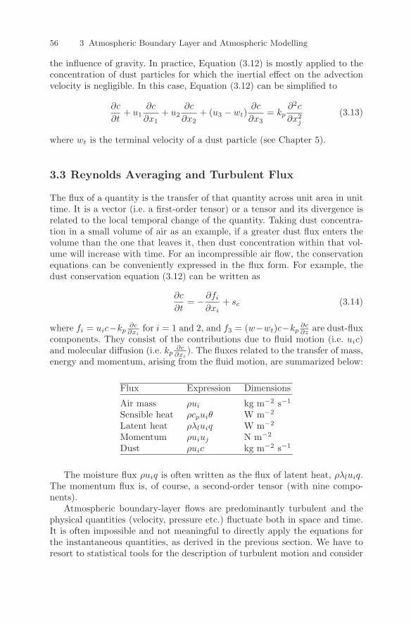
56 3 Atmospheric Boundary Layer and Atmospheric Modelling
the influence of gravity. In practice, Equation (3.12) is mostly applied to theconcentration of dust particles for which the inertial effect on the advectionvelocity is negligible. In this case, Equation (3.12) can be simplified to
∂c
∂t+ u1
∂c
∂x1+ u2
∂c
∂x2+ (u3 − wt)
∂c
∂x3= kp
∂2c
∂x2j
(3.13)
where wt is the terminal velocity of a dust particle (see Chapter 5).
3.3 Reynolds Averaging and Turbulent Flux
The flux of a quantity is the transfer of that quantity across unit area in unittime. It is a vector (i.e. a first-order tensor) or a tensor and its divergence isrelated to the local temporal change of the quantity. Taking dust concentra-tion in a small volume of air as an example, if a greater dust flux enters thevolume than the one that leaves it, then dust concentration within that vol-ume will increase with time. For an incompressible air flow, the conservationequations can be conveniently expressed in the flux form. For example, thedust conservation equation (3.12) can be written as
∂c
∂t= − ∂fi
∂xi+ sc (3.14)
where fi = uic−kp∂c∂xi
for i = 1 and 2, and f3 = (w−wt)c−kp∂c∂z are dust-flux
components. They consist of the contributions due to fluid motion (i.e. uic)and molecular diffusion (i.e. kp
∂c∂xi
). The fluxes related to the transfer of mass,energy and momentum, arising from the fluid motion, are summarized below:
Flux Expression Dimensions
Air mass ρui kg m−2 s−1
Sensible heat ρcpuiθ W m−2
Latent heat ρλluiq W m−2
Momentum ρuiuj N m−2
Dust ρuic kg m−2 s−1
The moisture flux ρuiq is often written as the flux of latent heat, ρλluiq.The momentum flux is, of course, a second-order tensor (with nine compo-nents).
Atmospheric boundary-layer flows are predominantly turbulent and thephysical quantities (velocity, pressure etc.) fluctuate both in space and time.It is often impossible and not meaningful to directly apply the equations forthe instantaneous quantities, as derived in the previous section. We have toresort to statistical tools for the description of turbulent motion and consider
3.3 Reynolds Averaging and Turbulent Flux 57
the statistical moments, such as the mean, variance and covariance of the tur-bulent variables. In order to derive the equations for the statistical moments,we separate the quantities under consideration into their mean and turbulentcomponents. Thus, for any variable a, we have that
a = a + a′ (3.15)
where a is the mean component of a and a′ is the deviation of a from a.The average of a flux, for instance, that of dust flux, ρuic, can be expressed
asρuic = ρ(ui + u′
i)(c + c′) = ρuic + ρu′ic
′ (3.16)
The term ρu′ic
′ is the dust flux due to turbulent motion, which is in generalnot zero. The above expression implies that the average dust flux can beconsidered to consist of two components; namely, dust transport by the meanflow and a turbulent dust flux. Similarly, the mean of the sensible-heat flux is
ρcpuiθ = ρcpuiθ + ρcpu′iθ
′ (3.17)
and of the momentum flux is
ρuiuj = ρuiuj + ρu′iu
′j (3.18)
where ρu′iu
′j are the Reynolds shear stress. Let us consider an air cube for
a moment. The term ρu′iu
′j can be interpreted as the force per unit area in
the xi direction acting on the face of the cube with the face direction inthe xj direction. For example, ρu′w′ is the force in the x direction actingon the face with face direction in the z direction. The Reynolds shear stressis also a symmetric tensor of nine components with six independent ones, asρu′
iu′j = ρu′
ju′i. The components ρu′w′ and ρv′w′, namely, the vertical fluxes of
streamwise momentum are the most important ones as far as the atmosphericboundary-layer and wind-erosion studies are concerned.
Turbulent motion leads to the transport of a quantity without involvinga net transport of mass. The term u′
ic′ is formally similar to uic, except that
the perturbation values are used instead of the mean values of ui and c.The mechanism through which turbulence generates a dust flux is illustratedin Fig. 3.2a. If dust particles are emitted from the surface, there would be adecrease of mean dust concentration with height. Near the surface, turbulencecan be depicted as swirling motions, in which fluid parcels from position 1are mixed downward (negative w′), while others from position 2 are mixedupward (positive w′) to take the place of downward moving parcels. Themean mass transfer associated with this process, ρw′, is zero. However, thedownward moving air parcels, being associated with a lower dust concentration(negative c′), result in a positive product w′c′. The upward moving parcels,being associated with a higher dust concentration (positive c′), also result ina positive flux w′c′. Both the upward and downward moving air contribute
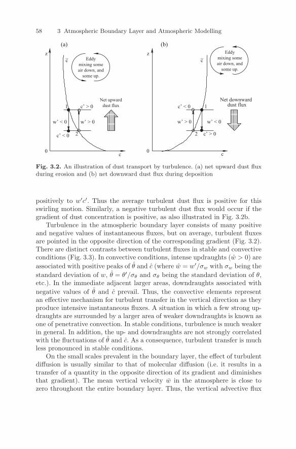
58 3 Atmospheric Boundary Layer and Atmospheric Modelling
1
2 2
1Net upward
dust flux
c c
c−c− Eddymixing someair down, and
some up.
Eddymixing someair down, and
some up.
Net downwarddust fluxc’ > 0
w’ > 0 w’ > 0
c’ > 0
w’ < 0
c’ < 0
c’ < 0
z
0
(a) (b)z
0
w’ < 0
Fig. 3.2. An illustration of dust transport by turbulence. (a) net upward dust fluxduring erosion and (b) net downward dust flux during deposition
positively to w′c′. Thus the average turbulent dust flux is positive for thisswirling motion. Similarly, a negative turbulent dust flux would occur if thegradient of dust concentration is positive, as also illustrated in Fig. 3.2b.
Turbulence in the atmospheric boundary layer consists of many positiveand negative values of instantaneous fluxes, but on average, turbulent fluxesare pointed in the opposite direction of the corresponding gradient (Fig. 3.2).There are distinct contrasts between turbulent fluxes in stable and convectiveconditions (Fig. 3.3). In convective conditions, intense updraughts (w > 0) areassociated with positive peaks of θ and c (where w = w′/σw with σw being thestandard deviation of w, θ = θ′/σθ and σθ being the standard deviation of θ,etc.). In the immediate adjacent larger areas, downdraughts associated withnegative values of θ and c prevail. Thus, the convective elements representan effective mechanism for turbulent transfer in the vertical direction as theyproduce intensive instantaneous fluxes. A situation in which a few strong up-draughts are surrounded by a larger area of weaker downdraughts is known asone of penetrative convection. In stable conditions, turbulence is much weakerin general. In addition, the up- and downdraughts are not strongly correlatedwith the fluctuations of θ and c. As a consequence, turbulent transfer is muchless pronounced in stable conditions.
On the small scales prevalent in the boundary layer, the effect of turbulentdiffusion is usually similar to that of molecular diffusion (i.e. it results in atransfer of a quantity in the opposite direction of its gradient and diminishesthat gradient). The mean vertical velocity w in the atmosphere is close tozero throughout the entire boundary layer. Thus, the vertical advective flux
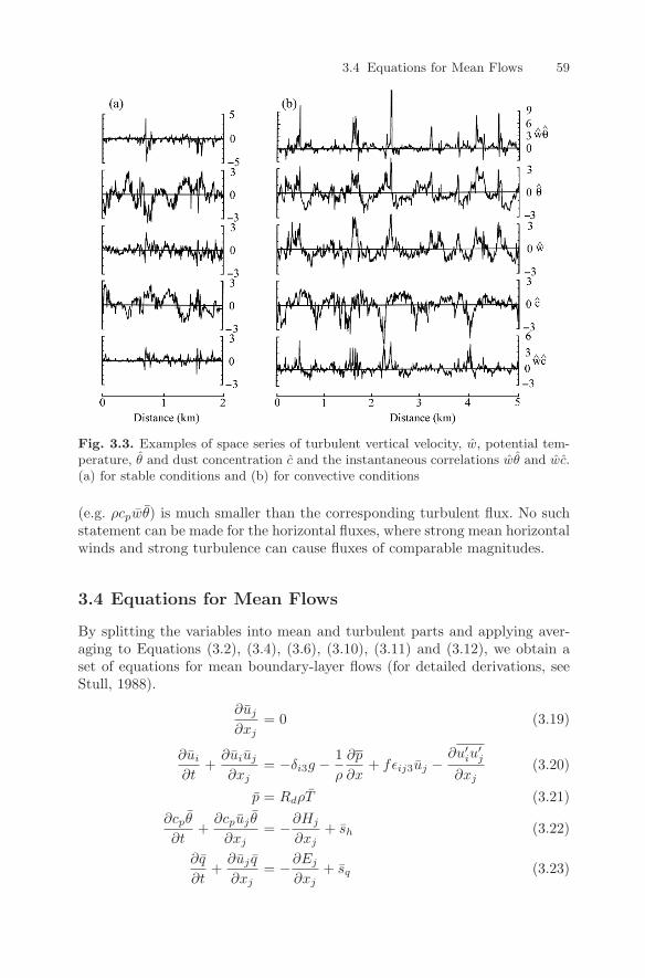
3.4 Equations for Mean Flows 59
Fig. 3.3. Examples of space series of turbulent vertical velocity, w, potential tem-perature, θ and dust concentration c and the instantaneous correlations wθ and wc.(a) for stable conditions and (b) for convective conditions
(e.g. ρcpwθ) is much smaller than the corresponding turbulent flux. No suchstatement can be made for the horizontal fluxes, where strong mean horizontalwinds and strong turbulence can cause fluxes of comparable magnitudes.
3.4 Equations for Mean Flows
By splitting the variables into mean and turbulent parts and applying aver-aging to Equations (3.2), (3.4), (3.6), (3.10), (3.11) and (3.12), we obtain aset of equations for mean boundary-layer flows (for detailed derivations, seeStull, 1988).
∂uj
∂xj= 0 (3.19)
∂ui
∂t+
∂uiuj
∂xj= −δi3g − 1
ρ
∂p
∂x+ fεij3uj −
∂u′iu
′j
∂xj(3.20)
p = RdρT (3.21)∂cpθ
∂t+
∂cpuj θ
∂xj= −∂Hj
∂xj+ sh (3.22)
∂q
∂t+
∂uj q
∂xj= −∂Ej
∂xj+ sq (3.23)
60 3 Atmospheric Boundary Layer and Atmospheric Modelling
∂c
∂t+
∂uj c
∂xj− wt
∂c
∂z= −∂Fj
∂xj+ sc (3.24)
where Ej , Fj and Hj are respectively the jth component of turbulent fluxesof moisture, dust and heat, and sq, sc and sh are respectively the sources formoisture, dust and heat; Rj is the jth component of the mean radiation flux.In the above equations, we have neglected the effects of the molecular motion.
3.5 Equations for Turbulent Fluxes and Variances
Turbulent fluxes, such as cpu′jθ
′, u′jc
′ and u′iu
′j , appear in Equations (3.19)–
(3.24). To apply these equations for modelling atmospheric boundary-layerflows, the turbulent fluxes must be determined through either parameterisa-tions or using prognostic equations. As most of the relevant prognostic equa-tions can be found in Stull (1988), for instance, only the prognostic equationfor the turbulent dust flux is given here.
3.5.1 Turbulent Dust Flux and Dust Concentration Variance
The turbulent dust flux equation can be derived through the following steps:
• Substitute c = c + c′ into Equation (3.12)• Subtract Equation (3.24) from the resulting equation to obtain an equation
for c′
• Similarly, derive an equation for u′i
• Multiply u′i with the c′ equation and c′ with the u′
i equation and combinethe two equations to obtain an equation for u′
ic′
• Average the u′ic
′ equation
Finally, the equations for the turbulent dust flux can be written as
∂u′ic
′
∂t+ uj
∂u′ic
′
∂xj− wt
∂u′ic
′
∂z=
−u′jc
′ ∂ui
∂xj− u′
iu′j
∂c
∂xj−
∂u′ju
′ic
′
∂xj+ δi3
c′θ′g
θ+
p′
ρ
∂c′
∂xi− 2εuic
(3.25)
Again, the vertical component of the turbulent dust flux is the most importantone. Under the assumption of horizontal homogeneity and zero mean verticalwind, we have
∂w′c′
∂t− wt
∂w′c′
∂z= −σ2
w
∂c
∂z+
c′θ′g
θ− ∂w′w′c′
∂z− 2εwc (3.26)
Equation (3.26) implies that the temporal change of turbulent dust flux ismainly influenced by (1) the advection related to settling wt∂w′c′/∂z; (2) the
3.5 Equations for Turbulent Fluxes and Variances 61
production related to mean dust concentration profile and turbulence intensity−σ2
w∂c/∂z and to buoyancy c′θ′g/θ; (3) the turbulent transport −∂w′w′c′/∂z;and (4) the molecular dissipation −2εwc. The usefulness of Equation (3.26) inwind-erosion studies has not been fully explored.
To derive the prognostic equation for dust concentration variance, we mul-tiply the c′ equation with 2c′. By applying the Reynolds averaging to theresulting equation, we obtain
∂σ2c
∂t+ uj
∂σ2c
∂xj− wt
∂σ2c
∂z= −2c′u′
j
∂c
∂xj−
∂u′jc
′2
∂xj− 2εc (3.27)
where εc = kp(∂c′/∂xj)2 is the molecular dissipation rate for dust-concentration variance, which is always positive. Equation (3.27) shows thatthe local change of dust concentration variance is mainly influenced by (1) theadvection related to fluid motion and particle settling uj∂σ2
c/∂xj −wt∂σ2c/∂z;
(2) the production related to mean dust concentration gradient and turbu-lent dust flux −2u′
jc′∂c/∂xj ; (3) turbulent transport −∂u′
jc′2/∂xj ; and (4)
molecular dissipation −2εc. As for Equation (3.26), the application of Equa-tion (3.27) in wind-erosion studies requires further exploration.
3.5.2 Turbulent Kinetic Energy
By definition turbulent kinetic energy is given by
e =12(u′2 + v′2 + w′2)
The turbulent kinetic energy equation is one of the most important equationsfor atmospheric boundary-layer studies. Following a similar procedure for thederivation of the equation of dust-concentration variance, we obtain the equa-tions for the variances of u, v and w. A summation of the three equationsleads to the turbulent kinetic energy equation, which can be written as
∂e
∂t+ uj
∂e
∂xj= δj3
g
θu′
jθ′ − u′
iu′j
∂ui
∂xj− u′
j
∂e
∂xj− 1
ρ
∂u′ip
′
∂xj− ε (3.28)
where ε = ν(
∂u′i
∂xj
)2
is the viscous dissipation rate for turbulent kinetic energy.This term is always positive and causes a decrease in turbulent kinetic energywith time by converting it irreversibly to heat. If we use a coordinate systemwhich is aligned with the mean wind, U , and assume horizontal homogeneity,we obtain a much simplified equation
∂e
∂t=
g
θw′θ′ +
τ
ρ
∂U
∂z− ∂w′e
∂z− 1
ρ
∂w′p′
∂z− ε (3.29)
where τ = −ρu′w′ is the vertical component of the momentum flux, which isconventionally taken to be positive when pointing downward. The term g
θw′θ′
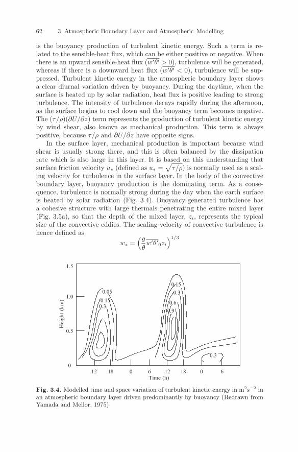
62 3 Atmospheric Boundary Layer and Atmospheric Modelling
is the buoyancy production of turbulent kinetic energy. Such a term is re-lated to the sensible-heat flux, which can be either positive or negative. Whenthere is an upward sensible-heat flux (w′θ′ > 0), turbulence will be generated,whereas if there is a downward heat flux (w′θ′ < 0), turbulence will be sup-pressed. Turbulent kinetic energy in the atmospheric boundary layer showsa clear diurnal variation driven by buoyancy. During the daytime, when thesurface is heated up by solar radiation, heat flux is positive leading to strongturbulence. The intensity of turbulence decays rapidly during the afternoon,as the surface begins to cool down and the buoyancy term becomes negative.The (τ/ρ)(∂U/∂z) term represents the production of turbulent kinetic energyby wind shear, also known as mechanical production. This term is alwayspositive, because τ/ρ and ∂U/∂z have opposite signs.
In the surface layer, mechanical production is important because windshear is usually strong there, and this is often balanced by the dissipationrate which is also large in this layer. It is based on this understanding thatsurface friction velocity u∗ (defined as u∗ =
√τ/ρ) is normally used as a scal-
ing velocity for turbulence in the surface layer. In the body of the convectiveboundary layer, buoyancy production is the dominating term. As a conse-quence, turbulence is normally strong during the day when the earth surfaceis heated by solar radiation (Fig. 3.4). Buoyancy-generated turbulence hasa cohesive structure with large thermals penetrating the entire mixed layer(Fig. 3.5a), so that the depth of the mixed layer, zi, represents the typicalsize of the convective eddies. The scaling velocity of convective turbulence ishence defined as
w∗ =(g
θw′θ′0zi
)1/3
Hei
ght
(km
)
0.05
0.150.3
0.15
0.3
0.6
0.9
0.3
18 0 6 612 18 0120
0.5
1.0
1.5
Time (h)
Fig. 3.4. Modelled time and space variation of turbulent kinetic energy in m2s−2 inan atmospheric boundary layer driven predominantly by buoyancy (Redrawn fromYamada and Mellor, 1975)
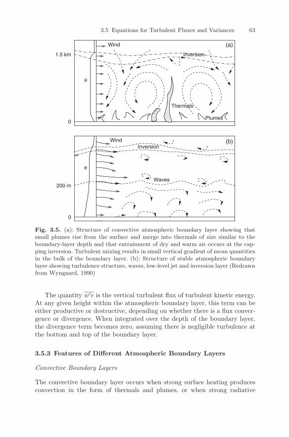
3.5 Equations for Turbulent Fluxes and Variances 63
Inversion
Thermals
Plumes
Waves
Inversion
Wind
Wind
θ
θ
1.5 km
0
(a)
(b)
200 m
0
Fig. 3.5. (a): Structure of convective atmospheric boundary layer showing thatsmall plumes rise from the surface and merge into thermals of size similar to theboundary-layer depth and that entrainment of dry and warm air occurs at the cap-ping inversion. Turbulent mixing results in small vertical gradient of mean quantitiesin the bulk of the boundary layer. (b): Structure of stable atmospheric boundarylayer showing turbulence structure, waves, low-level jet and inversion layer (Redrawnfrom Wyngaard, 1990)
The quantity w′e is the vertical turbulent flux of turbulent kinetic energy.At any given height within the atmospheric boundary layer, this term can beeither productive or destructive, depending on whether there is a flux conver-gence or divergence. When integrated over the depth of the boundary layer,the divergence term becomes zero, assuming there is negligible turbulence atthe bottom and top of the boundary layer.
3.5.3 Features of Different Atmospheric Boundary Layers
Convective Boundary Layers
The convective boundary layer occurs when strong surface heating producesconvection in the form of thermals and plumes, or when strong radiative
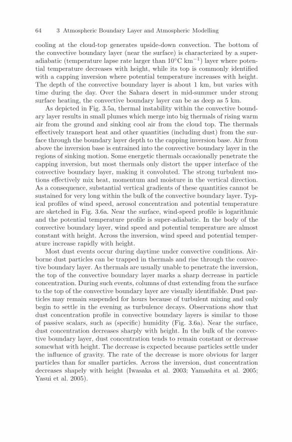
64 3 Atmospheric Boundary Layer and Atmospheric Modelling
cooling at the cloud-top generates upside-down convection. The bottom ofthe convective boundary layer (near the surface) is characterized by a super-adiabatic (temperature lapse rate larger than 10C km−1) layer where poten-tial temperature decreases with height, while its top is commonly identifiedwith a capping inversion where potential temperature increases with height.The depth of the convective boundary layer is about 1 km, but varies withtime during the day. Over the Sahara desert in mid-summer under strongsurface heating, the convective boundary layer can be as deep as 5 km.
As depicted in Fig. 3.5a, thermal instability within the convective bound-ary layer results in small plumes which merge into big thermals of rising warmair from the ground and sinking cool air from the cloud top. The thermalseffectively transport heat and other quantities (including dust) from the sur-face through the boundary layer depth to the capping inversion base. Air fromabove the inversion base is entrained into the convective boundary layer in theregions of sinking motion. Some energetic thermals occasionally penetrate thecapping inversion, but most thermals only distort the upper interface of theconvective boundary layer, making it convoluted. The strong turbulent mo-tions effectively mix heat, momentum and moisture in the vertical direction.As a consequence, substantial vertical gradients of these quantities cannot besustained for very long within the bulk of the convective boundary layer. Typ-ical profiles of wind speed, aerosol concentration and potential temperatureare sketched in Fig. 3.6a. Near the surface, wind-speed profile is logarithmicand the potential temperature profile is super-adiabatic. In the body of theconvective boundary layer, wind speed and potential temperature are almostconstant with height. Across the inversion, wind speed and potential temper-ature increase rapidly with height.
Most dust events occur during daytime under convective conditions. Air-borne dust particles can be trapped in thermals and rise through the convec-tive boundary layer. As thermals are usually unable to penetrate the inversion,the top of the convective boundary layer marks a sharp decrease in particleconcentration. During such events, columns of dust extending from the surfaceto the top of the convective boundary layer are visually identifiable. Dust par-ticles may remain suspended for hours because of turbulent mixing and onlybegin to settle in the evening as turbulence decays. Observations show thatdust concentration profile in convective boundary layers is similar to thoseof passive scalars, such as (specific) humidity (Fig. 3.6a). Near the surface,dust concentration decreases sharply with height. In the bulk of the convec-tive boundary layer, dust concentration tends to remain constant or decreasesomewhat with height. The decrease is expected because particles settle underthe influence of gravity. The rate of the decrease is more obvious for largerparticles than for smaller particles. Across the inversion, dust concentrationdecreases shapely with height (Iwasaka et al. 2003; Yamashita et al. 2005;Yasui et al. 2005).
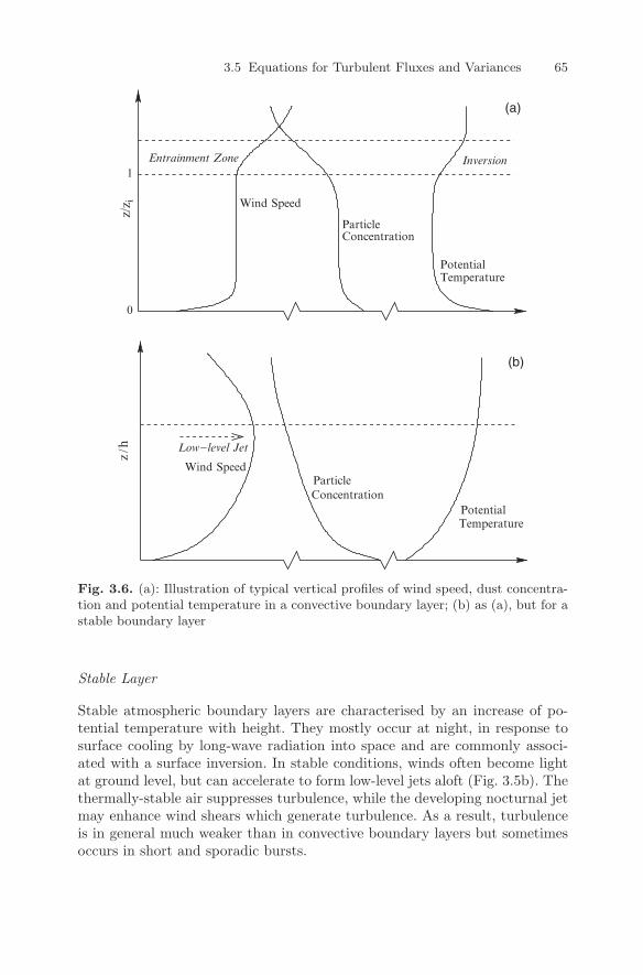
3.5 Equations for Turbulent Fluxes and Variances 65
1
0
TemperaturePotential
Particle
Inversion
z/z i Wind Speed
Concentration
Entrainment Zone
(a)
Temperature
ParticleConcentration
z/h Low−level Jet
Potential
Wind Speed
(b)
Fig. 3.6. (a): Illustration of typical vertical profiles of wind speed, dust concentra-tion and potential temperature in a convective boundary layer; (b) as (a), but for astable boundary layer
Stable Layer
Stable atmospheric boundary layers are characterised by an increase of po-tential temperature with height. They mostly occur at night, in response tosurface cooling by long-wave radiation into space and are commonly associ-ated with a surface inversion. In stable conditions, winds often become lightat ground level, but can accelerate to form low-level jets aloft (Fig. 3.5b). Thethermally-stable air suppresses turbulence, while the developing nocturnal jetmay enhance wind shears which generate turbulence. As a result, turbulenceis in general much weaker than in convective boundary layers but sometimesoccurs in short and sporadic bursts.
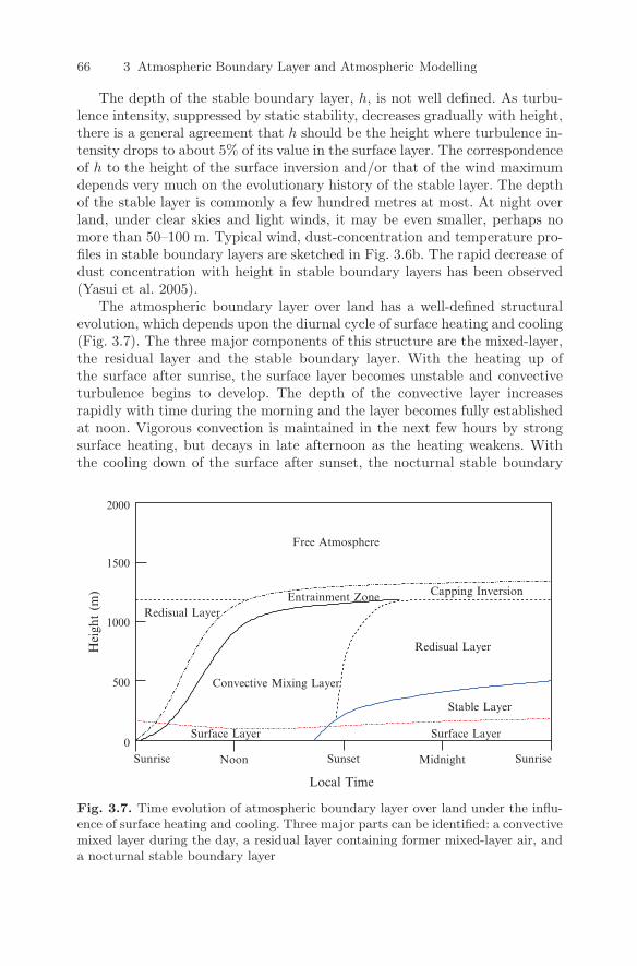
66 3 Atmospheric Boundary Layer and Atmospheric Modelling
The depth of the stable boundary layer, h, is not well defined. As turbu-lence intensity, suppressed by static stability, decreases gradually with height,there is a general agreement that h should be the height where turbulence in-tensity drops to about 5% of its value in the surface layer. The correspondenceof h to the height of the surface inversion and/or that of the wind maximumdepends very much on the evolutionary history of the stable layer. The depthof the stable layer is commonly a few hundred metres at most. At night overland, under clear skies and light winds, it may be even smaller, perhaps nomore than 50–100 m. Typical wind, dust-concentration and temperature pro-files in stable boundary layers are sketched in Fig. 3.6b. The rapid decrease ofdust concentration with height in stable boundary layers has been observed(Yasui et al. 2005).
The atmospheric boundary layer over land has a well-defined structuralevolution, which depends upon the diurnal cycle of surface heating and cooling(Fig. 3.7). The three major components of this structure are the mixed-layer,the residual layer and the stable boundary layer. With the heating up ofthe surface after sunrise, the surface layer becomes unstable and convectiveturbulence begins to develop. The depth of the convective layer increasesrapidly with time during the morning and the layer becomes fully establishedat noon. Vigorous convection is maintained in the next few hours by strongsurface heating, but decays in late afternoon as the heating weakens. Withthe cooling down of the surface after sunset, the nocturnal stable boundary
Capping Inversion
Redisual Layer
Stable Layer
Convective Mixing Layer
Local Time
Sunrise Noon Sunset Midnight Sunrise
Hei
ght
(m)
Surface LayerSurface Layer
Redisual LayerEntrainment Zone
Free Atmosphere
0
500
1000
1500
2000
Fig. 3.7. Time evolution of atmospheric boundary layer over land under the influ-ence of surface heating and cooling. Three major parts can be identified: a convectivemixed layer during the day, a residual layer containing former mixed-layer air, anda nocturnal stable boundary layer
3.6 Surface Layer 67
layer develops over night. Above this stable layer is the residual layer of theconvective boundary layer.
3.6 Surface Layer
3.6.1 Flux-Gradient Relationship
In the atmospheric surface layer, the turbulent fluxes of momentum, mass andheat are controlled by the strong vertical gradients of the corresponding meanquantities, and hence the mechanism that leads to turbulent fluxes (Fig. 3.2)is analogous to that governing the molecular diffusion in laminar flows. Basedon this analogy, we can express the turbulent fluxes of momentum, heat anddust in terms of the gradients in the vertical direction of the correspondingmean variables:
τR = Kmρ∂U/∂z (3.30)H = −Khρcp∂θ/∂z (3.31)F = −Kpρ∂c/∂z (3.32)
where Km, Kh and Kp are exchange coefficients for momentum, heat and dust,in dimensions of [L2T−1, e.g. m2s−1]; U , θ and c are respectively the meanwind speed, mean potential temperature and mean dust concentration. Thisformulation of the flux-gradient relationship is known as the K-theory. TheK-theory is based on the small-eddy concept: It is assumed that turbulenttransport is a result of local mixing by eddies of size much smaller than thecharacteristic scale in which the corresponding mean quantity varies vertically.Note that τR, in contrast to H and F , is conventionally defined positive whenit is pointed downward. The exchange coefficients Km, Kh and Kp are respec-tively the counterparts of the kinematical molecular viscosity ν, the moleculardiffusivity for heat kh and that for dust particles kp, in laminar flows. There-fore, Km is also known as eddy (or turbulent) viscosity and Kh and Kp areknown as eddy diffusivity. The magnitudes of Km etc. are typically three or-ders of magnitude larger than their molecular counterparts. Also, they are notconstants but functions of the turbulent properties of the atmosphere.
A simple expression for eddy viscosity, Km, can be obtained based on di-mensional arguments. As the dimensions of Km are [L2T−1], Km must be aproduct of a velocity and a length. Because Km represents the capacity of theflow to transfer momentum for a given gradient of mean wind through turbu-lent mixing, it is intuitive to assume that Km must depend on the intensityand the size of turbulent eddies. This typical size of eddies, l, is also knownas the mixing length. Thus, the essence of the mixing-length theory is that
Km ∝ u∗l
with u∗ being a velocity scale. Similar arguments can be made for Kh. Forneutral surface layers, Kh/Km ≈ 1 but is in general a function of the thermalstability of the surface layer (Section 3.7.1).
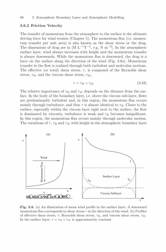
68 3 Atmospheric Boundary Layer and Atmospheric Modelling
3.6.2 Friction Velocity
The transfer of momentum from the atmosphere to the surface is the ultimatedriving force for wind erosion (Chapter 5). The momentum flux (i.e. momen-tum transfer per unit area) is also known as the shear stress or the drag.The dimensions of drag are in [M L−1T−2, e.g. N m−2]. In the atmosphericsurface layer, wind always increases with height and the momentum transferis always downwards. While the momentum flux is downward, the drag is aforce on the surface along the direction of the wind (Fig. 3.8a). Momentumtransfer in the flow is realized through both turbulent and molecular motions.The effective (or total) shear stress, τ , is composed of the Reynolds shearstress, τR, and the viscous shear stress, τM ,
τ = τR + τM (3.33)
The relative importance of τR and τM depends on the distance from the sur-face. In the body of the boundary layer, i.e. above the viscous sub-layer, flowsare predominantly turbulent and, in this region, the momentum flux occursmainly through turbulence, and thus τ is almost identical to τR. Closer to thesurface, especially within the viscous layer right next to the surface, the flowis dominated by viscosity, turbulence is weak and τR becomes insignificant.In this region, the momentum flux occurs mainly through molecular motion.The variations of τ , τR and τM with height in the atmospheric boundary layer
Wind
Viscous Sublayer
τ
τ
zz
τ u
τMτR
(a) (b)
Mom
entu
m F
lux
Surface Layer
Fig. 3.8. (a) An illustration of mean wind profile in the surface layer. A downwardmomentum flux corresponds to shear stress τ in the direction of the wind. (b) Profilesof effective shear stress, τ , Reynolds shear stress, τR, and viscous shear stress, τM .In the surface layer, τ = τR + τM is approximately constant
3.6 Surface Layer 69
are as illustrated in Fig. 3.8b. In the surface layer, τ remains approximatelyconstant with height.
The friction velocity, u∗, is defined as
u∗ =√
τ/ρ (3.34)
Clearly, u∗ is not the speed of the flow but simply another expression for themomentum flux at the surface. As u∗ is a convenient description of the forceexerted on the surface by wind shear, it emerges as one of the most importantquantities in wind-erosion studies. Equation (3.34) can be rewritten as
u∗ =√
u′w′ ∝ σ
where σ is the standard deviation of velocity fluctuations. Thus, u∗ is also adescriptor of turbulence intensity in the surface layer and is thus an adequatescaling velocity for turbulent fluctuations there.
Depending upon its characteristics, the surface can be considered to bedynamically smooth if the sizes of the surface roughness elements are toosmall to affect the flow, or otherwise to be dynamically rough. A criterion fordetermining whether a surface is rough or smooth is the roughness elementsReynolds number,
Rer = u∗Dr/ν (3.35)
with Dr being a measure of typical roughness-element size. The surface canbe considered to be rough if Rer exceeds about 300. Dr is around 10 mm fora u∗ of 0.4 m s−1 because ν = 1.5 × 10⁻⁵ m2 s−1.
If a sufficiently large roughness element protrudes into the flow, it producesa drag on the flow. This drag occurs because of the pressure difference betweenthe windward side and the leeward side of the roughness element. The pressureon the windward side of the roughness element is larger than that on theleeward side. An integration of pressure over the surfaces of all roughnesselements on a unit area of the ground surface gives the pressure drag
τr =∫
pds
The transfer of momentum from the atmosphere to the surface is achievedeventually through the viscous effect and pressure drag on the surface rough-ness elements. For a smooth surface, the pressure drag is negligible and theflow characteristics in the viscous layer can be understood based on simplephysical considerations. The flow speed U in this region is a function of heightz, depending on only the viscous-shear stress τ (=τM ), the kinematic molec-ular viscosity ν, and air density ρ, so that
U = U(z, τ, ν, ρ) (3.36)
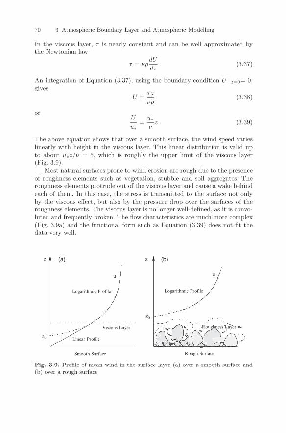
70 3 Atmospheric Boundary Layer and Atmospheric Modelling
In the viscous layer, τ is nearly constant and can be well approximated bythe Newtonian law
τ = νρdU
dz(3.37)
An integration of Equation (3.37), using the boundary condition U |z=0= 0,gives
U =τz
νρ(3.38)
orU
u∗=
u∗ν
z (3.39)
The above equation shows that over a smooth surface, the wind speed varieslinearly with height in the viscous layer. This linear distribution is valid upto about u∗z/ν = 5, which is roughly the upper limit of the viscous layer(Fig. 3.9).
Most natural surfaces prone to wind erosion are rough due to the presenceof roughness elements such as vegetation, stubble and soil aggregates. Theroughness elements protrude out of the viscous layer and cause a wake behindeach of them. In this case, the stress is transmitted to the surface not onlyby the viscous effect, but also by the pressure drop over the surfaces of theroughness elements. The viscous layer is no longer well-defined, as it is convo-luted and frequently broken. The flow characteristics are much more complex(Fig. 3.9a) and the functional form such as Equation (3.39) does not fit thedata very well.
(a) (b)z z
u
z0
z0
Linear Profile
Logarithmic Profile Logarithmic Profile
Viscous Layer
u
Rough SurfaceSmooth Surface
Roughness Layer
Fig. 3.9. Profile of mean wind in the surface layer (a) over a smooth surface and(b) over a rough surface
3.6 Surface Layer 71
3.6.3 Logarithmic Wind Profile and Roughness Length
In the surface layer above either a smooth or a rough surface, where theeffective shear stress is approximately constant with height (Fig. 3.8b), theprofile of mean wind obeys the logarithmic law. For neutral surface layers Km
can be expressed asKm = κu∗z (3.40)
where κ is the von Karman constant. The reported values of κ in most at-mospheric boundary-layer studies range between 0.35 to 0.4. Substituting theexpressions for τ (i.e. τ = ρu2
∗) and Km into Equation (3.30), we obtain
∂U
∂z=
u∗κz
z ≥ z0 (3.41)
Note that in Equation (3.41), z cannot be equal to zero but needs to be largerthan zero. In other words, Equation (3.41) is valid for z ≥ z0 with z0 beingsome height above the ground surface. An integration of Equation (3.41) overz from z0 to z yields the logarithmic wind profile
U(z) =u∗κ
ln(
z
z0
)(3.42)
We call z0 the aerodynamic roughness length of the surface. In wind-erosion studies, z0 is a widely used parameter and it is important to under-stand its interpretations. Formally, z0 is a constant of integration introducedin the derivation of the logarithmic wind profile. A z0 would not exist if Equa-tion (3.40) were not used. Equation (3.42) implies that at z = z0, the meanwind vanishes when extrapolated logarithmically downward. For a fixed meanwind speed at z, larger z0 implies larger u∗ or larger downward momentumflux. Hence, z0 is a description of the capacity of the surface for absorbingmomentum.
Some experimental studies indicate that z0 is about 1/30 the height ofthe roughness elements. Such a rule of thumb is useful only for specific cases.In general, the relationship between z0 and the physical size of the roughnesselements is not simple. This is because the capacity of the surface in absorbingmomentum, which z0 represents, depends on the interferences of the turbulentwakes generated by the roughness elements. We shall examine z0 in more detailin Chapter 6, when we discuss the Owen effect of saltation.
The logarithmic wind profile applies both to smooth and rough surfaces,as illustrated in Fig. 3.9. For practical wind-erosion problems, both u∗ and z0
can be determined through fitting the measurements of mean wind with thelogarithmic wind profile. If we plot U measured at different z against ln z, wewould obtain a straight line with its slope being u∗/κ and its intercept being−(u∗/κ) ln z0.
For a smooth surface, the centeroid of momentum absorption occurs atz = 0. A rough surface can be considered to be a smooth surface superposed
72 3 Atmospheric Boundary Layer and Atmospheric Modelling
with roughness elements and the centreroid of momentum absorption is nolonger at z = 0 but at a distance away from the surface z = zd. This dis-tance, zd, is the displacement height. The logarithmic wind profile can bemore generally written as
U(z) =u∗κ
ln(
z − zd
z0
)(3.43)
Both z0 and zd depend on the geometric features of the roughness elements(e.g. height, width etc.) and their spatial arrangement. For a dense canopyof forest of height zh, zd is about 0.7zh while for a dense urban canopy, zd isclose to zh (Macdonald et al. 1998).
Equations (3.39) and (3.42) are derived based on simple assumptions onthe profiles of u∗ and Km. More generally, we assume that both u∗ and Km
are functions of height
u∗ = fu(z)Km = u∗fk(z)
The wind profile can now be determined as follows:
U(z) =∫ z
d+z0
fu(z)fk(z)
dz (3.44)
The linear wind profile given by Equation (3.39) is a special case with fu andfk being constant, and the logarithmic wind profile given by Equation (3.42) isa special case with fu being constant and fk being a linear function of height.Suppose both fu and fk increase linearly with height with fu(z) = a+ bz andfk(z) = κz, then we have
U(z) =a
κln
(zd
z0
)+
b
κ(z − z0) (3.45)
To have the knowledge of fu and fk is quite useful in studying flow in thesaltation layers as we shall discuss further in Chapter 6.
3.6.4 Stability Measures
The structure of the atmospheric boundary layer and the behaviour of turbu-lence both depend on stability. There are a number of stability measures foratmospheric boundary-layer flows, one of which is the static stability given interms of the vertical gradient of potential temperature, namely,
Stable ∂θ/∂z > 0
Neutral ∂θ/∂z = 0
Unstable ∂θ/∂z < 0
3.6 Surface Layer 73
In statically-stable conditions, an air parcel displaced vertically by a dis-turbance would experience a buoyancy force bringing it back towards itsorigin, while in statically-unstable conditions, the air parcel would experi-ence a buoyancy force accelerating it further away from its origin. As ∂θ/∂zis negatively related to sensible-heat flux, the static stability also describeswhether buoyancy generates turbulent kinetic energy. In statically-stable con-ditions, buoyancy suppresses turbulence while in statically-unstable condi-tions, it enhances it.
A more accurate indicator for the development of turbulence is theRichardson number which has several forms. A frequently used one is theflux Richardson number:
Rf = −g
θw′θ′
(u2∗∂U
∂z
)−1
(3.46)
As can be seen from Equation (3.29), Rf is the ratio between thermal sup-pression and mechanical production of turbulent kinetic energy, and thus thecritical flux Richardson number is 1. For Rf > 1, buoyancy destruction ofturbulent kinetic energy dominates over shear production, thus the flow be-comes less turbulent and is dynamically stable. For Rf < 1, shear productiondominates over buoyancy destruction, thus the flow becomes more turbulentand is dynamically unstable. Other forms of the Richardson number have thesame physical meaning, but different critical values. For example, the gradientRichardson number is given in terms of the gradients of potential temperatureand wind speed
Ri =g
θ
∂θ
∂z
(∂U
∂z
)−2
(3.47)
The critical gradient Richardson number is 0.25.Wind shear near the surface can be significantly modified by the stability
of the atmospheric boundary layer. Assuming horizontal homogeneity (∂/∂xand ∂/∂y = 0), stationarity (∂/∂t = 0) and that the divergence of turbulentkinetic energy flux is negligible, Equation (3.29) can be simplified to
g
θw′θ′ + u2
∗∂u
∂z− ε = 0 (3.48)
If we take ε = u3∗/κz and Km = κzu∗ for the atmospheric surface layer, it
follows that (∂u
∂z
)2
=g
θ
w′θ′
κzu∗+
u∗κz
∂u
∂z(3.49)
In a statically-neutral surface layer, w′θ′ ≡ 0, and an integration of the aboveequation gives the logarithmic wind profile. For stable and unstable situations,the wind profile is modified as illustrated in Fig. 3.10. For the unstable situ-ation, a stronger wind shear occurs near the surface, as stronger turbulencetransfers momentum more efficiently from higher levels to lower levels and
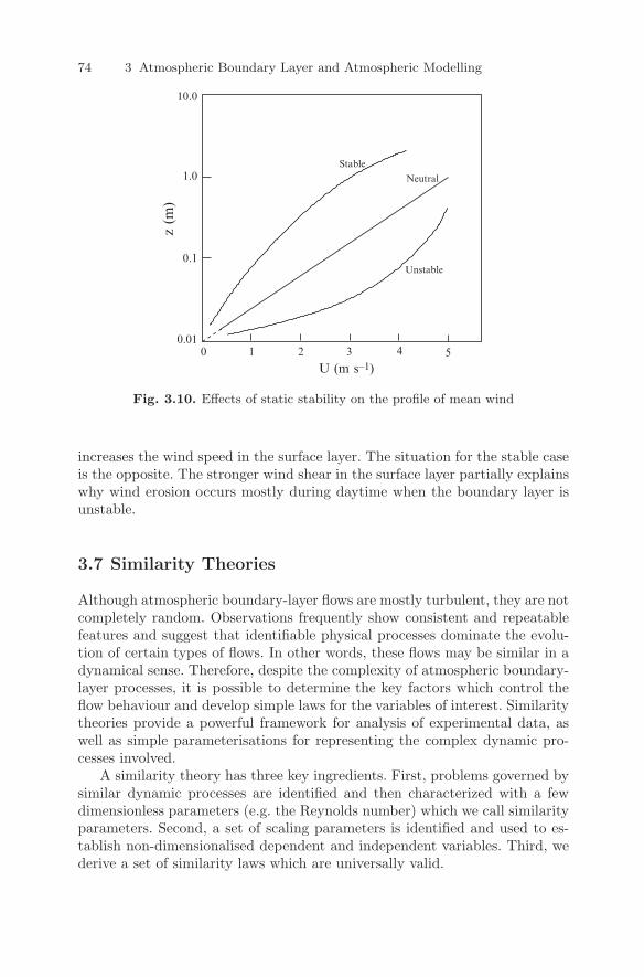
74 3 Atmospheric Boundary Layer and Atmospheric Modelling
Stable
Unstable
Neutral
U (m s-1)
0.01
0.1
1.0
10.0
z (m
)
0 1 2 3 4 5
Fig. 3.10. Effects of static stability on the profile of mean wind
increases the wind speed in the surface layer. The situation for the stable caseis the opposite. The stronger wind shear in the surface layer partially explainswhy wind erosion occurs mostly during daytime when the boundary layer isunstable.
3.7 Similarity Theories
Although atmospheric boundary-layer flows are mostly turbulent, they are notcompletely random. Observations frequently show consistent and repeatablefeatures and suggest that identifiable physical processes dominate the evolu-tion of certain types of flows. In other words, these flows may be similar in adynamical sense. Therefore, despite the complexity of atmospheric boundary-layer processes, it is possible to determine the key factors which control theflow behaviour and develop simple laws for the variables of interest. Similaritytheories provide a powerful framework for analysis of experimental data, aswell as simple parameterisations for representing the complex dynamic pro-cesses involved.
A similarity theory has three key ingredients. First, problems governed bysimilar dynamic processes are identified and then characterized with a fewdimensionless parameters (e.g. the Reynolds number) which we call similarityparameters. Second, a set of scaling parameters is identified and used to es-tablish non-dimensionalised dependent and independent variables. Third, wederive a set of similarity laws which are universally valid.
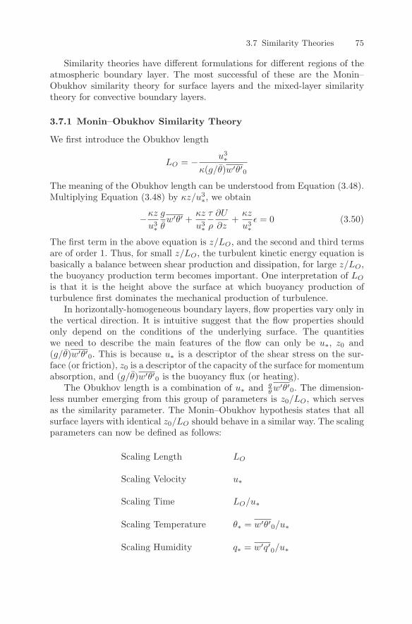
3.7 Similarity Theories 75
Similarity theories have different formulations for different regions of theatmospheric boundary layer. The most successful of these are the Monin–Obukhov similarity theory for surface layers and the mixed-layer similaritytheory for convective boundary layers.
3.7.1 Monin–Obukhov Similarity Theory
We first introduce the Obukhov length
LO = − u3∗
κ(g/θ)w′θ′0
The meaning of the Obukhov length can be understood from Equation (3.48).Multiplying Equation (3.48) by κz/u3
∗, we obtain
−κz
u3∗
g
θw′θ′ +
κz
u3∗
τ
ρ
∂U
∂z+
κz
u3∗ε = 0 (3.50)
The first term in the above equation is z/LO, and the second and third termsare of order 1. Thus, for small z/LO, the turbulent kinetic energy equation isbasically a balance between shear production and dissipation, for large z/LO,the buoyancy production term becomes important. One interpretation of LO
is that it is the height above the surface at which buoyancy production ofturbulence first dominates the mechanical production of turbulence.
In horizontally-homogeneous boundary layers, flow properties vary only inthe vertical direction. It is intuitive suggest that the flow properties shouldonly depend on the conditions of the underlying surface. The quantitieswe need to describe the main features of the flow can only be u∗, z0 and(g/θ)w′θ′0. This is because u∗ is a descriptor of the shear stress on the sur-face (or friction), z0 is a descriptor of the capacity of the surface for momentumabsorption, and (g/θ)w′θ′0 is the buoyancy flux (or heating).
The Obukhov length is a combination of u∗ and gθ w′θ′0. The dimension-
less number emerging from this group of parameters is z0/LO, which servesas the similarity parameter. The Monin–Obukhov hypothesis states that allsurface layers with identical z0/LO should behave in a similar way. The scalingparameters can now be defined as follows:
Scaling Length LO
Scaling Velocity u∗
Scaling Time LO/u∗
Scaling Temperature θ∗ = w′θ′0/u∗
Scaling Humidity q∗ = w′q′0/u∗
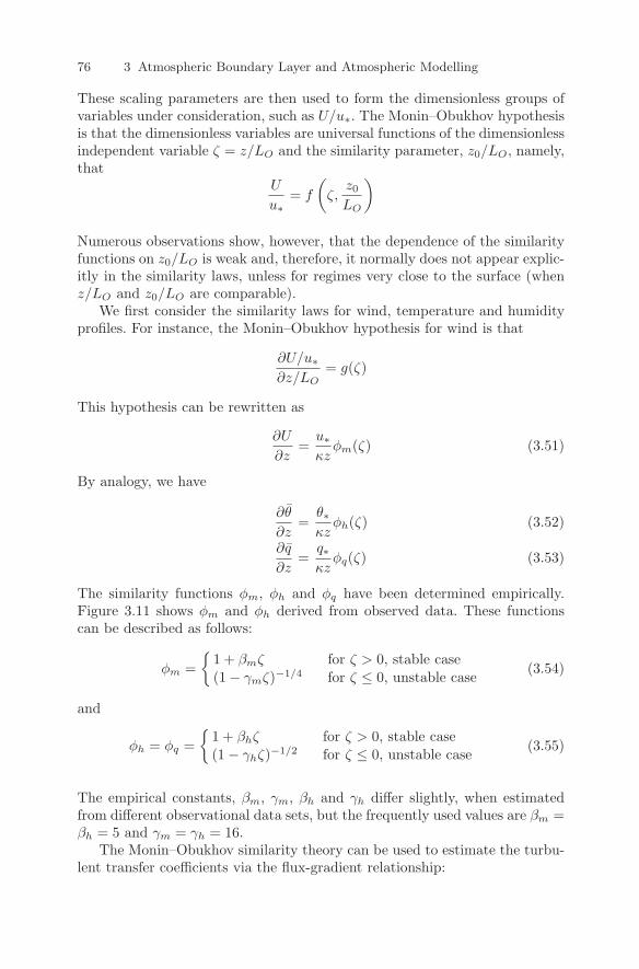
76 3 Atmospheric Boundary Layer and Atmospheric Modelling
These scaling parameters are then used to form the dimensionless groups ofvariables under consideration, such as U/u∗. The Monin–Obukhov hypothesisis that the dimensionless variables are universal functions of the dimensionlessindependent variable ζ = z/LO and the similarity parameter, z0/LO, namely,that
U
u∗= f
(ζ,
z0
LO
)
Numerous observations show, however, that the dependence of the similarityfunctions on z0/LO is weak and, therefore, it normally does not appear explic-itly in the similarity laws, unless for regimes very close to the surface (whenz/LO and z0/LO are comparable).
We first consider the similarity laws for wind, temperature and humidityprofiles. For instance, the Monin–Obukhov hypothesis for wind is that
∂U/u∗∂z/LO
= g(ζ)
This hypothesis can be rewritten as
∂U
∂z=
u∗κz
φm(ζ) (3.51)
By analogy, we have
∂θ
∂z=
θ∗κz
φh(ζ) (3.52)
∂q
∂z=
q∗κz
φq(ζ) (3.53)
The similarity functions φm, φh and φq have been determined empirically.Figure 3.11 shows φm and φh derived from observed data. These functionscan be described as follows:
φm =
1 + βmζ for ζ > 0, stable case(1 − γmζ)−1/4 for ζ ≤ 0, unstable case
(3.54)
and
φh = φq =
1 + βhζ for ζ > 0, stable case(1 − γhζ)−1/2 for ζ ≤ 0, unstable case
(3.55)
The empirical constants, βm, γm, βh and γh differ slightly, when estimatedfrom different observational data sets, but the frequently used values are βm =βh = 5 and γm = γh = 16.
The Monin–Obukhov similarity theory can be used to estimate the turbu-lent transfer coefficients via the flux-gradient relationship:
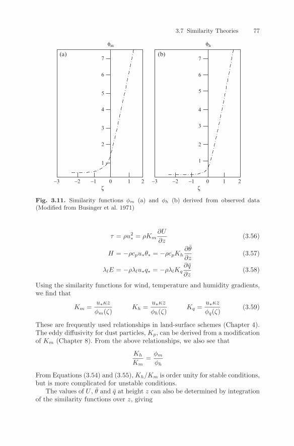
3.7 Similarity Theories 77
ζζ
φm φh
6
5
4
2
1
3
7 7
6
5
4
3
2
1
-3 -2 -1 0 1 1-3 -2 -1 0
(a) (b)
2 2
Fig. 3.11. Similarity functions φm (a) and φh (b) derived from observed data(Modified from Businger et al. 1971)
τ = ρu2∗ = ρKm
∂U
∂z(3.56)
H = −ρcpu∗θ∗ = −ρcpKh∂θ
∂z(3.57)
λlE = −ρλlu∗q∗ = −ρλlKq∂q
∂z(3.58)
Using the similarity functions for wind, temperature and humidity gradients,we find that
Km =u∗κz
φm(ζ)Kh =
u∗κz
φh(ζ)Kq =
u∗κz
φq(ζ)(3.59)
These are frequently used relationships in land-surface schemes (Chapter 4).The eddy diffusivity for dust particles, Kp, can be derived from a modificationof Km (Chapter 8). From the above relationships, we also see that
Kh
Km=
φm
φh
From Equations (3.54) and (3.55), Kh/Km is order unity for stable conditions,but is more complicated for unstable conditions.
The values of U , θ and q at height z can also be determined by integrationof the similarity functions over z, giving
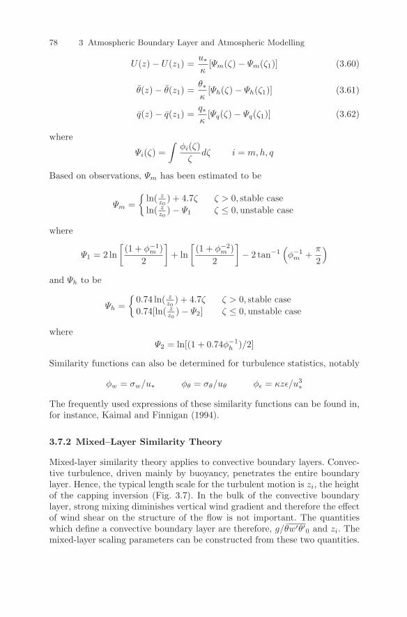
78 3 Atmospheric Boundary Layer and Atmospheric Modelling
U(z) − U(z1) =u∗κ
[Ψm(ζ) − Ψm(ζ1)] (3.60)
θ(z) − θ(z1) =θ∗κ
[Ψh(ζ) − Ψh(ζ1)] (3.61)
q(z) − q(z1) =q∗κ
[Ψq(ζ) − Ψq(ζ1)] (3.62)
where
Ψi(ζ) =∫
φi(ζ)ζ
dζ i = m,h, q
Based on observations, Ψm has been estimated to be
Ψm =
ln( zz0
) + 4.7ζ ζ > 0, stable caseln( z
z0) − Ψ1 ζ ≤ 0,unstable case
where
Ψ1 = 2 ln[(1 + φ−1
m )2
]+ ln
[(1 + φ−2
m )2
]− 2 tan−1
(φ−1
m +π
2
)
and Ψh to be
Ψh =
0.74 ln( zz0
) + 4.7ζ ζ > 0, stable case0.74[ln( z
z0) − Ψ2] ζ ≤ 0,unstable case
whereΨ2 = ln[(1 + 0.74φ−1
h )/2]
Similarity functions can also be determined for turbulence statistics, notably
φw = σw/u∗ φθ = σθ/uθ φε = κzε/u3∗
The frequently used expressions of these similarity functions can be found in,for instance, Kaimal and Finnigan (1994).
3.7.2 Mixed–Layer Similarity Theory
Mixed-layer similarity theory applies to convective boundary layers. Convec-tive turbulence, driven mainly by buoyancy, penetrates the entire boundarylayer. Hence, the typical length scale for the turbulent motion is zi, the heightof the capping inversion (Fig. 3.7). In the bulk of the convective boundarylayer, strong mixing diminishes vertical wind gradient and therefore the effectof wind shear on the structure of the flow is not important. The quantitieswhich define a convective boundary layer are therefore, g/θw′θ′0 and zi. Themixed-layer scaling parameters can be constructed from these two quantities.
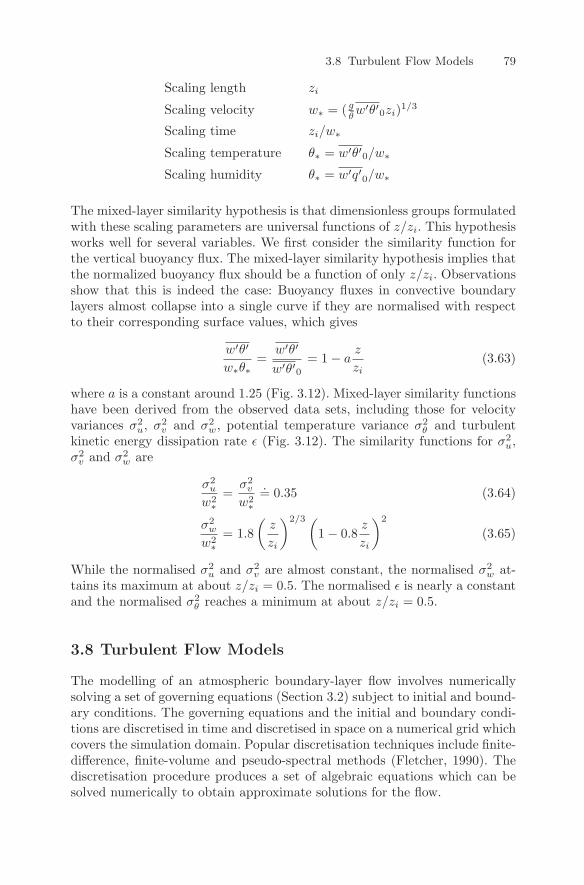
3.8 Turbulent Flow Models 79
Scaling length zi
Scaling velocity w∗ = ( gθw′θ′0zi)1/3
Scaling time zi/w∗
Scaling temperature θ∗ = w′θ′0/w∗
Scaling humidity θ∗ = w′q′0/w∗
The mixed-layer similarity hypothesis is that dimensionless groups formulatedwith these scaling parameters are universal functions of z/zi. This hypothesisworks well for several variables. We first consider the similarity function forthe vertical buoyancy flux. The mixed-layer similarity hypothesis implies thatthe normalized buoyancy flux should be a function of only z/zi. Observationsshow that this is indeed the case: Buoyancy fluxes in convective boundarylayers almost collapse into a single curve if they are normalised with respectto their corresponding surface values, which gives
w′θ′
w∗θ∗=
w′θ′
w′θ′0= 1 − a
z
zi(3.63)
where a is a constant around 1.25 (Fig. 3.12). Mixed-layer similarity functionshave been derived from the observed data sets, including those for velocityvariances σ2
u, σ2v and σ2
w, potential temperature variance σ2θ and turbulent
kinetic energy dissipation rate ε (Fig. 3.12). The similarity functions for σ2u,
σ2v and σ2
w are
σ2u
w2∗
=σ2
v
w2∗
.= 0.35 (3.64)
σ2w
w2∗
= 1.8(
z
zi
)2/3 (1 − 0.8
z
zi
)2
(3.65)
While the normalised σ2u and σ2
v are almost constant, the normalised σ2w at-
tains its maximum at about z/zi = 0.5. The normalised ε is nearly a constantand the normalised σ2
θ reaches a minimum at about z/zi = 0.5.
3.8 Turbulent Flow Models
The modelling of an atmospheric boundary-layer flow involves numericallysolving a set of governing equations (Section 3.2) subject to initial and bound-ary conditions. The governing equations and the initial and boundary condi-tions are discretised in time and discretised in space on a numerical grid whichcovers the simulation domain. Popular discretisation techniques include finite-difference, finite-volume and pseudo-spectral methods (Fletcher, 1990). Thediscretisation procedure produces a set of algebraic equations which can besolved numerically to obtain approximate solutions for the flow.
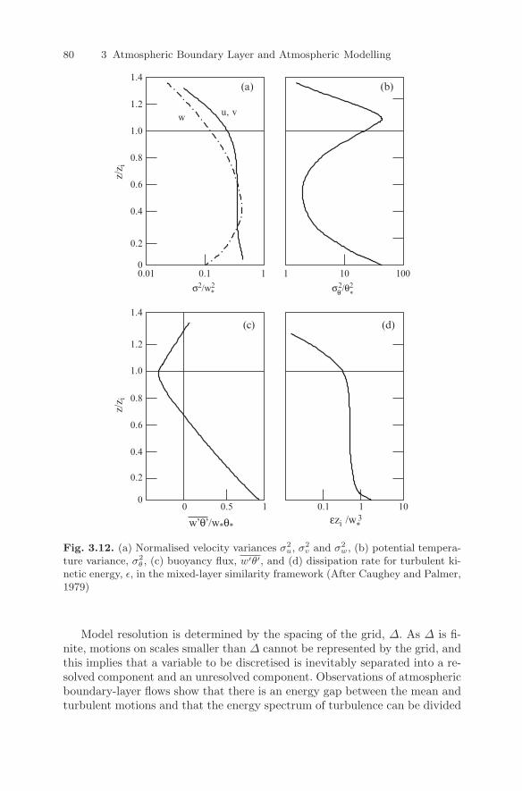
80 3 Atmospheric Boundary Layer and Atmospheric Modelling
0.1
0 1 1 100.5 0.1
10.01 10 1001
z/z i
z/z i
w u, v
σ2/w2*
w’θ’/w*θ*
1.2
1.0
0.8
0.6
0.4
0.2
0
1.4
σ2/θ2*θ
1.4
1.2
1.0
0.8
0.6
0.4
0.2
0
εzi /w 3*
(a)
(c) (d)
(b)
Fig. 3.12. (a) Normalised velocity variances σ2u, σ2
v and σ2w, (b) potential tempera-
ture variance, σ2θ , (c) buoyancy flux, w′θ′, and (d) dissipation rate for turbulent ki-
netic energy, ε, in the mixed-layer similarity framework (After Caughey and Palmer,1979)
Model resolution is determined by the spacing of the grid, ∆. As ∆ is fi-nite, motions on scales smaller than ∆ cannot be represented by the grid, andthis implies that a variable to be discretised is inevitably separated into a re-solved component and an unresolved component. Observations of atmosphericboundary-layer flows show that there is an energy gap between the mean andturbulent motions and that the energy spectrum of turbulence can be divided
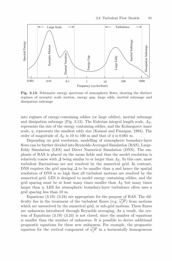
3.8 Turbulent Flow Models 81
10 100 10000.10.010.001 1
Syno
ptic
Mot
ion
Diu
rnal
Var
iatio
n
Ener
gy G
ap
Larg
e Ed
dy
Iner
tial S
ubra
nge
TurbulenceLarge ScaleSp
ectra
l Ene
rgy
Frequency (cycles/hour)
Dis
sipa
tion
Subr
ange
Fig. 3.13. Schematic energy spectrum of atmospheric flows, showing the distinctregimes of synoptic scale motion, energy gap, large eddy, inertial subrange anddissipation subrange
into regimes of energy-containing eddies (or large eddies), inertial subrangeand dissipation subrange (Fig. 3.13). The Eulerian integral length scale, ΛE ,represents the size of the energy containing eddies, and the Kolmogorov innerscale, η, represents the smallest eddy size (Kaimal and Finnigan, 1994). Theorder of magnitude of ΛE is 10 to 100 m and that of η is 0.001 m.
Depending on grid resolution, modelling of atmospheric boundary-layerflows can be further divided into Reynolds-Averaged Simulation (RAS), Large-Eddy Simulation (LES) and Direct Numerical Simulation (DNS). The em-phasis of RAS is placed on the mean fields and thus the model resolution isrelatively coarse with ∆ being similar to or larger than ΛE . In this case, mostturbulent fluctuations are not resolved by the numerical grid. In contrast,DNS requires the grid spacing ∆ to be smaller than η and hence the spatialresolution of DNS is so high that all turbulent motions are resolved by thenumerical grid. LES is designed to model energy containing eddies, and thegrid spacing must be at least many times smaller than ΛE but many timeslarger than η. LES for atmospheric boundary-layer turbulence often uses agrid spacing less than 10 m.
Equations (3.19)–(3.24) are appropriate for the purpose of RAS. The dif-ficulty lies in the treatment of the turbulent fluxes (e.g. u′
jθ′) from motions
which are unresolved by the numerical grid, or sub-grid motions. These fluxesare unknowns introduced through Reynolds averaging. As a result, the sys-tem of Equations (3.19)–(3.24) is not closed, since the number of equationsis smaller than the number of unknowns. It is possible to derive additionalprognostic equations for these new unknowns. For example, the prognosticequation for the vertical component of u′
jθ′ in a horizontally homogeneous
82 3 Atmospheric Boundary Layer and Atmospheric Modelling
flow can be written as
∂w′θ′
∂t= σ2
w
∂θ
∂z− ∂w′w′θ′
∂z+
σ2θg
θ+
p′
ρ
∂θ′
∂z− 2εwθ (3.66)
However, other new unknowns appear in the above equation, such as the triplecorrelation term w′w′θ′. If a similar procedure is followed to derive additionalequations for w′w′θ′, more unknowns will be introduced and the equationsystem remains open. In fact, the number of unknowns increases faster thanthe number of equations as we move to higher orders.
The basic approach to achieving a closed system of equations is param-eterisation. This means that the quantities for which a prognostic equationis missing are expressed in terms of the already-existing prognostic variablesand some parameters. Different orders of closure have been used in modellingboundary-layer flows. In first-order closure, equations for Reynolds-averagedvariables are retained in the model and second-order moments (e.g. w′θ′)are expressed in terms of first-order ones (e.g. θ) and parameters. In second-order closure, equations for first- and second-order moments are retained inthe model and third-order moments (e.g. w′w′θ′) are expressed by means ofsecond-order moments (e.g. w′θ′) and parameters. The parameters are usuallyempirical constants and/or simple functions of space and time. Parameterisa-tions depend on an understanding of the physical problem involved and thus,different models may employ different parameterisations.
K-theory is a simple and widely used first-order closure technique. Thisparameterisation specifies the relationship between a turbulent flux and thegradient of the corresponding mean quantity. In general, we have that
u′jξ
′ = −Kξ∂ξ
∂xj(3.67)
where the parameter Kξ is the eddy diffusivity for ξ, an arbitrary scalar. K-theory is best applicable to atmospheric surface layers where the small-eddyconcept is adequate. The Monin–Obukhov similarity theory provides a fairlyaccurate method of estimating the eddy diffusivities for momentum, heat andvarious passive scalars (Equation 3.59).
The e−ε closure is another widely used technique for modelling boundary-layer flows (Detering and Etling, 1985). The e− ε closure is also based on thesmall-eddy concept, but the eddy viscosity is calculated using the Prandtl–Kolmogorov hypothesis that
Km = cee2/ε
where ce is a coefficient. For the e− ε closure, the prognostic equations for theturbulent kinetic energy, e, and the dissipation rate of turbulent kinetic energy,ε, are retained in the governing equation system and numerically solved alongwith the other prognostic equations. The prognostic equation for ε can be
3.8 Turbulent Flow Models 83
derived from the equations of motion or from an equation of turbulent vortexintensity (Tennekes and Lumley, 1972), and for the horizontally homogeneouscase is
∂ε
∂t= cε1
ε
e
[−∂u′w′
∂z− ∂v′w′
∂z
]+ cε2
ε
e
g
θw′θ′ − ∂w′ε
∂z− cε3
ε2
e(3.68)
where
w′ε = − K
cε4
∂ε
∂z
The constants used in the e− ε model are determined empirically by compar-ing simulated results with observations (such as wind-tunnel observations).The values commonly used are ce = 0.09, cε1 = 1.44, cε2 = 1.0, cε3 = 1.92,cε4 = 1.30. Mellor and Yamada (1974, 1982) introduced a hierarchy of modelsfor atmospheric boundary-layer flows, with closure at different levels. The so-called Level-4 model of Mellor and Yamada retains prognostic equations forsecond moments and requires the solution of 13 partial differential equations.Mellor and Yamada (1974) have separated the velocity covariance prognosticequation into isotropic (i = j) and anisotropic (i = j) parts and performed ascale analysis, identifying the relative importance of each term and systemat-ically neglecting higher-order terms. This scaling analysis reduces the Level-4model to a Level-3 one. The latter consists of two partial differential equa-tions and eight algebraic equations. A further simplification can be introducedby neglecting the total time derivative and the diffusion term in the Level-3model. This simplification is based on considerations of computational effi-ciency. The resulting system is a Level-2 1
2 closure similar to the e− ε closure.The Mellor–Yamada scheme in its various forms is widely used in modellingatmospheric boundary-layer flows.
K-theory, e− ε closure and Mellor–Yamada schemes are all local closures,in which an unknown quantity at any point in space is parameterized by val-ues and/or gradients of known quantities at the same point. An alternative tolocal closure is non-local closure, in which an unknown quantity at any pointin space is parameterized by values and/or gradients of known quantities atmany points. In non-local closure, the advective nature of structured eddies,especially turbulence in convective boundary layers, is recognised in turbulenttransport. Non-local closure schemes assume that turbulence is a superposi-tion of eddies, each of which is associated with an advective process takingplace on the scale of the eddy size. Non-local closure is much more difficult toimplement in numerical models and has therefore not yet been widely used.
Since the pioneering work of Deardorff (1970), LES has been appliedwidely to studying atmospheric turbulent flows (e.g. Moeng, 1984; Schu-mann, 1993). Unfortunately, we have not yet fully taken the advantage ofLES in wind-erosion modelling, although its potential usefulness in studying
84 3 Atmospheric Boundary Layer and Atmospheric Modelling
the interactions between turbulent flows and soil erosion is obvious. For prob-lems such as the protection of soil surfaces by windbreaks, deposition of soilparticles in the wake region of isolated shrubs, the evolution of sand dunesand particle entrainment by convective turbulence, LES may offer valuableinformation which is otherwise difficult to obtain.
The model structure and numerical procedures for LES and RAS are sim-ilar. In fact, LES and RAS can be carried out using the same numerical codewith minor modifications. However, we note that LES is designed to modelenergy-containing eddies and it differs from RAS in several aspects:
• LES requires higher spatial and temporal resolution than RAS, but as thegrid size and integral time step for LES increase, the results of LES andRAS will become similar.
• Instead of Reynolds averaging, averaging over grid size is required.Commonly used techniques include volume averaging (Deardorff, 1970),volume-balance methods (Schumann, 1975) and Gaussian filters (Leonard,1974).
• A subgrid model is required to parameterize the effects of small eddiesupon the large eddies, rather than those of turbulence upon the meanflow. The Smagorinsky–Lilly (Smagorinsky, 1963) model is widely used.
Figure 3.14 shows an example of LES for flow over a windbreak of height hwith a porosity of 0.5. The simulation domain is 12 h long, 4 h wide and4 h high and is consisted of 72 × 48 × 48 grid points. In this example, LESprovides detailed information on turbulence field (Fig. 3.14a) and the meanflow field (Fig. 3.14b) in the vicinity of the windbreak. This type of informationis required in studying the effect of windbreaks on the prevention of winderosion.
Typical spatial resolution of Direct Numerical Simulation (DNS) is severalmillimetres. The requirement of DNS for extremely high spatial resolutionimplies that it can only be applied to a small spatial domain, as it is tooexpensive computationally. The usefulness of DNS in wind-erosion studies liesin its ability to provide a tool for investigation of detailed erosion mechanisms.Examples of this are drag partitioning and erosion pattern in the vicinity ofindividual roughness elements (see Chapter 9). In many ways, DNS providesvaluable information for wind-erosion studies, which is difficult to obtain fromtraditional wind-tunnel experiments. Figure 3.15 shows a simulation of flowspeed around roughness elements mounted on the surface and the distributionof local momentum flux in the vicinity of these elements. In this example, fivecylinders with a diameter of 5 mm and a height of 10 mm are placed on thesurface of a domain 150 mm long, 65 mm wide and 50 mm high. The gridresolution is 1 mm and the input flow speed in 10 m s−1. The simulationshows the reduced flow speed and the enhanced local momentum flux in thewake region of the obstacles.
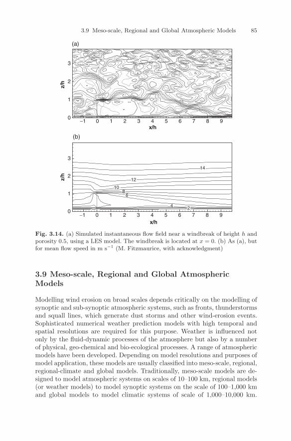
3.9 Meso-scale, Regional and Global Atmospheric Models 85
12
0
1
2
3
(b)
x/h
(a)
0
1
2
3
−1 0 1 2 3 4 5 6 7 8 9
810
6
14
12
4 2
−1 0 1 2 3 4 5 6 7 8 9x/h
z/h
z/h
Fig. 3.14. (a) Simulated instantaneous flow field near a windbreak of height h andporosity 0.5, using a LES model. The windbreak is located at x = 0. (b) As (a), butfor mean flow speed in m s−1 (M. Fitzmaurice, with acknowledgment)
3.9 Meso-scale, Regional and Global AtmosphericModels
Modelling wind erosion on broad scales depends critically on the modelling ofsynoptic and sub-synoptic atmospheric systems, such as fronts, thunderstormsand squall lines, which generate dust storms and other wind-erosion events.Sophisticated numerical weather prediction models with high temporal andspatial resolutions are required for this purpose. Weather is influenced notonly by the fluid-dynamic processes of the atmosphere but also by a numberof physical, geo-chemical and bio-ecological processes. A range of atmosphericmodels have been developed. Depending on model resolutions and purposes ofmodel application, these models are usually classified into meso-scale, regional,regional-climate and global models. Traditionally, meso-scale models are de-signed to model atmospheric systems on scales of 10–100 km, regional models(or weather models) to model synoptic systems on the scale of 100–1,000 kmand global models to model climatic systems of scale of 1,000–10,000 km.
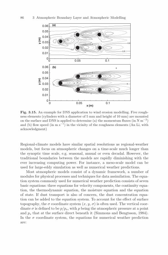
86 3 Atmospheric Boundary Layer and Atmospheric Modelling
2 2
4
4
4
4 46
66
6
6
8
8
8 6
8
8
10
10
10
10
x (m)0 0.05 0.1
(b)
0
0
0.8
0.8
0.8
0.8
0.8
0.8
0.8
0.8
0.8
1.6
1.6
(a)
y(m
)y
(m)
0
0.01
0.02
0.03
0.04
0.05
0.06
0
0.01
0.02
0.03
0.04
0.05
0.06
0 0.05 0.1
Fig. 3.15. An example for DNS application to wind erosion modelling. Five rough-ness elements (cylinders with a diameter of 5 mm and height of 10 mm) are mountedon the surface and DNS is applied to determine (a) the momentum fluxes (in N m−2)and (b) flow speed (in m s−1) in the vicinity of the roughness elements (An Li, withacknowledgment)
Regional-climate models have similar spatial resolutions as regional-weathermodels, but focus on atmospheric changes on a time-scale much longer thanthe synoptic time scale, e.g. seasonal, annual or even decadal. However, thetraditional boundaries between the models are rapidly diminishing with theever increasing computing power. For instance, a meso-scale model can beused for large-eddy simulation as well as numerical weather predictions.
Most atmospheric models consist of a dynamic framework, a number ofmodules for physical processes and techniques for data assimilation. The equa-tion system commonly used for numerical weather prediction consists of sevenbasic equations: three equations for velocity components, the continuity equa-tion, the thermodynamic equation, the moisture equation and the equationof state. If dust transport is also of concern, the dust concentration equa-tion can be added to the equation system. To account for the effect of surfacetopography, the σ coordinate system (x, y, σ) is often used. The vertical coor-dinate σ is defined to be p/ps, with p being the atmospheric pressure at a pointand ps that at the surface direct beneath it (Simmons and Bengtsson, 1984).In the σ coordinate system, the equations for numerical weather predictionare:
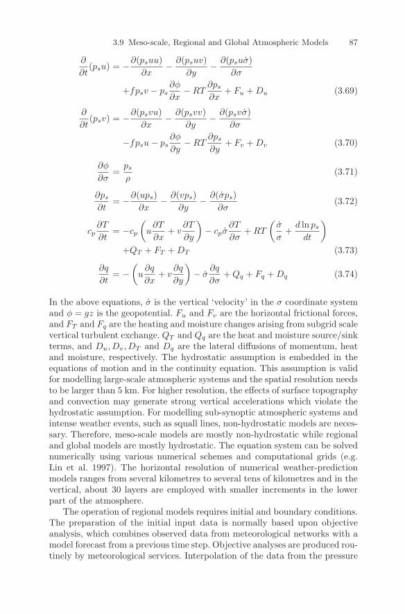
3.9 Meso-scale, Regional and Global Atmospheric Models 87
∂
∂t(psu) = −∂(psuu)
∂x− ∂(psuv)
∂y− ∂(psuσ)
∂σ
+fpsv − ps∂φ
∂x− RT
∂ps
∂x+ Fu + Du (3.69)
∂
∂t(psv) = −∂(psvu)
∂x− ∂(psvv)
∂y− ∂(psvσ)
∂σ
−fpsu − ps∂φ
∂y− RT
∂ps
∂y+ Fv + Dv (3.70)
∂φ
∂σ=
ps
ρ(3.71)
∂ps
∂t= −∂(ups)
∂x− ∂(vps)
∂y− ∂(σps)
∂σ(3.72)
cp∂T
∂t= −cp
(u
∂T
∂x+ v
∂T
∂y
)− cpσ
∂T
∂σ+ RT
(σ
σ+
d ln ps
dt
)
+QT + FT + DT (3.73)
∂q
∂t= −
(u
∂q
∂x+ v
∂q
∂y
)− σ
∂q
∂σ+ Qq + Fq + Dq (3.74)
In the above equations, σ is the vertical ‘velocity’ in the σ coordinate systemand φ = gz is the geopotential. Fu and Fv are the horizontal frictional forces,and FT and Fq are the heating and moisture changes arising from subgrid scalevertical turbulent exchange. QT and Qq are the heat and moisture source/sinkterms, and Du,Dv,DT and Dq are the lateral diffusions of momentum, heatand moisture, respectively. The hydrostatic assumption is embedded in theequations of motion and in the continuity equation. This assumption is validfor modelling large-scale atmospheric systems and the spatial resolution needsto be larger than 5 km. For higher resolution, the effects of surface topographyand convection may generate strong vertical accelerations which violate thehydrostatic assumption. For modelling sub-synoptic atmospheric systems andintense weather events, such as squall lines, non-hydrostatic models are neces-sary. Therefore, meso-scale models are mostly non-hydrostatic while regionaland global models are mostly hydrostatic. The equation system can be solvednumerically using various numerical schemes and computational grids (e.g.Lin et al. 1997). The horizontal resolution of numerical weather-predictionmodels ranges from several kilometres to several tens of kilometres and in thevertical, about 30 layers are employed with smaller increments in the lowerpart of the atmosphere.
The operation of regional models requires initial and boundary conditions.The preparation of the initial input data is normally based upon objectiveanalysis, which combines observed data from meteorological networks with amodel forecast from a previous time step. Objective analyses are produced rou-tinely by meteorological services. Interpolation of the data from the pressure
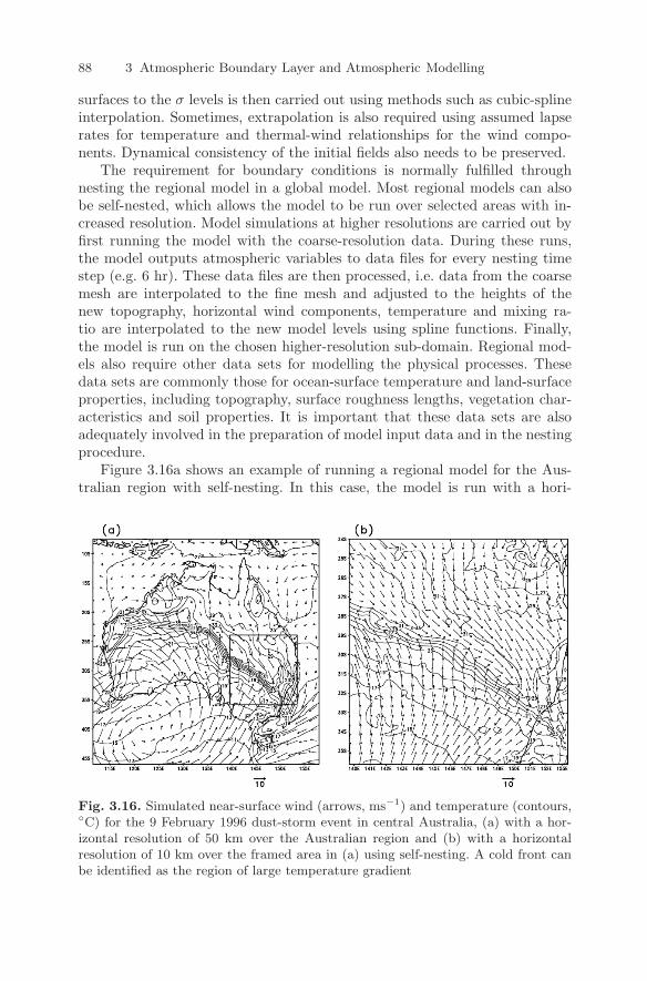
88 3 Atmospheric Boundary Layer and Atmospheric Modelling
surfaces to the σ levels is then carried out using methods such as cubic-splineinterpolation. Sometimes, extrapolation is also required using assumed lapserates for temperature and thermal-wind relationships for the wind compo-nents. Dynamical consistency of the initial fields also needs to be preserved.
The requirement for boundary conditions is normally fulfilled throughnesting the regional model in a global model. Most regional models can alsobe self-nested, which allows the model to be run over selected areas with in-creased resolution. Model simulations at higher resolutions are carried out byfirst running the model with the coarse-resolution data. During these runs,the model outputs atmospheric variables to data files for every nesting timestep (e.g. 6 hr). These data files are then processed, i.e. data from the coarsemesh are interpolated to the fine mesh and adjusted to the heights of thenew topography, horizontal wind components, temperature and mixing ra-tio are interpolated to the new model levels using spline functions. Finally,the model is run on the chosen higher-resolution sub-domain. Regional mod-els also require other data sets for modelling the physical processes. Thesedata sets are commonly those for ocean-surface temperature and land-surfaceproperties, including topography, surface roughness lengths, vegetation char-acteristics and soil properties. It is important that these data sets are alsoadequately involved in the preparation of model input data and in the nestingprocedure.
Figure 3.16a shows an example of running a regional model for the Aus-tralian region with self-nesting. In this case, the model is run with a hori-
Fig. 3.16. Simulated near-surface wind (arrows, ms−1) and temperature (contours,C) for the 9 February 1996 dust-storm event in central Australia, (a) with a hor-izontal resolution of 50 km over the Australian region and (b) with a horizontalresolution of 10 km over the framed area in (a) using self-nesting. A cold front canbe identified as the region of large temperature gradient
3.9 Meso-scale, Regional and Global Atmospheric Models 89
zontal resolution of 50 km, with the boundary conditions derived from theLimited Area Prediction System of the Australian Bureau of Meteorology,which provides the input data at a horizontal resolution of 75 km. This par-ticular weather event generated intense dust storms in the Simpson Desert ofAustralia. In order to examine the details of the frontal system, the regionalmodel is run in the self-nested mode for a selected area with the spatial resolu-tion increased from 50 km to 10 km. Figure 3.16b shows the simulated resultsnear the cold front. While the simulation with a coarse grid reveals the gen-eral features of the frontal system, the higher resolution model gives a moredetailed structure of the frontal system. As wind erosion is strongly variablein space, it is very useful to obtain atmospheric data at high resolution. Sincethe late 1980s, dust models have been constructed based on regional weathermodels. These dust models now have considerable skill for the simulation andprediction of dust storms (Uno et al. 2006).
Climate models can take many forms ranging from simple one-dimensionalenergy balance models to complex three-dimensional time-dependent generalcirculation models (GCMS) of the atmosphere and ocean. From the perspec-tive of wind erosion, climate models are mainly used to study the global dustcycle and the effect of dust on climate change (Zender et al. 2003; Ginoux et al.2004; Tanaka and Chiba, 2006). For these types of studies, three-dimensionaltime-dependent GCMS are more applicable, as detailed simulations of atmo-spheric parameters, such as wind and precipitation, can be obtained.
Climate is generally considered to represent the average behaviour ofthe climate system (including the atmosphere, hydrosphere, lithosphere,cryosphere and biosphere) over some long period of time. It is not associatedwith the exact sequence of daily weather fluctuations. Because of the inherentunpredictability of atmospheric and ocean flows, climate models are unableto predict the day-to-day sequence of weather events beyond a very fewweeks. The true utility of climate models lies in their ability to predict thestatistical properties of some future climate state. This statement applies alsoto long-term wind-erosion modelling.
Global climate models use a similar set of governing equations to regionalmodels, formulated mostly also in the σ coordinate system. With the rapidincrease of computing power, climate models are being run with increased hor-izontal and vertical resolution and increased sophistication in the treatment ofthe complex physical, geo-chemical and bio-ecological processes. As a result,the distinction between climate models and weather models has become lessobvious, apart from detailed numerical procedures. However, we note that, asclimate models attempt to model climate changes over long-time periods, thefundamental interactions between the atmosphere, the ocean and other com-ponents of the climate system become more and more important. Despite this,improvements in climate modelling in recent years have certainly provided thenecessary prerequisite for the assessment and prediction of wind-erosion cli-matology and led to new opportunities in wind-erosion studies.
4
Land-Surface Modelling
Wind erosion, a land-surface process itself, is closely related to other land-surface processes, in particular to soil hydrological and surface bio-ecologicalprocesses which determine the status of soil moisture and vegetation cover.Wind erosion occurs only if the soil is depleted of moisture and the lack ofvegetation cover is serious, as the capacity of the surface to resist wind erosiondepends critically on these factors. Hence, land-surface modelling is of criticalimportance to wind-erosion studies.
Land-surface modelling is in itself an important research topic, as vegeta-tion and soil play a major role in the climate system through their exchangeof mass, energy and momentum with the atmosphere. On the other hand,atmospheric conditions (wind, temperature and precipitation) also stronglyaffect the processes of the biosphere and the continental hydrosphere. The in-teractions between the land surface and the atmosphere constitute an activeresearch area. Sophisticated land-surface models for the simulation of theseinteractions have been developed in recent years. For atmospheric, hydrolog-ical and bio-ecological modelling, a land-surface scheme produces a range ofuseful outputs, such as (1) soil and vegetation temperatures; (2) surface netradiation, sensible-heat flux, latent-heat flux, ground-heat flux and soil-heatfluxes; (3) soil moisture and (4) flux components related to soil-water balance,including infiltration, soil water fluxes, runoff and drainage. As far as wind-erosion modelling is concerned, we are most interested in soil moisture in thevery top soil layer. In this chapter, we shall concentrate on the simulation ofsoil moisture using land-surface models.
Integrated wind-erosion modelling, as will be described in Chapter 9, andland-surface modelling have much in common. Apart from soil moisture, theparameterisations used in land-surface models for estimating friction velocityand the methodology used for the treatment of heterogeneous surfaces aredirectly transferable to wind-erosion modelling. Furthermore, wind-erosionand land-surface models share a considerable proportion of input data forsoil, vegetation and surface aerodynamic properties.
Y. Shao, Physics and Modelling of Wind Erosion, 91c© Springer Science+Business Media B.V. 2008
92 4 Land-Surface Modelling
4.1 General Aspects
The land surface mainly consists of soil (down to the water table) and veg-etation. The interest in land-surface modelling originates from the need toprovide atmospheric models with better lower-boundary conditions throughthe specification of the exchanges of momentum, energy and mass between theatmosphere and the land surface. The central task of a land-surface model is toquantify these exchanges which, as shown later, are closely related to surfacesoil hydrological processes, and hence the modelling of soil moisture becomesone of the critical issues for climate and weather models.
The processes which influence these exchanges are very complex, as theydepend both on atmospheric conditions and the physical and bio-ecologicalproperties of the land surface. The representation of these processes in a land-surface scheme is much simplified. Figure 4.1 shows the concept for such aland-surface scheme. We are mainly concerned with the energy and water bal-ance of the land surface, including the unsaturated soil layer and plants. Thestarting point is the soil-temperature equation and the soil-moisture equationof an unsaturated soil layer
∂T
∂t= − 1
Cs
∂Gt
∂z+ sh (4.1)
∂θ
∂t= −∂Gw
∂z+ sw (4.2)
where T is soil temperature, Cs is volumetric soil heat capacity (Cs = ρs cs,ρs is soil density and cs is specific heat capacity of the soil), θ is volumetricsoil water content, Gt and Gw are the heat flux and the volumetric water fluxthrough the soil, respectively, sh is a source/sink term for soil heat related tothe possible phase change of soil water, and sw is a source/sink term for soilmoisture related to processes such as transpiration.
Pores of various sizes occur in soil and a proportion of these pores is filledwith liquid water. The relative volume of this water in a unit volume of soil isdefined as volumetric soil water content, θ, often simply called soil moisture.If all soil pores are filled with water, the soil is saturated and the value ofsoil moisture is the saturation soil moisture, θs. Under natural conditions,soil cannot be dried completely and a small proportion of water is alwaystrapped in the smallest pores. The minimum value of soil moisture undernatural conditions is the air-dry soil moisture, θr. Both θs and θr depend onsoil type (see Section 4.6).
In Equations (4.1) and (4.2), land-surface properties are assumed to behorizontally homogeneous. The solution of these two equations involves theenergy and water fluxes at the interface between the atmosphere and land, asshown in Fig. 4.1. At the interface, Gt is affected by solar, atmospheric andland-surface radiations, turbulent heat transfer, evaporation and heat trans-fer in the soil, while Gw is affected by precipitation, evapotranspiration andrunoff. A land-surface scheme is, in principle, the algorithm required to solve
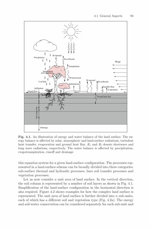
4.1 General Aspects 93
Drainage
PrecipitationRl-upward
Rs-reflected
Transpiration
Rl-downwardRl-upward
Rs-reflected
Sensible Heat
Leaf drip
InfiltrationFlood Flow
Sublimation
Snow
Ground heat flux
Soil
wat
er fl
ux
Wind
Interception
Evaporation
& Evaporation
Fig. 4.1. An illustration of energy and water balance of the land surface. The en-ergy balance is affected by solar, atmospheric and land-surface radiations, turbulentheat transfer, evaporation and ground heat flux. Rs and Rl denote shortwave andlong wave radiations, respectively. The water balance is affected by precipitation,evapotranspiration, runoff and drainage
this equation system for a given land-surface configuration. The processes rep-resented in a land-surface scheme can be broadly divided into three categories:sub-surface thermal and hydraulic processes, bare soil transfer processes andvegetation processes.
Let us now consider a unit area of land surface. In the vertical direction,the soil column is represented by a number of soil layers as shown in Fig. 4.1.Simplification of the land-surface configuration in the horizontal direction isalso required. Figure 4.2 shows examples for how the complex land surface isrepresented. The unit area of land surface is further divided into n sub-units,each of which has a different soil and vegetation type (Fig. 4.2a). The energyand soil-water conservation can be considered separately for each sub-unit and
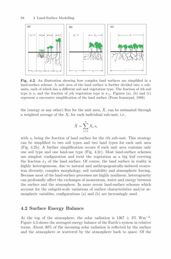
94 4 Land-Surface Modelling
s = 1
σf2
σf2
σf
σfi
σfn
σf1= 0 σ
f1= 0
s1 s1s2 s2si sn
(a) (b) (c)
Fig. 4.2. An illustration showing how complex land surfaces are simplified in aland-surface scheme. A unit area of the land surface is further divided into n sub-units, each of which has a different soil and vegetation type. The fraction of ith soiltype is si and the fraction of jth vegetation type is σfj . Figures (a), (b) and (c)represent a successive simplification of the land surface (From Irannejad, 1998)
the (energy or any other) flux for the unit area, X, can be estimated througha weighted average of the Xi for each individual sub-unit, i.e.,
X =n∑
i=1
Xi si
with si being the fraction of land surface for the ith sub-unit. This strategycan be simplified to two soil types and two land types for each unit area(Fig. 4.2b). A further simplification occurs if each unit area contains onlyone soil type and one land-use type (Fig. 4.2c). Most land-surface schemesuse simplest configuration and treat the vegetation as a big leaf coveringthe fraction σf of the land surface. Of course, the land surface in reality ishighly heterogeneous, due to natural and anthropogenically-induced ecosys-tem diversity, complex morphology, soil variability and atmospheric forcing.Because most of the land-surface processes are highly nonlinear, heterogeneitycan profoundly affect the exchanges of momentum, water and energy betweenthe surface and the atmosphere. In more recent land-surface schemes whichaccount for the subgrid-scale variations of surface characteristics and/or at-mospheric variables, configurations (a) and (b) are increasingly used.
4.2 Surface Energy Balance
At the top of the atmosphere, the solar radiation is 1367 ± 3% Wm−2.Figure 4.3 shows the averaged energy balance of the Earth’s system in relativeterms. About 30% of the incoming solar radiation is reflected by the surfaceand the atmosphere or scattered by the atmosphere back to space. Of the

4.2 Surface Energy Balance 95
5
17
14 22 11
100
57 464
109 236
20
Abs. by Atmos
Ref. fromclouds
Ref. fromsurface
Emitted fromatmosphere
Emitted fromsurface
Emitted fromsurface
Scattered fromatmosphere
Abs. by clouds
Shortwave Radiation Convective FluxesLongwave Radiation
96 23 6114Abs. from
cloudsAbs.
directlyAbs.
scatteredAbs. from
atmosphereLatent heat
from surfaceSensible Heatfrom surface
Emitted fromsurface
Fig. 4.3. Energy balance of the Earth system in percentage (After Bryant, 1997)
effective energy remaining in the system about 70% is transmitted throughthe atmosphere and absorbed by the Earth’s surface. To balance the absorbedenergy, the surface releases energy to the atmosphere through long wave radi-ation and turbulent transfers of sensible and latent heat. The Earth’s surfaceprovides about 2/3 of the energy input for the atmosphere and is hence themajor immediate energy source for atmospheric processes. The surface is theonly source of moisture. Evapotranspiration of water from the surface andits condensation in the atmosphere is the link between the energy and watercycles in the Earth’s system.
The evolution of soil moisture is closely related to that of soil temperature.This is because surface latent-heat fluxes due to evaporation and transpirationare coupled with the surface sensible-heat flux through the surface energy-balance equation
Rn(T0) − λlEv(T0) − H(T0) − Gt0(T0) = 0 (4.3)
where Rn is surface net radiation, λlEv, is latent-heat flux with Ev beingevaporation, H is sensible-heat flux, and Gt0 is ground heat flux. All energyfluxes are functions of the surface (skin) temperature T0. The net radiation,Rn, is a result of three radiation fluxes
Rn = (1 − α)Rs + εRl − εσT 40 (4.4)
where σ is the Stefan–Boltzmann constant, Rs is downward shortwave radia-tion, Rl is downward long wave radiation, α is the surface albedo and ε is thesurface emissivity. The emissivity of a substance according to Kirchhoff’s lawis equal to its absorptivity for the same wavelength range. Emissivity of thenatural substances on the Earth’s surface ranges from 0.90 to 0.99. However,in land-surface schemes a universal emissivity is usually assumed for all sur-face types. A value of 0.98 can be taken as the representative for both soil and
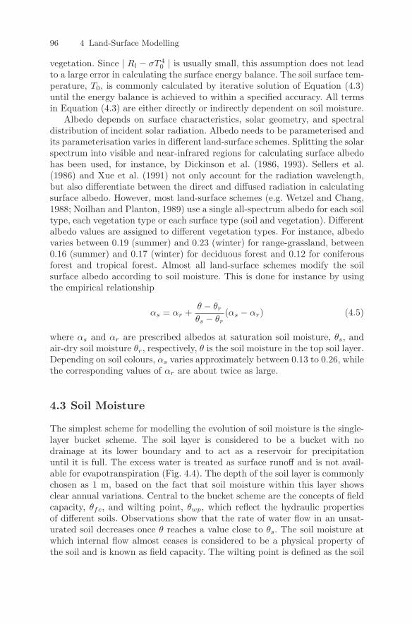
96 4 Land-Surface Modelling
vegetation. Since | Rl − σT 40 | is usually small, this assumption does not lead
to a large error in calculating the surface energy balance. The soil surface tem-perature, T0, is commonly calculated by iterative solution of Equation (4.3)until the energy balance is achieved to within a specified accuracy. All termsin Equation (4.3) are either directly or indirectly dependent on soil moisture.
Albedo depends on surface characteristics, solar geometry, and spectraldistribution of incident solar radiation. Albedo needs to be parameterised andits parameterisation varies in different land-surface schemes. Splitting the solarspectrum into visible and near-infrared regions for calculating surface albedohas been used, for instance, by Dickinson et al. (1986, 1993). Sellers et al.(1986) and Xue et al. (1991) not only account for the radiation wavelength,but also differentiate between the direct and diffused radiation in calculatingsurface albedo. However, most land-surface schemes (e.g. Wetzel and Chang,1988; Noilhan and Planton, 1989) use a single all-spectrum albedo for each soiltype, each vegetation type or each surface type (soil and vegetation). Differentalbedo values are assigned to different vegetation types. For instance, albedovaries between 0.19 (summer) and 0.23 (winter) for range-grassland, between0.16 (summer) and 0.17 (winter) for deciduous forest and 0.12 for coniferousforest and tropical forest. Almost all land-surface schemes modify the soilsurface albedo according to soil moisture. This is done for instance by usingthe empirical relationship
αs = αr +θ − θr
θs − θr(αs − αr) (4.5)
where αs and αr are prescribed albedos at saturation soil moisture, θs, andair-dry soil moisture θr, respectively, θ is the soil moisture in the top soil layer.Depending on soil colours, αs varies approximately between 0.13 to 0.26, whilethe corresponding values of αr are about twice as large.
4.3 Soil Moisture
The simplest scheme for modelling the evolution of soil moisture is the single-layer bucket scheme. The soil layer is considered to be a bucket with nodrainage at its lower boundary and to act as a reservoir for precipitationuntil it is full. The excess water is treated as surface runoff and is not avail-able for evapotranspiration (Fig. 4.4). The depth of the soil layer is commonlychosen as 1 m, based on the fact that soil moisture within this layer showsclear annual variations. Central to the bucket scheme are the concepts of fieldcapacity, θfc, and wilting point, θwp, which reflect the hydraulic propertiesof different soils. Observations show that the rate of water flow in an unsat-urated soil decreases once θ reaches a value close to θs. The soil moisture atwhich internal flow almost ceases is considered to be a physical property ofthe soil and is known as field capacity. The wilting point is defined as the soil
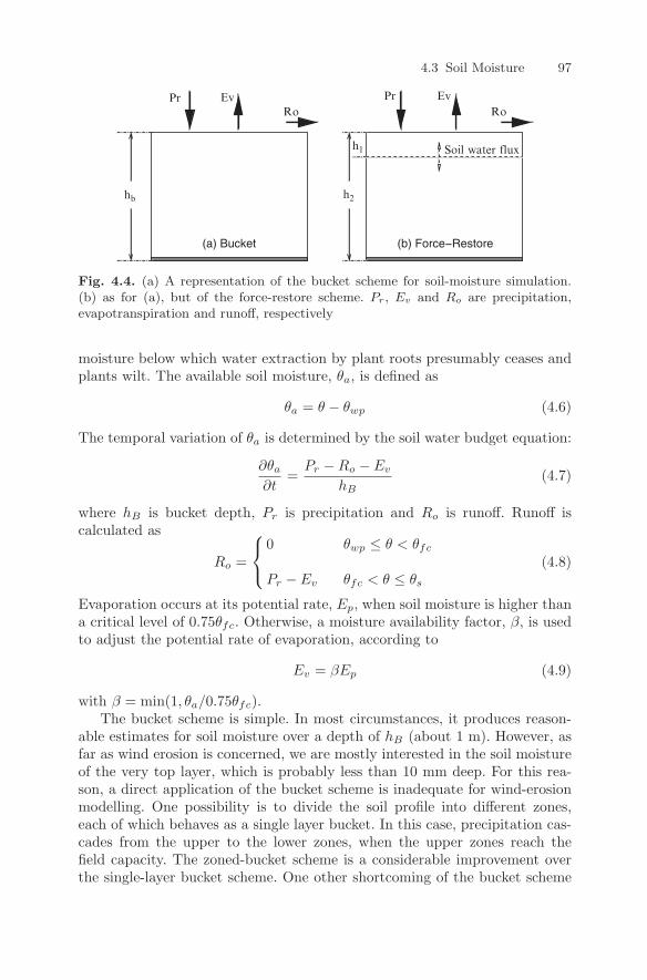
4.3 Soil Moisture 97
Soil water flux
PrRo
EvPrRo
hb h2
h1
Ev
(a) Bucket (b) Force−Restore
Fig. 4.4. (a) A representation of the bucket scheme for soil-moisture simulation.(b) as for (a), but of the force-restore scheme. Pr, Ev and Ro are precipitation,evapotranspiration and runoff, respectively
moisture below which water extraction by plant roots presumably ceases andplants wilt. The available soil moisture, θa, is defined as
θa = θ − θwp (4.6)
The temporal variation of θa is determined by the soil water budget equation:
∂θa
∂t=
Pr − Ro − Ev
hB(4.7)
where hB is bucket depth, Pr is precipitation and Ro is runoff. Runoff iscalculated as
Ro =
⎧⎨⎩
0 θwp ≤ θ < θfc
Pr − Ev θfc < θ ≤ θs
(4.8)
Evaporation occurs at its potential rate, Ep, when soil moisture is higher thana critical level of 0.75θfc. Otherwise, a moisture availability factor, β, is usedto adjust the potential rate of evaporation, according to
Ev = βEp (4.9)
with β = min(1, θa/0.75θfc).The bucket scheme is simple. In most circumstances, it produces reason-
able estimates for soil moisture over a depth of hB (about 1 m). However, asfar as wind erosion is concerned, we are mostly interested in the soil moistureof the very top layer, which is probably less than 10 mm deep. For this rea-son, a direct application of the bucket scheme is inadequate for wind-erosionmodelling. One possibility is to divide the soil profile into different zones,each of which behaves as a single layer bucket. In this case, precipitation cas-cades from the upper to the lower zones, when the upper zones reach thefield capacity. The zoned-bucket scheme is a considerable improvement overthe single-layer bucket scheme. One other shortcoming of the bucket scheme
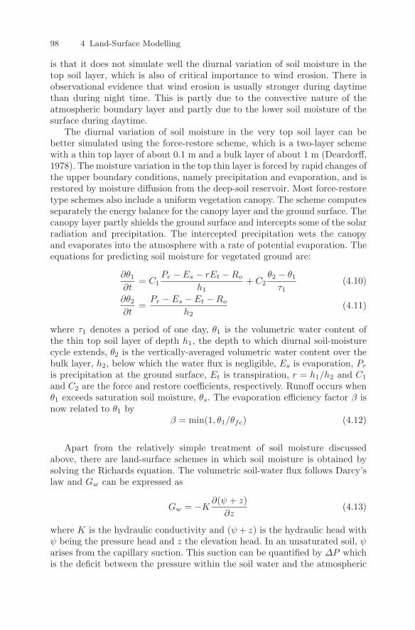
98 4 Land-Surface Modelling
is that it does not simulate well the diurnal variation of soil moisture in thetop soil layer, which is also of critical importance to wind erosion. There isobservational evidence that wind erosion is usually stronger during daytimethan during night time. This is partly due to the convective nature of theatmospheric boundary layer and partly due to the lower soil moisture of thesurface during daytime.
The diurnal variation of soil moisture in the very top soil layer can bebetter simulated using the force-restore scheme, which is a two-layer schemewith a thin top layer of about 0.1 m and a bulk layer of about 1 m (Deardorff,1978). The moisture variation in the top thin layer is forced by rapid changes ofthe upper boundary conditions, namely precipitation and evaporation, and isrestored by moisture diffusion from the deep-soil reservoir. Most force-restoretype schemes also include a uniform vegetation canopy. The scheme computesseparately the energy balance for the canopy layer and the ground surface. Thecanopy layer partly shields the ground surface and intercepts some of the solarradiation and precipitation. The intercepted precipitation wets the canopyand evaporates into the atmosphere with a rate of potential evaporation. Theequations for predicting soil moisture for vegetated ground are:
∂θ1
∂t= C1
Pr − Es − rEt − Ro
h1+ C2
θ2 − θ1
τ1(4.10)
∂θ2
∂t=
Pr − Es − Et − Ro
h2(4.11)
where τ1 denotes a period of one day, θ1 is the volumetric water content ofthe thin top soil layer of depth h1, the depth to which diurnal soil-moisturecycle extends, θ2 is the vertically-averaged volumetric water content over thebulk layer, h2, below which the water flux is negligible, Es is evaporation, Pr
is precipitation at the ground surface, Et is transpiration, r = h1/h2 and C1
and C2 are the force and restore coefficients, respectively. Runoff occurs whenθ1 exceeds saturation soil moisture, θs. The evaporation efficiency factor β isnow related to θ1 by
β = min(1, θ1/θfc) (4.12)
Apart from the relatively simple treatment of soil moisture discussedabove, there are land-surface schemes in which soil moisture is obtained bysolving the Richards equation. The volumetric soil-water flux follows Darcy’slaw and Gw can be expressed as
Gw = −K∂(ψ + z)
∂z(4.13)
where K is the hydraulic conductivity and (ψ + z) is the hydraulic head withψ being the pressure head and z the elevation head. In an unsaturated soil, ψarises from the capillary suction. This suction can be quantified by ∆P whichis the deficit between the pressure within the soil water and the atmospheric
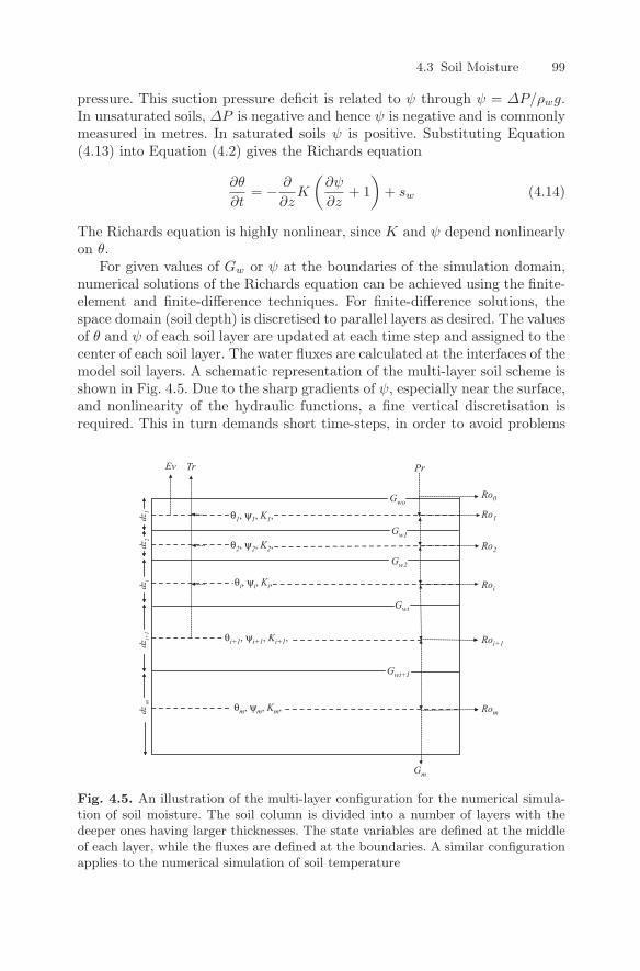
4.3 Soil Moisture 99
pressure. This suction pressure deficit is related to ψ through ψ = ∆P/ρwg.In unsaturated soils, ∆P is negative and hence ψ is negative and is commonlymeasured in metres. In saturated soils ψ is positive. Substituting Equation(4.13) into Equation (4.2) gives the Richards equation
∂θ
∂t= − ∂
∂zK
(∂ψ
∂z+ 1
)+ sw (4.14)
The Richards equation is highly nonlinear, since K and ψ depend nonlinearlyon θ.
For given values of Gw or ψ at the boundaries of the simulation domain,numerical solutions of the Richards equation can be achieved using the finite-element and finite-difference techniques. For finite-difference solutions, thespace domain (soil depth) is discretised to parallel layers as desired. The valuesof θ and ψ of each soil layer are updated at each time step and assigned to thecenter of each soil layer. The water fluxes are calculated at the interfaces of themodel soil layers. A schematic representation of the multi-layer soil scheme isshown in Fig. 4.5. Due to the sharp gradients of ψ, especially near the surface,and nonlinearity of the hydraulic functions, a fine vertical discretisation isrequired. This in turn demands short time-steps, in order to avoid problems
Gwo
Gw1
Gw2
Gwi
Gwi+1
Gm
Ev Tr Pr
θ1, ψ1, K1,
θ2, ψ2, K2,
θi, ψi, Ki,
θm, ψm, Km,
θi+1, ψi+1, Ki+1,
Ro0
Ro1
Ro2
Roi
Roi+1
Rom
dz1
dz2
dzi
dzi+
1dz
m
Fig. 4.5. An illustration of the multi-layer configuration for the numerical simula-tion of soil moisture. The soil column is divided into a number of layers with thedeeper ones having larger thicknesses. The state variables are defined at the middleof each layer, while the fluxes are defined at the boundaries. A similar configurationapplies to the numerical simulation of soil temperature
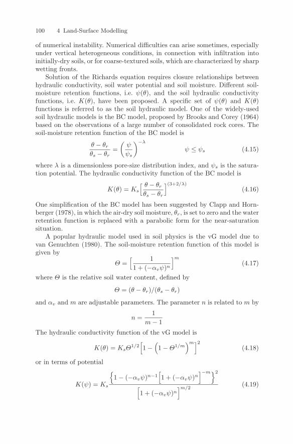
100 4 Land-Surface Modelling
of numerical instability. Numerical difficulties can arise sometimes, especiallyunder vertical heterogeneous conditions, in connection with infiltration intoinitially-dry soils, or for coarse-textured soils, which are characterized by sharpwetting fronts.
Solution of the Richards equation requires closure relationships betweenhydraulic conductivity, soil water potential and soil moisture. Different soil-moisture retention functions, i.e. ψ(θ), and the soil hydraulic conductivityfunctions, i.e. K(θ), have been proposed. A specific set of ψ(θ) and K(θ)functions is referred to as the soil hydraulic model. One of the widely-usedsoil hydraulic models is the BC model, proposed by Brooks and Corey (1964)based on the observations of a large number of consolidated rock cores. Thesoil-moisture retention function of the BC model is
θ − θr
θs − θr=
(ψ
ψs
)−λ
ψ ≤ ψs (4.15)
where λ is a dimensionless pore-size distribution index, and ψs is the satura-tion potential. The hydraulic conductivity function of the BC model is
K(θ) = Ks
[ θ − θr
θs − θr
](3+2/λ)
(4.16)
One simplification of the BC model has been suggested by Clapp and Horn-berger (1978), in which the air-dry soil moisture, θr, is set to zero and the waterretention function is replaced with a parabolic form for the near-saturationsituation.
A popular hydraulic model used in soil physics is the vG model due tovan Genuchten (1980). The soil-moisture retention function of this model isgiven by
Θ =[ 11 + (−αvψ)n
]m
(4.17)
where Θ is the relative soil water content, defined by
Θ = (θ − θr)/(θs − θr)
and αv and m are adjustable parameters. The parameter n is related to m by
n =1
m − 1
The hydraulic conductivity function of the vG model is
K(θ) = KsΘ1/2
[1 −
(1 − Θ1/m
)m]2
(4.18)
or in terms of potential
K(ψ) = Ks
1 − (−αvψ)n−1
[1 + (−αvψ)n
]−m2
[1 + (−αvψ)n
]m/2(4.19)
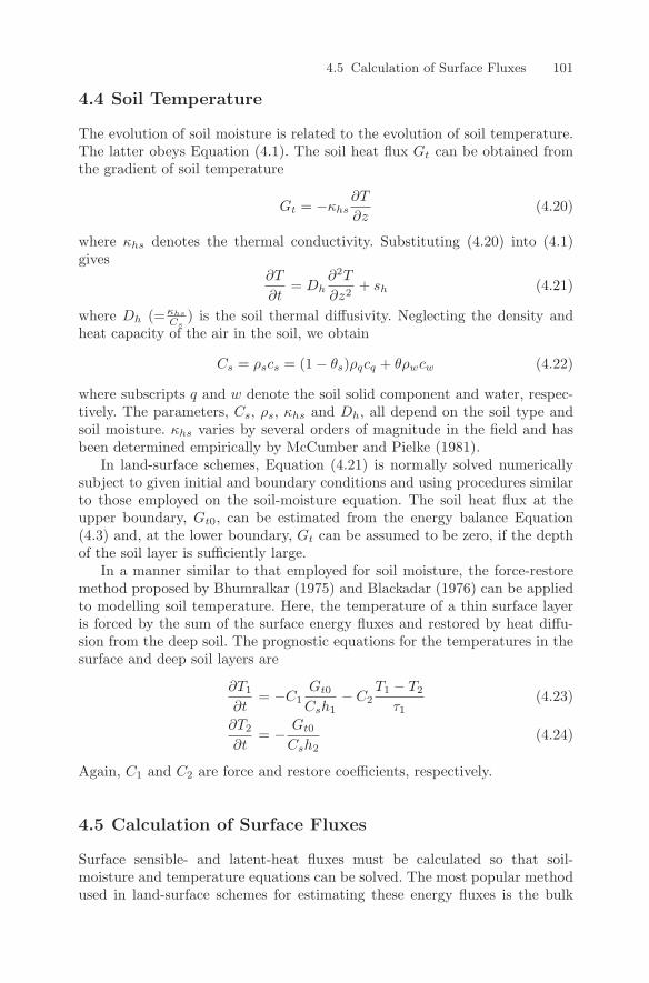
4.5 Calculation of Surface Fluxes 101
4.4 Soil Temperature
The evolution of soil moisture is related to the evolution of soil temperature.The latter obeys Equation (4.1). The soil heat flux Gt can be obtained fromthe gradient of soil temperature
Gt = −κhs∂T
∂z(4.20)
where κhs denotes the thermal conductivity. Substituting (4.20) into (4.1)gives
∂T
∂t= Dh
∂2T
∂z2+ sh (4.21)
where Dh (=κhs
Cs) is the soil thermal diffusivity. Neglecting the density and
heat capacity of the air in the soil, we obtain
Cs = ρscs = (1 − θs)ρqcq + θρwcw (4.22)
where subscripts q and w denote the soil solid component and water, respec-tively. The parameters, Cs, ρs, κhs and Dh, all depend on the soil type andsoil moisture. κhs varies by several orders of magnitude in the field and hasbeen determined empirically by McCumber and Pielke (1981).
In land-surface schemes, Equation (4.21) is normally solved numericallysubject to given initial and boundary conditions and using procedures similarto those employed on the soil-moisture equation. The soil heat flux at theupper boundary, Gt0, can be estimated from the energy balance Equation(4.3) and, at the lower boundary, Gt can be assumed to be zero, if the depthof the soil layer is sufficiently large.
In a manner similar to that employed for soil moisture, the force-restoremethod proposed by Bhumralkar (1975) and Blackadar (1976) can be appliedto modelling soil temperature. Here, the temperature of a thin surface layeris forced by the sum of the surface energy fluxes and restored by heat diffu-sion from the deep soil. The prognostic equations for the temperatures in thesurface and deep soil layers are
∂T1
∂t= −C1
Gt0
Csh1− C2
T1 − T2
τ1(4.23)
∂T2
∂t= − Gt0
Csh2(4.24)
Again, C1 and C2 are force and restore coefficients, respectively.
4.5 Calculation of Surface Fluxes
Surface sensible- and latent-heat fluxes must be calculated so that soil-moisture and temperature equations can be solved. The most popular methodused in land-surface schemes for estimating these energy fluxes is the bulk
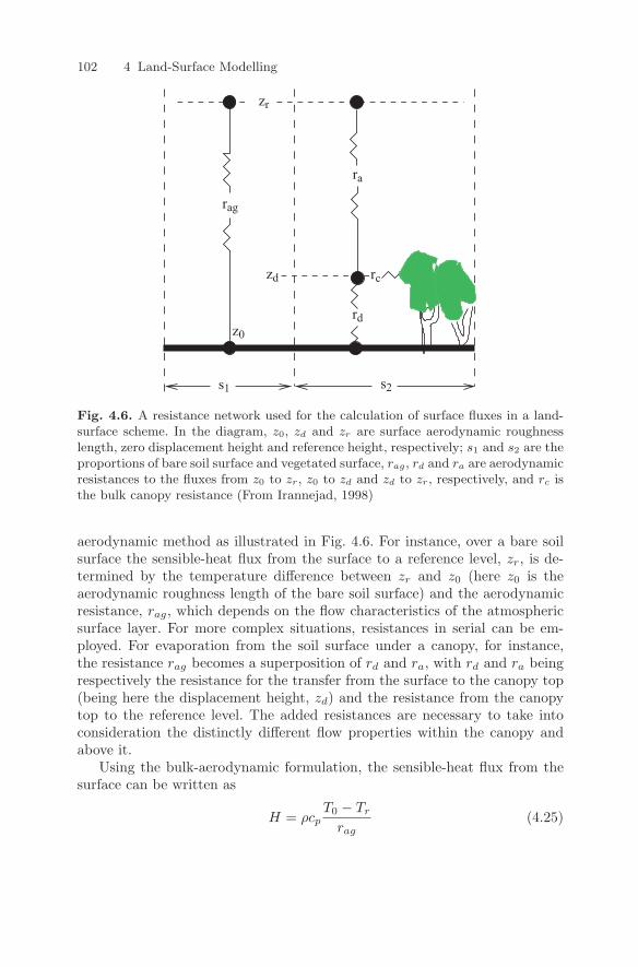
102 4 Land-Surface Modelling
s1 s2
zr
zd
z0
rag
ra
rc
rd
Fig. 4.6. A resistance network used for the calculation of surface fluxes in a land-surface scheme. In the diagram, z0, zd and zr are surface aerodynamic roughnesslength, zero displacement height and reference height, respectively; s1 and s2 are theproportions of bare soil surface and vegetated surface, rag, rd and ra are aerodynamicresistances to the fluxes from z0 to zr, z0 to zd and zd to zr, respectively, and rc isthe bulk canopy resistance (From Irannejad, 1998)
aerodynamic method as illustrated in Fig. 4.6. For instance, over a bare soilsurface the sensible-heat flux from the surface to a reference level, zr, is de-termined by the temperature difference between zr and z0 (here z0 is theaerodynamic roughness length of the bare soil surface) and the aerodynamicresistance, rag, which depends on the flow characteristics of the atmosphericsurface layer. For more complex situations, resistances in serial can be em-ployed. For evaporation from the soil surface under a canopy, for instance,the resistance rag becomes a superposition of rd and ra, with rd and ra beingrespectively the resistance for the transfer from the surface to the canopy top(being here the displacement height, zd) and the resistance from the canopytop to the reference level. The added resistances are necessary to take intoconsideration the distinctly different flow properties within the canopy andabove it.
Using the bulk-aerodynamic formulation, the sensible-heat flux from thesurface can be written as
H = ρcpT0 − Tr
rag(4.25)
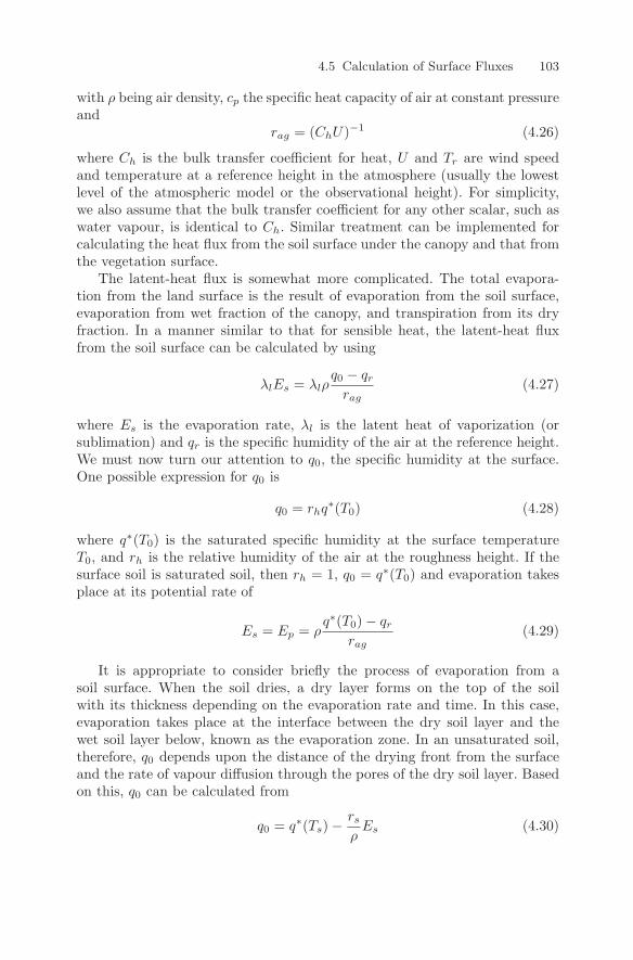
4.5 Calculation of Surface Fluxes 103
with ρ being air density, cp the specific heat capacity of air at constant pressureand
rag = (ChU)−1 (4.26)
where Ch is the bulk transfer coefficient for heat, U and Tr are wind speedand temperature at a reference height in the atmosphere (usually the lowestlevel of the atmospheric model or the observational height). For simplicity,we also assume that the bulk transfer coefficient for any other scalar, such aswater vapour, is identical to Ch. Similar treatment can be implemented forcalculating the heat flux from the soil surface under the canopy and that fromthe vegetation surface.
The latent-heat flux is somewhat more complicated. The total evapora-tion from the land surface is the result of evaporation from the soil surface,evaporation from wet fraction of the canopy, and transpiration from its dryfraction. In a manner similar to that for sensible heat, the latent-heat fluxfrom the soil surface can be calculated by using
λlEs = λlρq0 − qr
rag(4.27)
where Es is the evaporation rate, λl is the latent heat of vaporization (orsublimation) and qr is the specific humidity of the air at the reference height.We must now turn our attention to q0, the specific humidity at the surface.One possible expression for q0 is
q0 = rhq∗(T0) (4.28)
where q∗(T0) is the saturated specific humidity at the surface temperatureT0, and rh is the relative humidity of the air at the roughness height. If thesurface soil is saturated soil, then rh = 1, q0 = q∗(T0) and evaporation takesplace at its potential rate of
Es = Ep = ρq∗(T0) − qr
rag(4.29)
It is appropriate to consider briefly the process of evaporation from asoil surface. When the soil dries, a dry layer forms on the top of the soilwith its thickness depending on the evaporation rate and time. In this case,evaporation takes place at the interface between the dry soil layer and thewet soil layer below, known as the evaporation zone. In an unsaturated soil,therefore, q0 depends upon the distance of the drying front from the surfaceand the rate of vapour diffusion through the pores of the dry soil layer. Basedon this, q0 can be calculated from
q0 = q∗(Ts) −rs
ρEs (4.30)
104 4 Land-Surface Modelling
where q∗(Ts) is the saturation specific humidity at the evaporation zone wherethe temperature is Ts, rs is the resistance to vapour diffusion from the evap-oration zone to the surface. It is sufficiently accurate to assume that Ts = T0.Rearranging Equation (4.27) for q0, we obtain
q0 = qr +rag
ρEs (4.31)
Equating (4.30) and (4.31), we can eliminate q0 in calculating soil evaporationby using
Es = ρq∗(T0) − qr
rag + rs(4.32)
In Equation (4.32), rs needs to be estimated. The latter equation has beenused often to estimate the soil evaporation. Alternatively, Equation (4.27) canbe used for the purpose with q0 being approximated by the so-called α and βmethods (e.g. Mahfouf and Noilhan, 1991), i.e.
q0 =
⎧⎨⎩
βq∗(T0) + qr(1 − β), β method
rhq∗(T0), α method(4.33)
It thus follows that Es can be estimated by
Es =
⎧⎨⎩
ρβ q∗(T0)−qr
rag, β method
ρ rhq∗(T0)−qr
rag, α method
(4.34)
Obviously, both rh and β are functions of soil moisture in the very top soillayer. A very simple choice of β is, for instance, Equation (4.12). A summaryof various rh and β expressions can be found in Mahfouf and Noilhan (1991).
Transpiration is the flux of water vapour through the exposed plant leavesto the atmosphere. In a manner not unlike the unsaturated-soils case, thetranspiration zone is not at the surface, but is inside the ‘valve-like structure’of the leaves, namely the stomata. Transpiration involves the transfer of wa-ter vapour from plant stomata to the reference level through three sequentialpaths. First, water vapour is transferred by molecular diffusion from withinthe stomata to the leaf surface at zs, which is surrounded by a quasi-laminarboundary layer. Second, canopy turbulence carries water vapour from the leafsurface to the top of the canopy at zc. Finally, at the scale of the wholecanopy, atmospheric turbulence carries the water vapour from zc to the ref-erence height zr. The resistances for the three sequential transfer paths arethe stomatal resistance, rst, canopy air resistance, rac and above canopy airresistance, ra. The transpiration rate through this sequential process can becalculated from
Et = ρq∗(Tc) − qr
rst + rac + ra(4.35)
4.5 Calculation of Surface Fluxes 105
where q∗(Tc) is the saturation specific humidity at the leaf temperature Tc. Asthe canopy consists of many individual leaves, it is not practical to considerthe resistance for each individual stomata and each individual leaf. Instead, itis much simpler to consider the collection of all leaves to be a big leaf and touse rc, the stomatal resistance of this ‘leaf’ (known also as the bulk stomatalresistance or simply the canopy resistance). The transpiration rate from theentire canopy can then be calculated using Equation (4.35), with rst beingreplaced with rc.
We now briefly describe how the aerodynamic resistance, canopy air re-sistance and bulk stomatal resistance are estimated in land-surface schemes.In most schemes, the aerodynamic resistance is estimated using the Monin–Obukhov similarity theory. Using this theory, the bulk transfer coefficient Ch
is given by
Ch =κ2
ΨmΨh(4.36)
where Ψm and Ψh are the similarity functions already given in Chapter 3. Itfollows that the aerodynamic resistances, rag and ra, can be obtained usingEquation (4.26). The calculation of canopy air resistance, rac, is more compli-cated, as the Monin–Obukhov similarity theory does not apply to flows withinthe canopy, and rac varies with canopy configurations. One possible methodof estimating rac is to specify a profile of eddy diffusivity as shown in Fig. 8.17and then compute rac by integration of the reciprocal of the eddy diffusivity.
The canopy resistance is a quantity which is difficult to measure. In mostland-surface schemes, the stomatal resistance of a single leaf, rst, is calculatedand the bulk stomatal resistance, rc, is obtained using an Ohm’s-law analogyin which it is assumed that all leaves of the canopy operate in parallel. Thecommon expression for rc is that
rc =rst
La(4.37)
where La is leaf-area index, defined as the one-sided surface of all leaves overa unit area of land surface.
Different methods have been used to account for the canopy resistance,ranging from a constant value of rc for different vegetation types to thosewhich calculate rc by a multiple-factorial equation consisting of a minimumresistance and functions of environmental factors which influence the tran-spiration process. Jarvis (1976) proposed a model to describe the stomatalresistance as a function of radiation, ambient air CO2 concentration, atmo-spheric vapour-pressure deficit, leaf temperature and leaf-water potential. Themodel parameters are derived using non-linear regression analysis, assumingthat there was no synergistic interaction among the environmental variables.The proposed parameterisation of stomatal resistance is of the form
rst = rst,min(F1F2F3F4)−1 (4.38)
106 4 Land-Surface Modelling
where rst,min is the smallest value rst can reach. In Equation (4.38), F1 rep-resents the effect of the photosynthetically active radiation, parameterised by
F1 =f + rst,min/rst,max
1 + f(4.39)
where rst,max is the maximum stomatal resistance, corresponding to a situa-tion of closed stomata, and f is given by
f =1.1La
Rs
Rsl
where Rs is solar radiation and Rsl is a limiting value of 30 Wm−2 for forestand of 100 Wm−2 for crops and grassland. The factor F2 measures the effectof water stress on the canopy resistance, as
F2 =
⎧⎨⎩
1, θ > θfcθ−θwp
θfc−θwp, θwp ≤ θ ≤ θfc
0, θ < θwp
(4.40)
Here, θ takes the mean soil moisture in the root zone. F3 represents the effectof the water-vapour deficit, ∆q, in the air surrounding the leaves, which canbe written as
F3 = 1 − 0.6∆q (4.41)
F4 is the factor describing the effect of the air temperature, Ta, on the surfaceresistance and can be parameterised as
F4 = 1 − 0.0016(298 − Ta)2 (4.42)
4.6 Land-Surface Parameters
A land-surface scheme requires a set of atmospheric variables as input data, in-cluding downward short-wave solar radiation, downward infrared atmosphericradiation, precipitation, air temperature, wind speed, surface pressure andspecific humidity. The atmospheric forcing data can be obtained either fromobservations for given locations or, if the land-surface scheme is coupled withan atmospheric model, from the predictions of that model.
The land-surface scheme also requires parameters which specify a rangeof properties of the land-surface. Numerous studies have shown that the per-formance of a land-surface scheme is sensitive to the choice of land-surfaceparameters (Ek and Cuenca, 1994). While different land-surface schemes mayuse different parameters, they can be divided roughly into the categories forsurface vegetation, aerodynamics, radiation, soil hydraulics and thermal prop-erties, as listed in Table 4.1.
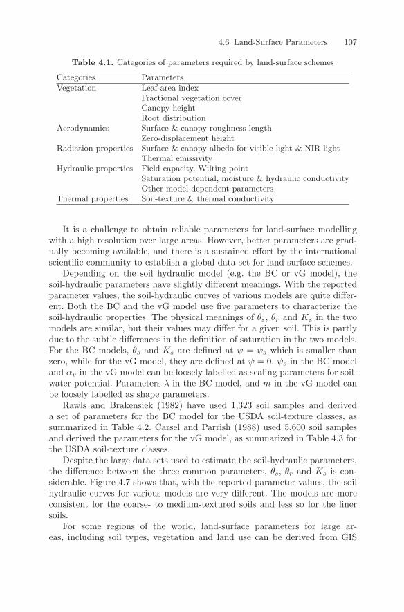
4.6 Land-Surface Parameters 107
Table 4.1. Categories of parameters required by land-surface schemes
Categories Parameters
Vegetation Leaf-area indexFractional vegetation coverCanopy heightRoot distribution
Aerodynamics Surface & canopy roughness lengthZero-displacement height
Radiation properties Surface & canopy albedo for visible light & NIR lightThermal emissivity
Hydraulic properties Field capacity, Wilting pointSaturation potential, moisture & hydraulic conductivityOther model dependent parameters
Thermal properties Soil-texture & thermal conductivity
It is a challenge to obtain reliable parameters for land-surface modellingwith a high resolution over large areas. However, better parameters are grad-ually becoming available, and there is a sustained effort by the internationalscientific community to establish a global data set for land-surface schemes.
Depending on the soil hydraulic model (e.g. the BC or vG model), thesoil-hydraulic parameters have slightly different meanings. With the reportedparameter values, the soil-hydraulic curves of various models are quite differ-ent. Both the BC and the vG model use five parameters to characterize thesoil-hydraulic properties. The physical meanings of θs, θr and Ks in the twomodels are similar, but their values may differ for a given soil. This is partlydue to the subtle differences in the definition of saturation in the two models.For the BC models, θs and Ks are defined at ψ = ψs which is smaller thanzero, while for the vG model, they are defined at ψ = 0. ψs in the BC modeland αv in the vG model can be loosely labelled as scaling parameters for soil-water potential. Parameters λ in the BC model, and m in the vG model canbe loosely labelled as shape parameters.
Rawls and Brakensiek (1982) have used 1,323 soil samples and deriveda set of parameters for the BC model for the USDA soil-texture classes, assummarized in Table 4.2. Carsel and Parrish (1988) used 5,600 soil samplesand derived the parameters for the vG model, as summarized in Table 4.3 forthe USDA soil-texture classes.
Despite the large data sets used to estimate the soil-hydraulic parameters,the difference between the three common parameters, θs, θr and Ks is con-siderable. Figure 4.7 shows that, with the reported parameter values, the soilhydraulic curves for various models are very different. The models are moreconsistent for the coarse- to medium-textured soils and less so for the finersoils.
For some regions of the world, land-surface parameters for large ar-eas, including soil types, vegetation and land use can be derived from GIS
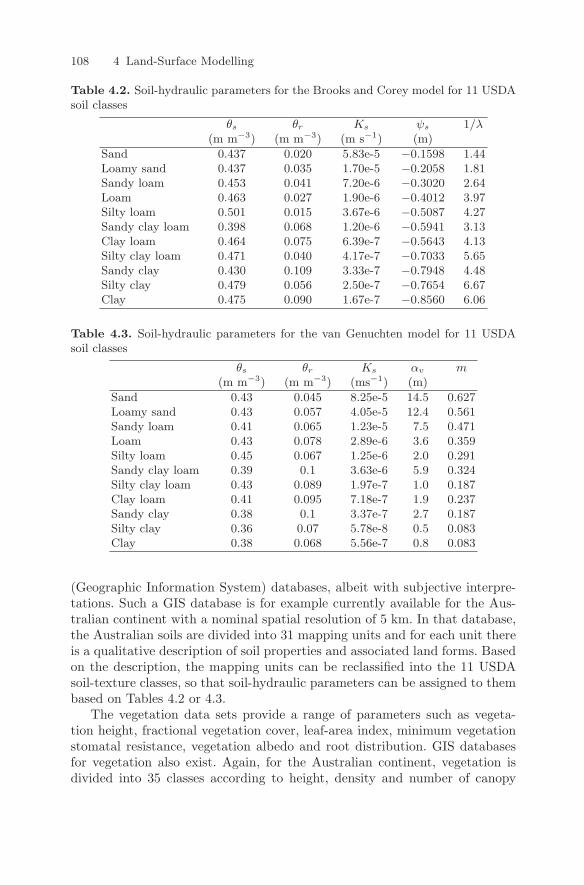
108 4 Land-Surface Modelling
Table 4.2. Soil-hydraulic parameters for the Brooks and Corey model for 11 USDAsoil classes
θs θr Ks ψs 1/λ(m m−3) (m m−3) (m s−1) (m)
Sand 0.437 0.020 5.83e-5 −0.1598 1.44Loamy sand 0.437 0.035 1.70e-5 −0.2058 1.81Sandy loam 0.453 0.041 7.20e-6 −0.3020 2.64Loam 0.463 0.027 1.90e-6 −0.4012 3.97Silty loam 0.501 0.015 3.67e-6 −0.5087 4.27Sandy clay loam 0.398 0.068 1.20e-6 −0.5941 3.13Clay loam 0.464 0.075 6.39e-7 −0.5643 4.13Silty clay loam 0.471 0.040 4.17e-7 −0.7033 5.65Sandy clay 0.430 0.109 3.33e-7 −0.7948 4.48Silty clay 0.479 0.056 2.50e-7 −0.7654 6.67Clay 0.475 0.090 1.67e-7 −0.8560 6.06
Table 4.3. Soil-hydraulic parameters for the van Genuchten model for 11 USDAsoil classes
θs θr Ks αv m(m m−3) (m m−3) (ms−1) (m)
Sand 0.43 0.045 8.25e-5 14.5 0.627Loamy sand 0.43 0.057 4.05e-5 12.4 0.561Sandy loam 0.41 0.065 1.23e-5 7.5 0.471Loam 0.43 0.078 2.89e-6 3.6 0.359Silty loam 0.45 0.067 1.25e-6 2.0 0.291Sandy clay loam 0.39 0.1 3.63e-6 5.9 0.324Silty clay loam 0.43 0.089 1.97e-7 1.0 0.187Clay loam 0.41 0.095 7.18e-7 1.9 0.237Sandy clay 0.38 0.1 3.37e-7 2.7 0.187Silty clay 0.36 0.07 5.78e-8 0.5 0.083Clay 0.38 0.068 5.56e-7 0.8 0.083
(Geographic Information System) databases, albeit with subjective interpre-tations. Such a GIS database is for example currently available for the Aus-tralian continent with a nominal spatial resolution of 5 km. In that database,the Australian soils are divided into 31 mapping units and for each unit thereis a qualitative description of soil properties and associated land forms. Basedon the description, the mapping units can be reclassified into the 11 USDAsoil-texture classes, so that soil-hydraulic parameters can be assigned to thembased on Tables 4.2 or 4.3.
The vegetation data sets provide a range of parameters such as vegeta-tion height, fractional vegetation cover, leaf-area index, minimum vegetationstomatal resistance, vegetation albedo and root distribution. GIS databasesfor vegetation also exist. Again, for the Australian continent, vegetation isdivided into 35 classes according to height, density and number of canopy
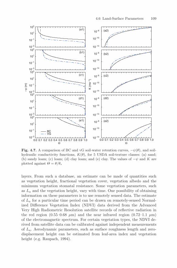
4.6 Land-Surface Parameters 109
Θ
BCVG
−ψ
(m
)
Θ
K (
ms−
1 )
(a1) (a2)
(b1) (b2)
(c1) (c2)
(d1) (d2)
(e1) (e2)
101
10−1
10−3
103
101
10−1
10−3
103
101
10−1
10−3
103
101
10−1
10−3
103
0.0 0.1 0.2 0.3 0.4 0.5 0.6 0.7 0.8 0.9 1.0 0.0 0.1 0.2 0.3 0.4 0.5 0.6 0.7 0.8 0.9 1.0
101
10−1
10−3
103
10−10
10−14
10−6
10−10
10−14
10−6
10−10
10−14
10−6
10−10
10−14
10−6
10−10
10−14
10−6
Fig. 4.7. A comparison of BC and vG soil-water retention curves, −ψ(θ), and soil-hydraulic conductivity functions, K(θ), for 5 USDA soil-texture classes: (a) sand;(b) sandy loam; (c) loam; (d) clay loam; and (e) clay. The values of −ψ and K areplotted against Θ = θ/θs
layers. From such a database, an estimate can be made of quantities suchas vegetation height, fractional vegetation cover, vegetation albedo and theminimum vegetation stomatal resistance. Some vegetation parameters, suchas La and the vegetation height, vary with time. One possibility of obtaininginformation on these parameters is to use remotely sensed data. The estimateof La for a particular time period can be drawn on remotely-sensed Normal-ized Difference Vegetation Index (NDVI) data derived from the AdvancedVery High Radiometric Resolution satellite records of reflective radiation inthe red region (0.55–0.68 µm) and the near infrared region (0.72–1.1 µm)of the electromagnetic spectrum. For certain vegetation types, the NDVI de-rived from satellite data can be calibrated against independent measurementsof La. Aerodynamic parameters, such as surface roughness length and zero-displacement height can be estimated from leaf-area index and vegetationheight (e.g. Raupach, 1994).
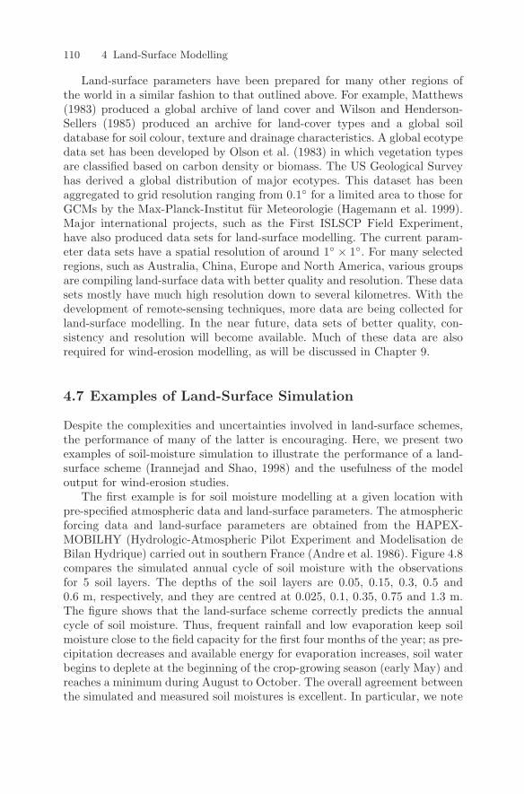
110 4 Land-Surface Modelling
Land-surface parameters have been prepared for many other regions ofthe world in a similar fashion to that outlined above. For example, Matthews(1983) produced a global archive of land cover and Wilson and Henderson-Sellers (1985) produced an archive for land-cover types and a global soildatabase for soil colour, texture and drainage characteristics. A global ecotypedata set has been developed by Olson et al. (1983) in which vegetation typesare classified based on carbon density or biomass. The US Geological Surveyhas derived a global distribution of major ecotypes. This dataset has beenaggregated to grid resolution ranging from 0.1 for a limited area to those forGCMs by the Max-Planck-Institut fur Meteorologie (Hagemann et al. 1999).Major international projects, such as the First ISLSCP Field Experiment,have also produced data sets for land-surface modelling. The current param-eter data sets have a spatial resolution of around 1 × 1. For many selectedregions, such as Australia, China, Europe and North America, various groupsare compiling land-surface data with better quality and resolution. These datasets mostly have much high resolution down to several kilometres. With thedevelopment of remote-sensing techniques, more data are being collected forland-surface modelling. In the near future, data sets of better quality, con-sistency and resolution will become available. Much of these data are alsorequired for wind-erosion modelling, as will be discussed in Chapter 9.
4.7 Examples of Land-Surface Simulation
Despite the complexities and uncertainties involved in land-surface schemes,the performance of many of the latter is encouraging. Here, we present twoexamples of soil-moisture simulation to illustrate the performance of a land-surface scheme (Irannejad and Shao, 1998) and the usefulness of the modeloutput for wind-erosion studies.
The first example is for soil moisture modelling at a given location withpre-specified atmospheric data and land-surface parameters. The atmosphericforcing data and land-surface parameters are obtained from the HAPEX-MOBILHY (Hydrologic-Atmospheric Pilot Experiment and Modelisation deBilan Hydrique) carried out in southern France (Andre et al. 1986). Figure 4.8compares the simulated annual cycle of soil moisture with the observationsfor 5 soil layers. The depths of the soil layers are 0.05, 0.15, 0.3, 0.5 and0.6 m, respectively, and they are centred at 0.025, 0.1, 0.35, 0.75 and 1.3 m.The figure shows that the land-surface scheme correctly predicts the annualcycle of soil moisture. Thus, frequent rainfall and low evaporation keep soilmoisture close to the field capacity for the first four months of the year; as pre-cipitation decreases and available energy for evaporation increases, soil waterbegins to deplete at the beginning of the crop-growing season (early May) andreaches a minimum during August to October. The overall agreement betweenthe simulated and measured soil moistures is excellent. In particular, we note
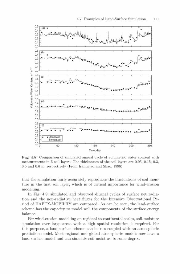
4.7 Examples of Land-Surface Simulation 111
0 60 120 180 240 300 360
Time, day
ObservedSimulated
Vol
umet
ric W
ater
Con
tent
, m3 m
−3
(a)
(b)
(c)
(d)
(f)
0.0
0.1
0.2
0.3
0.4
0.5
0.0
0.1
0.2
0.3
0.4
0.5
0.0
0.1
0.2
0.3
0.4
0.5
0.0
0.1
0.2
0.3
0.4
0.5
0.0
0.1
0.2
0.3
0.4
0.5
Fig. 4.8. Comparison of simulated annual cycle of volumetric water content withmeasurements in 5 soil layers. The thicknesses of the soil layers are 0.05, 0.15, 0.3,0.5 and 0.6 m, respectively (From Irannejad and Shao, 1998)
that the simulation fairly accurately reproduces the fluctuations of soil mois-ture in the first soil layer, which is of critical importance for wind-erosionmodelling.
In Fig. 4.9, simulated and observed diurnal cycles of surface net radia-tion and the non-radiative heat fluxes for the Intensive Observational Pe-riod of HAPEX-MOBILHY are compared. As can be seen, the land-surfacescheme has the capacity to model well the components of the surface energybalance.
For wind-erosion modelling on regional to continental scales, soil-moisturesimulation over large areas with a high spatial resolution is required. Forthis purpose, a land-surface scheme can be run coupled with an atmosphericprediction model. Most regional and global atmospheric models now have aland-surface model and can simulate soil moisture to some degree.
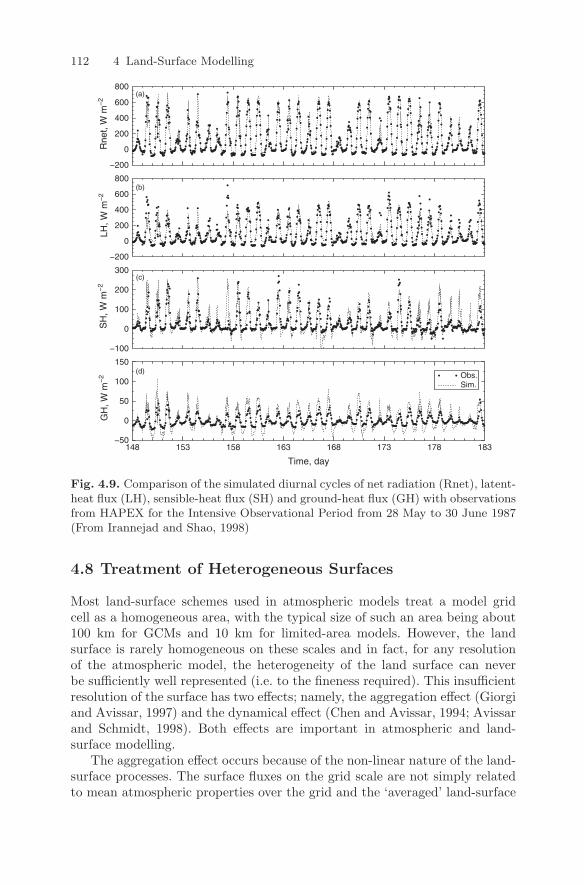
112 4 Land-Surface Modelling
148 153 158 163 168 173 178 183
Time, day
GH
, W m
−2 Obs.
Sim.
SH
, W m
−2
LH, W
m−
2R
net,
W m
−2
−200
0
200
400
600
800
−50
0
50
100
150
−100
0
100
200
300
−200
0
200
400
600
800
(a)
(b)
(c)
(d)
Fig. 4.9. Comparison of the simulated diurnal cycles of net radiation (Rnet), latent-heat flux (LH), sensible-heat flux (SH) and ground-heat flux (GH) with observationsfrom HAPEX for the Intensive Observational Period from 28 May to 30 June 1987(From Irannejad and Shao, 1998)
4.8 Treatment of Heterogeneous Surfaces
Most land-surface schemes used in atmospheric models treat a model gridcell as a homogeneous area, with the typical size of such an area being about100 km for GCMs and 10 km for limited-area models. However, the landsurface is rarely homogeneous on these scales and in fact, for any resolutionof the atmospheric model, the heterogeneity of the land surface can neverbe sufficiently well represented (i.e. to the fineness required). This insufficientresolution of the surface has two effects; namely, the aggregation effect (Giorgiand Avissar, 1997) and the dynamical effect (Chen and Avissar, 1994; Avissarand Schmidt, 1998). Both effects are important in atmospheric and land-surface modelling.
The aggregation effect occurs because of the non-linear nature of the land-surface processes. The surface fluxes on the grid scale are not simply relatedto mean atmospheric properties over the grid and the ‘averaged’ land-surface
4.8 Treatment of Heterogeneous Surfaces 113
parameters, and therefore, the surface fluxes on the grid scale can be wrong, ifthe heterogeneity of the land-surface is poorly represented. Wetzel and Chang(1987) have demonstrated that the spatial soil-moisture variability and thestrongly nonlinear connection between evapotranspiration and soil moistureresults in a relationship between the regional evapotranspiration and area-averaged soil moisture which is profoundly different to that which applies to apoint. In these situations, the grid-averaged surface fluxes can be substantiallydifferent from those calculated using the grid-averaged surface properties. Thedynamic effect occurs because land-surface heterogeneity generates subgridmotions which are not resolved by the numerical grid. In general, the subgridclosure for atmospheric fluxes is to parameterise the subgrid fluxes throughthe gradient of the grid variables. This approach contains no informationabout the land surface and thus it inevitably has inadequacies. Therefore,for a given resolution of the atmospheric model, we must consider how torepresent the unresolved surface properties and their possible impact on boththe calculation of the surface fluxes on the grid scale and the effect of subgridmotion generated by subgrid surface contrasts. Different strategies exist forthe representation of subgrid land-surface heterogeneity.
Averaging Surface Properties
If a grid cell is treated as homogeneous, parameters used for land-surface mod-elling are effective parameters defined either as the most frequently occurringparameter or as a weighted average of the parameters for all surface typeswithin the grid cell. For some parameters, averaging methods which accountfor local nonlinear processes are available (Lhomme, 1992; Mahrt et al. 1992).For instance, the effective roughness length can be calculated based on theconcept of blending height (Wierenga, 1986; Mason, 1988). The advantageof using effective grid-averaged parameters is the reduction of computationalcosts, but the method nevertheless compromises the adequacy with which theheterogeneity of the surface is represented.
PDF Representation
This representation of a heterogeneous land surface involves using a probabil-ity density function (PDF) to define the spatial distribution of the parametersand integrating relevant processes over that PDF. Johnson et al. (1993) andLi and Avissar (1994) applied this method to study the effect of heterogene-ity in stomatal resistance, leaf-area index, surface roughness, albedo and soilwetness on land-surface modelling, and showed that latent- and sensible-heatfluxes are sensitive to the spatial variability of these parameters.
Although the continuous PDF captures a wide range of the heterogeneityscales which occur within a grid cell, its application to complicated land-surface schemes encounters a number of difficulties. In practical computation,the PDF needs to be applied over a number of intervals, for each of which theland-surface scheme must be run. Using a small number of intervals tends to
114 4 Land-Surface Modelling
distort the shape of the PDF, while using a large number of intervals is com-putationally expensive. A land-surface scheme usually incorporates a largenumber of processes with many input parameters. If the heterogeneity of allprocesses is to be considered, a multi-dimensional joint PDF needs to be intro-duced. Suppose that there are N parameters and that the joint PDF can beexpressed as a product of N independent PDFs, each divided into I intervals.This operation would require solving the land-surface scheme IN times. Thisis computationally equivalent to solving the model over a very fine spatial netand changing the geographical spacing to a parameter spacing (Giorgi andAvissar, 1997).
To construct a PDF for a single parameter, let alone the range of param-eters, requires extensive information about the mean, variance and usuallyskewness and kurtosis of the distribution of the parameter over the region.Such information is rarely available. Furthermore, the complicated interac-tions of many processes involved in the natural environment make such afunction strongly space- and time-dependent.
Explicit Subgrid and Mosaic Methods
An alternative is to represent the subgrid-scale heterogeneity in a grid cell bya number of homogeneous subgrids (Avissar and Pielke, 1989). Each subgridis assumed to have fluxes directly to the atmosphere and independently ofother subgrids. Calculations are performed separately for each subgrid andweighted according to the relative surface area to each subgrid in order toprovide the grid-averaged state variables and fluxes. This is the explicit sub-grid approach. The latter approach can be simplified to the mosaic approach,in which all the areas having the same properties are combined into a tile.Figure 4.10 illustrates the mosaic approach in comparison with the explicitsubgrid method for an atmospheric model grid box. The mosaic approach does
5 5 6 4
2 3 8 8
5
Introduction of the Subgrid
6 4 6
1 1 9 7
5 5 6
6
4
4
2
2
3
3
8
8
8
8
5
5
6
6
4
4
6
6
1
1
1
1
9
9
7
7
556 9
75
4
1 2 3
8
(a) (b)
Rearrangement of Patches
Fig. 4.10. An illustration of (a) the mosaic method in contrast to (b) the explicitsubgrid method. The different land-surface types are numerated
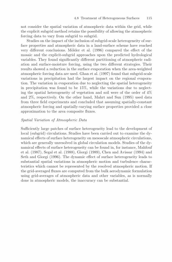
4.8 Treatment of Heterogeneous Surfaces 115
not consider the spatial variation of atmospheric data within the grid, whilethe explicit subgrid method retains the possibility of allowing the atmosphericforcing data to vary from subgrid to subgrid.
Studies on the impact of the inclusion of subgrid-scale heterogeneity of sur-face properties and atmospheric data in a land-surface scheme have reachedvery different conclusions. Molder et al. (1996) compared the effect of themosaic and the explicit-subgrid approaches upon the predicted hydrologicalvariables. They found significantly different partitioning of atmospheric radi-ation and surface-moisture forcing, using the two different strategies. Theirresults showed a reduction in the surface evaporation when the area-weightedatmospheric forcing data are used. Ghan et al. (1997) found that subgrid-scalevariations in precipitation had the largest impact on the regional evapora-tion. The variation in evaporation due to neglecting the spatial heterogeneityin precipitation was found to be 15%, while the variations due to neglect-ing the spatial heterogeneity of vegetation and soil were of the order of 4%and 2%, respectively. On the other hand, Mahrt and Sun (1995) used datafrom three field experiments and concluded that assuming spatially-constantatmospheric forcing and spatially-varying surface properties provided a closeapproximation to the area composite fluxes.
Spatial Variation of Atmospheric Data
Sufficiently large patches of surface heterogeneity lead to the development oflocal (subgrid) circulations. Studies have been carried out to examine the dy-namical effects of surface heterogeneity on mesoscale atmospheric circulations,which are generally unresolved in global circulation models. Studies of the dy-namical effects of surface heterogeneity can be found in, for instance, Mahfoufet al. (1987), Segal et al. (1988), Giorgi (1989), Chen and Avissar (1994) andSeth and Giorgi (1996). The dynamic effect of surface heterogeneity leads tosubstantial spatial variations in atmospheric motion and turbulence charac-teristics which cannot be represented by the resolved atmospheric motion. Ifthe grid-averaged fluxes are computed from the bulk aerodynamic formulationusing grid-averages of atmospheric data and other variables, as is normallydone in atmospheric models, the inaccuracy can be substantial.
5
Basic Aspects of Wind Erosion
5.1 Soil-Particle Characteristics
The processes of particle entrainment, transport and deposition involve a set ofparticle-to-flow, particle-to-surface and particle-to-particle interactions. Thephysical properties of individual particles, such as shape, size and density,play an important role in these interactions. These properties vary greatlyand are difficult to measure precisely in practice, but they must be adequatelydescribed in wind-erosion models.
The shape of a grain includes all aspects of its external morphology, suchas its general form (sphericity), its roundness (sharpness of edges and corners)and its surface roughness. Observations show that the shape of soil particles ishighly irregular (Gillette and Walker, 1977; Pye, 1994), ranging from spheresto plates in their gross form, from very-angular to well-rounded in their round-ness and from rough to smooth in their surface texture. In practice, the size ofa particle can be determined by directly measuring its external caliper dimen-sions. Several techniques are described in Chapter 11, among which sievingis the most-widely used direct-measuring method. A series of progressivelyfiner square-mesh sieves is used to separate particles, principally on the basisof their intermediate axial diameters (Kennedy et al. 1985). However, it isreadily understood that the idea of particle size is closely related to particleshape and the external caliper dimensions do not accurately represent the sizeof a particle unless its shape is well-defined.
To overcome the difficulties in precisely measuring particle shape andsize, we introduce the concept of equivalent particle size. The aerodynamicbehaviour of particles is reasonably well-understood only for spherical par-ticles. It is therefore necessary in theory, and also convenient, to treat soilparticles of different shapes as spheres, so that their aerodynamic and/oroptical behaviours can be described using mathematical expressions. Nearlyall theoretical models for particle entrainment and motion are based on theassumption that the particles are spheres. The equivalent particle size is mea-sured by the diameter of a sphere of which certain aerodynamic or optical
Y. Shao, Physics and Modelling of Wind Erosion, 117c© Springer Science+Business Media B.V. 2008
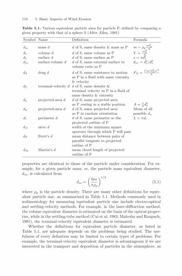
118 5 Basic Aspects of Wind Erosion
Table 5.1. Various equivalent particle sizes for particle P, defined by comparing agiven property with that of a sphere S (After Allen, 1981)
Symbol Name Definition Formula
dm mass d d of S, same density & mass as P m = ρpπd3
m6
dv volume d d of S, same volume as P V =πd3
v6
ds surface d d of S, same surface as P s = πd2s
dsv surface-volume d d of S, same external surface to dsv = d3v/d2
s
volume ratio as P
dd drag d d of S, same resistance to motion FD =CDπd2
dρv2
8
as P in a fluid with same viscosity& velocity
df terminal-velocity d d of S, same density &terminal velocity as P in a fluid ofsame density & viscosity
da projected-area d d of S, same projected areaas P resting in a stable position A = π
4d2
a
dp projected-area d d of S, same projected area Mean of allas P in random orientation possible da
dc perimeter d d of S, same perimeter as the L = πdc
projected outline of PdA sieve d width of the minimum square
aperture through which P will passdF Feret’s d mean distance between pairs of
parallel tangents to projectedoutline of P
dM Martin’s d mean chord length of projectedoutline of P
properties are identical to those of the particle under consideration. For ex-ample, for a given particle mass, m, the particle mass equivalent diameter,dm, is calculated from
dm =(
6m
πρp
)1/3
(5.1)
where ρp is the particle density. There are many other definitions for equiv-alent particle size, as summarized in Table 5.1. Methods commonly used insedimentology for measuring equivalent particle size include electro-opticaland settling-velocity methods. For example, in the laser-diffraction method,the volume equivalent diameter is estimated on the basis of the optical proper-ties, while in the settling-tube method (Cui et al. 1983; Malcolm and Raupach,1991), the terminal-velocity equivalent diameter is estimated.
Whether the definitions for equivalent particle diameter, as listed inTable 5.1, are adequate depends on the problems being studied. The use-fulness of every definition may be limited to certain types of problems. Forexample, the terminal-velocity equivalent diameter is advantageous if we areinterested in the transport and deposition of particles in the atmosphere, as
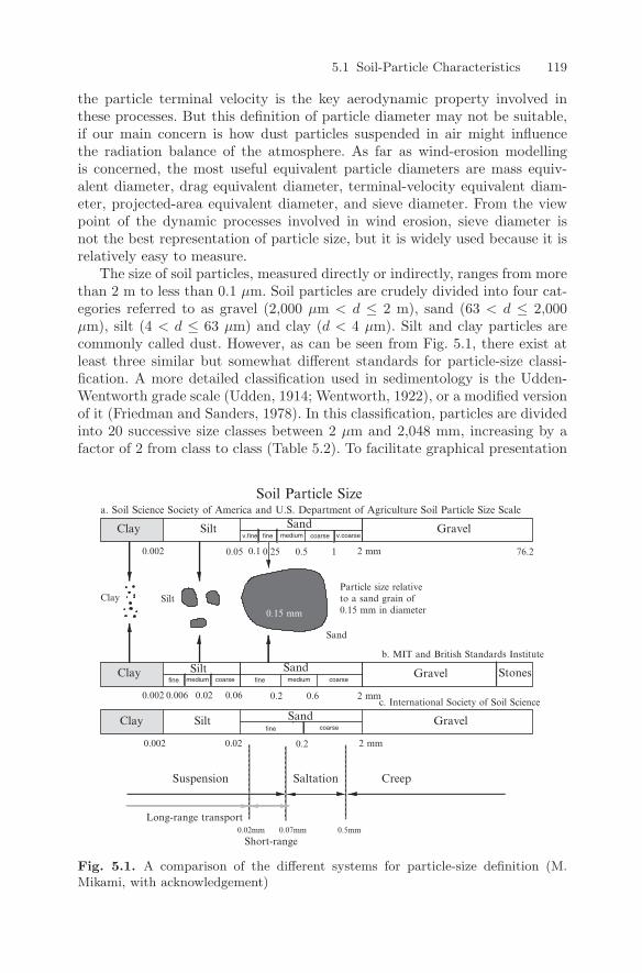
5.1 Soil-Particle Characteristics 119
the particle terminal velocity is the key aerodynamic property involved inthese processes. But this definition of particle diameter may not be suitable,if our main concern is how dust particles suspended in air might influencethe radiation balance of the atmosphere. As far as wind-erosion modellingis concerned, the most useful equivalent particle diameters are mass equiv-alent diameter, drag equivalent diameter, terminal-velocity equivalent diam-eter, projected-area equivalent diameter, and sieve diameter. From the viewpoint of the dynamic processes involved in wind erosion, sieve diameter isnot the best representation of particle size, but it is widely used because it isrelatively easy to measure.
The size of soil particles, measured directly or indirectly, ranges from morethan 2 m to less than 0.1 µm. Soil particles are crudely divided into four cat-egories referred to as gravel (2,000 µm < d ≤ 2 m), sand (63 < d ≤ 2,000µm), silt (4 < d ≤ 63 µm) and clay (d < 4 µm). Silt and clay particles arecommonly called dust. However, as can be seen from Fig. 5.1, there exist atleast three similar but somewhat different standards for particle-size classi-fication. A more detailed classification used in sedimentology is the Udden-Wentworth grade scale (Udden, 1914; Wentworth, 1922), or a modified versionof it (Friedman and Sanders, 1978). In this classification, particles are dividedinto 20 successive size classes between 2 µm and 2,048 mm, increasing by afactor of 2 from class to class (Table 5.2). To facilitate graphical presentation
Clay Silt Sand Gravel
Clay
Clay Stones
Silt Sand
0.15 mm
Sand
v.coarsecoarsemediumfinev.fine
fine medium esraocesraoc mediumfine
Gravel
GravelSandSilt
fine coarse
0.002 0.02 0.2
0.60.20.020.002
0.002 1 2 mm
2 mm
0.250.05 76.2
Particle size relativeto a sand grain of0.15 mm in diameter
Clay Silt
0.006
0.1 0.5
2 mm
0.06
a. Soil Science Society of America and U.S. Department of Agriculture Soil Particle Size Scale
b. MIT and British Standards Institute
c. International Society of Soil Science
SaltationSuspension
Long-range transport0.02mm 0.07mm 0.5mm
Short-range
Creep
Soil Particle Size
Fig. 5.1. A comparison of the different systems for particle-size definition (M.Mikami, with acknowledgement)
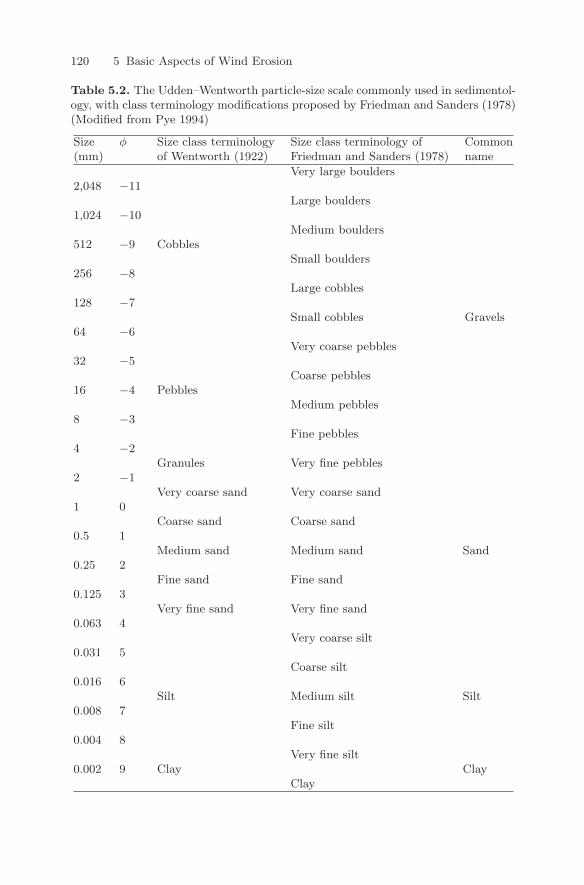
120 5 Basic Aspects of Wind Erosion
Table 5.2. The Udden–Wentworth particle-size scale commonly used in sedimentol-ogy, with class terminology modifications proposed by Friedman and Sanders (1978)(Modified from Pye 1994)
Size φ Size class terminology Size class terminology of Common(mm) of Wentworth (1922) Friedman and Sanders (1978) name
Very large boulders2,048 −11
Large boulders1,024 −10
Medium boulders512 −9 Cobbles
Small boulders256 −8
Large cobbles128 −7
Small cobbles Gravels64 −6
Very coarse pebbles32 −5
Coarse pebbles16 −4 Pebbles
Medium pebbles8 −3
Fine pebbles4 −2
Granules Very fine pebbles2 −1
Very coarse sand Very coarse sand1 0
Coarse sand Coarse sand0.5 1
Medium sand Medium sand Sand0.25 2
Fine sand Fine sand0.125 3
Very fine sand Very fine sand0.063 4
Very coarse silt0.031 5
Coarse silt0.016 6
Silt Medium silt Silt0.008 7
Fine silt0.004 8
Very fine silt0.002 9 Clay Clay
Clay
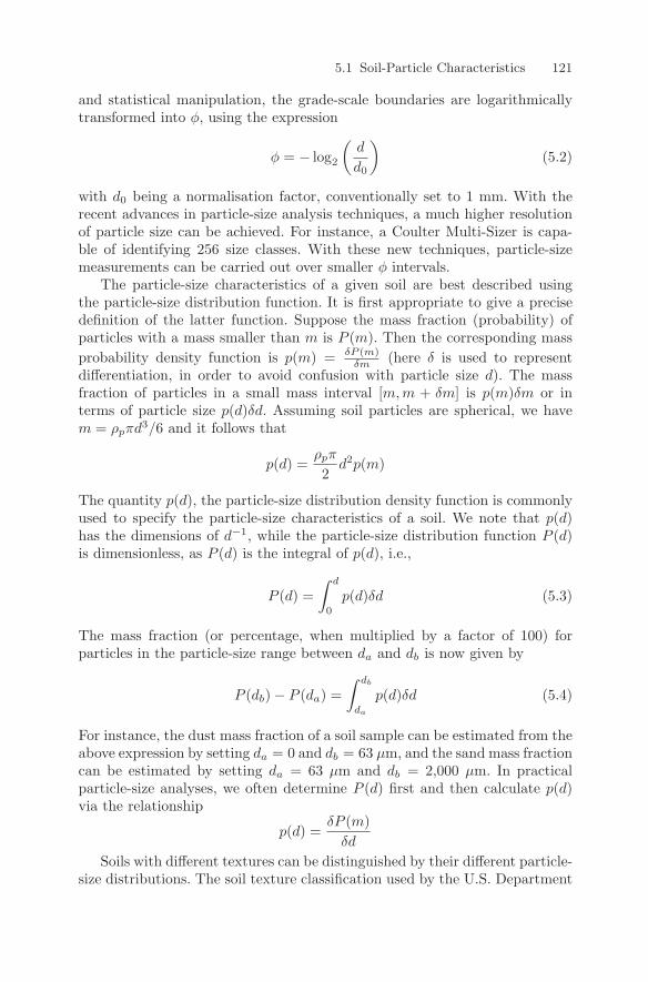
5.1 Soil-Particle Characteristics 121
and statistical manipulation, the grade-scale boundaries are logarithmicallytransformed into φ, using the expression
φ = − log2
(d
d0
)(5.2)
with d0 being a normalisation factor, conventionally set to 1 mm. With therecent advances in particle-size analysis techniques, a much higher resolutionof particle size can be achieved. For instance, a Coulter Multi-Sizer is capa-ble of identifying 256 size classes. With these new techniques, particle-sizemeasurements can be carried out over smaller φ intervals.
The particle-size characteristics of a given soil are best described usingthe particle-size distribution function. It is first appropriate to give a precisedefinition of the latter function. Suppose the mass fraction (probability) ofparticles with a mass smaller than m is P (m). Then the corresponding massprobability density function is p(m) = δP (m)
δm (here δ is used to representdifferentiation, in order to avoid confusion with particle size d). The massfraction of particles in a small mass interval [m,m + δm] is p(m)δm or interms of particle size p(d)δd. Assuming soil particles are spherical, we havem = ρpπd3/6 and it follows that
p(d) =ρpπ
2d2p(m)
The quantity p(d), the particle-size distribution density function is commonlyused to specify the particle-size characteristics of a soil. We note that p(d)has the dimensions of d−1, while the particle-size distribution function P (d)is dimensionless, as P (d) is the integral of p(d), i.e.,
P (d) =∫ d
0
p(d)δd (5.3)
The mass fraction (or percentage, when multiplied by a factor of 100) forparticles in the particle-size range between da and db is now given by
P (db) − P (da) =∫ db
da
p(d)δd (5.4)
For instance, the dust mass fraction of a soil sample can be estimated from theabove expression by setting da = 0 and db = 63 µm, and the sand mass fractioncan be estimated by setting da = 63 µm and db = 2,000 µm. In practicalparticle-size analyses, we often determine P (d) first and then calculate p(d)via the relationship
p(d) =δP (m)
δd
Soils with different textures can be distinguished by their different particle-size distributions. The soil texture classification used by the U.S. Department
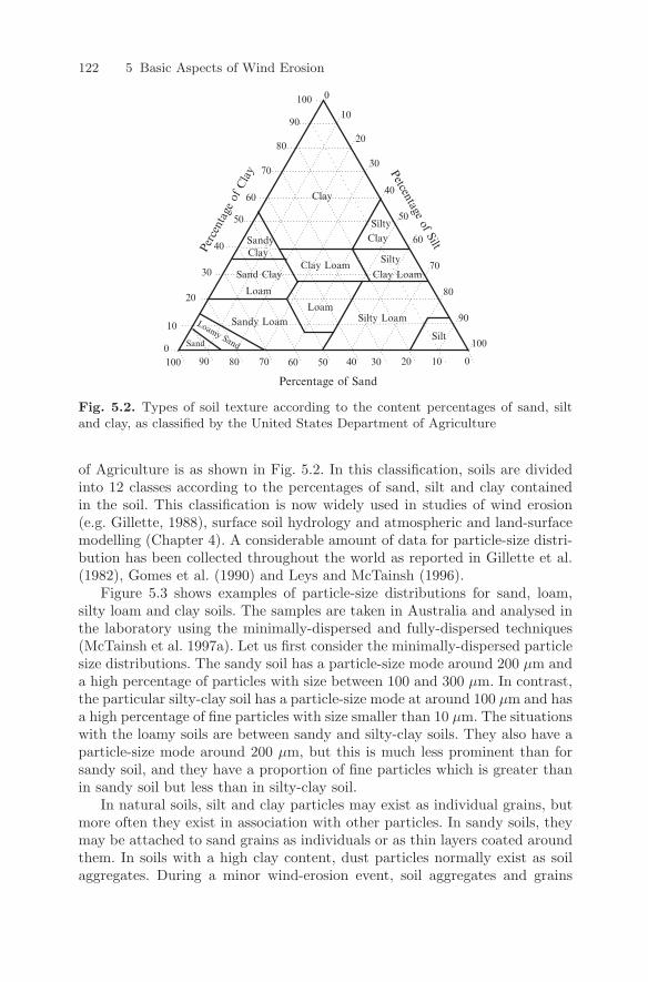
122 5 Basic Aspects of Wind Erosion
Sand0
10
20
30
40
50
60
70
80
90
100 0
10
20
30
40
50
60
70
80
90
100
Percentage of Sand
Petcentage of SiltPerc
enta
ge o
f Cla
y
Sand Clay
Loam
LoamSilty Loam
Clay Loam
ClaySilty
Silt
Clay LoamClay
Clay
Sandy
Loamy Sand
Sandy Loam
Silty
100 90 80 70 60 40 30 20 10 050
Fig. 5.2. Types of soil texture according to the content percentages of sand, siltand clay, as classified by the United States Department of Agriculture
of Agriculture is as shown in Fig. 5.2. In this classification, soils are dividedinto 12 classes according to the percentages of sand, silt and clay containedin the soil. This classification is now widely used in studies of wind erosion(e.g. Gillette, 1988), surface soil hydrology and atmospheric and land-surfacemodelling (Chapter 4). A considerable amount of data for particle-size distri-bution has been collected throughout the world as reported in Gillette et al.(1982), Gomes et al. (1990) and Leys and McTainsh (1996).
Figure 5.3 shows examples of particle-size distributions for sand, loam,silty loam and clay soils. The samples are taken in Australia and analysed inthe laboratory using the minimally-dispersed and fully-dispersed techniques(McTainsh et al. 1997a). Let us first consider the minimally-dispersed particlesize distributions. The sandy soil has a particle-size mode around 200 µm anda high percentage of particles with size between 100 and 300 µm. In contrast,the particular silty-clay soil has a particle-size mode at around 100 µm and hasa high percentage of fine particles with size smaller than 10 µm. The situationswith the loamy soils are between sandy and silty-clay soils. They also have aparticle-size mode around 200 µm, but this is much less prominent than forsandy soil, and they have a proportion of fine particles which is greater thanin sandy soil but less than in silty-clay soil.
In natural soils, silt and clay particles may exist as individual grains, butmore often they exist in association with other particles. In sandy soils, theymay be attached to sand grains as individuals or as thin layers coated aroundthem. In soils with a high clay content, dust particles normally exist as soilaggregates. During a minor wind-erosion event, soil aggregates and grains
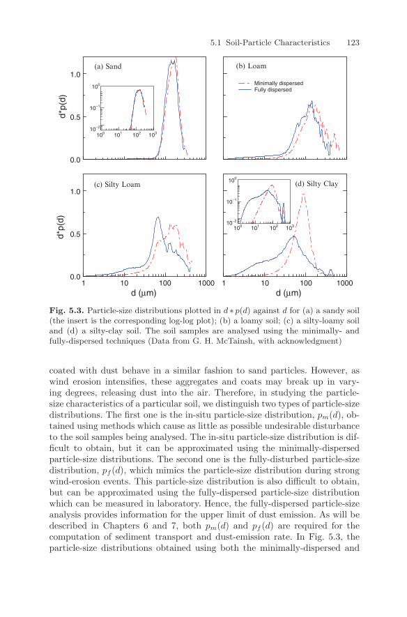
5.1 Soil-Particle Characteristics 123
Minimally dispersedFully dispersed
d*p(
d)d*
p(d)
d (µm)d (µm)
(a) Sand (b) Loam
(c) Silty Loam (d) Silty Clay
0.0
0.5
1.0
0.01 110 10100 1001000 1000
0.5
1.0
100
100 101 102 103
100 101 102 103
10−1
10−2
100
10−1
10−2
Fig. 5.3. Particle-size distributions plotted in d ∗ p(d) against d for (a) a sandy soil(the insert is the corresponding log-log plot); (b) a loamy soil; (c) a silty-loamy soiland (d) a silty-clay soil. The soil samples are analysed using the minimally- andfully-dispersed techniques (Data from G. H. McTainsh, with acknowledgment)
coated with dust behave in a similar fashion to sand particles. However, aswind erosion intensifies, these aggregates and coats may break up in vary-ing degrees, releasing dust into the air. Therefore, in studying the particle-size characteristics of a particular soil, we distinguish two types of particle-sizedistributions. The first one is the in-situ particle-size distribution, pm(d), ob-tained using methods which cause as little as possible undesirable disturbanceto the soil samples being analysed. The in-situ particle-size distribution is dif-ficult to obtain, but it can be approximated using the minimally-dispersedparticle-size distributions. The second one is the fully-disturbed particle-sizedistribution, pf (d), which mimics the particle-size distribution during strongwind-erosion events. This particle-size distribution is also difficult to obtain,but can be approximated using the fully-dispersed particle-size distributionwhich can be measured in laboratory. Hence, the fully-dispersed particle-sizeanalysis provides information for the upper limit of dust emission. As will bedescribed in Chapters 6 and 7, both pm(d) and pf (d) are required for thecomputation of sediment transport and dust-emission rate. In Fig. 5.3, theparticle-size distributions obtained using both the minimally-dispersed and
124 5 Basic Aspects of Wind Erosion
fully-dispersed techniques are shown for four soils samples. As can be seen,the fully-dispersed particle-size distributions can be profoundly different fromthe minimally-dispersed particle-size distributions, with the amount of fineparticles in the fully dispersed analyses being larger than in the minimally-dispersed ones. For the silty-clay soil sample (Fig. 5.3d) in particular, a largeproportion of particles around 100 µm observed in the minimally-dispersedanalysis are aggregates of fine particles. For the sandy soil (Fig. 5.3a, samplecollected in the Simpson Desert of Australia), the differences between pm(d)and pf (d) are much smaller. This implies that the sand-sized grains of thissoil are indeed sand grains rather than clay aggregates. Hence, the sandy soilhas a low content of fine particles and a low capacity for dust emission, asexpected.
5.2 Forces on an Airborne Particle
The motion of an airborne particle is influenced by several forces, includingthe gravity force, Fg, aerodynamic drag, Fd, aerodynamic lift, Fl, the Magnusforce due to particle rotation, Fm, and the electric force FE. The particle-to-air density ratio is defined to be σp = ρp/ρ, where the particle density, ρp, isaround 2,600 kg m−3 while the air density, ρ, is approximately 1.2 kg m−3.Since σp is of order 103, the action of buoyancy upon an airborne soil particleis negligible and hence, Fg is simply the particle weight. The vertical onlycomponent of Fg is −mg with g being the acceleration of gravity.
The physical mechanism which leads to aerodynamic drag is as illustratedin Fig. 5.4a. If the particle moves relative to the surrounding fluid, a forcein the opposite direction of that relative velocity is exerted by the fluid onthe particle. This force is known as the drag that arises from the pressuredifferences between the frontal region and the wake region of the particleand from the transfer of momentum from the fluid to the particle throughmolecular motion, namely the viscous effect. There is an equal and oppositeforce exerted by the particle on the fluid. The force exerted by the flow onthe particle is equal to the integral of total stress (or momentum flux) overthe surface of the particle. The ith component of the force per unit area on asurface with a unit direction vector n is
fi = [−pδij + σij ]nj = −pni + σijnj (5.5)
where p is pressure, δij is the well-known Kronecker second-order tensor andσij is the viscous stress tensor. The ith component of the drag, Fdi over thesurface, S, is given by
Fdi = −∫
S
pnidS +∫
S
σijnjdS (5.6)
The first term on the right hand side of Equation (5.6) represents the transferof momentum to the particle by the pressure forces and is independent of the
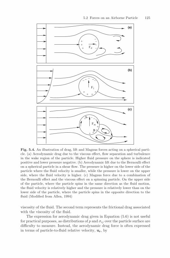
5.2 Forces on an Airborne Particle 125
A
++ +
+
--- --
--
+ +++
+++
--
-
-
(a)
(b)
(c)
F1
Fd
Fm
- -
B
Fig. 5.4. An illustration of drag, lift and Magnus forces acting on a spherical parti-cle. (a) Aerodynamic drag due to the viscous effect, flow separation and turbulencein the wake region of the particle. Higher fluid pressure on the sphere is indicatedpositive and lower pressure negative. (b) Aerodynamic lift due to the Bernoulli effecton a spherical particle in a shear flow. The pressure is higher on the lower side of theparticle where the fluid velocity is smaller, while the pressure is lower on the upperside, where the fluid velocity is higher. (c) Magnus force due to a combination ofthe Bernoulli effect and the viscous effect on a spinning particle. On the upper sideof the particle, where the particle spins in the same direction as the fluid motion,the fluid velocity is relatively higher and the pressure is relatively lower than on thelower side of the particle, where the particle spins in the opposite direction to thefluid (Modified from Allen, 1994)
viscosity of the fluid. The second term represents the frictional drag associatedwith the viscosity of the fluid.
The expression for aerodynamic drag given in Equation (5.6) is not usefulfor practical purposes, as distributions of p and σij over the particle surface aredifficulty to measure. Instead, the aerodynamic drag force is often expressedin terms of particle-to-fluid relative velocity, ur, by
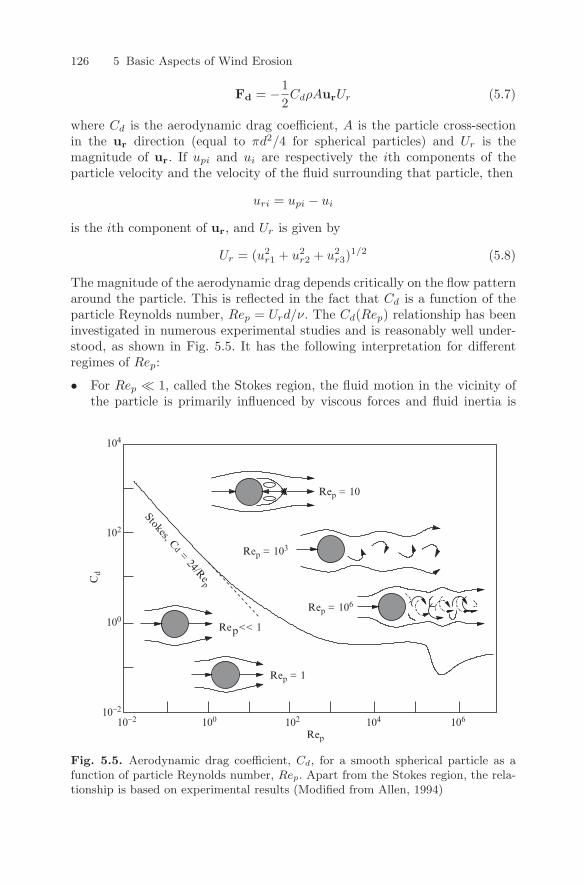
126 5 Basic Aspects of Wind Erosion
Fd = −12CdρAurUr (5.7)
where Cd is the aerodynamic drag coefficient, A is the particle cross-sectionin the ur direction (equal to πd2/4 for spherical particles) and Ur is themagnitude of ur. If upi and ui are respectively the ith components of theparticle velocity and the velocity of the fluid surrounding that particle, then
uri = upi − ui
is the ith component of ur, and Ur is given by
Ur = (u2r1 + u2
r2 + u2r3)
1/2 (5.8)
The magnitude of the aerodynamic drag depends critically on the flow patternaround the particle. This is reflected in the fact that Cd is a function of theparticle Reynolds number, Rep = Urd/ν. The Cd(Rep) relationship has beeninvestigated in numerous experimental studies and is reasonably well under-stood, as shown in Fig. 5.5. It has the following interpretation for differentregimes of Rep:
• For Rep 1, called the Stokes region, the fluid motion in the vicinity ofthe particle is primarily influenced by viscous forces and fluid inertia is
p
Cd
104
102
100
10-2
Rep
Rep = 1
Rep = 10
Rep = 106
Rep = 103
Re << 1
Stokes, Cd = 24/R
ep
104 10610210010-2
Fig. 5.5. Aerodynamic drag coefficient, Cd, for a smooth spherical particle as afunction of particle Reynolds number, Rep. Apart from the Stokes region, the rela-tionship is based on experimental results (Modified from Allen, 1994)
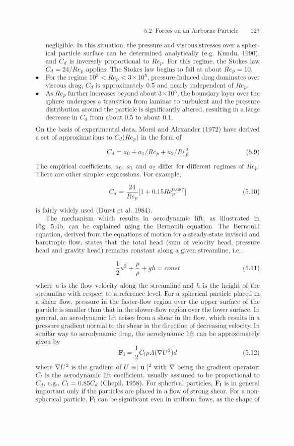
5.2 Forces on an Airborne Particle 127
negligible. In this situation, the pressure and viscous stresses over a spher-ical particle surface can be determined analytically (e.g. Kundu, 1990),and Cd is inversely proportional to Rep. For this regime, the Stokes lawCd = 24/Rep applies. The Stokes law begins to fail at about Rep = 10.
• For the regime 103 < Rep < 3×10⁵, pressure-induced drag dominates overviscous drag, Cd is approximately 0.5 and nearly independent of Rep.
• As Rep further increases beyond about 3×10⁵, the boundary layer over thesphere undergoes a transition from laminar to turbulent and the pressuredistribution around the particle is significantly altered, resulting in a largedecrease in Cd from about 0.5 to about 0.1.
On the basis of experimental data, Morsi and Alexander (1972) have deriveda set of approximations to Cd(Rep) in the form of
Cd = a0 + a1/Rep + a2/Re2p (5.9)
The empirical coefficients, a0, a1 and a2 differ for different regimes of Rep.There are other simpler expressions. For example,
Cd =24
Rep[1 + 0.15Re0.687
p ] (5.10)
is fairly widely used (Durst et al. 1984).The mechanism which results in aerodynamic lift, as illustrated in
Fig. 5.4b, can be explained using the Bernoulli equation. The Bernoulliequation, derived from the equations of motion for a steady-state inviscid andbarotropic flow, states that the total head (sum of velocity head, pressurehead and gravity head) remains constant along a given streamline, i.e.,
12u2 +
p
ρ+ gh = const (5.11)
where u is the flow velocity along the streamline and h is the height of thestreamline with respect to a reference level. For a spherical particle placed ina shear flow, pressure in the faster-flow region over the upper surface of theparticle is smaller than that in the slower-flow region over the lower surface. Ingeneral, an aerodynamic lift arises from a shear in the flow, which results in apressure gradient normal to the shear in the direction of decreasing velocity. Insimilar way to aerodynamic drag, the aerodynamic lift can be approximatelygiven by
Fl =12ClρA(∇U2)d (5.12)
where ∇U2 is the gradient of U ≡| u |2 with ∇ being the gradient operator;Cl is the aerodynamic lift coefficient, usually assumed to be proportional toCd, e.g., Cl = 0.85Cd (Chepil, 1958). For spherical particles, Fl is in generalimportant only if the particles are placed in a flow of strong shear. For a non-spherical particle, Fl can be significant even in uniform flows, as the shape of
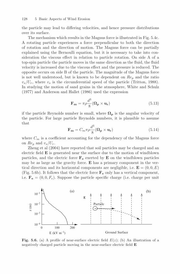
128 5 Basic Aspects of Wind Erosion
the particle may lead to differing velocities, and hence pressure distributionsover its surface.
The mechanism which results in the Magnus force is illustrated in Fig. 5.4c.A rotating particle experiences a force perpendicular to both the directionof rotation and the direction of motion. The Magnus force can be partiallyexplained using the Bernoulli equation, but it is necessary to take into con-sideration the viscous effect in relation to particle rotation. On side A of atop-spin particle the particle moves in the same direction as the fluid, the fluidvelocity is increased due to the viscous effect and the pressure is reduced. Theopposite occurs on side B of the particle. The magnitude of the Magnus forceis not well understood, but is known to be dependent on Rep and the ratiovs/Ur, where vs is the circumferential speed of the particle (Tritton, 1988).In studying the motion of sand grains in the atmosphere, White and Schulz(1977) and Anderson and Hallet (1986) used the expression
Fm = πρd3
8(Ωp × ur) (5.13)
if the particle Reynolds number is small, where Ωp is the angular velocity ofthe particle. For large particle Reynolds numbers, it is plausible to assumethat
Fm = Cmπρd3
8(Ωp × ur) (5.14)
where Cm is a coefficient accounting for the dependency of the Magnus forceon Rep and vs/Ur.
Zheng et al (2004) have reported that soil particles may be charged and anelectric field E is generated near the surface due to the motion of windblownparticles, and the electric force Fe exerted by E on the windblown particlesmay be as large as the gravity force. E has a primary component in the ver-tical direction and its horizontal components are negligible, i.e. E = (0, 0, E)(Fig. 5.6b). It follows that the electric force Fe only has a vertical component,i.e. Fe = (0, 0, Fe). Suppose the particle specific charge (i.e. charge per unit
E
Particle
z (m
)
(a) (b)
0 100 200
-
10−1
10−2
10−3
10−4
E (kV m−1) Ground Surface
Fig. 5.6. (a) A profile of near-surface electric field E(z); (b) An illustration of anegatively charged particle moving in the near-surface electric field E
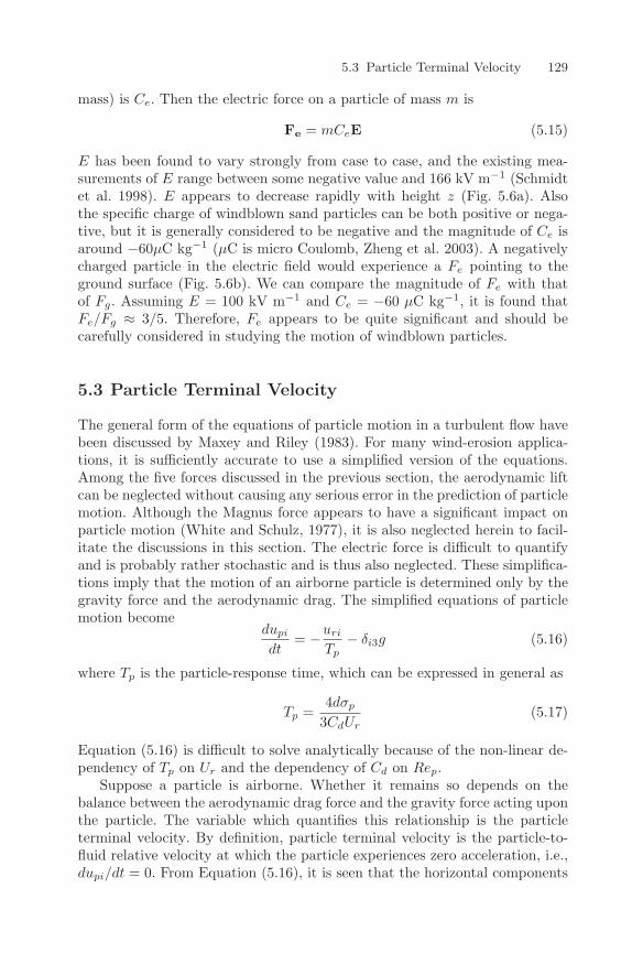
5.3 Particle Terminal Velocity 129
mass) is Ce. Then the electric force on a particle of mass m is
Fe = mCeE (5.15)
E has been found to vary strongly from case to case, and the existing mea-surements of E range between some negative value and 166 kV m−1 (Schmidtet al. 1998). E appears to decrease rapidly with height z (Fig. 5.6a). Alsothe specific charge of windblown sand particles can be both positive or nega-tive, but it is generally considered to be negative and the magnitude of Ce isaround −60µC kg−1 (µC is micro Coulomb, Zheng et al. 2003). A negativelycharged particle in the electric field would experience a Fe pointing to theground surface (Fig. 5.6b). We can compare the magnitude of Fe with thatof Fg. Assuming E = 100 kV m−1 and Ce = −60 µC kg−1, it is found thatFe/Fg ≈ 3/5. Therefore, Fe appears to be quite significant and should becarefully considered in studying the motion of windblown particles.
5.3 Particle Terminal Velocity
The general form of the equations of particle motion in a turbulent flow havebeen discussed by Maxey and Riley (1983). For many wind-erosion applica-tions, it is sufficiently accurate to use a simplified version of the equations.Among the five forces discussed in the previous section, the aerodynamic liftcan be neglected without causing any serious error in the prediction of particlemotion. Although the Magnus force appears to have a significant impact onparticle motion (White and Schulz, 1977), it is also neglected herein to facil-itate the discussions in this section. The electric force is difficult to quantifyand is probably rather stochastic and is thus also neglected. These simplifica-tions imply that the motion of an airborne particle is determined only by thegravity force and the aerodynamic drag. The simplified equations of particlemotion become
dupi
dt= −uri
Tp− δi3g (5.16)
where Tp is the particle-response time, which can be expressed in general as
Tp =4dσp
3CdUr(5.17)
Equation (5.16) is difficult to solve analytically because of the non-linear de-pendency of Tp on Ur and the dependency of Cd on Rep.
Suppose a particle is airborne. Whether it remains so depends on thebalance between the aerodynamic drag force and the gravity force acting uponthe particle. The variable which quantifies this relationship is the particleterminal velocity. By definition, particle terminal velocity is the particle-to-fluid relative velocity at which the particle experiences zero acceleration, i.e.,dupi/dt = 0. From Equation (5.16), it is seen that the horizontal components
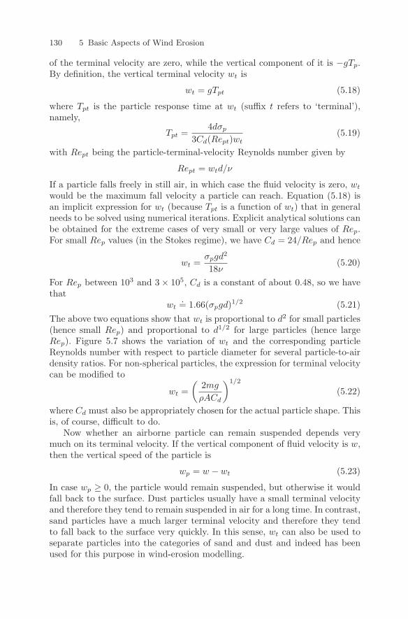
130 5 Basic Aspects of Wind Erosion
of the terminal velocity are zero, while the vertical component of it is −gTp.By definition, the vertical terminal velocity wt is
wt = gTpt (5.18)
where Tpt is the particle response time at wt (suffix t refers to ‘terminal’),namely,
Tpt =4dσp
3Cd(Rept)wt(5.19)
with Rept being the particle-terminal-velocity Reynolds number given by
Rept = wtd/ν
If a particle falls freely in still air, in which case the fluid velocity is zero, wt
would be the maximum fall velocity a particle can reach. Equation (5.18) isan implicit expression for wt (because Tpt is a function of wt) that in generalneeds to be solved using numerical iterations. Explicit analytical solutions canbe obtained for the extreme cases of very small or very large values of Rep.For small Rep values (in the Stokes regime), we have Cd = 24/Rep and hence
wt =σpgd2
18ν(5.20)
For Rep between 103 and 3 × 10⁵, Cd is a constant of about 0.48, so we havethat
wt.= 1.66(σpgd)1/2 (5.21)
The above two equations show that wt is proportional to d2 for small particles(hence small Rep) and proportional to d1/2 for large particles (hence largeRep). Figure 5.7 shows the variation of wt and the corresponding particleReynolds number with respect to particle diameter for several particle-to-airdensity ratios. For non-spherical particles, the expression for terminal velocitycan be modified to
wt =(
2mg
ρACd
)1/2
(5.22)
where Cd must also be appropriately chosen for the actual particle shape. Thisis, of course, difficult to do.
Now whether an airborne particle can remain suspended depends verymuch on its terminal velocity. If the vertical component of fluid velocity is w,then the vertical speed of the particle is
wp = w − wt (5.23)
In case wp ≥ 0, the particle would remain suspended, but otherwise it wouldfall back to the surface. Dust particles usually have a small terminal velocityand therefore they tend to remain suspended in air for a long time. In contrast,sand particles have a much larger terminal velocity and therefore they tendto fall back to the surface very quickly. In this sense, wt can also be used toseparate particles into the categories of sand and dust and indeed has beenused for this purpose in wind-erosion modelling.
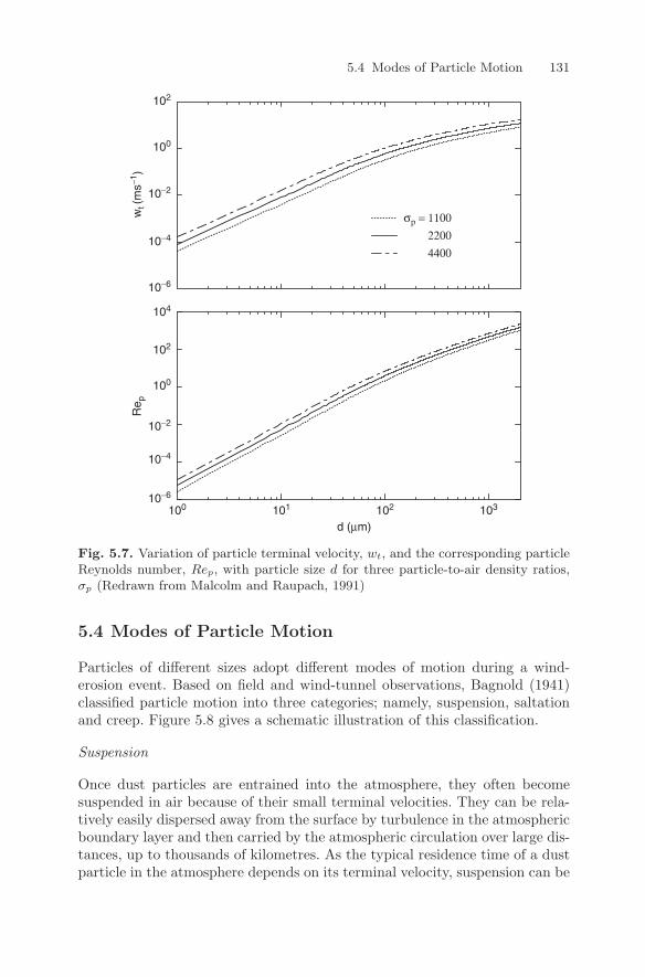
5.4 Modes of Particle Motion 131
100 101 102 103
d (µm)
102
102
104
100
100
10−2
10−2
10−4
10−4
10−6
10−6
wt (
ms−1
)R
e p
σp = 11002200 4400
Fig. 5.7. Variation of particle terminal velocity, wt, and the corresponding particleReynolds number, Rep, with particle size d for three particle-to-air density ratios,σp (Redrawn from Malcolm and Raupach, 1991)
5.4 Modes of Particle Motion
Particles of different sizes adopt different modes of motion during a wind-erosion event. Based on field and wind-tunnel observations, Bagnold (1941)classified particle motion into three categories; namely, suspension, saltationand creep. Figure 5.8 gives a schematic illustration of this classification.
Suspension
Once dust particles are entrained into the atmosphere, they often becomesuspended in air because of their small terminal velocities. They can be rela-tively easily dispersed away from the surface by turbulence in the atmosphericboundary layer and then carried by the atmospheric circulation over large dis-tances, up to thousands of kilometres. As the typical residence time of a dustparticle in the atmosphere depends on its terminal velocity, suspension can be
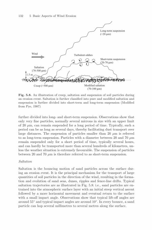
132 5 Basic Aspects of Wind Erosion
..... .... . . .. . .. . . .. .... ... . . ......... ....... .. .... .
Turbulent eddiesShort-term suspension(20-70 µm)
Modified saltation(70-100 µm)
1.5 m
Saltation(70-500 µm)
Long-term suspension(<20 µm)
Wind
....
.................... ...... .. .. ..............
Creep (>500 µm)
... . . . . . . . . . . . . . . . . . . . . . . .. . .. . . . . . . . . . . . . . . . . . . . . . . . . . . . . . . . . . . . . . . . . . . . . .
Fig. 5.8. An illustration of creep, saltation and suspension of soil particles duringan erosion event. Saltation is further classified into pure and modified saltation andsuspension is further divided into short-term and long-term suspension (Modifiedfrom Pye, 1987)
further divided into long- and short-term suspension. Observations show thatonly very fine particles, normally several microns in size with an upper limitof 20 µm, can remain suspended for a long period of time. Typically, such aperiod can be as long as several days, thereby facilitating dust transport overlarge distances. The suspension of particles smaller than 20 µm is referredto as long-term suspension. Particles with a diameter between 20 and 70 µmremain suspended only for a short period of time, typically several hours,and can hardly be transported more than several hundreds of kilometres, un-less the weather situation is extremely favourable. The suspension of particlesbetween 20 and 70 µm is therefore referred to as short-term suspension.
Saltation
Saltation is the bouncing motion of sand particles across the surface dur-ing an erosion event. It is the principal mechanism for the transport of largequantities of soil particles in the direction of the wind, resulting in the forma-tion and evolution of sand seas, dunes, ripples and fence-line drifts. Typicalsaltation trajectories are as illustrated in Fig. 5.8: i.e., sand particles are en-trained into the atmospheric surface layer with an initial steep vertical ascentfollowed by a more horizontal movement and eventual return to the surfacewith a small impact angle. Observations show that typical lift-off angles arearound 55 and typical impact angles are around 10. In every bounce, a sandparticle can hop several millimetres to several metres along the surface.
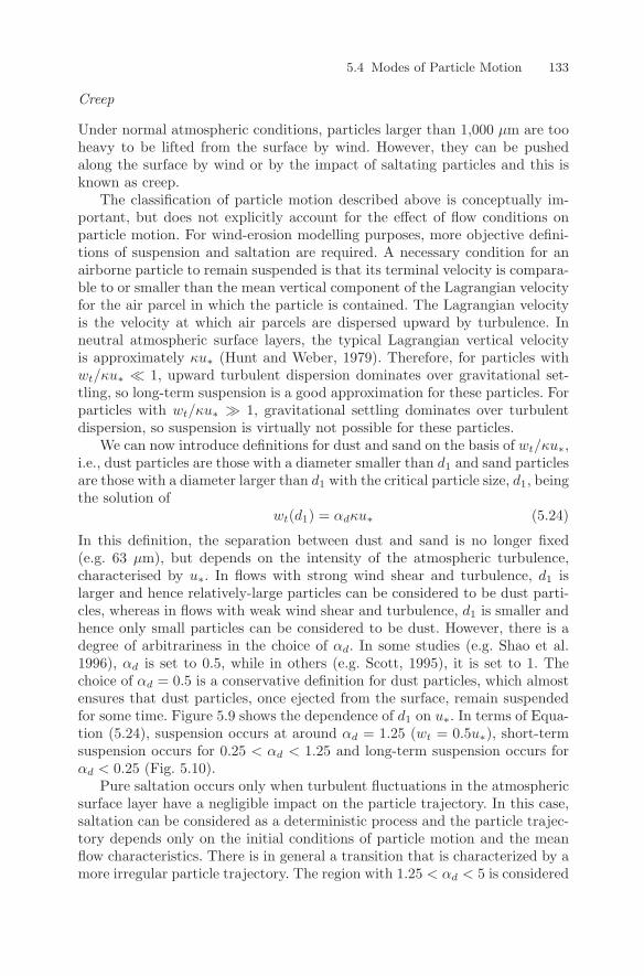
5.4 Modes of Particle Motion 133
Creep
Under normal atmospheric conditions, particles larger than 1,000 µm are tooheavy to be lifted from the surface by wind. However, they can be pushedalong the surface by wind or by the impact of saltating particles and this isknown as creep.
The classification of particle motion described above is conceptually im-portant, but does not explicitly account for the effect of flow conditions onparticle motion. For wind-erosion modelling purposes, more objective defini-tions of suspension and saltation are required. A necessary condition for anairborne particle to remain suspended is that its terminal velocity is compara-ble to or smaller than the mean vertical component of the Lagrangian velocityfor the air parcel in which the particle is contained. The Lagrangian velocityis the velocity at which air parcels are dispersed upward by turbulence. Inneutral atmospheric surface layers, the typical Lagrangian vertical velocityis approximately κu∗ (Hunt and Weber, 1979). Therefore, for particles withwt/κu∗ 1, upward turbulent dispersion dominates over gravitational set-tling, so long-term suspension is a good approximation for these particles. Forparticles with wt/κu∗ 1, gravitational settling dominates over turbulentdispersion, so suspension is virtually not possible for these particles.
We can now introduce definitions for dust and sand on the basis of wt/κu∗,i.e., dust particles are those with a diameter smaller than d1 and sand particlesare those with a diameter larger than d1 with the critical particle size, d1, beingthe solution of
wt(d1) = αdκu∗ (5.24)
In this definition, the separation between dust and sand is no longer fixed(e.g. 63 µm), but depends on the intensity of the atmospheric turbulence,characterised by u∗. In flows with strong wind shear and turbulence, d1 islarger and hence relatively-large particles can be considered to be dust parti-cles, whereas in flows with weak wind shear and turbulence, d1 is smaller andhence only small particles can be considered to be dust. However, there is adegree of arbitrariness in the choice of αd. In some studies (e.g. Shao et al.1996), αd is set to 0.5, while in others (e.g. Scott, 1995), it is set to 1. Thechoice of αd = 0.5 is a conservative definition for dust particles, which almostensures that dust particles, once ejected from the surface, remain suspendedfor some time. Figure 5.9 shows the dependence of d1 on u∗. In terms of Equa-tion (5.24), suspension occurs at around αd = 1.25 (wt = 0.5u∗), short-termsuspension occurs for 0.25 < αd < 1.25 and long-term suspension occurs forαd < 0.25 (Fig. 5.10).
Pure saltation occurs only when turbulent fluctuations in the atmosphericsurface layer have a negligible impact on the particle trajectory. In this case,saltation can be considered as a deterministic process and the particle trajec-tory depends only on the initial conditions of particle motion and the meanflow characteristics. There is in general a transition that is characterized by amore irregular particle trajectory. The region with 1.25 < αd < 5 is considered
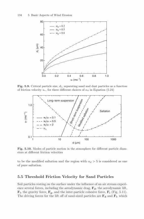
134 5 Basic Aspects of Wind Erosion
u* (ms−1)
d 1 (
µm)
αd = 0.2αd = 0.5αd = 0.8
0
20
40
60
80
0.0 0.2 0.4 0.6 0.8 1.0
Fig. 5.9. Critical particle size, d1, separating sand and dust particles as a functionof friction velocity u∗, for three different choices of αd in Equation (5.24)
d (µm)
u * (
ms−
1 )
wt/u* = 0.1wt/u* = 0.5wt/u* = 2u*t
Long−term suspension
Saltation
Sho
rt−te
rm s
uspe
nsio
nM
odifi
ed s
alta
tion
0.11 10 100 1000
1.0
Fig. 5.10. Modes of particle motion in the atmosphere for different particle diam-eters at different friction velocities
to be the modified saltation and the region with αd > 5 is considered as oneof pure saltation.
5.5 Threshold Friction Velocity for Sand Particles
Soil particles resting on the surface under the influence of an air stream experi-ence several forces, including the aerodynamic drag, Fd, the aerodynamic lift,Fl, the gravity force, Fg, and the inter-particle cohesive force, Fi (Fig. 5.11).The driving forces for the lift off of sand-sized particles are Fd and Fl, which
5.5 Threshold Friction Velocity for Sand Particles 135
are related to the wind shear near the surface and hence are functions of thefriction velocity, u∗. The threshold friction velocity, u∗t, is the minimum fric-tion velocity required for the aerodynamic forces to overcome the retardingforces, namely Fg and Fi, and to initialise the movement of soil particles.There are well established techniques for determining u∗ by measuring eitherthe profile of the mean wind or measuring directly the momentum flux in theatmospheric surface layer. In wind-tunnel and field studies, u∗t is commonlyset to the value of u∗ at which a small percentage of soil particles start tomove. Inevitably, the practical estimate of u∗t involves a certain degree ofsubjectivity in deciding what is a small percentage.
Threshold friction velocity is essentially a property of the soil surface,rather than that of a soil particle. It describes the capacity of the surface toresist wind erosion and is affected by a range of factors as will be discussedin later chapters. However, under ideal conditions, u∗t can be expressed as afunction of only particle size. To establish the u∗t(d) relationship under idealconditions is important as it defines the lower limit of the threshold frictionvelocity in reality. Several theories for u∗t(d) have been derived for soils withuniform and spherical particles spread loosely over a dry and unshelteredsurface. The theories developed by Bagnold (1941), Greeley and Iversen (1985)and the improvements due to Shao and Lu (2000) and McKenna Neuman(2003) are described below.
5.5.1 The Bagnold Scheme
For a particle of size d, u∗t(d) is determined by the balance of Fd, Fl, Fg
and Fi, as shown in Fig. 5.11. At the instant of particle motion the combinedretarding effect of Fg and Fi will be overcome by the combined lifting effect ofFd and Fl. The particle will tend to pivot about point P in a downstream di-rection. The balance of forces at the instant of particle lift-off can be obtainedby the summation of moments about the pivot point P ,
rdFd + rl(Fl − Fg) + rmFm − riFi = 0 (5.25)
where rd, rl and ri are moment arm lengths and Fd ≡| Fd |, etc. In the aboveequation, the moment of the particle is expressed as rmFm. In general, themoment arm lengths depend complicatedly on the arrangements of particlesand are difficult to determine. However, it is plausible to assume that theyare all proportional to the particle size, namely, rd = add, rl = ald, rm =amd and ri = aid with ad, al, am and ai being dimensionless coefficients.Equation (5.25) thus becomes
adFd + al(Fl − Fg) + amFm − aiFi = 0 (5.26)
A simple theory for u∗t(d) can be derived by considering only the balancebetween the aerodynamic drag and the gravity force
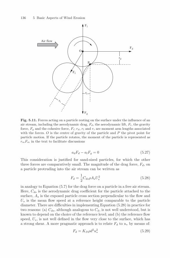
136 5 Basic Aspects of Wind Erosion
Fi
O
Fl
Fg
rl
ri
Air flow
P
rd
Fd
Fig. 5.11. Forces acting on a particle resting on the surface under the influence of anair stream, including the aerodynamic drag, Fd, the aerodynamic lift, Fl, the gravityforce, Fg and the cohesive force, Fi; rd, rl and ri are moment arm lengths associatedwith the forces. O is the centre of gravity of the particle and P the pivot point forparticle motion. If the particle rotates, the moment of the particle is represented asrmFm in the text to facilitate discussions
adFd − alFg = 0 (5.27)
This consideration is justified for sand-sized particles, for which the otherthree forces are comparatively small. The magnitude of the drag force, Fd, ona particle protruding into the air stream can be written as
Fd =12CdsρAsU
2s (5.28)
in analogy to Equation (5.7) for the drag force on a particle in a free air stream.Here, Cds is the aerodynamic drag coefficient for the particle attached to thesurface, As is the exposed particle cross section perpendicular to the flow andUs is the mean flow speed at a reference height comparable to the particlediameter. There are difficulties in implementing Equation (5.28) in practice fortwo reasons: (a) Cds, although analogous to Cd, is not well understood, but isknown to depend on the choice of the reference level; and (b) the reference flowspeed, Us, is not well defined in the flow very close to the surface, which hasa strong shear. A more pragmatic approach is to relate Fd to u∗ by means of:
Fd = KDρd2u2∗ (5.29)
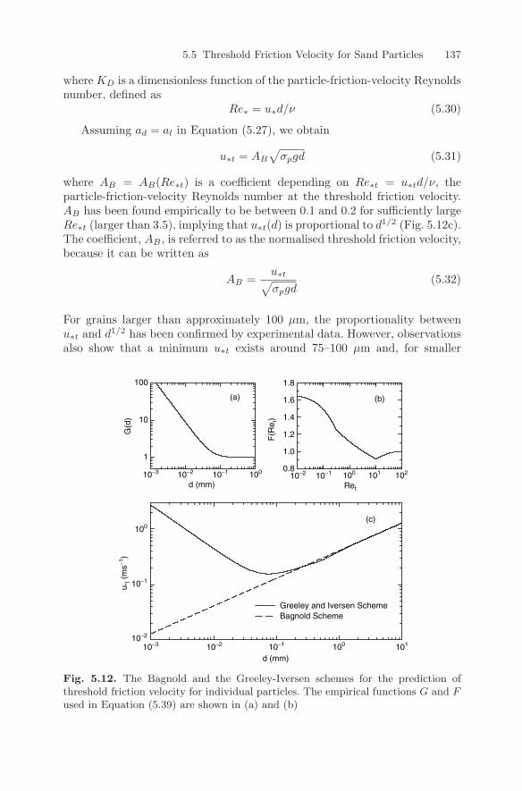
5.5 Threshold Friction Velocity for Sand Particles 137
where KD is a dimensionless function of the particle-friction-velocity Reynoldsnumber, defined as
Re∗ = u∗d/ν (5.30)
Assuming ad = al in Equation (5.27), we obtain
u∗t = AB
√σpgd (5.31)
where AB = AB(Re∗t) is a coefficient depending on Re∗t = u∗td/ν, theparticle-friction-velocity Reynolds number at the threshold friction velocity.AB has been found empirically to be between 0.1 and 0.2 for sufficiently largeRe∗t (larger than 3.5), implying that u∗t(d) is proportional to d1/2 (Fig. 5.12c).The coefficient, AB , is referred to as the normalised threshold friction velocity,because it can be written as
AB =u∗t√σpgd
(5.32)
For grains larger than approximately 100 µm, the proportionality betweenu∗t and d1/2 has been confirmed by experimental data. However, observationsalso show that a minimum u∗t exists around 75–100 µm and, for smaller
d (mm)
Greeley and Iversen SchemeBagnold Scheme
Ret
F(R
e t)
d (mm)
G(d
)
(a) (b)
(c)
10−3
10−3
10−2
10−2 10−1
10−2 10−110−1 100
100 101
100 101 102
1
10
100
0.8
1.0
1.2
1.4
1.6
1.8
100
10−2
10−1
u *t (
ms−1
)
Fig. 5.12. The Bagnold and the Greeley-Iversen schemes for the prediction ofthreshold friction velocity for individual particles. The empirical functions G and Fused in Equation (5.39) are shown in (a) and (b)
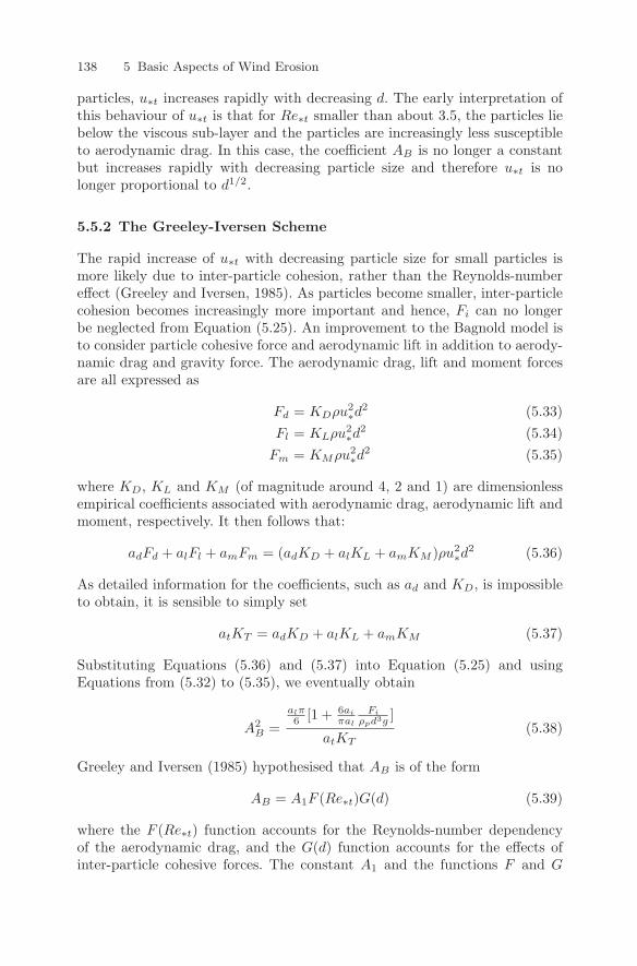
138 5 Basic Aspects of Wind Erosion
particles, u∗t increases rapidly with decreasing d. The early interpretation ofthis behaviour of u∗t is that for Re∗t smaller than about 3.5, the particles liebelow the viscous sub-layer and the particles are increasingly less susceptibleto aerodynamic drag. In this case, the coefficient AB is no longer a constantbut increases rapidly with decreasing particle size and therefore u∗t is nolonger proportional to d1/2.
5.5.2 The Greeley-Iversen Scheme
The rapid increase of u∗t with decreasing particle size for small particles ismore likely due to inter-particle cohesion, rather than the Reynolds-numbereffect (Greeley and Iversen, 1985). As particles become smaller, inter-particlecohesion becomes increasingly more important and hence, Fi can no longerbe neglected from Equation (5.25). An improvement to the Bagnold model isto consider particle cohesive force and aerodynamic lift in addition to aerody-namic drag and gravity force. The aerodynamic drag, lift and moment forcesare all expressed as
Fd = KDρu2∗d
2 (5.33)Fl = KLρu2
∗d2 (5.34)
Fm = KMρu2∗d
2 (5.35)
where KD, KL and KM (of magnitude around 4, 2 and 1) are dimensionlessempirical coefficients associated with aerodynamic drag, aerodynamic lift andmoment, respectively. It then follows that:
adFd + alFl + amFm = (adKD + alKL + amKM )ρu2∗d
2 (5.36)
As detailed information for the coefficients, such as ad and KD, is impossibleto obtain, it is sensible to simply set
atKT = adKD + alKL + amKM (5.37)
Substituting Equations (5.36) and (5.37) into Equation (5.25) and usingEquations from (5.32) to (5.35), we eventually obtain
A2B =
alπ6 [1 + 6ai
πal
Fi
ρpd3g ]
atKT(5.38)
Greeley and Iversen (1985) hypothesised that AB is of the form
AB = A1F (Re∗t)G(d) (5.39)
where the F (Re∗t) function accounts for the Reynolds-number dependencyof the aerodynamic drag, and the G(d) function accounts for the effects ofinter-particle cohesive forces. The constant A1 and the functions F and G
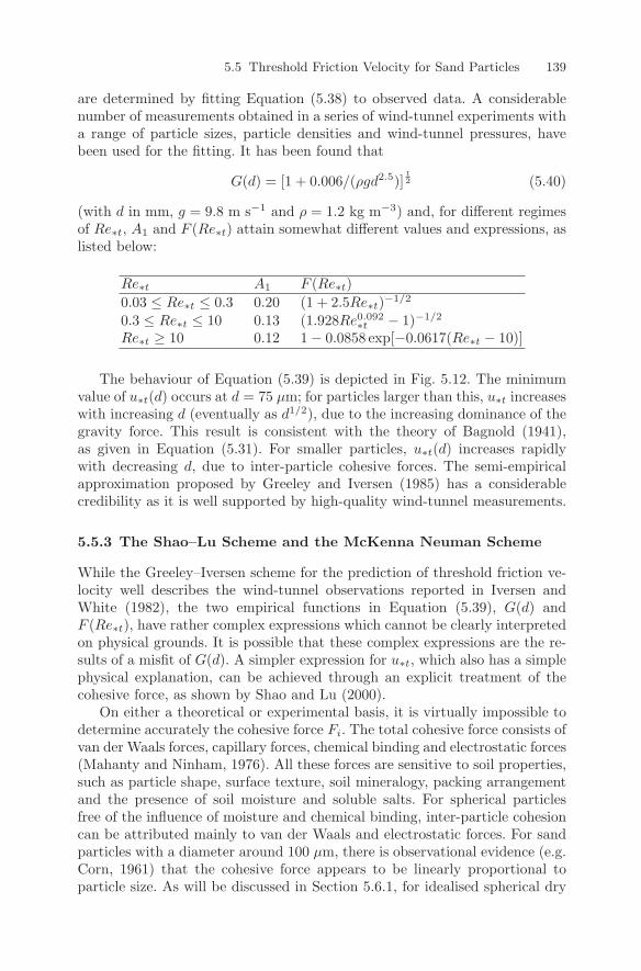
5.5 Threshold Friction Velocity for Sand Particles 139
are determined by fitting Equation (5.38) to observed data. A considerablenumber of measurements obtained in a series of wind-tunnel experiments witha range of particle sizes, particle densities and wind-tunnel pressures, havebeen used for the fitting. It has been found that
G(d) = [1 + 0.006/(ρgd2.5)]12 (5.40)
(with d in mm, g = 9.8 m s−1 and ρ = 1.2 kg m−3) and, for different regimesof Re∗t, A1 and F (Re∗t) attain somewhat different values and expressions, aslisted below:
Re∗t A1 F (Re∗t)0.03 ≤ Re∗t ≤ 0.3 0.20 (1 + 2.5Re∗t)−1/2
0.3 ≤ Re∗t ≤ 10 0.13 (1.928Re0.092∗t − 1)−1/2
Re∗t ≥ 10 0.12 1 − 0.0858 exp[−0.0617(Re∗t − 10)]
The behaviour of Equation (5.39) is depicted in Fig. 5.12. The minimumvalue of u∗t(d) occurs at d = 75 µm; for particles larger than this, u∗t increaseswith increasing d (eventually as d1/2), due to the increasing dominance of thegravity force. This result is consistent with the theory of Bagnold (1941),as given in Equation (5.31). For smaller particles, u∗t(d) increases rapidlywith decreasing d, due to inter-particle cohesive forces. The semi-empiricalapproximation proposed by Greeley and Iversen (1985) has a considerablecredibility as it is well supported by high-quality wind-tunnel measurements.
5.5.3 The Shao–Lu Scheme and the McKenna Neuman Scheme
While the Greeley–Iversen scheme for the prediction of threshold friction ve-locity well describes the wind-tunnel observations reported in Iversen andWhite (1982), the two empirical functions in Equation (5.39), G(d) andF (Re∗t), have rather complex expressions which cannot be clearly interpretedon physical grounds. It is possible that these complex expressions are the re-sults of a misfit of G(d). A simpler expression for u∗t, which also has a simplephysical explanation, can be achieved through an explicit treatment of thecohesive force, as shown by Shao and Lu (2000).
On either a theoretical or experimental basis, it is virtually impossible todetermine accurately the cohesive force Fi. The total cohesive force consists ofvan der Waals forces, capillary forces, chemical binding and electrostatic forces(Mahanty and Ninham, 1976). All these forces are sensitive to soil properties,such as particle shape, surface texture, soil mineralogy, packing arrangementand the presence of soil moisture and soluble salts. For spherical particlesfree of the influence of moisture and chemical binding, inter-particle cohesioncan be attributed mainly to van der Waals and electrostatic forces. For sandparticles with a diameter around 100 µm, there is observational evidence (e.g.Corn, 1961) that the cohesive force appears to be linearly proportional toparticle size. As will be discussed in Section 5.6.1, for idealised spherical dry
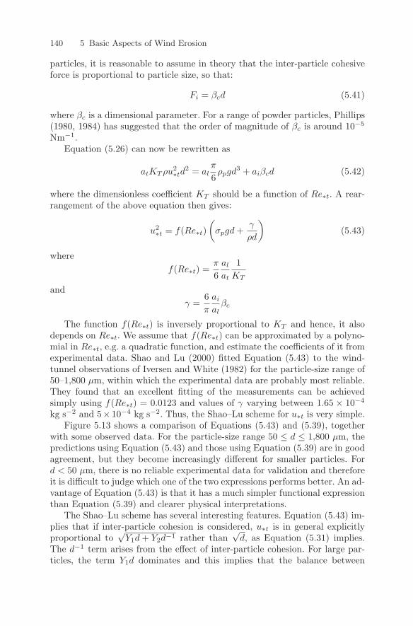
140 5 Basic Aspects of Wind Erosion
particles, it is reasonable to assume in theory that the inter-particle cohesiveforce is proportional to particle size, so that:
Fi = βcd (5.41)
where βc is a dimensional parameter. For a range of powder particles, Phillips(1980, 1984) has suggested that the order of magnitude of βc is around 10−5
Nm−1.Equation (5.26) can now be rewritten as
atKT ρu2∗td
2 = alπ
6ρpgd3 + aiβcd (5.42)
where the dimensionless coefficient KT should be a function of Re∗t. A rear-rangement of the above equation then gives:
u2∗t = f(Re∗t)
(σpgd +
γ
ρd
)(5.43)
wheref(Re∗t) =
π
6al
at
1KT
andγ =
6π
ai
alβc
The function f(Re∗t) is inversely proportional to KT and hence, it alsodepends on Re∗t. We assume that f(Re∗t) can be approximated by a polyno-mial in Re∗t, e.g. a quadratic function, and estimate the coefficients of it fromexperimental data. Shao and Lu (2000) fitted Equation (5.43) to the wind-tunnel observations of Iversen and White (1982) for the particle-size range of50–1,800 µm, within which the experimental data are probably most reliable.They found that an excellent fitting of the measurements can be achievedsimply using f(Re∗t) = 0.0123 and values of γ varying between 1.65 × 10⁻⁴
kg s−2 and 5× 10⁻⁴ kg s−2. Thus, the Shao–Lu scheme for u∗t is very simple.Figure 5.13 shows a comparison of Equations (5.43) and (5.39), together
with some observed data. For the particle-size range 50 ≤ d ≤ 1,800 µm, thepredictions using Equation (5.43) and those using Equation (5.39) are in goodagreement, but they become increasingly different for smaller particles. Ford < 50 µm, there is no reliable experimental data for validation and thereforeit is difficult to judge which one of the two expressions performs better. An ad-vantage of Equation (5.43) is that it has a much simpler functional expressionthan Equation (5.39) and clearer physical interpretations.
The Shao–Lu scheme has several interesting features. Equation (5.43) im-plies that if inter-particle cohesion is considered, u∗t is in general explicitlyproportional to
√Y1d + Y2d−1 rather than
√d, as Equation (5.31) implies.
The d−1 term arises from the effect of inter-particle cohesion. For large par-ticles, the term Y1d dominates and this implies that the balance between
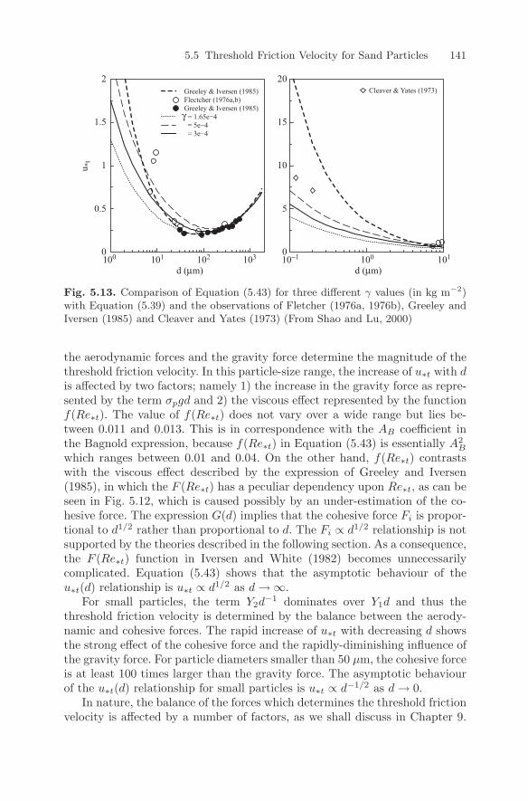
5.5 Threshold Friction Velocity for Sand Particles 141
u *t
Greeley & Iversen (1985)Flectcher (1976a,b)Greeley & Iversen (1985) = 1.65e−4 = 5e−4 = 3e−4
Cleaver & Yates (1973)
γ
0
0.5
1
1.5
2
100 101 10-1 100 101102 103 0
5
10
15
20
d (µm) d (µm)
Fig. 5.13. Comparison of Equation (5.43) for three different γ values (in kg m−2)with Equation (5.39) and the observations of Fletcher (1976a, 1976b), Greeley andIversen (1985) and Cleaver and Yates (1973) (From Shao and Lu, 2000)
the aerodynamic forces and the gravity force determine the magnitude of thethreshold friction velocity. In this particle-size range, the increase of u∗t with dis affected by two factors; namely 1) the increase in the gravity force as repre-sented by the term σpgd and 2) the viscous effect represented by the functionf(Re∗t). The value of f(Re∗t) does not vary over a wide range but lies be-tween 0.011 and 0.013. This is in correspondence with the AB coefficient inthe Bagnold expression, because f(Re∗t) in Equation (5.43) is essentially A2
B
which ranges between 0.01 and 0.04. On the other hand, f(Re∗t) contrastswith the viscous effect described by the expression of Greeley and Iversen(1985), in which the F (Re∗t) has a peculiar dependency upon Re∗t, as can beseen in Fig. 5.12, which is caused possibly by an under-estimation of the co-hesive force. The expression G(d) implies that the cohesive force Fi is propor-tional to d1/2 rather than proportional to d. The Fi ∝ d1/2 relationship is notsupported by the theories described in the following section. As a consequence,the F (Re∗t) function in Iversen and White (1982) becomes unnecessarilycomplicated. Equation (5.43) shows that the asymptotic behaviour of theu∗t(d) relationship is u∗t ∝ d1/2 as d → ∞.
For small particles, the term Y2d−1 dominates over Y1d and thus the
threshold friction velocity is determined by the balance between the aerody-namic and cohesive forces. The rapid increase of u∗t with decreasing d showsthe strong effect of the cohesive force and the rapidly-diminishing influence ofthe gravity force. For particle diameters smaller than 50 µm, the cohesive forceis at least 100 times larger than the gravity force. The asymptotic behaviourof the u∗t(d) relationship for small particles is u∗t ∝ d−1/2 as d → 0.
In nature, the balance of the forces which determines the threshold frictionvelocity is affected by a number of factors, as we shall discuss in Chapter 9.
142 5 Basic Aspects of Wind Erosion
For example, the aerodynamic force is temperature dependent, because airdensity ρ increases with decreasing temperature and hence, for a given u∗,the drag force on a particle is larger if temperature is lower. Further, viscosityν decreases with decreasing temperature, and KD is viscosity dependent atlow Reynolds number. Therefore, u∗t may be temperature dependent. Inter-particle cohesion also depends on a number of factors, one of which is soilmoisture. McKenna Neuman (2003) considered the effect of soil moisture onthe inter-particle cohesive force and suggested that Equation (5.41) can bewritten as
Fi = βcd+ | ∆P | Ac (5.44)
where Ac is the contact area between adjacent grains and ∆P is the capillary-suction pressure deficit. Equation (5.43) therefore becomes
u2∗t = A2
2f(Re∗t)(
σpgd +γ′
ρd2
)(5.45)
withγ′ =
6π
ai
al(βcd+ | ∆P | Ac)
The coefficient A2 is introduced to account for the temperature effect on u∗t.However, A2 is not substantially different from 1, because the effects due toair-density change and viscosity change arising from temperature change tendto compensate each other. For the four particle sizes, 210, 270, 430 and 610 µm,McKenna Neuman (2003) found A2 to be 1.14, 1.06, 1.06 and 1.25, respec-tively. Through fitting Equation (5.45) to observations, McKenna Neumanfound that
γ′ = 10−8− | ∆P | (1.15 × 10⁻⁸d − 5.8 × 10⁻⁵d2)
with | ∆P | given in Pa and d in m. The McKenna Neuman scheme, i.e.Equation (5.45), is one method of accounting for the impact of soil moistureon u∗t. Other methods will be discussed in Chapter 9.
5.6 Threshold Friction Velocity for Dust Particles
5.6.1 Relative Importance of Forces
The entrainment mechanism for sand and dust particles differs greatly becauseof the profound differences in the relative importance of the forces actingupon them. In particular, the cohesive force consists of van der Waals forces,electrostatic forces, capillary forces and chemical binding forces, but none ofthese forces can be predicted precisely. It is nevertheless useful to considerthem in some detail, so that their qualitative behaviour and the difficultiesinvolved in determining the threshold friction velocity for dust particles areunderstood.
5.6 Threshold Friction Velocity for Dust Particles 143
Van der Waals Forces
The attraction between uncharged micron-sized particles is due to van derWaals forces, which are short-range forces with the domain of importanceunder a diameter of a dust particle. Theories originating from the colloidalscience exist for the calculation of van der Walls forces in idealised situations,notably the Hamaker and Liftshitz theories as described in Langbein (1974)and Mahanty and Ninham (1976). For a small spherical particle of diameterd with a separation, δ, from a same-sized particle, one approximation for avan der Waals force between the two particles in vacuum is:
Fiv =hw
32πδ2d (5.46)
where hw is a coefficient varying between 10−18J and 10−21J , depending onthe material. The smallest value of δ is conventionally considered to be 0.4nm, because for regions with separation smaller than 0.4 nm, the interactionsbetween the particles are further complicated, as Verwey and Overbeek repul-sion (e.g. Theodoor and Overbeek, 1985) takes place. The above relationshipis considered to be valid for δ/d 1. For δ/d > 0.2, the van der Waals attrac-tion becomes negligible, being of the order of the Brownian forces. If particlesare surrounded by air, the van der Waals attraction between the two particlesmay increase due to the interactions between the gas molecules adsorbed onthe particles. At room temperature, van der Waals forces between particlescan be increased by up to two orders of magnitude with increasing pressure(Xie, 1997).
Electrostatic Forces
The electrostatic force applicable to dust emission is the non-conductor force.For smooth and ideally-spherical particles, they can be written as
Fie =πBpV
2d
2δ(5.47)
where V is the contact potential difference, which generally ranges from 0 toabout 0.5 volts, δ is the separation between the two adhering particles andBp is the permittivity of free space.
Capillary Forces
Capillary forces are caused by the moisture which condenses from the sur-rounding air onto the particle surface and then forms liquid bridges betweenneighbouring particles. The surface tension of these bridges results in cohesionbetween the particles. The capillary forces can be many times the weight ofthe particles involved when the surrounding air is close to saturation. It hasbeen shown (McKenna Neuman and Nickling, 1989) that the capillary forces
144 5 Basic Aspects of Wind Erosion
developed at inter-particle contacts surrounded by isolated wedges of waterare inversely proportional to moisture tension and directly proportional tothe geometric properties of the contacts. An approximation to the capillaryforces is
Fic = GicπT 2
en
| ∆P | (5.48)
where Ten is the surface tension of water, Gic is a dimensionless geometriccoefficient describing the shape of the contacts between grains and ∆P isthe pressure deficit between the pressure within the water wedge and theatmospheric pressure.
Other Forces
There are other types of inter-particle forces, such as chemical binding andcoulomb forces. Various salts in soils may interact with clay particles and formchemical bonds. The chemical processes involved are complicated, and themagnitude of the binding forces can only be determined through experiments(Chapter 9).
Real particles are not ideally spherical, smooth and non-deformable. Smallparticles often have the shapes of platelets with considerable surface roughnessand often show large deformation in the contact region. As a consequence,the theoretical predictions, such as Equations (5.46), are rarely applicable inpractice. It is readily appreciated that it is virtually impossible to determineaccurately the cohesive force acting on dust particles. Two crude conclusionsrelevant to estimating the threshold friction velocity for dust particles canbe drawn from the above discussions; namely, (1) the cohesive forces are intheory linearly proportional to the size of the dust particles and this simplerelationship should be used if no better information is available; and (2) theuncertainties in estimating the cohesive forces are at least several orders ofmagnitude.
Despite the uncertainties, it is interesting to analyse the relative impor-tance of the forces acting on particles of different sizes. We have seen in theprevious discussions that the gravity force is proportional to d3, the aerody-namic forces are proportional to d2 and the total cohesive force is in principalproportional to d. Figure 5.14 shows log-log plots of the gravity force, the totalcohesive force, and the total aerodynamic force at u∗ = 0.4 m s−1, as a func-tion of particle size. As can be seen, all three forces decrease with decreasingparticle size, but the gravity force and the total aerodynamic force decreasefaster than the cohesive force. In this example, for particles with a diameterless than 10 µm, the cohesive force dominates and the particles cannot belifted at the given friction velocity. For particles in the size range between10 and 300 µm, the total aerodynamic force is greater than both the gravityforce and the cohesive force and hence the particles in this size range can beentrained by the wind. For particle diameters larger than 300 µm, the gravityforce becomes the largest of the three.
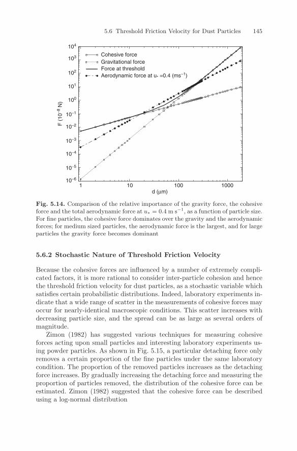
5.6 Threshold Friction Velocity for Dust Particles 145
d (µm)
104
103
102
101
100
10−1
10−2
10−3
10−4
10−5
10−6
1 10 100 1000
F (
10−8
N)
Cohesive forceGravitational forceForce at thresholdAerodynamic force at u* =0.4 (ms−1)
Fig. 5.14. Comparison of the relative importance of the gravity force, the cohesiveforce and the total aerodynamic force at u∗ = 0.4 m s−1, as a function of particle size.For fine particles, the cohesive force dominates over the gravity and the aerodynamicforces; for medium sized particles, the aerodynamic force is the largest, and for largeparticles the gravity force becomes dominant
5.6.2 Stochastic Nature of Threshold Friction Velocity
Because the cohesive forces are influenced by a number of extremely compli-cated factors, it is more rational to consider inter-particle cohesion and hencethe threshold friction velocity for dust particles, as a stochastic variable whichsatisfies certain probabilistic distributions. Indeed, laboratory experiments in-dicate that a wide range of scatter in the measurements of cohesive forces mayoccur for nearly-identical macroscopic conditions. This scatter increases withdecreasing particle size, and the spread can be as large as several orders ofmagnitude.
Zimon (1982) has suggested various techniques for measuring cohesiveforces acting upon small particles and interesting laboratory experiments us-ing powder particles. As shown in Fig. 5.15, a particular detaching force onlyremoves a certain proportion of the fine particles under the same laboratorycondition. The proportion of the removed particles increases as the detachingforce increases. By gradually increasing the detaching force and measuring theproportion of particles removed, the distribution of the cohesive force can beestimated. Zimon (1982) suggested that the cohesive force can be describedusing a log-normal distribution
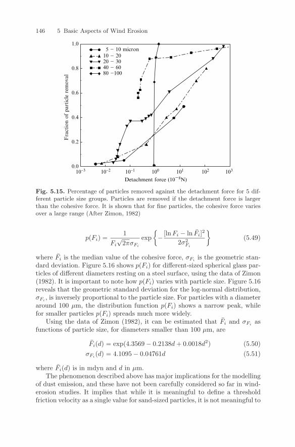
146 5 Basic Aspects of Wind Erosion
Detachment force (10−8N)
5 − 10 micron10 − 20 20 − 30 40 − 60 80 −100
Fra
ctio
n of
par
ticl
e re
mov
al
0.0
0.2
0.4
0.6
0.8
1.0
10310210110010-110-210-3
Fig. 5.15. Percentage of particles removed against the detachment force for 5 dif-ferent particle size groups. Particles are removed if the detachment force is largerthan the cohesive force. It is shown that for fine particles, the cohesive force variesover a large range (After Zimon, 1982)
p(Fi) =1
Fi
√2πσFi
exp− [lnFi − ln Fi]2
2σ2Fi
(5.49)
where Fi is the median value of the cohesive force, σFiis the geometric stan-
dard deviation. Figure 5.16 shows p(Fi) for different-sized spherical glass par-ticles of different diameters resting on a steel surface, using the data of Zimon(1982). It is important to note how p(Fi) varies with particle size. Figure 5.16reveals that the geometric standard deviation for the log-normal distribution,σFi
, is inversely proportional to the particle size. For particles with a diameteraround 100 µm, the distribution function p(Fi) shows a narrow peak, whilefor smaller particles p(Fi) spreads much more widely.
Using the data of Zimon (1982), it can be estimated that Fi and σFias
functions of particle size, for diameters smaller than 100 µm, are
Fi(d) = exp(4.3569 − 0.2138d + 0.0018d2) (5.50)σFi
(d) = 4.1095 − 0.04761d (5.51)
where Fi(d) is in mdyn and d in µm.The phenomenon described above has major implications for the modelling
of dust emission, and these have not been carefully considered so far in wind-erosion studies. It implies that while it is meaningful to define a thresholdfriction velocity as a single value for sand-sized particles, it is not meaningful to
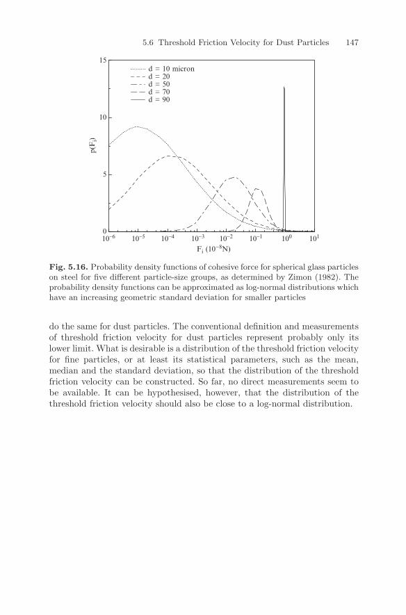
5.6 Threshold Friction Velocity for Dust Particles 147
10-6 10-5 10-4 10-3 10-2 10-1 100 101
Fi (10−8N)
p(F
i)
d = 10 micrond = 20 d = 50 d = 70 d = 90
0
5
10
15
Fig. 5.16. Probability density functions of cohesive force for spherical glass particleson steel for five different particle-size groups, as determined by Zimon (1982). Theprobability density functions can be approximated as log-normal distributions whichhave an increasing geometric standard deviation for smaller particles
do the same for dust particles. The conventional definition and measurementsof threshold friction velocity for dust particles represent probably only itslower limit. What is desirable is a distribution of the threshold friction velocityfor fine particles, or at least its statistical parameters, such as the mean,median and the standard deviation, so that the distribution of the thresholdfriction velocity can be constructed. So far, no direct measurements seem tobe available. It can be hypothesised, however, that the distribution of thethreshold friction velocity should also be close to a log-normal distribution.
6
The Dynamics and Modelling of Saltation
Saltation is one of the three major modes of particle motion during winderosion, along with suspension and creep. During an erosion event, a largenumbers of sand-sized particles hop along the surface in the wind direction,resulting in a horizontal transport of soil mass. This transport and the in-teractions between the particles, flow, surface roughness elements and to-pography lead to the evolution of sand dunes, the deformation of surfacetopography and the development of fence-line drifts in agriculture areas. Asaltating particle obtains momentum from the atmosphere and strikes the sur-face with an increased velocity. The impact of saltating particles is one of themajor mechanisms for dust emission, which is known as saltation bombard-ment (Gillette, 1974; Nickling and Gillies, 1989; Shao et al. 1993b and Alfaroet al. 1997).
Because saltation takes place in the atmospheric surface layer, the motionof saltating particles involves the interactions with a flow of strong verticalshear. If the load ratio is high, such as is the case very close to the surface,particle-to-particle collisions may occur. The lift off of particles from the sur-face and the impact of particles on the surface involve particle-to-surface andfluid-to-surface interactions. The saltation process also contains a large degreeof randomness, which originates from lift-off conditions and from turbulentfluctuations in the atmosphere.
Sand drift and the statistical behaviour of sand-particle motion are themain topics of saltation dynamics. A range of saltation models has been de-veloped, from simple analytical and semi-empirical ones for idealised situ-ations (Bagnold, 1941; Owen, 1964) to more complicated ones which haveto be solved numerically (Anderson and Haff, 1991; Shao and Li, 1999).In this Chapter, we discuss the dynamics of saltation and review the salta-tion models in the light of the considerable amount of wind-tunnel and fieldobservations.
Y. Shao, Physics and Modelling of Wind Erosion, 149c© Springer Science+Business Media B.V. 2008
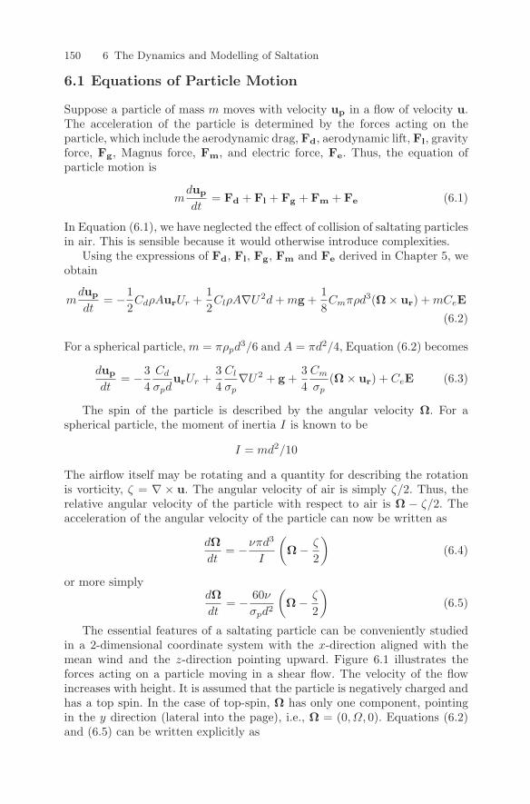
150 6 The Dynamics and Modelling of Saltation
6.1 Equations of Particle Motion
Suppose a particle of mass m moves with velocity up in a flow of velocity u.The acceleration of the particle is determined by the forces acting on theparticle, which include the aerodynamic drag, Fd, aerodynamic lift, Fl, gravityforce, Fg, Magnus force, Fm, and electric force, Fe. Thus, the equation ofparticle motion is
mdup
dt= Fd + Fl + Fg + Fm + Fe (6.1)
In Equation (6.1), we have neglected the effect of collision of saltating particlesin air. This is sensible because it would otherwise introduce complexities.
Using the expressions of Fd, Fl, Fg, Fm and Fe derived in Chapter 5, weobtain
mdup
dt= −1
2CdρAurUr +
12ClρA∇U2d + mg +
18Cmπρd3(Ω × ur) + mCeE
(6.2)
For a spherical particle, m = πρpd3/6 and A = πd2/4, Equation (6.2) becomes
dup
dt= −3
4Cd
σpdurUr +
34
Cl
σp∇U2 + g +
34
Cm
σp(Ω × ur) + CeE (6.3)
The spin of the particle is described by the angular velocity Ω. For aspherical particle, the moment of inertia I is known to be
I = md2/10
The airflow itself may be rotating and a quantity for describing the rotationis vorticity, ζ = ∇ × u. The angular velocity of air is simply ζ/2. Thus, therelative angular velocity of the particle with respect to air is Ω − ζ/2. Theacceleration of the angular velocity of the particle can now be written as
dΩdt
= −νπd3
I
(Ω − ζ
2
)(6.4)
or more simplydΩdt
= − 60ν
σpd2
(Ω − ζ
2
)(6.5)
The essential features of a saltating particle can be conveniently studiedin a 2-dimensional coordinate system with the x-direction aligned with themean wind and the z-direction pointing upward. Figure 6.1 illustrates theforces acting on a particle moving in a shear flow. The velocity of the flowincreases with height. It is assumed that the particle is negatively charged andhas a top spin. In the case of top-spin, Ω has only one component, pointingin the y direction (lateral into the page), i.e., Ω = (0, Ω, 0). Equations (6.2)and (6.5) can be written explicitly as
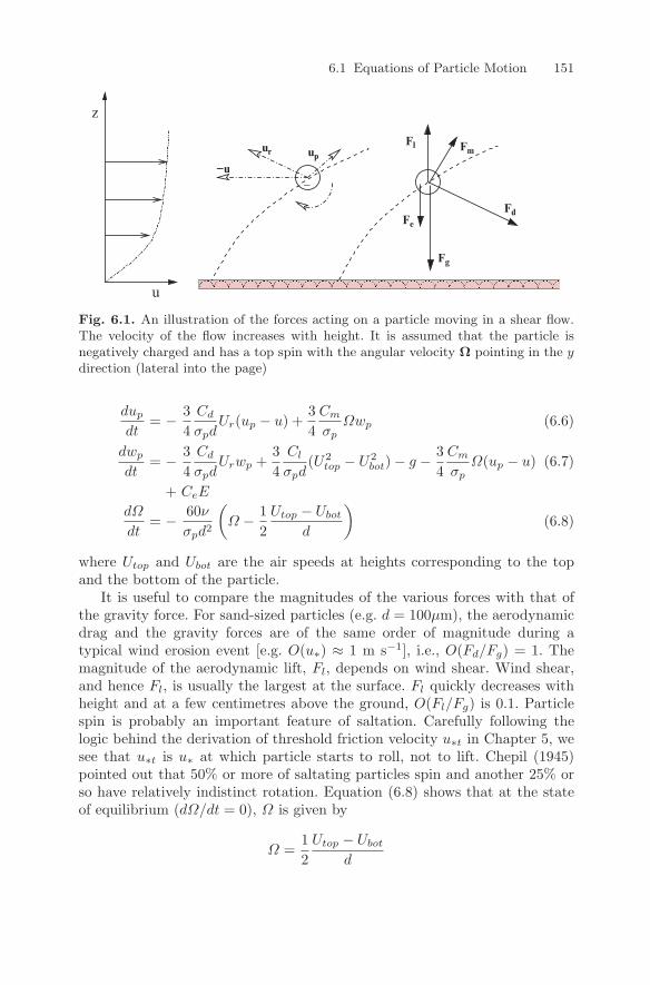
6.1 Equations of Particle Motion 151
FmFl
Fg
Fd
−u
ur up
z
u
Fe
−
Fig. 6.1. An illustration of the forces acting on a particle moving in a shear flow.The velocity of the flow increases with height. It is assumed that the particle isnegatively charged and has a top spin with the angular velocity Ω pointing in the ydirection (lateral into the page)
dup
dt= − 3
4Cd
σpdUr(up − u) +
34
Cm
σpΩwp (6.6)
dwp
dt= − 3
4Cd
σpdUrwp +
34
Cl
σpd(U2
top − U2bot) − g − 3
4Cm
σpΩ(up − u) (6.7)
+ CeE
dΩ
dt= − 60ν
σpd2
(Ω − 1
2Utop − Ubot
d
)(6.8)
where Utop and Ubot are the air speeds at heights corresponding to the topand the bottom of the particle.
It is useful to compare the magnitudes of the various forces with that ofthe gravity force. For sand-sized particles (e.g. d = 100µm), the aerodynamicdrag and the gravity forces are of the same order of magnitude during atypical wind erosion event [e.g. O(u∗) ≈ 1 m s−1], i.e., O(Fd/Fg) = 1. Themagnitude of the aerodynamic lift, Fl, depends on wind shear. Wind shear,and hence Fl, is usually the largest at the surface. Fl quickly decreases withheight and at a few centimetres above the ground, O(Fl/Fg) is 0.1. Particlespin is probably an important feature of saltation. Carefully following thelogic behind the derivation of threshold friction velocity u∗t in Chapter 5, wesee that u∗t is u∗ at which particle starts to roll, not to lift. Chepil (1945)pointed out that 50% or more of saltating particles spin and another 25% orso have relatively indistinct rotation. Equation (6.8) shows that at the stateof equilibrium (dΩ/dt = 0), Ω is given by
Ω =12
Utop − Ubot
d
152 6 The Dynamics and Modelling of Saltation
Suppose the wind profile is logarithmic. Then, we have approximately
Ω =12
u∗κ
1z + d
This implies that in general particles rotate faster and the Magnus force ismore important at smaller height. It has been observed that Ω varies overwide range, probably between 200π and 2000π s−1, and is typically around600π s−1 (300 revolutions per second, White and Schulz, 1977). At such Ω,O(Fm/Fg) is 0.1. As has been discussed in Chapter 5, the ratio of Fe/Fg canbe as large as 0.3 but is smaller in general. Hence, O(Fe/Fg) = 0.1 is probablya reasonable assumption. Again, the importance of Fe decreases with height.
As a first order of approximation, Fl, Fe and Fm can be neglected. Itfollows that the equation of particle motion can be simplified to
dup
dt= −3
4Cd
σpdUr(up − u) (6.9)
dwp
dt= −3
4Cd
σpdUrwp − g (6.10)
6.2 Uniform Saltation
We first consider the saltation of a single sand particle, or that of many iden-tical sand particles under identical flow and surface conditions. The obser-vations of saltation using photographic techniques by Bagnold (1941) andRice et al. (1996a) have revealed that particle trajectories normally contain alarge degree of randomness arising from irregular lift-off velocities and angles.As turbulence is relatively weak close to the surface and the inertia of sandgrains is relatively large, neglecting the influence of turbulent fluctuations onsaltation trajectories is sometimes a justifiable approximation. In this case,saltation particles would move through the air with different velocities, reachdifferent heights, travel different distances and impact the surface with differ-ent velocities and angles, depending only on the mean-flow characteristics andparticle lift-off conditions. If the lift-off conditions for all saltating particleswere identical, then their trajectories would be identical. We call this idealisedsaltation with identical trajectories uniform saltation.
The concept of uniform saltation allows the development of simple salta-tion models and it is justified for the reasons given below. Despite the largevariations, saltation trajectories possess some common features as illustratedin Fig. 6.2. Most particles, ejected from the surface by aerodynamic forces orby the impact of other saltating particles, take off with a large angle (about55), climb steeply to a maximum height, follow a flatter descending pathand finally strike the surface at a small angle (about 13). Certain aspectsof the bulk dynamic behaviour of saltating particles, such as the momentumexchange between particle and flow, can be explained simply and qualitativelyby considering the motion of a single particle with a characteristic trajectory.
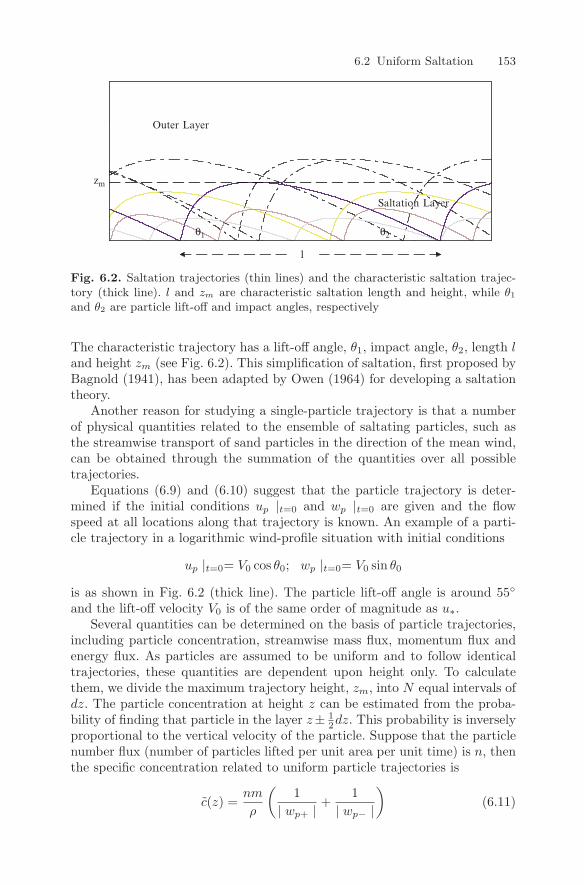
6.2 Uniform Saltation 153
l
zm
θ1 θ2
Outer Layer
Saltation Layer
Fig. 6.2. Saltation trajectories (thin lines) and the characteristic saltation trajec-tory (thick line). l and zm are characteristic saltation length and height, while θ1
and θ2 are particle lift-off and impact angles, respectively
The characteristic trajectory has a lift-off angle, θ1, impact angle, θ2, length land height zm (see Fig. 6.2). This simplification of saltation, first proposed byBagnold (1941), has been adapted by Owen (1964) for developing a saltationtheory.
Another reason for studying a single-particle trajectory is that a numberof physical quantities related to the ensemble of saltating particles, such asthe streamwise transport of sand particles in the direction of the mean wind,can be obtained through the summation of the quantities over all possibletrajectories.
Equations (6.9) and (6.10) suggest that the particle trajectory is deter-mined if the initial conditions up |t=0 and wp |t=0 are given and the flowspeed at all locations along that trajectory is known. An example of a parti-cle trajectory in a logarithmic wind-profile situation with initial conditions
up |t=0= V0 cos θ0; wp |t=0= V0 sin θ0
is as shown in Fig. 6.2 (thick line). The particle lift-off angle is around 55
and the lift-off velocity V0 is of the same order of magnitude as u∗.Several quantities can be determined on the basis of particle trajectories,
including particle concentration, streamwise mass flux, momentum flux andenergy flux. As particles are assumed to be uniform and to follow identicaltrajectories, these quantities are dependent upon height only. To calculatethem, we divide the maximum trajectory height, zm, into N equal intervals ofdz. The particle concentration at height z can be estimated from the proba-bility of finding that particle in the layer z± 1
2dz. This probability is inverselyproportional to the vertical velocity of the particle. Suppose that the particlenumber flux (number of particles lifted per unit area per unit time) is n, thenthe specific concentration related to uniform particle trajectories is
c(z) =nm
ρ
(1
| wp+ | +1
| wp− |
)(6.11)
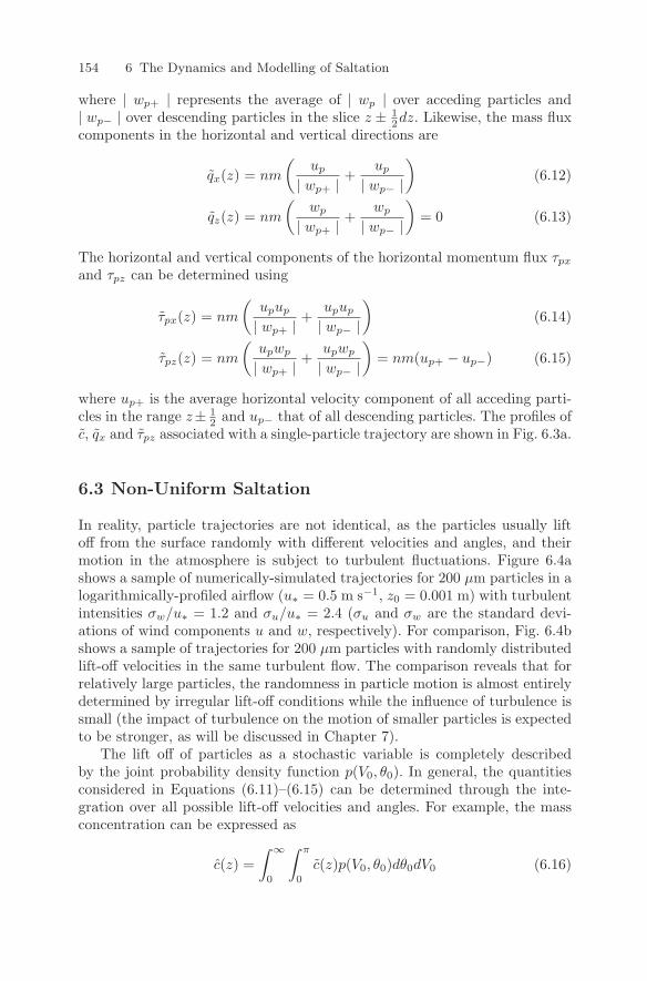
154 6 The Dynamics and Modelling of Saltation
where | wp+ | represents the average of | wp | over acceding particles and| wp− | over descending particles in the slice z ± 1
2dz. Likewise, the mass fluxcomponents in the horizontal and vertical directions are
qx(z) = nm
(up
| wp+ | +up
| wp− |
)(6.12)
qz(z) = nm
(wp
| wp+ | +wp
| wp− |
)= 0 (6.13)
The horizontal and vertical components of the horizontal momentum flux τpx
and τpz can be determined using
τpx(z) = nm
(upup
| wp+ | +upup
| wp− |
)(6.14)
τpz(z) = nm
(upwp
| wp+ | +upwp
| wp− |
)= nm(up+ − up−) (6.15)
where up+ is the average horizontal velocity component of all acceding parti-cles in the range z± 1
2 and up− that of all descending particles. The profiles ofc, qx and τpz associated with a single-particle trajectory are shown in Fig. 6.3a.
6.3 Non-Uniform Saltation
In reality, particle trajectories are not identical, as the particles usually liftoff from the surface randomly with different velocities and angles, and theirmotion in the atmosphere is subject to turbulent fluctuations. Figure 6.4ashows a sample of numerically-simulated trajectories for 200 µm particles in alogarithmically-profiled airflow (u∗ = 0.5 m s−1, z0 = 0.001 m) with turbulentintensities σw/u∗ = 1.2 and σu/u∗ = 2.4 (σu and σw are the standard devi-ations of wind components u and w, respectively). For comparison, Fig. 6.4bshows a sample of trajectories for 200 µm particles with randomly distributedlift-off velocities in the same turbulent flow. The comparison reveals that forrelatively large particles, the randomness in particle motion is almost entirelydetermined by irregular lift-off conditions while the influence of turbulence issmall (the impact of turbulence on the motion of smaller particles is expectedto be stronger, as will be discussed in Chapter 7).
The lift off of particles as a stochastic variable is completely describedby the joint probability density function p(V0, θ0). In general, the quantitiesconsidered in Equations (6.11)–(6.15) can be determined through the inte-gration over all possible lift-off velocities and angles. For example, the massconcentration can be expressed as
c(z) =∫ ∞
0
∫ π
0
c(z)p(V0, θ0)dθ0dV0 (6.16)
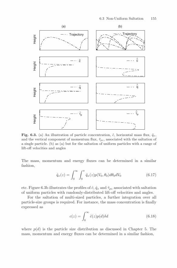
6.3 Non-Uniform Saltation 155
τp
q
c
(a)
Trajectory
τp
q
c
(b)
Trajectory
>
~
~
~ >>
Hei
ght
Hei
ght
Hei
ght
Hei
ght
Fig. 6.3. (a) An illustration of particle concentration, c, horizontal mass flux, qx,and the vertical component of momentum flux, τpz, associated with the saltation ofa single particle. (b) as (a) but for the saltation of uniform particles with a range oflift-off velocities and angles
The mass, momentum and energy fluxes can be determined in a similarfashion,
qx(z) =∫ ∞
0
∫ π
0
qx(z)p(V0, θ0)dθ0dV0 (6.17)
etc. Figure 6.3b illustrates the profiles of c, qx and τpz associated with saltationof uniform particles with randomly-distributed lift-off velocities and angles.
For the saltation of multi-sized particles, a further integration over allparticle-size groups is required. For instance, the mass concentration is finallyexpressed as
c(z) =∫ ∞
0
c(z)p(d)δd (6.18)
where p(d) is the particle size distribution as discussed in Chapter 5. Themass, momentum and energy fluxes can be determined in a similar fashion,
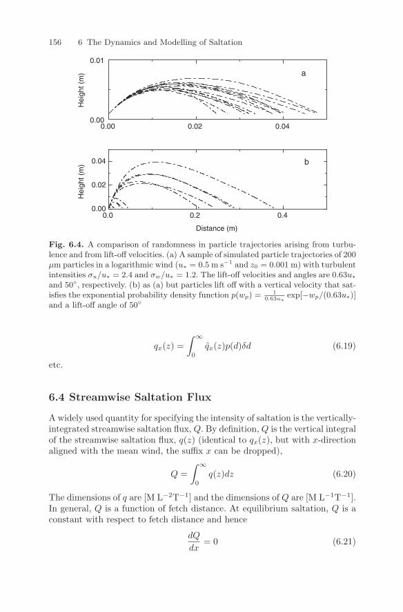
156 6 The Dynamics and Modelling of Saltation
Distance (m)
a
b
0.000.00 0.02 0.04
0.0 0.2 0.4
0.01
0.00
0.02
0.04
Hei
ght (
m)
Hei
ght (
m)
Fig. 6.4. A comparison of randomness in particle trajectories arising from turbu-lence and from lift-off velocities. (a) A sample of simulated particle trajectories of 200µm particles in a logarithmic wind (u∗ = 0.5 m s−1 and z0 = 0.001 m) with turbulentintensities σu/u∗ = 2.4 and σw/u∗ = 1.2. The lift-off velocities and angles are 0.63u∗and 50, respectively. (b) as (a) but particles lift off with a vertical velocity that sat-isfies the exponential probability density function p(wp) = 1
0.63u∗exp[−wp/(0.63u∗)]
and a lift-off angle of 50
qx(z) =∫ ∞
0
qx(z)p(d)δd (6.19)
etc.
6.4 Streamwise Saltation Flux
A widely used quantity for specifying the intensity of saltation is the vertically-integrated streamwise saltation flux, Q. By definition, Q is the vertical integralof the streamwise saltation flux, q(z) (identical to qx(z), but with x-directionaligned with the mean wind, the suffix x can be dropped),
Q =∫ ∞
0
q(z)dz (6.20)
The dimensions of q are [M L−2T−1] and the dimensions of Q are [M L−1T−1].In general, Q is a function of fetch distance. At equilibrium saltation, Q is aconstant with respect to fetch distance and hence
dQ
dx= 0 (6.21)
6.5 The Bagnold-Owen Saltation Equation 157
6.5 The Bagnold-Owen Saltation Equation
6.5.1 The Bagnold Model
Most saltating particles are confined to a thin layer close to the surface, whichwe refer to as the saltation layer. We could define, for instance, the depth of thesaltation layer as the height below which 90% of saltating particles are found.For uniform saltation, the depth of the saltation layer is simply the maximumheight zm of the saltation trajectory, which is of the order of V 2
0 /2g.The saltation theory of Bagnold (1941) is a uniform-saltation model based
on the momentum balance of the saltation layer. In this model, the momentumtransfer to the surface arising from the saltation of multiple particles is repre-sented by that arising from the characteristic saltation (Fig. 6.2). The charac-teristic saltation is assumed to have a lift-off velocity of (up1, wp1), an impactvelocity of (up2, wp2), a saltation height of zm and a saltation length of l.It is further assumed that particles lift off vertically and hence, up1 is zero.This latter assumption is based on the early wind-tunnel observations, whichwe now know are not entirely accurate (typical lift-off angles are around 55).However, it remains valid to assume that
up1 up2 (6.22)
The travel time of a particle over the distance l is approximately 2l/up2, andthe time required for that particle to cover 2zm is approximately 4zm/wp1.Since zm is proportional to w2
p1/2g and wp1 is proportional to u∗, the linearrelationship
up2
l=
g
cou∗(6.23)
can be established, where co is an empirical dimensionless coefficient.A saltating particle obtains momentum from the airflow as it moves
through it and loses momentum to the surface at impact. Therefore, the mo-mentum flux in the saltation layer is a consequence of both particle and fluidmotions (Fig. 6.7). Within the saltation layer, we have in general that:
ρu2∗ = τp(z) + τa(z) (6.24)
where ρu2∗ represents the total momentum flux transferred to the saltation
layer from the airflow above it, τp is the particle-borne momentum flux andτa is the airborne momentum flux, both varying with height. The magnitudeof τa at the surface, τa0, is not exactly known, but Owen (1964) has hypoth-esised that τa0 should approach ρu2
∗t if saltation is at equilibrium. Assumingthe correctness of the Owen hypothesis, we have that the particle-borne mo-mentum flux at the surface, τp0, is
τp0 = ρ(u2∗ − u2
∗t) (6.25)
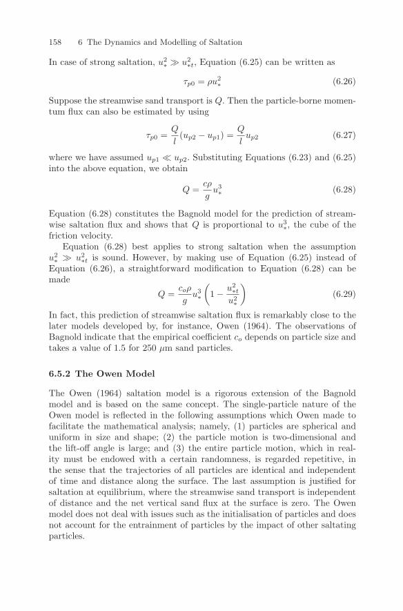
158 6 The Dynamics and Modelling of Saltation
In case of strong saltation, u2∗ u2
∗t, Equation (6.25) can be written as
τp0 = ρu2∗ (6.26)
Suppose the streamwise sand transport is Q. Then the particle-borne momen-tum flux can also be estimated by using
τp0 =Q
l(up2 − up1) =
Q
lup2 (6.27)
where we have assumed up1 up2. Substituting Equations (6.23) and (6.25)into the above equation, we obtain
Q =cρ
gu3∗ (6.28)
Equation (6.28) constitutes the Bagnold model for the prediction of stream-wise saltation flux and shows that Q is proportional to u3
∗, the cube of thefriction velocity.
Equation (6.28) best applies to strong saltation when the assumptionu2∗ u2
∗t is sound. However, by making use of Equation (6.25) instead ofEquation (6.26), a straightforward modification to Equation (6.28) can bemade
Q =coρ
gu3∗
(1 − u2
∗t
u2∗
)(6.29)
In fact, this prediction of streamwise saltation flux is remarkably close to thelater models developed by, for instance, Owen (1964). The observations ofBagnold indicate that the empirical coefficient co depends on particle size andtakes a value of 1.5 for 250 µm sand particles.
6.5.2 The Owen Model
The Owen (1964) saltation model is a rigorous extension of the Bagnoldmodel and is based on the same concept. The single-particle nature of theOwen model is reflected in the following assumptions which Owen made tofacilitate the mathematical analysis; namely, (1) particles are spherical anduniform in size and shape; (2) the particle motion is two-dimensional andthe lift-off angle is large; and (3) the entire particle motion, which in real-ity must be endowed with a certain randomness, is regarded repetitive, inthe sense that the trajectories of all particles are identical and independentof time and distance along the surface. The last assumption is justified forsaltation at equilibrium, where the streamwise sand transport is independentof distance and the net vertical sand flux at the surface is zero. The Owenmodel does not deal with issues such as the initialisation of particles and doesnot account for the entrainment of particles by the impact of other saltatingparticles.
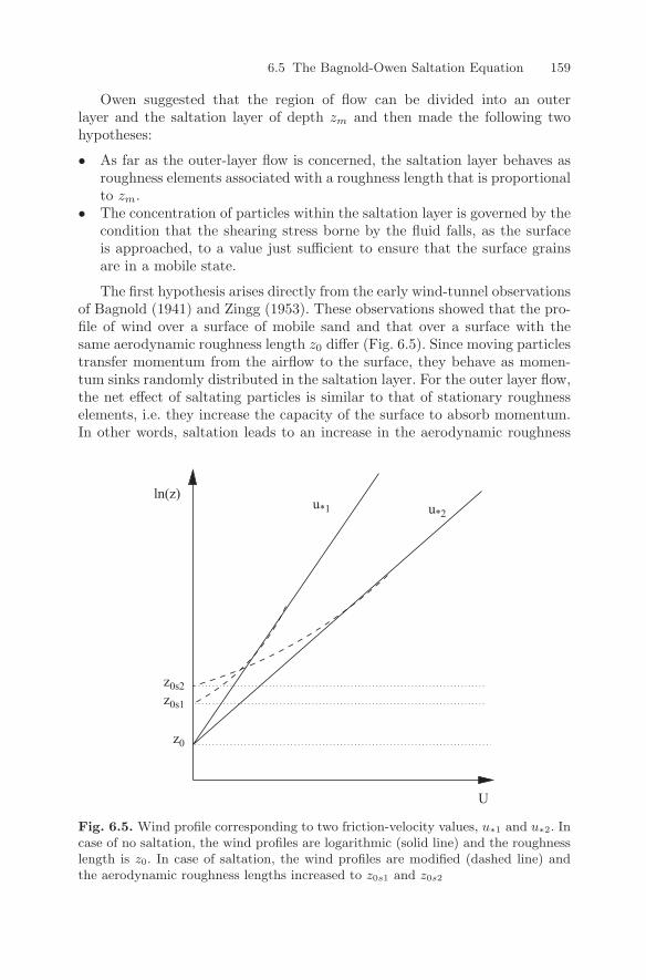
6.5 The Bagnold-Owen Saltation Equation 159
Owen suggested that the region of flow can be divided into an outerlayer and the saltation layer of depth zm and then made the following twohypotheses:
• As far as the outer-layer flow is concerned, the saltation layer behaves asroughness elements associated with a roughness length that is proportionalto zm.
• The concentration of particles within the saltation layer is governed by thecondition that the shearing stress borne by the fluid falls, as the surfaceis approached, to a value just sufficient to ensure that the surface grainsare in a mobile state.
The first hypothesis arises directly from the early wind-tunnel observationsof Bagnold (1941) and Zingg (1953). These observations showed that the pro-file of wind over a surface of mobile sand and that over a surface with thesame aerodynamic roughness length z0 differ (Fig. 6.5). Since moving particlestransfer momentum from the airflow to the surface, they behave as momen-tum sinks randomly distributed in the saltation layer. For the outer layer flow,the net effect of saltating particles is similar to that of stationary roughnesselements, i.e. they increase the capacity of the surface to absorb momentum.In other words, saltation leads to an increase in the aerodynamic roughness
z0s2z0s1
z0
U
u*1 u*2
ln(z)
Fig. 6.5. Wind profile corresponding to two friction-velocity values, u∗1 and u∗2. Incase of no saltation, the wind profiles are logarithmic (solid line) and the roughnesslength is z0. In case of saltation, the wind profiles are modified (dashed line) andthe aerodynamic roughness lengths increased to z0s1 and z0s2
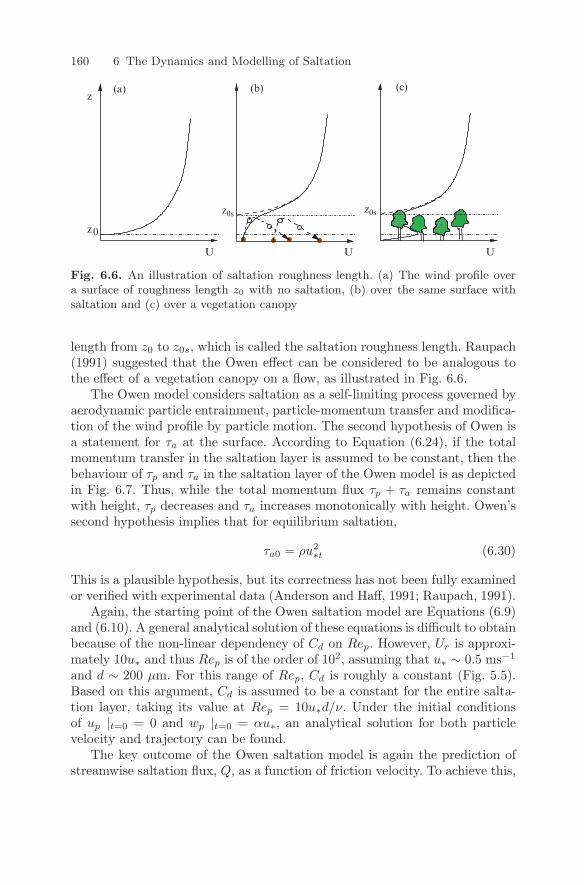
160 6 The Dynamics and Modelling of Saltation
(a) (b) (c)
U U
z0
z
z0sz0s
U
Fig. 6.6. An illustration of saltation roughness length. (a) The wind profile overa surface of roughness length z0 with no saltation, (b) over the same surface withsaltation and (c) over a vegetation canopy
length from z0 to z0s, which is called the saltation roughness length. Raupach(1991) suggested that the Owen effect can be considered to be analogous tothe effect of a vegetation canopy on a flow, as illustrated in Fig. 6.6.
The Owen model considers saltation as a self-limiting process governed byaerodynamic particle entrainment, particle-momentum transfer and modifica-tion of the wind profile by particle motion. The second hypothesis of Owen isa statement for τa at the surface. According to Equation (6.24), if the totalmomentum transfer in the saltation layer is assumed to be constant, then thebehaviour of τp and τa in the saltation layer of the Owen model is as depictedin Fig. 6.7. Thus, while the total momentum flux τp + τa remains constantwith height, τp decreases and τa increases monotonically with height. Owen’ssecond hypothesis implies that for equilibrium saltation,
τa0 = ρu2∗t (6.30)
This is a plausible hypothesis, but its correctness has not been fully examinedor verified with experimental data (Anderson and Haff, 1991; Raupach, 1991).
Again, the starting point of the Owen saltation model are Equations (6.9)and (6.10). A general analytical solution of these equations is difficult to obtainbecause of the non-linear dependency of Cd on Rep. However, Ur is approxi-mately 10u∗ and thus Rep is of the order of 102, assuming that u∗ ∼ 0.5 ms−1
and d ∼ 200 µm. For this range of Rep, Cd is roughly a constant (Fig. 5.5).Based on this argument, Cd is assumed to be a constant for the entire salta-tion layer, taking its value at Rep = 10u∗d/ν. Under the initial conditionsof up |t=0 = 0 and wp |t=0 = αu∗, an analytical solution for both particlevelocity and trajectory can be found.
The key outcome of the Owen saltation model is again the prediction ofstreamwise saltation flux, Q, as a function of friction velocity. To achieve this,
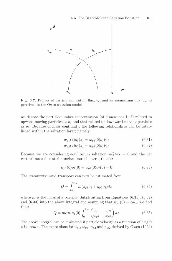
6.5 The Bagnold-Owen Saltation Equation 161
ττ*t
τaτp
z
zm
Fig. 6.7. Profiles of particle momentum flux, τp, and air momentum flux, τa, asperceived in the Owen saltation model
we denote the particle-number concentration (of dimensions L−3) related toupward-moving particles as o1 and that related to downward-moving particlesas o2. Because of mass continuity, the following relationships can be estab-lished within the saltation layer; namely,
wp1(z)o1(z) = wp1(0)o1(0) (6.31)wp2(z)o2(z) = wp2(0)o2(0) (6.32)
Because we are considering equilibrium saltation, dQ/dx = 0 and the netvertical mass flux at the surface must be zero, that is:
wp1(0)o1(0) + wp2(0)o2(0) = 0 (6.33)
The streamwise sand transport can now be estimated from
Q =∫ zm
0
m(up1o1 + up2o2)dz (6.34)
where m is the mass of a particle. Substituting from Equations (6.31), (6.32)and (6.33) into the above integral and assuming that wp1(0) = αu∗, we findthat:
Q = mαu∗o1(0)∫ zm
0
(up1
wp1− up2
wp2
)dz (6.35)
The above integral can be evaluated if particle velocity as a function of heightz is known. The expressions for up1, wp1, up2 and wp2 derived by Owen (1964)
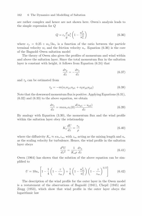
162 6 The Dynamics and Modelling of Saltation
are rather complex and hence are not shown here. Owen’s analysis leads tothe simple expression for Q
Q = coρ
gu3∗
(1 − u2
∗t
u2∗
)(6.36)
where co = 0.25 + wt/3u∗ is a function of the ratio between the particleterminal velocity wt and the friction velocity u∗. Equation (6.36) is the coreof the Bagnold–Owen saltation model
The theory of Owen also gives the profiles of momentum and wind withinand above the saltation layer. Since the total momentum flux in the saltationlayer is constant with height, it follows from Equation (6.24) that
dτp
dz= −dτa
dz(6.37)
and τp can be estimated from
τp = −m(o1wp1up1 + o2wp2up2) (6.38)
Note that the downward momentum flux is positive. Applying Equations (6.31),(6.32) and (6.33) to the above equation, we obtain
dτa
dz= mαu∗o1(0)
d(up1 − up2)dz
(6.39)
By analogy with Equation (3.30), the momentum flux and the wind profilewithin the saltation layer obey the relationship
KodU
dz=
τa
ρ(6.40)
where the diffusivity Ko ≈ κu∗zm, with zm acting as the mixing length and u∗as the scaling velocity for turbulence. Hence, the wind profile in the saltationlayer obeys
d2U
dz2=
1Koρ
dτa
dz(6.41)
Owen (1964) has shown that the solution of the above equation can be sim-plified to
U = 10u∗
[1 − 1
4
(1 − z
zm
)+
16
(1 − u2
∗t
u2∗
)(1 − z
zm
)3/2]
(6.42)
The description of the wind profile for the outer layer in the Owen modelis a restatement of the observations of Bagnold (1941), Chepil (1945) andZingg (1953), which show that wind profile in the outer layer obeys thelogarithmic law
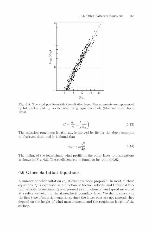
6.6 Other Saltation Equations 163
log 1
0 (z
/z0s)
U/u*
-1
0
4 8 12 16 20
1
2
Fig. 6.8. The wind profile outside the saltation layer. Measurements are representedby full circles, and z0s is calculated using Equation (6.44) (Modified from Owen,1964)
U =u∗κ
ln(
z
z0s
)(6.43)
The saltation roughness length, z0s, is derived by fitting the above equationto observed data, and it is found that
z0s = cz0u2∗
2g(6.44)
The fitting of the logarithmic wind profile in the outer layer to observationsis shown in Fig. 6.8. The coefficient cz0 is found to be around 0.02.
6.6 Other Saltation Equations
A number of other saltation equations have been proposed. In most of theseequations, Q is expressed as a function of friction velocity and threshold fric-tion velocity. Sometimes, Q is expressed as a function of wind speed measuredat a reference height in the atmospheric boundary layer. We shall discuss onlythe first type of saltation equations, since the latter ones are not general: theydepend on the height of wind measurements and the roughness length of thesurface.
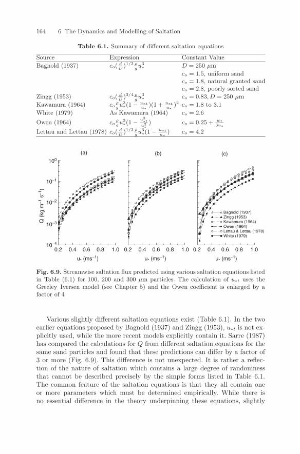
164 6 The Dynamics and Modelling of Saltation
Table 6.1. Summary of different saltation equations
Source Expression Constant Value
Bagnold (1937) co(dD
)1/2 ρgu3∗ D = 250 µm
co = 1.5, uniform sandco = 1.8, natural granted sandco = 2.8, poorly sorted sand
Zingg (1953) co(dD
)3/4 ρgu3∗ co = 0.83, D = 250 µm
Kawamura (1964) coρgu3∗(1 − u∗t
u∗)(1 + u∗t
u∗)2 co = 1.8 to 3.1
White (1979) As Kawamura (1964) co = 2.6
Owen (1964) coρgu3∗(1 − u2
∗t
u2∗
) co = 0.25 + wt3u∗
Lettau and Lettau (1978) co(dD
)1/2 ρgu3∗(1 − u∗t
u∗) co = 4.2
u* (ms−1) u* (ms−1) u* (ms−1)
Q (
kg m
−1 s
−1)
Bagnold (1937)Zingg (1953)Kawamura (1964)Owen (1964)Lettau & Lettau (1978)White (1979)
(a) (b) (c)
10−4
10−3
0.2 0.4 0.6 0.8 1.0 0.2 0.4 0.6 0.8 1.0 0.2 0.4 0.6 0.8 1.0
10−2
10−1
100
Fig. 6.9. Streamwise saltation flux predicted using various saltation equations listedin Table (6.1) for 100, 200 and 300 µm particles. The calculation of u∗t uses theGreeley–Iversen model (see Chapter 5) and the Owen coefficient is enlarged by afactor of 4
Various slightly different saltation equations exist (Table 6.1). In the twoearlier equations proposed by Bagnold (1937) and Zingg (1953), u∗t is not ex-plicitly used, while the more recent models explicitly contain it. Sarre (1987)has compared the calculations for Q from different saltation equations for thesame sand particles and found that these predictions can differ by a factor of3 or more (Fig. 6.9). This difference is not unexpected. It is rather a reflec-tion of the nature of saltation which contains a large degree of randomnessthat cannot be described precisely by the simple forms listed in Table 6.1.The common feature of the saltation equations is that they all contain oneor more parameters which must be determined empirically. While there isno essential difference in the theory underpinning these equations, slightly
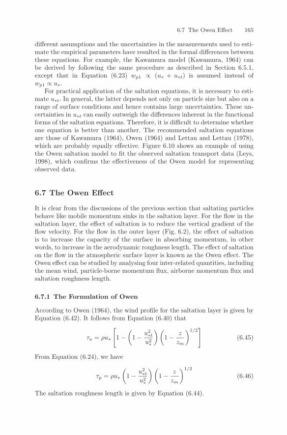
6.7 The Owen Effect 165
different assumptions and the uncertainties in the measurements used to esti-mate the empirical parameters have resulted in the formal differences betweenthese equations. For example, the Kawamura model (Kawamura, 1964) canbe derived by following the same procedure as described in Section 6.5.1,except that in Equation (6.23) wp1 ∝ (u∗ + u∗t) is assumed instead ofwp1 ∝ u∗.
For practical application of the saltation equations, it is necessary to esti-mate u∗t. In general, the latter depends not only on particle size but also on arange of surface conditions and hence contains large uncertainties. These un-certainties in u∗t can easily outweigh the differences inherent in the functionalforms of the saltation equations. Therefore, it is difficult to determine whetherone equation is better than another. The recommended saltation equationsare those of Kawamura (1964), Owen (1964) and Lettau and Lettau (1978),which are probably equally effective. Figure 6.10 shows an example of usingthe Owen saltation model to fit the observed saltation transport data (Leys,1998), which confirms the effectiveness of the Owen model for representingobserved data.
6.7 The Owen Effect
It is clear from the discussions of the previous section that saltating particlesbehave like mobile momentum sinks in the saltation layer. For the flow in thesaltation layer, the effect of saltation is to reduce the vertical gradient of theflow velocity. For the flow in the outer layer (Fig. 6.2), the effect of saltationis to increase the capacity of the surface in absorbing momentum, in otherwords, to increase in the aerodynamic roughness length. The effect of saltationon the flow in the atmospheric surface layer is known as the Owen effect. TheOwen effect can be studied by analysing four inter-related quantities, includingthe mean wind, particle-borne momentum flux, airborne momentum flux andsaltation roughness length.
6.7.1 The Formulation of Owen
According to Owen (1964), the wind profile for the saltation layer is given byEquation (6.42). It follows from Equation (6.40) that
τa = ρu∗
[1 −
(1 − u2
∗t
u2∗
)(1 − z
zm
)1/2]
(6.45)
From Equation (6.24), we have
τp = ρu∗
(1 − u2
∗t
u2∗
)(1 − z
zm
)1/2
(6.46)
The saltation roughness length is given by Equation (6.44).
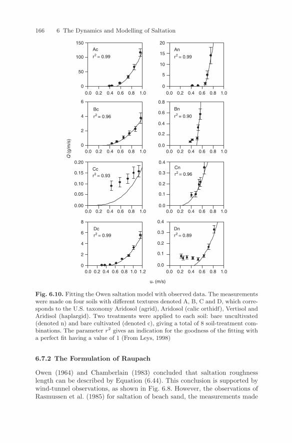
166 6 The Dynamics and Modelling of Saltation
Q (
g/m
/s)
u* (m/s)
150
100
50
20
15
10
5
0
0.20
0.15
0.10
0.05
0.00
0.4
0.3
0.2
0.1
0.0
0.4
0.3
0.2
0.1
0.0
0.8
0.6
0.4
0.2
0.0
0.0 0.2 0.4 0.6 0.8 1.0 0.0 0.2 0.4 0.6 0.8 1.0
0.0 0.2 0.4 0.6 0.8 1.0 0.0 0.2 0.4 0.6 0.8 1.0
0.0 0.2 0.4 0.6 0.8 1.0 0.0 0.2 0.4 0.6 0.8 1.0
0.00.0 0.2 0.4 0.6 0.8 1.0 1.2 0.2 0.4 0.6 0.8 1.0
Ac
r2 = 0.99
An
r2 = 0.99
Bc
r2 = 0.96
Bn
r2 = 0.90
Ccr2 = 0.93
Dcr2 = 0.99
Dnr2 = 0.89
Cnr2 = 0.96
0
0
2
4
6
0
2
4
6
8
Fig. 6.10. Fitting the Owen saltation model with observed data. The measurementswere made on four soils with different textures denoted A, B, C and D, which corre-sponds to the U.S. taxonomy Aridosol (agrid), Aridosol (calic orthidf), Vertisol andAridisol (haplargid). Two treatments were applied to each soil: bare uncultivated(denoted n) and bare cultivated (denoted c), giving a total of 8 soil-treatment com-binations. The parameter r2 gives an indication for the goodness of the fitting witha perfect fit having a value of 1 (From Leys, 1998)
6.7.2 The Formulation of Raupach
Owen (1964) and Chamberlain (1983) concluded that saltation roughnesslength can be described by Equation (6.44). This conclusion is supported bywind-tunnel observations, as shown in Fig. 6.8. However, the observations ofRasmussen et al. (1985) for saltation of beach sand, the measurements made
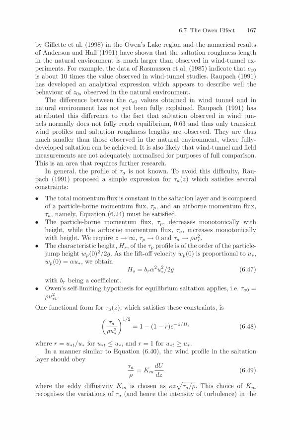
6.7 The Owen Effect 167
by Gillette et al. (1998) in the Owen’s Lake region and the numerical resultsof Anderson and Haff (1991) have shown that the saltation roughness lengthin the natural environment is much larger than observed in wind-tunnel ex-periments. For example, the data of Rasmussen et al. (1985) indicate that cz0
is about 10 times the value observed in wind-tunnel studies. Raupach (1991)has developed an analytical expression which appears to describe well thebehaviour of z0s observed in the natural environment.
The difference between the cz0 values obtained in wind tunnel and innatural environment has not yet been fully explained. Raupach (1991) hasattributed this difference to the fact that saltation observed in wind tun-nels normally does not fully reach equilibrium, 0.63 and thus only transientwind profiles and saltation roughness lengths are observed. They are thusmuch smaller than those observed in the natural environment, where fully-developed saltation can be achieved. It is also likely that wind-tunnel and fieldmeasurements are not adequately normalised for purposes of full comparison.This is an area that requires further research.
In general, the profile of τa is not known. To avoid this difficulty, Rau-pach (1991) proposed a simple expression for τa(z) which satisfies severalconstraints:
• The total momentum flux is constant in the saltation layer and is composedof a particle-borne momentum flux, τp, and an airborne momentum flux,τa, namely, Equation (6.24) must be satisfied.
• The particle-borne momentum flux, τp, decreases monotonically withheight, while the airborne momentum flux, τa, increases monotonicallywith height. We require z → ∞, τp → 0 and τa → ρu2
∗.• The characteristic height, Hs, of the τp profile is of the order of the particle-
jump height wp(0)2/2g. As the lift-off velocity wp(0) is proportional to u∗,wp(0) = αu∗, we obtain
Hs = brα2u2
∗/2g (6.47)
with br being a coefficient.• Owen’s self-limiting hypothesis for equilibrium saltation applies, i.e. τa0 =
ρu2∗t.
One functional form for τa(z), which satisfies these constraints, is(
τa
ρu2∗
)1/2
= 1 − (1 − r)e−z/Hs (6.48)
where r = u∗t/u∗ for u∗t ≤ u∗, and r = 1 for u∗t ≥ u∗.In a manner similar to Equation (6.40), the wind profile in the saltation
layer should obeyτa
ρ= Km
dU
dz(6.49)
where the eddy diffusivity Km is chosen as κz√
τa/ρ. This choice of Km
recognises the variations of τa (and hence the intensity of turbulence) in the
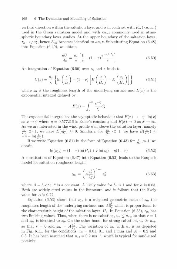
168 6 The Dynamics and Modelling of Saltation
vertical direction within the saltation layer and is in contrast with Ko (κu∗zm)used in the Owen saltation model and with κu∗z commonly used in atmo-spheric boundary layer studies. At the upper boundary of the saltation layer,τa → ρu2
∗, hence Km becomes identical to κu∗z. Substituting Equation (6.48)into Equation (6.49), we obtain
dU
dz=
u∗κ
[1z− (1 − r)
e−z/Hs
z
](6.50)
An integration of Equation (6.50) over z0 and z leads to
U(z) =u∗κ
ln
(z
z0
)− (1 − r)
[E
(z
Hs
)− E
(z0
Hs
)](6.51)
where z0 is the roughness length of the underlying surface and E(x) is theexponential integral defined by
E(x) =∫ ∞
x
e−ξ
ξdξ
The exponential integral has the asymptotic behaviour that E(x) → −η−ln(x)as x → 0 where η = 0.577216 is Euler’s constant; and E(x) → 0 as x → ∞.As we are interested in the wind profile well above the saltation layer, namelyz
Hs 1, we have E( z
Hs) ≈ 0. Similarly, for z0
Hs 1, we have E( z0
Hs) ≈
−η − ln( z0Hs
).If we write Equation (6.51) in the form of Equation (6.43) for z
Hs 1, we
obtainln(z0s) = (1 − r) ln(Hs) + r ln(z0) − η(1 − r) (6.52)
A substitution of Equation (6.47) into Equation (6.52) leads to the Raupachmodel for saltation roughness length
z0s =(
Au2∗
2g
)1−r
zr0 (6.53)
where A = brα2e−η is a constant. A likely value for br is 1 and for α is 0.63.
Both are widely cited values in the literature, and it follows that the likelyvalue for A is 0.22.
Equation (6.53) shows that z0s is a weighted geometric mean of z0, theroughness length of the underlying surface, and A
u2∗
2g which is proportional tothe characteristic height of the saltation layer, Hs. In Equation (6.53), z0s hastwo limiting values. Thus, when there is no saltation, u∗ ≤ u∗t, so that r = 1and z0s is identical to z0. On the other hand, for strong saltation, u∗ u∗t,so that r = 0 and z0s = A
u2∗
2g . The variation of z0s with u∗ is as depictedin Fig. 6.11, for the conditions, z0 = 0.01, 0.1 and 1 mm and A = 0.2 and0.3. It has been assumed that u∗t = 0.2 ms−1, which is typical for sand-sizedparticles.
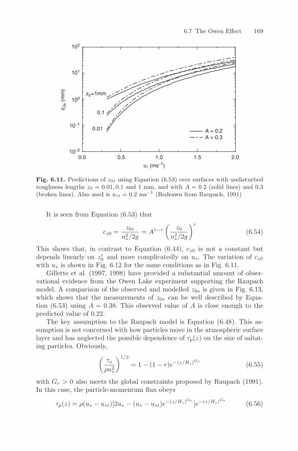
6.7 The Owen Effect 169
u* (ms−1)
10−2
10−1
100
101
102
z 0s
(mm
)
A = 0.2A = 0.3
z0=1mm
0.1
0.01
0.0 0.5 1.0 1.5 2.0
Fig. 6.11. Predictions of z0s using Equation (6.53) over surfaces with undisturbedroughness lengths z0 = 0.01, 0.1 and 1 mm, and with A = 0.2 (solid lines) and 0.3(broken lines). Also used is u∗t = 0.2 ms−1 (Redrawn from Raupach, 1991)
It is seen from Equation (6.53) that
cz0 =z0s
u2∗/2g
= A1−r
(z0
u2∗/2g
)r
(6.54)
This shows that, in contrast to Equation (6.44), cz0 is not a constant butdepends linearly on zr
0 and more complicatedly on u∗. The variation of cz0
with u∗ is shown in Fig. 6.12 for the same conditions as in Fig. 6.11.Gillette et al. (1997, 1998) have provided a substantial amount of obser-
vational evidence from the Owen Lake experiment supporting the Raupachmodel. A comparison of the observed and modelled z0s is given in Fig. 6.13,which shows that the measurements of z0s can be well described by Equa-tion (6.53) using A = 0.38. This observed value of A is close enough to thepredicted value of 0.22.
The key assumption to the Raupach model is Equation (6.48). This as-sumption is not concerned with how particles move in the atmospheric surfacelayer and has neglected the possible dependence of τp(z) on the size of saltat-ing particles. Obviously,
(τa
ρu2∗
)1/2
= 1 − (1 − r)e−(z/Hs)Gr(6.55)
with Gr > 0 also meets the global constraints proposed by Raupach (1991).In this case, the particle-momentum flux obeys
τp(z) = ρ(u∗ − u∗t)[2u∗ − (u∗ − u∗t)e−(z/Hs)Gr]e−(z/Hs)Gr
(6.56)
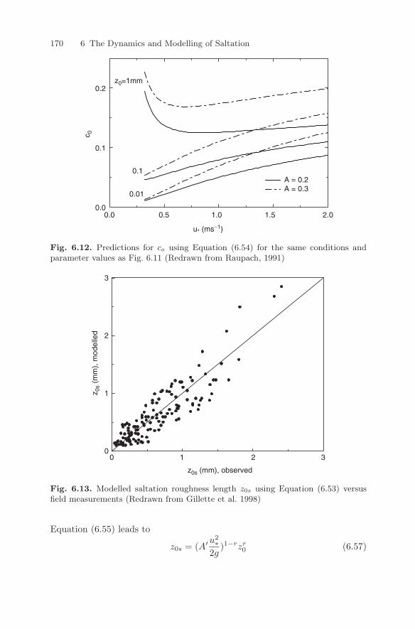
170 6 The Dynamics and Modelling of Saltation
u* (ms−1)
z0=1mm
0.0 0.5 1.0 1.5 2.0
c 0
A = 0.2A = 0.3
0.1
0.01
0.0
0.1
0.2
Fig. 6.12. Predictions for co using Equation (6.54) for the same conditions andparameter values as Fig. 6.11 (Redrawn from Raupach, 1991)
z0s (mm), observed
z 0s
(mm
), m
odel
led
0
1
2
3
0 1 2 3
Fig. 6.13. Modelled saltation roughness length z0s using Equation (6.53) versusfield measurements (Redrawn from Gillette et al. 1998)
Equation (6.55) leads to
z0s = (A′ u2∗
2g)1−rzr
0 (6.57)
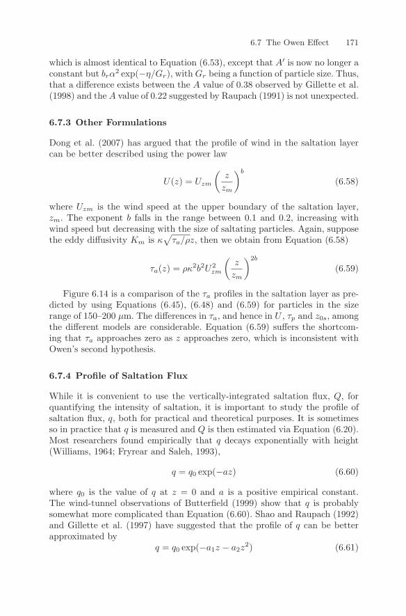
6.7 The Owen Effect 171
which is almost identical to Equation (6.53), except that A′ is now no longer aconstant but brα
2 exp(−η/Gr), with Gr being a function of particle size. Thus,that a difference exists between the A value of 0.38 observed by Gillette et al.(1998) and the A value of 0.22 suggested by Raupach (1991) is not unexpected.
6.7.3 Other Formulations
Dong et al. (2007) has argued that the profile of wind in the saltation layercan be better described using the power law
U(z) = Uzm
(z
zm
)b
(6.58)
where Uzm is the wind speed at the upper boundary of the saltation layer,zm. The exponent b falls in the range between 0.1 and 0.2, increasing withwind speed but decreasing with the size of saltating particles. Again, supposethe eddy diffusivity Km is κ
√τa/ρz, then we obtain from Equation (6.58)
τa(z) = ρκ2b2U2zm
(z
zm
)2b
(6.59)
Figure 6.14 is a comparison of the τa profiles in the saltation layer as pre-dicted by using Equations (6.45), (6.48) and (6.59) for particles in the sizerange of 150–200 µm. The differences in τa, and hence in U , τp and z0s, amongthe different models are considerable. Equation (6.59) suffers the shortcom-ing that τa approaches zero as z approaches zero, which is inconsistent withOwen’s second hypothesis.
6.7.4 Profile of Saltation Flux
While it is convenient to use the vertically-integrated saltation flux, Q, forquantifying the intensity of saltation, it is important to study the profile ofsaltation flux, q, both for practical and theoretical purposes. It is sometimesso in practice that q is measured and Q is then estimated via Equation (6.20).Most researchers found empirically that q decays exponentially with height(Williams, 1964; Fryrear and Saleh, 1993),
q = q0 exp(−az) (6.60)
where q0 is the value of q at z = 0 and a is a positive empirical constant.The wind-tunnel observations of Butterfield (1999) show that q is probablysomewhat more complicated than Equation (6.60). Shao and Raupach (1992)and Gillette et al. (1997) have suggested that the profile of q can be betterapproximated by
q = q0 exp(−a1z − a2z2) (6.61)
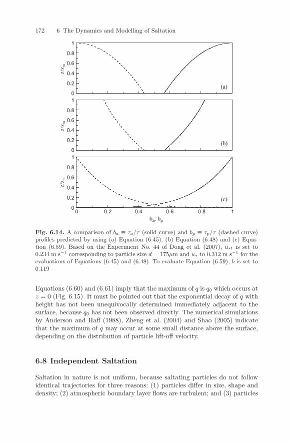
172 6 The Dynamics and Modelling of Saltation
ba; bp
z/z m
z/z m
z/z m
00 0.2 0.4 0.6 0.8 1
0.2
0.4
0.6
0.8
10
0.2
0.4
0.6
0.8
10
0.2
0.4
0.6
0.8
1
(a)
(b)
(c)
Fig. 6.14. A comparison of ba ≡ τa/τ (solid curve) and bp ≡ τp/τ (dashed curve)profiles predicted by using (a) Equation (6.45), (b) Equation (6.48) and (c) Equa-tion (6.59). Based on the Experiment No. 44 of Dong et al. (2007), u∗t is set to0.234 m s−1 corresponding to particle size d = 175µm and u∗ to 0.312 m s−1 for theevaluations of Equations (6.45) and (6.48). To evaluate Equation (6.59), b is set to0.119
Equations (6.60) and (6.61) imply that the maximum of q is q0 which occurs atz = 0 (Fig. 6.15). It must be pointed out that the exponential decay of q withheight has not been unequivocally determined immediately adjacent to thesurface, because q0 has not been observed directly. The numerical simulationsby Anderson and Haff (1988), Zheng et al. (2004) and Shao (2005) indicatethat the maximum of q may occur at some small distance above the surface,depending on the distribution of particle lift-off velocity.
6.8 Independent Saltation
Saltation in nature is not uniform, because saltating particles do not followidentical trajectories for three reasons: (1) particles differ in size, shape anddensity; (2) atmospheric boundary layer flows are turbulent; and (3) particles
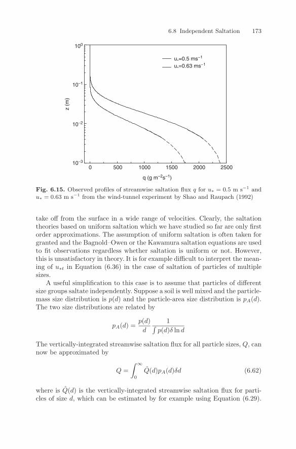
6.8 Independent Saltation 173
q (g m−2s−1)
z (m
)u*=0.5 ms−1
u*=0.63 ms−1
10−3
0 500 1000 1500 2000 2500
10−2
10−1
100
Fig. 6.15. Observed profiles of streamwise saltation flux q for u∗ = 0.5 m s−1 andu∗ = 0.63 m s−1 from the wind-tunnel experiment by Shao and Raupach (1992)
take off from the surface in a wide range of velocities. Clearly, the saltationtheories based on uniform saltation which we have studied so far are only firstorder approximations. The assumption of uniform saltation is often taken forgranted and the Bagnold–Owen or the Kawamura saltation equations are usedto fit observations regardless whether saltation is uniform or not. However,this is unsatisfactory in theory. It is for example difficult to interpret the mean-ing of u∗t in Equation (6.36) in the case of saltation of particles of multiplesizes.
A useful simplification to this case is to assume that particles of differentsize groups saltate independently. Suppose a soil is well mixed and the particle-mass size distribution is p(d) and the particle-area size distribution is pA(d).The two size distributions are related by
pA(d) =p(d)d
1∫p(d)δ ln d
The vertically-integrated streamwise saltation flux for all particle sizes, Q, cannow be approximated by
Q =∫ ∞
0
Q(d)pA(d)δd (6.62)
where is Q(d) is the vertically-integrated streamwise saltation flux for parti-cles of size d, which can be estimated by for example using Equation (6.29).
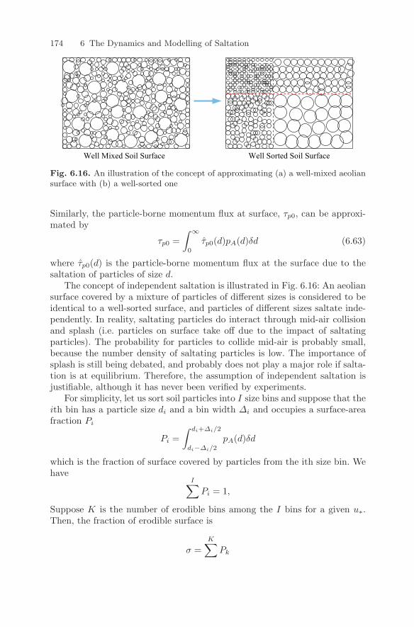
174 6 The Dynamics and Modelling of Saltation
Well Mixed Soil Surface Well Sorted Soil Surface
Fig. 6.16. An illustration of the concept of approximating (a) a well-mixed aeoliansurface with (b) a well-sorted one
Similarly, the particle-borne momentum flux at surface, τp0, can be approxi-mated by
τp0 =∫ ∞
0
τp0(d)pA(d)δd (6.63)
where τp0(d) is the particle-borne momentum flux at the surface due to thesaltation of particles of size d.
The concept of independent saltation is illustrated in Fig. 6.16: An aeoliansurface covered by a mixture of particles of different sizes is considered to beidentical to a well-sorted surface, and particles of different sizes saltate inde-pendently. In reality, saltating particles do interact through mid-air collisionand splash (i.e. particles on surface take off due to the impact of saltatingparticles). The probability for particles to collide mid-air is probably small,because the number density of saltating particles is low. The importance ofsplash is still being debated, and probably does not play a major role if salta-tion is at equilibrium. Therefore, the assumption of independent saltation isjustifiable, although it has never been verified by experiments.
For simplicity, let us sort soil particles into I size bins and suppose that theith bin has a particle size di and a bin width ∆i and occupies a surface-areafraction Pi
Pi =∫ di+∆i/2
di−∆i/2
pA(d)δd
which is the fraction of surface covered by particles from the ith size bin. Wehave
I∑Pi = 1,
Suppose K is the number of erodible bins among the I bins for a given u∗.Then, the fraction of erodible surface is
σ =K∑
Pk
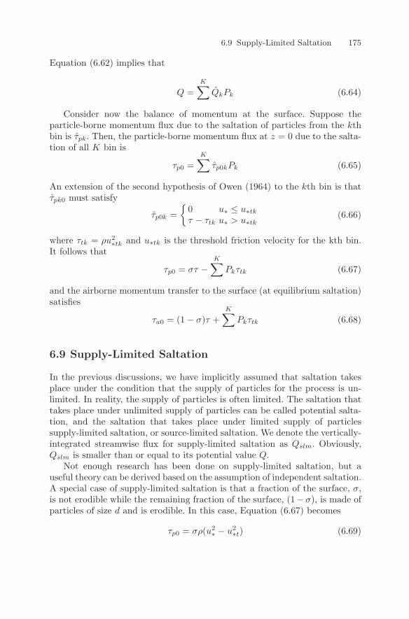
6.9 Supply-Limited Saltation 175
Equation (6.62) implies that
Q =K∑
QkPk (6.64)
Consider now the balance of momentum at the surface. Suppose theparticle-borne momentum flux due to the saltation of particles from the kthbin is τpk. Then, the particle-borne momentum flux at z = 0 due to the salta-tion of all K bin is
τp0 =K∑
τp0kPk (6.65)
An extension of the second hypothesis of Owen (1964) to the kth bin is thatτpk0 must satisfy
τp0k =
0 u∗ ≤ u∗tk
τ − τtk u∗ > u∗tk(6.66)
where τtk = ρu2∗tk and u∗tk is the threshold friction velocity for the kth bin.
It follows that
τp0 = στ −K∑
Pkτtk (6.67)
and the airborne momentum transfer to the surface (at equilibrium saltation)satisfies
τa0 = (1 − σ)τ +K∑
Pkτtk (6.68)
6.9 Supply-Limited Saltation
In the previous discussions, we have implicitly assumed that saltation takesplace under the condition that the supply of particles for the process is un-limited. In reality, the supply of particles is often limited. The saltation thattakes place under unlimited supply of particles can be called potential salta-tion, and the saltation that takes place under limited supply of particlessupply-limited saltation, or source-limited saltation. We denote the vertically-integrated streamwise flux for supply-limited saltation as Qslm. Obviously,Qslm is smaller than or equal to its potential value Q.
Not enough research has been done on supply-limited saltation, but auseful theory can be derived based on the assumption of independent saltation.A special case of supply-limited saltation is that a fraction of the surface, σ,is not erodible while the remaining fraction of the surface, (1− σ), is made ofparticles of size d and is erodible. In this case, Equation (6.67) becomes
τp0 = σρ(u2∗ − u2
∗t) (6.69)
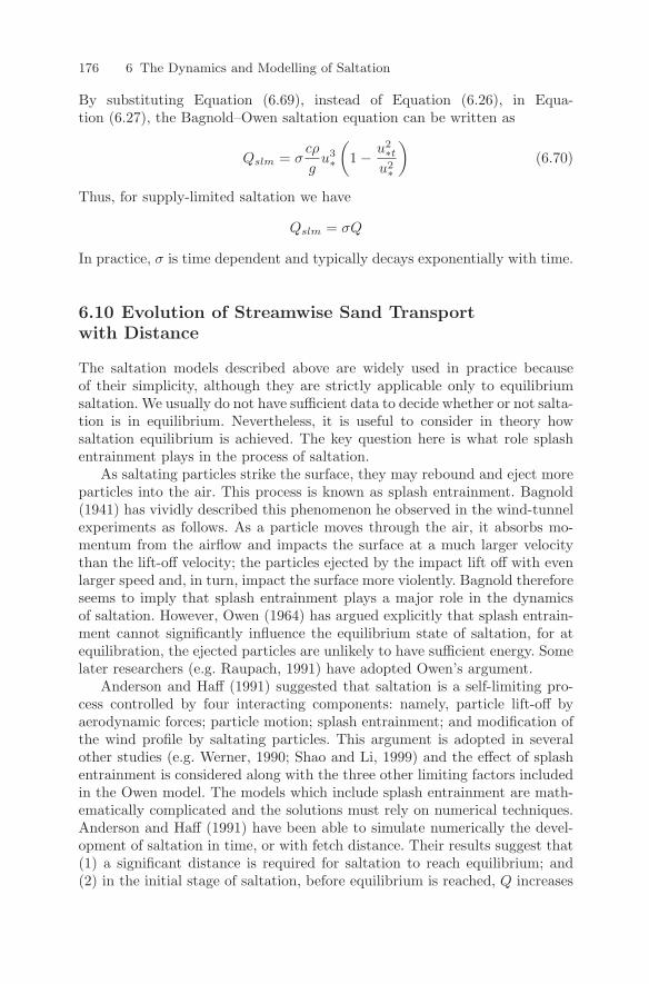
176 6 The Dynamics and Modelling of Saltation
By substituting Equation (6.69), instead of Equation (6.26), in Equa-tion (6.27), the Bagnold–Owen saltation equation can be written as
Qslm = σcρ
gu3∗
(1 − u2
∗t
u2∗
)(6.70)
Thus, for supply-limited saltation we have
Qslm = σQ
In practice, σ is time dependent and typically decays exponentially with time.
6.10 Evolution of Streamwise Sand Transportwith Distance
The saltation models described above are widely used in practice becauseof their simplicity, although they are strictly applicable only to equilibriumsaltation. We usually do not have sufficient data to decide whether or not salta-tion is in equilibrium. Nevertheless, it is useful to consider in theory howsaltation equilibrium is achieved. The key question here is what role splashentrainment plays in the process of saltation.
As saltating particles strike the surface, they may rebound and eject moreparticles into the air. This process is known as splash entrainment. Bagnold(1941) has vividly described this phenomenon he observed in the wind-tunnelexperiments as follows. As a particle moves through the air, it absorbs mo-mentum from the airflow and impacts the surface at a much larger velocitythan the lift-off velocity; the particles ejected by the impact lift off with evenlarger speed and, in turn, impact the surface more violently. Bagnold thereforeseems to imply that splash entrainment plays a major role in the dynamicsof saltation. However, Owen (1964) has argued explicitly that splash entrain-ment cannot significantly influence the equilibrium state of saltation, for atequilibration, the ejected particles are unlikely to have sufficient energy. Somelater researchers (e.g. Raupach, 1991) have adopted Owen’s argument.
Anderson and Haff (1991) suggested that saltation is a self-limiting pro-cess controlled by four interacting components: namely, particle lift-off byaerodynamic forces; particle motion; splash entrainment; and modification ofthe wind profile by saltating particles. This argument is adopted in severalother studies (e.g. Werner, 1990; Shao and Li, 1999) and the effect of splashentrainment is considered along with the three other limiting factors includedin the Owen model. The models which include splash entrainment are math-ematically complicated and the solutions must rely on numerical techniques.Anderson and Haff (1991) have been able to simulate numerically the devel-opment of saltation in time, or with fetch distance. Their results suggest that(1) a significant distance is required for saltation to reach equilibrium; and(2) in the initial stage of saltation, before equilibrium is reached, Q increases
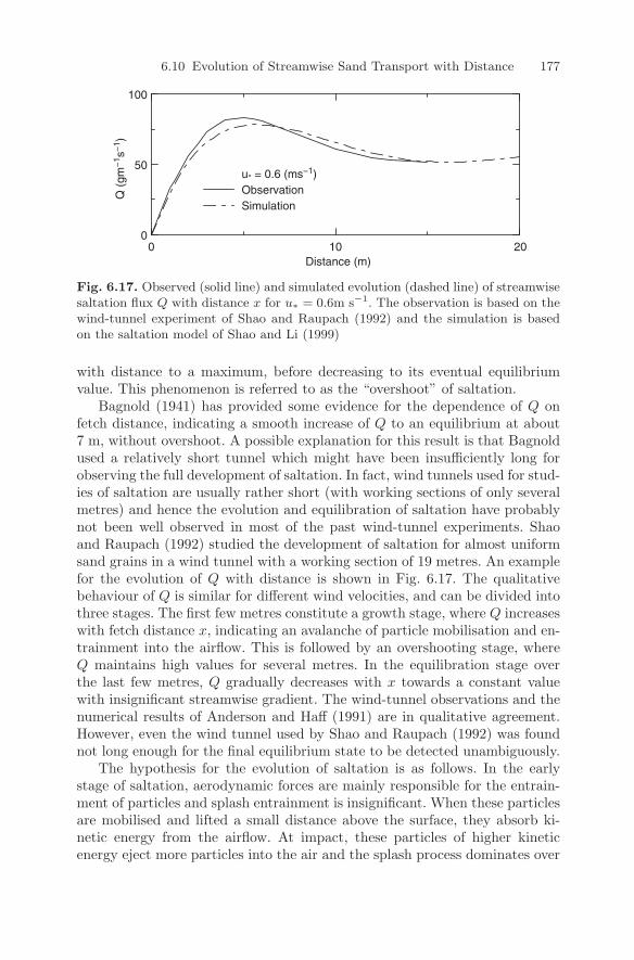
6.10 Evolution of Streamwise Sand Transport with Distance 177
10 200Distance (m)
Q (
gm−
1 s−
1 )
0
50
100
u* = 0.6 (ms−1)ObservationSimulation
Fig. 6.17. Observed (solid line) and simulated evolution (dashed line) of streamwisesaltation flux Q with distance x for u∗ = 0.6m s−1. The observation is based on thewind-tunnel experiment of Shao and Raupach (1992) and the simulation is basedon the saltation model of Shao and Li (1999)
with distance to a maximum, before decreasing to its eventual equilibriumvalue. This phenomenon is referred to as the “overshoot” of saltation.
Bagnold (1941) has provided some evidence for the dependence of Q onfetch distance, indicating a smooth increase of Q to an equilibrium at about7 m, without overshoot. A possible explanation for this result is that Bagnoldused a relatively short tunnel which might have been insufficiently long forobserving the full development of saltation. In fact, wind tunnels used for stud-ies of saltation are usually rather short (with working sections of only severalmetres) and hence the evolution and equilibration of saltation have probablynot been well observed in most of the past wind-tunnel experiments. Shaoand Raupach (1992) studied the development of saltation for almost uniformsand grains in a wind tunnel with a working section of 19 metres. An examplefor the evolution of Q with distance is shown in Fig. 6.17. The qualitativebehaviour of Q is similar for different wind velocities, and can be divided intothree stages. The first few metres constitute a growth stage, where Q increaseswith fetch distance x, indicating an avalanche of particle mobilisation and en-trainment into the airflow. This is followed by an overshooting stage, whereQ maintains high values for several metres. In the equilibration stage overthe last few metres, Q gradually decreases with x towards a constant valuewith insignificant streamwise gradient. The wind-tunnel observations and thenumerical results of Anderson and Haff (1991) are in qualitative agreement.However, even the wind tunnel used by Shao and Raupach (1992) was foundnot long enough for the final equilibrium state to be detected unambiguously.
The hypothesis for the evolution of saltation is as follows. In the earlystage of saltation, aerodynamic forces are mainly responsible for the entrain-ment of particles and splash entrainment is insignificant. When these particlesare mobilised and lifted a small distance above the surface, they absorb ki-netic energy from the airflow. At impact, these particles of higher kineticenergy eject more particles into the air and the splash process dominates over
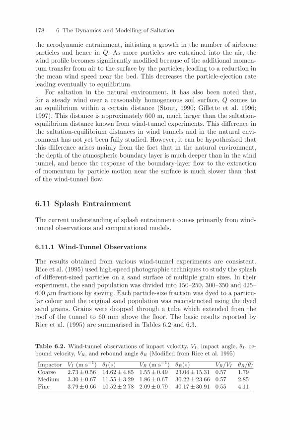
178 6 The Dynamics and Modelling of Saltation
the aerodynamic entrainment, initiating a growth in the number of airborneparticles and hence in Q. As more particles are entrained into the air, thewind profile becomes significantly modified because of the additional momen-tum transfer from air to the surface by the particles, leading to a reduction inthe mean wind speed near the bed. This decreases the particle-ejection rateleading eventually to equilibrium.
For saltation in the natural environment, it has also been noted that,for a steady wind over a reasonably homogeneous soil surface, Q comes toan equilibrium within a certain distance (Stout, 1990; Gillette et al. 1996;1997). This distance is approximately 600 m, much larger than the saltation-equilibrium distance known from wind-tunnel experiments. This difference inthe saltation-equilibrium distances in wind tunnels and in the natural envi-ronment has not yet been fully studied. However, it can be hypothesised thatthis difference arises mainly from the fact that in the natural environment,the depth of the atmospheric boundary layer is much deeper than in the windtunnel, and hence the response of the boundary-layer flow to the extractionof momentum by particle motion near the surface is much slower than thatof the wind-tunnel flow.
6.11 Splash Entrainment
The current understanding of splash entrainment comes primarily from wind-tunnel observations and computational models.
6.11.1 Wind-Tunnel Observations
The results obtained from various wind-tunnel experiments are consistent.Rice et al. (1995) used high-speed photographic techniques to study the splashof different-sized particles on a sand surface of multiple grain sizes. In theirexperiment, the sand population was divided into 150–250, 300–350 and 425–600 µm fractions by sieving. Each particle-size fraction was dyed to a particu-lar colour and the original sand population was reconstructed using the dyedsand grains. Grains were dropped through a tube which extended from theroof of the tunnel to 60 mm above the floor. The basic results reported byRice et al. (1995) are summarised in Tables 6.2 and 6.3.
Table 6.2. Wind-tunnel observations of impact velocity, VI , impact angle, θI , re-bound velocity, VR, and rebound angle θR (Modified from Rice et al. 1995)
Impactor VI (m s−1) θI() VR (m s−1) θR() VR/VI θR/θI
Coarse 2.73± 0.56 14.62± 4.85 1.55± 0.49 23.04± 15.31 0.57 1.79Medium 3.30± 0.67 11.55± 3.29 1.86± 0.67 30.22± 23.66 0.57 2.85Fine 3.79± 0.66 10.52± 2.78 2.09± 0.79 40.17± 30.91 0.55 4.11
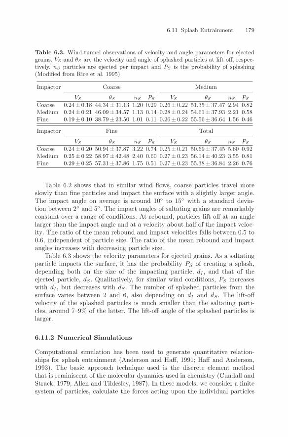
6.11 Splash Entrainment 179
Table 6.3. Wind-tunnel observations of velocity and angle parameters for ejectedgrains. VS and θS are the velocity and angle of splashed particles at lift off, respec-tively. nS particles are ejected per impact and PS is the probability of splashing(Modified from Rice et al. 1995)
Impactor Coarse Medium
VS θS nS PS VS θS nS PS
Coarse 0.24± 0.18 44.34± 31.13 1.20 0.29 0.26± 0.22 51.35± 37.47 2.94 0.82Medium 0.24± 0.21 46.09± 34.57 1.13 0.14 0.28± 0.24 54.61± 37.93 2.21 0.58Fine 0.19± 0.10 38.79± 23.50 1.01 0.11 0.26± 0.22 55.56± 36.64 1.56 0.46
Impactor Fine Total
VS θS nS PS VS θS nS PS
Coarse 0.24± 0.20 50.94± 37.87 3.22 0.74 0.25± 0.21 50.69± 37.45 5.60 0.92Medium 0.25± 0.22 58.97± 42.48 2.40 0.60 0.27± 0.23 56.14± 40.23 3.55 0.81Fine 0.29± 0.25 57.31± 37.86 1.75 0.51 0.27± 0.23 55.38± 36.84 2.26 0.76
Table 6.2 shows that in similar wind flows, coarse particles travel moreslowly than fine particles and impact the surface with a slightly larger angle.The impact angle on average is around 10 to 15 with a standard devia-tion between 2 and 5. The impact angles of saltating grains are remarkablyconstant over a range of conditions. At rebound, particles lift off at an anglelarger than the impact angle and at a velocity about half of the impact veloc-ity. The ratio of the mean rebound and impact velocities falls between 0.5 to0.6, independent of particle size. The ratio of the mean rebound and impactangles increases with decreasing particle size.
Table 6.3 shows the velocity parameters for ejected grains. As a saltatingparticle impacts the surface, it has the probability PS of creating a splash,depending both on the size of the impacting particle, dI , and that of theejected particle, dS . Qualitatively, for similar wind conditions, PS increaseswith dI , but decreases with dS . The number of splashed particles from thesurface varies between 2 and 6, also depending on dI and dS . The lift-offvelocity of the splashed particles is much smaller than the saltating parti-cles, around 7–9% of the latter. The lift-off angle of the splashed particles islarger.
6.11.2 Numerical Simulations
Computational simulation has been used to generate quantitative relation-ships for splash entrainment (Anderson and Haff, 1991; Haff and Anderson,1993). The basic approach technique used is the discrete element methodthat is reminiscent of the molecular dynamics used in chemistry (Cundall andStrack, 1979; Allen and Tildesley, 1987). In these models, we consider a finitesystem of particles, calculate the forces acting upon the individual particles
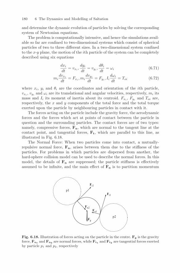
180 6 The Dynamics and Modelling of Saltation
and determine the dynamic evolution of particles by solving the correspondingsystem of Newtonian equations.
The problem is computationally intensive, and hence the simulations avail-able so far are confined to two-dimensional systems which consist of sphericalparticles of two to three different sizes. In a two-dimensional system confinedto the x-y plane, the motion of the ith particle of the system can be completelydescribed using six equations
dxi
dt= vxi
,dyi
dt= vyi
,dθi
dt= ωi (6.71)
midvxi
dt= Fxi
,midvyi
dt= Fyi
, Iidωi
dt= Toi (6.72)
where xi, yi and θi are the coordinates and orientation of the ith particle,vxi
, vyiand ωi are its translational and angular velocities, respectively, mi its
mass and Ii its moment of inertia about its centroid. Fxi, Fyi
and Toi are,respectively, the x and y components of the total force and the total torqueexerted upon the particle by neighbouring particles in contact with it.
The forces acting on the particle include the gravity force, the aerodynamicforces and the forces which act at points of contact between the particle inquestion and the surrounding particles. The contact forces are of two types:namely, compressive forces, Fn, which are normal to the tangent line at thecontact point, and tangential forces, Ft, which are parallel to this line, asillustrated in Fig. 6.18.
The Normal Force: When two particles come into contact, a mutually-repulsive normal force, Fn, arises between them due to the stiffness of theparticles. For problems in which particles are dispersed from another, thehard-sphere collision model can be used to describe the normal forces. In thismodel, the details of Fn are suppressed; the particle stiffness is effectivelyassumed to be infinite, and the main effect of Fn is to partition momentum
p1
p2
Ft2
Ft1
Fn2Fn1
Fg
Fig. 6.18. Illustration of forces acting on the particle in the centre. Fg is the gravityforce, Fn1 and Fn2 are normal forces, while Ft1 and Ft2 are tangential forces exertedby particle p1 and p2, respectively
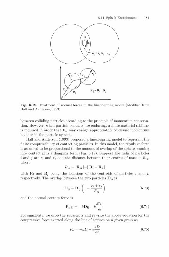
6.11 Splash Entrainment 181
δij = ri +rj −Rij
k
Rij = Ri − Rj
rirj
Rj
Rij
Ri
Fig. 6.19. Treatment of normal forces in the linear-spring model (Modified fromHaff and Anderson, 1993)
between colliding particles according to the principle of momentum conserva-tion. However, when particle contacts are enduring, a finite material stiffnessis required in order that Fn may change appropriately to ensure momentumbalance in the particle system.
Haff and Anderson (1993) proposed a linear-spring model to represent thefinite compressibility of contacting particles. In this model, the repulsive forceis assumed to be proportional to the amount of overlap of the spheres cominginto contact plus a damping term (Fig. 6.19). Suppose the radii of particlesi and j are ri and rj and the distance between their centres of mass is Rij ,where
Rij =| Rij |=| Ri − Rj |with Ri and Rj being the locations of the centroids of particles i and j,respectively. The overlap between the two particles Dij is
Dij = Rij
(1 − ri + rj
Rij
)(6.73)
and the normal contact force is
Fn,ij = −kDij − bdDij
dt(6.74)
For simplicity, we drop the subscripts and rewrite the above equation for thecompressive force exerted along the line of centres on a given grain as
Fn = −kD − bdD
dt(6.75)
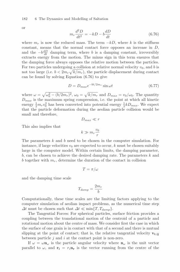
182 6 The Dynamics and Modelling of Saltation
or
mrd2D
dt2= −kD − b
dD
dt(6.76)
where mr is now the reduced mass. The term −kD, where k is the stiffnessconstant, means that the normal contact force opposes an increase in D,and the −bdD
dt damping term, where b is a damping constant, irreversiblyextracts energy from the motion. The minus sign in this term ensures thatthe damping force always opposes the relative motion between the particles.For two particles undergoing a collision at relative normal velocity v0, and b isnot too large (i.e. b < 2mr
√k/mr), the particle displacement during contact
can be found by solving Equation (6.76) to give
D = Dmaxe−bt/2mr sinωt (6.77)
where ω =√
ω20 − (b/2mr)2, ω0 =
√k/mr and Dmax = v0/ω0. The quantity
Dmax is the maximum spring compression, i.e. the point at which all kineticenergy 1
2mrv20 has been converted into potential energy 1
2kDmax. We expectthat the particle deformation during the aeolian particle collision would besmall and therefore,
Dmax r
This also implies thatk mr
v0
r
The parameters k and b need to be chosen in the computer simulation. Forinstance, if large velocities v0 are expected to occur, k must be chosen suitablylarge in the computer model. Within certain limits, the damping parameter,b, can be chosen to achieve the desired damping rate. The parameters k andb together with mr, determine the duration of the contact in collision
T = π/ω
and the damping time scale
Tdamp =2mr
b
Computationally, these time scales are the limiting factors applying to thecomputer simulation of aeolian impact problems, as the numerical time step∆t must be chosen such that ∆t minT, Tdamp.
The Tangential Forces: For spherical particles, surface friction provides acoupling between the translational motion of the centroid of a particle androtational motion about the centre of mass. We consider first the case in whichthe surface of one grain is in contact with that of a second and there is mutualslipping at the point of contact; that is, the relative tangential velocity vt,ij
between particle j and i at the contact point is non-zero.If ω = ωnω is the particle angular velocity where nω is the unit vector
parallel to ω, and ri = rinr is the vector running from the centre of the
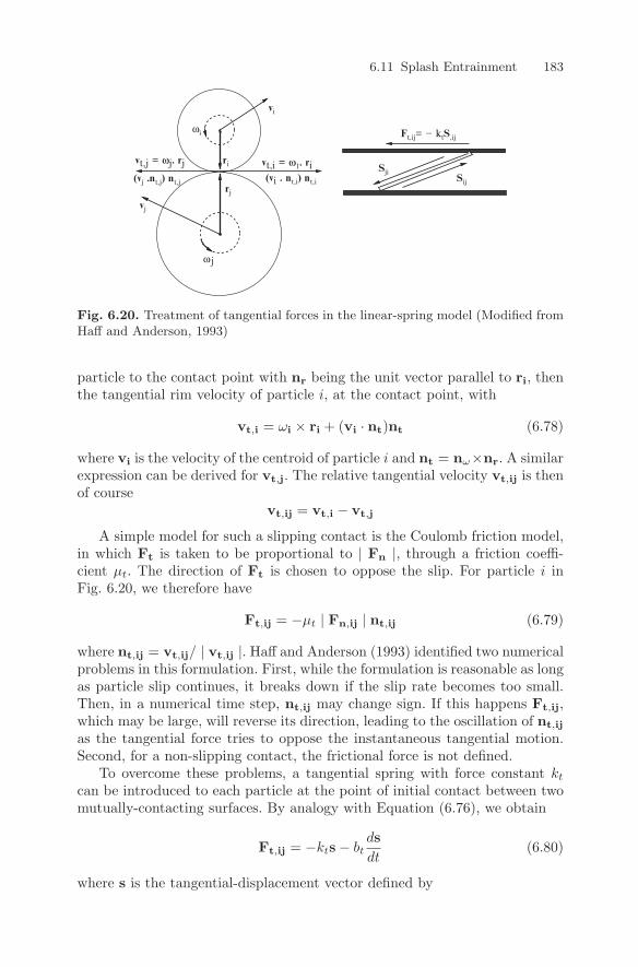
6.11 Splash Entrainment 183
jω
vt,j = ωj. rj vt,i = ω1. ri(vi . nt,i) nt,i(vj .nt,j) nt,j
Sji
Ft,ij= − ktS,ij
Sijrj
ri
vi
ωi
vj
Fig. 6.20. Treatment of tangential forces in the linear-spring model (Modified fromHaff and Anderson, 1993)
particle to the contact point with nr being the unit vector parallel to ri, thenthe tangential rim velocity of particle i, at the contact point, with
vt,i = ωi × ri + (vi · nt)nt (6.78)
where vi is the velocity of the centroid of particle i and nt = nω×nr. A similarexpression can be derived for vt,j. The relative tangential velocity vt,ij is thenof course
vt,ij = vt,i − vt,j
A simple model for such a slipping contact is the Coulomb friction model,in which Ft is taken to be proportional to | Fn |, through a friction coeffi-cient µt. The direction of Ft is chosen to oppose the slip. For particle i inFig. 6.20, we therefore have
Ft,ij = −µt | Fn,ij | nt,ij (6.79)
where nt,ij = vt,ij/ | vt,ij |. Haff and Anderson (1993) identified two numericalproblems in this formulation. First, while the formulation is reasonable as longas particle slip continues, it breaks down if the slip rate becomes too small.Then, in a numerical time step, nt,ij may change sign. If this happens Ft,ij,which may be large, will reverse its direction, leading to the oscillation of nt,ij
as the tangential force tries to oppose the instantaneous tangential motion.Second, for a non-slipping contact, the frictional force is not defined.
To overcome these problems, a tangential spring with force constant kt
can be introduced to each particle at the point of initial contact between twomutually-contacting surfaces. By analogy with Equation (6.76), we obtain
Ft,ij = −kts − btdsdt
(6.80)
where s is the tangential-displacement vector defined by
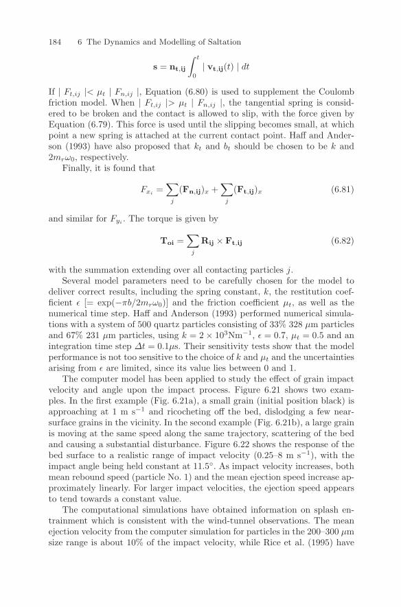
184 6 The Dynamics and Modelling of Saltation
s = nt,ij
∫ t
0
| vt,ij(t) | dt
If | Ft,ij |< µt | Fn,ij |, Equation (6.80) is used to supplement the Coulombfriction model. When | Ft,ij |> µt | Fn,ij |, the tangential spring is consid-ered to be broken and the contact is allowed to slip, with the force given byEquation (6.79). This force is used until the slipping becomes small, at whichpoint a new spring is attached at the current contact point. Haff and Ander-son (1993) have also proposed that kt and bt should be chosen to be k and2mrω0, respectively.
Finally, it is found that
Fxi=
∑j
(Fn,ij)x +∑
j
(Ft,ij)x (6.81)
and similar for Fyi. The torque is given by
Toi =∑
j
Rij × Ft,ij (6.82)
with the summation extending over all contacting particles j.Several model parameters need to be carefully chosen for the model to
deliver correct results, including the spring constant, k, the restitution coef-ficient ε [= exp(−πb/2mrω0)] and the friction coefficient µt, as well as thenumerical time step. Haff and Anderson (1993) performed numerical simula-tions with a system of 500 quartz particles consisting of 33% 328 µm particlesand 67% 231 µm particles, using k = 2 × 10³Nm−1, ε = 0.7, µt = 0.5 and anintegration time step ∆t = 0.1µs. Their sensitivity tests show that the modelperformance is not too sensitive to the choice of k and µt and the uncertaintiesarising from ε are limited, since its value lies between 0 and 1.
The computer model has been applied to study the effect of grain impactvelocity and angle upon the impact process. Figure 6.21 shows two exam-ples. In the first example (Fig. 6.21a), a small grain (initial position black) isapproaching at 1 m s−1 and ricocheting off the bed, dislodging a few near-surface grains in the vicinity. In the second example (Fig. 6.21b), a large grainis moving at the same speed along the same trajectory, scattering of the bedand causing a substantial disturbance. Figure 6.22 shows the response of thebed surface to a realistic range of impact velocity (0.25–8 m s−1), with theimpact angle being held constant at 11.5. As impact velocity increases, bothmean rebound speed (particle No. 1) and the mean ejection speed increase ap-proximately linearly. For larger impact velocities, the ejection speed appearsto tend towards a constant value.
The computational simulations have obtained information on splash en-trainment which is consistent with the wind-tunnel observations. The meanejection velocity from the computer simulation for particles in the 200–300 µmsize range is about 10% of the impact velocity, while Rice et al. (1995) have
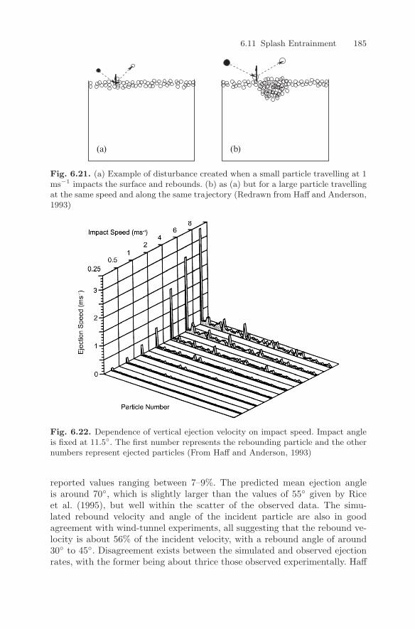
6.11 Splash Entrainment 185
)b()a(
Fig. 6.21. (a) Example of disturbance created when a small particle travelling at 1ms−1 impacts the surface and rebounds. (b) as (a) but for a large particle travellingat the same speed and along the same trajectory (Redrawn from Haff and Anderson,1993)
Fig. 6.22. Dependence of vertical ejection velocity on impact speed. Impact angleis fixed at 11.5. The first number represents the rebounding particle and the othernumbers represent ejected particles (From Haff and Anderson, 1993)
reported values ranging between 7–9%. The predicted mean ejection angleis around 70, which is slightly larger than the values of 55 given by Riceet al. (1995), but well within the scatter of the observed data. The simu-lated rebound velocity and angle of the incident particle are also in goodagreement with wind-tunnel experiments, all suggesting that the rebound ve-locity is about 56% of the incident velocity, with a rebound angle of around30 to 45. Disagreement exists between the simulated and observed ejectionrates, with the former being about thrice those observed experimentally. Haff
186 6 The Dynamics and Modelling of Saltation
and Anderson (1993) have attributed this disagreement to either a possibleunder-counting of out-of-plane ejecta, as the experiments detect grain mo-tion projected on to a plane containing the incident velocity vector, or to therestriction of the simulation to two dimensions.
6.12 Numerical Modelling of Saltation
Compared with the relatively simple saltation models described in the previ-ous sections of this chapter, the objective of the numerical models of saltationis to comprehensively simulate the dynamics of saltation. The basic frame-work of the existing models is as outlined in Anderson and Haff (1991) andShao and Li (1999). In these models, saltation is considered as a self-limitingfeedback process between air motion, particle motion and particle-air andparticle-surface interactions. The numerical models of saltation are in essencea coupling of three basic components: (1) a component for the atmosphericboundary-layer flow in which saltation takes place; (2) a component for par-ticle motion and (3) a component for simulation of particle-and-surface inter-actions. Although the models are rather complex, they have been shown tobe useful in addressing a number of issues which have remained so far incon-clusive from experimental studies and conceptual analyses. The treatment ofthe flow field among the existing models differs considerable. In some mod-els only the mean flow is considered (Ungar and Haff, 1987; and Andersonand Haff, 1991), in others turbulence is considered in addition to the meanflow by means of stochastic modelling (Anderson, 1987 and Shao, 2005) or bylarge-eddy simulation (Shao and Li, 1999). The employment of large-eddy sim-ulation in saltation modelling is computationally expensive, but is potentiallyvery useful in understanding saltation in turbulent flows. The theory and nu-merical techniques for boundary-layer flows have been outlined in Chapter 3,but interested readers should refer to more specialised books for details (e.g.Galperin and Orzag, 1993; Lesieur, 1997).
6.12.1 Simple Flow Model
The flow component of a saltation model can be made simple or complex,depending on the modelling requirements. Assuming that the air density isnot significantly altered by the presence of saltating particles, the governingequation system for boundary-layer flows with saltation can be written as,
∂uj
∂xj= 0 (6.83)
∂ui
∂t+ uj
∂ui
∂xj= −1
ρ
∂p
∂xi− δi3g + Km
∂2ui
∂x2j
− spi (6.84)
where Km is again eddy diffusivity and spi is the momentum sink arisingfrom particle motion, which can be expressed as the divergence of particle-momentum flux
6.12 Numerical Modelling of Saltation 187
spi = −1ρ
∂τpij
∂xj
For steady-state and horizontally-homogeneous saltation with the x directionaligned with the mean wind, the derivatives with respect to t, x and y inEquation (6.84) vanish and the flow has no components in the y and z direc-tions. The flow speed is maintained by an external force, such as a horizontalpressure gradient ∂p/∂x, which just overcomes the effect of friction at theboundaries. It follows that Equation (6.84) is reduced to a simple balance offorce in the x direction
∂τa
∂z+
∂τp
∂z= 0 (6.85)
Integrating Equation (6.85) from z = ∞ to z, and applying the boundaryconditions τp∞ = 0 and τa∞ = ρu2
∗, we obtain
τa(z) = ρu2∗ − τp(z) (6.86)
Since τa = ρKm∂U/∂z and Km = κ√
τa/ρz, it follows that
dU
dz=
1κz
(ρu2
∗ − τp
ρ
)1/2
(6.87)
This simple flow model is identical to that used by Owen (1964) and Raupach(1991).
Equation (6.87) applies only to steady state and horizontally homoge-neous saltation and is not suitable for studying saltation which is evolvingwith distance and time. Its application to unsteady-state and heterogeneoussaltation would imply that an instantaneous adjustment of flow to the changeof surface-momentum flux takes place. This is inadequate, of course, becausethe evolution of flow associated with saltation, similar to the evolution of flowover a surface with changing roughness length in space, requires a consider-able distance to reach a balance with the new underlying surface (Bradley,1968). The other disadvantage of using Equation (6.87) is that it is not suit-able for studying the interactions between saltating particles and turbulence(Butterfield, 1991; Stout and Zobeck, 1997).
6.12.2 Large-Eddy Simulation Model
More comprehensive simulations of boundary-layer flows can be achieved usingthe large-eddy simulation (LES) approach. The simulation of turbulent flowswith saltation is similar to that without saltation, except that the momentumsink term in Equation (6.84) needs to be estimated from the motion of saltat-ing particles. Suppose J particles are present in a control volume of size ∆3
for the LES model at a given time, sp in Equation (6.84) can be estimated byusing
sp =1
ρ∆3
J∑j=1
mjdupj
dt(6.88)
188 6 The Dynamics and Modelling of Saltation
where up is particle velocity. The eddy viscosity Km in Equation (6.84) can bemodelled using the Smagorinsky or the e−ε closure as described in Chapter 3.
For modelling saltation, the LES model requires high spatial resolutionnear the surface, and a stretched numerical mesh with a logarithmic decreasein mesh-size toward the ground should be used. This arrangement ensuresa sufficiently-high resolution for the calculation of particle trajectories andother physical quantities, such as saltation flux. The integration time stepsfor the flow model and the particle trajectory model can be different. Forexample, the time step for the flow model can be taken as 0.005 s and forthe particle trajectory model 0.0001 s (50 particle-trajectory integration stepsin every fluid-motion time step). The flow field can be initialised by using asimple logarithmic flow upon which random fluctuations of a given intensityare superposed. The flow model can then be run with a periodic boundarycondition such that the flow reaches equilibrium with the surface that has aspecified roughness length. Saltation is then introduced and both the fluidmotion and the particle motion are allowed to evolve simultaneously.
The lower-boundary condition is important, as it affects both the flowfield and the aerodynamic entrainment of particles. One possible approachis to divide the flow into an outer region and a saltation layer, as in theOwen saltation model. The depth of the inner region, Hs, is approximatelythe maximum height which most saltating particles reach. The flow speed onaverage in the outer region obeys Equation (6.43).
The friction velocity, u∗, can be obtained from the downward momentumflux at Hs. There is no conceptual difficulty in estimating this flux from theflow model which can estimate eddy diffusivity through a sub-grid closurescheme, such as the Smagorinsky or the e− ε closure. At the upper boundaryof the saltation layer, the momentum flux is entirely determined by the fluidmotion, which can thus be calculated by using Equation (6.49).
Within the saltation layer, while particle motion results in the momentumflux τp, τp+τa remains constant with height. The behaviour of τa and τp in gen-eral should be as illustrated in Fig. 6.7 with τp decreasing with height to zeroat height z = Hs and τa increasing with height to ρu2
∗ at z = Hs. The particle-momentum flux at the surface, τp0, can be estimated using Equation (6.92),and the airborne momentum flux at the surface, τa0, can be determined byusing the relationship τa0 = ρu2
∗ − τp0. At the lower boundary, wind shouldsatisfy Equation (6.49).
6.12.3 Particle Motion
It is common to study particle motion using a Lagrangian stochastic modelby following the trajectories of individual particles. This is more convenientthan treating the particulate phase as a continuum in a fashion similar tothe fluid phase, with the main advantage being that the particle-and-surfaceinteractions can be treated on clear physical grounds. To facilitate discussion,we confine the description of the model to uniform spherical particles with
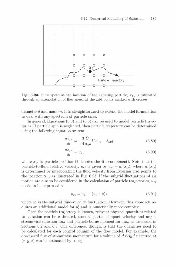
6.12 Numerical Modelling of Saltation 189
x
xParticle Trajectory
x
x
x x x
x
xx
x
x
xxx x
xp
Fig. 6.23. Flow speed at the location of the saltating particle, xp, is estimatedthrough an interpolation of flow speed at the grid points marked with crosses
diameter d and mass m. It is straightforward to extend the model formulationto deal with any spectrum of particle sizes.
In general, Equations (6.3) and (6.5) can be used to model particle trajec-tories. If particle spin is neglected, then particle trajectory can be determinedusing the following equation system
dupi
dt= −3
4Cd
σpdUruri − δi3g (6.89)
dxpi
dt= upi (6.90)
where xpi is particle position (i denotes the ith component). Note that theparticle-to-fluid relative velocity, uri is given by upi − ui(xp), where ui(xp)is determined by interpolating the fluid velocity from Eulerian grid points tothe location xp, as illustrated in Fig. 6.23. If the subgrid fluctuations of airmotion are also to be considered in the calculation of particle trajectories, uri
needs to be expressed as
uri = upi − (ui + u′i) (6.91)
where u′i is the subgrid fluid-velocity fluctuation. However, this approach re-
quires an additional model for u′i and is numerically more complex.
Once the particle trajectory is known, relevant physical quantities relatedto saltation can be estimated, such as particle impact velocity and angle,streamwise saltation flux and particle-borne momentum flux, as discussed inSections 6.2 and 6.3. One difference, though, is that the quantities need tobe calculated for each control column of the flow model. For example, thedownward flux of streamwise momentum for a volume of ∆x∆y∆z centred at(x, y, z) can be estimated by using
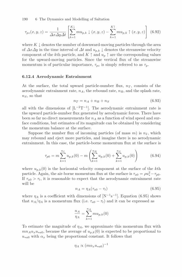
190 6 The Dynamics and Modelling of Saltation
τpz(x, y, z) =1
∆x∆y∆t
[K↓∑k=1
mup,k ↓ (x, y, z) −K↑∑k=1
mup,k ↑ (x, y, z)
](6.92)
where K ↓ denotes the number of downward-moving particles through the areaof ∆x∆y in the time interval of ∆t and up,k ↓ denotes the streamwise velocitycomponent of the kth particle, and K ↑ and up ↑ are the corresponding valuesfor the upward-moving particles. Since the vertical flux of the streamwisemomentum is of particular importance, τpz is simply referred to as τp.
6.12.4 Aerodynamic Entrainment
At the surface, the total upward particle-number flux, nT , consists of theaerodynamic entrainment rate, nA, the rebound rate, nR, and the splash rate,nS , so that
nT = nA + nR + nS (6.93)
all with the dimensions of [L−2T−1]. The aerodynamic entrainment rate isthe upward particle-number flux generated by aerodynamic forces. There havebeen so far no direct measurements for nA as a function of wind speed and sur-face conditions, but estimates of its magnitude can be obtained by consideringthe momentum balance at the surface.
Suppose the number flux of incoming particles (of mass m) is nI , whichmay rebound and eject more particles, and imagine there is no aerodynamicentrainment. In this case, the particle-borne momentum flux at the surface is
τp0 = m
nI∑k=1
up,k(0) − m
(nR∑k=1
up,k(0) +nS∑k=1
up,k(0)
)(6.94)
where up,k(0) is the horizontal velocity component at the surface of the kthparticle. Again, the air-borne momentum flux at the surface is τa0 = ρu2
∗−τp0.If τa0 > τt, it is reasonable to expect that the aerodynamic entrainment ratewill be
nA = ηA(τa0 − τt) (6.95)
where ηA is a coefficient with dimensions of [N−1s−1]. Equation (6.95) showsthat nA/ηA is a momentum flux (i.e. τa0 − τt) and it can be expressed as
nA
ηA=
nA∑k=1
mup,k(0)
To estimate the magnitude of ηA, we approximate this momentum flux withmnAαxu∗a0, because the average of up,k(0) is expected to be proportional tou∗a0 with αx being the proportional constant. It follows that
ηA ∝ (mαxu∗a0)−1
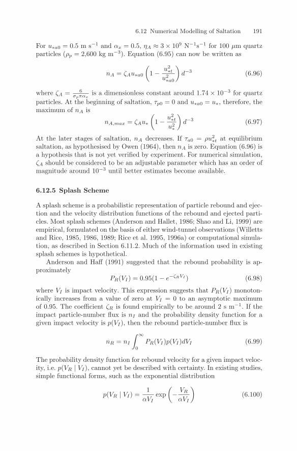
6.12 Numerical Modelling of Saltation 191
For u∗a0 = 0.5 m s−1 and αx = 0.5, ηA ≈ 3 × 10⁹ N−1s−1 for 100 µm quartzparticles (ρp = 2,600 kg m−3). Equation (6.95) can now be written as
nA = ζAu∗a0
(1 − u2
∗t
u2∗a0
)d−3 (6.96)
where ζA = 6σpπαx
is a dimensionless constant around 1.74 × 10⁻³ for quartzparticles. At the beginning of saltation, τp0 = 0 and u∗a0 = u∗, therefore, themaximum of nA is
nA,max = ζAu∗
(1 − u2
∗t
u2∗
)d−3 (6.97)
At the later stages of saltation, nA decreases. If τa0 = ρu2∗t at equilibrium
saltation, as hypothesised by Owen (1964), then nA is zero. Equation (6.96) isa hypothesis that is not yet verified by experiment. For numerical simulation,ζA should be considered to be an adjustable parameter which has an order ofmagnitude around 10−3 until better estimates become available.
6.12.5 Splash Scheme
A splash scheme is a probabilistic representation of particle rebound and ejec-tion and the velocity distribution functions of the rebound and ejected parti-cles. Most splash schemes (Anderson and Hallet, 1986; Shao and Li, 1999) areempirical, formulated on the basis of either wind-tunnel observations (Willettsand Rice, 1985, 1986, 1989; Rice et al. 1995, 1996a) or computational simula-tion, as described in Section 6.11.2. Much of the information used in existingsplash schemes is hypothetical.
Anderson and Haff (1991) suggested that the rebound probability is ap-proximately
PR(VI) = 0.95(1 − e−ζRVI ) (6.98)
where VI is impact velocity. This expression suggests that PR(VI) monoton-ically increases from a value of zero at VI = 0 to an asymptotic maximumof 0.95. The coefficient ζR is found empirically to be around 2 s m−1. If theimpact particle-number flux is nI and the probability density function for agiven impact velocity is p(VI), then the rebound particle-number flux is
nR = nI
∫ ∞
0
PR(VI)p(VI)dVI (6.99)
The probability density function for rebound velocity for a given impact veloc-ity, i.e. p(VR | VI), cannot yet be described with certainty. In existing studies,simple functional forms, such as the exponential distribution
p(VR | VI) =1
αVIexp
(− VR
αVI
)(6.100)
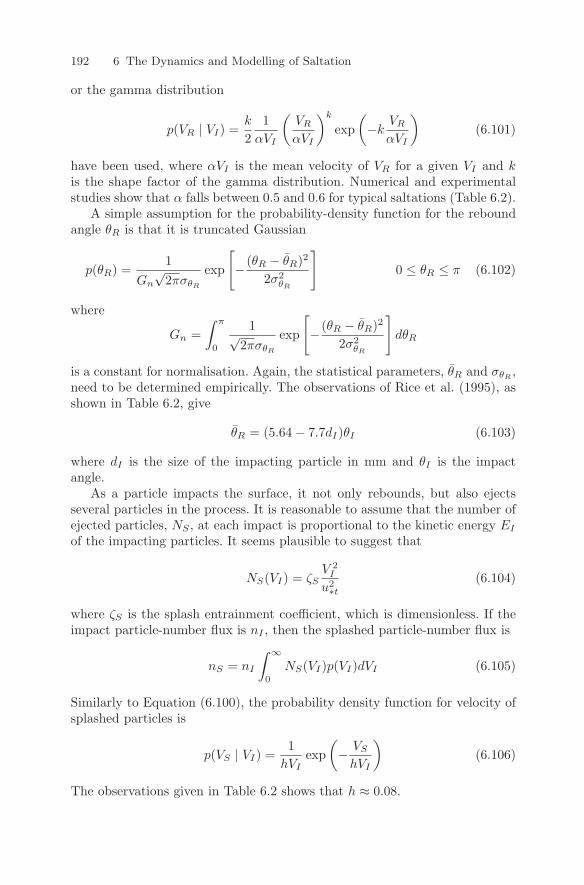
192 6 The Dynamics and Modelling of Saltation
or the gamma distribution
p(VR | VI) =k
21
αVI
(VR
αVI
)k
exp(−k
VR
αVI
)(6.101)
have been used, where αVI is the mean velocity of VR for a given VI and kis the shape factor of the gamma distribution. Numerical and experimentalstudies show that α falls between 0.5 and 0.6 for typical saltations (Table 6.2).
A simple assumption for the probability-density function for the reboundangle θR is that it is truncated Gaussian
p(θR) =1
Gn
√2πσθR
exp
[− (θR − θR)2
2σ2θR
]0 ≤ θR ≤ π (6.102)
where
Gn =∫ π
0
1√2πσθR
exp
[− (θR − θR)2
2σ2θR
]dθR
is a constant for normalisation. Again, the statistical parameters, θR and σθR,
need to be determined empirically. The observations of Rice et al. (1995), asshown in Table 6.2, give
θR = (5.64 − 7.7dI)θI (6.103)
where dI is the size of the impacting particle in mm and θI is the impactangle.
As a particle impacts the surface, it not only rebounds, but also ejectsseveral particles in the process. It is reasonable to assume that the number ofejected particles, NS , at each impact is proportional to the kinetic energy EI
of the impacting particles. It seems plausible to suggest that
NS(VI) = ζSV 2
I
u2∗t
(6.104)
where ζS is the splash entrainment coefficient, which is dimensionless. If theimpact particle-number flux is nI , then the splashed particle-number flux is
nS = nI
∫ ∞
0
NS(VI)p(VI)dVI (6.105)
Similarly to Equation (6.100), the probability density function for velocity ofsplashed particles is
p(VS | VI) =1
hVIexp
(− VS
hVI
)(6.106)
The observations given in Table 6.2 shows that h ≈ 0.08.
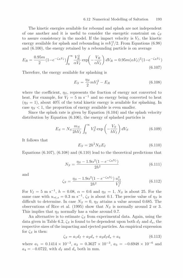
6.12 Numerical Modelling of Saltation 193
The kinetic energies available for rebound and splash are not independentof one another and it is useful to consider the energetic constraint on ζS
to assure consistency in the model. If the impact velocity is VI , the kineticenergy available for splash and rebounding is mV 2
I /2. From Equations (6.98)and (6.100), the energy retained by a rebounding particle is on average
ER =0.95m
2(1−e−ζRVI )
∫ ∞
0
V 2R
αVIexp
(− VR
αVI
)dVR = 0.95m(αVI)2(1−e−ζRVI )
(6.107)Therefore, the energy available for splashing is
ES =ηS
2mV 2
I − ER (6.108)
where the coefficient, ηS , represents the fraction of energy not converted toheat. For example, for VI = 5 m s−1 and no energy being converted to heat(ηS = 1), about 40% of the total kinetic energy is available for splashing. Incase ηS < 1, the proportion of energy available is even smaller.
Since the splash rate is given by Equation (6.104) and the splash velocitydistribution by Equation (6.106), the energy of splashed particles is
ES = NSmS
2hVI
∫ ∞
0
V 2S exp
(− VS
hVI
)dVS (6.109)
It follows thatES = 2h2NSEI (6.110)
Equations (6.107), (6.108) and (6.110) lead to the theoretical predictions that
NS =ηS − 1.9α2(1 − e−ζRVI )
2h2(6.111)
and
ζS =ηS − 1.9α2(1 − e−ζRVI )
2h2
u2∗t
V 2I
(6.112)
For VI = 5 m s−1, h = 0.08, α = 0.6 and ηS = 1, NS is about 25. For thesame case with u∗t,s = 0.3 m s−1, ζS is about 0.1. The precise value of ηS isdifficult to determine. In case NS = 0, ηS attains a value around 0.685. Theobservations of Rice et al. (1995) show that NS is normally around 2 or 3.This implies that ηS normally has a value around 0.7.
An alternative is to estimate ζS from experimental data. Again, using thedata given in Table 6.2, ζS is found to be dependent upon both dI and ds, therespective sizes of the impacting and ejected particles. An empirical expressionfor ζS is then:
ζS = a1dI + a2ds + a3dIds + a4 (6.113)
where a1 = 0.1414 × 10⁻³, a2 = 0.3627 × 10⁻³, a3 = −0.6948 × 10⁻⁶ anda4 = −0.0722, with dI and ds both in mm.
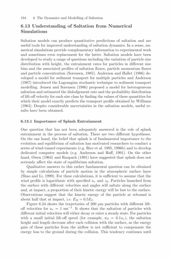
194 6 The Dynamics and Modelling of Saltation
6.13 Understanding of Saltation from NumericalSimulations
Saltation models can produce quantitative predictions of saltation and areuseful tools for improved understanding of saltation dynamics. In a sense, nu-merical simulations provide complementary information to experimental workand sometimes even replacement for the latter. Saltation models have beendeveloped to study a range of questions including the variation of particle sizedistribution with height, the entrainment rates for particles in different sizebins and the associated profiles of saltation fluxes, particle momentum fluxesand particle concentration (Sorensen, 1985). Anderson and Hallet (1986) de-veloped a model for sediment transport for multiple particles and Anderson(1987) introduced the Lagrangian stochastic technique to sediment transportmodelling. Jensen and Sorensen (1986) proposed a model for heterogeneoussaltation and estimated the dislodgement rate and the probability distributionof lift-off velocity for each size class by finding the values of these quantities forwhich their model exactly predicts the transport profile obtained by Williams(1964). Despite considerable uncertainties in the saltation models, useful re-sults have been obtained.
6.13.1 Importance of Splash Entrainment
One question that has not been adequately answered is the role of splashentrainment in the process of saltation. There are two different hypotheses.On the one hand, the belief that splash is of fundamental importance to theevolution and equilibrium of saltation has motivated researchers to conduct aseries of wind-tunnel experiments (e.g. Rice et al. 1995, 1996b) and to developdedicated computer models (e.g. Anderson and Haff, 1991). On the otherhand, Owen (1964) and Raupach (1991) have suggested that splash does notseriously affect the state of equilibrium saltation.
Qualitative answers to this rather fundamental question can be obtainedby simple calculations of particle motion in the atmospheric surface layer(Shao and Li, 1999). For these calculations, it is sufficient to assume that thewind profile is logarithmic with specified u∗ and z0. Particles launched fromthe surface with different velocities and angles will saltate along the surfaceand, at impact, a proportion of their kinetic energy will be lost to the surface.Observations suggest that the kinetic energy of the particle at rebound isabout half that at impact, i.e. ER = 0.5EI .
Figure 6.24 shows the trajectories of 200 µm particles with different lift-off velocities for u∗ = 1 ms−1. It shows that the saltation of particles withdifferent initial velocities will either decay or enter a steady state. For particleswith a small initial lift-off speed (for example, w0 = 0.1u∗), the saltationheight and length decrease after each collision with the surface, as the energygain of these particles from the airflow is not sufficient to compensate theenergy loss to the ground during the collision. This tendency continues until
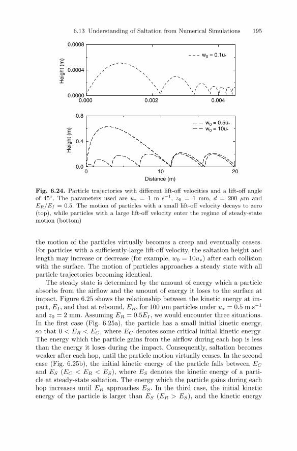
6.13 Understanding of Saltation from Numerical Simulations 195
02010Distance (m)
w0 = 0.1u*
w0 = 0.5u*w0 = 10u*
0.00000.000 0.002 0.004
0.0004
0.0008
Hei
ght (
m)
Hei
ght (
m)
0.0
0.4
0.8
Fig. 6.24. Particle trajectories with different lift-off velocities and a lift-off angleof 45. The parameters used are u∗ = 1 m s−1, z0 = 1 mm, d = 200 µm andER/EI = 0.5. The motion of particles with a small lift-off velocity decays to zero(top), while particles with a large lift-off velocity enter the regime of steady-statemotion (bottom)
the motion of the particles virtually becomes a creep and eventually ceases.For particles with a sufficiently-large lift-off velocity, the saltation height andlength may increase or decrease (for example, w0 = 10u∗) after each collisionwith the surface. The motion of particles approaches a steady state with allparticle trajectories becoming identical.
The steady state is determined by the amount of energy which a particleabsorbs from the airflow and the amount of energy it loses to the surface atimpact. Figure 6.25 shows the relationship between the kinetic energy at im-pact, EI , and that at rebound, ER, for 100 µm particles under u∗ = 0.5 m s−1
and z0 = 2 mm. Assuming ER = 0.5EI , we would encounter three situations.In the first case (Fig. 6.25a), the particle has a small initial kinetic energy,so that 0 < ER < EC , where EC denotes some critical initial kinetic energy.The energy which the particle gains from the airflow during each hop is lessthan the energy it loses during the impact. Consequently, saltation becomesweaker after each hop, until the particle motion virtually ceases. In the secondcase (Fig. 6.25b), the initial kinetic energy of the particle falls between EC
and ES (EC < ER < ES), where ES denotes the kinetic energy of a parti-cle at steady-state saltation. The energy which the particle gains during eachhop increases until ER approaches ES . In the third case, the initial kineticenergy of the particle is larger than ES (ER > ES), and the kinetic energy
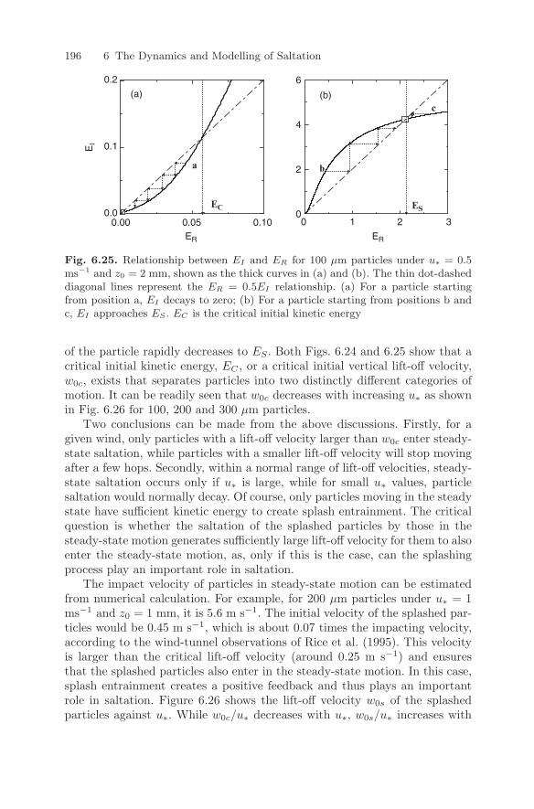
196 6 The Dynamics and Modelling of Saltation
ER ER
EI
EC ES
(a) (b)
a b
c
0.0
0.1
0.00 0.05 0.10
0.2
0
2
4
6
0 1 2 3
Fig. 6.25. Relationship between EI and ER for 100 µm particles under u∗ = 0.5ms−1 and z0 = 2 mm, shown as the thick curves in (a) and (b). The thin dot-dasheddiagonal lines represent the ER = 0.5EI relationship. (a) For a particle startingfrom position a, EI decays to zero; (b) For a particle starting from positions b andc, EI approaches ES . EC is the critical initial kinetic energy
of the particle rapidly decreases to ES . Both Figs. 6.24 and 6.25 show that acritical initial kinetic energy, EC , or a critical initial vertical lift-off velocity,w0c, exists that separates particles into two distinctly different categories ofmotion. It can be readily seen that w0c decreases with increasing u∗ as shownin Fig. 6.26 for 100, 200 and 300 µm particles.
Two conclusions can be made from the above discussions. Firstly, for agiven wind, only particles with a lift-off velocity larger than w0c enter steady-state saltation, while particles with a smaller lift-off velocity will stop movingafter a few hops. Secondly, within a normal range of lift-off velocities, steady-state saltation occurs only if u∗ is large, while for small u∗ values, particlesaltation would normally decay. Of course, only particles moving in the steadystate have sufficient kinetic energy to create splash entrainment. The criticalquestion is whether the saltation of the splashed particles by those in thesteady-state motion generates sufficiently large lift-off velocity for them to alsoenter the steady-state motion, as, only if this is the case, can the splashingprocess play an important role in saltation.
The impact velocity of particles in steady-state motion can be estimatedfrom numerical calculation. For example, for 200 µm particles under u∗ = 1ms−1 and z0 = 1 mm, it is 5.6 m s−1. The initial velocity of the splashed par-ticles would be 0.45 m s−1, which is about 0.07 times the impacting velocity,according to the wind-tunnel observations of Rice et al. (1995). This velocityis larger than the critical lift-off velocity (around 0.25 m s−1) and ensuresthat the splashed particles also enter in the steady-state motion. In this case,splash entrainment creates a positive feedback and thus plays an importantrole in saltation. Figure 6.26 shows the lift-off velocity w0s of the splashedparticles against u∗. While w0c/u∗ decreases with u∗, w0s/u∗ increases with
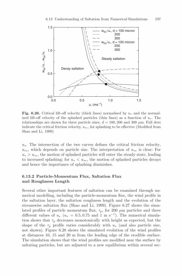
6.13 Understanding of Saltation from Numerical Simulations 197
u* (ms−1)
w0c
/u* ,
w0s
/u*
Decay saltation
Steady saltation
0.0
0.5
1.0
1.5
0.0 0.5 1.0 1.5
w0c /u*, d = 100 micron200300
w0s/u*, d = 100 micron200300
Fig. 6.26. Critical lift-off velocity (thick lines) normalised by u∗ and the normal-ized lift-off velocity of the splashed particles (thin lines) as a function of u∗. Therelationships are shown for three particle sizes, d = 100, 200 and 300 µm. Full dotsindicate the critical friction velocity, u∗c, for splashing to be effective (Modified fromShao and Li, 1999)
u∗. The intersection of the two curves defines the critical friction velocity,u∗c, which depends on particle size. The interpretation of u∗c is clear: Foru∗ > u∗c, the motion of splashed particles will enter the steady state, leadingto increased splashing; for u∗ < u∗c, the motion of splashed particles decaysand hence the importance of splashing diminishes.
6.13.2 Particle-Momentum Flux, Saltation Fluxand Roughness Length
Several other important features of saltation can be examined through nu-merical modelling, including the particle-momentum flux, the wind profile inthe saltation layer, the saltation roughness length and the evolution of thestreamwise saltation flux (Shao and Li, 1999). Figure 6.27 shows the simu-lated profiles of particle momentum flux, τp, for 200 µm particles and threedifferent values of u∗ (u∗ = 0.5, 0.75 and 1 m s−1). The numerical simula-tion shows that τp decreases monotonically with height as expected, but theshape of the τp profile varies considerably with u∗ (and also particle size,not shown). Figure 6.28 shows the simulated evolution of the wind profilesat distances 10, 15 and 20 m from the leading edge of the erodible surface.The simulation shows that the wind profiles are modified near the surface bysaltating particles, but are adjusted to a new equilibrium within several sec-
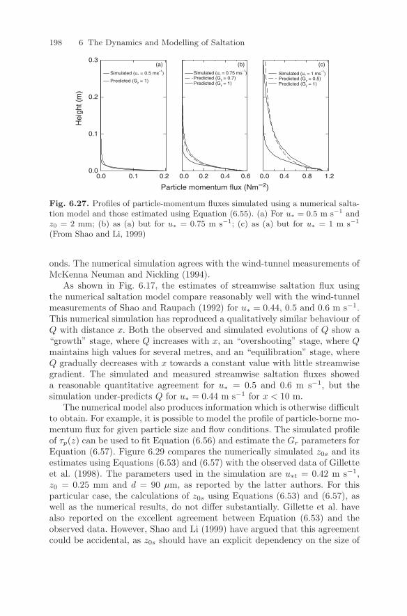
198 6 The Dynamics and Modelling of Saltation
Simulated (u* = 0.5 ms−1
)
Predicted (Gr = 1)
Particle momentum flux (Nm−2)
(a) (b) (c)
Hei
ght (
m)
0.00.0 0.0 0.0 0.4 0.8 1.20.2 0.4 0.60.1 0.2
0.1
0.2
0.3
Simulated (u* = 0.75 ms−1
)Predicted (Gr = 0.7)Predicted (Gr = 1)
Simulated (u* = 1 ms−1
)Predicted (Gr = 0.5)Predicted (Gr = 1)
Fig. 6.27. Profiles of particle-momentum fluxes simulated using a numerical salta-tion model and those estimated using Equation (6.55). (a) For u∗ = 0.5 m s−1 andz0 = 2 mm; (b) as (a) but for u∗ = 0.75 m s−1; (c) as (a) but for u∗ = 1 m s−1
(From Shao and Li, 1999)
onds. The numerical simulation agrees with the wind-tunnel measurements ofMcKenna Neuman and Nickling (1994).
As shown in Fig. 6.17, the estimates of streamwise saltation flux usingthe numerical saltation model compare reasonably well with the wind-tunnelmeasurements of Shao and Raupach (1992) for u∗ = 0.44, 0.5 and 0.6 m s−1.This numerical simulation has reproduced a qualitatively similar behaviour ofQ with distance x. Both the observed and simulated evolutions of Q show a“growth” stage, where Q increases with x, an “overshooting” stage, where Qmaintains high values for several metres, and an “equilibration” stage, whereQ gradually decreases with x towards a constant value with little streamwisegradient. The simulated and measured streamwise saltation fluxes showeda reasonable quantitative agreement for u∗ = 0.5 and 0.6 m s−1, but thesimulation under-predicts Q for u∗ = 0.44 m s−1 for x < 10 m.
The numerical model also produces information which is otherwise difficultto obtain. For example, it is possible to model the profile of particle-borne mo-mentum flux for given particle size and flow conditions. The simulated profileof τp(z) can be used to fit Equation (6.56) and estimate the Gr parameters forEquation (6.57). Figure 6.29 compares the numerically simulated z0s and itsestimates using Equations (6.53) and (6.57) with the observed data of Gilletteet al. (1998). The parameters used in the simulation are u∗t = 0.42 m s−1,z0 = 0.25 mm and d = 90 µm, as reported by the latter authors. For thisparticular case, the calculations of z0s using Equations (6.53) and (6.57), aswell as the numerical results, do not differ substantially. Gillette et al. havealso reported on the excellent agreement between Equation (6.53) and theobserved data. However, Shao and Li (1999) have argued that this agreementcould be accidental, as z0s should have an explicit dependency on the size of
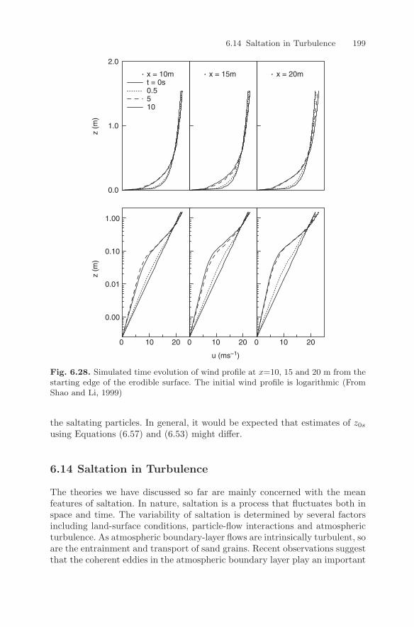
6.14 Saltation in Turbulence 199
u (ms−1)
x = 15m x = 20m
z (m
)z
(m)
0.0
1.0
2.0
x = 10mt = 0s0.5510
0.00
0 10 10 1020 20 200 0
0.01
0.10
1.00
Fig. 6.28. Simulated time evolution of wind profile at x=10, 15 and 20 m from thestarting edge of the erodible surface. The initial wind profile is logarithmic (FromShao and Li, 1999)
the saltating particles. In general, it would be expected that estimates of z0s
using Equations (6.57) and (6.53) might differ.
6.14 Saltation in Turbulence
The theories we have discussed so far are mainly concerned with the meanfeatures of saltation. In nature, saltation is a process that fluctuates both inspace and time. The variability of saltation is determined by several factorsincluding land-surface conditions, particle-flow interactions and atmosphericturbulence. As atmospheric boundary-layer flows are intrinsically turbulent, soare the entrainment and transport of sand grains. Recent observations suggestthat the coherent eddies in the atmospheric boundary layer play an important
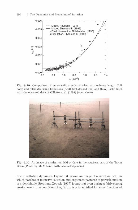
200 6 The Dynamics and Modelling of Saltation
u* (ms−1)
0.000
0.001
0.002
0.003
0.004
0.005
0.006
z 0s
(m)
Model, Raupach (1991)Model, Shao and Li (1999)Filed observation, Gillette et al. (1998) Simulation, Shao and Li (1999)
0.2 0.4 0.6 0.8 1.0 1.2 1.4
Fig. 6.29. Comparison of numerically simulated effective roughness length (fulldots) and estimates using Equations (6.53) (dot-dashed line) and (6.57) (solid line)with the observed data of Gillette et al. (1998) (open circle)
Fig. 6.30. An image of a saltation field at Qira in the southern part of the TarimBasin (Photo by M. Mikami, with acknowledgement)
role in saltation dynamics. Figure 6.30 shows an image of a saltation field, inwhich patches of intensive saltation and organized patterns of particle motionare identifiable. Stout and Zobeck (1997) found that even during a fairly strongerosion event, the condition of u∗ ≥ u∗t is only satisfied for some fractions of
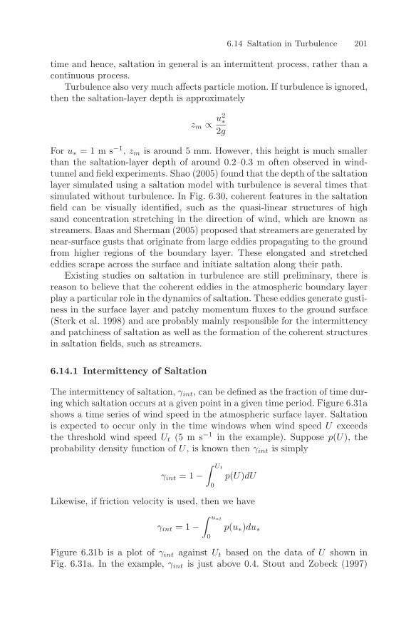
6.14 Saltation in Turbulence 201
time and hence, saltation in general is an intermittent process, rather than acontinuous process.
Turbulence also very much affects particle motion. If turbulence is ignored,then the saltation-layer depth is approximately
zm ∝ u2∗
2g
For u∗ = 1 m s−1, zm is around 5 mm. However, this height is much smallerthan the saltation-layer depth of around 0.2–0.3 m often observed in wind-tunnel and field experiments. Shao (2005) found that the depth of the saltationlayer simulated using a saltation model with turbulence is several times thatsimulated without turbulence. In Fig. 6.30, coherent features in the saltationfield can be visually identified, such as the quasi-linear structures of highsand concentration stretching in the direction of wind, which are known asstreamers. Baas and Sherman (2005) proposed that streamers are generated bynear-surface gusts that originate from large eddies propagating to the groundfrom higher regions of the boundary layer. These elongated and stretchededdies scrape across the surface and initiate saltation along their path.
Existing studies on saltation in turbulence are still preliminary, there isreason to believe that the coherent eddies in the atmospheric boundary layerplay a particular role in the dynamics of saltation. These eddies generate gusti-ness in the surface layer and patchy momentum fluxes to the ground surface(Sterk et al. 1998) and are probably mainly responsible for the intermittencyand patchiness of saltation as well as the formation of the coherent structuresin saltation fields, such as streamers.
6.14.1 Intermittency of Saltation
The intermittency of saltation, γint, can be defined as the fraction of time dur-ing which saltation occurs at a given point in a given time period. Figure 6.31ashows a time series of wind speed in the atmospheric surface layer. Saltationis expected to occur only in the time windows when wind speed U exceedsthe threshold wind speed Ut (5 m s−1 in the example). Suppose p(U), theprobability density function of U , is known then γint is simply
γint = 1 −∫ Ut
0
p(U)dU
Likewise, if friction velocity is used, then we have
γint = 1 −∫ u∗t
0
p(u∗)du∗
Figure 6.31b is a plot of γint against Ut based on the data of U shown inFig. 6.31a. In the example, γint is just above 0.4. Stout and Zobeck (1997)
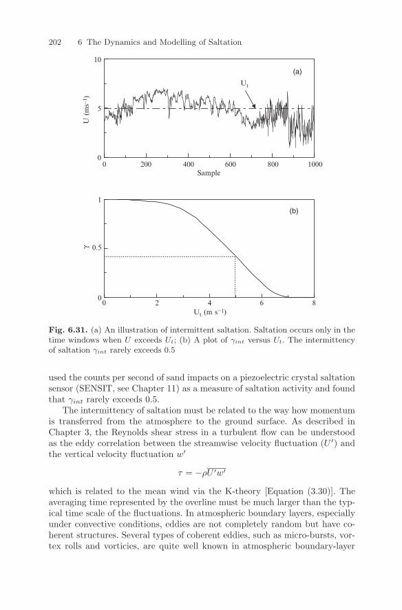
202 6 The Dynamics and Modelling of Saltation
Ut (m s−1)
γ
Sample
U (
ms-
1 )
(a)
(b)
Ut
0
5
10
0
0.5
1
0 2
0 200 400 600 800 1000
4 6 8
Fig. 6.31. (a) An illustration of intermittent saltation. Saltation occurs only in thetime windows when U exceeds Ut; (b) A plot of γint versus Ut. The intermittencyof saltation γint rarely exceeds 0.5
used the counts per second of sand impacts on a piezoelectric crystal saltationsensor (SENSIT, see Chapter 11) as a measure of saltation activity and foundthat γint rarely exceeds 0.5.
The intermittency of saltation must be related to the way how momentumis transferred from the atmosphere to the ground surface. As described inChapter 3, the Reynolds shear stress in a turbulent flow can be understoodas the eddy correlation between the streamwise velocity fluctuation (U ′) andthe vertical velocity fluctuation w′
τ = −ρU ′w′
which is related to the mean wind via the K-theory [Equation (3.30)]. Theaveraging time represented by the overline must be much larger than the typ-ical time scale of the fluctuations. In atmospheric boundary layers, especiallyunder convective conditions, eddies are not completely random but have co-herent structures. Several types of coherent eddies, such as micro-bursts, vor-tex rolls and vorticies, are quite well known in atmospheric boundary-layer
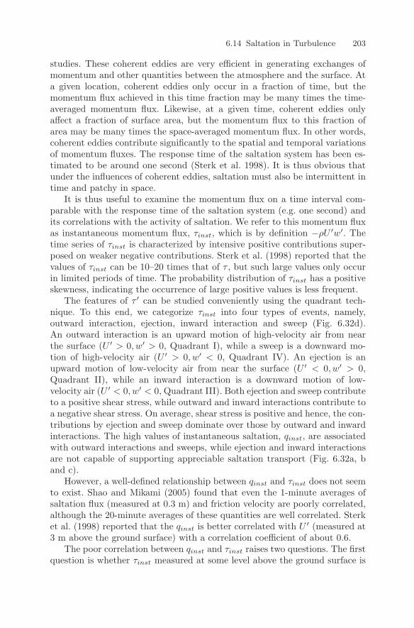
6.14 Saltation in Turbulence 203
studies. These coherent eddies are very efficient in generating exchanges ofmomentum and other quantities between the atmosphere and the surface. Ata given location, coherent eddies only occur in a fraction of time, but themomentum flux achieved in this time fraction may be many times the time-averaged momentum flux. Likewise, at a given time, coherent eddies onlyaffect a fraction of surface area, but the momentum flux to this fraction ofarea may be many times the space-averaged momentum flux. In other words,coherent eddies contribute significantly to the spatial and temporal variationsof momentum fluxes. The response time of the saltation system has been es-timated to be around one second (Sterk et al. 1998). It is thus obvious thatunder the influences of coherent eddies, saltation must also be intermittent intime and patchy in space.
It is thus useful to examine the momentum flux on a time interval com-parable with the response time of the saltation system (e.g. one second) andits correlations with the activity of saltation. We refer to this momentum fluxas instantaneous momentum flux, τinst, which is by definition −ρU ′w′. Thetime series of τinst is characterized by intensive positive contributions super-posed on weaker negative contributions. Sterk et al. (1998) reported that thevalues of τinst can be 10–20 times that of τ , but such large values only occurin limited periods of time. The probability distribution of τinst has a positiveskewness, indicating the occurrence of large positive values is less frequent.
The features of τ ′ can be studied conveniently using the quadrant tech-nique. To this end, we categorize τinst into four types of events, namely,outward interaction, ejection, inward interaction and sweep (Fig. 6.32d).An outward interaction is an upward motion of high-velocity air from nearthe surface (U ′ > 0, w′ > 0, Quadrant I), while a sweep is a downward mo-tion of high-velocity air (U ′ > 0, w′ < 0, Quadrant IV). An ejection is anupward motion of low-velocity air from near the surface (U ′ < 0, w′ > 0,Quadrant II), while an inward interaction is a downward motion of low-velocity air (U ′ < 0, w′ < 0, Quadrant III). Both ejection and sweep contributeto a positive shear stress, while outward and inward interactions contribute toa negative shear stress. On average, shear stress is positive and hence, the con-tributions by ejection and sweep dominate over those by outward and inwardinteractions. The high values of instantaneous saltation, qinst, are associatedwith outward interactions and sweeps, while ejection and inward interactionsare not capable of supporting appreciable saltation transport (Fig. 6.32a, band c).
However, a well-defined relationship between qinst and τinst does not seemto exist. Shao and Mikami (2005) found that even the 1-minute averages ofsaltation flux (measured at 0.3 m) and friction velocity are poorly correlated,although the 20-minute averages of these quantities are well correlated. Sterket al. (1998) reported that the qinst is better correlated with U ′ (measured at3 m above the ground surface) with a correlation coefficient of about 0.6.
The poor correlation between qinst and τinst raises two questions. The firstquestion is whether τinst measured at some level above the ground surface is
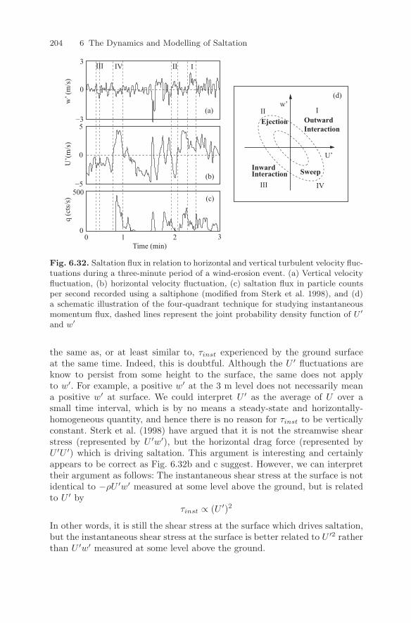
204 6 The Dynamics and Modelling of Saltation
w’
U’
I
III
II
IV
(a)
(d)
(c)
(b)
Time (min)210 3
U’(
m/s
)w
’ (m
/s)
III IV II Iq
(cts
/s)
InwardInteraction Sweep
0
3
−3
0
5
−5
0
500
OutwardInteraction
Ejection
Fig. 6.32. Saltation flux in relation to horizontal and vertical turbulent velocity fluc-tuations during a three-minute period of a wind-erosion event. (a) Vertical velocityfluctuation, (b) horizontal velocity fluctuation, (c) saltation flux in particle countsper second recorded using a saltiphone (modified from Sterk et al. 1998), and (d)a schematic illustration of the four-quadrant technique for studying instantaneousmomentum flux, dashed lines represent the joint probability density function of U ′
and w′
the same as, or at least similar to, τinst experienced by the ground surfaceat the same time. Indeed, this is doubtful. Although the U ′ fluctuations areknow to persist from some height to the surface, the same does not applyto w′. For example, a positive w′ at the 3 m level does not necessarily meana positive w′ at surface. We could interpret U ′ as the average of U over asmall time interval, which is by no means a steady-state and horizontally-homogeneous quantity, and hence there is no reason for τinst to be verticallyconstant. Sterk et al. (1998) have argued that it is not the streamwise shearstress (represented by U ′w′), but the horizontal drag force (represented byU ′U ′) which is driving saltation. This argument is interesting and certainlyappears to be correct as Fig. 6.32b and c suggest. However, we can interprettheir argument as follows: The instantaneous shear stress at the surface is notidentical to −ρU ′w′ measured at some level above the ground, but is relatedto U ′ by
τinst ∝ (U ′)2
In other words, it is still the shear stress at the surface which drives saltation,but the instantaneous shear stress at the surface is better related to U ′2 ratherthan U ′w′ measured at some level above the ground.
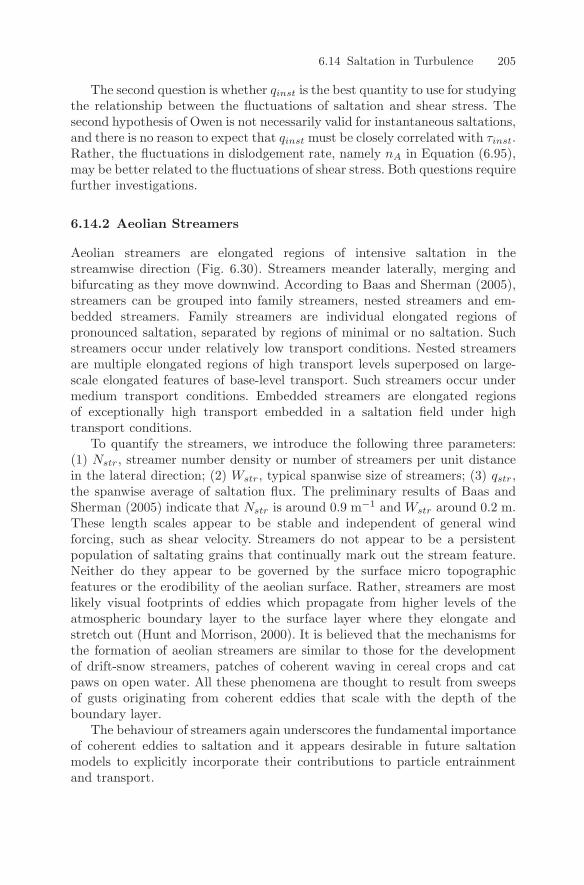
6.14 Saltation in Turbulence 205
The second question is whether qinst is the best quantity to use for studyingthe relationship between the fluctuations of saltation and shear stress. Thesecond hypothesis of Owen is not necessarily valid for instantaneous saltations,and there is no reason to expect that qinst must be closely correlated with τinst.Rather, the fluctuations in dislodgement rate, namely nA in Equation (6.95),may be better related to the fluctuations of shear stress. Both questions requirefurther investigations.
6.14.2 Aeolian Streamers
Aeolian streamers are elongated regions of intensive saltation in thestreamwise direction (Fig. 6.30). Streamers meander laterally, merging andbifurcating as they move downwind. According to Baas and Sherman (2005),streamers can be grouped into family streamers, nested streamers and em-bedded streamers. Family streamers are individual elongated regions ofpronounced saltation, separated by regions of minimal or no saltation. Suchstreamers occur under relatively low transport conditions. Nested streamersare multiple elongated regions of high transport levels superposed on large-scale elongated features of base-level transport. Such streamers occur undermedium transport conditions. Embedded streamers are elongated regionsof exceptionally high transport embedded in a saltation field under hightransport conditions.
To quantify the streamers, we introduce the following three parameters:(1) Nstr, streamer number density or number of streamers per unit distancein the lateral direction; (2) Wstr, typical spanwise size of streamers; (3) qstr,the spanwise average of saltation flux. The preliminary results of Baas andSherman (2005) indicate that Nstr is around 0.9 m−1 and Wstr around 0.2 m.These length scales appear to be stable and independent of general windforcing, such as shear velocity. Streamers do not appear to be a persistentpopulation of saltating grains that continually mark out the stream feature.Neither do they appear to be governed by the surface micro topographicfeatures or the erodibility of the aeolian surface. Rather, streamers are mostlikely visual footprints of eddies which propagate from higher levels of theatmospheric boundary layer to the surface layer where they elongate andstretch out (Hunt and Morrison, 2000). It is believed that the mechanisms forthe formation of aeolian streamers are similar to those for the developmentof drift-snow streamers, patches of coherent waving in cereal crops and catpaws on open water. All these phenomena are thought to result from sweepsof gusts originating from coherent eddies that scale with the depth of theboundary layer.
The behaviour of streamers again underscores the fundamental importanceof coherent eddies to saltation and it appears desirable in future saltationmodels to explicitly incorporate their contributions to particle entrainmentand transport.
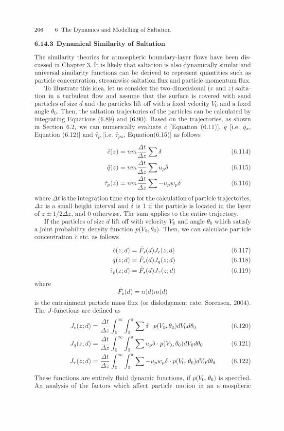
206 6 The Dynamics and Modelling of Saltation
6.14.3 Dynamical Similarity of Saltation
The similarity theories for atmospheric boundary-layer flows have been dis-cussed in Chapter 3. It is likely that saltation is also dynamically similar anduniversal similarity functions can be derived to represent quantities such asparticle concentration, streamwise saltation flux and particle-momentum flux.
To illustrate this idea, let us consider the two-dimensional (x and z) salta-tion in a turbulent flow and assume that the surface is covered with sandparticles of size d and the particles lift off with a fixed velocity V0 and a fixedangle θ0. Then, the saltation trajectories of the particles can be calculated byintegrating Equations (6.89) and (6.90). Based on the trajectories, as shownin Section 6.2, we can numerically evaluate c [Equation (6.11)], q [i.e. qx,Equation (6.12)] and τp [i.e. τpz, Equation(6.15)] as follows
c(z) = nm∆t
∆z
∑δ (6.114)
q(z) = nm∆t
∆z
∑upδ (6.115)
τp(z) = nm∆t
∆z
∑−upwpδ (6.116)
where ∆t is the integration time step for the calculation of particle trajectories,∆z is a small height interval and δ is 1 if the particle is located in the layerof z ± 1/2∆z, and 0 otherwise. The sum applies to the entire trajectory.
If the particles of size d lift off with velocity V0 and angle θ0 which satisfya joint probability density function p(V0, θ0). Then, we can calculate particleconcentration c etc. as follows
c(z; d) = Fs(d)Jc(z; d) (6.117)q(z; d) = Fs(d)Jq(z; d) (6.118)
τp(z; d) = Fs(d)Jτ (z; d) (6.119)
whereFs(d) = n(d)m(d)
is the entrainment particle mass flux (or dislodgement rate, Sorensen, 2004).The J-functions are defined as
Jc(z; d) =∆t
∆z
∫ ∞
0
∫ π
0
∑δ · p(V0, θ0)dV0dθ0 (6.120)
Jq(z; d) =∆t
∆z
∫ ∞
0
∫ π
0
∑upδ · p(V0, θ0)dV0dθ0 (6.121)
Jτ (z; d) =∆t
∆z
∫ ∞
0
∫ π
0
∑−upwpδ · p(V0, θ0)dV0dθ0 (6.122)
These functions are entirely fluid dynamic functions, if p(V0, θ0) is specified.An analysis of the factors which affect particle motion in an atmospheric
6.14 Saltation in Turbulence 207
surface-layer flow suggests that the J functions must only depend on u∗, z0
and d, because
• u∗ affects wind profile and turbulence intensity.• z0 affects wind profile.• d affects particle response to turbulent flow and particle terminal fall
velocity.
We expect that the J functions are ‘universal’ functions of z if properlynormalized.
Several interesting relationships can be established if the J-functions areknown. For instance, by making use of Equation (6.119), the dislodgementrate at equilibrium saltation is
Fs(d) =τ − τt(d)Jτ (0; d)
. (6.123)
The above equation is a manifestation of the second hypothesis of Owen (τp0 =τ − τt). From Equation (6.118), we also obtain
Fs(d) = Q(d)[∫ ∞
0
Jq(z; d)dz
]−1
(6.124)
where Q is the vertically-integrated streamwise saltation flux if the surface iscovered with uniform particles of size d.
Shao (2005) has estimated Jq using a Lagrangian stochastic model forparticle motion in atmospheric surface-layer flows. In the latter study, theprofiles of wind and turbulence are specified according to the Monin–Obukhovsimilarity theory, and p(V0, θ0) is given by
p(V0, θ0) = p(V0)p(θ0)
with p(V0) being an exponential distribution and p(θ0) a truncated Gaussiandistribution. It has been found that
Jq = Aq exp
(− zKq
LKqq
)(6.125)
where Aq is a dimensionless coefficient, Lq a scaling height and Kq a quan-tity that varies between 1 and 2. The meaning of Kq is clear. Because theparticle response to turbulent fluctuations is particle-size dependent, Jq mustalso be particle-size dependent. The saltation of large particles is not stronglyaffected by turbulence because of their large inertial. Hence, Jq is very muchdetermined by the initial conditions and is thus close to an exponential func-tion [because p(V0) is exponential], i.e., Kq = 1. The motion of small particlesis more strongly affected by turbulence. Hence, Jq is not determined by theinitial conditions but the process of turbulent diffusion and is thus close to a
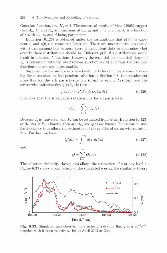
208 6 The Dynamics and Modelling of Saltation
Gaussian function, i.e., Kq = 2. The numerical results of Shao (2005) suggestthat Aq, Lq and Kq are functions of u∗, z0 and d. Therefore, Jq is a functionof z with u∗, z0 and d being parameters.
Equation (6.125) is obtained under the assumptions that p(V0) is expo-nential and p(θ0) is truncated Gaussian. There are uncertainties associatedwith these assumptions because there is insufficient data to determine whatexactly these distributions should be. Different p(V0, θ0) distributions wouldresult in different J functions. However, the essential (exponential) shape ofJq is consistent with the observations (Section 6.7.4) and thus the assumeddistributions are not unreasonable.
Suppose now the surface is covered with particles of multiple sizes. Follow-ing the discussions on independent saltation in Section 6.8, the entrainmentmass flux for the kth particle-size bin Fs(dk) is simply PkFs(dk) and thestreamwise saltation flux q(z; dk) is then
q(z; dk) = PkFs(dk)Jq(z; dk) (6.126)
It follows that the streamwise saltation flux for all particles is
q(z) =K∑
k=1
q(z; dk)
Because Jq is ‘universal’ and Fs can be estimated from either Equation (6.123)or (6.124), if Pk is known, then q(z; dk) and q(z) are known. The saltation sim-ilarity theory thus allows the estimation of the profiles of streamwise saltationflux. Further, we have
Q(dk) =∫ ∞
0
q(z; dk)δz (6.127)
and
Q =K∑
k=1
Q(dk) (6.128)
The saltation similarity theory also allows the estimation of q at any level z.Figure 6.33 shows a comparison of the simulated q using the similarity theory
Time (LT, day)
0
1
2
q (g
m−
2 s−
1 )
u * (m
s−1 )
qmod
qobs
0.4
0.5
0.6
u*
104.38 104.38 104.48 104.53 104.58
Fig. 6.33. Simulated and observed time series of saltation flux q in g m−2s−1,together with friction velocity u∗ for 14 April 2002 at Qira
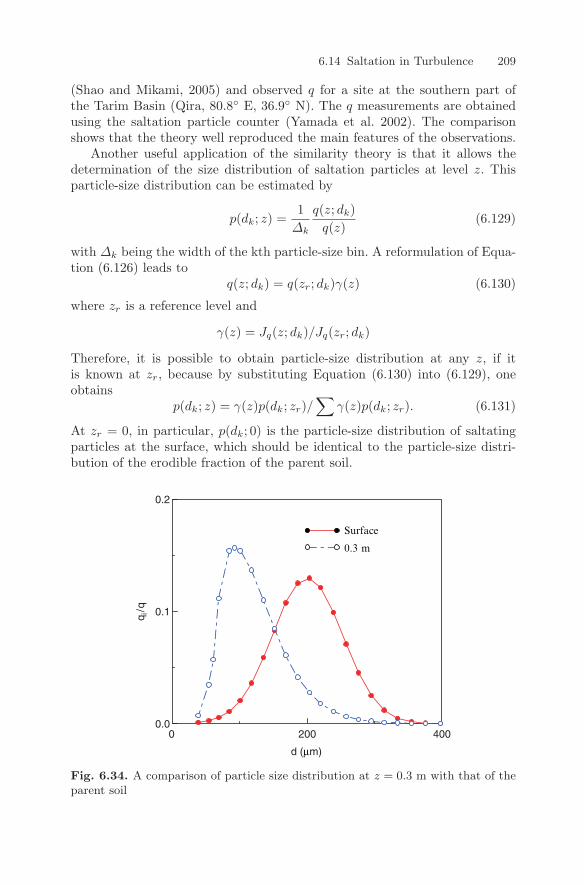
6.14 Saltation in Turbulence 209
(Shao and Mikami, 2005) and observed q for a site at the southern part ofthe Tarim Basin (Qira, 80.8 E, 36.9 N). The q measurements are obtainedusing the saltation particle counter (Yamada et al. 2002). The comparisonshows that the theory well reproduced the main features of the observations.
Another useful application of the similarity theory is that it allows thedetermination of the size distribution of saltation particles at level z. Thisparticle-size distribution can be estimated by
p(dk; z) =1
∆k
q(z; dk)q(z)
(6.129)
with ∆k being the width of the kth particle-size bin. A reformulation of Equa-tion (6.126) leads to
q(z; dk) = q(zr; dk)γ(z) (6.130)
where zr is a reference level and
γ(z) = Jq(z; dk)/Jq(zr; dk)
Therefore, it is possible to obtain particle-size distribution at any z, if itis known at zr, because by substituting Equation (6.130) into (6.129), oneobtains
p(dk; z) = γ(z)p(dk; zr)/∑
γ(z)p(dk; zr). (6.131)
At zr = 0, in particular, p(dk; 0) is the particle-size distribution of saltatingparticles at the surface, which should be identical to the particle-size distri-bution of the erodible fraction of the parent soil.
d (µm)
q i/q
Surface
0.3 m
0.00 200 400
0.1
0.2
Fig. 6.34. A comparison of particle size distribution at z = 0.3 m with that of theparent soil

210 6 The Dynamics and Modelling of Saltation
The predicted variation of particle-size distribution with height is as de-picted in Fig. 6.34 which shows that the modal particle size decreases withheight. Leys and McTainsh (1996) measured particle-size distributions at var-ious levels between the surface and 2 m and found there is a significant de-crease of the modal particle size with height below 0.5 m. The theory of Shaoand Mikami (2005) is consistent with the observations of Leys and McTainsh(1996).
7
Dust Emission
Dust-emission rate is the vertical mass flux of dust at the surface. The im-portance of determining the dust-emission rate is twofold. (1) Dust emissionis a key component of the global mineral-dust cycle and the associated nu-trient cycle. Dust particles, once airborne, can be diffused by turbulence intothe upper levels of the atmosphere and then carried over large distances bywinds and eventually deposited back to the surface. This process depletes fineparticles from the source regions of wind erosion. In agricultural areas, theloss of dust particles leads to gradual land degradation, because fine parti-cles are mostly rich in nutrients and organic matter. Mineral dust is a majorprovider of nutrient to the oceans. (2) Dust produced by wind erosion is a ma-jor source of atmospheric aerosols which have impacts on air quality, weatherand climate. It is not possible to calculate aerosol concentration in the at-mosphere with certainty unless the dust-emission rate can be estimated withaccuracy. Hence, the need for determining this quantity is obvious both forsoil conservation and atmospheric studies.
Dust emission over a large source areas can be estimated using diagnostictechniques (e.g. D’Almeida, 1986). This type of study requires reliable three-dimensional measurements of dust concentration and the flow field, both ofwhich are usually difficult to obtain for dust source regions. An alternative isto numerically estimate dust emission by means of dust-emission schemes. Inthis chapter, we examine the mechanisms for dust emission and study someof the existing dust schemes.
7.1 Dust Flux and Friction Velocity
We distinguish dust-emission rate, F , from net dust-emission rate, FN . Thelatter is the difference between F and dust-deposition rate, FD, i.e.,
FN = F − FD
Y. Shao, Physics and Modelling of Wind Erosion, 211c© Springer Science+Business Media B.V. 2008
212 7 Dust Emission
We shall study FD in Chapter 8. It appears that F has never been measureddirectly in practice. Rather, it is inferred from the measurements of the verticalflux of airborne dust in the atmospheric surface layer, Fair, which is constantwith height under the assumptions of steady state and horizontal homogeneity.In this respect, Fair is similar to the fluxes of other passive scalars. However,Fair itself consists of a component due to turbulent and molecular diffusion,Fair,d, and a component due to gravitational settling, Fair,s. By analogy toscalar fluxes, the diffusive dust flux can be estimated from the profile of dustconcentration by means of
Fair,d = −ρKp∂c
∂z(7.1)
where ρ is air density and Kp is the eddy diffusivity for dust particles and cis the specific dust concentration. Kp is affected both by atmospheric turbu-lence and by the particle response to turbulent fluctuations (e.g. the particle-trajectory crossing effect and the particle-inertial effect, Chapter 8). Hence,Kp is dependent on dust-particle size for given flow conditions. However, asan approximation, Kp can be assumed to be equal to the eddy diffusivity forscalar and expressed as
Kp = Km = κu∗z
for neutral atmospheric boundary-layer flows. For stable and unstable con-ditions, Km can be correspondingly modified by using the Monin–Obukhovsimilarity theory as outlined in Chapter 3.
Suppose the dust-concentration field is in steady state and is horizontallyhomogeneous. The dust-concentration equation, Equation (3.24), yields a sim-ple balance of gravitational settling and turbulent diffusion
wt∂c
∂z+
∂
∂z
(Kp
∂c
∂z
)= 0 (7.2)
where wt is the settling velocity. An integration of the above equation over zgives
−ρwtc − Kpρ∂c
∂z= F0 (7.3)
where F0 is a constant. Equation (7.3) implies that Fair is constant withheight (namely, −ρwtc−Kpρ∂c/∂z), but Fair,d and Fair,s (namely, −ρwtc) isnot. Equation (7.3) can be further integrated to yield the steady state profileof dust concentration
c =(
cr +F0
ρwt
)(z
zr
)−wt/κu∗
− F0
ρwt(7.4)
with cr being the dust concentration at the reference height, zr. Equation (7.4)implies that the dust-concentration profile obeys the power-law with c in-creasing with decreasing height, in contrast to the profile of a scalar, whichcommonly obeys the log-law. Suppose F0 = 0, then we have
7.1 Dust Flux and Friction Velocity 213
c = cr
(z
zr
)−wt/κu∗
(7.5)
Given this dust-concentration profile, we can see from Equation (7.3) thatthe magnitudes of both Fair,d and Fair,s increase with decreasing height. Theconclusion of the above analysis is that F is not identical Fair,d and Fair,d
is height dependent. For a steady-state dust concentration field with no dustemission, i.e. F0 = 0, Fair,d also obeys a power law
Fair,d = ρwtcr
(z
zr
)−wt/κu∗
(7.6)
In most field experiments on dust emission reported in the literature, onlyFair,d has been measured, and we have implicitly interpreted that
F = Fair,d
We must bear this interpretation in mind when we use the dust-emissionmeasurements.
Gillette (1977) reported probably the most comprehensive set of field mea-surements of F for 9 different soils and examined the relationship between Fand u∗. In his experiments, dust was collected using a specially-designed mem-brane filter placed at two different heights, and F was calculated using thediscrete version of Equation (7.1). The observed values of F are plotted againstu∗ in Fig. 7.1a (for 7 out of the 9 soils), together with the observed vertically-integrated streamwise saltation flux, Q. Figure 7.1b shows that the measuredsaltation flux is well described by the Q ∝ u3
∗ relationship except for the sandy-clay loam case and the clay loam case. In contrast, although F generally in-creases with u∗, there is a large scatter among the measurements and it is notpossible to describe the data with a definitive F (u∗) relationship (Fig. 7.1a).
Nickling and Gillies (1989, 1993) examined the relationship between dustemission and u∗ using data sets obtained in Mali (West Africa), Texas (USA)and Yukon (Canada). They reported dust-emission rate measured at 13 ex-perimental sites in southern Arizona by means of a portable wind tunnel. Thesites were selected on the basis of soil texture, vegetative cover, land use andanthropogenic disturbance. A considerable scatter also exists in their dataif no distinction is made between the soil-surface features. To investigate thescatter in the data, Nickling and Gillies classified the experimental sites basedon surface morphology and land use and grouped the data sets accordingly.Five classes were established, as follows: (1) Natural undisturbed desert sites;(2) Sites developed or modified by fluvial processes; (3) Construction sites; (4)Mine Tailings, and (5) Agricultural sites. The regression relationships derivedfor the first four classes are:
• Natural undisturbed desert sites: F ∝ u2.99∗
• Sites developed or modified by fluvial processes: F ∝ u3.32∗
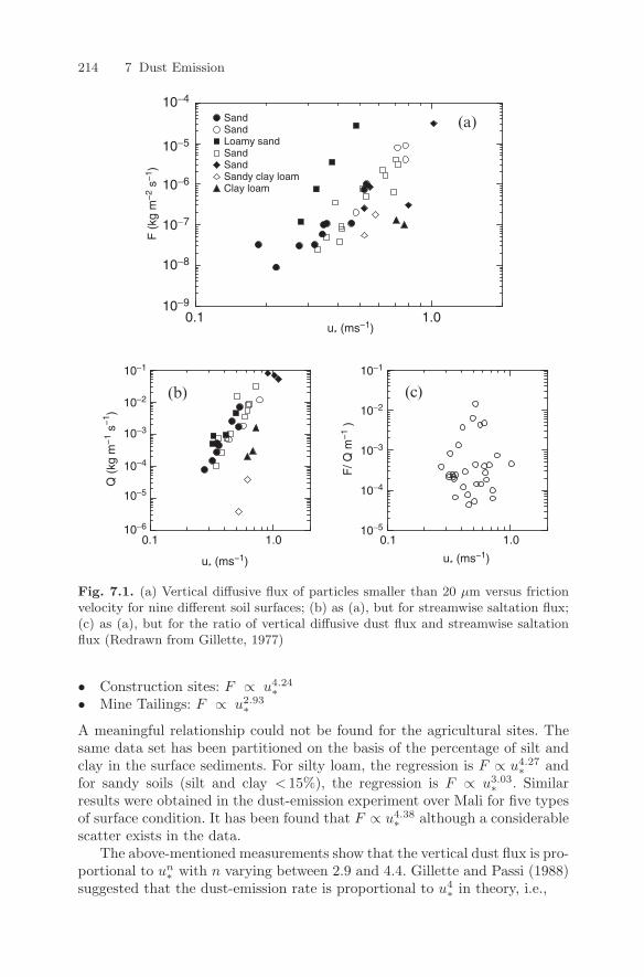
214 7 Dust Emission
u* (ms−1) u* (ms−1)
Q (
kg m
−1
s−1 )
0.1 1.0u* (ms−1)
F (
kg m
−2
s−1 )
SandSandLoamy sandSandSandSandy clay loamClay loam
(a)
(b) (c)
10−9
10−8
10−7
10−6
10−5
10−4
10−6
0.1 0.11.0 1.0
10−5
10−4
10−3
10−2
10−1
F/ Q
m−
1 )
10−5
10−4
10−3
10−2
10−1
Fig. 7.1. (a) Vertical diffusive flux of particles smaller than 20 µm versus frictionvelocity for nine different soil surfaces; (b) as (a), but for streamwise saltation flux;(c) as (a), but for the ratio of vertical diffusive dust flux and streamwise saltationflux (Redrawn from Gillette, 1977)
• Construction sites: F ∝ u4.24∗
• Mine Tailings: F ∝ u2.93∗
A meaningful relationship could not be found for the agricultural sites. Thesame data set has been partitioned on the basis of the percentage of silt andclay in the surface sediments. For silty loam, the regression is F ∝ u4.27
∗ andfor sandy soils (silt and clay < 15%), the regression is F ∝ u3.03
∗ . Similarresults were obtained in the dust-emission experiment over Mali for five typesof surface condition. It has been found that F ∝ u4.38
∗ although a considerablescatter exists in the data.
The above-mentioned measurements show that the vertical dust flux is pro-portional to un
∗ with n varying between 2.9 and 4.4. Gillette and Passi (1988)suggested that the dust-emission rate is proportional to u4
∗ in theory, i.e.,
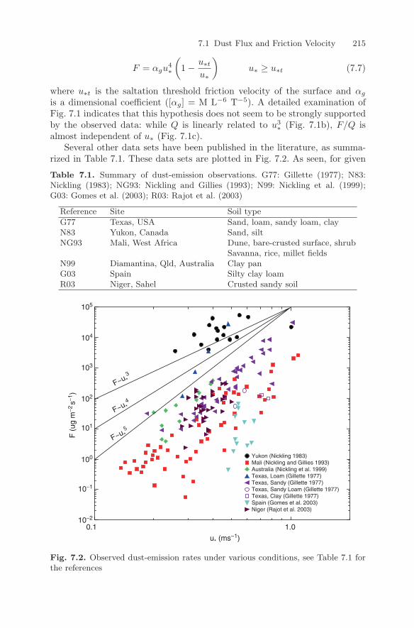
7.1 Dust Flux and Friction Velocity 215
F = αgu4∗
(1 − u∗t
u∗
)u∗ ≥ u∗t (7.7)
where u∗t is the saltation threshold friction velocity of the surface and αg
is a dimensional coefficient ([αg] = M L−6 T−5). A detailed examination ofFig. 7.1 indicates that this hypothesis does not seem to be strongly supportedby the observed data: while Q is linearly related to u3
∗ (Fig. 7.1b), F/Q isalmost independent of u∗ (Fig. 7.1c).
Several other data sets have been published in the literature, as summa-rized in Table 7.1. These data sets are plotted in Fig. 7.2. As seen, for given
Table 7.1. Summary of dust-emission observations. G77: Gillette (1977); N83:Nickling (1983); NG93: Nickling and Gillies (1993); N99: Nickling et al. (1999);G03: Gomes et al. (2003); R03: Rajot et al. (2003)
Reference Site Soil type
G77 Texas, USA Sand, loam, sandy loam, clayN83 Yukon, Canada Sand, siltNG93 Mali, West Africa Dune, bare-crusted surface, shrub
Savanna, rice, millet fieldsN99 Diamantina, Qld, Australia Clay panG03 Spain Silty clay loamR03 Niger, Sahel Crusted sandy soil
0.1 1.0
u* (ms−1)
F (
ug m
−2s−1
)
Yukon (Nickling 1983)Mali (Nickling and Gillies 1993)Australia (Nickling et al. 1999)Texas, Loam (Gillette 1977)Texas, Sandy (Gillette 1977)Texas, Sandy Loam (Gillette 1977)Texas, Clay (Gillette 1977)Spain (Gomes et al. 2003)Niger (Rajot et al. 2003)
F~u *3
F~u *4
F~u *5
10−2
10−1
100
101
103
102
104
105
Fig. 7.2. Observed dust-emission rates under various conditions, see Table 7.1 forthe references
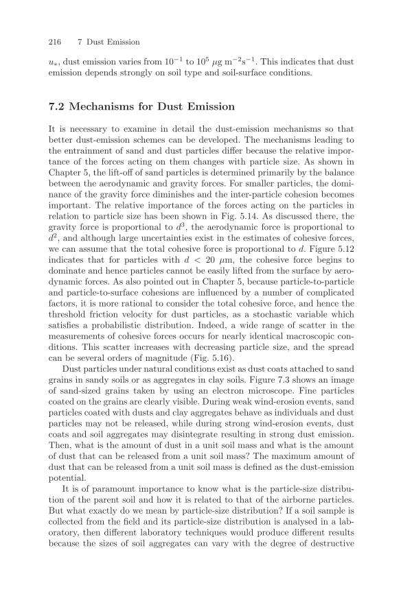
216 7 Dust Emission
u∗, dust emission varies from 10−1 to 105 µg m−2s−1. This indicates that dustemission depends strongly on soil type and soil-surface conditions.
7.2 Mechanisms for Dust Emission
It is necessary to examine in detail the dust-emission mechanisms so thatbetter dust-emission schemes can be developed. The mechanisms leading tothe entrainment of sand and dust particles differ because the relative impor-tance of the forces acting on them changes with particle size. As shown inChapter 5, the lift-off of sand particles is determined primarily by the balancebetween the aerodynamic and gravity forces. For smaller particles, the domi-nance of the gravity force diminishes and the inter-particle cohesion becomesimportant. The relative importance of the forces acting on the particles inrelation to particle size has been shown in Fig. 5.14. As discussed there, thegravity force is proportional to d3, the aerodynamic force is proportional tod2, and although large uncertainties exist in the estimates of cohesive forces,we can assume that the total cohesive force is proportional to d. Figure 5.12indicates that for particles with d < 20 µm, the cohesive force begins todominate and hence particles cannot be easily lifted from the surface by aero-dynamic forces. As also pointed out in Chapter 5, because particle-to-particleand particle-to-surface cohesions are influenced by a number of complicatedfactors, it is more rational to consider the total cohesive force, and hence thethreshold friction velocity for dust particles, as a stochastic variable whichsatisfies a probabilistic distribution. Indeed, a wide range of scatter in themeasurements of cohesive forces occurs for nearly identical macroscopic con-ditions. This scatter increases with decreasing particle size, and the spreadcan be several orders of magnitude (Fig. 5.16).
Dust particles under natural conditions exist as dust coats attached to sandgrains in sandy soils or as aggregates in clay soils. Figure 7.3 shows an imageof sand-sized grains taken by using an electron microscope. Fine particlescoated on the grains are clearly visible. During weak wind-erosion events, sandparticles coated with dusts and clay aggregates behave as individuals and dustparticles may not be released, while during strong wind-erosion events, dustcoats and soil aggregates may disintegrate resulting in strong dust emission.Then, what is the amount of dust in a unit soil mass and what is the amountof dust that can be released from a unit soil mass? The maximum amount ofdust that can be released from a unit soil mass is defined as the dust-emissionpotential.
It is of paramount importance to know what is the particle-size distribu-tion of the parent soil and how it is related to that of the airborne particles.But what exactly do we mean by particle-size distribution? If a soil sample iscollected from the field and its particle-size distribution is analysed in a lab-oratory, then different laboratory techniques would produce different resultsbecause the sizes of soil aggregates can vary with the degree of destructive
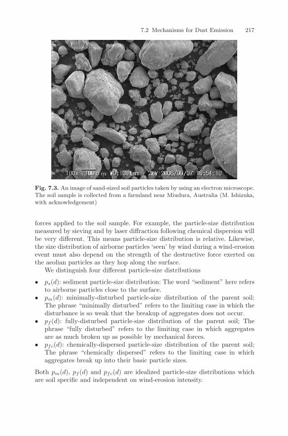
7.2 Mechanisms for Dust Emission 217
Fig. 7.3. An image of sand-sized soil particles taken by using an electron microscope.The soil sample is collected from a farmland near Miudura, Australia (M. Ishizuka,with acknowledgement)
forces applied to the soil sample. For example, the particle-size distributionmeasured by sieving and by laser diffraction following chemical dispersion willbe very different. This means particle-size distribution is relative. Likewise,the size distribution of airborne particles ‘seen’ by wind during a wind-erosionevent must also depend on the strength of the destructive force exerted onthe aeolian particles as they hop along the surface.
We distinguish four different particle-size distributions
• ps(d): sediment particle-size distribution: The word “sediment” here refersto airborne particles close to the surface.
• pm(d): minimally-disturbed particle-size distribution of the parent soil;The phrase “minimally disturbed” refers to the limiting case in which thedisturbance is so weak that the breakup of aggregates does not occur.
• pf (d): fully-disturbed particle-size distribution of the parent soil; Thephrase “fully disturbed” refers to the limiting case in which aggregatesare as much broken up as possible by mechanical forces.
• pfc(d): chemically-dispersed particle-size distribution of the parent soil;The phrase “chemically dispersed” refers to the limiting case in whichaggregates break up into their basic particle sizes.
Both pm(d), pf (d) and pfc(d) are idealized particle-size distributions whichare soil specific and independent on wind-erosion intensity.
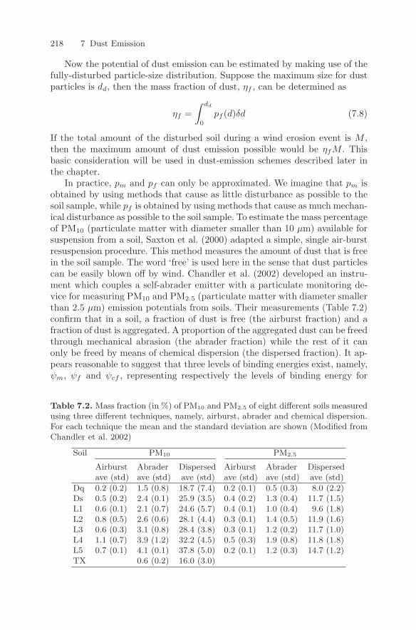
218 7 Dust Emission
Now the potential of dust emission can be estimated by making use of thefully-disturbed particle-size distribution. Suppose the maximum size for dustparticles is dd, then the mass fraction of dust, ηf , can be determined as
ηf =∫ dd
0
pf (d)δd (7.8)
If the total amount of the disturbed soil during a wind erosion event is M ,then the maximum amount of dust emission possible would be ηfM . Thisbasic consideration will be used in dust-emission schemes described later inthe chapter.
In practice, pm and pf can only be approximated. We imagine that pm isobtained by using methods that cause as little disturbance as possible to thesoil sample, while pf is obtained by using methods that cause as much mechan-ical disturbance as possible to the soil sample. To estimate the mass percentageof PM10 (particulate matter with diameter smaller than 10 µm) available forsuspension from a soil, Saxton et al. (2000) adapted a simple, single air-burstresuspension procedure. This method measures the amount of dust that is freein the soil sample. The word ‘free’ is used here in the sense that dust particlescan be easily blown off by wind. Chandler et al. (2002) developed an instru-ment which couples a self-abrader emitter with a particulate monitoring de-vice for measuring PM10 and PM2.5 (particulate matter with diameter smallerthan 2.5 µm) emission potentials from soils. Their measurements (Table 7.2)confirm that in a soil, a fraction of dust is free (the airburst fraction) and afraction of dust is aggregated. A proportion of the aggregated dust can be freedthrough mechanical abrasion (the abrader fraction) while the rest of it canonly be freed by means of chemical dispersion (the dispersed fraction). It ap-pears reasonable to suggest that three levels of binding energies exist, namely,ψm, ψf and ψcf , representing respectively the levels of binding energy for
Table 7.2. Mass fraction (in %) of PM10 and PM2.5 of eight different soils measuredusing three different techniques, namely, airburst, abrader and chemical dispersion.For each technique the mean and the standard deviation are shown (Modified fromChandler et al. 2002)
Soil PM10 PM2.5
Airburst Abrader Dispersed Airburst Abrader Dispersedave (std) ave (std) ave (std) ave (std) ave (std) ave (std)
Dq 0.2 (0.2) 1.5 (0.8) 18.7 (7.4) 0.2 (0.1) 0.5 (0.3) 8.0 (2.2)Ds 0.5 (0.2) 2.4 (0.1) 25.9 (3.5) 0.4 (0.2) 1.3 (0.4) 11.7 (1.5)L1 0.6 (0.1) 2.1 (0.7) 24.6 (5.7) 0.4 (0.1) 1.0 (0.4) 9.6 (1.8)L2 0.8 (0.5) 2.6 (0.6) 28.1 (4.4) 0.3 (0.1) 1.4 (0.5) 11.9 (1.6)L3 0.6 (0.3) 3.1 (0.8) 28.4 (3.8) 0.3 (0.1) 1.2 (0.2) 11.7 (1.0)L4 1.1 (0.7) 3.9 (1.2) 32.2 (4.5) 0.5 (0.3) 1.9 (0.8) 11.8 (1.8)L5 0.7 (0.1) 4.1 (0.1) 37.8 (5.0) 0.2 (0.1) 1.2 (0.3) 14.7 (1.2)TX 0.6 (0.2) 16.0 (3.0)
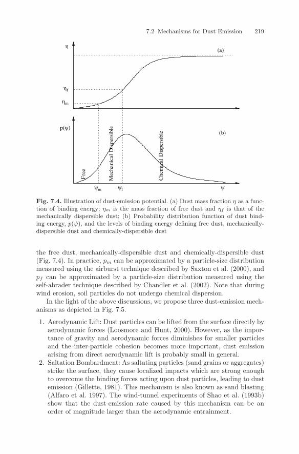
7.2 Mechanisms for Dust Emission 219
p(ψ)
(a)
(b)
Mec
hani
cal D
ispe
rsib
le
Che
mic
al D
ispe
rsib
le
Fre
eηf
ηm
η
ψψfψm
Fig. 7.4. Illustration of dust-emission potential. (a) Dust mass fraction η as a func-tion of binding energy; ηm is the mass fraction of free dust and ηf is that of themechanically dispersible dust; (b) Probability distribution function of dust bind-ing energy, p(ψ), and the levels of binding energy defining free dust, mechanically-dispersible dust and chemically-dispersible dust
the free dust, mechanically-dispersible dust and chemically-dispersible dust(Fig. 7.4). In practice, pm can be approximated by a particle-size distributionmeasured using the airburst technique described by Saxton et al. (2000), andpf can be approximated by a particle-size distribution measured using theself-abrader technique described by Chandler et al. (2002). Note that duringwind erosion, soil particles do not undergo chemical dispersion.
In the light of the above discussions, we propose three dust-emission mech-anisms as depicted in Fig. 7.5.
1. Aerodynamic Lift: Dust particles can be lifted from the surface directly byaerodynamic forces (Loosmore and Hunt, 2000). However, as the impor-tance of gravity and aerodynamic forces diminishes for smaller particlesand the inter-particle cohesion becomes more important, dust emissionarising from direct aerodynamic lift is probably small in general.
2. Saltation Bombardment: As saltating particles (sand grains or aggregates)strike the surface, they cause localized impacts which are strong enoughto overcome the binding forces acting upon dust particles, leading to dustemission (Gillette, 1981). This mechanism is also known as sand blasting(Alfaro et al. 1997). The wind-tunnel experiments of Shao et al. (1993b)show that the dust-emission rate caused by this mechanism can be anorder of magnitude larger than the aerodynamic entrainment.
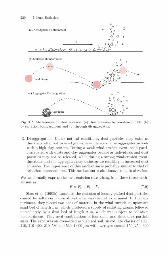
220 7 Dust Emission
(a) Aerodynamic Entrainment
(b) Saltation Bombardment
(c) Aggregates Disintegration
U
Aggregate
Sand Grain
Fig. 7.5. Mechanisms for dust emission. (a) Dust emission by aerodynamic lift, (b)by saltation bombardment and (c) through disaggregation
3. Disaggregation: Under natural conditions, dust particles may exist asdustcoats attached to sand grains in sandy soils or as aggregates in soilswith a high clay content. During a weak wind erosion event, sand parti-cles coated with dusts and clay aggregates behave as individuals and dustparticles may not be released, while during a strong wind-erosion event,dustcoats and soil aggregates may disintegrate resulting in increased dustemission. The importance of this mechanism is probably similar to that ofsaltation bombardment. This mechanism is also known as auto-abrasion.
We can formally express the dust-emission rate arising from these three mech-anisms as
F = Fa + Fb + Fc (7.9)
Shao et al. (1993b) examined the emission of loosely packed dust particlescaused by saltation bombardment in a wind-tunnel experiment. In that ex-periment, they placed two beds of material in the wind tunnel: an upstreamsand bed of length 1 m, which produced a supply of saltating grains, followedimmediately by a dust bed of length 2 m, which was subject to saltationbombardment. They used combinations of four sand- and three dust-particlesizes. The sand was an oven-dried aeolian red soil, sieved into classes of 100–210, 210–400, 210–530 and 530–1,000 µm with averages around 150, 250, 300
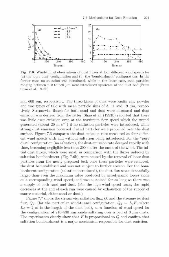
7.2 Mechanisms for Dust Emission 221
Time (s) Time (s)
UR = 8.3 ms−1(a) (b)
00 0120 120240 240360 360480 480
1
2
3
4
5
9.811.112.9
0
5
10
15
20
25F
(g
m−
2s−
1 )
Fig. 7.6. Wind-tunnel observations of dust fluxes at four different wind speeds for(a) the ‘pure dust’ configuration and (b) the ‘bombardment’ configurations. In theformer case, no saltation was introduced, while in the latter case, sand particlesranging between 210 to 530 µm were introduced upstream of the dust bed (FromShao et al. 1993b)
and 600 µm, respectively. The three kinds of dust were kaolin clay powderand two types of talc with mean particle sizes of 3, 11 and 19 µm, respec-tively. Streamwise fluxes for both sand and dust were measured and dustemission was derived from the latter. Shao et al. (1993b) reported that therewas little dust emission even at the maximum flow speed which the tunnelgenerated (about 20 m s−1) if no saltation particles were introduced, whilestrong dust emission occurred if sand particles were propelled over the dustsurface. Figure 7.6 compares the dust-emission rate measured at four differ-ent wind speeds with and without saltation being introduced. For the “puredust” configuration (no saltation), the dust-emission rate decayed rapidly withtime, becoming negligible less than 200 s after the onset of the wind. The ini-tial dust fluxes, which were small in comparison with the fluxes induced bysaltation bombardment (Fig. 7.6b), were caused by the removal of loose dustparticles from the newly prepared bed; once these particles were removed,the dust bed stabilised and was not subject to further erosion. For the bom-bardment configuration (saltation introduced), the dust flux was substantiallylarger than even the maximum value produced by aerodynamic forces aloneat a corresponding wind speed, and was sustained for as long as there wasa supply of both sand and dust. (For the high-wind speed cases, the rapiddecreases at the end of each run were caused by exhaustion of the supply ofsource material, either sand or dust.)
Figure 7.7 shows the streamwise saltation flux, Q, and the streamwise dustflux, Qd, (for the particular wind-tunnel configuration, Qd = LdF , whereLd = 2 m is the length of the dust bed), as a function of wind speed forthe configuration of 210–530 µm sands saltating over a bed of 3 µm dusts.The experiments clearly show that F is proportional to Q and confirm thatsaltation bombardment is a major mechanism responsible for dust emission.
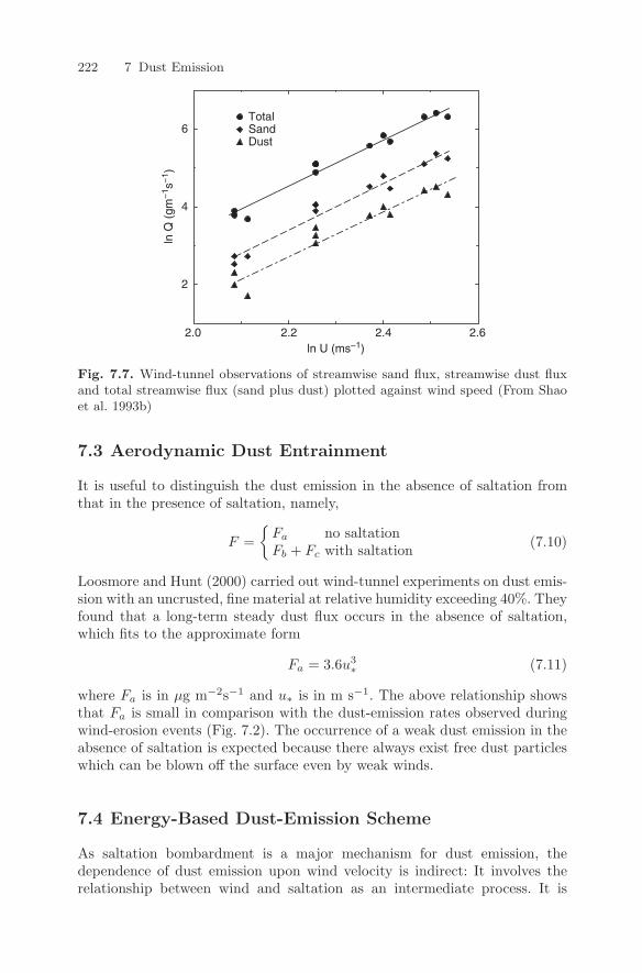
222 7 Dust Emission
2
4
6
ln Q
(gm
−1 s
−1 )
TotalSandDust
2.0 2.2 2.4 2.6ln U (ms−1)
Fig. 7.7. Wind-tunnel observations of streamwise sand flux, streamwise dust fluxand total streamwise flux (sand plus dust) plotted against wind speed (From Shaoet al. 1993b)
7.3 Aerodynamic Dust Entrainment
It is useful to distinguish the dust emission in the absence of saltation fromthat in the presence of saltation, namely,
F =
Fa no saltationFb + Fc with saltation (7.10)
Loosmore and Hunt (2000) carried out wind-tunnel experiments on dust emis-sion with an uncrusted, fine material at relative humidity exceeding 40%. Theyfound that a long-term steady dust flux occurs in the absence of saltation,which fits to the approximate form
Fa = 3.6u3∗ (7.11)
where Fa is in µg m−2s−1 and u∗ is in m s−1. The above relationship showsthat Fa is small in comparison with the dust-emission rates observed duringwind-erosion events (Fig. 7.2). The occurrence of a weak dust emission in theabsence of saltation is expected because there always exist free dust particleswhich can be blown off the surface even by weak winds.
7.4 Energy-Based Dust-Emission Scheme
As saltation bombardment is a major mechanism for dust emission, thedependence of dust emission upon wind velocity is indirect: It involves therelationship between wind and saltation as an intermediate process. It is
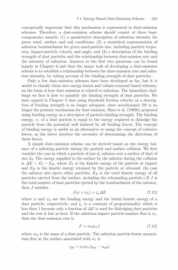
7.4 Energy-Based Dust-Emission Scheme 223
conceptually important that this mechanism is represented in dust-emissionschemes. Therefore, a dust-emission scheme should consist of three basiccomponents: namely, (1) a quantitative description of saltation intensity forgiven wind, surface and soil conditions; (2) a statistical representation ofsaltation bombardment for given sand-particle size, including particle trajec-tory, impact-particle velocity and angle; and (3) a description of the bindingstrength of dust particles and the relationship between dust-mission rate andthe intensity of saltation. Answers to the first two questions can be foundlargely in Chapter 6 and thus the major task of developing a dust-emissionscheme is to establish a relationship between the dust-emission rate and salta-tion intensity, by taking account of the binding strength of dust particles.
Only a few dust-emission schemes have been developed so far, but it isuseful to classify them into energy-based and volume-removal based schemes,on the basis of how dust emission is related to saltation. The immediate chal-lenge we face is how to quantify the binding strength of dust particles. Wehave argued in Chapter 5 that using threshold friction velocity as a descrip-tion of binding strength is no longer adequate, since aerodynamic lift is nolonger the primary mechanism for dust emission. Shao et al. (1993b) proposedusing binding energy as a descriptor of particle-binding strength. The bindingenergy, ψ, of a dust particle is equal to the energy required to dislodge theparticle from the potential well induced by all binding forces. The conceptof binding energy is useful as an alternative to using the concept of cohesiveforces, as the latter involves the necessity of determining the directions ofthese forces.
A simple dust-emission scheme can be derived based on the energy bal-ance of a saltating particle during the particle and surface collision. We firstconsider the case in which a particle of size ds saltates over a surface of dust ofsize dd. The energy supplied to the surface by the saltator during the collisionis ∆E = EI − ER, where EI is the kinetic energy of the particle at impactand ER is the kinetic energy retained by the particle at rebound. (In casethe saltator also ejects other particles, ER is the total kinetic energy of allparticles ejected from the surface, including the rebounding particle.) If J isthe total number of dust particles ejected by the bombardment of the saltator,then J satisfies
J(ψ + ψk) = ζe∆E (7.12)
where ψ and ψk are the binding energy and the initial kinetic energy of adust particle, respectively; and ζe is a constant of proportionality which isless than 1 because only a fraction of ∆E is used for dislodging dust particlesand the rest is lost as heat. If the saltation-impact particle-number flux is nI ,then the dust-emission rate is
F = mdnIJ (7.13)
where md is the mass of a dust particle. The saltation particle-borne momen-tum flux at the surface associated with nI is
τp0 = nIms(upI − upR)
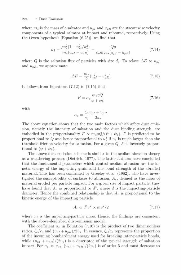
224 7 Dust Emission
where ms is the mass of a saltator and upI and upR are the streamwise velocitycomponents of a typical saltator at impact and rebound, respectively. Usingthe Owen hypothesis [Equation (6.25)], we find that
nI =ρu2
∗(1 − u2∗t/u2
∗)ms(upI − upR)
=Qg
comsu∗(upI − upR)(7.14)
where Q is the saltation flux of particles with size ds. To relate ∆E to upI
and upR, we approximate
∆E =ms
2(u2
pI − u2pR) (7.15)
It follows from Equations (7.12) to (7.15) that
F = αemdgQ
ψ + ψk(7.16)
withαe =
ζe
co
upI + upR
2u∗
The above equation shows that the two main factors which affect dust emis-sion, namely the intensity of saltation and the dust binding strength, areembodied in the proportionality F ∝ mdgQ/(ψ + ψk). F is predicted to beproportional to Q and hence proportional to u3
∗ if u∗ is much larger than thethreshold friction velocity for saltation. For a given Q, F is inversely propor-tional to (ψ + ψk).
The above dust-emission scheme is similar to the aeolian-abrasion theoryas a weathering process (Dietrich, 1977). The latter authors have concludedthat the fundamental parameters which control aeolian abrasion are the ki-netic energy of the impacting grain and the bond strength of the abradedmaterial. This has been confirmed by Greeley et al. (1982), who have inves-tigated the susceptibility of surfaces to abrasion, Ar, defined as the mass ofmaterial eroded per particle impact. For a given size of impact particle, theyhave found that Ar is proportional to d3, where d is the impacting-particlediameter. Hence the combined relationship is that Ar is proportional to thekinetic energy of the impacting particle
Ar ∝ d3v2 ∝ mv2/2 (7.17)
where m is the impacting-particle mass. Hence, the findings are consistentwith the above-described dust-emission model.
The coefficient αe in Equation (7.16) is the product of two dimensionlessratios, ζe/co and (upI + upR)/2u∗. In essence, ζe/co represents the proportionof the incoming bombardment energy used for breaking inter-particle bonds,while (upI + upR)/(2u∗) is a descriptor of the typical strength of saltationimpact. For u∗ u∗t, (upI + upR)/(2u∗) is of order 5 and must decrease to
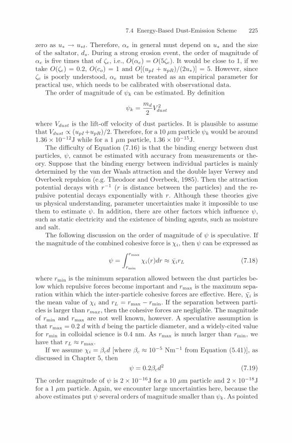
7.4 Energy-Based Dust-Emission Scheme 225
zero as u∗ → u∗t. Therefore, αe in general must depend on u∗ and the sizeof the saltator, ds. During a strong erosion event, the order of magnitude ofαe is five times that of ζe, i.e., O(αe) = O(5ζe). It would be close to 1, if wetake O(ζe) = 0.2, O(co) = 1 and O[(upI + upR)/(2u∗)] = 5. However, sinceζe is poorly understood, αe must be treated as an empirical parameter forpractical use, which needs to be calibrated with observational data.
The order of magnitude of ψk can be estimated. By definition
ψk =md
2V 2
dust
where Vdust is the lift-off velocity of dust particles. It is plausible to assumethat Vdust ∝ (upI+upR)/2. Therefore, for a 10 µm particle ψk would be around1.36 × 10−12J while for a 1 µm particle, 1.36 × 10⁻¹⁵J.
The difficulty of Equation (7.16) is that the binding energy between dustparticles, ψ, cannot be estimated with accuracy from measurements or the-ory. Suppose that the binding energy between individual particles is mainlydetermined by the van der Waals attraction and the double layer Verwey andOverbeek repulsion (e.g. Theodoor and Overbeek, 1985). Then the attractionpotential decays with r−1 (r is distance between the particles) and the re-pulsive potential decays exponentially with r. Although these theories giveus physical understanding, parameter uncertainties make it impossible to usethem to estimate ψ. In addition, there are other factors which influence ψ,such as static electricity and the existence of binding agents, such as moistureand salt.
The following discussion on the order of magnitude of ψ is speculative. Ifthe magnitude of the combined cohesive force is χi, then ψ can be expressed as
ψ =∫ rmax
rmin
χi(r)dr ≈ χirL (7.18)
where rmin is the minimum separation allowed between the dust particles be-low which repulsive forces become important and rmax is the maximum sepa-ration within which the inter-particle cohesive forces are effective. Here, χi isthe mean value of χi and rL = rmax − rmin. If the separation between parti-cles is larger than rmax, then the cohesive forces are negligible. The magnitudeof rmin and rmax are not well known, however. A speculative assumption isthat rmax = 0.2 d with d being the particle diameter, and a widely-cited valuefor rmin in colloidal science is 0.4 nm. As rmax is much larger than rmin, wehave that rL ≈ rmax.
If we assume χi = βcd [where βc ≈ 10−5 Nm−1 from Equation (5.41)], asdiscussed in Chapter 5, then
ψ = 0.2βcd2 (7.19)
The order magnitude of ψ is 2 × 10⁻¹⁶J for a 10 µm particle and 2 × 10⁻¹⁸Jfor a 1 µm particle. Again, we encounter large uncertainties here, because theabove estimates put ψ several orders of magnitude smaller than ψk. As pointed
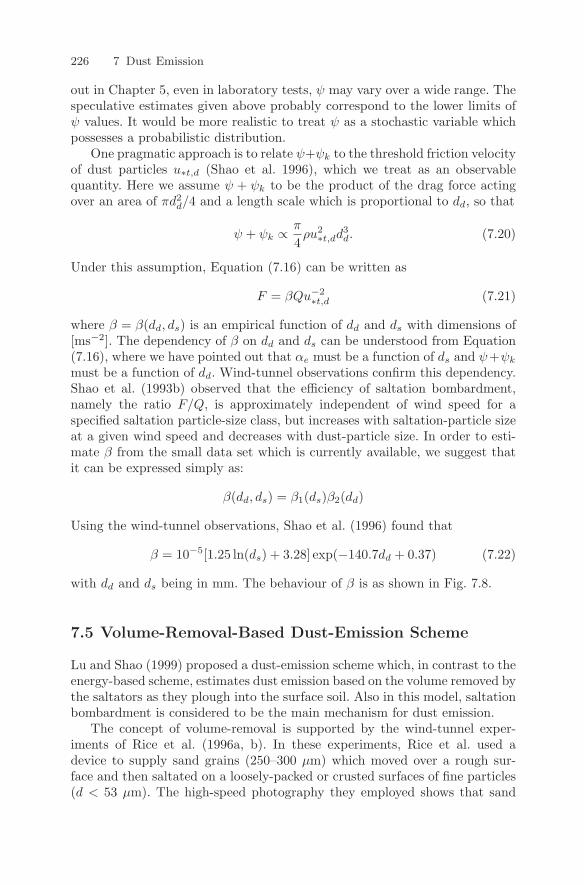
226 7 Dust Emission
out in Chapter 5, even in laboratory tests, ψ may vary over a wide range. Thespeculative estimates given above probably correspond to the lower limits ofψ values. It would be more realistic to treat ψ as a stochastic variable whichpossesses a probabilistic distribution.
One pragmatic approach is to relate ψ+ψk to the threshold friction velocityof dust particles u∗t,d (Shao et al. 1996), which we treat as an observablequantity. Here we assume ψ + ψk to be the product of the drag force actingover an area of πd2
d/4 and a length scale which is proportional to dd, so that
ψ + ψk ∝ π
4ρu2
∗t,dd3d. (7.20)
Under this assumption, Equation (7.16) can be written as
F = βQu−2∗t,d (7.21)
where β = β(dd, ds) is an empirical function of dd and ds with dimensions of[ms−2]. The dependency of β on dd and ds can be understood from Equation(7.16), where we have pointed out that αe must be a function of ds and ψ+ψk
must be a function of dd. Wind-tunnel observations confirm this dependency.Shao et al. (1993b) observed that the efficiency of saltation bombardment,namely the ratio F/Q, is approximately independent of wind speed for aspecified saltation particle-size class, but increases with saltation-particle sizeat a given wind speed and decreases with dust-particle size. In order to esti-mate β from the small data set which is currently available, we suggest thatit can be expressed simply as:
β(dd, ds) = β1(ds)β2(dd)
Using the wind-tunnel observations, Shao et al. (1996) found that
β = 10−5[1.25 ln(ds) + 3.28] exp(−140.7dd + 0.37) (7.22)
with dd and ds being in mm. The behaviour of β is as shown in Fig. 7.8.
7.5 Volume-Removal-Based Dust-Emission Scheme
Lu and Shao (1999) proposed a dust-emission scheme which, in contrast to theenergy-based scheme, estimates dust emission based on the volume removed bythe saltators as they plough into the surface soil. Also in this model, saltationbombardment is considered to be the main mechanism for dust emission.
The concept of volume-removal is supported by the wind-tunnel exper-iments of Rice et al. (1996a, b). In these experiments, Rice et al. used adevice to supply sand grains (250–300 µm) which moved over a rough sur-face and then saltated on a loosely-packed or crusted surfaces of fine particles(d < 53 µm). The high-speed photography they employed shows that sand
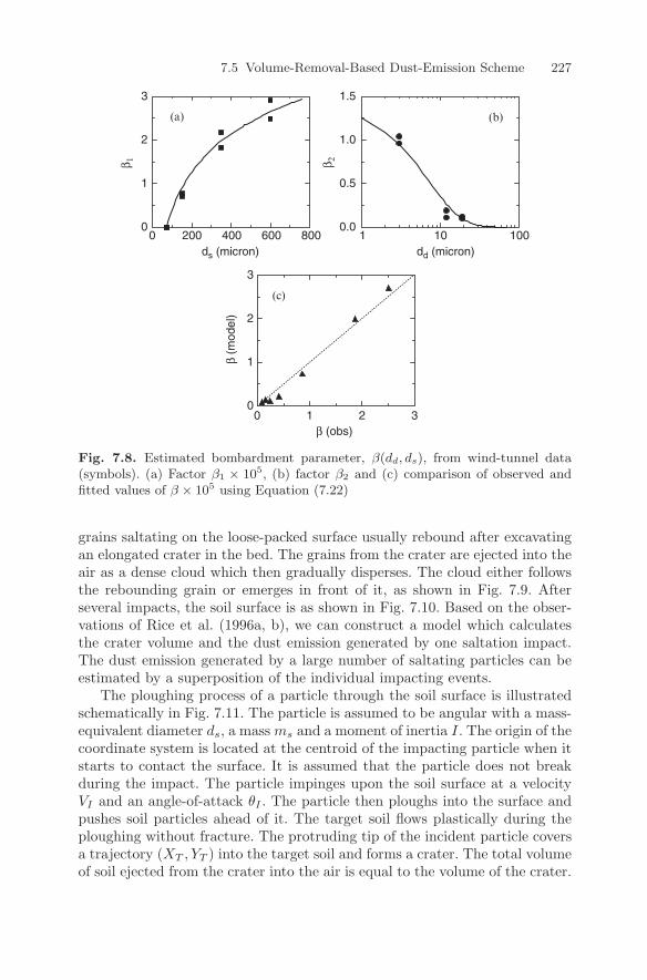
7.5 Volume-Removal-Based Dust-Emission Scheme 227
β (obs)
(a) (b)
(c)
0
1
2
3
0 1 10 100
0 1 2 3
200 400 600 800
0
1
2
3
β 1 β 2
β (m
odel
)0.0
0.5
1.0
1.5
ds (micron) dd (micron)
Fig. 7.8. Estimated bombardment parameter, β(dd, ds), from wind-tunnel data(symbols). (a) Factor β1 × 10⁵, (b) factor β2 and (c) comparison of observed andfitted values of β × 105 using Equation (7.22)
grains saltating on the loose-packed surface usually rebound after excavatingan elongated crater in the bed. The grains from the crater are ejected into theair as a dense cloud which then gradually disperses. The cloud either followsthe rebounding grain or emerges in front of it, as shown in Fig. 7.9. Afterseveral impacts, the soil surface is as shown in Fig. 7.10. Based on the obser-vations of Rice et al. (1996a, b), we can construct a model which calculatesthe crater volume and the dust emission generated by one saltation impact.The dust emission generated by a large number of saltating particles can beestimated by a superposition of the individual impacting events.
The ploughing process of a particle through the soil surface is illustratedschematically in Fig. 7.11. The particle is assumed to be angular with a mass-equivalent diameter ds, a mass ms and a moment of inertia I. The origin of thecoordinate system is located at the centroid of the impacting particle when itstarts to contact the surface. It is assumed that the particle does not breakduring the impact. The particle impinges upon the soil surface at a velocityVI and an angle-of-attack θI . The particle then ploughs into the surface andpushes soil particles ahead of it. The target soil flows plastically during theploughing without fracture. The protruding tip of the incident particle coversa trajectory (XT , YT ) into the target soil and forms a crater. The total volumeof soil ejected from the crater into the air is equal to the volume of the crater.
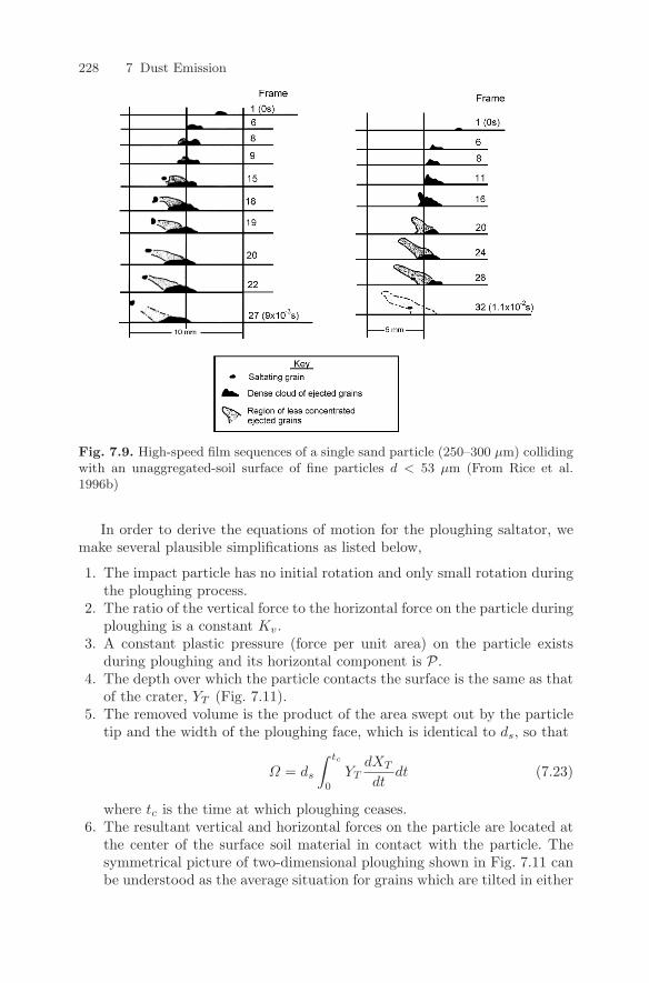
228 7 Dust Emission
Fig. 7.9. High-speed film sequences of a single sand particle (250–300 µm) collidingwith an unaggregated-soil surface of fine particles d < 53 µm (From Rice et al.1996b)
In order to derive the equations of motion for the ploughing saltator, wemake several plausible simplifications as listed below,
1. The impact particle has no initial rotation and only small rotation duringthe ploughing process.
2. The ratio of the vertical force to the horizontal force on the particle duringploughing is a constant Kv.
3. A constant plastic pressure (force per unit area) on the particle existsduring ploughing and its horizontal component is P.
4. The depth over which the particle contacts the surface is the same as thatof the crater, YT (Fig. 7.11).
5. The removed volume is the product of the area swept out by the particletip and the width of the ploughing face, which is identical to ds, so that
Ω = ds
∫ tc
0
YTdXT
dtdt (7.23)
where tc is the time at which ploughing ceases.6. The resultant vertical and horizontal forces on the particle are located at
the center of the surface soil material in contact with the particle. Thesymmetrical picture of two-dimensional ploughing shown in Fig. 7.11 canbe understood as the average situation for grains which are tilted in either
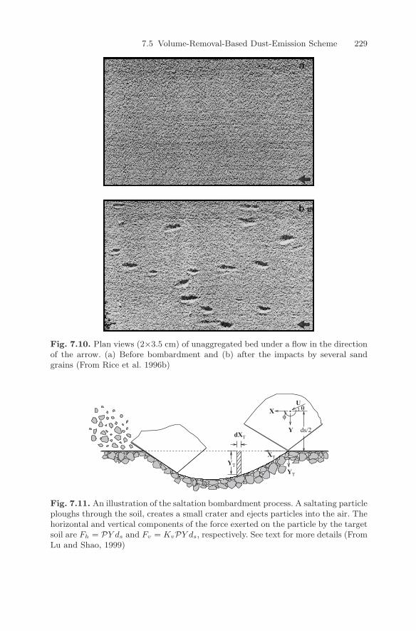
7.5 Volume-Removal-Based Dust-Emission Scheme 229
Fig. 7.10. Plan views (2×3.5 cm) of unaggregated bed under a flow in the directionof the arrow. (a) Before bombardment and (b) after the impacts by several sandgrains (From Rice et al. 1996b)
ds/2
XT
φX
Y
U
YT
dXT
YT
θ
Fig. 7.11. An illustration of the saltation bombardment process. A saltating particleploughs through the soil, creates a small crater and ejects particles into the air. Thehorizontal and vertical components of the force exerted on the particle by the targetsoil are Fh = PY ds and Fv = KvPY ds, respectively. See text for more details (FromLu and Shao, 1999)
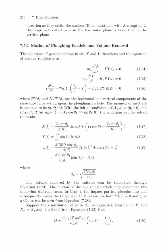
230 7 Dust Emission
direction as they strike the surface. To be consistent with Assumption 2,the projected contact area in the horizontal plane is twice that in thevertical plane.
7.5.1 Motion of Ploughing Particle and Volume Removal
The equations of particle motion in the X and Y directions and the equationof angular rotation ω are
msd2X
dt2+ PY ds = 0 (7.24)
msd2Y
dt2+ KvPY ds = 0 (7.25)
Id2ω
dt2+ PdsY
(ds
2− Y
)− 2(KvPY ds)Y = 0 (7.26)
where PY ds and KvPY ds are the horizontal and vertical components of theresistance force acting upon the ploughing particle. The moment of inertia Iis assumed to be msd
2s/12. With the initial conditions (X,Y, ω) = (0, 0, 0) and
(dX/dt, dY/dt, dω/dt) = (VI cos θI , VI sin θI , 0), the equations can be solvedto obtain
X(t) =VI sin θI
βvKvsin βvt +
(VI cos θI −
VI sin θI
Kv
)t (7.27)
Y (t) =VI
βvsin θI sin βvt (7.28)
ω(t) =3.75V 2
I sin2 θI
β2vd2
s
[2(βvt)2 + cos 2βvt − 1
](7.29)
+3VI sin θI
βvds(sin βvt − βvt)
where
βv =√
PKvds
ms
The volume removed by the saltator can be calculated throughEquation (7.23). The motion of the ploughing particle may encounter twosomewhat different cases. In Case 1, the impact particle ploughs into andsubsequently leaves the target soil. In this case, we have Y (tc) = 0 and tc =π/βv, as can be seen from Equation (7.28).
Suppose the contribution of ω to XT is neglected, then YT = Y andXT = X, and it is found from Equation (7.23) that
Ω =2msV
2I sin2 θI
KvP
(cot θI −
1Kv
). (7.30)
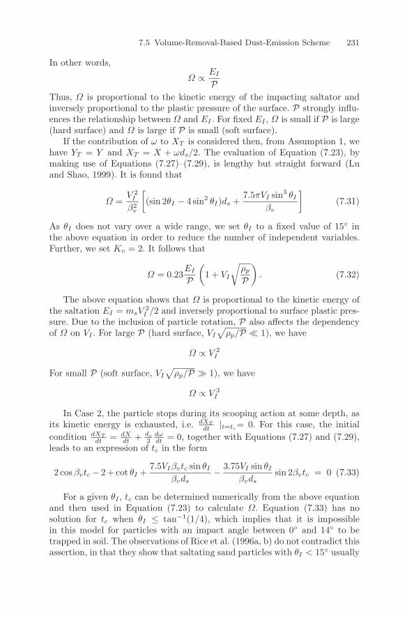
7.5 Volume-Removal-Based Dust-Emission Scheme 231
In other words,
Ω ∝ EI
PThus, Ω is proportional to the kinetic energy of the impacting saltator andinversely proportional to the plastic pressure of the surface. P strongly influ-ences the relationship between Ω and EI . For fixed EI , Ω is small if P is large(hard surface) and Ω is large if P is small (soft surface).
If the contribution of ω to XT is considered then, from Assumption 1, wehave YT = Y and XT = X + ωds/2. The evaluation of Equation (7.23), bymaking use of Equations (7.27)–(7.29), is lengthy but straight forward (Luand Shao, 1999). It is found that
Ω =V 2
I
β2v
[(sin 2θI − 4 sin2 θI)ds +
7.5πVI sin3 θI
βv
](7.31)
As θI does not vary over a wide range, we set θI to a fixed value of 15 inthe above equation in order to reduce the number of independent variables.Further, we set Kv = 2. It follows that
Ω = 0.23EI
P
(1 + VI
√ρp
P
). (7.32)
The above equation shows that Ω is proportional to the kinetic energy ofthe saltation EI = msV
2I /2 and inversely proportional to surface plastic pres-
sure. Due to the inclusion of particle rotation, P also affects the dependencyof Ω on VI . For large P (hard surface, VI
√ρp/P 1), we have
Ω ∝ V 2I
For small P (soft surface, VI
√ρp/P 1), we have
Ω ∝ V 3I
In Case 2, the particle stops during its scooping action at some depth, asits kinetic energy is exhausted, i.e. dXT
dt |t=tc= 0. For this case, the initial
condition dXT
dt = dXdt + ds
2dωdt = 0, together with Equations (7.27) and (7.29),
leads to an expression of tc in the form
2 cos βvtc − 2 + cot θI +7.5VIβvtc sin θI
βvds− 3.75VI sin θI
βvdssin 2βvtc = 0 (7.33)
For a given θI , tc can be determined numerically from the above equationand then used in Equation (7.23) to calculate Ω. Equation (7.33) has nosolution for tc when θI ≤ tan−1(1/4), which implies that it is impossiblein this model for particles with an impact angle between 0 and 14 to betrapped in soil. The observations of Rice et al. (1996a, b) do not contradict thisassertion, in that they show that saltating sand particles with θI < 15 usually
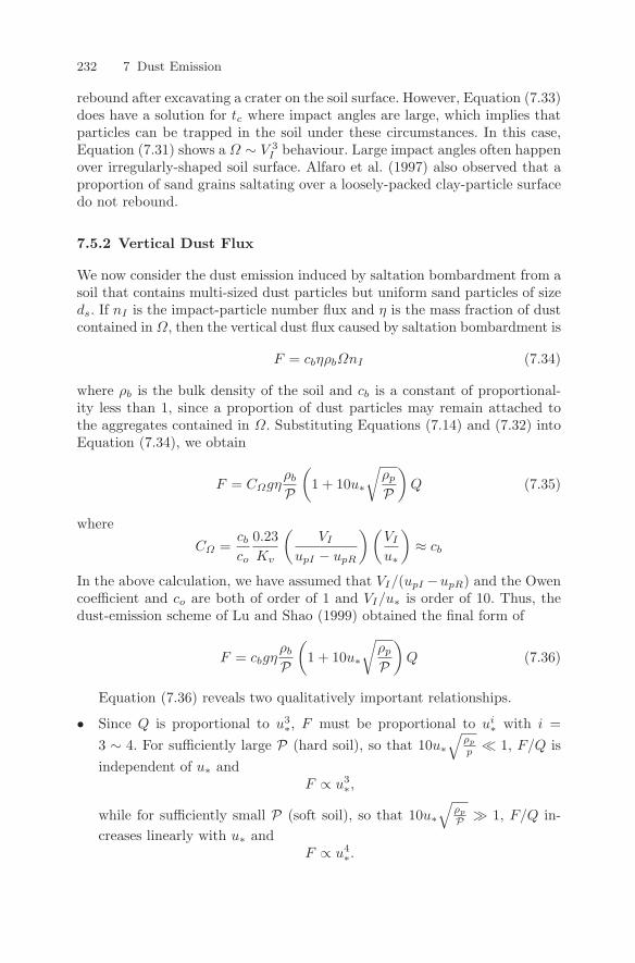
232 7 Dust Emission
rebound after excavating a crater on the soil surface. However, Equation (7.33)does have a solution for tc where impact angles are large, which implies thatparticles can be trapped in the soil under these circumstances. In this case,Equation (7.31) shows a Ω ∼ V 3
I behaviour. Large impact angles often happenover irregularly-shaped soil surface. Alfaro et al. (1997) also observed that aproportion of sand grains saltating over a loosely-packed clay-particle surfacedo not rebound.
7.5.2 Vertical Dust Flux
We now consider the dust emission induced by saltation bombardment from asoil that contains multi-sized dust particles but uniform sand particles of sizeds. If nI is the impact-particle number flux and η is the mass fraction of dustcontained in Ω, then the vertical dust flux caused by saltation bombardment is
F = cbηρbΩnI (7.34)
where ρb is the bulk density of the soil and cb is a constant of proportional-ity less than 1, since a proportion of dust particles may remain attached tothe aggregates contained in Ω. Substituting Equations (7.14) and (7.32) intoEquation (7.34), we obtain
F = CΩgηρb
P
(1 + 10u∗
√ρp
P
)Q (7.35)
where
CΩ =cb
co
0.23Kv
(VI
upI − upR
)(VI
u∗
)≈ cb
In the above calculation, we have assumed that VI/(upI −upR) and the Owencoefficient and co are both of order of 1 and VI/u∗ is order of 10. Thus, thedust-emission scheme of Lu and Shao (1999) obtained the final form of
F = cbgηρb
P
(1 + 10u∗
√ρp
P
)Q (7.36)
Equation (7.36) reveals two qualitatively important relationships.
• Since Q is proportional to u3∗, F must be proportional to ui
∗ with i =3 ∼ 4. For sufficiently large P (hard soil), so that 10u∗
√ρp
p 1, F/Q isindependent of u∗ and
F ∝ u3∗,
while for sufficiently small P (soft soil), so that 10u∗
√ρp
P 1, F/Q in-creases linearly with u∗ and
F ∝ u4∗.
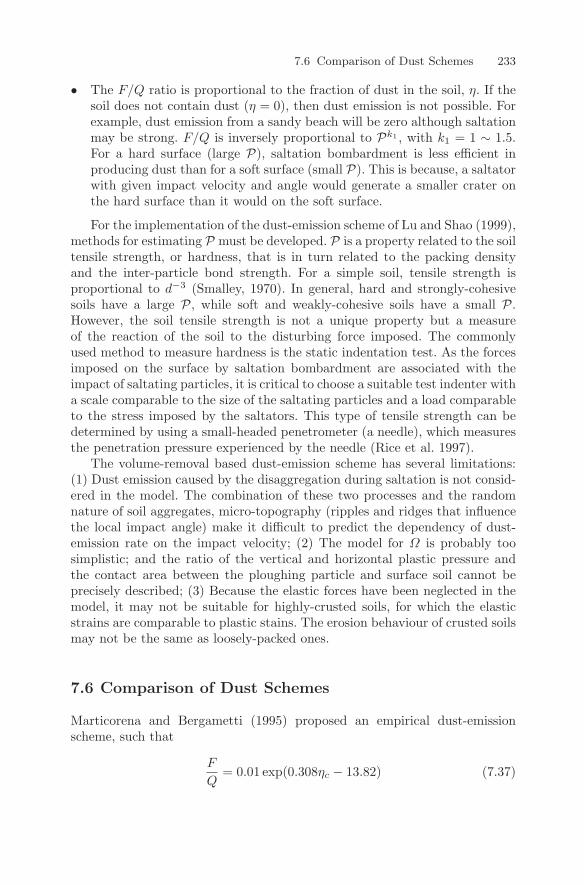
7.6 Comparison of Dust Schemes 233
• The F/Q ratio is proportional to the fraction of dust in the soil, η. If thesoil does not contain dust (η = 0), then dust emission is not possible. Forexample, dust emission from a sandy beach will be zero although saltationmay be strong. F/Q is inversely proportional to Pk1 , with k1 = 1 ∼ 1.5.For a hard surface (large P), saltation bombardment is less efficient inproducing dust than for a soft surface (small P). This is because, a saltatorwith given impact velocity and angle would generate a smaller crater onthe hard surface than it would on the soft surface.
For the implementation of the dust-emission scheme of Lu and Shao (1999),methods for estimating P must be developed. P is a property related to the soiltensile strength, or hardness, that is in turn related to the packing densityand the inter-particle bond strength. For a simple soil, tensile strength isproportional to d−3 (Smalley, 1970). In general, hard and strongly-cohesivesoils have a large P, while soft and weakly-cohesive soils have a small P.However, the soil tensile strength is not a unique property but a measureof the reaction of the soil to the disturbing force imposed. The commonlyused method to measure hardness is the static indentation test. As the forcesimposed on the surface by saltation bombardment are associated with theimpact of saltating particles, it is critical to choose a suitable test indenter witha scale comparable to the size of the saltating particles and a load comparableto the stress imposed by the saltators. This type of tensile strength can bedetermined by using a small-headed penetrometer (a needle), which measuresthe penetration pressure experienced by the needle (Rice et al. 1997).
The volume-removal based dust-emission scheme has several limitations:(1) Dust emission caused by the disaggregation during saltation is not consid-ered in the model. The combination of these two processes and the randomnature of soil aggregates, micro-topography (ripples and ridges that influencethe local impact angle) make it difficult to predict the dependency of dust-emission rate on the impact velocity; (2) The model for Ω is probably toosimplistic; and the ratio of the vertical and horizontal plastic pressure andthe contact area between the ploughing particle and surface soil cannot beprecisely described; (3) Because the elastic forces have been neglected in themodel, it may not be suitable for highly-crusted soils, for which the elasticstrains are comparable to plastic stains. The erosion behaviour of crusted soilsmay not be the same as loosely-packed ones.
7.6 Comparison of Dust Schemes
Marticorena and Bergametti (1995) proposed an empirical dust-emissionscheme, such that
F
Q= 0.01 exp(0.308ηc − 13.82) (7.37)
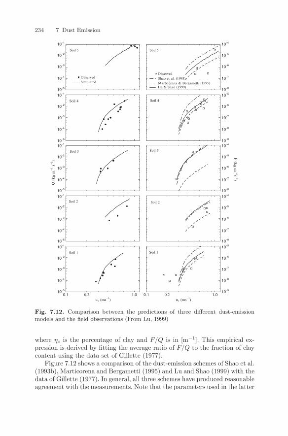
234 7 Dust Emission
Q (kg
m−
1 s−
1 )
ObservedSimulated
u* (ms−1)u* (ms−1)
F (kg m
−2s
−1)
ObservedShao et al. (1993)Marticorena & Bergametti (1995)Lu & Shao (1999)
Soil 1 Soil 1
Soil 2 Soil 2
Soil 3 Soil 3
Soil 4 Soil 4
Soil 5 Soil 5
10−1
10−2
10−3
10−4
10−5
10−1
10−2
10−3
10−4
10−5
10−1
10−2
10−3
10−4
10−5
10−1
10−2
10−3
10−4
10−5
10−1
10−2
10−3
10−4
10−5
10−4
10−5
10−6
10−7
10−8
10−5
10−6
10−7
10−8
10−9
10−4
10−5
10−6
10−7
10−8
10−4
10−5
10−6
10−7
10−8
10−5
10−6
10−7
10−8
10−9
0.1 1.00.2 0.1 1.00.2
Fig. 7.12. Comparison between the predictions of three different dust-emissionmodels and the field observations (From Lu, 1999)
where ηc is the percentage of clay and F/Q is in [m−1]. This empirical ex-pression is derived by fitting the average ratio of F/Q to the fraction of claycontent using the data set of Gillette (1977).
Figure 7.12 shows a comparison of the dust-emission schemes of Shao et al.(1993b), Marticorena and Bergametti (1995) and Lu and Shao (1999) with thedata of Gillette (1977). In general, all three schemes have produced reasonableagreement with the measurements. Note that the parameters used in the latter
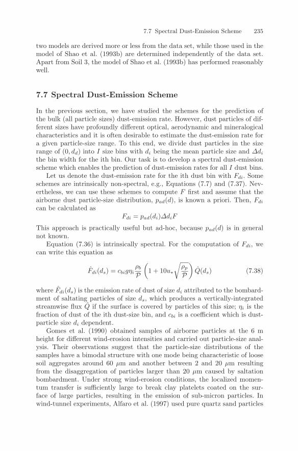
7.7 Spectral Dust-Emission Scheme 235
two models are derived more or less from the data set, while those used in themodel of Shao et al. (1993b) are determined independently of the data set.Apart from Soil 3, the model of Shao et al. (1993b) has performed reasonablywell.
7.7 Spectral Dust-Emission Scheme
In the previous section, we have studied the schemes for the prediction ofthe bulk (all particle sizes) dust-emission rate. However, dust particles of dif-ferent sizes have profoundly different optical, aerodynamic and mineralogicalcharacteristics and it is often desirable to estimate the dust-emission rate fora given particle-size range. To this end, we divide dust particles in the sizerange of (0, dd) into I size bins with di being the mean particle size and ∆di
the bin width for the ith bin. Our task is to develop a spectral dust-emissionscheme which enables the prediction of dust-emission rates for all I dust bins.
Let us denote the dust-emission rate for the ith dust bin with Fdi. Someschemes are intrinsically non-spectral, e.g., Equations (7.7) and (7.37). Nev-ertheless, we can use these schemes to compute F first and assume that theairborne dust particle-size distribution, pad(d), is known a priori. Then, Fdi
can be calculated asFdi = pad(di)∆diF
This approach is practically useful but ad-hoc, because pad(d) is in generalnot known.
Equation (7.36) is intrinsically spectral. For the computation of Fdi, wecan write this equation as
Fdi(ds) = cbigηiρb
P
(1 + 10u∗
√ρp
P
)Q(ds) (7.38)
where Fdi(ds) is the emission rate of dust of size di attributed to the bombard-ment of saltating particles of size ds, which produces a vertically-integratedstreamwise flux Q if the surface is covered by particles of this size; ηi is thefraction of dust of the ith dust-size bin, and cbi is a coefficient which is dust-particle size di dependent.
Gomes et al. (1990) obtained samples of airborne particles at the 6 mheight for different wind-erosion intensities and carried out particle-size anal-ysis. Their observations suggest that the particle-size distributions of thesamples have a bimodal structure with one mode being characteristic of loosesoil aggregates around 60 µm and another between 2 and 20 µm resultingfrom the disaggregation of particles larger than 20 µm caused by saltationbombardment. Under strong wind-erosion conditions, the localized momen-tum transfer is sufficiently large to break clay platelets coated on the sur-face of large particles, resulting in the emission of sub-micron particles. Inwind-tunnel experiments, Alfaro et al. (1997) used pure quartz sand particles
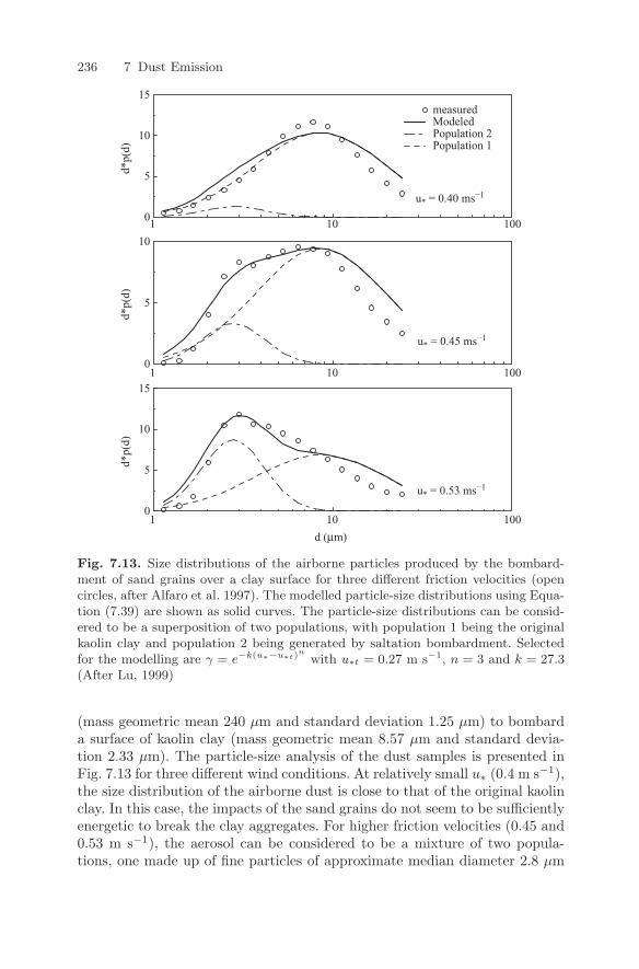
236 7 Dust Emission
d (µm)
d*p(
d)d*
p(d)
d*p(
d)measuredModeledPopulation 2Population 1
u* = 0.40 ms−1
u* = 0.45 ms−1
u* = 0.53 ms−1
10
15
10
15
0
5
0
5
10
0
5
1 10010
1 10010
1 10010
Fig. 7.13. Size distributions of the airborne particles produced by the bombard-ment of sand grains over a clay surface for three different friction velocities (opencircles, after Alfaro et al. 1997). The modelled particle-size distributions using Equa-tion (7.39) are shown as solid curves. The particle-size distributions can be consid-ered to be a superposition of two populations, with population 1 being the originalkaolin clay and population 2 being generated by saltation bombardment. Selectedfor the modelling are γ = e−k(u∗−u∗t)
n
with u∗t = 0.27 m s−1, n = 3 and k = 27.3(After Lu, 1999)
(mass geometric mean 240 µm and standard deviation 1.25 µm) to bombarda surface of kaolin clay (mass geometric mean 8.57 µm and standard devia-tion 2.33 µm). The particle-size analysis of the dust samples is presented inFig. 7.13 for three different wind conditions. At relatively small u∗ (0.4 m s−1),the size distribution of the airborne dust is close to that of the original kaolinclay. In this case, the impacts of the sand grains do not seem to be sufficientlyenergetic to break the clay aggregates. For higher friction velocities (0.45 and0.53 m s−1), the aerosol can be considered to be a mixture of two popula-tions, one made up of fine particles of approximate median diameter 2.8 µm
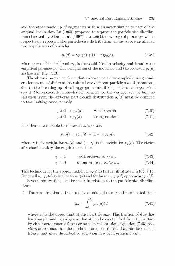
7.7 Spectral Dust-Emission Scheme 237
and the other made up of aggregates with a diameter similar to that of theoriginal kaolin clay. Lu (1999) proposed to express the particle-size distribu-tion observed by Alfaro et al. (1997) as a weighted average of p1 and p2 whichrespectively represent the particle-size distributions of the above-mentionedtwo populations of particles
ps(d) = γp1(d) + (1 − γ)p2(d), (7.39)
where γ = e−k(u∗−u∗t)n
and u∗t is threshold friction velocity and k and n areempirical parameters. The comparison of the modelled and the observed ps(d)is shown in Fig. 7.13.
The above example confirms that airborne particles sampled during wind-erosion events of different intensities have different particle-size distributions,due to the breaking up of soil aggregates into finer particles at larger windspeed. More generally, immediately adjacent to the surface, say within thesaltation layer, the airborne particle-size distribution ps(d) must be confinedto two limiting cases, namely
ps(d) → pm(d) weak erosion (7.40)ps(d) → pf (d) strong erosion. (7.41)
It is therefore possible to represent ps(d) using
ps(d) = γpm(d) + (1 − γ)pf (d), (7.42)
where γ is the weight for pm(d) and (1−γ) is the weight for pf (d). The choiceof γ should satisfy the requirements that
γ → 1 weak erosion, u∗ ∼ u∗t (7.43)γ → 0 strong erosion, u∗ u∗t, (7.44)
This technique for the approximation of ps(d) is further illustrated in Fig. 7.14.For small u∗, ps(d) is similar to pm(d) and for large u∗, ps(d) approaches pf (d).
Several observations can be made in relation to the particle-size distribu-tions:
1. The mass fraction of free dust for a unit soil mass can be estimated from
ηm =∫ dd
0
pm(d)δd (7.45)
where dd is the upper limit of dust particle size. This fraction of dust haslow enough binding energy so that it can be easily lifted from the surfaceby either aerodynamic forces or mechanical abrasion. Equation (7.45) pro-vides an estimate for the minimum amount of dust that can be emittedfrom a unit mass disturbed by saltation in a wind erosion event.
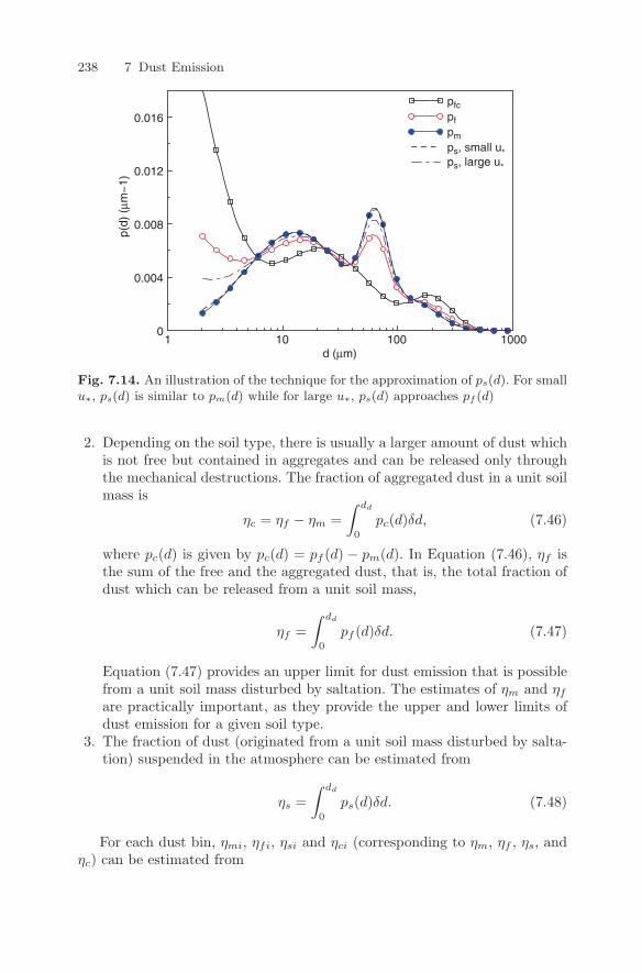
238 7 Dust Emission
d (µm)
p(d)
(µm
−1)
pfcpfpmps, small u*ps, large u*
0
0.004
0.008
0.012
0.016
1 10 100 1000
Fig. 7.14. An illustration of the technique for the approximation of ps(d). For smallu∗, ps(d) is similar to pm(d) while for large u∗, ps(d) approaches pf (d)
2. Depending on the soil type, there is usually a larger amount of dust whichis not free but contained in aggregates and can be released only throughthe mechanical destructions. The fraction of aggregated dust in a unit soilmass is
ηc = ηf − ηm =∫ dd
0
pc(d)δd, (7.46)
where pc(d) is given by pc(d) = pf (d) − pm(d). In Equation (7.46), ηf isthe sum of the free and the aggregated dust, that is, the total fraction ofdust which can be released from a unit soil mass,
ηf =∫ dd
0
pf (d)δd. (7.47)
Equation (7.47) provides an upper limit for dust emission that is possiblefrom a unit soil mass disturbed by saltation. The estimates of ηm and ηf
are practically important, as they provide the upper and lower limits ofdust emission for a given soil type.
3. The fraction of dust (originated from a unit soil mass disturbed by salta-tion) suspended in the atmosphere can be estimated from
ηs =∫ dd
0
ps(d)δd. (7.48)
For each dust bin, ηmi, ηfi, ηsi and ηci (corresponding to ηm, ηf , ηs, andηc) can be estimated from
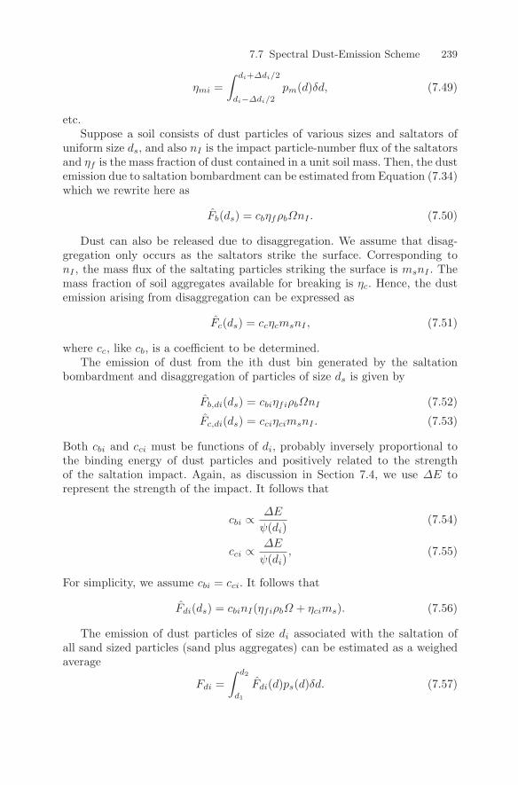
7.7 Spectral Dust-Emission Scheme 239
ηmi =∫ di+∆di/2
di−∆di/2
pm(d)δd, (7.49)
etc.Suppose a soil consists of dust particles of various sizes and saltators of
uniform size ds, and also nI is the impact particle-number flux of the saltatorsand ηf is the mass fraction of dust contained in a unit soil mass. Then, the dustemission due to saltation bombardment can be estimated from Equation (7.34)which we rewrite here as
Fb(ds) = cbηfρbΩnI . (7.50)
Dust can also be released due to disaggregation. We assume that disag-gregation only occurs as the saltators strike the surface. Corresponding tonI , the mass flux of the saltating particles striking the surface is msnI . Themass fraction of soil aggregates available for breaking is ηc. Hence, the dustemission arising from disaggregation can be expressed as
Fc(ds) = ccηcmsnI , (7.51)
where cc, like cb, is a coefficient to be determined.The emission of dust from the ith dust bin generated by the saltation
bombardment and disaggregation of particles of size ds is given by
Fb,di(ds) = cbiηfiρbΩnI (7.52)
Fc,di(ds) = cciηcimsnI . (7.53)
Both cbi and cci must be functions of di, probably inversely proportional tothe binding energy of dust particles and positively related to the strengthof the saltation impact. Again, as discussion in Section 7.4, we use ∆E torepresent the strength of the impact. It follows that
cbi ∝∆E
ψ(di)(7.54)
cci ∝∆E
ψ(di), (7.55)
For simplicity, we assume cbi = cci. It follows that
Fdi(ds) = cbinI(ηfiρbΩ + ηcims). (7.56)
The emission of dust particles of size di associated with the saltation ofall sand sized particles (sand plus aggregates) can be estimated as a weighedaverage
Fdi =∫ d2
d1
Fdi(d)ps(d)δd. (7.57)
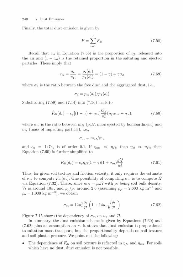
240 7 Dust Emission
Finally, the total dust emission is given by
F =I∑
i=1
Fdi (7.58)
Recall that cbi in Equation (7.56) is the proportion of ηfi released intothe air and (1 − cbi) is the retained proportion in the saltating and ejectedparticles. These imply that
cbi =ηsi
ηfi=
ps(di)pf (di)
= (1 − γ) + γσd (7.59)
where σd is the ratio between the free dust and the aggregated dust, i.e.,
σd = pm(di)/pf (di)
Substituting (7.59) and (7.14) into (7.56) leads to
Fdi(ds) = cy[(1 − γ) + γσd]Qg
u2∗
(ηfiσm + ηci), (7.60)
where σm is the ratio between mΩ (ρbΩ, mass ejected by bombardment) andms (mass of impacting particle), i.e.,
σm = mΩ/ms
and cy = 1/7co is of order 0.1. If ηmi ηfi, then ηci ≈ ηfi, thenEquation (7.60) is further simplified to
Fdi(ds) = cyηfi(1 − γ)(1 + σm)gQ
u2∗
(7.61)
Thus, for given soil texture and friction velocity, it only requires the estimateof σm to compute Fdi(ds). One possibility of computing σm is to compute Ωvia Equation (7.32). There, since mΩ = ρbΩ with ρb being soil bulk density,VI is around 10u∗ and ρp/ρb around 2.6 (assuming ρp = 2,600 kg m−3 andρb = 1,000 kg m−3), we obtain
σm = 12u2∗ρb
P
(1 + 14u∗
√ρb
P
)(7.62)
Figure 7.15 shows the dependency of σm on u∗ and P.In summary, the dust emission scheme is given by Equations (7.60) and
(7.62) plus an assumption on γ. It states that dust emission is proportionalto saltation mass transport, but the proportionality depends on soil textureand soil plastic pressure. We point out the following:
• The dependence of Fdi on soil texture is reflected in ηfi and ηmi. For soilswhich have no dust, dust emission is not possible.
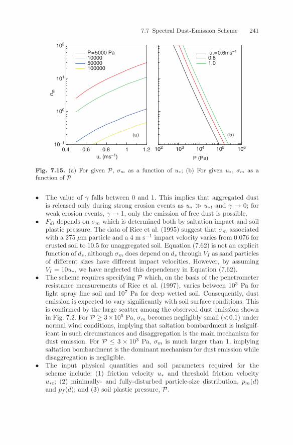
7.7 Spectral Dust-Emission Scheme 241
0.81.0
σ m
(b)(a)
10−1
0.4 0.6 0.8 1 1.2
100
101
102
102 103 104 105 106
P=5000 Pa1000050000100000
u* (ms−1)
u*=0.6ms−1
P (Pa)
Fig. 7.15. (a) For given P, σm as a function of u∗; (b) For given u∗, σm as afunction of P
• The value of γ falls between 0 and 1. This implies that aggregated dustis released only during strong erosion events as u∗ u∗t and γ → 0; forweak erosion events, γ → 1, only the emission of free dust is possible.
• Fdi depends on σm which is determined both by saltation impact and soilplastic pressure. The data of Rice et al. (1995) suggest that σm associatedwith a 275 µm particle and a 4 m s−1 impact velocity varies from 0.076 forcrusted soil to 10.5 for unaggregated soil. Equation (7.62) is not an explicitfunction of ds, although σm does depend on ds through VI as sand particlesof different sizes have different impact velocities. However, by assumingVI = 10u∗, we have neglected this dependency in Equation (7.62).
• The scheme requires specifying P which, on the basis of the penetrometerresistance measurements of Rice et al. (1997), varies between 103 Pa forlight spray fine soil and 107 Pa for deep wetted soil. Consequently, dustemission is expected to vary significantly with soil surface conditions. Thisis confirmed by the large scatter among the observed dust emission shownin Fig. 7.2. For P ≥ 3×10⁵ Pa, σm becomes negligibly small (<0.1) undernormal wind conditions, implying that saltation bombardment is insignif-icant in such circumstances and disaggregation is the main mechanism fordust emission. For P ≤ 3 × 10³ Pa, σm is much larger than 1, implyingsaltation bombardment is the dominant mechanism for dust emission whiledisaggregation is negligible.
• The input physical quantities and soil parameters required for thescheme include: (1) friction velocity u∗ and threshold friction velocityu∗t; (2) minimally- and fully-disturbed particle-size distribution, pm(d)and pf (d); and (3) soil plastic pressure, P.
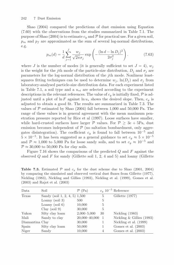
242 7 Dust Emission
Shao (2004) compared the predictions of dust emission using Equation(7.60) with the observations from the studies summarized in Table 7.1. Thepurpose of Shao (2004) is to estimate cy andP for practical use. For a given soil,pm and pf are approximated as the sum of several log-normal distributions,e.g.
pm(d) =1d
J∑j=1
wj√2πσj
exp
(− (ln d − ln Dj)2
2σ2j
). (7.63)
where J is the number of modes (it is generally sufficient to set J = 4), wj
is the weight for the jth mode of the particle-size distribution, Dj and σj areparameters for the log-normal distribution of the jth mode. Nonlinear least-squares fitting techniques can be used to determine wj , ln(Dj) and σj fromlaboratory-analysed particle-size distribution data. For each experiment listedin Table 7.1, a soil type and a u∗t are selected according to the experimentdescriptions in the relevant references. The value of cy is initially fixed, P is ad-justed until a plot of lnF against lnu∗ shows the desired slope. Then, cy isadjusted to obtain a good fit. The results are summarized in Table 7.3. Thevalues of P estimated by Shao (2004) fall between 1,000 and 50,000 Pa. Therange of these values is in general agreement with the mean maximum pen-etration pressure reported by Rice et al (1997). Loose surfaces have smaller,while hard-crusted surfaces have larger P values. For P ≥ 3e + 5Pa, dustemission becomes independent of P (no saltation bombardment, only aggre-gates disintegration). The coefficient cy is found to fall between 10−5 and5 × 10−5. It has been suggested as a general guidance to set cy ≈ 5 × 10⁻⁵
and P ≈ 1,000 to 5,000 Pa for loose sandy soils, and to set cy ≈ 10−5 andP ≈ 30,000 to 50,000 Pa for clay soils.
Figure 7.16 shows the comparisons of the predicted Q and F against theobserved Q and F for sandy (Gillette soil 1, 2, 4 and 5) and loamy (Gillette
Table 7.3. Estimated P and cy for the dust scheme due to Shao (2001, 2004)by comparing the simulated and observed vertical dust fluxes from Gillette (1977),Nickling (1983), Nickling and Gillies (1993), Nickling et al. (1999), Gomes et al.(2003) and Rajot et al. (2003)
Data Soil P (Pa) cy 10−5 Reference
Texas Sandy (soil 1, 2, 4, 5) 1,500 5 Gillette (1977)Loamy (soil 3) 500 5Loamy (soil 6) 10,000 5Clay (soil 9) 30,000 5
Yukon Silty clay loam 2,000–5,000 30 Nickling (1983)Mali Sandy to clay 20,000–40,000 1 Nickling & Gillies (1993)Diamantina Clay 30,000 1 Nickling et al. (1999)Spain Silty clay loam 50,000 1 Gomes et al. (2003)Niger Sandy 10,000 4 Gomes et al. (2003)
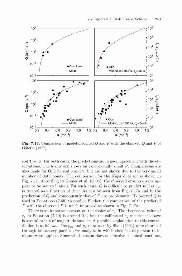
7.7 Spectral Dust-Emission Scheme 243
u* (ms−1)
Obs, sandModel
Q (
gm−
1 s−
1 )
F (
ugm
−2s−
1 )F
(ug
m−
2s−
1 )
Q (
gm−
1 s−
1 )
Obs, loam
ModelObsModed, p = 500Pa, cy= 5e−5
ObsModed, p = 1500Pa, cy= 5e−5
10−2
0.2 0.4 0.6 0.8 1.0 1.2u* (ms−1)
0.2 0.4 0.6 0.8 1.0 1.2
10−1
10−2
10−1
100
101
102
100
101
102
101
102
103
104
105
106
101
100
102
103
104
105
Fig. 7.16. Comparison of model-predicted Q and F with the observed Q and F ofGillette (1977)
soil 3) soils. For both cases, the predictions are in good agreement with the ob-servations. The loamy soil shows an exceptionally small P. Comparisons arealso made for Gillette soil 6 and 9, but are not shown due to the very smallnumber of data points. The comparison for the Niger data set is shown inFig. 7.17. According to Gomes et al. (2003), the observed erosion events ap-pear to be source limited. For such cases, Q is difficult to predict unless u∗t
is treated as a function of time. As can be seen from Fig. 7.17a and b, theprediction of Q and consequently that of F are problematic. If observed Q isused in Equations (7.60) to predict F , then the comparison of the predictedF with the observed F is much improved as shown in Fig. 7.17c.
There is an important caveat on the choice of cy. The theoretical value ofcy in Equation (7.60) is around 0.1, but the calibrated cy mentioned aboveis several orders of magnitude smaller. A possible explanation to this contra-diction is as follows. The pm and pf data used by Shao (2004) were obtainedthrough laboratory particle-size analysis in which chemical-dispersion tech-niques were applied. Since wind erosion does not involve chemical reactions,
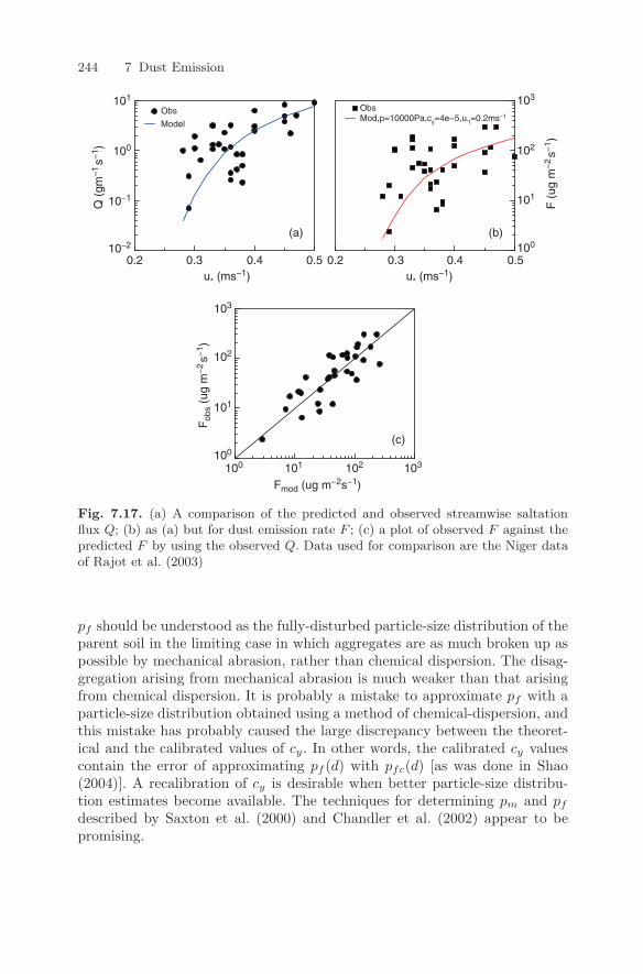
244 7 Dust Emission
u* (ms−1) u* (ms−1)
Q (
gm−
1s−
1 )Obs
Model
100
101
102
103
102
101
100
100 101 102 103
103
F (
ug m
−2s−
1 )
Fob
s (u
g m
−2s−
1 )
ObsMod,p=10000Pa,cy=4e−5,u*t=0.2ms−1
(a) (b)
(c)
10−2
0.2 0.20.3 0.30.4 0.40.5 0.5
10−1
100
101
Fmod (ug m−2s−1)
Fig. 7.17. (a) A comparison of the predicted and observed streamwise saltationflux Q; (b) as (a) but for dust emission rate F ; (c) a plot of observed F against thepredicted F by using the observed Q. Data used for comparison are the Niger dataof Rajot et al. (2003)
pf should be understood as the fully-disturbed particle-size distribution of theparent soil in the limiting case in which aggregates are as much broken up aspossible by mechanical abrasion, rather than chemical dispersion. The disag-gregation arising from mechanical abrasion is much weaker than that arisingfrom chemical dispersion. It is probably a mistake to approximate pf with aparticle-size distribution obtained using a method of chemical-dispersion, andthis mistake has probably caused the large discrepancy between the theoret-ical and the calibrated values of cy. In other words, the calibrated cy valuescontain the error of approximating pf (d) with pfc(d) [as was done in Shao(2004)]. A recalibration of cy is desirable when better particle-size distribu-tion estimates become available. The techniques for determining pm and pf
described by Saxton et al. (2000) and Chandler et al. (2002) appear to bepromising.
7.8 Discussions on Dust Schemes 245
7.8 Discussions on Dust Schemes
Our current capacity for modelling dust emission is still limited. It is nowagreed in general that the main mechanisms for dust emission are saltationbombardment and disaggregation. Therefore, dust emission must be directlyrelated to the intensity of saltation and indirectly related to wind shear atthe surface. Also importantly, dust emission must be inversely proportionalto the binding strength of dust particles. There are three types of dust-emission schemes, i.e., empirical forms, energy-based schemes and volume-removal based schemes. The energy-based schemes relate dust emission tosand drift, but the derivation of the dust-emission scheme does not state howdust emission precisely takes place. It therefore does not require detailed in-formation about individual saltating particles. The major difficulty of theenergy-based schemes is that the binding energy for dust particles is difficultto determine and the kinetic energy converted to heat during the impact isnot readily estimated. In contrast, the volume-removal based dust-emissionscheme takes into consideration the detailed physical process of dust emis-sion. In this model, the concept of binding is realised through the use of theplastic pressure, P, a descriptor of the binding strength of the soil surface, andthrough the use of cbi in Equation (7.56), a descriptor of the binding strengthof the soil aggregates.
The increased understanding of wind-erosion physics has enabled the de-velopment of dust-emission schemes on a firmer footing. However, the accuracyof the dust-emission schemes is limited by the lack of capacity in specifying thetemporal and spatial variations of model parameters. The difficulty in achiev-ing the accuracy of dust-emission schemes is exacerbated by the fact that dustemission can vary over several orders of magnitude. There is also a serious lackof high quality dust-flux measurements for dust-scheme validation.
The few existing dust-emission schemes are listed in Table 7.4. Discussionson the advantages and disadvantages of these schemes are further given inChapter 9.
Table 7.4. Dust-emission schemes. G77: Gillette (1977); GP88: Gillette and Passi(1988); MB95: Marticorena and Bergametti (1995); SRL96: Shao et al. (1996); LS99:Lu and Shao (1999); S04: Shao (2004)
Scheme Expression References Comments
1 F = αgu4∗(1 − u∗t/u∗) GP88 Hypothesis
2 F = 0.01Q exp(0.308ηc − 13.82) MB95 Empirical form3 F = βQu−2
∗t,d SRL96 Theory
4 F = (cbgηρb/P)(1 + 14u∗√
ρb/P)Q LS99 Theory
5 Fdi(ds) = cyηfi(1 − γ)(1 + σm)gQ/u2∗;
Fdi =∫
Fdi(d)ps(d)δd; F =∑
Fdi S04 Theory
8
Dust Transport and Deposition
Dust particles, once airborne, can be carried by winds to various distancesfrom the source region and deposited back onto the surface somewhere down-stream. Dust transport and deposition are thus key links in the dust cycle. Theunderstanding of these processes has applications in a wide range of researchfields. From the perspective of geological studies, dust transport and depo-sition are important mechanisms for the delivery of sediments and mineralsfrom continent to ocean and for the evolution of surface topography. For ex-ample, the formation of the loess plateau in China is believed to be a result ofthe deposition of dust and silt particles originating from the upstream desertareas. In the atmosphere, the presence of dust particles influences processessuch as cloud formation and radiation transfer. High concentration of fineparticulates in air is of concern to human health, and PM10 and PM2.5 havebeen used as key indicators of air quality. Dust particles from certain regionsmay carry harmful substances, and the fates of such particles are naturallyof environmental concern. In this chapter, we focus on the physics of dusttransport and deposition and study how these processes can be quantified.
8.1 Evidence of Dust Transport and Deposition
The distance dust particles travel in the atmosphere depends on flow condi-tions and particle size. It is useful to establish an approximate relationshipbetween dust-particle size and travel distance for specific atmospheric condi-tions. Suppose dust particles are raised by a storm which is strong enough tomix them though an atmospheric layer of depth H. Then the concentrationof dust in this layer obeys approximately
U∂ρc
∂x= −∂F
∂z(8.1)
where U is wind speed, x is distance, F is vertical dust flux and z is height.An integration of Equation (8.1) over z from the surface to the top of the dust
Y. Shao, Physics and Modelling of Wind Erosion, 247c© Springer Science+Business Media B.V. 2008
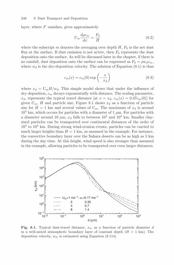
248 8 Dust Transport and Deposition
layer, where F vanishes, gives approximately
Umdρcm
dx=
F0
H(8.2)
where the subscript m denotes the averaging over depth H, F0 is the net dustflux at the surface. If dust emission is not active, then F0 represents the dustdeposition onto the surface. As will be discussed later in the chapter, if there isno rainfall, dust deposition onto the surface can be expressed as F0 = ρwdcm,where wd is the dry-deposition velocity. The solution of Equation (8.1) is thus
cm(x) = cm(0) exp(− x
xd
)(8.3)
where xd = UmH/wd. This simple model shows that under the influence ofdry deposition, cm decays exponentially with distance. The scaling parameter,xd, represents the typical travel distance [at x = xd, cm(x) = 0.37cm(0)] forgiven Um, H and particle size. Figure 8.1 shows xd as a function of particlesize for H = 1 km and several values of Um. The maximum of xd is around105 km, which occurs for particles with a diameter of 1 µm. For particles witha diameter around 10 µm, xd falls to between 102 and 103 km. Smaller clay-sized particles can be transported over continental distances of the order of103 to 104 km. During strong wind-erosion events, particles can be carried tomuch larger heights than H = 1 km, as assumed in the example. For instance,the convective boundary layer over the Sahara deserts can be as high as 5 kmduring the day time. At this height, wind speed is also stronger than assumedin the example, allowing particles to be transported over even larger distances.
d (µm)
x d (
km)
Um=1 ms−1; u*=0.17 ms−1
10−1
100
101
102
103
104
105
48
10310210110010−110−2
20.71.4
0.35
Fig. 8.1. Typical dust-travel distance, xd, as a function of particle diameter din a well-mixed atmospheric boundary layer of constant depth (H = 1 km). Thedeposition velocity, wd, is estimated using Equation (8.114)
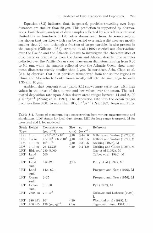
8.1 Evidence of Dust Transport and Deposition 249
Equation (8.3) indicates that, in general, particles travelling over largedistances are smaller than 20 µm. This prediction is supported by observa-tions. Particle-size analysis of dust samples collected by aircraft in southwestUnited States, hundreds of kilometres downstream from the source region,has shown that particles which can be carried over such a distance are mostlysmaller than 20 µm, although a fraction of larger particles is also present inthe samples (Gillette, 1981). Arimoto et al. (1997) carried out observationsover the Pacific and the Atlantic Oceans to investigate the characteristics ofdust particles originating from the Asian and African deserts. The samplescollected over the Pacific Ocean show mass-mean diameters ranging from 0.36to 5.4 µm, while the samples collected over the Atlantic Ocean show mass-mean diameters mostly smaller than 3 µm. In northeast Asia, Chun et al.(2001b) observed that dust particles transported from the source regions inChina and Mongolia to South Korea mostly fall into the size range between1.35 and 10 µm.
Ambient dust concentration (Table 8.1) shows large variations, with highvalues in the areas of dust storms and low values over the ocean. The esti-mated deposition rate upon Asian desert areas ranges between 14 and 2,100g m−2yr−1 (Zhang et al. 1997). The deposition rate into the ocean rangesfrom less than 0.001 to more than 10 g m−2yr−1 (Pye, 1987; Tegen and Fung,
Table 8.1. Range of maximum dust concentration from various measurements andsimulations. LDS stands for local dust storm, LRT for long-range transport, M formeasured and L for modelled
Study Height Concentration Size u∗ ReferenceType (µg m−3) (µm) (m s−1)
LDS 1 m 8×10³–2.5×10⁵ ≤10 0.4–0.6 Gillette and Walker (1977), MLDS 1.5 m 4 × 10³–2.6 × 10⁵ ≤10 0.3–0.5 Gillette and Walker (1977), MLDS 1–10 m 103–105 ≤10 0.3–0.6 Nickling (1978), MLDS 1–10 m 26–13,735 ≤10 0.2–1.0 Nickling and Gillies (1993), MLRT Bld. roof 280–5,000 Gao et al (1992), MLRT Land
surf.500 Talbot et al (1986), M
LRT Landsurf.
3.6–32.3 ≤2.5 Perry et al (1997), M
LRT Landsurf.
14.6–62.1 Prospero and Nees (1976), M
LRT Oceansurf.
2–25 Prospero and Nees (1976), M
LRT Oceansurf.
0.1–60 Pye (1987), M
LRT 2,000 m 2 × 10³ Nickovic and Dobricic (1996),L
LRT 980 hPa 105 ≤10 Westphal et al (1988), LLRT 960 hPa 129 (µg kg−1) Clay Tegen and Fung (1994), L
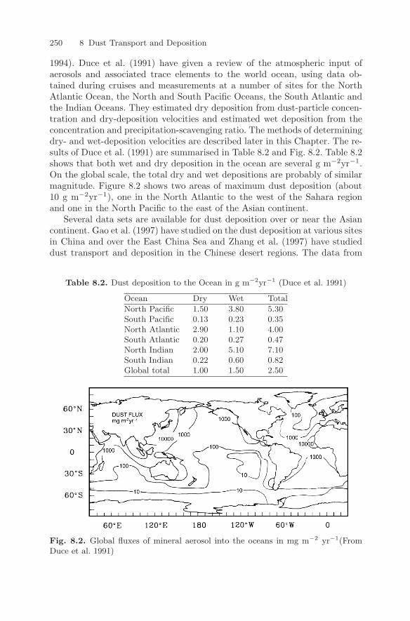
250 8 Dust Transport and Deposition
1994). Duce et al. (1991) have given a review of the atmospheric input ofaerosols and associated trace elements to the world ocean, using data ob-tained during cruises and measurements at a number of sites for the NorthAtlantic Ocean, the North and South Pacific Oceans, the South Atlantic andthe Indian Oceans. They estimated dry deposition from dust-particle concen-tration and dry-deposition velocities and estimated wet deposition from theconcentration and precipitation-scavenging ratio. The methods of determiningdry- and wet-deposition velocities are described later in this Chapter. The re-sults of Duce et al. (1991) are summarised in Table 8.2 and Fig. 8.2. Table 8.2shows that both wet and dry deposition in the ocean are several g m−2yr−1.On the global scale, the total dry and wet depositions are probably of similarmagnitude. Figure 8.2 shows two areas of maximum dust deposition (about10 g m−2yr−1), one in the North Atlantic to the west of the Sahara regionand one in the North Pacific to the east of the Asian continent.
Several data sets are available for dust deposition over or near the Asiancontinent. Gao et al. (1997) have studied on the dust deposition at various sitesin China and over the East China Sea and Zhang et al. (1997) have studieddust transport and deposition in the Chinese desert regions. The data from
Table 8.2. Dust deposition to the Ocean in g m−2yr−1 (Duce et al. 1991)
Ocean Dry Wet Total
North Pacific 1.50 3.80 5.30South Pacific 0.13 0.23 0.35North Atlantic 2.90 1.10 4.00South Atlantic 0.20 0.27 0.47North Indian 2.00 5.10 7.10South Indian 0.22 0.60 0.82Global total 1.00 1.50 2.50
Fig. 8.2. Global fluxes of mineral aerosol into the oceans in mg m−2 yr−1(FromDuce et al. 1991)
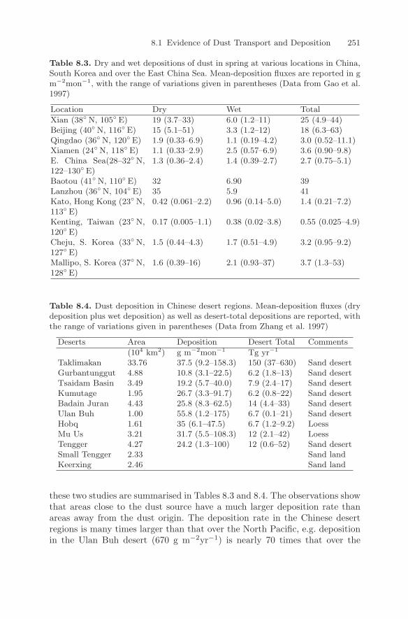
8.1 Evidence of Dust Transport and Deposition 251
Table 8.3. Dry and wet depositions of dust in spring at various locations in China,South Korea and over the East China Sea. Mean-deposition fluxes are reported in gm−2mon−1, with the range of variations given in parentheses (Data from Gao et al.1997)
Location Dry Wet Total
Xian (38 N, 105 E) 19 (3.7–33) 6.0 (1.2–11) 25 (4.9–44)Beijing (40 N, 116 E) 15 (5.1–51) 3.3 (1.2–12) 18 (6.3–63)Qingdao (36 N, 120 E) 1.9 (0.33–6.9) 1.1 (0.19–4.2) 3.0 (0.52–11.1)Xiamen (24 N, 118 E) 1.1 (0.33–2.9) 2.5 (0.57–6.9) 3.6 (0.90–9.8)E. China Sea(28–32 N,122–130 E)
1.3 (0.36–2.4) 1.4 (0.39–2.7) 2.7 (0.75–5.1)
Baotou (41 N, 110 E) 32 6.90 39Lanzhou (36 N, 104 E) 35 5.9 41Kato, Hong Kong (23 N,113 E)
0.42 (0.061–2.2) 0.96 (0.14–5.0) 1.4 (0.21–7.2)
Kenting, Taiwan (23 N,120 E)
0.17 (0.005–1.1) 0.38 (0.02–3.8) 0.55 (0.025–4.9)
Cheju, S. Korea (33 N,127 E)
1.5 (0.44–4.3) 1.7 (0.51–4.9) 3.2 (0.95–9.2)
Mallipo, S. Korea (37 N,128 E)
1.6 (0.39–16) 2.1 (0.93–37) 3.7 (1.3–53)
Table 8.4. Dust deposition in Chinese desert regions. Mean-deposition fluxes (drydeposition plus wet deposition) as well as desert-total depositions are reported, withthe range of variations given in parentheses (Data from Zhang et al. 1997)
Deserts Area Deposition Desert Total Comments
(104 km2) g m−2mon−1 Tg yr−1
Taklimakan 33.76 37.5 (9.2–158.3) 150 (37–630) Sand desertGurbantunggut 4.88 10.8 (3.1–22.5) 6.2 (1.8–13) Sand desertTsaidam Basin 3.49 19.2 (5.7–40.0) 7.9 (2.4–17) Sand desertKumutage 1.95 26.7 (3.3–91.7) 6.2 (0.8–22) Sand desertBadain Juran 4.43 25.8 (8.3–62.5) 14 (4.4–33) Sand desertUlan Buh 1.00 55.8 (1.2–175) 6.7 (0.1–21) Sand desertHobq 1.61 35 (6.1–47.5) 6.7 (1.2–9.2) LoessMu Us 3.21 31.7 (5.5–108.3) 12 (2.1–42) LoessTengger 4.27 24.2 (1.3–100) 12 (0.6–52) Sand desertSmall Tengger 2.33 Sand landKeerxing 2.46 Sand land
these two studies are summarised in Tables 8.3 and 8.4. The observations showthat areas close to the dust source have a much larger deposition rate thanareas away from the dust origin. The deposition rate in the Chinese desertregions is many times larger than that over the North Pacific, e.g. depositionin the Ulan Buh desert (670 g m−2yr−1) is nearly 70 times that over the
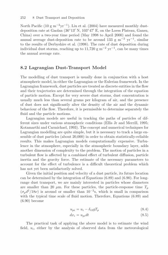
252 8 Dust Transport and Deposition
North Pacific (10 g m−2yr−1). Liu et al. (2004) have measured monthly dust-deposition rate at Gaolan (3613′ N, 10347′ E, on the Loess Plateau, Gansu,China) over a two-year time period (May 1998 to April 2000) and found theannual average dust-deposition rate to be around 133 g m−2 yr−1, similarto the results of Derbyshire et al. (1998). The rate of dust deposition duringindividual dust storms, reaching up to 11,720 g m−2 yr−1, can be many timesthe annual average rate.
8.2 Lagrangian Dust-Transport Model
The modelling of dust transport is usually done in conjunction with a hostatmospheric model, in either the Lagrangian or the Eulerian framework. In theLagrangian framework, dust particles are treated as discrete entities in the flowand their trajectories are determined through the integration of the equationof particle motion. Except for very severe dust storms, dust concentration isusually much less than several grams per kilogram of air, and the presenceof dust does not significantly alter the density of the air and the dynamicbehaviour of the flow. Therefore, it is permissible to determine separately thefluid and the particle motions.
Lagrangian models are useful in tracking the paths of particles of dif-ferent sizes under various atmospheric conditions (Ellis Jr and Merrill, 1995;Kotamarthi and Carmichael, 1993). The concept and numerical techniques forLagrangian modelling are quite simple, but it is necessary to track a large en-semble of dust particles (about 20,000) in order to obtain statistically-reliableresults. This makes Lagrangian models computationally expensive. Turbu-lence in the atmosphere, especially in the atmospheric boundary layer, addsanother dimension of complexity to the problem. The motion of particles in aturbulent flow is affected by a combined effect of turbulent diffusion, particleinertia and the gravity force. The estimate of the necessary parameters toaccount for the effect of turbulence is a difficult theoretical problem whichhas not yet been satisfactorily solved.
Given the initial position and velocity of a dust particle, its future locationcan be determined by the integration of Equations (6.89) and (6.90). For long-range dust transport, we are mainly interested in particles whose diametersare smaller than 20 µm. For these particles, the particle-response time Tp
(σpd2/18ν) is around or smaller than 10−2s, which is small in comparison
with the typical time scale of fluid motion. Therefore, Equations (6.89) and(6.90) become
upi = ui − δi3gTp (8.4)dxi = upidt (8.5)
The practical task of applying the above model is to estimate the windfield, ui, either by the analysis of observed data from the meteorological
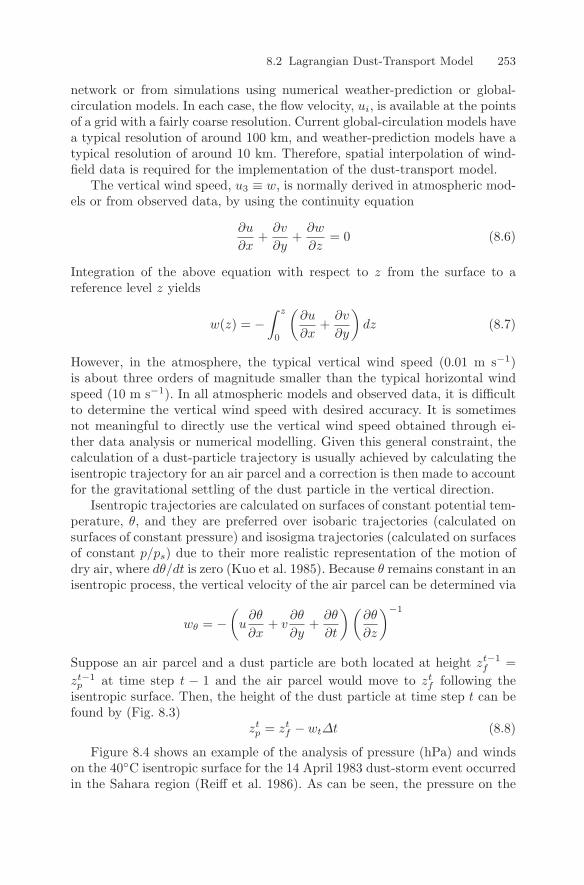
8.2 Lagrangian Dust-Transport Model 253
network or from simulations using numerical weather-prediction or global-circulation models. In each case, the flow velocity, ui, is available at the pointsof a grid with a fairly coarse resolution. Current global-circulation models havea typical resolution of around 100 km, and weather-prediction models have atypical resolution of around 10 km. Therefore, spatial interpolation of wind-field data is required for the implementation of the dust-transport model.
The vertical wind speed, u3 ≡ w, is normally derived in atmospheric mod-els or from observed data, by using the continuity equation
∂u
∂x+
∂v
∂y+
∂w
∂z= 0 (8.6)
Integration of the above equation with respect to z from the surface to areference level z yields
w(z) = −∫ z
0
(∂u
∂x+
∂v
∂y
)dz (8.7)
However, in the atmosphere, the typical vertical wind speed (0.01 m s−1)is about three orders of magnitude smaller than the typical horizontal windspeed (10 m s−1). In all atmospheric models and observed data, it is difficultto determine the vertical wind speed with desired accuracy. It is sometimesnot meaningful to directly use the vertical wind speed obtained through ei-ther data analysis or numerical modelling. Given this general constraint, thecalculation of a dust-particle trajectory is usually achieved by calculating theisentropic trajectory for an air parcel and a correction is then made to accountfor the gravitational settling of the dust particle in the vertical direction.
Isentropic trajectories are calculated on surfaces of constant potential tem-perature, θ, and they are preferred over isobaric trajectories (calculated onsurfaces of constant pressure) and isosigma trajectories (calculated on surfacesof constant p/ps) due to their more realistic representation of the motion ofdry air, where dθ/dt is zero (Kuo et al. 1985). Because θ remains constant in anisentropic process, the vertical velocity of the air parcel can be determined via
wθ = −(
u∂θ
∂x+ v
∂θ
∂y+
∂θ
∂t
)(∂θ
∂z
)−1
Suppose an air parcel and a dust particle are both located at height zt−1f =
zt−1p at time step t − 1 and the air parcel would move to zt
f following theisentropic surface. Then, the height of the dust particle at time step t can befound by (Fig. 8.3)
ztp = zt
f − wt∆t (8.8)
Figure 8.4 shows an example of the analysis of pressure (hPa) and windson the 40C isentropic surface for the 14 April 1983 dust-storm event occurredin the Sahara region (Reiff et al. 1986). As can be seen, the pressure on the
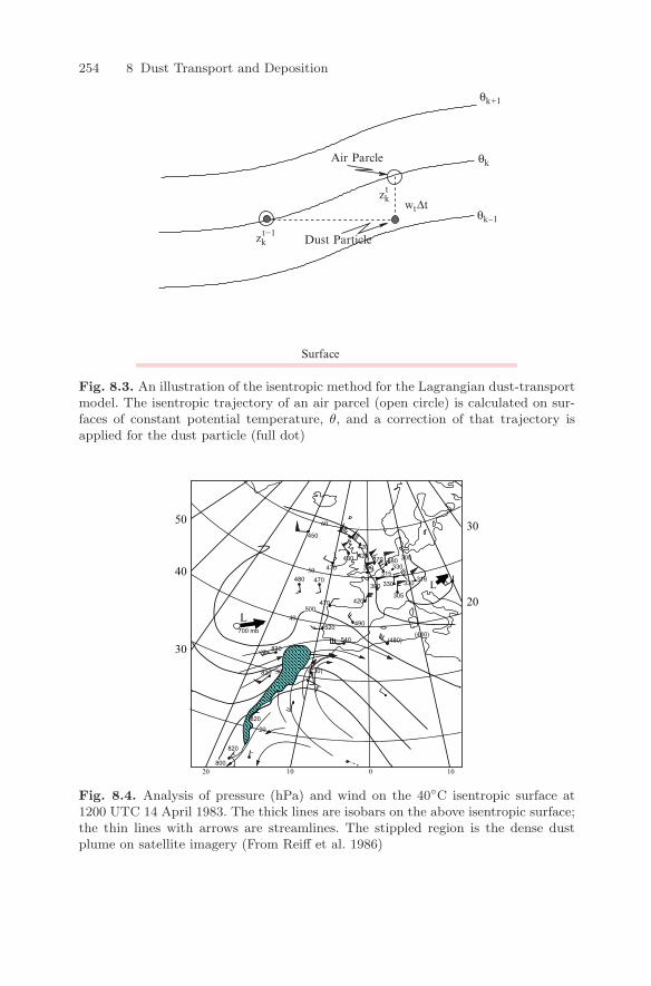
254 8 Dust Transport and Deposition
zkt−1
zkt
Surface
Dust Particle
Air Parcle
wt∆t
θk+1
θk-1
θk
Fig. 8.3. An illustration of the isentropic method for the Lagrangian dust-transportmodel. The isentropic trajectory of an air parcel (open circle) is calculated on sur-faces of constant potential temperature, θ, and a correction of that trajectory isapplied for the dust particle (full dot)
20 001 10
60
50
40
30
20
800
820
820
820
830
700 mb
L
L
500
520
540
490
470
470480
470430
450
420420
380 305330
330 316330
305
315390
370
420
(480)(440)
(730)
390
50 30
20
40
30
Fig. 8.4. Analysis of pressure (hPa) and wind on the 40C isentropic surface at1200 UTC 14 April 1983. The thick lines are isobars on the above isentropic surface;the thin lines with arrows are streamlines. The stippled region is the dense dustplume on satellite imagery (From Reiff et al. 1986)
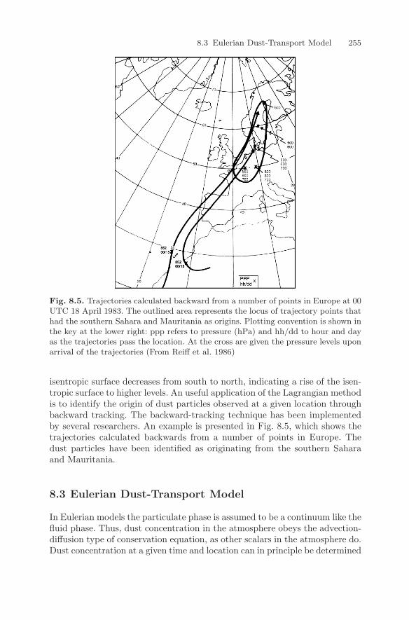
8.3 Eulerian Dust-Transport Model 255
Fig. 8.5. Trajectories calculated backward from a number of points in Europe at 00UTC 18 April 1983. The outlined area represents the locus of trajectory points thathad the southern Sahara and Mauritania as origins. Plotting convention is shown inthe key at the lower right: ppp refers to pressure (hPa) and hh/dd to hour and dayas the trajectories pass the location. At the cross are given the pressure levels uponarrival of the trajectories (From Reiff et al. 1986)
isentropic surface decreases from south to north, indicating a rise of the isen-tropic surface to higher levels. An useful application of the Lagrangian methodis to identify the origin of dust particles observed at a given location throughbackward tracking. The backward-tracking technique has been implementedby several researchers. An example is presented in Fig. 8.5, which shows thetrajectories calculated backwards from a number of points in Europe. Thedust particles have been identified as originating from the southern Saharaand Mauritania.
8.3 Eulerian Dust-Transport Model
In Eulerian models the particulate phase is assumed to be a continuum like thefluid phase. Thus, dust concentration in the atmosphere obeys the advection-diffusion type of conservation equation, as other scalars in the atmosphere do.Dust concentration at a given time and location can in principle be determined
256 8 Dust Transport and Deposition
if the sources and sinks of dust are specified and the initial and boundary con-ditions for the concentration field are given. One major challenge here, though,is that the processes, such as particle diffusion, dry deposition and wet depo-sition, must be adequately represented in the concentration equation. Sincemost atmospheric-flow models are formulated in the Eulerian framework, theadvection-diffusion type of conservation equation for dust particles can be in-corporated into them and solved with similar numerical techniques as alreadyexist in the atmospheric models.
Let us rewrite Equation (3.24) as
∂c
∂t+ u
∂c
∂x+ v
∂c
∂y+ (w − wt)
∂c
∂z
=∂
∂xKpx
∂c
∂x+
∂
∂yKpy
∂c
∂y+
∂
∂zKpz
∂c
∂z+ Sr + Sc
(8.9)
where Kpx, Kpy and Kpz are the dust-particle eddy diffusivities for the x, yand z directions, Sr is a source (or sink) term arising from wet removal andSc is a source (or sink) term arising from the dust-flux convergence due to dryand wet convections. The accompanying lower and upper boundary conditionsare
ρ(w − wt)c − ρKpz∂c
∂z= F0 at the surface
Kpz∂c
∂z= 0 at the top of the atmosphere
(8.10)
where F0 is the dust flux at the surface. In areas of active wind erosion, F0
is determined from the dust-emission schemes described in Chapter 7, andin areas with no active wind erosion, F0 is the flux caused by dry depositionwhich will be described in Section 8.6 of this chapter.
Numerically, the modelling of dust concentration and transport is closelylinked to the host atmospheric model. Equations (8.9) and (8.10) togetherwith the conditions for the side boundaries of the simulation domain can besolved for the prediction of dust concentration. The equations and boundaryconditions need to be discretised in accordance with the grid system of thehost atmospheric model, using either finite differencing or other discretisa-tion schemes. It is more elegant to solve Equation (8.9) simultaneously withother governing equations for the atmosphere, but it is often more convenientto solve it after the host atmospheric model has completed the calculationsfor each time step and the flow-field data for the new time step have be-come available. The host atmospheric model also calculates the eddy diffu-sivities, Kx, Ky and Kz, for passive scalars, from the modification of whichthe eddy diffusivity for dust particles, Kpx, Kpy and Kpz (Section 8.4) can bederived.
Because the particle terminal velocity, wt, and the eddy diffusivities fordust particles, Kpx etc., depend on particle size, it is desirable to separate dust
8.3 Eulerian Dust-Transport Model 257
particles into I dust bins, each with a particle-size range di+∆di. Suppose theconcentration of the ith particle-size group is ci, then the total concentration is
c =I∑
i=1
ci
The transport of each particle-size bin can then be treated independently ofthe other size bins, using Equation (8.9) and replacing c with ci
∂ci
∂t+ u
∂ci
∂x+ v
∂ci
∂y+ (w − wti)
∂ci
∂z
=∂
∂xKpxi
∂ci
∂x+
∂
∂yKpyi
∂ci
∂y+
∂
∂zKpzi
∂ci
∂z+ Sri + Sci
(8.11)
A unified set of rules does not seem to exist for the division of dust particlesinto different size bins (Uno et al. 2006). Westphal et al. (1987) used fourparticle-size intervals: d ≤ 2 µm, 2 < d ≤ 6 µm, 6 < d ≤ 60 µm andd > 60 µm. Tegen and Fung (1995) also used four, but somewhat different,particle-size groups with d ≤ 2 µm, 2 < d ≤ 20 µm, 20 < d ≤ 50 µm andd > 50 µm. It is useful to introduce a uniform set of dust-size bins to facilitatecomparison of future studies. Suppose we use wt as a criterion and assumethat wt varies by a factor of 4 within each dust-size bin or
wti+1/wti = 4
As wt is given by Equation (5.20), we have that
di+1/di = 2
From the above considerations, a division of dust particles into different sizegroups is proposed to be d ≤ 2 µm, 2 < d ≤ 5 µm, 5 < d ≤ 10 µm, 10 < d ≤20 µm, 20 < d ≤ 40 µm etc.
For numerical reasons, the advection-diffusion equation of the typeEquation(8.9) is often solved by splitting the advective from the diffusive terms. Theadvectivetermisfurthersplit intohorizontalandverticaladvections.Toillustratethe procedure, we can write Equation (8.9) as
∂c∗∂t
+ Ah = 0 (8.12)
∂c∗∗∂t
+ Av∗ = 0 (8.13)
∂c∗∗∗∂t
= D∗∗ (8.14)
∂c
∂t= Sr∗∗∗ + Sc∗∗∗ (8.15)
where Ah, Av and D denote the horizontal advective, vertical advective anddiffusive terms, respectively. These equations are solved sequentially. First,
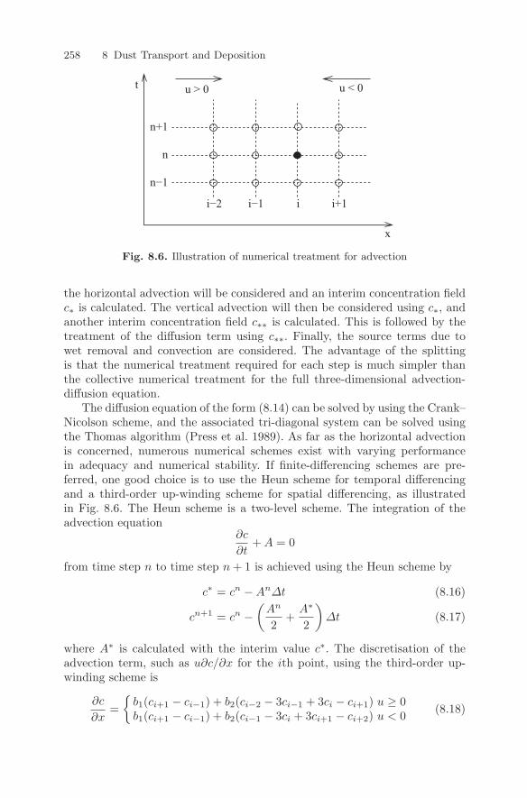
258 8 Dust Transport and Deposition
x
t u > 0 u < 0
i−2 i−1 i i+1
n−1
n+1
n
Fig. 8.6. Illustration of numerical treatment for advection
the horizontal advection will be considered and an interim concentration fieldc∗ is calculated. The vertical advection will then be considered using c∗, andanother interim concentration field c∗∗ is calculated. This is followed by thetreatment of the diffusion term using c∗∗. Finally, the source terms due towet removal and convection are considered. The advantage of the splittingis that the numerical treatment required for each step is much simpler thanthe collective numerical treatment for the full three-dimensional advection-diffusion equation.
The diffusion equation of the form (8.14) can be solved by using the Crank–Nicolson scheme, and the associated tri-diagonal system can be solved usingthe Thomas algorithm (Press et al. 1989). As far as the horizontal advectionis concerned, numerous numerical schemes exist with varying performancein adequacy and numerical stability. If finite-differencing schemes are pre-ferred, one good choice is to use the Heun scheme for temporal differencingand a third-order up-winding scheme for spatial differencing, as illustratedin Fig. 8.6. The Heun scheme is a two-level scheme. The integration of theadvection equation
∂c
∂t+ A = 0
from time step n to time step n + 1 is achieved using the Heun scheme by
c∗ = cn − An∆t (8.16)
cn+1 = cn −(
An
2+
A∗
2
)∆t (8.17)
where A∗ is calculated with the interim value c∗. The discretisation of theadvection term, such as u∂c/∂x for the ith point, using the third-order up-winding scheme is
∂c
∂x=
b1(ci+1 − ci−1) + b2(ci−2 − 3ci−1 + 3ci − ci+1) u ≥ 0b1(ci+1 − ci−1) + b2(ci−1 − 3ci + 3ci+1 − ci+2) u < 0 (8.18)
8.3 Eulerian Dust-Transport Model 259
with b1 = 1/(2δx) and b2 = 1/(6δx). The multi-dimensional wave-propagationslope-limiter approach proposed by LeVeque (1996) is also an excellent schemefor horizontal advection. This scheme is second order accurate in both timeand space and it eliminates numerical oscillations and maintains the positivityof the concentration field.
For vertical advection, the numerical scheme proposed by Bott (1989) ispopular. We rewrite Equation (8.13) as
∂c
∂t= −∂(w − wt)c
∂z(8.19)
With the assumption of constant grid spacing ∆z and time increment ∆t, thefinite difference flux form of the above equation reads
cn+1k = cn
k − ∆t
∆z[fn
k+1/2 − fnk−1/2] (8.20)
where cnk is the value of c at grid point k and time step n and fn
k+1/2 is thevertical flux [i.e. (w−wt)c] at level k + 1/2 and time step n. Bott’s advectionscheme is obtained by a non-linear renormalization of the advective fluxesfn
k+1/2 and fnk−1/2. These fluxes are computed using the integrated flux form
of Tremback et al. (1987) and then applying limits to the upper and lowervalues to make it positive definite. The basic idea is to assume that withingrid box k the distribution of c is given by a polynomial of order of l. Thefluxes can then be written as
fk+1/2 =∆z
∆t
[g+
l,k+1/2
gl,kck −
g−l,k+1/2
gl,k+1ck
]
with
g+l,k+1/2 = max(0, I+
l (ok+1/2))
g−l,k+1/2 = max(0, I−l (ok+1/2))
gl,k = max(Il,k, g+l,k+1/2 + g−l,k+1/2 + ε)
where ε is a small number, I+l (ok+1/2), I−l (ok+1/2) and Il,k are integrals which
can be evaluated as
I+l (ok+1/2) =
l∑j=0
ak,j
(j + 1)2j+1[1 − (1 − 2o+
k )j+1]
I−l (ok+1/2) =l∑
j=0
(−1)jak+1,j
(j + 1)2j+1[1 − (1 − 2o−k )j+1]
Il,k =l∑
j=0
ak,j
(j + 1)2j+1[(−1)j + 1]
o±k = ±(onk+1/2± | on
k+1/2 |)/2
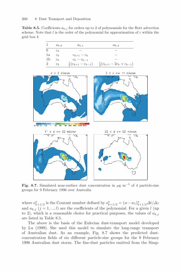
260 8 Dust Transport and Deposition
Table 8.5. Coefficients ak,j for orders up to 2 of polynomials for the Bott advectionscheme. Note that l is the order of the polynomial for approximation of c within thegrid box k
1 ak,0 ak,1 ak,2
0 ck − −1a ck ck+1 − ck −1b ck ck − ck−1 −2 ck
12(ck+1 − ck−1)
12(ck+1 − 2ck + ck−1)
Fig. 8.7. Simulated near-surface dust concentration in µg m−3 of 4 particle-sizegroups for 9 February 1996 over Australia
where onk+1/2 is the Courant number defined by on
k+1/2 = (w−wt)nk+1/2∆t/∆z
and ak,j (j = 1, ..., l) are the coefficients of the polynomial. For a given l (upto 2), which is a reasonable choice for practical purposes, the values of ak,j
are listed in Table 8.5.The above is the basis of the Eulerian dust-transport model developed
by Lu (1999). She used this model to simulate the long-range transportof Australian dust. As an example, Fig. 8.7 shows the predicted dust-concentration fields of six different particle-size groups for the 9 February1996 Australian dust storm. The fine-dust particles emitted from the Simp-
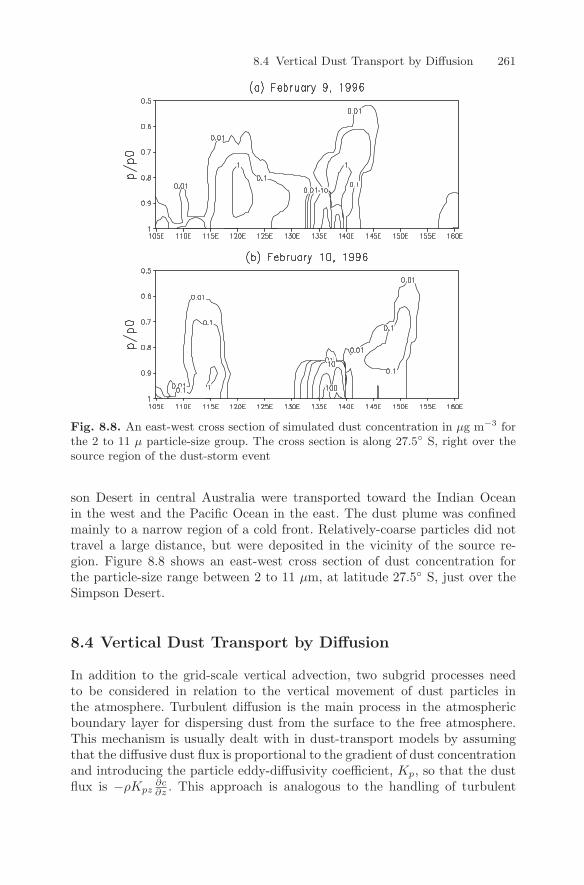
8.4 Vertical Dust Transport by Diffusion 261
Fig. 8.8. An east-west cross section of simulated dust concentration in µg m−3 forthe 2 to 11 µ particle-size group. The cross section is along 27.5 S, right over thesource region of the dust-storm event
son Desert in central Australia were transported toward the Indian Oceanin the west and the Pacific Ocean in the east. The dust plume was confinedmainly to a narrow region of a cold front. Relatively-coarse particles did nottravel a large distance, but were deposited in the vicinity of the source re-gion. Figure 8.8 shows an east-west cross section of dust concentration forthe particle-size range between 2 to 11 µm, at latitude 27.5 S, just over theSimpson Desert.
8.4 Vertical Dust Transport by Diffusion
In addition to the grid-scale vertical advection, two subgrid processes needto be considered in relation to the vertical movement of dust particles inthe atmosphere. Turbulent diffusion is the main process in the atmosphericboundary layer for dispersing dust from the surface to the free atmosphere.This mechanism is usually dealt with in dust-transport models by assumingthat the diffusive dust flux is proportional to the gradient of dust concentrationand introducing the particle eddy-diffusivity coefficient, Kp, so that the dustflux is −ρKpz
∂c∂z . This approach is analogous to the handling of turbulent
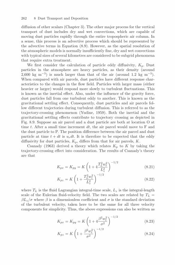
262 8 Dust Transport and Deposition
diffusion of other scalars (Chapter 3). The other major process for the verticaltransport of dust includes dry and wet convections, which are capable ofmoving dust particles rapidly through the entire tropospheric air column. Ina sense, this process is an advective process which should be represented bythe advective terms in Equation (8.9). However, as the spatial resolution ofthe atmospheric models is normally insufficiently fine, dry and wet convectionswith typical sizes of several kilometres are considered to be subgrid phenomenathat require extra treatment.
We first consider the calculation of particle eddy diffusivity, Kp. Dustparticles in the atmosphere are heavy particles, as their density (around2,600 kg m−3) is much larger than that of the air (around 1.2 kg m−3).When compared with air parcels, dust particles have different response char-acteristics to the changes in the flow field. Particles with larger mass (eitherheavier or larger) would respond more slowly to turbulent fluctuations. Thisis known as the inertial effect. Also, under the influence of the gravity force,dust particles fall from one turbulent eddy to another. This is known as thegravitational settling effect. Consequently, dust particles and air parcels fol-low different trajectories during turbulent diffusion. This is referred to as thetrajectory-crossing phenomenon (Yudine, 1959). Both the inertial and thegravitational settling effects contribute to trajectory crossing as depicted inFig. 8.9. Suppose an air parcel and a dust particle are both at location O attime t. After a small time increment dt, the air parcel would move to F andthe dust particle to P. The position difference between the air parcel and dustparticle at time t + dt is urdt. It is therefore to be expected that the eddydiffusivity for dust particles, Kp, differs from that for air parcels, K.
Csanady (1963) derived a theory which relates Kp to K by taking thetrajectory-crossing effect into consideration. The results of Csanady’s theoryare that
Kpx = Kpy = K
(1 + 4
T 2Lw2
t
L2z
)−1/2
(8.21)
Kpz = K
(1 +
T 2Lw2
t
L2z
)−1/2
(8.22)
where TL is the fluid Lagrangian integral-time scale, Lz is the integral-lengthscale of the Eulerian fluid-velocity field. The two scales are related by TL =βLz/σ where β is a dimensionless coefficient and σ is the standard deviationof the turbulent velocity, taken here to be the same for all three velocitycomponents for simplicity. Thus, the above expressions can also be written as
Kpx = Kpy = K
(1 + 4
β2w2t
σ2
)−1/2
(8.23)
Kpz = K
(1 +
β2w2t
σ2
)−1/2
(8.24)
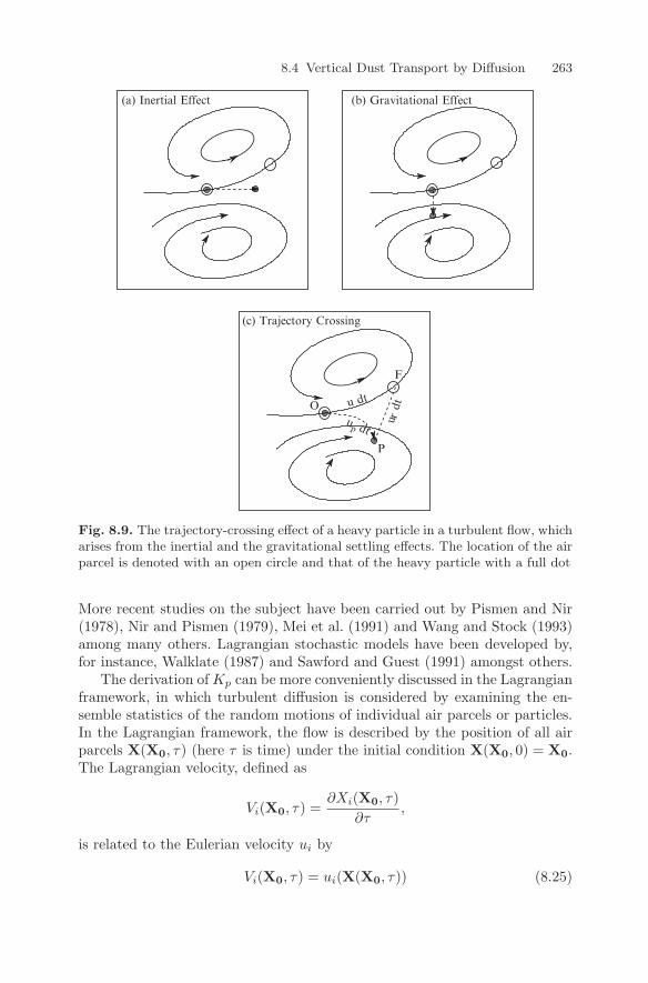
8.4 Vertical Dust Transport by Diffusion 263
up dt
u dt
P
F
O
(c) Trajectory Crossing
(a) Inertial Effect (b) Gravitational Effect
ru d
t
Fig. 8.9. The trajectory-crossing effect of a heavy particle in a turbulent flow, whicharises from the inertial and the gravitational settling effects. The location of the airparcel is denoted with an open circle and that of the heavy particle with a full dot
More recent studies on the subject have been carried out by Pismen and Nir(1978), Nir and Pismen (1979), Mei et al. (1991) and Wang and Stock (1993)among many others. Lagrangian stochastic models have been developed by,for instance, Walklate (1987) and Sawford and Guest (1991) amongst others.
The derivation of Kp can be more conveniently discussed in the Lagrangianframework, in which turbulent diffusion is considered by examining the en-semble statistics of the random motions of individual air parcels or particles.In the Lagrangian framework, the flow is described by the position of all airparcels X(X0, τ) (here τ is time) under the initial condition X(X0, 0) = X0.The Lagrangian velocity, defined as
Vi(X0, τ) =∂Xi(X0, τ)
∂τ,
is related to the Eulerian velocity ui by
Vi(X0, τ) = ui(X(X0, τ)) (8.25)
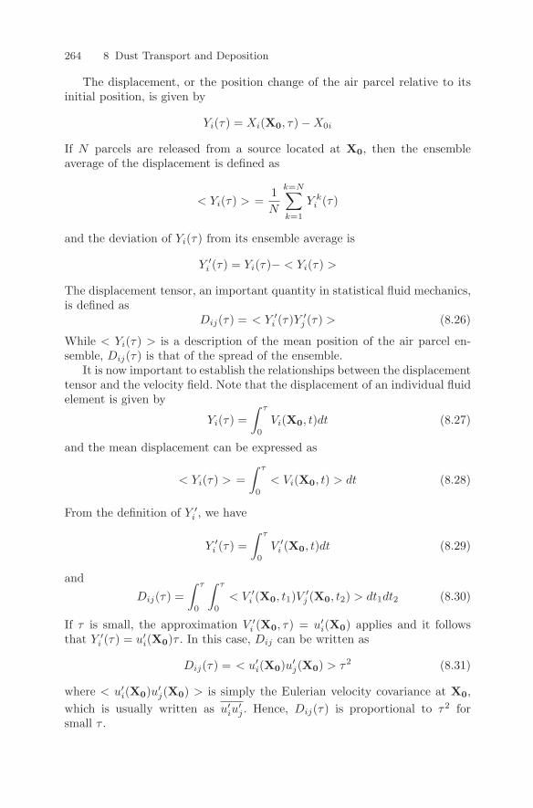
264 8 Dust Transport and Deposition
The displacement, or the position change of the air parcel relative to itsinitial position, is given by
Yi(τ) = Xi(X0, τ) − X0i
If N parcels are released from a source located at X0, then the ensembleaverage of the displacement is defined as
< Yi(τ) > =1N
k=N∑k=1
Y ki (τ)
and the deviation of Yi(τ) from its ensemble average is
Y ′i (τ) = Yi(τ)− < Yi(τ) >
The displacement tensor, an important quantity in statistical fluid mechanics,is defined as
Dij(τ) = < Y ′i (τ)Y ′
j (τ) > (8.26)
While < Yi(τ) > is a description of the mean position of the air parcel en-semble, Dij(τ) is that of the spread of the ensemble.
It is now important to establish the relationships between the displacementtensor and the velocity field. Note that the displacement of an individual fluidelement is given by
Yi(τ) =∫ τ
0
Vi(X0, t)dt (8.27)
and the mean displacement can be expressed as
< Yi(τ) > =∫ τ
0
< Vi(X0, t) > dt (8.28)
From the definition of Y ′i , we have
Y ′i (τ) =
∫ τ
0
V ′i (X0, t)dt (8.29)
andDij(τ) =
∫ τ
0
∫ τ
0
< V ′i (X0, t1)V ′
j (X0, t2) > dt1dt2 (8.30)
If τ is small, the approximation V ′i (X0, τ) = u′
i(X0) applies and it followsthat Y ′
i (τ) = u′i(X0)τ . In this case, Dij can be written as
Dij(τ) = < u′i(X0)u′
j(X0) > τ2 (8.31)
where < u′i(X0)u′
j(X0) > is simply the Eulerian velocity covariance at X0,which is usually written as u′
iu′j . Hence, Dij(τ) is proportional to τ2 for
small τ .
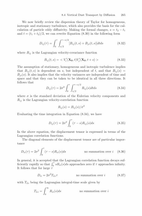
8.4 Vertical Dust Transport by Diffusion 265
We now briefly review the dispersion theory of Taylor for homogeneous,isotropic and stationary turbulence, which also provides the basis for the cal-culation of particle eddy diffusivity. Making the formal changes, s = t2 − t1and t = (t1 + t2)/2, we can rewrite Equation (8.30) in the following form
Dij(τ) =∫ τ
0
∫ τ−s/2
s/2
[Bij(t, s) + Bji(t, s)]dtds (8.32)
where Bij is the Lagrangian velocity-covariance function
Bij(t, s) = < V ′i (X0, t)V ′
j (X0, t + s) > (8.33)
The assumption of stationary, homogeneous and isotropic turbulence impliesthat Bij(t, s) is dependent on s, but independent of t, and that Bij(s) =Bji(s). It also implies that the velocity variances are independent of time andspace and that they can be taken to be identical in all three directions. Itfollows that
Dij(τ) = 2σ2
∫ τ
0
∫ τ−s/2
s/2
Rij(s)dtds (8.34)
where σ is the standard deviation of the Eulerian velocity components andRij is the Lagrangian velocity-correlation function
Rij(s) = Bij(s)/σ2
Evaluating the time integration in Equation (8.34), we have
Dij(τ) = 2σ2
∫ τ
0
(τ − s)Rij(s)ds (8.35)
In the above equation, the displacement tensor is expressed in terms of theLagrangian correlation functions.
The diagonal elements of the displacement tensor are of particular impor-tance
Dii(τ) = 2σ2
∫ τ
0
(τ − s)Rii(s)ds no summation over i (8.36)
In general, it is accepted that the Lagrangian correlation function decays suf-ficiently rapidly so that
∫ τ
0sRii(s)ds approaches zero if τ approaches infinity.
It follows that for large τ
Dii = 2σ2TLiτ no summation over i (8.37)
with TLi being the Lagrangian integral-time scale given by
TLi =∫ ∞
0
Rii(s)ds no summation over i
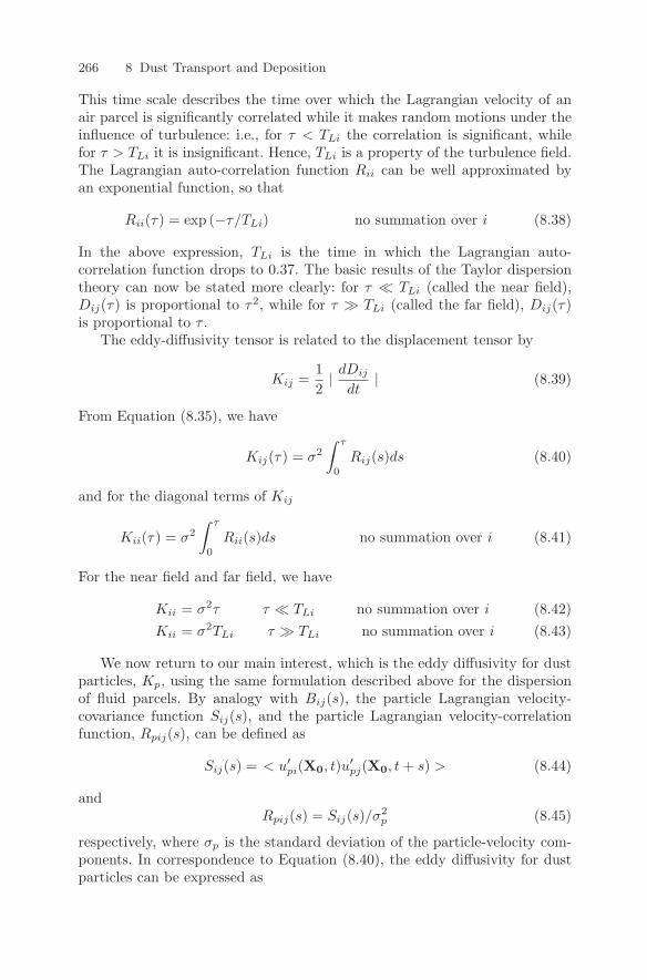
266 8 Dust Transport and Deposition
This time scale describes the time over which the Lagrangian velocity of anair parcel is significantly correlated while it makes random motions under theinfluence of turbulence: i.e., for τ < TLi the correlation is significant, whilefor τ > TLi it is insignificant. Hence, TLi is a property of the turbulence field.The Lagrangian auto-correlation function Rii can be well approximated byan exponential function, so that
Rii(τ) = exp (−τ/TLi) no summation over i (8.38)
In the above expression, TLi is the time in which the Lagrangian auto-correlation function drops to 0.37. The basic results of the Taylor dispersiontheory can now be stated more clearly: for τ TLi (called the near field),Dij(τ) is proportional to τ2, while for τ TLi (called the far field), Dij(τ)is proportional to τ .
The eddy-diffusivity tensor is related to the displacement tensor by
Kij =12| dDij
dt| (8.39)
From Equation (8.35), we have
Kij(τ) = σ2
∫ τ
0
Rij(s)ds (8.40)
and for the diagonal terms of Kij
Kii(τ) = σ2
∫ τ
0
Rii(s)ds no summation over i (8.41)
For the near field and far field, we have
Kii = σ2τ τ TLi no summation over i (8.42)Kii = σ2TLi τ TLi no summation over i (8.43)
We now return to our main interest, which is the eddy diffusivity for dustparticles, Kp, using the same formulation described above for the dispersionof fluid parcels. By analogy with Bij(s), the particle Lagrangian velocity-covariance function Sij(s), and the particle Lagrangian velocity-correlationfunction, Rpij(s), can be defined as
Sij(s) = < u′pi(X0, t)u′
pj(X0, t + s) > (8.44)
andRpij(s) = Sij(s)/σ2
p (8.45)
respectively, where σp is the standard deviation of the particle-velocity com-ponents. In correspondence to Equation (8.40), the eddy diffusivity for dustparticles can be expressed as
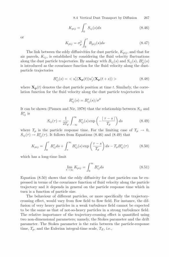
8.4 Vertical Dust Transport by Diffusion 267
Kpij =∫ τ
0
Sij(s)ds (8.46)
orKpij = σ2
p
∫ τ
0
Rpij(s)ds (8.47)
The link between the eddy diffusivities for dust particle, Kpij , and that forair parcels, Kij , is established by considering the fluid velocity fluctuationsalong the dust particle trajectories. By analogy with Bij(s) and Sij(s), B∗
ij(s)is introduced as the covariance function for the fluid velocity along the dust-particle trajectories
B∗ij(s) = < u′
i(Xp(t))u′j(Xp(t + s)) > (8.48)
where Xp(t) denotes the dust particle position at time t. Similarly, the corre-lation function for the fluid velocity along the dust particle trajectories is
R∗ij(s) = B∗
ij(s)/σ2
It can be shown (Pismen and Nir, 1978) that the relationship between Sij andB∗
ij is
Sij(τ) =1
2Tp
∫ ∞
−∞B∗
ij(s) exp(−| τ − s |
Tp
)ds (8.49)
where Tp is the particle response time. For the limiting case of Tp → 0,Sij(τ) → B∗
ij(τ). It follows from Equations (8.46) and (8.49) that
Kpij =∫ τ
0
B∗ijds +
∫ ∞
τ
B∗ij(s) exp
(τ − s
Tp
)ds − TpB
∗ij(τ) (8.50)
which has a long-time limit
limt→∞
Kpij =∫ ∞
0
B∗ijds (8.51)
Equation (8.50) shows that the eddy diffusivity for dust particles can be ex-pressed in terms of the covariance function of fluid velocity along the particletrajectory and it depends in general on the particle response time which inturn is a function of particle size.
The behaviour of different particles, or more specifically the trajectory-crossing effect, would vary from flow field to flow field. For instance, the dif-fusion of very heavy particles in a weak turbulence field cannot be expectedto be the same as that of not-so-heavy particles in a strong turbulence field.The relative importance of the trajectory-crossing effect is quantified usingtwo non-dimensional parameters; namely, the Stokes parameter and the driftparameter. The Stokes parameter is the ratio between the particle-responsetime, Tp, and the Eulerian integral-time scale, TE , i.e.,
268 8 Dust Transport and Deposition
St = Tp/TE
which is a measure of the relative importance of the inertial effect. The driftparameter is the ratio between the particle’s terminal velocity, wt, and thetypical velocity scale of the turbulence field, say u∗, so that
Dr = wt/u∗
which is a measure of the relative importance of the effect of gravity. (Frictionvelocity, u∗, is an excellent scaling parameter for turbulence in atmosphericsurface layers. For other regions of the atmosphere, other scaling velocitiesmay be required.)
As a simple case, suppose the inertial effect can be neglected, namelySt 1, as assumed by Csanady (1963). This implies that the trajectory-crossing effect is settling under gravity only. Under this assumption, Tp canbe set to zero in Equation (8.49) and the relationships Sij(s) = B∗
ij(s) andRpij(s) = R∗
ij(s) apply. Therefore, if B∗ij(s) or R∗
ij(s) can be estimated, thenKpij can be determined using Equation (8.46). In the following, we shall con-fine the discussions to the diagonal components of the particle eddy-diffusivitytensor, namely, Kpx ≡ Kp11, Kpy ≡ Kp22 and Kpz ≡ Kp33. First, we discussthe behaviour of the velocity auto-correlation functions R∗
ii = B∗ii/σ2 following
the argument of Csanady (1963).Consider a situation in which a stationary, homogeneous and isotropic
turbulence field has a mean flow velocity U in the horizontal direction of xand dust particles with St 1 are released into that field. The motion of theparticles will be examined in a frame which moves with the mean flow velocity.We assume that the velocity auto-correlation functions of the turbulent flowin the moving Eulerian frame are all exponential functions; namely (with nosummation over i),
Rii(τ) = exp(−| τ |
TLi
)(8.52)
Eii(τ) = exp(−| τ |
TEi
)(8.53)
fii(r) = exp(−| r |
Lfi
)(8.54)
gii(r) =(
1 − | r |2Lfi
)exp
(−| r |
Lfi
)(8.55)
where Eii is the temporal fluid Eulerian velocity-correlation function at agiven point in space, fii(r) and gii(r) are the longitudinal and transverse spa-tial fluid velocity-correlation functions at a given time, respectively; TEi isthe Eulerian integral-time scale and Lfi is the Eulerian integral-length scale.While Equation (8.52) is widely accepted in the literature and confirmed byobservations, the exponential shapes of the Eulerian correlation functions,Equations (8.53) and (8.54), are assumed for the convenience of mathematical
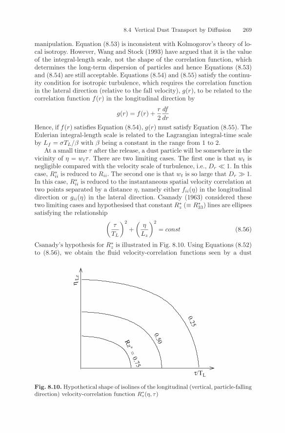
8.4 Vertical Dust Transport by Diffusion 269
manipulation. Equation (8.53) is inconsistent with Kolmogorov’s theory of lo-cal isotropy. However, Wang and Stock (1993) have argued that it is the valueof the integral-length scale, not the shape of the correlation function, whichdetermines the long-term dispersion of particles and hence Equations (8.53)and (8.54) are still acceptable. Equations (8.54) and (8.55) satisfy the continu-ity condition for isotropic turbulence, which requires the correlation functionin the lateral direction (relative to the fall velocity), g(r), to be related to thecorrelation function f(r) in the longitudinal direction by
g(r) = f(r) +r
2df
dr
Hence, if f(r) satisfies Equation (8.54), g(r) must satisfy Equation (8.55). TheEulerian integral-length scale is related to the Lagrangian integral-time scaleby Lf = σTL/β with β being a constant in the range from 1 to 2.
At a small time τ after the release, a dust particle will be somewhere in thevicinity of η = wtτ . There are two limiting cases. The first one is that wt isnegligible compared with the velocity scale of turbulence, i.e., Dr 1. In thiscase, R∗
ii is reduced to Rii. The second one is that wt is so large that Dr 1.In this case, R∗
ii is reduced to the instantaneous spatial velocity correlation attwo points separated by a distance η, namely either fii(η) in the longitudinaldirection or gii(η) in the lateral direction. Csanady (1963) considered thesetwo limiting cases and hypothesised that constant R∗
z (≡ R∗33) lines are ellipses
satisfying the relationship(τ
TL
)2
+(
η
Lz
)2
= const (8.56)
Csanady’s hypothesis for R∗z is illustrated in Fig. 8.10. Using Equations (8.52)
to (8.56), we obtain the fluid velocity-correlation functions seen by a dust
τ/TL
η /L
z
Rz ∗ =
0.75
0.25
0.50
Fig. 8.10. Hypothetical shape of isolines of the longitudinal (vertical, particle-fallingdirection) velocity-correlation function R∗
z(η, τ)
270 8 Dust Transport and Deposition
particle as
R∗x(τ, η) = R∗
y(τ, η) =(
1 − | η |2Lz
)exp
[− τ
Lz
(w2
t +σ2
β2
)1/2]
(8.57)
R∗z(τ, η) = exp
[− τ
Lz
(w2
t +σ2
β2
)1/2]
(8.58)
Substituting Equations (8.57) and (8.58) into Equation (8.50), setting Sii =R∗
iiσ2 and integrating Equations (8.57) and (8.58) with respect to τ , we obtain
the particle eddy diffusivity as given in Equations (8.21) and (8.22). Csanady’stheory shows that Kp can be derived from a modification of K through acorrection factor which involves TL, Lz and wt.
The above discussions show that the key to modelling Kp lies in the specificassumptions for R∗
ii, a quantity which cannot be directly measured. Walklate(1987) proposed an alternative to the Csanady model for R∗
ii; namely, that
R∗11(τ, η) = R∗
22(τ, η) = R11(τ)g11(η) (8.59)R∗
33(τ, η) = R33(τ)f33(η) (8.60)
A combination of the two equations above and Equations (8.52) and (8.53)leads to
R∗x(τ, η) = R∗
y(τ, η) =(
1 − | η |2Lz
)exp
(−| τ |
T ∗L
)(8.61)
R∗z(τ, η) = exp
(−| τ |
T ∗L
)(8.62)
where Lz = σTL/β and T ∗L is given by
T ∗L =
σTL
σ + βwt(8.63)
Walklate’s assumption leads to
Kpx = Kpy = K
(1 + 4
βwt
σ
)−1
(8.64)
Kpz = K
(1 +
βwt
σ
)−1
(8.65)
The performances of the Walklate and Csanady models differ substantiallyfrom one another.
In general, the particle-inertia effect also needs to be considered. UsingCsanady’s hypothesis (8.56) and substituting Equations (8.57) and (8.58) intoEquation (8.49), lengthy expressions for Rp11(τ) and Rp33(τ) can be derived(Wang and Stock, 1993)
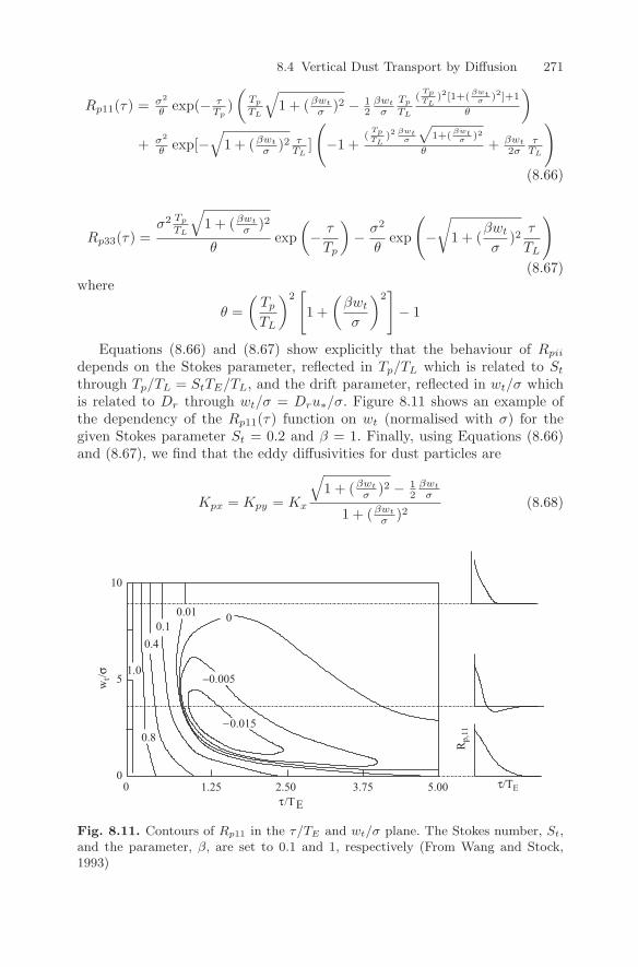
8.4 Vertical Dust Transport by Diffusion 271
Rp11(τ) = σ2
θ exp(− τTp
)(
Tp
TL
√1 + (βwt
σ )2 − 12
βwt
σTp
TL
(TpTL
)2[1+(βwt
σ )2]+1
θ
)
+ σ2
θ exp[−√
1 + (βwt
σ )2 τTL
]
(−1 +
(TpTL
)2βwt
σ
√1+(
βwtσ )2
θ + βwt
2στ
TL
)
(8.66)
Rp33(τ) =σ2 Tp
TL
√1 + (βwt
σ )2
θexp
(− τ
Tp
)− σ2
θexp
(−√
1 + (βwt
σ)2
τ
TL
)
(8.67)where
θ =(
Tp
TL
)2[1 +
(βwt
σ
)2]− 1
Equations (8.66) and (8.67) show explicitly that the behaviour of Rpii
depends on the Stokes parameter, reflected in Tp/TL which is related to St
through Tp/TL = StTE/TL, and the drift parameter, reflected in wt/σ whichis related to Dr through wt/σ = Dru∗/σ. Figure 8.11 shows an example ofthe dependency of the Rp11(τ) function on wt (normalised with σ) for thegiven Stokes parameter St = 0.2 and β = 1. Finally, using Equations (8.66)and (8.67), we find that the eddy diffusivities for dust particles are
Kpx = Kpy = Kx
√1 + (βwt
σ )2 − 12
βwt
σ
1 + (βwt
σ )2(8.68)
0
0.4
0.8
1.0
-0.015
-0.005
0.10.01
5.003.752.501.250τ/TE
τ/TE
wt/σ
Rp,
11
5
10
0
Fig. 8.11. Contours of Rp11 in the τ/TE and wt/σ plane. The Stokes number, St,and the parameter, β, are set to 0.1 and 1, respectively (From Wang and Stock,1993)
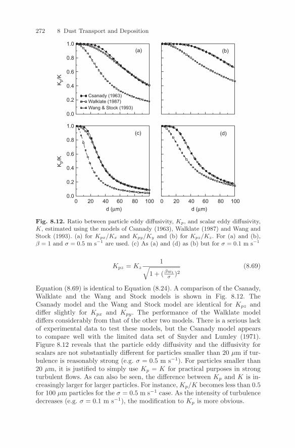
272 8 Dust Transport and Deposition
Csanady (1963)Walklate (1987)Wang & Stock (1993)
d (µm)d (µm)
Kp/
KK
p/K
(a) (b)
(c) (d)
0.00 20 40 60 10080 0 20 40 60 10080
0.2
0.4
0.6
0.8
1.0
0.0
0.2
0.4
0.6
0.8
1.0
Fig. 8.12. Ratio between particle eddy diffusivity, Kp, and scalar eddy diffusivity,K, estimated using the models of Csanady (1963), Walklate (1987) and Wang andStock (1993). (a) for Kpx/Kx and Kpy/Ky and (b) for Kpz/Kz. For (a) and (b),β = 1 and σ = 0.5 m s−1 are used. (c) As (a) and (d) as (b) but for σ = 0.1 m s−1
Kpz = Kz1√
1 + (βwt
σ )2(8.69)
Equation (8.69) is identical to Equation (8.24). A comparison of the Csanady,Walklate and the Wang and Stock models is shown in Fig. 8.12. TheCsanady model and the Wang and Stock model are identical for Kpz anddiffer slightly for Kpx and Kpy. The performance of the Walklate modeldiffers considerably from that of the other two models. There is a serious lackof experimental data to test these models, but the Csanady model appearsto compare well with the limited data set of Snyder and Lumley (1971).Figure 8.12 reveals that the particle eddy diffusivity and the diffusivity forscalars are not substantially different for particles smaller than 20 µm if tur-bulence is reasonably strong (e.g. σ = 0.5 m s−1). For particles smaller than20 µm, it is justified to simply use Kp = K for practical purposes in strongturbulent flows. As can also be seen, the difference between Kp and K is in-creasingly larger for larger particles. For instance, Kp/K becomes less than 0.5for 100 µm particles for the σ = 0.5 m s−1 case. As the intensity of turbulencedecreases (e.g. σ = 0.1 m s−1), the modification to Kp is more obvious.
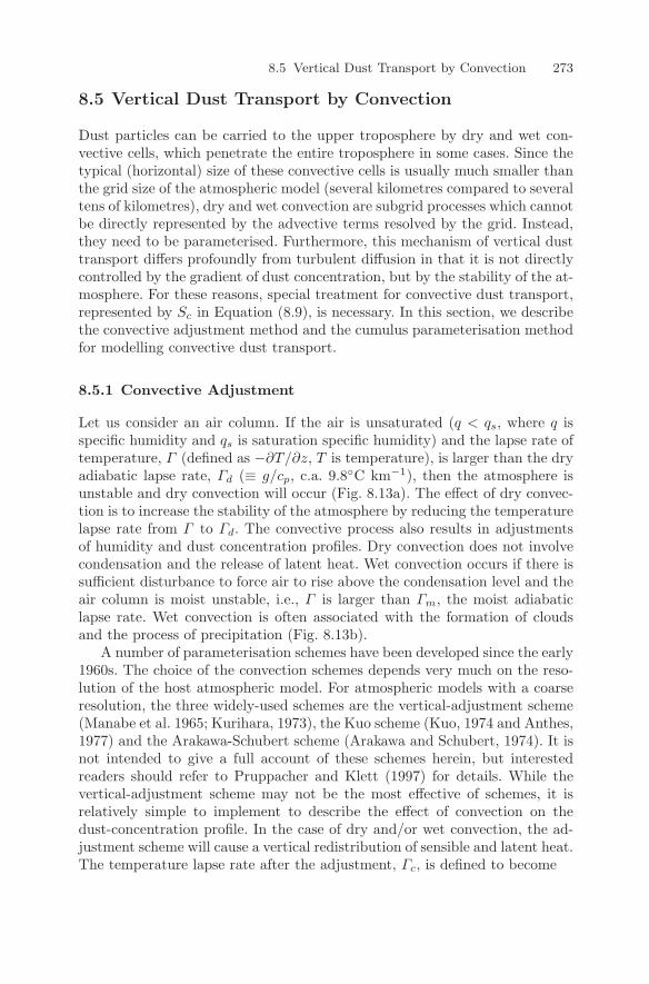
8.5 Vertical Dust Transport by Convection 273
8.5 Vertical Dust Transport by Convection
Dust particles can be carried to the upper troposphere by dry and wet con-vective cells, which penetrate the entire troposphere in some cases. Since thetypical (horizontal) size of these convective cells is usually much smaller thanthe grid size of the atmospheric model (several kilometres compared to severaltens of kilometres), dry and wet convection are subgrid processes which cannotbe directly represented by the advective terms resolved by the grid. Instead,they need to be parameterised. Furthermore, this mechanism of vertical dusttransport differs profoundly from turbulent diffusion in that it is not directlycontrolled by the gradient of dust concentration, but by the stability of the at-mosphere. For these reasons, special treatment for convective dust transport,represented by Sc in Equation (8.9), is necessary. In this section, we describethe convective adjustment method and the cumulus parameterisation methodfor modelling convective dust transport.
8.5.1 Convective Adjustment
Let us consider an air column. If the air is unsaturated (q < qs, where q isspecific humidity and qs is saturation specific humidity) and the lapse rate oftemperature, Γ (defined as −∂T/∂z, T is temperature), is larger than the dryadiabatic lapse rate, Γd (≡ g/cp, c.a. 9.8C km−1), then the atmosphere isunstable and dry convection will occur (Fig. 8.13a). The effect of dry convec-tion is to increase the stability of the atmosphere by reducing the temperaturelapse rate from Γ to Γd. The convective process also results in adjustmentsof humidity and dust concentration profiles. Dry convection does not involvecondensation and the release of latent heat. Wet convection occurs if there issufficient disturbance to force air to rise above the condensation level and theair column is moist unstable, i.e., Γ is larger than Γm, the moist adiabaticlapse rate. Wet convection is often associated with the formation of cloudsand the process of precipitation (Fig. 8.13b).
A number of parameterisation schemes have been developed since the early1960s. The choice of the convection schemes depends very much on the reso-lution of the host atmospheric model. For atmospheric models with a coarseresolution, the three widely-used schemes are the vertical-adjustment scheme(Manabe et al. 1965; Kurihara, 1973), the Kuo scheme (Kuo, 1974 and Anthes,1977) and the Arakawa-Schubert scheme (Arakawa and Schubert, 1974). It isnot intended to give a full account of these schemes herein, but interestedreaders should refer to Pruppacher and Klett (1997) for details. While thevertical-adjustment scheme may not be the most effective of schemes, it isrelatively simple to implement to describe the effect of convection on thedust-concentration profile. In the case of dry and/or wet convection, the ad-justment scheme will cause a vertical redistribution of sensible and latent heat.The temperature lapse rate after the adjustment, Γc, is defined to become
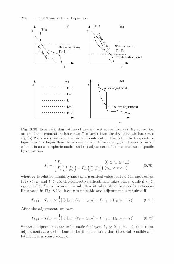
274 8 Dust Transport and Deposition
zz
zzk−2
k−1
k
k+1
k+2
(d)(c)
(a) (b)
Γ > Γm
Before adjustment
After adjustment
T(z)T(z)
c
Wet convection
Condensation level
Γ > Γd
Dry convectionDry adiabat
Moist adiabat
T T
Fig. 8.13. Schematic illustrations of dry and wet convection. (a) Dry convectionoccurs if the temperature lapse rate Γ is larger than the dry-adiabatic lapse rateΓd; (b) Wet convection occurs above the condensation level when the temperaturelapse rate Γ is larger than the moist-adiabatic lapse rate Γm; (c) Layers of an aircolumn in an atmospheric model; and (d) adjustment of dust-concentration profileby convection
Γc =
Γd (0 ≤ rh ≤ rhc)Γd
(1−rh
1−rhc
)+ Γm
(rh−rhc
1−rhc
)(rhc < r < 1) (8.70)
where rh is relative humidity and rhc is a critical value set to 0.5 in most cases.If rh < rhc and Γ > Γd, dry-convective adjustment takes place, while if rh >rhc and Γ > Γm, wet-convective adjustment takes place. In a configuration asillustrated in Fig. 8.13c, level k is unstable and adjustment is required if
Tk+1 − Tk−1 >12[Γc |k+1 (zk − zk+2) + Γc |k−1 (zk−2 − zk)] (8.71)
After the adjustment, we have
T ∗k+1 − T ∗
k−1 =12[Γc |k+1 (zk − zk+2) + Γc |k−1 (zk−2 − zk)] (8.72)
Suppose adjustments are to be made for layers k1 to k1 + 2n − 2, then theseadjustments are to be done under the constraint that the total sensible andlatent heat is conserved, i.e.,
8.5 Vertical Dust Transport by Convection 275
k1+2n−2∑k=k1
[cp(T ∗k−1 − Tk−1) + λl(q∗k−1 − qk−1)] = 0. (8.73)
There are several different ways in which q can be adjusted during a convec-tion process. One possibility is to assume that the relative humidity remainsunchanged during the adjustment process. In this case, it then follows that
q∗k = rhkqs(T ∗k )
where the saturation specific humidity, qs, as a function of T ∗k is given by the
Clausius-Clapeyron equation.While all convection processes modify the vertical profiles of temperature
and specific humidity, the extent to which such motions redistribute dust par-ticles through a convective column is unclear. Joussaume (1990) has suggestedthat convection would lead to a complete vertical mixing through the depthof the convective column and hence a uniform profile of dust concentration(Fig. 8.13d). Alternatively, it appears plausible to assume that the relativepattern of dust-particle redistribution is identical to that of specific humidity,namely,
c∗k = ckq∗k/qk
8.5.2 Cumulus Parameterisation
Cumulus parameterisation schemes have been developed for the prediction ofconvective precipitation in atmospheric models (Arakawa and Schubert, 1974;Fritsch and Chappel, 1980; Tiedtke, 1989). These schemes compute the con-vective air-mass fluxes associated with clouds. In some studies, several cloudtypes are considered (Gidel 1983; Dvortsov et al. 1998), while in others onecloud type is used to represent the effect of all cloud types (Gimson, 1997). Weuse the one-cloud-type model to illustrate the use of cumulus parameterisationin modelling convective dust transport.
A convective dust-transport equation is established based on the convec-tive air-mass fluxes associated with clouds. We imagine that an atmosphericmodel-grid cell is divided into area fractions αu, αd and αe = 1−αu −αd, oc-cupied respectively by updrafts, downdrafts and the environment (Fig. 8.14).Sc in Equation (8.9) can be written as
Sc = −∂w′c′
∂z|cv . (8.74)
The (kinematic) convective dust flux w′c′ |cv can be expressed as
w′c′|cv = αuwpucu + αdwpdcd + αewpece − wpc (8.75)
where wpu, wpd and wpe are the vertical velocities of particles in the updraft,downdraft and environment, respectively, cu, cd and ce are the correspondingparticle concentrations and
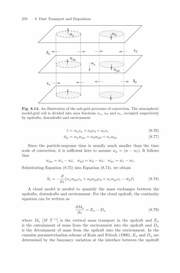
276 8 Dust Transport and Deposition
αu αd
εu
δuεd
δd
wpu
wpd
we
Fig. 8.14. An illustration of the sub-grid processes of convection. The atmosphericmodel-grid cell is divided into area fractions αu, αd and αe, occupied respectivelyby updrafts, downdrafts and environment
c = αucu + αdcd + αece (8.76)wp = αuwpu + αdwpd + αewpe (8.77)
Since the particle-response time is usually much smaller than the timescale of convection, it is sufficient here to assume wp = (w − wt). It followsthat
wpu = wu − wt; wpd = wd − wt; wpe = we − wt.
Substituting Equation (8.75) into Equation (8.74), we obtain
Sc = − ∂
∂z(αuwpucu + αdwpdcd + αewpece − wpc) (8.78)
A cloud model is needed to quantify the mass exchanges between theupdrafts, downdrafts and environment. For the cloud updraft, the continuityequation can be written as
∂Mu
∂z= Eu − Du (8.79)
where Mu [M T−1] is the vertical mass transport in the updraft and Eu
is the entrainment of mass from the environment into the updraft and Du
is the detrainment of mass from the updraft into the environment. In thecumulus parameterisation scheme of Kain and Fritsch (1990), Eu and Du aredetermined by the buoyancy variation at the interface between the updraft
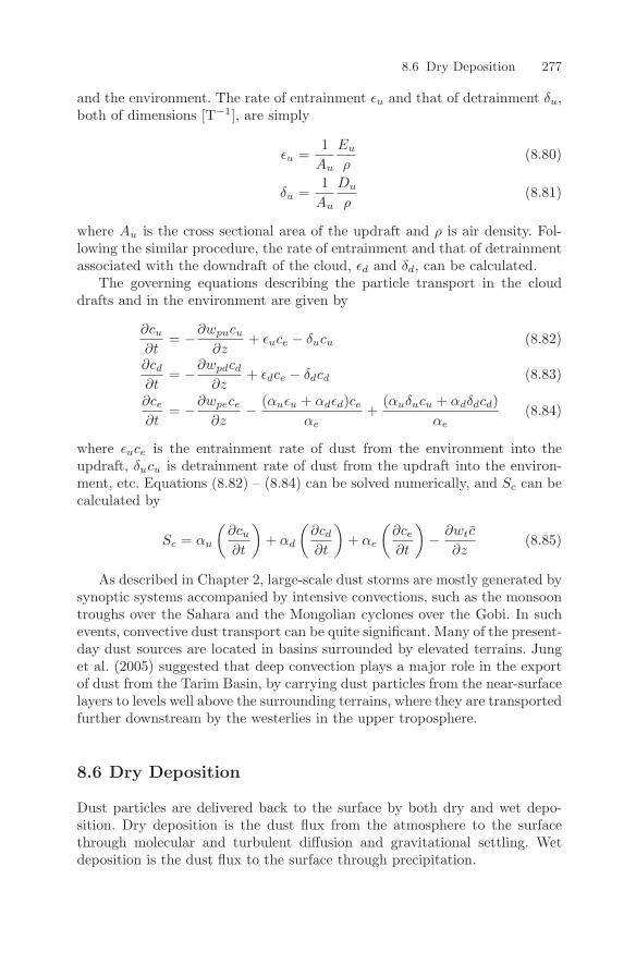
8.6 Dry Deposition 277
and the environment. The rate of entrainment εu and that of detrainment δu,both of dimensions [T−1], are simply
εu =1
Au
Eu
ρ(8.80)
δu =1
Au
Du
ρ(8.81)
where Au is the cross sectional area of the updraft and ρ is air density. Fol-lowing the similar procedure, the rate of entrainment and that of detrainmentassociated with the downdraft of the cloud, εd and δd, can be calculated.
The governing equations describing the particle transport in the clouddrafts and in the environment are given by
∂cu
∂t= −∂wpucu
∂z+ εuce − δucu (8.82)
∂cd
∂t= −∂wpdcd
∂z+ εdce − δdcd (8.83)
∂ce
∂t= −∂wpece
∂z− (αuεu + αdεd)ce
αe+
(αuδucu + αdδdcd)αe
(8.84)
where εuce is the entrainment rate of dust from the environment into theupdraft, δucu is detrainment rate of dust from the updraft into the environ-ment, etc. Equations (8.82) – (8.84) can be solved numerically, and Sc can becalculated by
Sc = αu
(∂cu
∂t
)+ αd
(∂cd
∂t
)+ αe
(∂ce
∂t
)− ∂wtc
∂z(8.85)
As described in Chapter 2, large-scale dust storms are mostly generated bysynoptic systems accompanied by intensive convections, such as the monsoontroughs over the Sahara and the Mongolian cyclones over the Gobi. In suchevents, convective dust transport can be quite significant. Many of the present-day dust sources are located in basins surrounded by elevated terrains. Junget al. (2005) suggested that deep convection plays a major role in the exportof dust from the Tarim Basin, by carrying dust particles from the near-surfacelayers to levels well above the surrounding terrains, where they are transportedfurther downstream by the westerlies in the upper troposphere.
8.6 Dry Deposition
Dust particles are delivered back to the surface by both dry and wet depo-sition. Dry deposition is the dust flux from the atmosphere to the surfacethrough molecular and turbulent diffusion and gravitational settling. Wetdeposition is the dust flux to the surface through precipitation.
278 8 Dust Transport and Deposition
By analogy with the bulk-transfer formulation of scalar fluxes in the at-mosphere, dry-deposition dust flux, Fd, can be expressed as
Fd = −ρwd[c(z) − c(0)] (8.86)
where c(0) and c(z) are dust concentrations at the surface and at the referencelevel z, respectively, and wd is the dry-deposition velocity. In general, wd isdependent on height, surface characteristics, flow properties and particle size.The dependency of wd on particle size has been emphasised in several studies(e.g. Arimoto et al. 1985; Dulac et al. 1989). So that dry deposition can beestimated with greater accuracy, the entire (mass) size distribution of dustparticles is usually divided into I groups and wd is estimated as a weightedaverage
wd =I∑
i=1
fiwdi
where fi and wdi are the mass fraction and the dry-deposition velocity of theith group. The difficult is, however, that the (mass) size distribution of air-borne dust cannot be easily assessed from instantaneous field measurements.In practice, dust samples obtained using devices such as high-volume dustsamplers are fitted with a monomodal lognormal particle-size distribution.The fitted particle-size distribution is then represented using up to 100 dis-crete successive size intervals, with each interval representing 1% of the totalmass, that is fi = 0.01. For each given particle-size interval, wdi can be de-rived from dry-deposition models as discussed in the following sections. Fordust particles of 1–5 µm, wd ranges between 0.01 and 0.05 m s−1. For mineralaerosols over the ocean, wd ranges between 0.003 m s−1 and 0.03 m s−1 (Duceet al. 1991).
8.6.1 Two-Layer Dry-Deposition Model: Smooth Surface
In general, the instantaneous vertical dust flux can be expressed as
Fd = ρwpc − ρκp∂c
∂z(8.87)
where κp is particle molecular diffusivity. It is useful to separate wp into twocomponents, wp = −wt + w′
p, where wt is particle terminal velocity and w′p is
the deviation of wp from −wt. Averaging Fd over time gives
Fd = ρ
(−wtc + w′
pc′ − κp
∂c
∂z
)(8.88)
where ρw′pc
′ is the dust flux due to turbulent mixing, which can be estimatedfrom the K-theory using
ρw′pc
′ = −ρKp∂c
∂z(8.89)
8.6 Dry Deposition 279
The vertical dust flux can then be written as (overbar is dropped forsimplicity)
Fd = ρ
[−wtc − (Kp + κp)
∂c
∂z
](8.90)
Equation (8.90) shows that dry deposition is comprised of a gravitationalsettling flux, −ρwtc and a diffusive flux, −ρ(Kp + κp)∂c/∂z which in turn iscomprised of a turbulent diffusive flux −ρKp∂c/∂z and a molecular diffusiveflux −ρκp∂c/∂z.
In the atmospheric boundary layer, the physical mechanisms responsiblefor vertical dust flux vary with height: In the bulk of the atmospheric bound-ary layer, gravitational settling and turbulent diffusion dominate, while in thelaminar layer immediately over the surface, gravitational settling and molecu-lar diffusion dominate. The final stage of deposition from the air to the surfaceis very complex in detail as it not only depends on flow properties, but also onthe properties of the dust particles and the surface. This stage of depositiontherefore requires special attention.
The situation is somewhat simpler if the surface is smooth and sticky.In this case, the surface can be treated as a perfect sink. In the two-layerdry-deposition model for smooth surfaces, the atmosphere below a certainheight (say about 10 m) is divided into two layers, an upper layer of depthδt, where turbulent diffusion dominates over molecular diffusion, and a lowerlayer of depth δm where molecular diffusion dominates over turbulent diffusion(Fig. 8.15). In the upper layer, the diffusive dust flux can be calculated using
Laminnar Layer
Turbulent Layer
δm
δt
Fig. 8.15. An illustration of the two-layer dry-deposition model. The atmosphericboundary layer is divided into an upper layer of depth δt and a lower layer of depthδm. In the upper layer, dry deposition results from settling and turbulent diffusion,while in the lower layer, it results from settling and molecular diffusion
280 8 Dust Transport and Deposition
the bulk-transfer formulation
−ρwdt[c(z) − c(δm)]
where wdt is the bulk-transfer conductance for dust particles in the upperlayer. Note that wdt has the dimensions of a velocity and is also known asthe turbulent-diffusion velocity for dust particles. As discussed in Chapter 3and 4, the bulk transfer conductance for momentum flux, ga, is
ga = CdU
with Cd being the drag coefficient and U the mean-flow speed at level z. It isplausible to assume that wdt is linearly related to ga, so that
wdt = ξga (8.91)
where ξ is a proportionality factor which depends upon particle size.The depth of the lower layer, δm, should not be too different from the depth
of the laminar layer, δ. We known from Chapter 3, over smooth surface, δ canbe approximated by
δ ∼ ν/u∗
with ν being the kinematic viscosity. Suppose u∗ = 0.5 m s−1 and ν =10−5 m s−1. Then, we have δ ≈ 2 × 10⁻⁴ m. The typical time scale forflow in the laminar layer can now be defined as δ/u∗ (i.e. ν/u2
∗). Hence, thedust-particle Stokes number, which is the ratio between the particle responsetime and the time scale of the flow, is given by
St =Tpu
2∗
ν(8.92)
By analogy with wdt, a molecular-diffusion velocity, wdm, can be defined.Although wdm requires further consideration, its order of magnitude shouldbe
wdm ∝ κp
δ= u∗S
−1m
where Sm = ν/κp is the Schmidt number. The Stokes–Einstein formula(Fuchs, 1964) can be used to estimate κp as
κp =kBT (1 + 2.5λ/d)
3πρνd
where d is particle diameter, kB is the Boltzmann constant (1.38 × 10⁻²³ JK−1), T is temperature and λ is the mean free path of air molecules (c.a.2 × 10−7 m). For 1 µm dust particles, Sm is of the order of magnitude 106
and wdm is of the order of magnitude 10−6 m s−1.The dust fluxes for the two layers can now be expressed using the bulk
formulation and the particle-diffusion velocities, wdt and wdm
8.6 Dry Deposition 281
Fd(z) = −ρwtc(z) − ρwdt[c(z) − c(δ)] (8.93)Fd(δ) = −ρwtc(δ) − ρwdm[c(δ) − c(0)] (8.94)
For simplicity, we assume that the dust flux in the upper layer is constant andhence that Fd(z) = Fd(δ). As the surface is assumed to be a perfect dust sink,we have c(0) = 0. By making use of Equation (8.86), wd can be obtained byeliminating c(δ) between Equations (8.93) and (8.94), so that
wd = wt +wdtwdm
wt + wdm + wdt(8.95)
Therefore, the dry-deposition velocity from z to the surface is com-posed of the gravitational settling velocity and a modification relatedboth to the dry-deposition velocity due to turbulent motion in the upperlayer and the dry-deposition velocity due to molecular diffusion in the lowerlayer. The limit for large particles is
wd = wt
and that for small particles is
wd =wdtwdm
wdm + wdt(8.96)
Equation (8.95) can also be written as
1wd − wt
=1
wdt+
1wdm
+wt
wdtwdm(8.97)
The advantage of the two-layer approach is that it leaves the possibilityopen for deriving a model for wdm on the basis of the microscopic physics. Ifwe treat the final stage of deposition purely as a molecular-diffusion problemand ignore the effects of other factors such as static electricity, we can arguablyapproximate wdm as
wdm = f1(u∗, St) + f2(u∗, Sm) (8.98)
The first function, related to the Stokes number, accounts for the particle in-ertial effect and the second function, related to the Schmidt number, accountsfor the capability of the fluid for particle diffusion. According to Slinn andSlinn (1981), wdm can be approximated as
wdm =52ga[S−1/2
m + 10−3/St ] (8.99)
Figure 8.16 shows a comparison of the two-layer model results with the ob-servations from water-flume and wind-tunnel experiments. Particles with adiameter between 0.1 to 1 µm have the smallest dry-deposition velocities. Foreven smaller particles, the deposition velocity increases due to the increased
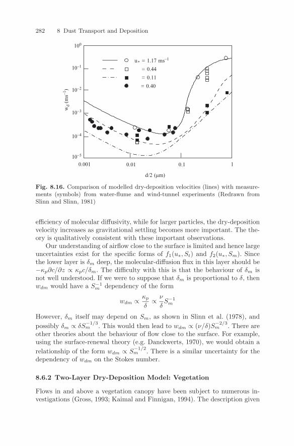
282 8 Dust Transport and Deposition
u* = 1.17 ms−1
10.010.001 0.1
= 0.44
= 0.11
= 0.40
wd (m
s−1 )
d/2 (µm)
10−5
10−4
10−3
10−2
10−1
100
Fig. 8.16. Comparison of modelled dry-deposition velocities (lines) with measure-ments (symbols) from water-flume and wind-tunnel experiments (Redrawn fromSlinn and Slinn, 1981)
efficiency of molecular diffusivity, while for larger particles, the dry-depositionvelocity increases as gravitational settling becomes more important. The the-ory is qualitatively consistent with these important observations.
Our understanding of airflow close to the surface is limited and hence largeuncertainties exist for the specific forms of f1(u∗, St) and f2(u∗, Sm). Sincethe lower layer is δm deep, the molecular-diffusion flux in this layer should be−κp∂c/∂z ∝ κpc/δm. The difficulty with this is that the behaviour of δm isnot well understood. If we were to suppose that δm is proportional to δ, thenwdm would have a S−1
m dependency of the form
wdm ∝ κp
δ∝ ν
δS−1
m
However, δm itself may depend on Sm, as shown in Slinn et al. (1978), andpossibly δm ∝ δS
−1/3m . This would then lead to wdm ∝ (ν/δ)S−2/3
m . There areother theories about the behaviour of flow close to the surface. For example,using the surface-renewal theory (e.g. Danckwerts, 1970), we would obtain arelationship of the form wdm ∝ S
−1/2m . There is a similar uncertainty for the
dependency of wdm on the Stokes number.
8.6.2 Two-Layer Dry-Deposition Model: Vegetation
Flows in and above a vegetation canopy have been subject to numerous in-vestigations (Gross, 1993; Kaimal and Finnigan, 1994). The description given
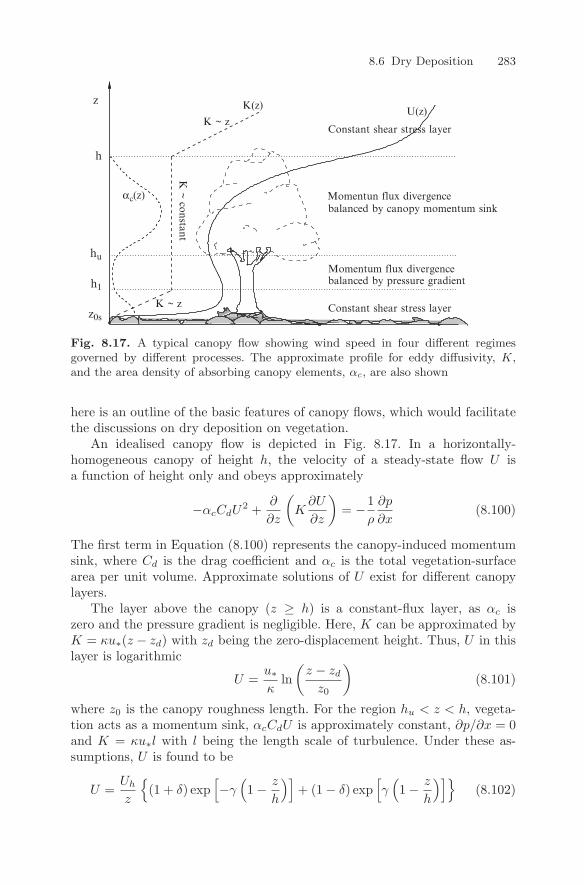
8.6 Dry Deposition 283
Constant shear stress layer
Momentun flux divergencebalanced by canopy momentum sink
Momentum flux divergence
Constant shear stress layer
balanced by pressure gradient
z K(z)
K ~ constant
U(z)
αc(z)
K ~ z
K ~ z
z0s
h1
hu
h
Fig. 8.17. A typical canopy flow showing wind speed in four different regimesgoverned by different processes. The approximate profile for eddy diffusivity, K,and the area density of absorbing canopy elements, αc, are also shown
here is an outline of the basic features of canopy flows, which would facilitatethe discussions on dry deposition on vegetation.
An idealised canopy flow is depicted in Fig. 8.17. In a horizontally-homogeneous canopy of height h, the velocity of a steady-state flow U isa function of height only and obeys approximately
−αcCdU2 +
∂
∂z
(K
∂U
∂z
)= −1
ρ
∂p
∂x(8.100)
The first term in Equation (8.100) represents the canopy-induced momentumsink, where Cd is the drag coefficient and αc is the total vegetation-surfacearea per unit volume. Approximate solutions of U exist for different canopylayers.
The layer above the canopy (z ≥ h) is a constant-flux layer, as αc iszero and the pressure gradient is negligible. Here, K can be approximated byK = κu∗(z − zd) with zd being the zero-displacement height. Thus, U in thislayer is logarithmic
U =u∗κ
ln(
z − zd
z0
)(8.101)
where z0 is the canopy roughness length. For the region hu < z < h, vegeta-tion acts as a momentum sink, αcCdU is approximately constant, ∂p/∂x = 0and K = κu∗l with l being the length scale of turbulence. Under these as-sumptions, U is found to be
U =Uh
z
(1 + δ) exp
[−γ
(1 − z
h
)]+ (1 − δ) exp
[γ(1 − z
h
)](8.102)
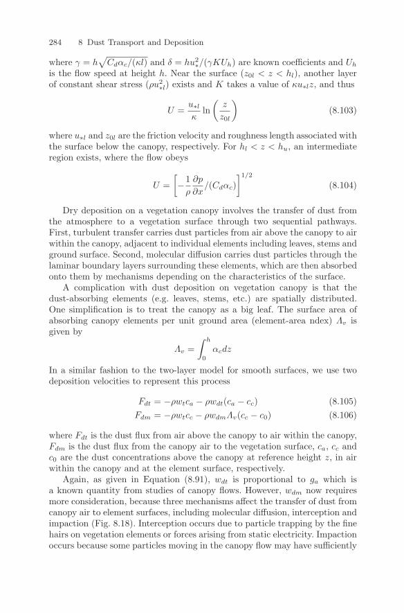
284 8 Dust Transport and Deposition
where γ = h√
Cdαc/(κl) and δ = hu2∗/(γKUh) are known coefficients and Uh
is the flow speed at height h. Near the surface (z0l < z < hl), another layerof constant shear stress (ρu2
∗l) exists and K takes a value of κu∗lz, and thus
U =u∗l
κln
(z
z0l
)(8.103)
where u∗l and z0l are the friction velocity and roughness length associated withthe surface below the canopy, respectively. For hl < z < hu, an intermediateregion exists, where the flow obeys
U =[−1
ρ
∂p
∂x/(Cdαc)
]1/2
(8.104)
Dry deposition on a vegetation canopy involves the transfer of dust fromthe atmosphere to a vegetation surface through two sequential pathways.First, turbulent transfer carries dust particles from air above the canopy to airwithin the canopy, adjacent to individual elements including leaves, stems andground surface. Second, molecular diffusion carries dust particles through thelaminar boundary layers surrounding these elements, which are then absorbedonto them by mechanisms depending on the characteristics of the surface.
A complication with dust deposition on vegetation canopy is that thedust-absorbing elements (e.g. leaves, stems, etc.) are spatially distributed.One simplification is to treat the canopy as a big leaf. The surface area ofabsorbing canopy elements per unit ground area (element-area ndex) Λv isgiven by
Λv =∫ h
0
αcdz
In a similar fashion to the two-layer model for smooth surfaces, we use twodeposition velocities to represent this process
Fdt = −ρwtca − ρwdt(ca − cc) (8.105)Fdm = −ρwtcc − ρwdmΛv(cc − c0) (8.106)
where Fdt is the dust flux from air above the canopy to air within the canopy,Fdm is the dust flux from the canopy air to the vegetation surface, ca, cc andc0 are the dust concentrations above the canopy at reference height z, in airwithin the canopy and at the element surface, respectively.
Again, as given in Equation (8.91), wdt is proportional to ga which isa known quantity from studies of canopy flows. However, wdm now requiresmore consideration, because three mechanisms affect the transfer of dust fromcanopy air to element surfaces, including molecular diffusion, interception andimpaction (Fig. 8.18). Interception occurs due to particle trapping by the finehairs on vegetation elements or forces arising from static electricity. Impactionoccurs because some particles moving in the canopy flow may have sufficiently
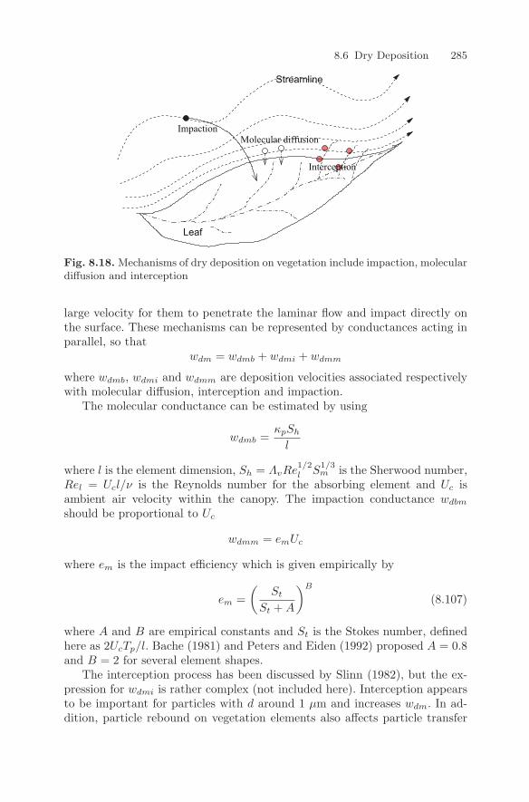
8.6 Dry Deposition 285
Interception
Molecular diffusionImpaction
Leaf
Streamline
Fig. 8.18. Mechanisms of dry deposition on vegetation include impaction, moleculardiffusion and interception
large velocity for them to penetrate the laminar flow and impact directly onthe surface. These mechanisms can be represented by conductances acting inparallel, so that
wdm = wdmb + wdmi + wdmm
where wdmb, wdmi and wdmm are deposition velocities associated respectivelywith molecular diffusion, interception and impaction.
The molecular conductance can be estimated by using
wdmb =κpSh
l
where l is the element dimension, Sh = ΛvRe1/2l S
1/3m is the Sherwood number,
Rel = Ucl/ν is the Reynolds number for the absorbing element and Uc isambient air velocity within the canopy. The impaction conductance wdbm
should be proportional to Uc
wdmm = emUc
where em is the impact efficiency which is given empirically by
em =(
St
St + A
)B
(8.107)
where A and B are empirical constants and St is the Stokes number, definedhere as 2UcTp/l. Bache (1981) and Peters and Eiden (1992) proposed A = 0.8and B = 2 for several element shapes.
The interception process has been discussed by Slinn (1982), but the ex-pression for wdmi is rather complex (not included here). Interception appearsto be important for particles with d around 1 µm and increases wdm. In ad-dition, particle rebound on vegetation elements also affects particle transfer
286 8 Dust Transport and Deposition
from the ambient canopy flow to the element surface. Rebound is significantfor particles in the 10–100 µm range and decreases wdm. Discussions on re-bound can also be found in Slinn (1982).
A similar expression to Equation (8.95) can be found for wd for vegetationcanopies by setting Fdt = Fdm and eliminating cc from Equations (8.105) and(8.106), assuming that c0 is known.
8.6.3 Single-Layer Dry-Deposition Model
Raupach et al. (1999) proposed a single-layer dry-deposition model whichis less demanding on data and parameterisations. In this model, the dry-deposition velocity is treated as a bulk single-layer conductance made up ofthree components acting in parallel
wd = wt + gbb + gbm (8.108)
The molecular conductance, gbb, and the impaction conductance, gbm, can berelated to the conductance for momentum, ga. Two processes which contributeto the transfer of momentum from the airflow to the surface, including thepressure drag and the viscous drag, are considered. So we may write
ga = gap + gav (8.109)
where gap is the conductance related to pressure drag and gav is that relatedto viscous drag. According to Thom (1971), ga, gap and gav are related by
gap = frga (8.110)gav = (1 − fr)ga (8.111)
where fr is the ratio of pressure drag to the total drag. Raupach et al. (1999)hypothesised that gbb is proportional to gav and gbm is proportional to gap.For gbb, the relationship is
gbb = avS−2/3m gav (8.112)
where av is a factor of order 1, accounting for different effects of inter-elementsheltering on the molecular transfer of particles and momentum. For gbm, therelationship is
gbb = apemgap (8.113)
where ap is another factor with similar physical meaning as av and em is asgiven in Equation (8.107). The final form of the single-layer model for wd is
wd = wt + ga[frapem + (1 − fr)avS−2/3m ] (8.114)
in which ap and av are empirical parameters. Although the theory is a consid-erable simplification of the multi-layer physics, it includes enough physics to
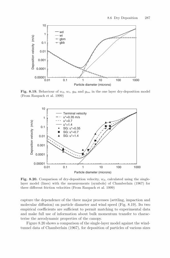
8.6 Dry Deposition 287
Dep
ositi
on v
eloc
ity (
m/s
)
0.00001
0.0001
0.001
0.01
0.1
1
10
0.01 0.1 1 10 100 1000
Particle diameter (microns)
wdwtgbmgbb
Fig. 8.19. Behaviour of wd, wt, gbb and gbm in the one layer dry-deposition model(From Raupach et al. 1999)
Particle diameter (microns)
Dep
ositi
on v
eloc
ity (
m/s
)
Terminal velocityu*=0.35 m/s u*=0.7u*=1.4SG: u*=0.35SG: u*=0.7SG: u*=1.4
0.00001
0.0001
0.001
0.01
0.1
1
10
0.01 0.1 1 10 100 1000
Fig. 8.20. Comparison of dry-deposition velocity, wd, calculated using the single-layer model (lines) with the measurements (symbols) of Chamberlain (1967) forthree different friction velocities (From Raupach et al. 1999)
capture the dependence of the three major processes (settling, impaction andmolecular diffusion) on particle diameter and wind speed (Fig. 8.19). Its twoempirical coefficients are sufficient to permit matching to experimental dataand make full use of information about bulk momentum transfer to charac-terise the aerodynamic properties of the canopy.
Figure 8.20 shows a comparison of the single-layer model against the wind-tunnel data of Chamberlain (1967), for deposition of particles of various sizes
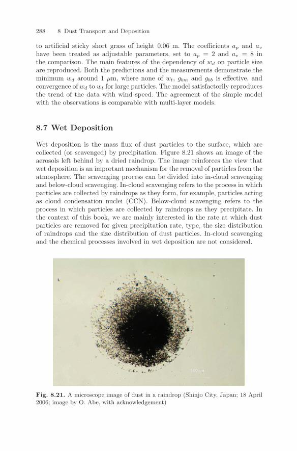
288 8 Dust Transport and Deposition
to artificial sticky short grass of height 0.06 m. The coefficients ap and av
have been treated as adjustable parameters, set to ap = 2 and av = 8 inthe comparison. The main features of the dependency of wd on particle sizeare reproduced. Both the predictions and the measurements demonstrate theminimum wd around 1 µm, where none of wt, gbm and gbb is effective, andconvergence of wd to wt for large particles. The model satisfactorily reproducesthe trend of the data with wind speed. The agreement of the simple modelwith the observations is comparable with multi-layer models.
8.7 Wet Deposition
Wet deposition is the mass flux of dust particles to the surface, which arecollected (or scavenged) by precipitation. Figure 8.21 shows an image of theaerosols left behind by a dried raindrop. The image reinforces the view thatwet deposition is an important mechanism for the removal of particles from theatmosphere. The scavenging process can be divided into in-cloud scavengingand below-cloud scavenging. In-cloud scavenging refers to the process in whichparticles are collected by raindrops as they form, for example, particles actingas cloud condensation nuclei (CCN). Below-cloud scavenging refers to theprocess in which particles are collected by raindrops as they precipitate. Inthe context of this book, we are mainly interested in the rate at which dustparticles are removed for given precipitation rate, type, the size distributionof raindrops and the size distribution of dust particles. In-cloud scavengingand the chemical processes involved in wet deposition are not considered.
Fig. 8.21. A microscope image of dust in a raindrop (Shinjo City, Japan; 18 April2006; image by O. Abe, with acknowledgement)
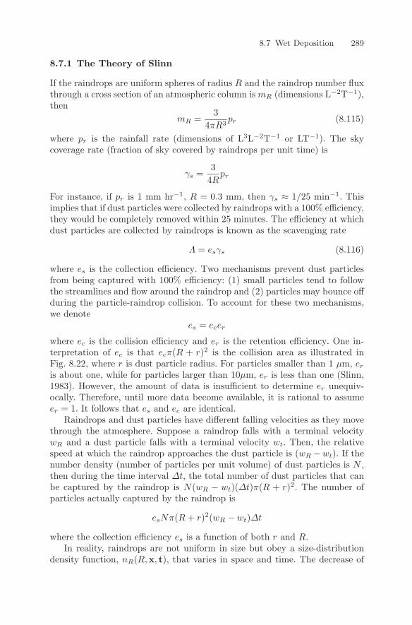
8.7 Wet Deposition 289
8.7.1 The Theory of Slinn
If the raindrops are uniform spheres of radius R and the raindrop number fluxthrough a cross section of an atmospheric column is mR (dimensions L−2T−1),then
mR =3
4πR3pr (8.115)
where pr is the rainfall rate (dimensions of L3L−2T−1 or LT−1). The skycoverage rate (fraction of sky covered by raindrops per unit time) is
γs =3
4Rpr
For instance, if pr is 1 mm hr−1, R = 0.3 mm, then γs ≈ 1/25 min−1. Thisimplies that if dust particles were collected by raindrops with a 100% efficiency,they would be completely removed within 25 minutes. The efficiency at whichdust particles are collected by raindrops is known as the scavenging rate
Λ = esγs (8.116)
where es is the collection efficiency. Two mechanisms prevent dust particlesfrom being captured with 100% efficiency: (1) small particles tend to followthe streamlines and flow around the raindrop and (2) particles may bounce offduring the particle-raindrop collision. To account for these two mechanisms,we denote
es = ecer
where ec is the collision efficiency and er is the retention efficiency. One in-terpretation of ec is that ecπ(R + r)2 is the collision area as illustrated inFig. 8.22, where r is dust particle radius. For particles smaller than 1 µm, er
is about one, while for particles larger than 10µm, er is less than one (Slinn,1983). However, the amount of data is insufficient to determine er unequiv-ocally. Therefore, until more data become available, it is rational to assumeer = 1. It follows that es and ec are identical.
Raindrops and dust particles have different falling velocities as they movethrough the atmosphere. Suppose a raindrop falls with a terminal velocitywR and a dust particle falls with a terminal velocity wt. Then, the relativespeed at which the raindrop approaches the dust particle is (wR −wt). If thenumber density (number of particles per unit volume) of dust particles is N ,then during the time interval ∆t, the total number of dust particles that canbe captured by the raindrop is N(wR − wt)(∆t)π(R + r)2. The number ofparticles actually captured by the raindrop is
esNπ(R + r)2(wR − wt)∆t
where the collection efficiency es is a function of both r and R.In reality, raindrops are not uniform in size but obey a size-distribution
density function, nR(R,x, t), that varies in space and time. The decrease of
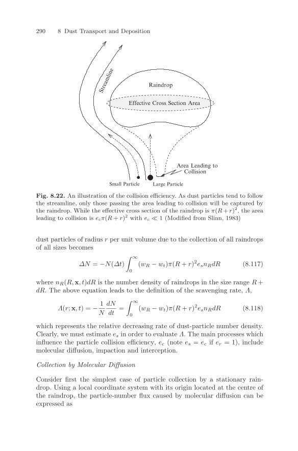
290 8 Dust Transport and Deposition
Stre
amlin
e
Area Leading to
Small Particle Large Particle
Collision
Effective Cross Section Area
Raindrop
Fig. 8.22. An illustration of the collision efficiency. As dust particles tend to followthe streamline, only those passing the area leading to collision will be captured bythe raindrop. While the effective cross section of the raindrop is π(R + r)2, the arealeading to collision is ecπ(R + r)2 with ec 1 (Modified from Slinn, 1983)
dust particles of radius r per unit volume due to the collection of all raindropsof all sizes becomes
∆N = −N(∆t)∫ ∞
0
(wR − wt)π(R + r)2esnRdR (8.117)
where nR(R,x, t)dR is the number density of raindrops in the size range R +dR. The above equation leads to the definition of the scavenging rate, Λ,
Λ(r;x, t) = − 1N
dN
dt=
∫ ∞
0
(wR − wt)π(R + r)2esnRdR (8.118)
which represents the relative decreasing rate of dust-particle number density.Clearly, we must estimate es in order to evaluate Λ. The main processes whichinfluence the particle collision efficiency, ec (note es = ec if er = 1), includemolecular diffusion, impaction and interception.
Collection by Molecular Diffusion
Consider first the simplest case of particle collection by a stationary rain-drop. Using a local coordinate system with its origin located at the centre ofthe raindrop, the particle-number flux caused by molecular diffusion can beexpressed as
8.7 Wet Deposition 291
fb = −κp∂N
∂s
where s is the distance from the coordinate centre. As particles are absorbedcompletely at the surface of the raindrop (s = R), the particle-number concen-tration at the raindrop surface is N |s=R= 0. At a sufficiently large distanceaway from the raindrop N |s=∞= N∞ is the ambient particle concentration.For the steady-state case, fb can be assumed to be constant, the solution forN is
N = N∞
(1 − R
s
)
It follows thatfb = −κpN∞
R
where the negative sign implies that the particle-number flux is directed to-wards the raindrop. In reality, fb may differ from −κpN∞/R for various rea-sons. This difference can be quantified using the Sherwood number, which isdefined as
Sh = fb
(−κpN∞
R
)−1
For the ideal situation described above, Sh = 1.For moving raindrops, the gradient of particles near the raindrop is not
uniformly distributed around the raindrop. It becomes larger in its front andsmaller in its wake. As a consequence, the particle flux caused by moleculardiffusion is also stronger on the front side of the raindrop and weaker in thewake. In general, the net effect is an increase of particle number flux overκpN∞/R. The increase depends on the detailed flow structure around themoving raindrop, which can be characterised by two parameters; namely, theraindrop Reynolds number,
ReR = wRR/ν
and the Schmidt number, which is the ratio of the kinematic viscosity to themolecular diffusivity for dust particles
Sm = ν/κp.
The raindrop Reynolds number is a statement on whether or not the flowaround the raindrop is turbulent. For ReR 1, flow around the rain-drop is laminar, while for ReR 1, a turbulent boundary layer develops(Fig. 8.23a, b). For Sm 1, the velocity boundary layer (∝ ν) would bethicker than an even-thinner particle diffusion layer (∝ κp), and the particlegradient would be large and the flux to the raindrop would therefore alsobe large (Fig. 8.23c, d). It has been found empirically that
Sh = 1 + 0.4Re1/2R S1/3
m (8.119)
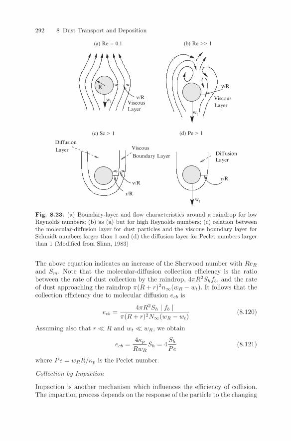
292 8 Dust Transport and Deposition
r/R
Layer
(a) Re = 0.1
R
wt
wt
Diffusion
wt
DiffusionLayer
Layer
ν/R
ν/R
ν/R
Viscous
Viscous
Boundary Layer
r/R
(b) Re >> 1
ViscousLayer
(d) Pe > 1(c) Sc > 1
Fig. 8.23. (a) Boundary-layer and flow characteristics around a raindrop for lowReynolds numbers; (b) as (a) but for high Reynolds numbers; (c) relation betweenthe molecular-diffusion layer for dust particles and the viscous boundary layer forSchmidt numbers larger than 1 and (d) the diffusion layer for Peclet numbers largerthan 1 (Modified from Slinn, 1983)
The above equation indicates an increase of the Sherwood number with ReR
and Sm. Note that the molecular-diffusion collection efficiency is the ratiobetween the rate of dust collection by the raindrop, 4πR2Shfb, and the rateof dust approaching the raindrop π(R + r)2n∞(wR − wt). It follows that thecollection efficiency due to molecular diffusion ecb is
ecb =4πR2Sh | fb |
π(R + r)2N∞(wR − wt)(8.120)
Assuming also that r R and wt wR, we obtain
ecb =4κp
RwRSh = 4
Sh
Pe(8.121)
where Pe = wRR/κp is the Peclet number.
Collection by Impaction
Impaction is another mechanism which influences the efficiency of collision.The impaction process depends on the response of the particle to the changing
8.7 Wet Deposition 293
flow field near the raindrop. After subtracting the terminal velocity from theparticle velocity, the equation of particle motion becomes
du′pi
dt= − 1
Tp(u′
pi − ui) (8.122)
Recall that u′pi is the deviation of particle velocity from its terminal velocity
and Tp is the particle response time. Suppose the velocity scale for the flowaround the raindrop is Uf , then the time scale of the fluid motion, Tf , is
R/Uf . Applying the normalisations upi = u′pi
Uf, ui = ui
Ufand t = t
Tfto the
above equation, we obtain the normalized equation of motion
dupi
dt= − 1
St(upi − ui) (8.123)
with St = Tp/Tf being the Stokes number. As can be seen, particles witha large response time (St → ∞) do not respond to the changes in the flowpattern and will therefore collide with the raindrop. For these particles, thecollision efficiency due to impact, ecm = 1. Particles with a small responsetime (St → 0), will follow the streamline completely and hence not collidewith the raindrop. For these particles, the collision efficiency due to impact,ecm = 0. There exists a critical Stokes number, St∗, so that for St ≤ St∗,ecm is practically zero. A simple mathematical expression which satisfies theabove requirement is
ecm = exp(− 1
St − St∗
)(8.124)
It has been suggested that St∗ is around 1/12.
Collection by Interception
The other mechanism which leads to particle and raindrop collision is in-terception. The idea behind this is that even if a particle had no mass andfollowed the streamline exactly, it could still be collected because of its finitesize. Fuchs (1964) suggested that the efficiency related to interception is
eci =3r
R(8.125)
Finally, the total collision efficiency due to molecular diffusion, interceptionand impaction is given by
ec = ecb + eci + ecm
Different approximations to ecb, eci and ecm are possible, which lead todifferent expressions of ec. Slinn (1984) proposed a semi-empirical relationshipfor ec which is essentially the same as the above-described theory but slightlydifferent in formulation
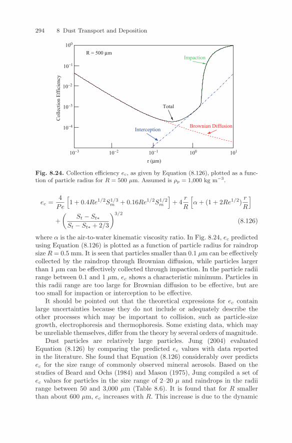
294 8 Dust Transport and Deposition
r (µm)
R = 500 µm
Total
Impaction
InterceptionBrownian Diffusion
Col
lect
ion
Effic
ienc
y
10-4
10-3
10-3 10-2
10-2
10-1 101
10-1
100
100
Fig. 8.24. Collection efficiency ec, as given by Equation (8.126), plotted as a func-tion of particle radius for R = 500 µm. Assumed is ρp = 1,000 kg m−3.
ec =4
Pe
[1 + 0.4Re1/2S1/3
m + 0.16Re1/2S1/2m
]+ 4
r
R
[α + (1 + 2Re1/2)
r
R
]
+(
St − St∗St − St∗ + 2/3
)3/2
(8.126)
where α is the air-to-water kinematic viscosity ratio. In Fig. 8.24, ec predictedusing Equation (8.126) is plotted as a function of particle radius for raindropsize R = 0.5 mm. It is seen that particles smaller than 0.1 µm can be effectivelycollected by the raindrop through Brownian diffusion, while particles largerthan 1 µm can be effectively collected through impaction. In the particle radiirange between 0.1 and 1 µm, ec shows a characteristic minimum. Particles inthis radii range are too large for Brownian diffusion to be effective, but aretoo small for impaction or interception to be effective.
It should be pointed out that the theoretical expressions for ec containlarge uncertainties because they do not include or adequately describe theother processes which may be important to collision, such as particle-sizegrowth, electrophoresis and thermophoresis. Some existing data, which maybe unreliable themselves, differ from the theory by several orders of magnitude.
Dust particles are relatively large particles. Jung (2004) evaluatedEquation (8.126) by comparing the predicted ec values with data reportedin the literature. She found that Equation (8.126) considerably over predictsec for the size range of commonly observed mineral aerosols. Based on thestudies of Beard and Ochs (1984) and Mason (1975), Jung compiled a set ofec values for particles in the size range of 2–20 µ and raindrops in the radiirange between 50 and 3,000 µm (Table 8.6). It is found that for R smallerthan about 600 µm, ec increases with R. This increase is due to the dynamic
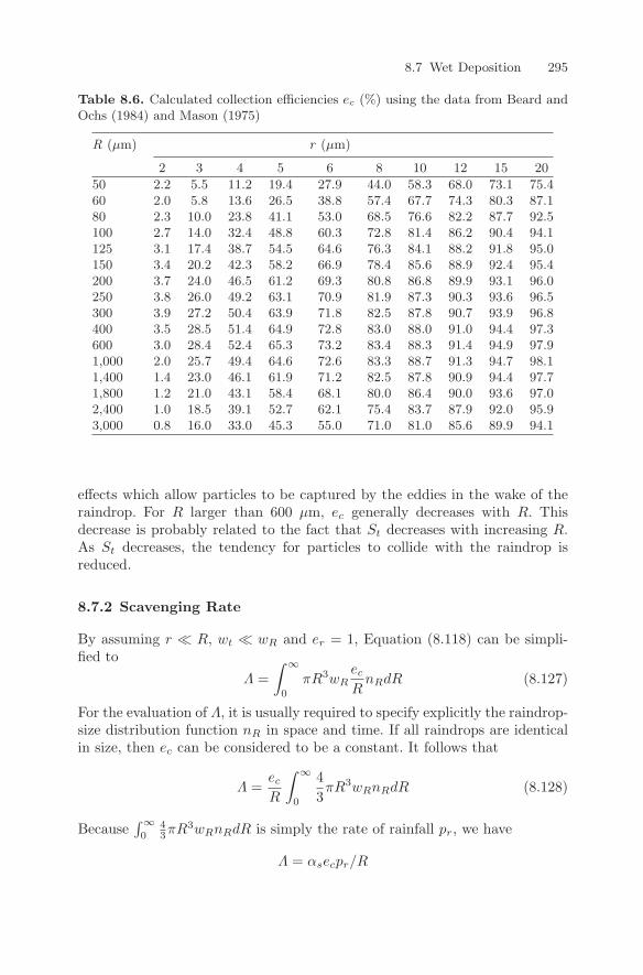
8.7 Wet Deposition 295
Table 8.6. Calculated collection efficiencies ec (%) using the data from Beard andOchs (1984) and Mason (1975)
R (µm) r (µm)
2 3 4 5 6 8 10 12 15 20
50 2.2 5.5 11.2 19.4 27.9 44.0 58.3 68.0 73.1 75.460 2.0 5.8 13.6 26.5 38.8 57.4 67.7 74.3 80.3 87.180 2.3 10.0 23.8 41.1 53.0 68.5 76.6 82.2 87.7 92.5100 2.7 14.0 32.4 48.8 60.3 72.8 81.4 86.2 90.4 94.1125 3.1 17.4 38.7 54.5 64.6 76.3 84.1 88.2 91.8 95.0150 3.4 20.2 42.3 58.2 66.9 78.4 85.6 88.9 92.4 95.4200 3.7 24.0 46.5 61.2 69.3 80.8 86.8 89.9 93.1 96.0250 3.8 26.0 49.2 63.1 70.9 81.9 87.3 90.3 93.6 96.5300 3.9 27.2 50.4 63.9 71.8 82.5 87.8 90.7 93.9 96.8400 3.5 28.5 51.4 64.9 72.8 83.0 88.0 91.0 94.4 97.3600 3.0 28.4 52.4 65.3 73.2 83.4 88.3 91.4 94.9 97.91,000 2.0 25.7 49.4 64.6 72.6 83.3 88.7 91.3 94.7 98.11,400 1.4 23.0 46.1 61.9 71.2 82.5 87.8 90.9 94.4 97.71,800 1.2 21.0 43.1 58.4 68.1 80.0 86.4 90.0 93.6 97.02,400 1.0 18.5 39.1 52.7 62.1 75.4 83.7 87.9 92.0 95.93,000 0.8 16.0 33.0 45.3 55.0 71.0 81.0 85.6 89.9 94.1
effects which allow particles to be captured by the eddies in the wake of theraindrop. For R larger than 600 µm, ec generally decreases with R. Thisdecrease is probably related to the fact that St decreases with increasing R.As St decreases, the tendency for particles to collide with the raindrop isreduced.
8.7.2 Scavenging Rate
By assuming r R, wt wR and er = 1, Equation (8.118) can be simpli-fied to
Λ =∫ ∞
0
πR3wRec
RnRdR (8.127)
For the evaluation of Λ, it is usually required to specify explicitly the raindrop-size distribution function nR in space and time. If all raindrops are identicalin size, then ec can be considered to be a constant. It follows that
Λ =ec
R
∫ ∞
0
43πR3wRnRdR (8.128)
Because∫∞0
43πR3wRnRdR is simply the rate of rainfall pr, we have
Λ = αsecpr/R
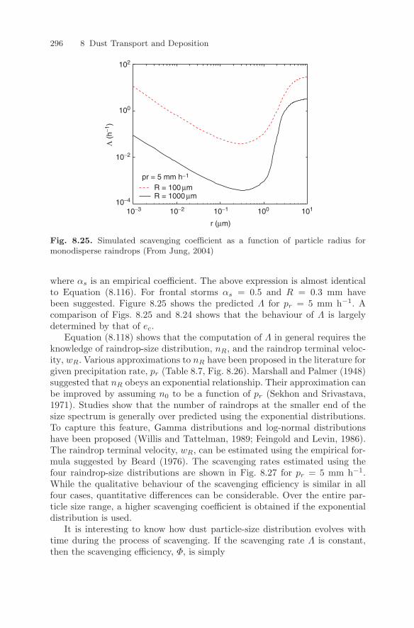
296 8 Dust Transport and Deposition
10−4
10−2
10−210−3 10−1 100 101
100
102
Λ (
h−1)
pr = 5 mm h−1
R = 100 µmR = 1000 µm
r (µm)
Fig. 8.25. Simulated scavenging coefficient as a function of particle radius formonodisperse raindrops (From Jung, 2004)
where αs is an empirical coefficient. The above expression is almost identicalto Equation (8.116). For frontal storms αs = 0.5 and R = 0.3 mm havebeen suggested. Figure 8.25 shows the predicted Λ for pr = 5 mm h−1. Acomparison of Figs. 8.25 and 8.24 shows that the behaviour of Λ is largelydetermined by that of ec.
Equation (8.118) shows that the computation of Λ in general requires theknowledge of raindrop-size distribution, nR, and the raindrop terminal veloc-ity, wR. Various approximations to nR have been proposed in the literature forgiven precipitation rate, pr (Table 8.7, Fig. 8.26). Marshall and Palmer (1948)suggested that nR obeys an exponential relationship. Their approximation canbe improved by assuming n0 to be a function of pr (Sekhon and Srivastava,1971). Studies show that the number of raindrops at the smaller end of thesize spectrum is generally over predicted using the exponential distributions.To capture this feature, Gamma distributions and log-normal distributionshave been proposed (Willis and Tattelman, 1989; Feingold and Levin, 1986).The raindrop terminal velocity, wR, can be estimated using the empirical for-mula suggested by Beard (1976). The scavenging rates estimated using thefour raindrop-size distributions are shown in Fig. 8.27 for pr = 5 mm h−1.While the qualitative behaviour of the scavenging efficiency is similar in allfour cases, quantitative differences can be considerable. Over the entire par-ticle size range, a higher scavenging coefficient is obtained if the exponentialdistribution is used.
It is interesting to know how dust particle-size distribution evolves withtime during the process of scavenging. If the scavenging rate Λ is constant,then the scavenging efficiency, Φ, is simply
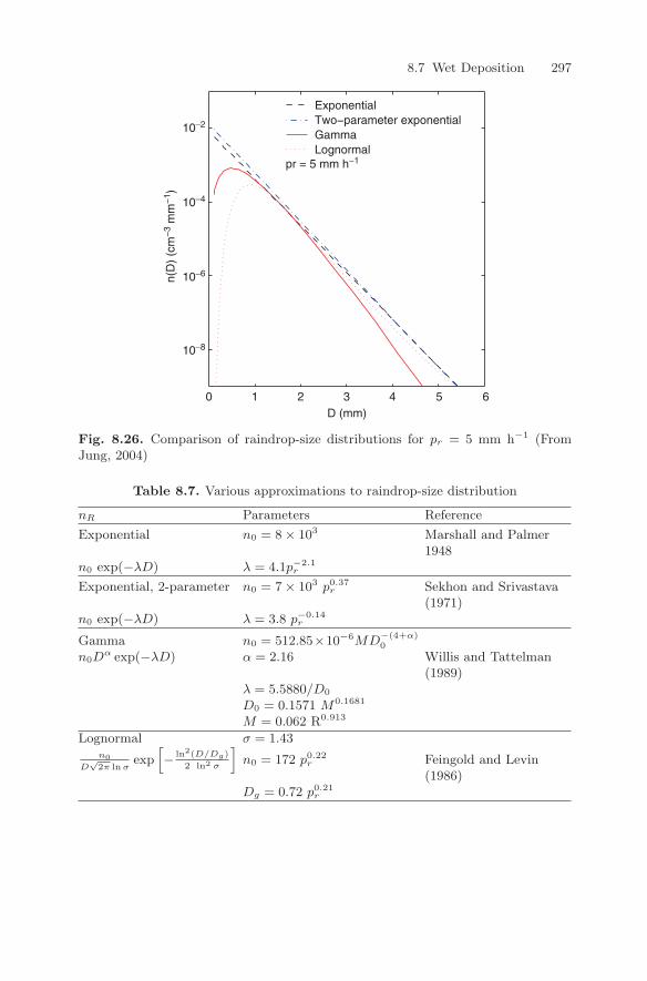
8.7 Wet Deposition 297
10−8
10−6
10−4
10−2
D (mm)
n(D
) (c
m−
3 m
m−
1 )pr = 5 mm h−1
ExponentialTwo−parameter exponentialGammaLognormal
0 1 2 3 4 5 6
Fig. 8.26. Comparison of raindrop-size distributions for pr = 5 mm h−1 (FromJung, 2004)
Table 8.7. Various approximations to raindrop-size distribution
nR Parameters Reference
Exponential n0 = 8 × 10³ Marshall and Palmer1948
n0 exp(−λD) λ = 4.1p−2.1r
Exponential, 2-parameter n0 = 7 × 10³ p0.37r Sekhon and Srivastava
(1971)n0 exp(−λD) λ = 3.8 p−0.14
r
Gamma n0 = 512.85×10⁻⁶MD−(4+α)0
n0Dα exp(−λD) α = 2.16 Willis and Tattelman
(1989)λ = 5.5880/D0
D0 = 0.1571 M0.1681
M = 0.062 R0.913
Lognormal σ = 1.43n0
D√
2π ln σexp
[− ln2(D/Dg)
2 ln2 σ
]n0 = 172 p0.22
r Feingold and Levin(1986)
Dg = 0.72 p0.21r
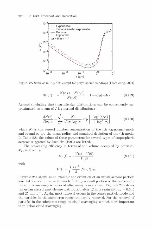
298 8 Dust Transport and Deposition
10−3
10−2
10−1
100
101
r (µm)
Λ (
s−1 )
pr = 5 mm h−1
ExponentialTwo−parameter exponentialGammaLognormal
10−7
10−6
10−5
10−4
10−3
10−2
Fig. 8.27. Same as in Fig. 8.25 except for polydisperse raindrops (From Jung, 2004)
Φ(r, t) = −N(r, t) − N(r, 0)N(r, 0)
= 1 − exp(−Λt) (8.129)
Aerosol (including dust) particle-size distributions can be conveniently ap-proximated as a sum of I log-normal distributions:
dN(r)d log r
=I∑
i=1
Ni√2π log σi
exp[− log2(r/ri)
2 log2 σi
](8.130)
where Ni is the aerosol number concentration of the ith log-normal modeand ri and σi are the mean radius and standard deviation of the ith mode.In Table 8.8, the values of these parameters for several types of troposphericaerosols suggested by Jaenicke (1993) are listed.
The scavenging efficiency in terms of the volume occupied by particles,ΦV , is given by
ΦV (t) = −V (t) − V (0)V (0)
(8.131)
with
V (t) =∫
4πr3
3N(r, t) dr
Figure 8.28a shows as an example the evolution of an urban aerosol particlesize distribution for pr = 25 mm h−1. Only a small portion of the particles inthe submicron range is removed after many hours of rain. Figure 8.28b showsthe urban aerosol particle size distribution after 12 hours rain with pr = 0.5, 5and 25 mm h−1. Again, most removal occurs in the coarse particle mode andthe particles in the submicron range are hardly removed. For the removal ofparticles in the submicron range, in-cloud scavenging is much more importantthan below-cloud scavenging.
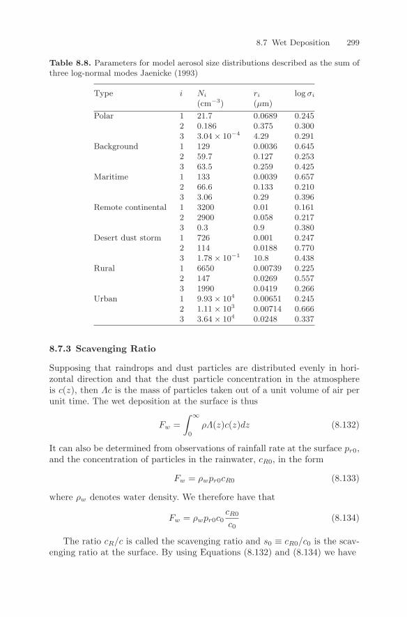
8.7 Wet Deposition 299
Table 8.8. Parameters for model aerosol size distributions described as the sum ofthree log-normal modes Jaenicke (1993)
Type i Ni ri log σi
(cm−3) (µm)
Polar 1 21.7 0.0689 0.2452 0.186 0.375 0.3003 3.04 × 10⁻⁴ 4.29 0.291
Background 1 129 0.0036 0.6452 59.7 0.127 0.2533 63.5 0.259 0.425
Maritime 1 133 0.0039 0.6572 66.6 0.133 0.2103 3.06 0.29 0.396
Remote continental 1 3200 0.01 0.1612 2900 0.058 0.2173 0.3 0.9 0.380
Desert dust storm 1 726 0.001 0.2472 114 0.0188 0.7703 1.78 × 10⁻¹ 10.8 0.438
Rural 1 6650 0.00739 0.2252 147 0.0269 0.5573 1990 0.0419 0.266
Urban 1 9.93 × 10⁴ 0.00651 0.2452 1.11 × 10³ 0.00714 0.6663 3.64 × 10⁴ 0.0248 0.337
8.7.3 Scavenging Ratio
Supposing that raindrops and dust particles are distributed evenly in hori-zontal direction and that the dust particle concentration in the atmosphereis c(z), then Λc is the mass of particles taken out of a unit volume of air perunit time. The wet deposition at the surface is thus
Fw =∫ ∞
0
ρΛ(z)c(z)dz (8.132)
It can also be determined from observations of rainfall rate at the surface pr0,and the concentration of particles in the rainwater, cR0, in the form
Fw = ρwpr0cR0 (8.133)
where ρw denotes water density. We therefore have that
Fw = ρwpr0c0cR0
c0(8.134)
The ratio cR/c is called the scavenging ratio and s0 ≡ cR0/c0 is the scav-enging ratio at the surface. By using Equations (8.132) and (8.134) we have
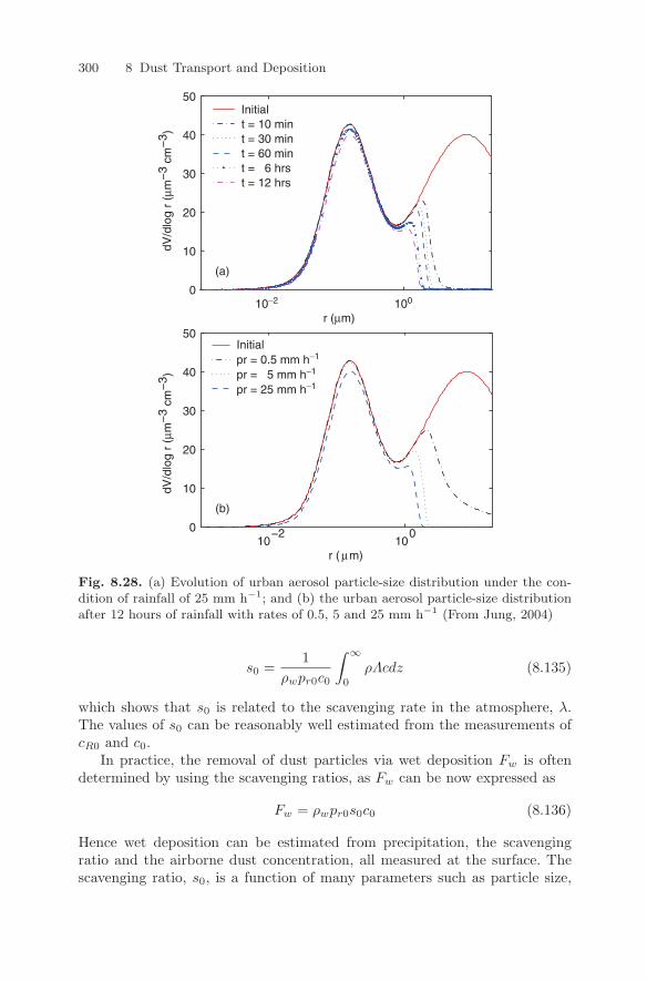
300 8 Dust Transport and Deposition
10−2 100
r (µm)
(a)
Initialt = 10 mint = 30 mint = 60 mint = 6 hrst = 12 hrs
dV/d
log
r (µ
m−
3 cm
−3 )
0
10
20
30
40
50
10−2
100
r ( µm)
dV/d
log
r (µ
m−
3 cm
−3 )
(b)
Initialpr = 0.5 mm h−1
pr = 5 mm h−1
pr = 25 mm h−1
0
10
20
30
40
50
Fig. 8.28. (a) Evolution of urban aerosol particle-size distribution under the con-dition of rainfall of 25 mm h−1; and (b) the urban aerosol particle-size distributionafter 12 hours of rainfall with rates of 0.5, 5 and 25 mm h−1 (From Jung, 2004)
s0 =1
ρwpr0c0
∫ ∞
0
ρΛcdz (8.135)
which shows that s0 is related to the scavenging rate in the atmosphere, λ.The values of s0 can be reasonably well estimated from the measurements ofcR0 and c0.
In practice, the removal of dust particles via wet deposition Fw is oftendetermined by using the scavenging ratios, as Fw can be now expressed as
Fw = ρwpr0s0c0 (8.136)
Hence wet deposition can be estimated from precipitation, the scavengingratio and the airborne dust concentration, all measured at the surface. Thescavenging ratio, s0, is a function of many parameters such as particle size,
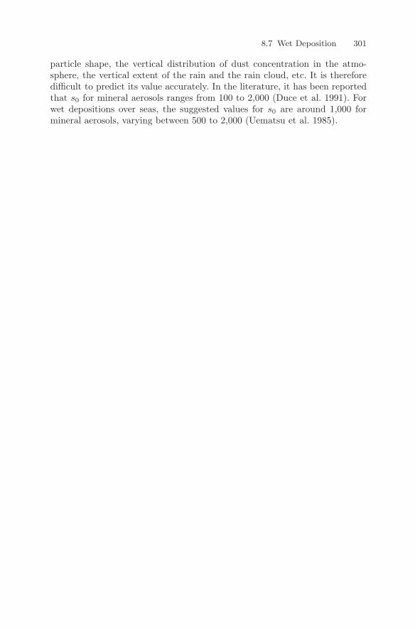
8.7 Wet Deposition 301
particle shape, the vertical distribution of dust concentration in the atmo-sphere, the vertical extent of the rain and the rain cloud, etc. It is thereforedifficult to predict its value accurately. In the literature, it has been reportedthat s0 for mineral aerosols ranges from 100 to 2,000 (Duce et al. 1991). Forwet depositions over seas, the suggested values for s0 are around 1,000 formineral aerosols, varying between 500 to 2,000 (Uematsu et al. 1985).
9
Integrated Wind-Erosion Modelling
The purpose of developing an integrated wind-erosion modelling system(IWEMS) is to produce quantitative predictions of wind erosion on scalesfrom local to global. The system should have the capacity of modelling thewhole wind-erosion process, from particle entrainment through transport todeposition. This is a formidable task because, as depicted in Fig. 1.1, winderosion is governed by a range of factors involving the atmosphere and theland surface. Thus, an IWEMS must couple models for the atmospheric, land-surface and aeolian processes and databases for land-surface parameters, sothat the dynamics of wind erosion and the environmental control factors areadequately represented.
The first attempt of combining atmospheric and land-surface data forlarge-scale wind-erosion assessment was made by Gillette and Hanson (1989)in their investigation on the dust production in the United States. Since thelater 1980s, global, regional and local dust models have been under devel-opment in the atmospheric research community. Earlier attempts on dustmodelling were made for instance by Westphal et al. (1988) and Joussaume(1990). More recent examples of global dust models include the studies ofZender et al. (2003), Ginoux et al. (2004) and Tanaka and Chiba (2006)among others. Examples of regional dust models include the studies of Shaoand Leslie (1997), Nickovic et al. (2001), Liu et al. (2001) and Gong et al.(2003). Seino et al. (2005) and Uno et al. (2005) simulated dust storms inthe Tarim Basin using a meso-scale dust model. Shao et al. (2003) appliedan integrated system to the real-time predictions of Asian dust storms withconsiderable success.
The approach of integrated wind-erosion modelling can be put into per-spective with several other methods used for wind-erosion assessment. Thesimplest one is to estimate the climatic distribution of wind strength andfrequency for a given area. Such a distribution gives an indication of the po-tential for wind to generate erosion, but not the actual wind-erosion rate andpattern. Another method is to compute a wind-erosion index (Chepil et al.1963; McTainsh et al. 1998) as a function of the environmental factors which
Y. Shao, Physics and Modelling of Wind Erosion, 303c© Springer Science+Business Media B.V. 2008
304 9 Integrated Wind-Erosion Modelling
affect wind erosion, such as wind speed, precipitation and evaporation. TheWind-erosion Equation (WEQ, Woodruff and Siddoway, 1965) is an empiricalscheme in which the driving parameters are descriptors of soil type, vegetation,roughness, climate and field length. Originally, WEQ uses annual averages ofthese descriptors to estimate the annual average soil loss. For estimates overshorter periods, WEQ was modified by Bondy et al. (1980) and Cole et al.(1983). More recent revisions to WEQ have led to the Revised Wind-erosionEquation (RWEQ) which includes input parameters such as planting date,tillage method and amount of residue from the previous crop; a weather gen-erator is then used to predict future erosion (Comis and Gerrietts, 1994). Theempirical nature of WEQ has limited its transferability to other areas of theworld from the Central Great Plains of the USA, for which it was originallydeveloped. Also, the complex interactions between the variables controllingwind erosion are not fully accounted for in the empirical WEQ. For this rea-son, a new, more process-oriented model called the Wind-erosion PredictionSystem (WEPS) has also been under development in the USA. This modelincludes sub-models for stochastic weather generation, crop growth, decom-position, soil, hydrology, tillage and erosion (Hagen, 1991).
By contrast, an IWEMS comprehensively integrates the dynamical andphysical models for a range of atmospheric, surface hydrological and aero-lian processes with data sets of land-surface parameters and wind-erosionmeasurements. Such a system takes the advantages of the progresses in at-mospheric modelling, data assimilation, remote sensing and GIS (GeographicInformation System), and thereby significantly expands the frontiers of aeo-lian research. Wind-erosion, together with dust modelling, has now becomean important component of Earth system modelling. An IWEMS is powerfulin that it provides quantitative estimates of wind-erosion related quantities ona wide range of scales. Of course, such a system is more difficult to implementand demands for more data. In this chapter, we discuss IWEMS structure andfunctioning, the practical problems one encounters in their implementationsand the possible solutions.
9.1 System Structure
A possible framework for an IWEMS is as illustrated in Fig. 9.1, which consistsof the following four major components:
1. Modelling2. Monitoring3. Database4. Data-assimilation.
The modelling component comprises an atmospheric model and mod-ules for aeolian, land-surface thermal and hydrological processes. The atmo-spheric model, either global, regional or meso-scale, serves as the host for theother modules. Most atmospheric models today have advanced numerics for
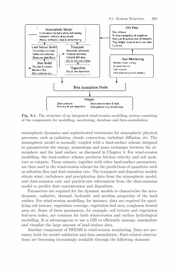
9.1 System Structure 305
Fig. 9.1. The structure of an integrated wind-erosion modelling system consistingof the components for modelling, monitoring, database and data-assimilation
atmospheric dynamics and sophisticated treatments for atmospheric physicalprocesses, such as radiation, clouds, convection, turbulent diffusion, etc. Theatmospheric model is normally coupled with a land-surface scheme designedto parameterise the energy, momentum and mass exchanges between the at-mosphere and the land surface, as discussed in Chapter 4. For wind-erosionmodelling, the land-surface scheme produces friction velocity and soil mois-ture as outputs. These outputs, together with other land-surface parameters,are then used in the wind-erosion scheme for the predictions of quantities suchas saltation flux and dust-emission rate. The transport and deposition modelsobtain wind, turbulence and precipitation data from the atmospheric model,and dust-emission rate and particle-size information from the dust-emissionmodel to predict dust concentration and deposition.
Parameters are required for the dynamic models to characterise the aero-dynamic, radiative, thermal, hydraulic and aerolian properties of the landsurface. For wind-erosion modelling, for instance, data are required for speci-fying soil texture, vegetation coverage, vegetation leaf area, roughness frontalarea etc. Some of these parameters, for example, soil texture and vegetationleaf-area index, are common for both wind-erosion and surface hydrologicalmodelling. It is advantageous to use a GIS to efficiently manage, manipulateand visualize the large amount of land-surface data.
Another component of IWEMS is wind-erosion monitoring. Data are nec-essary both for model validation and data assimilation. Dust-related observa-tions are becoming increasingly available through the following channels:
306 9 Integrated Wind-Erosion Modelling
1. Dust concentration can be derived from visibility measurements usingempirical relationships, which are made routinely at weather stations.The visibility-derived dust-concentration data are quantitatively ratherinaccurate, but provide an excellent spatial and temporal coverage of dustactivities.
2. Dust concentration measurements are also available from high- and low-volume samplers. These measurements are probably the most accurate,but are poor in spatial and temporal resolutions, because the measure-ments are made at a small number of locations and a measurement maytake days even weeks to complete.
3. A network of lidars is now functioning which produces aerosol-profile ob-servations at a number of locations in dust affected areas (Sugimoto et al.2003; Shimizu et al. 2004). Lidar data are nevertheless indirect and arelimited to selected areas. During severe dust events, lidar only providesinformation for the lower part of the atmosphere, as lidar signals oftencannot penetrate the dense dust layers.
4. Satellite remote sensing provides excellent spatial and temporal coverageof wind-erosion and dust-storm events, although the difficulties of con-verting satellite signals to physical quantities, such as dust load and dustsize distribution are not yet fully overcome.
5. Dust concentration can also be derived through radiation measurementsof, for example, sun photometers. Radiation measurements can be used todetermine dust optical thickness which is directly comparable with thatderived from satellite data.
Wind-erosion models are only approximations to a set of complex pro-cesses. Even if these processes were accurately represented in the models,model simulations may still diverge from reality due to inaccuracies in initialconditions and errors in model parameters and forcing data. This occurs oftenbecause the models are non-linear and sensitive to minute changes in initialconditions and parameters. It is a considerable advantage to use observa-tions to constrain the model simulations close to the reality. For this purpose,methods must be derived to optimally combine observations and model simu-lations. The procedure of combining observed data with model simulations toproduce an optimal prediction of an evolving system is known as data assimi-lation, optimal in a sense that the prediction error is minimized. The techniqueof data assimilation has been widely used in numerical weather, ocean andclimate predictions (e.g. Kalnay, 2003). It is also desirable to develop thedata assimilation technique as a component of IWEMS. Some progress hasbeen made in this area although there exist insufficient homogenized wind-erosion data for the purpose. We expect that with the rapid progress in remotesensing technology and other data retrieving techniques, the assimilation ofdust measurements into IWEMS simulation will soon become feasible.
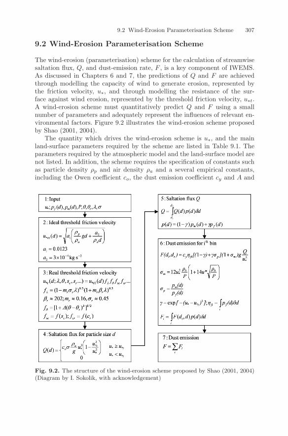
9.2 Wind-Erosion Parameterisation Scheme 307
9.2 Wind-Erosion Parameterisation Scheme
The wind-erosion (parameterisation) scheme for the calculation of streamwisesaltation flux, Q, and dust-emission rate, F , is a key component of IWEMS.As discussed in Chapters 6 and 7, the predictions of Q and F are achievedthrough modelling the capacity of wind to generate erosion, represented bythe friction velocity, u∗, and through modelling the resistance of the sur-face against wind erosion, represented by the threshold friction velocity, u∗t.A wind-erosion scheme must quantitatively predict Q and F using a smallnumber of parameters and adequately represent the influences of relevant en-vironmental factors. Figure 9.2 illustrates the wind-erosion scheme proposedby Shao (2001, 2004).
The quantity which drives the wind-erosion scheme is u∗, and the mainland-surface parameters required by the scheme are listed in Table 9.1. Theparameters required by the atmospheric model and the land-surface model arenot listed. In addition, the scheme requires the specification of constants suchas particle density ρp and air density ρa and a several empirical constants,including the Owen coefficient co, the dust emission coefficient cy and A and
Fig. 9.2. The structure of the wind-erosion scheme proposed by Shao (2001, 2004)(Diagram by I. Sokolik, with acknowledgement)
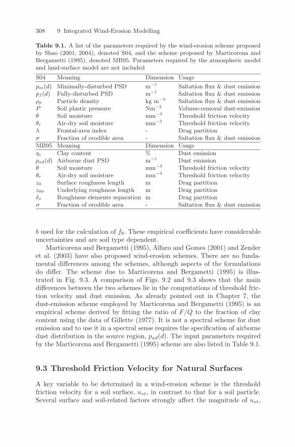
308 9 Integrated Wind-Erosion Modelling
Table 9.1. A list of the parameters required by the wind-erosion scheme proposedby Shao (2001, 2004), denoted S04, and the scheme proposed by Marticorena andBergametti (1995), denoted MB95. Parameters required by the atmospheric modeland land-surface model are not included
S04 Meaning Dimension Usage
pm(d) Minimally-disturbed PSD m−1 Saltation flux & dust emissionpf (d) Fully-disturbed PSD m−1 Saltation flux & dust emissionρp Particle density kg m−3 Saltation flux & dust emissionP Soil plastic pressure Nm−2 Volume-removal dust-emissionθ Soil moisture mm−3 Threshold friction velocityθr Air-dry soil moisture mm−3 Threshold friction velocityλ Frontal-area index - Drag partitionσ Fraction of erodible area - Saltation flux & dust emission
MB95 Meaning Dimension Usage
ηc Clay content % Dust emissionpad(d) Airborne dust PSD m−1 Dust emissionθ Soil moisture mm−3 Threshold friction velocityθr Air-dry soil moisture mm−3 Threshold friction velocityz0 Surface roughness length m Drag partitionz00 Underlying roughness length m Drag partitionδx Roughness elements separation m Drag partitionσ Fraction of erodible area - Saltation flux & dust emission
b used for the calculation of fθ. These empirical coefficients have considerableuncertainties and are soil type dependent.
Marticorena and Bergametti (1995), Alfaro and Gomes (2001) and Zenderet al. (2003) have also proposed wind-erosion schemes. There are no funda-mental differences among the schemes, although aspects of the formulationsdo differ. The scheme due to Marticorena and Bergametti (1995) is illus-trated in Fig. 9.3. A comparison of Figs. 9.2 and 9.3 shows that the maindifferences between the two schemes lie in the computations of threshold fric-tion velocity and dust emission. As already pointed out in Chapter 7, thedust-emission scheme employed by Marticorena and Bergametti (1995) is anempirical scheme derived by fitting the ratio of F/Q to the fraction of claycontent using the data of Gillette (1977). It is not a spectral scheme for dustemission and to use it in a spectral sense requires the specification of airbornedust distribution in the source region, pad(d). The input parameters requiredby the Marticorena and Bergametti (1995) scheme are also listed in Table 9.1.
9.3 Threshold Friction Velocity for Natural Surfaces
A key variable to be determined in a wind-erosion scheme is the thresholdfriction velocity for a soil surface, u∗t, in contrast to that for a soil particle.Several surface and soil-related factors strongly affect the magnitude of u∗t,
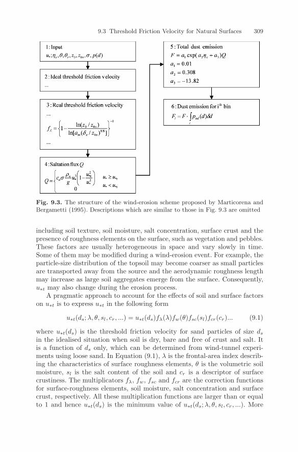
9.3 Threshold Friction Velocity for Natural Surfaces 309
Fig. 9.3. The structure of the wind-erosion scheme proposed by Marticorena andBergametti (1995). Descriptions which are similar to those in Fig. 9.3 are omitted
including soil texture, soil moisture, salt concentration, surface crust and thepresence of roughness elements on the surface, such as vegetation and pebbles.These factors are usually heterogeneous in space and vary slowly in time.Some of them may be modified during a wind-erosion event. For example, theparticle-size distribution of the topsoil may become coarser as small particlesare transported away from the source and the aerodynamic roughness lengthmay increase as large soil aggregates emerge from the surface. Consequently,u∗t may also change during the erosion process.
A pragmatic approach to account for the effects of soil and surface factorson u∗t is to express u∗t in the following form
u∗t(ds;λ, θ, sl, cr, ...) = u∗t(ds)fλ(λ)fw(θ)fsc(sl)fcr(cr)... (9.1)
where u∗t(ds) is the threshold friction velocity for sand particles of size ds
in the idealised situation when soil is dry, bare and free of crust and salt. Itis a function of ds only, which can be determined from wind-tunnel experi-ments using loose sand. In Equation (9.1), λ is the frontal-area index describ-ing the characteristics of surface roughness elements, θ is the volumetric soilmoisture, sl is the salt content of the soil and cr is a descriptor of surfacecrustiness. The multiplicators fλ, fw, fsc and fcr are the correction functionsfor surface-roughness elements, soil moisture, salt concentration and surfacecrust, respectively. All these multiplication functions are larger than or equalto 1 and hence u∗t(ds) is the minimum value of u∗t(ds;λ, θ, sl, cr, ...). More
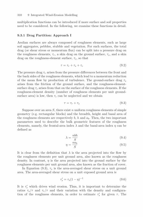
310 9 Integrated Wind-Erosion Modelling
multiplication functions can be introduced if more surface and soil propertiesneed to be considered. In the following, we examine these functions in detail.
9.3.1 Drag Partition: Approach I
Aeolian surfaces are always composed of roughness elements, such as largesoil aggregates, pebbles, stubble and vegetation. For such surfaces, the totaldrag (or shear stress or momentum flux) can be split into a pressure drag onthe roughness elements, τr, a skin drag on the ground surface, τs, and a skindrag on the roughness-element surface, τc, so that
τ = τr + τs + τc (9.2)
The pressure drag τr arises from the pressure differences between the front andthe back sides of the roughness elements, which lead to a momentum reductionof the mean flow by production of turbulence. The ground-surface drag τs
arises from the friction of the ground surface, and the roughness-element-surface drag τc arises from that on the surface of the roughness elements. If theroughness-element density (number of roughness elements per unit ground-surface area) is low, then τc can be neglected and we obtain
τ = τr + τs (9.3)
Suppose over an area S, there exist n uniform roughness elements of simplegeometry (e.g. rectangular blocks) and the breadth, height and basal area ofthe roughness elements are respectively b, h and ab. Then, the two importantparameters used to describe the bulk geometric features of the roughnesselements, namely, the frontal-area index λ and the basal-area index η can bedefined as
λ =nbh
S(9.4)
η =nab
S(9.5)
It is clear from the definition that λ is the area projected into the flow bythe roughness elements per unit ground area, also known as the roughnessdensity. In contrast, η is the area projected into the ground surface by theroughness elements per unit ground area, also known as the fraction of cover.
In Equation (9.3), τs is the area-averaged shear stress on a unit groundarea. The area-averaged shear stress on a unit exposed ground area is
τ ′s = τs(1 − η)−1 (9.6)
It is τ ′s which drives wind erosion. Thus, it is important to determine the
ratios τs/τ and τr/τ and their variation with the density and configura-tion of the roughness elements, in order to estimate τ ′
s for given τ . The
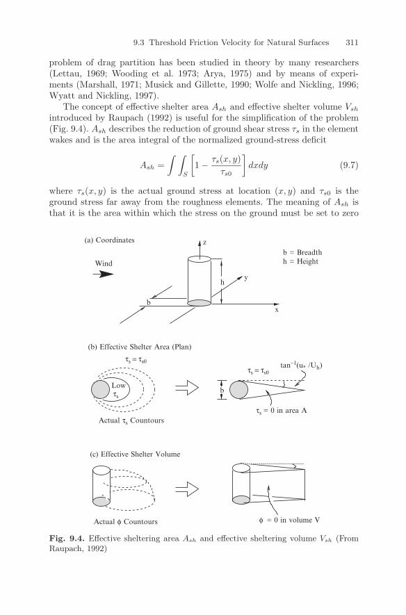
9.3 Threshold Friction Velocity for Natural Surfaces 311
problem of drag partition has been studied in theory by many researchers(Lettau, 1969; Wooding et al. 1973; Arya, 1975) and by means of experi-ments (Marshall, 1971; Musick and Gillette, 1990; Wolfe and Nickling, 1996;Wyatt and Nickling, 1997).
The concept of effective shelter area Ash and effective shelter volume Vsh
introduced by Raupach (1992) is useful for the simplification of the problem(Fig. 9.4). Ash describes the reduction of ground shear stress τs in the elementwakes and is the area integral of the normalized ground-stress deficit
Ash =∫ ∫
S
[1 − τs(x, y)
τs0
]dxdy (9.7)
where τs(x, y) is the actual ground stress at location (x, y) and τs0 is theground stress far away from the roughness elements. The meaning of Ash isthat it is the area within which the stress on the ground must be set to zero
Wind
b
z
y
x
Low
τs = 0 in area A
(a) Coordinates
(b) Effective Shelter Area (Plan)
b = Breadthh = Height
(c) Effective Shelter Volume
Actual φ Countours
tan−1(u* /Uh)τs = τs0
τs = τs0
τs
φ = 0 in volume V
h
b
Actual τs Countours
Fig. 9.4. Effective sheltering area Ash and effective sheltering volume Vsh (FromRaupach, 1992)
312 9 Integrated Wind-Erosion Modelling
to produce the same integrated stress deficit as that induced by the shelteringelement, i.e., ∫ ∫
S
τs(x, y)dxdy =∫ ∫
S−Ash
τs0dxdy
Vsh describes the effect of a given roughness element upon the pressuredrag on other elements in its vicinity. The drag force per unit volume, φ, onan obstacle of frontal area ao is φ ∼ aoU
2, where U is flow speed. Vsh is thevolume integral of the normalised deficit in φ which is induced by placing aroughness element on the surface, so that
Vsh =∫ ∫ ∫
Γ
[1 − φ(x, y, z)
φ0
]dxdydz (9.8)
where φ0 is the undisturbed value of φ far from the sheltering element andΓ is the air volume over surface S. Vsh is the volume within which the dragforce on the obstacle must be set to zero, to produce the same integrated forcedeficit as that induced by the sheltering element, that is
∫ ∫ ∫Γ
φdxdydz =∫ ∫ ∫
Γ−Vsh
φ0dxdydz
Raupach (1992) made two hypotheses. One specifies Ash and Vsh for asingle roughness element, and the other specifies the interactions between theroughness elements. They are:
• Hypothesis I: Ash and Vsh can be expressed as
Ash = cbhUh/u∗ (9.9)Vsh = hAsh (9.10)
where c is a coefficient and Uh is the mean wind speed at h.• Hypothesis II: For roughness elements distributed either uniformly or ran-
domly across a ground surface, the combined effective shelter area or vol-ume can be calculated by randomly superimposing individual shelter areasor volumes.
The validities of the two hypotheses are limited to the situations of low rough-ness densities. As roughness density increases, the interactions between thewakes associated with individual roughness elements become stronger andtheir collective effect cannot be simply described by superimposition.
Ground Stress
We consider now the attenuation of the ground stress as the roughness densityincreases. Suppose n roughness elements with an effective shelter area Ash areplaced on a ground area S. Then it follows from Hypothesis II that
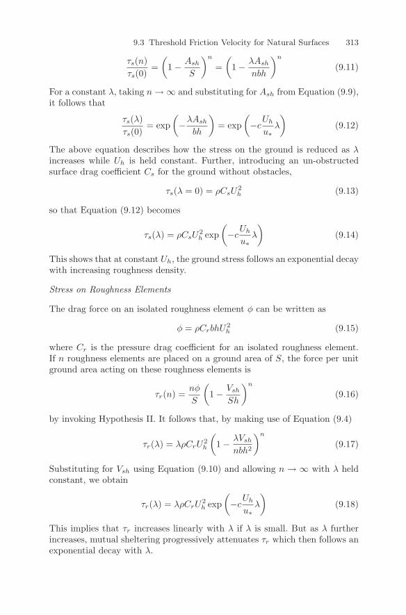
9.3 Threshold Friction Velocity for Natural Surfaces 313
τs(n)τs(0)
=(
1 − Ash
S
)n
=(
1 − λAsh
nbh
)n
(9.11)
For a constant λ, taking n → ∞ and substituting for Ash from Equation (9.9),it follows that
τs(λ)τs(0)
= exp(−λAsh
bh
)= exp
(−c
Uh
u∗λ
)(9.12)
The above equation describes how the stress on the ground is reduced as λincreases while Uh is held constant. Further, introducing an un-obstructedsurface drag coefficient Cs for the ground without obstacles,
τs(λ = 0) = ρCsU2h (9.13)
so that Equation (9.12) becomes
τs(λ) = ρCsU2h exp
(−c
Uh
u∗λ
)(9.14)
This shows that at constant Uh, the ground stress follows an exponential decaywith increasing roughness density.
Stress on Roughness Elements
The drag force on an isolated roughness element φ can be written as
φ = ρCrbhU2h (9.15)
where Cr is the pressure drag coefficient for an isolated roughness element.If n roughness elements are placed on a ground area of S, the force per unitground area acting on these roughness elements is
τr(n) =nφ
S
(1 − Vsh
Sh
)n
(9.16)
by invoking Hypothesis II. It follows that, by making use of Equation (9.4)
τr(λ) = λρCrU2h
(1 − λVsh
nbh2
)n
(9.17)
Substituting for Vsh using Equation (9.10) and allowing n → ∞ with λ heldconstant, we obtain
τr(λ) = λρCrU2h exp
(−c
Uh
u∗λ
)(9.18)
This implies that τr increases linearly with λ if λ is small. But as λ furtherincreases, mutual sheltering progressively attenuates τr which then follows anexponential decay with λ.
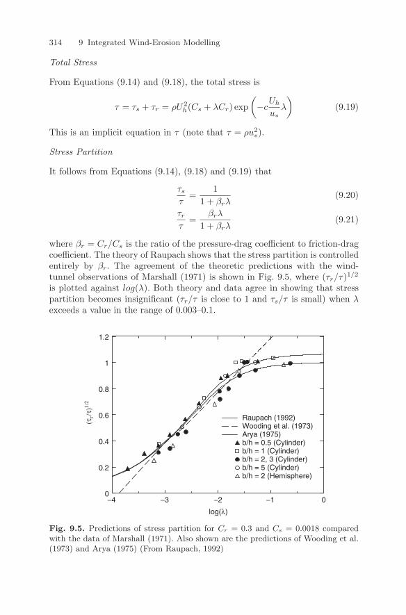
314 9 Integrated Wind-Erosion Modelling
Total Stress
From Equations (9.14) and (9.18), the total stress is
τ = τs + τr = ρU2h(Cs + λCr) exp
(−c
Uh
u∗λ
)(9.19)
This is an implicit equation in τ (note that τ = ρu2∗).
Stress Partition
It follows from Equations (9.14), (9.18) and (9.19) that
τs
τ=
11 + βrλ
(9.20)
τr
τ=
βrλ
1 + βrλ(9.21)
where βr = Cr/Cs is the ratio of the pressure-drag coefficient to friction-dragcoefficient. The theory of Raupach shows that the stress partition is controlledentirely by βr. The agreement of the theoretic predictions with the wind-tunnel observations of Marshall (1971) is shown in Fig. 9.5, where (τr/τ)1/2
is plotted against log(λ). Both theory and data agree in showing that stresspartition becomes insignificant (τr/τ is close to 1 and τs/τ is small) when λexceeds a value in the range of 0.003–0.1.
log(λ)
(τr/τ
)1/2
Raupach (1992)Wooding et al. (1973)Arya (1975)b/h = 0.5 (Cylinder)b/h = 1 (Cylinder)b/h = 2, 3 (Cylinder)b/h = 5 (Cylinder)b/h = 2 (Hemisphere)
0
0.2
0.4
0.6
0.8
1
1.2
−4 −3 −2 −1 0
Fig. 9.5. Predictions of stress partition for Cr = 0.3 and Cs = 0.0018 comparedwith the data of Marshall (1971). Also shown are the predictions of Wooding et al.(1973) and Arya (1975) (From Raupach, 1992)
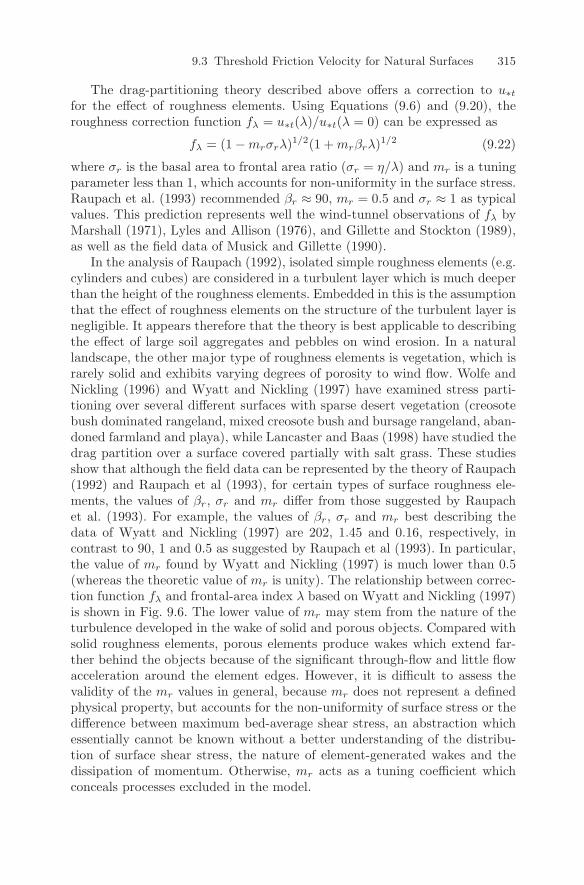
9.3 Threshold Friction Velocity for Natural Surfaces 315
The drag-partitioning theory described above offers a correction to u∗t
for the effect of roughness elements. Using Equations (9.6) and (9.20), theroughness correction function fλ = u∗t(λ)/u∗t(λ = 0) can be expressed as
fλ = (1 − mrσrλ)1/2(1 + mrβrλ)1/2 (9.22)
where σr is the basal area to frontal area ratio (σr = η/λ) and mr is a tuningparameter less than 1, which accounts for non-uniformity in the surface stress.Raupach et al. (1993) recommended βr ≈ 90, mr = 0.5 and σr ≈ 1 as typicalvalues. This prediction represents well the wind-tunnel observations of fλ byMarshall (1971), Lyles and Allison (1976), and Gillette and Stockton (1989),as well as the field data of Musick and Gillette (1990).
In the analysis of Raupach (1992), isolated simple roughness elements (e.g.cylinders and cubes) are considered in a turbulent layer which is much deeperthan the height of the roughness elements. Embedded in this is the assumptionthat the effect of roughness elements on the structure of the turbulent layer isnegligible. It appears therefore that the theory is best applicable to describingthe effect of large soil aggregates and pebbles on wind erosion. In a naturallandscape, the other major type of roughness elements is vegetation, which israrely solid and exhibits varying degrees of porosity to wind flow. Wolfe andNickling (1996) and Wyatt and Nickling (1997) have examined stress parti-tioning over several different surfaces with sparse desert vegetation (creosotebush dominated rangeland, mixed creosote bush and bursage rangeland, aban-doned farmland and playa), while Lancaster and Baas (1998) have studied thedrag partition over a surface covered partially with salt grass. These studiesshow that although the field data can be represented by the theory of Raupach(1992) and Raupach et al (1993), for certain types of surface roughness ele-ments, the values of βr, σr and mr differ from those suggested by Raupachet al. (1993). For example, the values of βr, σr and mr best describing thedata of Wyatt and Nickling (1997) are 202, 1.45 and 0.16, respectively, incontrast to 90, 1 and 0.5 as suggested by Raupach et al (1993). In particular,the value of mr found by Wyatt and Nickling (1997) is much lower than 0.5(whereas the theoretic value of mr is unity). The relationship between correc-tion function fλ and frontal-area index λ based on Wyatt and Nickling (1997)is shown in Fig. 9.6. The lower value of mr may stem from the nature of theturbulence developed in the wake of solid and porous objects. Compared withsolid roughness elements, porous elements produce wakes which extend far-ther behind the objects because of the significant through-flow and little flowacceleration around the element edges. However, it is difficult to assess thevalidity of the mr values in general, because mr does not represent a definedphysical property, but accounts for the non-uniformity of surface stress or thedifference between maximum bed-average shear stress, an abstraction whichessentially cannot be known without a better understanding of the distribu-tion of surface shear stress, the nature of element-generated wakes and thedissipation of momentum. Otherwise, mr acts as a tuning coefficient whichconceals processes excluded in the model.
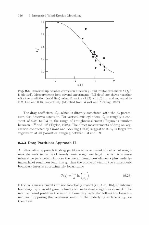
316 9 Integrated Wind-Erosion Modelling
λ
log λ
f−1
0.4
0.6
0.8
1.0
0.2
0−1−2−3
Fig. 9.6. Relationship between correction function fλ and frontal-area index λ (f−1λ
is plotted). Measurements from several experiments (full dots) are shown togetherwith the prediction (solid line) using Equation (9.22) with βr, σr and mr equal to202, 1.45 and 0.16, respectively (Modified from Wyatt and Nickling, 1997)
The drag coefficient, Cr, which is directly associated with the βr param-eter, also deserves attention. For vertical-axis cylinders, Cr is roughly a con-stant of 0.25 to 0.3 in the range of (roughness-element) Reynolds numberbetween 103 and 105 (Taylor, 1988). The direct measurements of drag on veg-etation conducted by Grant and Nickling (1998) suggest that Cr is larger forvegetation at all porosities, ranging between 0.3 and 0.9.
9.3.2 Drag Partition: Approach II
An alternative approach to drag partition is to represent the effect of rough-ness elements in terms of aerodynamic roughness length, which is a moreintegrative parameter. Suppose the overall (roughness elements plus underly-ing surface) roughness length is z0, then the profile of wind in the atmosphericboundary layer is approximately logarithmic
U(z) =u∗κ
ln(
z
z0
)(9.23)
If the roughness elements are not too closely spaced (i.e. λ < 0.05), an internalboundary layer would grow behind each individual roughness element. Themodified wind profile in the internal boundary layer also follows the logarith-mic law. Supposing the roughness length of the underlying surface is z00, wethen have
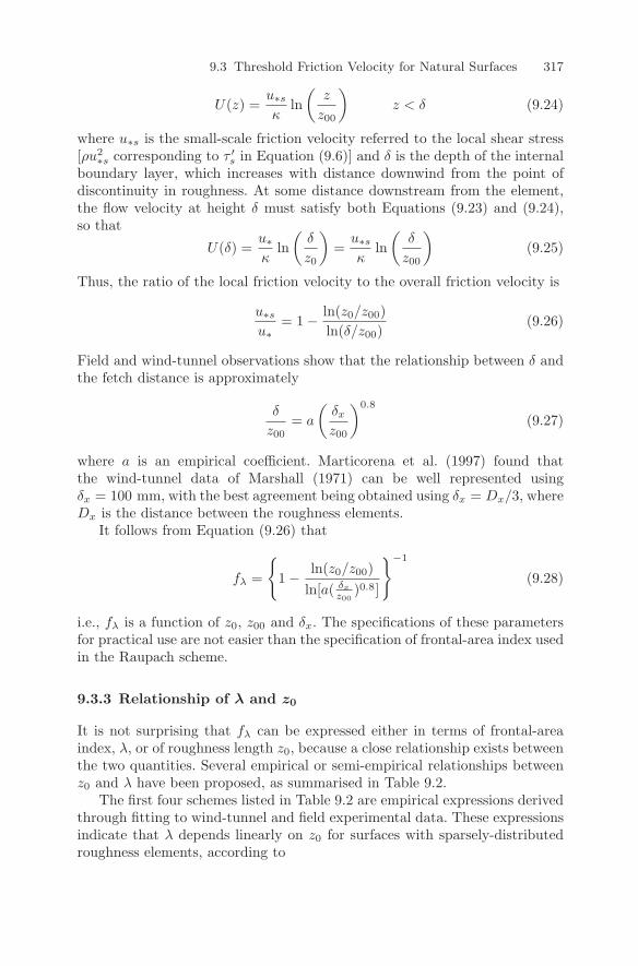
9.3 Threshold Friction Velocity for Natural Surfaces 317
U(z) =u∗s
κln
(z
z00
)z < δ (9.24)
where u∗s is the small-scale friction velocity referred to the local shear stress[ρu2
∗s corresponding to τ ′s in Equation (9.6)] and δ is the depth of the internal
boundary layer, which increases with distance downwind from the point ofdiscontinuity in roughness. At some distance downstream from the element,the flow velocity at height δ must satisfy both Equations (9.23) and (9.24),so that
U(δ) =u∗κ
ln(
δ
z0
)=
u∗s
κln
(δ
z00
)(9.25)
Thus, the ratio of the local friction velocity to the overall friction velocity is
u∗s
u∗= 1 − ln(z0/z00)
ln(δ/z00)(9.26)
Field and wind-tunnel observations show that the relationship between δ andthe fetch distance is approximately
δ
z00= a
(δx
z00
)0.8
(9.27)
where a is an empirical coefficient. Marticorena et al. (1997) found thatthe wind-tunnel data of Marshall (1971) can be well represented usingδx = 100 mm, with the best agreement being obtained using δx = Dx/3, whereDx is the distance between the roughness elements.
It follows from Equation (9.26) that
fλ =
1 − ln(z0/z00)
ln[a( δx
z00)0.8]
−1
(9.28)
i.e., fλ is a function of z0, z00 and δx. The specifications of these parametersfor practical use are not easier than the specification of frontal-area index usedin the Raupach scheme.
9.3.3 Relationship of λ and z0
It is not surprising that fλ can be expressed either in terms of frontal-areaindex, λ, or of roughness length z0, because a close relationship exists betweenthe two quantities. Several empirical or semi-empirical relationships betweenz0 and λ have been proposed, as summarised in Table 9.2.
The first four schemes listed in Table 9.2 are empirical expressions derivedthrough fitting to wind-tunnel and field experimental data. These expressionsindicate that λ depends linearly on z0 for surfaces with sparsely-distributedroughness elements, according to
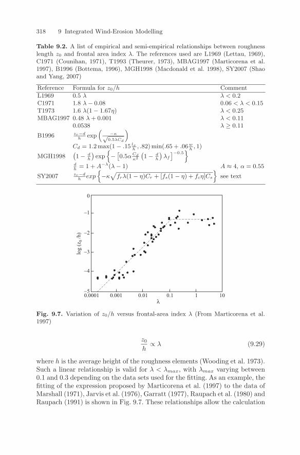
318 9 Integrated Wind-Erosion Modelling
Table 9.2. A list of empirical and semi-empirical relationships between roughnesslength z0 and frontal area index λ. The references used are L1969 (Lettau, 1969),C1971 (Counihan, 1971), T1993 (Theurer, 1973), MBAG1997 (Marticorena et al.1997), B1996 (Bottema, 1996), MGH1998 (Macdonald et al. 1998), SY2007 (Shaoand Yang, 2007)
Reference Formula for z0/h Comment
L1969 0.5 λ λ < 0.2C1971 1.8 λ − 0.08 0.06 < λ < 0.15T1973 1.6 λ(1 − 1.67η) λ < 0.25MBAG1997 0.48 λ + 0.001 λ < 0.11
0.0538 λ ≥ 0.11
B1996 zr−dh
exp(
−κ√0.5λCd
)Cd = 1.2 max(1 − .15 lx
h, .82) min(.65 + .06w
h, 1)
MGH1998(1 − d
h
)exp
−[0.5αCd
κ2
(1 − d
h
)λf
]−0.5
dh
= 1 + A−λ(λ − 1) A ≈ 4, α = 0.55
SY2007 zr−dh
exp−κ
√frλ(1 − η)Cr + [fs(1 − η) + fcη]Cs
see text
log
(z0 /
h)
λ
-5
-4
-3
-2
-1
0
0.1 1010.010.0010.0001
Fig. 9.7. Variation of z0/h versus frontal-area index λ (From Marticorena et al.1997)
z0
h∝ λ (9.29)
where h is the average height of the roughness elements (Wooding et al. 1973).Such a linear relationship is valid for λ < λmax, with λmax varying between0.1 and 0.3 depending on the data sets used for the fitting. As an example, thefitting of the expression proposed by Marticorena et al. (1997) to the data ofMarshall (1971), Jarvis et al. (1976), Garratt (1977), Raupach et al. (1980) andRaupach (1991) is shown in Fig. 9.7. These relationships allow the calculation
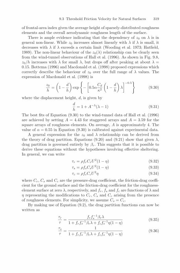
9.3 Threshold Friction Velocity for Natural Surfaces 319
of frontal-area index given the average height of sparsely-distributed roughnesselements and the overall aerodynamic roughness length of the surface.
There is ample evidence indicating that the dependency of z0 on λ is ingeneral non-linear. While z0 increases almost linearly with λ if λ is small, itdecreases with λ if λ exceeds a certain limit (Wooding et al. 1973; Hatfield,1989). The non-linear behaviour of the z0(λ) relationship can be clearly seenfrom the wind-tunnel observations of Hall et al. (1996). As shown in Fig. 9.8,z0/h increases with λ for small λ, but drops off after peaking at about λ =0.15. Bottema (1996) and Macdonald et al. (1998) proposed expressions whichcorrectly describe the behaviour of z0 over the full range of λ values. Theexpression of Macdonald et al. (1998) is
z0
h=
(1 − d
h
)exp
−
[0.5α
Cd
κ2
(1 − d
h
)λ
]−0.5
(9.30)
where the displacement height, d, is given byd
h= 1 + A−λ(λ − 1) (9.31)
The best fits of Equation (9.30) to the wind-tunnel data of Hall et al. (1996)are achieved by setting A = 4.43 for staggered arrays and A = 3.59 for thesquare arrays of roughness elements. On average, A is approximately 4. Thevalue of α = 0.55 in Equation (9.30) is calibrated against experimental data.
A general expression for the z0 and λ relationship can be derived fromthe theory of drag partition. Equations (9.20) and (9.21) show that given λ,drag partition is governed entirely by βr. This suggests that it is possible toderive these equations without the hypotheses involving effective sheltering.In general, we can write
τr = ρfrCrU2(1 − η) (9.32)
τs = ρfsCsU2(1 − η) (9.33)
τc = ρfcCcU2η (9.34)
where Cr, Cs and Cc are the pressure-drag coefficient, the friction-drag coeffi-cient for the ground surface and the friction-drag coefficient for the roughness-element surface at zero λ, respectively, and fr, fs and fc are functions of λ andη representing the modifications to Cr, Cs and Cc arising from the presenceof roughness elements. For simplicity, we assume Cs = Cc.
By making use of Equation (9.2), the drag partition functions can now bewritten as
τr
τ=
frf−1s βrλ
1 + frf−1s βrλ + fcf
−1s η(1 − η)
(9.35)
τs
τ=
11 + frf
−1s βrλ + fcf
−1s η(1 − η)
(9.36)
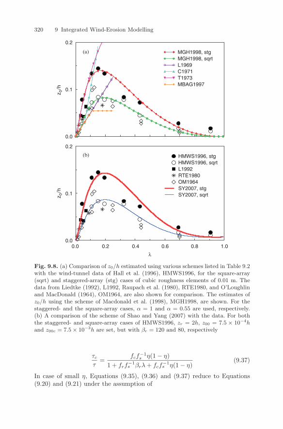
320 9 Integrated Wind-Erosion Modelling
HMWS1996, stgHMWS1996, sqrtL1992RTE1980OM1964SY2007, stgSY2007, sqrt
z 0/h
z 0/h
λ
(a)
(b)
MGH1998, stgMGH1998, sqrtL1969C1971T1973MBAG1997
0.0
0.1
0.2
0.0
0.1
0.2
0.0 0.2 0.4 0.6 0.8 1.0
Fig. 9.8. (a) Comparison of z0/h estimated using various schemes listed in Table 9.2with the wind-tunnel data of Hall et al. (1996), HMWS1996, for the square-array(sqrt) and staggered-array (stg) cases of cubic roughness elements of 0.01 m. Thedata from Liedtke (1992), L1992, Raupach et al. (1980), RTE1980, and O’Loughlinand MacDonald (1964), OM1964, are also shown for comparison. The estimates ofz0/h using the scheme of Macdonald et al. (1998), MGH1998, are shown. For thestaggered- and the square-array cases, α = 1 and α = 0.55 are used, respectively.(b) A comparison of the scheme of Shao and Yang (2007) with the data. For boththe staggered- and square-array cases of HMWS1996, zr = 2h, z00 = 7.5 × 10⁻⁴hand z00c = 7.5 × 10⁻³h are set, but with βr = 120 and 80, respectively
τc
τ=
fcf−1s η(1 − η)
1 + frf−1s βrλ + fcf
−1s η(1 − η)
(9.37)
In case of small η, Equations (9.35), (9.36) and (9.37) reduce to Equations(9.20) and (9.21) under the assumption of
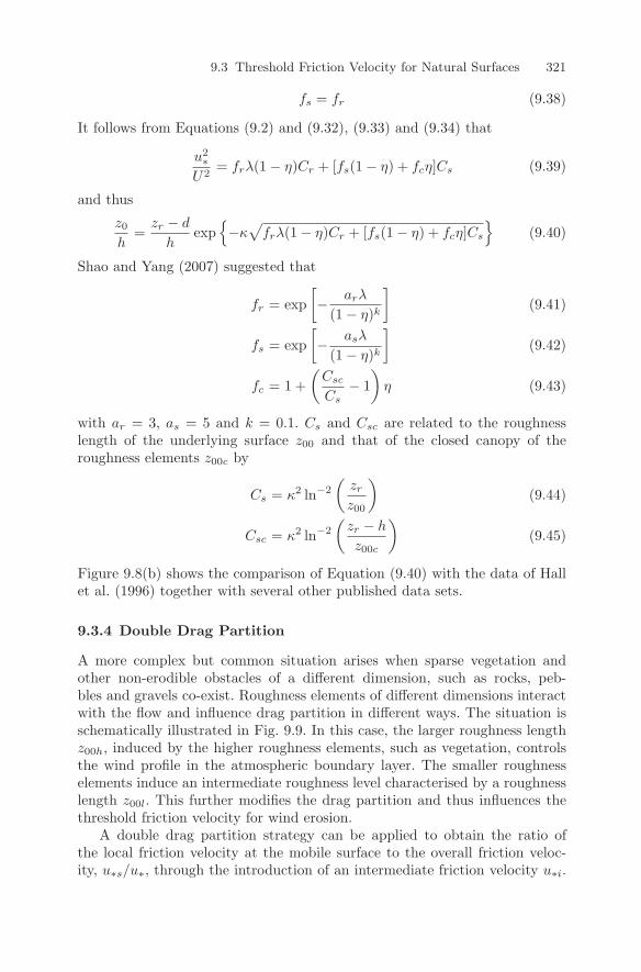
9.3 Threshold Friction Velocity for Natural Surfaces 321
fs = fr (9.38)
It follows from Equations (9.2) and (9.32), (9.33) and (9.34) that
u2∗
U2= frλ(1 − η)Cr + [fs(1 − η) + fcη]Cs (9.39)
and thus
z0
h=
zr − d
hexp
−κ
√frλ(1 − η)Cr + [fs(1 − η) + fcη]Cs
(9.40)
Shao and Yang (2007) suggested that
fr = exp[− arλ
(1 − η)k
](9.41)
fs = exp[− asλ
(1 − η)k
](9.42)
fc = 1 +(
Csc
Cs− 1
)η (9.43)
with ar = 3, as = 5 and k = 0.1. Cs and Csc are related to the roughnesslength of the underlying surface z00 and that of the closed canopy of theroughness elements z00c by
Cs = κ2 ln−2
(zr
z00
)(9.44)
Csc = κ2 ln−2
(zr − h
z00c
)(9.45)
Figure 9.8(b) shows the comparison of Equation (9.40) with the data of Hallet al. (1996) together with several other published data sets.
9.3.4 Double Drag Partition
A more complex but common situation arises when sparse vegetation andother non-erodible obstacles of a different dimension, such as rocks, peb-bles and gravels co-exist. Roughness elements of different dimensions interactwith the flow and influence drag partition in different ways. The situation isschematically illustrated in Fig. 9.9. In this case, the larger roughness lengthz00h, induced by the higher roughness elements, such as vegetation, controlsthe wind profile in the atmospheric boundary layer. The smaller roughnesselements induce an intermediate roughness level characterised by a roughnesslength z00l. This further modifies the drag partition and thus influences thethreshold friction velocity for wind erosion.
A double drag partition strategy can be applied to obtain the ratio ofthe local friction velocity at the mobile surface to the overall friction veloc-ity, u∗s/u∗, through the introduction of an intermediate friction velocity u∗i.
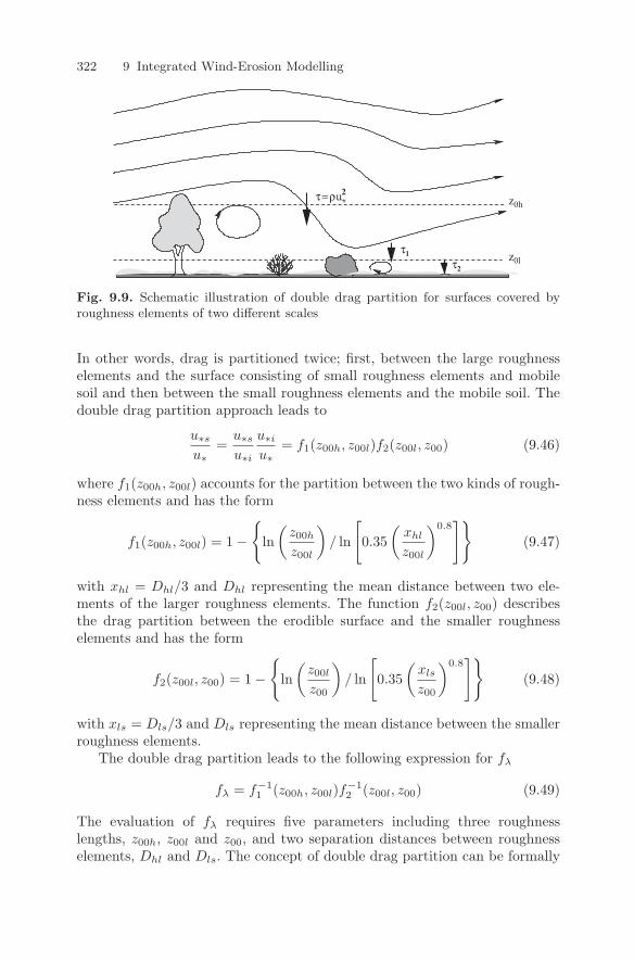
322 9 Integrated Wind-Erosion Modelling
τ=ρu
τ2
τ1
*2
z0h
z0l
Fig. 9.9. Schematic illustration of double drag partition for surfaces covered byroughness elements of two different scales
In other words, drag is partitioned twice; first, between the large roughnesselements and the surface consisting of small roughness elements and mobilesoil and then between the small roughness elements and the mobile soil. Thedouble drag partition approach leads to
u∗s
u∗=
u∗s
u∗i
u∗i
u∗= f1(z00h, z00l)f2(z00l, z00) (9.46)
where f1(z00h, z00l) accounts for the partition between the two kinds of rough-ness elements and has the form
f1(z00h, z00l) = 1 −
ln(
z00h
z00l
)/ ln
[0.35
(xhl
z00l
)0.8]
(9.47)
with xhl = Dhl/3 and Dhl representing the mean distance between two ele-ments of the larger roughness elements. The function f2(z00l, z00) describesthe drag partition between the erodible surface and the smaller roughnesselements and has the form
f2(z00l, z00) = 1 −
ln(
z00l
z00
)/ ln
[0.35
(xls
z00
)0.8]
(9.48)
with xls = Dls/3 and Dls representing the mean distance between the smallerroughness elements.
The double drag partition leads to the following expression for fλ
fλ = f−11 (z00h, z00l)f−1
2 (z00l, z00) (9.49)
The evaluation of fλ requires five parameters including three roughnesslengths, z00h, z00l and z00, and two separation distances between roughnesselements, Dhl and Dls. The concept of double drag partition can be formally
9.3 Threshold Friction Velocity for Natural Surfaces 323
expanded to multiple-drag partitioning. Supposing there are K layers of dif-ferent roughness elements, we would obtain
fλ =k=K∏k=1
f−1k (9.50)
9.3.5 Soil Moisture
In Chapter 5, we have accounted for the effect of soil moisture on u∗t byincluding the inter-particle cohesion due to soil moisture in Fi and have shownthat u∗t can be estimated using Equation (5.45).
In Equation (9.1), the effect of soil moisture on u∗t is represented usingthe moisture correction function, fw(θ), which is the ratio of the thresholdfriction velocity of a wet soil surface, u∗t(θ), to that of the dry surface (i.e. atair-dry soil moisture), u∗t(θr), so that
u∗t(θ) = u∗t(θr)fw(θ; Is) (9.51)
We expect that the dependency of fw on θ differs for different soil types, de-noted here with Is. Soil moisture can be defined in various ways. In the aboveequation, θ is the volumetric soil-water content with dimensions of L3L−3.This definition appears to be the most suitable as far as wind-erosion mod-elling is concerned, because most land-surface models (Chapter 4) producevolumetric soil water content as output, which can be directly used for wind-erosion modelling without conversion.
A number of experiments have been conducted on the effect of soil moistureon u∗t (Belly, 1964; Saleh and Fryrear, 1995; Chen et al. 1996). However, thefw function derived empirically from these experiments is not universal andin general fails to reproduce experimental data sets other than those fromwhich it is derived. The soil moisture correction described here is based on theconcept of cohesion reinforcement of wet soils, derived by McKenna Neumanand Nickling (1989) and Fecan et al. (1999).
Moisture is retained in soil by two processes which interact with the soilmatrix. Due to capillary forces, water wedges may form around the contactpoints of the grains, as shown in Fig. 9.10a; and due to molecular adsorp-tion, water films may appear on the grain surface. The adsorption of waterupon a solid surface is generally of an electrostatic nature, as the polarisedwater molecules attach to the charged faces of the solid. The strength of theelectrostatic attraction exerted upon the water molecules depends on the hy-groscopic properties of the soil particles. The adsorption is small for sand butincreases with the clay content of the soil. The inter-particle forces arisingfrom the adsorbed water film are much lower than the inter-particle capillaryforces (Chen et al. 1996). Therefore, the increase in threshold friction velocitywith soil moisture is attributed mainly to the inter-particle component of thecapillary forces.

324 9 Integrated Wind-Erosion Modelling
Cone 2
Cone 1
RR
Air
12
(a)
Water
Particle
Particle
RR
Air
12α2
α1
(b)
Fig. 9.10. (a) Representation of the water wedge in an idealised soil with spheri-cal grains of uniform size. (b) Representation of the contact area of soil grains bydissymmetrical cones suggested by McKenna Neuman and Nickling (1989)
The capillary force, Fc, occurring in a moist soil can be expressed as thesum of (i) a pressure force due to the pressure differential between the insideand the outside of the water wedge, and (ii) a tension force exerted by theair/water interface (Fisher, 1926). For spherical particles with the geometricconfiguration illustrated in Fig. 9.10a, it is found that
Fc =| ∆P | Ac + Tenl (9.52)
where Ac is the contact area (Ac = πR22), l is the perimeter of the contact
zone (l = 2πR2), Ten is the surface tension of water (0.072 kg s−2) and ∆Pis the pressure deficit between the inside of the water wedge and its outside(i.e., the atmosphere). ∆P is negative with | ∆P |= Ten( 1
R1− 1
R2), where
R1 is the radius of curvature of the air-water interface, depending on the soilmoisture and grain shape, and R2 is the curvature radius of the water wedge,depending on the soil moisture and grain shape. The application of the theoryinvolves the estimation of R1 and R2, which represent the geometry of thecontacts between particles, but are difficult to obtain for practical purposesof wind-erosion modelling. McKenna Neuman and Nickling (1989) suggestedthat the inter-particle contact can be approximated by dissymmetric cones(Fig. 9.10b). Applying these geometric considerations to Equation (9.52), itis found that
Fc = GπT 2
en
| ∆P | (9.53)
where G is a non-dimensional geometric coefficient depending rather compli-catedly on the angles α1 and α2 (Fig. 9.10b). This equation indicates that the
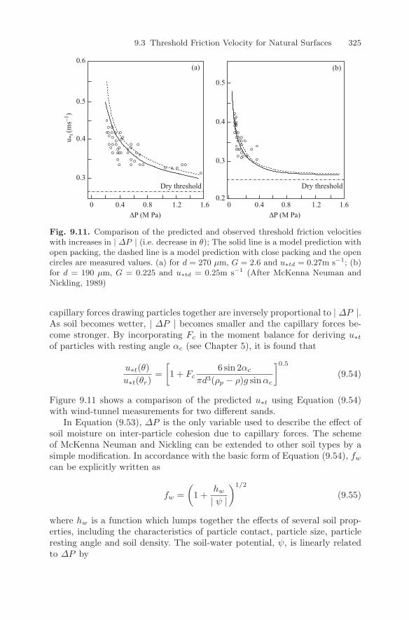
9.3 Threshold Friction Velocity for Natural Surfaces 325
(b)
1.6
Dry threshold Dry threshold
(a)u *
t (m
s−1 )
0.6
0.5
0.4
0.3
0 0 0.4 0.8 1.2 1.60.4 0.8 1.20.2
0.3
0.4
0.5
∆P (M Pa) ∆P (M Pa)
Fig. 9.11. Comparison of the predicted and observed threshold friction velocitieswith increases in | ∆P | (i.e. decrease in θ); The solid line is a model prediction withopen packing, the dashed line is a model prediction with close packing and the opencircles are measured values. (a) for d = 270 µm, G = 2.6 and u∗td = 0.27m s−1; (b)for d = 190 µm, G = 0.225 and u∗td = 0.25m s−1 (After McKenna Neuman andNickling, 1989)
capillary forces drawing particles together are inversely proportional to | ∆P |.As soil becomes wetter, | ∆P | becomes smaller and the capillary forces be-come stronger. By incorporating Fc in the moment balance for deriving u∗t
of particles with resting angle αc (see Chapter 5), it is found that
u∗t(θ)u∗t(θr)
=[1 + Fc
6 sin 2αc
πd3(ρp − ρ)g sinαc
]0.5
(9.54)
Figure 9.11 shows a comparison of the predicted u∗t using Equation (9.54)with wind-tunnel measurements for two different sands.
In Equation (9.53), ∆P is the only variable used to describe the effect ofsoil moisture on inter-particle cohesion due to capillary forces. The schemeof McKenna Neuman and Nickling can be extended to other soil types by asimple modification. In accordance with the basic form of Equation (9.54), fw
can be explicitly written as
fw =(
1 +hw
| ψ |
)1/2
(9.55)
where hw is a function which lumps together the effects of several soil prop-erties, including the characteristics of particle contact, particle size, particleresting angle and soil density. The soil-water potential, ψ, is linearly relatedto ∆P by
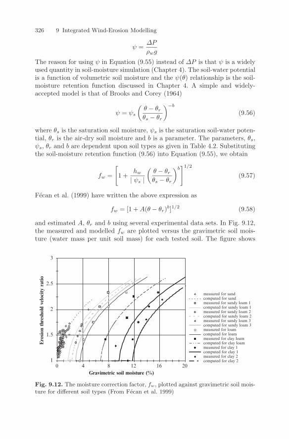
326 9 Integrated Wind-Erosion Modelling
ψ =∆P
ρwg
The reason for using ψ in Equation (9.55) instead of ∆P is that ψ is a widelyused quantity in soil-moisture simulation (Chapter 4). The soil-water potentialis a function of volumetric soil moisture and the ψ(θ) relationship is the soil-moisture retention function discussed in Chapter 4. A simple and widely-accepted model is that of Brooks and Corey (1964)
ψ = ψs
(θ − θr
θs − θr
)−b
(9.56)
where θs is the saturation soil moisture, ψs is the saturation soil-water poten-tial, θr is the air-dry soil moisture and b is a parameter. The parameters, θs,ψs, θr and b are dependent upon soil types as given in Table 4.2. Substitutingthe soil-moisture retention function (9.56) into Equation (9.55), we obtain
fw =
[1 +
hw
| ψs |
(θ − θr
θs − θr
)b]1/2
(9.57)
Fecan et al. (1999) have written the above expression as
fw = [1 + A(θ − θr)b]1/2 (9.58)
and estimated A, θr and b using several experimental data sets. In Fig. 9.12,the measured and modelled fw are plotted versus the gravimetric soil mois-ture (water mass per unit soil mass) for each tested soil. The figure shows
Gravimetric soil moisture (%)
measured for sandcomputed for sandmeasured for sandy loam 1computed for sandy loam 1measured for sandy loam 2computed for sandy loam 2measured for sandy loam 3computed for sandy loam 3measured for loamcomputed for loammeasured for clay loamcomputed for clay loammeasured for clay 1computed for clay 1measured for clay 2computed for clay 2
Ero
sion
thr
esho
ld v
eloc
ity
ratio
1
1.5
2
2.5
3
0 4 8 12 16 20
Fig. 9.12. The moisture correction factor, fw, plotted against gravimetric soil mois-ture for different soil types (From Fecan et al. 1999)
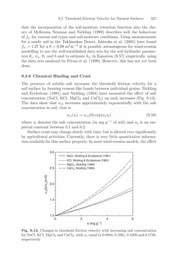
9.3 Threshold Friction Velocity for Natural Surfaces 327
that the incorporation of the soil-moisture retention function into the the-ory of McKenna Neuman and Nickling (1989) describes well the behaviourof fw for various soil types and soil-moisture conditions. Using measurementsfor a sandy soil in the Taklimakan Desert, Ishizuka et al. (2005) have foundfw = 1.27 for a θ = 0.09 m3m−3 It is possibly advantageous for wind-erosionmodelling to use the well-established data sets for the soil hydraulic parame-ters θs, ψs, θr and b and to estimate hw in Equation (9.57) empirically, usingthe data sets analysed by Fecan et al. (1999). However, this has not yet beendone.
9.3.6 Chemical Binding and Crust
The presence of soluble salt increases the threshold friction velocity for asoil surface by forming cement-like bonds between individual grains. Nicklingand Ecclestone (1981) and Nickling (1984) have measured the effect of saltconcentration (NaCl, KCl, MgCl2 and CaCl2) on such increases (Fig. 9.13).The data show that u∗t increases approximately exponentially with the saltconcentration in soil, that is
u∗t(sl) = u∗t(0) exp(assl) (9.59)
where sl denotes the salt concentration (in mg g−1 of soil) and as is an em-pirical constant between 0.1 and 0.2.
Surface crust may change slowly with time, but is altered very significantlyby agricultural activities. Currently, there is very little quantitative informa-tion available for this surface property. In most wind-erosion models, the effect
NaCl, Nickling & Ecclestone (1981)
KCl, Nickling & Ecclestone (1981)
MgCl2, Nickling (1984)CaCl2, Nickling (1984)
u *t(s
)/u *t
(s=
0)
1.00 2 4 6
1.5
2.0
2.5
3.0
s (mg g−1)
Fig. 9.13. Changes in threshold friction velocity with increasing salt concentrationfor NaCl, KCl, MgCl2 and CaCl2, with as equal to 0.0994, 0.1061, 0.1609 and 0.1739,respectively
328 9 Integrated Wind-Erosion Modelling
of surface crust was subjectively estimated from a general description of soiltypes, with the values for the crust correction function, fsc, being artificiallyset to, for instance, 1 for sandy soils and 3 clay soils. The random changes(i.e. caused by ploughing) on the compactness of the soil surface have beenignored. For agricultural areas under frequent cultivation, this may result inan underestimate of erosion rate.
9.4 Sand Drift and Dust Emission of Soils with MultipleParticle Sizes
As discussed in Chapter 6, the (vertically-integrated) streamwise saltationflux for a soil of uniform particle size ds can be estimated using the Owenmodel
Q(ds) =
coAeρu3
∗g [1 − (u∗t
u∗)2] (u∗ ≥ u∗t)
0 (u∗ < u∗t)(9.60)
where u∗t can be estimated using Equation (9.1) and Ae is the fraction oferodible area. The Owen coefficient, co, is associated with some uncertainties.In theory, co is not a constant but dependent on wt(ds)/u∗, equal to 0.25 +wt(ds)/3u∗ in Owen’s original formulation. The typical value of co is aroundone, but with a considerable scatter. Several other models are available forthe prediction of Q(ds) as discussed in Chapter 6, and the performances ofthese models are quite similar.
One of the problems in applying the Owen (or any other) saltation modelto natural aeolian surfaces is that soil particles are in general not uniform, witha possible exception of well-sorted sand dunes. It is not known in theory howthe streamwise saltation flux for a multi-size soil depends on u∗, because theinteractions between particles of different sizes are too difficult to model. Noris it exactly known how u∗t can be estimated for multi-size soils. Physically-based analytical expressions for u∗t are so far not available for multi-size soils,although empirical expressions for it have been derived from experimental data(Bisal and Ferguson, 1970; Gillette, 1983).
In wind-erosion schemes, a modification to Equation (9.60) can be made toaccommodate the multi-size effect (Marticorena and Bergametti, 1995; Shaoet al. 1996). Suppose p(d) is the particle-size distribution of the parent soil.The mass fraction of particles with diameters ranging between d and d+ δd isthen p(d)δd. We assume that the dependency of the streamwise saltation fluxfor a particular particle-size group, Q(ds), on u∗ and u∗t(ds) is not signifi-cantly altered by the presence of particles of other sizes. The total streamwisesaltation flux for all particle sizes, Q, is then evaluated as a weighted integralof Q(ds) for particle sizes ds in the sand-size range (d1 < ds < d2) by:
Q =∫ d2
d1
Q(ds)p(ds)δds (9.61)
9.4 Sand Drift and Dust Emission of Soils with Multiple Particle Sizes 329
where d1 and d2 define the upper and lower limits of saltation particle sizefor a given u∗. If the detailed particle-size distribution p(d) is not available,discretised information can be used. For instance, gentle sieving may be usedto determine the soil fractions Pfin, Pmed and Pcos of fine, medium and coarsesand, with typical particle sizes dfin, dmed and dcos, respectively. Then Q canbe estimated from
Q = PfinQ(dfin) + PmedQ(dmed) + PcosQ(dcos) (9.62)
which is a discrete version of Equation (9.61).Marticorena and Bergametti (1995) proposed a slightly different but sim-
ilar modification to the calculation of Q for multi-size soils. The relative con-tribution to the total flux by each size group is assumed to be proportionalto the relative surface area it occupies on the surface. The surface coveredby each grain is represented to its basal surface, S(ds), which is πd2/4 for aspherical particle of diameter d. Note that since p(d)δd is the mass fractionof particles in the size range of [d, d + δd], the number of particles in this sizegroup is
6ρpπd3
p(d)δd
and the area these particles occupy is
32ρpd
p(d)δd
The total area occupied by all sand-sized particles is
ST =∫ d2
d1
32ρpds
p(ds)δds
Now a normalised basal surface can be introduced in the form
δSr(d) =1
ST
32ρpd
p(d)δd
The total streamwise saltation flux can be computed by a weighted integrationof the Owen equation
Q =∫ d2
d1
Q(ds)δSr(ds) (9.63)
Several dust-emission schemes have been proposed, as described inChapter 7. In the following, we provide a summary of and a discussionon these schemes.
Scheme-I: The dust-emission rate, F , is parameterised in terms of thepower of wind speed or friction velocity, and an empirical particle-size distri-bution is imposed on F to obtain dust emission rates for different particle-sizebins. The scheme can be formulated as follows:
330 9 Integrated Wind-Erosion Modelling
F = αg(un∗ − un
∗t) (9.64)
Fj = P (dj)F (9.65)
where u∗ is friction velocity, u∗t is threshold friction velocity, Fj is the dustemission rate and P (dj) the dust-mass fraction of the jth particle-size bin. Thecoefficient αg is empirical, in which various wind-erosion factors are lumpedtogether. The F ∝ un
∗ relationship is first proposed by Gillette and Passi(1988). Field observations suggest this relationship is not unreasonable and nfalls mostly in the range of 3–5, but is often set to 4. Scheme-I is popular dueto the simplicity in its formulation. However, it is not simple to estimate itsparameters in practice. The αg coefficient must be specified empirically, butthere are no guidelines for its specification. If we set n = 4, then the dimensionsof αg are [M L−6 T3], suggesting that αg may be affected by a number offactors. There is confusion in the literature regarding the interpretation of u∗t
in Scheme-I: It is sometimes interpreted as the threshold friction velocity of thesurface and sometimes as that of dust particles. The former is more reasonable.Equation (9.65) requires the specification of P (dj) which is unknown.
Scheme-II: These schemes have the common feature in that they areconstructed upon the basis of simplified micro-scopic wind-erosion physics,supplemented with dust climate data derived from observations. As an exam-ple, we consider the scheme proposed by Zender et al. (2003). A soil is assumedto consist of several modes, such as the sand, silt and clay. The dust-emissionrate for the jth particle-size bin, Fj is parameterised as
Fj = TzAzSzαzQ
I∑i=1
Mi,j (9.66)
where I is the number of modes; Mi,j is the mass fraction of particle-size binj in mode i; Tz is a tuning factor selected to produce a good climatologicalsimulation, e.g., Tz = 7× 10⁻⁴ would result in a global dust emission of 1500Tg yr−1 (d < 10 µm) in the study of Zender et al. (2003). Az is the fraction oferodible surface; αz is the saltation bombardment efficiency (Marticorena andBergametti, 1995); Q is the streamwise saltation flux; and Sz is the sourceerodibility factor.
A positive aspect of the scheme is that observed data, in particular satel-lite data, are used to constrain the scheme behaviour by tuning Tz and Sz.However, there are two main problems associated with this approach. (1) Thetuning of Tz and Sz requires the global dust emission to be known, but this isnot the case. In practice, the global dust emission, i.e., the integral of Fj overthe globe, is assumed to be such that the model estimated global dust load isin some sort of agreement with the inversely-calculated global dust load fromsatellite remote sensing. Unfortunately, the latter has very large uncertain-ties. For example, the inverse calculation of dust load depends on dust opticaldepth which is closely linked to the fine-particle (less than 1 µm diameter)
9.4 Sand Drift and Dust Emission of Soils with Multiple Particle Sizes 331
concentration, while dust load is largely dependent on the surpramicron par-ticle concentration. (2) Global dust load is determined not only by dust emis-sion, but also by dust deposition. Very little is known about the global dustdeposition. Thus, the dust emission estimates using Equation (9.66) are notindependent from the uncertainties in dust deposition estimates.
Scheme-III: According to Marticorena and Bergametti (1995), the ratiobetween dust emission rate and vertically integrated saltation flux, F/Q, canbe expressed as
F
Q= a1 exp(a2ηc − a3) (9.67)
where ηc is the percentage of clay, F/Q is in [m−1] and a1, a2 and a3 areempirical coefficients. By fitting Equation (9.67) to the data set of Gillette(1977), it is found that a1, a2 and a3 are respectively 0.01, 0.31 and 13.82.Despite of its simplicity, Scheme-III is practically useful and has captured twoimportant aspects of the dust emission process, namely, (1) dust emission isproportional to sand drift intensity and (2) this proportionality is dependenton clay content. However, to assume F/Q to depend on ηc only is obviouslyan over simplification of the dust emission process. The empirical nature ofthe scheme is clear because a1, a2 and a3 are neither universal constants norparameters derived from physical arguments. The scheme is not spectral be-cause it does not allow the predictions of dust emission in different particlesize groups unless a treatment similar to Equation (9.65) is implemented. An-other minor problem with Equation (9.67) is that at ηc = 0, F/Q > 0, whichis not fully consistent with the physics considerations behind the scheme.
Scheme-IV: A binding-energy based scheme has been proposed by Shaoet al. (1993b, 1996). The emission of dust of size dd due to the saltation ofsand grains of size ds is given by
F (dd, ds) = β1(ds)β2(dd)Q(ds)u−2∗t (dd) (9.68)
where
β1(ds) = 10−5[1.25 ln(ds) + 3.28] (9.69)β2(dd) = exp(−140.7dd + 0.37) (9.70)
with dd and ds being in mm. The rate of dust emission for the jth dustparticle-size bin Fj is determined by
Fj =∫ dj2
dj1
β2(d)u−2∗t (d)p(d)δd ·
∫ d2
d1
β1(d)Q(d)p(d)δd (9.71)
where dj1 and dj2 are the lower and upper limit of the jth dust particle-sizebin and d1 and d2 are the lower and upper size limit of saltating particles.The total dust emission rate is
F =J∑
j=1
Fj (9.72)
332 9 Integrated Wind-Erosion Modelling
with J being the number of dust particle-size bins. An assumption whichlies in the core of Scheme-IV is that the process of dust emission is a linearcombination of saltation bombardment of various sand particle sizes. A specificproblem with Equation (9.68) is that β1 and β2 are derived based a small setof idealized wind-tunnel experiments.
Scheme-V: Taking into consideration the three dust emission mechanisms(aerodynamic entrainment, saltation bombardment and aggregates disintegra-tion), Lu and Shao (1999) and Shao (2001, 2004) suggested that
F (dj , ds) = cyηfj[(1 − γ) + γσp](1 + σm)
gQ
u2∗
(9.73)
where F (dj , ds) is the dust emission rate for the jth particle-size bin generatedby the saltation of particles of size ds, cy is a dimensionless coefficient and γis a weighting function which satisfies
γ =
1 u∗ → u∗t
0 u∗ → ∞ (9.74)
Q is the streamwise saltation flux of ds; g is acceleration due to gravity;σp = pm(di)/pf (di) with pm(di) and pf (di) being the minimally- and fully-disturbed particle-size distribution. The bombardment efficiency σm is esti-mated by
σm = 12u2∗ρp
P
(1 + 14u∗
√ρb
P
)(9.75)
where ρb is soil bulk density and P is soil plastic pressure.This is a spectral model, because the rate of dust emission for any particle
size bin is determined by
Fj =∫ d2
d1
F (dj , d)δd (9.76)
The total dust emission rate is
F =J∑
j=1
Fj (9.77)
with J being the number of dust size bins. The values of cy fall between 10−5
and 5 × 10⁻⁵ and P falls between 1,000 and 50,000 Pa.In Scheme-V, the micro-physics of dust emission has been taken into con-
sideration. It is more complex than the other schemes, but is still very simple.The input parameters required by Scheme-V have physical interpretations.However, the applications of Scheme-V are humped by the lack of soil andland-surface data that are not yet readily available, in particular the soil plas-tic pressure and the minimally- and fully-disturbed parent soil particle-sizedistributions.
9.5 Climatic Constraints on Dust Emission 333
In general, dust emission mechanisms require further investigation. Thedifficulty in achieving the accuracy of dust emission schemes is exacerbatedbecause dust emission can vary by several orders of magnitude. A major prob-lem facing the dust modelling community is the lack of direct dust flux datafor model validation.
9.5 Climatic Constraints on Dust Emission
Because of the large uncertainties in regional and global dust models, it isdesirable to apply climatic constraints to the estimates of dust emission, suchthat the simulated dust-source pattern and intensity are not inconsistent withclimatic observations. To this end, we introduce a erodibility index, Se, anddefine Se = 0 as the non-source region and Se > 0 as the source region. Twoparticular useful sources of data for establishing the climatic constraints onerodibilty are surface weather data and satellite data.
9.5.1 Erodibility Derived from Synoptic Data
The synoptic records from weather stations are the best data available foranalysing dust climatology. According to the WMO (World MeteorologicalOrganisation) protocol, dust events are classified according to visibility intothe categories of:
• Dust in Suspension: widespread dust in suspension, not raised at or nearthe station at the time of observation; visibility is usually not greater than10 km
• Blowing Dust: raised dust or sand at the time of observation, reducingvisibility to 1–10 km
• Dust Storm: strong winds lift large quantities of dust particles, reducingvisibility to between 200 and 1000 m
• Severe Dust Storm: very strong winds lift large quantities of dust particles,reducing visibility to less than 200 m
Synoptic records are collected at a large number of stations at 3-hourly in-tervals over the past few decades. These records are valuable for studyingdust-storm distribution and frequency, near-surface dust concentration, cli-matic background and synoptic systems for dust-storm generations.
For a given weather station, the frequencies of the four dust-event cate-gories, respectively denoted as fDIS , fBD, fDS and fSDS , can be estimated as
fDIS = ADIS/Aobs
etc. where ADIS is the number of dust-in-suspension records and Aobs is thatof total synoptic records. The frequency of all dust events is then
fDE = fDIS + fBD + fDS + fSDS
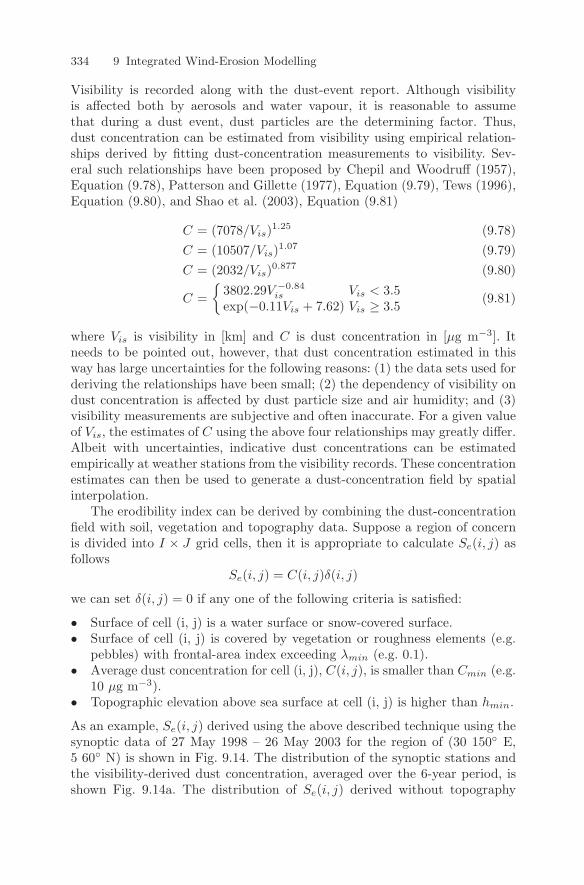
334 9 Integrated Wind-Erosion Modelling
Visibility is recorded along with the dust-event report. Although visibilityis affected both by aerosols and water vapour, it is reasonable to assumethat during a dust event, dust particles are the determining factor. Thus,dust concentration can be estimated from visibility using empirical relation-ships derived by fitting dust-concentration measurements to visibility. Sev-eral such relationships have been proposed by Chepil and Woodruff (1957),Equation (9.78), Patterson and Gillette (1977), Equation (9.79), Tews (1996),Equation (9.80), and Shao et al. (2003), Equation (9.81)
C = (7078/Vis)1.25 (9.78)C = (10507/Vis)1.07 (9.79)C = (2032/Vis)0.877 (9.80)
C =
3802.29V −0.84is Vis < 3.5
exp(−0.11Vis + 7.62) Vis ≥ 3.5 (9.81)
where Vis is visibility in [km] and C is dust concentration in [µg m−3]. Itneeds to be pointed out, however, that dust concentration estimated in thisway has large uncertainties for the following reasons: (1) the data sets used forderiving the relationships have been small; (2) the dependency of visibility ondust concentration is affected by dust particle size and air humidity; and (3)visibility measurements are subjective and often inaccurate. For a given valueof Vis, the estimates of C using the above four relationships may greatly differ.Albeit with uncertainties, indicative dust concentrations can be estimatedempirically at weather stations from the visibility records. These concentrationestimates can then be used to generate a dust-concentration field by spatialinterpolation.
The erodibility index can be derived by combining the dust-concentrationfield with soil, vegetation and topography data. Suppose a region of concernis divided into I × J grid cells, then it is appropriate to calculate Se(i, j) asfollows
Se(i, j) = C(i, j)δ(i, j)
we can set δ(i, j) = 0 if any one of the following criteria is satisfied:
• Surface of cell (i, j) is a water surface or snow-covered surface.• Surface of cell (i, j) is covered by vegetation or roughness elements (e.g.
pebbles) with frontal-area index exceeding λmin (e.g. 0.1).• Average dust concentration for cell (i, j), C(i, j), is smaller than Cmin (e.g.
10 µg m−3).• Topographic elevation above sea surface at cell (i, j) is higher than hmin.
As an example, Se(i, j) derived using the above described technique using thesynoptic data of 27 May 1998 – 26 May 2003 for the region of (30 150 E,5 60 N) is shown in Fig. 9.14. The distribution of the synoptic stations andthe visibility-derived dust concentration, averaged over the 6-year period, isshown Fig. 9.14a. The distribution of Se(i, j) derived without topography
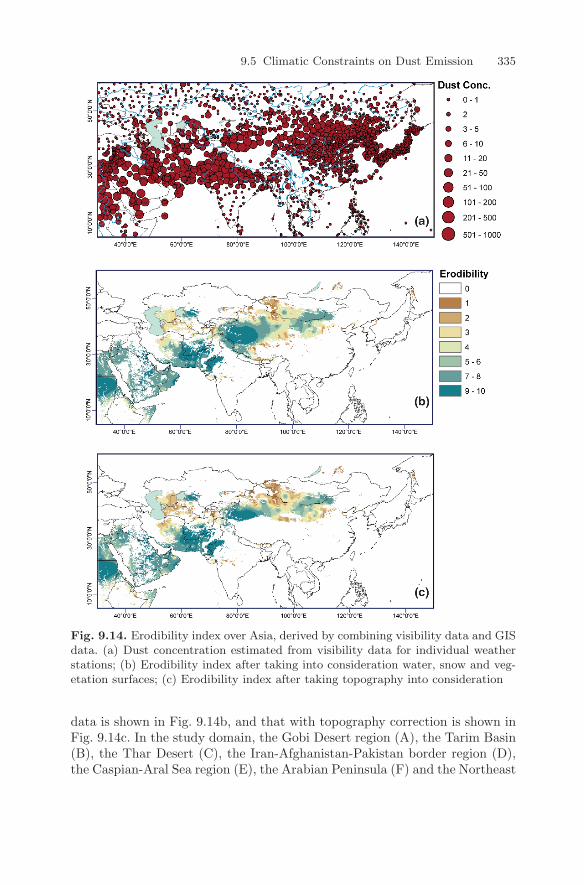
9.5 Climatic Constraints on Dust Emission 335
Fig. 9.14. Erodibility index over Asia, derived by combining visibility data and GISdata. (a) Dust concentration estimated from visibility data for individual weatherstations; (b) Erodibility index after taking into consideration water, snow and veg-etation surfaces; (c) Erodibility index after taking topography into consideration
data is shown in Fig. 9.14b, and that with topography correction is shown inFig. 9.14c. In the study domain, the Gobi Desert region (A), the Tarim Basin(B), the Thar Desert (C), the Iran-Afghanistan-Pakistan border region (D),the Caspian-Aral Sea region (E), the Arabian Peninsula (F) and the Northeast
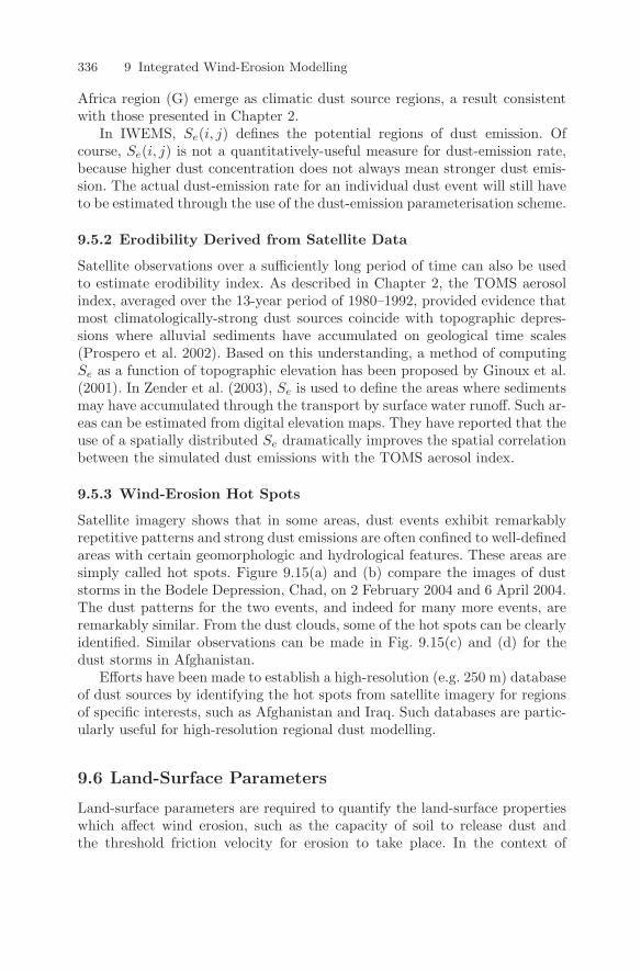
336 9 Integrated Wind-Erosion Modelling
Africa region (G) emerge as climatic dust source regions, a result consistentwith those presented in Chapter 2.
In IWEMS, Se(i, j) defines the potential regions of dust emission. Ofcourse, Se(i, j) is not a quantitatively-useful measure for dust-emission rate,because higher dust concentration does not always mean stronger dust emis-sion. The actual dust-emission rate for an individual dust event will still haveto be estimated through the use of the dust-emission parameterisation scheme.
9.5.2 Erodibility Derived from Satellite Data
Satellite observations over a sufficiently long period of time can also be usedto estimate erodibility index. As described in Chapter 2, the TOMS aerosolindex, averaged over the 13-year period of 1980–1992, provided evidence thatmost climatologically-strong dust sources coincide with topographic depres-sions where alluvial sediments have accumulated on geological time scales(Prospero et al. 2002). Based on this understanding, a method of computingSe as a function of topographic elevation has been proposed by Ginoux et al.(2001). In Zender et al. (2003), Se is used to define the areas where sedimentsmay have accumulated through the transport by surface water runoff. Such ar-eas can be estimated from digital elevation maps. They have reported that theuse of a spatially distributed Se dramatically improves the spatial correlationbetween the simulated dust emissions with the TOMS aerosol index.
9.5.3 Wind-Erosion Hot Spots
Satellite imagery shows that in some areas, dust events exhibit remarkablyrepetitive patterns and strong dust emissions are often confined to well-definedareas with certain geomorphologic and hydrological features. These areas aresimply called hot spots. Figure 9.15(a) and (b) compare the images of duststorms in the Bodele Depression, Chad, on 2 February 2004 and 6 April 2004.The dust patterns for the two events, and indeed for many more events, areremarkably similar. From the dust clouds, some of the hot spots can be clearlyidentified. Similar observations can be made in Fig. 9.15(c) and (d) for thedust storms in Afghanistan.
Efforts have been made to establish a high-resolution (e.g. 250 m) databaseof dust sources by identifying the hot spots from satellite imagery for regionsof specific interests, such as Afghanistan and Iraq. Such databases are partic-ularly useful for high-resolution regional dust modelling.
9.6 Land-Surface Parameters
Land-surface parameters are required to quantify the land-surface propertieswhich affect wind erosion, such as the capacity of soil to release dust andthe threshold friction velocity for erosion to take place. In the context of
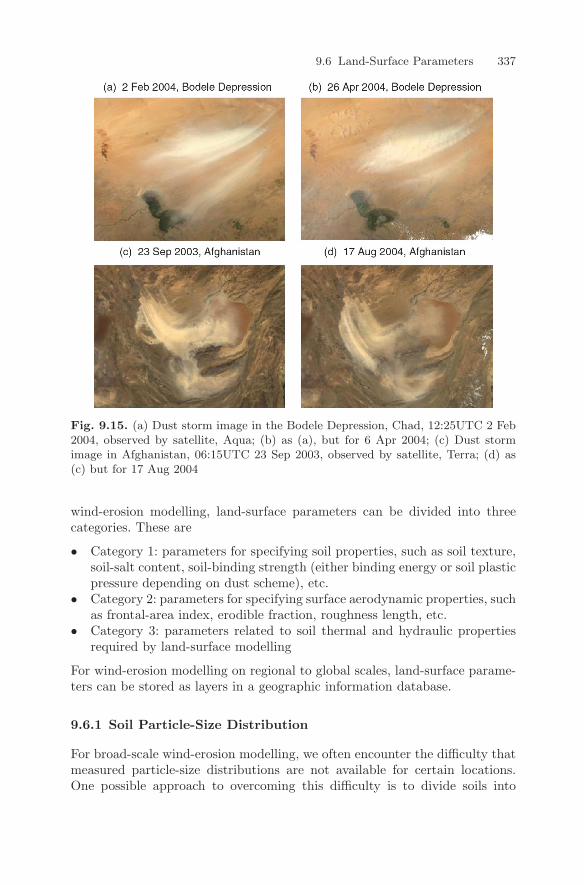
9.6 Land-Surface Parameters 337
Fig. 9.15. (a) Dust storm image in the Bodele Depression, Chad, 12:25UTC 2 Feb2004, observed by satellite, Aqua; (b) as (a), but for 6 Apr 2004; (c) Dust stormimage in Afghanistan, 06:15UTC 23 Sep 2003, observed by satellite, Terra; (d) as(c) but for 17 Aug 2004
wind-erosion modelling, land-surface parameters can be divided into threecategories. These are
• Category 1: parameters for specifying soil properties, such as soil texture,soil-salt content, soil-binding strength (either binding energy or soil plasticpressure depending on dust scheme), etc.
• Category 2: parameters for specifying surface aerodynamic properties, suchas frontal-area index, erodible fraction, roughness length, etc.
• Category 3: parameters related to soil thermal and hydraulic propertiesrequired by land-surface modelling
For wind-erosion modelling on regional to global scales, land-surface parame-ters can be stored as layers in a geographic information database.
9.6.1 Soil Particle-Size Distribution
For broad-scale wind-erosion modelling, we often encounter the difficulty thatmeasured particle-size distributions are not available for certain locations.One possible approach to overcoming this difficulty is to divide soils into
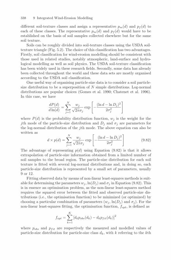
338 9 Integrated Wind-Erosion Modelling
different soil-texture classes and assign a representative pm(d) and pf (d) toeach of these classes. The representative pm(d) and pf (d) would have to beestablished on the basis of soil samples collected elsewhere but for the samesoil texture.
Soils can be roughly divided into soil-texture classes using the USDA soil-texture triangle (Fig. 5.2). The choice of this classification has two advantages.Firstly, soil classification for wind-erosion modelling should be consistent withthose used in related studies, notably atmospheric, land-surface and hydro-logical modelling as well as soil physics. The USDA soil-texture classificationhas been widely used in these research fields. Secondly, some data has alreadybeen collected throughout the world and these data sets are mostly organisedaccording to the USDA soil classification.
One useful way of organising particle-size data is to consider a soil particle-size distribution to be a superposition of N simple distributions. Log-normaldistributions are popular choices (Gomes et al. 1990; Chatenet et al. 1996).In this case, we have
dP (d)d ln(d)
=N∑
j=1
wj√2πσj
exp
[− (ln d − ln Dj)2
2σ2j
]
where P (d) is the probability distribution function, wj is the weight for thejth mode of the particle-size distribution and Dj and σj are parameters forthe log-normal distribution of the jth mode. The above equation can also bewritten as
d × p(d) =N∑
j=1
wj√2πσj
exp
[− (ln d − ln Dj)2
2σ2j
](9.82)
The advantage of representing p(d) using Equation (9.82) is that it allowsextrapolation of particle-size information obtained from a limited number ofsoil samples to the broad region. The particle-size distribution for each soiltexture is fitted with several log-normal distributions and, in doing so, eachparticle-size distribution is represented by a small set of parameters, usually9 or 12.
Fitting observed data by means of non-linear least-squares methods is suit-able for determining the parameters wj , ln(Dj) and σj in Equation (9.82). Thisis in essence an optimisation problem, as the non-linear least-squares methodrequires the squared error between the fitted and observed particle-size dis-tributions (i.e., the optimisation function) to be minimized (or optimized) bychoosing a particular combination of parameters (wj , ln(Dj) and σj). For thenon-linear least-squares fitting, the optimisation function, fopt, is defined as
fopt =K∑
k=1
[dkpobs(dk) − dkpfit(dk)]2
where pobs and pfit are respectively the measured and modelled values ofparticle-size distribution for particle-size class dk, with k referring to the kth
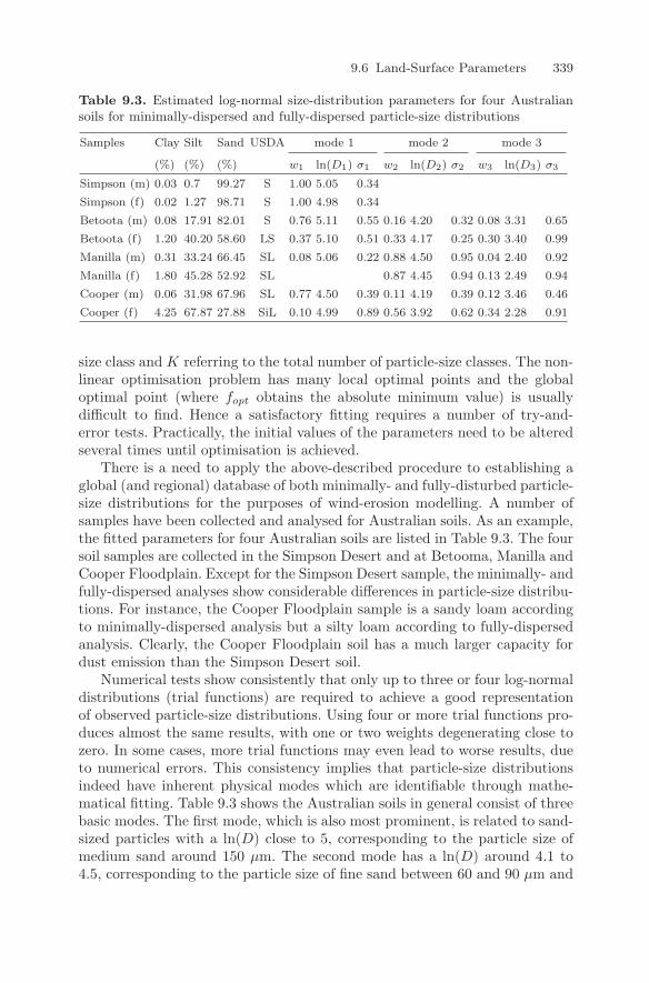
9.6 Land-Surface Parameters 339
Table 9.3. Estimated log-normal size-distribution parameters for four Australiansoils for minimally-dispersed and fully-dispersed particle-size distributions
Samples Clay Silt Sand USDA mode 1 mode 2 mode 3
(%) (%) (%) w1 ln(D1) σ1 w2 ln(D2) σ2 w3 ln(D3) σ3
Simpson (m) 0.03 0.7 99.27 S 1.00 5.05 0.34
Simpson (f) 0.02 1.27 98.71 S 1.00 4.98 0.34
Betoota (m) 0.08 17.91 82.01 S 0.76 5.11 0.55 0.16 4.20 0.32 0.08 3.31 0.65
Betoota (f) 1.20 40.20 58.60 LS 0.37 5.10 0.51 0.33 4.17 0.25 0.30 3.40 0.99
Manilla (m) 0.31 33.24 66.45 SL 0.08 5.06 0.22 0.88 4.50 0.95 0.04 2.40 0.92
Manilla (f) 1.80 45.28 52.92 SL 0.87 4.45 0.94 0.13 2.49 0.94
Cooper (m) 0.06 31.98 67.96 SL 0.77 4.50 0.39 0.11 4.19 0.39 0.12 3.46 0.46
Cooper (f) 4.25 67.87 27.88 SiL 0.10 4.99 0.89 0.56 3.92 0.62 0.34 2.28 0.91
size class and K referring to the total number of particle-size classes. The non-linear optimisation problem has many local optimal points and the globaloptimal point (where fopt obtains the absolute minimum value) is usuallydifficult to find. Hence a satisfactory fitting requires a number of try-and-error tests. Practically, the initial values of the parameters need to be alteredseveral times until optimisation is achieved.
There is a need to apply the above-described procedure to establishing aglobal (and regional) database of both minimally- and fully-disturbed particle-size distributions for the purposes of wind-erosion modelling. A number ofsamples have been collected and analysed for Australian soils. As an example,the fitted parameters for four Australian soils are listed in Table 9.3. The foursoil samples are collected in the Simpson Desert and at Betooma, Manilla andCooper Floodplain. Except for the Simpson Desert sample, the minimally- andfully-dispersed analyses show considerable differences in particle-size distribu-tions. For instance, the Cooper Floodplain sample is a sandy loam accordingto minimally-dispersed analysis but a silty loam according to fully-dispersedanalysis. Clearly, the Cooper Floodplain soil has a much larger capacity fordust emission than the Simpson Desert soil.
Numerical tests show consistently that only up to three or four log-normaldistributions (trial functions) are required to achieve a good representationof observed particle-size distributions. Using four or more trial functions pro-duces almost the same results, with one or two weights degenerating close tozero. In some cases, more trial functions may even lead to worse results, dueto numerical errors. This consistency implies that particle-size distributionsindeed have inherent physical modes which are identifiable through mathe-matical fitting. Table 9.3 shows the Australian soils in general consist of threebasic modes. The first mode, which is also most prominent, is related to sand-sized particles with a ln(D) close to 5, corresponding to the particle size ofmedium sand around 150 µm. The second mode has a ln(D) around 4.1 to4.5, corresponding to the particle size of fine sand between 60 and 90 µm and
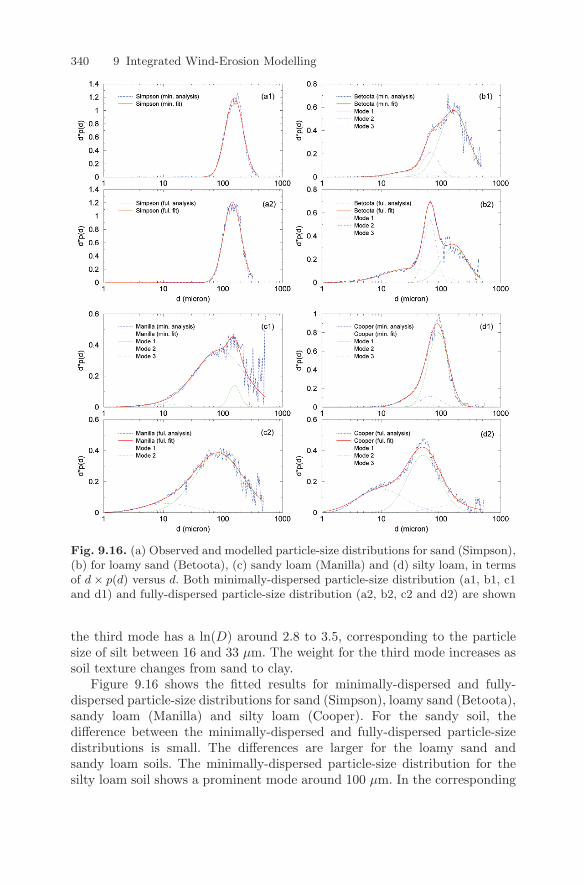
340 9 Integrated Wind-Erosion Modelling
Fig. 9.16. (a) Observed and modelled particle-size distributions for sand (Simpson),(b) for loamy sand (Betoota), (c) sandy loam (Manilla) and (d) silty loam, in termsof d × p(d) versus d. Both minimally-dispersed particle-size distribution (a1, b1, c1and d1) and fully-dispersed particle-size distribution (a2, b2, c2 and d2) are shown
the third mode has a ln(D) around 2.8 to 3.5, corresponding to the particlesize of silt between 16 and 33 µm. The weight for the third mode increases assoil texture changes from sand to clay.
Figure 9.16 shows the fitted results for minimally-dispersed and fully-dispersed particle-size distributions for sand (Simpson), loamy sand (Betoota),sandy loam (Manilla) and silty loam (Cooper). For the sandy soil, thedifference between the minimally-dispersed and fully-dispersed particle-sizedistributions is small. The differences are larger for the loamy sand andsandy loam soils. The minimally-dispersed particle-size distribution for thesilty loam soil shows a prominent mode around 100 µm. In the corresponding
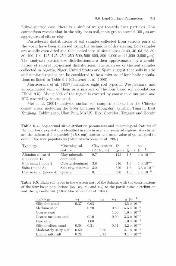
9.6 Land-Surface Parameters 341
fully-dispersed case, there is a shift of weight towards finer particles. Thiscomparison reveals that in the silty loam soil, most grains around 100 µm areaggregates of silt or clay.
Particle-size distributions of soil samples collected from various parts ofthe world have been analysed using the technique of dry sieving. Soil samplesare usually oven dried and then sieved into 10 size classes (<40, 40–63, 63–80,80–100, 100–125, 125–250, 250–500, 500–800, 800–1,000 and 1,000–2,000 µm).The analysed particle-size distributions are then approximated by a combi-nation of several log-normal distributions. The analyses of the soil samplescollected in Algeria, Niger, United States and Spain suggest that soils in aridand semiarid regions can be considered to be a mixture of four basic popula-tions as listed in Table 9.4 (Chatenet et al. 1996).
Marticorena et al. (1997) identified eight soil types in West Sahara, andapproximated each of them as a mixture of the four basic soil populations(Table 9.5). About 50% of the region is covered by coarse medium sand and20% covered by coarse sand.
Mei et al. (2004) analysed surface-soil samples collected in the Chinesedesert areas, including the Gobi (in Inner Mongolia), Gurban Tungut, EastXinjiang, Taklimakan, Ulan Buh, Mu US, Hexi Corridor, Tengger and Horqin
Table 9.4. Log-normal size-distribution parameters and mineralogical features ofthe four basic populations identified in soils in arid and semiarid regions. Also listedare the estimated fine-particle (<5.8 µm) content and mean value of γbi assigned toeach of the four populations (After Marticorena et al. 1997)
Typology Mineralogical Clay content D σ γbi
feature (<5.8 µm) (µm) (µm) (m−1)
Alumino-silicated Clay minerals 9.7 125 1.8 1 × 10⁻³
silt (mode 1) dominantFine sand (mode 2) Quartz dominant 3.6 210 1.6 1 × 10⁻⁴
Salts (mode 3) Salt-clay minerals 3.2 520 1.6 3.3 × 10⁻⁴
Coarse sand (mode 4) Quartz 0. 690 1.6 1 × 10⁻⁵
Table 9.5. Eight soil types in the western part of the Sahara, with the contributionsof the four basic populations (w1, w2, w3 and w4) to the particle-size distributionand the γb coefficient (After Marticorena et al. 1997)
Typology w1 w2 w3 w4 γb (m−1)
Silty fine sand 0.37 0.63 4.5 × 10⁻⁴
Medium sand 0.20 0.80 5.5 × 10⁻⁵
Coarse sand 1.00 1.0 × 10⁻⁵
Coarse medium sand 0.10 0.90 3.3 × 10⁻⁵
Fine sand 1.00 1.0 × 10⁻⁴
Silty medium sand 0.38 0.31 0.31 4.2 × 10⁻⁴
Moderately salty silt 0.50 0.50 4.1 × 10⁻⁴
Highly salty silt 0.25 0.75 3.1 × 10⁻⁴
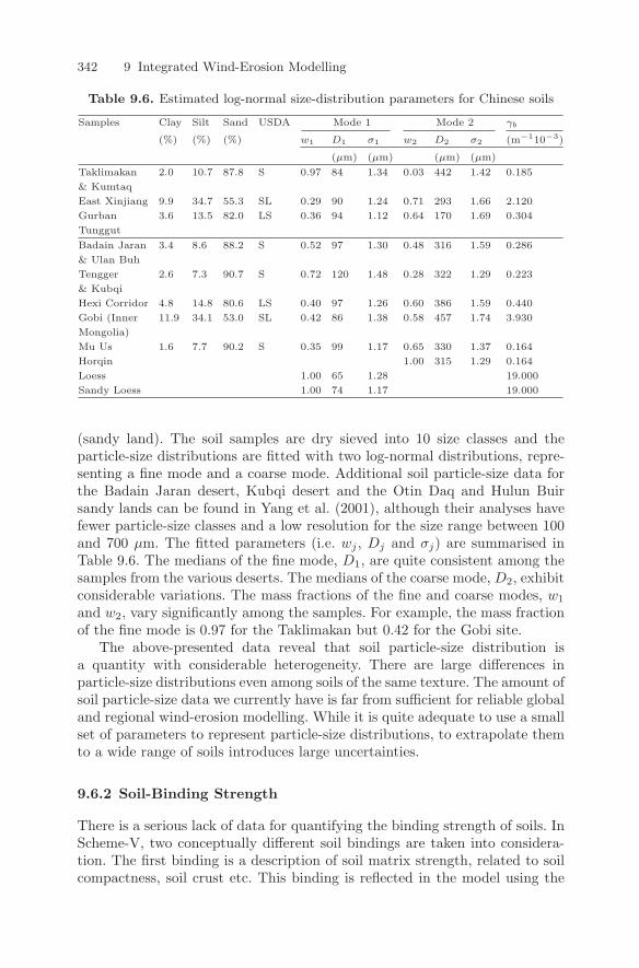
342 9 Integrated Wind-Erosion Modelling
Table 9.6. Estimated log-normal size-distribution parameters for Chinese soils
Samples Clay Silt Sand USDA Mode 1 Mode 2 γb
(%) (%) (%) w1 D1 σ1 w2 D2 σ2 (m−110−3)
(µm) (µm) (µm) (µm)
Taklimakan 2.0 10.7 87.8 S 0.97 84 1.34 0.03 442 1.42 0.185
& Kumtaq
East Xinjiang 9.9 34.7 55.3 SL 0.29 90 1.24 0.71 293 1.66 2.120
Gurban 3.6 13.5 82.0 LS 0.36 94 1.12 0.64 170 1.69 0.304
Tunggut
Badain Jaran 3.4 8.6 88.2 S 0.52 97 1.30 0.48 316 1.59 0.286
& Ulan Buh
Tengger 2.6 7.3 90.7 S 0.72 120 1.48 0.28 322 1.29 0.223
& Kubqi
Hexi Corridor 4.8 14.8 80.6 LS 0.40 97 1.26 0.60 386 1.59 0.440
Gobi (Inner 11.9 34.1 53.0 SL 0.42 86 1.38 0.58 457 1.74 3.930
Mongolia)
Mu Us 1.6 7.7 90.2 S 0.35 99 1.17 0.65 330 1.37 0.164
Horqin 1.00 315 1.29 0.164
Loess 1.00 65 1.28 19.000
Sandy Loess 1.00 74 1.17 19.000
(sandy land). The soil samples are dry sieved into 10 size classes and theparticle-size distributions are fitted with two log-normal distributions, repre-senting a fine mode and a coarse mode. Additional soil particle-size data forthe Badain Jaran desert, Kubqi desert and the Otin Daq and Hulun Buirsandy lands can be found in Yang et al. (2001), although their analyses havefewer particle-size classes and a low resolution for the size range between 100and 700 µm. The fitted parameters (i.e. wj , Dj and σj) are summarised inTable 9.6. The medians of the fine mode, D1, are quite consistent among thesamples from the various deserts. The medians of the coarse mode, D2, exhibitconsiderable variations. The mass fractions of the fine and coarse modes, w1
and w2, vary significantly among the samples. For example, the mass fractionof the fine mode is 0.97 for the Taklimakan but 0.42 for the Gobi site.
The above-presented data reveal that soil particle-size distribution isa quantity with considerable heterogeneity. There are large differences inparticle-size distributions even among soils of the same texture. The amount ofsoil particle-size data we currently have is far from sufficient for reliable globaland regional wind-erosion modelling. While it is quite adequate to use a smallset of parameters to represent particle-size distributions, to extrapolate themto a wide range of soils introduces large uncertainties.
9.6.2 Soil-Binding Strength
There is a serious lack of data for quantifying the binding strength of soils. InScheme-V, two conceptually different soil bindings are taken into considera-tion. The first binding is a description of soil matrix strength, related to soilcompactness, soil crust etc. This binding is reflected in the model using the
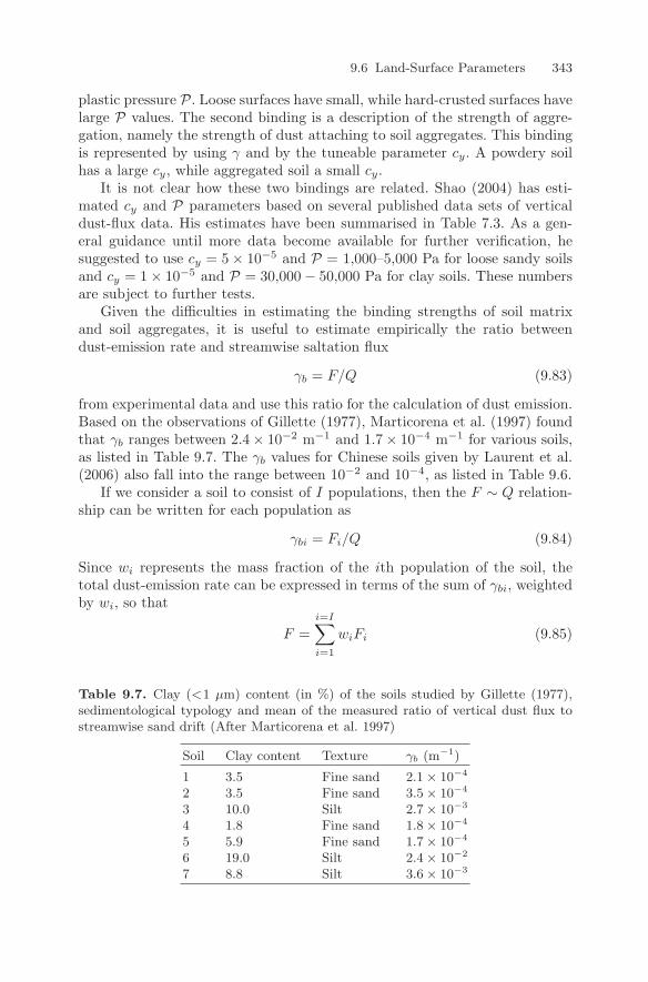
9.6 Land-Surface Parameters 343
plastic pressure P. Loose surfaces have small, while hard-crusted surfaces havelarge P values. The second binding is a description of the strength of aggre-gation, namely the strength of dust attaching to soil aggregates. This bindingis represented by using γ and by the tuneable parameter cy. A powdery soilhas a large cy, while aggregated soil a small cy.
It is not clear how these two bindings are related. Shao (2004) has esti-mated cy and P parameters based on several published data sets of verticaldust-flux data. His estimates have been summarised in Table 7.3. As a gen-eral guidance until more data become available for further verification, hesuggested to use cy = 5 × 10⁻⁵ and P = 1,000–5,000 Pa for loose sandy soilsand cy = 1 × 10⁻⁵ and P = 30,000 − 50,000 Pa for clay soils. These numbersare subject to further tests.
Given the difficulties in estimating the binding strengths of soil matrixand soil aggregates, it is useful to estimate empirically the ratio betweendust-emission rate and streamwise saltation flux
γb = F/Q (9.83)
from experimental data and use this ratio for the calculation of dust emission.Based on the observations of Gillette (1977), Marticorena et al. (1997) foundthat γb ranges between 2.4 × 10⁻² m−1 and 1.7 × 10⁻⁴ m−1 for various soils,as listed in Table 9.7. The γb values for Chinese soils given by Laurent et al.(2006) also fall into the range between 10−2 and 10−4, as listed in Table 9.6.
If we consider a soil to consist of I populations, then the F ∼ Q relation-ship can be written for each population as
γbi = Fi/Q (9.84)
Since wi represents the mass fraction of the ith population of the soil, thetotal dust-emission rate can be expressed in terms of the sum of γbi, weightedby wi, so that
F =i=I∑i=1
wiFi (9.85)
Table 9.7. Clay (<1 µm) content (in %) of the soils studied by Gillette (1977),sedimentological typology and mean of the measured ratio of vertical dust flux tostreamwise sand drift (After Marticorena et al. 1997)
Soil Clay content Texture γb (m−1)
1 3.5 Fine sand 2.1 × 10⁻⁴
2 3.5 Fine sand 3.5 × 10⁻⁴
3 10.0 Silt 2.7 × 10⁻³
4 1.8 Fine sand 1.8 × 10⁻⁴
5 5.9 Fine sand 1.7 × 10⁻⁴
6 19.0 Silt 2.4 × 10⁻²
7 8.8 Silt 3.6 × 10⁻³
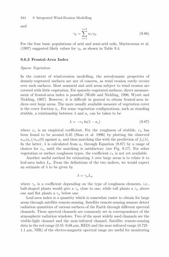
344 9 Integrated Wind-Erosion Modelling
and
γb =i=I∑i=1
wiγbi (9.86)
For the four basic populations of arid and semi-arid soils, Marticorena et al.(1997) suggested likely values for γbi as shown in Table 9.4.
9.6.3 Frontal-Area Index
Sparse Vegetation
In the context of wind-erosion modelling, the aerodynamic properties ofdensely-vegetated surfaces are not of concern, as wind erosion rarely occursover such surfaces. Most semiarid and arid areas subject to wind erosion arecovered with little vegetation. For sparsely-vegetated surfaces, direct measure-ment of frontal-area index is possible (Wolfe and Nickling, 1996; Wyatt andNickling, 1997). However, it is difficult in general to obtain frontal-area in-dices over large areas. The more usually available measure of vegetation coveris the cover fraction ac. For some vegetation configurations, such as standingstubble, a relationship between λ and ac can be taken to be
λ = −cλ ln(1 − ac) (9.87)
where cλ is an empirical coefficient. For the roughness of stubble, cλ hasbeen found to be around 0.35 (Shao et al. 1996) by plotting the observedu∗t(ac)/u∗t(0) against ac and then matching this with the prediction of fλ(λ).In the latter, λ is calculated from ac through Equation (9.87) by a range ofchoices for cλ, until the matching is satisfactory (see Fig. 9.17). For othervegetation or surface roughness types, the coefficient cλ is not yet available.
Another useful method for estimating λ over large areas is to relate it toleaf-area index La. From the definitions of the two indices, we would expectan estimate of λ to be given by
λ = γaLa
where γa is a coefficient depending on the type of roughness elements, i.e.,ball-shaped plants would give a γa close to one, while tall plants a γa aboveone and flat plants a γa below one.
Leaf-area index is a quantity which is somewhat easier to obtain for largeareas through satellite remote-sensing. Satellite remote-sensing sensors detectradiation quantities of various surfaces of the Earth through different spectralchannels. These spectral channels are commonly set in correspondence of theatmospheric radiation windows. Two of the most widely used channels are thevisible-light channel and the near-infrared channel. Satellite remote-sensingdata in the red range (0.55–0.68 µm, RED) and the near-infrared range (0.725–1.1 µm, NIR) of the electro-magnetic spectral range are useful for monitoring
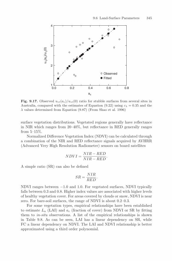
9.6 Land-Surface Parameters 345
ac
u *t(a
c)/u
*t(0
)
ObservedFitted
10.0 0.2 0.4 0.6 0.8
2
3
4
Fig. 9.17. Observed u∗t(ac)/u∗t(0) ratio for stubble surfaces from several sites inAustralia, compared with the estimates of Equation (9.22) using cλ = 0.35 and theλ values determined from Equation (9.87) (From Shao et al. 1996)
surface vegetation distributions. Vegetated regions generally have reflectancein NIR which ranges from 20–40%, but reflectance in RED generally rangesfrom 5–15%.
Normalized Difference Vegetation Index (NDVI) can be calculated througha combination of the NIR and RED reflectance signals acquired by AVHRR(Advanced Very High Resolution Radiometer) sensors on board satellites
NDV I =NIR − RED
NIR − RED.
A simple ratio (SR) can also be defined
SR =NIR
RED.
NDVI ranges between −1.0 and 1.0. For vegetated surfaces, NDVI typicallyfalls between 0.3 and 0.8. Higher index values are associated with higher levelsof healthy vegetation cover. For areas covered by clouds or snow, NDVI is nearzero. For bare-soil surfaces, the range of NDVI is about 0.2–0.3.
For some vegetation types, empirical relationships have been establishedto estimate La (LAI) and ac (fraction of cover) from NDVI or SR by fittingthem to in-situ observations. A list of the empirical relationships is shownin Table 9.8. As can be seen, LAI has a linear dependency on SR, whileFC a linear dependency on NDVI. The LAI and NDVI relationship is betterapproximated using a third order polynomial.
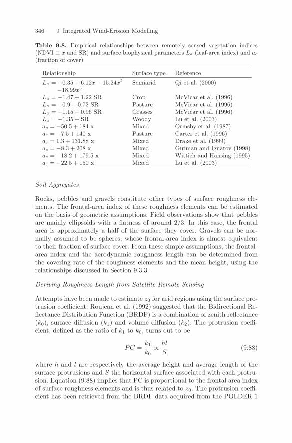
346 9 Integrated Wind-Erosion Modelling
Table 9.8. Empirical relationships between remotely sensed vegetation indices(NDVI ≡ x and SR) and surface biophysical parameters La (leaf-area index) and ac
(fraction of cover)
Relationship Surface type Reference
La = −0.35 + 6.12x − 15.24x2 Semiarid Qi et al. (2000)−18.99x3
La = −1.47 + 1.22 SR Crop McVicar et al. (1996)La = −0.9 + 0.72 SR Pasture McVicar et al. (1996)La = −1.15 + 0.96 SR Grasses McVicar et al. (1996)La = −1.35 + SR Woody Lu et al. (2003)ac = −50.5 + 184 x Mixed Ormsby et al. (1987)ac = −7.5 + 140 x Pasture Carter et al. (1996)ac = 1.3 + 131.88 x Mixed Drake et al. (1999)ac = −8.3 + 208 x Mixed Gutman and Ignatov (1998)ac = −18.2 + 179.5 x Mixed Wittich and Hansing (1995)ac = −22.5 + 150 x Mixed Lu et al. (2003)
Soil Aggregates
Rocks, pebbles and gravels constitute other types of surface roughness ele-ments. The frontal-area index of these roughness elements can be estimatedon the basis of geometric assumptions. Field observations show that pebblesare mainly ellipsoids with a flatness of around 2/3. In this case, the frontalarea is approximately a half of the surface they cover. Gravels can be nor-mally assumed to be spheres, whose frontal-area index is almost equivalentto their fraction of surface cover. From these simple assumptions, the frontal-area index and the aerodynamic roughness length can be determined fromthe covering rate of the roughness elements and the mean height, using therelationships discussed in Section 9.3.3.
Deriving Roughness Length from Satellite Remote Sensing
Attempts have been made to estimate z0 for arid regions using the surface pro-trusion coefficient. Roujean et al. (1992) suggested that the Bidirectional Re-flectance Distribution Function (BRDF) is a combination of zenith reflectance(k0), surface diffusion (k1) and volume diffusion (k2). The protrusion coeffi-cient, defined as the ratio of k1 to k0, turns out to be
PC =k1
k0∝ hl
S(9.88)
where h and l are respectively the average height and average length of thesurface protrusions and S the horizontal surface associated with each protru-sion. Equation (9.88) implies that PC is proportional to the frontal area indexof surface roughness elements and is thus related to z0. The protrusion coeffi-cient has been retrieved from the BRDF data acquired from the POLDER-1
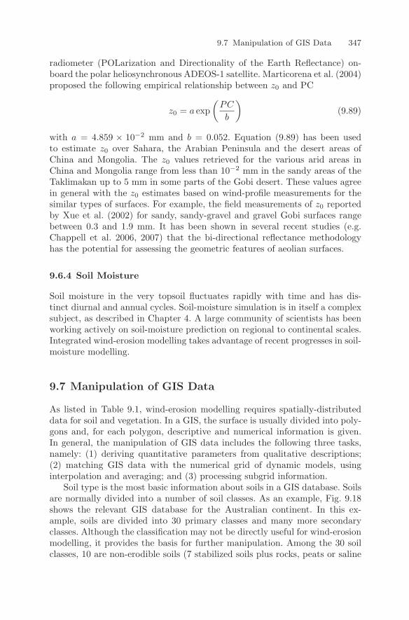
9.7 Manipulation of GIS Data 347
radiometer (POLarization and Directionality of the Earth Reflectance) on-board the polar heliosynchronous ADEOS-1 satellite. Marticorena et al. (2004)proposed the following empirical relationship between z0 and PC
z0 = a exp(
PC
b
)(9.89)
with a = 4.859 × 10⁻² mm and b = 0.052. Equation (9.89) has been usedto estimate z0 over Sahara, the Arabian Peninsula and the desert areas ofChina and Mongolia. The z0 values retrieved for the various arid areas inChina and Mongolia range from less than 10−2 mm in the sandy areas of theTaklimakan up to 5 mm in some parts of the Gobi desert. These values agreein general with the z0 estimates based on wind-profile measurements for thesimilar types of surfaces. For example, the field measurements of z0 reportedby Xue et al. (2002) for sandy, sandy-gravel and gravel Gobi surfaces rangebetween 0.3 and 1.9 mm. It has been shown in several recent studies (e.g.Chappell et al. 2006, 2007) that the bi-directional reflectance methodologyhas the potential for assessing the geometric features of aeolian surfaces.
9.6.4 Soil Moisture
Soil moisture in the very topsoil fluctuates rapidly with time and has dis-tinct diurnal and annual cycles. Soil-moisture simulation is in itself a complexsubject, as described in Chapter 4. A large community of scientists has beenworking actively on soil-moisture prediction on regional to continental scales.Integrated wind-erosion modelling takes advantage of recent progresses in soil-moisture modelling.
9.7 Manipulation of GIS Data
As listed in Table 9.1, wind-erosion modelling requires spatially-distributeddata for soil and vegetation. In a GIS, the surface is usually divided into poly-gons and, for each polygon, descriptive and numerical information is given.In general, the manipulation of GIS data includes the following three tasks,namely: (1) deriving quantitative parameters from qualitative descriptions;(2) matching GIS data with the numerical grid of dynamic models, usinginterpolation and averaging; and (3) processing subgrid information.
Soil type is the most basic information about soils in a GIS database. Soilsare normally divided into a number of soil classes. As an example, Fig. 9.18shows the relevant GIS database for the Australian continent. In this ex-ample, soils are divided into 30 primary classes and many more secondaryclasses. Although the classification may not be directly useful for wind-erosionmodelling, it provides the basis for further manipulation. Among the 30 soilclasses, 10 are non-erodible soils (7 stabilized soils plus rocks, peats or saline
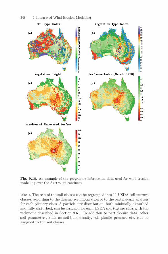
348 9 Integrated Wind-Erosion Modelling
Fig. 9.18. An example of the geographic information data used for wind-erosionmodelling over the Australian continent
lakes). The rest of the soil classes can be regrouped into 11 USDA soil-textureclasses, according to the descriptive information or to the particle-size analysisfor each primary class. A particle-size distribution, both minimally-disturbedand fully-disturbed, can be assigned for each USDA soil-texture class with thetechnique described in Section 9.6.1. In addition to particle-size data, othersoil parameters, such as soil-bulk density, soil plastic pressure etc. can beassigned to the soil classes.
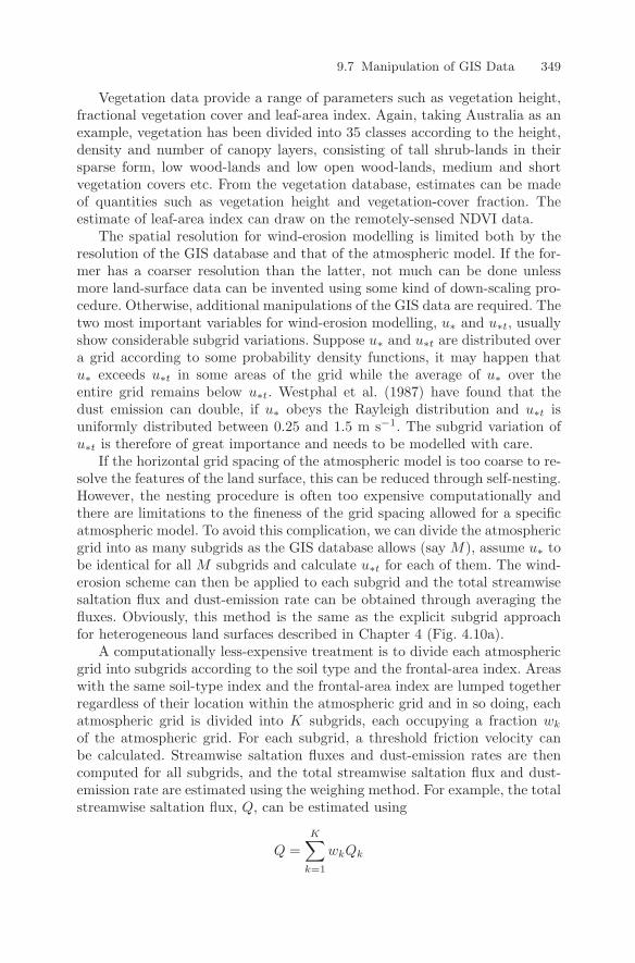
9.7 Manipulation of GIS Data 349
Vegetation data provide a range of parameters such as vegetation height,fractional vegetation cover and leaf-area index. Again, taking Australia as anexample, vegetation has been divided into 35 classes according to the height,density and number of canopy layers, consisting of tall shrub-lands in theirsparse form, low wood-lands and low open wood-lands, medium and shortvegetation covers etc. From the vegetation database, estimates can be madeof quantities such as vegetation height and vegetation-cover fraction. Theestimate of leaf-area index can draw on the remotely-sensed NDVI data.
The spatial resolution for wind-erosion modelling is limited both by theresolution of the GIS database and that of the atmospheric model. If the for-mer has a coarser resolution than the latter, not much can be done unlessmore land-surface data can be invented using some kind of down-scaling pro-cedure. Otherwise, additional manipulations of the GIS data are required. Thetwo most important variables for wind-erosion modelling, u∗ and u∗t, usuallyshow considerable subgrid variations. Suppose u∗ and u∗t are distributed overa grid according to some probability density functions, it may happen thatu∗ exceeds u∗t in some areas of the grid while the average of u∗ over theentire grid remains below u∗t. Westphal et al. (1987) have found that thedust emission can double, if u∗ obeys the Rayleigh distribution and u∗t isuniformly distributed between 0.25 and 1.5 m s−1. The subgrid variation ofu∗t is therefore of great importance and needs to be modelled with care.
If the horizontal grid spacing of the atmospheric model is too coarse to re-solve the features of the land surface, this can be reduced through self-nesting.However, the nesting procedure is often too expensive computationally andthere are limitations to the fineness of the grid spacing allowed for a specificatmospheric model. To avoid this complication, we can divide the atmosphericgrid into as many subgrids as the GIS database allows (say M), assume u∗ tobe identical for all M subgrids and calculate u∗t for each of them. The wind-erosion scheme can then be applied to each subgrid and the total streamwisesaltation flux and dust-emission rate can be obtained through averaging thefluxes. Obviously, this method is the same as the explicit subgrid approachfor heterogeneous land surfaces described in Chapter 4 (Fig. 4.10a).
A computationally less-expensive treatment is to divide each atmosphericgrid into subgrids according to the soil type and the frontal-area index. Areaswith the same soil-type index and the frontal-area index are lumped togetherregardless of their location within the atmospheric grid and in so doing, eachatmospheric grid is divided into K subgrids, each occupying a fraction wk
of the atmospheric grid. For each subgrid, a threshold friction velocity canbe calculated. Streamwise saltation fluxes and dust-emission rates are thencomputed for all subgrids, and the total streamwise saltation flux and dust-emission rate are estimated using the weighing method. For example, the totalstreamwise saltation flux, Q, can be estimated using
Q =K∑
k=1
wkQk
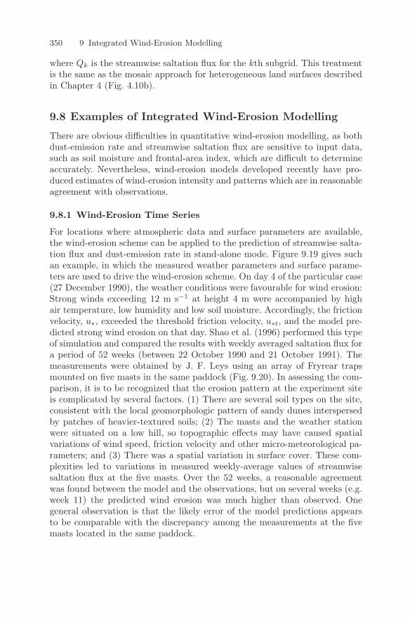
350 9 Integrated Wind-Erosion Modelling
where Qk is the streamwise saltation flux for the kth subgrid. This treatmentis the same as the mosaic approach for heterogeneous land surfaces describedin Chapter 4 (Fig. 4.10b).
9.8 Examples of Integrated Wind-Erosion Modelling
There are obvious difficulties in quantitative wind-erosion modelling, as bothdust-emission rate and streamwise saltation flux are sensitive to input data,such as soil moisture and frontal-area index, which are difficult to determineaccurately. Nevertheless, wind-erosion models developed recently have pro-duced estimates of wind-erosion intensity and patterns which are in reasonableagreement with observations.
9.8.1 Wind-Erosion Time Series
For locations where atmospheric data and surface parameters are available,the wind-erosion scheme can be applied to the prediction of streamwise salta-tion flux and dust-emission rate in stand-alone mode. Figure 9.19 gives suchan example, in which the measured weather parameters and surface parame-ters are used to drive the wind-erosion scheme. On day 4 of the particular case(27 December 1990), the weather conditions were favourable for wind erosion:Strong winds exceeding 12 m s−1 at height 4 m were accompanied by highair temperature, low humidity and low soil moisture. Accordingly, the frictionvelocity, u∗, exceeded the threshold friction velocity, u∗t, and the model pre-dicted strong wind erosion on that day. Shao et al. (1996) performed this typeof simulation and compared the results with weekly averaged saltation flux fora period of 52 weeks (between 22 October 1990 and 21 October 1991). Themeasurements were obtained by J. F. Leys using an array of Fryrear trapsmounted on five masts in the same paddock (Fig. 9.20). In assessing the com-parison, it is to be recognized that the erosion pattern at the experiment siteis complicated by several factors. (1) There are several soil types on the site,consistent with the local geomorphologic pattern of sandy dunes interspersedby patches of heavier-textured soils; (2) The masts and the weather stationwere situated on a low hill, so topographic effects may have caused spatialvariations of wind speed, friction velocity and other micro-meteorological pa-rameters; and (3) There was a spatial variation in surface cover. These com-plexities led to variations in measured weekly-average values of streamwisesaltation flux at the five masts. Over the 52 weeks, a reasonable agreementwas found between the model and the observations, but on several weeks (e.g.week 11) the predicted wind erosion was much higher than observed. Onegeneral observation is that the likely error of the model predictions appearsto be comparable with the discrepancy among the measurements at the fivemasts located in the same paddock.
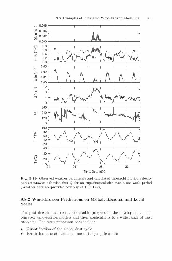
9.8 Examples of Integrated Wind-Erosion Modelling 351
Time, Dec. 1990
u *t
u *
1024 26 28 30
20
30
40
20406080
100
0
120
240
360
0
4
8
12
0.00
0.01
0.02
0.03
0.00.20.40.60.8
0.000
0.002
0.004
0.006
T (
o C)
Rh
(%)
DD
U (
ms−
1 )w
(m
3 m−
3 )u *
, u*t (
ms−
1 )Q
(gm
−1 s−
1 )
Fig. 9.19. Observed weather parameters and calculated threshold friction velocityand streamwise saltation flux Q for an experimental site over a one-week period(Weather data are provided courtesy of J. F. Leys)
9.8.2 Wind-Erosion Predictions on Global, Regional and LocalScales
The past decade has seen a remarkable progress in the development of in-tegrated wind-erosion models and their applications to a wide range of dustproblems. The most important ones include:
• Quantification of the global dust cycle• Prediction of dust storms on meso- to synoptic scales
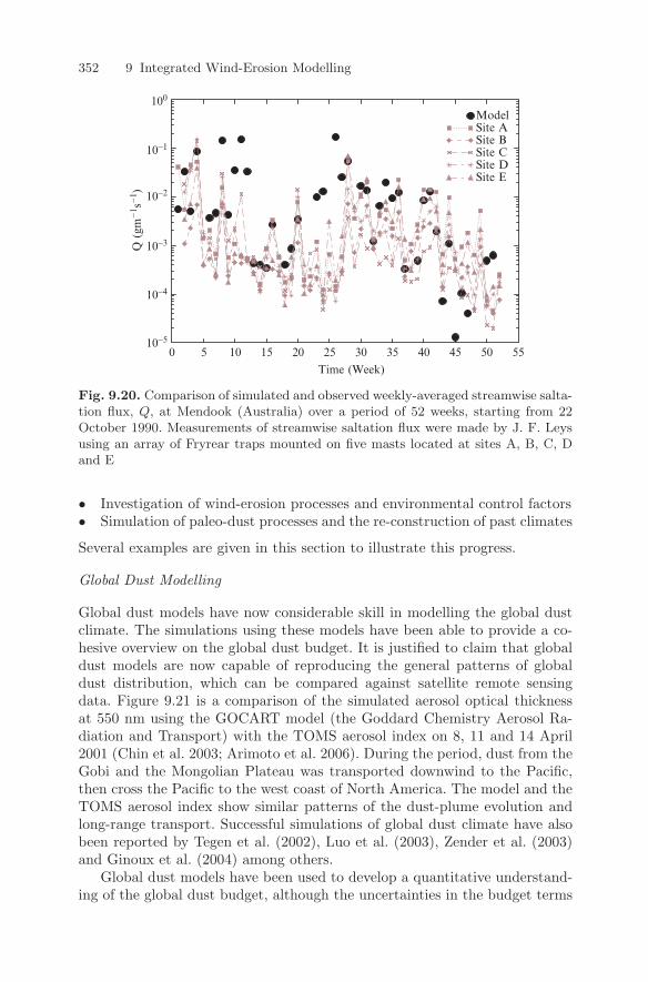
352 9 Integrated Wind-Erosion Modelling
Time (Week)
10-50 5 10 15 20 25 30 35 40 45 50 55
10-4
10-3
10-2
10-1
100
Q (
gm−
1 s−
1 )
ModelSite ASite BSite CSite DSite E
Fig. 9.20. Comparison of simulated and observed weekly-averaged streamwise salta-tion flux, Q, at Mendook (Australia) over a period of 52 weeks, starting from 22October 1990. Measurements of streamwise saltation flux were made by J. F. Leysusing an array of Fryrear traps mounted on five masts located at sites A, B, C, Dand E
• Investigation of wind-erosion processes and environmental control factors• Simulation of paleo-dust processes and the re-construction of past climates
Several examples are given in this section to illustrate this progress.
Global Dust Modelling
Global dust models have now considerable skill in modelling the global dustclimate. The simulations using these models have been able to provide a co-hesive overview on the global dust budget. It is justified to claim that globaldust models are now capable of reproducing the general patterns of globaldust distribution, which can be compared against satellite remote sensingdata. Figure 9.21 is a comparison of the simulated aerosol optical thicknessat 550 nm using the GOCART model (the Goddard Chemistry Aerosol Ra-diation and Transport) with the TOMS aerosol index on 8, 11 and 14 April2001 (Chin et al. 2003; Arimoto et al. 2006). During the period, dust from theGobi and the Mongolian Plateau was transported downwind to the Pacific,then cross the Pacific to the west coast of North America. The model and theTOMS aerosol index show similar patterns of the dust-plume evolution andlong-range transport. Successful simulations of global dust climate have alsobeen reported by Tegen et al. (2002), Luo et al. (2003), Zender et al. (2003)and Ginoux et al. (2004) among others.
Global dust models have been used to develop a quantitative understand-ing of the global dust budget, although the uncertainties in the budget terms
9.8 Examples of Integrated Wind-Erosion Modelling 353
60
40
20
0N
60
40
20
0N
60
40
20
0N90E
0.00 0.03 0.05 0.08 0.1 0.15 0.2 0.25 0.3 0.5 1.0 2.0 < 0 0.3 0.5 0.8 0.9 1.0 1.1 1.2 1.5 2.0 3.0 2.0
120E 180 150W 120W150E 90E 120E 180 150W 120W150E
(b) TOMS Al, 8 Apr 2001(a) GOCART AOT, 8 Apr 2001
(d) 8 Apr 2001(c) 11 Apr 2001
(f) 8 Apr 2001(e) 14 Apr 2001
Fig. 9.21. Comparison of the GOCART simulated dust patterns, shown as aerosoloptical thickness at 550 nm, with the TOMS aerosol index for 8, 11 and 14 April2001. During the episode, dust originating from the Gobi and the Mongolian Plateauwas transported downwind to the Pacific, then cross the Pacific to the west coast ofNorth America (From Arimoto et al. 2006)
remain to be large. The key global dust budget terms include global dustemission, F , dust deposition, D and dust load L, defined respectively as
F =∫
S
Fds
D =∫
S
Dds
L =∫
Ω
CdΩ
where F is dust emission [M L−2 T−1], D is dust deposition [M L−2 T−1], Cis dust (mass) concentration [M L−3], S is the area of the entire earth surfaceand Ω is the volume of the atmosphere. The dimensions of F and D are [MT−1] and those of L are [M]. It is also useful to define the dust load for an aircolumn over a unit ground surface
Lc =∫
H
Cdz
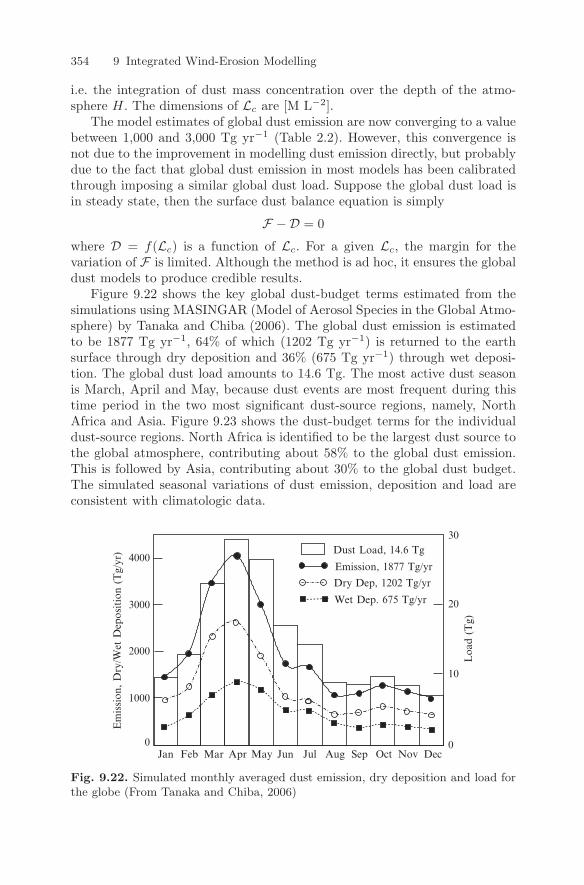
354 9 Integrated Wind-Erosion Modelling
i.e. the integration of dust mass concentration over the depth of the atmo-sphere H. The dimensions of Lc are [M L−2].
The model estimates of global dust emission are now converging to a valuebetween 1,000 and 3,000 Tg yr−1 (Table 2.2). However, this convergence isnot due to the improvement in modelling dust emission directly, but probablydue to the fact that global dust emission in most models has been calibratedthrough imposing a similar global dust load. Suppose the global dust load isin steady state, then the surface dust balance equation is simply
F −D = 0
where D = f(Lc) is a function of Lc. For a given Lc, the margin for thevariation of F is limited. Although the method is ad hoc, it ensures the globaldust models to produce credible results.
Figure 9.22 shows the key global dust-budget terms estimated from thesimulations using MASINGAR (Model of Aerosol Species in the Global Atmo-sphere) by Tanaka and Chiba (2006). The global dust emission is estimatedto be 1877 Tg yr−1, 64% of which (1202 Tg yr−1) is returned to the earthsurface through dry deposition and 36% (675 Tg yr−1) through wet deposi-tion. The global dust load amounts to 14.6 Tg. The most active dust seasonis March, April and May, because dust events are most frequent during thistime period in the two most significant dust-source regions, namely, NorthAfrica and Asia. Figure 9.23 shows the dust-budget terms for the individualdust-source regions. North Africa is identified to be the largest dust source tothe global atmosphere, contributing about 58% to the global dust emission.This is followed by Asia, contributing about 30% to the global dust budget.The simulated seasonal variations of dust emission, deposition and load areconsistent with climatologic data.
Loa
d (T
g)
Wet Dep. 675 Tg/yr
Dry Dep, 1202 Tg/yr
Emission, 1877 Tg/yr
Dust Load, 14.6 Tg
Jan Feb Mar Apr May Jun Jul Aug Sep Oct Nov Dec0
4000
3000
2000
1000
Em
ission
, D
ry/W
et D
epos
itio
n (T
g/yr
)
30
20
10
0
Fig. 9.22. Simulated monthly averaged dust emission, dry deposition and load forthe globe (From Tanaka and Chiba, 2006)
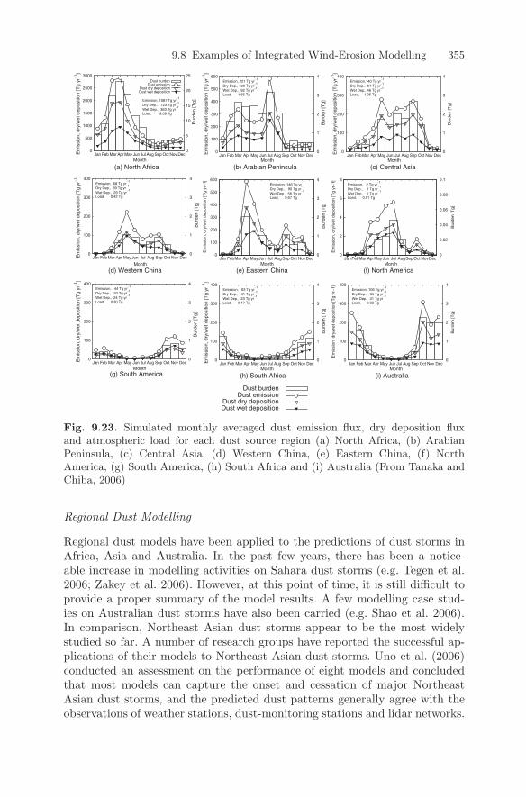
9.8 Examples of Integrated Wind-Erosion Modelling 355
(h) South Africa
Dust burdenDust emission
Dust dry depositionDust wet deposition
0
2
4
6
8
Jan FebMar AprMayJun Jul AugSep Oct NovDec 0
0.02
0.04
0.06
0.08
0.1
Em
issi
on, d
ry/w
et d
epos
ition
[Tg
yr−1
]
Bur
den
[Tg]
Month
Emission, 2 Tg yr−1
Dry Dep., 1 Tg yr−1
Wet Dep., 1 Tg yr−1
Load, 0.01 Tg
0
100
200
300
400
Jan Feb Mar Apr May Jun Jul Aug Sep Oct Nov Dec 0
1
2
3
4
Em
issi
on, d
ry/w
et d
epos
ition
[Tg
yr−1
]
Bur
den
[Tg]
Month
Emission, 106 Tg yr−1
Dry Dep., 65 Tg yr−1
Wet Dep., 41 Tg yr−1
Load, 0.92 Tg
(c) Central Asia
(f) North America
(i) Australia
0
500
1000
1500
2000
2500
3000E
mis
sion
, dry
/wet
dep
ositi
on [T
g yr
−1]
Em
issi
on, d
ry/w
et d
epos
ition
[Tg
yr−1
]E
mis
sion
, dry
/wet
dep
ositi
on [T
g yr
−1]
Em
issi
on, d
ry/w
et d
epos
ition
[Tg
yr−1
]E
mis
sion
, dry
/wet
dep
ositi
on [T
g yr
−1]
Em
issi
on, d
ry/w
et d
epos
ition
[Tg
yr−1
]
Bur
den
[Tg]
Month
Emission, 1087 Tg yr−1
Dry Dep., 723 Tg yr−1
Wet Dep., 363 Tg yr−1
Load, 9.09 Tg
Dust burdenDust emission
Dust dry depositionDust wet deposition
0
1
2
3
4
Bur
den
[Tg]
Month
Emission, 68 Tg yr−1
Dry Dep., 39 Tg yr−1
Wet Dep., 29 Tg yr−1
Load, 0.42 Tg
Jan Feb Mar Apr May Jun Jul Aug Sep Oct Nov Dec 0
1
2
3
4
Bur
den
[Tg]
Month
Emission, 44 Tg yr−1
Dry Dep., 20 Tg yr−1
Wet Dep., 24 Tg yr−1
Load, 0.30 Tg
(a) North Africa
(d) Western China
(g) South America
Jan Feb Mar Apr May Jun Jul Aug Sep Oct Nov Dec 0
1
2
3
4
Bur
den
[Tg]
Month
Emission, 221 Tg yr−1
Dry Dep., 129 Tg yr−1
Wet Dep., 92 Tg yr−1
Load, 1.65 Tg
0
100
200
300
400
500
600
Jan FebMar AprMay Jun Jul Aug Sep Oct NovDec 0
1
2
3
4
Em
issi
on, d
ry/w
et d
epos
ition
[Tg
yr−1
]
Bur
den
[Tg]
Month
Emission, 146 Tg yr−1
Dry Dep., 90 Tg yr−1
Wet Dep., 56 Tg yr−1
Load, 0.67 Tg
Jan Feb Mar Apr May Jun Jul Aug Sep Oct Nov Dec 0
1
2
3
4
Bur
den
[Tg]
Month
Emission, 63 Tg yr−1
Dry Dep., 41 Tg yr−1
Wet Dep., 23 Tg yr−1
Load, 0.47 Tg
(b) Arabian Peninsula
(e) Eastern China
Jan FebMar Apr May Jun Jul Aug Sep Oct Nov Dec0
1
2
3
4
Bur
den
[Tg]
Month
Emission,140 Tg yr−1
Dry Dep., 94 Tg yr−1
Wet Dep., 46 Tg yr−1
Load, 1.05 Tg
0
5
10
15
20
25
Jan Feb Mar Apr May Jun Jul Aug Sep Oct Nov Dec 0
100
200
300
400
500
600
0
100
200
300
400
0
100
200
300
400
Jan Feb Mar Apr May Jun Jul Aug Sep Oct Nov Dec
0
100
200
300
400
0
100
200
300
400
Fig. 9.23. Simulated monthly averaged dust emission flux, dry deposition fluxand atmospheric load for each dust source region (a) North Africa, (b) ArabianPeninsula, (c) Central Asia, (d) Western China, (e) Eastern China, (f) NorthAmerica, (g) South America, (h) South Africa and (i) Australia (From Tanaka andChiba, 2006)
Regional Dust Modelling
Regional dust models have been applied to the predictions of dust storms inAfrica, Asia and Australia. In the past few years, there has been a notice-able increase in modelling activities on Sahara dust storms (e.g. Tegen et al.2006; Zakey et al. 2006). However, at this point of time, it is still difficult toprovide a proper summary of the model results. A few modelling case stud-ies on Australian dust storms have also been carried (e.g. Shao et al. 2006).In comparison, Northeast Asian dust storms appear to be the most widelystudied so far. A number of research groups have reported the successful ap-plications of their models to Northeast Asian dust storms. Uno et al. (2006)conducted an assessment on the performance of eight models and concludedthat most models can capture the onset and cessation of major NortheastAsian dust storms, and the predicted dust patterns generally agree with theobservations of weather stations, dust-monitoring stations and lidar networks.
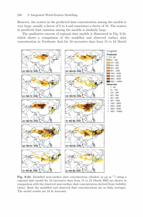
356 9 Integrated Wind-Erosion Modelling
However, the scatter in the predicted dust concentration among the models isvery large, usually a factor of 2 to 4 and sometimes a factor of 10. The scatterin predicted dust emission among the models is similarly large.
The qualitative success of regional dust models is illustrated in Fig. 9.24,which shows a comparison of the modelled and observed surface dustconcentration in Northeast Asia for 10 successive days from 15 to 24 March
Arabian Sea Bayof
Bengal
SouthChina Sea
Seaof
Japan
EastChinaSea
C (ug/m3)
Predicted0 - 5051 - 100101 - 200201 - 300301 - 500501 - 10001001 - 20002001 - 30003001 - 50005001 - 10000
Observed1 - 5051 - 100101 - 200201 - 300301 - 500501 - 10001001 - 20002001 - 30003001 - 50005001 - 10000
Arabian Sea
Arabian Sea Arabian Sea
Arabian Sea Arabian Sea
Arabian Sea Arabian Sea
Arabian Sea Arabian Sea
Bayof
Bengal
SouthChina Sea
Seaof
Japan
EastChinaSea
Bayof
Bengal
SouthChina Sea
Seaof
Japan
EastChinaSea
Bayof
Bengal
SouthChina Sea
Seaof
Japan
EastChinaSea
Bayof
Bengal
SouthChina Sea
Seaof
Japan
EastChinaSea
Bayof
Bengal
SouthChina Sea
Seaof
Japan
EastChinaSea
Bayof
Bengal
SouthChina Sea
Seaof
Japan
EastChinaSea
Bayof
Bengal
SouthChina Sea
Seaof
Japan
EastChinaSea
Bayof
Bengal
SouthChina Sea
Seaof
Japan
EastChinaSea
Bayof
Bengal
SouthChina Sea
Seaof
Japan
EastChinaSea
Text
(e): Mar 19, 2002
(a): Mar 15, 2002 (b): Mar 16, 2002
(c): Mar 17, 2002 (d): Mar 18, 2002
(f): Mar 20, 2002
(g): Mar 21, 2002 (h): Mar 22, 2002
(j): Mar 24, 2002(i): Mar 23, 2002
Fig. 9.24. Modelled near-surface dust concentration (shaded, in µg m−3) using aregional dust model for 10 successive days from 15 to 24 March 2002 are shown incomparison with the observed near-surface dust concentration derived from visibility(dots). Both the modelled and observed dust concentrations are in daily averages.The model results are 24 hr forecasts
9.8 Examples of Integrated Wind-Erosion Modelling 357
2002. The model results are the 24-hour forecasts using a regional dust model(Shao et al. 2003) and the observed dust concentrations are derived from thevisibility data using Equation (9.81). The modelled and observed surface dustconcentration agree well both in magnitude and spatial distribution, and themodel simulations have captured the evolution of the dust episodes. In Aprilin Asia, dust weather occurs every day and a strong dust event occurs everyfew days. During the 10-day period, a severe dust storm developed on 19March over the Gobi Desert along the China-Mongolia border. At the centerof the storm (105 E, 42 N), dust concentration exceeded 10 mg m−3. In thefollowing two days, the storm moved eastward, dust became widely spreadand dust concentration was decreasing. By 21 March, dust covered a largearea of China, Korea, Japan and the adjacent regions. By 22 March, a dustband stretching several thousand kilometres could be seen. Figure 9.25 showsthe dust emission during the 10 days. As can be seen, the main source regionfor the dust event was the Gobi Desert along the China-Mongolia border.The strongest dust emission, reaching 5 mg m−2 s−1, occurred over the Gobion 19 March 2002.
On the basis of model simulations, quantitative statements can be madeon Asian dust storms, despite of the large uncertainties. The maximum dustemission associated with individual dust storms over the Gobi is found to bearound 5–10 mg m−2 s−1 (Park and In, 2003; Shao et al. 2003; Han et al.2004). Much of the emitted dust is deposited back to the surface so the netdust emission is much smaller. The regions of net positive dust flux (source) aremainly the deserts in China and southern Mongolia. In the peak dust season(spring), the Gobi Desert has the strongest net dust emission, reaching up to500 tn km−2 mon−1. Net negative dust flux (sink) covers a large downstreamarea of China, Korea and Japan. The Loess Plateau, situated immediatelydownstream of the Gobi, is the strongest dust sink, receiving about 20–50 tnkm−2 mon−1 in the peak dust season. A high dust load zone exists along thenorthern border of the Tibet Plateau, over the Tarim Basin and the Zhunge’erBasin. To the east of the main source region, the high dust-load zone diverges.During the peak dust season, the order of magnitude of total dust emission,deposition and load are 40± 30 Mt day−1, 30 ± 20 Mt day−1 and 10 ± 5 Mt,respectively.
Example of Meso-Scale Dust Modelling
The meso-scale features of dust storms associated with atmospheric systemssuch as squallines, microbursts and convection deserve in depth investigation.Efforts have been made to model dust problems with high resolutions. Forexample, Uno et al. (2005) have used the CFORS model to study the char-acteristics of dust transport in the Taklimakan with a spatial resolution of9 km. Their model has been able to reproduce the complex flow patternswhich produce dust storms in the Tarim Basin, e.g., the strong down slopewind from the Tianshan Mountains and the strong easterly flow from the
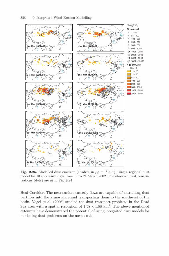
358 9 Integrated Wind-Erosion Modelling
Bayof
SeaofJapan
EastChinaSea
C (ug/m3)Observed
1 - 5051 - 100101 - 200201 - 300301 - 500501 - 10001001 - 20002001 - 30003001 - 50005001 - 10000
F (ug/m2/s)0 - 1011 - 2021 - 5051 - 100101 - 200201 - 500501 - 10001001 - 20002001 - 5000
Bayof
SeaofJapan
EastChinaSea
Bayof
SeaofJapan
EastChinaSea
Bayof
SeaofJapan
EastChinaSea
Bayof
SeaofJapan
EastChinaSea
Bayof
Seaof
Japan
EastChinaSea
Bayof
SeaofJapan
EastChinaSea
Bayof
Seaof
Japan
EastChinaSea
Bayof
SeaofJapan
EastChinaSea
Bayof
Seaof
Japan
EastChinaSea
Text
(e): Mar 19, 2002
2002 ,61 raM :)b(2002 ,51 raM :)a(
(c): Mar 17, 2002 (d): Mar 18, 2002
(g): Mar 21, 2002
(f): Mar 20, 2002
(h): Mar 22, 2002
2002 ,42 raM :)j(2002 ,32 raM :)i(
Fig. 9.25. Modelled dust emission (shaded, in µg m−2 s−1) using a regional dustmodel for 10 successive days from 15 to 24 March 2002. The observed dust concen-trations (dots) are as in Fig. 9.24
Hexi Corridor. The near-surface easterly flows are capable of entraining dustparticles into the atmosphere and transporting them to the southwest of thebasin. Vogel et al. (2006) studied the dust transport problems in the DeadSea area with a spatial resolution of 1.58 × 1.88 km2. The above mentionedattempts have demonstrated the potential of using integrated dust models formodelling dust problems on the meso-scale.
9.9 Data Assimilation 359
9.9 Data Assimilation
The technique of data assimilation has been under development over the pasthalf century and has been very successfully applied to atmospheric and oceanicmodelling (Kalnay, 2003). Similar to weather and climate models, dust mod-els are also associated with uncertainties which arise from inadequacies inmodel physics and inaccuracies in model parameters, forcing data and ini-tial conditions. The technique of data assimilation is to combine measure-ments and model estimates to achieve an optimal prediction and therebyimprove the model performance. The popular data assimilation techniquesused for numerical weather and climate predictions include three-dimensionalvariational data assimilation (3DVAR), four-dimensional variational data as-similation (4DVAR), Kalman filtering and several its variations, such as theExtended Kalman filtering and the Ensemble Kalman filtering. The readermay refer to Kalnay (2003) for insightful discussions on these techniques.
While data assimilation is the standard of practice in numerical weatherprediction and climate modelling, its application to dust modelling has beenhumped by the lack of adequate dust measurements. However, dust-relateddata are becoming increasingly available. Dust concentration can be derivedusing empirical relationships from the visibility data at a large number ofweather stations. While the so-derived data set is relatively low in accuracy,it does have the advantages of broad spatial coverage and regular temporalcoverage. Dust concentration measurements are now available from high- andlow-volume samplers at air-quality monitoring stations. These measurementsare more accurate, but are poor in spatial and temporal resolution. In the dust-affected areas of Asia, a network of lidar is now functioning which producesaerosol profile estimates by observing quantities such as extinction coefficient(Sugimoto et al. 2003; Shimizu et al. 2004). Lidar data are indirect and arelimited to some locations. During dust events, lidar only provides informationfor the lower part of the atmosphere, as lidar signals often cannot penetratethe dense dust layer. Satellite remote sensing offers an important source ofdata. Methods for converting satellite signals to practically useful physicalquantities, such as dust load are now being developed. It is envisaged thatwith the enrichment of in situ dust observations and the progress in remotesensing technology and inverse data-analysis techniques, data assimilation indust modelling will become more widely applied in the near future.
Yumimoto et al. (2007) applied the 4DVAR technique to modelling Asiandust storms, by assimilating the lidar extinction coefficient data into theRAMS/CFORS model for adjoint inversion of dust emission. Suppose themodel domain consists of I × J × K grid points and the dust concentrationvector, Cn, denotes the dust concentrations at all grid points at time step n.Then, we can formally write the discrete governing equation for dust concen-tration as
Cn+1 = ICn + O(Cn)dt + Edt (9.90)
360 9 Integrated Wind-Erosion Modelling
where I is the unit matrix, O is the model operator representing advection,diffusion and reaction. E is the dust-source vector of length I × J ×K, whichcan be expressed as the divergence of model-subgrid turbulent dust flux. Atthe ground surface, the vertical component of the dust flux, i.e. dust emissionrate, is the most important, which we estimate using a dust emission scheme,which we can formally write as,
F = αf(u∗, u∗t) (9.91)
where α is a dust-emission coefficient which is a function of surface conditions.To optimize the estimate of α by assimilating lidar extinction coefficient y,the cost function is defined as
J(bfα0) =12(α0 − αb)T B−1(α0 − αb) +
12
N∑i=1
(Hαi − yi)T R−1(Hαi − yi)
(9.92)The first term on the right hand side of the above equation represents thedeparture of α from the first guess value αb, weighted by the backgrounderror covariance B. The second term represents the discrepancy between thesimulated and observed dust extinction coefficient weighted by the observationerror covariance R. The observational operator H converts α into y. Theminimization of the cost function J can be achieved through an iterativeprocess using the conjugate gradient or the quasi-Newton method (Liu andNocedal, 1989). Yumimoto et al. (2007) concluded that the implementationof the 4DVAR technique can result in a significant improvement in the dustmodel performance. The data used by the latter authors were restricted tolidar measurements. However, 4DVAR is capable of including measurementsof dust monitoring stations (e.g. PM10 and TSP) and satellite retrievals (e.g.aerosol optical thickness and the Aerosol Index). It is expected that in the nearfuture, the assimilation of these data will further improve the performance ofdust models.
10
Sand Dunes, Dynamics and Modelling
The world’s deserts show a variety of different types of sand dunes with fas-cinating shapes and patterns (Fig. 10.1). The focus of this chapter is on thedynamics and computational modelling of sand dunes and dune fields. This isagain a complex problem, but in general the dynamics of sand dunes is gov-erned by the interactions between (1) the atmospheric flow, (2) the motion ofsand grains and (3) the dune morphological characteristics. We shall discussthese three topics in some detail.
The study on desert dunes has a history of more than a hundred years.Explorations on desert dunes began in the late 19th century, and by 1980 allmajor desert dune areas have been explored (Goudie, 1999). A comprehen-sive description of dune fields worldwide can be found in Wilson (1972). Thenumber of basic dune forms is fairly small (Section 2), but a variety of combi-nations of dune types can occur. Dune combinations are mainly of two cate-gories: (1) compound dunes made up of two or more dunes of the same basictype, coalescing or overlapping, and (2) complex dunes in which two or moredifferent basic types are combined or superimposed (McKee, 1979). Recentadvances in aircraft and satellite imagery have enabled a better classificationof sand-dune types, more reliable measures of large-scale desert morphologyand development of hypotheses for the mechanisms of dune formation andevolution.
Studies on sand dunes have been made through wind-tunnel and field ex-periments, theoretical analysis and computational simulation. Wind-tunnelexperiments are useful in studying flow over dunes and micro-scopic sand mo-tions, but are not suitable for studying the dynamics of large-scale dune fields,because the requirement for dynamic similarity between the wind-tunnel andnatural conditions are difficult to fulfil. Only a few field experiments on dunedynamics have been reported (e.g. McKenna Neuman et al. 1997; Nicklinget al. 2002). Field experiments are time consuming and expensive to conductand are limited to time periods much shorter than the time scale of dune fieldevolution. In general, there remains a lack of direct observations of flow struc-ture, sand transport and deposition, which are critical to the understanding of
Y. Shao, Physics and Modelling of Wind Erosion, 361c© Springer Science+Business Media B.V. 2008
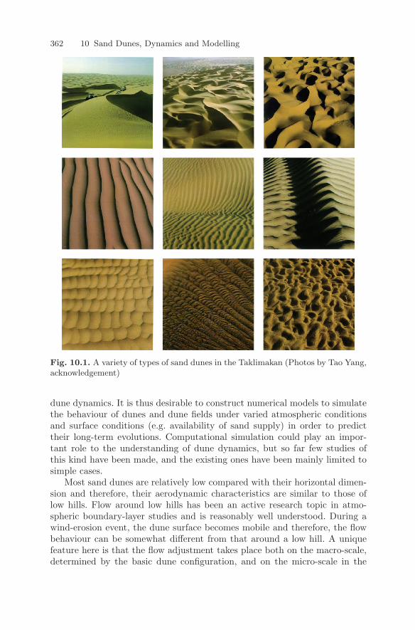
362 10 Sand Dunes, Dynamics and Modelling
Fig. 10.1. A variety of types of sand dunes in the Taklimakan (Photos by Tao Yang,acknowledgement)
dune dynamics. It is thus desirable to construct numerical models to simulatethe behaviour of dunes and dune fields under varied atmospheric conditionsand surface conditions (e.g. availability of sand supply) in order to predicttheir long-term evolutions. Computational simulation could play an impor-tant role to the understanding of dune dynamics, but so far few studies ofthis kind have been made, and the existing ones have been mainly limited tosimple cases.
Most sand dunes are relatively low compared with their horizontal dimen-sion and therefore, their aerodynamic characteristics are similar to those oflow hills. Flow around low hills has been an active research topic in atmo-spheric boundary-layer studies and is reasonably well understood. During awind-erosion event, the dune surface becomes mobile and therefore, the flowbehaviour can be somewhat different from that around a low hill. A uniquefeature here is that the flow adjustment takes place both on the macro-scale,determined by the basic dune configuration, and on the micro-scale in the
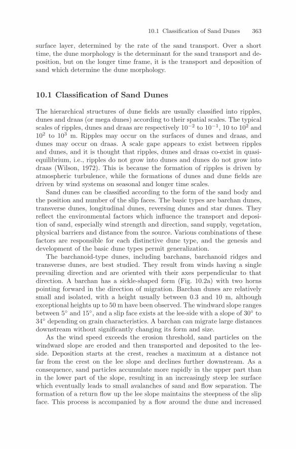
10.1 Classification of Sand Dunes 363
surface layer, determined by the rate of the sand transport. Over a shorttime, the dune morphology is the determinant for the sand transport and de-position, but on the longer time frame, it is the transport and deposition ofsand which determine the dune morphology.
10.1 Classification of Sand Dunes
The hierarchical structures of dune fields are usually classified into ripples,dunes and draas (or mega dunes) according to their spatial scales. The typicalscales of ripples, dunes and draas are respectively 10−2 to 10−1, 10 to 102 and102 to 103 m. Ripples may occur on the surfaces of dunes and draas, anddunes may occur on draas. A scale gape appears to exist between ripplesand dunes, and it is thought that ripples, dunes and draas co-exist in quasi-equilibrium, i.e., ripples do not grow into dunes and dunes do not grow intodraas (Wilson, 1972). This is because the formation of ripples is driven byatmospheric turbulence, while the formations of dunes and dune fields aredriven by wind systems on seasonal and longer time scales.
Sand dunes can be classified according to the form of the sand body andthe position and number of the slip faces. The basic types are barchan dunes,transverse dunes, longitudinal dunes, reversing dunes and star dunes. Theyreflect the environmental factors which influence the transport and deposi-tion of sand, especially wind strength and direction, sand supply, vegetation,physical barriers and distance from the source. Various combinations of thesefactors are responsible for each distinctive dune type, and the genesis anddevelopment of the basic dune types permit generalization.
The barchanoid-type dunes, including barchans, barchanoid ridges andtransverse dunes, are best studied. They result from winds having a singleprevailing direction and are oriented with their axes perpendicular to thatdirection. A barchan has a sickle-shaped form (Fig. 10.2a) with two hornspointing forward in the direction of migration. Barchan dunes are relativelysmall and isolated, with a height usually between 0.3 and 10 m, althoughexceptional heights up to 50 m have been observed. The windward slope rangesbetween 5 and 15, and a slip face exists at the lee-side with a slope of 30 to34 depending on grain characteristics. A barchan can migrate large distancesdownstream without significantly changing its form and size.
As the wind speed exceeds the erosion threshold, sand particles on thewindward slope are eroded and then transported and deposited to the lee-side. Deposition starts at the crest, reaches a maximum at a distance notfar from the crest on the lee slope and declines further downstream. As aconsequence, sand particles accumulate more rapidly in the upper part thanin the lower part of the slope, resulting in an increasingly steep lee surfacewhich eventually leads to small avalanches of sand and flow separation. Theformation of a return flow up the lee slope maintains the steepness of the slipface. This process is accompanied by a flow around the dune and increased
364 10 Sand Dunes, Dynamics and Modelling
Fig. 10.2. Schematic illustration of common dune forms (After McKee, 1979)
wind speed (hence stronger erosion) on both sides of the dune, resulting inthe formation of the two horns. The migration speed of a barchan is related tothe rate of sand transport over the crest and inversely related to the height.Bagnold (1941) showed that the migration speed of a barchan is
Vm =Qc
ρbhc(10.1)
where Qc is the streamwise saltation flux over the crest, ρb is the bulk density,and hc is dune height. Observations show that barchans advance between 5and 30 m y−1. The derivation of Equation (10.1) is given in Section 10.2.
Where the sand supply is sufficiently large, individual barchan dunesmay link up and form a parallel wavy ridge perpendicular to the prevail-ing wind (Fig. 10.2b). Transverse dunes are essentially parallel barchanoidridges (Fig. 10.2c), which occur with an even greater sand supply. Comparedwith barchanoid ridges, transverse dunes have a relatively straight crest. Sim-ilar to barchans, barchanoid ridges and transverse dunes advance by means oferosion on the windward flanks and deposition on the slip face. The celerityof the transverse-dune movement is in direct proportion to the wind velocityand inverse proportion to its height.
The longitudinal dunes appear in general as parallel straight ridges withslip faces on both sides (Fig. 10.2d). A typical longitudinal dune is 20–50 mhigh, 100 m or more wide, and has a length ranging from a few hundred metresto several hundred kilometres. This type of dune dominates the world’s deserts
10.1 Classification of Sand Dunes 365
with remarkable continuity and geometrical regularity, occurring in the LibyanDesert, in Saudi Arabia, the Dasht-e-Lut desert in Iran, and some areas ofthe Gobi desert, the Indian desert and the deserts in Australia (the GreatVictoria, the Great Sandy and the Simpson Deserts). In general, the spacingof the dunes is around 2–3 km. Unlike transverse dunes, the longitudinaldunes elongate. The elongation depends on wind velocity and the angle ofwind relative to the crest. While barchanoid-type dunes occur only in areaswhere the wind has a predominant direction, longitudinal dunes occur wherethe wind has bi-directional or multi-directional regimes. Consequently, overlarge areas on the world’s deserts, suitable conditions for the formation oflongitudinal dunes exist. This partially explains the worldwide predominanceof the longitudinal dune type.
The mechanism governing the formation of longitudinal dunes isinteresting. Bagnold (1941) hypothesized that bi-directional wind regimesare fundamental to the formation of ridges, but later proposed an auxiliarythermal-convection mechanism. More recent studies have also suggested thatthe morphology and dynamics of longitudinal dunes involve a wind structureof regular spiral vortices with axes parallel to the flow (Hanna, 1969). Thesevortices are helicoidal flows, which occur in pairs: one left-handed, the otherright handed, as shown in Fig. 10.4. However, Tsoar (1983) has presenteddetailed flow measurements over longitudinal dunes, in which they are de-veloped by means of two dominant wind directions. Each wind encountersthe dune obliquely and is deflected at the lee flank in a net direction parallelto the crest line as a result of flow separation. The associated pattern ofsand transport, erosion and deposition is much more complex than previouslysuggested.
If the prevailing wind has a small angle of attack, φi, to the crest line, achange in wind direction occurs on the lee flank. The deflected motion alongthe lee flank is a result of flow separation. The incident wind may be con-sidered to have two components: one parallel to the crest line, U cos φi, andone perpendicular component, U sin φi. The separation caused by the perpen-dicular component generates a return flow on the lee flank. Consequently, ifthe wind approaches a straight longitudinal dune obliquely, the wind direc-tion on the lee flank is deflected, leading to a flow pattern as illustrated inFig. 10.5. There is a direct relationship between φi and the direction of thedeflected wind on the lee flank. Observations show that the deflected wind in-creases gradually on the lee flank for φi < 40, while wind decreases abruptlywhere φi becomes less acute. Because the dune meanders, φi changes alongthe dune, resulting in a complicated field of flow convergence and divergenceon the lee side.
Sand deposited on the lee flank of a longitudinal dune comes directly orindirectly from the windward flank. In the case of large φi, there is a decreasein wind velocity just leeward of the crest line which leads to the depositionof sand and the development of a slip surface. In cases of small φi, the sanderoded from the windward flank is not deposited on the lee flank but continuesto move along the dune crest line. In addition, the winds also erode sand from
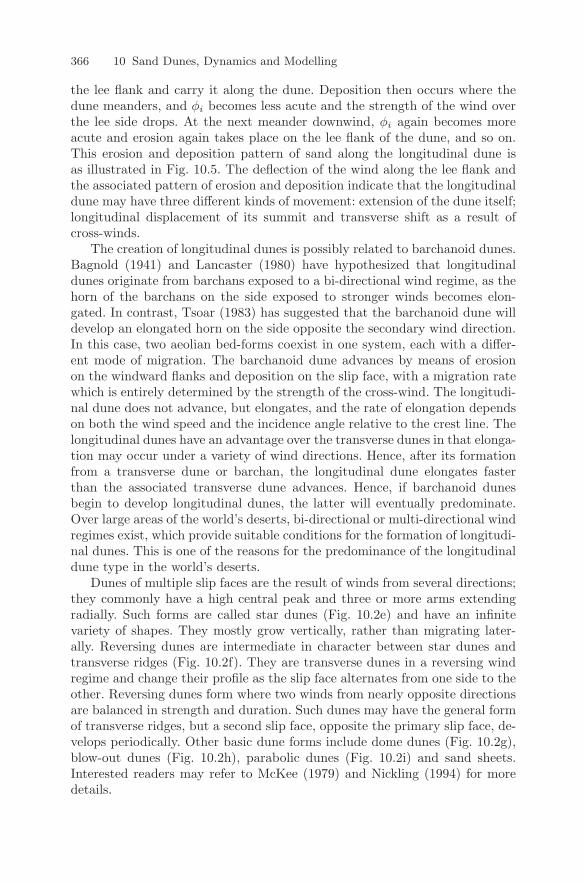
366 10 Sand Dunes, Dynamics and Modelling
the lee flank and carry it along the dune. Deposition then occurs where thedune meanders, and φi becomes less acute and the strength of the wind overthe lee side drops. At the next meander downwind, φi again becomes moreacute and erosion again takes place on the lee flank of the dune, and so on.This erosion and deposition pattern of sand along the longitudinal dune isas illustrated in Fig. 10.5. The deflection of the wind along the lee flank andthe associated pattern of erosion and deposition indicate that the longitudinaldune may have three different kinds of movement: extension of the dune itself;longitudinal displacement of its summit and transverse shift as a result ofcross-winds.
The creation of longitudinal dunes is possibly related to barchanoid dunes.Bagnold (1941) and Lancaster (1980) have hypothesized that longitudinaldunes originate from barchans exposed to a bi-directional wind regime, as thehorn of the barchans on the side exposed to stronger winds becomes elon-gated. In contrast, Tsoar (1983) has suggested that the barchanoid dune willdevelop an elongated horn on the side opposite the secondary wind direction.In this case, two aeolian bed-forms coexist in one system, each with a differ-ent mode of migration. The barchanoid dune advances by means of erosionon the windward flanks and deposition on the slip face, with a migration ratewhich is entirely determined by the strength of the cross-wind. The longitudi-nal dune does not advance, but elongates, and the rate of elongation dependson both the wind speed and the incidence angle relative to the crest line. Thelongitudinal dunes have an advantage over the transverse dunes in that elonga-tion may occur under a variety of wind directions. Hence, after its formationfrom a transverse dune or barchan, the longitudinal dune elongates fasterthan the associated transverse dune advances. Hence, if barchanoid dunesbegin to develop longitudinal dunes, the latter will eventually predominate.Over large areas of the world’s deserts, bi-directional or multi-directional windregimes exist, which provide suitable conditions for the formation of longitudi-nal dunes. This is one of the reasons for the predominance of the longitudinaldune type in the world’s deserts.
Dunes of multiple slip faces are the result of winds from several directions;they commonly have a high central peak and three or more arms extendingradially. Such forms are called star dunes (Fig. 10.2e) and have an infinitevariety of shapes. They mostly grow vertically, rather than migrating later-ally. Reversing dunes are intermediate in character between star dunes andtransverse ridges (Fig. 10.2f). They are transverse dunes in a reversing windregime and change their profile as the slip face alternates from one side to theother. Reversing dunes form where two winds from nearly opposite directionsare balanced in strength and duration. Such dunes may have the general formof transverse ridges, but a second slip face, opposite the primary slip face, de-velops periodically. Other basic dune forms include dome dunes (Fig. 10.2g),blow-out dunes (Fig. 10.2h), parabolic dunes (Fig. 10.2i) and sand sheets.Interested readers may refer to McKee (1979) and Nickling (1994) for moredetails.
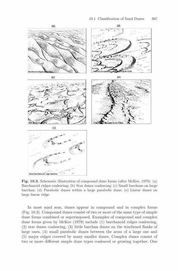
10.1 Classification of Sand Dunes 367
Fig. 10.3. Schematic illustration of compound dune forms (after McKee, 1979). (a)Barchanoid ridges coalescing; (b) Star dunes coalescing; (c) Small barchans on largebarchan; (d) Parabolic dunes within a large parabolic dune; (e) Linear dunes onlarge linear ridge
In most sand seas, dunes appear in compound and in complex forms(Fig. 10.3). Compound dunes consist of two or more of the same type of simpledune forms combined or superimposed. Examples of compound and complexdune forms given by McKee (1979) include (1) barchanoid ridges coalescing,(2) star dunes coalescing, (3) little barchan dunes on the windward flanks oflarge ones, (4) small parabolic dunes between the arms of a large one and(5) major ridges covered by many smaller dunes. Complex dunes consist oftwo or more different simple dune types coalesced or growing together. One
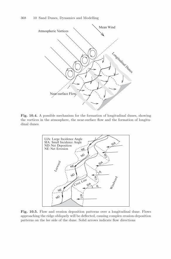
368 10 Sand Dunes, Dynamics and Modelling
Longitudinal Dunes
Mean WindAtmospheric Vortices
Near-surface Flow
Fig. 10.4. A possible mechanism for the formation of longitudinal dunes, showingthe vortices in the atmosphere, the near-surface flow and the formation of longitu-dinal dunes
LIA
LIA
φi
φi
Crest Line
Lee
war
d
Win
dwar
d
ND
ND
ND
LIA: Large Incidence AngleSIA: Small Incidence AngleND:Net DepositionNE:Net Errosion
SIA
SIA
SIA
LIA
NE
NE
NE
Fig. 10.5. Flow and erosion deposition patterns over a longitudinal dune. Flowsapproaching the ridge obliquely will be deflected, causing complex erosion-depositionpatterns on the lee side of the dune. Solid arrows indicate flow directions
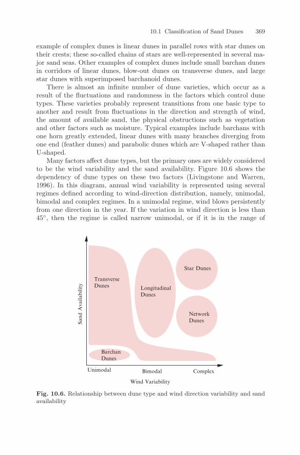
10.1 Classification of Sand Dunes 369
example of complex dunes is linear dunes in parallel rows with star dunes ontheir crests; these so-called chains of stars are well-represented in several ma-jor sand seas. Other examples of complex dunes include small barchan dunesin corridors of linear dunes, blow-out dunes on transverse dunes, and largestar dunes with superimposed barchanoid dunes.
There is almost an infinite number of dune varieties, which occur as aresult of the fluctuations and randomness in the factors which control dunetypes. These varieties probably represent transitions from one basic type toanother and result from fluctuations in the direction and strength of wind,the amount of available sand, the physical obstructions such as vegetationand other factors such as moisture. Typical examples include barchans withone horn greatly extended, linear dunes with many branches diverging fromone end (feather dunes) and parabolic dunes which are V-shaped rather thanU-shaped.
Many factors affect dune types, but the primary ones are widely consideredto be the wind variability and the sand availability. Figure 10.6 shows thedependency of dune types on these two factors (Livingstone and Warren,1996). In this diagram, annual wind variability is represented using severalregimes defined according to wind-direction distribution, namely, unimodal,bimodal and complex regimes. In a unimodal regime, wind blows persistentlyfrom one direction in the year. If the variation in wind direction is less than45, then the regime is called narrow unimodal, or if it is in the range of
Star Dunes
NetworkDunes
BarchanDunes
TransverseDunes Longitudinal
Dunes
ComplexBimodalUnimodal
Wind Variability
Sand
Ava
ilabi
lity
Fig. 10.6. Relationship between dune type and wind direction variability and sandavailability
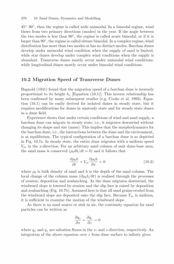
370 10 Sand Dunes, Dynamics and Modelling
45–90, then the regime is called wide unimodal. In a bimodal regime, windblows from two primary directions (modes) in the year. If the angle betweenthe two modes is less than 90, the regime is called acute bimodal, or if it islarger than 90, the regime is called obtuse bimodal. In a complex regime, winddistribution has more than two modes or has no distinct modes. Barchan dunesdevelop under unimodal wind condition when the supply of sand is limited,while star dunes develop under complex wind conditions when the supply isabundant. Transverse dunes mostly occur under unimodal wind conditions,while longitudinal dunes mostly occur under bimodal wind conditions.
10.2 Migration Speed of Transverse Dunes
Bagnold (1941) found that the migration speed of a barchan dune is inverselyproportional to its height hc [Equation (10.1)]. This inverse relationship hasbeen confirmed by many subsequent studies (e.g. Cooke et al. 1993). Equa-tion (10.1) can be easily derived for isolated dunes in steady state, but itrequires modifications for dunes in unsteady state and for steady state dunesin a dune field.
Experience shows that under certain conditions of wind and sand supply, abarchan dune can migrate in steady state, i.e., it migrates downwind withoutchanging its shape and size (mass). This implies that the morphodynamics forthe barchan dune, i.e., the interactions between the dune and the environment,is at equilibrium. The typical configuration of a barchan dune is as depictedin Fig. 10.7a. In steady state, the entire dune migrates with a uniform speedVm in the x-direction. For an arbitrary sand column of unit dune-base area,the sand mass is conserved (ρbdh/dt = 0) and it follows that
∂ρbh
∂t+ Vm
∂ρbh
∂x= 0 (10.2)
where ρb is bulk density of sand and h is the depth of the sand column. Thelocal change of the column mass (∂ρbh/∂t) is realised through the processesof erosion, deposition and avalanching. As the dune migrates downwind, thewindward slope is lowered by erosion and the slip face is raised by depositionand avalanching (Fig. 10.7b). Assumed here is that all sand grains eroded fromthe windward slope are deposited onto the slip face. Because Vm is uniform,it is sufficient to examine the motion of the windward slope.
As there is no sand source or sink in air, the continuity equation for sandparticles can be written as
∂qx
∂x+
∂qz
∂z= 0
where qx and qz are saltation fluxes in the x- and z-direction, respectively. Anintegration of the above equation over z from dune surface to infinity gives
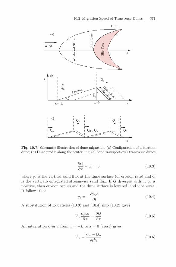
10.2 Migration Speed of Transverse Dunes 371
x
Qu
Qc Qc
QdQd = Qu
(c)
x
Brink
Lin
e
Wind
x=−L x
z
Qu
Qc
(b)
(a)
Slip
Fac
e
Win
dwar
d Sl
ope
Horn
ErosionAvalanching
Deposition
ashc
x=0
Fig. 10.7. Schematic illustration of dune migration. (a) Configuration of a barchandune; (b) Dune profile along the center line; (c) Sand transport over transverse dunes
∂Q
∂x− qe = 0 (10.3)
where qe is the vertical sand flux at the dune surface (or erosion rate) and Qis the vertically-integrated streamwise sand flux. If Q diverges with x, qe ispositive, then erosion occurs and the dune surface is lowered, and vice versa.It follows that
qe = −∂ρbh
∂t(10.4)
A substitution of Equations (10.3) and (10.4) into (10.2) gives
Vm∂ρbh
∂x=
∂Q
∂x(10.5)
An integration over x from x = −L to x = 0 (crest) gives
Vm =Qc − Qu
ρbhc(10.6)
372 10 Sand Dunes, Dynamics and Modelling
where Qu is the upstream sand transport. For an isolated sand dune, Qu = 0and the above equation reduces to Equation (10.1).
An interesting observation from Equation (10.5) is that the vertically-integrated streamwise sand flux at any x muxt obey
Q(x) = Qu + ρbVm tan(as)(x + L) (10.7)
This implies that Q(x) increases linearly with x, and this increase is propor-tional to Vm and to the steepness of the windward slope, tan(as). It is furtherseen from Equation (10.3) that qe is a constant independent of x. It is relatedto Vm by
qe = ρbVm tan(as) (10.8)
For a dune in a dune field, Qu is in general not zero. If the dune is insteady state then Qu must be equal to Qd, the sand transport downstream tothe dune, i.e.,
Qu = Qd
as illustrated in Fig. 10.7c. Qd, thus Qu, can be related to Qc by introducingthe sand-trapping efficiency, ηd. As sand is transported cross the dune crest,a fraction of the sand is deposited on the slip face. By definition, ηd is theratio between the amount of the sand deposited to that transported over thecrest. It follows that
Qd = Qu = Qc(1 − ηd) (10.9)
Therefore, the migration speed of a dune in the dune field needs to be ex-pressed as
Vm =ηdQc
ρbhc(10.10)
Since ηd falls between zero and one, a dune in a dune fields migrates moreslowly than an isolated dune. This occurs because the erosion rate on thewindward slope of the dune is slowed down due to the deposition of sandtransported from the upstream dune.
Sand-trapping efficiency is related to the motion of sand grains. Fieldmeasurements on dunes of different sizes and aspect ratios indicate that sandgrains blown off the crest generally fall onto the slip face within a short dis-tance from the crest (several meters), and the rate of grain fall decreasesexponentially with the distance from the crest (Nickling et al. 2002). Ander-son (1988) studied the trajectories of the sand grains lifting off at the dunecrest and found that ηd can be expressed as a function of friction velocity atthe dune crest, u∗c, dune height hc and sand grain size d
ηd = f(u∗c, hc, d)
It is inversely proportional to u∗c, but proportional to hc and d. While theseconclusions are preliminary, they seem to be reasonable in a qualitative sense.
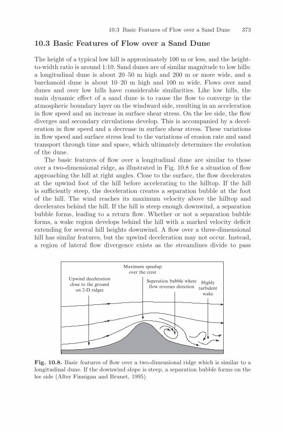
10.3 Basic Features of Flow over a Sand Dune 373
10.3 Basic Features of Flow over a Sand Dune
The height of a typical low hill is approximately 100 m or less, and the height-to-width ratio is around 1:10. Sand dunes are of similar magnitude to low hills:a longitudinal dune is about 20–50 m high and 200 m or more wide, and abarchanoid dune is about 10–20 m high and 100 m wide. Flows over sanddunes and over low hills have considerable similarities. Like low hills, themain dynamic effect of a sand dune is to cause the flow to converge in theatmospheric boundary layer on the windward side, resulting in an accelerationin flow speed and an increase in surface shear stress. On the lee side, the flowdiverges and secondary circulations develop. This is accompanied by a decel-eration in flow speed and a decrease in surface shear stress. These variationsin flow speed and surface stress lead to the variations of erosion rate and sandtransport through time and space, which ultimately determines the evolutionof the dune.
The basic features of flow over a longitudinal dune are similar to thoseover a two-dimensional ridge, as illustrated in Fig. 10.8 for a situation of flowapproaching the hill at right angles. Close to the surface, the flow deceleratesat the upwind foot of the hill before accelerating to the hilltop. If the hillis sufficiently steep, the deceleration creates a separation bubble at the footof the hill. The wind reaches its maximum velocity above the hilltop anddecelerates behind the hill. If the hill is steep enough downwind, a separationbubble forms, leading to a return flow. Whether or not a separation bubbleforms, a wake region develops behind the hill with a marked velocity deficitextending for several hill heights downwind. A flow over a three-dimensionalhill has similar features, but the upwind deceleration may not occur. Instead,a region of lateral flow divergence exists as the streamlines divide to pass
Highlyturbulent
wake
Seperation bubble whereflow reverses direction
Maximum speedupover the crest
Upwind decelerationclose to the ground
on 2-D ridges
Fig. 10.8. Basic features of flow over a two-dimensional ridge which is similar to alongitudinal dune. If the downwind slope is steep, a separation bubble forms on thelee side (After Finnigan and Brunet, 1995)
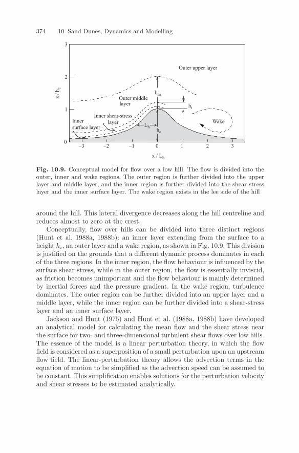
374 10 Sand Dunes, Dynamics and Modelling
0
x / Lh
2
1
3
z / h
c
Innersurface layer
Wake
Outer middle
Outer upper layer
Inner shear-stresslayer
layer hi
hm
hcLh
10 32-2 -1-3
Fig. 10.9. Conceptual model for flow over a low hill. The flow is divided into theouter, inner and wake regions. The outer region is further divided into the upperlayer and middle layer, and the inner region is further divided into the shear stresslayer and the inner surface layer. The wake region exists in the lee side of the hill
around the hill. This lateral divergence decreases along the hill centreline andreduces almost to zero at the crest.
Conceptually, flow over hills can be divided into three distinct regions(Hunt et al. 1988a, 1988b): an inner layer extending from the surface to aheight hi, an outer layer and a wake region, as shown in Fig. 10.9. This divisionis justified on the grounds that a different dynamic process dominates in eachof the three regions. In the inner region, the flow behaviour is influenced by thesurface shear stress, while in the outer region, the flow is essentially inviscid,as friction becomes unimportant and the flow behaviour is mainly determinedby inertial forces and the pressure gradient. In the wake region, turbulencedominates. The outer region can be further divided into an upper layer and amiddle layer, while the inner region can be further divided into a shear-stresslayer and an inner surface layer.
Jackson and Hunt (1975) and Hunt et al. (1988a, 1988b) have developedan analytical model for calculating the mean flow and the shear stress nearthe surface for two- and three-dimensional turbulent shear flows over low hills.The essence of the model is a linear perturbation theory, in which the flowfield is considered as a superposition of a small perturbation upon an upstreamflow field. The linear-perturbation theory allows the advection terms in theequation of motion to be simplified as the advection speed can be assumed tobe constant. This simplification enables solutions for the perturbation velocityand shear stresses to be estimated analytically.
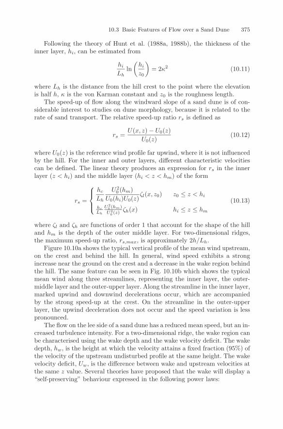
10.3 Basic Features of Flow over a Sand Dune 375
Following the theory of Hunt et al. (1988a, 1988b), the thickness of theinner layer, hi, can be estimated from
hi
Lhln
(hi
z0
)= 2κ2 (10.11)
where Lh is the distance from the hill crest to the point where the elevationis half h, κ is the von Karman constant and z0 is the roughness length.
The speed-up of flow along the windward slope of a sand dune is of con-siderable interest to studies on dune morphology, because it is related to therate of sand transport. The relative speed-up ratio rs is defined as
rs =U(x, z) − U0(z)
U0(z)(10.12)
where U0(z) is the reference wind profile far upwind, where it is not influencedby the hill. For the inner and outer layers, different characteristic velocitiescan be defined. The linear theory produces an expression for rs in the innerlayer (z < hi) and the middle layer (hi < z < hm) of the form
rs =
⎧⎪⎨⎪⎩
hc
Lh
U20 (hm)
U0(hi)U0(z)ζl(x, z0) z0 ≤ z < hi
hc
Lh
U20 (hm)
U20 (z)
ζh(x) hi ≤ z ≤ hm
(10.13)
where ζl and ζh are functions of order 1 that account for the shape of the hilland hm is the depth of the outer middle layer. For two-dimensional ridges,the maximum speed-up ratio, rs,max, is approximately 2h/Lh.
Figure 10.10a shows the typical vertical profile of the mean wind upstream,on the crest and behind the hill. In general, wind speed exhibits a strongincrease near the ground on the crest and a decrease in the wake region behindthe hill. The same feature can be seen in Fig. 10.10b which shows the typicalmean wind along three streamlines, representing the inner layer, the outer-middle layer and the outer-upper layer. Along the streamline in the inner layer,marked upwind and downwind decelerations occur, which are accompaniedby the strong speed-up at the crest. On the streamline in the outer-upperlayer, the upwind deceleration does not occur and the speed variation is lesspronounced.
The flow on the lee side of a sand dune has a reduced mean speed, but an in-creased turbulence intensity. For a two-dimensional ridge, the wake region canbe characterised using the wake depth and the wake velocity deficit. The wakedepth, hw, is the height at which the velocity attains a fixed fraction (95%) ofthe velocity of the upstream undisturbed profile at the same height. The wakevelocity deficit, Uw, is the difference between wake and upstream velocities atthe same z value. Several theories have proposed that the wake will display a“self-preserving” behaviour expressed in the following power laws:
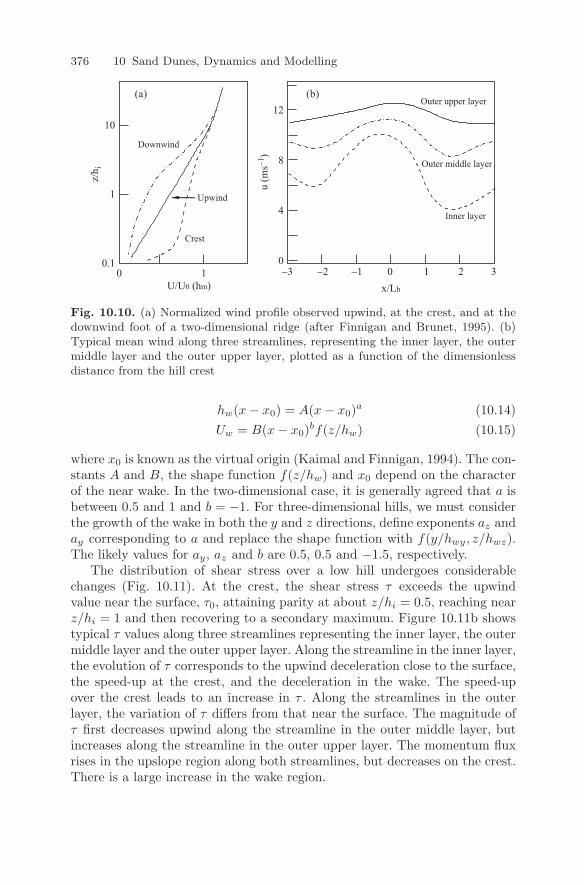
376 10 Sand Dunes, Dynamics and Modelling
Crest
Downwind
Upwind
)b()a(
x/Lh
u (m
s-1 )
Outer upper layer
Outer middle layer
Inner layer
z/h i
U/U0 (hm)
1
0.10 1
10
0
4
8
12
-3 -2 -1 0 1 2 3
Fig. 10.10. (a) Normalized wind profile observed upwind, at the crest, and at thedownwind foot of a two-dimensional ridge (after Finnigan and Brunet, 1995). (b)Typical mean wind along three streamlines, representing the inner layer, the outermiddle layer and the outer upper layer, plotted as a function of the dimensionlessdistance from the hill crest
hw(x − x0) = A(x − x0)a (10.14)Uw = B(x − x0)bf(z/hw) (10.15)
where x0 is known as the virtual origin (Kaimal and Finnigan, 1994). The con-stants A and B, the shape function f(z/hw) and x0 depend on the characterof the near wake. In the two-dimensional case, it is generally agreed that a isbetween 0.5 and 1 and b = −1. For three-dimensional hills, we must considerthe growth of the wake in both the y and z directions, define exponents az anday corresponding to a and replace the shape function with f(y/hwy, z/hwz).The likely values for ay, az and b are 0.5, 0.5 and −1.5, respectively.
The distribution of shear stress over a low hill undergoes considerablechanges (Fig. 10.11). At the crest, the shear stress τ exceeds the upwindvalue near the surface, τ0, attaining parity at about z/hi = 0.5, reaching nearz/hi = 1 and then recovering to a secondary maximum. Figure 10.11b showstypical τ values along three streamlines representing the inner layer, the outermiddle layer and the outer upper layer. Along the streamline in the inner layer,the evolution of τ corresponds to the upwind deceleration close to the surface,the speed-up at the crest, and the deceleration in the wake. The speed-upover the crest leads to an increase in τ . Along the streamlines in the outerlayer, the variation of τ differs from that near the surface. The magnitude ofτ first decreases upwind along the streamline in the outer middle layer, butincreases along the streamline in the outer upper layer. The momentum fluxrises in the upslope region along both streamlines, but decreases on the crest.There is a large increase in the wake region.
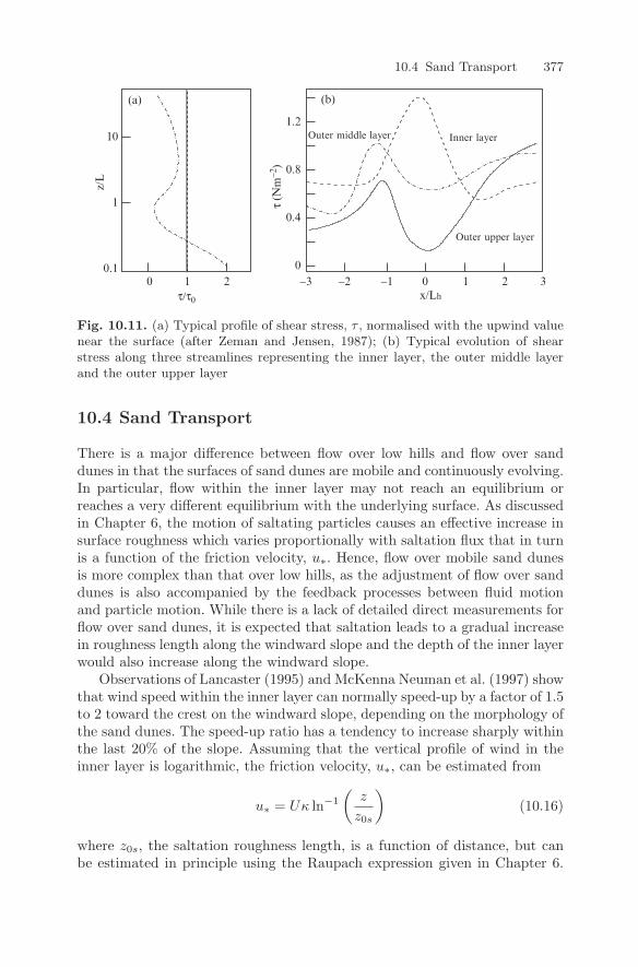
10.4 Sand Transport 377
x/Lhτ/τ0
τ (N
m−2
)
(a) (b)
Inner layerOuter middle layer
Outer upper layer
z/L
10
1
0.10 1 2 −2−3 −1 0 1 2 3
0
0.4
0.8
1.2
Fig. 10.11. (a) Typical profile of shear stress, τ , normalised with the upwind valuenear the surface (after Zeman and Jensen, 1987); (b) Typical evolution of shearstress along three streamlines representing the inner layer, the outer middle layerand the outer upper layer
10.4 Sand Transport
There is a major difference between flow over low hills and flow over sanddunes in that the surfaces of sand dunes are mobile and continuously evolving.In particular, flow within the inner layer may not reach an equilibrium orreaches a very different equilibrium with the underlying surface. As discussedin Chapter 6, the motion of saltating particles causes an effective increase insurface roughness which varies proportionally with saltation flux that in turnis a function of the friction velocity, u∗. Hence, flow over mobile sand dunesis more complex than that over low hills, as the adjustment of flow over sanddunes is also accompanied by the feedback processes between fluid motionand particle motion. While there is a lack of detailed direct measurements forflow over sand dunes, it is expected that saltation leads to a gradual increasein roughness length along the windward slope and the depth of the inner layerwould also increase along the windward slope.
Observations of Lancaster (1995) and McKenna Neuman et al. (1997) showthat wind speed within the inner layer can normally speed-up by a factor of 1.5to 2 toward the crest on the windward slope, depending on the morphology ofthe sand dunes. The speed-up ratio has a tendency to increase sharply withinthe last 20% of the slope. Assuming that the vertical profile of wind in theinner layer is logarithmic, the friction velocity, u∗, can be estimated from
u∗ = Uκ ln−1
(z
z0s
)(10.16)
where z0s, the saltation roughness length, is a function of distance, but canbe estimated in principle using the Raupach expression given in Chapter 6.
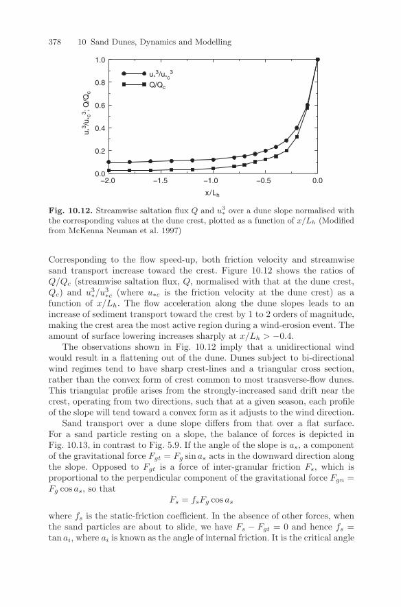
378 10 Sand Dunes, Dynamics and Modelling
x/Lh
u *3 /u *c
3 ; Q
/Qc
u*3/u*c
3
Q/Qc
0.0
0.2
0.4
0.6
0.8
1.0
−2.0 −1.5 −1.0 −0.5 0.0
Fig. 10.12. Streamwise saltation flux Q and u3∗ over a dune slope normalised with
the corresponding values at the dune crest, plotted as a function of x/Lh (Modifiedfrom McKenna Neuman et al. 1997)
Corresponding to the flow speed-up, both friction velocity and streamwisesand transport increase toward the crest. Figure 10.12 shows the ratios ofQ/Qc (streamwise saltation flux, Q, normalised with that at the dune crest,Qc) and u3
∗/u3∗c (where u∗c is the friction velocity at the dune crest) as a
function of x/Lh. The flow acceleration along the dune slopes leads to anincrease of sediment transport toward the crest by 1 to 2 orders of magnitude,making the crest area the most active region during a wind-erosion event. Theamount of surface lowering increases sharply at x/Lh > −0.4.
The observations shown in Fig. 10.12 imply that a unidirectional windwould result in a flattening out of the dune. Dunes subject to bi-directionalwind regimes tend to have sharp crest-lines and a triangular cross section,rather than the convex form of crest common to most transverse-flow dunes.This triangular profile arises from the strongly-increased sand drift near thecrest, operating from two directions, such that at a given season, each profileof the slope will tend toward a convex form as it adjusts to the wind direction.
Sand transport over a dune slope differs from that over a flat surface.For a sand particle resting on a slope, the balance of forces is depicted inFig. 10.13, in contrast to Fig. 5.9. If the angle of the slope is as, a componentof the gravitational force Fgt = Fg sin as acts in the downward direction alongthe slope. Opposed to Fgt is a force of inter-granular friction Fs, which isproportional to the perpendicular component of the gravitational force Fgn =Fg cos as, so that
Fs = fsFg cos as
where fs is the static-friction coefficient. In the absence of other forces, whenthe sand particles are about to slide, we have Fs − Fgt = 0 and hence fs =tan ai, where ai is known as the angle of internal friction. It is the critical angle
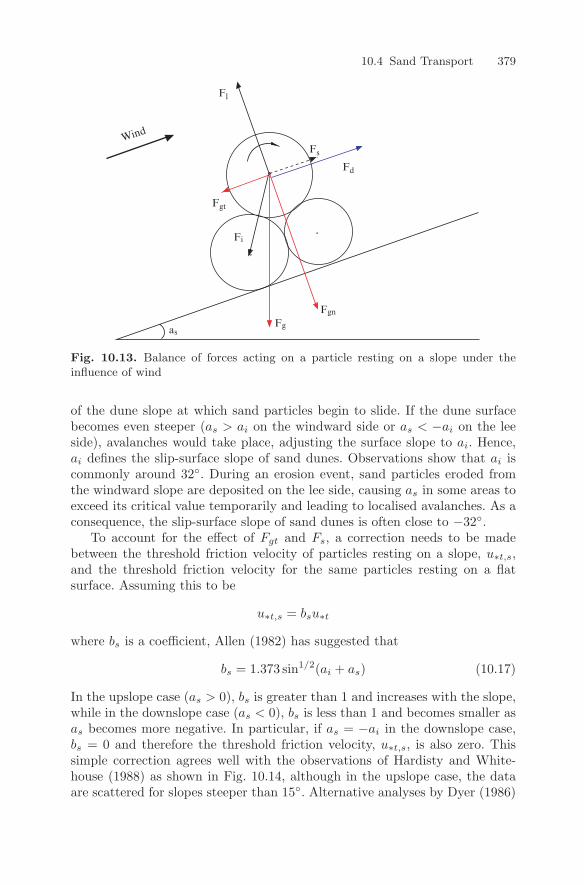
10.4 Sand Transport 379
Wind
Fl
Fs
Fd
Fgt
Fi
Fgas
Fgn
Fig. 10.13. Balance of forces acting on a particle resting on a slope under theinfluence of wind
of the dune slope at which sand particles begin to slide. If the dune surfacebecomes even steeper (as > ai on the windward side or as < −ai on the leeside), avalanches would take place, adjusting the surface slope to ai. Hence,ai defines the slip-surface slope of sand dunes. Observations show that ai iscommonly around 32. During an erosion event, sand particles eroded fromthe windward slope are deposited on the lee side, causing as in some areas toexceed its critical value temporarily and leading to localised avalanches. As aconsequence, the slip-surface slope of sand dunes is often close to −32.
To account for the effect of Fgt and Fs, a correction needs to be madebetween the threshold friction velocity of particles resting on a slope, u∗t,s,and the threshold friction velocity for the same particles resting on a flatsurface. Assuming this to be
u∗t,s = bsu∗t
where bs is a coefficient, Allen (1982) has suggested that
bs = 1.373 sin1/2(ai + as) (10.17)
In the upslope case (as > 0), bs is greater than 1 and increases with the slope,while in the downslope case (as < 0), bs is less than 1 and becomes smaller asas becomes more negative. In particular, if as = −ai in the downslope case,bs = 0 and therefore the threshold friction velocity, u∗t,s, is also zero. Thissimple correction agrees well with the observations of Hardisty and White-house (1988) as shown in Fig. 10.14, although in the upslope case, the dataare scattered for slopes steeper than 15. Alternative analyses by Dyer (1986)
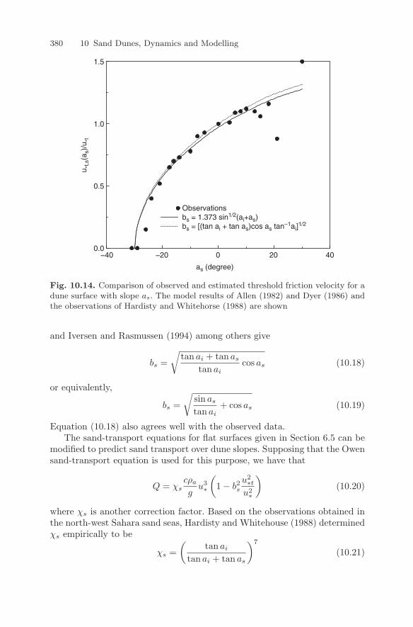
380 10 Sand Dunes, Dynamics and Modelling
as (degree)
u *t,s
(as)
/u*t
Observationsbs = 1.373 sin1/2(ai+as)bs = [(tan ai + tan as)cos as tan−1ai]
1/2
0.0
0.5
1.0
1.5
−40 −20 0 20 40
Fig. 10.14. Comparison of observed and estimated threshold friction velocity for adune surface with slope as. The model results of Allen (1982) and Dyer (1986) andthe observations of Hardisty and Whitehorse (1988) are shown
and Iversen and Rasmussen (1994) among others give
bs =√
tan ai + tan as
tan aicos as (10.18)
or equivalently,
bs =√
sin as
tan ai+ cos as (10.19)
Equation (10.18) also agrees well with the observed data.The sand-transport equations for flat surfaces given in Section 6.5 can be
modified to predict sand transport over dune slopes. Supposing that the Owensand-transport equation is used for this purpose, we have that
Q = χscρa
gu3∗
(1 − b2
s
u2∗t
u2∗
)(10.20)
where χs is another correction factor. Based on the observations obtained inthe north-west Sahara sand seas, Hardisty and Whitehouse (1988) determinedχs empirically to be
χs =(
tan ai
tan ai + tan as
)7
(10.21)
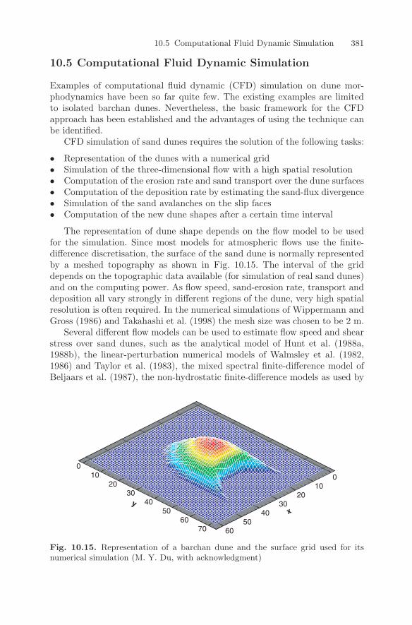
10.5 Computational Fluid Dynamic Simulation 381
10.5 Computational Fluid Dynamic Simulation
Examples of computational fluid dynamic (CFD) simulation on dune mor-phodynamics have been so far quite few. The existing examples are limitedto isolated barchan dunes. Nevertheless, the basic framework for the CFDapproach has been established and the advantages of using the technique canbe identified.
CFD simulation of sand dunes requires the solution of the following tasks:
• Representation of the dunes with a numerical grid• Simulation of the three-dimensional flow with a high spatial resolution• Computation of the erosion rate and sand transport over the dune surfaces• Computation of the deposition rate by estimating the sand-flux divergence• Simulation of the sand avalanches on the slip faces• Computation of the new dune shapes after a certain time interval
The representation of dune shape depends on the flow model to be usedfor the simulation. Since most models for atmospheric flows use the finite-difference discretisation, the surface of the sand dune is normally representedby a meshed topography as shown in Fig. 10.15. The interval of the griddepends on the topographic data available (for simulation of real sand dunes)and on the computing power. As flow speed, sand-erosion rate, transport anddeposition all vary strongly in different regions of the dune, very high spatialresolution is often required. In the numerical simulations of Wippermann andGross (1986) and Takahashi et al. (1998) the mesh size was chosen to be 2 m.
Several different flow models can be used to estimate flow speed and shearstress over sand dunes, such as the analytical model of Hunt et al. (1988a,1988b), the linear-perturbation numerical models of Walmsley et al. (1982,1986) and Taylor et al. (1983), the mixed spectral finite-difference model ofBeljaars et al. (1987), the non-hydrostatic finite-difference models as used by
010
2030
4050
60
xy
010
2030
4050
6070
Fig. 10.15. Representation of a barchan dune and the surface grid used for itsnumerical simulation (M. Y. Du, with acknowledgment)
382 10 Sand Dunes, Dynamics and Modelling
Wippermann and Gross (1986) and the large-eddy simulation model as usedby Takahashi et al. (1998). These models have different numerical sophistica-tions. The linear perturbation models deal easily with arbitrary distributionsof terrain roughness and elevation, and the computational requirements formemory and process time are low. The surface height is Fourier transformed,the solution for each wave number is calculated individually, and the solu-tion is inverse-transformed to real space. Although the applicability of thesetypes of models is confined in theory to flows with small perturbations, nu-merical tests show that they allow quite large perturbations in both terrainelevation and roughness and are adequate for many practical applications.These models have limitations in the simulation of flow fields because of thesimple treatment of advection and the level of closure. However, the maindifficulty in applying these types of models to sand-dune simulation is thatthey only simulate steady-state flows and do not easily allow the interactionsof sand transport and surface-layer flow without major modifications. Fromthis point of view, the unsteady flow models, such as the non-hydrostaticfinite-difference and the large-eddy simulation model, are more suitable formodelling sand dunes, although they are much more difficult to implementcomputationally.
10.5.1 Flow-Model Implementation: Non-hydrostatic Model
Non-hydrostatic models originally designed for the simulation of atmosphericflows on micro- to meso-scales (several metres to several kilometres) can bemodified for the purpose of modelling flow over sand dunes. One such modelhas been implemented by Wippermann and Gross (1986) for studying theformation and migration of individual barchan dunes.
A typical non-hydrostatic model consists of the equations of motion, theconservation equation of heat and a diagnostic equation for the dynamicpart of the pressure deviation. The continuity equation, the equations of mo-tion and the temperature equation in the Cartesian coordinate system afterReynolds averaging can be written as
∂uj
∂xj= 0 (10.22)
dui
dt= −cpθ
∂Π
∂xi+ fεij3uj − δi3g −
∂u′iu
′j
∂xj(10.23)
dθ
dt= −
∂θ′u′j
∂xj(10.24)
where θ is potential temperature and Π is the Exner function, defined as
Π =(
p
ps
)RLcp
10.5 Computational Fluid Dynamic Simulation 383
with p being pressure and ps being that at a reference level, commonly set to1000 hPa. The sub-grid momentum fluxes u′
iu′j and sub-grid heat fluxes u′
iθ′
are determined through parameterisations.For numerical reasons, the Exner function and the potential temperature
are divided into a large-scale component (index 0) and a meso-scale deviation(index *) therefrom, so that
Π = Π0 + Π∗ (10.25)θ = θ0 + θ∗ (10.26)
The large-scale flow is assumed to be geostrophic and hydrostatic, and the(Exner) pressure deviation Π∗ is the non-hydrostatic component, also knownas the dynamic (Exner) pressure.
Hence the equations of motion become
du
dt= −cpθ
∂Π∗
∂x+ f(v − vg
θ
θ0) −
∂u′u′j
∂xj(10.27)
dv
dt= −cpθ
∂Π∗
∂y− f(u − ug
θ
θ0) −
∂v′u′j
∂xj(10.28)
dw
dt= −cpθ
∂Π∗
∂z−
∂w′u′j
∂xj(10.29)
So that the flow field determined through discretised prognostic equations alsofulfils the continuity equation, a correction term to Π∗ must be introducedat each step of the numerical integration. This numerical procedure leads toa prognostic equation for Π∗ (see e.g. Gross, 1993 for details). Depending onthe parameterisation schemes used to estimate the sub-grid fluxes, additionalprognostic equations may be required. A popular closure scheme currently inuse is based on Mellor and Yamada (1982). For instance, if the Mellor andYamada Level 2.5 closure is used (commonly known as the e-l closure, wheree is turbulent kinetic energy and l the mixing length), a prognostic equationfor turbulent kinetic energy is also required.
For simulation of flow over sand dunes, the coordinate system can beconveniently chosen so that the x-axis is in the direction of the basic wind.It is also advantageous to transform the equations into the terrain-followingcoordinate system (x, y, η) where
η =z − z0 − h(x, y)htop − h(x, y)
with h being the height of dune terrain and htop being the top of the simula-tion domain at which the fields of the atmospheric variables are not affectedby topography. The vertical velocity in the transform system is ω = dη/dt.Normally, the equations are transformed into terrain-following coordinatesbefore being coded.
384 10 Sand Dunes, Dynamics and Modelling
At the inflow and outflow boundaries, as well as the lateral boundaries,either the prognostic variables and the dynamic-pressure deviation or theirderivatives can be specified. For instance, at the inflow boundary, u(η) canbe specified and v, ω and ∂Π∗/∂x can be set to 0, whereas at the outflowboundary, the radiation condition after Orlanski can be used. For the lateralboundaries, u(η) can be specified and ∂u/∂y, ∂ω/∂y and ∂Π∗/∂y can be setto zero. At the upper boundary where η = 1, the vertical derivatives of u, v,ω and Π∗ must vanish. At the lower boundary η = 0, u, v and ω need to beset to 0 and Π∗ has to be adjusted in such a way that ∂Π∗/∂η = 0 and thecontinuity equation for incompressible flow is satisfied everywhere in the field.
How to estimate the friction velocity is of particular importance for study-ing the migration of sand dunes. There is not yet a well-established theory forsand dune situations. However, a similar approach to that for a flat surfacemay be adopted. Supposing that the saltation roughness length is z0s, thefriction velocity can be estimated using Equation (10.16).
10.5.2 Flow-Model Implementation: Large-Eddy Model
Large-eddy simulation models are also suitable for modelling flows over sanddunes, as suggested by Takahashi et al. (1998). This approach requires thespatial resolution of the model to be down to the inertial subrange of tur-bulence and is therefore difficult to apply for general purposes, except forstudying individual dunes. However, this approach provides the possibility ofstudying the details of interactions between sand transport and turbulence inthe dune environment.
To catch the influence of sudden variations of topography, Takahashiet al. (1998) proposed using a generalized terrain-following coordinate sys-tem (ξ, ψ, ζ). The vertical coordinate ζ is orthogonal to the ground surfacewhich corresponds to ζ = 0. Orthogonal relations also exist between the verti-cal coordinate and the other two coordinates ξ and ψ. The transition betweenthe Cartesian coordinate and the generalized terrain-following coordinate hasthe following relationship:
(U, V,W )T = J(u, v, w)T (10.30)
where J is the Jacobian matrix, given by
J =
⎛⎝ ξx ξy ξz
ψx ψy ψz
ζx ζy ζz
⎞⎠
and U , V and W are the velocity components in the generalized terrain-following coordinates (ξ, ψ, ζ), respectively, while u, v and w are those in theCartesian coordinates (x, y, z) and ξx is ∂ξ/∂x, etc. Under the Boussinesqapproximation, the three-dimensional non-hydrostatic, incompressible atmo-spheric continuity equation and equation of motion in the generalized terrain-following coordinate system may be written as
10.5 Computational Fluid Dynamic Simulation 385
∂U/J
∂ξ+
∂V/J
∂ψ+
∂W/J
∂ζ= 0 (10.31)
∂(ui/J)∂t
+∂(Uui/J)
∂ξ+
∂(V ui/J)∂ψ
+∂(Wui/J)
∂ζ(10.32)
= − ∂(ξiP/J)∂ξ
− ∂(ψiP/J)∂ψ
− ∂(ζiP/J)∂ζ
+∂[(ξxτi1 + ξyτi2 + ξzτi3)/J ]
∂ξ
+∂[(ψxτi1 + ψyτi2 + ψzτi3)/J ]
∂ψ+
∂[(ζxτi1 + ζyτi2 + ζzτi3)/J ]∂ζ
with J being the determinant of J , P = p/ρ, (ξ1, ξ2, ξ3 ≡ ∂ξ∂x , ∂ξ
∂y , ∂ξ∂z ) etc. For
large-eddy simulation models, the Smagorinsky (1963) closure can be used asfollows
τij = νDij (10.33)
Dij = ξj∂ui
∂ξ+ ψj
∂ui
∂ψ+ ζj
∂ui
∂ζ+ ξi
∂uj
∂ξ+ ψi
∂uj
∂ψ+ ζi
∂uj
∂ζ(10.34)
ν = (Cs∆)2
⎛⎝1
2
3∑i,j=1
D2ij
⎞⎠
1/2
(10.35)
∆3 = ∆x∆y∆z = ∆ξ∆η∆ζ (10.36)Cs = 0.12 (10.37)
The boundary conditions given in the previous subsection are also suitablefor the large-eddy model.
10.5.3 Computation of Erosion and Deposition Rates
Having determined the distribution of the friction velocity on the sand dune,the streamwise saltation flux, Q, can be determined using the sand-transportEquation (10.20). Note that the friction velocity is a vector which changesdirection over the dune as the mean wind converges and diverges around it.The direction of the sand-transport vector is the same as the friction-velocityvector, which can be estimated as φ = arc tan(v/u). The components of theQ vector, Qx and Qy can be estimated as
Qx = Q cos φ; Qy = Q sin φ
The dune surface will be eroded, if Q diverges. Otherwise, deposition willoccur if Q converges. This is true, as long as the slope of the surface is smallerthan the slope of the slip face. The tendency equation for the sand-dune heightis given by
∂h
∂t= − 1
ρbdivQ | as |≤| ai | (10.38)
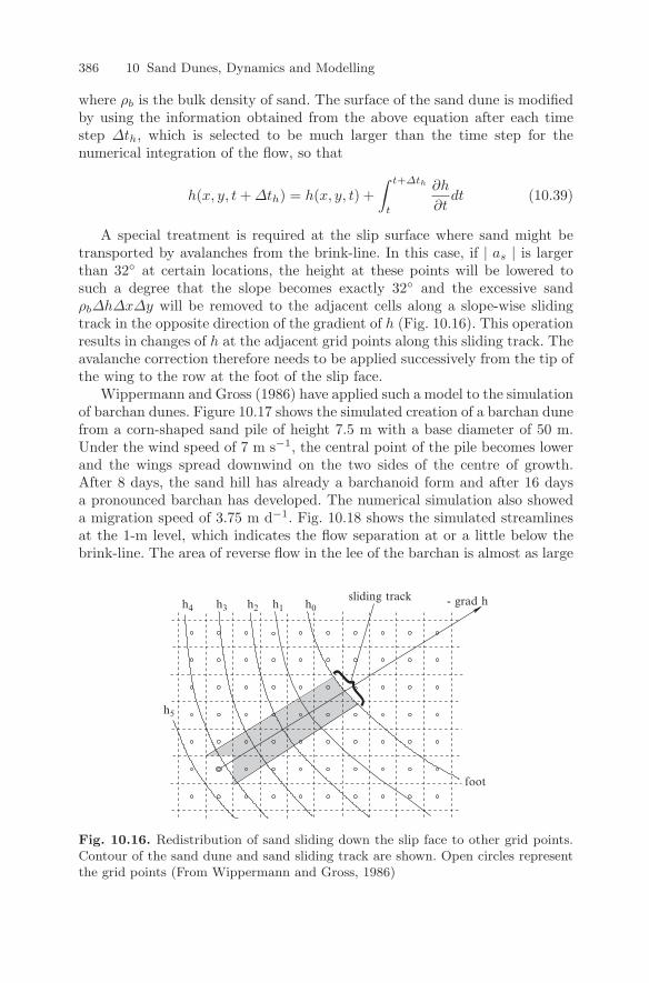
386 10 Sand Dunes, Dynamics and Modelling
where ρb is the bulk density of sand. The surface of the sand dune is modifiedby using the information obtained from the above equation after each timestep ∆th, which is selected to be much larger than the time step for thenumerical integration of the flow, so that
h(x, y, t + ∆th) = h(x, y, t) +∫ t+∆th
t
∂h
∂tdt (10.39)
A special treatment is required at the slip surface where sand might betransported by avalanches from the brink-line. In this case, if | as | is largerthan 32 at certain locations, the height at these points will be lowered tosuch a degree that the slope becomes exactly 32 and the excessive sandρb∆h∆x∆y will be removed to the adjacent cells along a slope-wise slidingtrack in the opposite direction of the gradient of h (Fig. 10.16). This operationresults in changes of h at the adjacent grid points along this sliding track. Theavalanche correction therefore needs to be applied successively from the tip ofthe wing to the row at the foot of the slip face.
Wippermann and Gross (1986) have applied such a model to the simulationof barchan dunes. Figure 10.17 shows the simulated creation of a barchan dunefrom a corn-shaped sand pile of height 7.5 m with a base diameter of 50 m.Under the wind speed of 7 m s−1, the central point of the pile becomes lowerand the wings spread downwind on the two sides of the centre of growth.After 8 days, the sand hill has already a barchanoid form and after 16 daysa pronounced barchan has developed. The numerical simulation also showeda migration speed of 3.75 m d−1. Fig. 10.18 shows the simulated streamlinesat the 1-m level, which indicates the flow separation at or a little below thebrink-line. The area of reverse flow in the lee of the barchan is almost as large
- grad hsliding track
foot
h4
h5
h3 h2 h1 h0
Fig. 10.16. Redistribution of sand sliding down the slip face to other grid points.Contour of the sand dune and sand sliding track are shown. Open circles representthe grid points (From Wippermann and Gross, 1986)
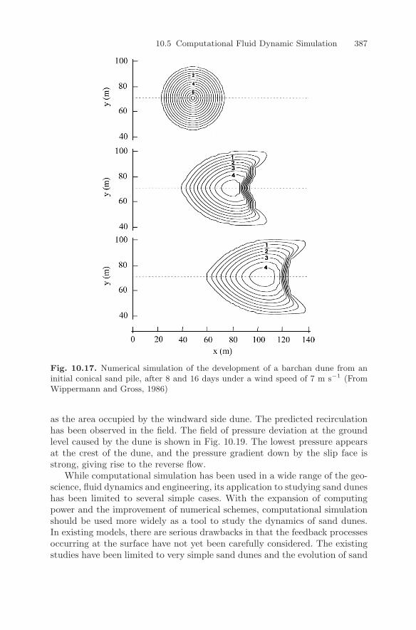
10.5 Computational Fluid Dynamic Simulation 387
Fig. 10.17. Numerical simulation of the development of a barchan dune from aninitial conical sand pile, after 8 and 16 days under a wind speed of 7 m s−1 (FromWippermann and Gross, 1986)
as the area occupied by the windward side dune. The predicted recirculationhas been observed in the field. The field of pressure deviation at the groundlevel caused by the dune is shown in Fig. 10.19. The lowest pressure appearsat the crest of the dune, and the pressure gradient down by the slip face isstrong, giving rise to the reverse flow.
While computational simulation has been used in a wide range of the geo-science, fluid dynamics and engineering, its application to studying sand duneshas been limited to several simple cases. With the expansion of computingpower and the improvement of numerical schemes, computational simulationshould be used more widely as a tool to study the dynamics of sand dunes.In existing models, there are serious drawbacks in that the feedback processesoccurring at the surface have not yet been carefully considered. The existingstudies have been limited to very simple sand dunes and the evolution of sand
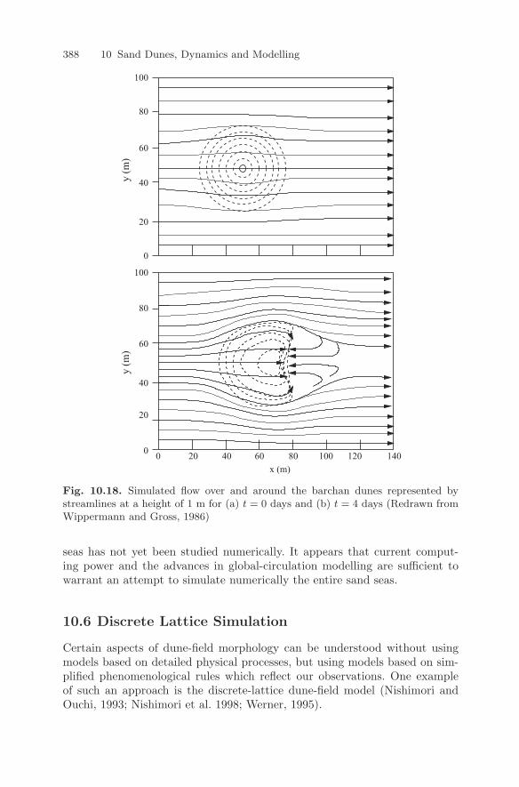
388 10 Sand Dunes, Dynamics and Modelling
x (m)
0
20
100
0 0 20 40 60 80 100 120 140
20
40
60
80
100
40
60
80y
(m)
y (m
)
Fig. 10.18. Simulated flow over and around the barchan dunes represented bystreamlines at a height of 1 m for (a) t = 0 days and (b) t = 4 days (Redrawn fromWippermann and Gross, 1986)
seas has not yet been studied numerically. It appears that current comput-ing power and the advances in global-circulation modelling are sufficient towarrant an attempt to simulate numerically the entire sand seas.
10.6 Discrete Lattice Simulation
Certain aspects of dune-field morphology can be understood without usingmodels based on detailed physical processes, but using models based on sim-plified phenomenological rules which reflect our observations. One exampleof such an approach is the discrete-lattice dune-field model (Nishimori andOuchi, 1993; Nishimori et al. 1998; Werner, 1995).
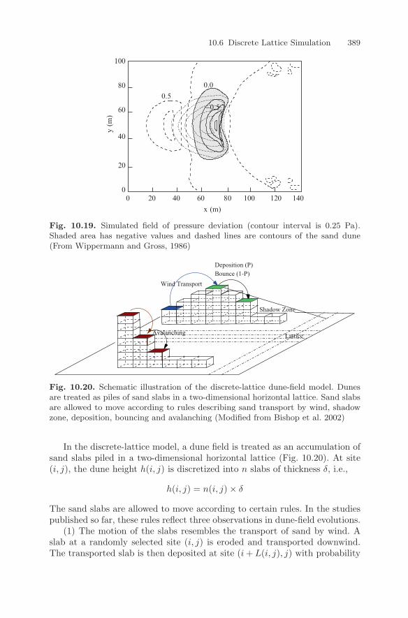
10.6 Discrete Lattice Simulation 389
y (m
)
0.5
0.0
−0.5
1401201004020 080 60
x (m)
0
20
40
60
80
100
Fig. 10.19. Simulated field of pressure deviation (contour interval is 0.25 Pa).Shaded area has negative values and dashed lines are contours of the sand dune(From Wippermann and Gross, 1986)
Deposition (P)
Wind TransportBounce (1-P)
Shadow Zone
Avalanching Lattice
Fig. 10.20. Schematic illustration of the discrete-lattice dune-field model. Dunesare treated as piles of sand slabs in a two-dimensional horizontal lattice. Sand slabsare allowed to move according to rules describing sand transport by wind, shadowzone, deposition, bouncing and avalanching (Modified from Bishop et al. 2002)
In the discrete-lattice model, a dune field is treated as an accumulation ofsand slabs piled in a two-dimensional horizontal lattice (Fig. 10.20). At site(i, j), the dune height h(i, j) is discretized into n slabs of thickness δ, i.e.,
h(i, j) = n(i, j) × δ
The sand slabs are allowed to move according to certain rules. In the studiespublished so far, these rules reflect three observations in dune-field evolutions.
(1) The motion of the slabs resembles the transport of sand by wind. Aslab at a randomly selected site (i, j) is eroded and transported downwind.The transported slab is then deposited at site (i + L(i, j), j) with probability
390 10 Sand Dunes, Dynamics and Modelling
P , where L(i, j), the distance moved, is site dependent. If the slab is notdeposited at this site, then it is transported further to the site (i + L(i, j) +L(i + L(i, j), j), j) etc. The deposition probability P can be set to 0.6 for asite with at least one slab and 0.4 for a site with no slab. L can be interpretedto be the typical hopping length of saltation, which depends on wind speed.
(2) Shadow zones are defined in the lattice, where erosion does not occurand the deposition probability P is one. For example, the shadow zone canbe defined as 15 from the dune crest. This would correspond to the flowre-attachment distance from the crest downwind, which is about four timesthe dune height.
(3) Avalanching occurs at the place of the steepest descent. If the numberof the slabs between any neighbouring sites differ by tan(32)/δ, a slab willbe transferred to the neighbouring site.
Obviously, the discrete-lattice approach is very simplistic. However, Bishopet al. (2002) have shown that despite the simplicity, the approach can generatedunes which resemble dunes in nature. One advantage of the approach is thatthe rules for slab erosion and transport can be easily introduced one by onein the simulation and the simulation may lead to a qualitative understandingwhether a particular rule is important to the dune-field evolution.
11
Techniques for Wind-Erosion Measurements
11.1 Wind-Tunnel Measurements
Much of our understanding of wind erosion is derived from wind-tunnel ex-periments, in which the phenomenon is observed under controlled conditions.Laboratory wind tunnels have been used for the investigation of saltation (e.g.Bagnold, 1941), the determination of threshold friction velocity (e.g. Iversen etal. 1987), the process of drag partitioning (Marshall, 1971; McKenna Neumanand Nickling, 1995), the equilibration of saltation (Shao and Raupach, 1992),the process of dust emission (Shao et al. 1993b; Rice et al. 1996a, 1996b), aswell as the formation and evolution of sand dunes (Tsoar et al. 1985). Portablewind tunnels, which can be set up in the field, have been used to study winderosion on natural soil surfaces by Gillette et al. (1980, 1982), Nickling andGillies (1989) and Leys and Raupach (1991), among others (Fig. 11.1). Aparticularly useful application of portable wind tunnels is to study how envi-ronmental factors influence the threshold of wind erosion, by applying wind-tunnel tests over the natural surface and then over that same surface withmodifications.
In using a wind tunnel, attention needs to be paid to several importantissues. Firstly, the wind-tunnel flows must satisfy several criteria, so that theyreasonably-well represent those occurring in the natural environment. Thesecriteria are as listed below:
• Wind-tunnel flows must reproduce the mean-wind profiles commonly ob-served in atmospheric boundary layers, which are logarithmic with heightin thermally-neutral conditions, so that the aerodynamic forces acting onthe surface are realistic.
• The intensity and scale of turbulence in the flows close to the groundmust be realistic to ensure correct characteristics for momentum and masstransfer.
• The flow must be spatially-uniform to avoid local scouring by anomalousregions of high surface stress.
Y. Shao, Physics and Modelling of Wind Erosion, 391c© Springer Science+Business Media B.V. 2008
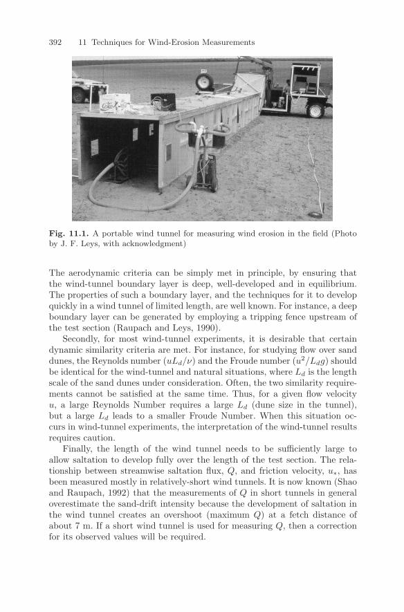
392 11 Techniques for Wind-Erosion Measurements
Fig. 11.1. A portable wind tunnel for measuring wind erosion in the field (Photoby J. F. Leys, with acknowledgment)
The aerodynamic criteria can be simply met in principle, by ensuring thatthe wind-tunnel boundary layer is deep, well-developed and in equilibrium.The properties of such a boundary layer, and the techniques for it to developquickly in a wind tunnel of limited length, are well known. For instance, a deepboundary layer can be generated by employing a tripping fence upstream ofthe test section (Raupach and Leys, 1990).
Secondly, for most wind-tunnel experiments, it is desirable that certaindynamic similarity criteria are met. For instance, for studying flow over sanddunes, the Reynolds number (uLd/ν) and the Froude number (u2/Ldg) shouldbe identical for the wind-tunnel and natural situations, where Ld is the lengthscale of the sand dunes under consideration. Often, the two similarity require-ments cannot be satisfied at the same time. Thus, for a given flow velocityu, a large Reynolds Number requires a large Ld (dune size in the tunnel),but a large Ld leads to a smaller Froude Number. When this situation oc-curs in wind-tunnel experiments, the interpretation of the wind-tunnel resultsrequires caution.
Finally, the length of the wind tunnel needs to be sufficiently large toallow saltation to develop fully over the length of the test section. The rela-tionship between streamwise saltation flux, Q, and friction velocity, u∗, hasbeen measured mostly in relatively-short wind tunnels. It is now known (Shaoand Raupach, 1992) that the measurements of Q in short tunnels in generaloverestimate the sand-drift intensity because the development of saltation inthe wind tunnel creates an overshoot (maximum Q) at a fetch distance ofabout 7 m. If a short wind tunnel is used for measuring Q, then a correctionfor its observed values will be required.
11.2 Sand Measurements 393
It is worthwhile to point out that several important conclusions reachedon the basis of wind-tunnel experiments differ profoundly from those derivedfrom field experiments. There are two examples. The first one is that thesaltation roughness length z0s (see Chapter 6) observed in wind tunnels is wellapproximated by Equation (6.44). The coefficient co = 0.02 in that equation isstrongly supported by early wind-tunnel observations (see Fig. 6.8). However,the field observations of Gillette et al (1998) show that z0s is an order ofmagnitude larger (Fig. 6.13). The second example is that the observationsof Shao and Raupach (1992) indicate that the distance required for saltationto reach equilibrium is approximately 20 m in a wind tunnel, while the fieldobservations in Owen’s lake (Gillette et al. 1997) show that this distance isaround 1 km. The differences between wind-tunnel and field experiments,reflected in z0s and the distance of saltation equilibration, have not yet beenfully explained.
11.2 Sand Measurements
The most important quantities to measure in wind-erosion research are thestreamwise saltation flux, Q, and the vertical dust flux, F . The techniquesfor measuring these two fluxes are quite different. Q can be measured us-ing various sand traps, while F is commonly derived through measuring theprofile of dust concentration. Assuming dust concentration is horizontally ho-mogeneous, the vertical dust flux for a given particle group of size d can beestimated using the following equation
F (d) = −wt(d)c(z, d) − Kp(z, d)δc(z, d)
δz(11.1)
where the two terms on the right hand side of the above equation are thegravitational settling flux and the diffusive flux, respectively. The methods fordetermining the particle terminal velocity, wt, and particle-eddy diffusivity,Kp, have been described in Chapters 5 and 8, respectively. In some previousstudies, the gravitational settling flux has been neglected in the calculation ofF (d). It is recommended here that both terms in the above equation shouldbe measured in future studies, because −wtc is not necessarily much smallerthan −Kpδc/δz.
11.2.1 Passive Samplers
There is a variety of sand samplers differing in dimension, aerodynamic be-haviour and efficiency. Samplers can be classified as in-situ samplers andremote-sensing samplers. Further, we classify the in-situ samplers as eitheractive or passive. Active samplers are equipped with pumping devices tomaintain a flow through their intakes, while passive samplers rely on wind
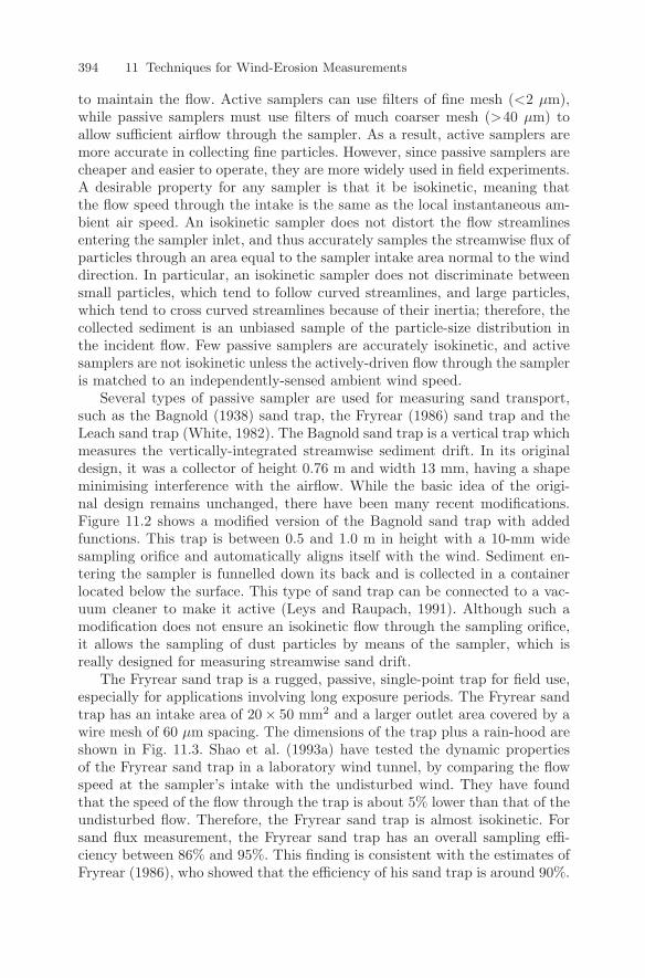
394 11 Techniques for Wind-Erosion Measurements
to maintain the flow. Active samplers can use filters of fine mesh (<2 µm),while passive samplers must use filters of much coarser mesh (>40 µm) toallow sufficient airflow through the sampler. As a result, active samplers aremore accurate in collecting fine particles. However, since passive samplers arecheaper and easier to operate, they are more widely used in field experiments.A desirable property for any sampler is that it be isokinetic, meaning thatthe flow speed through the intake is the same as the local instantaneous am-bient air speed. An isokinetic sampler does not distort the flow streamlinesentering the sampler inlet, and thus accurately samples the streamwise flux ofparticles through an area equal to the sampler intake area normal to the winddirection. In particular, an isokinetic sampler does not discriminate betweensmall particles, which tend to follow curved streamlines, and large particles,which tend to cross curved streamlines because of their inertia; therefore, thecollected sediment is an unbiased sample of the particle-size distribution inthe incident flow. Few passive samplers are accurately isokinetic, and activesamplers are not isokinetic unless the actively-driven flow through the sampleris matched to an independently-sensed ambient wind speed.
Several types of passive sampler are used for measuring sand transport,such as the Bagnold (1938) sand trap, the Fryrear (1986) sand trap and theLeach sand trap (White, 1982). The Bagnold sand trap is a vertical trap whichmeasures the vertically-integrated streamwise sediment drift. In its originaldesign, it was a collector of height 0.76 m and width 13 mm, having a shapeminimising interference with the airflow. While the basic idea of the origi-nal design remains unchanged, there have been many recent modifications.Figure 11.2 shows a modified version of the Bagnold sand trap with addedfunctions. This trap is between 0.5 and 1.0 m in height with a 10-mm widesampling orifice and automatically aligns itself with the wind. Sediment en-tering the sampler is funnelled down its back and is collected in a containerlocated below the surface. This type of sand trap can be connected to a vac-uum cleaner to make it active (Leys and Raupach, 1991). Although such amodification does not ensure an isokinetic flow through the sampling orifice,it allows the sampling of dust particles by means of the sampler, which isreally designed for measuring streamwise sand drift.
The Fryrear sand trap is a rugged, passive, single-point trap for field use,especially for applications involving long exposure periods. The Fryrear sandtrap has an intake area of 20× 50 mm2 and a larger outlet area covered by awire mesh of 60 µm spacing. The dimensions of the trap plus a rain-hood areshown in Fig. 11.3. Shao et al. (1993a) have tested the dynamic propertiesof the Fryrear sand trap in a laboratory wind tunnel, by comparing the flowspeed at the sampler’s intake with the undisturbed wind. They have foundthat the speed of the flow through the trap is about 5% lower than that of theundisturbed flow. Therefore, the Fryrear sand trap is almost isokinetic. Forsand flux measurement, the Fryrear sand trap has an overall sampling effi-ciency between 86% and 95%. This finding is consistent with the estimates ofFryrear (1986), who showed that the efficiency of his sand trap is around 90%.
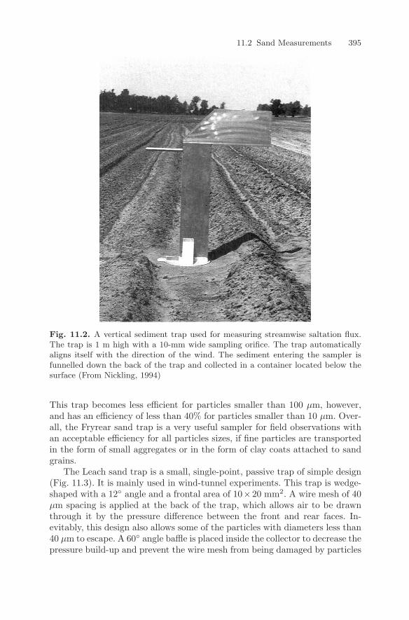
11.2 Sand Measurements 395
Fig. 11.2. A vertical sediment trap used for measuring streamwise saltation flux.The trap is 1 m high with a 10-mm wide sampling orifice. The trap automaticallyaligns itself with the direction of the wind. The sediment entering the sampler isfunnelled down the back of the trap and collected in a container located below thesurface (From Nickling, 1994)
This trap becomes less efficient for particles smaller than 100 µm, however,and has an efficiency of less than 40% for particles smaller than 10 µm. Over-all, the Fryrear sand trap is a very useful sampler for field observations withan acceptable efficiency for all particles sizes, if fine particles are transportedin the form of small aggregates or in the form of clay coats attached to sandgrains.
The Leach sand trap is a small, single-point, passive trap of simple design(Fig. 11.3). It is mainly used in wind-tunnel experiments. This trap is wedge-shaped with a 12 angle and a frontal area of 10×20 mm2. A wire mesh of 40µm spacing is applied at the back of the trap, which allows air to be drawnthrough it by the pressure difference between the front and rear faces. In-evitably, this design also allows some of the particles with diameters less than40 µm to escape. A 60 angle baffle is placed inside the collector to decrease thepressure build-up and prevent the wire mesh from being damaged by particles
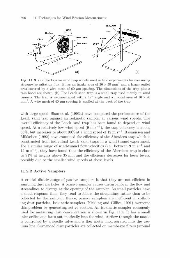
396 11 Techniques for Wind-Erosion Measurements
Fig. 11.3. (a) The Fryrear sand trap widely used in field experiments for measuringstreamwise saltation flux. It has an intake area of 20 × 50 mm2 and a larger outletarea covered by a wire mesh of 60 µm spacing. The dimensions of the trap plus arain hood are shown. (b) The Leach sand trap is a small trap used mainly in windtunnels. The trap is wedge-shaped with a 12 angle and a frontal area of 10 × 20mm2. A wire mesh of 40 µm spacing is applied at the back of the trap
with large speed. Shao et al. (1993a) have compared the performance of theLeach sand trap against an isokinetic sampler at various wind speeds. Theoverall efficiency of the Leach sand trap has been found to depend on windspeed. At a relatively-low wind speed (9 m s−1), the trap efficiency is about83%, but increases to about 90% at a wind speed of 12 m s−1. Rasmussen andMikkelsen (1992) have examined the efficiency of the Aberdeen trap which isconstructed from individual Leach sand traps in a wind-tunnel experiment.For a similar range of wind-tunnel flow velocities (i.e., between 9 m s−1 and12 m s−1), they have found that the efficiency of the Aberdeen trap is closeto 91% at heights above 35 mm and the efficiency decreases for lower levels,possibly due to the smaller wind speeds at those levels.
11.2.2 Active Samplers
A crucial disadvantage of passive samplers is that they are not efficient insampling dust particles. A passive sampler causes disturbance in the flow andstreamlines to diverge at the opening of the sampler. As small particles havea small response time, they tend to follow the streamlines rather than to becollected by the sampler. Hence, passive samplers are inefficient in collect-ing dust particles. Isokinetic samplers (Nickling and Gillies, 1991) overcomethis problem by generating active suction. An isokinetic sampler commonlyused for measuring dust concentration is shown in Fig. 11.4. It has a smallinlet orifice and faces automatically into the wind. Airflow through the nozzleis controlled by a needle valve and a flow meter incorporated into the vac-uum line. Suspended dust particles are collected on membrane filters (around
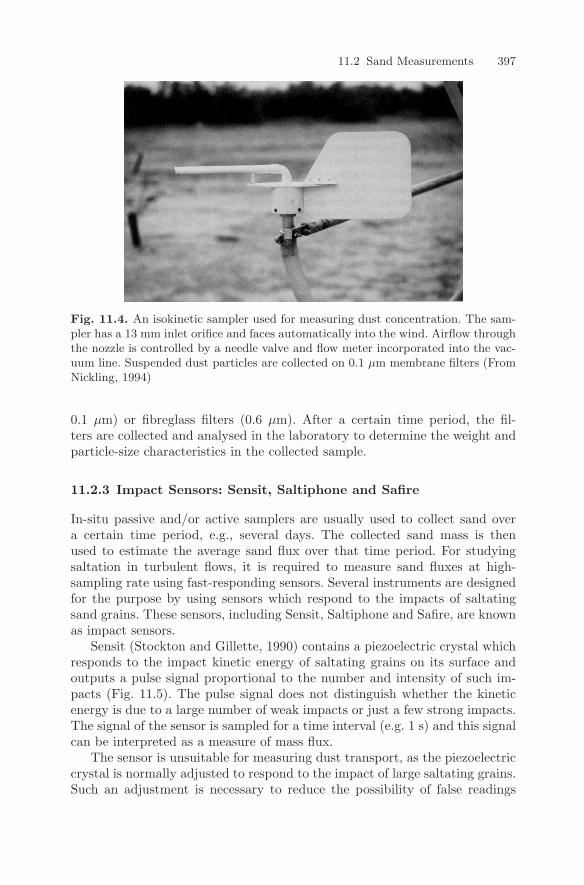
11.2 Sand Measurements 397
Fig. 11.4. An isokinetic sampler used for measuring dust concentration. The sam-pler has a 13 mm inlet orifice and faces automatically into the wind. Airflow throughthe nozzle is controlled by a needle valve and flow meter incorporated into the vac-uum line. Suspended dust particles are collected on 0.1 µm membrane filters (FromNickling, 1994)
0.1 µm) or fibreglass filters (0.6 µm). After a certain time period, the fil-ters are collected and analysed in the laboratory to determine the weight andparticle-size characteristics in the collected sample.
11.2.3 Impact Sensors: Sensit, Saltiphone and Safire
In-situ passive and/or active samplers are usually used to collect sand overa certain time period, e.g., several days. The collected sand mass is thenused to estimate the average sand flux over that time period. For studyingsaltation in turbulent flows, it is required to measure sand fluxes at high-sampling rate using fast-responding sensors. Several instruments are designedfor the purpose by using sensors which respond to the impacts of saltatingsand grains. These sensors, including Sensit, Saltiphone and Safire, are knownas impact sensors.
Sensit (Stockton and Gillette, 1990) contains a piezoelectric crystal whichresponds to the impact kinetic energy of saltating grains on its surface andoutputs a pulse signal proportional to the number and intensity of such im-pacts (Fig. 11.5). The pulse signal does not distinguish whether the kineticenergy is due to a large number of weak impacts or just a few strong impacts.The signal of the sensor is sampled for a time interval (e.g. 1 s) and this signalcan be interpreted as a measure of mass flux.
The sensor is unsuitable for measuring dust transport, as the piezoelectriccrystal is normally adjusted to respond to the impact of large saltating grains.Such an adjustment is necessary to reduce the possibility of false readings
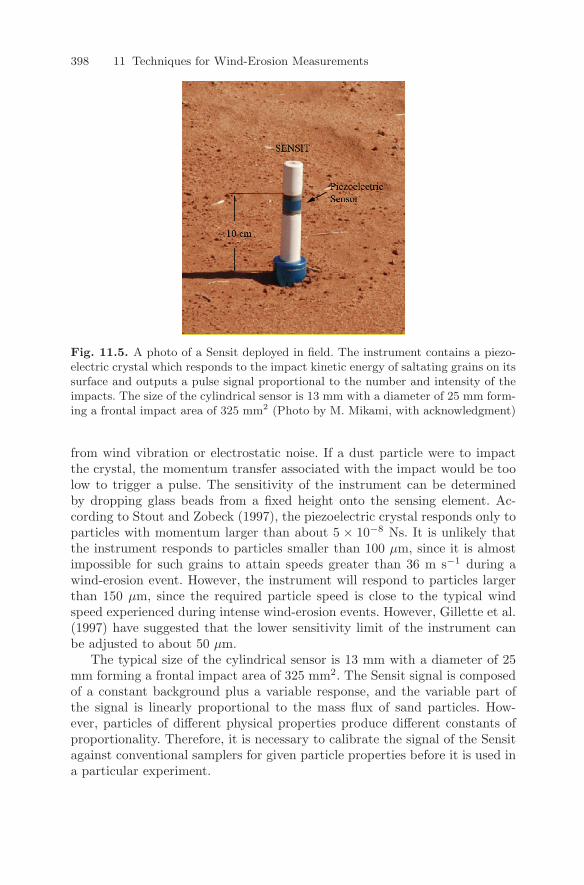
398 11 Techniques for Wind-Erosion Measurements
Fig. 11.5. A photo of a Sensit deployed in field. The instrument contains a piezo-electric crystal which responds to the impact kinetic energy of saltating grains on itssurface and outputs a pulse signal proportional to the number and intensity of theimpacts. The size of the cylindrical sensor is 13 mm with a diameter of 25 mm form-ing a frontal impact area of 325 mm2 (Photo by M. Mikami, with acknowledgment)
from wind vibration or electrostatic noise. If a dust particle were to impactthe crystal, the momentum transfer associated with the impact would be toolow to trigger a pulse. The sensitivity of the instrument can be determinedby dropping glass beads from a fixed height onto the sensing element. Ac-cording to Stout and Zobeck (1997), the piezoelectric crystal responds only toparticles with momentum larger than about 5 × 10⁻⁸ Ns. It is unlikely thatthe instrument responds to particles smaller than 100 µm, since it is almostimpossible for such grains to attain speeds greater than 36 m s−1 during awind-erosion event. However, the instrument will respond to particles largerthan 150 µm, since the required particle speed is close to the typical windspeed experienced during intense wind-erosion events. However, Gillette et al.(1997) have suggested that the lower sensitivity limit of the instrument canbe adjusted to about 50 µm.
The typical size of the cylindrical sensor is 13 mm with a diameter of 25mm forming a frontal impact area of 325 mm2. The Sensit signal is composedof a constant background plus a variable response, and the variable part ofthe signal is linearly proportional to the mass flux of sand particles. How-ever, particles of different physical properties produce different constants ofproportionality. Therefore, it is necessary to calibrate the signal of the Sensitagainst conventional samplers for given particle properties before it is used ina particular experiment.
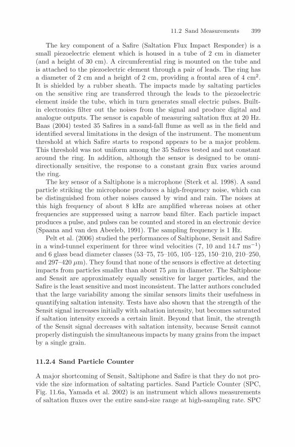
11.2 Sand Measurements 399
The key component of a Safire (Saltation Flux Impact Responder) is asmall piezoelectric element which is housed in a tube of 2 cm in diameter(and a height of 30 cm). A circumferential ring is mounted on the tube andis attached to the piezoelectric element through a pair of leads. The ring hasa diameter of 2 cm and a height of 2 cm, providing a frontal area of 4 cm2.It is shielded by a rubber sheath. The impacts made by saltating particleson the sensitive ring are transferred through the leads to the piezoelectricelement inside the tube, which in turn generates small electric pulses. Built-in electronics filter out the noises from the signal and produce digital andanalogue outputs. The sensor is capable of measuring saltation flux at 20 Hz.Baas (2004) tested 35 Safires in a sand-fall flume as well as in the field andidentified several limitations in the design of the instrument. The momentumthreshold at which Safire starts to respond appears to be a major problem.This threshold was not uniform among the 35 Safires tested and not constantaround the ring. In addition, although the sensor is designed to be omni-directionally sensitive, the response to a constant grain flux varies aroundthe ring.
The key sensor of a Saltiphone is a microphone (Sterk et al. 1998). A sandparticle striking the microphone produces a high-frequency noise, which canbe distinguished from other noises caused by wind and rain. The noises atthis high frequency of about 8 kHz are amplified whereas noises at otherfrequencies are suppressed using a narrow band filter. Each particle impactproduces a pulse, and pulses can be counted and stored in an electronic device(Spaana and van den Abeeleb, 1991). The sampling frequency is 1 Hz.
Pelt et al. (2006) studied the performances of Saltiphone, Sensit and Safirein a wind-tunnel experiment for three wind velocities (7, 10 and 14.7 ms−1)and 6 glass bead diameter classes (53–75, 75–105, 105–125, 150–210, 210–250,and 297–420 µm). They found that none of the sensors is effective at detectingimpacts from particles smaller than about 75 µm in diameter. The Saltiphoneand Sensit are approximately equally sensitive for larger particles, and theSafire is the least sensitive and most inconsistent. The latter authors concludedthat the large variability among the similar sensors limits their usefulness inquantifying saltation intensity. Tests have also shown that the strength of theSensit signal increases initially with saltation intensity, but becomes saturatedif saltation intensity exceeds a certain limit. Beyond that limit, the strengthof the Sensit signal decreases with saltation intensity, because Sensit cannotproperly distinguish the simultaneous impacts by many grains from the impactby a single grain.
11.2.4 Sand Particle Counter
A major shortcoming of Sensit, Saltiphone and Safire is that they do not pro-vide the size information of saltating particles. Sand Particle Counter (SPC,Fig. 11.6a, Yamada et al. 2002) is an instrument which allows measurementsof saltation fluxes over the entire sand-size range at high-sampling rate. SPC
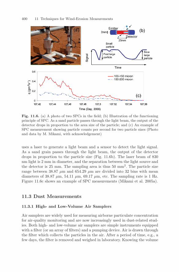
400 11 Techniques for Wind-Erosion Measurements
Fig. 11.6. (a) A photo of two SPCs in the field; (b) Illustration of the functioningprinciple of SPC. As a sand particle passes through the light beam, the output of thedetector drops in proportion to the area size of the particle; and (c) An example ofSPC measurement showing particle counts per second for two particle sizes (Photoand data by M. Mikami, with acknowledgement)
uses a laser to generate a light beam and a sensor to detect the light signal.As a sand grain passes through the light beam, the output of the detectordrops in proportion to the particle size (Fig. 11.6b). The laser beam of 830nm light is 2 mm in diameter, and the separation between the light source andthe detector is 25 mm. The sampling area is thus 50 mm2. The particle sizerange between 38.87 µm and 654.29 µm are divided into 32 bins with meandiameters of 38.87 µm, 54.11 µm, 69.17 µm, etc. The sampling rate is 1 Hz.Figure 11.6c shows an example of SPC measurements (Mikami et al. 2005a).
11.3 Dust Measurements
11.3.1 High- and Low-Volume Air Samplers
Air samplers are widely used for measuring airborne particulate concentrationfor air-quality monitoring and are now increasingly used in dust-related stud-ies. Both high- and low-volume air samplers are simple instruments equippedwith a filter (or an array of filters) and a pumping device. Air is drawn throughthe filter which collects the particles in the air. After a period of time, e.g., afew days, the filter is removed and weighed in laboratory. Knowing the volume
11.3 Dust Measurements 401
of air that has passed through the filter and the mass of the particles collectedon the filter, the airborne particulate concentration can be determined.
The expressions high-volume and low-volume refer to the flow rate of airpassing through the sampler. For high-volume samplers, the flow rate is be-tween 100 and 1,000 L min−1, and for low-volume samplers, it is less than 100L min−1. The use of high- or low-volume samplers depends on the purposeof the measurement. A high-volume sampler is commonly used to measurethe concentration of TSP (Total Suspended Particulates), because it collectsaerosols of all sizes, including the relatively large ones thanks to the highspeed of the flow entering into it. A low-volume sampler is commonly used tomeasure the concentration of fine particles (e.g. PM10 or PM2.5). Due to therelatively low speed of the flow entering the sampler, only small particles canbe collected, because large particles do not follow the flow due to their largeinertia.
Due to the differences in inertia, particles of different sizes follow differenttrajectories in a flow which changes its direction and speed. This property isexploited to measure aerosol concentration and size distribution. Figure 11.7illustrates the design of the Andersen sampler. The sampler consists of anumber of stages which contain evenly distributed orifices. As the directionof the flow changes at an orifice, particles which do not follow the flow tendto settle in that stage. The later stages have successively smaller orifices andare placed closer together to create a sharper change in flow direction andspeed and thereby increase the efficiency for collecting smaller particles. In thisprocess, the dust sample is separated into ranges of particle sizes, although theranges collected by the different stages overlap somewhat. Andersen samplersare usually used as low-volume samplers (with a flow rate of 28.3 L min−1)
Stage 1
Stage 2
Stage 8
Back Up
Airflow
Airflow
Filter
Plate
> 11.0
7.0 - 11.0
4.7 - 7.0
3.3 - 4.7
2.1 - 3.3
1.1 - 2.1
0.65 - 1.10.43 - 0.65
< 0.43
Fig. 11.7. Structure of an Andersen sampler
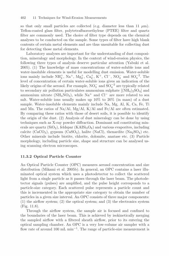
402 11 Techniques for Wind-Erosion Measurements
so that only small particles are collected (e.g. diameter less than 11 µm).Teflon-coated glass filter, polytetrafluoroethylene (PTEE) filter and quartzfilter are commonly used. The choice of filter type depends on the chemicalanalyses to be conducted on the sample. Some types of filter have high blankcontents of certain metal elements and are thus unsuitable for collecting dustfor detecting those metal elements.
Laboratory analyses are important for the understanding of dust composi-tion, mineralogy and morphology. In the context of wind-erosion physics, thefollowing three types of analysis deserve particular attention (Yabuki et al.2005). (1) The knowledge of mass concentrations of water-soluble ions andwater-insoluble elements is useful for modelling dust emission. Water-solubleions mainly include NH+
4 , Na+, Mg+2 , Ca+
2 , K+, Cl−, NO−3 and SO−2
4 . Thelevel of concentration of certain water-soluble ions gives an indication of thelikely origins of the aerosol. For example, NO−
3 and SO−24 are typically related
to secondary air pollution particulates ammonium sulphate [(NH4)2SO4] andammonium nitrate (NH4NO3), while Na+ and Cl− are more related to seasalt. Water-soluble ions usually makes up 10% to 20% (in mass) of a dustsample. Water-insoluble elements mainly include Na, Mg, Al, K, Ca, Fe, Tiand Mn. The ratios of Na/Al, Mg/Al, K/Al and Fe/Al are often estimated.By comparing these ratios with those of desert soils, it is possible to identifythe origin of the dust. (2) Analysis of dust mineralogy can be done by usingtechniques such as X-ray powder diffraction. Dominant soil constituting min-erals are quartz (SiO2), feldspar (KAISi3O8) and various evaporites, includingcalcite (CaCO3), gypsum (CaSO4), halite (NaCl), thenardite (Na2SO4) etc.Other minerals include biotite, chlorite, dolomite, anatase etc. (3) Particlemorphology, including particle size, shape and structure can be analysed us-ing scanning electron microscopes.
11.3.2 Optical Particle Counter
An Optical Particle Counter (OPC) measures aerosol concentration and sizedistribution (Mikami et al. 2005b). In general, an OPC contains a laser illu-minated optical system which uses a photodetector to collect the scatteredlight from a single particle as it passes through the laser beam. The photode-tector signals (pulses) are amplified, and the pulse height corresponds to aparticle-size category. Each scattered pulse represents a particle count andthis is incremented in the appropriate size category to obtain the number ofparticles in a given size interval. An OPC consists of three major components:(1) the airflow system; (2) the optical system; and (3) the electronics system(Fig. 11.8).
Through the airflow system, the sample air is focused and confined tothe boundaries of the laser beam. This is achieved by isokinetically mergingthe sampled airflow with a filtered sheath airflow, prior to its entering theoptical sampling chamber. An OPC is a very low-volume air sampler with aflow rate of around 100 mL min−1. The range of particle-size measurement is
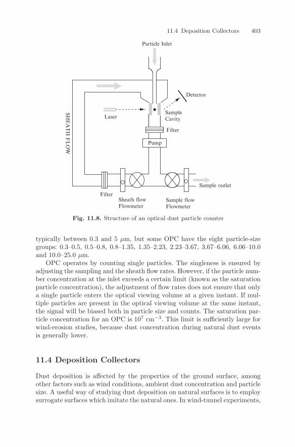
11.4 Deposition Collectors 403
Sample outlet
SampleCavity
Particle Inlet
Laser
FilterSheath flowFlowmeter
Sample flowFlowmeter
Detector
Filter
Pump
SHE
AT
H F
LO
W
Fig. 11.8. Structure of an optical dust particle counter
typically between 0.3 and 5 µm, but some OPC have the eight particle-sizegroups: 0.3–0.5, 0.5–0.8, 0.8–1.35, 1.35–2.23, 2.23–3.67, 3.67–6.06, 6.06–10.0and 10.0–25.0 µm.
OPC operates by counting single particles. The singleness is ensured byadjusting the sampling and the sheath flow rates. However, if the particle num-ber concentration at the inlet exceeds a certain limit (known as the saturationparticle concentration), the adjustment of flow rates does not ensure that onlya single particle enters the optical viewing volume at a given instant. If mul-tiple particles are present in the optical viewing volume at the same instant,the signal will be biased both in particle size and counts. The saturation par-ticle concentration for an OPC is 107 cm−3. This limit is sufficiently large forwind-erosion studies, because dust concentration during natural dust eventsis generally lower.
11.4 Deposition Collectors
Dust deposition is affected by the properties of the ground surface, amongother factors such as wind conditions, ambient dust concentration and particlesize. A useful way of studying dust deposition on natural surfaces is to employsurrogate surfaces which imitate the natural ones. In wind-tunnel experiments,
404 11 Techniques for Wind-Erosion Measurements
surrogate surfaces are easy to install and to manage. A variety of surrogatesurfaces have been tested, including water or antifreeze, glass marbles, moistfilter paper, sticky surfaces, grass, moss, paper, snow, glass, plastic, metal,artificial grass, etc. (Sow et al. 2006).
However, surrogate surfaces are difficult to use in the field for long-termdust-deposition monitoring. Instead, dust-deposition collectors are often used.Many types of collector have been tried, ranging from simple householdbuckets to special devices, but none of collectors can be considered to bethe professional standard. Two of the more widely used types are the MarbleDust Collector (Goossens, 2006) and the Inverted Frisbee Collector (Hall et al.1994).
A Marble Dust Collector consists of a rectangular plastic tray (c.a.50×30×10 cm3) and a sieve container on top of the tray. The sieve containeris filled with two layers of marbles (c.a. 15 mm in diameter) which form a mar-ble filter. Dust settles on and between the marbles and is washed by rain (orusing water) into the plastic tray and collected via an outlet underneath thetray. The reason of using marbles is because they have very low microrough-ness and can prevent the splash of the dust from the collector by raindrops.The marble filter also acts as a dust trap which protects the dust that hassettled into it from resuspension. The Inverted Frisbee Collector consists of acircular stainless steel bowl about 30 cm in diameter and 4 cm deep and anaerodynamically-shaped aluminium deflector ring around the bowl. The innerdiameter of the ring is 38.4 cm and the outer diameter is 64 cm. A variation ofthe Inverted Frisbee Collector is to fill the bowl with marbles. Goossens (2006)examined the efficiency of the two types of collectors using water surface asreference and concluded that the efficiencies of these collectors are usually50% lower, often much lower, than that of the water surface.
11.5 Field Measurements
Field measurements are essential for understanding wind-erosion processesand for verifying wind-erosion models. A problem in the past with field mea-surements is that they are not sufficiently cohesive and reliable for testingwind-erosion models, especially dust models. While it is difficult to define ingeneral what a cohesive data set should be, a tentative list of quantities thatshould be measured is as proposed in Table 11.1.
The measurements of saltation flux can be made using an array of salta-tion traps, such as the Fryrear sand traps (Figs. 11.3 and 11.9). The traps areusually mounted on a tower to measure the fluxes of sand particles at variouslevels over a height of about 2 m. The main advantage of the Fryrear trapsis that they are robust and easy to maintain for long-term wind erosion mon-itoring. For measuring the saltation of different particle-size groups in highfrequency, SPC (Figs. 11.6 and 11.9) appears to be the most suitable sensordeveloped so far. Figure 11.9 shows an example setup of a field wind-erosion
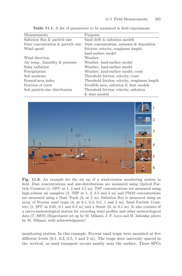
11.5 Field Measurements 405
Table 11.1. A list of parameters to be measured in field experiments
Measurements Purposes
Saltation flux & particle size Sand drift & saltation modelsDust concentration & particle size Dust concentration, emission & depositionWind speed Friction velocity, roughness length,
land-surface modelWind direction WeatherAir temp., humidity & pressure Weather, land-surface modelSolar radiation Weather, land-surface modelPrecipitation Weather, land-surface model, crustSoil moisture Threshold friction velocity, crustFrontal-area index Threshold friction velocity, roughness lengthFraction of cover Erodible area, saltation & dust modelsSoil particle-size distribution Threshold friction velocity, saltation
& dust models
Fig. 11.9. An example for the set up of a wind-erosion monitoring system infield. Dust concentrations and size-distributions are measured using Optical Par-ticle Counters (1, OPC at 1, 2 and 3.5 m); TSP concentrations are measured usinghigh-volume air samplers (2, TSP at 1, 2, 3.5 and 5 m) and PM10 concentrationsare measured using a Dust Track (3, at 2 m); Saltation flux is measured using anarray of Fryrear sand traps (4, at 0.1, 0.2, 0.5, 1 and 2 m), Sand Particle Coun-ters (5, SPC at 0.05, 0.1 and 0.3 m) and a Sensit (6, at 0.1 m). It also consists ofa micro-meteorological station for recording wind profiles and other meteorologicaldata (7, AWS) (Experiment set up by M. Mikami, J. F. Leys and M. Ishizuka; photoby M. Mikami, with acknowledgment)
monitoring station. In this example, Fryrear sand traps were mounted at fivedifferent levels (0.1, 0.2, 0.5, 1 and 2 m). The traps were unevenly spaced inthe vertical, as sand transport occurs mostly near the surface. Three SPCs
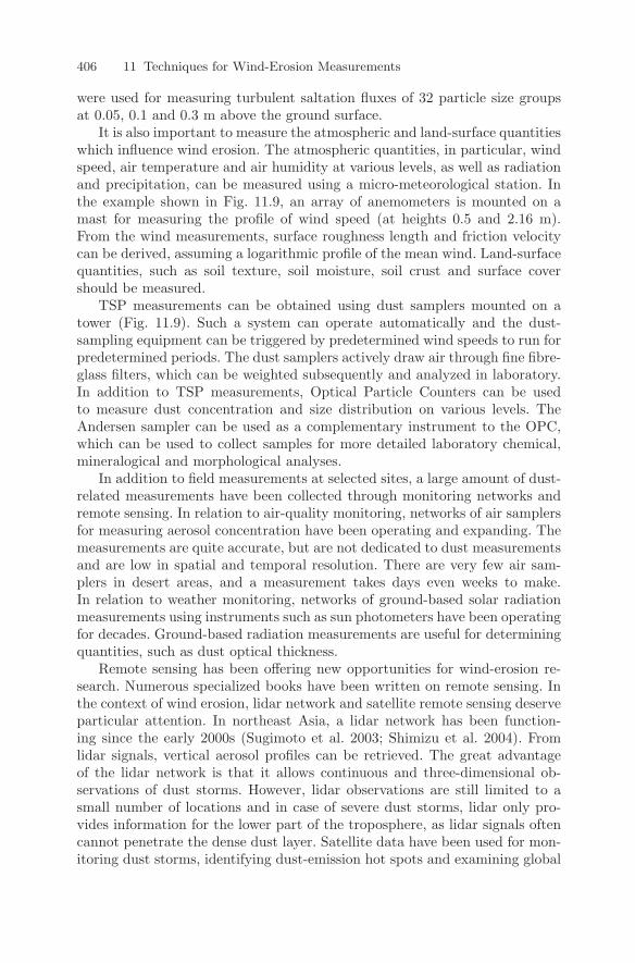
406 11 Techniques for Wind-Erosion Measurements
were used for measuring turbulent saltation fluxes of 32 particle size groupsat 0.05, 0.1 and 0.3 m above the ground surface.
It is also important to measure the atmospheric and land-surface quantitieswhich influence wind erosion. The atmospheric quantities, in particular, windspeed, air temperature and air humidity at various levels, as well as radiationand precipitation, can be measured using a micro-meteorological station. Inthe example shown in Fig. 11.9, an array of anemometers is mounted on amast for measuring the profile of wind speed (at heights 0.5 and 2.16 m).From the wind measurements, surface roughness length and friction velocitycan be derived, assuming a logarithmic profile of the mean wind. Land-surfacequantities, such as soil texture, soil moisture, soil crust and surface covershould be measured.
TSP measurements can be obtained using dust samplers mounted on atower (Fig. 11.9). Such a system can operate automatically and the dust-sampling equipment can be triggered by predetermined wind speeds to run forpredetermined periods. The dust samplers actively draw air through fine fibre-glass filters, which can be weighted subsequently and analyzed in laboratory.In addition to TSP measurements, Optical Particle Counters can be usedto measure dust concentration and size distribution on various levels. TheAndersen sampler can be used as a complementary instrument to the OPC,which can be used to collect samples for more detailed laboratory chemical,mineralogical and morphological analyses.
In addition to field measurements at selected sites, a large amount of dust-related measurements have been collected through monitoring networks andremote sensing. In relation to air-quality monitoring, networks of air samplersfor measuring aerosol concentration have been operating and expanding. Themeasurements are quite accurate, but are not dedicated to dust measurementsand are low in spatial and temporal resolution. There are very few air sam-plers in desert areas, and a measurement takes days even weeks to make.In relation to weather monitoring, networks of ground-based solar radiationmeasurements using instruments such as sun photometers have been operatingfor decades. Ground-based radiation measurements are useful for determiningquantities, such as dust optical thickness.
Remote sensing has been offering new opportunities for wind-erosion re-search. Numerous specialized books have been written on remote sensing. Inthe context of wind erosion, lidar network and satellite remote sensing deserveparticular attention. In northeast Asia, a lidar network has been function-ing since the early 2000s (Sugimoto et al. 2003; Shimizu et al. 2004). Fromlidar signals, vertical aerosol profiles can be retrieved. The great advantageof the lidar network is that it allows continuous and three-dimensional ob-servations of dust storms. However, lidar observations are still limited to asmall number of locations and in case of severe dust storms, lidar only pro-vides information for the lower part of the troposphere, as lidar signals oftencannot penetrate the dense dust layer. Satellite data have been used for mon-itoring dust storms, identifying dust-emission hot spots and examining global
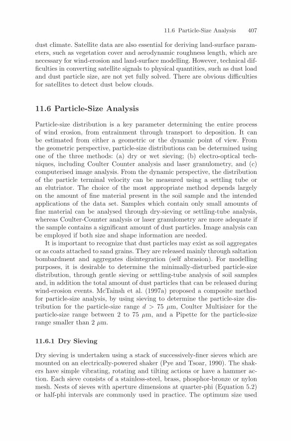
11.6 Particle-Size Analysis 407
dust climate. Satellite data are also essential for deriving land-surface param-eters, such as vegetation cover and aerodynamic roughness length, which arenecessary for wind-erosion and land-surface modelling. However, technical dif-ficulties in converting satellite signals to physical quantities, such as dust loadand dust particle size, are not yet fully solved. There are obvious difficultiesfor satellites to detect dust below clouds.
11.6 Particle-Size Analysis
Particle-size distribution is a key parameter determining the entire processof wind erosion, from entrainment through transport to deposition. It canbe estimated from either a geometric or the dynamic point of view. Fromthe geometric perspective, particle-size distributions can be determined usingone of the three methods: (a) dry or wet sieving; (b) electro-optical tech-niques, including Coulter Counter analysis and laser granulometry, and (c)computerised image analysis. From the dynamic perspective, the distributionof the particle terminal velocity can be measured using a settling tube oran elutriator. The choice of the most appropriate method depends largelyon the amount of fine material present in the soil sample and the intendedapplications of the data set. Samples which contain only small amounts offine material can be analysed through dry-sieving or settling-tube analysis,whereas Coulter-Counter analysis or laser granulometry are more adequate ifthe sample contains a significant amount of dust particles. Image analysis canbe employed if both size and shape information are needed.
It is important to recognize that dust particles may exist as soil aggregatesor as coats attached to sand grains. They are released mainly through saltationbombardment and aggregates disintegration (self abrasion). For modellingpurposes, it is desirable to determine the minimally-disturbed particle-sizedistribution, through gentle sieving or settling-tube analysis of soil samplesand, in addition the total amount of dust particles that can be released duringwind-erosion events. McTainsh et al. (1997a) proposed a composite methodfor particle-size analysis, by using sieving to determine the particle-size dis-tribution for the particle-size range d > 75 µm, Coulter Multisizer for theparticle-size range between 2 to 75 µm, and a Pipette for the particle-sizerange smaller than 2 µm.
11.6.1 Dry Sieving
Dry sieving is undertaken using a stack of successively-finer sieves which aremounted on an electrically-powered shaker (Pye and Tsoar, 1990). The shak-ers have simple vibrating, rotating and tilting actions or have a hammer ac-tion. Each sieve consists of a stainless-steel, brass, phosphor-bronze or nylonmesh. Nests of sieves with aperture dimensions at quarter-phi (Equation 5.2)or half-phi intervals are commonly used in practice. The optimum size used
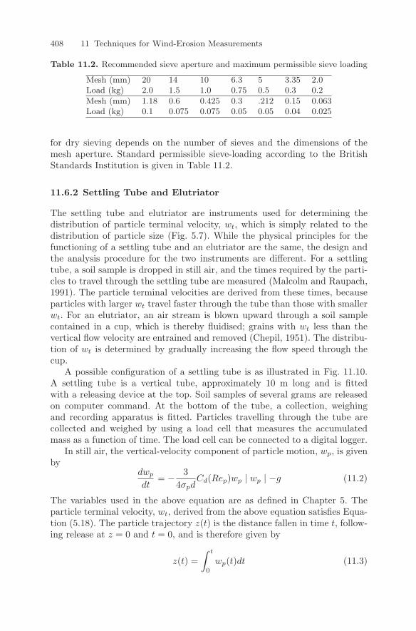
408 11 Techniques for Wind-Erosion Measurements
Table 11.2. Recommended sieve aperture and maximum permissible sieve loading
Mesh (mm) 20 14 10 6.3 5 3.35 2.0Load (kg) 2.0 1.5 1.0 0.75 0.5 0.3 0.2
Mesh (mm) 1.18 0.6 0.425 0.3 .212 0.15 0.063Load (kg) 0.1 0.075 0.075 0.05 0.05 0.04 0.025
for dry sieving depends on the number of sieves and the dimensions of themesh aperture. Standard permissible sieve-loading according to the BritishStandards Institution is given in Table 11.2.
11.6.2 Settling Tube and Elutriator
The settling tube and elutriator are instruments used for determining thedistribution of particle terminal velocity, wt, which is simply related to thedistribution of particle size (Fig. 5.7). While the physical principles for thefunctioning of a settling tube and an elutriator are the same, the design andthe analysis procedure for the two instruments are different. For a settlingtube, a soil sample is dropped in still air, and the times required by the parti-cles to travel through the settling tube are measured (Malcolm and Raupach,1991). The particle terminal velocities are derived from these times, becauseparticles with larger wt travel faster through the tube than those with smallerwt. For an elutriator, an air stream is blown upward through a soil samplecontained in a cup, which is thereby fluidised; grains with wt less than thevertical flow velocity are entrained and removed (Chepil, 1951). The distribu-tion of wt is determined by gradually increasing the flow speed through thecup.
A possible configuration of a settling tube is as illustrated in Fig. 11.10.A settling tube is a vertical tube, approximately 10 m long and is fittedwith a releasing device at the top. Soil samples of several grams are releasedon computer command. At the bottom of the tube, a collection, weighingand recording apparatus is fitted. Particles travelling through the tube arecollected and weighed by using a load cell that measures the accumulatedmass as a function of time. The load cell can be connected to a digital logger.
In still air, the vertical-velocity component of particle motion, wp, is givenby
dwp
dt= − 3
4σpdCd(Rep)wp | wp | −g (11.2)
The variables used in the above equation are as defined in Chapter 5. Theparticle terminal velocity, wt, derived from the above equation satisfies Equa-tion (5.18). The particle trajectory z(t) is the distance fallen in time t, follow-ing release at z = 0 and t = 0, and is therefore given by
z(t) =∫ t
0
wp(t)dt (11.3)
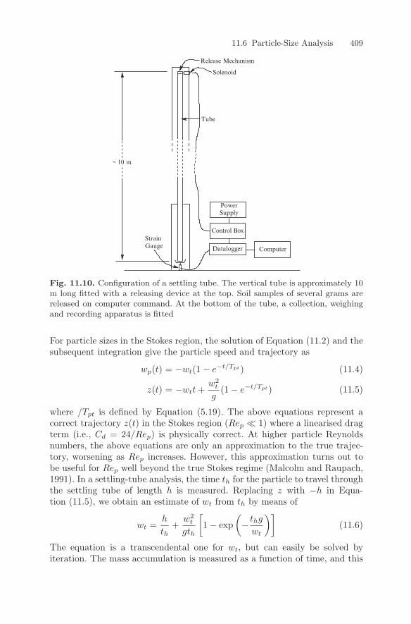
11.6 Particle-Size Analysis 409
Computer
Tube
Release Mechanism
Solenoid
StrainGauge
PowerSupply
~ 10 m
Datalogger
Control Box
Fig. 11.10. Configuration of a settling tube. The vertical tube is approximately 10m long fitted with a releasing device at the top. Soil samples of several grams arereleased on computer command. At the bottom of the tube, a collection, weighingand recording apparatus is fitted
For particle sizes in the Stokes region, the solution of Equation (11.2) and thesubsequent integration give the particle speed and trajectory as
wp(t) = −wt(1 − e−t/Tpt) (11.4)
z(t) = −wtt +w2
t
g(1 − e−t/Tpt) (11.5)
where /Tpt is defined by Equation (5.19). The above equations represent acorrect trajectory z(t) in the Stokes region (Rep 1) where a linearised dragterm (i.e., Cd = 24/Rep) is physically correct. At higher particle Reynoldsnumbers, the above equations are only an approximation to the true trajec-tory, worsening as Rep increases. However, this approximation turns out tobe useful for Rep well beyond the true Stokes regime (Malcolm and Raupach,1991). In a settling-tube analysis, the time th for the particle to travel throughthe settling tube of length h is measured. Replacing z with −h in Equa-tion (11.5), we obtain an estimate of wt from th by means of
wt =h
th+
w2t
gth
[1 − exp
(− thg
wt
)](11.6)
The equation is a transcendental one for wt, but can easily be solved byiteration. The mass accumulation is measured as a function of time, and this
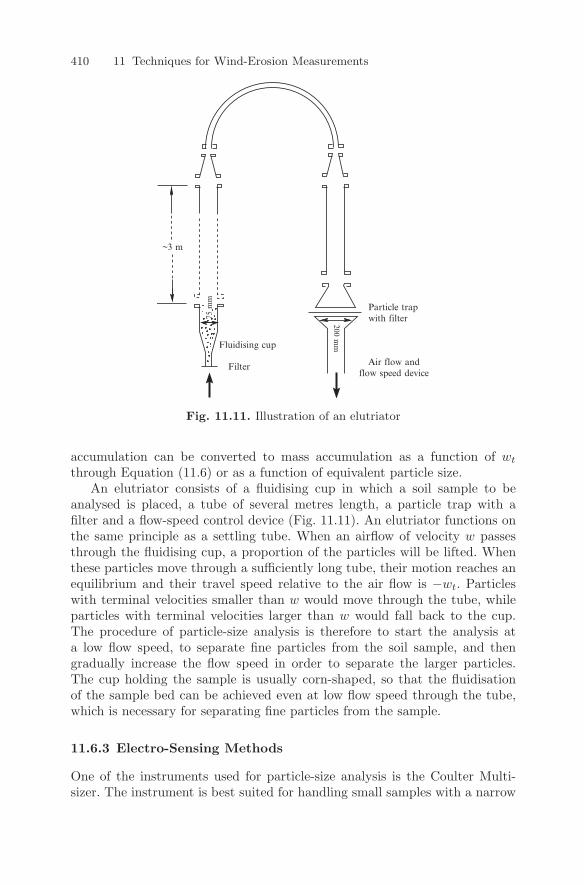
410 11 Techniques for Wind-Erosion Measurements
Air flow andflow speed device
Filter
Fluidising cup
~3 m
75 m
m
200 mm
Particle trapwith filter
Fig. 11.11. Illustration of an elutriator
accumulation can be converted to mass accumulation as a function of wt
through Equation (11.6) or as a function of equivalent particle size.An elutriator consists of a fluidising cup in which a soil sample to be
analysed is placed, a tube of several metres length, a particle trap with afilter and a flow-speed control device (Fig. 11.11). An elutriator functions onthe same principle as a settling tube. When an airflow of velocity w passesthrough the fluidising cup, a proportion of the particles will be lifted. Whenthese particles move through a sufficiently long tube, their motion reaches anequilibrium and their travel speed relative to the air flow is −wt. Particleswith terminal velocities smaller than w would move through the tube, whileparticles with terminal velocities larger than w would fall back to the cup.The procedure of particle-size analysis is therefore to start the analysis ata low flow speed, to separate fine particles from the soil sample, and thengradually increase the flow speed in order to separate the larger particles.The cup holding the sample is usually corn-shaped, so that the fluidisationof the sample bed can be achieved even at low flow speed through the tube,which is necessary for separating fine particles from the sample.
11.6.3 Electro-Sensing Methods
One of the instruments used for particle-size analysis is the Coulter Multi-sizer. The instrument is best suited for handling small samples with a narrow
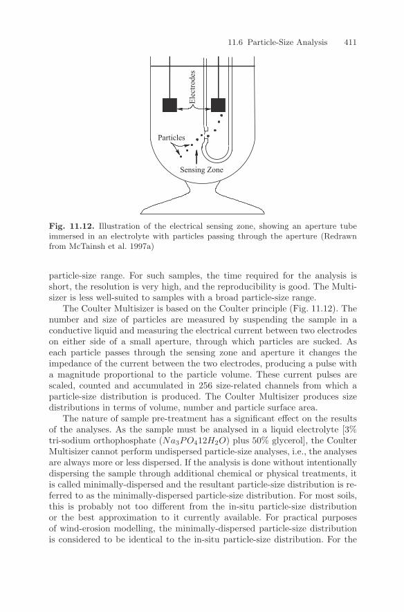
11.6 Particle-Size Analysis 411
Elec
trode
s
Particles
Sensing Zone
Fig. 11.12. Illustration of the electrical sensing zone, showing an aperture tubeimmersed in an electrolyte with particles passing through the aperture (Redrawnfrom McTainsh et al. 1997a)
particle-size range. For such samples, the time required for the analysis isshort, the resolution is very high, and the reproducibility is good. The Multi-sizer is less well-suited to samples with a broad particle-size range.
The Coulter Multisizer is based on the Coulter principle (Fig. 11.12). Thenumber and size of particles are measured by suspending the sample in aconductive liquid and measuring the electrical current between two electrodeson either side of a small aperture, through which particles are sucked. Aseach particle passes through the sensing zone and aperture it changes theimpedance of the current between the two electrodes, producing a pulse witha magnitude proportional to the particle volume. These current pulses arescaled, counted and accumulated in 256 size-related channels from which aparticle-size distribution is produced. The Coulter Multisizer produces sizedistributions in terms of volume, number and particle surface area.
The nature of sample pre-treatment has a significant effect on the resultsof the analyses. As the sample must be analysed in a liquid electrolyte [3%tri-sodium orthophosphate (Na3PO412H2O) plus 50% glycerol], the CoulterMultisizer cannot perform undispersed particle-size analyses, i.e., the analysesare always more or less dispersed. If the analysis is done without intentionallydispersing the sample through additional chemical or physical treatments, itis called minimally-dispersed and the resultant particle-size distribution is re-ferred to as the minimally-dispersed particle-size distribution. For most soils,this is probably not too different from the in-situ particle-size distributionor the best approximation to it currently available. For practical purposesof wind-erosion modelling, the minimally-dispersed particle-size distributionis considered to be identical to the in-situ particle-size distribution. For the
412 11 Techniques for Wind-Erosion Measurements
fully-dispersed analysis, the soil sample receives chemical and vigorous phys-ical dispersions to reduce it to its fundamental particle-size constituents. Atypical chemical treatment is to place the sample in a soil dispersant, suchas 3% tri-sodium orthophosphate and 1M sodium hydroxide (NaOH). Theparticle-size analysis of the soil sample after the chemical and physical treat-ments gives the fully-dispersed particle-size distribution. This particle-size dis-tribution is the best approximation available for that of the sediment during avery strong wind-erosion event. In wind-erosion modelling, the fully-dispersedparticle-size analysis is used to estimate the mass fraction of dust in a givensoil.
One of the advantages of the Coulter Multisizer is its capacity to analyzesamples in very small quantities down to about 0.1 g, while other particle-sizeanalysis techniques, such as hydrometer and sieve analyses, require samplesup to 30 g. This feature of the Coulter Multisizer allows the particle-size anal-ysis of sediment samples collected using high-volume samplers. The CoulterMultisizer also produces a relatively-high resolution for particle-size analysis,since particles are sized into 256 classes. The multisizer can measure particlesover a size range from 0.45 to 1200 microns, but there are practical difficul-ties with analyses at the coarse end (>150 µm), and the Multisizer appearsto underestimate the clay fraction (<2 µm) (McTainsh et al. 1997). For the<2 µm fraction, Pipette analysis can be performed instead.
11.6.4 Laser Granulometry
Laser granulometry is based on the principle that there is a direct relationshipbetween the size of particles and the degree to which they diffract light. In thecase of the Malvern Instruments Laser Particle Sizer Type 3600E, a beam ofmonochromatic light (wave length 633 nm) is passed through a cell containingthe sample in suspension and the diffracted light is focused onto a detectorwhich senses the angular distribution of scattered light energy (McCave et al.1986). The size range detected depends on the focal length of the focusinglens, which is placed between the sample cell and the detector. Grains arekept in suspension by a mechanical stirring device. Three lenses are availableeach of which divides the distribution into 15 size classes. The 300 mm focal-length lens has a range of 5.8–560 µm and is therefore most appropriate forsands. However, the coarsest of the 15 class intervals have a very wide range(261–264 µm).
11.7 Abrasion Emitter
The dust-emission potential of a given soil is the mass fraction of dust particlesthat can be released during the process of wind erosion. It is a key quantity tobe determined for dust-emission modelling. As pointed out in Chapter 7, thispotential is related to the observation that different techniques for particle-size
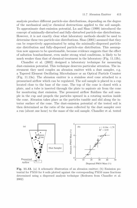
11.7 Abrasion Emitter 413
analysis produce different particle-size distributions, depending on the degreeof the mechanical and/or chemical destructions applied to the soil sample.To approximate dust-emission potential, Lu and Shao (1999) introduced theconcept of minimally-disturbed and fully-disturbed particle-size distributions.However, it is not exactly clear what laboratory methods should be used todetermine these two particle-size distributions. Shao (2001) assumed that theycan be respectively approximated by using the minimally-dispersed particle-size distribution and fully-dispersed particle-size distribution. This assump-tion now appears to be questionable, because evidence suggests that the effectof saltation bombardment, even under strong wind conditions, is likely to bemuch weaker than that of chemical treatment in the laboratory (Fig. 11.13b).
Chandler et al. (2002) designed a laboratory technique for measuringdust-emission potential. This technique deserves particular attention. The in-strument they used couples an abrasion emitter with a dust sampler, e.g.a Tapered Element Oscillating Microbalance or an Optical Particle Counter(Fig. 11.13a). The abrasion emitter is a stainless steel cone attached to apressurised airflow which can be regulated. The soil sample is placed in a cuplocated close to the base of the cone. The top of the cone is closed with aplate, and a tube is inserted through the plate to aspirate air from the conefor monitoring dust emission. The pressured airflow fluidizes the soil sam-ple in the cup and propels the particles upward in a rotating motion insidethe cone. Abrasion takes place as the particles tumble and slid along the in-terior surface of the cone. The dust-emission potential of the tested soil isthen determined as the ratio of the mass collected by the dust sampler overa run (about one hour) to the mass of the soil sample. Chandler et al. tested
Pressurized
Airflow
ConeAbrasion
y = 0.16x - 1.79R2 = 0.95
2
4
6
00 10 20 30 40 50
Dispersed PM10 Mass (%)
(a) (b)
Dust Sampler
Abr
asio
n PM
10 M
ass
(%)
Fig. 11.13. (a) A schematic illustration of an abrasion emitter; (b) Emission po-tential for PM10 for 8 soils plotted against the corresponding PM10 mass fractionsdetermined using a dispersed analysis technique (Redrawn from Chandler et al.2002)
414 11 Techniques for Wind-Erosion Measurements
the emission potential for PM10 and PM2.5 of 48 soils and found that theemission potential for PM10 is between 0.6% and 4.1% and that for PM2.5is between 0.5% and 1.9%. They also measured the mass fraction of PM10and PM2.5 in dispersed samples using laser diffraction and found that theamount of PM10 particles generated by abrasion is about 10–20% of that inthe dispersed samples (Fig. 11.13b).
12
Concluding Remarks
In his famous book entitled ‘The Physics of Blown Sand and Desert Dunes’,Bagnold (1941) focused on the studies of sand movement. At that time, salta-tion was the core subject of wind-erosion research. While the movement ofsand remains to be a subject of considerable interest today, the emphasis ofwind-erosion research has been shifted from sand to dust. This shift is clearlyseen in the recent trend of publications. In 2006, about 50% of wind-erosionrelated research papers was on dust, in contrast to about 5% in the 1940s(J. Stout, personal communication, 2006). This shift is accompanied by a re-markable expansion of the wind-erosion research territory, as reflected in thefollowing aspects.
• Scale: While earlier studies were mostly about sand motion on local scales,new studies deal with aeolian processes on scales ranging from local toglobal.
• Discipline: While earlier studies were problem specific, new studies aremulti-disciplinary.
• Research methods: The study on wind erosion is no longer of semi-empirical nature based on wind-tunnel and field experiments. In recentyears, a variety of new methods (e.g. numerical simulation, remote sensing,GIS etc.) and new instruments (e.g. sand particle counter, lidar networks,air samplers, satellite, etc.) have been used to study wind erosion from amuch broader perspective.
12.1 Current Research Topics
The recent achievements in wind-erosion research are significant, but our ca-pability for quantitative wind-erosion modelling and prediction remains to belimited for the following reasons.
• It is difficult to accurately determine the key parameters which affect winderosion. For instance, threshold friction velocity, u∗t, is a function of the
Y. Shao, Physics and Modelling of Wind Erosion 415c© Springer Science+Business Media B.V. 2008
,
416 12 Concluding Remarks
frontal- and basal-area indices of non-erodible roughness elements on anaeolian surface, respectively, λ and η (Chapter 9). Aeolian surfaces mostlyhave small λ and η values at which u∗t is particularly sensitive. It is not yetpossible to accurately estimate λ and η over extended aeolian surfaces. Thesensitive dependency of wind erosion on soil moisture is another example.Because soil moisture is affected by many atmospheric to hydrologicalfactors (Chapter 4), it is again not yet possible to measure and predictit with the accuracy required for wind-erosion modelling. There are otherquantities, such as dust-particle binding energy and soil-surface plasticpressure, which vary stochastically to a large degree. Even for a givenlocation and time, they are difficult to estimate reliably.
• Some fundamental aspects of wind-erosion physics are not well understood.For instance, dust emission is essentially generated by abrasion (saltationbombardment) and self-abrasion (aggregates disintegration) and the rateof dust emission critically depends on the cohesive forces acting on dustparticles. The strength of the cohesive forces varies over several orders ofmagnitude. In practice, the cohesive forces cannot be determined in a de-terministic manner. Therefore, dust-emission schemes contain parameterswhich must be determined empirically.
• There is a serious lack of high-quality and coherent observational data setsfor the rigorous validations of dust-emission and dust-deposition schemes.As a consequence, large uncertainties exist in scheme parameters.
• Wind-erosion events are mostly associated with certain synoptic and sub-synoptic severe-weather events. Such weather events are also the mostdifficult to predict using atmospheric models. For example, dust storms inAfrica are often related to the convective systems in the monsoon trough.Such systems are difficult to model as their modelling requires high spatialresolution of the atmospheric model. If we wish to simulate wind erosion ona broad scale with high spatial and temporal resolutions, we would needhigh-resolution land-surface parameters for soil texture, vegetation, soilhydraulic properties and surface aerodynamic properties. Such databasesare gradually becoming available, but their resolutions are still too coarsein general. The reliability of the data is usually worse for desert areaswhere wind erosion is the most severe.
The present emphases of wind-erosion research are on the followingproblems.
Integrated wind-erosion modelling systems: IWEMS offer a frame-work for studying the processes of wind erosion in a multi-disciplinary andcohesive fashion. They enable the simulation of the global dust cycle andthe predictions of dust storms. They also enable the establishment of wind-erosion prevention measures. Existing IWEMS already have a sound structureand are functional. Efforts are now being made to improve the performancesof IWEMS by applying the techniques of data assimilation. Satellite andground-based observations are now producing data suitable for the purpose.
12.1 Current Research Topics 417
Numerical experiments using both 3DV and 4DV algorithms have been carriedout. Improved estimates of soil moisture and vegetation cover are also becom-ing available, which can be combined with the outputs of land-surface andecological models to generate better input data for wind-erosion modelling.Past IWEMS applications were mostly focused on global- or regional-scaledust problems, but are now increasingly used to studying meso-scale dustproblems.
Computational simulation: With the ever increasing computing power,numerical experiments using sophisticated computer models are gradually re-placing certain types of conventional wind-tunnel experiments and makingcertain types of studies possible, when they were previously impossible. Forinstance, the evolution of sand dunes, the development and equilibration ofsaltation, splash entrainment, drag partitioning, dust devils etc. can all besimulated in detail by using computer models. The great advantage of thisapproach is its efficiency and flexibility.
Anderson and Haff (1991) among others have studied saltation in simpleboundary-layer flows. In these studies, saltation has been treated as a feedbackprocess governed by aerodynamic entrainment, particle motion, flow modifi-cation and splash entrainment. Butterfield (1991, 1993) and Stout and Zobeck(1997) have considered saltation in turbulent flows. The above-mentionedstudies have produced interesting results but, more importantly, they rep-resent the first stage of research on saltation in turbulent flows. Shao and Li(1999) have used a LES model combined with a particle-trajectory model tosimulate saltation in turbulent flows. While their work is preliminary, Shaoand Li have demonstrated that LES is a powerful tool to be used for thestudies of wind-erosion processes. The application of LES to modelling tur-bulent saltation has been hampered by several technical issues. For instance,large quantities of saltating particles hop along the surface in small steps; toaccount for the interactions between these particles and turbulent eddies inthe vicinity of the surface is numerically problematic.
Parameterisation and databases: The quantification of dust emissionis essential for dust modelling. In global and regional dust models, the es-timate of dust emission relies almost entirely on the dust-emission scheme.As described in Chapters 7 and 9, the formulations of dust-emission schemesare quite simple, but they consist of parameters which are difficult to esti-mate. Existing dust-emission schemes are mostly based on the understandingof the micro-scopic processes of wind erosion, but a mismatch exists be-tween the micro-scopic schemes and the macro-scopic (e.g. regional to global)parameters.
Similar observations can be made in regard to dust-deposition schemes.Existing dust-deposition schemes are based primarily on micro-scopic fluiddynamics and are yet to be rigorously tested against measurements. Again, agap exists between the formulation of the micro-scopic schemes and the needfor macro-scopic parameters. For instance, it is known in theory that dustdeposition is governed by gravitational settling and turbulent diffusion, but
418 12 Concluding Remarks
it is not well known how dust-deposition velocity for a natural surface (e.g. aforested area) can be estimated.
The need for a parameter database of wind-erosion modelling cannot beoverstated. Since the 1980s, the climate-research community has made a con-certed effort to establish the parameter database for land-surface models.The establishment of these databases has made land-surface simulation (seeChapter 4) a meaningful and indispensable component in atmospheric andhydrological models. In contrast, the parameter databases of wind-erosionmodelling are dismal. This situation is detrimental to the reliability of wind-erosion assessment and prediction. Thus, to establish a parameter databasefor wind-erosion modelling is an issue which deserves urgent attention. Thefollowing parameters are particularly important: (1) soil particle-size distri-bution; (2) fraction of erodible surface; (3) roughness frontal-area index oraerodynamic roughness length; (4) soil plastic pressure and (5) soil-particlebinding energy.
Measurements: The lack of measurements for dust emission, concen-tration and deposition has seriously hindered the progress of wind-erosionmodel development. New field experiments need to be carried so that datacan be obtained and wind-erosion schemes can be rigorously verified. TheJapan-Australia Dust Experiment (JADE) organised by Mikami et al. (2007,personal communication) has set a good example for field experiments. InJADE, both saltation and dust emission were measured, together with therelevant land-surface parameters, including soil particle-size distribution, soilmoisture and soil crustiness. Spatially distributed measurements of dust fluxesand concentration are needed for the validation of regional and global dustmodels. In some parts of the world (e.g. Northeast Asia) dust monitoringnetworks of air samplers, lidars and radiometers are now functioning.
Wind-erosion physics: the following problems are being activelystudied.
• Drag Partition: The theories of Arya (1975) and Raupach (1992) have es-tablished the relationship between the frontal-area index of roughness ele-ments and the ratio u∗t(d, λ)/u∗t(d, 0). These theories are based on strongassumptions and describe best the wind-tunnel data for situations of uni-form roughness elements. In nature, roughness elements are rarely uniform;instead, they are different in size and shape. The concept of frontal-areaindex is useful, but it is not clear how such an index can be estimated fornatural surfaces. The hypotheses used in deriving the drag-partitioningtheories also require further examination.
• Particle Lift-off Velocity: Particle lift-off velocity is one of the essential pa-rameters which determine the characteristics of saltation. It is a stochasticquantity which satisfies certain distributions. Wind-tunnel experiments arebeing carried out using sophisticated instruments (e.g. a particle-image ve-locimetry) to measure the particle lift-off velocity distributions for variousflow and aeolian surface conditions.
12.2 Dust Cycle in the Earth System 419
• Saltation Similarity: Given particle lift-off velocity distribution, the processof saltation may be a dynamically similar process. A saltation similaritytheory is useful for the estimates of a range of quantities, including theprofiles of saltation flux and particle momentum flux, and the relationshipbetween streamwise saltation flux and vertical particle-number flux (Shaoand Mikami, 2005).
• Stochastic Saltation: Saltation is a stochastic process, due to turbulence inthe atmospheric boundary-layer and the stochastic nature of the particlelift-off conditions. In the atmosphere, saltation shows coherent turbulentstructures (Baas, 2004).
• Source-limited Wind Erosion: Source-limited wind erosion has been men-tioned frequently in informal discussions. There have been however hardlyany formal publications on this problem until the recent work by Gilletteand Ono (2008).
• Wind-erosion over Heterogeneous Surfaces: Even on microscopic scale, theintensity of wind erosion can vary strongly in space. This implies thatwind erosion is a heterogeneous process. Bowker et al. (2007) have con-ducted a numerical simulation on the spatial patterns of saltation over aheterogeneous mesquite area of the northern Chihuahua Desert.
• Abrasion and Self-abrasion: An important issue remains to be how todetermine the cohesive forces and binding energy of dust particles.
• Surface Crust: Crust is an important factor which affects the strength ofwind erosion. Very little research has been done on this subject until therecent work by Ishizuka et al. (2008).
• Threshold Friction Velocity: Threshold friction velocity remains to be atopic under active research. McKenna Neumann and Sanderson (2007)have carried out an interesting wind-tunnel experiment and theoreticalanalysis on the effect of soil moisture on threshold friction velocity.
12.2 Dust Cycle in the Earth System
The Earth System, comprising of the atmosphere, hydrosphere, cryosphere,biosphere and lithosphere, is dynamic, open, multi-scale, interactive andnonlinear. The dynamic processes in the Earth System drive the cycles ofquantities such as energy, carbon, water vapour and dust, which in turn im-pact upon its fluid dynamic, thermodynamic and radiation processes. The dustcycle plays an important role in the Earth System because dust participatesin several key feedbacks.
Radiation: airborne dust is also known as mineral aerosol. The estimatedglobal dust emission of 2000 Mt yr−1 is about 30 times that of the anthro-pogenic aerosols. Aerosols influence the radiation balance of the Earth Systemdirectly, through scattering and absorbing various radiation components, andindirectly, by modifying the optical properties and lifetime of clouds. Aerosolsare believed to have a net effect of global cooling, compensating the global
420 12 Concluding Remarks
warming due to greenhouse gases. Aerosol radiative forcing is heterogeneous,i.e. in some regions it is stronger than the greenhouse-gas effect while in otherregions weaker. However, the radiative forcing due to dust is so far poorlyunderstood, because the information on the amount, distribution, size, shapeand mineralogy of dust particles in the atmosphere is not reliable.
Aerosol Chemistry: The optical properties and lifetime of dust andanthropogenic substances (particulates and gaseous species) can be drasticallyaltered through mixing and chemical reactions. For example, dust and blackcarbon form aggregates and this process makes the former more absorbing ofvisible and infrared radiation. In some parts of the world, dust particles areoften found to be coated with nitrates and sulphates. The Mediterranean andnorthern Africa region is for example a hot spot where dust from Sahara andpollutants from Europe interact. Northeast Asia is an other hot spot whereAsian dust, anthropogenic substances and sea salt interact.
Air Quality: Dust storms from North Africa can elevate the concen-tration of airborne particulates in southern Europe. Such problems are alsoprominent in the Middle East, Southwest Asia, Northeast Asia and Australia.Many contaminants that pose risks to human health and the environmentare found to be associated with dust, including metal, pesticides, dioxins andradionuclide.
Ocean Biochemistry: Iron is an essential micro-nutrient for phytoplank-ton growth. The dominant external supply of iron to the ocean is dust trans-ported from arid zones, such as the Sahara, central, southwest and northeastAsia, Australia and Patagonia. The marine ecology in the regions adjacent tothe major dust sources is sensitive to inputs of iron.
Cryosphere: Snow- and ice-surface albedo is significantly affected by theimpurities in snow grains (Aoki et al. 2003). In Asia, the snow impurities aremostly soot and dust, with an impurity concentration of around 0.5 ppmw.The impurity concentration in snow and ice and the aging of snow surfacedepend profoundly on aerosol deposition. In northern Hemisphere winter, upto 50% of the land surface is covered by snow. In the aging process, the snow-surface albedo can decrease from 0.95 to 0.65 for visible light and from 0.85to 0.4 for infrared light. These changes profoundly affect the snow/ice surfaceenergy balance.
Because of these important feedbacks, the research on dust has been ele-vated to be among the core subjects of Earth System studies.
References
Ackerman S (1989) Using the radiative temperature difference at 3.7 and 11 µm totrack dust outbreaks. Remote Sens Environ 27: 129–133
Ackerman S (1997) Remote sensing aerosols using satellite infrared observations.J Geophys Res 102: 17,069–17,079
Alfaro SC, Gomes L (2001) Modelling mineral aerosol production by wind erosion:Emission intensities and aerosol size distributions in source areas. J GeophysRes 106: 18,075–18,084
Alfaro SC, Gaudichet A, Gomes L, Maille M (1997) Modeling the size distributionof a soil aerosol produced by sandblasting. J Geophys Res 102: 11,239–11,249
Allen JRL (1982) Simple models for the shape and symmetry of tidal sand waves:(1) statically stable equilibrium forms. Mar Geol 48: 31–49
Allen JRL (1994) Fundamental properties of fluids and their relation to sedimenttransport processes. In: Pye K (ed) Sediment Transport and Depositional Pro-cesses, Blackwell Scientific Publications, Oxford, pp 25–60
Allen MD, Tildesley DJ (1987) Computer Simulation of Liquids. Clarendon, OxfordAllen T (1981) Particle Size Measurement. Chapman & Hall, LondonAnderson RS (1987) Eolian sediment transport as a stochastic process: the effects
of a fluctuating wind on particle trajectories. J Geology 95: 497–512Anderson RS (1988) The pattern of grainfall deposition in the lee of aeolian dunes.
Sedimentology 35: 175–188Anderson RS, Haff PK (1988) Simulation of eolian saltation. Science 241: 820–823Anderson RS, Haff PK (1991) Wind modification and bed response during saltation
of sand in air. Acta Mech, Suppl 1: 21–51Anderson RS, Hallet B (1986) Sediment transport by wind: Toward a general model.
Geol Soc Am Bull 97: 523–535Andre JC, Goutorbe JP, Perrier A (1986) HAPEX-MOBILHY: A hydrologic atmo-
spheric experiment for the study of water budget and evaporation flux at theclimate scale. Bull Am Meteor Soc 67: 138–144
Anthes RA (1977) A cumulus parameterization scheme utilizing a one-dimensionalcloud model. Mon Wea Rev 105: 270–286
Aoki T, Hachikubo A, Hori M (2003) Effects of snow physical parameters on short-wave broadband albedos. J Geophys Res 108: 4616, doi: 10.1029/2003JD003506
421
422 References
Arakawa A, Schubert WH (1974) Interaction of a cumulus cloud ensemble with thelarge-scale environment. J Atmos Sci 31: 674–701
Arimoto R, Duce RA, Ray BJ, Unni CK (1985) Atmospheric trace elements atEnewetak Atoll: 2. Transport to the ocean by wet and dry deposition. J GeophysRes 90: 2391–2408
Arimoto R, Ray BJ, Lewis NF, Tomza U (1997) Mass-particle size distribution ofatmospheric dust and the dry deposition of dust to the remote ocean. J GeophysRes 102: 15,867–15,874
Arimoto R, Kim YJ, Kim YP, Quinn PK, Bates TS, Anderson TL, Gong S, UnoI, Chin M, Huebert BJ, Clarke AD, Shinozuka Y, Weber RJ, Anderson SJR,Guazzotti A, Sullivan RC, Sodeman DA, Prather KA, Sokolik I (2006) Charac-terization of Asian dust during ace-Asia. Global Planet Change 52: 23–56
Arya SPS (1975) A drag partition theory for determining the large-scale roughnessparameter and wind stress on arctic pack ice. J Geophys Res 80: 1173–1184
Avissar R, Pielke RA (1989) A parameterization of heterogeneous land surface foratmospheric numerical models and its impact on regional meteorology. Mon WeaRev 117: 2113–2136
Avissar R, Schmidt T (1998) An evaluation of the scale at which ground-surface heatflux patchiness affects the convective boundary layer using large-eddy simulationmodel. J Atmos Sci 55(A):2666–2689
Baas ACW (2004) Evaluation of saltation flux impact responders (Safires) for mea-suring instantaneous aeolian sand transport intensity. Geomorphology 59: 99–118
Baas ACW, Sherman DJ (2005) Formation and behavior of aeolian streamers. J Geo-phys Res 110(doi: 10.1029/2004JF000270):F03,011
Bache DH (1981) Analysing particle deposition to plant canopies. Atmos Evnviron15: 1759–1761
Bagnold GA (1937) The transport of sand by wind. Geogr J 89: 409–438Bagnold GA (1938) The measurement of sand storms. In: Proc. R. Soc., Ser. A.,
London, 167, pp 282–291Bagnold RA (1941) The Physics of Blown Sand and Desert Dunes. Methuen, LondonBarry RG, Chorley RJ (2003) Atmosphere, Weather and Climate. Routledge, Lon-
donBeard K, Ochs H (1984) Collection and coalescence efficiencies for accretion. J Geo-
phys Res 89: 7165–7169Beard KV (1976) Terminal velocity and shape of cloud and precipitation drops aloft.
J Atmos Sci 33: 851–864Beljaars ACM, Walmsley JL, Taylor PA (1987) A mixed spectral finite-difference
model for neutrally stratified boundary-layer flow over roughness changes andtopography. Boundary-Layer Meteorol 38: 273–303
Belly PY (1964) Sand movement by wind. Tech. Rep. 1, US Army Coastal Engi-neering Research Center
Bhumralkar CM (1975) Numerical experiments on the computation of ground sur-face temperature in atmospheric general circulation models. J Appl Meteor 14:1246–1258
Bisal F, Ferguson W (1970) Effect of non-erodible aggregates and wheat stubble oninitiation of soil drifting. Canadian J Soil Sci 50: 31–34
Bishop SR, Momiji H, Carretero-Gonzalez R, Warren A (2002) Modelling desertdune fields based on discrete dynamics. Discrete Dyn Nat Soc 7: 7–17
References 423
Blackadar AK (1976) Modeling the nocturnal boundary layer. In: Proceedings ofthe Third Symposium on Atmospheric Turbulence, Diffusion and Air Quality,Am. Meteorol. Soc., Boston, MA, pp 46–49
Bondy E, Lyles L, Hayes WA (1980) Computing soil erosion by periods using a windenergy distribution. J Soil Water Cons 35: 173–176
Bott A (1989) A positive definite advection scheme obtained by nonlinear renormal-ization of the advective fluxes. Mon Wea Rev 117: 1006–1015
Bottema M (1996) Roughness parameters over regular rough surfaces: Experimentalrequirements and model validation. J Wind Eng Ind Aerodyn 64: 249–265
Bowker GE, Gillette DA, Bergametti G, Marticorena B, Heist DK (2007) Fine-scale simulations of aeolian sediment dispersion in a small area in the northernChihuahuan desert. J Geophys Res – Earth Surface doi: 10.1029/2007JF000748
Bradley EF (1968) A micrometeorological study of velocity profiles and surface dragin the region modified by a change in surface roughness. Quart J Roy MeteorSoc 94: 361–379
Brooks RH, Corey AT (1964) Hydraulic properties of porous media. In: HydrologyPaper 3, Colorado State University, Fort Collins, CO
Bryant E (1997) Climate Process and Change. Cambridge University Press,Melbourne
Businger JA, Wyngaard JC, Izumi Y, Bradley EF (1971) Flux profile relationshipsin the atmospheric surface layer. J Atmos Sci 28: 181–189
Butterfield GR (1991) Grain transport rates in steady and unsteady turbulent air-flows. Acta Mechanica, Suppl 1: 97–122
Butterfield GR (1993) Sand transport response to fluctuating wind velocity. In:NJ Clifford, JR French, J Hardisty (eds) Turbulence: Perspectives on Flow andSediment Transport, Wiley, New York, pp 305–335
Butterfield GR (1999) Near-bed mass flux profiles in aeolian sand transport: High-resolution measurements in a wind tunnel. Earth Surf Proc Landforms 25: 393–412
Callot Y, Marticorena B, Bergametti G (2000) Geomorphologic approach for mod-elling the surface features of arid environments in a model of dust emissions:application to the sahara desert. Geodinamica Acta 13: 245–270
Carlson TN (1979) Atmospheric turbidities in Saharan dust outbreaks as determinedby analysis of satellite brightness data. Mon Weather Rev 107: 322–335
Carsel RF, Parrish RS (1988) Developing joint probability distributions of soil waterretention characteristics. Water Resour Res 24: 755–769
Carter JO, Flood NF, McKeon GM, Peacock A, Beswick A (1996) Model frame-work, parameter derivation, model calibration, model validation, model outputs,web technology. Development of a National Drought Alert Strategic InformationSystem. Tech. Rep. QPI Report 20, Land and Water Resources Research andDevelopment Corporation, Queensland, Australia
Caughey SJ, Palmer SG (1979) Some aspects of turbulence structure through thedepth of the convective boundary layer. Quart J Roy Meteor Soc 105: 811–827
Chamberlain AC (1967) Transport of lycopodium spores and other small particlesto rough surfaces. Proc Roy Soc A296: 45–70
Chamberlain AC (1983) Roughness length of sea, sand, and snow. Boundary-LayerMeteorol 25: 405–409
424 References
Chan YC, McTainsh GH, Leys JF, McGowan H, Tews K (2005) Influence of the 23october 2002 dust storm on the air quality of four Australian cities. Water AirSoil Poll 164: 329–348
Chandler DG, Saxton KE, Kjelgaard J, Busacca AJ (2002) A technique to measurefine-dust emission potentials during wind erosion. Soil Sci Soc Am J 66: 1127–1133
Chappell A, Zobeck TM, Brunner G (2006) Using bi-directional soil spectral re-flectance to model soil surface changes induced by rainfall and wind-tunnel abra-sion. Remote Sensing of Environ 102: 328–343
Chappell A, Strong C, McTainsh G, Leys J (2007) Detecting induced in situ erodi-bility of a dust-producing playa in Australia using a bi-directional soil spectralreflectance model. Remote Sensing of Environ 106: 508–524
Chatenet B, Marticorena B, Gomes L, Bergametti G (1996) Assessing the micropedsize distributions of desert soils erodible by wind. Sedimentology 43: 901–911
Chen F, Avissar R (1994) The impact of land-surface moisture variability on lo-cal shallow convective cumulus and precipitation in large-scale models. J ApplMeteor 33: 1382–1401
Chen W, Dong Z, Li Z, Yang Z (1996) Wind tunnel test of the influence of moistureon the erodibility of loessial sandy loam soils by wind. J Arid Environ 34: 391–402
Chepil WS (1945) Dynamics of wind erosion: I. nature of movement of soil by wind.Soil Sci 60: 305–20
Chepil WS (1951) An air elutriator for determining the dry aggregate soil structurein relation to erodibility by wind. Soil Sci 71: 197–207
Chepil WS (1958) The use of evenly spaced hemispheres to evaluate aerodynamicforces on a soil surface. Transactions of American Geophysical Union 39: 397–403
Chepil WS, Woodruff NP (1957) Sedimentary characteristics of dust storms. ii.visibility and dust concentration. American J Sci 255: 104–114
Chepil WS, Woodruff NP (1963) The physics of wind erosion and its control. AdvAgron 15: 211–302
Chepil WS, Siddoway FH, Armburst DV (1963) Climatic index of wind erosionconditions in the Great Plains. Proc Soil Sci Soc Am 27: 449–452
ChinM,GinouxP,LucchesiR,HuebertB,WeberR,AndersonT,MasonisS,BlomquistB, Bandy A, Thornton D (2003) A global aerosol model forecast for the ace-Asiafield experiment. J Geophys Res 108(D23):8654. doi: 10.1029/2003JD003,642
Chun YS, Boo KO, Kim JY, Park S, Lee M (2001a) Synopsis, transport, and physicalcharacteristics of asian dust in korea. J Geophys Res 106: 18,461–18,469
Chun YS, Kim JY, Choi JC, Boo KO, Oh SN, Lee MH (2001b) Characteristicnumber size distribution of aerosol during Asian dust period in Korea. AtmosEnviron 35: 2715–2721
Clapp RB, Hornberger GM (1978) Empirical equations for some soil hydraulic prop-erties. Water Resour Res 14: 601–604
Cleaver JW, Yates B (1973) Mechanism of detachment of colloidal particles from aflat substrate in a turbulent flow. J Colloid Interface Sci 44: 464–474
Cole GW, Lyles L, Hagen LJ (1983) A simulation model of daily wind erosion soilloss. Trans Am Soc Agric Engrs 26: 1758–65
Comis D, Gerrietts M (1994) Stemming wind erosion. Agric Res 42: 8–15Cooke RU (1973) Geomophology in Deserts. University of California Press, Berkeley,
CA
References 425
Cooke RU, Warren A, Goudie AS (1993) Desert Geomophology. UCL Press, LondonCorn M (1961) Adhesion of solid particles to solid surface, i: A review. J Air Pollution
Control Assoc 11: 523Counihan J (1971) Wind tunnel determination of the roughness length as a function
of the fetch and the roughness density of three-dimensional roughness elements.Atmos Environ 5: 637–642
Csanady GT (1963) Turbulent diffusion of heavy particles in the atmosphere. JAtmos Sci 20: 201–208
Cui B, Komar PD, Baba J (1983) Settling velocities of natural sand grains in air. JSedim Petrol 53: 1205–1211
Cundall PA, Strack ODL (1979) A discrete numerical model for granular assemblies.Geotechnique 29: 47–65
D’Almeida GA (1986) A model for saharan dust transport. J Climate Appl Meteor25: 903–916
D’Almeida GA (1987) Desert aerosol characteristics and effects on climate. In:Leinen M, Sarnthein M (eds) Palaeoclimatology and Palaeometeorology: Mod-ern and Past Patterns of Global Atmospheric Transport, NATO ASI Series, C,vol 282, Springer, Berlin, pp 311–338
Danckwerts PV (1970) Gas-liquid Reactions. McGraw-Hill, New YorkDeardorff JW (1970) A numerical study of three-dimensional turbulent channel flow
at large Reynolds numbers. J Fluid Mech 41: 453–480Deardorff JW (1978) Efficient prediction of ground surface temperature and moisture
with inclusion of a layer of vegetation. J Geophys Res 83: 1889–1903Defant A, Defant F (1958) Physikalische Dynamik der Atmosphaere. Akad. Verlags-
ges., FrankfurtDerbyshire E, Meng X, Kemp RA (1998) Provenance, transport and characteristics
of modern aeolian dust in western Gansu Province, China, and interpretation ofthe Quaternary loess record. J Arid Environ 39: 497–516
Detering HW, Etling D (1985) Application of the k − ε turbulence model to theatmospheric boundary layer. Boundary-Layer Meteorol 33: 113–133
Dickinson RE, Henderson-Sellers A, Kennedy P, Wilson M (1986) Biosphere-Atmosphere Transfer Scheme (BATS) for NCAR Community Climate Model.Tech. Rep. TN–275+STR, National Centre for Atmospheric Research, Boulder,CO
Dickinson RE, Henderson-Sellers A, Kennedy P (1993) Biosphere-AtmosphereTransfer Scheme (BATS) Version 1e as coupled to the NCAR Community Cli-mate Model. Tech. Rep. TN–387+STR, National Centre for Atmospheric Re-search, Boulder, CO
Dietrich RV (1977) Impact abrasion of harder by softer materials. J Geol 85: 242–246Dong ZB, Wang HT, Qian GQ, Luo WY (2007) Shear stree with a blowing sand
cloud: a wind tunnel investigation. Geomorphology 00: 00–00, submittedDrake NA, Zhang X, Berkhout E, Bonifacio R, Grimes D, Wainwright J, Mulligan M
(1999) Modelling soil erosion at global and regional scales using remote sensingand gis techniques. In: Atkinson P, Tate N (eds) Spatial Analysis for RemoteSensing and GIS, Wiley, London, pp 241–262
Duce RA, Liss PS, Merrill JT, Atlas EL, Buat-Menard P, Hicks BB, Miller JM,Prospero JM, Arimoto R, Church TM, Ellis W, Galloway JN, Hansen L, JickellsTD, Knap AH, Reinhardt KH, Schneider B, Soudine A, Tokos JJ, Tsunogai S,
426 References
Wollast R, Zhou M (1991) The atmospheric input of trace species to the worldocean. Global Biogeochemical Cycles 5: 193–259
Dulac F, Buat-Menard P, Ezat U, Melki S, Bergametti G (1989) Atmospheric inputof trace metals to the western Mediterranean: uncertainties in modeling drydeposition from cascade impactor data. Tellus 41B:362–378
Durst F, Milojevic D, Schonung B (1984) Eulerian and Lagrangian predictions ofparticulate two-phase flows: a numerical study. Appl Math Modelling 8: 101–115
Dvortsov V, Geller M, Yudin V (1998) Parameterization of the convective transportin a two-dimensional chemistry-transport model and its validation with radon222 and other tracer simulations. J Geophys Res 103(D17):22,047–22,062
Dyer KR (1986) Coastal and Estuarine Sediment Dynamics. Wiley, New YorkEk M, Cuenca RH (1994) Variation in soil parameters: Implications for modeling
surface fluxes and atmospheric boundary-layer development. Boundary-LayerMeteorol 70: 369–383
Ellis Jr WG, Merrill JT (1995) Trajectories for Saharan dust transported to Bar-bados using Stokes’s law to describe gravitational settling. J Appl Meteor 34:1716–1726
Fecan F, Marticorena B, Bergametti G (1999) Parametrization of the increase ofthe aeolian erosion threshold wind friction velocity due to soil moisture for aridand semi-arid areas. Annales Geophysicae 17: 149–157
Feingold G, Levin Z (1986) The lognormal fit to raindrop spectra from frontal con-vective clouds in Israel. J Climate Appl Meteor 25: 1346–1363
Finnigan JJ, Brunet Y (1995) Turbulent airflow in forests on flat and hilly terrain.In: Coutts MP, Grace J (eds) Wind and Trees, Cambridge University Press,Cambridge, pp 3–40
Fisher RA (1926) On the capillary forces in an ideal soil: Correction of formulaegiven by W. B. Haines. J Agric Sci 16: 492–505
Fletcher B (1976a) The erosion of dust by an airflow. J Phys D (Appl Phys)9(17):913–924
Fletcher B (1976b) The incipient motion of granular materials. J Phys D (ApplPhys) 9(17):2471–2478
Fletcher CAJ (1990) Computational Techniques for Fluid Dynamics. Springer,Berlin
Friedman GM, Sanders JE (1978) Principles of Sedimentology. Wiley, New YorkFritsch J, Chappell CF (1980) Numerical prediction of convectively driven mesoscale
pressure systems. Part I: convective parameterization. J Atmos Sci 37: 1722–1733Fryrear DW (1986) A field dust sampler. J Soil and Water Cons 41: 117–119Fryrear DW, Saleh A (1993) Field wind erosion: Vertical distribution. Soil Science
155: 294–300Fuchs NA (1964) The Mechanics of Aerosols, Permagon Press, OxfordGalperin B, Orszag SA (1993) Large Eddy Simulation of Complex Engineering and
Geophysical Flow. Cambridge University Press, CambridgeGao Y, Arimoto R, Zhou MY, Merrill JT, Duce RA (1992) Relationships between the
dust concentrations over eastern Asia and the remote North Pacific. J GeophysRes 97(D9):9867–9872
Gao Y, Arimoto R, Duce RA, Zhang XY, Zhang GY, An ZS, Chen LQ, Zhou MY,Gu DY (1997) Temporal and spatial distributions of dust and its deposition tothe China Sea. Tellus 49B:172–189
References 427
Garratt JR (1977) Aerodynamic roughness and mean monthly surface stress overAustralia. Tech. Rep. DAR Tech. Pap. 29, CSIRO, Melbourne
Garratt JR (1984) Cold fronts and dust storms during the Australian summer 1982–1983. Weather 39: 98–103
Garratt JR (1992) The Atmospheric Boundary Layer. Cambridge University Press,Cambridge
Garratt JR (1997) Major dust storms. In: Webb E (ed) Windows on Meteorology,Australian Perspective, CSIRO Publishing, pp 236–241
Garratt JR, Howells PAC, Kowalczyk E (1989) The behaviour of dry cold frontstravelling along a coastline. Mon Wea Rev 117: 1208–1220
van Genuchten MT (1980) A closed-form equation for predicting the hydraulic con-ductivity of unsaturated soils. Soil Sci Soc Am J 44: 892–898
Ghan SJ, Liljegren JC, Shaw WJ, Hubbe JH, Doran JC (1997) Influence of subgridvariability on surface hydrology. J Climate 10: 3157–3366
Gidel L (1983) Cumulus cloud transport of transient tracers. J Geophys Res 88:6587–6599
Gill TE (1996) Eolian sediments generated by anthropogenic disturbances of playas:Human impacts on the geomorphic system and geomorphic impacts on the hu-man system. Geomorphology 17: 207–228
Gillette DA (1974) On the production of soil wind erosion aerosols having the poten-tial for long range transport. Journal de Recherches Atmospheriques 8: 735–744
Gillette DA (1977) Fine particulate emissions due to wind erosion. Trans Am SocAgric Engrs 20: 890–987
Gillette DA (1981) Production of dust that may be carried great distances. SpecPap Geol Soc Am 186: 11–26
Gillette DA (1983) Threshold velocities for wind erosion on natural terrestrial aridsurfaces (a summary). In: Pruppacher RS, Slinn W (eds) Precipitation Scaveng-ing, Dry Deposition and Resuspension, Elsevier, New York, pp 1047–1057
Gillette DA (1988) Threshold friction velocities for dust production for agriculturalsoils. J Geophys Res 93: 12,645–12,662
Gillette DA, Hanson KJ (1989) Spatial and temporal variability of dust productioncaused by wind erosion in the United States. J Geophys Res 94D:2197–2206
Gillette DA, Ono D (2008) Expressing sand supply limitation using a modified Owensaltation equation. Earth Surf Proc Landforms p in press
Gillette DA, Passi R (1988) Modeling dust emission caused by wind erosion. JGeophys Res 93(D11):14,233–14,242
Gillette DA, Stockton PH (1989) The effect of nonerodible particles on wind erosionat erodible surfaces. J Geophys Res 94: 12,885–12,893
Gillette DA, Walker TR (1977) Characteristics of airborne particles produced bywind erosion of sandy soil, high plains of west Texas. Soil Sci 123: 97–110
Gillette DA, Adams J, Endo L, Smith D (1980) Threshold velocities for input of soilparticles into the air by desert soils. J Geophys Res C85: 5621–5630
Gillette DA, Adams J, Muhs D, Kihl R (1982) Threshold friction velocities andrupture moduli for crusted desert soils for the input of soil particles into the air.J Geophys Res 87: 9003–9015
Gillette DA, Herbert G, Stockton PH, Owen PR (1996) Causes of the fetch effectin wind erosion. Earth Surf Proc Landforms 21: 641–659
Gillette DA, Fryrear DW, Xiao JB, P Stockton DO, Helm PJ, Gill TE, Ley T (1997)Large-scale variability of wind erosion mass flux rates at Owens Lake 1. vertical
428 References
profiles of horizontal mass fluxes of wind-eroded particles with diameter greaterthan 50 µm. J Geophys Res 102: 25,977–25,987
Gillette DA, Marticorena B, Bergametti G (1998) Change in the aerodynamic rough-ness height by saltating grains: experimental assessment, test of theory and op-erational parameterization. J Geophys Res 103: 6203–6209
Gillies JA, Nickling WG, McTainsh GH (1996) Dust concentrations and particle-size characteristics of an intense dust haze event: inland delta region, Mali, WestAfrica. Atmos Environ 30: 1081–1090
Gimson NR (1997) Pollution transport by convective clouds in a mesoscale model.Quart J Roy Meteor Soc 123: 1805–1828
Ginoux P, Chin M, Tegen I, Prospero J, Holben B, Dubovik O, Lin SJ (2001) Sourcesand distribution of dust aerosols simulated with the gocart model. J GeophysRes 106: 20,255–20,273
Ginoux P, Prospero JM, Torres O, Chin M (2004) Long-term simulation of globaldust distribution with the GOCART model: correlation with North AtlanticOscillation. Env Modelling & Software 19: 113–128
Giorgi F (1989) Two dimentional simulations of possible mesoscale effects of nuclearwar fires, I, Model description. J Geophys Res 94: 1127–1144
Giorgi F, Avissar R (1997) Representation of heterogeneity effects in earth systemmodeling: Experience from land surface modeling. Rev Geophys 35: 413–437
Gomes L, Bergametti G, Dulac F, Ezat U (1990) Assessing the actual size distri-bution of atmospheric aerosols collected with a cascade impactor. J Aerosol Soc21: 47–59
Gomes L, Rajot JL, Alfaro SC, Gaudichet A (2003) Validation of a dust productionmodel from measurements performed in semi-arid agricultural areas in Spainand Niger. Catena 52: 257–271
Gong S, Zhang XY, Zhao TL, McKendry IG, Jaffe DA, Lu NM (2003) Character-ization of soil dust aerosol in China and its transport and distribution during2001 ACE-Asia: 2. model simulation and validation. J Geophys Res 108: 4262,doi: 10.1029/2002JD002,633
Goossens D (2006) Bias in grain size distribution of deposited atmosphericdust due to the collection of particles in sediment catchers. CATENA (doi:10.1016/j.catena.2006.07.004)
Goudie AS (1983) Dust storms in space and time. Prog Phys Geog 7: 502–530Goudie AS (1999) The history of desert dune studies over the last 100 years, In:
AS Goudie, I Livingstone, S Stokes (eds), Aeolian Environments, Sediments andLandforms, Wiley, London
Goudie AS, Middleton NJ (2001) Saharan dust storms: Nature and consequences.Earth-Science Reviews 56: 179–204
Goudie AS, Wells GL (1995) The nature, distribution, and formation of pans in aridareas. Earth Sci Rev 38: 1–69
Grant PF, Nickling WG (1998) Direct field measurement of wind drag on vegetationfor application to windbreak design and modelling. Land Degrad and Develop9: 57–66
Greeley R, Iversen JD (1985) Wind as a Geological Process on Earth, Mars, Venusand Titan. Cambridge University Press, New York
Greeley R, Leach RN, Williams SH, White BR, Pollack JB, Krinsley DH, MarshallJR (1982) Rate of wind abrasion on Mars. J Geophys Res 87: 10,009–10,024
Gross G (1993) Numerical Simulation of Canopy Flows. Springer, Berlin
References 429
Gutman G, Ignatov V (1998) The deviation of the green vegetation fraction fromnoaa/avhrr data for use in numerical weather prediction models. Int J RemoteSensing 19: 1533–1543
Haff PK, Anderson RS (1993) Grain scale simulations of loose sedimentary beds: theexample of grain-bed impacts in aeolian saltation. Sedimentology 40: 175–198
Hagemann S, Botzet M, Dumenil L, Machenhauer B (1999) Derivation of globalGCM boundary conditions from 1 km land use satellite data. Report 289, Max-Planck-Institut fur Meteorologie, Hamburg
Hagen LJ (1991) A wind erosion prediction system to meet user needs. J Soil WaterCons 46: 106–112
Hall DJ, Upton SL, Marsland GW (1994) Designs for a deposition gauge and a fluxgauge for monitoring ambient dust. Atmos Environ 28: 2963–2979
Hall DJ, Macdonald R, Walker S, Spanton AM (1996) Measurements of dispersionwithin simulated urban arrays – a small scale wind tunnel study. Report, BREClient Report CR 178/96, Garston Watford
Han ZW, Ueda H, Matsuda K, Zhang RJ, Arao K, Kanai Y, Hasome H (2004)Model study on particle size segregation and deposition during asian dust eventsin march 2002. J Geophys Res 109:D19,205, doi: 10.1029/2004JD004,920
Hanna SR (1969) The formation of longitudinal sand dunes by large helical eddiesin the atmosphere. J Appl Meteor 8: 874–883
Hardisty J, Whitehouse RJS (1988) Evidence for a new sand transport process fromexperiments on Saharan dunes. Nature 332: 532–534
Hatfield JL (1989) Aerodynamic properties of partial canopies. Forest Meteorol 46:15–22
Herman JR, Bhartia P, Torres O, Hsu C, Seftor C, Celarier E (1997) Global dis-tribution of UV-absorbing aerosols from Nimbus 7/TOMS data. J Geophys Res102: 16,911–16,922
Herrmann L, Stahr K, Jahn R (1999) The importance of source region identificationand their properties for soil derived dust: the case of Harmattan dust sourcesfor eastern West Africa. Contrib Atmos Phys 72: 141–150
Hesse PP (1994) The record of continental dust from Australia in Tasman Seasediments. Quaternary Sci Rev 13(3):257–272
Huebert BJ, Bates T, Russell PB, Shi G, Kim YJ, Kawamura K, Carmichael G,Nakajima T (2003) An overview of ace-asia: Strategies for quantifying the re-lationships between asian aerosols and their climatic impacts. J Geophys Res108(doi: 10.1029/2003JD003550):8633
Hunt JCR, Morrison JF (2000) Eddy structure in turbulent boundary layers. Eur JMech 19(B):673–694
Hunt JCR, Weber AH (1979) A Lagrangian statistical analysis of diffusion from aground-level source in a turbulent boundary layer. Quart J Roy Meteor Soc 105:423–443
Hunt JCR, Leibovich S, Richards KJ (1988a) Turbulent shear flow over low hills.Quart J Roy Meteor Soc 114: 1435–1470
Hunt JCR, Richards KJ, Brighton PWM (1988b) Stably stratified shear flow overlow hills. Quart J Roy Meteor Soc 114: 859–886
Husar RB, Tratt DM, Schichtel BA, Falke SR, Li F, Jaffe D, Gasso S, Gill T,Laulainen NS, Lu F, Reheis MC, Chun Y, Westphal D, Holben BN, Gueymard C,McKendry I, Kuring N, Feldman GC, McClain C, Frouin RJ, Merrill J, DuBoisD, Vignola F, Murayama T, Nickovic S, Wilson WE, Sassen K, Sugimoto N,
430 References
Malm WC (2001) Asian dust events of April 1998. J Geophys Res 106: 18,317–18,330
Irannejad P (1998) Impact of land surface scheme structure on the prediction of soilmoisture and surface energy fluxes. Ph.D. thesis, the University of New SouthWales, Sydney
Irannejad P, Shao Y (1998) Description and validation of the atmosphere-land-surface interaction scheme (ALSIS) with HAPEX and Cabauw data. GlobalPlanet Change 19: 87–114
Ishizuka M, Mikami M, Leys J, Yamada Y, Heidenreich S, Shao Y, McTainsh GH(2008) Effects of soil moisture and dried rain-droplet crust on saltation and dustemission. JGR. In press
Ishizuka M, Mikami M, Zeng FJ, Gao WD, Yamada Y (2005) Measurements of soilwater content using time domain reflectometry sensor and water vapor in thesurface soil layer at the gobi site in the taklimakan desert. J Meteorol Soc Japan83: 987–999
Iversen JD, Rasmussen KR (1994) The effect of surface slope on saltation threshold.Sedimentology 41: 721–728
Iversen JD, White BR (1982) Saltation threshold on Earth, Mars and Venus. Sedi-mentology 29: 111–119
Iversen JD, Greeley R, Marshall JR, Pollack PB (1987) Aeolian saltation threshold:The effect of density ratio. Sedimentology 34: 699–706
Iwasaka Y, Shibata T, Nagatani T, Shi GY, Kim Y, Matsuki S, Trochikine A,Zhang D, abd M Nagatani DY, Nakata M, Xhen H, Li Z, Chen G, KawahiraB (2003) Large depolarization ratio of free tropospheric aerosols over the takli-makan desert revealed by lidar measurements: possible diffusion and transportof dust particles. J Geophys Res 108: 8652.doi: 10.1029/2002JD003,267
Jackson PS, Hunt JCR (1975) Turbulent wind flow over a low hill. Quart J RoyMeteor Soc 101: 929–955
Jaenicke R (1979) Monitoring and critical review of the estimated source strengthof mineral dust from the Sahara. In: Saharan Dust, Chichester edn, Wiley, pp233–242
Jaenicke R (1993) Tropospheric aerosols. In: Hobbs PV (ed) Aerosol-Cloud-ClimateInteractions, Academic Press, San Diego, CA
Jarvis PG (1976) The interpretation of the variations in leaf–water potential andstomatal conductance found in canopies in the field. Phil Trans Roy Soc London723: 517–529
Jarvis PG, James GB, Landsberg JJ (1976) Coniferous forest. In: Monteith JL (ed)Vegetation and the Atmosphere 2, Academic, San Diego, CA pp 171–240
Jensen JL, Sorensen M (1986) Estimation of some aeolian saltation transport pa-rameters: a re-analysis of Williams’ data. Sedimentology 33: 547–558
Johnson KD, Entekhabi D, Eagleson P (1993) The implementation and validationof improved land-surface hydrology in an atmospheric general circulation model.J Climate 6: 1009–1026
Joussaume S (1990) Three-dimensional simulation of the atmospheric cycle of desertdust particles using a general circulation model. J Geophys Res 95: 1909–1941
Jung EJ (2004) Numerical simulation of asian dust events: The impacts of convectivetransport and wet deposition. Ph.D. Thesis, The University of New South Wales
References 431
Jung EJ, Shao Y, Sakai T (2005) A study on the effects of convective transporton regional-scale asian dust storms in 2002. J Geophys Res 110:D20,201,doi:10.1029/2005JD005,808
Kaimal JC, Finnigan JJ (1994) Atmospheric Boundary Layer Flows, their Structureand Measurement, Oxford University Press, Oxford, p 289
Kain J, Fritsch J (1990) A one-dimensional entraining/detraining plume model andits application in convective parameterization. J Atmos Sci 47: 2784–2802
Kalnay E (2003) Atmospheric Modeling, Data Assimilation and Predictability, Cam-bridge University Press, Cambridge, p 341
Katsnelson J (1970) Frequency of duststorms at Be’er Sheva. Israel J Earth Sci 19:69–76
Kawamura R (1964) Study of sand movement by wind. In: Hydraulic Eng. Lab.Tech. Rep., University of California, Berkeley, CA HEL-2-8, pp 99–108
Kennedy SK, Meloy TP, Gurney TE (1985) Sieve data – size and shape information.J Sedim Petrol 55: 356–360
Kotamarthi VR, Carmichael GR (1993) A modeling study of the long-range trans-port of kosa using particle trajectory methods. Tellus 45B:426–441
Kundu PK (1990) Fluid Mechanics. Academic Press Inc., San Diego, CAKuo HL (1974) Further studies of the parameterization of the influence of cumulus
convection on large-scale flow. J Atmos Sci 31: 1232–1240Kuo YH, Skumanich M, Haagenson PL, Chang JS (1985) The accuracy of trajectory
models as revealed by the observing system simulation experiments. Mon WeaRev 113: 1852–1867
Kurihara Y (1973) A scheme of moist convective adjustment. Mon Wea Rev 101:547–553
Kurosaki Y, Mikami M (2005) Regional difference in the characteristics of dust eventin East Asia: relationship among dust outbreak, surface wind, and land surfacecondition. J Meteorol Soc Japan 83: 1–18
Lancaster N (1980) The formation of seif dunes from barchans – supporting evidencefor Bagnold’s model from the Namib Desert. Z Geomorph 24: 160–167
Lancaster N (1995) Geomorphology of Desert Dunes. Routledge, LondonLancaster N, Baas A (1998) Influence of vegetation cover on sand transport by wind:
field studies at Owens lake, California. Earth Surf Proc Landforms 23: 69–82Langbein D (1974) Theory of van der Waals Attraction, Springer, Berlin. Springer
Tracts in Modern PhysicsLaurent B, Marticorena B, Bergametti G, Mei F (2006) Modeling mineral dust
emissions from chinese and mongolian deserts. Global Planet Change 52: 121–141
Lawson TJ (1971) Haboob structure at Khartoum. Weather 26: 105–112Legrand M, N’doume C, Jankowiak I (1994) Satellite-derived climatology of the
Saharan aerosol. In: Lynch DK (ed) Passive Infrared Remote Sensing of Cloudsand the Atmosphere, Int. Soc. Opt. Eng., 2309, pp 127–135
Leonard A (1974) Energy cascade in large-eddy simulations of turbulent fluid flows.Adv Geophys 18(A):237–248
Lesieur M (1997) Turbulence in Fluids. Kluwer Academic, DordrechtLettau HH (1969) Note on aerodynamic roughness-parameter estimation on the
basis of roughness element description. J Appl Meteor 8: 828–832
432 References
Lettau K, Lettau HH (1978) Experimental and micrometeorological field studies ofdune migration. In: Lettau HH, Lettau K (eds) Exploring the World’s DriestClimate, University of Wisconsin, Madison, WI, pp 110–147
LeVeque RJ (1996) High-resolution conservative algorithms for advection in incom-pressible flow. SIAM J Numer Anal 33: 627–665
Leys J, McTainsh GH (1996) Sediment fluxes and particle grain size characteristicsof wind eroded sediments in south eastern Australia. Earth Surf Proc Landforms21: 661–671
Leys JF (1998) Wind erosion processes and sediments in southeastern Australia.Ph.D. Thesis, Griffith University, Brisbane
Leys JF, Raupach MR (1991) Soil flux measurements using a portable wind erosiontunnel. Aust J Soil Res 29: 533–52
Lhomme JP (1992) Energy balance of heterogeneous terrain: Averaging the control-ling parameters. Agric For Meteorol 61: 11–21
Li B, Avissar R (1994) The impact of spatial variability of land-surface characteris-tics on land-surface heat fluxes. J Climate 7: 527–537
Liedtke J (1992) An experimental investigation into the dispersion behavior in neu-tral and unstable zero pressure gradient boundary layers with different rough-nesses. Ph.D. thesis, University of Bundeswehr, Munich
Lin CA, Laprise R, Ritchie H (1997) Numerical Methods in Atmospheric andOceanic Modelling: the Andre J. Robert Memorial Volume. CMOS/NRC Re-search Press, Ontario
Littman T (1991) Dust storm frequency in Asia: climatic control and variability. IntJ Climatol 11: 393–412
Liu DC, Nocedal J (1989) On the limited memory bfgs method for large scale opti-mizatio. Math Program 45: 503–528
Liu LY, Shi PJ, Gao SY, Zou XY, Erdon H, Yan P, Li XY, Ta WQ, Wang JH, ZhangCL (2004) Dustfall in China’s western Loess Plateau as influenced by dust stormand haze events. Atmos Environ 38: 1699–1703
Liu M, Westphal DL, Wang S, Shimizu A, Sugimoto N, Zhou J, Chen Y (2001)A high-resolution numerical study of the Asian dust storms on April 2001. JGeophys Res 108(doi: 10.1029/2002JD003178):8653
Livingstone I, Warren A (1996) Aeolian Geomorphology. Addison Wesley Longman,Harlow
Loosmore GA, Hunt JR (2000) Below-threshold, non-abraded dust resuspension. JGeophys Res 105: 20,663–20,671
Lu H (1999) An integrated wind erosion modelling system with emphasis on dustemission and transport. Ph.D. thesis, the University of New South Wales, Sydney
Lu H, Shao Y (1999) A new model for dust emission by saltation bombardment. JGeophys Res 104: 16,827–16,842
Lu H, Raupach MR, McVicar TR, Barrett DJ (2003) Decomposition of vegetationcover into woody and herbaceous components using AVHRR NDVI time series.Remote Sensing of Environment 86: 1–18
Luo C, Mahowald NM, del Corral J (2003) Sensitivity study of meteorological pa-rameters on mineral aerosol mobilization, transport, and distribution. J GeophysRes 108: 4447, doi: 10.1029/2003JD003,483, doi: 10.1029/2003JD003483
Lyles L, Allison BE (1976) Wind erosion: the protective role of simulated standingstubble. Trans Am Soc Agric Engrs 19: 61–64
References 433
Macdonald RW, Griffiths RF, Hall DJ (1998) An improved method for the estima-tion of surface roughness of obstacle arrays. Atmos Environ 32: 3845–3862
Mahanty J, Ninham BW (1976) Dispersion Forces. Academic Press Inc., LondonMahfouf JF, Noilhan J (1991) Comparative study of various formulations of evapo-
ration from bare soil using in situ data. J Appl Meteor 30: 1354–1365Mahfouf JF, Richard E, Mascart P (1987) The influence of soil and vegetation on
the development of mesoscale circulations. J Appl Meteor 26: 1483–1495Mahrt L, Sun J (1995) Dependence of surface exchange coefficients on averaging
scale and grid size. Quart J Roy Meteor Soc 121: 1835–1852Mahrt L, Sun J, Vickers D, MacPherson JI, Pederson JR, Desjardins RL (1992)
Obeservations of fluxes and inland breezes over a heterogeneous surface. J AtmosSci 51: 2165–2178
Malcolm LP, Raupach MR (1991) Measurements in an air settling tube of the ter-minal velocity distribution of soil material. J Geophys Res 96: 15,275–15,286
Manabe S, Smagoriski J, Strickler RF (1965) Simulated climatology of a generalcirculation model with a hydrological cycle. Mon Wea Rev 93: 769–798
Marshall J, Palmer W (1948) Relation of raindrop size to intensity. J Meteorol 5:165–166
Marshall JK (1971) Drag measurements in roughness arrays of varying density anddistribution. Agric Meteoeol 8: 269–292
Marticorena B, Bergametti G (1995) Modelling the atmospheric dust cycle: 1. Designof a soil-derived dust emission scheme. J Geophys Res 100: 16,415–16,430
Marticorena B, Bergametti G, Aumont B, Callot Y, N’Doume C, Legrand M (1997)Modeling the atmospheric dust cycle: 2. Simulation of Saharan dust sources. JGeophys Res 102D(4):4387–4404
Marticorena B, Chazette P, Bergametti G, Dulac F, Legrand M (2004) Mappingthe aerodynamic roughness length of desert surfaces from the polder/adeos bi-directional reflectance product. Int J Remote Sensing 25: 603–626
Mason B (1975) Clouds, Rain and Rainmaking. Cambridge University Press, NewYork
Mason PJ (1988) The formation of aerally-averaged roughness length. Quart J RoyMeteor Soc 114: 399–420
Matthews E (1983) Global vegetation and land use: New high resolution data basesfor climate studies. J Appl Meteor 22: 474–487
Maxey MR, Riley JJ (1983) Equation of motion for a small rigid sphere in a nonuni-form flow. Phys Fluids 26: 883–889
McCave IN, Bryant RJ, Cooke HF, Coughanowr CA (1986) Evaluation of a laser-diffraction size analyzer for use with natural sediments. J Sediment Prtrol 56:561–564
McCumber MC, Pielke RA (1981) Simulation of the effects of surface fluxes of heatand moisture in a mesoscale numerical model. J Geophys Res 86(C10):9929–9938
McKee ED (1979) Introduction to a study of global sand seas. In: McKee ED (ed)A Study of Global Sand Seas, Prof. Pap. U.S. Geol. Surv., 1052, pp 1–17
McKenna Neuman C (2003) Effects of temperature and humidity upon the entrain-ment of sedimentary particles by wind. Boundary-Layer Meteorol 108: 61–89
McKenna Neuman C, Nickling WG (1989) A theoretical and wind tunnel investi-gation of the effect of capillary water on the entrainment of sediment by wind.Canadian J Soil Sci 69: 79–96
434 References
McKenna Neuman C, Nickling WG (1994) Momentum extraction with saltation:Implications for experimental evaluation of wind profile parameters. Boundary-Layer Meteorol 68: 35–50
McKenna Neuman C, Nickling WG (1995) Aeolian sediment flux decay: Non-linearbehaviour on development deflation lag surfaces. Earth Surf Proc Landforms 20:423–435
McKenna-Neuman C, Sanderson S (2007) Humidity control of particle emissions inaeolian systems. J Geophys Res – Earth Surface p doi: 10.1029/2007JF000780
McKenna Neuman C, Lancaster N, Nickling WG (1997) Relations between dunemorphology, air flow and sediment flux on reversing dunes, Silver Peak, NV.Sedimentology 44: 1103–1113
McTainsh GH, Pitblado JR (1987) Dust storms and related phenomena measuredfrom meteorological records in Australia. Earth Surf Proc Landforms 12: 415–424
McTainsh GH, Lynch AW, Burgess RC (1990) Wind erosion in eastern Australia.Aust J Soil Res 28: 323–339
McTainsh GH, Lynch AW, Hales R (1997a) Particle-size analysis of aeolian dusts,soils and sediments in very small quantities using a Coulter Multisizer. EarthSurf Proc Landforms 22: 1207–16
McTainsh GH, Nickling WG, Lynch AW (1997b) Dust deposition and particle sizein Mali, West Africa. Catena 29: 307–322
McTainsh GH, Lynch AW, Tews EK (1998) Climatic controls upon dust stormoccurrence in eastern Australia. J Arid Environ 39: 457–466
McVicar TR, Walker J, Jupp DLB, Pierce LL, Byrne GT, Dallwitz R (1996) RelatingAVHRR vegetation indices to in situ measurements of leaf area index. Tech. Rep.96.5, CSIRO, Division of Water Resources
Mei F, Zhang X, Lu H, Shen Z, Wang Y (2004) Characterization of MASDs of surfacesoils in north China and its influence on estimating dust emission. Chinese SciBull 49(20):2169–2176
Mei R, Adrian RJ, Hanratty TJ (1991) Particle dispersion in isotropic turbulenceunder Stokes drag and Basset force with gravitational settling. J Fluid Mech225: 481–495
Mellor GL, Yamada T (1974) A hierarchy of turbulence closure models for planetaryboundary layers. J Atmos Sci 31: 1791–1806
Mellor GL, Yamada T (1982) Development of a turbulence closure model for geo-physical fluid problems. Rev Geophys Space Phys 20: 851–875
Middleton NJ (1984) Dust storms in Australia: frequency, distribution and season-aliy. Search 15: 46–47
Middleton NJ (1986a) Dust storms in the Middle East. J Arid Environ 10: 83–96Middleton NJ (1986b) A geography of dust storms in south-west Asia. J Climatol
6: 183–196Middleton NJ (1991) Dust storms in the Mongolian People’s Republic. J Arid En-
viron 20: 287–297Mikami M, Aoki T, Ishizuka M, Yabuki S, Yamada Y, Gao WD, Zeng FJ (2005a)
Observation of number size distribution of desert aerosols in the south of theTaklimakan Desert, China. J Meteorol Soc Japan 83A:31–43
Mikami M, Yamada Y, Ishizuka M, Ishimaru T, Gao WD, Zeng FJ (2005b) Measure-ment of saltation process over gobi and sand dunes in the Taklimakan Desert,China, with newly developed sand particle counter. J Geophys Res 110: D18S02,doi: 10.1029/2004JD004,688
References 435
Mikami M, Shi GY, Uno I, Yabuki S, Iwasaka Y, Yasui M, Aoki T, Tanaka T,Kurosaki Y, Masuda K, Uchiyama A, Matsuki A, Sakai T, Takemi T, Nakawo M,Seino N, Ishizuka M, Satake S, Fujita K, Hara Y, Kai K, Kanayama S, HayashiM, Du M, Kanai Y, Yamada Y, Zhang XY, Shen Z, Zhou H, Abe O, NagaiT, Tsutsumi Y, Chiba M, Suzuki J (2006) Aeolian dust experiment on climateimpact: an overview of japan-sino joint project adec. Global Planet Change 52:142–172
Miller R, Tegen I, Perlwitz Z (2004) Surface radiative forcing by soil dustaerosols and the hydrologic cycle. J Geophys Res 109(D4):D04,203, doi:10.1029/2003JD004,085
Moeng CH (1984) A large-eddy-simulation model for the study of planetaryboundary-layer turbulence. J Atmos Sci 41: 2052–2062
Molder N, Raabe A, Tetzlaff G (1996) A comparison of two strategies on land surfaceheterogeneity used in a mesoscale β meteorological model. Tellus 48(A):733–749
Morsi SA, Alexander AJ (1972) An investigation of particle trajectories in two-phaseflow systems. J Fluid Mech 55: 193–208
Moulin C, Lambert CE, Dayan U, Masson V, Ramonet M, Bousquet P, LegrandM, Balkanski YJ, Guelle W, Marticorena B, Bergametti G, Dulac F (1998)Satellite climatology of African dust transport in the Mediterranean atmosphere.J Geophys Res 103: 13,137–13,144
Musick HB, Gillette DA (1990) Field evaluation of relationships between a vege-tation structural parameter and sheltering against wind erosion. Land DegradRehab 2: 87–94
Natsagdorj L, Jugder D, Chung YS (2003) Analysis of dust storms observed inmongolia during 1937 – 1999. Atmos Environ 37: 1401–1411
Nickling WG (1978) Eolian sediment transport during dust storms: Slims RiverValley, Yukon Territory, Canada. Canadian J Earth Sci 15: 1069–1084
Nickling WG (1983) Grain-size characteristics of sediment transported during duststorms. J Sedim Petrol 53: 1011–1024
Nickling WG (1984) The stabilizing role of bonding agents on the entrainment ofsediment by wind. Sedimentology 31: 111–117
Nickling WG (1994) Aeolian sediment transport and deposition. In: Pye K (ed)Sediment Transport and Depositional Processes, Blackwell Scientific, Oxford,pp 293–350
Nickling WG, Ecclestone M (1981) The effects of soluble salts on the threshold shearvelocity of fine sand. Sedimentology 28: 505–510
Nickling WG, Gillies J (1991) Sahelian aerosols (Mali). Tech. Rep. 3., Dept. ofGeography, University of Guelph, Ontario, Canada
Nickling WG, Gillies JA (1989) Emission of fine-graned particulates from desertsoils. In: Leinen M, Sarnthein M (eds) Paleoclimatology and Paleometeorology:Modern and Past Patterns of Global Atmospheric Transport, Kluwer Academic,Dordrecht, pp 133–165
Nickling WG, Gillies JA (1993) Dust emission and transport in Mali, West Africa.Sedimentology 40: 859–868
Nickling WG, McTainsh GH, Leys JF (1999) Dust emissions from the ChannelCountry of western Queensland, Australia. Z Geomorph N F 116: 1–17
Nickling WG, Neuman CM, Lancaster N (2002) Grainfall processes in the lee oftransverse dunes, Silver Peak, Nevada. Sedimentology 49: 191–209
436 References
Nickovic S, Dobricic S (1996) A model for long-range transport of desert dust. MonWea Rev 124: 2537–2544
Nickovic S, Wilson WE, Sassen K, Sugimoto N, Malm WC (2001) Asian dust eventsof april 1998. J Geophys Res 106: 18,317–18,330
Nir A, Pismen LM (1979) The effect of a steady drift on the dispersion of a particlein turbulent fluid. J Fluid Mech 94: 369–381
Nishimori H, Ouchi N (1993) Formation of ripple patterns and dunes by wind-blownsand. Phys Rev Letters 71: 197–200
Nishimori H, Yamasaki M, Andersen KH (1998) A simple model for the variouspattern dynamics of dunes. Int J Modern Phys B12: 257–272
Noilhan J, Planton S (1989) A simple parameterization of land surface processes formeteorological models. Mon Wea Rev 117: 536–549
O’Loughlin EM, MacDonald EG (1964) Some roughness-concentration effects onboundary resistance. La Houille Blanche 7: 773–782
Olson JS, Watts JA, Allison LJ (1983) Carbon in live vegetation of major worldecosystems. Tech. Rep. ORNL-5862, Oak Ridge Natinal Laboratory, Oak Ridge
Orgill M, Sehmel G (1976) Frequency and diurnal variation of dust storms in thecontinental United States. Atmos Environ 10: 813–825
Ormsby JP, Choudury BJ, Owe M (1987) Vegetation spatial variability and its effecton vegetation indices. Int J Remote Sensing 9: 1301–1506
Owen RP (1964) Saltation of uniform grains in air. J Fluid Mech 20: 225–242Park SU, In HJ (2003) Parameterization of dust emission for the simulation of the
Yellow Sand (Asian dust) event observed in March 2002 in Korea. J GeophysRes 108: 4618,doi: 10.1029/2003JD00,348
Patterson EM, Gillette DA (1977) Measurements of visibility vs. mass concentrationfor airborne soil particles. Atmos Environ 11: 193–196
Pease PP, Tchakerian VP, Tindale NW (1998) Aerosols over the Arabian Sea: geo-chemistry and source areas for aeolian desert dust. J Arid Environ 39: 477–496
Pelt RSV, Zobeck TM, Peters P, Visser S (2006) Wind tunnel testing and comparisonof three saltation impact sensors. In: Nickling W, Turner S, Gillies JA, PuddisterM (eds) Proceedings of International Conference on Aeolian Research, Universityof Guelph, Canada, p 38
Penner J, Andreae M, Annegarn H, Barrie L, Feichter J, Hegg D, Jayaraman A,Leaitch R, Murphy D, Nganga J, et al GP (2001) Climate change 2001. Inter-governmental Panel on Climate Change pp 291–329
Perry K, Cahill T, Eldred R, Dutcher D (1997) Long-range transport of NorthAfrican dust to the eastern United States. J Geophys Res 102(D10):11,225–12,238
Peters K, Eiden R (1992) Modelling the dry deposition velocity of aerosol particlesto a spruce forest. Atmos Environ 26A:2555–2564
Peterson ST, Junge CE (1971) Sources of particulate matter in the atmosphere. In:Kellog WW, Robinson GD (eds) Man’s Impact on the Climate, MIT Press, pp310–320
Phillips M (1980) A force balance model for particle entrainment into a fluid stream.J Phys D (Appl Phys) 13: 221–233
Phillips M (1984) Threshold wind velocity for particle entrainment at sub-atmospheric pressures as on the planet mars. Atmos Environ 18: 831–835
Pismen LM, Nir A (1978) On the motion of suspended particles in stationary ho-mogeneous turbulence. J Fluid Mech 84: 193–206
References 437
Press WH, Flannery BP, Teukolsky SA, Vetterling WT (1989) Numerical Recipes:the Art of Scientific Computing. Cambridge University Press, New York
Prospero JM (1996a) The atmospheric transport of particles to the ocean. In: VIttekkot, P Schafer, S Honjo, PJ Depetris (eds) Particle Flux in the Ocean,Wiley, Chichester, pp 19–52
Prospero JM (1996b) Saharan dust transport over the North Atlantic Ocean andMediterranean: an overview. In: Guerzoni S, Chester R (eds) The Impact ofDesert Dust Across the Mediterrannean, Kluwer Academic, Dordrecht, pp 133–151
Prospero JM, Carlson TN (1981) Saharan dust outbreaks over the tropical NorthAtlantic. Pure Appl Geophys 119: 677–691
Prospero JM, Nees RT (1976) Dust concentration in the atmosphere of the equatorialNorth Atlantic: Possible relationship to the Sahelian drought. Science 196: 1196–1198
Prospero JM, Ginoux P, Torres O, Nicholson SE, Gill TE (2002) Environmentalcharacterization of global sources of atmospheric soil dust identified with theNIMBUS 7 Total Ozone Mapping Spectrometer (TOMS) absorbing aerosol prod-uct. Rev Geophys 40(1):2–31
Pruppacher HR, Klett JD (1997) Microphysics of Clouds and Precipitation. KluwerAcademic, Dordrecht
Pye K (1987) Aeolian Dust and Dust Deposits. Academic Press, LondonPye K (1994) Properties of sediment particles. In: Pye K (ed) Sediment Transport
and Depositional Processes, Blackwell Scientific, Oxford, pp 1–24Pye K, Tsoar H (1990) Aeolian Sand and Sand Dunes. Unwin Hyman, LondonQi J, Kerr MS, Weltz M, Huete AR, Sorooshian S, Bryant R (2000) Leaf area index
estimates using remotely sensed data and brdf models in a semiarid region.Remote Sensing of Environment 73: 18–30
Qian W, Quan L, Shi S (2002) Variations of the dust storm in china and its climaticcontrol. J Climate 15: 1216–1229
Rajot JL, Alfaro SC, Gomes L, Gaudichet A (2003) Soil crusting on sandy soils andits influence on wind erosion. Catena 53: 1–16
Rasmussen KR, Mikkelsen HE (1992) The aeolian transport rate profile and theefficiency of sand traps. Sedimentology
Rasmussen KR, Sorensen M, Willetts BB (1985) Measurements of saltation andwind strength on beaches. In: OE Barndorff-Nielsen, JT Moller, KR Rasmussen,BB Willets (eds) Proceedings of the International Workshop on the Physics ofBlown Sand, Dept Theor. Statist., Aarhus University, Denmark, 8, pp 301–325
Raupach MR (1991) Saltation layer vegetation canopies and roughness lengths. ActaMechanica, Suppl 1: 135–144
Raupach MR (1992) Drag and drag partition on rough surfaces. Boundary-LayerMeteorol 60: 375–395
Raupach MR (1994) Simplified expressions for vegetation roughness length and zero-plane displacement as functions of canopy height and area index. Boundary-Layer Meteorol 71: 211–216
Raupach MR, Leys JF (1990) Aerodynamics of a portable wind erosion tunnel formeasuring soil erodibility by wind. Aust J Soil Res 28: 177–91
Raupach MR, Thom AS, Edwards I (1980) A wind-tunnel study of turbulent flowclose to regularly arrayed rough surfaces. Boundary-Layer Meteorol 18: 373–397
438 References
Raupach MR, Gillette DA, Leys JF (1993) The effect of roughness elements on winderosion thresholds. J Geophys Res 98: 3023–3029
Raupach MR, McTainsh GH, Leys JF (1994) Estimates of dust mass in recent majorAustralian dust storms. Aust J Soil and Water Cons 7: 20–24
Raupach MR, Briggs PR, Ahmad N, Edge VE (1999) Endosulfan transport ii: Mod-elling airborne dispersal and deposition by spray and vapour. J Env Qual inpress
Rawls WJ, Brakensiek DL (1982) Estimating soil water retention from soil proper-ties. J Irrig Drain Div Am Soc Civ Engrs 108: 166–171
Razakov R, Kosnazarov K (1996) Dust and salt transfer from the exposed bed of thearal sea and measures to decrease its environmental impact. In: P Micklin, WWilliams (eds) The Aral Sea Basin, NATO ASI Series 2, Environment, vol 12,Springer, Berlin, pp 95–102
Reheis MC, Goodmacher JC, Harden JW, McFadden LD, Rockwell TK, Shroba RR,Sowers JM, Taylor EM (1995) Quaternary soils and dust deposition in southernNevada and California. Geol Soc Am Bull 107: 1003–1022
Reiff J, Forbes GS, Spieksma FTM, Reynders JJ (1986) African dust reaching north-western Europe: A case study to verify trajectory calculations. J Climate ApplMeteor 25: 1543–1567
Rice MA, Willetts BB, McEwan IK (1995) An experimental study of multiple grain-size ejecta produced by collisions of saltating grains with a flat bed. Sedimentol-ogy 42: 695–706
Rice MA, Willetts BB, McEwan IK (1996a) Observations of collisions of saltatinggrains with a granular bed from high-speed cine-film. Sedimentology 43: 21–31
Rice MA, Willetts BB, McEwan IK (1996b) Wind erosion of crusted soil sediments.Earth Surf Proc Landforms 21: 279–293
Rice MA, Mullins CE, McEwan IK (1997) An analysis of soil crust strength inrelation to potential abrasion by saltating particles. Earth Surf Proc Landforms22: 869–883
Roujean JL, Leroy M, Deschamps PY (1992) A bidirectional reflectance model ofthe Earth’s surface for the correction of remote sensing data. J Geophys Res 97:20,455–20,468
Safar MI (1980) Frequency of Dust in Day-time Summer in Kuwait, MeteorologicalDepartment, State of Kuwait
Saleh A, Fryrear DW (1995) Threshold wind velocities of wet soils as affected bywind blown sand. Soil Sci 160: 304–309
Sarre RD (1987) Aeolian sand transport. Prog Phys Geogr 11: 157–182Sawford BL, Guest FM (1991) Lagrangian statistical simulation of the turbulent
motion of heavy particles. Boundary-Layer Meteorol 54: 147–166Saxton KE, Chandler D, Stetler L, Lamb B, Claiborn C, Lee BH (2000) Wind
erosion and fugitive dust fluxes on agricultural lands in the Pacific Northwest.Trans ASAE 43: 623–630
Schmidt DS, Schmidt RA, Dent JD (1998) Electrostatic force on saltating sand. JGeophys Res 103: 8997–9001
Schumann U (1975) Subgrid scale model for finite difference simulation of turbulentflows in plane channels and annuli. J Comp Phys 18: 376–404
Schumann U (1993) Large eddy simulation of turbulent convection over flat andwavy surfaces. In: B Galperin, SA Orszag (eds) Large Eddy Simulation of
References 439
Complex Engineering and Geophysical Flows, Cambridge University Press,Cambridge, pp 399–421
Schutz L (1980) Long range transport of desert dust with special emphasis on theSahara. Ann N Y Acad Sci 388: 515–532
Scott WD (1995) Measuring the erosivity of the wind. Catena 24: 163–175Segal M, Avissar R, McCumber MC, Pielke PA (1988) Evaluation of vegetation
effects on the generation and modification of mesoscale circulations. J AtmosSci 45: 2268–2292
Seino N, Sasaki H, Yamamoto A, Mikami M, Zhou H, Zeng F (2005) Numerical sim-ulation of meso-scale circulation in the tarim basin associated with dust events.J Meteorol Soc Japan 83(A):205–218
Sekhon R, Srivastava RC (1971) Doppler radar observations of drop-size distribu-tions in a thunderstorm. J Atmos Sci 28: 983–994
Sellers PJ, Mintz Y, Sud YC, Dalcher A (1986) A simplified biosphere model (SiB)for use within general circulation model. J Atmos Sci 43: 505–531
Seth A, Giorgi F (1996) A three-dimentional model study of organized mesoscalecirculations induced by vegetation. J Geophys Res 101: 7371–7391
Shao Y (2001) A model for mineral dust emission. J Geophys Res 106: 20,239–20,254Shao Y (2004) Simplification of a dust emission scheme and comparison with data.
J Geophys Res 109: doi: 10.1029/2003JD004,372Shao Y (2005) A similarity theory for saltation and application to aeolian mass flux.
Boundary-Layer Meteorol 115: 319–338Shao Y, Dong CH (2006) A review on East Asian dust storm climate, modelling and
monitoring. Global Planet Change 52: 1–22Shao Y, Leslie LM (1997) Wind erosion prediction over the Australian continent. J
Geophys Res 102: 30,091–30,105Shao Y, Li A (1999) Numerical modelling of saltation in atmospheric surface layer.
Boundary-Layer Meteorol 91: 199–225Shao Y, Lu H (2000) A simple expression for wind erosion threshold friction velocity.
J Geophys Res 105: 22,437–22,443Shao Y, Mikami M (2005) Heterogeneous saltation: theory, observation and com-
parison. Boundary-Layer Meteorol 115: 359–379Shao Y, Raupach MR (1992) The overshoot and equilibration of saltation. J Geophys
Res 97: 20,559–20,564Shao Y, Wang JJ (2003) A climatology of northeast Asian dust events. Meteorolo-
gische Zeitschrift 12: 175–183Shao Y, Yang Y (2007) A theory for drag partition over rough surfaces. J Geophys
Res – Earth Surface pp 00–00Shao Y, McTainsh GH, Leys JF, Raupach MR (1993a) Efficiency of sediment sam-
plers for wind erosion measurement. Aust J Soil Res 31: 519–532Shao Y, Raupach MR, Findlater PA (1993b) The effect of saltation bombardment
on the entrainment of dust by wind. J Geophys Res 98: 12,719–12,726Shao Y, Raupach MR, Leys JF (1996) A model for predicting aeolian sand drift and
dust entrainment on scales from paddock to region. Aust J Soil Res 34: 309–342Shao Y, Yang Y, Wang JJ, Song ZX, Leslie LM, Dong CH, Zhang ZH, Lin ZH, Kanai
Y, Yabuki S, Chun YS (2003) Real-time numerical prediction of northeast asiandust storms using an integrated modeling system. J Geophys Res 108: 4691 doi:10.1029/2003JD003,667
440 References
Shao Y, Leys JF, McTainsh GH, Tews K (2006) Numerical simulation of the october2002 dust event in australia. J Geophys Res 112: D0820,710.1029/2006JD007,767
Shimizu A, Sugimoto N, Matsui I, Arao K, Uno I, Murayama T, Kagawa N, AokiK, Uchiyama A, Yamazaki A (2004) Continuous observations of Asian dust andother aerosols by polarization lidars in China and Japan during ace-Asia. JGeophys Res 109: doi: 10.1029/2002JD003,253
Simmons AJ, Bengtsson L (1984) Atmospheric general circulation models, theirdesign and use for climate studies. In: JT Houghton (ed) The Global Climate,Cambridge University Press, pp 37–62
Singer A, Zobeck T, Poberezsky L, Argaman E (2003) The pm10 and pm2.5 dust gen-eration potential of soils/sediments in the Southern Aral Sea Basin, Uzbekistan.J Arid Environ 54: 705–728
Slinn SA (1982) Predictions for particle deposition to vegetative canopies. AtmosEnviron 16: 1785–1794
Slinn SA, Slinn WGN (1981) Modeling of atmospheric particle deposition to naturalwaters. In: Eisenreich SJ (ed) Atmospheric Pollutants in Natural Waters, AnnArbor Sc. Pub., Ann Arbor, MI, pp 23–53
Slinn WGN (1983) Air to sea transfer of particles. In: Liss PS, Slinn WGN (eds) Air-Sea Exchange of Gases and Particles, NATO ASI Series, D. Reidel PublishingCompany, Dordrecht, pp 299–405
Slinn WGN (1984) Precipitation scavenging. In: D Randerson (ed) AtmosphericScience and Power Production, DOE/TIC-27601, U.S. Department of Energy,Washington, DC, chap 11
Slinn WGN, Hasse L, Hicks BB, Hogan AW, D Lal PS, Liss KO, Munnich GA,Sehmel, Vittori O (1978) Some aspects of the transfer of atmospheric traceconstituents past the air-sea interface. Atmos Environ 12: 2055–2087
Smagorinsky J (1963) General circulation experiments with the primitive equations,part i: the basic experiment. Mon Wea Rev 91: 99–164
Smalley IJ (1970) Cohesion of soil particles and the intrinsic resistance of simplesoil systems to wind erosion. J Soil Sci 21: 154–161
Snyder WH, Lumley JL (1971) Some measurements of particle velocity autocorre-lation functions in a turbulent flow. J Fluid Mech 48: 41–71
Sorbjan Z (1989) Structure of the Atmospheric Boundary Layer, Prentice-Hall, NewJersey
Sorensen M (1985) Estimation of some aeolian saltation transport parameters fromtransport rate profiles. In: Barndorff-Nielsen OE, Moller JT, Rasmussen KR,Willets BB (eds) Proceedings of the International Workshop on the Physics ofBlown Sand, Dept Theor. Statist., Aarhus University, Denmark, 8, pp 141–190
Sorensen M (2004) On the rate of aeolian sand transport. Geomorphology 59: 53–62Sow M, Goossens D, Rajot JL (2006) Calibration of the mdco dust collector and of
four versions of the inverted frisbee dust deposition sampler. Geomorphology pdoi: 10.1016/j.geomorph.2006.05.013
Spaana WP, van den Abeeleb GD (1991) Wind borne particle measurements withacoustic sensors. Soil Technology 4(1):51–63
Sterk G, Jacobs AFG, van Boxel JH (1998) The effect of turbulent flow structureson saltation sand transport in the atmospheric boundary layer. Earth Surf ProcLandforms 23: 877–887
Stockton PH, Gillette DA (1990) Field measurement of the sheltering effect of veg-etation on erodible land surfaces. Land Degrad Rehab 2: 77–85
References 441
Stout JE (1990) Wind erosion within a simple field. Trans Am Soc Agric Engrs 33:1597–1600
Stout JE, Zobeck TM (1997) Intermittent saltation. Sedimentology 44: 959–970Stull RB (1988) An Introduction to Boundary Layer Meteorology, Kluwer Academic,
Norwell, p 666Sugimoto N, Uno I, Nishikawa M, Shimizu A, Matsui I, Dong X, Chen Y,
Quan H (2003) Record heavy Asian Dust in Beijing in 2002: Observationsand model analysis of recent events. Geophys Res Letters 30: 1640, doi:10.1029/2002GL016,349
Swap R, Ulanski S, Cobbett M, Garsgang M (1996) Temporal and spatial charac-teristics of saharan dust outbreaks. J Geophys Res 101(D2):4205–4220
Takahashi S, Du MY, Wu PM, Maki T, Kawashima S (1998) Three dimensionalnumerical simulation of the flow over complex terrain with windbreak hedge.Env Modelling & Software 13: 257–265
Talbot RW, Harris RC, Browell EV, Gregory GL, Sebacher DI, Beck SM (1986)Distribution and geochemistry of aerosols in the tropical North Atlantic tropo-sphere: Relationship to Saharan dust. J Geophys Res 91: 5173–5182
Tanaka TY, Chiba M (2006) A numerical study of the contributions of dust sourceregions to the global dust budget. Global Planet Change 52: 88–104
Taylor JLW P A, Salmon JR (1983) A simple model of neutrally stratifiedboundary-layer flow over real terrain incorporating wavenumber-dependent scal-ing. Boundary-Layer Meteorol 26: 169–189
Taylor PA (1988) Turbulent wakes in the atmospheric boundary layer. In: SteffenWL, Denmead OT (eds) Flow and Transport in the Natural Environment: Ad-vances and Applications, Springer, Berlin, pp 270–292
Tegen I, Fung I (1994) Modeling of mineral dust in the atmosphere: sources, trans-port, and optical thickness. J Geophys Res 99: 22,897–22,914
Tegen I, Fung I (1995) Contribution to the atmospheric mineral aerosol load fromland surface modification. J Geophys Res 100: 18,707–18,726
Tegen I, Harrison SP, Kohfeld K, Prentice IC, Coe M, Heimann M (2002) Impactof vegetation and preferential source areas on global dust aerosol: Results froma model study. J Geophys Res 107: 4576, doi: 10.1029/2001JD000,963
Tegen I, Heinold B, Todd M, Helmert J, Washington R, Dubovik O (2006) Modellingsoil dust aerosol in the bodele depression during the BoDEx campaign. AtmosChem Phys Discuss 6: 4171–4211
Tennekes H, Lumley JL (1972) A First Course in Turbulence, MIT Press, CambridgeTews EK (1996) Wind erosion rates from meteorological records in eastern Australia
1960-92. B.Sc. thesis, Griffith UniversityTheodoor J, Overbeek G (1985) Birth, life and death of colloids. In: Eicke HF (ed)
Modern Trends in Colloid Science in Chemistry and Biology, Springer, Berlin,pp 9–33
Theurer W (1973) Dispersion of ground-level emissions in complex built-up areas.Ph.D. thesis, University of Karlsruhe
Thom AS (1971) Momentum absorption by vegetation. Quart J Roy Meteor Soc 97:414–428
Thomas JV, Rajaguru SN, Singhvi AK, Kar A, Kailath AJ, Juyal N (1999) LatePleistocence-Holocence history of aeolian accumulation in the Thar Desert, In-dia. Z Geomorphol Supp 116: 181–194
442 References
Tiedtke M (1989) A comprehensive mass flux scheme for cumulus parameterizationin large-scale models. Mon Wea Rev 117: 1779–1800
Tindale NW, Pease PP (1999) Aerosols over the arabian sea: Atmospheric transportpathways and concentrations of dust and sea salt. Deep Sea Res 46: 1577–1595
Tremback CJ, Powell J, Cotton WR, Pielke RA (1987) The forward-in-time up-stream advection scheme: Extersion to higher orders. Mon Wea Rev 115: 540–555
Tripathi JK, Rajmani V (1999) Geochemistry of the loessic sediments on DelhiRidge, eastern Thar Desert, Rajasthan: Implications for exogenic processes.Chem Geol 155: 265–278
Tritton DJ (1988) Physical Fluid Dynamics, Clarendon Press, OxfordTsoar H (1983) Dynamic processes acting on a longitudinal (seif) sand dune. Sedi-
mentology 30: 567–578Tsoar H, Rasmussen KR, Sorensen M, Willetts BB (1985) Laboratory studies of flow
over dunes. In: OE Barndorff-Nielsen, JT Moller, KR Rasmussen, BB Willetts(eds) Proceedings of the International Workshop on the Physics of Blown Sand,Dept Theor. Statist., Aarhus University, Denmark, 8, pp 327–349
Udden JA (1914) Mechanical composition of some clastic sediments. Geol Soc AmBull 25: 655–744
Uematsu M, Duce RA, Prospero JM (1985) Deposition of atmospheric mineral par-ticles in the North Pacific Ocean. J Atmos Chem 3: 123–138
Ungar JE, Haff PK (1987) Steady state saltation in air. Sedimentology 34: 289–299Uno I, Harada K, Satake S, Hara Y, Wang Z (2005) Meteorological charac-
teristics and dust distribution of the Tarim Basin simulated by the nestingRAMS/CFORS dust model. J Meteorol Soc Japan 83(A):219–239
Uno I, Wang Z, Chiba M, Chun YS, Gong SL, Hara Y, Jung E, Lee SS, Liu M,Mikami M, Music S, Nickovic S, Satake S, Shao Y, Song Z, Sugimoto N, TanakaT, Westphal DL (2006) Dust model intercomparison (DMIP) study over Asia:overview. J Geophys Res 111, D12213: doi: 10.1029/2005JD006,575
Vogel B, Hoose C, Vogel H, Kottmeier C (2006) A model of dust transport appliedto the Dead Sea area. Meteorologische Zeitschrift 15(6):611–624
Walker PH, Costin AB (1971) Atmospheric dust accession in south-eastern Aus-tralia. Aust J Soil Res 9
Walklate PJ (1987) A random-walk model for dispersion of heavy particles in tur-bulent air flow. Boundary-Layer Meteorol 39: 175–190
Walmsley JL, Salmon JR, Taylor PA (1982) On the application of a model ofboundary-layer flow over low hills to real terrain. Boundary-Layer Meteorol 23:17–46
Walmsley JL, Taylor PA, Keith T (1986) A simple model of neutrally stratifiedboundary-layer flow over complex terrain with surface roughness modulations(MS3DJH/3R). Boundary-Layer Meteorol 36: 157–186
Wang LP, Stock DE (1993) Dispersion of heavy particles by turbulent motion. JAtmos Sci 50: 1897–1913
Wang SG, Yang DB, Jing J, Xu QY, Yang YF (1995) Study on the formative causesand countermeasures of the catastrophic sandstorm occurred in northwest China.JDesert Res 15(1):19–30, in Chinese
Washington R, Todd M, Middleton NJ, Goudie AS (2003) Dust-storm source areasdetermined by the Total Ozone Monitoring Spectrometer and surface observa-tions. Annals Assoc Am Geographers 93: 297–313
References 443
Wentworth CK (1922) A scale of grade and class terms for clastic sediments. J Geol30: 377–392
Werner BT (1990) A steady-state model of wind-blown sand transport. J Geol 98:1–17
Werner BT (1995) Eolian dunes: computer simulations and attractor interpretation.Geology 23: 1107–1110
Werner M, Tegen I, Harrison SP, Kohfeld KE, Prentice IC, Balkanski Y, RodheH, Roelandt C (2002) Seasonal and interannual variability of the mineral dustcycle under present and glacial climate conditions. J Geophys Res 107: 4744,doi: 10.1029/2002JD002,365
Westphal DL, Toon OB, Carson TN (1987) A two-dimensional numerical investiga-tion of the dynamics and microphysics of Saharan dust storms. J Geophys Res92(D3):3027–3049
Westphal DL, Toon OB, Carson TN (1988) A case study of mobilisation and trans-port of Saharan dust. J Atmos Sci 45: 2145–2175
Wetzel PJ, Chang JT (1987) Concerning the relationship between evapotranspira-tion and soil moisture. J Climate Appl Meteor 26: 375–391
Wetzel PJ, Chang JT (1988) Concerning the relationship between evapotranspira-tion and soil moisture. Mon Wea Rev 116: 600–621
White B (1979) Soil transport by winds on Mars. J Geophys Res 84: 4643–4651White BR (1982) Two-phase measurements of saltating turbulent boundary layer
flow. Int J Multiphase Flow 5: 459–473White BR, Schulz JC (1977) Magnus effect in saltation. J Fluid Mech 81: 497–512Wierenga J (1986) Roughness-dependent geographical interpolation of surface wind
speed averages. Quart J Roy Meteor Soc 112: 867–889Willetts BB, Rice MA (1985) Inter-saltation collisions. In: OE Barndorff-Nielsen,
JT Moller, KR Rasmussen, BB Willetts (eds) Proceedings of the InternationalWorkshop on the Physics of Blown Sand, Dept Theor. Statist., Aarhus Univer-sity, Denmark, 8, pp 83–100
Willetts BB, Rice MA (1986) Collisions in aeolian saltation. Acta Mechanica 63:255–265
Willetts BB, Rice MA (1989) Collision of quartz grains with a sand bed: The influ-ence of incident angle. Earth Surf Proc Landforms 14: 719–730
Williams G (1964) Some aspects of the eolian saltation load. Sedimentology 3: 257–287
Willis PT, Tattelman P (1989) Drop-size distributions associated with intense rain-fall. J Appl Meteor 28: 3–15
Wilson IG (1972) Aeolian bedforms – their development and origins. Sedimentology19: 173–210
Wilson MF, Henderson-Sellers A (1985) A global archive of land cover and soil datasets for use in general circulation climate models. J Climatol 5: 119–143
Wippermann FK, Gross G (1986) The wind-induced shaping and migration of anisolated dune: a numerical experiment. Boundary-Layer Meteorol 36: 319–334
Wittich KP, Hansing O (1995) Area averaged vegetation cover fraction estimatedfrom satellite data. Int J Biometeorology 38: 209–215
Wolfe SA, Nickling WG (1996) Shear stress partitioning in sparsely vegetated desertcanopies. Earth Surf Proc Landforms 21: 607–619
Wooding RA, Bradley EF, Marshall JK (1973) Drag due to regular roughness ele-ments of varying grometry. Boundary-Layer Meteorol 5: 285–308
444 References
Woodruff NP, Siddoway FH (1965) A wind erosion equation. Proc Soil Sci Soc Am29: 602–608
Wyatt VE, Nickling WG (1997) Drag and shear stress partitioning in sparse desertcreosote communities. Canadian J Earth Sci 34: 1486–1498
Wyngaard JC (1990) Scalar fluxes in the planetary boundary layer – theory, mod-elling and measurement. Boundary-Layer Meteorol 50: 49–75
Xie HY (1997) The role of interparticle forces in the fluidization of fine particles.Powder Technology 94: 99–108
Xue X, Wang T, Sun QW, Zhang WM (2002) Field and wind-tunnel stud-ies of aerodynamic roughness length. Boundary-Layer Meteorol 104(10.1023/A:1015527725443):151–163
Xue YK, Sellers PJ, Kinter JL, Shukla J (1991) A simplified biosphere model forglobal climate studies. J Climate 4: 345–364
Yabuki S, Kanayama S, Fu FF, Honda M, Yanagisawa F, Wei WS, Zeng FJ, Liu MZ,Shen ZB, Liu LC (2002) Physical and chemical characteristics of aeolian dustcollected over Asian dust source regions in China – comparison with atmosphericaerosols in an urban area at wako, Japan. J Arid Land Studies 11: 273–289
Yabuki S, Mikami M, Nakamura Y, Kanayama S, Fu FF, Liu MZ, Zhou HF (2005)The characteristics of atmospheric aerosol at Aksu, an Asian dust-source regionof North-West China: a summary of observations over the three years from March2001 to April 2004. J Meteorol Soc Japan 83(A): 45–72
Yamada T, Mellor GL (1975) A simulation of the Wangara atmospheric boundarylayer data. J Atmos Sci 32: 2309–2329
Yamada Y, Mikami M, Nagashima H (2002) Dust particle measuring system forstreamwise dust flux. J Aird Land Studies 11(4): 229–234
Yamashita K, Hayashi M, Irie M, Yamamoto K, Saga K, Ashida M, Shiraishi K,Okabe K (2005) Amount and state of mineral particles in the upper mixed layerand the lower free troposphere over Mt. Raizan, Southwestern Japan: Unmannedairplane measurements in the spring of 2003. J Meteorol Soc Japan 83(A): 121–136
Yang G, Xiao H, Tua W (2001) Black windstorm in northwest china: A case study ofthe strong sand-dust storm on may 5th 1993. global alarm: Dust and sandstormsfrom the world’s drylands. Tech. rep., Report of United Nations
Yasui M, Zhou JX, liu LC, Itabe T, Mizutani K, Aoki T (2005) Vertical profiles ofaeolian dust in a desert atmosphere observed using LIDAR in Shapotou, China.J Meteorol Soc Japan 83(A): 149–171
Yudine MI (1959) Physical considerations on heavy-particle diffusion. Adv Geophys6: 185–191
Yumimoto K, Uno I, Sugimoto N, Shimizu A, Satake S (2007) Adjoint inverse model-ing of dust emission and transport over East Asia. Geophys Res Lett 34: L08,806,doi: 10.1029/2006GL028,551
Zakey AS, Solmon F, Giorgi F (2006) Development and testing of a desert dustmodule in a regional climate model. Atmos Chem Phys Discuss 6: 1749–1792
Zeman O, Jensen NO (1987) Modification of turbulence characteristics in flow overhills. Quart J Roy Meteor Soc 113: 55–80
Zender CS, Bian H, Newman D (2003) Mineral Dust Entrainment and Deposition(DEAD) model: Description and 1990s dust climatology. J Geophys Res 108:4416

References 445
Zhang P, Lu NM, Hu XQ, Dong CH (2006) Identification and physical retrieval ofdust storm using three MODIS thermal IR channels. Global Planet Change 52:197–206
Zhang XY, Arimoto R, An ZS (1997) Dust emission from Chinese desert sourceslinked to variations in atmospheric circulation. J Geophys Res 102(D23): 28,041–28,047
Zheng XJ, Huang N, Zhou YH (2003) Laboratory measurement of electrificationof wind-blown sands and simulation of its effect on sand saltation movement. JGeophys Res 108: 4322
Zheng XJ, He LH, Zhou YH (2004) Theoretical model of the electric field producedby charged particles in windblown sand flux. J Geophys Res 109: D15,208
Zimon A (1982) Adhesion of Dust and Powder. Consultants Bureau, New YorkZingg AW (1953) Wind-tunnel studies of the movement of sedimentary material.
In: Proceedings of the 5th Hydraulic Conference, University of Iowa Studies inEngineering, Iowa City, IA, 34, pp 111–135

Index
abrasion emitter, 413
absorbing aerosol index, 30
active samplers, 393
adiabatic, 54
aerodynamic drag, 124, 125, 150
aerodynamic drag coefficient, 126
aerodynamic entrainment, 6, 188
aerodynamic entrainment rate, 190
aerodynamic lift, 127, 150, 219
aerodynamic lift coefficient, 127
aerodynamic resistance, 102
aerodynamic roughness length, 71, 346
aerosol index, 30
aerosols, 2
aggregated dust, 238
aggregates, 346
aggregation effect, 112
air samplers, 400
air samplers, high-volume, 400
air samplers, low-volume, 400
air-dry soil moisture, 92
albedo, 96
Anderson sampler, 401
angle of internal friction, 378
angular velocity, 150
atmospheric boundary layer, 49
atmospheric boundary layer depth, 49
Australia, 46
auto-abrasion, 220
available soil moisture, 97
avalanches, 363
Bagnold sand trap, 394Bagnold-Owen saltation model, 162barchanoid ridges, 363barchanoid-type dunes, 363barchans, 363, 364basal-area index, 310basic soil population, 341below-cloud scavenging, 288Bernoulli equation, 127bidirectional reflectance distribution
function, 346binding energy, 223, 225blowing dust, 333Boltzmann constant, 280bombardment entrainment, 6Bott advection scheme, 259brink-line, 386bulk aerodynamic method, 102bulk stomatal resistance, 105bulk transfer coefficient, 103
canopy air resistance, 104canopy resistance, 105canopy roughness length, 283capillary forces, 143, 324Cartesian coordinate system, 52central Asia, 36chemically-dispersed particle-size
distribution, 217closure, 82closure, e − ε, 82, 188closure, first-order, 82closure, second-order, 82
447

448 Index
cohesive force, 140collection by impaction, 292collection by interception, 293collection by molecular diffusion, 290collection efficiency, 289collision efficiency, 289, 290complex dunes, 361, 367compound dunes, 361, 367constant flux layer, 51continuity equation, 52convective boundary layer, 50, 63, 64convective boundary layer depth, 64convective scaling velocity, 62Coriolis force, 13Coulomb friction model, 183Coulter Multisizer, 411creep, 133critical friction velocity, 197critical lift-off velocity, 196crust, 327crust correction function, 328cumulus parameterisation, 275
data assimilation, 359definitions of dust and sand, 133diffusive dust flux, 212diffusive flux, 279direct numerical simulation, 81, 84disaggregation, 220discrete-lattice model, 389dislodgement rate, 205, 207dispersion theory, 265displacement height, 72displacement tensor, 264dissipation subrange, 81disturbed soil surfaces, 26, 27double drag partition, 321drag, 68drag partition, 311, 315, 316drift parameter, 267dry convection, 262, 273dry deposition, 7, 251, 277–279dry deposition, vegetation, 283, 284dry sieving, 407dry-deposition velocity, 278, 281dune type, 369dust, 5dust concentartion equation, 55dust concentration, 212
dust emission, 28dust emission, Sahara and Sahel region,
28dust emission, Scheme-I, 330dust emission, Scheme-II, 330dust emission, Scheme-III, 331dust emission, Scheme-IV, 332dust emission, Scheme-V, 332dust in suspension, 333dust sources, 19dust storm, 333dust transport, 250dust transport, Eulerian framework, 256dust transport, Lagrangian framework,
252dust-concentration profile, 212dust-deposition collectors, 404dust-deposition rate, 211dust-emission mechanisms, 216dust-emission rate, 211, 213, 221, 235dust-emission scheme, 223, 224, 226,
245dust-emission scheme, energy-based,
223dust-emission scheme, Lu-Shao, 232dust-emission scheme, Marticorena-
Bergametti, 233dust-emission scheme, spectral, 235dust-emission scheme, volume-removal
based, 223, 233dynamic effect, 113
eddy diffusivity, 67eddy diffusivity, dust particles, 77, 212,
266eddy viscosity, 67eddy-diffusivity tensor, 266effective shear stress, 68effective shelter area, 311effective shelter volume, 311ejection angle, 185El Nino, 47El Nino, 17electric force, 128, 150electrostatic force, 143element-area index, 284elevation head, 98elutriator, 410emissivity, 95
Index 449
energy conservation equation, 55equation of particle motion, 150, 152equation of state, 54equations of motion, 52equilibration of saltation, 177equilibrium saltation, 156, 160, 161, 176equivalent particle size, 117erodibility, 8erodibility index, 333, 334, 336erosivity, 8Eulerian integral-length scale, 81, 269Eulerian integral-time scale, 267evaporation, 103evaporation efficiency, 98
field capacity, 96flux Richardson number, 73force-restore method, 101free dust, 237friction velocity, 6, 62, 69friction-drag coefficient, 314frontal-area index, 309, 310, 344, 346Fryrear sand trap, 394, 405fully-disturbed particle-size distribution,
217
general circulation, 14geostrophic wind, 14GIS data, 347global circulation, 16global climate models, 89global dust emission, 28Gobi Desert, 16, 23, 51gradient Richardson number, 73gravitational settling flux, 279gravity force, 150ground stress, 312ground-surface drag, 310
Haboob, 35Harmattan, 21, 22, 33Harmattan haze, 22heterogeneous land surface, 113heterogeneous land surface, explicit
subgrid approach, 114, 349heterogeneous land surface, mosaic
approach, 114, 350heterogeneous land surface, PDF
approach, 113
Hexi Corridor, 41hot spots, 336hydraulic conductivity, 98hydraulic conductivity functions, 100hydraulic head, 98hypotheses of Raupach, 312
impact angle, 179impact velocity, 179, 184, 191, 196impaction, 284in-cloud scavenging, 288in-situ particle-size distribution, 123independent saltation, 174inertial layer, 51inertial subrange, 81inter-tropical convergence zone, 14interception, 284intermittency of saltation, 201inversion, 64isentropic trajectories, 253isokinetic, 394isokinetic sampler, 396
J-functions, 206
K-theory, 67, 82Kawamura model, 165Kolmogorov inner scale, 81
Lagrangian integral time scale, 262, 265Lagrangian stochastic model, 188Lagrangian velocity-correlation
function, 265Lagrangian velocity-correlation
function, particle, 266Lagrangian velocity-covariance function,
265Lagrangian velocity-covariance function,
particle, 266Lake Eyre, 45large eddies, 81large-eddy simulation, 81, 83, 187, 384laser granulometry, 412latent-heat coefficient, 55latent-heat flux, 103Leach sand trap, 395leaf-area index, 27, 105, 344length of wind tunnel, 392lift-off angle, splashed particles, 179
450 Index
lift-off velocity, splashed particles, 179linear perturbation theory, 374local closure, 83log-normal distribution, 145, 338logarithmic layer, 51logarithmic wind profile, 71, 72longitudinal dunes, 364, 365
Magnus force, 128, 150marble dust collector, 404mass fraction of dust, 218Mellor-Yamada scheme, 83Middle East, 34migration speed, 364, 372minimally-disturbed particle-size
distribution, 217mixed-layer scaling parameters, 78mixed-layer similarity functions, 79mixed-layer similarity hypothesis, 79mixed-layer similarity theory, 78mixing length, 67moisture conservation equation, 55moisture correction function, 323molecular diffusivity, 55moment of inertia, 150Monin-Obukhov, 105Monin-Obukhov hypothesis, 75, 76Monin-Obukhov similarity functions,
76, 77Monin-Obukhov similarity theory, 75,
76monsoons, 16
natural aeolian surfaces, 26net dust-emission rate, 211net radiation, 95non-hydrostatic model, 382non-linear least-squares method, 338normal force, 180normalized difference vegetation index,
345North Africa, 30northeast Asia, 39number of splashed particles, 179
Obukhov length, 75optical particle counter, 402overshoot of saltation, 177Owen effect, 71, 165
Owen hypotheses, 159, 160Owen saltation model, 158, 160, 328
particle eddy diffusivity, 262particle eddy diffusivity, Csanady’s
theory, 262particle terminal velocity, 129particle trajectories, 188particle-borne momentum flux, 157, 174particle-response time, 129particle-size distribution, 121, 216particle-size distribution, airborne dust,
235particle-size distribution, fully-
dispersed, 123, 340, 412particle-size distribution, fully-
disturbed, 123particle-size distribution, minimally-
dispersed, 122, 340, 411particle-to-fluid relative velocity, 125passive samplers, 393Peclet number, 292plastic pressure, 228Poisson equation, 55potential saltation, 175potential temperature, 54Prandtl-Kolmogorov hypothesis, 82pressure drag, 69pressure drag coefficient, 313pressure head, 98probability density function, 191probability density function, impact
velocity, 191probability density function, velocity of
splashed particles, 192probability-density function, rebound
angle, 192profile of saltation flux, 171
quadrant technique, 203
raindrop-size distribution, 296Raupach model, 168rebound angle, 185rebound probability, 191rebound rate, 190rebound velocity, 185regional model, 88retention efficiency, 289
Index 451
revised wind-erosion equation, 9, 304Reynolds number, 53Reynolds number, particle, 126Reynolds number, particle friction
velocity, 137Reynolds number, particle terminal
velocity, 130Reynolds number, raindrop, 291Reynolds number, roughness element,
69Reynolds shear stress, 57, 68Reynolds-averaged simulation, 81Richards equation, 98, 99Richardson number, 73roughness correction function, 315roughness length, 317roughness-element-surface drag, 310
Safire, 399Sahara, 30Sahel, 30saltation, 6, 132saltation bombardment, 6, 149, 219–223,
226, 232saltation bombardment, efficiency, 226saltation equations, 164saltation flux, 221saltation layer, 157, 159saltation models, 186saltation roughness length, 160, 163,
166, 168saltation similarity, 208saltation theory of Bagnold, 157saltation, characteristic trajectory, 153saltation, mass flux, 154saltation, modified, 134saltation, momentum flux, 154saltation, particle concentration, 153saltation, particle trajectory, 153saltation, self-limiting process, 160saltation-layer depth, 201Saltiphone, 399sand, 5sand blasting, 219sand transport, dune slope, 378, 380sand traps, 393sand-trapping efficiency, 372saturation soil moisture, 92scaling velocity, 62
scavenging rate, 289, 290scavenging ratio, 299Schmidt number, 280, 291sediment particle-size distribution, 217self-abrader emitter, 218sensible-heat flux, 102SENSIT, 397settling tube, 408Shamal, 21, 22, 35Sherwood number, 285, 291, 292sigma-coordinate system, 86single air-burst resuspension, 218single-layer dry-deposition model, 286slip-surface slope, 379soil hydraulic model, 100soil moisture, 323soil moisture, bucket scheme, 96soil plastic pressure, 241soil texture classification, 121soil-hydraulic parameters, 107soil-hydraulic parameters, Brooks and
Corey model, 107soil-hydraulic parameters, van
Genuchten model, 107soil-moisture equation, 92soil-moisture retention functions, 100soil-moisture retention functions,
Brooks and Corey model, 100soil-moisture retention functions, van
Genuchten model, 100soil-moisture, force-restore scheme, 98soil-temperature equation, 92soil-texture classes, 338source-limited saltation, 175Southern Oscillation, 17southwest Asia, 37, 39speed-up ratio, 375splash, 6splash entrainment, 176, 178, 184, 194splash entrainment coefficient, 192splash rate, 190splash scheme, 191squall lines, 20, 25stable boundary layer, 51, 65stable boundary layer depth, 66star dunes, 366static stability, 72steady-state saltation, 195Stefan-Boltzmann constant, 95
452 Index
Stokes law, 127Stokes number, 280, 293Stokes parameter, 267Stokes region, 126Stokes-Einstein formula, 280stomatal resistance, 104streamers, 205streamwise saltation flux, 156, 158, 198,
213streamwise saltation flux, multi-size
soils, 328, 329streamwise saltation flux, vertically-
integrated, 173stress on roughness elements, 313supply-limited saltation, 175surface energy-balance equation, 95surface layer scaling velocity, 62surface protrusion coefficient, 346suspension, 6, 132suspension, long-term, 132, 133suspension, short-term, 132, 133
Taklimakan Desert, 16tangential force, 182Tarim Basin, 43Taylor dispersion theory, 266terminal velocity, 56terminal velocity, raindrop, 296terrain-following coordinate system,
383, 384threshold friction velocity, 6, 135, 308,
323, 327threshold friction velocity, Bagnold
scheme, 135threshold friction velocity, correction
functions, 309threshold friction velocity, dune slope,
379threshold friction velocity, dust
particles, 145threshold friction velocity, Greeley-
Iversen scheme, 138threshold friction velocity, McKenna
Neuman scheme, 142
threshold friction velocity, normalised,137
threshold friction velocity, Shao-Luscheme, 139, 140
total stress, 314trade wind, 14trajectory-crossing, 262trajectory-crossing, gravitational
settling effect, 262trajectory-crossing, inertial effect, 262transpiration, 104transverse dunes, 363, 364troposphere, 49turbulent dust flux, 60turbulent flux, 60two-layer dry-deposition model, 279
Udden-Wentworth grade scale, 119uniform saltation, 152United States of America, 44up-winding scheme, 258
van der Waals forces, 143vertical-adjustment scheme, 273viscous layer, 52viscous shear stress, 53, 68visibility, 29volumetric soil heat capacity, 92volumetric soil water content, 92von Karman constant, 71
Walker circulation, 17wet convection, 262, 273wet deposition, 7, 251, 277, 288, 299wilting point, 96wind erosion, 1wind tunnel, 391wind-erosion equation, 8, 304wind-erosion modelling, 303wind-erosion modelling system, 303wind-erosion prediction system, 9, 304wind-erosion scheme, 307