geophysical detection of brick pavements

Geophysical detection of brick pavements13 June 2012

by: Bruce W. Bevan (Geosight)

SummaryBrick pavements appear to be difficult to identify with a geophysical survey. This is

true even though most brick is quite magnetic, and a magnetometer will detect a stronganomaly from it. The difficulty is caused by the complex and irregular anomaly that is foundover a brick pavement; this complexity results from the magnetic properties of brick changingby a large amount from one brick to the next. Therefore, it will not usually be possible todefine the shape and location of a brick pavement with a magnetometer.

This definition will be easier with a magnetic susceptibility meter, for the anomaly willbe much simpler than that from a magnetometer. However, the anomaly can also be muchfainter (relative to the noisiness of the measurement) with a magnetic susceptibility meter;furthermore, metallic objects may be detected so strongly that buried brick cannot be isolatedin the complex patterns caused by the metal. If these objects are iron, they will also confusea magnetometer’s survey.

Brick pavements may typically be invisible to a ground-penetrating radar if thesurrounding soil is rather sandy; the electrical properties of the brick and soil are then verysimilar. For this reason, these pavements will probably not be detected by a conductivity orresistivity survey either. However, if the soil above or below the pavement is very different,then any one of these three instruments may detect that pavement, although indirectly.

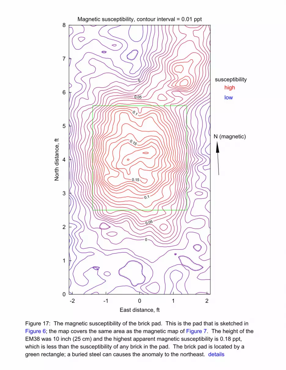
Figure 5 is a photograph of a small brick pavement, or pad, that was tested withseveral geophysical instruments. A survey with a magnetometer found the irregular patternshown in Figure 7, while a magnetic susceptibility meter revealed the simpler anomaly ofFigure 17. Unfortunately, the brick pad that is shown in Figure 27, which is an example froman archaeological site, was invisible to a magnetic susceptibility survey, for it was hidden bynearby anomalies that were much stronger than the anomaly of the brick.

IntroductionIt is valuable to reveal where brick pavements are buried at archaeological sites.

These pavements may be floors, walkways, or perhaps foundations. These brick featuresmay be rather shallow; because of that, perhaps some of the brick was later recycled into amodern structure. However, the accumulation of soil over a pavement may hide the brick sothat it is forgotten.

The bricks will probably lie on their large surfaces, and the pavements may have athickness of one brick. There will usually be no mortar between the bricks. Fired bricks arediscussed here, rather than unfired mud bricks.

The simplest tool for locating brick pavements is a pointed steel T-bar, or soil

The magnetic field of a brick pavement

penetrometer. This will work well where the brick is not very deep, and the soil is not toohard or stony. A shallow pavement may also cause the grass above the brick to dry morequickly than the surrounding grass.

Geophysical instruments may also be able to locate the brick. Brick differs from typicalsoils by being harder, less porous, and more magnetic. While the hardness of buriedfeatures can be revealed with a seismic survey, this survey is usually too slow for detailedexploration. The low porosity of brick might be detected with resistivity or conductivitymeasurements, but it appears that the electrical properties of brick can be similar enough tosome soils to make the bricks invisible. The firing of bricks in a kiln makes their clays (whichmay already be somewhat magnetic) even more magnetic.

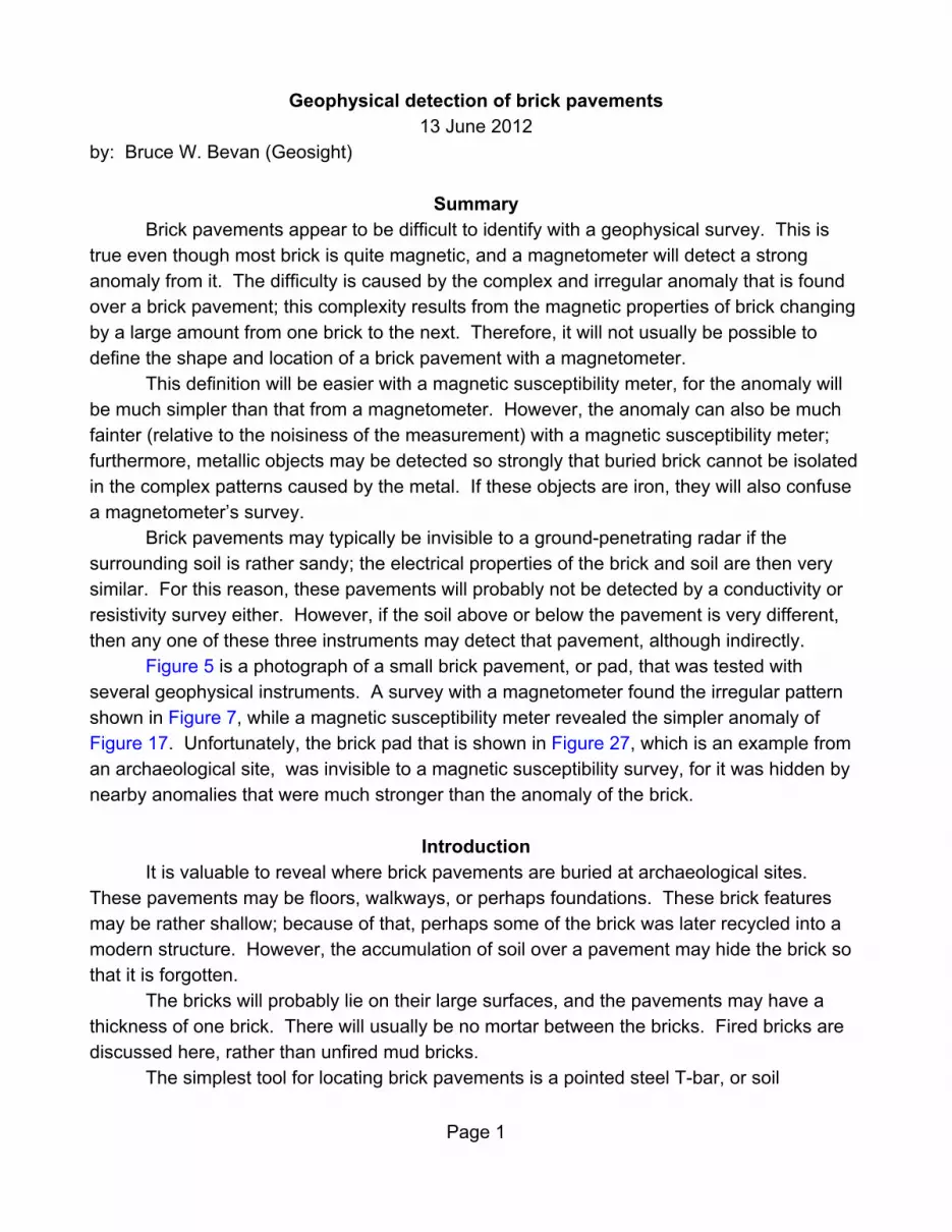
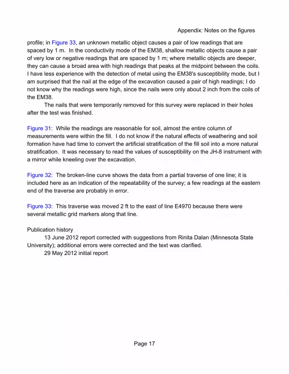
Two geophysical instruments that can detect the magnetism of brick are sketched inFigure 1. A magnetometer measures how the magnetic material in brick can warp themagnetic field of the Earth into moderately complex patterns like those in Figure 9. Anelectromagnetic induction meter can measure the magnetic susceptibility of brick; thisparameter quantifies the ease with which a magnetic field may be “conducted” through brick.

This report is divided into three sections. The first section discusses the magnetic fieldof a brick pad that was specially-constructed for these tests. The second section describesmagnetic susceptibility measurements over constructed brick pads and single bricks. Thefinal section shows that a small brick pavement at an archaeological site was invisible to asusceptibility survey because of interference from other features that were buried nearby.

The figures for the report follow the text; in the electronic version of this report, bluetext marks hyperlinks to these figures. The figure captions are long enough to be a goodsummary of this work, and further details about the surveys and figures are given in anappendix. Not all figures are mentioned in the text; some provide supplementary informationthat most readers may not need.

The magnetic field of a brick pavementBefore it is fired, the clay of a brick is not usually very magnetic; after the clay is fired

in a kiln, the resulting brick becomes a permanent magnet. While the magnetism is weakcompared to magnetic steel, it is possible that a brick could be the needle of a compass if thebrick was suspended by a string with enough care.

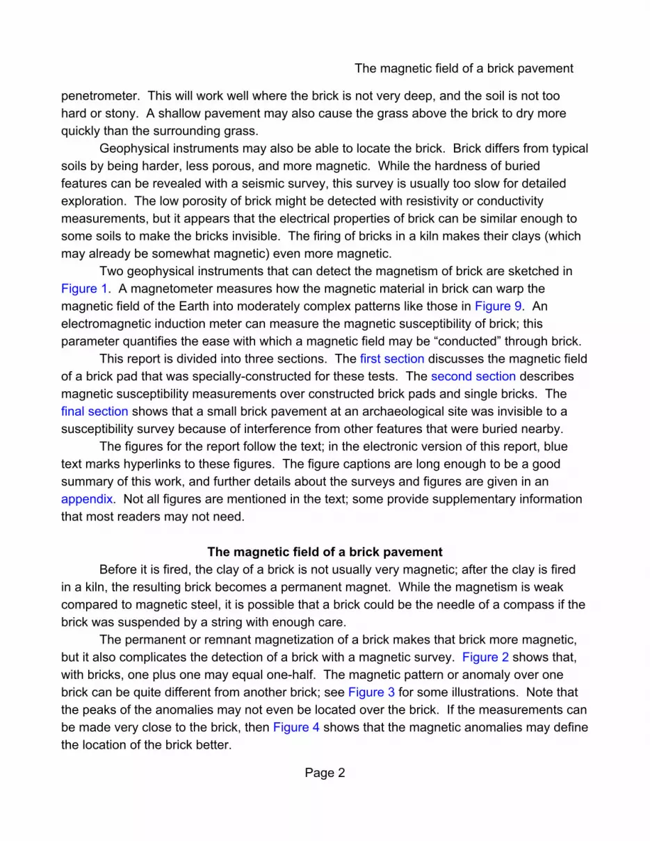
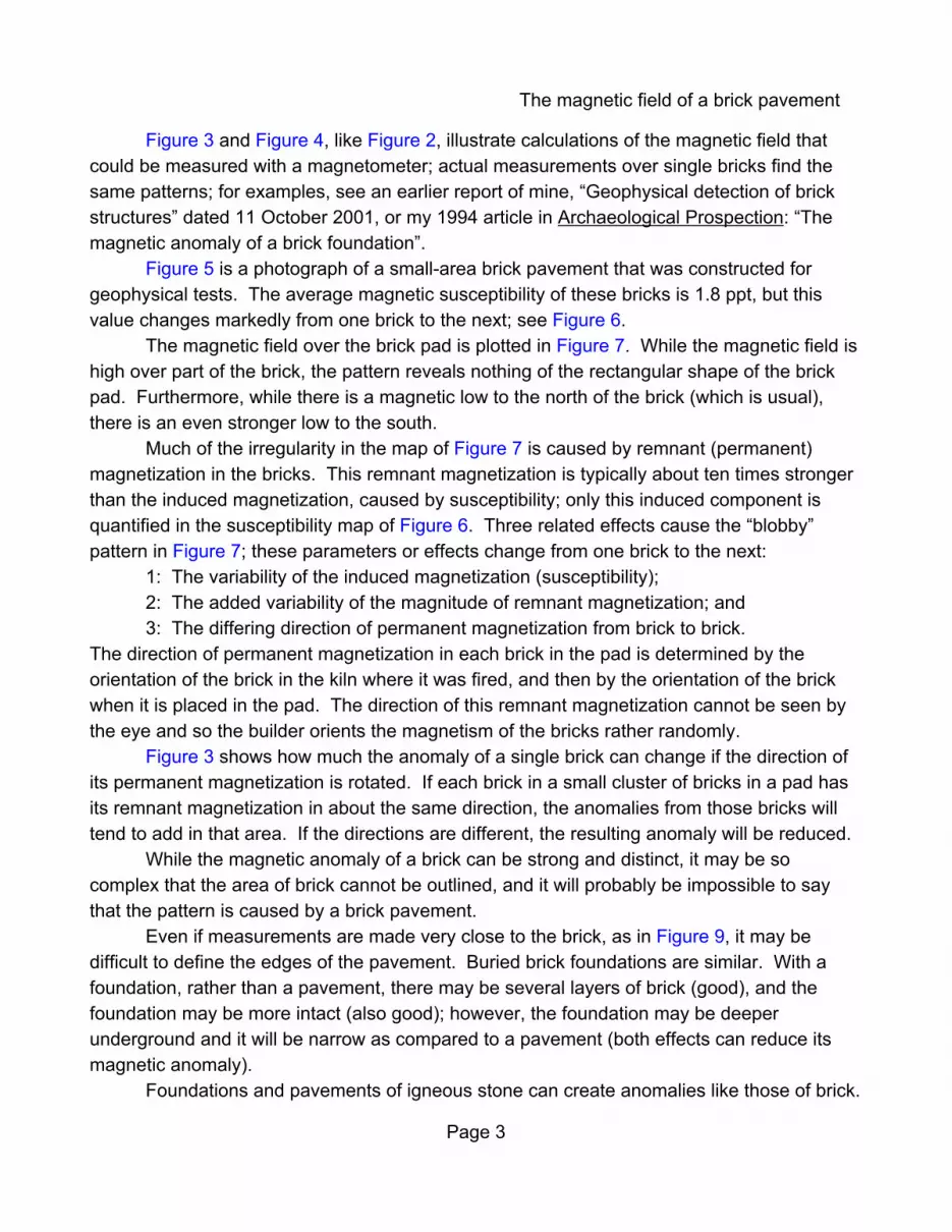
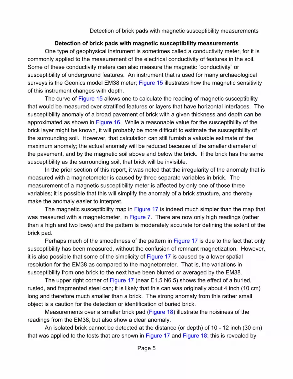
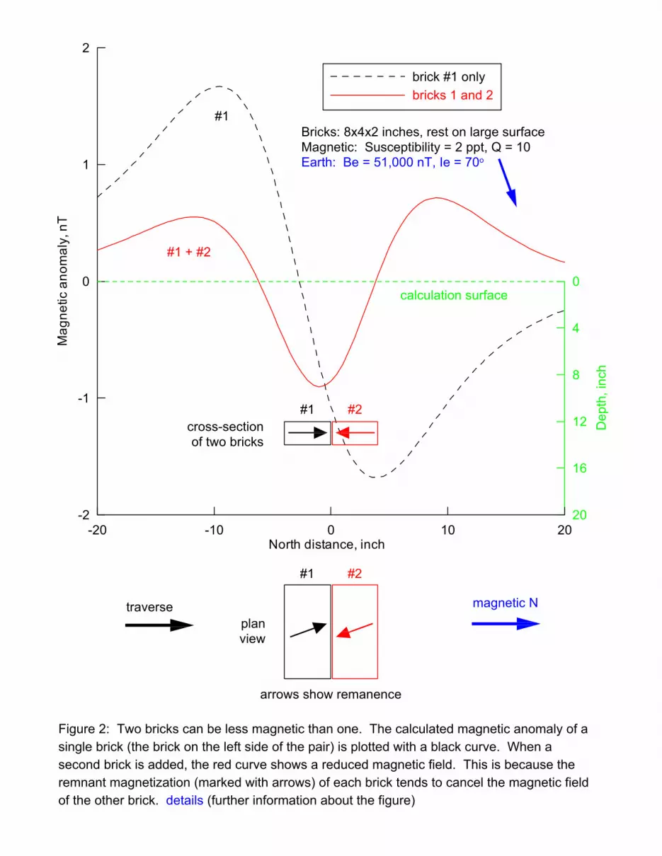
The permanent or remnant magnetization of a brick makes that brick more magnetic,but it also complicates the detection of a brick with a magnetic survey. Figure 2 shows that,with bricks, one plus one may equal one-half. The magnetic pattern or anomaly over onebrick can be quite different from another brick; see Figure 3 for some illustrations. Note thatthe peaks of the anomalies may not even be located over the brick. If the measurements canbe made very close to the brick, then Figure 4 shows that the magnetic anomalies may definethe location of the brick better.


Figure 3 and Figure 4, like Figure 2, illustrate calculations of the magnetic field thatcould be measured with a magnetometer; actual measurements over single bricks find thesame patterns; for examples, see an earlier report of mine, “Geophysical detection of brickstructures” dated 11 October 2001, or my 1994 article in Archaeological Prospection: “Themagnetic anomaly of a brick foundation”.

Figure 5 is a photograph of a small-area brick pavement that was constructed forgeophysical tests. The average magnetic susceptibility of these bricks is 1.8 ppt, but thisvalue changes markedly from one brick to the next; see Figure 6.

The magnetic field over the brick pad is plotted in Figure 7. While the magnetic field ishigh over part of the brick, the pattern reveals nothing of the rectangular shape of the brickpad. Furthermore, while there is a magnetic low to the north of the brick (which is usual),there is an even stronger low to the south.

Much of the irregularity in the map of Figure 7 is caused by remnant (permanent) magnetization in the bricks. This remnant magnetization is typically about ten times strongerthan the induced magnetization, caused by susceptibility; only this induced component isquantified in the susceptibility map of Figure 6. Three related effects cause the “blobby”pattern in Figure 7; these parameters or effects change from one brick to the next:

1: The variability of the induced magnetization (susceptibility);2: The added variability of the magnitude of remnant magnetization; and3: The differing direction of permanent magnetization from brick to brick.

The direction of permanent magnetization in each brick in the pad is determined by theorientation of the brick in the kiln where it was fired, and then by the orientation of the brickwhen it is placed in the pad. The direction of this remnant magnetization cannot be seen bythe eye and so the builder orients the magnetism of the bricks rather randomly.

Figure 3 shows how much the anomaly of a single brick can change if the direction ofits permanent magnetization is rotated. If each brick in a small cluster of bricks in a pad hasits remnant magnetization in about the same direction, the anomalies from those bricks willtend to add in that area. If the directions are different, the resulting anomaly will be reduced.

While the magnetic anomaly of a brick can be strong and distinct, it may be socomplex that the area of brick cannot be outlined, and it will probably be impossible to saythat the pattern is caused by a brick pavement.

Even if measurements are made very close to the brick, as in Figure 9, it may bedifficult to define the edges of the pavement. Buried brick foundations are similar. With afoundation, rather than a pavement, there may be several layers of brick (good), and thefoundation may be more intact (also good); however, the foundation may be deeperunderground and it will be narrow as compared to a pavement (both effects can reduce itsmagnetic anomaly).

Foundations and pavements of igneous stone can create anomalies like those of brick.


Examples of these patterns have been given in two publications:“Magnetic study of archaeological stone foundations at Loma Alta, Michoacan, Mexico”

by Luis Barba, Karl Link, Agustin Ortiz, and Albert Hesse on pages 786 - 789 (paper NS 1.5)in the Expanded Abstracts of the 66th annual meeting of the Society of ExplorationGeophysicists, held 10 - 15 November 1996.

“Magnetometric investigations of stone constructions within large ancient barrows ofDenmark and Crimea” by Tatyana Smekalova, Olfert Voss, Sergej Smekalov, Victor Myts,and Sergej Koltukhov on pages 461 - 482 of the journal Geoarchaeology (2005, volume 20,number 5).

It is likely that magnetic viscosity has an effect on the magnetic anomalies of brickstructures; as they remain stationary for decades, the direction of remnant magnetizationwithin each brick shifts slightly toward the current direction of magnetic north. The season ofthe year may also affect the magnetization of brick; this may be caused by differences intemperature and moisture content that control reversible chemical reactions or crystalformations. While the brick pad in Figure 5 has remained there for over nine years, magneticsurveys have not yet revealed a temporal change in the anomaly; this may be due primarilyto the fact that some of the bricks were replaced during that period. See the tests in Figures9 - 13.

A technical analysis of the magnetic anomalies over single bricks can reveal thedirection of magnetization within those bricks; Figure 4 shows how differing directions canchange the magnetic patterns. Even without this analysis of a magnetic map, a simpleobservation of the locations and polarities of the magnetic anomalies over bricks can allow anapproximation of their direction of magnetization; Figure 14 shows two examples. However,as the bricks are closer together or the height of the magnetic measurements is greater, theanomaly of one brick will overlap with and interfere with the anomalies of adjacent bricks; thiswill probably make it impossible to determine directions of magnetization within individualbricks with any accuracy.

However, the magnetic maps in Figure 9 and Figure 14 show some anomalies (high orlow) that are almost centered over the bricks that cause those anomalies. These bricksappear to have been fired in a kiln while resting on the large surfaces, or flats. These bricksnow lie on the surface of one of those two flats; if the anomaly is a magnetic high, the brickhas the same side down as it had in the kiln. Other high or low anomalies appear to be foundnear the edges of the bricks; these bricks appear to have been fired while resting on theirmedium-sized surfaces, or edges. The book Bricks and Brickmaking, by Karl Gurcke(University of Idaho Press, 1987), shows photographs of kilns (pages 30 and 31) where all ofthe bricks are resting on their medium-sized edges. The magnetic maps in this reportsuggest that a good fraction of these bricks were fired on their large surfaces; perhaps thisorientation was more common in smaller or older kilns.

Detection of brick pads with magnetic susceptibility measurements

Detection of brick pads with magnetic susceptibility measurementsOne type of geophysical instrument is sometimes called a conductivity meter, for it is

commonly applied to the measurement of the electrical conductivity of features in the soil. Some of these conductivity meters can also measure the magnetic “conductivity” orsusceptibility of underground features. An instrument that is used for many archaeologicalsurveys is the Geonics model EM38 meter; Figure 15 illustrates how the magnetic sensitivityof this instrument changes with depth.

The curve of Figure 15 allows one to calculate the reading of magnetic susceptibilitythat would be measured over stratified features or layers that have horizontal interfaces. Thesusceptibility anomaly of a broad pavement of brick with a given thickness and depth can beapproximated as shown in Figure 16. While a reasonable value for the susceptibility of thebrick layer might be known, it will probably be more difficult to estimate the susceptibility ofthe surrounding soil. However, that calculation can still furnish a valuable estimate of themaximum anomaly; the actual anomaly will be reduced because of the smaller diameter ofthe pavement, and by the magnetic soil above and below the brick. If the brick has the samesusceptibility as the surrounding soil, that brick will be invisible.

In the prior section of this report, it was noted that the irregularity of the anomaly that ismeasured with a magnetometer is caused by three separate variables in brick. Themeasurement of a magnetic susceptibility meter is affected by only one of those threevariables; it is possible that this will simplify the anomaly of a brick structure, and therebymake the anomaly easier to interpret.

The magnetic susceptibility map in Figure 17 is indeed much simpler than the map thatwas measured with a magnetometer, in Figure 7. There are now only high readings (ratherthan a high and two lows) and the pattern is moderately accurate for defining the extent of thebrick pad.

Perhaps much of the smoothness of the pattern in Figure 17 is due to the fact that onlysusceptibility has been measured, without the confusion of remnant magnetization. However,it is also possible that some of the simplicity of Figure 17 is caused by a lower spatialresolution for the EM38 as compared to the magnetometer. That is, the variations insusceptibility from one brick to the next have been blurred or averaged by the EM38.

The upper right corner of Figure 17 (near E1.5 N6.5) shows the effect of a buried,rusted, and fragmented steel can; it is likely that this can was originally about 4 inch (10 cm)long and therefore much smaller than a brick. The strong anomaly from this rather smallobject is a caution for the detection or identification of buried brick.

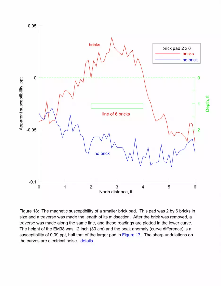
Measurements over a smaller brick pad (Figure 18) illustrate the noisiness of thereadings from the EM38, but also show a clear anomaly.

An isolated brick cannot be detected at the distance (or depth) of 10 - 12 inch (30 cm)that was applied to the tests that are shown in Figure 17 and Figure 18; this is revealed by

Susceptibility tests at an archaeological site

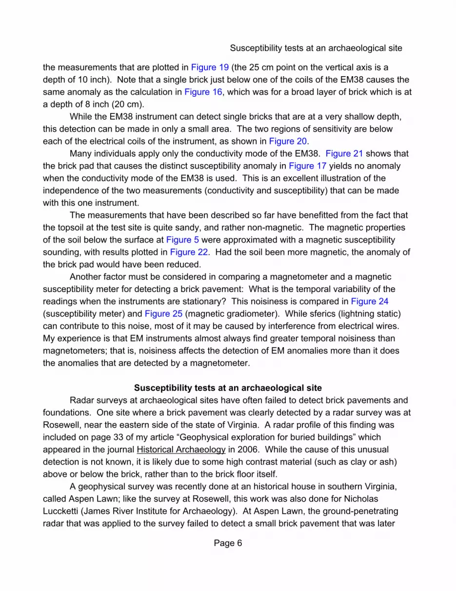
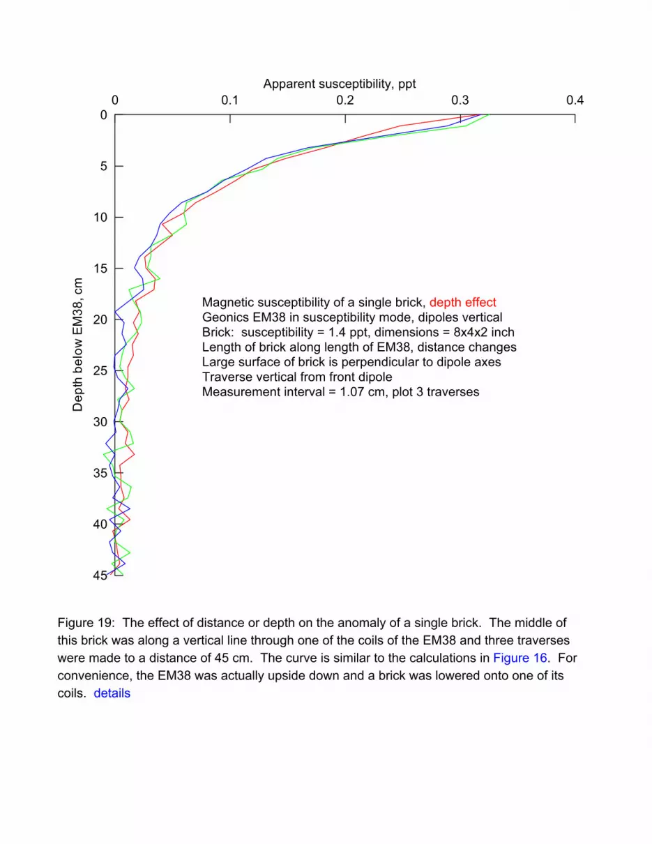
the measurements that are plotted in Figure 19 (the 25 cm point on the vertical axis is adepth of 10 inch). Note that a single brick just below one of the coils of the EM38 causes thesame anomaly as the calculation in Figure 16, which was for a broad layer of brick which is ata depth of 8 inch (20 cm).

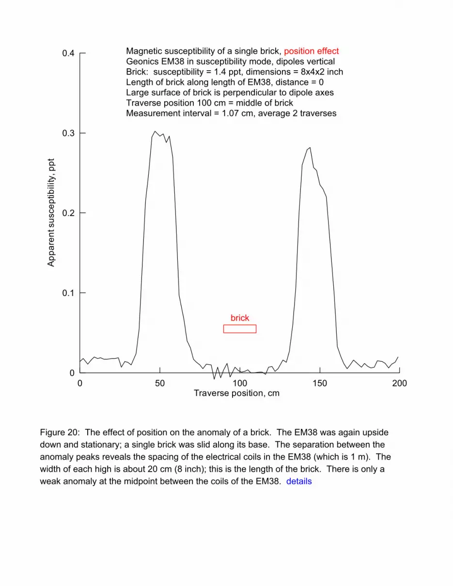
While the EM38 instrument can detect single bricks that are at a very shallow depth,this detection can be made in only a small area. The two regions of sensitivity are beloweach of the electrical coils of the instrument, as shown in Figure 20.

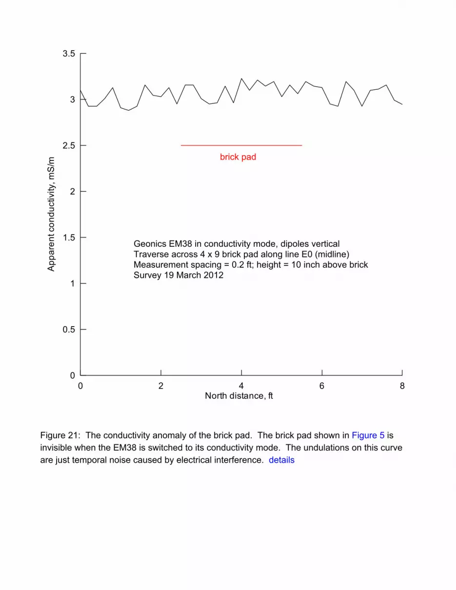
Many individuals apply only the conductivity mode of the EM38. Figure 21 shows thatthe brick pad that causes the distinct susceptibility anomaly in Figure 17 yields no anomalywhen the conductivity mode of the EM38 is used. This is an excellent illustration of theindependence of the two measurements (conductivity and susceptibility) that can be madewith this one instrument.

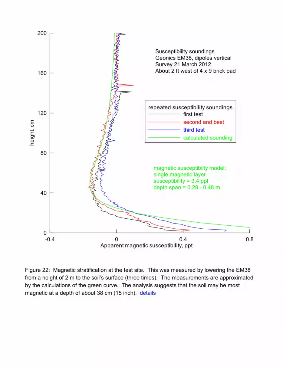
The measurements that have been described so far have benefitted from the fact thatthe topsoil at the test site is quite sandy, and rather non-magnetic. The magnetic propertiesof the soil below the surface at Figure 5 were approximated with a magnetic susceptibilitysounding, with results plotted in Figure 22. Had the soil been more magnetic, the anomaly ofthe brick pad would have been reduced.

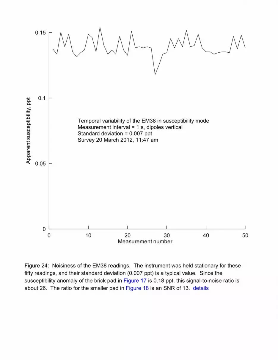
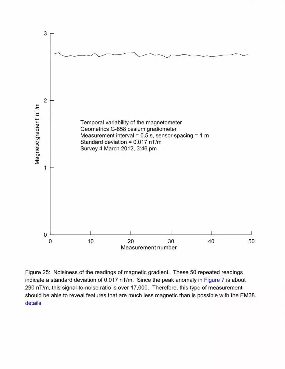
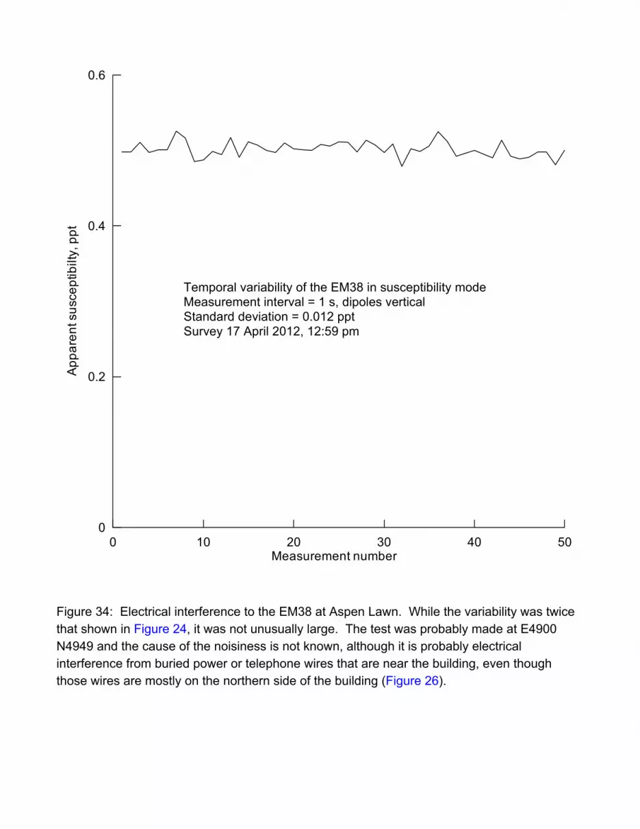
Another factor must be considered in comparing a magnetometer and a magneticsusceptibility meter for detecting a brick pavement: What is the temporal variability of thereadings when the instruments are stationary? This noisiness is compared in Figure 24(susceptibility meter) and Figure 25 (magnetic gradiometer). While sferics (lightning static)can contribute to this noise, most of it may be caused by interference from electrical wires. My experience is that EM instruments almost always find greater temporal noisiness thanmagnetometers; that is, noisiness affects the detection of EM anomalies more than it doesthe anomalies that are detected by a magnetometer.

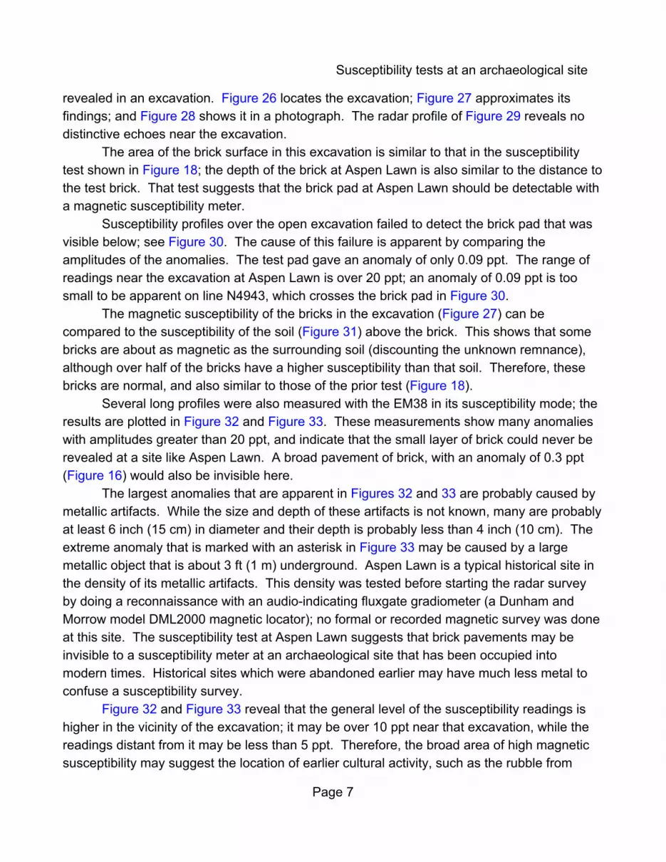
Susceptibility tests at an archaeological siteRadar surveys at archaeological sites have often failed to detect brick pavements and

foundations. One site where a brick pavement was clearly detected by a radar survey was atRosewell, near the eastern side of the state of Virginia. A radar profile of this finding wasincluded on page 33 of my article “Geophysical exploration for buried buildings” whichappeared in the journal Historical Archaeology in 2006. While the cause of this unusualdetection is not known, it is likely due to some high contrast material (such as clay or ash)above or below the brick, rather than to the brick floor itself.

A geophysical survey was recently done at an historical house in southern Virginia,called Aspen Lawn; like the survey at Rosewell, this work was also done for NicholasLuccketti (James River Institute for Archaeology). At Aspen Lawn, the ground-penetratingradar that was applied to the survey failed to detect a small brick pavement that was later

Susceptibility tests at an archaeological site

revealed in an excavation. Figure 26 locates the excavation; Figure 27 approximates itsfindings; and Figure 28 shows it in a photograph. The radar profile of Figure 29 reveals nodistinctive echoes near the excavation.

The area of the brick surface in this excavation is similar to that in the susceptibilitytest shown in Figure 18; the depth of the brick at Aspen Lawn is also similar to the distance tothe test brick. That test suggests that the brick pad at Aspen Lawn should be detectable witha magnetic susceptibility meter.

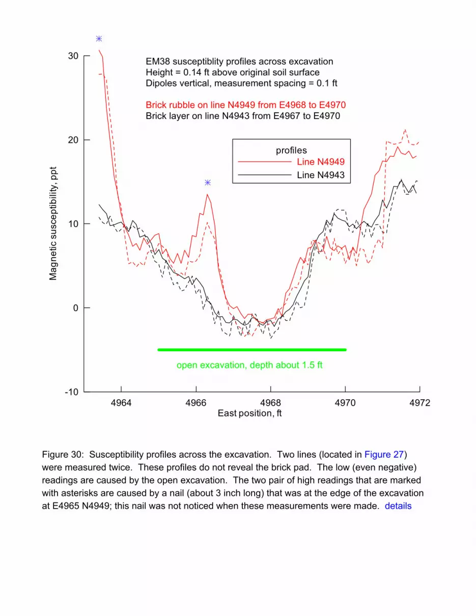
Susceptibility profiles over the open excavation failed to detect the brick pad that wasvisible below; see Figure 30. The cause of this failure is apparent by comparing theamplitudes of the anomalies. The test pad gave an anomaly of only 0.09 ppt. The range ofreadings near the excavation at Aspen Lawn is over 20 ppt; an anomaly of 0.09 ppt is toosmall to be apparent on line N4943, which crosses the brick pad in Figure 30.

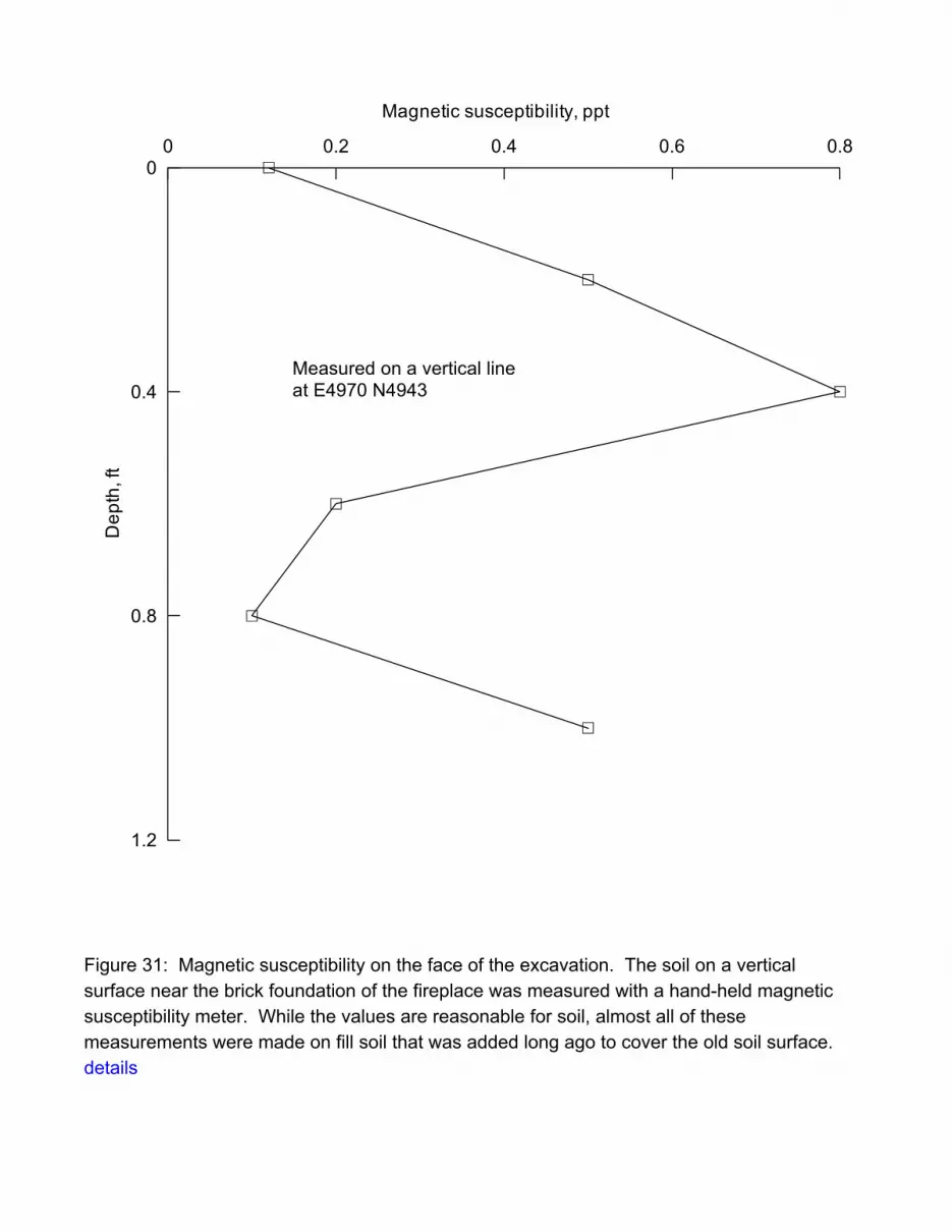
The magnetic susceptibility of the bricks in the excavation (Figure 27) can becompared to the susceptibility of the soil (Figure 31) above the brick. This shows that somebricks are about as magnetic as the surrounding soil (discounting the unknown remnance),although over half of the bricks have a higher susceptibility than that soil. Therefore, thesebricks are normal, and also similar to those of the prior test (Figure 18).

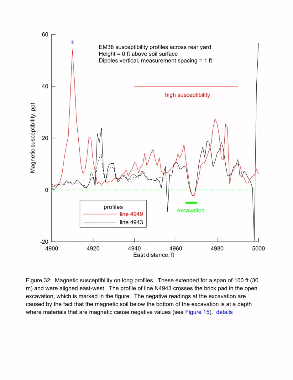
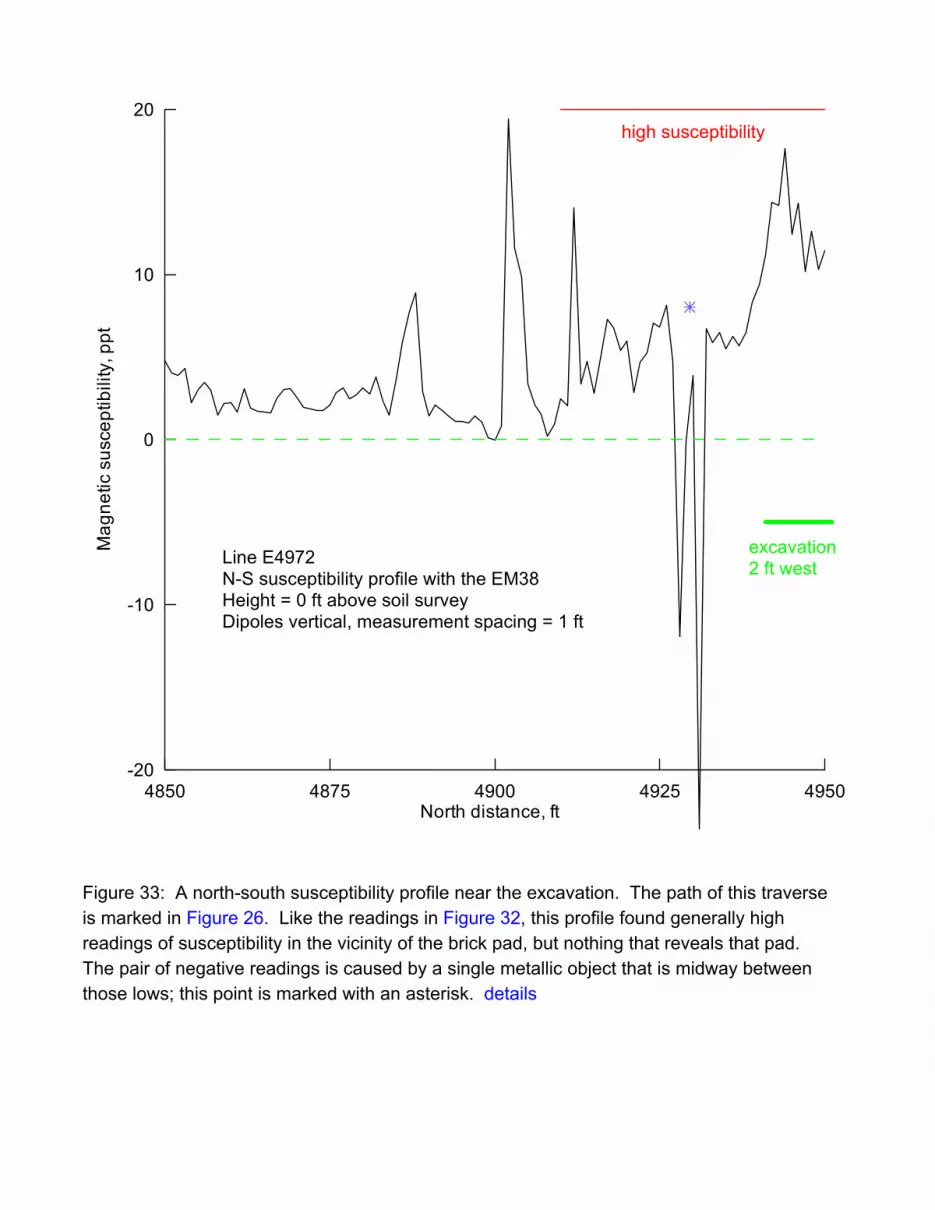
Several long profiles were also measured with the EM38 in its susceptibility mode; theresults are plotted in Figure 32 and Figure 33. These measurements show many anomalieswith amplitudes greater than 20 ppt, and indicate that the small layer of brick could never berevealed at a site like Aspen Lawn. A broad pavement of brick, with an anomaly of 0.3 ppt(Figure 16) would also be invisible here.

The largest anomalies that are apparent in Figures 32 and 33 are probably caused bymetallic artifacts. While the size and depth of these artifacts is not known, many are probablyat least 6 inch (15 cm) in diameter and their depth is probably less than 4 inch (10 cm). Theextreme anomaly that is marked with an asterisk in Figure 33 may be caused by a largemetallic object that is about 3 ft (1 m) underground. Aspen Lawn is a typical historical site inthe density of its metallic artifacts. This density was tested before starting the radar surveyby doing a reconnaissance with an audio-indicating fluxgate gradiometer (a Dunham andMorrow model DML2000 magnetic locator); no formal or recorded magnetic survey was doneat this site. The susceptibility test at Aspen Lawn suggests that brick pavements may beinvisible to a susceptibility meter at an archaeological site that has been occupied intomodern times. Historical sites which were abandoned earlier may have much less metal toconfuse a susceptibility survey.

Figure 32 and Figure 33 reveal that the general level of the susceptibility readings ishigher in the vicinity of the excavation; it may be over 10 ppt near that excavation, while thereadings distant from it may be less than 5 ppt. Therefore, the broad area of high magneticsusceptibility may suggest the location of earlier cultural activity, such as the rubble from

Conclusions

destroyed buildings, the altered strata from landscaping, or refuse disposal. Conductivityreadings from the EM38 have been found to be highest in these cultural areas (see page 39in the above-mentioned article in Historical Archaeology). Since buildings are sometimeslocated on topographic high points, geological effects may also cause these correlations.

ConclusionsThese tests have shown that brick pavements and pads can be detected with a

geophysical survey. While a magnetometer will give a strong anomaly, the pattern of thatanomaly will be poor for revealing the shape of the brick surface, and therefore the brick willprobably not be identifiable in the geophysical map. A magnetic susceptibility meter will givea much fainter anomaly over a brick surface, but the anomaly will be a good guide to thelocation of the brick. Unfortunately, a susceptibility meter can be even more sensitive tosmall and shallow metallic objects than a magnetometer; the susceptibility meter will alsodetect non-ferrous metals, in addition to iron. It is also possible that it may be important tolocate metallic artifacts on some sites, in particular those that were abandoned long ago.

Magnetic susceptibility surveys may be excellent for locating brick and other fired-earthsurfaces when this work is done at sites that contain little unwanted metal; thesearchaeological sites may be from early historic or from prehistoric periods. Illustrations ofsome susceptibility maps are included with a report of mine, “Conductivity or susceptibility?”,dated 25 September 2007.

Susceptibility surveys are good for locating dense concentrations of brick and ceramicrubble at these early sites; brick rubble may be thick where walls or chimneys have fallen. Where broad surfaces of rubble are found, a magnetometer may detect primarily the edges ofthese features, while a susceptibility meter will reveal the full extent of the feature.

None of these experiments have tested the effect of a brick pavement that has beenrefired in place during a conflagration. It is likely that the brick would not be remagnetized bythe heat of that fire, for the soil below might keep it cool. However, if the brick was everremagnetized, the anomaly that would be measured with a magnetometer would increase,while the susceptibility anomaly would remain the same.

Susceptibility surveys are also suitable for locating the central and active region ofarchaeological sites by the generally high readings of susceptibility that are found wherepeople worked and lived. See the publications of Rinita Dalan (Minnesota State University)for illustrations of this; a recent summary of her’s is: “A review of the role of magneticsusceptibility in archaeogeophysical studies in the USA: Recent developments andprospects” (Archaeological Prospection, volume 15, 2008, pages 1 - 31).

Appendix: Notes on the figuresThe typical reader will probably not need to read anything in this appendix. It contains

Appendix: Notes on the figures

details about the geophysical work and its analysis. However, if you have an unansweredquestion about this experiment, the answer might be here.

Figure 2: These calculations were made with my MultiMag computer program, and the brickswere modeled as uniformly-magnetized rectangular boxes. If the anomaly of brick #2 iscalculated separately, it is similar to the inverted anomaly of brick #1, although the locationsand amplitudes of the anomalies are somewhat different. While this calculation made avectorial addition of the magnetic fields of bricks 1 and 2, there would be essentially nodifference if a scalar addition was made; this is because the distance of the calculationsurface from the bricks is much greater than the separation of the magnetic material in thebricks.

The direction of the remnant magnetization of the bricks shown here would be createdif the bricks were set on their medium-sized faces in the kiln and the bricks were orientednorth-south. Then, the magnetization would be parallel to the large faces of the bricks. Evenif the bricks were not oriented north-south in the kiln, the remnant magnetization of the brickswould still end up being almost horizontal, since the inclination of the Earth’s field is steep, at70°.

Figure 3: These calculations, like those in Figure 4, were also made with the MultiMagprogram. The contour lines of magnetic lows have tick marks along their length; the contourmaps here have blue lines for low readings and red lines for highs. The magneticsusceptibility of each brick was set at 2 ppt, and the Q ratio was fixed at 10 (this is remnant /induced magnetization). The green rectangles locate the bricks; these lie with their large flatsurfaces horizontal. The black-line curve in Figure 2 is line E0 in the upper panel. Theinclination of remnant magnetization in the upper panel is horizontal; the inclination in thelower panel is 70°, which is the inclination angle of the Earth’s field (which has a magnitude of51,000 nT).

Since remnant magnetization is so much stronger than induced magnetization forthese bricks, the magnetic lows would turn if the bricks were rotated, and the direction ofremnant magnetization will point toward the magnetic low.

Figure 4: Green rectangles locate the bricks; the width of each map is half that in Figure 3. The parameters of the bricks and the Earth’s field are the same as for the calculations ofFigure 3.

Figure 5: This photograph was made on 29 February 2012. The bricks are 2 inch thick. These tests were made in the woods 40 m south of my house in Virginia. The bricks wereoriginally set on the surface of the soil; leaf litter and humus, perhaps with the additional


effect of earthworms, have now dropped the tops of the bricks to near the soil’s surface.

Figure 6: The measurements of susceptibility were made on 29 February 2012 with a modelJH-8 magnetic susceptibility meter from Geoinstruments (Finland). The readings in Figure 27and Figure 31 were also made with this instrument.

Note that the readings on the two ends of each brick are similar; the bricks are quiteuniform.

Except for the four bricks that were replaced in 2003, all of these bricks have remainedin place since June 2002. I have not measured the remnant magnetization of any of thesebricks. The bricks that are in this pad, and the others that were applied to this test, werefound loose on the surface near the ruins of brick buildings near my house in Virginia. Whilethe age of these structures is not known, they may date within the span of 1880 to 1940.

Figure 7: This survey was done on 22 March 2012 with a Geometrics G-858 magnetometer;the vertical spacing between its magnetic sensors was 1 m. Measurement traverses wenttoward grid north and readings were made at intervals of 0.5 s and about 0.1 ft; parallel linesprogressed toward the east and were spaced by 0.35 ft (half the length of the bricks). LineE0 passed along the midline of the matrix of bricks.

As the height of the magnetic measurements is increased, the anomaly will becomesimpler and approach that of a magnetic dipole. If this simple anomaly were analyzed for themagnetic moment (and its direction) of the approximate dipole, that moment wouldreasonably be the vectorial sum of the moments of individual bricks. This approximationassumes that the bricks form a relatively-compact mass, compared to the sensor’s height.

Figure 8: This survey was done on 4 March 2012. For simplicity in locating the survey, eachnorth-going line of traverse followed the junction between adjacent bricks; therefore theselines were spaced by about 0.7 ft. The sensor height for this survey, and that in Figure 7,was determined by the active middle of the cesium sensors, which is 2 inch above the bottomof the sensor housing (with the cable on the top of the housing). For these surveys, the lowersensor was slid along a 2 by 4 inch board that defined the line and height for each traverse.

Figure 9: This survey was done with a model FGM-5DTAA tri-axial fluxgate magnetometermanufactured by Walker Scientific. The magnetometer was controlled by an auxiliarycomputer, a model 200LX palmtop computer from HP; a computer program initiated eachreading, added a coordinate, then stored the measurement.

A large (4-ft square) and thin (1/8 inch) wooden board covered the brick pad and wasaligned with that pad; point E0.5 N0.5 was the southwestern corner of the brick pad as shownin Figure 6. Because of the uneven surface of the brick, the height to the active middle of the


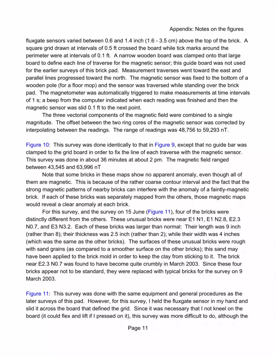
fluxgate sensors varied between 0.6 and 1.4 inch (1.6 - 3.5 cm) above the top of the brick. Asquare grid drawn at intervals of 0.5 ft crossed the board while tick marks around theperimeter were at intervals of 0.1 ft. A narrow wooden board was clamped onto that largeboard to define each line of traverse for the magnetic sensor; this guide board was not usedfor the earlier surveys of this brick pad. Measurement traverses went toward the east andparallel lines progressed toward the north. The magnetic sensor was fixed to the bottom of awooden pole (for a floor mop) and the sensor was traversed while standing over the brickpad. The magnetometer was automatically triggered to make measurements at time intervalsof 1 s; a beep from the computer indicated when each reading was finished and then themagnetic sensor was slid 0.1 ft to the next point.

The three vectorial components of the magnetic field were combined to a singlemagnitude. The offset between the two ring cores of the magnetic sensor was corrected byinterpolating between the readings. The range of readings was 48,756 to 59,293 nT.

Figure 10: This survey was done identically to that in Figure 9, except that no guide bar wasclamped to the grid board in order to fix the line of each traverse with the magnetic sensor. This survey was done in about 36 minutes at about 2 pm. The magnetic field rangedbetween 43,545 and 63,996 nT

Note that some bricks in these maps show no apparent anomaly, even though all ofthem are magnetic. This is because of the rather coarse contour interval and the fact that thestrong magnetic patterns of nearby bricks can interfere with the anomaly of a faintly-magneticbrick. If each of these bricks was separately mapped from the others, those magnetic mapswould reveal a clear anomaly at each brick.

For this survey, and the survey on 15 June (Figure 11), four of the bricks weredistinctly different from the others. These unusual bricks were near E1 N1, E1 N2.8, E2.3N0.7, and E3 N3.2. Each of these bricks was larger than normal: Their length was 9 inch(rather than 8); their thickness was 2.5 inch (rather than 2); while their width was 4 inches(which was the same as the other bricks). The surfaces of these unusual bricks were roughwith sand grains (as compared to a smoother surface on the other bricks); this sand mayhave been applied to the brick mold in order to keep the clay from sticking to it. The bricknear E2.3 N0.7 was found to have become quite crumbly in March 2003. Since these fourbricks appear not to be standard, they were replaced with typical bricks for the survey on 9March 2003.

Figure 11: This survey was done with the same equipment and general procedures as thelater surveys of this pad. However, for this survey, I held the fluxgate sensor in my hand andslid it across the board that defined the grid. Since it was necessary that I not kneel on theboard (it could flex and lift if I pressed on it), this survey was more difficult to do, although the


locational accuracy was good.The survey was done in about 31 minutes near 5 pm, and the range of the magnetic

field readings was 41,128 to 65,462 nT.

Figure 12: The lack of temporal correction may result in errors when maps from two differenttimes are compared; however, spatial errors between maps will probably be larger. Perhapsit would be easier to detect magnetic viscosity in the magnetic maps of a small number ofisolated bricks.

There are several locations where the residual anomalies extend across severalparallel lines of measurement, and where isolated anomalies match the location of a brick. Examples along E3 are found at N1.6, N3.1, and perhaps at N0.6, with another possibleexample at E2.2 N6.7. Could magnetic viscosity between the two days of survey be apparentat these locations?

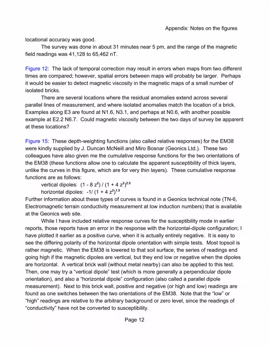
Figure 15: These depth-weighting functions (also called relative responses) for the EM38were kindly supplied by J. Duncan McNeill and Miro Bosnar (Geonics Ltd.). These twocolleagues have also given me the cumulative response functions for the two orientations ofthe EM38 (these functions allow one to calculate the apparent susceptibility of thick layers,unlike the curves in this figure, which are for very thin layers). These cumulative responsefunctions are as follows:

vertical dipoles: (1 - 8 z2) / (1 + 4 z2)2.5

horizontal dipoles: -1/ (1 + 4 z2)1.5

Further information about these types of curves is found in a Geonics technical note (TN-6,Electromagnetic terrain conductivity measurement at low induction numbers) that is availableat the Geonics web site.

While I have included relative response curves for the susceptibility mode in earlierreports, those reports have an error in the response with the horizontal-dipole configuration; Ihave plotted it earlier as a positive curve, when it is actually entirely negative. It is easy tosee the differing polarity of the horizontal dipole orientation with simple tests. Most topsoil israther magnetic. When the EM38 is lowered to that soil surface, the series of readings endgoing high if the magnetic dipoles are vertical, but they end low or negative when the dipolesare horizontal. A vertical brick wall (without metal nearby) can also be applied to this test. Then, one may try a “vertical dipole” test (which is more generally a perpendicular dipoleorientation), and also a “horizontal dipole” configuration (also called a parallel dipolemeasurement). Next to this brick wall, positive and negative (or high and low) readings arefound as one switches between the two orientations of the EM38. Note that the “low” or“high” readings are relative to the arbitrary background or zero level, since the readings of“conductivity” have not be converted to susceptibility.


While I have done many measurements with the EM38 in both its conductivity and itsmagnetic susceptibility modes, I believe that my error in the depth weighting function withhorizontal dipoles has never caused me an error in my surveys. This is probably because Ihave almost never applied that horizontal orientation because it is so sensitive to electricalinterference. The one time that I have applied a “horizontal dipole” survey in magneticsusceptibility mode was when I measured on the vertical face of an excavated trench (the“blade” of the EM38 was parallel to the soil’s surface). Since I knew that the readings couldhave only one polarity then, and that the susceptibilities must all be positive, I accidentallymade no error in the resulting measurements.

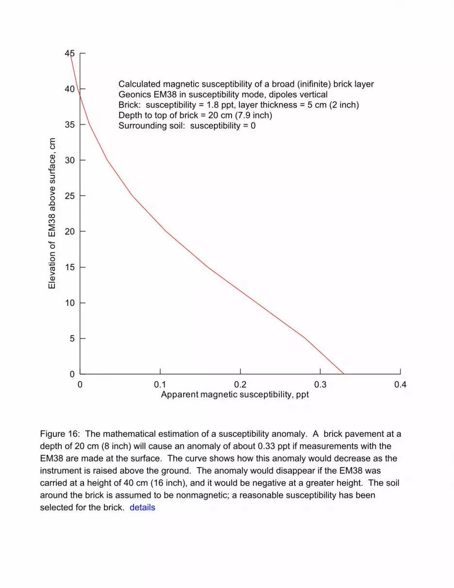
Figure 16: This curve was calculated with the cumulative response function that is listed inthe note for Figure 15; my program Ksound was used for this. The estimated anomaly of thebrick (0.33 ppt) can be divided by 0.058 to get the anomaly (with units of mS/m) that would bemeasured on the EM38; this value of 5.7 mS/m would cause a distinctive anomaly that wouldbe very apparent to the operator of the instrument.

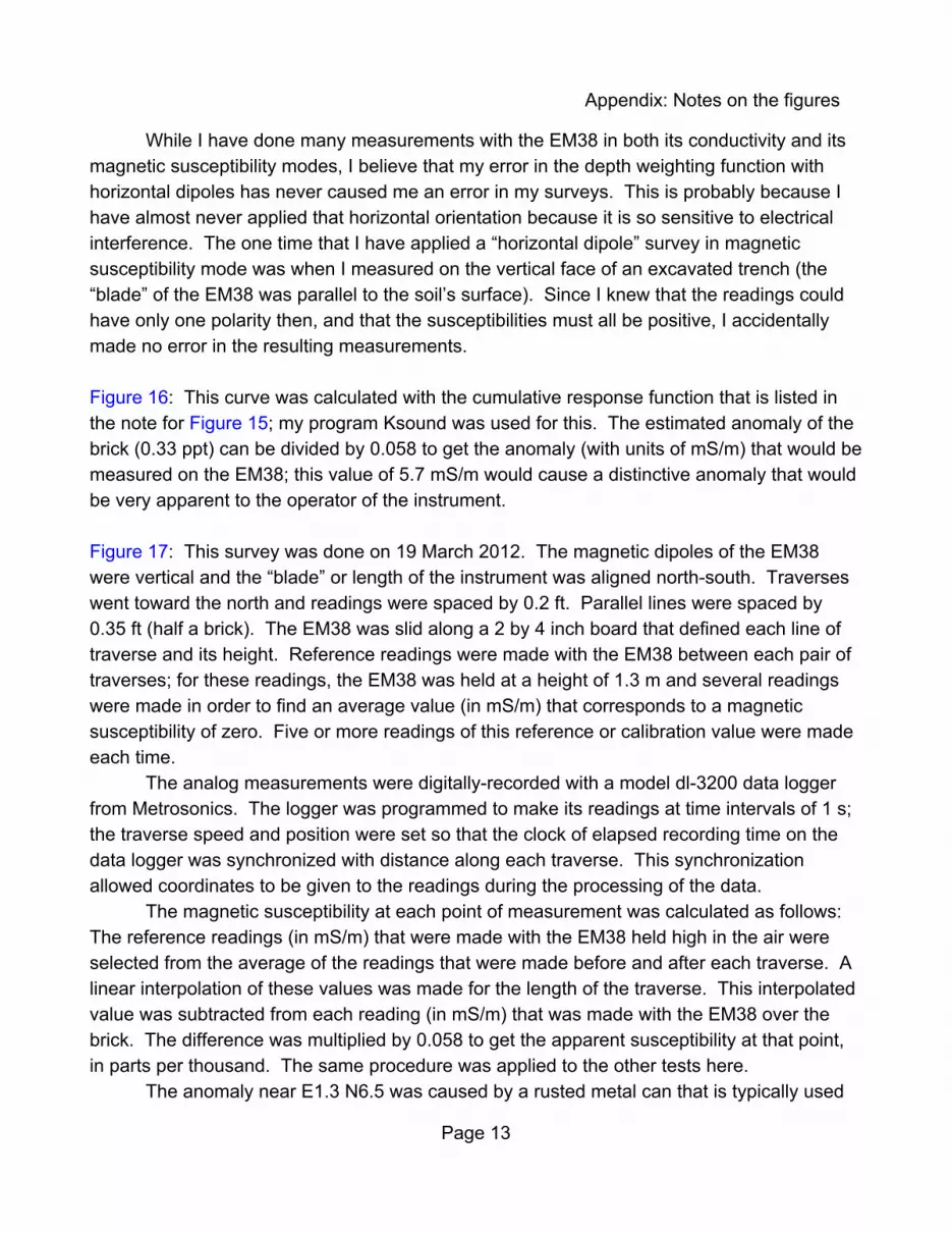
Figure 17: This survey was done on 19 March 2012. The magnetic dipoles of the EM38were vertical and the “blade” or length of the instrument was aligned north-south. Traverseswent toward the north and readings were spaced by 0.2 ft. Parallel lines were spaced by0.35 ft (half a brick). The EM38 was slid along a 2 by 4 inch board that defined each line oftraverse and its height. Reference readings were made with the EM38 between each pair oftraverses; for these readings, the EM38 was held at a height of 1.3 m and several readingswere made in order to find an average value (in mS/m) that corresponds to a magneticsusceptibility of zero. Five or more readings of this reference or calibration value were madeeach time.

The analog measurements were digitally-recorded with a model dl-3200 data loggerfrom Metrosonics. The logger was programmed to make its readings at time intervals of 1 s;the traverse speed and position were set so that the clock of elapsed recording time on thedata logger was synchronized with distance along each traverse. This synchronizationallowed coordinates to be given to the readings during the processing of the data.

The magnetic susceptibility at each point of measurement was calculated as follows: The reference readings (in mS/m) that were made with the EM38 held high in the air wereselected from the average of the readings that were made before and after each traverse. Alinear interpolation of these values was made for the length of the traverse. This interpolatedvalue was subtracted from each reading (in mS/m) that was made with the EM38 over thebrick. The difference was multiplied by 0.058 to get the apparent susceptibility at that point,in parts per thousand. The same procedure was applied to the other tests here.

The anomaly near E1.3 N6.5 was caused by a rusted metal can that is typically used


for food. While I attempted to remove this can before this survey was done, it is fragmentedand most of the fragments are below the root of a tree, and at a depth of perhaps 8 inch. This rusted can was also present for the magnetic maps that are plotted in Figure 7 andFigure 8, although no certain anomaly from the can is found in those maps (perhaps the highat the northeastern corner of Figure 8 is caused by the iron). I do not know why the magneticsurvey detected the can so little. As a guess, perhaps the fragments of metal weresufficiently rusted and reoriented that only induced magnetization remained, and this wasmuch weaker than the remnant magnetization that likely predominated before the can wasconverted to rust and became fragmented.

This test accidentally shows how sensitive the EM38 is to metal when it is operated inits magnetic susceptibility mode. One must be particularly careful to keep the data loggerdistant from the EM38 when these types of surveys are done. All metal (larger than a zipper)must be at least 1 m from the EM38, and it is better if metal is at least 1.5 m distant. Theeffect of metallic objects can be tested by bringing them close to one of the coils of astationary EM38 and watching for changes in the readings. If the data logger cannot be helddistant from the EM38, it may be best to fix it rigidly to the midpoint of the EM38 withadhesive tape; while it will be strongly-detected then, the detection will be constant, ratherthan variable. Since susceptibility values are differences of two readings, the constant effectof the metal can be eliminated.

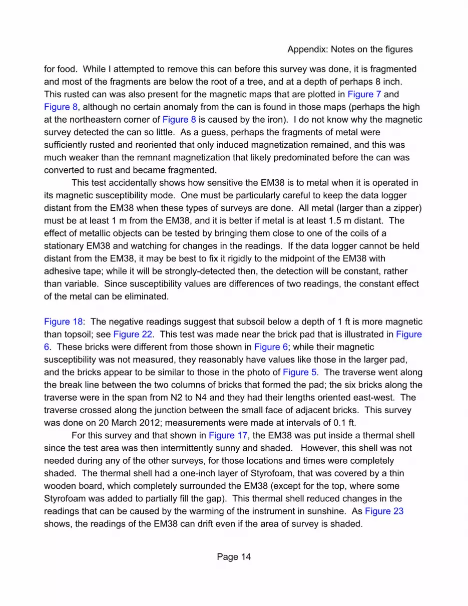
Figure 18: The negative readings suggest that subsoil below a depth of 1 ft is more magneticthan topsoil; see Figure 22. This test was made near the brick pad that is illustrated in Figure6. These bricks were different from those shown in Figure 6; while their magneticsusceptibility was not measured, they reasonably have values like those in the larger pad,and the bricks appear to be similar to those in the photo of Figure 5. The traverse went alongthe break line between the two columns of bricks that formed the pad; the six bricks along thetraverse were in the span from N2 to N4 and they had their lengths oriented east-west. Thetraverse crossed along the junction between the small face of adjacent bricks. This surveywas done on 20 March 2012; measurements were made at intervals of 0.1 ft.

For this survey and that shown in Figure 17, the EM38 was put inside a thermal shellsince the test area was then intermittently sunny and shaded. However, this shell was notneeded during any of the other surveys, for those locations and times were completelyshaded. The thermal shell had a one-inch layer of Styrofoam, that was covered by a thinwooden board, which completely surrounded the EM38 (except for the top, where someStyrofoam was added to partially fill the gap). This thermal shell reduced changes in thereadings that can be caused by the warming of the instrument in sunshine. As Figure 23shows, the readings of the EM38 can drift even if the area of survey is shaded.


Figure 19: These readings were made on 12 March 2012. The EM38 was set on a woodentable at a height of about 2.2 ft near the brick pad shown in Figure 6. The single brick thatwas tested here and for Figure 20 was similar to those in the brick pad of Figure 6. Thedimensions of this brick were 20.5 by 10.2 by 5.3 cm, so its volume was 1108 cm3. The massof the brick was 2299 g, so its density was 2.07 g/cm3. The magnetic susceptibility of thisbrick was measured at 24 points on its two large faces and the average value was 1.36 ppt(the range of the readings was 0.8 - 1.6 ppt).

Figure 20: These measurements were made on 11 March 2012. The forward dipole on theEM38 was at N50 cm. It is possible that the curve should be lowered by 0.02 ppt so that thereadings at the north and south ends will be about zero, making the values near N100 cmslightly negative.

Figure 21: The low conductivity reveals the fact that the soil contains a large fraction of sand. Perhaps this brick pad would show a conductivity anomaly if the surrounding soil was clayeyand had a high conductivity.

Figure 22: The vertical spacing between readings was 1 cm and the time interval was 1 s. Since it is moderately difficult to lower the EM38 at a steady rate for the 2-m span of thesounding, the curves differ. Principles and practices for doing these measurements aredescribed in a report written by myself and Rinita Dalan (Minnesota State University) called“Magnetic susceptibility sounding” and dated 2 April 2003.

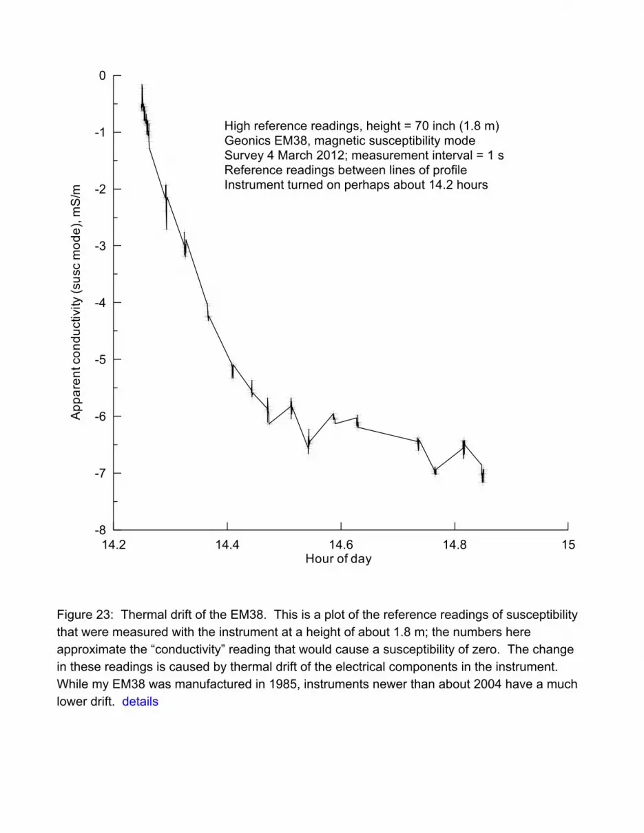
Figure 23: I originally thought that the drift of the readings of the EM38 was primarily causedby the instrument warming and cooling as it moved between sunny and shaded areas. Thisand other tests have suggested that a large part of the drift is caused by the heating of theinside of the instrument by power dissipated in its electrical components; this test was madein a shaded location, where the instrument had been setting for perhaps an hour. I probablyturned on the EM38 less than 15 minutes before the start of these measurements.

The data in this figure were measured as part of an early test of susceptibility readingsover the brick pad; the mapped readings were faulty and are not included here. For the latertests with the EM38, I was careful to turn on the EM38 about an hour before the start of thesurvey; the drift of the reference readings was lower then. The EM38 is very economical inits battery usage; the instrument should be left on for the entire day of each survey, even overa lunch hour.

Figure 24: This noise test was made near the brick pad shown in Figure 6. The instrumentwas held stationary for the series of readings. The nearest electrical power line is buried over


20 m to the north. The actual level of these readings is not important; that is, the curve heremay be shifted up or down any amount. This is also true for Figure 23 and Figure 34.

Figure 25: This test was also made in the vicinity of the brick pad.

Figure 26: My thanks go to Robin and Jamie Rawles, who own this property, for requestingthis survey and aiding my work, both during the original ground-penetrating radar survey on21 - 23 November 2011, and also for the susceptibility test that was done on 17 April 2012. Their house is located on Hicksford Road in a rural area near the town of Drewryville,Virginia. The grid for the archaeological and geophysical work was set up by Nick Luccketti,who coordinated my surveys at this site.

Figure 28: This brick archaeological feature is covered by a rather uniform layer of fill soilthat is over 1 ft thick; this soil has a gray color and it is not known when it was placed here. Perhaps it was spread on the earlier soil surface to cover or smooth that surface; however,the thickness of the fill appears to be unusually large.

It was difficult to chose whether to have the excavation open or not for this test. Arefilled excavation would mean that the susceptibility of the brick could not be measured (theexcavation would be refilled before I returned to the site); the stratification of the fill soil wouldalso be different from before the excavation was made. The air that fills the open excavationcauses a strong anomaly with lower readings; however, this open excavation appeared toallow the best test.

Figure 29: The ground-penetrating radar was a model SIR System-7, manufactured byGeophysical Survey Systems. The antenna was a model 3102, which has a predominantfrequency (when setting on soil) of about 315 MHz. The entire rear yard was explored withradar profiles that were spaced by either 5 ft or 2.5 ft.

Figure 30: These profiles and the other susceptibility readings at Aspen Lawn weremeasured on 17 April 2012. That day was mostly sunny and warm; there were nothunderstorms in the vicinity during the field work. An 8-ft long 2x4 plank was extendedacross the 5-ft wide excavation in order to guide the EM38 at a constant height. Measurements extended 1.5 ft or more outside the excavation. The “terrace” in the readingsbetween E4969 and E4971 may have its edges where the coils of the EM38 crossed the sideof the excavation.

The nail that caused a problem for the traverse on line N4949 was removed before theprofiles in Figure 32 were measured; this nail held a string that defined the perimeter of theexcavation. This vertical nail causes a pair of high readings, spaced by 1 m, along this


profile; in Figure 33, an unknown metallic object causes a pair of low readings that arespaced by 1 m. In the conductivity mode of the EM38, shallow metallic objects cause a pairof very low or negative readings that are spaced by 1 m; where metallic objects are deeper,they can cause a broad area with high readings that peaks at the midpoint between the coils. I have less experience with the detection of metal using the EM38's susceptibility mode, but Iam surprised that the nail at the edge of the excavation caused a pair of high readings; I donot know why the readings were high, since the nails were only about 2 inch from the coils ofthe EM38.

The nails that were temporarily removed for this survey were replaced in their holesafter the test was finished.

Figure 31: While the readings are reasonable for soil, almost the entire column ofmeasurements were within the fill. I do not know if the natural effects of weathering and soilformation have had time to convert the artificial stratification of the fill soil into a more naturalstratification. It was necessary to read the values of susceptibility on the JH-8 instrument witha mirror while kneeling over the excavation.

Figure 32: The broken-line curve shows the data from a partial traverse of one line; it isincluded here as an indication of the repeatability of the survey; a few readings at the easternend of the traverse are probably in error.

Figure 33: This traverse was moved 2 ft to the east of line E4970 because there wereseveral metallic grid markers along that line.

Publication history13 June 2012 report corrected with suggestions from Rinita Dalan (Minnesota State

University); additional errors were corrected and the text was clarified.29 May 2012 initial report

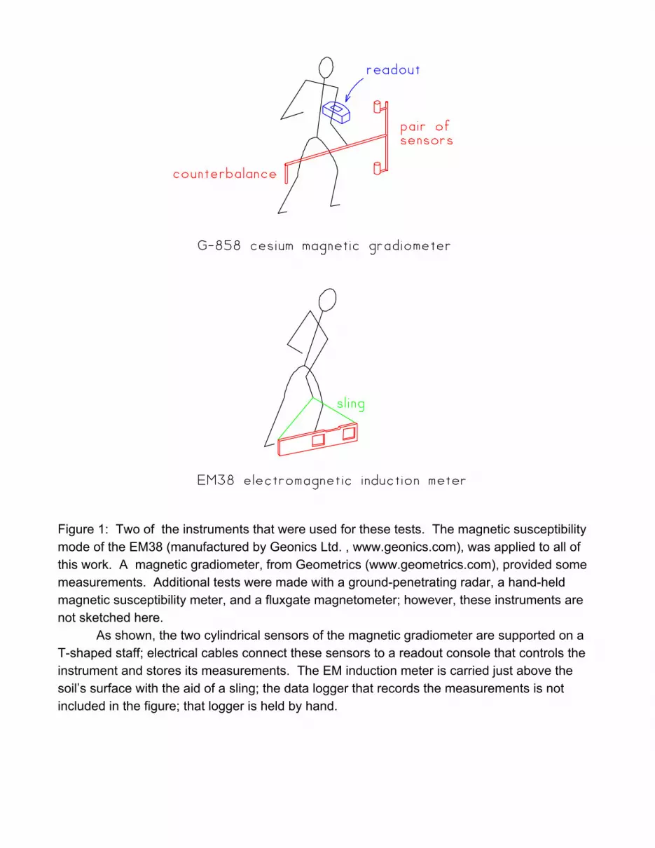
Figure 1: Two of the instruments that were used for these tests. The magnetic susceptibilitymode of the EM38 (manufactured by Geonics Ltd. , www.geonics.com), was applied to all ofthis work. A magnetic gradiometer, from Geometrics (www.geometrics.com), provided somemeasurements. Additional tests were made with a ground-penetrating radar, a hand-heldmagnetic susceptibility meter, and a fluxgate magnetometer; however, these instruments arenot sketched here.

As shown, the two cylindrical sensors of the magnetic gradiometer are supported on aT-shaped staff; electrical cables connect these sensors to a readout console that controls theinstrument and stores its measurements. The EM induction meter is carried just above thesoil’s surface with the aid of a sling; the data logger that records the measurements is notincluded in the figure; that logger is held by hand.

20

16

12

8

4

0

Dep

th, i

nch

-20 -10 0 10 20North distance, inch

-2

-1

0

1

2M

agne

tic a

nom

aly,

nT

brick #1 onlybricks 1 and 2

arrows show remanence

#1 #2

planview

magnetic Ntraverse

#1 #2cross-sectionof two bricks

calculation surface

Bricks: 8x4x2 inches, rest on large surfaceMagnetic: Susceptibility = 2 ppt, Q = 10Earth: Be = 51,000 nT, Ie = 70o

#1 + #2

#1

Figure 2: Two bricks can be less magnetic than one. The calculated magnetic anomaly of asingle brick (the brick on the left side of the pair) is plotted with a black curve. When asecond brick is added, the red curve shows a reduced magnetic field. This is because theremnant magnetization (marked with arrows) of each brick tends to cancel the magnetic fieldof the other brick. details (further information about the figure)

-20 -10 0 10 20East distance, inch

Brick rested on large surface in kiln

-20

-10

0

10

20

Nor

tht d

ista

nce,

inch

Rem

nant

: I =

70

deg,

D =

0 d

eg

-20 -10 0 10 20

Brick rested on medium-sized surface in kiln

-20

-10

0

10

20

Nor

tht d

ista

nce,

inch

Rem

nant

: I =

0 d

eg, D

= -2

0 de

g

Figure 3: The magnetic anomalies of two separate bricks (green rectangles). The patternsare quite different because of the differing directions of remnant magnetization; thesedirections are listed on the right side of each plot, and shown by arrows on the bricks. Thecalculations were made at a height of 1 ft (about 30 cm) above each brick, and the width ofeach plot is about 1 m. The interval between contour lines is 0.2 nT. details

-10 -5 0 5 10East distance, inch

Brick rested on large surface in kiln

-10

-5

0

5

10

Nor

tht d

ista

nce,

inch

Rem

nant

: I =

70

deg,

D =

0 d

eg

-10 -5 0 5 10

Brick rested on medium-sized surface in kiln

-10

-5

0

5

10

Nor

tht d

ista

nce,

inch

Rem

nant

: I =

0 d

eg, D

= -2

0 de

g

N (magnetic)

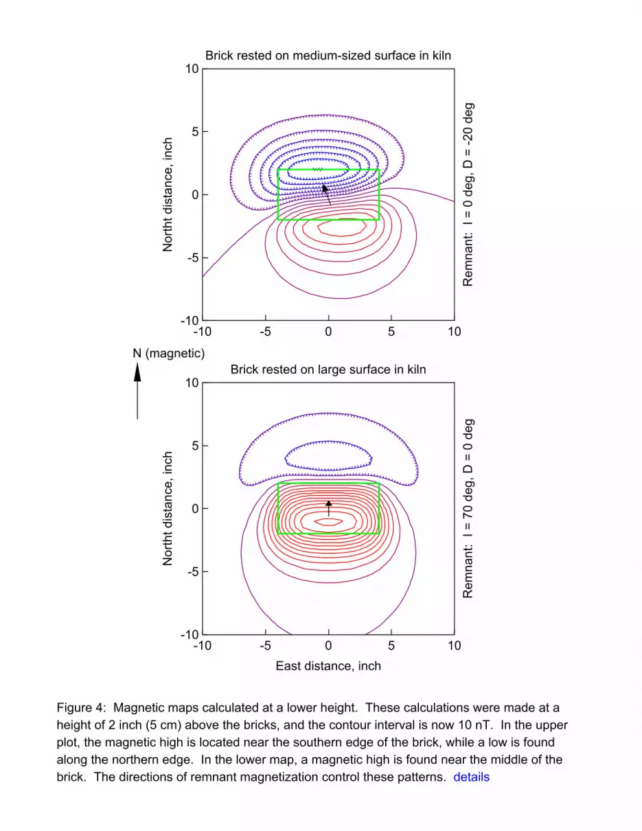
Figure 4: Magnetic maps calculated at a lower height. These calculations were made at aheight of 2 inch (5 cm) above the bricks, and the contour interval is now 10 nT. In the upperplot, the magnetic high is located near the southern edge of the brick, while a low is foundalong the northern edge. In the lower map, a magnetic high is found near the middle of thebrick. The directions of remnant magnetization control these patterns. details

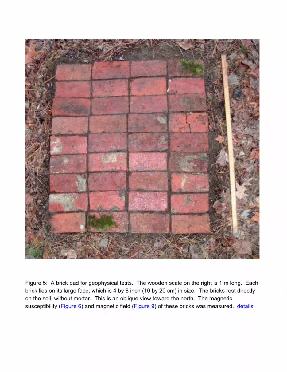
Figure 5: A brick pad for geophysical tests. The wooden scale on the right is 1 m long. Eachbrick lies on its large face, which is 4 by 8 inch (10 by 20 cm) in size. The bricks rest directlyon the soil, without mortar. This is an oblique view toward the north. The magneticsusceptibility (Figure 6) and magnetic field (Figure 9) of these bricks was measured. details

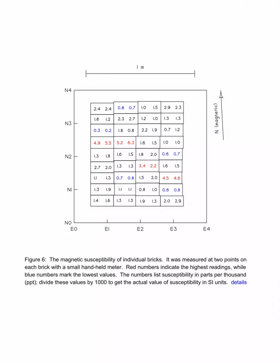
Figure 6: The magnetic susceptibility of individual bricks. It was measured at two points oneach brick with a small hand-held meter. Red numbers indicate the highest readings, whileblue numbers mark the lowest values. The numbers list susceptibility in parts per thousand(ppt); divide these values by 1000 to get the actual value of susceptibility in SI units. details

-2 -1 0 1 2East distance, ft

Magnetic gradient, survey 22 March 2012, contour interval = 20 nT/m

0

1

2

3

4

5

6

7

8

Nor

th d

ista

nce,

ft

N (magnetic)

magnetic low

magnetic high

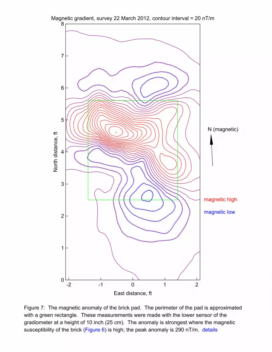
Figure 7: The magnetic anomaly of the brick pad. The perimeter of the pad is approximatedwith a green rectangle. These measurements were made with the lower sensor of thegradiometer at a height of 10 inch (25 cm). The anomaly is strongest where the magneticsusceptibility of the brick (Figure 6) is high; the peak anomaly is 290 nT/m. details


Magnetic gradient, survey 4 March 2012, contour intervl = 10 nT/m

0

1

2

3

4

5

6

7

8

Nor

th d

ista

nce,

ft N (magnetic)

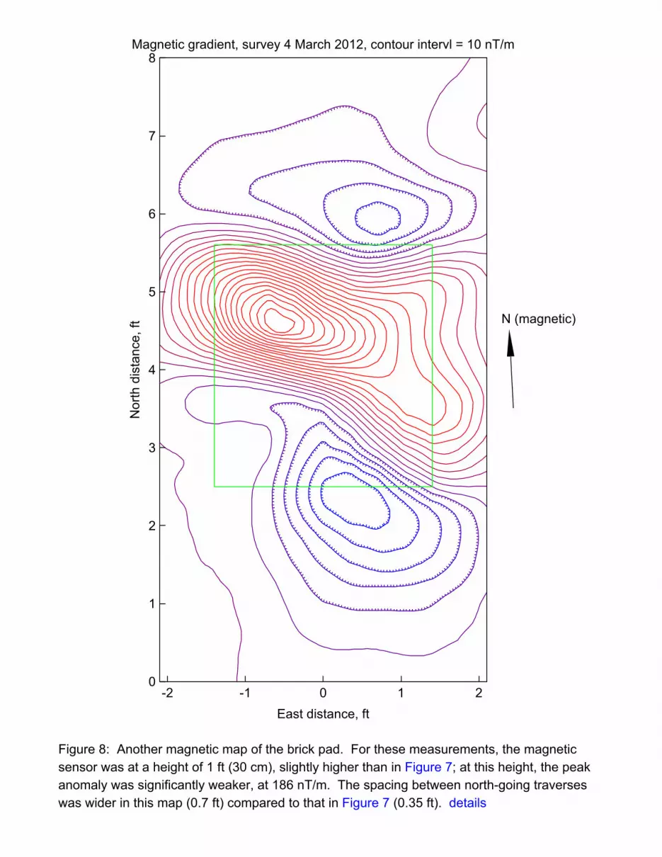
Figure 8: Another magnetic map of the brick pad. For these measurements, the magneticsensor was at a height of 1 ft (30 cm), slightly higher than in Figure 7; at this height, the peakanomaly was significantly weaker, at 186 nT/m. The spacing between north-going traverseswas wider in this map (0.7 ft) compared to that in Figure 7 (0.35 ft). details

0 1 2 3 4East distance, ft

Brick pad, survey 9 March 2003, contours at 500 nT

0

1

2

3

4

Nor

th d

ista

nce,

ft

N (magnetic)

magnetic lowmagnetic high

A

B

C

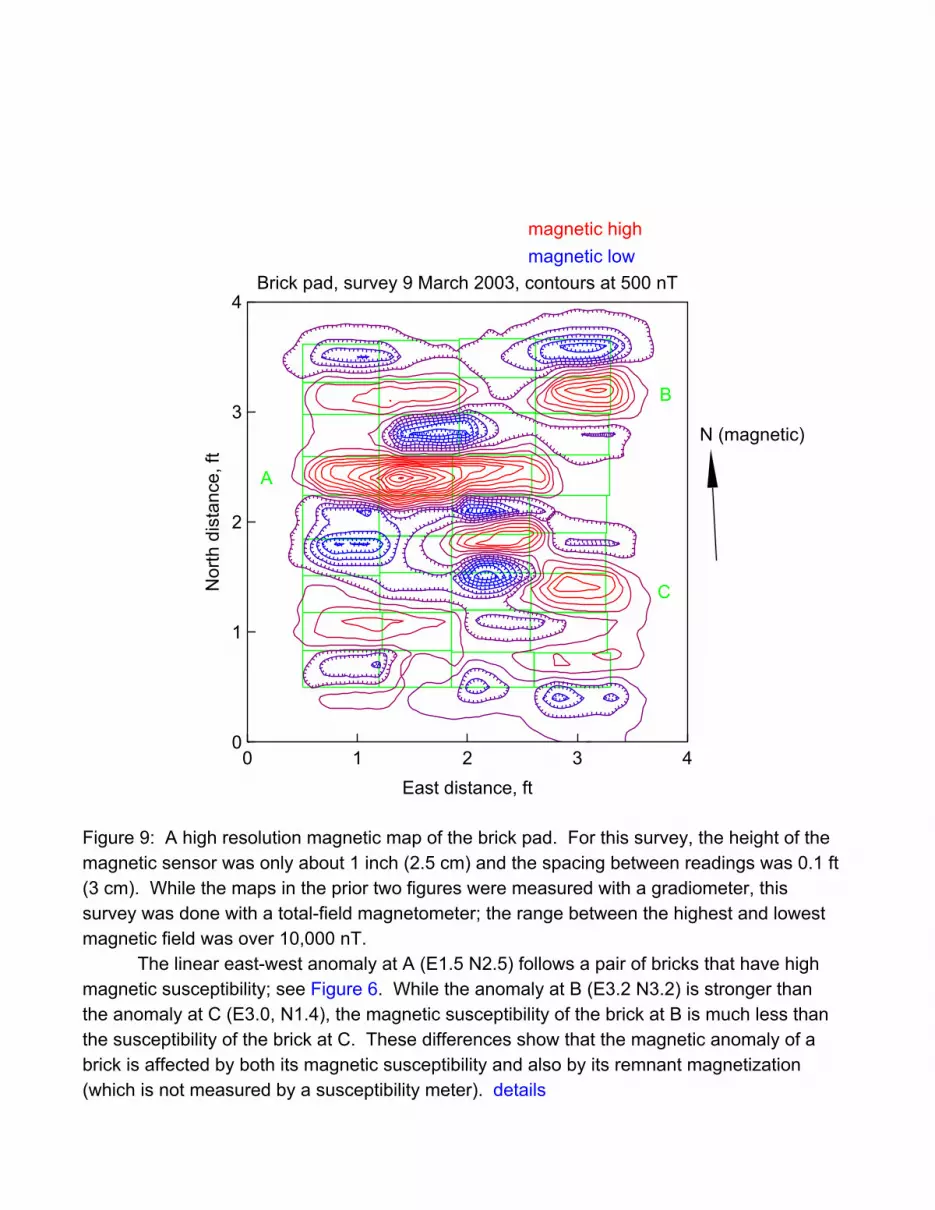
Figure 9: A high resolution magnetic map of the brick pad. For this survey, the height of themagnetic sensor was only about 1 inch (2.5 cm) and the spacing between readings was 0.1 ft(3 cm). While the maps in the prior two figures were measured with a gradiometer, thissurvey was done with a total-field magnetometer; the range between the highest and lowestmagnetic field was over 10,000 nT.

The linear east-west anomaly at A (E1.5 N2.5) follows a pair of bricks that have highmagnetic susceptibility; see Figure 6. While the anomaly at B (E3.2 N3.2) is stronger thanthe anomaly at C (E3.0, N1.4), the magnetic susceptibility of the brick at B is much less thanthe susceptibility of the brick at C. These differences show that the magnetic anomaly of abrick is affected by both its magnetic susceptibility and also by its remnant magnetization(which is not measured by a susceptibility meter). details


Brick pad, survey 16 June 2002, contours at 1000 nT

0

1

2

3

4

Nor

th d

ista

nce,

ft

N (magnetic)

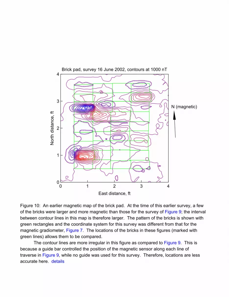
Figure 10: An earlier magnetic map of the brick pad. At the time of this earlier survey, a fewof the bricks were larger and more magnetic than those for the survey of Figure 9; the intervalbetween contour lines in this map is therefore larger. The pattern of the bricks is shown withgreen rectangles and the coordinate system for this survey was different from that for themagnetic gradiometer, Figure 7. The locations of the bricks in these figures (marked withgreen lines) allows them to be compared.

The contour lines are more irregular in this figure as compared to Figure 9. This isbecause a guide bar controlled the position of the magnetic sensor along each line oftraverse in Figure 9, while no guide was used for this survey. Therefore, locations are lessaccurate here. details



0

1

2

3

4

Nor

th d

ista

nce,

ft

N (magnetic)

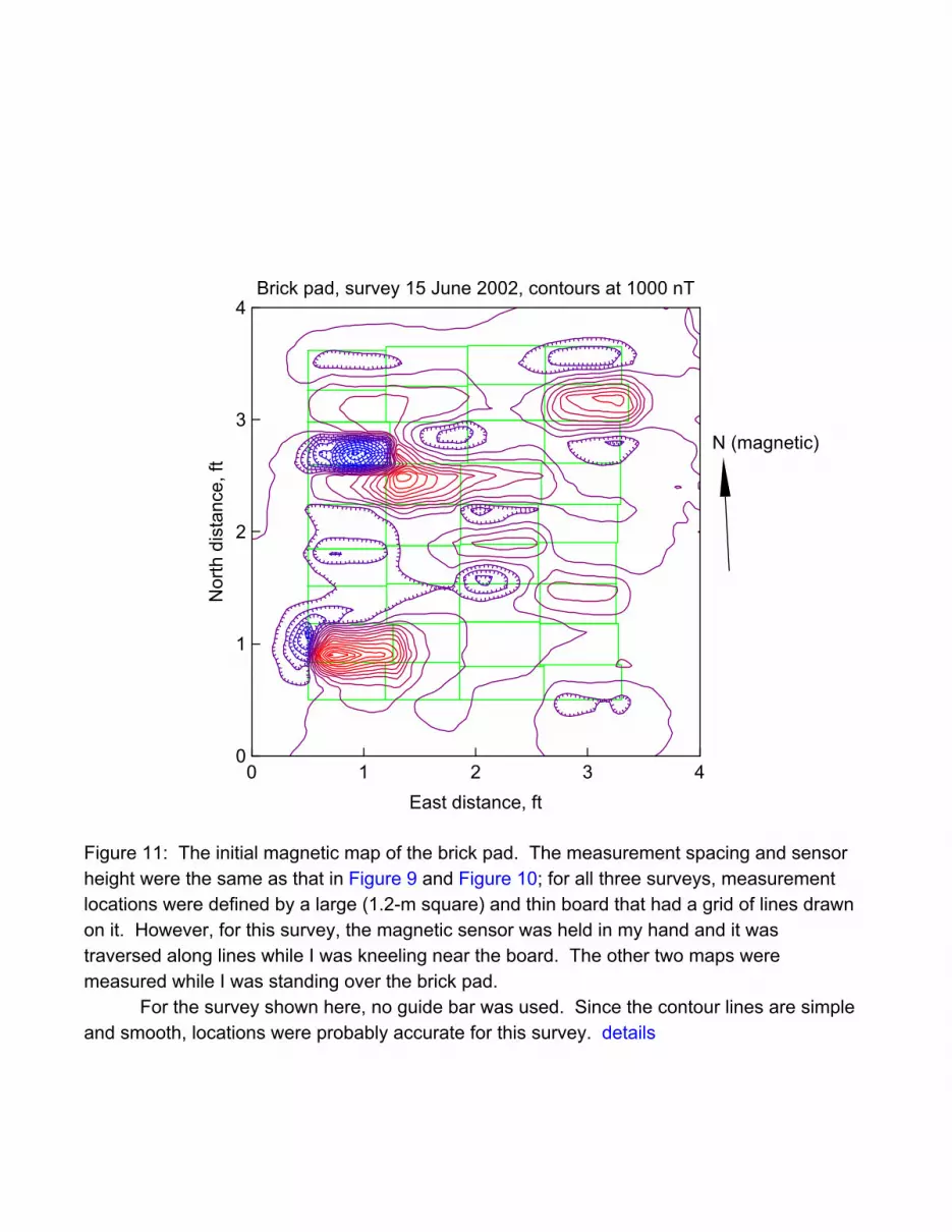
Figure 11: The initial magnetic map of the brick pad. The measurement spacing and sensorheight were the same as that in Figure 9 and Figure 10; for all three surveys, measurementlocations were defined by a large (1.2-m square) and thin board that had a grid of lines drawnon it. However, for this survey, the magnetic sensor was held in my hand and it wastraversed along lines while I was kneeling near the board. The other two maps weremeasured while I was standing over the brick pad.

For the survey shown here, no guide bar was used. Since the contour lines are simpleand smooth, locations were probably accurate for this survey. details


Brick pad, difference: 15 - 16 June 2002 surveys, contour interval = 500 nT

0

1

2

3

4

Nor

th d

ista

nce,

ft

N (magnetic)

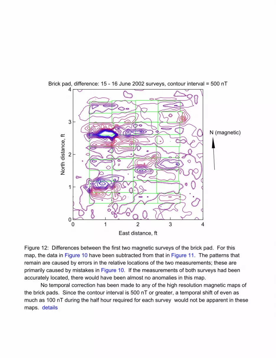
Figure 12: Differences between the first two magnetic surveys of the brick pad. For thismap, the data in Figure 10 have been subtracted from that in Figure 11. The patterns thatremain are caused by errors in the relative locations of the two measurements; these areprimarily caused by mistakes in Figure 10. If the measurements of both surveys had beenaccurately located, there would have been almost no anomalies in this map.

No temporal correction has been made to any of the high resolution magnetic maps ofthe brick pads. Since the contour interval is 500 nT or greater, a temporal shift of even asmuch as 100 nT during the half hour required for each survey would not be apparent in thesemaps. details

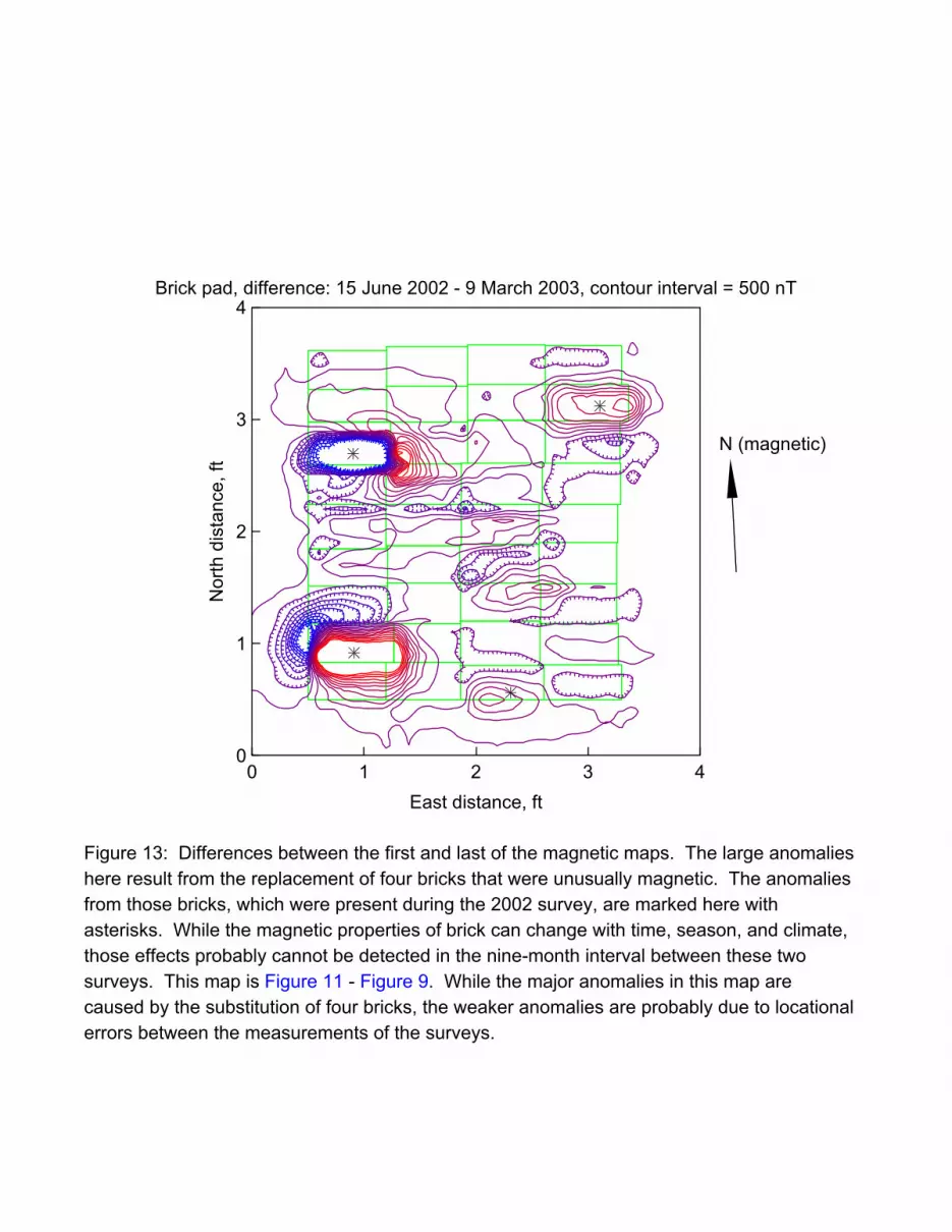
Figure 13: Differences between the first and last of the magnetic maps. The large anomalieshere result from the replacement of four bricks that were unusually magnetic. The anomaliesfrom those bricks, which were present during the 2002 survey, are marked here withasterisks. While the magnetic properties of brick can change with time, season, and climate,those effects probably cannot be detected in the nine-month interval between these twosurveys. This map is Figure 11 - Figure 9. While the major anomalies in this map arecaused by the substitution of four bricks, the weaker anomalies are probably due to locationalerrors between the measurements of the surveys.


Brick pad, difference: 15 June 2002 - 9 March 2003, contour interval = 500 nT

0

1

2

3

4

Nor

th d

ista

nce,

ft

N (magnetic)

0 0.5 1 1.5 2 2.5 3East distance, ft


0

0.5

1

1.5

Nor

th d

ista

nce,

ftN (magnetic)

magnetic low

magnetic high

B

A

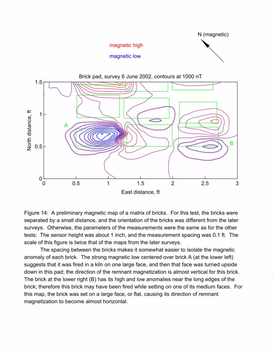
Figure 14: A preliminary magnetic map of a matrix of bricks. For this test, the bricks wereseparated by a small distance, and the orientation of the bricks was different from the latersurveys. Otherwise, the parameters of the measurements were the same as for the othertests: The sensor height was about 1 inch, and the measurement spacing was 0.1 ft. Thescale of this figure is twice that of the maps from the later surveys.

The spacing between the bricks makes it somewhat easier to isolate the magneticanomaly of each brick. The strong magnetic low centered over brick A (at the lower left)suggests that it was fired in a kiln on one large face, and then that face was turned upsidedown in this pad; the direction of the remnant magnetization is almost vertical for this brick. The brick at the lower right (B) has its high and low anomalies near the long edges of thebrick; therefore this brick may have been fired while setting on one of its medium faces. Forthis map, the brick was set on a large face, or flat, causing its direction of remnantmagnetization to become almost horizontal.

-2 -1 0 1 2 3 4

Depth weighting function, phi

2

1.5

1

0.5

0

Dep

th z

, m

dipoles verticaldipoles horizontal

The functions are, for vertical dipoles: phi(z) = 12z (3 - 8z2) / (1 + 4z2)7/2

for horizontal dipoles: phi(z) = -12z / (1 + 4z2)5/2

The depth weighting function for theGeonics EM38 electromagnetic induction meteroperating it its magnetic susceptibility mode.

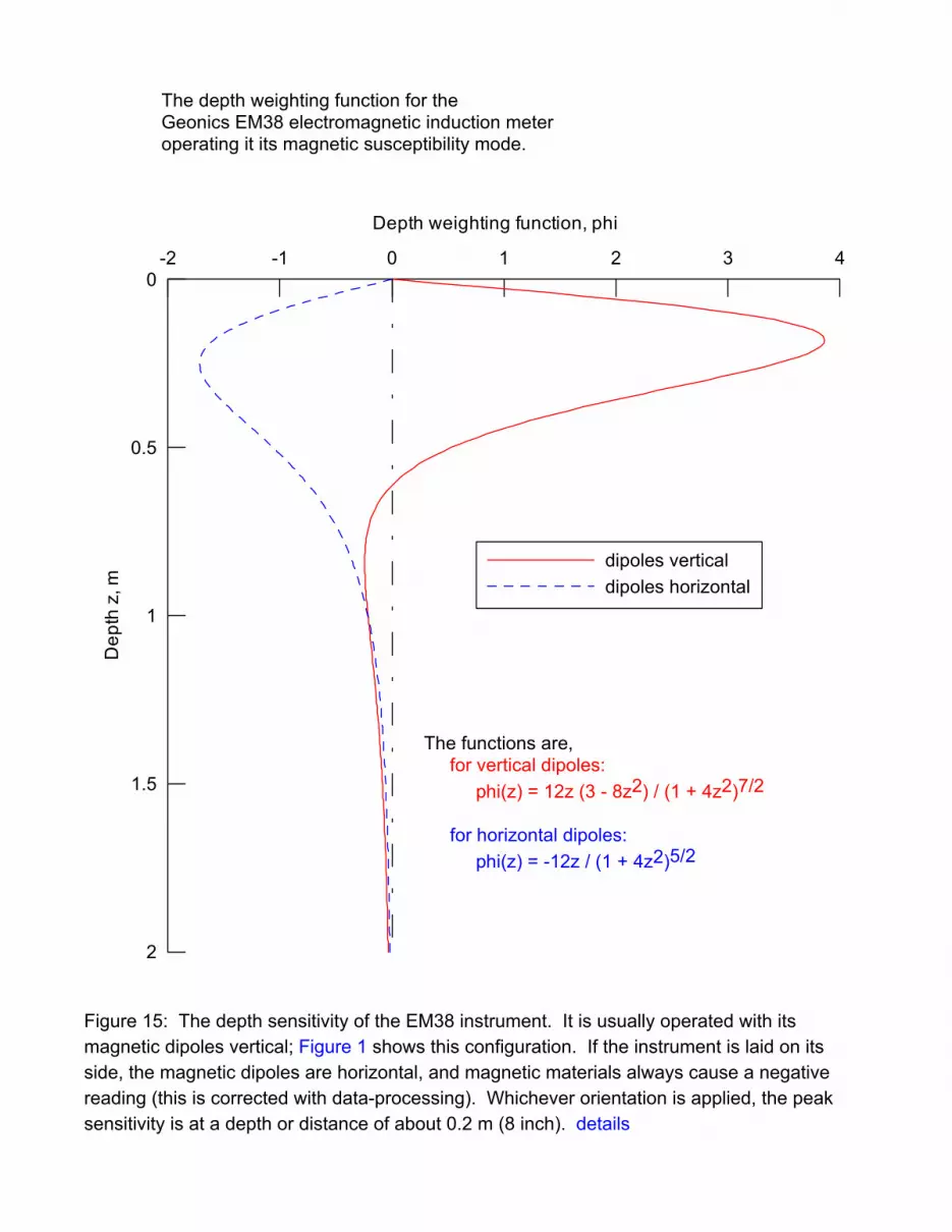
Figure 15: The depth sensitivity of the EM38 instrument. It is usually operated with itsmagnetic dipoles vertical; Figure 1 shows this configuration. If the instrument is laid on itsside, the magnetic dipoles are horizontal, and magnetic materials always cause a negativereading (this is corrected with data-processing). Whichever orientation is applied, the peaksensitivity is at a depth or distance of about 0.2 m (8 inch). details

0 0.1 0.2 0.3 0.4Apparent magnetic susceptibility, ppt

0

5

10

15

20

25

30

35

40

45El

evat

ion

of E

M38

abo

ve s

urfa

ce, c

m

Calculated magnetic susceptibility of a broad (inifinite) brick layerGeonics EM38 in susceptibility mode, dipoles verticalBrick: susceptibility = 1.8 ppt, layer thickness = 5 cm (2 inch)Depth to top of brick = 20 cm (7.9 inch)Surrounding soil: susceptibility = 0

Figure 16: The mathematical estimation of a susceptibility anomaly. A brick pavement at adepth of 20 cm (8 inch) will cause an anomaly of about 0.33 ppt if measurements with theEM38 are made at the surface. The curve shows how this anomaly would decrease as theinstrument is raised above the ground. The anomaly would disappear if the EM38 wascarried at a height of 40 cm (16 inch), and it would be negative at a greater height. The soilaround the brick is assumed to be nonmagnetic; a reasonable susceptibility has beenselected for the brick. details


Magnetic susceptibility, contour interval = 0.01 ppt

0

1

2

3

4

5

6

7

8

Nor

th d

ista

nce,

ft

N (magnetic)

high

low

susceptibility

Figure 17: The magnetic susceptibility of the brick pad. This is the pad that is sketched inFigure 6; the map covers the same area as the magnetic map of Figure 7. The height of theEM38 was 10 inch (25 cm) and the highest apparent magnetic susceptibility is 0.18 ppt,which is less than the susceptibility of any brick in the pad. The brick pad is located by agreen rectangle; a buried steel can causes the anomaly to the northeast. details

0 1 2 3 4 5 6North distance, ft

-0.1

-0.05

0

0.05Ap

pare

nt s

usce

ptib

ility

, ppt

2

1

0

Dep

th, f

t

brick pad 2 x 6bricksno brick

line of 6 bricks

no brick

bricks

Figure 18: The magnetic susceptibility of a smaller brick pad. This pad was 2 by 6 bricks insize and a traverse was made the length of its midsection. After the brick was removed, atraverse was made along the same line, and these readings are plotted in the lower curve. The height of the EM38 was 12 inch (30 cm) and the peak anomaly (curve difference) is asusceptibility of 0.09 ppt, half that of the larger pad in Figure 17. The sharp undulations onthe curves are electrical noise. details

0 0.1 0.2 0.3 0.4Apparent susceptibility, ppt

45

40

35

30

25

20

15

10

5

0

Dep

th b

elow

EM

38, c

m

Magnetic susceptibility of a single brick, depth effectGeonics EM38 in susceptibility mode, dipoles verticalBrick: susceptibility = 1.4 ppt, dimensions = 8x4x2 inchLength of brick along length of EM38, distance changesLarge surface of brick is perpendicular to dipole axesTraverse vertical from front dipoleMeasurement interval = 1.07 cm, plot 3 traverses

Figure 19: The effect of distance or depth on the anomaly of a single brick. The middle ofthis brick was along a vertical line through one of the coils of the EM38 and three traverseswere made to a distance of 45 cm. The curve is similar to the calculations in Figure 16. Forconvenience, the EM38 was actually upside down and a brick was lowered onto one of itscoils. details

0 50 100 150 200Traverse position, cm

0

0.1

0.2

0.3

0.4Ap

pare

nt s

usce

ptib

ility

, ppt

Magnetic susceptibility of a single brick, position effectGeonics EM38 in susceptibility mode, dipoles verticalBrick: susceptibility = 1.4 ppt, dimensions = 8x4x2 inchLength of brick along length of EM38, distance = 0Large surface of brick is perpendicular to dipole axesTraverse position 100 cm = middle of brickMeasurement interval = 1.07 cm, average 2 traverses

brick

Figure 20: The effect of position on the anomaly of a brick. The EM38 was again upsidedown and stationary; a single brick was slid along its base. The separation between theanomaly peaks reveals the spacing of the electrical coils in the EM38 (which is 1 m). Thewidth of each high is about 20 cm (8 inch); this is the length of the brick. There is only aweak anomaly at the midpoint between the coils of the EM38. details

0 2 4 6 8North distance, ft

0

0.5

1

1.5

2

2.5

3

3.5Ap

pare

nt c

ondu

ctiv

ity, m

S/m brick pad

Geonics EM38 in conductivity mode, dipoles verticalTraverse across 4 x 9 brick pad along line E0 (midline)Measurement spacing = 0.2 ft; height = 10 inch above brickSurvey 19 March 2012

Figure 21: The conductivity anomaly of the brick pad. The brick pad shown in Figure 5 isinvisible when the EM38 is switched to its conductivity mode. The undulations on this curveare just temporal noise caused by electrical interference. details

-0.4 0 0.4 0.8Apparent magnetic susceptibility, ppt

0

40

80

120

160

200he

ight

, cm

repeated susceptibility soundingsfirst testsecond and bestthird testcalculated sounding

Susceptibiilty soundingsGeonics EM38, dipoles verticalSurvey 21 March 2012About 2 ft west of 4 x 9 brick pad

magnetic susceptibilty model:single magnetic layersusceptibility = 3.4 pptdepth span = 0.28 - 0.48 m

Figure 22: Magnetic stratification at the test site. This was measured by lowering the EM38from a height of 2 m to the soil’s surface (three times). The measurements are approximatedby the calculations of the green curve. The analysis suggests that the soil may be mostmagnetic at a depth of about 38 cm (15 inch). details

14.2 14.4 14.6 14.8 15Hour of day

-8

-7

-6

-5

-4

-3

-2

-1

0Ap

pare

nt c

ondu

ctiv

ity (s

usc

mod

e), m

S/m

High reference readings, height = 70 inch (1.8 m)Geonics EM38, magnetic susceptibility modeSurvey 4 March 2012; measurement interval = 1 sReference readings between lines of profileInstrument turned on perhaps about 14.2 hours

Figure 23: Thermal drift of the EM38. This is a plot of the reference readings of susceptibilitythat were measured with the instrument at a height of about 1.8 m; the numbers hereapproximate the “conductivity” reading that would cause a susceptibility of zero. The changein these readings is caused by thermal drift of the electrical components in the instrument. While my EM38 was manufactured in 1985, instruments newer than about 2004 have a muchlower drift. details

0 10 20 30 40 50Measurement number

0

0.05

0.1

0.15Ap

pare

nt s

usce

ptib

ility

, ppt

Temporal variability of the EM38 in susceptibility modeMeasurement interval = 1 s, dipoles verticalStandard deviation = 0.007 pptSurvey 20 March 2012, 11:47 am

Figure 24: Noisiness of the EM38 readings. The instrument was held stationary for thesefifty readings, and their standard deviation (0.007 ppt) is a typical value. Since thesusceptibility anomaly of the brick pad in Figure 17 is 0.18 ppt, this signal-to-noise ratio isabout 26. The ratio for the smaller pad in Figure 18 is an SNR of 13. details


0

1

2

3M

agne

tic g

radi

ent,

nT/m

Temporal variability of the magnetometerGeometrics G-858 cesium gradiometerMeasurement interval = 0.5 s, sensor spacing = 1 mStandard deviation = 0.017 nT/mSurvey 4 March 2012, 3:46 pm

Figure 25: Noisiness of the readings of magnetic gradient. These 50 repeated readingsindicate a standard deviation of 0.017 nT/m. Since the peak anomaly in Figure 7 is about290 nT/m, this signal-to-noise ratio is over 17,000. Therefore, this type of measurementshould be able to reveal features that are much less magnetic than is possible with the EM38. details

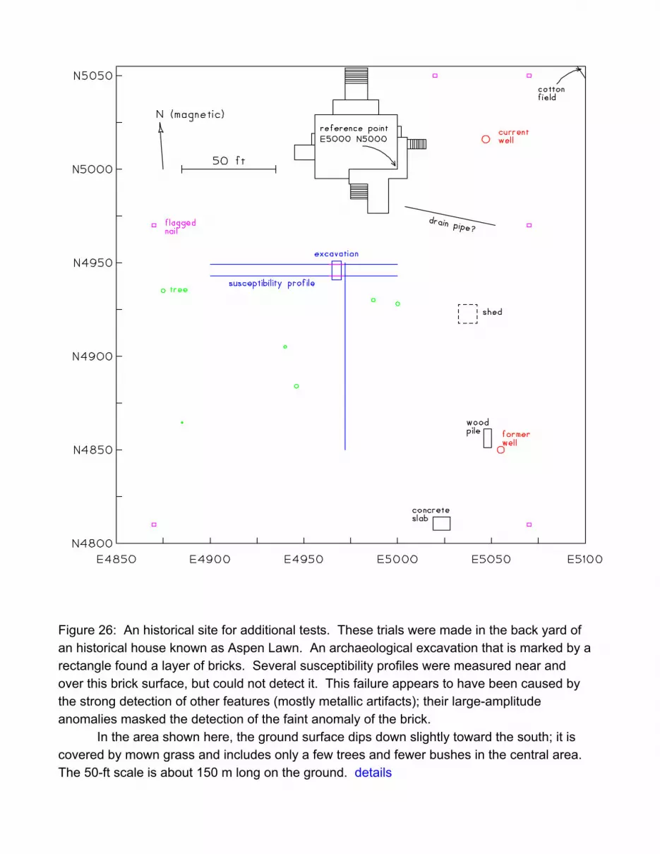
Figure 26: An historical site for additional tests. These trials were made in the back yard ofan historical house known as Aspen Lawn. An archaeological excavation that is marked by arectangle found a layer of bricks. Several susceptibility profiles were measured near andover this brick surface, but could not detect it. This failure appears to have been caused bythe strong detection of other features (mostly metallic artifacts); their large-amplitudeanomalies masked the detection of the faint anomaly of the brick.

In the area shown here, the ground surface dips down slightly toward the south; it iscovered by mown grass and includes only a few trees and fewer bushes in the central area. The 50-ft scale is about 150 m long on the ground. details

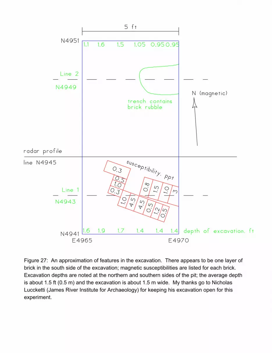
Figure 27: An approximation of features in the excavation. There appears to be one layer ofbrick in the south side of the excavation; magnetic susceptibilities are listed for each brick. Excavation depths are noted at the northern and southern sides of the pit; the average depthis about 1.5 ft (0.5 m) and the excavation is about 1.5 m wide. My thanks go to NicholasLuccketti (James River Institute for Archaeology) for keeping his excavation open for thisexperiment.

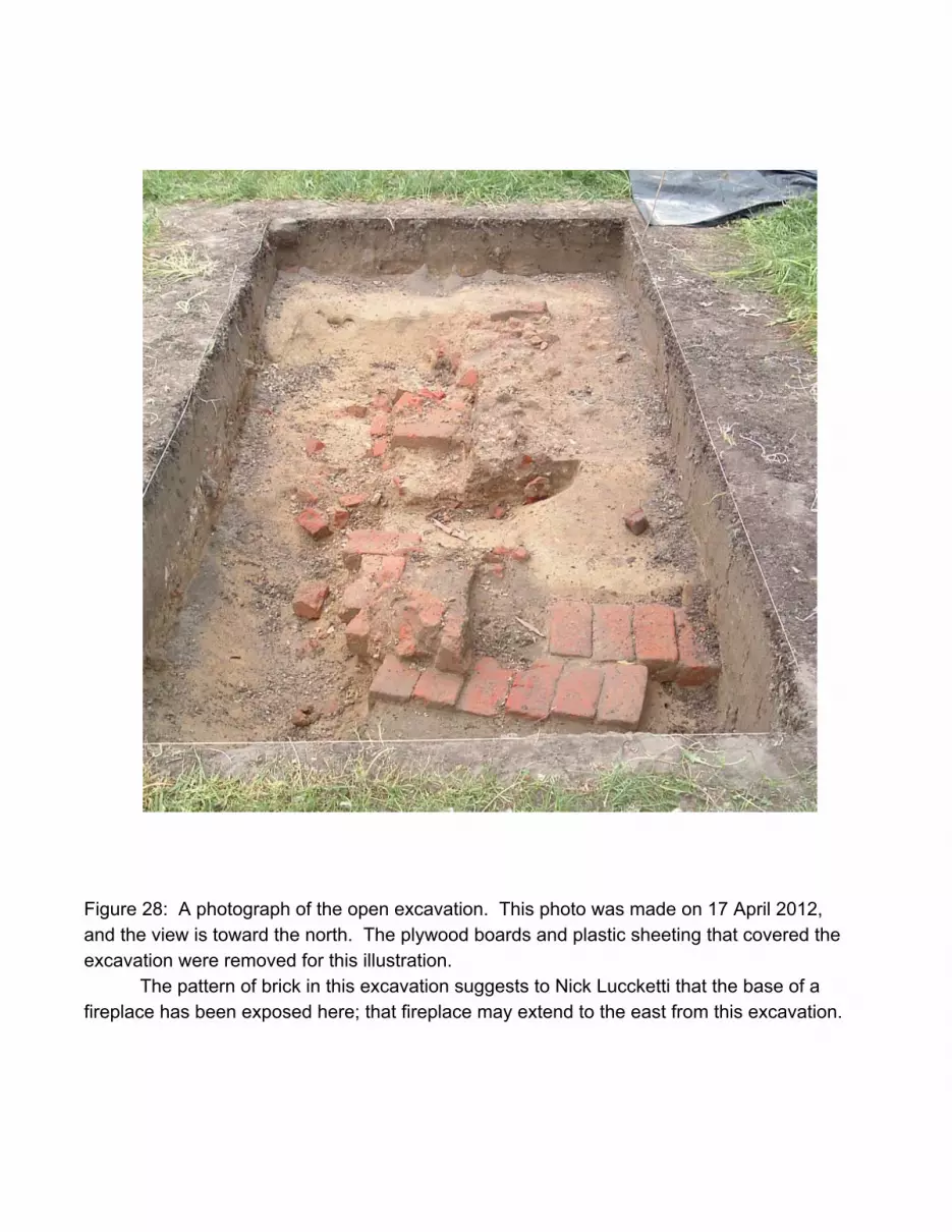
Figure 28: A photograph of the open excavation. This photo was made on 17 April 2012,and the view is toward the north. The plywood boards and plastic sheeting that covered theexcavation were removed for this illustration.

The pattern of brick in this excavation suggests to Nick Luccketti that the base of afireplace has been exposed here; that fireplace may extend to the east from this excavation.

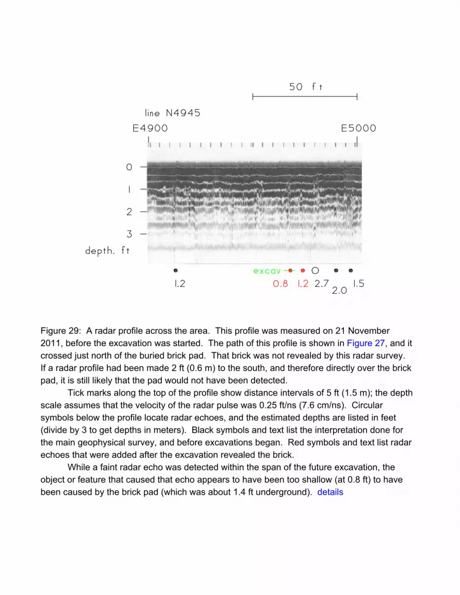
Figure 29: A radar profile across the area. This profile was measured on 21 November2011, before the excavation was started. The path of this profile is shown in Figure 27, and itcrossed just north of the buried brick pad. That brick was not revealed by this radar survey. If a radar profile had been made 2 ft (0.6 m) to the south, and therefore directly over the brickpad, it is still likely that the pad would not have been detected.

Tick marks along the top of the profile show distance intervals of 5 ft (1.5 m); the depthscale assumes that the velocity of the radar pulse was 0.25 ft/ns (7.6 cm/ns). Circularsymbols below the profile locate radar echoes, and the estimated depths are listed in feet(divide by 3 to get depths in meters). Black symbols and text list the interpretation done forthe main geophysical survey, and before excavations began. Red symbols and text list radarechoes that were added after the excavation revealed the brick.

While a faint radar echo was detected within the span of the future excavation, theobject or feature that caused that echo appears to have been too shallow (at 0.8 ft) to havebeen caused by the brick pad (which was about 1.4 ft underground). details

4964 4966 4968 4970 4972East position, ft

-10

0

10

20

30M

agne

tic s

usce

ptib

ility

, ppt

profilesLine N4949Line N4943

open excavation, depth about 1.5 ft

EM38 susceptiblity profiles across excavationHeight = 0.14 ft above original soil surfaceDipoles vertical, measurement spacing = 0.1 ft

Brick rubble on line N4949 from E4968 to E4970Brick layer on line N4943 from E4967 to E4970

Figure 30: Susceptibility profiles across the excavation. Two lines (located in Figure 27)were measured twice. These profiles do not reveal the brick pad. The low (even negative)readings are caused by the open excavation. The two pair of high readings that are markedwith asterisks are caused by a nail (about 3 inch long) that was at the edge of the excavationat E4965 N4949; this nail was not noticed when these measurements were made. details

0 0.2 0.4 0.6 0.8

Magnetic susceptibility, ppt

1.2

0.8

0.4

0

Dep

th, f

t

Measured on a vertical lineat E4970 N4943

Figure 31: Magnetic susceptibility on the face of the excavation. The soil on a verticalsurface near the brick foundation of the fireplace was measured with a hand-held magneticsusceptibility meter. While the values are reasonable for soil, almost all of thesemeasurements were made on fill soil that was added long ago to cover the old soil surface. details

4900 4920 4940 4960 4980 5000East distance, ft

-20

0

20

40

60M

agne

tic s

usce

ptib

ility

, ppt

profilesline 4949line 4943

excavation

EM38 susceptibility profiles across rear yardHeight = 0 ft above soil surfaceDipoles vertical, measurement spacing = 1 ft

high susceptibility

Figure 32: Magnetic susceptibility on long profiles. These extended for a span of 100 ft (30m) and were aligned east-west. The profile of line N4943 crosses the brick pad in the openexcavation, which is marked in the figure. The negative readings at the excavation arecaused by the fact that the magnetic soil below the bottom of the excavation is at a depthwhere materials that are magnetic cause negative values (see Figure 15). details

4850 4875 4900 4925 4950North distance, ft

-20

-10

0

10

20M

agne

tic s

usce

ptib

ility

, ppt

excavation2 ft westLine E4972

N-S susceptibility profile with the EM38Height = 0 ft above soil surveyDipoles vertical, measurement spacing = 1 ft

high susceptibility

Figure 33: A north-south susceptibility profile near the excavation. The path of this traverseis marked in Figure 26. Like the readings in Figure 32, this profile found generally highreadings of susceptibility in the vicinity of the brick pad, but nothing that reveals that pad. The pair of negative readings is caused by a single metallic object that is midway betweenthose lows; this point is marked with an asterisk. details


0

0.2

0.4

0.6Ap

pare

nt s

usce

ptib

ilty,

ppt

Temporal variability of the EM38 in susceptibility modeMeasurement interval = 1 s, dipoles verticalStandard deviation = 0.012 pptSurvey 17 April 2012, 12:59 pm

Figure 34: Electrical interference to the EM38 at Aspen Lawn. While the variability was twicethat shown in Figure 24, it was not unusually large. The test was probably made at E4900N4949 and the cause of the noisiness is not known, although it is probably electricalinterference from buried power or telephone wires that are near the building, even thoughthose wires are mostly on the northern side of the building (Figure 26).

geophysical detection of brick pavements

Documents