engineering sciences
TRANSCRIPT

Academic Studies inENGINEERING SCIENCES
Academic Studies in ENGINEERING SCIENCES
Editor
Assoc. Prof. Dr. Halil İbrahim Kurt
Engineeringlivredelyon.com
livredelyon
livredelyon
livredelyon
ISBN: 978-2-38236-050-7

ACADEMIC STUDIES
IN
ENGINEERING SCIENCES
Editor Assoc. Prof. Dr. Halil İbrahim Kurt
Lyon 2020

Editor • Assoc. Prof. Dr. Halil İbrahim Kurt 0000-0002-5992-8853
Cover Design • Aruull Raja
First Published • December 2020, Lyon
ISBN: 978-2-38236-050-7
© copyright
All rights reserved. No part of this publication may be reproduced, stored
in a retrieval system, or transmitted in any form or by an means, electronic,
mechanical, photocopying, recording, or otherwise, without the publisher’s
permission.
The chapters in this book have been checked for plagiarism by
Publisher • Livre de Lyon
Address • 37 rue marietton, 69009, Lyon France
website • http://www.livredelyon.com
e-mail • [email protected]

I
PREFACE
Experimental researches have contributed to the development of
education and training definitions in various periods. Although the
importance given to science and data-based academic studies is
mentioned today, it is observed that the studies conducted are far from the
scientific method. Disciplinary and/or interdisciplinary studies allow for
synthesis of ideas and the synthesis of characteristics from many
disciplines. At the same time it addresses scientists, engineers and
students’ individual differences and helps to develop important,
transferable skills. These skills, like critical thinking, communication,
analysis, interpretation and discussion are important and continually
developing at all stages of life.
One of the major objectives of this ‘Academic Studies in
Engineering’ was to present evidence and gather together the results of
research and development carried out on the engineering applications
during recent years. The book brought together scientists and engineers
involved in assessing the various engineering areas, with particular
emphasis on academic studies, applications and opinions.
The editor and editorial board hope that this book will be useful
to engineers and to scientists working towards an understanding of and
the resolution of the applications in the various fields of engineering that
we have to face in near future.
Assoc. Prof. Dr. Halil İbrahim Kurt

II
CONTENTS
PREFACE...………………………………………………………….....I
REFEREES………………………………………………………….. V
Chapter I Hasan HASIRCI
THE EFFECTS OF COUNTER GRAVITY CASTING
PROCESS PARAMETERS ON SOLIDIFICATION
BEHAVIOUR OF Al-Si ALLOY PRODUCED BY
REAL CASTING CONDITIONS………………….…...1
Chapter II Oğuz GIRIT
DETERMINATION OF SURFACE ROUGHNESS THROUGH
NOISE OF CUTTING TOOL IN MILLING OF AISI
1040 STEEL...................................................................11
Chapter III Sare ÇELIK & Türker TÜRKOĞLU
EFFECTS OF PROCESS PARAMETERS ON MECHANICAL
PROPERTIES OF Al-Al2O3-B4C HYBRID
COMPOSITES BY USING GREY RELATIONAL
ANALYSIS…………...….............................................39
Chapter IV Hasan HASIRCI
INFLUENCES OF AL AND ALTiB ADDITIONS ON THE
MICROSTRUCTURE AND MECHANICAL
PROPERTIES OF MgZnSn ALLOY POURED INTO
GREEN SAND MOLD……………………………......43
Chapter V Şefika KAYA & Yeliz AŞÇI
ADVANCED OXIDATION PROCESS TO DIFFERENT
INDUSTRIAL WASTEWATERS: SONOFENTON....57
Chapter VI Emine Sıla YIGIT & Fatma TUMSEK
TEMPLATED CARBONS WITH NATURAL ZEOLITE:
SYNTHESIS AND CHARACTERIZATION ………...67
Chapter VII Kamil ORMAN & Yunus BABACAN
MEMORY CIRCUIT ELEMENTS AND APPLICATIONS.....77
Chapter VIII Murat DENER
SMART CAMPUSES AND CAMPUS SECURITY………....103
IV
Chapter IX Ilker Huseyin CELEN & Eray ÖNLER & Hasan
Berk ÖZYURT
DRONE TECHNOLOGY IN PRECISION AGRICULTURE.121
Chapter X Mohammed WADI & Abdulfetah SHOBOLE
HISTORICAL RELIABILITY EVALUATION OF POWER
DISTRIBUTION SYSTEMS BASED ON MONTE
CARLO SIMULATION METHOD…………….........151
Chapter XI Emre DEMIR
NETWORK DISTANCE COEFFICIENT EFFECT ON
DETERMINING TRANSPORTATION FACILITY
LOCATION…………………......................................171
Chapter XII Emre Burcu OZKARAOVA
SUSTAINABLE GROUNDWATER REMEDIATION WITH
BIOBARRIERS USING AGRICULTURAL OR PLANT
PRODUCTION RESIDUES………............................183
Chapter XIII D. Aydınoğlu
ACTIVE FOOD PACKAGING TECHNOLOGY AS AN
APPLICATION IN THE FOOD INDUSTRY.............215

REFEREES
Prof. Dr. Duygu Kavak, Eskişehir Osmangazi University, Turkey
Assoc. Prof. Dr. Ali Hakan Işık Burdur Mehmet Akif Ersoy University,
Turkey
Assoc. Prof. Dr. Cengiz Polat Uzunoğlu, İstanbul University, Turkey
Assoc. Prof. Dr. İbrahim Aydoğdu Akdeniz University, Turkey
Assoc. Prof. Dr. Mehmet Fırat Baran, Siirt University, Turkey
Assoc. Prof. Dr. Sezgin Ersoy, Marmara University, Turkey
Asst. Prof. Dr. Alper Polat Munzur University, Turkey

VI
CHAPTER I
THE EFFECTS OF COUNTER GRAVITY CASTING
PROCESS PARAMETERS ON SOLIDIFICATION
BEHAVIOUR OF Al-Si ALLOY PRODUCED BY REAL
CASTING CONDITIONS
Hasan Hasirci1
1(Assoc. Prof. Dr.), Gazi University, e-mail: [email protected],
0000-0001-5520-4383
1. INTRODUCTION
In each casting process, inherent limitations are exhibited in either
performance or manufacturing cost. These processes include well-
documented technologies, such as low pressure, vacuum-assisted casting,
combinations of low pressure and vacuum, and squeeze casting (Campbell,
1999; Rasmussen, 2000; Dash and Malkhlouf 2001:1). In most cases,
performance is hindered by non-uniform metal flow, entrainment of gases
during the mould filling process, or segregation of impurities during
solidification (Dash and Malkhlouf 2001:1; Lee, Chang and Yeh 1990:187;
Loper and Prucha 1999:165). The development of the Counter Gravity
Casting (CGC) process eliminates these deficiencies by controlling mould
fill to insure true metal flow uniformity, preventing the entrance of gases
during filling and providing both directional and uniform solidification
(Rasmussen, 2000; Dash, 2001:1; Loper, 1999). This results in outstanding
strength and ductility for components produced by the CGC process
(Campbell, 1999; Dash and Malkhlouf 2001:1; Kuo, Hsu and Hwang
2001:2). CGC process is shown in Fig. 1 (Hasirci, 2006). A mould is
prepared from a wet sand mixture with air (gas) permeability to be used in
casting process. The bottom part of the mould has a cavity in order to be
filled up with liquid metal and the mould is immersed under vacuum into
the liquid metal. Vacuum is maintained until solidification of the liquid
metal has been completed. In the subsequent stage, the mould is removed
from the liquid metal. Finally, the mould is broken to get the castings.
The process has many advantages in terms of quality and process
control as well. These advantages include the ability to control the rate of
metal flow; formation of surface slag and re-oxidation macro inclusions
formed by the turbulence of pouring; and uniform fill out of all sections,
including superior flow into sections as thin as 1 mm (Campbell, 1999;
Dash and Malkhlouf 2001:1; Lee, Chang and Yeh 1990:187).

2
Fig. 1. Schematic illustration of the CGC method (Hasirci, 2006)
The increased use of cast alloys in automotive applications such as
engine blocks and cylinder heads creates the need for a deeper
understanding of fatigue performance and the influences of processing
parameters. In designing of cast automotive parts, it is important to have
an intimate knowledge of how alloy solidifies at different cross sections of
the cast part and how this influences mechanical properties (Dobrzañski,
Maniara and Sokolowski 2000:28). This knowledge enables the designer
to ensure that the casting will achieve the desired properties for its intended
application. The casting structure developed during solidification depends
not only on the nucleation potential of the melt, but also on the thermal
gradient imposed during solidification. Therefore, the features of casting
structure (grain size, secondary dendrite arm spacing and silicon
modification level) can be evaluated by examining the cooling curve
parameters (Hasirci, 2006; Dobrzañski, Maniara and Sokolowski
2000:28).
Mentioned above factors are of great importance in determining
material properties. While there are many studies in the literature about the
effects of various casting methods on solidification characteristics, the
effects of CGC method have not been investigated. The aim of this study
was to determine the effects of CGC process at real casting conditions on
cooling rate, grain size and other solidification characteristics of Al–9.42
wt.% Si alloy. At the same time, the grain size, solidification starting
temperature, time and range at different cooling rates (conventional casting
and CGC processes) were examined.
2. EXPERIMENTAL WORKS
The experimental alloy used in this investigation was melted in
electric resistance furnace at 670 ºC. The melt material was poured in
insulated mould (Fig. 2). Molten AlSi alloy was poured under 0 (Gravity
casting), 0.133 and 0.666 bar vacuum levels. The chemical composition of
this alloy is given in Table 1.

3
Fig. 2. Schematic illustration of experimental set-ups; (a) the CGC, and (b)
conventional casting process
Table 1. Chemical compositions of Al-Si commercial alloy
Si Fe Cu Mn Mg
9,42 0,38 0,05 0,431 0,36
Cr Ni Zn Ti Pb
0,015 0,04 0,06 0,10 0011
Al (Bal.)
The test specimens with 50x70 mm dimension were produced at
real casting conditions. The moulds had insulating coatings to allow for
low heat transfer only. Thermal analysis of cooling curve was performed
on all samples using high sensitivity thermocouples of K type (Fig. 2). Data
were acquired by a high speed data acquisition system linked to a personal
computer. Each poured sample was sectioned horizontally where the tip of
the thermocouple was located and it was prepared by standard grinding and
polishing procedures. Light microscopy was used to characterize the
macrostructures. Macrostructure measurements were carried out using an
Image-J analyzer program. Metallographic specimens were etched using
Tucker etching solution (15 ml HF, 45 ml HCl, 15 ml HNO3 and 25 ml
H2O).
3. RESULTS AND DISCUSSION
Research on the effects of the CGC processes on solidification
macro structures, cooling properties, solidification time and temperature is
very limited. In addition, a study on the cooling rate, grain size,
solidification temperature and duration of this method is not available.
Therefore, the results of this study were compared to the former study
results on pressure die and squeeze casting. In some studies (Kuo, Hsu and
Hwang 2001:2; Lee, Kim, Won and Cantor 2002:338; Niu, Hu, Pinwill and
Li 2000:105), it was mentioned that increased heat flow led to accelerated
solid activity. In earlier work (Lee, Kim, Won and Cantor 2002:338), it
4
was pointed out that the increasing applied pressure shortens solidification
time in squeeze casting. The solidification time of a casting by Chvorinov's
rule is the ratio of volume to surface area of casting. Therefore, by
increasing surface area of casting solidification time decreased (Hasirci,
2006). The solidification time also depends on heat transfer constant of
casting alloy and mould material. The effect of pressure on the
solidification time was not taken into consideration in Chvorinov's rule.
The vacuums on solidification processes have two type effects. The first
effect is suction pressure and other is increased cooling rate due to heat
absorption. Solidification under pressure occurs more quickly and reduce
feeding requirement due to the influence of pressure (Hasirci, 2006; Lee,
Kim, Won and Cantor 2002:338). In this study, the experimental results
showed that the increase in applied pressure leads to an increase in
solidification rate and even a very low pressure generates a significant
effect.
CGC process is a kind of low pressure casting method. In this
process, negative pressure (suction by vacuum) was used instead of
positive pressure (push). However, both of them have similar effects on
solidification. On the other hand, in some studies (Shabestari and Malekan
2005:44; Dobzaski, Kasprzak, Sokowski, Maniara and Krupiski 2005;
MacKay, Djurdjevic and Sokolowski 2000; Boileau, Zindel and Allison
1997:106; Bäckerud, Chai and Tamminnen 1992:2), it was found that
processing parameters (i.e. pressure, modification, grain refinement) have
shown a decreasing effect on grain size, solidification temperature and
time. The results of this experimental study revealed that vacuum has a
similar effect.
The casting structure developed during solidification depends not
only on the nucleation potential of the melt, but also on the thermal gradient
imposed during solidification. Therefore, the features of the casting
structure (grain size, silicon modification level) can be evaluated by
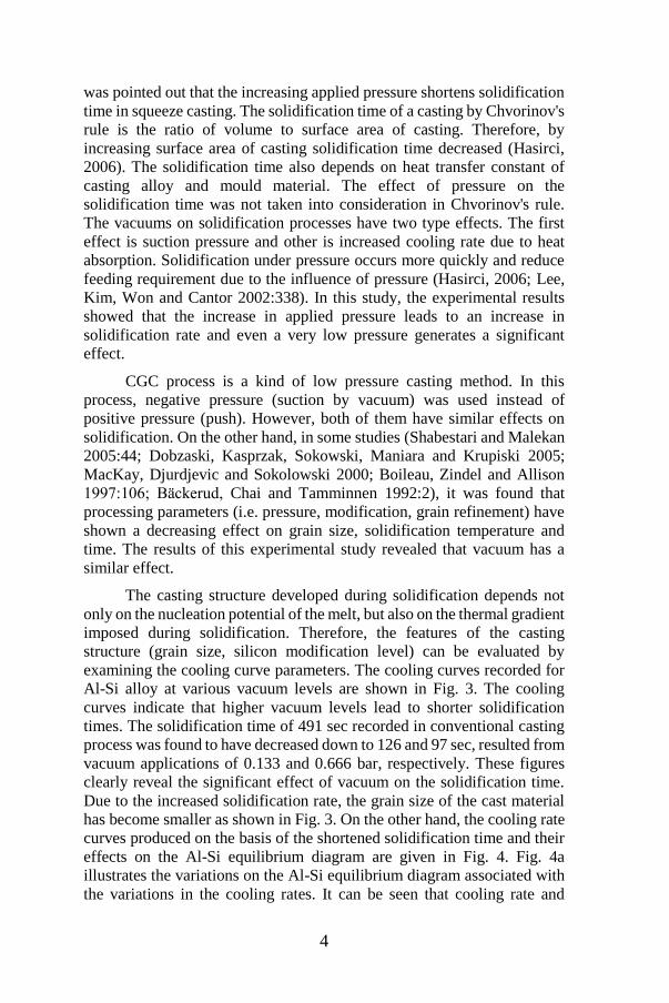
examining the cooling curve parameters. The cooling curves recorded for
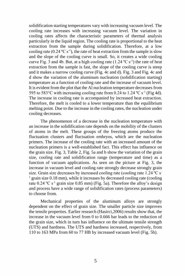
Al-Si alloy at various vacuum levels are shown in Fig. 3. The cooling
curves indicate that higher vacuum levels lead to shorter solidification
times. The solidification time of 491 sec recorded in conventional casting
process was found to have decreased down to 126 and 97 sec, resulted from
vacuum applications of 0.133 and 0.666 bar, respectively. These figures
clearly reveal the significant effect of vacuum on the solidification time.
Due to the increased solidification rate, the grain size of the cast material
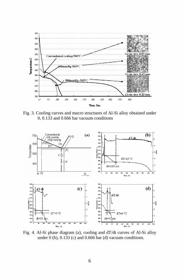
has become smaller as shown in Fig. 3. On the other hand, the cooling rate
curves produced on the basis of the shortened solidification time and their
effects on the Al-Si equilibrium diagram are given in Fig. 4. Fig. 4a
illustrates the variations on the Al-Si equilibrium diagram associated with
the variations in the cooling rates. It can be seen that cooling rate and
5
solidification starting temperatures vary with increasing vacuum level. The
cooling rate increases with increasing vacuum level. The variation in
cooling rates affects the characteristic parameters of thermal analysis
particularly in the liquid region. The cooling rate is proportional to the heat
extraction from the sample during solidification. Therefore, at a low
cooling rate (0.24 ºC s-1), the rate of heat extraction from the sample is slow
and the slope of the cooling curve is small. So, it creates a wide cooling
curve Fig. 3 and 4b. But, at a high cooling rate (1.24 ºC s-1) the rate of heat
extraction from the sample is fast, the slope of the cooling curve is steep
and it makes a narrow cooling curve (Fig. 4c and d). Fig. 3 and Fig. 4c and
d show the variation of the aluminum nucleation (solidification starting)
temperature as a function of cooling rate and the increase of vacuum level.
It is evident from the plot that the Al nucleation temperature decreases from
595 to 583°C with increasing cooling rate from 0.24 to 1.24 ºC s-1 (Fig 4d).
The increase in cooling rate is accompanied by increased heat extraction.
Therefore, the melt is cooled to a lower temperature than the equilibrium
melting point. Due to the increase in the cooling rates, the nucleation under
cooling decreases.
The phenomenon of a decrease in the nucleation temperature with
an increase in the solidification rate depends on the mobility of the clusters
of atoms in the melt. These groups of the freezing atoms produce the
fluctuation clusters and fluctuation embryos, which are the nucleation
primers. The increase of the cooling rate with an increased amount of the
nucleation primers is a well-established fact. This effect has influence on
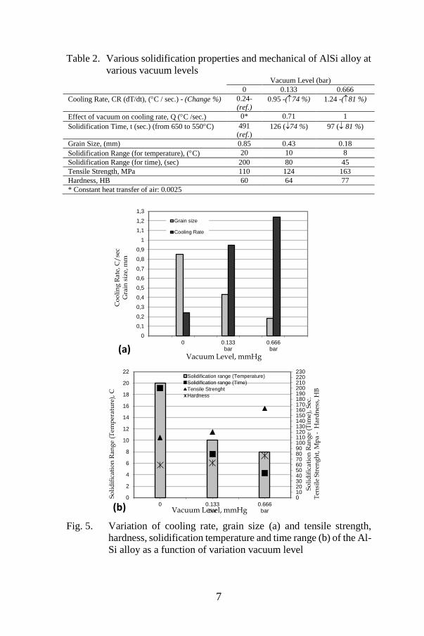
the grain size. Fig. 3, Table 2, Fig. 5a and b show the variation of the grain
size, cooling rate and solidification range (temperature and time) as a
function of vacuum applications. As seen on the picture at Fig. 3, the
increase in vacuum level and cooling rate strongly decrease strongly grain
size. Grain size decreases by increased cooling rate (cooling rate 1.24 ºC s-
1 grain size 0.18 mm), while it increases by decreased cooling rate (cooling
rate 0.24 ºC s-1 grain size 0.85 mm) (Fig. 5a). Therefore the alloy’s design
and process have a wide range of solidification rates (process parameters)
to choose from.
Mechanical properties of the aluminum alloys are strongly
dependent on the effect of grain size. The smaller particle size improves
the tensile properties. Earlier research (Hasirci,2006) results show that, the
increase in the vacuum level from 0 to 0.666 bar leads to the reduction of
the grain size, which in turn has influence on the ultimate tensile strength
(UTS) and hardness. The UTS and hardness increased, respectively, from
110 to 163 MPa from 60 to 77 HB by increased vacuum level (Fig. 5b).
6
Fig. 3. Cooling curves and macro structures of Al-Si alloy obtained under
0, 0.133 and 0.666 bar vacuum conditions
Fig. 4. Al-Si phase diagram (a), cooling and dT/dt curves of Al-Si alloy
under 0 (b), 0.133 (c) and 0.666 bar (d) vacuum conditions.
7
Table 2. Various solidification properties and mechanical of AlSi alloy at
various vacuum levels Vacuum Level (bar)
0 0.133 0.666
Cooling Rate, CR (dT/dt), (C / sec.) - (Change %) 0.24-
(ref.) 0.95 -(74 %) 1.24 -(81 %)
Effect of vacuum on cooling rate, Q (C /sec.) 0* 0.71 1
Solidification Time, t (sec.) (from 650 to 550C) 491
(ref.) 126 (74 %) 97 ( 81 %)
Grain Size, (mm) 0.85 0.43 0.18
Solidification Range (for temperature), (C) 20 10 8
Solidification Range (for time), (sec) 200 80 45
Tensile Strength, MPa 110 124 163
Hardness, HB 60 64 77
* Constant heat transfer of air: 0.0025
Fig. 5. Variation of cooling rate, grain size (a) and tensile strength,
hardness, solidification temperature and time range (b) of the Al-
Si alloy as a function of variation vacuum level
0
0,1
0,2
0,3
0,4
0,5
0,6
0,7
0,8
0,9
1
1,1
1,2
1,3
0 0.133bar
0.666bar
Co
oli
ng
Rat
e, C
/se
cG
rain
siz
e, m
m
Vacuum Level, mmHg
Grain size
Cooling Rate
(a)
0102030405060708090100110120130140150160170180190200210220230
0
2
4
6
8
10
12
14
16
18
20
22
0 0.133bar
0.666bar
So
lid
ific
atio
n R
ang
e (T
ime)
, S
ec.
Ten
sile
Str
eng
ht,
Mp
a -
Har
dn
ess,
HB
So
lid
ific
atio
n R
ang
e (T
emp
erat
ure
), C
Vacuum Level, mmHg
Solidification range (Temperature)
Solidification range (Time)
Tensile Strenght
Hardness
(b)
8
On the other hand, the cooling rate has significant influence on
solidification temperature and time. Solidification temperature and time
range decreased (respectively, from 12 C and 155 sec to 8 C and 45 sec)
with increasing cooling rate (from 0.24 to 1.24 C s-1). Further,
solidification starting temperature (approximately 13 C) also decreased
with increasing cooling rate.
4. CONCLUSIONS
The results are summarized as follows:
Solidification parameters are affected by the vacuum level. The
cooling rate, solidification time and temperatures vary with an
increasing vacuum level.
Increasing the vacuum level increases the cooling rate (81%) and
significantly decreases the solidification (nucleate) range of AlSi alloy
(temperature and time respectively 2 and 81 %) and eutectic
temperature (2 ºC).
These phenomena lead to an increased number of nucleuses that affect
the size of the grains. Increasing the vacuum level significantly
decreases grain size (80%).
Solidification temperature and time range (respectively, from 12 C
and 155 sec to 8 C and 45 sec) decreased as a result of increasing
vacuum level.
9
REFERENCES
1) Campbell J. (1999). Casting. Butterworth –Heinemann, 1-55.
2) Güleyüpoglu S. (1997). Casting process design guidelines.
Transaction of American Foundry Society, 97-83, 869-876.
3) Rasmussen N W. (2000). New filling/feeding process produces
vertically-parted aluminum green sand castings. Modern Casting,
54-55.
4) Dash M and Malkhlouf M. (2001). Effect of key alloying elements on
the feeding characteristics of aluminum - silicon casting alloys.
Journal of Light Metals, 1, 251-265.
5) Lee Y W. Chang E. Lin Y L. and Yeh C H. (1990). Correlation of
feeding and mechanical properties of A206 aluminum alloy plate
casting, Transaction of American Foundry Society, 90-187, 935-
941.
6) Loper Jr C R. and Prucha T E. (1999). Feed metal transfer in AL-Cu-
Si alloys. Transaction of American Foundry Society, 90-165, 845-
853.
7) Kuo J H. Hsu F L. and Hwang W S. (2001). Development of an
interactive simulation system for the determination of the pressure-
time relationship during the filling in a low pressure casting process.
Science and Technology of Advanced Materials, 2, 131-145.
8) Hasirci H. (2006). Investigation of applicability of counter gravity
direction casting processes in green sand mould and effect of process
production casting part on structures and properties. Ph. D. Thesis,
University of Gazi, Institute of Science and Technology, TURKEY.
9) Dobrzañski L A, Maniara R, and Sokolowski J H. (2000). The effect
of cooling rate on microstructure and mechanical properties of AC
AlSi9Cu alloy. Archives of Materials Science and Engineering, 28-
2, 105-112.
10) Lee J H. Kim H S. Won CW. and Cantor B. (2002). Effect of the gap
distance on the cooling behavior and the microstructure of indirect
squeeze cast and gravity die cast 5083 wrought Al alloy. Materials
Science and Engineering A; 338, 182-190.
11) Niu X P. Hu B H. Pinwill I. and Li H. (2000). Vacuum assisted high
pressure die casting of aluminum alloys. Journal of Materials
Processing Technology, 105, 119-127.
12) Shabestari S G. and Malekan M. (2005). Thermal Analysis Study of
the Effect of the Cooling Rate on the Microstructure and

10
Solidification Parameters of 319 Aluminum Alloy. Canadian
Metallurgical Quarterly ISSN 0008-4433, 44-3, 305-312.
13) Dobrzaski L A, Kasprzak W, Sokowski J, Maniara R and Krupiski M.
(2005). Applications of the derivation analysis for assessment of the
ACAlSi7Cu alloy crystallization process cooled with different
cooling rate, COMMENT 2005 Proceedings of the 13th
International Scientific Conference, Gliwice-Wisa, 147-150.
14) MacKay R. Djurdjevic M. and Sokolowski J H. (2000). The Effect of
Cooling Rate on the Fraction Solid of the Metallurgical Reaction in
the 319 Alloy. Transaction of American Foundry Society, 521-530.
15) Boileau J M, Zindel J W and Allison JE. (1997). The Effect of
Solidification Time on the Mechanical Properties in a Cast A356-T6
Aluminum Alloy. Transactions of Automotive Engineers
Society ISSN 0096-736X, 106-5, 63-74.
16) Bäckerud L, Chai G, and Tamminen J. (1992). Solidification
Characteristics of Aluminum Alloys. Transaction of American
Foundry Society, 2, 5-56.

CHAPTER II
DETERMINATION OF SURFACE ROUGHNESS
THROUGH NOISE OF CUTTING TOOL IN MILLING OF
AISI 1040 STEEL
Oğuz Girit
(Asst. Prof. Dr.), Marmara University, e-mail: [email protected]
0000-0003-2287-9936
1. INTRODUCTION
The researchers, continues for reducing the time and the cost
required for manufacturing. Automated production and minimal
processing are one of the most important goals of modern manufacturing
[1]. To achieve this goal, it is highly prioritized to develop techniques to
minimize the needs for intermediate processes in production [2]. The
technology is currently available to researchers and engineers in the
manufacturing process [1]. The control system developed with the
combination of existing technologies reduces both production time and
cost [2]. One of the minor processes is the controlling the surface quality
of the produced part [1]. Determining the surface quality of each part is
both costly and a time consuming job [2]. Therefore, it is possible to
reduce the time and cost allocated to quality control by improving
prediction models and systems [2].
On Computer Numerical Control (CNC) machines, the correct
sizing and surface quality can be achieved by the correct selection of
machining parameters [1]. The machining parameters are parameters such
as cutting, feed, spindle, spindle speeds, depth of cut [2]. The selection of
these parameters is usually made either according to the experience of the
operator, the manual of the machine or the tool catalogs [3]. Nevertheless,
it is difficult to determine the feed and cutting speeds that can provide the
surface roughness and tolerance values specified in the manufacturing
drawings [4].
The tribological properties of the machined part surfaces are
primarily influenced by the surface shape [5]. The surface roughness is not
only an important factor in the traditional areas of tribology such as
abrasion, friction and lubrication, but also at the same time in sealing,
hydrodynamics, electricity, and heat transfer [6,7]. Surface roughness is
the most important factor in the industry. Surface treatments are affected

12
by many variables [5]. Reduction of surface roughness is subject to factors
such as the reduction of depth of cut, the use of low feed and high cutting
speeds, the increase of the coolant flow, the tip radius of the cutting tool
and the large chip angle values [3].
Kopac et al. emphasized what kind of results can be encountered in
the working conditions of tempered AISI 1060 and AISI 4140 steels which
are frequently used in practice and in the workings on the change of surface
roughness as a result of random selection of machining parameters. In their
work, low surface roughness values have been found to be achieved when
using high-radius cutting tools for both steels [8].
In Yuan et al. research on turning, it has been revealed that the
sharpness of a diamond cutting tool is one of the main factors affecting the
machining deformations and the roughness of the machined surface [9].
Their pilot tests with aluminum alloy samples showed that the surface
roughness of the workpiece, the microhardness of the workpiece, the
permanent surface stresses and the dislocation densities changed
depending on the tool tip radius [5]. The surfaces treated with the blunt tool
were found to be stiffer than those machined with a sharp tool [4]. Eriksen
observed the interactions between the different cutting speeds and
advancing speeds, cutting tool tip radius and fiber direction of the
thermoplastics reinforced with short fiber treated by turning [5].
It has been stated that it is possible to determine the optimum
machining conditions experimentally, however it does not match the
calculations of those theoretical parameters [7]. The surface roughness
increases when the feed speed is above 0.1 mm / g, the surface roughness
decreases when the tool tip radius decreases, the surface roughness
deteriorates when the cutting speed reaches 500 m / min, the high cutting
speed up to 1500 m / it is stated that the surface roughness of the processes
is independent of the cutting speed [3].
In this study, one of the most important criteria in determining the
surface quality in machining is the roughness value on the surface of the
produced part [6]. In milling operations, the model was developed and
roughness ratio was estimated by taking into account the shear forces and
vibrations to estimate the surface roughness [10]. In addition, it is possible
to estimate the surface roughness with the change in the pressure level of
the sound generated during cutting [11]. In this study, the change in
acoustic sound pressure during dry processing with DLC coated double
groove carbide end mill in AISI 1040 steel was recorded by microphone
and specialized software [6]. The relationship between the pressure change
of recorded sound and average surface roughness (Ra) was examined and
modeled using linear regression method [11]. In addition, the effect of the
13
cutting parameters on radial, tangential and axial forces was also
investigated [12].
In the research, modern production is one of the most important
targets of production, while also minimizing cost, increasing automation
and minimizing processing for optimal efficiency [3]. To achieve this goal,
it is highly prioritized to develop techniques to minimize the needs for
intermediate processes in production. Technology therefore leads
researchers and engineers in the production process [5]. The control system
developed with the combination of existing technologies reduces both
production time and cost. One of the minor processes is the controlling the
surface quality of the produced part. Controlling the surface quality of each
part is both costly and a time consuming job. Therefore, it is possible to
reduce the time and cost allocated to quality control by improving
estimation models and systems [3].
Ebner et al. measured the acustic sound at high cutting speeds in the
milling machine [13]. Ghosh and colleagues (2007) attempted to estimate
the CNC milling tool wear from the sound changes measured by the
sensors in their work [13]. Matthew et al. concluded that; it has been shown
that the cutting tool changes the sound pressure under various cutting
conditions and gives effective results [14]. Mannan et al. studied the
relationship between surface quality and the analysis of the noise produced
when the cutting tool during chip removal resulting from tool wear [15].
In this study, AISI 1040 medium-carbon steel was recorded in dB
with a specialized software program by listening to the change in acoustic
sound pressure generated by the dry milling of the two-headed DLC coated
carbide end mill. [6]. The relationship between the change in acoustic
sound pressure and surface roughness is examined and modeled by linear
regression. In addition, the forces generated in the dry milling are
interpreted taking into account the cutting parameters [3].
2. MATERIALS AND METHODS
2.1. Material and Experiment
CNC machine used in experimental setup is a milling machine
which is a series of O-M series with FANUC control which can perform
three axis linear and circular interpolation and it can perform ISO format
programming in metric and imperial units [16]. In this study, AISI 1040
medium carbon steel has been chosen as it is widely used. The mechanical
and chemical properties of the AISI 1040 steel material, used as workpiece
in the experimental work, are shown in Table 2. The force and acoustic
sound were recorded on a desktop computer with a KISTLER 9443B
dynamometer platform and a KISTLER 5019B amplifier combined with
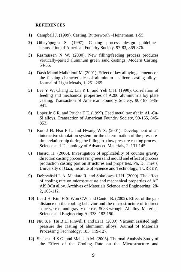
data acquisition. The setup of the experimental work is shown in Figure 1.
14
Figure 1. The experimental setup [3].
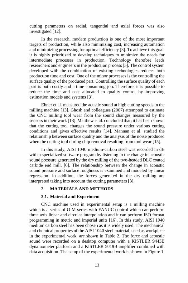
Figure 2. Schematic Presentation of Experiment Plan [3].
15
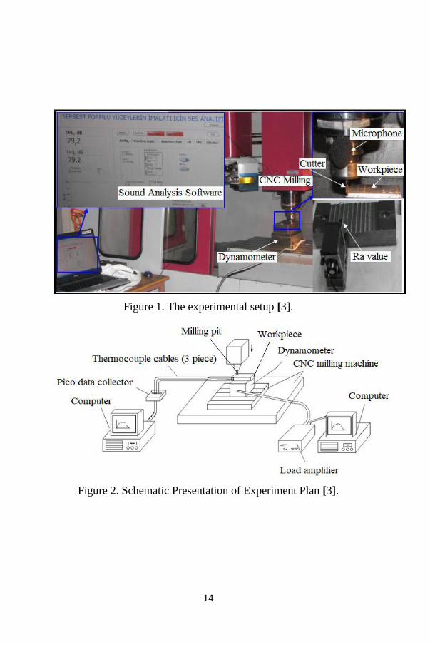
Table 1. CNC Milling Machine Technical Specifications [3].
Model Number VMC – 850 / 550+APC
Table work surface 40‖ x 20‖ (1000 x 500 mm)
Movement boundaries
: 31.5‖ (800 mm)
: 20‖ (500 mm)
: 17.7‖ (450 mm)
Spindle Motor power 10 HP (30 min.) / 7.4 HP (cnot)
Table loading capacity 1980 Lbs (900 kg)
Machine floor area 92.5‖ x 98.4‖ (2350 x 2500)
Machine weight 12100 Lbs (5500 kg)
Table 2. Mechanical and chemical (%) properties of AISI 1040 steel
material [12].
Hardness
(Bhn)
Flowing
(MPa)
Rupture
(MPa)
Elongation
(%)
Chemical structure
(%)
170 353 518 25
Fe(98.07);
C(0.329);
Cr(0.036); Cu(0.2);
Mn(0.69); Si(0.22);
Ni(0.01); Co(0.02);
Mo(0.02).
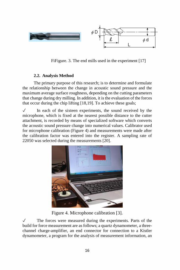
DLCM List 9330 end mills of NACHI company were used in this
study (Figure 3). The cutting tools used in this study have a full length (L)
= 60 mm, (l)= 20 mm, a stem diameter (d) = 10 mm, and a cutting mouth
diameter (D) = 9 mm.
16
FiFigure. 3. The end mills used in the experiment [17]
2.2. Analysis Method
The primary purpose of this research; is to determine and formulate
the relationship between the change in acoustic sound pressure and the
maximum average surface roughness, depending on the cutting parameters
that change during dry milling. In addition, it is the evaluation of the forces
that occur during the chip lifting [18,19]. To achieve these goals;
✓ In each of the sixteen experiments, the sound received by the
microphone, which is fixed at the nearest possible distance to the cutter
attachment, is recorded by means of specialized software which converts
the acoustic sound pressure change into numerical values. Calibrator used
for microphone calibration (Figure 4) and measurements were made after
the calibration factor was entered into the register. A sampling rate of
22050 was selected during the measurements [20].
Figure 4. Microphone calibration [3].
✓ The forces were measured during the experiments. Parts of the
build for force measurement are as follows; a quartz dynamometer, a three-
channel charge-amplifier, an end connector for connection to a Kistler
dynamometer, a program for the analysis of measurement information, an

17
ISA type A / D board for computer connection and interconnecting cables
[21].
✓ Cutting forces measured in tangential, radial and axial directions
are transformed into computer graphics using DynoWare software. After
each test, Ra values of the average surface roughness at the working
surface were measured by the MARH-Perthometer [21].
✓ The relationship between acoustic noise variation and average
surface roughness is modeled by a linear regression model [22].
✓ The relationship between radial, tangential and axial forces and
shear parameters is investigated [10].
3. EXPERIMENTAL DESIGN
Influence of the cutting parameters and the effect of cutting
geometry and parameters on surface roughness Ra and cutting force N on
milling of a AISI 1040 steel is discussed in this section [23]. Experimental
design has been carried out by Taguchi method in this study because the
traditional experiment design has been required to be highly complex,
challenging and it has to be repeated too many times [22, 24, 25]. Taguchi
method is beneficial for the experimental design of the machinability of
AISI 1040 steel material. Having optimized parameters is also fruitful for
keeping the response values at required levels [23]. In the experimental
study; cutting speed v = 40-130 m / min, feed rate f = 30-120 mm / g, and
chip depth, a = 0.75-3 mm. The L16 experimental design made according
to the Taguchi Method and the results measured during the experimental
study are shown in Table 3.
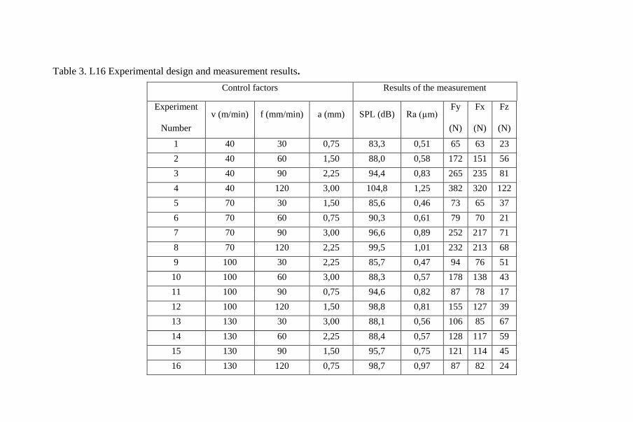
Table 3. L16 Experimental design and measurement results.
Control factors Results of the measurement
Experiment
Number
v (m/min) f (mm/min) a (mm) SPL (dB) Ra (µm) Fy
(N)
Fx
(N)
Fz
(N)
1 40 30 0,75 83,3 0,51 65 63 23
2 40 60 1,50 88,0 0,58 172 151 56
3 40 90 2,25 94,4 0,83 265 235 81
4 40 120 3,00 104,8 1,25 382 320 122
5 70 30 1,50 85,6 0,46 73 65 37
6 70 60 0,75 90,3 0,61 79 70 21
7 70 90 3,00 96,6 0,89 252 217 71
8 70 120 2,25 99,5 1,01 232 213 68
9 100 30 2,25 85,7 0,47 94 76 51
10 100 60 3,00 88,3 0,57 178 138 43
11 100 90 0,75 94,6 0,82 87 78 17
12 100 120 1,50 98,8 0,81 155 127 39
13 130 30 3,00 88,1 0,56 106 85 67
14 130 60 2,25 88,4 0,57 128 117 59
15 130 90 1,50 95,7 0,75 121 114 45
16 130 120 0,75 98,7 0,97 87 82 24

4. EXPERIMENTAL RESULTS AND EVALUATION
4.1. Evaluation of Acoustic Sound Change and Ra
Measurement Results
The change in the level of the acoustic sound obtained from the
experimental studies according to the two most effective cutting
parameters is given graphically in Figure 4. The sound pressure is
expressed in terms of "dB SPL"; is a term that refers to the sound pressure
level that acoustic sound waves apply to air molecules.
94 dB equals to SPL = 1 Pascal = 10 microbes. As seen in Figure 5,
the increase in the progression rate has resulted in an increase in the
acoustic volume. The change effect of the increase in chip depth on the
acoustic sound pressure is significantly lesser than the effect of the
progress rate.
Figure 5. Change in acoustic sound level depending on chip depth and
progress rate
20
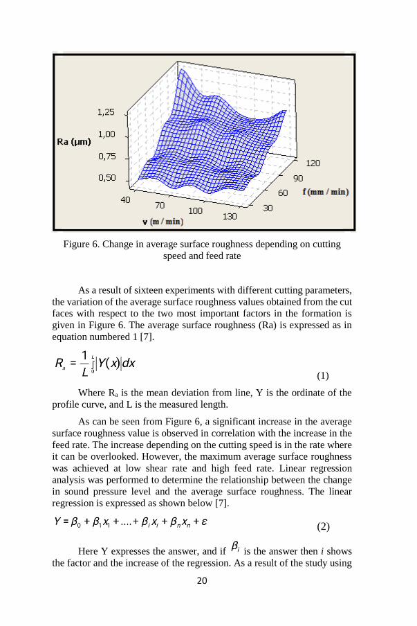
Figure 6. Change in average surface roughness depending on cutting
speed and feed rate
As a result of sixteen experiments with different cutting parameters,
the variation of the average surface roughness values obtained from the cut
faces with respect to the two most important factors in the formation is
given in Figure 6. The average surface roughness (Ra) is expressed as in
equation numbered 1 [7].
(1)
Where Ra is the mean deviation from line, Y is the ordinate of the
profile curve, and L is the measured length.
As can be seen from Figure 6, a significant increase in the average
surface roughness value is observed in correlation with the increase in the
feed rate. The increase depending on the cutting speed is in the rate where
it can be overlooked. However, the maximum average surface roughness
was achieved at low shear rate and high feed rate. Linear regression
analysis was performed to determine the relationship between the change
in sound pressure level and the average surface roughness. The linear
regression is expressed as shown below [7].
(2)
Here Y expresses the answer, and if is the answer then i shows
the factor and the increase of the regression. As a result of the study using
21
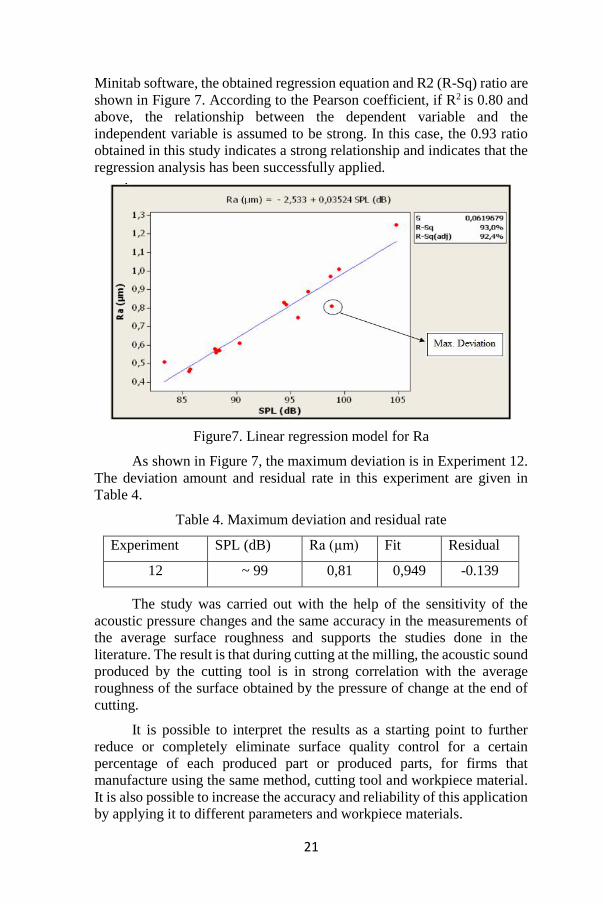
Minitab software, the obtained regression equation and R2 (R-Sq) ratio are
shown in Figure 7. According to the Pearson coefficient, if R2 is 0.80 and
above, the relationship between the dependent variable and the
independent variable is assumed to be strong. In this case, the 0.93 ratio
obtained in this study indicates a strong relationship and indicates that the
regression analysis has been successfully applied.
Figure7. Linear regression model for Ra
As shown in Figure 7, the maximum deviation is in Experiment 12.
The deviation amount and residual rate in this experiment are given in
Table 4.
Table 4. Maximum deviation and residual rate
Experiment SPL (dB) Ra (µm) Fit Residual
12 ~ 99 0,81 0,949 -0.139
The study was carried out with the help of the sensitivity of the
acoustic pressure changes and the same accuracy in the measurements of
the average surface roughness and supports the studies done in the
literature. The result is that during cutting at the milling, the acoustic sound
produced by the cutting tool is in strong correlation with the average
roughness of the surface obtained by the pressure of change at the end of
cutting.
It is possible to interpret the results as a starting point to further
reduce or completely eliminate surface quality control for a certain
percentage of each produced part or produced parts, for firms that
manufacture using the same method, cutting tool and workpiece material.
It is also possible to increase the accuracy and reliability of this application
by applying it to different parameters and workpiece materials.

22
4.2. Evaluation of Radial, Tangential and Axial Forces
Measurements of the shear forces generated during dry milling are
another consideration in this work. During manufacturing similar
workpiece material, it is important to determine the shear forces required
by the cutting tool during tooling in regards to tool wear and, of course,
workpiece surface quality.
In the study, Radial (Fy), Tangential (Fx) and Axial (Fz) forces that
occurred during cutting were measured using Kistler dynamometer and
amplifier. As expected, maximum forces were generated in the radial
direction (Figure 8). It is seen that the most effective factor is the rate of
progression in Figure 8, where two cutting parameters with dominant effect
on the formation of radial force. In addition, the increase in chip depth has
also increased the radial force.
From the perspective of the effect of the cutting parameters, the tangential
force measurement results, which show a similar tendency to the radial
force, are shown in Figure 9. In the formation of tangential force, the
dominant two factors are the feed rate and chip depth. However, tangential
force values were slightly less than radial force.
Figure 8. The effect of depth of cut and feed rate on radial force
generation
23
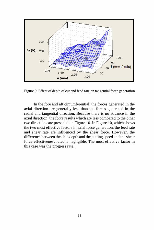
Figure 9. Effect of depth of cut and feed rate on tangential force generation
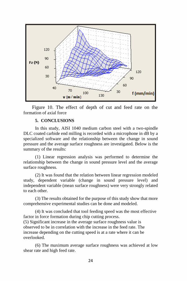
In the fore and aft circumferential, the forces generated in the
axial direction are generally less than the forces generated in the
radial and tangential direction. Because there is no advance in the
axial direction, the force results which are less compared to the other
two directions are presented in Figure 10. In Figure 10, which shows
the two most effective factors in axial force generation, the feed rate
and shear rate are influenced by the shear force. However, the
difference between the chip depth and the cutting speed and the shear
force effectiveness rates is negligible. The most effective factor in
this case was the progress rate.
24
Figure 10. The effect of depth of cut and feed rate on the formation of axial force
5. CONCLUSIONS
In this study, AISI 1040 medium carbon steel with a two-spindle
DLC coated carbide end milling is recorded with a microphone in dB by a
specialized software and the relationship between the change in sound
pressure and the average surface roughness are investigated. Below is the
summary of the results:
(1) Linear regression analysis was performed to determine the
relationship between the change in sound pressure level and the average
surface roughness.
(2) It was found that the relation between linear regression modeled
study, dependent variable (change in sound pressure level) and
independent variable (mean surface roughness) were very strongly related
to each other.
(3) The results obtained for the purpose of this study show that more
comprehensive experimental studies can be done and modeled.
(4) It was concluded that tool feeding speed was the most effective
factor in force formation during chip cutting process.
(5) Significant increase in the average surface roughness value is
observed to be in correlation with the increase in the feed rate. The
increase depending on the cutting speed is at a rate where it can be
overlooked.
(6) The maximum average surface roughness was achieved at low
shear rate and high feed rate.

25
(7) According to the Pearson coefficient, if R 2 is 0.80 and above,
the relationship between the dependent variable and the independent
variable is assumed to be strong. In this case, the 0.93 ratio obtained in this
study indicates a strong relationship and indicates that the regression
analysis has been successfully applied.
26
REFERENCES
[1] E. Yamaguti, J.F.A. Romero, A. Zanandrea, ABCM Symposium
Series Mechatronic. 2, 121 (2006).
[2] B.H. Amstead, P.F. Ostwald, M.L. Begeman. Manufacturing
Processes. 8th Edition. Singapore: John Willey & Sons Inc
1987.
[3] A. Akay. University of Marmara, Ins Pure and Applied Sci,
Mecha. Eng. (Master Thesis), İstanbul, Turkey (2009).
[4] T. Akasawa, H. Sakurai, M.T. Nakamura. J. Mater. Proces.
Technol. 143-144: 66 (2003).
[5] M. Kurt, E. Bagci, Y. Kaynak. Int. J. Adv. Manuf. Technol. 40,
458 (2009). DOI 10.1007/s00170-007-1368-2
[6] J. Paulo Davim. J. Mater. Proces. Technol. 116, 305 (2001).
DOI: 10.1016/S0924-0136(01)01063-9
[7] I,S, Kannan, A. Ghosh. Procedia Mater. Sci. 5, 2615 (2014).
DOI:10.1016/j. mspro. 2014.07.522
[8] J. Kopac, M. Bahor. J. Mater. Proces. Technol. 92–93, 381
(1999).
[9] Z. J. Yuan, M. Zhou, S. Dong. J. Mater. Proces. Technol. 62,
:327 (1996).
[10] P.T. Mativenga, N.A. Abukhshim, M.A. Sheikh. J. Eng. Manuf.
220, 657 (2005).
[11] S. Yıldız, B. Unsaçar. Measurement. 39, 80 (2006).
[12] Computer Numerical Control (CNC) Machining Accelerator
Toolkit For FANUC Series 30i-B, 31i-B, 32i-B, and 35i-B
CNC Systems Rockwell Automation Publication.
Luxemburg. (2012).
[13] I. D. Y. Ebner, J. F. A. Romero, A. Zanandrea, O. Saotome, J.
O. Gomes. ABCM Symposium Series in Mechatronic. 2, 121
(2006).
[14] S. C. Matthew, A. Mann, J. Gagliardi. Applied Acoustics. 43,
333 (1994).
[15] M. A. Mannan, A.A. Kassim, M. Jing. Pattern Recognition
Letters. 21, 969 (2000).
27
[16] K. Nagatomi, K. Yoshida, K. Banshoya. Mokuzai Gakkaishi.
40, 434 (1994).
[17] Nachi-Fujikoshi Corp. www.nachi-
fujikoshi.co.jp/eng/news/index.html. Catalog. Accessed 29
May 2018
[18] B. Prashanth, K. Jayabalan. Inter. J. Civil. Eng. Technol. 8, 115
(2017).
[19] N. Ghosh, Y.B. Ravi, A. Patra. Mecha. Syst. Signal. Proces. 21,
466 (2007).
[20] V. Ostasevicius, V. Jurenas, V. Augutis. Int. J. Adv. Manuf.
Technol. 88, 2803 (2017).
[21] P. N. Botsaris, J. A. Tsanakas. The International Conference of
COMADEM, Prague. 73 (2008).
[22] I. Korkut. Gazi Üniversity, Graduate School of Natural and
Applied Sciences, Doctora Thesis. Ankara. (1996).
[23] M. Ay. Acta Physica Polonica A, 131, 349 (2017).
[24] S. C. Carney, J. A. Mann, J. Gagliardi. Applied Acoustics. 43,
333 (1994).
[25] R. K. Roy. A primer on the taguchi method. Van Nostrand
Reinhold; New York (1990).

28
CHAPTER III
EFFECTS OF PROCESS PARAMETERS ON
MECHANICAL PROPERTIES OF Al-Al2O3-B4C HYBRID
COMPOSITES BY USING GREY RELATIONAL ANALYSIS
Sare Çelik1 & Türker Türkoğlu2
1(Prof. Dr.), Balikesir University, e-mail: [email protected]
0000-0001-8240-5447
2(MSc.), Balikesir University, e-mail: [email protected]
0000-0002-0499-9363
1.INTRODUCTION
Material properties such as high specific stiffness, strength, and
wear resistance are also strengthened by particle reinforced metal matrix
composites. These characteristics are also preferred in many areas and in
particular, aluminum metal matrix composites are responsible for the
energy absorption of structural components in the automotive sector
(Hedayatian, Momeni, Nezamabadi, & Vahedi, 2020; Kwon, Saarna,
Yoon, Weidenkaff, & Leparoux, 2014; Sharma, Nanda, & Pandey, 2018).
Boron carbide (B4C) with a high melting temperature has many
superior properties such as high compressive strength, high hardness,
chemical stability. In addition to these features, it is its negative feature
that it gives brittleness to the materials of which it is a component. As well
as high hardness and wear resistance, Alumina (Al2O3) decreases residual
stress on fracture toughness (Alihosseini, Dehghani, & Kamali, 2017;
Węglewski et al., 2019).
Metal matrix composites can be produced by a wide variety of
production methods such as powder metallurgy, stir casting, friction stir
processing (Avettand-Fènoël & Simar, 2016; Pang, Xian, Wang, & Zhang,
2018; Ramanathan, Krishnan, & Muraliraja, 2019). The most efficient
process is known to be manufacturing with powder metallurgy
(Yamanoglu, Daoud, & Olevsky, 2018). Compared to the stir casting
method, the dispersion of the reinforcements in the matrix would increase
the mechanical alloying of the matrix and reinforcement powders before
the powder metallurgy process. By avoiding these possible cluster
structures, it has been observed that the mechanical properties of the
produced composites have also improved. Cluster morphologies act like

30
stress density areas that accelerate crack production and cause losses from
mechanical properties (Bhoi, Singh, & Pratap, 2020).
Optimization provides to increase the benefits obtained by
minimizing the costs in many areas such as design, analysis, and
production in the industry. By analyzing the effects of factors on multi-
response, the Grey Relational Analysis method can evaluate optimal
process parameters for multiple experimental outcomes. Generally, Grey
Relational Analysis is performed by combining with the Taguchi method
(Kumar, 2020; Montgomery, 2017)
The volume percentage and size of the reinforcement are typically
the factors influencing the properties of hybrid composites. Studies
examining the effect of single/dual reinforcement size on mechanical
properties remained limited. In the optimization and the production
processes of composite materials, the optimum production parameters have
been determined by combining the Grey Relational Analysis method with
Taguchi in our study, since the Taguchi method was relatively insufficient
in explaining the multi-response characteristics. By using these methods
together, both individual response optimization and multiple response
optimization of production parameters can be possible. In this study, the
effect of single/dual size reinforcement and production parameters on
microstructural and mechanical properties of composites were investigated
and optimum process parameters were defined by Grey Relational
Analysis (GRA) combined with the Taguchi Analysis.
2. MATERIALS METHOD
Pure Al (purity 99.5%) was used as a matrix material in the study.
Al and Al2O3 powders have an average particle size of 60 μm, while B4C
powders have been selected to have a single/dual B4C reinforced particle
size (40 μm/40 μm+60 μm). Reinforcement content used in the study, it
has been fixed 10 wt.% B4C and 10 wt.% Al2O3. The powder metallurgy
method is determined as the method of consolidation of powders. Samples
were produced by the hot press and by grouping them according to
temperatures of 500 °C-600 °C, ball milling treatment, and B4C
reinforcement type. Table 1 shows the process parameters. The hybrid
composites were produced 15 mm in diameter and 10 mm in thickness.
Hardness measurements of hybrid composites load of 10 kg, applied
for 10 seconds. In order to determine the average hardness values, 5
measurements were taken from each sample. The compression test was
conducted by Zwick/Roel test machine at room temperature, loading speed
of 1 mm/min. The compacted microstructure was also investigated by an
optical microscope. Finally, experimental and numerical values were
investigated using the Grey Relational Analysis (GRA) method combined
with the Taguchi Analysis, and the results were presented comparatively.

31
Ball milling and B4C reinforcement size type parameters used in the study
have been defined as 0 and 1. In these definitions, it is defined as 1 if the
ball milling operation has been conducted and 0 if it is not. B4C
reinforcement size (40 μm) has been expressed as 0, while B4C
reinforcement size (40 μm+60 μm) has been expressed as 1.
Table 1: Process Parameters
Sample Ball milling B4C
reinforcement
size type
(single/dual)
Sintering
Temperature (°C)
1 0 0 500
2 0 0 600
3 1 0 500
4 1 0 600
5 0 1 500
6 0 1 600
7 1 1 500
8 1 1 600
3.RESULTS AND DISCUSSION
Hybrid composites for all production parameters have been
successfully produced by the powder metallurgy method.
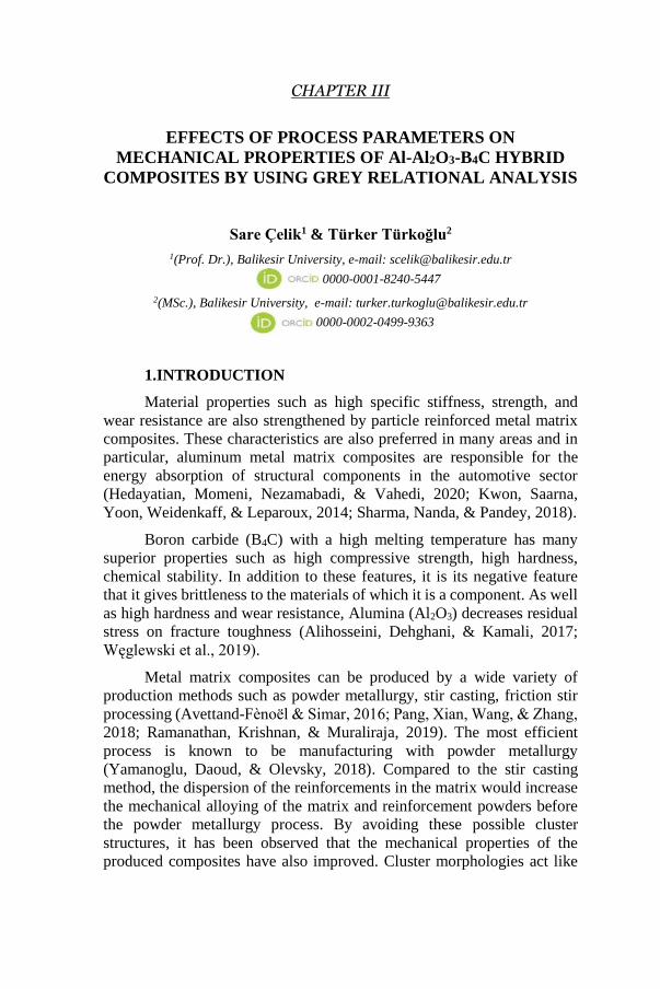
Microstructures were examined using an optical microscope and
camera connected to it. In Figure 1, it is observed that the reinforcements
are distributed uniformly within the matrix for all production parameters.
However, it has been determined that there are partial agglomeration zones
in the materials containing fine size reinforcement. It was stated in previous
studies that the reason for this uniform distribution in the internal structure
is the mechanical alloying process.
32
Figure 1: Optical microstructures of Hybrid Composite Samples
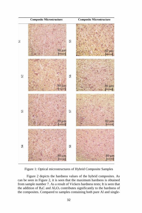
Figure 2 depicts the hardness values of the hybrid composites. As
can be seen in Figure 2, it is seen that the maximum hardness is obtained
from sample number 7. As a result of Vickers hardness tests; It is seen that
the addition of B4C and Al2O3 contributes significantly to the hardness of
the composites. Compared to samples containing both pure Al and single-
33
particle size B4C reinforcement, higher hardness values were obtained for
composites with dual particle size B4C. The reason for the hardness
increase in hybrid composites, It is thought that ceramic reinforcements
have higher hardness compared to aluminum metal (Asghar et al., 2018).
Homogeneous dispersion of ceramic particles by mechanical alloying
before hot pressing, and composite particle strength through the
strengthening of the dislocation density (Fan et al., 2018).
Figure 2: Hardness Values of Hybrid Composites
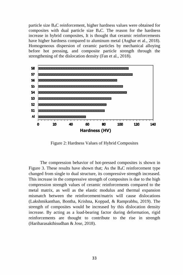
The compression behavior of hot-pressed composites is shown in
Figure 3. These results have shown that; As the B4C reinforcement type
changed from single to dual structure, its compressive strength increased.
This increase in the compressive strength of composites is due to the high
compression strength values of ceramic reinforcements compared to the
metal matrix, as well as the elastic modulus and thermal expansion
mismatch between the reinforcement/matrix will cause dislocations
(Lakshmikanthan, Bontha, Krishna, Koppad, & Ramprabhu, 2019). The
strength of composites would be increased by this dislocation density
increase. By acting as a load-bearing factor during deformation, rigid
reinforcements are thought to contribute to the rise in strength
(Hariharasakthisudhan & Jose, 2018).
Hardness (HV)
34
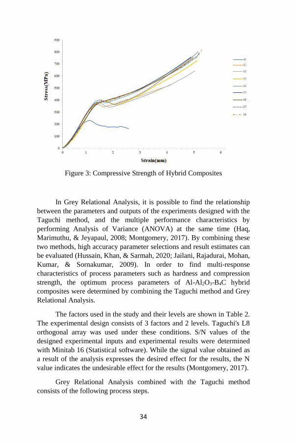
Figure 3: Compressive Strength of Hybrid Composites
In Grey Relational Analysis, it is possible to find the relationship
between the parameters and outputs of the experiments designed with the
Taguchi method, and the multiple performance characteristics by
performing Analysis of Variance (ANOVA) at the same time (Haq,
Marimuthu, & Jeyapaul, 2008; Montgomery, 2017). By combining these
two methods, high accuracy parameter selections and result estimates can
be evaluated (Hussain, Khan, & Sarmah, 2020; Jailani, Rajadurai, Mohan,
Kumar, & Sornakumar, 2009). In order to find multi-response
characteristics of process parameters such as hardness and compression
strength, the optimum process parameters of Al-Al2O3-B4C hybrid
composites were determined by combining the Taguchi method and Grey
Relational Analysis.
The factors used in the study and their levels are shown in Table 2.
The experimental design consists of 3 factors and 2 levels. Taguchi's L8
orthogonal array was used under these conditions. S/N values of the
designed experimental inputs and experimental results were determined
with Minitab 16 (Statistical software). While the signal value obtained as
a result of the analysis expresses the desired effect for the results, the N
value indicates the undesirable effect for the results (Montgomery, 2017).
Grey Relational Analysis combined with the Taguchi method
consists of the following process steps.

35
Step 1:
Determination of inputs and possible outputs in the production
process.
Table 2: Parameters and Levels of the Experimental Process
Parameters Level 1 Level 2
B4C reinforcement size
type 0 1
Ball milling 0 1
Temperature (°C) 500 600
Step 2:
Choosing the appropriate orthogonal arrays in the Taguchi method.
In this study, L8 orthogonal array was chosen (Table 3.)
Table 3: Orthogonal design L8 for responses
Sample Factors Responses
B4C
reinforcement
size type
Ball
Milling
Temp.
(°C)
Hardness
(HV)
Comp. St.
(MPa)
1 0 0 500 81 524
2 0 0 600 83 641
3 0 1 500 89 727
4 0 1 600 108 794
5 1 0 500 103 755
6 1 0 600 96 751
7 1 1 500 115 805
8 1 1 600 110 813
Step 3:
Evaluating the outputs by performing the experimental analysis.
Step 4:
Choosing the appropriate one for the following formulas and
calculating the S/N values.

36
i) If the results are to be maximized in the study; Larger the better
approach should be chosen. As it was desired to maximize hardness
and compressive strength values, Larger the better approach was
chosen in this study by using Equation 1.
𝑆
𝑁 𝑅𝑎𝑡𝑖𝑜 = −10𝑙𝑜𝑔10 (
1
𝑛) ∑
1
𝑦𝑖2
𝑛
𝑖=1
(1)
ii) If the results are to be minimized in the study; Smaller the better
approach should be chosen by using Equation 2.
𝑆
𝑁𝑅𝑎𝑡𝑖𝑜 = −10𝑙𝑜𝑔10 (
1
𝑛∑ 𝑦𝑖
2
𝑛
𝑖=1
) (2)
Step 5
Due to the different data values in the process, the calculated S / N
Ratio values are normalized between 0 and 1. Normalization is a method
of transformation that allows data to be distributed evenly and reduced to
a range that is made possible. Table 4 presents S/N ratio and normalized
S/N Ratio for hardness and compressive strength.
Table 4: S/N ratio and normalized S/N Ratio for Hardness and
Compressive Strength
Sample Response 1(Hardness) Response 2 (Comp. St.)
S/N ratio Normalized
S/N ratio
S/N ratio Normalized
S/N ratio
1 38,1697 0 54,3866 0
2 38,3816 0,06959 56,1372 0,45883
3 38,9878 0,26873 57,2307 0,74545
4 40,6685 0,82081 57,9964 0,94616
5 40,2567 0,68556 57,5589 0,83149
6 39,6454 0,48475 57,5128 0,81940
7 41,2140 1 58,1159 0,97748
8 40,8279 0,8731 58,2018 1

37
In Equation 3, the larger the better approach has been formulated.
𝑋𝑖𝑗∗ = (
𝑋𝑖𝑗 − 𝑚𝑖𝑛𝑗(𝑋𝑖𝑗)
𝑚𝑎𝑥𝑗(𝑋𝑖𝑗) − 𝑚𝑖𝑛𝑗(𝑋𝑖𝑗)) (3)
In Equation 4, the smaller the better approach has been formulated.
𝑋𝑖𝑗∗ = (
𝑚𝑎𝑥𝑗(𝑋𝑖𝑗) − 𝑋𝑖𝑗
𝑚𝑎𝑥𝑗(𝑋𝑖𝑗) − 𝑚𝑖𝑛𝑗(𝑋𝑖𝑗)) (4)
Since it was desired to have maximum compressive strength and
hardness values, Equation 3 was used for all target functions in the study.
Step 6
The Grey Relational co-efficient values of the normalized S / N
values were calculated using the following formula (Equation 5).
𝜁𝑖(𝑧) =𝛥𝑚𝑖𝑛 + 𝜁𝛥𝑚𝑎𝑥
𝛥0𝑖(𝑧) + 𝜁𝛥𝑚𝑎𝑥 (5)
K is the coefficient value, defined in the range 0≤K≤1
Step 7
Determination of Grey Relational Grade stages.
Grey relational grade is calculated by using Equation 6. Grey relational
coefficients, grey relational grade, and rank values are displayed in Table
5.
𝛾𝑖 =1
𝑛∑ 𝜁𝑖(𝑧)
𝑛
𝑧=1
(6)

38
Table 5: Grey Relational Coefficients, Grey Relational Grade and Rank
Values
Sample Grey relational coefficient Grey
relational
grade
Rank Hardness Comp. St.
1 0,33333 0,333333 0,333 8
2 0,34955 0,480231 0,415 7
3 0,40608 0,662654 0,534 6
4 0,73617 0,902792 0,819 3
5 0,61392 0,747939 0,681 4
6 0,49249 0,734649 0,614 5
7 1 0,956913 0,978 1
8 0,79766 1 0,899 2
Step 8
Determination of optimum performance factors
On the basis of grey relational grade, processing parameters effect
and optimum process parameters were calculated. In the light of these
evaluations, the initial optimum process parameters were obtained as a
combination of B4C reinforcement size type. 1, Ball Milling 1, and
sintering temperature 500 °C. Following these steps, when grey relational
grade values were calculated by Taguchi analysis, it was observed that the
highest effect on the process was achieved with Dual particle B4C
reinforced size and Ball Milled process.
Step 9
ANOVA for significant values
Further verification analysis was also performed through moreover
ANOVA. The results of the ANOVA are presented in Table 6. From
response Table 6, the Most effective parameters were determined
effectively. B4C reinforcement type and ball milling parameters were
found to be significant on multi-performance characteristics. (P-value
<0.05) Temperature is an important factor in sintering reactions in the
composite production process by the powder metallurgy method. Although
the temperature factor is expressed as insignificant in the optimization part
of the study, it is concluded that the two sintering temperature values used
in the study are sufficient for the composite production process since the
obtained mechanical properties are appropriate.
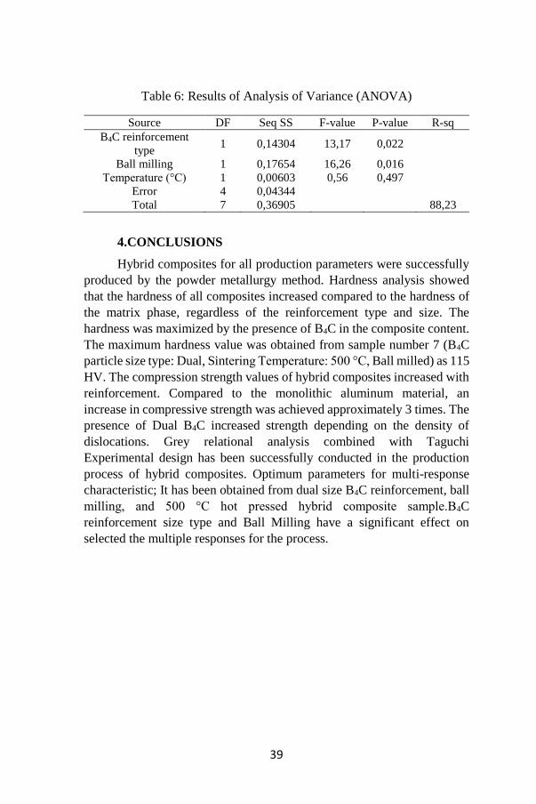
39
Table 6: Results of Analysis of Variance (ANOVA)
Source DF Seq SS F-value P-value R-sq
B4C reinforcement
type 1 0,14304 13,17 0,022
Ball milling 1 0,17654 16,26 0,016
Temperature (°C) 1 0,00603 0,56 0,497
Error 4 0,04344
Total 7 0,36905 88,23
4.CONCLUSIONS
Hybrid composites for all production parameters were successfully
produced by the powder metallurgy method. Hardness analysis showed
that the hardness of all composites increased compared to the hardness of
the matrix phase, regardless of the reinforcement type and size. The
hardness was maximized by the presence of B4C in the composite content.
The maximum hardness value was obtained from sample number 7 (B4C
particle size type: Dual, Sintering Temperature: 500 °C, Ball milled) as 115
HV. The compression strength values of hybrid composites increased with
reinforcement. Compared to the monolithic aluminum material, an
increase in compressive strength was achieved approximately 3 times. The
presence of Dual B4C increased strength depending on the density of
dislocations. Grey relational analysis combined with Taguchi
Experimental design has been successfully conducted in the production
process of hybrid composites. Optimum parameters for multi-response
characteristic; It has been obtained from dual size B4C reinforcement, ball
milling, and 500 °C hot pressed hybrid composite sample.B4C
reinforcement size type and Ball Milling have a significant effect on
selected the multiple responses for the process.
40
REFERENCES
Alihosseini, H., Dehghani, K., & Kamali, J. (2017). Microstructure
characterization, mechanical properties, compressibility and
sintering behavior of Al-B4C nanocomposite powders. Advanced
Powder Technology, 28(9), 2126–2134.
https://doi.org/10.1016/j.apt.2017.05.019
Asghar, Z., Latif, M. A., Rafi-ud-Din, Nazar, Z., Ali, F., Basit, A., …
Subhani, T. (2018). Effect of distribution of B4C on the mechanical
behaviour of Al-6061/B4C composite. Powder Metallurgy, 61(4),
293–300. https://doi.org/10.1080/00325899.2018.1501890
Avettand-Fènoël, M. N., & Simar, A. (2016). A review about Friction Stir
Welding of metal matrix composites. Materials Characterization,
120, 1–17. https://doi.org/10.1016/j.matchar.2016.07.010
Bhoi, N. K., Singh, H., & Pratap, S. (2020). Developments in the aluminum
metal matrix composites reinforced by micro/nano particles – A
review. Journal of Composite Materials, 54(6), 813–833.
https://doi.org/10.1177/0021998319865307
Fan, G., Jiang, Y., Tan, Z., Guo, Q., Xiong, D. bang, Su, Y., … Zhang, D.
(2018). Enhanced interfacial bonding and mechanical properties in
CNT/Al composites fabricated by flake powder metallurgy. Carbon,
130, 333–339. https://doi.org/10.1016/j.carbon.2018.01.037
Haq, A. N., Marimuthu, P., & Jeyapaul, R. (2008). Multi response
optimization of machining parameters of drilling Al/SiC metal
matrix composite using grey relational analysis in the Taguchi
method. International Journal of Advanced Manufacturing
Technology, 37(3–4), 250–255. https://doi.org/10.1007/s00170-
007-0981-4
Hariharasakthisudhan, P., & Jose, S. (2018). Influence of metal powder
premixing on mechanical behavior of dual reinforcement (Al2O3
(μm)/Si3N4 (nm)) in AA6061 matrix. Journal of Alloys and
Compounds, 731, 100–110.
https://doi.org/10.1016/j.jallcom.2017.10.002
Hedayatian, M., Momeni, A., Nezamabadi, A., & Vahedi, K. (2020).
Effect of graphene oxide nanoplates on the microstructure, quasi-
static and dynamic penetration behavior of Al6061 nanocomposites.
Composites Part B: Engineering, Vol 182.
https://doi.org/10.1016/j.compositesb.2019.107652
Hussain, M. Z., Khan, S., & Sarmah, P. (2020). Optimization of powder
metallurgy processing parameters of Al2O3/Cu composite through
Taguchi method with Grey relational analysis. Journal of King Saud

41
University - Engineering Sciences, 32(4), 274–286.
https://doi.org/10.1016/j.jksues.2019.01.003
Jailani, H. S., Rajadurai, A., Mohan, B., Kumar, A. S., & Sornakumar, T.
(2009). Multi-response optimisation of sintering parameters of Al-
Si alloy/fly ash composite using Taguchi method and grey relational
analysis. International Journal of Advanced Manufacturing
Technology, 45(3–4), 362–369. https://doi.org/10.1007/s00170-
009-1973-3
Kumar, M. (2020). Mechanical and Sliding Wear Performance of AA356-
Al2O3/SiC/Graphite Alloy Composite Materials: Parametric and
Ranking Optimization Using Taguchi DOE and Hybrid AHP-GRA
Method. Silicon. https://doi.org/10.1007/s12633-020-00544-9
Kwon, H., Saarna, M., Yoon, S., Weidenkaff, A., & Leparoux, M. (2014).
Effect of milling time on dual-nanoparticulate-reinforced aluminum
alloy matrix composite materials. Materials Science and
Engineering A, 590, 338–345.
https://doi.org/10.1016/j.msea.2013.10.046
Lakshmikanthan, A., Bontha, S., Krishna, M., Koppad, P. G., &
Ramprabhu, T. (2019). Microstructure, mechanical and wear
properties of the A357 composites reinforced with dual sized SiC
particles. Journal of Alloys and Compounds, 786, 570–580.
https://doi.org/10.1016/j.jallcom.2019.01.382
Montgomery, D. C. (2017). Design and Analysis of Experiments Ninth
Edition (Ninth). Opgehaal van https://lccn.loc.gov/2017002355
Pang, X., Xian, Y., Wang, W., & Zhang, P. (2018). Tensile properties and
strengthening effects of 6061Al/12 wt%B4C composites reinforced
with nano-Al2O3 particles. Journal of Alloys and Compounds, 768,
476–484. https://doi.org/10.1016/j.jallcom.2018.07.072
Ramanathan, A., Krishnan, P. K., & Muraliraja, R. (2019). A review on
the production of metal matrix composites through stir casting –
Furnace design, properties, challenges, and research opportunities.
Journal of Manufacturing Processes, Vol 42, bll 213–245.
https://doi.org/10.1016/j.jmapro.2019.04.017
Sharma, S., Nanda, T., & Pandey, O. P. (2018). Effect of dual particle size
(DPS) on dry sliding wear behaviour of LM30/sillimanite
composites. Tribology International, 123(November 2017), 142–
154. https://doi.org/10.1016/j.triboint.2017.12.031
Węglewski, W., Krajewski, M., Bochenek, K., Denis, P., Wysmołek, A.,
& Basista, M. (2019). Anomalous size effect in thermal residual
stresses in pressure sintered alumina-chromium composites.

42
Materials Science and Engineering A, 762(July).
https://doi.org/10.1016/j.msea.2019.138111
Yamanoglu, R., Daoud, I., & Olevsky, E. A. (2018). Spark plasma
sintering versus hot pressing–densification, bending strength,
microstructure, and tribological properties of Ti5Al2.5Fe alloys.
Powder Metallurgy, 61(2), 178–186.
https://doi.org/10.1080/00325899.2018.1441777
CHAPTER IV
INFLUENCES OF AL AND ALTiB ADDITIONS ON THE
MICROSTRUCTURE AND MECHANICAL PROPERTIES OF
MgZnSn ALLOY POURED INTO GREEN SAND MOLD
Hasan Hasirci1
1(Assoc. Prof. Dr.), Gazi University, e-mail: [email protected],
0000-0001-5520-4383
1. INTRODUCTION
Magnesium alloys have low density and other benefits such as: a
good vibration damping and the best from among all construction
materials: high dimension stability, connection of low density and huge
strength with reference to small mass, possibility to have application in
machines and with ease to put recycling process, which makes probability
to logging derivative alloys a very similar quality to original material
(Carlson, B.E. 1997; Cao and Wessén, 2004:35A; Cao, P., Qian, M. and
StJohn, D.H. 2004:5; Zhang, Z. R., and Tremblay, D. D. 2004: 385; Yang,
M. and Pan, F. 2010:31; Liang, M. X., Xiang, W., Lin, L. X. and Lei, Y.
2010:201-6). A desire to create as light vehicle constructions as possible
and connected with it low fuel consumption have made it possible to make
use of magnesium alloys as a constructional material in car wheels, engine
pistons, gear box and clutch housings, skeletons of sunroofs, framing of
doors, pedals, suction channels, manifolds, housings of propeller shafts,
differential gears, brackets, radiators and others (Dobrzański, L.A., Tański,
T., Čížek, L. and Domagała J. 2008:31).
Magnesium alloys generally produced by sand casting, pressure die
casting, permanent mold casting, squeeze casting, low pressure and
counter gravity casting are preferred because of having light weight and
good mechanical properties (Carlson, B.E. 1997; Zhang, Z. R., and
Tremblay, D. D. 2004: 385; Kurnaz, S.C., Sevik, H., Açıkgöz, S. and Özel,
A. 2011:509). These alloys can also be successfully sand cast providing
some general principles be followed, which are dictated by the particular
physical properties and chemical reactivity of magnesium (Carlson, B.E.
1997; Rzychoń, T., Kiełbus, A. and Lityńska-Dobrzyńska, L. 2013:83).
Because, sand casting is easier and cheaper than other casting processes.
Metal flow should be as smooth as possible to minimize oxidation.
Because of the low density of magnesium, there is a relatively small
pressure head in risers and sprues to assist the filling of molds. Sand molds

44
need to be permeable and the mold must be well vented to allow the
expulsion of air.
In general, magnesium alloys are based on Mg–Al systems, which
are relatively cheap, compared with other magnesium alloys available. It
is well known, Al containing Mg alloys include the β-Mg17 Al12 compound
that detrimentally influences the mechanical properties such as tensile
strength and impact resistance (Cao and Wessén, 2004:35A; Candan , S.,
Unal , M., Koc, E., Turen, Y. and Candan, E. 2010:509). One of the most
efficient ways to decrease the detrimental effect of the β-Mg17 Al12 phase
on the mechanical properties is to addition third alloying element
(Srinivasan, J. Swaminathan, M.K. Gunjan, U.T. Pillai, S. and Pai, B.C.
2010:527; Kim, B.H., Lee, S.W., Park, Y.H. and Park, I.M. 2010:493;
Suresh, M., Srinivasan, A., Ravi, K.R., Pillai, U.T.S. and B.C. Pai.
2009:525). The problem with early magnesium alloy castings was that
grain size tended to be large and variable, which often resulted in poor
mechanical properties, micro porosity and, in the case of wrought products,
excessive directional UTS of properties. Values of proof stress also tended
to be particularly low relative to tensile strength. Alloying element is added
to improve properties, especially grain refinement elements. Ca is an
effective way to improve the mechanical properties of AZ91 alloys at
elevated temperatures (Candan , S., Unal , M., Koc, E., Turen, Y. and
Candan, E. 2010:509; Wenwen, D., Yangshan, S., Xuegang, M., Feng, X.,
Min, Z. and Dengyun, W. 2003:356; Wu, G., Fan, Y., Gao, H., Zhai, C.
and Zhu, Y.P. 2005:408; Zhou, W., Aung, N.N. and Sun, Y. 2009:51;
Guangyin, Y., Yangshan, S. and Wenjiang, D. 2001:308; Wang, F., Wang,
Y., Mao, P., Lu, B. and Guo, Q. 2010:20). Other elements such as Sb, Bi
and Pb to AZ91 alloy could also increase the tensile strength and creep
resistance significantly (Candan , S., Unal , M., Koc, E., Turen, Y. and
Candan, E. 2010:509; Srinivasan, J. Swaminathan, M.K. Gunjan, U.T.
Pillai, S. and Pai, B.C. 2010:527; Zhou, W., Aung, N.N. and Sun, Y.
2009:51
Guangyin, Y., Yangshan, S. and Wenjiang, D. 2001:308). A recent
study (Kim, B.H., Lee, S.W., Park, Y.H., Park J. I.M. 2010:493) showed
that the presence of Sn contributed to the room and the elevated
temperature strength of magnesium alloy attributed to the formation of
dispersed short rod-like Mg2Sn phases. The addition of B in the form of
Al-4B master alloy significantly refines the grain size of AZ91 leading to
an improvement in the mechanical properties (Suresh, M., Srinivasan, A.,
Ravi, K.R., Pillai, U.T.S. and B.C. Pai. 2009:525). The beneficial effects
of rare-earth (RE) on mechanical properties including strength and creep
resistance of AZ91 alloys also have been reported (Candan , S., Unal , M.,
Koc, E., Turen, Y. and Candan, E. 2010:509). It is well known that Al–
5Ti–B master alloy is an effective grain refiner in aluminum alloys, and it
45
could also refine the magnesium alloy, and TiB2 particles were found to
nucleate the α-Mg grains. However, due to the low boron content, there is
a relatively small amount of TiB2 particles present in the Al–5Ti–B master
alloy. In this paper, the Ti to B atomic ratio is changed to improve the
effectiveness of the master alloy and to eliminate the residual Ti so as to
generate a larger amount of TiB2 particles and produce a new Al–4Ti–5B
master alloy (Wang, Y., Zeng X. and Ding,W. 2006:54; Chen, T.J., Wang,
R.Q., Ma, Y. and Hao, Y. 2012:34; Ma, X., Wang, X., Li, X. and Yang,
L. 2010:20; Xu, C., Lu, B., Lu, Z. and Liang, W. 2008:26).
The aim of the present study is to investigate the mechanical
properties and the microstructure of alloyed with different and high
amounts of Al and AlTiB of MgZnSn by surface coated and controlled
atmosphere sand casting.
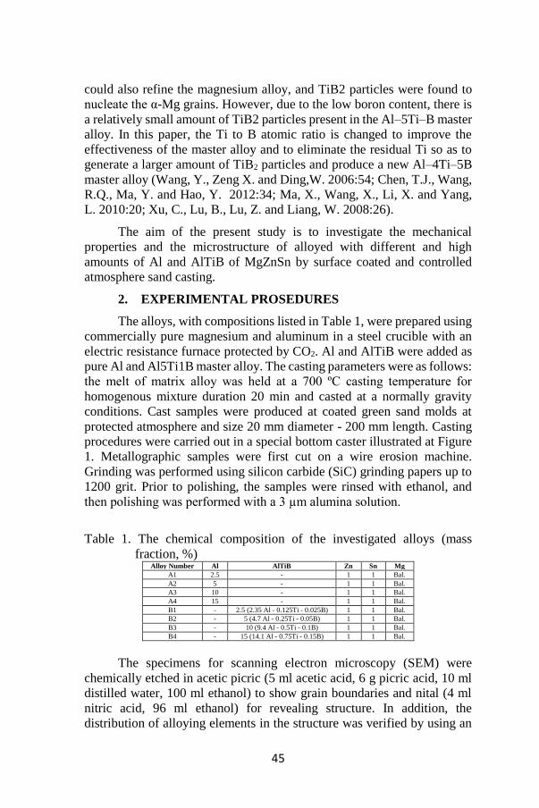
2. EXPERIMENTAL PROSEDURES
The alloys, with compositions listed in Table 1, were prepared using
commercially pure magnesium and aluminum in a steel crucible with an
electric resistance furnace protected by CO2. Al and AlTiB were added as
pure Al and Al5Ti1B master alloy. The casting parameters were as follows:
the melt of matrix alloy was held at a 700 ºC casting temperature for
homogenous mixture duration 20 min and casted at a normally gravity
conditions. Cast samples were produced at coated green sand molds at
protected atmosphere and size 20 mm diameter - 200 mm length. Casting
procedures were carried out in a special bottom caster illustrated at Figure
1. Metallographic samples were first cut on a wire erosion machine.
Grinding was performed using silicon carbide (SiC) grinding papers up to
1200 grit. Prior to polishing, the samples were rinsed with ethanol, and
then polishing was performed with a 3 µm alumina solution.
Table 1. The chemical composition of the investigated alloys (mass
fraction, %) Alloy Number Al AlTiB Zn Sn Mg
A1 2.5 - 1 1 Bal.
A2 5 - 1 1 Bal.
A3 10 - 1 1 Bal.
A4 15 - 1 1 Bal.
B1 - 2.5 (2.35 Al - 0.125Ti - 0.025B) 1 1 Bal.
B2 - 5 (4.7 Al - 0.25Ti - 0.05B) 1 1 Bal.
B3 - 10 (9.4 Al - 0.5Ti - 0.1B) 1 1 Bal.
B4 - 15 (14.1 Al - 0.75Ti - 0.15B) 1 1 Bal.
The specimens for scanning electron microscopy (SEM) were
chemically etched in acetic picric (5 ml acetic acid, 6 g picric acid, 10 ml
distilled water, 100 ml ethanol) to show grain boundaries and nital (4 ml
nitric acid, 96 ml ethanol) for revealing structure. In addition, the
distribution of alloying elements in the structure was verified by using an
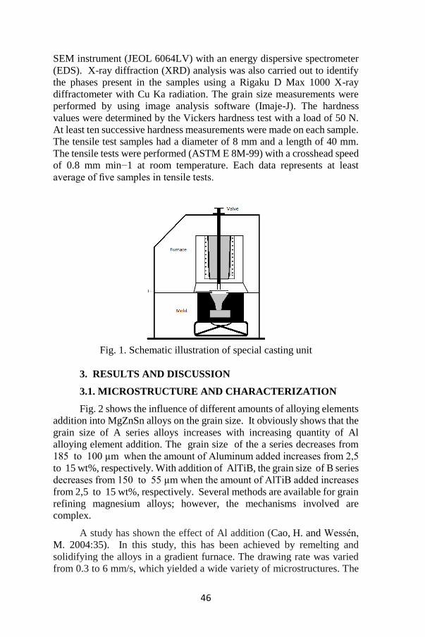
46
SEM instrument (JEOL 6064LV) with an energy dispersive spectrometer
(EDS). X-ray diffraction (XRD) analysis was also carried out to identify
the phases present in the samples using a Rigaku D Max 1000 X-ray
diffractometer with Cu Ka radiation. The grain size measurements were
performed by using image analysis software (Imaje-J). The hardness
values were determined by the Vickers hardness test with a load of 50 N.
At least ten successive hardness measurements were made on each sample.
The tensile test samples had a diameter of 8 mm and a length of 40 mm.
The tensile tests were performed (ASTM E 8M-99) with a crosshead speed
of 0.8 mm min−1 at room temperature. Each data represents at least
average of five samples in tensile tests.
Fig. 1. Schematic illustration of special casting unit
3. RESULTS AND DISCUSSION
3.1. MICROSTRUCTURE AND CHARACTERIZATION
Fig. 2 shows the influence of different amounts of alloying elements
addition into MgZnSn alloys on the grain size. It obviously shows that the
grain size of A series alloys increases with increasing quantity of Al
alloying element addition. The grain size of the a series decreases from
185 to 100 µm when the amount of Aluminum added increases from 2,5
to 15 wt%, respectively. With addition of AlTiB, the grain size of B series
decreases from 150 to 55 µm when the amount of AlTiB added increases
from 2,5 to 15 wt%, respectively. Several methods are available for grain
refining magnesium alloys; however, the mechanisms involved are
complex.
A study has shown the effect of Al addition (Cao, H. and Wessén,
M. 2004:35). In this study, this has been achieved by remelting and
solidifying the alloys in a gradient furnace. The drawing rate was varied
from 0.3 to 6 mm/s, which yielded a wide variety of microstructures. The
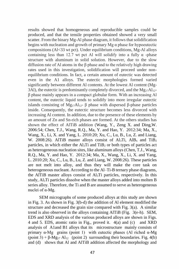
47
results showed that homogeneous and reproducible samples could be
produced, and that the tensile properties obtained showed a very small
scatter. From the binary Mg-Al phase diagram, it follows that solidification
begins with nucleation and growth of primary Mg α phase for hypoeutectic
compositions (Al<33 wt pct). Under equilibrium conditions, Mg-Al alloys
containing less than 12.7 wt pct Al will solidify into a fully α -phase
structure with aluminum in solid solution. However, due to the slow
diffusion rate of Al atoms in the β phase and to the relatively high drawing
rates used in this investigation, solidification will proceed under non-
equilibrium conditions. In fact, a certain amount of eutectic was detected
even in the A1 alloys. The eutectic morphologies formed varied
significantly between different Al contents. At the lowest Al content (Mg-
3Al), the eutectic is predominantly completely divorced, and the Mg17Al12-
β phase mainly appears in a compact globular form. With an increasing Al
content, the eutectic liquid tends to solidify into more irregular eutectic
islands consisting of Mg17Al12- β phase with dispersed β-phase particles
inside. Consequently, the eutectic structure becomes less divorced with
increasing Al content. In addition, due to the presence of these elements by
an amount of Zn and Sn-rich phases are formed. At the others studies has
shown the effect of AlTiB addition (Wang, Y., Zeng X. and Ding,W.
2006:54; Chen, T.J., Wang, R.Q., Ma, Y. and Hao, Y. 2012:34; Ma, X.,
Wang, X., Li, X. and Yang, L. 2010:20; Xu, C., Lu, B., Lu, Z. and Liang,
W. 2008:26). AlTiB master alloys consist of Al3Ti, AlBx and TiB2
particles, in which either the Al3Ti and TiB2 or both types of particles act
as heterogeneous nucleation sites, like aluminum alloys (Chen, T.J., Wang,
R.Q., Ma, Y. and Hao, Y. 2012:34; Ma, X., Wang, X., Li, X. and Yang,
L. 2010:20; Xu, C., Lu, B., Lu, Z. and Liang, W. 2008:26). These particles
are not melt into alloy, and thus they will make the core task on
heterogeneous nucleant. According to the Al–Ti-B ternary phase diagrams,
the AlTiB master alloys consist of Al3Ti particles, respectively. In this
study, Al3Ti particles dissolve when the master alloys added into molten B
series alloy. Therefore, the Ti and B are assumed to serve as heterogeneous
nuclei of α-Mg.
SEM micrographs of some produced alloys at this study are shown
in Fig. 3. As shown in Fig. 3(b-d) the addition of Al element modified the
structure and decreased the grain size compared with Fig. 3(a). A similar
trend is also observed in the alloys containing AlTiB (Fig. 3(e-h). SEM,
EDS and XRD analysis of the various produced alloys are shown in Figs.
4 and 5. EDS, atomic ratio in Fig., proved it. 4(a) and (c) and XRD
analysis of A1and B1 alloys that its microstructure mainly consists of
primary α-Mg grains (point 1) with eutectic phases (Al riched α-Mg
(point 3) + β-Mg17 Al12 (point 2) surrounding their boundaries. Fig. 4(b)
and (d) shows that Al and AlTiB addition affected the morphology and
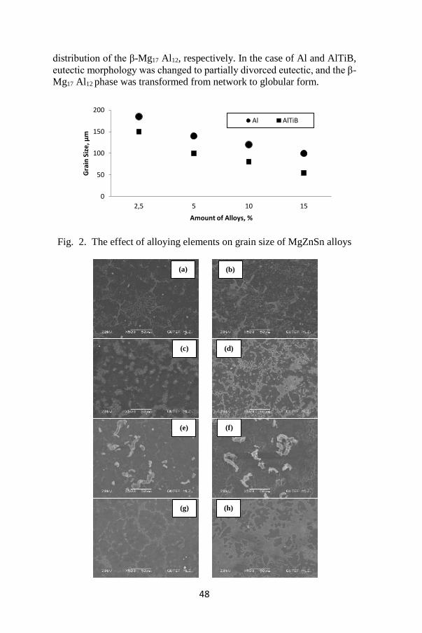
48
distribution of the β-Mg17 Al12, respectively. In the case of Al and AlTiB,
eutectic morphology was changed to partially divorced eutectic, and the β-
Mg17 Al12 phase was transformed from network to globular form.
Fig. 2. The effect of alloying elements on grain size of MgZnSn alloys
0
50
100
150
200
2,5 5 10 15
Gra
in S
ize
, µm
Amount of Alloys, %
Al AlTiB
(a)
(h) (g)
(f) (e)
(c) (d)
(b)
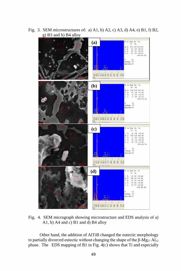
49
Fig. 3. SEM microstructures of: a) A1, b) A2, c) A3, d) A4, e) B1, f) B2,
g) B3 and h) B4 alloy
Fig. 4. SEM micrograph showing microstructure and EDS analysis of a)
A1, b) A4 and c) B1 and d) B4 alloy
Other hand, the addition of AlTiB changed the eutectic morphology
to partially divorced eutectic without changing the shape of the β-Mg17 Al12
phase. The EDS mapping of B1 in Fig. 4(c) shows that Ti and especially
(a)
(c)
(b)
(d)

50
B have extremely low or unknown solubility in Mg lattice and it is likely
that fine particles of pure Ti exist at around grain boundaries. Similar
results were reported by studies (Chen, T.J., Wang, R.Q., Ma, Y. and Hao,
Y. 2012:34; Ma, X., Wang, X., Li, X. and Yang, L. 2010:20; Xu, C., Lu,
B., Lu, Z. and Liang, W. 2008:26). For the β-Mg17 Al12 phase in B4 alloys,
titanium-containing particles may act as the heterogeneous nucleation site.
Therefore, the one of the main effects of Ti and B on microstructure is the
formation of partially divorced Mg17Al12 phase, as shown in Fig. 4(d).
When the studies on grain refinement in Mg materials are examined, it will
be seen that the grain refiner is generally used at low rates (0.1-2%). It is
not seen in these studies what results will be obtained if the grain refiner is
added at a high rate. One of the main objectives of this study is to
demonstrate the effects of high AI and ALTiB content. The results showed
that the increase in the addition amount was effective in reducing the grain
size, and that these addition rates could be used safely and successfully.
The XRD spectrums (Fig. 5.a-b) of all the alloys show that Al
addition did not result in the formation of Al containing any new phase.
But, other XRD spectrums (Fig. 5.c-d) of all the alloys show that AlTiB
addition result in the formation of containing at least some Ti and B
containing new phase (as impurities of AlB, TiB, AlTi etc.). However, it
can be seen in Fig. 5 (d) that α-Mg was detected in specimens and the
amount and shape of phase was greatly reduced with increasing Ti and B
with contained impurities of these alloys. In addition, β-Mg17 Al12 was
detected in specimens AlTi particles. β phase is smaller with increasing
amounts of AlTi particles.
Fig. 5. The XRD spectrums of a) A1, b) A4, c) B1 and d) B4 alloy
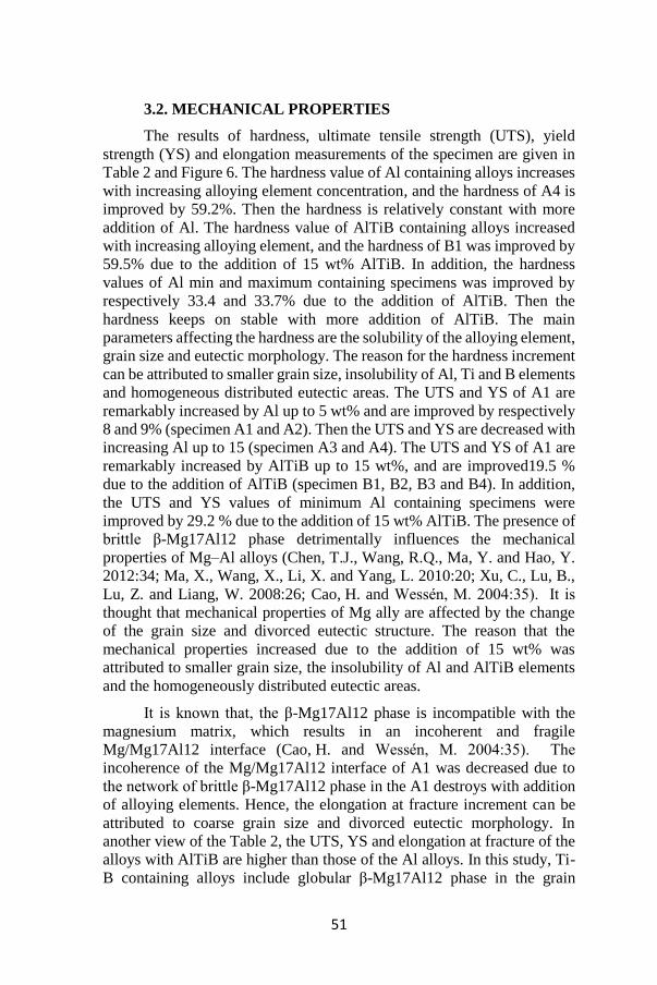
51
3.2. MECHANICAL PROPERTIES
The results of hardness, ultimate tensile strength (UTS), yield
strength (YS) and elongation measurements of the specimen are given in
Table 2 and Figure 6. The hardness value of Al containing alloys increases
with increasing alloying element concentration, and the hardness of A4 is
improved by 59.2%. Then the hardness is relatively constant with more
addition of Al. The hardness value of AlTiB containing alloys increased
with increasing alloying element, and the hardness of B1 was improved by
59.5% due to the addition of 15 wt% AlTiB. In addition, the hardness
values of Al min and maximum containing specimens was improved by
respectively 33.4 and 33.7% due to the addition of AlTiB. Then the
hardness keeps on stable with more addition of AlTiB. The main
parameters affecting the hardness are the solubility of the alloying element,
grain size and eutectic morphology. The reason for the hardness increment
can be attributed to smaller grain size, insolubility of Al, Ti and B elements
and homogeneous distributed eutectic areas. The UTS and YS of A1 are
remarkably increased by Al up to 5 wt% and are improved by respectively
8 and 9% (specimen A1 and A2). Then the UTS and YS are decreased with
increasing Al up to 15 (specimen A3 and A4). The UTS and YS of A1 are
remarkably increased by AlTiB up to 15 wt%, and are improved19.5 %
due to the addition of AlTiB (specimen B1, B2, B3 and B4). In addition,
the UTS and YS values of minimum Al containing specimens were
improved by 29.2 % due to the addition of 15 wt% AlTiB. The presence of
brittle β-Mg17Al12 phase detrimentally influences the mechanical
properties of Mg–Al alloys (Chen, T.J., Wang, R.Q., Ma, Y. and Hao, Y.
2012:34; Ma, X., Wang, X., Li, X. and Yang, L. 2010:20; Xu, C., Lu, B.,
Lu, Z. and Liang, W. 2008:26; Cao, H. and Wessén, M. 2004:35). It is
thought that mechanical properties of Mg ally are affected by the change
of the grain size and divorced eutectic structure. The reason that the
mechanical properties increased due to the addition of 15 wt% was
attributed to smaller grain size, the insolubility of Al and AlTiB elements
and the homogeneously distributed eutectic areas.
It is known that, the β-Mg17Al12 phase is incompatible with the
magnesium matrix, which results in an incoherent and fragile
Mg/Mg17Al12 interface (Cao, H. and Wessén, M. 2004:35). The
incoherence of the Mg/Mg17Al12 interface of A1 was decreased due to
the network of brittle β-Mg17Al12 phase in the A1 destroys with addition
of alloying elements. Hence, the elongation at fracture increment can be
attributed to coarse grain size and divorced eutectic morphology. In
another view of the Table 2, the UTS, YS and elongation at fracture of the
alloys with AlTiB are higher than those of the Al alloys. In this study, Ti-
B containing alloys include globular β-Mg17Al12 phase in the grain

52
boundaries, which can cause less stress concentration than Al containing
alloys. Therefore, the UTS, YS and elongation at fracture of the alloys
containing Ti-B was higher than those of the Al containing alloys.
Table 2. Changes of mechanical properties of MgZnSn alloy by addition
Al and AlTiB
Alloy
Number
Hardness,
HV
UTS,
MPa
YS,
MPa
Elongation,
%
A1 49,68 158,8 92 6
A2 57,78 174,6 102 5.2
A3 63,3 165,1 96 3.2
A4 79,1 168,2 98 2.4
B1 74,8 187 110 3.2
B2 79,3 190,4 118 4.1
B3 105 215 123 5.3
B4 119,3 223,5 130 5.8
Fig 6. Mechanical properties of MgZnSn alloys
Examination of fracture surface of tensile specimens via SEM
manifests the fracture behavior of the alloys, which is shown in Fig. 7. The
alloy with Al and AlTiB exhibited different surface morphology compared
to the base alloy A1. While it was seen the large, wide fracture areas on the
0
10
20
30
40
50
60
70
80
90
100
110
120
130
140
150
160
170
180
190
200
210
220
230
240
A1 A2 A3 A4 B1 B2 B3 B4
UTS
, MP
a, Y
S, M
Pa
Har
dn
ess
, HV
, Elo
ng.
%
Alloy Number
UTS
Elongation
Hardness
YS
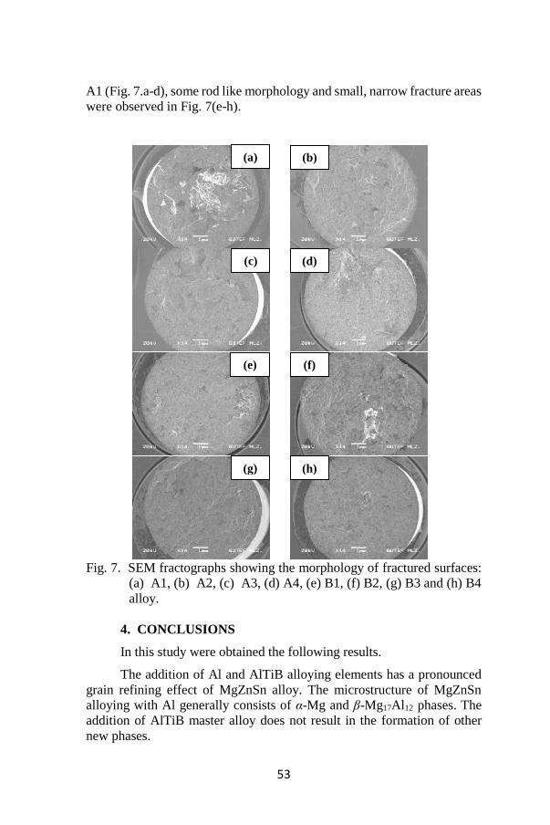
53
A1 (Fig. 7.a-d), some rod like morphology and small, narrow fracture areas
were observed in Fig. 7(e-h).
Fig. 7. SEM fractographs showing the morphology of fractured surfaces:
(a) A1, (b) A2, (c) A3, (d) A4, (e) B1, (f) B2, (g) B3 and (h) B4
alloy.
4. CONCLUSIONS
In this study were obtained the following results.
The addition of Al and AlTiB alloying elements has a pronounced
grain refining effect of MgZnSn alloy. The microstructure of MgZnSn
alloying with Al generally consists of α-Mg and β-Mg17Al12 phases. The
addition of AlTiB master alloy does not result in the formation of other
new phases.
(a)
(e) (f)
(b)
(d) (c)
(h) (g)
54
Metallographic studies showed that the addition of Al and AlTiB
elements changed the microstructure of Mg alloy and resulted in a partially
divorced eutectic. The addition of alloying elements did not result in the
formation of Al containing any new phase, but AlTiB produced new phase
(AlTi, AlB ect.).
The addition of AlTiB master alloy refines the grain of MgZnSn
alloys to some extent. The average grain size is about 185 μm for the
unrefined MgZnSn alloy and it decreases gradually with increasing AlTiB
addition. A minimum of 55 μm for the grain size can be obtained at an
optimum addition level (15% AlTiB). The grain size increases with further
addition of AlTiB. Microstructures of MgZnSn alloys with Al5Ti1B
addition are refined firstly and then coarsened with the increase of holding
time. This reveals that the refinement efficiency of AlTiB fades
increasingly after it is up to the optimum. TiB2, with high melting point
and hexagonal close-packed structure, is presumed to serve as the
heterogeneous nuclei of α-Mg. The grain refinement of α-Mg mainly
results from the existence of a large number of heterogeneous nucleation.
The hardness value of the alloys increased with both alloying
elements. AlTiB addition was much more effective than Al on the
hardness.
Al and AlTiB addition increased the UTS value of the alloys; the
latter was much more effective than the former.
ACKNOWLEDGEMENT
The author would like to thank the Scientific Research Department
of Gazi University (Project number 07-2011/64) for financial support in
this research.
55
REFERENCES
1) Carlson, B.E. (1997). Influence of processing variables and aluminum
content on the microstructure and mechanical properties of Mg-Al
Alloys. PhD Thesis, Materials Science and Engineering, University
of Michigan.
2) Cao, H. and Wessén, M. (2004:35A). Effect of Microstructure on
Mechanical Properties of As-Cast Mg-Al Alloys. Metallurgical and
Materials Transactions A, 35A, 309—319.
3) Cao, P., Qian, M. and StJohn, D.H. (2004:51). Effect of iron on grain
refinement of high-purity Mg–Al alloys. Scripta Materialia, 51,
125–129.
4) Zhang, Z. R., and Tremblay, D. D. (2004: 385). Microstructure and
mechanical properties of ZA104 (0.3–0.6Ca) die-casting
magnesium alloys. Materials Science and Engineering A 385, 286–
291.
5) Yang, M. and Pan, F. (2010:31). Effects of Sn addition on as-cast
microstructure, mechanical properties and casting fluidity of ZA84
magnesium alloy. Materials and Design, 31, 68–75.
6) Liang, M. X., Xiang, W., Lin, L. X. and Lei, Y. (2010:20). Effect of
Al5Ti1B master alloy on microstructures and properties of AZ61
alloys. Trans. Nonferrous Met. Soc.China 20, 397–401.
7) Dobrzański, L.A., Tański, T. and Čížek, L. and Domagała J.
(2008:31). Mechanical properties and wear resistance of magnesium
casting alloys. Journal of Achievements in Materials and
Manufacturing Engineering, 31 (1), 83-90.
8) Kurnaz, S.C., Sevik, H., Açıkgöz, S. and Özel, A. (2011:509).
Influence of titanium and chromium addition on the microstructure
and mechanical properties of squeeze cast Mg–6Al alloy”, Journal
of Alloys and Compounds. 509, 3190–3196.
9) Rzychoń, T., Kiełbus, A. and Lityńska-Dobrzyńska, L. (2013:83).
Microstructure, microstructural stability and mechanical properties
of sand-cast Mg–4Al–4RE alloy. Materials Characterization 83, 21–
34.
10) Candan , S., Unal , M., Koc, E., Turen, Y. and Candan, E. (2010:509).
Effects of titanium addition on mechanical and corrosion behaviours
of AZ91 magnesium alloy. Journal of Alloys and Compounds, 509
(5), 1958-1963.
11) Srinivasan, J. Swaminathan, M.K. Gunjan, U.T. Pillai, S. and Pai,
B.C. (2010:527). Effect of intermetallic phases on the creep
behavior of AZ91 magnesium alloy. Mater. Sci.Eng. A 527, 1395–
1403.
12) Kim, B.H., Lee, S.W., Park, Y.H. and Park, I.M. (2010:493).
The microstructure, tensile properties, and creep behavior of AZ91,
56
AS52 and TAS652 alloy”, J. Alloys Compd. 493, (2010), pp.502–
506.
13) Suresh, M., Srinivasan, A., Ravi, K.R., Pillai, U.T.S. and B.C. Pai.
(2009:525). Influence of boron addition on the grain refinement and
mechanical properties of AZ91 Mg alloy. Mater. Sci. Eng. A 525,
207–210.
14) Wenwen, D., Yangshan, S., Xuegang, M., Feng, X., Min, Z. and
Dengyun, W. (2003:356). Microstructure and mechanical properties
of Mg–Al based alloy with calcium and rare earth additions. Mater.
Sci. Eng. A 356, 1–7.
15) Wu, G., Fan, Y., Gao, H., Zhai, C. and Zhu, Y.P. (2005:408). The
effect of Ca and rare earth elements on the microstructure,
mechanical properties and corrosion behavior of AZ91D. Mater.
Sci. Eng. A 408, 255–263.
16) Zhou, W., Aung, N.N. and Sun, Y. (2009:51). Effect of antimony,
bismuth and calcium addition on corrosion and electrochemical
behaviour of AZ91 magnesium alloy. Corros. Sci. 51, 403–408.
17) Guangyin, Y., Yangshan, S. and Wenjiang, D. (2001:308). Effects of
Bismuth And Antimony Additions on the Microstructure And
Mechanical Properties Of AZ91 Magnesium Alloy. Mater. Sci. Eng.
A 308, 38–44.
18) Wang, F., Wang, Y., Mao, P., Lu, B. and Guo, Q. (2010:20). Effects
of combined addition of Y and Ca on Microstructure and
Mechanical Properties of Die Casting AZ91 Alloy. Trans.
Nonferrous Met. Soc. 20, 311–317.
19) Kim, B.H., Lee, S.W., Park, Y.H., Park J. I.M. (2010:493). The
Microstructure, Tensile Properties, And Creep Behavior of AZ91,
AS52 and TAS652 alloy. Alloys Compd. 493, 502–506.
20) Y. Wang, X. Zeng and W. Ding, “Effect of Al–4Ti–5B Master Alloy
On The Grain Refinement of AZ31 Magnesium Alloy”, Scripta
Materialia 54, (2006), pp.269–273.
21) Chen, T.J., Wang, R.Q., Ma, Y. and Hao, Y. (2012:34). Grain
refinement of AZ91D magnesium alloy by Al-Ti-B master alloy and
its effect on mechanical properties. Materials & Design, 34, 637-
648.
22) Ma, X., Wang, X., Li, X. and Yang, L. (2010:20). Effect of Al5Ti1B
master alloy on microstructures and properties of AZ61 alloys.
Trans. Nonferrous Met. Soc.China 20, 397−401.
23) Xu, C., Lu, B., Lu, Z. and Liang, W. (2008:26). Grain refinement of
AZ31 Magnesium alloy by Al-Ti-C-Y Master Alloy. Journal of Rare
Earths, 26 (4), 604-608.
24) Cao, H. and Wessén, M. (2004:35). Effect of microstructure on
mechanical properties of as-cast Mg-Al alloys”, Metallurgical and
Materials Transactions A, 35 (1), 309-319.
CHAPTER V
ADVANCED OXIDATION PROCESS TO DIFFERENT
INDUSTRIAL WASTEWATERS: SONOFENTON
Şefika Kaya1 & Yeliz Aşçı2
1(PhD) Eskisehir Osmangazi University, email: [email protected]
0000-0001-8277-4365
2(Prof.PhD) Eskisehir Osmangazi University, email: [email protected]
0000-0001-5618-058X
1. INTRODUCTION
In recent years, as industrialization has increased over time, the
negative effects of increased production on the environment have become
threatening to a clean environment. The inadequacy of traditional
treatment methods in bringing the contaminants in wastewater to discharge
standards, and the increasing costs with the removal of industrial
wastewater show that the industries need advanced treatment technologies.
Advanced oxidation processes using Fenton's reagents generate
hydroxyl radicals and destroy organic pollutants by converting them into
harmless compounds such as CO2, water and inorganic salts. The
advantages of Fenton reagents are high efficiency, cheapness, usability at
ambient temperature and pressure, non-toxicity, and ability to decompose
different organic compounds (Villegas-Guzman et al., 2017; Nidheesh &
Rajan, 2016). The classical Fenton process has several disadvantages such
as large amount of sludge production and catalyst deactivation with iron
complexing agents. In recent years advanced oxidation processes such as
heterogeneous Fenton, photoFenton, sonoFenton, ozonation have been
developed to overcome these problems (Shokoofehpoor et al., 2018).
Sound waves with a high frequency that the human ear cannot hear
is called ultrasound. Ultrases is an acoustic wave in a solid, liquid or gas
environment. Ultrasound is capable of generating high radicals in both low
(20 kHz) and high frequency (>200 kHz) ranges (Dogu et al, 2017). In
ultrasound waves, energy is transmitted by the vibration of the surrounding
molecules, where the waves begin to spread, and operates according to the
cavitation principle. Cavitation is an event that occurs in the liquid at very
short intervals, characterized by growth and collapse of microbubbles or
creating a space (Nunes et al., 2014). The heat from the cavity explosion

58
converts water into highly reactive hydrogen atoms and hydroxyl radicals
(· OH). In the rapid cooling phase, hydroxyl radicals and hydrogen atoms
come together to form hydrogen peroxide and molecular hydrogen,
respectively. Thus, organic compounds in the environment are oxidized or
reduced depending on the reactivity (Sivagami et al., 2019; Yang et al.,
2014).
In the sonoFenton process, more hydroxyl radicals are formed
because of Fenton reagents are used together with ultrasound (Al-Bsoul et
al., 2020; Malakootian & Asadzadeh, 2020; Ammar, 2016).
Fe(II) + H2O2 Fe(III) + ·OH + OH- (1)
H2O2 + US 2·OH (2)
H2O + US ·H + ·OH (3)
O2 + US 2·O (4)
H2O + ·O 2·OH (5)
Textile industry produces large amounts of intense colored
wastewater with high chemical oxygen demand, containing organic
pollutants. The dyestuffs used are difficult to biodegrade, toxic and
carcinogenic due to their complex chemical structure in water. Therefore,
discharging textile industry wastewater procreates an significant
environmental problem (Shahmoradi et al., 2019). In the production of
sunflower oil, the waste water from the refining section contains a
significant amount of oil, soap and NaOH. The first effect of this type of
wastewater on receiving environments is that the water's contact with air
is cut off and the amount of oxygen in the water decreases. Therefore, it is
very important to treatment these waters (Saatci et al., 2002).
In this study, COD removal eficiencies from textile industry
wastewater and sunflower oil industry wastewater were investigated by
sonoFenton process. The parameters such as iron ion concentration,
hydrogen peroxide concentration and reaction time were investigated and
optimum experimental conditions were determined.
2. MATERIALS AND METHODS
2.1. Materials
Experimental studies were carried out with sunflower oil industry
and textile industry wastewater. The sunflower oil industry wastewater was
supplied from an oil production factory in Eskişehir. This wastewater is
the exit water sent to the treatment unit as wastewater after neutralization
process in production. Textile industry wastewater was provided from the
reactive dyeing process water of an factory in Bursa. The characterization
of industrial wastewaters were represented in Table 1. Iron(II) sulphate

59
heptahydrate (FeSO4.7H2O) was obtained from Merck. Hydrogen peroxide
(30% w/w) was purchased by Sigma-Aldrich.
Table 1: Characterization of industrial wastewaters.
Sunflower oil
industry wastewater
Textile industry
wastewater
pH 9.5 9
COD, mg/L 7100 2535
2.2. SonoFenton process
Sonics VCX 750 brand ultrasonic homogenizer was used in
sonoFenton process experiments. Ultrasonic homogenizer has 20 kHz and
750 W operating characteristics. Firstly, the pH of the wastewater sample
was adjusted in experimental studies. Then, Fe(II) and H2O2 solutions were
added to the sample. The device was started by dipping the 13 mm probe
of the device into the sample to a depth of approximately 4 cm. At the end
of the experiment, the clear part of the sample was taken and necessary
measurements were made.
Figure 1: SONICS VCX 750 ultrasonic homogenizer and 13 mm probe.
2.3. Analysis
In the COD analysis, Hach Lange LCK 514 brand 13 mm diameter
COD test kits suitable for spectrophotometer device were used. 2 ml
sample was put into the kits and kept in Hach Lange LT 200 brand
thermoreactor at 148oC for 2 hours. Then, the COD removal efficiency was
calculated by making measurements in the spectrophotometer.
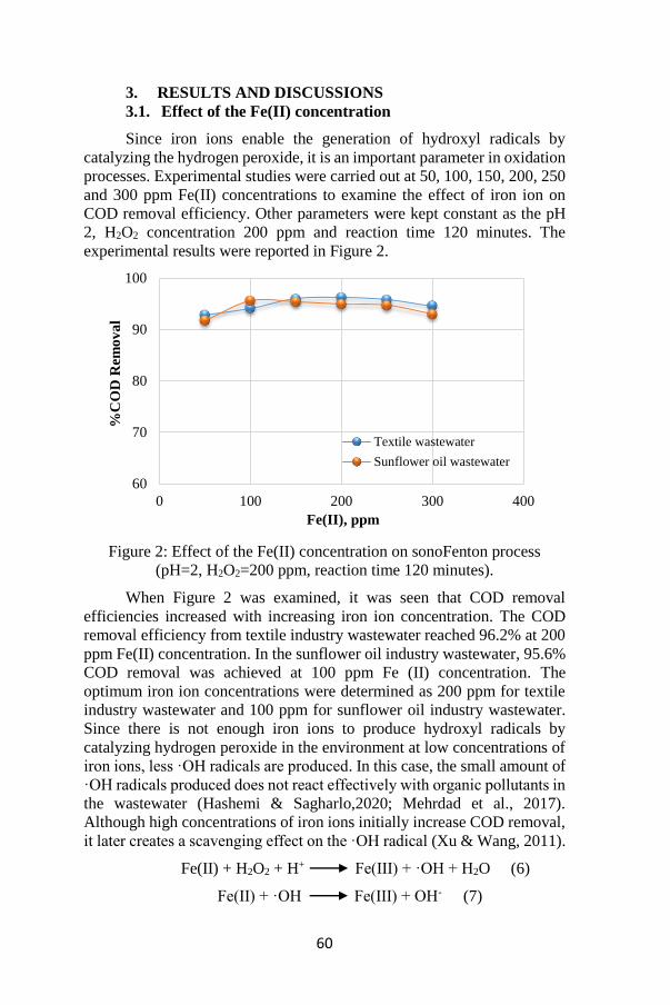
60
3. RESULTS AND DISCUSSIONS
3.1. Effect of the Fe(II) concentration
Since iron ions enable the generation of hydroxyl radicals by
catalyzing the hydrogen peroxide, it is an important parameter in oxidation
processes. Experimental studies were carried out at 50, 100, 150, 200, 250
and 300 ppm Fe(II) concentrations to examine the effect of iron ion on
COD removal efficiency. Other parameters were kept constant as the pH
2, H2O2 concentration 200 ppm and reaction time 120 minutes. The
experimental results were reported in Figure 2.
Figure 2: Effect of the Fe(II) concentration on sonoFenton process
(pH=2, H2O2=200 ppm, reaction time 120 minutes).
When Figure 2 was examined, it was seen that COD removal
efficiencies increased with increasing iron ion concentration. The COD
removal efficiency from textile industry wastewater reached 96.2% at 200
ppm Fe(II) concentration. In the sunflower oil industry wastewater, 95.6%
COD removal was achieved at 100 ppm Fe (II) concentration. The
optimum iron ion concentrations were determined as 200 ppm for textile
industry wastewater and 100 ppm for sunflower oil industry wastewater.
Since there is not enough iron ions to produce hydroxyl radicals by
catalyzing hydrogen peroxide in the environment at low concentrations of
iron ions, less ·OH radicals are produced. In this case, the small amount of
·OH radicals produced does not react effectively with organic pollutants in
the wastewater (Hashemi & Sagharlo,2020; Mehrdad et al., 2017).
Although high concentrations of iron ions initially increase COD removal,
it later creates a scavenging effect on the ·OH radical (Xu & Wang, 2011).
Fe(II) + H2O2 + H+ Fe(III) + ·OH + H2O (6)
Fe(II) + ·OH Fe(III) + OH- (7)
60
70
80
90
100
0 100 200 300 400
%C
OD
Rem
ov
al
Fe(II), ppm
Textile wastewater
Sunflower oil wastewater
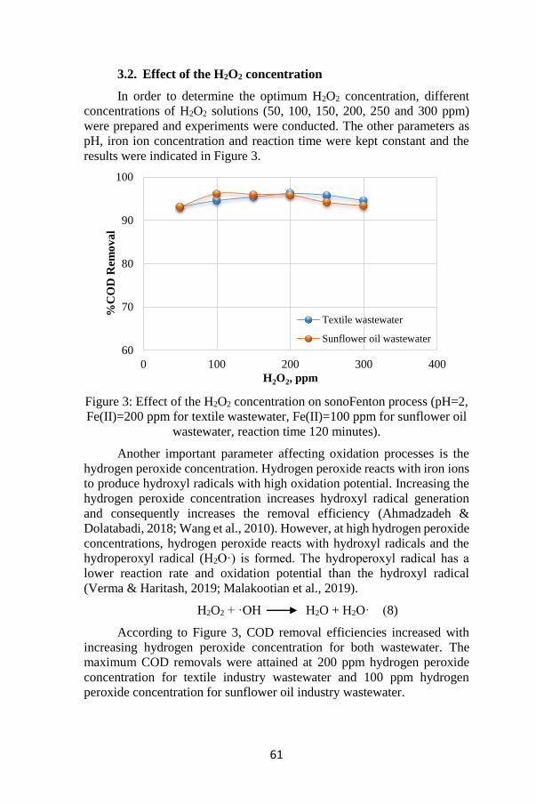
61
3.2. Effect of the H2O2 concentration
In order to determine the optimum H2O2 concentration, different
concentrations of H2O2 solutions (50, 100, 150, 200, 250 and 300 ppm)
were prepared and experiments were conducted. The other parameters as
pH, iron ion concentration and reaction time were kept constant and the
results were indicated in Figure 3.
Figure 3: Effect of the H2O2 concentration on sonoFenton process (pH=2,
Fe(II)=200 ppm for textile wastewater, Fe(II)=100 ppm for sunflower oil
wastewater, reaction time 120 minutes).
Another important parameter affecting oxidation processes is the
hydrogen peroxide concentration. Hydrogen peroxide reacts with iron ions
to produce hydroxyl radicals with high oxidation potential. Increasing the
hydrogen peroxide concentration increases hydroxyl radical generation
and consequently increases the removal efficiency (Ahmadzadeh &
Dolatabadi, 2018; Wang et al., 2010). However, at high hydrogen peroxide
concentrations, hydrogen peroxide reacts with hydroxyl radicals and the
hydroperoxyl radical (H2O·) is formed. The hydroperoxyl radical has a
lower reaction rate and oxidation potential than the hydroxyl radical
(Verma & Haritash, 2019; Malakootian et al., 2019).
H2O2 + ·OH H2O + H2O· (8)
According to Figure 3, COD removal efficiencies increased with
increasing hydrogen peroxide concentration for both wastewater. The
maximum COD removals were attained at 200 ppm hydrogen peroxide
concentration for textile industry wastewater and 100 ppm hydrogen
peroxide concentration for sunflower oil industry wastewater.
60
70
80
90
100
0 100 200 300 400
%C
OD
Rem
ov
al
H2O2, ppm
Textile wastewater
Sunflower oil wastewater
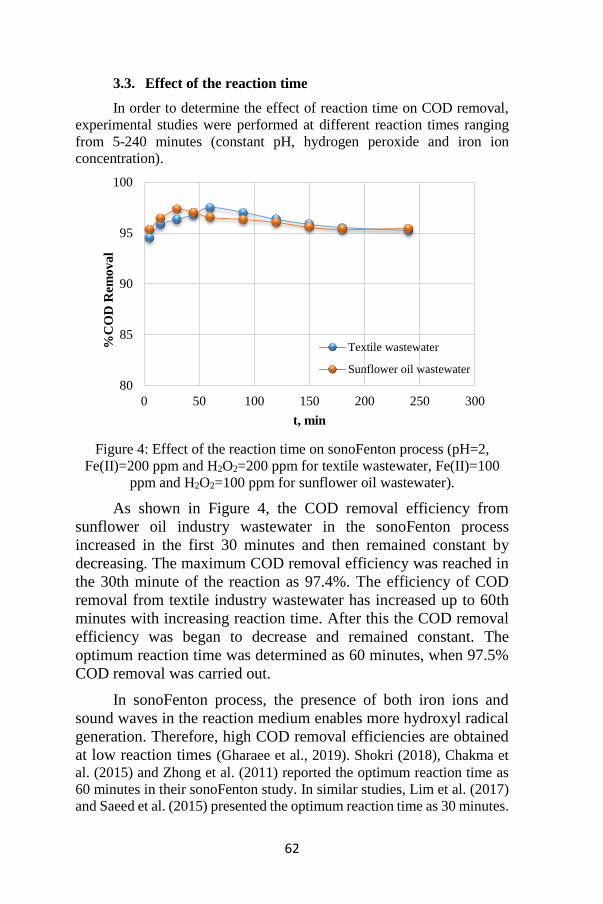
62
3.3. Effect of the reaction time
In order to determine the effect of reaction time on COD removal,
experimental studies were performed at different reaction times ranging
from 5-240 minutes (constant pH, hydrogen peroxide and iron ion
concentration).
Figure 4: Effect of the reaction time on sonoFenton process (pH=2,
Fe(II)=200 ppm and H2O2=200 ppm for textile wastewater, Fe(II)=100
ppm and H2O2=100 ppm for sunflower oil wastewater).
As shown in Figure 4, the COD removal efficiency from
sunflower oil industry wastewater in the sonoFenton process
increased in the first 30 minutes and then remained constant by
decreasing. The maximum COD removal efficiency was reached in
the 30th minute of the reaction as 97.4%. The efficiency of COD
removal from textile industry wastewater has increased up to 60th
minutes with increasing reaction time. After this the COD removal
efficiency was began to decrease and remained constant. The
optimum reaction time was determined as 60 minutes, when 97.5%
COD removal was carried out.
In sonoFenton process, the presence of both iron ions and
sound waves in the reaction medium enables more hydroxyl radical
generation. Therefore, high COD removal efficiencies are obtained
at low reaction times (Gharaee et al., 2019). Shokri (2018), Chakma et
al. (2015) and Zhong et al. (2011) reported the optimum reaction time as
60 minutes in their sonoFenton study. In similar studies, Lim et al. (2017)
and Saeed et al. (2015) presented the optimum reaction time as 30 minutes.
80
85
90
95
100
0 50 100 150 200 250 300
%C
OD
Rem
ov
al
t, min
Textile wastewater
Sunflower oil wastewater
63
4. CONCLUSION
In this study, the treatment of two different industrial wastewater
with different COD values were investigated. SonoFenton process studies
were carried out with textile industry wastewater and sunflower oil
industry wastewater. The COD removal efficiencies from wastewaters
were investigated and optimum experimental conditions (such as iron ion
concentration, hydrogen peroxide concentration and reaction time) were
determined. Under optimum experimental conditions (iron ion
concentration 200 ppm, hydrogen peroxide concentration 200 and reaction
time 60 minutes) 97.5% COD removal efficiency has been achieved for
textile industry wastewater. The optimum conditions for sunflower oil
industry wastewater were obtained as iron ion and hydrogen peroxide
concentrations 100 ppm and reaction time 30 minutes. Under these
conditions 97.4% COD removal efficiency was reached. In the sonoFenton
process, Fenton reagents are used together with ultrasound. Thus, more
hydroxyl radicals are produced and higher removal efficiency is acquired
in a short time. As a result, using the sonoFenton method in the treatment
of industrial wastewater is a highly innovative and highly efficient
alternative method.
5. ACKNOWLEDGMENTS
Eskişehir Osmangazi University Scientific Research Projects
Commission (with the project number 201615059) supported this study.
64
REFERENCES
Ahmadzadeh, S. and Dolatabadi, M. (2018). Removal of acetaminophen
from hospital wastewater using electro-Fenton process.
Environmental Earth Sciences volume 77, 53.
Ammar, H. B. (2016). Sono-Fenton process for metronidazole degradation
in aqueous solution: effect of acoustic cavitation and peroxydisulfate
anion. Ultrasonics Sonochemistry, 33, 164-169.
Al-Bsoul, A., Al-Shannag, M., Tawalbeh, M., Al-Taani, A. A., Lafi, W.
K., Al-Othman, A. and Alsheyab, M. (2020). Optimal conditions for
olive mill wastewater treatment using ultrasound and advanced
oxidation processes. Science of The Total Environment, 700,
134576.
Chakma, S., Das, L. and Moholkar, V. S. (2015). Dye decolorization with
hybrid advanced oxidation processes comprising sonolysis/Fenton-
like/photo-ferrioxalate systems: a mechanistic investigation.
Separation and Purification Technology, 156, 596-607.
Dogu, İ., Yalcin, M., Ileri, B. and Ayyildiz, O. (2017). Sono-
Electrochemical Treatment of Leather Wastewater, Çanakkale
Onsekiz Mart University. Journal of Graduate School of Natural and
Applied Sciences, 3(1), 1-23.
Gharaee, A., Khosravi-Nikou, M. R. and Anvaripour, B. (2019).
Hydrocarbon contaminated soil remediation: A comparison between
Fenton, sono-Fenton, photo-Fenton and sono-photo-Fenton
processes. Journal of Industrial and Engineering Chemistry, 79, 181-
193.
Hashemi, M. and Sagharlo, N. G. (2020). Optimization and evaluation of
the efficiency of sono-Fenton and photo-Fenton processes in the
removal of 2, 4, 6 trinitrotoluene (TNT) from aqueous solutions.
Journal of Advances in Environmental Health Research, 8, 38-45.
Lim, C. H., Ang, J. J., Lau, S. and Tay, M. G. (2017). Optimization of
hydroxyl radical production using electro-Fenton method for
chemical oxygen demand reduction in diluted palm oil mill effluent.
Water and Environment Journal, 31, 578-583.
Malakootian, M., Khatami, M., Ahmadian, M. and Asadzadeh, S. N.
(2019). Biogenic silver nanoparticles/hydrogen peroxide/ozone:
efficient degradation of Reactive Blue 19. BioNanoscience, 10, 1-8.
Malakootian, M. and Asadzadeh, S. N. (2020). Oxidative removal of
tetracycline by sono Fenton-like oxidation process in aqueous
media. Desalination and Water Treatment, 193, 302-401.

65
Mehrdad, A., Farkhondeh, S. and Hasaspoor, F. (2017). Kinetic study of
sonocatalytic degradation of Methylene blue by sonofenton process.
Journal of Applied Chemistry, 12(45), 83-90.
Nidheesh, P.V. and Rajan, R. (2016). Removal of rhodamine B from a
water medium usinghydroxyl and sulphate radicals generated by
iron loaded activated carbon. RSC Advances. 6, 5330-5340.
Nunes, M. A., Mello ,P. A., Bizzi, C. A., Diehl, L. O., Moreira, E. M.,
Souza, W. F., Emanuela, C., Gaudino, E. E, Cravotto, G. and Flo-
res, E. M. (2014). Evaluation of nitrogen effect on ultrasound-
assisted oxidative desulfurization process. Fuel Processing
Technology, 126, 521-527.
Saatci, Y., Arslan, E. I., Ipek, U. and Cici, M. (2002). Reduction of
Pollution Loads of Wastewater from Sunflower Seed Oil Factory.
Anadolu University Journal Of Science And Technology, 3, 49-58.
Saeed, M. O., Azizli, K., Isa, M. H. and Bashir, M. J. K. (2015).
Application of CCD in RSM to obtain optimize treatment of POME
using Fenton oxidation process. Journal of Water Process
Engineering, 8, 7-16.
Shahmoradi, B. Maleki, A. and Byrappa, K. (2015). Removal of disperse
orange 25 using in situ surface-modified iron-doped TiO2
nanoparticles. Desalination and Water Treatment, 53 (13), 3615-
3622.
Shokoofehpoor, F., Chaibakhsh, N. and Gilani A. G. (2018). Optimization
of sono-Fenton degradation of Acid Blue 113 using iron vanadate
nanoparticles. Journal Separation Science and Technology, 54,
2943-2958.
Shokri, A. (2018). Application of Sono–photo-Fenton process for
degradation of phenol derivatives in petrochemical wastewater
using full factorial design of experiment. International Journal of
Industrial Chemistry, 9, 295-303.
Sivagami, K., Anand, D., Divyapriya, G. and Nambi, I. (2019). Treatment
of petroleum oil spill sludge using the combined ultrasound and
Fenton oxidation process. Ultrasonics Sonochemistry, 51, 340-349.
Verma, M. and Haritash, A. K. (2019). Degradation of amoxicillin by
Fenton and Fenton-integrated hybrid oxidation processes. Journal of
Environmental Chemical Engineering, 7, 102886.
Villegas-Guzman, P., Giannakis, S., Rtimi, S., Grandjean, D., Bensimon,
M., de Alencas-tro, L.F., Torres-Palma, R. and Pulgarin, C. (2017).
A green solar photo-Fenton processfor the elimination of bacteria
and micropollutants in municipal wastewatertreatment using

66
mineral iron and natural organic acids. Applied Catalysis B:
Environmental.219, 538-549.
Wang, N., Zhu, L., Wang, M., Wang, D. and Tang, H. (2010). Sono-
enhanced degradation of dye pollutants with the use of H2O2
activated by Fe3O4 magnetic nanoparticles as peroxidase mimetic.
Ultrasonics Sonochemistry, 17, 78-83.
Xu, L. and Wang, J. A. (2011). Heterogeneous Fenton-like system with
nanoparticulate zero-valent iron for removal of 4-chloro-3-methyl
phenol. Journal of Hazardous Materials, 186(1), 256-64.
Yang, B., Zuo J., Tang X., Liu F., Yu X., Tang X., Jiang H. and Gan L.
(2014). Effective Ultrasound Electrochemical Degradation of
Methylene Blue Wastewater using A Nanocoated Elect-rode.
Ultrasonic Sonochemistry, 21 (4), 1310-1317.
Zhong, X., Royer, S., Zhang, H., Huang, Q., Xiang, L., Valange, S. and
Barrault, J. (2011). Mesoporous silica iron-doped as stable and
efficient heterogeneous catalyst for the degradation of CI Acid
Orange 7 using sono–photo-Fenton process. Separation and
Purification Technology, 80, 163-171.

CHAPTER VI
TEMPLATED CARBONS WITH NATURAL ZEOLITE:
SYNTHESIS AND CHARACTERIZATION
Emine Sıla Yiğit1 & Fatma Tümsek2
1 Eskişehir Osmangazi Universirty, e-mail: [email protected]
0000-0001-6326-8379
2(Assoc. Prof. Dr.), Eskişehir Osmangazi University, e-mail: [email protected]
0000-0003-2064-6215
INTRODUCTION
Carbon materials are used in separation processes such as water
and air purification, adsorption, catalysis or energy storage. The high
surface area and large pore volume of these materials and their high
mechanical stability and inert properties increase their use (Chen et al.,
2011). The hydrophobic nature of carbon surfaces are the most important
properties for many applications (Santos et al., 2010). Porous carbon
materials can be classified into three groups according to their pore
diameters as those with pore size less than 2 nm microporous, those with
pore size between 2-50 nm mesoporous, and those with pore size greater
than 50 nm macroporous (Upare et al., 2011).
Activated carbons are the most widely used carbon materials and
they are produced by various methods from carbonaceous raw materials.
The pore structure of carbon material is one of the most important
properties that determine its use in a specific process. Optimization of
experimental parameters during the carbonization/activation steps allows
the structural properties of the carbons to be designed.
However, despite great efforts and a lot of research done to control
pore size and pore size distribution, the complexity of the carbon
structure prevents the obtaining of carbons with a pore structure that can
be precisely controlled by conventional activation processes. Recent
developments in industrial technology have opened up new application
areas for porous carbons and this has required carbons with a specific
It is produced from the thesis titled “Templated Synthesis and Characterization of
Porous Carbon from Natural Zeolite and Sugar”.
68
porous structure. To meet such a requirement, many new approaches
have been proposed to control the pore structure (Kyotani, 2000).
Research into the template synthesis of porous carbon materials
has been ongoing since the first work of Knox et al in 1986, when they
presented the concept of planned porous carbon with template synthesis.
Since then, such porous carbon materials with uniform sizes of
micropore, mesopore and macropore have been synthesized using a
variety of inorganic templates. For this aim, a significant number of
studies have recently focused on the preparation of a designed carbon
material using a template material (Kyotani, 2000; Barata-Rodriques et
al., 2003; Böhme et al., 2005; Sakintuna and Yürüm, 2006; Santos et al.,
2010).
This method consists mainly of the following steps: (a) the
impregnation of a carbon source into the template material, (b) the
carbonization, and (c) the removal of the template material from the
structure. When this synthesis procedure is followed, the carbon formed
in the pores of the template transforms into a carbon framework, while
the volume covered by the template forms the pores of the resulting
carbon material. In other words, the carbon formed is the reverse copy of
the template material (Xia et al., 2011). Depending on the material used
as the template, carbons with different structure and pore size distribution
can be prepared. Silicas, zeolites, clays and pillared clays are inorganic
materials that can be used as templates (Santos et al., 2010). Polymers,
sucrose, phenolic resin or furfuryl alcohol are generally used as carbon
resources (Böhme et al., 2005).
Zeolites, which contain three-dimensional regular channels in their
structures, are substances with molecular sieve properties used for
adsorption and catalytic purposes. The carbons obtained by using zeolites
as templates offer the advantage of having large surface areas and
micropore volumes without the activation process required to open new
accessible micropore structures (Sakintuna et al., 2004). The use of
natural zeolite is important in that it is a cheap and abundant resource in
our country. The use of sugar as a carbon source also offers an
economical way to produce porous carbon by template synthesis, since
sugar is a natural and relatively inexpensive chemical.
The aim of this work is to obtain porous carbons with a certain
pore size distribution, which is particularly important in areas such as gas
separation, storage and catalysis. Accordingly, it is aimed to realize the
template synthesis of porous carbons using natural zeolite as inorganic
template and sugar as carbon source. The synthesis of porous carbons
was carried out at different sugar concentrations and different
carbonization temperatures. Thus, the effects of these synthesis
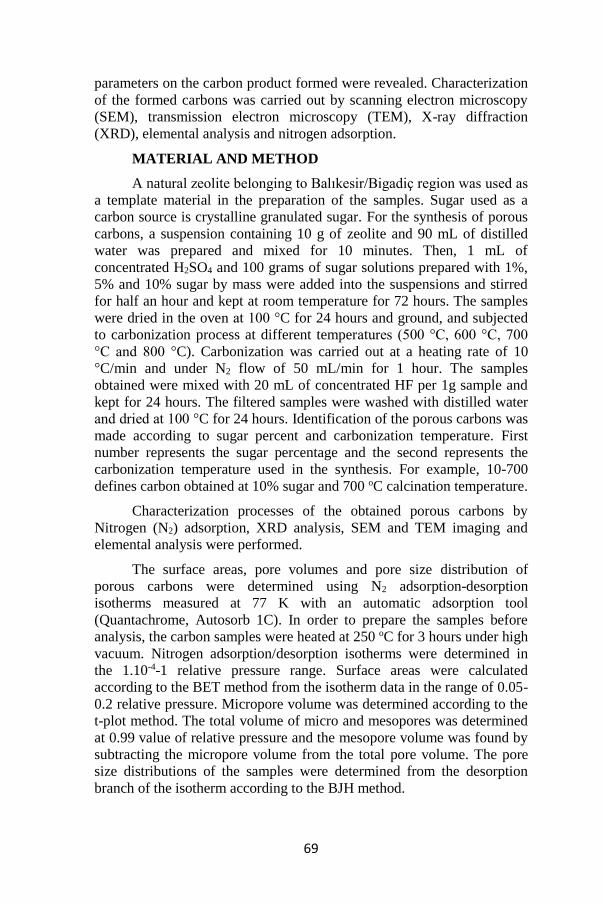
69
parameters on the carbon product formed were revealed. Characterization
of the formed carbons was carried out by scanning electron microscopy
(SEM), transmission electron microscopy (TEM), X-ray diffraction
(XRD), elemental analysis and nitrogen adsorption.
MATERIAL AND METHOD
A natural zeolite belonging to Balıkesir/Bigadiç region was used as
a template material in the preparation of the samples. Sugar used as a
carbon source is crystalline granulated sugar. For the synthesis of porous
carbons, a suspension containing 10 g of zeolite and 90 mL of distilled
water was prepared and mixed for 10 minutes. Then, 1 mL of
concentrated H2SO4 and 100 grams of sugar solutions prepared with 1%,
5% and 10% sugar by mass were added into the suspensions and stirred
for half an hour and kept at room temperature for 72 hours. The samples
were dried in the oven at 100 °C for 24 hours and ground, and subjected
to carbonization process at different temperatures (500 °C, 600 °C, 700
°C and 800 °C). Carbonization was carried out at a heating rate of 10
°C/min and under N2 flow of 50 mL/min for 1 hour. The samples
obtained were mixed with 20 mL of concentrated HF per 1g sample and
kept for 24 hours. The filtered samples were washed with distilled water
and dried at 100 °C for 24 hours. Identification of the porous carbons was
made according to sugar percent and carbonization temperature. First
number represents the sugar percentage and the second represents the
carbonization temperature used in the synthesis. For example, 10-700
defines carbon obtained at 10% sugar and 700 oC calcination temperature.
Characterization processes of the obtained porous carbons by
Nitrogen (N2) adsorption, XRD analysis, SEM and TEM imaging and
elemental analysis were performed.
The surface areas, pore volumes and pore size distribution of
porous carbons were determined using N2 adsorption-desorption
isotherms measured at 77 K with an automatic adsorption tool
(Quantachrome, Autosorb 1C). In order to prepare the samples before
analysis, the carbon samples were heated at 250 oC for 3 hours under high
vacuum. Nitrogen adsorption/desorption isotherms were determined in
the 1.10-4-1 relative pressure range. Surface areas were calculated
according to the BET method from the isotherm data in the range of 0.05-
0.2 relative pressure. Micropore volume was determined according to the
t-plot method. The total volume of micro and mesopores was determined
at 0.99 value of relative pressure and the mesopore volume was found by
subtracting the micropore volume from the total pore volume. The pore
size distributions of the samples were determined from the desorption
branch of the isotherm according to the BJH method.
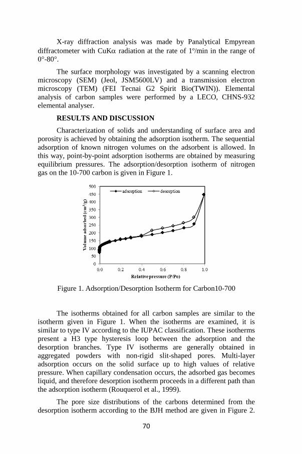
70
X-ray diffraction analysis was made by Panalytical Empyrean
diffractometer with CuK radiation at the rate of 1o/min in the range of
0°-80°.
The surface morphology was investigated by a scanning electron
microscopy (SEM) (Jeol, JSM5600LV) and a transmission electron
microscopy (TEM) (FEI Tecnai G2 Spirit Bio(TWIN)). Elemental
analysis of carbon samples were performed by a LECO, CHNS-932
elemental analyser.
RESULTS AND DISCUSSION
Characterization of solids and understanding of surface area and
porosity is achieved by obtaining the adsorption isotherm. The sequential
adsorption of known nitrogen volumes on the adsorbent is allowed. In
this way, point-by-point adsorption isotherms are obtained by measuring
equilibrium pressures. The adsorption/desorption isotherm of nitrogen
gas on the 10-700 carbon is given in Figure 1.
Figure 1. Adsorption/Desorption Isotherm for Carbon10-700
The isotherms obtained for all carbon samples are similar to the
isotherm given in Figure 1. When the isotherms are examined, it is
similar to type IV according to the IUPAC classification. These isotherms
present a H3 type hysteresis loop between the adsorption and the
desorption branches. Type IV isotherms are generally obtained in
aggregated powders with non-rigid slit-shaped pores. Multi-layer
adsorption occurs on the solid surface up to high values of relative
pressure. When capillary condensation occurs, the adsorbed gas becomes
liquid, and therefore desorption isotherm proceeds in a different path than
the adsorption isotherm (Rouquerol et al., 1999).
The pore size distributions of the carbons determined from the
desorption isotherm according to the BJH method are given in Figure 2.

71
According to the pore size distributions given in Figure 2, it is seen that
the pores are mostly in the range of 3-5 nm (30-50 Å). This corresponds
to the mesopores according to the IUPAC classification, which indicates
the presence of a mesopore framework in the template carbons.
The specific surface areas and the pore properties are presented in
Table 1.The surface areas of the carbons increased up to 700oC with the
increase in the carbonization temperature, and the increase in the
temperature to 800oC decreased the surface area value a little. With the
increase in the sugar percentage, the surface area values increased.
According to the results of nitrogen adsorption, carbon with the highest
specific surface area of 566 m2/g was obtained at 700oC for 10% sugar
and it was determined that the increase in carbonization temperature up to
700oC significantly increased the surface area. In the literature, the
surface area has been determined as 397 m2/g for porous carbon prepared
at 700oC by using natural zeolite template and furfuryl alcohol carbon
source (Sakintuna and Yürüm, 2006). With the increase in the sugar
percentage, the surface area values increased, as the 1% sugar ratio was
increased to 5%, the surface area value increased from 141m2/g to 552
m2/g. As a result of the increase in the sugar ratio from 5% to 10%, the
surface area increased to 566 m2/g.
Figure 2. Pore Size Distribution of Templated Carbons
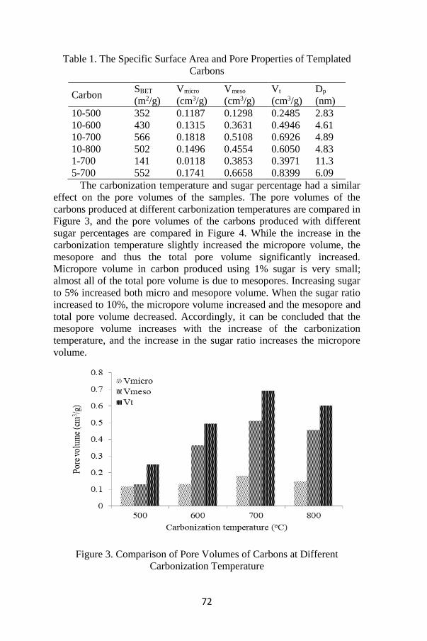
72
Table 1. The Specific Surface Area and Pore Properties of Templated
Carbons
Carbon SBET
(m2/g)
Vmicro
(cm3/g)
Vmeso
(cm3/g)
Vt
(cm3/g)
Dp
(nm)
10-500 352 0.1187 0.1298 0.2485 2.83
10-600 430 0.1315 0.3631 0.4946 4.61
10-700 566 0.1818 0.5108 0.6926 4.89
10-800 502 0.1496 0.4554 0.6050 4.83
1-700 141 0.0118 0.3853 0.3971 11.3
5-700 552 0.1741 0.6658 0.8399 6.09
The carbonization temperature and sugar percentage had a similar
effect on the pore volumes of the samples. The pore volumes of the
carbons produced at different carbonization temperatures are compared in
Figure 3, and the pore volumes of the carbons produced with different
sugar percentages are compared in Figure 4. While the increase in the
carbonization temperature slightly increased the micropore volume, the
mesopore and thus the total pore volume significantly increased.
Micropore volume in carbon produced using 1% sugar is very small;
almost all of the total pore volume is due to mesopores. Increasing sugar
to 5% increased both micro and mesopore volume. When the sugar ratio
increased to 10%, the micropore volume increased and the mesopore and
total pore volume decreased. Accordingly, it can be concluded that the
mesopore volume increases with the increase of the carbonization
temperature, and the increase in the sugar ratio increases the micropore
volume.
Figure 3. Comparison of Pore Volumes of Carbons at Different
Carbonization Temperature
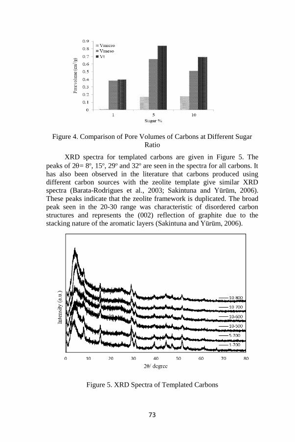
73
Figure 4. Comparison of Pore Volumes of Carbons at Different Sugar
Ratio
XRD spectra for templated carbons are given in Figure 5. The
peaks of 2= 8o, 15o, 29o and 32o are seen in the spectra for all carbons. It
has also been observed in the literature that carbons produced using
different carbon sources with the zeolite template give similar XRD
spectra (Barata-Rodrigues et al., 2003; Sakintuna and Yürüm, 2006).
These peaks indicate that the zeolite framework is duplicated. The broad
peak seen in the 20-30 range was characteristic of disordered carbon
structures and represents the (002) reflection of graphite due to the
stacking nature of the aromatic layers (Sakintuna and Yürüm, 2006).
Figure 5. XRD Spectra of Templated Carbons
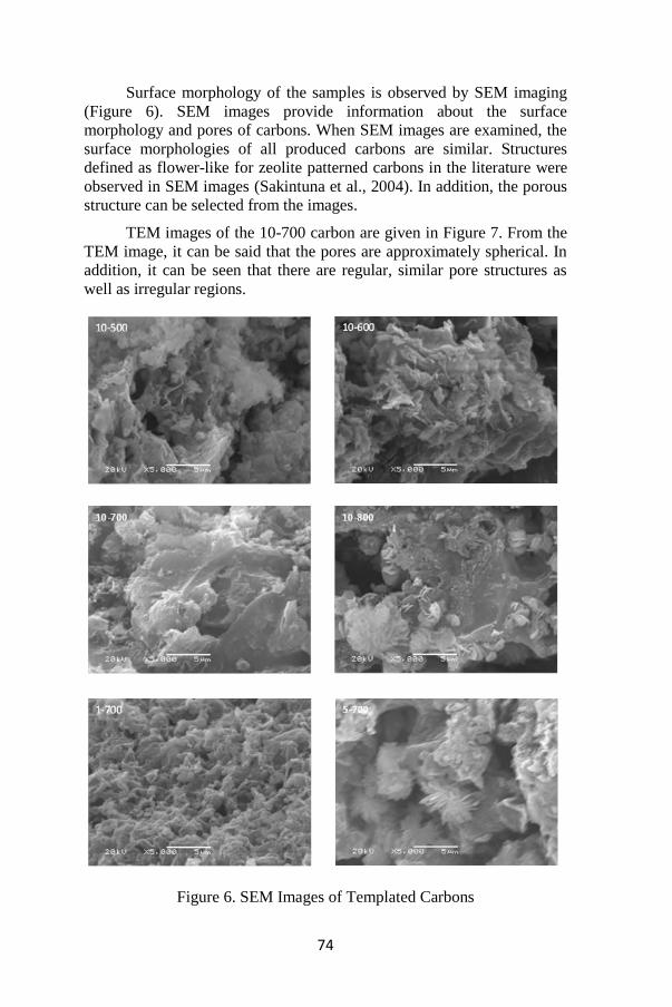
74
Surface morphology of the samples is observed by SEM imaging
(Figure 6). SEM images provide information about the surface
morphology and pores of carbons. When SEM images are examined, the
surface morphologies of all produced carbons are similar. Structures
defined as flower-like for zeolite patterned carbons in the literature were
observed in SEM images (Sakintuna et al., 2004). In addition, the porous
structure can be selected from the images.
TEM images of the 10-700 carbon are given in Figure 7. From the
TEM image, it can be said that the pores are approximately spherical. In
addition, it can be seen that there are regular, similar pore structures as
well as irregular regions.
Figure 6. SEM Images of Templated Carbons
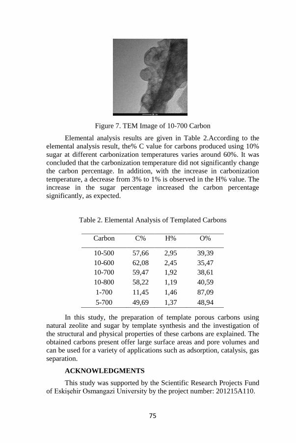
75
Figure 7. TEM Image of 10-700 Carbon
Elemental analysis results are given in Table 2.According to the
elemental analysis result, the% C value for carbons produced using 10%
sugar at different carbonization temperatures varies around 60%. It was
concluded that the carbonization temperature did not significantly change
the carbon percentage. In addition, with the increase in carbonization
temperature, a decrease from 3% to 1% is observed in the H% value. The
increase in the sugar percentage increased the carbon percentage
significantly, as expected.
Table 2. Elemental Analysis of Templated Carbons
In this study, the preparation of template porous carbons using
natural zeolite and sugar by template synthesis and the investigation of
the structural and physical properties of these carbons are explained. The
obtained carbons present offer large surface areas and pore volumes and
can be used for a variety of applications such as adsorption, catalysis, gas
separation.
ACKNOWLEDGMENTS
This study was supported by the Scientific Research Projects Fund
of Eskişehir Osmangazi University by the project number: 201215A110.
Carbon C% H% O%
10-500 57,66 2,95 39,39
10-600 62,08 2,45 35,47
10-700 59,47 1,92 38,61
10-800 58,22 1,19 40,59
1-700 11,45 1,46 87,09
5-700 49,69 1,37 48,94
76
REFERENCES
Barata-Rodrigues, P.M., Mays, T.J., Moggridge, G.D. (2003). Structured
carbon adsorbents from clay, zeolite and mesoporous
aluminosilicate templates, Carbon, 41, 2231–2246.
Böhme, K., Einicke, W.D. and Kepel, O. (2005). Templated synthesis of
mesoporous carbon from sucrose-the way from the silica pore
filling to the carbon material, Carbon 43, 1918-1925.
Chen, L.F., Liang, H.W., Lu, Y., Cui, C.H., Yu, S.H. (2011), Synthesis of
an attapulgite clay@carbon nanocomposite adsorbent by a
hydrothermal carbonization process and their application in the
removal of toxic metal ions from water, Langmuir, 27(14), 8998-
9004.
Knox, J.H., Kaur, B., Millward, G. R. (1986), Structure and Performance
of Porous Graphitic Carbon in Liquid-Chromatography, J.
Chromatogr, 352, 3-25.
Kyotani, T. (2000). Control of pore structure in carbon, Carbon, 38, 269-
286.
Rouquerol, F., Rouquerol, J. Sing, K. (1999), Adsorption by Powders and
Porous Solids, London: Academic Press.
Sakintuna, B., Aktaş, Z., Yürüm, Y. (2004), Templated synthesis of
porous carbons and flower-like carbon fluorides using natural
zeolite, Prepr. Pap. -Am. Chem. Soc., Div. Fuel Chem., 49(2), 696-
697.
Sakintuna, B., Yürüm, Y. (2006), Preparation and characterization of
mesoporous carbons using a Turkish natural zeolitic
template/furfuryl alcohol system, Microporous and Mesoporous
Materials, 93, 304-312.
Santos, C., Andrade, M., Vieira, A.L., Martins, A., Pires, J., Freire , C.
and Carvalho, A.P. (2010), Templated synthesis of carbon
materials mediated by porous clay heterostructures, Carbon, 48,
4049–4056.
Upare, D.P., Yoon, S., Lee, C.W. (2011), Nano-structured porous carbon
materials for catalysis and energy storage, Korean J. Chem. Eng.,
28(3), 731-743.
Xia, Y., Yang, Z., Mokaya, R. (2011), Templated Porous Carbon
Materials: Recent Developments, Bruce, D.W., Walton, R. O’Hare
D. (Eds.) in Porous Materials (p. 217-280), Hoboken, NJ, USA:
Wiley.

CHAPTER VII
MEMORY CIRCUIT ELEMENTS AND APPLICATIONS
Kamil Orman1 & Yunus Babacan2
1 Erzincan Binali Yıldırım University, e-mail: [email protected]
0000-0002-7236-9988
2 Erzincan Binali Yıldırım University, e-mail: [email protected]
0000-0002-6745-0626
INTRODUCTION
Resistors, capacitors and inductors as passive circuit elements
connect the relationships between voltage-current, charge-voltage and
flux-current respectively. But the connection of the flux and charge is
missing until Chua’s original paper [1]. Chua called the new circuit
element, memristor (memory+resistor), which provides the missing
relationship between flux and charge as shown in Fig.1 [1].
V
qi
ᵠ
dq=idt
dϕ =
Vdt
Resistor
dv=Rdi
Capacitor
dq=Cdv
Inductor
dϕ =Ldi
Memristor
dϕ =Mdq
Memristive System
Fig. 1. The fundamental two-terminal circuit elements.
But, Chua’s paper [1] didn’t attract researchers’ attention until
2008 [2]. Memristor did not implemented until this year because of the lack
78
of the advanced technology. Materials at nano-scales are suitable to
realized memristive devices. Researchers interested in the effect of the
memristor on the classical designed circuits. That is why emulator circuits
were designed [3-18] because of the fact that physical implemented
memristor did not obtained easily. The current-voltage relationship of
memristor can be defined by
1 2, ,... nV M x x x i (1)
where V and i are voltage and current respectively. M is memristance
(resistance of memristor), xi’s are state variables. The memristance
( ( ))MemristorR xwhich depends on the history exhibits non-linear
characteristics when applied appropriate frequency and voltage/current
signals.
( ) ( ) ( )MemristorV t R x i t (2)
The memristor has two main structures: doped region and undoped region.
Doped region exhibits low resistance thanks to rich electrons and undoped
region exhibits high resistance because of the lack of the electrons.
Memristance is as follow:
( ) 1Memristor ON OFFR x R x R x , ( )w
xD
(3)
The change of the x value is
2( )v ONRdx
i tdt D
(4)
Where v is electron mobility memristor, w and D denote the doped area
and thickness of the memristor area, respectively and ONR and OFFR
denote resistances for high and low dopant concentrations areas,
respectively. Researcher were added a function ( ( ))f x which is called
window function to take into account the nonlinear kinetics of dopants and
boundary limit effects of memristor [2,4,19-20]. The equation (4) is
rearranged as follows,
2( ) ( )v ONRdx
i t f xdt D
(5)
The first f(x) window function which is linear model was presented
by HP research team [2].
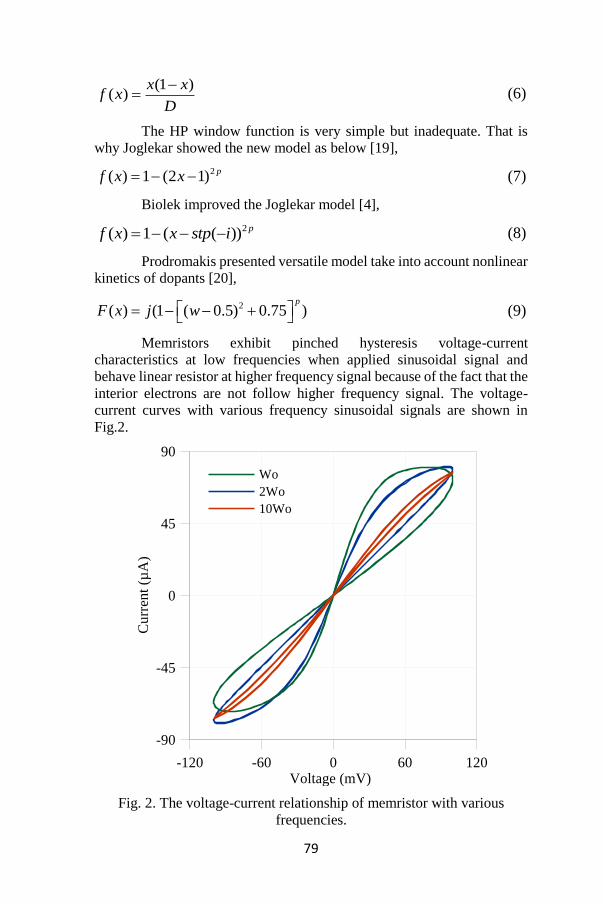
79
(1 )( )
x xf x
D
(6)
The HP window function is very simple but inadequate. That is
why Joglekar showed the new model as below [19],
2( ) 1 (2 1) pf x x (7)
Biolek improved the Joglekar model [4],
2( ) 1 ( ( )) pf x x stp i (8)
Prodromakis presented versatile model take into account nonlinear
kinetics of dopants [20],
2( ) (1 ( 0.5) 0.75 )p
F x j w (9)
Memristors exhibit pinched hysteresis voltage-current
characteristics at low frequencies when applied sinusoidal signal and
behave linear resistor at higher frequency signal because of the fact that the
interior electrons are not follow higher frequency signal. The voltage-
current curves with various frequency sinusoidal signals are shown in
Fig.2.
-120 -60 0 60 120Voltage (mV)
-90
-45
0
45
90
Cu
rren
t (µ
A)
Wo
2Wo
10Wo
Fig. 2. The voltage-current relationship of memristor with various
frequencies.

80
Stanley Williams mentioned how they found the missing
memristor with details [21] and they fabricated the memristors as a
multiple crossbar arrays. Both the scanning tunneling microscope image
and crossbar structure of the memristor is as shown in Fig.3.
The memristive behavior depends on the length of the doped
region. When the signal applied to the memristor, the doped region changes
depend on the direction and value of the applied signal. The detailed photo
is shown in Fig.3b for TiO2-x memristor.
(a) (b)
Fig. 3. a) The scanning tunneling microscope image of the memristor b)
The crossbar architecture is a fully connected mesh of perpendicular
wires [21].
The voltage-current curve for the first memristor which was
realized using TiO2 sandwich structure by HP research team is shown in
Fig.4 [2].
Fig. 4. The voltage-current relationship of the TiO2 memristor [2].
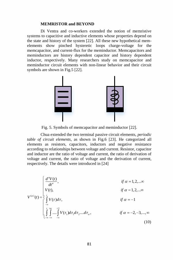
81
MEMRISTOR and BEYOND
Di Ventra and co-workers extended the notion of memristive
systems to capacitive and inductive elements whose properties depend on
the state and history of the system [22]. All these new hypothetical mem-
elements show pinched hysteretic loops charge-voltage for the
memcapacitor, and current-flux for the meminductor. Memcapacitors and
meminductors are history dependent capacitor and history dependent
inductor, respectively. Many researchers study on memcapacitor and
meminductor circuit elements with non-linear behavior and their circuit
symbols are shown in Fig.5 [22].
Fig. 5. Symbols of memcapacitor and meminductor [22].
Chua extended the two terminal passive circuit elements, periodic
table of circuit elements, as shown in Fig.6 [23]. He categorized all
elements as resistors, capacitors, inductors and negative resistance
according to relationships between voltage and current. Resistor, capacitor
and inductor are the ratio of voltage and current, the ratio of derivation of
voltage and current, the ratio of voltage and the derivation of current,
respectively. The details were introduced in [24]
( )
2
1 1 2
( ), 1,2,...
( ), 1,2,...
( )( ) , 1
.... ( ) .... , 2, 3,...,
a
a
t
t
d V tif
dt
V t if
V tV d if
V d d d if
(10)

82
( )
2
1 1 2
( ), 1,2,...
( ), 1,2,...
( )( ) , 1
.... ( ) .... , 2, 3,...,
t
t
d i tif
dt
i t if
i ti d if
i d d d if
(11)
The α and β values are orders of the voltage ( )( )V
and current
( )( )I respectively. For example, the circuit element is a resistor when α
and β values equal to zero, or the circuit element is capacitor when 0
and 1
2
1
1
0
0
-1
1
-2
2
0
1
-1
0
-2
2
2
1
1
0
0
-1
-1
-2
-2
1
2
0
1
-1
0
-2
-1
0
2
-1
1
-2
0
-2
2
-1
2
-2
1
2
-2
1
-2
2
-1
β
α
3
2
1
0
-2-3 -1 0 1 2 3
-1
-2
-3
Fig. 6. The periodic table of all two-terminal circuit elements. Resistors
line, capacitors line, inductors line and negative resistance line are red,
green, blue and yellow respectively.
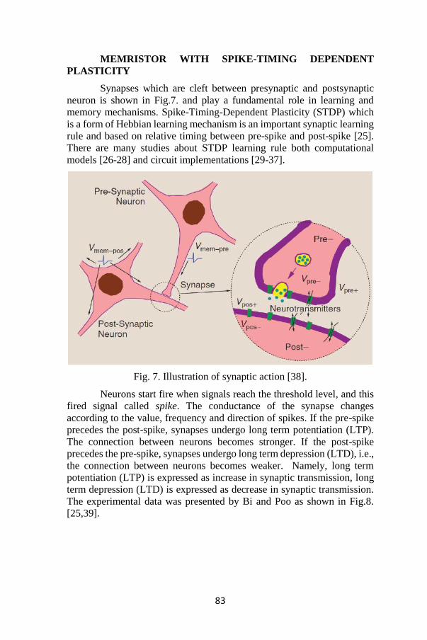
83
MEMRISTOR WITH SPIKE-TIMING DEPENDENT
PLASTICITY
Synapses which are cleft between presynaptic and postsynaptic
neuron is shown in Fig.7. and play a fundamental role in learning and
memory mechanisms. Spike-Timing-Dependent Plasticity (STDP) which
is a form of Hebbian learning mechanism is an important synaptic learning
rule and based on relative timing between pre-spike and post-spike [25].
There are many studies about STDP learning rule both computational
models [26-28] and circuit implementations [29-37].
Fig. 7. Illustration of synaptic action [38].
Neurons start fire when signals reach the threshold level, and this
fired signal called spike. The conductance of the synapse changes
according to the value, frequency and direction of spikes. If the pre-spike
precedes the post-spike, synapses undergo long term potentiation (LTP).
The connection between neurons becomes stronger. If the post-spike
precedes the pre-spike, synapses undergo long term depression (LTD), i.e.,
the connection between neurons becomes weaker. Namely, long term
potentiation (LTP) is expressed as increase in synaptic transmission, long
term depression (LTD) is expressed as decrease in synaptic transmission.
The experimental data was presented by Bi and Poo as shown in Fig.8.
[25,39].
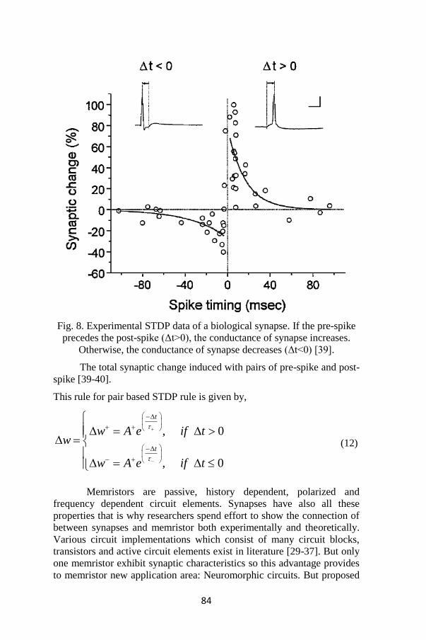
84
Fig. 8. Experimental STDP data of a biological synapse. If the pre-spike
precedes the post-spike (Δt>0), the conductance of synapse increases.
Otherwise, the conductance of synapse decreases (Δt<0) [39].
The total synaptic change induced with pairs of pre-spike and post-
spike [39-40].
This rule for pair based STDP rule is given by,
, 0
, 0
t
t
w A e if tw
w A e if t
(12)
Memristors are passive, history dependent, polarized and
frequency dependent circuit elements. Synapses have also all these
properties that is why researchers spend effort to show the connection of
between synapses and memristor both experimentally and theoretically.
Various circuit implementations which consist of many circuit blocks,
transistors and active circuit elements exist in literature [29-37]. But only
one memristor exhibit synaptic characteristics so this advantage provides
to memristor new application area: Neuromorphic circuits. But proposed
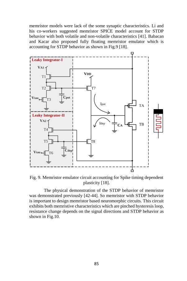
85
memristor models were lack of the some synaptic characteristics. Li and
his co-workers suggested memristor SPICE model account for STDP
behavior with both volatile and non-volatile characteristics [41]. Babacan
and Kacar also proposed fully floating memristor emulator which is
accounting for STDP behavior as shown in Fig.9 [18].
VA1
CpotVtau
VA2
CdepVtau
T1
T2
T3
T4
T5
T6
T7
T8
TA
TB
VDD
CA
Leaky Integrator-I
Leaky Integrator-II
Ipot
Idep
Fig. 9. Memristor emulator circuit accounting for Spike timing dependent
plasticity [18].
The physical demonstration of the STDP behavior of memristor
was demonstrated previously [42-44]. So memristor with STDP behavior
is important to design memristor based neuromorphic circuits. This circuit
exhibits both memristive characteristics which are pinched hysteresis loop,
resistance change depends on the signal directions and STDP behavior as
shown in Fig.10.
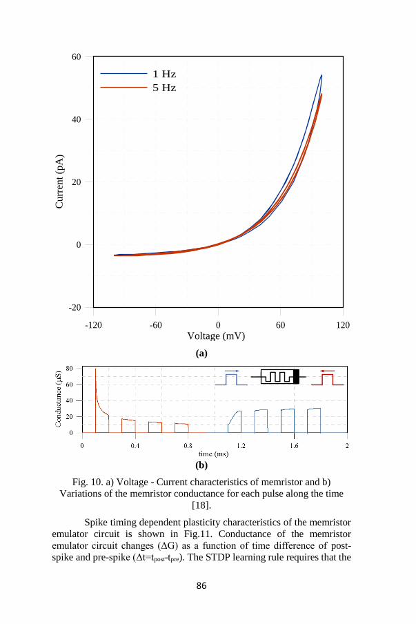
86
-120 -60 0 60 120
Voltage (mV)
-20
0
20
40
60C
urr
ent
(pA
)
1 Hz
5 Hz
(a)
(b)
Fig. 10. a) Voltage - Current characteristics of memristor and b)
Variations of the memristor conductance for each pulse along the time
[18].
Spike timing dependent plasticity characteristics of the memristor
emulator circuit is shown in Fig.11. Conductance of the memristor
emulator circuit changes (ΔG) as a function of time difference of post-
spike and pre-spike (Δt=tpost-tpre). The STDP learning rule requires that the
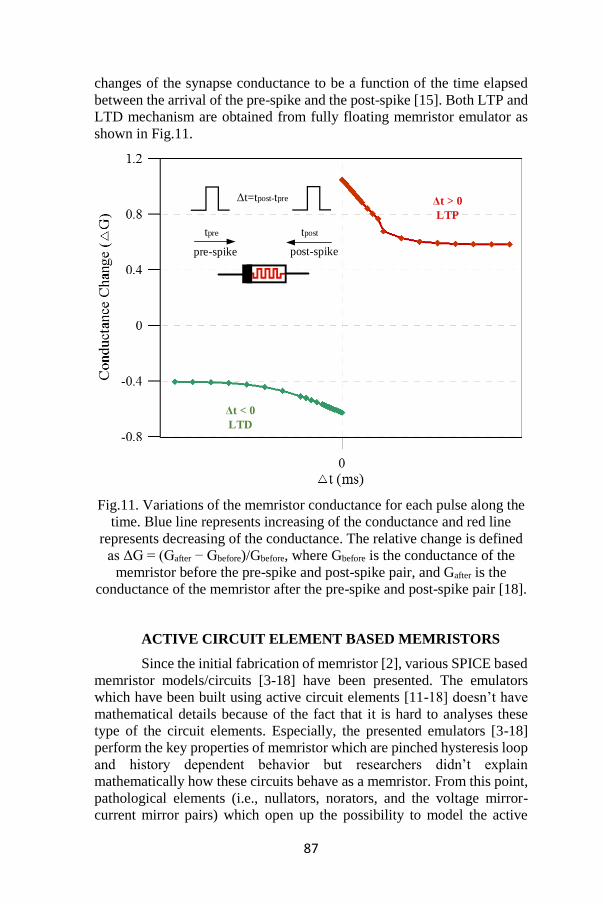
87
changes of the synapse conductance to be a function of the time elapsed
between the arrival of the pre-spike and the post-spike [15]. Both LTP and
LTD mechanism are obtained from fully floating memristor emulator as
shown in Fig.11.
Δt=tpost-tpre
tpre tpost
pre-spike
Δt < 0
LTD
Δt > 0
LTP
post-spike
Fig.11. Variations of the memristor conductance for each pulse along the
time. Blue line represents increasing of the conductance and red line
represents decreasing of the conductance. The relative change is defined
as ΔG = (Gafter − Gbefore)/Gbefore, where Gbefore is the conductance of the
memristor before the pre-spike and post-spike pair, and Gafter is the
conductance of the memristor after the pre-spike and post-spike pair [18].
ACTIVE CIRCUIT ELEMENT BASED MEMRISTORS
Since the initial fabrication of memristor [2], various SPICE based
memristor models/circuits [3-18] have been presented. The emulators
which have been built using active circuit elements [11-18] doesn’t have
mathematical details because of the fact that it is hard to analyses these
type of the circuit elements. Especially, the presented emulators [3-18]
perform the key properties of memristor which are pinched hysteresis loop
and history dependent behavior but researchers didn’t explain
mathematically how these circuits behave as a memristor. From this point,
pathological elements (i.e., nullators, norators, and the voltage mirror-
current mirror pairs) which open up the possibility to model the active
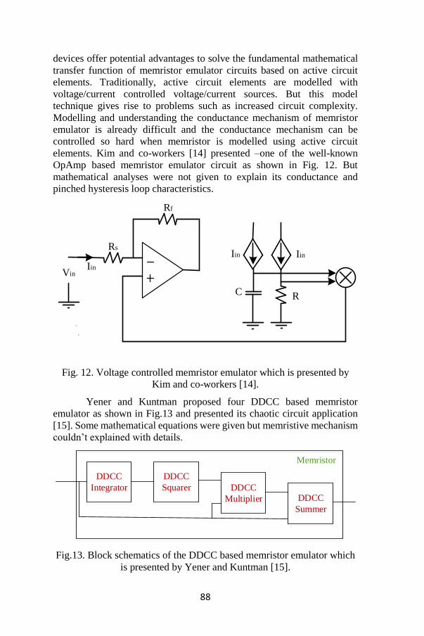
88
devices offer potential advantages to solve the fundamental mathematical
transfer function of memristor emulator circuits based on active circuit
elements. Traditionally, active circuit elements are modelled with
voltage/current controlled voltage/current sources. But this model
technique gives rise to problems such as increased circuit complexity.
Modelling and understanding the conductance mechanism of memristor
emulator is already difficult and the conductance mechanism can be
controlled so hard when memristor is modelled using active circuit
elements. Kim and co-workers [14] presented –one of the well-known
OpAmp based memristor emulator circuit as shown in Fig. 12. But
mathematical analyses were not given to explain its conductance and
pinched hysteresis loop characteristics.
outV
mg
Rs
Rf
Iin
Iin Iin
C R
Vin
Fig. 12. Voltage controlled memristor emulator which is presented by
Kim and co-workers [14].
Yener and Kuntman proposed four DDCC based memristor
emulator as shown in Fig.13 and presented its chaotic circuit application
[15]. Some mathematical equations were given but memristive mechanism
couldn’t explained with details.
DDCC
Integrator
DDCC
Squarer DDCC
Multiplier DDCC
Summer
Memristor
Fig.13. Block schematics of the DDCC based memristor emulator which
is presented by Yener and Kuntman [15].
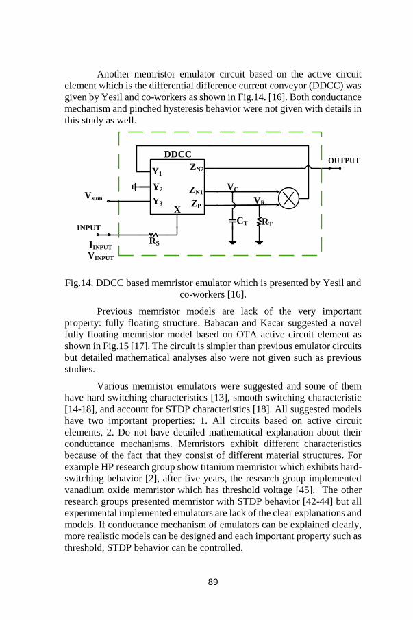
89
Another memristor emulator circuit based on the active circuit
element which is the differential difference current conveyor (DDCC) was
given by Yesil and co-workers as shown in Fig.14. [16]. Both conductance
mechanism and pinched hysteresis behavior were not given with details in
this study as well.
X
DDCC
VR
VC
VINPUT
RTCT
RSIINPUT
ZN1
ZP
ZN2Y1
Y3
Y2
Vsum
INPUT
OUTPUT
Fig.14. DDCC based memristor emulator which is presented by Yesil and
co-workers [16].
Previous memristor models are lack of the very important
property: fully floating structure. Babacan and Kacar suggested a novel
fully floating memristor model based on OTA active circuit element as
shown in Fig.15 [17]. The circuit is simpler than previous emulator circuits
but detailed mathematical analyses also were not given such as previous
studies.
Various memristor emulators were suggested and some of them
have hard switching characteristics [13], smooth switching characteristic
[14-18], and account for STDP characteristics [18]. All suggested models
have two important properties: 1. All circuits based on active circuit
elements, 2. Do not have detailed mathematical explanation about their
conductance mechanisms. Memristors exhibit different characteristics
because of the fact that they consist of different material structures. For
example HP research group show titanium memristor which exhibits hard-
switching behavior [2], after five years, the research group implemented
vanadium oxide memristor which has threshold voltage [45]. The other
research groups presented memristor with STDP behavior [42-44] but all
experimental implemented emulators are lack of the clear explanations and
models. If conductance mechanism of emulators can be explained clearly,
more realistic models can be designed and each important property such as
threshold, STDP behavior can be controlled.
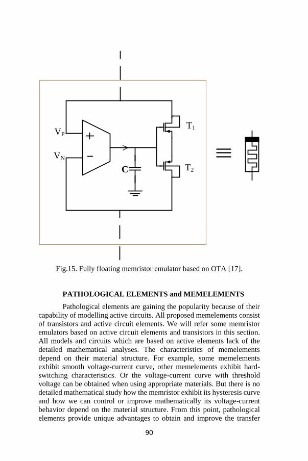
90
C
VN
VP
T1
T2
Fig.15. Fully floating memristor emulator based on OTA [17].
PATHOLOGICAL ELEMENTS and MEMELEMENTS
Pathological elements are gaining the popularity because of their
capability of modelling active circuits. All proposed memelements consist
of transistors and active circuit elements. We will refer some memristor
emulators based on active circuit elements and transistors in this section.
All models and circuits which are based on active elements lack of the
detailed mathematical analyses. The characteristics of memelements
depend on their material structure. For example, some memelements
exhibit smooth voltage-current curve, other memelements exhibit hard-
switching characteristics. Or the voltage-current curve with threshold
voltage can be obtained when using appropriate materials. But there is no
detailed mathematical study how the memristor exhibit its hysteresis curve
and how we can control or improve mathematically its voltage-current
behavior depend on the material structure. From this point, pathological
elements provide unique advantages to obtain and improve the transfer
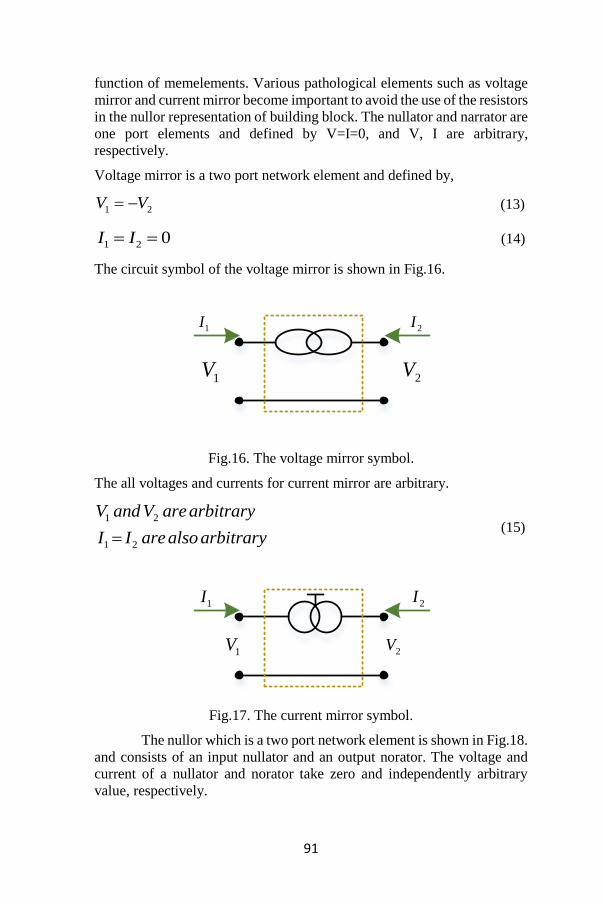
91
function of memelements. Various pathological elements such as voltage
mirror and current mirror become important to avoid the use of the resistors
in the nullor representation of building block. The nullator and narrator are
one port elements and defined by V=I=0, and V, I are arbitrary,
respectively.
Voltage mirror is a two port network element and defined by,
1 2V V (13)
1 2 0I I (14)
The circuit symbol of the voltage mirror is shown in Fig.16.
1V 2V
1I 2I
Fig.16. The voltage mirror symbol.
The all voltages and currents for current mirror are arbitrary.
1 2
1 2
V andV arearbitrary
I I arealsoarbitrary (15)
1V
2I1I
2V
Fig.17. The current mirror symbol.
The nullor which is a two port network element is shown in Fig.18.
and consists of an input nullator and an output norator. The voltage and
current of a nullator and norator take zero and independently arbitrary
value, respectively.
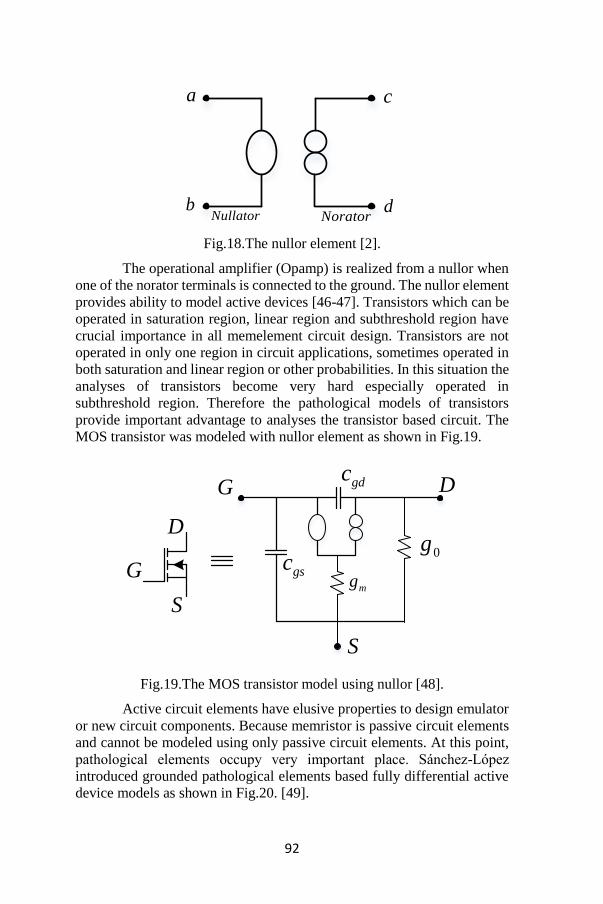
92
a
b
c
dNullator Norator
Fig.18.The nullor element [2].
The operational amplifier (Opamp) is realized from a nullor when
one of the norator terminals is connected to the ground. The nullor element
provides ability to model active devices [46-47]. Transistors which can be
operated in saturation region, linear region and subthreshold region have
crucial importance in all memelement circuit design. Transistors are not
operated in only one region in circuit applications, sometimes operated in
both saturation and linear region or other probabilities. In this situation the
analyses of transistors become very hard especially operated in
subthreshold region. Therefore the pathological models of transistors
provide important advantage to analyses the transistor based circuit. The
MOS transistor was modeled with nullor element as shown in Fig.19.
mg
G gdcD
0ggsc
S
G
D
S
Fig.19.The MOS transistor model using nullor [48].
Active circuit elements have elusive properties to design emulator
or new circuit components. Because memristor is passive circuit elements
and cannot be modeled using only passive circuit elements. At this point,
pathological elements occupy very important place. Sánchez-López
introduced grounded pathological elements based fully differential active
device models as shown in Fig.20. [49].
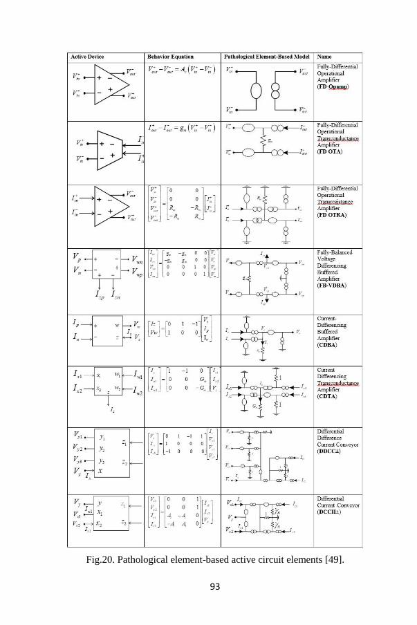
93
Fig.20. Pathological element-based active circuit elements [49].

94
We referred the active circuit elements based memristor emulator circuits
[11-18] and now we modified these circuits using pathological elements.
First of all, the circuit which was designed by Kim and co-workers is
modified as shown in Fig.21. Authors didn’t give details of the
mathematical analyses of the circuit because of the complexity of the
circuit. But the analyses are less complex when use the pathological
elements.
inV outV
mg
Rs
Rf
Iin
Iin Iin
C R
Fig.21. Memristor emulator based on OTA [17].
The other circuit which is based on DDCC active circuit element
was designed by Yesil et al. [16], this circuit has semi-floating
characteristics and strong voltage-current hysteresis curve. The schematic
of the circuit is shown in Fig. 22 when rearranged using the pathological
circuit elements.
1
1
1
11
1
RT
CT
VR
VCInput
Rs
Vsum
Fig.22. DDCC based memristor emulator which is presented by Yesil and
co-workers [16].
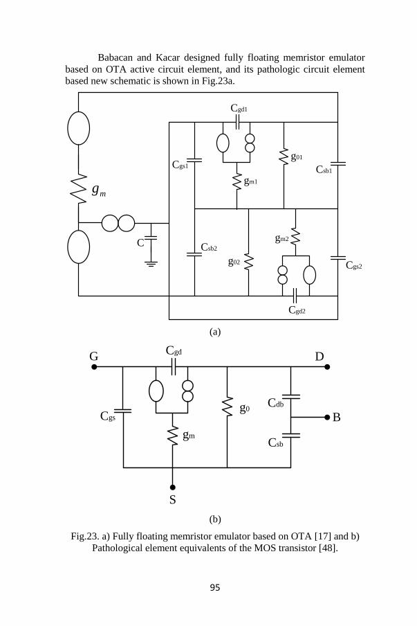
95
Babacan and Kacar designed fully floating memristor emulator
based on OTA active circuit element, and its pathologic circuit element
based new schematic is shown in Fig.23a.
Cgd1
Cgs1
g01
gm1
Csb1
Cgd2
Cgs2g02
gm2
Csb2
mg
C
(a)
CgdD
B
S
Cgs
G
g0
gm
Cdb
Csb
(b)
Fig.23. a) Fully floating memristor emulator based on OTA [17] and b)
Pathological element equivalents of the MOS transistor [48].
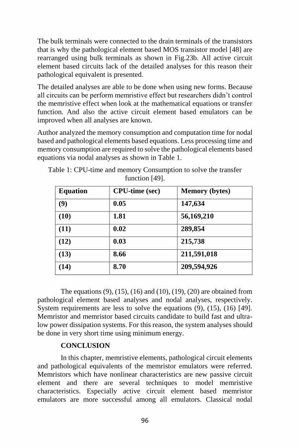
96
The bulk terminals were connected to the drain terminals of the transistors
that is why the pathological element based MOS transistor model [48] are
rearranged using bulk terminals as shown in Fig.23b. All active circuit
element based circuits lack of the detailed analyses for this reason their
pathological equivalent is presented.
The detailed analyses are able to be done when using new forms. Because
all circuits can be perform memristive effect but researchers didn’t control
the memristive effect when look at the mathematical equations or transfer
function. And also the active circuit element based emulators can be
improved when all analyses are known.
Author analyzed the memory consumption and computation time for nodal
based and pathological elements based equations. Less processing time and
memory consumption are required to solve the pathological elements based
equations via nodal analyses as shown in Table 1.
Table 1: CPU-time and memory Consumption to solve the transfer
function [49].
Equation CPU-time (sec) Memory (bytes)
(9) 0.05 147,634
(10) 1.81 56,169,210
(11) 0.02 289,854
(12) 0.03 215,738
(13) 8.66 211,591,018
(14) 8.70 209,594,926
The equations (9), (15), (16) and (10), (19), (20) are obtained from
pathological element based analyses and nodal analyses, respectively.
System requirements are less to solve the equations (9), (15), (16) [49].
Memristor and memristor based circuits candidate to build fast and ultra-
low power dissipation systems. For this reason, the system analyses should
be done in very short time using minimum energy.
CONCLUSION
In this chapter, memristive elements, pathological circuit elements
and pathological equivalents of the memristor emulators were referred.
Memristors which have nonlinear characteristics are new passive circuit
element and there are several techniques to model memristive
characteristics. Especially active circuit element based memristor
emulators are more successful among all emulators. Classical nodal

97
analyses of active circuits are difficult so all presented active circuit
element based memristor emulators are lack of the detailed mathematical
analyses. To know the transfer function of memristor is important because
of the fact that synaptic learning mechanism-Spike-Timing Dependent
Plasticity (STDP), associative learning mechanism and similar complex
operations can be implemented with memristor as presented before.
Therefore, the detailed mathematical analyses are essential to analyze and
improve the memristor and memristor based circuits. And also a nodal
analysis consumes more energy and time to solve the transfer function of
the circuit. That is why pathological circuit elements become significant
candidate to analyze, solve and improve the memristive elements and
memristor based circuit characteristics.

98
REFERENCES
[1] Chua LO (1971) Memristor-the missing circuit element. IEEE
Transactions on Circuit Theory, 507-519.
[2] Strukov DB, Snider GS, Stewart DR and R. S. Williams (2008) The
missing memristor found, Nature, 80–83.
[3] Wang Y and Liao X (2016) Stability analysis of multimode oscillations
in three coupled memristor-based circuits, AEU-International
Journal of Electronics and Communications, 1569-1579.
[4] Biolek Z, Biolek D and Biolkova V (2009) SPICE model of memristor
with nonlinear dopant drift, Radioengineering, 210-214.
[5] Shin S, Zheng L, Weickhardt G, Cho S, Kang SM (2013) Compact
circuit model and hardware emulation for floating memristor
devices, IEEE Circuits and Systems Magazine, 42-55.
[6] Zhang Y, Zhang X and Yu J (2009) Approximated SPICE model for
memristor. International Conference on Communications, Circuits
and Systems, ICCCAS.
[7] Biolek D, Biolek Z, and Biolkova V (2009) SPICE modeling of
memristive, memcapacitative and meminductive systems, Circuit
Theory and Design, European Conference on IEEE.
[8] Williams RS, Pickett MD and Strachan JP (2013) Physics-based
memristor models, IEEE International Circuits and Systems
(ISCAS).
[9] Yang JJ, Strukov DB and Stewart DR (2013) Memristive devices for
computing, Nature nanotechnology, 13-24.
[10] Kvatinsky S, Friedman EG, Kolodny A and Weiser UC (2013)
TEAM: threshold adaptive memristor model, Circuits and Systems
I: Regular Papers, IEEE Transactions on, 211-221.
[11] Abuelmaatti MT, Khalifa ZJ (2015) A continuous-level memristor
emulator and its application in a multivibrator circuit, AEU-
International Journal of Electronics and Communications, 771-
775.
[12] Sanchez-Lopeza C, Carrasco-Aguilar MA, Muniz-Montero C (2015)
A 16 Hz–160 kHz memristor emulator circuit, AEU-International
Journal of Electronics and Communications, 1208-1219.
[13] Babacan Y, Kacar F, Gurkan K (2016) A spiking and bursting neuron
circuit based on memristor, Neurocomputing, 86-91.
99
[14] Kim H et al. (2012) Memristor emulator for memristor circuit
applications, IEEE Transactions on Circuits and Systems I:
Regular Papers, 2422-2431.
[15] Yener Ş and Kuntman H (2012) A new CMOS based memristor
implementation, Applied Electronics International Conference,
pp.345-348, 2012.
[16] Yesil A, Babacan Y and Kacar F (2014) A new DDCC based
memristor emulator circuit and its applications, Microelectronics
Journal.
[17] Babacan Y and Kacar F (2016) Floating Memristor Emulator with
Subthreshold Region, Analog Integrated Circuits and Signal
Processing, 1-5.
[18] Babacan Y and Kacar F (2017) Memristor Emulator with Spike-
Timing-Dependent-Plasticity, International Journal of Electronics
and Communications, 16-22.
[19] Joglekar YN, Wolf SJ (2009) The elusive memristor: Properties of
basic electrical circuits, Eur. J. Phys., 30 (4), 661 -675.
[20] Peh, T, Papavassiliou, BP, Toumazou C, Prodromakis T (2011) A
Versatile Memristor Model With Nonlinear Dopant Kinetics,
IEEE Transactions on Electron Devices, 3099–3105.
[21] William SR (2008) How We Found The Missing Memristor, IEEE
Spectrum, 29-35.
[22] Di Ventra M, Pershin Y, Chua LO (2009) Circuit Elements With
Memory: Memristors, Memcapacitors, and
Meminductors, Proceedings of the IEEE.
[23] Chua LO, Nonlinear Circuit Foundations for Nanodevices, Part I: The
Four-Element Torus, Proceedings of the IEEE.
[24] Chua LO (1980) Device modeling via nonlinear circuit elements,
IEEE Trans. Circuits Syst., vol. CAS-27, pp. 1014-1044.
[25] Bi GQ and Poo MM (1998) Synaptic modifications in cultured
hippocampal neurons: dependence on spike timing, synaptic
strength, and postsynaptic cell type, J. Neuroscience, 10464-
10472.
[26] Song S, Miller K and Abbott L (2000) Competitive Hebbian learning
through spike-timing-dependent synaptic plasticity, Nature
Neuroscience, 919-926.
[27] Iannella N and Tanaka S (2006) Synaptic efficacy cluster formation
across the dendrite via STDP, Neuroscience Letters, 24-29.

100
[28] Iannella N, Launey T and Tanaka S (2010) Spike timing-dependent
plasticity as the origin of the formation of clustered synaptic
efficacy engrams, Neuroscience.
[29] Azghadi M, Al-Sarawi S, Iannella N and Abbott D (2013) A new
compact analog VLSI model for spike timing dependent plasticity,
IFIP/IEEE 21st Int. Conf. Very Large Scale Integr., 7-12.
[30] Azghadi M, Al-Sarawi S, Iannella N and Abbott D (2014) Tunable
low energy, compact and high performance neuromorphic circuit
for spike-based synaptic plasticity, Plos One.
[31] Azghadi M, Al-Sarawi S, Iannella N and Abbott D (2012) Design and
implementation of BCM rule based on spike-timing dependent
plasticity, 2012 international joint conference on neural networks
(IJCNN), 1-7.
[32] Cameron K, Boonsobhak V, Murray A, and Renshaw D (2005) Spike
timing dependent plasticity (STDP) can ameliorate process
variations in neuromorphic VLSI, IEEE Transactions on Neural
Networks, 1626-1627.
[33] Koickal T, Hamilton A, Tan S, Covington J, Gardner J, and Pearce T
(2007) Analog VLSI circuit implementation of an adaptive
neuromorphic olfaction chip, IEEE Transactions on Circuits and
Systems I: Regular Papers, 60-73.
[34] Azghadi M, Al-Sarawi S, Iannella N and Abbott D (2012) Efficient
design of triplet based spike-timing dependent plasticity, 2012
international joint conference on neural networks (IJCNN), 1-7.
[35] Azghadi M, Al-Sarawi S, Iannella N and Abbott D (2011) Novel VLSI
implementation for triplet-based spike-timing dependent
plasticity, In Proceedings of the 7th international conference on
intelligent sensors, sensor networks and information processing,
158-162.
[36] Indiveri G, Chicca E, and Douglas R (2006) A VLSI array of low-
power spiking neurons and bistable synapses with spike-timing
dependent plasticity, IEEE Transactions on Neural Networks, 211-
221.
[37] Tanaka H, Morie T, and Aihara K (2009) A CMOS spiking neural
network circuit with symmetric/asymmetric STDP function,
IEICE Trans. Fund. Electr., Commun. Comput. Sciences, 1690-
1698.
[38] Serrano-Gotarredona T, Prodromakis T, Linares-Barranco B (2013)
A Proposal for Hybrid Memristor-CMOS Spiking Neuromorphic
Learning Systems, IEEE Circuits and Systems Magazine, 74-88.

101
[39] Bi G, Poo MM (2001) Synaptic modification by correlated activity:
Hebb’s postulate revisited, Annu. Rev. Neuroscience, 139-166.
[40] Gerstner W, Kempter R, Hemmen JL and Wagner HA (1996) A neural
learning rule for sub-milisecond temporal coding, Nature, 76-78.
[41] Li Q, Serb A, Prodromakis T and Xu H (2015) Memristor SPICE
Model Accounting for Synaptic Activity Dependence, PLoS One,
1–12.
[42] Jo SH, Chang T, Ebong I, Bhadviya BB, Mazumder P, et al. (2010)
Nanoscale memristor device as synapse in neuromorphic systems.
Nano letters; 10: 1297–1301.
[43] Wang ZQ, Xu HY, Li XH, Yu H, Liu YC, et al. (2012) Synaptic
learning and memory functions achieved using oxygen ion
migration/diffusion in an amorphous InGaZnO memristor.
Advanced Functional Materials; 22: 2759–2765.
[44] Li Y, Zhong Y, Xu L, Zhang J, Xu X, et al. (2013) Ultrafast Synaptic
Events in a Chalcogenide Memristor. Scientific Reports, 3: 1619.
[45] Pickett MD, Medeiros-Ribeiro G, Williams S (2012) A scalable
neuristor built with Mott memristors, Nature Materials.
[46] Bruton LT (1980) RC Active Circuits, Englewood Cliffs, NJ:
Prentice- Hall, chapter 2 and 3.
[47] Davis AC (1967) The significance of nullators, norators and nullors
in active network theory, Radio and Electronic Engineer, pp. 256–
267.
[48] Sanchez-Lopez C, Tlelo-Cuautle E (2009) Symbolic Behavioral
Model Generation of Current-Mode Analog Circuits, IEEE
International Symposium on Circuits and Systems, ISCAS.
[49] Sanchez-Lopez C, Fernández FV, Tlelo-Cuautle E, Sheldon X-DT
(2011) Pathological Element-Based Active Device Models and
Their Application to Symbolic Analysis, IEEE Transactions On
Circuits And Systems—I: Regular Papers, 58(6).

102

CHAPTER VIII
SMART CAMPUSES AND CAMPUS SECURITY
Murat Dener1
1(Assoc. Prof. Dr.), Gazi University, e-mail: [email protected]
0000-0001-5746-6141
1. INTRODUCTION
According to the data of the Higher Education Institution, there are
203 universities in our country, including 129 state universities and 74
foundation universities. Considering that our existing universities have at
least one campus and some universities have more than one campus, it can
be seen that there are nearly 1000 campuses in our country. In addition,
approximately eight million students in total, including approximately
three million students at the associate degree level, approximately four and
a half million students at the undergraduate level, and approximately four
hundred thousand students at the graduate level, study at these campuses.
This increases the importance of our campuses. Now, there is a need for
smart campus solutions that leave traditional campus environment
approaches and include innovative solutions. Smart campus refers to an
intelligent infrastructure where smart sensors and actuators collaborate to
gather information and interact with the machines, vehicles and users of a
university campus. Creating a smart campus in universities around the
world is gaining importance. Because the university community has
become more mobile, student numbers are more unpredictable and funding
has become more uncertain. Investment in management knowledge is
required to focus campus strategies on resource efficiency and sharing, and
to improve decision making.
This study focused on the smart campus and campus security. In the
second part, smart solutions that can be found in the smart campus are
presented, and in the third part, the techniques and technologies required
to realize these systems are explained. In the fourth section, current studies
on smart campus and campus security are mentioned. In the last section,
the results of the study are given.

104
2. SMART SYSTEMS
Smart campus, educational institutions' advanced services, decision
making, campus sustainability, etc. is a new trend that allows it to combine
smart technologies with physical infrastructure.
Smart environments are systems that allow remote monitoring and
management of heating, cooling, ventilation, lighting and security systems
in the environment. These systems include water, electricity, natural gas,
internet etc. consumed in the environment. It may include measurement of
services. The internet control of electrical and electronic devices in the
environment such as refrigerators, ovens, fans, washer / dryers [1] is also
included in the concept of smart environment. Remote management of
curtains and blinds, garage, garden and doors, television / projection and
sound system, solar panels, gas leak controllers can also be included in this
system. In advanced smart environment systems, remote control of the
water and food of animals, monitoring the position of the inhabitants and
turning on and off doors and lights accordingly, health monitoring systems
for the elderly and the disabled can also be found.
Smart buildings are designed with the use of smart media
technologies in the size of office buildings, production and service
buildings, and residential blocks. Main services include heating, cooling,
humidification, lighting, ventilation, water and hot water distribution,
security and alarm system, gas control, fire control. Intelligent building
technologies have become indispensable for controlling energy and
operating costs, which have become important as buildings grow. Today,
smart buildings can monitor the residents of the building by watching their
magnetic ID cards, and they can reduce energy costs in unused parts of the
building with automatic door and lighting systems [1].
Moreover, the following systems and more should be found in smart
campus systems. These;
3d printing, Adjusting the temperature of the building, Air quality
tracking, Carbon dioxide levels in classrooms and offices, Collection
management and security system, Control of electronic devices in homes,
Crowd management, Culture and tourism movements, Cyber security,
Data-based crime prevention programs, Deformation and vibration
sensors, Detection of hazardous gases, Detection of unauthorized entries,
Detection of weapon sounds, Document tracking system, Drinking water
monitoring, Drones for risk assessment, Dynamic pricing, Education
digitalization, Emergency applications, Emergency response and disaster
services, Energy management, Energy usage tracking, Face reading,
Fingerprint reading, Fire systems, Following noise pollution, Health
management, Heating-cooling systems, Indoor air quality, Indoor
navigation, Intelligent systems for the disabled, Intrusion detection

105
systems, Library management, Lighting control systems, Locating
systems for doctors in the hospital, Measuring the humidity and pollution
levels of the specified areas, Monitoring noise levels, Monitoring of
environment information, Monitoring of institutional vehicles, Online
education,
Patient monitoring systems, Person and object tracking systems,
Pollution control, Robots, Smart bike rental, Smart buildings, Smart
classes, Smart education, Smart energy, Smart infrastructure, Smart
junction, Smart Lamps, Smart lighting, Smart management, Smart offices,
Smart Parking, Smart public administration, Smart society, Smart
tourism and entertainment, Social media data from students analysis
systems, Speed warning security systems, Sports-social activities
management, Student attendance-registration system, Swimming pool
remote measurement, Traffic control, Traffic light control systems,
Vehicle tracking systems, Waste management, Water management,
Weather, air pollution detection systems, Wi-fi - station, Wireless
monitoring of infrastructure.
3. TECHNICAL AND TECHNOLOGIES
Some of the techniques and technologies that should be known in
terms of developing the mentioned smart systems and ensuring security are
as follows: Information security, Cloud computing, Big data and data
analytics, Internet of Things, Robotics, Artificial Intelligence and Machine
Learning, Blockchain, Augmented reality, Sensor technologies, 5G and
beyond connection technologies.
Information security is the process of ensuring the integrity of the
information from the sender to the recipient in an environment where the
information is continuously accessible, without being corrupted, changed
or captured by others and transmitting it securely. TS ISO / IEC 27001 has
been prepared in order to establish and document an information security
management system and to provide the basic principles of the concept of
information security. The basic principles of the concept of information
security can be briefly illustrated by (CIA) acronym. These abbreviations
are as follows: Protection of confidentiality (ensuring that access to
information is available only to authorized persons). Integrity (protection
of information and information processing methods, accuracy and
completeness). Accessibility (ensuring that authorized personnel have
access to information and related assets when necessary).
Cloud computing is a set of software, system or platform-based
services that can be accessed and managed entirely over the internet instead
of local resources. It is a computing model that can be used independently
of place and time. This model; It offers fast access to all kinds of data

106
processing resources, including data storage areas, computer networks,
servers and applications, and can be easily configured. Cloud computing
and storage solutions offer businesses and individual users the opportunity
to develop and manage business through secure and high-processing data
centers spread around the world.
Big data and data analytics are all data collected from various
sources such as social media posts, blogs, photographs, videos, and log
files, converted into meaningful and processable form. In particular, it is
used by institutions such as companies, educational institutions and
hospitals to personalize information about end users and provide them with
better quality services. Approaches such as statistics science, modern
computing methods, computer science, artificial intelligence techniques,
machine learning algorithms and mathematics are used to obtain value
from high volume data. With big data analytics supported by different
disciplines, institutions are supported to make more effective decisions.
Internet of Things refers to the connection of objects used in daily
life to the internet. With the connection of the objects we see around us to
the internet, communication between objects takes place and as a result,
systems that help people and tools that increase the quality of life can
emerge.
Robotics is a multi-disciplinary science that deals with the design,
manufacture and use of robots. It is mostly preferred in places where
people's work will be risky and in the industry.
Artificial Intelligence and Machine Learning is a computer science
branch that works to create intelligent computers that can display
intelligent behaviors unique to humans, such as artificial intelligence
reasoning, language understanding, learning, and problem solving.
Machine Learning, on the other hand, refers to the scientific expression of
thinking and intelligent behavior mechanism and the concretization of this
mechanism in machines.
Blockchain is a designed technology where everyone can upload
programs, programs can be executed automatically, the current and
previous states of each program can be seen by everyone at all times and
the applications running on it are cryptologically secured.
Augmented reality includes many techniques, tools and methods
used to create a rich environment between reality and virtuality. It enables
the real world to be enriched with graphics, sound and animations
developed in computer environment. Unlike Virtual Reality, the main
purpose in Augmented Reality is not to create virtual environments that
imitate the real world; to enrich the real world in real-time and interactively
with virtual environments developed in computer environment.
107
Sensor technologies are the name given to the sense organs of
sensor, automatic control systems. Just like people perceive what is
happening in their environment with their sense organs, machines also
perceive values such as temperature, pressure, speed and so on through
their sensors. Devices that detect changes in the physical environment
around us instead of people are called sensors. Sensors are devices that can
detect physical changes and convert them into electrical signals very
quickly. These signals emerging in the sensors are controlled by the
microprocessor. In this way, it becomes possible to use sensors for many
different purposes [2].
5G and beyond connection technologies, 5G, are intended to be able
to operate in a highly heterogeneous environment characterized by the
presence of a wide variety of access technologies, multi-layer networks,
multiple device types, and multiple user interaction diversity. With 5G, a
much more flexible, sustainable and programmable structure will dominate
the next generation core network architecture compared to today. With 5G,
it is aimed to support higher bandwidth, lower latency and high amount of
data [3].
4. CURRENT STUDIES
The web of science database on smart campus and campus security
was scanned and important studies were presented here.
In the study [4], a new approach called wisdom campus has been put
forward. According to the authors, the wisdom campus is the ultimate form
of university computing, the further expansion and elevation of the digital
campus. Wisdom campus integrates cloud computing, mobile internet, big
data, knowledge management and other emerging information
technologies.
In the study [5], students with insufficient financial means can be
identified with big campus data. The proposed system can also alert the
counselors to provide psychological support to students in distress. The
system has significantly increased the efficiency and quality of student
management and reduced the workload of university staff.
The study [6] provides a comprehensive data set on electrical energy
consumption at the university. The total amount of electricity consumed at
Covenant University in Nigeria was measured, monitored and recorded on
a daily basis over a one-year period.
In the study [7], it is stated that new buildings and infrastructures in
Bogor Agricultural University cause a decrease in green open area and
increase in carbon dioxide emission. The aim of the study is to estimate the
amount of carbon stock using remote sensing technology to support the
low emission program.

108
The study [8] presents a comparison of energy generation costs from
gas-powered turbine and diesel-powered distributed electric power types
at Covenant University in Nigeria.
In the study [9], a strong data discovery is made on the daily internet
data traffic generated in a university campus.
In the study [10], information is produced about the use of smart
campus tools to improve the effective and efficient use of campuses. It is
stated that in order to use the resources of universities as effectively as
possible, it is necessary to benefit from smart campus tools. This problem
can be solved using.
In the study [11], cyber-physical system perspective is presented for
the smart water management system on campus.
In the study [12], participation management system was developed
as an Android application running on a smart tablet with the near field
communication standard.
In this study [13], cyber security and wireless sensor network
concepts as well as internet of things for smart campus are reviewed.
In the study [14], a database and smart campus mobile terminal
application were designed to manage and monitor the use of campus
energy in order to reach the smart campus.
In the study [15], to solve the problem of poor service quality, the
user's query range is introduced to present a new anonymous zoning
scheme.
In the study [16], an Energy Management System is recommended
for optimum operation of the Savona Campus Smart Polygeneration Micro
Grid in order to minimize overall production costs.
In the study [17], a different virus spread model was created for a
smart campus network, considering the differences between individuals,
and a method of extending the individual evolution process to the
evolutionary process of the whole network was proposed.
The study [18] proposes a susceptibility classification method based
on multi-specific fusion for Tibetan microblogs.
In the study [19], an effective and practical computational
outsourcing protocol that protects privacy for the local binary model
feature over large encrypted images is proposed.
In the study [20], a multi-source multimedia conference system
supported by cloud computing called Multimedia conference system
technology is designed and implemented.

109
The study [21] proposes an intelligent campus care and guidance
framework for students with facial recognition based on deep learning
through Internet of Things technologies.
The study [22] examined the design of an intelligent bus positioning
system based on the Internet of Things to improve bus delivery vehicles,
increase the efficiency of bus operations and implement a smart campus.
In the study [23], a student achievement prediction framework
including data processing and student achievement prediction is designed.
In the study [24], a mutual authentication protocol developed in
mobile RFID for smart campus is revealed by analyzing and examining
existing smart campus authentication protocols.
In the study [25], a smart campus automatic settlement PLC control
system was designed for the Internet of Things.
The study [26] introduces and analyzes the current research state of
the smart campus and the challenges in integrating various service data into
the smart campus.
In the study [27], a reliable edge caching and bandwidth allocation
scheme is presented for mobile users.
In the study [28], the smart campus hospital environment is
monitored, then real-time transmission, storage, and imaging data are
analyzed to intelligently define the smart campus hospital environment.
In the study [29], the characteristics of Weibo's communication and
the public opinion formation process of the microblog and its
communication mechanism are analyzed.
The study [30] analyzes the salient features of the smart campus
from the perspective of technology, business and construction mode and
proposes a smart campus architecture model.
The study [31] presents a new deep topical correlation analysis
approach for social media that provides robust and accurate topic detection.
In the study [32], under the background of the 5G network, the basic
technologies of the smart campus network teaching platform are discussed.
The study [33] proposed a new authentication protocol for smart
campuses, including Telecare Drug Information Systems.
The study [34] addresses classroom shortages caused by the gap
between enrollment and attendance on a real university campus.
Classrooms are equipped with Internet of Things (IoT) sensors to measure
real-time usage, using AI to predict attendance, and optimal allocation of
rooms to courses to minimize space waste.

110
In the study [35], it is aimed to investigate the underlying
communication networks for remote monitoring of electric vehicles
charging stations in a smart campus parking lot.
In the study [36], a Deep Neural Network based emotional
awareness campus virtual assistant was developed.
The study [37] optimizes the existing wireless video surveillance
system based on the Internet of Things to strengthen school security and
create a wireless smart campus.
The study [38] aims to design a framework for local energy trade
with electric vehicles in smart car parks where electric vehicles can
exchange energy by buying and selling prices.
In the study [39], an architecture is proposed for creating and
running responsive smart classes.
In the study [40], an IoT architecture that can transparently manage
different communication protocols in smart environments is presented and
research has been conducted for monitoring and controlling distributed
energy resources in a smart campus.
The study [41] reveals a comprehensive architecture that defines
various components and their interoperability in an intelligent education
environment.
In the study [42], it was stated that green campus is a concept
implemented by campuses where policies are directed to ecological
perspectives. They conducted research on water security in green
campuses.
In the study [43], Zigbee, LoRa, Bluethooth and WiFi were selected
as the most popular IoT protocols, and their performance was tested and
compared by establishing a network on the university campus.
The study [44] proposes a blockchain-based energy trading platform
for electric vehicles in smart campus parking lots.
The study [45] looks at a university campus in the center of Lisbon,
which requires a significant amount of electricity and natural gas to support
internal activities. The idea is to meet some of the energy consumption of
the campus with excess energy from solar systems installed in surrounding
residential buildings. The goal is to find the number and type of solar
equipment that maximizes the annual reduction of energy costs of the
campus where both residents and campus are viewed as a virtual storage
space.
111
The study [46] developed a new indoor positioning system
combined with the outdoor positioning system to support seamless indoor
and outdoor navigation and direction finding.
In the study [47], the differences between the network in the
traditional campus and the network in the smart campus are analyzed and
compared, and suggestions are made on how to create a smart campus from
cloud computing and internet of things perspectives.
In the study [48], campus network security is examined.
The study [49] proposes a Bluetooth Low Energy based student
positioning framework to automatically record student participation in
classrooms.
The study [50] proposes a technical architecture for the future Smart
Campus, consisting of 5G and IoT networks, complemented by distributed
computing and data analytics.
The study [51] aims to accelerate the information-generation process
of data collection and analysis for smart campus, current research and
current problems in smart campus planning.
In the study [52], the current literature is examined and a smart
campus outline based on smart city concepts is proposed.
The study [53] presents a case study in which emerging areas and
related technologies are explored to benefit communities and actively
engage their members as central players in such an intelligent environment.
The study [54] proposes a plan that can facilitate building a smart
and friendly campus.
The study [55] explains the development of the smart campus using
the Internet of Things (IoT) technology.
The study [56] presents the key features of this platform, with a
special emphasis on the functionality, services and potential offered by the
IoT platform, as well as the technological challenges encountered and
solutions adopted.
In the study [57], it is proposed to use a LoRaWAN fog computing-
based architecture to connect to IoT nodes deployed on the campus of A
Coruña University in Spain.
The study [58] addresses the need to educate students on how to
design complex sensor-based IoT ecosystems.
The study [59] explores the challenges of long-term real-world
Internet of Things (IoT) deployment on a university campus.
112
The study [60] integrates a large data framework that can analyze
data regardless of its format and provide effective responses to each
process.
In the study [61], the data produced by students in search of patterns
that allow students to be classified according to their needs are analyzed.
Once these needs are identified, it is possible to make decisions that
contribute to each student's learning; Artificial intelligence has been used
for this.
The study [62] proposes a new disaster management system such as
Named Data Networking Disaster Management, in which a producer
transmits a fire warning message to neighboring consumers.
In the study [63], combining big data technology and cloud
computing technology in smart campus construction to make campus
database system and campus management system mutually.
In the study [64], firstly, the capabilities of existing IoT applications
were determined. Then, it was stated how the information from IoT
applications should be used in organizational decision making processes.
In the study [65], it is proposed to develop an IoT-based energy
monitoring system prototype for the buildings in the Institut Teknologi
Sumatera campus area.
In the study [66], the application of smart room technology based on
Internet of Things is recommended to increase energy efficiency.
The study [67] deals with the security management of the campus
network to analyze the weakness of the campus network in threat
management.
5. CONCLUSIONS
Smart campuses are of great importance in social, financial and
environmental terms. Considering the technologies required to realize the
smart system, it can be clearly seen that there is no restriction in the
realization of the systems. In other words, the desired smart system can be
fulfilled with these technologies. The important thing is to pass right
thinking and dreaming right. We can think of the campus as a city. Students
spend 24 hours on campus from morning to evening, even at universities
with dormitories. They meet all their needs, including education, health,
sports and social, within the campus. There are hundreds of academic and
administrative staff on campus, together with students. Having a command
of this large living space is also attractive for managers. The answer to
questions such as how many people are on campus, or how many vehicles,
how much energy is consumed today and in which units, the status of the
waste on campus, the amount of water consumed and the quality of

113
drinking water, the conditions in campus classrooms and offices, and more.
will be able to reach easily. Considering the judgment that you cannot
improve what you cannot measure, everything on the campus will be
measured and necessary measures will be taken, unnecessary waste will be
prevented. Even if these systems bring a high financial burden in the first
place, they will pay for themselves over time. Internet of Things platforms
for Smart Cities are technologically complex, and using them on a large
scale involves high costs and risks. For this reason, pilot plans are
particularly important in this context, which allow the proof of concept to
be validated, to experiment with different technologies and services, and
to fine-tune them before moving them to real scenarios.
114
REFERENCES
1. Mutlu, M.E. (2018). New Communication Technologies, Anadolu
University Publications, E-ISBN 978-975-06-3046-0.
2. Pehlivanoglu, M. (2020), What is a Sensor?, https://muhendis
gelisim.com/sensor-nedir/.
3. 5GTR Forum Working Groups (2018), 5G and Beyond, White Book,
Information Technologies and Communication Authority.
4. Wang, H.Y. (2018). A research on the security of wisdom campus based
on geospatial big data, 6th International Conference on Computer-
Aided Design, Manufacturing, Modeling and Simulation (CDMMS
2018), 1967, DOI: 10.1063/1.5038997.
5. Wu, F., Zheng, Q.H., Tian, F., Suo, Z.H., Zhou, Y.A., Chao, K.M., Xu,
M., Shah, N., Liu, J., Li, F. (2020). Supporting poverty-stricken
college students in smart campus, Future Generation Computer
Systems-The International Journal of Escience, 111, 599-616.
6. Popoola, S.I., Atayero, A.A., Okanlawon, T.T., Omopariola, B.I.,
Takpor, O.A. (2018). Smart campus: Data on energy consumption
in an ICT-driven university, Data In Brief, 16, 780-793.
7. Lavista, L., Prasetyo, L.B., Hermawan, R. (2016). Dynamics change of
the above carbon stocks in Bogor Agricultural University, Darmaga
campus, 2nd International Symposium on Lapan-Ipb Satellite
(Lısat) for Food Security and Environmental Monitorıng, 33, 305-
316.
8. Okeniyi, J.O., Atayero, A.A., Popoola, S.I., Okeniyi, E.T., Alalade,
G.M. (2018). Smart campus: Data on energy generation costs from
distributed generation systems of electrical energy in a Nigerian
University, Data In Brief, 17, 1082-1090.
9. Adeyemi, O.J., Popoola, S.I., Atayero, A.A., Afolayan, D.G., Ariyo, M.,
Adetiba, E. (2018). Exploration of daily Internet data traffic
generated in a smart university campus, Data In Brief, 20, 30-52.
10. Valks, B., Arkesteijn, M., Den Heijer, A. (2019). Smart campus tools
2.0 exploring the use of real-time space use measurement at
universities and organizations, Facilities, 37(13), 961-980.
11. Abhishek, M.B., Shet, N.S.V. (2019). Cyber physical system
perspective for smart water management in a campus, Desalination
and Water Treatment, 147, 296-307.
12. Kamada, S., Ichimura, T., Shigeyasu, T., Takemoto, Y. (2014).
Registration system of cloud campus by using android smart tablet,
Springerplus, 3, DOI: 10.1186/2193-1801-3-761.
115
13. Sanchez-Torres, B., Rodriguez-Rodriguez, J.A., Rico-Bautista, D.W.,
Guerrero, C.D. (2018). Smart Campus: Trends in cybersecurity and
future development, Revista Facultad De Ingenieria, Universidad
Pedagogica Y Tecnologica De Colombia, 27(47), 93-101.
14. Zheng, W.B., Yang, Z., Feng, L., Fu, P., Shi, J.L. (2019). APP Design
of Energy Monitoring in Smart Campus Based on Android System,
International Journal of Online and Biomedical Engineering, 15(5),
18-27.
15. Sun, R.X., Xi, J.W., Yin, C.Y., Wang, J., Kim, G.J. (2018), Location
Privacy Protection Research Based on Querying Anonymous
Region Construction for Smart Campus, Mobile Information
Systems, 2018, DOI: 10.1155/2018/3682382.
16. Bracco, S., Brignone, M., Delfino, F., Procopio, R. (2017). An Energy
Management System for the Savona Campus Smart Polygeneration
Microgrid, IEEE Systems Journal, 11(3), 1799-1809.
17. Wang, L., Yao, C.H., Yang, Y.Q., Yu, X.H. (2018). Research on a
Dynamic Virus Propagation Model to Improve Smart Campus
Security, IEEE Access, 6, 20663-20672.
18. Qiu, L.R., Lei, Q., Zhang, Z. (2018). Advanced Sentiment
Classification of Tibetan Microblogs on Smart Campuses Based on
Multi-Feature Fusion, IEEE Access, 6, 17896-17904.
19. Xia, Z.H., Ma, X.H., Shen, Z.X., Sun, X.M., Xiong, N.N., Jeon, B.
(2018). Secure Image LBP Feature Extraction in Cloud-Based Smart
Campus, IEEE Access, 6, 30392-30401.
20. Zhang, W., Zhang, X.C., Shi, H.L. (2018). MMCSACC: A Multi-
Source Multimedia Conference System Assisted by Cloud
Computing for Smart Campus, IEEE Access, 6, 35879-35889.
21. Chen, L.W., Chen, T.P., Chen, D.E., Liu, J.X., Tsai, M.F. (2018). Smart
Campus Care and Guiding With Dedicated Video Footprinting
Through Internet of Things Technologies, IEEE Access, 6, 43956-
43966.
22. Feng, X.J., Zhang, J.L., Chen, J.H., Wang, G.Q., Zhang, L.Y., Li, R.Z.
(2018). Design of Intelligent Bus Positioning Based on Internet of
Things for Smart Campus, IEEE Access, 6, 60005-60015.
23. Qu, S.J., Li, K., Zhang, S.H., Wang, Y.C. (2018). Predicting
Achievement of Students in Smart Campus, IEEE Access, 6, 60264-
60273.
116
24. Zheng, L.J., Song, C.L., Cao, N., Li, Z.X., Zhou, W.F., Chen, J.Y.,
Meng, L.L. (2018). A New Mutual Authentication Protocol in
Mobile RFID for Smart Campus, IEEE Access, 6, 60996-61005.
25. Guo, G.Z. (2018). Design and Implementation of Smart Campus
Automatic Settlement PLC Control System for Internet of Things,
IEEE Access, 6, 62601-62611.
26. Yang, A.M., Li, S.S., Ren, C.H., Liu, H.X., Han, Y., Liu, L. (2018).
Situational Awareness System in the Smart Campus, IEEE Access,
6, 63976-63986.
27. Xu, Q.C., Su, Z., Wang, Y.T., Dai, M.H. (2018). A Trustworthy
Content Caching and Bandwidth Allocation Scheme With Edge
Computing for Smart Campus, IEEE Access, 6, 63868-63879.
28. Liang, Y., Chen, Z.X. (2018). Intelligent and Real-Time Data a
Acquisition for Medical Monitoring in Smart Campus, IEEE
Access, 6, 74836-74846.
29. Nan, F., Suo, Y.N., Jia, X.Y., Wu, Y.Y., Shan, S.J. (2018). Real-Time
Monitoring of Smart Campus and Construction of Weibo Public
Opinion Platform, IEEE Access, 6, 76502-76515.
30. Xu, X., Wang, Y.S., Yu, S.J. (2018). Teaching Performance Evaluation
in Smart Campus, IEEE Access, 6, 77754-77766.
31. Peng, J., Zhou, Y.Y., Sun, X.S., Su, J.S., Ji, R.R. (2019). Social Media
Based Topic Modeling for Smart Campus: A Deep Topical
Correlation Analysis Method, IEEE Access, 7, 7555-7564.
32. Xu, X., Sun, M.Y., Yang, S.C., Yu, S.J., Manogaran, G., Mastorakis,
G., Mavromoustakis, C.X., Li, D. (2019). Research on Key
Technologies of Smart Campus Teaching Platform Based on 5G
Network, IEEE Access, 7, 20664-20675.
33. Safkhani, M., Vasilakos, A. (2019). A New Secure Authentication
Protocol for Telecare Medicine Information System and Smart
Campus, IEEE Access, 7, 23514-23526.
34. Sutjarittham, T., Gharakheili, H.H., Kanhere, S.S., Sivaraman, V.
(2019). Experiences With IoT and AI in a Smart Campus for
Optimizing Classroom Usage, IEEE Internet Of Things Journal,
6(5), 7595-7607.
35. Ahmed, M.A., El-Sharkawy, M.R., Kim, Y.C. (2020). Remote
Monitoring of Electric Vehicle Charging Stations in Smart Campus
Parking Lot, Journal of Modern Power Systems and Clean Energy,
8(1), 124-132.
117
36. Chiu, P.S., Chang, J.W., Lee, M.C., Chen, C.H., Lee, D.S. (2020).
Enabling Intelligent Environment by the Design of Emotionally
Aware Virtual Assistant: A Case of Smart Campus, IEEE Access, 8,
62032-62041.
37. Zhou, Z.Q., Yu, H., Shi, H.S. (2020). Optimization of Wireless Video
Surveillance System for Smart Campus Based on Internet of Things,
IEEE Access, 8, 136434-136448.
38. Ahmed, M.A., Kim, Y.C. (2018). Energy Trading with Electric
Vehicles in Smart Campus Parking Lots, Applied Sciences-Basel,
8(10), DOI: 10.3390/app8101749.
39. Huang, L.S., Su, J.Y., Pao, T.L. (2019). A Context Aware Smart
Classroom Architecture for Smart Campuses, Applied Sciences-
Basel, 9(9), DOI: 10.3390/app9091837.
40. Pasetti, M., Ferrari, P., Silva, D.R.C., Silva, I., Sisinni, E. (2020). On
the Use of LoRaWAN for the Monitoring and Control of Distributed
Energy Resources in a Smart Campus, Applied Sciences-Basel,
10(1), DOI: 10.3390/app10010320.
41. Atif, Y., Mathew, S.S., Lakas, A. (2015). Building a smart campus to
support ubiquitous learning, Journal of Ambient Intelligence and
Humanized Computing, 6(2), 223-238.
42. Wimala, M., Zirads, B., Evelina, R. (2019). Water Security in Green
Campus Assessment Standard, 2018 International Conference on
Green Energy and Environment Engineering (CGEEE 2018), 93,
DOI: 10.1051/e3sconf/20199302003.
43. Del-Valle-Soto, C., Valdivia, L.J., Velazquez, R., Rizo-Dominguez, L.,
Lopez-Pimentel, J.C. (2019). Smart Campus: An Experimental
Performance Comparison of Collaborative and Cooperative
Schemes for Wireless Sensor Network, Energies, 12(16), DOI:
10.3390/en12163135.
44. Silva, F.C., Ahmed, M.A., Martinez, J.M., Kim, Y.C. (2019). Design
and Implementation of a Blockchain-Based Energy Trading
Platform for Electric Vehicles in Smart Campus Parking Lots,
Energies, 12(24), DOI: 10.3390/en12244814.
45. Rech, S., Casarin, S., Silva, C.S., Lazzaretto, A. (2020). University
Campus and Surrounding Residential Complexes as Energy-Hub: A
MILP Optimization Approach for a Smart Exchange of Solar
Energy, Energies, 13(11), DOI: 10.3390/en13112919.
46. Torres-Sospedra, J., Avariento, J., Rambla, D., Montoliu, R.,
Casteleyn, S., Benedito-Bordonau, M., Gould, M., Huerta, J. (2015).
Enhancing integrated indoor/outdoor mobility in a smart campus,
118
International Journal of Geographical Information Science, 29(11),
1955-1968.
47. Huang, C. (2017). On Study of Building Smart Campus under
Conditions of Cloud Computing and Internet of Things, 1st
International Global on Renewable Energy and Development
(IGRED 2017), 100, DOI: 10.1088/1755-1315/100/1/012118.
48. Huang, M., Luo, W.B., Wan, X. (2019). Research on Network Security
of Campus Network, 2018 International Symposium on Power
Electronics and Control Engineering (ISPECE 2018), 1187, DOI:
10.1088/1742-6596/1187/4/042113.
49. Puckdeevongs, A., Tripathi, N.K., Witayangkurn, A., Saengudomlert,
P. (2020). Classroom Attendance Systems Based on Bluetooth Low
Energy Indoor Positioning Technology for Smart Campus,
Information, 11(6), DOI: 10.3390/info11060329.
50. Jurva, R., Matinmikko-Blue, M., Niemela, V., Nenonen, S. (2020).
Architecture and Operational Model for Smart Campus Digital
Infrastructure, Wireless Personal Communications, 113(3), 1437-
1454.
51. Luo, L. (2018). Data Acquisition and Analysis of Smart Campus Based
on Wireless Sensor, Wireless Personal Communications, 102(4),
2897-2911.
52. Min-Allah, N., Alrashed, S. (2020). Smart campus-A sketch,
Sustainable Cities and Society, 59, DOI:
10.1016/j.scs.2020.102231.
53. Prandi, C., Monti, L., Ceccarini, C., Salomoni, P. (2020). Smart
Campus: Fostering the Community Awareness Through an
Intelligent Environment, Mobile Networks & Applications, 25(3),
945-952.
54. Dong, X., Kong, X.J., Zhang, F.L., Chen, Z., Kang, J.L. (2016).
OnCampus: a mobile platform towards a smart campus,
Springerplus, 5, DOI: 10.1186/s40064-016-2608-4.
55. Sari, M.W., Ciptadi, P.W., Hardyanto, R.H. (2017). Study of Smart
Campus Development Using Internet of Things Technology, IAES
International Conference on Electrical Engineering, Computer
Science and Informatics, 190, DOI: 10.1088/1757-
899X/190/1/012032.
56. Alvarez-Campana, M., Lopez, G., Vazquez, E., Villagra, V.A.,
Berrocal, J. (2017). Smart CEI Moncloa: An IoT-based Platform for
People Flow and Environmental Monitoring on a Smart University
Campus, Sensors, 17(12), DOI: 10.3390/s17122856.
119
57. Fraga-Lamas, P., Celaya-Echarri, M., Lopez-Iturri, P., Castedo, L.,
Azpilicueta, L., Aguirre, E., Suarez-Albela, M., Falcone, F.,
Fernandez-Carames, T.M. (2019). Design and Experimental
Validation of a LoRaWAN Fog Computing Based Architecture for
IoT Enabled Smart Campus Applications, Sensors, 19(15), DOI:
10.3390/s19153287.
58. Tabuenca, B., Garcia-Alcantara, V., Gilarranz-Casado, C., Barrado-
Aguirre, S. (2020). Fostering Environmental Awareness with Smart
IoT Planters in Campuses, Sensors, 20(8), DOI:
10.3390/s20082227.
59. Gilman, E., Tamminen, S., Yasmin, R., Ristimella, E., Peltonen, E.,
Harju, M., Loven, L., Riekki, J., Pirttikangas, S. (2020). Internet of
Things for Smart Spaces: A University Campus Case Study,
Sensors, 20(13), DOI: 10.3390/s20133716.
60. Villegas-Ch, W., Molina-Enriquez, J., Chicaiza-Tamayo, C., Ortiz-
Garces, I., Lujan-Mora, S. (2019). Application of a Big Data
Framework for Data Monitoring on a Smart Campus, Sustainability,
11(20), DOI: 10.3390/su11205552.
61. Villegas-Ch, W., Arias-Navarrete, A., Palacios-Pacheco, X. (2020).
Proposal of an Architecture for the Integration of a Chatbot with
Artificial Intelligence in a Smart Campus for the Improvement of
Learning, Sustainability, 12(4), DOI: 10.3390/su12041500.
62. Ali, Z., Shah, M.A., Almogren, A., Din, I.U., Maple, C., Khattak, H.A.
(2020). Named Data Networking for Efficient IoT-based Disaster
Management in a Smart Campus, Sustainability, 12(8), DOI:
10.3390/su12083088.
63. Tang, Z.J. (2017). On Study of Application of Big Data and Cloud
Computing Technology in Smart Campus, 1st Internatıonal Global
on Renewable Energy and Development (IGRED 2017), 100, DOI:
10.1088/1755-1315/100/1/012026.
64. Valks, B., Arkesteijn, M.H., Koutamanis, A., den Heijer, A.C. (2020).
Towards a smart campus: supporting campus decisions with Internet
of Things applications, Building Research and Information, DOI:
10.1080/09613218.2020.1784702.
65. Yuliansyah, H., Corio, D., Yunmar, R.A., Aziz, M.R.K. (2019). Energy
Monitoring System Based on Internet of Things Toward Smart
Campus in Institut Teknologi Sumatera, International Conference on
Science, Infrastructure Technology and Regional Development,
258, DOI: 10.1088/1755-1315/258/1/012008.

120
66. Yuliansyah, H., Corio, D., Yunmar, R.A., Aziz, M.R.K. (2019). Smart-
Room Technology Implementation Based on Internet of Things
Toward Smart Campus in Institut Teknologi Sumatera, International
Conference on Science, Infrastructure Technology and Regional
Development, 258, DOI: 10.1088/1755-1315/258/1/012053.
67. Zhou, D.R. (2019). Research on the Security Early Warning Model of
Campus Network Based on Log, 2018 4th International Conference
on Environmental Science and Material Application, 252, DOI:
10.1088/1755-1315/252/4/042080.
CHAPTER IX
DRONE TECHNOLOGY IN PRECISION AGRICULTURE
Ilker Huseyin Celen1 & Eray Önler2 & Hasan Berk Özyurt3
1 (Prof.Dr), Tekirdag Namik Kemal University, e-mail:, [email protected].
0000-0003-1652-379X,
2 (Dr.), Tekirdag Namik Kemal University, e-mail: [email protected]
0000-0001-7700-3742
3 (RA.), Tekirdag Namik Kemal University, e-mail: [email protected]
0000-0003-0775-1723
1.INTRODUCTION
The ongoing rapid and uncontrolled urbanization process in the
world, globalization trends, increasing planning needs, developments in
information technologies and the inevitability of environmental
management have made the sustainable development approach mandatory
today.
Agricultural production areas are decreasing, while the population
in the world is increasing very rapidly. As a result, the food need to feed
the population could not be met, bringing the concept of food safety to the
agenda. Nowadays, as arable lands are decreasing, in order to meet the food
needs of the world population; wider international cooperation, sustainable
agricultural development, environmental approaches, use of advanced
technology in agricultural production, etc. issues need to be focused
intensively. For this reason, agricultural production systems based on
information and technology, which enable the determination, analysis and
management of factors that vary in time and spatial in the field, have started
to be used widely for optimum gain, production efficiency, sustainability
and environmental protection.
In agricultural production using precision agriculture method,
optimum use of available resources, maximization of yield and minimum
environmental damage are aimed. In the precision farming method, the
agricultural area is not considered homogeneous but heterogeneous. It
helps to reduce the waste of pesticides to be used especially for the control
of weeds, diseases and pests. In addition, it enables the plants to get as
much nutrient as they need, resulting in more efficient production. In other
122
words, it can be considered as a management strategy to increase
production and quality by using information technologies. This aspect
differs from traditional agriculture. In the precision farming method, the
change on the land can be detected precisely by using local data. In this
way, farmers can have more information on their land and apply it in land
management. Detailed data on agricultural production areas can be
obtained by using appropriate technologies. With the detection of
variability on the land, fertilizers, chemicals and water can be used in
agricultural production as required. In this way, the optimization of
agricultural inputs is provided (Shibusawa, 1998).
The emergence and development of many technologies such as the
global positioning system (Global Positioning System, GPS), geographic
information system (GIS), smaller computer components, remote sensing,
automatic control, advanced data processing methods, telecommunications
have benefited this technology (Gibbons, 2000). The basis of these
applications is to determine the current situation in the field correctly and
to make applications according to the need. Precision agricultural
technologies are used in seeds, fertilizers, pesticides, etc. applications,
taking into account the temporal and spatial differences according to plant
and soil characteristics. This ensures more efficient and environmentally
friendly use of inputs. It is an approach that enables the use of new
technologies in agriculture. Thanks to these practices, the development of
the rural population, whose main source of economic income is agriculture,
can be continued by increasing the efficiency per unit area and reducing
migration to the city. Precision agricultural technology applications also
allow to obtain the desired optimum yield.
The main target in agriculture; is to create a structure based on
adequate and balanced nutrition of the society, using natural resources
sustainably and containing advanced technology. Considering that the
world population will exceed 9 billion by 2050 and the urbanization rate
will increase to 70%, this structure has a strategic priority. Techniques that
increase productivity and industrial applications come to the fore every
day. In the near future, artificial intelligence will be used effectively in the
agriculture sector and the use of nanotechnology will gain importance.
Agricultural research shows that innovative agriculture, agriculture
4.0 and precision agriculture practices will be used more in the future.
Because with the development of machine-machine communication, drone
applications, autonomous tractors, sensor technologies, cloud technology
and augmented reality applications, agriculture and. technology
relationship is increasing. As a result, a data-driven agricultural ecosystem
has started to emerge. While data-driven agriculture helps farmers to make
decisions and use opportunities effectively, automation systems ensure that
agricultural lands are used effectively.
123
When the farmer is guided with the right information, he/she can
maximize the earnings and the quality of the product he obtains when he
uses the right tools and applies agricultural inputs (fertilizers, pesticides,
water, etc.) at the right rate and time. Thus, more production can be
achieved with less input by using the resources correctly and effectively.
Digitalization in agriculture will play an important role in supporting
farmers' workloads as well as in dramatically transforming lives in rural
areas..
Internet of things applications used in agriculture are expected to
reach a volume of 30 billion dollars by 2023 on a global scale. The
intensive use of information technologies in different fields has led to the
creation of digital data. Developing hardware possibilities and data
processing solutions have made it easier to obtain information from this
data.
In the near future, it will be a priority to create digital systems and
develop digital literacy strategies and programs in the agricultural
ecosystem. Thus, farmers will have the opportunity to obtain and market
better products with the information flow and digital solutions obtained
from the field. Researchers' priority areas of study include developing data
exchange, data use and data analysis opportunities to generate added value
in agriculture and to evaluate digital solution opportunities.
The use of Unmanned Aerial Vehicle (UAV) in precision agriculture
applications started in the 1950s. Various analyzes can be made with these
UAVs and efficiency can be increased by finding suitable solutions as a
result of the evaluation (Rango et al., 2006). It is seen that different
applications are made according to the agricultural product grown in
agricultural production studies with UAVs. It is seen that UAVs are used
in different agricultural applications with different sensors. For example,
monitoring the maturity of coffee seeds (Herwitz et al., 2003), monitoring
winter wheat production using various fertilizers (Hunt et al., 2010),
determining and monitoring the productivity of rice fields (Swain, 2010),
monitoring vineyards, healthy and diseased determination of areas (Turner,
et al., 2011) etc. Information obtained by using UAVs with different
sensors (e.g. soil moisture, surface temperature, photosynthesis activity,
weed or pest infestation, etc.) are used for reduction of the total cost of
agricultural production, increase of production efficiency, accurate harvest
estimation, reduction and adaptation of climate change , environmental
sustainability issues.
2.Unmanned Aerial Vehicle Development
According to the Global Air Traffic Management Operational
Concept Doc. 9854, unmanned aerial vehicles are defined as vehicles that
are regulated and do not have a pilot. In other words, and in the simplest

124
definition, UAV (UAV: Unmanned Aerial Vehicle) is defined as an aircraft
that can go automatically, with GPS control, without a pilot
(Dictionary.com, 2016). Today, UAVs are aircrafts that are sent by a pilot
on the ground to perform a task with a remote control (Figure 1) or that are
automatically flown by loading a previously made flight program. The
historical development of UAVs is very old (Kahveci & Can, 2017).
UAVs are defined as "drone" or "UAV / UAS (Unmanned Aerial
Vehicle / Systems)" in the international literature and they actually mean
the same except for certain technical features. From a technical point of
view, the drone refers to unmanned aerial or marine vehicles that can go
automatically, while "UAV" refers to an aircraft that can fly unmanned,
has an engine, can be controlled and is itself a non-weapon like a "cruise"
missile. This definition has been expanded a little more and the
abbreviation UAS (Unmanned Aircraft / Aerial Systems) has been used.
The UAS definition includes the small aircraft and its related components
(ground control station and communication line) under 25 kg that can be
used without a pilot. In this context, the definition of "UAV / UAS" is
divided into two different classes. These are RPAS (Remotely Piloted
Aircraft Systems) and “Autonomous (Automated) UAS”. In the definition
of "RPAS", the aircraft is controlled by remote control by the pilot
(operator) on the ground. In the RPAS concept, auxiliary equipment such
as launch pad, command & control connections are also included. In the
definition of "Automatic UAS", there is no pilot intervention, it is fully
computer controlled and fully automatic. In conclusion; The terms
"Drone", "UAV / UAS" and "RPAS" are widely used synonymously by
users and there are no clear lines between them in international use.
However, as far as legislation is concerned, the use of "Automatic UAS"
is excluded from this definition as it is prohibited in almost all countries,
including the EU (Kahveci and Can, 2017).
Figure 1: UAV automatic flying (Anonymous, 2020a)
Air balloons are known as the ancestor of unmanned aerial vehicles
(Figure 2). The history of unmanned aerial vehicles is based on the
discovery of hydrogen gas by Henry Cavendish in 1766 (Anonymous,
2016a). With the realization that hydrogen gas is lighter than air, air

125
balloons construction has begun. The first balloons made were used in
unmanned flight trials in order to make manned flights. In the 19th century,
air balloons were used for military and scientific purposes. The first use of
UAVs for scientific purposes; French Physicist Jean Baptiste Biot and
French Chemist Joseph Louis Gay Lussac reached an altitude of 4 km in
1804 during the researches on the composition of air and the earth's
magnetic field (Anonymous, 2016b). During the American civil wars
(1861-1865), it was used by soldiers to attack with unmanned air balloons
by mounting flame-throwing guns (Anonymous, 2016c). French
Meteorologist Leon Philippe Teisserenc de Bort made meteorological
measurements at various heights using unmanned air balloons with
measuring instruments in 1902 (Anonymous, 2016d). Japan used fire bomb
loaded motorized air balloons that could fly from high altitudes in the
attacks against America in 1945 (Anonymous, 2016e). America used
balloons equipped with cameras to take images for military purposes in the
1950s (Davies and Harris, 1988).
People interested in the field of aviation carried out studies involving
primitive flight experiments to build steam powered airplanes and keep
them in the air between 1850 and 1900 (Anonymous, 2016f). The wing-
propeller and gasoline-powered bombs produced by the American Navy in
1918, which can travel up to 60 miles from a previously determined route,
are considered to be one of the pioneering work in the production of today's
modern unmanned aerial vehicles. In 1944, the Germans developed bombs
that could fly long distances by reaching a speed of 400 km / h with a jet
engine and could be controlled by radio waves. For a while, the necessity
and benefits of these tools began to be questioned and studies slowed
down. The fact that Israel used unmanned aerial vehicles against Syria in
the Lebanon war in 1982 and achieved a great success attracted attention
again on this technology (Anonymous, 2016g). It was later used for
surveillance and reconnaissance purposes during the 1990 Gulf War. Since
2002, America has started to use predator unmanned aerial vehicles, which
are among the modern drones of today, in war operations against terrorism.
All unmanned aerial vehicles built up to the last 10 years consist of fixed
wing ones. Later, rotary-wing, vertically movable, helicopter-like
unmanned aerial vehicles equipped with HD cameras were produced.
Today, UAVs with powerful autonomous control systems, ranging from
the size of a passenger plane to the size of an insect, can be produced. UAV
technology has been put into civilian use after 2010 and its usage areas are
increasing day by day as the relevant legal regulations are made.
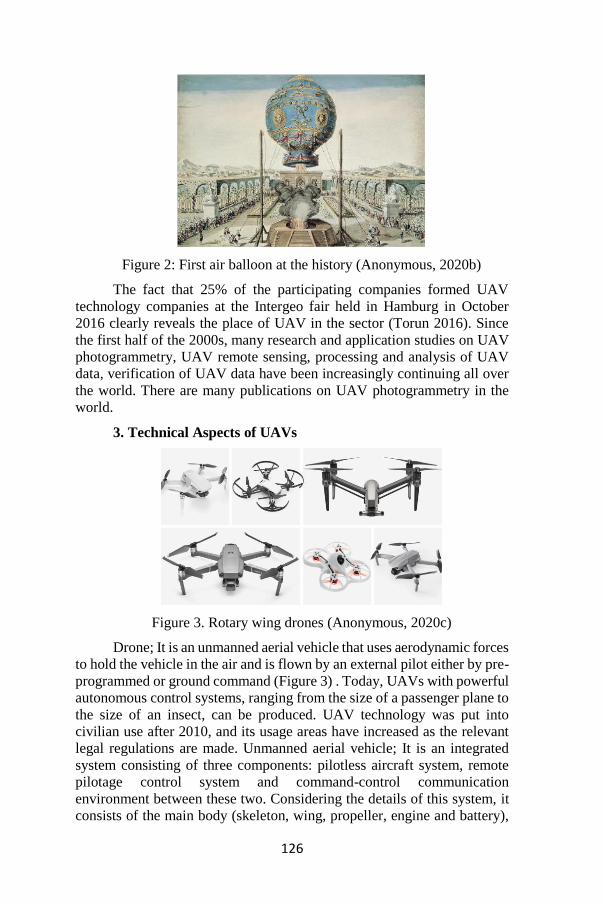
126
Figure 2: First air balloon at the history (Anonymous, 2020b)
The fact that 25% of the participating companies formed UAV
technology companies at the Intergeo fair held in Hamburg in October
2016 clearly reveals the place of UAV in the sector (Torun 2016). Since
the first half of the 2000s, many research and application studies on UAV
photogrammetry, UAV remote sensing, processing and analysis of UAV
data, verification of UAV data have been increasingly continuing all over
the world. There are many publications on UAV photogrammetry in the
world.
3. Technical Aspects of UAVs
Figure 3. Rotary wing drones (Anonymous, 2020c)
Drone; It is an unmanned aerial vehicle that uses aerodynamic forces
to hold the vehicle in the air and is flown by an external pilot either by pre-
programmed or ground command (Figure 3) . Today, UAVs with powerful
autonomous control systems, ranging from the size of a passenger plane to
the size of an insect, can be produced. UAV technology was put into
civilian use after 2010, and its usage areas have increased as the relevant
legal regulations are made. Unmanned aerial vehicle; It is an integrated
system consisting of three components: pilotless aircraft system, remote
pilotage control system and command-control communication
environment between these two. Considering the details of this system, it
consists of the main body (skeleton, wing, propeller, engine and battery),
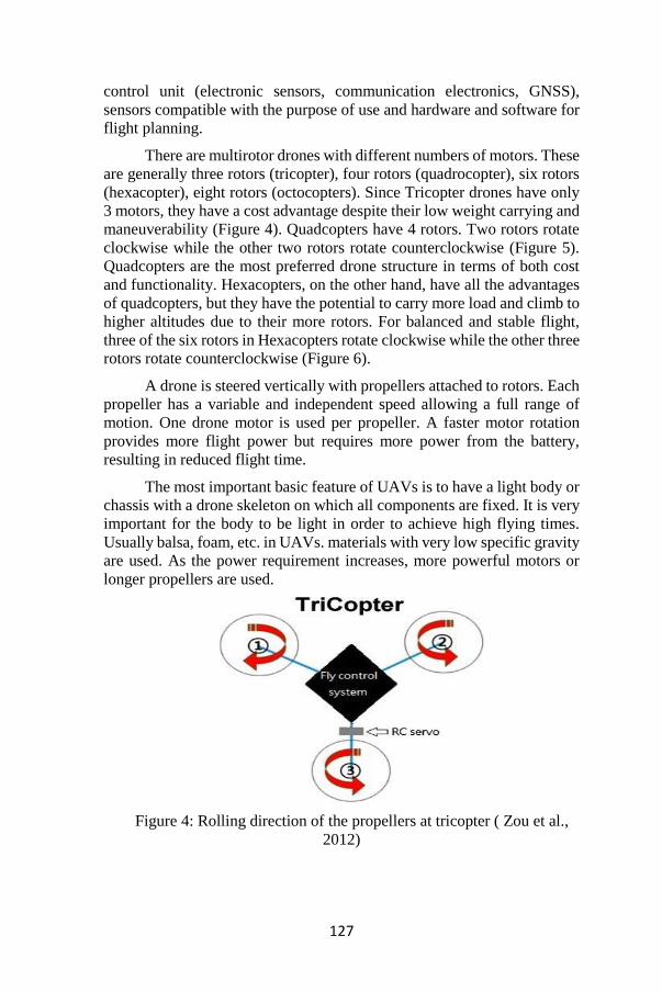
127
control unit (electronic sensors, communication electronics, GNSS),
sensors compatible with the purpose of use and hardware and software for
flight planning.
There are multirotor drones with different numbers of motors. These
are generally three rotors (tricopter), four rotors (quadrocopter), six rotors
(hexacopter), eight rotors (octocopters). Since Tricopter drones have only
3 motors, they have a cost advantage despite their low weight carrying and
maneuverability (Figure 4). Quadcopters have 4 rotors. Two rotors rotate
clockwise while the other two rotors rotate counterclockwise (Figure 5).
Quadcopters are the most preferred drone structure in terms of both cost
and functionality. Hexacopters, on the other hand, have all the advantages
of quadcopters, but they have the potential to carry more load and climb to
higher altitudes due to their more rotors. For balanced and stable flight,
three of the six rotors in Hexacopters rotate clockwise while the other three
rotors rotate counterclockwise (Figure 6).
A drone is steered vertically with propellers attached to rotors. Each
propeller has a variable and independent speed allowing a full range of
motion. One drone motor is used per propeller. A faster motor rotation
provides more flight power but requires more power from the battery,
resulting in reduced flight time.
The most important basic feature of UAVs is to have a light body or
chassis with a drone skeleton on which all components are fixed. It is very
important for the body to be light in order to achieve high flying times.
Usually balsa, foam, etc. in UAVs. materials with very low specific gravity
are used. As the power requirement increases, more powerful motors or
longer propellers are used.
Figure 4: Rolling direction of the propellers at tricopter ( Zou et al.,
2012)
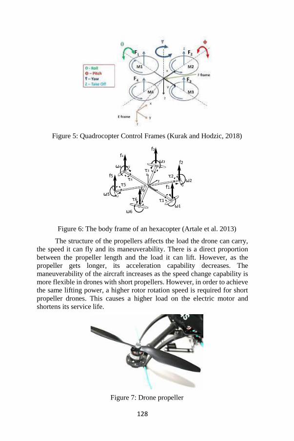
128
Figure 5: Quadrocopter Control Frames (Kurak and Hodzic, 2018)
Figure 6: The body frame of an hexacopter (Artale et al. 2013)
The structure of the propellers affects the load the drone can carry,
the speed it can fly and its maneuverability. There is a direct proportion
between the propeller length and the load it can lift. However, as the
propeller gets longer, its acceleration capability decreases. The
maneuverability of the aircraft increases as the speed change capability is
more flexible in drones with short propellers. However, in order to achieve
the same lifting power, a higher rotor rotation speed is required for short
propeller drones. This causes a higher load on the electric motor and
shortens its service life.
Figure 7: Drone propeller
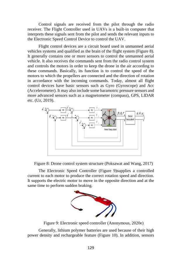
129
Control signals are received from the pilot through the radio
receiver. The Flight Controller used in UAVs is a built-in computer that
interprets these signals sent from the pilot and sends the relevant inputs to
the Electronic Speed Control Device to control the UAV.
Flight control devices are a circuit board used in unmanned aerial
vehicles systems and qualified as the brain of the flight system (Figure 8).
It generally contains one or more sensors to control the unmanned aerial
vehicle. It also receives the commands sent from the radio control system
and controls the motors in order to keep the drone in the air according to
these commands. Basically, its function is to control the speed of the
motors to which the propellers are connected and the direction of rotation
in accordance with the incoming commands. Today, almost all flight
control devices have basic sensors such as Gyro (Gyroscope) and Acc
(Accelerometer). It may also include some baramotric pressure sensors and
more advanced sensors such as a magnetometer (compass), GPS, LIDAR
etc. (Uz, 2019).
Figure 8: Drone control system structure (Poksawat and Wang, 2017)
The Electronic Speed Controller (Figure 9)supplies a controlled
current to each motor to produce the correct rotation speed and direction.
It supports the electric motor to move in the opposite direction and at the
same time to perform sudden braking.
Figure 9: Electronic speed controller (Anonymous, 2020e)
Generally, lithium polymer batteries are used because of their high
power density and rechargeable feature (Figure 10). In addition, sensors

130
such as accelerometers, gyroscopes, GPS and barometers can be used for
positional measurements. Cameras with many different features are often
installed for navigation and aerial photography.
Figure 10: Lithium based batteries (Anonymous, 2020f)
Drones can be controlled manually with a radio transmitter
controller (Figure 11). With the help of the levers on this controller, the
rotation speed and direction of the propellers are changed, allowing the
drone to perform various maneuvers. With the screens on some remote
controls, datas of various sensor and camera images can be monitored. In
addition, built-in sensors can provide useful settings such as automatic
altitude and fixed UAV position. The drone can also be flown
autonomously. The route and landing point of the drone can be determined
with a software.
Figure 11: Drone radio controllers (Anonymous, 2020g)
Depending on the technological development, the use of
smartphones and tablets instead of the control unit, the reduced costs of
various sensors (GPS, Wi-Fi receivers, MEMS INS sensors, visible band,
multi-spectral, thermal, hyper-spectral cameras, etc.) UAV production
costs have decreased. With the development of minimalized hardware
solutions in GNSS technology, location determination can be made more
accurately in navigation applications performed with PPK (Post Processed
Kinematic) GNSS (Colomina et.al, 2014). The top five sectors where UAV
finds the most common application on a global scale; real estate and
construction, photogrammetry (aerial measurement), film / aerial
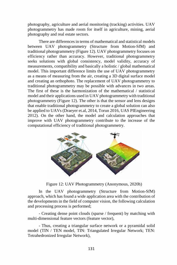
131
photography, agriculture and aerial monitoring (tracking) activities. UAV
photogrammetry has made room for itself in agriculture, mining, aerial
photography and real estate sectors.
There are differences in terms of mathematical and statistical models
between UAV photogrammetry (Structure from Motion-SfM) and
traditional photogrammetry (Figure 12). UAV photogrammetry focuses on
efficiency rather than accuracy. However, traditional photogrammetry
seeks solutions with global consistency, model validity, accuracy of
measurements, compatibility and basically a holistic / global mathematical
model. This important difference limits the use of UAV photogrammetry
as a means of measuring from the air, creating a 3D digital surface model
and creating an orthophoto. The replacement of UAV photogrammetry to
traditional photogrammetry may be possible with advances in two areas.
The first of these is the harmonization of the mathematical / statistical
model and their applications used in UAV photogrammetry with traditional
photogrammetry (Figure 12). The other is that the sensor and lens designs
that enable traditional photogrammetry to create a global solution can also
be applied to UAVs (Draeyer et.al, 2014, Torun 2016, UAS PIEngineering
2012). On the other hand, the model and calculation approaches that
improve with UAV photogrammetry contribute to the increase of the
computational efficiency of traditional photogrammetry.
Figure 12: UAV Photogrammetry (Anonymous, 2020h)
In the UAV photogrammetry (Structure from Motion-SfM)
approach, which has found a wide application area with the contribution of
the developments in the field of computer vision, the following calculation
and processing process is performed;
- Creating dense point clouds (sparse / frequent) by matching with
multi-dimensional feature vectors (feature vector),
- Thus, creating a triangular surface network or a pyramidal solid
model (TIN / TEN model, TIN: Triangulated Irregular Network; TEN:
Tetrahedronized Irregular Network),
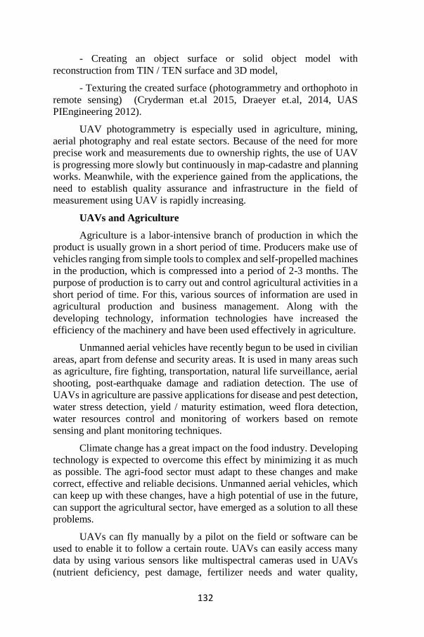
132
- Creating an object surface or solid object model with
reconstruction from TIN / TEN surface and 3D model,
- Texturing the created surface (photogrammetry and orthophoto in
remote sensing) (Cryderman et.al 2015, Draeyer et.al, 2014, UAS
PIEngineering 2012).
UAV photogrammetry is especially used in agriculture, mining,
aerial photography and real estate sectors. Because of the need for more
precise work and measurements due to ownership rights, the use of UAV
is progressing more slowly but continuously in map-cadastre and planning
works. Meanwhile, with the experience gained from the applications, the
need to establish quality assurance and infrastructure in the field of
measurement using UAV is rapidly increasing.
UAVs and Agriculture
Agriculture is a labor-intensive branch of production in which the
product is usually grown in a short period of time. Producers make use of
vehicles ranging from simple tools to complex and self-propelled machines
in the production, which is compressed into a period of 2-3 months. The
purpose of production is to carry out and control agricultural activities in a
short period of time. For this, various sources of information are used in
agricultural production and business management. Along with the
developing technology, information technologies have increased the
efficiency of the machinery and have been used effectively in agriculture.
Unmanned aerial vehicles have recently begun to be used in civilian
areas, apart from defense and security areas. It is used in many areas such
as agriculture, fire fighting, transportation, natural life surveillance, aerial
shooting, post-earthquake damage and radiation detection. The use of
UAVs in agriculture are passive applications for disease and pest detection,
water stress detection, yield / maturity estimation, weed flora detection,
water resources control and monitoring of workers based on remote
sensing and plant monitoring techniques.
Climate change has a great impact on the food industry. Developing
technology is expected to overcome this effect by minimizing it as much
as possible. The agri-food sector must adapt to these changes and make
correct, effective and reliable decisions. Unmanned aerial vehicles, which
can keep up with these changes, have a high potential of use in the future,
can support the agricultural sector, have emerged as a solution to all these
problems.
UAVs can fly manually by a pilot on the field or software can be
used to enable it to follow a certain route. UAVs can easily access many
data by using various sensors like multispectral cameras used in UAVs
(nutrient deficiency, pest damage, fertilizer needs and water quality,
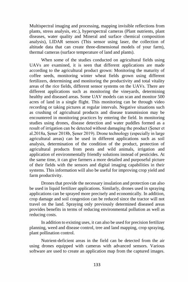
133
Multispectral imaging and processing, mapping invisible reflections from
plants, stress analysis, etc.), hyperspectral cameras (Plant nutrients, plant
diseases, water quality and Mineral and surface chemical composition
analysis), LIDAR sensors (This sensor using laser, the collection of
altitude data that can create three-dimensional models of your farm),
thermal cameras (surface temperature of land and plants).
When some of the studies conducted on agricultural fields using
UAVs are examined, it is seen that different applications are made
according to the agricultural product grown: Monitoring the maturity of
coffee seeds, monitoring winter wheat fields grown using different
fertilizers, determining and monitoring the productivity and total vitality
areas of the rice fields, different sensor systems on the UAVs. There are
different applications such as monitoring the vineyards, determining
healthy and diseased areas. Some UAV models can scan and monitor 500
acres of land in a single flight. This monitoring can be through video
recording or taking pictures at regular intervals. Negative situations such
as crushing of agricultural products and disease transmission may be
encountered in monitoring practices by entering the field. In monitoring
studies using drones, disease detection and water puddles formed as a
result of irrigation can be detected without damaging the product (Şener et
al.2018a, Şener 2018b, Şener 2019). Drone technology (especially in large
agricultural areas) can be used in different applications such as soil
analysis, determination of the condition of the product, protection of
agricultural products from pests and wild animals, irrigation and
application of environmentally friendly solutions instead of pesticides. At
the same time, it can give farmers a more detailed and purposeful picture
of their fields with the sensors and digital imaging capabilities in their
systems. This information will also be useful for improving crop yield and
farm productivity.
Drones that provide the necessary insulation and protection can also
be used in liquid fertilizer applications. Similarly, drones used in spraying
applications can be sprayed more precisely and economically. In addition,
crop damage and soil congestion can be reduced since the tractor will not
travel on the land. Spraying only previously determined diseased areas
provides benefits in terms of reducing environmental pollution as well as
reducing costs.
In addition to existing uses, it can also be used for precision fertilizer
planning, weed and disease control, tree and land mapping, crop spraying,
plant pollination control.
Nutrient-deficient areas in the field can be detected from the air
using drones equipped with cameras with advanced sensors. Various
software are used to create an application map from the captured images.

134
By using these software, fertilization program can be created to meet the
varying nutritional requirements of agricultural products in different parts
of the land. The purpose of the global positioning systems is to determine
the latitude, longitude and altitude coordinates of the field and / or
equipment according to the spatial and temporal data. Variable amounts
and doses of pesticides and fertilizers are applied to the field according to
the mapping principle created by this system. Positioning systems are
divided into two groups as ground-based and satellite-based (Keskin &
Görücü-Keskin, 2012).
Using techniques similar to manure planning, drone operators can
accurately assess weed and disease levels in arable crops (Figure 13). It
can collect data by identifying different characteristics of weeds and
affected areas. By analyzing this information, preventive determinations
and control can be made for products sensitive to weed species and
diseases. Especially in orchards, it provides convenience to producers in
terms of identifying and labeling trees infected with various diseases.
In addition to disease control by using UAVs (Figure 14), orchard
producers can benefit from accurate calculations of areas and tree and row
spacing reports. The same is true in forestry and timber production. The
ability to cover large terrains is a great advantage for mapping in general.
Hundreds of hectares of land can be mapped in a day with the help of
detailed systems that exactly define the boundary features. With the
obtained data, a 3D computer model is created to detect ground features
and possible changes. This information can be used to give field
measurements for application purposes or to support the machine software
to help the operator avoid hazards such as electrical wiring, flooding,
changes in waterways or drainage equipment.
Figure 13: Drone for weed mapping (Anonymous, 2020i)
Today, due to the decline in the number of bees, concerns have been
raised about the future of plant pollination, which is the basis of
horticulture and agricultural production worldwide. Using a drone
weighing only 15 grams, the researchers were able to fertilize the flowers
without harming the plant. Researchers are continuing their research into
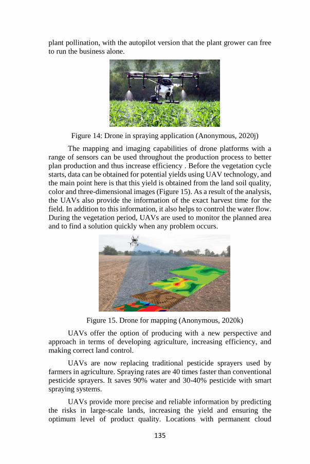
135
plant pollination, with the autopilot version that the plant grower can free
to run the business alone.
Figure 14: Drone in spraying application (Anonymous, 2020j)
The mapping and imaging capabilities of drone platforms with a
range of sensors can be used throughout the production process to better
plan production and thus increase efficiency . Before the vegetation cycle
starts, data can be obtained for potential yields using UAV technology, and
the main point here is that this yield is obtained from the land soil quality,
color and three-dimensional images (Figure 15). As a result of the analysis,
the UAVs also provide the information of the exact harvest time for the
field. In addition to this information, it also helps to control the water flow.
During the vegetation period, UAVs are used to monitor the planned area
and to find a solution quickly when any problem occurs.
Figure 15. Drone for mapping (Anonymous, 2020k)
UAVs offer the option of producing with a new perspective and
approach in terms of developing agriculture, increasing efficiency, and
making correct land control.
UAVs are now replacing traditional pesticide sprayers used by
farmers in agriculture. Spraying rates are 40 times faster than conventional
pesticide sprayers. It saves 90% water and 30-40% pesticide with smart
spraying systems.
UAVs provide more precise and reliable information by predicting
the risks in large-scale lands, increasing the yield and ensuring the
optimum level of product quality. Locations with permanent cloud

136
persistence or high turbidity become traceable and high resolution data can
be obtained.
It increases productivity by reducing the workload and time required
in the management of large-scale lands. It provides an economically
effective traceability of inaccessible areas that are difficult to work due to
its topography.
Since reliable results are obtained, it can be used easily in scientific
researches. Despite the bad environment and weather conditions, the stable
use of UAVs is proof that there will be significant progress in agriculture
compared to traditional methods. For this reason, UAVs are a promising
technology and alternative to old methods in low cost, comprehensive and
reliable data collection. Usage areas and the research opportunities it
creates indicate that UAVs will be increasingly used in the future and will
be constantly on the agenda.
UAV technology can collect data in agricultural areas faster, more
accurately and at lower cost. Today, negative effects and results of plant
protection applications made with conventional methods. For example, in
conventional spraying applications with a tractor, a small part of the
sprayed liquid can hold on the plant, while the rest flows into the soil. In
addition, it causes serious yield losses as it causes soil congestion and
crushing of agricultural products during tractor spraying.
With the decisions based on the analysis of the data obtained from
the sensors, exact accuracy in fertilizer applications can be effective in
efficiency and can reduce costs. This opportunity is valid not only for
macronutrients but also for micronutrients. With the same approach,
product losses can be minimized by monitoring the initiation and spread
stages of pests and diseases in an easy, cheap and timely manner. Naturally,
early diagnosis provides opportunity to use minimum insecticide and
pesticide, reduces environmental damage and brings cost reduction.
Beyond easy adaptation to the topography, UAV technology offers
a very rapid application opportunity compared to airborne spraying. With
spectral or thermal sensors, it can prevent possible drought damage by
guiding the producer about irrigation with analysis based on leaf-soil
moisture.
Another area of use is active applications that include precise
chemical application, pest removal and livestock control. UAVs started to
be used for agricultural purposes under the leadership of Japan in the 1980s
with the request of the development of an unmanned helicopter for
spraying from Yamaha company (Anonymous, 2016j). Later, it started to
take part in agriculture in order to overcome the problems caused by
satellite and air platforms in remote sensing (Tekin et al., 2015).
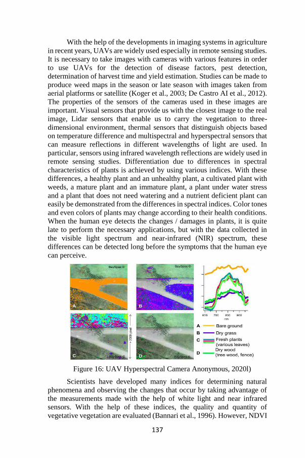
137
With the help of the developments in imaging systems in agriculture
in recent years, UAVs are widely used especially in remote sensing studies.
It is necessary to take images with cameras with various features in order
to use UAVs for the detection of disease factors, pest detection,
determination of harvest time and yield estimation. Studies can be made to
produce weed maps in the season or late season with images taken from
aerial platforms or satellite (Koger et al., 2003; De Castro AI et al., 2012).
The properties of the sensors of the cameras used in these images are
important. Visual sensors that provide us with the closest image to the real
image, Lidar sensors that enable us to carry the vegetation to three-
dimensional environment, thermal sensors that distinguish objects based
on temperature difference and multispectral and hyperspectral sensors that
can measure reflections in different wavelengths of light are used. In
particular, sensors using infrared wavelength reflections are widely used in
remote sensing studies. Differentiation due to differences in spectral
characteristics of plants is achieved by using various indices. With these
differences, a healthy plant and an unhealthy plant, a cultivated plant with
weeds, a mature plant and an immature plant, a plant under water stress
and a plant that does not need watering and a nutrient deficient plant can
easily be demonstrated from the differences in spectral indices. Color tones
and even colors of plants may change according to their health conditions.
When the human eye detects the changes / damages in plants, it is quite
late to perform the necessary applications, but with the data collected in
the visible light spectrum and near-infrared (NIR) spectrum, these
differences can be detected long before the symptoms that the human eye
can perceive.
Figure 16: UAV Hyperspectral Camera Anonymous, 2020l)
Scientists have developed many indices for determining natural
phenomena and observing the changes that occur by taking advantage of
the measurements made with the help of white light and near infrared
sensors. With the help of these indices, the quality and quantity of
vegetative vegetation are evaluated (Bannari et al., 1996). However, NDVI
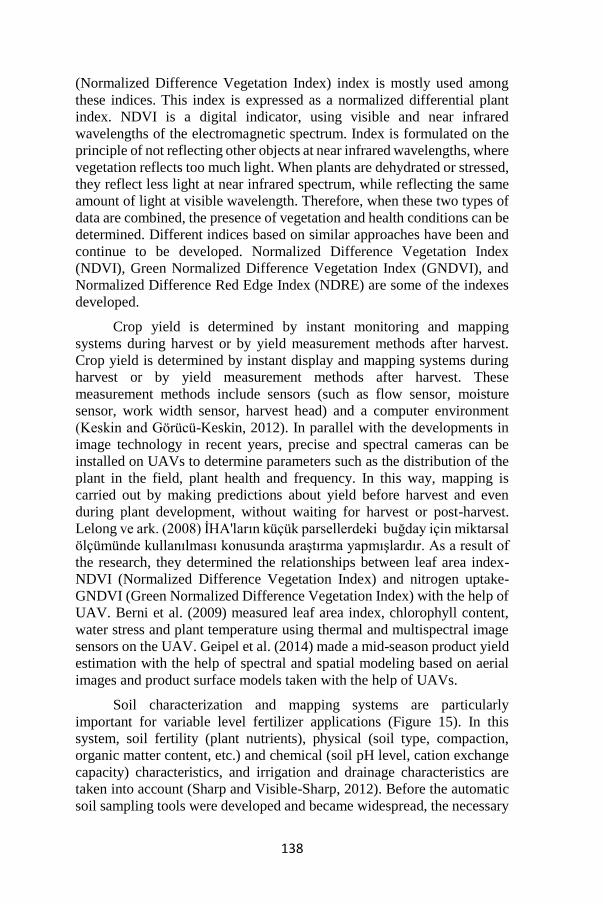
138
(Normalized Difference Vegetation Index) index is mostly used among
these indices. This index is expressed as a normalized differential plant
index. NDVI is a digital indicator, using visible and near infrared
wavelengths of the electromagnetic spectrum. Index is formulated on the
principle of not reflecting other objects at near infrared wavelengths, where
vegetation reflects too much light. When plants are dehydrated or stressed,
they reflect less light at near infrared spectrum, while reflecting the same
amount of light at visible wavelength. Therefore, when these two types of
data are combined, the presence of vegetation and health conditions can be
determined. Different indices based on similar approaches have been and
continue to be developed. Normalized Difference Vegetation Index
(NDVI), Green Normalized Difference Vegetation Index (GNDVI), and
Normalized Difference Red Edge Index (NDRE) are some of the indexes
developed.
Crop yield is determined by instant monitoring and mapping
systems during harvest or by yield measurement methods after harvest.
Crop yield is determined by instant display and mapping systems during
harvest or by yield measurement methods after harvest. These
measurement methods include sensors (such as flow sensor, moisture
sensor, work width sensor, harvest head) and a computer environment
(Keskin and Görücü-Keskin, 2012). In parallel with the developments in
image technology in recent years, precise and spectral cameras can be
installed on UAVs to determine parameters such as the distribution of the
plant in the field, plant health and frequency. In this way, mapping is
carried out by making predictions about yield before harvest and even
during plant development, without waiting for harvest or post-harvest.
Lelong ve ark. (2008) İHA'ların küçük parsellerdeki buğday için miktarsal
ölçümünde kullanılması konusunda araştırma yapmışlardır. As a result of
the research, they determined the relationships between leaf area index-
NDVI (Normalized Difference Vegetation Index) and nitrogen uptake-
GNDVI (Green Normalized Difference Vegetation Index) with the help of
UAV. Berni et al. (2009) measured leaf area index, chlorophyll content,
water stress and plant temperature using thermal and multispectral image
sensors on the UAV. Geipel et al. (2014) made a mid-season product yield
estimation with the help of spectral and spatial modeling based on aerial
images and product surface models taken with the help of UAVs.
Soil characterization and mapping systems are particularly
important for variable level fertilizer applications (Figure 15). In this
system, soil fertility (plant nutrients), physical (soil type, compaction,
organic matter content, etc.) and chemical (soil pH level, cation exchange
capacity) characteristics, and irrigation and drainage characteristics are
taken into account (Sharp and Visible-Sharp, 2012). Before the automatic
soil sampling tools were developed and became widespread, the necessary
139
analyzes to determine the soil properties were made by taking soil samples
from the field and taking them to the laboratory. However, thanks to special
cameras and sensors mounted on the UAV in recent years, mapping
operations have been carried out in a shorter time. Gago et al. (2015)
examined the plant-water relationships in the plant-scale study of scanning
images obtained from different types of UAVs such as unmanned
helicopters, multirotors, and fixed wings, and concluded that UAVs are
useful in irrigation management. Aldana-Jague et al. (2016) conducted
research on 2 hectares of land with drones equipped with multispectral
cameras (flying at 120 m altitude) to determine the amount of organic
carbon in the soil and reported that it has a potential use area. Neely et al.
(2016) reported that soil properties affect crop yield and quality, and that
they can predict crop yield at the end of the season by installing
multispectral cameras on the UAV.
In the crop and field conditions monitoring systems, it is aimed to
monitor the plant and field status on foot or by vehicle and to obtain border
maps. Although applications with vehicles are faster than applications by
foot, technological developments show that UAVs can also be used in this
area. Data obtained on a foot or off-road vehicle, in limited areas or over a
long period of time, is then loaded into the computer and evaluated. In
applications made with UAVs, it is displayed with the help of software.
The use of UAVs not only saves time with higher resolution images at low
altitudes, but also offers the opportunity to monitor larger areas in a short
time and take precise measurements by scanning the entire field surface.
Zarco-Tejada et al. (2013) reported that UAVs equipped with high-
resolution hyperspectral cameras can be used to determine the content of
leaf carotenoid in vineyards. Mesas-Carrascosa et al. (2015) reported that
UAV images can be used to determine soil and green parts (crops and
weeds) for weed management specific to the region during the growing
season. Ehsani and Maja (2013) stated that human-based observations on
product health may lead to loss of time, cost increase and human errors,
whereas UAV observations will be more effective. Zorlu (2016) monitored
the development process of the cotton plant with UAVs and made
evaluations about its development. The purpose of remote sensing systems
is to measure and monitor from a certain height and distance without
contacting the field and / or plant. Measurement and monitoring heights
can vary from a pole planted in the field to the satellite in space.
Measurement and imaging from the pole can be fixed or mounted on an
off-road vehicle. While the measurements and images taken from the
satellite can be monthly, weekly or daily, it is possible to take
measurements and images with UAVs at desired altitudes and at the
desired time - day and hour. Maps obtained by taking up-to-date images at
the desired time and area used in many areas can be used as an alternative
to satellite images. In the next stage, it can assist in fertilization, land
140
reclamation, urban planning, land use and planning. Stehr (2015) reported
that the image taken from 15 cm resolution UAV cameras is 40,000 times
better than the average satellite data and 44 times better than the best
commercial satellite image. Matese et al. (2015) compared the NDVI
images obtained from a vineyard by using UAVs, planes and satellites as
remote sensing platforms. They reported that UAVs are suitable in small
areas, 5 ha is the threshold, and satellite images can be viewed at a lower
cost in areas above 5 ha. Ehsani and Maja (2013) concluded that low
altitude UAVs are better than traditional aerial images when using thermal
and visible / near infrared images in distinguishing healthy and stressed
trees.
Classification of UAVs
Today, UAVs in many different shapes, sizes, configurations and
characters are produced (Table 1). Classifications based on flight range,
altitude and wing structure are mostly used (Table 2). (Blyenburgh, 1999;
Bento, 2008; Şahin, 2011).
Table 1. NATO UAS Classification (Szabolcsi, 2016)
UAVs are divided into two groups according to the wing type as
fixed wing and rotary wing . Although fixed-wing (aircraft) UAVs perform
fast and long-range missions, they cannot stay fixed in the air on the target
and cannot be used very close to the target surfaces. Due to their high
degree of control, rotary wing (helicopter) UAVs fly very close to the
target surface, but are used for shorter times and distances (Jurdak et al.,
2015). Fixed-wing UAVs are more advantageous to use than rotary-wing
UAVs with features such as simple construction, easier maintenance and
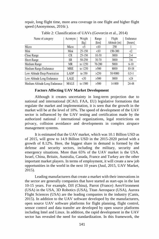
141
repair, long flight time, more area coverage in one flight and higher flight
speed (Anonymous, 2016i ).
Table 2: Classification of UAVs (Govorcin et al., 2014)
Factors Affecting UAV Market Development
Although it creates uncertainty in long-term projection due to
national and international (ICAO, FAA, EU) legislative formations that
regulate the market and implementation, it is seen that the growth in the
market will be at the level of 10%. The speed of development of the UAV
sector is influenced by the UAV testing and certification made by the
authorized national / international organizations, legal restrictions on
privacy, collision avoidance and developments in complex airspace
management systems.
It is estimated that the UAV market, which was 10.1 Billion USD as
of 2015, will grow to 14.9 Billion USD in the 2015-2020 period with a
growth of 8.12%. Here, the biggest share in demand is formed by the
defense and security sectors, including the military, security and
emergency situations. More than 65% of the UAV market is the USA.
Israel, China, Britain, Australia, Canada, France and Turkey are the other
important market players. In terms of employment, it will create a new job
opportunities in the world in the next 10 years (Juul, 2015, UAV Market,
2015).
Leading manufacturers that create a market with their innovations in
the sector are generally companies that have started as start-ups in the last
10-15 years. For example, DJI (China), Parrot (France) AeroVironment
(USA) in the USA, 3D Robotics (USA), Titan Aerospace (USA), Aurora
Flight Sciences (USA) are the leading companies in the industry (Canis,
2015). In addition to the UAV software developed by the manufacturers,
open source UAV software platforms for flight planning, flight control,
sensor control and data transfer are developed by open source platforms
including Intel and Linux. In addition, the rapid development in the UAV
sector has revealed the need for standardization. In this framework, the
142
study has been initiated to make the UAV software developed by ETHZ
the basic standard. The UAV technology developed by Google will open
up a new area of use as well as being very large-sized (larger than
passenger aircraft) for mapping, communication and internet access, taking
its power from solar energy, and having the ability to navigate beyond the
Troposphere, in the Stratosphere (~ 20 km).
Today, the use of UAVs can pose security threats, as revealed in
various instances (UAVs that landed in the White House by mistake in
2015, UAVs flying around airports). In UAVs for defense and military
purposes, the number of accidents obtained with open source information
in the 2007-2014 period is over 200. In this respect, it is imperative that
UAVs be examined in terms of safety. While it is an essential need to
establish the legal infrastructure of the UAV sector only due to accidents
that have occurred or are likely to happen; beyond that, insurance, trade,
certification, security etc. The fact that there is a need for more
comprehensive legislation covering areas cannot be ignored.
In addition to national legislation, UAV regulations are based on the
International Civil Aviation Convention set forth by the Chicago
Conference (UN Chicago Convention-1944) and the International Civil
Aviation Organization (ICAO) publications established on this basis
(1947) and international conventions ( Cary, et.al., 2011, UAS ICAO,
2011). Following the regulation published by ICAO in 2011 in terms of
creating UAV legislation; USA, EU, Australia, Sweden, UK, Canada etc.
Some countries have followed their legislative practice and experience.
RESULTS
The use of UAV has been increasing due to technological
developments and increases in labor costs in recent years. It should be
expected that UAVs will become more widespread as the legal regulations
regarding their use are completed.
The use of UAVs in agriculture can be profitable for large farms.
Drone applications and use with a state-supported organization will be
suitable for these farmers. These tools should be expected to become more
widespread with their efficiency-enhancing and time-saving advantages.
In the past, UAVs were mostly produced for military missions. It
has evolved in parallel with the technological developments in time and
has come to the present day and started to be used in various applications
for civilian purposes since 2010.
Thanks to the camera and battery technology developed in recent
years, high resolution images can be obtained from hundreds of hectares
of field in a single flight time with UAVs. These studies can be carried out
in a shorter time without the need for human and labor. In addition, it

143
provides the opportunity to receive images even in cloudy weather
conditions where images cannot be taken from satellites.
Unlike other sectors, there is no need for additional equipment other
than special camera and sensor devices in the use of UAVs in agriculture.
In fact, research has shown that 85% savings are achieved in forest seeding
applications by adding additional cameras - sensors to vehicles that are out
of use in military use. However, legal restrictions and security reservations
(private life, terrorist activities, etc.) remain as an obstacle to their spread.

144
LITERATURE
1. Aldana-Jague; E., Heckrath, G., Macdonald, A., van Wesemael, B., van
Oost, K. (2016). UASbased soil carbon mapping using VIS-NIR
(480-1000 nm) multi-spectral imaging: Potential and limitations.
Geoderma 275: 55-66.
2. Anonymous (2020a).
https://img.militaryaerospace.com/files/base/ebm/mae/image/2019/
02/content_dam_mae_online_articles_2019_02_heron_uav_26_feb
_2019.png?auto=format&w=720. Access Date: 12.11.2020
3. Anonymous (2020b). https://www.laodikeiaballoons.com/the-
experience/history-of-balloning. Access Date: 12.11.2020
4. Anonymous (2020c).
https://www.popularmechanics.com/technology/gadgets/g2983/the
-best-drones-review/ . Access Date: 12.11.2020
5. Anonymous (2020e). https://www.amazon.in/Robodo-Electronics-
Controller-Brushless-Quadcopter/dp/B00MTJ8QP6. Access Date:
12.11.2020
6. Anonymous (2020f).
https://industrial.panasonic.com/content/data/BT/pictures/lp3_lithi
um-ion_01_e.jpg. Access Date: 12.11.2020
7. Anonymous (2020g). https://encrypted-
tbn0.gstatic.com/images?q=tbn%3AANd9GcTxRoBwvSpDZBgN
NwyG_upc6dVn83dLJoIp1A&usqp=CAU. Access Date:
12.11.2020
8. Anonymous (2020h). https://wingtra.com/drone-photogrammetry-vs-
lidar/ Access Date: 12.11.2020
9. Anonymous (2020i). https://track32.nl/portfolio/drone-for-mapping-
weed-populations/. Access Date: 12.11.2020
10. Anonymous (2020j). https://meticulousblog.org/top-10-companies-in-
agriculture-drone-market/. Access Date: 12.11.2020
11. Anonymous (2020k). https://nias-uas.com/create-map-drone-data-real-
time/. Access Date: 12.11.2020
12. Anonymous (2020l). https://www.bayspec.com/spectroscopy/oci-uav-
hyperspectral-camera/. Access Date: 12.11.2020
13. Anonymous (2016a).
http://www.notablebiographies.com/CaCh/Cavendish-Henry.html.
Access Date: 29.11.2016.

145
14. Anonymous (2016b). Access Date: 29.11.2016
http://wwwgroups.dcs.st-and.ac.uk/history/Biographies/Biot.html
15. Anonymous, 2016c. ballooning/civil-
warballooning.html?referrer=https://www.google.com.tr/ Access
Date: 29.11.2016
16. Anonymous (2016c). http://www.history.com/news/attack-ofjapans-
killer-wwii-balloons-70-years-ago. Access Date: 29.11.2016
17. Anonymous (2016d).
https://en.wikipedia.org/wiki/Timeline_of_aviation_%E2
%80%93_19th_century. Access Date: 30.11.2016
18. Anonymous (2016e). http://www.rubincenter.org/2010/09/rodman-
2010-09- 07/ Access Date: 30.11.2016
19. Anonymous (2016f). http://www.dohenydrones.com/newsfixed-wing-
versus-rotary-wing Access Date: 30.11.2016
20. Anonymous (2016g). http://newatlas.com/uav-cropdusting/27974/
Access Date: 30th November 2016
21. Anonymous (2010). Unmanned aircraft systems: Terminology,
definitions and classification, Joint doctirin note3/10, United
Kingdom Ministry of Defence, May 2010, 21pp, United Kingdom.
22. Artale, V., Ricciardello, A., Milazzo, C. (2013). Mathematical
Modelling of Hexacopter, Applied Mathematical Sciences
7(97):4805-4811.
23. Bannari, A., Morin, D., Bonn, F., Huete, A. R.(1995) 'A Review of
Vegetation Indices', Remote Sensing Reviews, 13: 1, 95-120.
24. Bento, M.F. (2008) Unmanned Aerial Vehicle (An Overview).
(www.insidegnss.com/auto/janfeb08- wp.pdf (Access Date: May
2016)).
25. Berni, J.A.J., arco-Tejada, P.J., Suarez, L., Fereres, E. (2009). Thermal
and narrowband multispectral remote sensing for vegetation
monitoring from an unmanned aerial vehicle. IEEE Transactions on
Geoscience and Remote Sensing 47(3): 722-738.
26. Blyenburgh, P. V. (1999). UAVs: an Overview. Uninhabited Aerial
Vehicles (UAVs), Air and Space Europe Vol:1, No:5/6. pp. 43-47
27. Canis, B. (2015): Unmanned Aircraft Systems 8UAS): Commercial
Outlook for New Industry, Congressional Research Service, CRS
Report, 7-5700, R44192
28. Cary, L, Coyne, J. (2011): ICAO Unmanned Aircraft Systems (UAS),
Circular 328, 2011-2012 UAS Yearbook - UAS: The Global

146
Perspective – 9th Edition - June 2011 - Blyenburgh & Co © -
www.uvs-info.com - Page: 112/216
29. Colomina, I., Molina, P. (2014): Unmanned Aerial System for
Photogrammetry and Remote Sensing, Isprs Journal Of
Photogrammetry And Remote Sensıng, June 2014
30. Dean, H., Fujikawa, S. J., Linden, D. S., Daughtry, C. S., McCarty, G.
W., Hunt, R. (2010). Acquisition of NIR-Green-Blue Digital
Photographs from Unmanned Aircraft for Crop Monitoring. Remote
Sensing, 290-305.
31. De Castro A., I., Jurado-Expósito M., Peña-Barragán J., M., López-
Granados, F. (2012) Airborne Multi-spectral Imagery for Mapping
Cruciferous Weeds in Cereal and Legume Crops. Precis Agric 13(3):
302–321. doi: 10.1007/s11119-011-9247-0.
32. Dictionary.com, 2016,
http://dictionary.reference.com/browse/uav?s=t, Access Date: 14th
January 2016.
33. Draeyer B., Strecha, C. (2014): White paper: How accurate are UAV
surveying methods? Pix4D White paper, February 2014
34. Ehsani, R., Maja, J.M. (2013). The rise of small UAVs in precision
agriculture. Resource 20(4): 18- 19.
35. Gago, J., Douthe, C., Coopman, R.E., Gallego, P.P., Ribas-Carbo, M.,
Flexas, J., Escalona, J., Medrano, H. (2015). UAVs challenge to
assess water stress for sustainable agriculture. Agricultural Water
Management 153:9-19.
36. Geipel, J., Link, J., Claupein, W. (2014). Combined spectral and spatial
modeling of corn yield based on aerial images and crop surface
models acquired with an unmanned aircraft system. Remote Sensing
6 (11): 10335-10355.
37. Gibbons, G., 2000. Turning a farm art into science an overview of
precision farming. URL: http://www.precisionfarming.com.
38. Govorcin, M., Pribicevic, B., Dapo, E. (2014). Comparison And
Analysis Of Software Solutions For Creation Of A Digital Terrain
Model Using Unmanned Aerial Vehicles. 14th International
Multidisciplinary Scientific Geoconference Sgem 2014 -
Geoconference On Informatics
39. Jurdak, R., Elfes, A., Kusy, B., Tews, A., Hu, W., Hernandez, E.,
Kottege, N., Sikka, P. (2015). Autonomous surveillance for
biosecurity. Trends in Biotechnology 33(4): 201-207.
147
40. Juul, M. (2015): Civil drones in the European Union, European
Parliment, EPRS | European Parliamentary Research Service,
Octover 2015
41. Haser, A.B., 2010. Bu insansız hava aracından daha önce yapmamış
mıydık?, Bilim ve Teknik Dergisi, Aralık sayısı.
42. Herwitz, S. R., Johnson, L., Dunagon, S., Higgins, R., Sullivan, D.,
Zheng, J., Lobitz, B., Leung, J., Gallmeyer, B., Aoyagi, M., Slye,
R., Brass, J., Witt, G. (2003). Coffee field ripeness detection using
high resolution imaging systems on a solar-powered UAV, Proc.
30th Symp. Rem. Sens. Environ., TS-12.3, 3 pp., Honolulu, HI.
43. Kahveci, M., Can, N. (2017). S.Ü. Müh. Bilim ve Tekn. Derg., c.5, s.4,
ss. 511-535. İnsansız Hava Araçları: Tarihçesi, Tanımı, Dünyada Ve
Türkiye'deki Yasal Durumu. Selcuk Univ. J. Eng. Sci. Tech., v.5,
n.4, pp. 511-535, ISSN: 2147-9364 (Elektronik) DOI:
10.15317/Scitech.2017.109
44. Keskin, M., Gorucu-Keskin, S. (2012). Hassas Tarım Teknolojileri.
Hatay. Mustafa Kemal Üniversitesi Yayınları No:35. 210 s.
45. Koger, C., H., Shaw, D.R., Watson, C., E, Reddy, K.,N. (2003)
Detecting Late Season Weed Infestations in Soybean (Glycine max).
Weed Technol 17: 696-704. doi:10.1614/WT02-122.
46. Kurak, S., Hodzic, M. (2018). Control and Estimation of a Quadcopter
Dynamical Model. Periodicals of Engineering and Natural Sciences,
Vol:6, No:1, 63-75
47. Lelong, C.C.D. Burger, P., Jubelin, G., Roux, B., Labbe, S., Baret, F.
(2008). Assessment of unmanned aerial vehicles imagery for
quantitative monitoring of wheat crop in small plots. Sensors
8:3557-3585.
48. Mesas-Carrascosa, F.J., Torres-Sanchez, J., Clavero-Rumbao, I.,
Garcia-Ferrer, A., Pena, J.M., BorraSerrano, I., Lopez-Granados, F.
(2015). Assessing optimal flight parameters for generating accurate
multispectral orthomosaicks by UAV to support site-specific crop
management. Remote Sensing 7: 12793-12814.
49. Neely, H.L., Morgan, C.L.S., Stanislav, S., Rouze, G., Shi, Y.,
Thomasson, J.A., Valasek, J., Olsenholler, J. (2016). Strategies for
soil-based precision agriculture in cotton. Proc. SPIE 9866,
Autonomous Air and Ground Sensing Systems for Agricultural
Optimization and Phenotyping.
50. Poksawat, P., Wang, L. (2017). Automatic Tuning of Hexacopter
Attitude Control Systems with Experimental Validation. 21st
148
International Conference on System Theory, Control and
Computing Conference.
51. Rango, A., Laliberte, A., Steele, C., Herrick, J. E., Bestelmeyer, B.,
Schmugge, T., Jenkins, V. (2006). Using Unmanned Aerial Vehicles
for Rangelands: Current Applications and Future Potentials.
Environmental Practice, 159-168.
52. Shibusawa, S. (1998). Precision Farming and Terra-mechanics. Fifth
ISTVS Asia-Pacific Regional Conference in Korea, October 20-22.
53. Stehr, N. (2015). Drones: The newest technology for precision
agriculture. Nat.Sci.Educ. 44:89-91. Şahin, M. (2011). Sabit Kanatlı
Mini İnsansız Hava Aracının Geliştirilmesi Ve Ağaçlandırma
Çalışmalarında Kullanımı. Erciyes Üniv. Fen Bil. Ens. Yüksek
Lisans Tezi, Kayseri,91 s.
54. Szabolcsi, R. (2016). Beyond Training Minimums – A New Concept of
the UAV Operator Training Program. International conference
Knowledge Based Organization.
55. Swain, K. C., Thomson, S. J., Jayasuriya, H.P.W. 2010. Adoption of an
Unmanned Helicopter for Low-Altitude Remote Sensing to
Estimate Yield and Total Biomass of a Rice Crop.
56. Şahin, M. (2011). Sabit Kanatlı Mini İnsansız Hava Aracının
Geliştirilmesi Ve Ağaçlandırma Çalışmalarında Kullanımı. Erciyes
Üniv. Fen Bilimleri Ens. Yüksek Lisans Tezi, Kayseri, 91 s
57. Şener, M., Pehlivan, M., Tekiner, M., Alkan, C., Ozden, U.E., Erdem,
T., Celen I.H., Seren, A, Aydın, S.A., Kolsuz, H.U., Seyrek, K,
Gurescı, G., Kose G., Turan, L. (2019). Monitoring of irrigation
schemes by using thermal camera mounted UAVs, Fresenıus
Envıronmental Bulletın, Vol. 28:6, Pp. 4684-4691.
58. Şener, M., Boyraz Erdem, D., Alkan, C., Celen, I.H., Erdem, T.
(2018a). Unmanned Aerial Vehicle (UAV) for Monitoring
Agricultural Activity, Journal of Scientific and Engineering
Research, vol. 5, pp. 137-139.
59. Şener, M., Pehlivan, M., Tekiner, M., Alkan, C., Ozden, U.E., Erdem,
T., Celen I.H., Seren, A, Aydın, S.A., Kolsuz, H.U., Seyrek, K,
Gurescı, G., Kose G & Turan, L. (2018b). Unmanned Aerial Vehicle
(UAV) based remote sensing for crop pattern mapping, Turkey,
Fresenıus Envıronmental Bulletın, Vol. 27, Pp. 8831-8837.
60. Torun, A. (2016): Integrating Geospatial Technologies: Reflections on
Intergeo 2016, GIM International, November.

149
61. UAV Market (2015): The Global UAV Market 2015–2025, Ref Cpde:
DF0060SR, Jan 2015 UAS ICAO (2011): Unmanned Aircraft
Systems (UAS), Cir 328 AN/190, International Civil Aviation
Organization UAS PIEngineering (2012): Aspects of Accuracy in
UAS Photogrammetry, White Paper Version 1.0.4PIEneering Ltd.
62. Uz, U. (2019). Hexacopter Yapısında Bir İnsansız Hava Aracı İle
Elektronik İlaçlama/Sulama Sisteminin Oluşturulması. T.C.
İstanbul Gelişim Üniversitesi Fen Bilimleri Enstitüsü Umut Uz
Yüksek Lisans Tezi Mekatronik Mühendisliği Anabilim Dalı, 95
sayfa., İstanbul.
63. Zorlu, F. (2016). İnsansız Hava Aracı ile Pamuk Bitkisinin Gelişim
Sürecindeki Değişimlerin İzlenmesi ve Değerlendirilmesi. Harran
Üniversitesi Fen Bilimleri Ens. Yüksek Lisans Tezi, Şanlıurfa, 56s.
64. Zou, J., Su, K., Tso, H. (2012). The modeling and implementation of
tri-roto flying robot. Artificial Life and Robotics, 17, 86-91.
65. Turner, D., Lucieer, A., Watson, C. (2011). Development of an
Unmanned Aerial Vehicle (UAV) for hyper resolution vineyard
mapping based on visible, multispectral, and thermal imagery

150
CHAPTER X
HISTORICAL RELIABILITY EVALUATION OF POWER
DISTRIBUTION SYSTEMS BASED ON MONTE CARLO
SIMULATION METHOD
Mohammed Wadi1 & Abdulfetah Shobole2
1(Asst. Prof.) Istanbul Sabahattin Zaim University, e-mail: [email protected]
0000-0001-8928-3729
2(Asst. Prof.) Istanbul Sabahattin Zaim University, e-mail: [email protected]
0000-0002-3180-6504
1. INTRODUCTION
It is crucial to assess power systems' reliability to get the most
accurate and appropriate planning, operation, and maintenance decisions.
Historical assessment and predictive assessment are widely used methods
to assess the reliability of a distribution network. Predictive reliability
assessment is classified into two methods, analytical method and
simulation method. Besides, analytical methods can be categorized into
Markov modeling and network modeling groups (Koster et al., 1978).
Simulation methods are considered the most flexible methods. However, it
is computationally-burden. Since the historical reliability assessment based
on actual data, which is exceptionally crucial in reliability analysis and can
be a reference for comparison with other reliability assessment techniques
(A. A. Chowdhury, 2005), it is preferable by most utilities rather than a
predictive assessment. Thus, the utilities continually need to preserve and
collect the data for plans and studies. The actual collected data would
improve the system analyses in the future and the system's overall
reliability. The significance of reliability studies for utility operators is
crucial to determine the parts that are experiencing repeated failures, the
areas of the highest amount of energy not supplied, and the areas of weak
protection system (Wilson et al., 2006).
Many valuable works have been presented on historical reliability
assessment (Allan, 1994)(Kim & Singh, 2010)(Baharum et al.,
2013)(Abunima et al., 2018). Baharum et al. (Baharum et al., 2013),
assessed the historical reliability based on the collected from an electricity
distribution company in Baghdad, Iraq, and the two-parameter Weibull
Reliability Assessment of Closed Ring Power Distribution Systems

152
function. The statistical measures obtained by this analysis revealed the
weakest parts such as transformers and circuit breakers. In (Feng, 2006),
the actual data of 13 utilities in Canada are used to perform historical
reliability analysis to determine the performance and assess the financial
risk for their power distribution networks. Besides, it is established the
regulations that are required to specify the reward/penalty levels. In
(Wallnerström, 2008), the actual data for one Swedish power distribution
network for three years (2004 -2006) are used to perform historical
reliability analysis. The obtained result verified that the annual outage cost
per customer was more than 500 €. In (A. A. Chowdhury, 2005), the actual
data for two Canadian power distribution networks are utilized to improve
the performance-based regulation in a deregulated environment to
investigate the level of service reliability of these networks.
(Billinton & Pan, 2004) introduced a historical reliability assessment
based on actual reliability data taken from the Canadian Electricity
Association (CEA) service continuity reports. The study presented package
of reward/penalty structure based on the historic reliability record could be
integrated into a performance-based regulation plan. Historic reliability
data are therefore, extremely crucial for distribution system risk
assessment and remedial work in this new regime.
Monte Carlo Simulation (MCS) for reliability assessment in power
systems also have been appeared in the literature (Thoemmes et al.,
2010)(Schoemann et al., 2014)(Wijekularathna et al., 2019)(Godha et al.,
2011)(Al-Wafi et al., 2016)(Bakkiyaraj & Kumarappan, 2010).
MCS techniques based on non-sequential state transition sampling
reliability evaluation of power systems is proposed(Bakkiyaraj &
Kumarappan, 2010). This method is applied to Roy Billinton Test System
(RBTS) and verified its effectiveness compared with the sequential
simulation. In (Godha et al., 2011) MCS to assess the costs due to electric
supply interruptions in distribution power system. Feeder 1 of RBTS Bus-
2 is utilized to carry out the simulation and to confirm the applicability of
MCS.
The sequential time MCS is presented to assess distribution systems'
reliability due to severe weather (Cadini et al., 2017). MCS in combining
with stochastic models for describing uncertain weather conditions with a
cascading failure model based on a DC approximation of the power flows
and a proportional re-dispatch strategy is proposed. The sequential time
MCS method was tested by IEEE14 reference power system. The obtained
results show that rare, but highly severe (in terms of duration and intensity),
weather events may have, in general, a significant impact on the
distributions of the reliability performance indices of a power transmission
grid.

153
Also, in (Silva et al., 2016), the Quasi-Sequential MCS is also used
to assess the distributed generation's such as photovoltaic connection on
the power quality indices of distribution networks impact on system
reliability. The method was tested by a real distribution feeder with 1560
nodes. The obtained results show that PV penetration can cause about 31%
of improvements in the voltage conformity indices, and increases the
lifespan of the voltage regulators as a result of a reduction about 20% in
the number of tap changes.
This Chapter introduces historical reliability analysis for a real 4-
feeder power distribution network in Istanbul. Then, MCS is utilized to
estimate its future reliability. The obtained results from historical and MCS
are analyzed and compared.
In this Chapter, the following essential issues shall be discussed:
The value of reliability assessment analyses in planning, design,
and maintenance of power distribution networks;
Evaluating the reliability of actual 4-feeder power distribution
network in Istanbul via historical assessment;
Evaluating the reliability based on the MCS method;
Comparing the historical and MCS methods results;
They are presenting several vital recommendations for power
utilities and electric companies to improve their systems' reliability.
2. RELIABILITY CALCULATIONS
The components of any electric system are connected in two ways,
series, and parallel. Similarly, power distribution networks’ components are
connected in series, parallel, or combination of series and parallel.
Calculation of load point (LP) indices, i.e., failure rate (λ), mean outage
time (r), and the mean annual unavailability (U), is mandatory to calculate
the system reliability indices. SAIFI that defined as the total number of
customer interruptions by the total number of customers served, SAIDI
defined as the total customer interruption duration by the total number of
customers served, CAIDI that defined as the total customer interruption
duration by the total number of customer interruptions, ASAI defined as the
customer hours of available service by customer hours demand, expected
energy not supplied (ENS) is defined as the product sum of average LP
demand and the average outage time per year, and average expected energy
not supplied (AENS) is defined as the expected ENS by the total number of
customers served are the most crucial system reliability indices (Ali A.
Chowdhury & Koval, 2009). Tables 1 and 2 present the formulas to
calculate LP indices for series and parallel systems, respectively
(Mohammed Wadi et al., 2017).
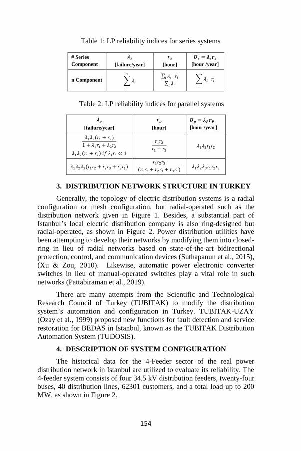
154
Table 1: LP reliability indices for series systems
# Series
Component
𝝀𝒔
[failure/year]
𝒓𝒔
[hour]
𝑼𝒔 = 𝝀𝒔𝒓𝒔
[hour /year]
n Component ∑ 𝜆𝑖
𝑛
𝑖
∑ 𝜆𝑖
𝑖 𝑟𝑖
∑ 𝜆𝑖 𝑖
∑ 𝜆𝑖
𝑖
𝑟𝑖
Table 2: LP reliability indices for parallel systems
𝝀𝒑
[failure/year]
𝒓𝒑
[hour]
𝑼𝒑 = 𝝀𝑷𝒓𝑷
[hour /year]
𝜆1𝜆2(𝑟1 + 𝑟2)
1 + 𝜆1𝑟1 + 𝜆2𝑟2
𝜆1𝜆2(𝑟1 + 𝑟2) 𝑖𝑓 𝜆𝑖𝑟𝑖 ≪ 1
𝑟1𝑟2
𝑟1 + 𝑟2
𝜆1𝜆2𝑟1𝑟2
𝜆1𝜆2𝜆3(𝑟1𝑟2 + 𝑟2𝑟3 + 𝑟3𝑟1) 𝑟1𝑟2𝑟3
(𝑟1𝑟2 + 𝑟2𝑟3 + 𝑟3𝑟1) 𝜆1𝜆2𝜆3𝑟1𝑟2𝑟3
3. DISTRIBUTION NETWORK STRUCTURE IN TURKEY
Generally, the topology of electric distribution systems is a radial
configuration or mesh configuration, but radial-operated such as the
distribution network given in Figure 1. Besides, a substantial part of
Istanbul’s local electric distribution company is also ring-designed but
radial-operated, as shown in Figure 2. Power distribution utilities have
been attempting to develop their networks by modifying them into closed-
ring in lieu of radial networks based on state-of-the-art bidirectional
protection, control, and communication devices (Suthapanun et al., 2015),
(Xu & Zou, 2010). Likewise, automatic power electronic converter
switches in lieu of manual-operated switches play a vital role in such
networks (Pattabiraman et al., 2019).
There are many attempts from the Scientific and Technological
Research Council of Turkey (TUBITAK) to modify the distribution
system’s automation and configuration in Turkey. TUBITAK-UZAY
(Ozay et al., 1999) proposed new functions for fault detection and service
restoration for BEDAS in Istanbul, known as the TUBITAK Distribution
Automation System (TUDOSIS).
4. DESCRIPTION OF SYSTEM CONFIGURATION
The historical data for the 4-Feeder sector of the real power
distribution network in Istanbul are utilized to evaluate its reliability. The
4-feeder system consists of four 34.5 kV distribution feeders, twenty-four
buses, 40 distribution lines, 62301 customers, and a total load up to 200
MW, as shown in Figure 2.
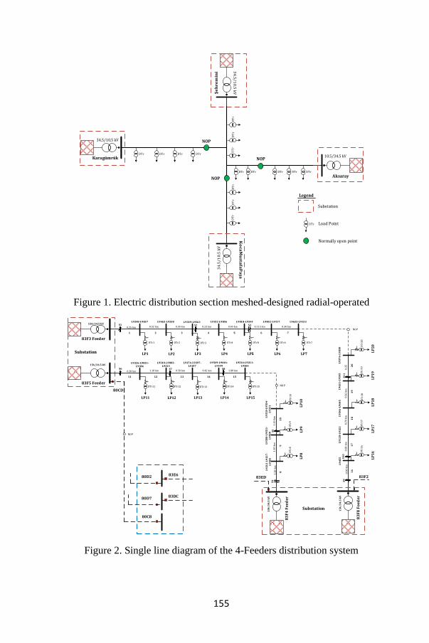
155
Karagümrük
34.5/10.5 kV
Substation
34
.5/
10
.5 k
VŞe
hre
min
i3
4.5
/1
0.5
kV
Ko
caM
usta
faP
aşa
Aksaray
10.5/34.5 kVDTr DTr DTr DTr
NOP
DT
r
DTr
DT
rD
Tr
DTr DTrDTr
NOP
DTr
DT
rD
Tr
DT
r
NOP
DTr Load Point
Normally open point
Legend
Figure 1. Electric distribution section meshed-designed radial-operated
Substation
S10.25 km
LP1
L9348-L9037
83F3 Feeder
83F5 Feeder
154/34.5 kV
154/34.5 kV
1
0.52 km
LP2
L9465-L9338
2
DTr1 DTr2
0.30 km
LP3
L9339-L9563
3
DTr3
0.23 km
LP4
L9152-L9006
4
DTr4
0.40 km
LP5
L9018-L9344
5
DTr5
0.115 km
LP6
L9002-L9117
6
DTr6
0.30 km
LP7
L9633-L9153
7
DTr7
S2 S3
S60.20 km
LP11
L9326-L9035-L9386
11
1.10 km
LP12
L9540-L9003-L9215
12
DTr11 DTr12
0.50 km
LP13
L9174-L9397-L9197
13
DTr13
0.42 km
LP14
L9569-L9646-L9199
14
DTr14
1.80 km
LP15
L9216-L9211-L9504
15
DTr15
S7 S8
83
F4
Fe
ed
er
15
4/
34
.5 k
V
S4
1.2
0 k
m
LP
8
L9
21
2-L
91
37
-L
95
05
8
1.1
0 k
m
LP
9
L9
30
8-L
90
21
-L
90
20
9
DT
r8D
Tr9
1.1
0 k
m
LP
10
L9
31
8-L
95
04
-L
92
11
10
DT
r10
S5
NOP
83
F8
Fe
ed
er
15
4/
34
.5 k
V
S9
0.9
0 k
m
LP
16
L9
45
5
16
0.8
0 k
m
LP
17
L9
12
8-L
91
22
17
DT
r16
DT
r17
0.7
0 k
m
LP
18
L9
54
6-L
96
45
18
DT
r18
0.5
6 k
m
LP
19
L9
65
1-L
95
45
19
DT
r19
0.2
5
L9
37
6-L
90
30
20
S1
0S
11
LP
20D
Tr2
0
NOP
Substation
83E6
83DC
80C8
80D7
80D2
80CD
83ED 83F2
NOP
Figure 2. Single line diagram of the 4-Feeders distribution system
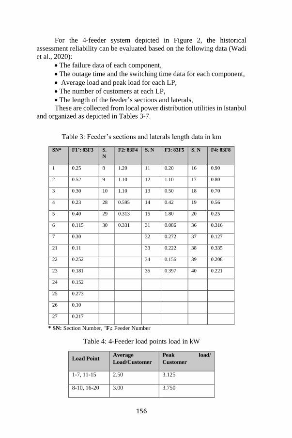
156
For the 4-feeder system depicted in Figure 2, the historical
assessment reliability can be evaluated based on the following data (Wadi
et al., 2020):
The failure data of each component,
The outage time and the switching time data for each component,
Average load and peak load for each LP,
The number of customers at each LP,
The length of the feeder’s sections and laterals,
These are collected from local power distribution utilities in Istanbul
and organized as depicted in Tables 3-7.
Table 3: Feeder’s sections and laterals length data in km
SN* F1+: 83F3 S.
N
F2: 83F4 S. N F3: 83F5 S. N F4: 83F8
1 0.25 8 1.20 11 0.20 16 0.90
2 0.52 9 1.10 12 1.10 17 0.80
3 0.30 10 1.10 13 0.50 18 0.70
4 0.23 28 0.595 14 0.42 19 0.56
5 0.40 29 0.313 15 1.80 20 0.25
6 0.115 30 0.331 31 0.086 36 0.316
7 0.30 32 0.272 37 0.127
21 0.11 33 0.222 38 0.335
22 0.252 34 0.156 39 0.208
23 0.181 35 0.397 40 0.221
24 0.152
25 0.273
26 0.10
27 0.217
* SN: Section Number, +Fi: Feeder Number
Table 4: 4-Feeder load points load in kW
Load Point Average
Load/Customer
Peak load/
Customer
1-7, 11-15 2.50 3.125
8-10, 16-20 3.00 3.750

157
5. HISTORICAL RELIABILITY ASSESSMENT OF 4-
FEEDER SYSTEM
The reliability indices for any system are classified into two groups,
LP indices such as λ, r, and U. Furthermore, system indices such as System
SAIFI, SAIDI, CAIDI, ASAI, ENS, and AENS as given in (Wadi et al.,
2018). The historical assessment results from 2012 to 2014 are summarized
in Tables 7 and 8. Besides, Figures 3, 4, 5, and 6 graphically show the
obtained results.
Table 5: 4-Feeder customer data
Load
Point
No. of
Customers
Load
Point
No. of
Customers
1 3305 11 3281
2 1447 12 3571
3 866 13 4742
4 2378 14 6335
5 640 15 8023
6 209 16 2611
7 549 17 2866
8 5439 18 2103
9 5216 19 663
10 7322 20 735
Table 6: 4-Feeder switches locations
Feeder Section No.
F1 *S (1,1), S (2,4), S (3,6)
F2 S (4,8), S (5,10)
F3 S (6,11), S (7,13), S (8,15)
F4 S (9,16), S (10,17), S (11,20)
*S (x, y): Switch location, where x is the number of switches, while y the number of sections
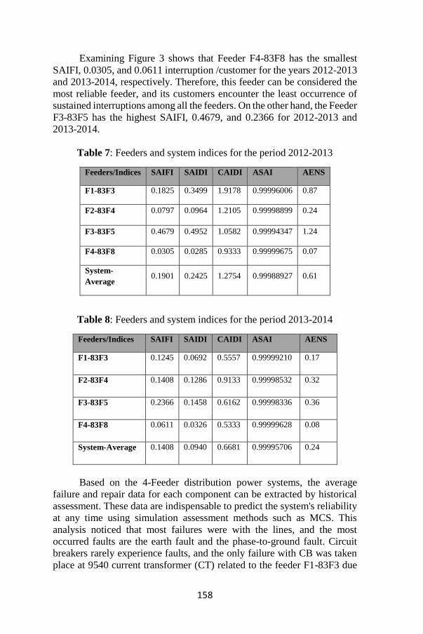
158
Examining Figure 3 shows that Feeder F4-83F8 has the smallest
SAIFI, 0.0305, and 0.0611 interruption /customer for the years 2012-2013
and 2013-2014, respectively. Therefore, this feeder can be considered the
most reliable feeder, and its customers encounter the least occurrence of
sustained interruptions among all the feeders. On the other hand, the Feeder
F3-83F5 has the highest SAIFI, 0.4679, and 0.2366 for 2012-2013 and
2013-2014.
Table 7: Feeders and system indices for the period 2012-2013
Feeders/Indices SAIFI SAIDI CAIDI ASAI AENS
F1-83F3 0.1825 0.3499 1.9178 0.99996006 0.87
F2-83F4 0.0797 0.0964 1.2105 0.99998899 0.24
F3-83F5 0.4679 0.4952 1.0582 0.99994347 1.24
F4-83F8 0.0305 0.0285 0.9333 0.99999675 0.07
System-
Average 0.1901 0.2425 1.2754 0.99988927 0.61
Table 8: Feeders and system indices for the period 2013-2014
Feeders/Indices SAIFI SAIDI CAIDI ASAI AENS
F1-83F3 0.1245 0.0692 0.5557 0.99999210 0.17
F2-83F4 0.1408 0.1286 0.9133 0.99998532 0.32
F3-83F5 0.2366 0.1458 0.6162 0.99998336 0.36
F4-83F8 0.0611 0.0326 0.5333 0.99999628 0.08
System-Average 0.1408 0.0940 0.6681 0.99995706 0.24
Based on the 4-Feeder distribution power systems, the average
failure and repair data for each component can be extracted by historical
assessment. These data are indispensable to predict the system's reliability
at any time using simulation assessment methods such as MCS. This
analysis noticed that most failures were with the lines, and the most
occurred faults are the earth fault and the phase-to-ground fault. Circuit
breakers rarely experience faults, and the only failure with CB was taken
place at 9540 current transformer (CT) related to the feeder F1-83F3 due
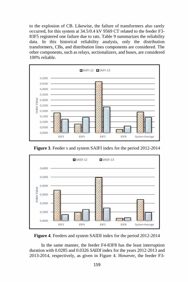
159
to the explosion of CB. Likewise, the failure of transformers also rarely
occurred, for this system at 34.5/0.4 kV 9569 CT related to the feeder F3-
83F5 registered one failure due to rats. Table 9 summarizes the reliability
data. In this historical reliability analysis, only the distribution
transformers, CBs, and distribution lines components are considered. The
other components, such as relays, sectionalizers, and buses, are considered
100% reliable.
Figure 3. Feeder s and system SAIFI index for the period 2012-2014
Figure 4. Feeders and system SAIDI index for the period 2012-2014
In the same manner, the feeder F4-83F8 has the least interruption
duration with 0.0285 and 0.0326 SAIDI index for the years 2012-2013 and
2013-2014, respectively, as given in Figure 4. However, the feeder F3-
0,0000
0,0500
0,1000
0,1500
0,2000
0,2500
0,3000
0,3500
0,4000
0,4500
0,5000
83F3 83F4 83F5 83F8 System-Average
Ind
ex V
alu
e
SAIFI-12 SAIFI-13
0,0000
0,1000
0,2000
0,3000
0,4000
0,5000
0,6000
83F3 83F4 83F5 83F8 System-Average
Ind
ex V
alu
e
SAIDI-12 SAIDI-13
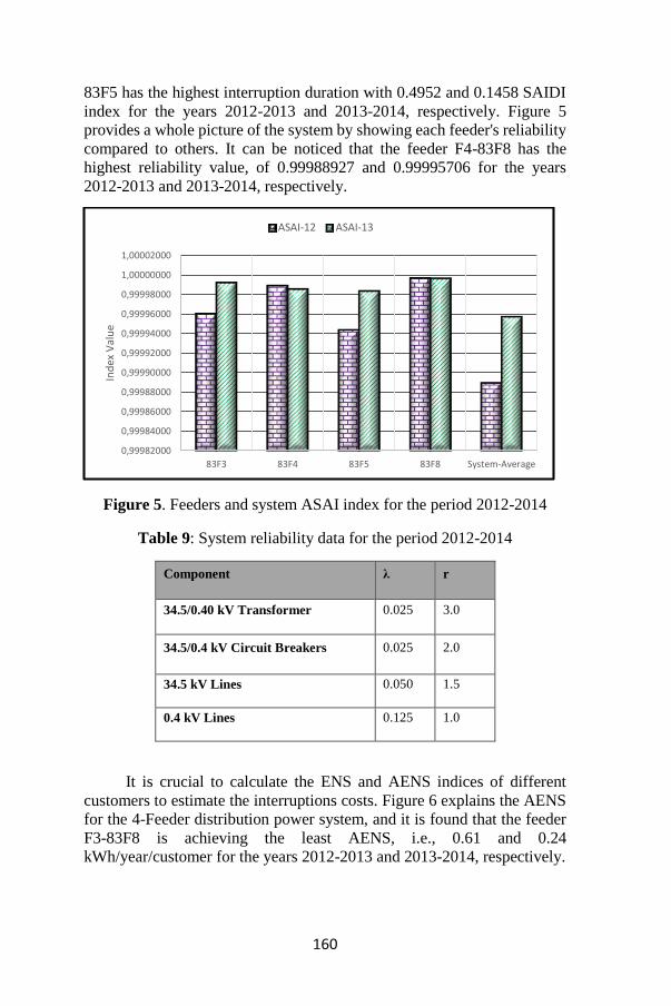
160
83F5 has the highest interruption duration with 0.4952 and 0.1458 SAIDI
index for the years 2012-2013 and 2013-2014, respectively. Figure 5
provides a whole picture of the system by showing each feeder's reliability
compared to others. It can be noticed that the feeder F4-83F8 has the
highest reliability value, of 0.99988927 and 0.99995706 for the years
2012-2013 and 2013-2014, respectively.
Figure 5. Feeders and system ASAI index for the period 2012-2014
Table 9: System reliability data for the period 2012-2014
Component λ r
34.5/0.40 kV Transformer 0.025 3.0
34.5/0.4 kV Circuit Breakers 0.025 2.0
34.5 kV Lines 0.050 1.5
0.4 kV Lines 0.125 1.0
It is crucial to calculate the ENS and AENS indices of different
customers to estimate the interruptions costs. Figure 6 explains the AENS
for the 4-Feeder distribution power system, and it is found that the feeder
F3-83F8 is achieving the least AENS, i.e., 0.61 and 0.24
kWh/year/customer for the years 2012-2013 and 2013-2014, respectively.
0,99982000
0,99984000
0,99986000
0,99988000
0,99990000
0,99992000
0,99994000
0,99996000
0,99998000
1,00000000
1,00002000
83F3 83F4 83F5 83F8 System-Average
Ind
ex V
alu
e
ASAI-12 ASAI-13
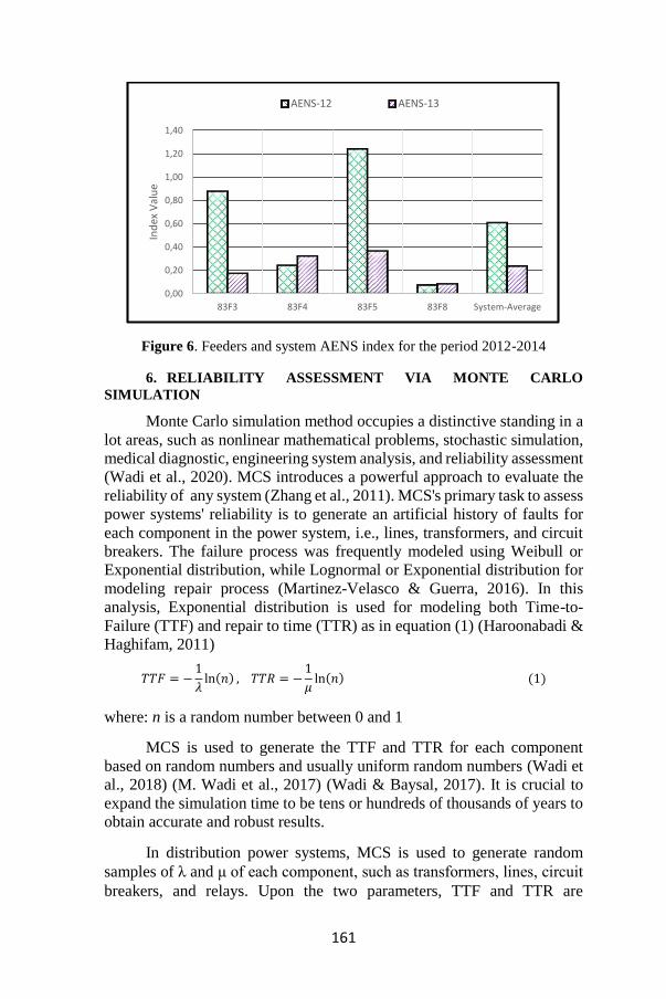
161
Figure 6. Feeders and system AENS index for the period 2012-2014
6. RELIABILITY ASSESSMENT VIA MONTE CARLO
SIMULATION
Monte Carlo simulation method occupies a distinctive standing in a
lot areas, such as nonlinear mathematical problems, stochastic simulation,
medical diagnostic, engineering system analysis, and reliability assessment
(Wadi et al., 2020). MCS introduces a powerful approach to evaluate the
reliability of any system (Zhang et al., 2011). MCS's primary task to assess
power systems' reliability is to generate an artificial history of faults for
each component in the power system, i.e., lines, transformers, and circuit
breakers. The failure process was frequently modeled using Weibull or
Exponential distribution, while Lognormal or Exponential distribution for
modeling repair process (Martinez-Velasco & Guerra, 2016). In this
analysis, Exponential distribution is used for modeling both Time-to-
Failure (TTF) and repair to time (TTR) as in equation (1) (Haroonabadi &
Haghifam, 2011)
𝑇𝑇𝐹 = −1
𝜆ln(𝑛) , 𝑇𝑇𝑅 = −
1
𝜇ln(𝑛) (1)
where: n is a random number between 0 and 1
MCS is used to generate the TTF and TTR for each component
based on random numbers and usually uniform random numbers (Wadi et
al., 2018) (M. Wadi et al., 2017) (Wadi & Baysal, 2017). It is crucial to
expand the simulation time to be tens or hundreds of thousands of years to
obtain accurate and robust results.
In distribution power systems, MCS is used to generate random
samples of λ and μ of each component, such as transformers, lines, circuit
breakers, and relays. Upon the two parameters, TTF and TTR are
0,00
0,20
0,40
0,60
0,80
1,00
1,20
1,40
83F3 83F4 83F5 83F8 System-Average
Ind
ex V
alu
e
AENS-12 AENS-13
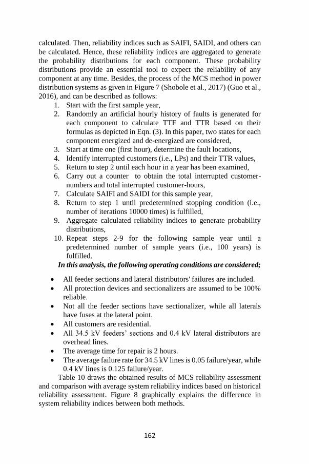
162
calculated. Then, reliability indices such as SAIFI, SAIDI, and others can
be calculated. Hence, these reliability indices are aggregated to generate
the probability distributions for each component. These probability
distributions provide an essential tool to expect the reliability of any
component at any time. Besides, the process of the MCS method in power
distribution systems as given in Figure 7 (Shobole et al., 2017) (Guo et al.,
2016), and can be described as follows:
1. Start with the first sample year,
2. Randomly an artificial hourly history of faults is generated for
each component to calculate TTF and TTR based on their
formulas as depicted in Eqn. (3). In this paper, two states for each
component energized and de-energized are considered,
3. Start at time one (first hour), determine the fault locations,
4. Identify interrupted customers (i.e., LPs) and their TTR values,
5. Return to step 2 until each hour in a year has been examined,
6. Carry out a counter to obtain the total interrupted customer-
numbers and total interrupted customer-hours,
7. Calculate SAIFI and SAIDI for this sample year,
8. Return to step 1 until predetermined stopping condition (i.e.,
number of iterations 10000 times) is fulfilled,
9. Aggregate calculated reliability indices to generate probability
distributions,
10. Repeat steps 2-9 for the following sample year until a
predetermined number of sample years (i.e., 100 years) is
fulfilled.
In this analysis, the following operating conditions are considered;
All feeder sections and lateral distributors' failures are included.
All protection devices and sectionalizers are assumed to be 100%
reliable.
Not all the feeder sections have sectionalizer, while all laterals
have fuses at the lateral point.
All customers are residential.
All 34.5 kV feeders’ sections and 0.4 kV lateral distributors are
overhead lines.
The average time for repair is 2 hours.
The average failure rate for 34.5 kV lines is 0.05 failure/year, while
0.4 kV lines is 0.125 failure/year.
Table 10 draws the obtained results of MCS reliability assessment
and comparison with average system reliability indices based on historical
reliability assessment. Figure 8 graphically explains the difference in
system reliability indices between both methods.
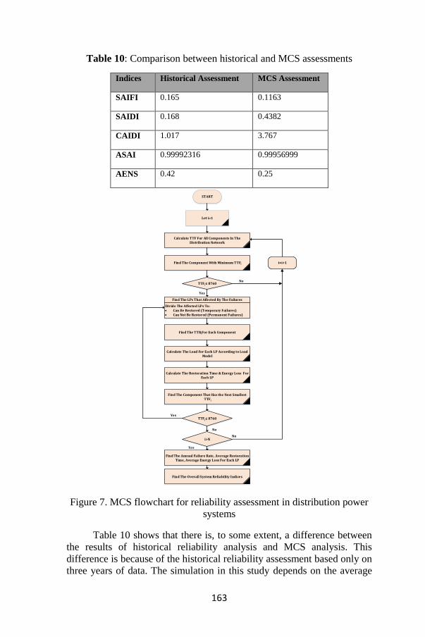
163
Table 10: Comparison between historical and MCS assessments
Indices Historical Assessment MCS Assessment
SAIFI 0.165 0.1163
SAIDI 0.168 0.4382
CAIDI 1.017 3.767
ASAI 0.99992316 0.99956999
AENS 0.42 0.25
START
Let i=1
Calculate TTF For All Components In The Distribution Network
Find The Component With Minimum TTF
TTF 8760
i=i+1
Find The LPs That Affected By The Failures
Divide The Affected LPs To: Can Be Restored (Temporary Failures) Can Not Be Restored (Permanent Failures)
Find The TTR For Each Component
Calculate The Load For Each LP According to Load Model
Calculate The Restoration Time & Energy Loss For Each LP
No
Yes
Find The Component That Has the Next Smallest TTF
TTF 8760
i>N
Yes
Yes
No
No
Find The Annual Failure Rate, Average Restoration Time, Average Energy Loss For Each LP
Find The Overall System Reliability Indices
i
i
i
i
i
Figure 7. MCS flowchart for reliability assessment in distribution power
systems
Table 10 shows that there is, to some extent, a difference between
the results of historical reliability analysis and MCS analysis. This
difference is because of the historical reliability assessment based only on
three years of data. The simulation in this study depends on the average
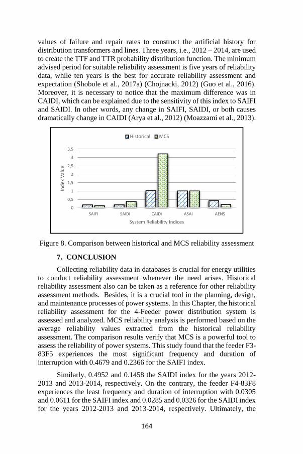
164
values of failure and repair rates to construct the artificial history for
distribution transformers and lines. Three years, i.e., 2012 – 2014, are used
to create the TTF and TTR probability distribution function. The minimum
advised period for suitable reliability assessment is five years of reliability
data, while ten years is the best for accurate reliability assessment and
expectation (Shobole et al., 2017a) (Chojnacki, 2012) (Guo et al., 2016).
Moreover, it is necessary to notice that the maximum difference was in
CAIDI, which can be explained due to the sensitivity of this index to SAIFI
and SAIDI. In other words, any change in SAIFI, SAIDI, or both causes
dramatically change in CAIDI (Arya et al., 2012) (Moazzami et al., 2013).
Figure 8. Comparison between historical and MCS reliability assessment
7. CONCLUSION
Collecting reliability data in databases is crucial for energy utilities
to conduct reliability assessment whenever the need arises. Historical
reliability assessment also can be taken as a reference for other reliability
assessment methods. Besides, it is a crucial tool in the planning, design,
and maintenance processes of power systems. In this Chapter, the historical
reliability assessment for the 4-Feeder power distribution system is
assessed and analyzed. MCS reliability analysis is performed based on the
average reliability values extracted from the historical reliability
assessment. The comparison results verify that MCS is a powerful tool to
assess the reliability of power systems. This study found that the feeder F3-
83F5 experiences the most significant frequency and duration of
interruption with 0.4679 and 0.2366 for the SAIFI index.
Similarly, 0.4952 and 0.1458 the SAIDI index for the years 2012-
2013 and 2013-2014, respectively. On the contrary, the feeder F4-83F8
experiences the least frequency and duration of interruption with 0.0305
and 0.0611 for the SAIFI index and 0.0285 and 0.0326 for the SAIDI index
for the years 2012-2013 and 2013-2014, respectively. Ultimately, the
0
0,5
1
1,5
2
2,5
3
3,5
SAIFI SAIDI CAIDI ASAI AENS
Ind
ex V
alu
e
System Reliability Indices
Historical MCS

165
reliability assessment is a powerful tool to define the power system's
weakness and then decide the relevant remedial actions needed to achieve
the required service reliability levels. Generally, power utilities and electric
companies can consider the following recommendations to improve their
systems’ reliability;
• Continuous and accurate registration of different failures and
interruptions by preparing certain forms, including all data required for
reliability assessment.
• Training the crew of maintenance to fill out the forms of reliability
on time, the date of fault, the cause of failure, and the exact period for
repair and restoration.
• Preparing a smart mobile application instead of filling out forms;
to increase registration speed and the accuracy of the collected data.
• Organizing the collected data into databases to simplify future
reliability studies.
• Increase the number of sectionalizers at feeder sections to reduce
the number of customers being interrupted.
• Replacing manual sectionalizers with automated ones to reduce the
time of restoration.
• Installing insulators and anti-bird cones on the top of poles impede
birds from access to distribution transformers and connections.
• To ward off the rodents, it is essential to use tightly sealed cabinets,
poison materials, or ultrasonic devices.

166
REFERENCES
Abunima, H., Teh, J., Lai, C. M., & Jabir, H. J. (2018). A systematic review
of reliability studies on composite power systems: A coherent
taxonomy motivations, open challenges, recommendations, and new
research directions. Energies, 11(9), 1–37.
https://doi.org/10.3390/en11092417
Al-Wafi, E., Al-Subhi, A., & Al-Muhaini, M. (2016). Reliability
assessment of a practical power system using Monte Carlo
simulation. 2015 Saudi Arabia Smart Grid, SASG 2015, 1–6.
https://doi.org/10.1109/SASG.2015.7449276
Allan, R. (1994). Power system reliability assessment-A conceptual and
historical review. Reliability Engineering and System Safety, 46(1),
3–13. https://doi.org/10.1016/0951-8320(94)90043-4
Arya, L. D., Choube, S. C., Arya, R., & Tiwary, A. (2012). Evaluation of
reliability indices accounting omission of random repair time for
distribution systems using Monte Carlo simulation. International
Journal of Electrical Power and Energy Systems, 42(1), 533–541.
https://doi.org/10.1016/j.ijepes.2012.04.064
Baharum, A., Alwan, F. M., & Hasson, S. T. (2013). A case study of
reliability and performance of the electric power distribution station
based on time between failures. Mathematical Problems in
Engineering, 2013. https://doi.org/10.1155/2013/583683
Bakkiyaraj, R. A., & Kumarappan, N. (2010). Evaluation of composite
reliability indices based on non-sequential Monte Carlo simulation
and particle swarm optimization. 2010 IEEE World Congress on
Computational Intelligence, WCCI 2010 - 2010 IEEE Congress on
Evolutionary Computation, CEC 2010.
https://doi.org/10.1109/CEC.2010.5586274
Billinton, R., & Pan, Z. (2004). Historic performance-based distribution
system risk assessment. IEEE Transactions on Power Delivery,
19(4), 1759–1765. https://doi.org/10.1109/TPWRD.2004.832404
Cadini, F., Agliardi, G. L., & Zio, E. (2017). A modeling and simulation
framework for the reliability/availability assessment of a power
transmission grid subject to cascading failures under extreme
weather conditions. Applied Energy, 185, 267–279.
https://doi.org/10.1016/j.apenergy.2016.10.086
Chojnacki, A. L. (2012). The use of extended Petri nets in analyzing the
reliability of MV / LV distribution transformer stations. Elektronika
167
Ir Elektrotechnika, 5(5), 17–22.
https://doi.org/10.5755/j01.eee.121.5.1645
Chowdhury, A. A. (2005). Distribution system risk assessment based on
historical reliability performance. 2005 IEEE International
Conference on Electro Information Technology, 2005, 1–7.
https://doi.org/10.1109/eit.2005.1626967
Chowdhury, Ali A., & Koval, D. O. (2009). Power Distribution System
Reliability: Practical Methods and Applications. Power Distribution
System Reliability: Practical Methods and Applications, 1–531.
https://doi.org/10.1002/9780470459355
Feng, Z. (2006). Electric Distribution System Risk Assessment Using
Actual Utility Reliability Data. Master Thesis, March.
Godha, N. R., Deshmukh, S. R., & Dagade, R. V. (2011). Application of
Monte Carlo simulation for reliability cost/worth analysis of
distribution system. 2011 International Conference on Power and
Energy Systems, ICPS 2011, December, 22–24.
https://doi.org/10.1109/ICPES.2011.6156644
Guo, H., Levi, V., & Buhari, M. (2016). Reliability assessment of smart
distribution networks. Proceedings of the 2015 IEEE Innovative
Smart Grid Technologies - Asia, ISGT ASIA 2015, 1–6.
https://doi.org/10.1109/ISGT-Asia.2015.7387037
Haroonabadi, H., & Haghifam, M. R. (2011). Generation reliability
assessment in power markets using Monte Carlo simulation and soft
computing. Applied Soft Computing Journal, 11(8), 5292–5298.
https://doi.org/10.1016/j.asoc.2011.05.031
Kim, H., & Singh, C. (2010). Reliability modeling and simulation in power
systems with aging characteristics. IEEE Transactions on Power
Systems, 25(1), 21–28.
https://doi.org/10.1109/TPWRS.2009.2030269
Koster, J. K., Cohn, L. H., Mee, R. B. B., & Collins, J. J. (1978). Late
Results of Operation for Acute Aortic Dissection Producing Aortic
Insufficiency. In Annals of Thoracic Surgery (Vol. 26, Issue 5).
https://doi.org/10.1016/S0003-4975(10)62926-8
Martinez-Velasco, J., & Guerra, G. (2016). Reliability Analysis of
Distribution Systems with Photovoltaic Generation Using a Power
Flow Simulator and a Parallel Monte Carlo Approach. Energies,
9(7), 537. https://doi.org/10.3390/en9070537
Moazzami, M., Hemmati, R., Haghighatdar Fesharaki, F., & Rafiee Rad,
168
S. (2013). Reliability evaluation for different power plant busbar
layouts by using sequential Monte Carlo simulation. International
Journal of Electrical Power and Energy Systems, 53, 987–993.
https://doi.org/10.1016/j.ijepes.2013.06.019
Ozay, N., Guven, A. N., Buyuksemerci, A., & Fettahlioglu, M. (1999).
Design and implementation of a feeder automation system for
distribution networks. International Conference on Electric Power
Engineering, PowerTech Budapest 1999, February 1999, 122.
https://doi.org/10.1109/PTC.1999.826553
Pattabiraman, S., Sampath, K., Kannan, M., Ganesan, R. G., & Narayanan,
K. (2019). Reliability Improvement in Radial Distribution System
through Reconfiguration. 2019 IEEE PES Innovative Smart Grid
Technologies Asia, ISGT 2019, 1963–1967.
https://doi.org/10.1109/ISGT-Asia.2019.8881119
Schoemann, A. M., Miller, P., Pornprasertmanit, S., & Wu, W. (2014).
Using Monte Carlo simulations to determine power and sample size
for planned missing designs. International Journal of Behavioral
Development, 38(5), 471–479.
https://doi.org/10.1177/0165025413515169
Shobole et al. (2017b). Valuation of reliability assessment for power
systems in terms of distribution system, a case study. 2017 6th
International Conference on Renewable Energy Research and
Applications, ICRERA 2017, Nov. 5-8, 1114–1118.
https://doi.org/10.1109/DISTRA.2017.8191227
Silva, E. N. M., Rodrigues, A. B., & Da Guia Da Silva, M. (2016).
Stochastic assessment of the impact of photovoltaic distributed
generation on the power quality indices of distribution networks.
Electric Power Systems Research, 135, 59–67.
https://doi.org/10.1016/j.epsr.2016.03.006
Suthapanun, C., Jirapong, P., Bunchoo, P., & Thararak, P. (2015).
Reliability assessment tool for radial and loop distribution systems
using DIgSILENT PowerFactory. ECTI-CON 2015 - 2015 12th
International Conference on Electrical Engineering/Electronics,
Computer, Telecommunications and Information Technology.
https://doi.org/10.1109/ECTICon.2015.7206929
Thoemmes, F., MacKinnon, D. P., & Reiser, M. R. (2010). Power analysis
for complex mediational designs using Monte Carlo methods.
Structural Equation Modeling, 17(3), 510–534.
https://doi.org/10.1080/10705511.2010.489379

169
Wadi, & Baysal, M. (2017). Reliability Assessment of Radial Networks Via
Modified Rbd Analytical Technique. 35(4), 717–726.
Wadi, Baysal, M., Shobole, A., & Tur, M. R. (2018). Reliability Evaluation
in Smart Grids via Modified Monte Carlo Simulation Method. 7th
International IEEE Conference on Renewable Energy Research and
Applications, ICRERA 2018, 5, 841–845.
https://doi.org/10.1109/ICRERA.2018.8566982
Wadi et al. (2020). Historical and Monte Carlo Simulation-Based
Reliability Assessment of Power Distribution Systems. Sigma
Journal of Engineering and Natural Sciences, 38(3), 1527.
Wadi, Mohammed, Baysal, M., & Shobole, A. (2017). Comparison
between open-ring and closed-ring grids reliability. 2017 4th
International Conference on Electrical and Electronics
Engineering, ICEEE 2017, 290–294.
https://doi.org/10.1109/ICEEE2.2017.7935836
Wallnerström, C. J. (2008). On Risk Management of Electrical
Distribution Systems and the Impact of Regulations On (RCM). In
Thesis Licentiate Stockholm Electrical Systems (Issue January
2008).
Wijekularathna, D. K., Manage, A. B. W., & Scariano, S. M. (2019). Power
analysis of several normality tests: A Monte Carlo simulation study.
Communications in Statistics: Simulation and Computation, 0(0), 1–
17. https://doi.org/10.1080/03610918.2019.1658780
Wilson, A., Graves, T., Hamada, M., & Reese, C. S. (2006). Advances in
System Reliability Assessment.
Xu, H., & Zou, H. (2010). Research on complex multi-state distribution
system reliability modeling and assessment methods based on
Bayesian networks and random set theory. 2010 China International
Conference on Electricity Distribution, CICED 2010, 1.
Zhang, X., Bie, Z., & Li, G. (2011). Reliability assessment of distribution
networks with distributed generations using Monte Carlo method.
Energy Procedia, 12(December), 278–286.
https://doi.org/10.1016/j.egypro.2011.10.038

170
APPENDIX
𝑆𝐴𝐼𝐹𝐼 = 𝑇𝑜𝑡𝑎𝑙 𝑁𝑢𝑚𝑏𝑒𝑟 𝑜𝑓 𝐶𝑢𝑠𝑡𝑜𝑚𝑒𝑟 𝐼𝑛𝑡𝑒𝑟𝑟𝑢𝑝𝑡𝑖𝑜𝑛𝑠
𝑇𝑜𝑡𝑎𝑙 𝑁𝑢𝑚𝑏𝑒𝑟 𝑜𝑓 𝐶𝑢𝑠𝑡𝑜𝑚𝑒𝑟𝑠 𝑆𝑒𝑟𝑣𝑒𝑑 =
∑ 𝜆𝑖 𝑖 𝑁𝑖
∑ 𝑁𝑖 𝑖
𝑆𝐴𝐼𝐷𝐼 = 𝑆𝑢𝑚 𝑜𝑓 𝐶𝑢𝑠𝑡𝑜𝑚𝑒𝑟 𝐼𝑛𝑡𝑒𝑟𝑟𝑢𝑝𝑡𝑖𝑜𝑛 𝐷𝑢𝑟𝑎𝑡𝑖𝑜𝑛𝑠
𝑇𝑜𝑡𝑎𝑙 𝑁𝑢𝑚𝑏𝑒𝑟 𝑜𝑓 𝐶𝑢𝑠𝑡𝑜𝑚𝑒𝑟𝑠 𝑆𝑒𝑟𝑣𝑒𝑑 =
∑ 𝑈𝑖 𝑖 𝑁𝑖
∑ 𝑁𝑖 𝑖
𝐶𝐴𝐼𝐷𝐼 = 𝑆𝑢𝑚 𝑜𝑓 𝐶𝑢𝑠𝑡𝑜𝑚𝑒𝑟 𝐼𝑛𝑡𝑒𝑟𝑟𝑢𝑝𝑡𝑖𝑜𝑛 𝐷𝑢𝑟𝑎𝑡𝑖𝑜𝑛𝑠
𝑇𝑜𝑡𝑎𝑙 𝑁𝑢𝑚𝑏𝑒𝑟 𝑜𝑓 𝐶𝑢𝑠𝑡𝑜𝑚𝑒𝑟 𝐼𝑛𝑡𝑒𝑟𝑟𝑢𝑝𝑡𝑖𝑜𝑛𝑠 =
∑ 𝑈𝑖 𝑖 𝑁𝑖
∑ 𝜆𝑖 𝑖 𝑁𝑖
𝐴𝑆𝐴𝐼 = 𝐶𝑢𝑠𝑡𝑜𝑚𝑒𝑟 𝐻𝑜𝑢𝑟𝑠 𝑜𝑓 𝐴𝑣𝑎𝑖𝑙𝑎𝑏𝑙𝑒 𝑆𝑒𝑟𝑣𝑖𝑐𝑒
𝐶𝑢𝑠𝑡𝑜𝑚𝑒𝑟 𝐻𝑜𝑢𝑟𝑠 𝐷𝑒𝑚𝑎𝑛𝑑𝑒𝑑 =
∑ 𝑖 𝑁𝑖 × 8760 − ∑ 𝑈𝑖
𝑖 𝑁𝑖
∑ 𝑖 𝑁𝑖 × 8760
𝐸𝑁𝑆 = Total Energy not Supplied by the System = ∑ 𝐿𝑖
𝑖
𝑈𝑖
𝐴𝐸𝑁𝑆 =Total Energy not Supplied
𝑇𝑜𝑡𝑎𝑙 𝑁𝑢𝑚𝑏𝑒𝑟 𝑜𝑓 𝐶𝑢𝑠𝑡𝑜𝑚𝑒𝑟𝑠 𝑆𝑒𝑟𝑣𝑒𝑑 =
∑ 𝐿𝑖𝑖 𝑈𝑖
∑ 𝑁𝑖 𝑖
where:
𝑁𝑖: is the number of customers of load point 𝑖 8760: is the number of hours in a calendar year
𝐿𝑖: is the average load connected to load point 𝑖
NOMENCLATURE
AENS: Average Energy Not Supplied (kWh/customer/year)
ASAI: Average System Availability Index BEDAS: Bosporus Electric Distribution LTD Company
CAIDI: Customer Average Interruption Duration Index (hour/failure) CEA: Canadian Electrical Association
CT: Central Transformer
DTr: Distribution Transformer ENS: Energy Not Supplied (MWh /year)
LP: Load Point
MC: Monte Carlo MCS Monte Carlo Simulation
RBTS Roy Billinton Test System
S: Switch SAIFI: System Average Interruption Frequency Index (interruption/customer)
SAIDI: System Average Interruption Duration Index (hour/interruption)
S. N. Section Number
TTF: Time to Failure
TTR: Time to Repair
TUBITAK: The Scientific and Technological Research Council of Turkey TUDOSIS: TUBITAK Distribution Automation System
U: Average Annual Outage (hour/year)
λ: Average Failure Rate (failure/year) for lines and cables (failure/year.km) µ Average Repair Rate (hour/year)
CHAPTER XI
NETWORK DISTANCE COEFFICIENT EFFECT ON
DETERMINING TRANSPORTATION FACILITY LOCATION
Emre Demir1 1(Asst. Prof.), Antalya Bilim University, e-mail: [email protected]
0000-0003-0013-4482
1. INTRODUCTION
Design in engineering can be identified as a decision-making
procedure to make solutions satisfying some specific needs. Most of the
engineering design problems contain multipart objective functions along with
several decision variables. Feasible solutions must be found for every kind of
designs characterized by potential decision variables of design parameters. At
this point, optimization becomes a great option to discover the most
appropriate solution among the solutions of the problem under specific
conditions. For such purposes, an optimization technique tries to find the most
suitable solution among all available feasible solutions. Traditional search
methods have been used for a long time for getting solutions of engineering
design problems. However, in real design problems, there can be a lot of
decision variables effecting on objective function which those can make the
problem very complicated. Therefore, there is a strong requirement to apply
operative optimization approaches (Parkinson et al. 2013; Aydogdu 2017).
One kind of such effective optimization methods is implementing a
metaheuristic algorithm. Metaheuristic algorithms are prescribed as advanced
and global search operators (Yang 2010). Many methods possess results
through trial and error which can be titled as a standard search engine. A
standard search engine finds numerous possibilities for the final solution.
However, metaheuristic algorithm can greatly reduce the number of
possibilities of a standard search engine. This provides convenience and
reliability to many researchers. A couple of examples of well-known
metaheuristic algorithms are particle swarm optimization (PSO) based on
social behavior of bird flocking and fish schooling, firefly algorithm (FA),
harmony search algorithm (HSA) based on music improvisation process.
Engineering designs and decision-making procedures are commonly
encountered in transportation, especially in the aviation sector. It continues to
develop rapidly in Turkey as in the whole world. The demand for aviation,
which is of great importance in freight and passenger transportation, is

172
increasing day by day. According to the General Directorate of Civil Aviation,
the fact that more passengers are carried than in the past shows that almost
everyone in Turkey has started to become accessible to aviation (SHGM
2020). As a result of the increasing demand, the opportunities in the aviation
sector increases. In addition, the number of aircrafts using the airports in
Turkey or landing and taking off at the airports in the country increases day
by day. Civil aviation in Turkey has made great strides in aviation
infrastructure in recent years. As new airports were put into service, the
number of domestic and international flights increased rapidly. Although the
rules in aviation are very strict, there may be crashes or accidents of various
sizes due to running into some setbacks (Uslu and Dönmez 2017). Although
these crashes or accidents occurring in the chain of faults are tried to be
minimized, loss of life and property during the accident is at a high level. In
such cases, emergency intervention aims at minimizing financial losses, and
most importantly, minimizing injuries and fatality rates. One of the ways to
minimize losses in airline accidents is rapid interventions during or after the
accident. When health, rescue or engineering service is provided quickly, the
time lost will be minimized and thus losses and expenses will be reduced.
When it comes to emergency response, airline transportation and the
properties of the airports in our country have an important place.
Location analysis can be performed to minimize losses. As an
example, Demir and Kockal (2019) determined the location of a facility that
is planned to serve the entire transportation network in order to minimize
financial losses. In another study (Demir 2018a), analyses were made to select
the airport with the most suitable location that can be used within the borders
of the country. The traffic rates of the airports were taken into account using
the Weizsfeld algorithm (WA) in line with the Weber problem (WP). Then,
Istanbul Sabiha Gokcen Airport was proposed as the airport that can provide
service to all airports in Turkey. However, in this research, the following
novelties are introduced. 1) Crow search algorithm (CSA) has never been used
for evaluating an optimum facility location for the airports in a country.
Therefore, the evaluation of finding an optimum facility location for the
airports in Turkey will be held by using CSA. 2) Although other algorithms
such as WA have been used for evaluating a facility location for the airports
(Demir 2018b) and for a cement plant (Demir and Kockal 2019); network
distance matrix and network distance coefficient were not included. Euclidean
distance matrix between the nodes were used as inputs rather than highway
network distance matrix depicting the costs between the nodes of a particular
network. In this study, however, highway network distance matrix indicates
the transportation costs between the nodes of the airports network in the
country. It is thought that the use of up-to-date optimization opportunities
together with up-to-date data will contribute to the national development by
making the supply or transportation needs faster in emergency situations.

173
This text is planned as follows. In the second part, the method to be
used is explained. Data collection and the attributes are introduced in the third
section. Also a design example is submitted in the same section to demonstrate
the analysis. Next, the findings that are encountered in line with the analyses
and discussion are presented. In the last part, a general evaluation is made
within the framework of the results.
2. METHODOLOGY
The problem of this study comes from finding the most convenient
aid facility location considering the travel matrix between the airports in the
country. Therefore, the objective with the parameters are described as follows
(2.1, 2.2).
Min ∑ 𝑘 ∗ 𝑎𝑖 ∗ √|𝑋𝑖 − 𝑋𝑓|2
+ |𝑌𝑖 − 𝑌𝑓|2
𝑛
𝑖=1
(2.1)
𝑘 =𝑑𝑖,𝑗
√|𝑋𝑖 − 𝑋𝑗|2
+ |𝑌𝑖 − 𝑌𝑗|2⁄
(2.2)
where;
𝑖, 𝑗 : node 𝑖 and node 𝑗 respectively
𝑘 : coefficient for distance cost
𝑎𝑖 : weight coefficient of node 𝑖 𝑋𝑖 : 𝑥 coordinate for node 𝑖 𝑌𝑖 : 𝑦 coordinate for node 𝑗
𝑋𝑓 : 𝑥 coordinate of the final node
𝑌𝑓 : 𝑦 coordinate of the final node
𝑑𝑖,𝑗 : network distance between node 𝑖 and node 𝑗
When 𝑖 and 𝑗 are equal to one another, 𝑘 can be accepted as 1 which
is a non-factor in formula (2.1). In this study, the CSA created by observing
the behavior of crows is used for optimization of a facility location. Crows are
members of smart bird species. Observations suggest that crow flocks’
behaviors have several similarities with optimization parameters. According
to a behavior type of crows, they follow the other birds and steal their food,
thus they find food sources. Moreover, crows hide their food to protect them
and try to fool other bird species. In this case, one can say that crows are
researchers, the environment is search area, positions of crow show a possible
solution, and quality of food source can be convenience function. Using this
behavioral similarity, CSA tries to simulate the crow's smart behavior to find
solutions for optimization problems. Considering all such behaviors, a
population-based metaheuristic algorithm is created. In this way, basic CSA
principles can be described as follows: crows live in flocks, they memorize

174
locational positions of places used for hiding objects, they follow birds to steal
their belongings, and they shelter their cache from theft (Askarzadeh 2016).
A d-dimensional environment with an input of a number of crows is
assumed in CSA. The number of crows which is flock size is 𝑁 and the
position of crow 𝑖 during iteration in search space is specified by a vector
𝑥𝑖,𝑖𝑡𝑒𝑟(𝑖 = 1,2, … , 𝑁; 𝑖𝑡𝑒𝑟 = 1,2, … , 𝑖𝑡𝑒𝑟𝑚𝑎𝑥) where 𝑥𝑖,𝑖𝑡𝑒𝑟 =
[𝑥1𝑖,𝑖𝑡𝑒𝑟, 𝑥2
𝑖,𝑖𝑡𝑒𝑟, … , 𝑥𝑑𝑖,𝑖𝑡𝑒𝑟]. Here 𝑖𝑡𝑒𝑟𝑚𝑎𝑥 is the maximum number of iterations.
Crows have memory to find the location of its hiding place. The location of
hiding place of the crow 𝑖 is shown by 𝑚𝑖,𝑖𝑡𝑒𝑟. In fact, each crow memorizes
that the location of its best experience. Crows move around in the
neighborhood to find a better food source (i.e. hiding places of food). One can
assume that crow 𝑗 wants to go to its hiding place 𝑚𝑗,𝑖𝑡𝑒𝑟 during the iteration.
In iteration, crow 𝑖 decides to follow crow 𝑗 to find the hiding place of crow
𝑗. In this situation, the following two cases may be seen.
Case-1: As crow 𝑖 follows crow 𝑗, crow 𝑗 does not notice this move.
Therefore, crow 𝑖 can merge to the hiding location of crow 𝑗. For case-1, crow
𝑖 gains a new position which is obtained as using the following equation (2.3).
𝑥𝑖,𝑖𝑡𝑒𝑟+1 = 𝑥𝑖,𝑖𝑡𝑒𝑟 + 𝑟𝑖 ∗ 𝑓𝑙𝑖,𝑖𝑡𝑒𝑟 ∗ (𝑚𝑗,𝑖𝑡𝑒𝑟 − 𝑥𝑖,𝑖𝑡𝑒𝑟) (2.3)
where 𝑟𝑖 is a randomly chosen number using a uniform distribution
between 0 and 1. 𝑓𝑙𝑖,𝑖𝑡𝑒𝑟 shows the flight length of crow 𝑖 at iteration 𝑖𝑡𝑒𝑟.
Case-2: Crow 𝑗 knows that it is followed by crow 𝑖. Therefore, crow 𝑗
wants to cheat crow 𝑖 by heading to another location of the search field to
prevent the cache. Case-1 and Case-2 can be combined as in (2.4).
𝑥𝑖,𝑖𝑡𝑒𝑟+1 = {𝑥𝑖,𝑖𝑡𝑒𝑟 + 𝑟𝑖 ∗ 𝑓𝑙𝑖,𝑖𝑡𝑒𝑟 ∗ (𝑚𝑖,𝑖𝑡𝑒𝑟 − 𝑥𝑖,𝑖𝑡𝑒𝑟) 𝑟𝑗 ≥ 𝐴𝑃𝑗,𝑖𝑡𝑒𝑟
𝑎 𝑟𝑎𝑛𝑑𝑜𝑚 𝑝𝑜𝑠𝑖𝑡𝑖𝑜𝑛 𝑜𝑡ℎ𝑒𝑟𝑤𝑖𝑠𝑒 (2.4)
where 𝑟𝑗 is a number chosen randomly with a uniform distribution
between 0 and 1. 𝐴𝑃𝑗,𝑖𝑡𝑒𝑟represents awareness probability of crow 𝑗 at
iteration 𝑖𝑡𝑒𝑟. Generally, metaheuristic algorithms contain two main
components which are intensification and diversification. Intensification is
basically concentrating on searching in a local area by being aware of there is
a good solution available in that particular region. Diversification is to
creating a wide variety of solutions to explore a global scale search area. When
discovering the best solutions in metaheuristic algorithms, the right balance
must be constructed between intensification and diversification. In the case of
CSA, the algorithm is mainly controlled by and awareness probability (AP)
when considering the balance between intensification and diversification.
Low values for AP increases intensification. In addition to this, an increased
AP value decreases the probability of searching good solutions in the
neighborhood. Also the search is continued on a global scale. In other words,

175
letting large AP values in CSA increases diversity of solutions. Given an AP
value, general steps of CSA are as follows.
Firstly, in step-1, problem and parameters are initialized.
Optimization problem, decision variables and constraints are defined.
Adjustable parameters of CSA such as flock size (𝑁), flight length (𝑓𝑙) awareness probability (AP), and maximum number of iterations (𝑖𝑡𝑒𝑟𝑚𝑎𝑥),
are submitted.
Secondly, step-2 initializes location of crow and memory of a crow.
A number of crows such as 𝑁 crows which are the members of the flock, are
randomly placed in a d-dimensional search area. Each crow indicates a
possible solution of the problem and 𝑑 is inserted as the number of decision
variables. When a memory is assigned to a crow, that crow has no experience
at the first. That means it does not remember an experience from its previous
moves. Moreover, it is assumed that crows hide their food at their starting
positions.
Thirdly, step-3 evaluates fitness function. By adding the decision
variable values into the objective function, quality value of the locations of
crows are computed. Later step-4 generates new position. As a crow would
like to discover a new location, it randomly selects on of the flocks such as
crow 𝑗. The crow follows crow 𝑗 to reveal a new food location (𝑚𝑗) hidden
by the crow 𝑗. This process repeats for all crows. Accordingly, checking the
applicability of new positions takes place in step-5. That means after new
positions are produced for each crow, the validity of them is inspected. If the
position is feasible, the crow position is updated. Otherwise, the position of
crow cannot be updated and thus it remains in the same position as it stands
before the move.
After deciding on the applicability of new positions, fitness function
for new positions is evaluated as step-6. In this step, the fitness function values
are computed for new positions of each crow. Then the memory should be
updated as changes happened in step-7. Using the equation (2.5) where 𝑓 ()
indicates the objective function value, the crows update their memories. When
the fitness function value of the crow’s new position is more appropriate than
the fitness function value of the memorized position, the memory of the crow
is updated in accordance with the new location.
𝑚𝑖,𝑖𝑡𝑒𝑟+1 = {𝑥𝑖,𝑖𝑡𝑒𝑟+1 𝑓(𝑥𝑖,𝑖𝑡𝑒𝑟+1) 𝑖𝑠 𝑏𝑒𝑡𝑡𝑒𝑟 𝑡ℎ𝑎𝑛 𝑓(𝑚𝑖,𝑖𝑡𝑒𝑟)
𝑚𝑖,𝑖𝑡𝑒𝑟 𝑜𝑡ℎ𝑒𝑟𝑤𝑖𝑠𝑒 (2.5)
Last but not least, the ending process criterion should be checked as
step-8. In this manner, step-4 and step-7 are repeated until 𝑖𝑡𝑒𝑟𝑚𝑎𝑥 is attained.
When the ending criterion or the finish criterion is met, the most convenient
position in objective function value is reported. Thus, this is the solution of
the optimization problem.
176
3. THE CASE STUDY
In this section, the data will be processed under two main headings.
The first is the preparation of geographic data and the second is the preparation
of transport data. Then, by using such processed data, the procedures and
methods in this study are applied.
3.1. LOCATION DATA
Location information is very important in the analysis of location
optimization problems. In this study, location data is carefully collected. The
costs such as distances between the airports are one of the main variables to
be used in the optimization method in this study. In that respect, geographical
coordinate information of fifty-five airports actively used in civil aviation in
Turkey has been of interest. The State Airports Authority (DHMİ) website
shares many information about the airports of the country. The website offers
location information in degrees, minutes, seconds for latitudes and longitudes
which is a common global geographic positioning system (DHMİ 2020).
However, because the optimization method used in this research will operate
on a plane-based system, it has become necessary to establish a plane
coordinate system. For this reason, projection changes were made in order to
transfer the coordinates of all airports to a horizontal plane. Mercator
projection which can be used worldwide in plane-based maps was preferred
to be used in optimization processes. It is not completely possible to
geometrically position the latitude and longitude coordinates in the Mercator
projection, since there is a special shape of our planet called geoid. Although
the Earth is flattened from the top and bulged from the sides and this makes
challenging positioning problems, the Mercator projection is one of the best
projections for conversions. Therefore, Snyder (2012), Demir (2018b), Demir
and Kockal (2019) used such practices in their studies.
3.2. TRANSPORTATION DATA
Transportation network data is one of the most important elements of
this study. Moreover, traffic data related to the network data is very crucial
for the analysis. Traffic data were obtained thanks to the DHMİ website,
which regularly stores data on the number of aircraft using the airports on a
monthly basis and presents them for research (DHMİ 2020). The most up-to-
date traffic data can be collected through the website. The following time
period of the traffic data is examined: From the full service time of Istanbul
Airport (i.e. from May 2019) to the measures taken by the Ministry of Interior
against the Coronavirus disease (COVID-19) pandemic. In short, the ten-
month time period from May 2019 to February 2020 is under the scope of
evaluation. It is assumed that the services provided at the fifty-five airports
within the scope of the assessment were performed under normal conditions
in this ten-month period. The traffic data during this period were included in
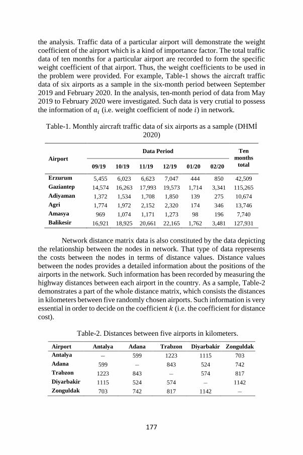
177
the analysis. Traffic data of a particular airport will demonstrate the weight
coefficient of the airport which is a kind of importance factor. The total traffic
data of ten months for a particular airport are recorded to form the specific
weight coefficient of that airport. Thus, the weight coefficients to be used in
the problem were provided. For example, Table-1 shows the aircraft traffic
data of six airports as a sample in the six-month period between September
2019 and February 2020. In the analysis, ten-month period of data from May
2019 to February 2020 were investigated. Such data is very crutial to possess
the information of 𝑎𝑖 (i.e. weight coefficient of node 𝑖) in network.
Table-1. Monthly aircraft traffic data of six airports as a sample (DHMİ
2020)
Airport
Data Period Ten
months
total 09/19 10/19 11/19 12/19 01/20 02/20
Erzurum 5,455 6,023 6,623 7,047 444 850 42,509
Gaziantep 14,574 16,263 17,993 19,573 1,714 3,341 115,265
Adiyaman 1,372 1,534 1,708 1,850 139 275 10,674
Agri 1,774 1,972 2,152 2,320 174 346 13,746
Amasya 969 1,074 1,171 1,273 98 196 7,740
Balikesir 16,921 18,925 20,661 22,165 1,762 3,481 127,931
Network distance matrix data is also constituted by the data depicting
the relationship between the nodes in network. That type of data represents
the costs between the nodes in terms of distance values. Distance values
between the nodes provides a detailed information about the positions of the
airports in the network. Such information has been recorded by measuring the
highway distances between each airport in the country. As a sample, Table-2
demonstrates a part of the whole distance matrix, which consists the distances
in kilometers between five randomly chosen airports. Such information is very
essential in order to decide on the coefficient 𝑘 (i.e. the coefficient for distance
cost).
Table-2. Distances between five airports in kilometers.
Airport Antalya Adana Trabzon Diyarbakir Zonguldak
Antalya – 599 1223 1115 703
Adana 599 – 843 524 742
Trabzon 1223 843 – 574 817
Diyarbakir 1115 524 574 – 1142
Zonguldak 703 742 817 1142 –
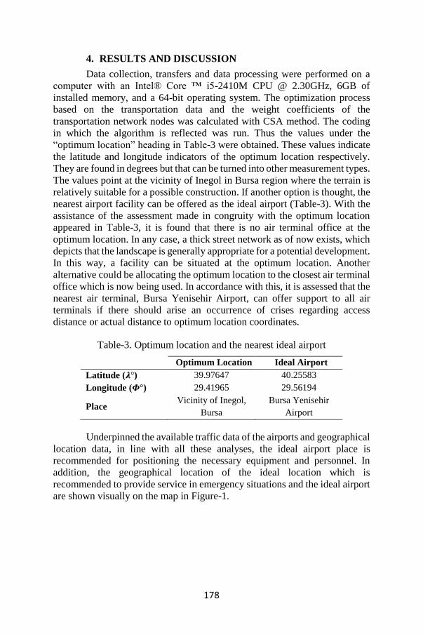
178
4. RESULTS AND DISCUSSION
Data collection, transfers and data processing were performed on a
computer with an Intel® Core ™ i5-2410M CPU @ 2.30GHz, 6GB of
installed memory, and a 64-bit operating system. The optimization process
based on the transportation data and the weight coefficients of the
transportation network nodes was calculated with CSA method. The coding
in which the algorithm is reflected was run. Thus the values under the
“optimum location” heading in Table-3 were obtained. These values indicate
the latitude and longitude indicators of the optimum location respectively.
They are found in degrees but that can be turned into other measurement types.
The values point at the vicinity of Inegol in Bursa region where the terrain is
relatively suitable for a possible construction. If another option is thought, the
nearest airport facility can be offered as the ideal airport (Table-3). With the
assistance of the assessment made in congruity with the optimum location
appeared in Table-3, it is found that there is no air terminal office at the
optimum location. In any case, a thick street network as of now exists, which
depicts that the landscape is generally appropriate for a potential development.
In this way, a facility can be situated at the optimum location. Another
alternative could be allocating the optimum location to the closest air terminal
office which is now being used. In accordance with this, it is assessed that the
nearest air terminal, Bursa Yenisehir Airport, can offer support to all air
terminals if there should arise an occurrence of crises regarding access
distance or actual distance to optimum location coordinates.
Table-3. Optimum location and the nearest ideal airport
Optimum Location Ideal Airport
Latitude (𝝀°) 39.97647 40.25583
Longitude (𝜱°) 29.41965 29.56194
Place Vicinity of Inegol,
Bursa
Bursa Yenisehir
Airport
Underpinned the available traffic data of the airports and geographical
location data, in line with all these analyses, the ideal airport place is
recommended for positioning the necessary equipment and personnel. In
addition, the geographical location of the ideal location which is
recommended to provide service in emergency situations and the ideal airport
are shown visually on the map in Figure-1.
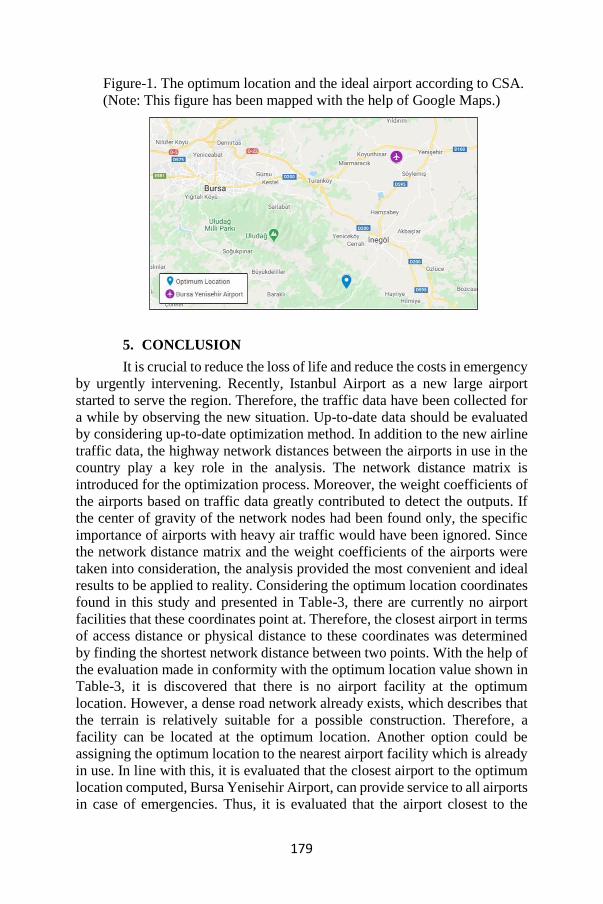
179
Figure-1. The optimum location and the ideal airport according to CSA.
(Note: This figure has been mapped with the help of Google Maps.)
5. CONCLUSION
It is crucial to reduce the loss of life and reduce the costs in emergency
by urgently intervening. Recently, Istanbul Airport as a new large airport
started to serve the region. Therefore, the traffic data have been collected for
a while by observing the new situation. Up-to-date data should be evaluated
by considering up-to-date optimization method. In addition to the new airline
traffic data, the highway network distances between the airports in use in the
country play a key role in the analysis. The network distance matrix is
introduced for the optimization process. Moreover, the weight coefficients of
the airports based on traffic data greatly contributed to detect the outputs. If
the center of gravity of the network nodes had been found only, the specific
importance of airports with heavy air traffic would have been ignored. Since
the network distance matrix and the weight coefficients of the airports were
taken into consideration, the analysis provided the most convenient and ideal
results to be applied to reality. Considering the optimum location coordinates
found in this study and presented in Table-3, there are currently no airport
facilities that these coordinates point at. Therefore, the closest airport in terms
of access distance or physical distance to these coordinates was determined
by finding the shortest network distance between two points. With the help of
the evaluation made in conformity with the optimum location value shown in
Table-3, it is discovered that there is no airport facility at the optimum
location. However, a dense road network already exists, which describes that
the terrain is relatively suitable for a possible construction. Therefore, a
facility can be located at the optimum location. Another option could be
assigning the optimum location to the nearest airport facility which is already
in use. In line with this, it is evaluated that the closest airport to the optimum
location computed, Bursa Yenisehir Airport, can provide service to all airports
in case of emergencies. Thus, it is evaluated that the airport closest to the

180
optimum location can serve the airports within the country in case of
emergency.
In this study, as a result of the analysis made considering the traffic
data and location data collected, Bursa Yenisehir Airport was proposed for the
positioning of the equipment and personnel that may be needed for emergency
response. It is considered that assigning this airport, where aid facilities can
be established, aims at minimizing the loss of life during or after disasters such
as any natural disaster or accident. As a result of this study and in line with
the recommendations of the research, it is expected that progress will be made
in minimizing the loss of life and reducing time and expense loss. Thus, a
significant contribution is expected to result in regional and countrywide
development.
181
REFERENCES
Askarzadeh, A. (2016). A novel metaheuristic method for solving constrained
engineering optimization problems: crow search
algorithm. Computers & Structures, 169, 1-12.
Aydogdu, I. (2017). Cost optimization of reinforced concrete cantilever
retaining walls under seismic loading using a biogeography-based
optimization algorithm with Levy flights. Engineering
Optimization, 49(3), 381-400.
Demir, E. (2018a). Havalimanlarında kalkış öncesi, acil durumlarda, yardım
alınabilecek en uygun lokasyonun Weber problemine uyarlanarak
belirlenmesi. Türk Coğrafya Dergisi, (70), 81-85.
Demir, E. (2018b). Approach for siting a support facility for transporting
supplies in emergency cases in the Republic of Bulgaria. In MATEC
Web of Conferences (Vol. 234, p. 06001). EDP Sciences.
Demir, E., & Kockal, N. U. (2019). Iterative methodology on locating a
cement plant. Journal of Inequalities and Applications, 2019(1), 1-8.
DHMİ, (2020), Devlet Hava Meydanları İşletmesi Genel Müdürlüğü
Havalimanları karşılaştırmalı istatistikleri,
<https://www.dhmi.gov.tr/sayfalar/istatistik.aspx>, accessed on 18
April 2020.
Parkinson, A. R., Balling, R., & Hedengren, J. D. (2013). Optimization
methods for engineering design. Brigham Young University, 5, 11.
SHGM, (2020), Sivil Havacılık Genel Müdürlüğü Faaliyet Raporu 2019,
<http://web.shgm.gov.tr/documents/sivilhavacilik/files/pdf/kurumsal
/faaliyet/2019.pdf>, accessed on 15 April 2020.
Snyder, J. P. (2012). MAP PROJECTIONS: A Working Manual (us
Geological Survey Professional Paper 1395). WWW
MILITARYBOOKSHOP Company U.
Uslu, S., & Dönmez, K. (2017). Hava Trafik Kontrol Kaynaklı Uçak
Kazalarının İncelenmesi. Mehmet Akif Ersoy Üniversitesi Sosyal
Bilimler Enstitüsü Dergisi, 9(18), 271-287.
Yang, X. S. (2010). Engineering optimization: an introduction with
metaheuristic applications. John Wiley & Sons.

182
CHAPTER XII
SUSTAINABLE GROUNDWATER REMEDIATION
WITH BIOBARRIERS USING AGRICULTURAL OR
PLANT PRODUCTION RESIDUES
Emre Burcu Özkaraova1
1(Assoc. Prof. Dr.) Ondokuz Mayıs University, e-mail: [email protected]
0000-0001-5033-2853
INTRODUCTION
The World’s population is estimated to be 7.7 Billion people (UN,
2019). Clean drinking water and food supplies are among the major
requirements. Despite the differences in cultural habits in consumption
and state of development, agricultural activities and livestock production
increased during the last century. The expansion and intensification of
agricultural activities caused to the detoriation of soil and water resources
(Mateo-Sagasta et al., 2017). Various contaminants, including
nitrogenous compounds, pesticides, growths regulators, veterinary
antibiotics have been detected (Menz et al., 2015). Intensified agricultural
activities also resulted in higher production of agricultural residues and
wastes (Obi et al., 2016). Residues/wastes from the harvesting and
processing of agricultural yields like crops, fruits, vegetables and animals
are accepted as crop residues and animal wastes, respectively (Obi et al.,
2016; Sabiiti, 2011). The estimated amount of agricultural residues and/or
wastes Worldwide is about 998 million tons per year (Agamuthu 2009).
Therefore, the management of agricultural residues/wastes based on the 4
R principles (reduce, reuse, recycle, recover) is of most importance.
These residues have been accepted as a resource and have been used for
many purposes besides conventional utilizations for biogas, energy,
compost and animal feed (Sabiiti, 2011; Zhang et al., 2012a).
Aiming the reduction of biodecomposable materials to be disposed
off at landfills, research continues for the reuse, recycling and utilization
of agro-residues like corn cob, straw and stover, olive and apricot stones,
rice and nut husk, nut shells etc. for potential uses in water purification
(El Nadi et al., 2014; Ghazy et al., 2016; Góngora-Echeverría et al.,
2017). These were also used as filling materials in permeable reactive
barrier systems and in-situ bioreactors (e.g. biowalls). Permeable reactive
barrier (PRB) is an in-situ sustainable groundwater remediation
technology that has been widely used and studied in groundwater
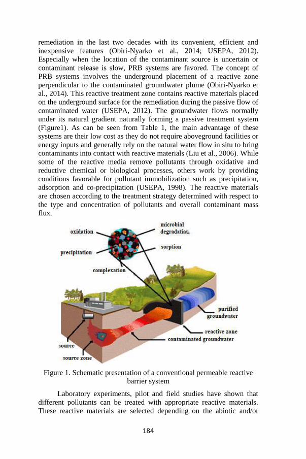
184
remediation in the last two decades with its convenient, efficient and
inexpensive features (Obiri-Nyarko et al., 2014; USEPA, 2012).
Especially when the location of the contaminant source is uncertain or
contaminant release is slow, PRB systems are favored. The concept of
PRB systems involves the underground placement of a reactive zone
perpendicular to the contaminated groundwater plume (Obiri-Nyarko et
al., 2014). This reactive treatment zone contains reactive materials placed
on the underground surface for the remediation during the passive flow of
contaminated water (USEPA, 2012). The groundwater flows normally
under its natural gradient naturally forming a passive treatment system
(Figure1). As can be seen from Table 1, the main advantage of these
systems are their low cost as they do not require aboveground facilities or
energy inputs and generally rely on the natural water flow in situ to bring
contaminants into contact with reactive materials (Liu et al., 2006). While
some of the reactive media remove pollutants through oxidative and
reductive chemical or biological processes, others work by providing
conditions favorable for pollutant immobilization such as precipitation,
adsorption and co-precipitation (USEPA, 1998). The reactive materials
are chosen according to the treatment strategy determined with respect to
the type and concentration of pollutants and overall contaminant mass
flux.
Figure 1. Schematic presentation of a conventional permeable reactive
barrier system
Laboratory experiments, pilot and field studies have shown that
different pollutants can be treated with appropriate reactive materials.
These reactive materials are selected depending on the abiotic and/or
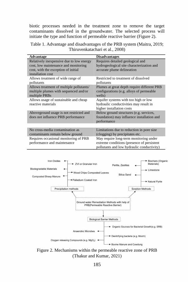
185
biotic processes needed in the treatment zone to remove the target
contaminants dissolved in the groundwater. The selected process will
initiate the type and function of permeable reactive barrier (Figure 2).
Table 1. Advantage and disadvantages of the PRB system (Maitra, 2019;
Thiruvenkatachari et al., 2008)
Advantage Disadvantages
Relatively inexpensive due to low energy
cost, low maintenance and monitoring
cost, with the exception of initial
installation cost
Requires detailed geological and
hydrogeological site characterization and
accurate plume delineation
Allows treatment of wide range of
pollutants
Restricted to treatment of dissolved
pollutants
Allows treatment of multiple pollutants/
multiple plumes with sequenced and/or
multiple PRBs
Plumes at great depth require different PRB
configurations (e.g. alloys of permeable
wells)
Allows usage of sustainable and cheap
reactive materials
Aquifer systems with too high or low
hydraulic conductivities may result in
higher installation costs
Aboveground usage is not restricted and
does not influence PRB performance
Below ground structures (e.g. services,
foundation) may influence installation and
performance
No cross-media contamination as
contaminants remain below ground
Limitations due to reduction in pore size
(clogging) by precipitates etc.
Requires occasional monitoring of PRB
performance and maintenance
May require long-term monitoring under
extreme conditions (presence of persistent
pollutants and low hydraulic conductivity)
Figure 2. Mechanisms within the permeable reactive zone of PRB
(Thakur and Kumar, 2021)
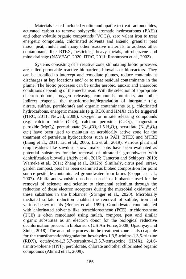
186
Materials tested included zeolite and apatite to treat radionuclides,
activated carbon to remove polycyclic aromatic hydrocarbons (PAHs)
and other volatile organic compounds (VOCs), zero valent iron to treat
energetic compounds, chlorinated solvents and arsenic, granular peat
moss, peat, mulch and many other reactive materials to address other
contaminants like BTEX, pesticides, heavy metals, nitrobenzene and
mine drainage (NAVFAC, 2020; ITRC, 2011; Rasmussen et al., 2002).
Systems consisting of a reactive zone stimulating biotic processes
are called permeable reactive biobarriers, biowalls or bioreactors. They
can be installed to intercept and remediate plumes, reduce contaminant
discharges at key locations and/ or to treat residual contaminants in the
plume. The biotic processes can be under aerobic, anoxic and anaerobic
conditions depending of the mechanism. With the selection of appropriate
electron donors, oxygen releasing compounds, nutrients and other
indirect reagents, the transformation/degradation of inorganic (e.g.
nitrate, sulfate, perchlorate) and organic contaminants (e.g. chlorinated
hydrocarbons, energetic materials (e.g. RDX and HMX) can be triggered
(ITRC, 2011; Newell, 2008). Oxygen or nitrate releasing compounds
(e.g. calcium oxide (CaO), calcium peroxide (CaO2), magnesium
peroxide (MgO2), percarbonate (Na2CO3·1.5 H2O2), persulfate (Na2S2O8)
etc.) have been used to maintain an aerobically active zone for the
treatment of petroleum hydrocarbons such as PAH, BTEX and MTBE
(Liang et al., 2011; Liu et al., 2006; Liu et al., 2019). Various plant and
crop residues like sawdust, straw, maize cobs have been evaluated as
potential substrates for the removal of nitrate in groundwater with
denitrification biowalls (Addy et al., 2016; Cameron and Schipper, 2010;
Warneke et al., 2011; Zhang et al., 2012b). Similarly, citrus peel, straw,
garden compost, peat has been examined as biobed composition for point
source pesticide contaminated groundwater from farms (Coppola et al.,
2007). Alfalfa and woodship has been used in a biobarrier used for the
removal of selenate and selenite to elemental selenium through the
reduction of these electron acceptors during the microbial oxidation of
these substrates in the biobarrier (Stringer et al., 2020). Microbially
mediated sulfate reduction enabled the removal of sulfate, iron and
various heavy metals (Benner et al., 1999). Groundwater contaminated
with chlorinated solvents like tetrachloroethene (PCE), trichloroethene
(TCE) is often remediated using mulch, compost, peat and similar
organic substrates as an electron donor for the biological reductive
dechlorination process in biobarriers (US Air Force, 2008; Upadhyay and
Sinha, 2018). The anaerobic process in the treatment zone is also capable
for the transformation/degradation hexahydro-1,3,5-trinitro-1,3,5-triazine
(RDX), octahydro-1,3,5,7-tetranitro-1,3,5,7-tetrazocine (HMX), 2,4,6-
trinitro-toluene (TNT), perchlorate, chlorate and other chlorinated organic
compounds (Ahmad et al., 2009).
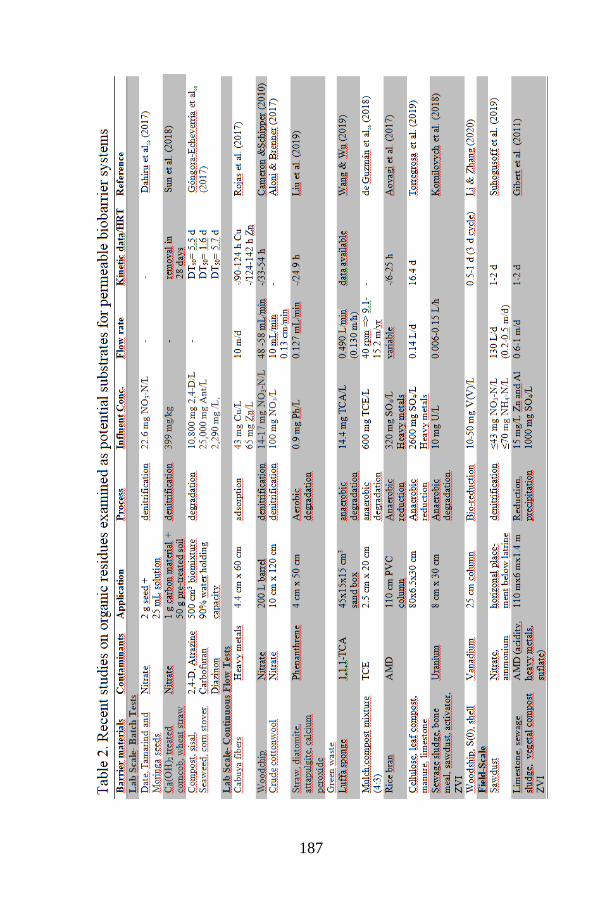
187
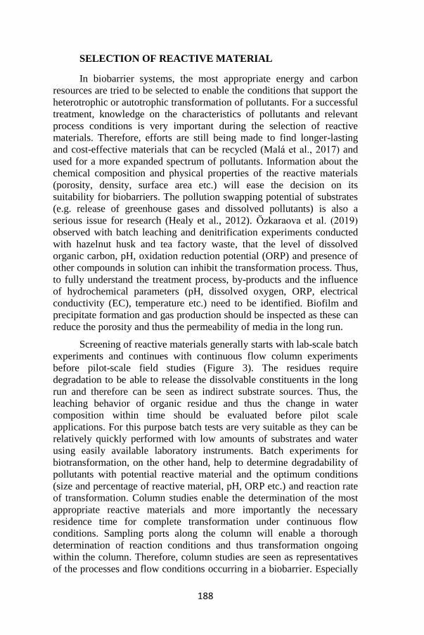
188
SELECTION OF REACTIVE MATERIAL
In biobarrier systems, the most appropriate energy and carbon
resources are tried to be selected to enable the conditions that support the
heterotrophic or autotrophic transformation of pollutants. For a successful
treatment, knowledge on the characteristics of pollutants and relevant
process conditions is very important during the selection of reactive
materials. Therefore, efforts are still being made to find longer-lasting
and cost-effective materials that can be recycled (Malá et al., 2017) and
used for a more expanded spectrum of pollutants. Information about the
chemical composition and physical properties of the reactive materials
(porosity, density, surface area etc.) will ease the decision on its
suitability for biobarriers. The pollution swapping potential of substrates
(e.g. release of greenhouse gases and dissolved pollutants) is also a
serious issue for research (Healy et al., 2012). Özkaraova et al. (2019)
observed with batch leaching and denitrification experiments conducted
with hazelnut husk and tea factory waste, that the level of dissolved
organic carbon, pH, oxidation reduction potential (ORP) and presence of
other compounds in solution can inhibit the transformation process. Thus,
to fully understand the treatment process, by-products and the influence
of hydrochemical parameters (pH, dissolved oxygen, ORP, electrical
conductivity (EC), temperature etc.) need to be identified. Biofilm and
precipitate formation and gas production should be inspected as these can
reduce the porosity and thus the permeability of media in the long run.
Screening of reactive materials generally starts with lab-scale batch
experiments and continues with continuous flow column experiments
before pilot-scale field studies (Figure 3). The residues require
degradation to be able to release the dissolvable constituents in the long
run and therefore can be seen as indirect substrate sources. Thus, the
leaching behavior of organic residue and thus the change in water
composition within time should be evaluated before pilot scale
applications. For this purpose batch tests are very suitable as they can be
relatively quickly performed with low amounts of substrates and water
using easily available laboratory instruments. Batch experiments for
biotransformation, on the other hand, help to determine degradability of
pollutants with potential reactive material and the optimum conditions
(size and percentage of reactive material, pH, ORP etc.) and reaction rate
of transformation. Column studies enable the determination of the most
appropriate reactive materials and more importantly the necessary
residence time for complete transformation under continuous flow
conditions. Sampling ports along the column will enable a thorough
determination of reaction conditions and thus transformation ongoing
within the column. Therefore, column studies are seen as representatives
of the processes and flow conditions occurring in a biobarrier. Especially
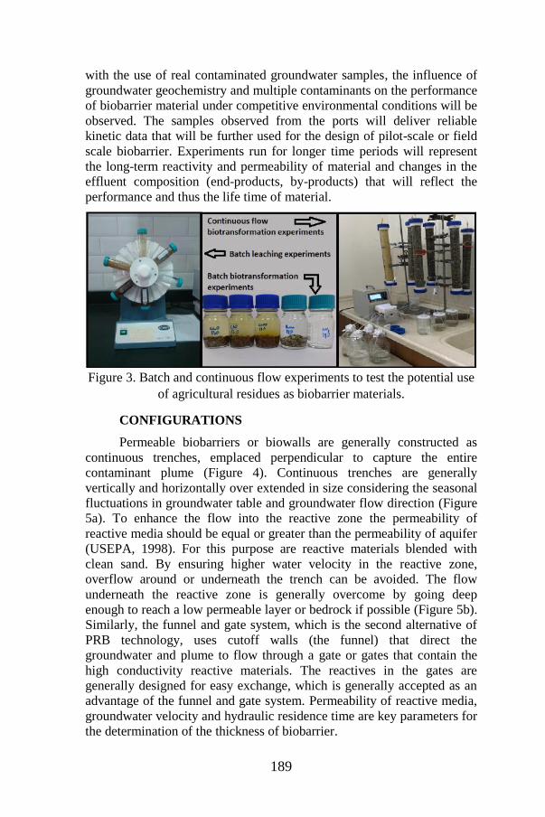
189
with the use of real contaminated groundwater samples, the influence of
groundwater geochemistry and multiple contaminants on the performance
of biobarrier material under competitive environmental conditions will be
observed. The samples observed from the ports will deliver reliable
kinetic data that will be further used for the design of pilot-scale or field
scale biobarrier. Experiments run for longer time periods will represent
the long-term reactivity and permeability of material and changes in the
effluent composition (end-products, by-products) that will reflect the
performance and thus the life time of material.
Figure 3. Batch and continuous flow experiments to test the potential use
of agricultural residues as biobarrier materials.
CONFIGURATIONS
Permeable biobarriers or biowalls are generally constructed as
continuous trenches, emplaced perpendicular to capture the entire
contaminant plume (Figure 4). Continuous trenches are generally
vertically and horizontally over extended in size considering the seasonal
fluctuations in groundwater table and groundwater flow direction (Figure
5a). To enhance the flow into the reactive zone the permeability of
reactive media should be equal or greater than the permeability of aquifer
(USEPA, 1998). For this purpose are reactive materials blended with
clean sand. By ensuring higher water velocity in the reactive zone,
overflow around or underneath the trench can be avoided. The flow
underneath the reactive zone is generally overcome by going deep
enough to reach a low permeable layer or bedrock if possible (Figure 5b).
Similarly, the funnel and gate system, which is the second alternative of
PRB technology, uses cutoff walls (the funnel) that direct the
groundwater and plume to flow through a gate or gates that contain the
high conductivity reactive materials. The reactives in the gates are
generally designed for easy exchange, which is generally accepted as an
advantage of the funnel and gate system. Permeability of reactive media,
groundwater velocity and hydraulic residence time are key parameters for
the determination of the thickness of biobarrier.

190
Figure 4. Conventional continuous trench permeable reactive barrier
Figure 5. Conventional continuous trench PRB configurations
For the success of a biobarrier, combined use of reactive materials,
installed as a mixture or in sequence is possible (Upadhyay and Sinha,
2018; Chu and Eivazi, 2018). Mixtures of substrates may also be more
effective in providing longevity and sustainability of microorganism in
the zone (Jamil and Clarke, 2013). This might be especially needed for
sites with multiple contaminants. In cases with higher pollutant
concentrations wider trenches may be needed to ensure the retention time
in biobarrier, the construction of additional trenches in parallel may be a
solution (US Air Force, 2008). These multiple biobarrier systems may
also enable the additional use of alternative reactives for providing
supportive and/or stimulative conditions before removal of target
contaminant (Figure 6) (Liu et al., 2006; Liu et al., 2013). These may also
reduce intermediate products directly or by extending the reaction zone,
especially when emplaced close to each other. Angled placement of
biobarrier centered to plume path may ensure capture of contaminants, by
avoiding their escape at the biobarrier ends (Figure 7).
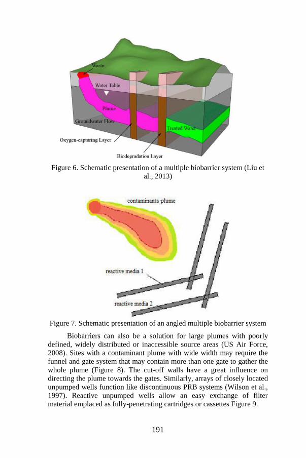
191
Figure 6. Schematic presentation of a multiple biobarrier system (Liu et
al., 2013)
Figure 7. Schematic presentation of an angled multiple biobarrier system
Biobarriers can also be a solution for large plumes with poorly
defined, widely distributed or inaccessible source areas (US Air Force,
2008). Sites with a contaminant plume with wide width may require the
funnel and gate system that may contain more than one gate to gather the
whole plume (Figure 8). The cut-off walls have a great influence on
directing the plume towards the gates. Similarly, arrays of closely located
unpumped wells function like discontinuous PRB systems (Wilson et al.,
1997). Reactive unpumped wells allow an easy exchange of filter
material emplaced as fully-penetrating cartridges or cassettes Figure 9.
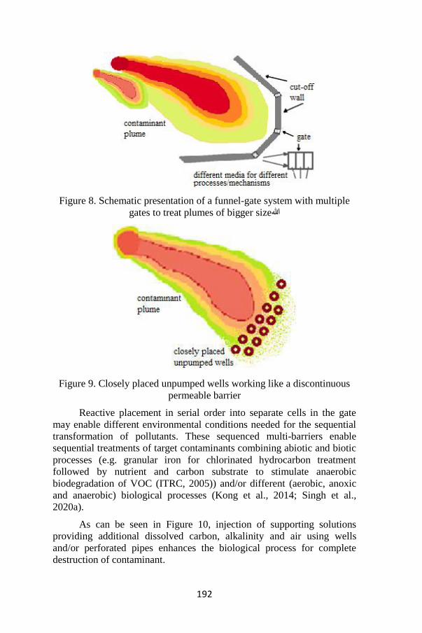
192
Figure 8. Schematic presentation of a funnel-gate system with multiple
gates to treat plumes of bigger sizeهللا
Figure 9. Closely placed unpumped wells working like a discontinuous
permeable barrier
Reactive placement in serial order into separate cells in the gate
may enable different environmental conditions needed for the sequential
transformation of pollutants. These sequenced multi-barriers enable
sequential treatments of target contaminants combining abiotic and biotic
processes (e.g. granular iron for chlorinated hydrocarbon treatment
followed by nutrient and carbon substrate to stimulate anaerobic
biodegradation of VOC (ITRC, 2005)) and/or different (aerobic, anoxic
and anaerobic) biological processes (Kong et al., 2014; Singh et al.,
2020a).
As can be seen in Figure 10, injection of supporting solutions
providing additional dissolved carbon, alkalinity and air using wells
and/or perforated pipes enhances the biological process for complete
destruction of contaminant.

193
Horizontal biobarriers or biowalls have been constructed to control
and/or treat vertically migrating contaminated groundwater or source
zones such as septic systems (ITRC, 2011; Suhogusoff et al., 2020),
waste piles, etc. The reactive material is directly placed as a horizontal
layer below the source zone, perpendicular to the vertical flow path.
When source area treatments are required and contaminated soil removal
is necessary biobarriers can be installed as a part of planned source area
activity (US Air Force, 2008). As seen in Figure 11, a recirculation
biobarrier placement within the excavated area may be helpful for
remediation below water table. The recirculation of contaminated
groundwater will rise the residence time in the treatment zone and thus
the removal efficiencies of pollutants. Additionally, the fluid injection
will result in hydraulic mounding within the biobarrier, increasing the
flow rate and thus the transport of released constituents down gradient of
the biobarrier. This actually may extend the treatment zone but may need
regulatory acceptance.
Figure 10. Schematic presentation of a permeable mulch biowall (US Air
Force, 2008)
.
Figure 11. Schematic presentation of a recirculating biobarrier (US Air
Force, 2008).
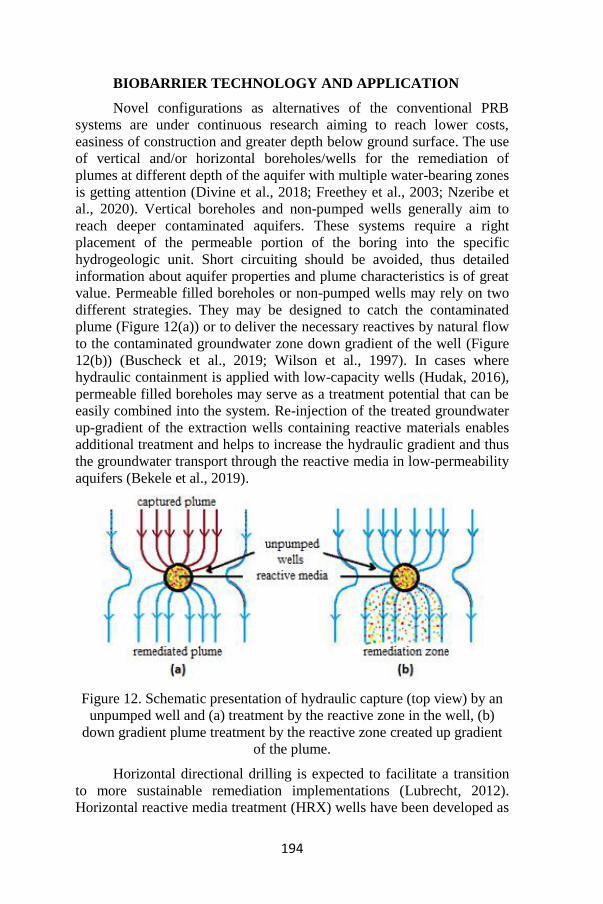
194
BIOBARRIER TECHNOLOGY AND APPLICATION
Novel configurations as alternatives of the conventional PRB
systems are under continuous research aiming to reach lower costs,
easiness of construction and greater depth below ground surface. The use
of vertical and/or horizontal boreholes/wells for the remediation of
plumes at different depth of the aquifer with multiple water-bearing zones
is getting attention (Divine et al., 2018; Freethey et al., 2003; Nzeribe et
al., 2020). Vertical boreholes and non-pumped wells generally aim to
reach deeper contaminated aquifers. These systems require a right
placement of the permeable portion of the boring into the specific
hydrogeologic unit. Short circuiting should be avoided, thus detailed
information about aquifer properties and plume characteristics is of great
value. Permeable filled boreholes or non-pumped wells may rely on two
different strategies. They may be designed to catch the contaminated
plume (Figure 12(a)) or to deliver the necessary reactives by natural flow
to the contaminated groundwater zone down gradient of the well (Figure
12(b)) (Buscheck et al., 2019; Wilson et al., 1997). In cases where
hydraulic containment is applied with low-capacity wells (Hudak, 2016),
permeable filled boreholes may serve as a treatment potential that can be
easily combined into the system. Re-injection of the treated groundwater
up-gradient of the extraction wells containing reactive materials enables
additional treatment and helps to increase the hydraulic gradient and thus
the groundwater transport through the reactive media in low-permeability
aquifers (Bekele et al., 2019).
Figure 12. Schematic presentation of hydraulic capture (top view) by an
unpumped well and (a) treatment by the reactive zone in the well, (b)
down gradient plume treatment by the reactive zone created up gradient
of the plume.
Horizontal directional drilling is expected to facilitate a transition
to more sustainable remediation implementations (Lubrecht, 2012).
Horizontal reactive media treatment (HRX) wells have been developed as

195
a passive treatment technique capable for the treatment of various
pollutants (Divine et al., 2018). This treatment technique involves a fully
screened large-diameter horizontal well located underground roughly
parallel to the main ground water flow direction. Working as an
engineered preferential flow path, it captures the contaminated ground
water and as passive flow continuous pollutants are cleaned-up by the
reactive media in the well (Figure 13).
Figure 13. Conceptional presentation of a horizontal reactive media
treatment well (Divine et al., 2018).
Electrokinetic (EK) soil remediation has recently been applied on-
site for the treatment of contaminated less permeable (clayey) soils for
which conventional remediation techniques were not found to be
effective (Reddy and Cameselle, 2009). Using sustainable energy sources
EK soil remediation is accepted as a green technology relying on the
installation of anode and cathode electrodes. By applying electrical
potential (I) ions (e.g. nutrients) are driven towards one of the electrodes
(electromigration), (II) pore water is moving (electroosmosis) and (III)
small colloids (e.g. microorganisms) become mobile (electrophoresis)
(Lima et al., 2017). This technology has been coupled with
bioremediation (Barba et al., 2018; Wick et al., 2007). EK is reported to
increase the transport of contaminants, nutrients, electron acceptors and
microorganisms, which are present in the soil pore fluid, consequently
promoting processes like bioattenuation, biostimulation and
bioaugmentation (Barba et al., 2019; Gill et al., 2014). To increase this
influence, the combination of EK with permeable biobarrier systems
seems very encouraging especially for low permeable soils (Mena et al.,
2016). Research on the combination of electrokinetic remediation with
both biotic and abiotic permeable reactive barriers (EK-PRB) systems
lead to the commercialization of technology under names such as
LasagnaTM and Electro-Klean (Andrade and dos Santos, 2020; Reddy and
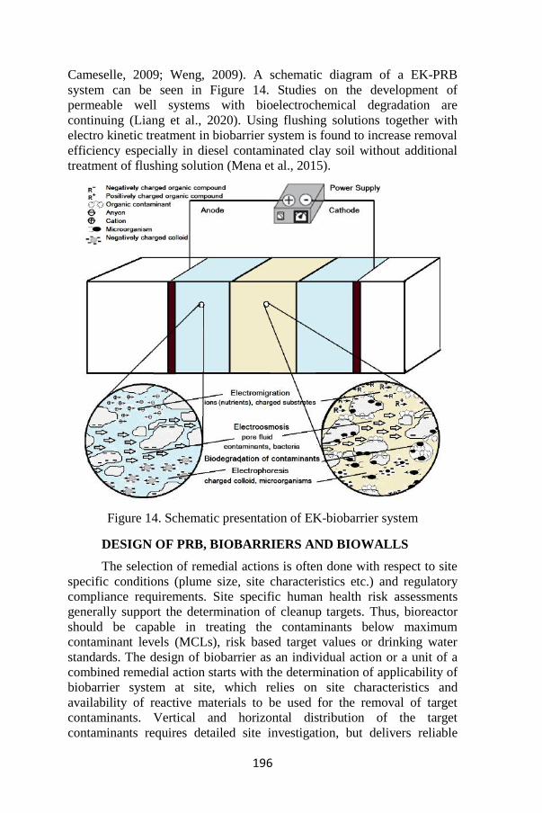
196
Cameselle, 2009; Weng, 2009). A schematic diagram of a EK-PRB
system can be seen in Figure 14. Studies on the development of
permeable well systems with bioelectrochemical degradation are
continuing (Liang et al., 2020). Using flushing solutions together with
electro kinetic treatment in biobarrier system is found to increase removal
efficiency especially in diesel contaminated clay soil without additional
treatment of flushing solution (Mena et al., 2015).
Figure 14. Schematic presentation of EK-biobarrier system
DESIGN OF PRB, BIOBARRIERS AND BIOWALLS
The selection of remedial actions is often done with respect to site
specific conditions (plume size, site characteristics etc.) and regulatory
compliance requirements. Site specific human health risk assessments
generally support the determination of cleanup targets. Thus, bioreactor
should be capable in treating the contaminants below maximum
contaminant levels (MCLs), risk based target values or drinking water
standards. The design of biobarrier as an individual action or a unit of a
combined remedial action starts with the determination of applicability of
biobarrier system at site, which relies on site characteristics and
availability of reactive materials to be used for the removal of target
contaminants. Vertical and horizontal distribution of the target
contaminants requires detailed site investigation, but delivers reliable
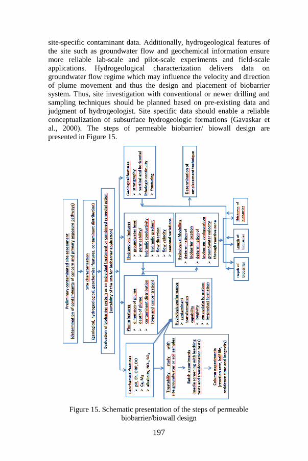
197
site-specific contaminant data. Additionally, hydrogeological features of
the site such as groundwater flow and geochemical information ensure
more reliable lab-scale and pilot-scale experiments and field-scale
applications. Hydrogeological characterization delivers data on
groundwater flow regime which may influence the velocity and direction
of plume movement and thus the design and placement of biobarrier
system. Thus, site investigation with conventional or newer drilling and
sampling techniques should be planned based on pre-existing data and
judgment of hydrogeologist. Site specific data should enable a reliable
conceptualization of subsurface hydrogeologic formations (Gavaskar et
al., 2000). The steps of permeable biobarrier/ biowall design are
presented in Figure 15.
Figure 15. Schematic presentation of the steps of permeable
biobarrier/biowall design
198
Lab-scale and pilot-scale experiments provide the relevant data for
material selection and reaction rates and half-lives of the relevant
transformation mechanism for contaminant removal. Longevity, cost-
effectiveness and environmental compatibility of reactive materials are
among the key parameters (USEPA, 1998). Longevity is not only related
to the properties of reactive material (leaching potential, material
structure, etc.) but also a function of contaminant distribution and
concentration variation, and geochemical (pH, ORP, EC and constituents)
and hydraulic characteristics (hydraulic conductivity and gradient) of the
groundwater within time. The hydraulic conductivity of the filter material
is always higher than the value of aquifer so that the contaminant plume
can be easily captured by the biobarrier system (USEPA, 1998). Thus, the
hydraulic conductivity of the site will guide the determination of the
hydraulic conductivity of reactive material, which is adjusted with lab-
scale experiments and so to say engineered before field-scale
applications.
The groundwater velocity is one of the most important parameters.
The groundwater velocity can be determined through tracer testing
(single-well tracer test, multiple-well test), direct in-situ measurement
with appropriate probes (e.g. colloidal borescope, University of Waterloo
Drive –Point Probe etc. (ITRC, 2005)). The velocity can be calculated
using the Darcy’s Law and site specific data on hydraulic gradients
(horizontal and vertical) and hydraulic conductivity of the aquifer
(Gavaskar et al., 2000). If the biobarrier is embedded into a confining
layer the determination of the vertical hydraulic gradient may not be of
importance, but if a confining layer is not available at relevant working
depth, the vertical hydraulic gradient needs to be investigated to enable to
selection of the depth of biobarrier for avoiding shortcuits.
As the horizontal hydraulic gradient and hydraulic conductivity is
influencing the residence time of contaminant and thus the determination
of the thickness of biobarrier system, the highest potential groundwater
velocity observed for the site should be used for system design.
Groundwater velocities below 0.3 m/day are found to be suitable for
biobarrier systems (US Air Force, 2008; ITRC, 2011). Velocities above
this value may require multiple trenches to ensure the residence time for
effective removal. Thus, at sites with high groundwater velocities, other
remediation techniques instead or for integration may be evaluated as
alternative options regarding the overall cost effectiveness of system.
Aquifers with low groundwater velocities may require a long time to treat
the contaminant plume as plume migration towards the biobarrier will
take time. In order to increase the velocity, the recirculation of water will
raise the hydraulic gradient and thus speed up the plume migration
towards the biobarrier system (US Air Force, 2008).

199
As the groundwater velocity is directly related to the hydraulic
conductivity a thorough investigation of aquifer system is required.
Aquifer systems comprised of different soil layers with lower or higher
hydraulic conductivities may induce preferential flow path of the
contaminant plume. Thus, a good understanding of the geology,
hydrogeology and geochemistry of the site is of primary importance
during the design of biobarrier system. The groundwater flow direction is
a key parameter for the placement of biobarrier and can be interpreted
using groundwater contour maps, which also enable the determination of
hydraulic gradient. If groundwater contour maps are not available, the
flow direction can be determined using three-groundwater elevations
(Kuo, 2014). Hydrogeological modeling may help to locate the biobarrier
system with regard to the plume size and behavior and variation in
vertical locations and thicknesses of soil layers. Generally, computer
programs like MODFLOW, FEFLOW or similar programs are used for
this purpose. These models and others like MODPATH also help to
determine the biobarrier configuration and dimensions, and assess
potential flow conditions within, below or around the barrier (Scott and
Folkes, 2000; Rad and Fazlali, 2020; Grajales-Mesa et al., 2020). The so-
called process-based models, on the other hand, help to evaluate the
longevity of biowall/biobarrier by interpreting potential biogeochemical
processes ongoing in the biobarrier (Singh et al., 2020b). On the contrary,
inadequacy in the investigation of geological and hydrogeological
features of the site often resulted in failure of permeable reactive barrier
and biobarrier systems.
The sizing and design of biobarrier systems depends entirely on the
concentration of pollutants in the groundwater and the groundwater flow
(EPA, 1998). Thus, the configuration and dimension of the biobarrier
system is determined according to site specific conditions (Figure 16).
Continuous trench biobarrier systems, called biowalls or mulch trenches,
are generally installed into shallow aquifers. The depth is between 15-21
m or less (Day and Schindler, 2020; Day et al., 1999; USEPA, 1998).
Actually, the trench depth is totally depending on the stability of
geological formation and the availability of equipment used for
excavation. Construction techniques and appropriate trenchers or
hydraulic excavators may be available, but costs are increasing
respectively. Systems such as sludge injection and hydraulic fracture
enable to overcome this kind of placement problem (USEPA, 1998).
Biobarrier systems should be long enough to capture the whole
width of plume under different seasonal variations of groundwater
behavior. Similarly, the biobarrier should be deep enough to cover the
total depth of plume. The thickness of biobarrier system should ensure
the necessary retention time of contaminants within the reactive zone for
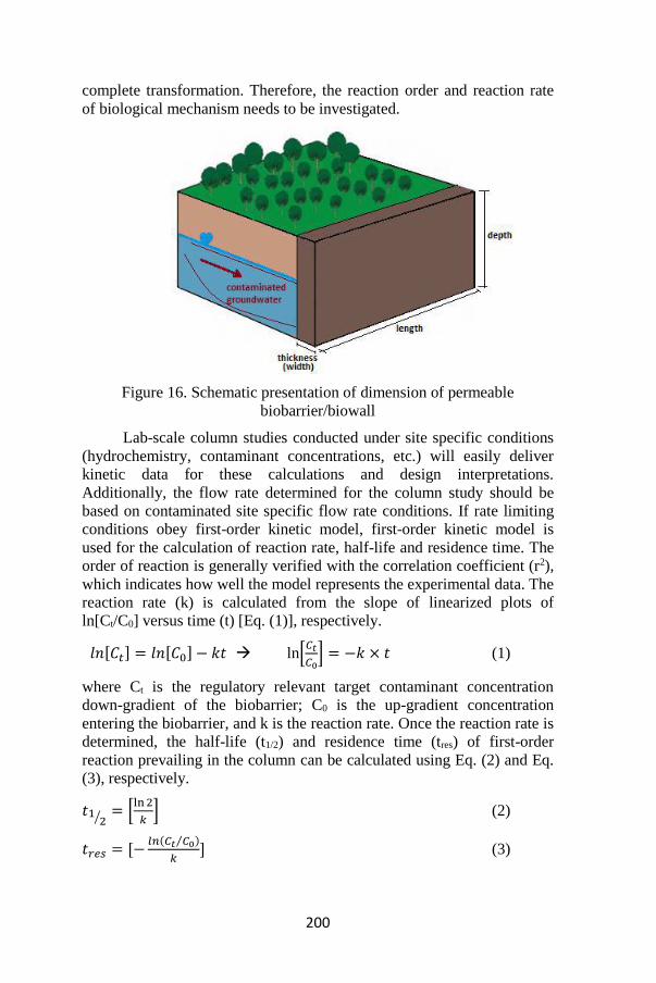
200
complete transformation. Therefore, the reaction order and reaction rate
of biological mechanism needs to be investigated.
Figure 16. Schematic presentation of dimension of permeable
biobarrier/biowall
Lab-scale column studies conducted under site specific conditions
(hydrochemistry, contaminant concentrations, etc.) will easily deliver
kinetic data for these calculations and design interpretations.
Additionally, the flow rate determined for the column study should be
based on contaminated site specific flow rate conditions. If rate limiting
conditions obey first-order kinetic model, first-order kinetic model is
used for the calculation of reaction rate, half-life and residence time. The
order of reaction is generally verified with the correlation coefficient (r2),
which indicates how well the model represents the experimental data. The
reaction rate (k) is calculated from the slope of linearized plots of
ln[Ct/C0] versus time (t) [Eq. (1)], respectively.
𝑙𝑛[𝐶𝑡] = 𝑙𝑛[𝐶0] − 𝑘𝑡 ln[𝐶𝑡
𝐶0] = −𝑘 × 𝑡 (1)
where Ct is the regulatory relevant target contaminant concentration
down-gradient of the biobarrier; C0 is the up-gradient concentration
entering the biobarrier, and k is the reaction rate. Once the reaction rate is
determined, the half-life (t1/2) and residence time (tres) of first-order
reaction prevailing in the column can be calculated using Eq. (2) and Eq.
(3), respectively.
𝑡12⁄ = [
ln 2
𝑘] (2)
𝑡𝑟𝑒𝑠 = [−𝑙𝑛(𝐶𝑡 𝐶0⁄ )
𝑘] (3)
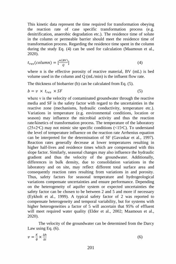
201
This kinetic data represent the time required for transformation obeying
the reaction rate of case specific transformation process (e.g.
denitrification, anaerobic degradation etc.). The residence time of solute
in the column or permeable barrier should meet the residence time of
transformation process. Regarding the residence time spent in the column
during the study Eq. (4) can be used for calculation (Maamoun et al.,
2020).
𝑡𝑟𝑒𝑠(𝑐𝑜𝑙𝑢𝑚𝑛) = [𝑛(𝐵𝑉)
𝑄] (4)
where n is the effective porosity of reactive material, BV (mL) is bed
volume used in the column and Q (mL/min) is the influent flow rate.
The thickness of biobarrier (b) can be calculated from Eq. (5).
𝑏 = 𝑣 × 𝑡𝑟𝑒𝑠 × 𝑆𝐹 (5)
where ν is the velocity of contaminated groundwater through the reactive
media and SF is the safety factor with regard to the uncertainties in the
reactive zone (mechanisms, hydraulic conductivity, temperature etc.).
Variations in temperature (e.g. environmental conditions, location or
season) may influence the microbial activity and thus the reaction
rate/kinetics of transformation process. The temperature of the laboratory
(25±2ᵒC) may not mimic site specific conditions (<15ᵒC). To understand
the level of temperature influence on the reaction rate Arrhenius equation
can be interpreted for the determination of SF (Gavaskar et al., 1997).
Reaction rates generally decrease at lower temperatures resulting in
higher half-lives and residence times which are compensated with this
slope factor. Similarly, seasonal changes may also influence the hydraulic
gradient and thus the velocity of the groundwater. Additionally,
differences in bulk density, due to consolidation variations in the
laboratory and on site, may reflect different total surface area and
consequently reaction rates resulting from variations in and porosity.
Thus, safety factors for seasonal temperature and hydrogeological
variations compensate uncertainties and ensure performance. Depending
on the heterogeneity of aquifer system or expected uncertainties the
safety factor can be chosen to be between 2 and 5 and more if necessary
(Eykholt et al., 1999). A typical safety factor of 2 was reported to
compensate heterogeneity and temporal variability, but for systems with
higher heterogeneities a factor of 5 will ascertain that 95% of effluent
will meet required water quality (Elder et al., 2002; Maamoun et al.,
2020).
The velocity of the groundwater can be determined from the Darcy
Law using Eq. (6).
𝑣 =𝐾
∅×
∆ℎ
∆𝑙 (6)

202
where K is the hydraulic conductivity of the reactive zone, ∆ℎ∆𝑙⁄ is the
hydraulic gradient and Ø is the porosity of reactive material. Pilot-scale
studies and investigations on-site will minimize uncertainties for
hydraulic conductivity, hydraulic gradient, and porosity. The hydraulic
conductivity of site can be determined with field measurements, such as
pump test or slup/bail test (ITRC, 2005). The hydraulic conductivity of
the reactive media is ideally determined in the laboratory with falling-
head or constant-head permeameter tests. Constant-head permeameter
tests are conducted with conventional permeameter facilities (Fetter,
1994; Gavaskar et al., 1997). Laboratory studies with columns set up as
constant head permeameters, also enables the determination of hydraulic
conductivity (Figure 17). Standard procedures explaining the
experimental study in detail, are available (e.g. ISO/TS 17892-11 and
ISO/FDIS 17312). The hydraulic conductivity can be calculated with the
help of Darcy law using Eq. (7) or Eq. (8).
𝐾 =𝑄𝑜𝑢𝑡
𝐴×
∆𝑙
∆ℎ (7)
where Qout is the discharge flow at the outlet of column, A is the cross-
sectional area, Δh is the difference in hydraulic head and Δl is the length
of reactive medium.
𝐾 =𝑉
𝐴×𝑡×
∆𝑙
∆ℎ (8)
where V is the water volume discharged during time (t). For an
appropriate determination of hydraulic conductivity, the hydraulic
gradient should be close to the value observed for the contaminated site.
If possible multiyear variations in the hydraulic gradient should be
considered during the study.
Figure 17. Schematic presentation of a column set up as a permeameter
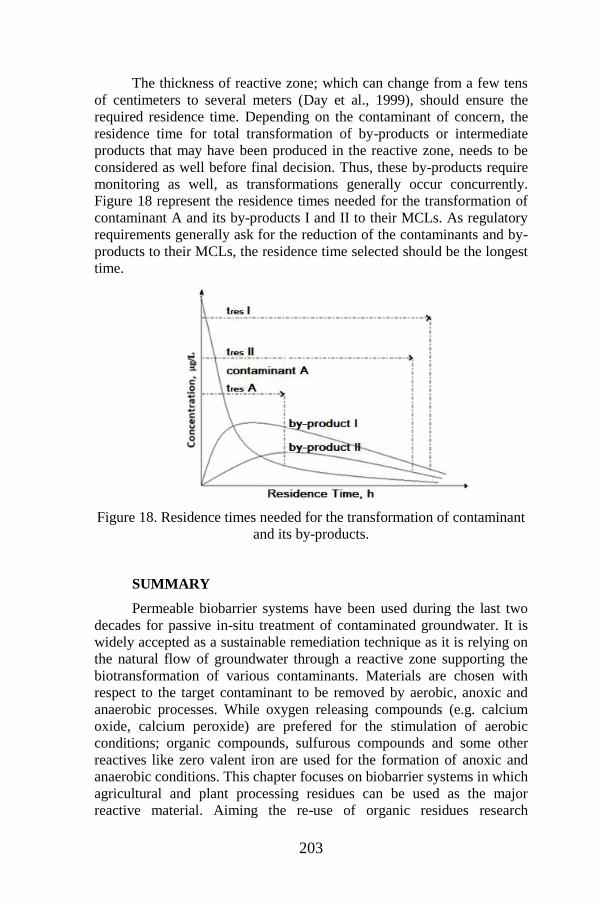
203
The thickness of reactive zone; which can change from a few tens
of centimeters to several meters (Day et al., 1999), should ensure the
required residence time. Depending on the contaminant of concern, the
residence time for total transformation of by-products or intermediate
products that may have been produced in the reactive zone, needs to be
considered as well before final decision. Thus, these by-products require
monitoring as well, as transformations generally occur concurrently.
Figure 18 represent the residence times needed for the transformation of
contaminant A and its by-products I and II to their MCLs. As regulatory
requirements generally ask for the reduction of the contaminants and by-
products to their MCLs, the residence time selected should be the longest
time.
Figure 18. Residence times needed for the transformation of contaminant
and its by-products.
SUMMARY
Permeable biobarrier systems have been used during the last two
decades for passive in-situ treatment of contaminated groundwater. It is
widely accepted as a sustainable remediation technique as it is relying on
the natural flow of groundwater through a reactive zone supporting the
biotransformation of various contaminants. Materials are chosen with
respect to the target contaminant to be removed by aerobic, anoxic and
anaerobic processes. While oxygen releasing compounds (e.g. calcium
oxide, calcium peroxide) are prefered for the stimulation of aerobic
conditions; organic compounds, sulfurous compounds and some other
reactives like zero valent iron are used for the formation of anoxic and
anaerobic conditions. This chapter focuses on biobarrier systems in which
agricultural and plant processing residues can be used as the major
reactive material. Aiming the re-use of organic residues research

204
continues on alternative materials, permeable biobarrier configurations
and technology combinations. Starting with batch and continuous flow
lab-scale studies, pilot scale and full-scale investigations complete the
research process. Batch and continuous flow studies carried out in the
laboratory deliver data for the suitability (leaching behaviour, kinetic
data, HRT and longevity) of reactive material. Relying on the laboratory
and site investigation data the biobarrier can be designed. Modeling
studies help to understand the groundwater regime and thus supports
proper selection of biobarrier location. Regarding the size and
contaminant distribution in the subsurface different biobarrier
configurations can be installed as a sustainable remedial action.
REFERENCES
Addy, K., Gold, A.J., Christianson, L.E., David M.B., Schipper, L.A. and
Ratigan, N.A. (2016). Denitrifying bioreactors for nitrate removal:
A meta-analysis. Journal of Environmental Quality, 45, 873-881.
doi:10.2134/jeq2015.07.0399.
Agamuthu, P. (2009, November). Challenges and opportunities in agro-
waste management: An Asian perspective. Inaugural meeting of
First Regional 3R Forum in Asia, Tokyo, Japan.
Ahmad, F., Adamson, D.T. and Farhat, S.K. (2009). Treatment of an
explosives plume in groundwater using an organic mulch biowall.
Remediation, 20, 21-40. doi: 10.1002/rem.20227.
Aloni, A. and Brenner, A. (2017). Use of cotton as a carbon source for
denitrification in biofilters for groundwater remediation. Water, 9,
714-724. doi: 10.3390/w9090714.
Andrade, D.C. and dos Santos, E.V. (2020). Combination of
electrokinetic remediation with permeable reactive barriers to
remove organic compounds from soils. Current Opinion in
Electrochemistry, 22, 136-144. doi: 10.1016/j.coelec.2020.06.002.
Aoyagi, T., Hamai, T., Hori, T., Sato, Y., Kobayashi, M., Sato, Y., Inaba,
T., Ogata, A., Habe, H. and Sakata, T. (2017). Hydraulic retention
time and pH affect the performance and microbial communities of
passive bioreactors for treatment of acid mine drainage. AMB
Express, 7, 142. doi: 10.1186/s13568-017-040-z.
Cameron, S.G. and Schipper, L.A. (2010). Nitrate removal and hydraulic
performance of organic carbon for use in denitrification beds.
Water Research, Ecological Engineering, 36, 1588–1595.
doi:10.1016/j.ecoleng.2010.03.010.
205
Barba, S., Villaseñor, J., Cañizarres, P. and Rodrigo, M.A. (2019).
Strategies for electrobioremediation ofoxyfluorten polluted soils.
Electrochimica Acta, 297, 137-144. doi: 10.1016/j.electacta.
2018.11.195.
Barba, S., López-Vizcaíno, R., Saez, C., Villaseñor, J., Cañizarres, P.,
Navarro, V. and Rodrigo, M.A. (2018). Electro-bioremediation at
the prototype scale: What it should be learned for scale-up.
Chemical Engineering Journal, 334, 2030-2038. doi:10.1016/
j.cej.2017.11.172.
Bekele, D.N., Du, J., de Freitas, L.G., Mallavarapu, M., Chadalavada, S.
and Naidu, R. (2019). Actively facilitated permeable reactive
barrier for remediation of TCE from a low permeability aquifer:
Field application, Journal of Hydrology, 572, 592-602. doi:
10.1016/j.jhydrol.2019.03.059.
Benner S.G., Blowes, D.W., Gould, W.D., Herbert, R.B. and Ptacek, C.J.
(1999). Geochemistry of a permeable reactive barrier for metals
and acid mine drainage. Environmental Science and Technology,
33, 2793-2799. doi: 10.1021/es981040u.
Buscheck, T., Mackay, D., Paradis, C., Schmidt, R. and de Sieyes, N.
(2019). Enhancing microbial sulfate reduction of hydrocarbons in
groundwater using permeable filled borings. Groundwater
Monitoring and Remediation, 39, 48-60. doi: 10.1111/gwmr.
12346.
Cameron, S.G. and Schipper, L.A. (2010). Nitrate removal and hydraulic
performance of organic carbon for use in denitrification beds.
Ecological Engineering, 36, 1588-1595. doi: 10.1016/j.ecoleng.
2010.03.010.
Chu, B. and Eivazi, F. (2018). Enhanced dissipation of selected
herbicides in a simulated organic matrix biobed: A system to
control on-farm point source pollution. Journal of Environmental
Quality, 47, 221-227. doi: 10.2134/jeq.2016.04.0124.
Coppola, L., Castillo, M.D.P., Monaci, E. and Vischetti, C. (2007).
Adaptation of the biobed composition for chlorpyrifos degradation
to southern europe conditions. Journal of Agricultural and Food
Chemistry, 55, 396-401. doi: 10.1021/jf062744n.
Dahiru, M., Bakar, N.K.A., Yusoff, I. and Ladan, M. (2017). Carbon
source screening for nitrate remediation in permeable reactive
barrier: Ion chromatography technique. Malaysian Journal of
Fundamental and Applied Sciences, 13, 732-736.
206
Day, S. and Schindler, R. (2020). Construction methods for the
installation of permeable reactive barriers using the bio-polymer
slurry method. [Adobe Acrobat Reader version] available at:
https://www.geo-solutions.com/wp-content/uploads/2017/03/4_
Installation_of_Permeable_ Reactive_Barriers.pdf
Day, S.R., O’Hannesin, S.F. and Marsden, L. (1999). Geotechnical
techniques for the construction of reactive barriers. Journal of
Hazardous Materials, B67, 285-297. doi: 10.1016/S0304-
3894(99)00044-8.
De Guzmán, G.T.N., Hapeman, C.J., Millner, P.D., Torrets, A., Jackson,
D. and Kjellerup, B.V. (2018). Presence of organohalide-respiring
bacteria in and around a permeable reactive barrier at a
trichloroethylene-contaminated Superfund site. Environmental
Pollution, 243, 766-776. doi: 10.1016/j.envpol.2018.08.095.
Divine, C.E., Roth, T., Crimi, M., DiMarco, A.C., Spurlin, M., Gillow, J.
and Leone, G. (2018). The Horizontal reactive media treatment
well (HRX well) for passive in-situ remediation. Groundwater
Monitoring and Remediation, 38, 56-65. doi: 10.1111/
gwmr.12252.
El Nadi, M.H., Elazizy, I. M. and Abdalla, M.A.F. (2014). Use of
agricultural wastes as biofilter media in aerobic sewage treatment.
Australian Journal of Basic and Applied Sciences, 8, 181-185.
Eykholt, G.R., Elder, C. and Benson, C.H. (1999). Effects of aquifer
heterogeneity and reaction mechanism uncertainty on a reactive
barrier. Journal of Hazardous Materials, 68, 73-96. doi:
10.1016/S0304-3894(99)00032-1.
Fetter, C.W. (1994). Applied hydrogeology. 3rd Ed. Merrill Publishing
Company, Columbus, Ohio, USA.
Freethey, G.W., Naftz, D.L., Rowland, R.C. and Davis, J.A. (2003).
Chapter 5-Deep aquifer remediation tools: theory, design, and
performance modeling. in: D.L. Naftz, S.J. Morrison, J.A. Davis
and C.C. Fuller (Ed.) Handbook of groundwater remediation using
permeable reactive barriers, application to radionuclides, trace
metals, and nutrients, Elsevier Science, USA, pp. 133-161.
Gavaskar, A., Gupta, N., Sass, B., Fox, T., Janosy, R., Cantrell, K. and
Olfenbuttel, R. (1997). Design guidance for application of
permeable reactive barriers to remediate dissolved chlorinated
solvents. AL/EQ-TR-1997-0014, Battelle, Columbus, Ohio, USA.
Gavaskar, A., Gupta, N., Sass, B., Janosy, R. and Hicks, J. (2000).
Design Guidance for Application of Permeable Reactive Barriers

207
for Groundwater Remediation, Final Report. Battelle, Columbus,
Ohio, USA.
Ghazy, M.R., Basiouny, M.A. and Badawy, M.H. (2016). Performance of
agricultural wastes as a biofilter media for low-cost wastewater
treatment technology, Advances in Research, 7, 1-13. doi:
10.9734/AIR/2016/27926.
Gibert, O., Rötting, T., Cortina, J.L., de Pablo, J., Ayora, C., Carrera, J.
and Bolzicco, J. (2011). In-situ remediation of acid mine drainage
using a permeable reactive barrier in Aznalcóllar (Sw Spain).
Journal of Hazardous Materials, 191, 287-295. doi:10.1016/j.
jazmat.2011.04.082
Gill, R.T., Harbottle, M.J., Smith, J.W.N. and Thornton, S.F. (2014).
Electrokinetic-enhanced bioremediation of organic contaminants:
A review of processes and environmental applications.
Chemosphere, 107, 31-42. doi: 10.1016/j.chemosphere.
2014.03.019.
Góngora-Echeverría, V.R., Martin-Laurent, F., Quintal-Franco, C.,
Giácoman-Vallejos, G. and Ponce-Caballero, C. (2017).
Agricultural effluent treatment in biobed systems using novel
substrates from southeastern Mexico: the relationship with
physicochemical parameters of biomixtures. Environmental
Science Pollution Research International, 24 (10) 9741-9753.
doi:10.1007/s11356-017-8643-z
Grajales-Mesa, S.J., Malina, G., Kret, E., Szklarczyk, T. (2020).
Designing a permeable reactive barrier to treat TCE contaminated
groundwater: Numerical modeling. Tecnologia y Ciencias del
Aqua, 11, 78-106. doi: 10.24850/j-tyca-2020-03-03.
Healy, M., Ibrahim, T.G., Lanigan, G.J., Serrenho, A.J. and Fenton, O.
(2012). Nitrate removal rate, efficiency and pollution swapping
potential of different organic carbon media in laboratory
denitrification bioreactors. Ecological Engineering, 40, 198-209.
doi: 10.1016/j.ecoleng.2011.12.010.
Hudak, P.F. (2016). ReNon-Pumped wells in backfilled trenches versus
permeable reactive barriers for containing and treating
contaminated groundwater. Environmental Practice, 18, 247-252.
doi: 10.1017/S1466046616000442.
Interstate Technology and Regulatory Council (ITRC), PRB: Technology
Update Team. (2011). Permeable reactive barrier: Technology
update. Technical/Regulatory Guidance SDMS DOCID#1142231,
Washington DC, USA.
208
Interstate Technology and Regulatory Council (ITRC). Permeable
Reactive Barrier Team. (2005). Permeable reactive barriers:
Lessons learned/New directions. PRB-4 Washington DC, USA.
Jamil, I.N. and Clarke, W.P. (2013). Bioremediation for acid mine
drainage: organic solid waste as carbon sources for sulfate-
reducing bacteria: A review. Journal of Mechanical Engineering
and Sciences, 5, 569-581. doi: 10.15282/jmes.5.2013.3.0054.
Kuo, J. (2014). Practical design calculations for groundwater and soil
remediation. CRC Press, Boca Raton, Fl, USA, ISBN-13: 978-1-
4665-8524-9.
Kong, X., Lui, F. and Huang, G. (2014). Removal of ammonium from
groundwater using multi-material permeable reactive barriers.
Chinese Journal of Environmental Engineering, 8, 1355-1360.
Kornilovych, B., Wireman, M., Ubaldini, S., Guglietta, D., Koshik, Y.,
Caruso, B. and Kovalchuk, I. (2018). Uranium removal from
groundwater by permeable reactive barrier with zero-valent iron
and organic carbon mixtures: laboratory and field studies. Metals,
8, 408-422. doi: 10.3390/met8060408.
Li, J. and Zhang, B. (2020). Woodship-sulfur packed biological
permeable reactive barrier for mixotrophic vanadium (V)
detoxification in groundwater. Science China Technological
Sciences, doi.org/10.1007/s11431-020-1655-6.
Liang, S.H., Kao, C.M., Kuo, Y.C. and Chen, K.F. (2011). Application of
persulfate-releasing barrier to remediate MTBE and benzene
contaminated groundwater. Journal of Hazardous Materials, 185,
1162-1168. doi.org/10.1016/j.jhazmat.2010.10.027.
Liang, Y., Ji, M., Zhai, H. and Wang, R. (2020). Removal of
benzo[a]pyrene from soil in a novel permeable electroactive well
system: Optimal integration of filtration, adsorption and
bioelectrochemical degradation. Separation and Purification
Technology, 252, 117458. doi: 10.1016/j.seppur.2020.117458.
Lima, A.T., Hofmann, A., Reynolds, D., Ptacek, C.J., Van Cappellen, P.,
Ottosen, L.M., Pamukcu, S., Alshawabekh, A., O’Carroll, D.M.,
Riis, C., Cox, E., Gent, D.B., Landis, R., Wang, J., Chowdhury,
A.I.A., Secord, E.L., Sanchez-Hachair, A. (2017). Environmental
electrokinetics for a sustainable subsurface. Chemosphere, 181,
122-133. doi: 10.1016/j.chemosphere.2017. 03.143.
Liu, C., Chen, X., Mack, E.E., Wang, S., Du, W., Yin, Y., Banwart, S.A.
and Guo, H. (2019). Evaluating a novel permeable reactive bio-
barrier to remediate PAH-contaminated groundwater. Journal of
209
Hazardous Materials, 368, 444-451. doi: 10.1016/j.jhazmat.
2019.01.069.
Liu, S.-J., Jiang, B., Huang, G-Q. and Li, X-G. (2006). Laboratory
column study for remediation of MTBE-contaminated groundwater
using a biological two-layer permeable barrier. Water Research,
40, 3401-3408. doi: 10.1016/j.watres.2006.07.015.
Liu, S-J., Zhao, Z-Y., Li, J., Wang, J. and Qi, Y. (2013). An aerobic two-
layer permeable reactive biobarrier for the remediation of nitrate-
contaminated groundwater. Water Research, 47, 5977-5985. doi:
10.1016/j.watres.2013.06.028.
Lubrecht, M.D. (2012). Horizontal directional drilling: A green and
sustainable technology for site remediation. Environmental Science
and Technology, 46, 2484-2489. doi: 10.1021/es203765q.
Maitra, S. (2019). Permeable reactive barrier: A technology for
groundwater remediation- A mini review, Research Journal of Life
Sciences, Bioinformatics. Pharmaceutical and Chemical Science, 5,
203-217. doi: 10.26479/2019.0501.21.
Malá, J., Bílková, Z., Hrıch, K., Schrımpelová, K., Michal Krıška, M. and
Šereš, M. (2017). Sustainability of denitrifying bioreactors with
various fill media. Plant and Soil Environment, 63, 442–448. doi:
10.17221/372/2017-PSE.
Maamoun, I., Aljamal, O., Falyouna, O., Eljamal, R. and Sugihara, Y.
(2020). Multi-objective optimization of permeable reactive barrier
design for Cr(VI) removal from groundwater. Ecotoxicology and
Environmental Safety, 200, 110773. doi: 10.1016/j.ecoenv.
2020.110773.
Mateo-Sagasta, J., Zadeh, S.M. and Turral H. (2017). Water pollution
from agriculture: a global review, Executive Summary, the Food
and Agriculture Organization (FAO) of the United Nations and the
International Water Management Institute (IWMI). [Adobe
Acrobat Reader version] available at: www.fao.org/3/a-i7754e.pdf
Mayacela Rojas, C.M., Rivera Velàsquez, M.F., Tavolaro, A., Molinari,
A. and Fallico, C. (2017). Use of vegetable fibers for PRB to
remove heavy metals from contaminated aquifers-Comparisons
among cabuya fibers; broom fibers and ZVI. International Journal
of Environmental Research and Public Health, 14, 684-701. doi:
10.3390/ijerph14070684.
Mena, E., Villaseñor, J., Rodrigo, M.A. and Cañizares, P. (2016).
Electrokinetic remediation of soil polluted with insoluble organics
using biological permeable reactive barriers: Effect of periodic
210
polarity reversal and voltage gradient. Chemical Engineering
Journal, 299, 30-36. doi: 10.1016/j.cej.2016.04.049.
Mena, E., Ruiz, C., Villaseñor, J., Rodrigo, M.A. and Cañizares, P.
(2015). Biological permeable reactive barriers coupled with
electrokinetic soil flushing for the treatment of diesel-polluted clay
soil. Journal of Hazardous Materials, 283, 131-139. doi:
10.1016/j.jhazmat.2014.08.069.
Menz, J., Schneider, M. and Kümmerer, K. (2015) Usage pattern-based
exposure screening as a simple tool for the regional priority-setting
in environmental risk assessment of veterinary antibiotics: A case
study of north-western Germany. Chemosphere, 127, 42-48. doi:
10.1016/j.chemosphere.2014.12.091.
Naval Facilities Engineering Command (NAVFAC) and Expeditionary
Warfare Center (EXWC). Permeable Reactive Barriers. [Adobe
Acrobat Reader version] available at: https://www.navfac.navy.mil
/navfac_worldwide/specialty_centers/exwc/products_and_services/
ev/go_erb/program-support/technologies.html
Newell, C. (2008). Treatment of RDX & HMX plumes using mulch
biowalls, Final Report (ESTCP Project ER-0426). GSI
Environmental, Inc., [Adobe Acrobat Reader version] available at:
file:///C:/Users/Burcu/ Downloads /ER-0426-FR.pdf
Nzeribe, B.N., Li, W., Crimi, M., Yao, G., Divine, C.E., McDonough, J.
and Wang, J. (2020). Hydraulic performance of the horizontal
reactive media treatment well: pilot and numerical study.
Groundwater Monitoring and Remediation, 40, 30-41. doi:
10.1111/gwmr.12406.
Obi, F.O., Ugwuishiwu B.O. and Nwakaire, J.N. (2016). Agricultural
waste concept, generation, utilization and management. Nigerian
Journal of Technology, 35, 957-964. doi: 10.4314/njt.v35i4.34.
Obiri-Nyarko, F. and Grajales-Meaa, S. (2014). An overview of
permeable reactive barriers for in situ sustainable groundwater
remediation. Chemosphere, 111, 243-259. doi: 10.1016/j.
chemosphere.2014.03.112.
Özkaraova, E.B., Kalin, B., Gkiouzepas, S. and Knapp, C.W. (2019).
Industrial and agricultural wastes as a potential biofilter media for
groundwater nitrate remediation, Desalination and Water
Treatment, 172, 330-343. doi:10.5004/dwt.2019.25015.
Rad, P.R. and Fazlali, A. (2020). Optimization of permeable reactive
barrier dimensions and location in groundwater remediation
211
contaminated by landfill pollution. Journal of Water Process
Engineering, 35, 101196. doi:10.1016/j.jwpe.2020.101196.
Rasmussen, G., Fremmersvik, G. and Olsen, R.A. (2002). Treatment of
creosote-contaminated groundwater in a peat/sand permeable
barrier-a column study. Journal of Hazardous Materials, B93, 285-
306. doi: 10.1016/s0304-3894(02)00056-0.
Reddy, K.A. and Cameselle, C. (2009). Overview of electrochemical
remediation technologies. in K.A. Reddy and C. Cameselle (Ed.),
Electrochemical remediation technologies for polluted soils,
sediments and groundwater, John Wiley & Sons, Inc., New Jersey,
USA. doi: 10.1016/j.gsd.2019.100317.
Sabiiti, E. (2011). Utilizing agricultural waste to enhance food security
and conserve the environment. African Journal of Food,
Agriculture, Nutrition and Development, 11, 1-9.
Scott, K.C. and Folkes, D.J. (2000, May). Groundwater modelling of a
permeable reactive barrier to enhance system performance,
Proceedings of the 2000 Conference on Hazardous Waste
Research, Denver Colorado, 348-355.
Singh, R., Chakma, S. and Birke, V. (2020a). Numerical modeling and
performance evaluation of multi-permeable reactive barrier system
for aquifer remediation susceptible to chloride contamination.
Groundwater for Sustainable Development, 10, 100317. doi:
10.1016/j.gsd.2019.100317.
Singh, R., Chakma, S. and Birke, V. (2020b). Long-term performance
evaluation of permeable reactive barrier for groundwater
remediation using visual Modflow. in: R. Sing, P. Shukla and P.
Singh, (Ed.), Environmental processes and management, Water
Science and Technology Library, Vol. 91, Springer.
Stringer, C., Wright, M. and Leatherman, C. (2020). Passive treatment of
selenium impacted groundwater with a biowall. NewFields,
[Adobe Acrobat Reader version] available at: https://www.mtech.
edu/mwtp/2015_presentations/tuesday/cam-stringer.pdf.
Suhogusoff, A.,V., Hirta, R., Aravena, R., Robertson, W.D., Ferrari,
L.C.K.M., Stimson, J., Blowes, D.W. (2019). Dynamics of nitrate
degradation along an alternative latrine improved by a sawdust
permeable reactive barrier (PRB) installed in an irregular
settlement in the municipality of São Paolo (Brazil). Ecological
Engineering, 138, 310-322. doi: 10.1016/j.ecoleng.2019.08.001.
Sun, Z., Zheng, T., Xin, J., Zheng, X., Hu, R., Subhan, F. and Shao, H.
(2018). Effects of alkali-treated agricultural residues on nitrate
212
removal and N2O reduction of denitrification in unsaturated soil.
Journal of Environmental Management, 214, 276-282. doi:
10.1016/j.jenvman.2018.02.078.
Thakur, A.K. and Kumar, M., Reappraisal of Permeable Reactive Barrier
as a sustainable groundwater remediation technology, in M.
Kumar, D.D. Snow, R. Honda and S. Mukherjee (Ed.),
Contaminants in drinking and wastewater sources, Challenges and
reigning technologies, Springer Nature Singapure Pte Ltd., ISBN
978-981-15-4598-6, 2021. pp. 179-208.
Thiruvenkatachari, R., Vigneswaran, S. and Naidu, R. (2008). Permeable
reactive barrier for groundwater remediation. Journal of Industrial
and Engineering Chemistry, 14, 145-156. doi:10.1016/j.jiec.
2007.10.001.
Torregrosa, M., Schwarz, A., Nancucheo, I. and Balladares, E. (2019).
Evaluation of the bio-protection mechanism in diffusive exchange
permeable reactive barriers for the treatment of acid mine drainage.
Science of the Total Environment, 655, 374-383. doi: 10.1016/j.
scitotenv.2018.11.083.
United Nations (UN), Department of Economic and Social Affairs,
Population Division (2019). World population prospects 2019:
highlights. (ST/ESA/SER.A/423), ISBN: 978-92-1-148316-1.
Upadhyay, S. and Sinha, A. (2018). Role of microorganisms in
Permeable Reactive Bio-Barriers (PRBBS) for environmental
clean-up: A review. Global Nest Journal, 20, 269-280.
US Air Force. (2008). Technical protocol for enhanced anaerobic
bioremediation using permeable mulch biowalls and bioreactors,
Final Report, Air Force Center for Engineering and the
Environment Technical Directorate Environmental Science
Division Technology Transfer Outreach Office, [Adobe Acrobat
Reader version] available at: https://clu-in.org/download/
techfocus/prb/Final-Biowall-Protocol-05-08.pdf.
U.S. Environmental Protection Agency (USEPA). (1998). Permeable
reactive barrier technologies for contaminant remediation. Office
of Solid Waste and Emergency Response, EPA/600/R-98/125.
U.S. Environmental Protection Agency (USEPA). (2012). A citizen’s
guide to permeable reactive barriers. Office of Solid Waste and
Emergency Response, EPA 542-F-12-015.
Warneke, S., Schipper, L.A., Matiasek, M.G., Scow, K.M., Cameron, S.,
Bruesewitz, D.A. and Mc Donald, I.R. (2011). Nitrate removal,
communities of denitrifiers and adverse effects in different carbon
213
substrates for use in denitrification beds. Water Research, 45,
5463-5475. doi: 10.1016/j.wtrs.2011.08.007.
Wang, W. and Wu, Y. (2017). A multi-path chain kinetic reaction model
to predict the evolution of 1,1,1-trichloroethane and its daughter
products contaminant-plume in permeable reactive bio-barriers.
Environmental Pollution, 253, 1021-1029. doi: 10.17632/
d9mgynhmc4.1.
Weng, C. (2009). Coupled Electrokinetic-Permeable Reactive Barriers.
in K.A. Reddy and C. Cameselle (Ed)., Electrochemical
Remediation Technologies for Polluted Soils, Sediments and
Groundwater, John Wiley & Sons, Inc., New Jersey, USA. doi:
10.1002/9780470523650.ch23.
Wick, L.Y., Shi, L. and Harms, H. (2007). Electro-bioremediation of
hydrophobic organic soil-contaminants: A review of fundamental
interactions. Electrochimica Acta, 52, 3441-3448. doi: 10.1016/j.
electacta.2006.03.117.
Wilson, R.D., Mackay, D.M. and Cherry, J.A. (1997). Arrays of
unpumped wells for plume migration control by semi-passive in
situ remediation. Groundwater Monitoring and Remediation, 17,
185-193.
Zhang, Z., Gonzalez, A.M., Davies, E.G.R. and Lui, Y. (2012a).
Agricultural wastes. Water Environment Research, 84, 1386-1406.
doi: 10.2175/106143012X13407275695193.
Zhang, J., Feng, C., Hong, S., Hao, H. and Yang, Y. (2012b). Behavior of
solid carbon sources for biological denitrification in groundwater
remediation. Water Science Technology, 65, 1696-1704. doi:
10.2166/wst.2012.070.

214
CHAPTER XIII
ACTIVE FOOD PACKAGING TECHNOLOGY AS AN
APPLICATION IN THE FOOD INDUSTRY
Demet Aydınoğlu1
1(Assoc. Prof. Dr). Yalova University, e-mail: [email protected]
0000-0002-6104-7668
Increasing the shelf life of food products in the food industry is one
of the vital issues in terms of the national economies both on a sectoral
basis and in total. Various technologies are available to present food
products to the consumer in the best quality, without losing their nutritional
values and specific properties. These technologies, also known as food
preservation techniques, start from the simplest and traditional drying and
fermentation, and can be listed as much more complex pasteurization,
sterilization, freezing technologies, the addition of various food
preservatives, and storage in a controlled-modified atmosphere1. At this
point, active food packaging technology emerges as a new method that can
be used in food preservation, and can be an alternative to some of the
above-mentioned methods. This technology can be defined as a technique
that aims to change or modify the atmosphere in the package by including
some active substances in the composition of packaging materials or
placing various active substances inserted in sachets or pads inside the
packaging. This way, the nutritional value and quality of the product is
preserved for a long time and thus the shelf life is extended2.
In terms of food safety, active food packaging technology has
received great attention recently and increasingly replacing the food
additives used during the food production processess. In fact, the
degradation of food products starts on the surface of the food, and in the
classical sense, the preservatives included in the food during production
are used more than necessary in this sense3. Essentially, protecting only the
surface of the food is very effective in increasing its shelf life.
The materials used in the active packaging technique for this
purpose are generally divided into two main groups as
absorbing/scavenging and releasing/emitting systems and the most
commonly used active packaging systems are: Oxygen scavengers,
moisture absorbers, ethylene scavengers, carbon dioxide releasers,
antioxidant releasers, and antimicrobial releasers2.

216
1) Oxygen scavenger systems: The oxygen scavengers contained
in this type of packaging help to preserve the quality of the food material
for a long time by reducing the oxygen ratio in the package to a certain
level, preventing oxidation reactions which is especially important for fatty
foods. These systems are also effective in the decrement in the growth of
mold and aerobic microorganisms in an oxygenated environment4,5. In fact,
foods are usually packaged in a modified atmosphere (MAP) or vacuum to
eliminate these mentioned unwanted situations6. However, these methods
alone are not fully sufficient. For example, in the study performed by Gibi
et al.7, the oxygen level in the headspace was achieved to decrease to only
0.5-2 vol% by applying vacuum packaging or MAP. On the other hand,
Mills at al.8 reported that it can be reduced to less than 0.1% in the case of
using oxygen scavengers.
Some of the oxygen absorbers/scavengers:iron powder, ascorbic
acid, various enzymes, unsaturated fatty acids9. Among them, the most
widely used oxygen scavenger is the iron powder, which easily oxidizes
and absorbs the oxygen in the environment2. In a study carried out with
polymer films incorporated to an iron powder it was observed that the film
had oxygen capacity of 33cm3 O2/m2 film in 4 day9.
The oxidation mechanism occurred in this type of packages is as
below10:
Fe Fe2+ + 2e
½ O2 + H2O + 2e 2OH-
Fe2+ + 2(OH)- Fe(OH)2
Fe(OH)2 + ½ O2+ ½ H2O Fe(OH)3
Some of the commercial oxygen scavenger active packagings are
Ageless® (Mitsubishi Gas Chemical), Amosorb® (ColorMatrix Group
Inc), Desi Pak® (Süd-Chemie AG), Oxbar® (Constar International Inc.),
FreshMax® (Multisorb Technologies), and Freshilizer® (Toppan Printing
Co.) etc.11.
2) Moisture scavenger systems: In this type of active packaging
system, containing moisture-retaining substances, , moisture absorbers
ensure that the humidity of the atmosphere in the food packaging is kept at
a certain level.. In this way, the absorption of moisture by the food, and
thus the growth of mold, yeast and bacteria on the food surface that
depends on water content/ activitiy is prevented or at least reduced, and
consequently the shelf life of the food is extended12,13. High humidity
should not be considered only from a microbial point of view. For example,
the high humidity percentages might cause the food to soften and reduce
the quality in dry products such as biscuits. Humidity is also an important
217
factor in packaged fruits and vegetables. The harvested fruits and
vegetables continue respiration, and this could cause formation of water
vapor resulted in an increment of humidity in the packaging. This increase
leads to both the fogging of the package and microbiological degradation
and also enzyamtic activity after a certain period of time. In order to control
the humidity in the packaging, humectants are used either by incorporating
them into the packaging material or by placing them in an adsorbent pad,
film coating, or pouch. Moisture scavengers can be divided into two main
groups: liquid absorbers and moisture traps14.
a) Liquid absorbers: These are in the form of a pad, paper, etc., and
are usually placed under the food product in the package. The most
common uses are for meat, fish, chicken, fruit and vegetables cuts with
high water activity5. These pads in the package usually consist of porous
materials, polymers such as polypropylene and polystyrene, foam and
porous polystyrene sheets or cellulose and their combination with
superabsorbent polymers/minerals/salts16. Essentially, adsorbent pads are
generally not considered as active packaging. However, there is a
difference here. According to the European Union Regulation No:
450/2009, it is stated that while adsorbent materials consisting of only a
natural structure, for example 100% cellulose, are not considered as active
materials, pads prepared by adding various active substances to the
structure to increase absorption can be considered as active packaging17.
b) Moisture scavengers (Desiccants): These are generally used by
placing them in a permeable bladder. They can also be integrated into an
absorbent pad, polymeric films, and humidity-regulating trays. The most
commonly used humectants are: silica, zeolite, bentonite, activated carbon,
salts (NaCl, KCl, and CaCl2), etc. While they absorb moisture thanks to
their highly porous structure, salts such as NaCl and KCl, in addition,
create an electrostatic interaction between the charge they carry and the
water molecules in the air, allowing moisture to be retained. The moisture
holding capacity of desiccants depends on their water vapor retention
isotherms18. In a study carried out by Mahajan et al.19, the moisture
absorber, prepared by combining bentonite/sorbitol/CaCl2 in certain
proportions, was proven to have moisture scanvenging capacity of 0.94 g
water per g desiccant at 96% relative humidity.
Some moisture-retaining active food packaging materials that have
taken place in the markets areHumidipak®/©, Thermarite®/©, Toppan®/©,
Peaksorb®/©, MINIPAX/© STRIPAX®/©, and DesiMax®/©11.
3) Ethylene scavenger systems: This system is particularly useful
for packaging of fresh or poorly processed fruits and vegetables. After the
harvesting of fruits and vegetables, their respiration continues for a while
causing them to become moist and soft, aside with destruction of
chlorophyll, especially in leafy vegetables reducing their shelf life20,21. The

218
main factors effective on the increment in respiratory rate are ambient
temperature and oxygen/carbon dioxide ratio. Ethylene is another effective
factor, also known as the maturation hormone2. Preventing the
accumulation of ethylene gas in the packaging and removing it from the
packaging atmosphere is very important in terms of increasing the shelf
life of vegetables and fruits. In this sense, various materials that are placed
in the package and ensure the capture of ethylene gas are used. Many of
these are either incorporated into the composition of the packaging
material or placed in the sachets that are inserted in the package. In general,
potassium permanganate is preferred by companies to obtain an ethylene
scavenger system. Potassium permanganate oxidizes ethylene to
acetaldehyde, and acetaldeyde to acetic acid, then acetic acid into carbon
dioxide and water22.
3 CH2 + 2 KMnO4 + H2O → 2 MnO2 + 3 CH3CHO + 2 KOH
3 CH3CHO + 2KMnO4 + H2O → 3CH3COOH + 2 MnO2 + 2 KOH
3 CH3COOH + 8 KMnO4 → 6 CO2 + 8 MnO2 + 8 KOH + 2 H2O
Because of being toxic, potassium permanganate can not be used for
he packages that are directly in contact with food, but it can be applied in
sachets. In most applications, potassium permanganate is used by mixing
at a ratio of 4-6% with various substances such as activated carbon, silica
gel, perlit, alümina, etc., and placed in a pouch23.
Another group used to absorb ethylene gas is nanoparticles such as
titanium dioxide and zinc oxide. In the study performed by Yang et al.24,
polyethylene blended with nanoparticles of Ag, TiO2 and kaolin were
tested to observe the effect of the prepared packaging material on the shelf
life of fresh strawberries at 4°C. The study revealed that active packaging
reduced the decay of fruit to 16.7%, while normal packaging contained no
active agent decreased to 26.8%.
Ethylene scavenger systems based on the principle of dispersing
minerals such as zeolite and clay in the packaging film have also been
developed11. Minerals added to the film material absorb ethylene, and at
the same time change the film's permeability properties and increase the
diffusion rates of ethylene and carbondioxide.
Ethylene scavengers are successfully used in the preservation of
tropical fruits such as kiwi, banana, avocado, pear, apple, grape, tomato,
sliced-chopped onion, spinach, and similar products2. Some of the
commercial ethylene scavengers are Neupalon®/© (Sekisu Jushi, Japan),
Hatofresh®/©Honsu paper, Japan), Evert-Fresh®/© Evert-Fresh,USA),
Peakfresh®/© (Peak fresh products, Australia), and Orega bag®/© (Cho Yang
Heung San. Co. USA)2,11.
219
4) Carbondioxide release/ scavenger systems: It is known from
the literature that CO2 has an antimicrobial effect and high levels of carbon
dioxide are widely used in certain foods such as fish, meat, cheese, etc. to
slow or prevent microbial growth. Since generally plastic films have higher
permeability for CO2 compared to O2 gas, gradually decreasing of the rate
of CO2 in the packaging cause increment in O2 rate, thus, promote
microbial growth.22. At this point, a packaging system that emits CO2 and
compensates for the lost CO2 is needed. A mixture of citric acid-sodium
bicarbonate is mostly used with this purpose. The reaction of citric acid-
sodium bicarbonate to capture carbon dioxide is as follows25:
NaHCO3 + C6H8O7 →CO2 + C6H7O7Na
On the other hand, in some cases, carbon dioxide formed as a result
of food spoilage or respiratory reactions should be removed from the
packaging. For example; in packed coffees carbon dioxide scavengers are
used, as, in the roasting stage of coffee beans, high amounts of CO2 is
released due to the Strecker decomposition reactions that takes place
between sugars and amines, and causing the packaging to swell, and even
explode. Generally, the active agent in carbondi oxide scavengers is
calcium hydroxide (Ca(OH)2). The reaction of calcium hydroxide to
capture carbon dioxide is as follows26:
CaO + H2O → Ca (OH)2
Ca (OH)2 + CO2 → CaCO3 + H2O
The most produced and used carbon dioxide scavenger systems have
two functions (oxygen and carbon dioxide scavengers. This way, they
provide both retardation of oxidative aroma changes and absorption of
carbon dioxide in the packaging. For example; the commercial O2 and CO2
scavenger sachets of FreshLock®/© and Ageless®/© retardate aromatic
changes and, at the same time, they absorb carbon dioxide in the
headspace26.
5) Antioxidant release systems: These active packaging systems
consist of various antioxidant substances that prevent food from
degradation occurby the effect of oxygen. As is known, in many food
products, autoxidation reactions take place naturally between the food
components and the oxygen in the atmosphere inside packaging and cause
a decrease in the quality of the product27. These reactions are largely
inhibited by the use of antioxidants. In general, antioxidants enable free
radicals to be inactivated by either binding the free oxygen radical that
causes autoxidation or by transferring the hydrogen atoms to these oxygen

220
radicals. This way, they keep from the formation of unwanted by-products
and new free radicals, and hence, extend the shelf life by preventing or at
least delaying the spoilage of foods28. The most known materials as
antioxidant release food packaging are butylated hydroxy anisole (BHA),
butylated hydroxytoluene (BHT) and various phenolic molecules such as
tertiary butylated hydroxyquinone (TBHQ) and silver zeolite29. In these
compounds, there is a mechanism that starts from the phenolic hydroxyl
group in the structure, and then proceeds as the free radical is retained by
the antioxidant30.
In recent years, considering the negative effects of synthetic
compounds on human health, the use of natural antioxidants rather than
synthetic ones is encouraged. Especially the use of polyphenols,
tocopherols, plant extracts and essential oils as natural antioxidants is of
great interest31-34, and with the use of natural antioxidants remarkable
results have been achieved. For example, Graciano-Verdugo et al.35
reported that LDPE films containing 1.9% and 3% α-tocopherol preserved
the oxidative stability of corn oil for more than four weeks compared to a
control bag without antioxidant. On the other hand, the antioxidant activity
of C (ascorbic acid) and E vitamins are also assesable. Vitamin E inhibits
free radicals with a mechanism similar to BHT, which originates from
phenolic hydroxyl in its structure, while ascorbic acid inactivates free
radicals by giving its hydrogen atom to the oxygen radical36. Especially in
America, BHT and BHA are used in the packaging of breakfast cereals and
some snack food products. However, the point to be considered here is that
the antioxidant effect required by the food is provided by the necessary
diffusion by the packaging material, and the relevant research on this
subject is ongoing37.
6) Antimicrobial release systems: In antimicrobial packaging
systems, an antimicrobial substance is added to the composition of the
packaging material or into a sachet placed in the package, or the inner
surface of the packaging material is coated with an antimicrobial
substance38. The basic mechanism in this type of packaging is that, the
antimicrobial substance either included in the packaging composition or
placed in the package with several ways, such as a sachet, is released in a
controlled manner and diffuses towards the surface of the food substance. The releasing antimicrobial substance helps the food to remain intact for a
long time by preventing the occurrence of microbial degradation reactions
that might occur on the outer surface of the food product. Silver is often
utilized as an antimicrobial agent in the antimicrobial packaging. In the
study of Soysal et al.39, it was proven that LDPE films containing silver-
zeolite reduced the total aerobic mesophilic bacteria count of chicken
samples 0.51 times compared to the samples in normal bags. Especially in
the Japanese plastic food packaging industry, silver zeolite is frequently
221
used. However, since it is expensive, it is applied as a thin layer laminate.
On the other hand, some antimicrobial substances that cannot withstand
the temperature at which polymer films are produced, are prepared by
coating them on the film surface afterwards. Nisin/methylcellulose or
nisin/zein coated polyethylene films can be given as examples. Apart from
these, nisin/ EDTA/citric acid adsorbed on polyethylene (PE),
polypropylene (PP), polyethylene terephthalate (PET) and
polyvinylchloride (PVC), and also pediosin adsorbed in cellulosic sachets
are other examples that can be evaluated as antimicrobial active packaging 23,40.
Farther than this, in some applications, polymer films such as
chitosan and poly-L-lysine, which have antimicrobial properties, are used.
Organic acids and their salts such as sorbate, benzoate and propionate, and
bacteriocins such as nisin and pediosin, and enzymes such as lysozyme are
the leading substances that have antimicrobial properties, and are used in
various ways. However, in recent years, natural antimicrobials such as
essential oils have replaced the synthetic antimicrobials especially in order
to increase food safety21,40.
Apart from all these, both oxygen absorbers and humidifiers, as well
as ethanol and carbon dioxide releases indirectly show antimicrobial
properties and can be evaluated within this group. In antimicrobial
packaging, there are many products under various trade names in the
foreign market, especially in Japan, America, England and France.
Zeomic®, Microban®, Microatmosphère™, Novaron®/TM/©, MicroFree™
are some of them11.
Conclusion
Active packaging technology has being received growing interest
day by day, because with the use of this technology it is achieved to extend
food shelf life that is great importance in food industry, without using food
additive, most of which are harmful for human health.
However, on the one hand, researches continue with various
materials to increase the effectiveness of these materials. On the other
hand, researches are carried out with natural materials to replace synthetic-
containing packaging materials. And it still stands before us as one of the
issues open to improvement.

222
REFERENCES
1. Adegoke GO, Olapade AA: Preservation of Plant and Animal Foods:
An Overview, in Bhat R, Alias AK, Paliyath G (Eds). Progress in
Food Preservation, West Sussex, John Wiley & Sons, 2012: 603-
611.
2. Yıldırım S, Röcker B, Pettersen MK, Nilsen-Nygaard J, Ayhan Z,
Rutkaite R, Radusin T, Suminska P, Marcos B, and Coma V.
Active packaging applications for food. Compr. Rev. Food Sci.
Food Saf, 2017: 17: 165–199.
3. Majumdar A, Pradhan N, Sadasivan J, Acharya A, Ojha N, Babu S,
Bose S: Food Degradation and Foodborne Diseases: A Microbial
Approach, in Holban AM, and Alexandru Mihai Grumezescu AM
(Eds). Microbial Contamination and Food Degradation A volume
in Handbook of Food Bioengineering Book, Massachusetts,
Academic Press, 2018:115-116.
4. Solovyov SE, Oxygen scavengers, in Yam KL (Ed). The Wiley
encyclopedia of packaging technology. 3 ed. Hoboken, New
Jersey, U.S.A.:John Wiley & Sons Ltd. 2010:841–50.
5. Arvanitoyannis IS, and Oikonomou G. Active and intelligent
packaging, in Arvanitoyannis IS (Ed). Modified atmosphere and
active packaging technologies. Boca Raton, Florida, U.S.A.: CRC
Press. 2012: 628–54.
6. Rooney ML, Introduction to active food packaging Technologies, in
Han J (Ed). Massachusetts, Academic Press, 2005:63-77.
7. Gibis D, Rieblinger K, Oxygen scavenging films for food application.
Procedia Food Science, 2011; 1: 229–234.
8. Mills A, Doyle G, Peiro AM, and Durrant J, Demonstration of a novel,
flexible, photocatalytic oxygen-scavenging polymer film. J.
Photochem. Photobiol. A. 2006; 177: 328–331.
9. Dey A, and Neogi S, Oxygen scavengers for food packaging
applications: A Review. Trends Food Sci Techno. 2019; 90: 26-
34.
10. Biji KP, Application of Active Packaging for Enhancing the Shelf life
of Yellowfin Tuna (Thunnus albacares Bonnaterre, 1788) During
Chilled Storage, Cochin University of Science and Technology,
2016: 101-102.
11. Pereira de Abreu DA, Cruz JM, and Paseiro Losada P. Active and
intelligent packaging for the food industry. Food Reviews
International, 2012; 28:146–187.
12. Labuza TP, Hyman CR, Moisture migration and control in multi-
domain foods. Trends Food Sci Technol 1998; 9: 47–55.
13. Day B, Active packaging of food, in: Kerry J, Butler P, (Eds)., Smart
packaging technologies for fast moving consumer goods.
Chichester, England: John Wiley & Sons Ltd. 2008: 1-18.

223
14. Brody AL, Strupinsky E, and Kline LR. Antimicrobial Packaging,
Active Packaging for Food Applications, Boca Raton, Florida,
U.S.A.: CRC Press. Brody and others 2001: 128-144.
15. Vermeiren L, Devlieghere F, van Beest M, de Kruijf N, and Debevere
J, Developments in the active packaging of foods, Trends in Food
Science&Technology, 1999; 10:77-86.
16. Scetar M, Kurek M, and Galic K, Trends in meat and meat products
packaging–a review, CJFST, 2010; 2: 32-48.
17. European Commission. 2009. EU Guidance to the Commission
Regulation (EC) No 450/2009 of 29 May 2009 on active and
intelligent materials and articles intended to come into the contact
with food (version 1.0). Available from:
https://ec.europa.eu/food/safety/chemical_safety/food_contact_m
aterials_en. Accessed 2017 October 24.
18. Sangerlaub S, Bohmer M, and Stramm C, Influence of stretching ratio
and salt concentration on the porosity of polypropylene films
containing sodium chloride particles, J. Appl. Polym. Sci, 2013; 3:
1238-1245.
19. Mahajan PV, Rodrigues FA, Motel A, Leonhard A, Development of
a moisture absorber for packaging of fresh mushrooms (Agaricus
bisporous). Postharvest Biol Tec 2008; 48: 408-414.
20. Saltveit ME. Effect of ethylene on quality of fresh fruits and
vegetables, Postharvest Biol Tec 1999; 15: 279-292.
21. Ozdemir M, and Floros JD, Active food packaging technologies. Crit
Rev Food Sci Nutr 2004; 44: 185-193.
22. Gaikwad KK, Singh S, Negi YS, Ethylene scavengers for active
packaging of fresh food produce. Environ. Chem. Lett. 2019. doi:10.1007/s10311-019-00938-1.
23. Abe K, and Watada A, Ethylene absorbent to maintain quality of
lightly processed fruits and vegetables. J. Food Sci. 1991; 56:
1589–1592.
24. Yang FM, Li HM, Li F, Xin ZH, Zhao LY, Zheng YH, Hu QH, Effect
of nano-packing on preservation quality of fresh strawberry
(Fragaria ananassa Duch. cv Fengxiang) during storage at 4 °C.
J Food Sci 75(3): C236-40..
25. Sadik T, Pillon C, Carrot C, and Reglero Ruiz JA, Dsc studies on the
decomposition of chemical blowing agents based on citric acid and
sodium bicarbonate. Thermochimica Acta, 2018; 659: 74-81.
http://www.plastik-ambalaj.com/tr/plastik-ambalaj-makale/887-aktif-
ambalajlama-teknolojisi-ve-akll-ambalajlar-Food Packaging
Technology, Mustafa Üçüncü) 26. Çakmakçı S, and Gökalp HY, Briefly oxidation in foods; antioxidants
and their use in the food industry. Journal of Atatürk University
Faculty of Agriculture, 1992; 232: 174-192.

224
27. Nerin C, Oxidation in foods and beverages and antioxidant
applications. Volume 2: Management in different industry sectors,
in : Deck EA, Elias RJ, McClements DJ, Antioxidant active food
packaging and antioxidant edible films, C. Nerin, CPS-
University of Zaragoza, Spain,2010, Cambridge, Woodhead
Publishing Limited 2010: 496-515
28. Karagöz Ş, and Demirdöven A, Current Applications in Food
Packaging: Modified Atmosphere, Active, Intelligent and
Nanotechnological Packaging Applications, Gaziosmanpasa
Journal of Scientific Research, 2017; 6: 9-21.
29. Abdel-Hameed HS, Ahmed NS, Amal M, and Nassar AM, Some
Ashless Detergent/Dispersant Additives for Lubricating Engine
Oil, Publisher: OmniScriptum GmbH & Co. KG, Germany,
2015: 38-39.
30. Ner´ın C, Tovar L, Djenane D, Camo J, Salafranca J, Beltr´an JA, and
Roncal´es P. Stabilization of beef meat by a new active packaging
containing natural antioxidants. J Agr Food Chem, 2006; 54: 7840-
7846.
31. Park HY, Kim SJ, Kim KM, You YS, Kim SY, and Han J,
Development of antioxidant packaging material by applying corn-
zein to LLDPE Film in combination with phenolic compounds. J
Food Sci 2012; 77: E273-279.
32. Barbosa-Pereira L, Cruz JM, Send´on R, Rodr´ıguez Bernaldo de
Quir´os A, Ares A, Castro-L´opez M, Abad MJ, Maroto J, and
Paseiro-Losada P, Development of antioxidant active films
containing tocopherols to extend the shelf life of fish. Food Contr
2013; 31: 236-243.
33. Marcos B, S´arraga C, Castellari M, Kappen F, Schennink G, and
Arnau J, Development of biodegradable films with antioxidant
properties based on polyesters containing α-tocopherol and olive
leaf extract for food packaging applications. Food Pack Shelf Life
2014; 1:140-150.
34. Graciano-Verdugo AZ, Soto-Valdez H, Peralta E, Cruz-Z´arate P,
Islas-Rubio AR, S´anchez-Valdes S, S´anchez-Escalante A,
Gonz´alez-M´endez N, and Gonz´alez-R´ıos H, Migration of α-
tocopherol from LDPE films to corn oil and its effect on the
oxidative stability. Food Res Intl, 2010; 43:1073-1078.
35. Nimse SB, Pal D, Free radicals, natural antioxidants, and their
reaction mechanisms, RSC Advances, 2015; 5: 27986-28006.
36. Gómez-Estaca J, López-de-Dicastillo C, Hernández-Muñoz P, Catalá
R, and Gavara, R, Advances in antioxidant active food packaging.
Trends in Food Science & Technology 2014; 35: 42-51.
37. Coma V, Bioactive packaging technologies for extended shelf life of
meat–based products. Meat Sci. 2008; 78: 90-103.

225
38. Soysal C¸ Bozkurt H, Dirican E, Güçlü M, Bozhüyük ED, Uslu AE,
and Kaya S. Effect of antimicrobial packaging on physicochemical
and microbial quality of chicken drumsticks. Food Contr 54: 294–
299.
39. Corrales M, Fernández A, and Han JH, Antimicrobial packaging
systems. Innovations in Food Packaging, 2014: 133-170.

226