sensor coverage and location for real-time traffic prediction in large-scale networks

1

Transportation Research Record: Journal of the Transportation Research Board,No. 2039, Transportation Research Board of the National Academies, Washington,D.C., 2007, pp. 1–15.DOI: 10.3141/2039-01

interact with real-time sensor data to support system managementdecisions and through estimation, prediction, and control generationcycles (1). For example, real-time dynamic traffic assignment (DTA)systems such as Dynasmart-X and DynaMIT use sensor measurementson a subset of the network links as a basis for estimating and predict-ing traffic conditions on a quasi-continuous basis. In particular, thesensor measurements are combined with current values and histor-ical information to estimate prevailing origin–destination (O-D)patterns and predict their near-term evolution, in addition to pre-dicting the network traffic patterns associated with these O-Ddemands. The objective of this study is to identify a set of sensorlocations that optimize the coverage of O-D demand flows of theroad network and maximize the information gains through observa-tion data over the network, while minimizing the uncertainty in theestimated O-D demand matrix.

This paper is composed of six sections. The second section pro-vides a review of early research on the sensor location problem. Thethird section presents a framework for approaching the sensor loca-tion problem and discusses models that can be used for the cases ofunlimited and limited numbers of sensors. The fourth section includesan analysis that illustrates the information gains and trade-offs asso-ciated with various sensor location schemes. The fifth section exam-ines the results produced using the proposed models. The final sectionconcludes the paper and delineates some areas of future work.

BACKGROUND

The growing need of agencies to obtain real-time information on thetraffic state of key facilities in the systems they manage is drivinginterest in cost-effective deployment of sensor technologies acrossthe networks they manage. This has led to greater interest in the sen-sor location problem. Understanding the trade-offs between sensorinvestments and information gain is critical to the agencies’ decisionmaking in this regard. A number of researchers have addressed lim-ited versions of the sensor location problem, primarily in the contextof O-D matrix estimation using link counts from road sensor stations.

The past two decades have seen development and application ofseveral approaches for the O-D matrix estimation problem. In general,these approaches fall into two categories: traffic-assignment-basedapproaches and statistical inference approaches.

The first category includes “information minimization” (entropymaximization) models. Van Zuylen and Willumsen (2) developed twomodels based on information minimization and entropy maximizationprinciples to estimate an O-D matrix from traffic counts that seeks toreproduce the observed link flows. Fisk (3) combined Van Zuylen andWillumsen’s (2) maximum entropy model with a user-equilibrium

Sensor Coverage and Location for Real-Time Traffic Prediction in Large-Scale Networks

Xiang Fei, Hani S. Mahmassani, and Stacy M. Eisenman

The ability to observe flow patterns and performance characteristicsof dynamic transportation systems remains an important challenge fortransportation agencies, notwithstanding continuing advances in surveil-lance and communication technologies. As these technologies continue tobecome more reliable and cost-effective, demand for travel informationis also growing, as are the potential and the ability to use sensor and probeinformation in sophisticated decision support systems for traffic systemsmanagement. This paper focuses on improving the efficiency of data col-lection in transportation networks by studying how sensor placementaffects network observability. The objective of this study is to identify aset of sensor locations that optimize the coverage of origin–destinationdemand flows of the road network and maximize the information gainsthrough observation data over the network, while minimizing the uncer-tainties of the estimated origin–destination demand matrix. The proposedsensor models consider problems where the numbers of sensors are lim-ited and unlimited. The paper also provides several examples to illustratethe relative effectiveness of the proposed methodologies.

The ability to observe flow patterns and performance characteristicsof dynamic transportation systems remains an important challengefor transportation agencies, notwithstanding continuing advances insurveillance and communication technologies. As these technologiescontinue to become more reliable and cost-effective, demand fortravel information is also growing, as are the potential and ability touse sensor and probe information in sophisticated decision supportsystems for traffic systems management. Whereas probe data basedon cellular-assisted Global Positioning System and other cellularphone technologies hold the promise of near-ubiquitous informationcoverage in a network, measurements on system state at given loca-tions using fixed sensors remain the backbone of most traffic man-agement centers for traffic management and control purposes. Giventhe deployment and maintenance costs of such installations, mostagencies are called on to determine the number and locations of suchsensors across a given network.

To improve the efficiency of data collection in transportation net-works, it is critical to understand how sensor placement affectsnetwork observability. Furthermore, a new generation of real-timenetwork traffic estimation and prediction systems is designed to

Department of Civil and Environmental Engineering, University of Maryland, 3130Jeong H. Kim Engineering Building, College Park, MD 20742-3021. Correspondingauthor: H. S. Mahmassani, [email protected].

model into a single mathematical problem in a bilevel programmingformulation. Recognizing that the number of O-D pairs (unknownvariables) in the O-D estimation problem is normally greater thanthe link traffic stations, it has become common practice to integratethe a priori O-D matrix with the link counts to identify a unique esti-mated O-D matrix. The second category includes maximum likeli-hood (ML) approaches, generalized least-squares (GLS) approaches,and a Bayesian inference approach. Spiess (4) assumed the O-Ddemand to be a realization from independent Poisson distributions withunknown means. A ML model was formulated to estimate these meansto reproduce the estimated link flows consistently with the observedflows. Cascetta (5) proposed a GLS estimator combining with trafficcounts via an assignment model. Bell (6) presented an algorithmfor the constrained GLS problem and established its convergence.Maher (7 ) assumed that the prior O-D matrix and the observedlink counts follow multivariate normal distributions and proposed aBayesian statistical approach to update the prior O-D matrix. Morerecently, new sources of information produced by emerging tech-nologies, such as automatic vehicle identification, have been used toestimate the O-D matrix with point sensor data (8–10).

Aware of the inherent connection between the O-D estimation prob-lem and link count observations, several researchers have approachedthe sensor location problem as an O-D covering problem. Lam andLo (11) proposed traffic flow volume and O-D coverage criteria todetermine priorities for locating sensors. By using a concept of maxi-mum possible relative error (MPRE) to bound the actual relative error,Yang et al. (12) formulated a simple quadratic programming problemand showed that, if an O-D pair is not covered by a sensor, the MPREis infinite. On the basis of the MPRE, Yang and Zhou (13) proposedfour basic rules for the sensor location problem:

Rule 1. O-D covering rule: A certain portion of trips between anyO-D pair should be observed.

Rule 2. Maximal flow fraction rule: For a particular O-D pair,link with the maximal fraction of that O-D flow should be selected.

Rule 3. Maximal flow-intercepting rule: Under a certain numberof sensors constraint, the maximal number of O-D pairs should beobserved.

Rule 4. Link-independence rule: The resultant traffic counts onthe selected links should not be linearly dependent.

Yim and Lam (14) evaluated the maximal net O-D capture rule andthe maximal total O-D capture rule on a large-scale network. Biancoet al. (15) proposed an iterative two-stage procedure that focuses onmaximizing “coverage” in terms of geographic connectivity and sizeof the O-D demand population. Chootinan et al. (16) formulated a bi-objective model for locating traffic counting stations for the purposeof O-D matrix estimation. They considered Yang and Zhou’s (13)maximal covering rule while minimizing the number of sensorsas two conflicting criteria and proposed a multiobjective method toobtain a good compromise solution. Ehlert et al. (17) extended Yangand Zhou’s (13) work, taking the existing sensors into account andthereby seeking a second-best solution. Yang et al. (18) extended theirwork to the screenline-based sensor location problem and formulatedan integer linear programming model. Pravinvongvuth et al. (19) pro-posed a methodology for selecting the most preferred plan from theset of Pareto optimal solutions obtained from solving a multiobjectiveautomatic vehicle identification reader location problem constrainedby the resource limitation as well as the O-D flow coverage. The pre-viously mentioned approaches were all proposed or implementedunder the assumption of error-free measurements, where the objec-

2 Transportation Research Record 2039

tive is to maximize O-D coverage. None of these studies consideredreducing the uncertainty in the O-D matrix estimates.

Eisenman et al. (20) proposed a conceptual Kalman-filtering-basedframework to maximize the information gain and minimize the errorof the estimated O-D demand matrix to find sensor locations. Theyused a simulation-based approach to evaluate the value of various sen-sor location schemes for real-time network traffic estimation and pre-diction applications in a large-scale network. Zhou and List (21)focused on locating a limited number of traffic-counting stations andautomatic vehicle identification readers in a network to maximizeexpected information gain for the subsequent O-D demand estimationproblem solution.

The approach presented here seeks to identify a set of sensor loca-tions that optimize the coverage of O-D demand flows of the roadnetwork and maximize the information gains through observationdata over the network, while minimizing the uncertainty in the esti-mated O-D demand matrix. It stands apart from most approachesin the literature in that it explicitly considers time-varying O-Ddemand.

FRAMEWORK

This section presents methodologic approaches to two variants of aso-called sensor location problem. The first methodology is focusedon solving the sensor location problem with an unlimited number ofsensors (unconstrained). The second methodology is focused onsolving the sensor location problem with a limited number of sensors(constrained).

Unlimited Network Sensors

Yang and Zhou (13) formulated a binary integer program to deter-mine the minimum number of sensor locations required to satisfy anO-D covering rule for a road network with a given prior O-D matrixand path selection.

where za = 1 if a sensor is located on link a and is 0 otherwise, andδaw = 1 if some trips between O-D pair w pass over link a ∈ A and0 otherwise. It can be shown that the resultant sensor location solu-tion satisfies the O-D covering rule and that selected links will beindependent. A large network containing many O-D zones and a significant number of links may be difficult to solve with this for-mulation. A heuristic used to solve the proposed formulationmight find only a set of feasible or suboptimal solutions instead ofthe optimal set. This is due to the trade-off between computationtime and solution quality. In addition, Yang and Zhou’s model isbased on static traffic assignment and considers an O-D pair cov-ered once a sensor is located on a single link of the paths betweenthat particular O-D pair. In reality, the path set between O-D pairsevolves with time of day. Thus, Yang and Zhou’s O-D coveringmodel does not guarantee a result in which all O-D pairs are coveredat all times throughout the day.

minimize

subject to

z

z w W

z

aa A

aw aa

a

∈

∈

∑

∑ ≥ ∈

=

δ 1

0

Α

,, 1 a A∈

Fei, Mahmassani, and Eisenman 3

Step 1. If τ < T, filter out the O-D pairs with flow less than ζτ.Run branch-and-bound (BnB) method to solve the binary integermodel to obtain the solution path set zτ of SLP-1. Otherwise, if τ ≥ T,

{zτa}, stop.

Step 2. Set τ = τ + 1, ζτ to satisfy the O-D coverage percentagein time interval τ; go to Step 1.

To illustrate the proposed model, Figure 1 shows the sensorlocations for two networks: Fort Worth, Texas, with 147 sensorsthat cover 156 O-D pairs [13 traffic analysis zones (TAZs)],including 180 nodes and 445 links, and Irvine, California, with238 sensors that cover 3,660 O-D pairs (61 TAZs) , including 326nodes and 626 links. The a priori relevant degree ζτ = 0 under the DTA. The time period of interest is the morning peak from6:30 to 8:30 a.m. Figure 2 presents the solution results for the static model proposed by Yang et al. (18). The same networksusing static information result in having 12 sensors and 44 sensors,respectively.

The results of the dynamic model show that, to cover each O-Dpair in the network across time, more sensors are needed thanthose obtained by solving the sensor location problem based onstatic traffic assignment. Figure 3 shows the minimum number ofrequired sensor locations for each departure time interval τ overthe analysis horizon.

Figure 1 shows the sensor locations on two real traffic networkscovering network O-D pairs in different departure time intervals from6:30 to 8:30 a.m. Although the sensor locations found by the algo-rithm for SLP-1 can cover all the O-D pairs across time, there mightexist more than one sensor covering the same O-D pair because theproposed problem has two dimensions: temporal and spatial. Insteadof considering the sensor locations for each time period separately, theSLP-1′ model integrates the constraint conditions during differentdeparture intervals into one constraint set and solves the binary inte-ger model using the BnB algorithm once the simulation assignment iscompleted and the resulting routing policies become available in allthe departure time intervals. Because it is assumed in this section thatthe number of sensors is unlimited, only solutions to model SLP-1 areanalyzed.

ZT

= ∪∈τ

(a) (b)

FIGURE 1 Sensor locations by DTA in (a) Fort Worth network and (b) Irvine network.

O-D Covering Problem with Time-Varying Network Flows

To account for sensor location problems on large-scale networkswith time-varying flows (e.g., determined with DTA methodology),a method is proposed that considers a time-varying path determi-nant. This model will result in a set of sensor locations on the linksalong the paths covering a subset of O-D pairs that experience O-Ddemand flows in excess of a minimum number of trips, ζτ, where ζτ isa threshold termed as the “ degree” that defines the relevant O-D pairsin any time interval. The following binary integer program formu-lation of the sensor location problem (SLP) is presented to providecoverage of the O-D pairs with a flow beyond a preset “relevantdegree” ζτ.

where zτa = 1 if a sensor is located on link a during departure time

τ and 0 otherwise, and δτaw = 1 if some trips with departure time

τ between O-D pair w traverse link a ∈ A and 0 otherwise. T is the planning horizon for sensor data collection.

Algorithm

Step 0. Run DTA simulation software [Dynasmart-X (22) in thisstudy] given a prior O-D demand matrix to get δτ

aw, a ∈ A, w ∈ W,τ ∈ T, τ = τ0.

ζ ζτ τ= 00

SLP- minimize

subject to

1

1

z

z w W

aa A

aw a

τ

τ τδ

∈∑

≥ ∈aa

w

a

aw

d T

z a A

∈∑ ≥ ∈

= ∈

=

Α

, with ,

, ,

as

τ τ

τ

τ

ζ τ

δ

0 1

ssignment from DTA, , ,d a A w W Tw⎢⎣ ⎥⎦ ∈ ∈ ∈τ


(a) (b)

FIGURE 2 Sensor locations by static model in (a) Fort Worth network and (b) Irvinenetwork.

0

5

10

15

20

25

30

35

40

1 6 5 4 3 2 8 7 9 10 11 12 13 14 15 16 17 18 19 20 21 22 23 24

Departure Time τ

Sen

sor

Nu

mb

er

Sensors on FortWorth Network

Sensors on Irvine Network

FIGURE 3 Number of sensors for each time period.

Model SLP-1′ is formulated as follows.

where za = 1 if a sensor is located on link a during departure time τand is 0 otherwise, and δτ

aw = 1 if some trips with departure time τ

SLP- minimize

subject to

′

≥ ∈

∈∑1

1

z

z w W

aa A

aw aa

δτ

∈∈∑ ≥ ∈

= ∈

=

Α

, with ,

, ,

assi

d T

z a A

w

a

aw

τ τ

τ

ζ τ

δ

0 1

ggnment from DTA, , ,d a A w W Tw⎢⎣ ⎥⎦ ∈ ∈ ∈τ

between O-D pair w pass over link a ∈ A, and 0 otherwise. T is theplanning horizon for sensor data collection.

Sensitivity Analysis on the Number of Sensors and Percentage O-D Coverage

A sensitivity analysis was conducted to explore the relationshipbetween the number of sensors and level of O-D coverage in a net-work. The purpose of this analysis is to explore the marginal value, interms of percentage coverage, of adding sensors to the network. Theanalysis also provides a platform to investigate the effect of sensorlocation on the O-D demand coverage rate.

By setting an appropriate ζτ in each departure time interval τ andsolving the corresponding SLP-1 model, Figure 4 shows differentsensor numbers required to provide different levels of O-D cover-


0

20

40

60

80

100

120

140

160

180

200

10% 30% 50% 70% 20% 40% 60% 80% 90%

O-D Coverage Percentage

Sen

sor

Nu

mb

er

Sensor Number on Fort Worth Network

Sensor Number on Irvine Network

FIGURE 4 Number of sensors needed to cover given percentage of O-D demand.

(a) (b)

FIGURE 5 Partial O-D demand coverage on (a) Fort Worth and (b) Irvine networks.

age in the Fort Worth and Irvine networks under the dynamicmodel. As expected, to cover more O-D pairs, more sensors haveto be installed in the network. These results also indicate that obtain-ing greater than 50% O-D coverage for either network requires a sig-nificant increase in the number of sensors. The results also indicatethat a fairly low number of judiciously placed sensors can providesubstantial coverage.

Figure 5 shows 23 sensors covering 50% of the O-D demandflow on the Fort Worth testbed network and 52 sensors cover-ing 60% of the O-D demand flow on the Irvine testbed network.The sensors are mostly distributed along freeways, where thelinks have higher flows than on arterial streets. The results revealthat, if resources are constrained, deploying sensors along thefreeway would make sense in terms of maximizing the O-D demandcoverage.

Limited Network Sensors (Constrained)

This section examines the sensor location O-D coverage problemwhen a finite number of sensors are deployed. The solutions forthe unlimited (unconstrained) sensor case that are presented inFigures 1 and 2 show a large number of sensors located on arteri-als and a much smaller number on the freeways. The sensitivityanalysis in the preceding subsection showed that a few well-placed sensors on freeways could provide a high percentage of theO-D coverage. Because freeways tend to have higher link flowsthan arterials, it makes sense that a larger percentage of O-D pairscould be covered by a smaller number of links. If the number ofsensors that can be placed in the network is limited, the goalbecomes one of both covering the O-D pairs and intercepting asmany O-D flows in the network as possible.

Notations and Problem Definition

N = set of zones, consisting of n zones;I = set of origin zones, consisting of n zones;J = set of destination zones, consisting of n zones;A = set of links, consisting of a links;W = set of O-D pairs;

Nod = number of O-D pairs, Nod = � I � × �J �;L = set of links with measurements;a = subscript for link in network, a ∈ A;w = subscript for O-D pair in network, w ∈ W;i = subscript for origin zone in network, i ∈ I;j = subscript for destination zone in network, j ∈ J;

C = vector of measurements (L × 1);H = mapping matrix (L × Nod), mapping demand flow to link

counts;D = demand vector, consisting of Nod entries d(i, j) ∈ D;

D̂(−) = a priori estimated demand vector, consisting of Nod

entries d̂ (i,j) (−) ∈ D̂(−);D̂(+) = a posteriori estimated demand vector, d̂ (i,j) (+) ∈ D̂(+);D̃(+) = a posteriori estimated demand error matrix;D̃(−) = a priori estimated demand error matrix;

PD̂(−) = a priori variance covariance matrix of demand matrix;PD̂(+) = a posteriori variance covariance matrix of the demand

matrix; and� = vector of random noise quantities ∼ N(0, R) corrupting

the measurements.

Generalized Least-Squares O-D Demand Estimator

Assume the relationship between the unknown O-D demand flowand measurements can be expressed as a linear combination with arandom, additive measurement error �. The measurement process ismodeled as follows:

The objective is to minimize the deviation between observed linkflows and estimated link flows, according to the GLS estimation,

With

the resultant GLS estimator is

Assuming the measurement errors are uncorrelated (e.g., R = I),it is easy to prove that

For any matrix H, the rank(H) = rank(HTH) = rank(HHT ), so thatif matrix H is of full rank, then the least-squares solution D̂(−) isunique and minimizes the sum-of-squared residuals. In other words,

ˆ ( )D H H H CT T−( ) = ( )−14

D̂ H R H H R CT T−( ) = ( )− − −1 1 1 (3)

∂∂ −( ) =J

D̂0

J C HD R C HDT

= − −( )( ) − −( )( )−ˆ ˆ1 (2)

C HD= + � (1)


the link counts on each observed link need to be linearly indepen-dent of each other.

According to Aitken’s theorem (22), the GLS estimator D̂(−) isthe minimum variance linear unbiased estimator in the generalizedregression model.

With time-varying weighting matrices K and K′, the recursiveform can be expressed as

because

Substituting Equations 1 and 5 into Equation 6 gives

D̂(−) or D̂(+) is unbiased. That is

By definition, E(�) = 0, Equations 7 and 8 give

Substituting Equation 9 into Equation 7

By definition, the posterior error variance covariance matrix

Substituting Equation 10 into Equation 11,

To minimize PD̂(+), the first-order optimization condition needsto be satisfied,

Thus, the optimal weight matrix, which is referred to as the Kalmangain matrix is

K P H HP H RD

TD

T= −( ) −( ) +( )−ˆ ˆ

1(14)

∂ +( )∂

= − −( ) −( ) + =P

KI KH P H KRD

DTˆ

ˆ2 2 0 (13)

P I KH D K I KH D K

I

D

T

ˆ +( ) = −( ) −( ) +( ) −( ) −( ) +( )= −

� ��

KKH P I KH KRKD

T T( ) −( ) −( ) +ˆ (12)

P E D E D D E D

E

D

T

ˆ +( ) = +( )( ) − +( )( ) +( )( ) − +( )( )=

� � � �

�� D DT+( ) +( )( ) (11)

� �D I KH D K+( ) = −( ) −( ) + � (10)

′ = ( )K I KH– (9)

E D E D D D E D

E D E D

ˆ

ˆ

+( )( ) = + +( )( ) = + +( )( )−( )( ) = +

� �

�DD D E D

E D

E D−( )( ) = + −( )( )⎫⎬⎪

⎭⎪⇒

+( )( ) =

−( )( ) =�

�

�

0

00

⎧⎨⎪

⎩⎪(8)

� �

�

D K D D K HD D

K KH I D K D

+( ) = ′ + −( )( ) + +( ) −

= ′ + −( ) + ′

�

−−( ) + K� (7)

ˆ

ˆ

D D D

D D D

+( ) = + +( )−( ) = + −( )

�

� (6)

ˆ ˆD K D KC+( ) = ′ −( ) + (5)

Substituting Equation 14 into Equation 12, the minimal updatedvariance covariance matrix is

A simple form of Kalman gain matrix can be expressed as

Equation 12 can be also expressed as

More detailed derivations and analysis of the optimal estimationand filtering relationship can be found elsewhere (24).

If it is assumed that the measurement error is independent, then Ris a diagonal matrix. So, Equation 16 can be written as follows:

The matrix H is a mapping matrix, mapping the O-D demand flowto the link counts; if it is assumed to be an identity matrix, one gets

The Kalman gain matrix in the sensor location problem can beinterpreted as the summation of information gain contributed byeach O-D pair passing over that observation link. It is “proportional”to the uncertainty in the estimate and “inversely proportional” to themeasurement noise (24). The relationship of Equation 15 declaresthat, given the a priori variance covariance estimated demand error,the larger the gain a link has, the more information it can collect tocorrect the estimated error. Compared with the a posteriori variancecovariance matrix, the gain matrix is much more sensitive to themeasurement errors that influence the estimated results.

On the basis of the preceding analysis, the objective in the con-strained sensor coverage model is to find the set of links that canmaximize the total information gains, constrained by the link inde-pendence and resource constraints. To maintain the unbiasedness ofthe O-D flow estimator, link independence should be satisfied.

To find the mapping matrix, H or the so-called time-dependentlink flow proportion matrix, the a priori estimated traffic demandshould be assigned to the network according to some assignmentrules (25). In this study, the drivers in the network were assumed totake the paths consistent with those generated under the dynamicuser equilibrium assignment. Dynamic user equilibrium and systemoptimization procedures are important components of Dynasmart-P(22), which is used to solve the dynamic user equilibrium assign-ment problem and find corresponding simulated time-dependentlink flows and mapping matrix H in this study.

Sensor Location Model and Algorithm

If L ≥ L̂0, where L̂0 is an optimal solution to SLP-1, the sensor loca-tions could cover the relevant subset of O-D pairs. The problem canbe formulated as SLP-2.

SLP- maximize SLP-2 2K z aa aa A∈∑ ( )

KP

RD=

+( )ˆ(19)

KP H

RD

T

=+( )ˆ

(18)

P P H R HD D

Tˆ ˆ− − −+( ) = −( ) +1 1 1 (17)

K P H RD

T= +( ) −ˆ

1 (16)

P I KH PD Dˆ ˆ+( ) = −( ) −( ) (15)


If L < L̂0, only partial relevant O-D pairs can be covered; thus, theproblem is formulated as SLP-2′.

Considering the magnitude of the O-D demand flow relative tothe variances, the model can be formulated as follows:

If L ≥ L̂0,

If L < L̂0

SLP- maximize trace

subj

′+( )( )

+( )⎛

⎝⎜

⎞

⎠⎟3

E D

PD

ˆ

ˆ

eect to

z L w W

P PH H

R

D

aa A

D D

T

≤ ∈

+( ) = −( ) +

+

∈

− −

∑

ˆ ˆ

ˆ

1 1

(( ) = + +( )= ∈

D D

z a Aa

�

0 1, ,

SLP- maximize trace

subje

3E D

PD

ˆ

ˆ

+( )( )+( )

⎛

⎝⎜

⎞

⎠⎟

cct to

z L w W

z w W T

P

aa A

aw aa A

D

≤ ∈

≥ ∈ ∈

+

∈

∈

−

∑∑δ ττ 1

1

,

ˆ (( ) = −( ) +

+( ) = + +( )= ∈

−PH H

R

D D D

z a A

D

T

a

aw

ˆ

ˆ

, ,

1

0 1

�

δττ τ= ⎢⎣ ⎥⎦ ∈ ∈ ∈assignment from DTAd a A w Ww , , , TT

SLP- maximize

subject to

′

≤ ∈

∈

∈

∑

∑

2 K z

z L w W

a aa A

aa A

KKP H

H P H ra A

z a

aD a

T

a D aT

aw W

a

=−( )

−( ) +∈

=∈∑ ˆ

ˆ

,

, ,0 1 ∈∈ A

subject to

SLP-z L w W b

z w

aa A

aw aa A

≤ ∈ ( )

≥ ∈∈

∈

∑

∑

2

1δτ WW T c

KP H

H P H raD a

T

a D aT

aw

,

ˆ

ˆ

SLP-τ ∈ ( )

=−( )

−( ) +∈

2

WW

aw w

a A d

d

∑ ∈ ( )

= ⎢⎣ ⎥⎦

, SLP-

assignment from D

2

δτ TTA SLP-,

, ,

, ,

2

0 1

e

a A w W T

z a Aa

( )∈ ∈ ∈

= ∈

τ

SSLP-2 f( )

The proposed models are computationally intensive. The majordifficulty is associated with calculating the Kalman gain matrix,because matrix inversion occurs at each time interval. The computa-tional intensity is especially noticeable in a large-scale network. Thesequential algorithm by Chui and Chen (26) was designed to avoiddirect computation of the inversion of the matrix, HPD̂(−)HT + R byassuming independence of the link measurement errors. Figure 6illustrates the sequential algorithm for the sensor location problem[similar to the sequential algorithm of Chui and Chen (26)].

BnB is a common strategy used to solve integer programs. BnBalgorithms have been developed in a variety of areas. Because ofits adaptability, BnB has been used in a variety of search algo-rithms, such as best-first search and depth-first search, as well asothers.

To accommodate solving the sensor location problem in a large-scale network, Algorithm 1 integrates the BnB algorithm with thesequential algorithm. Through the use of an efficient search algo-rithm, Algorithm 1 can be used to solve the SLP in a large-scale net-work. However, as the size of the network grows, the efficiency ofanalyzing different sensor location strategies will be reduced.

Algorithm 1 (Sequential Algorithm + BnB Algorithm)

Step 0 (initialization). Running DTA simulation software (22)given a prior O-D demand matrix to get link flow proportion Ha

under user equilibrium assignment, a ∈ A. Given PD̂(−) = P̂0, whichcan be from historical O-D data statistics or traffic-planning agents.

Step 1 (gain calculation). Using the sequential algorithm calcu-lating the link gains across the network.

Step 2 (BnB algorithm). With the calculated link gains across thenetwork, solving the proposed model as a binary integer model usingthe BnB algorithm.

An intuitive notion to solve the proposed model is selecting Llinks every time from the network G(V, A), calculating the total linkgains each time and selecting the locations having the largest link


gains. However, the number of combinations of L links from a totalof A links is

and the complexity of the computation will become nonpolyno-mial. Based on this notion, Heuristic 2 is developed to find the bestfeasible solution.

Heuristic 2

Step 0 (initialization). Run DTA simulation software (22) givena priori O-D demand matrix to obtain link flow proportions Ha underuser equilibrium assignment, a ∈ A. Calculate and sort the informa-tion gain on each link of the network using the previously mentionedsequential algorithm. Given PD̂(−) = P̂ 0, which could be obtainedfrom historical O-D data statistics or traffic-planning agencies. SetLS = φ, LS� = A − LS, Sod = φ, S

–od = W, where Sod is a set of O-D pairs

covered by sensors in set LS. Nsensor = 0, where Nsensor is the totalnumber of sensors in set LS.

Step 1 (stopping criterion). If number of links (Nsensor) in set LS,Nsensor = L, where L is a given sensor number or S

–od = φ or the preset

computation time is reached, stop. Output the best feasible solutionin set LS, Otherwise, go to Step 2.

Step 2 (maximal gain selection). If LS = φ, select link li, so thatgaini ≥ gainj, ∀j, i ≠ j, i, j ∈ LS�. Insert the selected link li into link setLS and let Nsensor = Nsensor + 1, Sod = {Nli}, S

–od = W − Sod, where Nli is

the set of O-D pairs newly covered by the selected link li, delete theselected link li from set LS�, go to Step 1. Otherwise, if LS ≠ φ, go toStep 3.

Step 3 (link selection). For each link in link set LS�, the O-D pairscovered by the link and in set Sod are marked by a + and the O-Dpairs covered by li and in set S

–od are marked by a −. n1(i) is the num-

ber of + values and n2(i) is the number of − values. Select link li sothat n1(i) ≥ n1( j), ∀j, i, j ∈ LS�.

If there exist links li, lj so that n1(i) > 0, n1( j) > 0, and n2(i) > n2( j)= 0, i, j ∈ LS�, select link lj.

Else if n1(i) > 0, n1( j) > 0 and n2(i) = n2( j) = 0, i, j ∈ LS�.If link gain on link i > link gain on link j, select link li.Else if link gain on link i ≤ link gain on link j, select link lj.

Else if there exist links li, lj so that n1(i) > n1( j) > 0, i, j ∈ LS�, selectlink li.

Else if there exist links li, lj so that nl(i) = nl( j) > 0, i, j ∈ LS�.If n2(i) > n2( j), select link lj.Else if n2(i) < n2( j), select link li.Else if n2(i) = n2( j) ≠ 0, select the link with less measurement

error.Else if n2(i) = n2( j) = 0, select the link with larger link information

gain.End if

Moved the O-D pairs covered by the selected link from set S–

od to setSod. Nsensor = Nsensor + 1. Go to Step 1.

As mentioned in last section, the link counts on each observedlink need to be linearly independent of each other. The basic ideain the proposed heuristic is to select links with the largest infor-mation gain while keeping the rank of link proportion matrix Hfull. Thus, the complexity of the proposed heuristic is determinedby the complexity of finding maximal O-D coverage given thesimulated link flow proportions, Ha, a ∈ A from Dynasmart-P and

AL

A

L A L( ) =−( )!

! !

PD(–)

HaPD(–)HaT + ra

PD(–)HaT

Ka =

PD(+) = (I – KH )PD(–)

K

D(+) = D(–) + K(C – HD(–))

D(+)

PD(+)

FIGURE 6 Sensor location problem sequential algorithmflowchart.

sorted link information gains. In general, this problem can be clas-sified as a maximum rank matrix completion problem, whichassigns values from some set to maximize the rank of the matrix. Itcan be shown that the computational complexity of the proposedalgorithm is O(n3), where n is the number of links in the network.

NUMERICAL EXAMPLES

A series of examples based on a six-node network is used to demon-strate the proposed methodology. To facilitate the ability to comparethe results of this research with the recent results of Zhou and List(21), the same example network was used.

The first example is a single-point sensor location, according tothe setup in Figure 7. O-D Pair 1 is from Node 1 to Node 2 and O-DPair 2 is from Node 1 to Node 3; O-D Pair 1 has two routes; 70% ofthe flow travels along path {1 4 5 2} and the remaining 30% of theflow travels along path {1 4 6 5 2}. Both O-D pairs have a flowvolume of 20 units. Assume

meaning that O-D Pair 1 has a larger a priori variance than O-D Pair 2.The standard deviation of the measurement error for a sensor isassumed to be 5% of the corresponding true flow volume.

PD̂

−( ) = ⎡⎣⎢

⎤⎦⎥

4 00 1


The sensor in Figure 7b covers O-D Pair 1 with larger varianceproducing larger gain than that in Figure 7c. Because the sensor inFigure 7d covers both O-D pairs and intercepts the largest O-D flowsin these scenarios, it collects the largest gain through the observa-tion counts even though the sensor in Figure 7d brings a larger errorthan that in Figure 7b and c. If the error in Figure 7d is reduced to 1,similar to that in Figure 7b and c, it has R = 1, K = [0.6667 0.1667]T,and gain = 8.337, producing larger information gain.

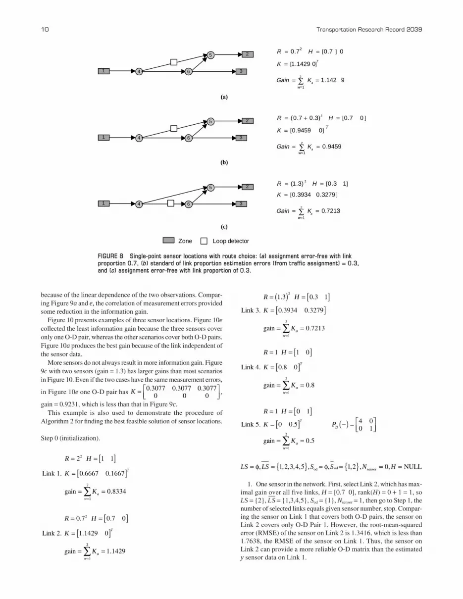
Figure 8 presents examples of single sensor locations with routechoice. Figure 8a presents an error-free link proportion estimate andthe measurement error proportional to the link flow scenario. The gainin that scenario is 1.1429, which is greater than all the scenarios in Fig-ure 6. This indicates that the measurement error could result inreduction of the link information gain. Figure 8b considers the linkproportion estimation error, which reduces the information gains.Although the sensor in Figure 8c covers both O-D pairs, it still cannotproduce the largest information gain because of the largest measure-ment error in the three scenarios. Even when the measurement error isreduced to 1, the gain matrix is K = [0.5085 0.4237]T and gain = 0.9322.

Figure 9 presents examples of two sensor locations. Figure 9acovers O-D Pair 1, Figure 9b covers O-D Pair 2, Figures 9c and dcover both O-D pairs, and Figure 9e covers O-D Pair 1 but the twosensors have a measurement error correlation between them. Asexpected, Figure 9c collected larger gains than the other scenariosbecause it covers both O-D pairs. Although Figure 9d covers bothO-D pairs as well, the information gain is smaller than in Figure 9c

1]

1

a=1

Ka = 0.5 Gain =

0 0.5 T K =

H = [0 R = I

1 3

2

4

5

6

0]

1

a=1

Ka = 0.8 Gain =

0 0.8 T K =

H = [1 R = I

1 3

2

4

5

6

1 3

2

4

5

6 20+20

14

6+20 20

20

1 0

0 4

K = 0

PD =

(d)

(b)

1

a=1

Ka = 0.8334 Gain =

1] H = [1 R = 22

K = 0.1667 0.6667 T

1 3

2

4

5

6

Zone Loop detector

(c)

(a)

FIGURE 7 Single-point sensor locations: (a) base case, (b) one sensor for O-D pair (1–2), (c) one sensor for O-D pair (1–3), and (d ) one sensor for both O-D pairs.

because of the linear dependence of the two observations. Compar-ing Figure 9a and e, the correlation of measurement errors providedsome reduction in the information gain.

Figure 10 presents examples of three sensor locations. Figure 10ecollected the least information gain because the three sensors coveronly one O-D pair, whereas the other scenarios cover both O-D pairs.Figure 10a produces the best gain because of the link independent ofthe sensor data.

More sensors do not always result in more information gain. Figure9c with two sensors (gain = 1.3) has larger gains than most scenariosin Figure 10. Even if the two cases have the same measurement errors,

in Figure 10e one O-D pair has ,

gain = 0.9231, which is less than that in Figure 9c.This example is also used to demonstrate the procedure of

Algorithm 2 for finding the best feasible solution of sensor locations.

Step 0 (initialization).

R H

K

K

T

aw

= = [ ]= [ ]

==

0 7 0 7 0

1 1429 0

2

1

. .

.Link 2.

gain22

1 1429∑ = .

R H

K

K

T

aw

= = [ ]= [ ]

==

2 1 1

0 6667 0 1667

2

Link 1.

gain

. .

11

2

0 8334∑ = .

K = ⎡⎣⎢

⎤⎦⎥

0 3077 0 30770 0

0 30770

. . .


1. One sensor in the network. First, select Link 2, which has max-imal gain over all five links, H = [0.7 0], rank(H) = 0 + 1 = 1, soLS = {2}, LS� = {1,3,4,5}, Sod = {1}, Nsensor = 1, then go to Step 1, thenumber of selected links equals given sensor number, stop. Compar-ing the sensor on Link 1 that covers both O-D pairs, the sensor onLink 2 covers only O-D Pair 1. However, the root-mean-squarederror (RMSE) of the sensor on Link 2 is 1.3416, which is less than1.7638, the RMSE of the sensor on Link 1. Thus, the sensor onLink 2 can provide a more reliable O-D matrix than the estimatedy sensor data on Link 1.

LS LS S S N= = { } = = { }φ φ, , , , , , , , ,1 2 3 4 5 1 2od od sensor == =0,H NULL

R H

K PT

D

= = [ ]= [ ] −( ) = ⎡

⎣⎢⎤⎦⎥

1 0 1

0 0 5 4 00 1

Link 5.

g

. ˆ

aain = ==

∑Kaw 1

2

0 5.

R H

K

K

T

aw

= = [ ]= [ ]

= ==

∑

1 1 0

0 8 0

0 81

2

Link 4.

gain

.

.

R H

K

= ( ) = [ ]= [ ]

1 3 0 3 1

0 3934 0 3279

2. .

. .Link 3.

gain == ==

∑Kaw 1

2

0 7213.

1 3

2

4

5

6

[ ]

[ ]

0.7213

3279.03934.0

13.0)3.1(

2

2

==

=

==

∑ aKGain

K

HR

1 3

2

4

5

6

[ ]

[ ]

142 9.1

01429.1

07.07.0

2

2

==

=

==

∑ a

T

KGain

K

HR

1 3

2

4

5

6

[ ]

[ ]

9459.0

09459.0

07.0)3.07.0(

2

2

==

=

=+=

∑ a

T

KGain

K

HR

Zone Loop detector

(a)

(b)

(c)

w=1

w=1

w=1

FIGURE 8 Single-point sensor locations with route choice: (a) assignment error-free with linkproportion 0.7, (b) standard of link proportion estimation errors (from traffic assignment) = 0.3,and (c) assignment error-free with link proportion of 0.3.


3333.03333.0

00

10

10

00

4444.04444.0

01

01

5.00

08.0

10

01

0.09090.0909

3636.03636.0

11

11

2

a=1

Ka = 0.8888Gain =

2

a=1

Ka = 0.6666Gain =

2

a=1

Ka = 0.909Gain =

2

a=1

Ka = 0.8648Gain =

2

a=1

Ka = 1.3Gain =

H =R = I

K =

H =R = I

K =

H =R = I

K =

H =R = I

K =

H =R =

K =

1 3

2

4

5

6

1 3

2

4

5

6

(e)

(a)

1 3

2

4

5

6

Zone Loop detector

(b)

00

4324.04324.0

01

01

125.0

25.01

(d)

1 3

2

4

5

6

(c)

1 3

2

4

5

6

FIGURE 9 Two-point sensor locations: (a) two uncorrelated sensors for O-D pair (1–2), (b) two uncorrelatedsensors for O-D pair (1–3), (c) two uncorrelated sensors for both O-D pairs, (d ) two uncorrelated sensors forboth O-D pairs, and (e) two partially correlated sensors for O-D pair (1–2).


0.3248

0.1368-

0.1368-0.1880

0.47860.3419

10

01

11

0.1623-

0.4057

0.1136-0.3026

0.28400.2434

01

07.0

11

0.1345-0.1345-0.3193

0.33610.33610.2017

01

01

11

0.26510.26510.0723

0.1928-0.1928-0.6747

10

10

11

3

a=1

Ka = 1.3333Gain =

3

a=1

Ka = 1.2357Gain =

3

a=1

Ka = 1.1932Gain =

3

a=1

Ka = 1.2772Gain =

3

a=1

Ka = 0.8889Gain =

H =R = 1.5I

K =

H =R = 1.5I

K =

H =R = 1.5I

K =

H =R = 1.5I

K =

H =R = 1.5I

K =1 3

2

4

5

6

1 3

2

4

5

6

(e)

(a)

1 3

2

4

5

6

Zone Loop detector

(b)

(d)

1 3

2

4

5

6

(c)

1 3

2

4

5

6

000

0.29630.29630.2963

01

01

01

FIGURE 10 Three-point sensor locations: (a) three uncorrelated sensors for both O-D pairs, (b) threeuncorrelated sensors for both O-D pairs, (c) three uncorrelated sensors for both O-D pairs, (d ) threeuncorrelated sensors for both O-D pairs, and (e) three uncorrelated sensors for O-D pair (1–2).

2. Two sensors in the network. After finding the first sensoron Link 2, go to Step 3. n1(1) = n1(3) = n1(5) = 1, n2(1) = n2(3) = 1,n2(5) = 0. Link 5 is selected, LS = {2,5}, LS� = {1,3,4}, Sod = {1,2},Nsensor = 2. Go to Step 1, stop. The total gain of sensors on Links 2and 5 is 1.6429, whereas the total gain of sensors on Links 2 and 1is 1.2956, and the total gain of sensors on Links 2 and 3 is 1.562.

The Irvine network (Figure 1) was used to demonstrate the pro-posed model. The simulation experiments were implemented on anIntel Xeon central processing unit 3.20-GHz 64-bit machine with8G memory.

The historical 2-h time-dependent O-D volumes were integratedinto one demand table as an a priori mean estimate because of the lim-ited sensor number constraint. It is assumed that the standard devia-tion of the a priori demand variance is 30% of the correspondingdemand volume in the historical demand table. The standard devia-tion of the measurement error is assumed constant. Dynasmart-P (22)was again used to assign the O-D volumes onto the network and rep-resent traffic flow evolution. Figure 11 shows the network covered by10 sensors. The two O-D pairs carrying the largest O-D volume are(53, 46) and (47, 52), accounting for about 36% of the total historicO-D demand. Sensor 1 and Sensor 2 covered these two O-D pairs. Infact, as illustrated in the previous small network, the independent sen-sors usually gave high link information gains. It is not sufficient tominimize the variance of the estimated O-D demand for one particu-lar O-D pair while leaving other O-D pairs uncovered. The proposedmethod tries to find the sensor locations that garner the largest possi-ble link information gains in conjunction with maximizing networkcoverage. The 10 sensors shown in Figure 11a covered about 51% ofthe total O-D trips and the 20 sensors shown in Figure 11b coveredabout 64% of the total O-D trips.

As discussed in the first section, only if the link mapping matrix Hhas full rank is the O-D demand estimator D̂(−) the best linear unbi-ased estimator. The gain matrix was derived based on the best linearunbiased estimator, which explained why the independent sensordata always produced the largest gains. The following observationsare made from those example results to maximize information gains:


1. The sensors need to be located on the links that can interceptthe most O-D flows.

2. The sensor observation data should be linearly independent.3. More sensors do not necessarily mean larger information

gains.4. The lower the measurement error, the greater the gain the

system may attain.

ANALYSIS MEASURES

To assess the impact of different sensor location strategies in con-junction with the O-D demand estimator error reduction, the RMSEof the O-D demand will be calculated to check the quality of the esti-mated O-D matrix. The RMSE is simply the square root of the meansquared error (MSE).

Proposition

The proposed models always produce the minimal MSE across allother O-D estimators.

Proof

In statistics, the MSE is defined (27 ) as follows:

As mentioned previously, the GLS O-D demand estimator isunbiased; thus, its MSE matrix is its covariance matrix. RecallEquation 17—the MSE of the O-D estimator is PD̂

−1(+) = PD̂−1(−) + HT

R−1 H. Because PD̂(−) is the a priori variance covariance matrix ofthe demand matrix and the objectives of both of the SLP-2 and SLP-3

MSE θ θ θ θ θ θ θˆ var ˆ ˆ ˆ ( )( ) = ( ) + −( ) −( )⎡⎣⎢

⎤⎦⎥E

T

20

Sensor 1 Sensor 2

(a) (b)

FIGURE 11 Sensor locations by link gain selection in Irvine network: (a) 10 sensors and (b) 20 sensors.

models are indirectly minimizing PD̂(+), the MSE based on the pro-posed models is thus the minimal statistics inference across all otherestimators. This completes the proof.

Under the time-dependent condition, the time dimension needsalso to be considered; the calculation is as follows:

where

dτw = ground truth O-D trips of O-D pair w at departure time τ,

d̂ τw = estimated O-D trip of O-D pair w at departure time τ,

W = set of O-D pairs,� L � = total number of O-D pairs in the set, and

T = number of departure time intervals.

In a given sensor location strategy, the RMSE is calculated acrossall the O-D pairs and across all the time intervals. Table 1 shows theRMSE of the previously mentioned numerical examples.

CONCLUDING REMARKS

This paper presents models that use the Kalman filtering method toexplore time-dependent maximal information gains across all thelinks in the network. The research proposes two types of sensorlocation models to solve an O-D coverage problem and a maximalinformation gain driven problem. The focus is on solving the sensorlocation problem as an O-D coverage problem under a DTA. A sen-sitivity analysis is conducted to explore the relationship between thenumber of sensors and the level of O-D coverage in a network. Thegoal is to produce a quality estimated O-D matrix that integrateslink observation data that minimize the variance of the O-D flowestimator. This research constructed an unbiased generalized least-squares estimator, using a linear relationship and link flow propor-tions obtained from a dynamic simulation-assignment procedure(Dynasmart-P). The models were developed to identify link sensorlocations that produce maximal information gains and maximal O-Dpair reliability. In addition, a sequential algorithm was developed to

RMSE =−( )

×

∑∑ d d

W T

w ww

τ τ

τ

ˆ 2


solve the proposed models. Several small numerical examples wereused to demonstrate the proposed methodology. Finally, the detec-tor configuration was evaluated on the basis of RMSE to prove theefficiency of the proposed methodology.

Recognizing the importance of sensor location and its relation-ship to the quality of an estimated O-D matrix, this paper establisheda connection between the two critical issues of traffic sensor loca-tion and estimation error based on Kalman filtering. Ongoingresearch is exploring efficient algorithms that can be used to solve thesensor location problem for O-D estimation in a real-time setting,using real-time observation data. In addition, an efficient frame-work is being designed to embed the proposed methodology into asimulation-based real-time network traffic estimation and predictionsystem (Dynasmart-X) that relies on DTA methodology to take fulladvantage of the dynamic sensor locations to estimate and predictO-D matrices in large-scale networks.

REFERENCES

1. Mahmassani, H. S., and X. Zhou. Transportation System Intelligence:Performance Measurement and Real-Time Traffic Estimation and Pre-diction in a Day-to-Day Learning Framework. In Advances in Control,Communication Networks, and Transportation Systems, in Honor ofPravin Varaiya (E. Abed, ed.), Birkhäuser, Basel, Switzerland, 2005,chapt. 16.

2. Van Zuylen, H. J., and L. G. Willumsen. The Most Likely Trip MatrixEstimated from Traffic Counts. Transportation Research Part B, Vol. 14,1980, pp. 281–293.

3. Fisk, C. S. On Combining Maximum Entropy Trip Matrix Estimationwith User Optimal Assignment. Transportation Research B, Vol. 22,1988, pp. 69–79.

4. Spiess, H. A Maximum-Likelihood Model for Estimating Origin-Destination Matrices. Transportation Research B, Vol. 21, 1987,pp. 395–412.

5. Cascetta, E. Estimation of Trip Matrices from Traffic Counts and Sur-vey Data: A Generalized Least Squares Estimator. TransportationResearch B, Vol. 18, 1984, pp. 289–299.

6. Bell, M. G. H. The Estimation of Origin-Destination Matrices by Con-strained Generalized Least Squares. Transportation Research B, Vol. 25,1991, pp. 13–22.

7. Maher, M. J. Inferences on Trip Matrices from Observations on LinkVolumes: A Bayesian Statistical Approach. Transportation Research B,Vol. 17, 1983, pp. 435–447.

8. Van der Zijpp, N. J., and R. Hamerslag. Improved Kalman FilterApproach for Estimating Origin–Destination Matrices for Freeway Cor-ridors. In Transportation Research Record 1443, TRB, NationalResearch Council, Washington, D.C., 1994, pp. 54–64.

9. Dixon, M. P., and L. R. Rilett. Real-Time OD Estimation Using Auto-matic Vehicle Identification and Traffic Count Data. Computer-AidedCivil and Infrastructure Engineering, Vol. 17, 2002, pp. 7–21.

10. Zhou, X. S., and H. S. Mahmassani. Dynamic Origin-DestinationDemand Estimation Using Automatic Vehicle Identification Data. IEEETransactions on Intelligent Transportation Systems, Vol. 7, No. 1, 2006,pp. 105–114.

11. Lam, W. H. K., and H. P. Lo. Accuracy of O-D Estimates from TrafficCounting Stations. Traffic Engineering and Control, Vol. 31, 1990,pp. 358–367.

12. Yang, H., Y. Iida, and T. Sasaki. An Analysis of the Reliability of anOrigin-Destination Trip Matrix Estimated from Traffic Counts. Trans-portation Research B, Vol. 25, 1991, pp. 351–363.

13. Yang, H., and J. Zhou. Optimal Traffic Counting Locations for Origin-Destination Matrix Estimation. Transportation Research B, Vol. 32,No. 2, 1998, pp. 109–126.

14. Yim, K. N., and H. K. Lam. Evaluation of Count Location SelectionMethods for Estimation of OD Matrices. Journal of TransportationEngineering, Vol. 124, No. 4, 1998, pp. 376–383.

TABLE 1 RMSE for Numerical Examples

Scenario (a) (b) (c)

One sensor coverage without route choice

RMSE 1.3416 2.1213 1.7638

One sensor coverage with route choice

RMSE 1.1986 1.3416 1.5681

Scenario (a) (b) (c) (d) (e)

Two sensor coverage

RMSE 1.2019 2.0817 1.1402 1.3817 1.2412

Three sensor coverage

RMSE 1.0978 1.1428 1.0885 1.3034 1.2019

15. Bianco, L., G. Confessore, and P. Reverberi. A Network Based Modelfor Traffic Sensor Location with Implications on O-D Matrix Estimates.Transportation Science, Vol. 35, 2001, pp. 50–60.

16. Chootinan, P., A. Chen, and H. Yang. A Bi-objective Counting Loca-tion Problem for Origin-Destination Trip Estimation. Transportmatrica,Vol. 1, No. 1, 2005, pp. 65–80.

17. Ehlert, A., M. G. H. Bell, and S. Grosso. The Optimization of TrafficCount Locations in Road Networks. Transportation Research B, Vol. 40,2006, pp. 460–479.

18. Yang, H., C. Yang, and L. P. Gan. Models and Algorithms for theScreen Line-Based Traffic Counting Location Problems. Computer &Operations Research, Vol. 33, 2006, pp. 836–858.

19. Pravinvongvuth, S., A. Chen, P. Chootinan, and S. Narupiti. A Method-ology for Selecting Pareto Optimal Solutions Developed by a Multi-objective AVI Reader Location Model. Journal of the Eastern AsiaSociety for Transportation Studies, Vol. 6, 2005, pp. 2441–2456.

20. Eisenman, S. M., X. Fei, X. Zhou, and H. S. Mahmassani. Numberand Location of Sensors for Real-Time Network Traffic Estimationand Prediction: Sensitivity Analysis. In Transportation Research Record:Journal of the Transportation Research Board, No. 1964, Transportation


Research Board of the National Academies, Washington, D.C., 2006,pp. 253–259.

21. Zhou, X., and G. F. List. An Information-Theoretic Sensor LocationModel for Traffic Origin Destination Demand Estimation Applications.Transportation Science, submitted.

22. Aitken, A. C. On Least Squares and Linear Combinations of Observa-tions. Proc., Royal Statistical Society, Vol. 55, 1935, pp. 42–48.

23. Gelb, A. Applied Optimal Estimation. MTI Press, Cambridge, Mass., 1974.24. Sheffi, Y. Urban Transportation Networks: Equilibrium Analysis with

Mathematical Programming Methods. Prentice Hall, Englewood Cliffs,N.J., 1985.

25. Maryland Transportation Initiative. DYNASMART-P, Version 1.2,User’s Guide. Prepared for U.S. Department of Transportation, 2006.

26. Chui, C. K., and G. Chen. Kalman Filtering with Real-Time Applications.IEEE Transactions on Aerospace and Electronic Systems, Vol. 27, No. 1,1991, pp. 149–154.

27. Greene, W. H. Econometric Analysis, 5th ed. Prentice Hall, UpperSaddle River, N.J., 2000.

The Transportation Network Modeling Committee sponsored publication of thispaper.

sensor coverage and location for real-time traffic prediction in large-scale networks

Documents