This article appeared in a journal published by Elsevier. The attachedcopy is furnished to the author for internal non-commercial researchand education use, including for instruction at the authors institution

and sharing with colleagues.

Other uses, including reproduction and distribution, or selling orlicensing copies, or posting to personal, institutional or third party

websites are prohibited.

In most cases authors are permitted to post their version of thearticle (e.g. in Word or Tex form) to their personal website orinstitutional repository. Authors requiring further information

regarding Elsevier’s archiving and manuscript policies areencouraged to visit:

http://www.elsevier.com/copyright

Author's personal copy

Efficient solution techniques for the integrated coverage, sink location androuting problem in wireless sensor networks

Evren Guney a, Necati Aras b, _I. Kuban Altınel b,n, Cem Ersoy c

a Industrial Engineering Department, Istanbul Arel University, Istanbul, Turkeyb Industrial Engineering Department, Bogazic- i University, _Istanbul, Turkeyc Computer Engineering Department, Bogazic- i University, _Istanbul, Turkey

a r t i c l e i n f o

Available online 16 September 2011

Keywords:

Wireless sensor networks

Integer programming

Tabu search

a b s t r a c t

Sensors are tiny electronic devices having limited battery energy and capability for sensing, data

processing and communicating. They can collectively behave to provide an effective wireless network

that monitors a region and transmits the collected information to gateway nodes called sinks. Most of the

applications require the operation of the network for long periods of times, which makes the efficient

management of the available energy resources an important concern. There are three major issues in the

design of sensor networks: sensor deployment or the coverage of the sensing area, sink location, and data

routing. In this work, we consider these three design problems within a unified framework and develop

two mixed-integer linear programming formulations. They are difficult to solve exactly. However, it is

possible to compute good feasible solutions of the sink location and routing problems easily, when the

sensors are deployed and their locations in the sensor field become known. Therefore, we propose a tabu

search heuristic that tries to identify the best sensor locations satisfying the coverage requirements. The

objective value corresponding to each set of sensor locations is calculated by solving the sink location and

routing problem. Computational tests carried out on randomly generated test instances indicate that the

proposed hybrid approach is both accurate and efficient.

& 2011 Elsevier Ltd. All rights reserved.

1. Introduction

Advances in micro-electromechanical systems, digital electronicsand wireless communications have enabled the development of low-cost, low-power multi-functional tiny devices called sensors. Theyuse battery power as the energy source and can communicatethrough wireless channels over relatively small distances. Eachsensor is usually equipped with one or more sensing units, one ormore transceivers, actuators, processors and storage units. As a resultof significant resource limitations such as limited memory, batterypower, signal processing, computation and communication capabil-ity, an individual sensor can only sense a small portion of itsenvironment. However, when a large number of these devices workin a collaborative fashion to carry out a certain task, they form awireless sensor network (WSN). WSNs give rise to a wide range ofreal-life applications in areas such as military, homeland security,health care, environment, agriculture, logistics, smart home or officedesign and other areas [26,5].

WSNs can be homogeneous consisting of identical sensors, orheterogeneous consisting of sensors with possibly different

technical characteristics and costs. Sensors that collectively forma WSN are deployed over an area of interest called the sensorfield. The energy source provided for a sensor is usually thebattery power which has not yet reached the stage to operate fora very long time without being recharged. Moreover, in a largenumber of applications sensors are intended to work in remote orhostile environments, and it is undesirable or impossible torecharge or replace their batteries. The lifetime of a WSN ismeasured by the time until it is disconnected; namely there existholes that do not collect or transmit any information. In otherwords, the WSN cannot provide an acceptable level of operatingquality beyond its lifetime. Therefore, conserving energy andprolonging the network lifetime is an important issue in thedesign of WSNs [27].

The transmission range of sensors is restricted as a conse-quence of their energy and size limitations, hence they cannotcommunicate through large distances. Therefore, each sensorneeds to transmit its data to a central unit called ‘‘base station’’or ‘‘sink’’, which is a larger device with a comparatively largeenergy supply and long-range transmission capabilities such asinternet or satellite communication.

There are various design issues in the construction of a WSN.One of the most important problems addressed in the literatureis the sensor coverage problem (CP). This problem is centered

Contents lists available at SciVerse ScienceDirect

journal homepage: www.elsevier.com/locate/caor

Computers & Operations Research

0305-0548/$ - see front matter & 2011 Elsevier Ltd. All rights reserved.

doi:10.1016/j.cor.2011.09.002

n Corresponding author. Tel.: þ90 212 3597076; fax: þ90 212 2651800.

E-mail address: altinel@boun.edu.tr (_I.K. Altınel).

Computers & Operations Research 39 (2012) 1530–1539

Author's personal copy

around a fundamental question: ‘‘How well do the sensorsobserve the physical space?’’ As pointed out by Meguerdichianet al. [23], coverage can be regarded as a measure of the quality ofservice of the sensing function in WSNs. Therefore, the CP isstudied thoroughly and there are many exact or approximatemethods to solve it (e.g., [6,14]). Also an interesting line ofresearch has emerged, where the CP is modeled as a mixed-integer linear programming (MILP) formulation [7,2].

In a typical WSN, each sensor collects and processes data, andtries to send this information to a sink. Since sensors’ commu-nication ranges are limited, the data packets carrying the sensedinformation usually have to follow multi-hop paths. The routingproblem (RP), which involves finding the most energy efficientsensor-to-sink routes for a given set of sensor and sink locations,is an essential problem in WSNs because data transmission is anenergy consuming task [1].

Determining the optimal sink locations is also an importantdesign issue to extend the lifetime of a WSN. The average numberof hops to reach a sink becomes a critical factor that is affected bythe sink locations. In a significant number of research studies, thesink locations are assumed to be determined a priori [18,20].However, the energy consumption and thus the lifetime of theWSN can be improved by finding the best location(s) of thesink(s) since these locations have an impact upon the sensor-to-sink data transmission routes [3]. The joint optimization of sinklocations and data routing is addressed in the sink location androuting problem (SLRP) that has received considerable attentionin the literature as it results in a more efficient network design[13,25,17].

In this work, we jointly consider the coverage, sink location,and data routing problems in heterogeneous WSNs. We refer tothis integrated problem as the coverage, sink location and routingproblem (CSLRP), and develop two mathematical programmingformulations by unifying these three design issues within a singlemodel. Unfortunately, the resulting MILP formulations can onlybe solved for small-sized instances using commercial solvers. Formedium and large-sized instances, we propose a hybrid solutionprocedure. In the outer loop, tabu search is employed to find near-optimal sensor locations satisfying the coverage requirements. Inthe inner loop, the remaining sink location and routing problemsare solved using various methods for the sensor locations fixed inthe outer loop. This integrated problem is also addressed in a veryrecent work [16]. However, the proposed benchmark model has amajor flaw, which makes the results given in that work unreli-able. The flaw stems from the fact that the data flow balanceequations in the MILP formulation are erroneous.

The rest of the paper is organized as follows. In the nextsection, we introduce the CSLRP and its mathematical program-ming formulations. The hybrid solution approach is explained inSection 3, while experimental results are reported in Section 4.We conclude the paper in Section 5 with some remarks.

2. Problem definition and mathematical programmingformulations

The objective of the CSLRP is to design a WSN such that thetotal available battery energy of the sensors in the WSN is spentin the most efficient way for transmitting (routing) data packetsfrom sensors to sinks. This also helps to prolong the lifetime of theWSN as much as possible. Before we present the mathematicalprogramming formulations for the CSLRP, we describe the pro-blem while defining the decision variables common for bothformulations.

The CSLRP is defined in a two-dimensional sensor field N with9N 9¼N points. We assume that every point of sensor field is a

candidate location for a sensor and/or sink, and there are 9K9¼ K

sensor types, where K denotes the set of sensor types. Each sensortype has a different cost, sensing and transmission range. The costof deploying a type-k sensor is equal to hk, and the availablebudget for sensor deployment is H monetary units. Given thatthere may be obstacles in the terrain where the sensors aredeployed, it is expected that there is inherent uncertainty asso-ciated with sensor readings and thus sensor detections must beformulated probabilistically as discussed in Brooks and Iyengar [4].Furthermore, it is also expected that sensors closer to a point inthe sensor field generally provide better coverage. To account forboth issues, we adopt probabilistic detection and let parameter qijk

denote the probability that a type-k sensor deployed at point i

generates sensing data for point j. These probabilities can becalculated for each ði,j,kÞ triplet by adopting an appropriate sensorterrain model. A common approach is to assume that a target atEuclidean distance dij from a type-k sensor is detected withprobability qijk ¼ e�akdij [9,10], where ak is a decay parameter thatdetermines the rate at which the detection probability of a type-k

sensor decreases with the distance. When binary decision vari-ables are defined as sik ¼ 1 if a type-k sensor is deployed at pointiAN , and sik ¼ 0 otherwise, ð1�qijksikÞ gives the probability that atarget located at point j is missed by a type-k sensor deployedat point i. Hence, under the assumption that sensing probabilitiesqijk are independent, the restriction which ensures that theoverall miss probability at point j does not exceed a givenmaximum allowable level 0otjo1 can be written asQ

iANQ

kAKð1�qijksikÞrtj. Although this inequality is non-linearin binary decision variables sik, it can be linearized as follows.When we take the natural logarithm of both sides of the inequal-ity, we obtain

PiAN

PkAK lnð1�qijksikÞr ln tj, which can be

rewritten asP

iANP

kAK lnð1�qijkÞsikr ln tj. This follows fromthe fact that lnð1�qijksikÞ ¼ 0 when sik ¼ 0 and lnð1�qijksikÞ ¼

lnð1�qijkÞ when sik ¼ 1. By multiplying both sides of the lastinequality with �1 and defining coefficients aijk ¼�lnð1�qijkÞ

and bj ¼�ln tj, we obtainP

iANP

kAKaijksikZbj, which can beregarded as a coverage constraint with bj representing a mini-mum coverage threshold. We would like to note that aijk and bj

are always positive.There are two other modeling alternatives for the sensor

coverage models in the literature. In perfect detection (see, forexample, [2,8,22]), where a sensor always detects a targetremaining in its range, aijk ¼ 1 if a type-k sensor deployed atpoint i covers (senses) point j, and aijk ¼ 0 otherwise. The coveragethreshold parameter bj represents the number of sensors thatneed to cover point j. In imperfect detection (see, for example,[22]), aijk is called the coverage intensity for point j provided by atype-k sensor at point i and bj coverage intensity threshold atpoint j. The coverage constraint in imperfect sensing ensures thatthe total coverage intensity at all points of the sensor field has toexceed the threshold level bj.

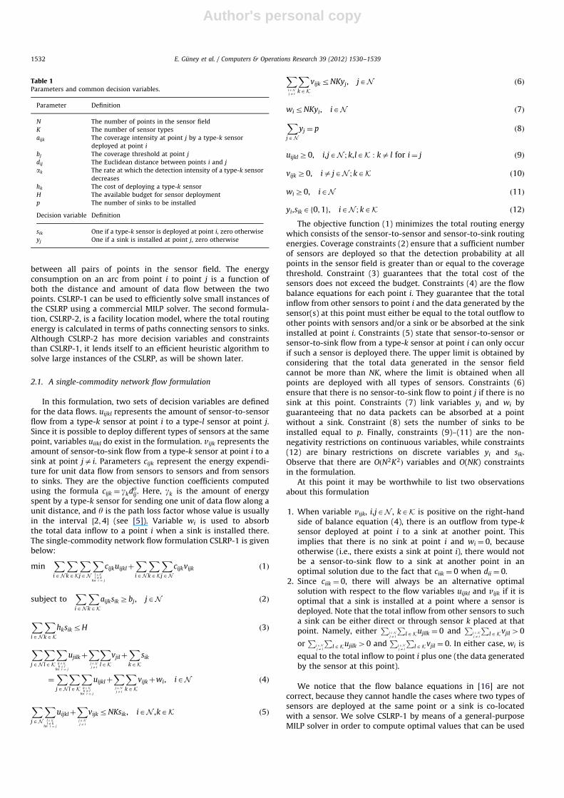
Given that the number of sinks to be installed is equal to p, wepropose two different MILP formulations for the CSLRP. Two ofthe decision variables are shared by both of the formulations. Thefirst one is the binary variable sik which has been introducedbefore. The second one is the binary variable yj which is equalto one if a sink is installed at point j, and zero otherwise. Itis assumed that a point in the sensor field can accommodatea sensor and a sink together. Furthermore, different types ofsensors can be placed at the same point. The parameters andcommon decision variables used in the models are shown inTable 1 for a quick reference. Besides these two sets of decisionvariables, there are others that have to be defined depending onthe formulation. The first formulation, CSLRP-1 is an arc-flowbased network design model, where the total routing energy iscomputed by summing up the energy consumptions on the arcs

E. Guney et al. / Computers & Operations Research 39 (2012) 1530–1539 1531

Author's personal copy

between all pairs of points in the sensor field. The energyconsumption on an arc from point i to point j is a function ofboth the distance and amount of data flow between the twopoints. CSLRP-1 can be used to efficiently solve small instances ofthe CSLRP using a commercial MILP solver. The second formula-tion, CSLRP-2, is a facility location model, where the total routingenergy is calculated in terms of paths connecting sensors to sinks.Although CSLRP-2 has more decision variables and constraintsthan CSLRP-1, it lends itself to an efficient heuristic algorithm tosolve large instances of the CSLRP, as will be shown later.

2.1. A single-commodity network flow formulation

In this formulation, two sets of decision variables are definedfor the data flows. uijkl represents the amount of sensor-to-sensorflow from a type-k sensor at point i to a type-l sensor at point j.Since it is possible to deploy different types of sensors at the samepoint, variables uiikl do exist in the formulation. vijk represents theamount of sensor-to-sink flow from a type-k sensor at point i to asink at point ja i. Parameters cijk represent the energy expendi-ture for unit data flow from sensors to sensors and from sensorsto sinks. They are the objective function coefficients computedusing the formula cijk ¼ gkdy

ij. Here, gk is the amount of energyspent by a type-k sensor for sending one unit of data flow along aunit distance, and y is the path loss factor whose value is usuallyin the interval ½2;4� (see [5]). Variable wi is used to absorbthe total data inflow to a point i when a sink is installed there.The single-commodity network flow formulation CSLRP-1 is givenbelow:

minXiAN

XkAK

XjAN

Xl AKl a k

for i ¼ j

cijkuijklþXiAN

XkAK

XjAN

cijkvijk ð1Þ

subject toXiAN

XkAK

aijksikZbj, jAN ð2Þ

XiAN

XkAK

hksikrH ð3Þ

XjAN

XlAK

Xk AKk a l

for i ¼ j

ujilkþX

j ANj a i

XlAK

vjilþXkAK

sik

¼XjAN

XlAK

Xk AKk a l

for i ¼ j

uijklþX

j ANj a i

XkAK

vijkþwi, iAN ð4Þ

XjAN

Xl AKl a k

for i ¼ j

uijklþX

j ANj a i

vijkrNKsik, iAN ,kAK ð5Þ

Xi ANj a i

XkAK

vijkrNKyj, jAN ð6Þ

wirNKyi, iAN ð7Þ

XjAN

yj ¼ p ð8Þ

uijklZ0, i,jAN ; k,lAK : ka l for i¼ j ð9Þ

vijkZ0, ia jAN ; kAK ð10Þ

wiZ0, iAN ð11Þ

yi,sikAf0;1g, iAN ; kAK ð12Þ

The objective function (1) minimizes the total routing energywhich consists of the sensor-to-sensor and sensor-to-sink routingenergies. Coverage constraints (2) ensure that a sufficient numberof sensors are deployed so that the detection probability at allpoints in the sensor field is greater than or equal to the coveragethreshold. Constraint (3) guarantees that the total cost of thesensors does not exceed the budget. Constraints (4) are the flowbalance equations for each point i. They guarantee that the totalinflow from other sensors to point i and the data generated by thesensor(s) at this point must either be equal to the total outflow toother points with sensors and/or a sink or be absorbed at the sinkinstalled at point i. Constraints (5) state that sensor-to-sensor orsensor-to-sink flow from a type-k sensor at point i can only occurif such a sensor is deployed there. The upper limit is obtained byconsidering that the total data generated in the sensor fieldcannot be more than NK, where the limit is obtained when allpoints are deployed with all types of sensors. Constraints (6)ensure that there is no sensor-to-sink flow to point j if there is nosink at this point. Constraints (7) link variables yi and wi byguaranteeing that no data packets can be absorbed at a pointwithout a sink. Constraint (8) sets the number of sinks to beinstalled equal to p. Finally, constraints (9)–(11) are the non-negativity restrictions on continuous variables, while constraints(12) are binary restrictions on discrete variables yi and sik.Observe that there are OðN2K2Þ variables and O(NK) constraintsin the formulation.

At this point it may be worthwhile to list two observationsabout this formulation

1. When variable vijk, i,jAN , kAK is positive on the right-handside of balance equation (4), there is an outflow from type-k

sensor deployed at point i to a sink at another point. Thisimplies that there is no sink at point i and wi ¼ 0, becauseotherwise (i.e., there exists a sink at point i), there would notbe a sensor-to-sink flow to a sink at another point in anoptimal solution due to the fact that ciik ¼ 0 when dii ¼ 0.

2. Since ciik ¼ 0, there will always be an alternative optimalsolution with respect to the flow variables uijkl and vijk if it isoptimal that a sink is installed at a point where a sensor isdeployed. Note that the total inflow from other sensors to sucha sink can be either direct or through sensor k placed at thatpoint. Namely, either

Pj ANj a i

PlAKujilk ¼ 0 and

Pj ANj a i

PlAKvjil40

orP

j ANj a i

PlAKujilk40 and

Pj ANj a i

PlAKvjil ¼ 0. In either case, wi is

equal to the total inflow to point i plus one (the data generatedby the sensor at this point).

We notice that the flow balance equations in [16] are notcorrect, because they cannot handle the cases where two types ofsensors are deployed at the same point or a sink is co-locatedwith a sensor. We solve CSLRP-1 by means of a general-purposeMILP solver in order to compute optimal values that can be used

Table 1Parameters and common decision variables.

Parameter Definition

N The number of points in the sensor field

K The number of sensor types

aijk The coverage intensity at point j by a type-k sensor

deployed at point i

bj The coverage threshold at point j

dij The Euclidean distance between points i and j

ak The rate at which the detection intensity of a type-k sensor

decreases

hk The cost of deploying a type-k sensor

H The available budget for sensor deployment

p The number of sinks to be installed

Decision variable Definition

sik One if a type-k sensor is deployed at point i, zero otherwise

yj One if a sink is installed at point j, zero otherwise

E. Guney et al. / Computers & Operations Research 39 (2012) 1530–15391532

Author's personal copy

in assessing the accuracy of the proposed heuristics. The inte-grated problem we deal with in this paper can also be formulatedas a multi-commodity network flow model where each sensor isassumed to generate a commodity, which makes the total numberof commodities N�K. We do not consider this type of formulationhere since it is computationally very demanding.

2.2. An assignment formulation

In this second formulation, we use binary variables xijk wherexijk ¼ 1 if a type-k sensor at point i is assigned to a sink at point j,and xijk ¼ 0 otherwise. To compute the corresponding routingenergy we need to know the arcs that are used in this assignment,i.e., the arcs of the path connecting the sensor at point i to the sinkat point j. For this purpose, we introduce binary variable zijk

lm,which is equal to one when arc (l,m) is used in the assignment of atype-k sensor at point i to a sink at point j. Similar to the firstformulation, clmk represents the flow energy between points l andm when there is a type-k sensor at point l. The resultingmathematical model CSLRP-2 is given below:

minXiAN

XjAN

XlAN

XmAN

XkAK

clmkzijklm ð13Þ

subject toXiAN

XkAK

aijksikZbj, jAN ð14Þ

XkAK

XiAN

hksikrH ð15Þ

XjAN

xijk ¼ sik, iAN ,kAK ð16Þ

xijkryj, i,jAN ,kAK ð17Þ

XjAN

yj ¼ p ð18Þ

XmAN

zijklm�

XmAN

zijkml ¼

xijk, l¼ i

0, lAN \fi,jg,

�xijk, l¼ j

8><>:

i,j,lAN ,ia j,kAK ð19Þ

XmAN

zijklmrel, i,j,lAN ,ia j,kAK ð20Þ

elrXkAK

slk, lAN ð21Þ

KelZ

XkAK

slk, lAN ð22Þ

zijklmZ0, i,j,l,mAN ,kAK ð23Þ

sik,yi,xijk,elAf0;1g, i,j,lAN ,kAK ð24Þ

The objective function (13) minimizes the total routing energyover all arcs. Coverage constraints (14) and the budget constraint(15) are the same as before. Assignment constraints (16) ensurethat each sensor is assigned to one and only one sink. Constraints(17) prohibit any assignment to point j if there is no sink at thatpoint. Here we prefer the strong version of this constraint set,which can be replaced by

PiAN

PkAKxijkrNKyj to obtain an

equivalent formulation. This version has fewer constraints, but ityields a weaker LP relaxation. Constraint (18) sets the number ofsinks to be installed in the sensor field to p. Constraints (19) arethe flow balance constraints. If there is an assignment xijk, thenthere must be a unit outflow from the source (type-k sensor atpoint i), a unit inflow to the destination (sink at point j), and for allother intermediate points the total inflow must be equal to the

total outflow. Constraints (20)–(22) together ensure that an arc(l,m) can only be used if there is a sensor at the tail l of arc (l,m).Note that if there is no sensor at point l (i.e.,

PkAKslk ¼ 0), then

constraint (21) forces el to be zero. On the other hand, if there is atleast one sensor at point l, then constraint (22) makes sure thatel ¼ 1. Recall that the only possibility of having more than onesensor at some point is that the deployed sensors are of differenttypes, and there can be at most K sensors at a point. Constraints(23) and (24) are, respectively, non-negativity and binary restric-tions on the variables. Note that although zijk

lm are non-negativevariables, at the optimum solution they only take binary values.This is due to the fact that constraints (19) are the flowconservation equations for the shortest path problem whenxijk ¼ 1.

In this formulation, the number of variables is OðN4KÞ and thenumber of constraints is OðN3KÞ. This means that it is a largerformulation than CSLRP-1. Computational experiments alsorevealed that it is less efficient than CSLRP-1 when both formula-tions are solved by a commercial state-of-the-art MILP solverwithin a time limit of 4 h. On the other hand, CSLRP-2 has animportant property which makes it very useful for computingapproximate solutions of CSLRP as will be explained in the nextsection: when the sensor locations are given, CSLRP-2 reduces tothe classical p-median problem.

3. A hybrid solution procedure

CSLRP is computationally very difficult and solving any of theproposed formulations by a general-purpose MILP solver usuallygenerates an optimal solution only for small instances. Formedium and large instances there is a need for efficient heuristicmethods. In this paper, we propose a hybrid solution procedurefor the solution of the CSLRP which utilizes the CSLRP-2 formula-tion. The outer loop of this procedure uses tabu search to identifythe best sensor locations satisfying the coverage and budgetrequirements, while in the inner loop sink locations and dataflow routes from sensors to sinks are determined in the best wayfor the sensor locations fixed by the outer loop.

Given a set of sensors that satisfies the coverage and budgetconstraints (i.e., sik are fixed), both CSLRP-1 and CSLRP-2 can bere-written in a simpler form by dropping the sik variables andsome of the constraints. For CSLRP-2 in particular, constraints(14), (15), (19), (20), (21), and (22) can be removed. The resultingformulation SLRP, which is given below, deals with the problem oflocating a prespecified number of sinks and assigning the givenset of sensors to these sinks. In this formulation, S denotes the setof points in the sensor field where sensors are deployed, and Ki isthe set of sensor types deployed at point i:

SLRP : minXiAS

XkAKi

XjAN

gijkxijk ð25Þ

subject toXjAN

xijk ¼ 1, iAS,kAKi ð26Þ

xijkryj, iAS,kAKi,jAN ð27Þ

XjAN

yj ¼ p ð28Þ

xijk,yjAf0;1g, iAS,kAKi,jAN ð29Þ

As can be noticed, SLRP is the formulation of the well-knownp-median problem where gijk’s, which are the objective functioncoefficients, constitute the energy consumption corresponding tothe minimum energy path between a type-k sensor at point i anda sink at point j. In other words, they are simply the sum of the

E. Guney et al. / Computers & Operations Research 39 (2012) 1530–1539 1533

Author's personal copy

energy consumptions on the arcs that forms the shortest path interms of energy. Note that when the locations and the types of thedeployed sensors are given, we can perform a preprocessing stepto determine the minimum energy path from each sensor to everycandidate sink location. These paths can be determined by solvinga shortest path problem between the given sensor locations andall the points in the sensor field since all points are candidate sinklocations. This task can effectively be carried out using a many-to-many shortest path algorithm such as the one by Floyd [12].

Tabu search (TS) is a metaheuristic algorithm that guides thelocal search to prevent it from being trapped in premature localoptima or cycling [15]. This is achieved by prohibiting the movesthat cause to return to previously visited solutions throughout acertain number of iterations. We use TS to make a search in thesolution space of sensor locations that are feasible with respect tocoverage and budget constraints. The objective values corre-sponding to these feasible sensor locations are computed bysolving the SLRP using three different methods which providethe routing of the data flows from sensors to sinks in the bestpossible way. Hence, we propose actually three heuristics thatdiffer in the inner loop of the hybrid solution procedure.

We apply an easy and quick strategy to find the initial sensordeployment. It is based on the greedy heuristic introduced byAltınel et al. [2], and deploys sensors at minimum cost withoutviolating the budget constraint by reducing the maximum level ofundercoverage. At each iteration of the heuristics, we generatecandidate neighborhood sets by using the following Add, Drop,and Swap moves: 1-Add, 2-Add, 1-Drop, 2-Drop, 1-Swap, and2-Swap. While one and two sensors are added randomly to theexisting set of sensors in the 1-Add and 2-Add moves, respec-tively, 1-Drop and 2-Drop moves involve the removal of one andtwo sensors, respectively. 1-Swap and 2-Swap moves, on theother hand, perform a random exchange of the locations of oneand two sensors, respectively. Effectively, this corresponds torandomly dropping an existing sensor (two existing sensors), andthen adding a new sensor (two new sensors) leaving the totalnumber of sensors unchanged. If the new sensor set obtained byany move is feasible, the objective value associated with it iscomputed by solving the corresponding SLRP model. In a hetero-geneous WSN, where there exist sensors with different sensingranges and costs, the above-mentioned moves may cause aninfeasibility by violating the coverage and/or budget constraints.When such an infeasibility is encountered, that move is notaccepted. The total number of neighbors generated by all themoves is equal to r. In our experiments we use different r valuesto work with different neighborhood sizes that may affect thequality of the solutions obtained by the proposed heuristic. Whilegenerating these neighbors, those moves that are in the tabu listare not allowed for a certain number of iterations unless thecorresponding objective value is better than the objective value ofthe incumbent.

Since the SLRP belongs to the class of the p-median problem, itcan be solved by one of the available solution methods that areknown to be efficient for this problem type. To this end, we choosethree methods. Two of them are the Lagrangean heuristic (LH) andthe nested-dual heuristic (NDH). The remaining method, greedyheuristic (GH), is a fast heuristic which is also easy to implement. Asa result, we have three TS heuristics, which differ in the inner loop ofthe hybrid solution procedure when solving the SLRP. We refer tothem as TS-LH, TS-NDH, and TS-GH. Below, we briefly overview LH,NDH, and GH that are used to solve the SLRP.

In our application of LH, we relax the assignment constraints(26) in the SLRP defined by expressions (25)–(29) with unrest-ricted Lagrange multipliers. The resulting Lagrangean subproblemdecomposes with respect to each grid point jAN . Each of thesesubproblems can be solved by inspection, and their objective

values can be ranked. The total of the sum of the p smallestobjective values and the sum of the Lagrange multipliers con-stitutes a lower bound for the SLRP. Subgradient optimization isused to solve the Lagrangean dual problem, whose objective is tofind the largest lower bound. At each iteration of the subgradientoptimization procedure, an upper bound is computed on theoptimal objective value of the SLRP. It is used to determine thevalue of the step length which is necessary to update the Lagrangemultipliers. The upper bound is obtained by constructing afeasible solution to the SLRP by making use of the binary locationvariables given by the Lagrangean subproblem that provides thelower bound.

The NDH heuristic was proposed by Mirchandani et al. [24] tosolve the p-median problem. This heuristic uses the approachdeveloped by Erlenkotter [11] for the solution of the uncapacitatedfacility location problem. Erlenkotter’s DUALOC method is a simpleascent adjustment procedure that solves the LP relaxation of theLagrangean dual problem in which the median constraint (28) isdualized. This enables the computation of a lower bound on theoptimal value. Then, a heuristic is used to obtain a feasible solutionto the p-median problem. The details of the application of LH andNDH heuristics to the SLRP can be found in Guney et al. [17].

The greedy heuristic (GH) for the p-median problem, sug-gested by Kuehn and Hamburger [19], is initialized with an emptyset of facility locations with an infinite objective value. Thenfacilities are added to this set one at a time by choosing thefacility whose addition results in the largest reduction in theobjective value.

In TS-LH, TS-NDH, and TS-GH, we use two termination criteria:the maximum number of iterations and the maximum number ofiterations without any improvement in the incumbent’s objectivevalue. In the TS-LH, TS-NDH, and TS-GH heuristics, num_iter andnum_nonimp_iter are counters that are used to keep the totalnumber of iterations and the number of iterations without animprovement in the incumbent (the best objective value obtainedso far). The parameters max_iter and max_nonimp_iter are, respec-tively, the limits for num_iter and num_nonimp_iter. Obj is theobjective value of the current sensor set obtained by solving theSLRP. Obj_Best_Neigh is the best solution among all the neighbor-ing solutions at a given iteration and Objn is the best solutionobtained throughout the algorithm. Finally, max_tabu_tenure is aparameter that sets the number of iterations during which asolution is kept in the tabu list. The basic steps of the TS heuristicsare given in Appendix using the aforementioned definitions.

4. Computational experiments

In this section, we report the accuracy and efficiency of theTS-LH, TS-NDH, and TS-GH heuristics. As the basis of our compar-isons, we take the objective value of the best feasible solutionprovided by CPLEX 11.2 when solving the CSLRP-1 withinthe allowed time limit of 4 h (14,400 s). By letting zIP to denotethe best objective value CPLEX computes for an instance andXAfzLH,zNDH,zGHg representing the best objective value obtainedby the proposed methods for the same instance, we can measurethe accuracy of the methods by computing the percent deviationsfrom zIP according to the formula:

100�X�zIP

zIPð30Þ

We also report the CPU times to assess the efficiency of thedifferent solution methods. All experiments are carried out on aDell PowerEdge 2400 computer with two 64-bit, 2.66-GHz Xeon5355 Quad Core processors and 28 GB memory.

E. Guney et al. / Computers & Operations Research 39 (2012) 1530–15391534

Author's personal copy

4.1. Instance generation

We consider an open area without many obstacles as thesensor field and choose a path loss factor of y¼ 2. The sensor fieldis assumed to consist of N¼ n� n grid points in a lattice structurewhere each point is a candidate site for the deployment of sensorsand locating the sinks. We generate 14 data sets where n takesvalues from the set {3–15,20}. Later on, we also assess theperformance of the solution methods on a set of test instanceswhere the points are distributed uniformly within the sensor fieldrather than being grid points. The coverage threshold bi is set to0.99 for all points, while the value of the available budget H forsensor deployment is determined as follows. First, the minimum-weight coverage problem is solved to optimality where theweights correspond to the unit costs of the sensors. Then, theoptimal objective value gives the minimum budget level Hmin thatis required to obtain a sensor network where all the grid pointsare covered. In other words, to prevent the infeasibility of theCSLRP we have to set the budget H at least equal to Hmin. For theexperiments, where we assess the accuracy and efficiency ofthe solution methods, we set H¼ 1:5Hmin. In a subsequent section,we carry out sensitivity analysis with respect to the parameters bi

and H. We do this by changing the value of H to various multiplesof Hmin and varying the coverage threshold bi.

In our experiments, we consider two types of sensors withdifferent characteristics. First, their costs are different as follows:h1 ¼ 10 and h2 ¼ 20. Consistent with their costs, the followingvalues are assigned to the coverage parameter ak that determinesthe rate at which the detection intensity of a type-k sensordecreases with the distance: a1 ¼ 0:5 and a2 ¼ 0:4. Note that themore expensive sensor has a lower a-value. The parameter gk isthe amount of energy spent by a type-k sensor for sending oneunit of data for unit distance. It is chosen as g1 ¼ 10 nA h andg2 ¼ 20 nA h for the two types of sensors, respectively [21]. Theampere-hour (A h) (its sub-units are milliampere-hour (mA h)and nanoampere-hour (nA h)) is a unit of electric charge, and isfrequently used in measurements of electrochemical systemssuch as electroplating and electrical batteries. For example, atypical AA type of battery contains 2200 mA h of electric charge.

The value of the path loss factor y that is used in the formulacijk ¼ gkdy

ij (which computes the energy consumption of thesensors) is set to two. In a real-life application, the number ofsinks to be installed is quite small. Therefore, we set p¼1, p¼2,and p¼3 in the experiments.

4.2. Performance of the hybrid solution procedure

As mentioned before, the outer loop of our hybrid solutionprocedure calls for tabu search to identify the best sensor locationssatisfying the coverage and budget requirements. The inner loopinvolves solving the sink location and routing problem SLRPformulated as a p-median model using three methods (LH, NDH,and GH) for each sensor location set fixed in the outer loop by tabusearch. Among these three methods, LH is computationally the mostintensive one, whereas GH is the fastest consuming the smallestamount of CPU time. Therefore, when determining the size of theneighborhood at each tabu search iteration we consider the differ-ence in the efficiency of the p-median heuristics. As a result, TS-LHhas the smallest neighborhood size (r¼50) where 10 solutions aregenerated randomly in the neighborhood of the current solutionusing each of the 1-Add, 2-Add, 1-Swap, and 2-Swap moves, whilefive solutions are generated using the 1-Drop and 2-Drop moves. ForTS-NDH, we double the number of neighboring solutions in eachcategory which gives rise to a neighborhood size r¼100. TS-GH, dueto its CPU time efficiency, has the largest neighborhood with r¼150where the number of solutions generated by each move is threetimes as large as that of TS-LH. The other parameters of the TSheuristics are set to the following values: max_iter ¼ 500 andmax_nonimp_iter ¼ 30 iterations.

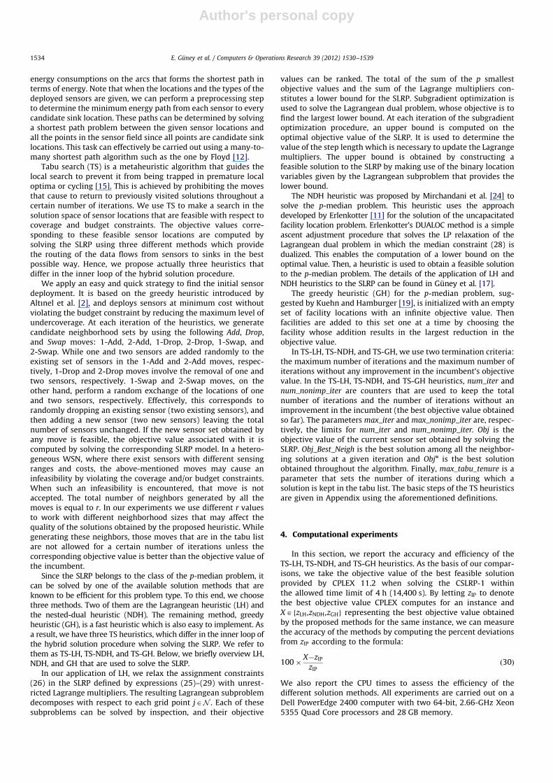
First, we consider the case with one sink (p¼1), and solve eachof the 14 test instances five times. Since the neighboring solutionsare generated randomly at each tabu search iteration, our heur-istics may yield a different solution for each run. Therefore, wereport in Table 2 both the best and average results generated byfive runs for each test instance. The first column includes thenumber of points N in the sensor field. The second column showsthe amount of energy spent corresponding to the best feasiblesolution obtained within a time limit of 14,400 s when the CSLRP-1 is solved using CPLEX 11.2. CPLEX can provide optimal solutionsonly for problems with Nr49 points. The values marked with ‘‘n’’are the corresponding optimal values. The remaining entries ofthis column are the objective values of the best feasible solutionsobtained within the time limit. The third to fifth columns displaythe percent deviations of the best and average objective valuesobtained by TS-LH, TS-NDH, and TS-GH heuristics from theobjective value found by solving CSLRP-1 using CPLEX. The lastfour columns give the CPU times spent by the methods. As can beseen by the best percent deviations, 6.9%, 6.3%, and 4.1% moreenergy is spent on the average when the WSN is setup by making

Table 2Comparison of the results when p¼1.

N Energy Best % dev. (avg. % dev.) CPU time (s)

CSLRP-1 TS-LH TS-NDH TS-GH CSLRP-1 TS-LH TS-NDH TS-GH

9 5n 0.0 (12.0) 0.0 (4.0) 0.0 (8.0) 0.1 9.8 0.9 0.1

16 11n 9.1 (16.4) 9.1 (14.5) 18.2 (21.8) 0.2 61.4 4.2 0.6

25 16n 0.0 (2.5) 0.0 (1.3) 0.0 (1.3) 1.2 399.3 77.8 24.2

36 30n 16.7 (24.0) 10.0 (13.3) 3.3 (7.3) 24.1 726.1 171.3 48.2

49 44n 22.7 (33.2) 15.9 (18.6) 22.7 (24.5) 901.4 886.4 382.5 89.5

64 75 6.7 (10.1) 6.7 (8.8) 2.7 (6.4) 14,400.0 1565.5 667.2 205.3

81 96 10.4 (12.9) 15.6 (16.7) 4.2 (5.6) 14,400.0 3945.9 720.5 130.9

100 132 6.8 (9.2) 6.1 (6.7) 4.5 (5.8) 14,400.0 6272.3 1217.9 238.1

121 177 10.7 (13.4) 13.6 (16.5) 7.3 (8.6) 14,400.0 8991.4 1802.5 384.6

144 225 12.0 (13.2) 14.7 (15.6) 10.2 (11.3) 14,400.0 12,016.2 4384.7 607.3

169 309 8.7 (9.7) 8.1 (9.0) 3.6 (4.3) 14,400.0 14,400.0 5979.4 990.8

196 440 �5.0 (�4.2) �0.9 (0.6) �7.7 (�7.2) 14,400.0 14,400.0 14,400.0 1378.1

225 532 0.2 (0.8) �1.5 (�0.7) �4.5 (�2.9) 14,400.0 14,400.0 14,400.0 2062.2

400 1750 �1.8 (�0.4) �9.2 (�7.1) �6.6 (�2.9) 14,400.0 14,400.0 14,400.0 8194.1

Avg. 274.4 6.9 (10.9) 6.3 (8.4) 4.1 (6.6) 9323.4 6605.3 4186.4 1025.3

E. Guney et al. / Computers & Operations Research 39 (2012) 1530–1539 1535

Author's personal copy

the decisions of sensor deployment, sink location and routingusing the three heuristics. TS-GH outperforms the other heuristicsin terms of accuracy, while it is also the best in terms of efficiency.

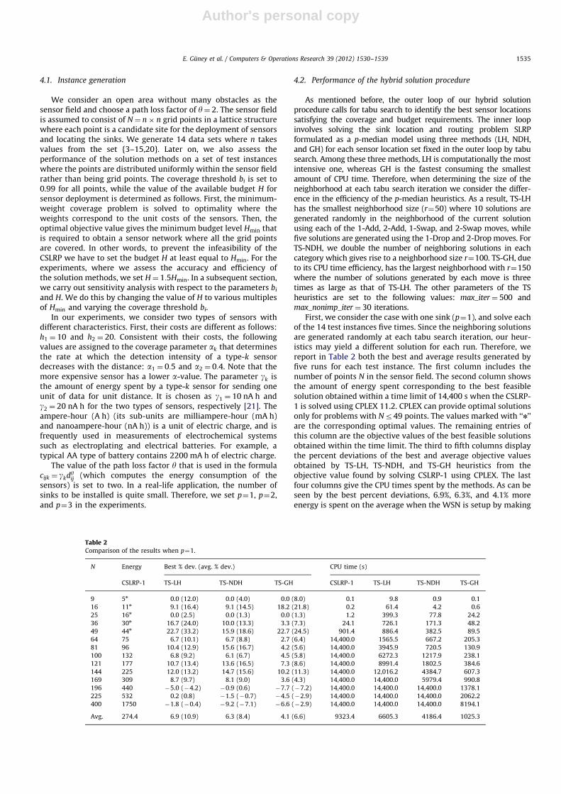
The results for p¼2 are displayed in Table 3. As is the case withp¼1, CPLEX cannot find any optimal solution for test instanceswith N449 within the allowed time limit. It can be observed thatthe best performing heuristic in terms of accuracy is TS-NDH withan average of 4.1% deviation, while TS-GH is once more the mostefficient. Note that there are some negative values for percentdeviations. They indicate that the heuristic solution is better thanthe best feasible solution CPLEX computes in 4 h.

Results given in Table 4 for p¼3 indicate that the bestperforming heuristics with respect to both criteria remain thesame. With regard to the efficiency, we can conclude that solvingthe CSLRP-1 by CPLEX requires 11.5 times as much time asneeded by the fastest heuristic TS-GH, on the average.

When we compare the objective values for the same testinstances (i.e., instances with the same number of grid points N),we observe that the energy consumptions decrease as the number ofthe sinks increases. This is an expected result because when there aremore sinks in the WSN, each sensor is, on the average, closer to thesinks, and thus less routing energy is consumed by the sensors.

4.3. Sensitivity analyses

We conduct further experiments to investigate the effect ofthree factors on the results: the available budget, the coveragethreshold, and the configuration of the candidate points in thesensor field. Each of these factors is considered separately in thefollowing.

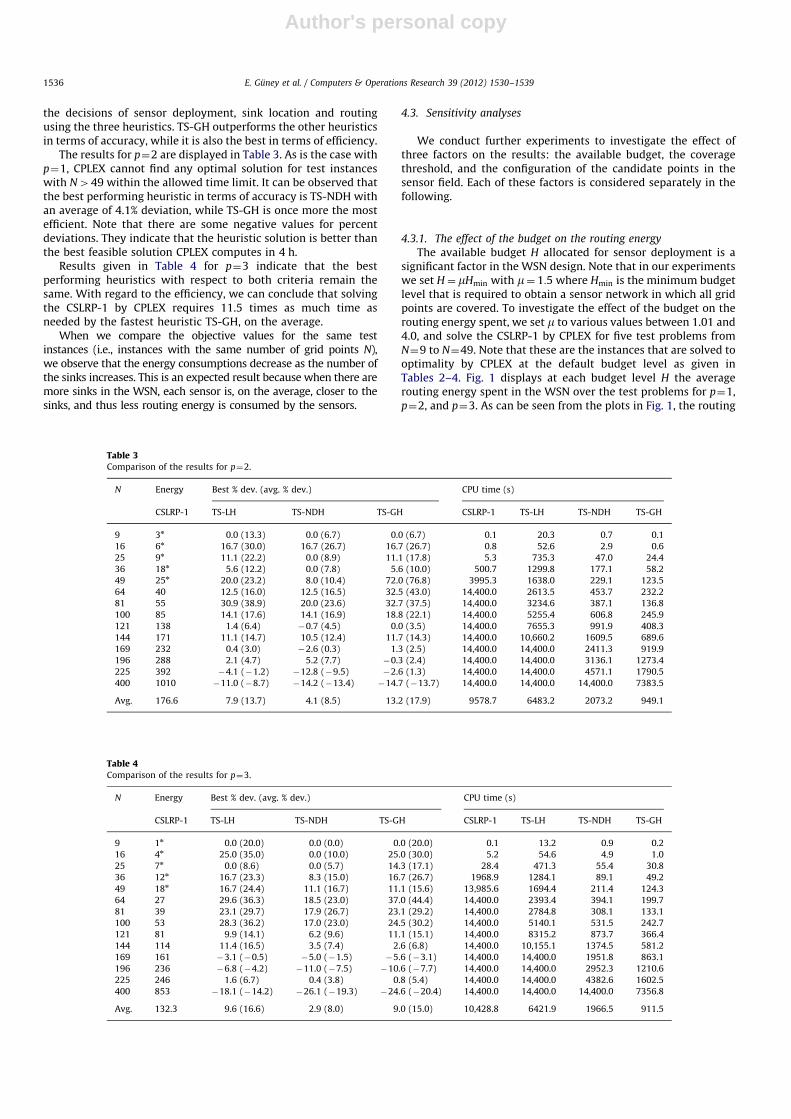
4.3.1. The effect of the budget on the routing energy

The available budget H allocated for sensor deployment is asignificant factor in the WSN design. Note that in our experimentswe set H¼ mHmin with m¼ 1:5 where Hmin is the minimum budgetlevel that is required to obtain a sensor network in which all gridpoints are covered. To investigate the effect of the budget on therouting energy spent, we set m to various values between 1.01 and4.0, and solve the CSLRP-1 by CPLEX for five test problems fromN¼9 to N¼49. Note that these are the instances that are solved tooptimality by CPLEX at the default budget level as given inTables 2–4. Fig. 1 displays at each budget level H the averagerouting energy spent in the WSN over the test problems for p¼1,p¼2, and p¼3. As can be seen from the plots in Fig. 1, the routing

Table 3Comparison of the results for p¼2.

N Energy Best % dev. (avg. % dev.) CPU time (s)

CSLRP-1 TS-LH TS-NDH TS-GH CSLRP-1 TS-LH TS-NDH TS-GH

9 3n 0.0 (13.3) 0.0 (6.7) 0.0 (6.7) 0.1 20.3 0.7 0.1

16 6n 16.7 (30.0) 16.7 (26.7) 16.7 (26.7) 0.8 52.6 2.9 0.6

25 9n 11.1 (22.2) 0.0 (8.9) 11.1 (17.8) 5.3 735.3 47.0 24.4

36 18n 5.6 (12.2) 0.0 (7.8) 5.6 (10.0) 500.7 1299.8 177.1 58.2

49 25n 20.0 (23.2) 8.0 (10.4) 72.0 (76.8) 3995.3 1638.0 229.1 123.5

64 40 12.5 (16.0) 12.5 (16.5) 32.5 (43.0) 14,400.0 2613.5 453.7 232.2

81 55 30.9 (38.9) 20.0 (23.6) 32.7 (37.5) 14,400.0 3234.6 387.1 136.8

100 85 14.1 (17.6) 14.1 (16.9) 18.8 (22.1) 14,400.0 5255.4 606.8 245.9

121 138 1.4 (6.4) �0.7 (4.5) 0.0 (3.5) 14,400.0 7655.3 991.9 408.3

144 171 11.1 (14.7) 10.5 (12.4) 11.7 (14.3) 14,400.0 10,660.2 1609.5 689.6

169 232 0.4 (3.0) �2.6 (0.3) 1.3 (2.5) 14,400.0 14,400.0 2411.3 919.9

196 288 2.1 (4.7) 5.2 (7.7) �0.3 (2.4) 14,400.0 14,400.0 3136.1 1273.4

225 392 �4.1 (�1.2) �12.8 (�9.5) �2.6 (1.3) 14,400.0 14,400.0 4571.1 1790.5

400 1010 �11.0 (�8.7) �14.2 (�13.4) �14.7 (�13.7) 14,400.0 14,400.0 14,400.0 7383.5

Avg. 176.6 7.9 (13.7) 4.1 (8.5) 13.2 (17.9) 9578.7 6483.2 2073.2 949.1

Table 4Comparison of the results for p¼3.

N Energy Best % dev. (avg. % dev.) CPU time (s)

CSLRP-1 TS-LH TS-NDH TS-GH CSLRP-1 TS-LH TS-NDH TS-GH

9 1n 0.0 (20.0) 0.0 (0.0) 0.0 (20.0) 0.1 13.2 0.9 0.2

16 4n 25.0 (35.0) 0.0 (10.0) 25.0 (30.0) 5.2 54.6 4.9 1.0

25 7n 0.0 (8.6) 0.0 (5.7) 14.3 (17.1) 28.4 471.3 55.4 30.8

36 12n 16.7 (23.3) 8.3 (15.0) 16.7 (26.7) 1968.9 1284.1 89.1 49.2

49 18n 16.7 (24.4) 11.1 (16.7) 11.1 (15.6) 13,985.6 1694.4 211.4 124.3

64 27 29.6 (36.3) 18.5 (23.0) 37.0 (44.4) 14,400.0 2393.4 394.1 199.7

81 39 23.1 (29.7) 17.9 (26.7) 23.1 (29.2) 14,400.0 2784.8 308.1 133.1

100 53 28.3 (36.2) 17.0 (23.0) 24.5 (30.2) 14,400.0 5140.1 531.5 242.7

121 81 9.9 (14.1) 6.2 (9.6) 11.1 (15.1) 14,400.0 8315.2 873.7 366.4

144 114 11.4 (16.5) 3.5 (7.4) 2.6 (6.8) 14,400.0 10,155.1 1374.5 581.2

169 161 �3.1 (�0.5) �5.0 (�1.5) �5.6 (�3.1) 14,400.0 14,400.0 1951.8 863.1

196 236 �6.8 (�4.2) �11.0 (�7.5) �10.6 (�7.7) 14,400.0 14,400.0 2952.3 1210.6

225 246 1.6 (6.7) 0.4 (3.8) 0.8 (5.4) 14,400.0 14,400.0 4382.6 1602.5

400 853 �18.1 (�14.2) �26.1 (�19.3) �24.6 (�20.4) 14,400.0 14,400.0 14,400.0 7356.8

Avg. 132.3 9.6 (16.6) 2.9 (8.0) 9.0 (15.0) 10,428.8 6421.9 1966.5 911.5

E. Guney et al. / Computers & Operations Research 39 (2012) 1530–15391536

Author's personal copy

energy consumption first decreases as the budget level increases.This initial reduction in the energy is due to the increased numberof deployed sensors. Note that a larger number of sensors can bedeployed due to the higher budget levels. This, in turn, decreasesthe average distance between sensors and sinks, and a smalleraverage distance reduces the routing energy spent. Being able todeploy more sensors due to a higher budget availability does notcontribute to a reduction in the routing energy after a certainpoint, however, because the number of data packets transmittedfrom sensors to sinks also increases. This latter factor leads to anincrease in the routing energy. Hence, the routing energy attainsits optimal value at a certain budget level, and remains at thisvalue for larger budget levels.

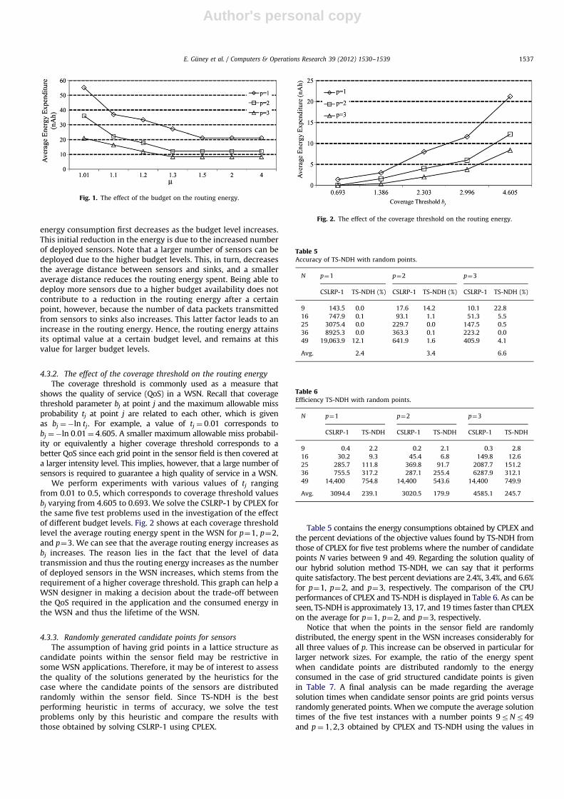
4.3.2. The effect of the coverage threshold on the routing energy

The coverage threshold is commonly used as a measure thatshows the quality of service (QoS) in a WSN. Recall that coveragethreshold parameter bj at point j and the maximum allowable missprobability tj at point j are related to each other, which is givenas bj ¼�ln tj. For example, a value of tj ¼ 0:01 corresponds tobj ¼�ln 0:01¼ 4:605. A smaller maximum allowable miss probabil-ity or equivalently a higher coverage threshold corresponds to abetter QoS since each grid point in the sensor field is then covered ata larger intensity level. This implies, however, that a large number ofsensors is required to guarantee a high quality of service in a WSN.

We perform experiments with various values of tj rangingfrom 0.01 to 0.5, which corresponds to coverage threshold valuesbj varying from 4.605 to 0.693. We solve the CSLRP-1 by CPLEX forthe same five test problems used in the investigation of the effectof different budget levels. Fig. 2 shows at each coverage thresholdlevel the average routing energy spent in the WSN for p¼1, p¼2,and p¼3. We can see that the average routing energy increases asbj increases. The reason lies in the fact that the level of datatransmission and thus the routing energy increases as the numberof deployed sensors in the WSN increases, which stems from therequirement of a higher coverage threshold. This graph can help aWSN designer in making a decision about the trade-off betweenthe QoS required in the application and the consumed energy inthe WSN and thus the lifetime of the WSN.

4.3.3. Randomly generated candidate points for sensors

The assumption of having grid points in a lattice structure ascandidate points within the sensor field may be restrictive insome WSN applications. Therefore, it may be of interest to assessthe quality of the solutions generated by the heuristics for thecase where the candidate points of the sensors are distributedrandomly within the sensor field. Since TS-NDH is the bestperforming heuristic in terms of accuracy, we solve the testproblems only by this heuristic and compare the results withthose obtained by solving CSLRP-1 using CPLEX.

Table 5 contains the energy consumptions obtained by CPLEX andthe percent deviations of the objective values found by TS-NDH fromthose of CPLEX for five test problems where the number of candidatepoints N varies between 9 and 49. Regarding the solution quality ofour hybrid solution method TS-NDH, we can say that it performsquite satisfactory. The best percent deviations are 2.4%, 3.4%, and 6.6%for p¼1, p¼2, and p¼3, respectively. The comparison of the CPUperformances of CPLEX and TS-NDH is displayed in Table 6. As can beseen, TS-NDH is approximately 13, 17, and 19 times faster than CPLEXon the average for p¼1, p¼2, and p¼3, respectively.

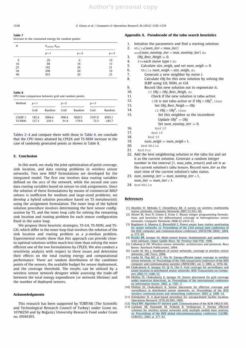
Notice that when the points in the sensor field are randomlydistributed, the energy spent in the WSN increases considerably forall three values of p. This increase can be observed in particular forlarger network sizes. For example, the ratio of the energy spentwhen candidate points are distributed randomly to the energyconsumed in the case of grid structured candidate points is givenin Table 7. A final analysis can be made regarding the averagesolution times when candidate sensor points are grid points versusrandomly generated points. When we compute the average solutiontimes of the five test instances with a number points 9rNr49and p¼ 1;2,3 obtained by CPLEX and TS-NDH using the values in

Fig. 1. The effect of the budget on the routing energy.

Fig. 2. The effect of the coverage threshold on the routing energy.

Table 5Accuracy of TS-NDH with random points.

N p¼1 p¼2 p¼3

CSLRP-1 TS-NDH (%) CSLRP-1 TS-NDH (%) CSLRP-1 TS-NDH (%)

9 143.5 0.0 17.6 14.2 10.1 22.8

16 747.9 0.1 93.1 1.1 51.3 5.5

25 3075.4 0.0 229.7 0.0 147.5 0.5

36 8925.3 0.0 363.3 0.1 223.2 0.0

49 19,063.9 12.1 641.9 1.6 405.9 4.1

Avg. 2.4 3.4 6.6

Table 6Efficiency TS-NDH with random points.

N p¼1 p¼2 p¼3

CSLRP-1 TS-NDH CSLRP-1 TS-NDH CSLRP-1 TS-NDH

9 0.4 2.2 0.2 2.1 0.3 2.8

16 30.2 9.3 45.4 6.8 149.8 12.6

25 285.7 111.8 369.8 91.7 2087.7 151.2

36 755.5 317.2 287.1 255.4 6287.9 312.1

49 14,400 754.8 14,400 543.6 14,400 749.9

Avg. 3094.4 239.1 3020.5 179.9 4585.1 245.7

E. Guney et al. / Computers & Operations Research 39 (2012) 1530–1539 1537

Author's personal copy

Tables 2–4 and compare them with those in Table 6, we concludethat the CPU times attained by CPLEX and TS-NDH increase in thecase of randomly generated points as shown in Table 8.

5. Conclusion

In this work, we study the joint optimization of point coverage,sink location, and data routing problems in wireless sensornetworks. Two new MILP formulations are developed for theintegrated model. The first one involves data routing variablesdefined on the arcs of the network, while the second one usesdata routing variables based on sensor-to-sink assignments. Sincethe solution of these formulations by means of commercial MILPsolvers is inefficient for medium and large-sized problems, wedevelop a hybrid solution procedure based on TS metaheuristicusing the assignment formulation. The outer loop of the hybridsolution procedure involves determining the best sensor config-uration by TS, and the inner loop calls for solving the remainingsink location and routing problem for each sensor configurationfixed in the outer loop.

We propose three heuristic strategies, TS-LH, TS-NDH, and TS-GH, which differ in the inner loop that involves the solution of thesink location and routing problem as a p-median problem.Experimental results show that this approach can provide close-to-optimal solutions within much less time than solving the moreefficient one of the two formulations by CPLEX. We also conduct asensitivity analysis with respect to three issues and determinetheir effects on the total routing energy and computationalperformance. These are random distribution of the candidatepoints of the sensors, the available budget for sensor deployment,and the coverage threshold. The results can be utilized by awireless sensor network designer while assessing the trade-offbetween the total energy expenditure (or network lifetime) andthe number of deployed sensors.

Acknowledgments

This research has been supported by TUB_ITAK (The Scientificand Technological Research Council of Turkey) under Grant no.107M250 and by Bogazic- i University Research Fund under Grantno. 05HA303.

Appendix A. Pseudocode of the tabu search heuristics

1. Initialize the parameters and find a starting solution;2. While(num_iteromax_iter)

and(num_nonimp_iteromax_nonimp_iter) do3. Obj_Best_Neigh :¼ 0.4. Foreach move type i do

5. Calculate size_neighi and set num_neigh :¼ 0.6. While num_neighosize_neighi do

7. Generate a new neighbor by move i.8. Calculate Obj for this new solution by solving the

SLRP using LH, NDH, or GH.9. Record this new solution not to regenerate it.10. If Obj4Obj_Best_Neigh, do11. Check if the new solution is tabu-active.12. Ifit is not tabu-active or if Obj4Objn, then13. Set Obj_Best_Neigh :¼ Obj

14. If Obj4Objn, then15. Set this neighbor as the incumbent

Update Objn :¼ Obj

Set num_nonimp_iter :¼ 0.16. End If

17. End If

18. End If

19. num_neigh :¼ num_neighþ1.20. End While

21. End For

22. Add the best neighboring solution to the tabu list and setit as the current solution. Generate a random integernumber in the interval [1, max_tabu_tenure] and set it asthe current solution’s tabu tenure. Record num_iter as thestart time of the current solution’s tabu status.

23. num_nonimp_iter :¼ num_nonimp_iterþ1,

num_iter :¼ num_iterþ1.24. End While

References

[1] Akyıldız IF, Melodia T, Chowdhury KR. A survey on wireless multimediasensor networks. Computer Networks 2007;51:921–60.

[2] Altınel _IK, Aras N, Guney E, Ersoy C. Binary integer programming formula-tions and heuristics for differentiated coverage in heterogeneous sensornetworks. Computer Networks 2008;52:2419–31.

[3] Bogdanov A, Maneva E, Riesenfeld S. Power-aware base station positioningfor sensor networks. in: Proceedings of the 23rd annual joint conference ofthe IEEE computer and communications conference (INFOCOM 2004); 2004.p. 575–85.

[4] Brooks RR, Iyengar SS. Multi-sensor fusion: fundamentals and applicationswith software. Upper Saddle River, NJ: Prentice Hall PTR; 1998.

[5] Callaway Jr EH. Wireless sensor networks: architectures and protocols. BocaRaton: Auerbach Publications; 2004.

[6] Cardei M, Wu J. Handbook of sensor networks, coverage in wireless sensornetworks. CRC Press; 2004.

[7] Cardei M, Thai MT, Li Y, Wu W. Energy-efficient target coverage in wirelesssensor networks. in: Proceedings of the 24th annual joint conference of the IEEEcomputer and communication societies (INFOCOM), vol. 3; 2005. p. 1976–84.

[8] Chakrabarty K, Iyengar SS, Qi H, Cho E. Grid coverage for surveillance andtarget location in distributed sensor networks. IEEE Transactions on Compu-ters 2002;51:1448–53.

[9] Dhillon SS, Chakrabarty K, Iyengar SS. Sensor placement for grid coverageunder imprecise detections. in: Proceedings of the international conferenceon information fusion; 2002. p. 1581–7.

[10] Dhillon SS, Chakrabarty K. Sensor placement for effective coverage andsurveillance in distributed sensor networks. in: Proceedings of the IEEEwireless communications and networking conference; 2003. p. 1609–14.

[11] Erlenkotter D. A dual-based procedure for uncapacitated facility location.Operations Research 1978;26:992–1009.

[12] Floyd RW. Algorithm 97 shortest path. Communication of the ACM 1962;6:345.[13] Gandam SR, Dawande M, Prakash R, Venkatesan S. Energy efficient

schemes for wireless sensor networks with multiple mobile base stations.in: Proceedings of the IEEE global telecommunications conference (GLOBE-COM’03); 2003. p. 377–81.

Table 7Increase in the consumed energy for random points.

N Erandom=Egrid

p¼1 p¼2 p¼3

9 29 6 10

16 68 16 13

25 192 26 21

36 298 20 19

49 433 26 23

Table 8CPU time comparison between grid and random points.

Method p¼1 p¼2 p¼3

Grid Random Grid Random Grid Random

CSLRP-1 185.4 3094.4 900.4 3020.5 3197.6 4585.1

TS-NDH 127.3 239.1 91.4 179.9 72.3 245.7

E. Guney et al. / Computers & Operations Research 39 (2012) 1530–15391538

Author's personal copy

[14] Ghosh A, Das SK. Coverage and connectivity issues in wireless sensornetworks: a survey. Pervasive and Mobile Computing 2008;4:303–34.

[15] Glover F, Laguna M. Tabu search. Dordrecht: Kluwer Academic Publishers;1997.

[16] Guney E, Altınel _IK, Aras N, Ersoy C. A tabu search heuristic for pointcoverage, sink location, and data routing in wireless sensor networks.in: EvoCOP 2010, Lecture notes in computer science, vol. 6022; 2010.p. 83–94.

[17] Guney E, Aras N, Altınel _IK, Ersoy C. Efficient integer programming formula-tions for optimum sink location and routing in heterogeneous wirelesssensor networks. Computer Networks 2010;54(6):1805–22.

[18] Kim H, Seok Y, Choi N, Choi Y, Kwon T. Optimal multi-sink positioning andenergy-efficient routing in wireless sensor networks. in: ICOIN 2005. Lecturenotes in computer science, vol. 3391; 2005. p. 264–75.

[19] Kuehn AA, Hamburger MJ. A heuristic program for locating warehouses.Management Science 1963;9:643–66.

[20] Lin L, Shroff NB, Srikant R. Energy-aware routing in sensor networks: a largesystem approach. Ad Hoc Networks 2007;5:818–31.

[21] Mainwaring A, Polastre J, Szewczyk R, Culler S, Anderson J. Wireless sensornetworks for habitat monitoring. In: WSNA’02, Atlanta, Georgia; 2002.

[22] Meguerdichian S, Potkonjak M. Low power 0/1 coverage and schedulingtechniques in sensor networks. UCLA Technical Reports 030001. Los Angeles,USA: UCLA; 2003.

[23] Meguerdichian S, Koushanfar F, Potkonjak M, Srivastava MB. Coverageproblems in wireless ad-hoc sensor networks. in: Proceedings of INFOCOM2001, twentieth annual joint conference of the IEEE computer and commu-nications societies, vol. 3; 2001. p. 1380–7.

[24] Mirchandani PB, Oudjit A, Wong RT. ‘Multidimensional’ extensions and anested dual approach for the m-median problem. European Journal ofOperational Research 1985;21:121–37.

[25] Shi Y, Hou YT, Efrat A. Algorithm design for a class of base station locationproblems in sensor networks. Wireless Networks 2009;15:21–8.

[26] Yick J, Mukherjee B, Ghosal D. Wireless sensor network survey. InternationalJournal of Computer and Telecommunications Networking 2008;52:2292–330.

[27] Younis M, Akkaya K. Strategies and techniques for node placement inwireless sensor networks: a survey. Ad Hoc Networks 2008;6:621–55.

E. Guney et al. / Computers & Operations Research 39 (2012) 1530–1539 1539