arX

iv:n

lin/0

6070

70v1

[nl

in.C

D]

30

Jul 2

006

Semiclassical Theory for ParametricCorrelation of Energy Levels

Taro Nagao1, Petr Braun2,3, Sebastian Muller4,Keiji Saito5, Stefan Heusler2 and Fritz Haake2

1 Graduate School of Mathematics, Nagoya University, Chikusa-ku,

Nagoya 464-8602, Japan2 Fachbereich Physik, Universitat Duisburg-Essen, 45117 Essen, Germany

3 Institute of Physics, Saint-Petersburg University, 198504,

Saint-Petersburg, Russia4 Cavendish Laboratory, University of Cambridge, J J Thomson Avenue,

Cambridge CB3 0HE, UK5 Department of Physics, Graduate School of Science, University of Tokyo,

Hongo 7-3-1, Bunkyo-ku, Tokyo 113-0033, Japan

Abstract

Parametric energy-level correlation describes the response of theenergy-level statistics to an external parameter such as the magneticfield. Using semiclassical periodic-orbit theory for a chaotic system,we evaluate the parametric energy-level correlation depending on themagnetic field difference. The small-time expansion of the spectralform factor K(τ) is shown to be in agreement with the prediction ofparameter dependent random-matrix theory to all orders in τ .

PACS: 05.45.Mt; 03.65.Sq

KEYWORDS: quantum chaos; periodic orbit theory; random matrices

1

1 Introduction

More than two decades have passed since the universal energy level statisticswas conjectured for classically chaotic systems[1]. Spectral correlations werefound to coincide with the predictions of Random Matrix Theory (RMT).If the system is time-reversal invariant, the energy-level correlation in thesemiclassical limit is asymptotically in agreement with the eigenvalue corre-lation of the Gaussian Orthogonal Ensemble (GOE) of random matrices. Ina magnetic field the time-reversal invariance is broken and the energy-levelstatistics is then qualitatively affected. In that case the Gaussian UnitaryEnsemble (GUE) gives a precise prediction for the asymptotic behavior ofthe energy-level correlation.

Much effort has been paid to explain the agreement with RMT in termsof the semiclassical periodic-orbit theory[2]. A typical physical quantity,the spectral form factor K(τ), can be written as a sum over periodic-orbitpairs. Berry calculated the leading contribution, of first order in the timevariable τ , by means of the diagonal approximation[3] which is applied toboth of the GOE and GUE universality classes. For a system with time-reversal invariance, the pairs of identical orbits and the pairs of mutuallytime reversed orbits both contribute to the first-order term. For a systemwithout time-reversal invariance, we need to care only about the pairs ofidentical orbits. In this way one is able to partially reproduce the RMTprediction using periodic-orbit theory.

Berry’s work was extended to the second-order term by Sieber and Richter(SR) who specified the family of contributing orbit pairs[4]. The possibilityto include more complicated orbit pairs by a combinatorial method was soonnoticed. Heusler et al. developed the analysis to the third-order term[5] andMuller et al. obtained the expansion in agreement with the RMT result toall orders[6, 7, 8].

On the other hand, it is also conjectured that parameter-dependent ran-dom matrices describe the transition of level statistics within and in be-tween the universality classes[9, 10]. Saito and Nagao[11] applied semiclassi-cal periodic-orbit theory to the parametric transition between the GOE andGUE universality classes and obtained agreement with “parametric” RMTup to the third order. In this paper, we deal with the parametric transitionwithin the GUE symmetry class, employing the magnetic field as the param-eter. Using semiclassical periodic-orbit theory, we evaluate the small-timeexpansion of the spectral form factor for the parametric correlation. The

2

agreement with parametric RMT is established to all orders.This paper is organized as follows. In § 2, a parametric random-matrix

theory is developed and an RMT prediction for the spectral form factor isdeduced. In § 3 and § 4, we employ periodic-orbit theory for a chaotic systemin a magnetic field to show that a small-time expansion of the form factoragrees with the RMT prediction. In § 5, the key identity (a sum formula)used in § 4 is proved. In addition, a similar description of the GOE to GUEtransition is briefly given in last section.

2 Parametric Random Matrix Theory

A parameter-dependent random-matrix theory (matrix Brownian-motion model)was first formulated by Dyson[12]. He considered an ensemble of N ×N her-mitian random matrices H which are close to an “unperturbed” hermitianmatrix H(0). The conditional probability distribution function of H is givenby

P (H ; σ|H(0)) dH ∝ exp

−Tr

(H − e−σH(0))2

1 − e−2σ

dH (2.1)

with

dH =N∏

j=1

dHjj

N∏

j<l

dReHjl dImHjl. (2.2)

The parametric motion of the matrix H depending on the fictitious timeparameter σ is of interest. At the initial time σ = 0, H is equated withthe hermitian matrix H(0). In the limit σ → ∞, the probability distributionfunction (p.d.f.) of H becomes that of the GUE

P (H ;∞|H(0)) dH ∝ e−TrH2

dH, (2.3)

which is independent of H(0).Let us denote the eigenvalues of the hermitian matrices H and H(0) as

x1, x2, · · · , xN and x(0)1 , x

(0)2 , · · · , x(0)

N , respectively. Then the p.d.f. of the

eigenvalues of H at σ (under the condition that xj = x(0)j (j = 1, 2, · · · , N)

at σ = 0) can be derived as

p(x1, x2, · · · , xN ; σ|x(0)1 , x

(0)2 , · · · , x(0)

N )N∏

j=1

dxj

3

∝N∏

j=1

e−(xj)2/2+(x(0)j

)2/2N∏

j<l

xj − xl

x(0)j − x

(0)l

det[g(xj, x(0)l )]j,l=1,2,···,N

N∏

j=1

dxj ,

(2.4)

where

g(x, y) = e−(x2+y2)/2∞∑

j=0

Hj(x)Hj(y)√πj!2j

e−(j+(1/2))σ (2.5)

with the Hermite polynomials

Hj(x) = (−1)jex2 dj

dxje−x2

. (2.6)

In the limit σ → ∞, this p.d.f. becomes the p.d.f. of the GUE eigenvaluesas

p(x1, x2, · · · , xN ;∞|x(0)1 , x

(0)2 , · · · , x(0)) = pGUE(x1, x2, · · · , xN ), (2.7)

where

pGUE(x1, x2, · · · , xN ) ∝N∏

j=1

e−(xj)2N∏

j<l

|xj − xl|2, (2.8)

as expected.Now we suppose that the initial matrix H(0) is a GUE random matrix,

so that the p.d.f. of x(0)1 , x

(0)2 , · · · , x(0)

N is also given by (2.8). Then the tran-sition within the GUE symmetry class (the GUE to GUE transition) is ob-served. The dynamical (density-density) correlation function which describesthe GUE to GUE transition is defined as

ρd(x; σ|y) = N2 I(x; σ|y)

I0, (2.9)

where

I(x1; σ|x(0)1 )

=∫ ∞

−∞dx2

∫ ∞

−∞dx3 · · ·

∫ ∞

−∞dxN

∫ ∞

−∞dx

(0)2

∫ ∞

−∞dx

(0)3 · · ·

∫ ∞

−∞dx

(0)N

× p(x1, x2, · · · , xN ; σ|x(0)1 , x

(0)2 , · · · , x(0)

N )pGUE(x(0)1 , x

(0)2 , · · · , x(0)

N )

(2.10)

andI0 =

∫ ∞

−∞dx∫ ∞

−∞dyI(x; σ|y). (2.11)

4

The dynamical correlation function describes correlations between the spec-tra of H and H0.

It is possible to evaluate the asymptotic limit N → ∞ of the dynamicalcorrelation function[13, 14]. Introducing scaled parameters η, X, Y as

σ = η/(4π2ρ2), x =√

2Nz + (X/ρ), y =√

2Nz + (Y/ρ) (2.12)

(ρ =√

2N(1 − z2)/π is the asymptotic eigenvalue density at√

2Nz, −1 <

z < 1), we find

ρd(x; σ|y)

ρ2− 1 ∼ ρ(ξ; η) ≡

∫ 1

0du eu2η/4 cos(πuξ)

∫ ∞

1dv e−v2η/4 cos(πvξ),

(2.13)where ξ = X − Y . The Fourier transform KRM(τ) =

∫∞−∞ dξ ei2πτξ ρ(ξ; η) is

called the form factor. For times in the interval 0 ≤ τ ≤ 1 the form factorcan be written as

KRM(τ) =1

2

∫ 1

1−2τdu e−λ(τ+u) =

e−λ

λsinh(λτ) , (2.14)

λ = ητ ; (2.15)

the variable λ was introduced here because it is the expansion of KRM(τ) inpowers of τ at fixed λ which is most naturally connected with the semiclas-sical periodic-orbit theory; this expansion

KRM(τ) = τe−λ∞∑

j=0

(λτ)2j

(2j + 1)!(2.16)

will be compared with a semiclassical result. For that purpose, we write theexpansion into the form

KRM(τ) = KdiagRM (τ) + Koff

RM(τ) (2.17)

with

K(diag)RM (τ) = τe−λ, K

(off)RM (τ) = τe−λ

∞∑

j=1

(λτ)2j

(2j + 1)!. (2.18)

In § 3, we evaluate the semiclassical form factor for a chaotic system andobtain the first-order term in agreement with K

(diag)RM (τ). Moreover, in § 4,

5

the semiclassical calculation is extended to yield a result in agreement withthe Laplace transform (taken for fixed η, using (2.15))

∫ ∞

0e−qλ K

(off)RM (τ)

τ 2

∣

∣

∣

∣

∣

∣

τ=λ/η

dλ =∞∑

j=1

1

(2j + 1)!

∫ ∞

0e−(q+1)λ

(

λ

η

)2j−1

λ2jdλ

=∞∑

j=1

1

η2j−1

(4j − 1)!

(2j + 1)!

1

(q + 1)4j. (2.19)

We thus show the agreement up to all orders.

3 Periodic-Orbit Theory for a Chaotic Sys-

tem

We consider a bounded quantum system with f degrees of freedom in a mag-netic field B, assuming that the corresponding classical dynamics is chaotic.Let us denote the energy by E and each phase space point by a 2f dimen-sional vector x = (q,p), where f dimensional vectors q and p specify theposition and momentum, respectively. In the semiclassical limit h → 0, theenergy-level density ρ(E; B) can be written in the form

ρ(E; B) ∼ ρav(E) + ρosc(E; B). (3.1)

Here ρav(E) is the local average of the level density and ρosc(E; B) describesthe fluctuation around the average.

The local average of the level density is equal to the number of Planckcells inside the energy shell

ρav(E) =Ω(E)

(2πh)f, (3.2)

where Ω(E) is the volume of the energy shell. We assume that the magneticfield is sufficiently weak such that the cyclotron radius is much larger than thesystem size and thus the presence of the magnetic field does not significantlychange Ω(E).

On the other hand, the fluctuation part is given by a sum over the classicalperiodic orbits γ as

ρosc(E; B) =1

πhRe

∑

γ

Aγei(Sγ (E)+θγ(B))/h, (3.3)

6

where Sγ is the classical action and Aγ is the stability amplitude (includingthe Maslov phase). The phase θγ(B) is a function of the magnetic field andis defined as

θγ(B) = B∫

γa(q) · dq = B

∫

gγ(t) dt, gγ(t) = a(qγ) ·dqγ

dt, (3.4)

where a(q) is the gauge potential which generates the unit magnetic fieldand qγ(t) describes a classical motion in the configuration space along theorbit γ.

In analogy with (2.13), we introduce the scaled parametric correlationfunction as

R(s; B, B′) =

⟨

ρ(

E + s2ρav(E)

; B)

ρ(

E − s2ρav(E)

; B′)

ρav(E)2

⟩

− 1

∼⟨

ρosc

(

E + s2ρav(E)

; B)

ρosc

(

E − s2ρav(E)

; B′)

ρav(E)2

⟩

. (3.5)

Here the angular bracket means two averages, one over the center energy Eand one over a time interval much smaller than the Heisenberg time

TH = 2πhρav(E) =Ω(E)

(2πh)f−1. (3.6)

The form factor, namely the Fourier transform of R(s; B, B′), is then writtenas

K(τ) =∫ ∞

−∞ds ei2πτsR(s; B, B′)

∼⟨

∫

dǫ eiǫτTH/hρosc

(

E + ǫ2; B)

ρosc

(

E − ǫ2; B′

)

ρav(E)

⟩

. (3.7)

Putting (3.3) into (3.7), we find that the form factor is expressed as a doublesum over periodic orbits

K(τ) ∼ 1

T 2H

⟨

∑

γ,γ′

AγA∗γ′ei(Sγ−Sγ′ )/hei(θγ (B)−θγ′ (B

′))/hδ(

τ − Tγ + Tγ′

2TH

)

⟩

(3.8)

(an asterisk means a complex conjugate), where Tγ and Tγ′ are the periodsof the periodic orbit γ and its partner γ′, which “feel” the magnetic fields B

7

and B′, respectively. We assume that the difference between these fields issufficiently small so that its influence on the classical motion can be neglected;we only have to keep the resulting difference between the magnetic phasesθγ(B) − θγ′(B′).

Let us now denote by γT a stretch of the periodic orbit γ whose dura-tion T is much larger than all classical correlation times; this stretch cancoincide with the whole orbit (and then T is the orbit period). For timeslarge compared to the classical scales mentioned, successive changes of thevelocity dqγ/dt can be regarded as independent random events[15], so thata replacement of gγ(t) by Gaussian white noise is justified. An average of afunctional F [gγT ] over Gaussian white noise is evaluated as

〈〈 F [gγT ] 〉〉 =

∫

Dgγ exp

[

− 1

4D

∫ T

0dt(gγ(t))

2

]

F [gγ]

∫

Dgγ exp

[

− 1

4D

∫ T

0dt(gγ(t))

2

] (3.9)

and implies a correlation 〈〈gγ(t)gγ(t′)〉〉 = 2Dδ(t − t′). Including this Gaus-

sian average (carried over the whole duration of the periodic orbits), werewrite the form factor as

K(τ) ∼ 1

T 2H

⟨

∑

γ,γ′

AγA∗γ′ei(Sγ−Sγ′ )/h〈〈ei(θγ(B)−θγ′ (B

′))/h〉〉δ(

τ − Tγ + Tγ′

2TH

)

⟩

.

(3.10)We shall evaluate the small-τ expansion of this semiclassical form factor,restricting ourselves to homogeneously hyperbolic systems with two degreesof freedom (f = 2).

Let us begin with adapting Berry’s diagonal approximation[3] to correla-tions between two spectra pertaining to different values of the magnetic field.In this approximation, one first considers the contributions of periodic-orbitpairs γ′ = γ. The key ingredient is Hannay and Ozorio de Almeida (HOdA)’ssum rule[16]

1

T 2H

∑

γ

|Aγ|2 δ(

τ − Tγ

TH

)

= τ. (3.11)

Using this sum rule and the Gaussian average (3.9) for pairs of identicalorbits (γ, γ) we find

1

T 2H

∑

γ

|Aγ |2 δ(

τ − Tγ

TH

)

〈〈ei(θγ (B)−θγ (B′))/h〉〉 = τe−aT . (3.12)

8

Here T is the period τTH . Since the Heisenberg time TH is of the order1/h and a = (B − B′)2D/h2 the decay rate at τ fixed is proportional to(B−B′)2/h3. The contribution of pairs of identical orbits does not vanish inthe limit h → 0 provided the field difference is scaled such that this parameterremains finite.

Consider now the case when the magnetic field is so weak that its influenceon the orbital motion can be neglected. Then the system is close to beingtime-reversal invariant, and its periodic orbits occur in almost mutually time-reversed pairs (γ, γ); these must be taken into account as well. However wecan check that the pair (γ, γ) yields no contribution. This will be true if bothB and B′ are quantum mechanically large in the sense

B, B′ ≫ O(h3/2), (3.13)

which does not prevent the field difference from being quantum mechanicallysmall. Namely, as the phase factor θγ changes sign under time reversal,

1

T 2H

∑

γ

|Aγ|2 δ(

τ − Tγ

TH

)

〈〈ei(θγ(B)−θγ (B′))/h〉〉 = τ〈〈ei(θγ(B)+θγ (B′))/h〉〉 → 0

(3.14)in the limit h → 0. It means that pairs of time reversed orbits do notcontribute to the form factor if (3.13) holds.

Putting the above results together, we obtain the diagonal approximationof the form factor as

K(diag)PO = τe−aT . (3.15)

This is in agreement with the first-order term of the RMT prediction (2.16),if the RMT parameter λ is identified with aT .

4 Off-diagonal Contributions

We are now in a position to calculate the off-diagonal contribution. In orderto identify the family of periodic-orbit pairs responsible for the leading off-diagonal terms, we note the fact that long periodic orbits have close self-encounters where two or more orbit segments come close in phase space.The duration of the relevant self-encounters are of the order of the Ehrenfesttime TE [7]. Although TE is logarithmically divergent in the limit h → 0,it is still vanishingly small compared to the period (which is of the order

9

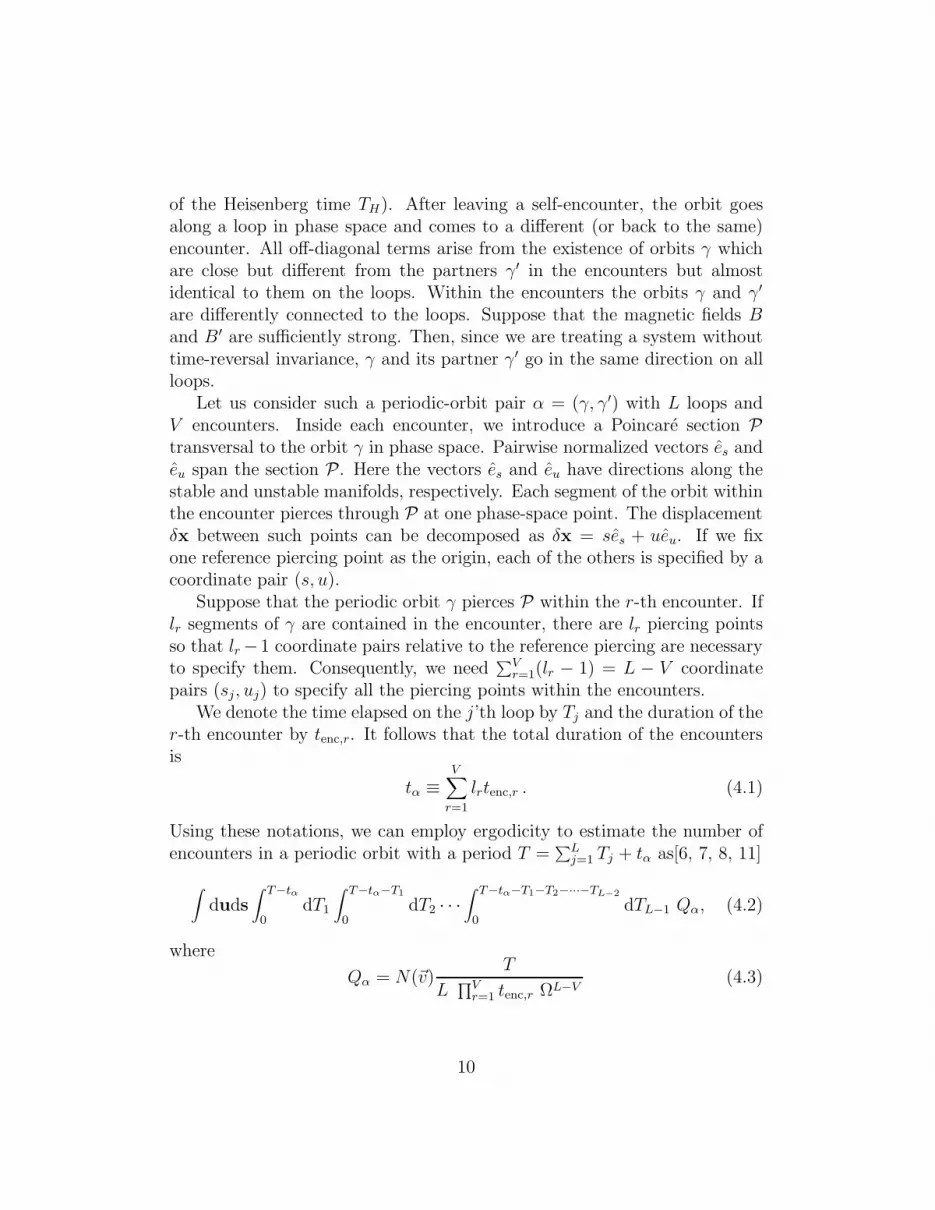
of the Heisenberg time TH). After leaving a self-encounter, the orbit goesalong a loop in phase space and comes to a different (or back to the same)encounter. All off-diagonal terms arise from the existence of orbits γ whichare close but different from the partners γ′ in the encounters but almostidentical to them on the loops. Within the encounters the orbits γ and γ′

are differently connected to the loops. Suppose that the magnetic fields Band B′ are sufficiently strong. Then, since we are treating a system withouttime-reversal invariance, γ and its partner γ′ go in the same direction on allloops.

Let us consider such a periodic-orbit pair α = (γ, γ′) with L loops andV encounters. Inside each encounter, we introduce a Poincare section Ptransversal to the orbit γ in phase space. Pairwise normalized vectors es andeu span the section P. Here the vectors es and eu have directions along thestable and unstable manifolds, respectively. Each segment of the orbit withinthe encounter pierces through P at one phase-space point. The displacementδx between such points can be decomposed as δx = ses + ueu. If we fixone reference piercing point as the origin, each of the others is specified by acoordinate pair (s, u).

Suppose that the periodic orbit γ pierces P within the r-th encounter. Iflr segments of γ are contained in the encounter, there are lr piercing pointsso that lr −1 coordinate pairs relative to the reference piercing are necessaryto specify them. Consequently, we need

∑Vr=1(lr − 1) = L − V coordinate

pairs (sj, uj) to specify all the piercing points within the encounters.We denote the time elapsed on the j’th loop by Tj and the duration of the

r-th encounter by tenc,r. It follows that the total duration of the encountersis

tα ≡V∑

r=1

lrtenc,r . (4.1)

Using these notations, we can employ ergodicity to estimate the number ofencounters in a periodic orbit with a period T =

∑Lj=1 Tj + tα as[6, 7, 8, 11]

∫

duds∫ T−tα

0dT1

∫ T−tα−T1

0dT2 · · ·

∫ T−tα−T1−T2−···−TL−2

0dTL−1 Qα, (4.2)

where

Qα = N(~v)T

L∏V

r=1 tenc,r ΩL−V(4.3)

10

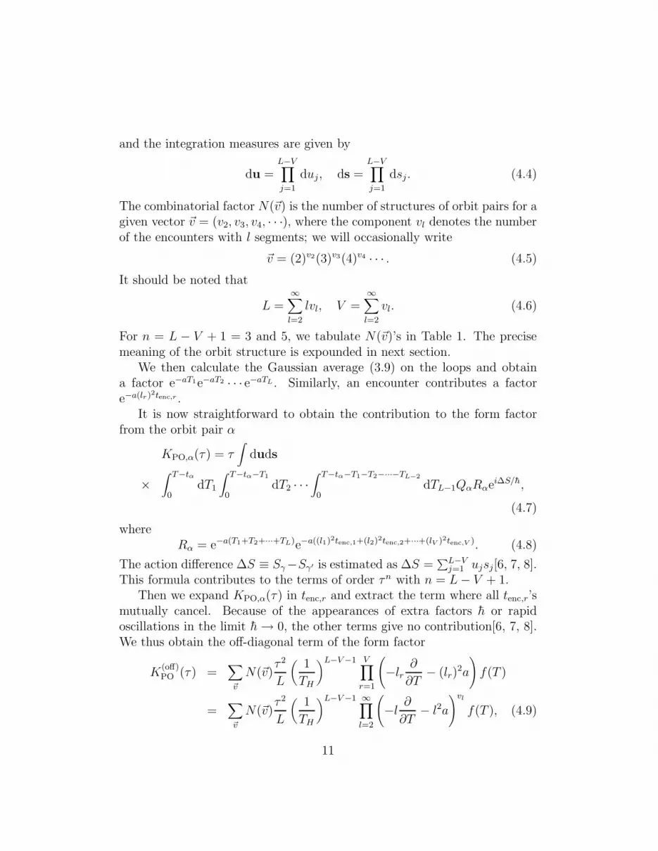
and the integration measures are given by

du =L−V∏

j=1

duj, ds =L−V∏

j=1

dsj . (4.4)

The combinatorial factor N(~v) is the number of structures of orbit pairs for agiven vector ~v = (v2, v3, v4, · · ·), where the component vl denotes the numberof the encounters with l segments; we will occasionally write

~v = (2)v2(3)v3(4)v4 · · · . (4.5)

It should be noted that

L =∞∑

l=2

lvl, V =∞∑

l=2

vl. (4.6)

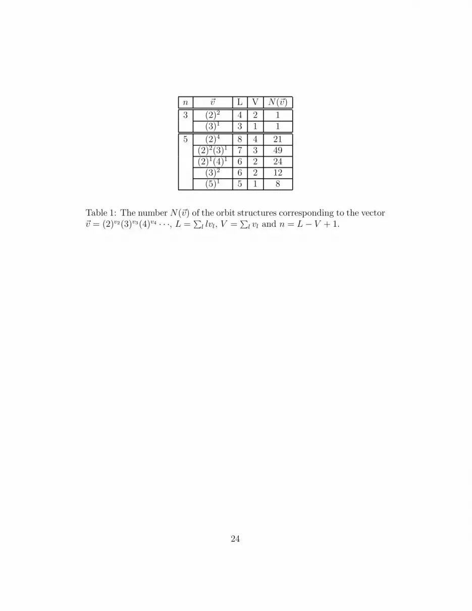
For n = L − V + 1 = 3 and 5, we tabulate N(~v)’s in Table 1. The precisemeaning of the orbit structure is expounded in next section.

We then calculate the Gaussian average (3.9) on the loops and obtaina factor e−aT1e−aT2 · · · e−aTL . Similarly, an encounter contributes a factore−a(lr)2tenc,r .

It is now straightforward to obtain the contribution to the form factorfrom the orbit pair α

KPO,α(τ) = τ∫

duds

×∫ T−tα

0dT1

∫ T−tα−T1

0dT2 · · ·

∫ T−tα−T1−T2−···−TL−2

0dTL−1QαRαei∆S/h,

(4.7)

whereRα = e−a(T1+T2+···+TL)e−a((l1)2tenc,1+(l2)2tenc,2+···+(lV )2tenc,V ). (4.8)

The action difference ∆S ≡ Sγ−Sγ′ is estimated as ∆S =∑L−V

j=1 ujsj[6, 7, 8].This formula contributes to the terms of order τn with n = L − V + 1.

Then we expand KPO,α(τ) in tenc,r and extract the term where all tenc,r’smutually cancel. Because of the appearances of extra factors h or rapidoscillations in the limit h → 0, the other terms give no contribution[6, 7, 8].We thus obtain the off-diagonal term of the form factor

K(off)PO (τ) =

∑

~v

N(~v)τ 2

L

(

1

TH

)L−V −1 V∏

r=1

(

−lr∂

∂T− (lr)

2a

)

f(T )

=∑

~v

N(~v)τ 2

L

(

1

TH

)L−V −1 ∞∏

l=2

(

−l∂

∂T− l2a

)vl

f(T ), (4.9)

11

where

f(T ) =∫ T

0dT1

∫ T−T1

0dT2 · · ·

∫ T−T1−T2−···−TL−2

0dTL−1e

−a(T1+T2+···TL). (4.10)

Let us put λ = aT and calculate the Laplace transform of K(off)PO (τ)/τ 2 as

∫ ∞

0e−qλ K

(off)PO (τ)

τ 2dλ

=∑

~v

N(~v)1

L

(

1

TH

)L−V −1 ∫ ∞

0dλe−qλ

∞∏

l=2

(

−l∂

∂T− l2a

)vl

f(T )

=∑

~v

N(~v)a

L

(

1

TH

)L−V −1 ∞∏

l=2

(

−laq − l2a)vl 1

(aq + a)L

=∞∑

n=2

1

(q + 1)n−1

(

1

aTH

)n−2 L−V +1=n∑

~v

N(~v)∞∏

l=2

(

1 + (l − 1)1

q + 1

)vl

,

(4.11)

where N(~v) = N(~v)(−1)V ∏∞l=2 lvl/L. In the above equation, a simple graph-

ical rule is observed: each loop contributes a factor 1/(a(q + 1)) and eachencounter contributes −la(q + l). In next section, we shall prove a sumformula for n ≥ 2

L−V +1=n∑

~v

N(~v)∞∏

l=2

(

1 + (l − 1)1

q + 1

)vl

=

(2n − 3)!

n!

(

1

q + 1

)n−1

, n odd,

0, n even,(4.12)

from which it follows that∫ ∞

0e−qλ K

(off)PO (τ)

τ 2dλ =

∞∑

j=1

1

(aTH)2j−1

(4j − 1)!

(2j + 1)!

1

(q + 1)4j. (4.13)

As aTH = (aT )(TH/T ) = λ/τ = η, this is in agreement with the RMT result(2.19).

5 A Sum Formula for N (~v)

In this section we shall give a proof for the sum formula (see (4.12))

L−V +1=n∑

~v

N(~v)∞∏

l=2

(1 + (l − 1)x)vl =

(2n − 3)!

n!xn−1, n odd,

0, n even(5.1)

12

with n ≥ 2. For that purpose we introduce a number NP (~v) depending onthe vector

~v = (1)v1(2)v2(3)v3(4)v4 · · · (5.2)

and set L =∑∞

l=1 lvl and V =∑∞

l=1 vl. Let us denote an “encounter” permu-tation of the numbers 1, 2, · · · , L as

Penc =

(

1 2 3 · · · LPenc(1) Penc(2) Penc(3) · · · Penc(L)

)

(5.3)

and define a “loop” permutation

Ploop =

(

1 2 3 · · · L − 1 L2 3 4 · · · L 1

)

. (5.4)

We define NP (~v) as the number of permutations Penc which satisfy the fol-lowing two conditions.

(A) The permutation Penc has vl cycles of length l.

(B) The product PloopPenc is a permutation with a single cycle.

Then it follows that

N((2)v2(3)v3(4)v4 · · ·) = NP ((1)0(2)v2(3)v3(4)v4 · · ·). (5.5)

In order to explain the reason, let us suppose the following situation. Theencounters include

∑Vr=1 lr = L orbit segments in total, so that there are L

“entrances” where the orbits come in and L “exits” where the orbits go out.A periodic orbit γ comes in an encounter at the first “entrance” and goesout at the first “exit”. Then it comes to the second “entrance” and goes outat the second “exit”. It continues to follow the connection pattern

j-th “entrance” → j-th “exit” → (j + 1)-th “entrance”

and finally goes out at the L-th “exit” and then comes back to the first“entrance” again. On the other hand, the partner orbit γ′ comes in anencounter at the first “entrance” and goes out at Penc(1)-th “exit”. Then itmust go to the PloopPenc(1)-th “entrance”, as the partners go along the sameloop. It continues to follow the pattern

j-th “entrance” → Penc(j)-th “exit” → PloopPenc(j)-th “entrance”

In this manner, if a permutation Penc is given, the structure of a periodicorbit γ′ is specified.

13

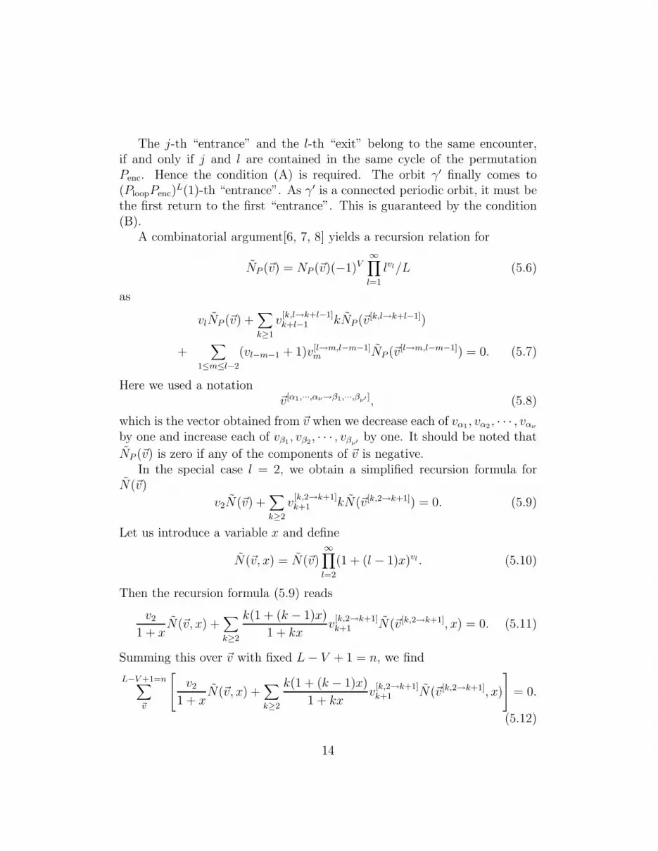
The j-th “entrance” and the l-th “exit” belong to the same encounter,if and only if j and l are contained in the same cycle of the permutationPenc. Hence the condition (A) is required. The orbit γ′ finally comes to(PloopPenc)

L(1)-th “entrance”. As γ′ is a connected periodic orbit, it must bethe first return to the first “entrance”. This is guaranteed by the condition(B).

A combinatorial argument[6, 7, 8] yields a recursion relation for

NP (~v) = NP (~v)(−1)V∞∏

l=1

lvl/L (5.6)

as

vlNP (~v) +∑

k≥1

v[k,l→k+l−1]k+l−1 kNP (~v[k,l→k+l−1])

+∑

1≤m≤l−2

(vl−m−1 + 1)v[l→m,l−m−1]m NP (~v[l→m,l−m−1]) = 0. (5.7)

Here we used a notation~v[α1,···,αν→β1,···,βν′ ], (5.8)

which is the vector obtained from ~v when we decrease each of vα1 , vα2 , · · · , vαν

by one and increase each of vβ1 , vβ2, · · · , vβν′by one. It should be noted that

NP (~v) is zero if any of the components of ~v is negative.In the special case l = 2, we obtain a simplified recursion formula for

N(~v)

v2N(~v) +∑

k≥2

v[k,2→k+1]k+1 kN(~v[k,2→k+1]) = 0. (5.9)

Let us introduce a variable x and define

N(~v, x) = N(~v)∞∏

l=2

(1 + (l − 1)x)vl . (5.10)

Then the recursion formula (5.9) reads

v2

1 + xN(~v, x) +

∑

k≥2

k(1 + (k − 1)x)

1 + kxv

[k,2→k+1]k+1 N(~v[k,2→k+1], x) = 0. (5.11)

Summing this over ~v with fixed L − V + 1 = n, we find

L−V +1=n∑

~v

v2

1 + xN(~v, x) +

∑

k≥2

k(1 + (k − 1)x)

1 + kxv

[k,2→k+1]k+1 N(~v[k,2→k+1], x)

= 0.

(5.12)

14

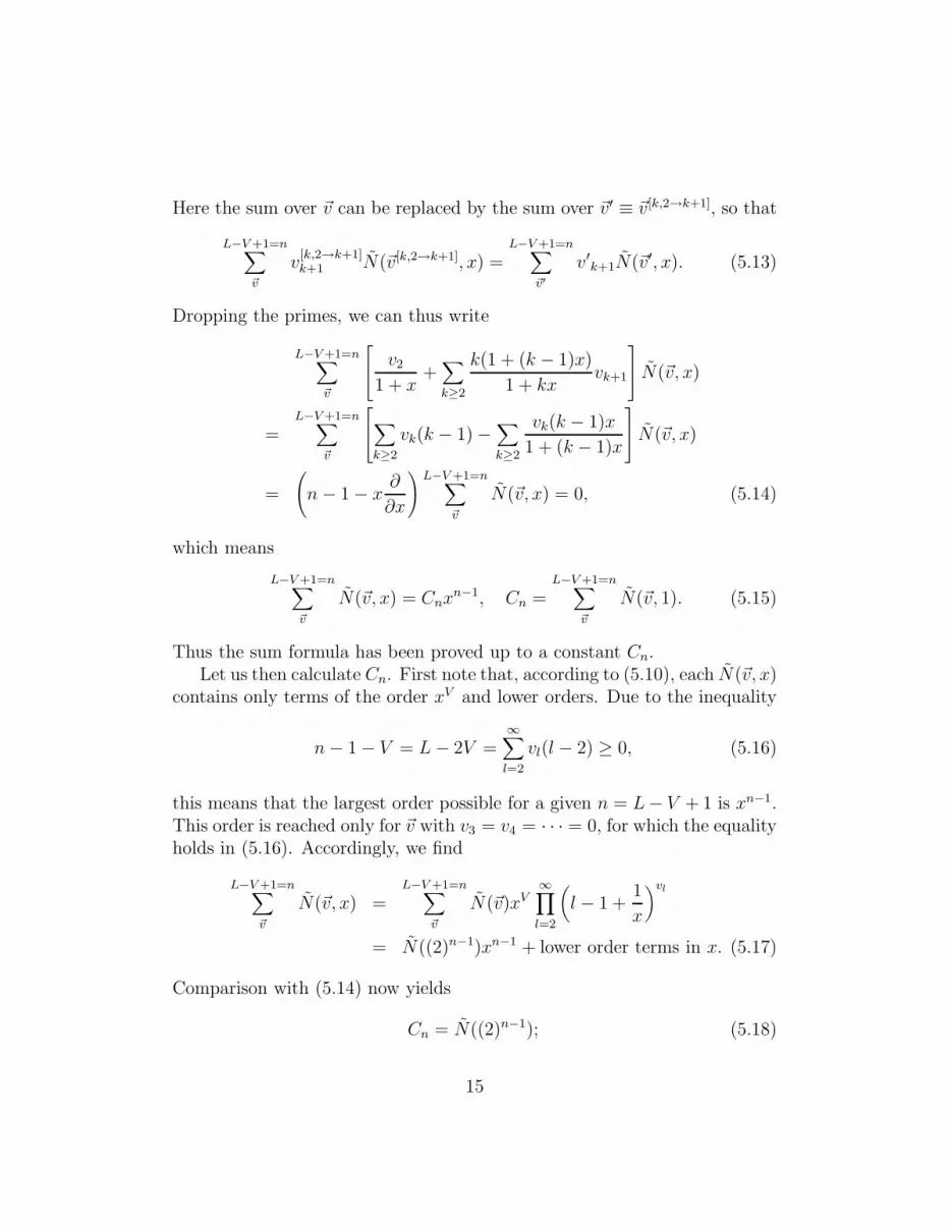
Here the sum over ~v can be replaced by the sum over ~v′ ≡ ~v[k,2→k+1], so that

L−V +1=n∑

~v

v[k,2→k+1]k+1 N(~v[k,2→k+1], x) =

L−V +1=n∑

~v′

v′k+1N(~v′, x). (5.13)

Dropping the primes, we can thus write

L−V +1=n∑

~v

v2

1 + x+∑

k≥2

k(1 + (k − 1)x)

1 + kxvk+1

N(~v, x)

=L−V +1=n∑

~v

∑

k≥2

vk(k − 1) −∑

k≥2

vk(k − 1)x

1 + (k − 1)x

N(~v, x)

=

(

n − 1 − x∂

∂x

)

L−V +1=n∑

~v

N(~v, x) = 0, (5.14)

which means

L−V +1=n∑

~v

N(~v, x) = Cnxn−1, Cn =L−V +1=n∑

~v

N(~v, 1). (5.15)

Thus the sum formula has been proved up to a constant Cn.Let us then calculate Cn. First note that, according to (5.10), each N(~v, x)

contains only terms of the order xV and lower orders. Due to the inequality

n − 1 − V = L − 2V =∞∑

l=2

vl(l − 2) ≥ 0, (5.16)

this means that the largest order possible for a given n = L− V + 1 is xn−1.This order is reached only for ~v with v3 = v4 = · · · = 0, for which the equalityholds in (5.16). Accordingly, we find

L−V +1=n∑

~v

N(~v, x) =L−V +1=n∑

~v

N(~v)xV∞∏

l=2

(

l − 1 +1

x

)vl

= N((2)n−1)xn−1 + lower order terms in x. (5.17)

Comparison with (5.14) now yields

Cn = N((2)n−1); (5.18)

15

all terms of lower orders in x must mutually cancel. In order to evaluateN((2)n−1), we can utilize a closed expression for NP (~v) (with vj ≥ 0 forj ≤ Λ and vj = 0 for j > Λ)

NP (~v) =(−1)V

L(L + 1)

v1∑

h1=0

v2∑

h2=0

· · ·vΛ∑

hΛ=0

(−1)∑Λ

j=1(j+1)hj

(Λ∑

j=1

jhj)!(Λ∑

j=1

j(vj − hj))!

Λ∏

j=1

[hj !(vj − hj)!]

,

(5.19)which was derived by Jurgen Muller[17]. Using the identity

∫ ∞

0e−ssjds = j!, (5.20)

we can rewrite Jurgen Muller’s formula as

NP (~v) =(−1)V

L(L + 1)

∫ ∞

0dx∫ ∞

0dy e−xe−y

∞∏

j=1

(yj − (−x)j)vj

vj !, (5.21)

so that

N((2)n−1) = NP ((2)n−1)

=(−1)n−1

2(n − 1)(2n − 1)(n − 1)!

∫ ∞

0dx∫ ∞

0dy e−xe−y(y2 − x2)n−1

=(−1)n−1

4(n − 1)(2n − 1)(n − 1)!

∫ ∞

0ds∫ s

−sdt e−ssn−1tn−1

=

(2n − 3)!

n!, n odd,

0, n even(5.22)

(s = x + y, t = x − y), which establishes the desired result (5.1).It is easy to check that Jurgen Muller’s formula holds for ~v’s with small

L − V (for example, NP ((1)1) = −1). Therefore, in order to prove it ingeneral, it is sufficient to verify that it fulfills the recursion relation (5.7).For that purpose, we first define an “average” 〈· · ·〉~v of a function f(x, y) as

〈f(x, y)〉~v =∫ ∞

0dx∫ ∞

0dye−xe−yf(x, y)

∞∏

j=1

(yj − (−x)j)vj . (5.23)

16

Since NP (~v) = 0 if any of vj is negative, (5.7) evidently holds if vl = 0. Hencewe focus on the case vl ≥ 1. Then partial integrations yield a relation

〈1〉~v − l

⟨

yl−1 + (−x)l−1

yl − (−x)l

⟩

~v

= 〈1〉~v −⟨

∂

∂y

(

yl

yl − (−x)l

)

− ∂

∂x

(

(−x)l

yl − (−x)l

)

− ly2l−1 − (−x)2l−1

(yl − (−x)l)2

⟩

~v

=∫ ∞

0dx∫ ∞

0dye−xe−y

×[

yl

yl − (−x)l

∂

∂y− (−x)l

yl − (−x)l

∂

∂x− l

y2l−1 − (−x)2l−1

(yl − (−x)l)2

]

∞∏

j=1

(yj − (−x)j)vj

(5.24)

for l = 1, 2, · · · , L. Using this relation and the identity[

yl

yl − (−x)l

∂

∂y− (−x)l

yl − (−x)l

∂

∂x

]

∞∏

j=1

(yj − (−x)j)vj

=∑

k≥1

kvkyk+l−1 − (−x)k+l−1

(yl − (−x)l)(yk − (−x)k)

∞∏

j=1

(yj − (−x)j)vj , (5.25)

we can readily derive

〈1〉~v − l

⟨

yl−1 + (−x)l−1

yl − (−x)l

⟩

~v

=∑

k≥1

k

⟨

(vk − δkl)yk+l−1 − (−x)k+l−1

(yl − (−x)l)(yk − (−x)k)

⟩

~v

.

(5.26)The following identity

∫ ∞

0dx∫ ∞

0dy e−ωxe−ωy 1

x + y

∞∏

j=1

(yj − (−x)j)vj

= ω−L−1∫ ∞

0dx∫ ∞

0dy e−xe−y 1

x + y

∞∏

j=1

(yj − (−x)j)vj (5.27)

can be proved by a transformation of the variables ωx 7→ x, ωy 7→ y. Differ-entiating the both sides of this identity with respect to ω and then puttingω = 1, we obtain a relation

1

L + 1〈1〉~v =

⟨

1

x + y

⟩

~v

, (5.28)

17

from which it follows that

1

L + 1〈1〉~v =

⟨

1

yl − (−x)l

yl−1 + (−x)l−1 − xyl−1 + y(−x)l−1

x + y

⟩

~v

. (5.29)

Then, utilizing

xyl−1 + y(−x)l−1

x + y= −1

2

∑

1≤m≤l−2

[

(−x)myl−m−1 + (−x)l−m−1ym]

, (5.30)

we find

− 2

L + 1〈1〉~v + l

⟨

yl−1 + (−x)l−1

yl − (−x)l

⟩

~v

=∑

1≤m≤l−2

⟨

(ym − (−x)m)(yl−m−1 − (−x)l−m−1)

yl − (−x)l

⟩

~v

. (5.31)

Adding the both sides of (5.26) and (5.31), we arrive at

L − 1

L + 1〈1〉~v =

∑

k≥1

k

⟨

(vk − δkl)yk+l−1 − (−x)k+l−1

(yl − (−x)l)(yk − (−x)k)

⟩

~v

+∑

1≤m≤l−2

⟨

(ym − (−x)m)(yl−m−1 − (−x)l−m−1)

yl − (−x)l

⟩

~v

, (5.32)

which gives the desired recursion relation (5.7) with Jurgen Muller’s formula(5.21) substituted.

6 The GOE to GUE Transition

The equal-parameter correlation function R(s; B, B) describes the transitionbetween the GOE and GUE universality classes as the magnetic field Bincreases from zero[11, 18, 19]. In this section, we shall reproduce Saito andNagao’s semiclassical calculation[11] of the form factor (the Fourier transformof R(s; B, B)) and further derive a sum formula analogous to (5.1) as aconjecture.

The RMT prediction of the form factor in this case is derived from Pandeyand Mehta’s two-matrix model[20]. For small τ (0 ≤ τ ≤ 1), it can be written

18

as

KRM(τ) = τ +1

2

∫ 1

1−2τdk

k

k + 2τe−µ(k+τ)

= τ + e−µτ + e−µ

(

sinh τµ

µ− τ

)

− 2τ 2eµ(τ−1)∫ 1

0

e−2τµy

1 + 2τydy.

(6.1)

In the GOE limit the parameter µ is zero and in the GUE limit it goes toinfinity.

The semiclassical argument is similar to that in § 3 and § 4. The differenceis that we have to take account of the mutually time reversed pairs of loopsand segments of classical orbits. Following a similar argument as in § 3, weobtain a diagonal approximation for the form factor

K(diag)PO (τ) = τ + τe−bT , (6.2)

b = 4B2D/h2 . (6.3)

The RMT parameter µ should be equated with bT in reference to the semi-classical result.

In order to extend the calculation to the off-diagonal terms, we needto introduce integers nenc,r and M characterizing the structure of the orbitpairs as follows. Let us fix an arbitrary direction (+) in which the orbits passthrough the r-th encounter and call the opposite direction (−). Suppose thatthe orbit γ passes through the encounter #(+)(γ) and #(−)(γ) times in (+)and (−) directions, respectively. We then define the number nenc,r as

nenc,r =1

2

∣

∣

∣

#(+)(γ) − #(−)(γ)

−

#(+)(γ′) − #(−)(γ′)∣

∣

∣ . (6.4)

Moreover we define M as the number of the pairs of mutually time reversedloops.

As before, for a general orbit pair α with L loops and V encounters, thenumber of encounters in one periodic orbit of a period T is evaluated as

∫

duds∫ T−tα

0dT1

∫ T−tα−T1

0dT2 · · ·

∫ T−tα−T1−T2−···−TL−2

0dTL−1 Qα, (6.5)

where

Qα = N(v, M)T

L∏V

r=1 tenc,r ΩL−V. (6.6)

19

Here the combinatorial factor N(v, M) depends on a matrix v and M . Thecomponent vlm of the matrix v is the number of the encounters with lr = land nenc,r = m. One can write

v = (2, 0)v20(2, 1)v21(2, 2)v22 · · · . (6.7)

Following the argument in [6, 7, 8], we can identify N(v, M) with the numberof generalized permutations satisfying suitable conditions.

Let us consider the effect of the gauge potential. The Gaussian average(3.9) on the loops gives a factor e−bT1e−bT2 · · · e−bTM , while from an encounterit yields e−b(nenc,r)2tenc,r . Thus we conclude that the total contribution to theform factor from the orbit pair α is

KPO,α(τ) = τ∫

duds

×∫ T−tα

0dT1

∫ T−tα−T1

0dT2 · · ·

∫ T−tα−T1−T2−···−TL−2

0dTL−1QαRαei∆S/h

(6.8)

with

Rα = e−b(T1+T2+···+TM )e−b((nenc,1)2tenc,1+(nenc,2)2tenc,2+···+(nenc,V )2tenc,V ). (6.9)

This contributes to the terms of order τn with n = L − V + 1. As beforewe expand KPO,α(τ) in tenc,r and extract the term where all tenc,r’s mutuallycancel. Then we find that the off diagonal contribution to the form factor is

K(off)PO (τ) =

∑

v

L∑

M=0

N(v, M)τ 2

L

(

1

TH

)L−V −1 ∞∏

l=2

∞∏

m=0

(

−l∂

∂T− m2b

)vlm

f(T, M),

(6.10)where

f(T, M) =∫ T

0dT1

∫ T−T1

0dT2 · · ·

∫ T−T1−T2−···−TL−2

0dTL−1e

−b(T1+T2+···TM ).

(6.11)If M = 0, the direction of motion along all loops and hence in all encountersdoes not change in the partner orbit; consequently nenc,r = 0 for all encoun-ters. The corresponding structures also exist in the case without time-reversalinvariance, so that

N(v, 0) =

N((2)v20(3)v30 · · ·), if all vnj with j 6= 0 vanish,0, otherwise.

(6.12)

20

Here N(~v) is the number of structures introduced in § 4 and § 5. Timereversal of each such partner orbit produces another partner with M = L;therefore

N(v, L) =

N((2)v22(3)v33 · · ·), if all vnj with j 6= n vanish,0, otherwise.

(6.13)

Note that the structures with M = 0, L may exist only for odd n = L−V +1;see [7].

Noting the above relations for the combinatorial factors, we can eval-uate the contribution of the structures with M = 0, L in the same wayas in § 4, namely by Laplace-transforming the corresponding summands inK

(off)PO (τ)/τ 2, using the sum rule (5.1) for N(~v) and transforming back to the

time representation. The contribution of the structures with M = 0 turns outto be zero whereas the structures with M = L reproduce the third summandin the last line of (6.1). On the other hand, making the Laplace transform of

the part of K(off)PO (τ)/τ 2 with 1 ≤ M ≤ L − 1 and equating the result to the

corresponding RMT prediction deduced from the integral in the last line of(6.1), we arrive at a conjecture

L−V +1=n∑

v

L−1∑

M=1

N(v, M)

L

(−1)V

(1 + x)M

∞∏

l=2

∞∏

m=0

(l + m2x)vlm

=1

(1 + x)n−1

n−1∑

p=1

(

x

1 + x

)n−p−1

(2n − p − 3)!n−1∑

j=p

(−1)j2j

j(n − j − 1)!(j − p)!.

(6.14)

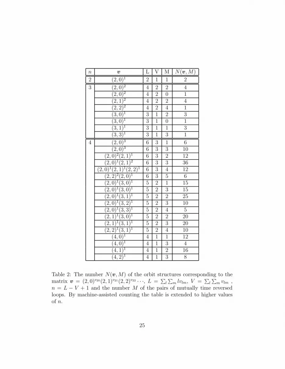
In the cases n = 2 and 3, the conjecture (6.14) was substantially proved in[11]; by machine-assisted counting it was verified up to n = 7. For small val-ues of n up to 4, the relevant N(v, M)’s are tabulated in Table 2. Moreover,putting x = 0, we obtain

L−V +1=n∑

v

L−1∑

M=1

N(v, M)

L(−1)V

∞∏

l=2

lvl = (−2)n−1 (n − 2)!

n − 1(6.15)

(vl =∑∞

m=0 vlm), which is relevant to the GOE form factor. This specialcase was proved in [6, 7, 8]. The full proof of (6.14) is an interesting openproblem.

21

Acknowledgements

This work was partially supported by the Ministry of Education, Culture,Sports, Science and Technology, Government of Japan (KAKENHI 16740224)and by the Sonderforschungsbereich SFB/TR12 of the Deutsche Forschungs-gemeinschaft. The authors are grateful to Dr. Jurgen Muller for providinghis original result[17] before publication.

References

[1] O. Bohigas, M.J. Giannoni and C. Schmit, Phys. Rev. Lett. 52

(1984) 1.

[2] M. Gutzwiller, Chaos in Classical and Quantum Mechanics

(Springer, 1990).

[3] M.V. Berry, Proc. R. Soc. London A400 (1985) 229.

[4] M. Sieber and K. Richter, Physica Scripta T90 (2001) 128.

[5] S. Heusler, S. Muller, P. Braun and F. Haake, J. Phys. A37 (2004)L31.

[6] S. Muller, S. Heusler, P. Braun, F. Haake and A. Altland, Phys.Rev. Lett. 93 (2004) 014103-1.

[7] S. Muller, S. Heusler, P. Braun, F. Haake and A. Altland, Phys.Rev. E72 (2005) 046207.

[8] S. Muller, Periodic-Orbit Approach to Universality in Quan-

tum Chaos (doctoral thesis, Universitat Duisburg-Essen, 2005),nlin.CD/0512058.

[9] G. Lenz and F. Haake, Phys. Rev. Lett. 65 (1990) 2325.

[10] F. Haake, Quantum Signatures of Chaos (2nd edition, Springer,2000).

[11] K. Saito and T. Nagao, Phys. Lett. A352 (2006) 380.

[12] F.J. Dyson, J. Math. Phys. 3 (1962) 1191.

22

[13] H. Spohn, Hydrodynamic Behavior and Interacting Particle Systems

(the IMA Volumes in Mathematics and its Applications vol.9, G.Papanicolaou (ed.), Springer, 1987) 151.

[14] T. Nagao and P.J. Forrester, Phys. Lett. A247 (1998) 42.

[15] K. Richter, Semiclassical Theory of Mesoscopic Quantum Systems

(Springer, 2000).

[16] J.H. Hannay and A.M. Ozorio de Almeida, J. Phys. A17 (1984)3429.

[17] J. Muller, ”On a mysterious partition identity”, preprint, 2003.

[18] O. Bohigas, M.-J. Giannoni, A.M. Ozorio de Almeida and C.Schmit, Nonlinearity 8 (1995) 203.

[19] T. Nagao and K. Saito, Phys. Lett. A311 (2003) 353.

[20] A. Pandey and M.L. Mehta, Commun. Math. Phys. 87 (1983) 449.

23

n ~v L V N(~v)

3 (2)2 4 2 1(3)1 3 1 1

5 (2)4 8 4 21(2)2(3)1 7 3 49(2)1(4)1 6 2 24

(3)2 6 2 12(5)1 5 1 8

Table 1: The number N(~v) of the orbit structures corresponding to the vector~v = (2)v2(3)v3(4)v4 · · ·, L =

∑

l lvl, V =∑

l vl and n = L − V + 1.

24

n v L V M N(v, M)

2 (2, 0)1 2 1 1 2

3 (2, 0)2 4 2 2 4(2, 0)2 4 2 0 1(2, 1)2 4 2 2 4(2, 2)2 4 2 4 1(3, 0)1 3 1 2 3(3, 0)1 3 1 0 1(3, 1)1 3 1 1 3(3, 3)1 3 1 3 1

4 (2, 0)3 6 3 1 6(2, 0)3 6 3 3 10

(2, 0)2(2, 1)1 6 3 2 12(2, 0)1(2, 1)2 6 3 3 36

(2, 0)1(2, 1)1(2, 2)1 6 3 4 12(2, 2)2(2, 0)1 6 3 5 6(2, 0)1(3, 0)1 5 2 1 15(2, 0)1(3, 0)1 5 2 3 15(2, 0)1(3, 1)1 5 2 2 25(2, 0)1(3, 2)1 5 2 3 10(2, 0)1(3, 3)1 5 2 4 5(2, 1)1(3, 0)1 5 2 2 20(2, 1)1(3, 1)1 5 2 3 20(2, 2)1(3, 1)1 5 2 4 10

(4, 0)1 4 1 1 12(4, 0)1 4 1 3 4(4, 1)1 4 1 2 16(4, 2)1 4 1 3 8

Table 2: The number N(v, M) of the orbit structures corresponding to thematrix v = (2, 0)v20(2, 1)v21(2, 2)v22 · · ·, L =

∑

l

∑

m lvlm, V =∑

l

∑

m vlm ,n = L − V + 1 and the number M of the pairs of mutually time reversedloops. By machine-assisted counting the table is extended to higher valuesof n.

25