semiclassical effects and the onset of inflation
TRANSCRIPT
arX
iv:g
r-qc
/920
9007
v1 1
6 Se
p 19
92
Semiclassical Effects and the Onset of Inflation
Esteban Calzetta
[*] Instituto de Astronomıa y Fısica del Espacio
cc 67, suc 28, (1428) Buenos Aires, Argentina
Maria Sakellariadou
[†,‡] Research Group on General Relativity
Faculte des Sciences, Universite Libre de Bruxelles
CP 231 Campus Plaine, Boulevard du Triomphe, 1050 Bruxelles, Belgium
(Received )
We present a class of exact solutions to the constraint equations of General Rel-
ativity coupled to a Klein - Gordon field, these solutions being isotropic but not
homogeneous. We analyze the subsequent evolution of the consistent Cauchy data
represented by those solutions, showing that only certain special initial conditions
eventually lead to successfull Inflationary cosmologies. We argue, however, that these
initial conditions are precisely the likely outcomes of quantum events occurred before
the inflationary era.
98.80.Cq,98.80.Dr
Typeset Using REVTEX
1
I. INTRODUCTION
In this paper we address the issue of the relevance of semiclassical cosmological effects to
Inflation in the Very Early Universe. To this end, we consider spherically symmetric models
in which the geometry is coupled to a massive, free, minimally coupled real scalar field. We
propose a particular choice of gauge, which allows us to solve Einstein’s constraint equations
( see below ) exactly, in closed form, in the case of interest. We then use the self consistent
Cauchy data so obtained to discuss the necessary conditions for “natural” Inflation (see
below), and match these conditions against those likely to result out of a semiclassical era.
From this analysis, we conclude that semiclassical effects enhance the likelihood of Inflation.
The combination of the Hot Big Bang Model and Inflation provides at present the most
comprehensive picture of the evolution of the Universe at our disposal. To the well known
successfull quantitative predictions of the Big Bang model ( such as the existence and tem-
perature of the Cosmic Microwave Background, the relative abundances of light elements
and the red shift of distant galaxies [1] ), Inflation adds a plausible explanation for the
near critical value of the observed density in the Universe [2]. It also predicts a primordial
fluctuations spectrum whose amplitude has the right order of magnitude, as checked against
recent observations [3] However, this class of cosmological models rests on the assumption
of highly specific initial conditions for the cosmic evolution. This situation is hardly accept-
able, specially because alleviating the fine tuning of initial conditions, as required by the Big
Bang model, was historically one of the motivations to investigate inflationary cosmologies
[4].
It should be stressed that the proper study of the necessary conditions for Inflation
requires the consideration of nonlinear effects; indeed, linear perturbations of an Inflationary
solution are eventually redshifted away, and cannot affect the global characther of the cosmic
evolution [5]. However, nonlinear perturbations can decouple themselves from the Hubble
flow and destroy the homogeneity that Inflation is supposed to bring about.
Non linear perturbations of an Inflationary model have been considered by a number
2
of authors [6], most notably in a series of numerical simulations by Goldwirth and Piran
[7]. These analysis concur in that Inflation demands initial conditions which are already
homogeneous over regions larger than the original horizon size. This homogeneity cannot
be accounted for through ( classical ) physical processes acting in the pre - Inflationary era.
Therefore, to achieve successfull Inflation in classical cosmology, some fine tuning of initial
conditions cannot be avoided.
The details of how initial conditions should be fixed vary with the different versions of
the inflationary model in the literature. In this paper, we shall consider only the “chaotic”
inflationary model [8], where Inflation is sustained by the stress energy of a free Klein Gordon
field, in an Universe born from an initial singularity. We choose these models because their
extreme simplicity makes them the most universal of inflationary cosmologies.
The limitations on initial conditions required by chaotic inflation can be understood
in a back of the envelope calculation, as follows. Suppose an inflaton field φ of mass m,
varying over distances λ, being the source for an inflationary expansion with Hubble constant
H ∼ mφ/mp, where mp stands for Planck’s mass . The condition of vacuum dominance
requires mλ ≫ 1 and φ ≪ mφ, where a dot is a derivative with respect to cosmological
time. On the other hand, under conditions of slow roll over, φ ∼ m2φ/H, from where we
get φ ≫ mp, and λ ≫ m−1 ≫ H−1. A more carefull analysis shows that λ should be some
ten times the horizon size [9].
While this result shows that Inflation in no way frees the present state of the Universe
from dependence on initial conditions, the question remains about the relative likelihood of
inflationary initial conditions as opposed to generic ones. Nevertheless, here too, as long as
we remain within the framework of classical cosmology, Inflation proves itself of little use.
General Relativity being a time reversal invariant theory, final and initial configurations are
in a one to one correspondence. Therefore no mechanism such as Inflation can enhance
the likelihood of a particular set of final states ( of course, this holds as long as one does
not introduce an ad hoc measure in configuration space ). In other words, the inflationary
hypothesis does not render a homogeneous and isotropic Universe any more likely than
3
simply to assume homogeneity and isotropy to begin with.
The situation changes when semiclassical effects are taken into account. Indeed, while
quantum fields in curved spaces evolve unitarily, it is generally impossible in concrete sit-
uations to determine exactly the quantum state of a given field. For example, while we
know the occupation numbers of the different modes in the Background Microwave Radi-
ation, we would be hardly pressed to determine the correlations between different modes
as well. Therefore, in practice, quantum fluctuations act as a bath or environment for the
macroscopic degrees of freedom of the Universe, and these evolve following a dissipative
effective dynamics, whereby time reversal invariance is broken [10]. Under these circum-
stances, while we know that the present state of the Universe cannot be rendered totally
independent of initial conditions, it makes sense again to ask for the relative likelihood of
inflating cosmologies.
A similar set of questions have already been investigated in the framework of homoge-
neous cosmological models. In ref. [11] it has been shown that the back reaction of conformal
particles created by a Taub Universe helps to delay recollapse [12], and thereby increases
the likelihood of Inflation ( in these models, Inflation occurs when the Universe reaches a
size such that the cosmological constant overpowers shear in the Hamiltonian constraint ).
This was done by following the evolution self consistently, in the approximation were the
back reaction of created particles is taken into account, but vacuum polarization terms are
neglected.
In this paper, we shall study the relevance of semiclassical effects to Inflation in inho-
mogeneous but isotropic, with respect to a singled out point, models. In this context, to
solve for the evolution self consistently is no longer possible. Rather, we shall follow the
strategy of concentrating on a particular Cauchy surface, which is assumed to lie at the
future of the semiclassical era, but at the past of the inflationary one. Thus, the Cauchy
data on this surface are themselves the outcome of the semiclassical era. We shall study
self consistent sets of Cauchy data, that is, solutions of Einstein’s constraint equations, and
obtain conditions for a set of data to lead to “natural”Inflation. We shall consider Inflation
4
to be natural if there is a significative probability that, well after Inflation has begun, any
nondescript observer will find him or herself into an Inflating, near Friedmann - Robertson
- Walker like region. Then we shall show that these conditions are already contained in
the requirement of consistence with an earlier semiclassical era. In other words, we shall
conclude that semiclassical effects select Cauchy data leading to natural Inflation.
Our analysis shall proceed in the Hamiltonian, or ADM [13], formulation of General
Relativity. Any spherically symmetric metric comprises two physical degrees of freedom,
and two Lagrange multipliers, the lapse function, and the shift in the radial direction; the
Klein - Gordon field introduces an extra degree of freedom. The Lagrange multipliers are
associated to two nontrivial constraints, which in turn allow us to impose two arbitrary gauge
conditions on the model ( we shall use this freedom to simplify the equations below, rather
than opting for a gauge invariant formulation ). Our tactic shall be to use the constraints and
the gauge freedom to fix entirely the space metric and the geometrodynamical momenta; the
lapse and shift are then defined by the requirement of consistency of the dynamical Einstein’s
equations. This approach leaves the Klein - Gordon equation ( written in Hamiltonian form
) as the only dynamical law.
In this paper we shall keep a specific physical situation in mind. We found it convenient
to take advantage of the gauge freedom in General Relativity to obtain this particular
scenario in its simplest form. For this reason, we shall adopt a “custom made” gauge, rather
than any of the usual choices, such as maximal slicing [13], a Tolman - like metric [14], or a
synchronous gauge. For the same reason, we shall develop an analysis of the Einstein - Klein
- Gordon system from first principles, rather than apply the general solutions available in
the literature [15].
The situation of interest is as follows. As we have seen in our “back of the envelope”
argument above, successfull chaotic Inflation requires a very high and homogeneous initial
value of the field ( we shall not discuss here the possible sources of such field values; they
occur in quantum cosmological models based on the Hartle - Hawking “ no boundary ”
proposal [16]). Whatever the mechanism to provide such configuration, it is physically
5
likely that quantum and/or thermal fluctuations will result in creating “holes” in the field,
that is, regions where the value of the field gets closer to its ( vanishing ) equilibrium value.
Of course a deep enough “hole” will not inflate at all, but a shallow “hole” may be capable
of inflating, thus becoming an Inflationary island or bubble in a larger Universe. This island
is, nevertheless, surrounded by a transition layer where conditions are far from homogeneity.
The naturalness condition, over and above the usual conditions on the field for there to be
Inflation, concerns the relative sizes of the island and the transition layer.
For simplicity, we shall consider a single island, so we shall assume that the field is high
and homogeneous far from the origin. Under these conditions, the metric will approach
asymptotically a Friedmann - Robertson - Walker ( FRW ) form. We shall use our gauge
freedom to force the three metric to keep a FRW form everywhere. Departures from homo-
geneity shall be coded into the lapse and shift functions. As we shall see below, in this gauge
we shall be able to display the dependence of these functions on the field and its conjugated
momentum in detail. This, in turn, will allow us to translate the naturalness condition into
a concrete inequality for the Cauchy data. In a number of cases of interest, such as when
the field momentum vanishes, the field itself being arbitrary, we shall obtain closed form,
exact expressions for lapse and shift. This is already a vast generalization over previously
known results [6,7,9]; the general case can be handled perturbatively.
Allthough we shall not discuss the evolution of these Cauchy data in detail, we shall show
below that the naturalness condition puts limits on the shift function accross the transition
layer. On the other hand, as we shall discuss in more detail in the body of the paper,
we expect the Universe to be conformally flat ( vanishing Weyl tensor ) by the end of the
quantum era [17]. The exact form of the self consistent Cauchy data previously obtained
shall allow us to show that, in this model, conformal flatness results in the same type of
conditions than naturalness. In this sense, therefore, it can be said that semiclassical effects
select for naturally inflating Cauchy data.
This result is both of relevance to cosmology, and of great interest as a non trivial ap-
plication of quantum field theory in curved spaces (QFTCS). This theory being only an
6
approximation to a yet unknown fully quantized theory of gravity, its meaningful applica-
tions are confined to weakly quantum effects, where gravitational quantum behavior is not
expected to be relevant. Given these restrictions, QFTCS is only capable to yield entirely
new results in phenomena where quantum effects are able to acummulate over time, there
being no classical phenomena in a position to screen them. The canonical example where
these conditions are fullfilled is Black Hole evaporation [18], which is still now possibly the
main area of development in QFTCS. Conformal particle creation, from the vacuum, in
cosmological settings, is similarly a cumulative, intrinsically quantum phenomenon. The
study of the effect of particle creation processes on the shape of our Universe is therefore,
beyond its relevance to cosmology, one of the few areas where QFTCS leads to observable
predictions, not to be obtained in classical theory.
The paper is organized as follows. In next section we present the model and the solution
of Einstein’s constraint equations. In section III, we discuss the conditions for natural
Inflation, the effect on Cauchy data of a semiclassical era, and the relationship between the
two. In section IV we briefly state our conclusions. A technical discussion of the solution of
the constraint equations for nonvanishing field momenta is included as an appendix.
II. SELF CONSISTENT SPHERICALLY SYMMETRIC CAUCHY DATA
A. Canonical Variables and Hamiltonian
In this section, we shall carry out an analysis of spherically symmetric solutions of the
constraint equations of the Einstein - Klein - Gordon system, in order to discuss in the next
section which Cauchy data eventually lead to acceptable inflationary cosmologies. We shall
adopt for our discussion the ADM formalism, whose starting point is the 3+1 decomposition
of the space - time metric as
ds2 = −N2dt2 + gij(dxi + N idt)(dxj + N jdt) (1)
7
Here, gij is the metric induced on a space like surface, on which the 3 + 1 decomposition
is based, and N , N i are the lapse and shift functions which describe the embedding of the
spatial surface into the four dimensional space time ( we follow MTW [13] conventions; latin
indexes run from 1 to 3 ). Assuming spherical symmetry, we may simplify Eq.(1) to
ds2 = −N2(R, t)dt2 + A2(R, t)(dR + ν(R, t)dt)2 + B2(R, t)dΩ, (2)
where we introduced ν = N1 and dΩ = dθ2 + sin2 θdϕ2. It is convenient to choose the
conformal degree of freedom of the space metric as one of the geometrodynamical variables.
Therefore, we rewrite Eq. (2) as
ds2 = −N2(R, t)dt2 + e2α(R,t)X−4/3(R, t)(dR + ν(R, t)dt)2 + X2/3(R, t)dΩ (3)
The peculiar parametrization of the conformal metric will be of use below.
If we take α and X as geometrodynamical canonical coordinates, then the canonical
momenta shall be parametrized in terms of two independent degrees of freedom, Πα and
ΠX , canonically conjugated to the respective variables. The full momentum tensor density,
in R, θ, ϕ coordinates, becomes
Πij = (
1
6)[Παδi
j +3
2XΠX(δi
j − 3δi1δ
1j )] (4)
With this parametrization, the “kinetic” term in the Hamiltonian
K = (16π
m2p
)Ng−1/2ΠijΠ
ji − (1/2)(Πi
i)2 (5)
(mp is Planck’s mass )becomes
K = (16π
m2p
)Ne−3α
24−Π2
α + 9X2Π2X (6)
The “shift” part of the Hamiltonian
S = Πij(Ni;j + Nj;i) (7)
becomes
8
S = (1/3)Πα(ν ′ + 3α′ν) − XΠXν ′ + X ′ΠXν, (8)
where a prime means a derivative with respect to R. Finally, the “potential” term
V = (−m2
p
16π)Ng1/2R (9)
( where R is the spatial curvature ) is best computed by observing that the spatial metric
is conformally flat. Indeed, introducing a new radial coordinate r through
dR
X=
dr
r(10)
The spatial metric becomes e2ω[dr2 + r2dΩ], where
ω = α + (1/3) lnX − ln r (11)
Therefore, we find
R = (−1)e−2ω4r−2∂rr2∂rω + 2(∂rω)2 (12)
or, in terms of R derivatives
V = (m2
p
16π)NeαX4/3[4α′′ + 2α′2 + (
16
3)α′(
X ′
X) + (
4
3)(
X ′
X)′ + (
14
9)(
X ′
X)2 − 2X−2] (13)
The matter field introduces a new canonical variable φ and its conjugated momentum Πφ,
and a new term in the Hamiltonian
Hm = νφ′Πφ +N
2e−3αΠ2
φ + eαX4/3φ′2 + e3αm2φ2 (14)
where m is the mass of the minimally coupled, real, non interacting field φ. The total
Hamiltonian is given by K + S + V + Hm.
B. Field Equations and Gauge Conditions
Having found the Hamiltonian of the model in the previous section, the field equations,
in Hamiltonian form, are found by taking variational derivatives in the usual way. Variation
with respect to lapse and shift yields the Hamiltonian and Momentum constraints
9
(16π
m2p
)e−3α
24−Π2
α + 9X2Π2X
+(m2
p
16π)eαX4/34α′′ + 2α′2 + (
16
3)α′(
X ′
X) + (
4
3)(
X ′
X)′ + (
14
9)(
X ′
X)2 − 2X−2
+1
2e−3αΠ2
φ + eαX4/3φ′2 + e3αm2φ2 = 0 (15)
(−1/3)Π′α + α′Πα + (XΠX)′ + X ′ΠX + φ′Πφ = 0 (16)
Variation with respect to the momenta yields the velocities
α =1
3(ν ′ + 3να′) − (
16π
m2p
)(Ne−3α
12)Πα (17)
X = −Xν ′ + X ′ν + (16π
m2p
)(3Ne−3α
4)X2ΠX (18)
φ = Ne−3αΠφ + νφ′ (19)
( where a dot stands for time derivative ). Variation with respect to φ yields
Πφ = (νΠφ)′ + (NeαX4/3φ′)′ − Ne3αm2φ, (20)
which, toghether with Eq. (19), is equivalent to the Klein - Gordon equation. It is unneces-
sary to take variations with respect to α and X, as the resulting equations are dependent
on those already derived.
We are thus left with six equations for eight unknowns, which must be supplemented
with two arbitrary gauge conditions. As discussed in the Introduction, we envisage solutions
which approach Friedmann - Robertson - Walker ( FRW) behavior at infinity, where the field
shall be assumed to be homogeneous. This boundary condition shall be easiest to implement
in a gauge where the three metric is constrained to be already in FRW form everywhere,
so that deviations from homogeneity are encoded solely in the lapse and shift functions.
Therefore we impose as gauge conditions
α′ = 0 (21)
10
X = 3R (22)
The extreme simplicity of the functional dependence of X is the reason behind our uncon-
ventional parametrization of the space metric ( the metric becomes explicitly FRW under the
change of coordinates R = r3/3 ) . These gauge conditions still allow for time redefinitions;
the gauge can be totally fixed by demanding, e. g. , that the lapse function approaches 1
as R → ∞.
The field equations acquire a simpler form in terms of the non canonical variables Pα =
e−3αΠα, PX = e−3αΠX , and Pφ = e−3αΠφ. The constraints become
(2π
3m2p
)−P 2α + 9(3R)2P 2
X
+1
2P 2
φ + m2φ2 + e−2α(3R)4/3φ′2 = 0 (23)
(−1/3)P ′α + 3RP ′
X + 6PX + φ′Pφ = 0 (24)
The dynamical equations for α and X now become consistency conditions for the lapse and
shift, namely
α =1
3ν ′ − (
4π
3m2p
)NPα (25)
ν ′ − ν
R= (
36π
m2p
)RNPX (26)
The Klein - Gordon equation takes the form
φ − νφ′ = NPφ (27)
˙(e3αPφ) = e3α(νPφ)′ + eα(N(3R)4/3φ′)′ − Ne3αm2φ (28)
C. Solving the constraint equations
We turn now to the study of the solutions of the constraint and consistency equations
derived in the previous subsection. To this end, it is convenient to introduce the notation
11
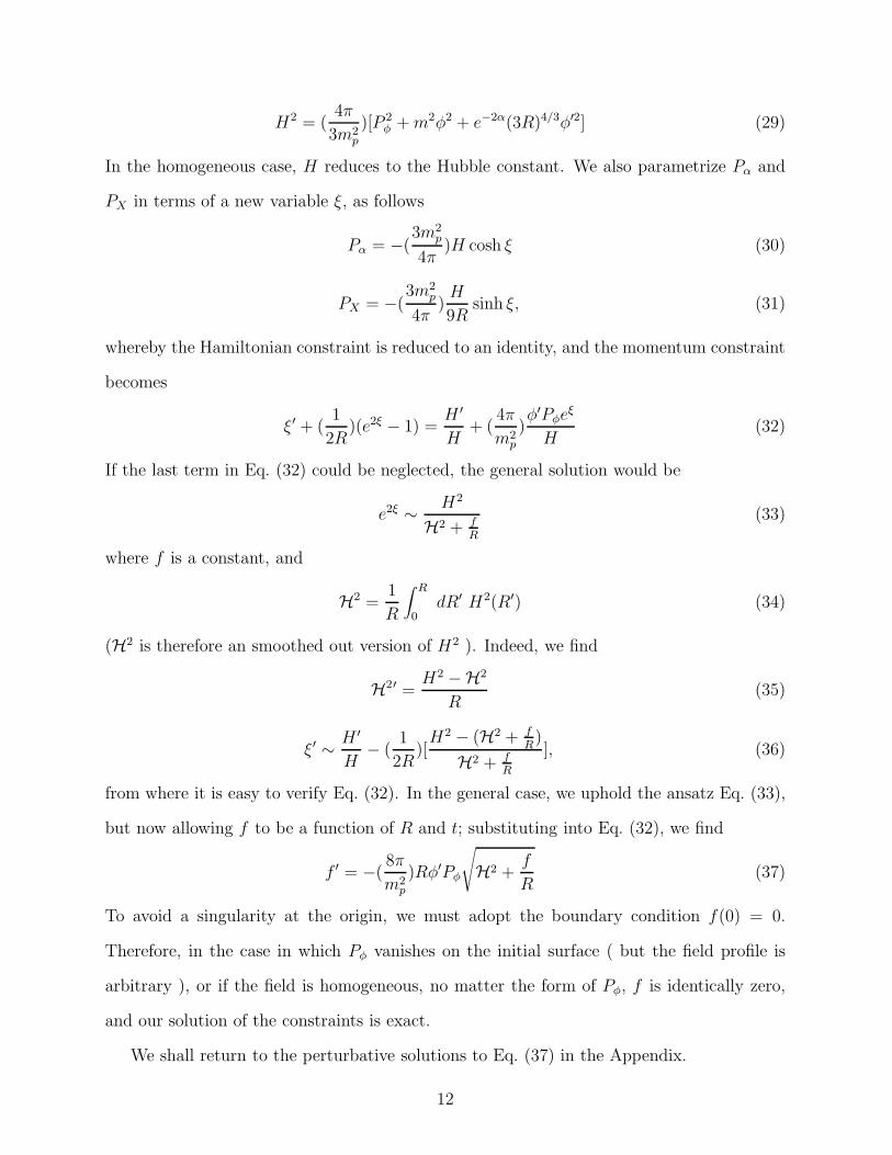
H2 = (4π
3m2p
)[P 2φ + m2φ2 + e−2α(3R)4/3φ′2] (29)
In the homogeneous case, H reduces to the Hubble constant. We also parametrize Pα and
PX in terms of a new variable ξ, as follows
Pα = −(3m2
p
4π)H cosh ξ (30)
PX = −(3m2
p
4π)H
9Rsinh ξ, (31)
whereby the Hamiltonian constraint is reduced to an identity, and the momentum constraint
becomes
ξ′ + (1
2R)(e2ξ − 1) =
H ′
H+ (
4π
m2p
)φ′Pφe
ξ
H(32)
If the last term in Eq. (32) could be neglected, the general solution would be
e2ξ ∼ H2
H2 + fR
(33)
where f is a constant, and
H2 =1
R
∫ R
0dR′ H2(R′) (34)
(H2 is therefore an smoothed out version of H2 ). Indeed, we find
H2′ =H2 −H2
R(35)
ξ′ ∼ H ′
H− (
1
2R)[
H2 − (H2 + fR)
H2 + fR
], (36)
from where it is easy to verify Eq. (32). In the general case, we uphold the ansatz Eq. (33),
but now allowing f to be a function of R and t; substituting into Eq. (32), we find
f ′ = −(8π
m2p
)Rφ′Pφ
√
H2 +f
R(37)
To avoid a singularity at the origin, we must adopt the boundary condition f(0) = 0.
Therefore, in the case in which Pφ vanishes on the initial surface ( but the field profile is
arbitrary ), or if the field is homogeneous, no matter the form of Pφ, f is identically zero,
and our solution of the constraints is exact.
We shall return to the perturbative solutions to Eq. (37) in the Appendix.
12
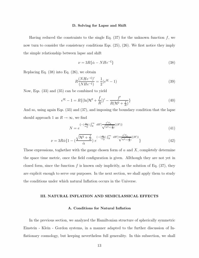
D. Solving for Lapse and Shift
Having reduced the constraints to the single Eq. (37) for the unknown function f , we
now turn to consider the consistency conditions Eqs. (25), (26). We first notice they imply
the simple relationship between lapse and shift
ν = 3Rα − NHe−ξ (38)
Replacing Eq. (38) into Eq. (26), we obtain
R(NHe−ξ)′
(NHe−ξ)=
1
2(e2ξ − 1) (39)
Now, Eqs. (33) and (35) can be combined to yield
e2ξ − 1 = R(ln[H2 +f
R])′ − f ′
R(H2 + fR) (40)
And so, using again Eqs. (33) and (37), and imposing the boundary condition that the lapse
should approach 1 as R → ∞, we find
N = e−( 4π
m2p)∫
∞
RdR′[
φ′Pφ√H2+(
fR
)
](R′)
(41)
ν = 3Rα1 − (
√
H2 + fR
α) e
(−( 4π
m2p)∫
∞
RdR′[
φ′Pφ√H2+(
fR
)
](R′))
(42)
These expressions, toghether with the gauge chosen form of α and X, completely determine
the space time metric, once the field configuration is given. Allthough they are not yet in
closed form, since the function f is known only implicitly, as the solution of Eq. (37), they
are explicit enough to serve our purposes. In the next section, we shall apply them to study
the conditions under which natural Inflation occurs in the Universe.
III. NATURAL INFLATION AND SEMICLASSICAL EFFECTS
A. Conditions for Natural Inflation
In the previous section, we analyzed the Hamiltonian structure of spherically symmetric
Einstein - Klein - Gordon systems, in a manner adapted to the further discussion of In-
flationary cosmology, but keeping nevertheless full generality. In this subsection, we shall
13
introduce a number of new assumptions, which will allow us to specialize the general for-
malism to an specific physical situation, a nonlinear perturbation of an otherwise successful
chaotic inflationary model. We shall derive from this analysis the conditions under which
Inflation may still be obtained after the perturbation.
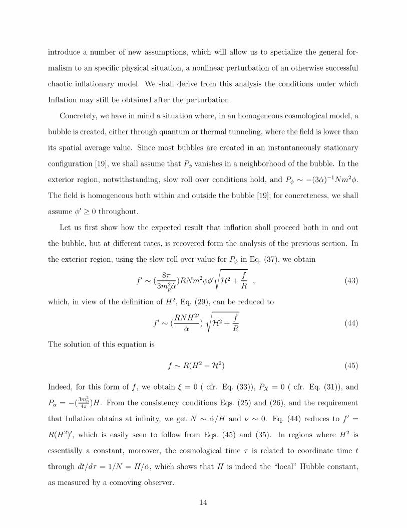
Concretely, we have in mind a situation where, in an homogeneous cosmological model, a
bubble is created, either through quantum or thermal tunneling, where the field is lower than
its spatial average value. Since most bubbles are created in an instantaneously stationary
configuration [19], we shall assume that Pφ vanishes in a neighborhood of the bubble. In the
exterior region, notwithstanding, slow roll over conditions hold, and Pφ ∼ −(3α)−1Nm2φ.
The field is homogeneous both within and outside the bubble [19]; for concreteness, we shall
assume φ′ ≥ 0 throughout.
Let us first show how the expected result that inflation shall proceed both in and out
the bubble, but at different rates, is recovered form the analysis of the previous section. In
the exterior region, using the slow roll over value for Pφ in Eq. (37), we obtain
f ′ ∼ (8π
3m2pα
)RNm2φφ′
√
H2 +f
R, (43)
which, in view of the definition of H2, Eq. (29), can be reduced to
f ′ ∼ (RNH2′
α)
√
H2 +f
R(44)
The solution of this equation is
f ∼ R(H2 −H2) (45)
Indeed, for this form of f , we obtain ξ = 0 ( cfr. Eq. (33)), PX = 0 ( cfr. Eq. (31)), and
Pα = −(3m2
p
4π)H . From the consistency conditions Eqs. (25) and (26), and the requirement
that Inflation obtains at infinity, we get N ∼ α/H and ν ∼ 0. Eq. (44) reduces to f ′ =
R(H2)′, which is easily seen to follow from Eqs. (45) and (35). In regions where H2 is
essentially a constant, moreover, the cosmological time τ is related to coordinate time t
through dt/dτ = 1/N = H/α, which shows that H is indeed the “local” Hubble constant,
as measured by a comoving observer.
14
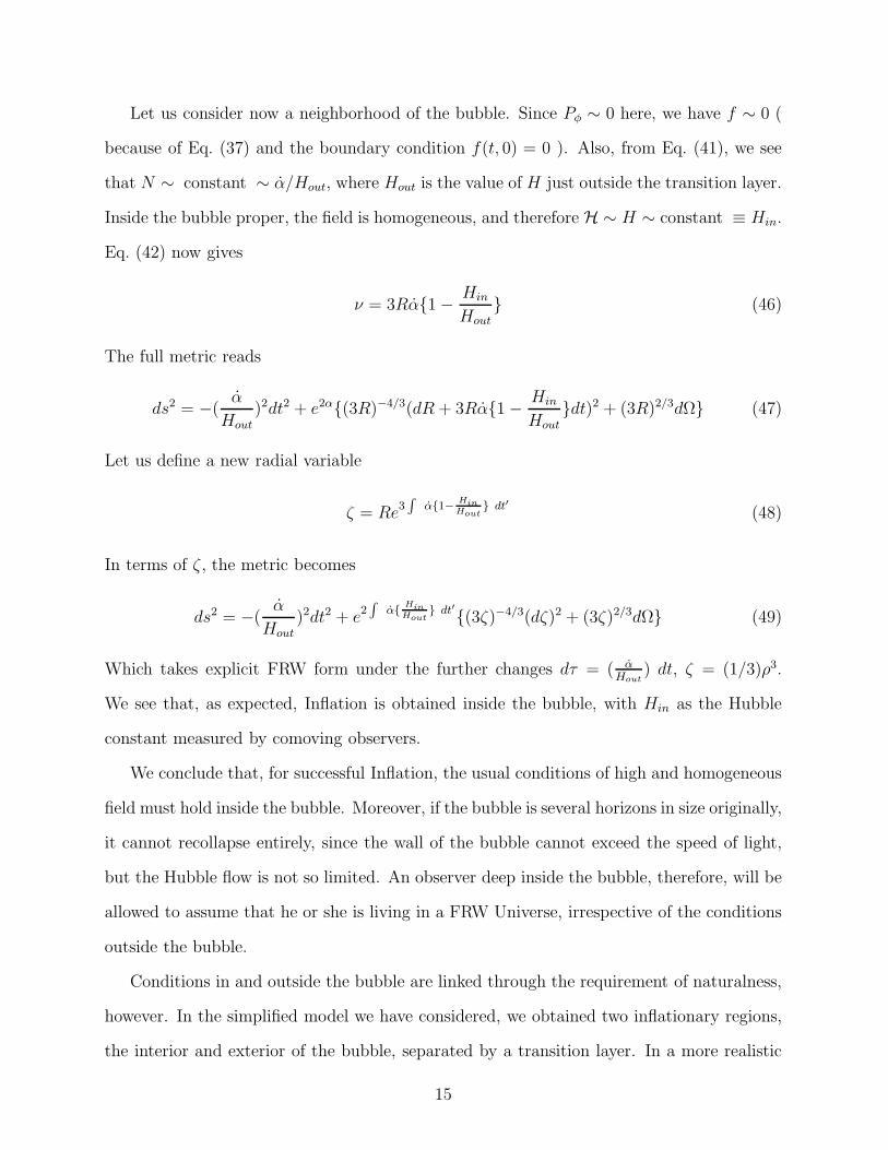
Let us consider now a neighborhood of the bubble. Since Pφ ∼ 0 here, we have f ∼ 0 (
because of Eq. (37) and the boundary condition f(t, 0) = 0 ). Also, from Eq. (41), we see
that N ∼ constant ∼ α/Hout, where Hout is the value of H just outside the transition layer.
Inside the bubble proper, the field is homogeneous, and therefore H ∼ H ∼ constant ≡ Hin.
Eq. (42) now gives
ν = 3Rα1 − Hin
Hout (46)
The full metric reads
ds2 = −(α
Hout
)2dt2 + e2α(3R)−4/3(dR + 3Rα1 − Hin
Hout
dt)2 + (3R)2/3dΩ (47)
Let us define a new radial variable
ζ = Re3∫
α1−HinHout
dt′(48)
In terms of ζ , the metric becomes
ds2 = −(α
Hout)2dt2 + e
2∫
αHinHout
dt′(3ζ)−4/3(dζ)2 + (3ζ)2/3dΩ (49)
Which takes explicit FRW form under the further changes dτ = ( αHout
) dt, ζ = (1/3)ρ3.
We see that, as expected, Inflation is obtained inside the bubble, with Hin as the Hubble
constant measured by comoving observers.
We conclude that, for successful Inflation, the usual conditions of high and homogeneous
field must hold inside the bubble. Moreover, if the bubble is several horizons in size originally,
it cannot recollapse entirely, since the wall of the bubble cannot exceed the speed of light,
but the Hubble flow is not so limited. An observer deep inside the bubble, therefore, will be
allowed to assume that he or she is living in a FRW Universe, irrespective of the conditions
outside the bubble.
Conditions in and outside the bubble are linked through the requirement of naturalness,
however. In the simplified model we have considered, we obtained two inflationary regions,
the interior and exterior of the bubble, separated by a transition layer. In a more realistic
15
model, we would consider a Universe composed of many bubbles, each with its own surround-
ing wall. Naturalness is the requirement that, at any generic instant, the volume inside the
bubbles should be a significative fraction of the volume inside the walls ( indeed, if we were
to carry the Copernican principle to extremes, we should demand that the volume within
the bubbles be much larger than the volume outside them ). A similar condition, easier to
implement, is that each bubble should be comparable in size to the wall surrounding it.
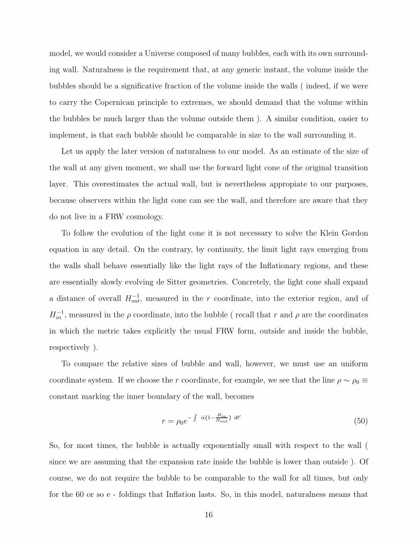
Let us apply the later version of naturalness to our model. As an estimate of the size of
the wall at any given moment, we shall use the forward light cone of the original transition
layer. This overestimates the actual wall, but is nevertheless appropiate to our purposes,
because observers within the light cone can see the wall, and therefore are aware that they
do not live in a FRW cosmology.
To follow the evolution of the light cone it is not necessary to solve the Klein Gordon
equation in any detail. On the contrary, by continuity, the limit light rays emerging from
the walls shall behave essentially like the light rays of the Inflationary regions, and these
are essentially slowly evolving de Sitter geometries. Concretely, the light cone shall expand
a distance of overall H−1out, measured in the r coordinate, into the exterior region, and of
H−1in , measured in the ρ coordinate, into the bubble ( recall that r and ρ are the coordinates
in which the metric takes explicitly the usual FRW form, outside and inside the bubble,
respectively ).
To compare the relative sizes of bubble and wall, however, we must use an uniform
coordinate system. If we choose the r coordinate, for example, we see that the line ρ ∼ ρ0 ≡
constant marking the inner boundary of the wall, becomes
r = ρ0e−
∫
α1−HinHout
dt′(50)
So, for most times, the bubble is actually exponentially small with respect to the wall (
since we are assuming that the expansion rate inside the bubble is lower than outside ). Of
course, we do not require the bubble to be comparable to the wall for all times, but only
for the 60 or so e - foldings that Inflation lasts. So, in this model, naturalness means that
16
the exponential contraction of the bubble should not be too noticeable for the first 60 e -
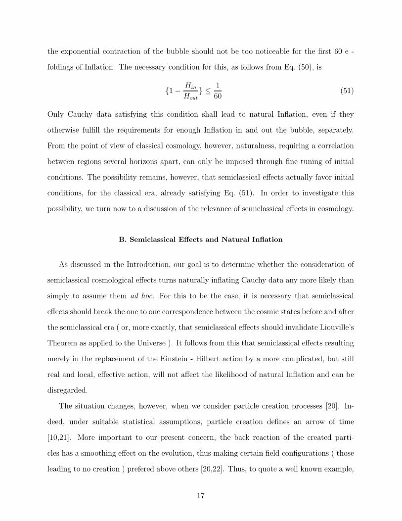
foldings of Inflation. The necessary condition for this, as follows from Eq. (50), is
1 − Hin
Hout ≤ 1
60(51)
Only Cauchy data satisfying this condition shall lead to natural Inflation, even if they
otherwise fulfill the requirements for enough Inflation in and out the bubble, separately.
From the point of view of classical cosmology, however, naturalness, requiring a correlation
between regions several horizons apart, can only be imposed through fine tuning of initial
conditions. The possibility remains, however, that semiclassical effects actually favor initial
conditions, for the classical era, already satisfying Eq. (51). In order to investigate this
possibility, we turn now to a discussion of the relevance of semiclassical effects in cosmology.
B. Semiclassical Effects and Natural Inflation
As discussed in the Introduction, our goal is to determine whether the consideration of
semiclassical cosmological effects turns naturally inflating Cauchy data any more likely than
simply to assume them ad hoc. For this to be the case, it is necessary that semiclassical
effects should break the one to one correspondence between the cosmic states before and after
the semiclassical era ( or, more exactly, that semiclassical effects should invalidate Liouville’s
Theorem as applied to the Universe ). It follows from this that semiclassical effects resulting
merely in the replacement of the Einstein - Hilbert action by a more complicated, but still
real and local, effective action, will not affect the likelihood of natural Inflation and can be
disregarded.
The situation changes, however, when we consider particle creation processes [20]. In-
deed, under suitable statistical assumptions, particle creation defines an arrow of time
[10,21]. More important to our present concern, the back reaction of the created parti-
cles has a smoothing effect on the evolution, thus making certain field configurations ( those
leading to no creation ) prefered above others [20,22]. Thus, to quote a well known example,
17
the possibility of conformal particle creation makes an isotropic universe a prefered alterna-
tive to anisotropic ones. For simple cosmological models, such as Bianchi type I universes
[17], it is actually possible to follow in detail the process of particle creation and isotropiza-
tion. Moreover, it has been shown that the connection between these phenomena is not
limited to the semiclassical era, extending as well to the fully quantum one [10,23].
The details of how particle creation proceeds in a given model depend on the peculiar
matter content of the model. In the absense of a generally accepted theory of elementary
particle physics, there is no absolute criteria for what a realistic theory should look like. How-
ever, as far as we are mostly concerned with processes occurring early on in the semiclassical
era, we can make some simplifications. Indeed, the main effects of a strong gravitational
field on elementary particles can be described by allowing masses and coupling constants
to run according to their renormalization group equations, the scale being fixed by suitable
curvature invariants [24,25]. It follows that asymptotically free theories of elementary par-
ticles actually become free in the early Universe, and that masses can be ignored. For spin
1/2 and 1, minimally coupled fields, this implies they become approximately conformally
invariant.
For scalar fields the situation is slightly more complex, because, while conformal coupling
is a fixed point of the 1 loop Renormalization Group equations, higher loop corrections
tend to make it unstable [24]. These small deviations from conformal invariance are not
important, nevertheless, because, in any case, creation of scalar particles is less efficient
than that of gauge and spinor fields.
The creation rate for conformal particles in nearly conformally flat Universes is given by
NC2/80π , where C2 is the square of the Weyl tensor, and N the effective number of particle
species, defined as N = N1 + N1/2/4 + N0/24, Ni being the number of species of spin i [17].
The value of N depends upon the particular theory of elementary particles being used; for
typical GUTs, N ∼ 100 to 1000 [26].
In view of the earlier discussion, any initial configuration with a nonzero Weyl tensor
will be brought towards conformal flatness by particle creation; correspondingly, towards
18
the end of the quantum era, the Weyl tensor should be negligible against the conformal part
of the curvature. In a near inflationary evolution, the curvature scale is set by the Hubble
constant, and our argument shows that the inequality C2H−4 ≪ 1 must hold.
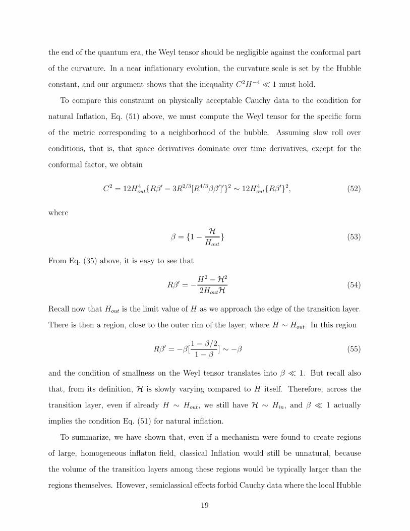
To compare this constraint on physically acceptable Cauchy data to the condition for
natural Inflation, Eq. (51) above, we must compute the Weyl tensor for the specific form
of the metric corresponding to a neighborhood of the bubble. Assuming slow roll over
conditions, that is, that space derivatives dominate over time derivatives, except for the
conformal factor, we obtain
C2 = 12H4outRβ ′ − 3R2/3[R4/3ββ ′]′2 ∼ 12H4
outRβ ′2, (52)
where
β = 1 − HHout
(53)
From Eq. (35) above, it is easy to see that
Rβ ′ = −H2 −H2
2HoutH(54)
Recall now that Hout is the limit value of H as we approach the edge of the transition layer.
There is then a region, close to the outer rim of the layer, where H ∼ Hout. In this region
Rβ ′ = −β[1 − β/2
1 − β] ∼ −β (55)
and the condition of smallness on the Weyl tensor translates into β ≪ 1. But recall also
that, from its definition, H is slowly varying compared to H itself. Therefore, across the
transition layer, even if already H ∼ Hout, we still have H ∼ Hin, and β ≪ 1 actually
implies the condition Eq. (51) for natural inflation.
To summarize, we have shown that, even if a mechanism were found to create regions
of large, homogeneous inflaton field, classical Inflation would still be unnatural, because
the volume of the transition layers among these regions would be typically larger than the
regions themselves. However, semiclassical effects forbid Cauchy data where the local Hubble
19
constant changes strongly between inflating regions. Therefore, in semiclassical cosmology,
successful Inflation is also natural, without the need of extra assumptions correlating the
value of the Inflaton field in the different inflating domains. In this sense, semiclassical
Inflation is more natural than its classical counterpart.
IV. CONCLUSIONS
The discussion in this paper has progressed in three stages, each using the results of the
previous one, but still essentially independent. In the first stage, we analyzed the constraint
equations of General Relativity coupled to a Klein - Gordon field. Assuming spherical
symmetry, we showed that the general solution to these constraints could be expressed
in terms of a single unknown function. In many cases of interest, this function may be
determined exactly, yielding consistent Cauchy data in closed, analytic, form. In the general
case, the unknown function may be computed perturbatively.
This result has been achieved through the use of a special gauge choice, devised to
simplify the constraint equations to the utmost. The only dynamical law in this approach
is the Klein - Gordon equation itself. The gain in simplicity of the constraints is paid for
in terms of the complexity which this equation acquires. However, being hyperbolic, the
Klein - Gordon equation is amenable to a qualitative treatment, which discloses the general
features of the cosmological evolution.
In the second stage of our reasoning, we developed such a qualitative analysis, seeking
to determine the necessary conditions for what we called “natural” inflation. Of course, to
obtain Inflation at all certain special initial conditions must be assumed, involving very high
and homogeneous initial values of the inflaton field. Our discussion aimed to show that, even
if these conditions were assumed locally, the resulting Universe would still be very different
to an Inflationary one, unless one further condition were added, “naturalness”, linking the
values of the field over several horizon lenghts. This result is not dependent upon the full
details of the Cauchy data previously found; however, knowledge of those data allowed us
20
to translate naturalness into a concrete inequality, which the Cauchy data must satisfy, in
order to lead to an admissible cosmology.
Finally, in the third stage of our argument we confronted our conditions for “natural”
Inflation against the present understanding of semiclassical cosmology. Based on the well
proven smoothing effect of particle creation, we argued that the Universe should have left
the semiclassical era in a state of near conformal flatness. This already puts a bound on the
possible gradients of the metric elements at the beginning of Inflation; our explicit form for
those metric elements allowed us to show that this bound actually implies the naturalness
condition previously derived.
There is an important caveat which goes with this argument, and which we would like to
make explicit here. In discussing the likely evolution of the Universe during the semiclassical
era, we are already assuming that the initial conditions at its beginning were not too extreme.
Indeed, the detailed models of semiclassical cosmologies in the literature assume for the most
part near Friedmann - Robertson - Walker conditions [27], and it would be unjustified to
extrapolate these results to arbitrarily strong inhomogeneities. Moreover, it should not be
expected that semiclassical effects could allways stabilize a classically growing perturbative
mode.
However, even under the most conservative reading of the literature, it should be accepted
that, under the statistical assumptions discussed in the Introduction, semiclassical evolution
is irreversible, and, in particular, that a nontrivial set of initial conditions is actually brought
to conformal flatness through particle creation and back reaction. These results are enough
to support our main conclusion, which is that semiclassical effects enhance the likelihood of
Inflation in the Early Universe. This conclusion, in turn, confirms the findings of previous
studies of inflation in homogeneous models [11].
It is certainly likely that a conclusion along these lines, given these hypothesis, could
have been reached through general arguments, independent of the detailed form of the
Cauchy data. However, the particular strategy we have followed is relevant in that it points
the way for further studies of classical and semiclassical Inflation. For example, the self
21
consistent Cauchy data for the Einstein - Klein - Gordon system we present here, provide
also an environment where such questions as the dependence on initial conditions of the
spectrum of density fluctuations in Inflation can be investigated. The relevant feature of
the solutions presented here is, of course, that in no way we have assumed small departures
from homogeneity.
We are continuing our research on these manyfold questions.
ACKNOWLEDGEMENTS
We would like to acknowledge the multiple comments and suggestions from the partici-
pants to the NATO Workshop on Origin of Structure in the Universe ( Pont d’Oye, Belgium,
1992), specially L. Grishchuk, A. Starobinsky, W. Unruh and R. Wald, where a preliminary
draft of this work was presented.
E. C. wishes to thank the hospitality of the RGGR group at the Free University ( Brussels
); M. S. that of the GTCRG group at IAFE ( Buenos Aires ).
This work was supported by CONICET, UBA and Fundacion Antorchas ( Argentina ),
and by the Directorate General for Science Research and Development of the Comission of
the European Communities under contract No CI1-0540-M(TT).
APPENDIX: PERTURBATIVE SOLUTIONS TO THE CONSTRAINTS
In the main body of the paper we have shown that the full geometry can be parametrized
in terms of a single function f , obeying Eq. (37). In particular cases, such as when Pφ
vanishes identically, f ≡ 0, and the metric can be worked out explicitly. However, as we
pointed out above, it would be unrealistic to assume such conditions throughout space. For
successfull inflationary models, moreover, we must have f ∼ R(H2 −H2) for large R. It is
interesting, therefore, to investigate the solutions to Eq. (37) in non trivial cases.
If we assume, as in the main body of the paper, φ′ ≥ 0 and Pφ ≤ 0 ( in Inflation,
φ′ = 0 and Pφ ∼ −m2φ/3H ), then f ′ is positive, and f is a non decreasing and non
22
negative function of R. Under these conditions, it is possible to build a sequence of functions
approximating f as follows: the first function f0 in the sequence is identically zero, and the
n-th is the solution to
fn′ = −(
8π
m2p
)Rφ′Pφ
√
H2 +fn−1
R(56)
With boundary condition fn(0) = 0.
We observe that all functions in the sequence are positive and non decreasing. The
sequence itself is nondecreasing at every point: f1 is certainly larger than zero, because it
starts at zero, and has a positive derivative; f2 is larger than f1, because both are positive,
nondecreasing functions, with the same value at the origin, and f2 has the larger derivative,
etc. Therefore, the sequence fn(R) has a limit for every R, and the limit function satisfies
Eq. (37).
This method of successive approximations is appealing not only because convergence is
guaranteed, but also because at every step it is possible to estimate its accuracy. Indeed,
from Eqs. (37) and (56) we see that
(f − fn)′ = −(8π
m2p
)Rφ′Pφ√
H2 +f
R−
√
H2 +fn−1
R (57)
Since the square root is a convex function, it follows that
(f − fn)′ ≤ −(8π
m2p
)φ′Pφ2√
H2 +fn−1
R−1(f − fn−1) (58)
And a fortiori
(f − fn)′ ≤ h(R)(f − fn−1) (59)
where
h(R) = −(4π
m2p
)φ′Pφ
H (60)
Eq. (59) can be rewritten as
(f − fn)′ − h(R)(f − fn) ≤ h(R)(fn − fn−1) (61)
23
which in turn leads to
f ≤ fn +∫ R
0dR′ h(R′)e
∫ R
R′dR′′ h(R′′)(fn − fn−1) (62)
This is the sought for bound on f
24
REFERENCES
∗ E - mail address: [email protected]
† E - mail address: [email protected]
‡ Present Address: Physics Department, University of Tours, France.
1 S. Weinberg, Gravitation and Cosmology (Wiley, New York, 1972).
2 E. Kolb and M. Turner, The Early Universe ( Addison - Wesley, New York, 1990 ).
3 G. Smoot et al. , Structure in the COBE DMR First Year Maps, Astrophys. J. Lett., to
appear.
4 A. Guth, Phys. Rev D23, 347 (1981).
5 J. Bardeen, Phys. Rev. D22, 1882 (1980); J. Frieman and C. Will, Astrophys. J. 259,
437 (1982); H. Feldman and R. Brandenberger, Phys. Lett 227B, 359 (1989); 220B, 361
(1989); D. Salopek and D. Bond, Phys. Rev. D43, 1005 (1991).
6 H. Kurki - Suonio, J. Centrella, R. Matzner and J. wilson, Phys. Rev. D35, 435 (1987).
7 T. Piran and R. Williams, Phys. Lett. 163B, 331 (1985); T. Piran, ibid. 181B, 238
(1986); D. Goldwirth and T. Piran, Phys. Rev. D40, 3263 (1989); D. Goldwirth, Phys.
Lett. 243B, 41 (1990); D. Goldwirth and T. Piran, Phys. Rev. Lett. 64, 2852 (1990); D.
Goldwirth, Phys. Rev. D43, 3204 (1991);
8 A. Linde, Phys. Lett. 129B, 177 (1983).
9 E. Calzetta and M. Sakellariadou, Phys. Rev D45, 2802 (1992).
10 B. L. Hu, Physica A158, 399 (1989); E. Calzetta and B. L. Hu, Phys. Rev. D40, 656
(1989).
11 E. Calzetta, Phys. Rev D44, 3043 (1991).
12 X. Lin and R. Wald, Phys. Rev. D40, 3280 (1989);D41, 2444 (1990).
25
13 C. Misner, K. Thorne and J. Wheeler, Gravitation ( Freeman, San Francisco, 1973).
14 L. Landau and E. Lifschitz, Classical Theory of Fields (Pergamon, London, 1975).
15 B. Berger, D. Chitre. V. Montcrieff and Y. Nutku, Phys. Rev. D5, 2467 (1972); W. Unruh,
Phys. Rev. D14, 870 (1974); see also the treatment of spherically symmetric Cauchy data
in P. Bizon, E. Malec and N. O Murchadha, Class. Q. Grav. 6, 961 (1989); Phys. Rev.
Lett. 61, 1147 (1988); U. Brauer and E. Malec, Phys. Rev. D45, R1836 (1992); E. Malec
and N. O Murchadha, Trapped Surfaces and Spherically Closed Cosmologies, preprint
(1992).
16 S. Hawking, in 300 Years of Gravitation, edited by S. Hawking and W. Israel ( Cambridge
University Press, Cambridge (UK), 1987).
17 Ya. B. Zel’dovich and A. Starobinsky, JETP Lett. 26, 252 (1977); B. L. Hu and L. Parker,
Phys. Rev. D17, 933 (1978); J. Hartle and B. L. Hu, ibid. D20, 1772 (1979); E. Calzetta
and B. L. Hu, ibid. D35, 495 (1987); J. P. Paz, ibid. D41, 1054 (1990).
18 S. Hawking, Comm. Math. Phys. 43, 199 (1975).
19 S. Coleman, Phys. Rev. D15, 2929 (1977), and Aspects of Symmetry ( Cambridge Uni-
versity Press, Cambridge (UK), 1985).
20 L. Parker, Phys. Rev. Lett. 21, 562 (1968); Phys. Rev. 183, 1057 (1969); in Asymptotic
Structure of Space Time, edited by F. Esposito and L. Witten ( Plenum, New York, 1977
).
21 B. L. Hu and H. Kandrup, Phys. Rev. D35, 1776 (1987); H. Kandrup, ibid. D37, 3505
(1988); ibid. D38, 1773 (1988).
22 Ya. B. Zel’dovich, in Magic without Magic, edited by J. Klauder ( Freeman, San Francisco,
1972 ), p. 277; L. Parker, Phys. Rev. Lett. 50, 1009 (1983).
23 E. Calzetta, Phys. Rev. D43, 2498 (1991); E. Calzetta, M. Castagnino and R. Scocci-
26
marro, ibid. D45, 2806 (1992).
24 L. Parker and D. Toms, , Phys. Rev. Lett. 52, 1269 (1984); Phys. Rev. D29, 1584 (1984).
25 E. Calzetta, I. Jack and L. Parker, Phys. Rev. Lett. 55, 1241 (1985); Phys. Rev. D33,
953 (1986), (E) D34, 1235 (1986); E. Calzetta, Ann. Phys. (NY) 166, 214 (1986).
26 G. G. Ross, Grand Unified Theories ( Benjamin / Cummings, Menlo Park, 1985).
27 Among the few exceptions let us quote B. L. Hu, Phys. Rev. D8, 1048 (1973) and D9,
3263 (1974).
27