arX

iv:q

uant

-ph/

9611

030v

1 1

8 N

ov 1

996

UICHEP-TH/96-18

quant-ph/9611030

Accuracy of Semiclassical Methodsfor Shape Invariant Potentials

Marina Hruska1, Wai–Yee Keung2 and Uday Sukhatme3

Department of Physics, University of Illinois at Chicago,

845 W. Taylor Street, Chicago, Illinois 60607-7059.

Abstract

We study the accuracy of several alternative semiclassical methods by computing analyt-

ically the energy levels for many large classes of exactly solvable shape invariant potentials.

For these potentials, the ground state energies computed via the WKB method typically devi-

ate from the exact results by about 10%, a recently suggested modification using nonintegral

Maslov indices is substantially better, and the supersymmetric WKB quantization method

gives exact answers for all energy levels.

1 e-mail: f2hruska@rcub.rcub.bg.ac.yu, Permanent address: Vlajkoviceva 28, 11000 Belgrade, Yugoslavia.2e-mail: keung@uic.edu3e-mail: sukhatme@uic.edu

1. Introduction

A variety of semiclassical methods have been proposed and used for determining the energy

levels of one-dimensional potentials. The standard WKB method is discussed in most quantum

mechanical texts [1, 2] but there are several recently suggested modifications based on supersym-

metric quantum mechanics [3], energy dependent phase losses at the classical turning points with

nonintegral Maslov indices [4], and other related approaches [5]. As expected, all semiclassical

methods yield good energy eigenvalues En for large values of the quantum number n. However,

their accuracy varies quite substantially for small values of n depending on the choice of potential.

Also, many potentials only have a small number of bound states, so that the possibility of consid-

ering large values of n does not exist. In this paper, we make a stringent test of the accuracy of

various semiclassical methods by computing the eigenenergies of the ground state and other low

lying states for many large classes of potentials which have the property of shape invariance [6]

under supersymmetry transformations. We have chosen shape invariant potentials since (i) they

are exactly solvable and all eigenvalues are explicitly known; (ii) the integrals appearing in the

semiclassical quantization conditions can all be performed analytically; (iii) the nonintegral Maslov

indices used in the recent semiclassical approach [4] of Friedrich and Trost (FT) can be expressed

in terms of superpotentials. Our plan is to first review three semiclassical approaches and the main

ideas involving shape invariant potentials. We will then compute the quantization condition inte-

grals analytically and determine energy eigenvalues. The results are presented in Tables 1 and 2,

and we give some concluding remarks on the accuracy of various semiclassical approaches.

2. Semiclassical Quantization Conditions

(i) WKB Quantization: The usual form of the semiclassical energy quantization condition

(in units of h = 2m = 1) is [1, 2]∫ xR

xL

dx√

E − V (x) = (n+µ

4)π , µ =

φL + φR

π/2, (n = 0, 1, 2, ...) , (1)

where the classical turning points xL and xR are given by V (xL) = V (xR) = E. The Maslov index

µ denotes the total phase loss during one period in units of π/2. It contains contributions from the

phase losses φL and φR due to reflections at the left and right classical turning points xL and xR

respectively. In the standard WKB approach, one takes φL = φR = π/2, and an integer Maslov

index µ = 2 for all energy levels. This gives the familiar result (n + 12)π for the right hand side of

the WKB quantization condition.

(ii) SWKB Quantization: Another semiclassical approach [3] which has been widely studied

in recent years is based on the ideas of supersymmetric quantum mechanics[9]. Here, the super-

symmetric partner potentials V−(x) and V+(x) are given in terms of the superpotential W (x) by

2

V± = W 2(x) ±W ′(x). For the case of unbroken supersymmetry, V−(x) and V+(x) have degenerate

energy levels except that V−(x) has an additional level at E(−)0 = 0. The corresponding ground

state wave function ψ(−)0 (x) is related to the superpotential W (x) via

W (x) = −ψ

(−)0

′

(x)

ψ(−)0 (x)

; ψ(−)0 (x) ∝ e−

∫

xdx′W (x′) . (2)

The supersymmetric WKB (SWKB) approach [3] results from combining the ideas of supersymme-

try with the lowest order WKB method. The SWKB quantization condition is

∫ x′

R

x′

L

dx√

E(−) −W 2(x) = nπ , (n = 0, 1, 2, ...) , (3)

where the two turning points x′L and x′R are given by W (x) = ±√E(−). Note that for n = 0, the

turning points coincide and the SWKB quantization condition gives the exact result E(−)0 = 0 for

the ground state energy.

(iii) Friedrich-Trost Quantization: This very recent proposal [4] makes use of the stan-

dard quantization condition [eq. (1)] with nonintegral, energy-dependent Maslov indices µ. More

specifically, the phase loss is taken to be given by

tan(φL

2) =

ψ′(xL)

kψ(xL), tan(

φR

2) = −

ψ′(xR)

kψ(xR), (4)

where k ≡√E − Vmin and Vmin is the minimum value of the potential V (x). In Ref. [4], it was

suggested that one could use the lowest order WKB wave function in eq. (4) in order to determine

the phase losses φL, φR for any practical application. Indeed, it was shown that for power law

potentials xp with p = 4, 5, 6, this method gave better numerical results for the ground state

energies than the standard WKB method, and also substantially improved wave functions.

The FT approach of using the WKB wave function in eq. (4) is rather cumbersome. It can be

significantly simplified for the ground state by using eq. (2) . The phase losses φL, φR can then be

re-written as

tan(φL

2) = −

W (xL)

k, tan(

φR

2) =

W (xR)

k. (5)

In this paper, we will assume eq. (5) to be valid for all energy levels in computing eigenenergies by

the FT approach.

3. Shape Invariant Potentials

Given a superpotential W (x, a0) depending on a set of parameters a0, the supersymmetric

partner potentials V±(x, a0) are given by

V±(x, a0) = W 2(x, a0) ±W ′(x, a0) . (6)

3

These partner potentials are shape invariant if they both have the same x-dependence Upton a

change of parameters a1 = f(a0) and an additive constant R(a0). The shape invariance condition

is

V+(x, a0) = V−(x, a1) +R(a0) . (7)

This special property permits an immediate analytic determination of energy eigenvalues [6] and

eigenfunctions [7]. For unbroken supersymmetry, the eigenvalues are

E(−)0 = 0 , E(−)

n =n−1∑

k=0

R(ak) . (8)

Many aspects of the bound states and scattering matrices of shape invariant potentials have been

studied [9] including several choices [10] for the change of parameters a1 = f(a0). In this paper,

we confine our attention to shape invariant potentials corresponding to a translational change of

parameters.

4. Computation of Energy Eigenvalues

All known families of shape invariant potentials in which the change of parameters is a translation

a1 = a0 +β are listed in Table 1. Names of the potentials and the corresponding superpotentials are

given. Also tabulated is the minimum value V−min of the potential V−(x) and the position xmin of

the minimum. Subtracting V−min from V−(x) yields the tabulated potential V (x), whose minimum

value is clearly Vmin = 0. The exact energy eigenvalues Eexactn for V (x) coming from eq. (8) are

also given.

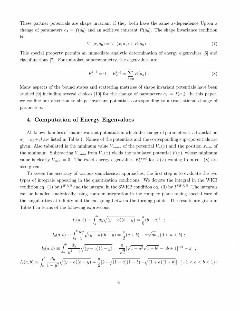
To assess the accuracy of various semiclassical approaches, the first step is to evaluate the two

types of integrals appearing in the quantization conditions. We denote the integral in the WKB

condition eq. (1) by IWKB and the integral in the SWKB condition eq. (3) by ISWKB. The integrals

can be handled analytically using contour integration in the complex plane taking special care of

the singularities at infinity and the cut going between the turning points. The results are given in

Table 1 in terms of the following expressions:

I1(a, b) ≡∫ b

ady

√

(y − a)(b− y) =π

8(b− a)2 ;

I2(a, b) ≡∫ b

a

dy

y

√

(y − a)(b− y) =π

2(a+ b) − π

√ab , (0 < a < b) ;

I3(a, b) ≡∫ b

a

dy

y2 + 1

√

(y − a)(b− y) =π√2[√

1 + a2√

1 + b2 − ab+ 1]1/2 − π ;

I4(a, b) ≡∫ b

a

dy

1 − y2

√

(y − a)(b− y) =π

2[2−

√

(1 − a)(1 − b)−√

(1 + a)(1 + b)] , (−1 < a < b < 1) ;

4

I5(a, b) ≡∫ b

a

dy

y2 − 1

√

(y − a)(b− y) =π

2[√

(a+ 1)(b+ 1) −√

(a− 1)(b− 1) − 2] , (1 < a < b) ;

In all the above integrals, the limits a, b are real numbers with a < b. We have given explicit

expressions for the above integrals since they are not easily available in standard integration tables.

Once IWKB and ISWKB have been computed, one can apply the quantization conditions to see

how accurate the WKB, SWKB and FT approaches are. For the WKB and SWKB approaches,

it is possible to get complete analytic results - these are shown in Table 1. The FT approach is

also mostly analytical, but the final computations need numerical work. Results corresponding to

specific numerical choices of the parameters appearing in the potentials are shown in Table 2.

As an illustrative example, consider the Rosen-Morse II (hyperbolic) potential, for which the

superpotential is

W (x) = A tanhαx+B

A.

With a change of variables y = tanhαx, the SWKB integral is

ISWKB =A

α

∫ y′

R

y′

L

dy

1 − y2

√

[−y2 −2B

A2+ (

E

A2−B2

A4)]

with turning points given by Ay′ + BA

= ±√E(−). One then sees that the integral is A

αI4(y

′

L, y′

R).

Substitution into the SWKB quantization condition ISWKB = nπ and solving for E(−) gives

E(−)SWKBn = A2 − (A− nα)2 +

B2

A2−

B2

(A− nα)2

which is the exact answer for all energy levels ! Similar steps give the WKB integral to be IWKB =√A(A+α)

αI4(yL, yR) where the turning point are given by

A(A + α)y2 + 2By + (B2

A(A+ α)− E) = 0 .

Substitution into the WKB quantization condition IWKB = (n + 12)π and solving for the energy

gives

EWKBn = A(A+ α) − (

√

A(A+ α) −α

2− nα)

2

+B2

A(A+ α)−

B2

(√

A(A+ α) − α2− nα)

2

The WKB approach does not give the exact eigenvalues. The full energy computation for the FT

quantization condition is harder to carry out analytically. For the numerical choice α = 1, A =

2, B = 1, we see from Table 2 that the ground state energy EFT0 is lower than the exact energy by

3.2% whereas EWKB0 is higher than the exact energy by 9.7%.

5. Conclusion

5

We have given a complete analytic treatment of the energy levels of shape invariant potentials

(with a translational change of parameters) for various semiclassical quantization conditions. As

expected from previous work [7], the SWKB energy levels are exact. The WKB energy levels

are exact for the one-dimensional harmonic oscillator and the Morse potentials only. For other

potentials the results are not exact, and this has historically led to ad hoc Langer corrections [11].

Typically, one sees from Table 1 that the ground state energy from the WKB method deviates from

the exact result by about 10%. The new semiclassical approach of Friedrich and Trost is exact only

for the one-dimensional harmonic oscillator and no other shape invariant potential. However, in

general, it gives significantly more accurate ground state energies than the WKB method.

This work was supported in part by the U. S. Department of Energy.

Table Captions

Table 1: List of all shape invariant potentials and their eigenvalues. Analytic expressions for

the integrals in the WKB and SWKB quantization condition are given, along with the energy

eigenvalues. For these potentials, the SWKB results are always exact, whereas the WKB results

are exact only for the harmonic oscillator and Morse potentials.

Table 2: Comparison of the exact ground state energies of shape invariant potentials with results

from the WKB and Friedrich-Trost method. The percent errors are also shown. The SWKB results

are not shown, since they are always exact for the potentials under consideration.

6

References

[1] N. Froman and P. O. Froman, JWKB Approximation, Contributions to the Theory, (North-

Holland, Amsterdam, 1965).

[2] L. D. Landau and E. M. Lifshitz, Quantum Mechanics, (Pergamon, Oxford, 1965).

[3] A. Comtet, A. Bandrauk and D. K. Campbell, Phys. Lett. B150, 159 (1985); A. Khare, Phys.

Lett. B161, 131 (1985).

[4] H. Friedrich and J. Trost, Phys. Rev. Lett. 76, 4869 (1996) and Phys. Rev. A54, 1136 (1996).

[5] J. M. Robbins, S. C. Creagh and R. G. Littlejohn, Phys. Rev. A41, 6052 (1990); V. S. Popov,

B. M. Karnakov and V. D. Mur, Phys. Lett. A210, 402 (1996); R. Leacock and M. Padgett,

Phys. Rev. Lett. 50, 3 (1983).

[6] L. Gendenshtein, JETP Lett. 38, 356 (1983).

[7] R. Dutt, A. Khare and U. Sukhatme, Phys. Lett. B181, 295 (1986).

[8] R. Adhikari, R. Dutt, A. Khare and U. Sukhatme, Phys. Rev. A38, 1679 (1986); K. Raghu-

nathan, M. Seetharaman and S. Vasan, Phys. Lett. B188, 351 (1987); D. Barclay and C. J.

Maxwell, Phys. Lett. A157, 351 (1991).

[9] For recent reviews of supersymmetric quantum mechanics, see, F. Cooper, A. Khare and U.

Sukhatme, Phys. Rep. 251, 267 (1995); A. Lahiri, P. Roy and B. Bagchi, Int. Jour. Mod. Phys.

A5, 1383 (1990); R. Haymaker and A. R. P. Rau, Amer. Jour. Phys. 54, 928 (1986); L. E.

Gendenshtein and I. V. Krive, Sov. Phys. Usp. 28, 695 (1985).

[10] A. Khare and U. Sukhatme, Jour. Phys. A26, L901 (1993); D. Barclay et al., Phys. Rev. A48,

2786 (1993); A. Gangopadhyaya and U. Sukhatme, UIC preprint, to appear in Phys. Lett. A

(1996).

[11] K. E. Langer, Phys. Rev. 51, 669 (1937).

7

Name Super V�min, the xmin, V (x) = V�(x) IWKB = ISWKB =of potential minimum of V�(xmin) �V�min, Note: Eexactn , ESWKBn R xRxL dxpE � V (x) R x0Rx0L dxpE �W 2(x) EWKBnpotential W (x) V� =W 2 �W 0 = V�min V (xmin) = 0Shifted oscillator 12!x �12! 0 14!2x2 (n+ 12)! �E=! �E=! (n + 12)!Three 12!r � (l+1)r !pl(l + 1) 14!2r2 + l(l + 1)=r2 2n! � V�min �E2! �E2! 2n! + !dimensional �(l + 32)! [4l(l + 1)=!2] 14 �!pl(l + 1)oscillatorCoulomb e22(l+1) � (l+1)r � e44l(l+1)2 2l(l + 1)=e2 �e2r + l(l+1)r2 e44 ( 1l(l+1) �e2=pe4=(l2 + l)� 4E �e2=pe4=(l + 1)2 � 4E e44 [(l2 + l)�1+ e44(l2+l) � 1(n+l+1)2 ) ��pl2 + l ��(l + 1) �(n +pl2 + l+ 12)�2]Morse A (A+ �=2)2 �� (A+ �2 ) (A+ �2 )2�Be��x �A�� �2=4 1� log BA+�=2 (A+ �=2� Be��x)2 �(A � n�)2 ���p(A+ �2 )2 � E �� (A�pA2 � E) �(A� n�)2Rosen- A tanh�x B2=A2 �A� B2=(A2 +A�) A2 + A�� (A� n�)2 pA(A+ �)I4(yL; yR)=� AI4(y0L; y0R)=� �(1 + 2n)pA(A+ �)Morse II +B=A �B2=(A2 + A�) � 1� tanh�1 BA2+A� +A(A+ �) tanh2 �x + B2A2+A� � B2(A�n�)2 yL + yR = �2B=(A2 +A�) y0L + y0R = �2B=A2 ��2(12 + n)2 +B2=(A2 +A�)(hyperbolic) (B < A2) +2B tanh�x yLyR = B2(A2+A�)2 � EA2+A� y0Ly0R = B2A4 � EA2 �B2=(pA2 +A�� �2 � n�)2�A coth�r B2=A2 +A� B2=(A2 �A�) A2 � A�� (A+ n�)2 pA(A� �)I5(yL; yR)=� AI5(y0L; y0R)=� ��(1 + 2n)pA(A� �)Eckart +B=A �B2=(A2 � A�) 1� coth�1 BA2�A� +A(A� �) coth2 �r + B2A2�A� � B2(A+n�)2 yL + yR = 2B=(A2 �A�) y0L + y0R = 2B=A2 ��2(12 + n)2 +B2=(A2 �A�)(B > A2) �2B coth�r yLyR = B2(A2�A�)2 � EA2�A� y0Ly0R = B2A4 � EA2 �B2=(pA2 �A�+ �2 + n�)2Rosen- �A cot�x B2=A2 �A� B2=(A2 �A�) �A2 + A�+ (A+ n�)2 pA(A� �)I3(yL; yR)=� AI3(y0L; y0R)=� +�(1 + 2n)pA(A� �)Morse I �B=A �B2=(A2 � A�) � 1� cot�1 BA2�A� +A(A� �) cot2 �x + B2A2�A� � B2(A+n�)2 yL + yR = �2B=(A2 �A�) y0L + y0R = �2B=A2 +�2(12 + n)2 +B2=(A2 �A�)(trigonometric) (0 � �x � �) +2B cot�x yLyR = B2(A2�A�)2 � EA2�A� y0Ly0R = B2A4 � EA2 �B2=(pA2 �A�+ �2 + n�)2Scarf II A tanh�x A2 � L L+ Csech2�x(hyperbolic) +Bsech �x C = B2 �A2 � A� � 1� sinh�1 D2L +Dsech �x tanh�x L � (A� n�)2 �� (pL�pL � E) �� (A�pA2 � E) L� (pL� n�� �2 )2D = 2AB + �B 2L = pC2 +D2 �CGeneralized A coth�r A2 � L L+ Ccsch2�rP�oschl- �Bcsch �r C = A2 +B2 + A� 1� cosh�1 D2L �Dcsch �r coth�r L � (A� n�)2 �� (pL�pL � E) �� (A�pA2 � E) L� (pL� n�� �2 )2Teller (A < B) 2L = C �pC2 �D2 D = 2AB + �BScarf I A tan�x �A2 + L �L + Csec2�x(trigonometric) �B sec�x C = A2 +B2 � A� 1� sin�1 D2L �Dsec �x tan�x (A+ n�)2 � L �� (pL+ E �pL) �� (pA2 + E � A) (pL+ n� + �2 )2 � L(A > B) 2L = C +pC2 �D2 D = 2AB � �B (j�xj � �2 )Table 1: List of all shape invariant potentials and their eigenvalues. Analyticexpressions for the integrals in the WKB and SWKB quantization condition aregiven, along with the energy eigenvalues. For these potentials, the SWKB resultsare always exact, whereas the WKB results are exact only for the harmonicoscillator and Morse potentials.

FriedrichName of Choice of Super Potential Eexact0 EWKB0 Percent -Trost PercentPotential Parameters Potential V (x) (Eexact1 ) error EFT0 errorShifted 12! 12! 0 12! 0oscillator | 12!x 14!2x2 (1:5!)Three ! = 2 2.1716 2 8.07% 2.158 0.61%dimensional l = 1 r � 2r (p2=r � r)2 (6.1716)oscillatorCoulomb e = 1 0.0625 0.5677 9.17% 0.05580 10.7%l = 1 14 � 2r 2( 1r � 14 )2 (0.09722)� = 2Morse A = 1 1� e�2x (2� e�2x)2 3 3 0 2.7587 8.04%B = 1Rosen- � = 1Morse II A = 2 2 tanhx+ 12 16 (1 + 6 tanhx)2 1.9167 2.1030 9.72% 1.8549 3.22%B = 1� = 1Eckart A = 2 3� 2 coth r 2(coth r � 3)2 7 6.511 7.00% 6.1540 12.1%B = 6Rosen- � = 1Morse I A = 2 �1� 2 cotx 2(1 + cotx)2 3 2.5727 14.25% 2.9356 2.14%(trigonometric) B = 2 (8.5556)� = 1 12 (p10 � 1)Scarf II A = 1 tanhx �sech2x 1.0811 1.19257 10.31% 1.02981 4.74 %(hyperbolic) B = 1 +sechx +3sechx tanhxGeneralized � = 1 112 �p10P�oschl- A = 1 coth r +11csch2r 1.33772 1.2790 4.39% 1.2576 5.99%Teller B = 3 �3cschr �9cschr coth rScarf I � = 1 � 72 �p6(trigonometric) A = 3 3 tanx +7 sec2 x 3.0505 2.689 11.8% 3.1285 2.56%B = 1 � secx �5 secx tanx (10.0505)Table 2: Comparison of the exact ground state energies of shape invariantpotentials with results from the WKB and Friedrich-Trost method. The percenterrors are also shown. The SWKB results are not shown, since they are alwaysexact for the potentials under consideration.