seasonality in six enterically transmitted diseases and ambient temperature

Seasonality in six enterically transmitted diseases

and ambient temperature

E. N. NAUMOVA 1*, J. S. JAGAI1, B. MATYAS 2, A. DEMARIA JR.2,

I. B. MACNEILL 3AND J. K. GRIFFITHS1

1 Tufts University School of Medicine, Boston, MA, USA2 Massachusetts Department of Public Health, Boston, MA, USA3 University of Western Ontario, London, Canada

(Accepted 3 April 2006; first published online 19 June 2006)

SUMMARY

We propose an analytical and conceptual framework for a systematic and comprehensive

assessment of disease seasonality to detect changes and to quantify and compare temporal

patterns. To demonstrate the proposed technique, we examined seasonal patterns of six

enterically transmitted reportable diseases (EDs) in Massachusetts collected over a 10-year period

(1992–2001). We quantified the timing and intensity of seasonal peaks of ED incidence and

examined the synchronization in timing of these peaks with respect to ambient temperature.

All EDs, except hepatitis A, exhibited well-defined seasonal patterns which clustered into two

groups. The peak in daily incidence of Campylobacter and Salmonella closely followed the

peak in ambient temperature with the lag of 2–14 days. Cryptosporidium, Shigella, and Giardia

exhibited significant delays relative to the peak in temperature (y40 days, P<0.02). The

proposed approach provides a detailed quantification of seasonality that enabled us to detect

significant differences in the seasonal peaks of enteric infections which would have been lost

in an analysis using monthly or weekly cumulative information. This highly relevant to

disease surveillance approach can be used to generate and test hypotheses related to disease

seasonality and potential routes of transmission with respect to environmental factors.

INTRODUCTION

In temperate climates, waterborne or foodborne

enteric infections typically alternate periods of low

endemic levels with periods with outbreaks, forming a

typical seasonal pattern. For example, illness caused

by Salmonella spp. or Campylobacter jejuni rises in

the summer and declines in the winter [1–7]. Enteric

infections caused by the protozoans Giardia and

Cryptosporidium also exhibit seasonal variation, al-

though shifted towards autumn [8–14]. In contrast,

hepatitis A and shigellosis seasonality is not mar-

ked [4].

Consistent temporal fluctuations for diseases

with similar sources for exposure or similar routes of

transmission, suggest the presence of environmental

factors that synchronize seasonal variation [15].

Deviations from an established seasonal pattern may

provide important clues to the factors that influence

disease occurrence. These factors may include chan-

ges in the sources of exposure and spread, changes in

the affected population, or differences in the pathogen

itself. Ecological disturbances, perhaps from climate

* Author for correspondence : E. N. Naumova, Ph.D., AssociateProfessor, Department of Public Health and Family Medicine,Tufts University School of Medicine, 136 Harrison Ave, Boston,MA 02111, USA.(Email : [email protected])

Epidemiol. Infect. (2007), 135, 281–292. f 2006 Cambridge University Press

doi:10.1017/S0950268806006698 Printed in the United Kingdom

change, may influence the emergence and prolifer-

ation of parasitic diseases, including cryptosporidiosis

and giardiasis [16]. Ambient temperature has been

associated with short-term temporal variations (week-

to-week and month-to-month) in reported cases of

food poisoning in the United Kingdom, often caused

by Salmonella [17–20]. Increased temperatures and

extreme precipitation events have also been shown to

have a short-term effect on health outcomes [21–23].

To quote Epstein [24], ‘climate constrains the range of

infectious diseases, while weather affects the timing

and intensity of outbreaks ’. It is plausible that the

temporal pattern in ambient temperature may deter-

mine, in part, the timing and magnitude of the peak of

a disease incidence curve for specific enteric diseases.

An understanding of how specific environmental

factors influence human disease may improve disease

forecasting, enhance the design of integrated warning

systems, and advance the development of efficient

outbreak detection algorithms. Although seasonality

is a well-known characteristic of enteric infections,

simple analytical tools for the examination, evalu-

ation, and comparison of seasonal patterns are lim-

ited. Herein, we offer a framework for seasonality

assessment, and a parametric approach for season-

ality evaluation. We contrast our approach with non-

parametric modelling. To demonstrate the proposed

method, while providing step-by-step instructions for

implementation, we examine the variability in sea-

sonality of six enteric diseases with respect to ambient

temperature in the temperate climate of Massachu-

setts (MA) over the last decade. We consider two

parasite infections (Giardia and Cryptosporidium),

three bacterial infections (Salmonella, Campylobacter

and Shigella), and one viral disease, hepatitis A. All

of these enteric infections can be waterborne and/or

foodborne, have low endemic winter incidence rates

and localized outbreaks, typically exhibit a yearly

summer or autumn peak, and are diseases reportable

to the Massachusetts Department of Public Health

(MDPH).

METHODS

Data abstraction

We abstracted all reported laboratory-confirmed

cases (45 816 records, without personal identifiers) for

six diseases: giardiasis, cryptosporidiosis, salmonel-

losis, campylobacteriosis, shigellosis, and hepatitis A.

The number of cases by disease is shown in Table 1.

The abstraction covers all of MA over a 10-year per-

iod (3653 days) from 1 January 1992 to 31 December

2001. Criteria for reportable cases to MDPH include:

for cryptosporidiosis and giardiasis – demonstration

of Cryptosporidium oocysts or Giardia lamblia cysts in

stool ; demonstration ofCryptosporidium orG. lamblia

cysts in intestinal fluid or small-bowel biopsy speci-

mens; or demonstration of Cryptosporidium or G.

lamblia antigen in stool by a specific immuno-

diagnostic test [e.g. enzyme-linked immunosorbent

assay (ELISA)] ; for salmonellosis (non-typhoid)

and shigellosis – isolation of Salmonella or Shigella

species from any clinical specimen; for hepatitis

A – serological evidence of recent hepatitis A virus

infection (anti-hepatitis A IgM antibody) associated

with a consistent clinical syndrome, or known ex-

posure to an infectious case with or without symp-

toms in the contact. For each reported case, variables

necessary for spatial and temporal analysis were

Table 1. Proposed characteristics to describe seasonality for exposure and outcome variables

Proposed characteristics describing seasonalityFor exposure (e.g. averageambient temperature)

For outcome (e.g. reportedenteric disease incidence)

Average maximum value – seasonal peak max{Y(t)}=b0+c max{Y(t)}=exp{b0+c}Average minimum value – seasonal nadir min{Y(t)}=b0xc min{Y(t)}=exp{b0xc}Average intensity – the difference between maximumand minimum values

I=2c I=exp{b0+c}xexp{b0xc}

Average relative intensity – the ratio of the maximumand minimum values on the seasonal curve

IR=(b02xc2 )/(b0xc )2 IR=exp{2c }

Average peak timing – the temporal position of themaximum point on the seasonal curve (expressed

in days)

PE=365(1–y/p)/2 PD=365(1–y/p)/2

Average lag – the difference between the peak time ofexposure and the peak timing of disease incidence

PExPD

282 E. N. Naumova and others

obtained: sex, age, zip code of residence, and dates of

disease onset and reporting. Using the date of disease

onset, the time series of daily counts of reported

laboratory-confirmed cases of the six enteric diseases

(EDs) were created.

Daily ambient temperature records from 38

MA monitoring stations were abstracted from the

National Climatic Data Center (NCDC) Summary

of the Day database (EarthInfo Inc., Boulder, CO,

USA). A daily average of recorded maximum tem-

perature was calculated from all active stations. On

any given day, data were available from at least 94%

of stations. Of the 14 MA counties, 12 counties had

from 1 to 6 active stations. The counties with the

most stations [Worcester (6), Essex (5), Middlesex (5),

and Plymouth (5)] include half of MA’s population.

The two counties without stations, Franklin and

Nantucket, are among the least densely populated

in the state. A time series of the daily averaged

maximum ambient temperature was created.

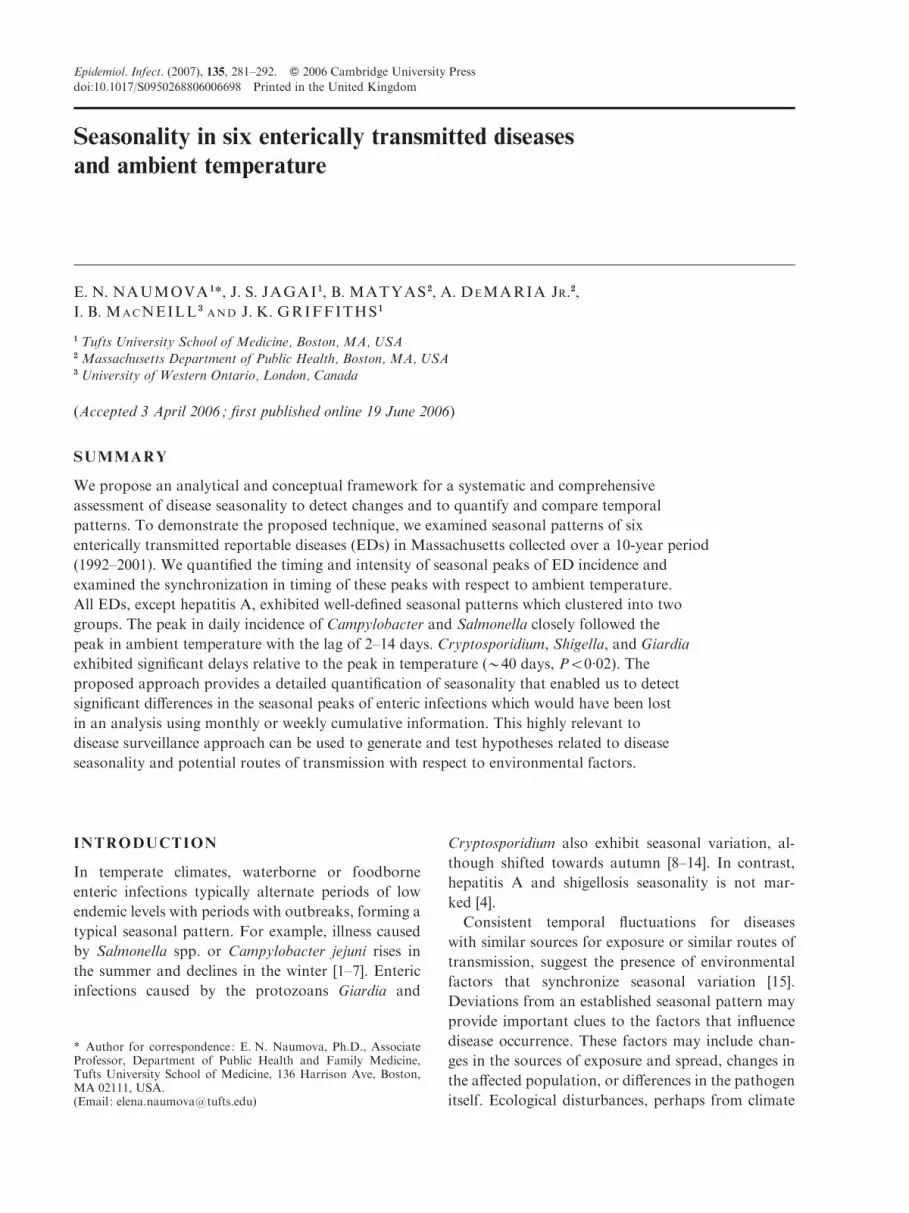
Conceptual framework for seasonality assessment

We define ‘seasonality ’ as systematic, or repetitive,

periodic fluctuations in a variable of interest (i.e.

disease incidence or environmental exposure, e.g.

temperature) that occur within the course of a year. It

can be characterized by the magnitude, timing, and

duration of a seasonal increase. We define the time of

the seasonal peak, a parameter of interest, as the

position of the maximum point on the seasonal curve.

The maximum and minimum values on the seasonal

curve, the difference between, and the ratio of

these values are the magnitude-related measures. The

conceptual framework for measuring the temporal

relation between seasonal patterns in environmental

temperatures and disease incidence is shown on

Figure 1. The synchronization in disease incidence and

environmental factors can be viewed as a special case

when multiple time series exhibit common period-

icities [25] and can be characterized, in part, by a lag,

a difference between peak timing in disease incidence

and exposure.

This conceptual framework is expressed via model

(1) as follows:

Y(t)=c cos (2pvt+y)+e(t), (1)

where Y(t) is a time series ; the periodic component

has a frequency of v, an amplitude of c, and a

phase angle of y ; and {e(t), t=1, 2, …, n} is an i.i.d.

sequence of random variables with E[e(t)]=0 and

Var[e(t)]=s2. This easy-to-interpret model describes a

seasonal curve by a cosine function with symmetric

rise and fall over a period of a full year. The locations

of two points, the seasonal curve peak and nadir, can

be determined using a shift, or phase angle parameter,

y, which reflects the timing of the peak relative to the

origin. If y=1, there is no shift of the peak relative to

the origin, and the curve peaks in the summer on the

182nd day; if 1<y<2 then there is a shift towards

autumn; and if 0<y<1 then the shift is towards

spring. For convenience, an origin can be set at the

calendar year beginning 1 January, but it can be also

reset at any other day. The shift parameter can be

expressed in days and used for seasonality com-

parison. The amplitude of fluctuations between two

extreme points is controlled via parameter c. If c=0,

there is no seasonal increase. Estimates of model (1)

are difficult to obtain because both y and c are

unknown, but its equivalent model (2) :

Y(t)=b1 sin (2pvt)+b2 cos (2pvt)+e(t), (2)

is easy to fit by the least squares procedure available

in commercial statistical software programs. Else-

where, we have proposed an approach, which allows

us to combine the ease of fitting model (2) and the

simplicity and elegance of interpretation of model (1),

by using the d-method [26]. We demonstrated that

estimates of the amplitude and shift parameters of

model (1) can be obtained from the estimates of

model (2) : for the amplitude, the estimates of the

mean and variance are

cc=f (bb1, bb2)=d(bb 21+bb 2

2 )12,

where d=1, if b2>0, and d =x1, if b2<0 and

Var(cc)=(ss 2b1bb 21+ss 2

b2bb 22+2ssb1b2

bb1bb2)=(bb21+bb 2

2 ),

and the phase angle estimates are

yy=xarctan(bb1=bb2) and

Var(yy)=(ss2b1bb 22+ss 2

b2bb 21x2ssb1b2

bb1bb2)=(bb21+bb 2

2 )2:

Parametric modelling procedures

To describe the seasonal pattern in the daily time

series of temperature and infections and estimate its

parameters, we used generalized linear models (GLM)

with a Gaussian distribution for ambient temperature

as the outcome variable of interest using model A:

Y(t)=b0+b1 sin (2pvt)+b2 cos (2pvt)+e(t), (3)

Seasonality in six enteric diseases and temperature 283

and a Poisson distribution if the studied outcome is

daily disease counts, model B:

log [Y(t)]=b0+b1 sin (2pvt)+b2 cos (2pvt)+e(t):

(4)

In both models, b0 is an intercept, a baseline of a

seasonal pattern, and t is time in days (t=1, 2, …, N,

where N is the number of days in a time series).

To properly express the frequency, we set v=1/N.

The exp{b0} for the Poisson regression reflects mean

daily disease counts over a study period. Using the

estimates of the amplitude and the phase angle, we

may now propose seasonality characteristics to help

us in assessing seasonality. They are listed in Table 1,

and include: the average maximum value (of either

exposure or disease incidence), the average minimum

value, their absolute and relative intensities, the

average peak timing in days, and the average lag

period in days between peak exposure and peak

disease incidence. Importantly, by using estimates

of the variance for the amplitude and the phase

angle parameters, the upper and lower confidence

intervals can be also estimated for all proposed

characteristics.

Characteristics Definition Units

Maximum Position of maximum point on the seasonal curve of temperature or disease incidence

Days

Minimum Position of minimum point on the seasonal curve of temperature or disease incidence

DaysTiming

Lag Difference between time of temperature maximum and time of disease incidence maximum

Days

Maximum Maximum value on seasonal curve of temperature or disease incidence

Degrees/Cases

Minimum Minimum value on seasonal curve of temperature or disease incidence

Degrees/Cases

Amplitude Difference between maximum and minimum of seasonal curve for temperature or disease incidence

Degrees/Cases Intensity

MagnitudeRatio of maximum value divided by minimum value of the seasonal curve

Unit-less

One-year cycle

Lag

150 250 350–1

4

10

15

21

27

0·5

0·7

0·9

1·1

1·3

Tem

pera

ture

(ºC

)

Dis

ease

inci

denc

e

Days

Time of disease incidence minimum

Time of temperature minimum

Time of temperature maximum

Time of disease incidence maximum

Tem

pera

ture

am

plitu

de

Dis

ease

inci

denc

e am

plitu

de

Temperature maximum

Temperature minimum

Disease incidence maximum

Disease count minimum

Fig. 1. Characteristics of seasonality : Graphical depiction and definition for daily time series of exposure (ambient tem-perature) and outcome (disease incidence) variables. The red labels are related to exposure measures and the blue labels are

related to disease incidence measures.


Non-parametric modelling procedures

As the basis for comparisons of models A and B

to a commonly used in epidemiology approach,

we applied a model that includes a set of indicator

variables to reflect a week of the year and adapts the

Gaussian or Poisson distributions as an outcome’s

distributional assumption [27] :

Y(t)=b0+biXi+e(t), (Model C)

or

log [Y(t)]=b0+biXi+e(t), (Model D)

where Y={y1, y2, …, yN}, is a time series of daily

counts or daily temperature, X is a matrix of indicator

variables for a week of observation, bi are slopes for a

corresponding indicator of a week (for i=2, …, 53),

b0 is an mean value for the reference week (in our case,

the first week of the year), and e is an error term.

Based on regression parameters of model D, we

estimated a predicted number of cases for a given

week, e.g. Y0*=exp{b0} is an estimate at week 1;

Yi*=exp{b0+bi} is an estimate at week i. For each

estimate, we calculated a corresponding 95% con-

fidence interval, 95% CI= exp {b0+bit1�96(Sb0+

Sbi )=2} , where Sbi is a standard error of a regression

parameter bi. To describe a period of seasonal

increase we determined weeks with high rates : if the

predicted number of cases for i week, Ri, had a value

less than a pre-specified cut point, Rc, then we as-

signed this week to a period of seasonal increase. We

selected three cut points as the 75th, 85th, and 95th

percentiles of a distribution of predicted weekly

incidence. Similar estimations, except for exponenti-

ation, were performed for the temperature (model C).

For each model and each ED the percent of

variance explained was calculated. All analysis was

performed using S-plus 4.5 (Insightful Corp., Seattle,

WA, USA) statistical software.

RESULTS

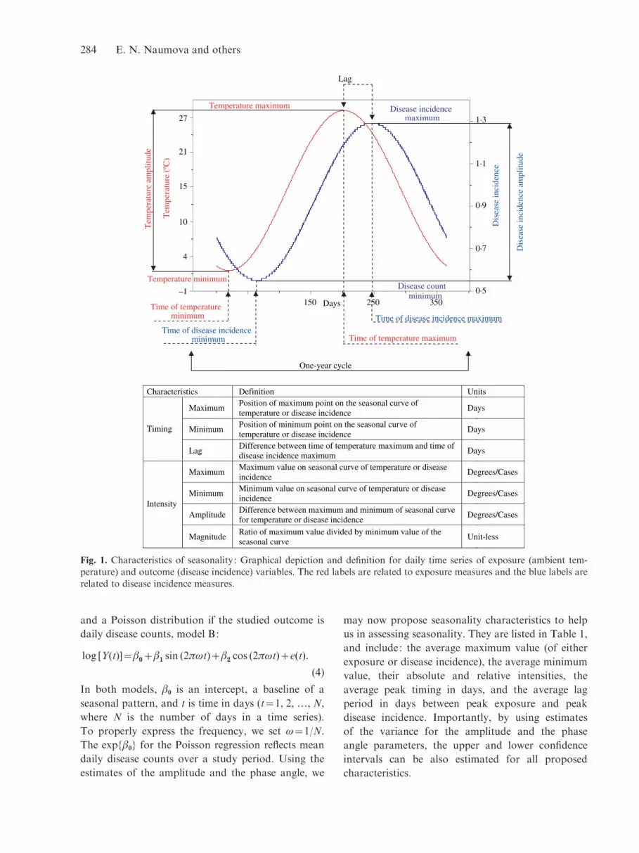
Three-dimensional scatter plots with superimposed

linear regression surfaces were created to illustrate

temperature–ED incidence relations over time (Fig. 2).

These show 10-year trends in disease incidence, with

respect to daily ambient temperature. The annual

summer disease increase is far more pronounced than

any of the annual trends for the six EDs. The time

series of daily values of ambient temperature is shown

in Figure 3a.

Descriptive statistics of laboratory-confirmed

reported cases for all six EDs are shown in Table 2:

total number of cases, daily mean with standard

deviation, the range (expressed as 25th and 75th

percentiles), and the maximum observable number

of cases per day. Salmonella, Campylobacter, and

Giardia are the most commonly reported EDs in MA.

Due to outbreaks, the range of daily fluctuation is

poorly captured by the 25th and 75th percentiles, and

the difference between the daily maximum and the

daily mean typically exceeds seven standard devi-

ations. Reporting of Cryptosporidium was low until

1995, when an unusual number of cryptosporidiosis

cases were diagnosed in Worcester, MA.

Table 2. Reported laboratory-confirmed infections and their seasonal characteristics

Temperature(xC/day)

Campylo-bacteriosis Salmonellosis Shigellosis

Crypto-sporidiosis Giardiasis Hepatitis A

Total cases 14 992 15 518 3202 528 9504 2072

Mean¡S.D. 14.97¡9.92 4.10¡3.02 4.25¡3.33 0.88¡1.31 0.14¡0.48 2.60¡2.57 0.57¡0.861st, 3rd quartile (6.6, 23.8) (2, 5) (2, 6) (0, 1) (0, 0) (1, 4) (0, 1)Maximum 34.56 26 32 13 9 22 7

Model A Model B

PredictedMin, max value (2.2, 27.8) (2.55, 6.03) (2.32, 6.75) (0.46, 1.42) (0.06, 0.28) (1.74, 3.64) (0.46, 0.69)

Average intensity 7.78 3.47 4.43 0.96 0.22 1.91 0.23Relative intensity 2.28 2.36 2.91 3.07 5.00 2.10 1.49Peak (days) 206¡0.22 208¡0.79 219¡0.30 247¡1.26 242¡1.73 249¡1.18 269¡9.81

LCI, UCI (days) (206–207) (206–209) (218–219) (245–250) (239–246) (247–251) (249–288)Variation explainedby seasonality

83% 17% 23% 8% 6% 8% 1%

LCI, lower confidence interval ; UCI, upper confidence interval.


Seasonal characteristics

The magnitude and timing of a seasonal increase,

estimated from model A (for temperature) and model

B (for ED) are shown in Table 2. The seasonal curve

for ambient temperature peaked at the 206th (¡0.2)

day of the year (typically 24 or 25 July, week 29) with

an average maximum temperature of y8.89 xC. Ten

superimposed time series of daily values of ambient

temperature together with the predicted seasonal

curve are shown in Figure 3b. The predicted seasonal

pattern for daily disease counts for each disease

(Fig. 4a) and daily magnitude for each disease

(Fig. 4b) are illustrated.

For the five EDs with a relationship to ambient

temperature, two groups emerged. Peak Campylo-

bacter incidence essentially coincided with the peak

in temperature (day 208¡0.8, P=0.89). Salmonella

incidence peaked 13 days after the peak in ambient

temperature. In another group, reported cryptospor-

idiosis and shigellosis peaked contemporaneously

almost 1 month after the temperature peak (242¡1.7

and 247¡1.3, P<0.02). Reported giardiasis peaked 1

week after cryptosporidiosis (249¡1.2, P<0.01),

in the first week of September. The small variability

in the timing of these seasonal peaks reflects the

consistency of the seasonal pattern for these dis-

eases. The variability exhibited by Salmonella and

(a)

18

12

Gia

rdia

sis

6

0

8027

15

4

–1

°C °F

60

40

20 800

1600

2400

3200

(b)

Cry

ptos

pori

dios

is

0·0

2·5

5·0

7·5

8027

15

4

–1

°C°F

60

40

20 800

1600

2400

3200

(d )

Cam

pylo

bact

erio

sis

0

8

16

24

8027

15

4

–1

°C°F

60

40

20 800

1600

2400

3200

(f )

Hep

atiti

s A

0

2

4

5

8027

15

4

–1

°C°F

60

40

20 800

1600

2400

3200

(c)

Salm

onel

losi

s

16

24

32

8

0

8027

15

4

–1

°C°F

60

40

20 800

1600

2400

3200

(e)

Shig

ello

sis

8

12

4

0

8027

15

4

–1

°C°F

60

40

20 800

1600

2400

3200

Fig. 2. Disease trend for six EDs: 3D graphical representations of disease incidence against time (in days) and ambienttemperature (xC aligned with xF), which show the annual trend over 10 years for each disease.


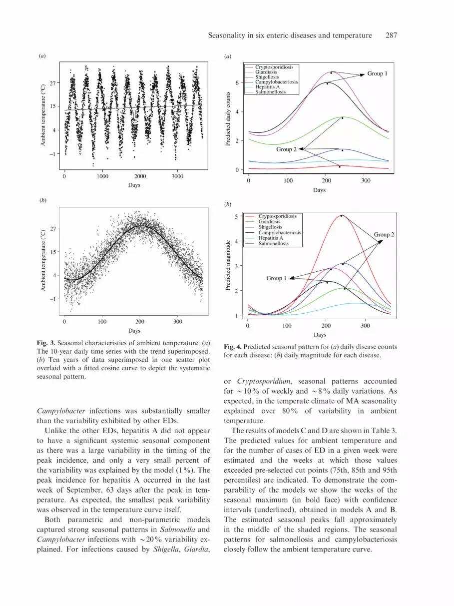
Campylobacter infections was substantially smaller

than the variability exhibited by other EDs.

Unlike the other EDs, hepatitis A did not appear

to have a significant systemic seasonal component

as there was a large variability in the timing of the

peak incidence, and only a very small percent of

the variability was explained by the model (1%). The

peak incidence for hepatitis A occurred in the last

week of September, 63 days after the peak in tem-

perature. As expected, the smallest peak variability

was observed in the temperature curve itself.

Both parametric and non-parametric models

captured strong seasonal patterns in Salmonella and

Campylobacter infections with y20% variability ex-

plained. For infections caused by Shigella, Giardia,

or Cryptosporidium, seasonal patterns accounted

for y10% of weekly and y8% daily variations. As

expected, in the temperate climate of MA seasonality

explained over 80% of variability in ambient

temperature.

The results of models C andD are shown in Table 3.

The predicted values for ambient temperature and

for the number of cases of ED in a given week were

estimated and the weeks at which those values

exceeded pre-selected cut points (75th, 85th and 95th

percentiles) are indicated. To demonstrate the com-

parability of the models we show the weeks of the

seasonal maximum (in bold face) with confidence

intervals (underlined), obtained in models A and B.

The estimated seasonal peaks fall approximately

in the middle of the shaded regions. The seasonal

patterns for salmonellosis and campylobacteriosis

closely follow the ambient temperature curve.

(a)

Days

0 1000 2000 3000

40

60

27

15

4

–1

Am

bien

t tem

pera

ture

(°C

)

(b)

Days

0 100 200 300

20

40

60

8027

15

4

–1

Am

bien

t tem

pera

ture

(˚C

)

Fig. 3. Seasonal characteristics of ambient temperature. (a)The 10-year daily time series with the trend superimposed.(b) Ten years of data superimposed in one scatter plot

overlaid with a fitted cosine curve to depict the systematicseasonal pattern.

(a)

0 100 200 300

Days

0

2

4

6

Pred

icte

d da

ily c

ount

s

•

•

•

•

•

Group 1

Group 2

Cryptosporidiosis GiardiasisShigellosisCampylobacteriosisHepatitis ASalmonellosis

(b)

Days

Pred

icte

d m

agni

tude

0 100 200 300

1

2

3

4

5 CryptosporidiosisGiardiasisShigellosisCampylobacteriosisHepatitis ASalmonellosis

•

••

••

Group 1

Group 2

Fig. 4. Predicted seasonal pattern for (a) daily disease countsfor each disease ; (b) daily magnitude for each disease.


Table 3. The predicted weekly values, the mean, and three upper percentiles (75th, 85th, and 95th),

and percent variability explained by models C and D, for ambient temperature (xC) and for the number of cases

of ED respectively

Weekno.

Temp.(xC)

Campylo-bacteriosis

Salmon-ellosis Shigellosis

Crypto-sporidiosis Giardiasis Hepatitis A

1 3.40 2.45 2.77 0.68 0.07 2.20 0.34

2 2.18 2.97 2.73 0.56 0.03 2.11 0.573 1.97 2.51 2.03 0.64 0.09 1.46 0.564 1.72 2.46 2.19 1.13 0.10 2.03 0.445 1.88 3.20 2.81 0.73 0.07 2.50 0.63

6 1.83 2.64 2.39 0.54 0.04 1.94 0.507 4.39 2.41 2.64 0.64 0.06 1.73 0.438 4.56 2.83 2.53 0.53 0.07 1.69 0.46

9 4.34 2.77 2.64 0.49 0.10 2.11 0.7910 6.16 2.84 2.59 0.49 0.14 1.96 0.6111 6.41 2.97 2.76 0.64 0.04 2.59 0.43

12 8.86 2.94 2.59 0.73 0.06 1.70 0.4713 11.46 3.16 2.97 0.53 0.10 2.41 0.5914 12.13 2.69 3.23 0.39 0.06 1.91 0.4315 12.84 3.07 3.33 0.39 0.09 2.31 0.41

16 15.91 3.40 3.10 0.34 0.13 1.70 0.3917 16.86 3.60 3.84 0.56 0.06 2.19 0.5618 17.72 4.07 3.71 0.30 0.06 2.19 0.54

19 18.86 3.84 3.99 0.60 0.16 2.09 0.3920 20.10 4.19 3.66 0.59 0.07 1.66 0.3921 21.08 4.83 4.14 0.71 0.09 1.53 0.40

22 22.76 5.89 4.64 0.87 0.11 2.49 0.5923 24.74 5.14 5.37 0.86 0.13 2.01 0.4024 24.75 6.91 6.19 0.66 0.10 2.27 0.39

25 26.78 6.46 6.11 0.61 0.14 2.09 0.5026 26.67 7.01 6.46 0.80 0.19 3.34 0.5327 27.72 7.34 6.31 0.91 0.20 2.43 0.7628 27.95 6.74 6.24 0.94 0.10 2.94 0.53

29 27.21 6.14 6.19 1.39 0.09 3.31 0.5130 27.29 6.20 6.76 1.80 0.16 3.39 0.5331 28.22 5.29 7.61 1.83 0.31 3.81 0.71

32 26.14 5.51 6.87 1.70 0.34 3.64 0.7433 25.61 5.17 7.47 1.71 0.43 4.43 0.7134 26.51 4.57 6.67 1.67 0.41 3.53 0.70

35 25.59 5.37 7.33 1.93 0.26 4.69 0.6936 23.72 4.46 6.09 1.30 0.49 3.79 0.7737 23.19 4.40 6.01 1.46 0.20 4.51 0.7738 20.18 3.93 5.40 1.24 0.30 3.37 0.63

39 18.93 4.66 5.27 1.26 0.21 3.79 0.9040 18.06 4.17 4.54 1.04 0.34 3.31 0.7041 16.78 4.06 4.69 0.97 0.13 3.57 0.50

42 15.90 4.04 3.77 1.11 0.16 3.06 0.5443 14.98 4.17 3.89 0.80 0.13 2.80 0.5944 12.73 4.19 3.27 0.97 0.09 3.09 0.79

45 10.12 3.97 3.27 0.81 0.17 2.59 0.8346 9.65 4.09 3.59 0.81 0.14 3.23 0.8147 8.89 3.51 2.73 0.83 0.04 2.03 0.59

48 8.85 3.47 3.97 0.87 0.11 2.01 0.4049 6.48 2.97 3.36 0.67 0.03 2.04 0.4450 4.56 3.20 3.23 0.79 0.19 2.17 0.4351 4.07 2.40 2.43 0.43 0.09 1.74 0.39

52 1.99 2.41 2.99 0.43 0.07 1.81 0.6153 x0.98 2.50 1.93 0.36 0.07 2.57 0.43


CONCLUSION

Although seasonality is a well-known phenomenon in

the epidemiology of many diseases, simple analytical

tools for the examination, evaluation, and com-

parison of seasonal patterns are limited. Analyses of

disease seasonality have also been restricted by the

lack of precision inherent in using monthly or weekly

means. Herein we offer a framework for uniform,

comprehensive, systematic, seasonality assessment via

a parametric approach, using daily frequencies. This

approach is highly relevant to disease surveillance,

which sifts through daily frequencies of disease as

well as specially designed epidemiological studies.

We propose simple, easily understood characteristics

for the intensity and timing of a seasonal peak.

These allow us to quantify seasonality in a con-

sistent manner and to compare relationships between

diseases and environmental factors.

We applied this approach to the study of enteric

diseases in MA. We found that infections caused by

Salmonella and Campylobacter closely follow the

ambient temperature curve. If we knew nothing else,

we might hypothesize that Salmonella and Campylo-

bacter infections share a dominant route of exposure

that is strongly influenced by ambient temperature.

Foodborne transmission is an obvious candidate

for this route, given the capacity of Salmonella to

grow in contaminated food and the paucity of person-

to-person spread with Campylobacter infections.

Indeed, food contamination is believed to be the most

significant mode of transmission for Salmonella and

Campylobacter [28–30].

In contrast, the seasonal increase in Giardia,

Shigella, and Cryptosporidium infections form a sep-

arate cluster peaking a month after the temperature

peak, strongly suggesting different route(s) of expo-

sure than for Salmonella or Campylobacter. Reasons

for this month-long temporal delay (lag) include dif-

ferences in routes of transmission, amplification of

infection related to person-to-person spread, survival

of pathogens in the environment, incubation periods

after ingestion, differences in diseases manifestation

and testing practices, or combinations thereof. Out-

breaks of cryptosporidiosis, giardiasis, or shigellosis

associated with drinking water and recreational water

use occur in the warm summer months [2, 5, 31, 32].

Hot weather leads to higher water consumption [33],

promotes outdoor swimming [34], other recreational

water use, and other outdoor activities. Person-to-

person spread may also be increased due to the close

quarters and poor hygiene of outdoor activities,

such as camping or swimming, and person-to-person

spread may amplify outbreaks pushing peaks to a

later time period. Prior work suggests that contami-

nated water is a dominant source of exposure for

cryptosporidiosis and giardiasis [35, 36], although

foodborne transmission is certainly possible [37].

We cannot comment on the possibility that foreign

travel, presence of HIV infection, specific water

sources, or specific recreational water exposures were

involved in these findings, as the data collected by

Commonwealth of Massachusetts does not contain

detailed information on these potential risk factors.

The differences in seasonality between the first

(Salmonella and Campylobacter infection) and the

second cluster (Giardia, Shigella, and Cryptospor-

idium infections) could be in part associated with the

probability of acute clinical syndromes, as well as

testing and reporting practices. For each record in the

database, a few dates were provided: date on event,

date of disease onset, date of diagnosis, date of

specimen collection, and date of reporting. We ex-

amined the differences amongst all the dates and

selected the date of disease onset as the most reliable

characteristic. In any passive surveillance a delay

Table 3 (cont.)

Week

no.

Temp.

(xC)

Campylo-

bacteriosis

Salmon-

ellosis Shigellosis

Crypto-

sporidiosis Giardiasis Hepatitis A

Mean14.73 4.08 4.21 0.87 0.14 2.60 0.56

75% 23.72 4.83 6.01 1.04 0.17 3.31 0.6985% 26.22 5.59 6.26 1.32 0.22 3.54 0.75

95% 27.46 6.81 7.05 1.75 0.37 4.06 0.80

% Var 84 20 25 12 10 11 3

Bold values indicate weeks of the seasonal maximum; underlining indicates confidence intervals (obtained in models Aand B). Shaded regions indicate where estimated seasonal peaks fall.


between time of clinical manifestation and time of

diagnosis and testing is practically unavoidable,

however, we assume that this delay is systematic over

the course of year and the lag between the peak in

ambient temperature and an the peak in diseases

includes this systematic component.

The seasonal pattern in cryptosporidiosis observed

in this study, differs from the seasonal patterns

reported by others where a slight increase in the

number of positive stool tests for Cryptosporidium

parvum and in the number of cases of cryptospor-

idiosis among HIV patients occurred in the spring

compared with other seasons, but the difference was

not statistically significant [38]. This fact could be

indicative of differences in predominant routes of

exposure in the HIV-infected population. If there is a

spring peak in cryptosporidiosis in MA, it is not cap-

tured in the surveillance data that we analysed in this

study, in part due to the fact that the highest fraction

of samples for cryptosporidiosis came from children

(60%) not adults. Although, the surveillance data

have been shown to be underreported and over-

sampled in certain situations, such as during the 1995

Worcester cryptosporidiosis outbreak [14], the estab-

lished surveillance system on enteric infection has

valuable potential for quantifying disease trends and

seasonal patterns.

In this paper we have assumed a common para-

metric form for seasonality, a cosine function. The

shape of a cosine periodic function is defined by its

shift parameter, which reflects the point of maximum

amplitude, and by the length of a period, which

implies that only one peak is observable in one

calendar year. This assumption may not hold if a

disease exhibits two seasonal peaks [39] ; however, the

proposed model can be extended so both peaks will

be evaluated [26]. In any case, we recommend an

exploration of the potential form for a seasonal

pattern via nonlinear or non-parametric methods

prior to modelling.

We compared our parametric approach with that

of non-parametric modelling, which has an intuitive

appeal and is often used for surveillance data

(Table 3). The non-parametric model provides a

reasonably good approximation for seasonal vari-

ation, and allows one to make a reliably independent

assessment of a specific week’s disease incidence

against that of a reference week. However, this ap-

proach does not take into account temporal depen-

dency, and treats each week as a separate independent

category. As expected, the non-parametric model with

a set of indicator variables for weeks explained a

larger percentage of the variability than did the

parametric model using daily counts, in part due to a

lesser impact of calendar effects (holidays or day of the

week effects) in weekly aggregation. However, this

possible advantage is strongly diminished by themajor

difficulties in comparing results of non-parametric

models.

For both non-parametric and parametric ap-

proaches, we utilized a Poisson regression model to

predict ED incidence. Although a Poisson assumption

is well suited for non-negative right-skewed outcomes,

such as daily or weekly cases of infections, and can be

a suitable approximation for a seasonal mean, we

found the tails of the observed distributions of daily

ED counts were longer than for a Poisson-like distri-

bution. Approximation of the outcome by the Poisson

distribution leads to the underestimation of predicted

rates for days or weeks with very high rates, meaning

that the actual degree of summer/autumn increase

might be higher than predicted. We think that the

model can be improved in the future by using more

sophisticated tools for handling extreme values

relating to outbreaks. However, until superimposed

non-seasonal variation can be better predicted and

identified, the selection of such tools is arbitrary.

One methodological aspect of this approach de-

serves special comment. The vast majority of epide-

miological studies of ED seasonality have used crude

quarterly or monthly aggregate data. This prevents a

fully detailed, accurate, or comprehensive analysis of

a seasonal pattern and may even be misleading [40].

The use of daily time series for these infections

enabled us to detect significant differences in the

seasonal peaks of enteric infections, which would

have been lost in an analysis using monthly or weekly

cumulative information. Examination of weekly rates

substantially improves the evaluation of seasonal

curves when compared to monthly data, but a

systematic approach to the issue of week assignment

in the long time series has often been lacking. The

analysis of disease seasonality would benefit from

the proposed approach, which can be used both as

a routine in disease surveillance and as a part of

specially designed epidemiological studies.

ACKNOWLEDGEMENTS

We thank the Massachusetts Department of Public

Health for support throughout this project and for

providing us with surveillance data. We also thank


the EPA and the National Institute of Allergy and

Infectious Diseases who provided funding through

grant AI43415 to E.N.N., J.G., J.K.G. and I.B.M.

DECLARATION OF INTEREST

None.

REFERENCES

1. Amin OM. Seasonal prevalence of intestinal parasites inthe United States during 2000. American Journal ofTropical Medicine and Hygiene 2002; 66 : 799–803.

2. Barwick RS, et al. Surveillance for waterborne-diseaseoutbreaks – United States, 1997–1998. MMWR. CDCSurveillance Summaries 2000; 49 : 1–21.

3. Bean NH, et al. Surveillance for foodborne-diseaseoutbreaks – United States, 1988–1992. MMWR. CDCSurveillance Summaries 1996; 45 : 1–66.

4. Bowman C, Flint J, Pollari F. Canadian integratedsurveillance report : Salmonella, Campylobacter, patho-genic E. coli and Shigella, from 1996 to 1999. Canadian

Communicable Disease Report 2003; 29 (Suppl. 1) : 1–6.5. Lee SH, et al. Surveillance for waterborne-disease

outbreaks – United States, 1999–2000. MMWR. CDCSurveillance Summaries 2002; 51 : 1–47.

6. Levy DA, et al. Surveillance for waterborne-diseaseoutbreaks – United States, 1995–1996. MMWR. CDCSurveillance Summaries 1998; 47 : 1–34.

7. Olsen SJ, et al. Surveillance for foodborne-diseaseoutbreaks – United States, 1993–1997. MMWR. CDCSurveillance Summaries 2000; 49 : 1–62.

8. Addiss DG, et al. Epidemiology of giardiasis inWisconsin : increasing incidence of reported cases andunexplained seasonal trends. American Journal ofTropical Medicine and Hygiene 1992; 47 : 13–19.

9. Birkhead G, Vogt RL. Epidemiologic surveillancefor endemic Giardia lamblia infection in Vermont. Theroles of waterborne and person-to-person transmission.

American Journal of Epidemiology 1989; 129 : 762–768.10. Dietz V, et al. Active, multisite, laboratory-based sur-

veillance forCryptosporidium parvum.American Journal

of Tropical Medicine and Hygiene 2000; 62 : 368–372.11. Furness BW, Beach MJ, Roberts JM. Giardiasis

surveillance – United States, 1992–1997.MMWR.CDC

Surveillance Summaries 2000; 49 : 1–13.12. Greig JD, et al.A descriptive analysis of giardiasis cases

reported in Ontario, 1990–1998. Canadian Journal ofPublic Health 2001; 92 : 361–365.

13. Majowicz SE, et al. Descriptive analysis of endemiccryptosporidiosis cases reported in Ontario, 1996–1997.Canadian Journal of Public Health 2001; 92 : 62–66.

14. Naumova EN, et al. Use of passive surveillance data tostudy temporal and spatial variation in the incidence ofgiardiasis and cryptosporidiosis. Public Health Report

2000; 115 : 436–447.15. Hald T, Andersen JS. Trends and seasonal variations in

the occurrence of Salmonella in pigs, pork and humans

in Denmark, 1995–2000. Berliner und MunchenerTierarztliche Wochenschrift 2001; 114 : 346–349.

16. Patz JA, et al. Effects of environmental change onemerging parasitic diseases. International Journal ofParasitology 2000; 30 : 1395–1405.

17. Bentham G, Langford IH. Climate change and the inci-dence of food poisoning in England and Wales.International Journal of Biometeorology 1995; 39 : 81–86.

18. Bentham G, Langford IH. Environmental temperaturesand the incidence of food poisoning in England andWales. International Journal of Biometeorology 2001;

45 : 22–26.19. Cowden JM, et al. Outbreaks of foodborne infectious

intestinal disease in England andWales : 1992 and 1993.

Communicable Disease Report. CDR Review 1995; 5 :R109–R117.

20. Djuretic T, Wall PG, Nichols G. General outbreaks of

infectious intestinal disease associated with milk anddairy products in England and Wales : 1992 to 1996.[Erratum appears in CDR. CDR Review 1997; 7 : R54].Communicable Disease Report. CDR Review 1997; 7 :

R41–R45.21. Checkley W, et al. Effect of El Nino and ambient tem-

perature on hospital admissions for diarrhoeal diseases

in Peruvian children. Lancet 2000; 355 : 442–450.22. Curriero FC, et al. The association between extreme

precipitation and waterborne disease outbreaks in the

United States, 1948–1994 [see comment]. AmericanJournal of Public Health 2001; 91 : 1194–1199.

23. Smoyer KE. A comparative analysis of heat waves and

associated mortality in St. Louis, Missouri – 1980 and1995. International Journal of Biometeorology 1998; 42 :44–50.

24. Epstein PR. Climate change and emerging infectious

diseases. Microbes and Infection 2001; 3 : 747–754.25. MacNeill IB. A test of whether several time series share

common periodicities. Biometrika 1977; 64 : 495–508.

26. Naumova EN, MacNeill IB. Seasonality assessment forbiosurveillance systems. In Balakrishnan N, et al., eds.Advances in Statistical Methods for the Health Sciences :

applications to cancer andAIDS studies, genome sequenceanalysis, and survival analysis. Boston: Birkhauser, 2006.

27. McCullagh P, Nelder JA. Generalized Linear Models.New York: Chapman and Hall, 1989.

28. Hobbs BC, Roberts D. Food Poisoning and FoodHygiene. London: Edward Arnold, 1997.

29. Kusumaningrum HD, et al. Survival of foodborne

pathogens on stainless steel surfaces and cross-contamination to foods. International Journal of FoodMicrobiology 2003; 85 : 227–236.

30. Mead PS, et al. Food-related illness and death in theUnited States. Emerging Infectious Diseases 1999; 5 :607–625.

31. Fleming CA, et al. An outbreak of Shigella sonneiassociated with a recreational spray fountain. AmericanJournal of Public Health 2000; 90 : 1641–1642.

32. Joce RE, et al. An outbreak of cryptosporidiosis

associated with a swimming pool. Epidemiology andInfection 1991; 107 : 497–508.


33. Gofti-Laroche L, et al. Description of drinking waterintake in French communities (E.M.I.R.A. study)

[in French]. Revue Epidemiologique et Sante Publique2001; 49 : 411–422.

34. CDC. Surveillance data from swimming pool in-

spections – selected states and counties, United States,May–September 2002. Morbidity and Mortality WeeklyReport 2003; 52 : 513–516.

35. Rose JB, et al. Climate variability and change

in the United States : potential impacts on water-and foodborne diseases caused by microbiologicagents. Environmental Health Perspectives 2001; 109

(Suppl. 2) : 211–221.36. Stuart JM, et al. Risk factors for sporadic giardiasis : a

case-control study in southwestern England. Emerging

Infectious Diseases 2003; 9 : 229–233.

37. Rose JB, Slifko TR. Giardia, Cryptosporidium, andCyclospora and their impact on foods : a review. Journal

of Food Protein 1999; 62 : 1059–1070.38. Inungu JN, Morse AA, Gordon C. Risk factors,

seasonality, and trends of cryptosporidiosis among

patients infected with human immunodeficiency virus.American Journal of Tropical Medicine and Hygiene2000; 62 : 384–387.

39. Naumova EN, et al. Effect of precipitation on seasonal

pattern variability in cryptosporidiosis recorded by theNorth West England surveillance system in 1990–1999.Journal of Water and Health 2005; 3 : 185–196.

40. da Silva Lopes ACB. Spurious deterministic seasonalityand autocorrelation corrections with quarterly data :Further Monte Carlo results. Empirical Economics

1999; 24 : 341–359.


seasonality in six enterically transmitted diseases and ambient temperature

Documents