J O U R N A L O F E N V I R O N M E N T A L S C I E N C E S 4 1 ( 2 0 1 6 ) 6 9 – 8 0

Ava i l ab l e on l i ne a t www.sc i enced i r ec t . com

ScienceDirect

www.e l sev i e r . com/ loca te / j es

A case study of development and application of a streamlinedcontrol and response modeling system for PM2.5 attainmentassessment in China

Shicheng Long1, Yun Zhu1,⁎, Carey Jang2, Che-Jen Lin1,3, Shuxiao Wang4, Bin Zhao4,Jian Gao5, Shuang Deng5, Junping Xie1, Xuezhen Qiu1

1. School of Environment and Energy, South China University of Technology, Guangzhou Higher Education Mega Center, Guangzhou 510006, China2. USEPA/Office of Air Quality Planning & Standards, RTP, NC 27711, USA3. Department of Civil Engineering, Lamar University, Beaumont, TX 77710-0024, USA4. State Key Joint Laboratory of Environment Simulation and Pollution Control, School of Environment, Tsinghua University, Beijing 100084, China5. Chinese Research Academy of Environmental Sciences, Beijing 100012, China

A R T I C L E I N F O

⁎ Corresponding author. E-mail: zhuyun@scu

http://dx.doi.org/10.1016/j.jes.2015.05.0191001-0742 © 2015 The Research Center for Ec

A B S T R A C T

Article history:Received 17 February 2015Revised 20 May 2015Accepted 21 May 2015Available online 26 July 2015

This article describes the development and application of a streamlined air control andresponse modeling system with a novel response surface modeling-linear coupled fittingmethod and a new module to provide streamlined model data for PM2.5 attainmentassessment in China. This method is capable of significantly reducing the dimensionsrequired to establish a response surface model, as well as capturing more realistic responseof PM2.5 to emission changes with a limited number of model simulations. The newlydeveloped module establishes a data link between the system and the Software for ModelAttainment Test—Community Edition (SMAT-CE), and has the ability to rapidly providemodel responses to emission control scenarios for SMAT-CE using a simple interface. Theperformance of this streamlined system is demonstrated through a case study of theYangtze River Delta (YRD) in China. Our results show that this system is capable ofreproducing the Community Multi-Scale Air Quality (CMAQ) model simulation results withmaximum mean normalized error < 3.5%. It is also demonstrated that primary emissionsmake a major contribution to ambient levels of PM2.5 in January and August (e.g., more than50% contributed by primary emissions in Shanghai), and Shanghai needs to have regionalemission control both locally and in its neighboring provinces to meet China's annual PM2.5

National Ambient Air Quality Standard. The streamlined system provides a real-timecontrol/response assessment to identify the contributions of major emission sources toambient PM2.5 (and potentially O3 as well) and streamline air quality data for SMAT-CE toperform attainment assessments.© 2015 The Research Center for Eco-Environmental Sciences, Chinese Academy of Sciences.

Published by Elsevier B.V.

Keywords:Response surface modelRSM-Linear coupled fittingAir quality modelingAttainment assessmentPM2.5

t.edu.cn (Yun Zhu).

o-Environmental Sciences, Chinese Academy of Sciences. Published by Elsevier B.V.

70 J O U R N A L O F E N V I R O N M E N T A L S C I E N C E S 4 1 ( 2 0 1 6 ) 6 9 – 8 0

Introduction

Fine particulate matter pollution (PM2.5) has been one of themost important environmental pollution issues in Chinarecently due to its adverse influences on regional haze (Sunet al., 2014; Zhao et al., 2013b), public health and global climatechange (Buonocore et al., 2014; Tai et al., 2010). According tothe air quality reports of the China National EnvironmentalMonitoring Centre (CNEMC), the monitored annual averagePM2.5 of most Chinese cities (China National EnvironmentalMonitoring Centre Centre(CNEMC), 2013) substantially ex-ceeds the Grade II China National Ambient Air QualityStandard (35 μg/m3) (Ministry of Environmental Protection ofthe People's Republic of China, MEP, 2012). A large portion ofPM2.5 in China is attributable to anthropogenic emissions suchas gaseous precursors and primary PM emissions from powerplants, industrial & domestic sectors, and transportation (Dong etal., 2014; Fu et al., 2013; Wang and Hao, 2012), especially forprimary PMemissions (Xing, 2011; Zhao et al., 2013a). To estimatethe response of PM2.5 to anthropogenic emissions under variouscontrol strategies, air quality models are an effective and widelyused tool for attainment assessments in air qualitymanagement.The Community Multi-scale Air Quality (CMAQ) model, as apowerful air quality model tool, has been widely employed tocompare the efficacy of various emission control strategies inChina (Streets et al., 2007; Wang et al., 2010; Zhao et al., 2013b)and other countries (Appel et al., 2012; Byun and Schere, 2006;Chemel et al., 2014). However, it is extremely time-consumingforCMAQ toestimate a large number of controlmeasures due tothe high computational costs and the complicated nature of therequired emission/ meteorology inputs and processing (Fann etal., 2012; Foley et al., 2014; Xing et al., 2011). Therefore, a softwarepackage called Response Surface Model—Visualization AnalysisTool (RSM-VAT) has been developed to address this issue.

RSM-VAT is an innovative reduced form of air qualitymodel, which has been continually improved and appliedsuccessfully in testing and evaluation for PM2.5 (US EPA, 2006b;Zhao et al., 2014; Zhu et al., 2015) and ozone (US EPA, 2006a;Xing et al., 2011). However, there are two limitations inRSM-VAT. One is that the errors of RSM prediction performancessharply increase with the increase of variables since the samplespace is greatly increased with the increase of dimensions (Xinget al., 2011). It requires many thousands of CMAQ model runs(samples) to build a reliable RSM prediction when the number ofvariables is more than a certain threshold (e.g., 56), which isunrealistic for CMAQ (Appel et al., 2011). There is also anassumption in RSM-VAT that all control variables involved inbuilding the response surface model have a nonlinear responseto pollutants (e.g., PM2.5). This assumption is not appropriate forprimary PM2.5. PM2.5 is a mixture consisting of nonlinearcontributions from gaseous precursors (e.g., SO2, NH3 and NOx)and linear contributions from primary/direct PM2.5 emissionsources (Dong et al., 2014; Li et al., 2014; Xing, 2011). In China,especially in the YRD region, the proportion of contributionsfrom total primary PM2.5 emissions can be as high as 46% (Zhaoet al., 2014). To overcome these limitations, we improve theprevious version of RSM-VAT with a new RSM-Linear coupledfitting method. The updated response modeling system signif-icantly reduces the dimensions required to establish a response

surface model and captures the realistic response of fineparticles to both primary and secondary source changes witha reasonable number of model simulations.

The Software for Model Attainment Test—CommunityEdition (SMAT-CE) is a powerful regulatory model tool todemonstrate the air quality attainment for emission controlstrategies by combining monitoring data with modeled datafrom CMAQ or from the Comprehensive Air Quality Modelwith extensions (CAMx) (US EPA, 2007; Wang et al., 2015).However, the model output format cannot be directly used inSMAT-CE for efficient attainment assessment. The RSM-VATcan address this challenge, but these two software tools areoperated in a stand-alone fashion and the SMAT-CE is unableto identify the griddedmodel data fromRSM-VAT due to theirdifferent data formats. As such, amodule for outputting griddedmodel data to SMAT-CE in the updated response modeling tool(RSM-VAT) was developed. The module establishes a data linkbetween this updated RSM tool and SMAT-CE, which providesstreamlined model data for PM2.5 and O3 attainment assess-ment. Finally, a case study on PM2.5 in the Yangtze River Delta(YRD) was conducted for attainment assessments in this paper.The streamlinedmodeling tool in this case study demonstratesan innovative approach that could provide real-time control/response assessment to identify the contributions of majoremission sources to ambient PM2.5 (and potentially O3 as well)as well as streamline air quality data for SMAT-CE to performPM2.5 and O3 attainment assessments.

1. Methodology

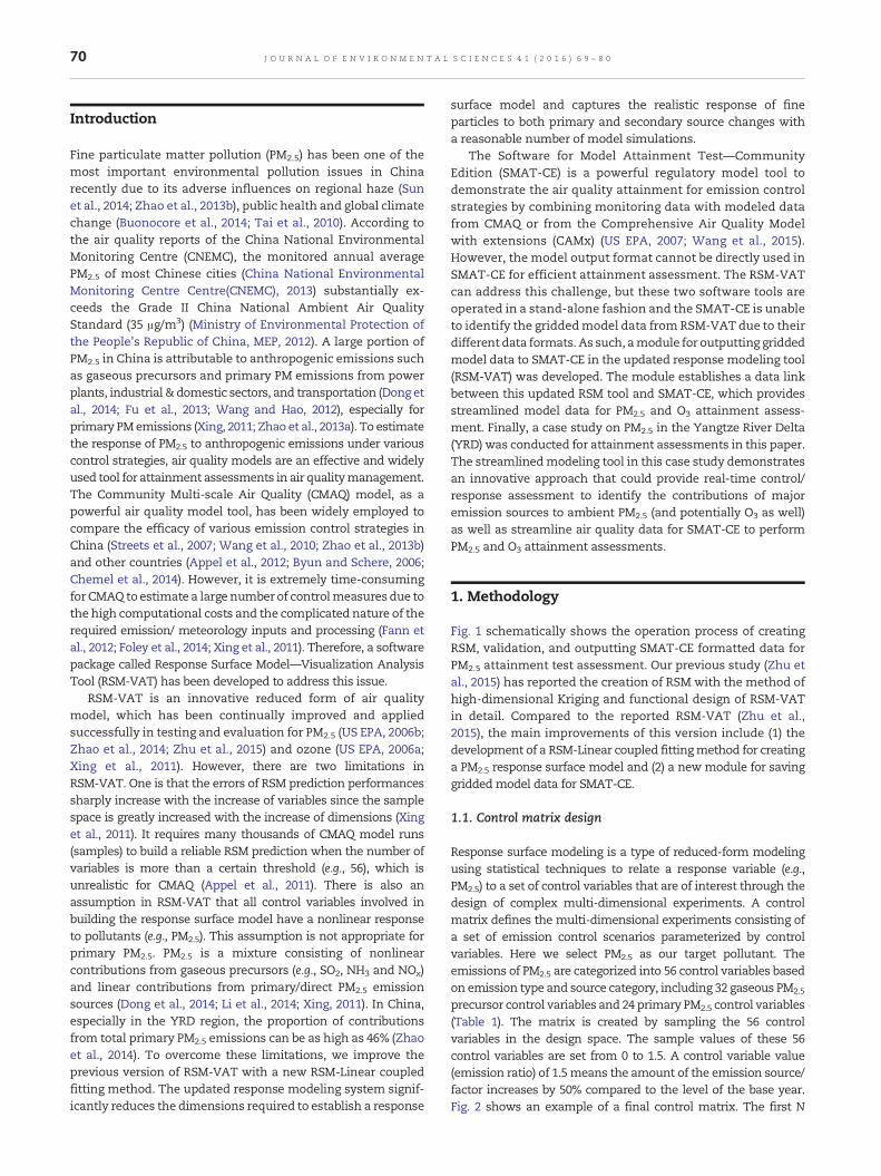
Fig. 1 schematically shows the operation process of creatingRSM, validation, and outputting SMAT-CE formatted data forPM2.5 attainment test assessment. Our previous study (Zhu etal., 2015) has reported the creation of RSM with the method ofhigh-dimensional Kriging and functional design of RSM-VATin detail. Compared to the reported RSM-VAT (Zhu et al.,2015), the main improvements of this version include (1) thedevelopment of a RSM-Linear coupled fittingmethod for creatinga PM2.5 response surface model and (2) a new module for savinggridded model data for SMAT-CE.

1.1. Control matrix design

Response surface modeling is a type of reduced-form modelingusing statistical techniques to relate a response variable (e.g.,PM2.5) to a set of control variables that are of interest through thedesign of complex multi-dimensional experiments. A controlmatrix defines the multi-dimensional experiments consisting ofa set of emission control scenarios parameterized by controlvariables. Here we select PM2.5 as our target pollutant. Theemissions of PM2.5 are categorized into 56 control variables basedon emission type and source category, including 32 gaseous PM2.5

precursor control variables and 24 primary PM2.5 control variables(Table 1). The matrix is created by sampling the 56 controlvariables in the design space. The sample values of these 56control variables are set from 0 to 1.5. A control variable value(emission ratio) of 1.5means the amount of the emission source/factor increases by 50% compared to the level of the base year.Fig. 2 shows an example of a final control matrix. The first N

71J O U R N A L O F E N V I R O N M E N T A L S C I E N C E S 4 1 ( 2 0 1 6 ) 6 9 – 8 0

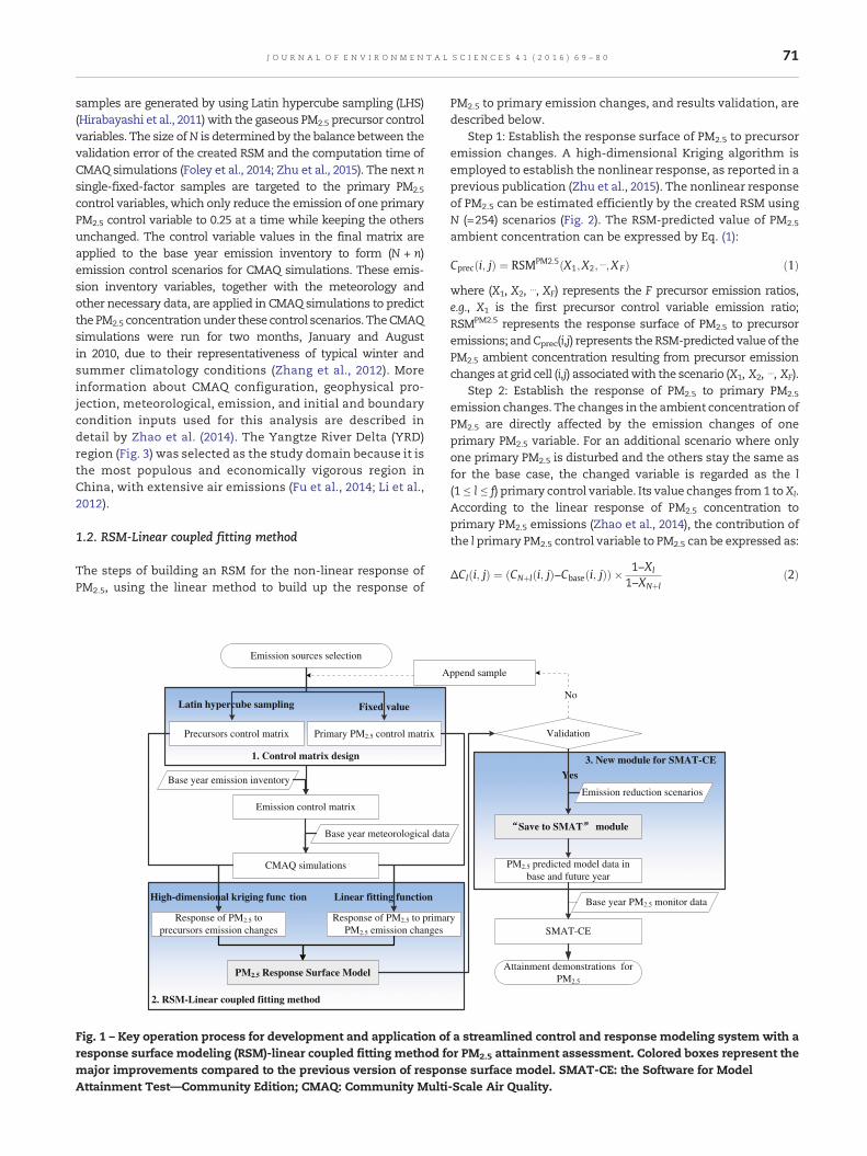
samples are generated by using Latin hypercube sampling (LHS)(Hirabayashi et al., 2011) with the gaseous PM2.5 precursor controlvariables. The size ofN is determined by the balance between thevalidation error of the created RSM and the computation time ofCMAQ simulations (Foley et al., 2014; Zhu et al., 2015). The next nsingle-fixed-factor samples are targeted to the primary PM2.5

control variables, which only reduce the emission of one primaryPM2.5 control variable to 0.25 at a time while keeping the othersunchanged. The control variable values in the final matrix areapplied to the base year emission inventory to form (N + n)emission control scenarios for CMAQ simulations. These emis-sion inventory variables, together with the meteorology andother necessary data, are applied in CMAQ simulations to predictthe PM2.5 concentrationunder these control scenarios. TheCMAQsimulations were run for two months, January and Augustin 2010, due to their representativeness of typical winter andsummer climatology conditions (Zhang et al., 2012). Moreinformation about CMAQ configuration, geophysical pro-jection, meteorological, emission, and initial and boundarycondition inputs used for this analysis are described indetail by Zhao et al. (2014). The Yangtze River Delta (YRD)region (Fig. 3) was selected as the study domain because it isthe most populous and economically vigorous region inChina, with extensive air emissions (Fu et al., 2014; Li et al.,2012).

1.2. RSM-Linear coupled fitting method

The steps of building an RSM for the non-linear response ofPM2.5, using the linear method to build up the response of

CMAQ simulations

PM2.5 Response Surface Model

Base year emission inventory

Base year meteorological data

Emission sources selection

Emission control matrix

1. Control matrix design

Precursors control matrix Primary PM2.5 control matrix

A

Response of PM2.5 to primaPM2.5 emission changes

Response of PM2.5 to precursors emission changes

2. RSM-Linear coupled fitting method

Latin hypercube sampling Fixed value

High-dimensional kriging func tion Linear fitting function

Fig. 1 – Key operation process for development and application oresponse surface modeling (RSM)-linear coupled fitting method fmajor improvements compared to the previous version of respoAttainment Test—Community Edition; CMAQ: Community Multi

PM2.5 to primary emission changes, and results validation, aredescribed below.

Step 1: Establish the response surface of PM2.5 to precursoremission changes. A high-dimensional Kriging algorithm isemployed to establish the nonlinear response, as reported in aprevious publication (Zhu et al., 2015). The nonlinear responseof PM2.5 can be estimated efficiently by the created RSM usingN (=254) scenarios (Fig. 2). The RSM-predicted value of PM2.5

ambient concentration can be expressed by Eq. (1):

Cprec i; jð Þ ¼ RSMPM2:5 X1;X2; ⋯;X Fð Þ ð1Þ

where (X1, X2, ⋯, XF) represents the F precursor emission ratios,e.g., X1 is the first precursor control variable emission ratio;RSMPM2.5 represents the response surface of PM2.5 to precursoremissions; andCprec(i,j) represents the RSM-predicted value of thePM2.5 ambient concentration resulting from precursor emissionchanges at grid cell (i,j) associatedwith the scenario (X1, X2, ⋯, XF).

Step 2: Establish the response of PM2.5 to primary PM2.5

emission changes. The changes in the ambient concentrationofPM2.5 are directly affected by the emission changes of oneprimary PM2.5 variable. For an additional scenario where onlyone primary PM2.5 is disturbed and the others stay the same asfor the base case, the changed variable is regarded as the l(1 ≤ l ≤ f) primary control variable. Its value changes from1 toXl.According to the linear response of PM2.5 concentration toprimary PM2.5 emissions (Zhao et al., 2014), the contribution ofthe l primary PM2.5 control variable to PM2.5 can be expressed as:

ΔCl i; jð Þ ¼ CNþl i; jð Þ−Cbase i; jð Þð Þ � 1−Xl

1−XNþlð2Þ

Validation

Attainment demonstrations for PM2.5

Save to SMAT module

Emission reduction scenarios

SMAT-CE

Base year PM2.5 monitor data

ppend sample

No

PM2.5 predicted model data in base and future year

ry

3. New module for SMAT-CE

Yes

f a streamlined control and response modeling system with aor PM2.5 attainment assessment. Colored boxes represent thense surface model. SMAT-CE: the Software for Model-Scale Air Quality.

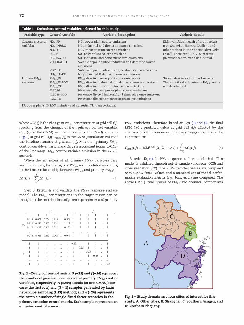
Table 1 – Emissions control variables selected for this study.

Variable type Control variable Variable description Variable details

Gaseous precursorvariables

NOx_PP NOx power plant source emissions Eight variables in each of the 4 regions(e.g., Shanghai, Jiangsu, Zhejiang andother regions in the Yangtze River Delta(YRD)). There are 8 × 4 = 32 gaseousprecursor control variables in total.

NOx_IN&DO NOx industrial and domestic source emissionsNOx_TR NOx transportation source emissionsSO2_PP SO2 power plant source emissionsSO2_IN&DO SO2 industrial and domestic source emissionsVOC_IN&DO Volatile organic carbon industrial and domestic source

emissionsVOC_TR Volatile organic carbon transportation source emissionsNH3_IN&DO NH3 industrial & domestic source emissions

Primary PM2.5

variablesPM2.5_PP PM2.5 directed power plant source emissions Six variables in each of the 4 regions.

There are 6 × 4 = 24 primary PM2.5 controlvariables in total.

PM2.5_IN&DO PM2.5 directed industrial and domestic source emissionsPM2.5_TR PM2.5 directed transportation source emissionsPMC_PP PM coarse directed power plant source emissionsPMC_IN&DO PM coarse directed industrial and domestic source emissionsPMC_TR PM coarse directed transportation source emissions

PP: power plants; IN&DO: industry and domestic; TR: transportation.

72 J O U R N A L O F E N V I R O N M E N T A L S C I E N C E S 4 1 ( 2 0 1 6 ) 6 9 – 8 0

where ΔCl(i,j) is the change of PM2.5 concentration at grid cell (i,j)resulting from the changes of the l primary control variable;CN + l(i,j) is the CMAQ simulation value of the (N + l) scenario(Fig. 2) at grid cell (i,j); Cbase (i,j) is the CMAQ simulation value ofthe baseline scenario at grid cell (i,j); Xl is the l primary PM2.5

control variable emission, and XN + l is a constant (equal to 0.25)of the l primary PM2.5 control variable emission in the (N + l)scenario.

When the emissions of all primary PM2.5 variables varysimultaneously, the changes of PM2.5 are calculated accordingto the linear relationship between PM2.5 and primary PM2.5:

ΔC i; jð Þ ¼Xf

l¼1

ΔCl i; jð Þ: ð3Þ

Step 3: Establish and validate the PM2.5 response surfacemodel. The PM2.5 concentrations in the target region can bethought as the contributions of gaseous precursors and primary

F1 1 1 1 ... 1

0.129 0.677 0.074 0.915 ... 0.529

0.836 0.250 0.802 0.871 ... 1.127

0.182 1.452 0.153 0.732 ... 0.170

... ... ... ... ... ...

0.388 0.521 0.195 0.262 ... 0.977

1 1 1 1 ... 1

1 1

N

⎧⎪⎪⎪⎨⎪⎪⎪⎩

f

1 1 ... 1

1 1 1 1 ... 1

1 1 1 1 ... 1

... ... ... ... ... ...

1 1 1 1 ... 1

1 1 1 1 ... 1

1

n

⎧⎪⎪⎪⎨⎪⎪⎪⎩

0.25 1 1 1 ... 1

1 1 1 ... 1 1 0.25 1 1 ... 1

1 1 1 1 ... 1 1 1 0.25 1 ... 1

1 1 1 1 ... 1 1 1 1 0.25 ... 1

... ... ... ... ... ... ... ... ... ..

1 1 1 1 ... 1

. ... ...

1 1 1 1 ... 0.25

Fig. 2 – Design of control matrix. F (=32) and f (=24) representthe number of gaseous precursors and primary PM2.5 controlvariables, respectively; N (=254) stands for one CMAQ basecase (the first row) and (N − 1) samples generated by Latinhypercube sampling (LHS) method; and n (=24) representsthe sample number of single-fixed-factor scenarios in theprimary emission control matrix. Each sample represents anemission control scenario.

PM2.5 emissions. Therefore, based on Eqs. (1) and (3), the finalRSM PM2.5 predicted value at grid cell (i,j) affected by thechanges of both precursors and primary PM2.5 emissions can beexpressed as:

Cpred i; jð Þ ¼ RSMPM2:5 X1;X2; ⋯;X Fð Þ þXf

l¼1

ΔCl i; jð Þ: ð4Þ

BasedonEq. (4), the PM2.5 response surfacemodel is built. Thismodel is validated through out-of-sample validation (OOS) andcross validation (CV). The RSM-predicted values are comparedwith CMAQ “true” values and a standard set of model perfor-mance evaluation metrics (e.g., bias, error) are computed. Theabove CMAQ “true” values of PM2.5 and chemical components

A

D

B

C

Fig. 3 – Study domain and four cities of interest for thisstudy. A: Other cities, B: Shanghai, C: Southern Jiangsu, andD: Northern Zhejiang.

73J O U R N A L O F E N V I R O N M E N T A L S C I E N C E S 4 1 ( 2 0 1 6 ) 6 9 – 8 0

wereprovidedandvalidatedwith observational data byTsinghuaUniversity. The CMAQ-observation validation results of normal-ized mean biases (NMBs) range from −15% to 24% (Zhao et al.,2014). When the RSM prediction error or bias exceeds acceptableranges, a certain amount of samples will be added for CMAQsimulations until the error is within an acceptable range.

1.3. Emission reduction scenarios

Table 2 lists three emission reduction scenarios targeted onseveral pollutants, i.e., NOx, SO2, NH3, and primary PM2.5. SinceVOC emissions have a minor effect on PM2.5 concentrationsdue to the significant underestimation of secondary organicaerosol formation in the current CMAQ model (Carlton et al.,2010), we did not consider a VOC reduction scenario in this paper.Case #1 focuses on the reduction of NOx, SO2, NH3, and primaryPM2.5 emissions outside of Shanghai. Case #2 represents theemission reduction of the same pollutants as in Case #1 forShanghai. As documented in the literature (Wang and Hao,2012;Wang et al., 2014a), emission controls in a single city arenot an effective way to realize the air quality standard,because air pollution is a complex phenomenon and influ-enced by both local emissions and regional transport fromneighboring areas. Therefore, we design Case #3 to representan emission reduction of the same pollutant emissions inthe entire YRD region. The emission ratios in these threescenarios are in accordance with the maximum feasiblereduction described by Wang et al. (2014b).

1.4. Functional module for output model data to SMAT-CE

Since the gridded air quality model data from RSM-VATcannot be used directly as inputs for SMAT-CE due to dataformat differences (e.g., projection), a functional modulenamed “Save to SMAT” is developed in RSM-VAT. Thismoduleimplements the coordinate conversions and grid-relatedcomputations, and then outputs the SMAT-CE formatteddata for attainment assessments.

In RSM-VAT, the model data are based on a Lambertconformal conic (LCC) projection. The coordinates of each gridcell are in the format of column and row indexes. In contrast,SMAT-CE formatted model data require latitude and longitudecoordinates at the centroid of each grid cell. To get this coordinateinformation, an open-source geographic information systems(GIS) library (DotSpatial, http://dotspatial.codeplex.com/) is intro-duced. The functionality of map projection transformations inthis library is extended into RSM-VAT to provide coordinateconversion and then compute the latitude/longitude of each gridcell in the modeling domain. After that, several data fields (e.g.,grid cell ID) are added to the output gridded model file, whichinclude a grid cell ID, grid-cell values of PM2.5, and the modelmonth or quarter.

With this module, users only need to input the emissioncontrol scenario and right-click on the pollutant spatialdistribution plot to select “Save to SMAT”, then the corre-sponding SMAT-CE formatted gridded model data will beexported in *.csv format. In this study, a base year and threefuture years' gridded model files were derived from thismodule and each model file consisted of two simulatedmonthly average PM2.5 concentrations (January and August).

1.5. Air quality attainment assessment in SMAT-CE

SMAT-CE is primarily intended as a tool to implement themodeled attainment tests for particulate matter (PM2.5), ozone(O3) and regional haze (visibility). It statistically estimates afuture design value (DVF) at a specific site (a monitoring site orgrid cell) by using a base-year observational data and themodel data obtained from the base-year and future-year airquality simulations. The model data of the base and futureyears are used for calculating the ratio of the model's future tobase-year predictions at monitoring sites. The ratios are calledrelative response factors (RRF). The DVF of pollutants isestimated at monitoring sites by multiplying RRF locations“near” each monitor by the base-year observation value. Thefuture-year design values are compared to the NAAQS. If allfuture site-specific pollutant design values are less than orequal to the concentration specified in the NAAQS, the test ispassed. A detailed description of this attainment methodol-ogy and approach is available in the study by Wang et al.(2015).

In this study, gridded model data for a base year and threefuture years' scenarios, as well as base-year PM2.5 monitoringdata from Shanghai, were used as inputs for SMAT-CE. Theestimated results consist of (1) spatial distribution of futureyear PM2.5 concentration and (2) future year PM2.5 concentra-tions at the 10 national monitoring sites in Shanghai. Thefirst one was facilitated to evaluate the effectiveness of threeproposed emission reduction scenarios, while the other onewas applied to conduct PM2.5 NAAQS attainment testing atShanghai monitoring sites.

2. Results and discussion

2.1. Validation of RSM-Linear coupled fitting tool

RSM can reproduce the simulation results of CMAQ byvarious validation methods (Zhu et al., 2015). The crossvalidation (CV) results (available at http://www.abacas-dss.com/) demonstrate the good performance of our created RSM(including January and August) in the YRD with meannormalized bias (MNB) < 1% and mean normalized error(MNE) < 1%. Here, we concentrate on the validation of thedeveloped linear fitting algorithm. A set of 28 additionalscenarios are introduced to validate the performance of thisalgorithm by out-of-sample (OOS) validation. The first 24scenarios, corresponding to the 24 primary PM2.5 controlvariables (cases 1–24), are single-fixed-factor samples whereonly one control variable of primary PM2.5 changes from 0.25to 0.50 at a time and the others remain the same as the basecase. The next 4 scenarios (cases 25–28) are generatedrandomly by the LHS method, in which all primary PM2.5

control variables are changed simultaneously. The predictedPM2.5 concentrations for these scenarios are compared to thecorresponding CMAQ simulation results using model evalu-ation metrics (e.g., mean normalized bias). As shown inFig. 4a, the overall errors over these 28 scenarios were smallin both January and August, with the median value of 0%.Only a few discrete points in August varied from −1.5% to

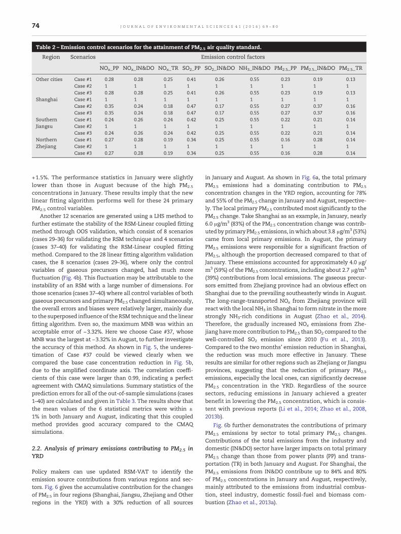
Table 2 – Emission control scenarios for the attainment of PM2.5 air quality standard.

Region Scenarios Emission control factors

NOx_PP NOx_IN&DO NOx_TR SO2_PP SO2_IN&DO NH3_IN&DO PM2.5_PP PM2.5_IN&DO PM2.5_TR

Other cities Case #1 0.28 0.28 0.25 0.41 0.26 0.55 0.23 0.19 0.13Case #2 1 1 1 1 1 1 1 1 1Case #3 0.28 0.28 0.25 0.41 0.26 0.55 0.23 0.19 0.13

Shanghai Case #1 1 1 1 1 1 1 1 1 1Case #2 0.35 0.24 0.18 0.47 0.17 0.55 0.27 0.37 0.16Case #3 0.35 0.24 0.18 0.47 0.17 0.55 0.27 0.37 0.16

SouthernJiangsu

Case #1 0.24 0.26 0.24 0.42 0.25 0.55 0.22 0.21 0.14Case #2 1 1 1 1 1 1 1 1 1Case #3 0.24 0.26 0.24 0.42 0.25 0.55 0.22 0.21 0.14

NorthernZhejiang

Case #1 0.27 0.28 0.19 0.34 0.25 0.55 0.16 0.28 0.14Case #2 1 1 1 1 1 1 1 1 1Case #3 0.27 0.28 0.19 0.34 0.25 0.55 0.16 0.28 0.14

74 J O U R N A L O F E N V I R O N M E N T A L S C I E N C E S 4 1 ( 2 0 1 6 ) 6 9 – 8 0

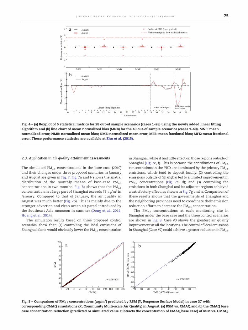
+1.5%. The performance statistics in January were slightlylower than those in August because of the high PM2.5

concentrations in January. These results imply that the newlinear fitting algorithm performs well for these 24 primaryPM2.5 control variables.

Another 12 scenarios are generated using a LHS method tofurther estimate the stability of the RSM-Linear coupled fittingmethod through OOS validation, which consist of 8 scenarios(cases 29–36) for validating the RSM technique and 4 scenarios(cases 37–40) for validating the RSM-Linear coupled fittingmethod. Compared to the 28 linear fitting algorithm validationcases, the 8 scenarios (cases 29–36), where only the controlvariables of gaseous precursors changed, had much morefluctuation (Fig. 4b). This fluctuation may be attributable to theinstability of an RSM with a large number of dimensions. Forthose scenarios (cases 37–40) where all control variables of bothgaseous precursors and primary PM2.5 changed simultaneously,the overall errors and biases were relatively larger, mainly dueto the superposed influence of theRSM techniqueand the linearfitting algorithm. Even so, the maximum MNB was within anacceptable error of −3.32%. Here we choose Case #37, whoseMNB was the largest at −3.32% in August, to further investigatethe accuracy of this method. As shown in Fig. 5, the underes-timation of Case #37 could be viewed clearly when wecompared the base case concentration reduction in Fig. 5b,due to the amplified coordinate axis. The correlation coeffi-cients of this case were larger than 0.99, indicating a perfectagreement with CMAQ simulations. Summary statistics of theprediction errors for all of the out-of-sample simulations (cases1–40) are calculated and given in Table 3. The results show thatthe mean values of the 6 statistical metrics were within ±1% in both January and August, indicating that this coupledmethod provides good accuracy compared to the CMAQsimulations.

2.2. Analysis of primary emissions contributing to PM2.5 inYRD

Policy makers can use updated RSM-VAT to identify theemission source contributions from various regions and sec-tors. Fig. 6 gives the accumulative contribution for the changesof PM2.5 in four regions (Shanghai, Jiangsu, Zhejiang and Otherregions in the YRD) with a 30% reduction of all sources

in January and August. As shown in Fig. 6a, the total primaryPM2.5 emissions had a dominating contribution to PM2.5

concentration changes in the YRD region, accounting for 78%and 55% of the PM2.5 change in January and August, respective-ly. The local primary PM2.5 contributedmost significantly to thePM2.5 change. Take Shanghai as an example, in January, nearly6.0 μg/m3 (83%) of the PM2.5 concentration change was contrib-utedby primary PM2.5 emissions, inwhich about 3.8 μg/m3 (53%)came from local primary emissions. In August, the primaryPM2.5 emissions were responsible for a significant fraction ofPM2.5, although the proportion decreased compared to that ofJanuary. These emissions accounted for approximately 4.0 μg/m3 (59%) of the PM2.5 concentrations, including about 2.7 μg/m3

(39%) contributions from local emissions. The gaseous precur-sors emitted from Zhejiang province had an obvious effect onShanghai due to the prevailing southeasterly winds in August.The long-range-transported NOx from Zhejiang province willreact with the local NH3 in Shanghai to formnitrate in themorestrongly NH3-rich conditions in August (Zhao et al., 2014).Therefore, the gradually increased NOx emissions from Zhe-jiang havemore contribution to PM2.5 than SO2 compared to thewell-controlled SO2 emission since 2010 (Fu et al., 2013).Compared to the twomonths' emission reduction in Shanghai,the reduction was much more effective in January. Theseresults are similar for other regions such as Zhejiang or Jiangsuprovinces, suggesting that the reduction of primary PM2.5

emissions, especially the local ones, can significantly decreasePM2.5 concentration in the YRD. Regardless of the sourcesectors, reducing emissions in January achieved a greaterbenefit in lowering the PM2.5 concentration, which is consis-tent with previous reports (Li et al., 2014; Zhao et al., 2008,2013b).

Fig. 6b further demonstrates the contributions of primaryPM2.5 emissions by sector to total primary PM2.5 changes.Contributions of the total emissions from the industry anddomestic (IN&DO) sector have larger impacts on total primaryPM2.5 change than those from power plants (PP) and trans-portation (TR) in both January and August. For Shanghai, thePM2.5 emissions from IN&DO contribute up to 84% and 80%of PM2.5 concentrations in January and August, respectively,mainly attributed to the emissions from industrial combus-tion, steel industry, domestic fossil-fuel and biomass com-bustion (Zhao et al., 2013a).

Mea

n no

rmal

ized

bia

s (%

)Pe

rfor

man

ce s

tatis

tics

(%)

MFB

AugustJanuarya

b January

August

Linear-fitting algorithmRSM-Linear coupledfitting method

Case number

MFE MNB MNE NMB NME

3

2

1

0

-1

-2

-3

2

1

0

-1

-2

-3

-4RSM technique

0 2 4 6 8 10 12 14 16 18 20 22 24 26 28 30 32 34 36 38 40

Outlier of PM2.5 in a grid cellVariation range of the 6 statistical metrics

Fig. 4 – (a) Boxplot of 6 statistical metrics for 28 out-of sample scenarios (cases 1–28) using the newly added linear fittingalgorithm and (b) line chart of mean normalized bias (MNB) for the 40 out-of sample scenarios (cases 1–40). MNE: meannormalized error; NMB: normalized mean bias; NME: normalized mean error; MFB: mean fractional bias; MFE: mean fractionalerror. These performance statistics are available at Zhu et al. (2015).

75J O U R N A L O F E N V I R O N M E N T A L S C I E N C E S 4 1 ( 2 0 1 6 ) 6 9 – 8 0

2.3. Application in air quality attainment assessments

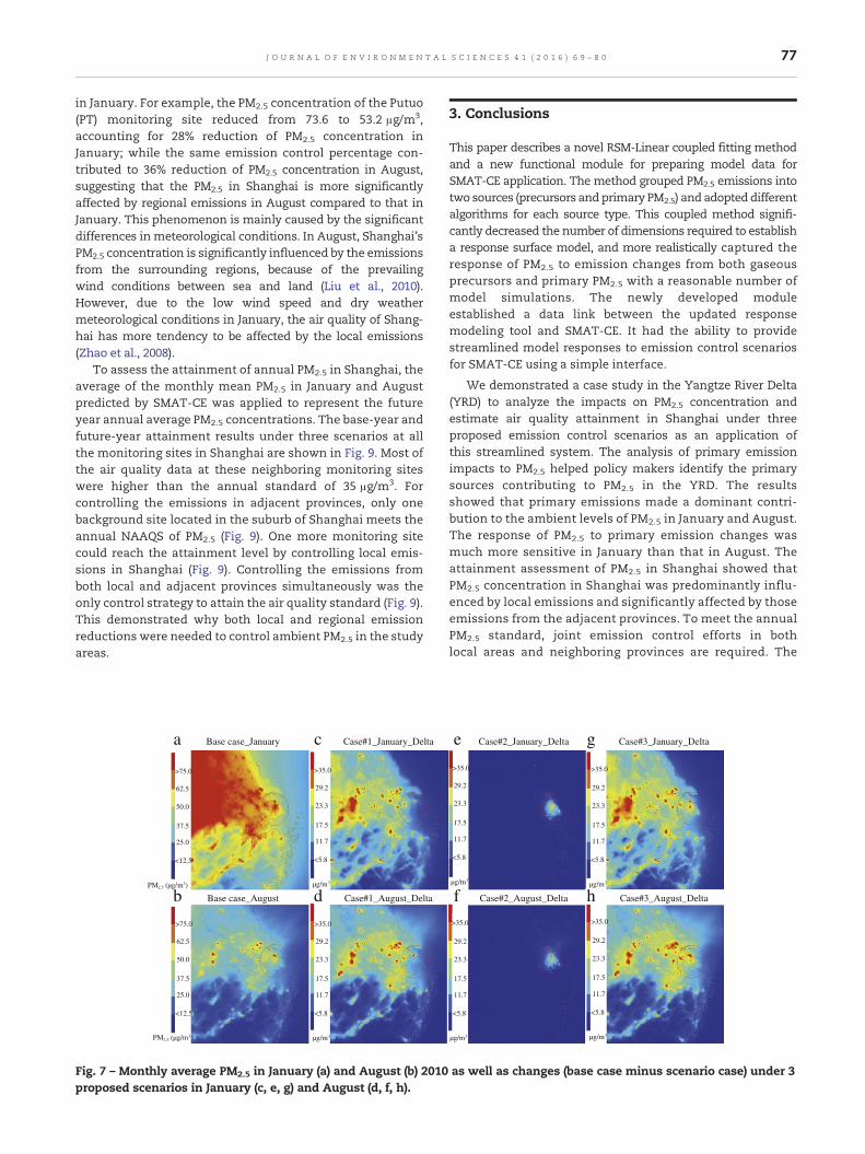
The simulated PM2.5 concentrations in the base case (2010)and their changes under three proposed scenarios in Januaryand August are given in Fig. 7. Fig. 7a and b shows the spatialdistribution of the monthly means of base-case PM2.5

concentrations in two months. Fig. 7a shows that the PM2.5

concentration in a large part of Shanghai exceeds 75 μg/m3 inJanuary. Compared to that of January, the air quality inAugust was much better (Fig. 7b). This is mainly due to thestronger advection and clean ocean air parcel introduced bythe Southeast Asia monsoon in summer (Dong et al., 2014;Huang et al., 2014).

The simulation results based on three proposed controlscenarios show that: (1) controlling the local emissions ofShanghai alone would obviously lower the PM2.5 concentration

0 20 40 60 80 100 120 140 160 180 2000

20

40

60

80

100

120

140

160

180

200

RSM

CMAQ

r = 0.997878

a

Fig. 5 – Comparison of PM2.5 concentrations (μg/m3) predicted bycorresponding CMAQ simulations (X, Community Multi-scale Aircase concentration reduction (predicted or simulated value subtr

in Shanghai, while it had little effect on those regions outside ofShanghai (Fig. 7e, f). This is because the contributions of PM2.5

concentrations in the YRD are dominated by the primary PM2.5

emissions, which tend to deposit locally; (2) controlling theemissions outside of Shanghai led to a limited improvement inPM2.5 concentrations (Fig. 7c, d); and (3) controlling theemissions in both Shanghai and its adjacent regions achieveda satisfactory effect, as shown in Fig. 7g and h. Comparison ofthese results shows that the governments of Shanghai andthe neighboring provinces need to coordinate their emissionreduction efforts to decrease the PM2.5 concentration.

The PM2.5 concentrations at each monitoring site inShanghai under the base case and the three control scenariosare shown in Fig. 8. Case #3 shows the greatest air qualityimprovement at all the locations. The control of local emissionsin Shanghai (Case #2) could achieve a greater reduction in PM2.5

-90 -80 -70 -60 -50 -40 -30 -20 -10 0-90

-80

-70

-60

-50

-40

-30

-20

-10

0

RSM

-CM

AQ

bas

e ca

se

CMAQ-CMAQ base case

r = 0.9942857

b

RSM (Y, Response Surface Model) in case 37 withQuality) in August. (a) RSM vs. CMAQ and (b) the CMAQ baseacts the concentration of CMAQ base case) of RSM vs. CMAQ.

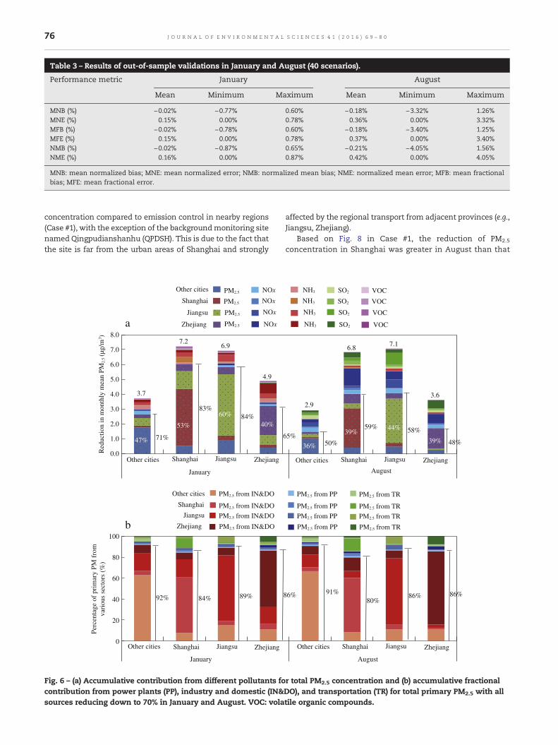
Table 3 – Results of out-of-sample validations in January and August (40 scenarios).

Performance metric January August

Mean Minimum Maximum Mean Minimum Maximum

MNB (%) −0.02% −0.77% 0.60% −0.18% −3.32% 1.26%MNE (%) 0.15% 0.00% 0.78% 0.36% 0.00% 3.32%MFB (%) −0.02% −0.78% 0.60% −0.18% −3.40% 1.25%MFE (%) 0.15% 0.00% 0.78% 0.37% 0.00% 3.40%NMB (%) −0.02% −0.87% 0.65% −0.21% −4.05% 1.56%NME (%) 0.16% 0.00% 0.87% 0.42% 0.00% 4.05%

MNB: mean normalized bias; MNE: mean normalized error; NMB: normalized mean bias; NME: normalized mean error; MFB: mean fractionalbias; MFE: mean fractional error.

76 J O U R N A L O F E N V I R O N M E N T A L S C I E N C E S 4 1 ( 2 0 1 6 ) 6 9 – 8 0

concentration compared to emission control in nearby regions(Case #1), with the exception of the backgroundmonitoring sitenamed Qingpudianshanhu (QPDSH). This is due to the fact thatthe site is far from the urban areas of Shanghai and strongly

47%

53%

60%

40%

71%

83%84%

3.7

7.2 6.9

4.9

0.0

1.0

2.0

3.0

4.0

5.0

6.0

7.0

8.0

January

Red

uctio

n in

mon

thly

mea

n PM

2.5(µ

g/m

3 )

PM2.5 NOx

PM2.5 NOx

PM2.5 NOx

PM2.5 NOx

92% 84% 89%

0

20

40

60

80

100

yraunaJ

Perc

enta

ge o

f pr

imar

y PM

fro

mva

riou

s se

ctor

s (%

)

a

b

Other cities

Other cities

Shanghai

Shanghai

Jiangsu

Jiangsu

Zhejiang

Zhejiang

Other cities

Other cities

Shanghai

Shanghai

Jiangsu

Jiangsu

Zhejiang

Zhejiang

PM2.5 from IN&DO

PM2.5 from IN&DO

PM2.5 from IN&DO

PM2.5 from IN&DO

Fig. 6 – (a) Accumulative contribution from different pollutants focontribution from power plants (PP), industry and domestic (IN&sources reducing down to 70% in January and August. VOC: vola

affected by the regional transport from adjacent provinces (e.g.,Jiangsu, Zhejiang).

Based on Fig. 8 in Case #1, the reduction of PM2.5

concentration in Shanghai was greater in August than that

36%

39%44%

39%65%

50%

59% 58%

48%

2.9

6.8 7.1

3.6

August

NH3 SO2 VOC

NH3 SO2 VOC

NH3 SO2 VOC

NH3 SO2 VOC

86% 91%80%

86% 86%

tsuguA

Other cities Shanghai Jiangsu Zhejiang

Other cities Shanghai Jiangsu Zhejiang

PM2.5 from PP PM2.5 from TR

PM2.5 from PP PM2.5 from TRPM2.5 from PP PM2.5 from TR

PM2.5 from PP PM2.5 from TR

r total PM2.5 concentration and (b) accumulative fractionalDO), and transportation (TR) for total primary PM2.5 with alltile organic compounds.

77J O U R N A L O F E N V I R O N M E N T A L S C I E N C E S 4 1 ( 2 0 1 6 ) 6 9 – 8 0

in January. For example, the PM2.5 concentration of the Putuo(PT) monitoring site reduced from 73.6 to 53.2 μg/m3,accounting for 28% reduction of PM2.5 concentration inJanuary; while the same emission control percentage con-tributed to 36% reduction of PM2.5 concentration in August,suggesting that the PM2.5 in Shanghai is more significantlyaffected by regional emissions in August compared to that inJanuary. This phenomenon is mainly caused by the significantdifferences inmeteorological conditions. In August, Shanghai'sPM2.5 concentration is significantly influenced by the emissionsfrom the surrounding regions, because of the prevailingwind conditions between sea and land (Liu et al., 2010).However, due to the low wind speed and dry weathermeteorological conditions in January, the air quality of Shang-hai has more tendency to be affected by the local emissions(Zhao et al., 2008).

To assess the attainment of annual PM2.5 in Shanghai, theaverage of the monthly mean PM2.5 in January and Augustpredicted by SMAT-CE was applied to represent the futureyear annual average PM2.5 concentrations. The base-year andfuture-year attainment results under three scenarios at allthe monitoring sites in Shanghai are shown in Fig. 9. Most ofthe air quality data at these neighboring monitoring siteswere higher than the annual standard of 35 μg/m3. Forcontrolling the emissions in adjacent provinces, only onebackground site located in the suburb of Shanghai meets theannual NAAQS of PM2.5 (Fig. 9). One more monitoring sitecould reach the attainment level by controlling local emis-sions in Shanghai (Fig. 9). Controlling the emissions fromboth local and adjacent provinces simultaneously was theonly control strategy to attain the air quality standard (Fig. 9).This demonstrated why both local and regional emissionreductions were needed to control ambient PM2.5 in the studyareas.

a c

db

Base case_January

Base case_August

Case#1_January_Delta

Case#1_August_Delta

>75.0

62.5

50.0

37.5

25.0

<12.5

PM2.5 (µg/m3)

PM2.5 (µg/m3)

>35.0

29.2

23.3

17.5

11.7

<5.8

µg/m3

>35.0

29.2

23.3

17.5

11.7

<5.8

µg/m3

>75.0

62.5

50.0

37.5

25.0

<12.5

Fig. 7 – Monthly average PM2.5 in January (a) and August (b) 2010proposed scenarios in January (c, e, g) and August (d, f, h).

3. Conclusions

This paper describes a novel RSM-Linear coupled fitting methodand a new functional module for preparing model data forSMAT-CE application. The method grouped PM2.5 emissions intotwo sources (precursors and primary PM2.5) and adopted differentalgorithms for each source type. This coupled method signifi-cantly decreased the number of dimensions required to establisha response surface model, and more realistically captured theresponse of PM2.5 to emission changes from both gaseousprecursors and primary PM2.5 with a reasonable number ofmodel simulations. The newly developed moduleestablished a data link between the updated responsemodeling tool and SMAT-CE. It had the ability to providestreamlined model responses to emission control scenariosfor SMAT-CE using a simple interface.

We demonstrated a case study in the Yangtze River Delta(YRD) to analyze the impacts on PM2.5 concentration andestimate air quality attainment in Shanghai under threeproposed emission control scenarios as an application ofthis streamlined system. The analysis of primary emissionimpacts to PM2.5 helped policy makers identify the primarysources contributing to PM2.5 in the YRD. The resultsshowed that primary emissions made a dominant contri-bution to the ambient levels of PM2.5 in January and August.The response of PM2.5 to primary emission changes wasmuch more sensitive in January than that in August. Theattainment assessment of PM2.5 in Shanghai showed thatPM2.5 concentration in Shanghai was predominantly influ-enced by local emissions and significantly affected by thoseemissions from the adjacent provinces. To meet the annualPM2.5 standard, joint emission control efforts in bothlocal areas and neighboring provinces are required. The

f h

e g

Case#2_August_Delta Case#3_August_Delta

Case#2_January_Delta Case#3_January_Delta

>35.0

29.2

23.3

17.5

11.7

<5.8

µg/m3

>35.0

29.2

23.3

17.5

11.7

<5.8

µg/m3

>35.0

29.2

23.3

17.5

11.7

<5.8

µg/m3

>35.0

29.2

23.3

17.5

11.7

<5.8

µg/m3

as well as changes (base case minus scenario case) under 3

71.9 69.2 70.7 69.1 73.6

42.7

74.9

85.8 79.5

69.3 64.4 63.1 64.6 63.1

67.1

33.8

68.6

78.2 72.5

62.8 54.6

50.0 53.3 53.1 53.2

40.4

55.0 63.3

59.9 56.9

46.4 43.4 46.5 46.4 46.1

31.0

48.1 55.0 52.2 49.6

0

20

40

60

80

100

HK JA PDXQ PDZJ PT QPDSH SWC XHSSD YPSP PDCS

PM2.

5 con

cent

ratio

n (µ

g/m

3 )PM

2.5 c

once

ntra

tion

(µg/

m3 )

Base case_Jan Case#1_Jan Case#2_Jan Case#3_Jan

44.6 43.0 43.9 42.9 45.7

26.5

46.5

53.3 49.4

43.1

34.4 33.5 32.7 31.5 35.6

14.8

34.9 40.0

37.4

30.4 29.1 27.5 29.3 29.3 29.3

23.2

30.8 35.6

32.6 31.1

18.7 18.0 17.9 17.6 19.1

11.3

19.1 22.2 20.4

18.3

0

10

20

30

40

50

60

HK JA PDXQ PDZJ PT QPDSH SWC XHSSD YPSP PDCS

Base case_Aug Case#1_Aug Case#2_Aug Case#3_Aug

Fig. 8 – Comparison between base-year (2010) and future-year monthly mean PM2.5 under 3 scenarios in January and Augustfor the 10 national monitoring sites in Shanghai. HK: Hongkou, JA: Jing'an, PDXQ: Pudongxinqu, PDZJ: Pudongzhangjiang, PT:Putuo, QPDSH: Qingpudianshanhu, SWC: Shiwuchang, XHSSD: Xuhuishangshida, YPSP: Yangpusipiao, PDCS:Pudongchuansha.

78 J O U R N A L O F E N V I R O N M E N T A L S C I E N C E S 4 1 ( 2 0 1 6 ) 6 9 – 8 0

developed modeling tool serves as an efficient and stream-lined science-based platform for identifying emissionsources leading to air pollution and for air quality attain-ment assessments.

Acknowledgments

Financial support and data source for this work is provided bythe US Environmental Protection Agency (No. OR13810-001.04A10-0223-S001-A02) and Guangzhou Environmental Protec-tion Bureau (No. x2hjB2150020), the project of an integratedmodeling and filed observational verification on the

Case#1Base year C

Fig. 9 – Comparison between a base-year and three proposed futsites in Shanghai.

deposition of typical industrial point-source mercury emis-sions in the Pearl River Delta. This work is also partlysupported by the funding of Guangdong Provincial Key Labora-tory of Atmospheric Environment and Pollution Control (No.2011A060901011), the project of Atmospheric Haze CollaborationControl Technology Design (No. XDB05030400) from the ChineseAcademy of Sciences and the Ministry of EnvironmentalProtection's Special Funds for Research on Public Welfare (No.201409002). Partly financial support is also provided by theGuangdong Provincial Department of Science and Technology,the project of demonstration research of air qualitymanagementcost-benefit analysis and attainment assessments technology(No. 2014A050503019).

Case #3ase #2

ure-year scenarios' PM2.5 attainment results at 10 monitoring

79J O U R N A L O F E N V I R O N M E N T A L S C I E N C E S 4 1 ( 2 0 1 6 ) 6 9 – 8 0

R E F E R E N C E S

Appel, K.W., Gilliam, R.C., Davis, N., Zubrow, A., Howard, S.C.,2011. Overview of the atmospheric model evaluation tool(AMET) v1.1 for evaluating meteorological and air qualitymodels. Environ. Model Softw. 26 (4), 434–443.

Appel, K.W., Chemel, C., Roselle, S.J., Francis, X.V., Hu, R.M.,Sokhi, R.S., et al., 2012. Examination of the CommunityMultiscale Air Quality (CMAQ) model performance over theNorth American and European domains. Atmos. Environ. 53,142–155.

Buonocore, J.J., Dong, X., Spengler, J.D., Fu, J.S., Levy, J.I., 2014.Using the Community Multiscale Air Quality (CMAQ) model toestimate public health impacts of PM2.5 from individual powerplants. Environ. Int. 68, 200–208.

Byun, D., Schere, K.L., 2006. Review of the governing equations,computational algorithms, and other components of themodels 3 Community Multiscale Air Quality (CMAQ) ModelingSystem. Appl. Mech. Rev. 59, 51–77.

Carlton, A.G., Bhave, P.V., Napelenok, S.L., Edney, E.O., Sarwar, G.,Pinder, R.W., et al., 2010. Model representation of secondaryorganic aerosol in CMAQv4.7. Environ. Sci. Technol. 44 (22),8553–8560.

Chemel, C., Fisher, B.E.A., Kong, X., Francis, X.V., Sokhi, R.S., Good,N., et al., 2014. Application of chemical transport model CMAQto policy decisions regarding PM2.5 in the UK. Atmos. Environ.82, 410–417.

China National EnvironmentalMonitoring Centre Centre(CNEMC),2013. Monthly Air Quality Reports over 74 Cities Available at:http://www.cnemc.cn/publish/totalWebSite/0666/newList_1.html.

Dong, X.Y., Li, J., Fu, J.S., Gao, Y., Huang, K., Zhuang, G.S., 2014.Inorganic aerosols responses to emission changes in YangtzeRiver Delta, China. Sci. Total Environ. 481, 522–532.

Fann, N., Baker, K.R., Fulcher, C.M., 2012. Characterizing thePM2.5-related health benefits of emission reductions for 17industrial, area and mobile emission sectors across the U.S.Environ. Int. 49, 141–151.

Foley, K.M., Napelenok, S.L., Jang, C., Phillips, S., Hubbell, B.J.,Fulcher, C.M., 2014. Two reduced form air quality modelingtechniques for rapidly calculating pollutant mitigationpotential across many sources, locations and precursoremission types. Atmos. Environ. 98, 283–289.

Fu, X., Wang, S.X., Zhao, B., Xing, J., Cheng, Z., Liu, H., et al., 2013.Emission inventory of primary pollutants and chemicalspeciation in 2010 for the Yangtze River Delta region, China.Atmos. Environ. 70, 39–50.

Fu, X., Wang, S.X., Cheng, Z., Xing, J., Zhao, B., Wang, J.D., et al.,2014. Source, transport and impacts of a heavy dust event inthe Yangtze River Delta, China, in 2011. Atmos. Chem. Phys. 14(3), 1239–1254.

Hirabayashi, S., Kroll, C.N., Nowak, D.J., 2011. Component-baseddevelopment and sensitivity analyses of an air pollutant drydeposition model. Environ. Model Softw. 26 (6), 804–816.

Huang, K., Fu, J.S., Gao, Y., Dong, X.Y., Zhuang, G.S., Lin, Y.F., 2014.Role of sectoral and multi-pollutant emission control strategiesin improving atmospheric visibility in the Yangtze River Delta,China. Environ. Pollut. 184, 426–434.

Li, L., Chen, C.H., Huang, C., Huang, H.Y., Zhang, G.F., Wang, Y.J., etal., 2012. Process analysis of regional ozone formation over theYangtze River Delta, China using the Community Multi-scaleAir Quality modeling system. Atmos. Chem. Phys. 12 (22),10971–10987.

Li, L., Huang, C., Huang, H.Y., Wang, Y.J., Yan, R.S., Zhang, G.F., etal., 2014. An integrated process rate analysis of a regional fineparticulate matter episode over Yangtze River Delta in 2010.Atmos. Environ. 91, 60–70.

Liu, X.-H., Zhang, Y., Cheng, S.-H., Xing, J., Zhang, Q., Streets, D.G.,et al., 2010. Understanding of regional air pollution over Chinausing CMAQ, part I performance evaluation and seasonalvariation. Atmos. Environ. 44 (20), 2415–2426.

Ministry of Environmental Protection of the People's Republic ofChina (MEP), 2012. Ambient Air Quality Standards: GB 3095-2012Available at: http://kjs.mep.gov.cn/hjbhbz/bzwb/dqhjbh/dqhjzlbz/201203/t20120302_224165.htm.

Streets, D.G., Fu, J.S., Jang, C.J., Hao, J.M., He, K.B., Tang, X.Y., et al.,2007. Air quality during the 2008 Beijing Olympic Games.Atmos. Environ. 41 (3), 480–492.

Sun, J., Schreifels, J.,Wang, J., Fu, J.S.,Wang, S.X., 2014. Cost estimate ofmulti-pollutant abatement from the power sector in the YangtzeRiver Delta region of China. Energy Policy 69, 478–488.

Tai, A.P.K., Mickley, L.J., Jacob, D.J., 2010. Correlations betweenfine particulate matter (PM2.5) and meteorological variablesin the United States: implications for the sensitivity of PM2.5

to climate change. Atmos. Environ. 44 (32), 3976–3984.US EPA, 2006a. Technical support document for the proposed

mobile source air toxics rule: ozone modeling. Office of AirQuality Planning and Standards. Research Triangle Park, NC.

US EPA, 2006b. Technical support document for the proposed PMNAAQS rule: response surface modeling. In: U.S.Environmental Protection Agency Office of Air QualityPlanning and Standards R T P, NC 27711 (Ed.), U.S. Environ-mental Protection Agency Office of Air Quality Planning andStandards. Research Triangle Park, NC 27711.

US EPA, 2007. Guidance on the use of models and other analysesfor demonstrating attainment of air quality goals for ozone,PM2.5, and regional haze. In: Standards O o A Q P a, Division O oA Q A, Group O o A Q M (Eds.), U.S. Environmental ProtectionAgency, p. 262.

Wang, S.X., Hao, J.M., 2012. Air quality management in China:issues, challenges, and options. J. Environ. Sci. 24 (1), 2–13.

Wang, S.X., Zhao, M., Xing, J., Wu, Y., Zhou, Y., Lei, Y., et al., 2010.Quantifying the air pollutants emission reduction during the2008 Olympic games in Beijing. Environ. Sci. Technol. 44 (7),2490–2496.

Wang, S.X., Xing, J., Zhao, B., Jang, C., Hao, J.M., 2014a. Effective-ness of national air pollution control policies on the air qualityin metropolitan areas of China. J. Environ. Sci. 26 (1), 13–22.

Wang, S.X., Zhao, B., Cai, S.Y., Klimont, Z., Nielsen, C., McElroy,M.B., et al., 2014b. Emission trends and mitigation options forair pollutants in East Asia. Atmos. Chem. Phys. Discuss. 14 (2),2601–2674.

Wang, H., Zhu, Y., Jang, C., Lin, C.-J., Wang, S., Fu, J.S., et al., 2015.Design and demonstration of a next-generation air qualityattainment assessment system for PM2.5 and O3. J. Environ. Sci.29, 178–188.

Xing, J., 2011. Study on the Nonlinear Responses of Air Quality toPrimary Pollutant Emissions. Tsinghua University.

Xing, J., Wang, S.X., Jang, C., Zhu, Y., Hao, J.M., 2011. Nonlinearresponse of ozone to precursor emission changes in China: amodeling study using response surface methodology. Atmos.Chem. Phys. 11 (10), 5027–5044.

Zhang, H.L., Li, J.Y., Ying, Q., Yu, J.Z., Wu, D., Cheng, Y., et al., 2012.Source apportionment of PM2.5 nitrate and sulfate in Chinausing a source-oriented chemical transport model. Atmos.Environ. 62, 228–242.

Zhao, Y., Wang, S., Duan, L., Lei, Y., Cao, P., Hao, J., 2008. Primaryair pollutant emissions of coal-fired power plants in China:current status and future prediction. Atmos. Environ. 42 (36),8442–8452.

Zhao, B., Wang, S.X., Dong, X.Y., Wang, J.D., Duan, L., Fu, X., et al.,2013a. Environmental effects of the recent emission changesin China: implications for particulate matter pollution and soilacidification. Environ. Res. Lett. 8 (2), 024031. http://dx.doi.org/10.1088/1748-9326/8/2/024031.

80 J O U R N A L O F E N V I R O N M E N T A L S C I E N C E S 4 1 ( 2 0 1 6 ) 6 9 – 8 0

Zhao, B., Wang, S.X., Wang, J.D., Fu, J.S., Liu, T.H., Xu, J.Y., et al.,2013b. Impact of national NOX and SO2 control policies onparticulate matter pollution in China. Atmos. Environ. 77,453–463.

Zhao, B., Wang, S.X., Fu, K., Xing, J., Fu, J.S., Jang, C., et al., 2014.Assessing the nonlinear response of fine particles to precursoremissions: development and application of an Extended

Response Surface Modeling technique (ERSM v1.0). Geosci.Model Dev. Discuss. 7 (4), 5049–5085.

Zhu, Y., Lao, Y., Jang, C., Lin, C.J., Xing, J., Wang, S., et al., 2015.Development and case study of a science-based softwareplatform to support policy making on air quality. J. Environ.Sci. 27, 97–107.