robust feedback linearization for minimum phase systems
TRANSCRIPT

Robust Feedback Linearization for Minimum Phase Systems
Sohail Iqbal* . Christopher Edwards** Aamer Iqbal Bhatti*
* Control & Signal Processing Research Group, Department of Electronic Engineering, Mohammad Ali Jinnah University, Islamabad, Pakistan.
(e-mail: [email protected], [email protected]). ** Control & Instrumentation Group, Engineering Department, University of Leicester,
UK (e-mail: [email protected] )
Abstract: In this paper, synthesis of robust feedback linearization procedure for nonlinear systems with stable zero dynamics is explored employing robust exact observer for estimation of the states as well as drift terms simultaneously on the basis of just available output of the system. The detail knowledge of the mathematical model of the system is no more crucial. Finite time convergence of the complete closed loop system is proved and thus a form of separation principle is satisfied i.e., the controller and observer can be designed separately. The simulation results verify robustness as well as performance of the pro-posed technique.
Keywords: Feedback Linearization; Observers for Nonlinear Systems; Higher Order Sliding Mode
1. INTRODUCTION
It is a great challenge to achieve desired output performance from a nonlinear system in the presence of substantial uncer-tainties. The problem becomes more difficult when only out-put information is available and the system model is not ex-actly known. Usually observers e.g. Kalman filters (Kalman, 1960), Luenberger observers (Luenberger, 1964), sliding mode observers (Edwards and Spurgeon, 1998), high gain observers (Khalil, 2002) and second order sliding mode ob-servers (Davila et al, 2005) are used to reconstruct the state information on the basis of a nominal model of the system. The estimated state information is then used in robust or adaptive control schemes to achieve the desired results.
Compared to results based on state feedback control, results established on output information alone are less plentiful: notable exceptions are output feedback dynamic sliding mode methods (Lu and Spurgeon, 1999), the universal SISO output feedback controller (Levant, 2002), output feedback sliding mode controllers for linear uncertain systems (Edwards, Spurgeon and Hebden, 2003; Yan, Spurgeon, and Edwards, 2005).
A different approach to address the same problem is to esti-mate the disturbance or drift terms which constitute the com-bined effects of model uncertainties, unknown parameters, the influence of internal dynamics, etc; and cancel them via feedback action (Radke and Gao, 2006). For this approach the model is transformed into the Generalized Controllable Canonical Form (GCCF) (Isidori, 1995; Slotine and Li, 1991) and the state vector and drift terms are estimated via a High Gain Observer (HGO) (Khalil, 2002) or a robust exact differ-entiator (Levant, 1998 and Levant, 2003). On the basis of this information, a feedback linearizating control (Isidori, 1995; Slotine and Li, 1991) is used to convert the system into an equivalent linear system. One key benefit of this approach
over robust control based on sliding mode or higher order sliding mode approaches, is that it does not require conserva-tive upper bounds on the nonlinear terms and thus does not result in aggressive control action. Examples based on HGO schemes can be seen in (Esfandiari and Khalil, 1992; Khalil, 1999; Freidovich and Khalil, 2006) and case studies with robust exact differentiator can be reviewed in (Bartolini et al, 2002; Shtessel et al, 2007; Benallegue, Mokhtari and Frid-man, 2008; Iqbal, Edwards and Bhatti, 2010).
In (Esfandiari and Khalil, 1992; Khalil, 1999), an output feedback controller for nonlinear systems using a HGO is proposed which robustly estimates an appropriate number of derivatives of the output together with the drift terms. An output feedback controller for nonlinear systems has been proposed in (Bartolini et al, 2002) that estimates the deriva-tives of the outputs with the help of the robust exact differ-entiator (Levant, 1998). These derivatives are then used to create a sliding surface for a second order sliding mode con-troller. Robust feedback linearization based on a nominal model has been recently presented by (Freidovich and Khalil, 2006). In the approach of Freidovich and Khalil, (2006) the extended HGO is used to estimate unmeasured derivatives and the drift terms. In (Benallegue, Mokhtari and Fridman, 2008), robust feedback linearization is also performed by using a higher order sliding mode differentiator for a quadro-tor UAV system. However in the work of (Benallegue, Mok-htari and Fridman, 2008) the states and external disturbance effects are estimated based on a nominal model of the plant.
In this paper the authors propose a technique for feedback linearization of nonlinear systems with internal (“unob-served”) dynamics on the basis of a modified robust exact differentiator (Levant 1998; Levant 2003). This observer can estimates the states as well as the drift terms based only on the available output of the system, and without detail knowl-edge of the mathematical model of the system. The method-
Preprints of the 18th IFAC World CongressMilano (Italy) August 28 - September 2, 2011
Copyright by theInternational Federation of Automatic Control (IFAC)
11151

ology proposed in this paper is similar to the work of (Frei-dovich and Khalil, 2006) however here, a HOSM observer rather than a HGO is employed to estimate the required de-rivatives and uncertainties. The idea is to first transform the tracking error dynamics of the system into the GCCF, and then to use a modified robust exact differentiator to estimate the states as well as the combined effect of the drift terms. The controller then nullifies the effects of the drift terms, and imposes specific closed loop dynamics using a simple linear term. The states and the drift term estimates are all obtained in finite time. Consequently a type of separation principle holds and the controller and observer can be designed inde-pendently.
The idea of estimating drift terms for the purpose of cancel-ing them via feedback is from (Shtessel et al, 2007). In the work of (Shtessel et al, 2007) only relative degree one struc-tures are considered. In (Iqbal, Edwards and Bhatti, 2010), the authors extended this idea to relative degree two systems. In the current paper the authors consider relative degree 𝑟 ≤ 𝑛 systems which include zero dynamics.
The remainder of the paper is structured as follows; Section II deals with the problem formulation. In Section III Robust Feedback Linearization along with a modified robust exact estimator is discussed. A case study involving a DC motor to validate the proposed technique through simulation is consid-ered in Section IV. Conclusions are drawn in Section V.
2. THE PROBLEM FORMULATION
Consider a Single Input Single Output (SISO) dynamical system with well defined relative degree 𝑟 ≤ 𝑛 which can be written in Generalized Controllable Canonical Form (GCCF) (Isidori, 1995; Slotine and Li, 1991) as follow �̇� = 𝜉 �̇� = 𝜉 ⋮ �̇� = 𝑓(𝑡, 𝜉, 𝑧) + 𝑔(𝑡, 𝜉)𝑢 �̇� = 𝜓(𝑡, 𝜉, 𝑧) 𝑦 = 𝜉 (2.1)
where 𝜉 𝜖 ℛ is observable state vector, 𝑧 𝜖 ℛ is the zero dynamics, 𝑢 𝜖 ℛ is the control input and 𝑓(. ) and 𝑔(. ) are smooth vector fields.
Assumption: The zero-dynamics �̇� = 𝜓(𝑡, 𝜉, 𝑧) is input-to-state stable, so the system (2.1) is minimum phase (Isidori, 1995; Khalil, 2002).
The system in (2.1) can be written in the form �̇� = 𝐴𝜉 + 𝐵[𝑓(𝑡, 𝜉, 𝑧) + 𝑔(𝑡, 𝜉)𝑢] 𝑧 = 𝜓(𝑡, 𝜉, 𝑧) 𝑦 = 𝐶𝜉 (2.2)
where 𝐴 = ⎣⎢⎢⎢⎡0 1 00 0 10 0 0 ⋯⋯⋯ 000⋮ ⋮ ⋮ ⋱ 10 0 0 0 0⎦⎥⎥⎥
⎤, 𝐵 = ⎣⎢⎢⎢
⎡00⋮01⎦⎥⎥⎥⎤, 𝐶 = ⎣⎢⎢⎢
⎡10⋮00⎦⎥⎥⎥⎤
.
Suppose 𝜉 is the estimate of the state vector 𝜉(𝑡) and 𝑔 𝑡, 𝜉 is the input gain of the system, reconstructed using the ob-served states. Then system (2.2) can be written in the form
�̇� = 𝐴𝜉 + 𝐵 𝑓(𝑡, 𝜉, 𝑧, ∆ ) + 𝑔 𝑡, 𝜉 𝑢 𝑧 = 𝜓(𝑡, 𝜉, 𝑧) 𝑦 = 𝐶𝜉 (2.3)
where ∆ = 𝑔(𝑡, 𝜉) − 𝑔 𝑡, 𝜉 is uncertainty in the input chan-nel.
If all the states (including the zero dynamics) are available and the function 𝑓(. ) is precisely known in (2.3) and 𝑔 𝑡, 𝜉 ≠ 0, then a feedback linearization control law for the system is given by
𝑢 = , (−𝑓(𝑡, 𝜉, 𝑧, ∆ ) − 𝐾𝜉) (2.4)
where 𝐾 𝜖 ℛ is a design gain vector. Using this control law in (2.3) yields linear closed loop dynamics
�̇� = (𝐴 − 𝐵𝐾)𝜉 (2.5)
The gain matrix 𝐾 can be designed using any modern or clas-sical state-space technique e.g. pole placement, LQR or LMI methods etc, such that 𝐴 − 𝐵𝐾 is Hurwitz and the states 𝜉 meet the desired performance objectives of the closed loop system.
However, in reality, in most engineering systems only the output of the system is available and the function 𝑓(. ) is un-known (or not known perfectly). As a result the ideal control law in (2.4) is not realizable. Instead the control law
𝑢 = , −𝑓 − 𝐾𝜉 (2.6)
is employed where 𝑓 and 𝜉 are estimates of 𝑓(. ) and 𝜉(𝑡) respectively. If the states and the drift term are correctly es-timated so that 𝑓 → 𝑓(. ) and 𝜉 → 𝜉(𝑡) in finite time, the ef-fect of control (2.4) can be achieved, and the desired per-formance indicated in (2.5) can be obtained in finite time.
Remark 1: Here it is assumed that 𝑔(𝑡, 𝜉) is bounded away from zero for all 𝜉 𝜖 ℛ . Since the estimated drift term 𝑓and the state estimates 𝜉 are bounded (as established in the next section), the control effort proposed in (2.6) is bounded.
The following section propose an observer structure to gener-ate the estimates 𝜉 and 𝑓 in (2.6) which converge to the true values in finite time.
3. ROBUST EXACT OBSERVER
Since only the output of the system (2.3) is available and the closed loop dynamics (2.5) is also sensitive to unknown drift term 𝑓(. ), so the control law (2.4) is not realistic. The overall closed system therefore requires a good estimate of the states and the drift signals to cancel out its effects.
Assume the control 𝑢(𝑡) is Lebesgue-measurable and the unknown drift function 𝑓(. ) is 𝑛 − 𝑟 times differentiable and satisfies 𝑓( )(. ) < 𝐿, where 𝐿 > 0 is the Lipshitz con-stant. Then the modified ‘robust exact observer’ structure can be introduced as part of the closed loop to compensate for the undesired disturbances and estimate precisely the un-measured but observable state in finite time. The approach of (Freidovich and Khalil, 2006) is similar in terms of method-ology, but instead a HGO is used to obtain the estimates.
Preprints of the 18th IFAC World CongressMilano (Italy) August 28 - September 2, 2011
11152

For notational convenience define 𝑓 ≡ 𝑓 . The proposed ob-server structure can be written as follows �̇� = 𝑣 𝑣 = −𝜆 𝐿 ( )⁄ 𝜉 − 𝜉 ( )⁄ 𝑠𝑖𝑔𝑛 𝜉 − 𝜉 + 𝜉 �̇� = 𝑣 𝑣 = −𝜆 𝐿 ⁄ 𝜉 − 𝑣 ( )⁄ 𝑠𝑖𝑔𝑛 𝜉 − 𝑣 + 𝜉 ⋮ �̇� = 𝑓 + 𝑔 𝑡, 𝜉 𝑢, 𝑓= −𝜆 𝐿 ( )⁄ 𝜉 − 𝑣 ( ) ( )⁄ 𝑠𝑖𝑔𝑛 𝜉− 𝑣 ) + 𝜉 ⋮ �̇� = 𝑓 𝑓 = −𝜆 𝐿 ⁄ 𝜉 − 𝑓 ⁄ 𝑠𝑖𝑔𝑛 𝜉 − 𝑓 + 𝜉 �̇� = −𝜆 𝐿 𝑠𝑖𝑔𝑛 𝜉 − 𝑓 (3.1)
The parameters 𝜆 can be chosen recursively as suggested in (Levant, 2003). The observer (3.1) has a different structure to the one in (Shtessel et al, 2007; Iqbal, Edwards and Bhatti, 2010) because a relative degree 𝑟 ≤ 𝑛 system is considered in (2.3). Note that the estimates of the higher derivatives of the drift term have no direct relevance to the internal dynam-ics of the system.
Theorem 1: Suppose the parameters of the observer 𝜆 ,𝜆 , … , 𝜆 are properly chosen and the output of the system 𝜉 (𝑡) and the input signal u(𝑡) are bounded and Lebesgue-measurable. Then in the absence of noise the following equalities are established in finite time: 𝜉 = 𝜉 , ∀ 𝑖 =1, … , 𝑟; 𝜉 = 𝑓(𝑡, 𝜉, 𝑧, ∆ ); 𝜉 = 𝑓 (𝑡, 𝜉, 𝑧, ∆ ), ∀ 𝑗 =𝑟 + 1, … , 𝑛. Proof: Define 𝜑 = 𝜉 − 𝜉 𝜑 = 𝜉 − 𝜉 ̇ ⋮ 𝜑 = 𝜉 − 𝜉( ) 𝜑 = 𝜉 − 𝑓(𝑡, 𝜉, 𝑧, ∆ ) ⋮ 𝜑 = 𝜉 − 𝑓( )(𝑡, 𝜉, 𝑧, ∆ ) 𝜑 = 𝜉 − 𝑓( )(𝑡, 𝜉, 𝑧, ∆ ) (3.2)
From system (2.1) and the observer described in (3.1), 𝜉 − 𝑣 = 𝜉 − �̇� = 𝜉 − �̇� − �̇� = 𝜑 − �̇� ⋮ 𝜉 − 𝑓 = 𝜉 − �̇� + 𝑔(. )𝑢
= 𝜉 − �̇� − 𝜉( ) + 𝑔(. )𝑢 = 𝜉 − �̇� − 𝑓(. ) − 𝑔(. )𝑢 + 𝑔(. )𝑢 = 𝜉 − 𝑓(. ) − �̇� = 𝜑 − �̇� ⋮ 𝜉 − 𝑓 = 𝜉 − �̇� = 𝜉 − �̇� − 𝑓( )(. )
= 𝜑 − �̇�
By using these definitions, the observer in (3.1) can be writ-ten as �̇� = −𝜆 𝐿 ( )⁄ |𝜑 | ( )⁄ 𝑠𝑖𝑔𝑛(𝜑 ) + 𝜑 �̇� = −𝜆 𝐿 ⁄ |𝜑 − �̇� |( )⁄ 𝑠𝑖𝑔𝑛(𝜑 − �̇� ) + 𝜑 ⋮ �̇� = −𝜆 𝐿 ⁄ |𝜑 − �̇� | ⁄ 𝑠𝑖𝑔𝑛(𝜑 − �̇� ) + 𝜑 �̇� 𝜖 − 𝜆 𝐿 𝑠𝑖𝑔𝑛(𝜑 − �̇� ) + [−𝐿, +𝐿] (3.3)
The structure in (3.3) is similar to the exact differentiator from (Levant 1998; Levant 2003). For ease of implementa-tion, the equations can be written in such a way that the de-rivatives on the right hand side of each equation are excluded (Levant, 2003; Shtessel et al, 2007). The resulting differential inclusion can be understood in the Flippov sense (Flippov, 1988). It is easy to see that the differential inclusion in (3.3) is invariant with respect to the dilation 𝑡 ↦ 𝜅𝑡 and 𝜑 ↦ 𝜅 𝜑 ∀𝜅 > 0, 𝑖 = 0, … , 𝑛
and therefore the system is homogenous: furthermore its ho-mogeneity degree is equal to –1. Therefore in the absence of noise, the quantities 𝜑 → 0 in finite time and the following exact equalities are obtained (in finite time): 𝜑 = 𝜉 − 𝜉 = 0 ⟹ 𝜉 = 𝜉 𝜑 − �̇� = 0 ⟹ 𝜉 − �̇� − �̇� + �̇� = 0 ⟹ 𝜉 − �̇� = 0 ⟹ 𝜉 = �̇� = 𝜉 ⋮ 𝜑 − �̇� = 0 ⟹ 𝜉 = 𝜉( ) = 𝜉 𝜑 − �̇� = 0 ⟹ 𝜉 − 𝑓(. ) − 𝜉 ̇ + 𝜉( )
⟹ 𝜉 − 𝑓(. ) ⟹ 𝜉 = 𝑓(. ) 𝜑 − �̇� = 0
⟹ 𝜉 − �̇�(. ) − �̇� + �̇�(. ) = 0 ⟹ 𝜉 − �̇�(. ) = 0 ⟹ 𝜉 = �̇�(. )
⋮ 𝜑 − �̇� = 0 ⟹ 𝜉 = 𝑓( )(. ) 𝜑 − �̇� = 0 ⟹ 𝜉 = 𝑓( )(. )
This proves the theorem.
Theorem 1 assumes the inputs and outputs of the system in (2.3) are noise free. The next theorem explores the impact of noise on the estimates 𝜉.
Theorem 2: Suppose in presence of noise, the output noise is bounded, i.e. 𝜑 ∈ [−𝜀, 𝜀] and the input signal is bounded and Lebesgue-measurable, i.e. 𝑢 ∈ −𝑘𝜀( )⁄ , 𝑘𝜀( )⁄ . Then the following inequalities can be established in finite time for some positive constants 𝜇 and 𝜂 . 𝜉 − 𝜉 ≤ 𝜇 𝜀 𝜉 − 𝜉 ̇ ≤ 𝜇 𝜀( )⁄ ⋮ 𝜉 − 𝜉( ) ≤ 𝜇 𝜀( )⁄
Preprints of the 18th IFAC World CongressMilano (Italy) August 28 - September 2, 2011
11153
𝜉 − 𝑓(. ) ≤ 𝜇 𝜀( )⁄ ⋮ 𝜉 − 𝑓 (. ) ≤ 𝜂 𝜀( )⁄ , ∀ 𝑖 = 𝑟 + 1, … , 𝑛 (3.4)
where the noise 𝜉 ∈ [−𝜀, 𝜀] and 𝑢 ∈ −𝑘𝜀( )⁄ , 𝑘𝜀( )⁄ .
Proof: By using definitions (3.2), the observer in (3.1) can be rewritten as (3.3). The structure in (3.3) is similar to the ro-bust exact differentiator (Levant 1998; Levant 2003). The system in (3.3) is homogenous and its homogeneity degree is equal to –1 with respect to the transformation: 𝐺 : (𝑡, 𝜑, 𝜀) ↦ (𝜅𝑡, 𝜅 𝜑 , 𝜅 𝜀) ∀𝜅 > 0, 𝑖 = 0, . . , 𝑛
Again by using definitions (3.2) and assuming that the noise can be represent by 𝜑 = 𝜇 𝜀 sin (𝜇 𝜀⁄ ) ⁄ , it is easy to prove the inequalities given in (3.4).
This proves the theorem.
Remark 2: In particular, it can be seen that 𝜉 is bounded and constitutes a finite time estimate of the unknown drift term 𝑓(𝑡, 𝜉, 𝑧, Δ ). In addition, since the state estimates 𝜉 are also bounded, the control law in (2.6) is bounded.
Theorem 1 and 2 demonstrate the finite time convergence of the observer given in (3.1). In the next theorem, the stability analysis for the complete closed-loop system is given.
Theorem 3: Assume that the zero dynamics of the system are stable, the drift term 𝑓(𝑡, 𝜉, 𝑧, Δ ) in (2.3) is a smooth vector field on ℛ , and moreover, 𝜉 and 𝑓 are exactly estimated. Then the closed loop system (2.3) with control law in (2.6) and the observer in (3.1) is stable.
Proof: When exact measurements of 𝜉 and 𝑓 are available from using the observer (3.1), the term 𝑓 will exactly cancel the drift term 𝑓(𝑡, 𝜉, 𝑧, Δ ) and the dynamics in (2.5) will be established in finite time. Designing K by using any modern or classical state-space methods ensures that 𝐴 − 𝐵𝐾 is Hurwitz and the closed loop system associated with (2.3) is stable.
As shown in Theorem 1, the observer in (3.1) can easily be transformed into structure (3.3) by using the definitions (3.2). The resulting system is homogenous and its homogeneity degree is equal to –1 by using following dilation: 𝑡 ↦ 𝜅𝑡 and 𝜑 ↦ 𝜅 𝜑 ∀𝜅 > 0, 𝑖 = 1, . . , 𝑛 + 1
Here the zero dynamics of the system are assumed to be sta-ble, the observer (3.1) is finite time stable and the control law (2.6) is bounded and convergent. Utilizing the separation principle, the overall closed loop system is stable.
This proves the theorem.
The remainder of the paper considers simulations using the proposed control law on a mathematical model of a DC mo-tor with LuGre friction.
4. SIMULATION STUDIES
In this section, the proposed control scheme is demonstrated for a DC motor with a rigid arm attached (Freidovich and Khalil, 2006). The dynamics are given by
𝐽�̈� = 𝑘 𝑢 − 𝐹 (4.1)
where in system (4.1), J represents the total moment of iner-tia of the rotor and the arm, 𝑘 is the motor input constant, 𝑢 is the applied terminal voltage and 𝜃 represents shaft posi-tion. The term F is the unknown frictional torque and can be represent by the dynamical LuGre model as given in (Canu-das de Wit et al, 1995) 𝐹 = 𝑧 + 𝜎 (𝜀 �̇�) + 𝜎 �̇� 𝜀 �̇� = �̇� − ̇ ̇ 𝑧 (4.2)
where 𝜀 is the reciprocal of the average stiffness of the bris-tles, 𝜎 is the damping coefficient of the bristles, 𝜎 is the viscous friction, and the Stribeck curve can be defined as,
𝑠 �̇� = 𝐹 + (𝐹 − 𝐹 )𝑒 ̇ ⁄ �̇� > 0 𝐹 + (𝐹 − 𝐹 )𝑒 ̇ ⁄ �̇� < 0 𝑠(0 ) + 𝑠(0 ) 2⁄ �̇� = 0 (4.3)
where 𝑣 is the Stribeck velocity of the motor and 𝐹 ± and 𝐹 ± are the coulomb and static frictions respectively.
Let 𝜃 be the reference shaft speed, and 𝜉 = 𝜃 − 𝜃 be the tracking error, then �̇� = 𝜉 = �̇� − �̇� and �̇� = �̈� − �̈�. It is easy to verify, as discussed in (Canudas de Wit et al, 1995), that the zero dynamics are input-to-state stable.
The system (4.1) can be represented as �̇� = 𝜉 �̇� = 𝑓(𝑡, 𝜉, 𝑧, Δ ) + 𝑔 𝑡, 𝜉 𝑢 �̇� = 𝜓(𝑡, 𝜉, 𝑧) (4.4)
where𝑓(. ) = �̈� − 𝐹 + Δ , 𝑔(. ) = , 𝜓(. ) = �̇� − ̇ ̇ 𝑧
and Δ is the difference between the actual and nominal value of the input constant.
All the parameters of the DC motor and their nominal values are listed in Table 1.
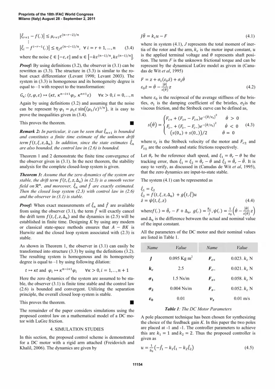
Name Value Name Value 𝑱 0.095 Kg m2 𝑭𝒄 0.023. 𝑘 N 𝒌𝒄 2.5 𝑭𝒄 0.021. 𝑘 N 𝝈𝟏 1.5 Ns/m 𝑭𝒔 0.058. 𝑘 N 𝝈𝟐 0.004 Ns/m 𝑭𝒔 0.052. 𝑘 N 𝜺𝟎 0.01 𝒗𝒔 0.01 m/s
Table 1: The DC Motor Parameters
A pole placement technique has been chosen for synthesizing the choice of the feedback gain K. In this paper the two poles are placed at -1 and -1. The controller parameters to achieve this are 𝑘 = 1 and 𝑘 = 2. Thus the proposed controller is given as 𝑢 = −𝑓 − 𝑘 𝜉 − 𝑘 𝜉 (4.5)
Preprints of the 18th IFAC World CongressMilano (Italy) August 28 - September 2, 2011
11154

where 𝑓 is the estimate of the drift term 𝑓(. ) and 𝜉 is the estimate of the state 𝜉 . The proposed observer structure for the system is as follows: �̇� = 𝑣 𝑣 = −𝜆 𝐿 ⁄ 𝜉 − 𝜉 ⁄ 𝑠𝑖𝑔𝑛 𝜉 − 𝜉 + 𝜉 �̇� = 𝑓 + 𝑏 𝑢 𝑓 = −𝜆 𝐿 ⁄ 𝜉 − 𝜉 ⁄ 𝑠𝑖𝑔𝑛 𝜉 − 𝜉 + 𝜉 �̇� = −𝜆 𝐿 𝑠𝑖𝑔𝑛 𝜉 − 𝑓 (4.6) where 𝜆 = 5, 𝜆 = 10 and 𝜆 = 5.
Figure 4.1 shows the simulation results of the proposed con-troller with a sinusoidal reference signal. The first subplot demonstrates the speed response and the second subplot dis-plays the control effort. As illustrated, the speed tracks the reference signal very effectively. Moreover the control force does not exhibit any chattering effects.
Figure 4.1: The Speed Response and Control Effort of Sinu-soidal Reference Signal
Figure 4.2 demonstrates the tracking of the drift term by the proposed observer. As shown in the figure, the observer accu-rately tracks the drift signal after a certain (finite) time.
Figure 4.2: The Actual and Observed Drift Term
Figure 4.3 shows a comparison between the actual and ob-served state. It is clear from the figure that the observed state follows the actual state component 𝜉 accurately.
Figure 4.3: The Actual and Observed State 𝜉
The validity of the proposed controller for a square waveform as the reference speed for the DC motor is discussed below.
Figure 4.4 shows the simulation results of the proposed con-troller for speed control of the DC motor with a square wave reference signal. The first subplot shows the tracking of ref-erence signal and second subplot demonstrates the controller effort. As illustrated, the speed follows the reference signal precisely.
Figure 4.4: The Speed Response and Control Effort
Figure 4.5 exhibits the tracking of the drift term by the pro-posed observer. As shown by the figure, the observer pre-cisely tracks the drift signal after a certain (finite) time.
Figure 4.5: The Actual and Observed Drift Terms
0 1 2 3 4 5 6 7 8 9 10-1.5
-1
-0.5
0
0.5
1
1.5
Time (sec)
Spe
ed (
rad/
sec)
0 1 2 3 4 5 6 7 8 9 10-0.05
-0.04
-0.03
-0.02
-0.01
0
0.01
0.02
0.03
0.04
0.05
Time (sec)
Con
trol
Eff
ort
(Vol
ts)
Motor Speed Reference Signal
0 1 2 3 4 5 6 7 8 9 10-1.5
-1
-0.5
0
0.5
1
1.5
Time (sec)
Drif
t T
erm
Observed Drift Term Actual Drift Term
0 1 2 3 4 5 6 7 8 9 10-0.04
-0.02
0
0.02
0.04
0.06
0.08
0.1
0.12
Time (sec)
Observed State
Actual State
0 10 20 30 40 50 60-1.5
-1
-0.5
0
0.5
1
1.5
Time (sec)
Spe
ed (
rad/
sec)
0 10 20 30 40 50 60-1
-0.8
-0.6
-0.4
-0.2
0
0.2
0.4
0.6
0.8
1
Time (sec)
Con
trol
Eff
ort
(Vol
ts)
Motor Speed
Reference Signal
0 10 20 30 40 50 60-40
-30
-20
-10
0
10
20
30
40
Time (sec)
Drif
t T
erm
Actual Drift Term
Observed Drift Term
Preprints of the 18th IFAC World CongressMilano (Italy) August 28 - September 2, 2011
11155
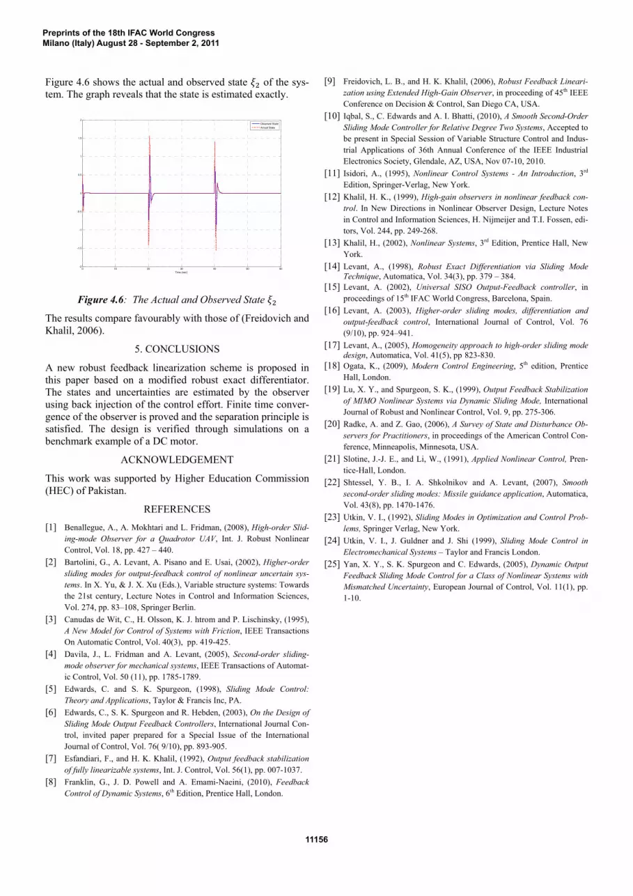
Figure 4.6 shows the actual and observed state 𝜉 of the sys-tem. The graph reveals that the state is estimated exactly.
Figure 4.6: The Actual and Observed State 𝜉
The results compare favourably with those of (Freidovich and Khalil, 2006).
5. CONCLUSIONS
A new robust feedback linearization scheme is proposed in this paper based on a modified robust exact differentiator. The states and uncertainties are estimated by the observer using back injection of the control effort. Finite time conver-gence of the observer is proved and the separation principle is satisfied. The design is verified through simulations on a benchmark example of a DC motor.
ACKNOWLEDGEMENT
This work was supported by Higher Education Commission (HEC) of Pakistan.
REFERENCES
[1] Benallegue, A., A. Mokhtari and L. Fridman, (2008), High-order Slid-ing-mode Observer for a Quadrotor UAV, Int. J. Robust Nonlinear Control, Vol. 18, pp. 427 – 440.
[2] Bartolini, G., A. Levant, A. Pisano and E. Usai, (2002), Higher-order sliding modes for output-feedback control of nonlinear uncertain sys-tems. In X. Yu, & J. X. Xu (Eds.), Variable structure systems: Towards the 21st century, Lecture Notes in Control and Information Sciences, Vol. 274, pp. 83–108, Springer Berlin.
[3] Canudas de Wit, C., H. Olsson, K. J. htrom and P. Lischinsky, (1995), A New Model for Control of Systems with Friction, IEEE Transactions On Automatic Control, Vol. 40(3), pp. 419-425.
[4] Davila, J., L. Fridman and A. Levant, (2005), Second-order sliding-mode observer for mechanical systems, IEEE Transactions of Automat-ic Control, Vol. 50 (11), pp. 1785-1789.
[5] Edwards, C. and S. K. Spurgeon, (1998), Sliding Mode Control: Theory and Applications, Taylor & Francis Inc, PA.
[6] Edwards, C., S. K. Spurgeon and R. Hebden, (2003), On the Design of Sliding Mode Output Feedback Controllers, International Journal Con-trol, invited paper prepared for a Special Issue of the International Journal of Control, Vol. 76( 9/10), pp. 893-905.
[7] Esfandiari, F., and H. K. Khalil, (1992), Output feedback stabilization of fully linearizable systems, Int. J. Control, Vol. 56(1), pp. 007-1037.
[8] Franklin, G., J. D. Powell and A. Emami-Naeini, (2010), Feedback Control of Dynamic Systems, 6th Edition, Prentice Hall, London.
[9] Freidovich, L. B., and H. K. Khalil, (2006), Robust Feedback Lineari-zation using Extended High-Gain Observer, in proceeding of 45th IEEE Conference on Decision & Control, San Diego CA, USA.
[10] Iqbal, S., C. Edwards and A. I. Bhatti, (2010), A Smooth Second-Order Sliding Mode Controller for Relative Degree Two Systems, Accepted to be present in Special Session of Variable Structure Control and Indus-trial Applications of 36th Annual Conference of the IEEE Industrial Electronics Society, Glendale, AZ, USA, Nov 07-10, 2010.
[11] Isidori, A., (1995), Nonlinear Control Systems - An Introduction, 3rd Edition, Springer-Verlag, New York.
[12] Khalil, H. K., (1999), High-gain observers in nonlinear feedback con-trol. In New Directions in Nonlinear Observer Design, Lecture Notes in Control and Information Sciences, H. Nijmeijer and T.I. Fossen, edi-tors, Vol. 244, pp. 249-268.
[13] Khalil, H., (2002), Nonlinear Systems, 3rd Edition, Prentice Hall, New York.
[14] Levant, A., (1998), Robust Exact Differentiation via Sliding Mode Technique, Automatica, Vol. 34(3), pp. 379 – 384.
[15] Levant, A. (2002), Universal SISO Output-Feedback controller, in proceedings of 15th IFAC World Congress, Barcelona, Spain.
[16] Levant, A. (2003), Higher-order sliding modes, differentiation and output-feedback control, International Journal of Control, Vol. 76 (9/10), pp. 924–941.
[17] Levant, A., (2005), Homogeneity approach to high-order sliding mode design, Automatica, Vol. 41(5), pp 823-830.
[18] Ogata, K., (2009), Modern Control Engineering, 5th edition, Prentice Hall, London.
[19] Lu, X. Y., and Spurgeon, S. K., (1999), Output Feedback Stabilization of MIMO Nonlinear Systems via Dynamic Sliding Mode, International Journal of Robust and Nonlinear Control, Vol. 9, pp. 275-306.
[20] Radke, A. and Z. Gao, (2006), A Survey of State and Disturbance Ob-servers for Practitioners, in proceedings of the American Control Con-ference, Minneapolis, Minnesota, USA.
[21] Slotine, J.-J. E., and Li, W., (1991), Applied Nonlinear Control, Pren-tice-Hall, London.
[22] Shtessel, Y. B., I. A. Shkolnikov and A. Levant, (2007), Smooth second-order sliding modes: Missile guidance application, Automatica, Vol. 43(8), pp. 1470-1476.
[23] Utkin, V. I., (1992), Sliding Modes in Optimization and Control Prob-lems, Springer Verlag, New York.
[24] Utkin, V. I., J. Guldner and J. Shi (1999), Sliding Mode Control in Electromechanical Systems – Taylor and Francis London.
[25] Yan, X. Y., S. K. Spurgeon and C. Edwards, (2005), Dynamic Output Feedback Sliding Mode Control for a Class of Nonlinear Systems with Mismatched Uncertainty, European Journal of Control, Vol. 11(1), pp. 1-10.
0 10 20 30 40 50 60-2
-1.5
-1
-0.5
0
0.5
1
1.5
2
Time (sec)
Observed State
Actual State
Preprints of the 18th IFAC World CongressMilano (Italy) August 28 - September 2, 2011
11156