exact linearization of nonlinear systems with outputs

Math. Systems Theory 21, 63-83 (1988) Mathematical Systems Theory ©1988 Sonnger-Verlag New York Inc.

Exact Linearization of Nonlinear Systems with Outputs*

D. Cheng, ~ A. Isidori, 2 W. Respondek, 3 and T. J. Tarn 4

= Institute of Systems Science, Academy of Sciences, Beijing, People's Republic of China

2 Department of Information and Systems Science, Universita di Roma "'La Sapienza', Rome, Italy

3 Institute of Mathematics, Polish Academy of Sciences, Warsaw, Poland

4 Department of Systems Sciences and Mathematics, Washington University, St. Louis, Missouri, USA

Abstract. This paper discusses the problem of using feedback and coordinates transformation in order to transform a given nonlinear system with outputs into a controllable and observable linear one. We discuss separately the effect of change of coordinates and, successively, the effect of both change of coordinates and feedback transformation. One of the main results of the paper is to show what extra conditions are needed, in addition to those required for input-output-wise linearization, in order to achieve full linearity of both state-space equations and output map.

I. Introduction

In the last years there has been an increasing interest in the problem of compensat- ing the nonlinearities of a nonlinear control system. Among all the problems of this kind, the most natural question is that of when there exists a local (or global) change of coordinates, i.e., a diffeomorphism, in the state space that carries the given nonlinear system into a linear one. Krener [1] showed the importance of the Lie algebra of vector fields associated with the system in studying such a question and gave an answer to this problem. Brockett [2] enlarged the class of

*This research was supported in part by the National Science Foundation under Grants ECS-8515899, DMC-8309527, and INT-8519654.

64 D. Cheng, A. Isidori, W. Respondek, and T. J. Tam

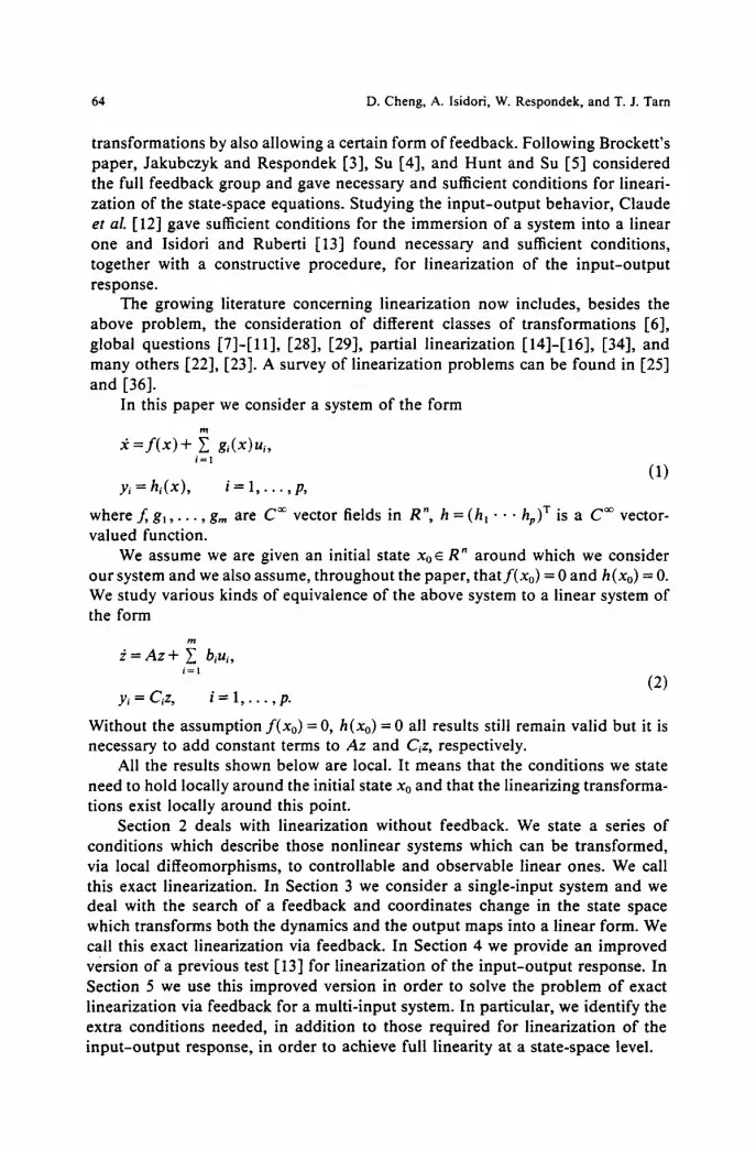
transformations by also allowing a certain form of feedback. Following Brockett 's paper, Jakubczyk and Respondek [3], Su [4], and Hunt and Su [5] considered the full feedback group and gave necessary and sufficient conditions for linearization of the state-space equations. Studying the input-output behavior, Claude et al. [12] gave sufficient conditions for the immersion of a system into a linear one and Isidori and Ruberti [13] found necessary and sufficient conditions, together with a constructive procedure, for linearization of the input-output response.

The growing literature concerning linearization now includes, besides the above problem, the consideration of different classes of transformations [6], global questions [7]-[11], [28], [29], partial linearization [14]-[16], [34], and many others [22], [23]. A survey of linearization problems can be found in [25] and [36].

In this paper we consider a system of the form

g = f ( x ) + ~ g,(x)ui, i = 1

(1) Yi = hi(x) , i= 1 , . . . , p ,

where f, g~ . . . . ,gm are C ~ vector fields in R n, h = (hl • • • hp) r is a C ~ vector- valued function.

We assume we are given an initial state Xo~ R n around which we consider our system and we also assume, throughout the paper, that f(xo) = 0 and h(xo) = O. We study various kinds of equivalence of the above system to a linear system of the form

= A z + ~ biui, i = l

(2) y i=Ciz , i = l , . . . , p .

Without the assumption f ( xo) = O, h(xo) = 0 all results still remain valid but it is necessary to add constant terms to Az and C~z, respectively.

All the results shown below are local. It means that the conditions we state need to hold locally around the initial state Xo and that the linearizing transformations exist locally around this point.

Section 2 deals with linearization without feedback. We state a series of conditions which describe those nonlinear systems which can be transformed, via local diffeomorphisms, to controllable and observable linear ones. We call this exact linearization. In Section 3 we consider a single-input system and we deal with the search of a feedback and coordinates change in the state space which transforms both the dynamics and the output maps into a linear form. We call this exact linearization via feedback. In Section 4 we provide an improved version of a previous test [13] for linearization of the input-output response. In Section 5 we use this improved version in order to solve the problem of exact linearization via feedback for a multi-input system. In particular, we identify the extra conditions needed, in addition to those required for linearization of the input-output response, in order to achieve full linearity at a state-space level.

Exact Linearization of Nonlinear Systems with Outputs 65

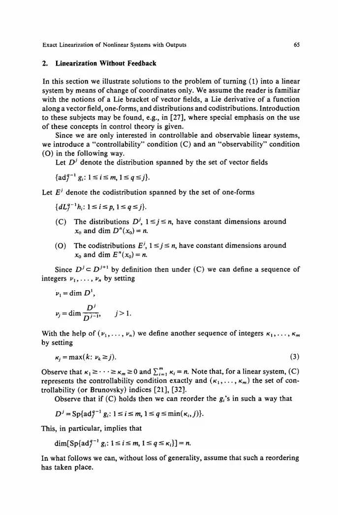
2. Linearization Without Feedback

In this section we illustrate solutions to the problem o f turning (1) into a linear system by means o f change of coordinates only. We assume the reader is familiar with the notions o f a Lie bracket o f vector fields, a Lie derivative of a function along a vector field, one-forms, and distributions and codistributions. In t roduct ion to these subjects may be found, e.g., in [27], where special emphasis on the use o f these concepts in control theory is given.

Since we are only interested in control lable and observable linear systems, we int roduce a "controllabil i ty" condi t ion (C) and an "observabi l i ty" condit ion (O) in the following way.

Let D j denote the distribution spanned by the set o f vector fields

{ad~ -1 gi: l < - i < - m , l < - q < - j } •

Let E j denote the codistribution spanned by the set o f one-forms

{dL~--~hi: l <_i<_p, l <_q<_j}.

(C) The distributions D j, 1 <-j <-n, have constant dimensions a round xo and dim D"(Xo) = n.

(O) The codistributions E j, 1 - < j - n, have constant dimensions a round Xo and dim E"(Xo) = n.

Since D ~ c D ~+~ by definition then under (C) we can define a sequence o f integers t q , . . . , v, by setting

v 1 = dim D l,

D j ~,j = dim DS_-----i, j > 1.

With the help o f ( v l , - - . , ~',) we define another sequence o f integers Kl . . . . , K,. by setting

K~ = max(k : ~'k ->j). (3)

m

Observe that K 1 ->. • • >- Km > 0 and ~i=1 Ki = n. Note that, for a linear system, (C) represents the controllability condi t ion exactly and (K~ . . . . , Kin) the set o f controllability (or Brunovsky) indices [21], [32].

Observe that if (C) holds then we can reorder the g~'s in such a way that

D j = Sp{ad~ -1 gi: 1 <- i <- m, 1 <- q <- min(Ki,j)}.

This, in particular, implies that

dim[Sp{ad~ -1 gi: 1 -< i_< m, I -< q -< Ki}] = n.

In what follows we can, without loss o f generality, assume that such a reordering has taken place.

66 D. Cheng, A. lsidori, W. Respondek, and T. J. Tam

As for the condition (O), since E J c E j+~ by definition, we can define a sequence of integers oh, • • . , w, by setting

trt = dim E 1,

E ~ = dim E j------S, j > 1,

and then another s equence /z , , . . . , /~p given by

/zj = max(k: O'k -->j).

Observe that /zt->-..--p.p_->0 and ~ = l ~ = n. Note that, for a linear system, (O) represents the observability condition exactly and (/~, . . . . ,/~p) the set of observability indices [32].

If (O) holds we can reorder the hi's in such a way that

E j = Sp{dL~-~h~: 1 <- i <- p, 1 <- q <- min(/z, j)}

and this, in particular, implies

dim[Sp{dL~-~h~: 1 <- i<_p, 1 -< q-< ~} ] = n.

In what follows we can, without loss of generality, assume that such a reordering has taken place.

The following statement presents several equivalent necessary and sufficient conditions for exact linearization via diffeomorphisms.

Theorem 1. The following conditions are equivalent:

(a) System (1) is equivalent, under a (local) diffeomorphism z = ~b(x), to the controllable and observable linear system (2).

(b) System (1) satisfies (C), (O), and ((31) L~ Lg . . . Lg, hj=Oforall l<_j<_p, alIK>_l, andallO<_iq <-

m'( where go=f ) , when at least two of the iq' s differ from O.

(c) System (1) satisfies (C), (0) , and

(G2) L~L~hi = constant for all 1 <-j <-- m, all 1 <- i <- p, and all 0 <- q <- r S + ~ i - 1 .

(d) System (1) satisfies (C), (O), and

(G3) [ad~gj, ad~g~]=Oforal l l<-i , j<_m, allO<_q<_Ks, O<_r<_K . and L~,L~h~ = constant for all 1 <-j<- m, all 1 <- i<p, and all O < - q < n j - l .

(e) System (1) satisfies (C), (O), and

Ek'O C~kdL~hj, for all 1 <- i<--p, where the i , (G4) dL~,h,=~=~ ~ - ' Cjk S are real numbers, and LgjL~h~ =constant for all l <-j <_ m, all l < i < p , andal l O< q < p . - 1.

Remark 1. The same exact linearization problem has been considered by Nijmeijer [18] who proved the- equivalence (a)c:~(b). For single-input single- output systems Hunt et al. [22] showed the equivalence (a)¢~ (c).


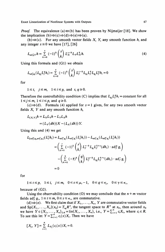
Proof The equivalence (a)c:>(b) has been proven by Nijmeijer [18]. We show the implication ( b ) ~ ( c ) ~ ( d ) ~ ( e ) ~ ( a ) .

( b ) ~ ( c ) . For any smooth vector fields X, Y, any smooth function h, and any integer s-> 0 we have [17], [26]

Lad~:yh= k=0~(--1)k(Sk) Lsx-kLYLkh" (4)

Using this formula and (G1) we obtain

L~d~g,( Lg L~h~) = L) LgL)LgLyh,=O k = o ~ \ k J

for

l<-t, j<--m, l<-i<--p, and s,q>-O.

Therefore the controllability condition (C) implies that LgL~h~ = constant for all l <-j<-m, l <-i<-p, and q->0.

(c)=>(d). Formula (4) applied for s = 1 gives, for any two smooth vector fields X, Y and any smooth function h,

Ltx.ylh = LxLyh - LyLxh

= (Lr(dh))X - (Lx(dh)) Y.

Using this and (4) we get

I.~ad~gs,ad~g,]( L)ht) = Lad~ g~( Lad~g, ( L)ht) ) - Lad;g, ( Lad~gs( L)ht) )

-(k~_O(-r)k(qk)L]-kLgsL~÷S(dh,)'ad, g~ )

= 0

for

l<_t<_p, l<---i, j ~ m , 0--<s--</~t-1 , 0--<q-<Kj, 0~/--<K~,

because of (G2). Using the observability condition (O) we may conclude that the n + m vector

fields ad} g,, 1 --~ t ~ m, 0 ~ s ~ K,, are commutative. ( d ) ~ ( e ) . We first claim that if X I , . . . , Xn, Y are commutative vector fields

and S p { X 1 , . . . , Xn}(xo) = T~R", the tangent space to R" at Xo, then around xo we have Y~ {X l , . . . , X,}La = l in{X~, . . . , X,}, i.e., Y = ~ = l c~X~, where cie R.

y ~ To see this let =}2~=~ c~(x)X, Then we have

[Xj, Y] = ~ Lxj(Ci(x))Xi =0 , i=1


Hence

Lx,(Ci(X)) =0 for j = 1 , . . . , n,

i.e., ci(x) = constant. N o w denote Xq~ = ad~ g~, 1 <- i - m, 0-< q - K~ - 1. We use the above result

for Y = a d ~ J g i and { X t , . . . , X , } = { X q i : l<-i<-m,O<-q<-Ki-1}. F r o m (G3) we have

[Xq,, ad~ g~] = 0

and hence

a d ? gj = ~ c"X,, (5)

for suitable constants c a (depending on j ) . Assume now that

ad~ gj = ~. c"Xt,.

Compute

ad~ +1 gj = [f, ad) g~] = E c"[f , X,,] = Y. c"[f, ad) g,]. (6)

We have t + 1 -< x~. Thus, f rom (5) and from the definition o f X , , every summand on the r ight-hand side o f (6) belongs to lin{X,}. Therefore, by an induction argument ,

ad~ gj ~ lin{Xa: 1 - i - m, 0 - t - Kj - 1} (7)

for every 1 <-j-< m and s >- 0. Next since (G3) gives

Ls~L~h~=constant for l<-i<-p, l<-j<-m, and O<-q<-Kj-1,

we can see, using formula (4) again, that

Lad~g,(h~)=constant for l<-i<-p, l<-j<-m, and O<-q<-Kj-1. (8)

According to (7), equation (8) remains true for any q -> 0. Hence it is also true that

LaaTg,(L~h~)=constant for l <-i<-p, l <-j<-m, and any q,s>-O.

This, in particular, implies the second part o f (G4), i.e.,

LgjL~(h~)=constant for l<-i<-p, l<-j<-m, and 0 - < s < - / z ~ - l .

To prove the first part o f (G4) denote

(gl , • • •, ad.7 ~-~ g~, g2 . . . . , gin, • • -, ad.7"-~g,,)=a ( X ~ , . . . , X , ) = X

and

( dhl . . . . . dL~'-~h~, d h 2 , . . . , dhp,. . . , dL;,-~hp) T= H.

Then we have

H ( x ) . X ( x ) = E (9)

and

dL~,h,(x). X ( x ) = e,, (10)


where E is an n x n nonsingular constant matrix and e~ is a 1 x n constant row vector. Since X ( x ) is nonsingular then (9) and (10) imply the first part of (G4).

( e ) ~ ( a ) . Introduce new local coordinates as ( z l , . . . , z~) r = ( z , 1 , . . . , z l , , , ZEt , . . . , Zp,,,) T such that

ziq=L~-lh~, l<_i<_p, l<_q<_l.~ i.

This is a valid change of coordinates because of the observability assumption (O). Now (G4) implies that in these coordinates we have

y~ = zil ,

~iq "~ Ziq+l ~- ~ iq ujgj (z) , 1 < q < ~ - 1, j=l

~i~,, = Y~ c~'zs, + ~ i~, ujgj ' (z) , j = l

where gjq denotes the components of gj. From

LsjL~hi=constant , l<--j<-m, l<_i<_p, 0_<q_</zi-1,

we deduce that gj-q(z) =cons tant and thus in z coordinates (1) takes the linear form (2). []

Remark 2. Condition (G2) seems to be stated in the most elegant and compact form. However, we also formulate (G3) and (G4) because they are helpful in studying feedback iinearization as we will see later. Meanwhile, from the proof of Theorem 1 we can see that condition (G3) (resp. (G4)) can be used for the equivalence of (1) to a controllable (resp. observable) linear system. We state it as follows.

Corollary 2. The nonlinear system (1) is equivalent to a controllable linear system o f the form (2) with nonzero Ci i f and only i f conditions (C) and (G3) hold, and LgjL~h~ ~ O fo r some 1 <-j <- m, k < Kj. Respectively, (1) is equivalent to an observable linear system o f the form (2) with nonzero bj i f and only i f conditions ( 0 ) and (G4) hold, and Lg, L~hi ~ 0 for some 1 <- i <- p, k < IZ~.

Remark 3. It can be easily deduced from the proof that we may state conditions (c) and (d) of Theorem 1 in an equivalent form when replacing every/zi and kj by n. This creates some redundancy but avoids computing the controllability and /o r observability indices. An equivalent of Corollary 2 can also be stated in this form.

3. Feedback Linearization of Single-Input Single-Output Systems

In this and in the following sections we discuss linearization by means of diffeomorphism together with state feedback control

u=~(x)+~(x)v, (11)


where a is a smooth (m vector)-valued function,/3 is a smooth (m x m matrix)- valued function, both defined in a neighborhood of Xo. It is also assumed that /3(x) is nonsingular for all x in this neighborhood.

Necessary and sufficient conditions for linearization of the input-output behavior have been established in [ 13]. In this paper we show how these conditions have to be strengthened in order to obtain, via feedback and local state-space diffeomorphism, a fully linear state-space description.

We deal first with the case of a single-input single-output system, which is much easier. In this case we recall that a system

= f ( x ) + g(x)u, u e R, (12)

y = h ( x ) , y ~ R ,

is said to have characteristic number S at Xo if

LgL~h(x) = 0 for all x near Xo, for all k < 8 ,

LgL~h(xo) ~ O.

Using this notation, we can state the following result.

Theorem 3. System (12) is equivalent to the controllable linear system (2), with nonzero C, under a diffeomorphism ~b and a state feedback of the form (11), if and only if:

(i) g, adyg , . . . , ad7 -~ g are linearly independent at Xo. (ii) The system has characteristic number 8 < n at Xo.

(iii) The vector fields f and ~, defined by

f ( x ) = f ( x ) + g(x )a (x), (13)

if(x) = g(x)/3(x), (14)

with a(x) and/3(x) given by

-L~+'h(x) 1 a ( x ) = LgL}h(x) ' /3(x) = L~L~h(x)~ ' (15)

are such that the n + 1 vector fields ~, ad? if, . . . . ad~ff are commutative.

Proof (Necessity). Without loss of generality, we may assume that (2) is a Brunovsky canonical form [21]. Set z = 6 (x) . It follows that

f ' ( z ) = ( 6 , 2 9 ° 6 - ' ( z ) = ( a ( z ) , z l , . . . , z n - , ) T,

g'(z) = (~b.f) o 6-1(z) = (b(z), 0 , . . . , 0) T,

h ' ( z ) = h o 6-1(z) = c~z~ + . . . + c . z n ,

where 4). denotes the differential of 6, a and b are smooth functions, b(z) # 0 is nonzero for all z near 6(Xo), and C l , . . . , c, are real numbers. From this, a simple computat ion shows that (i) is true.


As for (ii), note that LgL~h(x )= k , (Lg,L},h) o 49(x). Assume cl . . . . ck = 0 and Ck+ 1 ~ O. An easy computa t ion shows tha t ~ ' Lg,L'f.h (z) = 0 for all i -< k - 1 and L, .L~,h ' ( z )= Ck+lb(z). The lat ter is nonzero at z = ~b(Xo) and therefore B = k < - n - 1 .

To check (iii) , note that in the z -coord ina tes

a( z ) 1

b (z ) c6+lb(z)

-L~,+lh'(z) ot'(z) = ot o dp-'(z) = Lg.L~,h'(z) -

1 [ 3 ' ( z ) = ~ o ~ - ' ( z ) - - -

c~÷,b(z)'

f ' ( z ) = i f ( z ) + g ' ( z ) a ' ( z )

- - ( c6+2z~ +" • • + c.z._8_a),

[ IT - 1 (c~+2zl+ "+c,,z,,_~-O, z l , . . z,,-1 = A z , C6+1

g' (z ) = g ' ( z ) f l ' ( z ) = 1 , 0 . . . . , 0 = b,

where A is a cons tant matr ix and b is a cons tan t vector . Therefore

ad~-, g ' = (--1)kAkb = constant

and cond i t ion (iii) follows. (Sufficiency). Observe that, f rom the def in i t ion o f 6, we have

L ~ h = L ; h , k<-6,

for any a. F r o m this and the def ini t ions o f a and fl given in the s ta tement o f the theorem, it fol lows that

Leh = L~L?h . . . . . L~L~-~h = O,

L~L~h = L~L~h = ~LgL~h = 1,

L ~ + l h = L j L ~ h = O ,

and therefore

L~L~h=O for all k > 6 + 1 .

Thus, LgL~h = c o n s t a n t for all 0 - < k - < n - 1. The system

= 7 (x ) + ~(x)v,

y = h (x )

satisfies cond i t ion (C) (which is f e e d b a c k invar ian t [3]) and cond i t ion (G3) o f Theorem 1. Hence (compare Coro l l a ry 2) it is equ iva len t to a con t ro l l ab le l inear system via a d i f feomorphism. This comple tes the proof . [ ]

In .case the system has one input and p > 1 ou tputs , the previous resul t can be easi ly ex t ended to yield the fo l lowing s ta tement .


Corollary 4. Suppose m = 1. Then system (1) is equivalent to a controllable linear system (2), with nonzero C, under a diffeomorphism ¢b and a state feedback o f the form ( I 1), i f and only if:

(i) g, a d f g , . . . , ad~-' g are linearly independent at Xo. (ii) For some j, 1 <-j <- p, the triplet {f, g, hi} has characteristic number 8j < n

at xo. (iii) The vector fields (13) and (14), with a and fl still as in (15) but with h

replaced by hi, are such that the n + 1 vector fields g, ad• ~ , . . . , ad~ ~ are commutative.

(iv) L~L~hi = constant for all 0 <- k<_ n - 1 and all 1 <- i<-p, i # j .

4. Input-Output Linearization, via Feedback, of Multivariable Systems

In order to develop an extension of Theorem 3 to systems with m > 1 inputs and p > 1 outputs, it is convenient to summarize first some known facts about linearization of the input-output behavior. We synthesize here some results from [13] and, in addition, we show that the test for input-output linearizability contained therein can be substantially improved.

We recall that a system of the form (1) is said to be input-output iinearizable around Xo by a feedback of the form (11) if the implementation of such a feedback yields an input-output behavior of the form

y ( t ) = q ( t , Xo)+ ~ - k i ( t - r )v i (1") dr. i=1

From this definition, in view of some well-known properties of the input- output expansions of systems of the form (1) (see, e.g., [20]), it is necessary to state the following result.

Lemma 5 [13]. System (1) is input-output linearizable around Xo by the feedback (11) i f and only i f L~L~h(x) = constant around Xo for all k >- O, where f = f + ga and p, = gB.

In order to derive existence conditions, and a constructive procedure yielding such a feedback, it is useful to proceed in the following way. First, we improve Lemma 5 by showing that any linearizing feedback is characterized by a finite set of constraints.

Lemma 6. Consider a system

~ = f ( x ) + g ( x ) u = f ( x ) + ~ gi(x)ui, i = l

y = h ( x ) = ( h i ( x ) , . . . , h , ( x ) ) T

with x ~ M, an n-dimensional manifold. I f

LsL~h (x) = constant

for all 0 <- k<-2n - 1 , then (17) holds for all k.

(16)

(17)


Proof. Recall that (see p. 49 of [27]), on an open and dense submanifold M ' ~ M, the largest codistribution Q invariant under f , g ~ , . . . , g m which contains span{dh~, . . . ,dhp} is locally spanned by exact one-forms such as t o=d(Lg ,o . . . Lg, hj) where r < - n - 1 and O<-ik <--m, with g o = f Since (17) holds we see, in particular, that Q is locally spanned by exact one-forms such as to=dL~hj, l<-j<-p, O<-k<-rj. Let d i m ( Q ) = q and choose new coordinates ( z ~ , . . . , Zq, ~ , . . . , 2,_q)= 4,(x) with the z/s functions in the set {L~hj; l<-j<-p, 0 <- k_< ~}. Using these coordinates system (16) becomes (see, e.g., pp. 29-30 of [27])

=f~(z) + g~(z)u, (18a)

~" = fz(z, ~) + g2(z, 2)u, (18b)

y = h , ( z ) . (18c)

Clearly, (LgL~h)ocb-~(z)=LgL~,h~(z) for all k - 0 . From this and (17) it is possible to deduce that

ad~, glr(Z) = constant, l<-r<-m, O<-s<-n. (19)

As a matter of fact, a consequence of (17) is that

constant = Lg, L~,L~,hlj 5 k (-1)~(dL~-h~j, a s = ( -1 ) Lad), g,L~h~j = df, glr).

Since each of the z~'s has a form z~=Lkrh~: (with k < _ n - 1 ) the last equation proves that

(dz~, ad}, g~,) = ith element of ad~, g~, = constant for all s -< n,

as required. Return now to equations (18a), (18c) and note that the ith row of g~(x),

having a form (dz~, g)= LgL:h~, is constant, i.e., g~(x) = B, where B is a constant q x rn matrix. The elements of h~(z) are precisely some of the zi's and therefore also h~(z) = Czz, where C~ is a constant p x q matrix. Using (19) we deduce a similar property for (at least a decomposition of) f~(z).

Let R denote the smallest distribution invariant underf~, g ~ , . . . , gtm which contains s p a n { g H , . . . , g~r~}- An easy computation (see, e.g., pp. 33-39 of [27]) shows that in this case, because of (19), R has the expression

R = Span{ad~, gt,; 1 <- r <- m, 0 <- s <- n - 1}.

Let d i m ( R ) = r. Since R is spanned by constant q-vectors, it is possible to find a (q - r) x q matrix P" of real numbers, with rank (q - r), such that P"v = 0 for

all v ~ R. Now choosing any other r x q matrix P ' such that p,, is nonsingular,

the change of coordinates (z', z")= (P'z, P"z) splits (18a), (18c) into (see, e.g., p. 29 of [27])

e' =f ' ( z ' , z") + B'u, (20a)

e" =f" (z" ) , (20b)

y = C 'z '+ C"Z". (20c)


In addition, it is easy to see that

f ' ( z', z") = A' z' + y( z"),

where A is a constant matrix, because all the vectors in (19) (including the one corresponding to s = n) are constant. From (20) and (18b), a direct calculation shows that

LgL~h(x)=C'(A')kB ' for all k->0.

Thus, L,L~h(x) is constant around any point of M' , an open and dense subset of M. Being a smooth function, it is constant for each x ~ M. []

This result is rather important because it shows that in order to find feedback which linearizes the input-output behavior of (1) we only have to satisfy the conditions

L. i L~ h ( x ) =constant

for all k -< 2n - 1. To check whether or not such a feedback exists and to calculate it, we recall

the results of [13]. Set

Tk(X) = LgL~h(x)

and consider a sequence of Toeplitz matrices

"To(x) T,(x) . . . Tk(X) ]

Mk(X) = 0 To(x) "'" Tk-,(X) I . . . . . . . . . . . . . . . . . . . . . . , , .

I 0 0 "'" To(x) ]

with k -< 2n - t. We say that Xo is a regular point for M, if the rank of Mk(X) is constant for

all x near Xo. If this is the case we denote the rank of Mk(Xo) by rK(Mk). With Mk we associate another integer, the dimension of the vector space generated over the field R by the rows of Mk, and we denote this number by rn(Mk). Clearly, rR(Mk) >-- rK(Mk).

Using this notation it is possible to state the following result, a synthesis of the main theorem of [13] and Lemma 6.

Theorem 7. System (1) is input-output linearizable around Xo by the feedback (11) if and only if, for all k <- 2n - 1 , Xo is a regular point of the matrix Mk and rn(Mk)=rK(Mk).

An actual test for the fulfillment of the conditions stated in this theorem and the construction of an input-output linearizing feedback are provided, as is known, by the so-called Structure Algorithm. This is summarized here, without proof, for the reader's convenience.


Algorithm. Step 1. Suppose Xo is a regular point of Mo. If and only if rR(Mo) = rn (Mo) there exists a nonsingular matrix of real numbers, denoted by

where P~ performs row permutations, such that

V, To(x)=[S'(oX)],

where S,(x) is an ro x m matrix and rank S,(xo) = to. Set

6, = ro,

7,(x) = P,h(x), ~/,(x) = Klh(x)

and note that

L ~ y , ( x ) = S,(x), Lg~,(x) =0.

I f To(x) = O, then P~ must be considered as a matrix with no rows and K1 is the identity matrix.

Step i. Consider the matrix

L~v,(x) =r s'-'~x:' l

Lgy,- , (x) LLgL:9,-,(x)J L,L:y,_,(x)

and let Xo be a regular point of this matrix. If and only if

r s,-, 1 r ',-, 1 rR L L~L[9,-,J = rK LL=Ly~,_,J

there exists a nonsingular matrix of real numbers, denoted by

L o 01 • -. 0 Pi

K', . - . KI- , ~Cl

where P~ performs row permutations, such that

[ Lg3q.(x)

~'l~,,,:,~x, __ [ s f , ] , ,[LgL1~,-,(x)


where Si(x) is an ri-i x m matrix and rank Si(xo) = r~_~. Set

~i = r i - I - - r i - 2 ,

yi(X) = PiLf'Yi-i(x),

~,(x) = K'I y , ( x )+" " " + K I - , y , - , (x ) + K~Lff/ ,_,(x)

and note that

• = Si(x), Lgy,(x)

L ~ i ( x ) = O.

I f the rank condition is satisfied but the last p - r~-2 rows of the matrix depend on the first r~-2, then the step degenerates, P~ must be considered as a matrix with no rows, KI the identity matrix, 6~ = 0, and S~(x)= S~_Jx).

After this algorithm has been cycled 2n times, a set of functions Y~, . . . , "/2, is defined (note that some of them are only "formal ly" counted in the sequence, the ones corresponding to degenerate steps of the algorithm, which do not actually exist) from which a linearizing feedback can be constructed. Set

F(x) = [ y'(:x) ] (21)

L j and recall that S2. = LgF is an rz._ l X m matrix, of rank r2._ 1 at Xo. Then the equations

[LgF(x)]a (x) = - L j F ( x ) , (22)

[L~r(x)]/3(x) = [I~._, 0] (23)

can be solved for a and/3 in a neighborhood of Xo. These a and/3 are such as to impose (see [13])

Le L~h (x) = constant

for all k-< 2 n - 1 and therefore solve the input -output linearization problem.

5. Feedback Linearization of Multi-Input-Multi-Output Nonlinear Systems

In this section we consider nonlinear control systems of the form

Y c = f ( x ) + g ( x ) u = f ( x ) + ~ I d i g i ( x ) , x ~ R " , x(O)=xo, i=1

y = h (x ) = (hi(x), • • •, hp(x)) "r. (24)


We study the feedback exact linearization problem, i.e., we seek a feedback pair (a, /3) such that the feedback modified system is equivalent, by a (local) coordinates change, to a linear system of the form

~ = Az + Bu = Az + ~ uib~, i = !

(25) y = C z .

The main result of this section shows that if such a feedback exists then it can be computed via the structure algorithm given in Section 4, thus generalizing the result of Section 3. In the case of uniqueness of feedback (22)-(23) which linearizes the input-output map (i.e., when rank LgF(xo)=m) this gives a verifiable condition for feedback exact linearization. Then we formulate and prove a result stating that any controllable linear system can be made observable via static feedback. This leads us to a feedback exact linearization condition, dual in a sense to the main theorem, which does not involve computing the Lie brackets.

We have the following.

Theorem 8. System (24) is feedback exact linearizable to a controllable system of the form (25) if and only if:

(i) (24) satisfies the controllability condition (C), (ii) (24) is input-output linearizable in a neighborhood of xo,

(iii) there exists a solution (a, [3) of (22), (23) such that

[ad~g, ,ad~ff j ]=0, for l<-i, j<-m, O<-q+r<-2n-1,

where f = f + g a , g=g/3. (26)

Remark 4. If the solution of (22), (23) is unique (i.e., when rank LgF(xo) = m, and this includes, in particular, single-input multi-output systems, see Section 3) the above result gives a verifiable condition for feedback exact linearization.

Remark 5. There is a lot of redundancy in (26). To avoid it we may formulate the above theorem, as will be clear from the proof, in the following form: (24) is feedback exact linearizable to a controllable system of the form (25) if and only if:

(ii) (24) is input-output linearizable in a neighborhood of Xo, (ii') there exists a solution (a, [3) of (22), (23) such that the system

.~ = f + ~u (27)

satisfies the controllability assumption (C) and

[ad~g~,ad}ffj]=O, I<--i, j<--m, O<--q+r--<ff,+Yj-1, (28)

where the ffi's are the controllability indices of (27) (see (3)).

Observe that under the above assumptions ( x l , . . . , K,,) = (ff~ . . . . , ~,,), because the numbers t,~ =d im Di(x) are feedback invariant (see [3] for the proof), however, we may need to reorder the ~;'s.


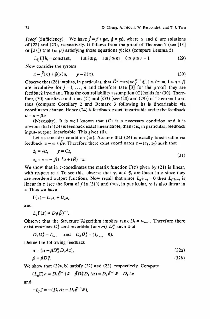
Proof (Sufficiency). We have f = f + g a , ~ =.gfl, where a and /3 are solutions of(22) and (23), respectively. It follows from the proof of Theorem 7 (see [13] or [27]) that (a, fl) satisfying those equations yields (compare Lemma 5)

LiL~hi=constant, l<_i<-p, l<_j~-m, O<-q<-n-1. (29)

Now consider the system

= f ( x ) +~,(x)u, y = h(x). (30)

Observe that (26) implies, in particular, tha t /5 j = sp{ad~-' g'~, 1 -< i-< m, 1 < q <j} are involutive for j = 1 , . . . , n and therefore (see [3] for the proof) they are feedback invariant. Thus the controllability assumption (C) holds for (30). There- fore, (30) satisfies conditions (C) and (G3) (see (28) and (29)) of Theorem 1 and thus (compare Corollary 2 and Remark 3 following it) is linearizable via coordinates change. Hence (24) is feedback exact linearizable under the feedback u = a + ~ v .

(Necessity). It is well known that (C) is a necessary condition and it is obvious that if (24) is feedback exact linearizable, then it is, in particular, feedback input-output linearizable. This gives (ii).

Let us consider condition (iii). Assume that (24) is exactly linearizable via feedback u = ti +fir. Therefore there exist coordinates z = (z,, z2) such that

z l = A z , y = Cz, ~2 = v = - ( f ) - ' 5 + ( f ) - ' u . (31)

We show that in z-coordinates the matrix function F(z) given by (21) is linear, with respect to z. To see this, observe that y~ and ~ are linear in z since they are reordered output functions. Now recall that since Lg~_ ,=0 then Lf@~_~ is linear in z (see the form o f f in (31)) and thus, in particular, y~ is also linear in z. Thus we have

F(z) = DlZl + D'Z2

and

L~r(z) = D2(/3)-'.

Observe that the Structure "Algorithm implies rank D~ = r_,,_,. Therefore there exist matrices D* and invertible ( m x m) /5* such that

D2D*=L2._, and Dz/5*=(lr2._, 0).

Define the following feedback

a = (~ - f D * D , A z ) , (32a)

fl = fD*.. (32b)

We show that (32a, b) satisfy (22) and (23), respectively. Compute

(LgF)a = D2f-~(t~ - f D ~ D ~ A z ) = D2fl -~& -D~mz

and

- L f r = - ( D , A z - D2f- ' ff),


which proves (22). To prove (23) compute

(L~F) f l=(D2~- ' ) (~O '~ )=[ I ,~ ._ , o].

Now we show that (a, fl) given by (32a, b) satisfies (iii). In z-coordinates we have

A z g=gf l= (~*2*) and ] = f + g a = [ _ D . D , A z ] ,

because - f l - ~ + f l - ~ ( 6 - f l D * D ~ A z ) = - D * D ~ A z . Therefore the system 2 = "f+ ~u is linear in z-coordinates and thus satisfies (iii). []

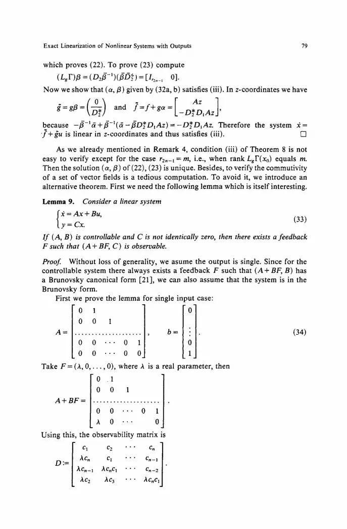
As we already mentioned in Remark 4, condition (iii) of Theorem 8 is not easy to verify except for the case r2~_~ = m, i.e., when rank Lgr(xo) equals m. Then the solution (a, fl) of (22), (23) is unique. Besides, to verify the commutivity of a set of vector fields is a tedious computation. To avoid it, we introduce an alternative theorem. First we need the following lemma which is itself interesting.

Lemma 9. Consider a linear system

Yc = A x + Bu, y = Cx. (33)

I f (A, B) is controllable and C is not identically zero, then there exists a feedback F such that ( A + BF, C) is observable.

Proof Without loss of generality, we asume the output is single. Since for the controllable system there always exists a feedback F such that ( A + BF, B) has a Brunovsky canonical form [21], we can also assume that the system is in the Brunovsky form.

First we prove the lemma for single input case:

A =

ol 1 0 0 1

0 0 - - - 0 1] /

o o . . - o o. I i] b =

Take F = (A, 0 , . . . , 0), where A is a real parameter, then

I 0 1

0 0 1

A + B F . . . . . . . . . . . . . . . . . . . . . . .

0 0 . . . 0 1

h 0 . . . 0

Using this, the observability matrix Is

I Cl C2 • . . e n ] D:= ACn C; " ' " C,-] [.

A C n - 1 ACnCl • . . Cn_ 2 [ 1 Ac2 Aca • • " Ac.c~l

.I

(34)


Assume c~ ~ 0. Then

det D = + ( c~ ) ~ - ~ + lower-order terms,

so we can choose A such that det D ~ 0. I f cn = c~_~ . . . . . cn_, = 0, c~-r-~ # 0, r < n - 2 . Then

det D = +(Cr)~A'-~ + lower-order terms.

Hence there also exists such A which makes det D # 0. I f cn = c , - t . . . . . c2 = 0, then c~ # 0 since C # 0. Set A = 0, then det D # 0.

The multi- input case follows immediately from the single-input case and Heyman ' s lemma [30] (see also p. 49 o f [31]) which states that, for any controllable (A, B) and any b e Im B, there exists F such that (A+BF, b) is controllable. [ ]

Lemma 9 immediately gives the following.

Corollary 10. System (24) is feedback exact linearizable to a controllable and observable system of the form (25) i f and only if (24) satisfies (C) and conditions (ii) and (iii) of Theorem 8.

Proof. I f (24) satisfies (C), (ii), and (iii), then, according to Theorem 8, it can be t ransformed via feedback and coordinates change to a controllable linear form (25). Then applying more feedback to the linear system obtained, as indicated by Lemma 9, we get a controllable and observable form. The necessity part is obvious. [ ]

Now we state the dual linearization result.

Theorem 11. System (24) is feedback exact linearizable to a controllable system of the form (25) i f and only if:

(i) (24) satisfies (C). (ii) There exist a feedback, pair (a, fl ) (defined in a neighborhood of xo) such

that

L~L~h~=constant, l < j < - m , l<-i<-p, 0 - < q < - 2 n - 1 , (35)

and

dh rank . = n, (36)

IL?/'dhJx=xo where f = f + ga and ~ = gfl.

Remark 6. Observe that the above theorem (see the proof) , in fact, gives the necessary and sufficient condit ion for (24) to be feedback exact l inearizable to a controllable and observable system of the form (25). Therefore it can be seen as a dual to Corol lary 10.


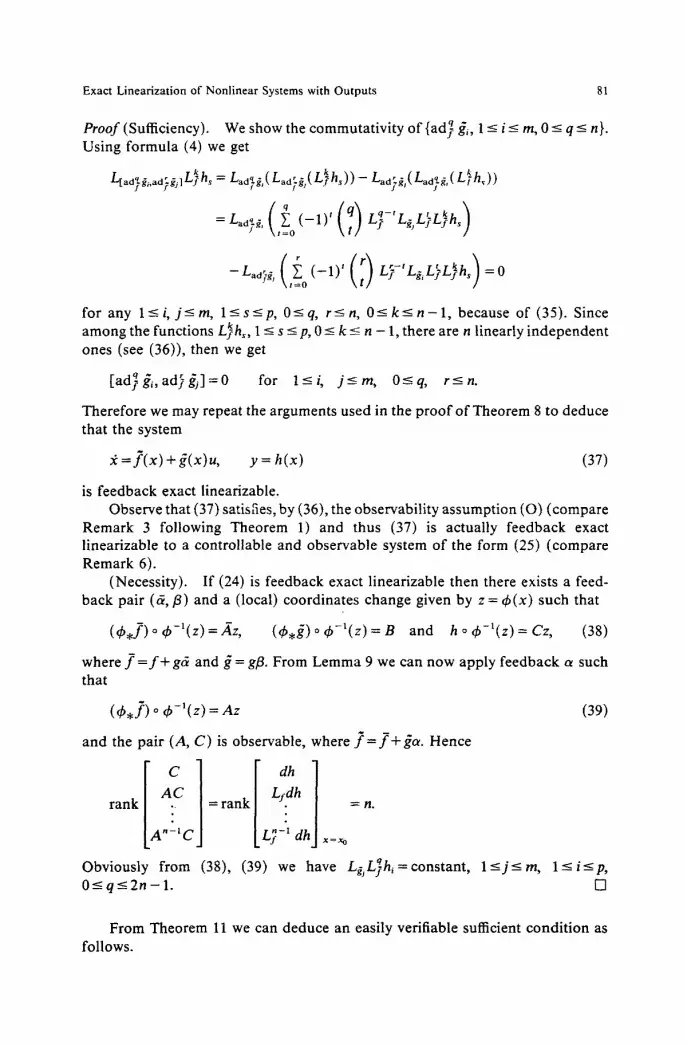
Proof (Sufficiency). We show the commuta t iv i ty o f{ad~ gi, 1 -< i - < m, 0 < - q-< n}. Using fo rmula (4) we get

L[ad~,ad~ffi]L~hs = Lad~,( Zad~ffl( t~hs) ) -- Lad~,( Zad~.f.,( L~h~) )

tq-t t k

-gaa~f,(,=~o(-a)'(;)L}-tL~,L}L}hs)=O

for any l<-i,j<-m, l<-s<-p, O<-q, r<-n, O<-k<--n-1, because of (35). Since a m o n g the funct ions L~h~, 1 <-- s <- p, 0-< k ~< n - 1, there are n l inearly independen t ones (see (36)), then we get

[ a d ~ f f , , a d ~ g j ] = 0 for 1--<i, j<-m, O<-q, r<_n.

Therefore we may repeat the arguments used in the p r o o f o f Theorem 8 to deduce that the system

= f ( x ) + g(x)u, y = h(x) (37)

is f eedback exact linearizable. Observe that (37) satisfies, by (36), the observabi l i ty assumpt ion (O) ( compare

R e m a r k 3 following Theorem 1) and thus (37) is actual ly f eedback exact l inearizable to a control lable and observable system o f the form (25) ( compare Remark 6).

(Necessi ty) . I f (24) is feedback exact l inearizable then there exists a feedback pair (fi,/3) and a (local) coordinates change given by z = ~b(x) such that

(6 , f )o~-~(z )=Az , ( 6 , f f ) o 6 - ~ ( z ) = B and ho6-1(z)=Cz, (38)

where f = f + g& and ff = g/3. From L e m m a 9 we can now apply f eedback a such that

( q~,f) o ¢b-~(z) = Az (39)

and the pa i r (A, C) is observable, where f= f+~ ,a . Hence

rank . = rank h = n.

[A~-'C J LLy ahJ Obvious ly f rom (38), (39) we have q - -<j-< LejL~h~-constant, 1 m, l<-i<-p, O--<q----2n-1. []

F rom Theorem 11 we can deduce an easily verifiable sufficient condi t ion as follows.


Corollary 12. Assume that (24) satisfies:

(i) The controllability assumption (C). (ii) There exist solutions a and fl o f equations (22) and (23), respectively, such

that the rank condition (36) is satisfied.

Then (24) is feedback exact linearizable to a controllable and observable system o f

the f o rm (25).

Proof. Since solut ions o f (22), (23) sat isfy (35) then this co ro l l a ry fol lows i m m e d i a t e l y f rom Theorem 11. []

6. Conclusions

This p a p e r dea ls with the p rob l em of nonl inear i t i es c o m p e n s a t i o n for a non l inea r control sys tem with outputs . We give a list o f equiva len t cond i t ions which guaran tee l inear iza t ion via s ta te-space coord ina te s change. Then we s tudy the f e e d b a c k l inear iza t ion prob lem. We prove tha t i f there exists a f e e d b a c k which l inear izes the dynamics and the ou tpu t then this can be c o m p u t e d via a non l inea r vers ion o f S i lverman ' s Structure Algor i thm. F o r a subclass o f non l inea r systems this leads to a verifiable cond i t ion for f eedback l inear iza t ion . The ou tpu t f eedback l inear iza t ion , which is not t rea ted in this pape r , is s tud ied in [25] and [35].

References

[1] A.J. Krener, On the Equivalence of Control Systems and Linearization of Nonlinear Systems, SIAM J. Control Optim., 11 (1973), 670-676.

[2] R.W. Brockett, Feedback Invadants for Nonlinear Systems, Proc. IFAC Congress, Helsinki, 1978.

[3] B. Jakubczyk and W. Respondek, On Linearization of Control Systems, Bull. Acad. Polon. Sci. Sdr. Sci. Math., 28 (1980), 517-522.

[4] R. Su, On the Linear Equivalents of Nonlinear Systems, Systems Control Lett., 2 (1982), 48-52. [5] L.R. Hunt and R. Su, Linear Equivalents of Nonlinear Time-Varying Systems, Int. Symp.

Math. Theory of Networks and Systems, Santa Monica, CA, 1981. [6] W. Respondek, Geometric Methods in Linearization of Control Systems, in Mathematical

Control Theory, Banach Center Publications, Vol. 14 (Proc. Conf., Warsaw, 1980) (Cz. Olech, B. Jakubczyk, and J. Zabczyk, eds.), Polish Scientific Publishers, Warsaw, 1985, pp. 453-467.

[7] W. M. Boothby, Some Comments on Global Linearization of Nonlinear Systems, Systems Control Lett., 4 (1984), 143-147.

[8] L.R. Hunt, R. Su, and G. Meyer, Global Transformations of Nonlinear Systems, IEEE Trans. Automat. Control, 28 (1983), 24-30.

[9] D. Cheng, T. J. Tam, and A. Isidori, Global Feedback Linearization of Nonlinear Systems, Proc. 23rd IEEE Conf. Decision and Control, Las Vegas, Nevada, 1984.

[10] D. Cheng, T. J. Tam, and A. Isidori, Global External Linearization of Nonlinear Systems Via Feedback, IEEE Trans. Automat. Control, 30 (1985), 808-811.

[11] W. Respondek, Global Aspects of Linearization, Equivalence to Polynomial Forms and Decomposition of Nonlinear Systems, in [33], pp. 257-284.

[12] D. Claude, M. Fliess, and A. Isidori, Immersion Directe et par Bouclage, d'un systeme non lineaire dans un lineaire, C. R. Acad. Sci. Paris, 296 (1983), 237-240.


[13] A. Isidori and A. Ruberti, On the Synthesis of Linear Input-Output Responses for Nonlinear Systems, Systems Control Lett., 4 (t984), 17-22.

[14] A. Isidori and A. J. Krener, On Feedback Equivalence of Nonlinear Systems, Systems Control Left., 2 (1982), 118-121.

[15] A.J. Krener, A. Isidori, and W. Respondek, Partial and Robust Linearization by Feedback, Proc. 22nd 1EEE Conf. Decision and Control, San Antonio, Texas, 1983, pp. 126-130.

[16] W. Respondek, Partial Linearization, Decompositions and Fibre Linear Systems, in Theory and Applications of Nonlinear Control Systems, MTNS, Vol. 85 (C. I. Byrnes and A. Lindquist, eds.), North-Holland, Amsterdam, 1986, pp. 137-154.

[17] D. Cheng, On Linearization and Decoupling Problems of Nonlinear Systems, D.Sc. Disserta- tion, Washington University, St. Louis, Missouri, August, I985.

[18] H. Nijmeijer, State-space Equivalence of an Affine Non-linear System with Outputs to Minimal Linear Systems, lnternat. J. Control, 39 (1984), 919-922.

[19] V. Lakshmikantham (ed.), Nonlinear Analysis and Applications, Lecture Notes in Pure and Applied Mathematics, Vol. 109, Marcel Dekker, New York, 1987.

[20] M. Fliess, M. Lamnabhi, and F. L. Lagarrigue, An Algebraic Approach to Nonlinear Functional Expansions, IEEE Trans. Circuits and Systems, 30 (1983), 554-570.

[21] P. Brunovsky, A Classification of Linear Controllable Systems, Kibernetica (Praha), 6 (1970), 173-188.

[22] L.R. Hunt, M. Luksic, and R. Su, Exact Linearizations of Input-Output Systems, lnternat. Z Control, 43 (1986), 247-255.

[23] L.R. Hunt, M. Luksic, and R. Su, Nonlinear Input-Output Systems, in [19], pp. 261-266. [24] L.M. Silverman, Inversion of Multivariable Linear Systems, IEEE Trans. Automat. Control,

14 (1969), 270-276. [25] W. Respondek, Linearization, Feedback and Lie Brackets, in Geometric Theory o f Nonlinear

Control Systems (Proc. Int. Conf., Bierutowice, 1984) (B. Jakubczyk, W. Respondek, and K. Tchon, eds.), Wroclaw Technical University Press, Wroclaw, 1985, pp. 131-166.

[26] A.J. Krener and A. Isidori, Linearization by Output Injection and Nonlinear Observers, Systems" Control Lett., 3 (1983), 47-52.

[27] A. Isidori, Nonlinear Control Systems: An Introduction, Lecture Notes in Control and Informa- tion Sciences, Vol. 72, Springer-Verlag, Berlin, 1985.

[28] W. M. Boothby, Global Feedback Linearizability of Locally Linearizable Systems, in [33], pp. 439-455.

[29] W. Dayawansa, W. M. Boothby, and D. L. Elliott, Global State and Feedback Equivalence of Nonlinear Systems, Systems Control Lett., 6 (1985), 229-234.

[30] M. Heymann, Pole Assignment in Multi-lnput Linear Systems, IEEE Trans. Automat. Control, 13 (1968), 748-749.

[31 ] W.M. Wonham, Linear Multivariable Control: A Geometric Approach, 2nd edn., Springer-Verlag, Berlin, 1979.

[32] J. Ackerman, Abtastregling, Vols. I and II, Springer-Verlag, Berlin, 1983. [33] M. Fliess and M. Hazewinkel (eds.), Algebraic and Geometric Methods in Nonlinear Control

Theory (Proc. Conf., Paris, 1985), Reidel, Dordrecht, 1986. [34] R. Marino, On the Largest Feedback Linearizable Subsystem, Systems Control Lett., 6 (1986),

345-351. [35] W. Respondek, Output Feedback Linearization with an Application to Nonlinear Observers,

to be published. [36] D. Claude, Everything You Always Wanted to Know about Linearization but were Afraid to

Ask, in [33], pp. 381-438.

Received September 22, 1987.

exact linearization of nonlinear systems with outputs

Documents