robotics 01peeqw - ladispe
TRANSCRIPT

ROBOTICS
01PEEQW
Basilio Bona
DAUIN – Politecnico di Torino
Mobile & Service Robotics
Kinematics
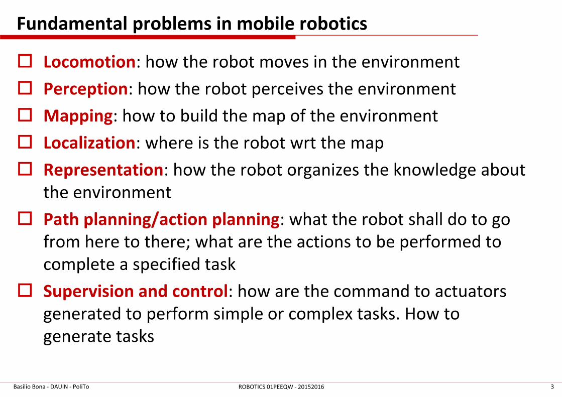
Fundamental problems in mobile robotics
� Locomotion: how the robot moves in the environment
� Perception: how the robot perceives the environment
� Mapping: how to build the map of the environment
� Localization: where is the robot wrt the map
� Representation: how the robot organizes the knowledge about
the environment
� Path planning/action planning: what the robot shall do to go
from here to there; what are the actions to be performed to
complete a specified task
� Supervision and control: how are the command to actuators
generated to perform simple or complex tasks. How to
generate tasks
3ROBOTICS 01PEEQW - 20152016Basilio Bona - DAUIN - PoliTo
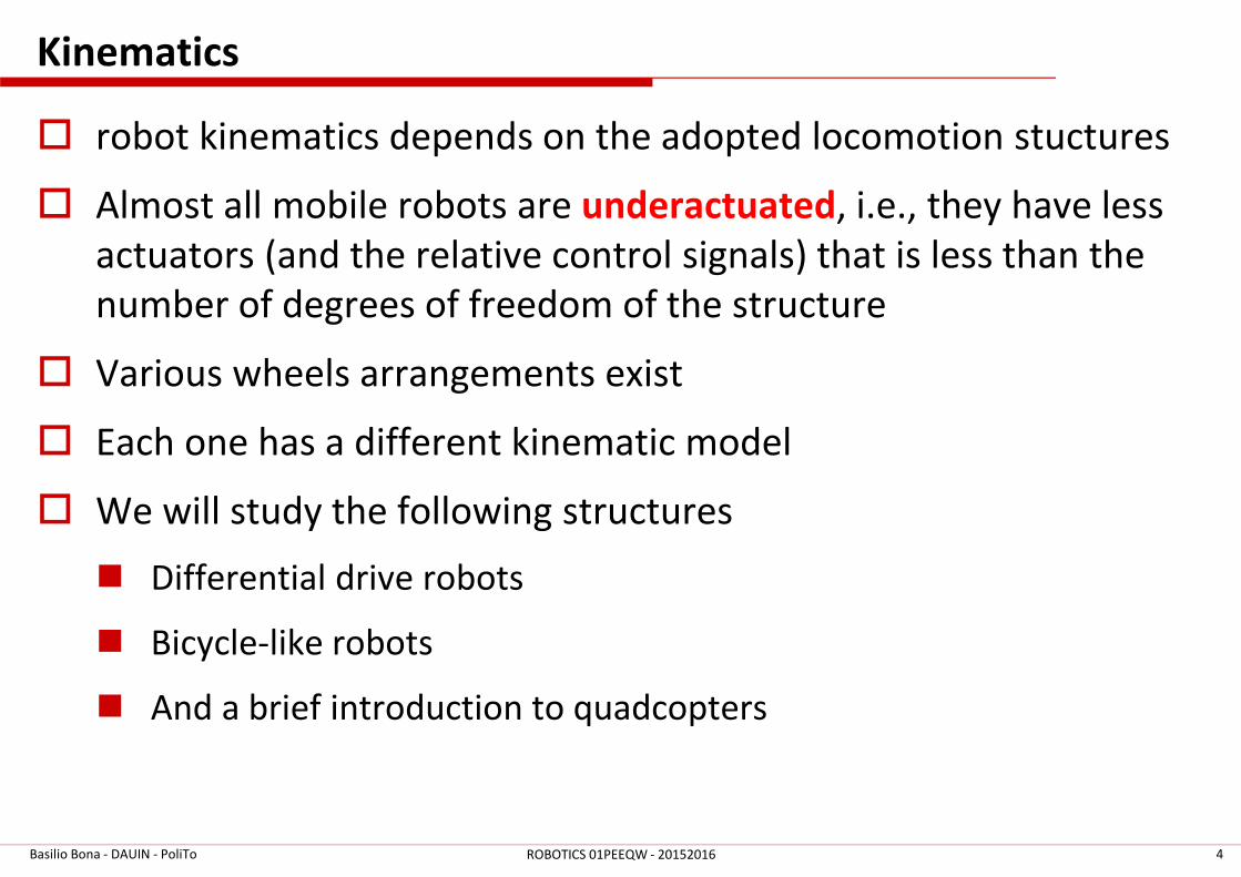
Kinematics
� robot kinematics depends on the adopted locomotion stuctures
� Almost all mobile robots are underactuated, i.e., they have less
actuators (and the relative control signals) that is less than the
number of degrees of freedom of the structure
� Various wheels arrangements exist
� Each one has a different kinematic model
� We will study the following structures
� Differential drive robots
� Bicycle-like robots
� And a brief introduction to quadcopters
Basilio Bona - DAUIN - PoliTo 4ROBOTICS 01PEEQW - 20152016
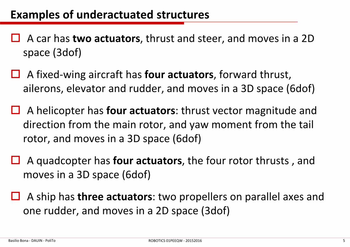
Examples of underactuated structures
� A car has two actuators, thrust and steer, and moves in a 2D
space (3dof)
� A fixed-wing aircraft has four actuators, forward thrust,
ailerons, elevator and rudder, and moves in a 3D space (6dof)
� A helicopter has four actuators: thrust vector magnitude and
direction from the main rotor, and yaw moment from the tail
rotor, and moves in a 3D space (6dof)
� A quadcopter has four actuators, the four rotor thrusts , and
moves in a 3D space (6dof)
� A ship has three actuators: two propellers on parallel axes and
one rudder, and moves in a 2D space (3dof)
Basilio Bona - DAUIN - PoliTo 5ROBOTICS 01PEEQW - 20152016
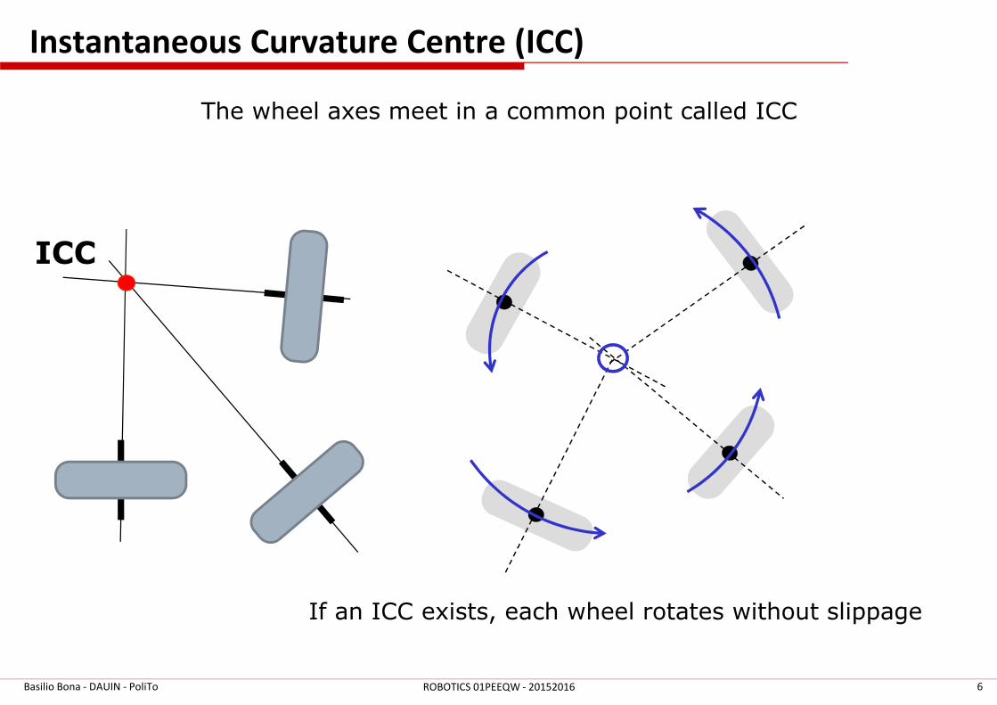
Instantaneous Curvature Centre (ICC)
Basilio Bona - DAUIN - PoliTo 6ROBOTICS 01PEEQW - 20152016
ICC
If an ICC exists, each wheel rotates without slippage
The wheel axes meet in a common point called ICC
ICC
Basilio Bona - DAUIN - PoliTo 7ROBOTICS 01PEEQW - 20152016
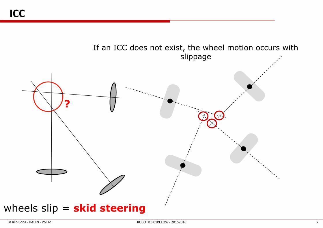
?
wheels slip = skid steering
If an ICC does not exist, the wheel motion occurs with slippage
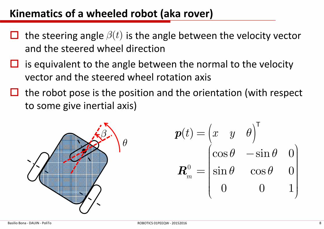
Kinematics of a wheeled robot (aka rover)
� the steering angle is the angle between the velocity vector
and the steered wheel direction
� is equivalent to the angle between the normal to the velocity
vector and the steered wheel rotation axis
� the robot pose is the position and the orientation (with respect
to some give inertial axis)
( )
0
( )
cos sin 0
sin cos 0
0 0 1m
t x y θ
θ θ
θ θ
= − =
p
R
T
( )tβ
Basilio Bona - DAUIN - PoliTo ROBOTICS 01PEEQW - 20152016 8
βθ
Kinematics
Basilio Bona - DAUIN - PoliTo 9ROBOTICS 01PEEQW - 20152016
d
mω
α
αδ
rϕ=v ɺ
Wω
mi
mj
Wi
Wj
0R
mR
x
y
WR
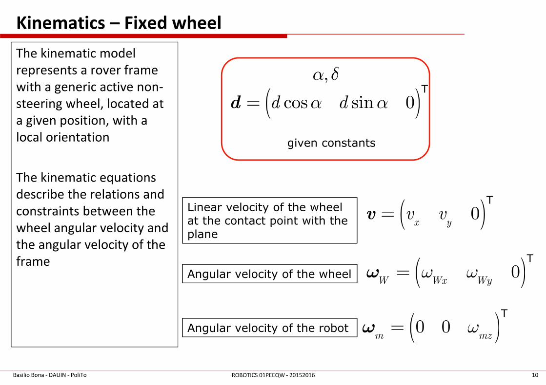
Kinematics – Fixed wheel
Basilio Bona - DAUIN - PoliTo 10ROBOTICS 01PEEQW - 20152016
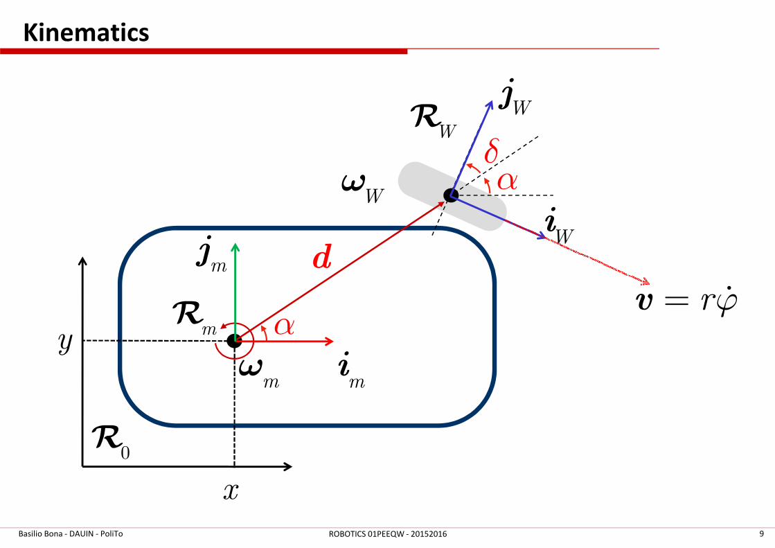
The kinematic model
represents a rover frame
with a generic active non-
steering wheel, located at
a given position, with a
local orientation
The kinematic equations
describe the relations and
constraints between the
wheel angular velocity and
the angular velocity of the
frame
( )0x yv v=v
T
( )0W Wx Wyω ω=ω
T
( )0 0m mz
ω=ω
T
Linear velocity of the wheel at the contact point with the plane
Angular velocity of the wheel
Angular velocity of the robot
,α δ
( )cos sin 0d dα α=dT
given constants
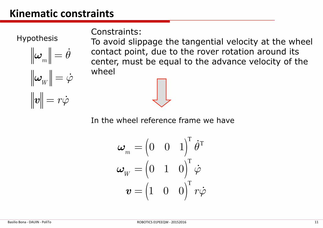
Kinematic constraints
Basilio Bona - DAUIN - PoliTo 11ROBOTICS 01PEEQW - 20152016
Hypothesis
m
W
r
θ
ϕ
ϕ
=
=
=v
ɺ
ɺ
ɺ
ω
ω
Constraints:To avoid slippage the tangential velocity at the wheel contact point, due to the rover rotation around its center, must be equal to the advance velocity of the wheel
In the wheel reference frame we have
( )( )( )
TT
T
T
0 0 1
0 1 0
1 0 0
m
W
r
θ
ϕ
ϕ
=
=
=v
ɺ
ɺ
ɺ
ω
ω
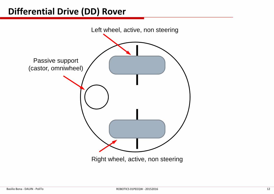
Differential Drive (DD) Rover
Basilio Bona - DAUIN - PoliTo 12ROBOTICS 01PEEQW - 20152016
Left wheel, active, non steering
Passive support(castor, omniwheel)
Right wheel, active, non steering
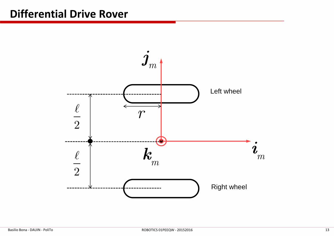
Differential Drive Rover
Basilio Bona - DAUIN - PoliTo 13ROBOTICS 01PEEQW - 20152016
mi
mj
mk
Left wheel
2
ℓ r
Right wheel
2
ℓ
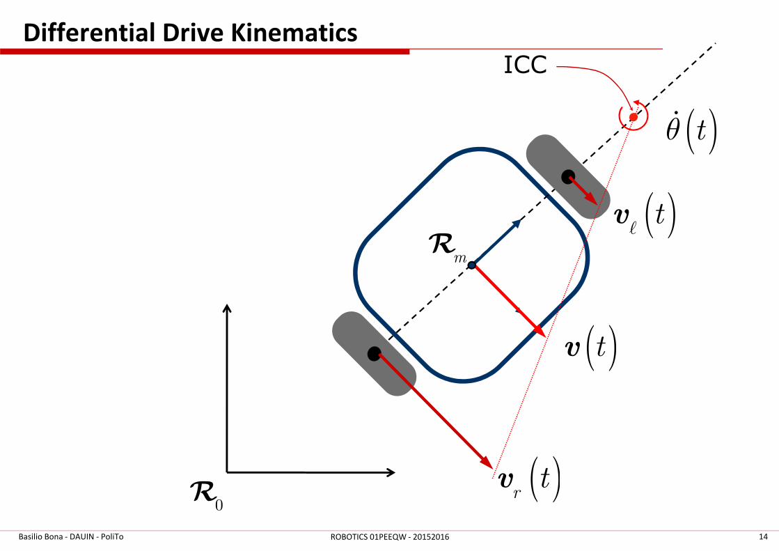
Differential Drive Kinematics
Basilio Bona - DAUIN - PoliTo 14ROBOTICS 01PEEQW - 20152016
( )tθɺ
( )tv
( )tvℓ
( )rtv
ICC
0R
mR
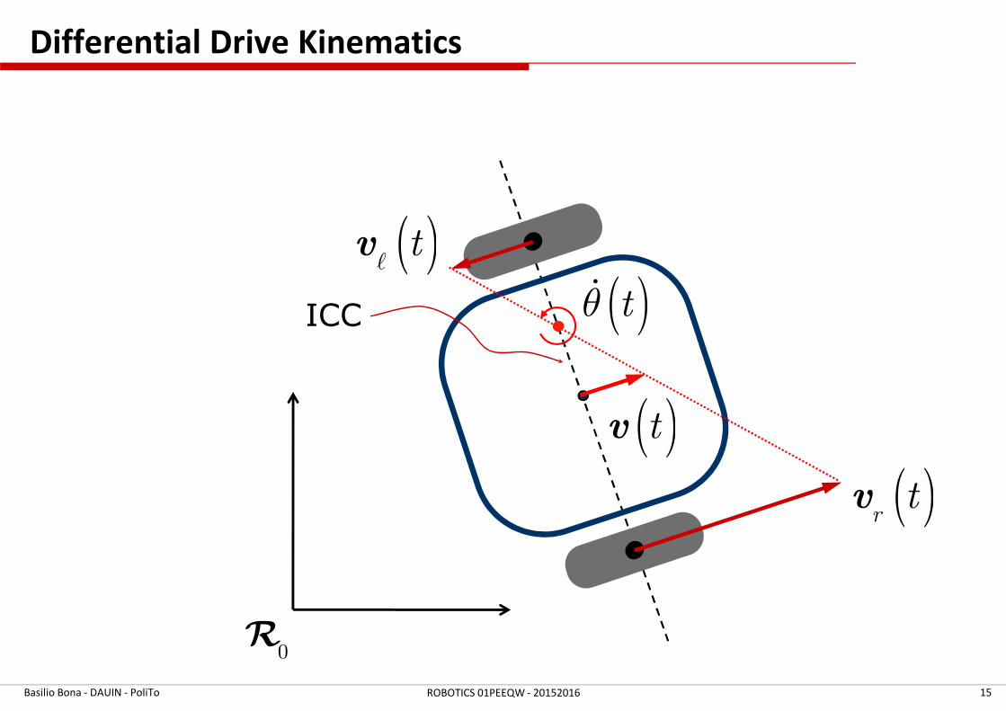
Differential Drive Kinematics
Basilio Bona - DAUIN - PoliTo 15ROBOTICS 01PEEQW - 20152016
( )tvℓ
( )rtv
( )tθɺ
( )tv
ICC
0R
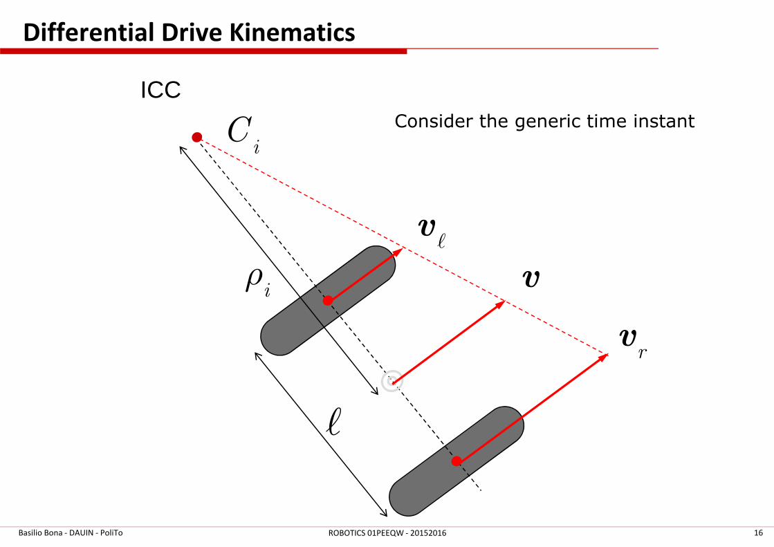
Differential Drive Kinematics
Basilio Bona - DAUIN - PoliTo 16ROBOTICS 01PEEQW - 20152016
vℓ
rv
v
ICC
iC
iρ
Consider the generic time instant
ℓ
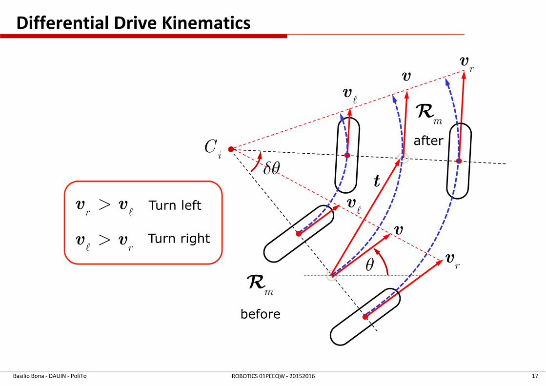
Differential Drive Kinematics
Basilio Bona - DAUIN - PoliTo 17ROBOTICS 01PEEQW - 20152016
mR
before
after
vℓ
rv
v
vℓ
rv
v
iC
r>v v
ℓ
r>v v
ℓ
Turn left
Turn right
mR
tδθ
θ
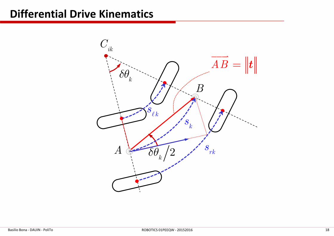
Differential Drive Kinematics
Basilio Bona - DAUIN - PoliTo 18ROBOTICS 01PEEQW - 20152016
ks
A
B
AB = t����
2kδθ
ikC
kδθ
rks
ksℓ
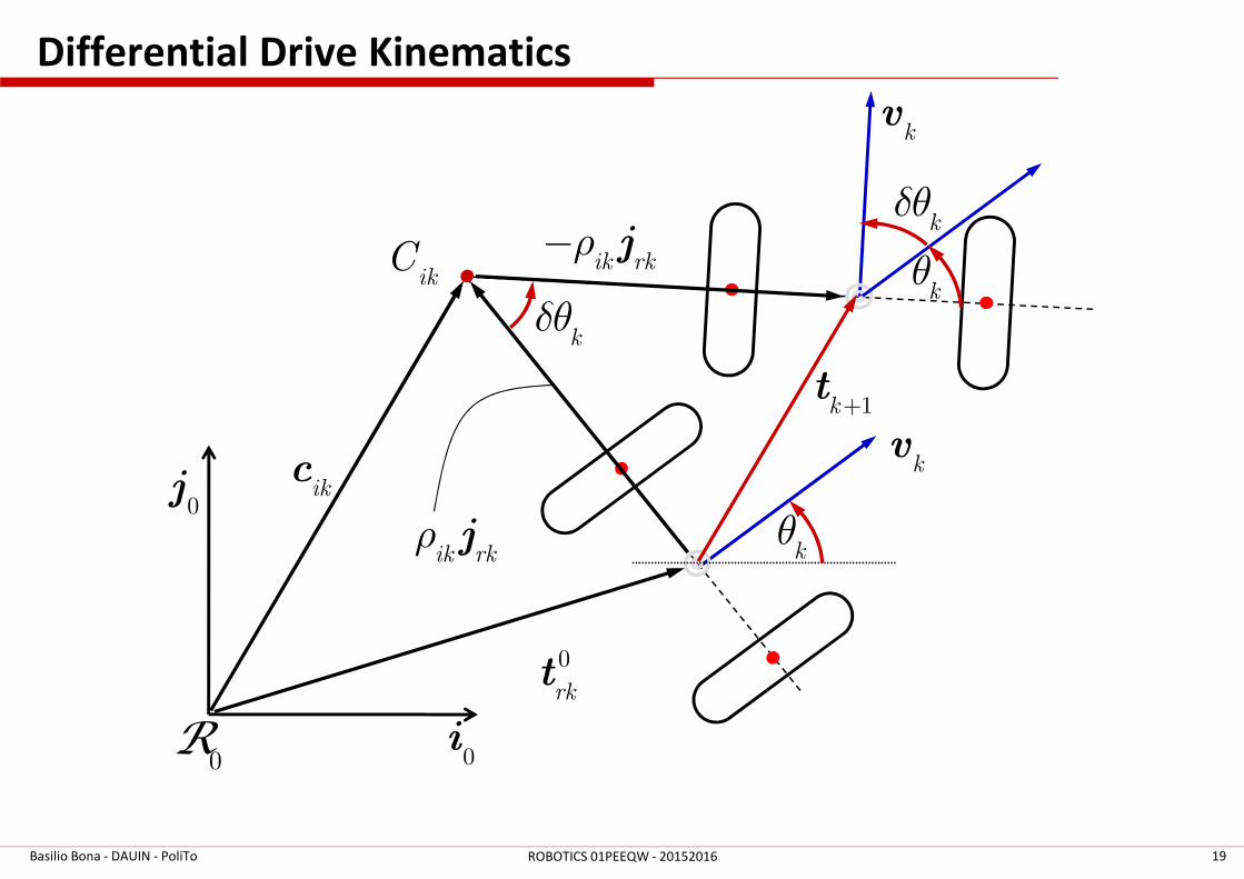
Differential Drive Kinematics
Basilio Bona - DAUIN - PoliTo 19ROBOTICS 01PEEQW - 20152016
ikC
1k+t
kθ
kδθ
0i
0j
0
rkt
ikc
ik rkρ− j
ik rkρ j
0R
kθ
kδθ
kv
kv

Differential Drive Kinematics
Basilio Bona - DAUIN - PoliTo 20ROBOTICS 01PEEQW - 20152016
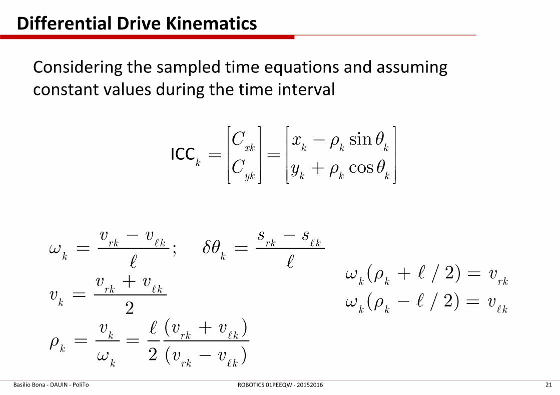
Differential Drive Kinematics
Considering the sampled time equations and assuming
constant values during the time interval
Basilio Bona - DAUIN - PoliTo 21ROBOTICS 01PEEQW - 20152016
( / 2)
( / 2)k k rk
k k k
v
v
ω ρ
ω ρ
+ =
− =ℓ
ℓ
ℓ
ICCsin
cosxk k k k
k
yk k k k
C x
C y
ρ θ
ρ θ
− = = +
;
2( )
2 ( )
rk k rk k
k k
rk k
k
k rk k
k
k rk k
v v s s
v vv
v v v
v v
ω δθ
ρω
− −= =
+=
+= =
−
ℓ ℓ
ℓ
ℓ
ℓ
ℓ ℓ
ℓ
Differential Drive Kinematics
Basilio Bona - DAUIN - PoliTo 22ROBOTICS 01PEEQW - 20152016
1
d
dk k k k kT
tω θ ω θ θ δθ+= ⇒ −≃ ≐
1
1
1
cos( ) sin( ) 0
sin( ) cos( ) 0
0 0 1
k k k k xk xk
k k k k yk yk
k k k
x x C C
y y C C
δθ δθ
δθ δθ
θ θ δθ
+
+
+
− − = − +
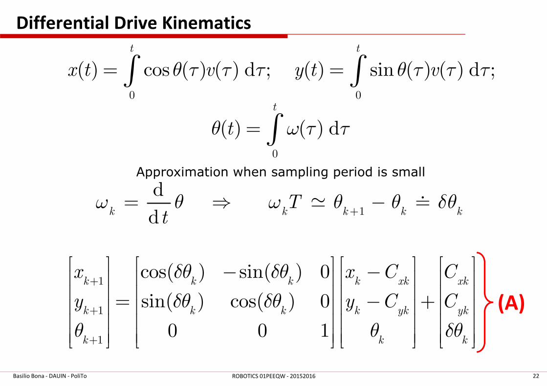
Approximation when sampling period is small
0 0
0
( ) cos ( ) ( ) d ; ( ) sin ( ) ( ) d ;
( ) ( ) d
t t
t
x t v y t v
t
θ τ τ τ θ τ τ τ
θ ω τ τ
= =
=
∫ ∫
∫
(A)

Differential Drive Kinematics
Basilio Bona - DAUIN - PoliTo 23ROBOTICS 01PEEQW - 20152016
1
1
1
cos
sink k k k
k k k k
k k k
x x v T
y y v T
T
θ
θ
θ θ ω
+
+
+
= += +
= +
EULER APPROXIMATION

Differential Drive Kinematics
Basilio Bona - DAUIN - PoliTo 24ROBOTICS 01PEEQW - 20152016
1
1
1
1cos
2
1sin
2
k k k k k
k k k k k
k k k
x x v T T
y y v T T
T
θ ω
θ ω
θ θ ω
+
+
+
= + + = + +
= +
RUNGE-KUTTA APPROXIMATION
Differential Drive Kinematics
Basilio Bona - DAUIN - PoliTo 25ROBOTICS 01PEEQW - 20152016
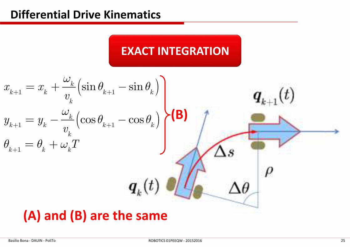
EXACT INTEGRATION
( )
( )
1 1
1 1
1
sin sin
cos cos
k
k k k k
k
k
k k k k
k
k k k
x xv
y yv
T
ωθ θ
ωθ θ
θ θ ω
+ +
+ +
+
= + −
= − −
= +
(B)
(A) and (B) are the same
Differential Drive Kinematics
Basilio Bona - DAUIN - PoliTo 26ROBOTICS 01PEEQW - 20152016
Path Planning
Basilio Bona - DAUIN - PoliTo 27ROBOTICS 01PEEQW - 20152016
Path Planning
Basilio Bona - DAUIN - PoliTo 28ROBOTICS 01PEEQW - 20152016
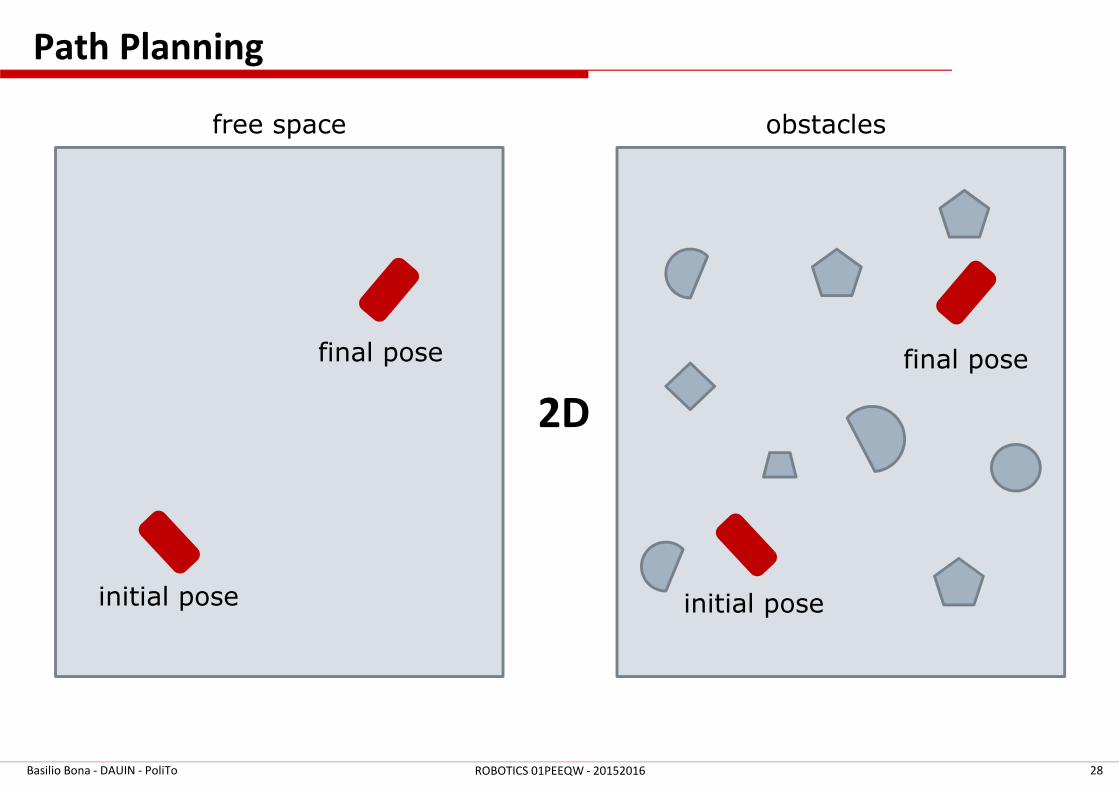
initial pose
final pose
initial pose
final pose
obstaclesfree space
2D
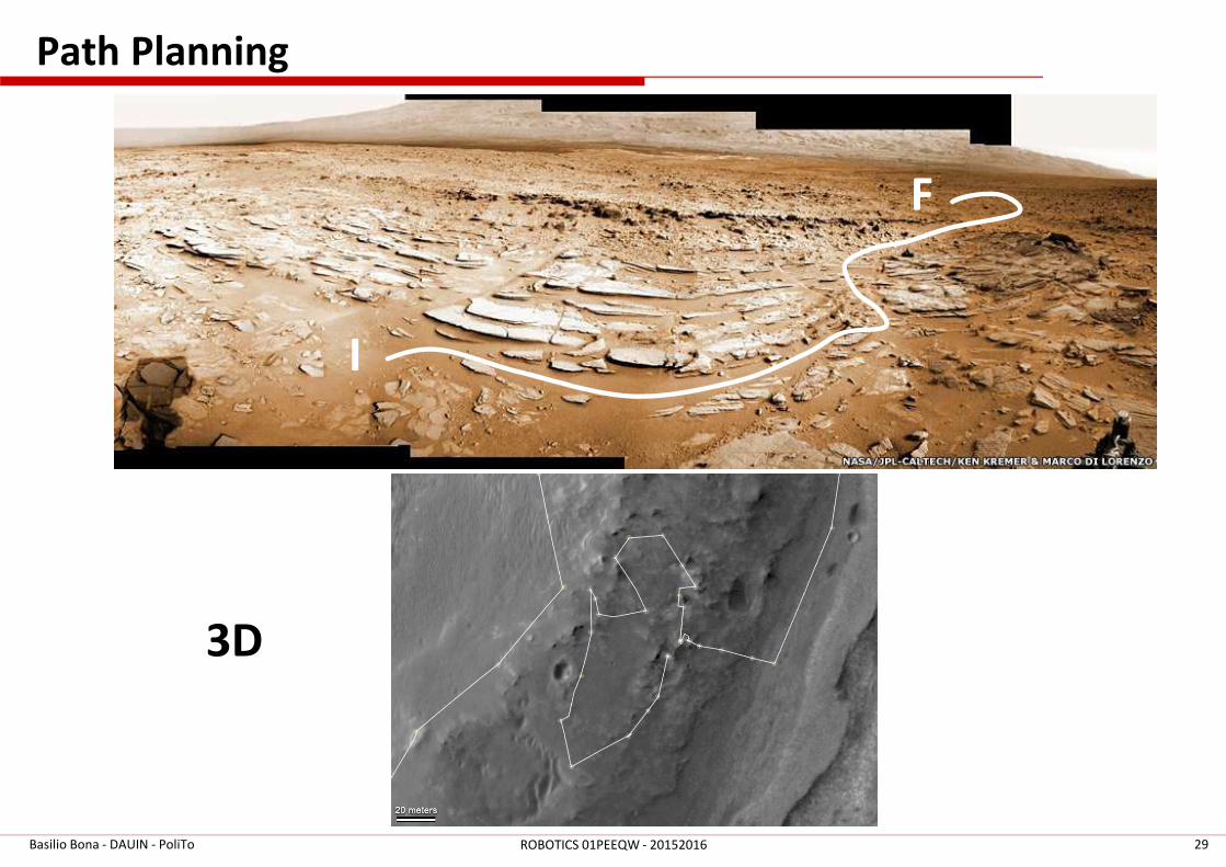
Path Planning
Basilio Bona - DAUIN - PoliTo 29ROBOTICS 01PEEQW - 20152016
3D
F
I
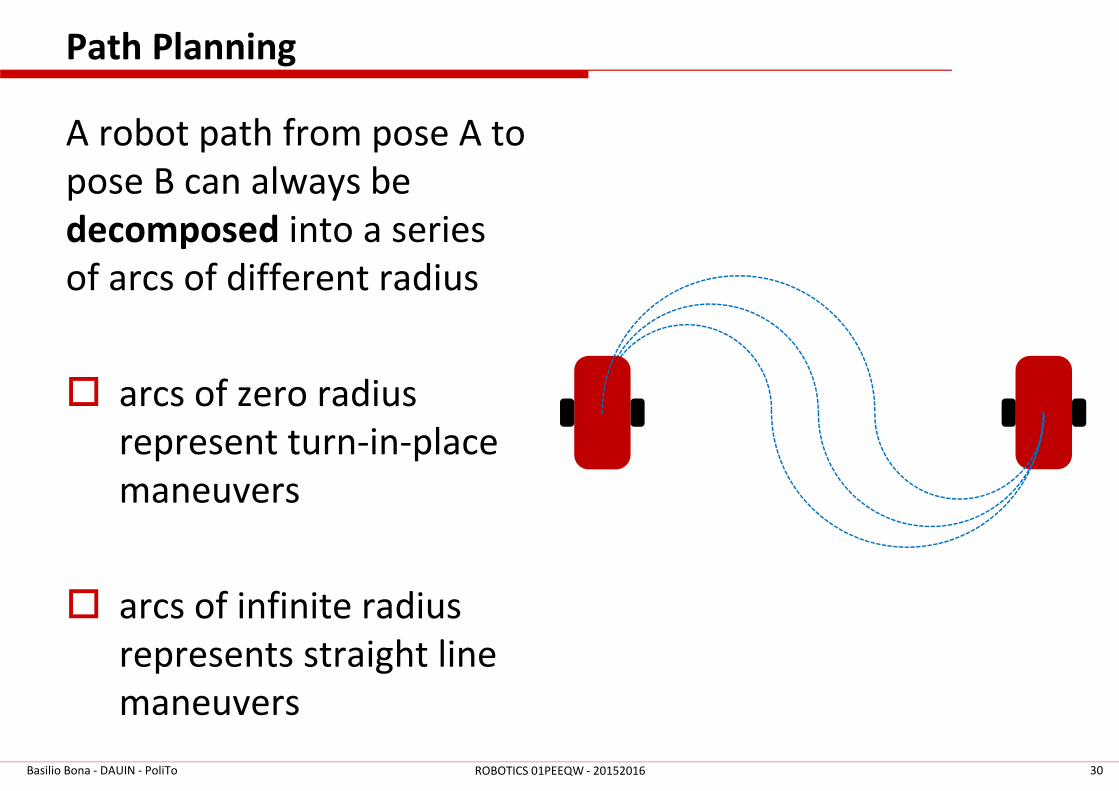
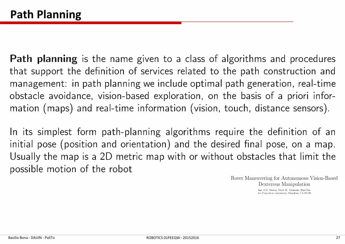
Path Planning
A robot path from pose A to
pose B can always be
decomposed into a series
of arcs of different radius
� arcs of zero radius
represent turn-in-place
maneuvers
� arcs of infinite radius
represents straight line
maneuvers
Basilio Bona - DAUIN - PoliTo 30ROBOTICS 01PEEQW - 20152016
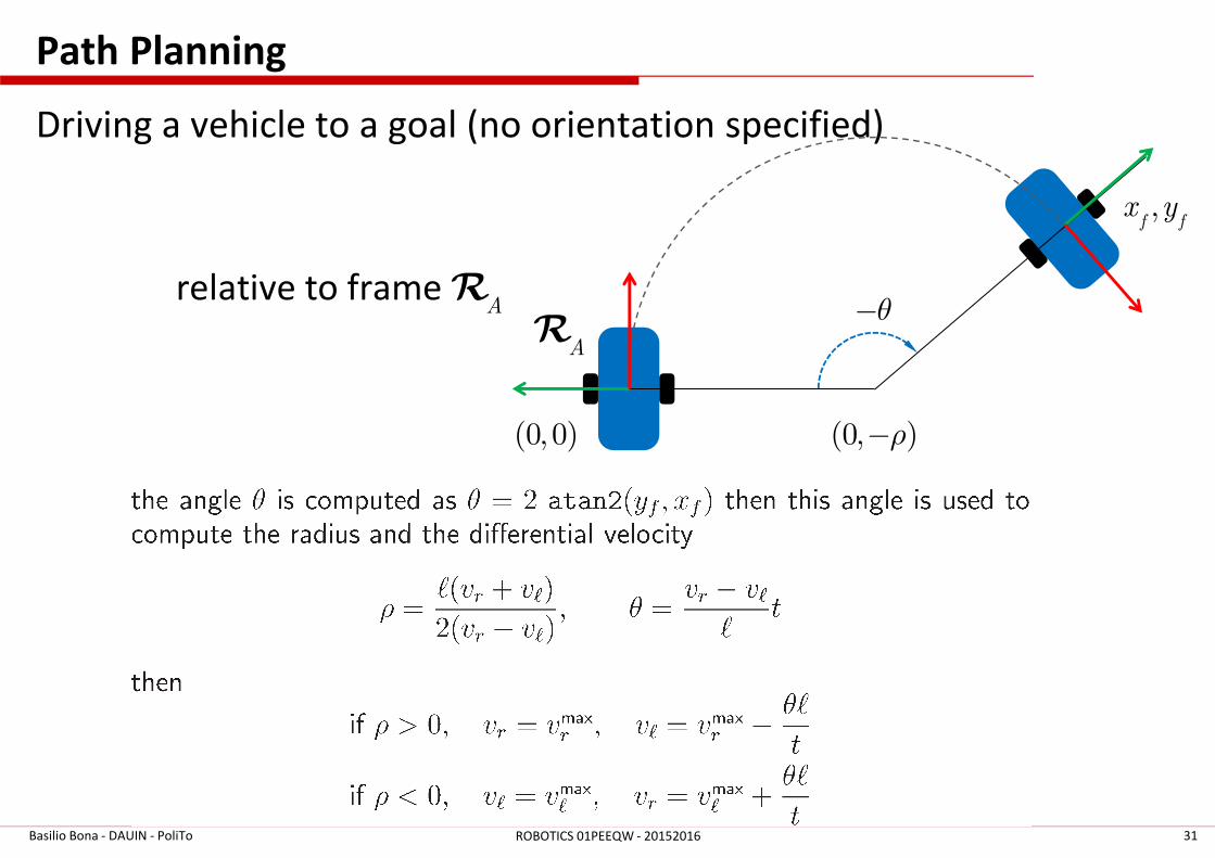
Path Planning
Driving a vehicle to a goal (no orientation specified)
Basilio Bona - DAUIN - PoliTo 31ROBOTICS 01PEEQW - 20152016
θ−
(0, 0)
,f fx y
(0, )ρ−
AR
Arelative to frame R
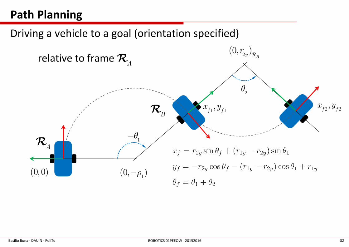
Path Planning
Driving a vehicle to a goal (orientation specified)
Basilio Bona - DAUIN - PoliTo 32ROBOTICS 01PEEQW - 20152016
1θ−
(0, 0)
1 1,
f fx y
1(0, )ρ−
AR
2θ
2(0, )
yr
BR
2 2,
f fx y
Arelative to frame R
BR
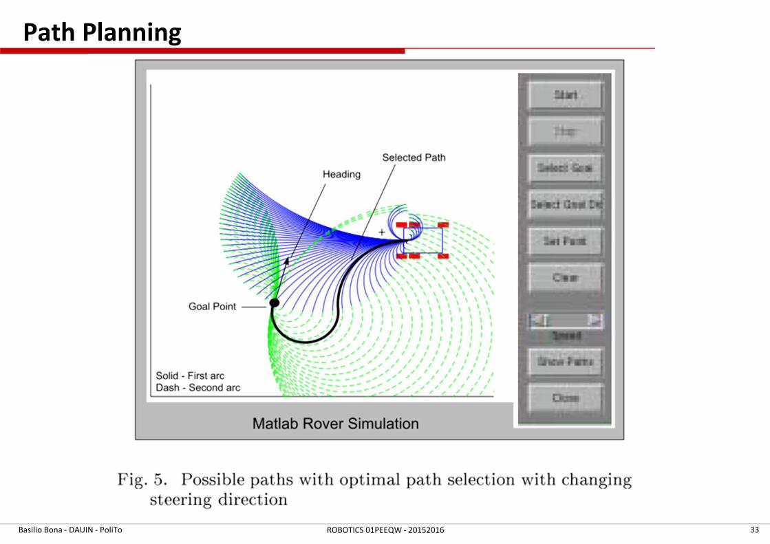
Path Planning
Basilio Bona - DAUIN - PoliTo 33ROBOTICS 01PEEQW - 20152016
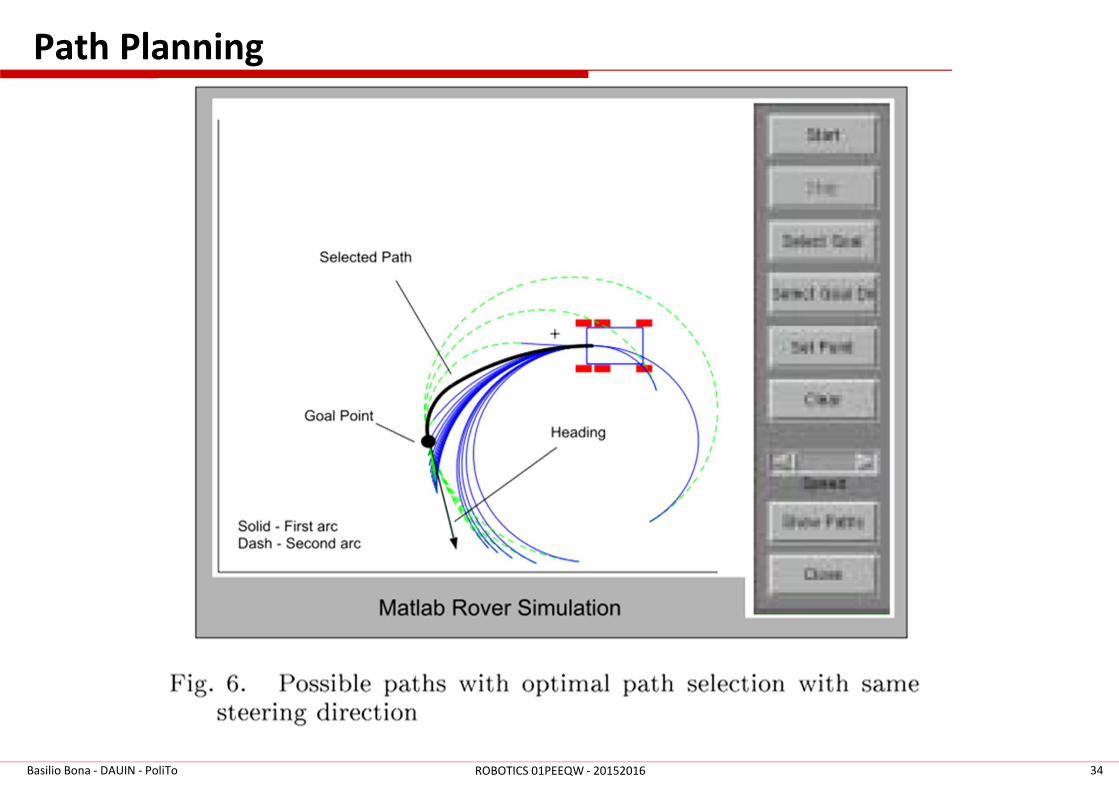
Path Planning
Basilio Bona - DAUIN - PoliTo 34ROBOTICS 01PEEQW - 20152016
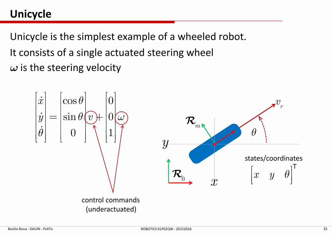
Unicycle
Unicycle is the simplest example of a wheeled robot.
It consists of a single actuated steering wheel
ω is the steering velocity
Basilio Bona - DAUIN - PoliTo 35ROBOTICS 01PEEQW - 20152016
mR
0R
x
yθ
rvcos 0
sin 0
0 1
x
y v
θ
θ ω
θ
= +
ɺ
ɺ
ɺ
control commands
(underactuated)
x y θ
T
states/coordinates
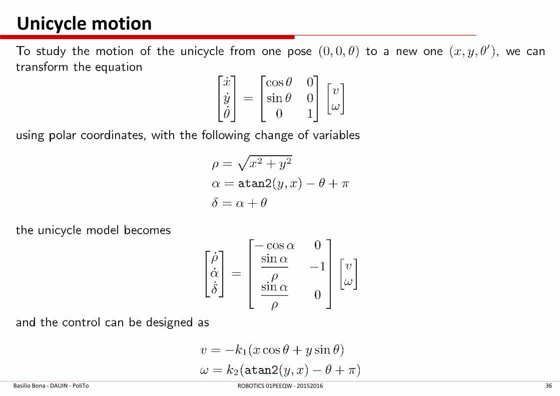
Unicycle motion
Basilio Bona - DAUIN - PoliTo 36ROBOTICS 01PEEQW - 20152016
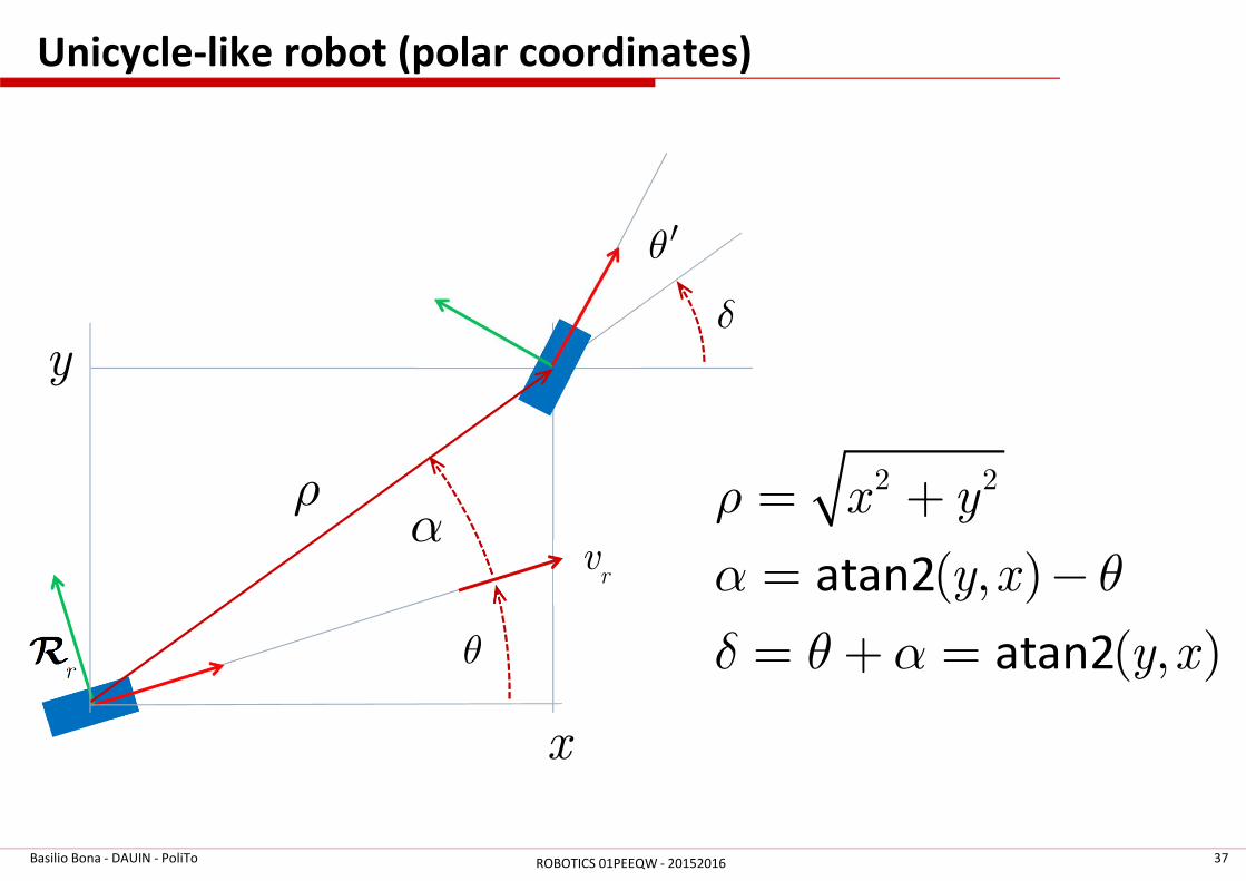
Unicycle-like robot (polar coordinates)
Basilio Bona - DAUIN - PoliTo 37ROBOTICS 01PEEQW - 20152016
x
θ
δ
rR
rv
ρα
y
2 2
( , )
( , )
x y
y x
y x
ρ
α θ
δ θ α
= +
= −
= + =
atan2
atan2
θ′
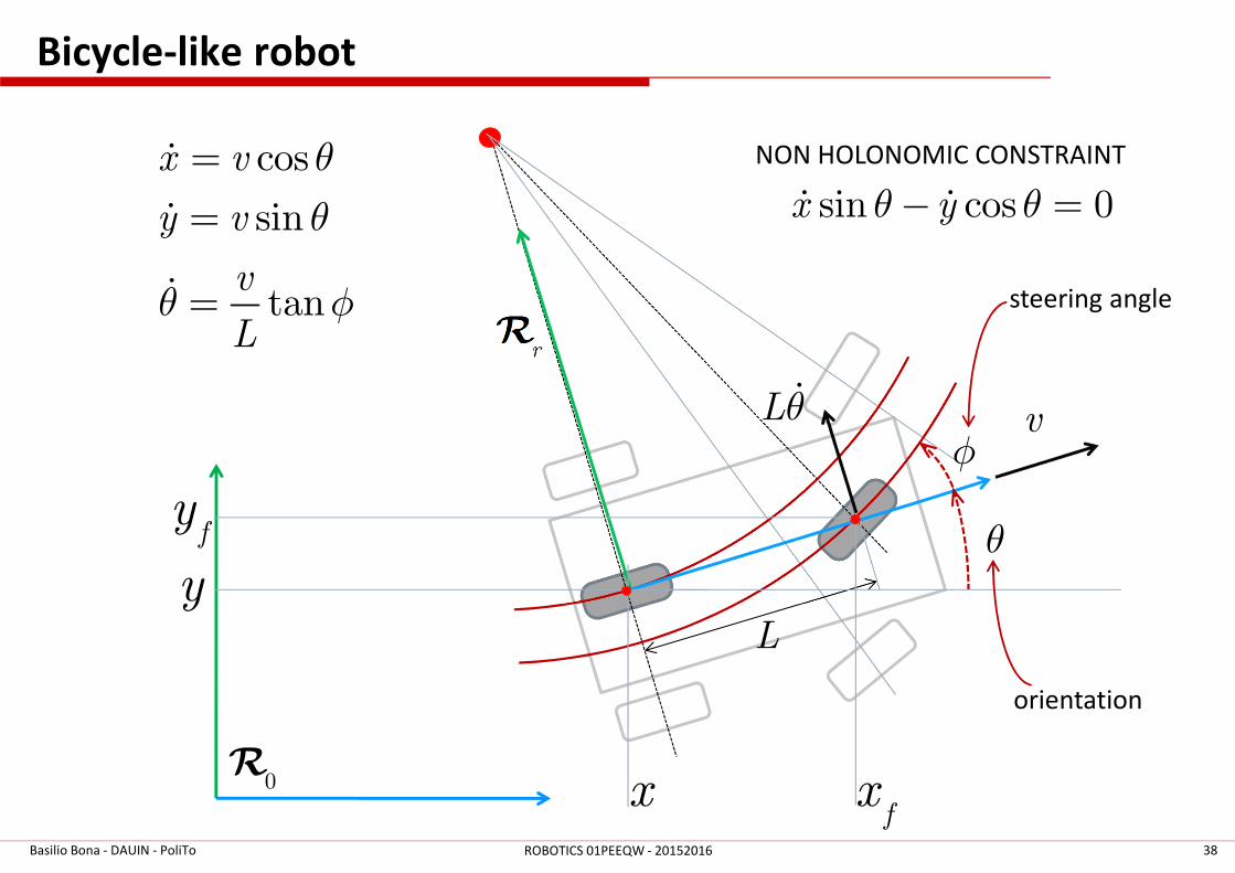
Bicycle-like robot
Basilio Bona - DAUIN - PoliTo 38ROBOTICS 01PEEQW - 20152016
x
y
rR
0R
θ
L
φv
cos
sin
tan
x v
y v
v
L
θ
θ
θ φ
=
=
=
ɺ
ɺ
ɺ
NON HOLONOMIC CONSTRAINT
sin cos 0x yθ θ− =ɺ ɺ
Lθɺ
fy
fx
steering angle
orientation
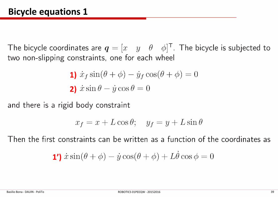
Bicycle equations 1
Basilio Bona - DAUIN - PoliTo 39ROBOTICS 01PEEQW - 20152016
1’)
2)
1)
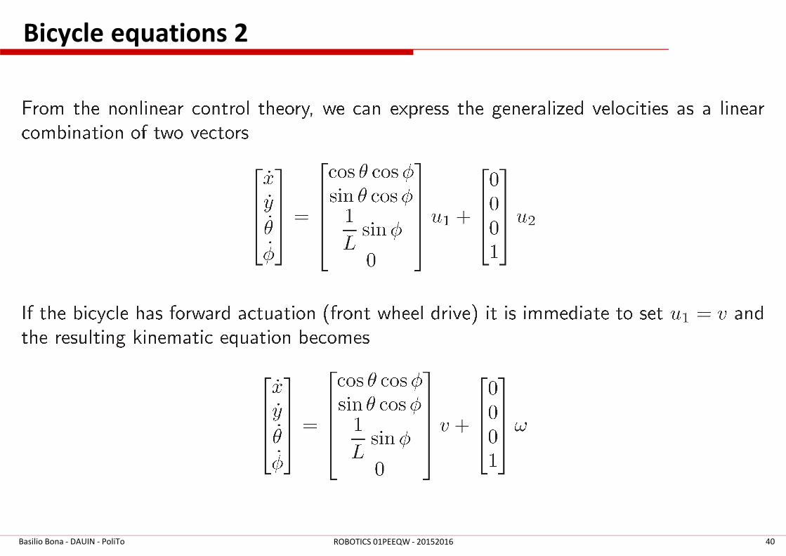
Bicycle equations 2
Basilio Bona - DAUIN - PoliTo 40ROBOTICS 01PEEQW - 20152016
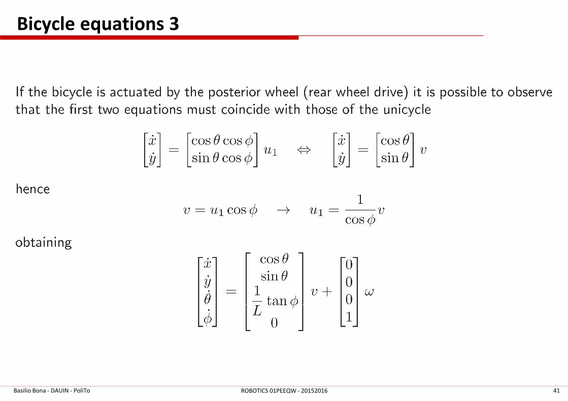
Bicycle equations 3
Basilio Bona - DAUIN - PoliTo 41ROBOTICS 01PEEQW - 20152016

Bicycle equations 5
Basilio Bona - DAUIN - PoliTo 42ROBOTICS 01PEEQW - 20152016
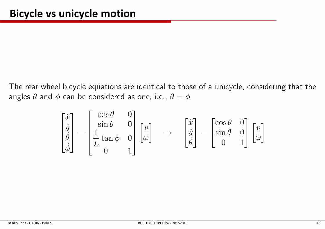
Bicycle vs unicycle motion
Basilio Bona - DAUIN - PoliTo 43ROBOTICS 01PEEQW - 20152016
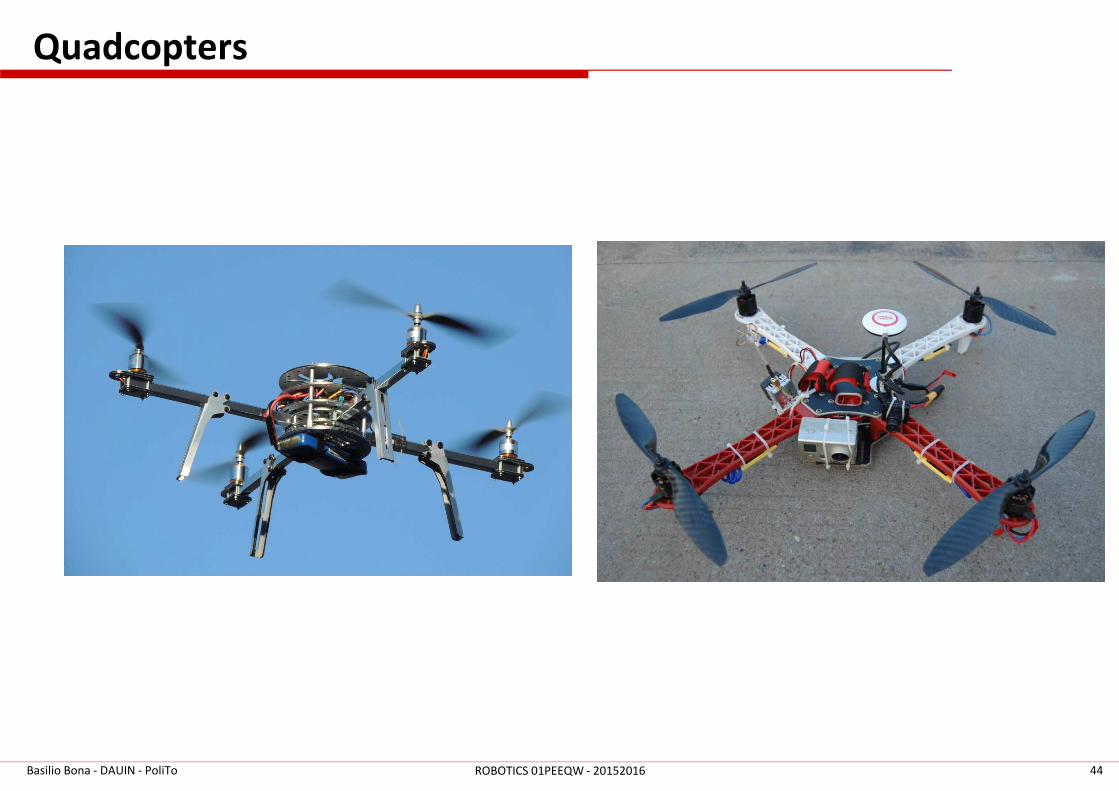
Quadcopters
Basilio Bona - DAUIN - PoliTo 44ROBOTICS 01PEEQW - 20152016
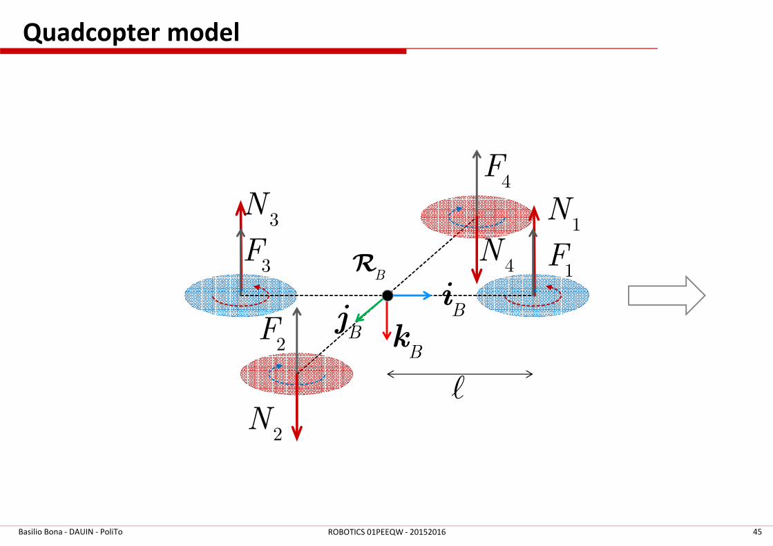
Quadcopter model
Basilio Bona - DAUIN - PoliTo 45ROBOTICS 01PEEQW - 20152016
ℓ
4F
BR
3N
Bk
Bi
Bj
4N
2F
2N
3F
1N
1F
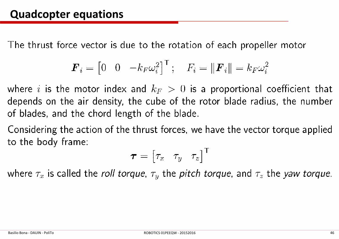
Quadcopter equations
Basilio Bona - DAUIN - PoliTo 46ROBOTICS 01PEEQW - 20152016
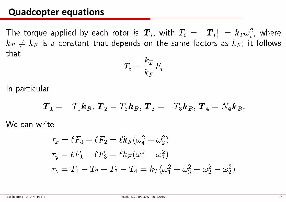
Quadcopter equations
Basilio Bona - DAUIN - PoliTo 47ROBOTICS 01PEEQW - 20152016
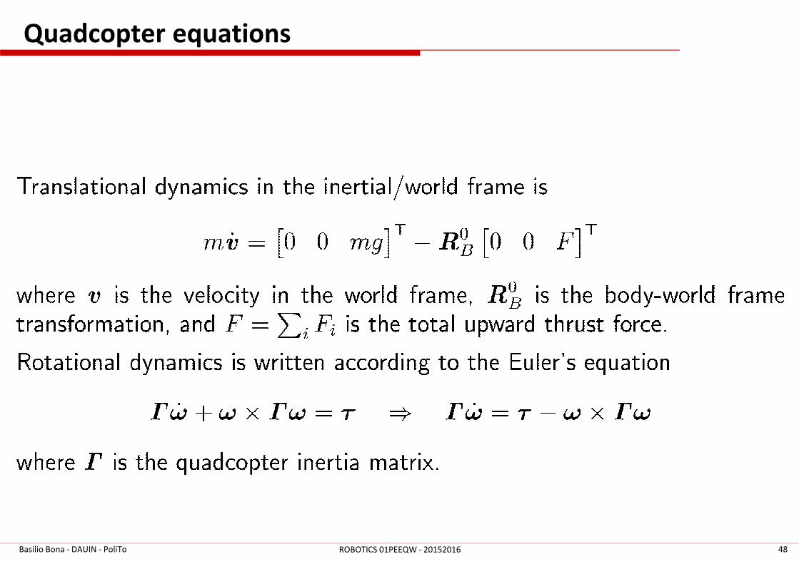
Quadcopter equations
Basilio Bona - DAUIN - PoliTo 48ROBOTICS 01PEEQW - 20152016
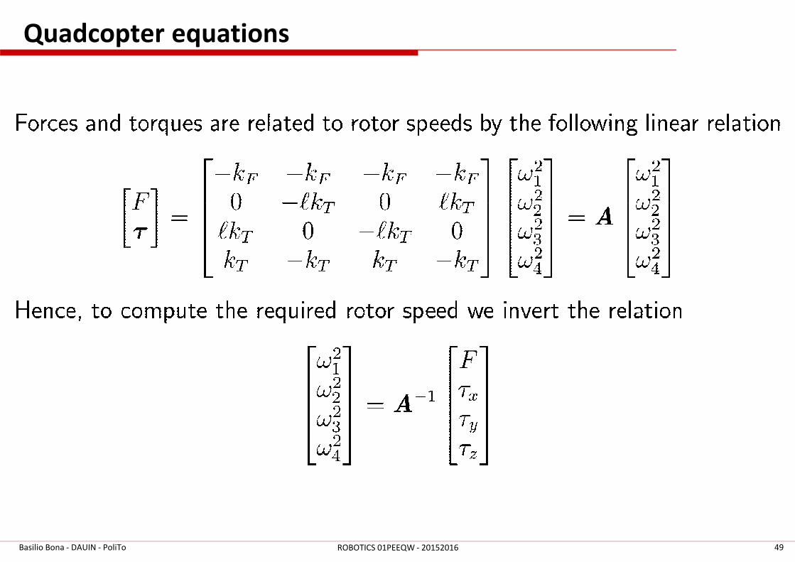
Quadcopter equations
Basilio Bona - DAUIN - PoliTo 49ROBOTICS 01PEEQW - 20152016
Odometry
Odometry is the estimation of the successive robot poses based on
the wheel motion. Wheel angles are measured and used for
pose computation
Odometric errors increase with the distance covered, and are due to
many causes, e.g.
� Imperfect knowledge of the wheels geometry
� Unknown contact points: in the ideal DD robot there are two
geometric contact points between wheels and ground. In real
robots the wheels are several centimeters wide and the actual
contact points are undefined
� Slippage of the wheel wrt the terrain
Errors can be compensated sensing the environment around the
robot and comparing it with known data (maps, etc.)
Basilio Bona - DAUIN - PoliTo 50ROBOTICS 01PEEQW - 20152016
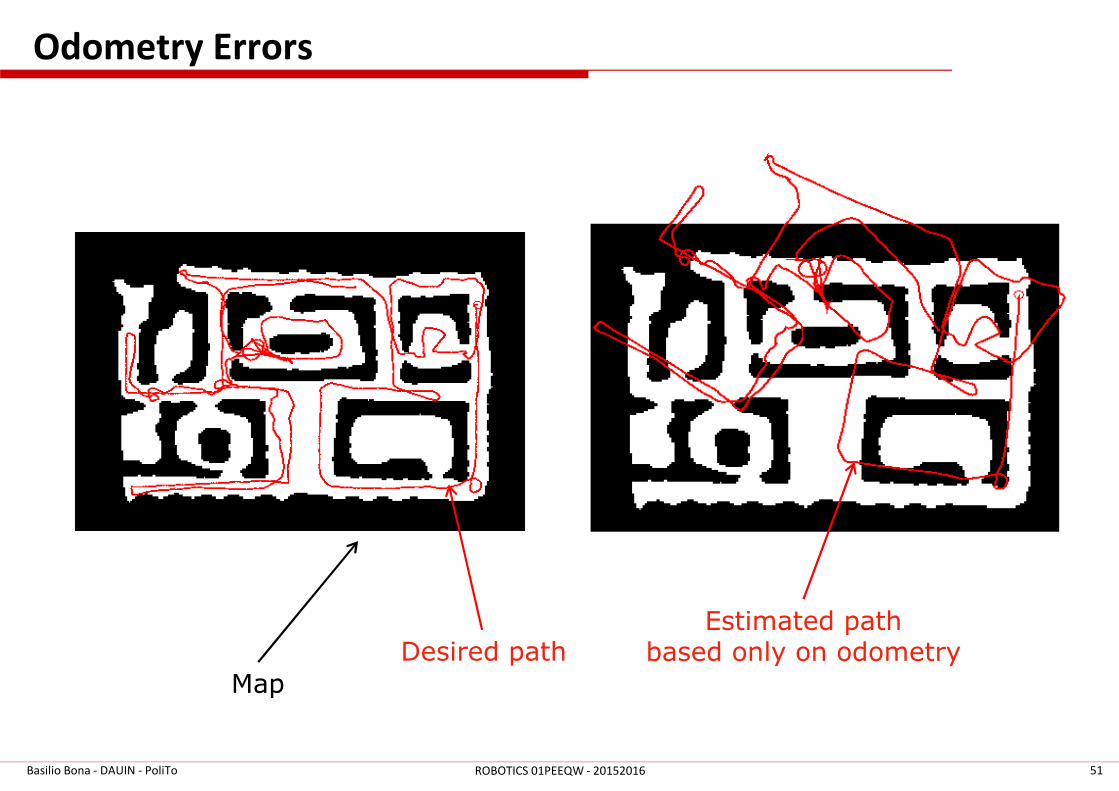
Odometry Errors
Basilio Bona - DAUIN - PoliTo 51ROBOTICS 01PEEQW - 20152016
Map
Desired pathEstimated path
based only on odometry
Visual odometry
Visual odometry is the estimation of the robot poses based only on
the acquisition of successive images of the environment
Stereo visual odometry uses two cameras to estimate the ego-
motion of a camera by tracking features in a video sequence.
If the camera system is calibrated then the full 3D Euclidean
geometry can be reconstructed
Using a single camera, the reconstruction is up to an unknown scale
factor
A RGB-D (Kinect or similar) camera can be used
Basilio Bona - DAUIN - PoliTo 52ROBOTICS 01PEEQW - 20152016
Other important problems that must be addressed
Basilio Bona - DAUIN - PoliTo 53ROBOTICS 01PEEQW - 20152016
1. Mapping: how to build environment maps (geometrical vs
semantic maps)
2. Localization: where am I in the map?
3. Simultaneous Localization and Mapping (SLAM): build a map
and at the same time localize the robot in the map while
moving
4. Path planning: the definition of an “optimal” geometric path
in the environment from A to B, and avoid obstacles
Path Planning – A map is given
� Path planning algorithm: it computes which route to take, from
the initial to the final pose, based on the current internal
representation of the terrain possibly considering a “cost
function” (minimum time, minimum energy, maximum comfort,
etc.)
� Complete path generation: the path is created as a sequence of
successive moves from the initial pose to the final one
� Motion planning: is the execution of the above defined
theoretical route; it translates the plan from the internal
representation to the physical movement of the wheels
� Next move selection: at each step, the algorithm must decide
which way to move next. An efficient dynamic implementation
is required
Basilio Bona - DAUIN - PoliTo 54ROBOTICS 01PEEQW - 20152016
Path Planning
Basilio Bona - DAUIN - PoliTo 55ROBOTICS 01PEEQW - 20152016
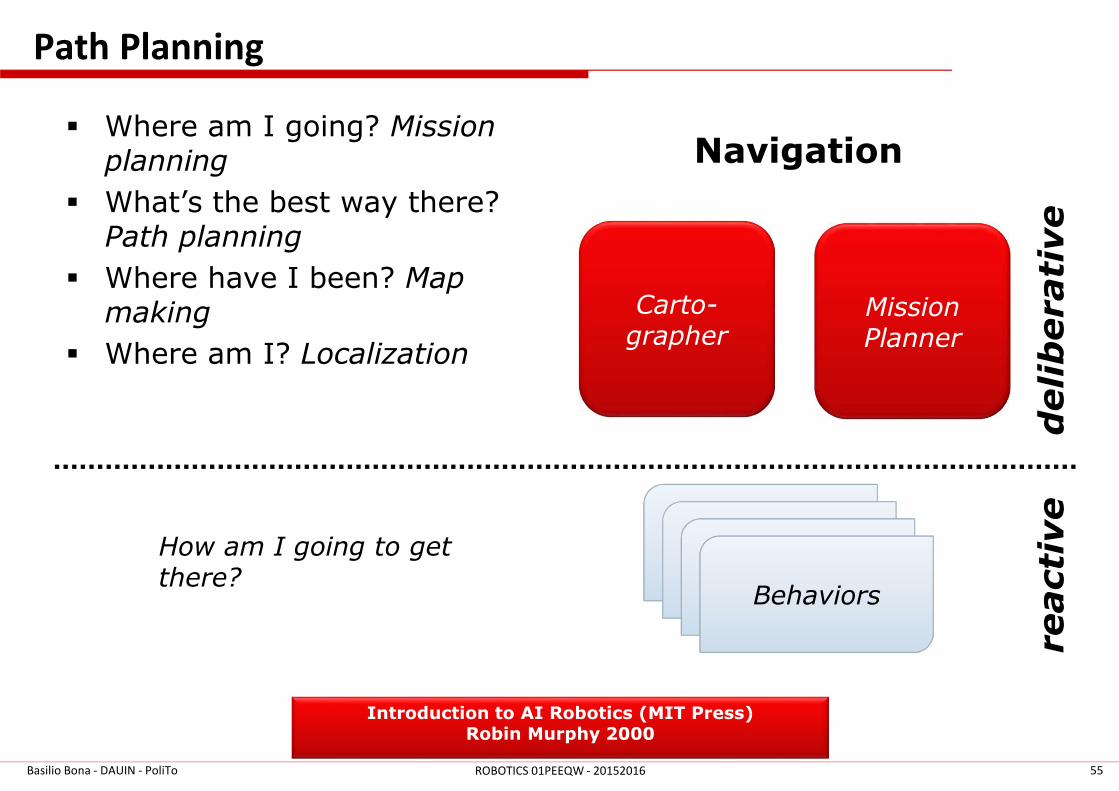
Introduction to AI Robotics (MIT Press) Robin Murphy 2000
Navigation� Where am I going? Mission
planning
� What’s the best way there? Path planning
� Where have I been? Map making
� Where am I? Localization
MissionPlanner
Carto-grapher
BehaviorsBehaviors
BehaviorsBehaviors
deliberative
reactive
How am I going to getthere?
Path Planning
Basilio Bona - DAUIN - PoliTo 56ROBOTICS 01PEEQW - 20152016
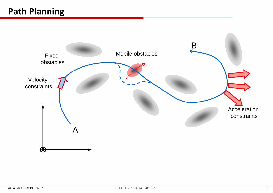
A
BFixed
obstacles
Mobile obstacles
Acceleration constraints
Velocity constraints
Path Planning
Basilio Bona - DAUIN - PoliTo 57ROBOTICS 01PEEQW - 20152016
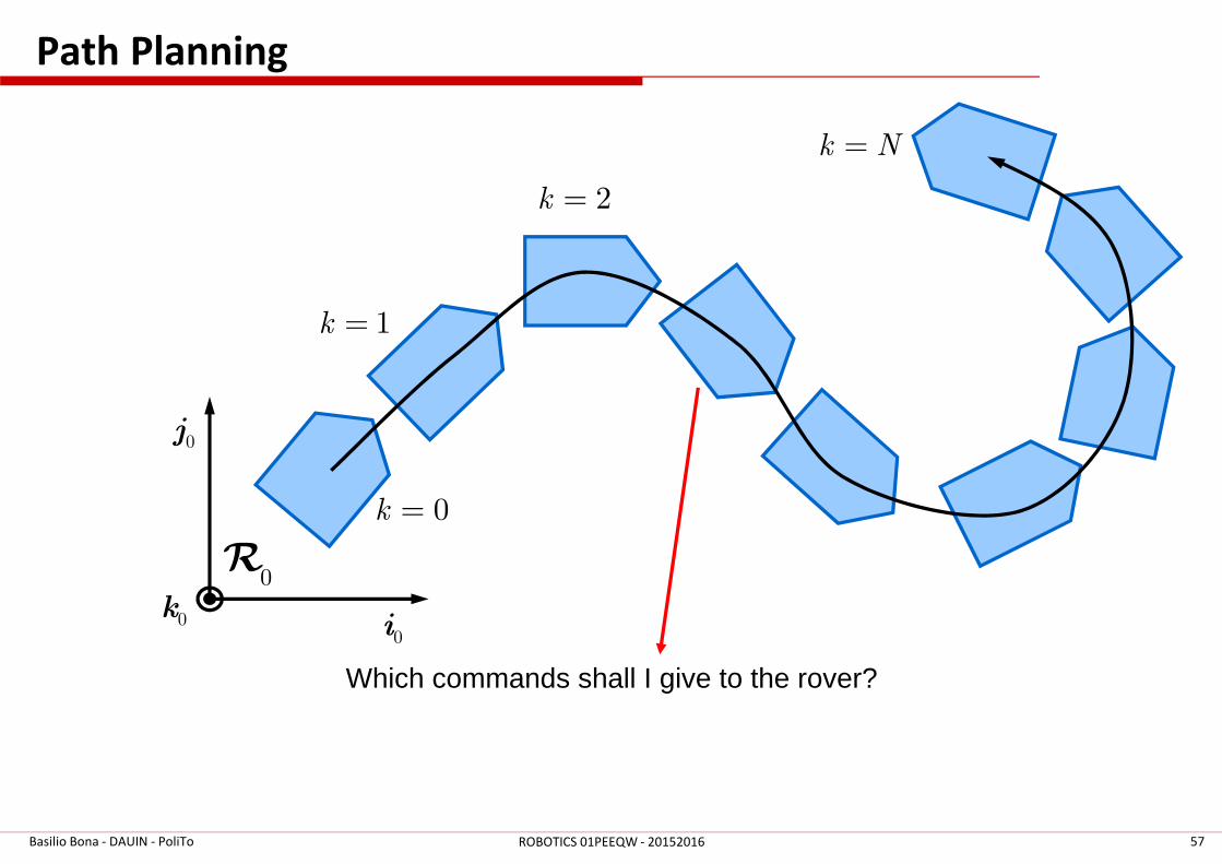
0i
0j
0k
0k =
1k =
2k =
k N=
Which commands shall I give to the rover?
0R
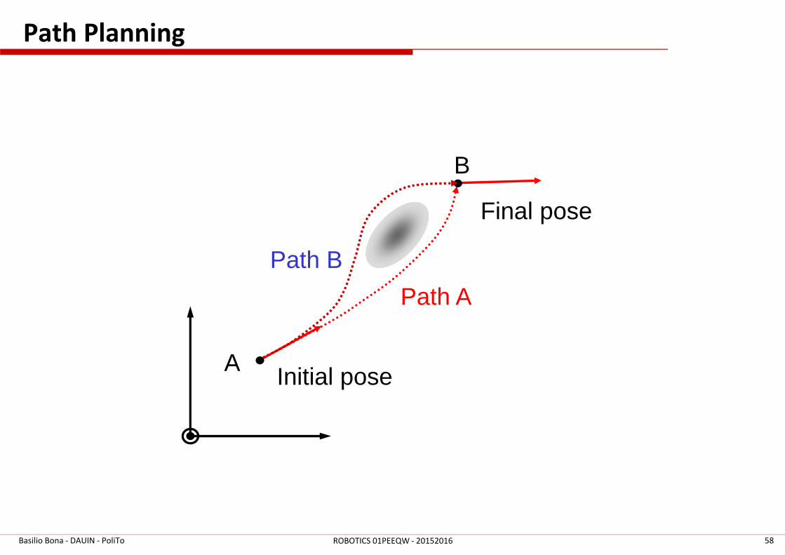
Path Planning
Basilio Bona - DAUIN - PoliTo 58ROBOTICS 01PEEQW - 20152016
Initial pose
Final pose
Path A
Path B
A
B

Motion Planning
Basilio Bona - DAUIN - PoliTo 59ROBOTICS 01PEEQW - 20152016
Initial pose
Final pose
Move 1: rotation
Move 3:rotation
A
B
Move 2: go straight
Non-holonomic constraints
Basilio Bona - DAUIN - PoliTo 60ROBOTICS 01PEEQW - 20152016
� Non-holonomic constraints limit the possible incremental
movements in the configuration space of the robot
� Robots with differential drive move on a circular trajectory and
cannot move sideways
� Omni-wheel robots can move sideways
Holonomic vs. Non-Holonomic
� Non-holonomic constraints reduce the control space with respect
to the current configuration (e.g., moving sideways is impossible)
� Holonomic constraints reduce the configuration space
Basilio Bona - DAUIN - PoliTo ROBOTICS 01PEEQW - 20152016 61
62ROBOTICS 01PEEQW - 20152016
Academic year 2010/11 by Prof. Alessandro De Luca
Basilio Bona - DAUIN - PoliTo
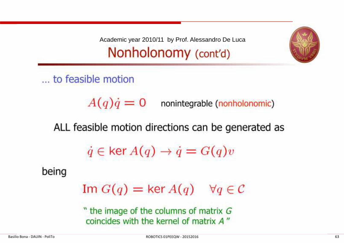
63ROBOTICS 01PEEQW - 20152016
Academic year 2010/11 by Prof. Alessandro De Luca
Basilio Bona - DAUIN - PoliTo

64ROBOTICS 01PEEQW - 20152016
Academic year 2010/11 by Prof. Alessandro De Luca
Basilio Bona - DAUIN - PoliTo
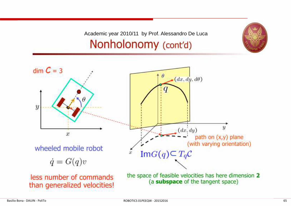
65ROBOTICS 01PEEQW - 20152016
Academic year 2010/11 by Prof. Alessandro De Luca
Basilio Bona - DAUIN - PoliTo