THE BASICS OF ROBOTICS

LAHDEN

AMMATTIKORKEAKOULU

Tekniikan ala

Kone- ja tuotantotekniikka

Mekatroniikka

Opinnäytetyö

Syksy 2011

Fareed Shakhatreh

1

Lahti University of Applied Sciences

Machine- and production technology

SHAKHATREH, FAREED: The basics of robotics

Mechatronics thesis, 122 pages

Autumn 2011

ABSTRACT

The basics of robotics are one of the rare subjects to be handled as a whole

in a due to the extreme diversity of scientific technologies it incorporates. It uses

quite many fields of technology, for example; mechanical engineering, electrical

engineering, computer sciences, electronics, sensors, actuators and artificial

intelligent. It is a multidimensional area which takes advantage of all engineering

studies that exist in our life besides a hard mathematical module application

which is required to be applied. One of the biggest challenges of writing this

thesis was to uncover enough material that involves robotic design.

To understand the mechanical design of a robot we need to study matrix, vectors,

derivate, integral and basic physics, servo motor selection and design in addition

to choose the gears and linking methods. Hydraulics and pneumatics are quite

important in this field and to know how we can create communication between

sensors and actuators through a programmable logic system, finally programming

is the method of communication.

The aim of my thesis is to pick out the most important subjects that handle robot

design. I tried to be brief and direct to the subject and tried to summarize the most

important aspect in this field that was quite a big challenge in my thesis because

of huge amount of different technologies that are handled.

Any student who will read my thesis will find it an orientation towards

understanding robot design and pointing out the most important tips on this field,

since it is brief and short and goes straight to the point.

Keywords: Degree of freedom, Robot, Articulated robot, Trajectory planning, Mapping

Lahden ammattikorkeakoulu

Kone- ja tuotantotekniikka

SHAKHATREH, FAREED: Robotics perusteet

Mekatroniikan opinnäytetyö, 122 sivua

Syksy 2011

TIIVISTELMÄ

Robotiikan perusteet, yksi harvinaisista aiheista, jota käsitellään päättötyössä

kokonaisena sen takia, että siinä sovelletaan suuri määrä eri tieteen tekniikoita.

Siinä käytetään melko monia tekniikan aloja kuten koneenrakennus,

sähkötekniikka, tietojenkäsittely, elektroniikka, anturit, toimilaitteet ja

keinotekoinen äly. Voimme nähdä, että se on moniulotteinen ala, joka hyödyntää

kaikkia insinööriopintoja, joita elämässämme on, lisäksi vaikean matemaattisen

moduulin soveltamista vaaditaan. Yksi suurimmista haasteista tämän päättötyön

teossa oli löytää tarpeeksi materiaalia, mikä kattaa vain robottisuunnittelun ja

keskittyä lähinnä kyseiseen alueeseen. Päättötyössäni olen yrittänyt poimia

tärkeimmän aiheen, joka käsittelee robottisuunnittelua ja keskittyä lähinnä siihen

suuntaan. Samaan aikaan olen yrittänyt olla lyhyt ja ytimekäs aiheessa ja yrittänyt

kiteyttää tämän alan tärkeimmän näkökohdan, mikä oli melko suuri haaste

päättötyössäni käsiteltävien eri tekniikoiden suuren määrän vuoksi.

Ymmärtääksemme robotin mekaanista suunnittelua meidän täytyy opiskella

matriiseja, vektoreita, derivaattoja, integraaleja ja fysiikan perusteita, meidän

täytyy opiskella melko hyvin servomoottorien valikoimaa ja suunnittelua, sen

lisäksi valita vaihteet ja yhdistämismetodit. Hydrauliikka- ja pneumatiikkatietous

ovat melko tärkeitä tällä alalla, ja kuinka voimme luoda viestintää anturien ja

toimilaitteiden välillä ohjelmoitavan logiikkajärjestelmän kautta, lopulta

ohjelmointi on tapa viestiä.

Kuka tahansa opiskelija, joka lukee päättötyöni, se olisi hänelle kuin orientaatio

robottisuunnittelun ymmärtämiseen ja se osoittaa tärkeimmät vinkit tällä alalla,

koska se on lyhyt, se menee suoraan asiaan.

Avainsanat: Vapausasteita, Robot, Kiertyväniveliset robotit, Kehityskaari suunnittelu

, Mapping.

1 INTRODUCTION .......................................................................................... 1

2 INTRODUCTION FOR ROBOTICS BASICS .................................................. 2

2.1 Introduction ............................................................................................ 2

2.2 Automation ............................................................................................ 2

2.3 Robot applications in our lives .................................................................. 3

2.4 Types of robot ........................................................................................ 6

2.5 Required studies in robotics ...................................................................... 8

2.6 Extrapolating from nature ......................................................................... 9

2.7 Comparing robots to humans .................................................................... 9

2.8 Programming a robot by teaching method .................................................. 9

2.9 Typical programming of an industrial robot .............................................. 10

2.10 Accuracy and repeatability of addressable points ............................... 11

3 TECHNOLOGIES OF A ROBOT .................................................................. 12

3.1 Introduction .......................................................................................... 12

3.2 Sub systems .......................................................................................... 12

3.3 Transmission system (Mechanics) ........................................................... 17

3.4 Power generation and storage system ....................................................... 20

3.5 Sensors ................................................................................................ 20

3.6 Electronics ........................................................................................... 25

3.7 Algorithms and software ........................................................................ 27

4 SERVO MOTOR DESIGN ........................................................................... 28

4.1 Introduction .......................................................................................... 28

4.2 Servo motor main types ......................................................................... 28

4.3 Application types in servo motor ............................................................. 31

4.4 How to define a suitable servo motor speed .............................................. 32

4.5 Servo motor gearbox ............................................................................. 32

4.6 Servo motor gearbox .......................................................................... 32

4.7 Choosing a suitable gearbox ................................................................... 33

4.8 Controlling inertia ................................................................................ 34

4.9 A Base servo motor example in a robot .............................................. 36

4.10 Resolution ........................................................................................... 38

5 INDUSTRIAL ROBOT ................................................................................ 40

5.1 Introduction ......................................................................................... 40

5.2 History of a robot ................................................................................ 40

5.3 Main types of an industrial robot ......................................................... 41

5.4 Main robot motions ............................................................................. 42

5.5 Scara robot vs articulated robot: ......................................................... 44

5.6 End effectors ...................................................................................... 45

6 INDUSTRIAL MANIPULATORS AND ITS KINEMATICS ........................... 46

6.1 Introduction ......................................................................................... 46

6.2 Links and joints ................................................................................... 46

6.3 Degree of freedom .............................................................................. 50

6.4 Types of robotic chains ....................................................................... 51

6.5 Degree of freedom in opened chains .................................................. 51

6.6 Degree of freedom in closed chains .................................................... 51

6.7 Stewart platform .................................................................................. 54

6.8 Defining work space area ................................................................... 55

6.9 How to define the inverse kinematics in 2R manipulator ..................... 58

6.10 How to define the inverse kinematics in 3R manipulator ..................... 58

7 TRAJECTORY DEFINITION ...................................................................... 59

7.1 Forward position problem ................................................................... 60

7.2 Inverse position problem ..................................................................... 60

7.3 Simple example with planar 2R ........................................................... 60

7.4 3R planar manipulator ......................................................................... 62

7.5 Prismatic joints calculation .................................................................. 64

8 POSITION, ORIENTATION, FRAMES ....................................................... 65

8.1 Introduction ......................................................................................... 65

8.2 Transformation .................................................................................... 69

8.3 Mapping involving general frames....................................................... 70

8.4 Translation operators .......................................................................... 72

8.5 Compound transformation .................................................................. 73

9 TRAJECTORY PLANNING IN ROBOTICS ................................................ 74

9.1 Introduction ......................................................................................... 74

9.2 Required data for trajectory planning .................................................. 74

9.3 Constraints ......................................................................................... 76

9.4 Subject to constraints .......................................................................... 76

9.5 Cubic polynomials ............................................................................... 76

9.6 Why to use cubic segment? ................................................................ 83

9.7 Common strategy 4-3-4 trajectory: ...................................................... 84

9.8 Coordinate motion .............................................................................. 85

10 Attachment 1 .......................................................................................... 88

1 TRAJECTORY PLANNING BY USING ROBOT STUDIO .......................... 88

1.1 Introduction ......................................................................................... 88

1.2 Creating new station and saving it ...................................................... 88

1.3 Moving robot joint space ..................................................................... 94

1.4 Target teach method ........................................................................... 97

1.5 Create program using virtual flex pendant ......................................... 102

1

1 INTRODUCTION

Many of us are wondering how a robot functions, what types of technologies are

used in a robot and why we need a robot in our life. The aim is to provide the

reader with a clear, simple explanation of robotics. The information is directed

towards engineering students, and engineers who are interested in a robotics.

In the beginning, you will find a general idea and the development of robot

technologies, some applications of an industrial robot and a non-industrial robot.

How robotics has developed in the last few decades and how it begins to play a

vital role in our industrial life.

The topic of the thesis is to summarize and cover the most important areas of a

robot structure and design. My target was to provide the reader with an easy,

simple way by using a lot of different pictures, drawings and mathematic

examples to make the subject of robotics simple to understand and easy to follow

step by step from the basics until the most complicated forms. Robotics study

becomes an extremely large field because it contains a huge amount of different

technologies, but I have covered the most important areas.

2

2 INTRODUCTION FOR ROBOTICS BASICS

2.1 Introduction

This chapter explains automation system and different types of automation. Why

we need robots in our life. What kind of advantages we can receive from robots

by viewing robot applications and the quality that can be provided by comparison

to human work.

2.2 Automation

Hard automation: This kind of automation cannot handle product design

variations, mass production for example; conventional machinery, packaging,

sewing and manufacturing small parts. Adjustability is possible but it can only

handle specific tasks with no possibility of changing its own task. These

machines can be seen in our homes (washing machines, dish washers, etc).

Programmable Automation: This form of automation began with the arrival of

the computer. People began programming machines to do a variety of tasks. It is

flexible because of a computer control, can handle variations, batch product, and

product design.

Autonomous (Independent): Endowed with a decision making capability

through the use of sensors. A robot belongs to this kind of automation and it is a

combination of microprocessor and conventional automation systems which can

provide a very powerful system. Its high level machinery capabilities combined

with fault recognition and correction abilities provided by highly evolved

computer systems. This means it can carry out work traditionally carried out by

humans. Examples of existing autonomous systems are animals and human

beings.

Animals when they see food they move toward it using sense of smell or they

escape when they react against danger due to senses of fear (sensors).

3

Human beings are the highest level of autonomous systems because they think

and they can change plan at any moment due to their high intelligence.

Robots cannot reach the same high level as humans because they are

programmed to do certain tasks according to certain factors which are completely

programmed by human beings, but they have no possibilities to change plan like

humans or plan new things unless the programmer programs them to change the

plan. Because of high development of machines, sensors, actuator, digital

electronics and microprocessor technology it became possible to create a robot

which is autonomous (Teijo Lahtinen, Lecture at Lahti University of Applied

Sciences 2009).

2.3 Robot applications in our lives

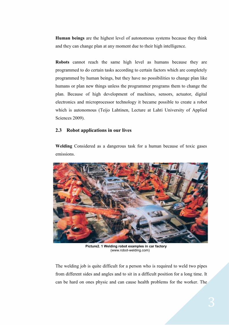
Welding Considered as a dangerous task for a human because of toxic gases

emissions.

The welding job is quite difficult for a person who is required to weld two pipes

from different sides and angles and to sit in a difficult position for a long time. It

can be hard on ones physic and can cause health problems for the worker. The

Picture2. 1 Welding robot examples in car factory (www.robot-welding.com)

4

difficulty for a human is to see all the sides of welded devices when he needs to

weld around a pipe as he can only see one side of the pipe.

Painting has similar problems to welding due to the use of toxic chemical

products. Below is an example picture 2.2 of a factory robot painting a car as it

moves slowly along a conveyer.

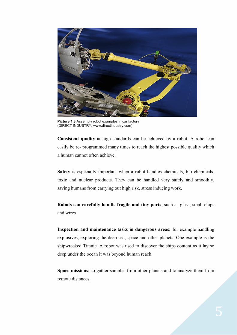
Assembly operation: When we assemble a chip we need to be very precise

because of very fine wires which require very precise and accurate tasks which a

human cannot handle but, on the other hand, is easy for a robot.

Picture 2.2 Painting robot examples in car factory (YASKAWA MOTOMAN, www.yaskawamotoman.co.uk)

5

Picture 1.3 Assembly robot examples in car factory (DIRECT INDUSTRY, www.directindustry.com)

Consistent quality at high standards can be achieved by a robot. A robot can

easily be re- programmed many times to reach the highest possible quality which

a human cannot often achieve.

Safety is especially important when a robot handles chemicals, bio chemicals,

toxic and nuclear products. They can be handled very safely and smoothly,

saving humans from carrying out high risk, stress inducing work.

Robots can carefully handle fragile and tiny parts, such as glass, small chips

and wires.

Inspection and maintenance tasks in dangerous areas: for example handling

explosives, exploring the deep sea, space and other planets. One example is the

shipwrecked Titanic. A robot was used to discover the ships content as it lay so

deep under the ocean it was beyond human reach.

Space missions: to gather samples from other planets and to analyze them from

remote distances.

6

2.4 Types of robot

1. Industrial robots. painting and welding robots

Advantages of a painting robot:

Robot painting is equal, uniform with high quality and precision. It can reach

very difficult places due to their high degree of flexibility which can be

difficult for humans, but can be achieved easily by robots. A human needs to

carry heavy painting gun and wear a mask for protection against toxic

chemicals. A robot´s repetition rate is high as it does not suffer from fatigue.

Safety levels which can be achieved by using a robot are high by saving

humans from the smell chemical toxics.

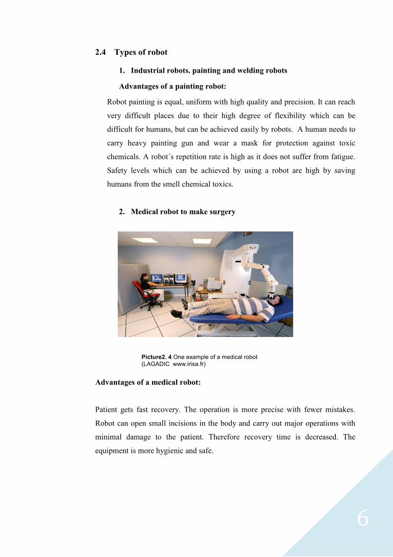
2. Medical robot to make surgery

Advantages of a medical robot:

Patient gets fast recovery. The operation is more precise with fewer mistakes.

Robot can open small incisions in the body and carry out major operations with

minimal damage to the patient. Therefore recovery time is decreased. The

equipment is more hygienic and safe.

Picture2. 4 One example of a medical robot

(LAGADIC www.irisa.fr)

7

3. Mobile robot with legs or wheel for chemical power plant, under see

or remote areas and bombs fields. The advantage in leg robot is that it

can avoid step over obstacles which can be dangerous like bomb or

even to protect objects from being destroyed due to robot moving over

them.

4. Robotics aircrafts and boats without pilot which are guided from a

station on the ground, which are used by army or rescue mission.

Picture2. 5 Leg robot picture

(http://whollysblog.com/wordpress/tag/robot/)

Picture 2.6 Example of mobile robot

(http://www.globalsecurity.org)

Figure 2.7 example of a robot aircraft ( http://www.wired.com/dangerroom/2008/03/pilots-yanked-o/)

8

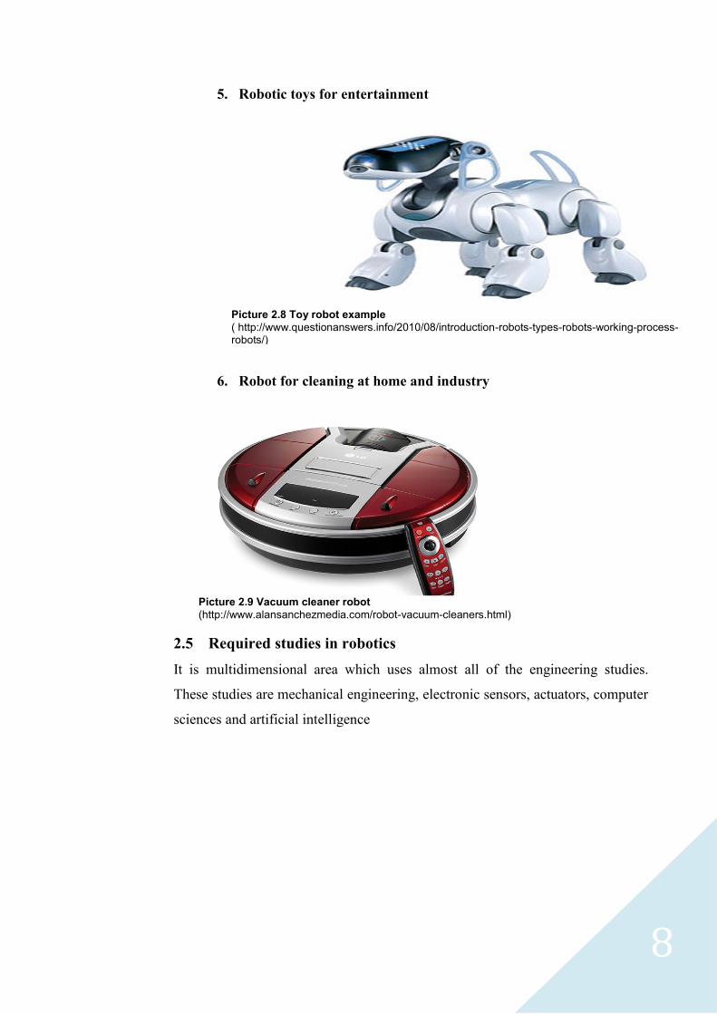
5. Robotic toys for entertainment

6. Robot for cleaning at home and industry

2.5 Required studies in robotics

It is multidimensional area which uses almost all of the engineering studies.

These studies are mechanical engineering, electronic sensors, actuators, computer

sciences and artificial intelligence

Picture 2.8 Toy robot example ( http://www.questionanswers.info/2010/08/introduction-robots-types-robots-working-process-robots/)

Picture 2.9 Vacuum cleaner robot (http://www.alansanchezmedia.com/robot-vacuum-cleaners.html)

9

2.6 Extrapolating from nature

As an example humans and animals have arms and fingers to manipulate objects.

Legs for locomotion, muscles as actuators, eyes provide vision, nose for smelling,

ears for hearing, tongue for tasting, skin for feeling and nerves for

communication between the brain and actuators.

2.7 Comparing robots to humans

Manipulation is equal to Arms and fingers driven by motors and other forms of

actuation. Vision is equal to camera. Hearing is equal to microphone. Feeling is

equal to tactile sensors. Communication is equal to wires, fiber optics and radio.

Brain is equal to computers and microprocessors. Smell and taste are still under

development (Matti Pitkälä, Lecture on Lahti University of Applied sciences

2011).

2.8 Programming a robot by teaching method

The same technique we use to teach children to write the alphabet by holding the

child’s hand and going through the writing process step by step. When we are

teaching the robot to do a certain job we control the movement of the robot hand

or end effector at the same time we record the motion of each individual joints.

Then we play back the recording and the robot begins to move independently as

taught. The quality of recording results in the work carried out. This work is

carried out by a skilled worker. When the work arrives on a conveyer to the

robot, the robot replays the stored recording then robot performs the required

task. Other ways to teach a robot to undertake certain tasks is by use of a program

that creates a virtual world. Then we stimulate the work to be carried out by the

robot’s joint motion parameters stored in the memory. The robot is then capable

of replaying the recording. (Craig 2005 340)

10

2.9 Typical programming of an industrial robot

Industrial robot is programmed by moving objects from position 1 to position 5

by moving joints vertically or horizontally to pick up and place an object through

the following steps:

Define points from P1 to P5:

1. Safely move above work piece (defined as P1)

2. 10 cm above work piece (defined as P2)

3. At position to take work piece from conveyer (defined as P3)

4. 10 cm above conveyer with low speed (defined as P4)

5. At position to leave work piece (defined as P5)

Define program:

1. Move to P1

2. Move to P2

3. Move to P3

4. Close gripper

5. Move to P2

6. Move to P4

7. Move to P5

8. Open gripper

9. Move to P4

10. Move to P1 and finish

(Wikipedia http://en.wikipedia.org/wiki/Industrial_robot )

11

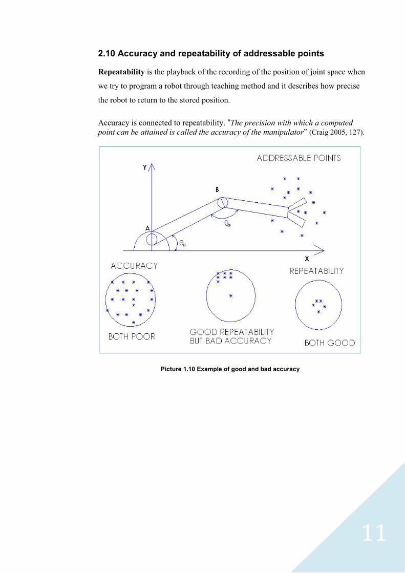
2.10 Accuracy and repeatability of addressable points

Repeatability is the playback of the recording of the position of joint space when

we try to program a robot through teaching method and it describes how precise

the robot to return to the stored position.

Accuracy is connected to repeatability. “The precision with which a computed

point can be attained is called the accuracy of the manipulator” (Craig 2005, 127).

Picture 1.10 Example of good and bad accuracy

12

3 TECHNOLOGIES OF A ROBOT

3.1 Introduction

In this chapter I will introduce robot sub systems and some parts that are used in

robot structure. This section will give a brief introduction to actuators, sensors,

motor drive, electronics, power supplies, algorithms and software, mechanical

parts and combining methods between these parts.

3.2 Sub systems

Actuators and transmission systems they are solenoid, motor drive, pneumatic

and hydraulic system which allows the robot to move. Mechanics parts are

motors usually rotate and a mechanism to transfer motion to all the necessary

parts of a robot to create the motion that is required. Usually robots require a

power supply, this kind of supply depends on what a robot is required to do,

and if it is a mobile robot then you need to decide the size of battery beside

the efficiency since power supply will be in the board of robot, but if it is not

mobile robot then electricity can be fed through a supply cable. Power storage

system is battery or some other electronic devices. Sensors are two types

Internal and external, there are many sensors in a robot which considered as

the senses in a robot. Micro- controller and processors are the brain that

controls the whole system. Algorithms and software are two models higher

level and low level, programmer need to create software and algorithms to

run the robot in a desired way.

13

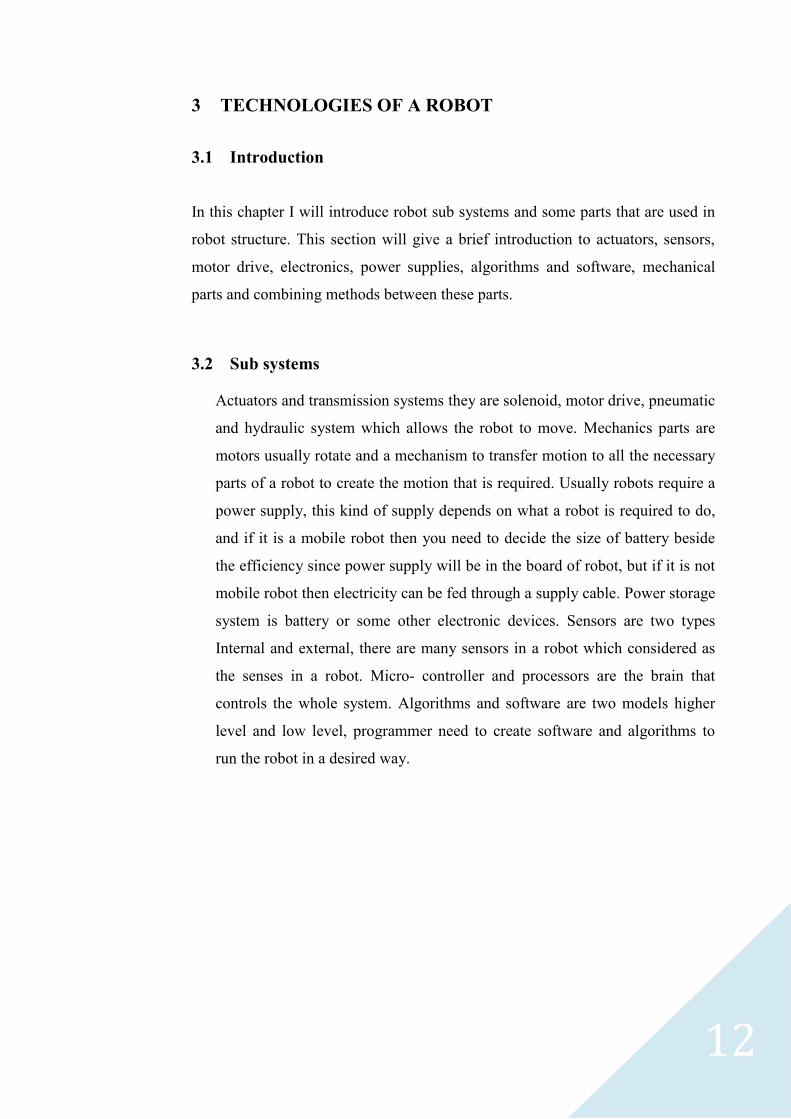
Actuators:

Actuators are essentially the prime movers providing linear force and motion.

Conventional: Pneumatics, hydraulics.

Pneumatic and hydraulic design consideration:

With this kind of system there is input and output in the cylinder, through

these input and output we pump air for pneumatic system and clean filtered

oil for hydraulic system to make the piston move outside and inside to

provide us with linear force and motion. You need to know in robot system

how far the piston should go outside or go inside, in pneumatic system we

cannot control how far the piston can go outside or inside unless you put ring

in the piston rod, but in hydraulic system we can control the extension of

piston by controlling the oil flow through flow control valves. Pneumatic

system is used when we do not need a large force to push, but hydraulics is

used when a system demands a large force, especially with big machines. The

problem with hydraulic system is leakage on the other hand is not a big

problem in pneumatic system since it uses air. (Robert H 2006, 128-134)

Picture 3.1 Pneumatic valve system

(http://www.stcvalve.com/)

Picture 3.2 Pneumatic Cylinder

(http://www.industrialmuscle.co.uk/pneumatics.htm)

14

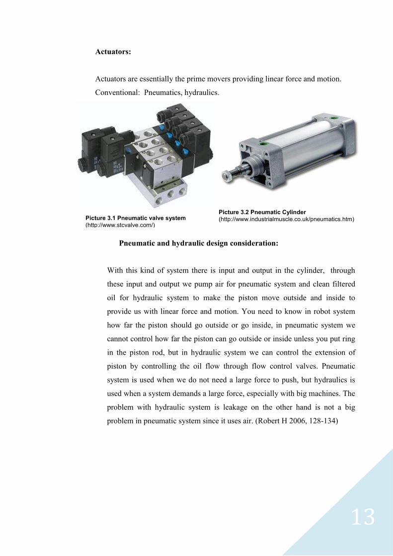
Permanent magnet motors and stepper motors are the joint space in a robot

that creates rotational motion.

Design consideration for servo motor:

When we design a robot, we take into consideration the torque, speed and the

gearbox size which should not be so heavy to the motor drive capacity. We

should pay attention to the weight of motor drives and gearboxes because the

base motor drive needs to carry all the motor drives and gearboxes which

require quite big torque and stronger motor in the base. The selection should

be harmonic and motor should match the load. When motor rotates in a

certain degree it should send feedback to the controller and to take feedback

from the controller when it needs to stop rotating, this happens through an

encoder which can read the degree of rotation. Nowadays these controllers

are mounted in the back of the motor drive. Controller manipulates voltage

and ampere to control the motor drive speed. (Teijo Lahtinen, Lecture on

Lahti university of Applied Sciences 2011)

Picture 3.3Servo motor (http://salecnc.com/catalog/product_info.php?products_id=48&osCsid=8e3292ae10e4b2f68b41591b83e471a4)

15

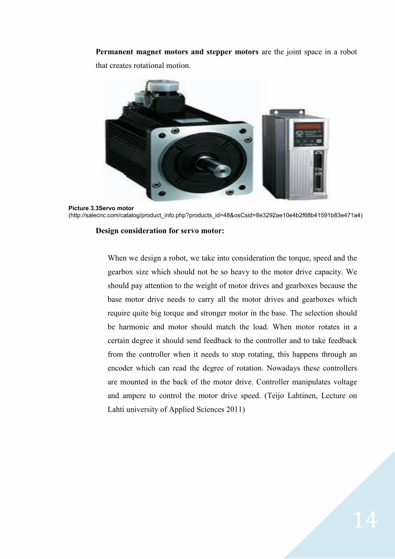
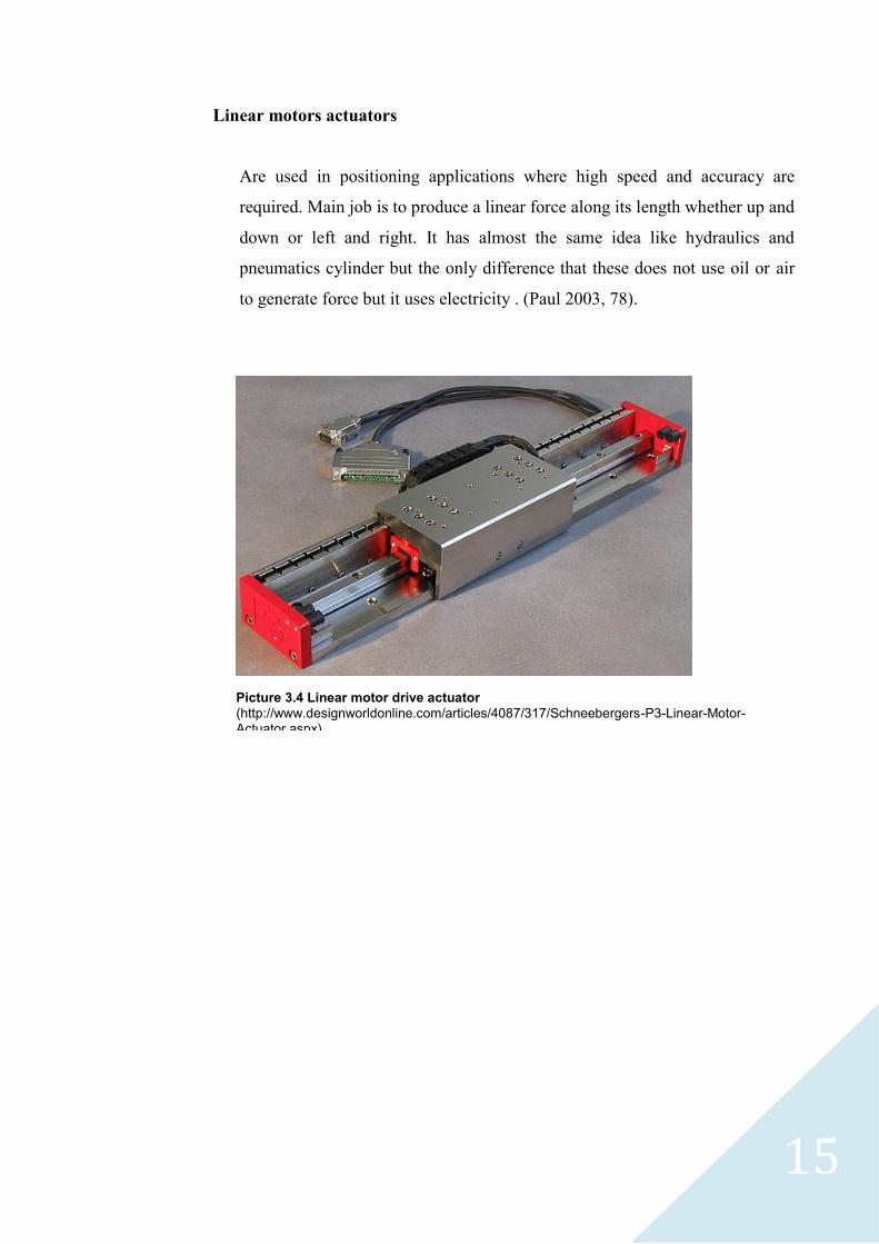
Linear motors actuators

Are used in positioning applications where high speed and accuracy are

required. Main job is to produce a linear force along its length whether up and

down or left and right. It has almost the same idea like hydraulics and

pneumatics cylinder but the only difference that these does not use oil or air

to generate force but it uses electricity . (Paul 2003, 78).

Picture 3.4 Linear motor drive actuator (http://www.designworldonline.com/articles/4087/317/Schneebergers-P3-Linear-Motor-Actuator.aspx)

16

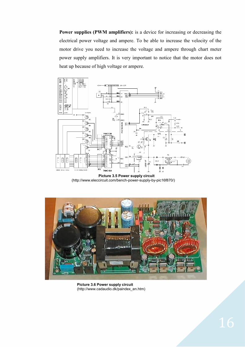
Power supplies (PWM amplifiers): is a device for increasing or decreasing the

electrical power voltage and ampere. To be able to increase the velocity of the

motor drive you need to increase the voltage and ampere through chart meter

power supply amplifiers. It is very important to notice that the motor does not

heat up because of high voltage or ampere.

Picture 3.5 Power supply circuit

(http://www.eleccircuit.com/bench-power-supply-by-pic16f870/)

Picture 3.6 Power supply circuit

(http://www.cadaudio.dk/paindex_en.htm)

17

3.3 Transmission system (Mechanics)

1. Gears: the lighter the gear the better motion, less torque and higher

speed. Some of this model is spur helical, bevel, worm, rack and pinion,

and many others. (Paul 2003, 108).

2. Chains:

Picture 3.7 Gear picture

(http://soheelali.blogspot.com/)

Picture 2.8 Chain (http://robomatter.com/Shop-By-Product-Type/Hardware/VEX/Mechanics?page=1&sort=3a)

18

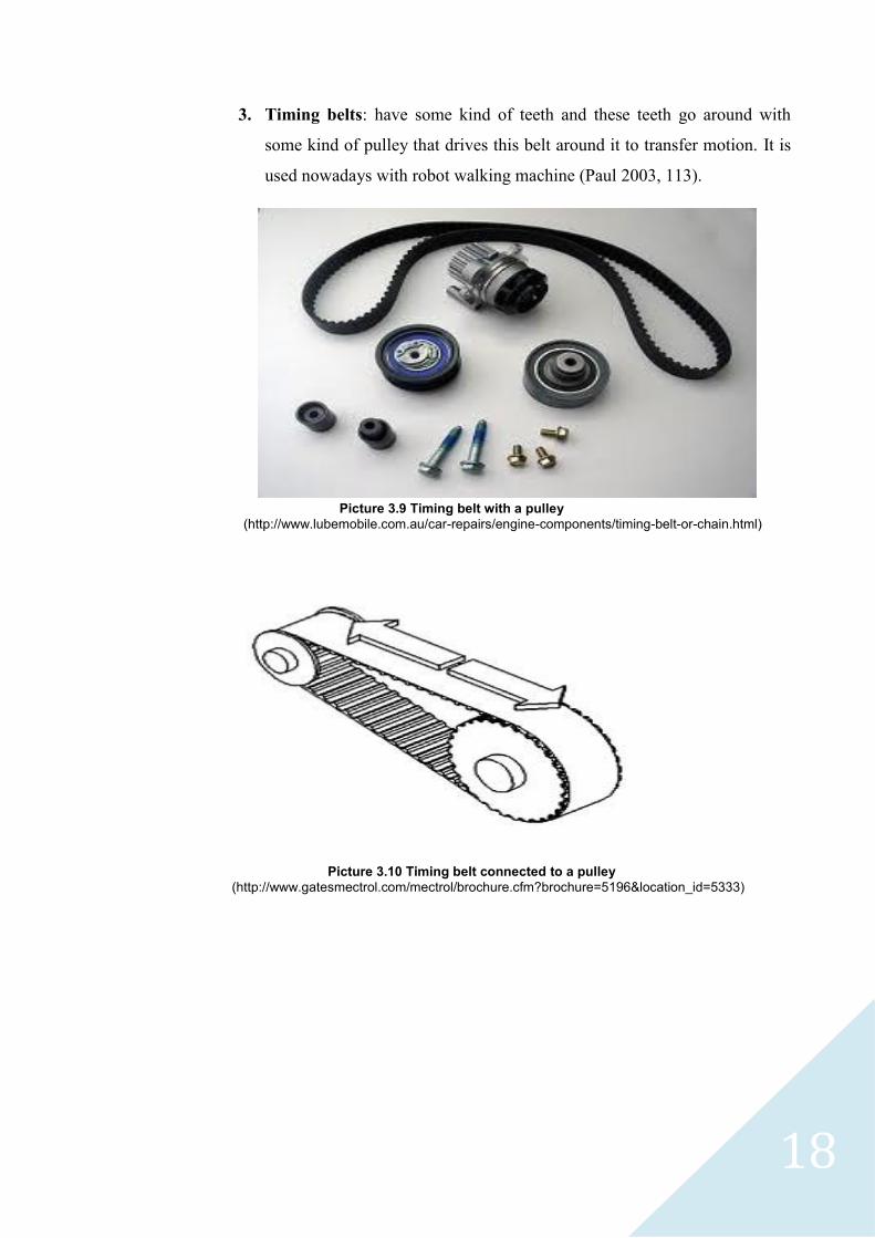
3. Timing belts: have some kind of teeth and these teeth go around with

some kind of pulley that drives this belt around it to transfer motion. It is

used nowadays with robot walking machine (Paul 2003, 113).

Picture 3.10 Timing belt connected to a pulley (http://www.gatesmectrol.com/mectrol/brochure.cfm?brochure=5196&location_id=5333)

Picture 3.9 Timing belt with a pulley (http://www.lubemobile.com.au/car-repairs/engine-components/timing-belt-or-chain.html)

19

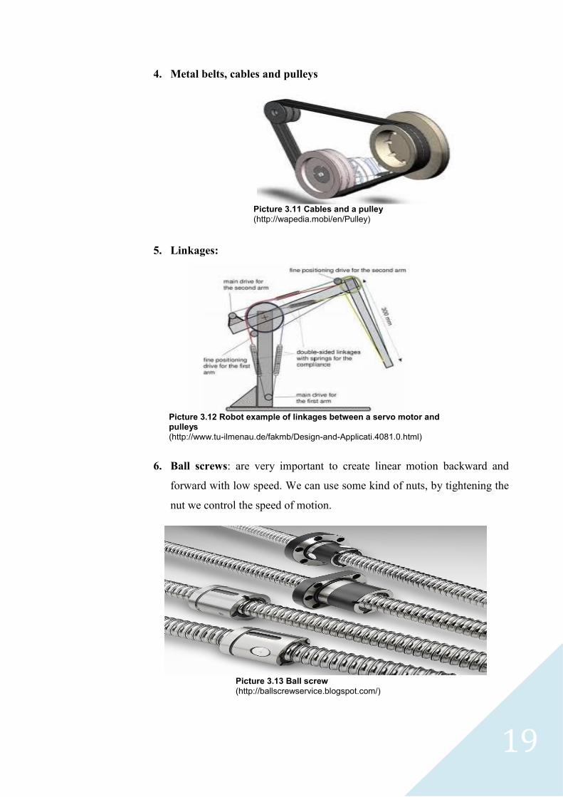
4. Metal belts, cables and pulleys

5. Linkages:

6. Ball screws: are very important to create linear motion backward and

forward with low speed. We can use some kind of nuts, by tightening the

nut we control the speed of motion.

Picture 3.11 Cables and a pulley (http://wapedia.mobi/en/Pulley)

Picture 3.12 Robot example of linkages between a servo motor and pulleys (http://www.tu-ilmenau.de/fakmb/Design-and-Applicati.4081.0.html)

Picture 3.13 Ball screw (http://ballscrewservice.blogspot.com/)

20

3.4 Power generation and storage system

Solar cells are working on the moon or in space since we need renewable

energy for example sun light. Fuel cells are used in a big heavy robot so a

diesel engine is required and fuel to run it, these engines power is based on

hydrogen and oxygen burning. Rechargeable cells are more in use nowadays

due to the technology advancements means that rechargeable cells can

contain quite a lot of energy for example: batteries that are in use in mobile

phones they can last long time.

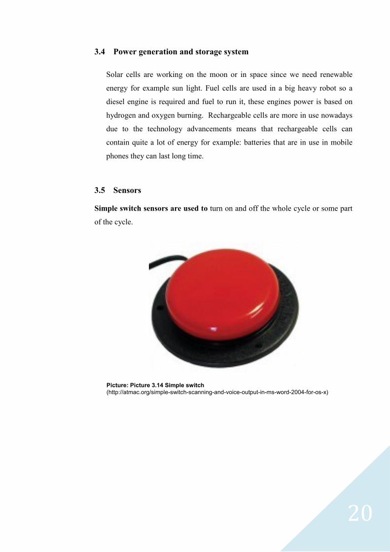
3.5 Sensors

Simple switch sensors are used to turn on and off the whole cycle or some part

of the cycle.

Picture: Picture 3.14 Simple switch (http://atmac.org/simple-switch-scanning-and-voice-output-in-ms-word-2004-for-os-x)

21

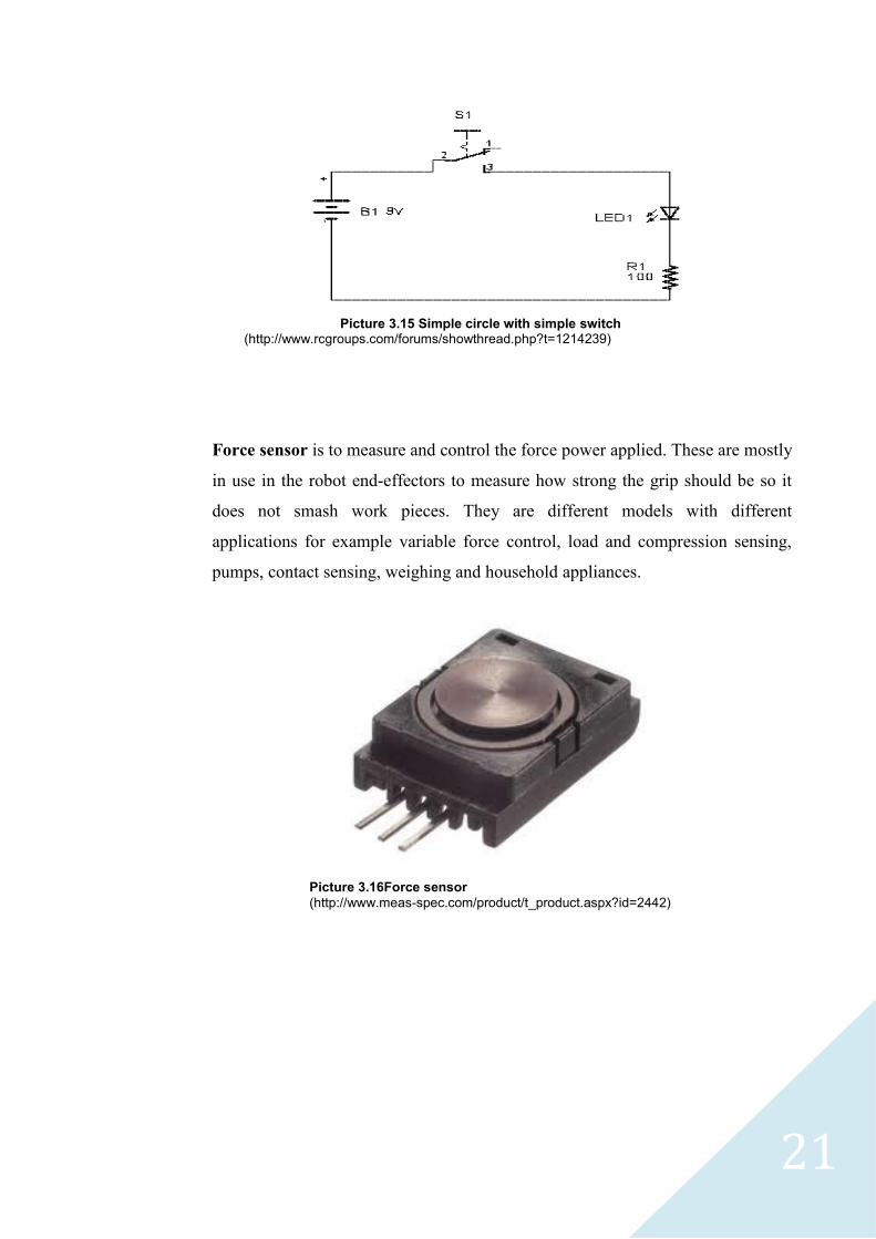
Force sensor is to measure and control the force power applied. These are mostly

in use in the robot end-effectors to measure how strong the grip should be so it

does not smash work pieces. They are different models with different

applications for example variable force control, load and compression sensing,

pumps, contact sensing, weighing and household appliances.

Picture 3.16Force sensor

(http://www.meas-spec.com/product/t_product.aspx?id=2442)

Picture 3.15 Simple circle with simple switch (http://www.rcgroups.com/forums/showthread.php?t=1214239)

22

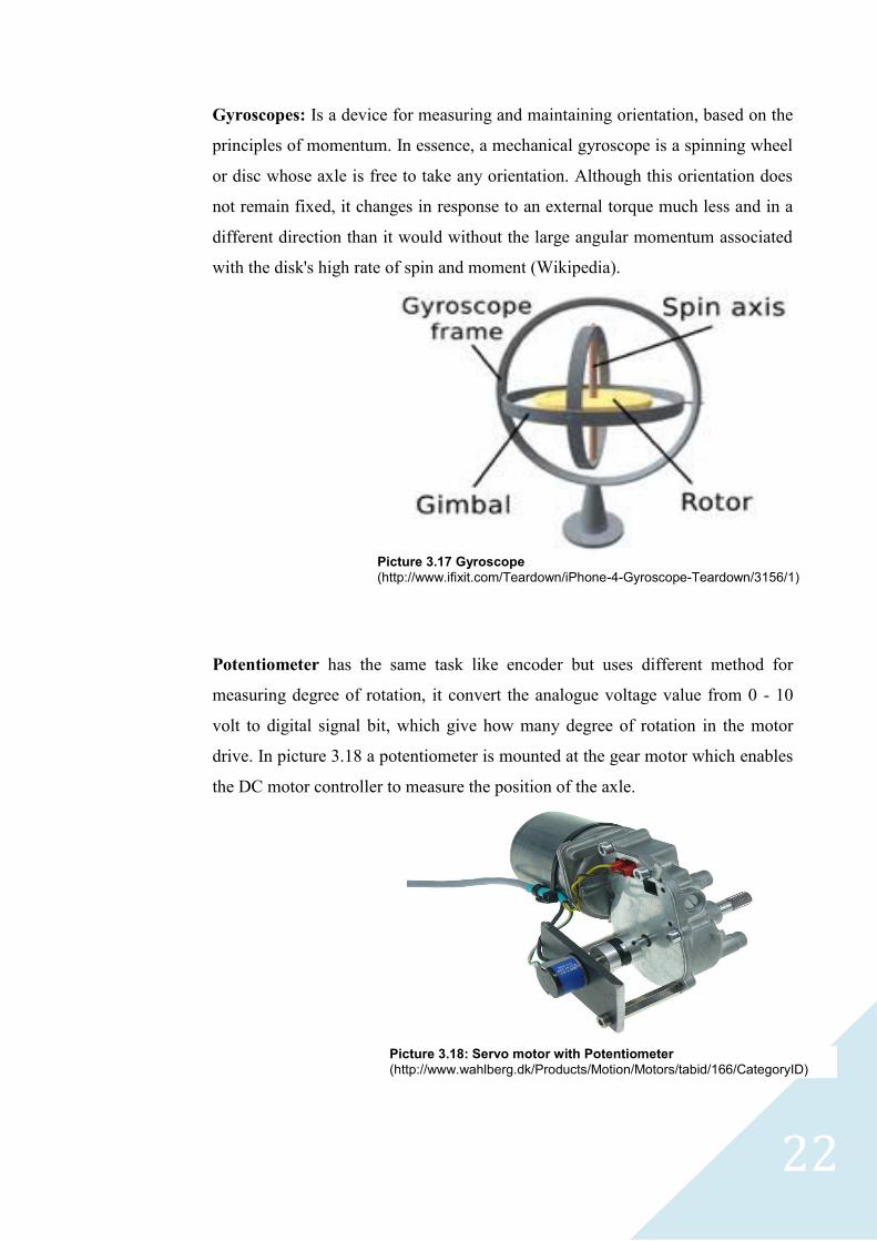
Gyroscopes: Is a device for measuring and maintaining orientation, based on the

principles of momentum. In essence, a mechanical gyroscope is a spinning wheel

or disc whose axle is free to take any orientation. Although this orientation does

not remain fixed, it changes in response to an external torque much less and in a

different direction than it would without the large angular momentum associated

with the disk's high rate of spin and moment (Wikipedia).

Potentiometer has the same task like encoder but uses different method for

measuring degree of rotation, it convert the analogue voltage value from 0 - 10

volt to digital signal bit, which give how many degree of rotation in the motor

drive. In picture 3.18 a potentiometer is mounted at the gear motor which enables

the DC motor controller to measure the position of the axle.

Picture 3.17 Gyroscope (http://www.ifixit.com/Teardown/iPhone-4-Gyroscope-Teardown/3156/1)

Picture 3.18: Servo motor with Potentiometer

(http://www.wahlberg.dk/Products/Motion/Motors/tabid/166/CategoryID)

23

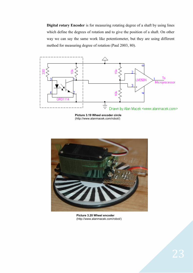
Digital rotary Encoder is for measuring rotating degree of a shaft by using lines

which define the degrees of rotation and to give the position of a shaft. On other

way we can say the same work like potentiometer, but they are using different

method for measuring degree of rotation (Paul 2003, 80).

Picture 3.20 Wheel encoder (http://www.alanmacek.com/robot/)

Picture 3.19 Wheel encoder circle (http://www.alanmacek.com/robot/)

24

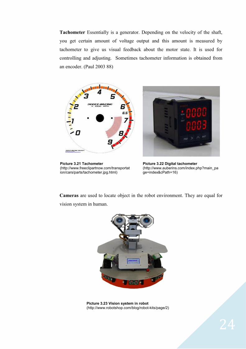
Tachometer Essentially is a generator. Depending on the velocity of the shaft,

you get certain amount of voltage output and this amount is measured by

tachometer to give us visual feedback about the motor state. It is used for

controlling and adjusting. Sometimes tachometer information is obtained from

an encoder. (Paul 2003 88)

Cameras are used to locate object in the robot environment. They are equal for

vision system in human.

Picture 3.21 Tachometer (http://www.freeclipartnow.com/transportation/cars/parts/tachometer.jpg.html)

Picture 3.22 Digital tachometer (http://www.auberins.com/index.php?main_page=index&cPath=16)

Picture 3.23 Vision system in robot (http://www.robotshop.com/blog/robot-kits/page/2)

25

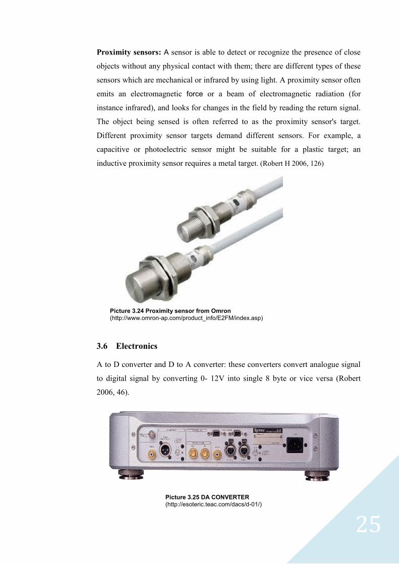
Proximity sensors: A sensor is able to detect or recognize the presence of close

objects without any physical contact with them; there are different types of these

sensors which are mechanical or infrared by using light. A proximity sensor often

emits an electromagnetic force or a beam of electromagnetic radiation (for

instance infrared), and looks for changes in the field by reading the return signal.

The object being sensed is often referred to as the proximity sensor's target.

Different proximity sensor targets demand different sensors. For example, a

capacitive or photoelectric sensor might be suitable for a plastic target; an

inductive proximity sensor requires a metal target. (Robert H 2006, 126)

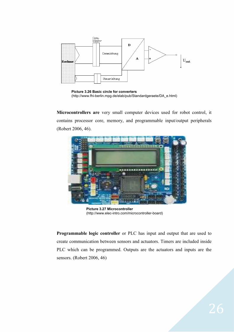
3.6 Electronics

A to D converter and D to A converter: these converters convert analogue signal

to digital signal by converting 0- 12V into single 8 byte or vice versa (Robert

2006, 46).

Picture 3.24 Proximity sensor from Omron (http://www.omron-ap.com/product_info/E2FM/index.asp)

Picture 3.25 DA CONVERTER (http://esoteric.teac.com/dacs/d-01/)

26

Microcontrollers are very small computer devices used for robot control, it

contains processor core, memory, and programmable input/output peripherals

(Robert 2006, 46).

Programmable logic controller or PLC has input and output that are used to

create communication between sensors and actuators. Timers are included inside

PLC which can be programmed. Outputs are the actuators and inputs are the

sensors. (Robert 2006, 46)

Picture 3.26 Basic circle for converters (http://www.fhi-berlin.mpg.de/elab/pub/Standardgeraete/DA_e.html)

Picture 3.27 Microcontroller (http://www.elec-intro.com/microcontroller-board)

27

Power Electronics are used for running motor drive and controlling the motor

speed by converting electrical power voltage and ampere to a suitable amount to

produce suitable speed in the motor drive.

3.7 Algorithms and software

Mean step by step procedure and logic programming language through logical

event sequence by planning the whole task at the beginning, then controlling the

motors and actuators through using feedback signal that are obtained from

sensors., programmer need to plan trajectory of each individual actuator motions

and to plan trajectories of end effectors. To get in the end harmonic motion with

suitable speed based on logic system and task requirement.

(Robert 2006, 49-50).

Picture 3.28 Power electronics (http://www.instructables.com/id/BLDC-Motor-Control-with-Arduino-salvaged-HD-motor/step8/The-Power-Electronics/)

28

4 SERVO MOTOR DESIGN

4.1 Introduction

Servo motor is the main prime mover of the robot. This section will cover the

most important of servo motor types which concerns mainly robot, servo motor

behavior in respect to torque, speed, current and voltage, and how to control the

speed, type of application and how to choose the right servo motor with a suitable

gearbox.

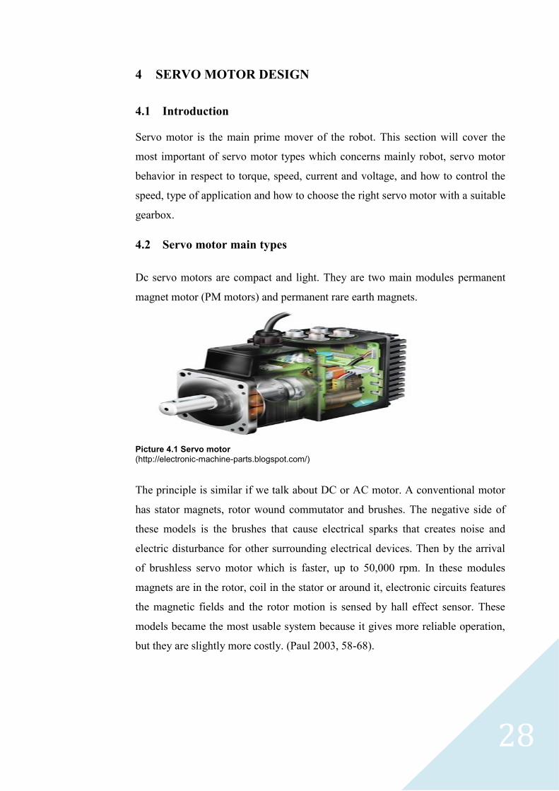
4.2 Servo motor main types

Dc servo motors are compact and light. They are two main modules permanent

magnet motor (PM motors) and permanent rare earth magnets.

Picture 4.1 Servo motor (http://electronic-machine-parts.blogspot.com/)

The principle is similar if we talk about DC or AC motor. A conventional motor

has stator magnets, rotor wound commutator and brushes. The negative side of

these models is the brushes that cause electrical sparks that creates noise and

electric disturbance for other surrounding electrical devices. Then by the arrival

of brushless servo motor which is faster, up to 50,000 rpm. In these modules

magnets are in the rotor, coil in the stator or around it, electronic circuits features

the magnetic fields and the rotor motion is sensed by hall effect sensor. These

models became the most usable system because it gives more reliable operation,

but they are slightly more costly. (Paul 2003, 58-68).

29

Performance characteristic of motor drive based on figure 4.2:

According to the figure 4.2 there is a stall torque point, no load speed point, there

is also specific voltage, which drives the motor to no load speed and stall torque.

We notice that if we heavily load the motor then the speed is zero.

Picture 4.2 Behavior of a servo motor with different speed and torque

We notice from the following figure 4.3:

There is no load current

Kt is the motor constant value

Picture 4.3 Load torque and current

30

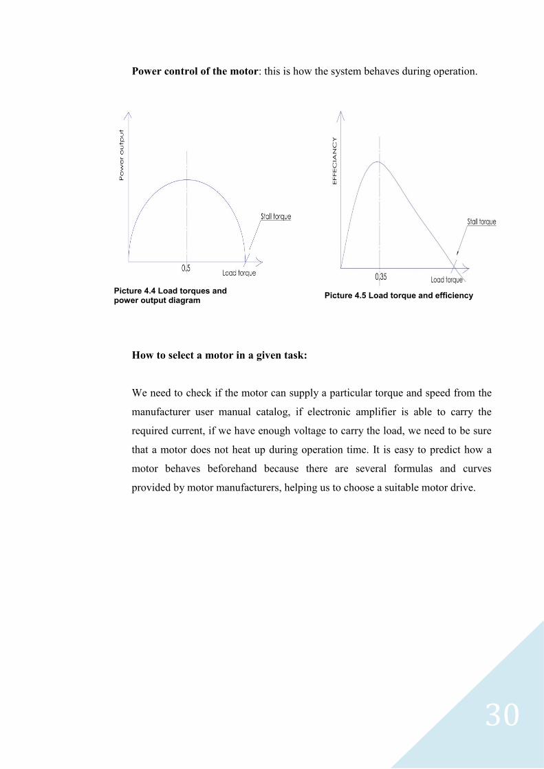
Power control of the motor: this is how the system behaves during operation.

How to select a motor in a given task:

We need to check if the motor can supply a particular torque and speed from the

manufacturer user manual catalog, if electronic amplifier is able to carry the

required current, if we have enough voltage to carry the load, we need to be sure

that a motor does not heat up during operation time. It is easy to predict how a

motor behaves beforehand because there are several formulas and curves

provided by motor manufacturers, helping us to choose a suitable motor drive.

Picture 4.4 Load torques and power output diagram

Picture 4.5 Load torque and efficiency

31

4.3 Application types in servo motor

A. Application – continues duty operation

When we drive a certain load in a particular speed or variable speed during a

period of time, we need to take into consideration the load torque, speed and if

electronic circuit is able to supply the required current and voltage.

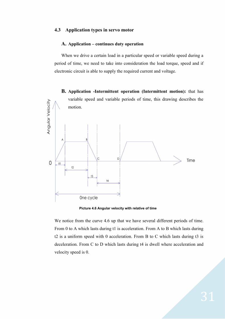
B. Application -Intermittent operation (Intermittent motion): that has

variable speed and variable periods of time, this drawing describes the

motion.

We notice from the curve 4.6 up that we have several different periods of time.

From 0 to A which lasts during t1 is acceleration. From A to B which lasts during

t2 is a uniform speed with 0 acceleration. From B to C which lasts during t3 is

deceleration. From C to D which lasts during t4 is dwell where acceleration and

velocity speed is 0.

Picture 4.6 Angular velocity with relative of time

32

4.4 How to define a suitable servo motor speed

We need first to calculate the speed of load, reduction ratio value by gearbox and

the horse power or KW of the motor drive capacity.

4.5 Servo motor gearbox

Every motor drive has a certain load and the motor speed is quite high for

example 3000 rpm or more. We need to make reduction for the speed through

choosing suitable size for the gear box since the gear box has contributed for the

carried load speed. If the speed is not continued at the same level, but it is

variable during variable time, we need to figure out how to solve this problem.

4.6 Servo motor gearbox

Every motor drive has a certain load and the motor speed is quite high for

example 3000 rpm or more. We need to make reduction for the speed through

choosing suitable size for the gear box since the gear box has contributed for the

carried load speed.

If the speed is not continues in the same level, but it is variable during variable

time, we need to figure out how to solve this problem.

33

4.7 Choosing a suitable gearbox

Reduction: most of the cases we face are reductions but there are little cases

of increases. We need to know the maximum speed of load (rpm) of motor drive

from the guide manual which has been provided by a motor drive manufacturer.

(Max speed of load)*2= (max allowable speed of motor*G)

For example maximum allowable speed for a motor is 3000 rpm and

transmission ratio is 0.1.

How to calculate maximum speed of load?

(Max speed of load)*2= (3000*0,1)

Maximum speed of load = 150

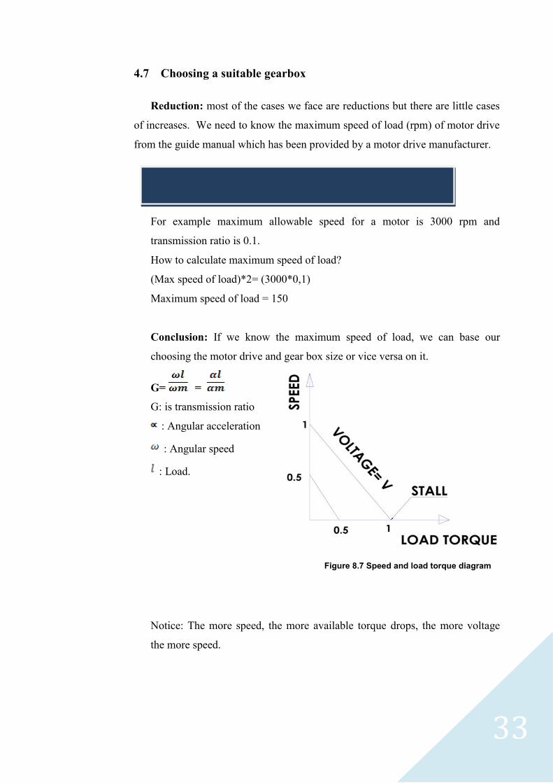
Conclusion: If we know the maximum speed of load, we can base our

choosing the motor drive and gear box size or vice versa on it.

G= =

G: is transmission ratio

: Angular acceleration

: Angular speed

: Load.

Notice: The more speed, the more available torque drops, the more voltage

the more speed.

Figure 8.7 Speed and load torque diagram

34

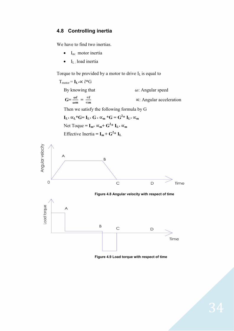
4.8 Controlling inertia

We have to find two inertias.

Im: motor inertia

IL : load inertia

Torque to be provided by a motor to drive IL is equal to

Tmotor = IL* *G

By knowing that : Angular speed

G=

=

: Angular acceleration

Then we satisfy the following formula by G

IL* L*G= IL* G * m *G = G2* IL* m

Net Toque = Im* m+ G2* IL* m

Effective Inertia = Im + G2* IL

Figure 4.8 Angular velocity with respect of time

Figure 4.9 Load torque with respect of time

35

In figure 4.9 the sum of torque from 0 to A = to sum of torque A to B +B to C

From 0 to A during time t1 according to figure 4.10

The motor angular acceleration =

=

Torque T1= (Im* G2* IL) + Tf*

Tf : torque friction

: Efficiency

: angular speed in A

From A to B during time t2

the angular motor acceleration =0 (constant velocity)

Torque T2 = Tf*

From B to C during time t3

the motor angular acceleration =

=

Torque T3= (Im*

* IL) - Tf*

It is minus friction because friction aids deceleration.

TRMS =√

Now we can select the suitable motor according to the following drawing.

Figure 4.10 Angular velocity with respect of several period of time

36

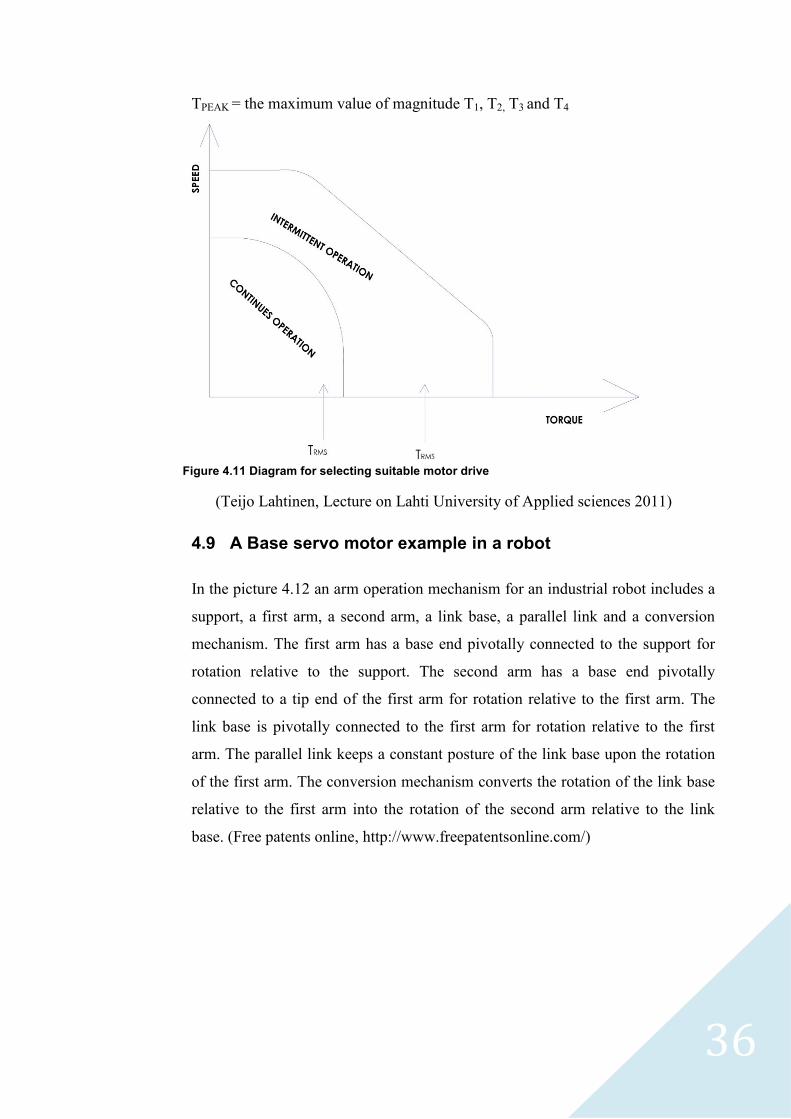
TPEAK = the maximum value of magnitude T1, T2, T3 and T4

(Teijo Lahtinen, Lecture on Lahti University of Applied sciences 2011)

4.9 A Base servo motor example in a robot

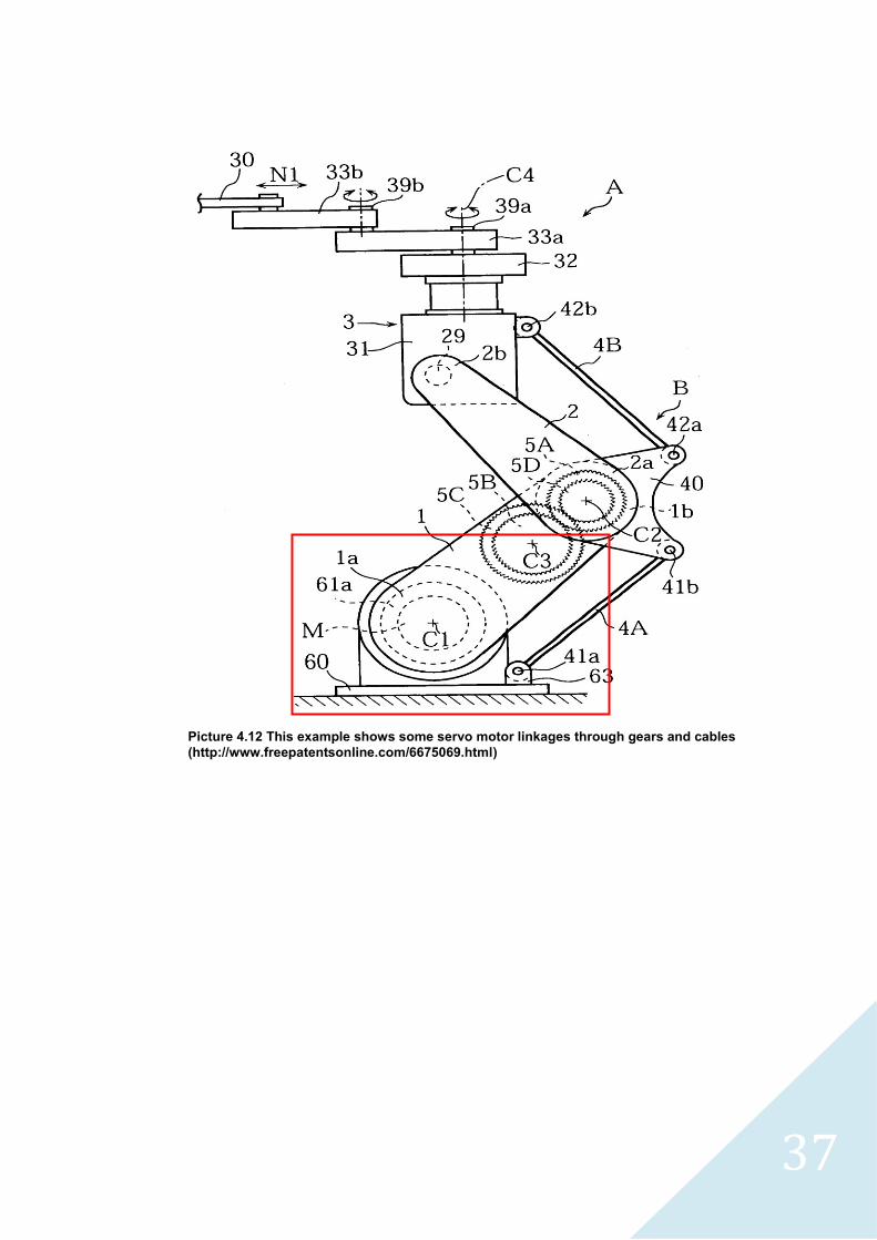
In the picture 4.12 an arm operation mechanism for an industrial robot includes a

support, a first arm, a second arm, a link base, a parallel link and a conversion

mechanism. The first arm has a base end pivotally connected to the support for

rotation relative to the support. The second arm has a base end pivotally

connected to a tip end of the first arm for rotation relative to the first arm. The

link base is pivotally connected to the first arm for rotation relative to the first

arm. The parallel link keeps a constant posture of the link base upon the rotation

of the first arm. The conversion mechanism converts the rotation of the link base

relative to the first arm into the rotation of the second arm relative to the link

base. (Free patents online, http://www.freepatentsonline.com/)

Figure 4.11 Diagram for selecting suitable motor drive

37

Picture 4.12 This example shows some servo motor linkages through gears and cables

(http://www.freepatentsonline.com/6675069.html)

38

4.10 Resolution

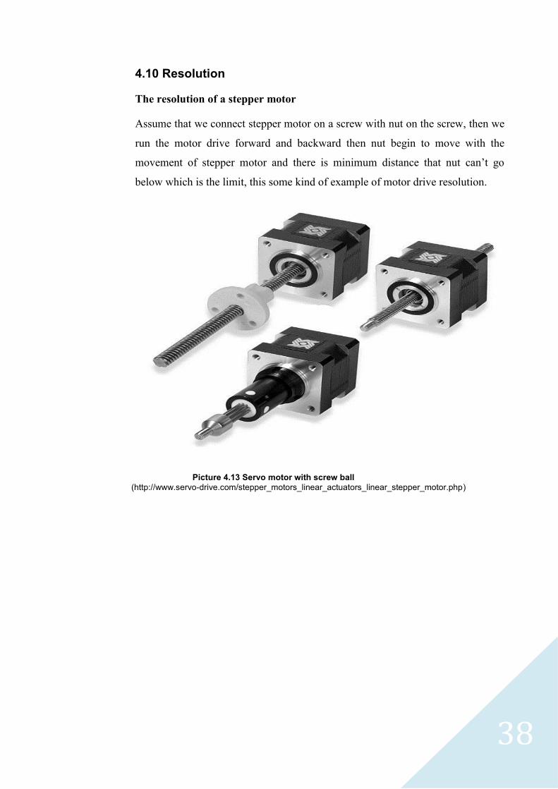
The resolution of a stepper motor

Assume that we connect stepper motor on a screw with nut on the screw, then we

run the motor drive forward and backward then nut begin to move with the

movement of stepper motor and there is minimum distance that nut can’t go

below which is the limit, this some kind of example of motor drive resolution.

Picture 4.13 Servo motor with screw ball

(http://www.servo-drive.com/stepper_motors_linear_actuators_linear_stepper_motor.php)

39

Servo motor drive gets feedback from an encoder or a potential meter

Resolution depends on the number of lines inside encoder, the more resolution

you want the more expensive encoder and the more lines it has.

For example, encoder that has 360 lines means that it has one degree of resolution

but it cannot go below one degree.

Potential meter uses different method, which is analogue signal, which is

converted to digital through electronics.

Example: let us assume potential meter signal is 10 volt which equal 8 bit then:

28= 256 digit

360o / 256= 1.4 Resolution per step.(Robert H 2006, 43).

Picture 4.14 : Optical incremental rotary encoder

(http://www.directindustry.com/prod/gsi-microe-systems/optical-incremental-rotary-encoders-39494-523542.html)

40

5 INDUSTRIAL ROBOT

5.1 Introduction

I will try to give a brief history about an industrial robot, covering different types

of industrial robots and their differences especially articulated robot and scara

robot and their differences, besides giving small introductory idea about the end

effector and its rotational movement types.

5.2 History of a robot

It began in 1954 when Devol and Egelberger created the first robot and a

computer was just about coming, so they built not sophisticated controller robot

but they created programmable system that can do a variety of tasks. Then they

established the Unimation company that manufactured these programmable

systems (Wikipedia, http://en.wikipedia.org/wiki/Industrial_robot).

In 1970 in the University of Stanford they created an arm which is actuated

through electrical servo motor and controlled by a computer to do variety of tasks

(Wikipedia, http://en.wikipedia.org/wiki/Industrial_robot). In 1981 Japanese

created Scara arm which is especially designed for product assembly. The idea of

this robot is to do what human does and sony walk man was the first robot

assembly (Wikipedia http://en.wikipedia.org/wiki/SCARA_robot).

The typical industrial robot which looks like a human arm has six different joints

like an elbow joint, a shoulder joint and a rest joint. These joints are powered by

a servo motor or a hydraulic motor or whatever type of motor. These powered

motor joints enable robot to reach objects in several ways. The amount of joint

space motor drive is depending on the nature of a robot task. One motions less on

motor drive less. There are several types of robot with less motor drive for

example 4 different joint space. The more sophisticated the job the more motions

we require so extra motor drive is need. All these six motor drives need to be

controlled to achieve specific task and sometimes we do not need to use all of

them so we eliminate some motor joint depending on the task requirements.

(http://en.wikipedia.org/wiki/Industrial_robot)

41

5.3 Main types of an industrial robot

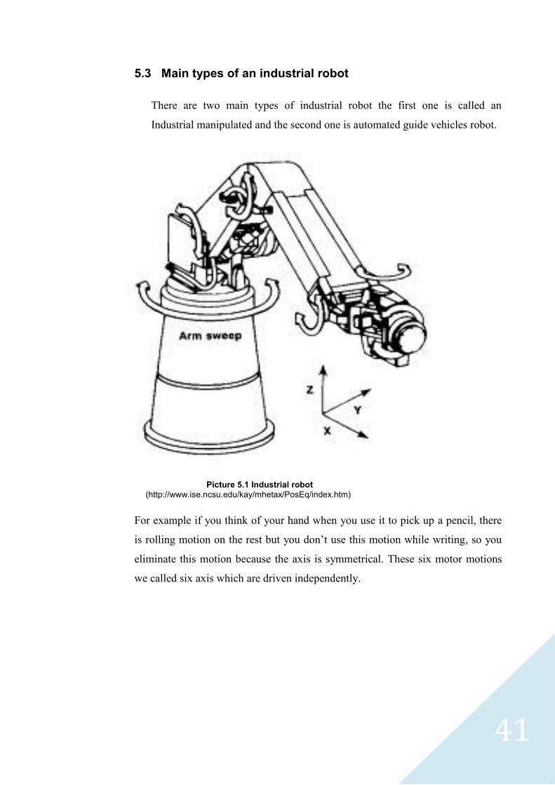
There are two main types of industrial robot the first one is called an

Industrial manipulated and the second one is automated guide vehicles robot.

For example if you think of your hand when you use it to pick up a pencil, there

is rolling motion on the rest but you don’t use this motion while writing, so you

eliminate this motion because the axis is symmetrical. These six motor motions

we called six axis which are driven independently.

Picture 5.1 Industrial robot

(http://www.ise.ncsu.edu/kay/mhetax/PosEq/index.htm)

42

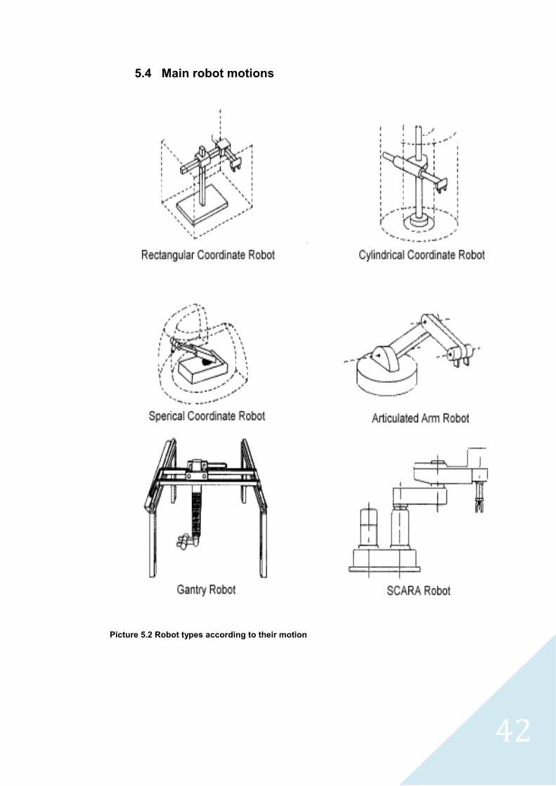
5.4 Main robot motions

Picture 5.2 Robot types according to their motion

43

Rectangular coordinate motion (Cartesian): there are three different

motions which are X, Y, Z or in other word this robot can move up and down,

left and right, backward and forward, but it has no rotation or degrees. In this

kind of model it is easy to control motion just by giving the coordinates, then

a robot moves according to (x, y, z) values.

Cylindrical coordinate Robot: it has rotational movement on the base and

Cartesian motion in the upper part.

Spherical coordinate robot: is a robot with two rotary joints and one

prismatic joint.

Articulated arm robot: it looks like human arms base rotational like a

shoulder, an elbow and a rest which give us more motion with certain angels

which is not possible by Cartesian robot. This model is more complicated to

control because you need to calculate angles, velocity and acceleration to get

a desired motion and requires solving plenty of equation.

Gantry robot: is a linear motion robot and has another industrial name as a

linear robot.

Scara robot: is created by Japanese 1979 for assembly tasks because it

moves in two planes. It is simple to use in assembly operation, when you

need to tight a screw and to hold it vertically then to rotate the screw and

push down you don’t require very big sophisticated robot, so Scara robot is

the best choice for a similar operation or like pushing object down like gear

box and so on.

44

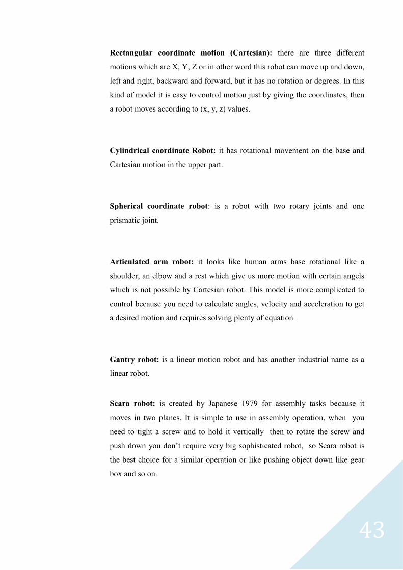
All these models are used by engineers and every model has positive and

negative sides. Depended on the job requirement we try to choose the right model

to suite our requirement.

5.5 Scara robot vs articulated robot:

Features Articulated robot Scara robot

Reach 2.5 m 1.2 m

Pay load 125 kg 10 to 50 kg

Waist rotation 360 degrees 120 degrees

Rotational Speed 100 to 200 degrees/sec tip speed 2 met/sec

Repeatability 0.4 mm 0.03 to 0.05 mm

Weight 1600 kg 30 to 100 kg

There is even more features to compare but these are the main features that can

make the difference between an articulated robot and a Scara robot.

Picture 5.3 Scara robot

(http://news.thomasnet.com/fullstory/SCARA-Robot-performs-high-speed-operations-466161)

45

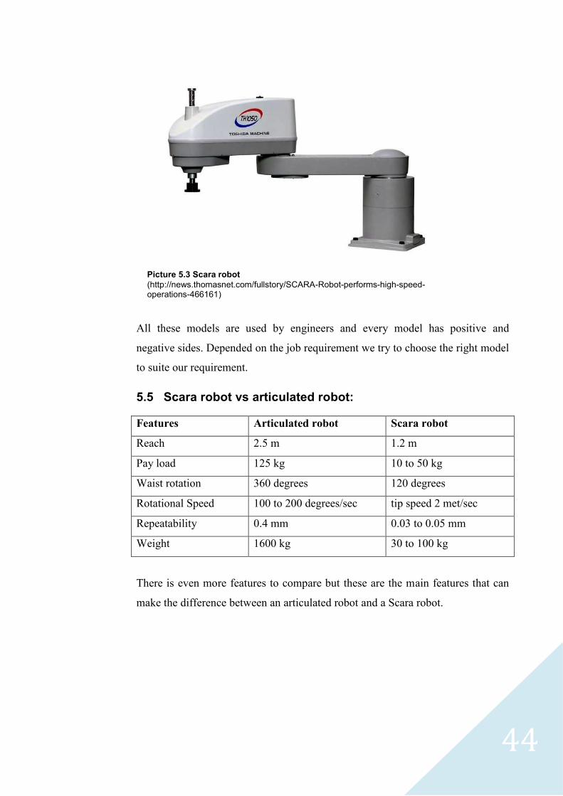
5.6 End effectors

Is a robot hand that grabs an object and moves it from one place to another. In the

end effectors usually there are three rotational motions with three different

motors and it equal human rest for lifting objects. End effector are different

model with different task option.

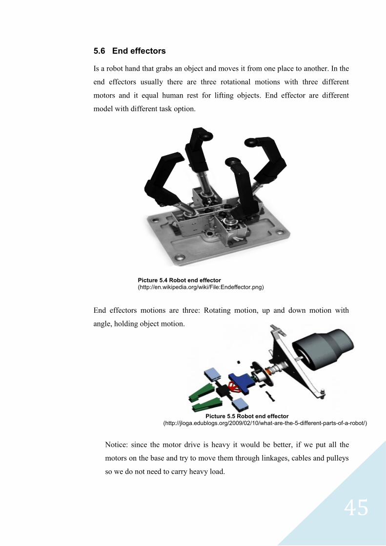
End effectors motions are three: Rotating motion, up and down motion with

angle, holding object motion.

Notice: since the motor drive is heavy it would be better, if we put all the

motors on the base and try to move them through linkages, cables and pulleys

so we do not need to carry heavy load.

Picture 5.5 Robot end effector

(http://jloga.edublogs.org/2009/02/10/what-are-the-5-different-parts-of-a-robot/)

Picture 5.4 Robot end effector

(http://en.wikipedia.org/wiki/File:Endeffector.png)

46

6 INDUSTRIAL MANIPULATORS AND ITS KINEMATICS

6.1 Introduction

In this section I will try to give an idea about types of links and joints and the

serial chains combination, also to focus on explaining the term (degree of

freedom) in an open chain and a closed chain and how to calculate it. Beside that

I give several drawing examples about different types of links and chains to make

the idea easy and clear to understand. In the end of this section I will define the

work space area for a robot and what type of work space we have. I explain 2R

and 3R manipulator work space beside the direct and inverse kinematics work

space.

First we need to define the following:

Serial chain is a combination of links and joints in the space.

Notice: we need to understand the word degree of freedom and to know how to

define how many degrees of freedom a robot has.

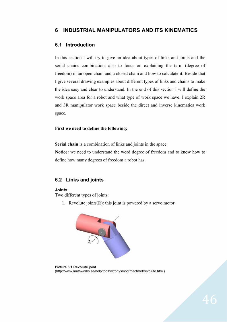
6.2 Links and joints Joints:

Two different types of joints:

1. Revolute joints(R): this joint is powered by a servo motor.

Picture 6.1 Revolute joint

(http://www.mathworks.se/help/toolbox/physmod/mech/ref/revolute.html)

47

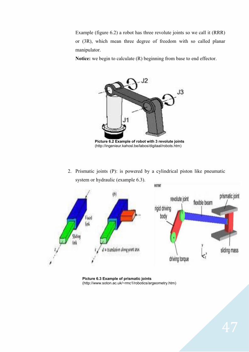
Example (figure 6.2) a robot has three revolute joints so we call it (RRR)

or (3R), which mean three degree of freedom with so called planar

manipulator.

Notice: we begin to calculate (R) beginning from base to end effector.

2. Prismatic joints (P): is powered by a cylindrical piston like pneumatic

system or hydraulic (example 6.3).

Picture 6.2 Example of robot with 3 revolute joints

(http://ingenieur.kahosl.be/labos/digitaal/robots.htm)

Picture 6.3 Example of prismatic joints

(http://www.soton.ac.uk/~rmc1/robotics/argeometry.htm)

48

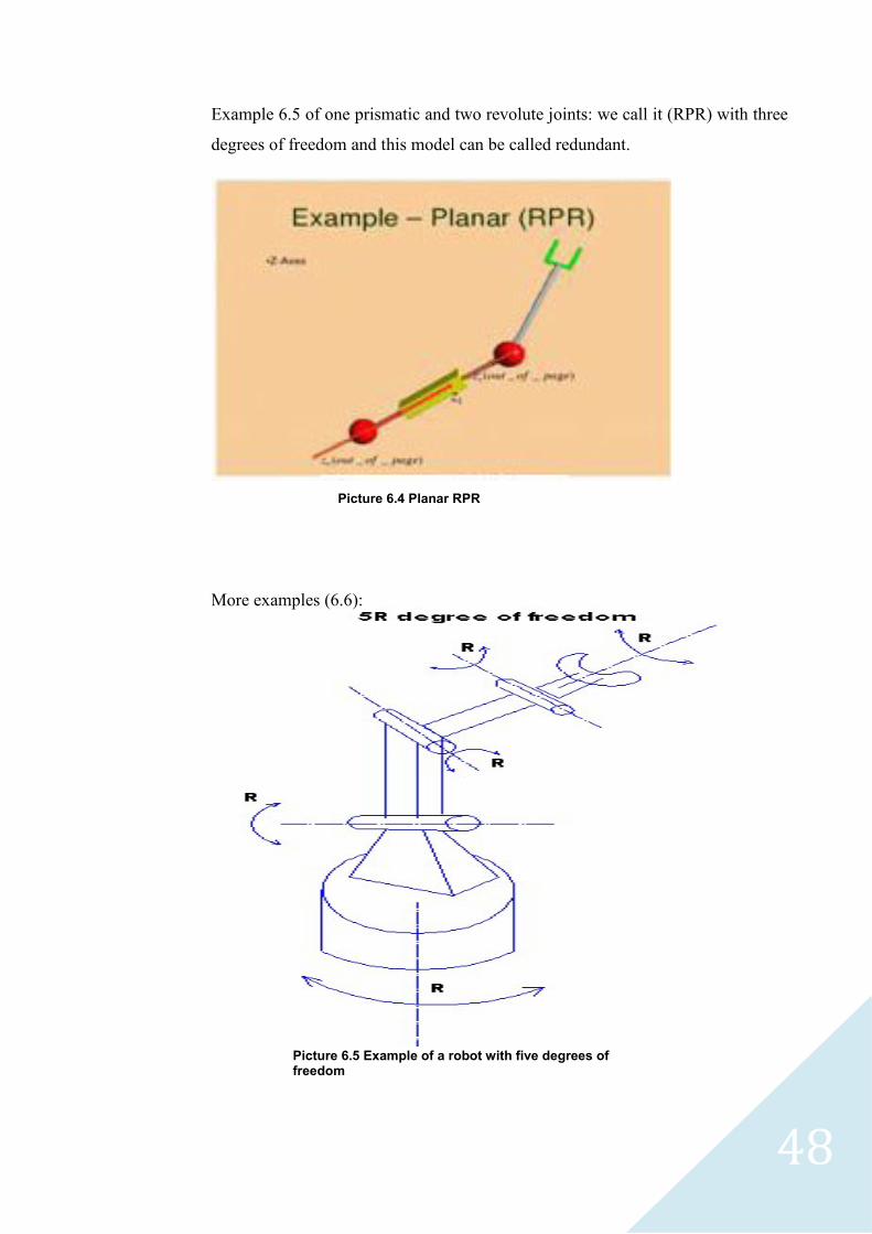
Example 6.5 of one prismatic and two revolute joints: we call it (RPR) with three

degrees of freedom and this model can be called redundant.

More examples (6.6):

Picture 6.4 Planar RPR

Picture 6.5 Example of a robot with five degrees of freedom

49

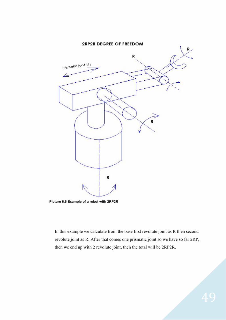
In this example we calculate from the base first revolute joint as R then second

revolute joint as R. After that comes one prismatic joint so we have so far 2RP,

then we end up with 2 revolute joint, then the total will be 2RP2R.

Picture 6.6 Example of a robot with 2RP2R

50

6.3 Degree of freedom

First I need to explain the term degree of freedom (DOF).

When I fix a joint and prevent any movement then I can say that this joint has

zero degree of freedom but when I mount a joint with a motor drive, then it loses

two degrees of freedom and it will have just one degree of freedom because it

moves in one plane.

Notice: in the space there is six degrees of freedom.

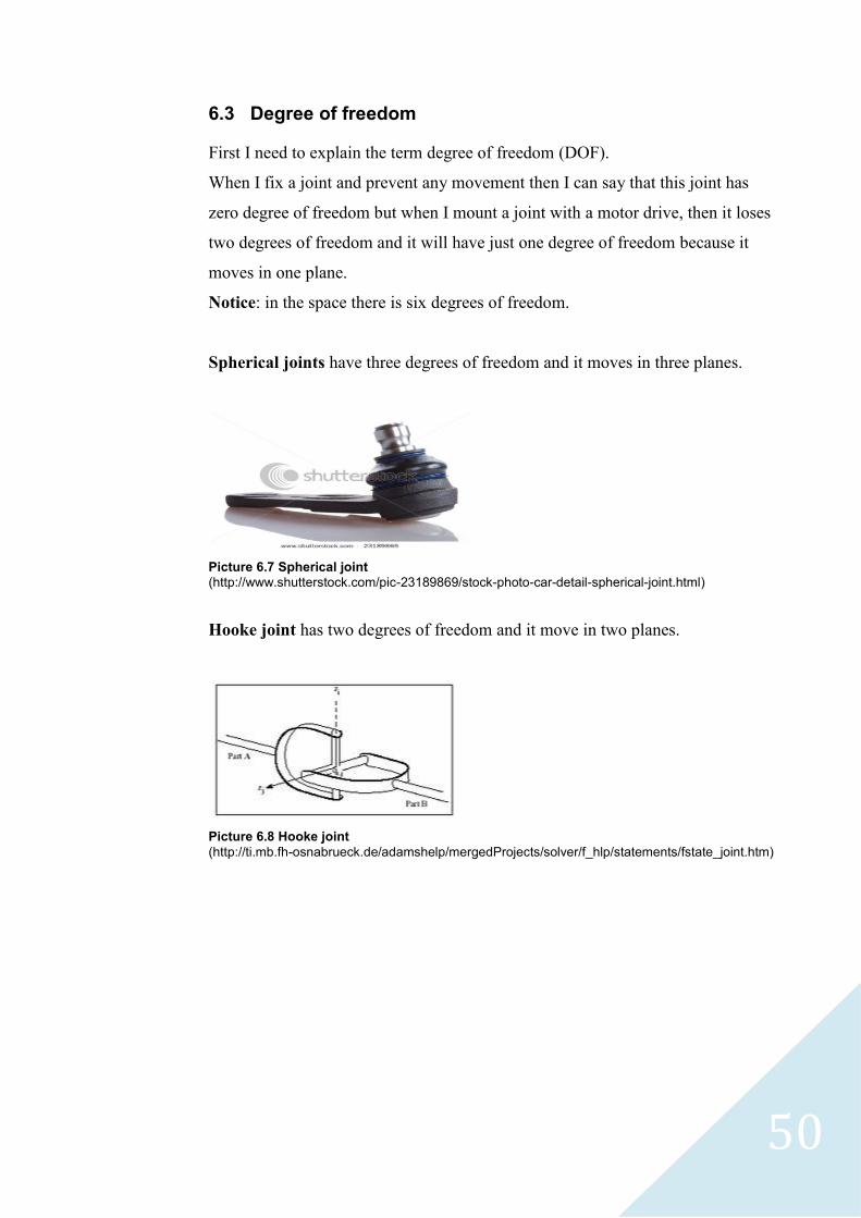
Spherical joints have three degrees of freedom and it moves in three planes.

Picture 6.7 Spherical joint

(http://www.shutterstock.com/pic-23189869/stock-photo-car-detail-spherical-joint.html)

Hooke joint has two degrees of freedom and it move in two planes.

Picture 6.8 Hooke joint

(http://ti.mb.fh-osnabrueck.de/adamshelp/mergedProjects/solver/f_hlp/statements/fstate_joint.htm)

51

6.4 Types of robotic chains

6.5 Degree of freedom in opened chains

Picture 6.9 Example of four degrees of freedom in open chain

In open chains it is easy to calculate how many degrees of freedom. For a robot

just by calculating the rotations axes and prismatic axes. In the example up we

have four revolute joints that means we have four degrees of freedom

6.6 Degree of freedom in closed chains

How to calculate degree of freedom for closed chains?

We need to define how many links, revolute joints and prismatic joints.

degree of freedom= 3(n-1)-2 -2

: Number of revolute joints

: Number of prismatic joints

n: Number of links

52

Example 1

In the example up we calculate degree of freedom this way:

3(5-1)-2(5)-2(0)= 2 dof

Example 2

degree of freedom= 3(n-1)-2 -2

degree of freedom=3(5-1)-2 -2 = 2dof

Picture 6.10 Closed chain

Picture 6.11 Closed chain by a prismatic joint

53

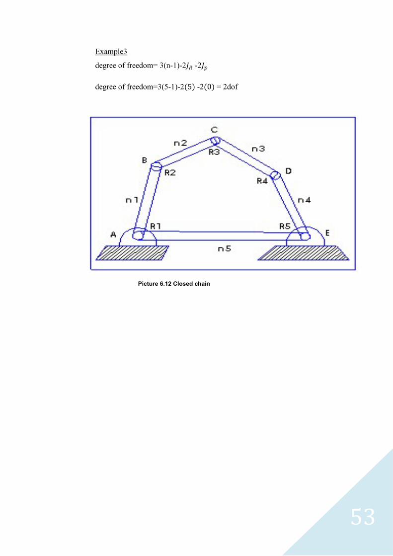
Example3

degree of freedom= 3(n-1)-2 -2

degree of freedom=3(5-1)-2 -2 = 2dof

Picture 6.12 Closed chain

54

Parallel chains

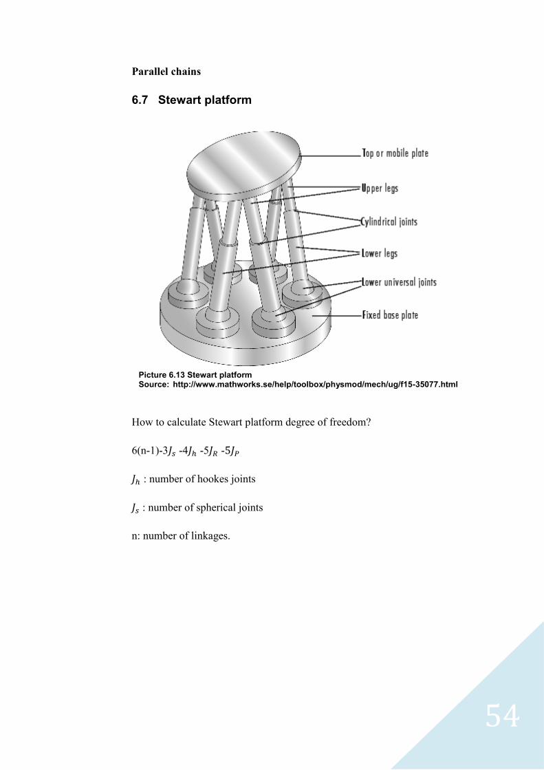
6.7 Stewart platform

How to calculate Stewart platform degree of freedom?

6(n-1)-3 -4 -5 -

: number of hookes joints

: number of spherical joints

n: number of linkages.

Picture 6.13 Stewart platform Source: http://www.mathworks.se/help/toolbox/physmod/mech/ug/f15-35077.html

55

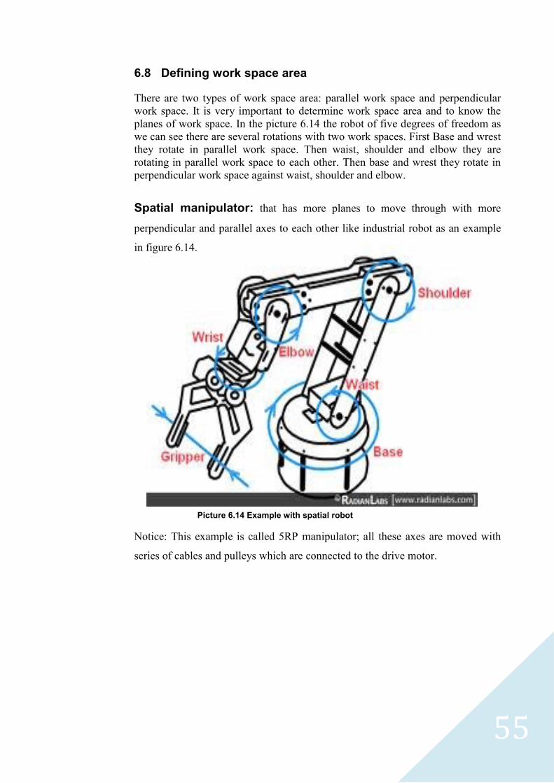
6.8 Defining work space area

There are two types of work space area: parallel work space and perpendicular

work space. It is very important to determine work space area and to know the

planes of work space. In the picture 6.14 the robot of five degrees of freedom as

we can see there are several rotations with two work spaces. First Base and wrest

they rotate in parallel work space. Then waist, shoulder and elbow they are

rotating in parallel work space to each other. Then base and wrest they rotate in

perpendicular work space against waist, shoulder and elbow.

Spatial manipulator: that has more planes to move through with more

perpendicular and parallel axes to each other like industrial robot as an example

in figure 6.14.

Notice: This example is called 5RP manipulator; all these axes are moved with

series of cables and pulleys which are connected to the drive motor.

Picture 6.14 Example with spatial robot

56

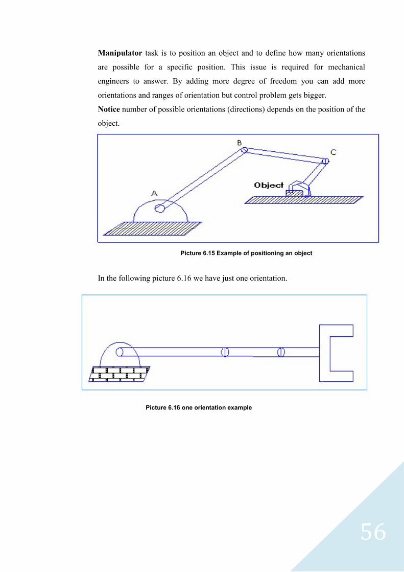
Manipulator task is to position an object and to define how many orientations

are possible for a specific position. This issue is required for mechanical

engineers to answer. By adding more degree of freedom you can add more

orientations and ranges of orientation but control problem gets bigger.

Notice number of possible orientations (directions) depends on the position of the

object.

In the following picture 6.16 we have just one orientation.

Picture 6.15 Example of positioning an object

Picture 6.16 one orientation example

57

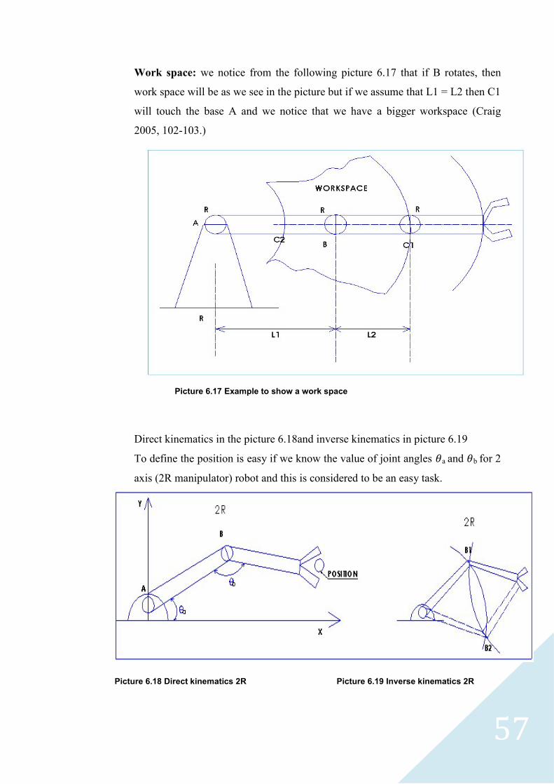
Work space: we notice from the following picture 6.17 that if B rotates, then

work space will be as we see in the picture but if we assume that L1 = L2 then C1

will touch the base A and we notice that we have a bigger workspace (Craig

2005, 102-103.)

Direct kinematics in the picture 6.18and inverse kinematics in picture 6.19

To define the position is easy if we know the value of joint angles a and b for 2

axis (2R manipulator) robot and this is considered to be an easy task.

Picture 6.17 Example to show a work space

Picture 6.18 Direct kinematics 2R

Picture 6.19 Inverse kinematics 2R

58

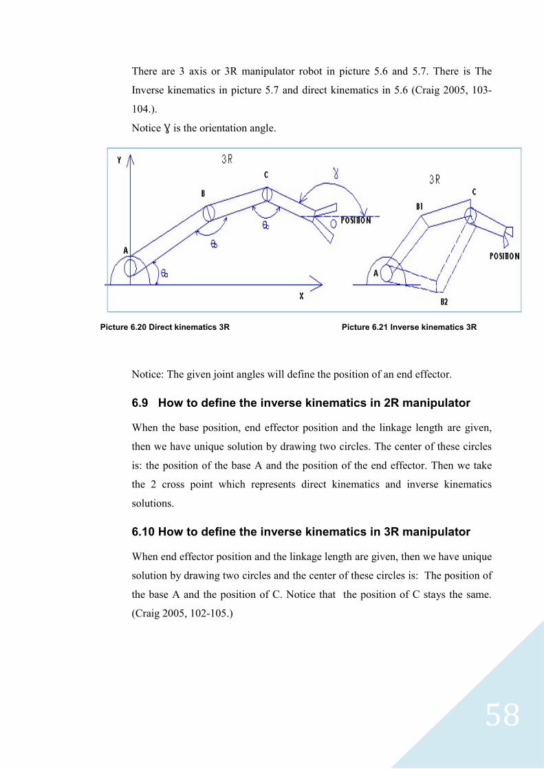
There are 3 axis or 3R manipulator robot in picture 5.6 and 5.7. There is The

Inverse kinematics in picture 5.7 and direct kinematics in 5.6 (Craig 2005, 103-

104.).

Notice is the orientation angle.

Notice: The given joint angles will define the position of an end effector.

6.9 How to define the inverse kinematics in 2R manipulator

When the base position, end effector position and the linkage length are given,

then we have unique solution by drawing two circles. The center of these circles

is: the position of the base A and the position of the end effector. Then we take

the 2 cross point which represents direct kinematics and inverse kinematics

solutions.

6.10 How to define the inverse kinematics in 3R manipulator

When end effector position and the linkage length are given, then we have unique

solution by drawing two circles and the center of these circles is: The position of

the base A and the position of C. Notice that the position of C stays the same.

(Craig 2005, 102-105.)

Picture 6.20 Direct kinematics 3R

Picture 6.21 Inverse kinematics 3R

59

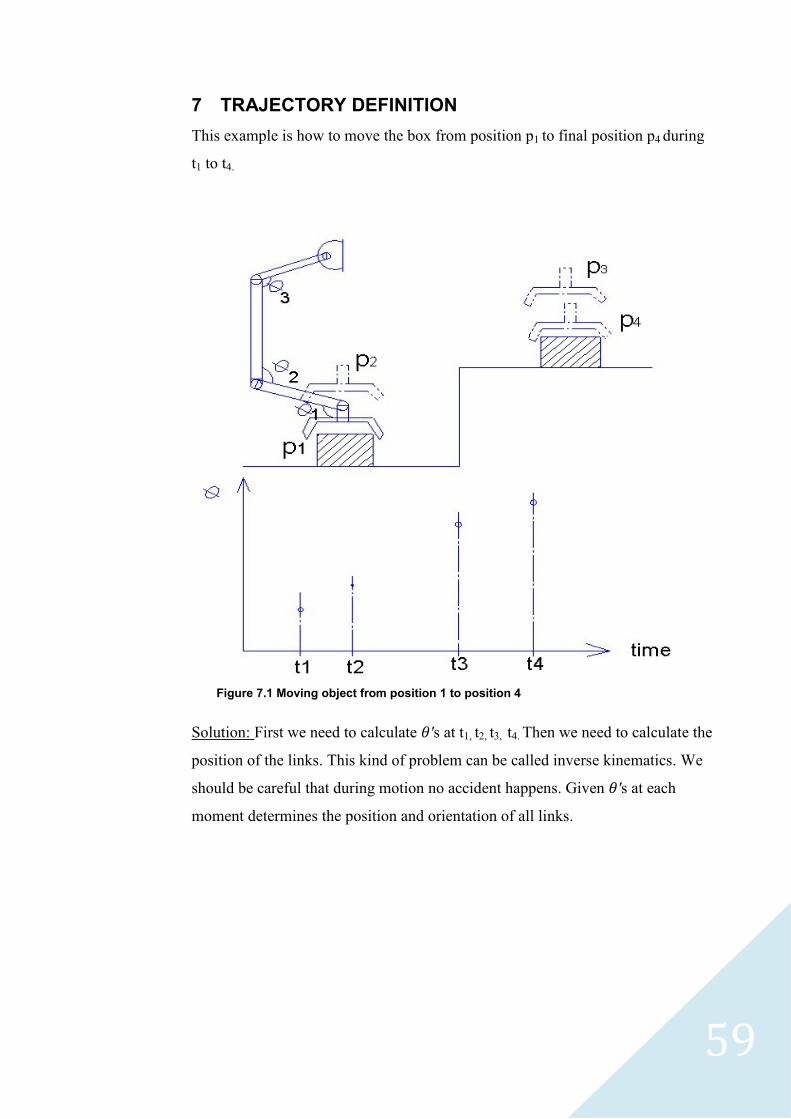
7 TRAJECTORY DEFINITION

This example is how to move the box from position p1 to final position p4 during

t1 to t4.

Solution: First we need to calculate s at t1, t2, t3, t4. Then we need to calculate the

position of the links. This kind of problem can be called inverse kinematics. We

should be careful that during motion no accident happens. Given s at each

moment determines the position and orientation of all links.

Figure 7.1 Moving object from position 1 to position 4

60

7.1 Forward position problem

Fixed parameters of the mechanisms values of joint variables will determine

position and orientations of all links.

7.2 Inverse position problem

Fixed bars of the mechanisms position and orientations of end effector will

determine the values of joint variables.

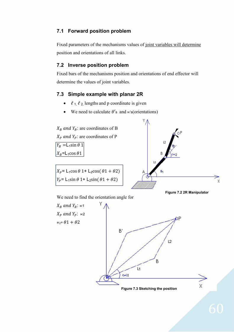
7.3 Simple example with planar 2R

1, 2, lengths and p coordinate is given

We need to calculate s and ’s(orientations)

: are coordinates of B

: are coordinates of P

L1

=L1

= L1 + L2

= L1 + L2

We need to find the orientation angle for

: 1

: 2

2=

Figure 7.2 2R Manipulator

Figure 7.3 Sketching the position

61

To find we use the following formula:

1= atan

– acos(

√

)

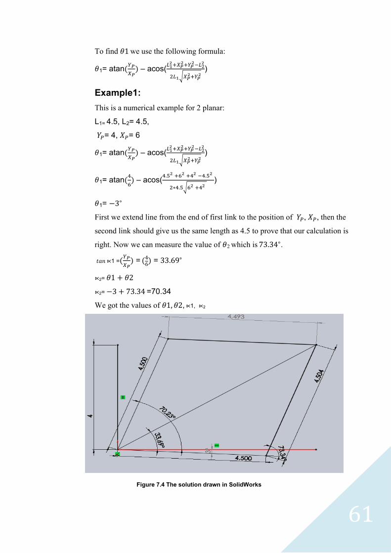
Example1:

This is a numerical example for 2 planar:

L1= 4.5, L2= 4.5,

= 4, = 6

1= atan

– acos(

√

)

1= atan

– acos(

√ )

1=

First we extend line from the end of first link to the position of , , then the

second link should give us the same length as 4.5 to prove that our calculation is

right. Now we can measure the value of 2 which is .

1 =

=

=

2=

2= =70.34

We got the values of , 1, 2

Figure 7.4 The solution drawn in SolidWorks

62

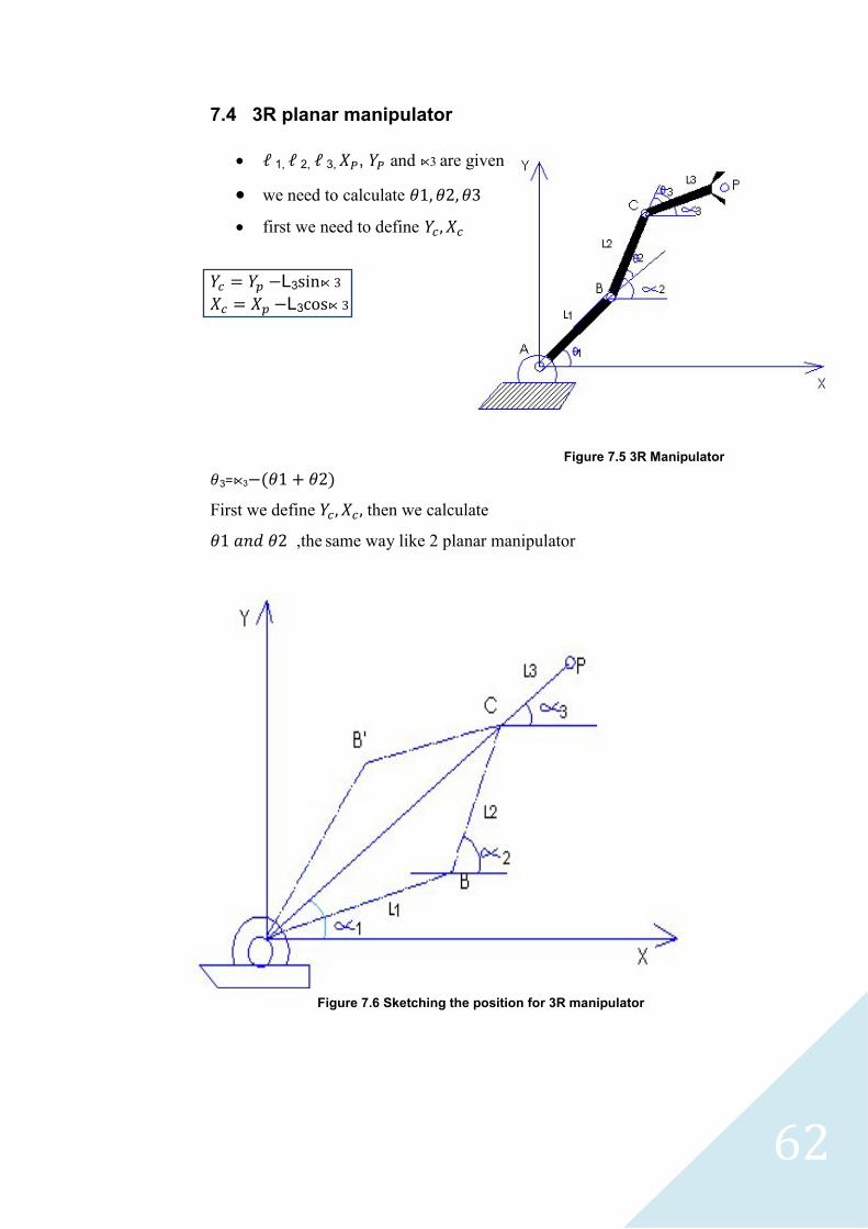
7.4 3R planar manipulator

1, 2, 3, , and 3 are given

we need to calculate

first we need to define

L3

L3

3= 3

First we define then we calculate

,the same way like 2 planar manipulator

Figure 7.5 3R Manipulator

Figure 7.6 Sketching the position for 3R manipulator

63

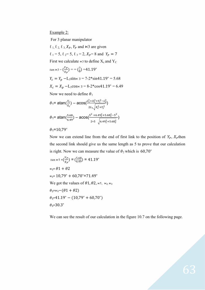
Example 2:

For 3 planar manipulator

1, 2, 3, , and 3 are given

1 = 5, 2= 5, 3 = 2, = 8 and

First we calculate 3 to define Xc and YC

3 =

= =

=

L3 = 7-2*sin = 5.68

L3 = 8-2*cos = 6.49

Now we need to define 1

1= atan

– acos(

√

)

1= atan

– acos(

√

)

1=

Now we can extend line from the end of first link to the position of , then

the second link should give us the same length as 5 to prove that our calculation

is right. Now we can measure the value of 2 which is

1 =

=

=

2=

2= =

We got the values of , 1, 2, 3

3= 3

3=

3=

We can see the result of our calculation in the figure 10.7 on the following page.

64

7.5 Prismatic joints calculation

3p manipulator

We assume according to the following drawing that we have three prismatic

joints which move in 3D space so we just need to find values of S1, S2 and S3.

S1 =

S2 =

S3 =

Figure 7.7 Sketching the position in SolidWorks

Figure 7.8 Prismatic joints manipulator

65

8 POSITION, ORIENTATION, FRAMES

8.1 Introduction

In this section I will try to summarize how to define position coordinate on the

space with respect to the origin frame and to calculate the transformation when

this frame rotates with respect to the base frame.

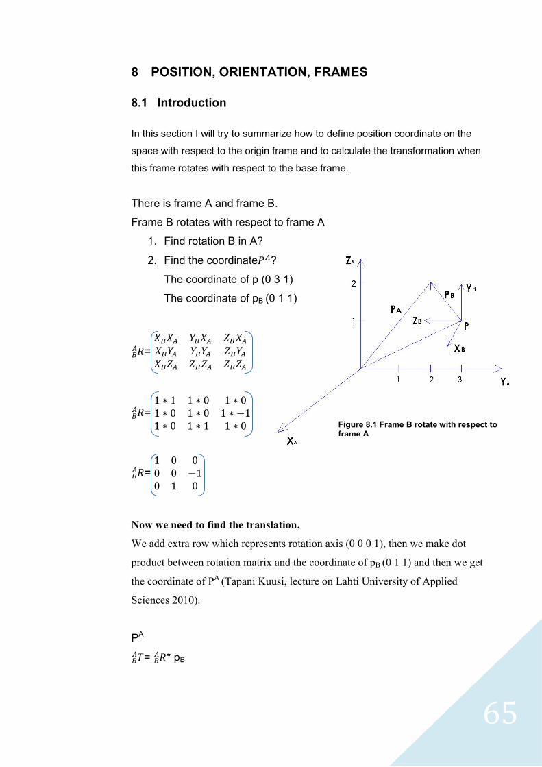
There is frame A and frame B.

Frame B rotates with respect to frame A

1. Find rotation B in A?

2. Find the coordinate ?

The coordinate of p (0 3 1)

The coordinate of pB (0 1 1)

=

=

=

Now we need to find the translation.

We add extra row which represents rotation axis (0 0 0 1), then we make dot

product between rotation matrix and the coordinate of pB (0 1 1) and then we get

the coordinate of PA

(Tapani Kuusi, lecture on Lahti University of Applied

Sciences 2010).

PA

=

* pB

Figure 8.1 Frame B rotate with respect to frame A

66

=

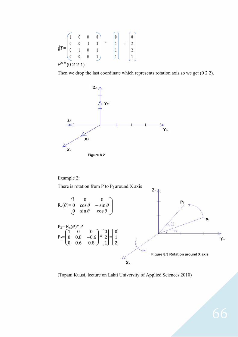
PA = (0 2 2 1)

Then we drop the last coordinate which represents rotation axis so we get (0 2 2).

Example 2:

There is rotation from P to P2 around X axis

Rx( )=

P2= Rx( )* P

P2=

*

=

(Tapani Kuusi, lecture on Lahti University of Applied Sciences 2010)

Figure 8.2

Figure 8.3 Rotation around X axis

67

Example

In the following example frame B rotates with respect to frame A.

We have 3 different rotations.

1. Rotation around X axis which rotates with angle

2. Rotation around y axis which rotates with angle

3. Rotation around z axis which rotates with angle

XYZ( ) )= ( ) * ( ) * ( )

XYZ( ) ) =

Figure 8.4 Rotation axes

(Craig 2005, 42)

68

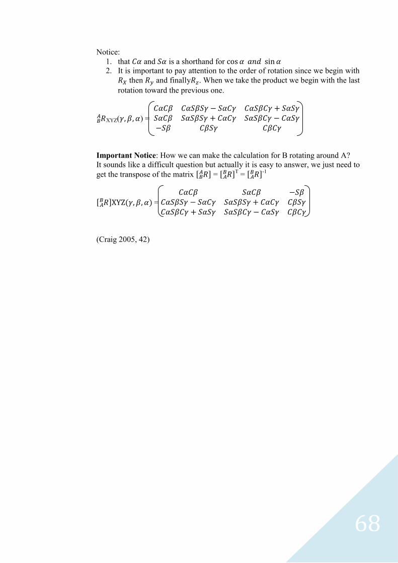
Notice:

1. that and is a shorthand for

2. It is important to pay attention to the order of rotation since we begin with

then and finally . When we take the product we begin with the last

rotation toward the previous one.

XYZ( ) =

Important Notice: How we can make the calculation for B rotating around A?

It sounds like a difficult question but actually it is easy to answer, we just need to

get the transpose of the matrix [ ] = [

]T = [ ]-1

[ ] =

(Craig 2005, 42)

69

8.2 Transformation

We use matrices to transform vectors.

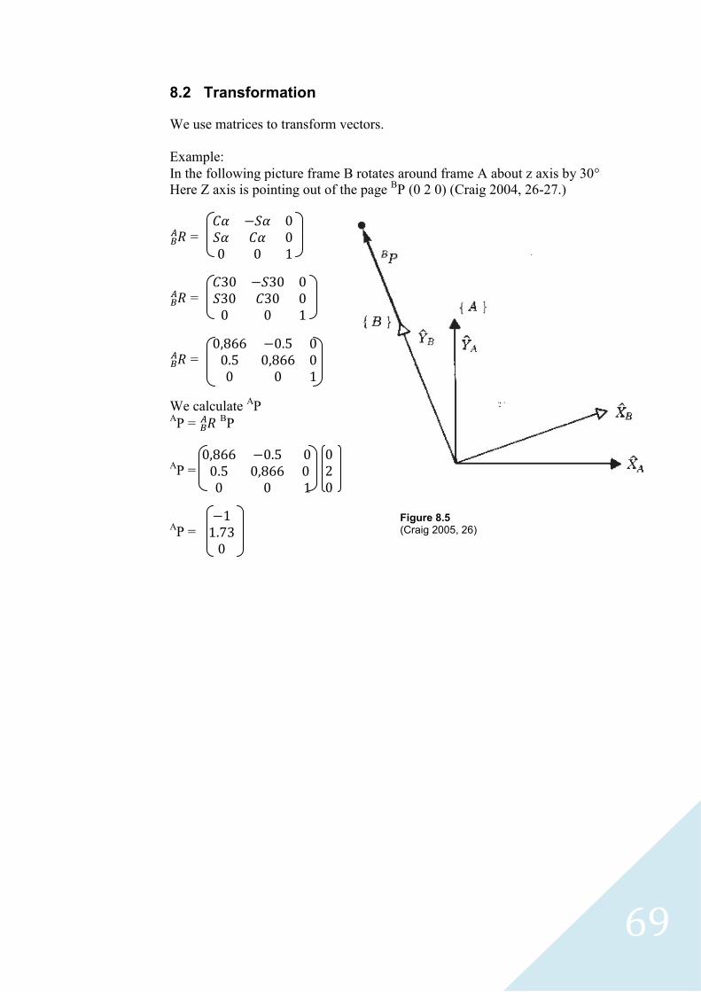
Example:

In the following picture frame B rotates around frame A about z axis by 30

Here Z axis is pointing out of the page BP (0 2 0) (Craig 2004, 26-27.)

=

=

=

We calculate AP

AP =

BP

AP =

AP =

Figure 8.5 (Craig 2005, 26)

70

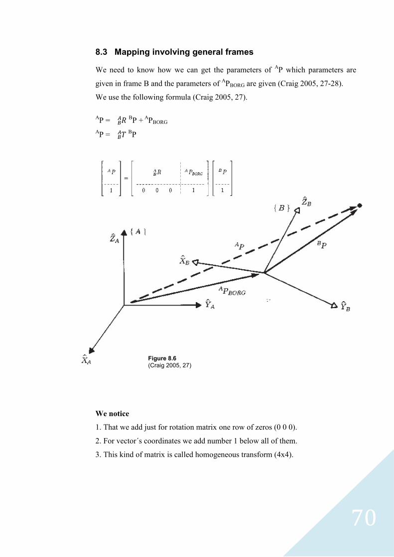
8.3 Mapping involving general frames

We need to know how we can get the parameters of AP which parameters are

given in frame B and the parameters of APBORG are given (Craig 2005, 27-28).

We use the following formula (Craig 2005, 27).

AP =

BP +

APBORG

AP =

BP

We notice

1. That we add just for rotation matrix one row of zeros (0 0 0).

2. For vector´s coordinates we add number 1 below all of them.

3. This kind of matrix is called homogeneous transform (4x4).

Figure 8.6

(Craig 2005, 27)

71

Example:

Frame B has rotated with relative to frame A bout Z axis by 30 degrees and

translated 10 units in XA, and 5 units in Ya.

Find AP where

BP = (3 7 0)

T (Craig 2005, 29).

The definition of frame B is

Given

BP=

AP =

BP

AP =

Figure 8.7

(Craig 2005, 29)

72

8.4 Translation operators

Operator is the same like rotation and translation but the interpretation is

different.

Example of operator:

According to the following picture the vector AP

1 is rotated around Z axis by 30

degrees and translate it 10 units in XA and 5 units in Ya .

Find AP

2 when the coordinate of

AP

1 (3 7 0)

T (Craig 2005, 33).

Solution:

The operator T which performs the rotation and translation is:

Then AP2= T

AP

1

AP2=

AP2=

Figure 8.8

(Craig 2005, 33)

73

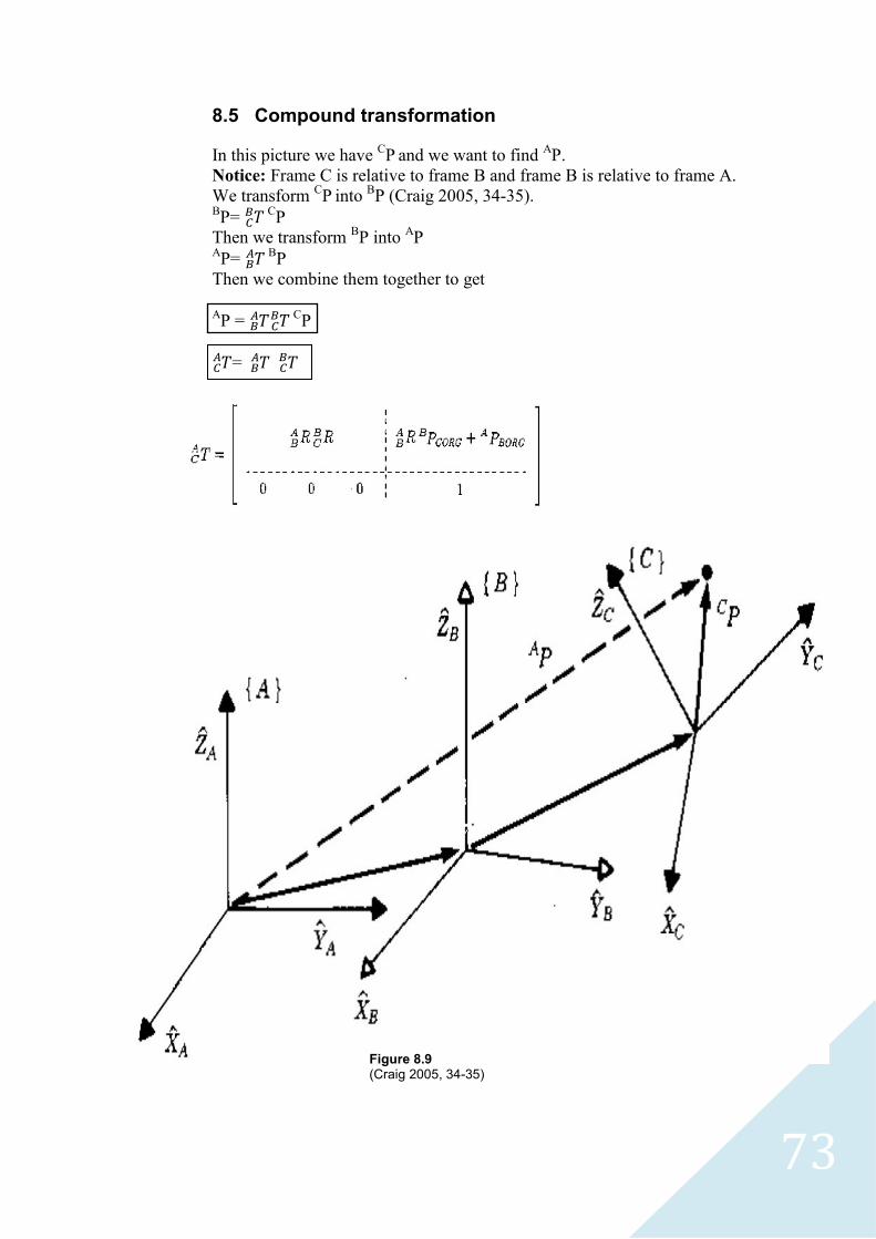
8.5 Compound transformation

In this picture we have CP and we want to find

AP.

Notice: Frame C is relative to frame B and frame B is relative to frame A.

We transform CP into

BP (Craig 2005, 34-35).

BP=

CP

Then we transform BP into

AP

AP=

BP

Then we combine them together to get

AP =

C

P

=

Figure 8.9 (Craig 2005, 34-35)

74

9 TRAJECTORY PLANNING IN ROBOTICS

9.1 Introduction

In this section I will try to cover how to make a path around trajectory, the base

of creating path, what is the required data for creating path and how we can make

the system to choose the speed, also time and acceleration when we just define

the basic required data for trajectory planning.

9.2 Required data for trajectory planning

When we think about trajectory we mainly focus in moving object from position

A to position B.

In trajectory planning we try to define first the following data

Initial point

Final point

Via point: intermediate point between initial and final points.

Point to point planning is a continuous path motion like in welding for example.

How we plan point to point: First we define task specification.

Mapping:

World coordinate

Joint space

Figure 9.1

75

XB 1

YB 2

XB = 1 1 + 2 2 (equation 1)

YB = 1 1 + 2 2 (equation 2)

Given 1, 2 XB , YB (linear algebra)

So we need to define the value of 1 , 2 to achieve certain position in B.

1, 2 are given.

Given to find 1, 2 (nonlinear algebra)

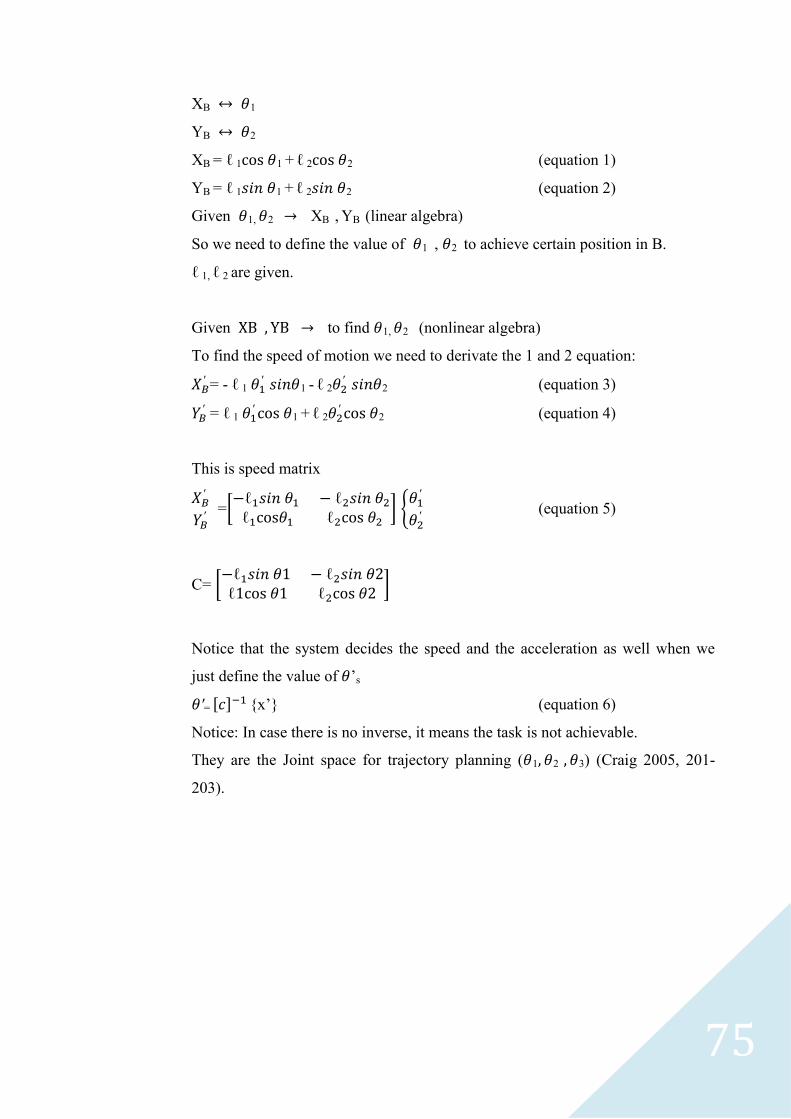
To find the speed of motion we need to derivate the 1 and 2 equation:

= - 1

1 - 2 2 (equation 3)

= 1 1 + 2

2 (equation 4)

This is speed matrix

=[

] {

(equation 5)

C= [

]

Notice that the system decides the speed and the acceleration as well when we

just define the value of ’s

= [ ] {x’} (equation 6)

Notice: In case there is no inverse, it means the task is not achievable.

They are the Joint space for trajectory planning ( 1 2 3) (Craig 2005, 201-

203).

76

9.3 Constraints

In order to make smooth motion we need to put some constraints between via

points

max (acceleration)

Torque

Robot should Move from initial points to final points through via points because

of intermediate point (obstacles) within specified duration of time.

9.4 Subject to constraints

joint space trajectory planning

single joint revolute (t)

move position initial i to final position

i= i , i’ , i’’

j= j, j’, j’’

9.5 Cubic polynomials

Ʈ : Local time frame

Tij: the duration time

From i j

Ʈ 0 : Tij

(Ʈ)= C0 + C1 Ʈ +C2 Ʈ2+ C3 Ʈ

3……….+ Cn Ʈ

n (equation 7)

C: velocity

Specified i , i’, j, j’

Specified i , i’, i’’, j, j’, j’’

Figure 9.2

77

we have 6 coefficients C0- C5

Case:

(Ʈ)= C0 + C1 Ʈ +C2 Ʈ2+ C3 Ʈ

3

(0)= i i = i’

(Tij)= j (Tij) = j’

i = C0 (Ʈ)= C0 + C1 Ʈ +C2 Ʈ2+ C3 Ʈ

3

i’ = C1 (Ʈ)= C1 + 2C2 Ʈ +3C3 Ʈ2

(equation 8)

j = C0 + C1 Tij +C2 Tij 2

+ C3 Tij 3

(equation 9)

j’ = C1 + 2C2 Tij +3C3 Tij 2

(equation 10)

C2 =

( j- i) (equation 11)

C3=

j- i) (equation 12)

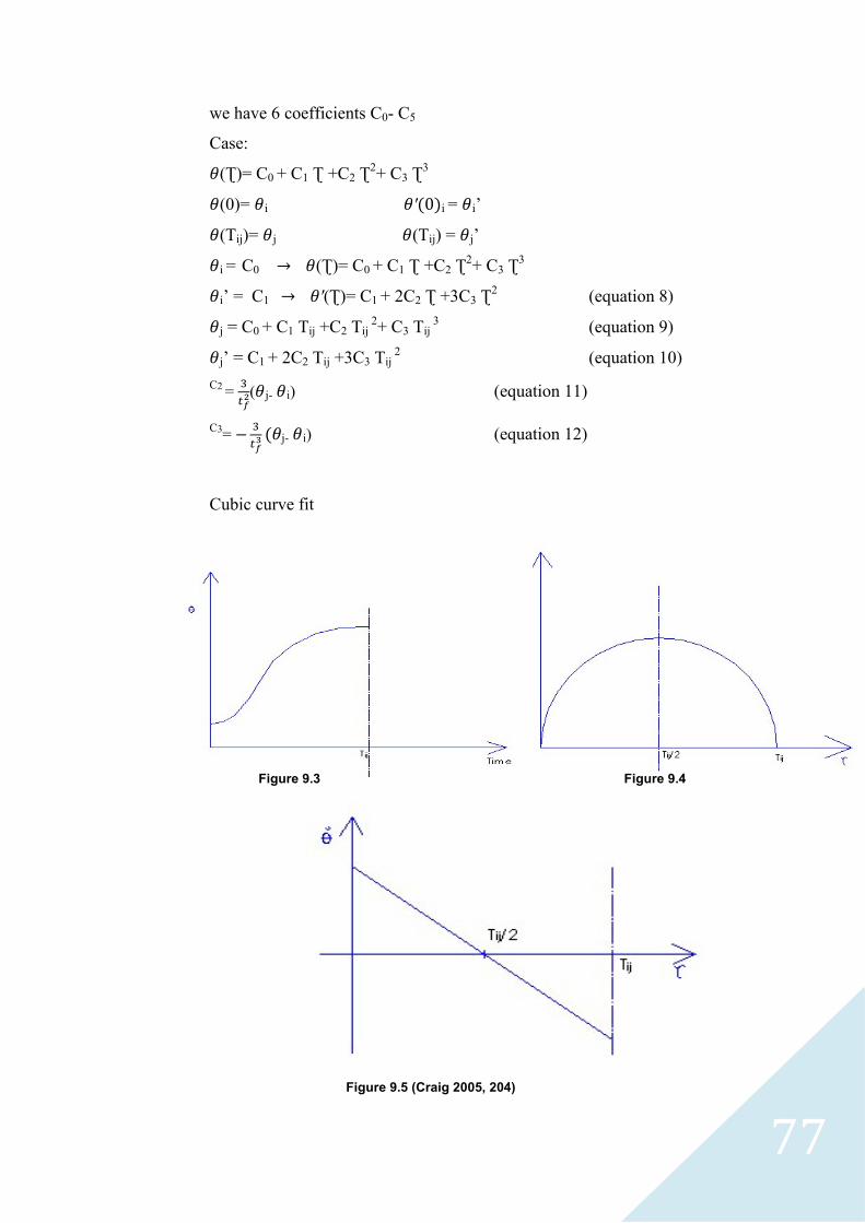
Cubic curve fit

Figure 9.3

Figure 9.4

Figure 9.5 (Craig 2005, 204)

78

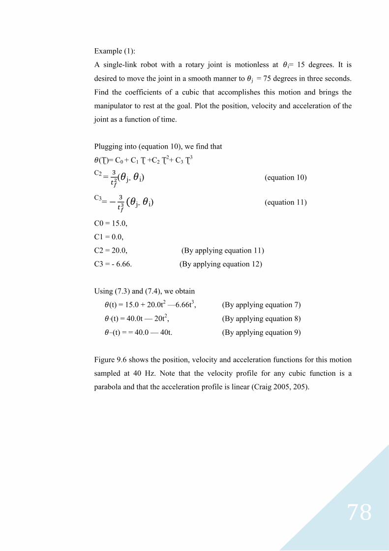
Example (1):

A single-link robot with a rotary joint is motionless at i= 15 degrees. It is

desired to move the joint in a smooth manner to j = 75 degrees in three seconds.

Find the coefficients of a cubic that accomplishes this motion and brings the

manipulator to rest at the goal. Plot the position, velocity and acceleration of the

joint as a function of time.

Plugging into (equation 10), we find that

(Ʈ)= C0 + C1 Ʈ +C2 Ʈ2+ C3 Ʈ

3

C2 =

( j- i) (equation 10)

C3=

j- i) (equation 11)

C0 = 15.0,

C1 = 0.0,

C2 = 20.0, (By applying equation 11)

C3 = - 6.66. (By applying equation 12)

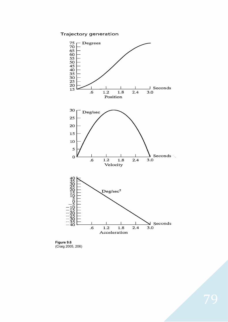
Using (7.3) and (7.4), we obtain

(t) = 15.0 + 20.0t2 —6.66t

3, (By applying equation 7)

’(t) = 40.0t — 20t2, (By applying equation 8)

’’(t) = = 40.0 — 40t. (By applying equation 9)

Figure 9.6 shows the position, velocity and acceleration functions for this motion

sampled at 40 Hz. Note that the velocity profile for any cubic function is a

parabola and that the acceleration profile is linear (Craig 2005, 205).

79

Figure 9.6

(Craig 2005, 206)

80

User specify n+2

Final position

Position velocity

User has to give Cartesian data and large data which is kinematically consistent:

Another constraints user interface must be simple

Task space Joint space

Initial position Final position

i j

i’ j’

‘n’ via point

(n+2) position/velocity data

User should specify the following for creating trajectory:

Initial position

Final position

Via points

Notice: Position specifies velocity to be chosen by the system.

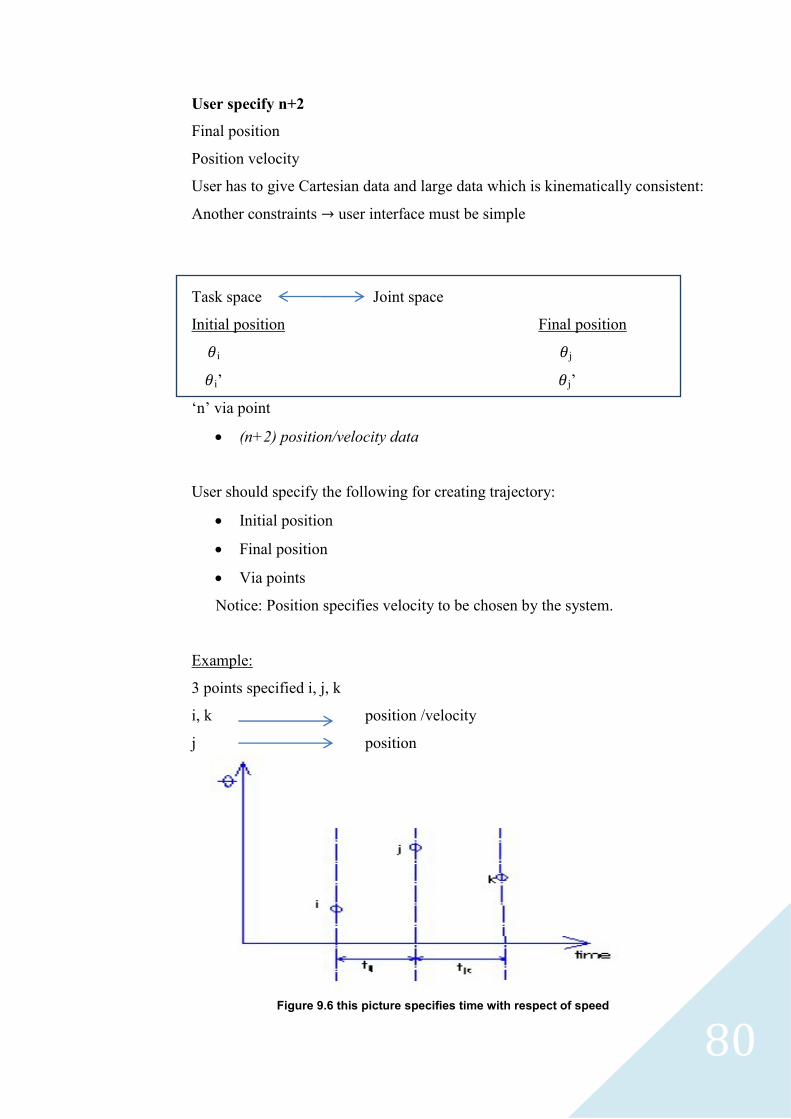
Example:

3 points specified i, j, k

i, k position /velocity

j position

Figure 9.6 this picture specifies time with respect of speed

81

Two cubic curves (segment)

i j j k

(Ʈ)= C0 + C1 Ʈ +C2 Ʈ2+ C3 Ʈ

3 (Ʈ)= b0 + b1 Ʈ +b2 Ʈ2+ b3 Ʈ

3

Ʈ : 0 tij Ʈ : 0 tjk

(0)= i (0)= j

(0)= i (tjk)= k

(tij)= j (tjk)= k

at j:

Continuity of velocity and acceleration

(Ʈ)= C0 + C1 Ʈ +C2 Ʈ2+ C3 Ʈ

3 ij

(Ʈ)= C1 + 2C2 Ʈ +3C3 Ʈ2

(Ʈ)= 2C2 + 6C3Ʈ

at jk:

(Ʈ)= b0 + b1 Ʈ +b2 Ʈ2+ b3 Ʈ

3 jk

(Ʈ)= b1 + 2b2 Ʈ +3b3 Ʈ2

(Ʈ)= 2b2 + 6b3Ʈ

Velocity continues at j

C1 + 2C2 tij+3C3(tij) 2

= b1 (Craig 2005, 208-210.)

2C2 +6C3(tij) = 2b2

We have 8 equations with 8 coefficients.

82

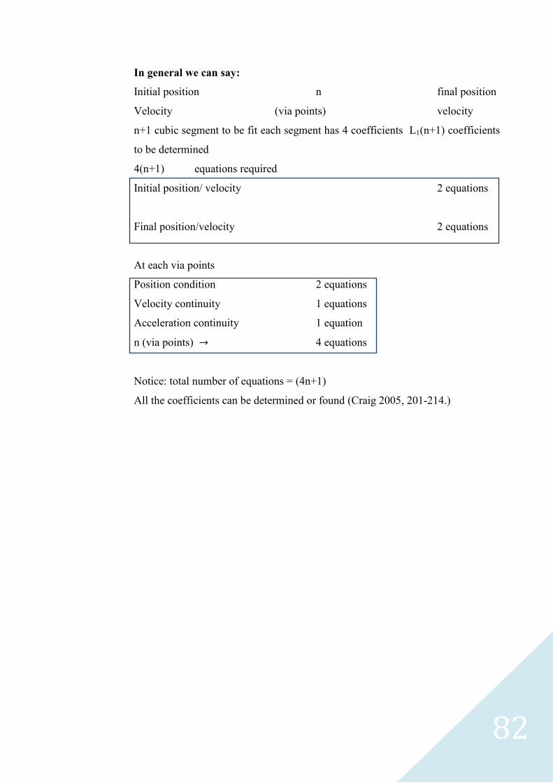
In general we can say:

Initial position n final position

Velocity (via points) velocity

n+1 cubic segment to be fit each segment has 4 coefficients L1(n+1) coefficients

to be determined

4(n+1) equations required

Initial position/ velocity 2 equations

Final position/velocity

2 equations

At each via points

Position condition 2 equations

Velocity continuity 1 equations

Acceleration continuity 1 equation

n (via points) 4 equations

Notice: total number of equations = (4n+1)

All the coefficients can be determined or found (Craig 2005, 201-214.)

83

9.6 Why to use cubic segment?

Lowest degree polynomial that ensure velocity and acceleration

continuity is guaranteed

Easy to work with

We can use lower or higher polynomial also.

Move from position

’ ’ ’ ’

We notice that we have six coefficients

Example: pick and place application

There are three points:

1. initial position ( )

2. left up position (L)

3. set down position (s)

4. final position ( )

For individual joint:

Figure 9.7

Figure 9.8

84

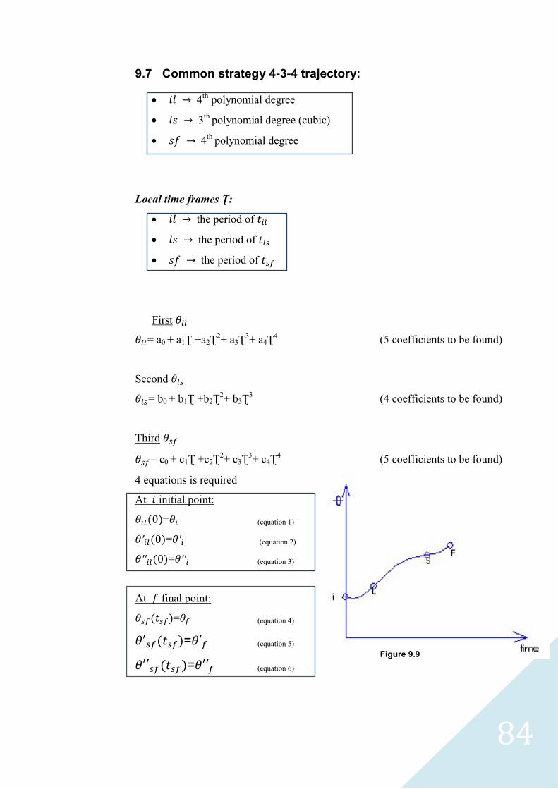
9.7 Common strategy 4-3-4 trajectory:

4th polynomial degree

3th polynomial degree (cubic)

4th polynomial degree

Local time frames Ʈ:

the period of

the period of

the period of

First

= a0 + a1Ʈ +a2Ʈ2+ a3Ʈ

3+ a4Ʈ

4 (5 coefficients to be found)

Second

= b0 + b1Ʈ +b2Ʈ2+ b3Ʈ

3 (4 coefficients to be found)

Third

= c0 + c1Ʈ +c2Ʈ2+ c3Ʈ

3+ c4Ʈ

4 (5 coefficients to be found)

4 equations is required

At initial point:

= (equation 1)

= (equation 2)

= (equation 3)

At final point:

= (equation 4)

= (equation 5)

= (equation 6)

Figure 9.9

85

At left up point: = (equation 7) = (equation 8) = (0) (equation 9/ velocity)

= (0) (equation 10/ acceleration

At set down point: = (equation 11) = (equation 12)

= (0) (equation 13/ velocity)

= (0) (equation 14/ acceleration)

Notice: all the coefficients of 4-3-4 trajectory can be found.

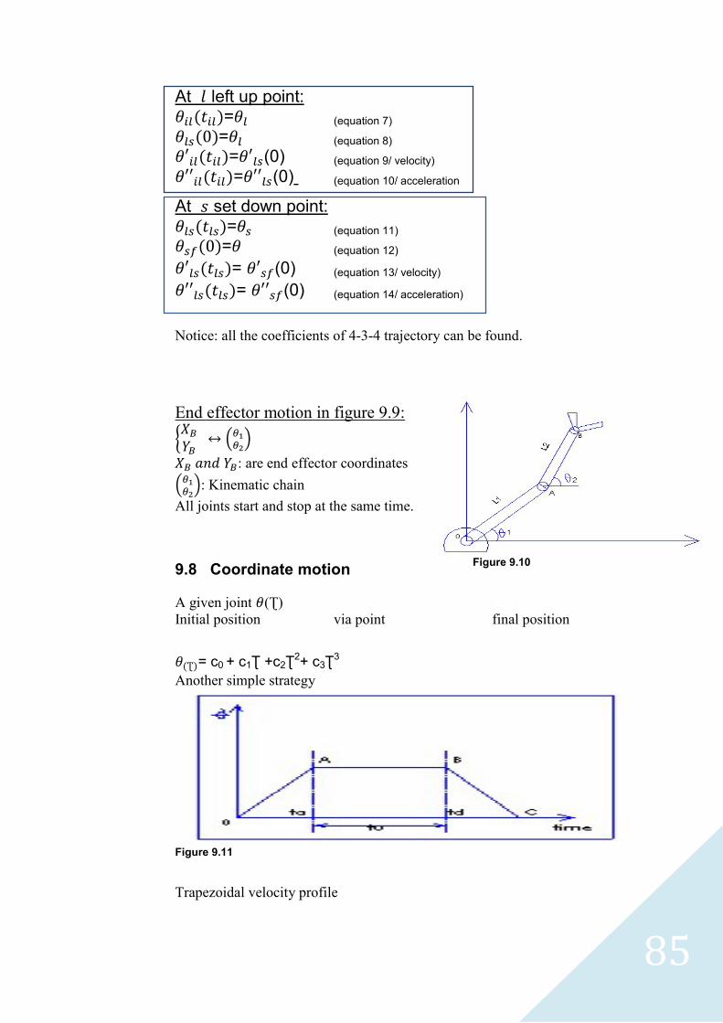
End effector motion in figure 9.9:

{

( )

: are end effector coordinates

( ): Kinematic chain

All joints start and stop at the same time.

9.8 Coordinate motion

A given joint (Ʈ)

Initial position via point final position

= c0 + c1Ʈ +c2Ʈ2+ c3Ʈ

3

Another simple strategy

Figure 9.11

Trapezoidal velocity profile

Figure 9.10

86

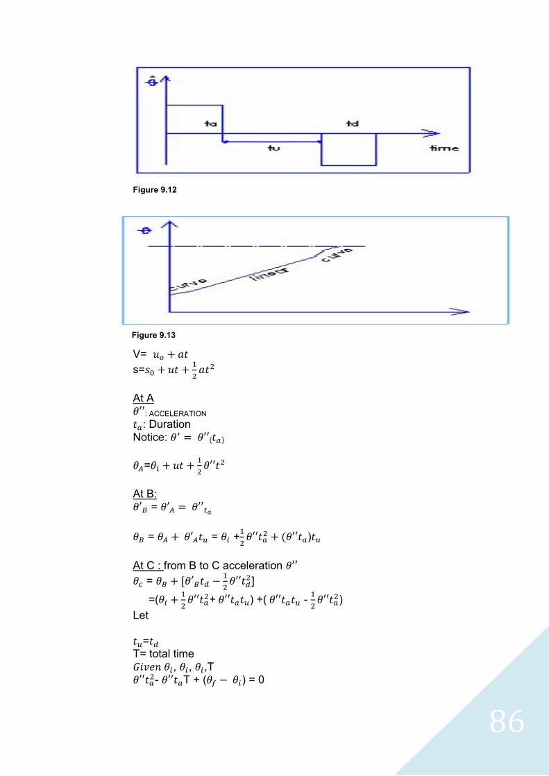
Figure 9.12

V=

s=

At A

: ACCELERATION

: Duration Notice: ( )

=

At B: =

= = +

)

At C : from B to C acceleration

= [

]

=(

+ ) +( -

)

Let

= T= total time

, , ,T

- T + ( ) = 0

Figure 9.13

87

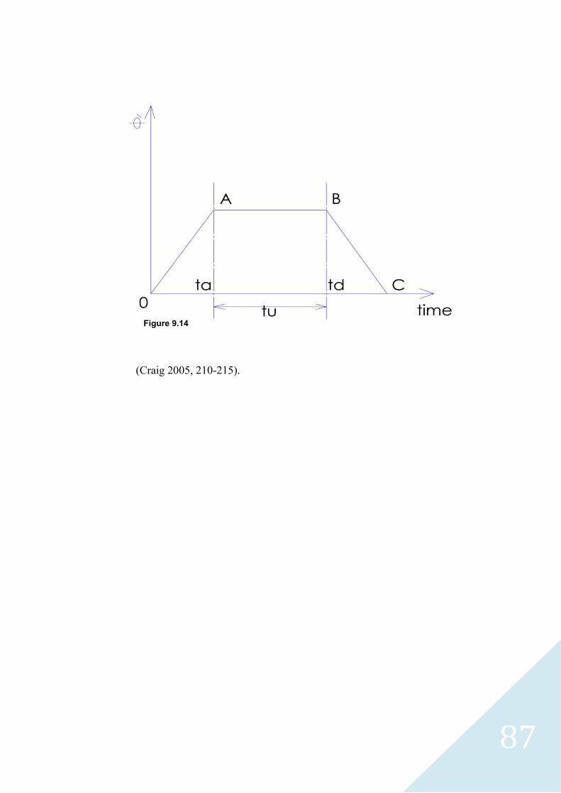
(Craig 2005, 210-215).

Figure 9.14

88

10 Attachment 1

1 TRAJECTORY PLANNING BY USING ROBOT STUDIO

1.1 Introduction

In this section I will try to give brief introduction about how we can create path

using robot studio through using simulation and virtual flex pendant since they

are two different ways, so I will try to explain each way separately beside give

introduction about how we can choose from ABB Library geometry and tools and

how we can set their position in robot environment.

1.2 Creating new station and saving it

First we need to choose any robot type by clicking ABB library (watch

picture 1).

‘

Picture 1 (robot studio screenshot)

How to open new station and to choose robot from ABB library

89

Select the Icon import library then select equipment then you go down and

select any tool by clicking any tool for example I will choose any end effector

tool from the library (watch picture 2).

Picture 2 (robot studio screenshot)

How to select from ABB library end effector tool and some other geometry

End effector tools

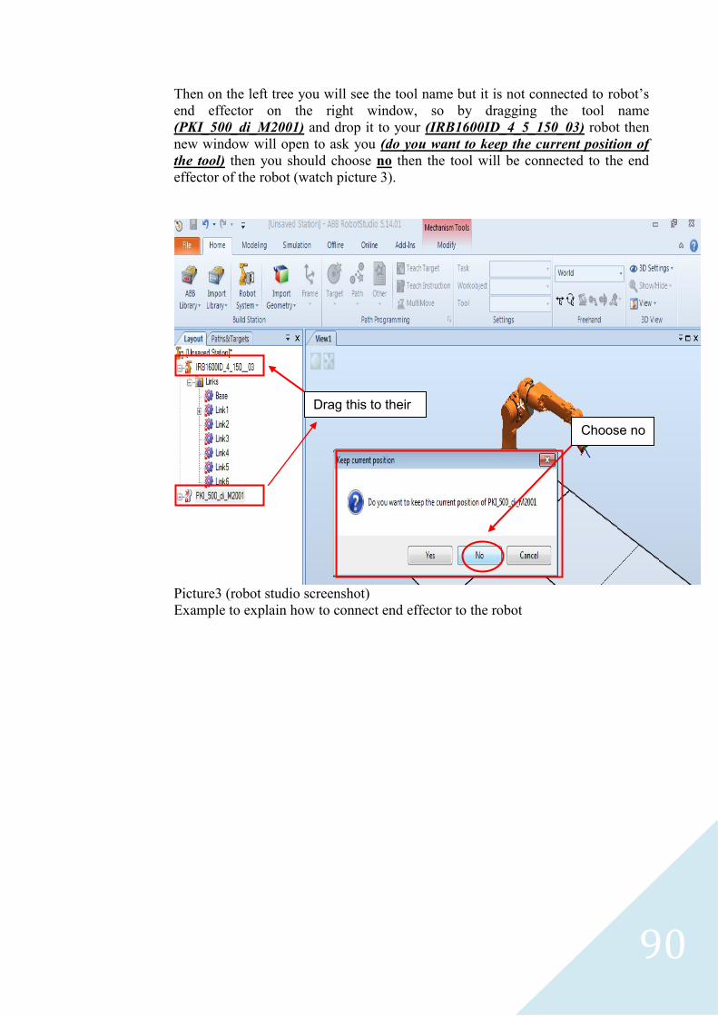
90

Then on the left tree you will see the tool name but it is not connected to robot’s

end effector on the right window, so by dragging the tool name

(PKI_500_di_M2001) and drop it to your (IRB1600ID_4_5_150_03) robot then

new window will open to ask you (do you want to keep the current position of

the tool) then you should choose no then the tool will be connected to the end

effector of the robot (watch picture 3).

Picture3 (robot studio screenshot)

Example to explain how to connect end effector to the robot

Drag this to their

Choose no

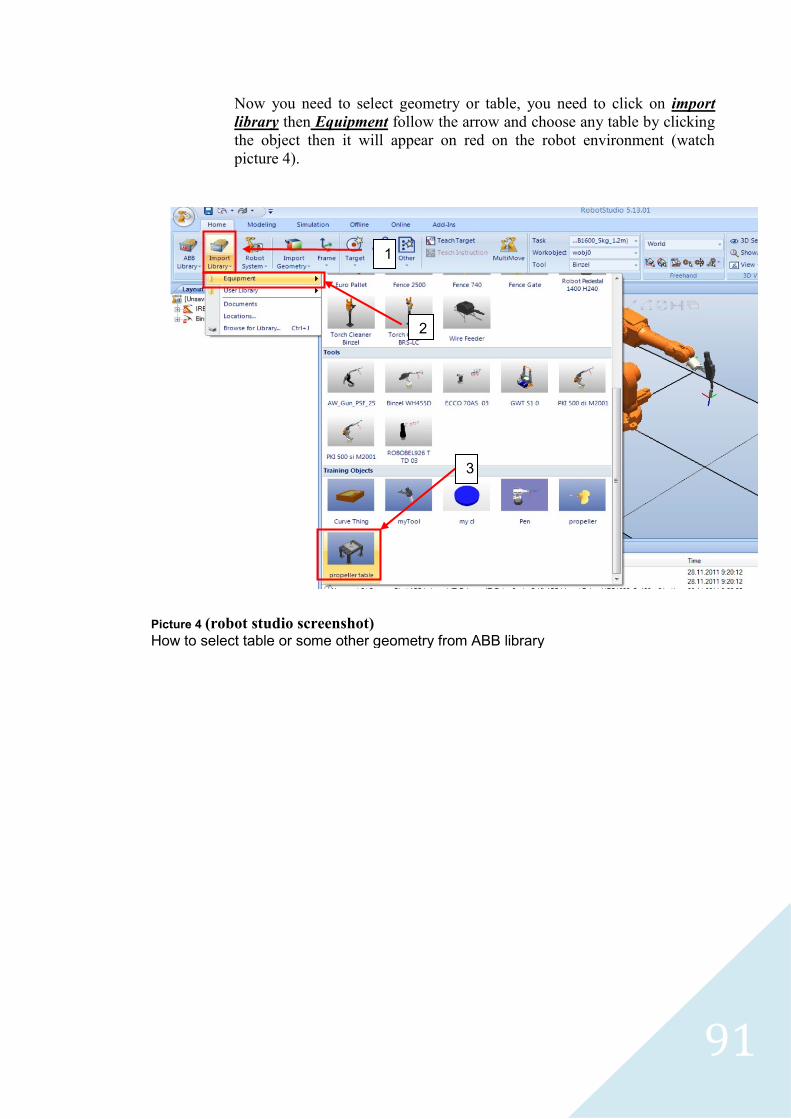
91

Now you need to select geometry or table, you need to click on import

library then Equipment follow the arrow and choose any table by clicking

the object then it will appear on red on the robot environment (watch

picture 4).

Picture 4 (robot studio screenshot)

How to select table or some other geometry from ABB library

1

2

3

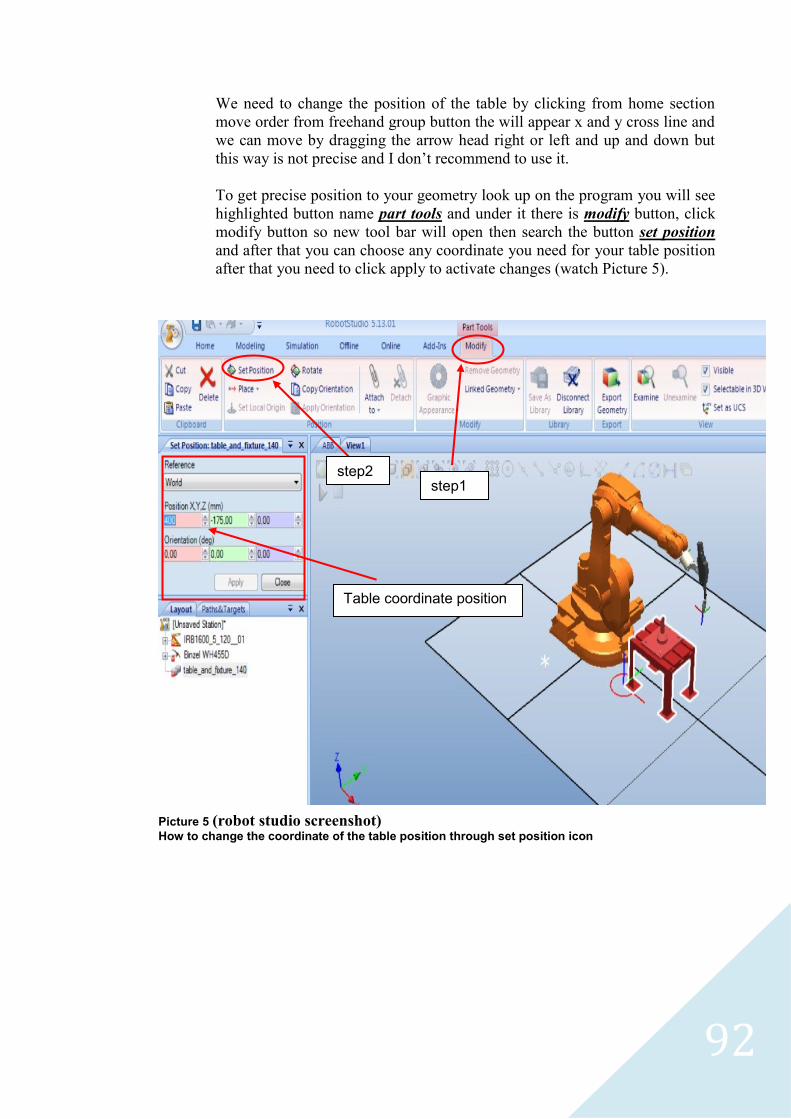
92

We need to change the position of the table by clicking from home section

move order from freehand group button the will appear x and y cross line and

we can move by dragging the arrow head right or left and up and down but

this way is not precise and I don’t recommend to use it.

To get precise position to your geometry look up on the program you will see

highlighted button name part tools and under it there is modify button, click

modify button so new tool bar will open then search the button set position

and after that you can choose any coordinate you need for your table position

after that you need to click apply to activate changes (watch Picture 5).

step1 step2

Table coordinate position

Picture 5 (robot studio screenshot)

How to change the coordinate of the table position through set position icon

93

Now you need to save the station by clicking up in the left side corner by

selecting save as then new window will open to rename your station and to select

where to save your station.

Picture 6 (robot studio screenshot)

How to save new station

Picture 7 (robot studio screenshot)

Giving a name the station and to choose location on the computer to save it.

Step1

Step2

Step 3

94

1.3 Moving robot joint space

Firstly we make right click on the robot tree on the left side on layout

section then we have several options and from these options we have

jump home which return robot to default position but you need to focus

also on using mechanism joint log and mechanism linear jog beside the

free hand option.

Step 3

Picture 8 (robot studio screenshot)

Right click on IRB robot so we get the option we need

Joint space manipulator

Right click on robot tree

You can move robot joint space from here also.

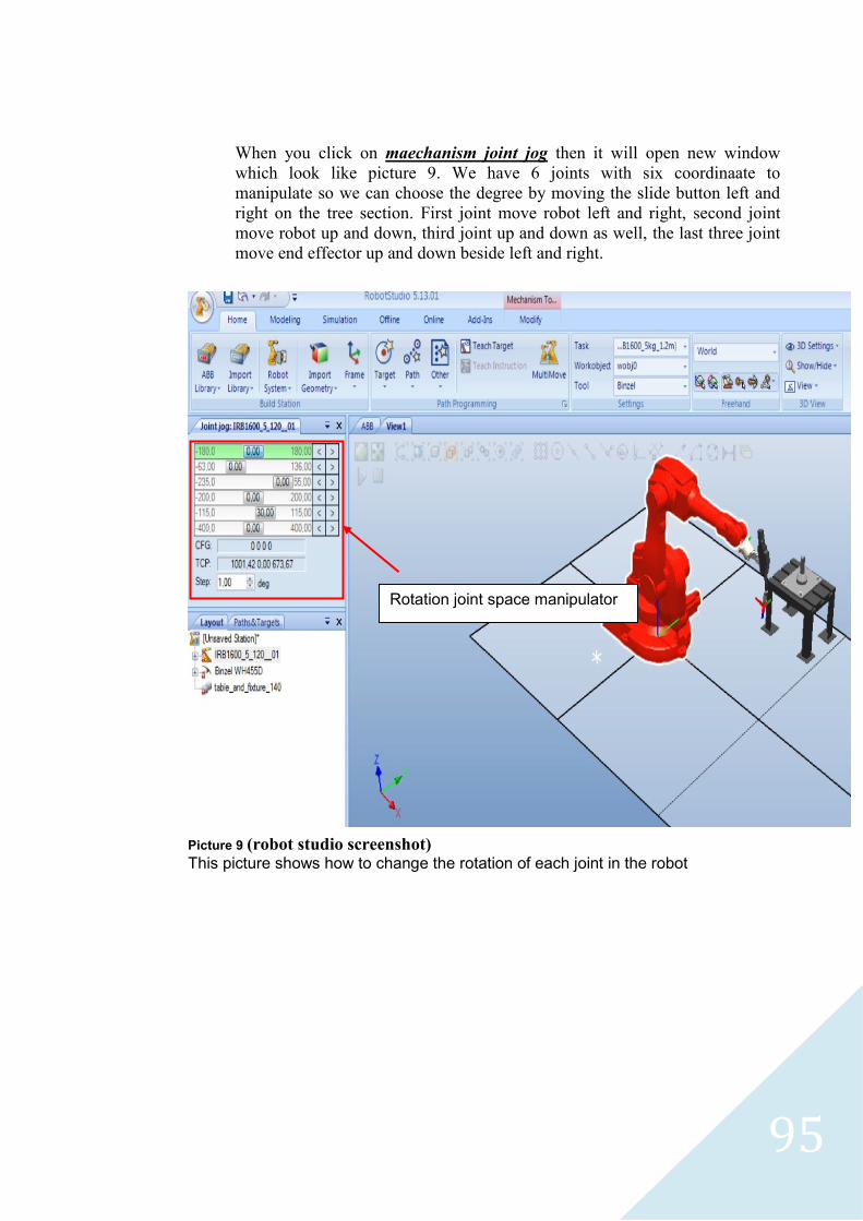
95

When you click on maechanism joint jog then it will open new window

which look like picture 9. We have 6 joints with six coordinaate to

manipulate so we can choose the degree by moving the slide button left and

right on the tree section. First joint move robot left and right, second joint

move robot up and down, third joint up and down as well, the last three joint

move end effector up and down beside left and right.

Picture 9 (robot studio screenshot)

This picture shows how to change the rotation of each joint in the robot

Rotation joint space manipulator

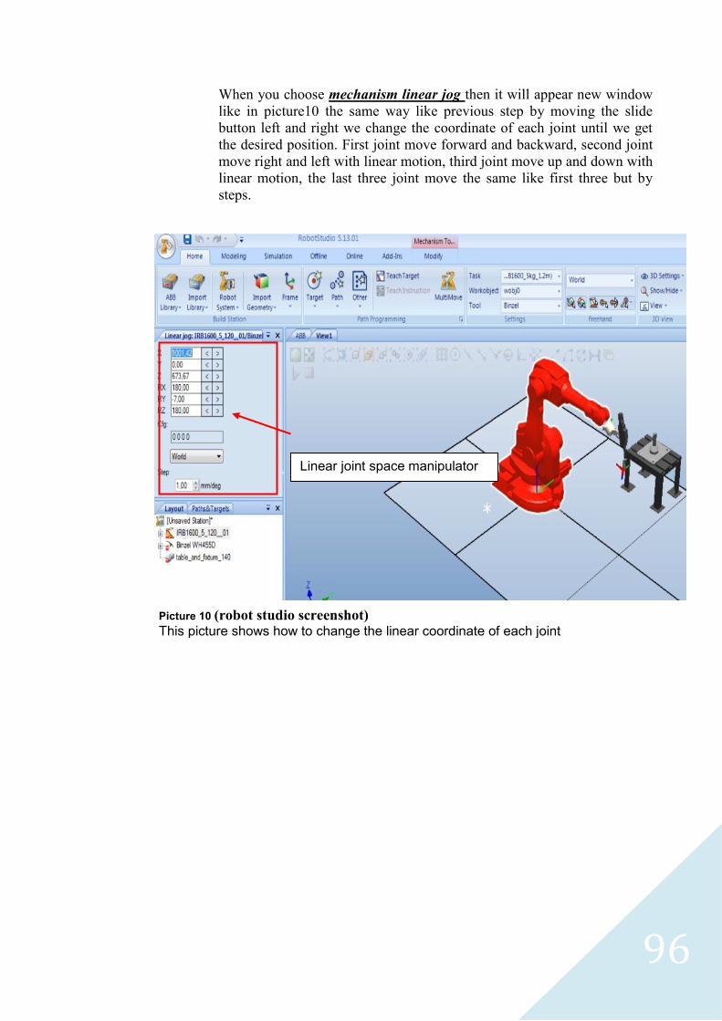
96

When you choose mechanism linear jog then it will appear new window

like in picture10 the same way like previous step by moving the slide

button left and right we change the coordinate of each joint until we get

the desired position. First joint move forward and backward, second joint

move right and left with linear motion, third joint move up and down with

linear motion, the last three joint move the same like first three but by

steps.

Picture 10 (robot studio screenshot)

This picture shows how to change the linear coordinate of each joint

Linear joint space manipulator

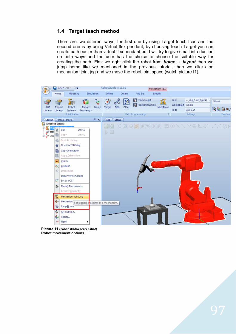
97

1.4 Target teach method There are two different ways, the first one by using Target teach Icon and the second one is by using Virtual flex pendant, by choosing teach Target you can create path easier than virtual flex pendant but I will try to give small introduction on both ways and the user has the choice to choose the suitable way for

creating the path. First we right click the robot from home layout then we jump home like we mentioned in the previous tutorial, then we clicks on mechanism joint jog and we move the robot joint space (watch picture11).

Picture 11 (robot studio screenshot) Robot movement options

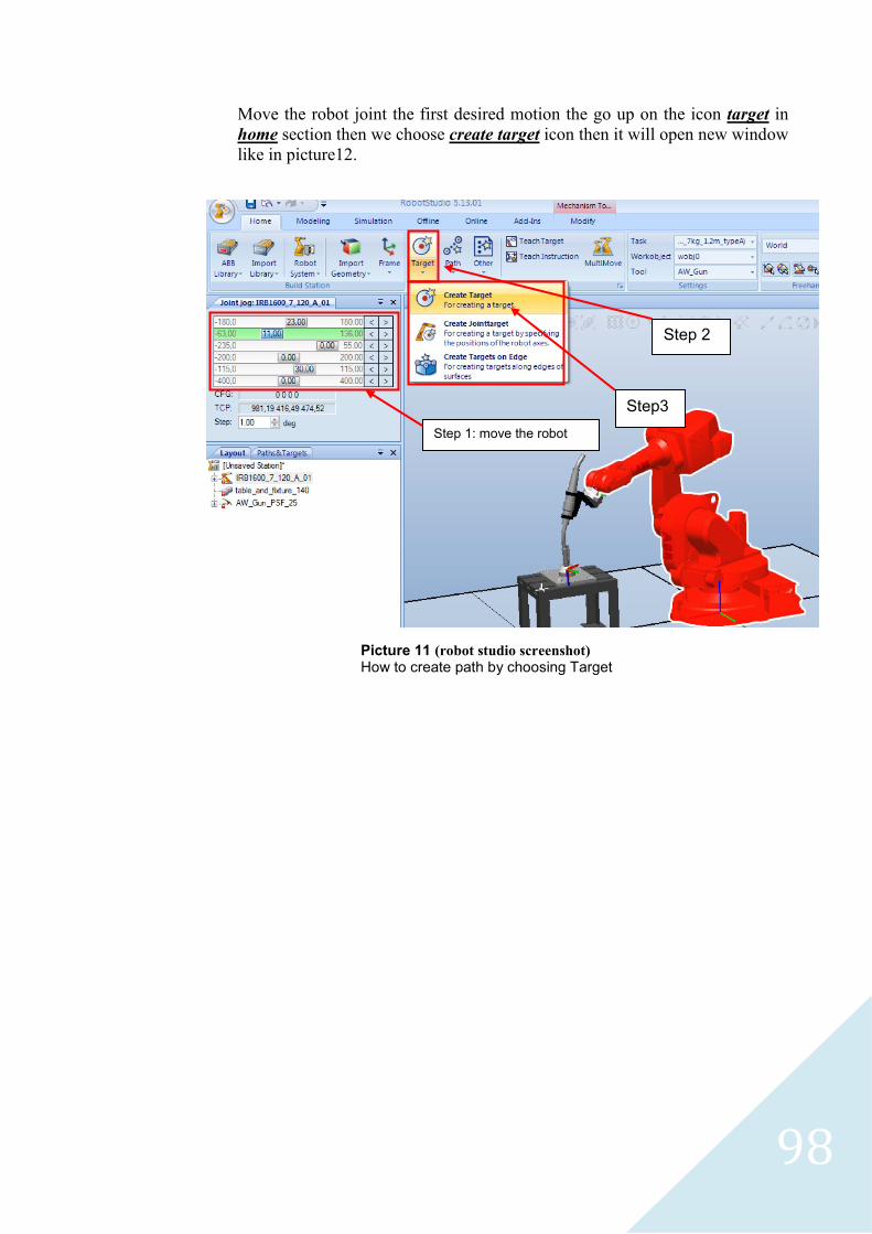
98

Move the robot joint the first desired motion the go up on the icon target in

home section then we choose create target icon then it will open new window

like in picture12.

Picture 11 (robot studio screenshot) How to create path by choosing Target

Step 1: move the robot

Step 2

Step3

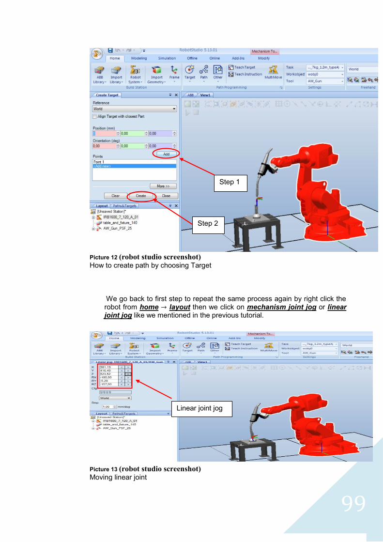
99

We go back to first step to repeat the same process again by right click the robot from home layout then we click on mechanism joint jog or linear joint jog like we mentioned in the previous tutorial.

Step 1

Step 2

Picture 12 (robot studio screenshot)

How to create path by choosing Target

Linear joint jog

Picture 13 (robot studio screenshot)

Moving linear joint

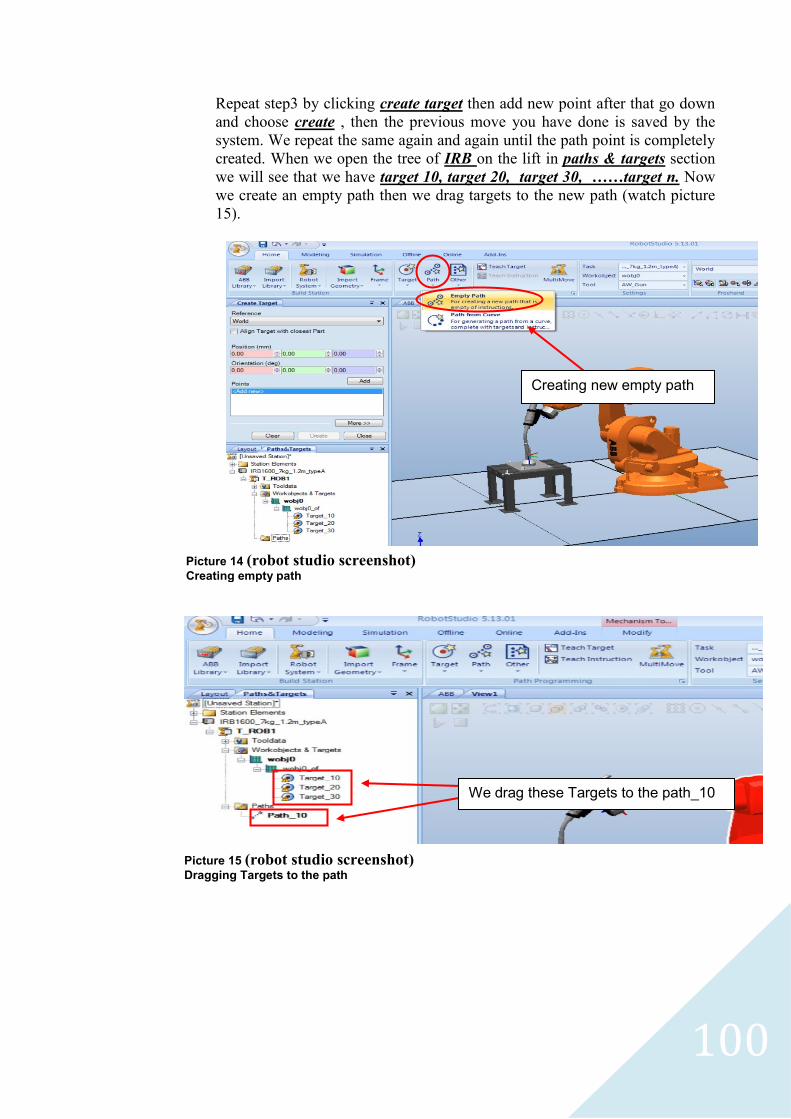
100

Repeat step3 by clicking create target then add new point after that go down

and choose create , then the previous move you have done is saved by the

system. We repeat the same again and again until the path point is completely

created. When we open the tree of IRB on the lift in paths & targets section

we will see that we have target 10, target 20, target 30, ……target n. Now

we create an empty path then we drag targets to the new path (watch picture

15).

Picture 14 (robot studio screenshot) Creating empty path

Picture 15 (robot studio screenshot) Dragging Targets to the path

We drag these Targets to the path_10

Creating new empty path

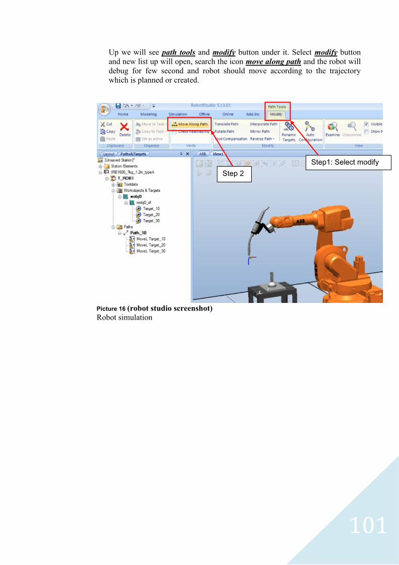
101

Up we will see path tools and modify button under it. Select modify button

and new list up will open, search the icon move along path and the robot will

debug for few second and robot should move according to the trajectory

which is planned or created.

Picture 16 (robot studio screenshot)

Robot simulation

Step1: Select modify

Step 2

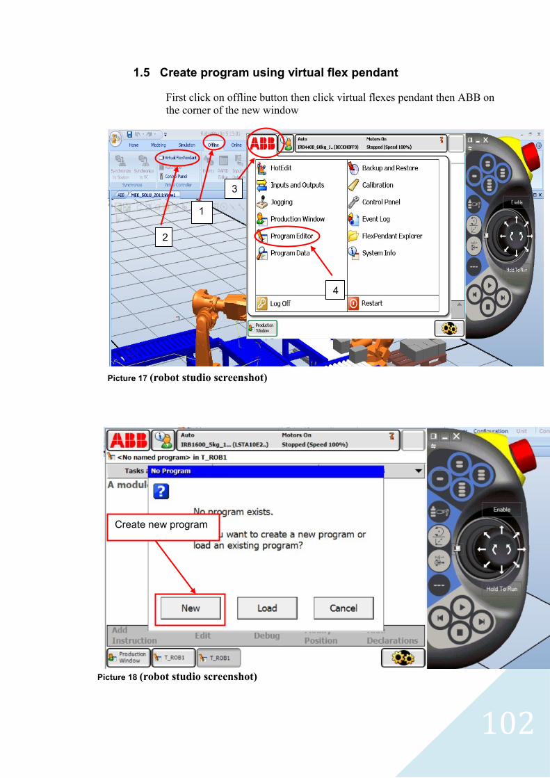
102

1.5 Create program using virtual flex pendant

First click on offline button then click virtual flexes pendant then ABB on

the corner of the new window

1

2

3

4

Create new program

Picture 17 (robot studio screenshot)

Picture 18 (robot studio screenshot)

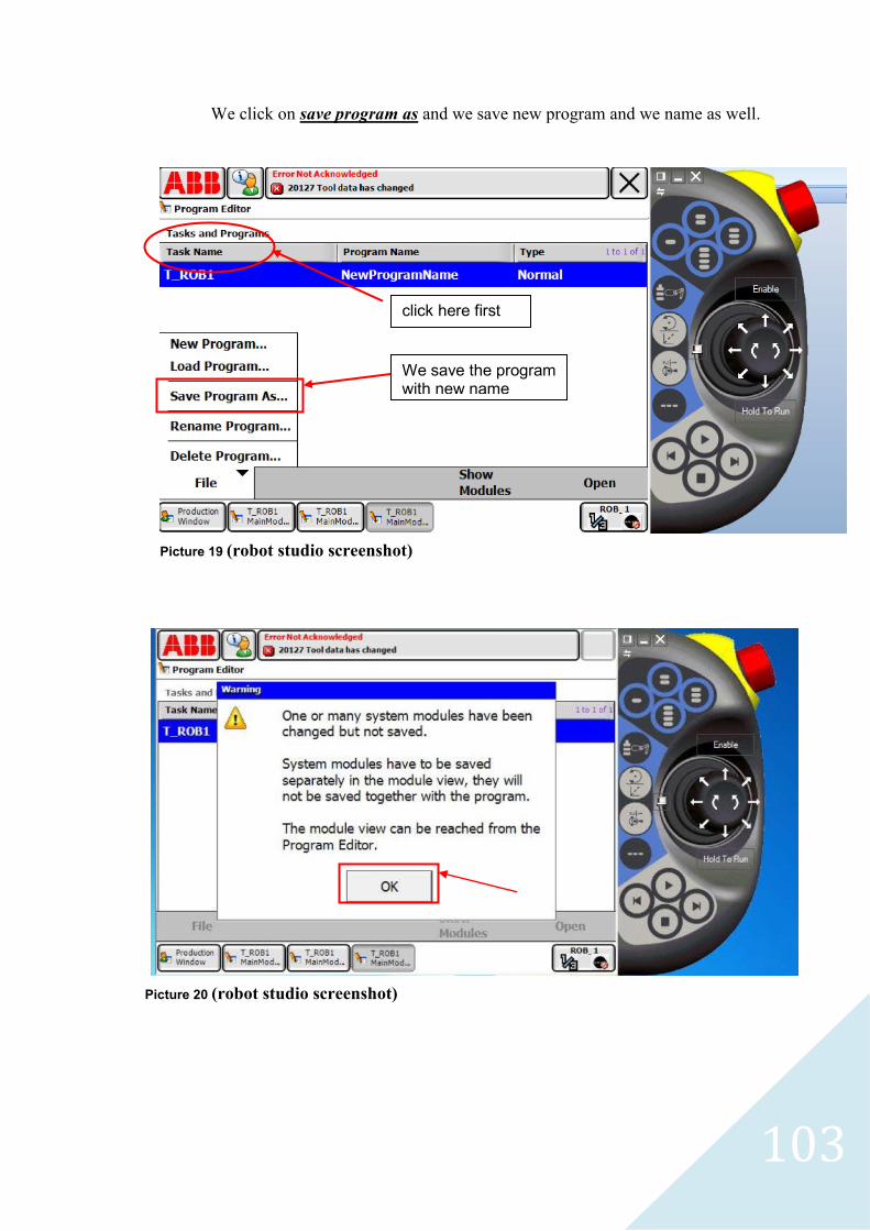
103

We click on save program as and we save new program and we name as well.

We save the program with new name

click here first

Picture 19 (robot studio screenshot)

Picture 20 (robot studio screenshot)

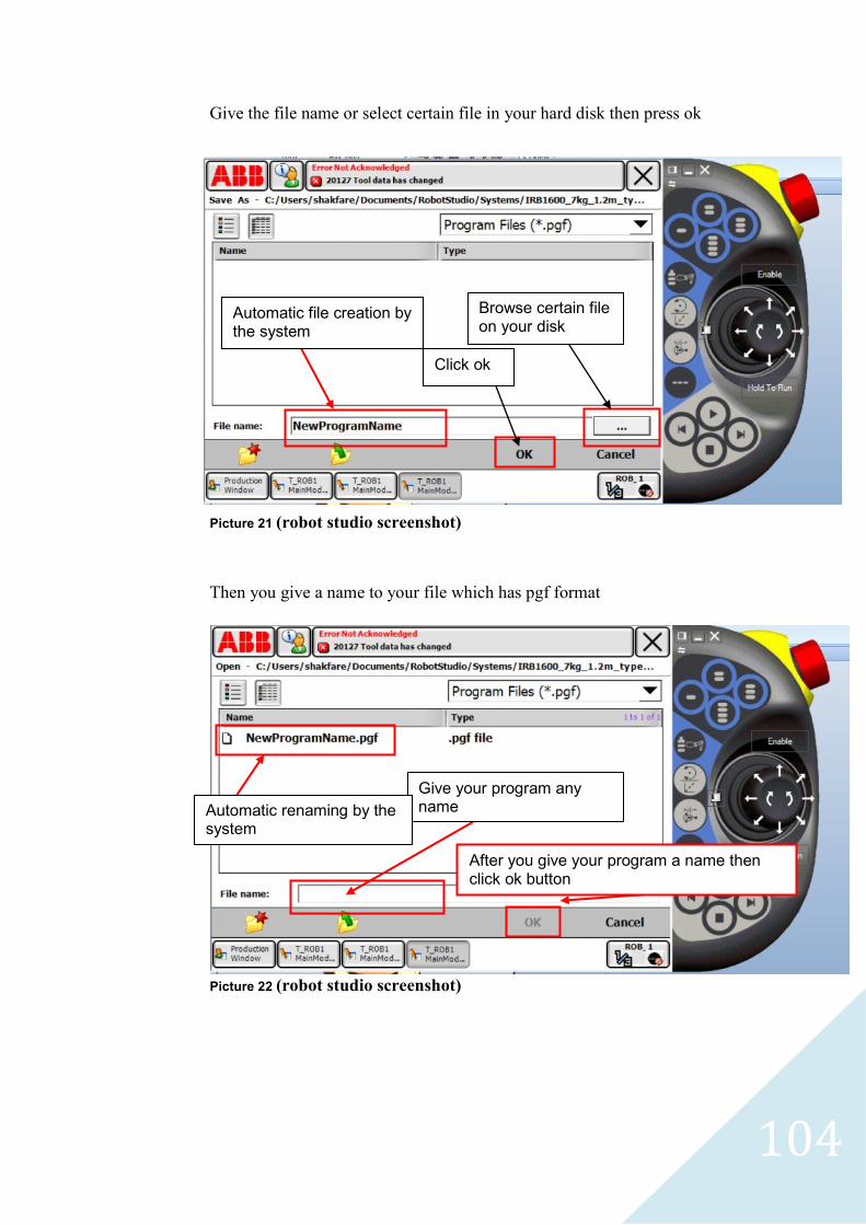
104

Give the file name or select certain file in your hard disk then press ok

Then you give a name to your file which has pgf format

Picture 22 (robot studio screenshot)

Automatic file creation by the system

Browse certain file on your disk

Click ok

Give your program any name Automatic renaming by the

system

After you give your program a name then click ok button

Picture 21 (robot studio screenshot)

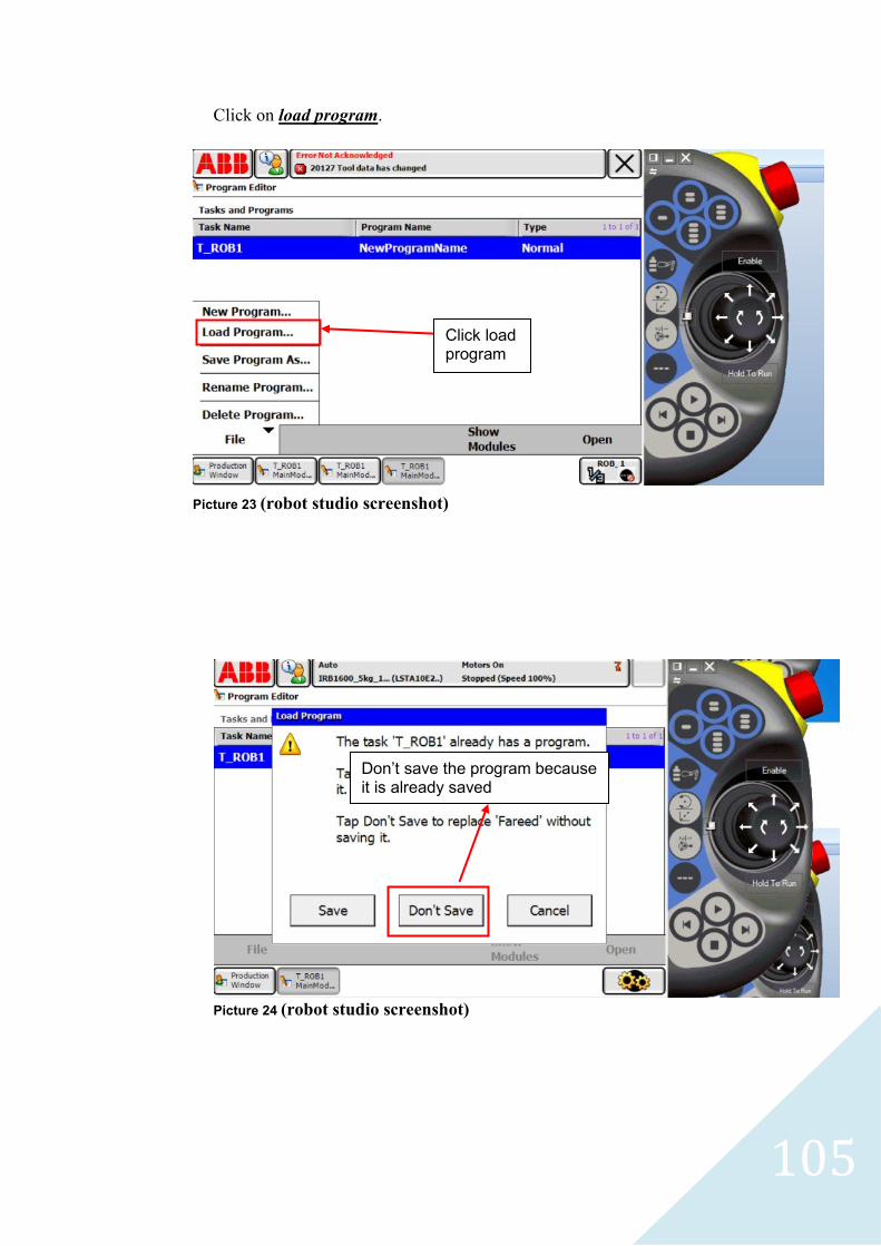
105

Click on load program.

Picture 24 (robot studio screenshot)

Click load program

Don’t save the program because it is already saved

Picture 23 (robot studio screenshot)

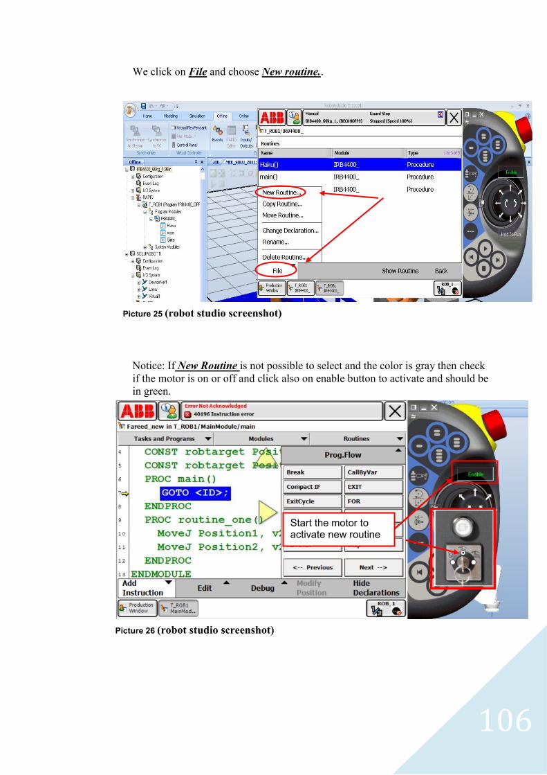
106

We click on File and choose New routine..

Notice: If New Routine is not possible to select and the color is gray then check

if the motor is on or off and click also on enable button to activate and should be

in green.

Picture 25 (robot studio screenshot)

Start the motor to activate new routine

Picture 26 (robot studio screenshot)

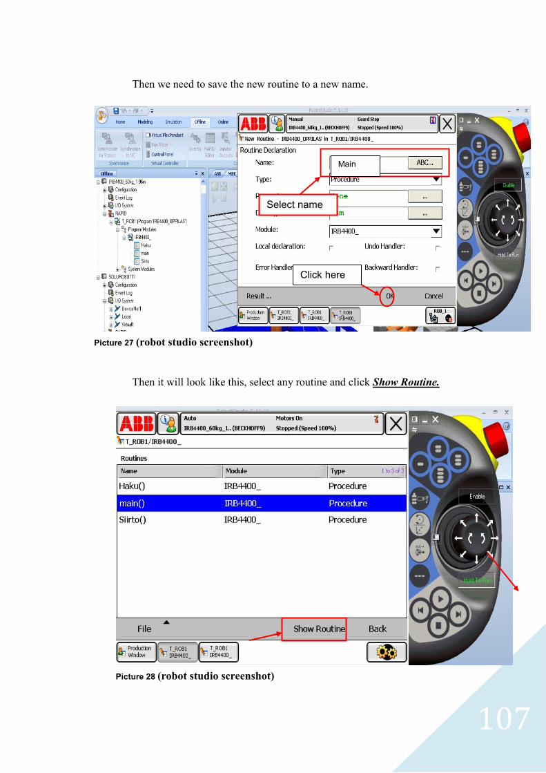
107

Then we need to save the new routine to a new name.

Then it will look like this, select any routine and click Show Routine.

Picture 27 (robot studio screenshot)

Picture 28 (robot studio screenshot)

Select name

Click here

Main

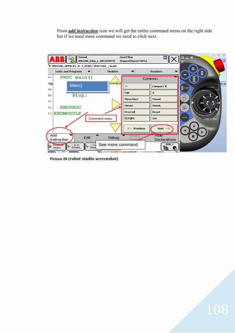
108

From add instruction icon we will get the entire command menu on the right side

but if we need more command we need to click next.

Command menu

See more command

Picture 29 (robot studio screenshot)

Main()

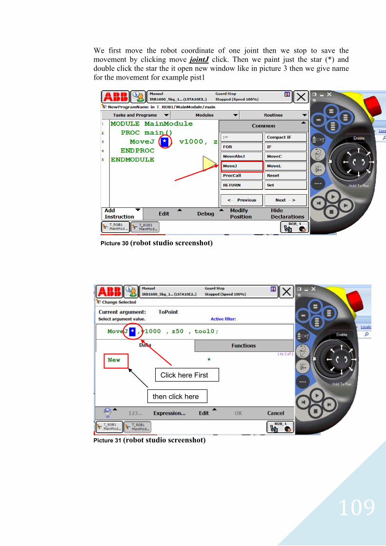
109

We first move the robot coordinate of one joint then we stop to save the

movement by clicking move jointJ click. Then we paint just the star (*) and

double click the star the it open new window like in picture 3 then we give name

for the movement for example pist1

Picture 31 (robot studio screenshot)

Click here First

Picture 30 (robot studio screenshot)

then click here

110

Picture 32 (robot studio screenshot)

Picture 33 (robot studio screenshot)

The given name

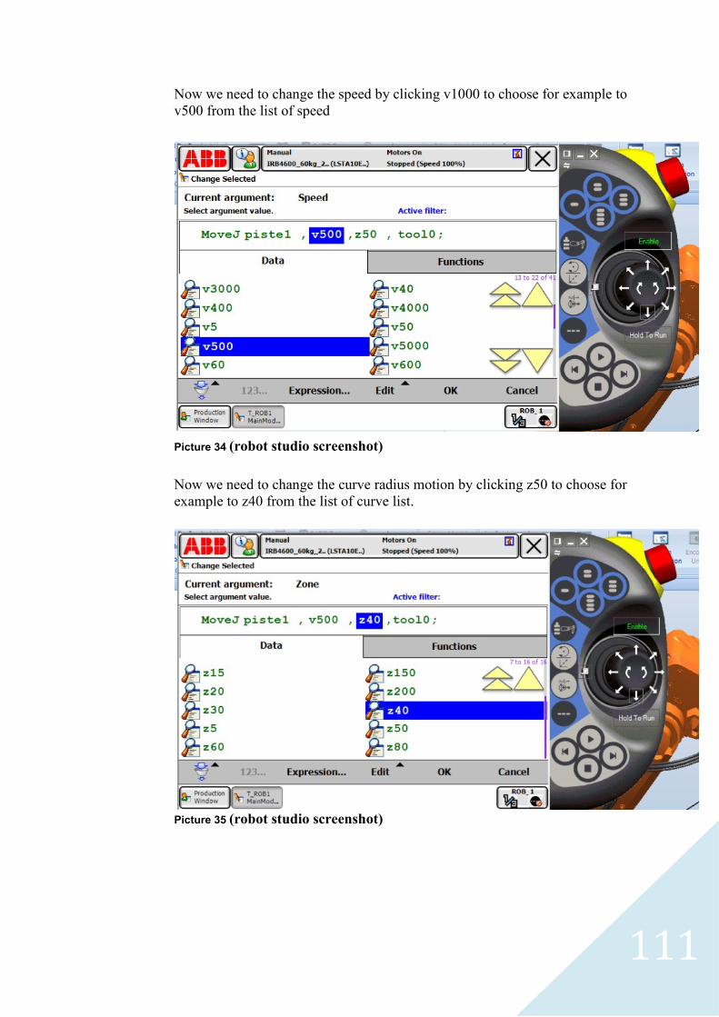
111

Now we need to change the speed by clicking v1000 to choose for example to

v500 from the list of speed

Now we need to change the curve radius motion by clicking z50 to choose for

example to z40 from the list of curve list.

Picture 35 (robot studio screenshot)

Picture 34 (robot studio screenshot)

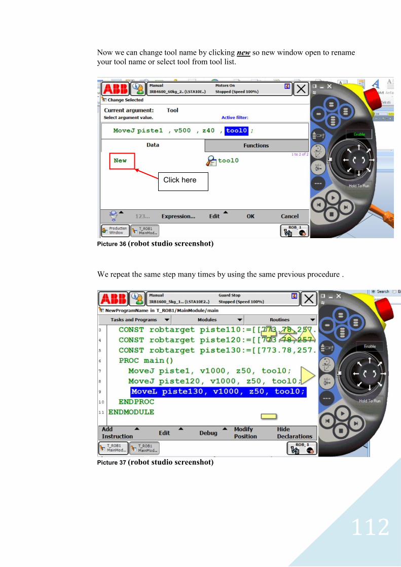
112

Now we can change tool name by clicking new so new window open to rename

your tool name or select tool from tool list.

Picture 36 (robot studio screenshot)

We repeat the same step many times by using the same previous procedure .

Picture 37 (robot studio screenshot)

Click here

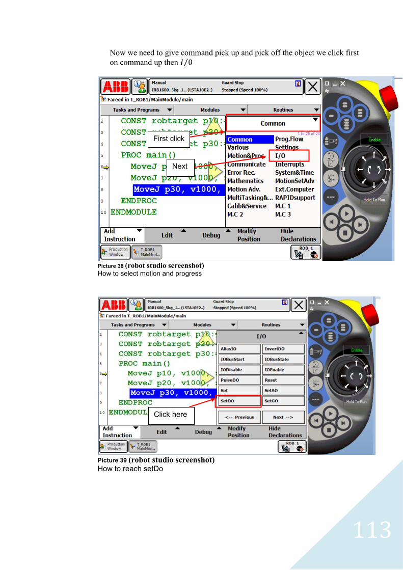
113

Now we need to give command pick up and pick off the object we click first

on command up then ⁄

Picture 38 (robot studio screenshot) How to select motion and progress

Picture 39 (robot studio screenshot) How to reach setDo

First click

Next

Click here

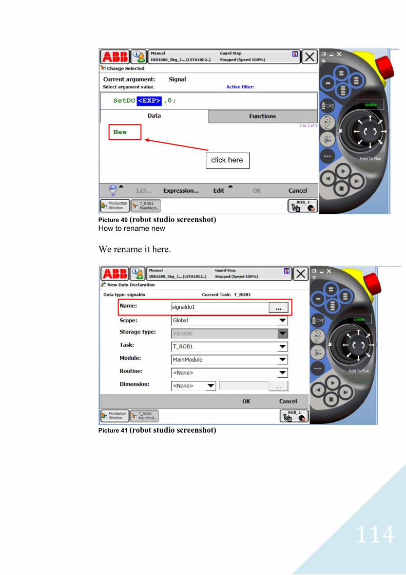
114

Picture 40 (robot studio screenshot) How to rename new

We rename it here.

Picture 41 (robot studio screenshot)

click here

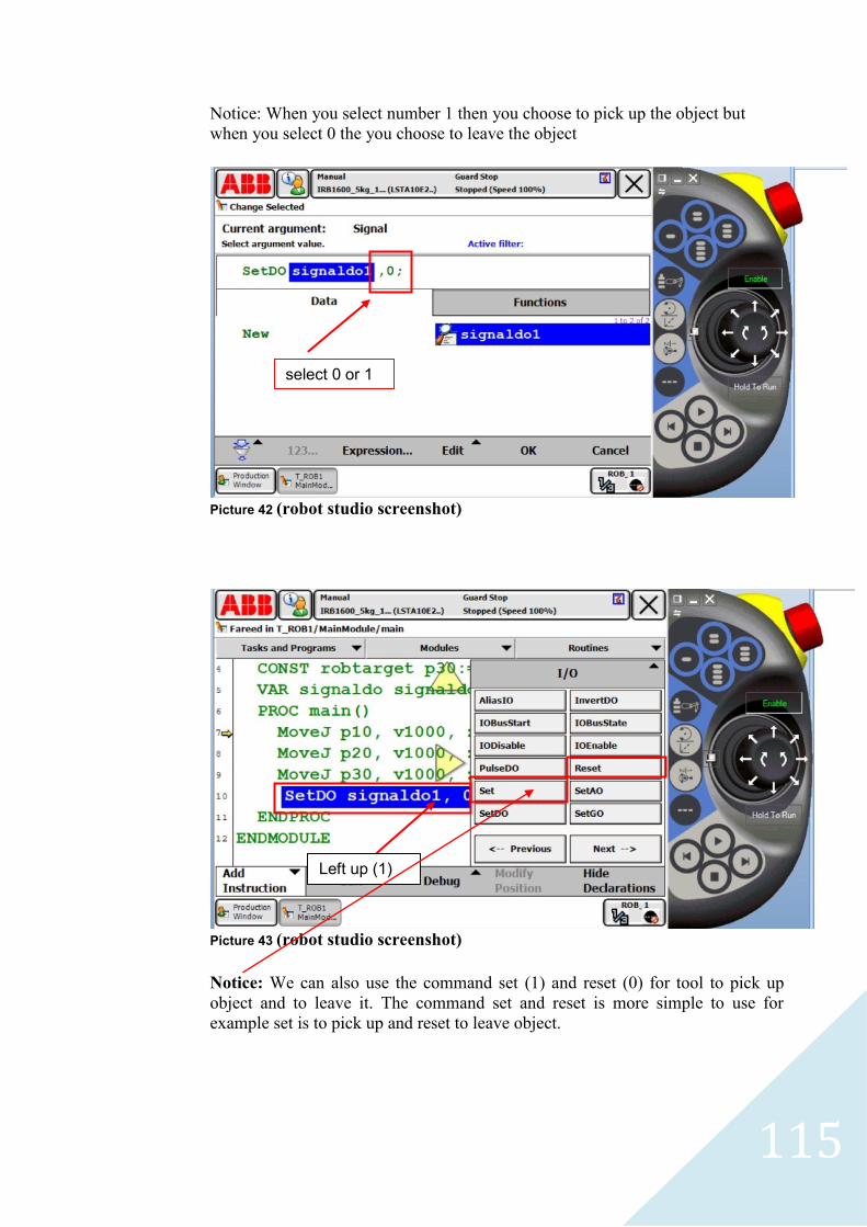
115

Notice: When you select number 1 then you choose to pick up the object but

when you select 0 the you choose to leave the object

Picture 42 (robot studio screenshot)

Picture 43 (robot studio screenshot)

Notice: We can also use the command set (1) and reset (0) for tool to pick up

object and to leave it. The command set and reset is more simple to use for

example set is to pick up and reset to leave object.

select 0 or 1

Left up (1)

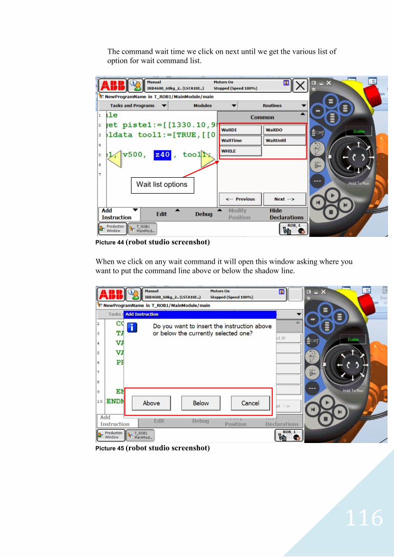
116

The command wait time we click on next until we get the various list of

option for wait command list.

Picture 44 (robot studio screenshot)

When we click on any wait command it will open this window asking where you

want to put the command line above or below the shadow line.

Picture 45 (robot studio screenshot)

Wait list options

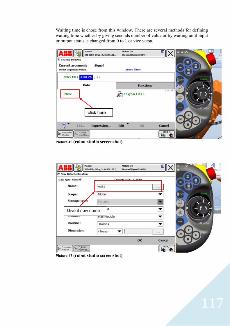
117

Waiting time is chose from this window. There are several methods for defining

waiting time whether by giving seconds number of value or by waiting until input

or output status is changed from 0 to 1 or vice versa.

Picture 46 (robot studio screenshot)

Picture 47 (robot studio screenshot)

click here

Give it new name

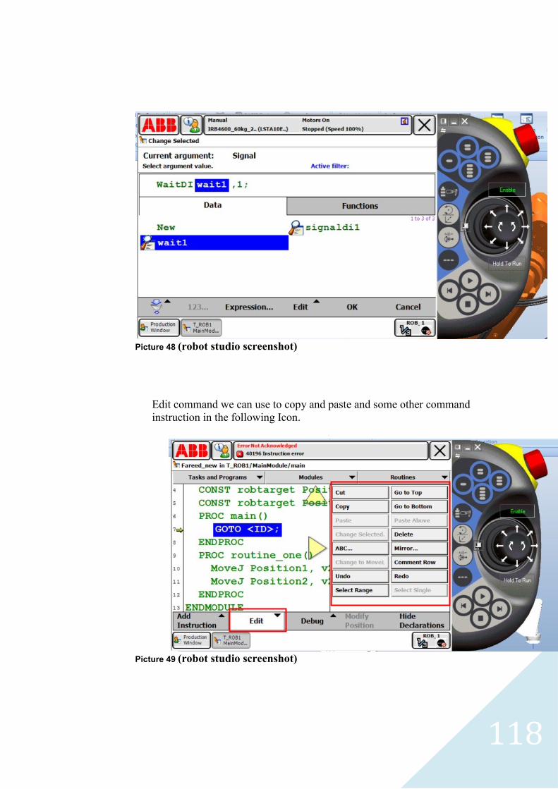
118

Picture 48 (robot studio screenshot)

Edit command we can use to copy and paste and some other command

instruction in the following Icon.

Picture 49 (robot studio screenshot)

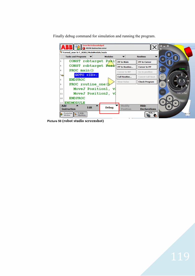
119

Finally debug command for simulation and running the program.

Picture 50 (robot studio screenshot)

120

CONCLUSION

The basics of robotics are quite an extensive field and wide study, which

requires both theoretical study and work experience to apply with a theoretical

study. Anyone reading my thesis will find it like an introduction for robotics and

the first step for beginning to understand a robot. During work experience the

knowledge will increase fast by combining theoretical knowledge with the

practice. In my thesis I concentrated on the beginning in the robot types and

applications and tried to give the reader an idea why we need robots in our lives.

Then about robot technology and the structure of a robot were also introduced by

writing about the mechanical parts and electrical parts that we use in building a

robot and what is the purpose of each part, besides providing pictures of robot

parts because pictures can give the reader a better idea on the subject without to

begin to imagine something, which is completely wrong. In the end I would say

that robotics study is challenging and complicated and I recommend anyone to

begin with simple stuff by playing with some sensors and actuators and try to

create logic system and gradually the knowledge will grow with more practice.

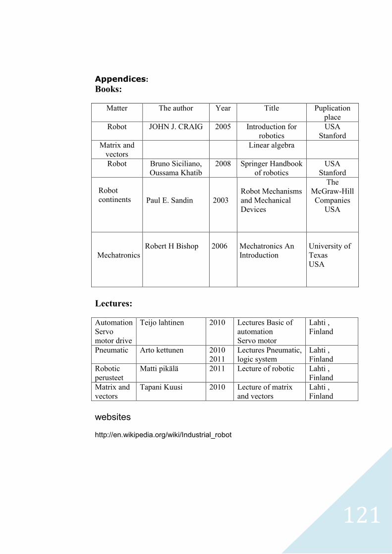
121

Appendices:

Books:

Matter The author Year Title Puplication

place

Robot JOHN J. CRAIG 2005 Introduction for

robotics

USA

Stanford

Matrix and

vectors

Linear algebra

Robot Bruno Siciliano,

Oussama Khatib

2008 Springer Handbook

of robotics

USA

Stanford

Robot

continents

Paul E. Sandin

2003

Robot Mechanisms

and Mechanical

Devices

The

McGraw-Hill

Companies

USA

Mechatronics

Robert H Bishop

2006

Mechatronics An

Introduction

University of

Texas

USA

Lectures:

Automation

Servo

motor drive

Teijo lahtinen 2010 Lectures Basic of

automation

Servo motor

Lahti ,

Finland

Pneumatic Arto kettunen 2010

2011

Lectures Pneumatic,

logic system

Lahti ,

Finland

Robotic

perusteet

Matti pikälä 2011 Lecture of robotic Lahti ,

Finland

Matrix and

vectors Tapani Kuusi 2010 Lecture of matrix

and vectors Lahti ,

Finland

websites http://en.wikipedia.org/wiki/Industrial_robot