1

Resolution Enhancement of Video Sequences with

Simultaneous Estimation of the Regularization Parameter

Hu He, Lisimachos P. Kondi

Dept. of Electrical Engineering, SUNY at Buffalo, Buffalo, NY 14260

ABSTRACT

In this paper, we propose a technique for the estimation of the regularization parameter for image resolution

enhancement (super-resolution) based on the assumptions that it should be a function of the regularized

noise power of the data and that its choice should yield a convex functional whose minimization would

give the desired high-resolution image. The regularization parameter acts adaptively to determine the trade-

off between fidelity to the received data and prior information about the image. Experimental results are

presented and conclusions are drawn.

Keywords: Resolution enhancement, super-resolution, MAP estimation, image restoration, regularization

1. INTRODUCTION

In many imaging systems, the resolution of the detector array of the camera is not sufficiently high for a

particular application. Furthermore, the capturing process introduces additive noise and the point spread

function of the lens and the effects of the finite size of the photo-detectors further degrade the acquired

video frames. The goal of resolution enhancement is to estimate a high-resolution image from a sequence

of low-resolution images while also compensating for the above-mentioned degradations.

Resolution enhancement using multiple frames is possible when there exists subpixel motion between the

captured frames. Thus, each of the frames provides a unique look into the scene. An example scenario is

the case of a camera that is mounted on an aircraft and is imaging objects in the far field. The vibrations of

the aircraft will generally provide the necessary motion between the focal plane array and the scene, thus

yielding frames with subpixel motion between them and minimal occlusion effects.

2

In this paper, we extend our previous results [1] by proposing a technique for the estimation of the

regularization parameter. The rest of the paper is organized as follows. In section 2, a Maximum A

Posteriori (MAP) formulation is presented for the super-resolution problem and it is shown that, for

specific choice of prior model, the MAP cost function is equivalent to a Tikhonov regularization cost

function. In section 3, we rewrite the cost function in multi-channel form to establish the relationship

between the overall regularization parameter and the individual parameters for each channel. We then

develop our technique for the estimation of the regularization parameter. In section 4, experimental results

are presented. Finally, in section 5, conclusions are drawn.

2. REGULARIZED COST FUNCTION OF RESOLUTION ENHANCEMENT

The problem of video super-resolution is an active research area. We next outline a few of the approaches

that have appeared in the literature. Among the earliest efforts in the field is the work by Tsai and Huang

[2]. Their method operates in the frequency domain and capitalizes on the shifting property of the Fourier

Transform, the aliasing relationship between the Continuous Fourier Transform (CFD) and the Discrete

Fourier Transform (DFT), and the fact that the original scene is assumed to be band limited. The above

properties are used to construct a system of equations relating the aliased DFT coefficients of the observed

images to samples of the CFT of the unknown high-resolution image. The system of equations is solved,

yielding an estimate of the DFT coefficients of the original high-resolution image, which can then be

obtained using inverse DFT. This technique was further improved by Tekalp et. al. in [3] by taking into

account a Linear Shift Invariant (LSI) blur Point Spread Function (PSF) and using a least squares approach

to solving the system of equations. The big advantage of the frequency domain methods is their low

computational complexity. However, these methods are applicable only to global motion and a priori

information about the high-resolution image cannot be exploited.

Most of the other resolution enhancement techniques that have appeared in the literature operate in the

spatial domain. The most computationally efficient techniques involve interpolation of non-uniformly

spaced samples. This requires the computation of the optical flow between the acquired low-resolution

frames are combined in order to create a high-resolution frame. Interpolation techniques are used to

estimate pixels in the high-resolution frame that did not correspond to pixels in one of the acquired frames.

3

Finally, image restoration techniques are used to compensate for the blurring introduced by the imaging

device. A method based on this idea is the Temporal Accumulation of Registered Image Data (TARID) [4],

developed by the Naval Research Laboratory (NRL).

Another method that has appeared in the literature is the iterated backprojection method [5]. In this method,

the estimate of the high-resolution image is updated by backprojecting the error between motion-

compensated, blurred and subsampled versions of the current estimate of the high-resolution image and the

observed low-resolution images, using an appropriate backprojection operator.

Another proposed method is the Projection Onto Convex Sets (POCS) [6], [7]. In this method, the space of

high-resolution images is intersected with a set of convex constraint sets representing desirable image

characteristics, such as positivity, bounded energy, fidelity to data, smoothness, etc.

Another class of resolution enhancement algorithms is based on stochastic techniques. Methods in this class

include Maximum Likelihood (ML) [8] and Maximum A Posteriori (MAP) approaches [9], [10], [11], [12].

MAP estimation with an edge preserving Huber-Markov random field image prior is studied in [9], [10],

[11]. MAP based resolution enhancement with simultaneous estimation of registration parameters (motion

between frames) has been proposed in [1], [12]. The MAP methods lead to solving a regularized cost

function. The regularization parameter of the cost function plays a very important role in the reconstruction

of high-resolution image, while its selection is a kind of art. The L-curve method chooses the “L-corner”,

the point with maximum curvature on the L-curve, as the one corresponding to regularization parameter

[13]. Iterative adaptive algorithms with automatically updated regularization parameter have been proposed

for image restoration [14], [15]. However, little research has been done for the super-resolution scenario.

The objective of this paper is to extend these results to super-resolution.

In the following, we use the same formulation and notation as in [12]. The image degradation process can

be modeled by a linear blur, motion, subsampling by pixel averaging and an additive Gaussian noise

process. In the following, we order all vectors lexicographically. We assume that p low-resolution frames

are observed, each of size 21 NN × . The desired high-resolution image [ ]TNzzz ,,, 21 L=z is of

size 2211 NLNLN = , where 1L and 2L represent the down-sampling factors in the horizontal and

4

vertical directions respectively. Let the kth low-resolution frame be denoted as

[ ]TMkkkk yyy ,2,1, ,, L=y for pk L,2,1= and where 21NNM = . The full set of p observed low-

resolution images can be denoted as

[ ] [ ]TpMTT

pTT yyy ,,,,,, 2121 LL == yyyy . (1)

The observed low-resolution frames are related to the high-resolution image through the following model:

∑=

+=N

rmkrkrmkmk zwy

1,,,, )( ηs , (2)

for Mm L,2,1= and pk L,2,1= . The weight )(,, krmkw s represents the “contribution” of the rth

high-resolution pixel to the mth low-resolution observed pixel of the kth frame, which implements blur,

motion and pixel averaging. The vector [ ]TKkkkk sss ,2,1, ,, L=s contains the K registration parameters

for frame k, representing translational shift, rotation, affine transformation parameters, or other motion

parameters. This motion is measured in reference to a fixed high-resolution grid. The term mk ,η

represents additive noise samples that are assumed to be independent and identically distributed (i.i.d.)

Gaussian noise samples with variance 2ησ . We can rewrite Equation (2) in matrix notation

nzWy s += , (3)

where matrix [ ]TTp

TT,2,1, ,,, ssss WWWW L= contains the values rmkw ,, and [ ]TpMηηη L,, 21=n . The

multivariate p.d.f of y given z and s is

( ) ( )

−−−= zWyzWysz,y ssT

pMpMrP 22

21exp

)2(

1)(η

η

σσπ

. (4)

We can form a MAP estimate of the high-resolution image z and the registration parameters

s simultaneously, given the observed y . The estimates can be computed as

5

)(maxarg ysz,s,zsz,

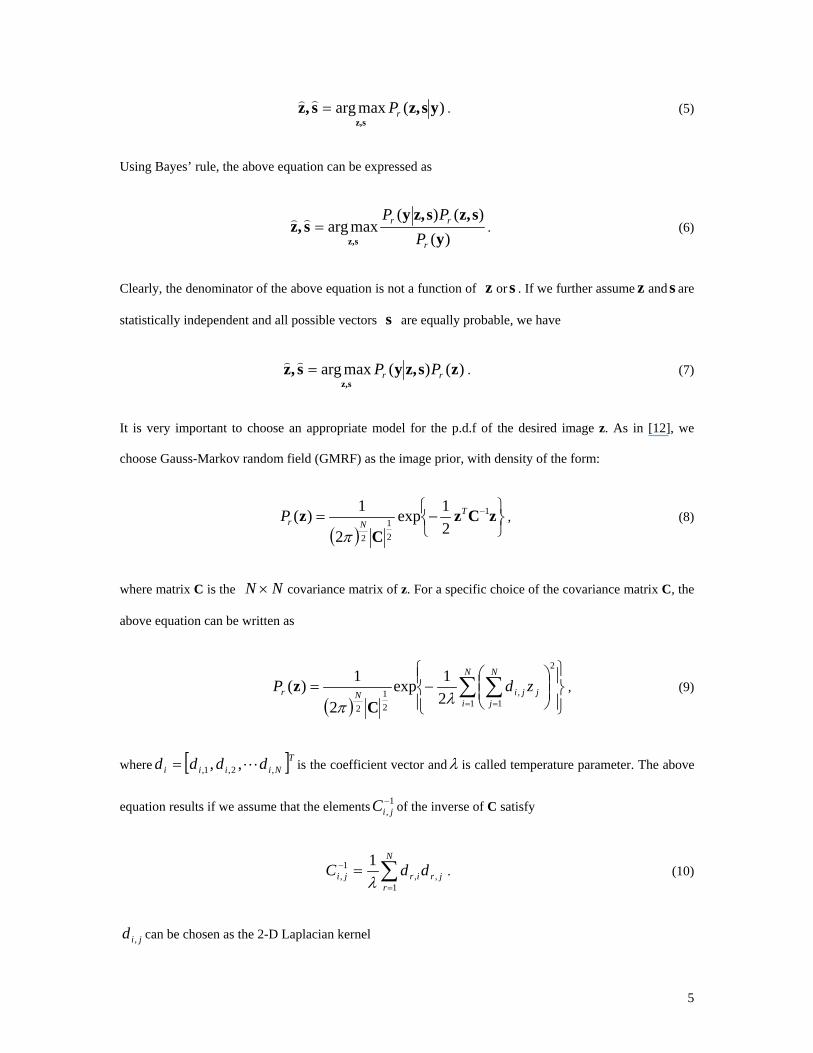
rP=)) . (5)

Using Bayes’ rule, the above equation can be expressed as

)()()(

maxargy

sz,sz,ys,z

sz, r

rr

PPP

=)) . (6)

Clearly, the denominator of the above equation is not a function of z or s . If we further assume z and s are

statistically independent and all possible vectors s are equally probable, we have

)()(maxarg zsz,ys,zsz,

rr PP=)) . (7)

It is very important to choose an appropriate model for the p.d.f of the desired image z. As in [12], we

choose Gauss-Markov random field (GMRF) as the image prior, with density of the form:

( )

−= − zCz

Cz 1

21

221exp

2

1)( TNrP

π, (8)

where matrix C is the NN × covariance matrix of z. For a specific choice of the covariance matrix C, the

above equation can be written as

( )

−= ∑ ∑

= =

N

i

N

jjjiNr zdP

1

2

1,

21

221exp

2

1)(λπ C

z , (9)

where [ ]TNiiii dddd ,2,1, ,, L= is the coefficient vector andλ is called temperature parameter. The above

equation results if we assume that the elements 1,−

jiC of the inverse of C satisfy

∑=

− =N

rjrirji ddC

1,,

1,

1λ

. (10)

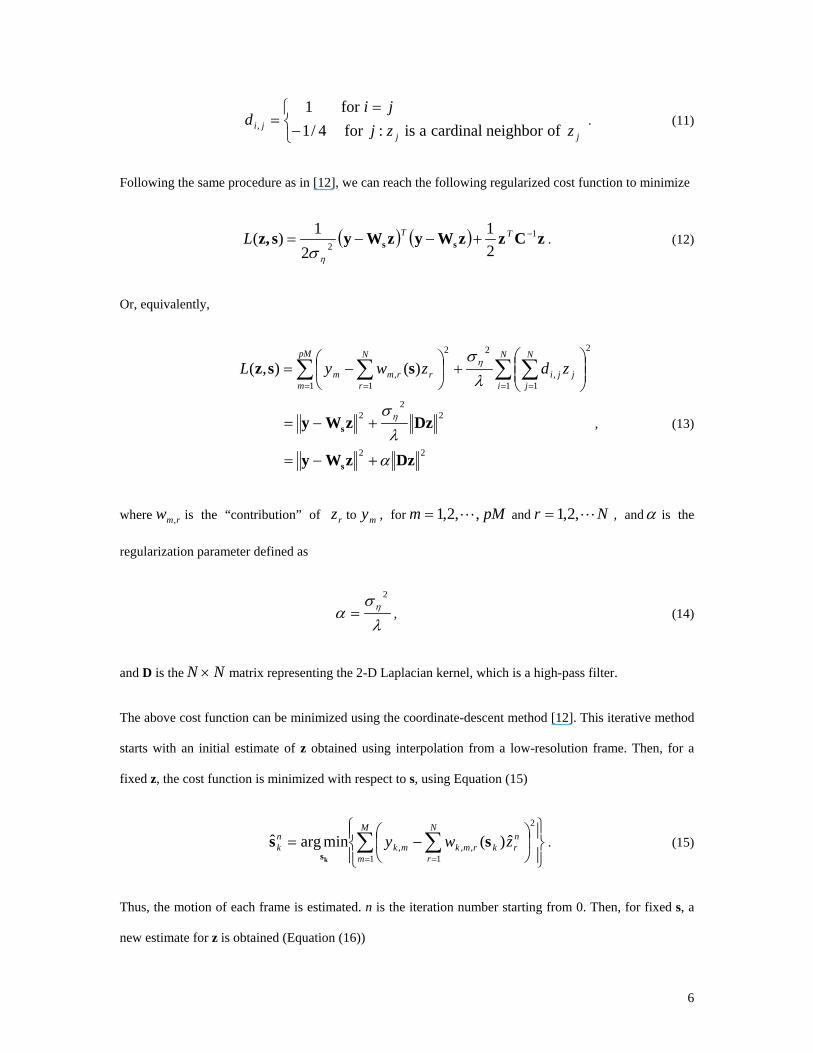
jid , can be chosen as the 2-D Laplacian kernel

6

−

==

jjji zzj

jid

ofneighborcardinalais:for4/1for1

, . (11)

Following the same procedure as in [12], we can reach the following regularized cost function to minimize

( ) ( ) zCzzWyzWysz, ss1

2 21

21)( −+−−= TTLησ

. (12)

Or, equivalently,

22

22

2

1 1

2

1,

22

1, )(),(

DzzWy

DzzWy

ssz

s

s

αλσ

λσ

η

η

+−=

+−=

+

−= ∑ ∑ ∑∑

= = ==

pM

m

N

i

N

jjji

N

rrrmm zdzwyL

, (13)

where rmw , is the “contribution” of rz to my , for pMm ,,2,1 L= and Nr L,2,1= , andα is the

regularization parameter defined as

λσ

α η2

= , (14)

and D is the NN × matrix representing the 2-D Laplacian kernel, which is a high-pass filter.

The above cost function can be minimized using the coordinate-descent method [12]. This iterative method

starts with an initial estimate of z obtained using interpolation from a low-resolution frame. Then, for a

fixed z, the cost function is minimized with respect to s, using Equation (15)

−= ∑ ∑

= =

M

m

N

r

nrkrmkmk

nk zwy

1

2

1,,, ˆ)(minargˆ ss

ks. (15)

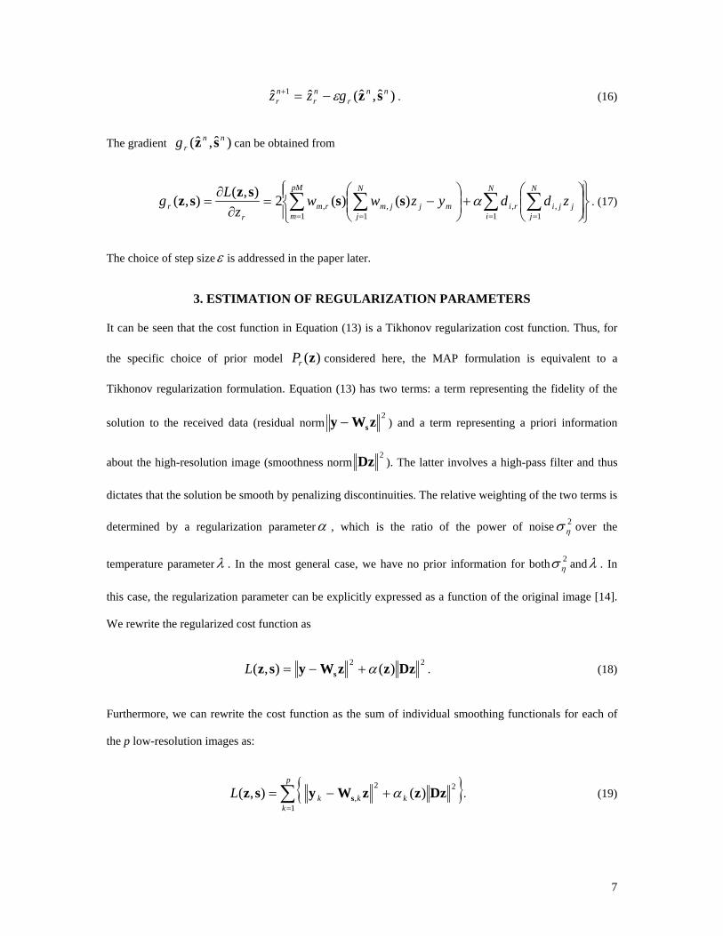
Thus, the motion of each frame is estimated. n is the iteration number starting from 0. Then, for fixed s, a

new estimate for z is obtained (Equation (16))

7

)ˆ,ˆ(ˆˆ 1 nnr

nr

nr gzz szε−=+ . (16)

The gradient )ˆ,ˆ( nnrg sz can be obtained from

+

−=

∂∂

= ∑ ∑∑ ∑= == =

N

i

N

jjjiri

pM

m

N

jmjjmrm

rr zddyzww

zLg

1 1,,

1 1,, )()(2),(),( αssszsz . (17)

The choice of step sizeε is addressed in the paper later.

3. ESTIMATION OF REGULARIZATION PARAMETERS

It can be seen that the cost function in Equation (13) is a Tikhonov regularization cost function. Thus, for

the specific choice of prior model )(zrP considered here, the MAP formulation is equivalent to a

Tikhonov regularization formulation. Equation (13) has two terms: a term representing the fidelity of the

solution to the received data (residual norm2zWy s− ) and a term representing a priori information

about the high-resolution image (smoothness norm2Dz ). The latter involves a high-pass filter and thus

dictates that the solution be smooth by penalizing discontinuities. The relative weighting of the two terms is

determined by a regularization parameterα , which is the ratio of the power of noise 2ησ over the

temperature parameterλ . In the most general case, we have no prior information for both 2ησ andλ . In

this case, the regularization parameter can be explicitly expressed as a function of the original image [14].

We rewrite the regularized cost function as

22 )(),( DzzzWysz s α+−=L . (18)

Furthermore, we can rewrite the cost function as the sum of individual smoothing functionals for each of

the p low-resolution images as:

{ }∑=

+−=p

kkkkL

1

22, )(),( DzzzWysz s α . (19)

8

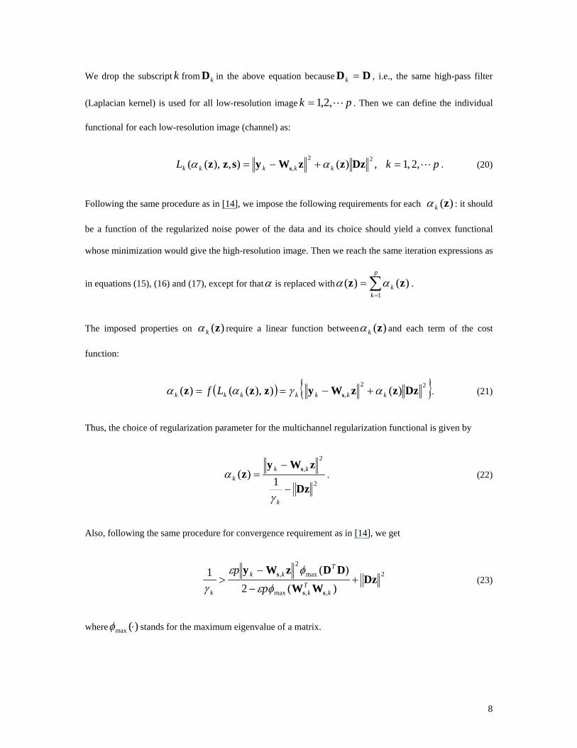
We drop the subscript k from kD in the above equation because DD =k , i.e., the same high-pass filter

(Laplacian kernel) is used for all low-resolution image pk L,2,1= . Then we can define the individual

functional for each low-resolution image (channel) as:

pkL kkkkk L,2,1,)(),),(( 22, =+−= DzzzWyszz s αα . (20)

Following the same procedure as in [14], we impose the following requirements for each )(zkα : it should

be a function of the regularized noise power of the data and its choice should yield a convex functional

whose minimization would give the high-resolution image. Then we reach the same iteration expressions as

in equations (15), (16) and (17), except for thatα is replaced with ∑=

=p

kk

1)()( zz αα .

The imposed properties on )(zkα require a linear function between )(zkα and each term of the cost

function:

( ) { }22, )()),(()( DzzzWyzzz s kkkkkkk Lf αγαα +−== . (21)

Thus, the choice of regularization parameter for the multichannel regularization functional is given by

2

2,

1)(

Dz

zWyz s

−

−=

k

kkk

γ

α . (22)

Also, following the same procedure for convergence requirement as in [14], we get

2

,,max

max2

,

)(2)(1 Dz

WWDDzWy

ss

s +−

−>

kT

k

Tkk

k pp

φε

φε

γ (23)

where )(max ⋅φ stands for the maximum eigenvalue of a matrix.

9

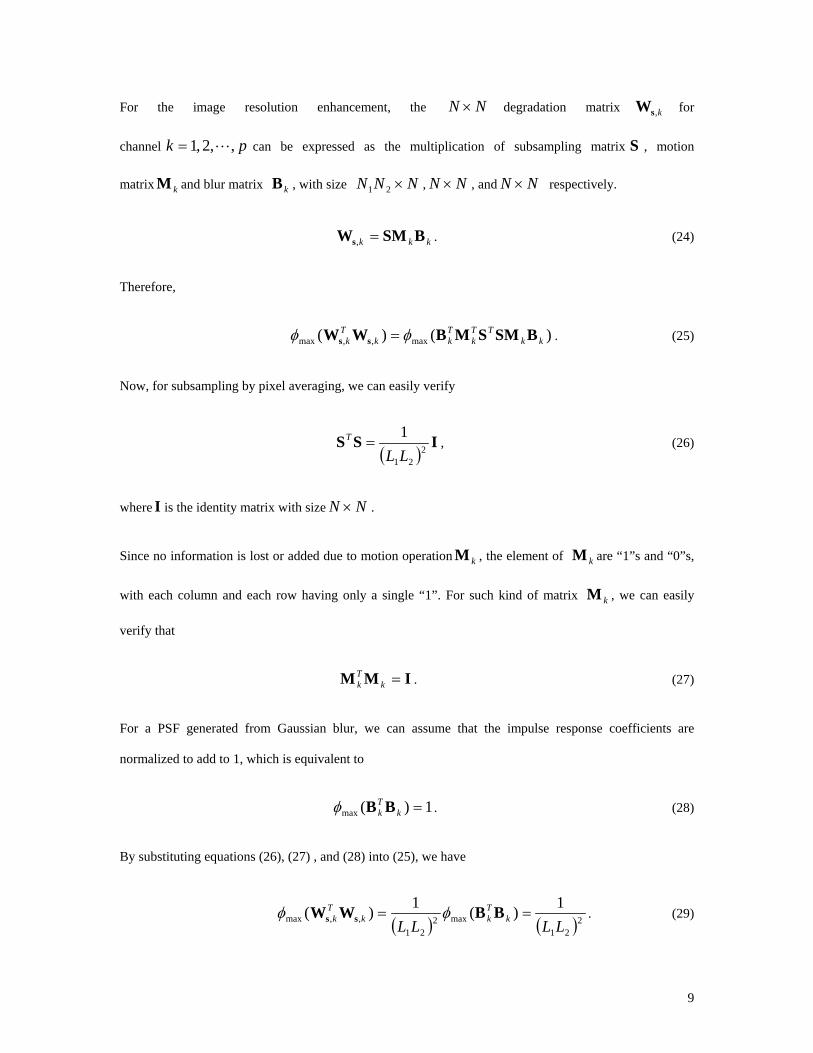
For the image resolution enhancement, the NN × degradation matrix k,sW for

channel pk ,,2,1 L= can be expressed as the multiplication of subsampling matrix S , motion

matrix kM and blur matrix kB , with size NNN ×21 , NN × , and NN × respectively.

kkk BSMWs =, . (24)

Therefore,

)()( max,,max kkTT

kTkk

Tk BSMSMBWW ss φφ = . (25)

Now, for subsampling by pixel averaging, we can easily verify

( )ISS 2

21

1LL

T = , (26)

where I is the identity matrix with size NN × .

Since no information is lost or added due to motion operation kM , the element of kM are “1”s and “0”s,

with each column and each row having only a single “1”. For such kind of matrix kM , we can easily

verify that

IMM =kTk . (27)

For a PSF generated from Gaussian blur, we can assume that the impulse response coefficients are

normalized to add to 1, which is equivalent to

1)(max =kTk BBφ . (28)

By substituting equations (26), (27) , and (28) into (25), we have

( ) ( )221

max221

,,max1)(1)(LLLL k

Tkk

Tk == BBWW ss φφ . (29)

10

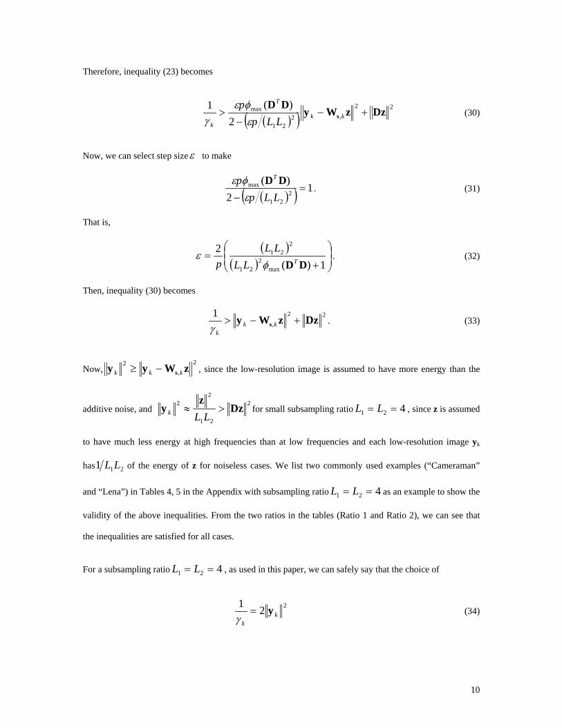
Therefore, inequality (23) becomes

( )( )22

,221

max

2)(1 DzzWy

DDs +−

−> kk

T

k LLppεφε

γ (30)

Now, we can select step sizeε to make

( )( ) 12

)(2

21

max =− LLpp T

εφε DD

. (31)

That is,

( )( )

+=

1)(2

max2

21

221

DDTLLLL

p φε . (32)

Then, inequality (30) becomes

22,

1 DzzWy s +−> kkkγ

. (33)

Now,2

,2 zWyy s kkk −≥ , since the low-resolution image is assumed to have more energy than the

additive noise, and 2

21

22 Dz

zy >≈

LLk for small subsampling ratio 421 == LL , since z is assumed

to have much less energy at high frequencies than at low frequencies and each low-resolution image yk

has 211 LL of the energy of z for noiseless cases. We list two commonly used examples (“Cameraman”

and “Lena”) in Tables 4, 5 in the Appendix with subsampling ratio 421 == LL as an example to show the

validity of the above inequalities. From the two ratios in the tables (Ratio 1 and Ratio 2), we can see that

the inequalities are satisfied for all cases.

For a subsampling ratio 421 == LL , as used in this paper, we can safely say that the choice of

221k

k

y=γ

(34)

11

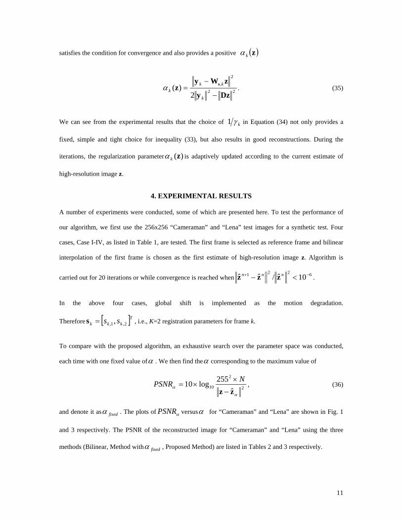
satisfies the condition for convergence and also provides a positive ( )zkα

22

2,

2)(

Dzy

zWyz s

−

−=

k

kkkα . (35)

We can see from the experimental results that the choice of kγ1 in Equation (34) not only provides a

fixed, simple and tight choice for inequality (33), but also results in good reconstructions. During the

iterations, the regularization parameter )(zkα is adaptively updated according to the current estimate of

high-resolution image z.

4. EXPERIMENTAL RESULTS

A number of experiments were conducted, some of which are presented here. To test the performance of

our algorithm, we first use the 256x256 “Cameraman” and “Lena” test images for a synthetic test. Four

cases, Case I-IV, as listed in Table 1, are tested. The first frame is selected as reference frame and bilinear

interpolation of the first frame is chosen as the first estimate of high-resolution image z. Algorithm is

carried out for 20 iterations or while convergence is reached when 6221 10ˆ/ˆˆ −+ <− nnn zzz .

In the above four cases, global shift is implemented as the motion degradation.

Therefore [ ]Tkkk ss 2,1, ,=s , i.e., K=2 registration parameters for frame k.

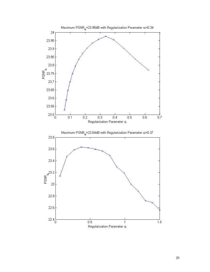
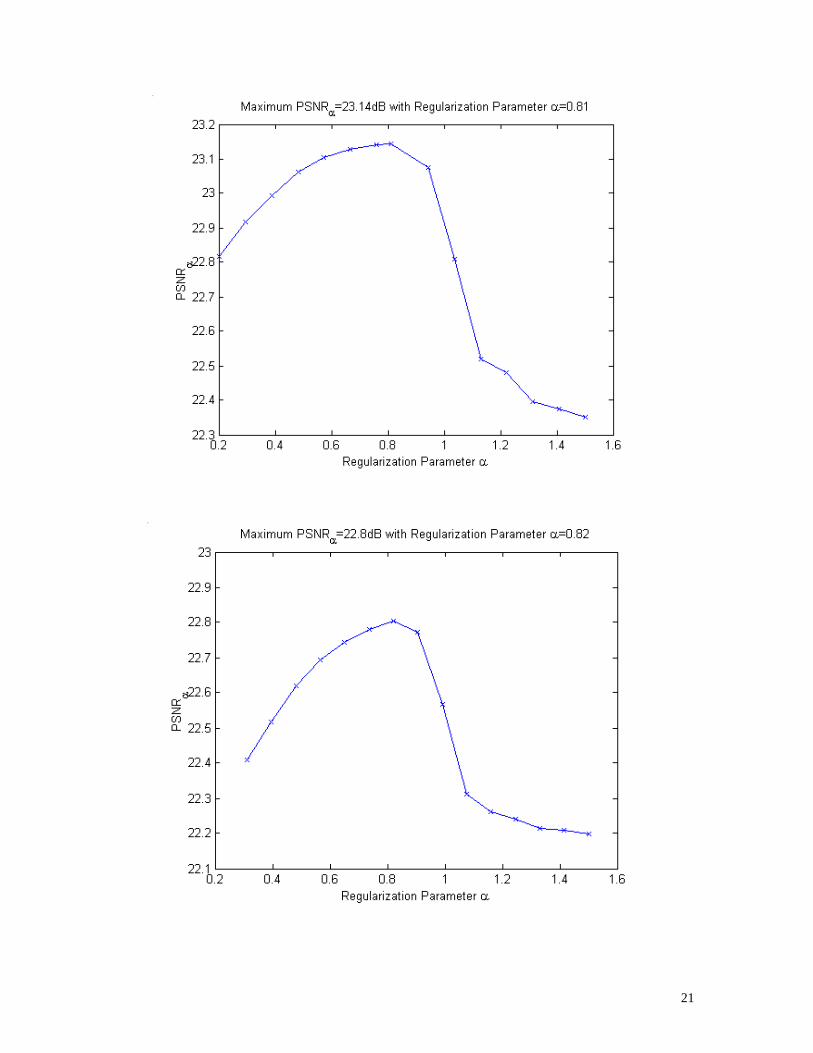
To compare with the proposed algorithm, an exhaustive search over the parameter space was conducted,

each time with one fixed value ofα . We then find theα corresponding to the maximum value of

2

2

10ˆ

255log10α

αzz −×

×=NPSNR , (36)

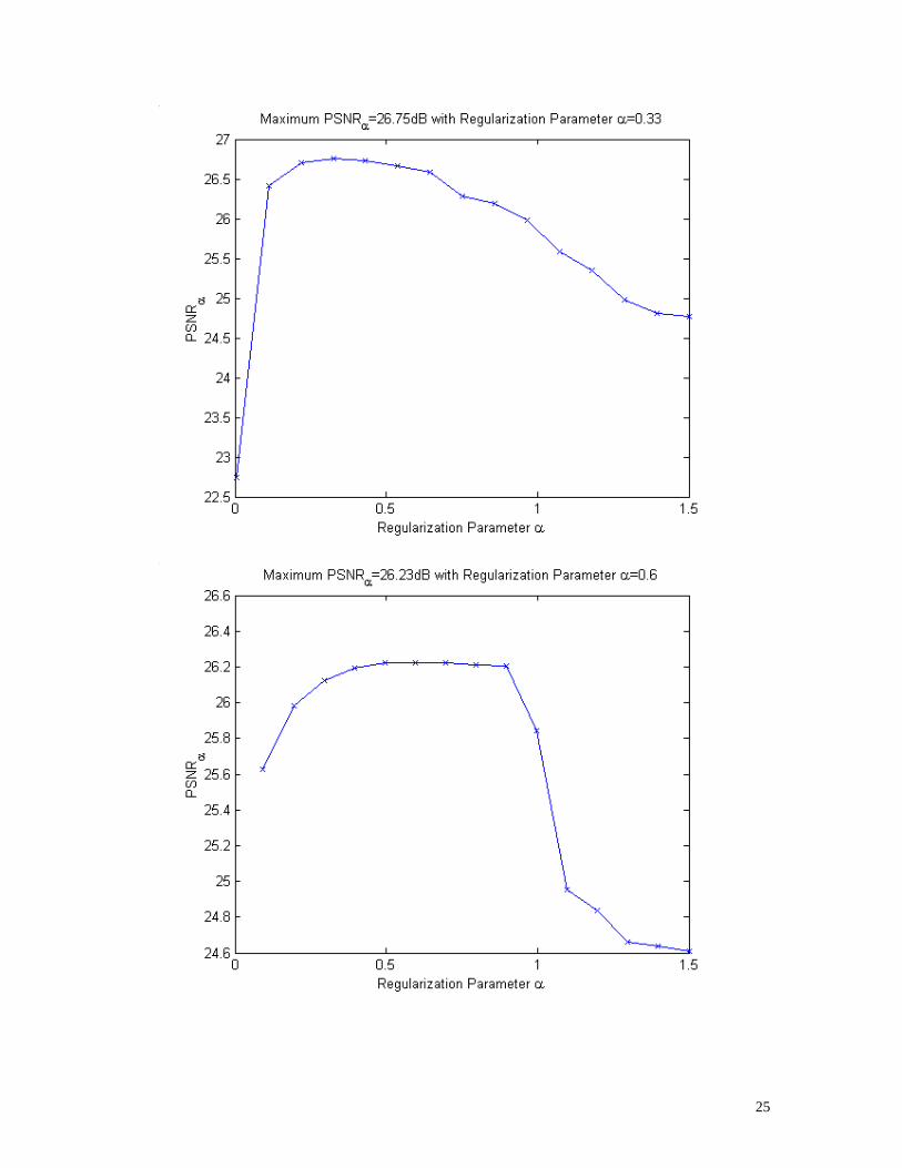
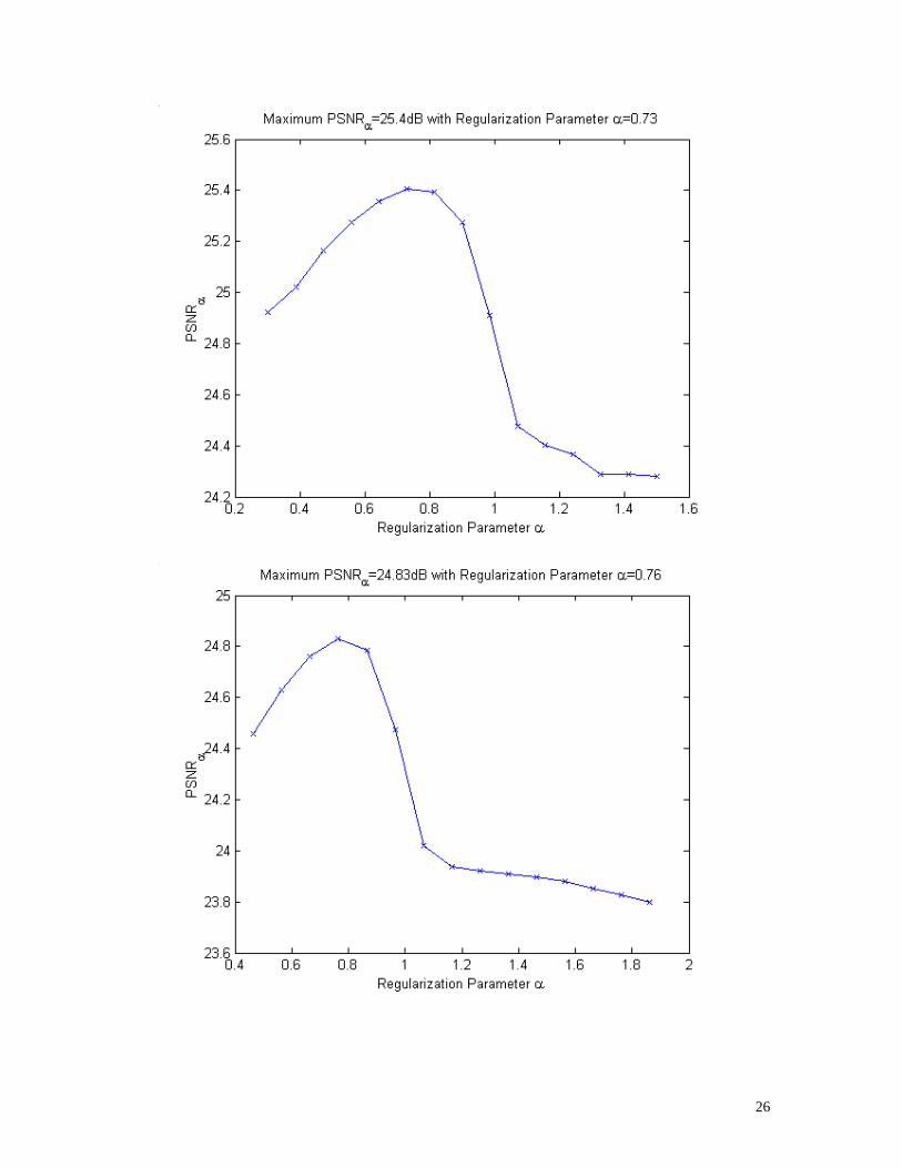
and denote it as fixedα . The plots of αPSNR versusα for “Cameraman” and “Lena” are shown in Fig. 1

and 3 respectively. The PSNR of the reconstructed image for “Cameraman” and “Lena” using the three

methods (Bilinear, Method with fixedα , Proposed Method) are listed in Tables 2 and 3 respectively.

12

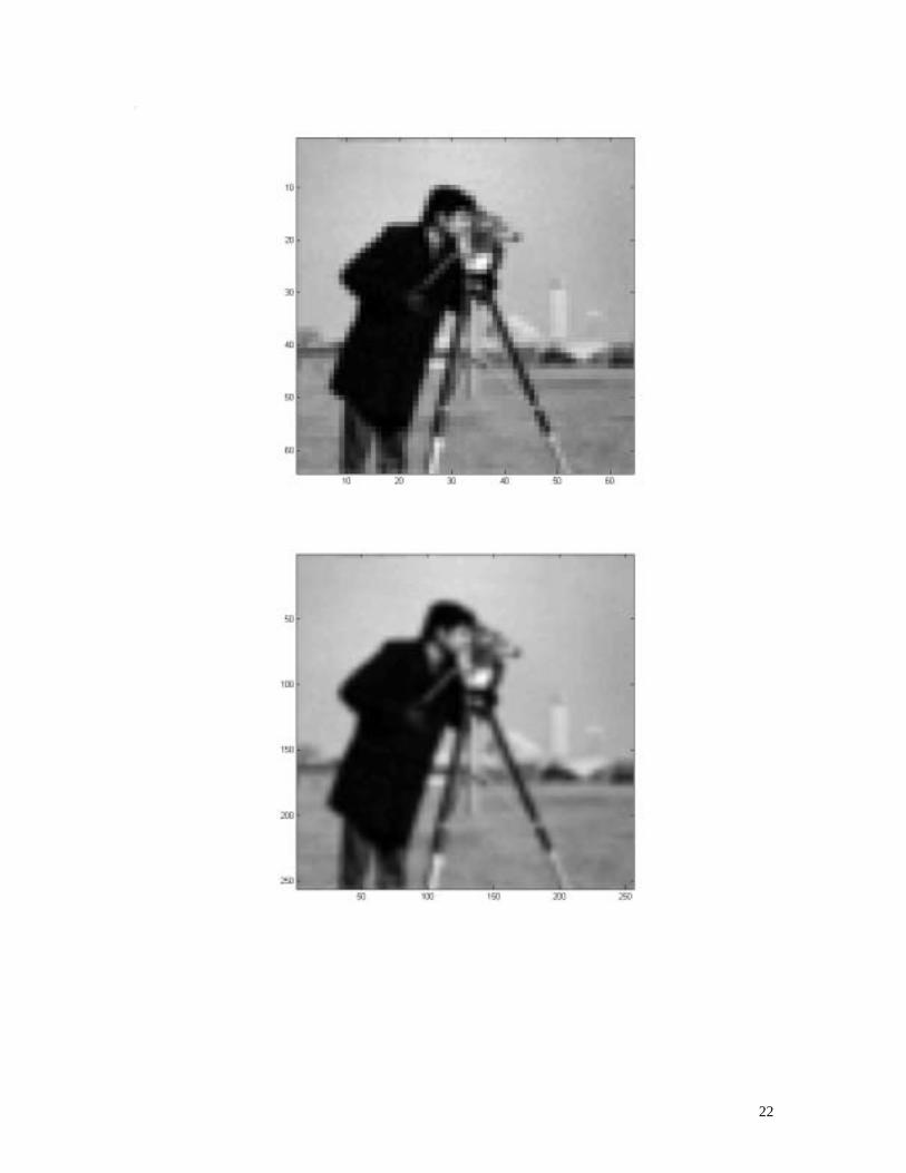
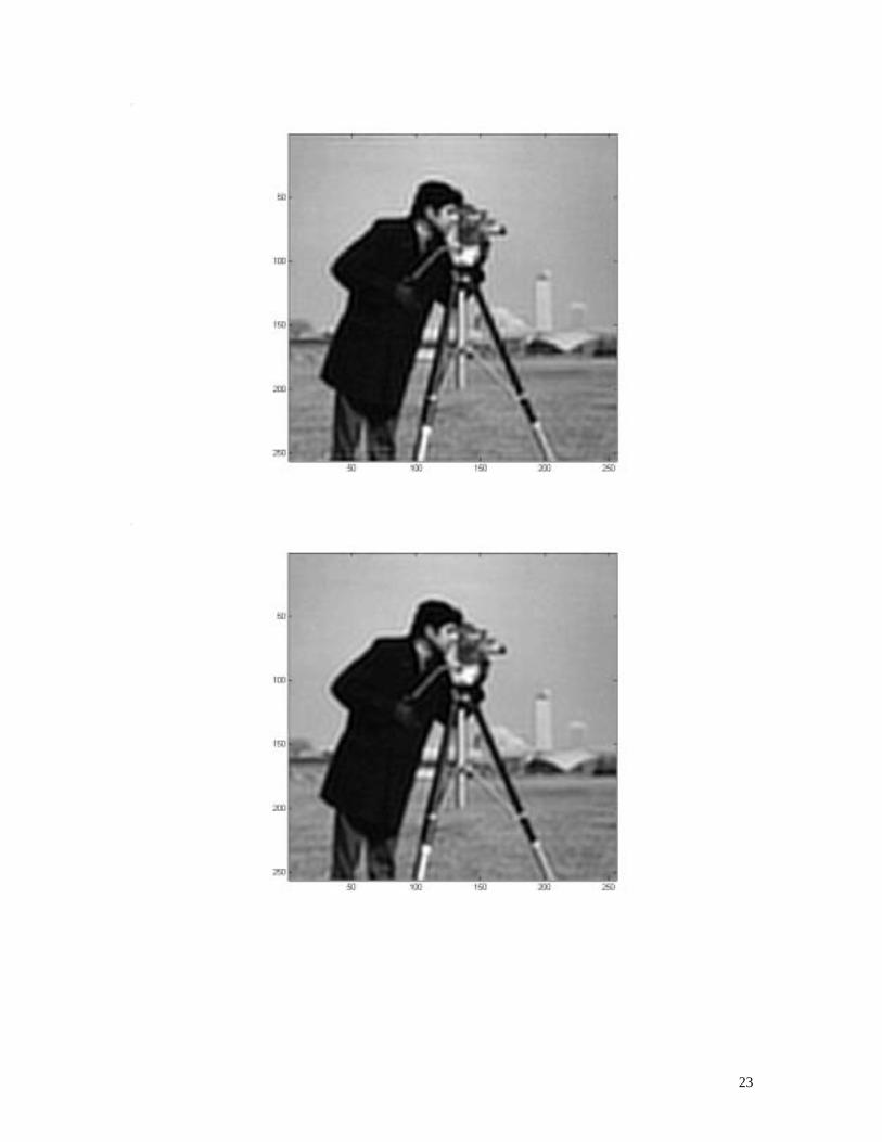
The reference frame, bilinear interpolation of the reference frame and the reconstructed images from

Method with fixedα and Proposed Method of “Cameraman” in Case I are shown in Fig. 2(a)-(d),

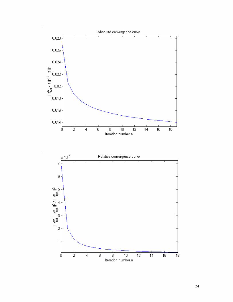
respectively. In Fig. 2(e) and 2(f), the absolute convergence curve (the plot of22

ˆ zzz −n versus

iteration number n) and relative convergence curve (the plot of221 ˆˆˆ nnn zzz −+ versus iteration

number n) are shown for the Proposed Method.

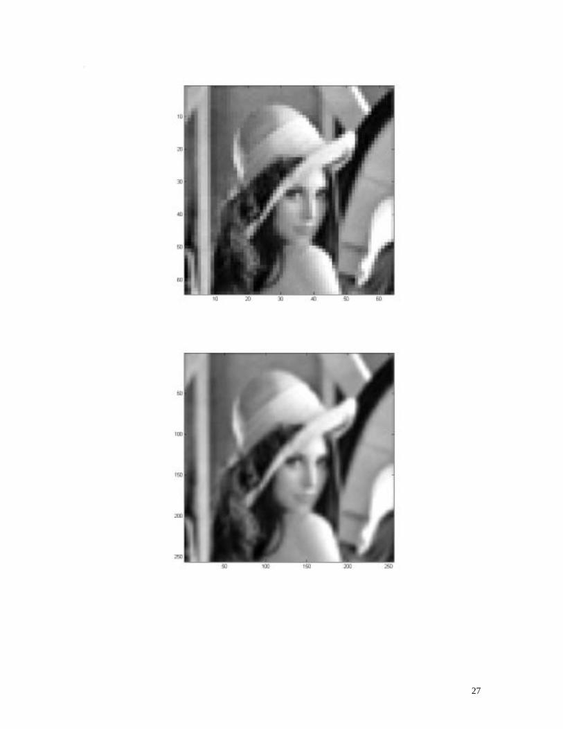
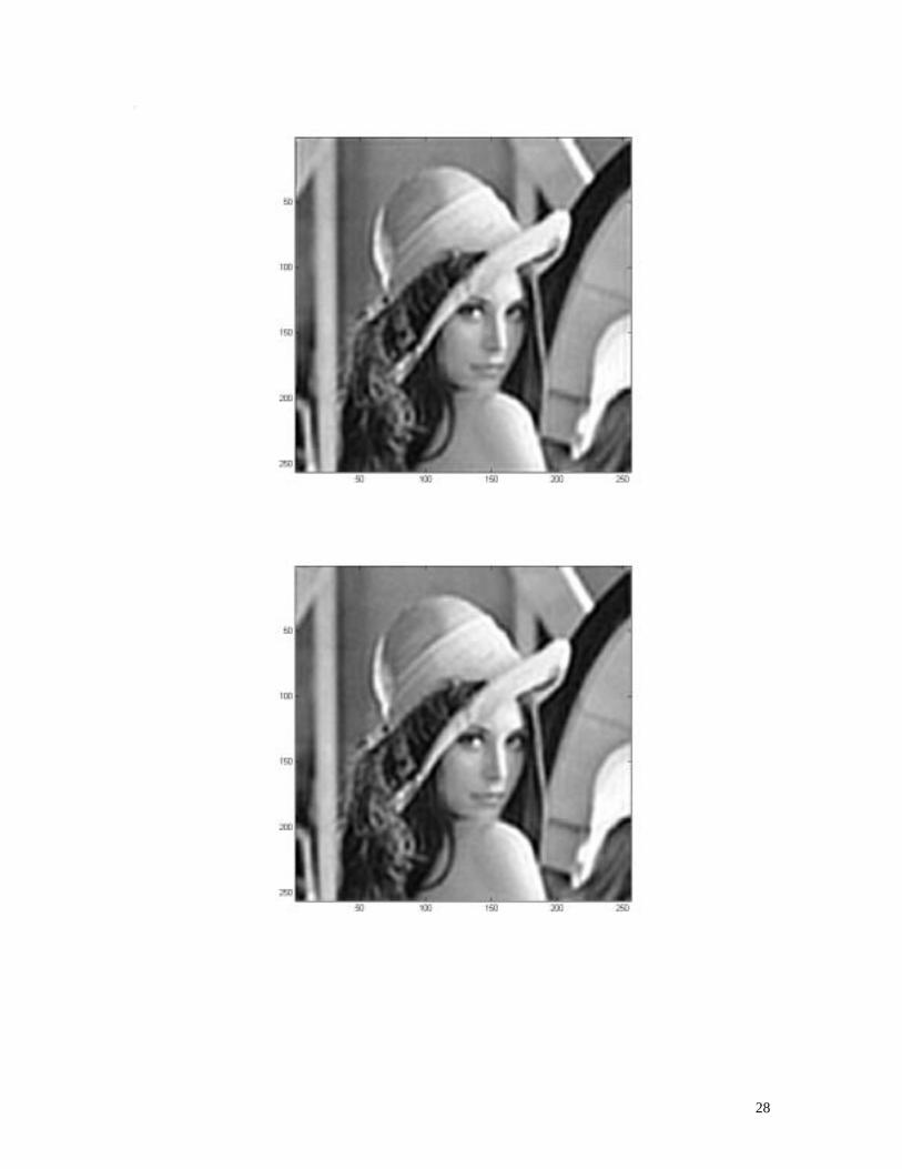
The reference frame, bilinear interpolation of the reference frame and the reconstructed images from

Method with fixedα and Proposed Method of “Lena” in Case I are shown in Fig. 4(a)-(d), respectively. In

Fig. 4(e) and 4(f), the absolute convergence curve and relative convergence curve are shown for Proposed

Method.

For all the four cases in Tables 2 and 3, the Proposed Method gives the highest PSNR and best visual

quality for both “Cameraman” and “Lena” (2~3 dB better than bilinear interpolation, and up to 0.25dB

better than Method with fixedα ). For real data, the original high-resolution image is not available,

thus αPSNR in Equation (36) can not be evaluated. We will show next that Proposed Method provides a

good regularization parameter without exhaustive search or trial and error method.

Next, we used real data of an infrared video sequence provided to us by the Naval Research Laboratory,

Washington, D.C., to test the proposed algorithm. 20 frames of low-resolution image with size 128x128

pixels were used. Up-sample ratio is L1=L2=4. We assumed a Gaussian point spread function for the lens

and estimated its variance at 1.7 using trial and error. Bilinear interpolation of the first frame was chosen as

the first estimate of high-resolution image z. Joint MAP registration technique was applied to estimate the

motion, with the high-resolution estimate partitioned into macro blocks (Equation (15)). Three Point Search

(TSS) with search window ±7 and Sum of Squared Errors (SSE) criteria was applied to decide the motion

vector between the 16x16 macro block in the high-resolution estimate and the corresponding 4x4 macro

block in the low-resolution image. When reconstructing the high-resolution image, these motion vectors

13

(registration parameters) were used to compensate the motion. We assumed that convergence was reached

when 6221 10ˆ/ˆˆ −+ <− nnn zzz .

There were totally ( ) ( ) 10241616512512 =×÷× macro blocks in the high-resolution image, and each

macro block had two translational shift parameters. Therefore [ ]Tkkkk sss 2048,2,1, ,, L=s , i.e.,

204810242 =×=K registration parameters for frame k.

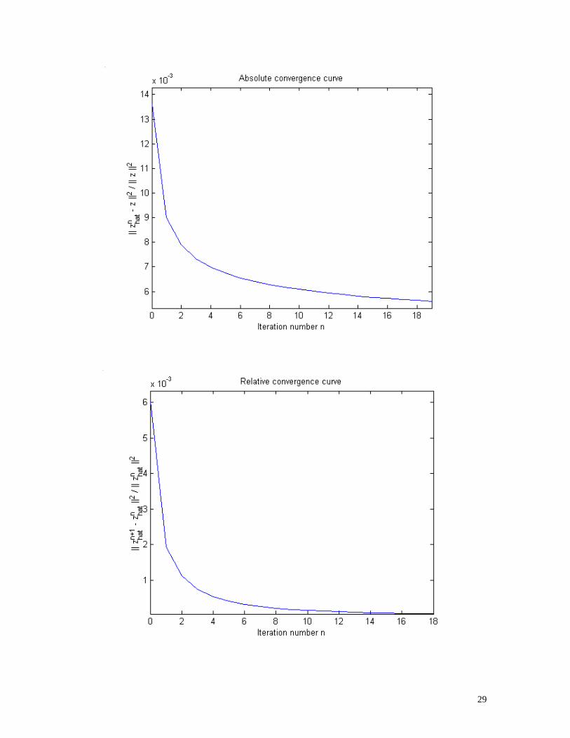
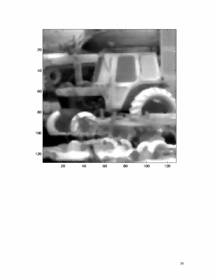
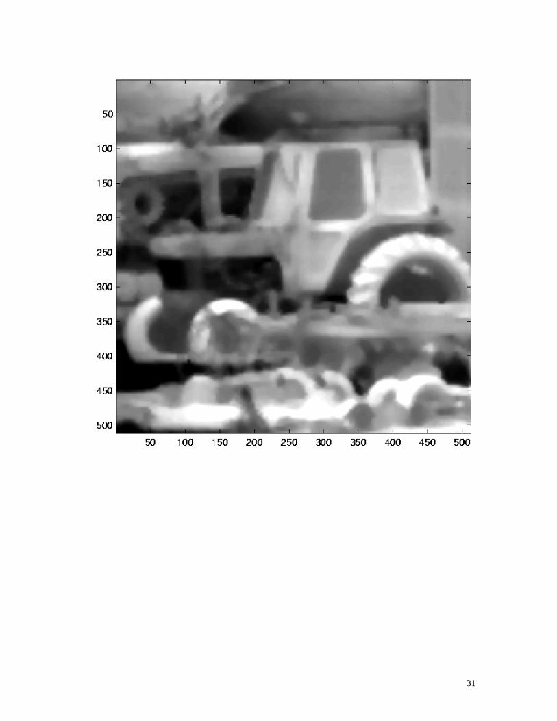
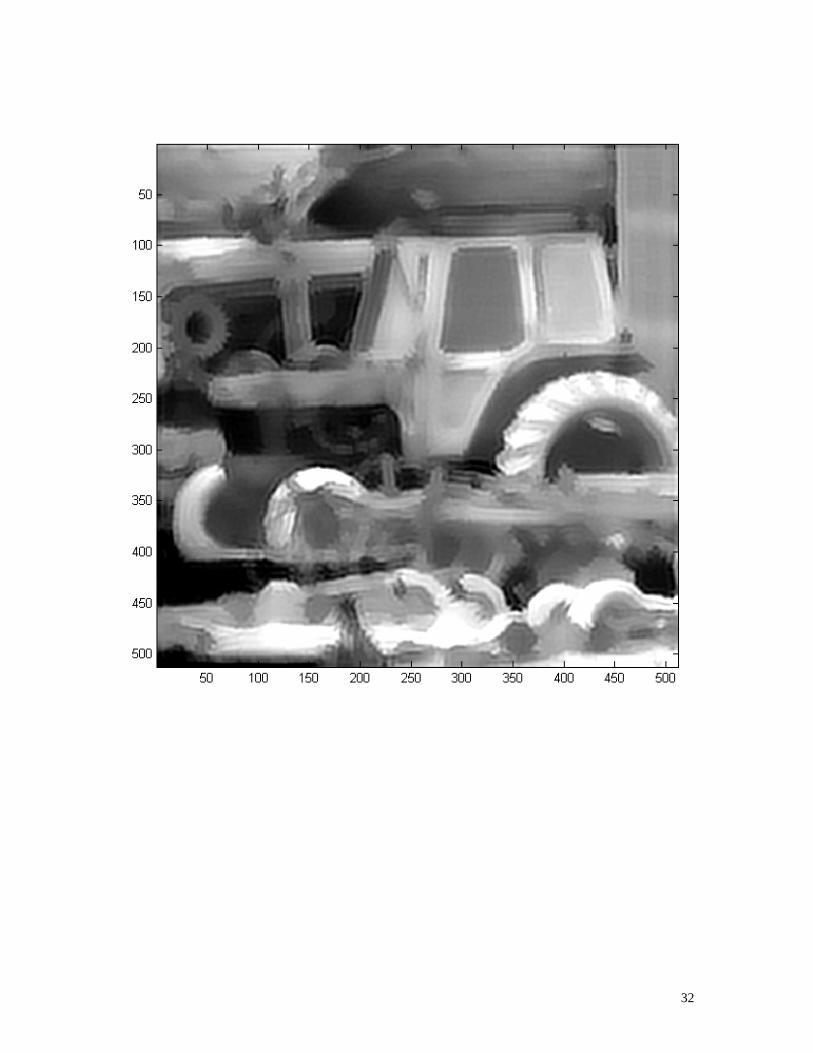
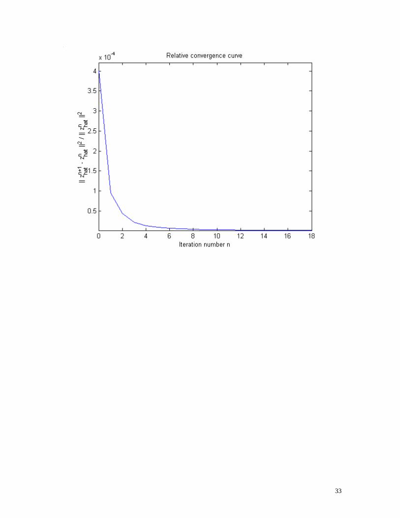
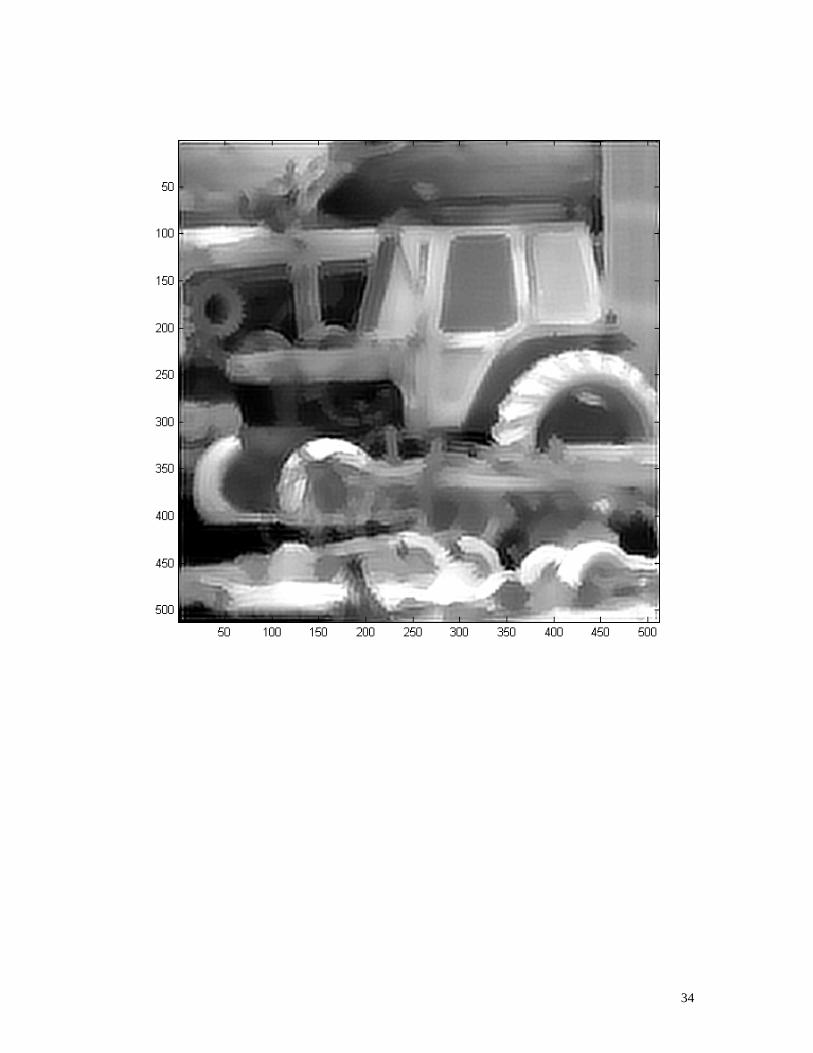
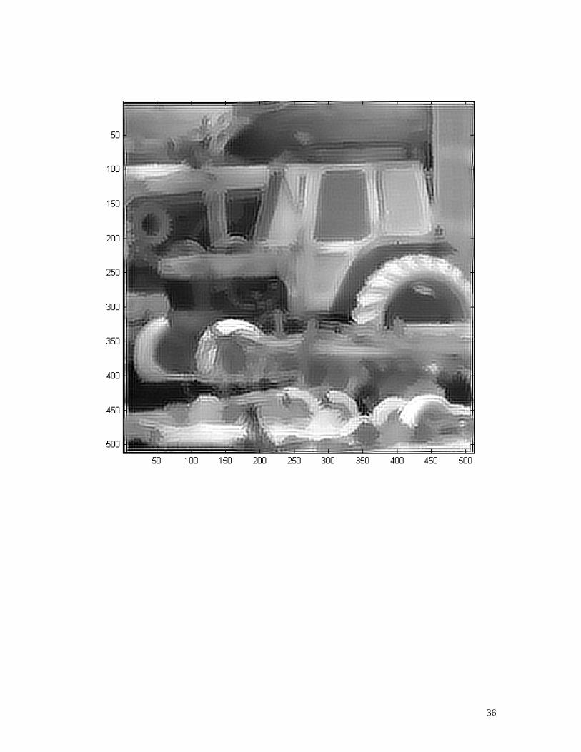
The first frame of the low video sequence, bilinear interpolation of the first frame, Proposed Method, the

relative convergence curve for Proposed Method (compared with the previous estimate of high-resolution

image “truck”) are shown in Fig. 5(a)-(d). From the relative convergence curves, we can see the Proposed

Method converges very fast.

The visually best reconstructed image using a fixed valued regularization parameter is obtained

with 1.0=α , shown in Fig. 5(e) via trial and error, with the help of human interaction. Although it

provides a good result, the computation cost is huge and involves human’s subjective influence.

Reconstructed images using two fixed valued regularization parameters 310=α and 310−=α are shown

in Fig. 5(f) and Fig. 5(g). As expected, image in Fig. 5(f) is “over-smoothened” and the image in Fig. 5(g)

is “noise-amplified”, which means arbitrarily selected and fixed valued regularization parameter may lead

to bad results. On the contrary, reconstructed high-resolution image using the proposed method with

simultaneous estimation of regularization parameter provides the best visual effect and much less

computation cost efficiently.

5. CONCLUSIONS

We have proposed a technique for the estimation of the regularization parameter for digital image

resolution enhancement. Our experimental results demonstrate the performance of the proposed algorithm.

Experimental results using both synthetic and real data are presented. For the synthetic results, in addition

to a subjective evaluation, we also present objective PSNR results. In all the cases considered, the proposed

algorithm gives a better reconstruction than results obtained using an optimal fixed-valued choice of the

regularization parameter, obtained using exhaustive search.

14

6. REFERENCES

1. L.P. Kondi, D. Scribner, J. Schuler, "A Comparison of Digital Image Resolution Enhancement

Techniques", SPIE AeroSense, Orlando, FL, April 2002.

2. R. Tsai and T. Huang, “Multiframe image restoration and registration,” in Advances in Computer

Vision and Image Processing, vol. 1, pp. 317-339, JAI Press Inc., 1984

3. A. M. Tekalp, M. K. Ozkan, and M.I. Sezan, “High-resolution image reconstruction from low-

resolution image sequences and space-varying image restoration,” in Proceeding of the International

Conference on Acoustics, Speech and Signal Processing, vol. III, (San Francisco, CA), pp. 169-172,

1992

4. J. M. Schuler, J. G. Howard, P. R. Warren, and D. A. Scribner, “TARID-based image super-

resolution,” in Proceeding of SPIE AeroSense, vol. 4719, (Orlando, Florida), pp. 247-254, 2002.

5. M. Irani and S. Peleg, “Motion analysis for image enhancement: Resolution, occlusion, and

transparency,” Journal of Visual Communications and Image Representation, vol. 4. pp. 324-335, Dec.

1993.

6. A. J. Patti, M.I. Sezan, and A. M. Tekalp, “Super-resolution video reconstruction with arbitrary

sampling lattices and nonzero apperature time,” IEEE Transactions on Image Processing, vol. 6. pp.

1064-1076, Aug. 1997.

7. P. E. Erem, M.I. Sezan, and A. M. Tekalp, “Robust, object-based high-resolution image reconstruction

from low-resolution video,” IEEE Transactions on Image Processing, vol. 6. pp. 1446-1451, Oct.

1997.

8. B. C. Tom and A. K. Katsaggelos, “Reconstruction of a high-resolution image from multiple degraded

mis-registered low-resolution images,” in Proceeding of the Conference on Visual Communications

and Image Processing, vol. 2308, pp.971-981. Sept. 1994

9. R. R. Schultz and R. L. Stevenson, “Extraction of high-resolution frames from video sequences,” IEEE

Trans. Image Processing, vol. 5, pp. 996–1011, June 1996.

10. R. R. Schultz and R. L. Stevenson, “Extraction of high-resolution frames from video sequences,” in

Proc. IEEE Int. Conf. Acoustics, Speech, Signal Processing, Detroit, MI, May 1995.

15

11. R. R. Schultz and R. L. Stevenson, “A Bayesian approach to image expansion for improved

definition,” IEEE Trans. Image Processing, vol. 3, pp. 233–242, May 1994.

12. R. C. Hardie, K. J. Barnard, “Joint MAP Registration and High-Resolution Image Estimation Using a

Sequence of Undersampled Images,” IEEE Trans. Image Processing, Vol. 6, No. 12, pp. 621–1633,

December 1997.

13. P. C. Hansen, “Rank-Deficient and Discrete Ill-Posed Problems”, SIAM 1997.

14. M. G. Kang, A. K. Katsaggelos, "Simultaneous Multichannel Image Restoration and Estimation of the

Regularization parameters", IEEE Trans. Image Processing, May 1997, pp. 774-778.

15. M. G. Kang, A. K. Katsaggelos, “General Choice of the Regularization Functional in Regularized

Image Restoration,” IEEE Trans. Image Processing, Vol. 4, No. 12, pp. 594–602, May 1995.

16. B. C. Tom, A. K. Katsaggelos, “Resolution Enhancement of Monochrome and Color Video Using

Motion Compensation,” IEEE Trans. Image Processing, Vol. 10, No. 2, pp. 278–287, February 2001.

17. E. Kaltenbacher and R. C. Hardie, “High-resolution infrared image reconstruction using multiple low-

resolution aliased frames,” in Proc. IEEE Nat. Aerospace Electronics Conf., Dayton, OH, May 1996.

18. N. P. Galatsanos, A.K. Katsaggelos, R.T. Chin, and A. D. Hillery, “Least squares restoration of

multichannel images”, IEEE Trans. Acoust. Speech, Signal Processing, Vol. 39, no. 10, pp. 2222-2236,

Oct., 1991.

19. R. R. Schultz and R. L. Stevenson, “Improved Definition Video Frame Enhancement,” Proc. IEEE Int.

Conf. Acoustics, Speech, Signal Processing, vol. 4, pp. 2169–2171, May 1995.

20. H. Stark and P. Oskoui, “High-resolution image recovery from imageplane arrays, using convex

projections,” J. Opt. Soc. Amer. A, vol. 6,pp. 1715–1726, 1989.

21. A. M. Tekalp, Digital Video Processing. Englewood Cliffs, NJ: Prentice-Hall, 1995.

7. APPENDIX: JUSTIFICATION OF INEQUALITY (33)

We define the following two ratios for the convenience to test inequality (33).

Ratio 1: { }2,

2

,,2,1min zWyy s kkkpk

−= L

16

Ratio 2: { }22

,,2,1min Dzy kpk L=

256x256 “Cameraman” and “Lena” are used as the two original high-resolution images. The results are

summarized in Tables 4, 5.

8. BIOGRAPHICS

Hu He received the M.S. in the Department of Electrical Engineering of State University of New York at

Buffalo in 2002. Currently, He is a Ph.D. candidate in the same university. His research interests include

image and video resolution enhancement. He has been a student member of IEEE since 2001 till now.

Lisimachos P. Kondi received the Diploma degree in electrical engineering from the Aristotle University of

Thessaloniki, Greece, in 1994 and the M.S. and Ph.D. degrees in electrical and computer engineering from

Northwestern University, Evanston, IL, USA, in 1996 and 1999, respectively. During the 1999-2000

academic year, he was a post-doctoral research associate at Northwestern University. Since August 2000,

he is an Assistant Professor of electrical engineering at the State University of New York at Buffalo, USA.

During the summer of 2001, he was a U.S. Navy/ASEE Summer Faculty Fellow at the U.S. Naval

Research Laboratory, Washington, DC, USA. His current research interests include image and video

processing and compression, wireless communications and wireless video transmission, image restoration

and super-resolution, and shape coding.

17

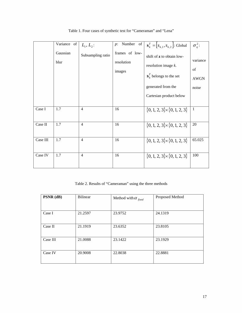
Table 1. Four cases of synthetic test for “Cameraman” and “Lena”

Variance of

Gaussian

blur

21 , LL :

Subsampling ratio

p: Number of

frames of low-

resolution

images

[ ]2,1, , kkTk ss=s : Global

shift of z to obtain low-

resolution image k.

Tks belongs to the set

generated from the

Cartesian product below

2ησ :

variance

of

AWGN

noise

Case I 1.7 4 16 { } { }3,2,1,03,2,1,0 × 1

Case II 1.7 4 16 { } { }3,2,1,03,2,1,0 × 20

Case III 1.7 4 16 { } { }3,2,1,03,2,1,0 × 65.025

Case IV 1.7 4 16 { } { }3,2,1,03,2,1,0 × 100

Table 2. Results of “Cameraman” using the three methods

PSNR (dB) Bilinear Method with fixedα Proposed Method

Case I 21.2597 23.9752 24.1319

Case II 21.1919 23.6352 23.8105

Case III 21.0088 23.1422 23.1929

Case IV 20.9008 22.8038 22.8881

18

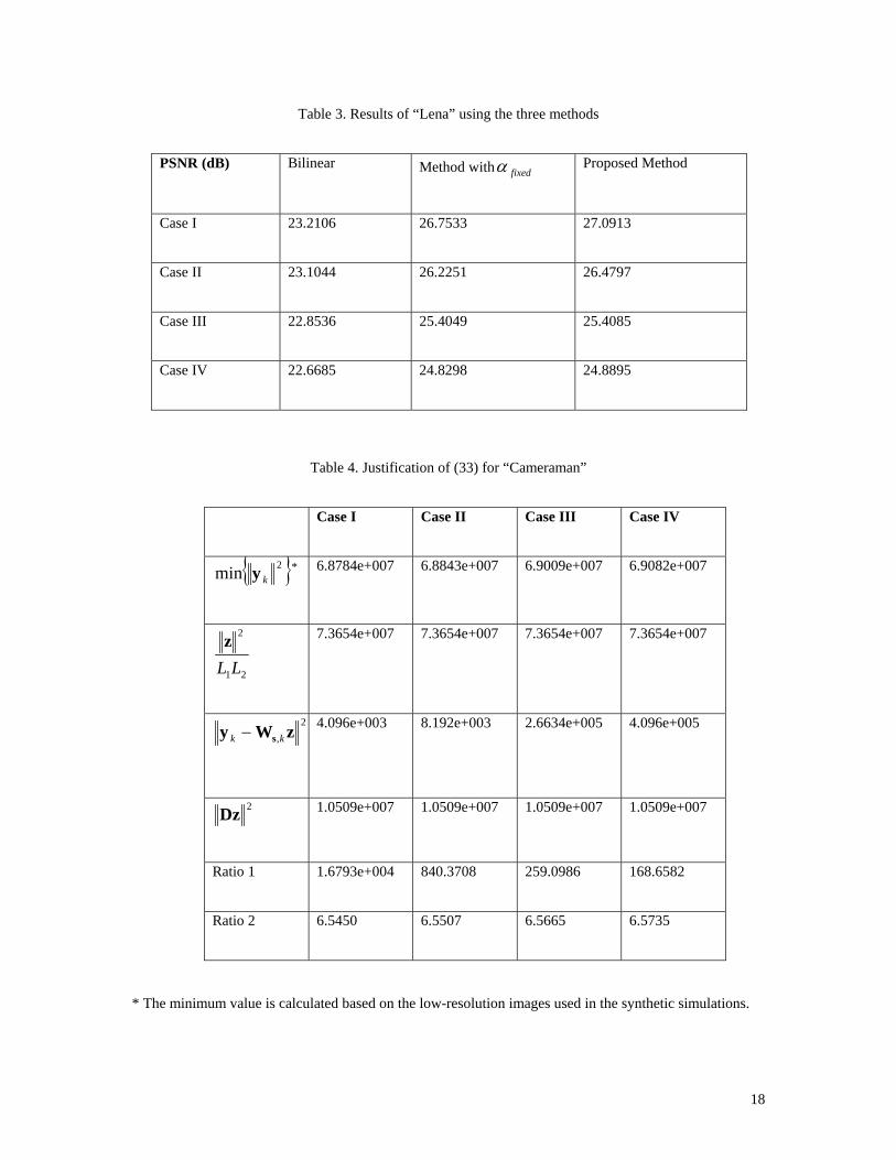
Table 3. Results of “Lena” using the three methods

PSNR (dB) Bilinear Method with fixedα Proposed Method

Case I 23.2106 26.7533 27.0913

Case II 23.1044 26.2251 26.4797

Case III 22.8536 25.4049 25.4085

Case IV 22.6685 24.8298 24.8895

Table 4. Justification of (33) for “Cameraman”

Case I Case II Case III Case IV

{ }2min ky * 6.8784e+007 6.8843e+007 6.9009e+007 6.9082e+007

21

2

LLz

7.3654e+007 7.3654e+007 7.3654e+007 7.3654e+007

2, zWy s kk −

4.096e+003 8.192e+003 2.6634e+005 4.096e+005

2Dz 1.0509e+007 1.0509e+007 1.0509e+007 1.0509e+007

Ratio 1 1.6793e+004 840.3708 259.0986 168.6582

Ratio 2 6.5450 6.5507 6.5665 6.5735

* The minimum value is calculated based on the low-resolution images used in the synthetic simulations.

19

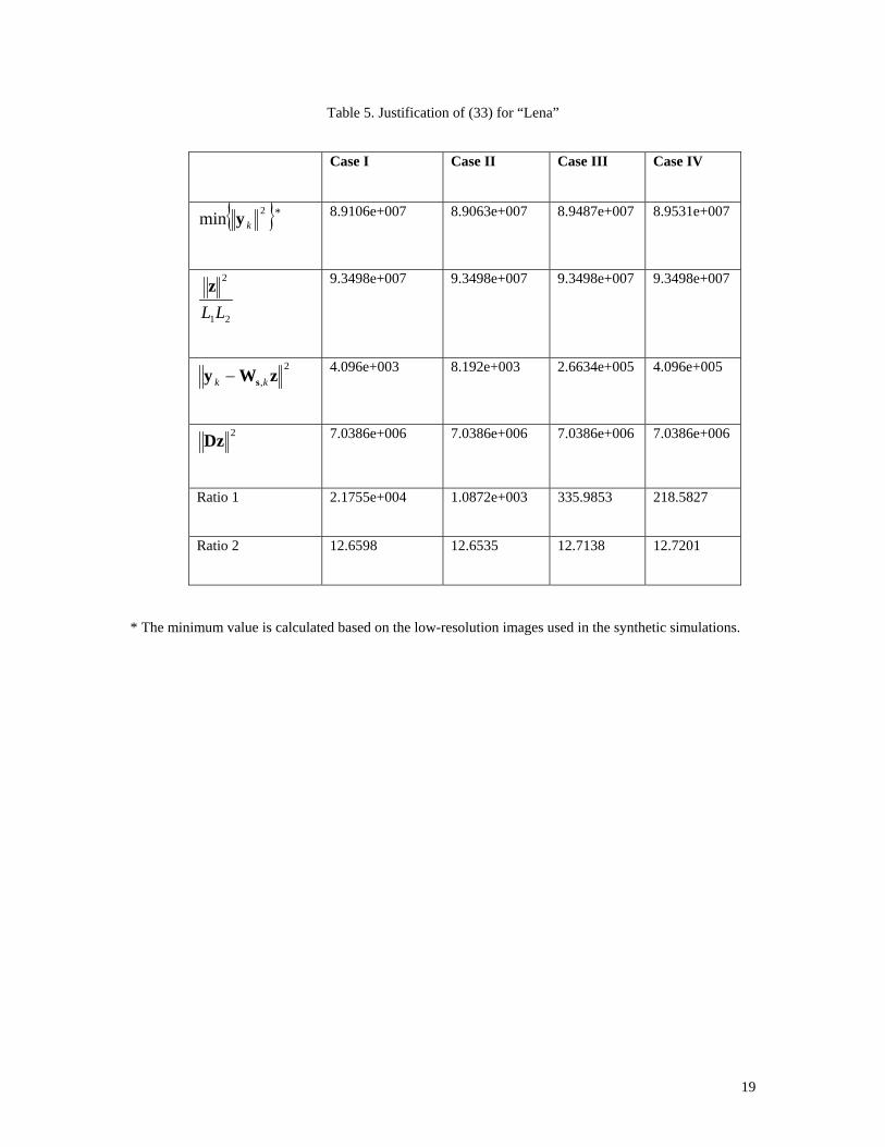
Table 5. Justification of (33) for “Lena”

Case I Case II Case III Case IV

{ }2min ky * 8.9106e+007 8.9063e+007 8.9487e+007 8.9531e+007

21

2

LLz

9.3498e+007 9.3498e+007 9.3498e+007 9.3498e+007

2, zWy s kk −

4.096e+003 8.192e+003 2.6634e+005 4.096e+005

2Dz 7.0386e+006 7.0386e+006 7.0386e+006 7.0386e+006

Ratio 1 2.1755e+004 1.0872e+003 335.9853 218.5827

Ratio 2 12.6598 12.6535 12.7138 12.7201

* The minimum value is calculated based on the low-resolution images used in the synthetic simulations.

20

21

22

23

24

25

26

27

28

29

30

31

32

33

34

35

36

37

10. LIST OF FIGURES

Fig. 1(a). Plot of αPSNR versusα for “Cameraman” using fixed regularization parameter in Case I

Fig. 1(b). Plot of αPSNR versusα for “Cameraman” using fixed regularization parameter in Case II

Fig. 1(c). Plot of αPSNR versusα for “Cameraman” using fixed regularization parameter in Case III

Fig. 1(d). Plot of αPSNR versusα for “Cameraman” using fixed regularization parameter in Case IV

Fig. 2(a). Reference frame of “Cameraman” (Case I)

Fig. 2(b). Bilinear interpolation of reference frame of “Cameraman” (Case I)

Fig. 2(c). Reconstructed image of “Cameraman” from Method with fixedα (Case I)

Fig. 2(d). Reconstructed image of “Cameraman” using Proposed Method (Case I)

Fig. 2(e). Absolute convergence curve of “Cameraman” using Simultaneous (Case I)

Fig. 2(f). Relative convergence curve of “Cameraman” using Proposed Method (Case I)

Fig. 3(a). Plot of αPSNR versusα for “Lena” using fixed regularization parameter in Case I

Fig. 3(b). Plot of αPSNR versusα for “Lena” using fixed regularization parameter in Case II

Fig. 3(c). Plot of αPSNR versusα for “Lena” using fixed regularization parameter in Case III

Fig. 3(d). Plot of αPSNR versusα for “Lena” using fixed regularization parameter in Case IV

Fig. 4(a). Reference frame of “Lena” (Case I)

Fig. 4(b). Bilinear interpolation of “Lena” (Case I)

Fig. 4(c). Reconstructed image of “Lena” from Method with fixedα (Case I)

Fig. 4(d). Reconstructed image from of “Lena” using Proposed Method (Case I)

Fig. 4(e). Absolute convergence curve of “Lena” using Proposed Method (Case I)

Fig. 4(f). Relative convergence curve of “Lena” using Proposed Method (Case I)

38

Fig. 5(a). Original image (first frame of “truck” sequence)

Fig. 5(b). Bilinear interpolation of first frame of “truck” sequence

Fig. 5(c). Reconstructed high-resolution “truck” image using MAP with simultaneous estimation of

regularization parameter

Fig. 5(d). Relative convergence curve of constructed high-resolution “truck” image using MAP with

simultaneous estimation of regularization parameter

Fig. 5(e). Reconstructed high-resolution “truck” image using joint MAP with fixed regularization

parameter 1.0=α

Fig. 5(f). Reconstructed high-resolution “truck” image using joint MAP with fixed regularization

parameter 310=α

Fig. 5(g). Reconstructed high-resolution “truck” image using joint MAP with fixed regularization

parameter 310−=α