grid powered nonlinear image registration with locally adaptive regularization

Medical Image Analysis 8 (2004) 325–342

www.elsevier.com/locate/media

Grid powered nonlinear image registration with locallyadaptive regularization

Radu Stefanescu *, Xavier Pennec, Nicholas Ayache

INRIA Sophia, Epidaure, 2004 Rte des Lucioles, BP 93, F-06902 Sophia-Antipolis Cedex, France

Available online 20 July 2004

Abstract

Multi-subject non-rigid registration algorithms using dense deformation fields often encounter cases where the transformation to

be estimated has a large spatial variability. In these cases, linear stationary regularization methods are not sufficient. In this paper,

we present an algorithm that uses a priori information about the nature of imaged objects in order to adapt the regularization of the

deformations. We also present a robustness improvement that gives higher weight to those points in images that contain more

information. Finally, a fast parallel implementation using networked personal computers is presented. In order to improve the

usability of the parallel software by a clinical user, we have implemented it as a grid service that can be controlled by a graphics

workstation embedded in the clinical environment. Results on inter-subject pairs of images show that our method can take into

account the large variability of most brain structures. The registration time for images of size 256� 256� 124 is 5 min on 15

standard PCs. A comparison of our non-stationary visco-elastic smoothing versus solely elastic or fluid regularizations shows that

our algorithm converges faster towards a more optimal solution in terms of accuracy and transformation regularity.

� 2004 Elsevier B.V. All rights reserved.

Keywords: Image registration; Non-rigid transformation; Nonlinear diffusion; Adaptive regularization; Parallel computing; Grid computing; Brain

atlas; Multi-subject image fusion

1. Introduction

The purpose of non-rigid registration is to estimate

the transformation of the 3D space that maps each point

p in the target image I to its most similar point (match)

T ðpÞ in the source image J . It is of interest to require the

transformation to be a homeomorphism, i.e. a contin-

uous function with a continuous inverse. This property

is particularly useful to avoid topology problems when

applying the recovered transformation to a labeled atlas.Unlike the intra-subject registration problem, which

is well-posed and corresponds to matching two instances

of the same physical reality, the multi-subject registra-

tion problem is often ill-posed. For instance, in brain

registration, the topology of the brain, the shape of the

ventricles, the number and shape of the sulci vary sig-

nificantly from one individual to another. Not only

* Corresponding author. Tel.: +33-4-95-38-79-27; fax: +33-4-92-76-

69.

E-mail address: [email protected] (R. Stefanescu).

1361-8415/$ - see front matter � 2004 Elsevier B.V. All rights reserved.

doi:10.1016/j.media.2004.06.010

these algorithms have to deal with the ambiguity of the

structures to match, but they also have to take intoaccount the spatially varying nature of the deformation.

Multi-subject registration is an essential tool in neu-

ro-science. Building and using brain atlases entirely de-

pends on reliable multi-subject non-rigid registration.

Also in the study of anatomical variability, shapes are

compared using non-rigid registration. In functional

magnetic resonance images (fMRI), the comparison of

the brain activity of different subjects is performedthrough the inter-subject non-rigid registration of the

corresponding anatomical MRI’s. When registering

such images, the algorithm has to estimate inhomoge-

neous deformations that are smooth in some parts of the

images and highly varying in others.

1.1. Related work

By using a dense deformation field and an intensity-

based registration technique, Pennec et al. (1999)

and Cachier et al. (2003) proposed a pair-and-smooth

mail to: [email protected]

326 R. Stefanescu et al. / Medical Image Analysis 8 (2004) 325–342

algorithm which uses a gradient descent on a similarity

criterion (typically the sum of square differences or the

cross correlation of intensities) and uniform Gaussian

smoothing to regularize the transformation. Gaussian

smoothing acts as a low-pass filter on the transforma-tion. As it is stationary, it has the same scale r every-

where in space. Thus, it either excessively smoothes the

transformation in highly varying regions, or keeps some

noise in more stable areas. However, the algorithm is

fast, and the computation time can be further reduced

by using a parallel implementation that exploits its

separability, as described in (Stefanescu et al., 2004a). A

similar approach was used by Collins and Evans (1997),who formulated the registration as a trade-off between a

similarity criterion (normalized cross correlation) and a

(still spatially uniform) regularization operator. In order

to reduce the computation time at each iteration, they

omit computing the gradient of the similarity criterion at

the points where this gradient had low values at the

previous iteration. In order to perform atlas to subject

registration, Guimond et al. (2001) begin by recoveringa parametric intensity transformation between the two

images before registering with an intensity based simi-

larity criterion. Hermosillo et al. (2002) implemented the

trade-off between similarity and regularity as a partial

differential equation, and tackled the case of multi-

modal registration with more complex criteria, such as

mutual information and correlation ratio (initially in-

troduced by Roche et al. (1998, 2001)). In order to dealwith inhomogeneous transformations, Hermosillo et al.

regularize the transformation using anisotropic diffu-

sion, based on the local image intensities as done by

Nagel and Enkelmann (1986).

Other authors search the transformation in a lower

dimensional space. Rueckert et al. (1999) used B-splines

distributed on a regular grid in order to model free-form

deformations to register MR mammographies. This al-gorithm also uses intensity-based matching. However,

time constraints usually limit the model to a relatively

small number of degrees of freedom, thereby lowering

its spatial resolution.

In order to dynamically tune the number of degrees of

freedom that describe the transformation, some authors

have used multi-resolution approaches. Hellier et al.

(2001) use a locally affine model at each bloc of a spa-tially adaptive space decomposition. They estimate the

transformation in a robust manner with respect to voxels

contributing unreliable information, and use a multigrid

refinement scheme to avoid heavy computations in

irrelevant areas of images, thereby decreasing the com-

putation time to about an hour. Rohde et al. (2003)

select, on a multi-resolution grid, the points that best

optimize the normalized mutual information in order todrive a radial basis transformation model. Thanks to the

local support of the radial basis functions, the similarity

criterion is only computed for a relatively small number

of voxels. A similar threshold on the gradient of the cost

function has previously been used in (Collins and Evans,

1997). The multi-resolution framework allows a spatially

adaptive description of the transformation. Its effective

precision is limited to the final grid resolution (smallerdetails cannot be modeled), which has to remain rather

coarse in order to achieve reasonable computation times

(reported by Rohde et al. (2003) to be about 3 h for

typical images and a final grid of size 17� 17� 15).

However, as the authors predict, this time may be sig-

nificantly decreased by a parallel implementation.

Ferrant et al. (2002) use an active surface to drive a

finite element biomechanical model of the brain. Themain advantage is the ability to take into account

the anatomy of objects in the images. However, due to

the limited resolution of the tetrahedrization imposed by

computation time constraints, the algorithm is less

adapted to the estimation of deformations with fine

details. Being based on an active surface, the algorithm

only uses the information present in the images around

that surface, and presents a high sensitivity to thequality of its initial segmentation. Furthermore, the

mechanical simulation of the tissues has no particular

physical justification in the multi-subject case.

Ganser et al. (2004) implemented an electronic Ta-

lairach and Tournoux brain atlas. They used a feature-

based method to estimate the correspondences which

drive a free-form deformation model based on radial

basis functions. The main advantage of their system isthat the transformation is determined only by clinically

relevant points of interest (cortex, ventricles, commis-

sures and tumors), and interpolated in the remainder of

the brain. Like Ferrant et al., Ganser et al. used feature-

based methods to estimate the correspondences only for

the voxels which are important for their application, and

the two algorithms share the same potential weakness:

an accurate segmentation of these features is required.

1.2. Goal

The purpose of our work is to combine some of the

advantages of the approaches presented above in a new

framework: first, we want to use the ability of the dense

transformation algorithms to take into account the en-

tire information present in the image and detect finedetails. Meanwhile, we want to guarantee the invert-

ibility of the estimated transformation, in order to avoid

potential topology problems when applying it to a seg-

mentation (e.g. labeled atlas, contour surface). Second,

we want to adapt the registration process to the nature

of the objects present in the images: the optimal level of

the transformation regularity is not the same every-

where. In regions where the deformation has smallvariations, we want to impose a higher degree of regu-

larity than in areas where these variations are expected

to be large. Third, the information present in the images

R. Stefanescu et al. / Medical Image Analysis 8 (2004) 325–342 327

at different places is not equally important (e.g. uniform

intensity regions versus edges). We would like to register

precisely homologous points in certain regions, while

interpolating the deformation field in others.

Since the registration process is time consuming, wealso address the problem of the computation time. From

this point of view, our goal is to be able to run the algo-

rithm in a sufficiently short time (typically a few minutes)

to be embedded in a more complex processing pipeline

and allow for a possible interactivity between algorithm

and user. We address this problem by using a parallel

implementation on a cluster of networked personal

computers. This type of parallel computing platform isreadily available in many places and we present a mean to

access it from the clinical environment (or any other net-

workedPC)over a local area networkor over the Internet.

1.3. Paper organization

In Section 2 we present a non-rigid registration

framework that allows us to guarantee the invertibilityand to locally adapt the degree of regularity of the dense

transformation. Using an approach based on a priori

confidence in the similarity criterion, we also reduce the

weight of points that do not bring useful information to

registration. In order to avoid large computation times,

we present in Section 3 a numerical scheme that uses

inversions of tridiagonal matrices, which can be per-

formed in real time. In Section 4, we develop a fastparallel implementation on an inexpensive cluster of

personal computers, which enabled us to reduce the

computation time for a full 3D registration of images of

size 256� 256� 124 to only 5 min on 15 standard PCs.

In Section 5, we apply our algorithm to T1-MRI brain

images and present results showing that the registration

software is able to retrieve large and highly inhomoge-

neous deformations. Furthermore, the estimated defor-mations are smooth and invertible. Section 6 exposes

some of the research tracks opened up by the method.

2. Method

As images are discrete, a natural representation of a

non-rigid transformation is the displacement of eachvoxel of the target image, i.e. a vectorial displacement

field UðpÞ such that T ðpÞ ¼ p þ UðpÞ. Using these no-

tations, a point p with intensity IðpÞ in the target image

corresponds to a point T ðpÞ with intensity Jðp þ UðpÞÞin the source image. To simplify notations, we denote by

ðJ � UÞðpÞ,Jðp þ UðpÞÞ 1 the transformed (or resam-

pled) source image.

1 Using the composition symbol ‘‘�’’ is an abuse of notation, since

the composition of functions is effectively done with the transforma-

tion T ðpÞ ¼ p þ UðpÞ.

In order to clarify the description of our method, our

presentation will follow the derivation of the demons al-

gorithm Thirion (1998) as presented by Pennec et al.

(1999). Our choice was motivated by the fact that it uses a

dense displacement field, it is fast, easy to understand, andhas been relatively widely used so far (Bricault et al., 1998;

Webb et al., 1999; Prima et al., 1998). In order to better

explain in the following sections the contributions we

propose, let us investigate inmore details how the demons

algorithm works, and what are its main weaknesses.

2.1. A quick overview of the demons algorithm

The demons algorithm alternates the maximization of

the similarity and the regularity criteria. The similarity is

maximized through a gradient descent that we describe

below, while the regularity is enforced by convolving the

deformation field with a stationary Gaussian. The al-

gorithm can use different similarity criteria, such as the

smallest squared distance (SSD) (Pennec et al., 1999) or

the local correlation coefficient (Cachier and Pennec,2000). Since the SSD criterion is commonly accepted as

a reliable method for monomodal registration, we will

use it as an example throughout this paper. More

powerful similarity metrics for multi-modal registration

are described by Roche et al. (1998), Guimond et al.

(2001), Hermosillo et al. (2002), Cachier and Pennec

(2000) and Roche et al. (2000).

The gradient descent step can be described as follows:given the current value of the deformation U , the goal is

to find a small additive correction u that minimizes the

chosen similarity criterion. A first order Taylor expan-

sion leads to

SSDðI ;J � ðU þ uÞÞ

¼Z

IðpÞ½ � ðJ � ðU þ uÞÞðpÞ�2 dp

� SSDðI ;J �UÞ

þZ

2 ðJ �UÞðpÞ½ � IðpÞ� ðrJÞ �U½ �ðpÞ>uðpÞdp: ð1Þ

As by definitionRf ðpÞ>uðpÞdp is the dot product of

the vector functions f and u, we get by identification:

rSSD ¼ 2 ðJ � UÞðpÞ½ � IðpÞ� ðrJÞ � U½ �ðpÞ:From the Taylor expansion, we can see that the criterion

is minimized if we update the current displacement field

Un at iteration n by adding a small fraction � of the

gradient un ¼ �� rSSD to obtain Unþ1 ¼ Un þ un. Thisfirst order gradient descent is usually the evolution

equation used in PDE approaches (Hermosillo et al.,

2002). The demons algorithm corresponds to a slightlymore complex second order gradient descent scheme

where the gradient is renormalized using an approxi-

mation of the second order derivative of the SSD cri-

terion (Pennec et al., 1999).


This scheme is efficient, but suffers from several

drawbacks:

• The additive correction scheme presented above does

not re-compute the gradient of the source image at

each optimization step, but rather resamples it. InSection 2.2, we argue that this additive scheme be-

comes invalid with large local rotations, and it may

lead to a non-invertible transformation. Therefore,

we propose a ‘‘compositive scheme’’ that tackles all

types of displacements and, furthermore, ensures

the invertibility of the recovered transformation.

• In many real cases, deformations are highly inhomo-

geneous in certain areas, and exhibit a large spatialcoherence in others. In Section 2.3, we explain that

the regularization with a uniform Gaussian is not

adapted to recover such deformations, and that elas-

tic models are computationally expensive to solve.

Thus, we propose a faster regularization method that

is compatible with inhomogeneous deformations and

has low computation times.

• The demons algorithm, like many others, takes allvoxels into account in an equal manner. Based on

the observation that some areas in images contribute

more relevant information than others, we describe in

Section 2.4 a method that weights the local influence

of the correction field in the registration based on a

priori information about the local reliability of the

similarity criterion at each voxel.

2 Once again, we use the composition symbol ‘‘�’’ to characterize the

action performed by the corresponding transformation Id þ u, ratherthan by the displacement field itself u.

2.2. A ‘‘compositive’’ scheme for large deformations and

invertibility

The additive formulation of the Taylor expansion of

the SSD leads to a gradient descent direction propor-

tional to the resampled gradient of the source image rJ ,without changing its direction. In real cases, where the

deformation contains large local rotations, the directionof the gradient of the criterion will slowly become par-

allel to the contours of the resampled image J � U ,

thereby diminishing its efficiency at each iteration. Fig. 1

presents an example of a 90� rotation of a simple image.

At the beginning of the registration, both schemes

evolve in similar manners (Fig. 1(b)). However, as the

rotation is gradually recovered, the additive scheme

yields correction fields that tend to become parallel tothe contour lines, and the efficiency of the correction

decreases (Fig. 1(c)).

Following Trouv�e (1998), Miller and Younes (2001)

and Chefd’hotel et al. (2002), we replace the addition of

the correction and displacement fieldsUnþ1 ¼ Un þ un bythe composition of the corresponding transformations. If

Id is the identity transformation, this corresponds to

Id þ Unþ1 ¼ ðId þ UnÞ � ðId þ unÞ¼ Id þ Un � ðId þ unÞ þ un:

Thus, denoting by ðU � uÞðpÞ ¼ Uðp þ uðpÞÞ þ uðpÞ 2

the result of the transformation composition on the

displacement fields, we end up with the update equation

Unþ1 ¼ Un � un. One can remark that a first order Tay-

lor expansion of ðU � uÞ yields

ðU � uÞðpÞ ¼ Uðpþ uðpÞÞ þ uðpÞ¼ UðpÞ þrUðpÞTuðpÞ þ uðpÞ þOðkuk2Þ: ð2Þ

Therefore, the two schemes are equivalent if the dis-

placement field is locally constant (rU � 0), which

corresponds to a (local) translation.The goal is now to find the correction field u that

minimizes SSDðI ; J � ðU � uÞÞ. Taking J 0 ¼ J � U(Eulerian formulation), we came back to the additive (or

Lagrangian) formulation with U 0 ¼ 0 since ð0 � uÞ ¼ u.Therefore, we have

SSDðI ;J � ðU � uÞÞ¼ SSDðI ;J 0 � ð0þ uÞÞ

� SSDðI ;J 0Þ þZ

2 ðJ 0ÞðpÞ�

� IðpÞ�rðJ 0Þ� �

ðpÞ>uðpÞdp

� SSDðI ;J �UÞ

þZ

2 ðJ �UÞðpÞ½ � IðpÞ� rðJ �UÞ½ �ðpÞ>uðpÞdp: ð3Þ

Thus, the major difference with the additive scheme

(Eq. (1)) lies that we now take the gradient of the re-

sampled image rðJ � UÞ instead of the resampled gra-

dient of the original image ðrJÞ � U . To summarize, theusual additive scheme consists in computing the gradient

of the SSD at the current displacement field Un and then

to update the displacement using a fraction of this

gradient:

Unþ1 ¼ Un � �2 J � Un½ � I � ðrJÞ � Un½ �: ð4Þ

The equivalent compositive scheme is

Unþ1 ¼ Un � ð � �2 J � Un½ � I � rðJ � UnÞ½ �Þ: ð5Þ

The fraction � of the gradient that is taken at each

optimization step is an algorithm parameter. Section 5.3

shows a method to automatically tune it.One can notice in Fig. 1 that the gradient of the de-

formed source image is now updated with the compos-

itive scheme: at each iteration, the correction is

perpendicular to the contour lines, which increases the

convergence rate (Fig. 1(d)). This simple example

translates into the general case if we consider the two

small images as being merely local details of larger ones.

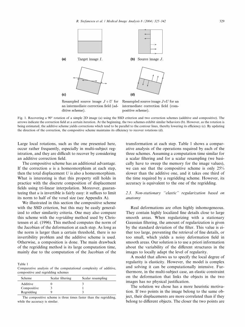
Fig. 1. Recovering a 90� rotation of a simple 2D image (a) using the SSD criterion and two correction schemes (additive and compositive). The

arrows indicate the correction field at a certain iteration. At the beginning, the two schemes exhibit similar behaviors (b). However, as the rotation is

being estimated, the additive scheme yields corrections which tend to be parallel to the contour lines, thereby lowering its efficiency (c). By updating

the direction of the correction, the compositive scheme maintains its efficiency to recover rotations (d).


Large local rotations, such as the one presented here,

occur rather frequently, especially in multi-subject reg-istration, and they are difficult to recover by considering

an additive correction field.

The compositive scheme has an additional advantage.

If the correction u is a homeomorphism at each step,

then the total displacement U is also a homeomorphism.

What is interesting is that this property still holds in

practice with the discrete composition of displacement

fields using tri-linear interpolation. Moreover, guaran-teeing that u is invertible is fairly easy: it suffices to limit

its norm to half of the voxel size (see Appendix A).

We illustrated in this section the compositive scheme

with the SSD criterion, but this may be easily general-

ized to other similarity criteria. One may also compare

this scheme with the regridding method used by Chris-

tensen et al. (1996). This method computes the norm of

the Jacobian of the deformation at each step. As long asthe norm is larger than a certain threshold, there is no

invertibility problem and the additive scheme is used.

Otherwise, a composition is done. The main drawback

of the regridding method is its large computation time,

mainly due to the computation of the Jacobian of the

Table 1

Comparative analysis of the computational complexity of additive,

compositive and regridding schemes

Scheme Scalar filtering Scalar resampling

Additive 0 3

Compositive 3 1

Regridding 9 3

The compositive scheme is three times faster than the regridding,

while the accuracy is similar.

transformation at each step. Table 1 shows a compar-

ative analysis of the operations required by each of thethree schemes. Assuming a computation time similar for

a scalar filtering and for a scalar resampling (we basi-

cally have to sweep the memory for the image values),

we can see that the compositive scheme is only 25%

slower than the additive one, and it takes one third of

the time required by a regridding scheme. However, its

accuracy is equivalent to the one of the regridding.

2.3. Non-stationary ‘‘elastic’’ regularization based on

anatomy

Real deformations are often highly inhomogeneous.

They contain highly localized fine details close to large

smooth areas. When regularizing with a stationary

Gaussian filtering, the amount of regularization is given

by the standard deviation of the filter. This value is ei-ther too large, preventing the retrieval of fine details, or

too small, which yields a noisy deformation field in

smooth areas. Our solution is to use a priori information

about the variability of the different structures in the

images to locally adapt the level of regularity.

A model that allows us to specify the local degree of

regularity is elasticity. However, the model is complex

and solving it can be computationally intensive. Fur-thermore, in the multi-subject case, an elastic constraint

on the deformation that links the objects in the two

images has no physical justification.

The solution we chose has a more heuristic motiva-

tion. If two points in the image belong to the same ob-

ject, their displacements are more correlated than if they

belong to different objects. The closer the two points are


to each other, the more their displacements are corre-

lated. Our idea is to use a locally constant Gaussian

model inside each object. It has the advantage of al-

lowing the different objects to evolve more freely inside

the image space, while enforcing the coherence of eachobject. Inside each object, the choice of the Gaussian has

a triple motivation:

(1) Smoothing by a Gaussian is not far from the simu-

lation of an elastic displacement and it can model it

with a reasonable approximation (Bro-Nielsen,

1996).

(2) The strength of the regularity constraint is described

by the local width of the Gaussian. By tuning the lo-cal standard deviation of the Gaussian, we can reg-

ularize inhomogeneous deformations that alternate

smooth and highly varying regions.

(3) As we will see below, solving this locally constant

Gaussian model is fast and easily implementable

on a parallel system.

We chose to implement our non-stationary Gaussian

regularization using a non-stationary diffusion filter oneach of the components Ua (a 2 fx; y; zg) of the dis-

placement field:

oUa

ot¼ divðDrUaÞ; ð6Þ

where D is a diffusion (or stiffness) tensor.

If the diffusion tensor is constant and isotropic, it can be

described by a scalar value d (D ¼ d I3, I3 being theidentity matrix). In this case, Eq. (6) describes a linear

diffusion filter, which can be implemented using a con-

volution with a stationary Gaussian. The larger d is, the

more important is the diffusion. To fit our purpose of

tolerating large deformations in certain areas and small

deformations in others, it suffices to make d a scalar field

and give it large values in areas where we expect little

deformations and small values in areas that may containlarge ones. In this case, d encodes the anatomical

knowledge that we have on the deformability of the tis-

sues. Currently, d is estimated by using region-based

segmentation algorithms. Since d expresses the local

stiffness of the source image J , we only need to segment

this image to compute it. However, unlike feature-based

registration that needs an accurate segmentation of the

structures to match, our algorithm only needs a fuzzysegmentation. In Section 5 we will show a method to

automatically estimate the d field for T1 MRI images of

the brain.

The correlation of the deformation can also be direc-

tional. The displacement of a point is in some cases more

correlated with its neighbors along some preferential

directions than along others. For instance, when regis-

tering the brain surface, it is important to leave the de-formation quite free perpendicularly to the surface while

regularizing along the tangent plane to maintain the

consistency of the surface. In this case, theD tensor in Eq.

(6) is not isotropic. Its components describe the amount

of regularization along the different directions. This an-

isotropic case is potentially more powerful, especially

when registering with a probabilistic atlas such as the one

described by Thompson et al. (2000). We intend to in-vestigate this interesting feature in the near future.

2.4. Confidence-based weighting of the correction field

The images we register are inevitably noisy. This

noise has a strong impact on the gradient of the simi-

larity criterion, especially in intensity uniform areas

where the local signal to noise ratio is low. When reg-ularizing the displacement, these spurious values tend to

weaken the well defined displacement ‘‘forces’’ located

at edges. The goal of this section is to filter out these

unreliable values from the raw correction field. For this,

we use a method inspired by the image-guided aniso-

tropic diffusion (Weickert, 1997): once the correction

field u is computed, its components ua along each axis

are filtered using a diffusion equation:

ouaotðpÞ ¼ ð1� kðpÞÞðDuaÞðpÞ; where kðpÞ 2 ½0; 1�: ð7Þ

If k is a spatially constant field, the above equation

amounts to a Gaussian diffusion, which was previously

used in similar conditions (Cachier et al., 2003; D’Ag-

ostino et al., 2003). If k varies spatially, it measures the

local degree of smoothing applied to ua. For kðpÞ ¼ 1,the local displacement uaðpÞ will be locally unaffected by

the above partial differential equation (PDE). In case of

smaller values for kðpÞ, the gradient field is locally

smoothed. This feature is particularly well adapted to

our problem. In areas where the signal to noise level is

low, we smooth the correction field, thereby attenuating

the effects of noise. The k field measures the local con-

fidence in the similarity criterion.Points that are reliable landmarks in the source image

are those where the neighborhood has a characteristic

pattern that cannot be produced by noise. The confi-

dence can therefore be taken as a measure of the local

intensity variability in the source image, such as the local

variance or gradient. This type of measure is static, since

it only has to be computed once, at the beginning of the

algorithm. The expression we used is derived fromWeickert (2000) in the case of non-stationary image

diffusion:

kðpÞ ¼ exp�crJk kk

� �40B@

1CA: ð8Þ

The confidence described in the above equations is

close to 1 for large image gradients, and to 0 in uniform

areas. k is a contrast parameter that discriminates low

contrast regions (that are mainly diffused) from highcontrast ones (that preserve the edges in the deformation


field), and c is a scalar parameter usually taken around

3.3 (see Weickert, 2000). We show in Section 5.3 how

these parameters are tuned.

The confidence field k can also be used to encode

some anatomical knowledge: in certain applications,especially in difficult multi-subject cases, one might

choose to deliberately ignore certain aspects of the im-

ages, which could make the registration fail (e.g. tumors,

marker-enhanced regions). In such applications one can

impose the confidence to be null in areas that are con-

sidered irrelevant for the registration.

This formulation of the confidence can be under-

stood as being a kind of soft feature-based registration.Indeed, depending on the method used to estimate

correspondences, registration algorithms are classified

into two main categories. Intensity-based algorithms

treat images as sets of voxels characterized by their

intensity which contribute in equal measure to the final

transformation. Feature-based registration consists in

estimating correspondences by matching geometric

structures in the images, such as surfaces or lines. Ourmethod is somewhere in-between. Voxels do not have

the same weight in the computation of the correspon-

dences. The ones which are on the edges of significant

structures have a larger weight than the others. By

using a kind of fuzzy features extraction, our algorithm

is able to take into account the structures visible in

the images, without needing generally error-prone

segmentations.Similar approaches have been used in image regis-

tration. Ourselin et al. (2000) estimate the correspon-

dences in the case of rigid and affine registration using

block-matching. Only the blocks in the source image

that have a variance larger than a certain threshold are

taken into account. The Nagel–Enkelmann operator

(Nagel and Enkelmann, 1986) used by Alvarez et al.

(2000) and Hermosillo et al. (2002) also uses a measureof the local variation of the source image to weight an

elastic-type matching.

2.5. Method summary

The methodology we described in the previous

sections is summarized in the following iterative

algorithm.(1) The gradient of the similarity criterion is computed

in the Eulerian framework; a small fraction (of max-

imum magnitude lower than half the voxel size) is

taken as the correction field u. For instance, the

SSD criterion yields:

u ¼ ��2 J � Un½ � I � rðJ � UnÞ½ �: ð9Þ

(2) The correction field is filtered using Eq. (7):

ouaotðpÞ ¼ ð1� kðpÞÞðDuaÞðpÞ:

The confidence measure kðpÞ depends on the gradi-

ent of the source image (Section 2.4). The numerical

scheme is detailed in Section 3.

(3) The regularized correction field is composed with

the current deformation field (Section 2.2):

U U � u:(4) The displacement field is finally regularized using the

diffusion equation (6):

oUa

ot¼ divðDrUaÞ:

The local stiffness tensor D depends on the type of

tissue that is deformed (Section 2.3). Again, the

numerical scheme is detailed in Section 3.The algorithm loop is stopped either when the rela-

tive improvement of the similarity criterion value is

too small or when a maximal number of iteration is

reached. In order to accelerate the convergence, this

iterative optimization algorithm is embedded in a multi-

resolution approach, as most non-rigid registration

algorithms.

2.6. Discussion: a visco-elastic regularization?

Our algorithm has two levels of regularization. The

first one acts on the correction field, which can be seenas the velocity field. Thus, its regularization can be

interpreted as a non-stationary viscous fluid constraint.

On the contrary, the regularization of the displacement

field can be understood as imposing a kind of elastic

behavior. Consequently, the combination of the

two regularizations ends up in a sort of viscoelastic

movement.

In (Christensen et al., 1996), it is argued that, in orderto recover large deformations, a fluid model of defor-

mation is necessary. If we do not take into account the

elastic regularization, our model of deformation can be

seen as a fluid one. However, the purely fluid model has

a drawback: it does not preserve the anatomical coher-

ence of images. Indeed, since there is no constraint on

the displacement field itself, the model allows too large

local volume expansions or contractions. Mathemati-cally, this translates into values of the Jacobian of the

transformation that are either very large or very close to

0. This poses a problem with partial volumes and non-

corresponding structures (e.g. in brain imaging, partial

cerebro-spinal fluid/white matter voxels being trans-

formed into grey nuclei, or structures contracting and

eventually vanishing). Furthermore, when noise gener-

ates spurious gradients in otherwise uniform areas,strong artifacts appear in the deformation field inside

these regions. These side-effects occur due to the un-

constrained nature of the fluid model when optimizing

the similarity. On the other hand, an elastic regulariza-

tion may prevent algorithms from recovering large


deformations, but it is able to enforce an a priori con-

straint on the shapes in the resampled result image.

Our solution is a hybrid one. It composes the cor-

rection field with the displacement rather than adding it,

and the regularization of the correction follows a fluidmodel. However, we choose to perform a selective

elastic regularization in the areas where, due to ana-

tomical reasons, the displacement of neighboring voxels

should be coherent. This enables us to inject in the

algorithm some a priori information to constrain the

deformations.

3. Numerical scheme

As we have seen, both the confidence-based filtering

(Eq. (7)) and the regularization (Eq. (6)) can be de-

scribed using non-stationary diffusion PDE’s on scalar

fields v (the x, y and z components of U and u). In this

section we tackle the problem of efficiently solving such

equations in the isotropic case. A similar method hasbeen used by Fischer and Modersitzki (1999) and

Modersitzki (2004).

3.1. Explicit, implicit and semi-implicit schemes

The simplest way of solving an image diffusion

equation such as

ovot¼ divðdrvÞ

on a discrete image v is to compute the derivatives using

finite differences and then reformulate the problem using

a matrix vector multiplication. Considering the image vas a big one dimensional vector v of size N containing

successively all its voxels (e.g. N ¼ dimx� dimy � dimz

for a 3D image), the derivatives can be encoded into abig N � N matrix A, so that we get for the explicit

scheme:

vtþDt � vt

Dt¼ Atvt;

where t is the time and Dt is the time step. The Laplacian

matrix At depends on the time t if the diffusion field d is

time varying.

For this explicit scheme, all the variables on the right

side are known at time t, and the resolution is simplyvtþDt ¼ vt þ DtAtvt. However, such an approach is very

slow, since the time step has to be very small in order to

avoid divergence (Weickert et al., 1998). This drawback

can be avoided by solving the implicit scheme, which

contains on the right side only the variables at the time

t þ Dt:

vtþDt � vt

Dt¼ AtþDtvtþDt:

This scheme is guaranteed to be stable for all values

of Dt. However, it is complicated to solve (since we do

not know AtþDt), and therefore a semi-implicit scheme is

often preferred:

vtþDt � vt

Dt¼ AtvtþDt:

This amounts to solving the equation

vtþDt ¼ ðIN � DtAtÞ�1vt:

3.2. The semi-implicit scheme in 3D: AOS

Let us investigate first the resolution of the above

equation in one dimension. Since we use finite differ-

ences, the value vtþDti at each point of index i dependsonly on vtþDti�1 , vtþDti and vtþDtiþ1 . Therefore, the matrix At is

tridiagonal, and so is IN � DtAt. The inversion of a tri-

diagonal matrix can be achieved using the Thomas al-

gorithm (Press et al., 1993), which consists in a LR

decomposition followed by forward and backward

substitution steps (see Appendix B). This first order re-

cursive algorithm operates in linear time.

In the three-dimensional case, a problem arises: thematrix to invert is no longer tridiagonal, which leads to

a much higher computation time. In order to address

this problem, Weickert et al. (1998) introduced the Ad-

ditive Operator Scheme (AOS), which makes the reso-

lution of the PDE separable, thereby simplifying the

computations. If the filtering operator is separable, we

can consider the Laplacian operator A to be the sum of

his projection on the three axes A ¼P

a2fx;y;zgAa.Therefore

vtþDt ¼ IN

� Dt

Xa2fx;y;zg

Aa

!�1vt:

In the case of non-stationary diffusion, he then used

the following approximation, justified by a Taylor ex-

pansion of both members:

vtþDt ¼ IN

� Dt

Xa2fx;y;zg

Aa

!�1vt

¼ 1

3

Xa2fx;y;zg

ðIN � 3DtAaÞ�1vt þ OðDt2Þ:

This reduces the 3D diffusion to three 1D ones, thusreplacing the inversion of a non-tridiagonal matrix with

three inversions of tridiagonal ones. In practice, we

obtain in our iterative optimization algorithm an

equivalent computational load for one AOS regulari-

zation step and for the computation of the gradient of

the similarity criterion.

2

3

3

4

4

5

5

6

6

7

7

8

8

8

9

9

1

2

3

4

5

6

7

10

Line 3

Line 4

Line 5

Line 6

Line 7

Line 8

Line 1

Line 2

Processor 3 Processor 2Processor 1

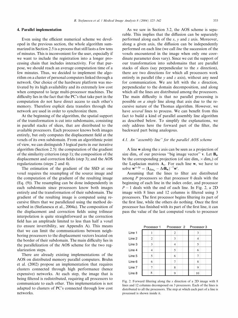
Fig. 2. Forward filtering along the x direction of a 2D image with 8

lines and 12 columns decomposed on 3 processors. Each of the lines is

distributed to all the processors. The step at which each part of a line is

processed is shown inside it.


4. Parallel implementation

Even using the efficient numerical scheme we devel-

oped in the previous section, the whole algorithm sum-

marized in Section 2.5 is a process that still lasts a few tensof minutes. This is inconvenient for the user, especially if

we want to include the registration into a longer pro-

cessing chain that includes interactivity. For that pur-

pose, we should reach an average computation time of a

few minutes. Thus, we decided to implement the algo-

rithm on a cluster of personal computers linked through a

network. Our choice of the hardware platform was mo-

tivated by its high availability and its extremely low costwhen compared to large multi-processor machines. The

difficulty lies in the fact that the PC’s that take part in the

computation do not have direct access to each other’s

memory. Therefore explicit data transfers through the

network are used in order to synchronize them.

At the beginning of the algorithm, the spatial support

of the transformation is cut into subdomains, consisting

in parallel stacks of slices, that are distributed to theavailable processors. Each processor knows both images

entirely, but only computes the displacement field at the

voxels of its own subdomain. From an algorithmic point

of view, we can distinguish 3 logical parts in our iterative

algorithm (Section 2.5): the computation of the gradient

of the similarity criterion (step 1); the composition of the

displacement and correction fields (step 3); and the AOS

regularizations (steps 2 and 4).The estimation of the gradient of the SSD at one

voxel requires the resampling of the source image and

the computation of the gradient of the resulting image

(Eq. (9)). The resampling can be done independently in

each subdomain since processors know both images

entirely and the transformation of their subdomain. The

gradient of the resulting image is computed using re-

cursive filters that we parallelized using the method de-scribed in (Stefanescu et al., 2004a). The composition of

the displacement and correction fields using trilinear

interpolation is quite straightforward as the correction

field has an amplitude limited to less than half a voxel

(to ensure invertibility, see Appendix A). This means

that we can limit the communications between neigh-

boring processors to the displacement vectors located on

the border of their subdomain. The main difficulty lies inthe parallelization of the AOS scheme for the two reg-

ularization steps.

There are already existing implementations of the

AOS on distributed memory parallel computers. Bruhn

et al. (2002) propose an implementation that requires

clusters connected through high performance (hence

expensive) networks. At each step, the image that is

being filtered is redistributed, requiring all processors tocommunicate to each other. This implementation is not

adapted to clusters of PC’s connected through low cost

networks.

As we saw in Section 3.2, the AOS scheme is sepa-

rable. This implies that the diffusion can be separately

performed along each of the x, y and z axis. Moreover,

along a given axis, the diffusion can be independently

performed on each line (we call line the succession of thevoxels encountered in the image when only one coor-

dinate parameter does vary). Since we cut the support of

our transformation into subdomains that are parallel

stacks of slices (say perpendicular to the x direction),

there are two directions for which all processors work

entirely in parallel (the y and z axis), without any need

for communication. We are left with the x direction,

perpendicular to the domain decomposition, and alongwhich all the lines are distributed among the processors.

The main difficulty is that no parallel processing is

possible on a single line along that axis due to the re-

cursive nature of the Thomas algorithm. However, we

have several lines to process. We can benefit from this

fact to build a kind of parallel assembly line algorithm

as described below. To simplify the explanations, we

only address here the forward part of the filter, thebackward part being analogous.

4.1. An ‘‘assembly line’’ for the parallel AOS scheme

A line w along the x axis can be seen as a projection of

size dimx of our previous ‘‘big image vector’’ v. Let Bw

be the corresponding projection (of size dimx� dimx) of

the Laplacian matrix Ax. For each line w, we have tosolve wtþDt ¼ ðIdimx

� DtBwÞ�1wt.

Assuming that the lines to filter are distributed

among P processors so that processor 0 deals with the

beginning of each line in the index order, and processor

P � 1 deals with the end of each line. In Fig. 2, a 2D

image with 8 lines and 12 columns is filtered using 3

processors. The first processor begins filtering its part of

the first line, while the others do nothing. Once the firstprocessor has finished with its part of the first line, it can

pass the value of the last computed voxels to processor


2, who can begin filtering its own part of the first line.

Meanwhile, processor 1 filters its part of the first line,

while the third processor does nothing. At the third step,

processors 1 and 2 have finished filtering their respective

parts of the second and first line. The first processorsends the necessary values to processor 2, while the

processor 2 does the same with processor 3. Now all the

three processors can begin working on lines 3, 2 and 1.

As an example, the 5th line is processed by the 1st

processor at step 5, the second at step 6, and the third at

step 7. At step 5, the first, second and third processors

process their parts of the fifth, fourth and third lines.

The algorithm establishes a communication patternthat strongly resembles an industrial assembly line. One

line is processed by a single processor at a time, but all

the processors work simultaneously on different lines.

As we have shown above, our assembly line takes a

number of steps equal to the number of processors be-

fore being fully functional. If there is only one line, no

parallelism is possible. On that line, the recursivity of the

algorithm imposes that no voxel can be processed priorto or in parallel with its predecessor in the index order.

The full acceleration is achieved if the number of lines in

the image is much larger than the number of processors,

which is generally true with the size of standard medical

images and usual clusters of PC’s. This algorithm has

the advantage of keeping communications to a mini-

mum by not requiring any data redistribution. A more

formal description of the entire AOS algorithm (in-cluding forward and backwards steps) can be found in

Appendix C.

4.2. A registration grid service

In order to integrate our registration algorithm into a

clinical environment, we would like to control it through

a graphical user interface. There are two reasons thatmotivate this need. Firstly, in many applications, the

registration is part of a larger sequential tool chain that

includes interactive operations. Secondly, the registra-

tion itself could benefit from interactivity, by allowing

the user to input some higher-level anatomical knowl-

edge into the process. For instance, we describe in Sec-

tion 5.2 a procedure to estimate the stiffness field that

uses a minimal interactivity with the user. In the futurewe would like to include the possibility for the user to

dynamically correct the registration algorithm when the

estimated deformation is locally wrong. Thus, from the

user’s point of view, the registration software should

run on a visualization workstation within the clinical

environment.

Our algorithm has been optimized for execution on

an inexpensive and powerful parallel machine: thecluster of workstations. Thanks to its low cost and

versatility, this parallel platform is an obvious choice for

healthcare organizations. However, due to their special

administration needs, clusters are more likely to be

found in data centers than in clinical environments. The

problem we face is how to use the best of both worlds:

the interactivity of a visualization workstation and the

computing power of a cluster.Our solution consists in a grid service running on a

parallel computer outside the clinical environment

which provides on demand the computing power needed

to perform the registration (Stefanescu et al., 2004b). A

similar system has been described by Ino et al. (2003).

The grid service is controlled by a graphics interface that

provides the interaction with the user on a visualization

workstation. By using encryption, the system is securelyused even through long distance non-secured networks.

Since the communications between the graphics inter-

face and the cluster are compressed, the system is usable

even with an inexpensive network (e.g. DSL).

5. Experiments and results

We tested our algorithm by registering several 3D

T1-weighted MRI images (Fig. 3(a) and (b)) of Par-

kinsonian subjects. These images were acquired pre-

operatively under stereotactic conditions, in order to

select optimal targets for deep brain stimulation. All

images have the same sizes 256� 256� 124. In order to

recover large displacements that do not reflect anatom-

ical differences, image couples were affinely registeredbefore the non-rigid registration.

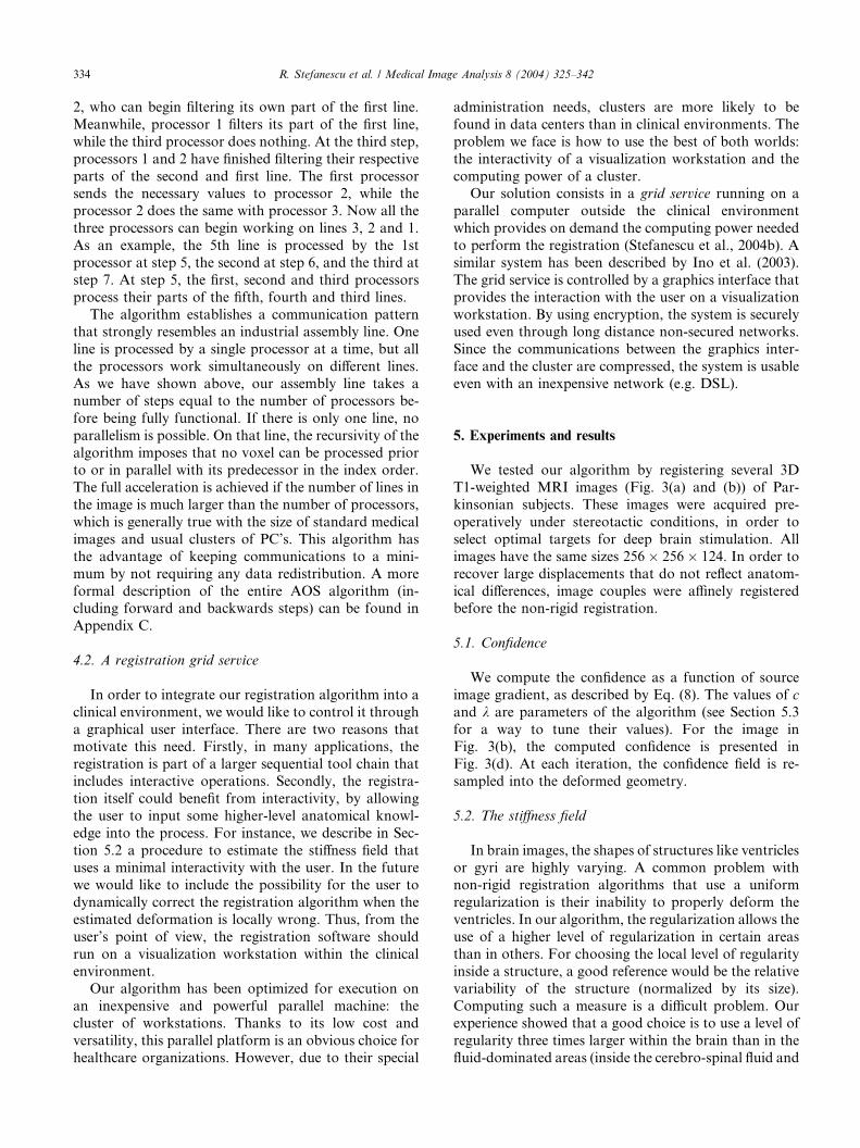
5.1. Confidence

We compute the confidence as a function of source

image gradient, as described by Eq. (8). The values of cand k are parameters of the algorithm (see Section 5.3

for a way to tune their values). For the image inFig. 3(b), the computed confidence is presented in

Fig. 3(d). At each iteration, the confidence field is re-

sampled into the deformed geometry.

5.2. The stiffness field

In brain images, the shapes of structures like ventricles

or gyri are highly varying. A common problem withnon-rigid registration algorithms that use a uniform

regularization is their inability to properly deform the

ventricles. In our algorithm, the regularization allows the

use of a higher level of regularization in certain areas

than in others. For choosing the local level of regularity

inside a structure, a good reference would be the relative

variability of the structure (normalized by its size).

Computing such a measure is a difficult problem. Ourexperience showed that a good choice is to use a level of

regularity three times larger within the brain than in the

fluid-dominated areas (inside the cerebro-spinal fluid and

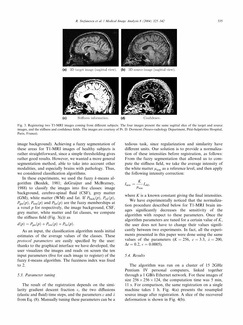
Fig. 3. Registering two T1-MRI images coming from different subjects. The four images present the same sagittal slice of the target and source

images, and the stiffness and confidence fields. The images are courtesy of Pr. D. Dormont (Neuro-radiology Department, Piti�e-Salp�etri�ere Hospital,

Paris, France).


image background). Achieving a fuzzy segmentation of

these areas for T1-MRI images of healthy subjects is

rather straightforward, since a simple thresholding gives

rather good results. However, we wanted a more general

segmentation method, able to take into account othermodalities, and especially brains with pathology. Thus,

we considered classification algorithms.

In these experiments, we used the fuzzy k-means al-

gorithm (Bezdek, 1981; deGruijter and McBratney,

1988) to classify the images into five classes: image

background, cerebro-spinal fluid (CSF), grey matter

(GM), white matter (WM) and fat. If PbackðpÞ, PcsfðpÞ,PgmðpÞ, PwmðpÞ and PfatðpÞ are the fuzzy memberships ata voxel p for respectively, the image background, CSF,

grey matter, white matter and fat classes, we compute

the stiffness field (Fig. 3(c)) as

dðpÞ ¼ PgmðpÞ þ PwmðpÞ þ PfatðpÞ:As an input, the classification algorithm needs initial

estimates of the average values of the classes. These

protocol parameters are easily specified by the user:

thanks to the graphical interface we have developed, the

user visualizes the images and reads on screen the ten

input parameters (five for each image to register) of thefuzzy k-means algorithm. The fuzziness index was fixed

to 2.

5.3. Parameter tuning

The result of the registration depends on the simi-

larity gradient descent fraction �, the two diffusions

(elastic and fluid) time steps, and the parameters c and kfrom Eq. (8). Manually tuning these parameters can be a

tedious task, since regularization and similarity have

different units. Our solution is to provide a normaliza-

tion of these intensities before registration, as follows:

From the fuzzy segmentation that allowed us to com-

pute the stiffness field, we take the average intensity ofthe white matter lwm as a reference level, and then apply

the following intensity correction:

Inew ¼Klwm

Iold;

where K is a known constant giving the final intensities.

We have experimentally noticed that the normaliza-

tion procedure described below for T1-MRI brain im-

ages significantly decreases the sensitivity of the

algorithm with respect to these parameters. Once the

algorithm parameters are tuned for a certain value of K,the user does not have to change their values signifi-

cantly between two experiments. In fact, all the experi-ments presented in this paper were done using the same

values of the parameters (K ¼ 256, c ¼ 3:3, k ¼ 200,

Dt ¼ 0:2, � ¼ 0:0005).

5.4. Results

The algorithm was run on a cluster of 15 2GHz

Pentium IV personal computers, linked togetherthrough a 1 GB/s Ethernet network. For these images of

size 256� 256� 124, the computation time was 5 min,

11 s. For comparison, the same registration on a single

machine takes 1 h. Fig. 4(a) presents the resampled

source image after registration. A slice of the recovered

deformation is shown in Fig. 4(b).

3 Such an inversion of the deformation field is needed for instance to

propagate atlas labels to patient images when these images are

registered into the geometry of the atlas.

Fig. 4. Result of the registration of images in Fig. 3(b) and (a).


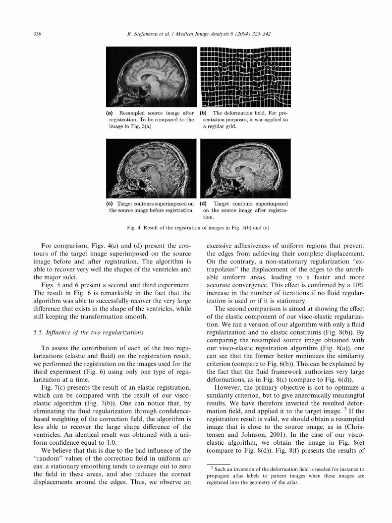
For comparison, Figs. 4(c) and (d) present the con-

tours of the target image superimposed on the source

image before and after registration. The algorithm is

able to recover very well the shapes of the ventricles andthe major sulci.

Figs. 5 and 6 present a second and third experiment.

The result in Fig. 6 is remarkable in the fact that the

algorithm was able to successfully recover the very large

difference that exists in the shape of the ventricles, while

still keeping the transformation smooth.

5.5. Influence of the two regularizations

To assess the contribution of each of the two regu-

larizations (elastic and fluid) on the registration result,

we performed the registration on the images used for the

third experiment (Fig. 6) using only one type of regu-

larization at a time.

Fig. 7(c) presents the result of an elastic registration,

which can be compared with the result of our visco-elastic algorithm (Fig. 7(b)). One can notice that, by

eliminating the fluid regularization through confidence-

based weighting of the correction field, the algorithm is

less able to recover the large shape difference of the

ventricles. An identical result was obtained with a uni-

form confidence equal to 1.0.

We believe that this is due to the bad influence of the

‘‘random’’ values of the correction field in uniform ar-eas: a stationary smoothing tends to average out to zero

the field in these areas, and also reduces the correct

displacements around the edges. Thus, we observe an

excessive adhesiveness of uniform regions that prevent

the edges from achieving their complete displacement.

On the contrary, a non-stationary regularization ‘‘ex-

trapolates’’ the displacement of the edges to the unreli-able uniform areas, leading to a faster and more

accurate convergence. This effect is confirmed by a 10%

increase in the number of iterations if no fluid regular-

ization is used or if it is stationary.

The second comparison is aimed at showing the effect

of the elastic component of our visco-elastic regulariza-

tion. We ran a version of our algorithm with only a fluid

regularization and no elastic constraints (Fig. 8(b)). Bycomparing the resampled source image obtained with

our visco-elastic registration algorithm (Fig. 8(a)), one

can see that the former better minimizes the similarity

criterion (compare to Fig. 6(b)). This can be explained by

the fact that the fluid framework authorizes very large

deformations, as in Fig. 8(c) (compare to Fig. 6(d)).

However, the primary objective is not to optimize a

similarity criterion, but to give anatomically meaningfulresults. We have therefore inverted the resulted defor-

mation field, and applied it to the target image. 3 If the

registration result is valid, we should obtain a resampled

image that is close to the source image, as in (Chris-

tensen and Johnson, 2001). In the case of our visco-

elastic algorithm, we obtain the image in Fig. 8(e)

(compare to Fig. 8(d)). Fig. 8(f) presents the results of

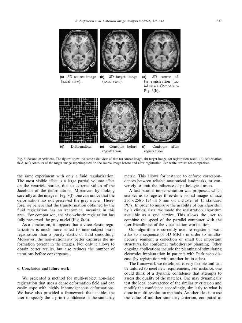
Fig. 5. Second experiment. The figures show the same axial view of the: (a) source image, (b) target image, (c) registration result, (d) deformation

field, (e,f) contours of the target image superimposed on the source image before and after registration. See white arrows for comparison.


the same experiment with only a fluid regularization.

The most visible effect is a large partial volume effect

on the ventricle border, due to extreme values of theJacobian of the deformations. Moreover, by looking

carefully at the image in Fig. 8(f), one can notice that the

deformation has not preserved the grey nuclei. There-

fore, we believe that the transformation obtained by the

fluid registration has no anatomical meaning in this

area. For comparison, the visco-elastic registration has

fully preserved the grey nuclei (Fig. 8(e)).

As a conclusion, it appears that a visco-elastic regu-larization is much more suited to inter-subject brain

registration than a purely elastic or fluid smoothing.

Moreover, the non-stationarity better captures the in-

formation present in the images. Not only it allows to

obtain better results, but also reduces the number of

iterations before convergence.

6. Conclusion and future work

We presented a method for multi-subject non-rigid

registration that uses a dense deformation field and can

easily cope with highly inhomogeneous deformations.

We have also provided a framework that enables the

user to specify the a priori confidence in the similarity

metric. This allows for instance to enforce correspon-

dences between reliable anatomical landmarks, or con-

versely to limit the influence of pathological areas.A fast parallel implementation was proposed, which

enables us to register three-dimensional images of size

256� 256� 124 in 5 min on a cluster of 15 standard

PC’s. In order to improve the usability of our algorithm

by a clinical user, we made the registration algorithm

available as a grid service. This allows the user to

combine the speed of the parallel computer with the

user-friendliness of the visualization workstation.Our algorithm is currently used to register a brain

atlas to a sequence of 3D MRI’s in order to simulta-

neously segment a collection of small but important

structures for conformal radiotherapy planning. Other

ongoing applications include the planning of stimulating

electrodes implantation in patients with Parkinson dis-

ease (by registration with another brain atlas).

The framework we developed is very flexible and canbe tailored to meet new requirements. For instance, one

could think of a dynamic confidence that attempts to

assess the quality of the matches. One may dynamically

test the local convergence of the similarity criterion and

modify the confidence accordingly, similarly to what is

done in multi-resolution methods. Another idea is to use

the value of another similarity criterion, computed at

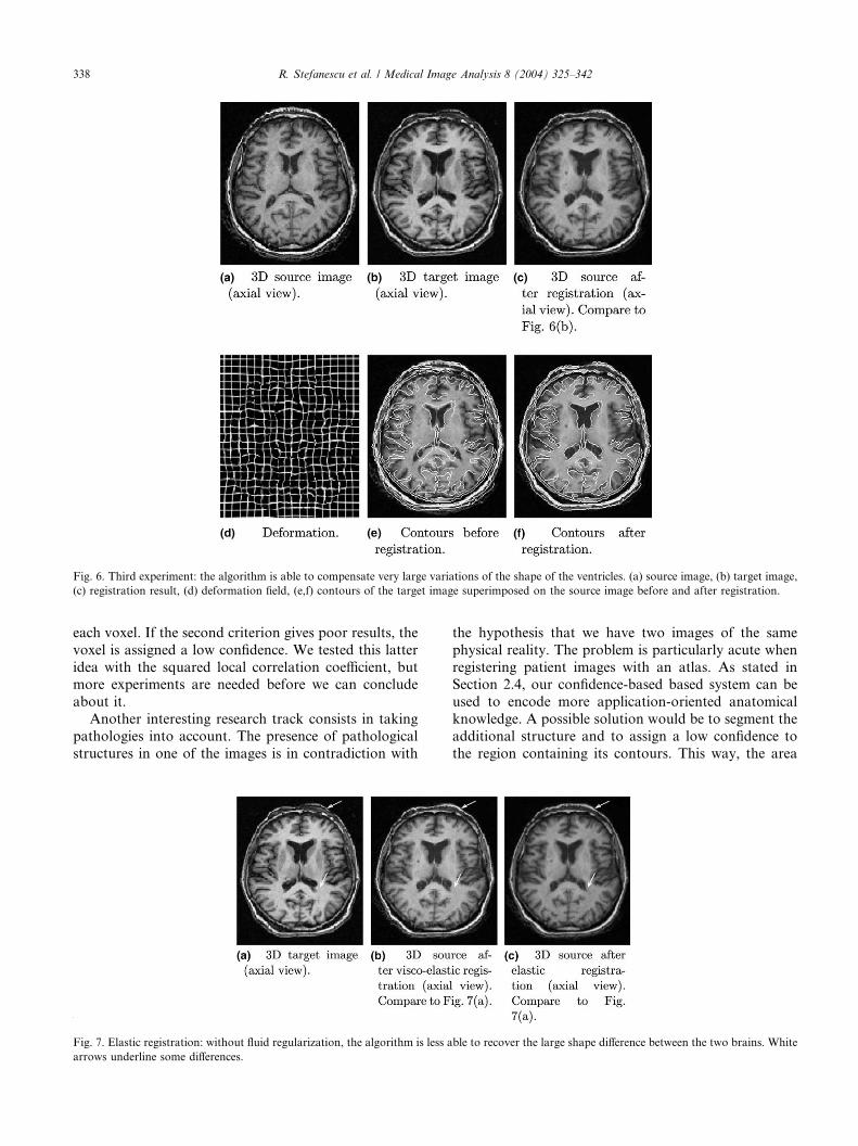
Fig. 6. Third experiment: the algorithm is able to compensate very large variations of the shape of the ventricles. (a) source image, (b) target image,

(c) registration result, (d) deformation field, (e,f) contours of the target image superimposed on the source image before and after registration.


each voxel. If the second criterion gives poor results, the

voxel is assigned a low confidence. We tested this latter

idea with the squared local correlation coefficient, butmore experiments are needed before we can conclude

about it.

Another interesting research track consists in taking

pathologies into account. The presence of pathological

structures in one of the images is in contradiction with

Fig. 7. Elastic registration: without fluid regularization, the algorithm is less a

arrows underline some differences.

the hypothesis that we have two images of the same

physical reality. The problem is particularly acute when

registering patient images with an atlas. As stated inSection 2.4, our confidence-based based system can be

used to encode more application-oriented anatomical

knowledge. A possible solution would be to segment the

additional structure and to assign a low confidence to

the region containing its contours. This way, the area

ble to recover the large shape difference between the two brains. White

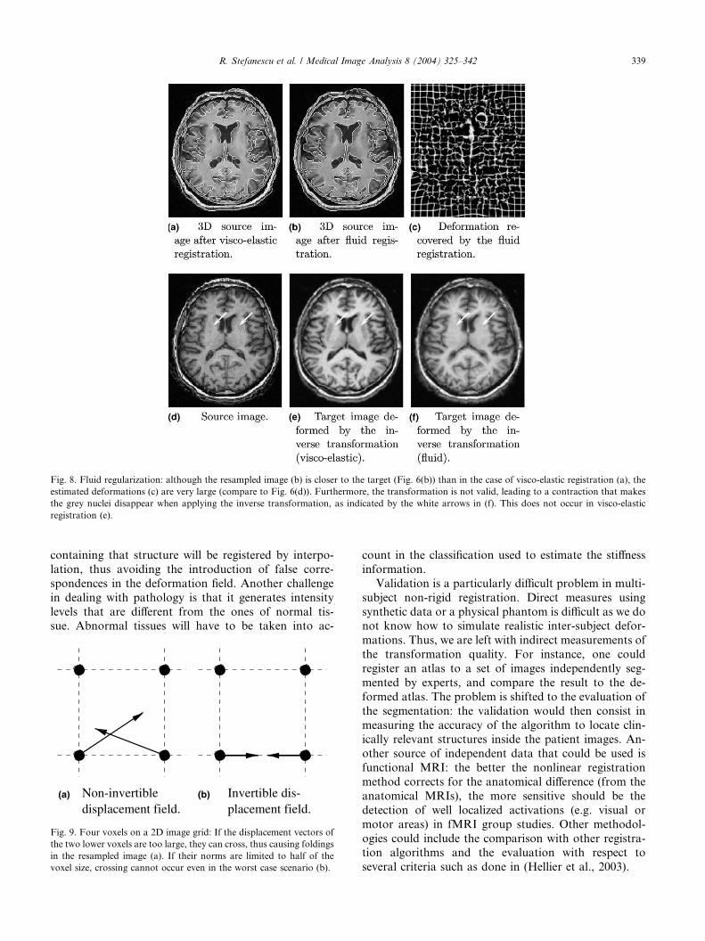
Fig. 8. Fluid regularization: although the resampled image (b) is closer to the target (Fig. 6(b)) than in the case of visco-elastic registration (a), the

estimated deformations (c) are very large (compare to Fig. 6(d)). Furthermore, the transformation is not valid, leading to a contraction that makes

the grey nuclei disappear when applying the inverse transformation, as indicated by the white arrows in (f). This does not occur in visco-elastic

registration (e).


containing that structure will be registered by interpo-

lation, thus avoiding the introduction of false corre-

spondences in the deformation field. Another challenge

in dealing with pathology is that it generates intensity

levels that are different from the ones of normal tis-sue. Abnormal tissues will have to be taken into ac-

(a) Non-invertibledisplacement field.

(b) Invertible dis-placement field.

Fig. 9. Four voxels on a 2D image grid: If the displacement vectors of

the two lower voxels are too large, they can cross, thus causing foldings

in the resampled image (a). If their norms are limited to half of the

voxel size, crossing cannot occur even in the worst case scenario (b).

count in the classification used to estimate the stiffness

information.

Validation is a particularly difficult problem in multi-

subject non-rigid registration. Direct measures using

synthetic data or a physical phantom is difficult as we donot know how to simulate realistic inter-subject defor-

mations. Thus, we are left with indirect measurements of

the transformation quality. For instance, one could

register an atlas to a set of images independently seg-

mented by experts, and compare the result to the de-

formed atlas. The problem is shifted to the evaluation of

the segmentation: the validation would then consist in

measuring the accuracy of the algorithm to locate clin-ically relevant structures inside the patient images. An-

other source of independent data that could be used is

functional MRI: the better the nonlinear registration

method corrects for the anatomical difference (from the

anatomical MRIs), the more sensitive should be the

detection of well localized activations (e.g. visual or

motor areas) in fMRI group studies. Other methodol-

ogies could include the comparison with other registra-tion algorithms and the evaluation with respect to

several criteria such as done in (Hellier et al., 2003).


Acknowledgements

This work was partially supported by the French

region of Provence-Alpes-Cote d’Azur. The images are

courtesy of Pr. D. Dormont (Neuro-radiology Depart-ment, Piti�e-Salp�etri�ere Hospital, Paris, France). We es-

pecially thank our colleagues Vincent Arsigny and Eric

Bardinet for the fruitful discussions that helped clarify

essential aspects of this work.

Appendix A. Guaranteeing the invertibility of a displace-ment field based on the norm of its vectors

Fig. 9 presents four voxels of a two-dimensional im-

age on a regular grid, and the displacement vectors of

the two lower voxels. If the norms of these vectors are

large, they can potentially cross and cause foldings in

the resampled image (Fig. 9(a)). Invertibility of the

displacement field can be easily ensured by limiting thenorm of these vectors to half of the voxels size

(Fig. 9(b)). This way, even in the worst case scenario,

vectors cannot cross and the displacement field is always

invertible. This avoids the computation of the Jacobian

at each iteration, as it is done by Christensen et al.

(1996).

Appendix B. The Thomas algorithm

Given a tridiagonal matrix B, the purpose is to solve

the linear system

Bu ¼ d;

where B is the tri-diagonal matrix

B ¼

a1 b1

c2 a2 b2

. .. . .

. . ..

cN�1 aN�1 bN�1cN aN

0BBBBB@

1CCCCCA: ð10Þ

The first step is the LR decomposition B ¼ LR with Lbeing a lower bidiagonal matrix and R an upper bidi-

agonal matrix:

L ¼

1

l2 1

. .. . .

.

lN 1

0BBBB@

1CCCCA;

R ¼

m1 r1

. .. . .

.

mN�1 rN�1mN

0BBBB@

1CCCCA: ð11Þ

The decomposition algorithm is the following:

m1 ¼ a1r1 ¼ b1for i ¼ 2; 3; . . . ;N :

li ¼ ci=mi�1mi ¼ ai � libi�1ri ¼ bi

The remainder of the algorithm consists in a forward

followed by a backward substitution:

//Forward substitution:

y1 ¼ d1for i ¼ 2; 3; . . . ;N :

yi ¼ di � liyi�1//Backward substitution:

uN ¼ yN=mN

for i ¼ N � 1; . . . ; 1:ui ¼ ðyi � biuiþ1Þ=mi

Appendix C. The parallel AOS scheme

A rigorous pseudo-code description of the entire al-

gorithm is given below. The goal is to invert in parallel

M tridiagonal matrices B0;B1; . . . ;BM�1 of size N � N ,

on P processors. If we equally distribute each line to all

processors, each processor p is responsible for process-

ing the components apNPþ1;...;ðpþ1ÞNP , bpNPþ1;...;ðpþ1ÞNP andcpNPþ1;...;ðpþ1ÞNP . It also memorizes a part of the elements of

the matrices L and R: the elements of the vectors l, r andm with the same indices. In order to minimize the total

number of messages, we fuse in the algorithm below the

loops that compute the LR decomposition and the for-

ward substitution step.

fi :¼ p NP þ 1 the first index memorized by processor p

li :¼ ðp þ 1Þ NP the last index memorized by processor

p//Fused LR decomposition and forward

substitution steps

for each matrix j 2 ½0;M � 1� doif p ¼ 0 then

mj1 :¼ aj1 //fi ¼ 1

rj1 :¼ bj1

yj1 :¼ d1else

receive mjfi�1, bj

fi�1 and yjfi�1 from processor

p � 1ljfi :¼ cjfi=m

jfi�1

mjfi :¼ ajfi � ljfib

jfi�1

rjfi :¼ bjfi

yjfi :¼ djfi � ljfiy

jfi�1

for i :¼ fiþ 1 to li dolji :¼ cji=m

ji�1


mji :¼ aji � ljib

ji�1

rji :¼ bji

yji :¼ dji � lji y

ji�1

if p 6¼ P � 1 then

send mjli, b

jli and yjli to processor p þ 1

//Backward substitution

for each matrix j 2 ½0;M � 1� doif p ¼ P � 1 then

uN ¼ yN=mN //li ¼ Nelse

receive ujliþ1 from processor p þ 1ujli :¼ ðy

jli � bj

liujliþ1Þ=m

jli

for i :¼ li� 1 down to fi douji :¼ ðyji � bj

i ujiþ1Þ=m

ji

if p 6¼ 0 then

send ujfi to processor p � 1

References

Alvarez, L., Weickert, J., S�anchez, J., 2000. Reliable estimation of

dense optical flow fields with large displacements. International

Journal of Computer Vision 39 (1), 41–56.

Bezdek, J., 1981. Pattern Recognition with Fuzzy Objective Function

Algorithms. Plenum Press, New York.

Bricault, I., Ferretti, G., Cinquin, P., 1998. Registration of real and

CT-derived virtual bronchoscopic images to assist transbronchial

biopsy. Transactions in Medical Imaging 17 (5), 703–714.

Bro-Nielsen, M., 1996. Medical image registration and surgery

simulation. Ph.D. thesis, IMM-DTU.

Bruhn, A., Jacob, T., Fischer, M., Kohlberger, T., Weickert, J.,

Br€uning, U., Schn€orr, C., 2002. Designing 3D nonlinear diffusion

filters for high performance cluster computing. In: Proceedings of

DAGM’02, vol. 2449 of LNCS, pp. 396–399.

Cachier, P., Pennec, X., 2000. 3D non-rigid registration by gradient

descent on a gaussian-windowed similarity measure using convo-

lutions. In: Proceedings of IEEE Workshop on Mathematical

Methods in Biomedical Image Analysis (MMBIA’00), pp. 182–

189.

Cachier, P., Bardinet, E., Dormont, D., Pennec, X., Ayache, N., 2003.

Iconic feature based nonrigid registration: The PASHA algorithm.

Computer Vision and Image Understanding – Special Issue on

Nonrigid Registration 89 (2–3), 272–298.

Chefd’hotel, C., Hermosillo, G., Faugeras, O., 2002. Flows of

diffeomorphisms for multimodal image registration. In: Proceed-

ings of IEEE International Symposium on Biomedical Imaging, pp.

8–11.

Christensen, G., Johnson, H., 2001. Consistent image registration.

IEEE Transactions on Medical Imaging 20 (7), 568–582.

Christensen, G., Rabitt, R., Miller, M., 1996. Deformable templates

using large deformation kinetics. IEEE Transactions on Image

Processing 5 (10), 1435–1447.

Collins, D., Evans, A., 1997. Animal: validation and applications of

nonlinear registration-based segmentation. International Journal

of Pattern Recognition and Artificial Intelligence 11 (8), 1271–

1294.

D’Agostino, E., Maes, F., Vandermeulen, D., Suetens, P., 2003. A

viscous fluid model for multimodal non-rigid image registration

using mutual information. Medical Image Analysis 7 (4), 565–575.

deGruijter, J., McBratney, A., 1988. Classification and Related

Methods of Data Analysis. Elsevier Science, Amsterdam (Chapter:

A modified fuzzy k means for predictive classification, pp. 97–104).

Ferrant, M., Nabavi, A., Macq, B., Black, P., Jolesz, F., Kikinis, R.,

Warfield, S., 2002. Serial registration of intraoperative MR images

of the brain. Medical Image Analysis 6 (4), 337–359.

Fischer, B., Modersitzki, J., 1999. Fast inversion of matrices arising in

image processing. Numerical Algorithms 22, 1–11.

Ganser, K., Dickhaus, H., Metzner, R., Wirtz, C., 2004. A deformable

digital brain atlas system according to Talairach and Tournoux.

Medical Image Analysis 8, 3–22.

Guimond, A., Roche, A., Ayache, N., Meunier, J., 2001. Multimodal

brain warping using the demons algorithm and adaptative intensity

corrections. IEEE Transaction on Medical Imaging 20 (1), 58–69.

Hellier, P., Barillot, C., M�emin, E., P�erez, P., 2001. Hierarchical

estimation of a dense deformation field for 3-D robust registration.

IEEE Transactions on Medical Imaging 20 (5), 388–402.

Hellier, P., Barillot, C., Corouge, I., Gibaud, B., Le Goualher, G.,

Collins, D., Evans, A., Malandain, G., Ayache, N., Christensen,

G., Johnson, H., 2003. Retrospective evaluation of inter-subject

brain registration. IEEE Transactions on Medical Imaging 22 (9),

1120–1130.

Hermosillo, G., Chefd’hotel, C., Faugeras, O., 2002. Variational

methods in multimodal image matching. International Journal of

Computer Vision 50 (3), 329–343.

Ino, F., Ooyama, K., Kawasaki, Y., Takeuchi, A., Mizutani, Y.,

Masumoto, J., Sato, Y., Sugano, N., Nishii, T., Miki, H.,

Yoshikawa, H., Yonenobu, K., Tamura, S., Ochi, T., Hagihara,

K., 2003. A high performance computing service over the internet

for nonrigid image registration. In: Proceedings of Computer

Assisted Radiology and Surgery (CARS 2003), vol. 1256 of

International Congress Series, pp. 193–199.

Miller, M., Younes, L., 2001. Group actions, homeomorphisms, and

matching: a general framework. International Journal of Computer

Vision 41 (1/2), 61–84.

Modersitzki, J., 2004. Numerical Methods for Image Registration.

Oxford University Press, Oxford.

Nagel, H.-H., Enkelmann, W., 1986. An investigation of smoothness

constraints for the estimation of displacement vector fields from

image sequences. IEEE Transactions on Pattern Analysis and

Machine Intelligence 8 (5), 565–593.

Ourselin, S., Roche, A., Prima, S., Ayache, N., 2000. Block matching:

a general framework to improve robustness of rigid registration of

medical images. In: Proceedings of International Conference on

Medical Image Computing and Computer-Assisted Intervention

(MICCAI 2000), vol. 1935 of LNCS. Springer-Verlag, Berlin, pp.

557–566.

Pennec, X., Cachier, P., Ayache, N., 1999. Understanding the

‘‘demon’s algorithm’’: 3D non-rigid registration by gradient

descent. In: Proceedings of International Conference on Medical

Image Computing and Computer-Assisted Intervention (MICCAI

1999), vol. 1679 of LNCS. Springer-Verlag, Berlin, pp. 597–605.

Press, W., Flannery, B., Teukolsky, S., Vetterling, W., 1993. Numer-

ical Recipes in C: The Art of Scientific Computing. Cambridge

University Press, Cambridge.

Prima, S., Thirion, J.-P., Subsol, G., Roberts, N., 1998. Automatic

analysis of normal brain dissymmetry of males and females in MR

images. In: Proceedings of International Conference on Medical

Image Computing and Computer-Assisted Intervention (MICCAI

1998), vol. 1496 of LNCS. Springer-Verlag, Berlin, pp. 770–779.

Roche, A., Malandain, G., Pennec, X., Ayache, N., 1998. The

correlation ratio as a new similarity measure for multimodal image

registration. In: Proceedings of International Conference on

Medical Image Computing and Computer-Assisted Intervention

(MICCAI 1998), vol. 1496 of LNCS. Springer-Verlag, Cambridge,

USA, pp. 1115–1124.

Roche, A., Malandain, G., Ayache, N., 2000. Unifying maximum

likelihood approaches in medical image registration. International

Journal of Imaging Systems and Technology: Special Issue on 3D

Imaging 11 (1), 71–80.


Roche, A., Pennec, X., Malandain, G., Ayache, N., 2001. Rigid

registration of 3D ultrasound with MR images: a new approach

combining intensity and gradient information. IEEE Transactions

on Medical Imaging 20 (10), 1038–1049.

Rohde, G., Aldroubi, A., Dawant, B., 2003. The adaptive bases

algorithm for intensity based nonrigid image registration. Special

issue on image registration. IEEE Transactions on Medical

Imaging 22, 1470–1479.

Rueckert, D., Sonoda, L., Hayes, C., Hill, D., Leach, M., Hawkes, D.,

1999. Non-rigid registration using free-form deformations: appli-

cation to breast MR images. IEEE Transactions on Medical

Imaging 18 (8), 712–712.

Stefanescu, R., Pennec, X., Ayache, N., 2004a. Grid-enabled non-rigid

registration of medical images. Parallel Processing Letters (in

press).

Stefanescu, R., Pennec, X., Ayache, N., 2004b. A grid service for the

interactive use of a parallel non-rigid registration algorithm of

medical images. Methods of Information in Medicine (in press).

Thirion, J.-P., 1998. Image matching as a diffusion process: an analogy

with Maxwell’s demons. Medical Image Analysis 2 (3), 243–260.

Thompson, P., Woods, R., Mega, M., Toga, A., 2000. Mathematical/

computational challenges in creating deformable and probabilistic

atlases of the human brain. Human Brain Mapping 9 (2), 81–92.

Trouv�e, A., 1998. Diffeomorphisms groups and pattern matching in

image analysis. International Journal of Computer Vision 28 (3),

213–221.

Webb, J., Guimond, A., Roberts, N., Eldridge, P., Chadwick, D.,

Meunier, J., Thirion, J.-P., 1999. Automatic detection of hippo-

campal atrophy on magnetic resonance images. Magnetic Reso-

nance Imaging 17 (8), 1149–1161.

Weickert, J., 1997. A review of nonlinear diffusion filtering. In:

Proceedings of Scale-Space Theory in Computer Vision, vol. 1252

of Lecture Notes in Computer Science. Springer-Verlag, Berlin, pp.

3–28.

Weickert, J., 2000. Applications of nonlinear diffusion in image

processing and computer vision. Acta Mathematica Universitatis

Comenianae 70 (1), 33–50.

Weickert, J., Haar, B., Viergever, R., 1998. Efficient and reliable

schemes for nonlinear diffusion filtering. IEEE Transactions on

Image Processing 7, 398–410.

grid powered nonlinear image registration with locally adaptive regularization

Documents