viscoelastic regularization and strain softening

III European Conference on Computational Mechanics Solids, Structures and Coupled Problems in Engineering

C.A. Mota Soares et.al. (eds.) Lisbon, Portugal, 5–8 June 2006

VISCO-ELASTIC REGULARIZATION AND STRAIN SOFTENING

Rui S. Cardoso*,1, Vitor D. Silva†, Humberto Varum*,2

*University of Aveiro Department of Civil Engineering

Campus Universitário de Santiago, P-3810-193 Aveiro, Portugal E-mail: [email protected] [email protected]

†University of Coimbra Department of Civil Engineering

Polo II da universidade-Pinhal de Marrocos, P-3030-290 Coimbra, Portugal E-mail: [email protected]

Keywords: Regularization, Visco-elasticity, Elasto-plasticity, Drucker-Prager, Radial Return.

Abstract. In this paper it is intended to verify the capacity of regularization of the numerical solution of an elasto-plastic problem with linear strain softening. The finite element method with a displacement approach is used. Drucker-Prager yield criteria is considered. The radial return method is used for the integration of the elasto-plastic constitutive relations. An elasto-visco-plastic scheme is used to regularize the numerical solution. Two constitutive laws have been developed and implemented in a FE-program, the first represent the radial return method applied to Drucker-Prager yield criteria and the second is a time integration procedure for the Maxwell visco-elastic model. Attention is paid to finite deformations. An associative plastic flow is considered in the Drucker-Prager elasto-plastic model. The algorithms are tested in two problems with softening. Figures showing the capability of the algorithms to regularize the solution are presented.

Rui S. Cardoso, Vitor D. Silva and Humberto Varum

2

1 INTRODUCTION The use of the finite element method to solve elasto-plastic problems with strain softening

behaviour, leads to the numerical collapse of the computation before the solution is obtained [1, 3, 4, 6, 11]. In fact the tangential global matrix ceases to be positive definite and non-uniqueness of the solution exists. This behaviour leads to pathological mesh sensitivity of the results and when modeled with finite elements where strain discontinuities arise, the plastic deformation is localized into bands of intense straining, where the band width of the localized deformations and their patterns are set by the mesh spacing [10, 11, 12]. Here, the term localization refers to situations in which the concentration of deformation into a band emerges as an outcome of the constitutive behaviour of the material and it is a characteristic feature of the inelastic deformations [11].

The purpose of the present work is to verify that the introduction of artificial viscosity in the constitutive law allows to reduce in a large scale the mesh dependency of the solution and restore the existence of a unique solution with continuous displacement [1, 3, 4, 6, 11, 14]. The procedure is general, and therefore has the advantage of allowing the regularization of any elasto-plastic material and at the same time to model time dependent material behaviour. Furthermore, the elasto-visco-plastic constitutive equations are amenable to unconditionally stable integration. The solutions are stable and convergent with mesh refinement.

As it is usual in elastoplasticity, the Drucker-Prager model presented here is formulated in terms of rate equations [1, 4, 8, 14], which leads to an incremental formulation in the numerical integration.

The numerical integration of the elasto-plastic rate equations is carried out via a backward linear interpolation scheme, the radial return method, an unconditionally stable stress point algorithm in the hardening case [1, 4, 8].

The visco-elastic equations are integrated by using also an implicit and unconditionally stable algorithm [2, 3, 4, 6].

This study is reported in three parts. In the first (sections 2, 3 and 4), some elementary background used in elastoplasticity, applied to Drucker-Prager criteria are summarized. The objective is to motivate the subsequent regularization procedure. In the second (section 5) the elasto-visco-plastic procedure is analyzed and in the third and last part (sections 6 and 7), some numerical examples are analyzed.

2 BASIC CONCEPTS FOR ELASTOPLASTICITY

2.1 Basic equations

As usual in elastoplasticity, material behaviour can be characterized by a set of constitutive relations of the general form [4, 6, 9, 14]

pij

eijij ddd εεε += , (1)

eijijklij dDd εσ = , (2)

( ) 0,, =kF pijij εσ , (3)

ij

pij

Qdd

σλε∂∂

= . (4)


3

Where pij

eijij ddd εεε and , denote the total, elastic and plastic strain incremental tensors

components, ijdσ the Cauchy stress tensor components, F a yield function, k defines the amount of plastic deformation which depends on the plastic strain history, λd is the plastic multiplier, a proportionality constant, and Q is the potential function.

Eq. 1 expresses the commonly assumed additive decomposition of infinitesimal strain into elastic and plastic parts. Eq. 2 establishes the elastic response (generalized Hooke´s law) and is characterized by means of general linear stress-strain relations through a stiffness tensor

ijklD . The symmetry relations klijijkl DD = are assumed. Eq. 3 represents the yield function considered. Finally, Eq. 4 expresses that the plastic strain increment is proportional to the potencial surface Q .

2.2 Material stiffness matrix When performing the computation in an incremental displacement approach, the finite

element method requires, within the increment, the calculation of the elastic material stiffness matrix or material tangential elasto-plastic stiffness matrix, depending on the load increment being elastic or elasto-plastic. The elasto-plastic tangential stiffness is a function of the stress tensor [14].

2.2.1 Elastic stiffness matrix The elastic stress increment is related to the strain increment by a symmetric matrix of

constants [5, 6, 9, 10, 14] as follows

{ } [ ]{ }εσ dDd = , (5) eijijklij dDd εσ = , ijklD is the fourth order tensor of elasticity modulus, here assumed isotropic,

[ ]D is the material elastic stiffness and }...,,{}{ 33,2111 σσσσ dddd T = .

2.2.2 Tangential elasto-plastic stiffness matrix The tangential elasto-plastic stiffness matrix, in incremental analysis, is defined by Eq. 6,

which relates the strain increments to the stress increments

[ ] [ ] [ ][ ]

[ ]

}{ }{ }{

}}{{ }{

εσ dAbDa

DabDDd

epD

T

T

4444 34444 21

+−= , (6)

where [ ]epD is the elasto-plastic matrix and A a parameter defined by

λddk

kFA∂∂

−= , (7)

where k is a softening (hardening) parameter (section 3) and λd is the proportionality constant defined in Eq. 4, and determined as presented in sections 3 and 4. The mathematical development that leads to Eq. 6 can be found in [6, 14]. Since the plasticity is associative, it comes


4

∂∂

∂∂

=

33

11}{

σ

σ

F

F

a M , { }

∂∂

∂∂

=

33

11

σ

σ

F

F

b M (8)

Since de plasticity here considered is associative, }{}{ ba = .

3 DRUCKER-PRAGER MODEL For completeness, the basic equations of elastoplasticity applied to Drucker-Prager yield

criteria theory are reviewed in this section.

3.1 Drucker-Prager yield condition The implementation of the finite deformation plasticity model has been performed for the

pressure-dependent Drucker-Prager yield criterion. The Drucker-Prager yield is defined in terms of the two first invariants of the stress tensor. More precisely, it may be defined in

terms of the mean stress, mI

σ=31 and the square root of the second invariant of the deviatoric

stress component )3(31

221

'2 IIJ −= . The elastic domain is then defined by the following

expression [6, 9, 12, 14]

( ) 03

,, '2

1'21 =−+= kJ

IJIF c ασ , (9)

where

)sin3(3sin2

φφα

−= , (10)

C is the cohesion, φ the angle of friction and k the softening (hardening) parameter,

φφ

cos6)sin3( 3 −

=k

C . (11)

In principal stress space, the Drucker-Prager yield function plots as a circular cone with axis along the space diagonal as illustrated in Fig. 1.

σ =σ =σ

σ

σ

σ

Fig.1 Drucker-Prager yield function plotted in principal stress space.


5

A fundamental postulate of plasticity theory is that a stress point must remain on or within the domain defined by the yield function throughout the deformation. This requirement is expressed mathematically as

0≤F . (12)

Violation of Eq. 12 implies plastic material response and means that the point must be returned to the yield surface via the plastic flow rule.

3.2 Elastic deformation The Hooke’s law is considered for the elastic behaviour

eijijklij dDd εσ = , (13)

where ijklD can be written as

jkiljlikklijijkl GGD δδδδδλδ ++= , (14)

in which λ is Lamé’s constant; G the shear modulus and ijδ the Kronecker delta. The isotropic and deviatoric components of the Drucker-Prager model have significantly

different character, so it is worthwhile to separate the equations, which describe the elastic deformation. The superimposed dot denotes time differentiation.

{ } }'{31}{

... Iv εεε += , (15)

where =v.ε trace ε is the volumetric strain rate and '

.ε the deviatoric strain rate

=}{.σ { }43421

stressisotropic

v IK

.ε

43421stressdeviatoric

.}' {G 2 ε+ , (16)

where [ ]{ } { }IKID 31

= and [ ] }'{ 2}'{ ..εε GD = . Thus considering a linear variation of theses

quantities in the time step t∆ ,

{ } }{G 2}{ 'εεσ ∆+∆=∆ IK v . (17)

3.3 Flow rule

During plasticity, the normality rule is applied [1, 4, 6, 8, 9, 14]

ij

pij

Qdd

σλε∂∂

= . (18)

Since an associative flow rule is used, FQ =

( ) kJI

kJIF −+= '2

1'21 3,, α , (19)

substituting Eq. 19 in Eq. 18

)3

( '2

1 kJI

ddij

pij −+

∂∂

= ασ

λε . (20)


6

3.4 Softening rule

The isotropic softening behaviour of the Drucker-Prager model is defined by the amount of plastic deformation, a linear softening rule is used. A negative value of the parameter θ leads to softening.

)1(0 ∫+= pdkk εθ , (21)

with k the softening parameter (Eq. 3 and 7), and

pij

pij

p ddd εεε21

= ijij aad21 λ= , (22)

where

pdkdk εθ 0= ijij aadk21 0 λθ= , (23)

so

20 6

141 αλθ += dkdk . (24)

Since the flow rule is associate, ijp

ij ad λε = with ij

ijFaσ∂∂

= .

The mathematical development that leads to the Eq. 24 can be found in [6]. In terms of rate equation, Eq. 24 takes the following form

2.

0

.

61

41 αλθ += kk , with

dtdkk =

. and

dtdλλ =

.. (25)

The parameter A of the global tangential elasto-plastic matrix material stiffness, Eqs. 6 and 7, is given by

61

41

61

41

1

20

20

+=⇒+=

=∂∂

−

αθλ

αλθ kddkdkdk

kF

⇒ 20 6

141 αθ += kA . (26)

4 ALGORITHM FOR THE INTEGRATION OF ELASTOPLASTIC CONSTITUTIVE RELATIONS

For the integration of the rate equations governing the material elasto-plastic behaviour, a backward linear interpolation scheme is used. This leads to a stable and implicit algorithm, furthermore the algorithm is first order accurate. It is remarked that the accuracy and stability with which constitutive relations are integrated has a direct impact on the overall accuracy and stability of the analysis.

In this section the radial return method algorithm for Drucker-Prager model is presented. This method is equivalent to an implicit backward Euler integration also known as the closest point algorithm [1, 6, 8].

This algorithm falls in the category of the return mapping algorithms. A return mapping algorithm can be conveniently defined based on the elastic/plastic split (Eq. 28), by first integrating the elastic equations to obtain a elastic predictor, the trial stress, which is then


7

taken as an initial condition for the plastic equation. These define a plastic corrector whereby the elastically predicted stresses are relaxed onto a suitable updated yield surface.

In the context of finite element analysis, stress updates take place at the Gauss points and the incremental deformation is given. The problem to be addressed, therefore, is to update the know state variables i

pii σεε , , and iλ associated with a converged configuration iB into their

corresponding values 1111 and , , ++++ iip

ii λσεε on the update configuration 1+iB . In this process the incremental displacements id∆ defining the geometric updated 1+→ ii BB are assumed given.

The linear integration of a variable X in the time step t∆ , is calculated, solving the following equation [1]

t X XXX n

.

nnn ∆

+−+= ++ 1

.

1 )1( ξξ (27)

When ξ =1, Eq. 27 reduces to a implicit backward Euler integration. As already said the isotropic and deviatoric components of the Drucker-Prager model have

significantly different character, so it is worthwhile to separate the equations, which describe the plastic deformation in these two components. Considering the additive decomposition of

the strain rate tensor }{.ε in the elastic e}{

.ε and the plastic components p}{

.ε , it becomes

[ ] eD }{ }{..εσ = = [ ] )}{}{(

..pD εε − . (28)

Splitting the strain rate tensor in isotropic and deviatoric components, from Eq. 28

{ } }' {31}{

...εεε += Iv ⇒ [ ] { } )}{}' {

31( }{

....p

v ID εεεσ −+= . (29)

Since

{ }ap..

}{ λε = ⇒ ) }{ 31}{

21( }{ '

. .Ip ασ

τλε += , (30)

where '2J=τ , substituting Eq. 30 in Eq. 29,

[ ] { }

+−+= )} {

31}' {

21 ( }' {

31 }{

....IID v ασ

τλεεσ . (31)

Taking in account the relations

[ ] }{ }{ 31 IKID = , [ ] }'{ 2}'{

..εε GD = and [ ] }'{ 2 }'{

..σσ GD = , (32)

and substituting in Eq. 31,

=}{.σ

44 344 21stressisotropic

v IK

..}){( αλε −

444 3444 21stressdeviatoric

G

..}' {}' {G 2 σ

τλε −+ . (33)

The numerical integration of Eq. 33 is performed via a linear interpolation of .λ and

.σ ,

using a collocation parameter 1=ζ (backward linear interpolation).

From Eq. 33 and mI

σ=31 ,


8

}{}){(...

IIK mv σαλε =− Kvm )( ...αλεσ −=⇒ , (34)

and

})' {21}' {(G 2 }' {

...σ

τλεσ −= , (35)

considering σ=X in Eq. 27

tnnn ∆+= ++ 1.

1 σσσ , (36)

and λ =X

tn ∆=∆ +1

.}{}{ σσ and tnn ∆=∆ ++ 1

.

1 λλ . (37)

Substituting Eq.37 in Eq. 34 and 35,

⇒∆−=∆ + tKnvm )( 1

..αλεσ =∆ mσ vK ε∆ ( 1+∆− nλ )α , (38)

⇒∆−=∆ + tn })' {21}' {(G 2 }'{ 1

..σ

τλεσ }'{ σ∆ = )}' {

21}' {(G 2 1

11 +

++∆−∆ n

nn σ

τλε , (39)

K and G represent the bulk and shear moduli, respectively, substituting Eq. 38 in Eq. 36

4434421trm

vnmnm Kσ

εσσ ∆+=+1 =∆− + βλ 1nK 1 +∆− ntrm K λασ , (40)

and since

}{}{}{ ''1

' σσσ ∆+=+ nn , (41)

substituting Eq. 39 in Eq. 41

1'

11

}{

''1

' }{}{2}{}{'

+++

+ ∆−∆+= nnn

nnGG

tr

σλτ

εσσσ

44 344 21, (42)

then

∆−=

∆+=

++

++

+

.

}{1

1}{

11

'

11

1'

ntrmnm

tr

nn

n

K

G

λασσ

σλ

τ

σ

(43)

Since '2J=τ

tr

nn

n Gτ

λτ

τ1

1

11

1

++

+

∆+= ⇒ 11 ++ ∆−= n

trn G λττ . (44)

Since Eq. 9 must be satisfied at the end of the load increment,

0 111 =−+ +++ nnnm kτσα ⇒α

τσ 11

1

++ +−=

+

nnm

kn

, (45)

from Eq. 23


9

2101 6

141 αλθ +∆+= ++ nnn kkk , (46)

220

1

KG61

41 ααθ

αστλ

+++

+−=∆ +

k

k trn

tr

n , (47)

Eq. 40, 44 and 46 becomes

+−=

+∆+=

∆−=

+++

++

++

,

61

41

111

2101

11

ατ

σ

αλθ

λττ

nnnm

nnn

ntr

n

k

kkk

G

(48)

The radial return factor, in Eq. 43, can be written as a function of 1+nk

=∆

++

+

1

1 1

1

n

nGτλ

=∆+ ++

+

11

1

nn

n

G λττ

=+tr

n

ττ 1

trnmnk

τ

σα 11 ++ − . (49)

Eqs. (47) and (48) define the new stresses and softening parameter.

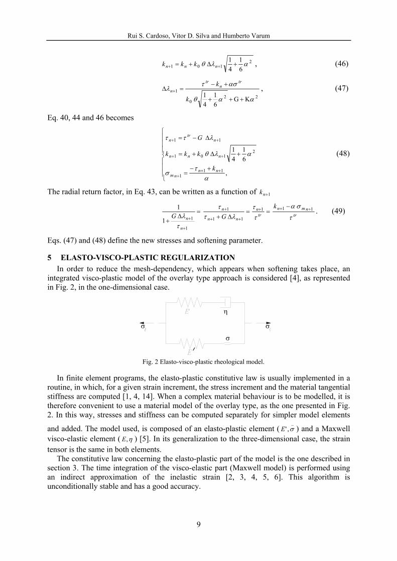
5 ELASTO-VISCO-PLASTIC REGULARIZATION In order to reduce the mesh-dependency, which appears when softening takes place, an

integrated visco-plastic model of the overlay type approach is considered [4], as represented in Fig. 2, in the one-dimensional case.

η

σ

σ

σ

Fig. 2 Elasto-visco-plastic rheological model.

In finite element programs, the elasto-plastic constitutive law is usually implemented in a

routine, in which, for a given strain increment, the stress increment and the material tangential stiffness are computed [1, 4, 14]. When a complex material behaviour is to be modelled, it is therefore convenient to use a material model of the overlay type, as the one presented in Fig. 2. In this way, stresses and stiffness can be computed separately for simpler model elements

and added. The model used, is composed of an elasto-plastic element (_

,' σE ) and a Maxwell visco-elastic element ( η ,E ) [5]. In its generalization to the three-dimensional case, the strain tensor is the same in both elements.

The constitutive law concerning the elasto-plastic part of the model is the one described in section 3. The time integration of the visco-elastic part (Maxwell model) is performed using an indirect approximation of the inelastic strain [2, 3, 4, 5, 6]. This algorithm is unconditionally stable and has a good accuracy.


10

The advantages of using a positive definite matrix at each iteration step are not only economic, but also allow the computation to be extended to strain softening material or non-associative laws [14].

The Maxwell model is composed of a serial assembly of an elastic (spring) of stiffness E and a viscous element (dashpot), whose coefficient of viscosity is η . The constitutive law of the models reads

E

... σ

ησε += , (50)

where σ is the stress in the Maxwell model component and the dot denotes, as usually, the time derivate. Integrating this differential equation and defining d0ε as the strain in the dashpot at the beginning of the time step t∆ ,

−−= ∫

∆ −∆−∆− t sttd dseeE

0

)( 0 ββ εβεεσ with

ηβ E= , (51)

where ts ∆≤≤0 is the time variable. The strain in the dashpot after the time increment is then

( )dseeE

t sttdd ∫

∆ −∆−∆− +=−=

0

0 ββ εβεσεε . (52)

Considering a linear interpolation function for the evolution of the total strain ε in the time step, sC 0 += εε ( C is a constant).

( )ttdd eCtCe ∆−∆− −

−+∆+=

0

0 1 ββ

βεεε . (53)

The stability analysis of this time integration algorithm can be found in [3].

The new stress is then

( )dE εεσ −= 11 with tC∆+= 01 εε , (54)

As the constitutive law is to be used in an incremental form, the stress increment must be computed

( ) ( )dd EE 00101 εεεεσσσ −−−=−=∆ , (55)

where 0σ is the stress at the beginning of the time step. Substituting Eq. 53 in Eq. 55

( ) εβ

σσβ

β ∆∆

−+−−=∆

∆−∆−

1 1

0 E

tee

tt , (56)

with tC ∆=∆ ε . A three-dimensional generalization of Eq. 56 is easily performed, if a constant Poisson’s coefficient is used. Defining the matrix [5]

[ ] ( )( )νν

νν

νννν

νννννν

ν21 1

1

210000002100000021000000100010001

−+

−−

−−

−−

= , (57)


11

the tensorial three-dimensional equivalent of σ∆ takes the form

( ) [ ] }{ 1}{ 1 }{

0 εν

βσσ

ββ ∆

∆−

+−−=∆∆−

∆− Et

eet

t . (58)

The visco-elastic material stiffness is then

[ ]νβε

σ β

teE

dd t

∆−

=

∆∆ ∆−

1

(59)

6 ELEMENTS USED IN THE FEA The elements used in the examples analysed in section 7 belong to the FEPS 3.3 library,

[13]. All these elements are isoparametric Lagrangean type with linear and quadratic shape functions.

The concept of isoparametric element is fully described in the literature [14], and the advantages in using them have been investigated in [12].

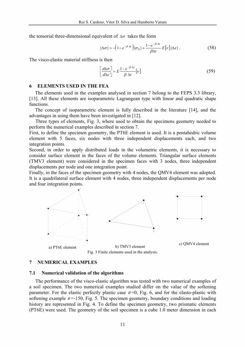
Three types of elements, Fig. 3, where used to obtain the specimens geometry needed to perform the numerical examples described in section 7. First, to define the specimen geometry, the PT6E element is used. It is a pentahedric volume element with 5 faces, six nodes with three independent displacements each, and two integration points. Second, in order to apply distributed loads in the volumetric elements, it is necessary to consider surface element in the faces of the volume elements. Triangular surface elements (TMV3 element) were considered in the specimen faces with 3 nodes, three independent displacements per node and one integration point. Finally, in the faces of the specimen geometry with 4 nodes, the QMV4 element was adopted. It is a quadrilateral surface element with 4 nodes, three independent displacements per node and four integration points.

a) PT6E element

b) TMV3 element

c) QMV4 element

Fig. 3 Finite elements used in the analysis.

7 NUMERICAL EXAMPLES

7.1 Numerical validation of the algorithms The performance of the visco-elastic algorithm was tested with two numerical examples of

a soil specimen. The two numerical examples studied differ on the value of the softening parameter. For the elastic perfectly plastic case θ =0, Fig. 6, and for the elasto-plastic with softening example θ =-150, Fig. 5. The specimen geometry, boundary conditions and loading history are represented in Fig. 4. To define the specimen geometry, two prismatic elements (PT6E) were used. The geometry of the soil specimen is a cube 1.0 meter dimension in each


12

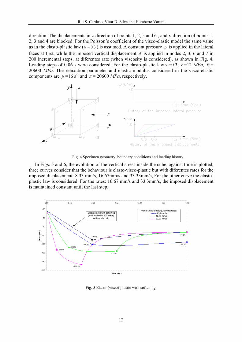
direction. The displacements in z-direction of points 1, 2, 5 and 6 , and x-direction of points 1, 2, 3 and 4 are blocked. For the Poisson´s coefficient of the visco-elastic model the same value as in the elasto-plastic law ( 3.0=ν ) is assumed. A constant pressure p is applied in the lateral faces at first, while the imposed vertical displacement d is applied in nodes 2, 3, 6 and 7 in 200 incremental steps, at diferentes rate (when viscosity is considered), as shown in Fig. 4. Loading steps of 0.06 s were considered. For the elasto-plastic lawα =0.3, k =12 MPa, 'E = 20600 MPa. The relaxation parameter and elastic modulus considered in the visco-elastic components are β =16 s-1 and E = 20600 MPa, respectively.

p

dp

p x

y

z

d

Fig. 4 Specimen geometry, boundary conditions and loading history.

In Figs. 5 and 6, the evolution of the vertical stress inside the cube, against time is plotted, three curves consider that the behaviour is elasto-visco-plastic but with diferentes rates for the imposed displacement: 8.33 mm/s, 16.67mm/s and 33.33mm/s, For the other curve the elasto-plastic law is considered. For the rates: 16.67 mm/s and 33.3mm/s, the imposed displacement is maintained constant until the last step.

-90,15-72,29

-113,00

-146,90

-106,90

-115,90

-95,27-100,30

-160

-140

-120

-100

-80

-60

-40

-20

00,00 0,20 0,40 0,60 0,80 1,00 1,20

Time (sec.)

Stre

ss (M

Pa)

elasto-visco-plasticity, loading rates:------- 8.33 mm/s ------- 16,67 mm/s ------- 33,33 mm/s

Elasto-plastic with softening (load applied in 200 steps).

Without viscosity

Fig. 5 Elasto-(visco)-plastic with softening.


13

-90,15

-113,20

-159,80

-90,72

-130,50

-106,20

-100,30

-111,40

-180

-160

-140

-120

-100

-80

-60

-40

-20

00,00 0,20 0,40 0,60 0,80 1,00 1,20

Time (sec.)

Stre

ss (M

Pa)

Elasto-visco-plasticity, loading rates:------- 8,33 mm/s------- 16,67 mm/s------- 33,33 mm/s

Elastic perfectly plastic (Load applied in 200 steps).

Without viscosity

Fig. 6 Elasto-(visco)-perfectly plastic.

7.2 Elasto-visco-plastic model

In order to test the described elasto-visco-plastic regularization techniques in the presence of severe softening, the formation of shear bands in a soil specimen is simulated using the rheological model of Fig. 2. The model was implemented in FEPS [13], without consideration of dynamic effects and using a classical computation of elasto-plastic material stiffness.

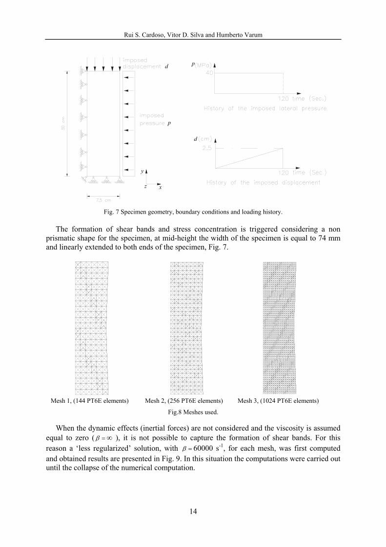
The shear bands simulation is obtained by considering three different meshes on the same specimen. The efficiency of the regularization procedures is analyzed in the case of severe softening, the softening parameter θ is considered equal to –150. The specimen geometry, boundary conditions and loading history are represented in Fig. 7.

The computation is three-dimensional although the problem is plane, since the displacements in z-direction are blocked. A constant Poisson coefficient 3.0=ν is assumed for the elasto-plastic and elasto-visco-plastic law. A constant pressure p is applied totally for t = 0 seconds in the lateral faces and the imposed displacement varies linearly from 0 to 2.5 cm in 120 seconds, corresponding to a deformation rate of 0.208 mm/s, has shown in Fig. 7. For the elasto-plastic law α =0.3, k =12 MPa, 'E = 20 600 Mpa, where assumed. The relaxation parameter and the elastic modulus considered in the visco-elastic components are β =16 s-1 and E = 20 600 MPa, respectively.


14

p

y

x

d

p

d

z

Fig. 7 Specimen geometry, boundary conditions and loading history.

The formation of shear bands and stress concentration is triggered considering a non

prismatic shape for the specimen, at mid-height the width of the specimen is equal to 74 mm and linearly extended to both ends of the specimen, Fig. 7.

Mesh 1, (144 PT6E elements) Mesh 2, (256 PT6E elements) Mesh 3, (1024 PT6E elements)

Fig.8 Meshes used.

When the dynamic effects (inertial forces) are not considered and the viscosity is assumed equal to zero ( =β ∞ ), it is not possible to capture the formation of shear bands. For this reason a ‘less regularized’ solution, with =β 60000 s-1, for each mesh, was first computed and obtained results are presented in Fig. 9. In this situation the computations were carried out until the collapse of the numerical computation.


15

t= 93.50 seconds

Mesh 1 t = 88.08 seconds


Mesh 3

Fig. 9 Deformed meshes at he moment of the computational collapse, and with low viscosity 1 000 60 −= sβ .

It is observed the sharp localization of plastification within a narrow band containing not more than 2 elements in the thickness. Furthermore, it was not possible to apply all the imposed displacement since calculations stops due to numerical collapse. It can be observed that, both the deformed shape and the time of computational collapse are quite different in the three meshes.

In the computations with regularization, the value of the relaxation modulus β was gradually decreased ( =β 16 s-1) until a shear band with more than one element in the width was obtained. In the following figures (Figs. 10 and 11) the numerical elasto-plastic solution is regularized with a visco-elastic procedure.

t = 93.5 seconds



Mesh 3

Fig. 10 Deformed meshes, with high viscosity -1s 16=β .


16

t = 120 seconds t = 120 seconds t = 120 seconds

Mesh 1 Mesh 2 Mesh 3

Fig. 11 Deformed meshes for t = 120 seconds, -1s 60=β .

8 CONCLUDING REMARKS Viscoelasticity has been introduced as a procedure to regularize the elasto-plastic solution,

when strain softening occurs. The procedure adopted is general and therefore has the advantage of allowing the regularization of any elasto-plastic material. Stable and convergent solutions are obtained. In fact, the bands of intense straining appear latter and the dependence on the mesh refinement is strongly reduced.

It is remarked that, for mesh refinement the elasto-plastic problem did not allow to apply the total load without numerical collapse, Fig. 9. The bigger the mesh refinement bigger is the band of straining, which also occur sooner. Increasing the mesh refinement, the band of straining enlarges and occurs sooner

The procedure to obtain bands of intense straining is computationally expensive. For the mesh 3 it was necessary 20 hours of computations (1.5 GHz processor) to obtain the results corresponding to the last load increment

An efficient implicit time stepping algorithm was used to advance the solution in time. An unconditionally stress point algorithm was used to integrate the elasto-plastic constitutive equations. Therefore, the most important numerical restriction of the proposed computational procedure is introduced by the relaxation module β , which controls the amplitude of the regularization. The shear band widths depend crucially on the viscosity. A sufficiently high value the viscosity parameter is used, the value β =16 sec.-1 has made possible to obtain good results for the three considered meshes.

In the FE-computations a total lagrangian formulation was used, being assumed that the used constitutive laws represent the relation between Piola-Kirchhoff stresses and Green strains.


17

REFERENCES

[1] V. D. Silva, F. Casadei, An implementation of the Cam-Clay elasto-plastic model using a backward interpolation and visco-Plastic regularization, Technical Note N.º I.96.239, Institute for Systems, Informatics and Safety, Joint Research Centre, Ispra, Italy, 1996.

[2] J. Argyris, I. St. Doltsinis, V. D. Silva, Constitutive modelling and computation of non-linear viscoelastic solids – Part I: Rheological Models and Numerical Integration Techniques. Computer Methods in Applied Mechanics and Engineering, Vol. 88 No.2, pp. 135-163, 1991.

[3] V. D Silva, A simple model for viscous regularization of elasto-plastic constitutive laws with softening. Communications in Numerical Methods in Engineering, John Wiley & Sons, Ltd., Vol. 20, pp. 547-568, 2004.

[4] V. D Silva, Viscoplastic regularization of a Cam-Clay FE-Implementation, ECCM’99, European Conference on Computational Mechanics, 31 August- 3September 1999, München, paper nº 442.

[5] V. D. Silva, Mechanics and Strength of Materials, ISBN 3-540-25131-6, 529 p., 402 illus., Springer, 2006.

[6] R. Cardoso, Regularização visco-elástica de problemas elasto-plásticos com amaciamento, MS.c Thesis, University of Coimbra, 2001 (in Portuguese).

[7] H. Varum, R. Cardoso, A geometrical non-linear model for cable systems analysis, Second International Conference on Textile Composites and Inflatable Structures, Eds. E. Onãte and B. Kröplin, Stuttgart 2-5 October 2005, pp. 234-242.

[8] M. Ortiz, E. P. Popov, Accuracy and stability of integration algorithms for elasto-plastic constitutive relations, International Journal For Numerical Methods in Engineering, Vol. 21, pp. 1561-1576, 1986.

[9] B. Loret, J. H. Prevost, Accurate numerical solution for Drucker-Prager elastic-plastic models. Computer Methods in Applied Mechanics and Engineering, Vol. 54, pp. 259-277 North Holland, 1986.

[10] B. Loret, J. H. Prevost, Dynamic strain localization in elasto-(visco)-plastic Solids, Part 1. General formulation and one-dimensional examples. Computer Methods in Applied Mechanics and Engineering, Vol. 83, pp. 247-273 North Holland, 1990.

[11] A. Needleman, Material rate dependence and mesh sensivity in localization problems. Computer Methods in Applied Mechanics and Engineering, Vol. 67, pp. 69-85 North Holland, 1988.

[12] G. C. Nayak, O. C. Zienkiewicz, Elasto-plastic stress analysis. A generalization for various constitutive relations including strain softening. International Journal for Numerical Methods in Engineering, Vol 5, pp. 113-135, 1972.

[13] H. Wüstenberg, FEPS 3.3- Finite Element Programming System, Element Library. ICA Report No. 22. Stuttgart, 1986.

[14] O. C. Zienkiewicz, R. L. Taylor, The Finite Element Method, Volume 2, Fourth Edition, McGraw-Hill, London, 1991.

viscoelastic regularization and strain softening

Documents