modeling anisotropic undersampling of magnetic resonance angiographies and reconstruction of a...
TRANSCRIPT
Signal Processing 84 (2004) 743–762www.elsevier.com/locate/sigpro
Modeling anisotropic undersampling of magnetic resonanceangiographies and reconstruction of a high-resolution isotropic
volume using half-quadratic regularization techniques
Elodie Roullota;b;1, Alain Hermentb, Isabelle Blocha ;∗, Alain de Cesareb,Mila Nikolovaa, Elie Mousseauxb;c
aD�epartement TSI-CNRS UMR 5141 LTCI, Ecole Nationale Sup�erieure des T�el�ecommunications, 46 rue Barrault, 75013 Paris, FrancebINSERM U494, Paris, France
cHopital Europ�een Georges Pompidou (HEGP), Paris, France
Received 28 July 2003
Abstract
In this paper we address the problem of reconstructing a high resolution volumic image from several low resolution datasets. A solution to this problem is proposed in the particular framework of magnetic resonance angiography (MRA), wherethe resolution is limited by a trade-o5 between the spatial resolution and the acquisition time, both being proportional tothe number of samples acquired in k-space. For this purpose only the meaningful spatial frequencies of the 3D k-spaceof the vessel are acquired, which is achieved using successive acquisitions with decreased spatial resolution, leading tohighly anisotropic data sets in one or two speci8c directions. The reconstruction of the MRA volume from these data setsrelies on an edge-preserving regularization method and leads to two di5erent implementations: the 8rst one is based on aconjugate gradient algorithm, and the second one on half-quadratic developments. The hyper parameters of the method wereexperimentally determined using a set of simulated data, and promising results were obtained on aorta and carotid arteryacquisitions, where on the one hand a good 8delity to the acquired data is maintained, and on the other hand homogeneousareas are smooth and edges are well preserved. Half-quadratic regularization proved to be particularly well adapted to theMRA problem and leads to a fast iterative algorithm requiring only scalar and FFT computations.? 2003 Elsevier B.V. All rights reserved.
Keywords: Magnetic resonance angiography; High-resolution; Undersampling; Edge-preserving regularization; Half-quadratic regularization
∗ Corresponding author. Tel.: +33-1-45-817585; fax:+33-1-45-813794.
E-mail addresses: [email protected] (E. Roullot), [email protected] (A. Herment), [email protected] (I. Bloch),[email protected] (A. de Cesare), [email protected](M. Nikolova), [email protected](E. Mousseaux).
1 Current address: ESME-Sudria, 4 rue Blaise Desgo5e, 75006Paris, France.
1. Introduction
Due to its numerous advantages for the patient(non-allergenic, non-ionizing), magnetic resonanceangiography (MRA) already challenges X-ray An-giography as the reference modality for the imagingof the large arteries and peripheral vascular network
0165-1684/$ - see front matter ? 2003 Elsevier B.V. All rights reserved.doi:10.1016/j.sigpro.2003.12.013
744 E. Roullot et al. / Signal Processing 84 (2004) 743–762
[26]. Magnetic resonance imaging (MRI) relies on theso-called “frequency (respectively phase) encoding”principle: the frequencies (respectively the phases)of the received signals are proportional to the spatialpositions of the voxels which emitted those signals,provided that convenient magnetic gradient 8eldshave been applied during the acquisition. As a con-sequence, the data acquired in MRI are the Fouriertransform of the image and are called “k-space”.When acquiring a 3D MR volume, spatial discrim-
ination is achieved using frequency encoding in onedirection and phase encoding in the two other direc-tions. The acquisition time of a 3D MRA data set is
Tacq = TRN�N�; (1)
where the repetition time TR includes the time neededto measure a “line” of the k-space along the frequencyencoding direction, and N� and N� are the numbersof encoding steps in both phase encoding directions.The voxel size can be expressed as
V = k1N�
1N�
; (2)
where k is a constant depending on the acquisitionsetup.Eqs. (1) and (2) show that 3D MRI is drastically
limited by a trade-o5 between the acquisition time andthe spatial resolution.In order to reduce the acquisition time, technical
improvements have been implemented such as the de-velopment of very fast and intense space encodinggradients.Acquiring larger and larger regions of the k-space
with a single RF pulse has also been proposed. Thisapproach leads to multishot or EPI sequences, mostoften designed for Cartesian k-space, but also leadsto the development of non-Cartesian k-space 8llings.Time-sparing k-space trajectories are, for example,spiral trajectories [11], circular sampling [3,30],rosette trajectories [21], or PROPELLER line tra-jectories [23]. These data have to be converted to aCartesian grid before to be transformed into the MRimage; this resampling is achieved using interpolationmethods [22] or, most often, gridding methods [29].
Acquiring an incomplete k-space was proposed asan alternative to the previously mentioned techniquesand was mainly implemented using Cartesian grid ac-quisitions. The simplest way to spare time during the
acquisition is to omit a number of lines. Half-k-spacetechniques omit almost all “positive” frequencies ina given phase encoding direction except in the cen-ter of the k-space, and use the symmetry propertiesof the Fourier transform of real data to estimate themissing “half-k-space”. Cao et al. [7] as well asPlevritis et al. [24] use anatomical prior knowledgeto optimally choose the samples to omit. Dologlouet al. [12] present an SVD-based estimation of thesemissing samples.We propose a di5erent approach to improve acquisi-
tion time without degrading the resolution, consistingin acquiring only the k-space regions containing theuseful spatial frequencies of the gadolinium enhancedvessel [18]. It was shown that using two or three dou-ble oblique acquisitions orthogonal to each other madeit possible to collect the k-space data adapted to recon-struct a stenosed artery segment in routine examina-tions. The method, unlike previous ones, does not tryto cover the whole k-space. The previously mentionedmethods achieve a time gain using a sparse samplingof the k-space, but they keep trying to cover both thelow and high frequencies of the k-space. Here a densesampling is proposed, but for each acquisition a selec-tion is made to only acquire the meaningful frequen-cies, which is also a way to decrease the acquisitiontime.In practice, the method can be formulated in the im-
age domain as the acquisition of few volumic data setswith complementary resolutions, each of them con-taining the high frequencies missing in the other ones.Then the reconstruction of a unique high-resolutionisotropic volume is performed.This paper investigates the possibility to signi8-
cantly improve the quality of the MRA reconstructionby introducing edge-preserving regularization tech-niques.Because the center of k-space is favored by the ac-
quisition process, the frequency content of the whitehomogenous gadolinium enhanced vessels may becorrectly accounted for. In addition we introduceda L2 norm regularization term to further improvehomogeneity and SNR of the vascular image. Con-cerning the edges of the vessel, it is expected thatthe high frequencies missing in one acquisition willbe substituted by the high frequencies containedin the other acquisitions. However, sharp and pre-cisely located edges being a major requirement for
E. Roullot et al. / Signal Processing 84 (2004) 743–762 745
segmentation and quantization of vessels in MRA,we also introduce some a priori knowledge into thereconstruction method in order to further outlineedges. This is achieved by using edge-preserving reg-ularization techniques. Finally we expect that edgerestoration will also contribute to improve the qualityof the reconstruction when the vessel is incorrectlyaligned in the geometry of the k-space acquisition.In this case, some additional high frequencies can bemissed because the frequency support of the image isno more totally included in the acquired k-space.Section 2.1 presents the original acquisition se-
quence on which our work is based, whereas Section2.2 describes the reconstruction method. In order tosolve the combination problem, an accurate modelingof the anisotropic undersampling of M.R. images isrequired, which is presented in Section 3.1. The crite-ria for combining the acquisitions are expressed as anenergy function to be minimized, detailed in Section3.2. In Section 4 we show how to take advantageof both the properties of the model in the spectraldomain, and those of half-quadratic regularizationalgorithms, leading to the development of a simpleand eMcient reconstruction algorithm. Results werevalidated on simulated data (Section 5) and resultson real data are shown in Section 6.
2. Acquisition and combination strategy
2.1. Description of the acquisition process
In this section, we present the acquisition scheme,which consists in acquiring three anisotropically un-dersampled 3D MR volumes.Since the acquisition time is proportional to the im-
age dimensions in both phase encoding directions foran unchanged 8eld of view (i.e. an unchanged valueof the product voxel dimension × number of voxels)in each direction of the space, the acquisition time canthus be reduced by decreasing the number of voxelsin both phase encoding directions.Accordingly, we propose to acquire three volumes,
each having decreased resolutions along both phaseencoding directions. This is achieved by permutationof the frequency encoding direction, so that for eachdirection, at least one of the three volumes presentsa “good” resolution (Fig. 1b). The so-called “refer-ence volume” of Fig. 1a is the volume that would be
N f
NφNΦ
N
N
Nφ3
f3
Φ3
Nf2
Nφ2
NΦ2
f1N
NΦ1
Nφ1
(a)
(b)
Fig. 1. (a) The reference volume, obtained with a conventionalacquisition scheme. (b) The acquisition strategy in the generalcase, which consists in decreasing the resolution in both phaseencoding directions for each acquisition, and in permutating theencoding directions between the di5erent acquisitions.
acquired in a conventional acquisition scheme provid-ing in each direction the best of the resolutions of thethree volumes in the considered direction. An isotropicreference volume is dealt with in the following for thesake of readability.According to the properties of the Fourier trans-
form, acquiring an undersampled volume correspondsto acquiring a truncated k-space, i.e. a k-space with-out the highest frequencies along the undersamplingdirection.It would also be possible to acquire two volumes
instead of three, and thus to decrease the resolutionin only one of the two phase encoding directions, inorder to always keep two “good” resolutions in anyof the volumes for each direction. In the following,for the sake of generality we will always consider thethree-acquisition case in our theoretical developments.Having de8ned the acquisition sequence, we can
now compute the resulting acquisition time accordingto Eq. (1). Let Nfi be the numbers of voxels in thefrequency encoding direction in the ith volume, andN�i and N�i the numbers of voxels in both phase en-coding directions, according to Fig. 1. The repetitiontime TR is supposed to be the same for all the acqui-sitions. Let us recall that a variable number of vox-els in the frequency direction would not lead to anyimprovement, since it does not a5ect signi8cantly theacquisition time.According to Eq. (1), the time needed to acquire
the ith volume Vi (i varying from 1 to 3) is
Ti = TRN�iN�i (3)
746 E. Roullot et al. / Signal Processing 84 (2004) 743–762
leading to a total acquisition time of
T1+2+3 = TR(N�1N�1 + N�2N�2 + N�3N�3); (4)
whereas the acquisition time for a unique volume Vwith dimensions N�N�Nf would be
T0 = TRN�N�: (5)
The time gain can thus be expressed as
GT = 1 − T1+2+3
T0
= 1 − (N�1N�1 + N�2N�2 + N�3N�3)N�N�
: (6)
This gain only depends on the ratios between theresolutions in the multiple acquisition case and the ref-erence acquisition case. For instance, if N�i = N�=3,and N�i = N�=3 the whole acquisition time is threetimes shorter; if N�i =N�=
√3, and N�i =N�=
√3, the
acquisition time remains unchanged but the SNR andresolution of the reconstructed volume will be im-proved. Finally if N�i = N�, and N�i = N�, the bestresolution can be achieved by increasing the acquisi-tion time to three breath-holdings of the patient: thistriples the overall acquisition time and therefore alsothe resolution.Studying the behavior of the acquisition process in
terms of noise is not as easy as in terms of acquisitiontime: as a matter of fact, the noise variance in the 8nalhigh resolution volume does not only depend on theacquisition process, but also on the combination strat-egy. However, acquiring an undersampled volumeallows to reduce the noise variance when compared tothe reference high-resolution volume, since the noisestandard deviation � is related to the volume dimen-sions as �=Nf
√N�N�. According to the acquisition
process, the low frequency coeMcients of the k-spaceare acquired two or three times, leading to dataredundancy and thus to an improvement of the SNR.Moreover, since the reconstruction method we pro-pose includes a L2 regularization, noise will be furtherattenuated in the reconstruction process.
2.2. Combining the undersampled volumes
Having de8ned the acquisition scheme as inSection 2.1, our goal is now to reconstruct a uniquehigh-resolution volume from three undersampled
versions. This is a reconstruction or restoration prob-lem and belongs to the family of inverse problems[4,10,19]. Since the data are discrete and the imag-ing system is band-limited, it can be proven thatthe solution is not unique and thus that the problemis ill-posed. For such problems, so-called general-ized solutions are used such as the Wiener 8lter[1]. Moreover, most discrete inverse problems areill-conditioned, i.e. noise in the data is ampli8ed dur-ing the inversion process, which leads to unaccept-able solutions. Therefore, approximate solutions areproposed and a priori information is introduced: thematter is to de8ne a set of acceptable solutions (i.e.with limited error) and to choose among these solu-tions the best one according to an a priori criterion.This regularization generally consists in minimizingan objective function (also called energy function) ofthe form Q + ��, where Q measures the 8delity tothe data, � measures the regularity of the solution,and � is a weighting factor of the regularization.The a priori criterion � has to be chosen according
to the foreseen use of the reconstructed signal or im-age; the numerous applications that impose a preciseedge localization, for example, call for the frameworkof edge-preserving regularization. In this framework,the term � to be minimized is generally expressedas a sum over all sites (i.e. voxels in 3D images) ofa regularization function (also called ’-function) ap-plied to the neighbor di5erences. The choice of the’-function determines the quality of the solution andthe optimization method to be used; it has been ad-dressed by many authors [6,9,15].Here, the forseen application includes vessel seg-
mentation and stenosis quanti8cation. According tothese considerations, it appears that the framework ofedge-preserving regularization methods is well suitedto the present problem.The choice of the a priori criteria and the expression
of the energy function are detailed in Section 3.
3. Edge-preserving reconstruction
The energy function to be minimized has thefollowing form:
E = Q + ��; (7)
E. Roullot et al. / Signal Processing 84 (2004) 743–762 747
where � leads to a trade-o5 between �, the regular-ization term, and Q, the 8delity to the data.The expression of the energy function requires an
accurate modeling of the anisotropic undersampling;this is developed below in Section 3.1. Section 3.2presents the energy function in more details, and itsconvexity is discussed in Section 3.3. The choice ofthe optimization algorithm is justi8ed in Section 3.4.
3.1. Modeling of the undersampling
Let Ixy be the image acquired with a decreased res-olution along x and y; let Ixz and Iyz be the two otheracquisitions de8ned in the same way. Ixy for instanceis related to the wished high resolution image IHR by
Ixy(x; y; z) =Nx∑k=0
Ny∑l=0
Dxy(k; l)IHR(x − k; y − l; z);
(8)
where Dxy is the undersampling operator along x andy. Dxy is separable:
Dxy(k; l) = Dx(k)Dy(l); (9)
where Dx and Dy are the undersampling operatorsalong x and y respectively.Note that Ixy, Iyz, Ixz, and IHR are the discrete
Fourier transforms (DFTs) of k-spaces with di5erentspectral supports: it seems reasonable to extend thesesupports to the smallest common cartesian support.This is achieved by interpolation and presented inAppendix A.Let us now express the operators Dx, Dy and Dz.
Let JHR be the DFT of IHR, and Jxy that of Ixy. Therelation between JHR and IHR is
J (fx; fy; fz)
=
Nx2 −1∑
x′=−Nx2
Ny
2 −1∑y′=−Ny
2
Nz2 −1∑
z′=−Nz2
FNx(fx; x′)FNy(fy; y′)
×FNz (fz; z′)IHR(x′; y′; z′); (10)
where FN denotes the discrete Fourier transformmatrix operator of size N :
FN (n; k) =1N
e−j2�nk=N with
n; k = −N2
· · · N2
− 1: (11)
The inverse DFT matrix operator is de8ned as
F−1N (n; k) = e j2�nk=N with
n; k = −N2
· · · N2
− 1: (12)
As mentioned above, the acquisition process consistsin acquiring a truncated k-space, i.e. Ixy is related toJHR by
Ix(x; y; z)
=
N ′x2 −1∑
fx=−N ′x2
N ′y
2 −1∑fy=−
N ′y
2
Nz2 −1∑
fz=−Nz2
F−1Nx
(x; fx)F−1Ny
(y; fy)
×F−1Nz
(z; fz)J (fx; fy; fz): (13)
Note the truncated summation limits in x and y direc-tions. Eqs. (10) and (13) give the following relationbetween IHR and Ixy:
Ix(x; y; z)
=
N ′x2 −1∑
fx=−N ′x2
N ′y
2 −1∑fy=−
N ′y
2
Nz2 −1∑
fz=−Nz2
[F−1Nx
(x; fx)
×F−1Ny
(y; fy)F−1Nz
(z; fz)
×Nx2 −1∑
x′=−Nx2
Ny
2 −1∑y′=−Ny
2
Nz2 −1∑
z′=−Nz2
FNx(fx; x′)FNy(fy; y′)
×FNz (fz; z′)I(x′; y′; z′)] (14)
from which it can be easily derived that the degrada-tion operator is linear and separable.Let us then consider the degradation operator along
one direction at a time, for instance Dx along x,working on a one-dimensional vector (i.e. a row fromthe 3D image taken along direction x). We can thenexpress the operator as a matrix within the frame-work of linear algebra. Under these conditions, theone-dimensional DFT of Ix(•; y; z) isDFT(Ix) =MxFxIHR ; (15)
748 E. Roullot et al. / Signal Processing 84 (2004) 743–762
where Mx is a Nx × Nx diagonal matrix:
Mx(i; i) = 1 if − N ′x2 + 16 i6 N ′
x2 − 1;
Mx(i; i) = 0:5 if i = −N ′x2 or i = N ′
x2 ;
Mx(i; i) = 0 otherwise:
(16)
This expression with the 0.5 coeMcient guarantees theconsistency with Appendix A regarding the constraintof keeping real-valued images. Therefore
Ix = F−1x MxFxIHR : (17)
Thus
Ix = DxIHR ; (18)
where the degradation operator Dx is expressed as
Dx = F−1x MxFx: (19)
The analytic expression of Dx is provided inAppendix B and it can be easily seen that it is acirculant operator. The operators Dy and Dz can beexpressed in a similar way. The whole 3D problemcan also be expressed with matrix operators, but itrequires to work on vector data (i.e. to put the 3Dimage matrix into a large vector) and to transform theoperators Dx, Dy and Dz into large matrix operators,according to [25,27]. In the following we will dealwith such vectors and matrices and use bold font todistinguish them from the operators working in onedimension. For example, Dx denotes the “big” matrixworking on the “big” vector IHR obtained by concate-nation of all the images values into a “big” columnvector; the way to compute Dx from Dx is detailedin [25,27]. Such linear algebra notations allow toexpress for example Eq. (8) with matrix operators:
Ixy = DxDyIHR : (20)
3.2. The energy function
3.2.1. Fidelity to the dataThe matter is to minimize the sum of the quadratic
errors between the reconstructed image and the data:
Q= ‖DxyIrec − Ixy‖2 + ‖DyzIrec − Iyz‖2
+‖DzxIrec − Izx‖2; (21)
where Dxy, Dyz and Dzx are the “big” undersamplingoperators obtained from those of Section 3.1, ‖:‖ rep-resents the quadratic norm, Irec is the high-resolutionimage at current iteration (the optimization of E isbased on an iterative method), Ixy, Iyz and Ixz are thelow-resolution input images put in vector form.
3.2.2. Regularization termAsmentioned in Section 2.2, the regularization term
� is de8ned as a ’-function of the neighbor di5er-ences; here the chosen ’-function is called (to avoidconfusion with the phase encoding directions) and isapplied to the 8rst order neighbor di5erences. Let N
be the N × N matrix operator of the neighbor di5er-ences. Since data are acquired in the spectral domain,and the DFT implicitly assumes the periodicity of bothsignal and spectrum, the border conditions are chosenhere to be periodic ones, leading to
N =
1 0 · · · 0 −1
−1 1 0
0. . .
. . ....
.... . .
. . . 0
0 · · · 0 −1 1
: (22)
The regularization term � takes the following form:
�= ‖ (�yIrec)‖1 + ‖ (�xIrec)‖1+‖ (�zIrec)‖1; (23)
where �x, �y and �z are the “big” matrices obtainedfrom N according to Section 3.1 and to [25,27], and‖‖1 denotes the L1 norm.The choice of the potential function results
from a trade-o5: the ideal edge-preserving potentialfunctions are those which have an asymptotic Natbehavior towards in8nity, such as that of Blake andZisserman [6], Geman and McClure [16], or Hebertand Leahy [17]; unfortunately, all these functionsare not convex and therefore compel to use time-consuming optimization algorithms.On the contrary, the function that is best suited to
fast algorithms such as the conjugate gradient algo-rithm is that of Tikhonov (quadratic function), but un-fortunately it smoothes discontinuities.
E. Roullot et al. / Signal Processing 84 (2004) 743–762 749
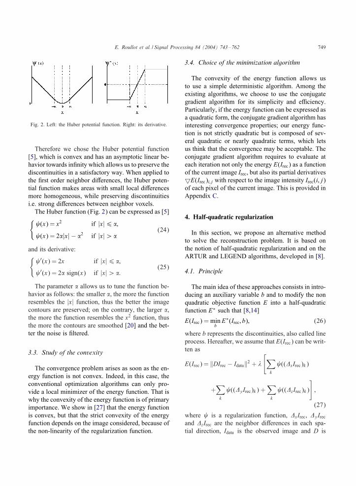
Fig. 2. Left: the Huber potential function. Right: its derivative.
Therefore we chose the Huber potential function[5], which is convex and has an asymptotic linear be-havior towards in8nity which allows us to preserve thediscontinuities in a satisfactory way. When applied tothe 8rst order neighbor di5erences, the Huber poten-tial function makes areas with small local di5erencesmore homogeneous, while preserving discontinuitiesi.e. strong di5erences between neighbor voxels.The Huber function (Fig. 2) can be expressed as [5]{ (x) = x2 if |x|6 !;
(x) = 2!|x| − !2 if |x|¿!(24)
and its derivative:{ ′(x) = 2x if |x|6 !;
′(x) = 2! sign(x) if |x|¿!:(25)
The parameter ! allows us to tune the function be-havior as follows: the smaller !, the more the functionresembles the |x| function, thus the better the imagecontours are preserved; on the contrary, the larger !,the more the function resembles the x2 function, thusthe more the contours are smoothed [20] and the bet-ter the noise is 8ltered.
3.3. Study of the convexity
The convergence problem arises as soon as the en-ergy function is not convex. Indeed, in this case, theconventional optimization algorithms can only pro-vide a local minimizer of the energy function. That iswhy the convexity of the energy function is of primaryimportance. We show in [27] that the energy functionis convex, but that the strict convexity of the energyfunction depends on the image considered, because ofthe non-linearity of the regularization function.
3.4. Choice of the minimization algorithm
The convexity of the energy function allows usto use a simple deterministic algorithm. Among theexisting algorithms, we choose to use the conjugategradient algorithm for its simplicity and eMciency.Particularly, if the energy function can be expressed asa quadratic form, the conjugate gradient algorithm hasinteresting convergence properties; our energy func-tion is not strictly quadratic but is composed of sev-eral quadratic or nearly quadratic terms, which letsus think that the convergence may be acceptable. Theconjugate gradient algorithm requires to evaluate ateach iteration not only the energy E(Irec) as a functionof the current image Irec, but also its partial derivatives�E(Irec)i; j with respect to the image intensity Irec(i; j)of each pixel of the current image. This is provided inAppendix C.
4. Half-quadratic regularization
In this section, we propose an alternative methodto solve the reconstruction problem. It is based onthe notion of half-quadratic regularization and on theARTUR and LEGEND algorithms, developed in [8].
4.1. Principle
The main idea of these approaches consists in intro-ducing an auxiliary variable b and to modify the nonquadratic objective function E into a half-quadraticfunction E∗ such that [8,14]
E(Irec) = minb
E∗(Irec; b); (26)
where b represents the discontinuities, also called lineprocess. Hereafter, we assume that E(Irec) can be writ-ten as
E(Irec) = ‖DIrec − Idata‖2 + �
[∑k
(( xIrec)k)
+∑k
(( yIrec)k) +∑k
(( zIrec)k)
];
(27)
where is a regularization function, xIrec, yIrecand zIrec are the neighbor di5erences in each spa-tial direction, Idata is the observed image and D is
750 E. Roullot et al. / Signal Processing 84 (2004) 743–762
the degradation operator. The auxiliary variable canbe de8ned in two ways. In the 8rst one [8], it is as-sumed that (
√(u)) is strictly convex and b∈ [0; 1]
is de8ned such that (u) = inf b bu2 + &(b). In thesecond approach [2], it is assumed that u2 − (u) isstrictly convex, and b∈ [0;+∞] is de8ned such that (u)= inf b (b−u)2 +&(b). The ARTUR algorithm isbased on the 8rst approach, while LEGEND is basedon the second one.For regularization functions which are convex,
non-bounded and with bounded 8rst derivative, it canbe proved that E∗(Irec; b) is quadratic in Irec for 8xedb, and E∗(Irec; b) is convex in b for 8xed Irec; thevalue of b which minimizes E∗(Irec; b) for 8xed Irecis known analytically.The algorithms rely on these properties and alter-
natively minimize E∗ in b for 8xed Irec and in Irec for8xed b.Both problems can be expressed with linear alge-
bra and amount to solve a linear system of the formAIrec = c (see [27]). In ARTUR, A depends on the it-eration, while it is constant in LEGEND. Moreover, inthe case of LEGENDA is invertible, while this is ques-tionable in the case of ARTUR. For these reasons, wechose to express the problem using LEGEND, 8rstlyin the spatial domain, and then alternatively in thespectral domain, for reasons that will be explained inSection 4.2.
4.2. LEGEND algorithm in the spatial domain
According to the principle explained above, the al-gorithm has to compute Inrec by solving ∇E = 0 for8xed bn
x , bny and bn
z , and to compute the auxiliary vari-ables bn+1
x , bn+1y and bn+1
z as functions of Inrec (in theseexpressions, n denotes the iteration number).It has been shown in [8] that bn+1
x can be expressedas
(bn+1x )k =
[1 − ′[(�xInrec)k ]
2(�xInrec)k
](�xInrec)k : (28)
For the 8rst computation, we have to derive an ex-pression of ∇E = 0. The regularization term can bewritten as
�(Irec) = infbx;by;bz
[�∗(Irec; bx; by; bz)] (29)
with
�∗ =∑
i
∑j
∑k
(by(i; j; k) − (Irec(i; j; k)
−Irec(i − 1; j; k)))2 + &(by(i; j; k))
+∑
i
∑j
∑k
(bx(i; j; k) − (Irec(i; j; k)
−Irec(i; j − 1; k)))2 + &(bx(i; j; k))
+∑
i
∑j
∑k
(bz(i; j; k) − (Irec(i; j; k)
−Irec(i; j; k − 1)))2 + &(bz(i; j; k)) (30)
i.e., using matricial notations:
�∗ = (bx − �xIrec)T(bx − �xIrec)
+(by − �yIrec)T(by − �yIrec)
+(bz − �zIrec)T(bz − �zIrec)
+∑k
[&(bx(k)) + &(by(k)) + &(bz(k))]: (31)
The partial derivatives of �∗ with respect to Irec are
��∗ = 2[�Tx �xIrec − �T
x bx + �Ty�yIrec
−�Tyby + �T
z �zIrec − �Tz bz] (32)
from which we derive the following expression of�E∗:
�E∗ = 2[DTxyDxy + DT
yzDyz + DTxzDxz
+�(�Tx �x + �T
y�y + �Tz �z)]Irec
−2[DTxyIxy + DT
yzIyz + DTxzIxz
+�(�Tx bx + �T
yby + �Tz bz)] (33)
and �E∗ = 0 is equivalent to
[DTxyDxy + DT
yzDyz + DTxzDxz
+�(�Tx �x + �T
y�y + �Tz �z)]Irec
=[DTxyIxy + DT
yzIyz + DTxzIxz
+�(�Tx bx + �T
yby + �Tz bz)] (34)
which is an expression of the form AIn+1rec = c with A
constant and where c depends on Inrec.
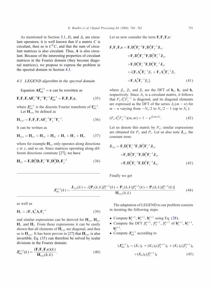
E. Roullot et al. / Signal Processing 84 (2004) 743–762 751
As mentioned in Section 3.1, Dx and x are circu-lant operators; it is well known that if a matrix C iscirculant, then so is CTC, and that the sum of circu-lant matrices is also circulant. Thus, A is also circu-lant. Because of the interesting properties of circulantmatrices in the Fourier domain (they become diago-nal matrices), we propose to express the problem inthe spectral domain in Section 4.3.
4.3. LEGEND algorithm in the spectral domain
Equation AIn+1rec = c can be rewritten as
FxFyFzAF−1x F−1
y F−1z Jn+1
rec = FxFyFzc; (35)
where Jn+1rec is the discrete Fourier transform of In+1
rec .Let Hxyz be de8ned as
Hxyz = FxFyFzAF−1x F−1
y F−1z : (36)
It can be written as
Hxyz = Hxy + Hyz + Hxz + Hx + Hy + Hz ; (37)
where for example Hxy only operates along directionsx et y, and so on. Since matrices operating along dif-ferent directions commute [27], we have
Hxy = FxDTx DxF−1
x FyDTyDyF−1
y (38)
as well as
Hx = �Fx�Tx �xF−1
x (39)
and similar expressions can be derived for Hyz, Hxz,Hy and Hz. From these expressions it can be easilyshown that all elements of Hxyz are diagonal, and thusso is Hxyz. It has been proven in [27] that Hxyz is alsoinvertible. Eq. (35) can therefore be solved by scalardivisions in the Fourier domain:
Jn+1rec (k) =
(FxFyFzc)(k)Hxyz(k; k)
: (40)
Let us now consider the term FxFyFzc:
FxFyFzc = FxDTx F
−1x FyDT
yF−1y Jxy
+FyDTyF
−1y FzDT
z F−1z Jyz
+FxDTx F
−1x FzDT
z F−1z Jxz
+�[Fx�Tx F
−1x (x + Fy�
TyF
−1y (y
+Fz�Tz F
−1z (z]; (41)
where (x, (y and (z are the DFT of bx, by and bz
respectively. Since x is a circulant matrix, it followsthat Fx T
x F−1x is diagonal, and its diagonal elements
are expressed as the DFT of the series x(m − n) form − n varying from −Nx=2 to Nx=2 − 1 (up to Nx):
(Fx Tx F
−1x )(m;m) = 1 − e j2�m=Nx : (42)
Let us denote this matrix by Px; similar expressionsare obtained for Py and Pz. Let us also note Jxyz theconstant term:
Jxyz = FxDTx F
−1x FyDT
yF−1y Jxy
+FyDTyF
−1y FzDT
z F−1z Jyz
+FxDTx F
−1x FzDT
z F−1z Jxz: (43)
Finally we get
Jn+1rec (k) =
Jxyz(k) + �[Px(k; k)(n+1x (k) + Py(k; k)(n+1
y (k) + Pz(k; k)(n+1z (k)]
Hxyz(k; k)(44)
The adaptation of LEGEND to our problem consistsin iterating the following steps:
• Compute bn+1x , bn+1
y , bn+1z using Eq. (28).
• Compute the DFT (n+1x , (n+1
y , (n+1z of bn+1
x , bn+1y ,
bn+1z .
• Compute Jn+1rec according to
(Jn+1rec )k = (K1)k + (K2)k((n+1
x )k + (K3)k((n+1y )k
+(K4)k((n+1z )k (45)
752 E. Roullot et al. / Signal Processing 84 (2004) 743–762
Fig. 3. Left: the high-resolution phantom, Middle: simulation of thenoisy acquisition with undersampling along x, Right: simulation ofthe noisy acquisition with undersampling along y. Undersamplingratio is here 64/20.
with
(K1)k =(Jxyz)k(Hxyz)k;k
;
(K2)k = �(Px)k;k(Hxyz)k;k
;
(K3)k = �(Py)k;k(Hxyz)k;k
;
(K4)k = �(Pz)k;k(Hxyz)k;k
: (46)
• Compute the inverse DFT In+1rec of Jn+1
rec .
Note that in Cartesian coordinates, the DFT bene8tsof FFT algorithms.
5. Validation and discussion
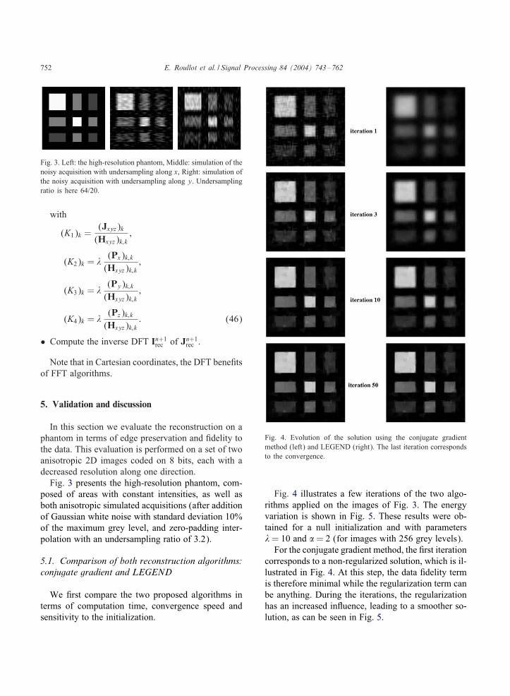
In this section we evaluate the reconstruction on aphantom in terms of edge preservation and 8delity tothe data. This evaluation is performed on a set of twoanisotropic 2D images coded on 8 bits, each with adecreased resolution along one direction.Fig. 3 presents the high-resolution phantom, com-
posed of areas with constant intensities, as well asboth anisotropic simulated acquisitions (after additionof Gaussian white noise with standard deviation 10%of the maximum grey level, and zero-padding inter-polation with an undersampling ratio of 3.2).
5.1. Comparison of both reconstruction algorithms:conjugate gradient and LEGEND
We 8rst compare the two proposed algorithms interms of computation time, convergence speed andsensitivity to the initialization.
Fig. 4. Evolution of the solution using the conjugate gradientmethod (left) and LEGEND (right). The last iteration correspondsto the convergence.
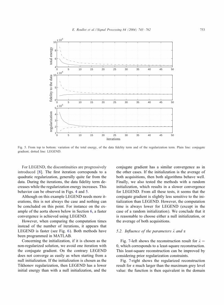
Fig. 4 illustrates a few iterations of the two algo-rithms applied on the images of Fig. 3. The energyvariation is shown in Fig. 5. These results were ob-tained for a null initialization and with parameters�= 10 and != 2 (for images with 256 grey levels).For the conjugate gradient method, the 8rst iteration
corresponds to a non-regularized solution, which is il-lustrated in Fig. 4. At this step, the data 8delity termis therefore minimal while the regularization term canbe anything. During the iterations, the regularizationhas an increased inNuence, leading to a smoother so-lution, as can be seen in Fig. 5.
E. Roullot et al. / Signal Processing 84 (2004) 743–762 753
0 5 10 15 20 25 30 35 40 45 504
6
8
10x 106
0 5 10 15 20 25 30 35 40 45 500
5
10x 106
0 5 10 15 20 25 30 35 40 45 501
2
3
4
5x 10⁵
iterations
regu
lari
zatio
nfi
delit
y to
the
data
tota
l ene
rgy
Fig. 5. From top to bottom: variation of the total energy, of the data 8delity term and of the regularization term. Plain line: conjugategradient; dotted line: LEGEND.
For LEGEND, the discontinuities are progressivelyintroduced [8]. The 8rst iteration corresponds to aquadratic regularization, generally quite far from thedata. During the iterations, the data 8delity term de-creases while the regularization energy increases. Thisbehavior can be observed in Figs. 4 and 5.Although on this example LEGEND needs more it-
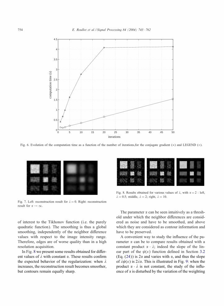
erations, this is not always the case and nothing canbe concluded on this point. For instance on the ex-ample of the aorta shown below in Section 6, a fasterconvergence is achieved using LEGEND.However, when comparing the computation times
instead of the number of iterations, it appears thatLEGEND is faster (see Fig. 6). Both methods havebeen programmed in MATLAB.Concerning the initialization, if it is chosen as the
non-regularized solution, we avoid one iteration withthe conjugate gradient. On the contrary LEGENDdoes not converge as easily as when starting from anull initialization. If the initialization is chosen as theTikhonov regularization, then LEGEND has a lowerinitial energy than with a null initialization, and the
conjugate gradient has a similar convergence as inthe other cases. If the initialization is the average ofboth acquisitions, then both algorithms behave well.Finally, we also tested the methods with a randominitialization, which results in a slower convergencefor LEGEND. From all these tests, it seems that theconjugate gradient is slightly less sensitive to the ini-tialization than LEGEND. However, the computationtime is always lower for LEGEND (except in thecase of a random initialization). We conclude that itis reasonable to choose either a null initialization, orthe average of both acquisitions.
5.2. In>uence of the parameters � and !
Fig. 7-left shows the reconstruction result for � =0, which corresponds to a least-square reconstruction.This least-square reconstruction can be improved byconsidering prior regularization constraints.Fig. 7-right shows the regularized reconstruction
result for ! much larger than the maximum grey levelvalue: the function is then equivalent in the domain
754 E. Roullot et al. / Signal Processing 84 (2004) 743–762
0 5 10 15 20 25 30 35 40 45 500
0.5
1
1.5
2
2.5
3
3.5
4
4.5
iterations
com
puta
tion
time
(s)
Fig. 6. Evolution of the computation time as a function of the number of iterations,for the conjugate gradient (∗) and LEGEND (◦).
Fig. 7. Left: reconstruction result for �= 0. Right: reconstructionresult for ! → ∞.
of interest to the Tikhonov function (i.e. the purelyquadratic function). The smoothing is thus a globalsmoothing, independently of the neighbor di5erencevalues with respect to the image intensity range.Therefore, edges are of worse quality than in a highresolution acquisition.In Fig. 8 we present some results obtained for di5er-
ent values of � with constant !. These results con8rmthe expected behavior of the regularization: when �increases, the reconstruction result becomes smoother,but contours remain equally sharp.
Fig. 8. Results obtained for various values of �, with != 2 : left,� = 0:5; middle, � = 2; right, � = 10.
The parameter ! can be seen intuitively as a thresh-old under which the neighbor di5erences are consid-ered as noise and have to be smoothed, and abovewhich they are considered as contour information andhave to be preserved.A convenient way to study the inNuence of the pa-
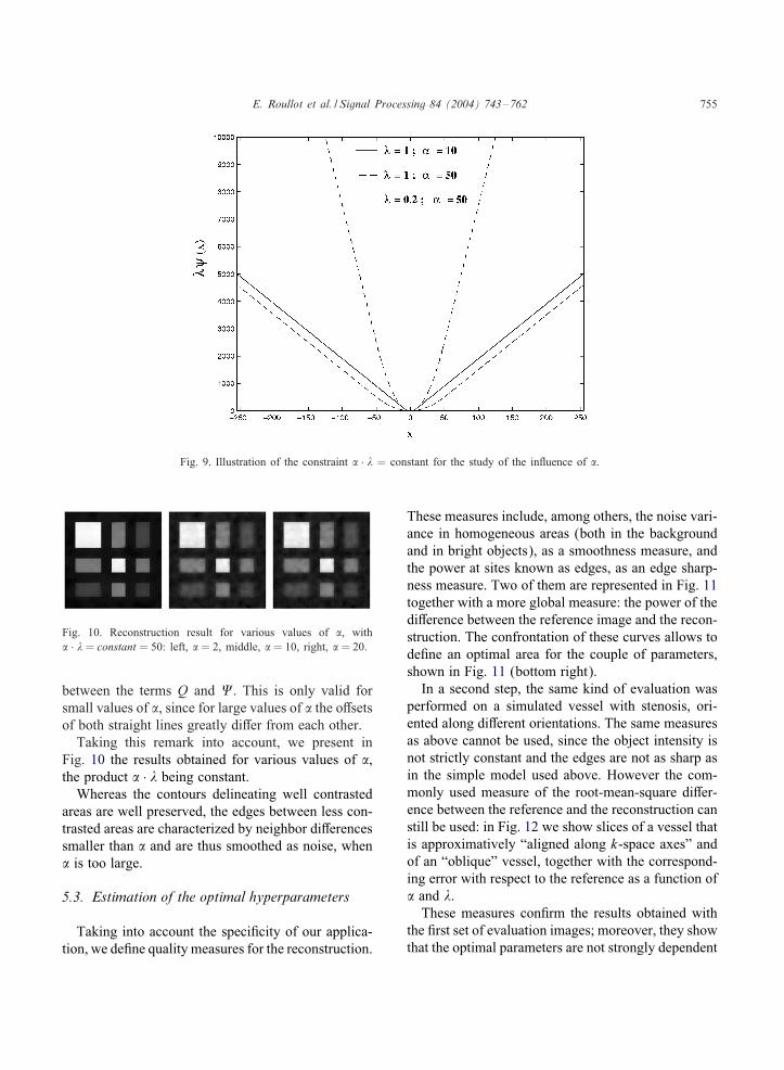
rameter ! can be to compare results obtained with aconstant product ! · �; indeed the slope of the lin-ear part of the (x) function de8ned in Section 3.2(Eq. (24)) is 2! and varies with !, and thus the slopeof � (x) is 2�!. This is illustrated in Fig. 9: when theproduct ! · � is not constant, the study of the inNu-ence of ! is disturbed by the variation of the weighting
E. Roullot et al. / Signal Processing 84 (2004) 743–762 755
Fig. 9. Illustration of the constraint ! · � = constant for the study of the inNuence of !.
Fig. 10. Reconstruction result for various values of !, with! · � = constant = 50: left, ! = 2, middle, ! = 10, right, ! = 20.
between the terms Q and �. This is only valid forsmall values of !, since for large values of ! the o5setsof both straight lines greatly di5er from each other.Taking this remark into account, we present in
Fig. 10 the results obtained for various values of !,the product ! · � being constant.Whereas the contours delineating well contrasted
areas are well preserved, the edges between less con-trasted areas are characterized by neighbor di5erencessmaller than ! and are thus smoothed as noise, when! is too large.
5.3. Estimation of the optimal hyperparameters
Taking into account the speci8city of our applica-tion, we de8ne quality measures for the reconstruction.
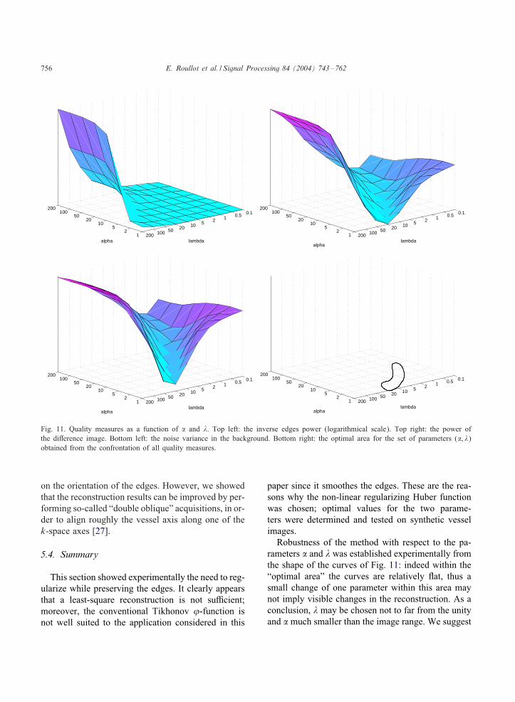
These measures include, among others, the noise vari-ance in homogeneous areas (both in the backgroundand in bright objects), as a smoothness measure, andthe power at sites known as edges, as an edge sharp-ness measure. Two of them are represented in Fig. 11together with a more global measure: the power of thedi5erence between the reference image and the recon-struction. The confrontation of these curves allows tode8ne an optimal area for the couple of parameters,shown in Fig. 11 (bottom right).In a second step, the same kind of evaluation was
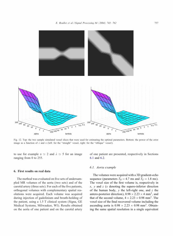
performed on a simulated vessel with stenosis, ori-ented along di5erent orientations. The same measuresas above cannot be used, since the object intensity isnot strictly constant and the edges are not as sharp asin the simple model used above. However the com-monly used measure of the root-mean-square di5er-ence between the reference and the reconstruction canstill be used: in Fig. 12 we show slices of a vessel thatis approximatively “aligned along k-space axes” andof an “oblique” vessel, together with the correspond-ing error with respect to the reference as a function of! and �.These measures con8rm the results obtained with
the 8rst set of evaluation images; moreover, they showthat the optimal parameters are not strongly dependent
756 E. Roullot et al. / Signal Processing 84 (2004) 743–762
12
510
2050
100200
0.10.5125102050100200lambdaalpha
12
510
2050
100200
0.10.5125102050100200lambda
alpha
12
510
2050
100200
0.10.5125102050100200lambda
alpha
12
510
2050
100200
0.10.5125102050100200
alphalambda
Fig. 11. Quality measures as a function of ! and �. Top left: the inverse edges power (logarithmical scale). Top right: the power ofthe di5erence image. Bottom left: the noise variance in the background. Bottom right: the optimal area for the set of parameters (!; �)obtained from the confrontation of all quality measures.
on the orientation of the edges. However, we showedthat the reconstruction results can be improved by per-forming so-called “double oblique” acquisitions, in or-der to align roughly the vessel axis along one of thek-space axes [27].
5.4. Summary
This section showed experimentally the need to reg-ularize while preserving the edges. It clearly appearsthat a least-square reconstruction is not suMcient;moreover, the conventional Tikhonov ’-function isnot well suited to the application considered in this
paper since it smoothes the edges. These are the rea-sons why the non-linear regularizing Huber functionwas chosen; optimal values for the two parame-ters were determined and tested on synthetic vesselimages.Robustness of the method with respect to the pa-
rameters ! and � was established experimentally fromthe shape of the curves of Fig. 11: indeed within the“optimal area” the curves are relatively Nat, thus asmall change of one parameter within this area maynot imply visible changes in the reconstruction. As aconclusion, � may be chosen not to far from the unityand ! much smaller than the image range. We suggest
E. Roullot et al. / Signal Processing 84 (2004) 743–762 757
12
510
2050
100200
0.10.5125102050100200lambdaalpha
12
510
2050
100200
0.10.5125102050100200lambdaalpha
Fig. 12. Top: the two sample simulated vessel slices that were used for estimating the optimal parameters. Bottom: the power of the errorimage as a function of � and ! (left: for the “straight” vessel, right: for the “oblique” vessel).
to use for example ! � 2 and � � 5 for an imageranging from 0 to 255.
6. First results on real data
The method was evaluated on 8ve sets of undersam-pled MR volumes of the aorta (two sets) and of thecarotid artery (three sets). For each of the 8ve patients,orthogonal volumes with complementary spatial res-olutions were acquired. Each volume was acquiredduring injection of gadolinium and breath-holding ofthe patient, using a 1:5 T clinical system (Signa, GEMedical Systems, Milwaukee, WI). Results obtainedon the aorta of one patient and on the carotid artery
of one patient are presented, respectively in Sections6.1 and 6.2.
6.1. Aorta example
The volumes were acquired with a 3D gradient-echosequence (parameters TR = 4:7 ms and TE = 1:8 ms).The voxel size of the 8rst volume is, respectively inx, y and z (x denoting the supero-inferior directionof the human body, y the left-right one, and z theantero-posterior direction), 0:98× 2:23× 4 mm3, andthat of the second volume, 4× 2:23× 0:98 mm3. Thevoxel size of the 8nal recovered volume including theascending aorta is 0:98 × 2:23 × 0:98 mm3. Obtain-ing the same spatial resolution in a single equivalent
758 E. Roullot et al. / Signal Processing 84 (2004) 743–762
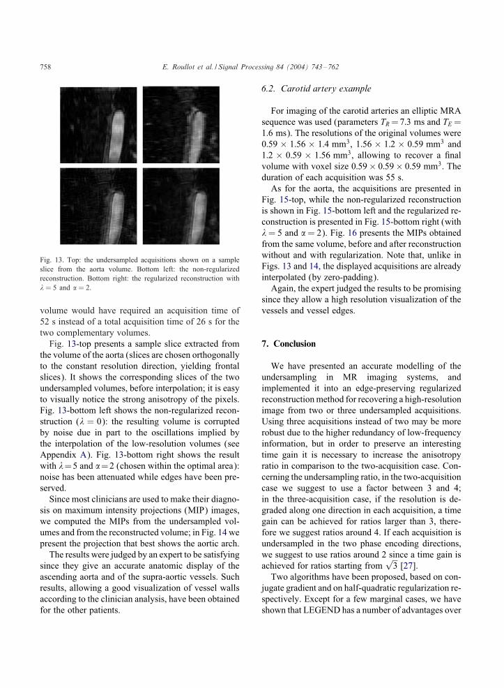
Fig. 13. Top: the undersampled acquisitions shown on a sampleslice from the aorta volume. Bottom left: the non-regularizedreconstruction. Bottom right: the regularized reconstruction with� = 5 and ! = 2.
volume would have required an acquisition time of52 s instead of a total acquisition time of 26 s for thetwo complementary volumes.Fig. 13-top presents a sample slice extracted from
the volume of the aorta (slices are chosen orthogonallyto the constant resolution direction, yielding frontalslices). It shows the corresponding slices of the twoundersampled volumes, before interpolation; it is easyto visually notice the strong anisotropy of the pixels.Fig. 13-bottom left shows the non-regularized recon-struction (� = 0): the resulting volume is corruptedby noise due in part to the oscillations implied bythe interpolation of the low-resolution volumes (seeAppendix A). Fig. 13-bottom right shows the resultwith �=5 and !=2 (chosen within the optimal area):noise has been attenuated while edges have been pre-served.Since most clinicians are used to make their diagno-
sis on maximum intensity projections (MIP) images,we computed the MIPs from the undersampled vol-umes and from the reconstructed volume; in Fig. 14 wepresent the projection that best shows the aortic arch.The results were judged by an expert to be satisfying
since they give an accurate anatomic display of theascending aorta and of the supra-aortic vessels. Suchresults, allowing a good visualization of vessel wallsaccording to the clinician analysis, have been obtainedfor the other patients.
6.2. Carotid artery example
For imaging of the carotid arteries an elliptic MRAsequence was used (parameters TR=7:3 ms and TE =1:6 ms). The resolutions of the original volumes were0:59 × 1:56 × 1:4 mm3, 1:56 × 1:2 × 0:59 mm3 and1:2 × 0:59 × 1:56 mm3, allowing to recover a 8nalvolume with voxel size 0:59× 0:59× 0:59 mm3. Theduration of each acquisition was 55 s.As for the aorta, the acquisitions are presented in
Fig. 15-top, while the non-regularized reconstructionis shown in Fig. 15-bottom left and the regularized re-construction is presented in Fig. 15-bottom right (with�= 5 and != 2). Fig. 16 presents the MIPs obtainedfrom the same volume, before and after reconstructionwithout and with regularization. Note that, unlike inFigs. 13 and 14, the displayed acquisitions are alreadyinterpolated (by zero-padding).Again, the expert judged the results to be promising
since they allow a high resolution visualization of thevessels and vessel edges.
7. Conclusion
We have presented an accurate modelling of theundersampling in MR imaging systems, andimplemented it into an edge-preserving regularizedreconstructionmethod for recovering a high-resolutionimage from two or three undersampled acquisitions.Using three acquisitions instead of two may be morerobust due to the higher redundancy of low-frequencyinformation, but in order to preserve an interestingtime gain it is necessary to increase the anisotropyratio in comparison to the two-acquisition case. Con-cerning the undersampling ratio, in the two-acquisitioncase we suggest to use a factor between 3 and 4;in the three-acquisition case, if the resolution is de-graded along one direction in each acquisition, a timegain can be achieved for ratios larger than 3, there-fore we suggest ratios around 4. If each acquisition isundersampled in the two phase encoding directions,we suggest to use ratios around 2 since a time gain isachieved for ratios starting from
√3 [27].
Two algorithms have been proposed, based on con-jugate gradient and on half-quadratic regularization re-spectively. Except for a few marginal cases, we haveshown that LEGEND has a number of advantages over

E. Roullot et al. / Signal Processing 84 (2004) 743–762 759
Fig. 14. Left and middle: the MIPs computed from both undersampled volumes. Right: the MIP computed after regularized reconstructionwith � = 5 and ! = 2.
Fig. 15. Top: the undersampled acquisitions shown on a sample slice from the carotids volume. Bottom left: the non-regularizedreconstruction. Bottom right: the regularized reconstruction with � = 5 and ! = 2.
Fig. 16. Top: the undersampled acquisitions shown as a MIP from the neck. Bottom left: the non-regularized reconstruction. Bottom right:the regularized reconstruction with � = 5 and ! = 2.
the conjugate gradient method: it is easier to imple-ment thanks to our formulation in the spectral domain;it shows a better convergence in terms of computa-
tion time; it progressively introduces discontinuities.Intensive use of FFTs in the optimization schemesmakes the method well designed for Cartesian k-space
760 E. Roullot et al. / Signal Processing 84 (2004) 743–762
8lling. However it can be applied to any non-Cartesianacquisition sequence provided that a re-gridding ofthe data onto a cartesian grid was made previously. Itcould also be extended to processing data in the gen-uine non-Cartesian geometry of acquisition. Howeverthe FFT computation should then be replaced by aDFT algorithm that would considerably increase thereconstruction time.We have presented reconstruction results on the
aorta, using two acquisitions undersampled in onephase encoding direction, and on the carotid artery, us-ing three acquisitions undersampled in the two phaseencoding directions. The reconstruction provides a de-noised and homogeneous image of the vascular lumenwith sharp edges. Furthermore, although a misalign-ment of the vessel with respect to the k-space axescan lead to a loss of high frequencies in the acquireddata, the method seems to be robust enough to allowany orientations of the vessel. However, for clinicalevaluation some further work remains: in this paper,each sequence is acquired in a distinct apnea, whichcan lead to artifacts due to the breathing of the pa-tient between the acquisitions. A rigid registration wasperformed manually, which is of course not optimal.Work is currently being performed on the develop-ment of dedicated sequences, allowing to acquire thevolumes during one breath-holding.
Appendix A. Expression of the zero-padding inter-polation
In order not to modify the frequency content of theundersampled data, interpolation is achieved using aspecial version of the zero-padding method [28]. Ac-cording to the acquisition strategy presented in Section2.1, each undersampled image needs to be interpolatedin two directions, but this can be achieved separatelyalong both directions. This interpolation is presentedhere in the x direction as an example.Let IN
′x be the undersampled image along direction
x, with dimensionN ′ along x; let INx be the correspond-ing high-resolution image, with dimension N ¿N ′
along x. (In order to simplify the notations, we assumethat both N and N ′ are even; for odd dimensions, theexpressions can be derived by taking the appropriatesummation limits.)
Let JN ′denote the DFT on the lines of IN
′x , and JN
the DFT on the lines of INx . Let us express INx as afunction of IN
′x .
The expression of INx (x; y) as a function of JN (k; y)results from an inverse DFT:
INx (x; y; z) =
N2 −1∑
k=−N2
JN (k; y; z)e j2�xk=N : (A.1)
Zero-padding interpolation consists in padding theDFT of the signal to be interpolated with zeros inorder to arti8cially increase its spatial sampling rate.Thus, JN and JN ′
are related as follows:
JN (k; y; z)
=
JN ′(k; y; z) for k = −N ′
2 · · · N ′2 − 1
0 for k = −N2 · · · − N ′
2 − 1
and k = N ′2 · · · N
2 − 1:
(A.2)
Therefore
INx (x; y; z) =
N ′2 −1∑
k=−N ′2
JN ′(k; y; z)e j2�xk=N : (A.3)
Moreover
JN ′(k; y; z) =
1N ′
N ′2 −1∑
l=−N ′2
IN′
x (l; y; z)e−j2�kl=N ′: (A.4)
which yields
INx (x; y; z) =1N ′
N ′2 −1∑
l=−N ′2
IN′
x (l; y; z)
×N ′2 −1∑
k=−N ′2
e−j2�kl=N ′e j2�xk=N : (A.5)
Let us introduce h(m) such that
INx (x; y; z) =
N ′2 −1∑
l=−N ′2
IN′
x (l; y; z)h(xN ′
N− l
): (A.6)
E. Roullot et al. / Signal Processing 84 (2004) 743–762 761
h(m) can be expressed as
h(m) =1N ′ e
−j�m=N ′ sin �msin(�m=N ′)
; (A.7)
Themain problem of this conventional zero-paddinginterpolation method resides in the fact that interpo-lation of real data provides complex data (for evendimensions). Because of the hypothesis that we aredealing with the magnitude of the M.R. image, i.e.with a real-valued image, it is more convenient toconstrain the interpolated image to be real-valued.The solution that minimizes the norm of the quadraticerror with respect to the above solution, under theconstraint that h(m) must be real-valued, can be com-puted easily [13,27] as the real part of the abovesolution, i.e.:
h(m) =1N ′ cos
(�
mN ′
) sin �msin(�m=N ′)
; (A.8)
This function is quite similar to the well-known sincfunction.
Appendix B. Analytic expression of the undersam-pling operators
In Section 3.1 the degradation operator was ex-pressed as the matrix product:
Dx = F−1x MxFx: (B.1)
Let us express Dx analytically:
(MxFx)m;n =
Nx2 −1∑
k=−Nx2
(Mx)m;k(Fx)k;n
=
e−j2�mn=Nx if − N ′x2 + 1
6m6N ′
x
2− 1;
0:5 e−j2�mn=Nx if m= −N ′x2 or
m= N ′x2 ;
0 else(B.2)
with m; n varying from −Nx=2 to Nx=2 − 1; thus
(Dx)m;n = (F−1x MxFx)m;n
=
Nx2 −1∑
k=−Nx2
(F−1x )m;k(MxFx)k;n
=
N ′x2 −1∑
k=−N ′x2 +1
e j2�k(m−n)=Nx
+0:5(ej2�((m−n)=Nx)(−N ′x =2)
+ej2�((m−n)=Nx)(N ′x =2))
= cos(�n − mNx
)sin(�(n − m)N ′
x=Nx)sin(�(n − m)=Nx)
:
(B.3)
Dy and Dz can be expressed in a similar manner.
Appendix C. Gradient of the energy function
The gradient of the energy function can be ex-pressed as
∇E(x; y; z) = ∇Q(x; y; z) + �∇�(x; y; z): (C.1)
Each of these terms are detailed below.From the expression of Q in Section 3.2 it can be
derived that
�Q= 2(DTx DxIrec − DT
x Ix + DTyDyIrec
−DTyIy + DT
z DzIrec − DTz Iz): (C.2)
For the regularization term � also introduced inSection 3.2, we get
�/ =�Tx
′(�xIrec) + �Ty
′(�yIrec)
+�Tz
′(�zIrec): (C.3)
References
[1] H.C. Andrews, B.R. Hunt, Digital Image Restoration,Prentice-Hall, Englewood Cli5s, NJ, 1977.
762 E. Roullot et al. / Signal Processing 84 (2004) 743–762
[2] G. Aubert, M. Barlaud, L. Blanc-Feraud, P. Charbonnier,A deterministic algorithm for edge-preserving computedimaging using legendre transform, in: Proceedings ofthe IEEE International Conference on Pattern Recognition(ICPR), Vol. 3, 1994, pp. 188–191.
[3] H. Azhari, O.E. Denisova, A. Montag, E.P. Shapiro,Circular sampling: perspective of a time-saving scanningprocedure, Magnetic Resonance Imaging 14 (6) (1996)625–631.
[4] M. Bertero, P. Boccacci, Introduction to Inverse Problemsin Imaging, Institute of Physics Publishing, New York,1998.
[5] M.J. Black, A. Rangarajan, On the uni8cation of line process,outlier rejection, and robust statistics with applications inearly vision, Internat. J. Comput. Vision 19 (1) (1996)57–91.
[6] A. Blake, A. Zisserman, Visual Reconstruction, MIT Press,Cambridge, MA, 1987.
[7] Y. Cao, D.N. Levin, Using prior knowledge ofhuman anatomy to constrain MR image acquisitionand reconstruction: half K-space and full K-spacetechniques, Magnetic Resonance Imaging 15 (6) (1997)669–677.
[8] P. Charbonnier, L. Blanc-Feraud, G. Aubert, M. Barlaud,Two deterministic half-quadratic regularization algorithms forcomputed imaging, in: Proceedings of the IEEE InternationalConference on Image Processing (ICIP), Vol. 2, 1994,pp. 168–172.
[9] P. Charbonnier, L. Blanc-Fraud, G. Aubert, M. Barlaud,Deterministic edge-preserving regularization in computerimaging, IEEE Trans. Image Processing 6 (2) (February1997) 298–311.
[10] G. Demoment, Image reconstruction and restoration: overviewof common estimation structures and problems, IEEE Trans.Acoust. Speech Signal Process. 37 (12) (December 1989)2024–2036.
[11] E.H. Dillon, M.S. Van Leeuwen, M.A. Fernandez, W.P. Mali,Spiral CT angiography, AJR Amer. J. Roentgenol. 160 (6)(1993) 1273–1278.
[12] I. Dologlou, D. van Ormondt, G. Carayannis, MRI scantime reduction through non-uniform sampling and SVD-basedestimation, Signal Processing 55 (1996) 207–219.
[13] D. Fraser, Interpolation by the FFT revisited—anexperimental investigation, IEEE Trans. Acoust. SpeechSignal Process. 37 (5) (May 1989) 665–675.
[14] D. Geman, C. Reynolds, Non linear image recovery withhalf-quadratic regularization, IEEE Trans. Image Process. 4(7) (July 1995) 932–946.
[15] D. Geman, G. Reynolds, Constrained restoration and therecovery of discontinuities, IEEE Trans. Pattern Anal.Machine Intell. 14 (3) (March 1992) 367–383.
[16] S. Geman, D. McClure, Statistical methods for tomographicimage reconstruction, Bull. Internat. Statist. Inst. LII-4:5–21(1987).
[17] T. Hebert, R. Leahy, A generalized EM algorithm for 3-DBayesian reconstruction from poisson data using Gibbs priors,IEEE Trans. Med. Imaging 8 (2) (June 1989) 194–202.
[18] A. Herment, E. Roullot, I. Bloch, O. Jolivet, A. De Cesare,F. Frouin, J. Bittoun, Local reconstruction of stenosedsections of artery using multiple MRA acquisitions, MagneticResonance Med. 49 (2003) 731–742.
[19] R.L. Lagendijk, Iterative identi8cation and restoration ofimages, Ph.D. Thesis, Technische Universiteit Delft, TheNetherlands, 1990.
[20] M. Nikolova, Local strong homogeneity of a regularizedestimator, SIAM J. Appl. Math. 61 (2) (1999) 633–658.
[21] D.C. Noll, Multishot rosette trajectories for spectrallyselective MR imaging, IEEE Trans. Med. Imaging 16 (4)(August 1997) 372.
[22] J.A. Parker, R.V. Kenyon, D.E. Troxel, Comparison ofinterpolating methods for image resampling, IEEE Trans.Med. Imaging 2 (1) (March 1983) 31–39.
[23] J.G. Pipe, Motion correction with PROPELLER MRI:application to head motion and free-beating cardiac imaging,Magnetic Resonance Med. 42 (5) (1999) 963–969.
[24] S.K. Plevritis, A. Macovski, MRS imaging using anatomicallyK-space sampling and extrapolation, Magnetic ResonanceMed. 34 (1995) 686–693.
[25] W.K. Pratt, Digital Image Processing, Wiley-Interscience,New York, 1991.
[26] M.R. Prince, Contrast-enhanced MR angiography: theory andoptimization, Magnetic Resonance Imaging Clin. N. Amer. 6(2) (May 1998) 257–267.
[27] E. Roullot, Analysis of multiple anisotropic acquisitions in 3DMagnetic Resonance Angiography: modeling and regularizedreconstruction for improving the spatial resolution. Ph.D.Thesis, Ecole Nationale Superieure des Telecommunications,December 2001, (in French).
[28] R.W. Schafer, B. Gold, A digital signal processing approachto interpolation, Proc. IEEE 61 (1973) 692–702.
[29] H. Schomberg, J. Timmer, The gridding method for imagereconstruction by Fourier transformation, IEEE Trans. Med.Imaging 14 (3) (September 1995) 596–607.
[30] X. Zhou, Z.P. Liang, S.L. Gewalt, G.P. Cofer, P.C. Lauterbur,A fast echo technique with circular sampling, MagneticResonance Med. 39 (1998) 23–27.