moveout approximation for horizontal transversely isotropic and vertical transversely isotropic...

Geophysical Prospecting, 2010, 58, 577–597 doi: 10.1111/j.1365-2478.2009.00856.x

Moveout approximation for horizontal transversely isotropicand vertical transversely isotropic layered medium. Part I:1D ray propagation‡

Igor Ravve∗ and Zvi KorenParadigm Geophysical, Research & Development, Gav-Yam Center, No. 9 Shenkar St., PO Box 2061, Herzliya B 46120, Israel

Received May 2009, revision accepted November 2009

ABSTRACTAnisotropy in subsurface geological models is primarily caused by two factors: sed-imentation in shale/sand layers and fractures. The sedimentation factor is mainlymodelled by vertical transverse isotropy (VTI), whereas the fractures are modelledby a horizontal transversely isotropic medium (HTI). In this paper we study hy-perbolic and non-hyperbolic normal reflection moveout for a package of HTI/VTIlayers, considering arbitrary azimuthal orientation of the symmetry axis at each HTIlayer. We consider a local 1D medium, whose properties change vertically, with flatinterfaces between the layers. In this case, the horizontal slowness is preserved; thus,the azimuth of the phase velocity is the same for all layers of the package. In gen-eral, however, the azimuth of the ray velocity differs from the azimuth of the phasevelocity. The ray azimuth depends on the layer properties and may be different foreach layer. In this case, the use of the Dix equation requires projection of the move-out velocity of each layer on the phase plane. We derive an accurate equation forhyperbolic and high-order terms of the normal moveout, relating the traveltime tothe surface offset, or alternatively, to the subsurface reflection angle. We relate theazimuth of the surface offset to its magnitude (or to the reflection angle), consideringshort and long offsets. We compare the derived approximations with analytical raytracing.

Key words: Anisotropy, Modelling, Inversion, Parameter estimation, Velocityanalysis.

INTRODUCTION

Transversely isotropic models with both vertical and hori-zontal symmetry axes have been extensively studied (e.g.,Thomsen 1986). Within a given horizontal transverselyisotropic (HTI) layer, the fractures are considered alignedwith a specific azimuth (e.g., Bakulin, Grechka and Tsvankin2000a,b). In this study we extend the existing work on move-

‡This paper is based on extended abstracts P0126 and P0128 pre-sented at the 71th EAGE Conference & Exhibition Incorporating SPEEUROPEC 2009, 8–11 June 2009 in Amsterdam, the Netherlands.∗E-mail: [email protected]

out approximation in HTI layered medium (e.g., Al-Dajaniand Tsvankin 1998; Grechka and Tsvankin 1999), account-ing for the deviation of the ray velocity from the phase velocityplane at each HTI layer. Consequently, the resulting relation-ships include the direction of the phase velocity, described byits zenith angle, θphs (angle between the phase velocity andthe vertical axis) and azimuth angle, ϕphs. For a flat reflector,the zenith angle of the phase velocity is also the reflection an-gle. This study consists of two parts. In Part I we study thehyperbolic and non-hyperbolic approximations of the move-out for a package of horizontal transversely isotropic, verticaltransversely isotropic and isotropic layers, including the trav-eltime, the magnitude and the direction of the offset on the

C© 2010 European Association of Geoscientists & Engineers 577

578 I. Ravve and Z. Koren

Sn

rerayV

inrayV

rephsV

inphsV

axissymmetry

z

rayax ϕ

αα

θ

θ

ϕ

phsax ϕϕ

ray

phs

axissymmetry

phs

ray

x

y

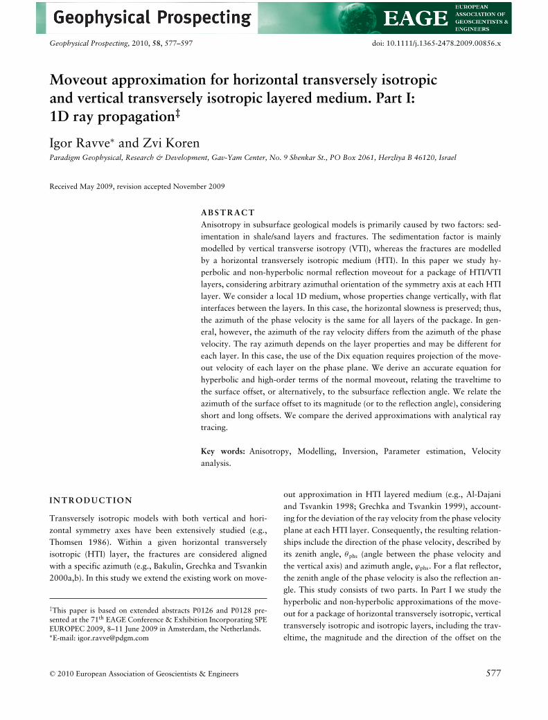
Figure 1 Reflection scheme for HTI medium.

Earth’s surface versus ray parameters. In Part II we introducethe effective model for the package of layers and establish itsparameters from the traveltime errors, under the hyperbolicapproximation.

The incident-reflected raypath in a vertically varying HTIlayered medium with a flat reflector is symmetric due to thefact that the normal to the reflection plane is perpendicular tothe axis of symmetry. Thus, the one-way path and the one-waymoveout can be studied. (An extension to dipping layers is be-yond the scope of this paper.) We derive the total traveltimeand the lateral propagation for a package of layers, summingup these parameters for each individual layer. Since the az-imuth of the phase velocity is the same for all layers, it can beconsidered a reference azimuth. The lateral displacements inthe layers have different directions; therefore, before addingthese values, we split them into two horizontal components: xcomponent in the direction of the phase velocity azimuth andy component normal to x. To make this decomposition possi-ble, we establish the difference between the azimuth of the rayvelocity and the azimuth of the phase velocity. Generally, thisdifference depends on both the zenith and the azimuth anglesof the phase velocity but for near-vertical rays (small zenithangles) the value of the zenith angle is not essential. Obviously,within isotropic and vertical transversely isotropic layers, theazimuths of the ray and the phase velocities are equal. Wepresent a full derivation of the method and its application.

RAY TRACING I N H OR I Z ON T A LTRANSVERSELY I SOT R OPI C M E DI UM

Figure 1 shows the reflection scheme for a HTI layer. Weintroduce the zenith angles of the group and phase velocities,θ ray and θphs, as the deviations of these velocities from the

vertical axis z. For a flat reflector, the vertical axis z coincideswith the normal nS to the reflection surface and the zenithangle of the phase velocity is also the reflection angle. Theazimuths of the ray and phase velocities are ϕray and ϕphs,respectively. Since ϕphs is constant for all layers, then withoutany loss of generality, one can assume ϕphs = 0. The ray andphase angles αray and αphs are defined as the angles betweenthe corresponding velocities (ray or phase) and the mediumaxis of symmetry, as shown in Fig. 1, where subscript ‘in’stands for incident and ‘re’ for reflected. The phase velocitiesare shown by blue lines, the ray velocities by red lines and thegreen line shows the direction of the medium symmetry axis.

In this section we derive the relationships for the compo-nents of the lateral propagation and for the traveltime thatwill be later used for the series approximation describing near-vertical rays. The lateral propagation h reads

h = z tan θray = toVver tan θray, (1)

where z is the layer thickness, to is the vertical time and Vver isthe vertical compression velocity of the HTI layer. The lateralpropagation components are

hx = h cos(ϕray − ϕphs), hy = h sin(ϕray − ϕphs), (2)

and the traveltime is

t = LVray

= toVver

cos θrayVray, (3)

where L is the length of the raypath within the given layerand Vray is the ray (group) velocity. Recall that each layer ishomogeneous and thus the raypath through each layer is astraight intercept, with refractions at the interfaces. We showin Appendix A that the zenith angle of the ray velocity dependson the zenith angle of the phase velocity,

cos θray

cos θphs= sin αray

sin αphs, (4)

and the difference between the azimuths of the ray and thephase velocities is

sin(ϕray − ϕphs) = − sin(αray − αphs

)sin(ϕax − ϕphs)

sin θray sin αphs, (5)

where ϕax is the azimuth of the medium axis of symmetry. Weshow in Appendix B that for an HTI layer the phase angle isrelated to the zenith angle of the phase velocity,

cos αphs = sin θphs cos(ϕax − ϕphs). (6)

Obviously, for a vertical transversely isotropic layer, zenithangle of the phase velocity coincides with the phase angle and

C© 2010 European Association of Geoscientists & Engineers, Geophysical Prospecting, 58, 577–597

Moveout approximation in HTI/VTI layered medium 579

zenith angle of the ray velocity coincides with the ray angle,

αphs = θphs, αray = θray. (7)

The ray angle αray, along with the ray and phase velocities, Vray

and Vphs, can be established using the known relationships fora transversely isotropic (TI) medium (Tsvankin 2001). Thecorresponding relationships are summarized in Appendix B.For an HTI medium, the ‘orthorhombic’ set of Thomsen pa-rameters δ2, ε2, f 2 and Vver may be converted to TI parametersδ, ε, f and VP, where the last one is the axial compression ve-locity (Tsvankin 1997b; Grechka and Tsvankin 1999; Contr-eras, Grechka and Tsvankin 1999). Conversion relationshipsare listed in Appendix C.

To test the analytical results, ray tracing was performedfrom the reflection point up to the surface with a given zenithangle of the phase velocity θphs. The lateral slowness, which isconstant along the ray, reads

p = sin θphs,r

Vphs,r(θphs,r

) , (8)

where subscript ‘r’ stands for the lowermost layer that includesthe reflection point. For all upper layers, we solve equation (8)for the unknown zenith angle θphs,i, given the lateral slownessp. Details of the solution are explained in Appendix D; thesolution is exact for large offsets as well.

PROPAGATION OF N EA R - V E R T I C A L RAYS

We have developed the sixth-order moveout approximationfor a horizontal transversely isotropic (HTI)/vertical trans-versely isotropic (VTI) layered medium, which leads to afourth-order approximation for the difference between the az-imuth of the offset on the Earth’s surface and the azimuth ofthe phase velocity. In addition, we have added an asymptoticcorrection, which makes these approximations exact for infi-nite offsets. The derivations of the sixth-order approximationare too long for the journal paper format and therefore, wepresent here only the series approximation up to the fourthorder for the moveout and up to the second order for thesurface offset azimuth. The leading term of the moveout ap-proximation includes the normal moveout velocity Vnmo. Themoveout components are derived as the series of small param-eters �αphs,i, where �αphs,i are different for individual layers.For an HTI layer, parameter �αphs,i is the difference betweenthe right angle and the phase angle of the given layer i,

�αphs,i = π/2 − αphs,i . (9)

A similar approach is applied to VTI layers, where the smallparameter is the phase angle itself. The details of the seriesderivation are explained in Appendix E for an HTI layer andin Appendix F for a VTI layer. In Appendix G we derive thenormal moveout (NMO) velocity for a unique HTI layer,

V2nmo

V2ver

= 1 + 4δ2(1 + δ2) cos2(ϕax − ϕphs)1 + 2δ2 cos2(ϕax − ϕphs)

. (10)

We then demonstrate that our result obtained versus thephase velocity azimuth agrees with Tsvankin (1997a) rela-tionship for the NMO velocity versus the ray (group) velocityazimuth. We also show that our quartic term for the moveoutagrees with that obtained by Al-Dajani and Tsvankin (1998).Then we study the propagation through a package of HTI,VTI and isotropic layers and we use Snell’s law (equation(8)) to obtain the parameters �αph,i for each individual layerversus the ray lateral slowness p, see Appendix H for details.Summing up the traveltimes and the offset components for theindividual layers, we find the traveltime for the whole packageversus the global offset, or alternatively versus the ray slow-ness. The derivation is presented in Appendix I. Dependenceof the offset azimuth on the offset magnitude is explained inAppendix J. The proof derivation for the NMO velocity andthe offset azimuth for a package of layers are presented inAppendix K. For a package of HTI/VTI layers, the resultingNMO velocity is given by

toV2nmo =

(∑Apx,i

)2 + (∑Apy,i

)2∑Apx,i

. (11)

The azimuth of the surface offset is given by

tan(ϕoff − ϕphs

) =∑

Apy,i∑Apx,i

, (12)

where for an HTI layer

Apx,i = [1 + 2δ2,i cos2

(ϕax,i − ϕphs

)]to,i V2

ver,i

Apy,i = δ2,i sin 2(ϕax,i − ϕphs

)to,i V2

ver,i ,(13)

and for a VTI (and an isotropic) layer

Apx,i = (1 + 2δi ) to,i V2ver,i , Apy,i = 0. (14)

For a package with HTI layers, the Dix summation rule (1955)for the moveout velocity is no longer valid, i.e., the resultingNMO velocity is not the rms (root mean square) value ofNMO velocities for individual layers. However, the projec-tion of the NMO velocity of the package on the azimuthof the phase velocity is still the rms value of the individual



projections,

toV2nmo cos2

(ϕoff − ϕphs

) =∑

to,i V2nmo,i cos2

(ϕray,i − ϕphs

).

(15)

Finally, in Appendix L we show that the hyperbolic move-out approximation can also be obtained versus the reflectionangle θphs,r.

NUMERICAL EXAMPLES

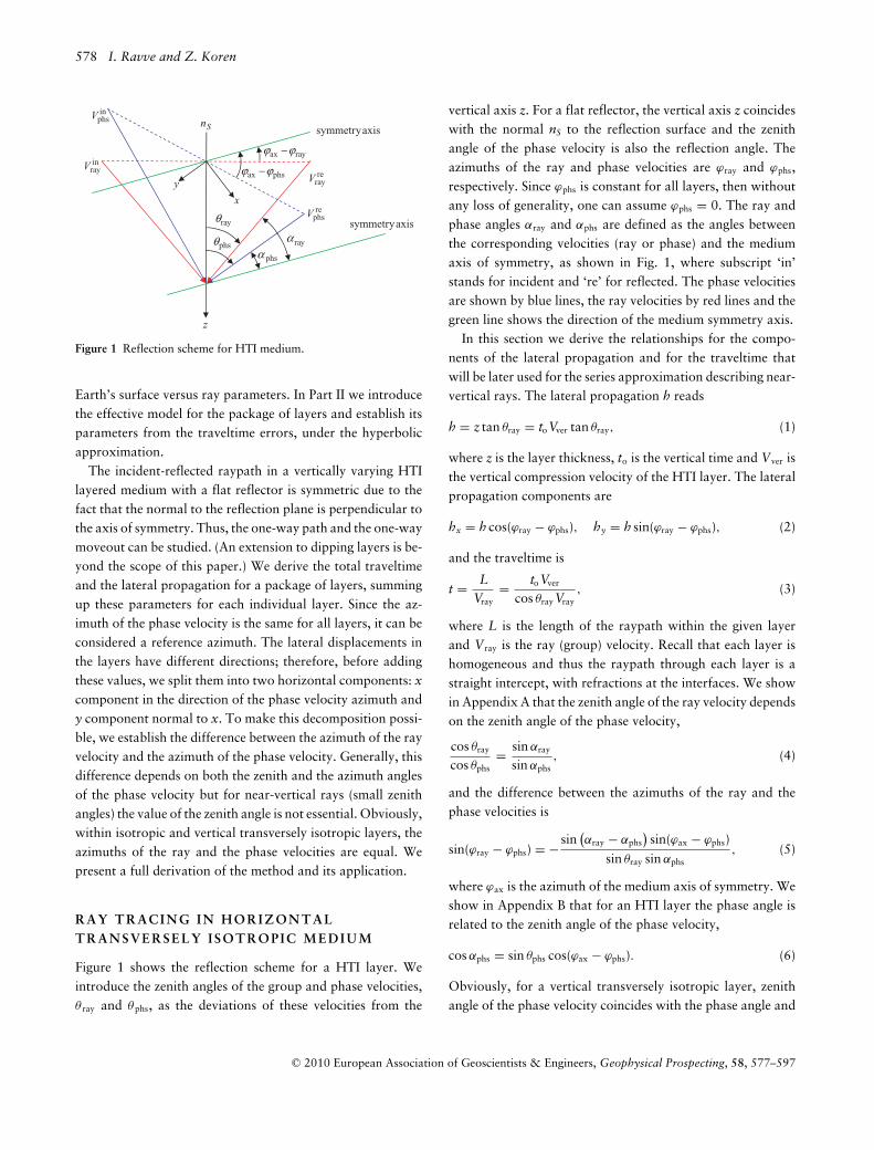
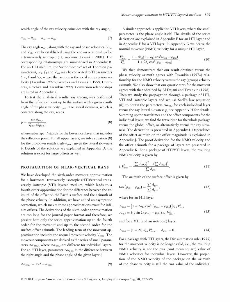
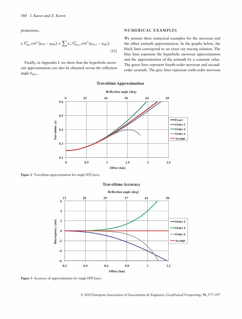
We present three numerical examples for the moveout andthe offset azimuth approximation. In the graphs below, theblack lines correspond to an exact ray tracing solution. Theblue lines represent the hyperbolic moveout approximationand the approximation of the azimuth by a constant value.The green lines represent fourth-order moveout and second-order azimuth. The grey lines represent sixth-order moveout

0.2

0.3

0.4

0.5

0.6

0 0.5 1 1.5 2 2.5

Trav

elti

me

(s)

Offset (km)

Traveltime Approximation

Exact

Order 2

Order 4

Order 6

Asympt.

0 25 44 56 64 69

Reflection angle (deg)

Figure 2 Traveltime approximation for single HTI layer.

-6

-4

-2

0

2

4

6

0.2 0.4 0.6 0.8 1 1.2

Dis

crep

ancy

(m

s)

Offset (km)

Traveltime Accuracy

Order 2

Order 4

Order 6

Asympt.

11 20 29 37 44 50


Figure 3 Accuracy of approximation for single HTI layer.



-2

-1

0

1

2

3

4

5

6

7

0 0.51 1.5 2 2.5 3

Azi

mut

h (d

eg)

Offset (km)

Surface Offset Azimuth

Exact

Constant

Order 2

Order 4

Asympt.

0 25 44 56 64 69 72


Figure 4 Offset approximation for single HTI layer.

1.5

2

2.5

3

3.5

4

4.5

0 2 4 6 8 10

Trav

elti

me

(s)

Offset (km)


Exact

Order 2

Order 4

Order 6

Asympt.

0 27 47 60 68 74


Figure 5 Traveltime approximation for Package 1.

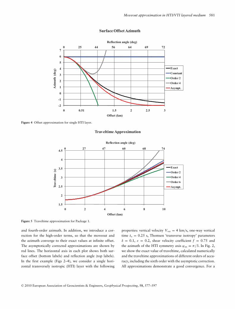
and fourth-order azimuth. In addition, we introduce a cor-rection for the high-order terms, so that the moveout andthe azimuth converge to their exact values at infinite offset.The asymptotically corrected approximations are shown byred lines. The horizontal axis in each plot shows both sur-face offset (bottom labels) and reflection angle (top labels).In the first example (Figs 2–4), we consider a single hori-zontal transversely isotropic (HTI) layer with the following

properties: vertical velocity Vver = 4 km/s, one-way verticaltime to = 0.25 s, Thomsen ‘transverse isotropy’ parametersδ = 0.1, ε = 0.2, shear velocity coefficient f = 0.75 andthe azimuth of the HTI symmetry axis ϕax = π/3. In Fig. 2,we show the exact value of traveltime, calculated numericallyand the traveltime approximations of different orders of accu-racy, including the sixth order with the asymptotic correction.All approximations demonstrate a good convergence. For a



-3

-2

-1

0

1

2

3

1 1.5 2 2.5 3 3.5

Dis

crep

ancy

(m

s)

Offset (km)

Traveltime Accuracy

Exact

Order 2

Order 4

Order 6

Asympt.

14 21 27 33 38 42.5


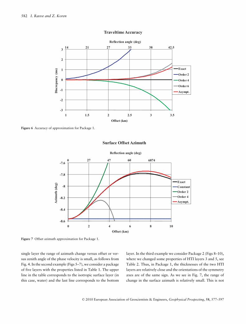
Figure 6 Accuracy of approximation for Package 1.

-8.6

-8.4

-8.2

-8

-7.8

-7.6

0 2 4 6 8 10

Azi

mut

h (d

eg)

Offset (km)


Exact

Constant

Order 2

Order 4

Asympt.

47 60 6874


0 27

Figure 7 Offset azimuth approximation for Package 1.

single layer the range of azimuth change versus offset or ver-sus zenith angle of the phase velocity is small, as follows fromFig. 4. In the second example (Figs 5–7), we consider a packageof five layers with the properties listed in Table 1. The upperline in the table corresponds to the isotropic surface layer (inthis case, water) and the last line corresponds to the bottom

layer. In the third example we consider Package 2 (Figs 8–10),where we changed some properties of HTI layers 3 and 5, seeTable 2. Thus, in Package 1, the thicknesses of the two HTIlayers are relatively close and the orientations of the symmetryaxes are of the same sign. As we see in Fig. 7, the range ofchange in the surface azimuth is relatively small. This is not



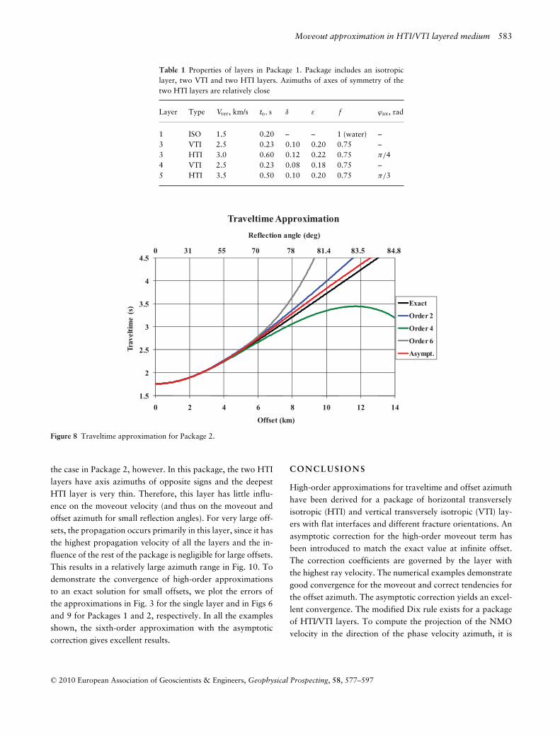
Table 1 Properties of layers in Package 1. Package includes an isotropiclayer, two VTI and two HTI layers. Azimuths of axes of symmetry of thetwo HTI layers are relatively close

Layer Type Vver, km/s to, s δ ε f ϕax, rad

1 ISO 1.5 0.20 – – 1 (water) –3 VTI 2.5 0.23 0.10 0.20 0.75 –3 HTI 3.0 0.60 0.12 0.22 0.75 π/44 VTI 2.5 0.23 0.08 0.18 0.75 –5 HTI 3.5 0.50 0.10 0.20 0.75 π/3

1.5

2

2.5

3

3.5

4

4.5

0 2 4 6 8 10 12 14

Trav

elti

me

(s)

Offset (km)


Exact

Order 2

Order 4

Order 6

Asympt.

8.485.380755130 78 81.4


Figure 8 Traveltime approximation for Package 2.

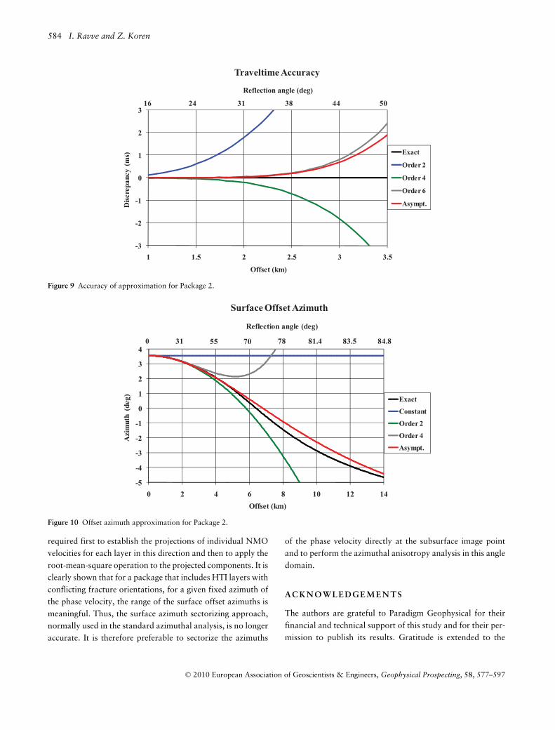
the case in Package 2, however. In this package, the two HTIlayers have axis azimuths of opposite signs and the deepestHTI layer is very thin. Therefore, this layer has little influ-ence on the moveout velocity (and thus on the moveout andoffset azimuth for small reflection angles). For very large off-sets, the propagation occurs primarily in this layer, since it hasthe highest propagation velocity of all the layers and the in-fluence of the rest of the package is negligible for large offsets.This results in a relatively large azimuth range in Fig. 10. Todemonstrate the convergence of high-order approximationsto an exact solution for small offsets, we plot the errors ofthe approximations in Fig. 3 for the single layer and in Figs 6and 9 for Packages 1 and 2, respectively. In all the examplesshown, the sixth-order approximation with the asymptoticcorrection gives excellent results.

CONCLUSIONS

High-order approximations for traveltime and offset azimuthhave been derived for a package of horizontal transverselyisotropic (HTI) and vertical transversely isotropic (VTI) lay-ers with flat interfaces and different fracture orientations. Anasymptotic correction for the high-order moveout term hasbeen introduced to match the exact value at infinite offset.The correction coefficients are governed by the layer withthe highest ray velocity. The numerical examples demonstrategood convergence for the moveout and correct tendencies forthe offset azimuth. The asymptotic correction yields an excel-lent convergence. The modified Dix rule exists for a packageof HTI/VTI layers. To compute the projection of the NMOvelocity in the direction of the phase velocity azimuth, it is



-3

-2

-1

0

1

2

3

1 1.5 2 2.5 3 3.5

Dis

crep

ancy

(m

s)

Offset (km)

Traveltime Accuracy

Exact

Order 2

Order 4

Order 6

Asympt.

16 24 31 38 44 50


Figure 9 Accuracy of approximation for Package 2.

-5

-4

-3

-2

-1

0

1

2

3

4

0 2 4 6 8 10 12 14

Azi

mut

h (d

eg)

Offset (km)


Exact

Constant

Order 2

Order 4

Asympt.

0 31 55 70 83.5 84.878 81.4


Figure 10 Offset azimuth approximation for Package 2.

required first to establish the projections of individual NMOvelocities for each layer in this direction and then to apply theroot-mean-square operation to the projected components. It isclearly shown that for a package that includes HTI layers withconflicting fracture orientations, for a given fixed azimuth ofthe phase velocity, the range of the surface offset azimuths ismeaningful. Thus, the surface azimuth sectorizing approach,normally used in the standard azimuthal analysis, is no longeraccurate. It is therefore preferable to sectorize the azimuths

of the phase velocity directly at the subsurface image pointand to perform the azimuthal anisotropy analysis in this angledomain.

ACKNOWLEDGEMENTS

The authors are grateful to Paradigm Geophysical for theirfinancial and technical support of this study and for their per-mission to publish its results. Gratitude is extended to the



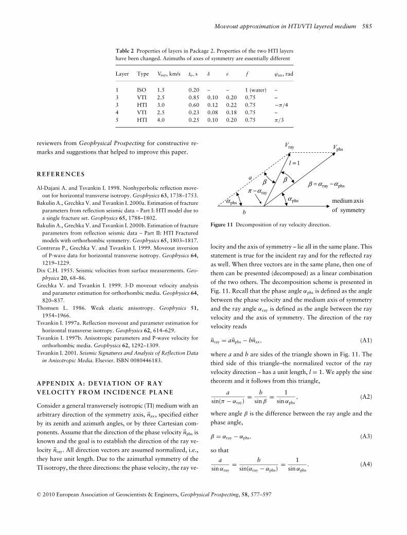
Table 2 Properties of layers in Package 2. Properties of the two HTI layershave been changed. Azimuths of axes of symmetry are essentially different

Layer Type Vver, km/s to, s δ ε f ϕax, rad

1 ISO 1.5 0.20 – – 1 (water) –3 VTI 2.5 0.85 0.10 0.20 0.75 –3 HTI 3.0 0.60 0.12 0.22 0.75 −π/44 VTI 2.5 0.23 0.08 0.18 0.75 –5 HTI 4.0 0.25 0.10 0.20 0.75 π/3

reviewers from Geophysical Prospecting for constructive re-marks and suggestions that helped to improve this paper.

REFERENCES

Al-Dajani A. and Tsvankin I. 1998. Nonhyperbolic reflection move-out for horizontal transverse isotropy. Geophysics 63, 1738–1753.

Bakulin A., Grechka V. and Tsvankin I. 2000a. Estimation of fractureparameters from reflection seismic data – Part I: HTI model due toa single fracture set. Geophysics 65, 1788–1802.

Bakulin A., Grechka V. and Tsvankin I. 2000b. Estimation of fractureparameters from reflection seismic data – Part II: HTI Fracturedmodels with orthorhombic symmetry. Geophysics 65, 1803–1817.

Contreras P., Grechka V. and Tsvankin I. 1999. Moveout inversionof P-wave data for horizontal transverse isotropy. Geophysics 64,1219–1229.

Dix C.H. 1955. Seismic velocities from surface measurements. Geo-physics 20, 68–86.

Grechka V. and Tsvankin I. 1999. 3-D moveout velocity analysisand parameter estimation for orthorhombic media. Geophysics 64,820–837.

Thomsen L. 1986. Weak elastic anisotropy. Geophysics 51,1954–1966.

Tsvankin I. 1997a. Reflection moveout and parameter estimation forhorizontal transverse isotropy. Geophysics 62, 614–629.

Tsvankin I. 1997b. Anisotropic parameters and P-wave velocity fororthorhombic media. Geophysics 62, 1292–1309.

Tsvankin I. 2001. Seismic Signatures and Analysis of Reflection Datain Anisotropic Media. Elsevier. ISBN 0080446183.

APPENDIX A: DEVIATION OF RAYVELOCITY FROM INCIDENCE PLANE

Consider a general transversely isotropic (TI) medium with anarbitrary direction of the symmetry axis, �nax, specified eitherby its zenith and azimuth angles, or by three Cartesian com-ponents. Assume that the direction of the phase velocity �nphs isknown and the goal is to establish the direction of the ray ve-locity �nray. All direction vectors are assumed normalized, i.e.,they have unit length. Due to the azimuthal symmetry of theTI isotropy, the three directions: the phase velocity, the ray ve-

phsVrayV

symmetryof

axismediumphs

phsray=a

b

1=l

phs

rayπ αα α

ααβ ββ

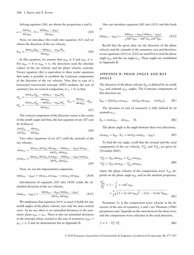
Figure 11 Decomposition of ray velocity direction.

locity and the axis of symmetry – lie all in the same plane. Thisstatement is true for the incident ray and for the reflected rayas well. When three vectors are in the same plane, then one ofthem can be presented (decomposed) as a linear combinationof the two others. The decomposition scheme is presented inFig. 11. Recall that the phase angle αphs is defined as the anglebetween the phase velocity and the medium axis of symmetryand the ray angle αray is defined as the angle between the rayvelocity and the axis of symmetry. The direction of the rayvelocity reads

�nray = a�nphs − b�nax, (A1)

where a and b are sides of the triangle shown in Fig. 11. Thethird side of this triangle–the normalized vector of the rayvelocity direction – has a unit length, l = 1. We apply the sinetheorem and it follows from this triangle,

asin(π − αray)

= bsin β

= 1sin αphs

, (A2)

where angle β is the difference between the ray angle and thephase angle,

β = αray − αphs, (A3)

so that

asin αray

= bsin(αray − αphs)

= 1sin αphs

. (A4)



Solving equation (A4), we obtain the projections a and b,

a = sin αray

sin αphs, b = sin(αray − αphs)

sin αphs. (A5)

Next, we introduce this result into equation (A1) and weobtain the direction of the ray velocity,

�nray = sin αray�nphs − sin(αray − αphs)�nax

sin αphs. (A6)

In this equation, we assume that αphs �= 0 and αphs �= π .For αphs = 0 or αphs = π , the directions (and the absolutevalues) of the ray velocity and the phase velocity coincide.Vector equation (A6) is equivalent to three scalar equationsthat make it possible to establish the Cartesian componentsof the direction of the ray velocity. Note that in case of ahorizontal transversely isotropic (HTI) medium, the axis ofsymmetry has no vertical component, nz

ax = 0, so that

nxray =

sin αraynxphs − sin(αray − αphs)nx

ax

sin αphs,

nyray =

sin αraynyphs − sin(αray − αphs)ny

ax

sin αphs,

nzray = sin αray

sin αphs· nz

phs.

(A7)

The vertical component of the direction vector is the cosineof the zenith angle and thus, the last equation of set (A7) canbe written as

cos θray

cos θphs= sin αray

sin αphs. (A8)

Two other equations of set (A7) yield the azimuth of theray velocity,

sin ϕray = sin αray sin θphs sin ϕphs − sin(αray − αphs) sin ϕax

sin θray sin αphs,

cos ϕray = sin αray sin θphs cos ϕphs − sin(αray − αphs) cos ϕax

sin θray sin αphs.

(A9)

Next, we use the trigonometric expansion,

sin(ϕray − ϕphs) = sin ϕray cos ϕphs − cos ϕray sin ϕphs. (A10)

Introduction of equation (A9) into (A10) yields the az-imuthal deviation of the ray velocity,

sin(ϕray − ϕphs) = − sin(αray − αphs) sin(ϕax − ϕphs)sin θray sin αphs

. (A11)

We emphasize that equation (A11) is exact: it holds for anyzenith angles of the phase velocity (not only for near-verticalrays). As we see, there is no azimuthal deviation in the sym-metry plane ϕphs = ϕax. There is also no azimuthal deviationin the isotropic plane, normal to the axis of symmetry, ϕphs =ϕax + π/2 and we demonstrate this in Appendix B.

One can introduce equation (A8) into (A11) and this leadsto

sin(ϕray − ϕphs) = − sin(αray − αphs) sin(ϕax − ϕphs)√sin2 αphs − sin2 αray cos2 θphs

. (A12)

Recall that the given data are the direction of the phasevelocity and the azimuth of the symmetry axis and therefore,to use equations (A11) or (A12) we need first to find the phaseangle αphs and the ray angle αray. These angles are establishedin Appendix B.

APPENDIX B: PHASE ANGLE A ND RAYANGLE

The direction of the phase velocity �nphs is defined by its zenithθphs and azimuth ϕphs angles. The Cartesian components ofthis direction are

�nphs = {sin θphs cos ϕphs, sin θphs sin ϕphs, cos θphs

}. (B1)

The direction of axis of symmetry is fully defined by itsazimuth ϕax,

�nax = {cos ϕax, sin ϕax, 0} . (B2)

The phase angle is the angle between these two directions,

cos αphs = �nphs · �nax = sin θphs cos(ϕax − ϕphs). (B3)

To find the ray angle, recall that the normal and the axialcomponents of the ray velocity, Vnr

ray and Vaxray, are given by

(Tsvankin 2001)

Vnrray = Vphs sin αphs + V′

phs cos αphs,

Vaxray = Vphs cos αphs − V′

phs sin αphs,(B4)

where the phase velocity of the compression wave Vphs de-pends on the phase angle αphs and on the medium properties,

V2phs

V2P

= 1 − f2

+ ε sin2 αphs

+ 12

√(f + 2ε sin2 αphs

)2 − 2 f (ε − δ) sin2 2αphs.(B5)

Parameter VP is the compression wave velocity in the di-rection of the axis of symmetry, δ and ε are Thomsen (1986)parameters and f depends on the ratio between the shear waveand the compression wave velocities in the axial direction,

f = 1 − V2S /V2

P . (B6)



Prime in equation (B4) means derivative with respect to thephase angle αphs,

2VphsV′phs

V2P

= ε sin 2αphs

+ ε ( f + ε) − [2 f (ε − δ) + ε2

]cos 2α√(

f + 2ε sin2 αphs)2 − 2 f (ε − δ) sin2 2αphs

× sin 2αphs.

(B7)

According to equation (B4), the ray velocity is

Vray =√

Vnr2ray + Vax2

ray =√

V2phs + V′2

phs. (B8)

The ray angle is

sin αray = Vnrray

Vray=

Vphs sin αphs + V′phs cos αphs

Vray,

cos αray = Vaxray

Vray=

Vphs cos αphs − V′phs sin αphs

Vray. (B9)

Combining the two equations of set (B9), we obtain

cos(αray − αphs) = Vphs

Vray,

sin(αray − αphs) =V′

phs

Vray, tan(αray − αphs) =

V′phs

Vphs. (B10)

It is clearly seen from equation (B10) that the ray angleexceeds the phase angle when the derivative of the phase ve-locity V ′

phs is positive (a common case but not a must) and theray angle is less than the phase angle when the derivative isnegative (Tsvankin 2001).

Comment: when a ray propagates in the isotropic planeϕphs = ϕax + π/2, whose azimuth is normal to the axis ofsymmetry, equation (B3) yields that the phase angle is theright angle, αphs = π/2. It follows from equation (B7) that inthis case the derivative vanishes, V ′

phs = 0. The phase and theray velocities coincide, αray = αphs. Finally, equation (A12)yields that there is no azimuthal deviation in the isotropicplane, ϕray = ϕphs.

APPENDIX C: T WO SE T S OF T H OMSENPARAMETERS FOR H T I M E DI UM

Consider a local frame of reference 1-2-3 and a horizon-tal transversely isotropic (HTI) medium with the symmetryaxis coinciding with axis 1. There are two ways to assign theThomsen parameters for this medium:� Considering HTI as a particular case of transverse isotropy

(TI)� Considering HTI as a particular case of orthorhombic

medium (Tsvankin 1997b; Contreras et al. 1999)

In the first case, the HTI Thomsen parameters are similarto the VTI (vertical transverse isotropy) Thomsen parame-ters but the horizontal axis 1 is the axis of symmetry insteadof the vertical axis 3. It is more suitable to work with the‘orthorhombic’ definitions but equation (B5) for the phase ve-locity versus phase angle (Tsvankin 2001) appears in termsof ‘TI’ Thomsen parameters. Therefore, we will need bothdefinitions and the conversion relationships between them.Note that VP is the axial compression velocity, while Vver isthe vertical compression velocity. Other parameters have in-dex 2 for the ‘orthorhombic’ case and no index for the ‘TI’case. Parameter f expresses the relationship between the axialcompression velocity and the axial shear velocity (coupled SVshear). Parameter f 2 expresses the relationship between thevertical compression velocity and the vertical shear velocity(also for SV shear). For the ‘orthorhombic’ case, the Thomsenparameters are defined by

V2ver = C33

ρ, f2 = V2

ver − V2Sver

V2ver

= C33 − C55

C33,

δ2 = (C13 + C55)2 − (C33 − C55)2

2C33 (C33 − C55), ε2 = C11 − C33

2C33,

γ2 = C55 − C44

2C44

(C1)

Alternatively, for the ‘TI’ case, the Thomsen parameters aredefined by

V2P = C11

ρ, f = V2

P − V2S

V2P

= C11 − C55

C11,

δ = (C13 + C55)2 − (C11 − C55)2

2C11 (C11 − C55), ε = C33 − C11

2C11,

γ = C44 − C55

2C55,

(C2)

where ρ is the density and Cij are the components of themedium stiffness matrix. Combining equation sets (C1) and(C2), we eliminate the components of the stiffness matrix andobtain the ‘two-way’ relationships between the ‘orthorhom-bic’ and ‘TI’ Thomsen parameters, used to describe the hori-zontal transverse isotropy. Vertical compression velocity ver-sus axial compression velocity is given by

V2P = (1 + 2ε2) × V2

ver, V2ver = (1 + 2ε) × V2

P . (C3)

Relationships for Thomsen parameter epsilon are

ε = − ε2

1 + 2ε2, ε2 = − ε

1 + 2ε. (C4)



Relationships for Thomsen parameter delta are

δ = − (2ε2 − δ2) × f2 + 2ε22

(1 + 2ε2) × ( f2 + 2ε2), δ2 = − (2ε − δ) × f + 2ε2

(1 + 2ε) × ( f + 2ε).

(C5)

Relationships for shear /compression ratio in vertical direc-tion versus axial direction are

f = f2 + 2ε2

1 + 2ε2, f2 = f + 2ε

1 + 2ε. (C6)

Relationships for Thomsen parameter gamma (needed forpure shear only) are

γ = ε2 − γ2

1 + 2γ2, γ2 = − ε + γ + 2εγ

(1 + 2γ ) × (1 + 2ε). (C7)

We note on the special symmetry of the forward-backwardrelationships for all parameters except those for pure shearonly (γ and γ 2). Note that elliptic condition is the same forboth cases, i.e., the following two equations are equivalent,

ε = δ and ε2 = δ2. (C8)

The relationships between the two sets of Thomsen param-eters are presented by Tsvankin (1997a).

APPENDIX D: RA Y T R A C I N G I NHORIZONTAL T R A N SV ER SL Y ISOT R OPICAND V ERTICAL T R A N SV ER SE LYISOTROPIC LA Y E R E D M EDI UM

In this appendix we explain the exact ray tracing procedure,valid for any rays, with arbitrary zenith angles, i.e., not nec-essarily near-vertical rays. The start point is located in thelowermost layer and the arrival point is on the Earth’s sur-face. The azimuth of the phase velocity ϕphs is given and thedip angle of the phase velocity θphs is specified at the startpoint. The goal is to obtain the components hx and hy of theoffset on the Earth’s surface and the total traveltime t. First,we establish the horizontal slowness, constant for all layers ofthe package. For this, we calculate the phase angle αphs. If the‘root layer’ is vertical transversely isotropic (VTI), then thephase angle is equal to the zenith angle of the phase velocity.If the root layer is horizontal transversely isotropic (HTI), weobtain the phase angle from equation (6). Next, we use equa-tion (B5) to establish the phase velocity, Vphs(αphs). Then thelateral slowness is delivered by equation (8).

Now, for an arbitrary layer, the zenith angle of the phasevelocity θphs is unknown but the lateral slowness is known andconstant for all layers. We consider the propagation throughtwo types of medium, HTI and VTI. Combining equations (6)

to (8), we obtain

pVphs(αphs

)cos(ϕax − ϕphs) = cos αphs for HTI,

pVphs(αphs

) = sin αphs for VTI, (D1)

with the phase velocity Vphs delivered by equation (B5). Wesolve equation (D1) for the unknown phase angle αphs. In caseof an HTI layer, equation (D1) may be expanded to

Acos4 αphs − 2B cos2 αphs + C = 0, (D2)

where

A = 1 + 2ε p̄2HTI − 2 f (ε − δ) p̄4

HTI,

B = (1 + ε − f/2) p̄2HTI + (ε − 2 f ε + f δ) p̄4

HTI,

C = (1 − f )(1 + 2ε) p̄4HTI.

(D3)

In case of a VTI layer, equation (D1) may be expanded to

Asin4 αphs − 2B sin2 αphs + C = 0, (D4)

where

A = 1 − 2ε p̄2VTI − 2 f (ε − δ) p̄4

VTI,

B = (1 − f/2) p̄2VTI − (ε − f δ) p̄4

VTI,

C = (1 − f ) p̄4VTI.

(D5)

Parameters p̄HTI and p̄VTI are normalized horizontal slow-ness,

p̄HTI ≡ VP p cos(ϕax − ϕphs), p̄VTI ≡ VP p. (D6)

Quadratic equations (D2) and (D4) have two roots. In caseof the HTI medium, a smaller phase angle αphs correspondsto a larger phase velocity Vphs and thus to P-wave. In case ofthe VTI medium, a larger phase angle corresponds to a largerphase velocity and P-wave.

After the phase angle αphs is found, the zenith angle of thephase velocity is delivered by equation (6) for an HTI layerand for a VTI layer these two angles coincide, θphs = αphs. Weapply equations (B5) and (B7) to find the phase velocity Vphs

and its derivative V ′phs with respect to the phase angle αphs.

Then we exploit equation (B9) to obtain the ray angle αray.For a VTI layer, the zenith angle of the ray velocity θ ray =αray and for an HTI layer we use equation (4) to find θ ray andthen equation (5) to obtain the azimuthal deviation. Finally,we apply equations (1) and (2) to obtain the components hx

and hy of the lateral propagation and equation (3) to obtainthe traveltime through the given layer.



APPENDIX E : PROPAGATION OFNEAR-VERTIC A L R A Y I N H OR I Z ON T ALTRANSVERSEL Y I SOT R OPI C LA Y ER

Applying equation (B5) for the phase velocity in the trans-versely isotropic (TI) medium and converting the Thomsenparameters with relationships (C3)–(C6), we obtain a seriesapproximation for the phase velocity in a horizontal trans-versely isotropic (HTI) layer versus the small parameter �αphs,i

defined by equation (9),

Vphs,i

Vver,i= 1 + δ2,i�α2

phs,i + 6Mi − δ2,i (2 + 3δ2,i )6

· �α4phs,i ,

(E1)

where the following notation is used,

Mi ≡ (ε2,i − δ2,i ) ( f2,i + 2δ2,i )f2,i

. (E2)

The ray velocity is approximated by

Vray,i

Vver,i= 1 + δ2,i (1 + 2δ2,i )�α2

phs,i

+ 6Mi (1 + 8δ2,i ) − δ2,i (1 + 2δ2,i )(2 + 15δ2,i + 6δ2

2,i

)6

�α4phs,i .

(E3)

The phase angle is given by equation (9), while the ray angleis approximated by

αray,i = π

2− (1 + 2δ2,i )�αphs,i

+ 4δ2,i (1 + δ2,i )(1 + 2δ2,i ) − 12Mi

3�α3

phs,i . (E4)

Ratio Ri = sin αray,i/sin αphs,i, needed to find the zenith angleof the ray velocity, is given by

Ri = 1 − 2δ2,i (1 + δ2)�α2phs,i

+ 23

× (1 + δ2,i )[δ2,i

(1 + 9δ2,i + 9δ2

2,i

) − 6Mi]�α4

phs,i .

(E5)

It follows from equation (A8) that

cos θray,i = Ri cos θphs,i , (E6)

where the zenith angle of the phase velocity is given by equa-tion (B3). The zenith angle of the ray velocity is approximatedby

sin θray,i = Ch,i�αphs,i

cos(ϕax,i − ϕphs)

+[

4Mi (1 + 2δ2,i ) cos(ϕax,i − ϕphs)Ch,i

−(1 + 12δ2,i + 12δ2

2,i

)Ch,i

6 cos(ϕax,i − ϕphs)

]�α3

phs,i , (E7)

where the following notation is used,

Ch,i ≡√

1 + 4δ2,i (1 + δ2,i ) cos2(ϕax,i − ϕphs), (E8)

For a hyperbolic approximation, the azimuth of the ray an-gle is independent of �αphs,i and for the fourth-order approxi-mation it includes the term dependent on the small parameter,

cos(ϕray,i − ϕphs

) = cos �ϕo,i

− 2Mi sin �ϕo,i sin 2(ϕax,i − ϕphs)C2

h,i

�α2phs,i ,

sin(ϕray,i − ϕphs

) = sin �ϕo,i

+ 2Mi cos �ϕo,i sin 2(ϕax,i − ϕphs)C2

h,i

�α2phs,i , (E9)

where

cos �ϕo,i ≡ 1 + 2δ2,i cos2(ϕax,i − ϕphs)Ch,i

,

sin �ϕo,i ≡ δ2,i sin 2(ϕax,i − ϕphs)Ch,i

. (E10)

Note that the deviation of the ray velocity from the inci-dence plane ϕray,i − ϕphs is not a small value even for near-vertical rays with infinitesimal �αphs,i.

The lateral propagation is

hi

to,i Vver,i= Ch,i�αphs,i

cos(ϕax,i − ϕphs)+ cos(ϕax,i − ϕphs)

Ch,i

×[

4Mi (1 + 2δ2,i ) − 2δ2,i (1 + δ2,i )3

− cos2(ϕax,i − ϕphs) − 3C2h,i

6 cos4(ϕax,i − ϕphs)

]�α3

phs,i , (E11)

and its components are

hx,i

to,i Vver,i= Ch,i cos �ϕo,i

cos(ϕax,i − ϕphs)�αphs,i

+ [Qi × Ch,i cos �ϕo,i + 4Mi cos(ϕax,i − ϕphs)

]�α3

phs,i ,

hy,i

to,i Vver,i= Ch,i sin �ϕo,i

cos(ϕax,i − ϕphs)�αphs,i

+ [Qi × Ch,i sin �ϕo,i + 4Mi sin(ϕax,i − ϕphs)

]�α3

phs,i ,

(E12)

where

Qi ≡ 3 − cos2(ϕax,i − ϕphs)6 cos3(ϕax,i − ϕphs)

. (E13)



Finally, the traveltime is

ti − to,i

to,i= Ch,i cos �ϕo,i

2 cos2(ϕax,i − ϕphs)�α2

phs,i

+[

3Mi − δ2,i (2 + 3δ2,i )6

+ 9 − 4 (1 − 3δ2,i ) cos2(ϕax,i − ϕphs)24 cos4(ϕax,i − ϕphs)

]�α4

phs,i . (E14)

APPENDIX F : PROPAGATION OFN E A R - V E R T I C A L R A Y I N V E R T I C A LTRANSVERSELY I SOT R OPI C LA Y ER

Now the medium symmetry axis is vertical and the zenithangle of the phase velocity coincides with the phase angle.The phase angle is small, therefore we will use the notation

αphs,i = �αphs,i . (F1)

The zenith angle of the ray velocity coincides with the rayangle as shown in equation (7). Expanding the phase velocityinto the power series, we obtain

Vphs,i

Vver,i= 1 + δi�α2

phs,i

+[

(εi − δi ) ( fi + 2δi )fi

− δ (2i + 3δi )6

]�α4

phs,i . (F2)

Expanding the ray velocity into the power series, we obtain

Vray,i

Vver,i= 1 + δi (1 + 2δi ) �α2

phs,i

+[

(εi − δi ) ( fi + 2δi ) (1 + 8δi )fi

− δi (1 + 2δi )(2 + 15δi + 6δ2

i

)6

]�α4

phs,i .(F3)

The ray angle is

αray,i = (1 + 2δi ) �αphs,i

+[

4 (εi − δi ) ( fi + 2δi )fi

− 4δi (1 + δi ) (1 + 2δi )3

]�α3

phs,i .

(F4)

The traveltime is

ti − to,i

to,i= 1 + 2δi

2�α2

phs,i

+[

3 (εi − δi ) ( fi + 2δi )fi

+ (1 + 2δi ) (5 − 6δi )24

]�α4

phs,i .(F5)

The offset is

hi

to,i Vver,i= (1 + 2δi ) �αphs,i

+[

1 + 2δi

3+ 4 (εi − δi ) ( fi + 2δi )

fi

]�α3

phs,i . (F6)

In case of the vertical transversely isotropic (VTI) layer, theazimuth of the ray velocity coincides with the azimuth of thephase velocity and therefore there is no normal component ofthe lateral shift,

hx,i = h, hy,i = 0. (F7)

APPENDIX G: PROPAGATION THROUGHA S INGLE HORIZONTAL TRANSVERSELYISOTROPIC LAYER

In this appendix, we find the moveout velocity and the non-hyperbolic (fourth-order) moveout term for a particular casewhen the energy propagates through a single horizontal trans-versely isotropic (HTI) layer, given the azimuth of the phasevelocity and we show that these results coincide with themoveout approximation through the azimuth of the surfaceoffset. For a single HTI layer, the azimuth of the surface off-set and the azimuth of the ray velocity are the same things.According to the definition of the normal moveout velocity,

V2nmo = lim

h→0

h2

t2 − t2o

. (G1)

For small offsets, the moveout reads

t2 − t2o = (t + to) (t − to) ≈ 2to (t − to) . (G2)

Approximation (G2) can be used to establish the hyperbolicterm and can not be used for high- order terms. To calculatethe limit in equation (G1), only the quadratic terms (withrespect to the small parameter �αphs) are needed. It followsfrom equation (E11) that

h2

t2o V2

ver

=C2

h�α2phs

cos2(ϕax − ϕphs)

= 1 + 4δ2(1 + δ2) cos2(ϕax − ϕphs)cos2(ϕax − ϕphs)

· �α2phs.

(G3)

It follows from equation (E14) that

t − toto

=Ch cos �ϕo�α2

phs

2 cos2(ϕax − ϕphs)

= 1 + 2δ2 cos2(ϕax − ϕphs)2 cos2(ϕax − ϕphs)

· �α2phs.

(G4)



Introduction of equations (G2)–(G4) into (G1) leads to thenormal moveout (NMO) velocity for an individual layer,

V2nmo

V2ver

= 1 + 4δ2(1 + δ2) cos2(ϕax − ϕphs)1 + 2δ2 cos2(ϕax − ϕphs)

= Ch

cos �ϕo.

(G5)

To compare this formula with the known result, we needto convert the azimuth of the phase velocity into the azimuthof the ray velocity. Note that the azimuth of the ray velocitywith respect to the azimuth of the medium symmetry axis maybe presented as

ϕray − ϕax = (ϕray − ϕphs) − (ϕax − ϕphs), (G6)

and this leads to

sin(ϕray − ϕax) = sin(ϕray − ϕphs) cos(ϕax − ϕphs)

− cos(ϕray − ϕphs) sin(ϕax − ϕphs). (G7)

It follows from equations (E9) and (E10) that for the hy-perbolic approximation,

sin(ϕray − ϕphs) ≈ δ2 sin 2(ϕax − ϕphs)Ch

,

cos(ϕray − ϕphs) ≈ 1 + 2δ2 cos2(ϕax − ϕphs)Ch

. (G8)

Substitution of equation (G8) into (G7) leads to

sin(ϕray − ϕax) = sin(ϕphs − ϕax)√1 + 4δ2(1 + δ2) cos2(ϕphs − ϕax)

= sin(ϕphs − ϕax)Ch

. (G9)

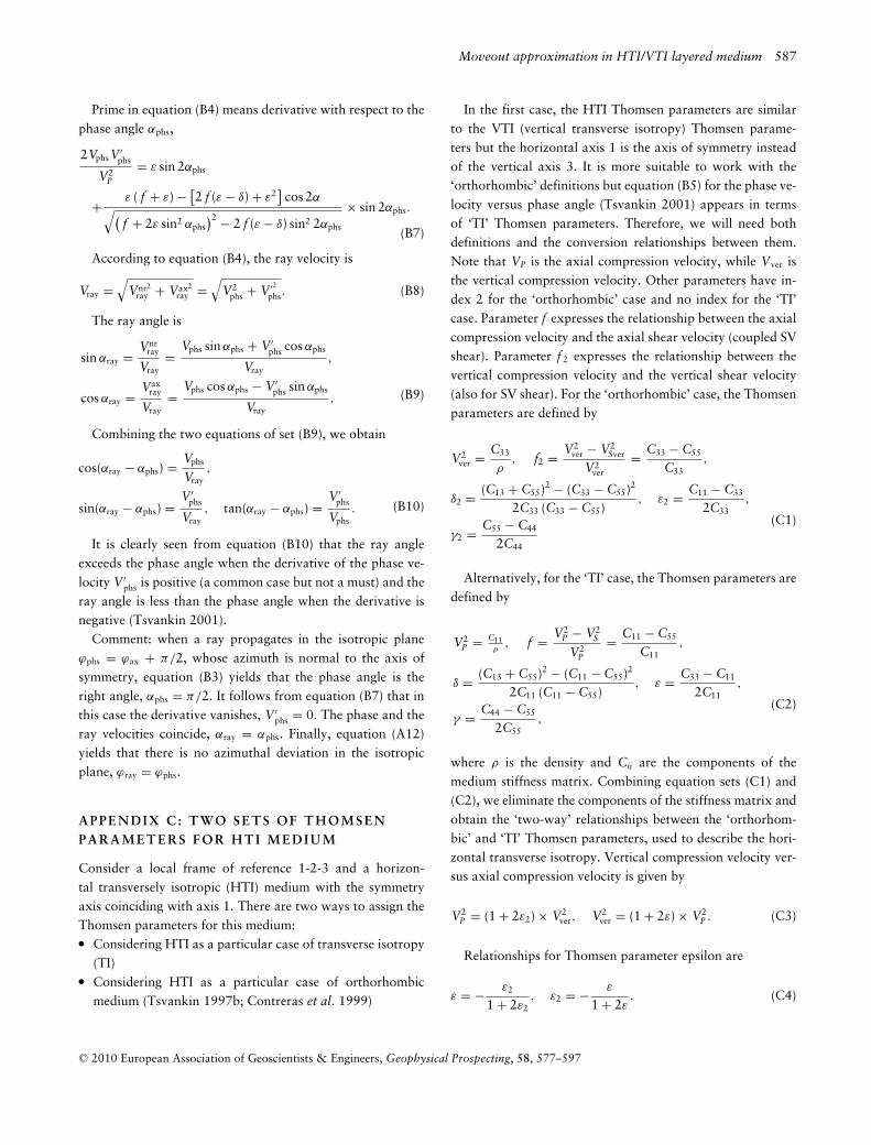
The NMO velocity versus the ray velocity azimuth is givenby Tsvankin (1997a),

V2nmo

V2ver

= 1 + 2δ2

1 + 2δ2 sin2(ϕray − ϕax). (G10)

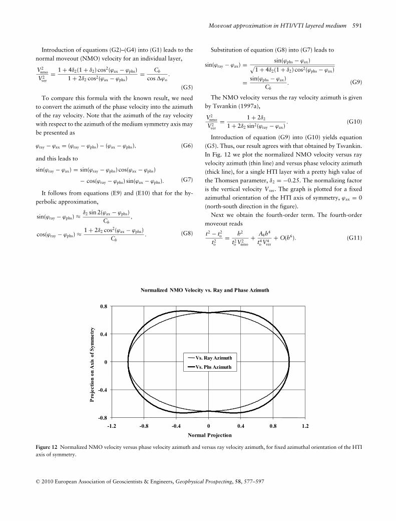
Introduction of equation (G9) into (G10) yields equation(G5). Thus, our result agrees with that obtained by Tsvankin.In Fig. 12 we plot the normalized NMO velocity versus rayvelocity azimuth (thin line) and versus phase velocity azimuth(thick line), for a single HTI layer with a pretty high value ofthe Thomsen parameter, δ2 = −0.25. The normalizing factoris the vertical velocity Vver. The graph is plotted for a fixedazimuthal orientation of the HTI axis of symmetry, ϕax = 0(north-south direction in the figure).

Next we obtain the fourth-order term. The fourth-ordermoveout reads

t2 − t2o

t2o

= h2

t2o V2

nmo

+ A4h4

t4o V4

ver

+ O(h6). (G11)

-0.8

-0.4

0

0.4

0.8

-1.2 -0.8 -0.4 0 0.4 0.8 1.2

Pro

ject

ion

on A

xis

of S

ymm

etry

Normal Projection

Normalized NMO Velocity vs. Ray and Phase Azimuth

Vs. Ray Azimuth

Vs. Phs Azimuth

Figure 12 Normalized NMO velocity versus phase velocity azimuth and versus ray velocity azimuth, for fixed azimuthal orientation of the HTIaxis of symmetry.



Neglecting the high-order terms, we obtain

A4 = limh→0

(t2 − t2

o

) × V2nmo − h2

V2nmo

× t2o V4

ver

h4. (G12)

To calculate the limit, the values in the numerator shouldbe obtained up to the fourth-order terms, because the second-order terms cancel. Introducing the expansion for the offsetand the traveltime (equations (E11) and (E14)) into (G12), weobtain

A4 = −2(ε2 − δ2)( f2 + 2δ2) cos4(ϕax − ϕphs)f2C4

h

×[1 + 8δ2 sin2(ϕax − ϕphs)

C2h

]. (G13)

Note that this expression does not coincide with the quarticcoefficient of the moveout expressed through the azimuth ofthe ray velocity. According to Al-Dajani and Tsvankin (1998),the quartic coefficient is

Aray4 = −2(ε2 − δ2)( f2 + 2δ2) cos4(ϕray − ϕax)

f2(1 + 2δ2)4. (G14)

Introducing equation (G9) into (G14), we obtain, for thefourth-order moveout approximation,

Aray4 = −2(ε2 − δ2)( f2 + 2δ2) cos4(ϕax − ϕphs)

f2C4h

+ O(h2) .

(G15)

Comparing this result to equation (G13), we observe thatthe second term in the square brackets is missing. The reasonis that the difference between the azimuths of the phase andthe ray velocity is only approximately independent of the off-set magnitude. For small offsets (hyperbolic approximation)the azimuth shift may be considered constant. For large off-sets (non-hyperbolic approximation), this assumption is nolonger valid. In other words, equations (G8) and (G9) are notexact. The azimuth of the ray velocity changes with respectto the azimuth of the phase velocity as the offset magnitudeincreases. Should we keep constant the azimuth of the rayvelocity with respect to the medium symmetry axis, then theincrease of the offset magnitude changes the azimuth of thephase velocity with respect to the azimuth of the symmetryaxis and this causes a small correction in the value of themoveout velocity. This correction yields an additional fourth-order term and results in a full balance. To check the balance,we consider the fourth-order moveout approximation in both

the ‘phase frame’ and ‘ray frame’ of reference,

t2 − t2o︸︷︷︸

moveout

= h2

V2nmo

+ A4h4

t2o V4

ver︸︷︷︸moveout in “phase” frame

= h2

V2nmo,ray

+ Aray4 h4

t2o V4

ver︸︷︷︸moveout in “ray” frame

. (G16)

We will show that the moveout equation is equivalent inboth frames of reference, i.e., that equation (G16) holds. Thus,we will demonstrate that(

1V2

nmo,ray

− 1V2

nmo

)× t2

o V4ver

h2= A4 − Aray

4 . (G17)

The normal moveout velocity in the ‘ray frame’ is given byequation (G10), which can be considered exact. However, theazimuth of the ray velocity with respect to the axis of sym-metry, ϕray − ϕax, is only approximately constant. With theuse of equation (E9) we can obtain the second-order approx-imation for the ray velocity azimuth (needed for fourth-ordermoveout),

sin2(ϕray − ϕax) = sin2(ϕphs − ϕax)C2

h

− 2(ε2 − δ2)(1 + 2δ2)( f2 + 2δ2) sin2 2(ϕax − ϕphs)f2C4

h

× �α2phs.

(G18)

Introduction of equation (G18) into (G10) leads to

V2nmo,ray

V2ver

= V2nmo

V2ver

+ 4δ2(ε2 − δ2)( f2 + 2δ2) sin2 2(ϕax − ϕphs)f2C2

h cos2 �ϕo× �α2

phs,(G19)

where the first term in equation (G19) is the NMO velocity inthe ‘phase frame of reference’ and the other term representsthe non-hyperbolic correction. Neglecting the high-order termin equation (E11) for the offset expansion, we obtain

�α2phs = cos2(ϕax,i − ϕphs)

C2h

× h2

t2o V2

ver

. (G20)

Thus, in the ‘ray frame of reference’, the NMO velocity de-pends (slightly) on the offset magnitude h, because this mag-nitude affects the phase shift between the ray velocity and themedium axis of symmetry, ϕray − ϕax. Introduction of equa-tion (G20) into (G19) results in

V2nmo,ray

V2ver

= V2nmo

V2ver

+ 4δ2(ε2 − δ2)( f2 + 2δ2) cos2(ϕax,i − ϕphs) sin2 2(ϕax − ϕphs)f2C4

h cos2 �ϕo

× h2

t2o V2

ver

. (G21)



Thus, in the ray frame of reference, the hyperbolic moveoutterm, with the corrections up to order four, becomes,

1V2

nmo,ray

= 1V2

nmo

− 4δ2(ε2 − δ2)( f2 + 2δ2) cos2(ϕax,i − ϕphs) sin2 2(ϕax − ϕphs)f2C4

h cos2 �ϕo

× h2

t2o V4

nmo

. (G22)

Introduction of equation (G5) into (G22) results in(1

V2nmo,ray

− 1V2

nmo

)× t2

o V4ver

h2=

− 4δ2(ε2 − δ2)( f2 + 2δ2) cos2(ϕax,i − ϕphs) sin2 2(ϕax − ϕphs)

f2C6h

.

(G23)

It follows from equations (G13) and (G15) that

A4 − Aray4 =

− 4δ2(ε2 − δ2)( f2 + 2δ2) cos2(ϕax,i − ϕphs) sin2 2(ϕax − ϕphs)

f2C6h

.

(G24)

Combining equations (G23) and (G24), we conclude thatrelationship (G17) is proved. The fourth-order terms in equa-tion (G16) are balanced.

APPENDIX H: PROPAGATION THROUGHA PACKAGE OF H OR I Z ON T A LTRANSVERSELY I SOT R OPI C A N DVERTICAL TRA N SV ER SE LY I SOT R OPICL A Y E R S

In Appendices E and F, we derived the offset and traveltimeversus the small parameter �αphs, which is the phase angle fora vertical transversely isotropic (VTI) layer and the deviationof the phase angle from π/2 for a horizontal transverselyisotropic (HTI) layer. This parameter, while being small, isdifferent for individual layers: �αphs is piecewise-constant,with the discontinuities at the interfaces between the layers.However, there is another parameter, the horizontal slownessp, which is preserved constant through all layers due to Snell’stransmission law at the interfaces between the layers. For anylayer i, the horizontal slowness is given by equation (8). Foran HTI layer, according to equation (B3),

sin θphs,i = cos αphs,i

cos(ϕax,i − ϕphs)= sin �αphs,i

cos(ϕax,i − ϕphs). (H1)

Introduction of equation (H1) into (8) leads to

sin �αphs,i

Vphs(�αphs,i )= p cos(ϕax,i − ϕphs). (H2)

To obtain the third-order approximation of slowness, thesecond approximation of the phase velocity suffices. Applyingequation (8) and the third-order approximation for the sinefunction,

sin �αphs,i = �αphs,i −�α3

phs,i

6(H3)

and neglecting the high-order terms, we obtain

�αphs,i − �α3phs,i/6

1 + δ2,i�α2phs,i

= pVver,i cos(ϕax,i − ϕphs). (H4)

Up to the third-order terms, this is equivalent to

�αphs,i − 1 + 6δ2,i

6× �α3

phs,i = pVver,i cos(ϕax,i − ϕphs).

(H5)

For small slowness p, the series in equation (H5) can beinverted, so that we can obtain the residual phase angle �αphs,i

versus slowness p,

�αphs,i = pVver,i cos(ϕax,i − ϕphs)

+ 1 + 6δ2,i

6× p3V3

ver,i cos3(ϕax,i − ϕphs). (H6)

We will also need the powers �αkphs,i up to k = 4 and the

required accuracy is the slowness to power four, p4

�α2phs,i = p2V2

ver,i cos2(ϕax,i − ϕphs)

+ 1 + 6δ2,i

3× p4V4

ver,i cos4(ϕax,i − ϕphs),

�α3phs,i = p3V3

ver,i cos3(ϕax,i − ϕphs),

�α4phs,i = p4V4

ver,i cos4(ϕax,i − ϕphs). (H7)

Introduction of equations (H6), (H7) into equation (E12)for the offset components of an HTI layer leads to

hx,i = Ch,i cos �ϕo,i to,i V2ver,i p

+ [Rh,i cos �ϕo,i + 4 f2,i Qh,i cos(ϕax,i − ϕphs)

]to,i V4

ver,i p3,

hy,i = Ch,i sin �ϕo,i to,i V2ver,i p

+ [Rh,i sin �ϕo,i + 4 f2,i Qh,i sin(ϕax,i − ϕphs)

]to,i V4

ver,i p3.(H8)

Introduction of equations (H6), (H7) into equation (E14)for the traveltime of an HTI layer leads to

ti = to,i + Ch,i cos �ϕo,i to,i V2ver,i

2p2

+ [Pxy,i + 3 f2,i Qh,i cos(ϕax,i − ϕphs)

]to,i V4

ver,i p4, (H9)



where the following notations are used

Qh,i ≡ (ε2,i − δ2,i )( f2,i + 2δ2,i ) cos3(ϕax,i − ϕphs)f 22,i

,

Rh,i ≡ C2h,i cos �ϕo,i

2, Pxy,i ≡ 3C2

h,i cos2 �ϕo,i

8. (H10)

Now consider a VTI layer. In this case the zenith angle ofthe phase velocity coincides with the phase angle and equation(8) simplifies to

sin �αphs,i

Vphs(�αphs,i )= p. (H11)

Expand the sine function and the phase velocity into thepower series, we obtain an equation similar to (H4),

�αphs,i − �α3phs,i/6

1 + δi�α2phs,i

= pVver,i . (H12)

Up to the third-order terms, this is equivalent to

�αphs,i − 1 + 6δi

6�α3

phs,i = pVver,i . (H13)

The inverted series is

�αphs,i = pVver,i + 1 + 6δi

6× p3V3

ver,i . (H14)

The powers �αkphs,i are presented exactly like in equation

(H7), we just replace the coefficients δ2,i by δi. Equation (F6)for the offset leads to

hi = (1 + 2δi ) to,i V2ver,i p

+[

(1 + 2δi )2

2+ 4 (εi − δi ) ( fi + 2δi )

fi

]to,i V4

ver,i p3.

(H15)

As already mentioned, in a VTI layer the azimuths of thephase velocity and the ray velocity coincide and therefore theoffset in a VTI layer, has x-component only. Introduction ofequations (H6) and (H7) (with δ2 replaced by δ) into equation(F5) for the traveltime of the VTI layer results in

ti = to,i + 1 + 2δ

2to,i V2

ver,i p2

+[

3 (1 + 2δi )2

8+ 3 (εi − δi ) ( fi + 2δi )

fi

]to,i V4

ver,i p4.

(H16)

An isotropic layer can be considered as a particular case ofeither HTI or VTI and this leads to

hi = to,i V2i p + to,i V4

i

2p3, (H17)

ti = to,i + to,i V2i

2p2 + 3to,i V4

i

8p4. (H18)

We can now sum up the offset components and the trav-eltime for all individual HTI, VTI and isotropic layers of thepackage and obtain the resulting values.

APPENDIX I : TRAVELTIMEAPPROXIMATION FOR PACKAGEOF LAYERS

Consider a package that includes horizontal transverselyisotropic (HTI), vertical transversely isotropic (VTI) andisotropic layers, with flat interfaces between them. Assumea near-vertical ray with a small horizontal slowness p (ascompared to the slowness magnitude V−1

phs). According to theresults obtained in Appendix H, the ‘longitudinal’ componentof the lateral shift on the Earth’s surface can be approximatedby

hx =∑

i

hx,i = Apx p + Bpx p3, (I1)

where all three types of layers: HTI, VTI and isotropic, con-tribute to the coefficients,

Apx =∑

i

AHTIpx,i +

∑i

AVTIpx,i +

∑i

AISOpx,i ,

Bpx =∑

i

BHTIpx,i +

∑i

BVTIpx,i +

∑i

BISOpx,i .

(I2)

The transverse component of the lateral shift receives a con-tribution from the HTI layers only and it can be approximatedby

hy =∑

i

hy,i = Apy p + Bpy p3. (I3)

The transverse coefficients are

Apy =∑

i

AHTIpy,i , Bpy =

∑i

BHTIpy,i . (I4)

It follows from equation (H8) that

AHTIpx,i = Ch,i cos �ϕo,i to,i V2

ver,i , AHTIpy,i = Ch,i sin �ϕo,i to,i V2

ver,i ,

(I5)

and

BHTIpx,i = [

Rh,i cos �ϕo,i + 4 f2,i Qh,i cos(ϕax,i − ϕphs)]

to,i V4ver,i ,

BHTIpy,i = [

Rh,i sin �ϕo,i + 4 f2,i Qh,i sin(ϕax,i − ϕphs)]

to,i V4ver,i .

(I6)

It follows from equations (H15) that

AVTIph,i = AVTI

px,i = (1 + 2δi ) to,i V2ver,i , AISO

ph,i = AISOpx,i = to,i V2

ver,i .

(I7)



and

BVTIph,i = BVTI

px,i =[

(1 + 2δi )2

2+ 4 (εi − δi ) ( fi + 2δi )

fi

]to,i V4

ver,i ,

BISOph,i = BISO

px,i = to,i V4ver,i

2.

(I8)

The traveltime can be approximated by

t =∑

i

ti = to + Apt p2 + Bpt p4, to =∑

i

to,i . (I9)

where

Apt =∑

i

AHTIpt,i +

∑i

AVTIpt,i +

∑i

AISOpt,i ,

Bpt =∑

i

BHTIpt,i +

∑i

BVTIpt,i +

∑i

BISOpt,i . (I10)

It follows from equations (H9), (H16) and (H18) that foran HTI layer,

AHTIpt,i = Ch,i cos �ϕo,i to,i V2

ver,i

2,

BHTIpt,i = [

Pxy,i + 3 f2,i Qh,i cos(ϕax,i − ϕphs)]

to,i V4ver,i , (I11)

for a VTI layer,

AVTIpt,i = 1 + 2δ

2to,i V2

ver,i ,

BVTIpt,i =

[3 (1 + 2δi )

2

8+ 3 (εi − δi ) ( fi + 2δi )

fi

]to,i V4

ver,i , (I12)

and for an isotropic layer,

AISOpt,i = to,i V2

ver,i

2, BVTI

pt,i = 3to,i V4ver,i

8. (I13)

With equation (I9), the moveout becomes (up to the fourthorder of slowness)

t2 − t2o = 2to Apt p2 + (

A2pt + 2to Bpt

)p4. (I14)

Introduce the following notations,

Aph ≡√

A2px + A2

py, Bph ≡√

B2px + B2

py,

Kph ≡ Apx Bpx + Apy Bpy.(I15)

According to equations (I1) and (I3), the surface offsetsquared becomes

h2 = h2x + h2

y = A2ph p2 + 2Kph p4. (I16)

We will also need the offset raised to power four. Neglectingthe high-order terms,

h4 = A4ph p4. (I17)

Now we can obtain the normal moveout (NMO) velocity,

V2nmo = lim

p→0

h2

t2 − t2o

(I18)

Introduction of equations (I14) and (I16) into (I18) leads to

V2nmo = A2

ph

2to Apt. (I19)

Of course, only the second-order terms contribute to theNMO velocity. It follows from equations (H8), (H9) for anHTI layer and from equations (H15), (H15) for a VTI layerand (H17), (H18) for an isotropic layer, that in all cases

Apx = 2Apt, (I20)

so that equation (I19) can be rewritten as

toV2nmo = A2

ph/Apx. (I21)

Comment: note that in case there are only VTI (andisotropic) layers in the package, Apy = 0 and it follows fromequation (I14) that

toV2nmo = Apx =

∑i

(1 + 2δi )to,i V2ver,i =

∑i

to,i V2nmo,i . (I22)

If, in addition there are also HTI layers, whose azimuth ofthe symmetry axis coincides with the azimuth of the phasevelocity (so that the ray propagation occurs in the plane ofsymmetry), it then follows from equations (G5), (H8) and(H9) that equation (I22) still holds and δi should be replacedin this equation by δ2,i for HTI layers. Thus, in this particularcase the Dix rms velocity formula holds but for a general casewith arbitrary orientation of HTI layers, the Dix rule in itsstandard form is no longer valid. The Dix rms summation,however, can be formulated in a modified form and this rulewill be considered later, after we establish the lateral directionof the moveout (azimuth of the offset on the surface).

The fourth-order moveout approximation can be presentedin the following form,

t2 − t2o = h2

V2nmo

+ A4h4

t2o V4

nmo

, (I23)

where A4 is the dimensionless fourth-order coefficient. Thiscoefficient can be established by

A4 = limp→0

(t2 − t2

o − h2

V2nmo

)× t2

o V4nmo

h4

= t2o V2

nmo limp→0

(t2 − t2

o

) × V2nmo − h2

h4. (I24)

The result is

A4 = 14

+ to Bpt

2A2pt

− toApt

× Kph

A2ph

. (I25)



APPENDIX J : MOVEOUT D IRECTIONFOR PACKAGE OF LA Y ER S

The azimuth of the surface offset is

tan(ϕoff − ϕphs

) = hy/hx, (J1)

where hx and hy are the longitudinal and transverse (lateral)components of the offset on the Earth’s surface. The longi-tudinal component is in the direction of the azimuth of thephase velocity. Introduce equations (I1) and (I3) into (J1),

tan(ϕoff − ϕphs

) = Apy + Bpy p2

Apx + Bpx p2. (J2)

For small values of parameter p, equation (J2) is equivalent to

tan(ϕoff − ϕphs

) = Apy

Apx+ Atan ϕ p2, (J3)

where

Atan ϕ = Apx Bpy − Apy Bpx

A2px

. (J4)

Alternatively, we may expand the angle itself rather than itstangent,

ϕoff − ϕphs = arctanApy

Apx+ Aϕoff p2, (J5)

where

Aϕoff = Apx Bpy − Apy Bpx

A2ph

. (J6)

It follows from equation (I16) that up to the second orderof the offset,

p2 = h2/A2ph. (J7)

Introduction of equation (J7) into equation (J5) leads to

tan(ϕoff − ϕphs

) = Apy/Apx + Ah tan ϕh2, (J8)

where

Ah tan ϕ = Apx Bpy − Apy Bpx

A2px A2

ph

. (J9)

Alternatively, should we expand the angle itself,

ϕoff − ϕphs = arctanApy

Apx+ Ahϕh2, (J10)

where

Ahϕ = Apx Bpy − Apy Bpx

A4ph

. (J11)

If we use the hyperbolic approximation for the moveout,the offset azimuth ϕoff may be considered approximately con-stant (independent of the offset magnitude h). If the fourth-order approximation is used to estimate the moveout, then

the quadratic approximation should be applied for the offsetazimuth, respectively.

APPENDIX K: DIX R ULE FOR NORMALMOVEOUT V ELOCITY

As we already discussed, the Dix summation rule for the nor-mal moveout velocity does not hold (in its standard form) incase of a package with horizontal transversely isotropic (HTI)and vertical transversely isotropic (VTI) layers. However, theDix equation may be slightly modified so that it becomes valid.According to equation (I21),

toV2nmo =

(∑Apx,i

)2 + (∑Apy,i

)2∑Apx,i

. (K1)

It follows from equations (E9), (E10) and (H8) that for anHTI layer

Apx,i = [1 + 2δ2,i cos2(ϕax,i − ϕphs)

]to,i V2

ver,i ,

Apy,i = δ2,i sin 2(ϕax,i − ϕphs)to,i V2ver,i .

(K2)

while for a VTI (and an isotropic) layer

Apx,i = (1 + 2δi ) to,i V2ver,i , Apy,i = 0. (K3)

According to equation (J3), within the hyperbolic approxi-mation, the moveout direction reads

tan(ϕoff − ϕphs

) =∑

Apy,i∑Apx,i

. (K4)

Therefore, equation (K1) can be rearranged as

toV2nmo∑

Apx,i=

(∑Apx,i

)2 + (∑Apy,i

)2(∑Apx,i

)2 =

1 + tan2 (ϕoff − ϕphs

) = cos−2 (ϕoff − ϕphs

),

(K5)

or alternatively,

toV2nmo cos2

(ϕoff − ϕphs

) =∑

Apx,i . (K6)

Combining equations (E9), (E10) and (G5) with the firstequation of set (K2), we conclude that for a single HTI layer,

Apx,i = to,i V2nmo,i cos2

(ϕray,i − ϕphs

). (K7)

where the hyperbolic approximation should be used for thephase shift between the ray velocity azimuth and the phase



velocity azimuth,

ϕray,i − ϕphs = �ϕo,i , (K8)

see equation (E10) for �ϕo. Combining equations (K6) and(K7), we obtain

toV2nmo cos2

(ϕoff − ϕphs

) =∑

to,i V2nmo,i cos2(ϕray,i − ϕphs)

=∑

Apx,i = Apx.(K9)

The projection of the normal moveout (NMO) velocity inthe direction of the phase velocity azimuth is the rms value ofthe projections of individual NMO velocities for each layer inthis direction. This statement can be considered as the modi-fied Dix rule for a package of HTI/VTI layers. The projectionof the NMO velocity on the phase azimuth, Vnmo cos ϕoff, isthe rms value of the corresponding projections for individuallayers. Neglecting the high-order term, we rearrange equation(J8) as

tan(ϕoff − ϕphs)

=∑

to,i V2nmo,i sin(ϕray,i − ϕphs) cos(ϕray,i − ϕphs)∑

to,i V2nmo,i cos2(ϕray,i − ϕphs)

. (K10)

APPENDIX L : MOVEOUT A PPROXIMATIONVERSUS REFLECTION ANGLE

The hyperbolic moveout approximation can also be obtainedversus the reflection angle θphs,r (zenith angle of the phase ve-locity at the reflection point). Neglecting the high-order termin equation (I14) (i.e., applying the hyperbolic approximation)and using equation (I20), we obtain

t2 − t2o

t2o

= p2 Apx

to. (L1)

Next, we apply equation (K9) to equation (L1),

t2 − t2o

t2o

= p2V2nmo cos2(ϕoff − ϕphs). (L2)

Finally, the horizontal slowness can be expressed throughthe zenith angle. With the hyperbolic approximation,

p = sin θphs,r

Vphs,r≈ sin θphs,r

Vver,r≈ θphs,r

Vver,r. (L3)

Since the hyperbolic approximation is already assumed inequations (L2) and (L3), the moveout simplifies to

t2 − t2o

t2o

= sin2 θphs,rV2nmo cos2(ϕoff − ϕphs)

V2ver,r

≈θ2

phs,rV2nmo cos2(ϕoff − ϕphs)

V2ver,r

. (L4)


moveout approximation for horizontal transversely isotropic and vertical transversely isotropic...

Documents