velocity-independent τ-p moveout in a horizontally layered vti medium

Velocity-independent τ-p moveout in a

horizontally-layered VTI medium a

aPublished in Geophysics, 76, no. 4, U45-U57, (2011)

Lorenzo Casasanta and Sergey Fomel

ABSTRACT

Local slopes of seismic events carry complete information about the structure ofthe subsurface. This information is sufficient for accomplishing all time-domainimaging tasks, without the need to estimate or know the seismic velocity model.We develop a velocity-independent τ -p imaging approach to perform moveout cor-rection in horizontally-layered VTI media. The effective and interval anisotropicparameters turn into data attributes through the use of slopes and become di-rectly mappable to the zero-slope traveltime. The τ -p transform is the naturaldomain for anisotropy parameter estimation in layered media, because the phasevelocity is given explicitly in terms of p. Therefore, the τ -p transform allowsfor reflection-traveltime modeling and inversion that are simpler than traditionalmethods based on Taylor-series expansions of traveltime in t-X domain. Syn-thetic and field data tests demonstrate the practical effectiveness of our method.

INTRODUCTION

macro model of the subsurface and remains one of the most labor-intensive and time-consuming procedures in the conventional approach to seismic data analysis (Yil-maz, 2000). In time-domain imaging, effective seismic velocities are picked fromcoherency scans. Moreover, anisotropic velocity model building requires more thanjust a single parameter scan for nonhyperbolic traveltime approximation (Alkhalifahand Tsvankin, 1995). This means that anisotropic velocity analysis is at least twicemore computationally intensive than its traditional isotropic counterpart. Conven-tional human-aided velocity analysis takes up a significant part of the time neededto process seismic data. Even with semi-automatic picking software, this phase alonemight take weeks or even months for modern 3D data sets. Several approaches havebeen proposed to automatize and simplify velocity analysis and traveltime pickingprocedures in order to reduce the time and manual work required for handpickedvelocities (Lambare, 2008; Lambare et al., 2003; Siliqi et al., 2007). However, thesetools still require significant manual inspection and editing for quality control.

The idea of using local event slopes estimated from prestack seismic data goesback to the work of Rieber (1936) and Riabinkin (1957). Several following papers

TCCS-1

Casasanta & Fomel 2 Velocity-independent τ − p moveout

outline the importance of local data slopes in seismic data processing, particularlythe role that slope estimates play in the algorithm of stereotomography (Sword, 1987;Lambare, 2008; Lambare et al., 2003). The concept of velocity-independent time-domain imaging goes back to Ottolini (1983). Wolf et al. (2004) pointed out that itis possible to perform hyperbolic moveout velocity-analysis by estimating local dataslopes in the prestack data domain using an automated method such as plane-wavedestruction (Fomel, 2002). This methodology is attractive because it can be lesstime-consuming than the manual work required to handpick velocities.

By estimating local event slopes in prestack seismic reflection data, Fomel (2007b)demonstrated that it is possible to accomplish all common time-domain imaging tasks,from normal moveout to prestack time migration, without the need to estimate seis-mic velocities or other attributes. Local slopes contain complete information aboutthe reflection geometry. Once they are estimated, seismic velocities and all the othermoveout parameters turn into data attributes and become directly mappable from theprestack data domain into the time-migrated image domain. Fomel (2007b) focusedon the isotropic prestack time processing and showed several results of oriented (slope-based) velocity analysis and imaging, both on synthetic and real data. Although hedeveloped the mathematical framework for velocity-independent non-hyperbolic pro-cessing in the time-offset t-X domain, he did not provide examples to demonstrate itsuse and efficacy. Burnett and Fomel (2009a,b) extended the method to 3D ellipticallyanisotropic moveout corrections.

In this paper, we extend the concept of velocity-independent seismic processing toP-wave VTI data in the τ -p or slant-stack domain obtained by Radon-transformingCMP data. We account for VTI anisotropy only, but the theory developed hereshould work for a general anisotropic horizontally-layered velocity model. We assumethat each layer is laterally homogeneous with a horizontal symmetry plane and thatthe incidence plane represents a symmetry plane for the model as a whole so thatwave propagation is two-dimensional. The τ -p transform is the natural domain foranisotropic parameter estimation in layered media (van der Baan and Kendall, 2002;Douma and van der Baan, 2008; Fomel, 2008) because it allows for simpler and moreaccurate moveout modeling and inversion than the conventional methods appliedin t-X domain. Since the horizontal slowness is preserved, each trace in τ -p CMPgathers sees the contributions of rays that share the same segments of trajectory inthe layers. Therefore, one can simply sum the contribution of each individual layerand obtain the overall τ -p moveout signature. This makes modelling or ray tracing alinear procedure. Moreover, by literally subtracting all the unwanted layers, we canisolate the contribution of a specific layer and access directly its interval parameterswithout relying on the effective-parameter approximations as normally happens int-X domain.

After τ -p transform, seismic data are mapped to the slowness domain, wherethe reflection signature depends on the vertical component of phase slowness. Phasevelocity is the natural parameter to work with in the case of anisotropic data, becauseexplicit expressions exist for phase velocities in all the anisotropic media that display

TCCS-1


an horizontal symmetry plane. Unfortunately, exact expressions for τ -p signaturesare not always practical. Nevertheless, approximate expressions provide accuratetraveltime predictions (Tsvankin et al., 2010).

After describing the advantages of processing anisotropic data in the τ -p domain,we derive the oriented (slope-based) NMO equation that describes direct mappingfrom prestack data to zero-slope time (analogous to zero-offset time in t-X domain).We obtain the effective values of anisotropy parameters as data attributes derivedfrom local slope and curvature estimates and directly mappable to the appropriatezero-slope time. Similarly to conventional t-X processing, several procedures appliedin τ -p domain rely on coherency analysis (van der Baan and Kendall, 2002; Sil andSen, 2008) or traveltime picking plus inversion (Wang and Tsvankin, 2009; Fowleret al., 2008) to retrieve the anisotropy parameters. We believe that our procedure ismore attractive because it is fully automated and less time-consuming than searchingfor the best-fit moveout trajectory through simultaneous two-parameter inversion orsemblance scans.

Interval parameters as well as effective parameters can be regarded as data at-tributes obtained from local slopes. Unlike t-X domain, processing data in τ -p offerstwo alternatives to conventional Dix (1955) inversion: stripping and Fowler’s equa-tions (Fowler et al., 2008). These relations can be considered as the VTI extension ofthe “straightedge determination of interval velocity” method proposed by Claerbout(1978). These three formulations for interval-parameter inversion require an estimateof the local-curvature field. To estimate curvature, we perform a numerical dif-ferentiation of the slope estimates. This procedure usually returns noisy and biasedcurvature values that affect parameter estimation, especially for those parametersthat control long-spread/large-angle moveout.

Fowler’s equations offer a solution to this problem. In these equations, the curva-ture dependence is absorbed by the zero-slope time that we can estimate by applyingthe predictive painting algorithm (Fomel, 2010). This approach does not involve anycurvature estimation and represents a more robust way for obtaining the zero-slopetime mapping field required (1) to automatically flatten or NMO correct the τ -p CMPgathers (2) to retrieve interval parameters using the curvature-independent Fowler’sequations. This last approach to data processing makes the anisotropy-parameterestimation closer to an imaging processing task. Its only requirement is the abilityto extract the best local-slope field from the data.

THE τ-p DOMAIN

The τ -p transform is the natural domain for anisotropy parameters estimation inlayered or vertically varying media with horizontal symmetry planes (van der Baanand Kendall, 2002; Douma and van der Baan, 2008; Sil and Sen, 2008; Tsvankinet al., 2010). Since the horizontal slowness is preserved upon propagation, the τ -p transform allows simpler and more accurate traveltime modeling (ray tracing) and

TCCS-1


inversion (layer stripping). Moreover, the τ -p transform is a plane-wave decomposi-tion. Therefore, the phase velocity, rather than the group velocity, is the relevantvelocity. The group velocity controls instead traveltime in the traditional t-X do-main (Tsvankin, 2006). Unfortunately, the exact expressions for the group velocitiesin terms of the group angle are difficult to obtain and cumbersome for practical use.As a result, it requires either ray tracing for exact t-X modeling in anisotropic mediaor the use of multi-parameter traveltime approximations. In this domain, the moststraightforward and widely used approximation for P-waves reflection moveout comesfrom the Taylor series expansion of traveltime or squared traveltime around the zerooffset (Taner and Koehler, 1969; Ursin and Stovas, 2006):

tk(x) =N∑n=0

A2n x2n with k = 1, 2 (1)

Although it is possible to derive exact formulas for all the series coefficients (Al-Dajani and Tsvankin, 1998; Tsvankin, 1995, 2006), equation 1 loses its accuracy withincreasing offset to depth ratio. Fomel and Stovas (2010) introduced recently a gen-eralized functional form for approximating reflection moveout at large offsets. Whilethe classic Alkhalifah and Tsvankin (1995) 4th-order Taylor/Pade approximation usesthree parameters, the generalized approximation involves five parameters, which canbe determined from the zero-offset computation and from tracing one nonzero-offsetray. In a homogeneous quasi-acoustic VTI medium (Alkhalifah, 1998), the general-ized approximation of Fomel and Stovas (2010) reduces to the three-term traveltimeapproximation of Fomel (2004), which is practical and more accurate than otherknown three-parameter formulas for non-hyperbolic moveout.

The τ -p domain provides an attractive alternative to computing P-wave reflection-moveout curves. The τ -p transform stacks the data gathered in t-X domain alongstraight lines, whose direction

t = τ + p X, (2)

is parametrized by the horizontal slowness p and the intercept time τ (blue linesin figure 1a). Hence, the τ -p transform maps the data to the slowness domain,where traveltime depends on the vertical components q of the down and upgoingphase slowness [equation 20 in van der Baan and Kendall (2002)]. Considering ananisotropic medium with a horizontal symmetry plane (VTI, HTI and orthorhombicwith one of the symmetry axis aligned to the depth direction), the τ -p reflectionmoveout formula simplifies to

τ(p) = τ0 VP0 q(p) , (3)

where τ0 = 2zVP0

is the zero-slope/zero-offset two way traveltime in a homogeneouslayer with thickness z and vertical velocity VP0. According to the Christoffel equation,q(p) =

√1/v2(p) − p2 and v = v(p) is the phase velocity as a function of the ray

parameter p.

TCCS-1


p

Δx

Δτ 0

τ 0(1)(x1,p)

τ 0(2)(x 2,p)

X

t

τ

(a)

Δτ 0

τ 0(1)(x1,p)

τ 0(2)(x 2,p)

p

τ

p

−x1

−x 2

(b)

Figure 1: Comparison between event geometry in t-X (a) and τ -p (b). The τ -p domainnaturally unveils the position of equal slope events. If the medium is a stack ofhorizontal homogeneous layers, a τ -p trace collects the contribution of rays, withray parameter p, that share common ray segments in each layer. Moreover, localslopes R = dτ

dpare related to emerging offset x = −R. After the original t-X data

is τ -p transformed, we can measure zero-slope traveltime ∆τ0 = ∂τ0∂τ

∆τ and offset∆x = −∂R

∂τ∆τ differences at common slope p points, by simple differentiation along

τ .

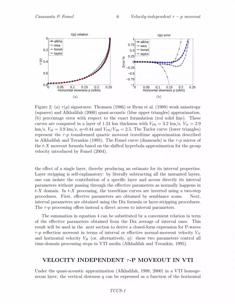
Equation 3 remains exact as long as we use the exact expression for the phasevelocity v(p) (red solid line in figure 2a). Exact expressions exist for all types ofanisotropic media with a horizontal symmetry plane. Unfortunately, the exact and thehighly accurate (Stovas and Fomel, 2010) expressions for τ -p signatures are not verypractical because they depend on multiple parameters. In practice, one may preferto employ three-parameters approximate relations for the phase velocity. Althoughthese signatures are approximate, they are more reliable then the τ -p transformedversion of their dual-pair in the t-X domain (figure 2b).

We can extend the result in equation 3 to a stack of N horizontal homogeneouslayers with horizontal symmetry planes. According to Snell’s law, the horizontal slow-ness p is preserved upon propagation through each layer. Thus, the total intercepttime τ from the bottom of N -th layer is the summation of each interval intercepttime ∆τn in the N contributing layers:

τ(p) =∑N

n=1∆τn =

∑N

n=1VP0,n qn(p) ∆τ0,n , (4)

where each single intercept time ∆τn obviously depends just on interval parameterscharacterizing the n-th layer. Equation 4 states that in the τ -p domain both the raytracing (forward modeling) and layer stripping (inversion) are linear processes. Eachtrace in a τ -p gather collects the contribution of rays that share common segments oftrajectory in the layers (Figure 1a). Moreover, the τ -p domain helps us also to isolate

TCCS-1


0 0.05 0.1 0.15 0.2 0.25

0

0.2

0.4

0.6

0.8

τ(p) relation

Horizontal slowness p (s/km)

τ (s

)

alkhaweafomeltaylor

(a)

0 0.05 0.1 0.15 0.2 0.25−1

−0.75

−0.5

−0.25

0

0.25

0.5

0.75

1τ(p) error

Horizontal slowness p (s/km)

Err

or %

alkhaweafomeltaylor

(b)

Figure 2: (a) τ(p) signatures: Thomsen (1986) or Byun et al. (1989) weak anisotropy(squares) and Alkhalifah (2000) quasi-acoustic (blue upper triangles) approximation.(b) percentage error with respect to the exact formulation (red solid line). Thesecurves are computed in a layer of 1.24 km thickness with VP0 = 3.2 km/s, VN = 2.9km/s, VH = 3.9 km/s, η=0.44 and VP0/VS0 = 2.5. The Taylor curve (lower triangles)represent the τ -p transformed quartic moveout traveltime approximation describedin Alkhalifah and Tsvankin (1995). The Fomel curve (diamonds) is the τ -p mirror ofthe t-X moveout formula based on the shifted hyperbola approximation for the groupvelocity introduced by Fomel (2004).

the effect of a single layer, thereby producing an estimate for its interval properties.Layer stripping is self-explanatory: by literally subtracting all the unwanted layers,one can isolate the contribution of a specific layer and access directly its intervalparameters without passing through the effective parameters as normally happens int-X domain. In t-X processing, the traveltime curves are inverted using a two-stepprocedures. First, effective parameters are obtained by semblance scans. Next,interval parameters are obtained using the Dix formula or layer-stripping procedures.The τ -p processing offers instead a direct access to interval parameters.

The summation in equation 4 can be substituted by a convenient relation in termof the effective parameters obtained from the Dix average of interval ones. Thisresult will be used in the next section to derive a closed-form expression for P-wavesτ -p reflection moveout in terms of interval or effective normal-moveout velocity VNand horizontal velocity VH (or, alternatively, η): these two parameters control alltime-domain processing steps in VTI media (Alkhalifah and Tsvankin, 1995).

VELOCITY INDEPENDENT τ-P MOVEOUT IN VTI

Under the quasi-acoustic approximation (Alkhalifah, 1998, 2000) in a VTI homoge-neous layer, the vertical slowness q can be expressed as a function of the horizontal

TCCS-1


slowness p:

q(p) =1

VP0

√1− V 2

Hp2

1− [V 2H − V 2

N ]p2, (5)

where VH and VN are the horizontal and normal moveout velocity in the layer. Inthe following equations, the hat superscript (ˆ) indicates layer or interval parameters.Considering a stack of N horizontal homogeneous layers with horizontal symmetryplanes, we can insert equation 5 into equation 4 to obtain an expression for theτ -p reflection time from the bottom of the N -th layer, as follows:

τ(p) =∑N

n=1

√√√√ 1− V 2H,np

2

1− [V 2H,n − V 2

N,n]p2∆τ0,n (6)

where ∆τ0,n is the two way vertical time for the n-th layer. To simplify the followingtheoretical derivations, we assume that, instead of having a layered velocity model,interval parameters are vertically-varying continuous profiles. Therefore, we replacethe summation in formula 6 with an integral along the vertical time τ0 and arrive atthe following τ -p moveout formula for a vertically-heterogeneous VTI medium:

τ(p) =

τ0∫0

√1− V 2

H(ξ)p2

1− [V 2H(ξ)− V 2

N(ξ)]p2dξ, (7)

where VN = VN(ξ) and VH = VH(ξ) are (smooth) functions for interval NMO and hor-izontal velocities, and τ0 is the vertical time. The vertical heterogeneity is measured

as a function of τ0. The anellipticity parameter η = 12

(V 2

H

V 2N

− 1)

is also a function of

the vertical time τ0. Using effective parameters, equation 7 can be approximated by

τ(p) ≈ τ0

√1− V 2

H(τ0)p2

1− [V 2H(τ0)− V 2

N(τ0)]p2, (8)

where the effective NMO VN and horizontal VH velocity are related to the inter-val parameters through the second- and fourth-order average velocities (Taner andKoehler, 1969; Ursin and Stovas, 2006) by the following direct Dix-type formulas:

V 2N(τ0) =

1

τ0

τ0∫0

V 2N(ξ)dξ, (9)

S(τ0)V4N(τ0) =

1

τ0

τ0∫0

S(ξ)V 4N(ξ)dξ, (10)

where S is the ratio between the fourth- and second-order moments or the hetero-geneity factor (de Bazelaire, 1988; Alkhalifah, 1997; Siliqi and Bousquie, 2000).

TCCS-1


Equation 8 is basically the four-parameters rational approximation defined in τ -pdomain Stovas and Fomel (2010)

τ(p) ≈ τ0

√1− V 2

Np2 +

AV 4N p

4

1−B V 2N p

2, (11)

with parameter A = (1−S)/4 defined from the Taylor series expansion of the exact τ -p function (Ursin and Stovas, 2006). Under the acoustic VTI approximation, B = −Aand the equation 11 now depends on three parameters only. Finally, to be consistent

with equation 8, the heterogeneity coefficient becomes S = 4V 2H

V 2N

−3. In principle, it is

possible to use any other three-parameters approximation in τ -p domain apart fromthe rational approximation 11 like, for example, the shifted ellipse approximationgiven by Stovas and Fomel (2010). The reason for choosing the approximation 8 isthat it accurately describes the τ -p moveout for a single VTI layer (blue line in figure2b). Nevertheless, approximation 8 remains valid for vertically heterogeneous VTImedia with a decrease in accuracy for larger angles (large values of p) because of theDix averaging

Letting R represent the slope τ ′(p) and Q the curvature τ ′′(p), we differentiateequation 8 once

R(τ, p) = − τ(V 2H − Y )p

(1− p2Y ) (1− p2V 2H), (12)

and twice

Q(τ, p) = − τF (p)(V 2H − Y )

(1− p2Y )2 (1− p2V 2H)

2 , (13)

where F (p) = 1 + 2p2Y − 3p4V 2HY with Y = V 2

H − V 2N . Equations 12 and 13 provide

an analytical description of the slope and curvature fields for given effective valuesVN and VH . Here we have omitted the τ0 dependency for clarity in the notation.Since τ -p and t-X domains are mapped by the linear transformation in equation 2,we observe that

τ ′(p) = R = −x. (14)

Thus, the negative of the slope R has the physical meaning of emerging offset, aspointed out by van der Baan (2004). Moreover, when the curvature Q changes sign,there is an inflection point in the τ -p wavefront that is as a condition for caustics int-X domain. (Roganov and Stovas, 2011).

Given slope R and curvature Q fields in a τ -p CMP gather, we can eliminate thevelocity VN and the parameter Y in equations 12 and 13, thus obtaining a “velocity-independent” (Fomel, 2007b) moveout equation in the τ -p domain:

τ0(τ, p) = τ

√τpQ+ 3τR− 3pR2

τpQ+ 3τR + pR2. (15)

Equation 15 describes a direct mapping from events in the prestack τ -p datadomain to zero-slope time τ0. This equation represents the oriented or slope-based

TCCS-1


moveout correction. As follows from equations 12 and 13, the effective parameters, ifneeded for other tasks, are given by the following relations as a function of the slopeand curvature estimates (see Table 1):

V 2N(τ, p) = −1

p

16τR3

ND, (16)

V 2H(τ, p) =

1

p2

N − 4τR

N, (17)

and

η(τ, p) =1

p

N(4τR−D)

32τR3. (18)

In the above equations, N = τpQ+ 3τR− 3pR2 and D = τpQ+ 3τR + pR2 repre-sent the terms in the numerator N and denominator D of the square root in equation15. In the isotropic or elliptically anisotropic case (VN = VH or η = 0), equations 15to 18 simplify to equations

τ0(τ, p) =√τ 2 − τpR (19)

and

V 2N(τ, p) =

R

p(pR− τ), (20)

previously published by Fomel (2007b).

The anisotropic parameters VN and VH (or η) are no longer a requirement forthe moveout correction, as in the case of conventional NMO processing, but ratherthey are data attributes derived from local slopes and curvatures. Moreover, theseparameters are mappable directly to the appropriate zero-slope time τ0, accordingto equation 15.

SYNTHETIC EXAMPLE OF EFFECTIVE-PARAMETERESTIMATION

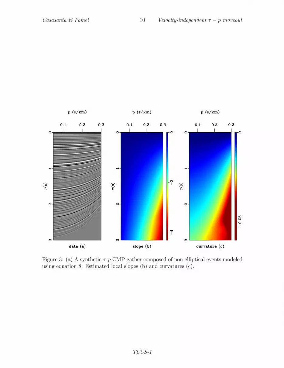
We first test our method on a synthetic example, where the exact velocity model isknown. The example is introduced in Figure 3. The synthetic data were generated byapplying inverse τ -p NMO with time-variable effective velocities. Both the effectiveNMO VN and horizontal VH velocity increase linearly with vertical time and includea sinusoidal change with time, as described by the following relations

VN (τ0) = 2.0 + 0.03 sin(2πτ02

) + 0.08τ0,

VH (τ0) = 2.2− 0.02 sin(2πτ03

) + 0.05τ0.

The CMP maximum offset-to-depth ratio is nearly 2.0 for large value of the hor-izontal slope p. This should guarantee the necessary data sensitivity for resolvinghigh-order moveout parameters (Tsvankin, 2006). Figure 3b shows local event slopes

TCCS-1


Figure 3: (a) A synthetic τ -p CMP gather composed of non elliptical events modeledusing equation 8. Estimated local slopes (b) and curvatures (c).

TCCS-1


R measured from the data using the plane-wave destruction (PWD) algorithm (seeAppendix A). Plane-wave destruction predicts each seismic trace from a neighboringone along local slopes. As explained in appendix A, local slopes are extracted byminimizing the prediction error in an iterative regularized least-squares optimization.Shaping regularization controls the smoothness of the estimated slope field (Fomel,2007a). If the seismic data are particularly noisy, a more aggressive regularizationcan help in getting a more consistent and stable estimate. For cleaner data, lesssmoothing yields a better-resolved and detailed slope field.

Unlike slopes, we don’t directly estimate the curvature field Q. We computethe curvature by simply differentiating the slope estimate. Since slope R = R(τ, p)depends on both the current ray parameter p and the time τ = τ(p), which is againa function of p, we compute the derivative of the slope field by a straightforwardapplication of the chain rule, as follows:

Q =∂R

∂p+R

∂R

∂τ, (21)

The slope gradient components are easily obtained by numerical differentiation. Un-fortunately, this procedure suffers from numerical instability, because finite differencesact like a high-pass filter that enhances the high frequency noise, especially when weare dealing with real data set with poor SNR (signal-to-noise ratio). A noisy orbiased estimate of the curvature field may affect the final result. Figure 3c shows thecurvature field Q for the synthetic data, computed according to equation 21.

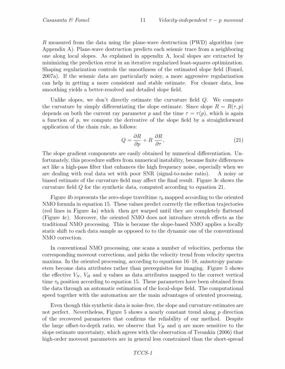
Figure 4b represents the zero-slope traveltime τ0 mapped according to the orientedNMO formula in equation 15. These values predict correctly the reflection trajectories(red lines in Figure 4a) which then get warped until they are completely flattened(Figure 4c). Moreover, the oriented NMO does not introduce stretch effects as thetraditional NMO processing. This is because the slope-based NMO applies a locallystatic shift to each data sample as opposed to to the dynamic one of the conventionalNMO correction.

In conventional NMO processing, one scans a number of velocities, performs thecorresponding moveout corrections, and picks the velocity trend from velocity spectramaxima. In the oriented processing, according to equations 16–18, anisotropy param-eters become data attributes rather than prerequisites for imaging. Figure 5 showsthe effective VN , VH and η values as data attributes mapped to the correct verticaltime τ0 position according to equation 15. These parameters have been obtained fromthe data through an automatic estimation of the local-slope field. The computationalspeed together with the automation are the main advantages of oriented processing.

Even though this synthetic data is noise-free, the slope and curvature estimates arenot perfect. Nevertheless, Figure 5 shows a nearly constant trend along p directionof the recovered parameters that confirms the reliability of our method. Despitethe large offset-to-depth ratio, we observe that VH and η are more sensitive to theslope estimate uncertainty, which agrees with the observation of Tsvankin (2006) thathigh-order moveout parameters are in general less constrained than the short-spread

TCCS-1


Figure 4: (b) Time mapping of each data sample from τ -p time to the zero-slope timeτ0 according to relation 15. These time values predict correctly reflection traveltimetrajectory, the red lines in (a), which are then warped until they are completelyflattened (c)

TCCS-1


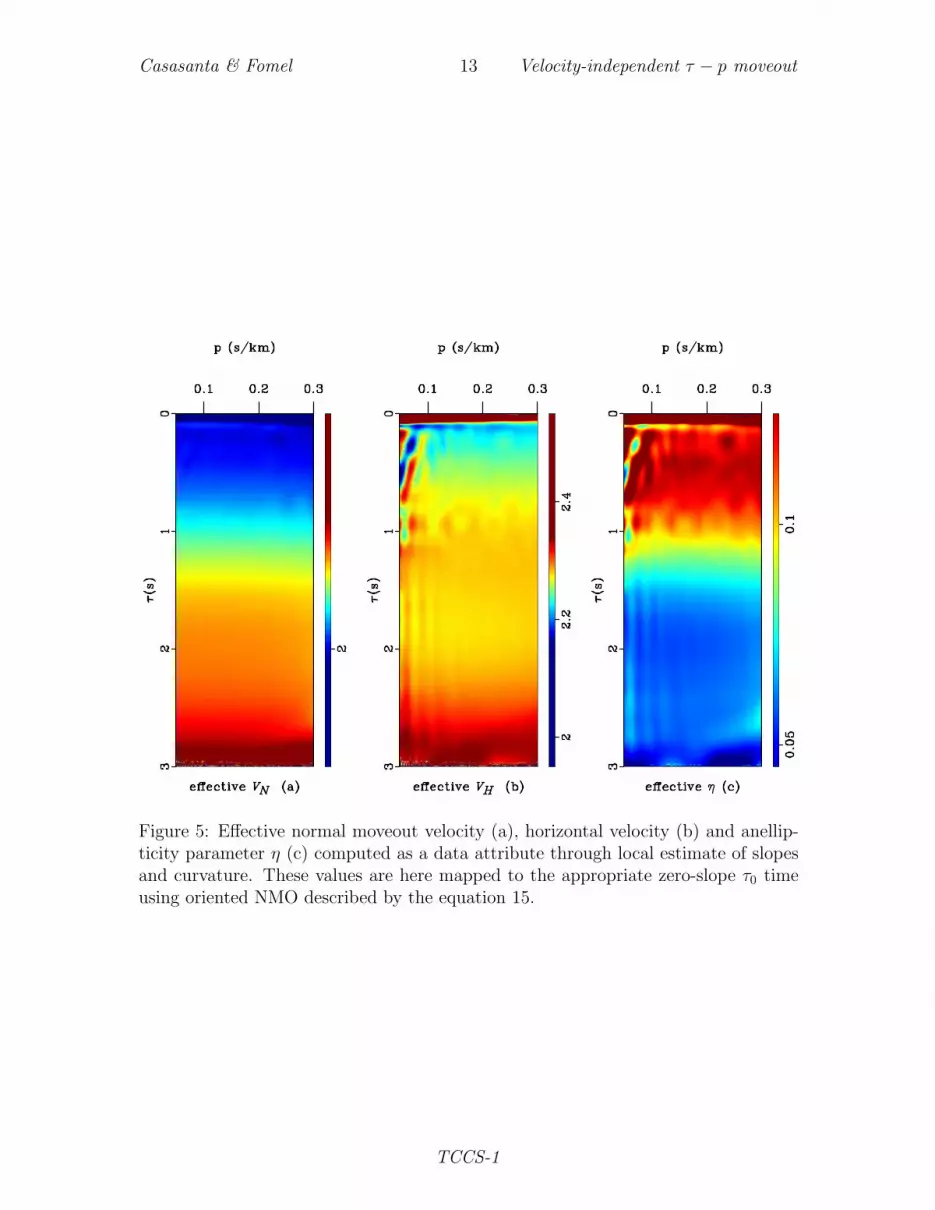
Figure 5: Effective normal moveout velocity (a), horizontal velocity (b) and anellip-ticity parameter η (c) computed as a data attribute through local estimate of slopesand curvature. These values are here mapped to the appropriate zero-slope τ0 timeusing oriented NMO described by the equation 15.

TCCS-1


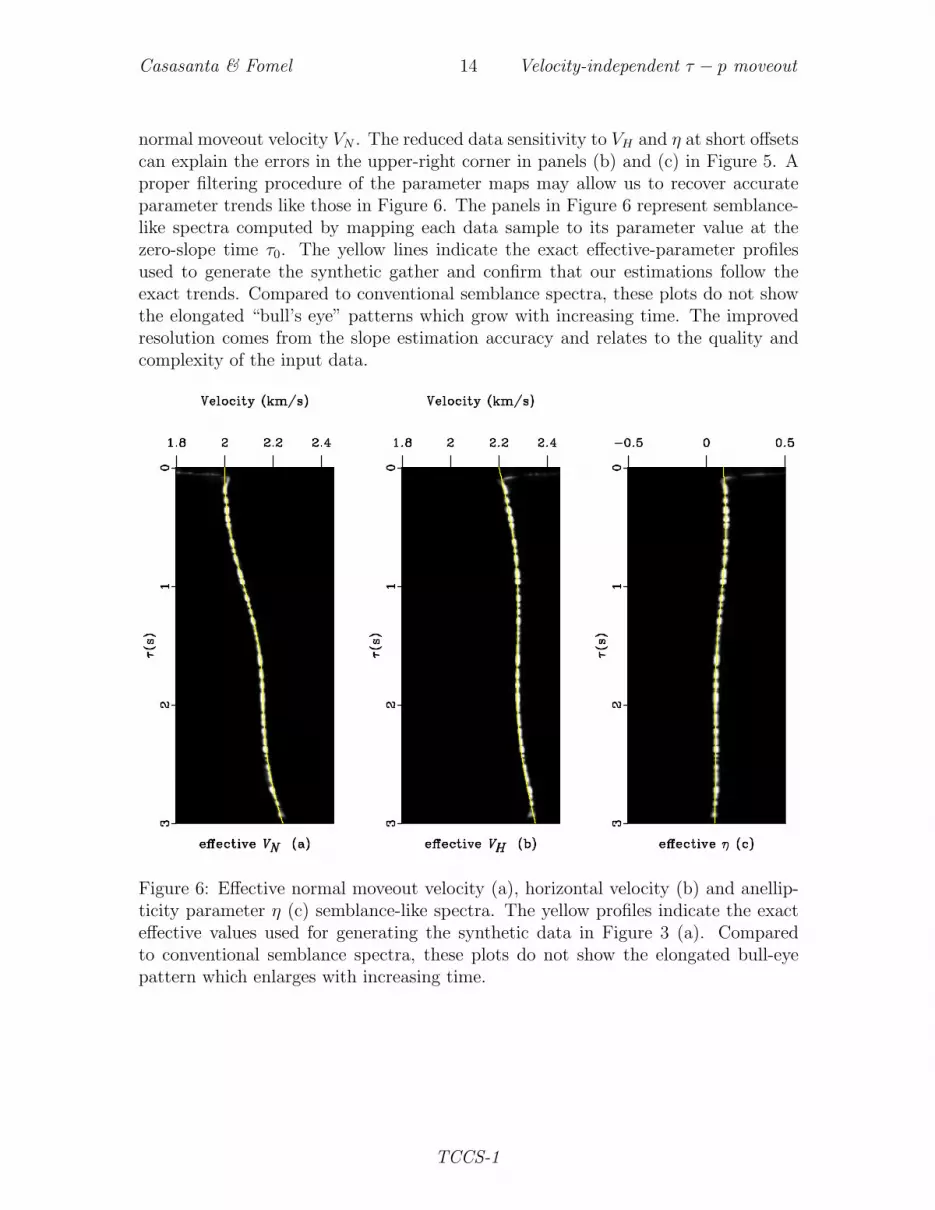
normal moveout velocity VN . The reduced data sensitivity to VH and η at short offsetscan explain the errors in the upper-right corner in panels (b) and (c) in Figure 5. Aproper filtering procedure of the parameter maps may allow us to recover accurateparameter trends like those in Figure 6. The panels in Figure 6 represent semblance-like spectra computed by mapping each data sample to its parameter value at thezero-slope time τ0. The yellow lines indicate the exact effective-parameter profilesused to generate the synthetic gather and confirm that our estimations follow theexact trends. Compared to conventional semblance spectra, these plots do not showthe elongated “bull’s eye” patterns which grow with increasing time. The improvedresolution comes from the slope estimation accuracy and relates to the quality andcomplexity of the input data.

Figure 6: Effective normal moveout velocity (a), horizontal velocity (b) and anellip-ticity parameter η (c) semblance-like spectra. The yellow profiles indicate the exacteffective values used for generating the synthetic data in Figure 3 (a). Comparedto conventional semblance spectra, these plots do not show the elongated bull-eyepattern which enlarges with increasing time.

TCCS-1


ESTIMATION OF INTERVAL PARAMETERS

Similarly to effective parameters, interval parameters can also be regarded as dataattributes obtained from local slopes. Unlike the t-X domain, the τ -p domain offersus several alternatives to conventional Dix (1955) processing for retrieving intervalvalues. In this section, we analyze three different options for extracting intervalparameters in the τ -p domain.

τ0 R Q Rτ Qτ τ0,τ

Effective VN VH η 3 3 3

Interval VN VH η

Dix 3 3 3 3 3

Stripping 3 3 3

Fowler 3 3 3

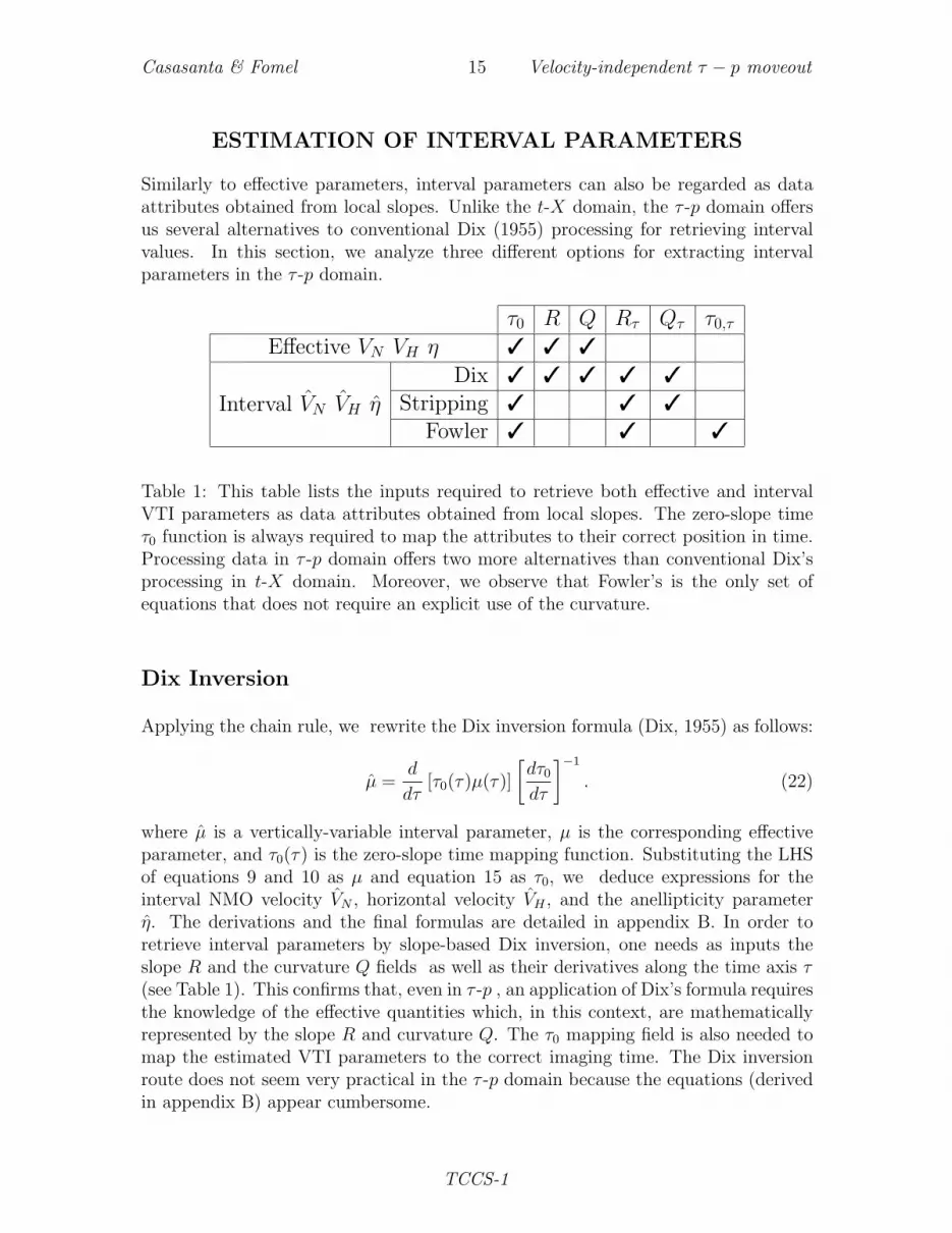
Table 1: This table lists the inputs required to retrieve both effective and intervalVTI parameters as data attributes obtained from local slopes. The zero-slope timeτ0 function is always required to map the attributes to their correct position in time.Processing data in τ -p domain offers two more alternatives than conventional Dix’sprocessing in t-X domain. Moreover, we observe that Fowler’s is the only set ofequations that does not require an explicit use of the curvature.

Dix Inversion

Applying the chain rule, we rewrite the Dix inversion formula (Dix, 1955) as follows:

µ =d

dτ[τ0(τ)µ(τ)]

[dτ0dτ

]−1

. (22)

where µ is a vertically-variable interval parameter, µ is the corresponding effectiveparameter, and τ0(τ) is the zero-slope time mapping function. Substituting the LHSof equations 9 and 10 as µ and equation 15 as τ0, we deduce expressions for theinterval NMO velocity VN , horizontal velocity VH , and the anellipticity parameterη. The derivations and the final formulas are detailed in appendix B. In order toretrieve interval parameters by slope-based Dix inversion, one needs as inputs theslope R and the curvature Q fields as well as their derivatives along the time axis τ(see Table 1). This confirms that, even in τ -p , an application of Dix’s formula requiresthe knowledge of the effective quantities which, in this context, are mathematicallyrepresented by the slope R and curvature Q. The τ0 mapping field is also needed tomap the estimated VTI parameters to the correct imaging time. The Dix inversionroute does not seem very practical in the τ -p domain because the equations (derivedin appendix B) appear cumbersome.

TCCS-1


Claerbout’s straightedge method

Claerbout (1978) suggested that interval velocity in an isotropic (VN = VH) layeredmedium could be estimated with a pen and a straightedge by measuring the offsetdifference ∆x between equal slope p points on two reflection events (Figure 1a). Thecomputation of ∆x is straightforward after a CMP gather has been transformed intothe τ -p domain. In fact, the τ -p transform naturally aligns seismic events with equalslope along the same trace (Figure 1b). Moreover, local slopes R(τ, p) = dτ/dp arerelated to the emerging offset x = −R (van der Baan, 2004) , therefore Claerbout’sinversion formula can be expressed as

V 2N(τ, p) =

Rτ

p2Rτ − p, (23)

where Rτ = ∂R(τ, p)/∂τ and VN is the NMO interval velocity that we map back tozero-slope time τ0 using the isotropic velocity independent τ -p NMO, as suggested byFomel (2007b). The details of the derivation are in appendix C.

The two methods discussed next can be thought of as two alternative extensionsfor VTI media of the original Claerbout’s straightedge method.

Stripping equations

The first alternative to the Dix inversion is what we call stripping equations (Casas-anta and Fomel, 2010). Starting from the integral equation 7 for τ -p reflection move-out and employing the chain rule (equation C-4), we first deduce an expression forslope Rτ (equation C-5) and curvature Qτ (equation C-6) using τ -derivatives, thatnow depend on the interval parameters. Then, solving for VN and VH , we obtain thefollowing expressions:

V 2N(τ, p) = −1

p

16R3τ

ND, (24)

V 2H(τ, p) =

1

p2

N − 4Rτ

N, (25)

and

η(τ, p) =1

p

N(4Rτ − D)

32τR3τ

, (26)

which provide an estimate for the interval parameters. In the above equations, N =pQτ+ 3Rτ−3pR2

τ and D = pQτ +3Rτ +pR2τ , which corresponds to the interval values

of the numerator N and denominator D of the square root in equation 15. Theserelations are very similar to those previously derived for the effective parameters(equations 16–18). However, they require the τ derivative of the slope and curvaturefields (Table 1). This result agrees with the discussion above about layer strippingin τ -p. In this domain, layer stripping reduces to computing traveltime differences

TCCS-1


(equation 4) at each horizontal slowness p. Therefore, differentiating the effectiveslope R and curvature Q fields in τ provides the necessary information to access theinterval parameters directly. This is the power of the τ -p domain as opposed to t-X ,where the only practical path to interval parameters is through Dix inversion thatrequires the knowledge of effective parameters. The zero-slope time τ0 is needed tomap the interval parameter estimates to the correct vertical time (Table 1).

Fowler’s equations

The second alternative to get VTI interval parameters comes from the integral for-mulation of the τ -p moveout signature in equation 7. The derivation is detailed inAppendix C. We first compute τ0,τ = ∂τ0/∂τ and then, applying the chain rule, Rτ .

Solving for VN and VH , we arrive at the following relations:

V 2N(τ, p) = −

[τ 20,τ − 1]2

p3τ 20,τ Rτ

, (27)

V 2H(τ, p) =

τ 20,τ [1−Rτ ] + 1

p3τ 20,τ Rτ

, (28)

which are equivalent to those proposed previously by Fowler et al. (2008). Accordingto equations 27 and 28, the gradients of offset x and the zero-slope time τ0 measuredat common slope locations p on two consecutive seismic event return the VTI intervalparameters for the layer bounded by these two events (Figure 1a). Fowler et al.(2008) first pick traveltime curves in t-X domain, and then differentiate those curvesin offset to compute slopes p. Finally, for any given p value on each seismic event,they determine the corresponding ∆x and ∆τ0 values (Figure 1a). The main practicallimitation in this inversion scheme is the difficulty of picking seismic events accurately.

The processing becomes easier if it is accomplished in τ -p with automatic slopeestimation. First, τ -p transform unveils the position of equal slope events. Second,τ0,τ and Rτ are measured automatically (without event picking) on the τ -p trans-formed CMP gather. The quantity τ0,τ can be estimated as the τ finite differenceof τ0 values computed according to velocity-independent moveout equation 15. Thezero-slope time τ0 function is still needed to map the interval parameter estimatedusing equations 27 and 28 to the correct vertical time (Table 1).

FLATTENING BY PREDICTIVE PAINTING

As shown in Table 1, Fowler’s is the only set of equations that do not require anexplicit use of the curvature Q. The dependence on the curvature is absorbed by theτ0 function. The other two sets of equations, Dix and stripping formulas, as well asthe equations for effective parameters, do need curvature. The curvature computationcan be problematic when the data are contaminated by noise. This makes these three

TCCS-1


methods (effective, stripping, and Dix) less practical when applied to real data withpoor SNR. However, Fowler’s rules represent a way to circumvent the problem. Infact, if we can find an algorithm that estimates the τ0 mapping function directly fromthe data, all the curvature issues will get solved.

The desired algorithm exists and is known as seismic image flattening. The idea ofusing local slopes for automatic flattening was introduced by Bienati and Spagnolini(2001) and Lomask et al. (2006). Flattening by predictive painting (appendix A) usesthe local-slope field to construct a recursive prediction operator (equation A-4) thatspreads a traveltime reference trace in the image and predicts the reflecting surfaceswhich are then unwrapped until the image is flattened.

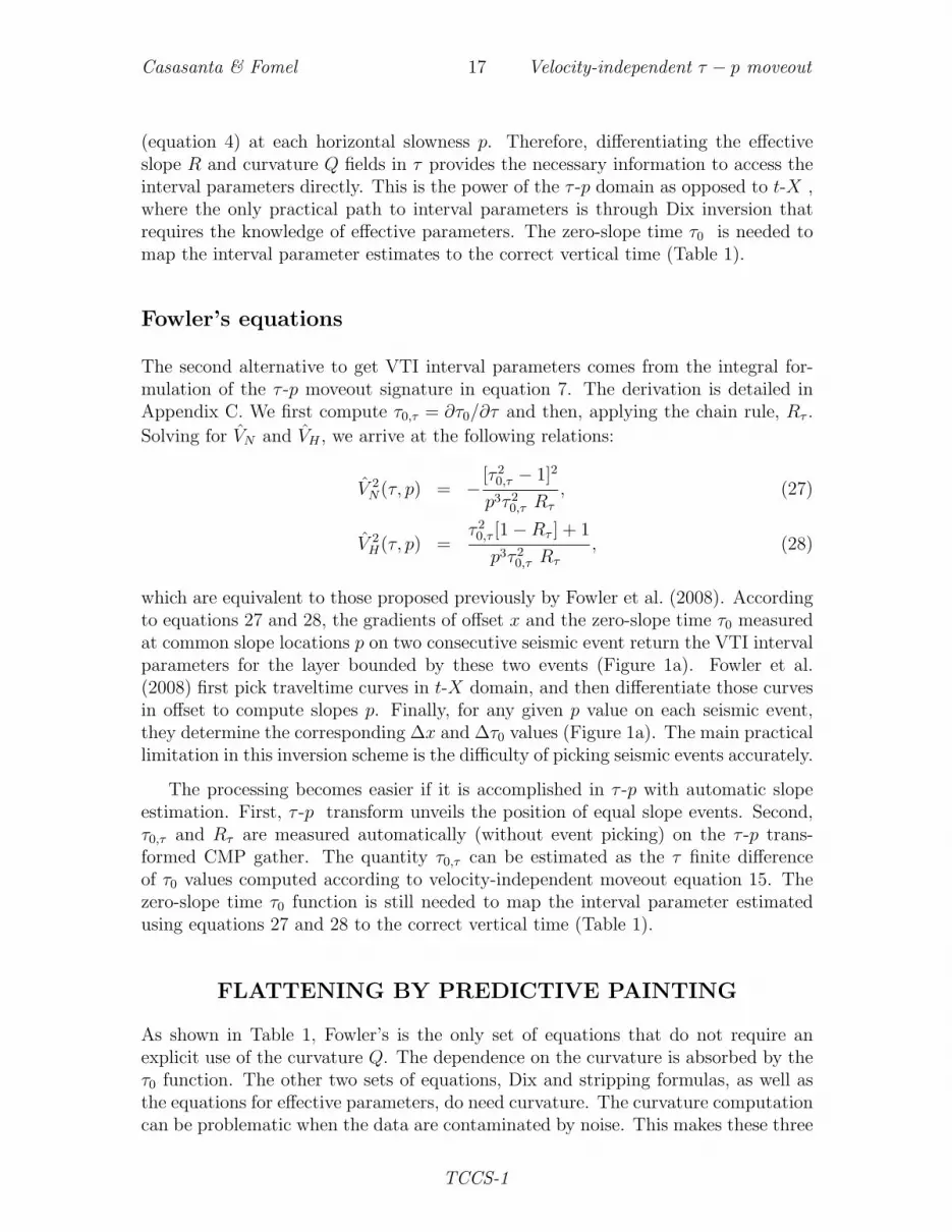
We propose bypassing the issue of estimating the zero-slope time τ0 field by usingthe predictive painting approach. Let us discuss how it works on the previouslyshown synthetic data in Figure 7a. Figure 7b shows local event slope R measuredfrom the data using the PWD algorithm. Figure 7c shows how predictive paintingspreads a zero-slope time τ0 reference trace along local data slopes to predict thezero-slope time τ0 mapping field and hence the geometry of the traveltime reflectioncurves along τ -p CMP gather. Because this procedure does not involve curvaturecomputations, it represents a much more robust way of obtaining the τ0 field that isneeded by the inversion formulas in equations 27 and 28. After τ0 has been found, wealso have what we need to perform gather flattening (Burnett and Fomel, 2009a,b).Unshifting each trace (Figure 7d) automatically flattens the data, thus performinga velocity-independent τ -p NMO correction. As expected, all events are perfectlyaligned, and the correction does not suffer from instabilities of curvature estimation.Moreover, predictive painting is automatic and does not require any prior assumptionsabout the moveout shape.

Now, given the slope field R and its zero-slope time field τ0, we retrieve intervalparameters using equations 27 and 28. In Figure 8, the estimated NMO (a) horizontalvelocities (b) and the anellipticity (c) parameter are mapped to the appropriate zero-slope time using the painted zero-slope time τ0 field (Figure 7c). The exact intervalprofiles (yellow lines) are recovered nearly perfectly although the resolution slightlyworsens with respect to the effective profiles (Figure 6). The main reason is theinstability of the additional numerical differentiation along the τ direction that allthe approaches require.

FIELD DATA EXAMPLE

Figure 9 presents the results of the proposed τ -p processing on a field data examplefrom a marine acquisition. Figure 9a shows a τ -p transformed CMP gather. The dataare taken from a deep water (3.5 s of sea-depth) dataset with poor offset sampling(∼ 100 m) that aliases the steepest seismic events. Spatial aliasing creates artifactsin τ -p domain that bias the PWD slope estimate. In order to mitigate the effect ofthe aliasing, we interpolated the raw data by means of an FX algorithm (Spitz, 1991).

TCCS-1


Figure 7: Synthetic CMP τ -p transformed gather (a), estimated local slopes (b), zeroslope time τ0 obtained by predictive painting (c), and the gather flattened (d).

TCCS-1


Figure 8: Fowler’s equation based inversion to interval normal moveout (a) horizontalvelocity (b) and anellipticity parameter η (c). The yellow lines represent the exactvalues used for generating the synthetic dataset in figure 3 (a).

TCCS-1


Figure 9: τ -p or Radon transformed data from a marine acquisition (a). The dataare fairly clean even though there is a slight decrease in SNR for later and steepestevents. The CMP maximum offset-to-depth ratio reaches 1.5 for larger value of thehorizontal slope p. Dominant local-slope field (b) measured using PWD algorithm.Using the slopes we estimate the zero-slope time τ0 mapping fields (c) that predictsreflection curves by which we flatten the original gather (d).

TCCS-1


The original trace recording is 7.0 s long but, since the SNR decreases significantlyafter 5.0 s, we window the CMP gather and process seismic events only between 3.0and 6.0 s. The CMP maximum offset-to-depth ratio reaches 1.5 for larger value of thehorizontal slope p. As for the synthetic case, the data should carry enough informationto well resolve the horizontal velocity and the anellipticity parameter. Figure 9b showsthe dominant local-slopeR field automatically measure from the data using the PWDalgorithm. As in the synthetic case, we use these slopes to construct the predictionoperator that allows us to paint the zero-slope traveltime map τ0 along the reflectionevents (Figure 9c). The τ0 values are finally used to unwrap the trace shifts untilthe gather is completely flattened. The good alignment of the NMO corrected traces(Figure 9d) confirms the robustness of predictive painting with real data. Figure 10shows spectra of the recovered interval parameters using Fowler’s equations 27 and28. The plots are overlaid with the profiles (yellow curves) recovered using a layer-based t-X Dix inversion (Ferla and Cibin, 2009) and by the profiles obtained afteran automated picking of the recovered trends. Our solution (red curves) follows theDix trends (yellow curves) even though it exhibits a slight decrease in accuracy. Thepoor SNR for later and steeper events and the numerical differentiation of the zero-slope traveltime τ0 and slope R make the field data results noisier. As expected, thehigh-order moveout parameters appear to be more sensitive to the noise. Moreover,the more pronounced enlargement of the η trend in comparison with the VH trendconfirms that the latter parameter is better constrained by the data (Tsvankin, 2006).

DISCUSSION

In the conventional NMO processing, one needs to scan over a range of possible ve-locities and pick the appropriate velocity trend from semblance maxima. Therefore,the cost of velocity scanning is roughly proportional to the number of scanned ve-locities NV times the input data size. Anisotropic velocity analysis is performed bysimultaneously scanning two (or more) parameters. Consequently, the number of trialvelocities/parameters squares, which increases the computational time dramatically.In oriented processing, the effective anisotropy parameters turn into data attributesaccording to equations 16–18. These parameters are directly mapped from the slopefield R to the correct zero-slope/offset traveltime τ0. The cost of local slope estima-tion with plane-wave destruction method is proportional to the data size times thenumber of estimation iterations NI times the 2D filter size NF . Typically NI = 10and NF = 6, which roughly correspond to scanning NV = 60 velocities. However,unlike semblance analysis, this cost does not increase if we are estimating one, twoor more parameters. The cost of the semblance scan becomes even more prohibitivewhen processing wide-azimuth data. The computational advantages of our approachare encouraging especially with respect to multi-azimuth processing and orthorhom-bic velocity analysis, where time processing is controlled by at least five parameters(Tsvankin, 2006).

Automation, in addition to speed, is another clear advantage of the slope-based

TCCS-1


Figure 10: Parameters spectra for interval normal moveout (a), horizontal velocity (b)and anellipticity parameter η (c). These spectra result from the application of Fowler’sequations using painted τ0 field. The red lines are the profiles after an automatedpicking of the estimated spectra. The yellow lines are the recovered profiles after alayer-based t-X Dix inversion procedure (Ferla and Cibin, 2009).

TCCS-1


processing. Slope estimation provided by plane-wave destruction represents an au-tomated approach to velocity analysis. It may require a limited user-interaction inchoosing input parameters. A user-supplied initial guess for the slope field can accel-erate the nonlinear optimization , thereby providing a more reliable estimate for theslopes. The smoothness of the output slopes is controlled by shaping regularization;the length of a 2-D triangular smoothing filter controls smoothness along p and τdirection in the τ -p transformed CMP data. If the input seismic data are not regu-larly and properly sampled in space, as often happens in wide-azimuth acquisition,the τ -p transform may add to the data coherent-noise artifacts. This can affect thefinal result of PWD slope estimation. Thus, if the seismic τ -p data are noisy, in-creasing the length of smoothing filters can help in achieving a more stable solution,despite some loss in resolution. In contrast, for high SNR data, less smoothing yieldsbetter-resolved slope fields.

All the equations we have developed in this paper hold for S-wave data as longas we use two parameters S-wave phase-velocity approximation (Stovas, 2009). Thecombination of the results from P-wave and S-wave processing may enable a retrievalof all the elastic parameters needed to build an initial VTI anisotropic model suitablefor depth processing.

The application of the proposed method is also limited by the underlying assump-tion of vertical variation of the velocity model with the horizontal symmetry plane. Inprinciple, the method can handle limited lateral variation of the velocity. Therefore,it can be used for dense anisotropic moveout analysis at the early stages of processing.

CONCLUSIONS

Local slopes of seismic events carry complete information about the structure of thesubsurface. We have developed a velocity-independent τ -p imaging approach to per-form moveout correction in 2D layered VTI media. We process Radon-transformeddata because τ -p is the natural domain for anisotropic parameter estimation invertically-variable media. Effective VTI parameters turn into data attributes throughthe use of slopes and are directly mappable to the zero-slope traveltime. Interval pa-rameters turn into data attributes as well. We have developed the analytical theoryfor the slope-based Dix inversion in τ -p , as well as two alternative sets of equationsthat can be regarded as an extension of Claerbout’s method for straightedge determi-nation of interval velocity. Both sets of equations exploit the intrinsic layer strippingpower of the τ -p domain to estimate interval parameters directly without involvingeffective parameters.

The equations we have introduced to retrieve both effective and interval param-eters in VTI media require directly or indirectly an estimation of the local datacurvature. On the other hand, Fowler’s equations do not require an explicit use ofthe curvature. Therefore, we propose bypassing the curvature estimation by exploit-ing a curvature-independent estimation of the zero-slope time τ0 field that, together

TCCS-1


with the slopes, provides the input to Fowler’s method. The zero-slope time can befound efficiently by employing the predictive painting algorithm. A reference trace atthe zero-slope time τ0 is spread along the local data slope to predict the τ0 field alongreflection curves in the τ -p CMP gather. This estimation appears robust and efficientenough to enable automated, slope-based, dense estimation of interval parameters.

ACKNOWLEDGMENTS

The first author thanks Nicola Bienati, Paul Fowler, and Ilya Tsvankin for fruitfuland stimulating discussions. A special acknowledgment goes to Giuseppe Drufucaand the members of the DSP(GEO) research group at Politecnico di Milano for theirsupport. The second author acknowledges partial financial support from ExxonMobiland RPSEA1 and thanks Tariq Alkhalifah, Will Burnett, and Yang Liu for helpfuldiscussions. Both the authors are indebted to Alexey Stovas and the anonymousreviewer for their excellent reviews. Their suggestions and insightful remarks haveimproved the clarity of the paper.

REFERENCES

Al-Dajani, A., and I. Tsvankin, 1998, Nonhyperbolic reflection moveout for horizontaltransverse isotropy: Geophysics, 63, 1738–1753.

Alkhalifah, T., 1997, Velocity analysis using nonhyperbolic moveout in transverselyisotropic media: Geophysics, 62, 1839–1854.

——–, 1998, Acoustic approximations for processing in transversely isotropic media:Geophysics, 63, 623–631.

——–, 2000, An acoustic wave equation for anisotropic media: Geophysics, 65, 1239–1250.

Alkhalifah, T., and I. Tsvankin, 1995, Velocity analysis for transversely isotropicmedia: Geophysics, 60, 1550–1566.

Bienati, N., and U. Spagnolini, 2001, Multidimensional wavefront estimation fromdifferential delays: IEEE Trans. on Geoscience and Remote Sensing, 39, 655–664.

Burnett, W., and S. Fomel, 2009a, 3D velocity-independent elliptically anisotropicmoveout correction: Geophysics, 74, WB129–WB136.

——–, 2009b, Moveout analysis by time-warping: SEG Technical Program ExpandedAbstracts, 28, 3710–3714.

1The funding by RPSEA was provided through the Ultra-Deepwater and Unconventional NaturalGas and Other Petroleum Resource program authorized by the U.S. Energy Policy Act of 2005.RPSEA (www.rpsea.org) is a nonprofit corporation whose mission is to provide a stewardship role inensuring the focused research, development and deployment of safe and environmentally responsibletechnology that can effectively deliver hydrocarbons from domestic resources to the citizens of theUnited States. RPSEA, operating as a consortium of premier U.S. energy research universities,industry, and independent research organizations, manages the program under a contract with theU.S. Department of Energy’s National Energy Technology Laboratory.

TCCS-1


Byun, B. S., D. Corrigan, and J. E. Gaiser, 1989, Anisotropic velocity analysis forlithology discrimination: Geophysics, 54, 1564–1574.

Casasanta, L., and S. Fomel, 2010, Velocity independent τ -p moveout in layered VTImedia: 72nd EAGE Conference & Exhibition, EAGE, Expanded Abstract C030.

Claerbout, J., 1992, Earth sounding analysis: Processing versus inversion: Blackwell.Claerbout, J. F., 1978, Straightedge determination of interval velocity, in SEP-14:

Stanford Exploration Project, 13–16.de Bazelaire, E., 1988, Normal moveout revisited: Inhomogeneous media and curved

interfaces: Geophysics, 53, 143–157.Dix, C. H., 1955, Seismic velocities from surface measurements: Geophysics, 20,

68–86.Douma, H., and M. van der Baan, 2008, Rational interpolation of qP-traveltimes

for semblance-based anisotropy estimation in layered VTI media: Geophysics, 73,D53–D62.

Ferla, M., and P. Cibin, 2009, Interval anisotropic parameters estimation in a leastsquares sense — application on congo mtpn real dataset: SEG Technical ProgramExpanded Abstracts, 28, 296–300.

Fomel, S., 2002, Applications of plane-wave desctruction filters: Geophysics, 67,1946–1960.

——–, 2004, On anelliptic approximations for qP velocities in VTI media: Geophys-ical Prospecting, 52, 247–259.

——–, 2007a, Shaping regularization in geophysical estimation problems: Geophysics,72, R29–R36.

——–, 2007b, Velocity-independent time-domain seismic imaging using local eventslopes: Geophysics, 72, S139–S147.

——–, 2008, Nonlinear shaping regularization in geophysical inverse problems: SEGTechnical Program Expanded Abstracts, 27, 2046–2051.

——–, 2010, Predictive painting of 3d seismic volumes: Geophysics, 75, A25–A30.Fomel, S., and A. Stovas, 2010, Generalized nonhyperbolic moveout approximation:

Geophysics, 75, U9–U18.Fowler, P. J., A. Jackson, J. Gaffney, and D. Boreham, 2008, Direct nonlinear travel-

time inversion in layered VTI media: SEG Technical Program Expanded Abstracts,27, 3028–3032.

Lambare, G., 2008, Stereotomography: Geophysics, 73, VE25–VE34.Lambare, G., M. Alerini, R. Baina, and P. Podvin, 2003, Stereotomography : A fast

approach for velocity macro-model estimation: SEG Technical Program ExpandedAbstracts, 22, 2076–2079.

Lomask, J., A. Guitton, S. Fomel, J. Claerbout, and A. A. Valenciano, 2006, Flat-tening without picking: Geophysics, 71, P13–P20.

Ottolini, R., 1983, Velocity independent seismic imaging: Technical report, StanforExploration Project.

Riabinkin, L. A., 1957, Fundamentals of resolving power of controlled directionalreception (CDR) of seismic waves, in Slant-stack processing, 1991: Soc. of Expl.Geophys. (Translated and paraphrased from Prikladnaya Geofiizika, 16, 3-36), 36–60.

TCCS-1


Rieber, F., 1936, A new reflection system with controlled directional sensitivity: Geo-physics, 1, 97–106.

Roganov, Y., and A. Stovas, 2011, Caustics in a periodically layered transverselyisotropic medium with vertical symmetry axis: Geophysical Prospecting, DOI:10.1111/j.1365–2478.2010.00924.x.

Sil, S., and M. Sen, 2008, Azimuthal τ -p analysis in anisotropic media: GeophysicalJournal International, 175, 587–597.

Siliqi, R., and N. Bousquie, 2000, Anelliptic time processing based on a shifted hy-perbola approach: SEG Technical Program Expanded Abstracts, 19, 2245–2248.

Siliqi, R., P. Herrmann, A. Prescott, and L. Capar, 2007, High-order RMO pickingusing uncorrelated parameters: SEG Technical Program Expanded Abstracts, 26,2772–2776.

Spitz, S., 1991, Seismic trace interpolation in the F-X domain: Geophysics, 56, 785–794.

Stovas, A., 2009, Direct Dix-type inversion in a layered VTI medium: SEG TechnicalProgram Expanded Abstracts, 28, 2506–2510.

Stovas, A., and S. Fomel, 2010, The generalized non-elliptic moveout approximationin the τ -p domain: SEG Technical Program Expanded Abstracts, 253–257.

Sword, C. H., 1987, Tomographic determination of interval velocities from reflectionseismic data: The method of controlled directional reception: PhD thesis, StanfordUniversity.

Taner, M. T., and F. Koehler, 1969, Velocity spectra—digital computer derivationapplications of velocity functions: Geophysics, 34, 859–881.

Thomsen, L., 1986, Weak elastic anisotropy: Geophysics, 51, 1954–1966.Tsvankin, I., 1995, Normal moveout from dipping reflectors in anisotropic media:

Geophysics, 60, 268–284.——–, 2006, Seismic signatures and analysis of reflection data in anisotropic media:

Elsevier.Tsvankin, I., J. Gaiser, V. Grechka, M. van der Baan, and L. Thomsen, 2010, Seismic

anisotropy in exploration and reservoir characterization: An overview: Geophysics,75, 75A15–75A29.

Ursin, B., and A. Stovas, 2006, Traveltime approximations for a layered transverselyisotropic medium: Geophysics, 71, D23–D33.

van der Baan, M., 2004, Processing of anisotropic data in the tau-p domain: I—Geometric spreading and moveout corrections: Geophysics, 69, 719–730.

van der Baan, M., and J. M. Kendall, 2002, Estimating anisotropy parameters andtraveltimes in the tau-p domain: Geophysics, 67, 1076–1086.

Wang, X., and I. Tsvankin, 2009, Estimation of interval anisotropy parameters usingvelocity-independent layer stripping: Geophysics, 74, WB117–WB127.

Wolf, K., D. Rosales, A. Guitton, and J. Claerbout, 2004, Robust moveout withoutvelocity picking: SEG Technical Program Expanded Abstracts, 23, 2423–2426.

Yilmaz, O., 2000, Seismic data analysis: SEG.

TCCS-1


APPENDIX A

LOCAL PLANE-WAVES OPERATORS

Local plane-wave operators model seismic data (Fomel, 2002) . The mathematicalbasis is the local plane differential equation

∂P

∂x+ σ

∂P

∂t= 0 , (A-1)

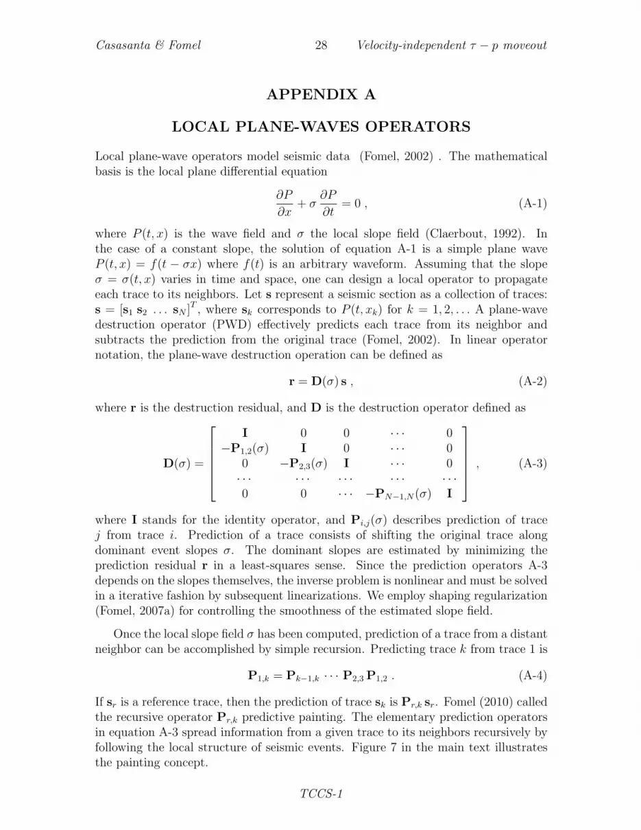
where P (t, x) is the wave field and σ the local slope field (Claerbout, 1992). Inthe case of a constant slope, the solution of equation A-1 is a simple plane waveP (t, x) = f(t − σx) where f(t) is an arbitrary waveform. Assuming that the slopeσ = σ(t, x) varies in time and space, one can design a local operator to propagateeach trace to its neighbors. Let s represent a seismic section as a collection of traces:s = [s1 s2 . . . sN ]T , where sk corresponds to P (t, xk) for k = 1, 2, . . . A plane-wavedestruction operator (PWD) effectively predicts each trace from its neighbor andsubtracts the prediction from the original trace (Fomel, 2002). In linear operatornotation, the plane-wave destruction operation can be defined as

r = D(σ) s , (A-2)

where r is the destruction residual, and D is the destruction operator defined as

D(σ) =

I 0 0 · · · 0

−P1,2(σ) I 0 · · · 00 −P2,3(σ) I · · · 0· · · · · · · · · · · · · · ·0 0 · · · −PN−1,N(σ) I

, (A-3)

where I stands for the identity operator, and Pi,j(σ) describes prediction of tracej from trace i. Prediction of a trace consists of shifting the original trace alongdominant event slopes σ. The dominant slopes are estimated by minimizing theprediction residual r in a least-squares sense. Since the prediction operators A-3depends on the slopes themselves, the inverse problem is nonlinear and must be solvedin a iterative fashion by subsequent linearizations. We employ shaping regularization(Fomel, 2007a) for controlling the smoothness of the estimated slope field.

Once the local slope field σ has been computed, prediction of a trace from a distantneighbor can be accomplished by simple recursion. Predicting trace k from trace 1 is

P1,k = Pk−1,k · · · P2,3 P1,2 . (A-4)

If sr is a reference trace, then the prediction of trace sk is Pr,k sr. Fomel (2010) calledthe recursive operator Pr,k predictive painting. The elementary prediction operatorsin equation A-3 spread information from a given trace to its neighbors recursively byfollowing the local structure of seismic events. Figure 7 in the main text illustratesthe painting concept.

TCCS-1


APPENDIX B

MATHEMATICAL DERIVATION OF SLOPE-BASED DIXINVERSION

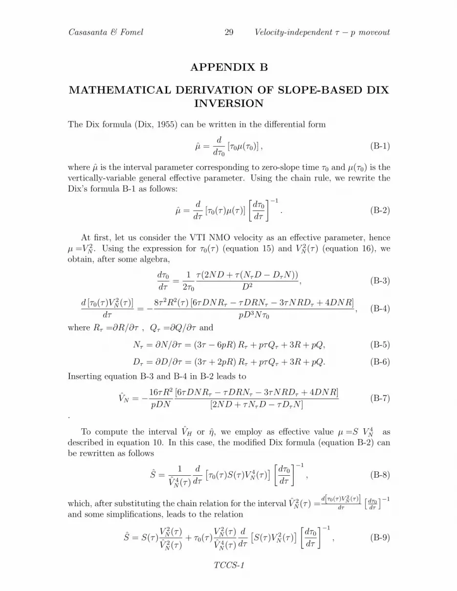
The Dix formula (Dix, 1955) can be written in the differential form

µ =d

dτ0[τ0µ(τ0)] , (B-1)

where µ is the interval parameter corresponding to zero-slope time τ0 and µ(τ0) is thevertically-variable general effective parameter. Using the chain rule, we rewrite theDix’s formula B-1 as follows:

µ =d

dτ[τ0(τ)µ(τ)]

[dτ0dτ

]−1

. (B-2)

At first, let us consider the VTI NMO velocity as an effective parameter, henceµ =V 2

N . Using the expression for τ0(τ) (equation 15) and V 2N(τ) (equation 16), we

obtain, after some algebra,

dτ0dτ

=1

2τ0

τ(2ND + τ(NτD −DτN))

D2, (B-3)

d [τ0(τ)V 2N(τ)]

dτ= −8τ 2R2(τ) [6τDNRτ − τDRNτ − 3τNRDτ + 4DNR]

pD3Nτ0, (B-4)

where Rτ =∂R/∂τ , Qτ =∂Q/∂τ and

Nτ = ∂N/∂τ = (3τ − 6pR)Rτ + pτQτ + 3R + pQ, (B-5)

Dτ = ∂D/∂τ = (3τ + 2pR)Rτ + pτQτ + 3R + pQ. (B-6)

Inserting equation B-3 and B-4 in B-2 leads to

VN = −16τR2

pDN

[6τDNRτ − τDRNτ − 3τNRDτ + 4DNR]

[2ND + τNτD − τDτN ](B-7)

.

To compute the interval VH or η, we employ as effective value µ =S V 4N as

described in equation 10. In this case, the modified Dix formula (equation B-2) canbe rewritten as follows

S =1

V 4N(τ)

d

dτ

[τ0(τ)S(τ)V 4

N(τ)] [dτ0

dτ

]−1

, (B-8)

which, after substituting the chain relation for the interval V 2N(τ) =

d[τ0(τ)V 2N (τ)]

dτ

[dτ0dτ

]−1

and some simplifications, leads to the relation

S = S(τ)V 2N(τ)

V 2N(τ)

+ τ0(τ)V 2N(τ)

V 4N(τ)

d

dτ

[S(τ)V 2

N(τ)] [dτ0

dτ

]−1

, (B-9)

TCCS-1


which involves only the mapping relations for the zero-slope time τ0(τ) (formula 15)effective NMO velocity V 2

N(τ) (formula 16), and the anellipticity parameter obtainedby equation 18 as S(τ) = 1 + 8η(τ). From the interval parameter S, we can go backto interval V 2

H = V 2N (S + 3)/4 and η = (S − 1)/8.

In the case of isotropy or elliptical anisotropy (VN = VH), equations B-3 and B-4simplify to

dτ0dτ

=2τ − p(R + τRτ )

2τ0, (B-10)

d [τ0(τ)V 2N(τ)]

dτ=

1

2

pR(R + τRτ )− 2Rττ2

τ0p(pR− τ)(B-11)

Inserting equations B-10 and B-11 in formula B-2, we get

VN =1

p(pR− τ)

pR(R + τRτ )− 2Rττ2

2τ − p(R + τRτ ). (B-12)

This equation is the analog of equation 15 in (Fomel, 2008).

APPENDIX C

MATHEMATICAL DERIVATION OF STRIPPINGEQUATIONS

Starting from the integral representation of τ -p signature in equation 7, we arrive atthe expression of the slope R and the curvature Q fields as the following integrals:

R(τ0, p) =

τ0∫0

F ′(p, ξ)dξ, (C-1)

Q(τ0, p) =

τ0∫0

F ′′(p, ξ)dξ, (C-2)

where

F(τ0, p) =

√1− V 2

H(τ0)p2

1− [V 2H(τ0)− V 2

N(τ0)]p2,

F ′ = dFdp

and F ′′ = d2Fdp2

. According to equation 7, it descends that

τ0,τ (τ, p) =

[∂τ0∂τ

]−1

=1

F(p, τ). (C-3)

Therefore, applying the chain rule

∂

∂τ=

[∂τ

∂τ0

]−1∂

∂τ0=

1

F(τ, p)

∂

∂τ0, (C-4)

TCCS-1


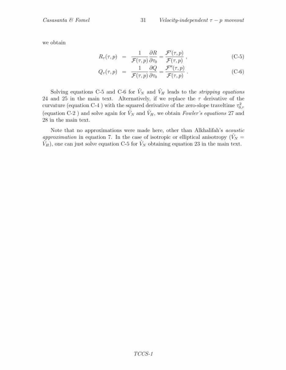
we obtain

Rτ (τ, p) =1

F(τ, p)

∂R

∂τ0=F ′(τ, p)F(τ, p)

, (C-5)

Qτ (τ, p) =1

F(τ, p)

∂Q

∂τ0=F ′′(τ, p)F(τ, p)

. (C-6)

Solving equations C-5 and C-6 for VN and VH leads to the stripping equations24 and 25 in the main text. Alternatively, if we replace the τ derivative of thecurvature (equation C-4 ) with the squared derivative of the zero-slope traveltime τ 2

0,τ

(equation C-2 ) and solve again for VN and VH , we obtain Fowler’s equations 27 and28 in the main text.

Note that no approximations were made here, other than Alkhalifah’s acousticapproximation in equation 7. In the case of isotropic or elliptical anisotropy (VN =VH), one can just solve equation C-5 for VN obtaining equation 23 in the main text.

TCCS-1

velocity-independent τ-p moveout in a horizontally layered vti medium

Documents