numerical differentiation from a viewpoint of regularization theory

MATHEMATICS OF COMPUTATIONVolume 75, Number 256, October 2006, Pages 1853–1870S 0025-5718(06)01857-6Article electronically published on May 15, 2006

NUMERICAL DIFFERENTIATIONFROM A VIEWPOINT OF REGULARIZATION THEORY

SHUAI LU AND SERGEI V. PEREVERZEV

Abstract. In this paper, we discuss the classical ill-posed problem of nu-merical differentiation, assuming that the smoothness of the function to bedifferentiated is unknown. Using recent results on adaptive regularization ofgeneral ill-posed problems, we propose new rules for the choice of the stepsizein the finite-difference methods, and for the regularization parameter choice innumerical differentiation regularized by the iterated Tikhonov method. Thesemethods are shown to be effective for the differentiation of noisy functions,and the order-optimal convergence results for them are proved.

1. Introduction

How do we approximate a derivative y′(t) of a smooth function y(t), t ∈ [0, 1]?This question is discussed extensively in computational mathematics, and thereare many different formulae for numerical differentiation. At the same time, theproblem of numerical differentiation is known to be ill-posed [4] in the sense thata small perturbation in the values of y(t) may lead to large errors in the computedderivative. This fact has the unpleasant consequence that the function yδ(t), whichdiffers imperceptibly from y(t), has a derivative which differs vastly from y′(t).Since in practice data will almost never be exactly available, one has to be awareof numerical instabilities when a noisy observation yδ instead of y is known. In thiscase the perturbation δ(t) = y(t)− yδ(t) represents measurement error or roundingerror and can be a nondifferentiable function having a quite erratic nature. Hence,in order to approximate y′(t) in a stable way, regularization methods should beapplied.

These methods fall into two categories: methods which use noisy data yδ(t)in a nondiscretized form, and methods based only on a finite amount of discreteinformation regarding yδ(t). The well-known forward difference approximation

y′(t) ≈ yhδ (t) =

yδ(t + h) − yδ(t)h

(1.1)

is the simplest example of the method from the first category. Using (1.1) for re-construction y′(t) one presupposes that the value yδ(t+h), for example, is availablefor any sufficiently small h. Because as it has been observed in [6], [22], differenceschemes may construct stable regularizing algorithms only if a stepsize h is chosenproperly. An example of the method from the second category can be found in [7],

Received by the editor November 3, 2004 and, in revised form, April 19, 2005.

2000 Mathematics Subject Classification. Primary 65D25; Secondary 65J20.Key words and phrases. Numerical differentiation, adaptive regularization, unknown smooth-

ness, finite-difference methods, Tikhonov regularization.

c©2006 American Mathematical SocietyReverts to public domain 28 years from publication

1853

1854 SHUAI LU AND SERGEI V. PEREVERZEV

where a derivative S′n(t) of a natural cubic spine Sn(t) solving the minimization

problem

1n − 1

n−1∑i=1

(yδ(ti) − Sn(ti))2 + α ‖ S′′n ‖2→ min(1.2)

is taken as an approximation for y′(t). To construct S′n(t) one should know only

the values yδ(ti) at the points {ti}ni=0 ⊂ [0, 1], t0 = 0, tn = 1, and choose the

regularization parameter α in (1.2).These examples allow us to see a common distinguishing feature of numeri-

cal differentiation methods from both above-mentioned categories. Namely, thesemethods always have some parameter that should be used for problem regulariza-tion. For example, a stepsize h plays the role of regularization parameter for themethod (1.1). A number of regularization parameter choice techniques have beendeveloped for numerical differentiation. They yield satisfactory results when thesmoothness of the function to be differentiated is given very precisely [1], [2], [22],[26]. However, in applications this smoothness is usually unknown, as one can seeit from the following example.

Example 1.1. In the simplest one-dimensional case the cooling of hot glass ismodelled by the parabolic system of the form

∂u

∂t=

∂2u

∂x2, u(0, x) = uin(x),

∂u

∂x(t, 0) = β0(t),

∂u

∂x(t, 1) = β1(t),(1.3)

(t, x) ∈ (0, T ] × [0, 1],

and one is interested in determining the heat exchange coefficients β0,β1 by meansof measurements of the boundary temperature. Assume that we have only a noisymeasurement uδ

0(t),uδ1(t) of the boundary temperature u(t, 0),u(t, 1) on the whole

time interval [0, T ], where δ is a small parameter used for measuring the noiselevel. Such data allow us to determine an approximate distribution u = uδ(t, x) ofthe temperature u = u(t, x) in the whole interval [0, 1] as a solution of the initialboundary-value problem with a noisy Dirichlet condition:

∂u

∂t=

∂2u

∂x2, u(0, x) = uin(x), u(t, 0) = uδ

0(t), u(t, 1) = uδ1(t),(1.4)

(t, x) ∈ (0, T ] × [0, 1].

From the unique solvability of (1.3), (1.4) it follows that the solution u(t, x) of(1.3) corresponding to the “true” coefficients β0,β1 is the same as the solution of(1.4) with “pure” boundary data u(t, 0),u(t, 1) instead of uδ

0,uδ1. In view of the

well-posedness of (1.4) the deviation of u(t, x) from uδ(t, x) is of the same order asthe noise level. Then without loss of generality we can assume that ‖ u − uδ ‖≤ δ.

As soon as uδ has been determined from (1.4), the heat exchange coefficients canbe approximated as follows:

β0(t) ≈uδ(t, h) − uδ

0(t)h

, β1(t) ≈uδ

1(t) − uδ(t, 1 − h)h

.(1.5)

Keeping in mind that the values uδ(t, h),uδ(t, 1−h) are available for any h ∈ (0, 1),approximation (1.5) can be considered as a numerical differentiation method of thefirst category, because it uses the noisy data uδ(t, x) in a nondiscretized form.

NUMERICAL DIFFERENTIATION 1855

At the same time, one does not know a priori the smoothness of the functionu(t, x) to be differentiated. This smoothness depends on the so-called compatibilityconditions

duin

dx(0) = β0(0),

duin

dx(1) = β1(0).(1.6)

If they are not satisfied, then ∂u∂x (t, ·) may be discontinuous for t = 0. On the other

hand, one cannot check (1.6), because β0(t) and β1(t) are the only functions thatshould be recovered. Thus, the regularization parameter h in (1.5) should be chosenwithout knowledge of the smoothness of function u(t, x) to be differentiated.

Surprisingly enough, in the case of unknown smoothness we cannot find any re-sults providing us with the recipe for regularization parameter choice for numericaldifferentiation. Only in the paper [7] the discrepancy principle for the choice ofthe regularization parameter α in (1.2) has been discussed. This principle is usu-ally applied in the case of unknown smoothness, but its efficiency for numericaldifferentiation has been proved in [7] under the assumption that the function to bedifferentiated is two times differentiable.

Thus, there is a gap in the analysis of such an important computational procedureas numerical differentiation, and the goal of the present paper is to fill it out. Itwill be done on the basis of recent results of regularization theory [15]–[17], [20].

In Section 2 we discuss the case of nondiscretized noisy data and suggest ana posteriori rule for the choice of the stepsize h in the finite-difference methods.Numerical differentiation with discrete noisy information is discussed in Section3. In this section we make use of the adaptive regularization strategy from [16]for solving the corresponding Volterra equation, which is an alternative to thefinite-difference methods. Numerical experiments supporting theoretical results arepresented in both sections. Section 4 contains some concluding remarks.

2. Regularized finite-difference methods

2.1. Adaptive choice of the stepsize. Within the framework of the finite-differ-ence method Dl

h, l ∈ N , the approximate value of the derivative y′ at the pointt ∈ (0, 1) is calculated as

y′(t) ≈ Dlhy(t) = h−1

l∑j=−l

aljy(t + jh),

where alj are some fixed real numbers, and a stepsize h is so small that t+jh ∈ (0, 1)

for j = −l,−l+1, . . . , 0, . . . , l. The last restriction means that the distance betweenpoint t and the boundary points of the interval should be sufficiently large. If insteadof y only yδ ∈ C[0, 1] is available such that

‖ y − yδ ‖C[0,1]≤ δ,(2.1)

then the method Dlh produces the approximation

Dlhyδ(t) = h−1

l∑j=−l

aljyδ(t + jh),

and its error can be estimated as

|y′(t) − Dlhyδ(t)| ≤ |y′(t) − Dl

hy(t)| + |Dlhy(t) − Dl

hyδ(t)|,(2.2)


where the first term on the right-hand side is the consistency error of Dlh, whereas

the second term is a propagation error. It can be bounded as

|Dlhy(t) − Dl

hyδ(t)| ≤ δ

h

l∑j=−l

|alj |,(2.3)

and under the assumption (2.1) this bound is the best possible one. Moreover,it does not depend on the smoothness of the function y, which is assumed to beunknown.

On the other hand, the consistency error crucially depends on the smoothness ofthe function to be differentiated . Usually, for properly chosen coefficients al

j onehas the bound

|y′(t) − Dlhy(t)| ≤ crh

r−1 ‖ y(r) ‖C[0,1],(2.4)

for the consistency error provided that y ∈ Cr[0, 1].At the same time method Dl

h should be robust in the sense that its consistencyerror should converge to zero with h → 0 even for function y having very modestsmoothness properties. It can be seen from the following example.

Example 2.1. For l = 1, a1−1 = 0, a1

0 = −1, a11 = 1 the finite-difference method

Dlh gives us the well-known forward difference approximation (1.1). It satisfies (2.4)

with r = 2 provided that y ∈ C2[0, 1], but for y ∈ Cr[0, 1], r > 2, the order O(h)cannot be improved in general. On the other hand, for y ∈ C1[0, 1] the consistencyerror of the forward difference approximation can be estimated as follows:∣∣∣∣y′(t) − y(t + h) − y(t)

h

∣∣∣∣ =1h

∣∣∣∣∣∫ t+h

t

{y′(t) − y′(τ )}dτ

∣∣∣∣∣≤ 1

h

∫ t+h

t

|y′(t) − y′(τ )|dτ ≤ ω(y′; h),

where the quantity

ω(f ; h) := supt,τ :

|t−τ|≤h

|f(t) − f(τ )|

is known in function theory as a modulus of continuity of a real-valued function f .It is well known that for y′ ∈ C[0, 1] (i.e., y ∈ C1[0, 1]) ω(y′; h) → 0 as h → 0. Itmeans that the consistency error of the forward difference approximation convergesto zero for any continuously differentiable function.

As Example 2.1 shows, the standard finite-difference methods have in commonthat their consistency error is decreasing for decreasing h. Therefore, in general itis natural to assume that there exists a nondecreasing function ψ(h) = ψ(y; Dl

h; h)such that 0 = ψ(0) ≤ ψ(h) and

|y′(t) − Dlhy(t)| ≤ ψ(h).

Combining it with (2.3) one arrives at the bound

|y′(t) − Dlhyδ(t)| ≤ ψ(h) + dl

δ

h,(2.5)


where

dl =l∑

j=−l

|alj |.

Suppose we are given a finite set HN of possible stepsizes h = hi, i = 1, 2, . . . , N ,

δ = h1 < h2 < · · · < hN < 1,

and the corresponding set of the approximate values Dlhi

yδ(t) of the derivativeproduced by the finite-difference method Dl

h for h = hi, i = 1, 2, . . . , N .As in [17], a nondecreasing function ψ : [0, 1] → [0, 1] will be called admissible for

t ∈ (0, 1), y ∈ C1[0, 1], HN , Dlh if it satisfies (2.5) for any h ∈ HN and ψ(δ) < dl.

Let Ψt(y) = Ψt(y, HN , Dlh) be the set of all such admissible functions. In view

of (2.5) the quantity

eδ(y, HN , Dlh) = inf

ψ∈Ψt(y)min

h∈HN

{ψ(h) + dlδ

h}

is the best possible accuracy that can be guaranteed for approximation y′(t) withinthe framework of the method Dl

h under assumption (2.1). We will now present aprinciple for the adaptive choice of the stepsize h+ ∈ HN that allows us to reachthis best possible accuracy up to multiplier 6ρ, where

ρ = ρ(HN ) = maxi=1,2,...,N

hi+1

hi.

As we will see, such h+ can be chosen without any a priori information concerningsmoothness y ∈ C1[0, 1]. The idea of our adaptive principle has its origin in thepaper [11], devoted to statistical estimation of function y(t) with unknown Holdersmoothness from direct observation blurred by Gaussian white noise. In the contextof general ill-posed problems this idea has been realized in [5], [25], [8], [15]–[17],[20]. We use this idea for the adaptive choice of the stepsize in finite-differencemethods because the structure of the error estimate (2.5) is very similar to the lossfunction of statistical estimation, where some parameter always controls the trade-off between the bias and the variance of the risk. If, as is usual for statisticians, wewill treat the terms in the right-hand side of (2.5) as bias and variance, respectively,then the idea is to choose the maximal h for which the “bias” ψ(h) is still dominatedby the “variance” dl

δh .

Let HδN (Dl

h) be the set of all hi ∈ HN such that for any hj ≤ hi, hj ∈ HN ,

|Dlhi

yδ(t) − Dlhj

yδ(t)| ≤ 4dlδ

hj, j = 1, 2, . . . , i.

The stepsize h+ we are interested in is now defined as

h+ = max{hi ∈ HδN (Dl

h)}.We stress that the admissible functions ψ ∈ Ψt(y), as well as any other informationconcerning the smoothness of the function to be differentiated, are not involvedin the process of the choice of h+. We can now formulate the main result of thissection.

Theorem 2.1. For any y ∈ C1[0, 1]

|y′(t) − Dlh+

yδ(t)| ≤ 6ρeδ(y, HN , Dlh).


Proof. Let ψ ∈ Ψt(y, HN , Dlh) be any admissible function and let us temporarily

introduce the stepsizes

hj0 = hj0(ψ) = max{hj ∈ HN : ψ(hj) ≤ dlδ

hj},

hj1 = hj1(ψ) = argmin{ψ(hj) + dlδ

hj, hj ∈ HN , j = 1, 2, . . . , N}.

Observe that

dlδ

hj0

≤ ρ(ψ(hj1) +dlδ

hj1

),(2.6)

because either hj1 ≤ hj0 in which case

dlδ

hj0

≤ dlδ

hj1

< ρ(ψ(hj1) +dlδ

hj1

), ρ > 1,

or hj0 < hj0+1 ≤ hj1 . But then, by the definition of hj0 , it holds true that dlδhj0+1

<

ψ(hj0+1) and

dlδ

hj0

=hj0+1

hj0

dlδ

hj0+1≤ ρψ(hj0+1) ≤ ρψ(hj1) < ρ(ψ(hj1) +

dlδ

hj1

).

We now show that hj0 ≤ h+. Indeed, for any hj ≤ hj0 , hj ∈ HN ,

|Dlhj0

yδ(t) − Dlhj

yδ(t)| ≤ |y′(t) − Dlhj0

yδ(t)| + |y′(t) − Dlhj

yδ(t)|(2.7)

≤ ψ(hj0) + dlδ

hj0

+ ψ(hj) + dlδ

hj

≤ 2ψ(hj0) + dlδ

hj0

+ dlδ

hj

≤ 3dlδ

hj0

+ dlδ

hj≤ 4dl

δ

hj.

It means that hj0 ∈ HδN (Dl

h) and

hj0 ≤ h+ = max{hi ∈ HδN (Dl

h)}.

Using this and (2.6), one can continue as follows:

|y′(t) − Dlh+

yδ(t)| ≤ |y′(t) − Dlhj0

yδ(t)| + |Dlhj0

yδ(t) − Dlh+

yδ(t)|

≤ ψ(hj0) + dlδ

hj0

+ 4dlδ

hj0

≤ 6dlδ

hj0

≤ 6ρ(ψ(hj1) + dlδ

hj1

)

≤ 6ρ minh∈HN

{ψ(h) + dlδ

h}.

This estimation holds true for the arbitrary admissible function ψ ∈ Ψt(y). There-fore, we conclude that

|y′(t) − Dlh+

yδ(t)| ≤ 6ρ infψ∈Ψt(y)

minh∈HN

{ψ(h) + dlδ

h}.

The proof is complete. �


Remark 2.1. In view of (2.7) the rule for the choice h+ can also be formulated inone of the following forms:

h+ = max{hj ∈ HN : |Dlhj

yδ(t) − Dlhi

yδ(t)| ≤ dlδ(3hj

+1hi

), i = 1, 2, . . . , j},

h+ = max{hj ∈ HN : |Dlhj

yδ(t) − Dlhi

yδ(t)| ≤ 2dlδ(1hj

+1hi

), i = 1, 2, . . . , j}.

It is easy to check that for these rules Theorem 2.1 is still valid. On the other hand,in a practical test, these rules did sometimes produce more accurate results.

2.2. Numerical test. We test our rule for the adaptive choice of the stepsize onthe function

y(t) = |t|7 + |t − 0.25|7 + |t − 0.5|7 + |t − 0.75|7 + |t − 0.85|7 ∈ C6[0, 1].(2.8)

The numerical values yδ(t+ jh) used in the test are the results of a simple programin which the perturbation y(t + jh)− yδ(t + jh) ∈ [−δ, δ], δ = 0.01 · y(0.5) ∼ 10−5,is produced by a uniform random number generator.

The function (2.8) was used for numerical experiments in the paper [21], whereseveral new and rather sophisticated finite-difference methods were proposed. Weborrow two of them. Namely, D2

h with the coefficients

a20 = 0, a2

1 = a2−1 =

23, a2

2 = −a2−2 = − 1

12,

and D4h with the coefficients

a40 = 0, a4

1 = a4−1 =

65288760

, a42 = −a4

−2 = −12728760

,

a43 = −a4

−3 =1288760

, a44 = −a4

−4 =3

8760.

Moreover, we also use well-known centered difference approximation D1h with the

coefficients a10 = 0, a1

1 = −a1−1 = 1

2 . The above-mentioned formulae meet (2.4)with a different value r. Namely, for D1

h one has

D1hy(t) = y′(t) +

y(3)(θ)2

h2,

and in [21] it has been shown that

D2hy(t) = y′(t) − y(6)(θ)

30h5, D4

hy(t) = y′(t) +4

511y(8)(θ)h7,

for some θ ∈ (0, 1). As to the stability problem due to noise error propagation,this was not discussed in [21]. As the same time, in Remark 5.1 of [21] it hasbeen suggested that according to the regularity of the function, the correspondingformula should be used for the estimate of its derivative, because for nonsmoothfunctions like (2.8) all the higher order formulae produce even worse results. Inaccordance with this suggestion the method D2

h with h = 0.1 has been used in [21]for estimating y′(0.5) = 0.09650714062500. Obtained accuracy is 0.001071 ∼ 10−3.

In our test we applied the above-mentioned formulae to noisy data yδ(t + jh)with the stepsizes h = hi = 0.02 · i, i = 1, 2, . . . , and the first rule from Remark 2.1was used for determining h+. For the method D2

h it gave h+ = 0.12, and the valuey′(0.5) was estimated with error 0.001885 ∼ 10−3, i.e., for noisy data the sameorder of accuracy as in [21] was obtained. It is perhaps also instructive to see that


for the stepsize h = 0.2, for example, the error is 0.016934, i.e., almost ten timeslarger.

For the methods D1h and D4

h the results are even better. Namely, D1h, h = h+ =

0.06, and D4h, h = h+ = 0.2, give the value y′(0.5) with errors −5.3209 · 10−4

and −2.44106 · 10−4, respectively. These tests do not support the suggestion fromRemark 5.4 of [21] that in practice only the lower order formulae should be usedso that no unexpected errors could occur. But from a viewpoint of regularizationtheory the results of the tests are not so surprising, because the order of some finite-difference method Dl

h (i.e., the highest possible r in (2.4)) can be interpreted as aqualification of the regularization method based on Dl

h, and, as it is well known(see, for example, [15]), if the regularization parameter (i.e., stepsize h) is properlychosen, then the higher the qualification of the method is, the better the resultsthat can be obtained.

Another interesting observation is that in the considered case D1h+

and D4h+

givethe same order of accuracy, 10−4. It also is in good agreement with the theory,because function (2.8) belongs to Cr[0, 1] for r = 6, and the best possible order ofaccuracy that can be guaranteed for such functions under the noise level δ ∼ 10−5

is δr−1

r = δ56 ∼ 10−4. Thus, in the considered case both methods can realize the

best order of accuracy provided that the stepsize is chosen properly.Note that for each specific y and yδ the best possible stepsize hideal ∈ HN could

be defined as

hideal = arg min{|y′(t) − Dlhi

yδ(t)|, hi ∈ HN , i = 1, 2, . . .N}.

Of course, such hideal is not numerically feasible. Our next test shows how far h+

can be from this ideal stepsize.Consider y(t) = sin(t−0.4)/(t−0.4) and simulate noisy data in such a way that

yδ(t ± jh) = y(t ± jh) ± (−1)jδ, δ = 10−5. We use a centered difference approxi-mation D1

h defined above. Then for t = 0.5 and H15 = {0.02 · i, i = 1, 2, . . . , 15},hideal = 0.16, h+ = 0.28. On the other hand, the error of the method D1

h withh = hideal is 1.47654 ·10−4, while for h = h+ D1

h approximate y′(0.5) with the error2.96007 · 10−4. As one can see, in considered case h+ differs from hideal. Neverthe-less, D1

h gives the accuracy of the same order as a finite-difference method with theideal stepsize.

3. Numerical differentiation with discrete noisy information

3.1. Setting of the problem. Suppose y(t) is a smooth function that has at leastone square integrable derivative on the interval [0, 1], i.e., y ∈ W 1

2 (0, 1). Assumethat noisy samples yε

i of the values y(ti) are known at the points of the grid σ ={0 = t0 < t1 < · · · < tn = 1}. Let |σ| = max{ti − ti−1, i = 1, 2, . . . , n} be the meshsize of the grid and suppose

|y(ti) − yεi | ≤ ε, i = 0, 1, 2, . . . , n,(3.1)

where ε is a known level of noise in the data. We are interested in finding anapproximation of y′(t) from the given data {yε

i}.At this point we note that in the situation considered the use of finite-difference

methods discussed in Section 2 may not be very satisfactory since the values yδ(t+jh) may not be available for all desired stepsizes h.


Therefore, one usually takes an approach discussed, for example, in [4, 19, 22],and rewrites the numerical differentiation of a smooth function y as a Volterraproblem

Ax(t) :=∫ t

0

x(τ )dτ = y(t), 0 ≤ t ≤ 1.(3.2)

Below we assume that

y(0) = yε0 = 0,(3.3)

i.e., the initial data are known exactly. Then it is clear that x(t) = y′(t) is a uniquesolution of (3.2).

On the other hand, since only the noisy samples {yεi} are available, one has an

equation

Ax = y, ‖y − yδ‖L2 ≤ δ,(3.4)

which is exactly the problem to be solved, where yδ and A are given and x andy are unknown. If the grid σ is fixed, then, as it is well known (see, for example,[13]), the best possible order of accuracy that can be guaranteed for the recoveryof function y ∈ W 1

2 from a noisy sample {yεi} is O(|σ|+ ε). This optimal order can

be realized by the piecewise linear interpolation

Sσ({yεi}; t) =

n∑i=1

bσi (t)yε

i ,

where

bσi (t) =

⎧⎪⎪⎪⎪⎪⎪⎨⎪⎪⎪⎪⎪⎪⎩

t−ti−1ti−ti−1

, t ∈ [ti−1, ti],

ti+1−tti+1−ti

, t ∈ [ti, ti+1], i = 1, 2, . . . , n − 1,

0, t /∈ [ti−1, ti+1],

bσn(t) =

⎧⎪⎨⎪⎩

t−tn−1tn−tn−1

, t ∈ [tn−1, tn],

0, t /∈ [tn−1, tn].

Indeed,

‖y − Sσ({yεi}; ·)‖L2 ≤ ‖y − Sσ({y(ti)}; ·)‖L2 + ‖

n∑i=1

bσi (·)(y(ti) − yε

i )‖L2

≤ c|σ|‖y′‖L2 + ε.

It means that yδ and δ can be chosen in (3.4) as

yδ(t) = Sσ({yεi}; ·), δ = d0(ε + |σ|),(3.5)

where d0 is some designed parameter (constant) that can be fixed using any a prioriestimation for ‖y′‖L2 , or assuming |σ| to be so small that ‖y′‖L2 |σ| can be neglectedcompared to ε.

Several regularization methods can be applied to numerical differentiation treatedas an ill-posed problem (3.4), (3.5). For example, it has been observed in [22] thatthe operator A from (3.4) acts in the Hilbert space L2(0, 1) as a monotone operator,i.e., ∀x ∈ L2(0, 1), 〈Ax, x〉 ≥ 0, where 〈·, ·〉 is the standard inner product in L2(0, 1).


This observation allows us to use Lavrentiev regularization, as has been suggestedin [12, 24] for ill-posed operator equations with monotone operators. Moreover,in [22] a regularization method for solving (3.4) as a special case of a nonlinearill-posed problem with monotone operators has been proposed, and its convergencefor δ → 0 has been proved. But these methods as well as any other regularizationtechniques are only numerically feasible after appropriate discretization. On theother hand, a general discretization strategy for linear ill-posed problems has beenrecently discussed in [16]. In the next subsection we apply the results from [16] tothe numerical differentiation problem (3.4), (3.5). It will allow us to construct asimple numerical scheme which automatically adapts to any unknown smoothnessof the function to be differentiated.

3.2. Discretized Tikhonov regularization for numerical differentiation.Tikhonov regularization and its iterated version are probably the most widelyknown regularization techniques. Therefore, we restrict ourselves to the analysis ofthese methods.

The Tikhonov method for a noisy linear equation (3.4) consists, it will be re-called, in determining the regularized approximation xδ

α as a unique solution of theequation

αxδα + A∗Axδ

α = A∗yδ,(3.6)

where α is a positive regularization parameter.Within the framework of the iterated Tikhonov method of order p the regularized

approximation xδα,p is determined by the recursion

αxδα,l + A∗Axδ

α,l = αxδα,l−1 + A∗yδ,(3.7)

l = 1, 2, . . . , p , xδα,0 = 0, xδ

α,1 = xδα,

i.e., the equation of the form (3.6) should be solved p times.To discretize the equations (3.6), (3.7) one can use a Galerkin method based,

for example, on the trial space of piecewise linear functions Vm+1 = span{bmi }m

i=0,where

bmi (t) = bσm

i (t), i = 1, 2, . . . , m, σm ={

i

m

}m

i=0

, bm0 (t) = bm

m(1 − t),

and bσi are defined above. Then the Galerkin approximation xδ

α,l,m of xδα,l has the

form

xδα,l,m(t) =

m∑i=0

zli bm

i (t),(3.8)

and should solve the variational problem

〈v, αxδα,l,m + A∗Axδ

α,l,m − αxδα,l−1,m − A∗yδ〉 = 0(3.9)


for all v ∈ Vm+1. It is convenient to rewrite (3.9) as the following system of linearalgebraic equations with respect to unknown coefficients zl

i from (3.8):

αm∑

i=0

zli〈bm

i , bmj 〉 +

m∑i=0

zli〈Abm

i , Abmj 〉

= αm∑

i=0

zl−1i 〈bm

i , bmj 〉 + 〈Abm

j , yδ〉,

j = 0, 1, . . . , m, l = 1, 2, . . . , p, z0i = 0, i = 0, 1, . . . , m.

(3.10)

Keeping in mind that bmi and yδ are piecewise linear functions, the primitives Abm

j

as well as the entries of the associated stiffness matrix and of the right-hand sideof (3.10) can be computed exactly. Moreover, Abm

i , 〈Abmi , Abm

j 〉, 〈bmi , bm

j 〉 can beprecomputed in advance.

Thus, the numerical scheme (3.8), (3.10) can be easily realized, and the mainquestion now is connected with the choice of the discretization parameter m andthe regularization parameter α.

In principle, one could choose the regularization parameter α following the ap-proach described in Section 2, provided the error ‖y′−xδ

α,l,m‖ has the bias-variancestructure given in (2.5). The difference is that ‖y′−xδ

α,l,m‖ is driven by two param-eters α and m, while |y′−Dl

hyδ| depends only on one parameter h. One possibilityis to choose m in such a way that the error caused by the discretization will bedominated by the regularization error. To choose such m one should estimate thecontribution of the discretization to the total error, and this requires special as-sumptions concerning the smoothness of x = y′. This distinguishes discretized reg-ularization of numerical differentiation (3.2) from finite-difference methods, whichcan be regularized without any additional smoothness assumptions.

When studying numerical differentiation (3.2), one usually assumes that thefunction y belongs to an appropriate Sobolev or Besov space. The most convenientway, however, constructs the smoothness class directly from the underlying operatorA, and thus measures the smoothness in terms of general source conditions

x = y′ = ϕ(A∗A)v, v ∈ L2(0, 1),(3.11)

an approach which recently has become attractive (see [9], [23], [3], [15]-[18]). Thefunction ϕ here is continuous, increasing and satisfies ϕ(0) = 0. It is more flexi-ble to describe smoothness than just the usual scales of Sobolev or Besov spaces.For example, (3.11) with ϕ(λ) = λk, k = 1, 2, . . . , means that y′ has a Sobolevsmoothness described as y′ ∈ W 2k

2 (0, 1).In [16] the authors argue that in dealing with discretized regularization methods

it is convenient to assume that the smoothness index function ϕ in (3.11) can berepresented as a product

ϕ(λ) = θ(λ)ψ(λ), λ ∈ [0, 1], θ(0) = 0,(3.12)

of some nondecreasing Lipschitz continuous function ψ(λ) and operator monotonefunction θ(λ). Recall that the function θ(λ) is operator monotone on [0, 1] if, forany pair of self-adjoint operators U , V with spectra in [0, 1] such that U ≤ V , wehave θ(U) ≤ θ(V ) (i.e., ∀x, 〈θ(U)x, x〉 ≤ 〈θ(V )x, x〉).

For the sake of simplicity we assume, more specifically, either θ2(λ) to be concave,or θ(λ) ≤ c

√λ, where c is some positive constant. The classes of such operator


monotone functions will be denoted by M+ and M−, respectively. Observe that upto a certain extent these classes complement each other, because for any θ ∈ M+,θ(0) = 0, θ2(λ) ≥ θ2(1)λ, and thus θ(λ) > c

√λ for c <

√θ(1).

Let (M+ ∪M−)×Lip be the class of all functions represented in the form (3.12)with θ ∈ M+ ∪ M−, ψ ∈ Lip. Examples 1-4 of [14] show that the general sourceconditions (3.11) with ϕ ∈ (M+ ∪M−)× Lip cover all types of smoothness studiedso far in the theory of ill-posed problems.

Let Qm be an orthogonal projector onto the trial space Vm+1 defined above. Itis easy to see that the numerical scheme (3.8), (3.10) is a combination of iteratedTikhonov method (3.7) using a projection method based on Qm, Vm+1, becausexδ

α,l,m solves an equation

αx + QmA∗AQmx = αQmxδα,l−1,m + QmA∗yδ,

which is just a projection of (3.7) onto Vm+1.A general discretization strategy for solving linear ill-posed problems by pro-

jection methods has been proposed recently in [16]. In the considered case thisstrategy suggests choosing m to be the smallest integer such that

‖A − AQm‖L2→L2 ≤ min{√

α,δ√α}.(3.13)

Observe that

‖A − AQm‖L2→L2 = ‖(I − Qm)A∗‖L2→L2 ,

where

A∗x(t) =∫ 1

t

x(τ )dτ, t ∈ [0, 1],

acts as a linear continuous operator from L2 to the Sobolev space W 12 , ‖A∗‖L2→W 1

2

< 2. Moveover, it is well known that the accuracy of the piecewise linear approxi-mation can be estimated as

‖I − Qm‖W 12 →L2

= supg:‖g‖

W12≤1

infgm∈Vm+1

‖g − gm‖L2 ≤ c0m−1,

where c0 is some absolute constant. Then

‖A − AQm‖L2→L2 ≤ ‖I − Qm‖W 12 →L2

‖A∗‖L2→W 12

< 2c0m−1,

and the discretization parameter m can be chosen as

m = 2c0 max{α− 12 , α

12 δ−1}.(3.14)

It has been observed in [16] that such discretization strategy is the most efficientamong all known ones in the sense of the size of the corresponding linear system(3.10). If this size is not a crucial point of the computational procedure, then thediscretization parameter can be chosen independently of α in such a way that theerror caused by the data noise (inevitable error) would not be dominated by thediscretization error. Such a value of m can also be extracted from (3.13), (3.14)using the well-known fact that the value of regularization parameter α should belarger than δ2. Then max{α− 1

2 , α12 δ−1} ≤ δ−1 and

m = 2c0δ−1(3.15)

also meet (3.13).


Proposition 3.1. Assume that y′ satisfies (3.11) with ϕ ∈ (M+ ∪M−)×Lip, andp is such that λp

ϕ(λ) is nondecreasing for λ ∈ [0, 1]. Then for m chosen as (3.14) or(3.15)

‖y′ − xδα,p,m‖L2 ≤ c1ϕ(α) +

2(2 +√

p)δ√α

,

where δ is given by (3.5), and the constant c1 does not depend on α,δ,m.

This proposition follows immediately from Corollary 1 of [16].Thus, under the assumptions of Proposition 3.1 the estimation for the error

‖y′ − xδα,p,m‖ has the bias-variance structure just as in (2.5), and the approach

described in Section 2 can be applied for choosing the regularization parameter α.In practical applications the value of the regularization parameter α is often

selected from some geometric sequence

∆N = {αi = δ2qi, i = 0, 1, . . . , N}, q > 1, qN ∼ δ−2.

Then by analogy with the adaptive strategy described in Section 2 we choose α+ ∈∆N as

α+ = max{αi ∈ ∆N : ‖xδαi,p,m − xδ

αj ,p,m‖L2 ≤8(2 +

√p)δ

√αj

,(3.16)

j = 0, 1, . . . , i}.

Theorem 3.1. Under the assumption of Proposition 3.1 for m chosen as (3.14)or (3.15)

‖y′ − xδα+,p,m‖L2 ≤ cϕ(θ−1

ϕ (δ)),

where θϕ(λ) =√

λϕ(λ), and the constant c depends only on ϕ,c1,q.

Proof (Sketch). We apply the same arguments as in the proof of Theorem 2.1, butthis time hj = √

αj , j = 0, 1, . . . , N , ρ =√

q, l = p, dp = 2(2 +√

p), and we dealonly with one admissible function ψ(hj) = c1ϕ(h2

j), where c1 is the constant fromProposition 3.1. Let h be a solution of equation ψ(h) = dp

δh , i.e., h = (θ−1

ϕ (dpδc1

))12 .

In the same way as in the proof of Theorem 2.1 one can show that

hj0 ≤ h+ =√

α+, hj0 ≤ h ≤ ρhj0 ,

and

‖y′ − xδα+,p,m‖ ≤ 6dpδ

hj0

≤ 6ρdpδ

h= 6ρψ(h) = 6ρϕ(θ−1

ϕ (dpδ

c1)).

To complete the proof we need to show that there exists a constant cp (dependingonly on p and c1) such that

ϕ(θ−1ϕ (

dpδ

c1)) ≤ cpϕ

(θ−1

ϕ (δ)).

If dp ≤ c1, then in view of the monotony of ϕ and θ−1ϕ this inequality holds true

with any cp ≥ 1.Consider the case dp > c1. Since λP

ϕ(λ) is nondecreasing we have

λp

ϕ(λ)≤ (2λ)p

ϕ(2λ)⇒ ϕ(2λ) ≤ 2pϕ(λ).


It means that ϕ(λ) satisfies the so-called ∆2-condition: ϕ(2λ) ≤ cϕ(λ) withc = 2p.

For any γ > 1 iterating this ∆2-condition one can find the integer numberi ≤ log2 2γ such that 2i−1 ≤ γ ≤ 2i, and for any λ ∈ [0, 1]

ϕ(γλ) ≤ 2pϕ(γ

2λ)≤ 22pϕ

( γ

22λ)≤ · · · ≤ 2piϕ

( γ

2iλ)≤ (2γ)pϕ(λ).

Moreover, in view of monotony of ϕ and θ−1ϕ for any β > 1

β =θϕ(θ−1

ϕ (βλ))

θϕ(θ−1ϕ (λ))

=ϕ(θ−1

ϕ (βλ))√

θ−1ϕ (βλ)

ϕ(θ−1ϕ (λ))

√θ−1

ϕ (λ)≥

√θ−1

ϕ (βλ)θ−1

ϕ (λ),

i.e.,

θ−1ϕ (βλ) ≤ β2θ−1

ϕ (λ).

Then,

ϕ

(θ−1

ϕ (dp

c1δ)

)≤ ϕ

(d2

p

c21

θ−1ϕ (δ)

)≤

(2d2

p

c21

)p

ϕ(θ−1ϕ (δ)),

which allows us to complete the proof. �

Note that smoothness index function ϕ from (3.11) is not involved in the processof the choice of α+. Moreover, from Corollary 1 of [15] it follows that under theassumptions (3.4) and (3.11) the order of accuracy ϕ(θ−1

ϕ (δ)) cannot be improvedin general.

3.3. Numerical examples. A program to test the numerical viability of theschemes (3.8), (3.10) with parameter choice rule (3.16) was written in MATLAB.In the following numerical tests we choose α from ∆30 = {αi = 0.00008 · (1.1)i, i =0, 1, . . . , 30}. The number of grid points is m = 200. The number of observationpoints is n = 200, and these points are randomly distributed in [0, 1]. The per-turbations y(ti) − yε

i were produced by a uniform random number generator withε = 0.001. The parameter d0 in (3.5) was taken as d0 = 10−1, i.e., δ ∼ ε. Moreover,we used a simple Tikhonov regularization method, i.e., p = 1.

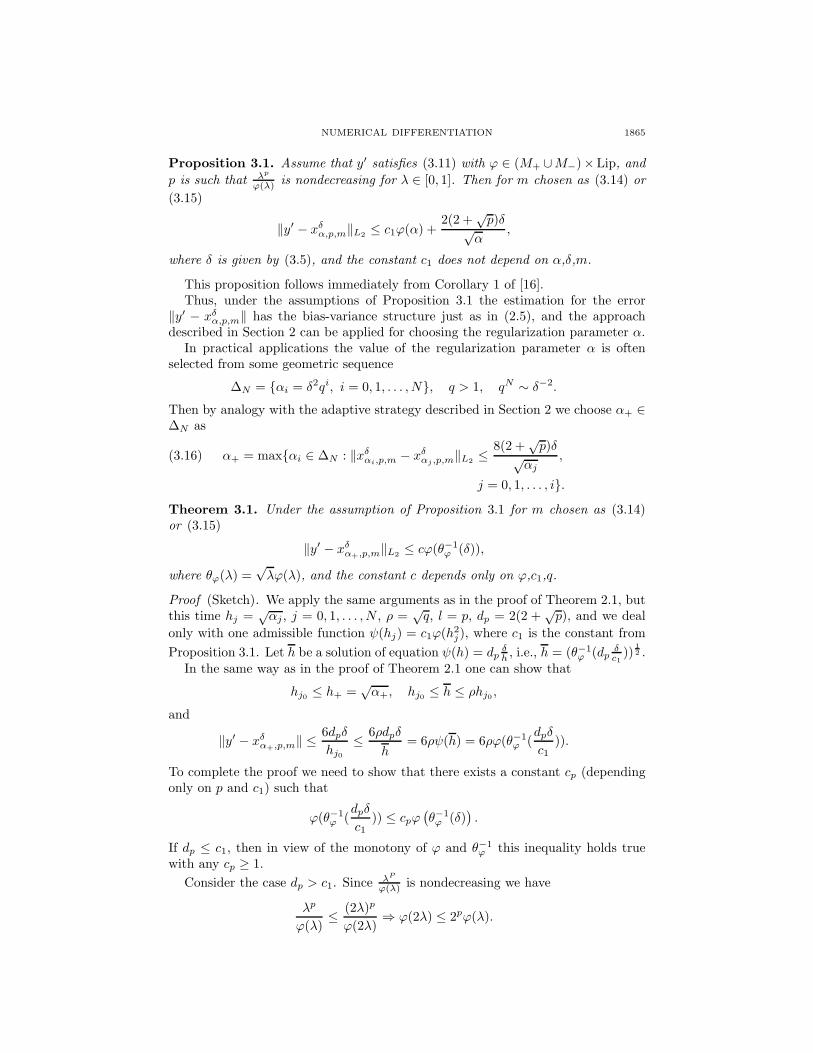
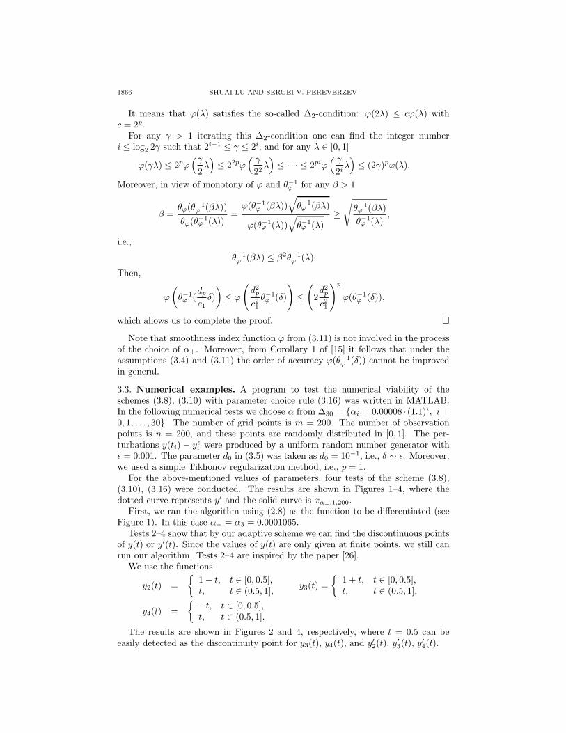
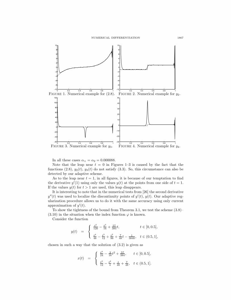
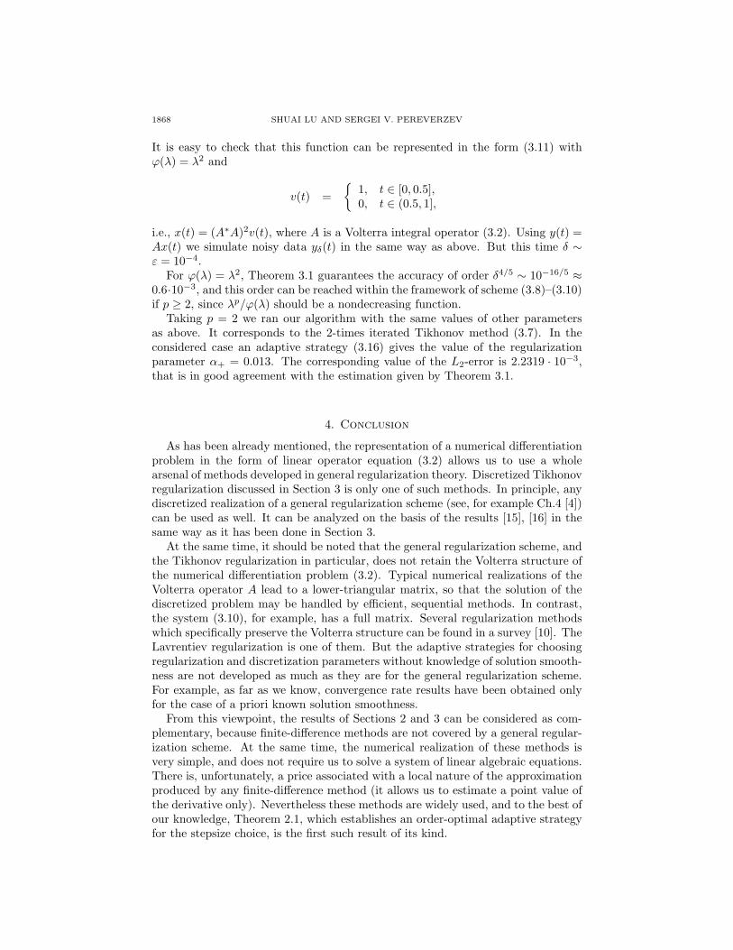
For the above-mentioned values of parameters, four tests of the scheme (3.8),(3.10), (3.16) were conducted. The results are shown in Figures 1–4, where thedotted curve represents y′ and the solid curve is xα+,1,200.

First, we ran the algorithm using (2.8) as the function to be differentiated (seeFigure 1). In this case α+ = α3 = 0.0001065.

Tests 2–4 show that by our adaptive scheme we can find the discontinuous pointsof y(t) or y′(t). Since the values of y(t) are only given at finite points, we still canrun our algorithm. Tests 2–4 are inspired by the paper [26].

We use the functions

y2(t) ={

1 − t, t ∈ [0, 0.5],t, t ∈ (0.5, 1], y3(t) =

{1 + t, t ∈ [0, 0.5],t, t ∈ (0.5, 1],

y4(t) ={

−t, t ∈ [0, 0.5],t, t ∈ (0.5, 1].

The results are shown in Figures 2 and 4, respectively, where t = 0.5 can beeasily detected as the discontinuity point for y3(t), y4(t), and y′

2(t), y′3(t), y′

4(t).


0 0.2 0.4 0.6 0.8 1−10

−8

−6

−4

−2

0

2

4

6

8

10

0 0.2 0.4 0.6 0.8 1−10

−8

−6

−4

−2

0

2

4

6

8

10

Figure 1. Numerical example for (2.8). Figure 2. Numerical example for y2.

0 0.2 0.4 0.6 0.8 1−60

−40

−20

0

20

40

60

80

100

120

0 0.2 0.4 0.6 0.8 1−30

−20

−10

0

10

20

30

40

50

Figure 3. Numerical example for y3. Figure 4. Numerical example for y4.

In all these cases α+ = α2 = 0.000088.Note that the leap near t = 0 in Figures 1–3 is caused by the fact that the

functions (2.8), y2(t), y3(t) do not satisfy (3.3). So, this circumstance can also bedetected by our adaptive scheme.

As to the leap near t = 1, in all figures, it is because of our temptation to findthe derivative y′(1) using only the values y(t) at the points from one side of t = 1.If the values y(t) for t > 1 are used, this leap disappears.

It is interesting to note that in the numerical tests from [26] the second derivativey′′(t) was used to localize the discontinuity points of y′(t), y(t). Our adaptive reg-ularization procedure allows us to do it with the same accuracy using only currentapproximation of y′(t).

To show the tightness of the bound from Theorem 3.1, we test the scheme (3.8)–(3.10) in the situation when the index function ϕ is known.

Consider the function

y(t) =

⎧⎨⎩

t5

120 − t3

16 + 57384 t, t ∈ [0, 0.5],

t4

48 − t3

12 + t2

96 + 748 t − 1

3840 , t ∈ (0.5, 1],

chosen in such a way that the solution of (3.2) is given as

x(t) =

⎧⎨⎩

t4

24 − 316 t2 + 57

384 , t ∈ [0, 0.5],

t3

12 − t2

4 + t48 + 7

48 , t ∈ (0.5, 1].


It is easy to check that this function can be represented in the form (3.11) withϕ(λ) = λ2 and

v(t) ={

1, t ∈ [0, 0.5],0, t ∈ (0.5, 1],

i.e., x(t) = (A∗A)2v(t), where A is a Volterra integral operator (3.2). Using y(t) =Ax(t) we simulate noisy data yδ(t) in the same way as above. But this time δ ∼ε = 10−4.

For ϕ(λ) = λ2, Theorem 3.1 guarantees the accuracy of order δ4/5 ∼ 10−16/5 ≈0.6·10−3, and this order can be reached within the framework of scheme (3.8)–(3.10)if p ≥ 2, since λp/ϕ(λ) should be a nondecreasing function.

Taking p = 2 we ran our algorithm with the same values of other parametersas above. It corresponds to the 2-times iterated Tikhonov method (3.7). In theconsidered case an adaptive strategy (3.16) gives the value of the regularizationparameter α+ = 0.013. The corresponding value of the L2-error is 2.2319 · 10−3,that is in good agreement with the estimation given by Theorem 3.1.

4. Conclusion

As has been already mentioned, the representation of a numerical differentiationproblem in the form of linear operator equation (3.2) allows us to use a wholearsenal of methods developed in general regularization theory. Discretized Tikhonovregularization discussed in Section 3 is only one of such methods. In principle, anydiscretized realization of a general regularization scheme (see, for example Ch.4 [4])can be used as well. It can be analyzed on the basis of the results [15], [16] in thesame way as it has been done in Section 3.

At the same time, it should be noted that the general regularization scheme, andthe Tikhonov regularization in particular, does not retain the Volterra structure ofthe numerical differentiation problem (3.2). Typical numerical realizations of theVolterra operator A lead to a lower-triangular matrix, so that the solution of thediscretized problem may be handled by efficient, sequential methods. In contrast,the system (3.10), for example, has a full matrix. Several regularization methodswhich specifically preserve the Volterra structure can be found in a survey [10]. TheLavrentiev regularization is one of them. But the adaptive strategies for choosingregularization and discretization parameters without knowledge of solution smooth-ness are not developed as much as they are for the general regularization scheme.For example, as far as we know, convergence rate results have been obtained onlyfor the case of a priori known solution smoothness.

From this viewpoint, the results of Sections 2 and 3 can be considered as com-plementary, because finite-difference methods are not covered by a general regular-ization scheme. At the same time, the numerical realization of these methods isvery simple, and does not require us to solve a system of linear algebraic equations.There is, unfortunately, a price associated with a local nature of the approximationproduced by any finite-difference method (it allows us to estimate a point value ofthe derivative only). Nevertheless these methods are widely used, and to the best ofour knowledge, Theorem 2.1, which establishes an order-optimal adaptive strategyfor the stepsize choice, is the first such result of its kind.


Acknowledgments

This research was supported by the Austrian Fonds Zur Forderung der Wis-senschaftlichen Forschung (FWF), Grant P17251-N12.

References

1. B.Anderssen, F.de Hoog, H.Hegland, A stable finite difference ansatz for higher order dif-ferentiation of non-exact data, Bull. Austral. Math. Soc., 22 (1998), 223–232. MR1642035(2000d:65037)

2. J.Cheng, M.Yamamoto, One new strategy for a priori choice of regularizing parameters inTikhonov’s regularization, Inverse Problems, 16 (2000), L31–38. MR1776470 (2001g:65073)

3. P.Deuflhard, H.W.Engl, O.Scherzer, A convergence analysis of iterative methods for the so-lution of nonlinear ill-posed problems under affinely invariant conditions, Inverse Problems,14 (1998), 1081–1106. MR1654603 (99j:65105)

4. H.W.Engl, M.Hanke, A.Neubauer, Regularization of Inverse Problems, Kluwer, Dordrect,1996. MR1408680 (97k:65145)

5. A.Goldenshluger, S.V.Pereverzev, Adaptive estimation of linear functionals in Hilbert scalesfrom indirect white noise observations, Probab. Theory Relat. Fields, 118 (2000), 169–186.MR1790080 (2001h:62055)

6. C.W.Groetsch, Differentiation of approximately specified functions, Am. Math. Mon., 98(1991), 847–850. MR1133003

7. M.Hanke, O.Scherzer, Inverse Problems light numerical differentiation, Am. Math. Mon., 108(2001), 512–521. MR1840657 (2002e:65089)

8. H.Harbrecht, S.Pereverzev, R.Schneider, Self-regularization by projection for noisy pseudo-differential equations of negative order, Numer. Math., 95 (2003), 123–143. MR1993941(2004j:65075)

9. M.Hegland, Variable Hilbert scales and their interpolation inequalities with applications toTikhonov regularization, Appl. Anal., 59 (1995), 207–223. MR1378036 (97a:65060)

10. P.K.Lamm, A survey of regularization methods for first-kind Volterra equations (English sum-mary), Surveys on solution methods for inverse problems, 53–82, Springer, Vienna, 2000.MR1766739 (2001b:65148)

11. O.V.Lepskii, A problem of adaptive estimation in Gaussian white noise, Theory Probab.Appl., 36 (1990), 454–466. MR1091202 (93j:62212)

12. F.Liu, M.Z.Nashed, Convergence of regularized solutions of nonlinear ill-posed problems withmonotone operators, Partial Differntial Equations and Application, Dekker, New York (1996),353-361. MR1371608 (97m:65112)

13. P.Mathe, S.V.Pereverzev, Optimal discretization of inverse problems in Hilbert scales. Regu-larization and self-regularization of projection methods, SIAM J. Numer. Analysis, 38 (2001),1999-2021. MR1856240 (2002g:62063)

14. P.Mathe, S.V.Pereverzev, Moduli of continuity for operator valued functions, Numer. Funct.Anal. Optim., 23 (2002), 623–631. MR1923828 (2003g:47029)

15. P.Mathe, S.V.Pereverzev, Geometry of linear ill-posed problems in variable Hilbert scales,

Inverse Problems, 19 (2003), 789–803. MR1984890 (2004i:47021)16. P.Mathe, S.V.Pereverzev, Discretization strategy for linear ill-posed problems in variable

Hilbert scales, Inverse Problems, 19 (2003), 1263–1277. MR2036530 (2004k:65097)17. P.Mathe, S.V.Pereverzev, Regularization of some linear ill-posed problems with discretized

random noisy data, Math. Comp. (Accepted).18. M.T.Nair, E.Schock, U.Tautenhahn, Morozov’s discrepancy principle under general source

conditions, Z. Anal. Anwendungen, 22 (2003), 199-214. MR1962084 (2004a:65069)19. A.Neumaier, Solving ill-conditioned and singular linear systems: A tutorial on regularization,

SIAM Rev., 40 (1998), 636-666. MR1642811 (99f:65066)20. S.Pereverzev, E.Schock, On the adaptive selection of the parameter in regularization of ill-

posed problems, SIAM J. Numer. Analysis, 43 (2005), 2060–2076. MR219233121. R.Qu, A new approach to numerical differentiation and integration, Math. Comput. Mod-

elling, 24 (1996), 55-68. MR1426303 (98b:65024)22. A.G.Ramm, A.B.Smirnova, On stable numerical differentiation, Math. Comp., 70 (2001),

1131–1153. MR1826578 (2002a:65046)

http://www.ams.org/mathscinet-getitem?mr=1642035









































23. U.Tautenhahn, Optimality for ill-posed problems under general source conditions, Numer.Funct. Anal. Optim., 19 (1998), 377–398. MR1624930 (99g:65073)

24. U.Tautenhahn, On the method of Lavrentiev regularization for nonlinear ill-posed problems,Inverse Problems, 18 (2002), 191–207. MR1893590 (2002m:47079)

25. A.Tsybakov, On the best rate of adaptive estimation in some inverse problems, C. R. Acad.Sci. Paris Ser. I Math., 330 (2000), 835–840. MR1769957 (2001c:62058)

26. Y.B.Wang, X.Z.Jia, J.Cheng, A numerical differentiation method and its application to recon-

struction of discontinuity, Inverse Problems, 18 (2002), 1461–1476. MR1955897 (2004b:65086)

Johann Radon Institute for Computational and Applied Mathematics (RICAM), Aus-

trian Academy of Science, Altenbergerstrasse 69, A-4040 Linz, Austria

E-mail address: [email protected]

Johann Radon Institute for Computational and Applied Mathematics (RICAM), Aus-

trian Academy of Science, Altenbergerstrasse 69, A-4040 Linz, Austria

E-mail address: [email protected]









numerical differentiation from a viewpoint of regularization theory

Documents