receptive fields and tuning curves
TRANSCRIPT

THEORETICAL NEUROSCIENCE I
Lecture 9: Receptive fields and tuning curves
Prof. Jochen Braun
Otto-von-Guericke-Universitat Magdeburg,Cognitive Biology Group

Content
1. Frog vision
2. Cat vision
3. Receptive fields, response variability, and tuning curves
4. Reverse correlation methods
1
Sensation, perception, and representation
Possible stages of sensory processing (vision, audition, somatosensation,
olfaction, gustation):
• Sensation: a physical stimulus impinges on receptors cells of a
sensory organ. Elementary properties of stimulation are transduced
into neural activity (e.g., light, sound).
• Perception (human): the mental process of becoming aware of,
understanding, and recognizing the physical causes of sensory
stimulation. Perception produces the insight that guides behaviour.
• Representation: As the initial sensory activity propagates from
receptors to thalamus, primary sensory cortex, secondary sensory
cortex, and associative cortex, its neural representation continues to
change. Presumably, this succession of representations contributes to
perception.
2
1 Frog vision
From Lettvin, Maturana, McCulloch, and Pitts (1959):
“A Frog hunts on land by vision. He escapes enemies mainly by seeing
them. His eyes do not move, as do ours, to follow prey, attend
suspicious event, or search for things of interest. If his body changes its
position with respect to gravity or the whole visual world is rotated
about him, then he shows compensatory eye movements. These
movements enter his hunting and evading habits only, e.g. as he sits on
a rocking lily pad. Thus, his eyes are actively stabilized. He has no
fovea, or region of greatest acuity in vision, upon which he must center
a part of the image . . .
From Lettvin, Maturana, McCulloch, and Pitts (1959):
. . . The frog does not seem to see or, at any rate, is not concerned with
the detail of stationary parts of the world around him. He will starve to
death surrounded by food, if it is not moving. His choice of food is
determined only by size and movement. He will leap to capture any
object the size of an insect or worm, providing it moves like one. He can
be fooled easily not only by a piece of dangled meat but by any moving
small object. His sex life is conducted by sound and touch. His choice of
paths in escaping enemies does not seem to be governed by anything
more devious than leaping to where it is darker. Since he is equally at
home in water and on land, why should it matter where he lights after
jumping or what particular direction he takes? He does remember a
moving thing provided it stays within his field of vision and he is not
distracted.”
3

Frog Eye Characteristics
The thick lens gives the animal a large field of view. The frog is
naturally nearsighted (-6 diopters) giving it a focus of approximately 6
inches. Frogs and toads can change their focus by moving the lens out
towards the cornea. The advantage of nearsightedness is that it blurs
the background clutter making foreground object characterization much
easier.
Figure 1: [1]
Response Classes of the Ganglion Cells
Class 1 and class 2 ganglion cells project to the brain via unmyelinated
fibers having conduction velocities of 20 to 50 centimeters per second.
They make up 97 percent of the optic nerve (Maturana - 1959).
• Class 1 neurons (edge detectors): These neurons have oval receptive
fields from 1.5 to 4 degrees in size. They detect the completeness
and sharpness of both light and dark edges. They respond to
stationary edges, but more vigorously to edge movement.
• Class 2 neurons (convexity detectors): These neurons have oval
receptive fields ranging in size from 2.5 to 5 degrees. They seem to
detect the dark leading edge (head) of any worm or bug. If the
stimulus stops beforer eaching the RF center, the response slowly
4
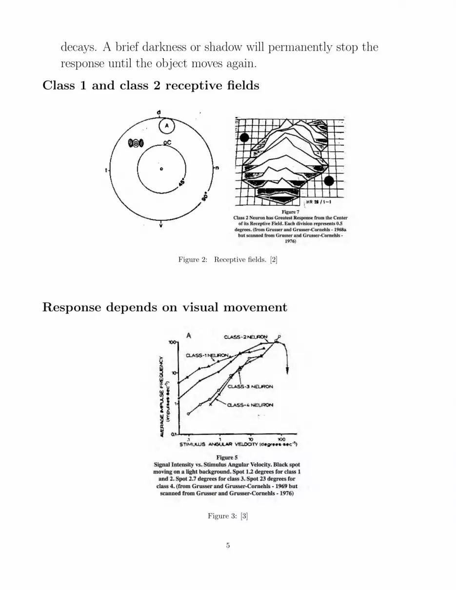
decays. A brief darkness or shadow will permanently stop the
response until the object moves again.
Class 1 and class 2 receptive fields
Figure 2: Receptive fields. [2]
Response depends on visual movement
Figure 3: [3]
5

What the frog’s eyes tell the frog’s brain
(Lettvin, Maturana, McCulloch, Pitts, 1968)
The output of the retina is a set of four distributed operations on the
visual image. 1) local sharp edges and contrasts, 2) curvature of edge of
a dark object, 3) movement of edges, 4) local dimmings by movement or
darkening. Each operation maps the retina continuously on a single
sheet in the frog’s brain. There are four such sheets, and their maps are
in registration.
We have described each operation in terms of its common factors. So
what does a particular fibre measure? The degree to which a particular
quality is present (the quality that excites the fibre maximally).
The operations have much more a flavor of perception than of
sensation, if that distinction has any meaning now (1968!).
Summary frog vision
• “The eye speaks to the brain in a language already highly organized
and interpreted, instead of transmitting an accurate copy of light on
receptors. . . . Since the purpose of a frog’s vision is to get him food
and allow him to evade predators, it is not enough to know the
reaction of his visual system to points of light.”
• Sensory systems (e.g., vision) are optimized for a specific ecological
niche and behavior.
• Sensory neurons are particularly sensitive to behaviorally relevant
stimuli (e.g., edible prey).
• Presumed (‘putative’) neural correlates of perception already in
retinal ganglion cell responses.
6
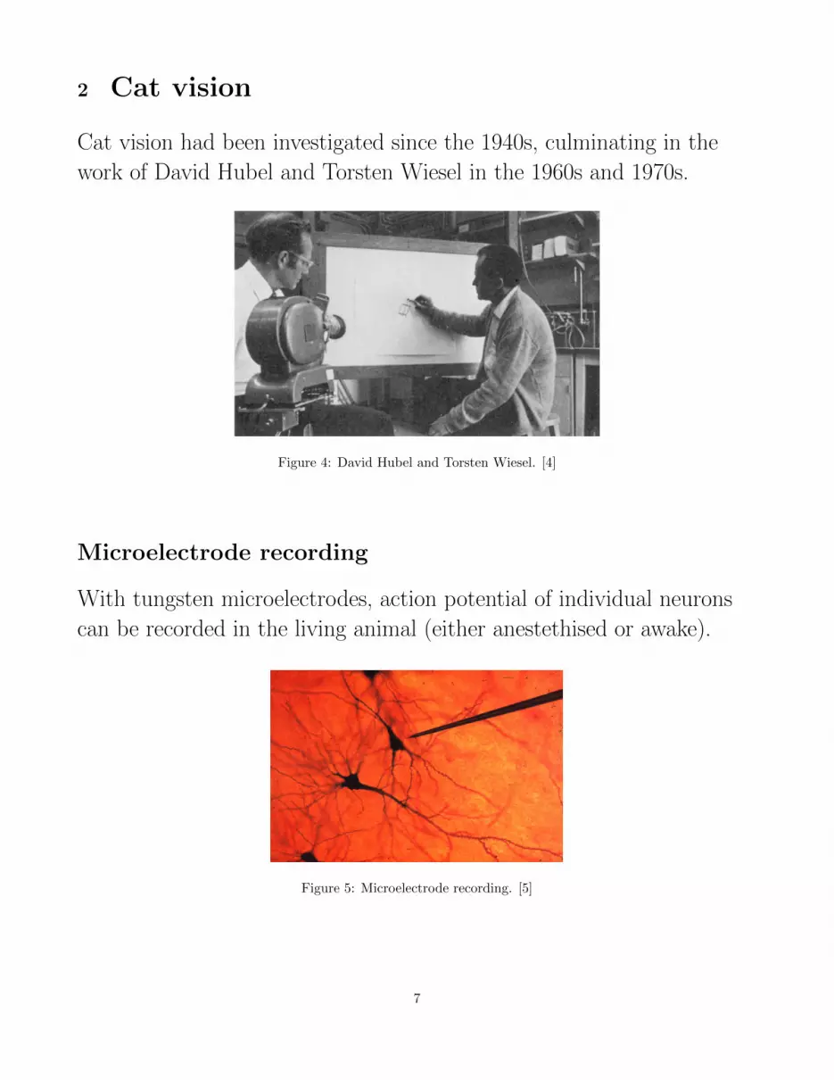
2 Cat vision
Cat vision had been investigated since the 1940s, culminating in the
work of David Hubel and Torsten Wiesel in the 1960s and 1970s.
Figure 4: David Hubel and Torsten Wiesel. [4]
Microelectrode recording
With tungsten microelectrodes, action potential of individual neurons
can be recorded in the living animal (either anestethised or awake).
Figure 5: Microelectrode recording. [5]
7

Visually responsive neurons can be recorded in retina, lateral geniculate
nucleus, and visual cortex.
Figure 6: ON/OFF and center/surround structure. [6]
t
V
500 ms
Off On Off
Ganglion Cell Responseto Illumination
Figure 7: ON/OFF and center/surround structure. [7]
8
t
V
500 ms
Off On Off
Ganglion Cell Responseto Illumination
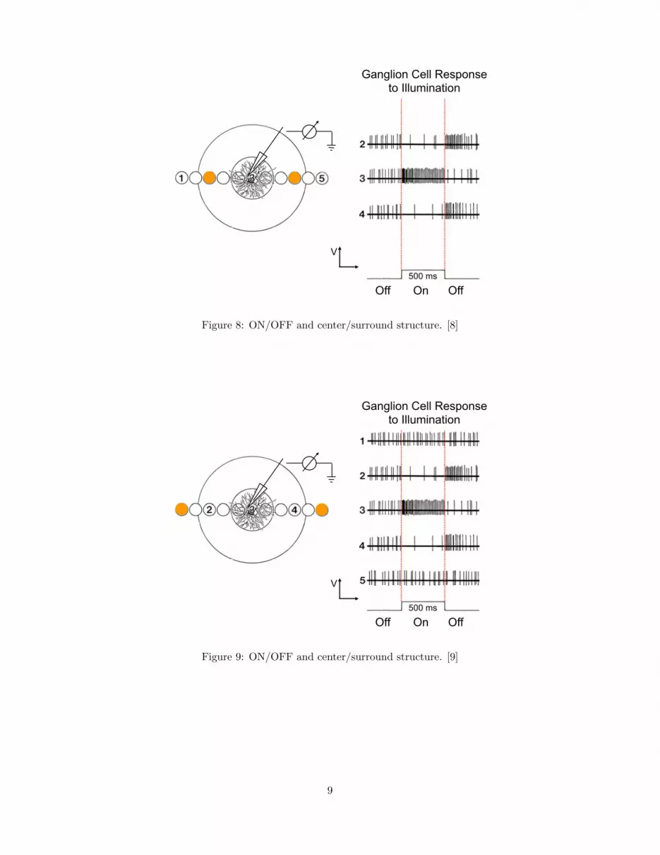
Figure 8: ON/OFF and center/surround structure. [8]
t
V
500 ms
Off On Off
Ganglion Cell Responseto Illumination
Figure 9: ON/OFF and center/surround structure. [9]
9

t
V
500 ms
Off On Off
Ganglion Cell Responseto Illumination
Receptive Field
Figure 10: ON/OFF and center/surround structure. [10]
t
V
500 ms
Off On Off
Ganglion Cell Responseto Illumination
Receptive Field
ExcitatoryCenter
Figure 11: ON/OFF and center/surround structure. [11]
10

Receptive Field
Inhibitory Surroundt
V
500 ms
Off On Off
Ganglion Cell Responseto Illumination
Figure 12: ON/OFF and center/surround structure. [12]
Receptive Field
Inhibitory Surround
ExcitatoryCenter t
V
500 ms
Off On Off
Ganglion Cell Responseto Illumination
Figure 13: ON/OFF and center/surround structure. [13]
Summary ON/OFF and center/surround
11
Visually response neurons in the cat retina and in the lateral geniculate
nucleus of the thalamus show a particular receptive field structure:
• Small size (∼ 0.1◦ in fovea).
• Separate ON and OFF regions.
• ON regions respond to onset of light or offset of dark.
• OFF regions respond to onset of dark or offset of light.
• Small center with larger (concentric) surround.
• ON-center, OFF-surround (or vice versa).
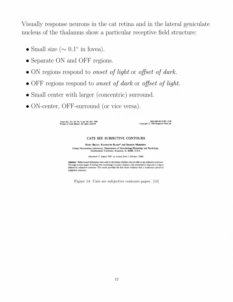
Figure 14: Cats see subjective contours paper. [14]
12
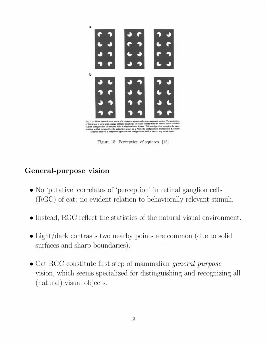
Figure 15: Perception of squares. [15]
General-purpose vision
• No ‘putative’ correlates of ‘perception’ in retinal ganglion cells
(RGC) of cat: no evident relation to behaviorally relevant stimuli.
• Instead, RGC reflect the statistics of the natural visual environment.
• Light/dark contrasts two nearby points are common (due to solid
surfaces and sharp boundaries).
• Cat RGC constitute first step of mammalian general purpose
vision, which seems specialized for distinguishing and recognizing all
(natural) visual objects.
13

3 Receptive fields, response variability, andtuning curves
Neuroscientists describe the responses of sensory neurons and formulate
hypotheses as to their contribution to behaviour.
Several heuristic concepts have proven extremely useful.
We now introduce three of these concepts.
Adopting this descriptive approach, we do not take any position on theissue of ‘perception’ versus ‘sensation’. The neural responses we describewill gradually become less ‘sensation-like’ and more ‘perception-like’.
Definition:
A ”receptive field” is the area in sensory space where
stimulation is required to drive a neuron.
Figure 16: Receptive fields. [16]
Definition:
“Response variability” is the variability of a neuron’s
response to repeated presentation of identical stimuli.
The activity of neurons is variable both in the absence and in the
presence of stimuli. Thus, repeated presentation of identical stimuli
typically elicits a wide range of responses.
14

Consequently, the response of a neuron to different stimuli needs to be
characterized statistically. Measurements must be performed multiple
times to establish response mean and response variance.
Response variability limits the informativeness of a neuron’s response!
Definition:
A ”tuning curve” is the dependence of the average
response on one particular stimulus parameter.
A neuron’s response typically depends on many different stimulus
parameters. A tuning curve characterizes the response as a function of
just one of these parameters. It is measured by repeatedly presenting
stimuli with different parameter values.
A neuron has many different tuning curves (one for each parameter
affecting its response). A tuning curve characterizes the neuron’s
response partially, but never completely.
A tuning curve r = f (s) is the average number of spikes relicited by presentation of a particular stimulus attributes.
Gaussian tuning
Tuning for stimulus orientation in the primary visual cortex of monkey:
r = f (s) = rmax exp
−1
2
s− smaxσs
2 Gaussian tuning
15

Figure 17: Gaussian tuning. [17]
Cosine tuning
Tuning for direction of arm movement in the primary motor cortex of
monkey:
r = f (s) = r0 + (rmax − r0) cos (s− smax) Cosine tuning
Figure 18: Cosine tuning. [18]
Sigmoidal tuning
Tuning for binocular disparity in the primary visual cortex of monkey
(approximated by logistic function):
16
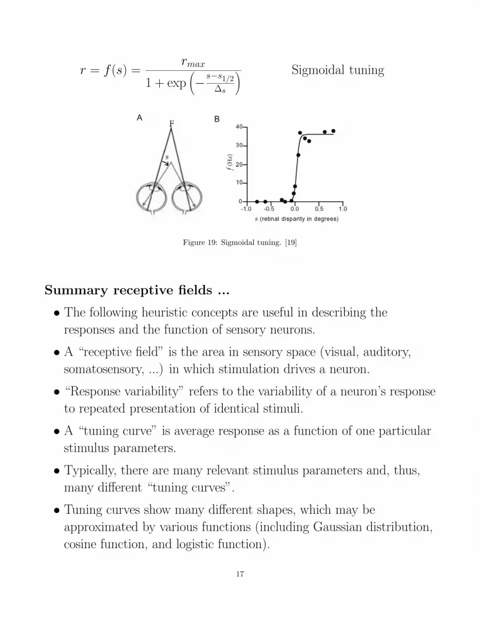
r = f (s) =rmax
1 + exp(−s−s1/2
∆s
) Sigmoidal tuning
Figure 19: Sigmoidal tuning. [19]
Summary receptive fields ...
• The following heuristic concepts are useful in describing the
responses and the function of sensory neurons.
• A “receptive field” is the area in sensory space (visual, auditory,
somatosensory, ...) in which stimulation drives a neuron.
• “Response variability” refers to the variability of a neuron’s response
to repeated presentation of identical stimuli.
• A “tuning curve” is average response as a function of one particular
stimulus parameters.
• Typically, there are many relevant stimulus parameters and, thus,
many different “tuning curves”.
• Tuning curves show many different shapes, which may be
approximated by various functions (including Gaussian distribution,
cosine function, and logistic function).
17
4 Reverse correlation methods
We seek more systematic and objective ways of describing neuronal
responses.
To this end, we bombard a neuron with a rapid sequence of stimuli,
drawn randomly from a large ensemble.
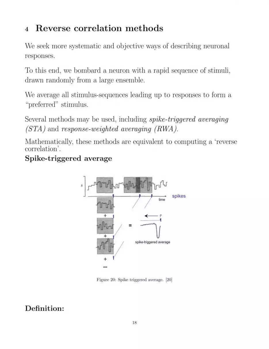
We average all stimulus-sequences leading up to responses to form a
“preferred” stimulus.
Several methods may be used, including spike-triggered averaging
(STA) and response-weighted averaging (RWA).
Mathematically, these methods are equivalent to computing a ‘reversecorrelation’.
Spike-triggered average
spikes
Figure 20: Spike triggered average. [20]
Definition:
18

The spike-triggered average stimulus 〈s(−τ )〉 is the average
value of the stimulus at some time τ before a spike is fired.
Spike times ti
Stimulus function s(t)
Reversed and shifted s(ti − τ )
Note that s(ti − τ ) is the stimulus stretching backwards in time from ti,as τ grows from 0 to ∞To compute the spike-triggered average stimulus, we average over the
stimulus functions which stretch back in time from each spike ti:
〈s(−τ )〉 =1
n
n∑i=1
s(ti − τ )
where n is the number of spikes per trial.
STA example
Figure 21: STA example. [21]
19

0 50 100 150 200 250 300 350 4000.2
0.4
0.6
0.8
1
Stim
ulu
s0 50 100 150 200 250 300 350 400
time [ms]
0
0.2
0.4
0.6
0.8
1
Response
Figure 22: Example stimulus and response.
0 5 10 15 20
time [ms]
0.45
0.5
0.55
0.6
Stim
ulu
s
Nspike
= 1
Figure 23: Spike-triggered average.
20
0 2 4 6 8 10 12 14 16 18 20
time [ms]
0.3
0.4
0.5
0.6
0.7
0.8
0.9
Stim
ulu
s
Nspike
= 7
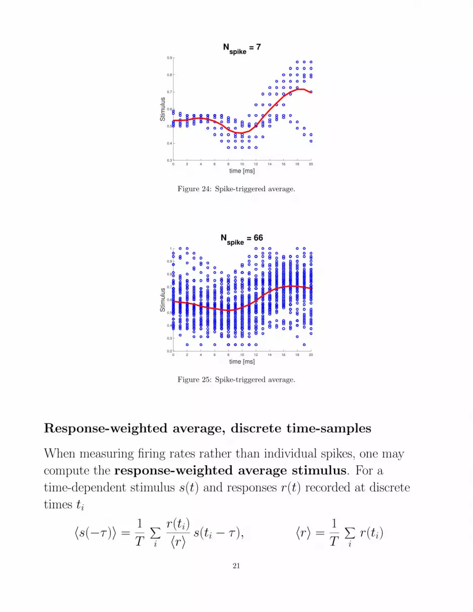
Figure 24: Spike-triggered average.
0 2 4 6 8 10 12 14 16 18 20
time [ms]
0.2
0.3
0.4
0.5
0.6
0.7
0.8
0.9
1
Stim
ulu
s
Nspike
= 66
Figure 25: Spike-triggered average.
Response-weighted average, discrete time-samples
When measuring firing rates rather than individual spikes, one may
compute the response-weighted average stimulus. For a
time-dependent stimulus s(t) and responses r(t) recorded at discrete
times ti
〈s(−τ )〉 =1
T
∑i
r(ti)
〈r〉s(ti − τ ), 〈r〉 =
1
T
∑ir(ti)
21
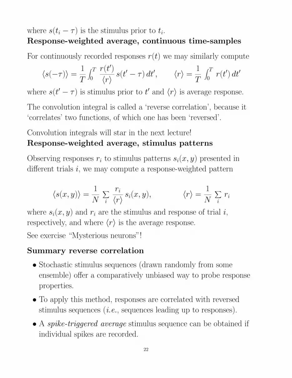
where s(ti − τ ) is the stimulus prior to ti.
Response-weighted average, continuous time-samples
For continuously recorded responses r(t) we may similarly compute
〈s(−τ )〉 =1
T
∫ T0
r(t′)
〈r〉s(t′ − τ ) dt′, 〈r〉 =
1
T
∫ T0r(t′) dt′
where s(t′ − τ ) is stimulus prior to t′ and 〈r〉 is average response.
The convolution integral is called a ‘reverse correlation’, because it
‘correlates’ two functions, of which one has been ‘reversed’.
Convolution integrals will star in the next lecture!
Response-weighted average, stimulus patterns
Observing responses ri to stimulus patterns si(x, y) presented in
different trials i, we may compute a response-weighted pattern
〈s(x, y)〉 =1
N
∑i
ri〈r〉
si(x, y), 〈r〉 =1
N
∑iri
where si(x, y) and ri are the stimulus and response of trial i,
respectively, and where 〈r〉 is the average response.
See exercise “Mysterious neurons”!
Summary reverse correlation
• Stochastic stimulus sequences (drawn randomly from some
ensemble) offer a comparatively unbiased way to probe response
properties.
• To apply this method, responses are correlated with reversed
stimulus sequences (i.e., sequences leading up to responses).
• A spike-triggered average stimulus sequence can be obtained if
individual spikes are recorded.
22

• A response-weighted average stimulus sequence can be computed if
firing rates are recorded.
• Mathematically, both methods involve the reverse correlation, or
convolution, between response and stimulus sequences.
• A response-weighted average can be computed also for distinct
stimulus patterns.
23
5 References1. Neurophysology of the Anuran Visual System*. J. Grsser, et al. Page 298, figure 1A . Ref:
https://link.springer.com/chapter/10.1007
2. Heinz Wscle, personal communication.
3. Heinz Wscle, personal communication.
4. Deep Learning Summit (DLS01-1). Slide Share. Anonymous, 2017. Slide 17. Ref:https://www.slideshare.net/AmazonWebServices/deep-learning-summit-dls011
5. Eavesdropping on Neurons. Harvard Brain Tour. Anonymous, 2016. Image 3 Ref:http://braintour.harvard.edu/archives/portfolio-items/eavesdropping-on-neurons
6. Dendritenbaum und konzentrisches rezeptives Feld einer ON-Zentrum-Ganglienzelle. Extrem News.Anonymous. Image 1 Ref:https://www.extremnews.com/berichte/gesundheit/e01c12cc1d3c89f/d02812cc2034dd9/info
7. Dendritenbaum und konzentrisches rezeptives Feld einer ON-Zentrum-Ganglienzelle. Extrem News.Anonymous. Image 1 Ref:https://www.extremnews.com/berichte/gesundheit/e01c12cc1d3c89f/d02812cc2034dd9/info
8. Dendritenbaum und konzentrisches rezeptives Feld einer ON-Zentrum-Ganglienzelle. Extrem News.Anonymous. Image 1 Ref:https://www.extremnews.com/berichte/gesundheit/e01c12cc1d3c89f/d02812cc2034dd9/info
9. Dendritenbaum und konzentrisches rezeptives Feld einer ON-Zentrum-Ganglienzelle. Extrem News.Anonymous. Image 1 Ref:https://www.extremnews.com/berichte/gesundheit/e01c12cc1d3c89f/d02812cc2034dd9/info
10. Dendritenbaum und konzentrisches rezeptives Feld einer ON-Zentrum-Ganglienzelle. Extrem News.Anonymous. Image 1 Ref:https://www.extremnews.com/berichte/gesundheit/e01c12cc1d3c89f/d02812cc2034dd9/info
11. Dendritenbaum und konzentrisches rezeptives Feld einer ON-Zentrum-Ganglienzelle. Extrem News.Anonymous. Image 1 Ref:https://www.extremnews.com/berichte/gesundheit/e01c12cc1d3c89f/d02812cc2034dd9/info
12. Dendritenbaum und konzentrisches rezeptives Feld einer ON-Zentrum-Ganglienzelle. Extrem News.Anonymous. Image 1 Ref:https://www.extremnews.com/berichte/gesundheit/e01c12cc1d3c89f/d02812cc2034dd9/info
13. Dendritenbaum und konzentrisches rezeptives Feld einer ON-Zentrum-Ganglienzelle. Extrem News.Anonymous. Image 1 Ref:https://www.extremnews.com/berichte/gesundheit/e01c12cc1d3c89f/d02812cc2034dd9/info
14. Cats see subjective contours. Cresap Neuroscience Laboratory. 1988. Mary Bravo, et al. Ref:https://www.gwern.net/docs/catnip/1988-bravo.pdf
15. Cats see subjective contours. Cresap Neuroscience Laboratory. 1988. Mary Bravo, et al. Fig. 2 Ref:https://www.extremnews.com/berichte/gesundheit/e01c12cc1d3c89f/d02812cc2034dd9/info
16. Visual fields interpretation in glaucoma: A focus on static automated perimetry. Community eye health /International Centre for Eye Health. 25. 1-8. Yaqub, Moustafa, 2012. Figure 2.https://www.researchgate.net/figure/
Diagram-of-the-visual-fi-eld-for-the-right-eye-The-three-regions-of-the-fi-eld-are-the_
fig1_248384750
24

17. Motion-based position coding in the visual system: a computational study. A Khoei, Mina, 2014. Figure 1.Ref: https://www.researchgate.net/figure/Seminal-results-of-Hubel-and-Wiesel-figure-adopted-from-Hubel-and-Wiesel-1968_fig1_
280736145
18. What is the neural code? Spike coding. Sekuler lab, Brandeis. Slide 11. Ref:https://courses.cs.washington.edu/courses/cse528/09sp/Lect2.pdf
19. What is the neural code? Spike coding. Sekuler lab, Brandeis. Slide 12. Ref:https://courses.cs.washington.edu/courses/cse528/09sp/Lect2.pdf
20. What is the neural code? Spike coding. Sekuler lab, Brandeis. Slide 20. Ref:https://courses.cs.washington.edu/courses/cse528/09sp/Lect2.pdf
21. What is the neural code? Spike coding. Sekuler lab, Brandeis. Slide 21. Ref:https://courses.cs.washington.edu/courses/cse528/09sp/Lect2.pdf
25