automatic mapping of multiplexed social receptive fields by

ARTICLE

Automatic mapping of multiplexed social receptivefields by deep learning and GPU-accelerated 3DvideographyChristian L. Ebbesen 1,2,3,4,5✉ & Robert C. Froemke 1,2,3,4,5✉

Social interactions powerfully impact the brain and the body, but high-resolution descriptions

of these important physical interactions and their neural correlates are lacking. Currently,

most studies rely on labor-intensive methods such as manual annotation. Scalable and

objective tracking methods are required to understand the neural circuits underlying social

behavior. Here we describe a hardware/software system and analysis pipeline that combines

3D videography, deep learning, physical modeling, and GPU-accelerated robust optimization,

with automatic analysis of neuronal receptive fields recorded in interacting mice. Our system

(“3DDD Social Mouse Tracker”) is capable of fully automatic multi-animal tracking with

minimal errors (including in complete darkness) during complex, spontaneous social

encounters, together with simultaneous electrophysiological recordings. We capture posture

dynamics of multiple unmarked mice with high spatiotemporal precision (~2 mm, 60 frames/

s). A statistical model that relates 3D behavior and neural activity reveals multiplexed ‘social

receptive fields’ of neurons in barrel cortex. Our approach could be broadly useful for neu-

robehavioral studies of multiple animals interacting in complex low-light environments.

https://doi.org/10.1038/s41467-022-28153-7 OPEN

1 Skirball Institute of Biomolecular Medicine, New York University School of Medicine, New York, NY 10016, USA. 2Neuroscience Institute, New YorkUniversity School of Medicine, New York, NY 10016, USA. 3 Department of Otolaryngology, New York University School of Medicine, New York, NY 10016,USA. 4Department of Neuroscience and Physiology, New York University School of Medicine, New York, NY 10016, USA. 5 Center for Neural Science, NewYork University, New York, NY 10003, USA. ✉email: [email protected]; [email protected]

NATURE COMMUNICATIONS | (2022) 13:593 | https://doi.org/10.1038/s41467-022-28153-7 | www.nature.com/naturecommunications 1

1234

5678

90():,;

http://crossmark.crossref.org/dialog/?doi=10.1038/s41467-022-28153-7&domain=pdf




http://orcid.org/0000-0002-3492-9841

http://orcid.org/0000-0002-3492-9841

http://orcid.org/0000-0002-3492-9841

http://orcid.org/0000-0002-3492-9841

http://orcid.org/0000-0002-3492-9841

http://orcid.org/0000-0002-1230-6811

http://orcid.org/0000-0002-1230-6811

http://orcid.org/0000-0002-1230-6811

http://orcid.org/0000-0002-1230-6811

http://orcid.org/0000-0002-1230-6811

mailto:[email protected]

mailto:[email protected]

www.nature.com/naturecommunications


Objective quantification of natural social interactions isdifficult. The majority of our knowledge about rodentsocial behavior comes from hand-annotation of videos,

yielding ethograms of discrete social behaviors such as ‘socialfollowing’, ‘mounting’, or ‘anogenital sniffing’1. It is widelyappreciated that these methods are susceptible to experimenterbias and have limited throughput. There is an additional problemwith these approaches, in that manual annotation of behavioryields limited information about movement kinematics andphysical body postures. This shortcoming is especially critical forstudies relating neural activity patterns or other physiologicalsignals to social behavior. For example, neural activity in manyareas of the cerebral cortex is strongly modulated by movementand posture2,3, and activity profiles in somatosensory regions canbe difficult to analyze without understanding the physics andhigh-resolution dynamics of touch. Important aspects of socialbehavior, from gestures to light touch and momentary glancescan be transient and challenging to observe in most settings, butcritical to capturing the details and changes to social relationshipsand networks4,5.

The use of deep convolutional networks to recognize objects inimages has revolutionized computer vision, and consequently,also led to major advances in behavioral analysis. Drawing uponthese methodological advances, several recent publications havedeveloped algorithms for single animal6–13 and multi-animaltracking14–21. These methods function by detection of key-pointsin 2D videos, and estimation of 3D postures is not straightfor-ward in interacting animals, where some form of spatiotemporalregularization is needed to ensure that tracking is stable anderror-free, even when multiple animals are closely interacting.During mounting or allo-grooming, for example, interactinganimals block each other from the camera view, and trackingalgorithms can fail. Having a large number of cameras film theanimals from all sides can solve these problems22,23, but this hasrequired extensive financial resources for equipment, laboratoryspace, and processing power, which renders widespread useinfeasible.

Some recent single24- and multi-animal17–19 tracking methodshave bypassed the problem of estimating the 3D posture of closelyinteracting animals by training a classifier to replicate humanlabeling discrete behavioral categories, such as attack andmounting. This approach is very powerful for automaticallygenerating ethograms; however, for relating neural data tobehavior, the lack of detailed information about movement andposture kinematics of interacting animals can be a criticaldrawback. In essentially every brain region, neural activity ismodulated by motor signals25–28 and vestibular signals2,3,29.Thus, any observed differences in neural activity between beha-vioral categories may simply be related instead to differences inmovements and postures made by the animals in those differentcategories. To reveal how neural circuits process body language,touch, and other social cues21 during a social interaction,descriptions of neural coding must be able to account for theseimportant but complex motor- and posture-related activity pat-terns or confounds.

In parallel with deep-learning-based tracking methods, somestudies have used depth-cameras for animal tracking, by fitting aphysical 3D body-model of the animal to 3D data30–32. Thesemethods are powerful because they can explicitly model the 3Dmovement and poses of multiple animals, throughout the socialinteraction. However, due to technical limitations of depth ima-ging hardware (e.g., frame rate, resolution, motion blur), to date ithas been possible only to extract partial posture informationabout small and fast-moving animals, such as lab mice. Conse-quently, when applied to mice, these methods are prone totracking mistakes when interacting animals get close to each

other and the tracking algorithms require continuous manualsupervision to detect and correct errors. This severely restrictsthroughput, making tracking across long time scales infeasible.

Here we describe a system for multi-animal tracking andneuro-behavioral data analysis that combines ideal features fromboth approaches: The 3D Deep-learning, Depth-video SocialMouse Tracker (“3DDD Social Mouse Tracker”, https://github.com/chrelli/3DDD_social_mouse_tracker/). Our methodfuses physical modeling of depth data and deep learning-basedanalysis of synchronized color video to estimate 3D body pos-tures, enabling us to reliably track multiple mice during natur-alistic social interactions. Our method is fully automatic (i.e.,quantitative, scalable, and free of experimenter bias), is based oninexpensive consumer cameras, and is implemented in Python, asimple and widely used computing language. Our method iscapable of tracking the animals using only infrared video chan-nels (i.e., in visual darkness for mice, a nocturnal species), is self-aligning, and requires only a few hundred labeled frames fortraining. We combine our tracking method with silicon proberecordings of single-unit activity in barrel cortex to demonstratethe usefulness of a continuous 3D posture estimation and aninterpretable body model: We implement a full-automatic neuraldata analysis pipeline (included along with the tracking code),that yields a population-level map of neural tuning to the featuresof a social interaction (social touch, movements, postures, spatiallocation, etc.) directly from raw behavior video and spike trains.

ResultsRaw data acquisition. We built an experimental setup thatallowed us to capture synchronized color images and depthimages from multiple angles, while simultaneously recordingsynchronized neural data (Fig. 1a). We used inexpensive, state-of-the-art ‘depth cameras’ for computer vision and robotics. Thesecameras contain several imaging modules: one color sensor, twoinfrared sensors, and an infrared laser projector (Fig. 1b). Ima-ging data pipelines, as well as intrinsic and extrinsic sensor cali-bration parameters can be accessed over USB through a C/C++SDK with Python bindings. We placed four depth cameras, aswell as four synchronization LEDs around a transparent acryliccylinder which served as our behavioral arena (Fig. 1c).

Each depth camera projects a static dot pattern across theimaged scene, adding texture in the infrared spectrum toreflective surfaces (Fig. 1d). By imaging this highly-texturedsurface simultaneously with two infrared sensors per depthcamera, it is possible to estimate the distance of each pixel in theinfrared image to the depth camera by stereopsis (by locallyestimating the binocular disparity between the textured images).Since the dot pattern is static and only serves to add texture,multiple cameras do not interfere with each other and it ispossible to image the same scene simultaneously from multipleangles. Simultaneous capture from all angles is one key aspect ofour method, not possible with depth imaging systems that rely onactively modulated light (such as the Microsoft Kinect system andearlier versions of the Intel Realsense cameras, where multi-viewcapture requires offset capture times).

Since mouse movement is fast (on a millisecond time scale33),it is vital to minimize motion blur in the infrared images and thusthe final 3D data (‘point-cloud’). To this end, our method relieson two key features. First, we use depth cameras where theinfrared sensors have a global shutter (e.g., Intel D435) ratherthan a rolling shutter (e.g., Intel D415). Using a global shutterreduces motion blur in individual image frames, but also enablessynchronized image capture across cameras. Without synchroni-zation between cameras, depth images are taken at differenttimes, which adds blur to the composite point-cloud. We set

ARTICLE NATURE COMMUNICATIONS | https://doi.org/10.1038/s41467-022-28153-7

2 NATURE COMMUNICATIONS | (2022) 13:593 | https://doi.org/10.1038/s41467-022-28153-7 | www.nature.com/naturecommunications

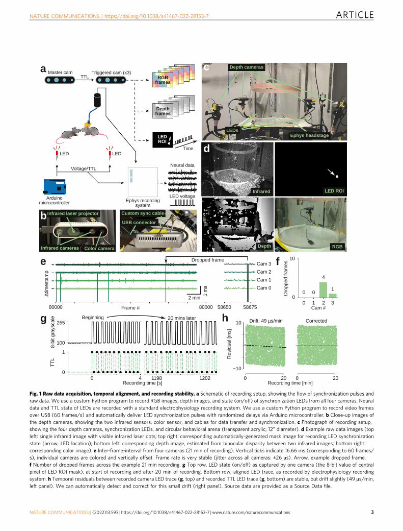
https://github.com/chrelli/3DDD_social_mouse_tracker/



Fig. 1 Raw data acquisition, temporal alignment, and recording stability. a Schematic of recording setup, showing the flow of synchronization pulses andraw data. We use a custom Python program to record RGB images, depth images, and state (on/off) of synchronization LEDs from all four cameras. Neuraldata and TTL state of LEDs are recorded with a standard electrophysiology recording system. We use a custom Python program to record video framesover USB (60 frames/s) and automatically deliver LED synchronization pulses with randomized delays via Arduino microcontroller. b Close-up images ofthe depth cameras, showing the two infrared sensors, color sensor, and cables for data transfer and synchronization. c Photograph of recording setup,showing the four depth cameras, synchronization LEDs, and circular behavioral arena (transparent acrylic, 12” diameter). d Example raw data images (topleft: single infrared image with visible infrared laser dots; top right: corresponding automatically-generated mask image for recording LED synchronizationstate (arrow, LED location); bottom left: corresponding depth image, estimated from binocular disparity between two infrared images; bottom right:corresponding color image). e Inter-frame-interval from four cameras (21 min of recording). Vertical ticks indicate 16.66 ms (corresponding to 60 frames/s), individual cameras are colored and vertically offset. Frame rate is very stable (jitter across all cameras: ±26 µs). Arrow, example dropped frame.f Number of dropped frames across the example 21 min recording. g Top row, LED state (on/off) as captured by one camera (the 8-bit value of centralpixel of LED ROI mask), at start of recording and after 20 min of recording. Bottom row, aligned LED trace, as recorded by electrophysiology recordingsystem. h Temporal residuals between recorded camera LED trace (g, top) and recorded TTL LED trace (g, bottom) are stable, but drift slightly (49 μs/min,left panel). We can automatically detect and correct for this small drift (right panel). Source data are provided as a Source Data file.

NATURE COMMUNICATIONS | https://doi.org/10.1038/s41467-022-28153-7 ARTICLE




custom firmware configurations in our recording program, suchthat all infrared sensors on all four cameras are hardware-synchronized to each other by TTL-pulses via custom-built,buffered synchronization cables (Fig. 1b).

We wrote a custom multithreaded Python program with onlinecompression, that allowed us to capture the following types of rawdata from all four cameras simultaneously: 8-bit RGB images (320× 210 pixels, 60 frames/s), 16-bit depth images (320 × 240 pixels,60 frames/s) and the 8-bit intensity trace of a blinking LED(60 samples/s, automatically extracted in real-time from theinfrared images). Our program also captures camera meta-data,such as hardware time-stamps and frame numbers of each image,which allows us to identify and correct for possible droppedframes. On a standard desktop PC, the recording system had veryfew dropped frames and the video recording frame rate and theimaging and USB image transfer pipeline were stable (Fig. 1e, f).

Temporal stability and temporal alignment. In order to relatetracked behavioral data to neural recordings, we need precisetemporal synchronization. Digital hardware clocks are generallystable but their internal speed can vary, introducing drift betweenclocks. Thus, even though all depth cameras provide hardwaretimestamps for each acquired image, for long-term recordings,across behavioral time scales (hours to days), a secondary syn-chronization method is required.

For synchronization to neural data, our recording program uses aUSB-controlled Arduino microprocessor to output a train ofrandomly-spaced voltage pulses during recording. These voltagepulses serve as TTL triggers for our neural acquisition system(sampled at 30 kHz) and drive LEDs, which are filmed by the depthcameras (Fig. 1a). The cameras sample an automatically detectedROI to sample the LED state at 60 frames/s, integrating across a fullinfrared frame exposure (Fig. 1g). We use a combination of cross-correlation and robust regression to automatically estimate andcorrect for shift and drift between the depth camera hardware clocksand the neural data. Since we use random pulse trains forsynchronization, alignment is unambiguous and we can achievesuper-frame-rate-precision. In a typical experiment, we estimatedthat the depth camera time stamps drifted with ~49 µs/min. Foreach recording, we automatically estimate and correct for this driftto yield stable residuals between TTL flips and depth frameexposures (Fig. 1h). Note that the neural acquisition system is notrequired for synchronization, so for a purely behavioral study, wecan run the same LED-based protocol to correct for potential shiftand drift between cameras by choosing one camera as a reference.

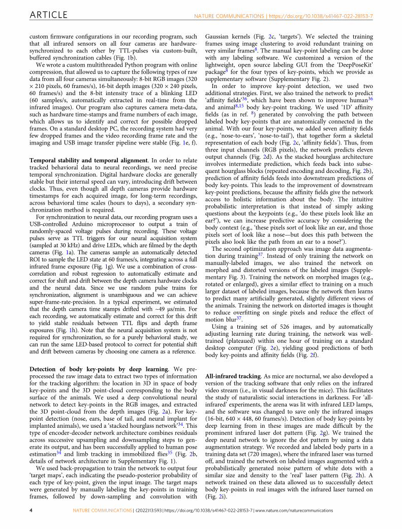
Detection of body key-points by deep learning. We pre-processed the raw image data to extract two types of informationfor the tracking algorithm: the location in 3D in space of bodykey-points and the 3D point-cloud corresponding to the bodysurface of the animals. We used a deep convolutional neuralnetwork to detect key-points in the RGB images, and extractedthe 3D point-cloud from the depth images (Fig. 2a). For key-point detection (nose, ears, base of tail, and neural implant forimplanted animals), we used a ‘stacked hourglass network’34. Thistype of encoder-decoder network architecture combines residualsacross successive upsampling and downsampling steps to gen-erate its output, and has been successfully applied to human poseestimation34 and limb tracking in immobilized flies35 (Fig. 2b,details of network architecture in Supplementary Fig. 1).

We used back-propagation to train the network to output four‘target maps’, each indicating the pseudo-posterior probability ofeach type of key-point, given the input image. The target mapswere generated by manually labeling the key-points in trainingframes, followed by down-sampling and convolution with

Gaussian kernels (Fig. 2c, ‘targets’). We selected the trainingframes using image clustering to avoid redundant training onvery similar frames8. The manual key-point labeling can be donewith any labeling software. We customized a version of thelightweight, open source labeling GUI from the ‘DeepPoseKit’package8 for the four types of key-points, which we provide assupplementary software (Supplementary Fig. 2).

In order to improve key-point detection, we used twoadditional strategies. First, we also trained the network to predict‘affinity fields’36, which have been shown to improve human36

and animal8,15 body key-point tracking. We used ‘1D’ affinityfields (as in ref. 8) generated by convolving the path betweenlabeled body key-points that are anatomically connected in theanimal. With our four key-points, we added seven affinity fields(e.g., ‘nose-to-ears’, ‘nose-to-tail’), that together form a skeletalrepresentation of each body (Fig. 2c, ‘affinity fields’). Thus, fromthree input channels (RGB pixels), the network predicts elevenoutput channels (Fig. 2d). As the stacked hourglass architectureinvolves intermediate prediction, which feeds back into subse-quent hourglass blocks (repeated encoding and decoding, Fig. 2b),prediction of affinity fields feeds into downstream predictions ofbody key-points. This leads to the improvement of downstreamkey-point predictions, because the affinity fields give the networkaccess to holistic information about the body. The intuitiveprobabilistic interpretation is that instead of simply askingquestions about the keypoints (e.g., ‘do these pixels look like anear?’), we can increase predictive accuracy by considering thebody context (e.g., ‘these pixels sort of look like an ear, and thosepixels sort of look like a nose—but does this path between thepixels also look like the path from an ear to a nose?’).

The second optimization approach was image data augmenta-tion during training37. Instead of only training the network onmanually-labeled images, we also trained the network onmorphed and distorted versions of the labeled images (Supple-mentary Fig. 3). Training the network on morphed images (e.g.,rotated or enlarged), gives a similar effect to training on a muchlarger dataset of labeled images, because the network then learnsto predict many artificially generated, slightly different views ofthe animals. Training the network on distorted images is thoughtto reduce overfitting on single pixels and reduce the effect ofmotion blur37.

Using a training set of 526 images, and by automaticallyadjusting learning rate during training, the network was well-trained (plateaued) within one hour of training on a standarddesktop computer (Fig. 2e), yielding good predictions of bothbody key-points and affinity fields (Fig. 2f).

All-infrared tracking. As mice are nocturnal, we also developed aversion of the tracking software that only relies on the infraredvideo stream (i.e., in visual darkness for the mice). This facilitatesthe study of naturalistic social interactions in darkness. For ‘all-infrared’ experiments, the arena was lit with infrared LED lamps,and the software was changed to save only the infrared images(16-bit, 640 × 448, 60 frames/s). Detection of body key-points bydeep learning from in these images are made difficult by theprominent infrared laser dot pattern (Fig. 2g). We trained thedeep neural network to ignore the dot pattern by using a dataaugmentation strategy. We recorded and labeled body parts in atraining data set (720 images), where the infrared laser was turnedoff, and trained the network on labeled images augmented with aprobabilistically generated noise pattern of white dots with asimilar size and density to the ‘real’ laser pattern (Fig. 2h). Anetwork trained on these data allowed us to successfully detectbody key-points in real images with the infrared laser turned on(Fig. 2i).




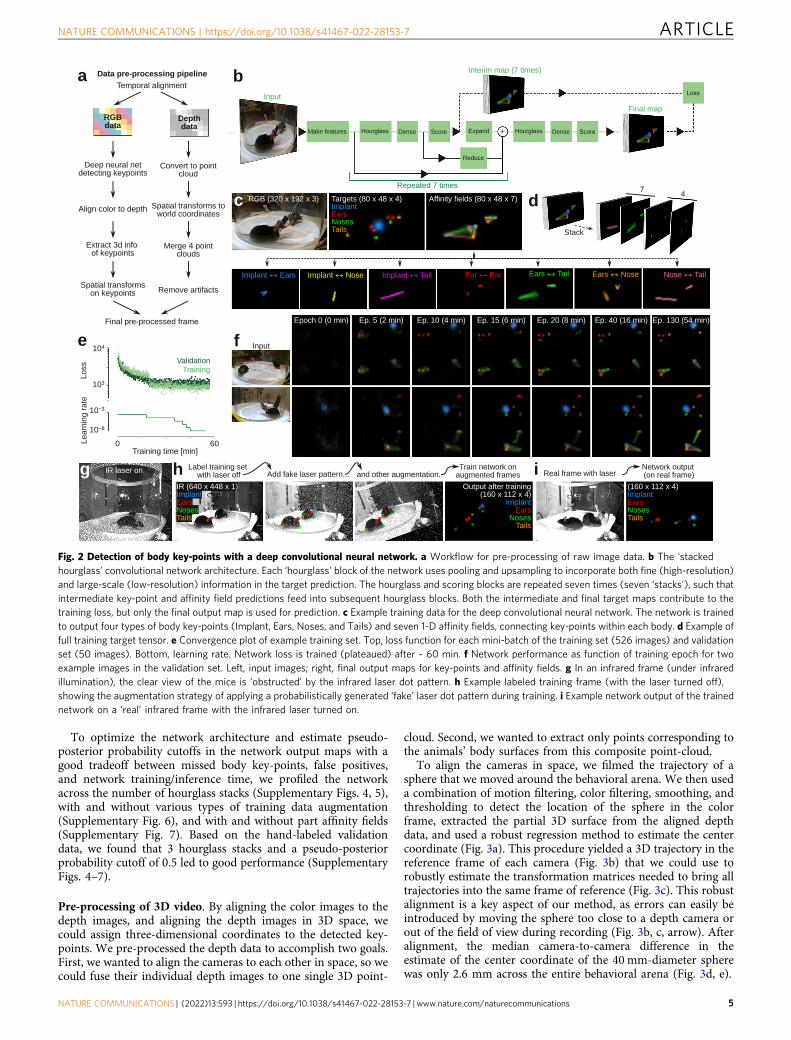
To optimize the network architecture and estimate pseudo-posterior probability cutoffs in the network output maps with agood tradeoff between missed body key-points, false positives,and network training/inference time, we profiled the networkacross the number of hourglass stacks (Supplementary Figs. 4, 5),with and without various types of training data augmentation(Supplementary Fig. 6), and with and without part affinity fields(Supplementary Fig. 7). Based on the hand-labeled validationdata, we found that 3 hourglass stacks and a pseudo-posteriorprobability cutoff of 0.5 led to good performance (SupplementaryFigs. 4–7).

Pre-processing of 3D video. By aligning the color images to thedepth images, and aligning the depth images in 3D space, wecould assign three-dimensional coordinates to the detected key-points. We pre-processed the depth data to accomplish two goals.First, we wanted to align the cameras to each other in space, so wecould fuse their individual depth images to one single 3D point-

cloud. Second, we wanted to extract only points corresponding tothe animals’ body surfaces from this composite point-cloud.

To align the cameras in space, we filmed the trajectory of asphere that we moved around the behavioral arena. We then useda combination of motion filtering, color filtering, smoothing, andthresholding to detect the location of the sphere in the colorframe, extracted the partial 3D surface from the aligned depthdata, and used a robust regression method to estimate the centercoordinate (Fig. 3a). This procedure yielded a 3D trajectory in thereference frame of each camera (Fig. 3b) that we could use torobustly estimate the transformation matrices needed to bring alltrajectories into the same frame of reference (Fig. 3c). This robustalignment is a key aspect of our method, as errors can easily beintroduced by moving the sphere too close to a depth camera orout of the field of view during recording (Fig. 3b, c, arrow). Afteralignment, the median camera-to-camera difference in theestimate of the center coordinate of the 40 mm-diameter spherewas only 2.6 mm across the entire behavioral arena (Fig. 3d, e).

Fig. 2 Detection of body key-points with a deep convolutional neural network. a Workflow for pre-processing of raw image data. b The ‘stackedhourglass’ convolutional network architecture. Each ‘hourglass’ block of the network uses pooling and upsampling to incorporate both fine (high-resolution)and large-scale (low-resolution) information in the target prediction. The hourglass and scoring blocks are repeated seven times (seven ‘stacks’), such thatintermediate key-point and affinity field predictions feed into subsequent hourglass blocks. Both the intermediate and final target maps contribute to thetraining loss, but only the final output map is used for prediction. c Example training data for the deep convolutional neural network. The network is trainedto output four types of body key-points (Implant, Ears, Noses, and Tails) and seven 1-D affinity fields, connecting key-points within each body. d Example offull training target tensor. e Convergence plot of example training set. Top, loss function for each mini-batch of the training set (526 images) and validationset (50 images). Bottom, learning rate. Network loss is trained (plateaued) after ~ 60 min. f Network performance as function of training epoch for twoexample images in the validation set. Left, input images; right, final output maps for key-points and affinity fields. g In an infrared frame (under infraredillumination), the clear view of the mice is ‘obstructed’ by the infrared laser dot pattern. h Example labeled training frame (with the laser turned off),showing the augmentation strategy of applying a probabilistically generated ‘fake’ laser dot pattern during training. i Example network output of the trainednetwork on a ‘real’ infrared frame with the infrared laser turned on.





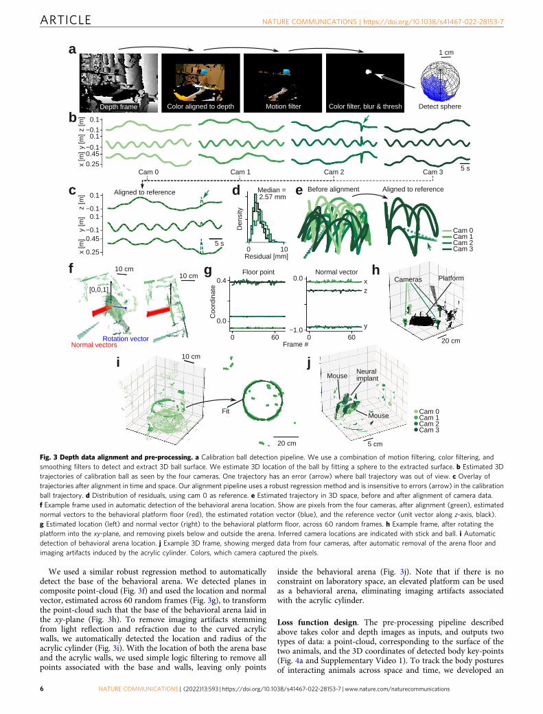
We used a similar robust regression method to automaticallydetect the base of the behavioral arena. We detected planes incomposite point-cloud (Fig. 3f) and used the location and normalvector, estimated across 60 random frames (Fig. 3g), to transformthe point-cloud such that the base of the behavioral arena laid inthe xy-plane (Fig. 3h). To remove imaging artifacts stemmingfrom light reflection and refraction due to the curved acrylicwalls, we automatically detected the location and radius of theacrylic cylinder (Fig. 3i). With the location of both the arena baseand the acrylic walls, we used simple logic filtering to remove allpoints associated with the base and walls, leaving only points

inside the behavioral arena (Fig. 3j). Note that if there is noconstraint on laboratory space, an elevated platform can be usedas a behavioral arena, eliminating imaging artifacts associatedwith the acrylic cylinder.

Loss function design. The pre-processing pipeline describedabove takes color and depth images as inputs, and outputs twotypes of data: a point-cloud, corresponding to the surface of thetwo animals, and the 3D coordinates of detected body key-points(Fig. 4a and Supplementary Video 1). To track the body posturesof interacting animals across space and time, we developed an

Fig. 3 Depth data alignment and pre-processing. a Calibration ball detection pipeline. We use a combination of motion filtering, color filtering, andsmoothing filters to detect and extract 3D ball surface. We estimate 3D location of the ball by fitting a sphere to the extracted surface. b Estimated 3Dtrajectories of calibration ball as seen by the four cameras. One trajectory has an error (arrow) where ball trajectory was out of view. c Overlay oftrajectories after alignment in time and space. Our alignment pipeline uses a robust regression method and is insensitive to errors (arrow) in the calibrationball trajectory. d Distribution of residuals, using cam 0 as reference. e Estimated trajectory in 3D space, before and after alignment of camera data.f Example frame used in automatic detection of the behavioral arena location. Show are pixels from the four cameras, after alignment (green), estimatednormal vectors to the behavioral platform floor (red), the estimated rotation vector (blue), and the reference vector (unit vector along z-axis, black).g Estimated location (left) and normal vector (right) to the behavioral platform floor, across 60 random frames. h Example frame, after rotating theplatform into the xy-plane, and removing pixels below and outside the arena. Inferred camera locations are indicated with stick and ball. i Automaticdetection of behavioral arena location. j Example 3D frame, showing merged data from four cameras, after automatic removal of the arena floor andimaging artifacts induced by the acrylic cylinder. Colors, which camera captured the pixels.




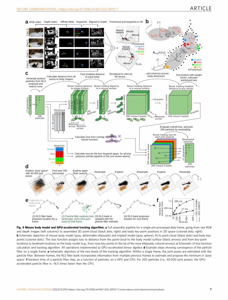
Fig. 4 Mouse body model and GPU-accelerated tracking algorithm. a Full assembly pipeline for a single pre-processed data frame, going from raw RGBand depth images (left columns) to assembled 3D point-cloud (black dots, right) and body key-point positions in 3D space (colored dots, right).b Schematic depiction of mouse body model (gray, deformable ellipsoids) and implant model (gray sphere), fit to point-cloud (black dots) and body key-points (colored dots). The loss function assigns loss to distance from the point-cloud to the body model surface (black arrows) and from key-pointlocations to landmark locations on the body model (e.g., from nose key-points to the tip of the nose ellipsoids; colored arrows). c Schematic of loss functioncalculation and tracking algorithm. All operations implemented as GPU-accelerated tensor algebra. d Example steps showing convergence of the particlefilter on a single frame. e Schematic depiction of the two levels of the tracking algorithm: Within a single frame, the joint poses are estimated with theparticle filter. Between frames, the RLS filter bank incorporates information from multiple previous frames to estimate and propose the minimum in ‘posespace’. f Iteration time of a particle filter step, as a function of particles, on a GPU and CPU. For 200 particles (i.e., 40.000 joint poses), the GPU-accelerated particle filter is ~16.5 times faster than the CPU.





algorithm that incorporates information from both data types.The basic idea of the tracking algorithm is that for every frame,we fit the mouse bodies by minimizing a loss function of both thepoint-cloud and key-points, subject to a set of spatiotemporalregularizations.

For the loss function, we made a simple parametric model ofthe skeleton and body surface of a mouse. The body modelconsists of two prolate spheroids (the ‘hip ellipsoid’ and ‘headellipsoid’), with dimensions based on an average adult mouse(Fig. 4b). The head ellipsoid is rigid, but the hip ellipsoid has afree parameter (s) modifying the major and minor axes to allowthe hip ellipsoids to be longer and narrower (e.g., duringstretching, running, or rearing) or shorter and wider (e.g., whenstill or self-grooming). The two ellipsoids are connected by a jointthat allows the head ellipsoid to turn left/right and up/downwithin a cone corresponding to the physical movement limits ofthe neck.

Keeping the number of degrees of freedom low is vital to makeloss function minimization computationally feasible38. Due to therotational symmetry of the ellipsoids, we could choose aparametrization with 8 degrees of freedom per mouse body: thecentral coordinate of the hip ellipsoid (x, y, z), the rotation ofthe major axis of the hip ellipsoid around the y- and z-axis (β, γ),the left/right and up/down rotation of the head ellipsoid (θ, φ),and the stretch of the hip ellipsoids (s). For the implanted animal,we added an additional sphere to the body model, approximatingthe surface of the head-mounted neural implant (Fig. 4b).The sphere is rigidly attached to the head ellipsoid and has onedegree of freedom; a rotational angle (ψ) that allows the sphere torotate around the head ellipsoid, capturing head tilt of theimplanted animal. Thus, in total, the joint pose (the body poses ofboth mice) was parametrized by only 17 variables.

To fit the body model, we adjusted these parameters tominimize a weighted sum of two loss terms: (i) The shortestdistance from every point in the point-cloud to body modelsurface. (ii) The distance from detected key-points to theircorresponding location on the body model surface (e.g., nose key-points near the tip of one of the head ellipsoids, tail key-pointsnear the posterior end of a hip ellipsoid).

We then used several different approaches for optimizing thetracking. First, for each of the thousands of point in the point-cloud, we needed to calculate the shortest distance to the bodymodel ellipsoids. Calculating these distances exactly is notcomputationally feasible, as this requires solving a six-degreepolynomial for every point39. As an approximation, we insteadused the shortest distance to the surface, along a path that passesthrough the centroid (Supplementary Fig. 8a, b). Calculating thisdistance could be implemented as pure tensor algebra40, whichcould be executed efficiently on a GPU in parallel for all pointssimultaneously. Second, to reduce the effect of imaging artifactsin the color and depth imaging (which can affect both the point-cloud or the 3D coordinates of the key-points), we clippeddistance losses at 3 cm, such that distant ‘outliers’ do contributeand not skew the fit (Supplementary Fig. 8c). Third, because pixeldensity in the depth images depends on the distance from thedepth camera, we weighed the contribution of each point in thepoint-cloud by the squared distance to the depth camera(Supplementary Fig. 8d). Fourth, to ensure that the minimizationdoes not converge to unphysical joint postures (e.g., where themouse bodies are overlapping), we added a penalty term to theloss function if the body models overlap. Calculating overlapbetween two ellipsoids is computationally expensive41, so wecomputed overlaps between implant sphere and spheres centeredon the body ellipsoids with a radius equal to the minor axis(Supplementary Fig. 8f). Fifth, to ensure spatiotemporal con-tinuity of body model estimates, we also added a penalty term to

the loss function, penalizing overlap between the mouse body inthe current frame, and other mouse bodies in the previous frame.This ensures that the bodies do not switch place, something thatcould otherwise happen if the mice are in joint poses with certainmirror symmetries (Supplementary Fig. 8g, h).

GPU-accelerated robust optimization. Minimizing the lossfunction requires solving three major challenges. The first chal-lenge is computational speed. The number of key-points andbody parts is relatively low (~tens), but the number of points inthe point-cloud is large (~thousands), which makes the lossfunction computationally expensive. For minimization, we needto evaluate the loss function multiple times per frame (at 60frames/s). If loss function evaluation is not fast, tracking becomesunusably slow. The second challenge is that the minimizer has toproperly explore the loss landscape within each frame and avoidlocal minima. In early stages of developing this algorithm, wewere only tracking interacting mice with no head implant. In thatcase, for the small frame-to-frame changes in body posture, theloss function landscape was nonlinear, but approximately convex,so we could use a fast, derivative-based minimizer to trackchanges in body posture (geodesic Levenberg-Marquardt steps38).For use in neuroscience experiments, however, one or more micemight carry a neural implant for recording or stimulation. Theimplant is generally at a right angle and offset from the ‘hinge’between the two hip and head ellipsoids, which makes the lossfunction highly non-convex42. The final challenge is robustnessagainst local minima in state space. Even though a body postureminimizes the loss in a single frame, it might not be an optimalfit, given the context of other frames (e.g., spatiotemporal con-tinuity, no unphysical movement of the bodies).

To solve these three challenges—speed, state space exploration,and spatiotemporal robustness—we designed a custom GPU-accelerated minimization algorithm, which incorporates ideas fromannealed particle filters43 and online Bayesian filtering (Fig. 4c). Tomaximize computational speed, the algorithm was implemented aspure tensor algebra in Pytorch, a high-performance GPU computinglibrary44. Annealed particle filters are suited to explore highly non-convex loss surfaces43, which allowed us to avoid local minimawithin each frame. Between frames, we used online filtering, to avoidbeing trapped in low-probability solutions given the context of thepreceding tracking. For every frame, we first proposed the state ofthe 17-parameters using a recursive least-squares (‘RLS’) filter banktrained on preceding frames. After particle filter-based loss functionminimization within a single frame, we updated the RLS filter bank,and proposed a particle filter starting point for the next frame(Fig. 4d, e).

The ‘two-layer’ tracking strategy (particle filter within framesand RLS filter between frames) has three major advantages. First,by proposing a solution from the RLS bank, we often already startthe loss function minimization close to the new minimum.Second, if the RLS filter deems that the fit for a single frame isunlikely (an outlier), based on the preceding frames, this fit willonly weakly update the filter bank, and thus only weakly perturbthe upcoming tracking. This gives us a convenient way to balancethe information provided by the fit of a single frame, and the‘context’ provided by previous frames. Third, the RLS filter-basedapproach is only dependent on previously tracked frames, notfuture frames. This is in contrast to other approaches toincorporating context that rely on versions of backwards beliefpropagation5,16,35. Note that since our algorithm only relies onpast data for tracking, it is possible—in future work—to optimizeour algorithm for real-time use in closed-loop experiments.

For each recording, we first automatically initiated the trackingalgorithm: We automatically scanned forward in the video to find




a frame, where the mice were well separated (assessed by k-meansclustering of the 3D positions of the body key-points into twoclusters, and by requiring that the ‘cross-mouse’ cluster distanceis at least 5 cm (Supplementary Fig. 9). From this starting point,we explored the loss surface with 200 particles (Fig. 4d). Wegenerated the particles by perturbing the proposed minimum byquasi-random, low-discrepancy sampling45 (SupplementaryFig. 10). We exploited the fact that the loss function structureallowed us to execute several key steps in parallel, across multipleindependent dimensions, and implemented these calculations asvectorizes tensor operations. This allowed us to leverage thepower of CUDA kernels for fast tensor algebra on the GPU44.Specifically, to efficiently calculate the point-cloud loss (shortestdistance from a point in the point-cloud to the surface of a bodymodel), we calculated the distance to all five body modelspheroids for all points in the point-cloud and for all 200particles, in parallel (Fig. 4c). We then applied fast minimizationkernels across the two body models, to generate a smallestdistance to either mouse, for all points in the point cloud. Becausethe mouse body models are independent, we only had to apply aminimization kernel to calculate the smallest distance, for everypoint, to 40,000 (200 × 200) joint poses if the two mice. Theseparallel computation steps are a key aspect of our method, whichallows our tracking algorithm to avoid the ‘curse of dimension-ality’, by not exploring a 17-dimensional space, but rather explorethe intersection of two independent 8-dim and 9-dim subspacesin parallel. We found that our GPU-accelerated implementationof the filter increased the processing time of a single frame bymore than an order of magnitude compared to a fast CPU (e.g.,~16-fold speed increase for 200 particles, Fig. 4f).

Tracking algorithm performance. To ensure that the trackingalgorithm did not get stuck in suboptimal solutions, we forced theparticle filter to explore a large search space within every frame(Supplementary Fig. 11a–c). In successive iterations, we graduallymade perturbations to the particles smaller and smaller byannealing the filter43), to approach the minimum. At the end ofeach iteration, we ‘resampled’ the particles by picking the 200joint poses with the lowest losses in the 200-by-200 matrix oflosses. This ‘top-k’ resampling strategy has two advantages. First,it can be done without fully sorting the matrix46, the mostcomputationally expensive step in resampling47. Second, it pro-vides a type of ‘importance sampling’. During resampling, someposes in the next iteration might be duplicates (picked from thesame row or column in the 200-by-200 loss matrix.), allowingparticles in each subspace to collapse at different rates (if theparticle filter is very certain about one body pose, but not theother, for example).

By investigating the performance of the particle filter acrossiterations, we found that the filter generally converged sufficientlywithin five iterations (Supplementary Fig. 11d, SupplementaryVideo 2) to provide good tracking across frames (SupplementaryFig. 11e). In every frame, the particle filter fit yields a noisyestimate of the 3D location of the mouse bodies. Thetransformation from the joint pose parameters (e.g., rotationangles, spine scaling) to 3D space is highly nonlinear, so simplesmoothing of the trajectory in pose parameter space would distortthe trajectory in real space. Thus, we filtered the trackedtrajectories by a combination of Kalman-filtering and maximumlikelihood-based smoothing48,49 and 3D rotation smoothing inquaternion space50 (Supplementary Fig. 12 and SupplementaryVideo 3).

Representing the joint postures of the two animals with thisparametrization was highly data efficient, reducing the memoryfootprint from ~3.7 GB/min for raw color/depth image data, to

~0.11 GB/min for pre-processed point-cloud/key-point data to ~1MB/min for tracked body model parameters. On a regulardesktop computer with a single GPU, we could do key-pointdetection in color image data from all four cameras in ~2× realtime (i.e., it took 30 min to process a 1 h experimental session).Depth data processing (point-cloud merging and key-pointdeprojection) ran at ~0.7× real time, and the tracking algorithmran at ~0.2× real time (if the filter uses 200 particles and 5 filteriterations per frame). Thus, for a typical experimental session(~ hours), we would run the tracking algorithm overnight, whichis possible because the code is fully automatic.

Error detection. Error detection and correction is a criticalcomponent of behavioral tracking. Even if error rates are nom-inally low, errors are non-random, and errors often happenexactly during the behaviors in which we are most interested:interactions. In multi-animal tracking, two types of tracking errorare particularly fatal as they compound over time: identity errorsand body orientation errors (Supplementary Fig. 13a). In con-ventional tracking approaches using only 2D videos, it is oftendifficult to correctly track identities when interacting mice areclosely interacting, allo-grooming, or passing over and under eachother. Although swapped identities can be corrected later oncethe mice are well-separated again, this still leaves individualbehavior during the actual social interaction unresolved5,16. Wefound that our tracking algorithm was robust against bothidentity swaps (Supplementary Fig. 13b–e) and body directionswaps (Supplementary Fig. 14). This observation agrees with thefact that tracking in 3D space (subject to our implemented spa-tiotemporal regularizations) should in principle allow betteridentity tracking. In full 3D space it is easier to determine who isrearing over whom during an interaction, for example.

To test our algorithm for subtler errors, we manually inspected500 frames, randomly selected across an example 21 minrecording session. In these 500 frames, we detected only a singletracking mistake, corresponding to 99.8% correct tracking(Supplementary Fig. 15a). The identified tracking mistake wasvisible as a large, transient increase in the point-cloud lossfunction (Supplementary Fig. 15b). After the tracking mistake,the robust particle filter quickly recovered to correct trackingagain (Supplementary Fig. 15c). By detecting such loss functionanomalies, or by detecting ‘unphysical’ postures or movements inthe body models, potential tracking mistakes can be automatically‘flagged’ for inspection (Supplementary Fig. 15c, d). Afterinspection, errors can be manually corrected or automaticallycorrected in many cases, for example by tracking the particle filterbackwards in time after it has recovered. As the algorithmrecovers after a tracking mistake, it is generally unnecessary toactively supervise the algorithm during tracking, and manualinspection for potential errors can be performed after running thealgorithm overnight. We provide a GUI for viewing and qualitycontrol of tracked behavior (raw data, body skeleton, ellipsoidsurfaces, and time trajectory) running in an interactive Jupyternotebook (Supplementary Fig. 2b and Supplementary Video 5).

Automated analysis of movement kinematics and social events.As a validation of our tracking method, we demonstrate that ourmethods can automatically extract both movement kinematicsand behavioral states (movement patterns, social events) duringspontaneous social interactions. Some unsupervised methods fordiscovering structure and states in behavioral data do not rely onan explicit body model of the animal, and instead, use statisticalmethods to detect behavioral states directly from trackedfeatures6,33,51–53. In an alternative approach, some supervisedmethods label behavioral events of interest by hand on training





data, and then train a classifier to find similar events in unlabeleddata17–19. Both of these types of analysis are compatible with ourmethod (e.g., by running directly on the time series data of the 17dimensions that parametrize the body models of the two animals,Supplementary Fig. 11). Our tracking system yields an easilyinterpretable 3D body model of the animals, which makes twoadditional types of analyses straightforward as well: First, we caneasily define 3D body postures or multi-animal postures ofinterest as templates16,30. Second, we can use unsupervisedmethods to discover behavioral states in the 3D reference frameof the animal’s own body, making these models and statesstraightforward to interpret and ‘sanity check’ (manually inspectfor errors).

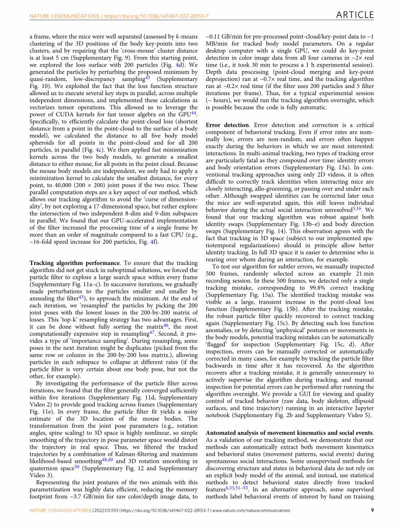
To demonstrate posture-template-based analysis, we definedsocial behaviors of interest as templates and matched thesetemplates to tracked data. We know that anogenital sniffing54 andnose-to-nose touch55 are prominent events in rodent socialbehavior, so we designed a template to detect these events. In thistemplate, we exploited the fact that we could easily calculate bothbody postures and movement kinematics, in the reference frameof each animal’s own body. For every frame, we first extracted the3D coordinates of the body model skeleton (SupplementaryFig. 12a). From these skeleton coordinates, we calculated theposition (Fig. 5a) and a three-dimensional speed vector for eachmouse (‘forward speed’, along the hip ellipsoid, ‘left speed’perpendicular to the body axis, and ‘up speed’ along the z-axis;Fig. 5b). We also calculated three instantaneous ‘social distances’,defined as the 3D distance between the tip of each animal’s noses(‘nose-to-nose’; Fig. 5b), and from the tip of each animal’s nose tothe posterior end of the conspecific’s hip ellipsoid (‘nose-to-tail’;Fig. 5b). From these social distances, we could automaticallydetect when the mouse bodies were in a nose-to-nose or a nose-to-tail configuration (Fig. 5c). It is straightforward to furthersubdivide these social events by body postures and kinematics, inorder to separate stationary nose-to-tail configurations (anogen-ital sniffing/grooming) and nose-to-tail configurations duringlocomotion (social following).

To demonstrate unsupervised behavioral state discovery, weused GPU-accelerated probabilistic programming56 and statespace modeling to automatically detect and label movementstates. To discover types locomotor behavior, we fitted a ‘sticky’multivariate hidden Markov model57 to the two components ofthe speed vector that lie in the xy-plane (SupplementaryFig. 16a–h). With five hidden states, this model yieldedinterpretable movement patterns that correspond to knownmouse locomotor ‘syllables’: resting (no movement), turning leftand right, and moving forward at slow and fast speeds (Fig. 5d).Fitting a similar model with three hidden states to the z-component of the speed vector (Supplementary Fig. 16i–n)yielded interpretable and known ‘rearing syllables’: rest, rearingup, and ducking down (Fig. 5e). Using the maximum a posterioriprobability from these fitted models, we could automaticallygenerate locomotor ethograms and rearing ethograms for the twomice (Fig. 5b).

In line with previous observations, we found that movementbouts were short (medians, rest/left/right/fwd/fast-forward: 0.83/0.50/0.52/0.45/0.68 s, a ‘sub-second’ timescale33). In the locomo-tion ethograms, bouts of rest were longer than bouts ofmovement (all p < 0.05, Mann–Whitney U-test; Fig. 5f) andbouts of fast forward locomotion was longer than other types oflocomotion (all p < 0.001, Mann–Whitney U-test; Fig. 5f). In therearing ethograms, the distribution of rests was very wide,consisting of both long (~seconds) and very short (~tenths of asecond) periods of rest (Fig. 5g). As expected, by plotting therearing height against the duration of rearing syllables, we foundthat short rests in rearing were associated with standing high on

the hind legs (the mouse rears up, waits for a brief moment beforeducking back down), while longer rests happened when themouse was on the ground (‘rearing’ and ‘crouching’, Fig. 5h). Likethe movement types and durations, the transition probabilitiesfrom the fitted hidden Markov models were also in agreementwith known behavioral patterns. In the locomotion model, forexample, the most likely transition from “rest” was to “slowforward”. From “slow forward”, the mouse was likely to transitionto “turning left”, “fast forward” or “turning right”, it was unlikelyto transition directly from “fast forward” to “rest” or from“turning left” to “turning right, and so on (SupplementaryFig. 16o, p).

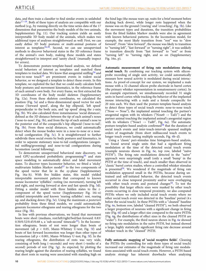
Automatic measurement of firing rate modulations duringsocial touch. By combining our tracking system with silicon-probe recording of single unit activity, we could automaticallymeasure how neural activity is modulated during social interac-tions. As proof-of-concept for our system, we implanted a malemouse with a 32-channel silicon probe electrode in barrel cortex(the primary whisker representation in somatosensory cortex). Inan example experiment, we simultaneously recorded 31 singleunits in barrel cortex while tracking the behavior of the implantedmouse interacting with a male and a female conspecific for20 min each. We then used the posture-template-based analysisto detect three types of social touch events: nose-to-nose touch(“Nose ↔ Nose”), the implanted animal touching the partner’sanogenital region with its whiskers (“Nose0 → Tail1”) and thepartner animal touching the implanted animal’s anogenital regionwith its whiskers (“Nose1 → Tail0”, Fig. 6a). The automaticposture-template-based analysis confirmed58 that the duration ofsocial touch events and inter-touch-intervals spanned multipleorders of magnitude (from short millisecond touch events tolonger touch events lasting multiple seconds, Fig. 6b–d).

Using a ‘classic’ peri-stimulus time histogram-based analysis,we found several single units that had a significant firingmodulation at the time of the detected social touch events(example neurons shown in Fig. 6e, top row, labeled “naïvePSTH”). The firing rate modulations detected in the “naïve”approach were surprisingly small (only a small ‘bump’ in thePSTH at the time of touch), and much smaller than observed in‘classic’ barrel cortex studies, where a controlled whisker stimulusis presented59. We wondered if the magnitude of firing ratemodulation appeared small in the PSTHs, because during un-trained and self-initiated behavior, the detected touch eventsoccurred in close temporal proximity and/or were overlappingwith other touch events and postural changes58. To test thepossibility that larger effects sizes were masked by other touchevents occurring in close temporal proximity, we also computedPSTHs where we only included social touch events where noother social touch event was detected in the ‘baseline’ period (4 sbefore the social touch). In these PSTHs with a “cleaned” baseline(Fig. 6e, bottom row, labeled “cleaned PSTH”), we both observeda larger proportion of neurons with a significant change in firingrate (Fig. 6f) and a larger effect size compared to the naïve PSTHs(Fig. 6g, the distributions of effect sizes in the cleaned PSTH are“wider”). For example, the third neuron shown in Fig. 6e showedno firing rate modulation in the naïve PSTH, but instead showeda large, highly statistically significant firing rate decrease aroundwhisker touch in the “cleaned” PSTH.

Fully automatic mapping of ‘social receptive fields’. Cleaningthe PSTHs (by controlling for only three types of social touch)increased our estimates of the magnitude of firing rate modula-tions associated with social touch events. However, a PSTH-basedanalysis strategy has inherent drawbacks when analyzing




naturalistic behavior. During free behavior, touch, movement,and postural changes happen simultaneously, as continuous andoverlapping variables. Furthermore, in line with “vicarious”somatosensory responses reported in human somatosensorycortex60 and barrel cortex responses observed just before touch61,barrel cortex neurons may be related to the behavior of thepartner animal, in a kind of “mirror neuron”-like response.

To deal with these challenges, we drew inspiration from thediscovery of multiplexed spatial coding in hippocampal circuits62

and developed a fully-automatic python pipeline that canautomatically discover ‘social’ receptive fields. Our trackingmethod is able to recover the 3D posture and head direction ofboth animals: The head direction of the implanted animal wasgiven by the skeleton of the body model (the implant is fixed to

Fig. 5 Automatic classification of movement patterns and behavioral states during social interactions. a Tracked position of both mice, across anexample 21 min recording. b Extracted behavioral features: three speed components (forward, left, and up in the mice’s egocentric reference frames), andthree ‘social distances’ (nose-to-nose distance and two nose-to-tail distances). Colors indicate ethograms of automatically detected behavioral states.c Examples of identified social events: nose-to-nose-touch, and anogenital nose-contacts. d Mean and covariance (3 standard deviations indicated byellipsoids) for each latent state for the forward/leftward running (dots indicate a subsample of tracked speeds, colored by their most likely latent state)e Mean and variance of latent states in the z-plane (shaded color) as well as distribution of tracked data assigned to those latent states (histograms)f Distribution of the duration of the five behavioral states in the xy-plane. Periods of rest (blue) are the longest (p < 0.05, two-sided Mann–Whitney U-tests) and bouts of fast forward movement (green) are longer other movement bouts (p < 0.001, two-sided Mann–Whitney U-tests). g Distribution ofduration of the three behavioral states in the z-plane. Periods of rest (light blue) are either very short or very long. h Plot of body elevation against behaviorduration. Short periods of rest happen when the z-coordinate is high (the mouse rears up, waits for a brief moment before ducking back down), whereaslong periods of rest happen when the z-coordinate is low (when the mouse is resting or moving around the arena, ρ = −0.47, p < 0.001, two-sidedSpearman’s rank correlation coefficient test). Source data and analysis scripts that generate the figures are available in the associated code/data files(see “Methods”).





the head). For computational efficiency, we exploited therotational symmetry of the body model of the non-implantedpartner to decrease the dimensionality of the search space duringtracking (Fig. 4c) and used the 3D coordinates of the detected‘ear’ key-points to infer the 3D head direction of the partner(Supplementary Figs. 17, 18).

Using the full 3D body model of both animals, we designed ouranalysis pipeline to automatically extract 45 continuous featuresthat might be associated with firing rate changes in a socialinteraction: social “between-animal” features (nose-to-nose dis-tance, nose-to-partner’s-genitals distance, relative orientation ofthe partner with respect to the implanted animal, and a temporalderivative of the distance between the center of the two hipellipsoids that measures if the animals are moving towards eachother or away from each other, Fig. 7a), postural features (headyaw/pitch/roll, etc.), spatial features (to detect ‘spatial’ activity,such as place fields, border or head-direction activity), movementfeatures (temporal derivatives of the running trajectory, temporalderivatives of posture angles, etc.), and posture, space andmovement features of the partner animal (Fig. 7b, SupplementaryFig. 19a, detailed feature table in “Methods”).

We assumed the following generative model of the observedneuronal spike trains62: A neuron’s spike train is generated by aPoisson process, and the rate of this Poisson process is

determined by a linear combination of the behavioral predictors:Each predictor is associated with its own tuning curve, all tuningcontributions are summed and passed through an exponentialnonlinearity to map the rate of the Poisson process to a positivevalue (Fig. 7c). To determine what behavioral features signifi-cantly contribute to the firing rate modulation of a neuron, andthe associated tuning curves, we used a model comparisonapproach: Starting from a null model where the observed spikesare simply generated by a Poisson process with a constant rate, weiteratively added predictors that passed a cross-validatedsignificance criterion (a significant increase in likelihoodcompared to a simpler model). The tuning curves wereregularized to be smooth and allowed to be re-fit with eachadditional predictor added to the multiplexed code (details in“Methods”).

Using this analysis approach, we found several neurons with amultiplexed encoding of features of the social interactions(Fig. 7d, e). Because of the 3D body models, the discoveredneural coding schemes were straightforward to interpret andcompare to expected touch-related response patterns in barrelcortex59. For example, the example neuron shown in Fig. 7d isstrongly modulated by social facial touch (strongly tuned to a lownose-to-nose distance) and strongly lateralized (the neuron isstrongly tuned to orientation angle, with a peak at ~ −π/2, i.e.,

Fig. 6 Automatic measurement of firing rate modulations during social touch. a Automatically-detected social touch events in mouse implanted withsilicon probe (Si-probe) with 31 single-units from barrel cortex during a single 20min behavioral session. Yellow, nose-to-nose; purple, implanted-nose-to-partner-tail; blue, partner-nose-to-implanted-tail. b Distribution of touch durations with male (dashed) and female (solid) partner (p = 0.000084, N = 64/46 male/female, two-sided Mann–Whitney U-test). c Percentage of behavioral session classified as social touch events, by partner sex, for two behavioralsessions. d Distribution of inter-touch-intervals for the two example behavioral sessions. e Social touch PSTHs for four neurons. For each neuron, the toprow shows ‘naïve’ PSTHs (aligned to social touch event) and the bottom row shows ‘cleaned’ PSTHs (we only include events where no other social touchevent occurred in the −4 to 0 s period before the detected social touch). The PSTHs in the bottom row have fewer trials, but show much larger effect sizes.(p-values indicate paired, two-tailed Wilcoxon signed rank tests, see “Methods”) f, Percentage of neurons that pass a p < 0.05 significance criterion, basedon the ‘naïve’ and ‘cleaned’ PSTHs shown above. g Distributions of effect size (measured as a firing rate modulation index), based on the ‘naïve’ and‘cleaned’ PSTHs shown above. Source data and analysis scripts that generate the figures are available in the associated code/data files (see “Methods”).




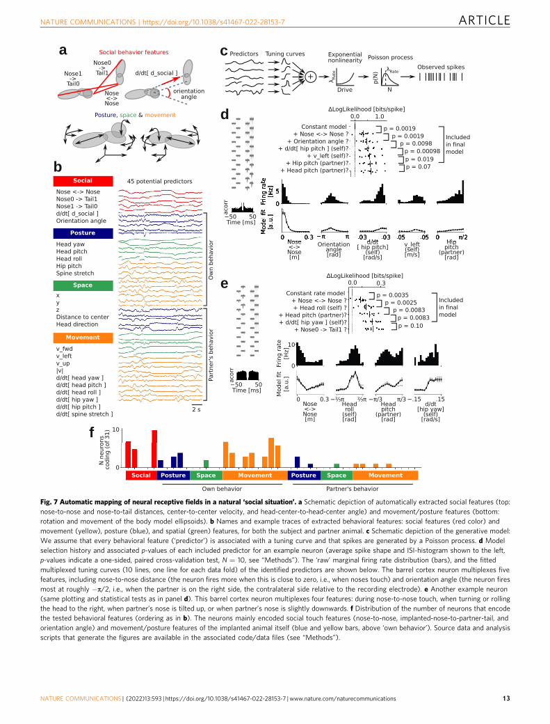
Fig. 7 Automatic mapping of neural receptive fields in a natural ‘social situation’. a Schematic depiction of automatically extracted social features (top:nose-to-nose and nose-to-tail distances, center-to-center velocity, and head-center-to-head-center angle) and movement/posture features (bottom:rotation and movement of the body model ellipsoids). b Names and example traces of extracted behavioral features: social features (red color) andmovement (yellow), posture (blue), and spatial (green) features, for both the subject and partner animal. c Schematic depiction of the generative model:We assume that every behavioral feature (‘predictor’) is associated with a tuning curve and that spikes are generated by a Poisson process. d Modelselection history and associated p-values of each included predictor for an example neuron (average spike shape and ISI-histogram shown to the left,p-values indicate a one-sided, paired cross-validation test, N = 10, see “Methods”). The ‘raw’ marginal firing rate distribution (bars), and the fittedmultiplexed tuning curves (10 lines, one line for each data fold) of the identified predictors are shown below. The barrel cortex neuron multiplexes fivefeatures, including nose-to-nose distance (the neuron fires more when this is close to zero, i.e., when noses touch) and orientation angle (the neuron firesmost at roughly −π/2, i.e., when the partner is on the right side, the contralateral side relative to the recording electrode). e Another example neuron(same plotting and statistical tests as in panel d). This barrel cortex neuron multiplexes four features: during nose-to-nose touch, when turning or rollingthe head to the right, when partner’s nose is tilted up, or when partner’s nose is slightly downwards. f Distribution of the number of neurons that encodethe tested behavioral features (ordering as in b). The neurons mainly encoded social touch features (nose-to-nose, implanted-nose-to-partner-tail, andorientation angle) and movement/posture features of the implanted animal itself (blue and yellow bars, above ‘own behavior’). Source data and analysisscripts that generate the figures are available in the associated code/data files (see “Methods”).





when the partner is on the contralateral side of the animal’s face,relative to the implanted recording electrode). The exampleneuron shown in Fig. 7e was also strongly tuned to social facialtouch (tuned to a low nose-to-nose distance), was strongly tunedto a positive head roll (i.e., when the head is turned such that thewhisker field contralateral to the recording electrode is in contactwith the floor) and was strongly tuned to a positive temporalderivative of the hip ellipsoid yaw (when the animal is runningcounterclockwise, e.g., along the edge of the arena, such that thecontralateral whisker field is brushing against the arena wall orother obstacles). Across the population, we found that theneurons overwhelmingly encoded whisker touch and orientationangle (lateralization), and the posture and movements of theimplanted animal, but not the partner animal (Fig. 7f).

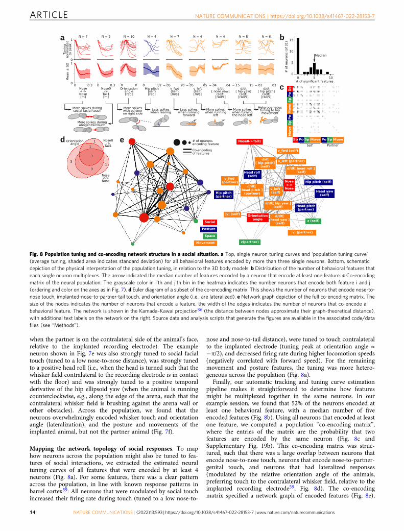
Mapping the network topology of social responses. To maphow neurons across the population might also be tuned to fea-tures of social interactions, we extracted the estimated neuraltuning curves of all features that were encoded by at least 4neurons (Fig. 8a). For some features, there was a clear patternacross the population, in line with known response patterns inbarrel cortex59: All neurons that were modulated by social touchincreased their firing rate during touch (tuned to a low nose-to-

nose and nose-to-tail distance), were tuned to touch contralateralto the implanted electrode (tuning peak at orientation angle ≈−π/2), and decreased firing rate during higher locomotion speeds(negatively correlated with forward speed). For the remainingmovement and posture features, the tuning was more hetero-geneous across the population (Fig. 8a).

Finally, our automatic tracking and tuning curve estimationpipeline makes it straightforward to determine how featuresmight be multiplexed together in the same neurons. In ourexample session, we found that 52% of the neurons encoded atleast one behavioral feature, with a median number of fiveencoded features (Fig. 8b). Using all neurons that encoded at leastone feature, we computed a population “co-encoding matrix”,where the entries of the matrix are the probability that twofeatures are encoded by the same neuron (Fig. 8c andSupplementary Fig. 19b). This co-encoding matrix was struc-tured, such that there was a large overlap between neurons thatencode nose-to-nose touch, neurons that encode nose-to-partner-genital touch, and neurons that had lateralized responses(modulated by the relative orientation angle of the animals,preferring touch to the contralateral whisker field, relative to theimplanted recording electrode59, Fig. 8d). The co-encodingmatrix specified a network graph of encoded features (Fig. 8e),

Fig. 8 Population tuning and co-encoding network structure in a social situation. a Top, single neuron tuning curves and ‘population tuning curve’(average tuning, shaded area indicates standard deviation) for all behavioral features encoded by more than three single neurons. Bottom, schematicdepiction of the physical interpretation of the population tuning, in relation to the 3D body models. b Distribution of the number of behavioral features thateach single neuron multiplexes. The arrow indicated the median number of features encoded by a neuron that encode at least one feature. c Co-encodingmatrix of the neural population: The grayscale color in i’th and j’th bin in the heatmap indicates the number neurons that encode both feature i and j(ordering and color on the axes as in Fig. 7). d Euler diagram of a subset of the co-encoding matrix: This shows the number of neurons that encode nose-to-nose touch, implanted-nose-to-partner-tail touch, and orientation angle (i.e., are lateralized). e Network graph depiction of the full co-encoding matrix. Thesize of the nodes indicates the number of neurons that encode a feature, the width of the edges indicates the number of neurons that co-encode abehavioral feature. The network is shown in the Kamada–Kawai projection86 (the distance between nodes approximate their graph-theoretical distance),with additional text labels on the network on the right. Source data and analysis scripts that generate the figures are available in the associated code/datafiles (see “Methods”).




which would then be amenable to various methods of networktopology analysis (e.g., locality, clustering, subgraph motifs, etc.).Thus, our fully-automatic pipeline enables direct connectionsfrom raw behavioral videography and spike train recordings tohigher-order statistics about how features of a social interactionare mapped onto a neural population during naturalisticbehavior.

DiscussionWe combined 3D videography, deep learning, and GPU-accelerated robust optimization to estimate the posture dynam-ics of multiple freely-moving mice, engaging in naturalistic socialinteractions. Our method is cost-effective (requiring only inex-pensive consumer depth cameras and a GPU), has high spatio-temporal precision, is compatible with neural implants forcontinuous electrophysiological recordings, and tracks unmarkedanimals of the same coat color (e.g., enabling behavioral studies intransgenic mice). Our method is fully automatic, which makes themethod scalable across multiple PCs or GPUs. Automatictracking allows us to investigate social behavior across longbehavioral time scales beyond what is feasible with manualannotation, for example to elucidate developmental trajectories,dynamics of social learning, or individual differences amonganimals63,64, among other types of questions. Finally, our methoduses no message-passing from future frames, but only relies onpast data, which makes the method a promising starting point forreal-time tracking. A major next step for future work is to applysuch algorithms to animal behavior in different conditions. Forexample, the algorithm can easily be adapted to track other ani-mal body shapes such as juvenile mice, other species, or movable,deformable objects that are part of more complexexperimental environments.

In social interactions, rodents respond to the behavior ofconspecifics, but we are only beginning to discover how therodent brain encodes complex features such as gaze direction orbody postures of others3,21,65,66. Compared to our knowledgeabout, for example, sensorimotor mirror neurons in monkeys67

and vicarious sensory responses in human subjects60 (bothfoundational to theories about human social cognition68 andempathy69), we still know very little about a putative rodentmirror neuron system69. For demonstration and validation, weapplied our analysis pipeline to barrel cortex neurons, and wereable to recover expected neural tuning to (lateralized) whiskertouch and movement59. Our end-to-end tracking method andanalysis pipeline maps tuning to movements and postures of thepartner’s body, and is thus ideally suited to detect potential socialinteraction systems such as rodent ‘mirror neuron’ signals inother brain areas70,71. The 45 predictor features that we haveincluded in our analysis pipeline could be expanded to addadditional features of interest. Similar to multiplexed spatialtuning in parahippocampal cortices (e.g., “conjunctive” grid- andhead-direction cells72), we model multiplexed tuning asmultiplicative62. It is straightforward to modify our model com-parison code to also consider other coding schemes, such asnonlinear or conditional interactions between predictors. This isof particular interest to the social neuroscience of joint action,where movements and postures can have particular socialmeaning when performed in coordination with a social partner21.

Social dysfunctions can be devastating symptoms in a multitudeof mental conditions, including autism spectrum disorders, socialanxiety, depression, and personality disorders73. Social interactionsalso powerfully impact somatic physiology, and social interactionsare emerging as a promising protective and therapeutic element insomatic conditions, such as inflammation74 and chronic pain75.Disorders characterized by deficits in social interaction and

communication generally lack effective treatment options, largelybecause even the neurobiological basis of ‘healthy’ social behavioris poorly understood. In addition to relating behavior to neuralactivity, automated 3D body tracking can yield a high-fidelityreadout of behavioral changes associated with manipulations ofneural activity, both at short (e.g., optogenetic), medium (e.g.,pharmacological), and long (e.g., gene knockout) time scales.

Long-term multi-animal behavior tracking has a particularadvantage in comparative social neuroscience. For example,human genomics have linked several genes to autism2–4, but westill know little about how these genetic changes increase the riskof autism. A ‘computational ethology’76 approach to socialbehavior analysis based on automatic posture tracking (such aspioneered in laboratory studies of insects, worms, and fish20,77–82

and in field ethology83–86) does not require us to a priori imaginehow, e.g., autism-related gene perturbations manifest in mice, butcan identify subtle changes in higher-order behavioral statisticswithout human observer bias. By recording long periods of socialinteractions, it may be possible to use methods from computa-tional topology to ask how the high-dimensional space defined bytouch, posture, and movement dynamics is impacted by differentgenotypes or pathological conditions. The statistical power andgranularity of the long-term continuous 3D behavior data mayallow us to identify what specific core components of socialbehaviors are altered in different social relations, by variousneuroactive drugs, and in disease states53.

Our algorithm is automatic, does not use any message-passingfrom future frames, and robustly recovers from tracking mistakes.Thus, it is possible in principle to run the algorithm in real-time.Currently, the processing time per frame is higher than thecamera frame rate, but the algorithm is also not yet fully opti-mized for speed. For example, in the current version of thealgorithm, we first record the images to disk, and then read andpre-process the images later. This is convenient for algorithmdevelopment and exploration, but writing and reading the imagesto disk, and moving them onto and off a GPU are time-intensivesteps. Going forward, it is important to explore ways to increasetracking robustness further, such as for example using the opticalflow between video frames to link key-points together in multi-animal tracking15, using a 3D convolutional neural network todetect body key-points by considering ‘un-projected’ views fromall cameras around the behavioral arena simultaneously10, real-time painting-in of depth artifacts87, and better online trajectoryforecasting with a network trained to propose trajectories basedon previously tracked mouse movements. Experimentation andoptimization are clearly needed, but our algorithm—requiringdata transfer from only a few cameras, with deep convolutionalnetworks, physical modeling, and particle filter tracking imple-mented as tensor algebra on the same GPU—is a promisingstarting point for the development of real-time, multi-animal 3Dtracking, compatible with head-mounted electrophysiology.

MethodsAnimal welfare and ethics. All experimental procedures were performedaccording to animal welfare laws under the supervision of local ethics committees.All procedures were approved under NYU School of Medicine IACUC protocols.Animals were kept on a 12h/12h light cycle with ad libitum access to food andwater. Mice presented as partner animals were housed socially in same-sex cages,and post-surgery implanted animals were housed in single animal cages. Neuralrecordings electrodes were implanted on the dorsal skull under isoflurane anes-thesia, with a 3D-printed electrode drive and a hand-built mesh housing.

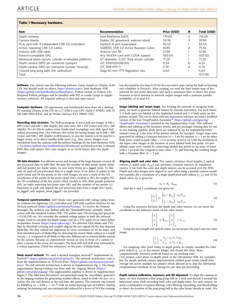
Hardware. Necessary hardware and approximate prices are shown in Table 1.Setting up the system also requires general lab electronics (tape, wire, solderingequipment, etc.), including: • Four infrared or red LEDs. • Two 0.1” pin headers orjumper wires. • Four 20 kOhm resistors. • Four 22 nF capacitors. • One 200 Ohmresistor (or same order of magnitude). • One stick (for moving ping-pong ballduring calibration).





Software. Our system uses the following software: Linux (tested on Ubuntu 16.04LTE, but should work on others, https://ubuntu.com/), Intel Realsense SDK(https://github.com/IntelRealSense/librealsense), Python (tested on Python 3.6).Required Python packages will be installed with PIP or conda (script in supple-mentary software). All required software is free and open source.

Computer hardware. All experiments and benchmarks were done on a desktopPC running Ubuntu 16.04 LTE on a 3.7 GHz 6-core CPU (Intel i7-8700K), with 32GB 2400 MHz RAM, and an Nvidia GeForce RTX 2080Ti GPU.

Recording data structure. The Python program is set to pull raw images at 640 ×480 (color) and 640 × 480 (depth), but only saves 320 × 210 (color) and 320 × 240(depth). We do this to reduce noise (multi-pixel averaging), save disk space andreduce processing time. Our software also works for saving images up to 848 × 480(color) and 848 × 480 (depth) at 60 frames/s, in case the system is to be used for abigger arena, or to detect smaller body parts (e.g., eyes, paws). Images weretransferred from the cameras with the python bindings for the Intel Realsense SDKv. 2.0 (https://github.com/IntelRealSense/librealsense) and saved as 8-bit, 3-channelPNG files with opencv (for color images) or as 16-bit binary files (for depthimages).

3D data structure. For efficient access and storage of the large datasets, we save allpre-processed data to hdf5 files. Because the number of data points (point-cloudand key-points) per frame varies, we save every frame as a jagged array. To thisend, we pack all pre-processed data to a single array. If we detect N points in thepoint-cloud and M key-points in the color images, we save a stack of the 3Dcoordinates of the points in the point-cloud (Nx3, raveled to 3N), the weights (N),the 3D coordinates of the key-points (Mx3, raveled to 3M), their pseudo-posterior(M), an index indicating key-point type (M), and the number of key-points (1).Functions to pack and unpack the pre-processed data from a single line (‘pack_-to_jagged’ and ‘unpack_from_jagged’) are provided.

Temporal synchronization. LED blinks were generated with voltage pulses froman Arduino (on digital pin 12), controlled over USB with a python interface for theFirmata protocol (https://github.com/tino/pyFirmata). To receive the Firmatamessages, the Arduino was flashed with the ‘StandardFirmata’ example, whichcomes with the standard Arduino IDE. TTL pulses were 150 ms long and spaced by~U(150,350) ms. We recorded the emitted voltage pulses in both the infraredimages (used to calculate the depth image) and on a TTL input on an Open EphysAcquisition System (https://open-ephys.org/). We detected LED blinks and TTLflips by threshold crossing and roughly aligned the two signals by the first detectedblink/flip. We first refined the alignment by cross correlation in 10 ms steps, andthen identified pairs of blinks/flips by detecting the closest blink, subject to a cutoff(zscore < 2, compared to all blink-to-flip time differences) to remove blinks missedby the camera (because an experimenter moved an arm in front of a camera toplace a mouse in the arena, for example). The final shift and drift were estimated bya robust regression (Theil-Sen estimator) on the pairs of blinks/links.

Deep neural network. We used a stacked hourglass network34 implemented inPytorch44 (https://github.com/pytorch/pytorch). The network architecture code isfrom the implementation in ‘PyTorch-Pose’ (https://github.com/bearpaw/pytorch-pose). The full network architecture is shown in Supplementary Fig. 1. The Imageaugmentation during training was done with the ‘imgaug’ library (https://github.com/aleju/imgaug). Our augmentation pipeline is shown in SupplementaryFigure 3. The ‘fake laser dot pattern’ was generated using the ‘snowflakes’ generatorin the imgaug routines for generating weather effects, tuned to look—by eye—to asimilar dot size and density to the real laser dot pattern. The network was trainedby RMSProp (α = 0.99, ε = 10−8) with an initial learning rate of 0.00025. Duringtraining, the learning rate was automatically reduced by a factor of 10 if the training

loss decreased by less than 0.1% for five successive steps (using the built-in learningrate scheduler in Pytorch). After training, we used the final output map of thenetwork for key-point detection, and used a maximum filter to detect key-pointlocations as local maxima in network output images with a posterior pseudo-probability of at least 0.5.

Image labeling and target maps. For training the network to recognize bodyparts, we need to generate labeled frames by manual annotation. For each frame,1–5 body parts are labeled on the implanted animal and 1–4 body parts on thepartner animal. This can be done with any annotation software; we used a modifiedversion of the free ‘DeepPoseKit-Annotator’8 (https://github.com/jgraving/DeepPoseKit-Annotator/) included in the Supplementary Code. This softwareallows easy labeling of the necessary points, and pre-packages training data for usein our training pipeline. Body parts are indexed by i/p for implanted/partneranimal (‘nose_p’ is the nose of the partner animal, for example). Target maps weregenerated by adding a Gaussian function (σ = 3 px for implant, σ = 1 px for otherbody parts, scaled to peak value = 1) to an array of zeros (at 1/4th the resolution ofthe input color image) at the location of every labeled body key-point. 1D partaffinity maps were created by connecting labeled key-points in an array of zeroswith a 1 px wide line (clipped to max value = 1), and blurring the resulting imagewith a Gaussian filter (σ = 3 px).

Aligning depth and color data. The camera intrinsics (focal lengths, f, opticalcenters, p, depth scale, dscale) and extrinsics (rotation matrices, R, translationvectors, �t) for both the color and depth sensors can be accessed over the SDK.Depth and color images were aligned to each other using a pinhole camera model.For example, the z coordinate of a single depth pixel with indices (ic; id) and 16-bitdepth value, dij, is given by:

zd ¼ dij � dscale ð1ÞAnd the x and y coordinates are given by:

xdyd

� �¼

jd � px;d

� �� zd=f x;d

id � py;d

� �� zd=f y;d

ð2Þ

Using the extrinsics between the depth and color sensors, we can move thecoordinate to the reference frame of the color sensor:

x

y

z

264

375c

¼ Rd!c

x

y

z

264

375d

þ�td!c ð3Þ

Using the focal length and optical center, we can project the pixel onto the colorimage:

icjc

� �¼

f y;c � yc=zc þ py;cf x;c � xc=zc þ px;c

ð4Þ

For assigning color pixel values to depth pixels, we simply rounded the colorpixel indices (ic; id) to the nearest integer and cloned the value. Morecomputationally intensive methods based on ray-tracking exist(‘rs2_project_color_pixel_to_depth_pixel’ in the Librealsense SDK, for example),but the simple pinhole camera approximation yielded good results (small jitteraverage out across multiple key-points) which allowed us to skip the substantialcomputational overhead of ray tracing for our data pre-processing.

Depth camera calibration, exposure, and 3D alignment. To align the cameras inspace, we first mounted a blue ping-pong ball on a stick and moved it around thebehavioral arena while recording both color and depth video. For each camera, weused a combination of motion filtering, color filtering, smoothing, and thresholdingto detect the location of the ping-pong ball in the color frame (details in code). We

Table 1 Necessary hardware.

Item Recommendation Price (USD) N Total (USD)

Depth cameras Intel RealSense D435 179.00 4 716.00Camera stands Etubby 26” gooseneck webcam stand 24.96 4 99.84PCIe card with 4 independent USB 3.0 controllers Startech 4-port superspeed 83.54 1 83.54Active, repeating USB 3.0 cables UGREEN, USB 3.0 Active Repeater Cable 18.89 4 75.56Arduino with USB cable Arduino Uno R3 13.98 1 13.98Pytorch-compatible GPU Any NVIDIA card with CUDA support 500.00 1 500.00Behavioral arena (acrylic cylinder or elevated platform) 12”-diameter, 5/32” thick acrylic cylinder 71.20 1 71.20Depth camera GPIO pin connector (jumper) JST ASSHSSH28K305 0.54 8 4.32Depth camera GPIO pin connector (jumper housing) JST SHR-09V-S 0.19 4 0.76Colored ping-pong balls (for calibration) Stiga 40 mm ITTF Regulation size 6.64 1 6.64Total 1571.84



https://ubuntu.com/

https://github.com/IntelRealSense/librealsense

https://github.com/IntelRealSense/librealsense

https://github.com/tino/pyFirmata

https://open-ephys.org/

https://github.com/pytorch/pytorch

https://github.com/bearpaw/pytorch-pose

https://github.com/bearpaw/pytorch-pose

https://github.com/aleju/imgaug

https://github.com/aleju/imgaug

https://github.com/jgraving/DeepPoseKit-Annotator/

https://github.com/jgraving/DeepPoseKit-Annotator/


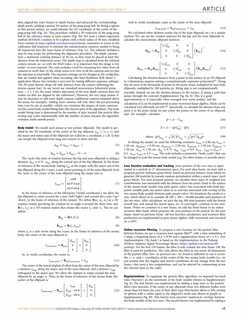
then aligned the color frames to depth frames and extracted the correspondingdepth pixels, yielding a partial 3D surface of the ping-pong ball. By fitting a sphereto this partial surface, we could estimate the 3D coordinate of the center of theping-pong ball (Fig. 3a). This procedure yielded a 3D trajectory of the ping-pongball in the reference frame of each camera (Fig. 3b). We used a robust regressionmethod (RANSAC routines to fit a sphere with a fixed radius of 40 mm, modifiedfrom routines in https://github.com/daavoo/pyntcloud), insensitive to errors in thecalibration ball trajectory to estimate the transformation matrices needed to bringall trajectories into the same frame of reference (Fig. 3c). The software includes astep-by-step recipe for performing the alignment procedure. The depth camerashave a minimum working distance of 20 cm, so they must be placed at least thisdistance from the behavioral arena. The depth map is calculated from the infraredcamera stream, so—as with the RGB video—it is important that the image is notunder- or over-exposed. The code includes a tool for streaming live video from allcameras to verify that: (i) the whole arena is in view of all the cameras and (ii) thatthe exposure is reasonable. The exposure settings can be changes in the config files,that are loaded and applied when recording (the Intel RealSense SDK demo Capplication library also includes a nice tool for testing different exposure settings).The 3D pixel density drops off with distance from the camera (following theinverse-square law). In our tested use (standard neuroscience behavioral arena,max. ~ 1 × 1 m), the exact relative placement of the four depth cameras does notmatter (as they are aligned by the calibration). However, for very large arenas, itmay be necessary to add more depth cameras (additional cameras mounted abovethe arena, for example). Adding more cameras will only affect the pre-processingtime (can be run in parallel—which can minimize the impact of more cameras),not the actual body model fitting time (the slowest part of the algorithm). The bodymodel fitting time is determined by the number of mice tracked (the particle filtersorting step scales exponentially with the number of mice, because the algorithmevaluates multi-animal poses).

Body model. We model each mouse at two prolate ellipsoids. The model is spe-cified by the 3D coordinate of the center of the hip ellipsoid, �chip ¼ x; y; z

� �, and

the major and minor axis of the ellipsoids are scaled by a coordinate, s 2 0; 1½ � thatcan morph the ellipsoid from long and narrow to short and fat:

ahip ¼ ahip;0 þ ahip;Δ � s ð5Þ

bhip ¼ bhip;0 þ bhip;Δ � ð1� sÞ ð6ÞThe ‘neck’ (the joint of rotation between the hip and nose ellipsoid) is sitting a

distance, dhip ¼ 0:75 � ahip, along the central axis of the hip ellipsoid. In the frameof reference of the mouse body (taking �chip as the origin, with the major axis of thehip ellipsoid along the x-axis), a unit vector pointing to of the nose ellipsoid, fromthe ‘neck’ to the center of the nose ellipsoid along the major axis is:

�enose ¼cosθ

sin θ cos ϕ

sin θ sinϕ

264

375 ð7Þ

In the frame of reference of the laboratory (‘world coordinates’), we allow thehip ellipsoid to rotate around the z-axis (‘left’/’right’) and around the y-axis (‘up’/’down’, in the frame of reference of the mouse). We define Rðαx ; αy ; αzÞ as a 3Drotation matrix specifying the rotation by an angle α around the three axes, andR �v1;�v2�

as a 3D rotation matrix that rotates the vector �v1 onto �v2. The we candefine:

Rhip ¼ Rð0; β; γÞ ð8Þ

Rhead ¼ Rð�ex ;�enoseÞ ð9Þwhere �ex is a unit vector along the x-axis. In the frame of reference of the mousebody, the center of the nose ellipsoid is:

�cnose;mouse ¼ Rhead

dnose0

0

264

375þ

dhip0

0

264

375 ð10Þ

So, in world coordinates, the center is:

�cnose;world ¼ Rhipcnose;mouse þ �chip ð11ÞThe center of the neural implant if offset from the center of the nose ellipsoid by

a distance ximpl along the major axis of the nose ellipsoid, and a distance zimpl

orthogonal to the major axis. We allow the implant to rotate around the noseellipsoid by an angle, ψ. Thus, in the frame of reference of the mouse body, thecenter of the ellipsoid is:

�cimpl;mouse ¼ Rhead

simpl

dimpl � cosψdimpl � sinψ

264

375þ

dhip0

0

264

375 ð12Þ

And in world coordinates, same as the center of the nose ellipsoid:

�cimpl;world ¼ Rhipcimpl;mouse þ �chip ð13ÞWe calculated other skeleton points (tip of the nose ellipsoid, etc.) in a similar

method. We can use the rotation matrices for the hip and the nose ellipsoids tocalculate the characteristic ellipsoid matrices:

Qhip ¼ Rhip

1=a2hip 0 0

0 1=b2hip 0

0 0 1=b2hip

2664

3775 Rhip

� �Tð14Þ

Qnose ¼ RhipRhead

1=a2nose 0 0

0 1=b2nose 0

0 0 1=b2nose

264

375 RhipRhead

� �Tð15Þ

Calculating the shortest distance from a point to the surface of an 3D ellipsoidin 3 dimensions requires solving a computationally-expensive polynomial39. Doingthis for each of the thousands of points in the point-cloud, multiplied by four bodyellipsoids, multiplied by 200 particles pr. fitting step is not computationally

tractable. Instead, we use the shortest distance to the surface, ed, along a path thatpasses through the centroid (Supplementary Fig. 8a, b). This is a goodapproximation to d (especially when averaged over many points), and thecalculation of ed can be implemented as pure vectorized linear algebra, which can becalculated very efficiently on GPU40. Specifically, to calculate the distance from anypoint �p in the point-cloud, we just center the points on the center of an ellipsoid,and—for example—calculate:

�p0 ¼ �p� �Chip ð16Þ

~d ¼ j1� k�p0k�1hipj � k�p0k ð17Þ

where; k�p0kQhip¼

ffiffiffiffiffiffiffiffiffiffiffiffiffih�p0; �p0i

pQhip

¼ffiffiffiffiffiffiffiffiffiffiffiffiffiffiffiffiffiffiffiffiffiffið�p0ÞTQhip�p0

qð18Þ

In fitting the model, we used the following constants: anose ¼ 2:00 cm; bnose ¼1:20 cm; ahipðminÞ ¼ 0:50 cm; ahipðmaxÞ ¼ 2:50 cm; bhipðminÞ ¼ 1:20 cm; bhipðmaxÞ ¼1:50 cm; dnose ¼ 1:00 cm; dhip ¼ 0:75 � ahip; rimpl ¼ 0:9 � bnose; ximpl ¼ dnoseþ0:5 � anose; zimpl ¼ 1:5 � rimpl. The code includes a parameter (‘body_scale’) that canbe changed to scale the mouse body model (e.g., for other strains, or juvenile mice).

Loss function evaluation and tracking. Joint position of the two mice is repre-sented as a particle in 17-dimensional space. For each data frame, we start with aproposal particle (leftmost green block, based on previous frames), from which wegenerate 200 particles by pseudo-random perturbation within a search space (nextgreen block). For each proposal particle, we calculate three types of weighted losscontributions: loss associated with the distance from the point-cloud to the surfaceof the mouse body models (top path, green color), loss associated with body key-points (middle path, key-point colors as in and loss associated with overlap of thetwo mouse body models (bottom path, purple color). We broadcast the results in away, which allows us to consider all 200 × 200 = 40.000 possible joint postures ofthe two mice. After calculation, we pick the top 200 joint postures with the lowestoverall loss, and anneal the search space, or—if converged—continue to the nextframe. When we continue to a new frame, we add the fitted frame to an onlinerecursive filter bank, which proposes the next position of the particle for the nextframe, based on previous frame. All loss function calculations, and recursive filterpredictions are implemented as pure tensor algebra, fully vectorized, and executedon a GPU.

Online recursive filtering. To propose a new location for the particle filterbetween frames, we use a recursive least squares filter89, with a time embedding of5 steps, a forgetting factor of μ ¼ 0:99 and a regularization factor of ε ¼ 0:1. Ourimplementation (‘rls_bank’) is based on the implementation in the Padasip(Python Adaptive Signal Processing) library (https://github.com/matousc89/padasip). For the first 150 frames, the filter is only trained, but after frame 150, thefilter is used for prediction. The code allows this filter to run across all dimensionsof the particle filter, but—in practical use—we found it sufficient to run it acrossthe x-, y- and z- coordinates of the center of the two mouse body models (i.e., wejust assume that the angular and stretch coordinates do not change from the lastframe—this saves a few computations, and can be selected by commenting in/outthe relevant lines in the code).

Regularizations. To regularize the particle filter algorithm, we imposed two hardrules (‘barriers’) on the movement of the body models (shown in SupplementaryFig. 8). The first barrier was implemented by adding a large term to the particlefilter’s loss function, if the center of any ellipsoids from two different bodies werecloser than 0.8 times the sum of their short axes (this barrier allows a 20% overlapof spheres with a radius equal to the ellipsoid’s small axis, drawn in purple inSupplementary Fig. 8f). This barrier term prevents ‘unphysical’ overlaps betweenthe body models of the two mice. The second barrier was implemented by adding a



https://github.com/daavoo/pyntcloud

https://github.com/matousc89/padasip

https://github.com/matousc89/padasip



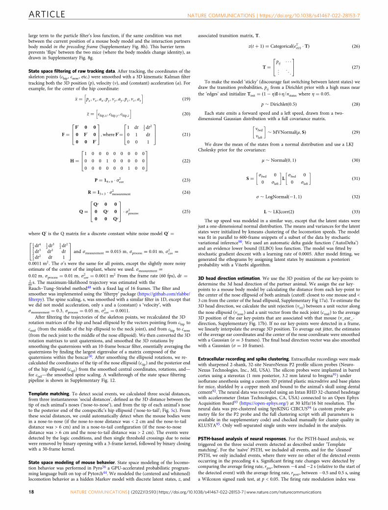
large term to the particle filter’s loss function, if the same condition was metbetween the current position of a mouse body model and the interaction partnersbody model in the preceding frame (Supplementary Fig. 8h). This barrier termprevents ‘flips’ between the two mice (where the body models change identity), asdrawn in Supplementary Fig. 8g.

State space filtering of raw tracking data. After tracking, the coordinates of theskeleton points (chip, cnose, etc.) were smoothed with a 3D kinematic Kalman filtertracking both the 3D position (p), velocity (v), and (constant) acceleration (a). Forexample, for the center of the hip coordinate:

�x ¼ px ; vx ; ax ; py ; vy ; ay ; pz ; vz ; azh i

ð19Þ

�z ¼ chip;x ; chip;y ; chip;zh i

ð20Þ

F ¼F0 0 0

0 F0 0

0 0 F0

264

375;where F0¼ 1 dt 1

2 dt2

0 1 dt

0 0 1

264

375 ð21Þ

H ¼1 0 0 0 0 0 0 0 0

0 0 0 1 0 0 0 0 0

0 0 0 0 0 0 1 0 0

264

375 ð22Þ

P ¼ 19´ 9 � σ2cov ð23Þ

R ¼ I3 ´ 3 � σ2measurement ð24Þ

Q ¼Q0 0 0

0 Q0 0

0 0 Q0

264

375 � σ2process ð25Þ

where Q’ is the Q matrix for a discrete constant white noise model Q0 ¼

14 dt

4 12 dt

3 12 dt

2

12 dt

3 dt2 dt12 dt

2 dt 1

24

35 and σmeasurement ¼ 0:015 m; σprocess ¼ 0:01 m; σ2cov ¼

0:0011 m2. The σ’s were the same for all points, except the slightly more noisyestimate of the center of the implant, where we used. σmeasurement ¼0:02 m; σprocess ¼ 0:01 m; σ2cov ¼ 0:0011 m2 From the frame rate (60 fps), dt ¼160 s: The maximum-likelihood trajectory was estimated with theRauch–Tung–Striebel method48 with a fixed lag of 16 frames. The filter andsmoother was implemented using the ‘filterpy’ package (https://github.com/rlabbe/filterpy). The spine scaling, s, was smoothed with a similar filter in 1D, except thatwe did not model acceleration, only s and a (constant) s ‘velocity’, withσmeasurement ¼ 0:3; σprocess ¼ 0:05 m; σ2cov ¼ 0:0011.

After filtering the trajectories of the skeleton points, we recalculated the 3Drotation matrices of the hip and head ellipsoid by the vectors pointing from chip tocmid (from the middle of the hip ellipsoid to the neck joint), and from chip to cnose(from the neck joint to the middle of the nose ellipsoid). We then converted the 3Drotation matrixes to unit quaternions, and smoothed the 3D rotations bysmoothing the quaternions with an 10-frame boxcar filter, essentially averaging thequaternions by finding the largest eigenvalue of a matrix composed of thequaternions within the boxcar50. After smoothing the ellipsoid rotations, we re-calculated the coordinates of the tip of the nose ellipsoid (ctip) and the posterior endof the hip ellipsoid (ctail) from the smoothed central coordinates, rotations, and—for ctail—the smoothed spine scaling. A walkthrough of the state space filteringpipeline is shown in Supplementary Fig. 12.

Template matching. To detect social events, we calculated three social distances,from three instantaneous ‘social distances’, defined as the 3D distance between thetip of each animal’s noses (‘nose-to-nose’), and from the tip of each animal’s noseto the posterior end of the conspecific’s hip ellipsoid (‘nose-to-tail’; Fig. 5c). Fromthese social distances, we could automatically detect when the mouse bodies werein a nose-to-nose (if the nose-to-nose distance was < 2 cm and the nose-to-taildistance was > 6 cm) and in a nose-to-tail configuration (if the nose-to-nosedistance was > 6 cm and the nose-to-tail distance was > 2 cm). The events weredetected by the logic conditions, and then single threshold crossings due to noisewere removed by binary opening with a 3-frame kernel, followed by binary closingwith a 30-frame kernel.

State space modeling of mouse behavior. State space modeling of the locomo-tion behavior was performed in Pyro56 a GPU-accelerated probabilistic program-ming language built on top of Pytorch44. We modeled the (centered and whitened)locomotion behavior as a hidden Markov model with discrete latent states, z, and

associated transition matrix, T.

z t þ 1ð Þ ¼ CategoricalðeTz tð Þ � TÞ ð26Þ

T ¼pij � � �... . .

.

24

35 ð27Þ

To make the model ‘sticky’ (discourage fast switching between latent states) wedraw the transition probabilities, pij from a Dirichlet prior with a high mass nearthe ‘edges’ and initialize Tinit ¼ ð1� ηÞIþη=nstates where η ¼ 0:05.

p � Dirichletð0:5Þ ð28ÞEach state emits a forward speed and a left speed, drawn from a two-

dimensional Gaussian distribution with a full covariance matrix.

vfwdvleft

� �� MVNormalðμ; SÞ ð29Þ

We draw the mean of the states from a normal distribution and use a LKJCholesky prior for the covariance:

μ � Normalð0; 1Þ ð30Þ

S ¼ σ fwd 0

0 σ left

� �L

σ fwd 0

0 σ left

� �ð31Þ

σ � LogNormalð�1; 1Þ ð32Þ

L � LKJcorrð2Þ ð33ÞThe up speed was modeled in a similar way, except that the latent states were

just a one-dimensional normal distribution. The means and variances for the latentstates were initialized by kmeans clustering of the locomotion speeds. The modelwas fit in parallel to 600-frame snippets of a subset of the data by stochasticvariational inference90. We used an automatic delta guide function (‘AutoDelta’)and an evidence lower bound (ELBO) loss function. The model was fitted bystochastic gradient descent with a learning rate of 0.0005. After model fitting, wegenerated the ethograms by assigning latent states by maximum a posterioriprobability with a Viterbi algorithm.

3D head direction estimation. We use the 3D position of the ear key-points todetermine the 3d head direction of the partner animal. We assign the ear key-points to a mouse body model by calculating the distance from each key-point tothe center of the nose ellipsoid of both animals (cutoff: closest to one mouse and <3 cm from the center of the head ellipsoid, Supplementary Fig 17a). To estimate the3D head direction, we calculate the unit rejection (vrej) between a unit vector alongthe nose ellipsoid (vnose) and a unit vector from the neck joint (cmid) to the average3D position of the ear key-points that are associated with that mouse (v_ear_-direction, Supplementary Fig. 17b). If no ear key-points were detected in a frame,we linearly interpolate the average 3D position. To average out jitter, the estimatesof the average ear coordinates and the center of the nose coordinate were smoothedwith a Gaussian (σ ¼ 3 frames). The final head direction vector was also smoothedwith a Gaussian (σ ¼ 10 frames).

Extracellular recording and spike clustering. Extracellular recordings were madewith sharpened 2-shank, 32-site NeuroNexus P2 profile silicon probes (Neuro-Nexus Technologies, Inc., MI, USA). The silicon probes were implanted in barrelcortex using a stereotax (1 mm posterior, 3.2 mm lateral to bregma91) underisoflurane anesthesia using a custom 3D printed plastic microdrive and base platesfor mice, shielded by a copper mesh and bound to the animal’s skull using dentalcement92. The neural data was recorded using an Intan RHD 32-channel headstagewith accelerometer (Intan Technologies, CA, USA) connected to an Open EphysAcquisition Board93 (https://open-ephys.org/) at 30 kHz/16 bit resolution. Theneural data was pre-clustered using SpyKING CIRCUS94 (a custom probe geo-metry file for the P2 probe and the full clustering script with all parameters isavailable in the supplementary code) and checked manually for cluster quality inKLUSTA95. Only well-separated single units were included in the analysis.

PSTH-based analysis of neural responses. For the PSTH-based analysis, wetriggered on the three social events detected as described under ‘Templatematching’. For the ‘naïve’ PSTH, we included all events, and for the ‘cleaned’PSTH, we only included events, where there were no other of the detected eventsoccurring in the preceding 4 s. Significant firing rate changes were detected bycomparing the average firing rate, rpre, between −4 and −2 s (relative to the start ofthe detected event) with the average firing rate, rpost, between −0.5 and 0.5 s, usinga Wilcoxon signed rank test, at p < 0.05. The firing rate modulation index was



https://github.com/rlabbe/filterpy

https://github.com/rlabbe/filterpy

https://open-ephys.org/


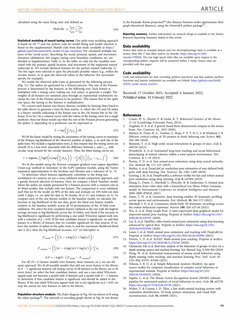
calculated using the same firing rates and defined as:

Mod:idx: ¼ rpost � rprerpost þ rpre

ð34Þ

Statistical modeling of neural tuning curves. Our spike train modeling approachis based on ref. 62 and our python code for model fitting and model selection isbased on the supplementary Matlab code from that study (available at https://github.com/GiocomoLab/ln-model-of-mec-neurons). We calculated multiple fea-tures of the ‘social scene’, describing the social, postural, spatial, and movementdynamics (definitions, bin ranges, tuning curve boundary conditions, etc. aredetailed in Supplementary Table 1). In the table, we only list the variables asso-ciated with the posture, spatial location, and movement of the implanted animal(subscript 0). We include identical features for the partner animal (subscript 1).The bin rages were selected to span the physically possible values (e.g., within thecircular arena), or to span the observed values in the behavior (for movementspeeds, for example).

We model the observed spike train as generated by the following process(Fig. 7c): The spikes are generated by a Poisson process. The rate of the Poissonprocess is determined by the features, in the following way: Each feature ismultiplied with a tuning curve (taking any real value), to generate a weight. Theweights of all features are summed, pass through an exponential nonlinearity (toclamp the rate of the Poisson process to be positive). This means that in the spikerate space, the tuning to the features is multiplicative.

We convert each feature into binary dummy variables by binning (bins listed inthe table above) to generate a time-by-bins matrix, A, where the i’th and j’th indexis a binary variable indicating if the feature was in the j’th feature bin in the i’thframe. If we let �c be a column vector with the values of the tuning curve for a singlepredictor, then our linear model says that the rate of the Poisson process generatingthe spikes, λ, depending on p predictors can be expressed as

�λ ¼ exp ∑pAp�cp

� �=dt ð35Þ

We fit the linear model by tuning the parameters of the tuning curves to maximizeof the Poisson log-likelihood of the observed number of spikes, n, in each bin of thespike train. We include a regularization term, β, that ensures that the tuning curves aresmooth (it is a loss term associated with the difference between ci and ciþ1, withcircular wrap-around for the circular features). Thus, the fitted tuning curves are:

c ¼ argmaxc ∑ilogP nijexp ∑

pAp�cp

� �� ∑

pβ ∑

i

12

cp;i � cp;iþ1

� �2� �

ð36Þ

We fit the models using the Newton conjugate gradient trust-region algorithm(‘trust-ncg’ method in ‘minimize’ in the SciPy optimize module, using the Taylorexpansion approximation to the Jacobian and Hessian and a tolerance of 1e−3).

To determine which features significantly contribute to the firing ratemodulation of a neuron, we use a cross-validated model comparison approach, anda greedy forward selection of features. First, we compare a fitted ‘baseline’ modelwhere the spikes are simply generated by a Poisson process with a constant rate to45 fitted models, that include only one feature. The comparison is cross-validated,such that we fit the model on 90% of the data and evaluate on 10% held-out data(with 3 skips, i.e., we split the data in 30 chunks, fit to 27, and evaluate on 3). Tocompare each of the one-feature models to the baseline model, we calculate theincrease in log-likelihood of the test data, given the fitted one-feature models(relative to the baseline model), across all 10 permutations of the 10-fold crossvalidation. We select the best candidate feature (defined as the one with the highestaverage increase in log-likelihood, across the 10 folds), and check if the increase inlog-likelihood is significant by performing a one-sided Wilcoxon signed-rank test,with a criterion of p < 0.05. If the best candidate feature is significant, we add thatfeature to a library of features that we consider significant for that neuron. If wehave the number of spikes in the spike train, �n, and the maximum-likelihood fittedrate is �λ cð Þ, then the log-likelihood increase, ΔL (in bits/spike) is:

Lmodel ¼ ∑iλi � nilog λi

� þ log ni!� � �

= ð37Þ

Lconstant ¼ ∑inh i � nilog nh ið Þ þ log ni!

� � �=∑

ini ð38Þ

ΔL¼�log 2ð Þ � Lmodel �Lconstant

� ð39ÞFor all (N > 1)-feature models (two features, three features, etc.), we use the

same approach: We fit all possible models that add one more feature to the libraryof N− 1 significant features (all tuning curves of all features in the library are re-fitevery time), we select the best candidate feature, and use a one-sided Wilcoxonsigned-rank test between a model with N features and a model with N− 1 featuresto determine if that candidate feature is significant and should be added to thelibrary. If the one-sided Wilcoxon signed-rank test is not significant at p < 0.05, westop the search for new features to add to the library.

Population structure analysis. The Euler diagram in Fig. 8d was drawn in R usingthe eulerr package96. The network co-encoding graph shown in Fig. 8e was drawn

in the Kamada–Kawai projection88 (the distance between nodes approximate theirgraph-theoretical distance), using the NetworkX python package97.

Reporting summary. Further information on research design is available in the NatureResearch Reporting Summary linked to this article.

Data availabilitySource data (and an example dataset and raw electrophysiology data) is available as aSource Data File (*.xlsx files) and/or on Zenodo: https://doi.org/10.5281/zenodo.5790820. The raw high-speed video files are available upon request to thecorresponding author, requests will be answered within 2 weeks. Source data areprovided with this paper.

Code availabilityCode and instructions for data recording (python functions) and data analysis (pythonfunctions and Jupyter notebooks) are available on Github: https://github.com/chrelli/3DDD_social_mouse_tracker/.

Received: 17 October 2021; Accepted: 6 January 2022;

References1. Crusio, W. E., Sluyter, F. & Gerlai, R. T. Behavioral Genetics of the Mouse

17–22 (Cambridge University Press, 2013).2. Angelaki, D. E. et al. A gravity-based three-dimensional compass in the mouse

brain. Nat. Commun. 11, 1855 (2020).3. Mimica, B., Dunn, B. A., Tombaz, T., Bojja, V. P. T. N. C. S. & Whitlock, J. R.

Efficient cortical coding of 3D posture in freely behaving rats. Science 362,584–589 (2018).

4. Shemesh, Y. et al. High-order social interactions in groups of mice. eLife 2,e00759 (2013).

5. Weissbrod, A. et al. Automated long-term tracking and social behaviouralphenotyping of animal colonies within a semi-natural environment. Nat.Commun. 4, 1–10 (2013).

6. Pereira, T. D. et al. Fast animal pose estimation using deep neural networks.Nat. Methods 16, 117–125 (2019).

7. Mathis, A. et al. DeepLabCut: markerless pose estimation of user-defined bodyparts with deep learning. Nat. Neurosci. 21, 1281–1289 (2018).

8. Graving, J. M. et al. DeepPoseKit, a software toolkit for fast and robust animalpose estimation using deep learning. eLife 8, e47994 (2019).

9. Zhang, L., Dunn, T., Marshall, J., Olveczky, B. & Linderman, S. Animal poseestimation from video data with a hierarchical von Mises–Fisher–Gaussianmodel. In International Conference on Artificial Intelligence and Statistics2800–2808 (PMLR, 2021).

10. Dunn, T. W. et al. Geometric deep learning enables 3D kinematic profilingacross species and environments. Nat. Methods 18, 564–573 (2021).

11. Marshall, J. D. et al. Continuous whole-body 3D kinematic recordings acrossthe rodent behavioral repertoire. Neuron 109, 420–437.e8 (2021).

12. Wu, A. et al. Deep Graph Pose: A semi-supervised deep graphical model forimproved animal pose tracking. Preprint at bioRxiv https://doi.org/10.1101/2020.08.20.259705 (2020).

13. Liu, X. et al. OptiFlex: video-based animal pose estimation using deep learningenhanced by optical flow. Preprint at bioRxiv https://doi.org/10.1101/2020.04.04.025494 (2020)

14. Lauer, J. et al. Multi-animal pose estimation and tracking with DeepLabCut.Preprint at bioRxiv https://doi.org/10.1101/2021.04.30.442096 (2021).

15. Pereira, T. D. et al. SLEAP: Multi-animal pose tracking. Preprint at bioRxivhttps://doi.org/10.1101/2020.08.31.276246 (2020).

16. Chaumont, Fde et al. Real-time analysis of the behaviour of groups of mice via adepth-sensing camera and machine learning. Nat. Biomed. Eng. 3, 930–942 (2019).

17. Hong, W. et al. Automated measurement of mouse social behaviors usingdepth sensing, video tracking, and machine learning. Proc. Natl. Acad. Sci.USA 112, E5351–E5360 (2015).

18. Nilsson, S. R. O. et al. Simple Behavioral Analysis (SimBA): An opensource toolkit for computer classification of complex social behaviors inexperimental animals. Preprint at bioRxiv https://doi.org/10.1101/2020.04.19.049452 (2020).

19. Segalin, C. et al. The Mouse Action Recognition System (MARS) softwarepipeline for automated analysis of social behaviors in mice. eLife 10, e63720https://doi.org/10.7554/eLife.63720 (2021).

20. Walter, T. & Couzin, I. D. TRex, a fast multi-animal tracking system withmarkerless identification, 2D body posture estimation, and visual fieldreconstruction. eLife 10, e64000 (2021).



https://github.com/GiocomoLab/ln-model-of-mec-neurons

https://github.com/GiocomoLab/ln-model-of-mec-neurons

https://doi.org/10.5281/zenodo.5790820

https://doi.org/10.5281/zenodo.5790820



https://doi.org/10.1101/2020.08.20.259705

https://doi.org/10.1101/2020.08.20.259705

https://doi.org/10.1101/2020.04.04.025494

https://doi.org/10.1101/2020.04.04.025494

https://doi.org/10.1101/2021.04.30.442096

https://doi.org/10.1101/2020.08.31.276246

https://doi.org/10.1101/2020.04.19.049452

https://doi.org/10.1101/2020.04.19.049452

https://doi.org/10.7554/eLife.63720



21. Ebbesen, C. L. & Froemke, R. C. Body language signals for rodent socialcommunication. Curr. Opin. Neurobiol. 68, 91–106 (2021).

22. Nath, T. et al. Using DeepLabCut for 3D markerless pose estimation acrossspecies and behaviors. Nat. Protoc. 14, 2152–2176 (2019).

23. Bala, P. C. et al. Automated markerless pose estimation in freely movingmacaques with OpenMonkeyStudio. Nat Commun 11, 4560 (2020).

24. Batty, E. et al. Advances in Neural Information Processing Systems 32 (edsWallach, H. et al.) 15706–15717 (Curran Associates, Inc., 2019).

25. Parker, P. R. L., Brown, M. A., Smear, M. C. & Niell, C. M. Movement-relatedsignals in sensory areas: Roles in natural behavior. Trends Neurosci. 43,581–595 (2020).

26. Kropff, E., Carmichael, J. E., Moser, M.-B. & Moser, E. I. Speed cells in themedial entorhinal cortex. Nature 523, 419–424 (2015).

27. Omrani, M., Kaufman, M. T., Hatsopoulos, N. G. & Cheney, P. D.Perspectives on classical controversies about the motor cortex. J. Neurophysiol.118, 1828–1848 (2017).

28. Georgopoulos, A. P., Kalaska, J. F., Caminiti, R. & Massey, J. T. On therelations between the direction of two-dimensional arm movements and celldischarge in primate motor cortex. J. Neurosci. 2, 1527–1537 (1982).

29. Kalaska, J. F. The representation of arm movements in postcentral and parietalcortex. Can. J. Physiol. Pharmacol. 66, 455–463 (1988).

30. Matsumoto, J. et al. A 3D-video-based computerized analysis of social andsexual interactions in rats. PLoS One 8, e78460 (2013).

31. Nakamura, T. et al. A markerless 3D computerized motion capture systemincorporating a skeleton model for monkeys. PLoS One 11, e0166154 (2016).

32. Sheets, A. L., Lai, P.-L., Fisher, L. C. & Basso, D. M. Quantitative evaluation of3D mouse behaviors and motor function in the open-field after spinal cordinjury using markerless motion tracking. PLoS One 8, e74536 (2013).

33. Wiltschko, A. B. et al. Mapping sub-second structure in mouse behavior.Neuron 88, 1121–1135 (2015).

34. Newell, A., Yang, K. & Deng, J. Stacked hourglass networks for human poseestimation. Preprint at https://arxiv.org/abs/1603.06937 (2016).

35. Günel, S. et al. DeepFly3D, a deep learning-based approach for 3D limb andappendage tracking in tethered, adult Drosophila. eLife 8, e48571 (2019).

36. Cao, Z., Simon, T., Wei, S.-E. & Sheikh, Y. Realtime multi-person 2D poseestimation using part affinity fields. Preprint at https://arxiv.org/abs/1611.08050 (2017).

37. Shorten, C. & Khoshgoftaar, T. M. A survey on image data augmentation fordeep learning. J. Big Data 6, 60 (2019).

38. Transtrum, M. K., Machta, B. B. & Sethna, J. P. Geometry of nonlinear leastsquares with applications to sloppy models and optimization. Phys. Rev. E 83,036701 (2011).

39. Hart, J. C. Graphics Gems (ed. Heckbert, P.) 113–119 (Academic Press, 1994).40. Kleinsteuber, M. & Hüper, K. Recent Advances in Optimization and its

Applications in Engineering (eds Diehl, M., Glineur, F., Jarlebring, E. &Michiels, W.) 73–82 (Springer, 2010).

41. Wang, W., Wang, J. & Kim, M.-S. An algebraic condition for the separation oftwo ellipsoids. Comput. Aided Geom. Des. 18, 531–539 (2001).

42. Choset, H. M. Principles of Robot Motion: Theory, Algorithms, andImplementation (MIT Press, 2005).

43. Deutscher, J. & Reid, I. Articulated body motion capture by stochastic search.Int. J. Comput. Vis. 61, 185–205 (2005).

44. Paszke, A. et al. Advances in Neural Information Processing Systems 32 (edsWallach, H. et al.) 8024–8035 (Curran Associates, Inc., 2019).

45. Sobol, I. M. On the distribution of points in a cube and the approximateevaluation of integrals. USSR Comput. Math. Math. Phys. 7, 86–112 (1967).

46. Das, G. Database Systems for Advanced Applications (eds Zhou, X., Yokota, H.,Deng, K. & Liu, Q.) 789–792 (Springer, 2009).

47. Murray, L. M., Lee, A. & Jacob, P. E. Parallel resampling in the particle filter. J.Comput. Graph. Stat. 25, 789–805 (2016).

48. Rauch, H. E., Tung, F. & Striebel, C. T. Maximum likelihood estimates oflinear dynamic systems. AIAA J. 3, 1445–1450 (1965).

49. Simon, D. Optimal State Estimation: Kalman, H∞, and Nonlinear Approaches(John Wiley & Sons, Inc., 2006).

50. Landis, M. F., Cheng, Y., Crassidis, J. L. & Oshman, Y. Averaging quaternions.J. Guid. Control Dyn. 30, 1193–1197 (2007).

51. Berman, G. J., Choi, D. M., Bialek, W. & Shaevitz, J. W. Mapping thestereotyped behaviour of freely moving fruit flies. J. R. Soc. Interface 11,20140672 (2014).

52. Berman, G. J., Bialek, W. & Shaevitz, J. W. Predictability and hierarchy inDrosophila behavior. Proc. Natl. Acad. Sci. USA 113, 11943–11948 (2016).

53. Wiltschko, A. B. et al. Revealing the structure of pharmacobehavioral spacethrough motion sequencing. Nat. Neurosci. https://doi.org/10.1038/s41593-020-00706-3 (2020).

54. Barnett, S. A. The Rat: A Study in Behaviour xvi, 248 (Aldine, 1963).55. Wolfe, J., Mende, C. & Brecht, M. Social facial touch in rats. Behav. Neurosci.

125, 900–910 (2011).

56. Bingham, E. et al. Pyro: Deep universal probabilistic programming. Preprint athttps://arxiv.org/abs/1810.09538 (2018).

57. Fox, E., Sudderth, E., Jordan, M. & Willsky, A. Bayesian nonparametricmethods for learning Markov switching processes. IEEE Signal Process. Mag.https://doi.org/10.1109/MSP.2010.937999 (2010).

58. Ebbesen, C. L., Bobrov, E., Rao, R. P. & Brecht, M. Highly structured, partner-sex- and subject-sex-dependent cortical responses during social facial touch.Nat. Commun. 10, 1–16 (2019).

59. Petersen, C. C. H. Sensorimotor processing in the rodent barrel cortex. Nat.Rev. Neurosci. 20, 533–546 (2019).

60. Keysers, C., Kaas, J. H. & Gazzola, V. Somatosensation in social perception.Nat. Rev. Neurosci. 11, 417–428 (2010).

61. Lenschow, C. & Brecht, M. Barrel cortex membrane potential dynamics insocial touch. Neuron 85, 718–725 (2015).

62. Hardcastle, K., Maheswaranathan, N., Ganguli, S. & Giocomo, L. M. Amultiplexed, heterogeneous, and adaptive code for navigation in medialentorhinal cortex. Neuron 94, e7 (2017).

63. Díaz López, B. When personality matters: Personality and social structure inwild bottlenose dolphins, Tursiops truncatus. Anim. Behav. 163, 73–84 (2020).

64. Tao, L., Ozarkar, S., Beck, J. M. & Bhandawat, V. Statistical structure oflocomotion and its modulation by odors. eLife 8, e41235 (2019).

65. Concha‐Miranda, M., Hartmann, K., Reinhold, A., Brecht, M. & Sanguinetti-Scheck, J. I. Play, but not observing play, engages rat medial prefrontal cortex.Eur. J. Neurosci. n/a, 4127–4138 (2020).

66. Carrillo, M. et al. Emotional mirror neurons in the rat’s anterior cingulatecortex. Curr. Biol. 29, 1301–1312.e6 (2019).

67. Kilner, J. M. & Lemon, R. N. What we know currently about mirror neurons.Curr. Biol. 23, R1057–R1062 (2013).

68. Hickok, G. Do mirror neurons subserve action understanding? Neurosci. Lett.540, 56–58 (2013).

69. Keysers, C. & Gazzola, V. Neuronal Correlates of Empathy 37–52 (Elsevier,2018).

70. Tombaz, T. et al. Action representation in the mouse parieto-frontal network.Sci. Rep. 10, 5559 (2020).

71. Carcea, I. et al. Oxytocin neurons enable social transmission of maternalbehaviour. Nature 596, 553–557 (2021).

72. Sargolini, F. et al. Conjunctive representation of position, direction, andvelocity in entorhinal cortex. Science 312, 758–762 (2006).

73. Porcelli, S. et al. Social brain, social dysfunction, and social withdrawal.Neurosci. Biobehav. Rev. 97, 10–33 (2019).

74. Uchino, B. N. et al. Social support, social integration, and inflammatorycytokines: A meta-analysis. Health Psychol. 37, 462–471 (2018).

75. Che, X., Cash, R., Ng, S. K., Fitzgerald, P. & Fitzgibbon, B. M. A systematicreview of the processes underlying the main and the buffering effect of socialsupport on the experience of pain. Clin. J. Pain 34, 1061–1076 (2018).

76. Anderson, D. J. & Perona, P. Toward a science of computational ethology.Neuron 84, 18–31 (2014).

77. Gal, A., Saragosti, J. & Kronauer, D J. anTraX, a software package for high-throughput video tracking of color-tagged insects. eLife 9, e58145 (2020).

78. Bozek, K., Hebert, L., Portugal, Y., Mikheyev, A. S. & Stephens, G. J. Markerlesstracking of an entire honey bee colony. Nat. Commun. 12, 1733 (2021).

79. Imirzian, N. et al. Automated tracking and analysis of ant trajectories showsvariation in forager exploration. Sci. Rep. 9, 13246 (2019).

80. Klibaite, U., Berman, G. J., Cande, J., Stern, D. L. & Shaevitz, J. W. Anunsupervised method for quantifying the behavior of paired animals. Phys.Biol. 14, 015006 (2017).

81. Franks, N. R. et al. Social behaviour and collective motion in plant-animalworms. Proc. R. Soc. B Biol. Sci. 283, 20152946 (2016).

82. Rosenthal, S. B., Twomey, C. R., Hartnett, A. T., Wu, H. S. & Couzin, I. D.Revealing the hidden networks of interaction in mobile animal groups allowsprediction of complex behavioral contagion. Proc. Natl. Acad. Sci. USA 112,4690–4695 (2015).

83. Adam, T. et al. Joint modelling of multi-scale animal movement data usinghierarchical hidden Markov models. Methods Ecol. Evol. 10, 1536–1550(2019).

84. Strandburg-Peshkin, A., Farine, D. R., Couzin, I. D. & Crofoot, M. C. Shareddecision-making drives collective movement in wild baboons. Science 348,1358–1361 (2015).

85. Patterson, T. A. et al. Statistical modelling of individual animal movement: anoverview of key methods and a discussion of practical challenges. AStA AdvStat Anal 101, 399–438 (2017).

86. Smith, J. E. & Pinter‐Wollman, N. Observing the unwatchable: Integratingautomated sensing, naturalistic observations and animal social networkanalysis in the age of big data. J. Anim. Ecol. n/a, 62–75(2020).

87. Gillis, W. et al. Revealing elements of naturalistic reinforcement learningthrough closed-loop action identification. In 2019 Neuroscience MeetingPlanner Program No. 146.17 (Society for Neuroscience, 2019).



https://arxiv.org/abs/1603.06937



https://doi.org/10.1038/s41593-020-00706-3

https://doi.org/10.1038/s41593-020-00706-3


https://doi.org/10.1109/MSP.2010.937999


88. Kamada, T. & Kawai, S. An algorithm for drawing general undirected graphs.Inf. Process. Lett. 31, 7–15 (1989).

89. Sayed, A. & Kailath, T. Digital Signal Processing Fundamentals Vol. 20094251,1–40 (CRC Press, 2009).

90. Blei, D. M., Kucukelbir, A. & McAuliffe, J. D. Variational inference: A reviewfor statisticians. J. Am. Stat. Assoc. 112, 859–877 (2017).

91. Franklin, K. B. J. & Paxinos, G. The Mouse Brain in Stereotaxic Coordinates(Academic Press, 2019).

92. Vöröslakos, M. et al. 3D-printed Recoverable Microdrive and Base PlateSystem for Rodent Electrophysiology. Bio-protocol 11, e4137–e4137 (2021).

93. Siegle, J. H. et al. Open Ephys: an open-source, plugin-based platform formultichannel electrophysiology. J. Neural Eng. 14, 045003 (2017).

94. Yger, P. et al. A spike sorting toolbox for up to thousands of electrodes validatedwith ground truth recordings in vitro and in vivo. eLife 7, 1–23 (2018).

95. Rossant, C. et al. Spike sorting for large, dense electrode arrays. Nat. Neurosci.19, 634–641 (2016).

96. Larsson, J. & Gustafsson, P. A Case Study in Fitting Area-Proportional EulerDiagrams with Ellipses Using eulerr. Proceedings of International Workshopon Set Visualization and Reasoning 2116, 84–91 https://cran.r-project.org/package=eulerr (2018).

97. Hagberg, A., Schult, D. & Swart, P. Exploring Network Structure, Dynamics,and Function using NetworkX. In Proceedings of the 7th Python in Scienceconference (eds Varoquaux, G., Vaught, T. & Millman, J.). 11-15 (SciPy 2008).http://conference.scipy.org/proceedings/scipy2008/paper_2/full_text.pdf

AcknowledgementsThis work was supported by The Novo Nordisk Foundation (C.L.E.), the NIH (DC012557,HD088411, and NS107616 to R.C.F.), and a Howard Hughes Medical Institute FacultyScholarship (R.C.F.). We thank György Buzsáki, David Tingley, and Manuel Valero for helpin establishing silicon probe recordings and for the gift of 3D printed silicon drive parts.

Author contributionsC.L.E. designed and implemented the system, performed experiments, analyzed the data,made figures, and wrote the first version of the manuscript. R.C.F. supervised the study.C.L.E and R.C.F. wrote the manuscript.

Competing interestsThe authors declare no competing interests.

Additional informationSupplementary information The online version contains supplementary materialavailable at https://doi.org/10.1038/s41467-022-28153-7.

Correspondence and requests for materials should be addressed to Christian L. Ebbesenor Robert C. Froemke.

Peer review information Nature Communications thanks the anonymous reviewer(s) fortheir contribution to the peer review of this work. Peer reviewer reports are available.

Reprints and permission information is available at http://www.nature.com/reprints

Publisher’s note Springer Nature remains neutral with regard to jurisdictional claims inpublished maps and institutional affiliations.

Open Access This article is licensed under a Creative CommonsAttribution 4.0 International License, which permits use, sharing,

adaptation, distribution and reproduction in any medium or format, as long as you giveappropriate credit to the original author(s) and the source, provide a link to the CreativeCommons license, and indicate if changes were made. The images or other third partymaterial in this article are included in the article’s Creative Commons license, unlessindicated otherwise in a credit line to the material. If material is not included in thearticle’s Creative Commons license and your intended use is not permitted by statutoryregulation or exceeds the permitted use, you will need to obtain permission directly fromthe copyright holder. To view a copy of this license, visit http://creativecommons.org/licenses/by/4.0/.

© The Author(s) 2022



https://cran.r-project.org/package=eulerr

https://cran.r-project.org/package=eulerr

http://conference.scipy.org/proceedings/scipy2008/paper_2/full_text.pdf

https://doi.org/10.1038/s41467-022-28153-7

http://www.nature.com/reprints

http://creativecommons.org/licenses/by/4.0/

http://creativecommons.org/licenses/by/4.0/



automatic mapping of multiplexed social receptive fields by

Documents