THEORETICAL ADVANCES

Fabien Feschet

Canonical representations of discrete curves

Received: 9 June 2004 / Accepted: 4 February 2005 / Published online: 10 June 2005� Springer-Verlag London Limited 2005

Abstract A new representation of digital curves isintroduced. It has the property of being unique andcanonical when computed on closed curves. The repre-sentation is based on the discrete notion of tangents andis complete in the sense that it contains all discrete seg-ments and all polygonalizations which can be con-structed with connected subsets of the original curve.This representation is extended for dealing with noisycurves and we also propose a multi-scale extension. Anapplication is given to curve decomposition into con-cave–convex parts and with application in syntacticalbased methods.

1 Introduction

Digital objects, curves, surfaces are commonly acquiredby physical sensors. Shapes can be obtained as theouter boundary of the digital acquisition of a planarobject and are thus usually described by a discretecurve. Two problems arise when considering the digi-tization of a real objects. One concerns the problem ofcharacterizing digitizations which preserve topologicalor differential properties of real objects [15, 18] andanother concerns the manipulation of the discrete datausing discrete methods [20, 21]. The first problem is avery challenging one but is not concerned by the pres-ent study; that is, we do not wonder how the discretedata were acquired and we only focus on their repre-sentation and manipulation. We thus suppose that wehave a list of points of Z2: It is obviously the case whenconsidering shapes. Describing discrete curves by theirlist of points is a common approach but lacks

geometrical information. It is a straightforward andsimple idea to try to use discrete lines and segments torepresent discrete curves with less geometrical primi-tives [23]. One of the standard approaches is the rep-resentation of discrete curves by discrete segmentsconnected by their endpoints leading to the notion ofpolygonalization [25]. However, this representation isextremely sensitive to the starting point of the compu-tation. This is not a drawback for open curves since it issufficient to take one of the extremities of the curve as astarting point. However, this behavior becomes animportant drawback when considering closed curves,since for closed curves no point can be privileged. Themain goal of this paper is to introduce a new repre-sentation, called the tangential cover, of closed or opendiscrete curves and to show that this representation hasthe property of being canonical meaning that nostarting point is privileged. This decomposition mightbe used in shape matching or shape classification butwe do not study its application to those problems in thepresent paper. Our goal is to propose a new way ofrepresenting discrete curves, on which new methods forshape analysis will be presented in future papers.

As will be explained later, the tangential cover hastwo interpretations: one is global and concerns thegeometrical structure of discrete segments built fromconnected portions of the curve, while the second islocal through the notion of discrete tangents. The mostinteresting property of the tangential cover is its com-pleteness meaning that it contains all possible discretesegments. As a consequence, this decomposition con-tains all the polygonalizations of the curve meaningthat if curves are described by our representation,classical methods remain valid with a simple linear timepreprocessing. An application of this representation isgiven for a decomposition of curves into homogeneousparts-in a sense formally described further on in thepaper. We also provide ways to extend the decompo-sition into a multi-scale representation to deal withnoisy curves. We end this paper with some conclusionsand perspectives after introducing the Farey arcs as

F. FeschetLLAIC1 - IUT Clermont-Ferrand 1 - Campus des Cezeaux,BP 86 - 63172, Aubiere, FranceE-mail: feschet@llaic3.u-clermont1.fr

Pattern Anal Applic (2005) 8: 84–94DOI 10.1007/s10044-005-0246-5

candidate curves for estimating the worst case space-complexity of our representation for which a linear-time algorithm is presented.

2 Tangential cover

All along the paper, a discrete curve is a list of points

C ¼ ðpiÞ0�i\n of Z2 which are connected. Self intersec-

tions of the curve are allowed as soon as the multiplepoints are duplicated in the list. The order induced bythe order of the indices is called the orientation of thecurve. As a consequence, left and right correspondsrespectively to smaller and higher indices. When thecurve is closed, indices are intended modulo the length nof the curve. The allowed connectivities are the standardfour and eight connectivities corresponding to theneighborhood of four points using the north, south, eastand west directions and the neighborhood of eightpoints containing all points with L¥ distance of one.When using the points of the eight connectivity minusthe ones of the four connectivity, we use the term stricteight connectivity. If the points of the curve are con-nected using only strict eight connectivity, we say thatthe curve is strictly eight connected, otherwise the curveis four connected. In this paper, we restrict our study tocurves either eight or four connected. For discrete lines,we refer to the survey article of Rosenfeld and Klette[22] and references therein.

2.1 Discrete lines and tangents

Definition 1 The set of points (x,y) of Z2 verifying

l � ax� by\lþ x ð1Þ

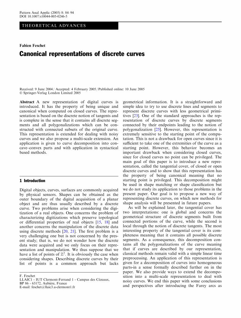
with l, a and b in Z and x in N� f0gis called thearithmetical line with slope a/b, with shift parameter land with thickness x. It is denoted by D(a, b, l, x).

Unformaly, the arithmetical lines correspond to allthe points with integer coordinates in a strip limited bythe lines ax�by=l and ax�by=l+x�1. The thicknessx corresponds to the number of lines of slope a/b withgoes through the integer points of the strip (see Fig. 1).

The width parameter x controls the thickness butalso the connectivity of the line. Indeed, arithmeticallines are:

a. disconnected if x<max (|a|,|b|),b. strictly eight connected if x=max (|a|,|b|),

c. strictly four connected if x=|a|+|b| andd. thick and four connected if x>|a|+|b|.

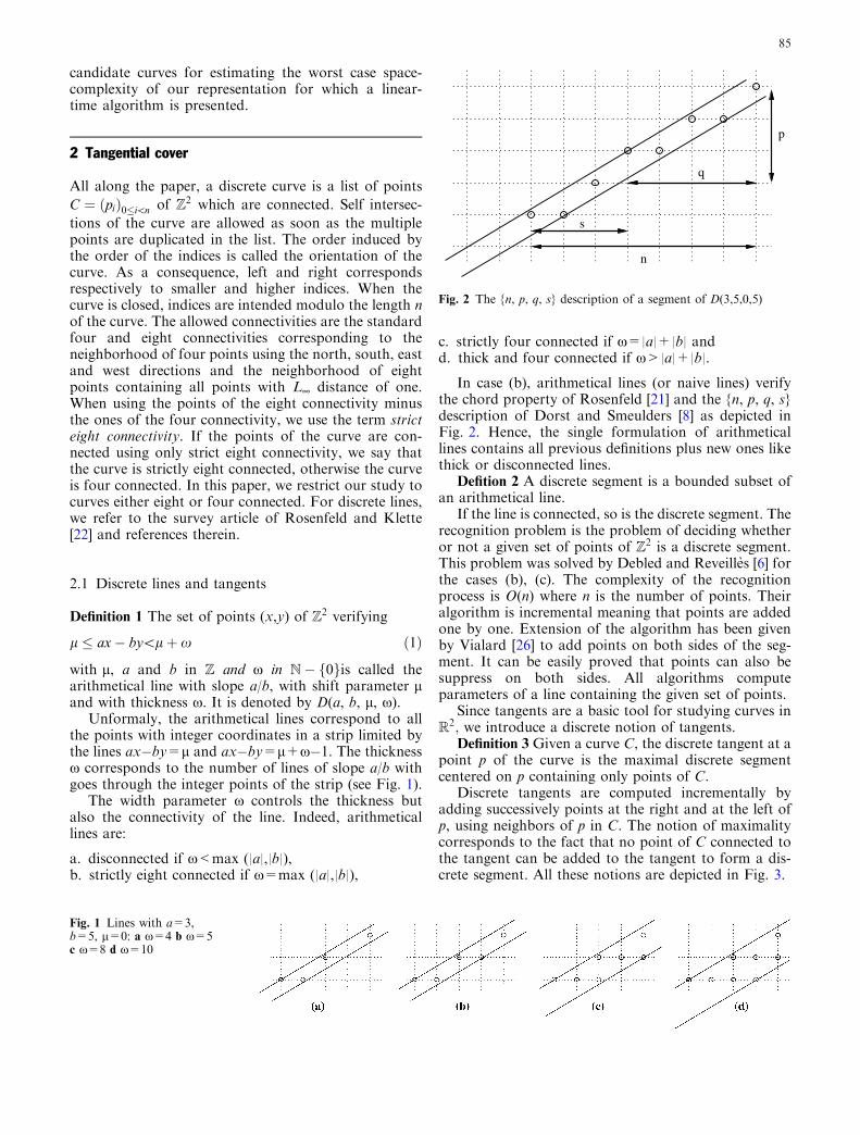
In case (b), arithmetical lines (or naive lines) verifythe chord property of Rosenfeld [21] and the {n, p, q, s}description of Dorst and Smeulders [8] as depicted inFig. 2. Hence, the single formulation of arithmeticallines contains all previous definitions plus new ones likethick or disconnected lines.

Defition 2 A discrete segment is a bounded subset ofan arithmetical line.

If the line is connected, so is the discrete segment. Therecognition problem is the problem of deciding whetheror not a given set of points of Z2 is a discrete segment.This problem was solved by Debled and Reveilles [6] forthe cases (b), (c). The complexity of the recognitionprocess is O(n) where n is the number of points. Theiralgorithm is incremental meaning that points are addedone by one. Extension of the algorithm has been givenby Vialard [26] to add points on both sides of the seg-ment. It can be easily proved that points can also besuppress on both sides. All algorithms computeparameters of a line containing the given set of points.

Since tangents are a basic tool for studying curves inR

2; we introduce a discrete notion of tangents.Definition 3 Given a curve C, the discrete tangent at a

point p of the curve is the maximal discrete segmentcentered on p containing only points of C.

Discrete tangents are computed incrementally byadding successively points at the right and at the left ofp, using neighbors of p in C. The notion of maximalitycorresponds to the fact that no point of C connected tothe tangent can be added to the tangent to form a dis-crete segment. All these notions are depicted in Fig. 3.

Fig. 1 Lines with a=3,b=5, l=0: a x=4 b x=5c x=8 d x=10

n

s

p

q

Fig. 2 The {n, p, q, s} description of a segment of D(3,5,0,5)

85

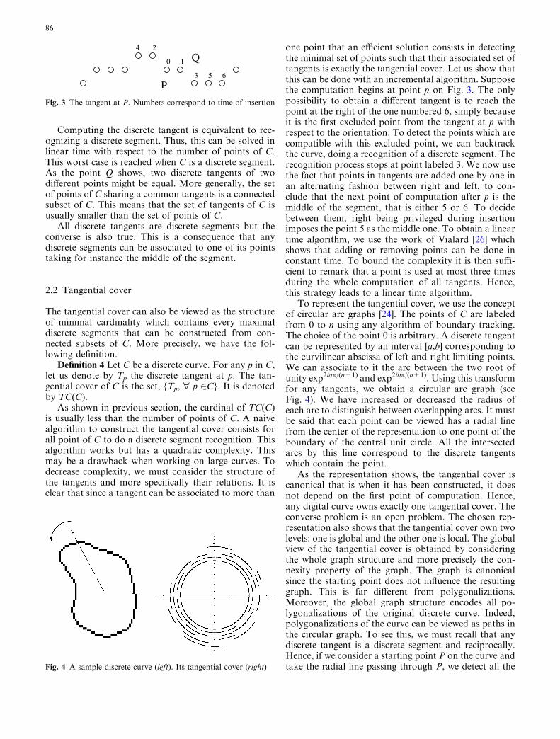
Computing the discrete tangent is equivalent to rec-ognizing a discrete segment. Thus, this can be solved inlinear time with respect to the number of points of C.This worst case is reached when C is a discrete segment.As the point Q shows, two discrete tangents of twodifferent points might be equal. More generally, the setof points of C sharing a common tangents is a connectedsubset of C. This means that the set of tangents of C isusually smaller than the set of points of C.

All discrete tangents are discrete segments but theconverse is also true. This is a consequence that anydiscrete segments can be associated to one of its pointstaking for instance the middle of the segment.

2.2 Tangential cover

The tangential cover can also be viewed as the structureof minimal cardinality which contains every maximaldiscrete segments that can be constructed from con-nected subsets of C. More precisely, we have the fol-lowing definition.

Definition 4 Let C be a discrete curve. For any p in C,let us denote by Tp the discrete tangent at p. The tan-gential cover of C is the set, {Tp, " p 2C}. It is denotedby TC(C).

As shown in previous section, the cardinal of TC(C)is usually less than the number of points of C. A naivealgorithm to construct the tangential cover consists forall point of C to do a discrete segment recognition. Thisalgorithm works but has a quadratic complexity. Thismay be a drawback when working on large curves. Todecrease complexity, we must consider the structure ofthe tangents and more specifically their relations. It isclear that since a tangent can be associated to more than

one point that an efficient solution consists in detectingthe minimal set of points such that their associated set oftangents is exactly the tangential cover. Let us show thatthis can be done with an incremental algorithm. Supposethe computation begins at point p on Fig. 3. The onlypossibility to obtain a different tangent is to reach thepoint at the right of the one numbered 6, simply becauseit is the first excluded point from the tangent at p withrespect to the orientation. To detect the points which arecompatible with this excluded point, we can backtrackthe curve, doing a recognition of a discrete segment. Therecognition process stops at point labeled 3. We now usethe fact that points in tangents are added one by one inan alternating fashion between right and left, to con-clude that the next point of computation after p is themiddle of the segment, that is either 5 or 6. To decidebetween them, right being privileged during insertionimposes the point 5 as the middle one. To obtain a lineartime algorithm, we use the work of Vialard [26] whichshows that adding or removing points can be done inconstant time. To bound the complexity it is then suffi-cient to remark that a point is used at most three timesduring the whole computation of all tangents. Hence,this strategy leads to a linear time algorithm.

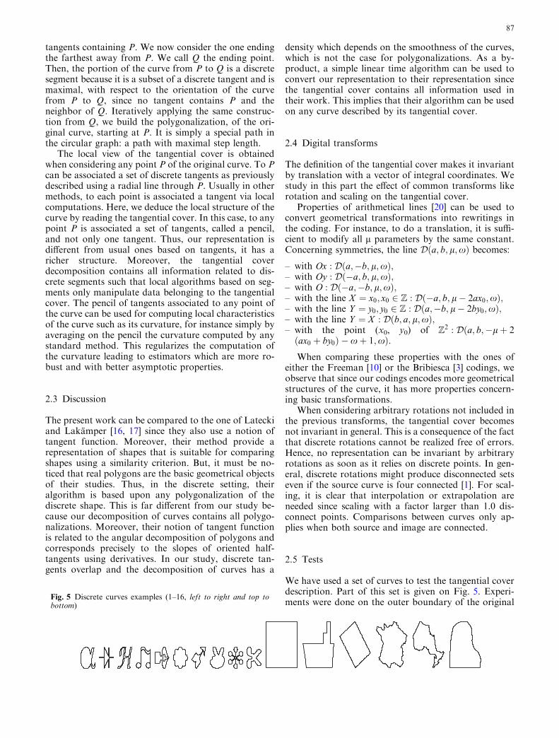
To represent the tangential cover, we use the conceptof circular arc graphs [24]. The points of C are labeledfrom 0 to n using any algorithm of boundary tracking.The choice of the point 0 is arbitrary. A discrete tangentcan be represented by an interval [a,b] corresponding tothe curvilinear abscissa of left and right limiting points.We can associate to it the arc between the two root ofunity exp2iap/(n+1) and exp2ibp/(n+1). Using this transformfor any tangents, we obtain a circular arc graph (seeFig. 4). We have increased or decreased the radius ofeach arc to distinguish between overlapping arcs. It mustbe said that each point can be viewed has a radial linefrom the center of the representation to one point of theboundary of the central unit circle. All the intersectedarcs by this line correspond to the discrete tangentswhich contain the point.

As the representation shows, the tangential cover iscanonical that is when it has been constructed, it doesnot depend on the first point of computation. Hence,any digital curve owns exactly one tangential cover. Theconverse problem is an open problem. The chosen rep-resentation also shows that the tangential cover own twolevels: one is global and the other one is local. The globalview of the tangential cover is obtained by consideringthe whole graph structure and more precisely the con-nexity property of the graph. The graph is canonicalsince the starting point does not influence the resultinggraph. This is far different from polygonalizations.Moreover, the global graph structure encodes all po-lygonalizations of the original discrete curve. Indeed,polygonalizations of the curve can be viewed as paths inthe circular graph. To see this, we must recall that anydiscrete tangent is a discrete segment and reciprocally.Hence, if we consider a starting point P on the curve andtake the radial line passing through P, we detect all the

P

0 1

2

3

4

5 6

Q

Fig. 3 The tangent at P. Numbers correspond to time of insertion

Fig. 4 A sample discrete curve (left). Its tangential cover (right)

86

tangents containing P. We now consider the one endingthe farthest away from P. We call Q the ending point.Then, the portion of the curve from P to Q is a discretesegment because it is a subset of a discrete tangent and ismaximal, with respect to the orientation of the curvefrom P to Q, since no tangent contains P and theneighbor of Q. Iteratively applying the same construc-tion from Q, we build the polygonalization, of the ori-ginal curve, starting at P. It is simply a special path inthe circular graph: a path with maximal step length.

The local view of the tangential cover is obtainedwhen considering any point P of the original curve. To Pcan be associated a set of discrete tangents as previouslydescribed using a radial line through P. Usually in othermethods, to each point is associated a tangent via localcomputations. Here, we deduce the local structure of thecurve by reading the tangential cover. In this case, to anypoint P is associated a set of tangents, called a pencil,and not only one tangent. Thus, our representation isdifferent from usual ones based on tangents, it has aricher structure. Moreover, the tangential coverdecomposition contains all information related to dis-crete segments such that local algorithms based on seg-ments only manipulate data belonging to the tangentialcover. The pencil of tangents associated to any point ofthe curve can be used for computing local characteristicsof the curve such as its curvature, for instance simply byaveraging on the pencil the curvature computed by anystandard method. This regularizes the computation ofthe curvature leading to estimators which are more ro-bust and with better asymptotic properties.

2.3 Discussion

The present work can be compared to the one of Lateckiand Lakamper [16, 17] since they also use a notion oftangent function. Moreover, their method provide arepresentation of shapes that is suitable for comparingshapes using a similarity criterion. But, it must be no-ticed that real polygons are the basic geometrical objectsof their studies. Thus, in the discrete setting, theiralgorithm is based upon any polygonalization of thediscrete shape. This is far different from our study be-cause our decomposition of curves contains all polygo-nalizations. Moreover, their notion of tangent functionis related to the angular decomposition of polygons andcorresponds precisely to the slopes of oriented half-tangents using derivatives. In our study, discrete tan-gents overlap and the decomposition of curves has a

density which depends on the smoothness of the curves,which is not the case for polygonalizations. As a by-product, a simple linear time algorithm can be used toconvert our representation to their representation sincethe tangential cover contains all information used intheir work. This implies that their algorithm can be usedon any curve described by its tangential cover.

2.4 Digital transforms

The definition of the tangential cover makes it invariantby translation with a vector of integral coordinates. Westudy in this part the effect of common transforms likerotation and scaling on the tangential cover.

Properties of arithmetical lines [20] can be used toconvert geometrical transformations into rewritings inthe coding. For instance, to do a translation, it is suffi-cient to modify all l parameters by the same constant.Concerning symmetries, the line Dða; b; l;xÞ becomes:

– with Ox : Dða;�b; l;xÞ;– with Oy : Dð�a; b; l;xÞ;– with O : Dð�a;�b; l;xÞ;– with the line X ¼ x0; x0 2 Z : Dð�a; b; l� 2ax0;xÞ;– with the line Y ¼ y0; y0 2 Z : Dða;�b; l� 2by0;xÞ;– with the line Y ¼ X : Dðb; a; l;xÞ;– with the point (x0, y0) of Z

2 : Dða; b;�lþ 2ðax0 þ by0Þ � xþ 1;xÞ:When comparing these properties with the ones of

either the Freeman [10] or the Bribiesca [3] codings, weobserve that since our codings encodes more geometricalstructures of the curve, it has more properties concern-ing basic transformations.

When considering arbitrary rotations not included inthe previous transforms, the tangential cover becomesnot invariant in general. This is a consequence of the factthat discrete rotations cannot be realized free of errors.Hence, no representation can be invariant by arbitraryrotations as soon as it relies on discrete points. In gen-eral, discrete rotations might produce disconnected setseven if the source curve is four connected [1]. For scal-ing, it is clear that interpolation or extrapolation areneeded since scaling with a factor larger than 1.0 dis-connect points. Comparisons between curves only ap-plies when both source and image are connected.

2.5 Tests

We have used a set of curves to test the tangential coverdescription. Part of this set is given on Fig. 5. Experi-ments were done on the outer boundary of the original

Fig. 5 Discrete curves examples (1–16, left to right and top tobottom)

87

shapes. The Freeman coding of the boundary is usedwith a boundary tracking procedure. The various curveshave been chosen to describe both linear objects and nonlinear objects. This is especially the case for the twomaps. To measure the performance, we simply comparethe number of points of the original curve and thenumber of segments in the tangential cover. The time ofcomputation is not a good measure because for curveswith about 2,000 points, it is either not measurable orindependant of the number of points.

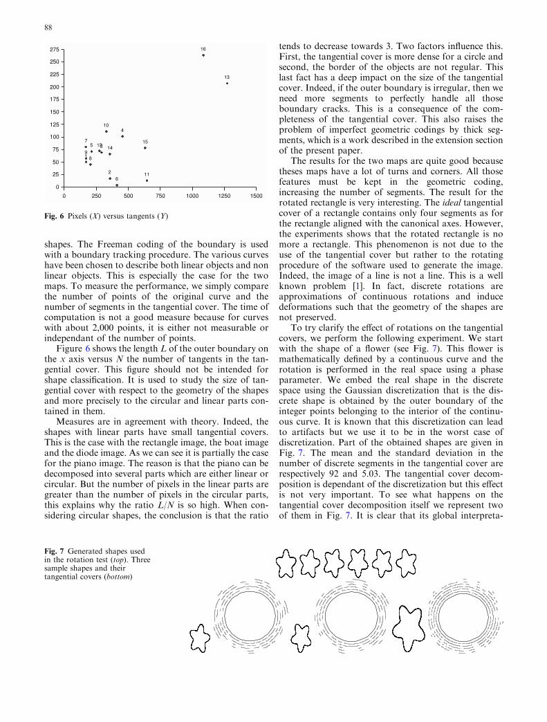
Figure 6 shows the length L of the outer boundary onthe x axis versus N the number of tangents in the tan-gential cover. This figure should not be intended forshape classification. It is used to study the size of tan-gential cover with respect to the geometry of the shapesand more precisely to the circular and linear parts con-tained in them.

Measures are in agreement with theory. Indeed, theshapes with linear parts have small tangential covers.This is the case with the rectangle image, the boat imageand the diode image. As we can see it is partially the casefor the piano image. The reason is that the piano can bedecomposed into several parts which are either linear orcircular. But the number of pixels in the linear parts aregreater than the number of pixels in the circular parts,this explains why the ratio L/N is so high. When con-sidering circular shapes, the conclusion is that the ratio

tends to decrease towards 3. Two factors influence this.First, the tangential cover is more dense for a circle andsecond, the border of the objects are not regular. Thislast fact has a deep impact on the size of the tangentialcover. Indeed, if the outer boundary is irregular, then weneed more segments to perfectly handle all thoseboundary cracks. This is a consequence of the com-pleteness of the tangential cover. This also raises theproblem of imperfect geometric codings by thick seg-ments, which is a work described in the extension sectionof the present paper.

The results for the two maps are quite good becausetheses maps have a lot of turns and corners. All thosefeatures must be kept in the geometric coding,increasing the number of segments. The result for therotated rectangle is very interesting. The ideal tangentialcover of a rectangle contains only four segments as forthe rectangle aligned with the canonical axes. However,the experiments shows that the rotated rectangle is nomore a rectangle. This phenomenon is not due to theuse of the tangential cover but rather to the rotatingprocedure of the software used to generate the image.Indeed, the image of a line is not a line. This is a wellknown problem [1]. In fact, discrete rotations areapproximations of continuous rotations and inducedeformations such that the geometry of the shapes arenot preserved.

To try clarify the effect of rotations on the tangentialcovers, we perform the following experiment. We startwith the shape of a flower (see Fig. 7). This flower ismathematically defined by a continuous curve and therotation is performed in the real space using a phaseparameter. We embed the real shape in the discretespace using the Gaussian discretization that is the dis-crete shape is obtained by the outer boundary of theinteger points belonging to the interior of the continu-ous curve. It is known that this discretization can leadto artifacts but we use it to be in the worst case ofdiscretization. Part of the obtained shapes are given inFig. 7. The mean and the standard deviation in thenumber of discrete segments in the tangential cover arerespectively 92 and 5.03. The tangential cover decom-position is dependant of the discretization but this effectis not very important. To see what happens on thetangential cover decomposition itself we represent twoof them in Fig. 7. It is clear that its global interpreta-

Fig. 6 Pixels (X) versus tangents (Y)

Fig. 7 Generated shapes usedin the rotation test (top). Threesample shapes and theirtangential covers (bottom)

88

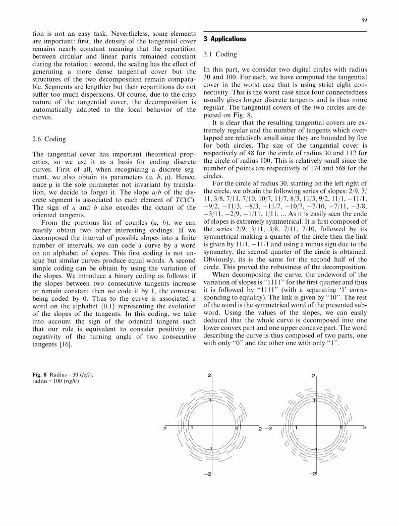
tion is not an easy task. Nevertheless, some elementsare important: first, the density of the tangential coverremains nearly constant meaning that the repartitionbetween circular and linear parts remained constantduring the rotation ; second, the scaling has the effect ofgenerating a more dense tangential cover but thestructures of the two decomposition remain compara-ble. Segments are lengthier but their repartitions do notsuffer too much dispersions. Of course, due to the crispnature of the tangential cover, the decomposition isautomatically adapted to the local behavior of thecurves.

2.6 Coding

The tangential cover has important theoretical prop-erties, so we use it as a basis for coding discretecurves. First of all, when recognizing a discrete seg-ment, we also obtain its parameters (a, b, l). Hence,since l is the sole parameter not invariant by transla-tion, we decide to forget it. The slope a/b of the dis-crete segment is associated to each element of TC(C).The sign of a and b also encodes the octant of theoriented tangents.

From the previous list of couples (a, b), we canreadily obtain two other interesting codings. If wedecomposed the interval of possible slopes into a finitenumber of intervals, we can code a curve by a wordon an alphabet of slopes. This first coding is not un-ique but similar curves produce equal words. A secondsimple coding can be obtain by using the variation ofthe slopes. We introduce a binary coding as follows: ifthe slopes between two consecutive tangents increaseor remain constant then we code it by 1, the conversebeing coded by 0. Thus to the curve is associated aword on the alphabet {0,1} representing the evolutionof the slopes of the tangents. In this coding, we takeinto account the sign of the oriented tangent suchthat our rule is equivalent to consider positivity ornegativity of the turning angle of two consecutivetangents [16].

3 Applications

3.1 Coding

In this part, we consider two digital circles with radius30 and 100. For each, we have computed the tangentialcover in the worst case that is using strict eight con-nectivity. This is the worst case since four connectednessusually gives longer discrete tangents and is thus moreregular. The tangential covers of the two circles are de-picted on Fig. 8.

It is clear that the resulting tangential covers are ex-tremely regular and the number of tangents which over-lapped are relatively small since they are bounded by fivefor both circles. The size of the tangential cover isrespectively of 48 for the circle of radius 30 and 112 forthe circle of radius 100. This is relatively small since thenumber of points are respectively of 174 and 568 for thecircles.

For the circle of radius 30, starting on the left right ofthe circle, we obtain the following series of slopes: 2/9, 3/11, 3/8, 7/11, 7/10, 10/7, 11/7, 8/3, 11/3, 9/2, 11/1, �11/1,�9/2, �11/3, �8/3, �11/7, �10/7, �7/10, �7/11, �3/8,�3/11, �2/9, �1/11, 1/11, ... As it is easily seen the codeof slopes is extremely symmetrical. It is first composed ofthe series 2/9, 3/11, 3/8, 7/11, 7/10, followed by itssymmetrical making a quarter of the circle then the linkis given by 11/1, �11/1 and using a minus sign due to thesymmetry, the second quarter of the circle is obtained.Obviously, its is the same for the second half of thecircle. This proved the robustness of the decomposition.

When decomposing the curve, the codeword of thevariation of slopes is ‘‘1111’’ for the first quarter and thusit is followed by ‘‘1111’’ (with a separating ‘1’ corre-sponding to equality). The link is given by ‘‘10’’. The restof the word is the symmetrical word of the presented sub-word. Using the values of the slopes, we can easilydeduced that the whole curve is decomposed into onelower convex part and one upper concave part. The worddescribing the curve is thus composed of two parts, onewith only ‘‘0’’ and the other one with only ‘‘1’’.

–2

–1

1

2

–2 –1 1 2

–2

–1

1

2

–2 –1 1 2

Fig. 8 Radius=30 (left),radius=100 (right)

89

3.2 Convex–concave decomposition

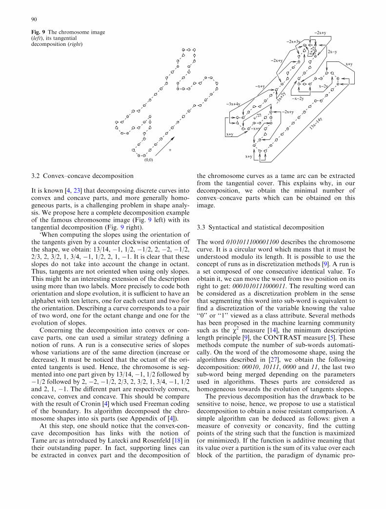
It is known [4, 23] that decomposing discrete curves intoconvex and concave parts, and more generally homo-geneous parts, is a challenging problem in shape analy-sis. We propose here a complete decomposition exampleof the famous chromosome image (Fig. 9 left) with itstangential decomposition (Fig. 9 right).

‘When computing the slopes using the orientation ofthe tangents given by a counter clockwise orientation ofthe shape, we obtain: 13/14, �1, 1/2, �1/2, 2, �2, �1/2,2/3, 2, 3/2, 1, 3/4, �1, 1/2, 2, 1, �1. It is clear that theseslopes do not take into account the change in octant.Thus, tangents are not oriented when using only slopes.This might be an interesting extension of the descriptionusing more than two labels. More precisely to code bothorientation and slope evolution, it is sufficient to have analphabet with ten letters, one for each octant and two forthe orientation. Describing a curve corresponds to a pairof two word, one for the octant change and one for theevolution of slopes.

Concerning the decomposition into convex or con-cave parts, one can used a similar strategy defining anotion of runs. A run is a consecutive series of slopeswhose variations are of the same direction (increase ordecrease). It must be noticed that the octant of the ori-ented tangents is used. Hence, the chromosome is seg-mented into one part given by 13/14, �1, 1/2 followed by�1/2 followed by 2, �2, �1/2, 2/3, 2, 3/2, 1, 3/4, �1, 1/2and 2, 1, �1. The different part are respectively convex,concave, convex and concave. This should be comparewith the result of Cronin [4] which used Freeman codingof the boundary. Its algorithm decomposed the chro-mosome shapes into six parts (see Appendix of [4]).

At this step, one should notice that the convex-con-cave decomposition has links with the notion ofTame arc as introduced by Latecki and Rosenfeld [18] intheir outstanding paper. In fact, supporting lines canbe extracted in convex part and the decomposition of

the chromosome curves as a tame arc can be extractedfrom the tangential cover. This explains why, in ourdecomposition, we obtain the minimal number ofconvex–concave parts which can be obtained on thisimage.

3.3 Syntactical and statistical decomposition

The word 0101011100001100 describes the chromosomecurve. It is a circular word which means that it must beunderstood modulo its length. It is possible to use theconcept of runs as in discretization methods [9]. A run isa set composed of one consecutive identical value. Toobtain it, we can move the word from two position on itsright to get: 0001010111000011. The resulting word canbe considered as a discretization problem in the sensethat segmenting this word into sub-word is equivalent tofind a discretization of the variable knowing the value‘‘0’’ or ‘‘1’’ viewed as a class attribute. Several methodshas been proposed in the machine learning communitysuch as the v2 measure [14], the minimum descriptionlength principle [9], the CONTRAST measure [5]. Thesemethods compute the number of sub-words automati-cally. On the word of the chromosome shape, using thealgorithms described in [27], we obtain the followingdecomposition: 00010, 10111, 0000 and 11, the last twosub-word being merged depending on the parametersused in algorithms. Theses parts are considered ashomogeneous towards the evolution of tangents slopes.

The previous decomposition has the drawback to besensitive to noise, hence, we propose to use a statisticaldecomposition to obtain a noise resistant comparison. Asimple algorithm can be deduced as follows: given ameasure of convexity or concavity, find the cuttingpoints of the string such that the function is maximized(or minimized). If the function is additive meaning thatits value over a partition is the sum of its value over eachblock of the partition, the paradigm of dynamic pro-

(0,0)

+

x+2y

x+y

x+y

x+y

Fig. 9 The chromosome image(left), its tangentialdecomposition (right)

90

-50 0 50 100

150

200

250 0

50 10

0 15

0 20

0 25

0 30

0

"kk45

0_-23

.c"

0 50 100

150

200

250

300

350 0

50 10

0 15

0 20

0 25

0

"SQU

ID/kk

450.c

"

0 50 100

150

200

250

300

350 0

20 40

60 80

100

120

140

"SQU

ID/kk

5.c"

0 50 100

150

200

250 0

20 40

60 80

100

120

"SQU

ID/kk

442.c

"

0 50 100

150

200

250 0

10 20

30 40

50 60

70 80

90 10

0

"SQU

ID/kk

201.c

"

0 50 100

150

200

250 0

20 40

60 80

100

120

"SQU

ID/kk

433.c

"

QUERY (#450) d = 0.617266 (#5) d = 0.966098

(#442) d = 0.979985 (#201) d = 0.990913 (#433) d = 0.994422

0 10 20 30 40 50 60 70

0 10

20 30

40 50

60 70

80 90

"kk21

5_0.4

5.c"

0 20 40 60 80 100

120

140

160 0

20 40

60 80

100

120

140

160

180

200

220

"SQU

ID/kk

215.c

"

0 20 40 60 80 100

120

140

160

180

200

220 0

10 20

30 40

50 60

70 80

90 10

0

"SQU

ID/kk

880.c

"

0 50 100

150

200

250

300 0

20 40

60 80

100

120

140

"SQU

ID/kk

1062

.c"

0 20 40 60 80 100

120

140

160

180

200

220 0

10 20

30 40

50 60

70 80

"SQU

ID/kk

883.c

"

0 20 40 60 80 100

120

140

160

180

200

220 0

10 20

30 40

50 60

70 80

90

"SQU

ID/kk

331.c

"

QUERY (#215) d = 0.70619 (#880) d = 0.997189

(#1062) d = 1.04456 (#883) d = 1.04467 (#331) d = 1.05083

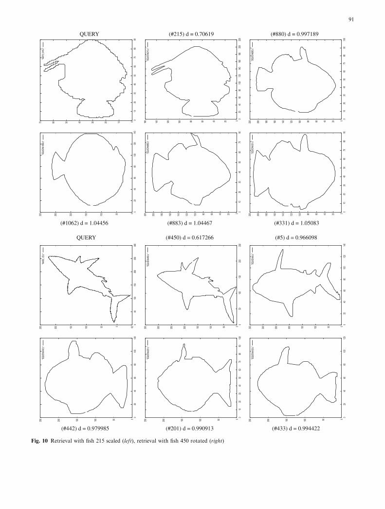
Fig. 10 Retrieval with fish 215 scaled (left), retrieval with fish 450 rotated (right)

91

gramming can be used to obtain an optimal timedecomposition.

4 Shape retrieval

The tangential cover decomposition was design as abuilding block to represent shapes. For instance, thetangential cover decomposition might be stored with theoriginal shapes in databases for answering subsequentqueries. To study the potential attractivity of the tan-gential cover in such situations we present preliminaryresults in shape retrieval. The database under study isthe SQUID database [19]. It contains around 1,100shapes of fish. For each shape, we computed its tan-gential cover using the four connexity, that is we usedfour connected discrete lines. Computing the whole1,100 tangential covers took less than 8 s on a pentiumIII processor under Linux.

For each tangential cover, we compute its canonicalassociated polygon as the following: the polygon is ob-tained by considering only the pixels which are either abeginning or an ending point of a tangent in the tan-gential cover. This process is linear time because it issufficient to iterate over the tangential cover once. Thusfor each shape, we constructed a real polygon whosevertices are points of the original digital curve. Thevertices of the polygons form a strict subset of the ori-ginal set of curve pixels. We stored the polygons asrepresentations of the fish curves.

When considering a query, we model the query has apolygon simply by connecting the list of pixels by realsegments. Then, we compare the polygon of the querywith those in the database. To measure the similaritybetween two polygons we used the approach of Arkinet al. [2] where the similarity is computed from theturning function. It should be noticed that the turningfunction can be deduced from the tangential cover usingthe slopes of the discrete tangents. We keep only the fivebest scores for comparison. We provide two experi-ments. The first one is conducted with a scale version offish number 215. The scale parameter was fixed to 0.45and the resulting curve was constructed as a four-con-nected digital curves. The five best scored shapes aregiven on Fig. 10 (left). The best one is fish 215. The otherones visually look similar to the query. It should benoticed that if we compare with the original fish 215shape (by connecting all its pixels), the distance functionis 0.749799 which is greater than the obtained value.

A second test was done with a rotated version of fishnumber 450 with a rotation of �23�. Again the rotatedcurve was constructed to be four-connected. The fivebest scored shapes are given on Fig. 10 (right). The bestcorresponding shape is fish number 450. Other shapesalso look similar to the query. When using the originalshape of fish 450, the distance is 0.636659 which is againgreater than the obtained value with the reducedpolygonal approximation.

The previous experiments are preliminary experi-ments to show that the tangential cover is applicable toshape retrieval. More features can be computed from thetangential cover and partial matching is also possiblesuch that this opens many perspectives for its use inshape retrieval or shape classification systems.

5 Complexity

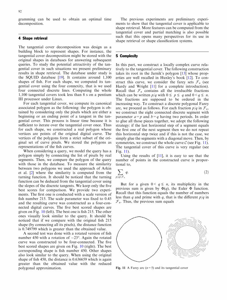
In this part, we construct a locally complex curve rela-tively to the tangential cover. The following constructiontakes its root in the Jarnik’s polygon [13] whose prop-erties are well recalled in Huxley’s book [12]. To con-struct this curve, we consider the farey sets F n (seeHardy and Wright [11] for a complete introduction).Recall that F n contains all the irreducible fractionswhich can be written p/q with 0 £ p £ q and 0<q £ n.The fractions are supposed to be ordered in theincreasing way. To construct a discrete polygonal Fareyarc, we proceed as follows. For each fraction p/q in F n;we construct the eight connected discrete segment withparameter a=p and b=q having two periods. In orderto glue all those pieces together, we adopt the followingstrategy: if the last horizontal step of a segment equalsthe first one of the next segment then we do not repeatthis horizontal step twice and if this is not the case, wesimply glue the segments with a diagonal move. Then, bysymmetries, we construct the whole curve C (see Fig. 11).The tangential cover of this curve is very regular (seeFig. 11).

Using the results of [11], it is easy to see that thenumber of points in the constructed curve is propor-tional to,X

p=q2F n

q: ð2Þ

But for a given 0< q £ n, its multiplicity in theprevious sum is given by U(q), the Euler U function.Recall that this function equals the number of numbersless than q and prime with q, that is the different p/q inF n: Thus, the previous sum equals

Fig. 11 A Farey arc (n=5) and its tangential cover

92

Xn

q¼1q:UðqÞ; ð3Þ

which converges to 3/p2·n3. Thus, the cardinal of anysets of the tangential cover is at least K �

ffiffiffiffiN3p

where K isa constant and N the length of the Farey arc. Thus thelocal thickness of the tangential cover is not a linearfunction of the number of points of the curve C: It is anopen question to compute the maximal local complexityof a discrete curve but we believe that the Farey arc isextremely closed to the worst case.

6 Extension

All previous elements in the paper suppose a perfectreconstruction of the curve C under study. Thus, if C is anoisy curve then, as the experiments showed, the tan-gential cover increases in length to manage all thosenoisy pixels. Our representation is perfect in a noisy freeworld but this is obviously not the case in many practicalapplications. To extend our representation to a noisycurve, the more natural way is to use thick lines, that iswe permit x to be greater than |a|+|b|. But we must notbe confused with this idea since at first, we do not knowa and b. Thus, we can fix x to be x0 in advance andrecognize discrete segment with arithmetical widthbounded above by x0. In this case, we do not assureconnectivity of the resulting segments since we do notcontrol the parameters a and b. To solve this problem weuse the fact that a thick line is a collection of four(respectively eight) connected lines plus some incompletelines. Hence, we can use a cover of thick lines by thicklines whose width is an exact multiples of a four(respectively eight) connected line. Thus, we can fix abound on the ratio x/(|a|+|b|) (resp. x/max(|a|,|b|)). Itmust be noticed that the second measure is the one usedby Debled et al in their notion of fuzzy segments [7]. It isstraightforward to generalize the tangential cover tothick segments. We loose the reconstruction possibility

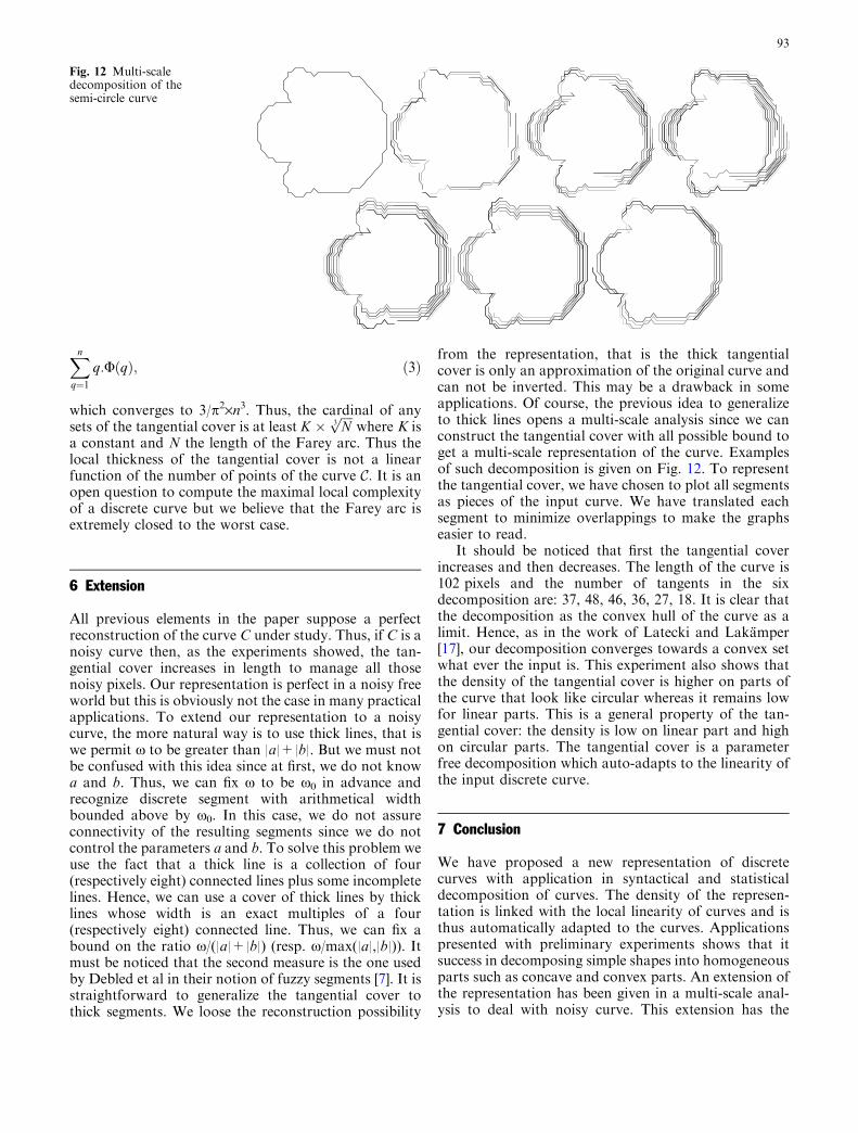
from the representation, that is the thick tangentialcover is only an approximation of the original curve andcan not be inverted. This may be a drawback in someapplications. Of course, the previous idea to generalizeto thick lines opens a multi-scale analysis since we canconstruct the tangential cover with all possible bound toget a multi-scale representation of the curve. Examplesof such decomposition is given on Fig. 12. To representthe tangential cover, we have chosen to plot all segmentsas pieces of the input curve. We have translated eachsegment to minimize overlappings to make the graphseasier to read.

It should be noticed that first the tangential coverincreases and then decreases. The length of the curve is102 pixels and the number of tangents in the sixdecomposition are: 37, 48, 46, 36, 27, 18. It is clear thatthe decomposition as the convex hull of the curve as alimit. Hence, as in the work of Latecki and Lakamper[17], our decomposition converges towards a convex setwhat ever the input is. This experiment also shows thatthe density of the tangential cover is higher on parts ofthe curve that look like circular whereas it remains lowfor linear parts. This is a general property of the tan-gential cover: the density is low on linear part and highon circular parts. The tangential cover is a parameterfree decomposition which auto-adapts to the linearity ofthe input discrete curve.

7 Conclusion

We have proposed a new representation of discretecurves with application in syntactical and statisticaldecomposition of curves. The density of the represen-tation is linked with the local linearity of curves and isthus automatically adapted to the curves. Applicationspresented with preliminary experiments shows that itsuccess in decomposing simple shapes into homogeneousparts such as concave and convex parts. An extension ofthe representation has been given in a multi-scale anal-ysis to deal with noisy curve. This extension has the

Fig. 12 Multi-scaledecomposition of thesemi-circle curve

93

drawback to be irreversible but may be useful inpolygonal simplification and/or curvature estimation.

Acknowledgements We thank Jacques Olivier Lachaud for theflower function and the anonymous referees whose commentsgreatly improved a previous version of the paper. Special thanks toF. Mokhtarian for making the SQUID database freely available.

References

1. Andres E (1996) The quasi-shear rotation. In: 6th DGCI,volume 1176 of Lecture Notes in Computer Science, pp 307–314

2. Arkin E, Chew P, Huttenlocher D, Kedem K, Mitchel J (1991)An efficiently computable metric for comparing polygonalshapes. IEEE Trans Pattern Anal Appl 13(3):209–215

3. Bribiesca E (1999) A new chain code. Pattern Recognit 32:235–251

4. Cronin TM (2003) Visualizing concave and convex partitioningof 2d contours. Pattern Recognit Lett 24(1–3):429–443

5. Van de Merckt T (1993) Decision trees in numerical attributespace. In: 13th international conference on artificial intelli-gence, Morgan Kaufmann, pp 1016–1021

6. Debled I, Reveilles JP (1994) A linear algorithm for segmen-tation of digital curves.In: 3rd IWPIA

7. Debled-Rennesson I, Remy JL, Rouyer J (2003) Segmentationof discrete curves into fuzzy segments. In: 9th internationalworkshop on combinatorial image analysis, vol 12 of ElectronicNotes in Discrete Mathathematics, Palermo, Italy

8. Dorst L, Smeulders AWM (1984) Discrete representation ofstraight lines. IEEE PAMI 6:450–463

9. Fayyad UM, Irani K (1993) Multiple-interval discretization ofcontinuous-valued attributes in induction graphs. In: 13thinternational conference on artificial intelligence, Morgan Ka-ufmann, pp 1022–1027

10. Freeman H (1961) On the encoding of arbitrary geometricconfigurations. IEEE Trans Elec Comput EC-10:260–268

11. Hardy GH, Wright EM (1960) An introduction to the theory ofnumbers, 4th edn. Oxford University Press, New York

12. Huxley MN (1996) Area, lattice points and exponential sums.Number 13 in London Mathematical Society Monographs.Oxford Science Publications, Oxford

13. Jarnik v (1925) Uber die Gitterpunkte auf konvexen Kurven.Math Zeitschrift 24:500–518

14. Kerber R (1992) Discretization of numeric attributes. In:Kerber R (ed) Tenth National conference on artificial intelli-gence. MIT Press, Cambridge, pp 123–128

15. Latecki LJ, Conrad C, Gross A (1998) Preserving topology by adigitization process. J Math Imaging Vis 8:131–159

16. Latecki LJ, Lakamper R (1999) Convexity rule for shapedecomposition based on discrete contour evolution. ComputVis IU 73(3):441–454

17. LateckiLJ,LakamperR(2000)Shapesimilaritymeasurebasedoncorrespondance of visual parts. IEEEPAMI 22(10):1185–1190

18. Latecki LJ, Rosenfeld A (1998) Supportedness and tameness:differentialles geometry of plane curves. Pattern Recognit31:607–622

19. Mokhtarian F, Abbasi S (2002) Shape similarity retrieval underaffine transforms. Pattern Recognit 35(1):31–41

20. Reveilles JP (1991) Geometrie discrete, calcul en nombres en-tiers et algorithmique. These d’etat, Universite Louis Pasteur,Strasbourg

21. Rosenfeld A (1974) Digital straight line segments. IEEE TransComput 23:1264–1269

22. Rosenfled A, Klette R (2004) Digital Straightness—a review.Discrete Appl Math 139(1–3):197–230

23. Rosin E (2000) Shape partitioning by convexity. IEEE TransSyst Man Cybern A 30(2):202–210

24. Schrijver A (2003) Combinatorial optimization—polyhedraand efficiency. Springer, Berlin Heidelberg New York

25. Smeulders AWM, Dorst L (1991) Decomposition of discretecurves into piecewise straight segments in linear time. ContempMath 119:169–195

26. Vialard A (1996) Geometrical parameters extraction from dis-crete paths. In: 6th international workshop DGCI, volume1176 of Lecture Notes in Computer Science, Springer, BerlinHeidelberg New York, pp 24–35

27. Zighed DA et al (1999) Encyclopedia of computer science andtechnology, vol 40, chapter discretization methods in super-vised learning. Marcel Dekker, pp 35–50

94