UNIVERSIDADE DE LISBOA

INSTITUTO SUPERIOR DE ECONOMIA E GESTÃO

Real World Economic Scenario Generator

Sara Bárbara Dutra Lopes

Orientadores:

Prof. Doutor Carlos Vázquez Cendón - Facultad de Informática da Universidade da Coruña

Prof. Doutora Maria do Rosário Grossinho - Instituto Superior de Economia e Gestão da

Universidade de Lisboa

Tese especialmente elaborada para obtenção do grau de Doutora em Matemática Aplicada à

Economia e Gestão

2020

UNIVERSIDADE DE LISBOA

INSTITUTO SUPERIOR DE ECONOMIA E GESTÃO

Real World Economic Scenario Generator

Sara Bárbara Dutra Lopes

Orientadores:

Prof. Doutor Carlos Vázquez Cendón - Facultad de Informática da Universidade da CoruñaProf. Doutora Maria do Rosário Grossinho - Instituto Superior de Economia e Gestão da Universidade de Lisboa

Presidente:

Doutor Nuno João de Oliveira ValérioProfessor Catedrático e Presidente do Conselho CientíficoInstituto Superior de Economia e Gestão da Universidade de Lisboa

Vogais:

Doutor Carlos Vasquez Cendón (orientador)Full ProfessorDepartamento de Matemáticas na Facultad de Informática da Universidade da Coruña, Espanha

Doutor João Pedro Vidal NunesProfessor CatedráticoISCTE Business School do ISCTE – Instituto Universitário de Lisboa

Doutora Raquel Medeiros GasparProfessora AssociadaInstituto Superior de Economia e Gestão da Universidade de Lisboa

Doutor Manuel Leote Tavares Inglês EsquívelProfessor AssociadoFaculdade de Ciências e Tecnologia da Universidade NOVA de Lisboa

Doutora Marta Cristina Vieira Faias MateusProfessora AuxiliarFaculdade de Ciências e Tecnologia da Universidade NOVA de Lisboa

Tese especialmente elaborada para obtenção do grau de Doutora em Matemática Aplicada à

Economia e Gestão

2020

Acknowledgements

First, I would like to thank to my supervisors: Professor Carlos Vázquez, who was always

available to discuss this work and to encourage me to succeed. Even with the physical

distance of working in different countries I felt I could always "knock on his office door".

Without his guidance, this journey would be much more difficult. Also I would like to

thank Professor Maria do Rosário Grossinho for all her support.

To my family: my mother, a continuous source of strength and love in the face of all

adversity - for her love, patience, affection, good mood and good values. To Luís, for his

love, patience and support during all this years. To my sister, for her love, encouragement

and my perfect niece, Omara.

Additionally, I would like to recognize the financial support from CEMAPRE, ISEG and

in particular the Mathematics Department. Also I would like to thank to Lusitania for

the financial support given during the first year of my PhD, and a specially to my former

manager Paulo Martins Silva for all his kindness and professionalism.

i

"Man has always learned from the past. After all, you can’t learn history in reverse!"

The Sword in the Stone

ii

Resumo

Neste trabalho apresentamos uma metodologia para simular a evolução das taxas de juros

sob medida de probabilidade real. Mais precisamente, usando o modelo de mercado

Shifted Lognormal LIBOR multidimensional e uma especificação do vetor do preço de

mercado do risco, explicamos como realizar simulações das taxas de juro futuras, usando

o método de Euler-Maruyama com preditor-corretor. A metodologia proposta permite

acomodar a presença de taxas de juro negativas, tal como é observado atualmente em

vários mercados.

Após definir a estrutura livre de default, generalizamos os resultados para incorporar a ex-

istência de risco de crédito nos mercados financeiros e desenvolvemos um modelo LIBOR

para obrigações com risco de crédito classificadas por ratings. Neste trabalho modelamos

diretamente os spreads entre as classificações de ratings de acordo com uma dinâmica

estocástica que garante a monotonicidade dos preços dos títulos relativamente às classifi-

cações por ratings.

Palavras-Chave: Modelo sob Medida Real, Simulação de Cenários, Solvência II, Taxas

de juro, Taxas Forward Lognormais Ajustadas, Preço de Risco, Risco de Crédito, Spreads,

Notações de Risco

iii

Abstract

In this work, we present a methodology to simulate the evolution of interest rates un-

der real world probability measure. More precisely, using the multidimensional Shifted

Lognormal LIBOR market model and a specification of the market price of risk vector

process, we explain how to perform simulations of the real world forward rates in the

future, using the Euler-Maruyama scheme with a predictor-corrector strategy. The pro-

posed methodology allows for the presence of negative interest rates as currently observed

in many markets.

After setting the default-free framework we generalize the results to incorporate the ex-

istence of credit risk to our model and develop a LIBOR model for defaultable bonds

with credit ratings. We model directly the inter-rating spreads according to a stochastic

dynamic that guarantees the monotonicity of bond prices with respect to the credit ratings.

Key Words: Real World Model, Scenario Simulation, Solvency II, Interest Rate, Shifted

Lognormal Forward Rates, Market Price of Risk, Credit Risk, Spreads, Credit Ratings

iv

Resumo alargado

O aumento sucessivo das exigências regulatórias e internas relacionadas com a correta

avaliação e gestão de riscos no sector bancário e segurador tornou imprescindível o mel-

hor entendimento da incerteza existente no mercado. Esta incerteza pode ser parcialmente

mitigada com a utilização de cenários que permitem avaliar como os balanços económi-

cos das empresas reagiriam em situações de mercado adversas. Neste trabalho pretende-

se construir um gerador de cenários económicos sob a medida de probabilidade real de

alguns dos fatores que mais afectam as empresas de seguros: taxas de juro e risco de

crédito.

Para definição do preço de produtos financeiros, cujo valor depende de realizações futuras

de um determinado fator de risco, utilizam-se modelos formulados sob a medida neutra

ao risco, desta forma os preços são obtidos como o valor descontado dos retornos futuros

esperados sob a hipótese habitual de não arbitragem no mercado. No entanto, quando

o objetivo é a simulação de valores futuros desses fatores, como necessário para avali-

ação de estratégias de investimento em carteiras sensíveis às taxas de juros em estudos de

Gestão de Ativos e Passivos e cálculos de requisitios de capital, as probabilidades neutras

ao risco não representam probabilidades reais, uma vez que sob esta medida assume-se

que a os preços das ações crescem à taxa de juro sem risco e as taxas forward são estima-

tivas não enviesadas das taxas futuras, o que não é realista, uma vez que isso implicaria

que os investidores não requerem compensação pelo risco de mudanças imprevisíveis no

futuro.

v

Para simular trajetórias futuras de fatores financeiros, isto é, para simular como o mundo

será no futuro, deve-se usar uma medida de probabilidade que reflita o facto de que os

investidores exigem um prémio de risco para manter nas suas carteiras os ativos com

risco.

Sob este paradigma, foram apresentadas várias possibilidades para geração de cenários

de taxas de juros. Por exemplo, Rebonato em [60] apresenta um método semiparamétrico

para simulação das trajectórias da estrutura temporal de taxas de juro, Hull e White [38]

propuseram uma abordagem simples para construir um modelo de short rate com um

fator sob a medida neutra ao risco e sob a medida real. Utilizando modelos de mercado

(market models), Norman em [58] introduziu uma forma paramétrica para o vector do

preço de mercado do risco (market price of risk) e Takashi em [72] apresenta o modelo de

mercado forwad LIBOR sob a medida do mundo real de uma forma rigorosa, obtendo o

preço de mercado do risco, resolvendo um problema mínimos quadrados para um modelo

de regressão com atraso.

Uma das principais dificuldades na modelização das taxas de juros é a escolha do processo

apropriado que se pretende estudar. Muitos dos modelos de taxa de juros são baseados na

evolução estocástica de uma determinada taxa de juro, geralmente a taxa de curto prazo

(short rate), uma vez que através destes modelos se conseguem obter fórmulas fechadas

para o preço de derivados financeiros. Uma desvantagem apresentada por esta classe de

modelos é que apresenta um número bastante limitado de graus de liberdade para permitir

o ajuste correto entre a estrutura de taxas de juro observada e a teórica.

Uma alternativa aos modelos de taxa de curto prazo é a especificação da dinâmica de toda

a curva de taxas de juro usando o modelo HJM [34], no qual a dinâmica das taxas for-

ward instantâneas é totalmente caracterizada pelas volatilidades instantâneas. Porém, a

principal desvantagem dos modelos do tipo HJM, advém do fato de as taxas instantâneas

não serem observáveis diretamente nos mercados, tornando por isso difícil a calibração

aos preços de mercado. Tendo em vista essa desvantagem, os modelos de mercado foram

vi

introduzidos por Brace, Gararek e Musiela [13] e, desde então, tornaram-se muito popu-

lares principalmente devido ao acordo existente entre esses modelos e fórmulas utilizadas

no mercado para a formação de preço de dois produtos derivados standard: caps e swap-

tions. Mais precisamente, o modelo Lognormal Forward LIBOR (LFM) permite obter o

preço de caps com a fórmula de Black-76 usualmente utilizada pelos traders.

Sob a abordagem LFM, as taxas forward LIBOR seguem uma distribuição lognormal

e, consequentemente, pressupõe-se que as taxas forward são positivas, o que era, até

recentemente, uma propriedade desejável. No entanto, taxas de juros negativas estão

presentes na economia atual. Por exemplo, o Banco Central Europeu e os bancos centrais

da Suíça, Dinamarca, Suécia e Japão estabeleceram taxas de juros negativas nas reservas

como mecanismo de política monetária com o objectivo de criar um estimulo à taxa de

crescimento economico, reduzindo a poupança e incentivando empréstimos a custos mais

baixos.

Como consequência, essa mudança do limite inferior das taxas de juros trouxe alguns

problemas aos modelos adoptados até agora, uma vez que muitas das metodologias ado-

tadas não conseguem lidar com taxas negativas.

Dadas as condições atuais do mercado, é possível obter uma solução alterando a condição

de fronteira das taxas de juros de zero para um valor negativo adequado e isso pode ser

alcançado usando o modelo de mercado Shifted Lognormal Forward LIBOR (SLFM).

Sob esta abordagem, optamos por modelar um conjunto de taxas forward que podem ser

observadas diretamente no mercado. Assim, usando o modelo SLFM, podemos garantir a

não existência de oportunidades de arbitragem nos mercados mantendo a flexibilidade do

modelo para capturar todos os movimentos possíveis de curvas sob uma estrutura coerente

para taxas de juros negativas.

Após a definição do modelo adoptado para a estrutura temporal de taxas de juro sem risco,

generalizamos os resultados para incorporar a existência de risco de crédito no mercado e

vii

desenvolvemos um modelo LIBOR para títulos com risco de default classificados através

de um sistema de ratings. Modelamos diretamente os spreads entre os ratings de acordo

com uma dinâmica estocástica que garante a monotonicidade dos preços dos títulos em

relação às classificações de crédito.

Este trabalho tem a seguinte estrutura: no Capítulo 1, apresentamos a estrutura regulatória

e como os cálculos de requisitos de capital podem ser realizados no âmbito da Solvência

II. O Capítulo 2 analisa os resultados relevantes na literatura sobre modelos de taxa de juro

sob a medida neutra ao risco e apresenta as técnicas para passar da medida neutra ao risco

para a medida real. No Capítulo 3, apresentamos o modelo proposto para o gerador de

cenários sob a medida real para taxas de juro e explicamos em detalhes como estimamos

os parâmetros e discutimos os resultados obtidos. O Capítulo 4 analisa os resultados

relevantes na literatura sobre modelos de risco de crédito e, no capítulo 5, apresentamos

a abordagem proposta para gerar cenários para spreads de crédito na medida real.

Os Capítulos 3 e 5 são as principais contribuições desta tese onde são apresentados novos

desenvolvimentos. Por fim, algumas conclusões e comentários sobre novos temas de

investigação são apresentadas no Capítulo 6.

viii

Long abstract

The increase of regulatory and internal demands on risk assessment and management of

assets and liabilities within banks and insurance companies led to the need of a better

understanding of the uncertainty in market risk factors, particularly in future scenarios

of interest rates. In this project we aim to construct a real world Economic Scenario

Generator (ESG) modeling some of the main financial risk factors that affect insurance

companies: interest rates, and credit spreads.

For pricing financial products, the value of which depends on future realizations of cer-

tain risk factors, one can rely on risk neutral models so that prices are obtained as the

discounted value of expected future payoffs under the standard hypotheses on frictionless

and complete markets.

However, in the assessment of investment strategies in interest-rate sensitive portfolios for

Asset-Liability Management studies and calculations of Economic Capital for Solvency

II, the objective is the simulation of future values of these underlying factors and products.

In these cases, the risk neutral probabilities do not represent real probabilities, as the drift

of the stock prices is assumed to be the risk free rate and the forward rates are unbiased

predictors of future rates, which is not realistic because that would imply that investors

require no compensation for the risk of unpredictable changes in the future.

In order to simulate future trajectories of financial factors, i.e. to simulate how the world

will look like in the future, one should use a probability measure that reflects the fact

ix

that investors demand a risk premium to hold risky assets. Under this paradigm many ap-

proaches have been presented for modelling interest rates. For instance, Rebonato in [60]

presents a semiparametric method to simulate yield curve paths using random sampling of

historical changes in the yield curve with a spring mechanism to guarantee correct shapes

of the generated curves. Hull and White [38] proposed a simple approach to construct a

one factor short rate model for both the risk neutral measure and the real world measure.

By using the LIBOR market model, Norman [58], introduced a parametric form for the

market price of risk vector and Takashi [72] presents the LIBOR market model under

the real world measure in a rigorous manner, thus obtaining the market price of risk by

solving a least square problem for a lag regression model.

One of the main problems in interest rate modeling is the choice of the appropriate pro-

cess to model. Many interest rate models focus on the stochastic evolution of a given

interest rate, usually the short rate, because they can provide closed pricing formulas due

to their analytical tractability. However, this class of models has a rather limited number

of degrees of freedom to allow for a correct match between the observed term structure

and the theoretical one. An alternative to short rate models is to specify the dynamics

of the entire yield curve using the arbitrage-free HJM [34] framework where the instan-

taneous forward rates dynamics are fully specified through their instantaneous volatility

structure. However, the main disadvantage of HJM type models comes from the fact that

the instantaneous rates are not directly observed in the markets, so that the calibration to

current market prices turns out to be difficult. Having in view this drawback, LIBOR mar-

ket models were introduced by Brace, Gatarek and Musiela [13] and have since become

very popular mainly due to the agreement between such models and market formulas for

pricing two basic derivative products: caps and swaptions. More precisely, the Lognormal

Forward LIBOR model (LFM) allows to price caps with Black’s cap formula used in the

markets.

Under the LFM approach, the implicit forward LIBOR rates follow a lognormal distri-

x

bution and, consequently, forward rates are guaranteed to be positive, which was, until

recently, a desirable property. However, negative interest rates are present in many current

economies. For example, the European Central Bank and central banks of Switzerland,

Denmark, Sweden and Japan have set negative interest rates on reserves with the argument

of economic growth rate estimulation by reducing savings and encouraging borrowing at

lower costs. Of course, this change of the lower bound for interest rates involves many

consequences in the models used until now, since many adopted methodologies cannot

cope with negative rates.

Given the current market conditions, a solution can be obtained by shifting the bound-

ary condition of interest rates from zero to an adequate negative value and this can be

achieved using the Shifted Lognormal Forward LIBOR market model (SLFM). Under this

approach, we choose to model a set of key forward LIBOR rates which can be directly

observed in the market. Then, using the SLFM model, we can guarantee no arbitrage

opportunities in interest rate markets and provide more flexibility to capture all possible

curve movements under a coherent framework for negative interest rates.

After setting the default-free framework, we generalize the results to incorporate the exis-

tence of credit risk to our model and develop a LIBOR model for defaultable bonds with

credit ratings. For this purpose, we directly model the inter-rating spreads according to a

stochastic dynamics that guarantees the monotonicity of bond prices with respect to the

credit ratings.

The outline of this work is as follows. In Chapter 1, we present the regulatory framework

and how capital requirement calculations can be accomplished under Solvency II. Chapter

2 briefly reviews the relevant results in the literature on interest rate models under the

risk neutral measure and presents the techniques to move from risk neutral to real world

measure. In Chapter 3, we present the proposed modeling approach for the real world

scenario generator for interest rates and explain in detail how we estimate the parameters

and present the obtained results. Chapter 4 reviews the relevant results in the literature on

xi

credit risk models. In Chapter 5, we present the proposed approach to generate scenarios

for credit spreads under the real world measure.

Chapters 3 and 5 are the main original contributions of this thesis where new develop-

ments are presented. Finally, some conclusions and comments on further research are set

out in Chapter 6.

xii

Contents

1 Motivation and financial framework 1

1.1 Solvency II . . . . . . . . . . . . . . . . . . . . . . . . . . . . . . . . . 4

1.1.1 Capital requirements . . . . . . . . . . . . . . . . . . . . . . . . 6

1.1.2 European standard formula . . . . . . . . . . . . . . . . . . . . . 7

1.2 Economic scenario generators in Solvency II . . . . . . . . . . . . . . . . 11

2 Interest rate models 14

2.1 Overview of interest rate models . . . . . . . . . . . . . . . . . . . . . . 14

2.2 Models under negative interest rates . . . . . . . . . . . . . . . . . . . . 18

2.3 Risk neutral shifted LIBOR market model . . . . . . . . . . . . . . . . . 19

2.3.1 Some definitions and notations . . . . . . . . . . . . . . . . . . . 19

2.3.2 The LIBOR market model . . . . . . . . . . . . . . . . . . . . . 21

2.4 Real world and risk neutral models . . . . . . . . . . . . . . . . . . . . . 27

2.4.1 Change of measure . . . . . . . . . . . . . . . . . . . . . . . . . 28

2.4.2 Market price of risk . . . . . . . . . . . . . . . . . . . . . . . . . 29

3 LIBOR Market Model under the real world measure 31

3.1 The model . . . . . . . . . . . . . . . . . . . . . . . . . . . . . . . . . . 31

3.2 Parameter estimation . . . . . . . . . . . . . . . . . . . . . . . . . . . . 36

3.3 Real world scenarios simulation . . . . . . . . . . . . . . . . . . . . . . 39

3.4 Results . . . . . . . . . . . . . . . . . . . . . . . . . . . . . . . . . . . . 40

4 Credit risk models 47

4.1 Overview of credit risk models . . . . . . . . . . . . . . . . . . . . . . . 47

4.2 Notation and risk neutral model setup . . . . . . . . . . . . . . . . . . . 50

5 LIBOR market model with credit risk under the real world measure 58

5.1 The model . . . . . . . . . . . . . . . . . . . . . . . . . . . . . . . . . . 59

5.2 Parameter estimation . . . . . . . . . . . . . . . . . . . . . . . . . . . . 62

5.3 Real world scenarios simulation . . . . . . . . . . . . . . . . . . . . . . 64

5.4 Results . . . . . . . . . . . . . . . . . . . . . . . . . . . . . . . . . . . . 65

6 Conclusion and future research 76

Bibliography 86

Appendix A Principal component analysis 87

xiv

List of Figures

1.1 Investment mix by insurers in EEA in Q42018 . . . . . . . . . . . . . . . 3

1.2 Balance sheet under Solvency II . . . . . . . . . . . . . . . . . . . . . . 5

1.3 Solvency Capital Requirement (SCR) according to the standard formula . 8

3.1 The first three principal components obtained from a principal compo-

nents analysis of monthly observed European shifted forward rates. . . . . 42

3.2 Ten thousand simulations of 1 year-ahead forward rates (grey), mean of

the simulatons (blue) and observed forward curve in 30 of June of 2017

(green). For simulation, data from December 2015 to June 2016 have

been used. . . . . . . . . . . . . . . . . . . . . . . . . . . . . . . . . . 43

3.3 Ten thousand simulations of the zero coupon bond prices at the end of the

first projection year (grey), mean of simulations (blue) and observed zero

coupon bond prices at 30 of June of 2017 (green). For simulation, data

from December 2015 to June 2016 have been used. . . . . . . . . . . . . 43

3.4 Ten thousand simulations(grey) of one year-ahead forward rates and mean

curve (blue). For simulation, data from December 2015 to June 2017 have

been used . . . . . . . . . . . . . . . . . . . . . . . . . . . . . . . . . . 45

5.1 Inter-rating spreads observed as of 30 June 2018. . . . . . . . . . . . . . 67

5.2 The first three principal components obtained from a principal compo-

nents analysis of monthly observed AAA-rated European shifted forward

rates. . . . . . . . . . . . . . . . . . . . . . . . . . . . . . . . . . . . . . 68

xv

5.3 The first seven principal components obtained from a principal compo-

nents analysis of monthly observed inter-rating spreads of European bonds. 68

5.4 Ten thousand simulations of 1 year-ahead forward rate curve for AAA

bonds (grey), observed forward curve on 30 June 2018 (dashed-black)

and observed forward curve on 30 June 2019 (black). . . . . . . . . . . . 70

5.5 Ten thousand simulations of 1 year-ahead inter-rating spreads for credit

ratings AAA and AA (grey), observed spread curve on 30 June 2018

(dashed-black) and observed spread curve on 30 June of 2019 (black)

(left) and corresponding forward rates for rating AA (right). . . . . . . . 70

5.6 Ten thousand simulations of 1 year-ahead inter-rating spreads for credit

ratings AAA and AA (grey), observed spread curve on 30 June 2018

(dashed-black) and observed spread curve on 30 June of 2019 (black)

(left) and corresponding forward rates for rating AA (right). . . . . . . . 70

5.7 Ten thousand simulations of 1 year-ahead inter-rating spreads for credit

ratings A and BBB (grey), observed spread curve on 30 June 2018 (dashed-

black) and observed spread curve on 30 June of 2019 (black) (left) and

corresponding forward rates for rating BBB (right). . . . . . . . . . . . . 71

5.8 Ten thousand simulations of 1 year-ahead inter-rating spreads for credit

ratings BBB and BB (grey), observed spread curve on 30 June 2018

(dashed-black) and observed spread curve on 30 June of 2019 (black)

(left) and corresponding forward rates for rating BB (right). . . . . . . . 71

5.9 Ten thousand simulations of 1 year-ahead inter-rating spreads for credit

ratings BB and B-CCC (grey), observed spread curve on 30 June 2018

(dashed-black) and observed spread curve on 30 June 2019 (black) (left)

and corresponding forward rates for rating B-CCC (right). . . . . . . . . 71

5.10 Histogram of % profit and loss. . . . . . . . . . . . . . . . . . . . . . . . 73

xvi

5.11 Ten thousand simulations of 1 year-ahead spot rate for each credit rating

(grey), last observed curve (dashed-black), observed forward curve in 30

of June of 2019 (black) and upward and downward scenarios according

to Solvency II methodology (red). . . . . . . . . . . . . . . . . . . . . . 75

xvii

List of Tables

1.1 Interest rate curve shocks by maturity . . . . . . . . . . . . . . . . . . . 10

3.1 One year forward rates observed on 30 June 2016 . . . . . . . . . . . . . 41

3.2 Estimated market price of risk Parameters . . . . . . . . . . . . . . . . . 42

3.3 Expected value, 97% confidence interval of zero coupon bond prices and

30 June 2017 observations . . . . . . . . . . . . . . . . . . . . . . . . . 44

3.4 Expected value and standard deviation of one year-ahead zero-coupon

bond prices . . . . . . . . . . . . . . . . . . . . . . . . . . . . . . . . . 46

5.1 One year forward rates observed on 30 June 2018. . . . . . . . . . . . . . 66

5.2 Countries by rating group as of 31 January 2016. . . . . . . . . . . . . . 66

5.3 Estimated market price of risk parameters of default-free forward rates. . 69

5.4 Estimated market price of risk parameters of inter-rating spreads. . . . . . 69

5.5 One year transition matrix with withdrawl . . . . . . . . . . . . . . . . . 72

5.6 One-year transition matrix without withdrawl. . . . . . . . . . . . . . . . 72

5.7 Average recovery rate by credit rating. . . . . . . . . . . . . . . . . . . . 73

5.8 Comparison between the SCR of the standard formula and the simulated

model. . . . . . . . . . . . . . . . . . . . . . . . . . . . . . . . . . . . . 74

xviii

Abbreviations

ESG Economic Scenario Generator(s)

EIOPA European Insurance and Occupational Pensions Authority

SCR Solvency Capital Requirement

MCR Minimum Capital Requirement

VaR Value at Risk

ES Expected Shortfall

SCRmkt Solvency Capital Requirement for Market Risk

Mktinterest Solvency Capital Requirement for Interest Rate Risk

Mktspread Solvency Capital Requirement for Spread Risk

PCA Principal Component Analysis

PCs Principal Components

HJM Heath-Jarrow-Morton model

LFM Lognormal Forward LIBOR Model

LSM Lognormal Swap Model

FRA Forward Rate Agreement

IRS Interest Rate Swap

ECB European Central Bank

ALM Asset - Liability Management

SDE Stochastic Differential Equation

xix

Notation

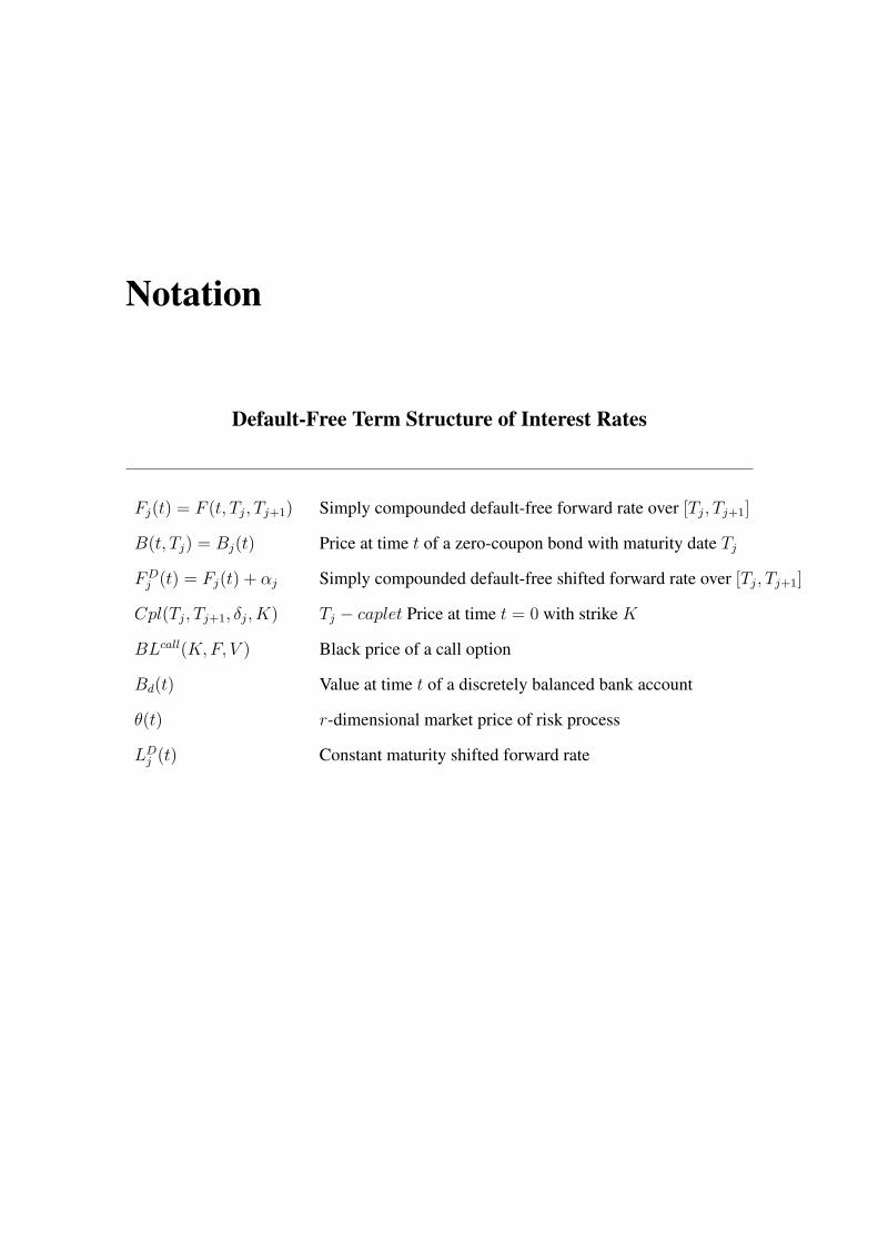
Default-Free Term Structure of Interest Rates

Fj(t) = F (t, Tj, Tj+1) Simply compounded default-free forward rate over [Tj, Tj+1]

B(t, Tj) = Bj(t) Price at time t of a zero-coupon bond with maturity date Tj

FDj (t) = Fj(t) + αj Simply compounded default-free shifted forward rate over [Tj, Tj+1]

Cpl(Tj, Tj+1, δj, K) Tj − caplet Price at time t = 0 with strike K

BLcall(K,F, V ) Black price of a call option

Bd(t) Value at time t of a discretely balanced bank account

θ(t) r-dimensional market price of risk process

LDj (t) Constant maturity shifted forward rate

Defaultable Term Structure of Interest Rates

Bj(t) Price at t of a defaultable zero-coupon bond with maturity date Tj

F ij (t) Forward LIBOR rate for credit rating i the period [Tj, Tj+1]

F i,Dj (t) Shifted forward LIBOR rate for credit rating i the period [Tj, Tj+1]

Sij(t) Forward inter-rating LIBOR spread between credit rating i and i− 1

Dij(t) Default-risk factor for credit rating i at time t for maturity Tj

H ij(t) Discrete-tenor forward default intensity for credit rating i

over the period [Tj, Tj+1]

θS(t) m-dimensional market price of risk process

P One-year transition matrix

Chapter 1

Motivation and financial framework

Solvency II directive [24] was approved in 2009. It aimed to enhance policyholders’

protection, to improve stability of the financial system, and to unify the insurance market

in the European Union as a whole, by establishing harmonized solvency requirements

across all member states. Solvency II has been in preparation since 2007 and came into

effect on 1 January 2016.

Along with many important new guidelines for risk management of insurance companies,

Solvency II directive mandates that the valuation of assets and liabilities should be done

using market consistent techniques. This means that the value of an asset or liability is its

market value, if it is readily traded on a deep, liquid and transparent market at the point in

time. Otherwise, its value would be given by a reasonable best estimate of what its market

value would have when readily traded at the relevant valuation date.

A market is defined as liquid when an individual or firm can quickly purchase or sell

an asset without causing a drastic adjustment in the asset price. A market is defined as

deep when a large number of assets can be bought and sold without significantly affecting

the price. A market is transparent when information about supply and prices is readily

available to the public.

1

In order to obtain the best estimate, insurance companies can use analytical techniques,

deterministic techniques or a scenario approach. Nevertheless, using an analytical ap-

proach would imply that the insurance company is able to find closed-form solutions to

value guarantees which is a very difficult task because some of the financial products sold

by insurance companies have embedded path-dependent options and high number of risk

factors. On the other hand, deterministic approaches imply simplified assumptions of the

market behaviour. Therefore, for many insurance companies Economic Scenario Gen-

erators (ESG) are the only practical and robust way to determine the market consistent

present value of the liabilities. An accurate and robust valuation can result in compet-

itive premiums for policyholders and allow for an optimal amount of reserving for the

insurance company, while maintaining the risk management thresholds.

Another very important regulatory change introduced by the Solvency II directive con-

cerns to the way risks should be accounted for and the introduction of a solvency margin

entirely based on risk sources and risk mitigation techniques, namely, Solvency Capital

Requirement (SCR).

In order to calculate SCR, insurance companies can choose the standard formula proposed

by EIOPA, where the SCR is decomposed in simpler terms divided by the risk they refer

to and it relies on some assumptions that are still under debate [27]. For instance, using

the standard formula, it is assumed that: correlations between risk factors can be fully

captured by using a linear correlation coefficient approach. Moreover, not all quantifiable

risks are explicitly formulated and, consequently, some risks, whose nature and calibra-

tion depend on the single undertaking specificity, may not be covered by the standard

formula. In particular, the simplifications considered for the market risk module include:

the assumption that only changes in the level of the market risk factors have impact on the

solvency level of an insurer and, in the specific case of the interest rate risk sub-module,

the underlying assumption that in times of lower interest rates the absolute shocks are

lower implies that the risk of deflation is not entirely captured.

2

Alternatively, SCR can be estimated using internal models, which would have to be ap-

proved by the supervisory authorities. It is in the latter case that a real world ESG becomes

relevant.

The position of an insurance portfolio is influenced by a large number of macroeconomic

risk factors, such as inflation, stock prices, real estate prices, and correlations between all

the different factors. Market risk accounts for 64% of the net SCR before diversification

benefits for standard formula users [28]. However, among all the market risks, the interest

rate risk represents the main contribution to the the market risk component of SCR [25].

Actually, the changes in the interest rate curves affect both sides of the insurer financial

books. On the other hand, the asset side is affected because insurers invest a significant

amount in government bonds usually with longer maturities (see Fig: 1.1). On the lia-

bilities side, the today’s value of future cash flows are directly influenced by the discount

rates. Typically, the effect of interest rate movements in the liabilities side has a more

material impact than in the assets side.

Figure 1.1: Investment mix by insurers in EEA in Q42018Source: EIOPA Statistics - accompanying note

The second most relevant asset class of insurance companies investments is the class of

corporate bonds. This implies that the risk related to credit quality changes, and conse-

3

quently, spread changes, should be accurately estimated and the corresponding adequately

capital reserved.

In this project, we aim to construct a real world ESG modeling two of the main financial

risk factors that affect insurance companies: interest rates and credit spreads.

1.1 Solvency II

The economic conditions faced by insurance companies during the last two decades and

the shortfalls in the previous regulatory framework, Solvency I, led European authorities

to rethink and reformulate the way insurance companies should calculate their solvency

positions.

Under Solvency I, the solvency requirements - the funds’ amount that insurance and rein-

surance companies in the European Union are required to hold - were calculated as a

percentage of the technical provisions. This simplified method had some shortcomings,

such as penalizing insurance companies with high technical provisions even if the value

was determined by prudence and risk averse managing actions. Moreover, the ratio fo-

cuses mainly on the liability side of the balance sheet and ignores risks occurring in the

assets side [69]. In order to increase internal regulations, local authorities across the Eu-

ropean Union, acting individually and independently, put in place several actions. These

specific actions led to significant differences in the criteria applied by each of the member

states.

Solvency II Framework Directive 2009/138/EC [24] was the response from the European

Commission to unify the regulatory structure in the EU insurance market. It is inspired by

the Basel II accord, [7], for the banking industry introduced in 2006. This new solvency

regime points to the risk profile of insurance and reinsurance undertakings, and it thrives

on creating better conditions to protect policyholders.

4

The proposed Solvency II framework has three main pillars defined by the European

Insurance and Occupational Pensions Authority (EIOPA1):

• Pillar 1 covers all the quantitative requirements that insurers must fulfill to demon-

strate that they have sufficient capital resources. It covers all components of the

economic balance sheet and defines two capital requirements: the Minimal Capital

Requirement (MCR) and the Solvency Capital Requirement (SCR);

• Pillar 2 sets out requirements for the governance and risk management of insurers,

as well as for the supervisory activities and powers of regulators;

• Pillar 3 focuses on disclosure and transparency requirements through public dis-

closures in the form of narrative and quantitative reports encouraging early warning

systems.

As a risk-based system, Solvency II focuses on risk identification and the accurate allo-

cation of capital to the identified risks. It is expected that undertakings with more risk

exposures will now have higher capital requirements, thus punishing risk-seeking, or at

least imprudent behaviors and reward risk mitigation actions.

In order to enter in more detail in SCR calculations, it is important to define some main

concepts of the Economic Balance Sheet as pictured in Fig 1.2

Figure 1.2: Balance sheet under Solvency IISource: EIOPA Presentations - Understanding the Solvency II Balance sheet 2013

1Former Committee of European Insurance and Occupational Pensions Supervisors (CEIOPS)

5

Technical provisions are the amount that an insurance company must hold to ensure that

it can meet its expected future obligations on insurance contracts. They are obtained

by summing the best estimate of the expected liabilities - in the form of a probability-

weighted average - plus a risk margin that takes into account the cost of capital that would

be required to sell the liabilities to a new knowledgeable undertaking.

Basic own funds are the value of the subordinated liabilities and the excess of assets over

liabilities, valued accordingly to the market consistent valuation principle, reduced by

the amount of own shares held by the insurance or reinsurance undertaking. They are

classified into tiers that represent how well and how fast they can absorb losses.

The Minimum Capital Requirement (MCR) represents the threshold below which the

insurance undertaking is exposed to an unacceptable level of risk leading to a necessary

intervention from the national regulatory agency .

Finally, the SCR is the total amount of funds that insurance and reinsurance companies in

the European Union are required to hold to ensure that their obligations to policyholders

over the following 12 months can be met with a 99.5% probability.

1.1.1 Capital requirements

The Minimum Capital Requirement (MCR) is the solvency threshold and, it is set to

represent a 12 months Value-at-Risk (VaR) calibrated to an 85% confidence level. If the

amount of eligible basic own funds of an insurance undertaking falls below this threshold,

then regulatory authorities will act in order to transfer the insurer’s liabilities to another

company and withdrawn the license of the undertaking.

The Solvency Capital Requirement (SCR) is defined as the VaR of the own funds of an

insurer set at a level of 99.5% over a one year period. SCR is usually interpreted as the

value that guarantees that only once in 200 years, the funds held are not enough to meet

the insurer’s obligations.

6

According to Solvency II directive, SCR should be calibrated in order to ensure that all

quantifiable risks to which an insurance or reinsurance undertaking is exposed are taken

into account. It should cover existing business, as well as the new business expected to be

written over the following 12 months. Furthermore, when calculating the SCR, insurance

and reinsurance undertakings must take into account the effect of risk-mitigation tech-

niques, provided that credit risk and other risks arising from the use of such techniques

are properly reflected in the SCR.

Both MCR and SCR are based on the concept of VaR, as it is easy to understand and

implement, although it has been noted that it is not a coherent risk measure, see [4] e.g.,

as it does not fulfill the required property of subadditivity. An alternative risk measure

has been proposed in the literature, see [1] and [41]: the Expected Shortfall (ES). ES is

defined as the expected value of the losses which are greater or equal than the VaR. As a

result, ES takes more into consideration the shape of the loss distribution in the tail of the

distribution. ES answers the question "if things go bad, how much do we expect to loose?"

where VaR answers the question "how bad can things get within a certain probability?"

[36].

1.1.2 European standard formula

The standard formula provided in the EIOPA Techical Specifications [26] is a simplified

calculation to obtain the SCR of a particular undertaking. Thus, the overall SCR for an

undertaking is defined as:

SCR = BSCR + SCRop + Adj , (1.1)

where SCRop is the capital requirement for operational risk, Adj is the sum of the adjust-

ment for the risk absorbing effect of technical provisions and deferred taxes, and BSCR

is the Basic Solvency Capital Requirement that combines capital requirements for six

major risk categories, as shown in Fig 1.3.

7

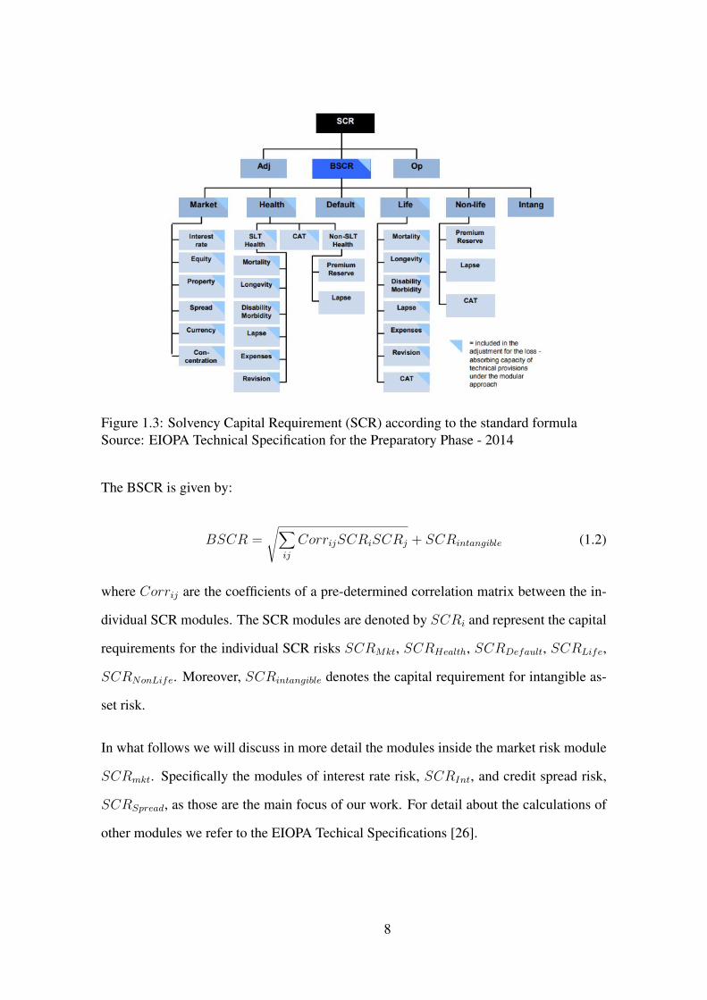
Figure 1.3: Solvency Capital Requirement (SCR) according to the standard formulaSource: EIOPA Technical Specification for the Preparatory Phase - 2014

The BSCR is given by:

BSCR =√∑

ij

CorrijSCRiSCRj + SCRintangible (1.2)

where Corrij are the coefficients of a pre-determined correlation matrix between the in-

dividual SCR modules. The SCR modules are denoted by SCRi and represent the capital

requirements for the individual SCR risks SCRMkt, SCRHealth, SCRDefault, SCRLife,

SCRNonLife. Moreover, SCRintangible denotes the capital requirement for intangible as-

set risk.

In what follows we will discuss in more detail the modules inside the market risk module

SCRmkt. Specifically the modules of interest rate risk, SCRInt, and credit spread risk,

SCRSpread, as those are the main focus of our work. For detail about the calculations of

other modules we refer to the EIOPA Techical Specifications [26].

8

Capital requirement for market risk

Under Solvency II, the market risk module reflects the risk arising from the level of market

prices of financial instruments, which have an impact upon the value of the assets and

liabilities of the undertaking, and it should reflect the structural mismatch between assets

and liabilities. These are scenario-based calculations and are based on the impact of

instantaneous shocks of the risk factors.

The standard formula of the market risk module aggregates equity risk, interest rate risk,

property risk, currency risk, spread risk and concentration risk. For each type of risk , the

formula assesses the required capital to overcome a set of specified scenarios. Then, the

individual capital requirements are aggregated, taking into account correlations between

risk factors, providing the market risk solvency capital requirement, SCRMkt.

The SCRMkt is given by :

SCRmkt =√∑

ij

CorrijMktiMktj (1.3)

where againCorrij are the coefficients of a pre-determined correlation matrix between the

individual SCRMkt components. These components, Mkti, are the capital requirements

for the individual market risk modules, Mktequity, Mktinterest, Mktproperty, Mktcurrency,

Mktspread and Mktconcentration.

Capital requirement for interest rate risk

The capital requirement for interest rate risk is determined as the maximum change in the

net value of assets and liabilities due to the revaluing of all interest rate sensitive items

under two pre-defined scenarios: an instantaneous upward movement of interest rates and

a downward movement.

These two scenarios for the term structures are obtained by multiplying the current interest

rate curve by (1 + sup) and (1 + sdown), where the upward stress sup(t) and the downward

9

stress sdown(t) for individual maturities are specified as in Table 1.1:

Maturity sup(t) sdown(t) Maturity sup(t) sdown(t)1 or shorter 70% -75% 12 37% -28%

2 70% -65% 13 35% -28%3 64% -56% 14 34% -28%4 59% -50% 15 33% -27%5 55% -46% 16 31% -28%6 52% -42% 17 30% -28%7 49% -39% 18 29% -28%8 47% -36% 19 27% -29%9 44% -33% 20 26% -29%

10 42% -31%90 or longer 20% 30%

11 39% -30%

Table 1.1: Interest rate curve shocks by maturity

Moreover, for maturities not specified above, the value of the shock is obtained by linear

interpolation. Also, irrespective of the above stress scenarios, the absolute increase of

interest rates in the upward scenario at any maturity should be at least one percentage

point. When, for a given maturity, the initial value of the interest rate is negative, the

undertaking should calculate the increase or decrease of the interest rate as the product

between the sup and sdown shock and the absolute value of the initial interest rate.

Capital requirement for credit spread risk

The spread risk is the risk of changes in the market value assets, liabilities, and financial

instruments caused by changes in credit spreads. It reflects the change in the market value

due to a movement in the yield curve relative to the risk-free interest rate term structure.

The spread risk module MktSpread, applies to bonds, in particular, corporate bonds, secu-

ritization positions, and credit derivatives.

For simplicity, we will focus the exposure in the capital requirement for the spread risk of

bonds and loans. In this case, the capital requirement is the immediate effect on the net

value of asset and liabilities expected in the event of an instantaneous decrease of values

in bonds and loans due to the widening of their credit spreads. This capital requirement

10

is given by the formula:

∑i

MViFup(ratingi, durationi) (1.4)

where MVi is the market value of the position and F up(ratingi, durationi) is a function

of the rating and the duration of the exposure, which is calibrated to deliver a shock

consistent with VaR 99.5% following a widening of credit spreads. The spread risk factor

is capped at a level of 100%.

1.2 Economic scenario generators in Solvency II

Even though it is not required by the authorities, insurance companies are encouraged

to implement their own internal model for the calculation of the SCR instead of using

the simplifications implied by the standard formula. The implementation of an internal

model has many advantages. First, it gives the undertakings a better understanding of the

risks they are exposed to, which leads to a better risk assessment. Secondly, it allows to

develop and obtain a tailor-made solution that represents all the specific business lines

and strategies, instead of using a formula that only takes into account the risks to which

an average undertaking is exposed.

In the case the undertaking chooses to use a full or partial internal model for capital

requirements calculation, one of the main required tools is an ESG that allows the com-

putation of VaR using simulation methods.

An ESG generates future scenarios for different risk factors. Moreover, it allows for the

possibility of generating full distributions of capital, rather than just point estimates at

given percentiles, which give a deeper understanding of the market risk.

In the insurance industry, there are two types of ESG with two different applications. On

the one hand, there are market consistent ESG that are used in the calculation of technical

11

provisions for insurance contracts with financial options and guarantees. On the other

hand, there are real world ESG which generate scenarios that reflect the expected future

evolution of the economy to support the calculation of the SCR. In both kinds of ESG,

the underlying models for the risk factors can be very similar. However, the parameters of

the models will change when we move from risk free to real world modeling, since real

world scenarios account for the risk premium so that calibration is done using historical

values instead of market prices, as it is the case in market consistent models. In this work,

we focus on the second type of ESG.

There are several ways to generate future scenarios. The simplest approach to scenario

generation is to use historical data (observations) as scenarios. This technique is known

as bootstrapping. It involves sampling, with replacement, from historical observations.

Even though it is a simple and intuitive approach, it has some disadvantages as it only

allows observed events to be simulated and assumes that the structure and conditions of

the market do not change. Also, this approach does not model the existing relationships

between macroeconomic variables and does not allow for expert intervention. Another

simplified methodology is to draw future observation of the risk factors from a standard

normal distribution as proposed by [42]. However this method is not able to capture the

long term dynamics of the risk factors and only linear correlations are modeled.

A popular approach for scenario generation under the real world measure is the use of

Principal Component Analysis (PCA) to reduce the dimensionality of the market risks

into a smaller number of factors and then to model these factors using possible multidi-

mensional models. The applications of PCA in scenario simulation can be found in mul-

tiple studies, in particular [30] apply this methodology for specifying stress scenarios for

interest rates and Value at Risk (VaR) calculations and [47] propose the use of principal

component analysis for projection of macroeconomic variables related to stress-testing

exercises in banking.

Another possibility is the use of vector autoregressive models (VAR) that allow the es-

12

timation of the relationships between different risk factors and are able to capture long

term dynamics between the risk factors since factors are modeled as a system of auto-

regressive equations with explicit dependencies between equations. The continuous-time

generalization of this methodology is the use of stochastic differential equations, and this

is the object of this thesis.

The outline of the rest of the document is as follows. Chapter 2 reviews the relevant

results in the literature on interest rate models under the risk neutral measure and presents

the techniques to move from risk neutral to real world measure. In Chapter 3 we present

the proposed modeling approach for the real world scenario generator for interest rates

and explain in detail how we estimated the parameters and present the obtained results.

In Chapter 4 we discuss the main setting and techniques for modeling credit risk and in

Chapter 5 we present the proposed approach to generate scenarios for credit spreads and

defaultable bond prices under the real world measure.

Chapters 3 and 5 are the main contributions of this thesis where new developments are

presented. At last, some conclusions and comments on further research are set out in

Chapter 6.

13

Chapter 2

Interest rate models

In this chapter, we set out the main characterization of the interest rate models and some

tools we use later in this work. In Section 2.1, we provide an overview of the existing

literature in interest rate modeling. In Section 2.2, we explain how the models have been

modified to accommodate negative interest rates observed in current markets. Section

2.3 is devoted to the introduction of the risk neutral version of the Shifted Forward LI-

BOR market model. Finally, in Section 2.4 we introduce the fundamental tools to rewrite

the model under the real world measure and we conclude with a discussion on previous

studies on the market price of risk process.

2.1 Overview of interest rate models

The term structure of interest rates is an essential element in finance. It is one of the

most important factors for pricing contingent claims, determining the cost of capital and

managing financial risk.

Some of the desired properties and objectives of interest rate models are its adherence to

data. More precisely, the ability to calibrate to market prices or historical data, the time or

cost needed to calibrate and simulate with the model. Also, it is desirable that the model

14

is intuitive enough and easy to understand for decision-makers.

We can distinguish two major classes of interest rate models that have been proposed in

the literature: deterministic and stochastic models.

In deterministic models, the spot or instantaneous forward rate is modelled by means of

a deterministic function of time and the maturity of the rate. Some of the most important

deterministic models used in the market are the Nelson-Siegel model [57], the Svensson

model [67] and the Bjork-Christensen model [8]. One key advantage of these models is

that they are parsimonious, which in turn leads to a lack in flexibility since they are not

able to account for all possible shapes of the interest rate term structure we see in prac-

tice. Also, when we are interested in pricing fixed-income securities that pay uncertain

cash-flows and where the potential correlations between interest rates and future cash-

flows play an important role, the deterministic models fail to provide this information.

Even with all these drawbacks, many actuaries continue to use deterministic scenarios for

modelling interest rates in performing asset adequacy analysis [3].

Another deterministic model worth referencing in view of the relevant role it plays in the

Solvency II framework is the Smith-Wilson method [66] for the projection of the risk-

free rates on a span of 135 years. In this extrapolation method, bond prices are modelled

directly and are defined as linear combinations of kernel functions depending on a set

of parameters defined by the supervision. The advantages of this approach are that it is a

simple, linear and a mechanized approach. Moreover, it provides a perfect fit for the liquid

zero-coupon bonds used in the calibration step. However, Lageras and Lindholm [48]

show that there are a number of problems with the Smith-Wilson method. In particular,

they show that discount factors extrapolated by the Smith-Wilson method may become

negative when the market curve exhibits a steep slope for high tenors and that hedging

strategies present oscillating behaviour. Moreover, Gourieroux and Monfort in [33] show

that the Smith-Wilson model is not consistent with the absence of arbitrage required by

Solvency II Directive.

15

In the group of stochastic models for the interest rate, we distinguish between short rate,

the HJB framework for the instantaneous forward rates and the market models approach.

Short rate models describe the spot interest rate evolution via a possible multi-dimensional

driving diffusion process in terms of some parameters. These parameters depend only in

the spot rate in endogenous models, such as Vasicek [70] and Cox, Ingersoll and Ross [18]

models. In the case of exogenous models such as Hull-White [37] and Black-Karasinski

[11] these parameters depend initially on time. These models are characterized by their

analytical tractability and consequent ease of use. The main disadvantages of short rate

models are that they focus on unobservable instantaneous interest rates, they rely on un-

realistic correlation patterns between points of the curve with different maturities and

they have poor calibration capabilities. Furthermore, in order to obtain realistic volatility

structures, the analytical tractability feature can be lost as we need to add more com-

plexity and stochastic factors to the model. Given the drawback of one-factor short-rate

models in assuming a perfect correlation between rates with different maturities when-

ever the correlation plays a more relevant role, we need to move to models allowing for

more realistic correlation patterns [15]. This can be achieved with multi-factor models, in

particular with two-factor short rate models such as two factor Hull and White [39] and

two factor CIR models [18]. However, even with a multi-factor model, the term structure

of interest rate exhibits a limited number of degrees of freedom.

An alternative to short rate models relies on the specification of the dynamics of the entire

yield curve. One of the most significant contributions for this type of models was pre-

sented by Heath, Jarrow and Morton [34], who extended the discrete binomial model of

forward rates by Ho and Lee [35], to continuous time. In the arbitrage-free HJM frame-

work, the instantaneous forward rates dynamics are fully specified through their instan-

taneous volatility structure. However, the main disadvantage of HJM type models comes

from the fact that the instantaneous rates are not directly observed in the markets, so that

the calibration to current market prices is turn out to be difficult. Having in view this

16

drawback, LIBOR market models were introduced by Brace, Gatarek and Musiela [13]

and have since become very popular mainly due to the agreement between such models

and market formulas for pricing two basic derivative products: caps and swaptions. In

the Lognormal Forward LIBOR Model (LFM), in the terminology of Brigo and Mercurio

[15], forward LIBOR rates are assumed to follow a lognormal distribution. From this

hypothesis, traders in the markets can use a Black/Scholes–like formula to price caps.

Analogously, assuming that swap rates follow a lognormal distribution, they can price

swaptions using the Lognormal Swap Model (LSM). Some advantages of these models

are that they model rates that are observable in the market (the forward rates and the swap

rates), avoid arbitrage among bonds and allow calibration to market data. However, LFM

and LSM are not compatible with each other, this meaning that if forward LIBOR rates

are lognormal under the associated forward measure, as assumed by the LFM, then for-

ward swap rates cannot be lognormal under the same measure, as assumed by the LSM.

Brace, Dun and Barton [12] suggest the adoption the LFM as the central model for the

two markets, mainly for its mathematical tractability. Moreover, they argue that LFM can

be considered for swaption pricing by using approximate equations which closely match

market prices.

More recently, Eberlein and Ozkan [23] introduced an extension of the LIBOR market

models based on Lévy processes. The consideration of jump processes has several advan-

tages since their distributional flexibility allows to better capture the empirical distribu-

tions of logarithmic returns. Moreover, they allow for the introduction of infinitely many

sources of risk by the use of a one-dimensional Lévy process with an infinite jump activity

[32]. However, option pricing and calibration are significantly less tractable in this setting

compared with the LFM.

17

2.2 Models under negative interest rates

Negative interest rates are present in current economies. For example, the European Cen-

tral Bank and central banks of Switzerland, Denmark, Sweden and Japan have set negative

interest rates on reserves with the argument of economic growth rate stimulation by reduc-

ing savings and encouraging borrowing at lower costs. Of course, this change of the lower

bound for interest rates involves many economic consequences. However, besides this,

they also involve a certain technical impact as the previously discussed models cannot

cope with negative rates.

Given this change of range in the interest rates, two options are available: remove the

boundary condition and allow for interest rates to assume any negative value or change

the boundary condition, such that a new floor less than zero is admissible. In the first

approach, examples of modelling include the short rate one-factor Hull-White model [37]

and the forward rate Bachelier model [6], under which forward rate dynamics is described

as a Brownian motion. The main disadvantage of both these models is that they allow the

occurrence of large negative rates.

The other possibility is the class of shifted or displayed models. Brigo and Mercurio [14]

propose the shifted Cox-Ingersoll-Ross (CIR++), as it is analytically tractable and can

reproduce volatility smiles. In the class of market models, the Shifted LIBOR market

model (SLFM) [46] provides the possibility for modeling negative interest rates while

maintaining the desirable characteristics of market models. The displaced models provide

a good interpretation. Moreover, if analytically formulas for pricing instruments exist in

the non-shifted version of the model, they will still be attainable under the displaced

version. One drawback of this methodology is that an additional shift parameter needs to

defined a priori. However, since historical data offer little guidance to the lower limit that

interest rates can take, the estimation of this shift parameter becomes a difficult task.

In current market practice, either the implied shifted lognormal volatility is quoted to-

18

gether with the shift parameter or the implied normal volatility from Bachelier model is

quoted.

In this thesis, we choose to model a set of key forward rates, which can be easily obtained

through prices of zero coupon bond prices observed in the market. Also, using the SLFM

model, we can guarantee no arbitrage opportunities in interest rate markets and provide

more flexibility to capture all possible curve movements under a coherent framework for

negative interest rates.

2.3 Risk neutral shifted LIBOR market model

2.3.1 Some definitions and notations

Definition 2.1. A T -maturity zero-coupon bond is a contract that guarantees its holder

the payment of one unit of currency at time T , with no intermediate payments. The

contract value at time t < T is denoted by B(t, T ).

Definition 2.2. The simply compounded spot interest rate prevailing at time t for the

maturity T is denoted by F (t, T ) and it is the constant rate at which an investment has to

be made to produce an amount of one unit of currency at maturity starting from B(t, T )

units of currency at time t.

We can obtain F (t, T ) in terms of B(t, T ) as follows :

F (t, T ) = 1−B(t, T )δ(t, T )B(t, T )

where we denote the time measure between t and T by δ(t, T ).

Definition 2.3. A forward rate agreement (FRA) is a contract involving three time

instants: the current time t, the expiry time T > t, and the maturity time S > T . The

contract gives its holder an interest rate payment for the period from T to S with fixed

19

rate K at maturity S against an interest payment over the same period with rate F (T, S).

The value of the FRA is denoted by FRA(t, T, S,K), and is given by:

FRA(t, T, S,K) = B(t, S)δ(T, S)K −B(t, T ) +B(t, S) .

Definition 2.4. The value of K which makes the contract fair is the forward LIBOR

interest rate prevailing at time t for the expiry T and maturity S. Thus, the forward

LIBOR interest rate is given by

F (t, T, S) = 1δ(S − T )

(B(t, T )B(t, S) − 1

).

Definition 2.5. An interest rate swap (IRS) is a contract that exchanges payments be-

tween two differently indexed legs, starting from a future time-instant. More precisely,

at every instant Ti in a prespecified set of dates Tα, Tα+1, . . . , Tβ , the fixed leg pays out

the amount NKδi corresponding to a fixed interest rate K, a nominal value N and a year

fraction δi between Ti−1 and Ti. The floating leg pays the amount NδiF (Ti−1, Ti) corre-

sponding to the floating interest rate F (Ti−1, Ti) resetting at the previous instant Ti−1 for

the maturity given by the current payment instant Ti.

When the fixed leg is paid and the floating leg is received the IRS is termed Payer IRS

(PFS), conversely in the other case we have a Receiver IRS (RFS). The value at time

t ≤ Tα of a RFS is given by

RFS(t, T, δ,N,K) = −NB(t, Tα) +NB(t, Tβ) +Nβ∑

i=α+1δiKB(t, Ti) .

Definition 2.6. The value of K such that the RFS contract value equals zero at time t

20

defines the swap LIBOR rate, Sα,β . Thus, we have

Sα,β = B(t, Tα)−B(t, Tβ)∑βi=α+1 δiB(t, Ti)

.

Definition 2.7. A cap is a contract that can be viewed as a payer IRS where each exchange

payment is executed only if it has positive value. At every instant Ti in a prespecified set

of dates Tα, Tα+1, . . . , Tβ , the cap holder receives (F (Ti−1, Ti) − K)+ for a predefined

strike/cap value K.

When the cap has only one payment date it is called a caplet. A cap contract can be

additively decomposed as a collection of caplets. This is exactly the market practice

to price a cap, as a sum of caplet prices. Each caplet price is the price of a call on a

lognormally distributed interest rate, so that the Black-formula can be applied.

Definition 2.8. A floor is a contract that can be viewed as a receiver IRS, where each

exchange payment is executed only if it has positive value. At every instant Ti in a pre-

specified set of dates Tα, Tα+1, . . . , Tβ the floor holder receives (K − F (Ti−1, Ti))+ for a

predefined strike/floor value K.

Similarly to caps, the contract type where the floor has only one payment date is called

a floorlet, and the price is obtained as the price each floorlet is obtained as the price of a

put option on the interest rate.

2.3.2 The LIBOR market model

We consider the tenor structure T = T0, T1, . . . , TN+1, with T0 = 0 and where Tj < Tk

for 0 ≤ j < k ≤ N . We define the corresponding accruals as δj = Tj+1−Tj , 0 ≤ j ≤ N .

For j = 0, 1, . . . , N + 1, let us denote by Bj(t) the price at time t of a zero-coupon bond

that matures at the tenor date Tj with Tj ≥ t. Moreover, for j = 1, . . . , N , let us define by

Fj(t) = F (t, Tj, Tj+1) the value at time t ≤ Tj of the forward LIBOR rate for the period

21

[Tj, Tj+1].

The forward LIBOR rates can be obtained in terms of the bond prices by using the fol-

lowing relation:

1 + δjFj(t) = Bj(t)Bj+1(t) , j = 1, . . . , N. (2.1)

In the setting of possible negative forward rates, we assume the that the diffusion coeffi-

cient for Fj is given by:

εj(t) [Fj(t) + αj] , (2.2)

where the shift parameter αj is a constant and εj is a deterministic function of time. In

this modified LIBOR market model, the dynamics of the forward rates in the terminal

measure Qj+1 is given by:

dFj(t) = [Fj(t) + αj] εj(t) · dW j+1, (2.3)

where εj(t) = ε1j(t), . . . , εrj(t) is the vector of volatility functions, and

W j+1(t) = W j+11 (t), . . . ,W j+1

r (t) denotes a multidimensional Brownian motion. We

note that the measure Qj+1 is associated with the numeraire Bj+1.

We also define the process of Forward Shifted rates, as they will be useful in future results:

FDj (t) = Fj(t) + αj, (2.4)

where αj is such that FDj (t) > 0, for all t > 0 and 0 < j ≤ N . Note that the dynamics of

FDj under the terminal measure Qj+1 is given by:

dFDj (t) = FD

j (t)εj(t) · dW j+1. (2.5)

In order to express the dynamics of all different forward LIBOR rates using a common

numeraire we choose a specific bond with fixed tenor, say Bk. However, when we dis-

22

cretize the drift terms that appear in the dynamics of all forward rates with tenor different

from k − 1, some rates will become more biased than others [15]. Another alternative

could be the use of the standard continuously compounded bank account. In this case,

the drift term of all the rates would depend on the instantaneous forward rate volatility,

which cannot be deduced from discrete forward rates. The most obvious alternative that

yields a more well-behaved dynamics for all the tenors comes from the consideration of

a discretely balanced bank account whose value at time t is given by

Bd(t) = B(t, Tm(t))m(t)−1∏j=0

(1 + δjFj(Tj)) ,

where m(t) is the notation for the next tenor date after time t, i.e., m(t) = Tj if Tj−1 ≤

t < Tj .

In this setting Bd can be understood as the value of a portfolio that starts with one unit

of currency at time 0 and this unit currency is invested in T1 zero-coupon bonds. Next,

for each tenor, the current value is reinvested in zero-coupon bonds for the next tenor.

Therefore, it can be thought as the discrete version of the continuously compounded bank

account. The measure associated with the numeraire Bd is called the spot measure.

Proposition 2.1. Under the spot measure, Qd, associated with the numeraire Bd, the

dynamics of FDj (t), for j = 1, . . . N and t < Tj , is the given by

dFDj (t)

FDj (t) = εj(t) ·

j∑i=m(t)

βDi (t)dt+ εj(t) · dW d(t) , (2.6)

where:

βDi (t) = εi(t)δiFDi (t)

1 + δi(FDi (t)− αi)

,

and W d is a multidimensional Brownian motion.

Proof. First, we consider the relative prices of the bonds B(t, Ti) with respect to the

23

numeraire Bd(t),

B(t, Ti)Bd(t)

= B(t, Ti)B(t, Tm(t))

m(t)−1∏j=0

(1 + δjFj(Tj))−1

=i−1∏

j=m(t)(1 + δjFj(t))−1

m(t)−1∏j=0

(1 + δjFj(Tj))−1

. (2.7)

Since B(t,Ti)Bd(t) are martingales under the spot measure, then we have

drift(B(t, Ti)Bd(t)

)= 0 . (2.8)

By using the identity (2.7) we obtain

d

(B(t, Ti)Bd(t)

)= d

i−1∏j=m(t)

(1 + δjFj(t))−1

m(t)−1∏j=0

(1 + δjFj(Tj))−1

(2.9)

=m(t)−1∏

j=0(1 + δjFj(Tj))

−1

d

i−1∏j=m(t)

(1 + δjFj(t))−1

,

24

Moreover, the following computations in the second term can be done,

d

i−1∏j=m(t)

(1 + δjFj(t))−1

=i−1∑

j=m(t)

i−1∏k=m(t)k 6=j

11 + δkFk(t)

d

(1

1 + δjFj(t)

)

+i−1∑

j,l=m(t)j>l

i−1∏k=m(t)k 6=j,l

11 + δkFk(t)

d

(1

1 + δjFj(t)

)d

( 11 + δlFl(t)

)

=i−1∑

j=m(t)

i−1∏k=m(t)

11 + δkFk(t)

(−δjdFj(t)

(1 + δjFj(t))2 +δ2j (dFj(t))2

(1 + δjFj(t))3

)

+i−1∑

j,l=m(t)j>l

i−1∏k=m(t)k 6=l,j

11 + δkFk(t)

(−δjdFj(t)

(1 + δjFj(t))2 +δ2j (dFj(t))2

(1 + δjFj(t))3

)(−δldFl(t)

(1 + δlFl(t))2 + δ2l (dFl(t))2

(1 + δlFl(t))3

)

=i−1∏

k=m(t)

11 + δkFk(t)

i−1∑j=m(t)

−δjdFj(t)1 + δjFj(t)

+δ2j (dFj(t))2

(1 + δjFj(t))2 +

+i−1∑

j,l=m(t)j>l

(−δldFl(t)1 + δlFl(t)

+ δ2l (dFl(t))2

(1 + δlFl(t))2

)(−δjdFj(t)1 + δjFj(t)

+δ2j (dFj(t))2

(1 + δjFj(t))2

)=

i−1∏k=m(t)

11 + δkFk(t)

i−1∑j=m(t)

−δjdFj(t)1 + δjFj(t)

+j∑

l=m(t)

δjdFj(t)(1 + δjFj(t))

δldFl(t)(1 + δlFl(t))

(2.10)

Therefore, combining equations (2.7), (2.9) and (2.10) , for i = 0, . . . , N + 1, we obtain:

i−1∑j=m(t)

drift

− δjdFj(t)1 + δjFj(t)

+j∑

l=m(t)

δjdFj(t)1 + δjFj(t)

δldFl(t)1 + δlFl(t)

) = 0 .

If we now consider

dFj(t) = dFDj (t) = FD

j (t)µDj dt+ FDj (t)εj · dW d(t) ,

and

dFj(t)dFi(t) = FDj F

Di (t)εj · εidt ,

we can obtain

−µDj δjF

Dj (t)dt

1 + δjFj(t)+

j∑l=m(t)

FDj (t)FD

l (t)εj · εlδjδldt(1 + δlFl(t))(1 + δjFj(t))

= 0 .

25

Finally, we deduce that

µDj (t) =j∑

l=m(t)

FDl (t)εj · εlδl1 + δlFl(t)

=j∑

l=m(t)

(Fl(t)− αl)εj · εlδl1 + δlFl(t)

. (2.11)

Furthermore, from (2.6) we can deduce immediately that:

dFj(t) = (Fj(t) +αj)j∑

i=m(t)

εj(t) · εi(t) δi (Fi(t) + αi)1 + δiFi(t)

dt+ (Fj(t) +αj) εj(t) · dW d(t) .

(2.12)

One of the advantages of the SLFM framework is that it preserves the analytical tractabil-

ity of the LFM model. In particular, if we consider a Tj − caplet, i.e., a call-option on the

future LIBOR rate, set at time Tj and with the payoff at time Tj+1 given by :

δj [Fj(Tj)−K]+ .

The price of the caplet at time t = 0 can be obtained as:

Cpl(Tj, Tj+1, δj, K) = δjBj+1(0)Ej+1[(Fj(Tj)−K)+

]= δjBj+1(0)Ej+1

[(FD

j (Tj)− (K + αj))+].

Next, since FDj follows a lognormal distribution, we can apply Black’s formula [9] for

pricing call-options and obtain:

Cpl(Tj, Tj+1, δj, K) = δjBj+1(0)BLcall(K + αj, Fj(0) + αj, vj) , (2.13)

where vj =√∫ Tj

0 |εj(t)|2 and

BLcall(K,F, V ) = FΦ(

ln(F/K) + V 2/2V

)−K

(ln(F/K)− V 2/2

V

),

26

with Φ denoting the standard normal distribution. A similar result can be obtained for

pricing floorlets using Black’s formula for put options.

2.4 Real world and risk neutral models

For pricing financial products, the value of which depends on future realizations of a cer-

tain risk factor, one can rely on risk neutral models. In this case, prices are obtained as the

discounted value of expected future payoffs under the standard hypotheses on frictionless

and complete markets. However, when the objective is the simulation of real future values

of these underlying factors and products, as it is the case in the assessment of investment

strategies in interest-rate sensitive portfolios for Asset-Liability Management studies and

calculations of Economic Capital for Solvency II, the risk neutral probabilities do not rep-

resent real probabilities, as the drift of the stock prices is assumed to be the risk free rate

and the forward rates are unbiased predictors of future rates. This is not realistic because

that would imply that investors require no compensation for the risk of unpredictable

changes in the future.

An important remark is the fact that when we generate a set of scenarios in a risk-neutral

way, each individual scenario can be considered a real world scenario. The difference

between risk-neutral scenarios and real world scenarios is not the paths themselves. The

difference is in the probability of these scenarios occurring or, more correctly, the distri-

bution of the scenarios. Both probability measures are equivalent, so if a path is possible

in a real world setting, it is also possible in a risk-neutral setting and vice-versa.

The main mathematical tool to change from the risk neutral measure to the real world one

is the Girsanov’s Theorem [31], which will be the topic of the next section.

27

2.4.1 Change of measure

Girsanov’s Theorem describes how the dynamics of stochastic processes change when

the original measure is changed into an equivalent probability measure. In mathematical

finance, it is usually used to move from the real world measure to the risk-neutral measure

as a tool for pricing derivatives. Here the idea is the opposite, as we have presented the dy-

namics of the shifted forward LIBOR rates in the spot measure, and now we are interested

in obtaining the dynamics of the process under the (physical) real world measure.

As in Equation 2.6 we consider a multidimensional Brownian motion, we will consider

the multidimensional version of Girsanov’s Theorem.

We start introducing important definitions in order to present the main results. For a

detailed proof of the results presented, we refer to [65].

Definition 2.9. For any probability measure Q defined on the filtered space (Ω,F), we

define the Q-null-set as follows:

NQ := A ∈ F : Q(A) = 0 .

Definition 2.10. Let Q and P be two measures defined on the filtered space (Ω,F). Q

and are P equivalent when NQ = NP. In this case, we use the notation Q ∼ P.

Theorem 2.1. Let (Ω,F ,Q) be a probability space and let Z be a nonnegative random

variable satisfying EQ [Z] = 1. Defining P as

P(A) =∫AZ(w)dQ(w) , ∀A ∈ F , (2.14)

then, P is a probability measure and P ∼ Q. Furthermore, if X is a nonnegative random

variable, then EP [X] = EQ [XZ].

28

Theorem 2.2. Let Q and P be equivalent measures defined on (Ω,F) . Then, there exists

an almost surely positive random variable Z, such that, E [Z] = 1 and P satisfies (2.14).

Definition 2.11. Let (Ω,F ,Q) be a probability space and let P be another probability

measure on (Ω,F) that is equivalent to Q. Moreover, let Z be an almost surely posi-

tive random variable that relates Q and P through (2.14). Then Z is called the Radon-

Nikodym derivative of P with respect to Q and we write Z = dPdQ .

Girsanov’s theorem shows the change in the dynamics of a process when we change the

underlying probability measure.

Theorem 2.3. (Girsanov’s Theorem) Let W (t), 0 ≤ t ≤ T be a Brownian motion on

a probability space (Ω,F ,Q), and let Ft, 0 ≤ t ≤ T , be a filtration for this Brownian

motion. Let θ(t) = θ1(t), . . . , θd(t) be a d-dimensional adapted process.

Define:

Z(t) = exp−∫ t

0θ(u) · dW (u)− 1

2

∫ t

0‖θ(u)‖2du

and

W (t) = W (t) +∫ t

0θ(u)du

and assume that

E[‖θ(u)‖2Z2(u)du

]<∞ .

Then, E [Z(T )] = 1 and, under the probability measure P given by (2.14), the process

W (t) is a d-dimensional Brownian motion.

2.4.2 Market price of risk

In the setting of Theorem 2.3, we denote by P the real-world probability measure and by

Q the risk-neutral measure. The problem of finding the equivalent real-world probability

measure is equivalent to the problem of defining the process θ known as the market price

29

of risk process.

By using US data, Willmot and Ahmad [2] examined the statistical properties of the spot

interest rate and the yield curve to identify the behavior of the market price of interest rate

risk. In their study, they concluded that the market price of interest rate risk is not constant

nor even a deterministic function of the short rate as it varies wildly from day to day, and

is not always negative. Hull and White [38] proposed a simple approach to construct a

one-factor short rate model for both the risk neutral measure and the real world measure in

which historical data are used jointly with market prices to create a joint measure model

for the short rate and estimate the real world drift. Their study shows that the market price

of interest rate risk depends on the maturity of interest rates used for its estimation.

In the LIBOR market model framework Norman [58] introduces a parametric form for

the market price of risk vector that leads to reasonable levels and shapes for real world

evolution of the yield curve. Takashi [72] presents the LIBOR market model under the

real world measure in a rigorous manner and obtains the market price of risk by solving

a least square problem for a lag regression model. Finally, he concludes that the market

price of risk can be mostly explained by changes in the historical forward LIBOR curve.

30

Chapter 3

LIBOR Market Model under the real

world measure

In this section we move from the risk neutral measure to the real world measure.

In Section 3.1, we describe the interest rates dynamics under the real world measure, prove

that the SLFM is arbitrage-free under the real world measure, and we present the market

price of risk process adopted for the real world setting. In Section 3.2, we explain how to

estimate the parameters based on historical information. The simulation methodologies

we follow are presented in Section 3.3. In the last section, we present the results of the

projected rates one year ahead from the last data point by using historical data of AAA-

rated European bonds.

The main results in this chapter have been published in [52].

3.1 The model

From the adopted risk neutral model and using Girsanov’s Theorem, we can write the

dynamics of the LIBOR rates under the real world measure using the following relation

31

between the r-dimensional Brownian motion under the real world measure, W P , and the

r-dimensional Brownian motion under the spot measure W d:

dW P (t) = dW d(t)− θ(t)dt , (3.1)

where θ(t) is the r-dimensional market price of risk process.

Let T > 0 be the time horizon and let (Ω,F ,Ft,P), t ∈ [0, T ] be the probability space,

where Ft is the augmented filtration, and P is the real world measure.

Let E be a set of continuous semi-martingales on [0, T ] , E+ = X ∈ E|X > 0 and

En = X|X = (X1, . . . , Xn), Xi ∈ E.

In the following, we omit the time dependency of the variables to enhance readability and

write, for instance, FDj (t) as FD

j and Bj(t) as Bj .

Definition 3.1. The price system B ∈ En is said to be arbitrage-free if there exists ξ ∈ E+

with ξ(0) = 1, such that ξBj are P-martingales for all j. ξ is called the state price deflator.

Proposition 3.1. Let θ : Ω × [0, T ] → Rd be an arbitrary predictable process with∫ T0 |θ|2ds < ∞ and let εj : [0, T ] → Rd be an arbitrary deterministic process for all j

and αj ∈ R+0 . Let FD

j be the solution to the following stochastic differential equation

(SDE) with initial condition FDj (0) > 0,

dFDj

FDj

=εj ·

j∑i=m(t)

βDi + εj · θdt+ εj · dW P (3.2)

where:

βDi = εiδiFDi

1 + δi(FDi − αi)

,

32

Moreover, assume that Bj has the following dynamics under the real world measure:

dBj

Bj

=µ−

j−1∑i=m(t)

βDi · θdt−

j−1∑i=m(t)

βDi · dW P (3.3)

where µ = log1 + δm(t)−1Fm(t)−1/δm(t)−1, with initial values

Bj(0) = ∏j−1i=0 (1 + δiFi(0))−1. Then, B is arbitrage-free and θ is a market price of risk.

Proof. At t = 0 we assume that

1 + δjFj(0) = Bj(0)/Bj+1(0), j = 1, . . . , n− 1 . (3.4)

We will prove that

1 + δjFj = Bj/Bj+1 . (3.5)

Since Fj = FDj − αj , we have that dFj = dFD

j and using (3.2) we obtain:

d(δjFj)1 + δjFj

=δjF

Dj εj

1 + δjFj·

j∑i=m(t)

βDi dt+δjF

Dj εj · θ

1 + δjFjdt+

δjFDj εj

1 + δjFj· dW P

=j∑

i=m(t)βDj β

Di dt+ βDj · θdt+ βDj · dW P (3.6)

The unique solution of (3.6) is given by:

1 + δjFj(t) = (1 + δjFj(0)) exp∫ t

0

βDj · θ +j∑

i=m(t)βDj β

Di −

|βDj |2

2

ds+∫ t

0βDj · dWP (s)

(3.7)

Moreover, equation (3.3) has the following solution:

Bj(t) = Bj(0) exp∫ t

0

µ− j−1∑i=m(t)

βDi · θ −12

∣∣∣∣ j−1∑i=m(t)

βDi

∣∣∣∣2 ds− ∫ t

0

j−1∑i=m(t)

βDi · dWP (s)

(3.8)

33

and it follows that:

Bj(t)Bj+1(t) = Bj(0)

Bj+1(0) exp∫ t

0

βDj · θ +j∑

i=m(t)βDi β

Dj −

|βDj |2

2

ds+∫ t

0βDj · dWP (s)

.

(3.9)

Thus, using the initial assumption (3.4) we can conclude that the left hand side of equation

(3.7) and (3.9) are equal.

In order to prove that B is arbitrage-free we define the process ξ : Ω × [0, T ] → R,

satisfying the SDE:dξ

ξ= −µdt− θ · dW P , (3.10)

with ξ(0) = 1 and obtain the dynamics of the process ξBj:

d(ξBj) = Bjdξ + ξdBj + dBjdξ =

= Bjξ−µdt− θ · dW P

+ ξBj

µ−

j−1∑i=m(t)

βDi · θdt−

j−1∑i=m(t)

βDi · dW P

+Bjξ−µdt− θ · dW P

µ−

j−1∑i=m(t)

βDi · θdt−

j−1∑i=m(t)

βDi · dW P

=

= − (Bjξ)

θ +j−1∑

i=m(t)βDi

· dW P .

Hence ξBj is a P-martingale for all j , so we can conclude that B is arbitrage-free.

Next, we assume that Fj has a piecewise constant instantaneous volatility, and therefore

also FDj . In this case, the volatilities depend only on the time-to-maturity (whole reset

periods between time t and the maturity of the rate), i.e:

εkj (t) = λkj−m(t) ,

34

and we can write the volatility functions in terms of an orthonormal basis1 Λki :

λki = σkΛki .

Let us consider the process of the market price of risk θ(t) as the excess return for taking a

unit amount of interest rate risk. [2] argue that since investors are not always rational, this

process should not be modeled as a constant (nor even as a piecewise constant function).

Also, for a fixed time, the market price of risk must be common to every interest rate

derivative with the same set of interest rates as underlying.

Since the specification of the market price of risk process adopted in [58] takes into ac-

count these two properties, we will consider an appropriate variation. In this case, the k

component of the market price of risk is assumed to have the following structure:

θk(t) = ak

σk

(bk −

N+m(t)−1∑i=m(t)

Λki−m(t) ln(FD

i (t))), (3.11)

where ak, σk and bk are parameters to be estimated from historical data and the vectors

Λi are the coefficients obtained from the principal component analysis of the historical

covariance matrix of the logarithm of shifted rates.

Under this specification of the market price of risk process, we assume that the market

price of risk is a linear function of the observed forward rates and introduce a mean

reversion dynamics in the forward rates, where the parameters bk and ak represent the

long run mean and speed of reversion of the kth factor, respectively.

Since we only have a finite number of observed rates, we need to extrapolate the inter-

est rates curve. For this purpose, we use the following recursive formula for future and

1N−1∑i=0

Λki Λl

i = δkl where N can be interpreted to be the number of maturities observable on the forward

rate curve.

35

unobserved rates:

Fi+N(t) = α(

(1+β)Fi+N−1(t)−βFi+N−2(t))

+(1−α)c+σε , i = 1, 2, . . . , (3.12)

where the parameters α and β reflect, respectively, the dependence on the long term in-

terest rate c and how much dependence on the slope of the yield curve the new rate has.

Moreover, ε is a normal random variate and σ its standard deviation. With this specifica-

tion, α, β and σ can be chosen by using the risk manager’s view of the future and c can

reflect the market expectations on the long term evolution of the interest rates.

3.2 Parameter estimation

In this section, the method for calibrating the real world model to historical data is de-

tailed. As already introduced, the real world dynamics of interest rates will be useful to

predict future evolutions in the markets. Moreover, in order to consistently perform the

simulations, we need to understand the past and incorporate that information in the model

in which the decision making process will be based. So, instead of calibrating the model

to current prices, we use historical estimation of the parameters of the model.

Adopting the methodology introduced in [58] and generalizing for a setting with negative

rates. We first consider a common constant accrual, i.e. δ = δj = Tj+1−Tj , and introduce

the following notation for the constant maturity default-free forward shifted rates:

LDj (t) = FD(t, t+ jδ, t+ (j + 1)δ) , j = 1, . . . , N. (3.13)

More precisely, LDj (t) denotes the observed value at time t of the forward shifted rates for

the period [t+ δj, t+ δ(j + 1)].

36

Under this notation, the dynamics of LDj satisfies:

dLDj (t) = LDj (t)λj · θ(t) + λj ·j∑i=1

βDi (t)dt+ LDj (t)λj · dW P (t). (3.14)

For convenience, we consider the stochastic differential equation for the dynamics of the

logarithm of the forward shifted rates:

d lnLDj (t) =λj · θ(t) + λj ·

j∑i=1

βDi (t)− 12‖λj‖

2

dt+ λj · dW P (t) . (3.15)

Next, we consider the covariance matrix Σ of the historical changes in the logarithms of

forward shifted rates and, using Principal Components Analysis, we recover the Λki ’s and

σk’s as the eigenvectors and eigenvalues of Σ, respectively. Also in this step, we define

the dimension of the volatility functions and the number of components of the market

price of risk process. Empirically, changes in interest rates can be largely explained by a

small number of factors: level, slope, bow, and higher order perturbations.

By considering a small time step, ∆t, between observations and using the Euler-Maruyama

scheme, we approximate the evolution of the logarithm of forward shifted rates as follows:

lnLDj (t+ ∆t) ≈ lnLDj (t) +(λj · θ(t) + µDj (t)− 1

2‖λj‖2)

∆t+ λj ·∆W P (t) , (3.16)

where

µDj (t) = λj ·j∑i=1

βDi (t) =j∑i=1

δλjλiLDi (t)

1 + δLi(t). (3.17)

If we define

ln LDj (t) = lnLDj (t) + µDj (t)− 12‖λj‖

2∆t (3.18)

37

we have that

lnLDj (t+ ∆t) = ln LDj (t) + λj · θ(t)∆t+ λj ·∆W P . (3.19)

Thus, by multiplying (3.19) by Λkj and summing over j, we obtain

fk(t+ ∆t) = fk(t) + ak(bk − fk(t))∆t+ σk∆W k for k = 1, 2, . . . r, (3.20)

where we have introduced

fk(t) =N∑j=1

Λkj lnLDj (t) , (3.21)

and

fk(t) =N∑j=1

Λkj ln LDj (t) . (3.22)

In order to estimate the parameters ak and bk, first from the historical data we define the

following series of observations:

Y k(t) = fk(t+ ∆t)− fk(t)

and

Xk(t) = fk(t) .

Next, we estimate the k regression models obtained from equation (3.20):

Y k(t) = ck +mkXk(t) + ek(t) , (3.23)

where

ek(t) = σk∆W k , mk = −ak∆t , ck = akbk∆t , (3.24)

so that we can recover ak and bk from mk and ck.

38

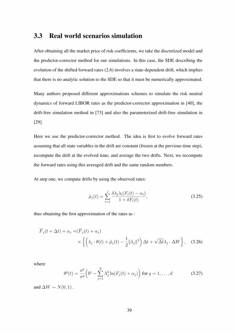
3.3 Real world scenarios simulation

After obtaining all the market price of risk coefficients, we take the discretized model and

the predictor-corrector method for our simulations. In this case, the SDE describing the

evolution of the shifted forward rates (2.6) involves a state-dependent drift, which implies

that there is no analytic solution to the SDE so that it must be numerically approximated.

Many authors proposed different approximations schemes to simulate the risk neutral

dynamics of forward LIBOR rates as the predictor-corrector approximation in [40], the

drift-free simulation method in [73] and also the parameterized drift-free simulation in

[29].

Here we use the predictor-corrector method. The idea is first to evolve forward rates

assuming that all state variables in the drift are constant (frozen at the previous time step),

recompute the drift at the evolved time, and average the two drifts. Next, we recompute

the forward rates using this averaged drift and the same random numbers.

At step one, we compute drifts by using the observed rates:

µj(t) =j∑i=1

δλjλi(Fi(t)− αi)1 + δFi(t)

, (3.25)

thus obtaining the first approximation of the rates as :

F j(t+ ∆t) + αj =(F j(t) + αj)

×(λj · θ(t) + µj(t)−

12‖λj‖

2)

∆t+√

∆tλj ·∆W, (3.26)

where

θq(t) = aq

σq

(bq −

N∑j=1

Λqj ln(Fj(t) + αj)

)for q = 1, . . . , d (3.27)

and ∆W ∼ N(0, 1) .

39

Next, we repeat the previous step using the F j’s instead of the Fj’s to compute µ∗j(t) and

θ∗q(t), thus obtaining the final approximation of the rates as:

Fj(t+ ∆t) + αj = (Fj(t) + αj) (3.28)

× exp(

λj ·θ(t) + θ∗(t)

2 +µj(t) + µ∗j(t)

2 − 12‖λj‖

2)

∆t+√

∆tλj ·∆W,

using the same values for ∆W .

3.4 Results

In this section, we present the estimation and simulation results of the real world LIBOR

market model. We use a three-factor version of the model.

The parameter estimates are obtained from the monthly historical observations of Euro-

pean AAA-government yield curves, ranging from 31 January 2015 up to 30 June 2016,

which are available in the European Central Bank database. Table 3.1 presents the for-

ward rate curve observed on 30 June 2016. At that time, negative forward rates of one

year tenor for the maturities of one to four years were prevailing.

40

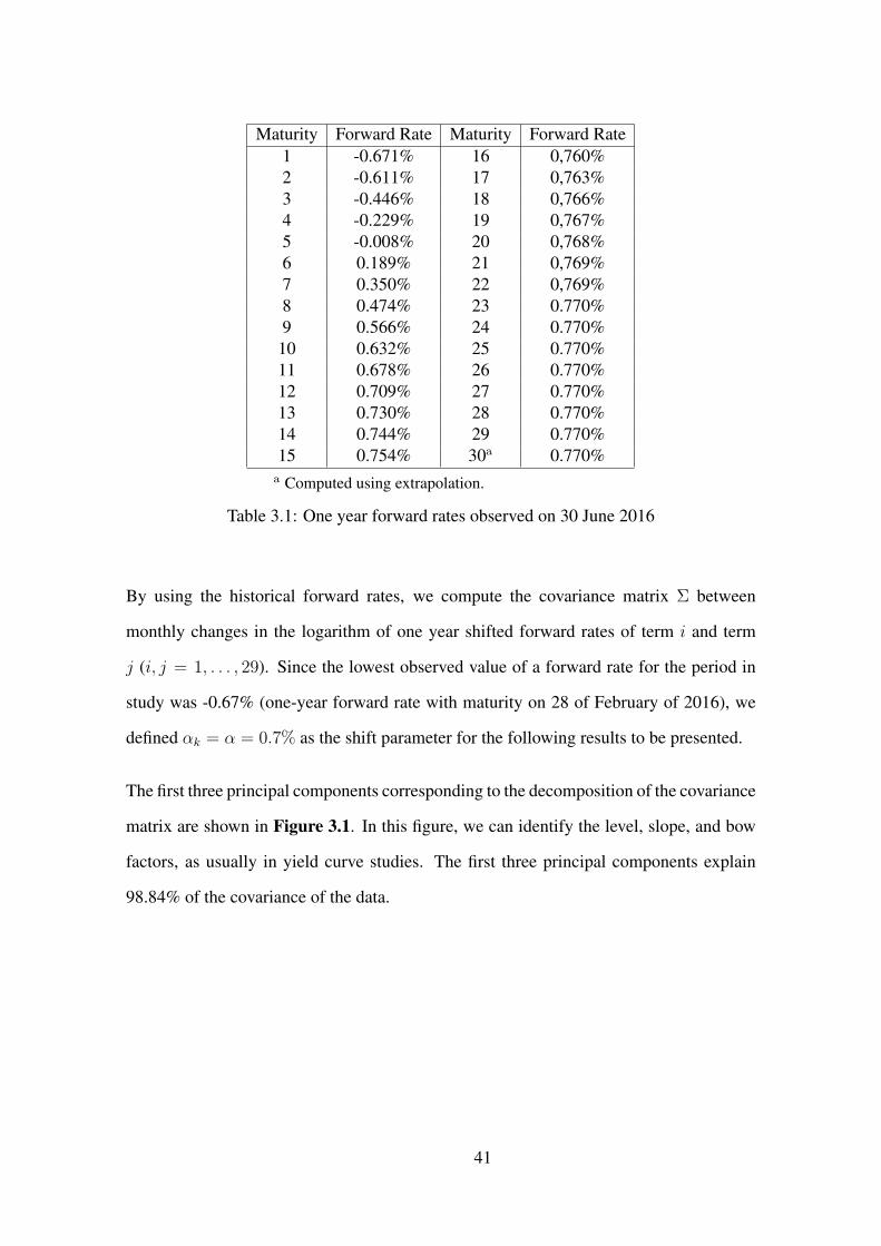
Maturity Forward Rate Maturity Forward Rate1 -0.671% 16 0,760%2 -0.611% 17 0,763%3 -0.446% 18 0,766%4 -0.229% 19 0,767%5 -0.008% 20 0,768%6 0.189% 21 0,769%7 0.350% 22 0,769%8 0.474% 23 0.770%9 0.566% 24 0.770%

10 0.632% 25 0.770%11 0.678% 26 0.770%12 0.709% 27 0.770%13 0.730% 28 0.770%14 0.744% 29 0.770%15 0.754% 30a 0.770%

a Computed using extrapolation.

Table 3.1: One year forward rates observed on 30 June 2016

By using the historical forward rates, we compute the covariance matrix Σ between

monthly changes in the logarithm of one year shifted forward rates of term i and term

j (i, j = 1, . . . , 29). Since the lowest observed value of a forward rate for the period in

study was -0.67% (one-year forward rate with maturity on 28 of February of 2016), we

defined αk = α = 0.7% as the shift parameter for the following results to be presented.

The first three principal components corresponding to the decomposition of the covariance

matrix are shown in Figure 3.1. In this figure, we can identify the level, slope, and bow

factors, as usually in yield curve studies. The first three principal components explain

98.84% of the covariance of the data.

41

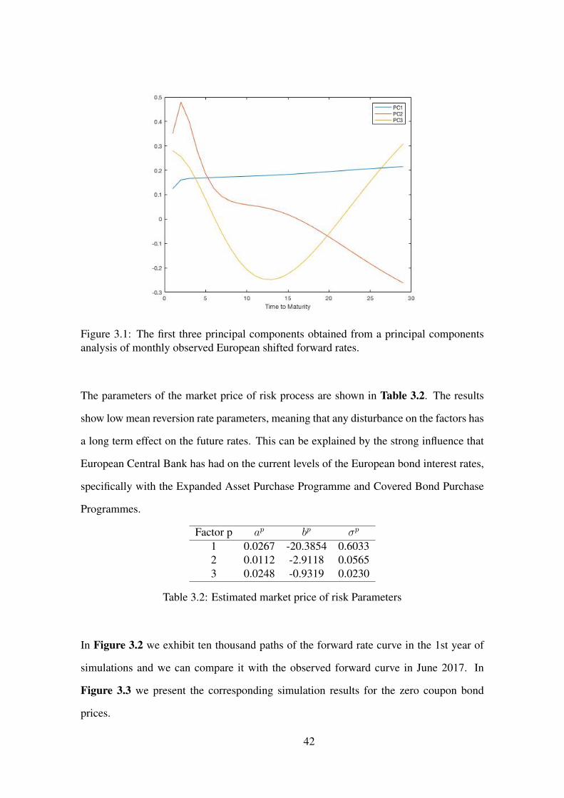
Figure 3.1: The first three principal components obtained from a principal componentsanalysis of monthly observed European shifted forward rates.

The parameters of the market price of risk process are shown in Table 3.2. The results

show low mean reversion rate parameters, meaning that any disturbance on the factors has

a long term effect on the future rates. This can be explained by the strong influence that

European Central Bank has had on the current levels of the European bond interest rates,

specifically with the Expanded Asset Purchase Programme and Covered Bond Purchase

Programmes.

Factor p ap bp σp

1 0.0267 -20.3854 0.60332 0.0112 -2.9118 0.05653 0.0248 -0.9319 0.0230

Table 3.2: Estimated market price of risk Parameters

In Figure 3.2 we exhibit ten thousand paths of the forward rate curve in the 1st year of

simulations and we can compare it with the observed forward curve in June 2017. In

Figure 3.3 we present the corresponding simulation results for the zero coupon bond

prices.

42

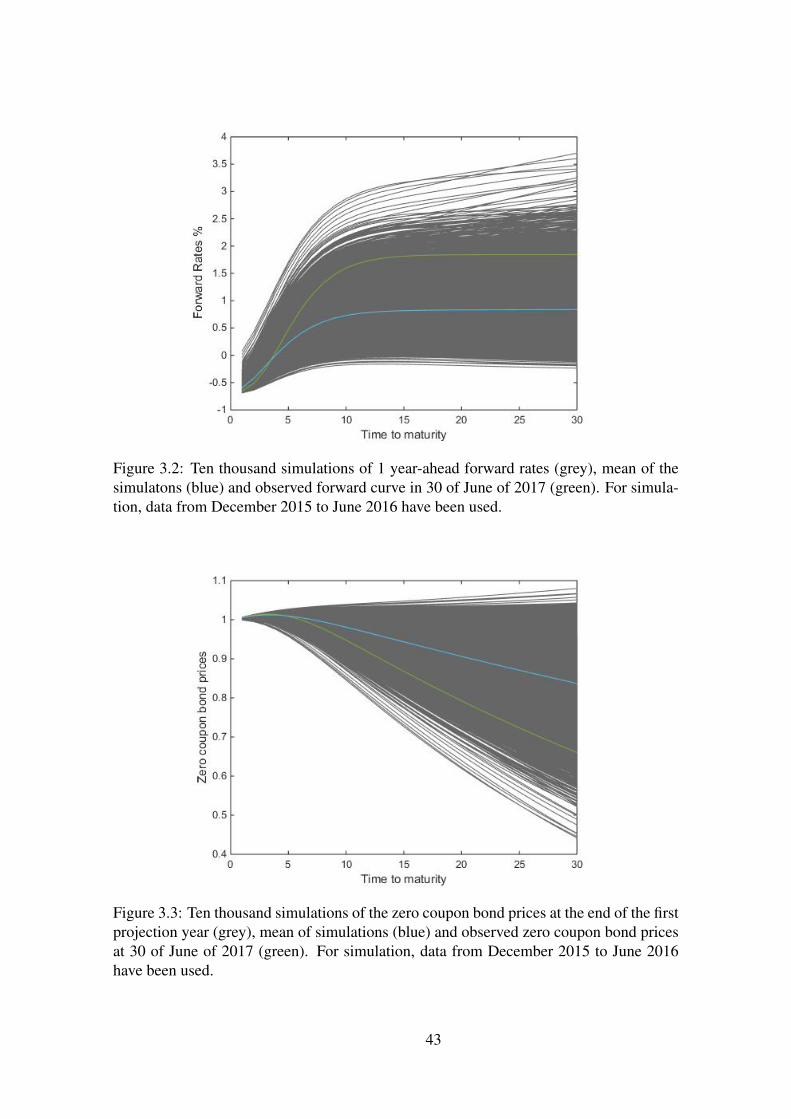
Figure 3.2: Ten thousand simulations of 1 year-ahead forward rates (grey), mean of thesimulatons (blue) and observed forward curve in 30 of June of 2017 (green). For simula-tion, data from December 2015 to June 2016 have been used.

Figure 3.3: Ten thousand simulations of the zero coupon bond prices at the end of the firstprojection year (grey), mean of simulations (blue) and observed zero coupon bond pricesat 30 of June of 2017 (green). For simulation, data from December 2015 to June 2016have been used.

43

The expected value and 97% confidence interval for each zero-coupon bond price with

maturities 1 to 30 years were computed using the ten thousand simulations, and the results

are shown in Table 3.3. By comparing the observed values for the bond prices in June of

2017 with the one year ahead predictions, we can report that for all maturities, the market

prices of bonds fall inside the confidence interval.

Maturity Mean Conf Interval Obs June 20171 1.0060 [1.0046,1.0073] 1.00652 1.0102 [1.0065,1.0139] 1.01173 1.0122 [1.0052,1.0192] 1.01434 1.0120 [1.0006,1.0233] 1.01335 1.0097 [0.9932,1.0263] 1.00866 1.0058 [0.9833,1.0283] 1.00047 1.0007 [0.9717,1.0296] 0.98968 0.9946 [0.9588,1.0304] 0.97679 0.9880 [0.9451,1.0308] 0.9624

10 0.9809 [0.9308,1.0310] 0.947311 0.9736 [0.9162,1.0309] 0.931612 0.9661 [0.9014,1.0308] 0.915713 0.9585 [0.8865,1.0306] 0.899814 0.9510 [0.8717,1.0303] 0.883815 0.9434 [0.8569,1.0300] 0.868116 0.9359 [0.8422,1.0296] 0.852517 0.9284 [0.8276,1.0293] 0.837218 0.9210 [0.8131,1.0289] 0.822119 0.9136 [0.7987,1.0286] 0.807220 0.9063 [0.7844,1.0283] 0.792621 0.8991 [0.7703,1.0279] 0.778322 0.8920 [0.7563,1.0276] 0.764223 0.8849 [0.7424,1.0273] 0.750324 0.8778 [0.7287,1.0270] 0.736825 0.8709 [0.7151,1.0267] 0.723426 0.8640 [0.7016,1.0264] 0.710327 0.8572 [0.6883,1.0261 0.697528 0.8504 [0.6751,1.0258] 0.684829 0.8437 [0.6620,1.0255] 0.672430a 0.8371 [0.6491,1.0251] 0.6602a Computed using extrapolation.

Table 3.3: Expected value, 97% confidence interval of zero coupon bond prices and 30June 2017 observations

In Figure 3.4 we present ten thousand paths for the forward rate curve for June 2018,

44

using the historical observations from January 2015 through June 2017. For this period

in study, the lowest observed rate was -0.91% (one-year forward rate with maturity one

year, observed on February 28th 2017) so we defined αk = α = 1% as the shift parameter

for the next results presented. Table 3.4 summarizes the results of the mean and standard

deviations of simulations for the zero-coupon bond prices.

Figure 3.4: Ten thousand simulations(grey) of one year-ahead forward rates and meancurve (blue). For simulation, data from December 2015 to June 2017 have been used

45

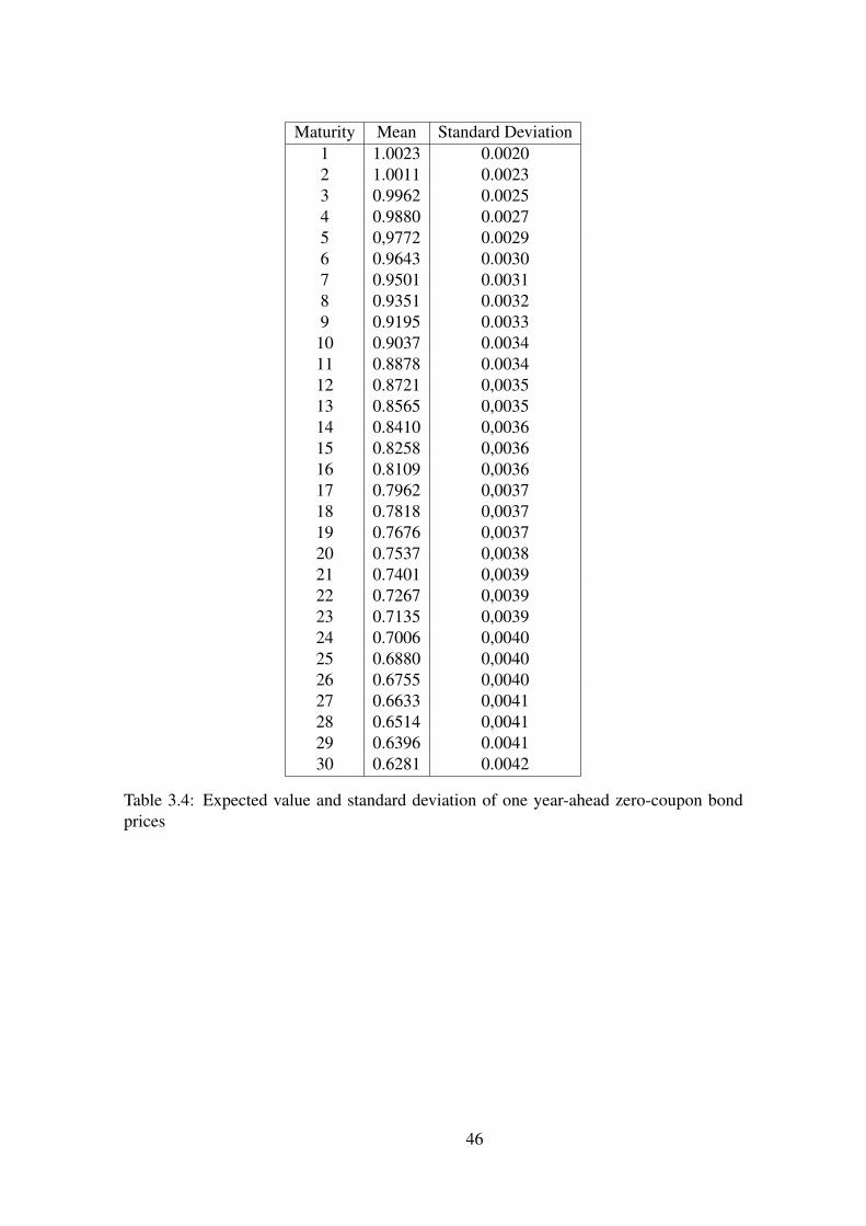
Maturity Mean Standard Deviation1 1.0023 0.00202 1.0011 0.00233 0.9962 0.00254 0.9880 0.00275 0,9772 0.00296 0.9643 0.00307 0.9501 0.00318 0.9351 0.00329 0.9195 0.0033

10 0.9037 0.003411 0.8878 0.003412 0.8721 0,003513 0.8565 0,003514 0.8410 0,003615 0.8258 0,003616 0.8109 0,003617 0.7962 0,003718 0.7818 0,003719 0.7676 0,003720 0.7537 0,003821 0.7401 0,003922 0.7267 0,003923 0.7135 0,003924 0.7006 0,004025 0.6880 0,004026 0.6755 0,004027 0.6633 0,004128 0.6514 0,004129 0.6396 0.004130 0.6281 0.0042

Table 3.4: Expected value and standard deviation of one year-ahead zero-coupon bondprices

46

Chapter 4

Credit risk models

In this chapter, we provide an overview of credit risk models and introduce some defi-

nitions and tools we use later in this work. In Section 4.1, we give an overview of the

existing literature in credit risk modeling. In Section 4.2, we present the main definitions

used to set the model approach under the risk neutral measure.

4.1 Overview of credit risk models

Credit risk represents an important subject in mathematical finance and contributes sig-

nificantly to the solvency capital requirement of insurance undertakings.

According to [61] credit risk refers to the risk associated with any kind of credit-linked

events, such as: changes in the credit quality (including downgrades or upgrades in credit

ratings), variations of credit spreads, and the default event. Default occurs when a coun-

terparty fails to meet its obligations in accordance with agreed terms in a contract. The

simplest example of such a contract is a bond, where the issuer may default (with a certain

probability) before or at the maturity date. In case that the issuer defaults, the bondholder

receives only a partial amount of the promised payment or nothing at all. Therefore, in-

vestors of corporate and sovereign bonds must assume not only interest rate risk but also

47

credit risk.

Many issuers of defaultable debt, including sovereigns, are assigned a publicly available

credit rating by rating agencies, such as Standard and Poor’s, Moody’s, or Fitch. A credit

rating represents a quantified evaluation of the creditworthiness of a borrower, in general

terms or with respect to a particular debt or financial obligation. It signals to market in-

vestors the level of default risk associated with certain company or instrument. In some

cases, due to regulation guidelines of risk mitigation, investors are restricted to invest-

ments in certain rating classes. This classification into rating classes allows the derivation

of benchmark credit curves for each rating class, which leads to complexity reduction.

Since both the current credit rating of a bond and the changes in credit ratings have a sig-

nificant effect on how the price is formed in the markets, when modeling credit spreads,

one should take into account the dynamics of the spreads for each credit rating and also

the transition probabilities between these ratings.

Modelling default is a difficult task given that default occurrences are rare. Sometimes

they occur unexpectedly, as firms try to avoid public dissemination of information when

faced with financial problems. Moreover, default implies losses that are unknown before

default occurs. Schönbucher in [64] decomposes credit risk in four components. First

component is arrival risk, a term for the uncertainty whether a default will occur or not

measured by the probability of default. Second component is timing risk, which refers to

the uncertainty about the precise time of default. Third components is recovery risk that

describes the uncertainty about the severity of the losses if a default has happened. The

fourth component is market risk, which describes the risk of changes in the market price

of a defaultable asset, even if no default occurs. A credit risk model should aim to capture

all the different components. However, this implies the model can be extremely complex,

which can make it computational unfeasible.

48

We refer to two different approaches to credit risk modelling: structural models and

reduced-form models. The first type was introduced by Merton [55] and Black and Cox

[10]. In structural models, credit risk of a corporate bond is measured by relating the firm

value of the issuing company to its liabilities since the value of the firms assets is modeled

exogenously, and default takes place as the first time the value process of the firm hits a

certain barrier. The foundation on fundamentals allows us to obtain correct relationships

between different securities from the same entity, although it has the drawback that it

turns out to be very hard to define a meaningful process for the firm’s value, and data

are rarely available. Another problem faced with this modeling approach comes from the

unrealistic short-term spreads it implies. Spreads result very low and tend towards zero

as the maturity of the debt decreases, which is contrary to empirical observations where

short maturity spreads are not negligible because even close to maturity the bondholder is

uncertain whether the full amount of money will be paid back or not.

In reduced-form models, the time of default is modeled directly as a stopping time with an

intensity process to be specified. Usually a Poisson process with random intensity (a Cox

process) is considered. This second approach is followed by Jarrow and Turnbull in [44],

where they consider that default is driven by a Poisson process with constant intensity and

known payoff at default. In Madan and Unal [54], the constant intensity is extended to

the case of random intensity. In Singleton and Duffie [20], the recovery rate is modeled

as a fraction of the value of the security immediately before default occurs.

The idea to make the probability of default of a corporate bond depend on the rating of the

issuer was proposed later with Lando [49]. Jarrow, Lando and Turnbull in [43] presented

a model for valuing risk debt that explicitly incorporates a firm’s rating as an indicator of

the likelihood of default using a deterministic Markov chain. Arvantis et al. [5] follow

the same idea while proposing a stochastic generator for a continuous-time Markov chain.

These credit models can be combined with any desired term-structure model for a default-

free debt and take into account the historical transition probabilities for the various credit

49

classes to determine the risk-adjusted probabilities used in valuation.

The inclusion of credit risk in interest rate market models was a recent development in-

troduced by Schönbucher in [63], who extended the forward LIBOR market model by

adding the so called defaultable forward LIBOR rates to the model. Moreover, he intro-

duced the survival-based pricing measures as a tool for the pricing of defaultable payoffs,

which allows the derivation of the no-arbitrage dynamics of defaultable forward rates and

forward credit spreads.

Even more recently, Eberlein, Kluge, and Schönbucher [22] constructed the Lévy LIBOR

model with default risk driven by a time-inhomogeneous Lévy process. Later Eberlein

and Grbac [21] extended the classical definition of the default-free forward Libor rate and

developed a rating based LIBOR market model to cover defaultable bonds with credit

ratings. Moreover, they modeled credit migration by a conditional Markov chain.

4.2 Notation and risk neutral model setup

Let (Ω,F ,Ft,Q) be the filtered probability space under the spot risk-neutral probability

measure, Q.

Credit ratings is a relevant concept in credit risk models. We consider the case where

the credit ratings are identified as elements of a finite set K = 1, 2, . . . , K. The rating

classes are ordered by their credit risk. This means that rating class 1 represents the best

possible credit quality while class K− 1 is the worst non-defaulted credit quality, and the

last class K represents the default state.

Definition 4.1. The rating of a bond is a stochastic process, denoted by C, so that for

each time t the rating of the bond is a random variable C(t) : Ω→ K.

Moreover, we consider the case where the migration between credit ratings is modeled by

a continuous-time conditional Markov chain C with state space K.

50

Under the previous assumption, the rating transition process satisfies the Markov property,

thus, at any time t, the probability of transition to another rating until time T > t only

depends on the current rating C(t) of the process:

P [C(T ) = r|Ft] = P [C(T ) = r|C(t)] , r = 1, . . . K .

A stochastic process satisfying the Markov property is defined a Markov process. Addi-

tionally, if the state space of this Markov process is countable, the process is defined a

Markov chain.

Definition 4.2. The transition probability matrix P (t, T ) for the time interval [t, T ] is

defined as:

P (t, T ) =

p1,1(t, T ) p1,2(t, T ) . . . p1,K(t, T )...

......

pK−1,1(t, T ) pK−1,2(t, T ) . . . pK−1,K(t, T )

pK,1(t, T ) pK,2(t, T ) . . . pK,K(t, T )

where, for all i, j ∈ K, the component pi,j(t, T ) represents the probability that the rating

process changes to rating j at time T , given that it was in rating i at time t; that is

pi,j(t, T ) = P [C(T ) = j|C(t) = i] , t ≤ T.

In particular, the last element in each row of the matrix represents the default probability

of each credit rating, i.e. p1,K(t, T ), . . . , pK−1,K(t, T ), pK,K(t, T ).

Note that the sum of the coefficients of each row equals one, since we always consider

51

the case where the entity can only transition to one of the credit ratings.1 That is,

K∑j=1

pi,j(t, T ) = 1 , ∀i ∈ K.

Moreover, we assume that if an entity enters default it can not recover, this meaning that

the default state K is absorbing. So, it holds that:

pK,1(t, T ) = . . . = pK,K−1(t, T ) = 0 and pK,K(t, T ) = 1 with t ≤ T .

Moreover, we assume the transition probabilities only depend on the time interval over

which the transitions take place (time-homogeneity), that is

P (t, T ) = P (T − t) , ∀ t ≤ T.

The generator matrix is another useful concept when modeling using Markov chains, as

it allows to obtain transition matrices for different time intervals.

Definition 4.3. A matrix G = (gi,j)i,j=1,...,K is called a generator matrix if it has the

following three properties:

• All diagonal entries are not positive, i.e. gi,i ≤ 0, i = 1, . . . , K

• All non-diagonal entries are not negative. i.e. gi,j ≥ 0, i, j = 1, . . . , K and i 6= j

• The sum of each row is zero, i.e.,K∑j=1

gi,j = 0, i = 1, . . . , K

Definition 4.4. Let P (0, 1) be the one-period transition probability matrix of a time-

homogeneous Markov chain. If there exists a generator matrix with the properties stated

in Definition 4.3 and such that P (0, 1) = eG then the matrix G is the generator matrix

of P .1in practice, a company can leave the rating system and get an unrated status.

52

Definition 4.5. For A ∈ F we denote by 1A the indicator function of A, i.e

1A(ω) =

1 if ω ∈ A

0 otherwise

Definition 4.6. The default time is defined as the first time the Markov chain reaches the

state K: τ = inft > 0, C(t) = K. The survival indicator function I is defined as

I(t) = 1τ>t. Thus, the survival indicator function I is one before default and jumps to

zero at the time of default τ .

Definition 4.7. A T -maturity defaultable zero-coupon bond is a contract that pays its

holder one unit of currency at time T , with no intermediate payments if no default occurs

before T . If default occurs before the maturity the bond’s holder receives a reduced

payment, called the recovery payment. The contract value at time t < T is denoted by

B(t, T ).

Definition 4.8. The recovery rate is the amount, expressed as a percentage, recovered

from a loan that is unable to settle the full outstanding amount.

In the literature, the most common assumptions on the recovery rate are: the zero-recovery,

recovery of market value, recovery of par value and recovery of treasury. In the case of

zero-recovery assumption, if default occurs the bondholder receives nothing. When re-

covery of face value is assumed, a fixed fraction of the face value of the bond is paid to the

investors at time of default, whereas, under the recovery of treasury assumption, a fixed

fraction of the face value of the bond is paid to the investors at time of maturity. Finally,

if recovery of treasury is assumed, the recovery value is expressed in terms of the market

value of equivalent default-free assets. For a detailed comparison of traditional recovery

models see [50] and [64].

We assume that recovery rates depend on the rating class from which the bond has de-

53

faulted. We represent the recovery rate by a vector q = (q1, q2, . . . , qK−1). Moreover, we

assume the recovery of treasury value hypothesis.

In this setup, the payoff at maturity of a defaultable zero-coupon bond with maturity Tj

and migration process C is given by

Bj(Tj) = 1τ>Tj + 1τ≤TjqCτ− =K−1∑i=1

1C(Tj)=i + 1C(Tj)=KqCτ− , (4.1)

where Cτ− := C(τ−) denotes the last rating prior to default (i.e. the rating class from

which the bond has defaulted). Hence,we postulate that the defaultable bond price process

is given by

Bj(t) =K−1∑i=1

Bij(t)1C(t)=i +Bj(t)qCτ−1C(t)=K , (4.2)

where Bij(t) denotes the price at time t of a defaultable zero-coupon bond that matures at

Tj with Tj ≥ t, provided that the bond is in rating i during the time interval [0, t].

Definition 4.9. We define by F ij (t) = F i(t, Tj, Tj+1) the value at time t ≤ Tj of the for-

ward LIBOR rate associated to the bond with credit rating i in the period [Tj, Tj+1].

This forward rate can be obtained as

F ij (t) =

Bij(t)−Bi

j+1(t)δjBi

j+1(t) , j = 1, . . . , N, i = 1, . . . , K − 1. (4.3)

For simplicity of notation, we assume that F 0j (t) := Fj(t) and that F 0,D

j (t) := FDj (t).

Next, we also define the forward shifted LIBOR rates for credit rating class i as

F i,Dj (t) = F i

j (t) + αj, (4.4)

for all t > 0, j = 1, . . . , N and i = 1, . . . , K , where αj is the same shift parameter used

in (2.4) and only depends on the tenor,

54

Definition 4.10. The default-risk factor for credit rating i at time t for maturity Tj is

defined as:

Dij(t) =

Bij(t)

Bi−1j (t)

, j = 1, . . . , N, i = 1, . . . , K − 1 . (4.5)

Definition 4.11. The discrete-tenor forward default intensity for credit rating i over

the period [Tj, Tj+1] as seen from time t is defined as

H ij(t) = 1

δj

(Dij(t)

Dij+1(t) − 1

), j = 1, . . . , N, i = 1, . . . , K − 1. (4.6)

The forward default intensities can be also written in terms of the bond prices in the form

H ij(t) = 1

δj

(Bi−1j+1(t)Bi

j(t)Bi−1j (t)Bi

j+1(t)− 1

), j = 1, . . . , N, i = 1, . . . , K − 1. (4.7)

It is easy to establish the following relationships between the forward rates and default

intensities:

H ij(t) =

F ij (t)− F i−1

j (t)1 + δjF

i−1j (t)

, j = 1, . . . , N, i = 1, . . . , K − 1. (4.8)

therefore we get

(1 + δjF

ij (t)

)=(1 + δjH

ij(t)

) (1 + δjF

i−1j (t)

), j = 1, . . . , N, i = 1, . . . , K − 1.

(4.9)

By applying equation (4.9) recursively, we can express every rating-dependent forward

rate as a product of the default-free forward rate and the forward default intensities as

follows:

(1 + δjF

ij (t)

)=(1 + δjF

0j (t)

) i∏k=1

(1 + δjH

kj (t)

), j = 1, . . . , N, i = 1, . . . , K − 1.

(4.10)

55

Definition 4.12. The forward inter-rating LIBOR spreads Sij are the spreads between

LIBOR rates for two successive credit rating classes. Therefore we have,

Sij(t) = F ij (t)− F i−1

j (t), j = 1, . . . , N, i = 1, . . . , K − 1. (4.11)

Since αj does not depend on the credit rating we have,

Sij(t) = F i,Dj (t)− F i−1,D

j (t), i = 1, . . . , K − 1. (4.12)

Moreover, we have the following relation between the default-free and defaultable for-

ward shifted rates:

F i,Dj (t) = FD

j (t) +i∑

h=1Shj (t), j = 1, . . . , N, i = 1, . . . , K − 1. (4.13)

There are two alternatives in the specification of the dynamics of the defaultable interest-

rates. Either we model the spreads S or the discrete intensities H . Both in Schönbucher

[63] and Eberlein and Grbac [21], they model the discrete intensities as it is more con-

venient for pricing purposes. In this work, given that we intend to incorporate credit

risk under the possibility of negative interest rates, we choose to model the inter-rating

spreads directly according to a stochastic dynamics that guarantees the monotonicity of

bond prices with respect to the credit ratings, i.e., Fj(t) < F 1j (t) < ... < FK−1

j (t), which

is consistent with the fact that lower credit ratings are reflected by higher interest rates.

Also, this specification allows us to capture the independent movements of each addi-

tional credit step that would not be so clear if we had chosen to model the spread over

risk-free forward rate for each credit rating.

Thus, under the spot measure, Q, we assume the following dynamics of the inter-rating

56

spreads

dSij(t)Sij(t)

= µS,ij (t)dt + εS,ij (t) · dW S,i(t), j = 1, . . . , N, i = 1, . . . , K − 1 , (4.14)

where: εS,ij represents the mi-dimensional volatility functions and W S,i is a multidimen-

sional Brownian motion for each credit rating class i.

Next, we recall the adopted model for the default-free shifted LIBOR rates in from Chap-

ter 2 as

dFDj (t)

FDj (t) = εj(t) ·

j∑i=m(t)

βDi (t)dt+ εj(t) · dW d(t) , (4.15)

where:

βDi (t) = εi(t)δiFDi (t)

1 + δi(FDi (t)− αi)

.

Moreover, combining equations (4.13), (4.14) and (4.15), we obtain the shifted LIBOR

rates for credit rating class i dynamics under the spot measure as

dF i,Dj (t) =

FDj (t)εj(t) ·

j∑l=m(t)

βDl (t) +i∑

h=1Shj (t)µS,hj (t)

dt+ FDj (t)εj(t) · dW d(t)

(4.16)

+i∑

h=1Shj (t)εS,hj (t) · dW S,h(t), j = 1, . . . , N, i = 1, . . . , K − 1.

Consequently, the dynamics of the LIBOR rates for credit rating class i is given by

dF ij (t) =

(Fj(t)− αj)εj(t) ·j∑

l=m(t)βDl (t) +

i∑h=1

Shj (t)µS,hj (t) dt+ (Fj(t)− αj)εj(t) · dW d(t)

(4.17)

+i∑

h=1Shj (t)εS,hj (t) · dW S,h(t), j = 1, . . . , N, i = 1, . . . , K − 1.

57

Chapter 5

LIBOR market model with credit risk

under the real world measure

In this section, we generalize the results presented in Chapter 3 by including credit risk in

the default-free model.

In Section 5.1, we present the proposed dynamics inter-rating spreads under the real world

measure and present the market price of risk process adopted for the real world setting.

In Section 5.2, we show how to estimate the parameters based on historical information

and Section 5.3 is dedicated to the simulation methodologies used. In the last section, we

present the results of the projected rates one year ahead from the last data point by using

historical data of sovereign European bonds.

The contents of this chapter have been published in [53].

58

5.1 The model

In order to have a more parsimonious model, we assume that the spreads for all credit

ratings are dependent on the same stochastic factor. This means that Equation (4.14) can

be rewritten and we consider the case where dynamics of the inter-rating spreads under

the spot measure, Q, are given by :

dSij(t)Sij(t)

= µS,ij (t)dt + εS,ij (t) · dW S(t), j = 1, . . . , N, i = 1, . . . , K − 1. (5.1)

where µS,ij (t) are the drifts under the spot measure, εS,ij (t) are the m-dimensional vectors

of volatility functions and dW S(t) is a multidimensional Brownian motion.

From the adopted risk neutral model, defined by Equation (4.15) and (5.1), and using

Girsanov’s theorem [31], we can write the dynamics of the default-free LIBOR rates and

inter-rating spreads under the real world measure using the following relations between

the r-dimensional and the m-dimensional Brownian motions under the real world mea-

sure, W P and W P,S , and the r-dimensional and m-dimensional Brownian motions under

the spot measure W d and W S:

dW P (t) = dW d(t)− θ(t)dt

dW P,S(t) = dW S(t)− θS(t)dt. (5.2)

where θ(t) and θS(t) are respectively the r-dimensional and m-dimensional market price

of risk processes.

In this setting, the dynamics of shifted LIBOR risk-free forward rates under the real world

measure are given by:

dFDj (t)

FDj (t) =

εj(t) ·j∑

l=m(t)βDl (t) + εj(t) · θ(t)

dt+ εj(t) · dW P (t) , (5.3)

59

where

βDl (t) = εl(t)δlFDl (t)

1 + δl(FDl (t)− αl)

,

and the dynamics of the inter-rating spreads are:

dSij(t)Sij(t)

=(θS(t) · εS,ij (t) + µS,ij (t)

)dt + εS,ij (t) · dWP,S(t), j = 1, ..., N, i = 1, ...,K − 1.

(5.4)

Therefore, we obtain the following SDE governing the shifted LIBOR rates for the credit

rating class i under the real world measure:

dF i,Dj (t) =

FDj (t)

εj(t) · j∑l=m(t)

βDl (t) + εj(t) · θ(t)

+i∑

h=1Shj (t)

(εS,hj (t) · θS(t) + µS,hj (t)

) dt+ FDj (t)εj(t) · dWP (t) +

i∑h=1

Shj (t)εS,hj (t) · dWP,S(t), j = 1, ..., N, i = 1, ...,K − 1.

(5.5)

Next we maintain the assumptions made in Chapter 3 regarding the volatility structure

of the default-free forward rate, particularly, that the default-free interest rates volatilities

depend only on the time-to-maturity:

εkj (t) = λkj−m(t) ,

In addition, we consider the case when Sij have piecewise constant instantaneous volatili-

ties and depend also only on the time-to-maturity, i.e:

εi,Sj (t) = νij−m(t) ,

and that we can write the volatility functions in terms of the corresponding orthonormal

basis1 Λ,Πi,S :

λkj = σkΛkj , νi,kj = ωkΠk

N×(i−1)+j .

1N−1∑j=0

Λkj Λl

j = δkl andN−1∑j=0

Πi,kj Πi,l

j = δkl for i = 1, ..K − 1 where N can be interpreted to be the

number of maturities observable on the forward rate curve.

60

We assume that the k component of the market price of risk for interest rates has the

following structure presented already in chapter 3:

θk(t) = ak

σk

(bk −

N+m(t)−1∑l=m(t)

Λkl−m(t) ln(FD

l (t))), (5.6)

where ak, σk and bk are parameters to be estimated from historical data, while the vectors

Λi are the coefficients obtained from the principal component analysis of the historical

covariance matrix of the logarithm of shifted rates.

Moreover, the same structure is proposed for the market price of risk of inter-rating

spreads, with the appropriate modifications as follows:

θS(t) = θS(t) + ρ(t) , (5.7)

where θS(t) is a vector with components given by

θS,k(t) = aS,k

ωk

(bS,k −

N+m(t)−1∑l=m(t)

K−1∑h=1

ΠkN×(h−1)+(l−m(t)) ln(Shl (t))

), (5.8)

where aS,k, ωk and bS,k are parameters to be estimated from historical data, the vectors

Πil are the coefficients obtained from the principal component analysis of the historical

covariance matrix of the logarithm of the inter-rating spreads and ρk(t) are the compone-

nents of the vector ρ(t) defined as the solution of the following system of (K−1)×(N−1)

linear equations:

µS,ij (t) + νi,kj · ρ(t) = 0 , (5.9)

such that θS(t) is the drift of the inter-rating spreads under the real world measure, and

equation (5.4) can be simplified to:

dSij(t)Sij(t)

= θS(t) · εS,ij (t)dt + εS,ij (t) · dW P,S(t), j = 1, ..., N, i = 1, ..., K − 1. (5.10)

61

5.2 Parameter estimation

In this section, the method for calibrating the real world model to historical data is de-

scribed. We mainly adopt the methodology used in Chapter 3 with the appropriate modi-

fications, since we are now modeling changes in the logarithm of the inter-rating spreads.

We consider a common constant accrual, i.e. δ = δj = Tj+1−Tj , and adopt the following

notation for the constant maturity defaultable forward shifted rates:

LD,ij (t) = FD,i(t, t+ jδ, t+ (j + 1)δ) , j = 1, . . . , N. (5.11)

More precisely LD,ij (t) denotes the observed value at time t of the forward shifted rates

for the period [t+ δj, t+ δ(j + 1)].

Under this notation, the inter rating spread observed at time t is defined as:

Sij(t) = LD,ij (t)− LD,i−1j (t),

and the dynamics of Sij satisfies the SDE:

dSij(t) = Sij(t)νij ·θS(t)dt+Sij(t)νij ·dW P,S(t), j = 1, . . . , N, i = 1, . . . , K−1. (5.12)

For convenience, we consider the stochastic differential equation for the dynamics of the

logarithm of the inter-ratings spreads:

d lnSij(t) =(νij · θS(t)− 1

2‖νij‖2)dt+ νij · dW P,S(t) . (5.13)

Next, we consider the covariance matrix Π of the historical changes in the logarithms of

forward inter-ratings spreads and, using Principal Components Analysis, we recover the

Πki ’s and ωS,k’s as the eigenvectors and eigenvalues of Π, respectively. Also in this step,

62

we define the dimension of the volatility functions and the number of components of the

market price of risk process. A common criteria to select the number of components to

retain is to use the proportion of total variance criteria where a predetermined threshold

is defined so that the number of factors retained accounts for that selected value of total

variation. Research on the term structure of interest rates, such as [51] and [19], suggests

that the term structure can be explained by a small number of underlying factors: level,

slope, bow, and higher order perturbations. Regarding the spreads, and to the best of

our knowledge, this is the first PCA study on the observations of the inter-rating spreads.

Previous studies of PCA applied to spreads (measured as the difference between yields

of the defaultable bond and the default-free rates) include [17] who found evidence of

one common factor for the corporate spread changes. In [62] PCA is applied to study

sovereign spreads in Latin America countries and two components were able to explain

90% of total variance in this case

By considering a small time step, ∆t, between observations and using the Euler-Maruyama

scheme, we approximate the evolution of the logarithm of inter-rating spreads as follows:

lnSij(t+ ∆t) = lnSij(t) +(νij · θS(t)− 1

2‖νij‖2)

∆t+ νij ·∆W P,S(t) , (5.14)

Next, we define

ln Sij(t) = lnSDi (t)− 12‖ν

ij‖2∆t, (5.15)

so that

lnSij(t+ ∆t) = ln Sij(t) + νij · θS(t)∆t+ νij ·∆W P,S . (5.16)

Thus, by multiplying (5.16) by ΠlN×(i−1)+j and summing over j and i, we obtain

gl(t+ ∆t) = gl(t) + aS,l(bS,l − gl(t)

)∆t+ ωS,l∆W S,l for l = 1, 2, . . .m (5.17)

63

where we have introduced

gl(t) =N∑j=1

K−1∑i=1

ΠlN×(i−1)+j lnSij(t) , (5.18)

and

gl(t) =N∑j=1

K−1∑i=1

ΠlN×(i−1)+j ln Sij(t) . (5.19)

In order to estimate the parameters aS,l and bS,l, first from the historical data we define

the following series of observations:

Z l(t) = gl(t+ ∆t)− gl(t) ,

and

U l(t) = gl(t) .

Next, we estimate the l regression models obtained from equation (5.17):

Z l(t) = cS,l +mS,lU l(t) + eS,l(t) , (5.20)

where

eS,l(t) = ωS,k∆W S,l , mS,l = −aS,l∆t , cS,l = aS,lbS,l∆t , (5.21)

so that we can recover aS,l and bS,l from mS,l and cS,l.

5.3 Real world scenarios simulation

After obtaining the real world measure parameters, we take the discretized model and the

predictor-corrector method for our simulations. We consider the first approximation of

64

the inter-rating spreads as:

Sij(t+ ∆t) =Sij(t)×(vij · θS(t)− 1

2‖vij‖2)

∆t+√

∆tvij ·∆W S, (5.22)

where

θS,q(t) = aS,q

ωS,q

(bS,q −

N∑j=1

K−1∑h=1

ΠqN×(h−1)+(l−1)S

hj (t)

)for q = 1, . . . ,m (5.23)

and ∆W S ∼ N(0, 1)

By repeating the previous step using the Sij’s instead of the Sij’s to compute θ∗S,q(t), we

obtain the final approximation of the spreads as:

Sij(t+ ∆t) = Sij(t)× exp(

vij ·θS(t) + θS∗(t)

2 − 12‖v

ij‖2)

∆t+√

∆tvij ·∆W S

,

using the same values for ∆W S .

We can obtain the price at time t + ∆t of a zero-coupon bond with credit rating i at time

t as follows:

Bij(t+ ∆t) =

K−1∑l=1

Blj(t)P (Ct+∆t = l|Ct = i)(1 + δF l

j(t+ ∆t)) + P (Ct+∆t = K|Ct = i)qi,

where

F lj(t+ ∆t) = Fj(t+ ∆t) + Slj(t+ ∆t)

and qi is the recovery rate for credit rating i.

5.4 Results

In this section, we present the estimation and simulation results of the real world LIBOR

market model with credit risk. We use a three-factor version of the model for the default-

65

free2 forward rates and a seven-factor model for the inter-rating spreads.

The parameter estimates are obtained from the historical observations of European gov-

ernment bond prices, ranging from 31 January 2016 up to 30 June 2018. Table 5.1

presents the forward rate curve observed on 30 June 2018. At that time, negative for-

ward rates of one year tenor for the maturities of one to three years were prevailing.

Maturity Forward Rate Maturity Forward Rate1 -0.556% 11 1.331%2 -0.381% 12 1.345%3 -0.018% 13 1.352%4 0.353% 14 1.353%5 0.665% 15 1.351%6 0.903% 16 1.349%7 1.072% 17 1.347%8 1.186% 18 1,345%9 1.260% 19 1,342%

10 1.305% 20 1,342%

Table 5.1: One year forward rates observed on 30 June 2018.

For this study, we consider 23 European countries in order to construct the benchmark

yield curves for each of the rating groups. The chosen countries are shown in Table 5.2.

We group the last two rating groups, B and CCC-C, in order to have more than one country

in each credit rating group.

AAA AA A BBB BB B CCC-CDenmark Austria Ireland Bulgaria Russia Armenia GreeceGermany Finland Malta Hungary Portugal Ukraine

Luxembourg France Latvia Italy TurkeyNetherlands Slovakia SpainSwitzerland Romania

Table 5.2: Countries by rating group as of 31 January 2016.

After grouping the countries we compute the inter-rating spreads for each sucessive rating

class. In Figure 5.1 the last observation of the inter-rating spreads is presented.

By using the historical forward rates, we compute the covariance matrix Σ between2We consider the AAA rated bonds as the default-free bonds.

66

Figure 5.1: Inter-rating spreads observed as of 30 June 2018.

monthly changes in the logarithm of one year shifted forward rates of term i and term

j (i, j = 1, . . . , 20). Since the lowest observed value of a forward rate for the period in

study was -0.72% (one-year forward rate with one year maturity observed on 28 February

of 2017) we defined αk = α = 0.8% as the shift parameter for the following results to

be presented. Note that this parameter can also be selected according to market expecta-

tions or risk manager views on the lower boundary for the forward rates in order to obtain

scenarios with rates bellow the threshold we have selected.

The first three principal components corresponding to the decomposition of the covariance

matrix are shown in Figure 5.2. In this figure we can identify the level, slope and bow

factors, as usually in yield curve studies. The first three principal components explain a

98.84% of the covariance of the data.

Regarding the principal components obtained from the decomposition of the covariance

matrix of the inter-rating spreads, we present in Figure 5.3 the first seven principal com-

ponents which explain a 90.58% of the covariance of the data.

67

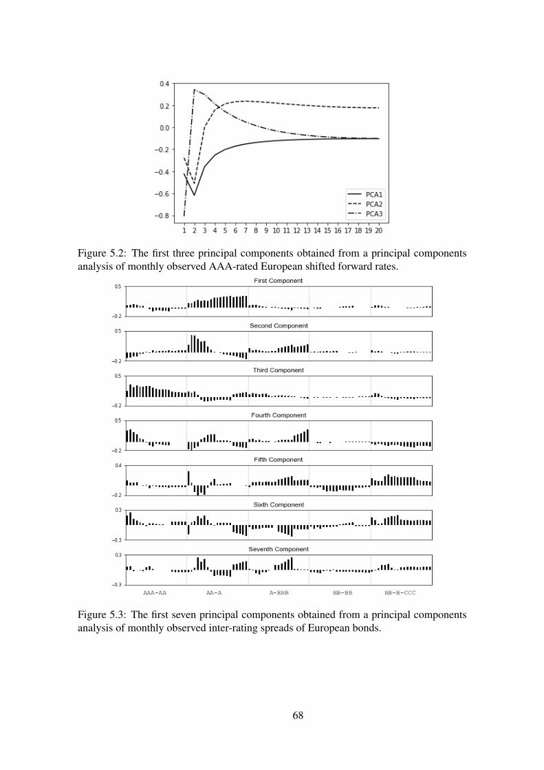
Figure 5.2: The first three principal components obtained from a principal componentsanalysis of monthly observed AAA-rated European shifted forward rates.

Figure 5.3: The first seven principal components obtained from a principal componentsanalysis of monthly observed inter-rating spreads of European bonds.

68

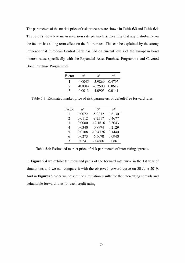
The parameters of the market price of risk processes are shown in Table 5.3 and Table 5.4.

The results show low mean reversion rate parameters, meaning that any disturbance on

the factors has a long term effect on the future rates. This can be explained by the strong

influence that European Central Bank has had on current levels of the European bond

interest rates, specifically with the Expanded Asset Purchase Programme and Covered

Bond Purchase Programmes.

Factor ap bp σp

1 0.0045 -5.9869 0.47952 -0.0014 -6.2500 0.06123 0.0013 -4.0905 0.0141

Table 5.3: Estimated market price of risk parameters of default-free forward rates.

Factor ap bp σp

1 0.0072 -5.2232 0.61302 0.0112 -8.2517 0.46773 0.0080 -12.1616 0.30434 0.0340 -0.8974 0.21295 0.0108 -10.4176 0.14406 0.0273 -6.5070 0.09407 0.0241 -0.4666 0.0861

Table 5.4: Estimated market price of risk parameters of inter-rating spreads.

In Figure 5.4 we exhibit ten thousand paths of the forward rate curve in the 1st year of

simulations and we can compare it with the observed forward curve on 30 June 2019.

And in Figures 5.5-5.9 we present the simulation results for the inter-rating spreads and

defaultable forward rates for each credit rating.

69

Figure 5.4: Ten thousand simulations of 1 year-ahead forward rate curve for AAA bonds(grey), observed forward curve on 30 June 2018 (dashed-black) and observed forwardcurve on 30 June 2019 (black).

Figure 5.5: Ten thousand simulations of 1 year-ahead inter-rating spreads for credit ratingsAAA and AA (grey), observed spread curve on 30 June 2018 (dashed-black) and observedspread curve on 30 June of 2019 (black) (left) and corresponding forward rates for ratingAA (right).

Figure 5.6: Ten thousand simulations of 1 year-ahead inter-rating spreads for credit ratingsAAA and AA (grey), observed spread curve on 30 June 2018 (dashed-black) and observedspread curve on 30 June of 2019 (black) (left) and corresponding forward rates for ratingAA (right).

70

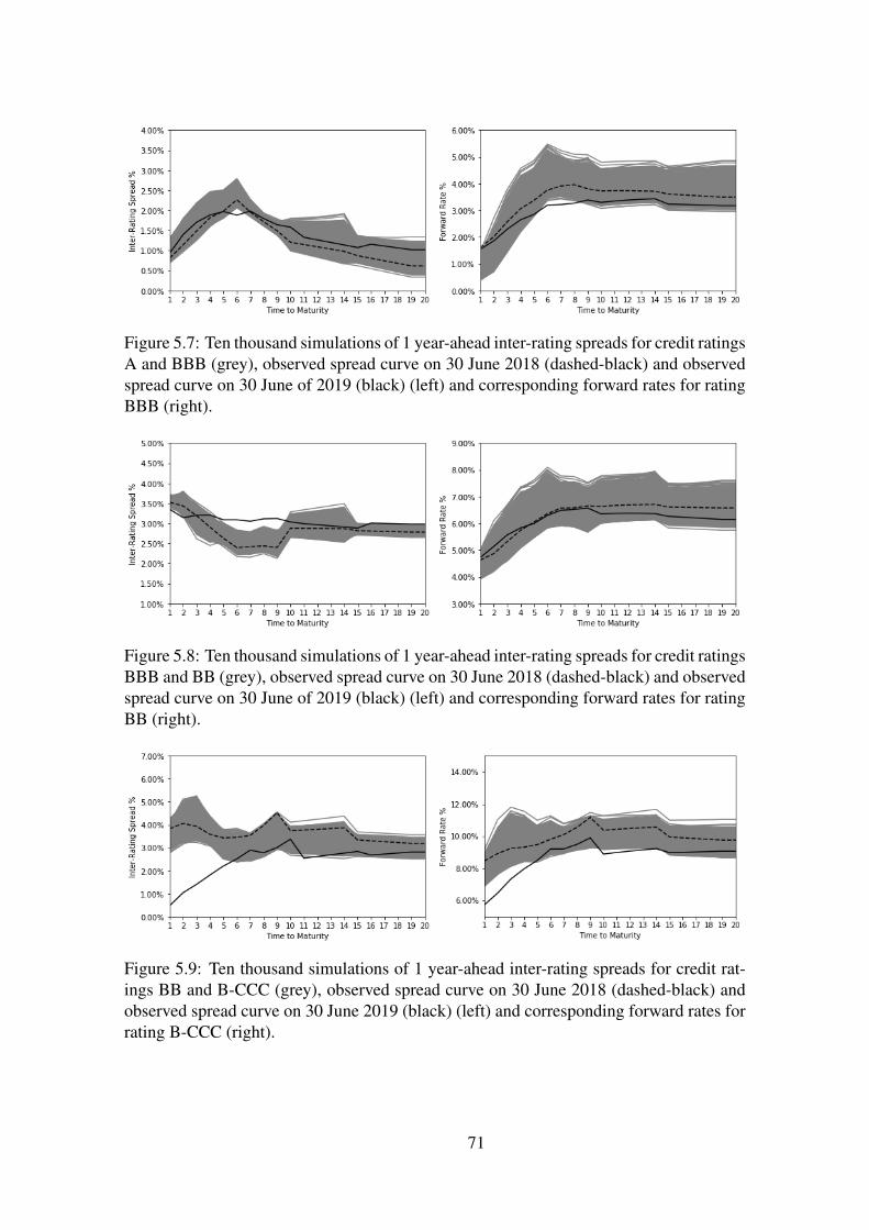
Figure 5.7: Ten thousand simulations of 1 year-ahead inter-rating spreads for credit ratingsA and BBB (grey), observed spread curve on 30 June 2018 (dashed-black) and observedspread curve on 30 June of 2019 (black) (left) and corresponding forward rates for ratingBBB (right).

Figure 5.8: Ten thousand simulations of 1 year-ahead inter-rating spreads for credit ratingsBBB and BB (grey), observed spread curve on 30 June 2018 (dashed-black) and observedspread curve on 30 June of 2019 (black) (left) and corresponding forward rates for ratingBB (right).

Figure 5.9: Ten thousand simulations of 1 year-ahead inter-rating spreads for credit rat-ings BB and B-CCC (grey), observed spread curve on 30 June 2018 (dashed-black) andobserved spread curve on 30 June 2019 (black) (left) and corresponding forward rates forrating B-CCC (right).

71

Note that in order to simulate the paths of bond prices in a one-year horizon we need

to take into account the rating-transitions occurring in one year and also the recovery

rates in case of default. For this study we consider the sovereign average one-year rating

migration rates from 1983 to 2018 provided in [56] and presented in Table 5.5.

From/To AAA AA A BBB BB B CC-C Withdrawn DAAA 96.774 3.077 0.033 0.083 0.000 0.000 0.000 0.033 0.000AA 3.048 93.141 2.477 0.699 0.106 0.000 0.000 0.529 0.000AA 0.000 3.878 91.879 3.059 1.120 0.065 0.000 0.000 0.000

BBB 0.000 0.000 5.920 88.818 4.787 0.439 0.037 0.000 0.000BB 0.000 0.000 0.000 7.493 84.936 6.617 0.331 0.117 0.506B 0.000 0.000 0.000 0.000 4.950 88.406 3.699 0.331 2.613

CCC-C 0.000 0.000 0.000 0.000 0.079 15.669 71.654 0.945 11.654D 0.000 0.000 0.000 0.000 0.000 0.000 0.000 0.000 100.000

Table 5.5: One year transition matrix with withdrawl

Since in practice it can happen that a debt issuer disappears from the data sample because

it is no longer rated and given that this fact is not considered in our modelling approach

we assume that the diagonal entries absorbe the exits from the system in order to obtain

a matrix without the class "Withdrawn" that corresponds to the fraction of the countries

that migrated to the non-rated class.

The grouping of the last two classes is done by weighting the probabilities of both classes

assuming a constant distribution provided by the report [56]. By using this technique,

from the original data in Table 5.5 we obtain in Table 5.6 the one-year transition proba-

bility matrix that can be used for the simulations.

From/To AAA AA A BBB BB B-CC-C D

AAA 96.807 3.077 0.033 0.083 0.000 0.000 0.000AA 3.048 93.671 2.477 0.699 0.106 0.000 0.000AA 0.000 3.878 91.879 3.059 1.120 0.065 0.000

BBB 0.000 0.000 5.920 88.818 4.787 0.475 0.000BB 0.000 0.000 0.000 7.493 85.052 6.948 0.506

B-CCC-C 0.000 0.000 0.000 0.000 4.091 91.701 4.209D 0.000 0.000 0.000 0.000 0.000 0.000 100.000

Table 5.6: One-year transition matrix without withdrawl.

For the rating classes with non-zero one year probability of default we use the average

72

recovery rates for each credit rating using the sovereign recovery rates from 1983 to 2018,

reported also in [56] as the average trading price in percentage of the par value of the bond

at the time the initial default event occurred, and we obtained the results in Table 5.7.

Rating Class Recovery Rate

BB 0.9515

B or lower 0.5977

Table 5.7: Average recovery rate by credit rating.

For the rest of this study we consider a portfolio with nominal value of 1,000,000 euros

in zero coupon bonds distributed by all credit ratings for maturities of 2, 5, 7, 10, 12,

15, 18 and 20 years and an additional investment of equal weight in the two higher rated

classes and maturity of 3 years. The present value of this portfolio as of 30 June 2018 was

747,929.95 euros. For this calculation, we have considered the observed forward rates for

AAA-rated bonds presented in Table 5.1 and the inter-rating spreads for each of the rating

classes presented in Figure 5.1 and observed on 30 June 2018. Figure 5.10 presents the

simulated profit and losses histogram for the portfolio.

Figure 5.10: Histogram of % profit and loss.

Given the observed generalized drop in interest rates of all maturities and throughout all

credit ratings, the one-year return on this portfolio was 3.569% on 30 June 2019.

Solvency II regulation defines that the capital requirement for interest rate risk is deter-

73

mined as the maximum change in the net value of assets and liabilities due to the revaluing

of all interest rate sensitive items under two pre-defined scenarios: an instantaneous up-

ward movement of interest rates and a downward movement. Note that for European

government bonds, the standard formula does not model transitions or defaults. The sce-

narios for the term structures are obtained by multiplying the current interest rate curve

by factors that are specified for each maturity in the Solvency II Technical Specifications

[26].

A comparison of the SCR produced by the model and the SCR of the standard formula is

shown in Table 5.8.

Standard Formula SCR Model VaR

9.178% 4.565 %

Table 5.8: Comparison between the SCR of the standard formula and the simulated model.

Note that the value obtained by applying the standard formula is considerably higher than

the one we obtain using the simulations of our model, even taking into account the rating

transitions and possibility of default for lower-rated bonds. We have also considered

the extreme case where the recovery rates for all the defaultable bonds is zero. For this

case we obtained a simulated VaR of 4.887%, which is still considerable lower than the

one given by the standard formula. By comparing the scenarios for the spot interest

rates for the different rating classes,in Figure 5.11, we obtain two conclusions: first, the

simulation results are lower when compared with the upward scenario obtained using

Solvency II stress methodology. Second, for higher credit ratings, the downward shock is

not penalizing enough, thus meaning that the negative setting of interest rates is still not

completely accounted for. This last fact turns out to be consistent with the new EIOPA

recommendations for 2020 review of Solvency II3.

It should be noted that this exercise is purely theoretical since, for meaningful Solvency

3Formal request to EIOPA for technical advice on the review of the Solvency II Directivehttps://ec.europa.eu/info/files/190211-request-eiopa-technical-advice-review-solvency-2

74

capital requirement calculations, both the asset and liabilities side of an insurance com-

pany should be considered. Furthermore, SCR formulas and stress methodologies were

designed to penalize mismatches between assets and liabilities.

Figure 5.11: Ten thousand simulations of 1 year-ahead spot rate for each credit rating(grey), last observed curve (dashed-black), observed forward curve in 30 of June of 2019(black) and upward and downward scenarios according to Solvency II methodology (red).

75

Chapter 6

Conclusion and future research

In this work, we have presented the shifted LIBOR market model for the simulation of

interest rates under the real world measure. The model includes a market price of risk

process, the parameters of which have been estimated by a principal component analysis

(PCA) technique. The proposed model allows for negative interest rates, as the ones

observed in current markets, and maintains realistic levels and shapes for the interest rate

curves. Using the historical yield curves of AAA-rated European bonds, ranging from

31 January 2015 up to 30 June 2016, we have simulated the one-year trajectories for the

forward rates and bond prices that are consistent with the observed forward rate curve on

30 June 2017.

After addressing the default-free framework, we have extended the setting to incorporate

the credit risk to our model, so that we have developed a shifted LIBOR model for default-

able bonds with credit ratings under the real world measure. For this purpose, we have

modeled the inter-rating spreads directly according to stochastic dynamics that guarantee

the monotonicity of bond prices with respect to the credit ratings as expected in the mar-

ket. In this setting, by using historical yield curves of bonds from 23 different European

countries, ranging from 31 January 2016 up to 30 June 2018, we have compared the sol-

76

vency capital requirements for an example portfolio of bonds with different credit ratings

and maturities. From this, we have concluded that we obtain lower capital requirements

than the when using the Solvency II methodology.

In the current economic environment of very low interest rates, for most of the credit rat-

ings our results present forward rates that are lower than the stressed downward movement

currently proposed by regulators. This current regulatory framework will be under revi-

sion during 2020. It is expected that both the upper and downward stress methodologies

will become more extreme than the ones currently proposed.

Regarding the interest rate and spread models chosen for this work, this models could

be extended to include stochastic volatilities by using the displaced diffusion stochastic

volatility LIBOR market model from [46] for the interest rate dynamics, or using the Lévy

LIBOR model proposed by [23] and [32], by adapting the risk neutral version to the real

world setting.

In this work, we do not model the correlations between the default-free rates and inter-

rating spreads directly. However, this could be achieved by performing a standard princi-

pal component analysis on both risk factors or by application of the principal component

analysis on rolling windows in order to be able to estimate the historical correlation be-

tween the factors.

Another possible extension of this work could include the calibration of the model param-

eters to corporate spreads and compare the results with the SCR spread formula.

Also, the consideration of other additional sources of risk could be aimed, such as liquid-

ity and currency risk that are present in global bond markets.

Finally, the ESG presented in this work can be used for many risk management purposes.

For example, it could be used as a tool in Asset- Liability Management or for internal

model calculations of interest rate and spread modules of SCR, as an alternative to the

77

standard formula proposed by regulators. Nevertheless, the ESG should be improved in

order to cover all the market risks an insurance company or a bank is subject to. Interest

rates and spread rates components presented in this work can be combined with models to

simulate future trajectories for other risk factors, such as inflation, equity returns, cross-

currency rates, and real estate prices.

78

Bibliography

[1] Acerbi, C. and Tasche, D., 2002. Expected shortfall: a natural coherent alternative

to Value at Risk. Economic Notes, volume 31(2):379–388.

[2] Ahmad, R. and Wilmott, P., 2007. The market price of interest-rate risk: measuring

and modelling fear and greed in the fixed-income markets. Wilmott magazine, pp.

64–70.

[3] Alberts, M.E., 2017. Modern deterministic scenarios for interest rates. Technical

report, Society of Actuaries.

[4] Artzner, P., Delbaen, F., Eber, J.M. and Heath, D., 1999. Coherent measures of risk.

Mathematical Finance, volume 9(3):203–228.

[5] Arvanitis, A., Gregory, J. and Laurent, J.P., 1999. Building models for credit spreads.

The Journal of Derivatives, volume 6(3):27–43.

[6] Bachelier, L., 1900. Théorie de la spéculation. Annales scientifiques de l’Ecole

Normale Supérieure, volume 3e série, 17:21–86.

[7] BIS, 2006. Basel II: International Convergence of Capital Measurement and Capital

Standards: A Revised Framework - Comprehensive Version. Basel Committee on

Banking Supervision.

79

[8] Björk, T. and Christensen, B., 1999. Interest rate dynamics and consistent forward

rate curves. Mathematical Finance, volume 9(4):323–348.

[9] Black, F., 1976. The pricing of commodity contract. Journal of Financial Economics,

volume 3(1-2):167–179.

[10] Black, F. and Cox, J., 1976. Valuing corporate securities: Some effects of bond

indenture provisions. The Journal of Finance, volume 31(2):351–367.

[11] Black, F. and Karasinski, P., 1991. Bond and option pricing when short rates are

lognormal. Financial Analysts Journal, volume 47(4):52–59.

[12] Brace, A., Dun, T. and Barton, G., 2001. Towards a central interest rate model. In

E. Jouini, J. Cvitanic and M. Musiela, editors, Option Pricing, Interest Rates and

Risk Management, chapter 8, pp. 278–313. Cambridge University Press.

[13] Brace, A., Gatarek, D. and Musiela, M., 1997. The market model of interest rate

dynamics. Mathematical Finance, volume 7(2):127–155.

[14] Brigo, D. and Mercurio, F., 2001. A deterministic–shift extension of analyti-

cally–tractable and time–homogeneous short–rate models. Finance and Stochastics,

volume 5(3):369–387.

[15] Brigo, D. and Mercurio, F., 2006. Interest Rate Models — Theory and Practice:

With Smile, Inflation and Credit. Springer Finance.

[16] Chapman, D.A. and Pearson, N.D., 2001. Recent Advances in Estimating Term-

Structure Models. Financial Analysts Journal, volume 57(4):77–95.

[17] Collin-Dufresne, P., Goldstein, R.S. and Martin, J.S., 2001. The determinants of

credit spread changes. The Journal of Finance, volume 56(6):2177–2207.

80

[18] Cox, J., Ingersoll, J. and Ross, S., 1985. A theory of the term structure of interest

rates. Econometrica, volume 53(2):385–407.

[19] Driessen, J., Melenberg, B. and Nijman, T., 2003. Common factors in international

bond returns. Journal of International Money and Finance, volume 22(5):629 – 656.

[20] Duffie, D. and Singleton, K.J., 1999. Modeling term structures of defaultable bonds.

The Review of Financial Studies, volume 12(4):687–720.

[21] Eberlein, E. and Grbac, Z., 2013. Rating based Lévy LIBOR Model. Mathematical

Finance, volume 23(4):591–626.

[22] Eberlein, E., Kluge, W. and Schönbucher, P., 2006. The Lévy Libor model with

default risk. Journal of Credit Risk, volume 2(2):3–42.

[23] Eberlein, E. and Özkan, F., 2005. The Lévy LIBOR model. Finance and Stochastics,

volume 9(2):327–348.

[24] EC, 2009. Directive 2009/138/EC of the European Parliament and of the Council

of 25 November 2009 on the taking-up and pursuit of the business of Insurance and

Reinsurance (Solvency II). European Commission.

[25] EIOPA, 2013. Report on QIS on IORPs. Technical report, EIOPA.

[26] EIOPA, 2014. Technical specification for the preparatory phase. Technical report,

EIOPA.

[27] EIOPA, 2014. The underlying assumptions in the standard formula for the Solvency

Capital Requirement calculation. Technical report, EIOPA.

[28] EIOPA, 2016. Insurance Stress Test 2016 report. Technical report, EIOPA.

[29] Fernández, J.L., Nogueiras, M.R., Pou, M. and Vázquez, C., 2014. A new parame-

terization for the drift-free simulation in the LIBOR market model. Revista de la Real

81

Academia de Ciencias Exactas, Fisicas y Naturales. Serie A. Matematicas, volume

109(1):73–92.

[30] Frye, J., 1997. Principals of Risk : Finding Value-at-Risk Through Factor-Based

Interest Rate Scenarios. Technical report.

[31] Girsanov, I.V., 1960. On transforming a certain class of stochastic processes by

absolutely continuous substitution of measures. Theory of Probability and its Ap-

plications, volume 5(3):285–301.

[32] Glau, K., Grbac, Z. and Papapantoleon, A., 2016. Advanced Modelling in Mathe-

matical Finance: In Honour of Ernst Eberlein, volume 189, chapter A unified view

of LIBOR models, pp. 423–452. Springer International Publishing.

[33] Gourieroux, C. and Monfort, A., 2015. A note on the Smith-Wilson family. Technical

report, CREST.

[34] Heath, D., Jarrow, R. and Morton, A., 1992. Bond pricing and the term structure

of interest rates: a new methodology for contigent claims valuation. Econometrica,

volume 60(1):77–105.

[35] Ho, T. and Lee, S.B., 1986. Term structure movements and pricing interest rate

contingent claims. The Journal of Finance, volume 41(5):1011–1029.

[36] Hull, J., 2015. Risk Management and Financial Institutions. Wiley.

[37] Hull, J. and White, A., 1990. Pricing interest rate derivative securities. The Review

of Financial Studies, volume 3(4):573–592.

[38] Hull, J.C., Sokol, A. and White, A., 2014. Modeling the short rate: the real and

risk-Neutral worlds. Working Paper No. 2403067.

82

[39] Hull, J.C. and White, A.D., 1994. Numerical procedures for implementing term

structure models II. The Journal of Derivatives, volume 2(2):37–48.

[40] Hunter, C., Jackel, P. and Joshi, M., 1999. Getting the drift. Risk, volume 14:81–84.

[41] Inui, K. and Kijima, M., 2005. On the significance of expected shortfall as a coherent

risk measure. Journal of Banking & Finance, volume 29(4):853 – 864.

[42] Jamshidian, F. and Zhu, Y., 1996. Scenario simulation: theory and methodology.

Finance and Stochastics, volume 1(1):43–67.

[43] Jarrow, R.A., Lando, D. and Turnbull, S.M., 1997. A Markov model for the term

structure of credit risk spreads. Review of Financial Studies, volume 10(2):481–

523.

[44] Jarrow, R.A. and Turnbull, S.M., 1995. Pricing derivatives on financial securities

subject to credit risk. Journal of Finance, volume 50(1):53–85.

[45] Jolliffe, I.T., 1986. Principal Component Analysis. Springer Series in Statistics.

Springer-Verlag New York.

[46] Joshi, M.S. and Rebonato, R., 2003. A displaced-diffusion stochastic volatility LI-

BOR market model: motivation, definition and implementation. Quantitative Fi-

nance, volume 3(6):458–469.

[47] Kapinos, P. and Mitnik, O.A., 2016. A Top-down Approach to Stress-testing Banks.

Journal of Financial Services Research, volume 49(2):229–264.

[48] Lageras, A. and Lindholm, M., 2016. Issues with the Smith–Wilson method. Insur-

ance: Mathematics and Economics, volume 71:93 – 102.

[49] Lando, D., 1998. On Cox processes and credit risky securities. Review of Deriva-

tives Research, volume 2(2-3):99–120.

83

[50] Lando, D., 2004. Credit Risk Modeling: Theory and Applications. Princeton Uni-

versity Press.

[51] Litterman, R.B. and Scheinkman, J., 1991. Common factors affecting bond returns.

The Journal of Fixed Income, volume 1(1):54–61.

[52] Lopes, S.D. and Vázquez, C., 2018. Real-world scenarios with negative interest

rates based on the LIBOR market model. Applied Mathematical Finance, vol-

ume 25(5-6):466–482.

[53] Lopes, S.D. and Vázquez, C., 2020. LIBOR Market Model including credit risk

under real world measure. Journal of Computational Finance, volume 24(3):1–30.

[54] Madan, D. and Unal, H., 1998. Pricing the risks of default. Review of Derivatives

Research, volume 2(2-3):121–160.

[55] Merton, R.C., 1974. On the pricing of corporate debt: The risk structure of interest

rates. Journal of Finance, volume 29(2):449–470.

[56] Moodys, 2019. Sovereign default and recovery rates 1983-2018. Technical report,

Moody’s.

[57] Nelson, C. and Siegel, A., 1987. Parsimonious modeling of yield curves. Journal of

Business, volume 60(4):473–489.

[58] Norman, J., 2009. Real world interest rate modelling with the BGM model. Working

Paper.

[59] Nunes, M.B.P., 2017. Portfolio seletion: a study using principal component analy-

sis. Master Thesis, Instituto Superior de Economia e Gestão.

[60] Rebonato, R., Mahal, S., Joshi, M., Buchholz, L.D. and Nyholm, K., 2005. Evolving

yield curves in the real-world measures: a semi parametric approach. Journal of

84

Risk, volume 7(3):29–62.

[61] Rutkowski, M. and Bielecki, T.R., 2004. Credit Risk: Modeling, Valuation and

Hedging. Springer Finance. Springer, Berlin, Heidelberg.

[62] Scherer, K.P. and Avellaneda, M., 2002. All for one...one for all? A principal com-

ponent analysis of latin american brady bond debt from 1994 to 2000. International

Journal of Theoretical and Applied Finance, volume 5(1):79–106.

[63] Schönbucher, P., 2001. A LIBOR market model with default risk. SSRN Electronic

Journal. doi:10.2139/ssrn.261051.

[64] Schönbucher, P.J., 2003. Credit Derivatives Pricing Models : Models, Pricing and

Implementation. John Wiley & Sons.

[65] Shreve, S., 2004. Stochastic Calculus for Finance II. Springer-Verlag New York.

[66] Smith, A. and Wilson, T., 2001. Fitting yield curves with long term constraints.

Technical report, Bacon and Woodrow.

[67] Svensson, L., 1994. Estimating and interpreting forward interest rates: sweden

1992-1944. NBER Working Paper Number 4871.

[68] Timm, N.H., 2002. Applied Multivariate Analysis. Springer Series in Statistics.

Springer-Verlag New York.

[69] Vandenabeele, T., 2014. Solvency II in s nutshell. Bank- en Financiewezen/Revue

bancaire et financière, volume 10.

[70] Vasicek, O., 1977. An equilibrium characterization of the term structure. Journal of

Financial Economics, volume 5(2):177–188.

[71] Wichern, D.W. and Johnson, R.A., 2007. Applied Multivariate Statistical Analysis.

Pearson Prentice Hall.

85

[72] Yasuoka, T., 2013. LIBOR market model under the real-world measure. Interna-

tional Journal of Theoretical and Applied Finance, volume 16(4):1–18.

[73] Zhao, X. and Glasserman, P., 1999. Arbitrage-free discretization of lognormal for-

ward LIBOR and swap rate models. Finance and Stochasticsl, volume 4(1):35–68.

86

Appendix A

Principal component analysis

Principal Component Analysis (PCA) is a technique to transform a set of p correlated

variables into a smaller set of uncorrelated called principal components (PCs). PCA is

designed to retain as much as possible the variation present in the data set. By form-

ing linear combinations of the original variables, PCA allows us to obtain a set of new

uncorrelated variables.

The PCs can be used to discover and interpret the dependencies that may exist among the

original variables and to reduce dimensionality. These characteristics contribute to the fact

that PCA has already been applied in a wide variety of areas such as biology, psychol-

ogy and genetics. In quantitative finance, PCA has been applied to the study of portfolio

allocation strategies in order to form uncorrelated portfolios [59] and is frequently used

to capture the variability in the movement of interest rates along the term structure. Fur-

thermore, when applied to the term structure of interest rates, empirical analysis generally

determines that a small number of principal components are enough to almost fully ex-

plain the dynamics observed in the markets. Litterman and Scheikman [51], analyzed the

US treasury yield curve and found that with just three factor they could explain most of

the movements in the yield curve. The interpretation of these principal components is that

87

they represent the level, slope, and curvature movements of the yield curve. This factor

decomposition of the term structure is rather stable through time [16] and common to

many economies. Moreover, Driessen et al. in [19] show that a five-factor model explains

98.5% of the cross-sectional variation in the expected bond returns of different maturities

in the US, Germany, and Japan.

We now present the method to obtain the principal components. Assuming that we have

p observable variables and define the random vector X = [X1, X2, . . . , Xp] with mean µ

and covariance matrix Σ of full rank p.

Consider the linear combinations

Y1 = a1X = a11X1 + a12X2 + . . .+ a1pXp

......

Yp = apX = ap1X1 + ap2X2 + . . .+ appXp

Then we have:

V ar(Yi) = aTi Σai i = 1, . . . , p (A.1)

Cov(Yi, Yk) = aTi Σak i, k = 1, . . . , p (A.2)

The principal components are the uncorrelated linear combinations that maximize (A.1)

restricted to cases where the coefficients have unit length, since, without this restriction,

we would be able to increase the variance of the linear combination arbitrarily. Then we

can define the principal components as

• The first principal component is the linear combination a1iTX that maximizes

V ar(aT1 X) subject to aT

1 a1 = 1.

• The second principal component is the linear combination aT2 X that maximizes

88

V ar(aT2 X) subject to aT

2 a2 = 1 and Cov(aT1 X, aT

2 X) = 0.

• The i-th principal component is the linear combination aTi X that maximizes V ar(aT

i X)

subject to aTj aj = 1 and Cov(aT

j X, aTk X) = 0 for k < i.

Given the eigenvalue-eigenvector pairs of the covariance matrix Σ, (λ1, e1),(λ2, e2), . . . , (λp, ep)

with λ1, λ2, . . . , λp ≥ 0, then the ith principal component is given by:

Yi = eTi X = ei1X1 + ei2X2 + . . .+ eipXp

and

V ar(Yi) = λi i = 1, 2, . . . , p

Cov(Yi, Yk) = 0 i, k = 1, 2, . . . , p

The proof for this result can be found in [71]. A useful concept when performing PCA is

the proportion of total variance explained by the ith principal component which is defined

as

λiλ1 + λ2 + . . .+ λp

i = 1, . . . , p

This concept allow us to have a quantitative criteria to select the number of components to

select, in order to retain a certain level of variance of the original data. The most common

criteria to select the number of components include the total variance explained, relative

sizes of eigenvalues and marginal increase in total variation. For a complete discussion

on this topic we refer to [45], [68] and [71].

The magnitude of the coefficient vector ei = [ei1, ei2, . . . , eip] measures the importance of

the variables X in the i-th principal component Yi for this reason, the inspection of this

coefficients are used to interpret the principal components.

89