sensors

Article

Real-Time Weather Monitoring and Prediction UsingCity Buses and Machine Learning

Zi-Qi Huang 1, Ying-Chih Chen 2 and Chih-Yu Wen 1,*1 Department of Electrical Engineering, Innovation and Development Center of Sustainable

Agriculture (IDCSA), National Chung Hsing University, Taichung 40227, Taiwan;g107093014@mail.nchu.edu.tw

2 Information Technology Department, Pou Chen Corporation, Taichung 40764, Taiwan;nathan.chen@pouchen.com

* Correspondence: cwen@dragon.nchu.edu.tw; Tel.: +88-604-2285-1549

Received: 4 August 2020; Accepted: 8 September 2020; Published: 10 September 2020�����������������

Abstract: Accurate weather data are important for planning our day-to-day activities. In order tomonitor and predict weather information, a two-phase weather management system is proposed,which combines information processing, bus mobility, sensors, and deep learning technologies toprovide real-time weather monitoring in buses and stations and achieve weather forecasts throughpredictive models. Based on the sensing measurements from buses, this work incorporates thestrengths of local information processing and moving buses for increasing the measurement coverageand supplying new sensing data. In Phase I, given the weather sensing data, the long short-termmemory (LSTM) model and the multilayer perceptron (MLP) model are trained and verified usingthe data of temperature, humidity, and air pressure of the test environment. In Phase II, the trainedlearning model is applied to predict the time series of weather information. In order to assess thesystem performance, we compare the predicted weather data with the actual sensing measurementsfrom the Environment Protection Administration (EPA) and Central Weather Bureau (CWB) ofTaichung observation station to evaluate the prediction accuracy. The results show that the proposedsystem has reliable performance at weather monitoring and a good forecast for one-day weatherprediction via the trained models.

Keywords: weather monitoring; weather prediction; bus systems; machine learning

1. Introduction

Weather plays an important role in people’s lives. Through weather monitoring, data analysisand forecasting can be performed to provide useful weather information [1]. In terms of forecasting,since there are many factors that affect weather changes, it is challenging to predict the weatheraccurately [2]. Considering system operations and processing technologies, the existing systems forweather monitoring and prediction can be described from the system architecture and the informationprocessing perspectives, respectively.

From the system architecture perspective, weather monitoring stations can be static or mobile.With the information provided by the fixed meteorological stations, there is some simulation softwarethat uses numeric simulation to define the temperature in each grid [3]. The precision of the estimatedcalculus for each grid is proportional to the number of weather stations distributed over the city.In Lim et al. [4], the National Weather Sensor Grid (NWSG) system is designed to monitor weatherinformation in real time over distributed areas in a city, where the weather stations are set inschools. In Sutar [5], a system is developed to enable the monitoring of weather parameters like

Sensors 2020, 20, 5173; doi:10.3390/s20185173 www.mdpi.com/journal/sensors

Sensors 2020, 20, 5173 2 of 21

temperature, humidity and light intensity. However, mobility issues and communication protocols arenot considered.

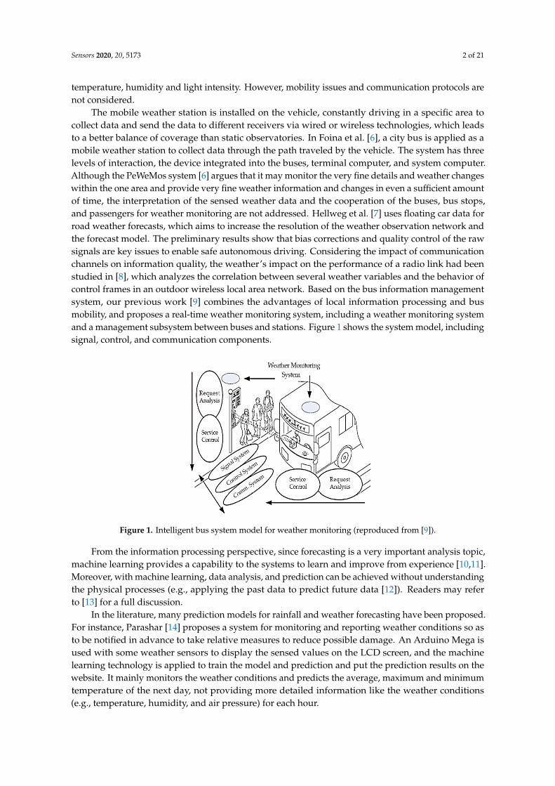
The mobile weather station is installed on the vehicle, constantly driving in a specific area tocollect data and send the data to different receivers via wired or wireless technologies, which leadsto a better balance of coverage than static observatories. In Foina et al. [6], a city bus is applied as amobile weather station to collect data through the path traveled by the vehicle. The system has threelevels of interaction, the device integrated into the buses, terminal computer, and system computer.Although the PeWeMos system [6] argues that it may monitor the very fine details and weather changeswithin the one area and provide very fine weather information and changes in even a sufficient amountof time, the interpretation of the sensed weather data and the cooperation of the buses, bus stops,and passengers for weather monitoring are not addressed. Hellweg et al. [7] uses floating car data forroad weather forecasts, which aims to increase the resolution of the weather observation network andthe forecast model. The preliminary results show that bias corrections and quality control of the rawsignals are key issues to enable safe autonomous driving. Considering the impact of communicationchannels on information quality, the weather’s impact on the performance of a radio link had beenstudied in [8], which analyzes the correlation between several weather variables and the behavior ofcontrol frames in an outdoor wireless local area network. Based on the bus information managementsystem, our previous work [9] combines the advantages of local information processing and busmobility, and proposes a real-time weather monitoring system, including a weather monitoring systemand a management subsystem between buses and stations. Figure 1 shows the system model, includingsignal, control, and communication components.

Sensors 2020, 20, x FOR PEER REVIEW 2 of 24

The mobile weather station is installed on the vehicle, constantly driving in a specific area to collect data and send the data to different receivers via wired or wireless technologies, which leads to a better balance of coverage than static observatories. In Foina et al. [6], a city bus is applied as a mobile weather station to collect data through the path traveled by the vehicle. The system has three levels of interaction, the device integrated into the buses, terminal computer, and system computer. Although the PeWeMos system [6] argues that it may monitor the very fine details and weather changes within the one area and provide very fine weather information and changes in even a sufficient amount of time, the interpretation of the sensed weather data and the cooperation of the buses, bus stops, and passengers for weather monitoring are not addressed. Hellweg et al. [7] uses floating car data for road weather forecasts, which aims to increase the resolution of the weather observation network and the forecast model. The preliminary results show that bias corrections and quality control of the raw signals are key issues to enable safe autonomous driving. Considering the impact of communication channels on information quality, the weather’s impact on the performance of a radio link had been studied in [8], which analyzes the correlation between several weather variables and the behavior of control frames in an outdoor wireless local area network. Based on the bus information management system, our previous work [9] combines the advantages of local information processing and bus mobility, and proposes a real-time weather monitoring system, including a weather monitoring system and a management subsystem between buses and stations. Figure 1 shows the system model, including signal, control, and communication components.

Figure 1. Intelligent bus system model for weather monitoring (reproduced from [9]).

From the information processing perspective, since forecasting is a very important analysis topic, machine learning provides a capability to the systems to learn and improve from experience [10,11]. Moreover, with machine learning, data analysis, and prediction can be achieved without understanding the physical processes (e.g., applying the past data to predict future data [12]). Readers may refer to [13] for a full discussion.

In the literature, many prediction models for rainfall and weather forecasting have been proposed. For instance, Parashar [14] proposes a system for monitoring and reporting weather conditions so as to be notified in advance to take relative measures to reduce possible damage. An Arduino Mega is used with some weather sensors to display the sensed values on the LCD screen, and the machine learning technology is applied to train the model and prediction and put the prediction results on the website. It mainly monitors the weather conditions and predicts the average, maximum and minimum temperature of the next day, not providing more detailed information like the weather conditions (e.g., temperature, humidity, and air pressure) for each hour.

Singh et al. [15] develops a low-cost, portable weather prediction system that can be used in remote areas, with data analysis and machine learning algorithms to predict weather conditions. The system architecture uses the Raspberry Pi as the main component with temperature, humidity, and

Figure 1. Intelligent bus system model for weather monitoring (reproduced from [9]).

From the information processing perspective, since forecasting is a very important analysis topic,machine learning provides a capability to the systems to learn and improve from experience [10,11].Moreover, with machine learning, data analysis, and prediction can be achieved without understandingthe physical processes (e.g., applying the past data to predict future data [12]). Readers may referto [13] for a full discussion.

In the literature, many prediction models for rainfall and weather forecasting have been proposed.For instance, Parashar [14] proposes a system for monitoring and reporting weather conditions so asto be notified in advance to take relative measures to reduce possible damage. An Arduino Mega isused with some weather sensors to display the sensed values on the LCD screen, and the machinelearning technology is applied to train the model and prediction and put the prediction results on thewebsite. It mainly monitors the weather conditions and predicts the average, maximum and minimumtemperature of the next day, not providing more detailed information like the weather conditions(e.g., temperature, humidity, and air pressure) for each hour.

Sensors 2020, 20, 5173 3 of 21

Singh et al. [15] develops a low-cost, portable weather prediction system that can be used in remoteareas, with data analysis and machine learning algorithms to predict weather conditions. The systemarchitecture uses the Raspberry Pi as the main component with temperature, humidity, and barometricpressure sensors to obtain the sensed values and then train according to the random forest classificationmodel, and predict whether it will rain. Note that although the system hardware in Singh et al. [15]and that of the proposed weather monitoring and forecasting systems are similar, the system inSingh et al. [15] only describes the probability of precipitation. In Varghese et al. [16], with RaspberryPi and weather sensors, data are collected, trained, and predicted using linear regression machinelearning models for evaluation via mean absolute error and median absolute error.

Instead of only considering the information processing perspective, this work simultaneouslyadopts the system architecture and the information processing perspectives. On the basis of the systemarchitecture in Chen et al. [9], a pair of bus stops and a bus, the gateway, and the server can work as agroup to dynamically operate the control system and communication system, which extend the systemto apply the collected data with machine learning algorithms for providing weather monitoring andforecasting. Note that given basic meteorological elements such as pressure, temperature, and humidity,this work focuses on the prediction of the temperature, humidity, and pressure for the next 24 hwith mild weather changes. For the forecast of severe weathers, in order to accelerate the trainingprocess and improve the predictive accuracy, Zhou et al. [17] state the predictors should contain majorenvironmental conditions, which include meteorological elements such as pressure, temperature,geopotential height, humidity, and wind, as well as a number of convective physical parameters(i.e., including additional and advanced sensor equipment) to build the prediction system.

The major contributions and features of this work are: (1) proposition of a novel real-timeweather monitoring and prediction system with basic meteorological elements; (2) development of aninformation processing scheme for increasing the management efficiency via a bus information system;(3) construction of machine learning models to analyze the trend of weather changes and predict theweather for the next 24 h. Table 1 describes the performance comparison of existing and proposedsystems, which shows that besides temperature prediction, the proposed system is able to provide aforecast of basic meteorological elements (e.g., temperature, humidity, pressure) for one-day weatherprediction via the trained models.

Table 1. Comparison of prediction behaviors.

System Training Model Prediction

Parashar [14] Multiple Linear Regression Model

1. Maximum and MinimumTemperatures on the Next Day

2. Mean Temperature on the Next Day

Singh et al. [15] The Random Forest Classification Raindrop Prediction

Varghese et al. [16] Linear Regression Model Maximum and Minimum Temperatureson the Next Day

The Proposed System1. Long Short-Term Memory Model2. Multilayer Perception Model

Temperature, Humidity, Pressure in theNext Twenty-Four Hours

The rest of the paper is organized as follows: Section 2 depicts the system architecture, includinginformation processing, data transmission/reception processes, the system components, and theimplementation of the system. Section 3 presents machine learning models and input data formats.Section 4 describes the experimental results of each processing block and depicts the performancecomparison of different prediction models. Finally, summarize this research in Section 5.

Sensors 2020, 20, 5173 4 of 21

2. System Description

2.1. Overview

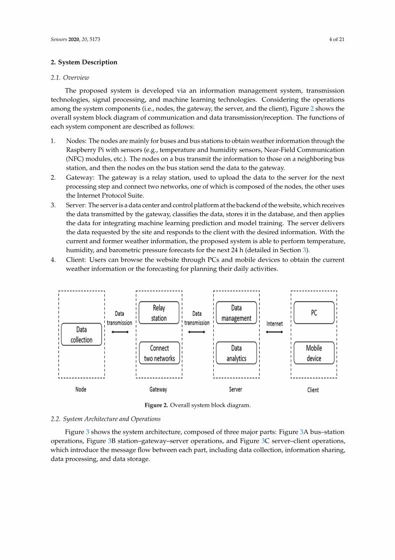
The proposed system is developed via an information management system, transmissiontechnologies, signal processing, and machine learning technologies. Considering the operationsamong the system components (i.e., nodes, the gateway, the server, and the client), Figure 2 shows theoverall system block diagram of communication and data transmission/reception. The functions ofeach system component are described as follows:

1. Nodes: The nodes are mainly for buses and bus stations to obtain weather information through theRaspberry Pi with sensors (e.g., temperature and humidity sensors, Near-Field Communication(NFC) modules, etc.). The nodes on a bus transmit the information to those on a neighboring busstation, and then the nodes on the bus station send the data to the gateway.

2. Gateway: The gateway is a relay station, used to upload the data to the server for the nextprocessing step and connect two networks, one of which is composed of the nodes, the other usesthe Internet Protocol Suite.

3. Server: The server is a data center and control platform at the backend of the website, which receivesthe data transmitted by the gateway, classifies the data, stores it in the database, and then appliesthe data for integrating machine learning prediction and model training. The server deliversthe data requested by the site and responds to the client with the desired information. With thecurrent and former weather information, the proposed system is able to perform temperature,humidity, and barometric pressure forecasts for the next 24 h (detailed in Section 3).

4. Client: Users can browse the website through PCs and mobile devices to obtain the currentweather information or the forecasting for planning their daily activities.

Sensors 2020, 20, x FOR PEER REVIEW 4 of 24

The rest of the paper is organized as follows: Section 2 depicts the system architecture, including information processing, data transmission/reception processes, the system components, and the implementation of the system. Section 3 presents machine learning models and input data formats. Section 4 describes the experimental results of each processing block and depicts the performance comparison of different prediction models. Finally, summarize this research in Section 5.

2. System Description

2.1. Overview

The proposed system is developed via an information management system, transmission technologies, signal processing, and machine learning technologies. Considering the operations among the system components (i.e., nodes, the gateway, the server, and the client), Figure 2 shows the overall system block diagram of communication and data transmission/reception. The functions of each system component are described as follows:

1. Nodes: The nodes are mainly for buses and bus stations to obtain weather information through the Raspberry Pi with sensors (e.g., temperature and humidity sensors, Near-Field Communication (NFC) modules, etc.). The nodes on a bus transmit the information to those on a neighboring bus station, and then the nodes on the bus station send the data to the gateway.

2. Gateway: The gateway is a relay station, used to upload the data to the server for the next processing step and connect two networks, one of which is composed of the nodes, the other uses the Internet Protocol Suite.

3. Server: The server is a data center and control platform at the backend of the website, which receives the data transmitted by the gateway, classifies the data, stores it in the database, and then applies the data for integrating machine learning prediction and model training. The server delivers the data requested by the site and responds to the client with the desired information. With the current and former weather information, the proposed system is able to perform temperature, humidity, and barometric pressure forecasts for the next 24 h (detailed in Section 3).

4. Client: Users can browse the website through PCs and mobile devices to obtain the current weather information or the forecasting for planning their daily activities.

Figure 2. Overall system block diagram.

Figure 2. Overall system block diagram.

2.2. System Architecture and Operations

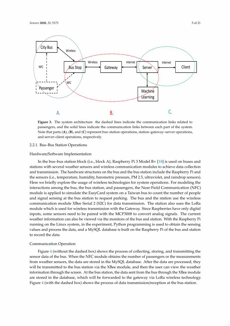
Figure 3 shows the system architecture, composed of three major parts: Figure 3A bus–stationoperations, Figure 3B station–gateway–server operations, and Figure 3C server–client operations,which introduce the message flow between each part, including data collection, information sharing,data processing, and data storage.

Sensors 2020, 20, 5173 5 of 21

Sensors 2020, 20, x FOR PEER REVIEW 5 of 24

2.2. System Architecture and Operations

Figure 3 shows the system architecture, composed of three major parts: Figure 3A bus–station operations, Figure 3B station–gateway–server operations, and Figure 3C server–client operations, which introduce the message flow between each part, including data collection, information sharing, data processing, and data storage.

Figure 3. The system architecture: the dashed lines indicate the communication links related to passengers, and the solid lines indicate the communication links between each part of the system. Note that parts (A), (B), and (C) represent bus–station operations, station–gateway–server operations, and server–client operations, respectively.

2.2.1. Bus–Bus Station Operations

Hardware/Software Implementation

In the bus–bus station block (i.e., block A), Raspberry Pi 3 Model B+ [18] is used on buses and stations with several weather sensors and wireless communication modules to achieve data collection and transmission. The hardware structures on the bus and the bus station include the Raspberry Pi and the sensors (i.e., temperature, humidity, barometric pressure, PM 2.5, ultraviolet, and raindrop sensors). Here we briefly explore the usage of wireless technologies for system operations. For modeling the interactions among the bus, the bus station, and passengers, the Near-Field Communication (NFC) module is applied to simulate the EasyCard system on a Taiwan bus to count the number of people and signal sensing at the bus station to request parking. The bus and the station use the wireless communication module XBee Serial 2 (S2C) for data transmission. The station also uses the LoRa module which is used for wireless transmission with the Gateway. Since Raspberries have only digital inputs, some sensors need to be paired with the MCP3008 to convert analog signals. The current weather information can also be viewed via the monitors of the bus and station. With the Raspberry Pi running on the Linux system, in the experiment, Python programming is used to obtain the sensing values and process the data, and a MySQL database is built on the Raspberry Pi of the bus and station to record the data.

Communication Operation

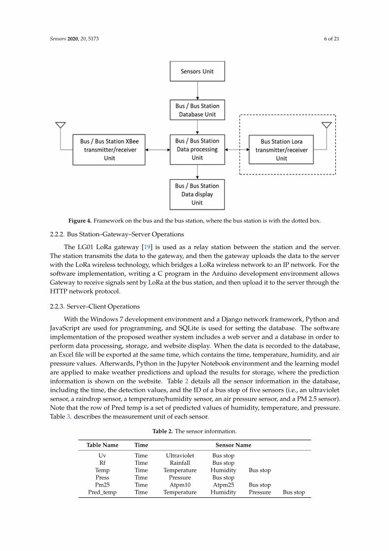
Figure 4 (without the dashed box) shows the process of collecting, storing, and transmitting the sensor data of the bus. When the NFC module obtains the number of passengers or the measurements from weather sensors, the data are stored in the MySQL database. After the data are processed, they will be transmitted to the bus station via the XBee module, and then the user can view the weather

Figure 3. The system architecture: the dashed lines indicate the communication links related topassengers, and the solid lines indicate the communication links between each part of the system.Note that parts (A), (B), and (C) represent bus–station operations, station–gateway–server operations,and server–client operations, respectively.

2.2.1. Bus–Bus Station Operations

Hardware/Software Implementation

In the bus–bus station block (i.e., block A), Raspberry Pi 3 Model B+ [18] is used on buses andstations with several weather sensors and wireless communication modules to achieve data collectionand transmission. The hardware structures on the bus and the bus station include the Raspberry Pi andthe sensors (i.e., temperature, humidity, barometric pressure, PM 2.5, ultraviolet, and raindrop sensors).Here we briefly explore the usage of wireless technologies for system operations. For modeling theinteractions among the bus, the bus station, and passengers, the Near-Field Communication (NFC)module is applied to simulate the EasyCard system on a Taiwan bus to count the number of peopleand signal sensing at the bus station to request parking. The bus and the station use the wirelesscommunication module XBee Serial 2 (S2C) for data transmission. The station also uses the LoRamodule which is used for wireless transmission with the Gateway. Since Raspberries have only digitalinputs, some sensors need to be paired with the MCP3008 to convert analog signals. The currentweather information can also be viewed via the monitors of the bus and station. With the Raspberry Pirunning on the Linux system, in the experiment, Python programming is used to obtain the sensingvalues and process the data, and a MySQL database is built on the Raspberry Pi of the bus and stationto record the data.

Communication Operation

Figure 4 (without the dashed box) shows the process of collecting, storing, and transmitting thesensor data of the bus. When the NFC module obtains the number of passengers or the measurementsfrom weather sensors, the data are stored in the MySQL database. After the data are processed, theywill be transmitted to the bus station via the XBee module, and then the user can view the weatherinformation through the screen. At the bus station, the data sent from the bus through the XBee moduleare stored in the database, which will be forwarded to the gateway via LoRa wireless technology.Figure 4 (with the dashed box) shows the process of data transmission/reception at the bus station.

Sensors 2020, 20, 5173 6 of 21

Sensors 2020, 20, x FOR PEER REVIEW 6 of 24

information through the screen. At the bus station, the data sent from the bus through the XBee module are stored in the database, which will be forwarded to the gateway via LoRa wireless technology. Figure 4 (with the dashed box) shows the process of data transmission/reception at the bus station.

Figure 4. Framework on the bus and the bus station, where the bus station is with the dotted box.

2.2.2. Bus Station–Gateway–Server Operations

The LG01 LoRa gateway [19] is used as a relay station between the station and the server. The station transmits the data to the gateway, and then the gateway uploads the data to the server with the LoRa wireless technology, which bridges a LoRa wireless network to an IP network. For the software implementation, writing a C program in the Arduino development environment allows Gateway to receive signals sent by LoRa at the bus station, and then upload it to the server through the HTTP network protocol.

2.2.3. Server–Client Operations

With the Windows 7 development environment and a Django network framework, Python and JavaScript are used for programming, and SQLite is used for setting the database. The software implementation of the proposed weather system includes a web server and a database in order to perform data processing, storage, and website display. When the data is recorded to the database, an Excel file will be exported at the same time, which contains the time, temperature, humidity, and air pressure values. Afterwards, Python in the Jupyter Notebook environment and the learning model are applied to make weather predictions and upload the results for storage, where the prediction information is shown on the website. Table 2 details all the sensor information in the database, including the time, the detection values, and the ID of a bus stop of five sensors (i.e., an ultraviolet sensor, a raindrop sensor, a temperature/humidity sensor, an air pressure sensor, and a PM 2.5 sensor). Note that the row of Pred temp is a set of predicted values of humidity, temperature, and pressure. Table 3. describes the measurement unit of each sensor.

Figure 4. Framework on the bus and the bus station, where the bus station is with the dotted box.

2.2.2. Bus Station–Gateway–Server Operations

The LG01 LoRa gateway [19] is used as a relay station between the station and the server.The station transmits the data to the gateway, and then the gateway uploads the data to the serverwith the LoRa wireless technology, which bridges a LoRa wireless network to an IP network. For thesoftware implementation, writing a C program in the Arduino development environment allowsGateway to receive signals sent by LoRa at the bus station, and then upload it to the server through theHTTP network protocol.

2.2.3. Server–Client Operations

With the Windows 7 development environment and a Django network framework, Python andJavaScript are used for programming, and SQLite is used for setting the database. The softwareimplementation of the proposed weather system includes a web server and a database in order toperform data processing, storage, and website display. When the data is recorded to the database,an Excel file will be exported at the same time, which contains the time, temperature, humidity, and airpressure values. Afterwards, Python in the Jupyter Notebook environment and the learning modelare applied to make weather predictions and upload the results for storage, where the predictioninformation is shown on the website. Table 2 details all the sensor information in the database,including the time, the detection values, and the ID of a bus stop of five sensors (i.e., an ultravioletsensor, a raindrop sensor, a temperature/humidity sensor, an air pressure sensor, and a PM 2.5 sensor).Note that the row of Pred temp is a set of predicted values of humidity, temperature, and pressure.Table 3. describes the measurement unit of each sensor.

Table 2. The sensor information.

Table Name Time Sensor Name

Uv Time Ultraviolet Bus stopRf Time Rainfall Bus stop

Temp Time Temperature Humidity Bus stopPress Time Pressure Bus stopPm25 Time Atpm10 Atpm25 Bus stop

Pred_temp Time Temperature Humidity Pressure Bus stop

Sensors 2020, 20, 5173 7 of 21

Table 3. The unit of each sensor.

Name Unit

Temperature ◦CHumidity %Ultraviolet UV Index

Pressure PaPM 2.5 µg/m3

Rainfall 0 à Rain1 à No rain

2.3. Machine Learning

To build a prediction model, this work applies the opensource data of the EnvironmentalProtection Administration (EPA) and the Central Weather Bureau (CWB) in Taiwan [20], about50,000 hourly measurements in the last six years of the Taichung Observatory, as the training datasource. Every measurement includes temperature, humidity, and air pressure at a 1 h measurementinterval. Before training the model, first, process the dataset. Next, organize the data according to aspecific format, and then perform predictive model training. Accordingly, the temperature, humidity,and air pressure values are first taken out from the opensource dataset. Next, the measurement data isdivided into training dataset, test dataset, and validation dataset, and then the average and standarddeviation of the three datasets are taken. Finally, the data are standardized.

3. Input Data Format

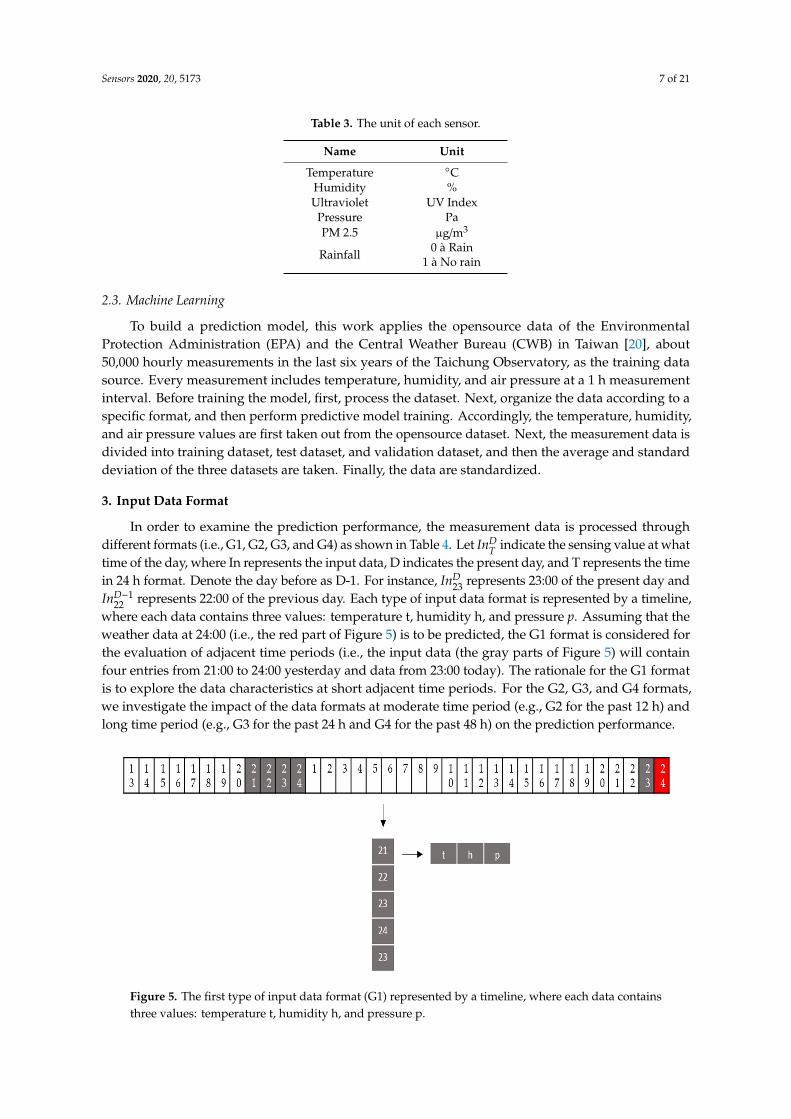
In order to examine the prediction performance, the measurement data is processed throughdifferent formats (i.e., G1, G2, G3, and G4) as shown in Table 4. Let InD

T indicate the sensing value at whattime of the day, where In represents the input data, D indicates the present day, and T represents the timein 24 h format. Denote the day before as D-1. For instance, InD

23 represents 23:00 of the present day andInD−1

22 represents 22:00 of the previous day. Each type of input data format is represented by a timeline,where each data contains three values: temperature t, humidity h, and pressure p. Assuming that theweather data at 24:00 (i.e., the red part of Figure 5) is to be predicted, the G1 format is considered forthe evaluation of adjacent time periods (i.e., the input data (the gray parts of Figure 5) will containfour entries from 21:00 to 24:00 yesterday and data from 23:00 today). The rationale for the G1 formatis to explore the data characteristics at short adjacent time periods. For the G2, G3, and G4 formats,we investigate the impact of the data formats at moderate time period (e.g., G2 for the past 12 h) andlong time period (e.g., G3 for the past 24 h and G4 for the past 48 h) on the prediction performance.

Sensors 2020, 20, x FOR PEER REVIEW 8 of 24

G3 𝐼𝑛 𝐼𝑛 𝐼𝑛 𝐼𝑛 𝐼𝑛

G4 𝐼𝑛 𝐼𝑛 … 𝐼𝑛 𝐼𝑛 … 𝐼𝑛 𝐼𝑛 … 𝐼𝑛 𝐼𝑛

Figure 5. The first type of input data format (G1) represented by a timeline, where each data contains three values: temperature t, humidity h, and pressure p.

Learning Model Architecture

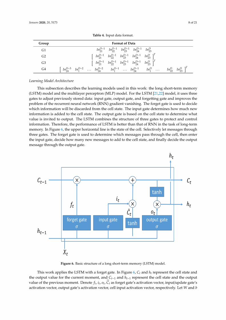
This subsection describes the learning models used in this work: the long short-term memory (LSTM) model and the multilayer perceptron (MLP) model. For the LSTM [21,22] model, it uses three gates to adjust previously stored data: input gate, output gate, and forgetting gate and improves the problem of the recurrent neural network (RNN) gradient vanishing. The forget gate is used to decide which information will be discarded from the cell state. The input gate determines how much new information is added to the cell state. The output gate is based on the cell state to determine what value is invited to output. The LSTM combines the structure of three gates to protect and control information. Therefore, the performance of LSTM is better than that of RNN in the task of long-term memory. In Figure 6, the upper horizontal line is the state of the cell. Selectively let messages through three gates. The forget gate is used to determine which messages pass through the cell, then enter the input gate, decide how many new messages to add to the cell state, and finally decide the output message through the output gate.

Figure 5. The first type of input data format (G1) represented by a timeline, where each data containsthree values: temperature t, humidity h, and pressure p.

Sensors 2020, 20, 5173 8 of 21

Table 4. Input data format.

Group Format of Data

G1 InD−121 InD−1

22 InD−123 InD−1

24 InD23

G2[

InD−121 InD−1

22 InD−123 InD−1

24 InD23

]T

G3[

InD−121 InD−1

22 InD−123 InD−1

24 InD23

]T

G4[

InD−324 InD−2

1 . . . InD−224 InD−1

1 . . . InD−124 InD

1 . . . InD22 InD

23

]T

Learning Model Architecture

This subsection describes the learning models used in this work: the long short-term memory(LSTM) model and the multilayer perceptron (MLP) model. For the LSTM [21,22] model, it uses threegates to adjust previously stored data: input gate, output gate, and forgetting gate and improves theproblem of the recurrent neural network (RNN) gradient vanishing. The forget gate is used to decidewhich information will be discarded from the cell state. The input gate determines how much newinformation is added to the cell state. The output gate is based on the cell state to determine whatvalue is invited to output. The LSTM combines the structure of three gates to protect and controlinformation. Therefore, the performance of LSTM is better than that of RNN in the task of long-termmemory. In Figure 6, the upper horizontal line is the state of the cell. Selectively let messages throughthree gates. The forget gate is used to determine which messages pass through the cell, then enterthe input gate, decide how many new messages to add to the cell state, and finally decide the outputmessage through the output gate.Sensors 2020, 20, x FOR PEER REVIEW 9 of 24

Figure 6. Basic structure of a long short-term memory (LSTM) model.

This work applies the LSTM with a forget gate. In Figure 6, 𝐶 and ℎ represent the cell state and the output value for the current moment, and 𝐶 and ℎ represent the cell state and the output value of the previous moment. Denote 𝑓 , 𝑖 , 𝑜 , 𝐶 as forget gate’s activation vector, input/update gate’s activation vector, output gate’s activation vector, cell input activation vector, respectively. Let 𝑊 and 𝑏 be a weight matrix and a bias vector parameter, respectively, which need to be learned during training. Let 𝜎 and 𝜎 be the sigmoid function and the hyperbolic tangent (Tanh) function, respectively.

The first step is to decide what information to throw away from the cell state via a sigmoid layer called the forget gate layer. It looks at ℎ and input vector 𝑥 , and outputs a number between 0 and 1 for each number in the cell state 𝐶 . Note that a 1 represents “completely keep this” while a 0 represents “completely get rid of this”. Thus, the forget gate’s activation vector is given by 𝑓 = 𝜎 (𝑊 ∙ ℎ , 𝑥 𝑏 ) (1)

The next step is to decide what new information to store in the cell state. The input gate layer and the Tanh layer are applied to create an update to the state. 𝑖 = 𝜎 (𝑊 ∙ ℎ , 𝑥 𝑏 ) (2) 𝐶 = 𝜎 (𝑊 ∙ ℎ , 𝑥 𝑏 ) (3)

Then, the new cell state 𝐶 is updated by 𝐶 = 𝑓 ∗ 𝐶 𝑖 ∗ 𝐶 (4)

Finally, based on the cell state, we need to decide what to output. First, we run a sigmoid layer which decides what parts of the cell state for the output. Then, we put the cell state through and multiply it by the output of the sigmoid gate, which yields 𝑜 = 𝜎 (𝑊 ∙ ℎ , 𝑥 𝑏 ) (5) ℎ = 𝑜 ∗ 𝜎 (𝐶 ) (6)

An MLP [23] model consists of at least three layers of nodes (an input layer, a hidden layer, and an output layer). In the MLP model, some neurons use nonlinear activation functions to simulate the

Figure 6. Basic structure of a long short-term memory (LSTM) model.

This work applies the LSTM with a forget gate. In Figure 6, Ct and ht represent the cell state andthe output value for the current moment, and Ct−1 and ht−1 represent the cell state and the outputvalue of the previous moment. Denote ft, it, ot, C̃t as forget gate’s activation vector, input/update gate’sactivation vector, output gate’s activation vector, cell input activation vector, respectively. Let W and b

Sensors 2020, 20, 5173 9 of 21

be a weight matrix and a bias vector parameter, respectively, which need to be learned during training.Let σg and σc be the sigmoid function and the hyperbolic tangent (Tanh) function, respectively.

The first step is to decide what information to throw away from the cell state via a sigmoid layercalled the forget gate layer. It looks at ht−1 and input vector xt, and outputs a number between 0 and1 for each number in the cell state Ct−1. Note that a 1 represents “completely keep this” while a 0represents “completely get rid of this”. Thus, the forget gate’s activation vector is given by

ft = σg(W f ·[ht−1, xt] + b f

)(1)

The next step is to decide what new information to store in the cell state. The input gate layer andthe Tanh layer are applied to create an update to the state.

it = σg(Wi·[ht−1, xt] + bi) (2)

C̃t = σc(WC·[ht−1, xt] + bC) (3)

Then, the new cell state Ct is updated by

Ct = ft ∗Ct−1 + it ∗ C̃t (4)

Finally, based on the cell state, we need to decide what to output. First, we run a sigmoid layerwhich decides what parts of the cell state for the output. Then, we put the cell state through andmultiply it by the output of the sigmoid gate, which yields

ot = σg(Wo · [ht−1, xt] + bO) (5)

ht = ot ∗ σc(Ct) (6)

An MLP [23] model consists of at least three layers of nodes (an input layer, a hidden layer, and anoutput layer). In the MLP model, some neurons use nonlinear activation functions to simulate thefrequency of action potential, or firing of biological neurons. Since MLPs are fully connected, eachnode in one layer connects with a certain weight to every node in the following layer. After each dataprocessing is completed, learning performs in the perceptron by adjusting the connection weights,which depends on the number of errors in the data output compared to the results.

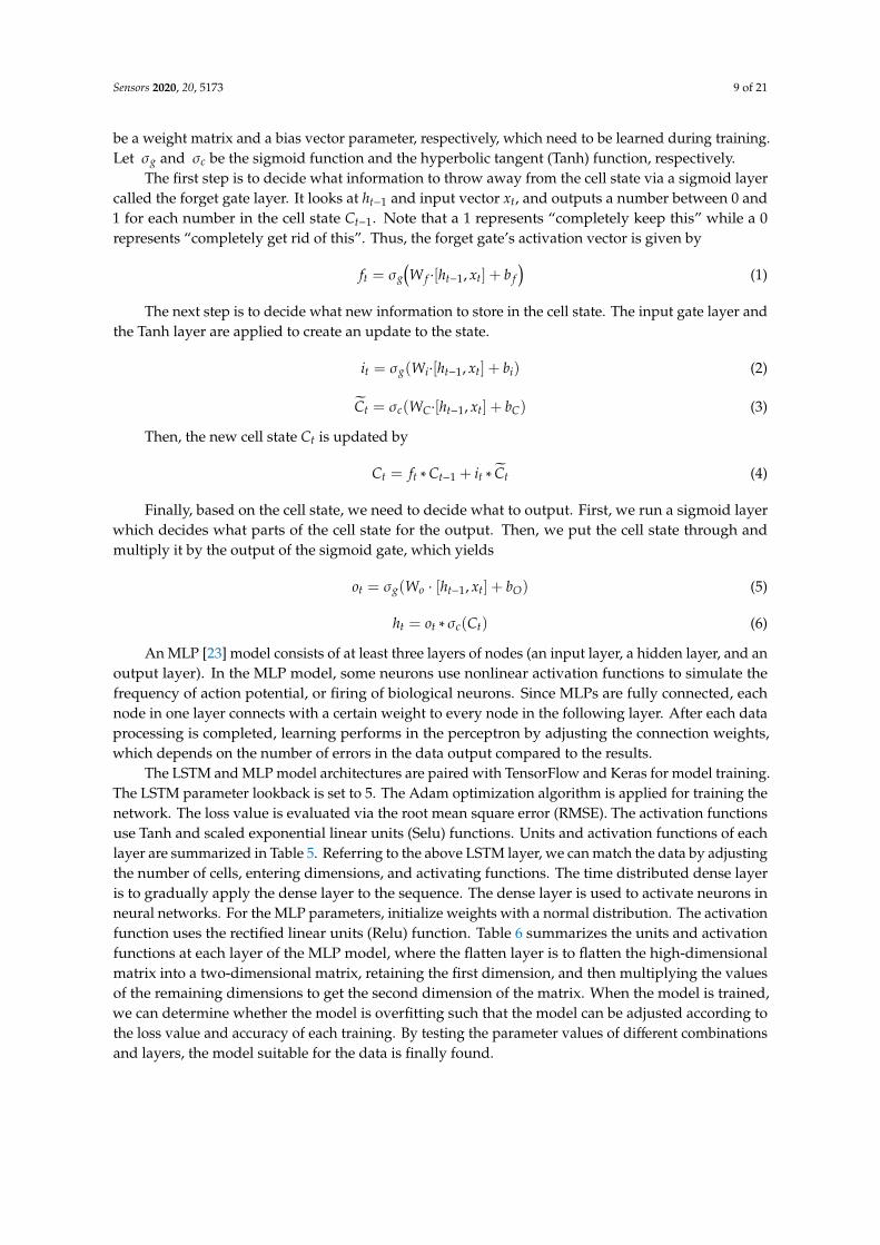
The LSTM and MLP model architectures are paired with TensorFlow and Keras for model training.The LSTM parameter lookback is set to 5. The Adam optimization algorithm is applied for training thenetwork. The loss value is evaluated via the root mean square error (RMSE). The activation functionsuse Tanh and scaled exponential linear units (Selu) functions. Units and activation functions of eachlayer are summarized in Table 5. Referring to the above LSTM layer, we can match the data by adjustingthe number of cells, entering dimensions, and activating functions. The time distributed dense layeris to gradually apply the dense layer to the sequence. The dense layer is used to activate neurons inneural networks. For the MLP parameters, initialize weights with a normal distribution. The activationfunction uses the rectified linear units (Relu) function. Table 6 summarizes the units and activationfunctions at each layer of the MLP model, where the flatten layer is to flatten the high-dimensionalmatrix into a two-dimensional matrix, retaining the first dimension, and then multiplying the valuesof the remaining dimensions to get the second dimension of the matrix. When the model is trained,we can determine whether the model is overfitting such that the model can be adjusted according tothe loss value and accuracy of each training. By testing the parameter values of different combinationsand layers, the model suitable for the data is finally found.

Sensors 2020, 20, 5173 10 of 21

Table 5. LSTM: units and activation functions of each layer.

Layer Units Activation Function

LSTM 50 tanhTime Distributed Dense 30

LSTM 30 tanhDense 15 seluDense 3 selu

Table 6. MLP: units and activation functions of each layer.

Layer Units Activation Function

Flatten 15Dense 15 reluDense 3

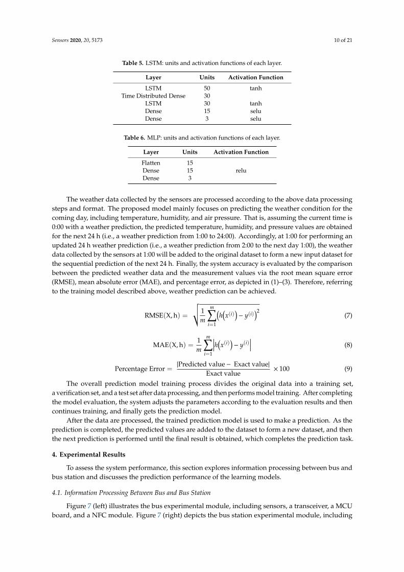
The weather data collected by the sensors are processed according to the above data processingsteps and format. The proposed model mainly focuses on predicting the weather condition for thecoming day, including temperature, humidity, and air pressure. That is, assuming the current time is0:00 with a weather prediction, the predicted temperature, humidity, and pressure values are obtainedfor the next 24 h (i.e., a weather prediction from 1:00 to 24:00). Accordingly, at 1:00 for performing anupdated 24 h weather prediction (i.e., a weather prediction from 2:00 to the next day 1:00), the weatherdata collected by the sensors at 1:00 will be added to the original dataset to form a new input dataset forthe sequential prediction of the next 24 h. Finally, the system accuracy is evaluated by the comparisonbetween the predicted weather data and the measurement values via the root mean square error(RMSE), mean absolute error (MAE), and percentage error, as depicted in (1)–(3). Therefore, referringto the training model described above, weather prediction can be achieved.

RMSE(X, h) =

√√1m

m∑i=1

(h(x(i)

)− y(i)

)2(7)

MAE(X, h) =1m

m∑i=1

∣∣∣∣h(x(i))− y(i)∣∣∣∣ (8)

Percentage Error =|Predicted value− Exact value|

Exact value× 100 (9)

The overall prediction model training process divides the original data into a training set,a verification set, and a test set after data processing, and then performs model training. After completingthe model evaluation, the system adjusts the parameters according to the evaluation results and thencontinues training, and finally gets the prediction model.

After the data are processed, the trained prediction model is used to make a prediction. As theprediction is completed, the predicted values are added to the dataset to form a new dataset, and thenthe next prediction is performed until the final result is obtained, which completes the prediction task.

4. Experimental Results

To assess the system performance, this section explores information processing between bus andbus station and discusses the prediction performance of the learning models.

4.1. Information Processing Between Bus and Bus Station

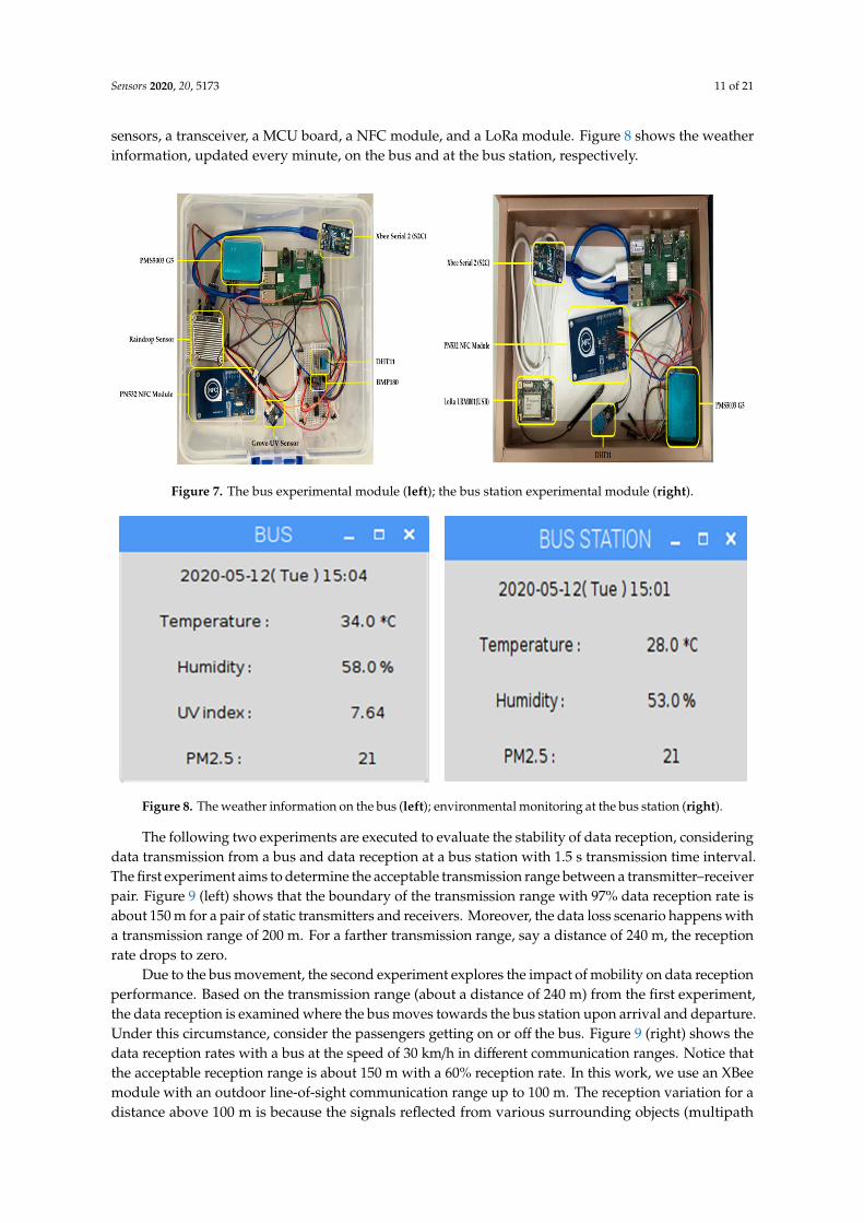
Figure 7 (left) illustrates the bus experimental module, including sensors, a transceiver, a MCUboard, and a NFC module. Figure 7 (right) depicts the bus station experimental module, including

Sensors 2020, 20, 5173 11 of 21

sensors, a transceiver, a MCU board, a NFC module, and a LoRa module. Figure 8 shows the weatherinformation, updated every minute, on the bus and at the bus station, respectively.Sensors 2020, 20, x FOR PEER REVIEW 12 of 24

Figure 7. The bus experimental module (left); the bus station experimental module (right).

Figure 8. The weather information on the bus (left); environmental monitoring at the bus station (right).

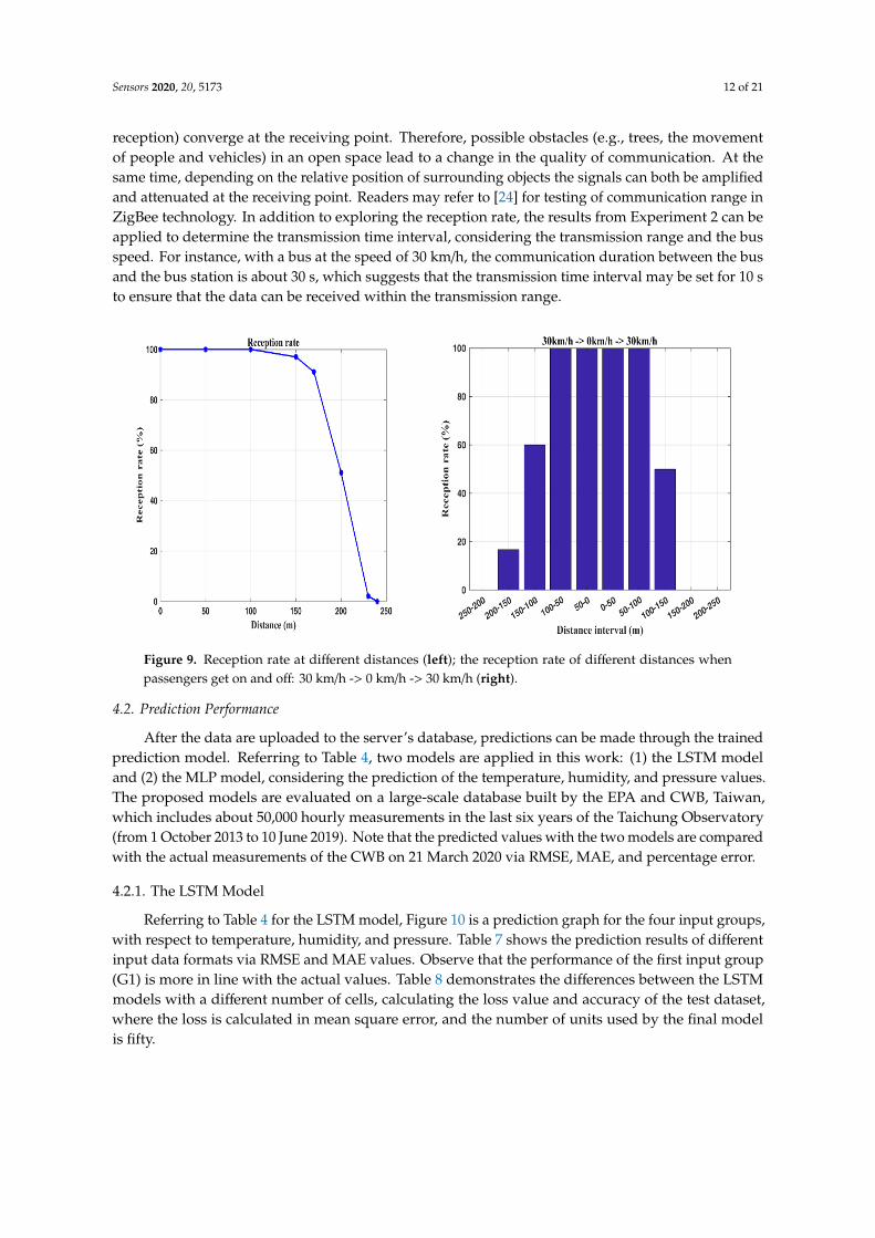
The following two experiments are executed to evaluate the stability of data reception, considering data transmission from a bus and data reception at a bus station with 1.5 s transmission time interval. The first experiment aims to determine the acceptable transmission range between a transmitter–receiver pair. Figure 9 (left) shows that the boundary of the transmission range with 97% data reception rate is about 150 m for a pair of static transmitters and receivers. Moreover, the data loss scenario happens with a transmission range of 200 m. For a farther transmission range, say a distance of 240 m, the reception rate drops to zero.

Figure 7. The bus experimental module (left); the bus station experimental module (right).

Sensors 2020, 20, x FOR PEER REVIEW 12 of 24

Figure 7. The bus experimental module (left); the bus station experimental module (right).

Figure 8. The weather information on the bus (left); environmental monitoring at the bus station (right).

The following two experiments are executed to evaluate the stability of data reception, considering data transmission from a bus and data reception at a bus station with 1.5 s transmission time interval. The first experiment aims to determine the acceptable transmission range between a transmitter–receiver pair. Figure 9 (left) shows that the boundary of the transmission range with 97% data reception rate is about 150 m for a pair of static transmitters and receivers. Moreover, the data loss scenario happens with a transmission range of 200 m. For a farther transmission range, say a distance of 240 m, the reception rate drops to zero.

Figure 8. The weather information on the bus (left); environmental monitoring at the bus station (right).

The following two experiments are executed to evaluate the stability of data reception, consideringdata transmission from a bus and data reception at a bus station with 1.5 s transmission time interval.The first experiment aims to determine the acceptable transmission range between a transmitter–receiverpair. Figure 9 (left) shows that the boundary of the transmission range with 97% data reception rate isabout 150 m for a pair of static transmitters and receivers. Moreover, the data loss scenario happens witha transmission range of 200 m. For a farther transmission range, say a distance of 240 m, the receptionrate drops to zero.

Due to the bus movement, the second experiment explores the impact of mobility on data receptionperformance. Based on the transmission range (about a distance of 240 m) from the first experiment,the data reception is examined where the bus moves towards the bus station upon arrival and departure.Under this circumstance, consider the passengers getting on or off the bus. Figure 9 (right) shows thedata reception rates with a bus at the speed of 30 km/h in different communication ranges. Notice thatthe acceptable reception range is about 150 m with a 60% reception rate. In this work, we use an XBeemodule with an outdoor line-of-sight communication range up to 100 m. The reception variation for adistance above 100 m is because the signals reflected from various surrounding objects (multipath

Sensors 2020, 20, 5173 12 of 21

reception) converge at the receiving point. Therefore, possible obstacles (e.g., trees, the movementof people and vehicles) in an open space lead to a change in the quality of communication. At thesame time, depending on the relative position of surrounding objects the signals can both be amplifiedand attenuated at the receiving point. Readers may refer to [24] for testing of communication range inZigBee technology. In addition to exploring the reception rate, the results from Experiment 2 can beapplied to determine the transmission time interval, considering the transmission range and the busspeed. For instance, with a bus at the speed of 30 km/h, the communication duration between the busand the bus station is about 30 s, which suggests that the transmission time interval may be set for 10 sto ensure that the data can be received within the transmission range.Sensors 2020, 20, x FOR PEER REVIEW 13 of 24

Figure 9. Reception rate at different distances (left); the reception rate of different distances when passengers get on and off: 30 km/h -> 0 km/h -> 30 km/h (right).

Due to the bus movement, the second experiment explores the impact of mobility on data reception performance. Based on the transmission range (about a distance of 240 m) from the first experiment, the data reception is examined where the bus moves towards the bus station upon arrival and departure. Under this circumstance, consider the passengers getting on or off the bus. Figure 9 (right) shows the data reception rates with a bus at the speed of 30 km/h in different communication ranges. Notice that the acceptable reception range is about 150 m with a 60% reception rate. In this work, we use an XBee module with an outdoor line-of-sight communication range up to 100 m. The reception variation for a distance above 100 m is because the signals reflected from various surrounding objects (multipath reception) converge at the receiving point. Therefore, possible obstacles (e.g., trees, the movement of people and vehicles) in an open space lead to a change in the quality of communication. At the same time, depending on the relative position of surrounding objects the signals can both be amplified and attenuated at the receiving point. Readers may refer to [24] for testing of communication range in ZigBee technology. In addition to exploring the receptionrate, the results from Experiment 2 can be applied to determine the transmission time interval,considering the transmission range and the bus speed. For instance, with a bus at the speed of 30km/h, the communication duration between the bus and the bus station is about 30 s, which suggeststhat the transmission time interval may be set for 10 s to ensure that the data can be received withinthe transmission range.

4.2. Prediction Performance

After the data are uploaded to the server’s database, predictions can be made through the trained prediction model. Referring to Table 4, two models are applied in this work: (1) the LSTM model and (2) the MLP model, considering the prediction of the temperature, humidity, and pressure values.The proposed models are evaluated on a large-scale database built by the EPA and CWB, Taiwan,which includes about 50,000 hourly measurements in the last six years of the Taichung Observatory(from 1 October 2013 to 10 June 2019). Note that the predicted values with the two models arecompared with the actual measurements of the CWB on 21 March 2020 via RMSE, MAE, andpercentage error.

4.2.1. The LSTM Model

Figure 9. Reception rate at different distances (left); the reception rate of different distances whenpassengers get on and off: 30 km/h -> 0 km/h -> 30 km/h (right).

4.2. Prediction Performance

After the data are uploaded to the server’s database, predictions can be made through the trainedprediction model. Referring to Table 4, two models are applied in this work: (1) the LSTM modeland (2) the MLP model, considering the prediction of the temperature, humidity, and pressure values.The proposed models are evaluated on a large-scale database built by the EPA and CWB, Taiwan,which includes about 50,000 hourly measurements in the last six years of the Taichung Observatory(from 1 October 2013 to 10 June 2019). Note that the predicted values with the two models are comparedwith the actual measurements of the CWB on 21 March 2020 via RMSE, MAE, and percentage error.

4.2.1. The LSTM Model

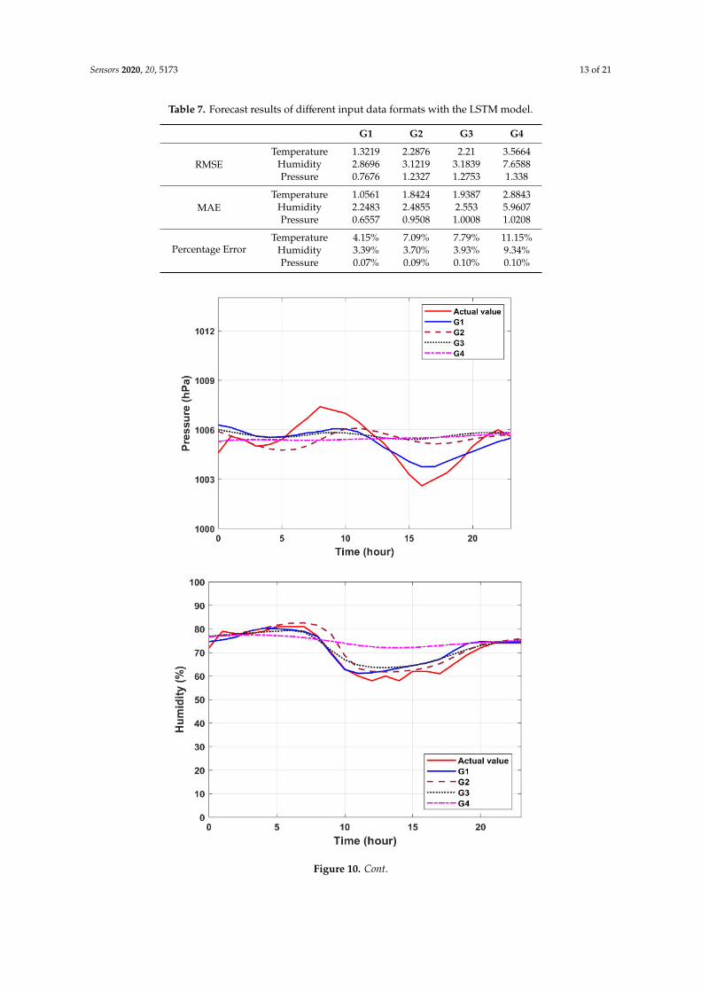
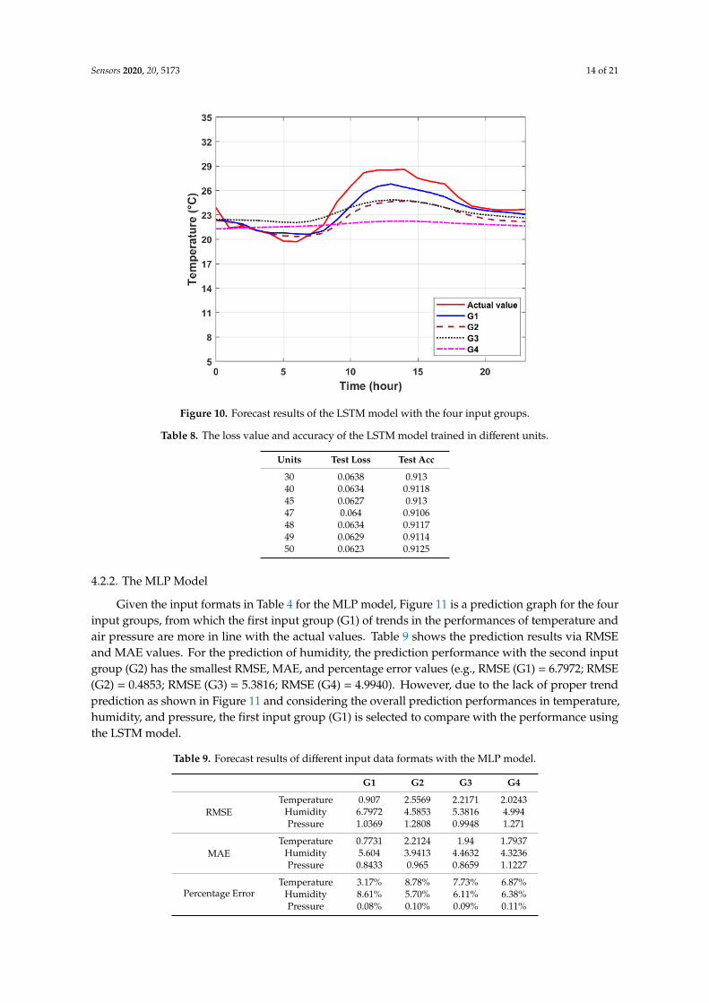
Referring to Table 4 for the LSTM model, Figure 10 is a prediction graph for the four input groups,with respect to temperature, humidity, and pressure. Table 7 shows the prediction results of differentinput data formats via RMSE and MAE values. Observe that the performance of the first input group(G1) is more in line with the actual values. Table 8 demonstrates the differences between the LSTMmodels with a different number of cells, calculating the loss value and accuracy of the test dataset,where the loss is calculated in mean square error, and the number of units used by the final modelis fifty.

Sensors 2020, 20, 5173 13 of 21

Table 7. Forecast results of different input data formats with the LSTM model.

G1 G2 G3 G4

RMSETemperature 1.3219 2.2876 2.21 3.5664

Humidity 2.8696 3.1219 3.1839 7.6588Pressure 0.7676 1.2327 1.2753 1.338

MAETemperature 1.0561 1.8424 1.9387 2.8843

Humidity 2.2483 2.4855 2.553 5.9607Pressure 0.6557 0.9508 1.0008 1.0208

Percentage ErrorTemperature 4.15% 7.09% 7.79% 11.15%

Humidity 3.39% 3.70% 3.93% 9.34%Pressure 0.07% 0.09% 0.10% 0.10%

Sensors 2020, 20, x FOR PEER REVIEW 14 of 24

Referring to Table 4 for the LSTM model, Figure 10 is a prediction graph for the four input groups, with respect to temperature, humidity, and pressure. Table 7 shows the prediction results of different input data formats via RMSE and MAE values. Observe that the performance of the first input group (G1) is more in line with the actual values. Table 8 demonstrates the differences between the LSTM models with a different number of cells, calculating the loss value and accuracy of the test dataset, where the loss is calculated in mean square error, and the number of units used by the final model is fifty.

Figure 10. Cont.

Sensors 2020, 20, 5173 14 of 21Sensors 2020, 20, x FOR PEER REVIEW 15 of 24

Figure 10. Forecast results of the LSTM model with the four input groups.

Table 7. Forecast results of different input data formats with the LSTM model.

G1 G2 G3 G4

RMSE Temperature 1.3219 2.2876 2.21 3.5664

Humidity 2.8696 3.1219 3.1839 7.6588 Pressure 0.7676 1.2327 1.2753 1.338

MAE Temperature 1.0561 1.8424 1.9387 2.8843

Humidity 2.2483 2.4855 2.553 5.9607 Pressure 0.6557 0.9508 1.0008 1.0208

Percentage Error Temperature 4.15% 7.09% 7.79% 11.15%

Humidity 3.39% 3.70% 3.93% 9.34% Pressure 0.07% 0.09% 0.10% 0.10%

Figure 10. Forecast results of the LSTM model with the four input groups.

Table 8. The loss value and accuracy of the LSTM model trained in different units.

Units Test Loss Test Acc

30 0.0638 0.91340 0.0634 0.911845 0.0627 0.91347 0.064 0.910648 0.0634 0.911749 0.0629 0.911450 0.0623 0.9125

4.2.2. The MLP Model

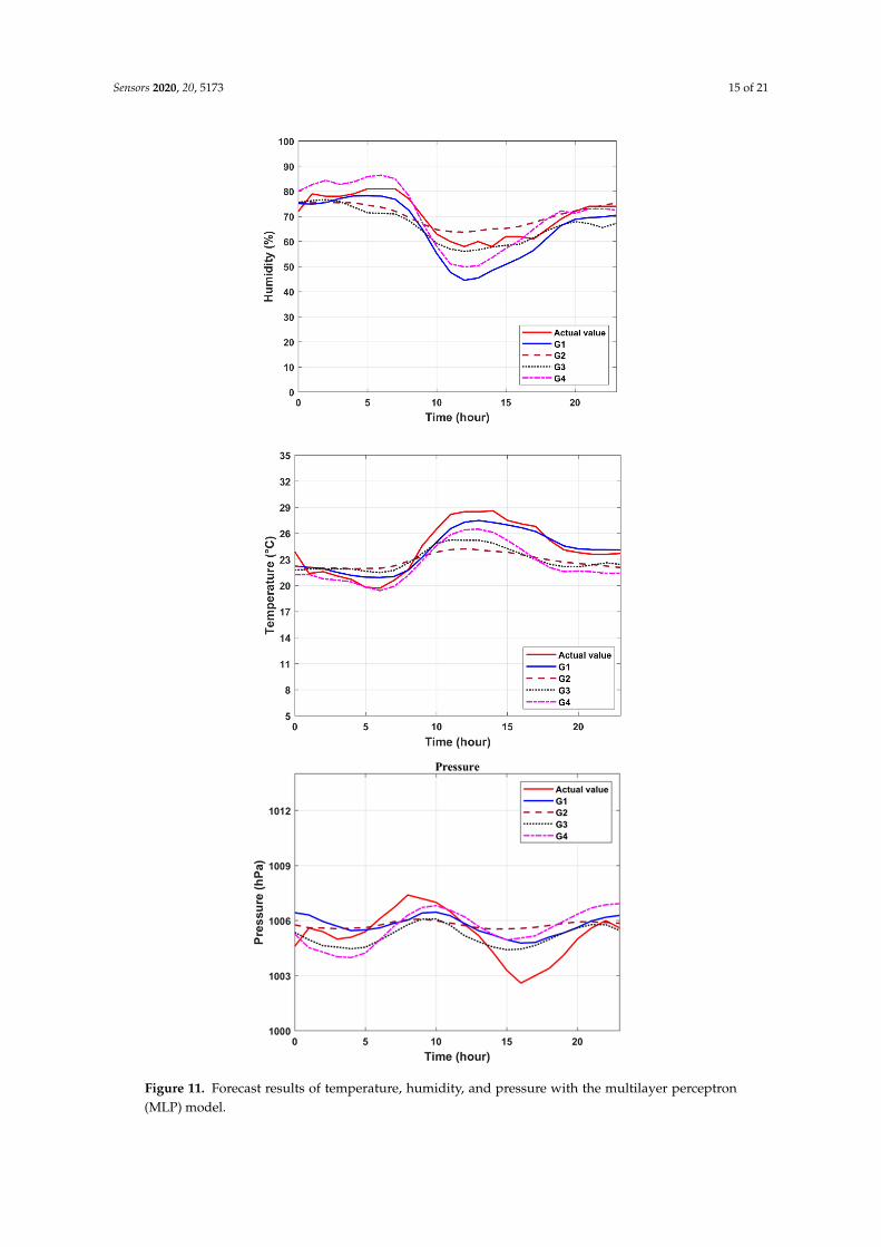
Given the input formats in Table 4 for the MLP model, Figure 11 is a prediction graph for the fourinput groups, from which the first input group (G1) of trends in the performances of temperature andair pressure are more in line with the actual values. Table 9 shows the prediction results via RMSEand MAE values. For the prediction of humidity, the prediction performance with the second inputgroup (G2) has the smallest RMSE, MAE, and percentage error values (e.g., RMSE (G1) = 6.7972; RMSE(G2) = 0.4853; RMSE (G3) = 5.3816; RMSE (G4) = 4.9940). However, due to the lack of proper trendprediction as shown in Figure 11 and considering the overall prediction performances in temperature,humidity, and pressure, the first input group (G1) is selected to compare with the performance usingthe LSTM model.

Table 9. Forecast results of different input data formats with the MLP model.

G1 G2 G3 G4

RMSETemperature 0.907 2.5569 2.2171 2.0243

Humidity 6.7972 4.5853 5.3816 4.994Pressure 1.0369 1.2808 0.9948 1.271

MAETemperature 0.7731 2.2124 1.94 1.7937

Humidity 5.604 3.9413 4.4632 4.3236Pressure 0.8433 0.965 0.8659 1.1227

Percentage ErrorTemperature 3.17% 8.78% 7.73% 6.87%

Humidity 8.61% 5.70% 6.11% 6.38%Pressure 0.08% 0.10% 0.09% 0.11%

Sensors 2020, 20, 5173 15 of 21

Sensors 2020, 20, x FOR PEER REVIEW 16 of 24

Table 8. The loss value and accuracy of the LSTM model trained in different units.

Units Test Loss Test Acc 30 0.0638 0.913 40 0.0634 0.9118 45 0.0627 0.913 47 0.064 0.9106 48 0.0634 0.9117 49 0.0629 0.9114 50 0.0623 0.9125

4.2.2. The MLP Model

Given the input formats in Table 4 for the MLP model, Figure 11 is a prediction graph for the four input groups, from which the first input group (G1) of trends in the performances of temperature and air pressure are more in line with the actual values. Table 9 shows the prediction results via RMSE and MAE values. For the prediction of humidity, the prediction performance with the second input group (G2) has the smallest RMSE, MAE, and percentage error values (e.g., RMSE (G1) = 6.7972; RMSE (G2) = 0.4853; RMSE (G3) = 5.3816; RMSE (G4) = 4.9940). However, due to the lack of proper trend prediction as shown in Figure 11 and considering the overall prediction performances in temperature, humidity, and pressure, the first input group (G1) is selected to compare with the performance using the LSTM model.

Sensors 2020, 20, x FOR PEER REVIEW 17 of 24

Figure 11. Forecast results of temperature, humidity, and pressure with the multilayer perceptron

(MLP) model.

Figure 11. Forecast results of temperature, humidity, and pressure with the multilayer perceptron(MLP) model.

Sensors 2020, 20, 5173 16 of 21

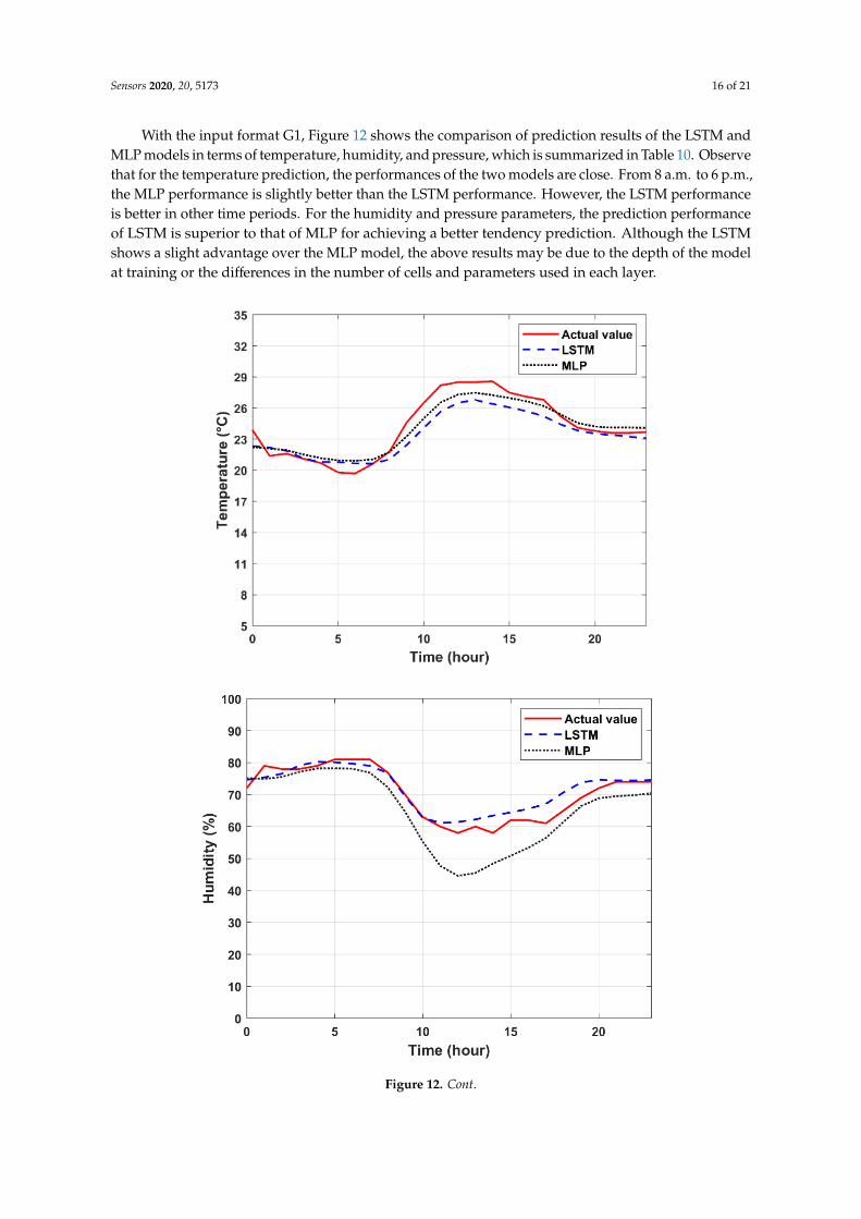
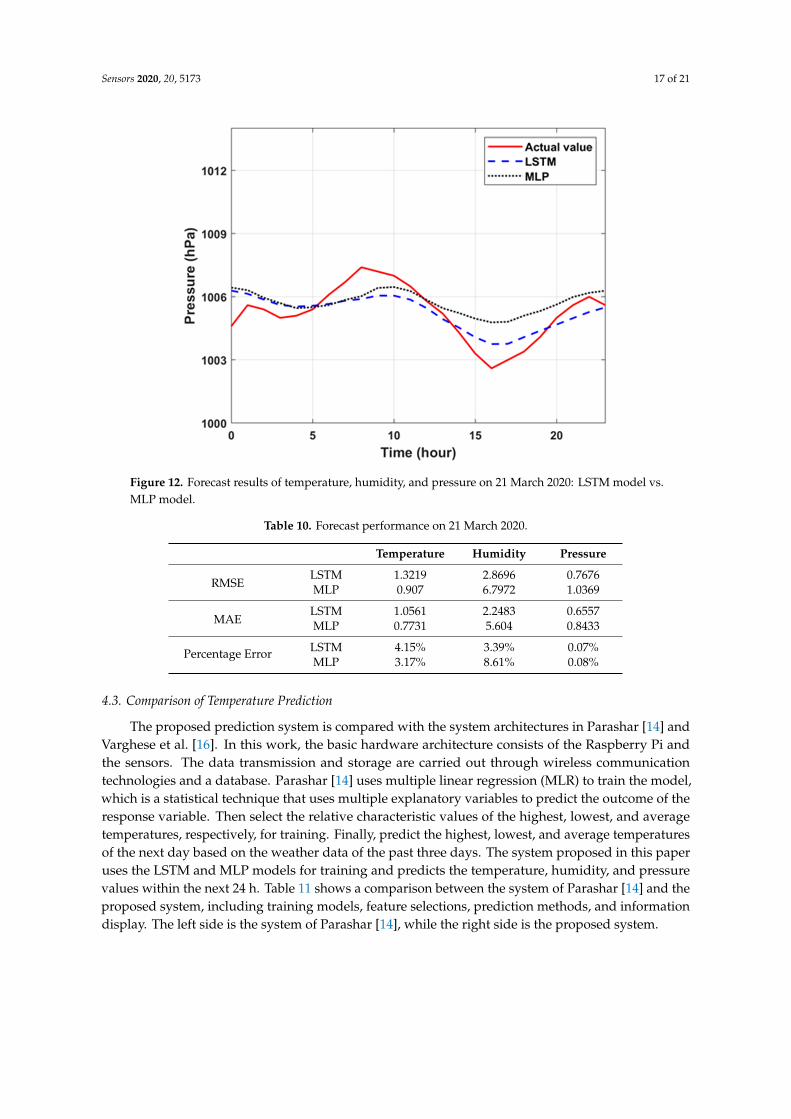
With the input format G1, Figure 12 shows the comparison of prediction results of the LSTM andMLP models in terms of temperature, humidity, and pressure, which is summarized in Table 10. Observethat for the temperature prediction, the performances of the two models are close. From 8 a.m. to 6 p.m.,the MLP performance is slightly better than the LSTM performance. However, the LSTM performanceis better in other time periods. For the humidity and pressure parameters, the prediction performanceof LSTM is superior to that of MLP for achieving a better tendency prediction. Although the LSTMshows a slight advantage over the MLP model, the above results may be due to the depth of the modelat training or the differences in the number of cells and parameters used in each layer.

Sensors 2020, 20, x FOR PEER REVIEW 19 of 25

Figure 12. Cont.

Sensors 2020, 20, 5173 17 of 21Sensors 2020, 20, x FOR PEER REVIEW 20 of 25

Figure 12. Forecast results of temperature, humidity, and pressure on 21 March 2020: LSTM model vs. MLP model.

Figure 12. Forecast results of temperature, humidity, and pressure on 21 March 2020: LSTM model vs.MLP model.

Table 10. Forecast performance on 21 March 2020.

Temperature Humidity Pressure

RMSELSTM 1.3219 2.8696 0.7676MLP 0.907 6.7972 1.0369

MAELSTM 1.0561 2.2483 0.6557MLP 0.7731 5.604 0.8433

Percentage Error LSTM 4.15% 3.39% 0.07%MLP 3.17% 8.61% 0.08%

4.3. Comparison of Temperature Prediction

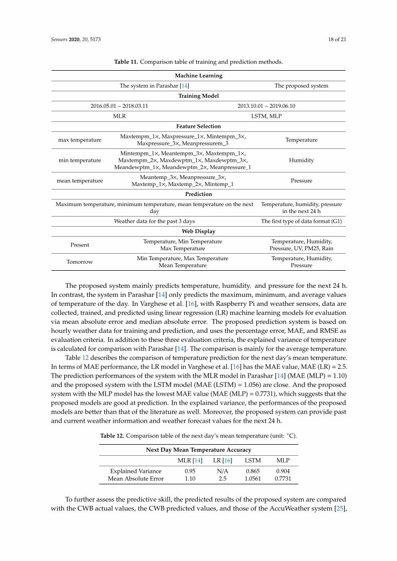
The proposed prediction system is compared with the system architectures in Parashar [14] andVarghese et al. [16]. In this work, the basic hardware architecture consists of the Raspberry Pi andthe sensors. The data transmission and storage are carried out through wireless communicationtechnologies and a database. Parashar [14] uses multiple linear regression (MLR) to train the model,which is a statistical technique that uses multiple explanatory variables to predict the outcome of theresponse variable. Then select the relative characteristic values of the highest, lowest, and averagetemperatures, respectively, for training. Finally, predict the highest, lowest, and average temperaturesof the next day based on the weather data of the past three days. The system proposed in this paperuses the LSTM and MLP models for training and predicts the temperature, humidity, and pressurevalues within the next 24 h. Table 11 shows a comparison between the system of Parashar [14] and theproposed system, including training models, feature selections, prediction methods, and informationdisplay. The left side is the system of Parashar [14], while the right side is the proposed system.

Sensors 2020, 20, 5173 18 of 21

Table 11. Comparison table of training and prediction methods.

Machine Learning

The system in Parashar [14] The proposed system

Training Model

2016.05.01 ~ 2018.03.11 2013.10.01 ~ 2019.06.10

MLR LSTM, MLP

Feature Selection

max temperature Maxtempm_1×, Maxpressure_1×, Mintempm_3×,Maxpressure_3×, Meanpressurem_3 Temperature

min temperatureMintempm_1×, Meantempm_3×, Maxtempm_1×,

Maxtempm_2×, Maxdewptm_1×, Maxdewptm_3×,Meandewptm_1×, Meandewptm_2×, Meanpressure_1

Humidity

mean temperature Meantemp_3×, Meanpressure_3×,Maxtemp_1×, Maxtemp_2×, Mintemp_1 Pressure

Prediction

Maximum temperature, minimum temperature, mean temperature on the nextday

Temperature, humidity, pressurein the next 24 h

Weather data for the past 3 days The first type of data format (G1)

Web Display

Present Temperature, Min TemperatureMax Temperature

Temperature, Humidity,Pressure, UV, PM25, Rain

Tomorrow Min Temperature, Max TemperatureMean Temperature

Temperature, Humidity,Pressure

The proposed system mainly predicts temperature, humidity. and pressure for the next 24 h.In contrast, the system in Parashar [14] only predicts the maximum, minimum, and average valuesof temperature of the day. In Varghese et al. [16], with Raspberry Pi and weather sensors, data arecollected, trained, and predicted using linear regression (LR) machine learning models for evaluationvia mean absolute error and median absolute error. The proposed prediction system is based onhourly weather data for training and prediction, and uses the percentage error, MAE, and RMSE asevaluation criteria. In addition to these three evaluation criteria, the explained variance of temperatureis calculated for comparison with Parashar [14]. The comparison is mainly for the average temperature.

Table 12 describes the comparison of temperature prediction for the next day’s mean temperature.In terms of MAE performance, the LR model in Varghese et al. [16] has the MAE value, MAE (LR) = 2.5.The prediction performances of the system with the MLR model in Parashar [14] (MAE (MLP) = 1.10)and the proposed system with the LSTM model (MAE (LSTM) = 1.056) are close. And the proposedsystem with the MLP model has the lowest MAE value (MAE (MLP) = 0.7731), which suggests that theproposed models are good at prediction. In the explained variance, the performances of the proposedmodels are better than that of the literature as well. Moreover, the proposed system can provide pastand current weather information and weather forecast values for the next 24 h.

Table 12. Comparison table of the next day’s mean temperature (unit: ◦C).

Next Day Mean Temperature Accuracy

MLR [14] LR [16] LSTM MLP

Explained Variance 0.95 N/A 0.865 0.904Mean Absolute Error 1.10 2.5 1.0561 0.7731

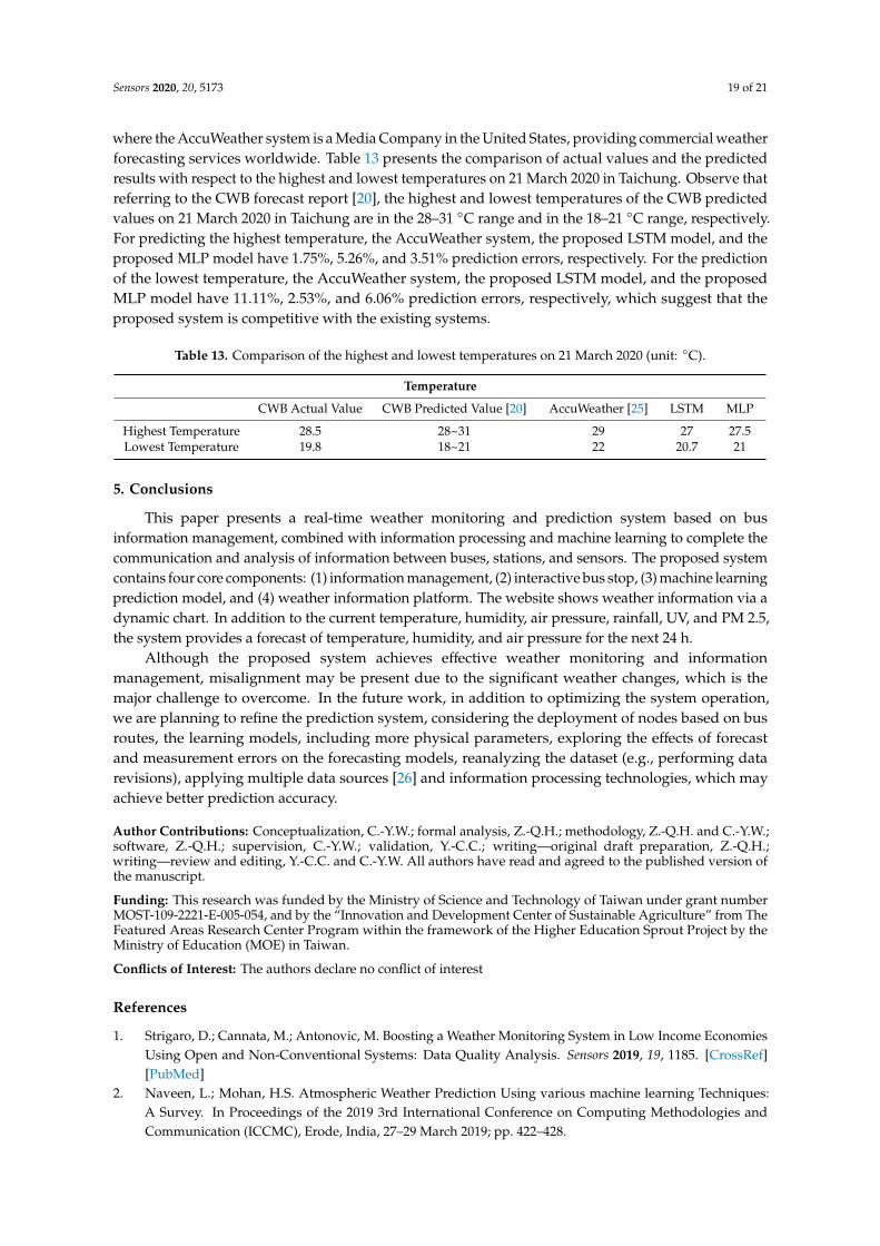
To further assess the predictive skill, the predicted results of the proposed system are comparedwith the CWB actual values, the CWB predicted values, and those of the AccuWeather system [25],

Sensors 2020, 20, 5173 19 of 21

where the AccuWeather system is a Media Company in the United States, providing commercial weatherforecasting services worldwide. Table 13 presents the comparison of actual values and the predictedresults with respect to the highest and lowest temperatures on 21 March 2020 in Taichung. Observe thatreferring to the CWB forecast report [20], the highest and lowest temperatures of the CWB predictedvalues on 21 March 2020 in Taichung are in the 28–31 ◦C range and in the 18–21 ◦C range, respectively.For predicting the highest temperature, the AccuWeather system, the proposed LSTM model, and theproposed MLP model have 1.75%, 5.26%, and 3.51% prediction errors, respectively. For the predictionof the lowest temperature, the AccuWeather system, the proposed LSTM model, and the proposedMLP model have 11.11%, 2.53%, and 6.06% prediction errors, respectively, which suggest that theproposed system is competitive with the existing systems.

Table 13. Comparison of the highest and lowest temperatures on 21 March 2020 (unit: ◦C).

Temperature

CWB Actual Value CWB Predicted Value [20] AccuWeather [25] LSTM MLP

Highest Temperature 28.5 28~31 29 27 27.5Lowest Temperature 19.8 18~21 22 20.7 21

5. Conclusions

This paper presents a real-time weather monitoring and prediction system based on businformation management, combined with information processing and machine learning to complete thecommunication and analysis of information between buses, stations, and sensors. The proposed systemcontains four core components: (1) information management, (2) interactive bus stop, (3) machine learningprediction model, and (4) weather information platform. The website shows weather information via adynamic chart. In addition to the current temperature, humidity, air pressure, rainfall, UV, and PM 2.5,the system provides a forecast of temperature, humidity, and air pressure for the next 24 h.

Although the proposed system achieves effective weather monitoring and informationmanagement, misalignment may be present due to the significant weather changes, which is themajor challenge to overcome. In the future work, in addition to optimizing the system operation,we are planning to refine the prediction system, considering the deployment of nodes based on busroutes, the learning models, including more physical parameters, exploring the effects of forecastand measurement errors on the forecasting models, reanalyzing the dataset (e.g., performing datarevisions), applying multiple data sources [26] and information processing technologies, which mayachieve better prediction accuracy.

Author Contributions: Conceptualization, C.-Y.W.; formal analysis, Z.-Q.H.; methodology, Z.-Q.H. and C.-Y.W.;software, Z.-Q.H.; supervision, C.-Y.W.; validation, Y.-C.C.; writing—original draft preparation, Z.-Q.H.;writing—review and editing, Y.-C.C. and C.-Y.W. All authors have read and agreed to the published version ofthe manuscript.

Funding: This research was funded by the Ministry of Science and Technology of Taiwan under grant numberMOST-109-2221-E-005-054, and by the “Innovation and Development Center of Sustainable Agriculture” from TheFeatured Areas Research Center Program within the framework of the Higher Education Sprout Project by theMinistry of Education (MOE) in Taiwan.

Conflicts of Interest: The authors declare no conflict of interest

References

1. Strigaro, D.; Cannata, M.; Antonovic, M. Boosting a Weather Monitoring System in Low Income EconomiesUsing Open and Non-Conventional Systems: Data Quality Analysis. Sensors 2019, 19, 1185. [CrossRef][PubMed]

2. Naveen, L.; Mohan, H.S. Atmospheric Weather Prediction Using various machine learning Techniques:A Survey. In Proceedings of the 2019 3rd International Conference on Computing Methodologies andCommunication (ICCMC), Erode, India, 27–29 March 2019; pp. 422–428.

Sensors 2020, 20, 5173 20 of 21

3. Lyons, W.A.; Tremback, C.J.; Pielke, R.A. Applications of the Regional Atmospheric Modeling System (RAMS)to provide input to photochemical grid models for the Lake Michigan Ozone Study (LMOS). J. Appl. Meteor.1995, 34, 1762–1786. [CrossRef]

4. Lim, H.B.; Ling, K.V.; Wang, W.; Yao, Y.; Iqbal, M.; Li, B.; Yin, X.; Sharma, T. The National Weather SensorGrid. In Proceedings of the ACM SenSys’07, Sydney, NSW, Australia, 6–9 November 2007.

5. Sutar, K.G. Low Cost Wireless Weather Monitoring System. Int. J. Eng. Technol. Manag. Res. 2015, 1, 35–39.[CrossRef]

6. Foina, A.; I-Deeb, A.E. PeWeMoS-Pervasive Weather Monitoring System. In Proceedings of the 20083rd International Conference on Pervasive Computing and Applications (ICPCA), Alexandria, Egypt,6–8 October 2008.

7. Hellweg, M.; Acevedo-Valencia, J.; Paschalidi, Z.; Nachtigall, J.; Kratzsch, T.; Stiller, C. Using floating cardata for more precise road weather forecasts. In Proceedings of the 2020 IEEE 91st Vehicular TechnologyConference (VTC2020-Spring), Antwerp, Belgium, 25–28 May 2020; pp. 1–3.

8. Bri, D.; Garcia, M.; Lloret, J.; Misic, J. Measuring the weather’s impact on MAC layer over 2.4 GHz outdoorradio links. Measurement 2015, 61, 221–233. [CrossRef]

9. Chen, Y.-C.; Chen, P.-Y.; Wen, C.-Y. Distributed bus information management for mobile weather monitoring.In Proceedings of the 2017 15th IEEE International Conference on ITS Telecommunications (ITST), Warsaw,Poland, 29–31 May 2017.

10. Hasan, N.; Uddin, M.T.; Chowdhury, N.K. Automated weather event analysis with machine learning.In Proceedings of the IEEE 2016 International Conference on Innovations in Science, Engineering andTechnology (ICISET), Dhaka, Bangladesh, 28–29 October 2016; pp. 1–5.

11. Lai, L.L.; Braun, H.; Zhang, Q.P.; Wu, Q.; Ma, Y.N.; Sun, W.C.; Yang, L. Intelligent weather forecast.In Proceedings of the IEEE International Conference on Machine Learning and Cybernetics, Shanghai, China,26–29 August 2004; pp. 4216–4221.

12. Salman, A.G.; Kanigoro, B.; Heryadi, Y. Weather forecasting using deep learning techniques. In Proceedings ofthe 2015 IEEE International Conference on Advanced Computer Science and Information Systems (ICACSIS),Depok, Indonesia, 10–11 October 2015; pp. 281–285.

13. Reddy, P.C.; Babu, A.S. Survey on weather prediction using big data analytics. In Proceedings of the 2017Second International Conference on Electrical, Computer and Communication Technologies (ICECCT),Coimbatore, India, 22–24 February 2017; pp. 1–6.

14. Parashar, A. IoT Based Automated Weather Report Generation and Prediction Using Machine Learning.In Proceedings of the 2019 2nd IEEE International Conference on Intelligent Communication andComputational Techniques (ICCT), Jaipur, India, 28–29 September 2019.

15. Singh, N.; Chaturvedi, S.; Akhter, S. Weather Forecasting Using Machine Learning Algorithm. In Proceedingsof the 2019 IEEE International Conference on Signal Processing and Communication (ICSC), NOIDA, India,7–9 March 2019.

16. Varghese, L.; Deepak, G.; Santhanavijayan, A. An IoT Analytics Approach for Weather Forecasting usingRaspberry Pi 3 Model B+. In Proceedings of the 2019 Fifteenth International Conference on InformationProcessing (ICINPRO), Bengaluru, India, 20–22 December 2019; pp. 1–5.

17. Zhou, K.; Zheng, Y.; Li, B.; Dong, W.; Zhang, X. Forecasting Different Types of Convective Weather: A DeepLearning Approach. J. Meteorol. Res. 2019, 33, 797–809. [CrossRef]

18. Raspberry Pi Hardware. Available online: https://www.raspberrypi.org/documentation/hardware/

raspberrypi/ (accessed on 3 August 2020).19. LG01 LoRa Gateway. Available online: https://www.dragino.com/index.php (accessed on 31 July 2020).20. The Central Weather Bureau, Taiwan. Available online: https://www.cwb.gov.tw/eng/ (accessed on

21 August 2020).21. Hochreiter, S.; Schmidhuber, J. Long short-term memory. Neural Comput. 1997, 9, 1735–1780. [CrossRef]

[PubMed]22. Olah, C. Understanding LSTM Networks. 2015. Available online: https://web.stanford.edu/class/

cs379c/archive/2018/class_messages_listing/content/Artificial_Neural_Network_Technology_Tutorials/OlahLSTM-NEURAL-NETWORK-TUTORIAL-15.pdf (accessed on 10 July 2020).

23. Haykin, S. Neural Networks: A Comprehensive Foundation, 2nd ed.; Prentice Hall: Upper Saddle River, NJ,USA, 1998; ISBN 0-13-273350-1.

Sensors 2020, 20, 5173 21 of 21

24. Kuzminykh, I.; Snihurov, A.; Carlsson, A. Testing of communication range in ZigBee technology.In Proceedings of the 2017 14th International Conference The Experience of Designing and Application ofCAD Systems in Microelectronics (CADSM), Lviv, Ukraine, 21–25 February 2017; pp. 133–136.

25. AccuWeather, Inc. Available online: https://www.accuweather.com/en/tw/taichung-city/315040/march-weather/315040?year=2020 (accessed on 20 August 2020).

26. Rao, J.; Garfinkel, C.I.; Chen, H.; White, I.P. The 2019 New Year stratospheric sudden warming and itsreal-time predictions in multiple S2S models. J. Geophys. Res. Atmos. 2019, 124, 11155–11174. [CrossRef]

© 2020 by the authors. Licensee MDPI, Basel, Switzerland. This article is an open accessarticle distributed under the terms and conditions of the Creative Commons Attribution(CC BY) license (http://creativecommons.org/licenses/by/4.0/).