Kandidatuppsats i matematisk statistikBachelor Thesis in Mathematical Statistics

Real currency exchange rateprediction.- A time series analysis.Malin Varenius

Matematiska institutionen

Kandidatuppsats 2017:13Matematisk statistikJuni 2017

www.math.su.se

Matematisk statistikMatematiska institutionenStockholms universitet106 91 Stockholm

Mathematical StatisticsStockholm UniversityBachelor Thesis 2017:13

http://www.math.su.se

Real currency exchange rate prediction.

- A time series analysis.

Malin Varenius∗

June 2017

Abstract

The foreign exchange market is the largest financial market in theworld and forecasting exchange rates are not solely an important taskfor investors, but also for policy makers. Since market participantdo not have access to future information, they try to model the ex-change rate by past information. In this thesis an ARIMA(1,1,0) anda VAR(1) model with the trade balance in the EU and the interestrate differential as additional variables are evaluated in a forecastingpurpose. It is concluded that a VAR(1) generates the most accurateforecasts during a 1-month horizon, while the ARIMA(1,1,0) is themore suitable model during a 3-month horizon. Both model outper-forms a random walk, which usually is considered to produce the mostaccurate forecasts.

∗Postal address: Mathematical Statistics, Stockholm University, SE-106 91, Sweden.E-mail: malin-varenius@hotmail.com. Supervisor: Filip Lindskog and Mathias Lindholm.

Acknowledgements

I would like to thank my supervisors Mathias Lindholm and Filip Lindskogfor their open minds and valuable suggestions during our discussions. Iwould also like to thank my fellow students for not only elaborating newideas, but also for continuously remembering me of the importance of havingfun while learning.

2

Contents

1 Introduction 6

2 Literature review and previous work 7

3 Theory 93.1 Macroeconomic variables . . . . . . . . . . . . . . . . . . . . . 9

3.1.1 Real exchange rate . . . . . . . . . . . . . . . . . . . . 93.1.2 Real interest rate . . . . . . . . . . . . . . . . . . . . . 93.1.3 The RERI relationship . . . . . . . . . . . . . . . . . . 9

3.2 Time series . . . . . . . . . . . . . . . . . . . . . . . . . . . . 103.2.1 Stationarity . . . . . . . . . . . . . . . . . . . . . . . . 103.2.2 AR . . . . . . . . . . . . . . . . . . . . . . . . . . . . . 103.2.3 MA . . . . . . . . . . . . . . . . . . . . . . . . . . . . 113.2.4 ARMA . . . . . . . . . . . . . . . . . . . . . . . . . . 113.2.5 ARIMA . . . . . . . . . . . . . . . . . . . . . . . . . . 113.2.6 SARIMA . . . . . . . . . . . . . . . . . . . . . . . . . 113.2.7 VAR . . . . . . . . . . . . . . . . . . . . . . . . . . . . 123.2.8 VECM . . . . . . . . . . . . . . . . . . . . . . . . . . . 13

3.3 Statistics and tests . . . . . . . . . . . . . . . . . . . . . . . . 133.3.1 Augmented Dickey-Fuller test . . . . . . . . . . . . . . 133.3.2 Autocorrelation and partial autocorrelation functions 143.3.3 Ljung-Box Portmanteau test . . . . . . . . . . . . . . 153.3.4 Johansen cointegration test . . . . . . . . . . . . . . . 153.3.5 Model specification methods . . . . . . . . . . . . . . 163.3.6 Root mean square error . . . . . . . . . . . . . . . . . 17

3.4 Forecasting time series models . . . . . . . . . . . . . . . . . . 17

4 Univariate analysis 204.1 EUR/USD real exchange rate . . . . . . . . . . . . . . . . . . 204.2 Macroeconomic variables . . . . . . . . . . . . . . . . . . . . . 27

5 Economic model 30

6 Forecasting 35

7 Discussion 37

8 Conclusions 39

9 Further research 40

Appendices 43

3

A Functions in R 43A.1 The auto.arima function . . . . . . . . . . . . . . . . . . . . 43

B Figures 44

C Tables 48

4

Abbreviations

ACF autocorrelation function

ADF augmented Dickey-Fuller

AIC Aikaike information criteria

AICc Aikaike information criteria with correction for finite samples

AR autoregressive

ARIMA autoregressive integrated moving average

ARMA autoregressive moving average

BIC Bayesian information criteria

ECB European central bank

FPE final prediction error

HQ Hannan-Quinn

i.i.d. independent and identically distributed

MA moving average

MLE maximum likelihood estimation

OLS ordinary least square

PACF partial autocorrelation function

RER real exchange rate

RIR real interest rate

RIRD real interest rate differential

SARIMA seasonal ARIMA

SC Schwarz criterion

TB trade balance

VAR vector autoregressive

VECM vector error correction model

5

1 Introduction

The foreign exchange market is the largest financial market in the world andforecasting exchange rates are not solely an important task for investors,but also for policy makers. The exchange rate has direct impact on nations’international trade, economic growth as well as on their interest rate. Thus,in a globalized world it is just as important for small open economies asfor large economies to understand what causes exchange rate fluctuations.However, the international financial market is rapidly changing due to theconstant access generated by electronic trading (King and Rime, 2010). Therapid changes cause the currency investments to entail an inevitable anduncontrollable risk. As a result, investors and policy makers constantly tryto forecast the change of the exchange rate in an attempt to minimize therisk of holding currency.

The main purpose of this thesis is to present a validate model which isable to forecast the real EUR/USD exchange rate in a statistical satisfyingway. We will in our pursuit of the best suitable model first try to explain theexchange rate by its historical values in a linear manner by determining aunivariate ARIMA model in section 4. However, macroeconomic literatureoften suggest that the exchange rate is better modelled by other economicvariables. For example, the International Fisher Effect theory states thatthe future spot exchange rate can be determined by the nominal interest ratedifferential. Although, since we in this thesis try to model the real exchangerate, we will instead make use of the related ”real exchange rate - realinterest rate differential” (RERI) relationship when making exchange ratepredictions. This differential variable as well as the trade balance in Europewill be the supplementary endogenous variables in our vector autoregressivemodel, also referenced to as the economic model, in section 5. These twomodels’ predicting capability will then be compared to a random walk insection 6 by computing forecast values for three succeeding months and thencompare these to the observed ones.

First following this introduction is a brief review of the existing literatureon exchange rate modelling as well as a synopsis of some recent papers onexchange rate forecasting. Thereafter, the theoretical framework in thisthesis will be outlined in section 3 including theory of specific models andtest before we begin to analyse the models above. Lastly, a discussion anconclusions will be made in section 6 and 7 respectively.

6

2 Literature review and previous work

There exist extensive literature on exchange rate modelling and forecast-ing. The numerous modelling approaches clearly emphasise the challengingnature of finding a representative model describing the fluctuations in theforeign exchange market. And as yet in literature, there is no specific modelapproach that fruitfully elucidate the changes of the EUR/USD exchangerate. The problem of forecasting was illustrated by Meese and Rogoff in1983 when the authors compared out-of-sample forecasts from both struc-tural and time series models. Meese and Rogoff (1983) find that althoughthe models fit very well in-sample, none of the models make more accuratepoint forecasts than a random walk, when the forecast accuracy was com-pared by computing the root mean squared forecast error. Since the journalarticle was written, many authors have tried to refine the models used, par-ticularly by incorporating the fact that the regressand in the study, thenatural logarithm of the exchange rate, likely is non-stationary.

Akincilar, Temiz and Sahin (2011) fit several models to daily data in aforecasting purpose of the USD/TL, EURO/TL and POUND/TL and findsthat the autoregressive integrated moving average (ARIMA) models givescomparable accurate forecasts. Additionally, Ayekple et al (2015) consideran ARIMA model for predicting the dynamics of the Ghana cedi to the USdollar. They find small differences between the out-of-sample forecasts forthe ARIMA and the random walk. However, some literature emphasisesthe fact that fundamental macroeconomic variables may contain predictivepower for exchange rate movements in the long-term. Weisang and Awasu(2014) presents three ARIMA models for the USD/EUR exchange rate usingdata of monthly macroeconomic variables and concludes that the exchangerate is best modelled by a linear relationship of its past three values and thepast three values of the log-levels share price index differential.

Another traditionally-used linear time series model that incorporate mul-tivariate systems is the vector autoregressive model (VAR) and the vectorerror correction model (VECM). Yu (2001) examines the monthly exchangerate for three North European countries by employing a VAR, restrictedVAR, VECM and a Bayesian VAR with several macroeconomic variablessuch as domestic and foreign money supply, output, short-term interest rateand price level. The conclusions are that the random walk has better fore-casting accuracy in the short term but that the models beat the random walkin the long term. Additionally, Mida (2013) compare 12 out-of-sample fore-casts of the monthly USD/EUR exchange rate between a random walk anda VAR with inflation, interest rate, unemployment rate and industrial pro-duction index. Mida (2013) concludes that the VAR model outperforms therandom walk in the short term, namely one to three months, but is heavilyoutperformed in the longer horizon of six, nine and twelve months. Further-more, Sellin (2007) evaluates the forecast ability of the Swedish Krona’s real

7

and nominal effective exchange rate by estimating a VECM model. Sellinincludes a cointegrating relationship between real exchange rate, relativeoutput, net foreign assets and the trade balance and finds the model tomake accurate forecast once the model has been augmented with an interestrate differential.

In this thesis, we aim to construct an adequate model for EUR/USD realexchange rate forecasting. Due to earlier research with varying outcomes, wefirst use past values to predict future values (our ARIMA model). Secondly,a VAR model with interest rate differential and trade balance in the Eurozone as additional variables is estimated. At last, the two models’ predictingabilities are evaluated.

8

3 Theory

In the following section the theoretical framework used in this thesis will beoutlined, including theory for the specific models and tests.

3.1 Macroeconomic variables

The theory in the following two subsections is from Blanchard, Amighiniand Giavazzi (2013).

3.1.1 Real exchange rate

The real exchange rate (RER) compares the purchasing power of two cur-rencies at the current nominal exchange rate and prices. Thus, the realexchange rate can be expressed as

RER = e · P*

P(1)

where e is the nominal exchange rate expressed as the domestic currencyprice of a foreign currency, P* the foreign price of a market basket and Pthe domestic price of a market basket.

3.1.2 Real interest rate

The real interest rate (RIR) is the rate of interest an investor receives afteraccounted for the inflation rate. The Fisher equation formally expresses theRIR as

RIR ≈ i− π (2)

where i is the nominal interest rate and π the inflation rate.

3.1.3 The RERI relationship

The real exhange rate - real interest rate differential (RERI) relationship iscentral to most open economy macroeconomic models and the reduced formof the equation is

RER = µ+ β(RIRt − RIR*t) + wt (3)

where the RER and RIR variables follow the previous notations in (1) and(2) respectively and RIR* denotes foreign RIR and wt is a disturbance term(Hoffman and MacDonald, 2003). The term RIRt−RIR*t is called the realinterest rate differential (RIRD).

9

3.2 Time series

A time series {Xt} is a set of observations xt indexed in time order t. Ifthe observations in a time series are recorded at successive equally spacedpoints in time it is called a discrete-time time series. (Brookwell and Davis,2002). These kind of time series will be dealt with in this thesis as the datapoints are recorded once every month.

3.2.1 Stationarity

The theory in this subsection can be found in Tsay (2010, chapter 2).

When performing different time series techniques one often assumes thatsome of the data’s properties do not change over time. The most fundamen-tal assumption is that the data is stationary. A time series {Xt} is said tobe strictly stationary if the joint distribution does not change when shiftedin time. A more commonly and weaker version of stationarity is often usedand that is when both the mean of {Xt} and the covariance between {Xt}and {Xt−l} is time invariant, l being an arbitrary integer. This leads us tothe definition of a weakly stationary time series:

Definition 3.1. A time series is said to be weakly stationary if

• E[Xt] = µ and

• Cov(Xt, Xt−l) = γl

where µ is a constant and γl only depends on the lag length l.

Hence, the two first moments of the distribution is of interest whenexamining a time series weak stationarity properties. This is shown in atime plot as the data points fluctuating with a constant variance arounda fixed mean. A time series that are stationary in levels is denoted I(0),whereas if a first difference is needed for the series to fulfil the requirementsis denoted I(1). Weak stationarity is of special interest when one wants tomake inference about future observations.

3.2.2 AR

The theory in the following five subsections can be found in Cryer and Chan(2008).

The autoregressive (AR) model is used when the output variable dependslinearly on its past values plus an innovation term et that incorporates ev-erything new in the series at time t that the past values fail to explain.Specifically, a pth-order autoregressive process {Xt} can be expressed as

Xt = φ1Xt−1 + φ2Xt−2 + ...+ φpXt−p + et, (4)

where we assume et is independent of Xt−1,Xt−2,Xt−3,... .

10

3.2.3 MA

The moving average (MA) process can be expressed as a weighted linearcombination of present and past white noise terms. The moving averageprocess of order q satisfies the equation

Xt = et − θ1et−1 − θ2et−2 − ...− θqet−q. (5)

3.2.4 ARMA

If a series have traits from both an autoregressive - and a moving averageprocess, we say that the series is a mixed autoregressive moving average(ARMA) process. In general, if the series {Xt} can be expressed as

Xt = φ1Xt−1 +φ2Xt−2 + ...+φpXt−p+et−θ1et−1−θ2et−2− ...−θqet−q (6)

we say that {Xt} is an ARMA(p,q) process.

3.2.5 ARIMA

If a time series does not exhibit the features connected to stationarity onelooks for transformations of the data to generate a new series with thedesired properties. If the data requires differencing to become stationary onetalks about the class of autoregressive integrated moving average (ARIMA)models. These models are a generalization of the class of ARMA modelsdiscussed previously and with ∆Xt = Xt − Xt−1 an ARIMA(p, 1, q) takesthe following form:

∆Xt = φ1∆Xt−1 + φ2∆Xt−2 + ...+ φp∆Xt−p+

et − θ1et−1 − θ2et−2 − ...− θqet−q.(7)

3.2.6 SARIMA

If a time series is a non-stationary seasonal process one may use the impor-tant tool of seasonal differencing. The seasonal difference of period s for theseries {Xt} is denoted ∇sXt and is defined as

∇sXt = Xt −Xt−s

A process is said to be a multiplicative seasonal ARIMA (SARIMA) modelwith nonseasonal orders p, d and q, seasonal P , D and Q, and seasonalperiod s if the differenceed series ∆Xt satisfies

∆Xt = ∇d∇Ds Xt (8)

We say that {Xt} is a SARIMA(p, d, q)(P,D,Q)s model with seasonal periods.

11

3.2.7 VAR

The theory in the succeeding two subsections can be found in Lutkepohl,Kratzig and Phillips (2004, chapter 3).

Ordinary models usually consider a unidirectional relationship where thevariable of interest is influenced by the predictor variables, but not the op-posite way. However, in many macroeconomic models the reversed is oftenalso true - all the variables have an effect on each other. When studying a setof macroeconomic time series vector autoregressive (VAR) models are fre-quently used. The structure is that each variable is a linear function of pastlags of itself and past lags of the other variables. With vector autoregressivemodels it is possible to approximate the actual process by arbitrarily choos-ing lagged variables. Thereby, one can form economic variables into a timeseries model without an explicit theoretical idea of the dynamic relations.

The basic model for a set of K time series variables of order p, a VAR(p)model, has the form

yt = A1yt−1 + ...+ Apyt−p + ut (9)

where the Ai’s are (KxK) coefficient matrices and ut is a vector of assumedzero-mean independent white noise processes. The covariance matrix of theerror terms, E(utut’)=Σu, then assumes to be time-invariant and positivedefinite. The error terms ui,t may be contemporaneously correlated, but areuncorrelated with any past or future disturbances and thus allowing for es-timation following the ordinary least square (OLS) method. By introducingthe notation Y =

[y1, ..., yT

], A =

[A1 : ... : Ap

], U =

[u1, ..., uT

]and

Z =[Z0, ..., ZT−1

], where

Zt−1 =

yt−1...yt−p

the model can be expressed as

Y = AZ +U .

and the OLS estimator of A is

A =[A1 : . . . : Ap

]= Y Z ′

(ZZ ′

)−1.

The covariance matrix Σu may be estimated in the usual way. By denotingthe OLS residuals as u = yt − AZt−1 the matrix

Σu =1

T −Kp

T∑t=1

utu′t (10)

12

where T is the number of observations and Σu is an estimator which isconsistent and asymptotically normally distributed independent of A.

Furthermore, the process is defined as stable if the determinant of the au-toregressive operator has no root in/on the complex unit circle. Otherwise,some or all of the time series variables are integrated.

3.2.8 VECM

If the variables in the time series vector yt has a common stochastic trend,there is a possibility that there exist linear combinations of the variables thatare I(0), even though the individual time series are I(1) . This phenomenon iscalled cointegration and two or more variables are cointegrated if there existsa long run equilibrium relationship between them. In that case a vector errorcorrection model (VECM) is useful since the model supports the analysis ofthe cointegration structure by combining levels and differences. The VECMis obtained from the VAR(p) model by subtracting yt−1 from both sides andrearranging. The result is the following form

∆yt = Πyt−1 + Γ1∆yt−1 + ...+ Γp−1∆yt−p+1 + ut (11)

where Π = −(Ik−A1− ...−Ap) contains the cointegrating relations and iscalled the long run part. Likewise, Γi = −(Ai+1 + ...+Ap), (i=1,...,p− 1),is referred to as the short run or the short term parameters. The sameassumptions about the error terms, ut, as in the VAR model also holdshere.

3.3 Statistics and tests

The theory in the succeeding three subsections can be found in Tsay (2010,chapter 2).

3.3.1 Augmented Dickey-Fuller test

If a time series appears non-stationary one may verify the existence of a unitroot in a AR(p) series by performing an augmented Dickey-Fuller (ADF)test. The null hypothesis H0 : β = 1 is tested against the alternative Ha :β ≤ 1 using the regression

Xt = ct + βXt−1 +

p−1∑i=1

∆Xt−i + et

where ct is a deterministic function of the time index t and ∆Xj = Xj−Xj−1is the differenced series of Xt. Thus, the ADF-test is the t-ratio of β − 1expressed as

ADF-test =β − 1

std(β)(12)

13

where β is the least-squares estimate of β. The interpretation of the ADF-test is if the null hypothesis is rejected, then the time series is stationary.

3.3.2 Autocorrelation and partial autocorrelation functions

The autocorrelation function (ACF) is considered when the linear depen-dence between Xt and its past values Xt−i is of interest. The autocorrela-tion coefficient between Xt and Xt−l is denoted ρl which under the weakassumption of stationarity is a function of l only:

ρl =Cov(Xt, Xt−l)

Var(Xt)(13)

where ρ0 = 1, ρl = ρ−l and −1 ≤ ρl ≤ 1.

The partial autocorrelation function (PACF) is a function of ACF and isthe amount of correlation between a variable and a lag of itself that isnot explained by correlations at all lower-order-lags. Considering the ARmodels:

Xt = φ0,1 + φ1,1Xt−1 + e1t,Xt = φ0,2 + φ1,2Xt−1 + φ2,2Xt−2 + e2t,Xt = φ0,3 + φ1,3Xt−1 + φ2,3Xt−2 + φ3,3Xt−3 + e3t,Xt = φ0,4 + φ1,4Xt−1 + φ2,4Xt−2 + φ3,4Xt−3 + φ4,4Xt−4 + e4t,

...

where φ0,j , φi,j and eit are, respectively, the constant term, the coefficientof Xt−i and the error term of an AR(j) model. Since the equations arein the form of a multiple linear regression we may estimate the coefficientsusing the ordinary least-square method. The estimates φ1,1, φ2,2 and φk,k ofrespective equation are called the lag-1, lag-2 and lag-k sample PACF of Xt.Thus, the complete sample PACF describes the time series’ serial correlationwith its previous values of a specific lag controlling for the values of the timeseries at all shorter lags.

By looking at the ACF and PACF plots one can tentatively identifythe number of MA and AR terms needed. If the PACF displays a sharpcutoff and/or the lag-1 autocorrelation is positive, then the series could beexplained by adding AR terms to the model. The lag at which the PACFcuts off is the indicated number of AR terms. In a similar manner, the lagat which the ACF cuts off indicates the number of MA terms. However, ifboth the ACF and PACF cuts off at a low lag order, a mixed ARMA modelcould be considered.

14

3.3.3 Ljung-Box Portmanteau test

A Ljung-Box Portmanteau test is performed to jointly test if several auto-correlations of Xt are zero. The null hypothesis H0 : ρ1 = ... = ρm = 0 istested against the alternative hypothesis Ha : ρi 6= 0 for some i ∈ {1, ...,m}with the test statistics

Q(m) = T (T + 2)

m∑l=1

ρ2lTl

(14)

where T denotes the sample size, ρ2l the sample autocovariance at lag l andm the number of autocovariances tested. Q(m) is asympototically a χ2(m)variable under the assumption that Xt is i.i.d.. The null hypothesis is thusrejected if Q(m) > χ2

α, where χ2α denotes the 100(1 − α)th percentile of a

chi-squared distribution with m degrees of freedom.

3.3.4 Johansen cointegration test

The theory in this subsection can be found in Burke and Hunter (2005,chapter 4).

Johansen cointegration test uses two test statistics do determine the numberof cointegration vectors. The first, the maximum eigenvalue statistic, teststhe null hypothesis of H0 : r ≤ j − 1 cointegrating relations against thealternative of Ha : r = j cointegrating relations for j ∈ {1, 2, ..., n}. It iscomputed as:

LRmax(j − 1, j) = −T · log(1− λj) = λmax(j − 1) (15)

where T is the sample size. Thus, the null hypothesis of no cointegratingrelationship against the alternative of one cointegrating relationship is testedby LRmax(0, 1) = −T · log(1− λ1) where λ1 is the largest eigenvalue.

The second test statistic, the trace statistic, tests the null hypothesisH0 : r ≤ j − 1 against the alternative Ha : r ≥ j for j ∈ {1, 2, ..., n}, and iscomputed as:

LRtrace(j − 1, n) = −T

[n∑i=j

log(1− λi)

]= λtrace(j − 1) (16)

Both tests rejects the null hypothesis for large values of the test statistic.Thus, if cv stands for the critical value of the test and λ(j− 1) the statistic,the form of the test is:

Reject H0 if λ(j − 1) > cv

The critical values for the two tests are different in general (except whenj = n) and come from non-standard null distributions that are dependent on

15

the sample size T and the number of cointegrating vectors being tested for.The interested reader can further read on the distribution theory leading tothe critical values of the test in appendix D in Burke and Hunter (2005).

3.3.5 Model specification methods

There is a number of approaches to choose the right ARMA(p,q) model.One of the most common is the Aikaike information criteria (AIC). Thiscriterion chooses the best model as the model that minimizes

AIC = −2log(maximum likelihood) + 2k,

where k is the total number of parameters; k = p + q + 1 if the modelcontains an intercept or constant term and k = p + q otherwise. The lastterm operates as a ”penalty function” where larger models are penaliseddue to many parameters. This helps to ensure the selection of parsimoniousmodels (Cryer and Chan, 2008).

Another approach is to select the model that minimizes the Bayesianinformation criteria (BIC). This criterion is defined as

BIC = −2log(maximum likelihood) + klog(n) (17)

and is known to return consistent p and q orders when the true processfollow an finite ARMA(p,q) process. On the other hand, if the process isnot of a finite order ARMA process, the AIC will return the best suitablemodel that reflects the true process.

Even though AIC is commonly used in model selection, it should beknown that it is a biased estimator and that the bias can be noticeable forlarge parameter per data ratios. Though, the Aikaike information criteriawith correction for finite samples (AICc) is an estimator which is shown toapproximately eliminate the bias by adding one more penalty term to theAIC. It is defined as

AICc = AIC +2(k + 1)(k + 2)

n− k − 2, (18)

where n is the sample size. It is suggested that for cases where k/n ≥10% AICc outperforms many selection criteria, including the AIC and BIC(Huruvich and Tsai, 1989).

Furthermore, when deciding on the appropriate lag order in a VAR modelthere are three other model selection criteria used, the Hannan-Quinn (HQ),Schwarz criterion (SC) and final prediction error (FPE) (Pfaff, 2008). They

16

are defined as

HQ = log det(∑u

(p)) +2log(log(T ))

TpK2, (19a)

SC = log det(∑u

(p)) +log(T )

TpK2, (19b)

FPE =(T + p∗

T − p∗)K

det(∑u

(p)) (19c)

where Σu(p) = T−1∑T

t=1 utu′t and p∗ is the total number of parameters in

each equation and p the lag order.

3.3.6 Root mean square error

Since the aim of this thesis is to construct and compare models for realexchange rate forecasting we need a measure of the models’ adequacy. Theroot mean square error (RMSE) measures the actual deviation from thepredicted value to the observed value.

Let Xi be the predicted value of the corresponding observed values Xi

at time i, then the root mean squared error is computed as

RMSE(X) =

√MSE(X) =

√√√√ 1

n

n∑i=1

(Xi −Xi)2 (20)

where n is the number of observations.

3.4 Forecasting time series models

As the main purpose of this thesis is to compare different models’ forecastingaccuracy by computing the root mean square error we need to be able tomake out-of-sample forecasts. An ARIMA(1,1,1) model will be illustrated asan example of the procedure of ARIMA forecasting . The example below isa modified example of the one illustrated in Hyndman and Athanasopoulos(2014, chapter 8.8).

An ARIMA(1,1,1) is on the form

∆Xt = φ1∆Xt−1 + et − θ1et−1

and by utilizing that ∆Xt = Xt−Xt−1, the equation above may be writtenas

Xt = (1 + φ1Xt−1)− φ1Xt−2 + et − θ1et−1. (21)

Hence, by replacing t by T + 1 we get

XT+1 = (1 + φ1)XT − φ1XT−1 + eT+1 − θ1eT

17

where, by assuming observations up to time T , all values on the right handside are known except for eT+1, which is replaced by zero, and eT which isreplaced by the last observed residual eT . Thus, the forecasted value in timeT + 1 is

XT+1|T = (1 + φ1)XT − φ1XT−1 − θ1eT .

Furthermore, a forecast of XT+2 is obtained by instead replacing t withT + 2 in equation (20) above. All values on the right hand side will beknown at time T except XT+1, which is replaced by XT+1|T , and eT+2 andeT+1, which both are replaced by zero. A forecasted value of XT+2 is thusgiven by

XT+2|T = (1 + φ1)XT+1|T − φ1XT .

The process continues in this manner to get point forecasts for all futuretime periods.

When plotting predicted values one usually depicts a shaded predictioninterval in the plot. A prediction interval is an estimated interval in whichfuture observations will fall, with a certain probability, given what has al-ready been observed. The calculation of ARIMA prediction intervals isdifficult and the derivation cumbersome, not providing a simple interpreta-tion. Thus, the interested reader can find the details of multi-step forecastintervals in Brockwell and Davis (2002, chapter 6.4). However, the firstprediction interval is easy to compute and is given by

XT+1|T ± c1−γ/2σ, (22)

where c1−γ/2 is the (1− γ/2) · 100 percentage point of the standard normaldistribution and σ the standard deviation of the residuals.

In a similar manner, one may forecast a VAR model according to theoryin Lutkepohl, Kratzig and Phillips (2004, chapter 3). Forecasts are generatedin a recursive manner for each variable in the VAR model following thenotation in equation (9). Assuming a fitted VAR model by OLS for allobservations up to time T the h-step ahead forecast is generated by

XT+h|T = A1XT+h−1 + ApXT+h−1.

The corresponding forecast error is

XT+h − XT+h|T = uT+h + φ1uT+h−1 + . . .+ φh−1uT+1

where it can be shown by successive substitution that

φs =

s∑j=1

φs−jAj , s = 1, 2, . . . ,

18

with φ0 = Ik and Aj = 0 for j > p. The ut is the one-step forecast errorin period t − 1 and as the forecasts are unbiased, the forecast errors haveexpectation 0. The mean square error of an h-step forecast is

Σy = E{(XT+h − XT+h|T )(XT+h − XT+h|T )′} =

h−1∑j=0

φjΣuφ′j .

If the processXt is Gaussian, implying ut ∈ i.i.d.N(0,Σu), then the forecasterrors follow a multivariate distribution. Thus the prediction interval is givenby

Xk,T+h|T ± c1−γ/2σk(h) (23)

where σk(h) is the square root of the kth diagonal element of Σy(h)

19

4 Univariate analysis

The most important step in building dynamic econometric models is to getan understanding of the characteristics of the individual time series variablesinvolved. This section will contain a thorough analysis of the EUR/USD realexchange rate as well as a somewhat lighter analysis of the real interest ratedifferential and the trade balance in the Euro zone, all series covering theperiod from January 1999 to February 2016. The analysis is important sincethe properties of the individual series will increase our understanding whenwe later analyse them together in a system of series. The central part of thisunivariate time series analysis is to discover if the series are stationary, sincethis will play a role in our vector autoregression modelling later. However,we will perform a more extensive analysis of the real exchange rate serieswith the aim to find a suitable ARIMA model for this series alone, as thisis one of the models whose predicting ability will be compared.

It is worth to mention that there are many other important determinantsof exchange rate changes that involves political and economic stability andthe demand for a country’s goods and services. However, increasing thenumber of variables in a single time series study does not generally lead toa better model since it makes it more difficult to capture the dynamic,intertemporal relationships between them. Therefore, the multiple timeseries analysis that follows in section 5 will focus on three variables, namelythe real interest rate differential, the trade balance in the Euro zone as wellas the variable of interest; the real exchange rate.

4.1 EUR/USD real exchange rate

The data for the real exchange rate in the following analysis is downloadedfrom the Statistical Data Warehouse of the European central bank (ECB). Itis measured as the European price level relative to the American price levelexpressed in US dollar.

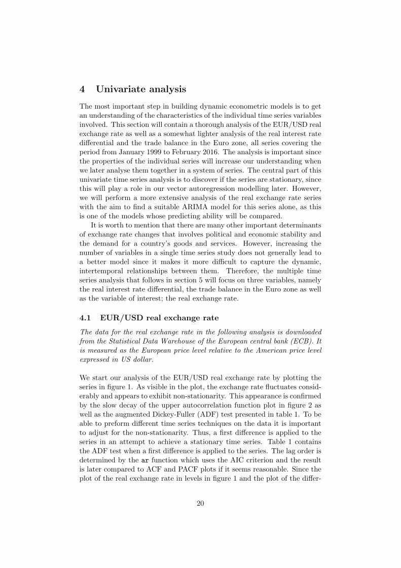
We start our analysis of the EUR/USD real exchange rate by plotting theseries in figure 1. As visible in the plot, the exchange rate fluctuates consid-erably and appears to exhibit non-stationarity. This appearance is confirmedby the slow decay of the upper autocorrelation function plot in figure 2 aswell as the augmented Dickey-Fuller (ADF) test presented in table 1. To beable to preform different time series techniques on the data it is importantto adjust for the non-stationarity. Thus, a first difference is applied to theseries in an attempt to achieve a stationary time series. Table 1 containsthe ADF test when a first difference is applied to the series. The lag order isdetermined by the ar function which uses the AIC criterion and the resultis later compared to ACF and PACF plots if it seems reasonable. Since theplot of the real exchange rate in levels in figure 1 and the plot of the differ-

20

enced series in figure 13 in appendix B do not reveal a linear deterministictrend a priori, both series is tested based on a model without a trend. Fur-thermore, the mean of the differenced series is not significantly different fromzero when a t-test is preformed and is therefore tested without a constant.On the contrary, the mean of the levels series is significantly nonzero andis thus tested based on a model with a constant. The test results in table1 indicate that the series is not stationary in levels but stationary in firstdifference. The appropriateness of a first difference is also demonstrated inthe differenced ACF in figure 2 where there is now a drop to zero quickly. Itis therefore concluded that the RER is integrated of order 1, I(1), and thatwe cannot reject a unit root in the levels series.

80

90

100

110

2000 2005 2010 2015

Year

EUR/U

SD [19

99 Q1

= 100]

Figure 1: The monthly real Euro/US dollar exchange rate

Augmented Dickey Fuller Unit Root test

Variable Deterministics Lag order P-value

RER constant 2 0.6063Diff RER 1 <0.01

Table 1: Unit root test for the levels and first differenced Real ExchangeRate series

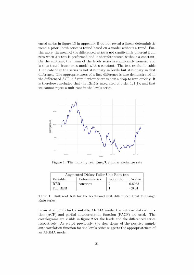
In an attempt to find a suitable ARIMA model the autocorrelation func-tion (ACF) and partial autocorrelation function (PACF) are used. Thecorrelograms are visible in figure 2 for the levels and the differenced seriesrespectively. As stated previously, the slow decay of the positive sampleautocorrelation function for the levels series suggests the appropriateness ofan ARIMA model.

21

Since the first lag is significant in both the ACF and PACF plot of thedifferenced RER series potential p and q values are 1. Therefore, a possiblecandidate is an ARIMA(1,1,1) model. To investigate the matter further weemploy the auto.arima function in R which uses a variation of the Hyndmanand Khandakar algorithm [5] to obtain a suitable ARIMA model. Thisalgorithm combine unit root tests, minimization of the AICc and maximumlikelihood estimation (MLE). The reader is referred to appendix A for furtherinformation of the steps.

As a result, the function returns an ARIMA(2,1,2) model with a seasonalAR at the 12th lag of order 1, a SARIMA(2,1,2)(1,0,0)12 model. Since itis not advantageous from a forecasting point of view to choose large p andq we restrict the auto.arima function to not look for seasonal components.This decision is based on the observation that we do not see a clear seasonalpattern in the series or a single significant spike at lag 12 in the PACF. Withthe imposed restriction, the auto.arima function return an ARIMA(1,1,0)model. Consequently, this initial analysis suggests three potential modelsfor the real exchange rate series. The models are fitted and the suppliedinformation criterion values computed. The results can be found in table 2below.

0.0 0.5 1.0 1.5

0.00.2

0.40.6

0.81.0

Lag

ACF

Levels RER

0.0 0.5 1.0 1.5

0.00.2

0.40.6

0.81.0

Lag

ACF

Diff RER

0.5 1.0 1.5

−0.2

0.20.4

0.60.8

1.0

Lag

Partial

ACF

0.5 1.0 1.5

−0.1

0.00.1

0.20.3

Lag

Partial

ACF

Figure 2: The acf and pacf for the levels series to the left and for thedifferenced series to the right. The lags on the y-axis are scaled by a 10−1-multiple.

The obtained AIC and AICc values in table 2 advocate theSARIMA(2,1,2)(1,0,0)12 as the most suitable model out of the three consid-ered. However, the BIC implies that the ARIMA(1,1,0) is the appropriatemodel and that the SARIMA model is the least appropriate model. Though,as one can see, the values obtained do not differ greatly between the modelsand since there were not much evidence of a seasonal effect in our data we

22

Information criterion values

Model AIC AICc BIC

ARIMA(1,1,1) 641.16 641.28 651.13SARIMA(2,1,2)(1,0,0)12 639.63 640.05 659.56ARIMA(1,1,0) 640.2 640.26 646.84

Table 2: Information criterion values for the different suitable ARIMA mod-els

choose to proceed our analysis with the ARIMA(1,1,1) model as well as theARIMA(1,1,0).

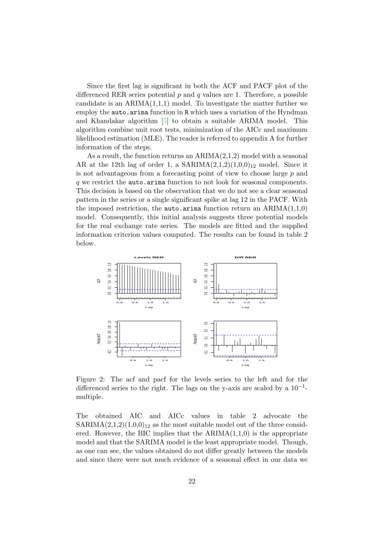
Thereon, we verify that the residuals of the fitted models possess thewanted properties by first establishing that they are normally distributedby normal quantile-quantile plots in figure 3 below.

−3 −2 −1 0 1 2 3

−4−2

02

Normal Q−Q Plot

Theoretical Quantiles

Sam

ple Q

uant

iles

−3 −2 −1 0 1 2 3

−4−2

02

Normal Q−Q Plot

Theoretical Quantiles

Sam

ple Q

uant

iles

Figure 3: Normal Q-Q plots of the residuals from the ARIMA(1,1,1) modelto the left and the ARIMA(1,1,0) model to the right.

The linearity of the points in figure 3 suggests that the data are normallydistributed. There is one data point that deviates from the rest and wedetect it as the one for November 2008. This is due to the financial crisisand a possible model for step response intervention could be employed butas the data point do not seem to interfere with the normality assumptionmore than appearing as an outlier we simply leave it and proceed with thepossibility of changing the model specification with a dummy variable later.

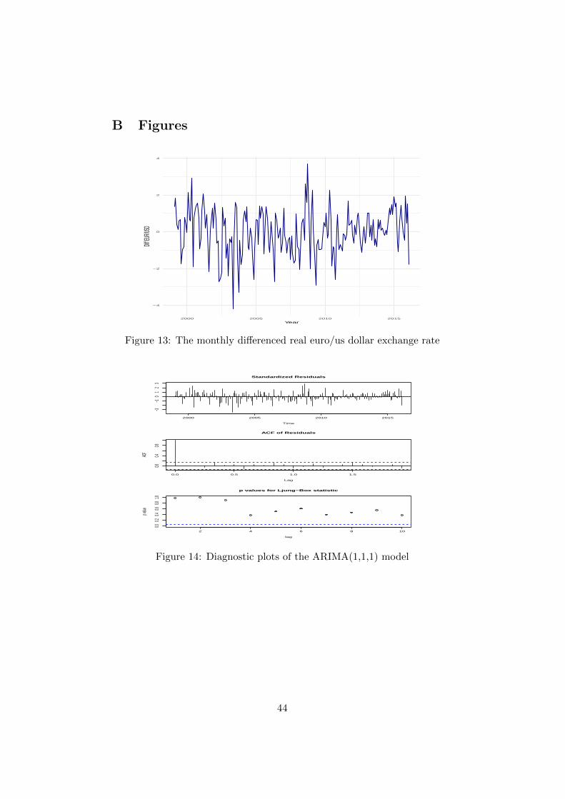
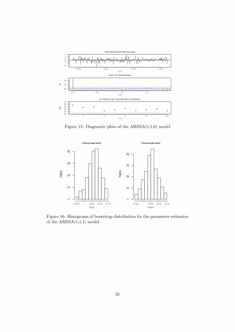
Thereon, we continue by plotting the standardized residuals togetherwith the sample ACF. These can be found in figure 14 and 15 in appendixB. The plots of the standardized residuals obtained from both models givesno indication of a nonzero mean, trend or changing variance and thus re-sembles white noise. The sample ACF of the residuals further indicates that

23

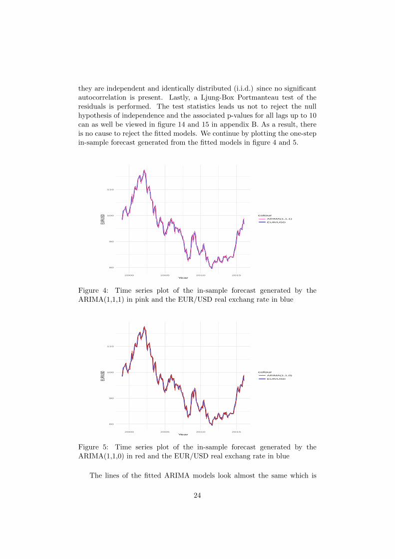
they are independent and identically distributed (i.i.d.) since no significantautocorrelation is present. Lastly, a Ljung-Box Portmanteau test of theresiduals is performed. The test statistics leads us not to reject the nullhypothesis of independence and the associated p-values for all lags up to 10can as well be viewed in figure 14 and 15 in appendix B. As a result, thereis no cause to reject the fitted models. We continue by plotting the one-stepin-sample forecast generated from the fitted models in figure 4 and 5.

80

90

100

110

2000 2005 2010 2015

Year

EUR/U

SD colour

ARIMA(1,1,1)

EUR/USD

Figure 4: Time series plot of the in-sample forecast generated by theARIMA(1,1,1) in pink and the EUR/USD real exchang rate in blue

80

90

100

110

2000 2005 2010 2015

Year

EUR/U

SD colour

ARIMA(1,1,0)

EUR/USD

Figure 5: Time series plot of the in-sample forecast generated by theARIMA(1,1,0) in red and the EUR/USD real exchang rate in blue

The lines of the fitted ARIMA models look almost the same which is

24

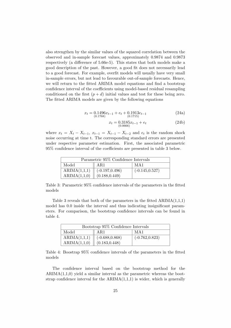
also strengthen by the similar values of the squared correlation between theobserved and in-sample forecast values, approximately 0.9874 and 0.9873respectively (a difference of 5.66e-5). This states that both models make agood description of the past. However, a good fit does not necessarily leadto a good forecast. For example, overfit models will usually have very smallin-sample errors, but not lead to favourable out-of-sample forecasts. Hence,we will return to the fitted ARIMA model equations and find a bootstrapconfidence interval of the coefficients using model-based residual resamplingconditioned on the first (p + d) initial values and test for these being zero.The fitted ARIMA models are given by the following equations

xt = 0.1496(0.1768)

xt−1 + et + 0.1913(0.1715)

et−1 (24a)

xt = 0.3185(0.0666)

xt−1 + et (24b)

where xt = Xt − Xt−1, xt−1 = Xt−1 − Xt−2 and et is the random shocknoise occurring at time t. The corresponding standard errors are presentedunder respective parameter estimation. First, the associated parametric95% confidence interval of the coefficients are presented in table 3 below.

Parametric 95% Confidence Intervals

Model AR1 MA1

ARIMA(1,1,1) (-0.197,0.496) (-0.145,0.527)ARIMA(1,1,0) (0.188,0.449)

Table 3: Parametric 95% confidence intervals of the parameters in the fittedmodels

Table 3 reveals that both of the parameters in the fitted ARIMA(1,1,1)model has 0.0 inside the interval and thus indicating insignificant param-eters. For comparison, the bootstrap confidence intervals can be found intable 4.

Bootstrap 95% Confidence Intervals

Model AR1 MA1

ARIMA(1,1,1) (-0.688,0.868) (-0.762,0.823)ARIMA(1,1,0) (0.183,0.448)

Table 4: Boostrap 95% confidence intervals of the parameters in the fittedmodels

The confidence interval based on the bootstrap method for theARIMA(1,1,0) yield a similar interval as the parametric whereas the boot-strap confidence interval for the ARIMA(1,1,1) is wider, which is generally

25

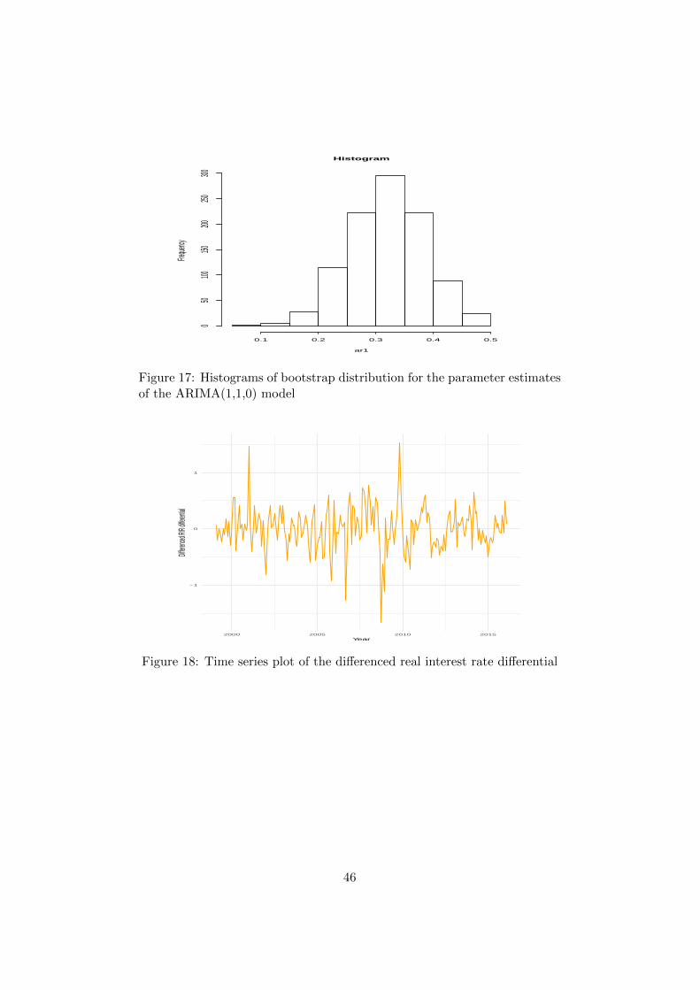
the case, and still includes 0.0. Therefore, we conclude that the parameterestimates in the ARIMA(1,1,1) model is insignificant at the 5% level. To givethe reader a more intuitive sense of the confidence intervals, histograms ofrespective bootstrap distribution for the parameter estimates can be foundin figure 16 and 17 in appendix B.

Since the estimates of the coefficients in the ARIMA(1,1,1) are insignif-icant we discard this model as suitable for the real exchange rate series.Thus, we continue our analyze with solely the ARIMA(1,1,0) model. Byutilizing that xt = Xt −Xt−1 and xt−1 = Xt−1 −Xt−2 equation (24b) canbe written on the equivalent form

Xt = 1.3185Xt−1 − 0.3185Xt−2 + et (25)

Its predicting ability will later be compared to the one of the economic modelin section 7.

26

4.2 Macroeconomic variables

The real interest rate differential is computed as the 3-month real Euriborrate minus the 3-month Libor rate in USD adjusted for the inflation in theUS. Moreover, the terms of trade is computed as the ratio between exportprices and import price. The data for the 3-month Euribor rate is down-loaded from the Statistical Data Warehouse of the ECB whereas the data forthe export price index in the Euro zone is downloaded from Eurostat. Lastlythe data for the import price index in the Euro zone, the inflation rate inthe US as well as the 3 month Libor rate in USD is downloaded from theFederal Reserve Bank of St. Louis.

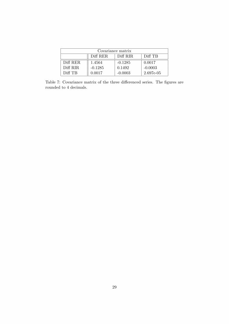
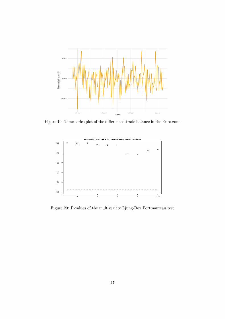
In this section a lighter analysis of the two macroeconomic variables; realinterest rate differential (RIRD) and European trade balance (TB) will bemade. We start by plotting the series in figure 6 and 7 respectively and wenotice that both series appear non-stationary with high volatility aroundthe immediate time and in the reverberations of the financial crisis. As aconsequence of the non-stationary characteristics, a first difference is appliedto both series and as observable in figure 18 and 19 in appendix B, thetransformation seems to be satisfying in a stationary purpose. Though, thetime series of the differenced RIRD appear to exhibit an outlier and weidentify it as the one for December 2008. The outlier is not adjusted fornow, but we may have to adjust the vector autoregressive model with adummy variable if the multivariate normality assumption is violated.

Next, an ADF test is used to detect whether the differenced series possessa unit root. Both the series are modelled without a constant since therespective t-tests do not reject a zero mean. The resulting p-values arepresented in table 5.

Augmented Dickey Fuller Unit Root test

Variable Deterministics Lag order P-value

Diff RIRD 1 <0.01Diff trade balance EU 1 <0.01

Table 5: Unit root test for the differenced macroeconomical variables

The ADF tests conclude both series to be I(1). This discovery will play asignificant role when we define an economic model in the next section sincethere is a possibility that the time series exhibit a common stochastic trenddue to all being I(1). However, before we proceed with finding a valid vectormodel some descriptive statistics of the differenced series are displayed intable 6 and 7 below.

The informative descriptive statistics in table 6 reveal that both of themacroeconomic series, but principally the differenced TB, is closely oscil-lating around zero. Table 7 display the covariance of the three differenced

27

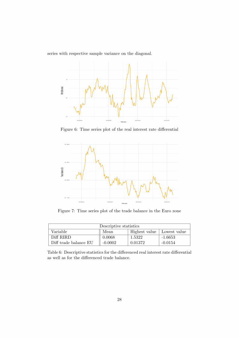
series with respective sample variance on the diagonal.

−2

0

2

2000 2005 2010 2015

Year

RIR diff

erential

Figure 6: Time series plot of the real interest rate differential

0.76

0.80

0.84

0.88

2000 2005 2010 2015

Year

Trade ba

lance E

U

Figure 7: Time series plot of the trade balance in the Euro zone

Descriptive statistics

Variable Mean Highest value Lowest value

Diff RIRD 0.0068 1.5322 -1.6653Diff trade balance EU -0.0002 0.01372 -0.0154

Table 6: Descriptive statistics for the differenced real interest rate differentialas well as for the differenced trade balance.

28

Covariance matrix

Diff RER Diff RIR Diff TB

Diff RER 1.4564 -0.1285 0.0017Diff RIR -0.1285 0.1492 -0.0003Diff TB 0.0017 -0.0003 2.697e-05

Table 7: Covariance matrix of the three differenced series. The figures arerounded to 4 decimals.

29

5 Economic model

In this section, we will define the model which includes endogenous macroe-conomic variables. Since the results of the stationarity test according toADF indicate that all series are stationary in their first difference, we initi-ate this section by testing for cointegration to detect if there exist a linearcombination of the variables that is stationary. The results of the Johansentest for cointegration using the maximum eigenvalue statistic can be foundin table 8 whereas the test with trace statistic can be found in table 9.

Statistic 10% 5% 1%

r ≤ 2 1.27 7.52 9.24 12.97

r ≤ 1 2.44 13.75 15.67 20.20

r = 0 14.86 19.77 22.00 26.81

Table 8: Johansen test for cointegration rank: Max eigenvalue statistic

Statistic 10% 5% 1%

r ≤ 2 1.27 7.52 9.24 12.97

r ≤ 1 3.71 17.85 19.96 24.60

r = 0 18.57 32.00 34.91 41.07

Table 9: Johansen test for cointegration rank: Trace statistic

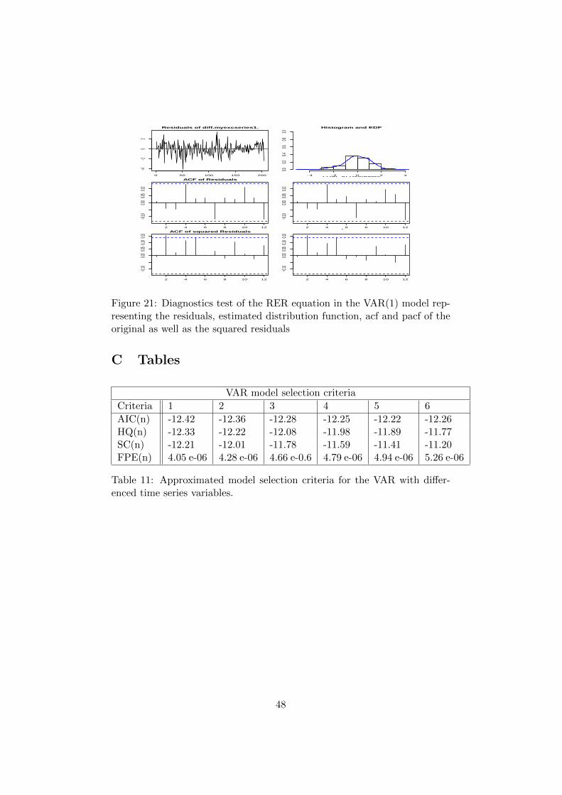
Both test statistics reject the hypothesis of a cointegrating vector at allsignificance levels. Hence, we continue by estimating a VAR model withthe differenced series. The lag order is first specified by the model selectioncriteria described in section 3.3.7. All the criteria selects a VAR(1) as themost suitable model. Values of the different criteria for up to six lags canbe found in table 11 in appendix C.

Thereafter we proceed with estimating a VAR(1) model by utilizing or-dinary least square per equation. The model is estimated without a constantterm. This do not seem contradictory since we tested the sample means ofthe first-differenced series and none of the means were significantly differentfrom zero. We therefore restrict the vector autoregressive model to excludedeterministic drifts in the individual series. As in the case of the ARIMAmodels in section 4, we initialize by performing a multivariate Ljung-BoxPortmanteau test to test for autocorrelation in the residuals. The test ispreformed to detect if the choice of one lag is to restrictive and if the datainstead should be modelled with a higher lag order. Autocorrelation in the

30

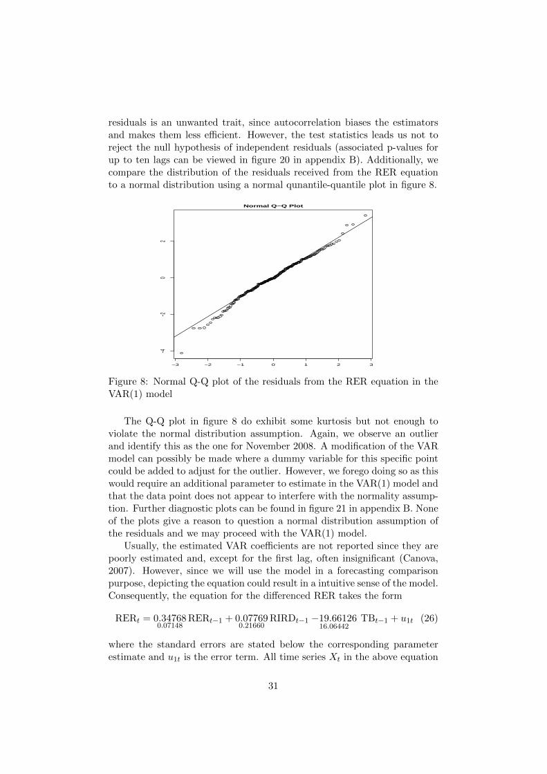
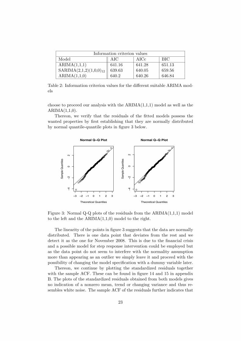
residuals is an unwanted trait, since autocorrelation biases the estimatorsand makes them less efficient. However, the test statistics leads us not toreject the null hypothesis of independent residuals (associated p-values forup to ten lags can be viewed in figure 20 in appendix B). Additionally, wecompare the distribution of the residuals received from the RER equationto a normal distribution using a normal qunantile-quantile plot in figure 8.

−3 −2 −1 0 1 2 3

−4−2

02

Normal Q−Q Plot

Figure 8: Normal Q-Q plot of the residuals from the RER equation in theVAR(1) model

The Q-Q plot in figure 8 do exhibit some kurtosis but not enough toviolate the normal distribution assumption. Again, we observe an outlierand identify this as the one for November 2008. A modification of the VARmodel can possibly be made where a dummy variable for this specific pointcould be added to adjust for the outlier. However, we forego doing so as thiswould require an additional parameter to estimate in the VAR(1) model andthat the data point does not appear to interfere with the normality assump-tion. Further diagnostic plots can be found in figure 21 in appendix B. Noneof the plots give a reason to question a normal distribution assumption ofthe residuals and we may proceed with the VAR(1) model.

Usually, the estimated VAR coefficients are not reported since they arepoorly estimated and, except for the first lag, often insignificant (Canova,2007). However, since we will use the model in a forecasting comparisonpurpose, depicting the equation could result in a intuitive sense of the model.Consequently, the equation for the differenced RER takes the form

RERt = 0.347680.07148

RERt−1 + 0.077690.21660

RIRDt−1 −19.6612616.06442

TBt−1 + u1t (26)

where the standard errors are stated below the corresponding parameterestimate and u1t is the error term. All time series Xt in the above equation

31

should be considered as Xt −Xt−1 since they are all differenced. The tablewith all of the estimated parameters can be found in table 12 in appendixC. The corresponding covariance matrix of all error terms, u1t, u2t and u3t,in the VAR(1) model is given by

Σu =

1.3094 −0.1056 0.0008−0.1056 0.1327 −9.252e− 050.0008 −9.252e− 0.5 0.2170e− 05

As a model validation check for a VAR model one can make use of the

formula for covariance of the causal series in Brockwell and Davis (2004,section 8.4). The authors derive the covariance of the series for a VAR(1)with one lag as

Σy = Σu +AΣuA′

By computing the matrix A with the parameter estimate table 12 in ap-pendix C we get the variance for differenced RER series to 1.4707, which issimilar to the value in the covariance matrix in section 4 which was 1.4564.

An initial observation of the RER equation is that the parameter esti-mate for the RERt−1 is quite similar to the estimate in the ARIMA(1,1,0) insection 3, with an additional value of approximately 0.03. Furthermore, it isworth to remark that the absolute contribution from the two macroeconomicvariables are quite small considering that both of these differenced series areclosely oscillating around zero. Thus, the resemblance of this model withthe ARIMA(1,1,0) is palpable. Furthermore, a 95% bootstrap confidenceinterval of the parameter estimates indicates, as outlined by Canova (2007),only the lagged RER to be significant.

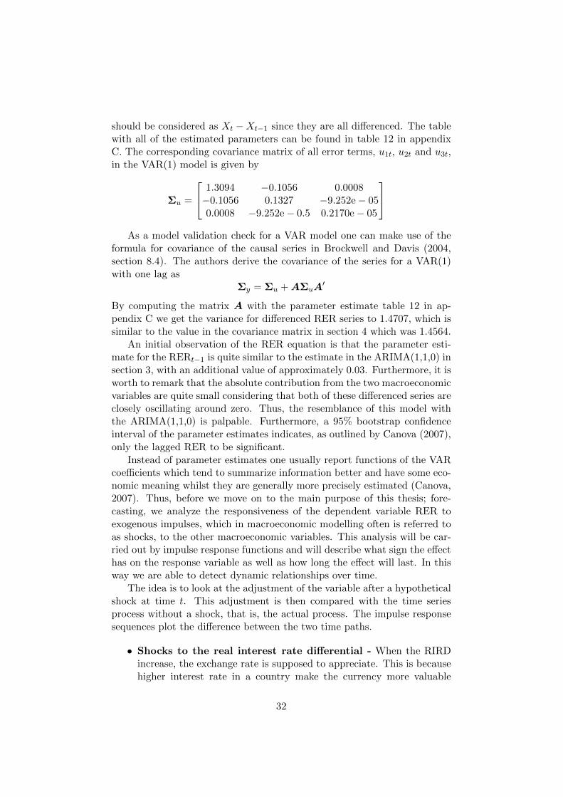
Instead of parameter estimates one usually report functions of the VARcoefficients which tend to summarize information better and have some eco-nomic meaning whilst they are generally more precisely estimated (Canova,2007). Thus, before we move on to the main purpose of this thesis; fore-casting, we analyze the responsiveness of the dependent variable RER toexogenous impulses, which in macroeconomic modelling often is referred toas shocks, to the other macroeconomic variables. This analysis will be car-ried out by impulse response functions and will describe what sign the effecthas on the response variable as well as how long the effect will last. In thisway we are able to detect dynamic relationships over time.

The idea is to look at the adjustment of the variable after a hypotheticalshock at time t. This adjustment is then compared with the time seriesprocess without a shock, that is, the actual process. The impulse responsesequences plot the difference between the two time paths.

• Shocks to the real interest rate differential - When the RIRDincrease, the exchange rate is supposed to appreciate. This is becausehigher interest rate in a country make the currency more valuable

32

relative to the country offering lower interest rate. We can see thatthis also is the case as depicted in figure 8 where the exchange rateresponded positively on a shock to the RIRD.

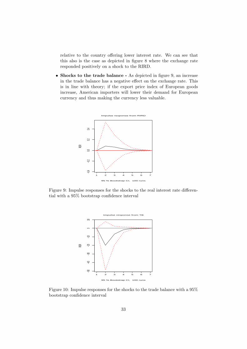
• Shocks to the trade balance - As depicted in figure 9, an increasein the trade balance has a negative effect on the exchange rate. Thisis in line with theory; if the export price index of European goodsincrease, American importers will lower their demand for Europeancurrency and thus making the currency less valuable.

1 2 3 4 5 6 7

−0.4

−0.2

0.00.2

0.4

xy$x

RER

Impulse response from RIRD

95 % Bootstrap CI, 100 runs

Figure 9: Impulse responses for the shocks to the real interest rate differen-tial with a 95% bootstrap confidence interval

1 2 3 4 5 6 7

−50−40

−30−20

−100

10

xy$x

RER

Impulse response from TB

95 % Bootstrap CI, 100 runs

Figure 10: Impulse responses for the shocks to the trade balance with a 95%bootstrap confidence interval

33

Since the real exchange rate responds according to theory after shocksto the macroeconomic variables we will continue analyzing the estimatedVAR(1) model in a forecasting purpose in the next section.

34

6 Forecasting

The main purpose of this thesis is to forecast the real EUR/USD exchangerate for the four months succeeding February 2016 and compare these pre-dicted values to the observed values. We will compare the forecast accuracyof the ARIMA(1,1,0) and the VAR(1) with a random walk, which is oftenconsidered to produce the best forecasts. The predicted values from therandom walk is thus the value of the latest observation, Xt = Xt−1, whichcorresponds to 96.7301. The choice of test period is set to three months.This is due to the fact that an ARIMA(1,1,0) would converge to a randomwalk when the amount of forecast steps increase.

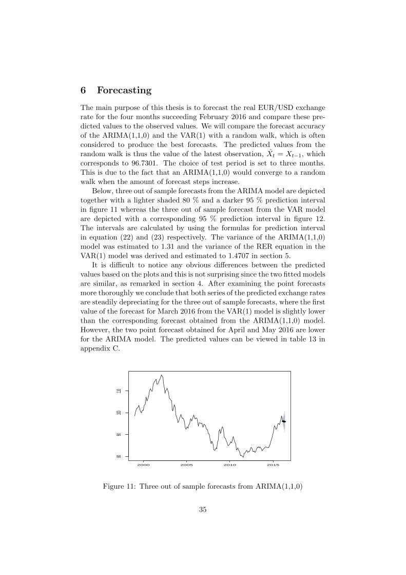
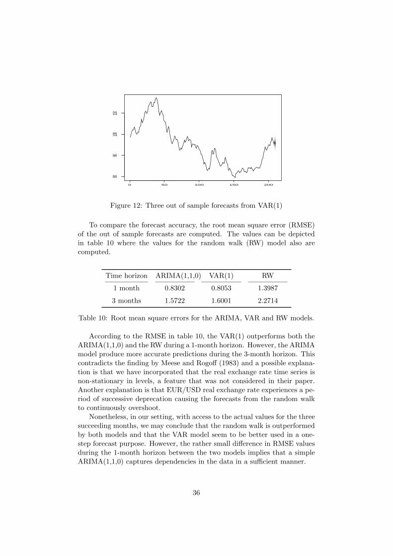
Below, three out of sample forecasts from the ARIMA model are depictedtogether with a lighter shaded 80 % and a darker 95 % prediction intervalin figure 11 whereas the three out of sample forecast from the VAR modelare depicted with a corresponding 95 % prediction interval in figure 12.The intervals are calculated by using the formulas for prediction intervalin equation (22) and (23) respectively. The variance of the ARIMA(1,1,0)model was estimated to 1.31 and the variance of the RER equation in theVAR(1) model was derived and estimated to 1.4707 in section 5.

It is difficult to notice any obvious differences between the predictedvalues based on the plots and this is not surprising since the two fitted modelsare similar, as remarked in section 4. After examining the point forecastsmore thoroughly we conclude that both series of the predicted exchange ratesare steadily depreciating for the three out of sample forecasts, where the firstvalue of the forecast for March 2016 from the VAR(1) model is slightly lowerthan the corresponding forecast obtained from the ARIMA(1,1,0) model.However, the two point forecast obtained for April and May 2016 are lowerfor the ARIMA model. The predicted values can be viewed in table 13 inappendix C.

2000 2005 2010 2015

8090

100110

Figure 11: Three out of sample forecasts from ARIMA(1,1,0)

35

0 50 100 150 200

8090

100110

Figure 12: Three out of sample forecasts from VAR(1)

To compare the forecast accuracy, the root mean square error (RMSE)of the out of sample forecasts are computed. The values can be depictedin table 10 where the values for the random walk (RW) model also arecomputed.

Time horizon ARIMA(1,1,0) VAR(1) RW

1 month 0.8302 0.8053 1.3987

3 months 1.5722 1.6001 2.2714

Table 10: Root mean square errors for the ARIMA, VAR and RW models.

According to the RMSE in table 10, the VAR(1) outperforms both theARIMA(1,1,0) and the RW during a 1-month horizon. However, the ARIMAmodel produce more accurate predictions during the 3-month horizon. Thiscontradicts the finding by Meese and Rogoff (1983) and a possible explana-tion is that we have incorporated that the real exchange rate time series isnon-stationary in levels, a feature that was not considered in their paper.Another explanation is that EUR/USD real exchange rate experiences a pe-riod of successive deprecation causing the forecasts from the random walkto continuously overshoot.

Nonetheless, in our setting, with access to the actual values for the threesucceeding months, we may conclude that the random walk is outperformedby both models and that the VAR model seem to be better used in a one-step forecast purpose. However, the rather small difference in RMSE valuesduring the 1-month horizon between the two models implies that a simpleARIMA(1,1,0) captures dependencies in the data in a sufficient manner.

36

7 Discussion

The purpose of this thesis was not to discover new results in the field ofexchange rate modelling and forecasting. However, it is still interesting tocompare the findings in this thesis to conclusions made in the literature oneconometric models and ARIMA models fitted to exchange rate time series.

In section 3 and 5, an ARIMA(1,1,0) model and a VAR(1) model withadditional macroeconomic variables were fitted to the EUR/USD real ex-change rate data. Both of these models were concluded to make betterpredictions than a random walk after the comparison of root mean squareerror values as a measure of forecast accuracy in section 7. This findingcontradicts the conclusion in the paper of Meese and Rogoff (1983). Theauthors found that the random walk model was superior to an ARMA model.However, a possible explanation of the diverging conclusion is that Meeseand Rogoff (1983) did not incorporate the fact that the exchange rate seriesprobably was non-stationary in levels. Though, after examining equation(25) we realise that the sum of the AR coefficients are 1 and thus, unlessthe past values have changed remarkably during the last two periods, we seethat our ARIMA(1,1,0) has similarities to a random walk.

The VAR(1) model in section 5 was derived with additional macroeco-nomic variables for the real interest rate differential and the trade balancein the EU. The parameter estimates for the lagged additional variables wereproven to be insignificant. However, economic theory suggests that thereare several important exchange rate determinants and other variables mayexplain the exchange rate fluctuations in a more sufficient manner. The find-ings of Yu (2001) and Mida (2013) diverges in the short- and long run. Yu(2001) concludes that neither a VAR, restricted VAR, VECM or a BayesianVAR generates better forecasts than a random walk in the short run butthat the models have better forecast accuracy in the long run. Meanwhile,Mida (2013) find the VAR model to outperform the random walk in theshort run but not in the long run. Sellin (2007) also finds a VECM modelfor the Swedish Krona’s real and nominal effective exchange rate to makeaccurate forecasts once the model has been augmented with an interest ratedifferential. The diverging results are most likely due to differing exchangerates and the usage of different macroeconomic variables. Thus, findingsignificant explanatory variables to an exchange rate is troublesome sinceinsignificant variables for one exchange rate may contain valuable informa-tion in explaining another.

Lastly, we have used monthly time series data for the period from Jan-uary 1999 to February 2016 in this thesis. Since the models are based onexplaining the past, they will be biased toward the past in the sense that theywill weigh historical information more heavily than newer information. Thiswill usually lead to poor prediction performance and is a problem when de-riving models that aim to forecast. Thus, using fewer variables and lags in a

37

model are usually beneficial in a forecasting perspective since overfit modelsoften have small in-sample errors, but not lead to favourable out-of-sampleforecasts. However, our ARIMA only have one AR-term and our VAR ismade up by solely three first-lagged variables. So the problem of overfittingis not applied here. Though the choice of other macroeconomic variables inour VAR may have yielded more accurate out-of-sample forecasts.

Additionally, new information is incorporated quickly on foreign ex-change markets due to its easy access for market participants. Market forcestend to adjust the market to a new equilibrium within a short time frame,often faster than a monthly or even a weekly frequency. Therefore, usingmonthly data do not allow one to quantify how the foreign exchange marketreact to some new information, e.g. a change in interest rates or a changein price level, since the change has already occurred and been consumed bythe time you predict it. Thus, daily data is probably more reliable whenpredicting exchange rate movements.

38

8 Conclusions

The main purpose of this thesis was to find a model that makes accuratepredictions of the real EUR/USD exchange rate for the three months suc-ceeding February 2016. It was first concluded that the real exchange ratewas non-stationary in levels but stationary in first difference after exam-ining the ADF-test presented in table 1 and the ACF and PACF plots infigure 2. Thereafter, we presented three different ARIMA models based on abuilt-in algorithm for automatic ARIMA modelling in R as well as from ex-aminations of the ACF and PACF plots in section 4.1. The candidates werean ARIMA(1,1,1), SARIMA(2,1,2)(1,0,0)12 and an ARIMA(1,1,0) model.Based on values of the Bayesian information criterion (BIC) as well as nosignificant 12th lag in the PACF plot in figure 2, the SARIMA(2,1,2)(1,0,0)12was considered the least appropriate model and the two remaining modelswere further analysed. The ARIMA(1,1,1) and ARIMA(1,1,0) displayedsimilar one-step-in-sample forecasts in figure 4 and both models’ residualswere presumably from a normal distribution based on quantile-quantile plotsdisplayed in figure 3. As the confidence interval for the parameters in theARIMA(1,1,1) model included 0.0, and thus were insignificant, we reachedto the conclusion that the ARIMA(1,1,0) was the most appropriate one ofthe three models we had begun our univariate analysis with.

Thereafter, in section 5, an economic model with trade balance in the EUas well as the interest rate differential as additional variables was estimated.Since all the variables were stationary in their first difference according tothe ADF-test in table 5, there was a possibility that there existed a linearcombination of the levels series that were stationary, and thus a long runrelationship between the variables. This kind of cointegrating relationshipwas tested for by two different Johansen test statistics, both rejecting suchhypothesis as observed in table 8 and 9. Thus, a VAR model with the firstdifferenced series was estimated. It was concluded that a VAR model withvariables of first lag was selected by all model selection criteria and that theresiduals with the real exchange rate as dependent variable in the VAR(1)model demonstrated residuals with desired properties; no autocorrelationand white noise resemblance. However, an outlier in the quantile-quantileplot in figure 8 was observed, but since the normality assumption was notviolated, a dummy variable was not added to the model.

When examining equation (26) of the real exchange rate, it was remarkedthat the equation resembled the one from the estimated ARIMA(1,1,0) inequation (25). As a last part of the analyze of the VAR(1) model, the realexchange rate impulse response to exogenous shocks to the other macroe-conomic variables were presented in figure 9 and 10. The conclusions werethat the response of the RER variable was in line with theory; an increasein the RIRD caused an appreciation, whereas an increase in the TB causeda depreciation.

39

Although economic theory suggests that other macroeconomic variablesimprove the explanation of exchange rate fluctuations, it is observed in sec-tion 7 that a simple ARIMA(1,1,0) model gives comparatively good one-step-forecast and even outperforms the VAR model during a 3-month timehorizon, when comparing RMSE with actual observed forecast values fromECB in table 10. Furthermore, the random walk is outperformed by bothmodels during both 1-month and 3-month horizon. This suggests that themost important variable to explain the real exchange rate is the lagged vari-able itself, which also is in line with the parameter estimations in the VARmodel in section 5 where only the first lagged RER variable was significant.Thus, this thesis concludes the ARIMA(1,1,0) with its simple interpretationcaptures dependencies in the data in a relatively sufficient manner.

9 Further research

Since the models are derived to explain the past, new information is notincorporated in the model. Thus, one possible extension to this thesis isto use rolling window forecasts where the parameters are re-estimated aftereach step in which we includes a new true observation. Furthermore, itwould be interesting to include a dummy variable in the model since weobserved an outlier in our quantile-quantile plots for the residuals in both theARIMA(1,1,0) model and the VAR(1) model. Lastly, the inclusion of othermacroeconomic variables may yield a different result where the parametersestimates are significant.

40

References

[1] Brockwell, Peter J. and Davis, Richard J. 2002. Second edition.Introduction to time series and forecasting. New York: Springer-VerlagNew York Inc.

[2] Hyndman, Rob J. and Athanasopoulos, George. 2014. Forecast-ing: principles and practice. https://www.otexts.org/fpp/ (Down-loaded 2017-03-28)

[3] Cryer, Jonathan D. and Chan, Kung-Sik. 2008. Time series anal-ysis with applications in R. Second edition. New York: Springer Sci-ence+Business Media, LCC.

[4] Tsay, Ruey S. 2010. Analysis of financial time series. Third edition.Hoboken, New Jersey: John Wiley Sons, Inc.

[5] Hyndman, Robert J. and Yeasmin Khandakar 2008. Auto-matic time series forecasting: the forecast package for R. Jour-nal of statistical software 27 (3). http://robjhyndman.com/papers/automatic-forecasting/

[6] Blanchard, Olivier Amighini, Alessia and Giavazzi, Frans-esco. 2013. Second edition. Macroeconomics a European perspective.Harlow: Pearson Education Limited.

[7] Hurvich, Clifford M. and Tsai, Chih-Ling. 1989. Regression andtime series model selection in small samples. Biometrika 76, 297-307.

[8] Canova, Fabio 2007. Methods for Applied Macroeconomic Research.Princeton University Press

[9] Lutkepohl, Helmut Kratzig, Markus and Phillips, PeterC.B. 2004. Applied time series econometrics. Cambridge UniversityPress.

[10] Pfaff, Bernhard. 2008. Analysis of integrated and cointegrated timeseries with R. New York: Springer Science+Business Media, LLC.

[11] Hoffmann, Mathias and MacDonald, Ronald 2003. A re-eximination of the link between real exchange rates and real interestrate differentials. CESifo 894.

[12] King, Michael R. and Rime, Dagfinn. 2010. The 4$ trillion ques-tion: what explains FX growth since the 2007 survey?. Bank for Inter-national Settlements December 2010.

41

[13] Meese, Richard A. and Rogoff, Kenneth. 1983. Empirical ex-change rate models of the seventies - Do they fit out of sample? Journalof International Economics 14, 3-24.

[14] Ayekple, Yao E. Harris, Emmanuel Frempong, Nana K. andAmevialor, Joshua.. 2015. Time series analysis of the exchange rateof the Ghanaian Cedi to the American dollar. Journal of MathematicsResearch 7(3), 46-53.

[15] Akincilar, Aykan Temiz, Izzettin and Sahin Erol. 2011. An ap-plication of exchange rate forecasting in Turkey. Gazi University Jour-nal of Science 24(4), 817-828.

[16] Weisang, Guillaume and Awazu, Yukika. 2014. Vagaries of theEuro: an Introduction to ARIMA Modeling. Case Studies In Business,Industry And Government Statistics 2(1), 45-55.

[17] Yu, Yongtao. 2011. Exchange rate forecasting model compar-ison: A case study in North Europe. Master thesis. UppsalaUniversity. http://www.diva-portal.se/smash/get/diva2:422759/FULLTEXT01.pdf. (Downloaded 2017-04-22)

[18] Mida, Jaroslav. 2011. Forecasting exchange rates: a VAR analysis.Bachelor thesis. Charles University in Prague.

[19] Burke, Simon P. and Hunter, John. 2005. Modelling non-stationary time series: a multivariate approach. Hampshire and NewYork: Palgrave MacMillan.

42

Appendices

A Functions in R

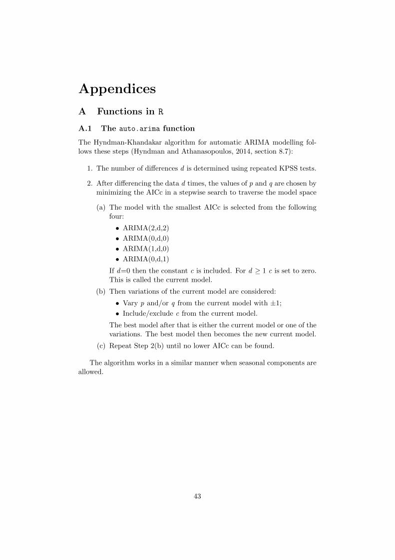
A.1 The auto.arima function

The Hyndman-Khandakar algorithm for automatic ARIMA modelling fol-lows these steps (Hyndman and Athanasopoulos, 2014, section 8.7):

1. The number of differences d is determined using repeated KPSS tests.

2. After differencing the data d times, the values of p and q are chosen byminimizing the AICc in a stepwise search to traverse the model space

(a) The model with the smallest AICc is selected from the followingfour:

• ARIMA(2,d,2)

• ARIMA(0,d,0)

• ARIMA(1,d,0)

• ARIMA(0,d,1)

If d=0 then the constant c is included. For d ≥ 1 c is set to zero.This is called the current model.

(b) Then variations of the current model are considered:

• Vary p and/or q from the current model with ±1;

• Include/exclude c from the current model.

The best model after that is either the current model or one of thevariations. The best model then becomes the new current model.

(c) Repeat Step 2(b) until no lower AICc can be found.

The algorithm works in a similar manner when seasonal components areallowed.

43

B Figures

−4

−2

0

2

4

2000 2005 2010 2015

Year

Diff EU

R/USD

Figure 13: The monthly differenced real euro/us dollar exchange rate

Standardized Residuals

Time

2000 2005 2010 2015

−3−1

01

23

0.0 0.5 1.0 1.5

0.00.4

0.8

Lag

ACF

ACF of Residuals

2 4 6 8 10

0.00.2

0.40.6

0.81.0

p values for Ljung−Box statistic

lag

p valu

e

Figure 14: Diagnostic plots of the ARIMA(1,1,1) model

44

Standardized Residuals

Time

2000 2005 2010 2015

−3−1

01

23

0.0 0.5 1.0 1.5

0.00.4

0.8

Lag

ACF

ACF of Residuals

2 4 6 8 10

0.00.2

0.40.6

0.81.0

p values for Ljung−Box statistic

lag

p valu

e

Figure 15: Diagnostic plots of the ARIMA(1,1,0) model

Histogram

ar1

Freque

ncy

−1.0 0.0 0.5 1.0

050

100150

200

Histogram

ma1

Freque

ncy

−1.0 0.0 0.5 1.0

050

100150

200

Figure 16: Histograms of bootstrap distribution for the parameter estimatesof the ARIMA(1,1,1) model

45

Histogram

ar1

Freque

ncy

0.1 0.2 0.3 0.4 0.5

050

100150

200250

300

Figure 17: Histograms of bootstrap distribution for the parameter estimatesof the ARIMA(1,1,0) model

−1

0

1

2000 2005 2010 2015

Year

Differe

nced R

IR diffe

rential

Figure 18: Time series plot of the differenced real interest rate differential

46

−0.01

0.00

0.01

2000 2005 2010 2015

Year

Differe

nced tr

ade ba

lance

EU

Figure 19: Time series plot of the differenced trade balance in the Euro zone

2 4 6 8 10

0.00.2

0.40.6

0.81.0

p−values of Ljung−Box statistics

m

Figure 20: P-values of the multivariate Ljung-Box Portmanteau test

47

Residuals of diff.myexcseries1.

0 50 100 150 200

−4−2

02

2 4 6 8 10 12

−0.10

0.00

0.05

0.10

ACF of Residuals

2 4 6 8 10 12

−0.10

0.00

0.05

0.10

0.15 ACF of squared Residuals

Histogram and EDF

Density

−4 −2 0 2 4

0.00.2

0.40.6

0.81.0

2 4 6 8 10 12

−0.10

0.00

0.05

0.10

PACF of Residuals

2 4 6 8 10 12

−0.10

0.00

0.05

0.10

0.15

PACF of squared Residuals

Figure 21: Diagnostics test of the RER equation in the VAR(1) model rep-resenting the residuals, estimated distribution function, acf and pacf of theoriginal as well as the squared residuals

C Tables

VAR model selection criteria

Criteria 1 2 3 4 5 6

AIC(n) -12.42 -12.36 -12.28 -12.25 -12.22 -12.26HQ(n) -12.33 -12.22 -12.08 -11.98 -11.89 -11.77SC(n) -12.21 -12.01 -11.78 -11.59 -11.41 -11.20FPE(n) 4.05 e-06 4.28 e-06 4.66 e-0.6 4.79 e-06 4.94 e-06 5.26 e-06

Table 11: Approximated model selection criteria for the VAR with differ-enced time series variables.

48

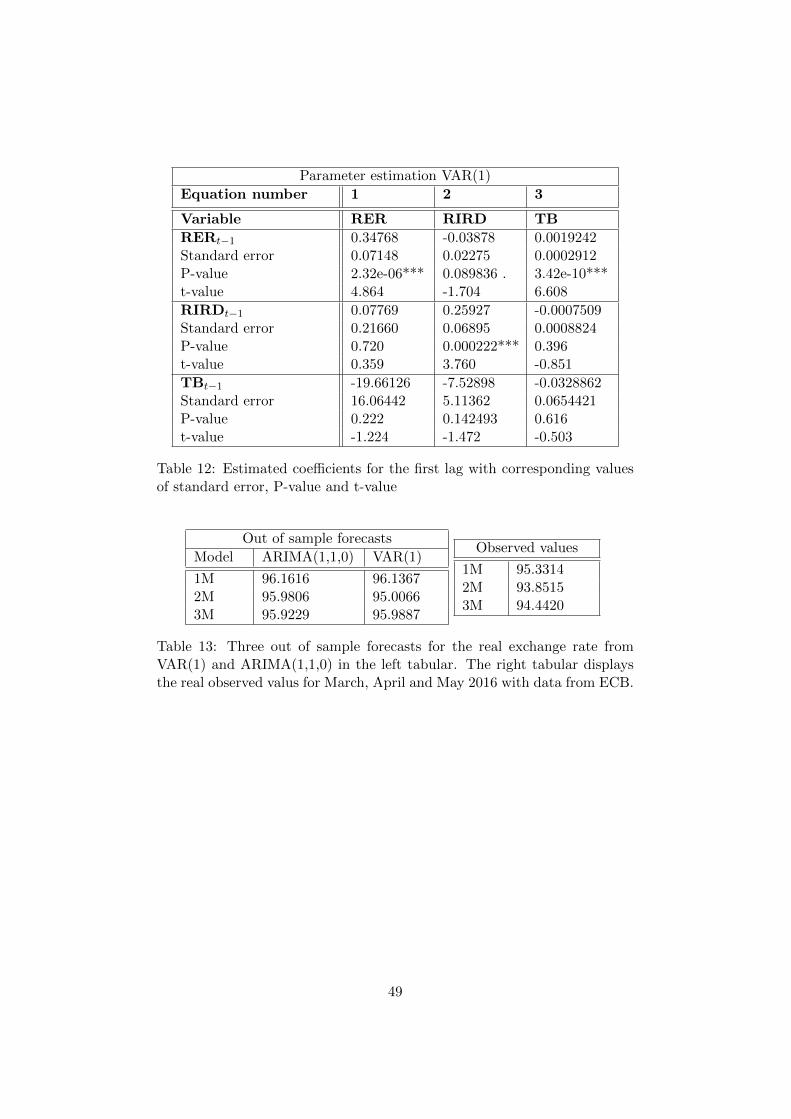
Parameter estimation VAR(1)

Equation number 1 2 3

Variable RER RIRD TB

RERt−1 0.34768 -0.03878 0.0019242Standard error 0.07148 0.02275 0.0002912P-value 2.32e-06*** 0.089836 . 3.42e-10***t-value 4.864 -1.704 6.608

RIRDt−1 0.07769 0.25927 -0.0007509Standard error 0.21660 0.06895 0.0008824P-value 0.720 0.000222*** 0.396t-value 0.359 3.760 -0.851

TBt−1 -19.66126 -7.52898 -0.0328862Standard error 16.06442 5.11362 0.0654421P-value 0.222 0.142493 0.616t-value -1.224 -1.472 -0.503

Table 12: Estimated coefficients for the first lag with corresponding valuesof standard error, P-value and t-value

Out of sample forecasts

Model ARIMA(1,1,0) VAR(1)

1M 96.1616 96.13672M 95.9806 95.00663M 95.9229 95.9887

Observed values

1M 95.33142M 93.85153M 94.4420

Table 13: Three out of sample forecasts for the real exchange rate fromVAR(1) and ARIMA(1,1,0) in the left tabular. The right tabular displaysthe real observed valus for March, April and May 2016 with data from ECB.

49