radulescu2016.pdf - edinburgh research archive

This thesis has been submitted in fulfilment of the requirements for a postgraduate degree

(e.g. PhD, MPhil, DClinPsychol) at the University of Edinburgh. Please note the following

terms and conditions of use:

This work is protected by copyright and other intellectual property rights, which are

retained by the thesis author, unless otherwise stated.

A copy can be downloaded for personal non-commercial research or study, without

prior permission or charge.

This thesis cannot be reproduced or quoted extensively from without first obtaining

permission in writing from the author.

The content must not be changed in any way or sold commercially in any format or

medium without the formal permission of the author.

When referring to this work, full bibliographic details including the author, title,

awarding institution and date of the thesis must be given.

E X P L O I T I N G VA R I A B L E I M P E D A N C E I N D O M A I N S W I T HC O N TA C T S

andreea radulescu

TH

E

U N I V E RS

IT

Y

OF

ED I N B U

RG

H

Doctor of PhilosophySchool of Informatics

University of Edinburgh

2016

Andreea Radulescu:

Exploiting variable impedance in domains with contacts

Doctor of Philosophy, 2016

supervisors:

Prof. Sethu Vijayakumar

Dr. Subramanian Ramamoorthy

All magic comes with a price.

— Rumpelstiltskin

A B S T R A C T

The control of complex robotic platforms is a challenging task, especially in de-

signs with high levels of kinematic redundancy. Novel variable impedance actua-

tors (VIAs) have recently demonstrated that, by allowing the ability to simultane-

ously modulate the output torque and impedance, one can achieve energetically

more efficient and safer behaviour. However, this adds further levels of actuation

redundancy, making planning and control of such systems even more complicated.

VIAs are designed with the ability to mechanically modulate impedance dur-

ing movement. Recent work from our group, employing the optimal control (OC)

formulation to generate impedance policies, has shown the potential benefit of

VIAs in tasks requiring energy storage, natural dynamic exploitation and robust-

ness against perturbation. These approaches were, however, restricted to systems

with smooth, continuous dynamics, performing tasks over a predefined time hori-

zon. When considering tasks involving multiple phases of movement, including

switching dynamics with discrete state transitions (resulting from interactions

with the environment), traditional approaches such as independent phase opti-

misation would result in a potentially suboptimal behaviour.

Our work addresses these issues by extending the OC formulation to a multi-

phase scenario and incorporating temporal optimisation capabilities (for robotic

systems with VIAs). Given a predefined switching sequence, the developed method-

ology computes the optimal torque and impedance profile, alongside the optimal

switching times and total movement duration. The resultant solution minimises

the control effort by exploiting the actuation redundancy and modulating the nat-

ural dynamics of the system to match those of the desired movement. We use a

monopod hopper and a brachiation system in numerical simulations and a hard-

ware implementation of the latter to demonstrate the effectiveness and robustness

of our approach on a variety of dynamic tasks.

The performance of model-based control relies on the accuracy of the dynamics

model. This can deteriorate significantly due to elements that cannot be fully cap-

tured by analytic dynamics functions and/or due to changes in the dynamics. To

circumvent these issues, we improve the performance of the developed framework

by incorporating an adaptive learning algorithm. This performs continuous data-

driven adjustments to the dynamics model while re-planning optimal policies that

reflect this adaptation. The results presented show that the augmented approach

is able to handle a range of model discrepancies, in both simulation and hardware

experiments using the developed robotic brachiation system.

v

L AY S U M M A RY

Recent technological developments have contributed to the development of a wide

range of robotic platforms. These modern systems are used in a wide range of

applications and differ from their classical counterparts in terms of complexity

and capabilities. One such capability is the modulation of impedance, using vari-

able impedance actuators (VIAs). This capability brings improved performance

in terms of energetically more efficient and safer behaviour. However, this adds

further complexity, making planning and control of such systems even more com-

plicated.

While previous studies addressed the control of systems with VIA capabilities,

the results focused on systems with smooth, continuous dynamics, performing

tasks over a predefined time horizon. When considering tasks involving multiple

phases of movement, including switching dynamics with discrete state transitions

(resulting from interactions with the environment, i.e., touch-down, lift-off), as

required by the new generation of robotic platforms, traditional approaches would

result in a potentially suboptimal behaviour.

In our work we address these issues by extending the OC formulation to a multi-

phase scenario for robotic systems with VIAs. Given a predefined locomotion pat-

tern, the developed methodology computes the optimal torque and impedance

profile, alongside the optimal switching times and total movement duration. We

use a monopod hopper and a brachiation system in numerical simulations and

a hardware implementation of the latter to demonstrate the effectiveness and ro-

bustness of our approach on a variety of dynamic tasks.

The method devised is model-based, hence its performance relies on the accu-

racy of the dynamics model. This can deteriorate significantly due to elements

that cannot be fully captured by standard mathematical models used and/or due

to changes in the dynamics. To circumvent these issues, we improve the perfor-

mance of the developed framework by incorporating an adaptive learning algo-

rithm. This method is able to adjust the model of the system online, using newly

collected data, which reflects the system’s behaviour. The results presented show

that the augmented approach is able to handle a range of model discrepancies, in

both simulation and hardware experiments using the developed robotic brachia-

tion platform.

vii

D E C L A R AT I O N

I declare that this thesis was composed by myself, that the work contained herein

is my own except where explicitly stated otherwise in the text, and that this work

has not been submitted for any other degree or professional qualification except

as specified.

Edinburgh, 2016

Andreea Radulescu

April 28, 2016

P U B L I C AT I O N S

Some ideas and figures have appeared previously in the following publications:

• Radulescu, A. and Howard, M. and Braun, D.J. and Vijayakumar, S. (2012).

"Exploiting variable physical damping in rapid movement tasks." Advanced

Intelligent Mechatronics (AIM), 2012 IEEE/ASME International Conference on.

• Nakanishi, J. and Radulescu, A. and Vijayakumar, S. (2013). "Spatio-temporal

optimization of multi-phase movements: Dealing with contacts and switch-

ing dynamics." Intelligent Robots and Systems (IROS), 2013 IEEE/RSJ Interna-

tional Conference on.

• Radulescu, A. and Nakanishi, J. and Vijayakumar, S. (2016). "Optimal Control

of Multi-Phase Movements with Learned Dynamics." International Conference

on Man-Machine Interactions (ICMMI), 2016 IEEE.


stiffness optimization with switching dynamics." Autonomous Robots, 2016

xi

A C K N O W L E D G M E N T S

There are a lot of people whom I wish to express gratitude to for their support,

help and advice.

Firstly, I would like to thank my supervisor Sethu Vijayakumar for providing me

with this opportunity and then encouraging and guiding me through the process.

Secondly, I would like to thank Matthew Howard for his guidance while making

my first steps into the world of research, Jun Nakanishi for his help and advice

in developing the optimisation framework, David J. Braun for the many consulta-

tions and patience. I have learned so much from all of you and to be able one day

to match your level of dedication and professionalism. A special thank you goes

to Andrius Sutas (for designing the electronics for my robotic platform and nu-

merous consultations regarding their use) and Alexander Enoch (for his feedback

on hardware design & use and advice on the perils of it).

I would like to thank my IPAB colleagues Luigi Acerbi, Adam Barnett, Joe

Henry, Vladimir Ivan, Hsiu-Chin Lin, Benjamin Rosman, and all the lovely people

from the School of Informatics, for their support and friendship and our regular

IPUB support sessions. A special thank you to my long suffering friend and flat-

mate Liane Guillou, for her support and patience in putting up with my weirdness,

particularly in the final months of the thesis.

I would like to thank all my friends around the world for keeping in touch

and tolerating my absentmindedness and regular lack of communication, as I was

getting mesmerised by the scientific process. Last, but not least, I would like to

thank my family for their patience and my parents in particular, without whom

none of this would have been possible.

xiii

C O N T E N T S

1 introduction . . . . . . . . . . . . . . . . . . . . . . . . . . . . . . . . . . 1

1.1 Variable Impedance Actuators . . . . . . . . . . . . . . . . . . . . . . . 1

1.2 Systems in Domains with Contacts . . . . . . . . . . . . . . . . . . . . 3

1.3 Adaptive Dynamics Learning . . . . . . . . . . . . . . . . . . . . . . . 5

1.4 Thesis outline . . . . . . . . . . . . . . . . . . . . . . . . . . . . . . . . 6

2 optimal control . . . . . . . . . . . . . . . . . . . . . . . . . . . . . . . 9

2.1 Introduction . . . . . . . . . . . . . . . . . . . . . . . . . . . . . . . . . 9

2.2 Optimal Control Theory . . . . . . . . . . . . . . . . . . . . . . . . . . 10

2.3 Iterative Optimal Control Methods . . . . . . . . . . . . . . . . . . . . 14

2.3.1 The iLQG Method . . . . . . . . . . . . . . . . . . . . . . . . . . 15

2.3.2 Practical Issues and Limitations . . . . . . . . . . . . . . . . . . 18

2.4 Summary . . . . . . . . . . . . . . . . . . . . . . . . . . . . . . . . . . . 20

3 optimal control of systems equipped with variable impedance

actuators . . . . . . . . . . . . . . . . . . . . . . . . . . . . . . . . . . . . 21

3.1 Related Work on the Design of VIAs . . . . . . . . . . . . . . . . . . . 21

3.2 Model of a Robotic System with Compliant Actuation . . . . . . . . . 24

3.2.1 Robot Dynamics . . . . . . . . . . . . . . . . . . . . . . . . . . . 24

3.2.2 Compliant Actuation . . . . . . . . . . . . . . . . . . . . . . . . 24

3.2.3 Optimal Control Formulation . . . . . . . . . . . . . . . . . . . 26

3.3 Previous Work on Optimal Control of VSAs . . . . . . . . . . . . . . . 27

3.4 Simultaneous and Independent Stiffness and Damping Modulation . 28

3.4.1 Damping in Variable Stiffness Actuators . . . . . . . . . . . . . 28

3.4.2 Example: Mechanically Adjustable Compliance and Control-

lable Equilibrium Position Actuator . . . . . . . . . . . . . . . . 29

3.4.3 Selecting the System Response . . . . . . . . . . . . . . . . . . . 30

3.4.4 Related Work . . . . . . . . . . . . . . . . . . . . . . . . . . . . . 31

3.4.5 Mechanism Design . . . . . . . . . . . . . . . . . . . . . . . . . 31

3.4.6 Control Framework . . . . . . . . . . . . . . . . . . . . . . . . . 34

3.4.7 Experiments: Exploiting Variable Physical Damping in Rapid

Movement Tasks . . . . . . . . . . . . . . . . . . . . . . . . . . . 35

3.5 Discussion and Conclusions . . . . . . . . . . . . . . . . . . . . . . . . 41

xv

4 systems with switching dynamics . . . . . . . . . . . . . . . . . . . 43

4.1 Contact Modelling . . . . . . . . . . . . . . . . . . . . . . . . . . . . . . 44

4.2 Optimal Control of Systems in Domains with Contacts . . . . . . . . 45

4.2.1 Hybrid Dynamics Formulation . . . . . . . . . . . . . . . . . . 45

4.2.2 Control Approaches using Hybrid Dynamics . . . . . . . . . . 46

4.2.3 Alternative Approaches to using Hybrid Dynamics . . . . . . 47

4.3 Optimal Impedance Modulation and Passive Dynamics Exploitation

in Domains with Contacts . . . . . . . . . . . . . . . . . . . . . . . . . 48

4.4 Developed Framework Outline . . . . . . . . . . . . . . . . . . . . . . 50

4.5 Optimisation Framework Formulation . . . . . . . . . . . . . . . . . . 51

4.5.1 Hybrid Dynamics with Time-Based Switching and Discrete

State Transition . . . . . . . . . . . . . . . . . . . . . . . . . . . . 51

4.5.2 Robot Dynamics with Variable Stiffness Actuation . . . . . . . 51

4.5.3 Multi Phase Movement Cost Function . . . . . . . . . . . . . . 53

4.5.4 Developed Multi-Phase Optimisation Method . . . . . . . . . . 53

4.6 Brachiating Robot Dynamics with VSA . . . . . . . . . . . . . . . . . . 57

4.7 Exploitation of Passive Dynamics with Spatio-Temporal Optimisa-

tion of Stiffness . . . . . . . . . . . . . . . . . . . . . . . . . . . . . . . . 60

4.7.1 Passive Control Strategy in Swing Movement with Variable

Stiffness Actuation . . . . . . . . . . . . . . . . . . . . . . . . . . 60

4.7.2 Optimisation of a Single Phase Movement in Brachiation Task 62

4.7.3 Benefit of Temporal Optimisation . . . . . . . . . . . . . . . . . 63

4.7.4 Benefit of Stiffness Variation . . . . . . . . . . . . . . . . . . . . 65

4.8 Spatio-Temporal Optimisation of Multiple Swings in Robot

Brachiation . . . . . . . . . . . . . . . . . . . . . . . . . . . . . . . . . . 67

4.9 Hardware Development . . . . . . . . . . . . . . . . . . . . . . . . . . 69

4.10 Evaluation on Hardware Platform . . . . . . . . . . . . . . . . . . . . . 70

4.10.1 Spatio-Temporal Optimisation for a Single-Phase Movement . 70

4.10.2 Multi-Phase Movement with Switching Dynamics and Dis-

crete State Transitions . . . . . . . . . . . . . . . . . . . . . . . . 71


5 hopping robot with impedance modulation . . . . . . . . . . . . 75

5.1 Previous Work on Control for Hopper System . . . . . . . . . . . . . 75

5.2 Experiments: Hopping Robot with VIA . . . . . . . . . . . . . . . . . 76

5.2.1 Dynamics Model of a Hopping Robot . . . . . . . . . . . . . . 76

5.2.2 Design of the Composite Cost Function . . . . . . . . . . . . . 79

xvi

5.2.3 Simulation Results . . . . . . . . . . . . . . . . . . . . . . . . . . 80


6 optimal control with learned dynamics . . . . . . . . . . . . . . 85

6.1 Introduction . . . . . . . . . . . . . . . . . . . . . . . . . . . . . . . . . 85

6.1.1 Adaptive Learning for Optimal Control . . . . . . . . . . . . . 86

6.1.2 Locally Weighted Projection Regression (LWPR) . . . . . . . . 88

6.1.3 Notes on practical issues concerning model learning and adap-

tive control methods . . . . . . . . . . . . . . . . . . . . . . . . . 89

6.2 Multi-Phase Optimisation with Adaptive Dynamics Learning . . . . 92

6.2.1 Hybrid Robot Dynamics with Variable Stiffness Actuation for

Time-based Switching and Discrete State Transition . . . . . . 92

6.2.2 Optimal Control of Switching Dynamics and Discrete State

Transition . . . . . . . . . . . . . . . . . . . . . . . . . . . . . . . 93

6.3 Brachiation System Dynamics . . . . . . . . . . . . . . . . . . . . . . . 94

6.4 Experimental Setup . . . . . . . . . . . . . . . . . . . . . . . . . . . . . 95

6.4.1 Individual Phase Learning . . . . . . . . . . . . . . . . . . . . . 96

6.4.2 Multi-phase Performance . . . . . . . . . . . . . . . . . . . . . . 98

6.4.3 Performance of Learning . . . . . . . . . . . . . . . . . . . . . . 99

6.5 Impedance Discrepancy . . . . . . . . . . . . . . . . . . . . . . . . . . . 100

6.6 Transfer Learning . . . . . . . . . . . . . . . . . . . . . . . . . . . . . . 102

6.6.1 General Background on Transfer Learning . . . . . . . . . . . . 102

6.6.2 Transfer Learning for Robotic Models . . . . . . . . . . . . . . 103

6.6.3 Transfer Learning : Forward Dynamics of Brachiation System 104

6.7 Hardware Experiments: Individual Phase Learning for a Brachiation

Robot . . . . . . . . . . . . . . . . . . . . . . . . . . . . . . . . . . . . . 108


7 conclusions . . . . . . . . . . . . . . . . . . . . . . . . . . . . . . . . . . . 113

i appendix . . . . . . . . . . . . . . . . . . . . . . . . . . . . . . . . . . . . . 117

A appendix : damping in variable stiffness actuators . . . . . . . 119

B appendix : system identification and estimation of damping

for the maccepa-vd . . . . . . . . . . . . . . . . . . . . . . . . . . . . . 121

C appendix : design and selection of the cost function for

the brachiation task . . . . . . . . . . . . . . . . . . . . . . . . . . . . 123

D appendix : hardware design details . . . . . . . . . . . . . . . . . . 127

D.1 Initial Design . . . . . . . . . . . . . . . . . . . . . . . . . . . . . . . . . 127

D.2 Final Design . . . . . . . . . . . . . . . . . . . . . . . . . . . . . . . . . 129

xvii

E appendix : modelling the hardware : parameter fitting . . . . 131

E.1 Natural Dynamics . . . . . . . . . . . . . . . . . . . . . . . . . . . . . . 131

E.2 Actuated Dynamics . . . . . . . . . . . . . . . . . . . . . . . . . . . . . 131

E.3 Motor Dynamics . . . . . . . . . . . . . . . . . . . . . . . . . . . . . . . 136

F appendix : lwpr set-up details . . . . . . . . . . . . . . . . . . . . . . 137

F.1 Parameter Selection . . . . . . . . . . . . . . . . . . . . . . . . . . . . . 137

F.2 Nature of the Discrepancy . . . . . . . . . . . . . . . . . . . . . . . . . 140

bibliography . . . . . . . . . . . . . . . . . . . . . . . . . . . . . . . . . . . . 141

xviii

1I N T R O D U C T I O N

Robotics research has seen a lot of progress since the days of the first serial in-

dustrial manipulators. Modern robotic systems come in diverse configurations

depending on their function. They are used in various fields ranging from the

entertainment industry to health-care and operate in environments highly danger-

ous to humans (e.g., space and deep sea exploration, search and rescue missions).

As a consequence of this wide range of applications, complex designs have

emerged (e.g., multi-fingered robotic arms or bipedal humanoid robots), which

are characterised by a tree-type kinematic structure and multiple constraints. The

control of these complex robotics platforms is a challenging task, due to the high

levels of kinematic redundancy and the discontinuity in the dynamics, introduced

by mechanical contact with the environment.

1.1 variable impedance actuators

By comparison, biological systems can achieve locomotion and manipulation tasks

with significant ease. They exert control over their limbs with notable versatility,

compliance and energy efficiency. This is achieved despite significant levels of de-

lay and noise affecting the biological motor systems [Faisal et al., 2008]. Such effi-

ciency is due in part to the considerable utilisation of joint impedance modulation.

This is mainly realised by co-contracting antagonistic muscle pairs in a manner

adapted to the task at hand [Mitrovic et al., 2010a]. Various studies indicate that

humans make use of impedance control in counteracting the effect of destabilising

external forces in early stages of dynamics learning and as an accuracy increasing

technique in general [Burdet et al., 2001; Franklin et al., 2007]. Biological systems

use motions that exploit, rather than overcome, the underlying non-linearities of

the physical systems.

The presence of compliant elements in the structure of robotic systems was in-

vestigated in [Sweet and Good, 1985], for an industrial robotic arm equipped with

flexible transmission. In an previous study [McCallion et al., 1979], an end-effector

design with passive compliance (implemented using a set of springs) was intro-

1

duced, in order to efficiently solve a "peg-in-the-hole" alignment task for assembly.

Subsequently, various designs of industrial robots with inbuilt compliance (e.g.,

compliant, position adaptive wrist) were developed and used in assembly tasks,

due to their ability to handle small misalignments between parts [Cho et al., 1987].

The potential benefits of impedance modulation for a variety of scenarios (e.g.,

prosthetics, tool manipulation) were suggested as early as [Hogan, 1984].

Inspired by these studies and by the aforementioned capabilities of biological

systems, the robotics community has recently developed a new generation of actu-

ators equipped with an additional mechanically adjustable compliant mechanism

[Groothuis et al., 2012; Petit et al., 2010; Schiavi et al., 2008; Visser et al., 2011;

Vitiello et al., 2008]. These variable impedance actuators (VIAs) can provide simul-

taneous modulation of impedance and output torque, with the purpose of achiev-

ing dynamic and flexible robotic movements. However, this adds further levels of

actuation redundancy, making planning and control of such systems even more

complicated.

The benefits of impedance modulation have come under investigation in several

studies. The duality principle introduced in [Anderson and Spong, 1988], stating

that a good rule would be for the robotics system to produce an impedance in-

versely proportional to that of the environment, was successfully used for simple

tracking tasks [Hogan, 1984]. Such simple presets are viable solutions only in spe-

cific cases, while in a more general set-up the robot has to adapt to changes in task

and the structure of the world.

This can only be achieved by continuous and fast modulation of impedance. Re-

cent work, employing the optimal control (OC) formulation to generate impedance

policies, has shown the potential advantage of VIAs in terms of noise rejection

[Mitrovic et al., 2009] and energy efficiency in highly dynamic, explosive tasks

[Braun et al., 2012b; Howard et al., 2010]. The benefits of their use include high

dynamic range (e.g., due to the ability to store energy in spring-like actuators)

[Braun et al., 2012b] and a stable and fast response (since compliance is built

into the actuator mechanically, sensory feedback is not as crucial in responding

to perturbations). The results are consistent with observed patterns displayed by

humans and other biological systems in adapting their impedance under similar

conditions [Mitrovic et al., 2010c].

2

1.2 systems in domains with contacts

These studies were based on traditional OC approaches and thus, focused on sys-

tems with smooth, continuous dynamics, performing tasks over a predefined time

horizon. When considering tasks involving multiple phases of movement, includ-

ing switching dynamics with discrete state transitions (resulting from interactions

with the environment), traditional OC approaches such as independent phase opti-

misation would result in a potentially suboptimal behaviour. In order to cope with

discontinuities introduced by varying contacts, several modifications, such as the

hybrid dynamics formulation, were constructed. These methods have proven fea-

sible in a variety of tasks involving contacts [Bätz et al., 2010; Grizzle et al., 2001;

Long et al., 2011; Rosa Jr. et al., 2012].

Several studies of impedance modulation in the context of domains with con-

tacts showed that actuators equipped with mechanical compliance provide a sig-

nificant energy efficiency improvement, due to their energy storage capabilities. In

[Stramigioli et al., 2008], the energy input requirements of the motors is reduced

by exploiting the compliance offered by the mechanical design. In [Vanderborght

et al., 2006], the authors employ a compliance actuator and control it to modulate

the natural dynamics of the system (to match that of the desired trajectory). Com-

bined with trajectory tracking, the approach significantly lowered the required

control effort. Though the study focused on an isolated robotic joint, the results

demonstrate how an optimised impedance modulation could improve the perfor-

mance of locomotion systems. In [Nakanishi et al., 2011] stiffness and temporal

optimisation is used at individual phase level, for periodic movements with an

emphasis on exploiting the intrinsic dynamics of the system for control efficiency.

The use of impedance modulation in scenarios involving interaction with the en-

vironment was shown to provide several safety benefits [Van Damme et al., 2009].

In [Goris et al., 2011], a robot with variable stiffness actuation is designed specif-

ically for safe human-robot interaction. The "peg-in-the-hole" problem from [Mc-

Callion et al., 1979] was revisited in [Tsumugiwa et al., 2002] and approached from

a human-robot cooperation perspective, where virtual stiffness control is used to

facilitate a successful task execution with increased precision.

Other advantages of variable impedance capabilities were observed in terms

of robustness and adaptability. These are often required by tasks involving unpre-

dictable changes in the environment and noise [Catalano et al., 2011; Yang et al.,

2011]. The need for adaptability and force accuracy becomes crucial in rehabilita-

3

tion and assistive technologies, such as exoskeletons [Veneman et al., 2007] and

prosthetics [Blaya et al., 2004].

Our work builds upon these prior efforts by extending the OC formulation to

a multi-phase scenario and incorporating temporal optimisation capabilities (for

robotic systems with VIAs). For a predefined switching sequence associated with

the task, the developed method outputs the optimal torque and impedance profile,

alongside the optimised temporal aspect (i.e., optimal switching times and total

movement duration). The obtained solution is characterised by minimal control

effort, realised by exploiting the actuation redundancy and modulating the natural

dynamics of the system to match those of the desired movement.

The use of continuously more advanced variable VIAs and control techniques

may lead to a new generation of robotic systems capable of close interaction with

humans. Their increased manipulation and locomotion performances could ap-

proach those of the biological systems from which they were originally inspired.

brachiation systems Our main platform, used for demonstrating the bene-

fits our developed methodology in both simulation and real hardware implemen-

tation, is a two-link brachiation system.

Brachiation is a type of locomotion, encountered in biological systems (e.g., pri-

mates, mainly gibbons), where movement is achieved using the arms by swinging

from one handhold to another [D’Août and Vereecke, 2011]. The use of muscle

activation and impedance modulation is crucial for the successful execution of the-

ses tasks. Various studies [Michilsens et al., 2009; Usherwood and Bertram, 2003]

have shown how active control of the muscle activation (and thus, modulation

of impedance) is used in these cases, in order to reach the desired target for this

arboreal locomotion.

The control of robotic brachiation systems has been the topic of numerous stud-

ies (Sec. 4.3) [Gomes and Ruina, 2005; Kajima et al., 2004; Nakanishi et al., 2011;

Rosa Jr. et al., 2012; Saito et al., 1994]. The utilisation of brachiation in practical

robotics applications was demonstrated for a wide range of tasks, such as bridge

inspection [Mazumdar and Asada, 2010] or maintenance of power and transmis-

sion lines [Rocha and Sequeira, 2004; Toussaint et al., 2009].

In our works, we focus on brachiation as locomotion task where the successful

reach of the desired handhold configuration is highly dependent on the efficient

use of the impedance modulation capabilities and exploitation of the natural dy-

namics of the system.

4

1.3 adaptive dynamics learning

The performance of model-based control is highly dependent on the accuracy of

the dynamics models employed, which are traditionally obtained from mechani-

cal engineering insights. However, certain elements cannot be fully captured by

analytic dynamics functions. Examples include friction from the joints or resulting

from cable movement [Siciliano and Khatib, 2008], which can vary in time. The

presence of flexible elements (e.g., springs used in VIAs designs) increases the

model complexity and the difficulty of model identification. Additionally, changes

in the behaviour of the system can occur due to wear and tear or due to the use of

a tool (thus modifying the mechanical chain structure) [Sigaud et al., 2011].

On-line adaptation of models provides a solution for capturing all these prop-

erties. Early approaches, such as on-line parameter identification [Sciavicco and

Villani, 2009], which tunes the parameters of a predefined model (dictated by

the mechanical structure) using data collected during operation, proved sufficient

for accurate control and remained a popular approach for a long time [Atkeson

et al., 1986; Khalil and Dombre, 2004]. The increased complexity of recent robotic

systems demands novel approaches capable of accommodating significantly non-

linear and unmodelled robot dynamics. Successful non-parametric model learning

methods use supervised learning to perform system identification with only lim-

ited prior information about its structure. By removing the restriction to a fixed

model structure, the model complexity can adapt in a data driven manner.

We improve the performance of the developed framework by incorporating an

adaptive learning algorithm. This performs continuous data-driven adjustments

to the dynamics model while re-planning optimal policies that reflect this adapta-

tion. By engaging these technique in the context of multiphase variable impedance

movements we build on prior efforts to employ adaptive dynamics learning in im-

proving the performance of robot control [Mitrovic et al., 2010a; Nakanishi et al.,

2005; Nguyen-Tuong and Peters, 2011]. We present results showing that the aug-

mented approach is able to handle a range of model discrepancies, in both simu-

lation and hardware experiments using the developed brachiation system.

5

1.4 thesis outline

In this opening chapter, we introduced the motivations and goals for our work,

and presented the corresponding setting for the developed methodology we em-

ploy throughout the thesis.

In Chapter 2, we outline the relevant background on OC theory. The main for-

mulation of an OC problem and the principal approaches for solving it are pre-

sented, with a focus on methods well suited for systems with multiple degrees

of freedom. We present the Iterative Linear Quadratic Gaussian (iLQG) method,

upon which our approach is built. Finally, we give a few brief remarks regarding

practical issues and we outline the changes presented in later chapters.

In Chapter 3, we start by introducing the concept of VIAs, actuators that al-

low for simultaneous modulation of the joint position and impedance. We show

the difficulty of planning and control for systems with such capabilities. We pro-

vide a summary of their benefits, as indicated by previous approaches. We follow

with our study into the little researched sub-field of variable damping (alongside

stiffness modulation) in the context of OC. Though they are redundant elements

from a mechanical perspective, we show that there is a clear advantage of having

variable damping capabilities. The amplitude of this effect is dependent on the

particularities of the hardware embodiment and the task at hand.

Original contributions:

• First time use of simultaneous and independent stiffness and damping modulations

in a single actuator design.

• A demonstration of the benefits of exploiting the variable physical damping through

OC in the context of rapid movement tasks.

In Chapter 4, we provide an overview of the theoretical background regarding

modelling and control of systems in domains with contacts. We indicate currently

uninvestigated aspects and present the developed approach addressing some of

the issues highlighted. We provide detailed investigations emphasising the bene-

fits of temporal and impedance modulation optimisation. We present both numer-

ical evaluations and experimental results, for validation in a physical scenario, of

brachiation tasks in a two-link brachiating robot with a variable stiffness actuator

(VSA) developed in our laboratory.

6


• Optimisation framework for multi-phase movement tasks featuring switching dy-

namics and contacts with the environment for systems with variable impedance ca-

pabilities.

• Showcasing the benefits of temporal and impedance modulation optimisation.

• Real hardware validation of the proposed approach, alongside the corresponding nu-

merical results from simulation experiments.

In Chapter 5, we extend the evaluation of our approach to a monopod hopper.

We discuss the additional difficulties introduces by the increasingly complex dy-

namics of this platform. We conclude with a set of simulation experiments demon-

strating the capabilities of this framework on numerical simulations of a monopod

hopper system, equipped with VSAs.


• Numerical simulations demonstrating the success of the proposed approach on a

platform with increased complexity of the dynamics (i.e., a monopod hopper with

VIA capabilities.

• A demonstration of the robustness against perturbations of the optimal feedback

controller for a continuous hopping task.

In Chapter 6 we augment our approach by addressing the challenging prob-

lem of model learning for control. We employ a (locally weighted non-parametric)

adaptive learning method to model the discrepancies in the system dynamics. This

allows for continuous adjustments to the dynamics model, while re-planning poli-

cies that reflect this adaptation. We present results showcasing the performance of

the augmented approach on a range of model discrepancies in both simulations

and hardware experiments using the developed brachiation system.


• Improved performance of the developed multi-phase optimisation framework by in-

corporating an adaptive learning approach.

• Real hardware validation of the extended methodology on the developed brachiation

robot with VSA capabilities.

In Chapter 7 we summarise the presented work and suggest possible research

directions for the future.

7

publication summary

The results detailed in Chapter 2 were published in [Radulescu et al., 2012]. Results

presented in Chapters 3 and 4 were included in [Nakanishi et al., 2013]. Part of the

work in Chapter 6 was published in [Radulescu et al., 2016]. Finally, a publication

based on Chapters 3 and 4 has recently been accepted for publication.

Publications and Submissions:

• Radulescu, A. and Howard, M. and Braun, D.J. and Vijayakumar, S. (2012).

"Exploiting variable physical damping in rapid movement tasks." Advanced

Intelligent Mechatronics (AIM), 2012 IEEE/ASME International Conference on.


optimization of multi-phase movements: Dealing with contacts and switch-

ing dynamics." Intelligent Robots and Systems (IROS), 2013 IEEE/RSJ Interna-

tional Conference on.

• Radulescu, A. and Nakanishi, J. and Vijayakumar, S. (2016). "Optimal Control

of Multi-Phase Movements with Learned Dynamics." International Conference

on Man-Machine Interactions (ICMMI), 2016 IEEE.


stiffness optimization with switching dynamics." Autonomous Robots, 2016:1-

19

8

2O P T I M A L C O N T R O L

In this chapter we discuss the relevant background on optimal control (OC) the-

ory. We first state the basic formulation of an OC problem and provide a brief

overview of the main approaches for solving it. We focus on methods well suited

for systems with multiple degrees of freedom. Next, we present our method of

choice (iLQG), upon which our approach is built. At the end, we give a few brief

remarks regarding practical issues and we outline the modifications presented in

later chapters.

2.1 introduction

Optimal control (OC) is concerned with finding a control law and the correspond-

ing state trajectories for a given system, such that a chosen optimality criterion is

satisfied. In order to devise the control logic, a mathematical model of the dynam-

ical system (system dynamics) and a performance index (cost function) are required.

Let x(t) ∈ Rn denote the state of a plant (consisting of joint angles q and ve-

locities q) and the control signal u(t) ∈ Rm applied at time t. The state-space

representation of the controlled system dynamics in the absence of discontinuities

is expressed as:

dx = F(x, u)dt+ G(x, u)dω ∈Rn, (2.1)

where F represents the dynamics function, ω ∈Rw is assumed to be the Brownian

motion noise, which is transformed by a possibly state- and control-dependent

matrix G(x, u) (diffusion coefficient). For fully deterministic systems, we consider

G(x, u) = 0 and reduce the dynamics to x = F(x, u)dt.

An OC problem can accept constraints on the values of the control variables

(e.g. imposed by the limitations of the actuators). In this case, the control inputs

u ∈ Rm are drawn from the set of admissible controls:

u ∈ [umin; umax] , (2.2)

9

where umin and umax are vectors expressing the lower and the upper bounds on

u, respectively.

A cost functional encodes the criteria for optimisation. This is a function of the

state and control variables, which can be expressed for a finite horizon t ∈ [0, T ]

task as:

J = ρ(x(T)) +∫T0

r(x(t), u(t), t) dt, (2.3)

where ρ(·) and r(·) are the terminal and running costs, respectively. These are

selected according to the application to encode the goals of the task.

An optimal control is a set of differential equations describing the paths of the

control variables that minimise the cost functional. The general stochastic optimal

control problem is then, given the initial state x(0) = x0 and desired final state

x(T) = xT , finding:

u∗ = arg minu

(J) , (2.4)

while satisfying the defined dynamics equations (2.1) and control constraints (2.2).

In the case of stochastic systems, the minimisation is performed on the expected

cost (on both the running and the final costs). This OC problem can be formulated

for both discrete and continuous domains [Todorov, 2006].

The solution can be provided in either open-loop control form, where the output

control law u is independent of the state variables, or in feedback control form,

where u is a function of the current state.

2.2 optimal control theory

Next, we give a brief overview of relevant findings in the area of OC. For fur-

ther details we refer the interested reader to some of the papers and well known

reference books [Bryson and Ho, 1975; Dyer and McReynolds, 1970; Stengel, 1994].

There are two different ways of deriving the optimal control: either by solving

the Hamilton-Jacobi-Bellman (HJB) equation [Stengel, 1994] (also called Bellman’s

optimality principle), or by using Pontryagin’s Minimum Principle (PMP) [Ross,

2009].

10

Bellman’s optimality principle introduces the concept of value function:

V(x(σ),σ) = ρ(x(T)) +∫Tσ

r(x(t), u(t), t) dt, (2.5)

which is the cost that will result from initialising the system in state x(σ) at time

σ and following the control law u. The principle states that optimal trajectories

remain optimal for intermediate points in time. For the evolution of the system

from t to t+ dt, this is formulated as:

V(x(t), t) = minu

r(x(t), u(t), t)dt+ V(x(t+ dt), t+ dt). (2.6)

The last term in (2.6) can be approximated using the first order Taylor expansion

as:

V(x(t+ dt), t+ dt) ≈ V(x(t), t) + V(x(t), t)dt+∇xV(x(t), t)x(t)dt, (2.7)

where ∇ is the gradient operator.

For the given formulation of the problem, we form the HJB equation (or simply

Bellman equation for the discrete case) by replacing (2.7) inside (2.6):

V(x(t), t) + minu

∇xV(x(t), t) ·F(x(t), u(t)) + r(x(t), u(t), t) = 0, (2.8)

while setting the terminal condition:

V(x(T), T) = ρ(x(T)). (2.9)

The HJB formulation provides sufficient conditions for optimality; the solutions

can be obtained by either value or policy iteration. Bellman’s optimality principle

renders a global solution, which can include a globally valid feedback control law

for stochastic scenarios [Bellman and Kalaba, 1965].

Solving the HJB equation involves a discretisation of the state-action space,

which can be non-trivial in practice. A too-sparse discretisation will result in poor

performance (due to poor representation of the actual state-action space). A too

fine one would lead to an exponential increase of the computational requirements

(for large degrees of freedom (DOFs) and complex systems). This issue has been

referred to by Bellman as "the curse of dimensionality".

To bypass the curse of dimensionality global methods rely on function approx-

imation, but this reduces the chances of convergence. Given the large dimension-

11

ality of the state space of robotic systems, local methods, based on PMP, have

traditionally been used.

The central idea behind the minimum principle states that the optimal trajectory

will have neighbouring solutions that do not result in a smaller cost. Thus, any

derivative of the cost function, taken along the optimal trajectory, should be zero.

Given the standard OC problem, the minimum principle is typically written in

a compact form using the Hamiltonian function:

H(x(t), u(t), p(t), t) := r(x(t), u(t), t) + p(t)TF(x(t), u(t)), (2.10)

where p(t) is the costate (gradient of the optimal cost-to-go function), with p(T) =∂∂xρ(x(T)). This allows the cost function in (2.3) to be reformulated as:

J = ρ(x(T)) +∫T0

[H(x(t), u(t), p(t), t) − p(t)TF(x(t), u(t))

]dt. (2.11)

If x∗(t) and u∗(t) with t ∈ [0, T ] represent the optimal solution for the given

problem then, according to the minimum principle, the following conditions must

be met:

x(t) =∂

∂pH∣∣∣(x=x∗, u=u∗)

(2.12)

p(t) = −∂

∂xH∣∣∣(x=x∗, u=u∗)

0 =∂

∂uH∣∣∣(x=x∗, u=u∗)

The minimum principle supplies necessary conditions for optimality; it refers

only to quantities along a specific trajectory. Methods based on the minimum prin-

ciple are called local, trajectory based or open-loop methods. Finding the solution

for the equations in (2.12) can be achieved via numerical methods such as relax-

ation (solving a boundary value problem), gradient descent or shooting [Polak,

2012]. Due to the local nature of the solutions, which provide only open-loop con-

trol laws, they do not generalise easily to stochastic problems.

An important milestone in OC theory was the Linear Quadratic Regulator (LQR),

formulated by [Kalman et al., 1960], which provides linear feedback of the state vari-

ables for a system with linear dynamics (F(x, u) = Ax + Bu) and quadratic perfor-

mance index (in both x and u).

12

The LQ problem is described by:

system dynamics : x = (Ax + Bu)dt, (2.13)

running cost : r(x, u) =1

2uTRu +

1

2xTQx,

final cost : ρ(x) =1

2xTQfx,

where R is symmetric positive definite, Q and Qf are positive semi-definite and u

is unconstrained. The corresponding Hamiltonian 1:

H = uTRu + xTQx + p(t)T (Ax + Bu), (2.14)

is minimised w.r.t u, with V(t) = p(t)x(t). This involves solving the Riccati differ-

ential equation:

−V(t) = ATV(t) + V(t)A − V(t)BR−1BTV(t) + Q, (2.15)

by initialising it with V(T) = Qf and integrating the ordinary differential equation

(ODE) backwards in time. The global optimal control law is given by:

u = −R−1BTV(t). (2.16)

This approach was later extended to the case of Gaussian noise, under the name

of Linear Quadratic Gaussian (LQG) compensator [Athans, 1971]. The benefits of the

LQ approach are: (i) it provides an analytic form of the solution via the Riccati

equations and (ii) it also offers a globally valid feedback control law.

In the case of systems that do not conform to the LQ framework, solving the

HJB equations requires a discretisation of the state-action space, which is not a

simple task to achieve for realistic situations (i.e., continuous state-action space).

Several methods to avoid this problem, by using sampling techniques, have been

explored successfully for the case of smooth enough dynamics and cost functions

[Atkeson, 2007].

Another approach for avoiding the curse of dimensionality is to contract the

space of interest to a narrow region in the vicinity of a nominal optimal trajectory.

In the vicinity of such trajectories, the problem can be approximated using the

LQ methodology and solved using (2.15) and (2.16). The final solution is obtained

by computing the optimal trajectory with the corresponding feedback law and

1 The factor 1/2 is omitted in order to simplify the derivation.

13

iteratively improving this solution until convergence. A well know example of

such an approach is the Iterative Linear Quadratic Gaussian (iLQG) method [Todorov

and Li, 2005]. This algorithm serves as the technique of choice in the development

of our framework. It will be explained in detail in the following section, after a

brief overview of related iterative methods.

2.3 iterative optimal control methods

As mentioned in the preceding sections, most numerical methods for OC can be

separated into two distinct categories. Global methods, based on the HJB equation,

provide a globally valid feedback control law (and, thus, can cope with stochas-

tic dynamics), but they do not scale well to higher dimensions due to the curse

of dimensionality. Local methods, based on PMP, avoid this by solving a set of

ODE, but they only return a locally optimal open-loop control law (therefore, they

cannot handle unexpected changes during execution).

Early approaches in optimal motor control focused on the open-loop formula-

tion [Li and Todorov, 2004]. Modern robotic set-ups often feature changing en-

vironments and robot-human interaction, which can introduce noise and delays.

Biological systems control their limbs with versatility, compliance and energy effi-

ciency, in the presence of significant levels of delay and noise [Faisal et al., 2008],

which is only possible due to an intricate feedback control scheme. This inspired

a shift towards optimal feedback control methods [Li and Todorov, 2004] in OC

for robotic systems. Since such systems can have a large number of DOFs, global

methods do not scale easily to their case.

A good compromise between local and global optimisation methods is obtained

by algorithms that compute an optimal trajectory together with a locally valid feed-

back law. Solving an ODE with boundary conditions (resulting from the minimum

principle) can be performed explicitly for specific cases (e.g., for an LQ problem).

Most numerical computing environments (e.g., MatLab, Octave) provide solvers

for such problems.

Coordinate Gradient Descent (CGD) uses PMP to compute the gradient of the

total cost wrt. the nominal control sequence and performs an optimised conjugate

gradient descent to solve the posed problem. Coordinate descent is based on the

idea that the minimisation of a multi-variable cost function can be achieved by

minimising it along one direction at a time.

14

Differential Dynamic Programming (DDP) [Dyer and McReynolds, 1970; Jacobson

and Mayne, 1970] performs regular dynamic programming in the vicinity of the

nominal trajectory using a second order approximation. Solutions are obtained by

iteratively improving nominal trajectories, each iteration performing a sequence

of backward and forward sweeps in time. In the backward sweep a control law is

obtained by approximating the time-dependent value function along the current

nominal trajectory. In the forward sweep an improved nominal control sequence

is computed. These iterations are repeated until the cost converges.

For a more detailed presentation and comparison of these methods we refer the

interested reader to the study in [Todorov and Li, 2003].

2.3.1 The iLQG Method

The iLQR (Iterative Linear Quadratic Regulator) framework first introduced in [Li

and Todorov, 2004] and generalised as the iLQG (Iterative Linear Quadratic Gaus-

sian) method in [Todorov and Li, 2005] is a fast approximate solver of optimal

control problems, closely related to the DDP approach. The method is based on

approximating the optimal control problem as linear-quadratic and performing

iterative improvements of the solutions around a nominal trajectory.

Compared with previously existing algorithms (CGD, DDP), the iLQG method

was shown to provide faster convergence. Combined with multiple initialisations,

to overcome local minimal issues, it was able to converge to a better solution in

terms of computation time and cost minimisation [Li and Todorov, 2004].

This section will present the details of the iLQG algorithm, in the form we

used as starting point for our development. We consider the standard OC task as

described by (2.1) : (2.4). The finite horizon allocated is discretised as t = (p− 1)∆t

and t ∈ [0, T ] with p ∈ [1 : P] are the discretisation steps and ∆t is the time step

(simulation rate).

The algorithm starts with the initial state x0 and an user-supplied nominal ini-

tial control sequence up := u((p − 1)∆t). The corresponding state trajectory xpis generated by running the control sequence through the deterministic forward

dynamics:

xp+1 = xp +∆tF(xp, up). (2.17)

15

The dynamics (2.1) are approximated locally using a linear model around the

nominal trajectory (x, u):

δxp+1 = (Fx)pδxp + (Fu)pδup + Cp(δup)ξp, (2.18)

where δxp := xp − xp, δup := up − up, ξp ∼ N(0, Iw) and:

(Fx)p = I +∆t∂F

∂x

∣∣∣xp

, (Fu)p = ∆t∂F

∂u

∣∣∣up

, (2.19)

Cp(∂up) = [c1,p + C1,p∂up, . . . , cw,p + Cw,p∂up], (2.20)

ci,p =√∆tG[i], Ci,p =

√∆t∂G

[i]

∂u ,

where G[i] is the i-th column of the matrix G (as defined in (2.1)). The last term in

(2.18) refers to the case when the dynamics are affected by control dependent noise.

Since the covariance of Brownian motion grows linearly with time, the standard

deviation of the discrete-time noise scales with√∆t.

Similarly the cost is approximated as quadratic:

δJ = ρTx δxP+δxPTρxxδxP+

∑Pp=1(r

Tx δx + rTuδu) (2.21)

+∑Pp=1(δx

T rxxδx + δxT rxuδu + δuT ruuδu),

with the cost-to-go:

vp(δxp) = ∆t(rp) + δxTp(rx) +1

2δxTp(rxx)δxp + (2.22)

δuTp(ru) +1

2δuTp(ruu)δup + δuTp(rxu)δxp.

Here the subscript notations x and u denote partial differentiation of the term with

respect to the subscript (e.g., ρx is the Jacobian of ρ with respect to x and ρxx is the

Hessian of ρ with respect to x). Inside the sums the subfix p ∈ [1 : P] is omitted:

rx = ∆t∂r

∂x

∣∣∣p

; ru = ∆t∂r

∂u

∣∣∣p

; (2.23)

rxx = ∆t∂2r

∂x2

∣∣∣p

; rxu = ∆t∂2r

∂x∂u

∣∣∣p

; ruu = ∆t∂2r

∂u2

∣∣∣p

;

ρx = ∆t∂ρ

∂x

∣∣∣P

; ρxx = ∆t∂2ρ

∂x2

∣∣∣P

.

16

Taking the two equations (2.18) and (2.21), we then form a local LQR subprob-

lem that can be solved efficiently via a modified Riccati-system [Li and Todorov,

2004]. The latter computes the required changes in the control towards the min-

imisation of the cost:

δup = lp + Lpδxp, (2.24)

which is then used to update the nominal command trajectory:

u← u + δu. (2.25)

The new nominal state trajectory x is computed via numerical simulation, and

the whole process is then repeated until convergence (i.e., δJ ≈ 0). Inside the main

iLQG loop, a factor β is used for a modified Levenberg-Marquardt optimisation.

Computing δup (Solution to the local LQR problem)

The optimal cost-to-go function (vp(δx)) is defined as the cost expected to accu-

mulate if the system (2.18) is initialised in state δx at time p and evolves under the

current control law:

vp(δx) = sp + δxT sp +1

2δxTSpδx. (2.26)

The cost-to-go (2.26) is obtained by approximating backwards in time, starting

with the conditions at the final step p = P, where the parameters are defined as:

sP = ρ , sP = ρx and SP = ρxx. For p < P, the parameters are updated recursively,

as described in the following procedure.

For each time step p = (P− 1) : −1 : 1:

a) Compute the terms g, G and H:

g := (ru)p + (FuT )p(s)p+1 +

∑i

CTi,pSp+1ci,p, (2.27)

G := (rxu)p + (FTu )p(S)p+1(I + (Fx)p),

H := (ruu)p + (FTu )p(S)p+1(Fu)p +∑i

CTi,pSp+1Ci,p.

b) Obtain the affine control law by minimising:

a(δu, δx) = δuT (g + Gδx) +1

2δuTHδu, (2.28)

17

with respect to u, which results in:

δu = −H−1(g + Gδx). (2.29)

The term H−1 is a modified version of the Hessian H obtained using mod-

ified Cholesky decomposition (in order to avoid negative eigenvalues, that

would cause the cost function to become arbitrarily negative):

[V, D] = eig(H) (2.30)

(the eigenvectors (V) and eigenvalues (D) of H)

If (D(i, i) < 0) : D(i, i) = 0 ∀iD = D + Iβ

H−1 = VD−1VT

The control law mentioned in (2.24) has a special form consisting of an open

loop component (lp) and a feedback element (Lpδxp). These correspond to

the first and second terms of the solution in (2.29).

c) Update the cost-to-go approximation parameters:

Sp = rxx + (I + (Fx)p)TSp+1(I + (Fx)p) + LTpHLp + LTpG + GTLp,

sp = rx + (I + (Fx)p)T sp+1 + LTpHlp + LTpg + GT lp, (2.31)

sp = r+ sp+1 +1

2

∑i

cTi,pSp+1ci,p +1

2lTpHlp + lTpg.

After the solution has converged, the algorithm returns the optimal control se-

quence u, the corresponding state trajectory x and the optimal feedback control

law L. A pseudocode of the iLQG method is given in Algorithm 1; for more de-

tails, we refer the reader to [Todorov and Li, 2005].

2.3.2 Practical Issues and Limitations

The iLQG algorithm, along with most optimal control algorithms can only handle

smooth dynamics and cost functions. We note that obtaining good optimisation

results with iLQG requires a fair amount of practical experience and a good un-

18

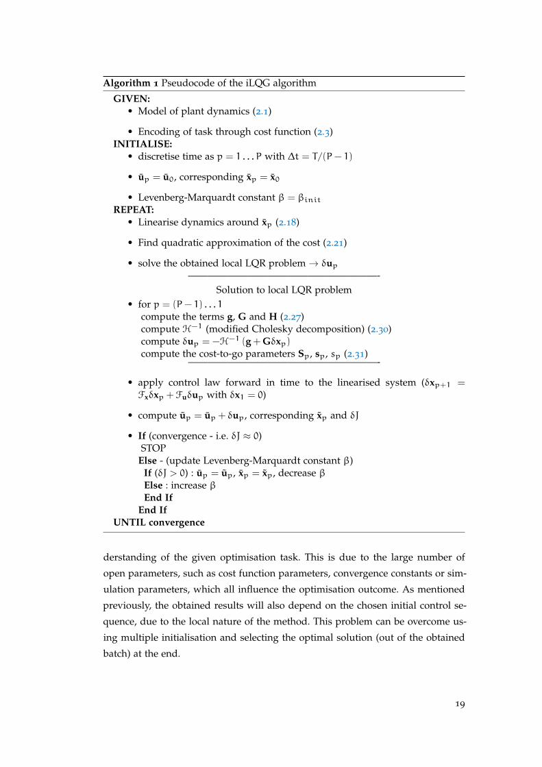
Algorithm 1 Pseudocode of the iLQG algorithm

GIVEN:• Model of plant dynamics (2.1)

• Encoding of task through cost function (2.3)INITIALISE:

• discretise time as p = 1 . . . P with ∆t = T/(P− 1)

• up = u0, corresponding xp = x0

• Levenberg-Marquardt constant β = βinitREPEAT:

• Linearise dynamics around xp (2.18)

• Find quadratic approximation of the cost (2.21)

• solve the obtained local LQR problem→ δup———————————————————-

Solution to local LQR problem• for p = (P− 1) . . . 1

compute the terms g, G and H (2.27)compute H−1 (modified Cholesky decomposition) (2.30)compute δup = −H−1 (g + Gδxp)compute the cost-to-go parameters Sp, sp, sp (2.31)

———————————————————-

• apply control law forward in time to the linearised system (δxp+1 =Fxδxp +Fuδup with δx1 = 0)

• compute up = up + δup, corresponding xp and δJ

• If (convergence - i.e. δJ ≈ 0)STOP

Else - (update Levenberg-Marquardt constant β)If (δJ > 0) : up = up, xp = xp, decrease βElse : increase βEnd If

End IfUNTIL convergence

derstanding of the given optimisation task. This is due to the large number of

open parameters, such as cost function parameters, convergence constants or sim-

ulation parameters, which all influence the optimisation outcome. As mentioned

previously, the obtained results will also depend on the chosen initial control se-

quence, due to the local nature of the method. This problem can be overcome us-

ing multiple initialisation and selecting the optimal solution (out of the obtained

batch) at the end.

19

When the control limits are reached within the solution, the algorithm resets the

feedback gains to zero. This allows iLQG to cope with bounds on the control input

(in a deterministic case), while in a stochastic scenario this problem can be avoided

by carefully shaping the cost function accordingly (i.e., adjusting the control cost

weights).

In addition to requiring smooth dynamics, in the currently existing implemen-

tation, iLQR/iLQG is designed to admit only predefined finite horizon tasks. The

task of choosing the time is left to the user and requires a significant amount of

tuning.

2.4 summary

In this chapter, we reviewed the main elements of OC theory. We summarised

the formulation and the main approaches, namely local and global methods. We

then presented the case of iterative techniques that constitute a good compromise

between the two. We focused on iLQG as our method of choice for investigation

and starting point for development.

In the next chapter, we introduce the concept of impedance modulation, which

creates redundancy in the controls. We present how this added DOF in the con-

trols can be exploited using OC and the benefits of impedance modulation, as

demonstrated by previous investigations. We expand on existing work by apply-

ing OC to a system capable of damping modulation, alongside that of stiffness

and position.

20

3O P T I M A L C O N T R O L O F S Y S T E M S E Q U I P P E D W I T H

VA R I A B L E I M P E D A N C E A C T U AT O R S

In this chapter we introduce the concept of actuators that allow for simultaneous

modulation of the joint position and impedance, called Variable Impedance Actuators

(VIAs). We present the difficulties raised by the task of planning for systems with

such redundancy in the controls. Then, we give a brief overview of their benefits

and previously used approaches.

We follow with a study on OC for an actuator capable of simultaneous and

independent physical damping and stiffness modulation. Using iLQG (Sec. 2.3.1),

we explore how variable physical damping can be exploited in the context of rapid

movements. Several numerical simulation results are presented, in addition to a

hardware experiment.

3.1 related work on the design of vias

The traditional approach regarding joint actuation used in robotic systems in the

past implies stiff dynamics. A stiff (non-VIA) actuator is capable to move to a spe-

cific position (or track a trajectory) with high accuracy; once the desired location

is reached, in the absence of a new command, it holds that position, regardless of

the external forces applied (within the design bounds).

This type of operation is acceptable in the case of robots acting in highly con-

strained environments, performing a well defined task that does not require adap-

tation, nor interaction with humans. Recent developments opened new areas where

robotic systems can be employed, some of which feature a changing environment

and working in close proximity to humans. This created a need for multifaceted

systems, able to meet these demands.

To address this need, several designs offering compliant actuation were imple-

mented [Vanderborght et al., 2012]. Most research has focused on the design of

Variable Stiffness Actuators (VSAs) [Ham et al., 2009]. These new implementations

showed significant improvement in terms of safety due to inbuilt compliance [Zinn

21

et al., 2004], energy efficiency, robustness to perturbations [Vanderborght et al.,

2013] and dynamic range [Hurst et al., 2004].

From the perspective of how the modulation of impedance is achieved we dis-

tinguish :

i active impedance, in which the hardware uses software control to emulate a

desired impedance behaviour [Loughlin et al., 2007]. This requires an actuator,

a sensor and a controller which are fast enough to create the desired result.

This technology is available in systems such as the DLR KUKA [Bischoff et al.,

2010] or the SARCOS robot [Bilodeau and Papadopoulos, 1998]. While this

approach has the capability of modulating the impedance in an on-line fashion,

for a theoretically infinite range and speed, it is unable to store energy or

exploit the natural dynamics [Vanderborght et al., 2013].

ii passive impedance, where the actuator contains a compliant element. This can

exhibit either fixed or adaptable impedance capabilities. Actuators in the latter

category are able to use their elastic components to store energy [Vanderborght

et al., 2013]. They require separate motors for position control and impedance

modulation. Most of the studies on design and control of such VIA focus on

stiffness modulation. In the next section we describe some of the available

implementations for these variable stiffness actuators (VSA).

variable stiffness actuators In terms of mechanical design for adapt-

able stiffness actuators in ii), three categories are distinguished [Vanderborght

et al., 2013]. Spring preload VSAs operate by modulating the pretension on a

spring (or a set of springs). A popular approach is the antagonistic design, with

antagonistic motors (e.g., Edinburgh SEA (Series Elastic Actuator) [Mitrovic et al.,

2010b] Fig. 3.1 (c)). There, two opposing actuators are used to modulate the posi-

tion (by moving in the same direction) and stiffness (by acting in opposite direc-

tions).

This has some deficiencies in terms of energy consumption: relying on co-contrac-

tion to increase stiffness requires the use of non-backdriveable actuators, otherwise

motor power must be used continuously to maintain a stable joint position at high

stiffness. Even if the appropriate actuators are selected, the energy cost of changing

stiffness from compliant to stiff can still be considerably high.

Using a design in which the motors are not opposed in the antagonistic way

allows for less energy consumption, a smaller volume and lower mass [Okada

et al., 2001; Zinn et al., 2004]. The series pretension design consists of a spring,

22

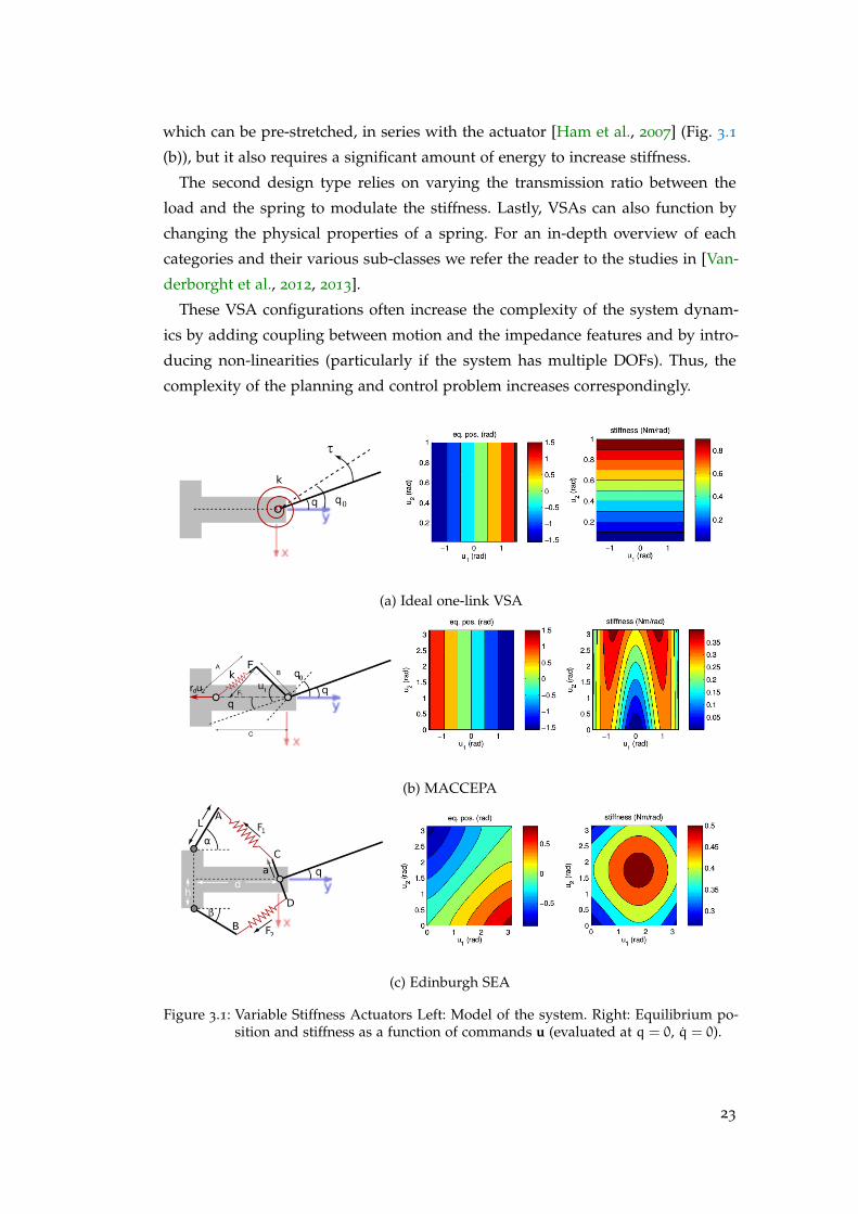
which can be pre-stretched, in series with the actuator [Ham et al., 2007] (Fig. 3.1

(b)), but it also requires a significant amount of energy to increase stiffness.

The second design type relies on varying the transmission ratio between the

load and the spring to modulate the stiffness. Lastly, VSAs can also function by

changing the physical properties of a spring. For an in-depth overview of each

categories and their various sub-classes we refer the reader to the studies in [Van-

derborght et al., 2012, 2013].

These VSA configurations often increase the complexity of the system dynam-

ics by adding coupling between motion and the impedance features and by intro-

ducing non-linearities (particularly if the system has multiple DOFs). Thus, the

complexity of the planning and control problem increases correspondingly.

(a) Ideal one-link VSA

(b) MACCEPA

(c) Edinburgh SEA

Figure 3.1: Variable Stiffness Actuators Left: Model of the system. Right: Equilibrium po-sition and stiffness as a function of commands u (evaluated at q = 0, q = 0).

23

3.2 model of a robotic system with compliant actuation

In this section we present a general model of a robotic system equipped with VSA

capabilities. We introduce the dynamics of the systems and the added complexity

of redundant actuation. We then address the question of control for such systems.

3.2.1 Robot Dynamics

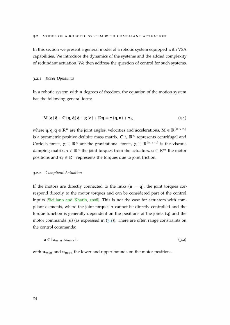
In a robotic system with n degrees of freedom, the equation of the motion system

has the following general form:

M (q) q + C (q, q) q + g (q) + Dq = τ (q, u) + τf, (3.1)

where q, q, q ∈ Rn are the joint angles, velocities and accelerations, M ∈ R(n x n)

is a symmetric positive definite mass matrix, C ∈ Rn represents centrifugal and

Coriolis forces, g ∈ Rn are the gravitational forces, g ∈ R(n x n) is the viscous

damping matrix, τ ∈ Rn the joint torques from the actuators, u ∈ Rm the motor

positions and τf ∈ Rn represents the torques due to joint friction.

3.2.2 Compliant Actuation

If the motors are directly connected to the links (u = q), the joint torques cor-

respond directly to the motor torques and can be considered part of the control

inputs [Siciliano and Khatib, 2008]. This is not the case for actuators with com-

pliant elements, where the joint torques τ cannot be directly controlled and the

torque function is generally dependent on the positions of the joints (q) and the

motor commands (u) (as expressed in (3.1)). There are often range constraints on

the control commands:

u ∈ [umin; umax] , (3.2)

with umin and umax the lower and upper bounds on the motor positions.

24

As mentioned previously, due to the nature of the VSAs, the relation between

the joint torques, joint angles and motor commands can be quite complicated 1:

τ(q, u) = AT (q, u)F(q, u), (3.3)

where A ∈ R(p x n)(p > n) is the moment-arm matrix, defined by the geometry of

the actuators, and F ∈ Rp are the corresponding forces due to the elastic elements

[Braun et al., 2012a] (determined by the physical characteristics of these elements).

The joint stiffness matrix (K ∈ R(n x n)) is defined as:

K(q, u) = −∂τ(q, u)∂q

=∂AT

∂qF + AT

∂F∂q

. (3.4)

In general this is a non-linear function of the state and commands and, depend-

ing on the implementation, the stiffness of the individual joints may be coupled

[Howard et al., 2011]. The formulation in (3.4) observes the dependencies between

the control inputs (u) and and the joint stiffness (K).

This dependency can allow independent modulation of the joint torques and

of the (passive) joint stiffness of the actuators, assuming the joint torque function

(3.3) is redundant with respect to the motor positions (i.e., m > n).

In an idealised VSA design (Fig. 3.1 (a) left) the stiffness and equilibrium po-

sition are directly controllable and independent, such that any combination is re-

alisable (within the actuator design capabilities). This is illustrated in Fig. 3.1 (a)

right panel where, any combination of equilibrium position (q0 = u1) and stiff-

ness (k = u2) is possible. However, real mechanisms rarely exhibit such idealised

behaviour.

By comparison, in the Mechanically Adjustable Compliance and Controllable

Equilibrium Position Actuator (MACCEPA [Ham et al., 2007] Fig. 3.1 (b)) and Ed-

inburgh series elastic actuator (Edinburgh SEA [Mitrovic et al., 2010b] Fig. 3.1 (c))

present much more intricate dependencies between the commands, equilibrium

position and stiffness. In the case of the MACCEPA the joint torque (3.3) is given

by:

τ (q,u1,u2) = κsBC sinα(1+

r u2 − (C−B)√B2 +C2 − 2BC cosα

), (3.5)

1 In several formulations the torque can depend on the joint velocity q (e.g., when considering vis-coelastic forces). The formulation used remains valid in those scenarios.

25

where B, C are shown in the diagram (Fig. 3.1 (b), left panel), r is the radius of

the drum attached to the pretensioning servo, α = u1 + q, and κs is the spring

constant of the spring. While the equilibrium position is only influenced by the

position of the first motor, the stiffness has a complex, non-linear dependency on

both the equilibrium position and spring pre-tension commands (Fig. 3.1 (b), right

panel).

Similarly, in the Edinburgh SEA (Fig. 3.1 (c)) the joint torque takes the form in:

τ(x, u) = −zT (a× F1 − a× F2), (3.6)

where z is the unit vector along the rotation axis, a = (a cosq,a sinq, 0)T , Fi (with

i ∈ 1, 2) are the forces due to the two springs. In this antagonistic design, there

is a highly non-linear relationship between the motor commands and the joint

equilibrium position and stiffness (Fig. 3.1 (c), right panel).

As shown by these examples, even a relatively simple VSA designs can present

quite a challenging task in terms of position and stiffness modulation. Simple pre-

sets, such as the duality principle [Anderson and Spong, 1988], are viable solutions

only for specific cases; in a real environment the robot has to adapt to changes in

the structure of the world and the tasks. This can only be achieved by continuous

and fast modulation of stiffness. The OC formulation can provide a good method-

ology for obtaining an adequate control strategy for such devices.

3.2.3 Optimal Control Formulation

In order to formulate an OC problem (Chapter 2.1), the system dynamics and a

performance index (cost function) are required. Given the previously described

robotic system with VSA, an adequate state-space representation would be:

x = f(x, u), (3.7)

where:

f=

x2

M−1(x1) (−C(x1, x2)x2 − g(x1) − Dx2 + τ(x1, x3))

(3.8)

and x =[xT1 ,xT2

]T=[qT ,qT

]T ∈ R2n. The range constraints on the motor positions

(3.2) can be incorporated as control constraints.

26

Given a cost functional (2.3), encoding the desired task, the optimal control u∗

defined in (2.4) can then be obtained using the methodology presented in Sec. 2.2.

Using the optimal control command obtained u∗ and the corresponding trajec-

tory x∗ =[q∗

Tq∗

T]T

, the optimal torques τ∗ and stiffness K∗ are obtained from

(3.3) and (3.4). The framework resolves the control redundancy (i.e., u ∈ Rm, m >

n) taking into consideration the specifics of the system (3.1), actuator (3.3) and task

(2.3) at hand [Nakamura and Hanafusa, 1987].

3.3 previous work on optimal control of vsas

As shown in the previous section, VSA configurations often increase the com-

plexity of the system dynamics by adding coupling between the motion and the

impedance features and by introducing non-linearities (particularly if the system

has multiple DOFs).

Various studies showed that, by fully including stiffness modulation in the op-

timisation problem, additional improvements can be achieved in terms of noise

rejection [Mitrovic et al., 2009]. In [Braun et al., 2012b] the energy efficiency of

a throwing movement is raised by controlling the control of actuator’s ability to

store and release energy. The same capability is explored for periodic tasks such as

brachiation [Nakanishi et al., 2011; Nakanishi and Vijayakumar, 2013]. In [Howard

et al., 2010] the authors show how a general impedance strategy for a hitting task

can be adapted to the particularities of a hardware implementation (i.e., actua-

tor and system dynamics). By devising a system specific solution, the dynamics

are fully exploited, ensuring a better task performance. Similarly, [Garabini et al.,

2011] showed how a much higher link velocity can be obtained when the VSA

capabilities are exploited for a hitting movement.

These results are consistent with observed patterns displayed by humans and

other biological systems in adapting their impedance under similar conditions

[Mitrovic et al., 2010c].

While stiffness modulation has been the focus of various studies, the damping

component of the impedance has been often overlooked. Our hypothesis is that

a VIA able to achieve simultaneous and independent stiffness and damping mod-

ulation would be able to combine the benefits of both approaches. There are, of

course, several difficulties, the most salient being the increase in complexity of the

system dynamics, and thus, of the planning and control problem.

27

In [Radulescu et al., 2012] we combine variable physical stiffness and damp-

ing in a single actuator using insights from adjustable dampers in haptic inter-

faces [Mehling et al., 2005; Srikanth et al., 2008]. In the next section, we present

the results obtained, which indicate that damping modulation, alongside those of

stiffness and position, can improve performance.

3.4 simultaneous and independent stiffness and damping modu-

lation

In this section we first discuss the issue of damping in the context of variable phys-

ical impedance actuation and present the hardware implementation employed in

our experiments. We then introduce the task used in our investigation and the

control framework employed for its realisation.

3.4.1 Damping in Variable Stiffness Actuators

To investigate the effects of damping modulation in this framework, we select the

simplest system available: a one-link compliant joint system moving on a horizon-

tal plane. The equation of motion (3.1) for such a system becomes:

Mq = τ+ τf. (3.9)

The torque from the actuators is defined in our case as τ = τk + τb, with τk and

τb representing the stiffness and damping torques, respectively.

An appropriate damping magnitude is required for the accurate control of the

VIA system. If the damping level is too low, oscillations occur during rapid move-

ments. If the level is too high, the response of the system becomes slow, rendering

many of the advantages of (variable) passive stiffness, such as energy storage, un-

exploitable. One may also say that, in general, it is natural to consider adding

variable damping to a system with variable stiffness in order to achieve an appro-

priate response (e.g., under-, over-, or critical damping) as the stiffness varies (for

a detailed analysis, see Appendix A). In the following, we explore these issues

with respect to a simple example of a variable stiffness actuator (VSA).

28

3.4.2 Example: Mechanically Adjustable Compliance and Controllable Equilibrium Posi-

tion Actuator

We selected for our experiments, as an example of a VSA that is easy to build and

intuitive to operate, the Mechanically Adjustable Compliance and Controllable

Equilibrium Position Actuator (MACCEPA), illustrated in Fig. 3.2.

uu

DAMPING

MOTOR

VARIABLE IMPEDANCE ACTUATOR

2

3

Figure 3.2: Mechanically Adjustable Compliance and Controllable Equilibrium PositionActuator (MACCEPA) [Ham et al., 2007] with Variable Damping: model (left)and robot (right). Parameters: r = 0.01m, B = 0.03m, C = 0.13m, link mass:0.125kg, link length: 0.295m, centre of mass location on the link: 0.1475m

The MACCEPA design allows simultaneous equilibrium position and joint stiff-

ness control by using two independently controlled servomotors (Fig. 3.1 (b),

right). The first servomotor (attached to the free-moving link) adjusts the position

of a lever of length B, while the second (attached to the base) adjusts the position

of a winding drum of radius r attached via a cord to the spring (Fig. 3.2, left).

The torque around the joint (3.5) is generated when a discrepancy is introduced

between the angle of the first servomotor u1 and that of the joint q (i.e., α :=

u1 − q 6= 0), thus extending the spring away from its rest length L0 = C − B.

The restorative spring force is F = −κs(l − l0), where κs is the spring constant

and l is the resultant length of the spring. The latter is given by the length A =

B2 + C2 − 2BCcosα (Fig. 3.2, left) plus any additional extension caused by the

pretensioning servo u2 , i.e., l = A+ ru2. The equilibrium position can be directly

controlled by setting q0 = u1, while the stiffness (k := −∂τ/∂q) is:

k (q,u1,u2) = κsBC cosα(1+

r u2 − (C−B)√B2 +C2 − 2BC cosα

)−κsB

2C2 sin2 α (ru2 − (C−B))

(B2 +C2 − 2BC cosα)32

. (3.10)

For full details of the derivation of the torque relationship (3.5) we refer the

reader to [Ham et al., 2007]. We note that, as with many VSA designs, the joint

29

torque and stiffness have a non-linear dependence on the joint and motor configu-

rations.

In addition to this existing design, we add a third control variable u3, corre-

sponding to damping modulation. Thus, for the combined system (MACCEPA

with Variable Damping, MACCEPA-VD) the torque relationship corresponding to

τ from (3.9) is:

τ (q, q,u1,u2,u3) = τk (q,u1,u2) + τb (q,u3) . (3.11)

The details of the mechanical design used are presented in Sec. 3.4.5.

3.4.3 Selecting the System Response

An adequate task-dependant system response is required for the efficient control

and operation of a VSA such as the MACCEPA. For periodic tasks, (e.g.,running),

we may desire an underdamped response, which will encourage oscillation through

the natural dynamics. On the other hand, in tasks such as tracking, we may re-

quire a response close to critical damping, to secure reaching the target reference

as quickly as possible while avoiding overshooting.

For one-link linear-time-invariant (LTI) systems, this is relatively straightfor-

ward, as the damping response is characterised by the damping ratio ξ:

ξ = b/2√kM, (3.12)

whereM represents the inertia, b the damping and k the stiffness. In an LTI system

selecting, for example, a critically damped response simply requires choosing b

such that ξ = 1.

However, systems equipped with VSA (e.g., k = k(q,u1,u2)) are not LTI by

definition. Choosing the damping response for such set-ups is non-trivial, and

requires the modulation of the damping b in a complex way. This is evident in the

case of the MACCEPA, given the nonlinear dependence of the stiffness (3.10) on

the joint and motor configurations.

Furthermore, since such systems are not LTI, the damping response is not well-

characterised through ξ as defined by (3.12) and so, for example, ensuring ξ = 1

(e.g., by coupling the stiffness and damping through (3.12)), may not result in

the fastest non-oscillatory response (i.e.,critical damping). This expectation is con-

firmed by the results obtained in our experiments (presented in Sec. 3.4.7).

30

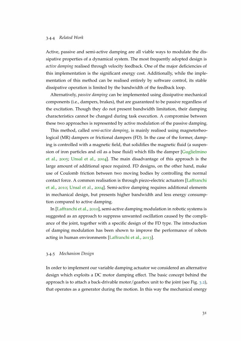
3.4.4 Related Work

Active, passive and semi-active damping are all viable ways to modulate the dis-

sipative properties of a dynamical system. The most frequently adopted design is

active damping realised through velocity feedback. One of the major deficiencies of

this implementation is the significant energy cost. Additionally, while the imple-

mentation of this method can be realised entirely by software control, its stable

dissipative operation is limited by the bandwidth of the feedback loop.

Alternatively, passive damping can be implemented using dissipative mechanical

components (i.e., dampers, brakes), that are guaranteed to be passive regardless of

the excitation. Though they do not present bandwidth limitation, their damping

characteristics cannot be changed during task execution. A compromise between

these two approaches is represented by active modulation of the passive damping.

This method, called semi-active damping, is mainly realised using magnetorheo-

logical (MR) dampers or frictional dampers (FD). In the case of the former, damp-

ing is controlled with a magnetic field, that solidifies the magnetic fluid (a suspen-

sion of iron particles and oil as a base fluid) which fills the damper [Guglielmino

et al., 2005; Unsal et al., 2004]. The main disadvantage of this approach is the

large amount of additional space required. FD designs, on the other hand, make

use of Coulomb friction between two moving bodies by controlling the normal

contact force. A common realisation is through piezo-electric actuators [Laffranchi

et al., 2010; Unsal et al., 2004]. Semi-active damping requires additional elements

in mechanical design, but presents higher bandwidth and less energy consump-

tion compared to active damping.

In [Laffranchi et al., 2010], semi-active damping modulation in robotic systems is

suggested as an approach to suppress unwanted oscillation caused by the compli-

ance of the joint, together with a specific design of the FD type. The introduction

of damping modulation has been shown to improve the performance of robots

acting in human environments [Laffranchi et al., 2013].

3.4.5 Mechanism Design

In order to implement our variable damping actuator we considered an alternative

design which exploits a DC motor damping effect. The basic concept behind the

approach is to attach a back-drivable motor/gearbox unit to the joint (see Fig. 3.2),

that operates as a generator during the motion. In this way the mechanical energy

31

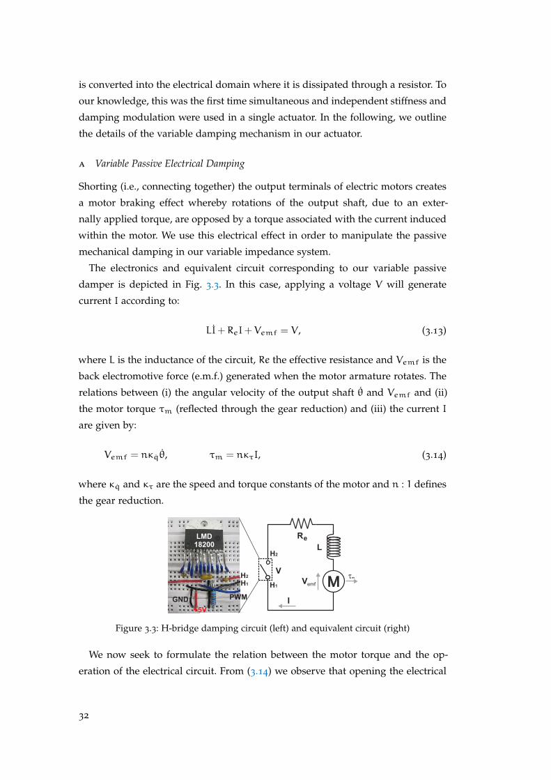
is converted into the electrical domain where it is dissipated through a resistor. To

our knowledge, this was the first time simultaneous and independent stiffness and

damping modulation were used in a single actuator. In the following, we outline

the details of the variable damping mechanism in our actuator.

a Variable Passive Electrical Damping

Shorting (i.e., connecting together) the output terminals of electric motors creates

a motor braking effect whereby rotations of the output shaft, due to an exter-

nally applied torque, are opposed by a torque associated with the current induced

within the motor. We use this electrical effect in order to manipulate the passive

mechanical damping in our variable impedance system.

The electronics and equivalent circuit corresponding to our variable passive

damper is depicted in Fig. 3.3. In this case, applying a voltage V will generate

current I according to:

LI+ ReI+ Vemf = V , (3.13)

where L is the inductance of the circuit, Re the effective resistance and Vemf is the

back electromotive force (e.m.f.) generated when the motor armature rotates. The

relations between (i) the angular velocity of the output shaft θ and Vemf and (ii)

the motor torque τm (reflected through the gear reduction) and (iii) the current I

are given by:

Vemf = nκqθ, τm = nκτI, (3.14)

where κq and κτ are the speed and torque constants of the motor and n : 1 defines

the gear reduction.

Figure 3.3: H-bridge damping circuit (left) and equivalent circuit (right)

We now seek to formulate the relation between the motor torque and the op-

eration of the electrical circuit. From (3.14) we observe that opening the electrical

32

circuit (i.e., I = 0) reduces the motor torque to zero τm = 0, while closing the

circuit, generates a torque dependent on V and θ. Additionally, if we assume that

the time constant τRL = L/R of the equivalent (RL) circuit is small 2 we can per-

form a steady-state approximation of the current as: I ≈ Iss = (V −Vemf)/Re, and

analytically approximate the torque relation:

τm = nκτIss =nκτ

ReV −

n2κτκq

Reθ. (3.15)

This connection shows that τm constitutes of a voltage dependent driving torque

(first term) and a motion dependent braking torque (second term). Correspond-

ingly, by shorting the terminals of the circuit together (i.e., V = 0), we can generate

viscous damping at the motor output shaft:

τb(θ) = −beθ = −n2κτκq

Reθ. (3.16)

This represents a purely passive damping provided by the motor in the absence

of any velocity feedback. As indicated by (3.16), the damping constant be depends

on the resistance of the equivalent circuit Re . Thus, by modulating this resistance,

we can achieve a variable passive damping effect. This can be obtained by dif-

ferent means, for example, we could add a mechanical variable resistor, digital

potentiometer, or another integrated circuit across the motor terminals to adjust

Re. In such a scenario the resistance of the equivalent circuit is the sum of the

internal resistance of the motor and the variable resistance component.

In our design, we do not employ variable resistance directly, but instead we

emulate its effect using an H-bridge (NSC: LMD18200) circuit. This circuit opens

and closes the connection between the motor terminals according to a PWM (pulse-

width modulation) signal with controllable duty cycle u3 ∈ [0, 1]. Consequently,

the damping is modulated according to the proportion of time the connection is

open or closed: if the connection is open the damping effect vanishes (i.e., u3 =

0 ⇒ τb = 0), while if the connection is closed maximal damping is achieved

(u3 = 1 ⇒ τb = −beθ). Experiments characterising the damping effect in our

robotic device are reported in Sec. 3.4.7.c. For details of the system identification

and estimation of the damping used in our work, please see Appendix B.

2 According to (3.13), the dynamics of the current follow an exponential tendency given by e−t/τRL.For our set-up, τRL = L/R = 7 × 10−5 (i.e., L = 1.37 × 10−3H, and Re = 20.2Ω ), making thesteady-state approximation of the current and the associated algebraic relation of the torque (3.15)feasible.

33

The variable damping mechanism described can be incorporated into numerous

VSAs by rigidly connecting the DC motor shaft to the rotating part of the joint. In

our implementation we use a spur gear rigidly attached to the free link to pick up

the joint rotation of the MACCEPA (see Fig. 3.2 (right)).

3.4.6 Control Framework

As discussed in Sec. 3.4.3, the non-linear, time-varying nature of many VIAs ren-

ders the appropriate selection of the damping a non-trivial task. In order to avoid

this difficulty, we use an optimal control approach to devise strategies for exploit-

ing this additional degree of freedom. We employ the iLQG control framework (as

described in Sec. 2.3.1).

In order to apply this control framework to the MACCEPA-VD, we define the

state and control inputs as x = (q, q)T = (x1, x2)T and u = (u1,u2,u3)T , respec-

tively. In this representation, we obtain q from (3.9) and replace it in (2.1), which

gives us:

x =

qq

=

x2

((τ(x, u) + τf)/J)

. (3.17)

The admissible command range, imposed by the mechanical stops in the ser-

vos and PWM restrictions, is (−π/2, 0, 0)T u (π/2,pi/2, 1)T . To encode the

objective of rapid, accurate reaching to some target, we define the cost function:

J =

∫T0

(q(t) − q∗)2 + εu(t)Tu(t)dt, (3.18)

where q∗ is the target point in joint space, and T is the maximum time duration

allowed for the movement.

We note that, the first term in (3.18) has several influences on the solution. Firstly,

it promotes rapid movement by penalising solutions for time spent away from the

target point q∗. Secondly, it ensures the system comes to a halt at the target (if the

target is reached before the final time T , the optimal solution is to remain there

to avoid incurring further costs). Finally, it penalises overshoot (i.e., deviations for

which q(t) − q∗ > 0). The second term acts to regularise solutions,with ε set to a

small constant value (in our experiments ε = 10−8).

34

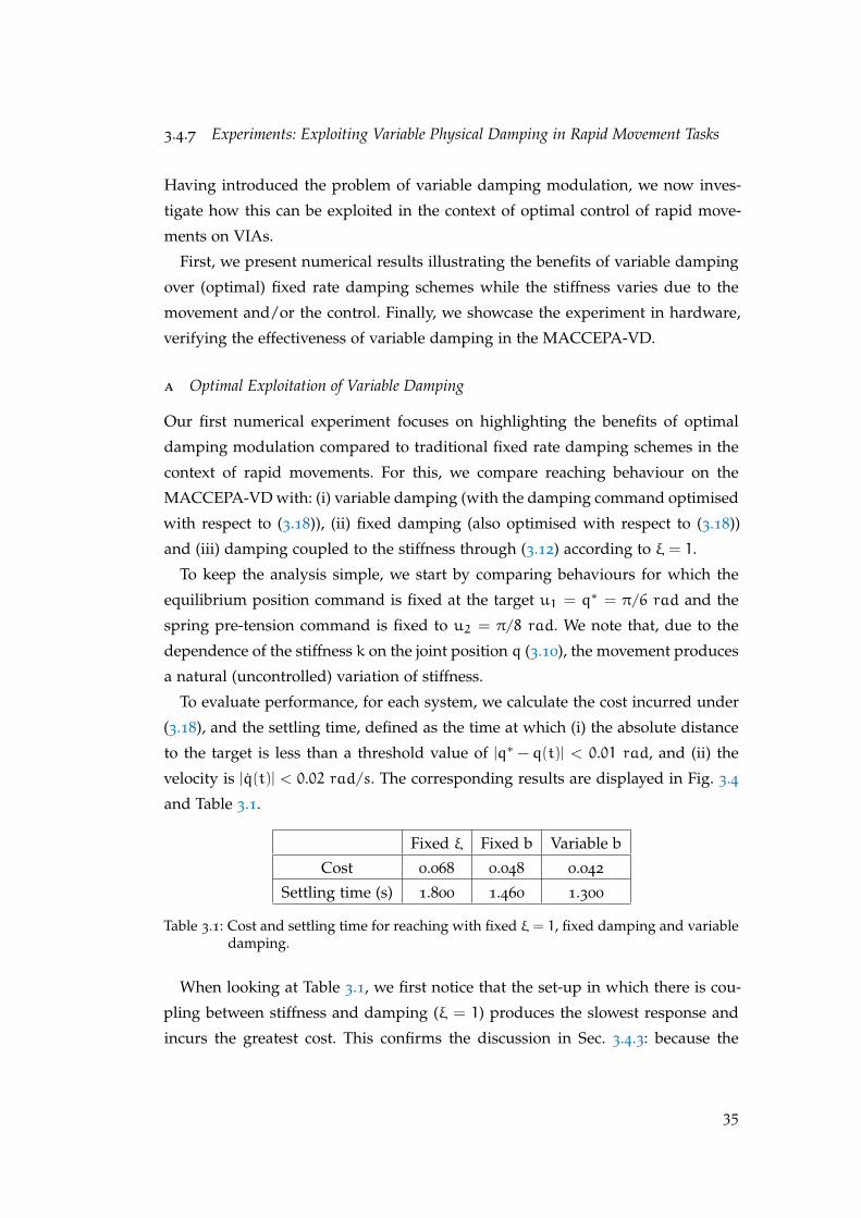
3.4.7 Experiments: Exploiting Variable Physical Damping in Rapid Movement Tasks

Having introduced the problem of variable damping modulation, we now inves-

tigate how this can be exploited in the context of optimal control of rapid move-

ments on VIAs.

First, we present numerical results illustrating the benefits of variable damping

over (optimal) fixed rate damping schemes while the stiffness varies due to the

movement and/or the control. Finally, we showcase the experiment in hardware,

verifying the effectiveness of variable damping in the MACCEPA-VD.

a Optimal Exploitation of Variable Damping

Our first numerical experiment focuses on highlighting the benefits of optimal

damping modulation compared to traditional fixed rate damping schemes in the

context of rapid movements. For this, we compare reaching behaviour on the

MACCEPA-VD with: (i) variable damping (with the damping command optimised

with respect to (3.18)), (ii) fixed damping (also optimised with respect to (3.18))

and (iii) damping coupled to the stiffness through (3.12) according to ξ = 1.

To keep the analysis simple, we start by comparing behaviours for which the

equilibrium position command is fixed at the target u1 = q∗ = π/6 rad and the

spring pre-tension command is fixed to u2 = π/8 rad. We note that, due to the

dependence of the stiffness k on the joint position q (3.10), the movement produces

a natural (uncontrolled) variation of stiffness.

To evaluate performance, for each system, we calculate the cost incurred under

(3.18), and the settling time, defined as the time at which (i) the absolute distance

to the target is less than a threshold value of |q∗ − q(t)| < 0.01 rad, and (ii) the

velocity is |q(t)| < 0.02 rad/s. The corresponding results are displayed in Fig. 3.4

and Table 3.1.

Fixed ξ Fixed b Variable b

Cost 0.068 0.048 0.042

Settling time (s) 1.800 1.460 1.300

Table 3.1: Cost and settling time for reaching with fixed ξ = 1, fixed damping and variabledamping.

When looking at Table 3.1, we first notice that the set-up in which there is cou-

pling between stiffness and damping (ξ = 1) produces the slowest response and

incurs the greatest cost. This confirms the discussion in Sec. 3.4.3: because the

35

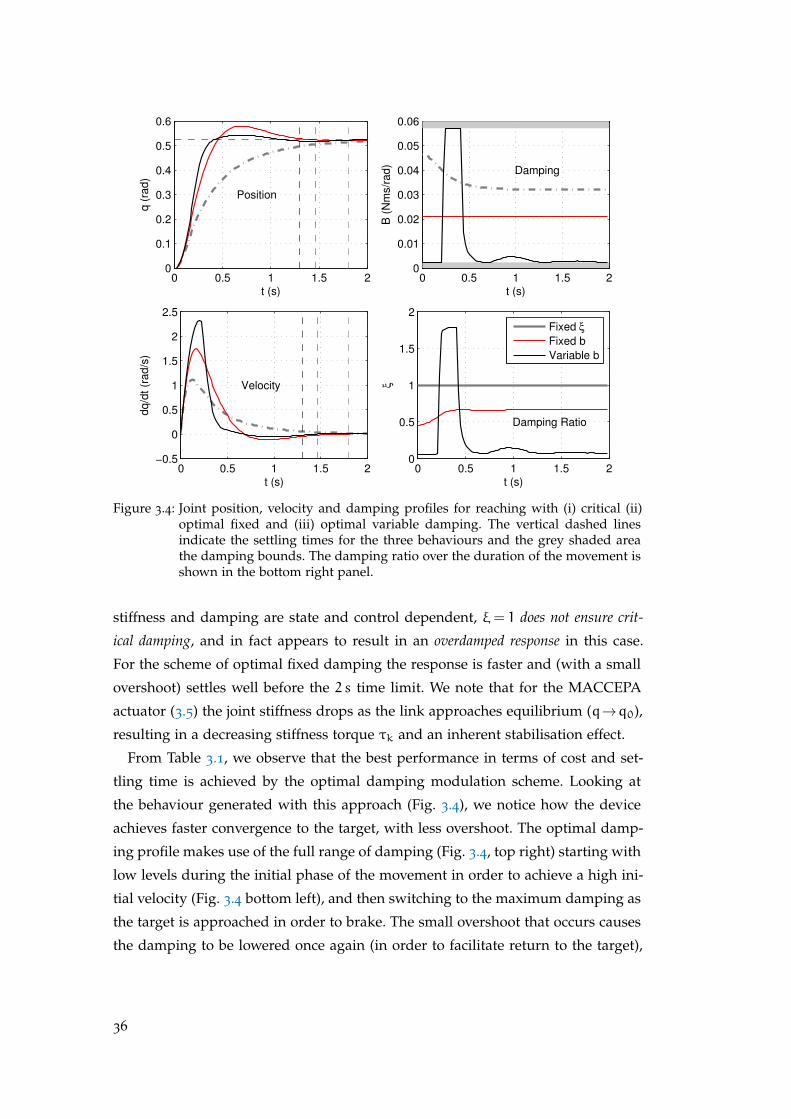
0 0.5 1 1.5 20

0.1

0.2

0.3

0.4

0.5

0.6

t (s)

q (

rad)

Position

0 0.5 1 1.5 20

0.01

0.02

0.03

0.04

0.05

0.06

t (s)

B (

Nm

s/r

ad)

Damping

0 0.5 1 1.5 2−0.5

0

0.5

1

1.5

2

2.5

t (s)

dq/d

t (r

ad/s

)

Velocity

0 0.5 1 1.5 20

0.5

1

1.5

2

t (s)

ξ

Damping Ratio

Fixed ξ

Fixed b

Variable b

Figure 3.4: Joint position, velocity and damping profiles for reaching with (i) critical (ii)optimal fixed and (iii) optimal variable damping. The vertical dashed linesindicate the settling times for the three behaviours and the grey shaded areathe damping bounds. The damping ratio over the duration of the movement isshown in the bottom right panel.

stiffness and damping are state and control dependent, ξ= 1 does not ensure crit-

ical damping, and in fact appears to result in an overdamped response in this case.

For the scheme of optimal fixed damping the response is faster and (with a small

overshoot) settles well before the 2 s time limit. We note that for the MACCEPA

actuator (3.5) the joint stiffness drops as the link approaches equilibrium (q→q0),

resulting in a decreasing stiffness torque τk and an inherent stabilisation effect.

From Table 3.1, we observe that the best performance in terms of cost and set-

tling time is achieved by the optimal damping modulation scheme. Looking at

the behaviour generated with this approach (Fig. 3.4), we notice how the device

achieves faster convergence to the target, with less overshoot. The optimal damp-

ing profile makes use of the full range of damping (Fig. 3.4, top right) starting with

low levels during the initial phase of the movement in order to achieve a high ini-

tial velocity (Fig. 3.4 bottom left), and then switching to the maximum damping as

the target is approached in order to brake. The small overshoot that occurs causes

the damping to be lowered once again (in order to facilitate return to the target),

36

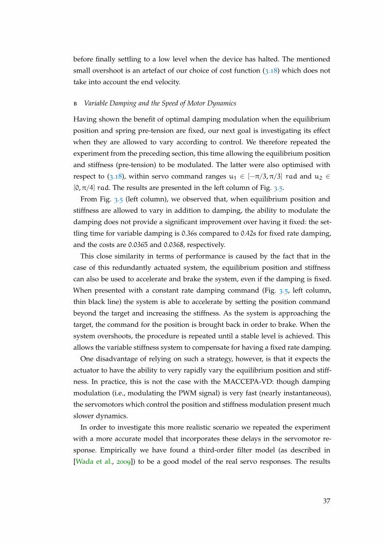
before finally settling to a low level when the device has halted. The mentioned

small overshoot is an artefact of our choice of cost function (3.18) which does not

take into account the end velocity.

b Variable Damping and the Speed of Motor Dynamics

Having shown the benefit of optimal damping modulation when the equilibrium

position and spring pre-tension are fixed, our next goal is investigating its effect

when they are allowed to vary according to control. We therefore repeated the

experiment from the preceding section, this time allowing the equilibrium position

and stiffness (pre-tension) to be modulated. The latter were also optimised with

respect to (3.18), within servo command ranges u1 ∈ [−π/3,π/3] rad and u2 ∈[0,π/4] rad. The results are presented in the left column of Fig. 3.5.

From Fig. 3.5 (left column), we observed that, when equilibrium position and

stiffness are allowed to vary in addition to damping, the ability to modulate the

damping does not provide a significant improvement over having it fixed: the set-

tling time for variable damping is 0.36s compared to 0.42s for fixed rate damping,

and the costs are 0.0365 and 0.0368, respectively.

This close similarity in terms of performance is caused by the fact that in the

case of this redundantly actuated system, the equilibrium position and stiffness

can also be used to accelerate and brake the system, even if the damping is fixed.

When presented with a constant rate damping command (Fig. 3.5, left column,

thin black line) the system is able to accelerate by setting the position command

beyond the target and increasing the stiffness. As the system is approaching the

target, the command for the position is brought back in order to brake. When the

system overshoots, the procedure is repeated until a stable level is achieved. This

allows the variable stiffness system to compensate for having a fixed rate damping.

One disadvantage of relying on such a strategy, however, is that it expects the

actuator to have the ability to very rapidly vary the equilibrium position and stiff-

ness. In practice, this is not the case with the MACCEPA-VD: though damping

modulation (i.e., modulating the PWM signal) is very fast (nearly instantaneous),

the servomotors which control the position and stiffness modulation present much

slower dynamics.

In order to investigate this more realistic scenario we repeated the experiment

with a more accurate model that incorporates these delays in the servomotor re-

sponse. Empirically we have found a third-order filter model (as described in

[Wada et al., 2009]) to be a good model of the real servo responses. The results

37

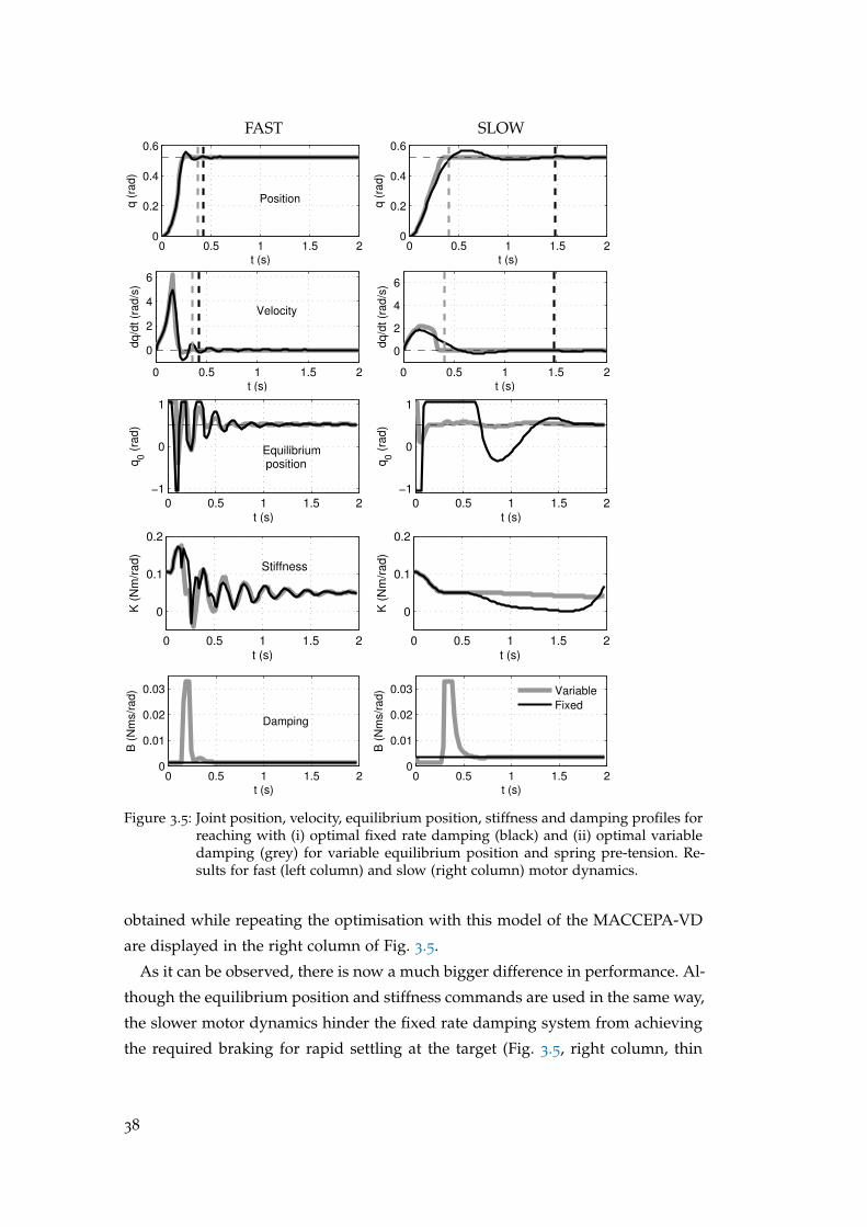
FAST SLOW

0 0.5 1 1.5 20

0.2

0.4

0.6

t (s)

q (

rad)

Position

0 0.5 1 1.5 20

0.2

0.4

0.6

t (s)

q (

rad)

0 0.5 1 1.5 2

0

2

4

6

dq

/dt

(ra

d/s

)

t (s)

Velocity

0 0.5 1 1.5 2

0

2

4

6

dq

/dt

(ra

d/s

)t (s)

0 0.5 1 1.5 2

−1

0

1

q0 (

rad)

t (s)

Equilibrium position

0 0.5 1 1.5 2

−1

0

1

q0 (

rad)

t (s)

0 0.5 1 1.5 2

0

0.1

0.2

K (

Nm

/ra

d)

t (s)

Stiffness

0 0.5 1 1.5 2

0

0.1

0.2

K (

Nm

/ra

d)

t (s)

0 0.5 1 1.5 20

0.01

0.02

0.03

B (

Nm

s/r

ad)

t (s)

Damping

0 0.5 1 1.5 20

0.01

0.02

0.03

t (s)

B (

Nm

s/r

ad)

Variable

Fixed

Figure 3.5: Joint position, velocity, equilibrium position, stiffness and damping profiles forreaching with (i) optimal fixed rate damping (black) and (ii) optimal variabledamping (grey) for variable equilibrium position and spring pre-tension. Re-sults for fast (left column) and slow (right column) motor dynamics.

obtained while repeating the optimisation with this model of the MACCEPA-VD

are displayed in the right column of Fig. 3.5.

As it can be observed, there is now a much bigger difference in performance. Al-

though the equilibrium position and stiffness commands are used in the same way,

the slower motor dynamics hinder the fixed rate damping system from achieving

the required braking for rapid settling at the target (Fig. 3.5, right column, thin

38

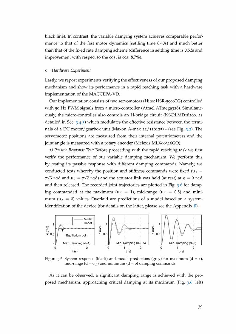
black line). In contrast, the variable damping system achieves comparable perfor-

mance to that of the fast motor dynamics (settling time 0.40s) and much better

than that of the fixed rate damping scheme (difference in settling time is 0.52s and

improvement with respect to the cost is cca. 8.7%).

c Hardware Experiment

Lastly, we report experiments verifying the effectiveness of our proposed damping

mechanism and show its performance in a rapid reaching task with a hardware

implementation of the MACCEPA-VD.

Our implementation consists of two servomotors (Hitec HSR-5990TG) controlled

with 50 Hz PWM signals from a micro-controller (Atmel ATmega328). Simultane-

ously, the micro-controller also controls an H-bridge circuit (NSC:LMD18200, as

detailed in Sec. 3.4.5) which modulates the effective resistance between the termi-

nals of a DC motor/gearbox unit (Maxon A-max 22/110125) - (see Fig. 3.2). The

servomotor positions are measured from their internal potentiometers and the

joint angle is measured with a rotary encoder (Melexis MLX90316GO).

1) Passive Response Test: Before proceeding with the rapid reaching task we first

verify the performance of our variable damping mechanism. We perform this

by testing its passive response with different damping commands. Namely, we

conducted tests whereby the position and stiffness commands were fixed (u1 =

π/3 rad and u2 = π/2 rad) and the actuator link was held (at rest) at q = 0 rad

and then released. The recorded joint trajectories are plotted in Fig. 3.6 for damp-

ing commanded at the maximum (u3 = 1), mid-range (u3 = 0.5) and mini-

mum (u3 = 0) values. Overlaid are predictions of a model based on a system-

identification of the device (for details on the latter, please see the Appendix B).

0 1 20

0.5

1

q (

rad

)

t (s)

Max. Damping (d=1)

Model

Robot

Equilibrium point

0 1 20

0.5

1

q (

rad)

t (s)

Mid. Damping (d=0.5)

0 1 20

0.5

1

q (

rad)

t (s)

Min. Damping (d=0)

Figure 3.6: System response (black) and model predictions (grey) for maximum (d = 1),mid-range (d = 0.5) and minimum (d = 0) damping commands.

As it can be observed, a significant damping range is achieved with the pro-

posed mechanism, approaching critical damping at its maximum (Fig. 3.6, left)

39

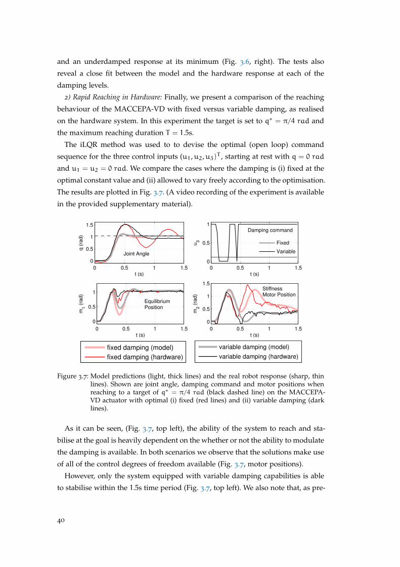
and an underdamped response at its minimum (Fig. 3.6, right). The tests also

reveal a close fit between the model and the hardware response at each of the

damping levels.

2) Rapid Reaching in Hardware: Finally, we present a comparison of the reaching

behaviour of the MACCEPA-VD with fixed versus variable damping, as realised

on the hardware system. In this experiment the target is set to q∗ = π/4 rad and

the maximum reaching duration T = 1.5s.

The iLQR method was used to to devise the optimal (open loop) command

sequence for the three control inputs (u1,u2,u3)T , starting at rest with q = 0 rad

and u1 = u2 = 0 rad. We compare the cases where the damping is (i) fixed at the

optimal constant value and (ii) allowed to vary freely according to the optimisation.

The results are plotted in Fig. 3.7. (A video recording of the experiment is available

in the provided supplementary material).

0 0.5 1 1.5

0

0.5

1

1.5

t (s)

q (

rad)

Joint Angle

0 0.5 1 1.5

0

0.5

1

t (s)

u3

Damping command

Fixed

Variable

0 0.5 1 1.5

0

0.5

1

t (s)

m1 (

rad)

EquilibriumPosition

0 0.5 1 1.5

0

0.5

1

1.5

t (s)

m2 (

rad)

StiffnessMotor Position

fixed damping (model)

fixed damping (hardware)

variable damping (model)

variable damping (hardware)

Figure 3.7: Model predictions (light, thick lines) and the real robot response (sharp, thinlines). Shown are joint angle, damping command and motor positions whenreaching to a target of q∗ = π/4 rad (black dashed line) on the MACCEPA-VD actuator with optimal (i) fixed (red lines) and (ii) variable damping (darklines).

As it can be seen, (Fig. 3.7, top left), the ability of the system to reach and sta-

bilise at the goal is heavily dependent on the whether or not the ability to modulate

the damping is available. In both scenarios we observe that the solutions make use

of all of the control degrees of freedom available (Fig. 3.7, motor positions).

However, only the system equipped with variable damping capabilities is able

to stabilise within the 1.5s time period (Fig. 3.7, top left). We also note that, as pre-

40

dicted in Sec. 3.4.7.b, the fixed rate damping scheme tries to compensate by using

the equilibrium position and pre-tension motors to brake. In the real device, the

relatively slow dynamics of the servomotors prevent it from doing so successfully.

3.5 discussion and conclusions

In this chapter we introduced the concept of VIAs. We discussed the difficulties

raised by the task of planning for systems equipped with them and presented

an overview of previous approaches. We highlighted the benefits of their use, as

outlined by preceding investigations.

A novel variable damping actuator for use in compliantly actuated systems was

presented in [Laffranchi et al., 2010]. The device was used to remove unwanted

oscillations occurring in such designs. In our work, we presented a mechanism

for implementing variable damping in variable physical impedance devices. As

opposed to the aforementioned device, this was the first time simultaneous and

independent stiffness and damping modulations were used in a single actuator

design.

We outlined how variable physical damping can be exploited through optimal

control in the context of rapid movement tasks. The simulation and hardware ex-

periments suggest a significant benefit of (i) variable damping over fixed ratio

damping schemes and (ii) variable damping over variable stiffness when consider-

ing the relative speed at which the two can be modulated.

The investigation focused on a rapid reaching task for a single link system. Fu-

ture work should extend these experiments, in order to to illustrate the role of

damping in multi-link variable impedance control and explore the relative bene-

fits of using variable damping versus variable stiffness in the context of energy

optimal behaviour.

In the next chapter we will build up on these results by addressing the optimal

control problem of robotic systems with VIAs in more complex scenarios. We will

present our optimisation framework, developed for handling the difficult domain

of switching dynamics and discontinuous state transitions.

41

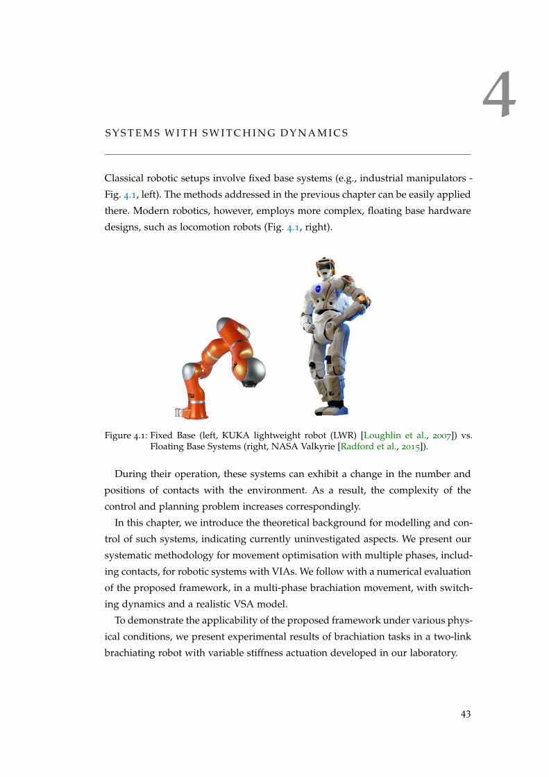
4S Y S T E M S W I T H S W I T C H I N G D Y N A M I C S

Classical robotic setups involve fixed base systems (e.g., industrial manipulators -

Fig. 4.1, left). The methods addressed in the previous chapter can be easily applied

there. Modern robotics, however, employs more complex, floating base hardware

designs, such as locomotion robots (Fig. 4.1, right).

Figure 4.1: Fixed Base (left, KUKA lightweight robot (LWR) [Loughlin et al., 2007]) vs.Floating Base Systems (right, NASA Valkyrie [Radford et al., 2015]).

During their operation, these systems can exhibit a change in the number and

positions of contacts with the environment. As a result, the complexity of the

control and planning problem increases correspondingly.

In this chapter, we introduce the theoretical background for modelling and con-

trol of such systems, indicating currently uninvestigated aspects. We present our

systematic methodology for movement optimisation with multiple phases, includ-

ing contacts, for robotic systems with VIAs. We follow with a numerical evaluation

of the proposed framework, in a multi-phase brachiation movement, with switch-

ing dynamics and a realistic VSA model.

To demonstrate the applicability of the proposed framework under various phys-

ical conditions, we present experimental results of brachiation tasks in a two-link

brachiating robot with variable stiffness actuation developed in our laboratory.

43

The contacts between the robotic systems and the environment increase the com-

plexity of the planning and control problem. Thus, we begin by giving an overview

of the main approaches for modelling them.

4.1 contact modelling

As two bodies come into contact, the generic collision between them is described

by the forces acting (i) along the line of impact (normal to the tangential plane at

the contact point [Meriam and Kraige, 2012]) and (ii) along the tangential plane

[Brach, 2007]. The coefficient of restitution acts along the normal direction (i) and is

a measure of the kinetic energy remaining at the end of the impact for the objects

to recoil, compared to the energy dissipated during the impact [Brach, 2007]. It

is formally defined as the ratio between the relative speed of the objects before

and after the collision [McGinnis, 2005]. The tangential coefficients (ii) refer to the

friction acting along the point (or area) of collision.

In dealing with contact analysis, the approaches are traditionally separated into

two main categories: discrete and continuous methods [Gilardi and Sharf, 2002]. In

the case of discrete (impulse momentum) methods, the impact is instantaneous. The

forces are impulsive, the kinetic variables have discontinuous changes, while no

displacement occurs during the impact and the other finite forces are deemed

negligible. Parameters such as the coefficient of restitution and impact ratio are

used to model the energy transfer [Wang and Mason, 1992]. On the tangential

direction, kinematic constraints, securing that no displacement occurs during the

impact, are introduced. Several models (e.g., Newton’s [Whittaker, 1970], Pois-

son’s [Routh et al., 1960], Stronge’s [Stronge, 1991]) are available, differentiated by

the way in which the aforementioned parameters are defined. The discrete formu-

lation is mainly employed for rigid body collisions. It does not extend easily to

general scenarios (e.g., multiple contact points) and relies on Coulomb’s law for

modelling friction, which has been reported to lead to inconsistencies or multiple

solutions [Gilardi and Sharf, 2002].

In the case of continuous (forced based) methods, the interaction forces act con-

tinuously; thus, they can be inserted in the equation of motion, for the duration

of the contact [Gilardi and Sharf, 2002]. The continuous analysis can be split into

two approaches: i) considering the contact model as an explicit functional rela-

tion between the contact forces and the generalised coordinates and their rates

[Deguet et al., 1998; Vukobratovic and Potkonjak, 1999], or ii) taking into account

44

the deformation caused by the contact [Bathe and Bouzinov, 1997; Farahani et al.,

2000]. The continuous formulation is not restricted to using Coulomb’s friction

model and allows generalisation. However, it can require tuning of the contact

parameters, which is non-trivial [Gilardi and Sharf, 2002].

Contacts with the environment introduce discontinuities in the dynamics of the

robotic systems and several methods for modelling their effect have been devel-

oped. While continuous methods allow a better generalisation, they necessitate sig-

nificant more tuning of the parameters than their discrete counterparts. Given a

system operating in domains with contacts the question of control becomes more

complicated. In the following section we discuss the main approaches for applying

OC in such scenarios.

4.2 optimal control of systems in domains with contacts

The traditional OC formalism introduced in Sec. 2.2 is designed to handle smooth,

continuous systems dynamics for tasks over a predetermined time horizon. In

order to cope with discontinuities introduced by varying contacts, several modifi-

cations were developed. In the following section, we present some of the resulting

approaches and their applications.

4.2.1 Hybrid Dynamics Formulation

Dynamics with intermittent contacts and impacts, such as locomotion and jug-

gling, are often modelled as hybrid dynamical systems [Bätz et al., 2010; Grizzle

et al., 2001; Long et al., 2011; Rosa Jr. et al., 2012]. This formulation consist of sets

of piece-wise continuous dynamics (4.1) and discontinuous state transition (4.2),

which encode the effect of a contact event:

x = fi(x, u), i ∈ I = 1, 2, · · · ,M, (4.1)

x+ = ∆(x−), (4.2)

where fi : Rn ×Rm → Rn is the i-th continuous dynamics function, x ∈ Rn

is the state vector, u ∈ Rm is the control input vector and I is the set of indices

for the continuous dynamics functions. When the dynamics switch from function

fi−1 to fi an instantaneous discontinuous state transition is assumed according to

45

the impact map ∆ which maps a pre-impact condition (x−) to a post-impact state

(x+).

Traditionally, when discussing the switching dynamics of the hybrid dynamical

systems, two classes emerge: time-based and state-based switching formulation. In

the time-based switching case, the discontinuous state jump occurs at a predefined

time : x = fi(x, u) for ti−1 6 t < ti. When the switching time is met, the mapping

∆ acts upon the state.

In state-based switching, the discontinuous jump arises when certain state con-

ditions are met. These systems can be more formally described using hybrid au-

tomata, which is an extension of the finite-state machine formalism [Lunze et al.,

2009]. Each discrete state is associated with a differential (or difference) equation,

describing the continuous evolution of the system in that state. Depending on the

complexity of the system, the encoding of the switching rules can be quite elabo-

rate.

4.2.2 Control Approaches using Hybrid Dynamics

From a control theoretic perspective, a significant effort was made to address op-

timal control problems of various classes of hybrid systems [Branicky et al., 1998;

Shaikh and Caines, 2007; Sussmann, 1999; Xu and Antsaklis, 2002, 2003a].

An extension of the Pontryagin’s Minimum Principle (Sec. 2.2), was developed

for the hybrid setting in the form of the Hybrid Minimum Principle (HMP) [Pic-

coli, 1998]. The HMP was applied to specific classes of systems, while considering

impact maps as either controls or constraints. By introducing realistic constraints

on the dynamics, the validity of the solution (for direct application on a hardware

platform) was ensured.

In [Long et al., 2011] state based switching is used and impacts were treated as

instantaneous state transition. The open-loop solution was obtained by first order

gradient descent. The convergence rate is much lower than that offered by second

order methods but, obtaining an explicit expression for the second order derivative

proved too exhausting even for simple cases, as the authors note.

Solving hybrid optimal control problems with state based switching is challeng-

ing even if the number and the sequence of switching are known a priori. This is

partially due to the need for additional constraints ensuring the states lie on the

switching surface at the time of switching. Finding this time is an ambitious task,

46

as it depends on the control commands and finding an analytic expression for it

is generally difficult [Xu and Antsaklis, 2003b].

In spite of the substantial amount of research on hybrid dynamics, examples in

the OC literature are confined to low-dimensional and simple dynamical systems,

and only a few robotic applications can be found for optimisation of movements

over multiple phases [Buss et al., 2002; Long et al., 2011].

4.2.3 Alternative Approaches to using Hybrid Dynamics

Instead of using hybrid dynamics modelling, different optimisation approaches

were proposed for dealing with multiple contact events, such as model predictive

control (MPC) [Camacho and Alba, 2013]. The method delivers an optimal solution

for a finite time horizon, but only applies it for the first step, after which the

process is repeated.

For example, [Erez et al., 2011] combines offline trajectory optimisation and on-

line MPC. The limit cycle of a periodic movement is found by offline optimisation

with an infinite-horizon average cost, while on-line MPC is used to obtain an op-

timal feedback control law. Another study [Kulchenko and Todorov, 2011], gener-

alises MPC from the usual finite horizon (or receding horizon) setup to a first-exit

setting (i.e., a solution is founds based on the assumption of an exit state), which

avoids dealing with discontinuities in the on-line optimisation phase. A modified

iLQG (Sec. 2.3.1) algorithm is used for on-line optimisation by running the for-

wards pass not for a predefined number of steps, but until it hits a terminal state.

However, as observed in [Rawlik, 2013], first-exit strategies can result in a poten-

tially suboptimal solution.

The work in [Tassa et al., 2012] proposes an iLQG based MPC with smooth ap-

proximation of contact forces without the need of switching dynamics. In [Posa

et al., 2014], the contact forces are explicitly included as constraints (using comple-

mentarity conditions) and directly optimised, together with the trajectories and

control commands, using sequential quadratic programming. As noted in the pre-

vious section, such state-based switching approaches can be very challenging, as

they require introducing additional constraints.

In [Morimoto and Atkeson, 2003] Minimax Differential Dynamic Programming

is used to find the control policy for a bipedal robotic system. The optimisation is

performed over the continuous dynamics for one step of walking. An impulse map

is used to compute the velocity change at the ground contact in the terminal cost

47

in order to ensure the periodicity of the trajectory (heel strike is always assumed to

occur at the fixed final time). However, the cost function is formulated for tracking

a given nominal trajectory obtained by a hand-tuned controller, while minimising

the control cost.

So far we have reviewed the major challenges posed by the introduction of

changing contacts for the planning and control problem. We have showed how

these contacts can be encoded and presented several approaches used to obtain

an OC solution for systems operating under these conditions. We have not yet

addressed the added difficulty of undertaking this task for systems with VIAs.

4.3 optimal impedance modulation and passive dynamics exploita-

tion in domains with contacts

For robotic systems performing a periodic task, actuators equipped with mechan-

ical compliance allow for energy storage [Stramigioli et al., 2008]. Exploiting the

compliance of the mechanical design reduces the energy input of the motor. In

[Sreenath et al., 2011] the energy consumption of the bipedal robot MABEL is

lowered by using the compliance caused by negative work at the time of impact,

instead of activating the actuators. In robot running, [Karssen and Wisse, 2011]

presents numerical studies to demonstrate that an optimised nonlinear leg stiff-

ness profile could improve robustness against disturbances. The importance of

exploitation of the intrinsic passive dynamics for efficient actuation and control is

discussed in the study of passive dynamic walking, where biped robots with no

or minimal actuation can exhibit human-like natural walking behaviour [Collins

et al., 2005].

Hybrid dynamics are an established way of describing the behaviour of realistic

robotic systems operating in domains with contacts. In our work we employ this

formulation alongside time-based switching for encoding the system dynamics.

We choose time-based switching with the aim of improving the tractability of the

optimisation problem (due to the difficulties raised by the state-based switching

formulation). The first system we use to showcase the benefits of our approach is

a two-link brachiation robot.

The brachiation system incorporates all the elements we are interested in ad-

dressing in our work (i.e., switching dynamics, caused by contacts with the envi-

48

ronment, VIA capabilities). Thus, it constitute a good test platform for showcasing

the benefits of our developed framework.

Next, we present relevant work conducted on robotic brachiation, in which the

system uses a form of locomotion inspired by that of primates, defined by swing-

ing from handhold to handhold like a pendulum [Eimerl and DeVore, 1966; Saito

et al., 1994]. Explicit exploitation of the passive dynamics with the help of gravity

is required in order to achieve the task.

control of brachiation systems Designing a brachiating controller is

a challenging problem since the system is underactuated (i.e., there is no actua-

tion at the handhold gripper). Significant efforts were made regarding control for

a class of underactuated systems, especially from a theoretical perspective [Luca

and Oriolo, 2002; Lynch et al., 2000; Nakamura et al., 1997; Spong, 1995]. A signif-

icant proportion this work [Lynch et al., 2000; Nakamura et al., 1997] focused on

motion planning for underactuated manipulators in a horizontal plane, and thus

not focusing on the influence of gravity. In these scenarios, the dynamic coupling

of link inertia is exploited during movement, rather than the passive dynamics

under gravity, as in the case of manipulators moving in the vertical plane.

In [Nakanishi et al., 2000] a brachiation system is controlled using active cancel-

lation of the plant dynamics with input-output linearisation to force the robot to

mimic the specified pendulum-like motion described in terms of target dynamics.

In [Nakanishi et al., 2011] temporal and stiffness optimisation for a brachiation

task are shown to result in lower control effort. In [Meghdari et al., 2013], a mul-

tiple shooting method is used to find optimal trajectories and the final time for a

single swing movement. The resulting behaviour is shown to reduce the control

effort in comparison to the method proposed in [Nakanishi et al., 2000].

In [Gomes and Ruina, 2005] passive brachiation is achieved by finding numer-

ical solutions for the initial conditions which lead to periodically continuous lo-

comotion without any joint torques. The work in [Rosa Jr. et al., 2012] extends

these results by investigating open-loop stable (unactuated downhill and powered

uphill) brachiation of a two-link model in the context of hybrid systems control, in-

cluding switching and discontinuous transitions. Motivated by this work [Gomes

and Ruina, 2005], we show that highly dynamic tasks, such as brachiation, can be

achieved by exploiting passive dynamics with simultaneous stiffness and temporal

optimisation in a compliantly actuated robot.

49

4.4 developed framework outline

As discussed in the previous sections, although a significant amount of research

addressed OC of hybrid systems, few applications focusing on movement opti-

misation over multiple switching events can be found and optimal impedance

modulation has not come under close study.

In our work we address these issues. We have already used OC of VIA, in the

form of stiffness and damping modulation in a single actuator, for a fixed base

robotic system (Sec. 3.4). We extend this research to robotic systems in domains

with contacts. Since the actuator is equipped with mechanical compliance, it can

be used to store energy [Stramigioli et al., 2008].

Thus, we suggest an approximate approach to the hybrid optimal control prob-

lem. We model the multiple phases of movement as time-based switching hybrid

dynamics assuming that the sequence of switching is known. In this set-up, we

address the following aspects:

1. Time-based switching dynamics with continuous control input

2. Discrete state transition

3. Realistic plant dynamics with a VSA model

4. Composite cost function for a multi-phase movement task

5. Optimisation of control command and stiffness

6. Optimisation of switching instances

7. Optimisation of final time (total movement duration)

The proposed formulation also delivers an optimal feedback control law, while

many trajectory optimisation algorithms typically provide only optimal feed for-

ward controls. While elements addressed in our approach have been treated sepa-

rately in previous works [Caldwell and Murphey, 2011a; Egerstedt et al., 2003; Xu

and Antsaklis, 2004], this is, to our knowledge, the first investigation to consider

all these issues at the same time.

The rest of this chapter is organised as follows: first, the hybrid optimal control

problem with time-based switching is formulated. Next, we present an iterative

solution method by extending the iterative linear quadratic regulator (iLQR) algo-

rithm [Li and Todorov, 2007] (Sec. 2.3.1), in order to incorporate switching dynam-

ics and discrete state transition. In addition, we present a temporal optimisation

algorithm for hybrid dynamics.

50

In the evaluation, we start by introducing a two-link brachiation system equipped

with a VSA with switching dynamics and discrete state transition. We showcase

the benefits and the effectiveness of our approach with experiments in simulation

and on a real hardware implementation.

4.5 optimisation framework formulation

4.5.1 Hybrid Dynamics with Time-Based Switching and Discrete State Transition

Consider a class of hybrid systems, as introduced in Sec. 4.2.1. Employing the time

based switching formulation [Xu and Antsaklis, 2003b] (4.1), (4.2) can be rewritten

in a more intuitive representation as in [Caldwell and Murphey, 2011b]:

x = fij(x, u), Tj 6 t < Tj+1 (4.3)

x(T+j ) = ∆(x(T−j )), (4.4)

with the finite number of switching given as K and the timed switching sequence

σ in [T0, Tf] is defined as [Xu and Antsaklis, 2003b] :

σ = ((T0, i0), (T1, i1), · · · , (TK, iK)), (4.5)

where T0 6 T1 6 · · · 6 TK 6 Tf = TK+1 (i.e., monotonically increasing switching

instances) and ij ∈ I for j = 0, · · · ,K. At t = Tj, the subsystem switches from

ij−1 to ij and subsystem ij is active for Tj 6 t < Tj+1. In our work, the sequence

of switching is assumed to be given. Figure 4.2 depicts a schematic diagram of a

hybrid system we consider in this investigation.

4.5.2 Robot Dynamics with Variable Stiffness Actuation

Using the general formulation introduced above, an individual rigid body dynam-

ics model (Sec. 3.2) is defined for each phase of the movement. Thus, we consider

the robot dynamics with variable stiffness actuation from (3.1):

Mi(q)q + Ci(q, q)q + gi(q) + Diq = τ(q, qm), (4.6)

where i denotes the i-th subsystem. At the same time, the positions of the motors

(qm) are not always instantaneously modulated though the motor commands (u),

51

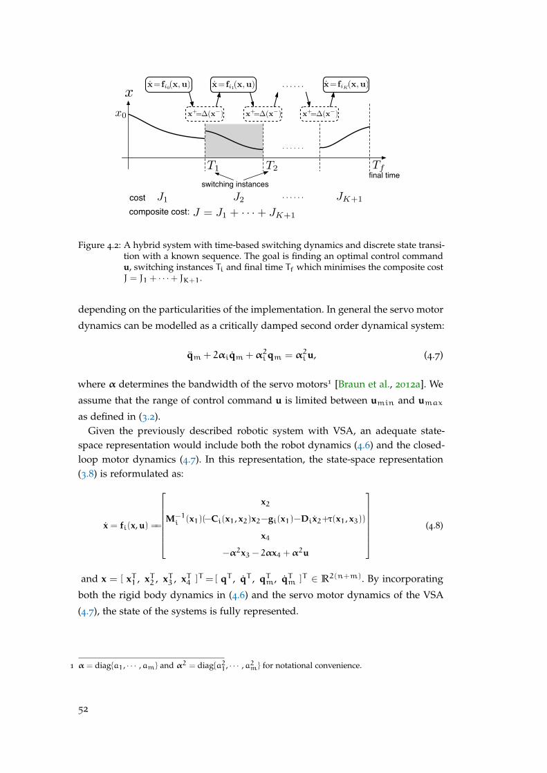
T1 T2

x

x0

JK+1J2J1J = J1 + · · ·+ JK+1

switching instancesfinal time

cost

composite cost:

x+=∆(x−)

x= fi0(x,u) x= fi1(x,u) x= fiK(x,u)

x+=∆(x−) x+=∆(x−)

Tf

· · · · · ·

· · · · · ·

· · · · · ·

Figure 4.2: A hybrid system with time-based switching dynamics and discrete state transi-tion with a known sequence. The goal is finding an optimal control commandu, switching instances Ti and final time Tf which minimises the composite costJ = J1 + · · ·+ JK+1.

depending on the particularities of the implementation. In general the servo motor

dynamics can be modelled as a critically damped second order dynamical system:

qm + 2αiqm +α2iqm = α2iu, (4.7)

where α determines the bandwidth of the servo motors1 [Braun et al., 2012a]. We

assume that the range of control command u is limited between umin and umaxas defined in (3.2).

Given the previously described robotic system with VSA, an adequate state-space representation would include both the robot dynamics (4.6) and the closed-loop motor dynamics (4.7). In this representation, the state-space representation(3.8) is reformulated as:

x = fi(x, u) ==

x2

M−1i (x1)(−Ci(x1, x2)x2−gi(x1)−Dix2+τ(x1, x3))

x4

−α2x3 − 2αx4 +α2u

(4.8)

and x = [ xT1 , xT2 , xT3 , xT4 ]T =[ qT , qT , qTm, qTm ]T ∈ R2(n+m). By incorporating

both the rigid body dynamics in (4.6) and the servo motor dynamics of the VSA

(4.7), the state of the systems is fully represented.

1 α = diaga1, · · · ,am and α2 = diaga21, · · · ,a2m for notational convenience.

52

4.5.3 Multi Phase Movement Cost Function

For the given dynamics we consider the composite cost function:

J = φ(x(Tf)) +K∑j=1

ψj(x(T−j )) +

∫TfT0

r(x, u)dt (4.9)

to describe the full movement with multiple phases, where φ(x(Tf)) is the terminal

cost, ψj(x(T−j )) is the via-point cost at the j-th switching instance and r(x, u) is the

running cost.

Using traditional OC approaches, each cost function can be (locally) optimised,

however, the total cost J =∑K+1j=1 Jj may be suboptimal. Under sequential optimi-

sation of separate cost functions, the via-point states for the j-th sequence may not

be necessarily optimal depending on the choice of the via-point cost ψj. This is

because separate optimisation does not consider future consequences of optimisa-

tion beyond the time horizon of Tj+1 when minimising the j-th cost function.

For a given set of plant dynamics (4.3) and state transition (4.4), the optimisation

problem we consider is to i) find an optimal feedback control law u = u(x, t) which

minimises the composite cost (4.9) and ii) simultaneously optimise the switching

instances T1, · · · , Tk and the final time Tf.

4.5.4 Developed Multi-Phase Optimisation Method

In this section, we first extend iLQR (deterministic version of iLQG presented

in Sec. 2.3.1 [Li and Todorov, 2007] 2) in order to incorporate timed switching

dynamics with discrete and discontinuous state transitions. We then present a

temporal optimisation algorithm to optimise the switching instances and the total

movement duration.

a Optimal Control of Switching Dynamics and Discrete State Transition

The iLQR method solves an optimal control problem by performing a locally linear

quadratic approximation of the nonlinear dynamics and the cost function around

a nominal trajectory x and control sequence u in discrete time, and iteratively

improves the solutions.

2 In this work, we assume deterministic plant dynamics.

53

In order to incorporate switching dynamics and discrete state transition with a

given switching sequence σ (4.5), the hybrid dynamics (4.3) and (4.4) are linearised

in discrete time around the nominal trajectory and control sequence as:

δxk+1 = Akδxk + Bkδuk (4.10)

δx+kj = Γkjδx−kj

(4.11)

Ak = I +∆t∂fij∂x

∣∣∣x=xk

, Bk = ∆t∂fij∂u

∣∣∣u=uk

(4.12)

Γkj = ∂∆∂x

∣∣x=x−kj

(4.13)

where δxk = xk − xk and δuk = uk − uk, k is the discrete time step and ∆t is the

sampling time, kj is the j-th switching instance in the discredited time step.

The composite cost function (4.9) is locally approximated in a quadratic form

as:

δJ = δxTNφx +1

2δxTNφxxδxN +

K∑j=1

(δxTk−jψjx +

N∑k=1

(δxTkrx + δuTkru

+1

2δxTkrxxδxk +

1

2δuTkruuδuk + δukruxδxk

)∆t (4.14)

and the optimal cost-to-go function is locally approximated as:

vk(δxk) =1

2δxTkSkδxk + δxTksk. (4.15)

The local control law:

δuk = lk + Lkδxk (4.16)

is obtained from the Bellman equation:

vk(δxk) = minδurk(δxk, δuk) + vk+1(δxk+1), (4.17)

by substituting (4.10) and (4.15) into the equation (4.17), where rk is the local

approximation of the running cost in (4.14).

54

The cost-to-go parameters Sk, sk in (4.15) are updated with a modified Riccati

equations: 3

Sk = rxx+ATkSk+1Ak + LTkHLk + LTkG + GTLk, (4.18)

sk = rx + ATksk+1 + LTkHlk + LTkg + GT lk, (4.19)

with:

H = ruu + BTkSk+1Bk, (4.20)

G = rux + BTkSk+1Ak, (4.21)

g = ru + BTksk+1. (4.22)

At the instance of discrete state transition k = kj, the following cost-to-go pa-

rameter update is added:

S−kj

= ψjxx + ΓTkj

S+kjΓkj , (4.23)

s−kj = ψjx + ΓTkj

s+kj , (4.24)

which is derived from the Bellman equation:

vkj(δx−kj) = costkj + vkj(δx

+kj) at k = kj, (4.25)

where ψjkj(δx−kj) is the local approximation of the via-point cost in (4.14).

Once we have a locally optimal control command δu, the nominal control se-

quence is updated as u← u+ δu. Then, the new nominal trajectory x is computed

by running the obtained control u and the above process is iterated until conver-

gence.

b Temporal Optimisation

In [Rawlik et al., 2010], a method is proposed for simultaneously optimising the

control commands and temporal parameters. A mapping β(t) from the real time

t to a canonical time t ′ is introduced as:

t ′ =∫t0

1

β(s)ds, (4.26)

3 At the final time k = N, SN = φxx and sN = φx.

55

and β(t) is optimised to scale the temporal aspect of the movement. This algo-

rithm is employed [Nakanishi et al., 2011; Nakanishi and Vijayakumar, 2013] for

optimising the frequency of periodic movement and the movement duration of

swing locomotion in a brachiation task. In these problems, (4.26) is dispensed with,

under the assumption that β(t) and ∆t are constant throughout the movement as:

∆t ′ =1

β∆t. (4.27)

In our work, in order to optimise the switching instance and the total movement

duration, we introduce a scaling parameter and sampling time for each duration

of between switching as:

∆t ′j =1

βj∆tj for Tj 6 t < Tj+1 where j = 0, · · · ,K. (4.28)

By optimising the vector of temporal scaling factors β = [ β0, · · · , βK ]T via

gradient descent:

β← β− η∇βJ, (4.29)

where η > 0 is a learning rate, or the Newton’s method:

β← β− (∇2βJ)−1∇βJ, (4.30)

we can obtain each switching instance:

Tj+1 = (kj+1 − kj)∆t′j + Tj (4.31)

and total movement duration:

Tf =

K∑j=0

(kj+1 − kj)∆t′j + T0, (4.32)

where k0 = 1 and kK+1 = N.

In the complete optimisation, computation of optimal feedback control law and

temporal scaling parameter update are iteratively performed, until convergence,

in an EM-like (expectation-maximisation) manner. A pseudocode of the complete

procedure is summarised in Algorithm 2.

56

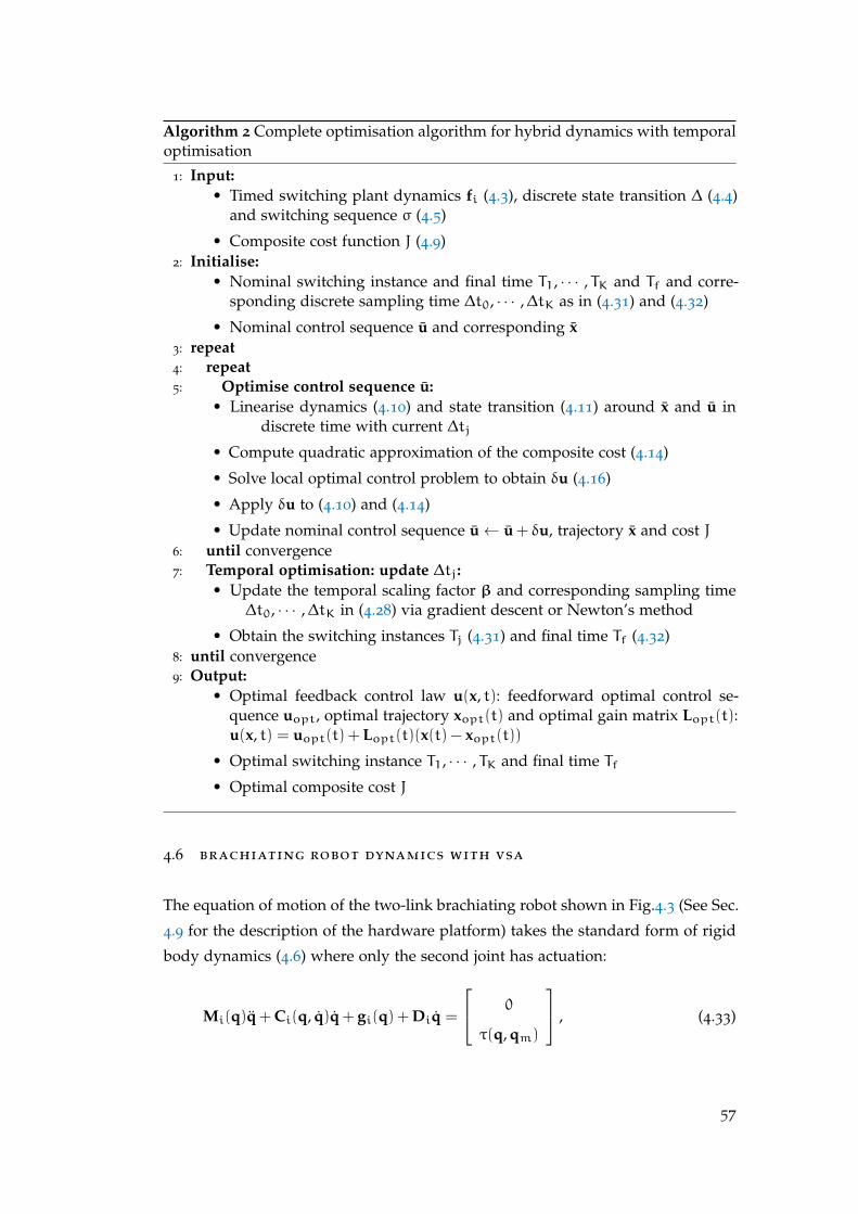
Algorithm 2 Complete optimisation algorithm for hybrid dynamics with temporaloptimisation

1: Input:• Timed switching plant dynamics fi (4.3), discrete state transition ∆ (4.4)

and switching sequence σ (4.5)

• Composite cost function J (4.9)2: Initialise:

• Nominal switching instance and final time T1, · · · , TK and Tf and corre-sponding discrete sampling time ∆t0, · · · ,∆tK as in (4.31) and (4.32)

• Nominal control sequence u and corresponding x3: repeat4: repeat5: Optimise control sequence u:

• Linearise dynamics (4.10) and state transition (4.11) around x and u indiscrete time with current ∆tj

• Compute quadratic approximation of the composite cost (4.14)

• Solve local optimal control problem to obtain δu (4.16)

• Apply δu to (4.10) and (4.14)

• Update nominal control sequence u← u + δu, trajectory x and cost J6: until convergence7: Temporal optimisation: update ∆tj:

• Update the temporal scaling factor β and corresponding sampling time∆t0, · · · ,∆tK in (4.28) via gradient descent or Newton’s method

• Obtain the switching instances Tj (4.31) and final time Tf (4.32)8: until convergence9: Output:

• Optimal feedback control law u(x, t): feedforward optimal control se-quence uopt, optimal trajectory xopt(t) and optimal gain matrix Lopt(t):u(x, t) = uopt(t) + Lopt(t)(x(t) − xopt(t))

• Optimal switching instance T1, · · · , TK and final time Tf• Optimal composite cost J

4.6 brachiating robot dynamics with vsa

The equation of motion of the two-link brachiating robot shown in Fig.4.3 (See Sec.

4.9 for the description of the hardware platform) takes the standard form of rigid

body dynamics (4.6) where only the second joint has actuation:

Mi(q)q + Ci(q, q)q + gi(q) + Diq =

0

τ(q, qm)

, (4.33)

57

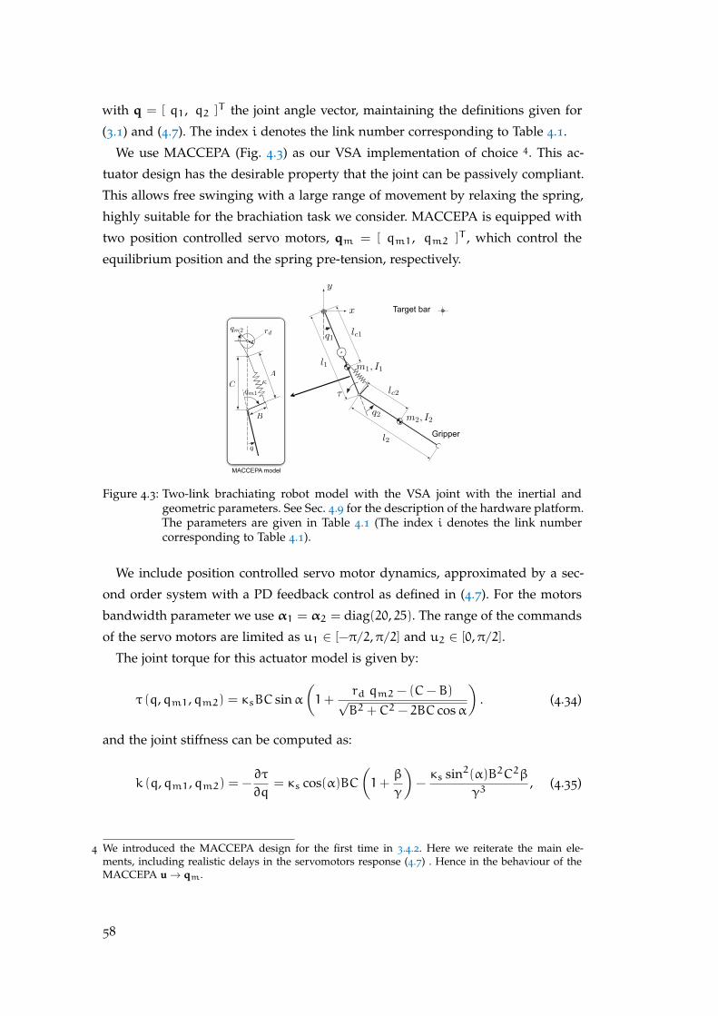
with q = [ q1, q2 ]T the joint angle vector, maintaining the definitions given for

(3.1) and (4.7). The index i denotes the link number corresponding to Table 4.1.

We use MACCEPA (Fig. 4.3) as our VSA implementation of choice 4. This ac-

tuator design has the desirable property that the joint can be passively compliant.

This allows free swinging with a large range of movement by relaxing the spring,

highly suitable for the brachiation task we consider. MACCEPA is equipped with

two position controlled servo motors, qm = [ qm1, qm2 ]T , which control the

equilibrium position and the spring pre-tension, respectively.

Target barx

y

l1

l2Gripper

lc2

lc1

m1, I1

m2, I2

q1

q2

τ

rd

A

qm2

qm1

B

C

q

κ

MACCEPA model

Figure 4.3: Two-link brachiating robot model with the VSA joint with the inertial andgeometric parameters. See Sec. 4.9 for the description of the hardware platform.The parameters are given in Table 4.1 (The index i denotes the link numbercorresponding to Table 4.1).

We include position controlled servo motor dynamics, approximated by a sec-

ond order system with a PD feedback control as defined in (4.7). For the motors

bandwidth parameter we use α1 = α2 = diag(20, 25). The range of the commands

of the servo motors are limited as u1 ∈ [−π/2,π/2] and u2 ∈ [0,π/2].

The joint torque for this actuator model is given by:

τ (q,qm1,qm2) = κsBC sinα(1+

rd qm2 − (C−B)√B2 +C2 − 2BC cosα

). (4.34)

and the joint stiffness can be computed as:

k (q,qm1,qm2) = −∂τ

∂q= κs cos(α)BC

(1+

β

γ

)−κs sin2(α)B2C2β

γ3, (4.35)

4 We introduced the MACCEPA design for the first time in 3.4.2. Here we reiterate the main ele-ments, including realistic delays in the servomotors response (4.7) . Hence in the behaviour of theMACCEPA u→ qm.

58

where κs is the spring constant, rd is the drum radius, α = qm1 − q, β = rdqm2 −

(C− B) and γ =√B2 +C2 − 2BC cos (qm1 − q) (see Fig. 4.3 for the definition of

the model parameters). The spring tension is given by:

F = κs(l− l0), (4.36)

where l =√B2 +C2 − 2BC cos(qm1 − q)+ rdqm2 is the current spring length and

l0 = C−B is the spring length at rest. The joint torque equation (4.34) can also be

rearranged in terms of the moment arm and the spring tension as:

τ =BC sin(qm1 − q)

γF. (4.37)

We note that MACCEPA has a relatively simple configuration in terms of actuator

design compared to other VSAs. However, the torque and stiffness relationships

in (4.34) and (4.35) are dependent on the current joint angle and two servo motor

angles in a complicated manner and its control is not straightforward.

We use the model parameters of the hardware platform (see Sec. 4.9 for details)

shown in Table 4.1.

Robot parameters i=1 i=2

Mass mi (kg) 1.390 0.527

Moment of inertia Ii (kgm2) 0.0297 0.0104

Link length li (m) 0.46 0.46

COM location lci (m) 0.362 0.233

Viscous friction di (Nm/s) 0.03 0.035

MACCEPA parameters valueSpring constant κs (N/m) 771

Lever length B (m) 0.03

Pin displacement C (m) 0.125

Drum radius rd (m) 0.01

Table 4.1: Model parameters of the two-link brachiating robot and the variable stiffnessactuator.

To formulate the optimisation, we use the state space representation in (4.8). At

the transition at handhold, an affine discrete state transition x+ = ∆(x−) = Γx−+γ

is introduced to shift the coordinate system for the next handhold and reset the

joint velocities of the robot to zero, which is defined as:

Γ = diag(Γ1, · · · , Γ4), (4.38)

59

where:

Γ1=

1 1

0 −1

, Γ2=

0 0

0 0

, Γ3=Γ4=

−1 0

0 1

(4.39)

and γ = [ −π, 0, · · · , 0 ]T . Note that in this example, we have ∆ = ∆1,2 = ∆2,1.

4.7 exploitation of passive dynamics with spatio-temporal optimi-

sation of stiffness

In this section, we explore the benefits of simultaneous variable stiffness and tem-

poral optimisation for tasks exploiting the intrinsic dynamics of the system. Brachi-

ation is an example of a highly dynamic manoeuvre, requiring the use of passive

dynamics for successful task execution. First, we discuss the implementation of a

passive control strategy with variable stiffness actuation.

Our focus in this section is on how passive dynamics can be exploited in a

single phase movement with the proposed OC framework. This is a particular in-

stantiation of the OC formulation for the case of a single set of dynamics, without

discrete state transition. Then, we present numerical simulations to demonstrate

the benefits of temporal optimisation and time-varying stiffness modulation in a

brachiation task. Later in Section 4.9, we report hardware experiments on a physi-

cal two-link brachiating robot with VSA.

4.7.1 Passive Control Strategy in Swing Movement with Variable Stiffness Actuation

A natural strategy would be to utilise gravity by making the joints passive and

compliant. For example, while walking, humans seem to let the lower leg swing

freely by relaxing the muscles controlling the knee joint during the swing phase

and increase stiffness only when necessary. Stiffness modulation is also observed

during a walking cycle in a cat locomotion study 5 [Akawaza et al., 1982]. This

contrasts with the approach of high gain position controllers used for biped robots

with stiff joints.

Consider the dynamics of a simplified single-link pendulum under the influence

of gravity. If we consider an idealised VSA model of the form τ = −k(q− qm),

5 To our knowledge, there are a large number of studies of stretch reflexes modulation in humanwalking, however, work specifically addressing stiffness modulation is very limited. For human armcyclic movement, [Bennett et al., 1992] reported time-varying stiffness modulation in the elbow joint.

60

where q is the joint angle, τ is the joint torque, k is the stiffness and qm is the

equilibrium position of the elastic actuator, then the dynamics can be written as:

ml2q+mgl sinq = τ = −k(q− qm), (4.40)

where m is the mass, l is the length and g is the gravitational constant. In this

idealised VSA model, we assume that k and qm are the control variables. From a

viewpoint of position control, one way of looking at this system is as a manipula-

tor with a flexible (elastic) joint, where we solve a tracking control problem [Spong,

1987]. In [Palli et al., 2008] a tracking control algorithm is proposed for such a flex-

ible joint manipulator with variable stiffness actuation, in order to achieve asymp-

totic tracking of the desired joint and stiffness trajectories based on input-output

linearisation. This constitutes an active cancellation of the intrinsic robot dynam-

ics. Note that the main focus of [Palli et al., 2008] is the tracking control of the

given joint and stiffness trajectories, and the problem of generating such desired

trajectories for a given specific task is not addressed.

Alternatively, by rearranging the dynamics of (4.40) (for sinq ≈ q) as:

ml2q+ (mgl+ k)q = v, (4.41)

where v = kqm, it can be observed that varying the stiffness of the actuator k in

the second term of the left hand side effectively changes the dynamics property

(e.g., the natural frequency of the pendulum). Thus, the control problem can be

framed as finding an appropriate (preferably small) stiffness profile k to modulate

the system dynamics (only when necessary) and compute the virtual equilibrium

trajectory qm [Shadmehr, 1990] to fulfil the specified task requirement, while max-

imally exploiting the natural dynamics.

In a realistic situation, obtaining the control solution to this effect is non-trivial,

due to the complexity of the system dynamics, actuator mechanisms, the require-

ment of coordination of multiple degrees of freedom and redundancy in actuation.

Next, we exploit the framework of optimal control and spatio-temporal optimisa-

tion of variable stiffness actuation to find appropriate control commands to imple-

ment the brachiation task.

61

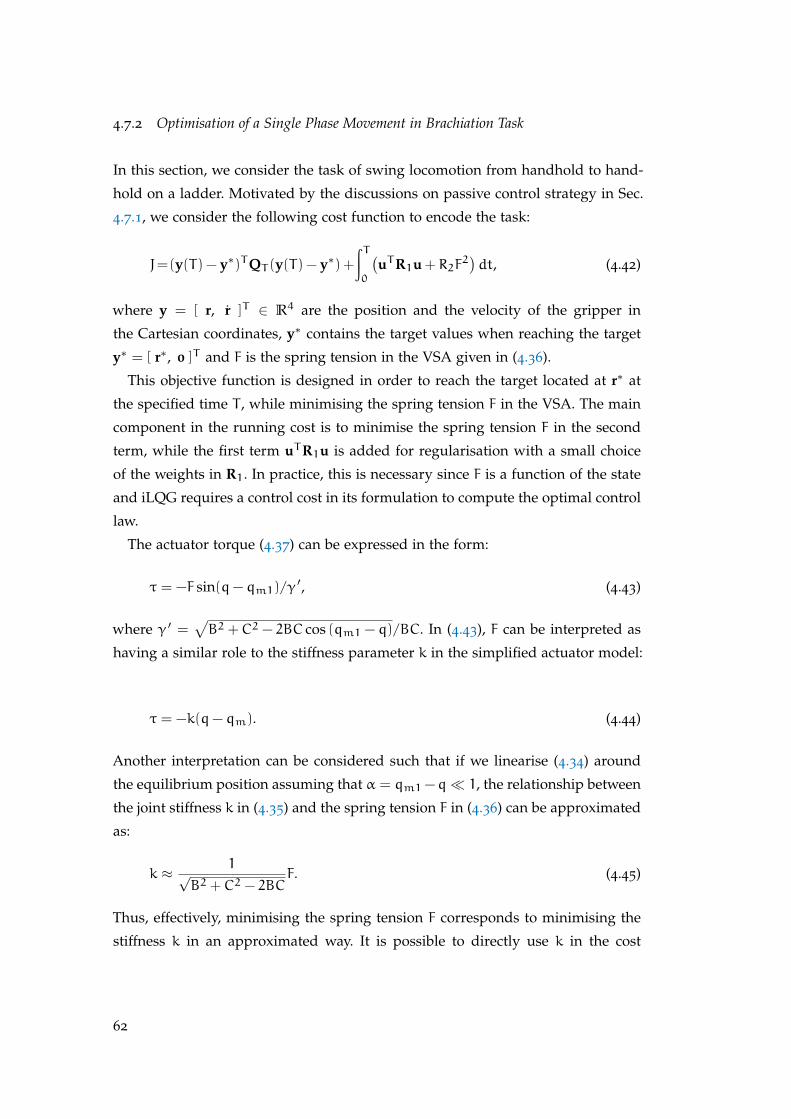
4.7.2 Optimisation of a Single Phase Movement in Brachiation Task

In this section, we consider the task of swing locomotion from handhold to hand-

hold on a ladder. Motivated by the discussions on passive control strategy in Sec.

4.7.1, we consider the following cost function to encode the task:

J=(y(T) − y∗)TQT (y(T) − y∗) +∫T0

(uTR1u + R2F

2)dt, (4.42)

where y = [ r, r ]T ∈ R4 are the position and the velocity of the gripper in

the Cartesian coordinates, y∗ contains the target values when reaching the target

y∗ = [ r∗, 0 ]T and F is the spring tension in the VSA given in (4.36).

This objective function is designed in order to reach the target located at r∗ at

the specified time T , while minimising the spring tension F in the VSA. The main

component in the running cost is to minimise the spring tension F in the second

term, while the first term uTR1u is added for regularisation with a small choice

of the weights in R1. In practice, this is necessary since F is a function of the state

and iLQG requires a control cost in its formulation to compute the optimal control

law.

The actuator torque (4.37) can be expressed in the form:

τ = −F sin(q− qm1)/γ ′, (4.43)

where γ ′ =√B2 +C2 − 2BC cos (qm1 − q)/BC. In (4.43), F can be interpreted as

having a similar role to the stiffness parameter k in the simplified actuator model:

τ = −k(q− qm). (4.44)

Another interpretation can be considered such that if we linearise (4.34) around

the equilibrium position assuming that α = qm1−q 1, the relationship between

the joint stiffness k in (4.35) and the spring tension F in (4.36) can be approximated

as:

k ≈ 1√B2 +C2 − 2BC

F. (4.45)

Thus, effectively, minimising the spring tension F corresponds to minimising the

stiffness k in an approximated way. It is possible to directly use k in the cost

62

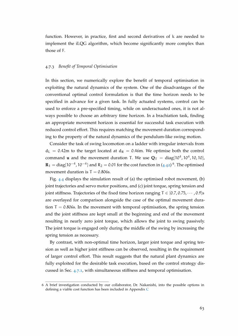
function. However, in practice, first and second derivatives of k are needed to

implement the iLQG algorithm, which become significantly more complex than

those of F.

4.7.3 Benefit of Temporal Optimisation

In this section, we numerically explore the benefit of temporal optimisation in

exploiting the natural dynamics of the system. One of the disadvantages of the

conventional optimal control formulation is that the time horizon needs to be

specified in advance for a given task. In fully actuated systems, control can be

used to enforce a pre-specified timing, while on underactuated ones, it is not al-

ways possible to choose an arbitrary time horizon. In a brachiation task, finding

an appropriate movement horizon is essential for successful task execution with

reduced control effort. This requires matching the movement duration correspond-

ing to the property of the natural dynamics of the pendulum-like swing motion.

Consider the task of swing locomotion on a ladder with irregular intervals from

dL = 0.42m to the target located at dR = 0.46m. We optimise both the control

command u and the movement duration T . We use QT = diag104, 104, 10, 10,

R1 = diag10−4, 10−4 and R2 = 0.01 for the cost function in (4.42) 6. The optimised

movement duration is T = 0.806s.

Fig. 4.4 displays the simulation result of (a) the optimised robot movement, (b)

joint trajectories and servo motor positions, and (c) joint torque, spring tension and

joint stiffness. Trajectories of the fixed time horizon ranging T ∈ [0.7, 0.75, · · · , 0.9]s

are overlayed for comparison alongside the case of the optimal movement dura-

tion T = 0.806s. In the movement with temporal optimisation, the spring tension

and the joint stiffness are kept small at the beginning and end of the movement

resulting in nearly zero joint torque, which allows the joint to swing passively.

The joint torque is engaged only during the middle of the swing by increasing the

spring tension as necessary.

By contrast, with non-optimal time horizon, larger joint torque and spring ten-

sion as well as higher joint stiffness can be observed, resulting in the requirement

of larger control effort. This result suggests that the natural plant dynamics are

fully exploited for the desirable task execution, based on the control strategy dis-

cussed in Sec. 4.7.1, with simultaneous stiffness and temporal optimisation.

6 A brief investigation conducted by our collaborator, Dr. Nakanishi, into the possible options indefining a viable cost function has been included in Appendix C

63

−0.8 −0.6 −0.4 −0.2 0 0.2 0.4 0.6 0.8−1

−0.8

−0.6

−0.4

−0.2

0 Target

(a) Movement of the robot (simulation) with optimal variable stiffness control (optimised durationT = 0.806s)

! !"# !"$ !"% !"& !"' !"( !") !"* !"+

$

!

$

,-./012/345617829:

,-./012/3456

1

1

! !"# !"$ !"% !"& !"' !"( !") !"* !"+

$

!

$

0.;51765<:

2/34517829:

658=-1;-0-81>-6.0.-/6

1

1

?#

?$

?;#

?;$

q2 with Topt

q1 with Topt

qm1 with Topt qm2 with Topt

(b) Joint trajectories and servo motor positions

! !"# !"$ !"% !"& !"' !"( !") !"* !"+

#

!

#

,-./010-234516789 ,-./010-2345

1

1

! !"# !"$ !"% !"& !"' !"( !") !"* !"+!

$!

&!

:;2./<105/:.-/1679 :;2./<105/:.-/

1

1

! !"# !"$ !"% !"& !"' !"( !") !"* !"+

!

#

$

0.8516:5=9

:0.>>/5::1678?2@A9 ,-./01:0.>>/5::

1

1

B

C

nearly zero joint torque

small spring tension

(c) Joint torque, spring tension and joint stiffness

Figure 4.4: Optimisation results of the swing locomotion task with temporal optimisation.In (b) and (c), grey thin lines show the plots for non-optimised T in the rangeof T = [0.7, 0.75, · · · , 0.9]s and blue thick lines show the plots for optimisedT = 0.806s. With temporal optimisation, at the beginning and the end of themovement, joint torque, spring tension and joint stiffness are kept small allow-ing the joint to swing passively in comparison to the non-optimal time cases.

64

In order to illustrate the effect of the servo motor dynamics characterised by

(4.7), Fig. 4.5 shows the servo motor position commands and actual motor angles

for the optimal movement duration, corresponding to the result in Fig. 4.4. Limi-

tations in the bandwidth of the servo motor response can be observed in this plot.

This suggests that the proposed optimal control framework can find appropriate

control commands taking this effect into account.

! !"# !"$ !"% !"& !"' !"( !") !"* %

$

#

!

#

$

%

+,-./01.23

4567./08493

1.8:;/-;+;8/<;1,+,;51/459/2;--4591

/

/

=-#/0<;1,+,;53

=-$/0<;1,+,;53

>#/02;--4593

>$/02;--4593

qm2

qm1

u1

u2

Figure 4.5: Servo motor commands ui (dotted line) and actual angle qmi (solid line) forthe results with optimal movement duration T = 0.806 (Fig. 4.4 (b) bottom).Servo motor response delay can be observed characterised by the servo motordynamics (4.7). The proposed optimal control framework finds appropriatecontrol commands taking this effect into account.

4.7.4 Benefit of Stiffness Variation

In this section, we investigate the benefit of time-varying stiffness modulation.

One of the characteristics of VSAs is their ability to simultaneously modulate joint

torque and stiffness. As discussed in Sec. 4.7.1, modulating stiffness effectively

alters the properties of the system dynamics, such as natural frequency. Thus, the

capability of modulating stiffness during the motion is potentially beneficial for

improving the task performance.

We demonstrate the benefit of time-varying modulation of stiffness by compar-

ing optimal variable stiffness control and optimal fixed stiffness control. In optimal

variable stiffness control, both control commands in u = [ u1(t), u2(t) ]T are op-

timised in a time-varying manner during the movement to independently control

the joint torque and the joint stiffness. In optimal constant stiffness control, the

command to the spring pre-tensioning servomotor is fixed to the optimal constant

value throughout the movement (i.e., u = [ u1(t), u2 ]T where u2 = const.). We

note that a constant command to the pre-tensioning servomotor u2 does not nec-

essarily mean constant joint stiffness with MACCEPA [Braun et al., 2012a].

65

Fig. 4.6 shows the simulation result of a swing locomotion for the intervals

dL = 0.42m and dR = 0.46m (the same configuration as in Sec. 4.7.3) with the op-

timal fixed stiffness control. Fig. 4.6 (a) illustrates the optimised movement of the

robot and (b) shows the servomotor commands and positions, where u2 and qm2are kept at their optimal constant value during the movement. The optimal time

horizon for this movement was T = 0.723s. The resultant movements in Fig. 4.4 (a)

(optimal variable stiffness) and Fig. 4.6 (a) (optimal constant stiffness) look compa-

rable. However, optimal constant stiffness control results in a higher cost J = 9.528

than that of the corresponding optimal variable stiffness case, which is J = 2.979.

−0.8 −0.6 −0.4 −0.2 0 0.2 0.4 0.6 0.8−1

−0.8

−0.6

−0.4

−0.2

0 Target

(a) Movement of the robot (simulation) with optimal fixed stiffness control (optimised movementduration T = 0.723s)

! !"# !"$ !"% !"& !"' !"( !") %

$

#

!

#

$

%

*+,-./0-12

3456-./7382

0-79:.,:*:7.;:0+*+:40.348.1:,,3480./<+=-8.>$2

.

.

?,#./;:0+*+:42

?,$./;:0+*+:42

>#./1:,,3482

>$./1:,,3482

qm1

u1

u2, qm2

(b) Servo motor commands ui (dotted line) and actual angle qmi (solid line) for the results withoptimal fixed stiffness control. Note that the pre-tension motor the command u2 and its actual

position qm2 are kept to the optimal constant value throughout the movement.

Figure 4.6: Optimisation results of the swing locomotion task with optimal fixed stiffnesscontrol. The intervals between the bars correspond to the case with optimalvariable stiffness control in Sec. 4.7.3.

a Stiffness Modulation and Range of Achievable Targets

Next, we compare the performance of variable and constant optimal stiffness con-

trol in terms of the range of distances that can be reached with the robot. Starting

66

from the bar at the nominal distance dL = 0.42m, we vary the target positions dRby 1cm and optimise the control commands and movement duration. When the

end effector position at t = Tf is within a tolerance of 1cm from the location of the

target, we assume that the trial is successful.

With optimal variable stiffness control, the robot was able to reach the target in

the range of dR ∈ [0.39, 0.59]m (the range of 20cm) while with optimal constant

stiffness control, it was dR ∈ [0.42, 0.52]m (the range of 10cm). These numerical

explorations illustrate the benefit of optimal variable stiffness control in terms of

the cost and range of distances achieved in swing locomotion in comparison to

optimal constant stiffness control.

4.8 spatio-temporal optimisation of multiple swings in robot

brachiation

To fully demonstrate the performance of our developed approach, we consider a

brachiating task with multiple phases of the movement as follows: First, the robot

swings up from the suspended posture to the target at d1 = 0.40 m and subse-

quently moves to the target located at d2 = 0.42 and d3 = 0.46 m, respectively.

The composite cost function to encode this task is given by:

J = (y(Tf) − y∗f)TQTf(y(Tf) − y∗f) +

K∑j=1

(y(T−j ) − y∗j )TQTj(y(T

−j ) − y∗j )

+

∫Tf0

(uTR1u + R2F

2)dt+wTT1, (4.46)

where K = 3 is the number of phases, y = [ r, r ]T ∈ R4 are the position

and the velocity of the gripper in the Cartesian coordinates measured from the

origin at current handhold, y∗ contains the target values when reaching the tar-

get y∗ = [ r∗, 0 ]T and F is the spring tension in the VSA. This cost func-

tion includes the time cost wTT1 for the swing up manoeuvre. We use QT =

QTj = diag104, 104, 10, 10, R1 = diag10−4, 10−4 and R2 = 0.01 and wT = 1.

In addition, we impose constraints on the range of the angle of the second joint

during the course of the swing up manoeuvre as q2min 6 q2 6 q2max , where

[q2min ,q2max ] = [−100, 100]deg, by adding a penalty term to the cost (4.46). This is

introduced considering the physical joint limit of the hardware platform used in

this study.

67

Fig. 4.7 (a) shows the sequence of the multi-phase movement of the robot op-

timised using the proposed algorithm including temporal optimisation. The op-

timised switching instance and total movement duration are T1 = 5.259s, T2 =

6.033s and Tf = 6.835s and the total cost is J = 37.815. Fig. 4.7 (b) shows the op-

timised joint trajectories and servo motor positions. Note that at the instance of

switching, denoted by vertical lines, discrete state transition can be observed in

these trajectories due to the definition of the coordinates transformation.

−0.5 0 0.5 1 1.5−1

−0.8

−0.6

−0.4

−0.2

0 d=0.40 d=0.42 d=0.46

optimized robot movement

(a) Optimised movement of the robot (simulation)

0 1 2 3 4 5 6

−2

0

2

join

t angle

(ra

d)

joint angles

1) swing up 2) 1st swing 3) 2nd swing

0 1 2 3 4 5 6

−2

0

2

time (sec)

angle

(ra

d)

servo motor positions

1) swing up 2) 1st swing 3) 2nd swing

q1

q2

qm1

qm2


Figure 4.7: (a) Optimised multi-phase movement of the robot. (b) Joint trajectories andservo motor positions of complete optimisation with temporal optimisation.

To illustrate the benefit of the proposed multi-phase formulation, we performed

a movement optimisation with a pre-specified nominal (fixed, non-optimal) time

horizon with T1 = 5.2s, T2 = 5.9s and Tf = 6.7s using the same cost parameters

in sequential and multi-phase optimisation. With sequential individual movement

optimisation, at the end of the final phase movement, a large overshoot was ob-

served (the distance from the target at t = Tf was 0.0697 m) incurring a signif-

icantly large total cost of J = 101.053. By contrast, with multi-phase movement

optimisation, for the same pre-specified time horizon, it was possible to find a

68

feasible solution within a tolerance of 1cm at the end of each phase at the bar. In

this case, the total cost was J = 50.228. These results demonstrate the benefit of

the multi-phase movement optimisation in finding optimal control commands and

temporal aspect of the movement using the proposed method resulting in lower

cost.

In the next section we briefly describe the developed hardware platform used

to showcase the applicability of the proposed framework under realistic physical

conditions. We then present the experimental results obtained on brachiation tasks

for the presented two-link robotic system with VSA.

4.9 hardware development

This section describes the hardware platform used in the experiments. Fig. 4.8

depicts the configuration of the brachiating robot with VSA. The elbow joint is

fitted with a MACCEPA actuator equipped two servo motors (Hitec HS-7940TH).

gripper

VSA Joint

spring

link 2

link 1

target bar

servo motor 1

servo motor 2

additional mass

Figure 4.8: Configuration of the two-link brachiating robot with VSA in CAD drawing.

Each link is fitted with a gripper driven by a single servo motor (Hitec HSR-

5990TG) which opens and closes it through a gear mechanism. The angle of the

first link is measured by integrating its angular velocity obtained through an IMU

unit (InvenSense MPU-6050) attached to the link. The angle of the second link is

69

measured by a rotary potentiometer (Alps RDC503013A) at the elbow joint. The

servo motor positions are measured through direct access to its internal poten-

tiometer. The operating frequency of control and measurement is 1 kHz.

The length of each link is 0.46 m and the total mass is about 1.92 kg. The link

parameters are computed from the CAD model, while friction coefficients and the

servo motor bandwidth parameters are estimated by fitting the actual responses

of the robot.

Our numerical exploration showed that with an inadequate mass distribution,

it was difficult to find an optimal solution in achieving desired swing locomotion

behaviour under the constraint. Thus, the mass distribution of the robot was em-

pirically adjusted to resemble the desirable natural dynamics required for the task

(see Table 4.1 for the parameters). An overview of the hardware design evolution

is provided in Appendix D.

The parameters in Table 4.1 were obtained from the CAD model of the system.

We performed data collection from the hardware system, under various command

input sets and compared the observed behaviour with those anticipated from the

simulation. We used a similar approach to tune the value of the bandwidth param-

eters in the motor dynamics model, α. An overview of the details regarding these

validation procedures is provided in Appendix E.

4.10 evaluation on hardware platform

This section presents experimental results implemented on the two-link brachiat-

ing variable stiffness robot hardware corresponding to the numerical simulations

reported in Sec. 4.7.3 and Sec. 4.8.

4.10.1 Spatio-Temporal Optimisation for a Single-Phase Movement

Fig. 4.9 shows the experimental result of a swing locomotion on the ladder with

the intervals of dL = 0.42 m and dR = 0.46 m. The optimised control commands

with the optimal movement duration obtained in the corresponding simulation in

Section 4.7.3 are used. In Fig. 4.9 (a), the movement of the robot is depicted, while

in Fig. 4.9 (b) the joint trajectories and servo motor positions are shown. This result

corresponds to the simulation in Fig. 4.4 for the optimal movement duration. In

the experiments, we only use the open-loop optimal control command to the servo

motors without state feedback as in [Braun et al., 2012a].

70

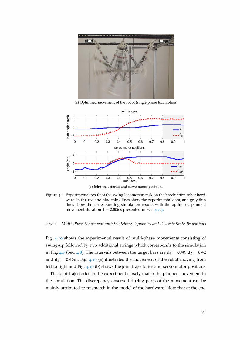
(a) Optimised movement of the robot (single phase locomotion)

0 0.1 0.2 0.3 0.4 0.5 0.6 0.7 0.8 0.9 1

−2

0

2

join

t angle

s (

rad)

joint angles

0 0.1 0.2 0.3 0.4 0.5 0.6 0.7 0.8 0.9 1

−2

0

2

time (sec)

angle

(ra

d)


q1

q2

qm1

qm2


Figure 4.9: Experimental result of the swing locomotion task on the brachiation robot hard-ware. In (b), red and blue think lines show the experimental data, and grey thinlines show the corresponding simulation results with the optimised plannedmovement duration T = 0.806 s presented in Sec. 4.7.3.

4.10.2 Multi-Phase Movement with Switching Dynamics and Discrete State Transitions

Fig. 4.10 shows the experimental result of multi-phase movements consisting of

swing-up followed by two additional swings which corresponds to the simulation

in Fig. 4.7 (Sec. 4.8). The intervals between the target bars are d1 = 0.40, d2 = 0.42

and d3 = 0.46m. Fig. 4.10 (a) illustrates the movement of the robot moving from

left to right and Fig. 4.10 (b) shows the joint trajectories and servo motor positions.

The joint trajectories in the experiment closely match the planned movement in

the simulation. The discrepancy observed during parts of the movement can be

mainly attributed to mismatch in the model of the hardware. Note that at the end

71

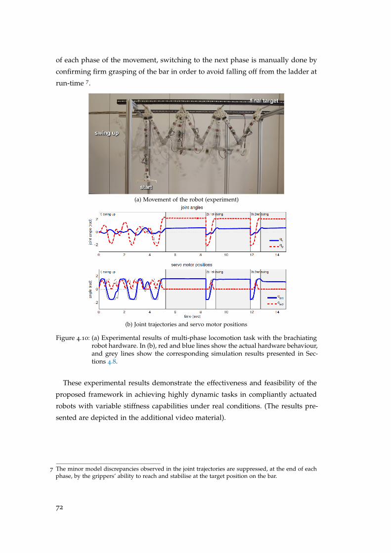
of each phase of the movement, switching to the next phase is manually done by

confirming firm grasping of the bar in order to avoid falling off from the ladder at

run-time 7.

(a) Movement of the robot (experiment)


Figure 4.10: (a) Experimental results of multi-phase locomotion task with the brachiatingrobot hardware. In (b), red and blue lines show the actual hardware behaviour,and grey lines show the corresponding simulation results presented in Sec-tions 4.8.

These experimental results demonstrate the effectiveness and feasibility of the

proposed framework in achieving highly dynamic tasks in compliantly actuated

robots with variable stiffness capabilities under real conditions. (The results pre-

sented are depicted in the additional video material).

7 The minor model discrepancies observed in the joint trajectories are suppressed, at the end of eachphase, by the grippers’ ability to reach and stabilise at the target position on the bar.

72


In this chapter, we presented the application of our systematic methodology for

movement optimisation with multiple phases and switching dynamics. We ad-

dress this in the context of robotic systems with VIA, with the focus on exploiting

the intrinsic dynamics of the system.

Tasks including switching dynamics and interaction with the environment are

approximately modelled as a hybrid dynamical system with time-based switching.

We showed the benefit of simultaneous temporal and variable stiffness optimisa-

tion leading to a lowered control effort and improved performance. We demon-

strated the effectiveness of the proposed approach in example tasks in both nu-

merical simulations and in a hardware implementation of a brachiating robot with

VSA.

In Sec. 4.7.3, we highlight the benefit of temporal optimisation for exploiting the

natural dynamics of the system. We use for this an example of a swing locomotion

task on a brachiation system with VSA capabilities. The selection of an optimal

time is crucial for lowering the required control effort. The results presented are

closely related to the work in [Nakanishi et al., 2011], which showed how, for a pe-

riodic motion of a brachiation system, finding an appropriate frequency matching

the natural one of the system, can reduce the control effort.

We showed the benefit of multi-phase movement optimisation on the brachi-

ation system in terms of cost and performance, compared to individual phase

optimisation. This is due to the multi-phase optimisation taking into considera-

tion future goals. This result might be less evident in the brachiation example

used, as the dynamics of the system define a reset in the joint velocities every time

the robot grasps the bar. However, the effect can be observed in the positions of

the VSA servomotors, which are appropriately adjusted at the end of each phase,

considering the next phase of the movement.

A significant practical consideration for time-based switching approaches is en-

suring the feasibility and approximation of the switching condition. This is gener-

ally determined by the given task and the associated cost function, as the switching

condition is imposed as a soft constraint by the via-point and terminal costs. In

the case of our brachiation system, given the design of the gripper in the physical

robot, a small error at the endpoint was tolerated considering that the robot was

able to grasp the bar.

73

The current methodology assumes the existence of a predefined sequence of

switching, where the switching conditions can be incorporated in the cost function.

If such a sequence is not available, a possible alternative approach can be provided

by one of the methods discussed in Sec. 4.2.3. Performing a temporal optimisation

in these scenarios would be more difficult as the switching time depends on the

trajectory of the system [Xu and Antsaklis, 2004].

In the next chapter we extend the evaluation of our proposed approach to a

monopod hopper. This constitutes a significantly more challenging platform in

terms of contacts (i.e., more complex impact map) and individual phase dynamics

(i.e., existence of a flight phase). We present numerical evaluations showcasing the

benefits of multi-phase optimisation on this increasingly complicated system.

74

5H O P P I N G R O B O T W I T H I M P E D A N C E M O D U L AT I O N

In this chapter we further demonstrate the effectiveness of the proposed approach,

introduced in Chapter 4. First, we provide a brief overview of the related work

regarding the control of the platform used in this chapter, the monopod hopper.

We then apply our methodology and present numerical evaluations on the chal-

lenging task of hopping locomotion.

The results presented show the feasibility of the developed framework, high-

lighting the benefits of multi-phase optimisation and the robustness of the ob-

tained optimal feedback controller.

5.1 previous work on control for hopper system

The monopod hopper is a well known platform, previously used in a variety of

studies on dynamics and control. A locomotion task for such a system includes

switching of different modes of dynamics (flight and stance) and complex discon-

tinuous state transition caused by the touch down impact.

During the stance phase the system is underactuated, while in the flight phase

the absence of contact with the ground does not allow control the system using

the contact forces. An additional difficulty in this task is the temporal optimisation

aspect. Finding the flight and stance times for successful task execution is highly

restricted by the intrinsic dynamics and the desired task specifications.

Thompson and Raibert explored passive dynamic locomotion on a one legged

hopper with hip compliance [Thompson and Raibert, 1990] and show that the

system can achieve a wide range of locomotion speeds. Many approaches were

based on Raibert’s control [Raibert and Tello, 1986]. The most engaging results re-

volved around the work of Martin Buehler et al. [Ahmadi and Buehler, 1997; Gre-

gorio et al., 1997; Sato and Buehler, 2004]. In their first attempts they adapted the

Raibert controller to their particular hopper design (the electrically actuated ARL

Monopod) [Gregorio et al., 1997]. In further studies they progressed by consider-

ing compliant elements in the hip and leg [Ahmadi and Buehler, 1997]. A similar

controller that exploits the passive dynamics, achieving stabilisation of a param-

75

eterised passive dynamic motion was proposed. In later work [Sato and Buehler,

2004] the Spring Loaded Inverted Pendulum (SLIP) model was considered, due to

being naturally stable, and thus the control problem was simplified.

Alternatives to the Raibert-based controllers were developed. In [François and

Samson, 1998], natural regimes were regarded as periodic orbits which could be

mapped and stabilised, an approach borrowed from [McGeer, 1990]. The method

involved a discrete-time controller, that applied impulsive forces computed at each

time step. Based on this method, [Hyon and Emura, 2002] devised a controller that

applied piecewise-constant forces. It used the intrinsic dynamics of the hybrid

system, instead of the pre-planned periodic solutions.

5.2 experiments : hopping robot with via

In our work we augment the hopping model from [Hyon and Emura, 2004] with

variable stiffness capabilities in the hip and leg actuators. We demonstrate the

feasibility of the proposed approach on this increasingly challenging platform.

Given the difficulties raised by the dynamics of the hopper system, a successful

task execution will rely heavily on a proper exploitation of the variable impedance

elements and the passive dynamics.

5.2.1 Dynamics Model of a Hopping Robot

The hopping dynamics switch between the flight phase (i = 1) and stance phase

(i = 2) at the switching instance Tk when either touch-down or lift-off conditions

are met. The configuration vector of the system is defined as q = [xcom,ycom, θ,φ, r]T

(see Fig. 5.1).

The flight dynamics (i = 1) are given as : Mxcom = 0, Mycom = −Mg,

Jlθ = −τhip, Jbφ = τhip,(5.1)

with r = r0. The stance dynamics (i = 2) are described as:(Jl +Mr

2)θ+ 2Mrrθ−Mrg sin θ = −τhip,

Jbθ = τhip,

Mr−Mrθ2 +Mg cos θ = τleg,

(5.2)

76

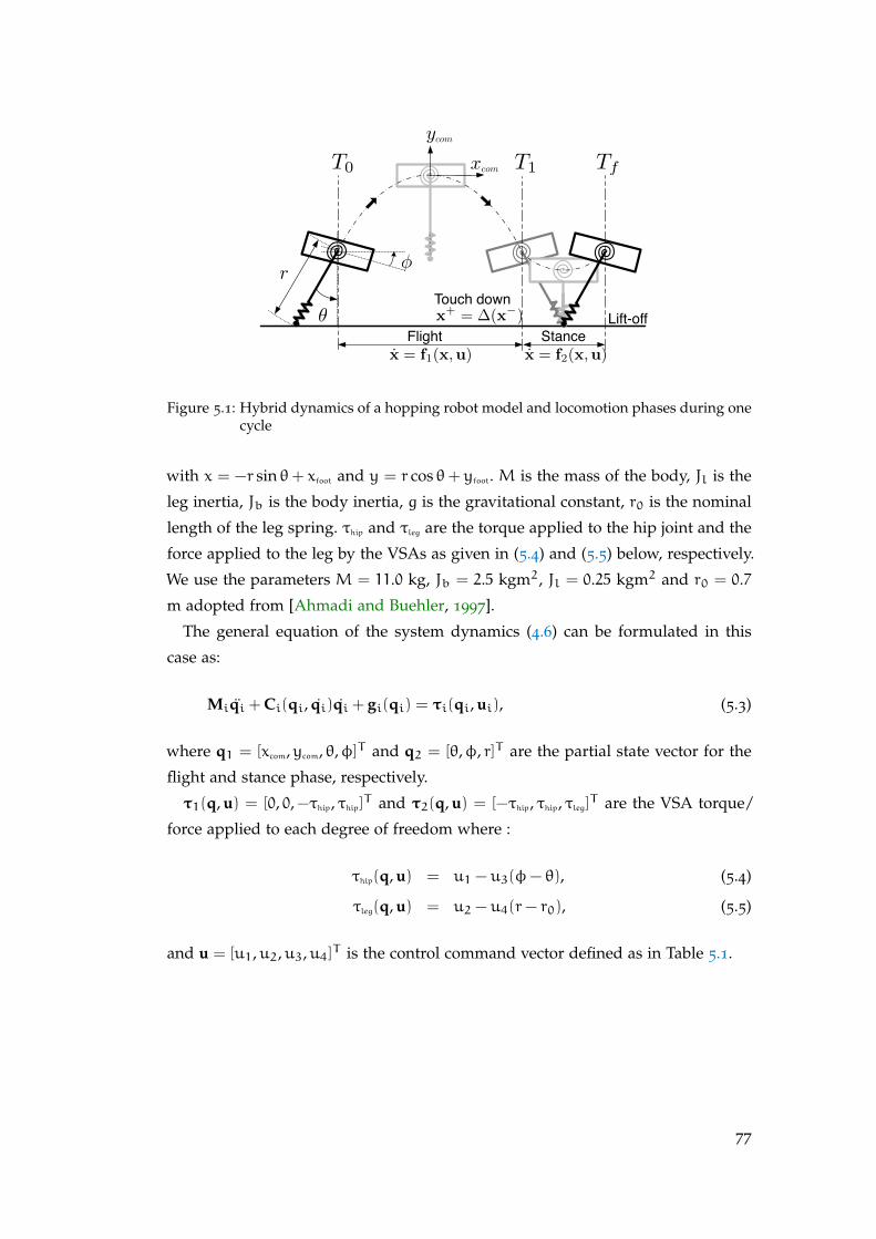
StanceFlight

Touch down

T0 Tf

φ

θ Lift-off

xcom

ycom

r

!

T1

x+ = ∆(x−)

x = f1(x,u) x = f2(x,u)

Figure 5.1: Hybrid dynamics of a hopping robot model and locomotion phases during onecycle

with x = −r sin θ+ xfoot and y = r cos θ+ yfoot. M is the mass of the body, Jl is the

leg inertia, Jb is the body inertia, g is the gravitational constant, r0 is the nominal

length of the leg spring. τhip and τleg are the torque applied to the hip joint and the

force applied to the leg by the VSAs as given in (5.4) and (5.5) below, respectively.

We use the parameters M = 11.0 kg, Jb = 2.5 kgm2, Jl = 0.25 kgm2 and r0 = 0.7

m adopted from [Ahmadi and Buehler, 1997].

The general equation of the system dynamics (4.6) can be formulated in this

case as:

Miqi + Ci(qi, qi)qi + gi(qi) = τi(qi, ui), (5.3)

where q1 = [xcom,ycom, θ,φ]T and q2 = [θ,φ, r]T are the partial state vector for the

flight and stance phase, respectively.

τ1(q, u) = [0, 0,−τhip, τhip]T and τ2(q, u) = [−τhip, τhip, τleg]T are the VSA torque/

force applied to each degree of freedom where :

τhip(q, u) = u1 − u3(φ− θ), (5.4)

τleg(q, u) = u2 − u4(r− r0), (5.5)

and u = [u1,u2,u3,u4]T is the control command vector defined as in Table 5.1.

77

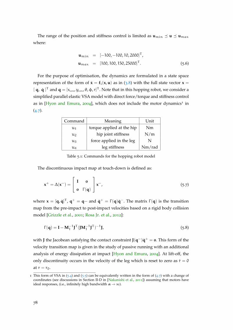
The range of the position and stiffness control is limited as umin u umaxwhere:

umin = [−100,−100, 10, 2000]T ,

umax = [100, 100, 150, 25000]T . (5.6)

For the purpose of optimisation, the dynamics are formulated in a state space

representation of the form of x = fi(x, u) as in (3.8) with the full state vector x =

[ q, q ]T and q = [xcom,ycom, θ,φ, r]T . Note that in this hopping robot, we consider a

simplified parallel elastic VSA model with direct force/torque and stiffness control

as in [Hyon and Emura, 2004], which does not include the motor dynamics1 in

(4.7).

Command Meaning Unit

u1 torque applied at the hip Nmu2 hip joint stiffness N/mu3 force applied in the leg Nu4 leg stiffness Nm/rad

Table 5.1: Commands for the hopping robot model

The discontinuous impact map at touch-down is defined as:

x+ = ∆(x−) =

I 0

0 Γ(q)

x−, (5.7)

where x = [q, q]T , q+ = q− and q+ = Γ(q)q−. The matrix Γ(q) is the transition

map from the pre-impact to post-impact velocities based on a rigid body collision

model [Grizzle et al., 2001; Rosa Jr. et al., 2012]:

Γ(q) = I − M−11 JT (JM−1

1 JT )−1J, (5.8)

with J the Jacobean satisfying the contact constraint J(q−)q+ = 0. This form of the

velocity transition map is given in the study of passive running with an additional

analysis of energy dissipation at impact [Hyon and Emura, 2004]. At lift-off, the

only discontinuity occurs in the velocity of the leg which is reset to zero as r = 0

at r = r0.

1 This form of VSA in (5.4) and (5.5) can be equivalently written in the form of (4.7) with a change ofcoordinates (see discussions in Section II-D in [Nakanishi et al., 2011]) assuming that motors haveideal responses, (i.e., infinitely high bandwidth α→∞).

78

5.2.2 Design of the Composite Cost Function

A stable locomotion of the system for an indefinitely long time consists of a re-

peated periodic hopping behaviour, with the period of one hopping cycle. Thus,

an optimised hopping behaviour can be reduced to a periodic one cycle trajectory.

In our experiment we consider directly obtaining this behaviour, while exploit-

ing the natural dynamics and the benefits of modulating stiffness. For this purpose,

first, we design a composite cost function for one hopping cycle, including both

the flight and stance phases and the touch-down condition. Then, the obtained

controller is applied to achieve multiple cycles.

We consider the following cost function:

J=(x(Tf) − x0)TQTf(x(Tf) − x0) +Ψ(x(T−1 )) +

∫Tf0

uTRudt, (5.9)

where QTf is a positive semi-definite matrix and R is a positive definite matrix.

The purpose of the first term is to achieve periodicity of the trajectory with x0 the

initial state. The second term consists of two criteria:

Ψ(x(T−1 )) = QT1,1(y−foot

− 0)2 +QT1,2(µ−)2, (5.10)

where QT1,1 and QT1,2 are positive weights. The term QT1,1(y−foot − 0)

2 penalises

the height of the foot from the ground y = 0 to approximately encode the touch-

down condition in a time-based formulation. Note that in order to minimise this

term, it is important to find an appropriate flight time T1, as the trajectory of

the centre of mass cannot be directly controlled in the flight phase for a given

initial lift-off condition. The termQT2,2(µ−)2 minimises energy loss at touch-down

where µ− is the energy dissipation coefficient [Hyon and Emura, 2004]:

µ−= x−com

cos θ− + y−com

sin θ− + r0θ−= x−

footcos θ− + y−

footsin θ−. (5.11)

This encoding is motivated from the study of passive running [Hyon and Emura,

2004] in order to find an appropriate leg angle and foot velocity relative to the

ground at touch-down. Note that for µ− = 0, there is no energy loss at impact. In

the running cost, we minimise the control effort u1 and u2, while small weights

are used for penalising the magnitude of stiffness u3 and u4 for regularisation.

The range of the control and stiffness is limited as ui,min 6 ui 6 ui,max (5.6).

79

The initial conditions were obtained by choosing the desired initial horizontal

velocity and lift-off angle of the leg (x0, θ0) and computing the remaining parame-

ters under the assumption of synchronisation between the oscillatory movements

of the leg swing and compression in the passive running model [Ahmadi and

Buehler, 1997; Hyon and Emura, 2004].

5.2.3 Simulation Results

We choose the desired initial condition at lift off as x0 = 2.0m and θ0 = −6.0deg.

Note that with this initial condition, the passive dynamics (i.e., no control is ap-

plied) of the robot can achieve several steps of running as reported in [Ahmadi

and Buehler, 1997; Hyon and Emura, 2004], however, it will eventually fail since

passive running is intrinsically unstable.

Using the proposed method, we simultaneously obtained the optimal feedback

control for the control commands (u1,u2) and stiffness (u3,u4), and found the

flight time T1 and the duration of the complete cycle Tf. The optimised flight

time and one hopping cycle are T1 = 0.410s and Tf = 0.490s. The total cost is

Jcomp = 1.624. The obtained controller is rooted in a time-based switching as-

sumption for one cycle. There could be some mismatch in the exact timing in

the switching condition when applied to realistic event-based switching dynamics

for multiple cycles of locomotion. One of the benefits of our approach is that it

provides a locally optimal feedback control law, hence deviations from the optimal

trajectory can be corrected. The results presented are featured in the additional

video material.

a Comparison to Individual Phase Optimisation

For comparison, we optimise the control command, stiffness and the movement

duration in a sequential manner individually for the flight phase, followed by the

stance phase, for one cycle of the movement. The optimised movement duration

for the flight phase is T1,ind = 0.410s and for the stance is Tstance,ind = 0.080s,

resulting in the total duration Tf,ind = 0.490s. The total cost for this individual op-

timisation is Jind = 1.686, which is comparable to the complete optimisation case

Jcomp = 1.624 mentioned above. The optimised trajectories, control commands

and stiffness profiles are similar between these two cases. However, interestingly,

we found a notable difference in the robustness of the controllers when applied

80

to the event-based switching dynamics, where the role of the feedback control be-

comes prominent.

The controller with complete cycle optimisation is able to achieve continuous

stable running over multiple cycles. By contrast, with the controller obtained by

individual optimisation, the robot fails after 25 steps of hopping. Although this

is an empirical observation, this difference could be justified by the difference in

the optimal feedback gains. In the complete cycle optimisation, these gains take

the future goal until the end of the hopping cycle into account, including both

the flight and stance phases with the via-point and terminal costs. However, in

the individual optimisation, corrections are made only considering the immediate

goal specified by the terminal cost in each phase. This result highlights the benefits

of optimising the whole cycle of the movement, in comparison to individually

optimising the movement in a sequential manner.

b Robustness against Perturbations

In the following simulation, we evaluate the robustness of the obtained optimal

feedback controller by applying external perturbations while running. At t = 1.0s,

the robot is pushed forward with Fx = 150N for 0.05s, and at t = 2.0s, a backward

perturbation is applied Fx = −250 (N) for the same duration of 0.05s.

Figure 5.2 (a) depicts the movement of the robot from t = 0.7 ∼ 3.9s. Figure

5.2 (b) shows the forward velocity x (top), body height ycom (middle), and leg

angle θ and hip angle φ (bottom) from t = 0 to t = 6s. Figure 5.2 (c) shows

the control commands u1 and u2 (top), hip stiffness u3 (centre) and leg stiffness

u4 (bottom). The simulation results illustrate that, after the perturbations were

applied, the robot was able to stabilise the periodic running behaviour without

falling over. This demonstrates the robustness of the optimal feedback controller

and the feasibility of the proposed approach in this setting.


In this chapter we presented further applications of our systematic methodology

for movement optimisation on the increasingly difficult task of hopping. With an

appropriate choice of the composite cost function to encode the task, we demon-

strated the effectiveness of the developed methodology in numerical simulations.

The benefits of multi-phase optimisation and the robustness of the feedback con-

troller obtained are highlighted.

81

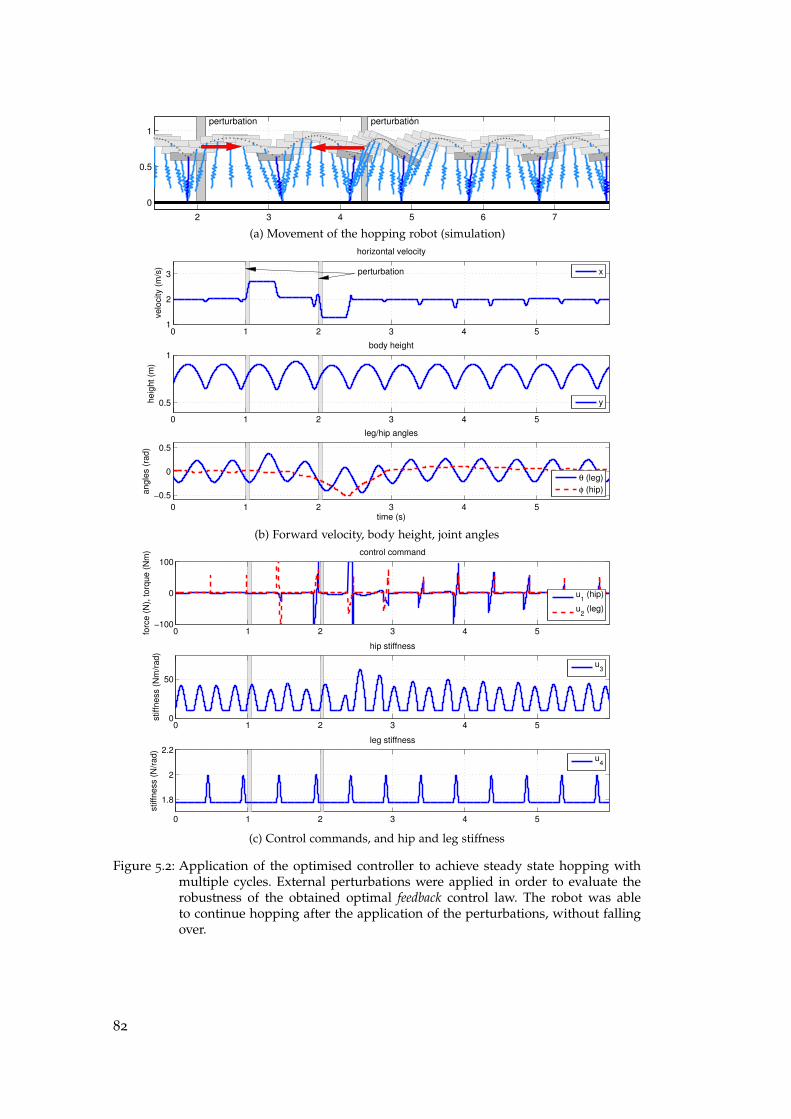
2 3 4 5 6 7

0

0.5

1perturbation perturbation

(a) Movement of the hopping robot (simulation)

0 1 2 3 4 51

2

3

horizontal velocity

velo

city (

m/s

)

perturbation

0 1 2 3 4 5

0.5

1body height

heig

ht (m

)

0 1 2 3 4 5

−0.5

0

0.5

time (s)

angle

s (

rad)

leg/hip angles

x

y

θ (leg)

φ (hip)

(b) Forward velocity, body height, joint angles

0 1 2 3 4 5−100

0

100

forc

e (

N),

torq

ue (

Nm

) control command

0 1 2 3 4 50

50

stiffness (

Nm

/rad)

hip stiffness

0 1 2 3 4 5

1.8

2

2.2

stiffness (

N/r

ad)

leg stiffness

u1 (hip)

u2 (leg)

u3

u4

(c) Control commands, and hip and leg stiffness

Figure 5.2: Application of the optimised controller to achieve steady state hopping withmultiple cycles. External perturbations were applied in order to evaluate therobustness of the obtained optimal feedback control law. The robot was ableto continue hopping after the application of the perturbations, without fallingover.

82

In addition to the discussion concerning the developed approach presented in

Sec. 4.11, we note that in the hopping example enforcing the feasibility of the

switching condition at touch-down is more critical. Hence, the weights of the cost

were empirically adjusted in order to reduce the mismatch. The temporal optimi-

sation also plays a crucial role, as finding a suitable movement duration is effective

in reducing the error. The results obtained showcase how certain mismatches in

the switching conditions can be overcome by using the feedback controller. Further

investigation is required on the extent of these capabilities.

In the next chapter we extend our approach to incorporate model learning in

order to address modelling uncertainties of the system dynamics [Mitrovic, 2010],

which pose a challenging problem, especially in the case of underactuated sys-

tems.

83

6O P T I M A L C O N T R O L W I T H L E A R N E D D Y N A M I C S

In the previous chapters we presented a systematic methodology for movement

optimisation with multiple phases and switching dynamics in robotic systems

with variable stiffness actuation. We showed the effectiveness of the proposed

approach in numerical simulations and on a hardware platform.

The investigation thus far assumes that the dynamics of the controlled systems

are given as an analytic rigid body dynamics model and that model is not chang-

ing over time. For the purpose of our previous tasks, this proved to be an effective

technique. In the current chapter we extend our approach to tasks where the dy-

namics are unknown, too complex to be accurately described by a rigid body

dynamics model and/or subject to methodical changes.

We formulate an online adaptation scheme capable of systematically improving

the multi-phase plans (stiffness modulation and position command) and switching

instances. By incorporating a locally weighted non-parametric learning method to

model the discrepancies in the system dynamics, the dynamics model is improved

on the fly. This is demonstrated on a realistic model of a VSA brachiating system

with excellent adaptation results.

6.1 introduction

The accuracy of model-based control is significantly dependent on that of the

models themselves. Traditional robotics employs models obtained from mechan-

ical engineering insights. Kinematic equations will provide accurate information

about the evolution of a rigid body configuration, given a precise knowledge of its

geometry. Similarly, the dynamics equation can incorporate well modelled factors

such as inertia, Coriolis and centrifugal effect or external forces.

However, there are certain elements that cannot be fully captured by these mod-

els, such as friction from the joints or resulting from cable movement [Siciliano

and Khatib, 2008], which can vary in time. The introduction of flexible elements

in the structure of a system increases the complexity of the model and makes the

identification of accurate dynamics significantly more difficult. Additionally, dur-

85

ing operation, the robot can suffer changes in its mechanical structure due to wear

and tear or due to the use of a tool (which modifies the mechanical chain structure)

[Sigaud et al., 2011].

On-line adaptation of models can provide a solution for capturing all these

properties. Early approaches, such as on-line parameter identification [Sciavicco and

Villani, 2009], which tunes the parameters of a predefined model (dictated by the

mechanical structure) using data collected during operation, proved sufficient for

accurate control and remained a popular approach for a long time [Atkeson et al.,

1986; Khalil and Dombre, 2004]. The increased complexity of latest robotic systems

demands novel approaches capable of accommodating significantly non-linear

and unmodelled robot dynamics. Successful non-parametric model learning meth-

ods use supervised learning to perform system identification with only limited

prior information about its structure - removing the restriction to a fixed model

structure, allowing the model complexity to adapt in a data driven manner.

In this chapter, we build on prior efforts to engage this techniques for robot

control [Mitrovic et al., 2010a; Nakanishi et al., 2005; Nguyen-Tuong and Peters,

2011] and apply this in the context of multiphase variable impedance movements.

Indeed, adaptive model learning has been used successfully in a wide range of

scenarios such as inverse dynamics control [Nguyen-Tuong et al., 2009; Vijayaku-

mar et al., 2002], inverse kinematics [Herbort et al., 2010; Ting et al., 2009], robot

manipulation and locomotion [Kalakrishnan et al., 2009; Schaal et al., 2002].

6.1.1 Adaptive Learning for Optimal Control

Classical OC is formulated using an analytic dynamics model, but recent work

[Atkeson et al., 1997; Mitrovic et al., 2010d] has shown that combining OC with

dynamics learning can produce a powerful and principled control strategy for

complex systems with redundant actuation.

Depending on which type of data is observed, the models obtained can be:

forward models, inverse models, mixed models and multi-step prediction mod-

els [Nguyen-Tuong and Peters, 2011]. There are various control architectures that

integrate learning mechanisms (e.g. direct modelling, indirect modelling, distal

teacher learning), depending on the way in which the model is being adapted

while in use. Direct modelling represents a direct mapping between the inputs and

the outputs in order to improve trajectory tracking performance by predicting the

required motor commands for a desired target state. In indirect modelling the learn-

86

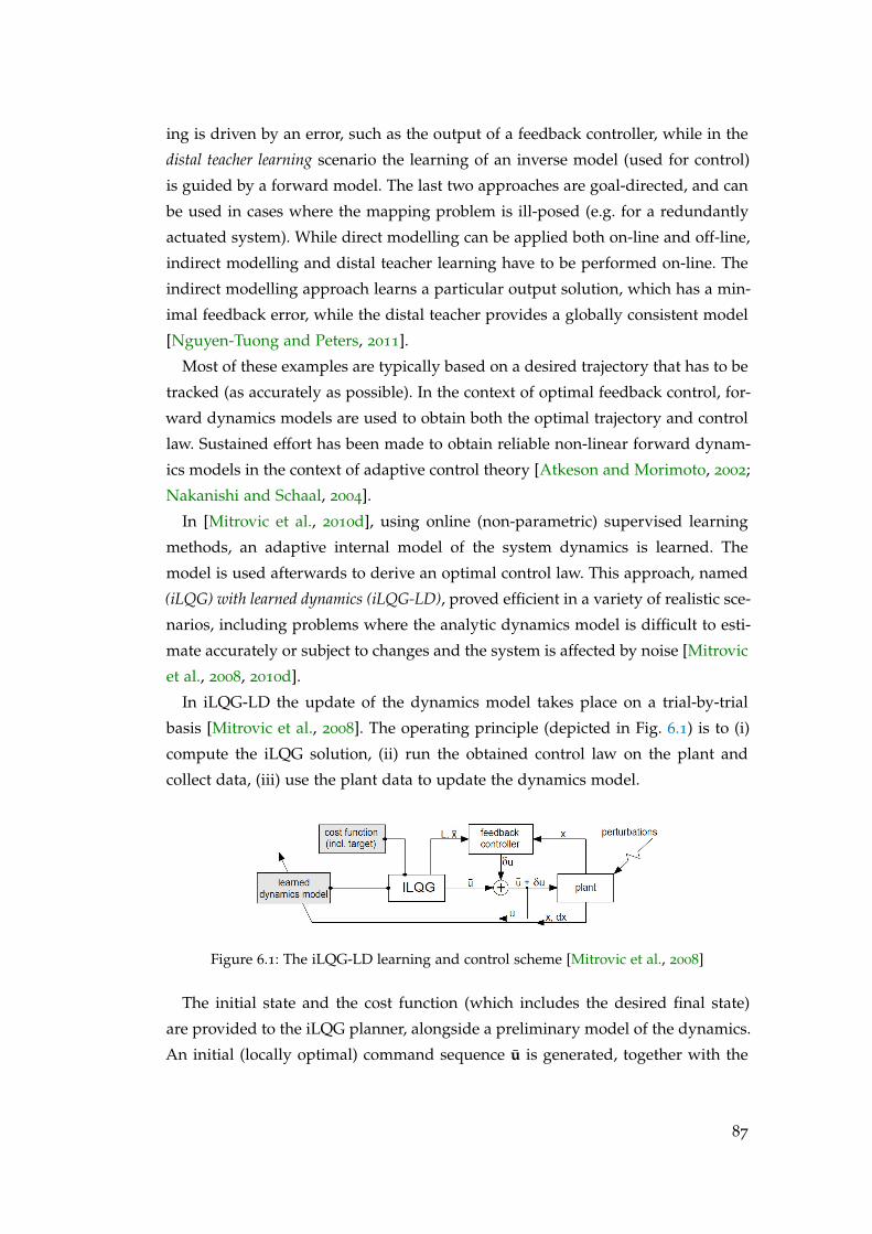
ing is driven by an error, such as the output of a feedback controller, while in the

distal teacher learning scenario the learning of an inverse model (used for control)

is guided by a forward model. The last two approaches are goal-directed, and can

be used in cases where the mapping problem is ill-posed (e.g. for a redundantly

actuated system). While direct modelling can be applied both on-line and off-line,

indirect modelling and distal teacher learning have to be performed on-line. The

indirect modelling approach learns a particular output solution, which has a min-

imal feedback error, while the distal teacher provides a globally consistent model

[Nguyen-Tuong and Peters, 2011].

Most of these examples are typically based on a desired trajectory that has to be

tracked (as accurately as possible). In the context of optimal feedback control, for-

ward dynamics models are used to obtain both the optimal trajectory and control

law. Sustained effort has been made to obtain reliable non-linear forward dynam-

ics models in the context of adaptive control theory [Atkeson and Morimoto, 2002;

Nakanishi and Schaal, 2004].

In [Mitrovic et al., 2010d], using online (non-parametric) supervised learning

methods, an adaptive internal model of the system dynamics is learned. The

model is used afterwards to derive an optimal control law. This approach, named

(iLQG) with learned dynamics (iLQG-LD), proved efficient in a variety of realistic sce-

narios, including problems where the analytic dynamics model is difficult to esti-

mate accurately or subject to changes and the system is affected by noise [Mitrovic

et al., 2008, 2010d].

In iLQG-LD the update of the dynamics model takes place on a trial-by-trial

basis [Mitrovic et al., 2008]. The operating principle (depicted in Fig. 6.1) is to (i)

compute the iLQG solution, (ii) run the obtained control law on the plant and

collect data, (iii) use the plant data to update the dynamics model.

Figure 6.1: The iLQG-LD learning and control scheme [Mitrovic et al., 2008]

The initial state and the cost function (which includes the desired final state)

are provided to the iLQG planner, alongside a preliminary model of the dynamics.

An initial (locally optimal) command sequence u is generated, together with the

87

corresponding state sequence x and feedback correction gains L. Applying the

feedback controller scheme, at each time step the control command is corrected by

δu = L(x − x), where x is the true state of the plant. The model of the dynamics

is updated using the information provided by the applied command u + δu and

observed state x.

6.1.2 Locally Weighted Projection Regression (LWPR)

This methodology employs a Locally Weighted Learning (LWL) method, called the

Locally Weighted Projection Regression (LWPR), to train a model of the dynamics in

an incremental fashion.

LWL algorithms are nonparametric local learning methods that proved success-

ful in the context of (online) motor learning scenarios [Atkeson et al., 1997]. In-

cremental LWL was proposed in [Schaal and Atkeson, 1998] (as the receptive field

weighted regression (RFWR) method) in order to provide fast learning rates and

computational efficiency. RFWR works by allocating resources in a data driven

fashion, allowing on-line adaptation to changes in the behaviour.

Since advanced mechanical systems can output data with potentially irrelevant

and/or redundant dimensions, it was shown that the motion data from such

system can often can be locally represented using low dimensional distributions

[Atkeson et al., 1997]. LWPR [Vijayakumar et al., 2005] exploits this property by

finding locally low dimensional projections that are used to perform a more ef-

ficient local function approximation. The regression function is constructed by

combining local linear models. During training the parameters of the local mod-

els (locality and fit) are updated using incremental partial least squares (PLS). PLS

projects the input onto a small number of directions in the input space along the

directions of maximal correlation with the output and then performs linear re-

gression on the projected inputs. This makes LWPR suitable for high dimensional

input spaces. Local models can be pruned or added on an as-need basis (e.g.,

when training data is generated in previously unexplored regions). The areas of

validity (receptive fields) of each local model are modelled by Gaussian kernels.

LWPR keeps a number of variables that hold sufficient statistics for the algorithm

to perform the required calculations incrementally. The method proved to be a ro-

bust and efficient technique for incremental learning of nonlinear models in high

dimensions [Mitrovic et al., 2010d].

88

We incorporate the iLQG-LD scheme into our approach involving learning the

dynamics of a brachiation system with VSA capabilities and employing it in plan-

ning for locomotion tasks. The method proved capable of adapting to changes

in the system’s properties and provided a better accuracy performance, than the

deterministic optimisation. Based on these results, iLQG-LD could be a strong

candidate for optimal control strategy for more complex hardware systems.

6.1.3 Notes on practical issues concerning model learning and adaptive control methods

In the previous sections we provided a brief outline of model learning techniques

for adaptive (optimal) control with a focus on the LWPR method in the context of

iLQG-LD. Employing this methodology for a specific task is not always straight-

forward. In this section we present an overview of the problems encountered in

customising a machine learning method for a robotics application. We describe

some of the associated approaches for addressing them, including those employed

in the context of our work.

a Model Learning

The accuracy of a model is strongly dependent on the training data provided,

which needs to be sufficiently rich for generalisation and has to cover the state

space associated with the scope of the model.

Many approaches for obtaining the required data have been devised, such as

sampling trajectories generated by random point-to-point movements [Swevers

et al., 1997] or by constrained optimisation [Gautier and Khalil, 1992]. To enhance

the richness of the data additional excitation (persistent excitation [Narendra and

Annaswamy, 1987]) is often required. This excitation can be naturally provided

by the nature of the system (e.g., perturbations affecting an aircraft) or artificially

generated (e.g., adding random perturbations to a system). In our work we employ

a similar technique by adding random perturbations to the solution obtained at

each step of the iLQG-LD and collecting data from the resulting trajectory.

Special attention is necessary to ensure the data is sufficiently smooth, a re-

quirement of most machine learning methods [Nguyen-Tuong and Peters, 2011].

Discontinuities of non-smooth functions can be approximated by kernel methods

[Rasmussen, 2006] or by local models and learning how to switch between these

models [Toussaint and Vijayakumar, 2005].

89

Robotic systems with high DOFs pose a challenge, due to the increased dimen-

sionality of the training data. This is normally handled by employing dimensional-

ity reduction approaches, which have been studied in machine learning for a long

time [Tenenbaum et al., 2000]. While some methods require special preprocessing

to eliminate the irrelevant and/or redundant information [Nguyen-Tuong and Pe-

ters, 2010b], the LWPR method is able to handle both redundant and irrelevant

training data [Vijayakumar et al., 2005].

If prior knowledge is available (in the form of a parametric model), this can

be incorporated into the learning method, rendering a semiparametric model. In

[Nguyen-Tuong and Peters, 2010a] this approach was used to learn an accurate

model with limited training data. In our experiments we use a similar technique

by exploiting the information available in the form of a preliminary (erroneous)

analytic model of the dynamics.

Most machine learning methods are designed for offline learning and run in

batch mode [Nguyen-Tuong and Peters, 2011]. The major motivation for online

learning, (which LWPR permits), is that one cannot cover the regions of interest in

advance, but these can be discovered during execution. This allows for incremen-

tal learning and partial forgetting of previous information. It constitutes a move

towards continuous adaptation, required in order to allow robots increased au-

tonomy [Thrun and Mitchell, 1995]. Modelling nonstationary systems is a neces-

sity for modern robotic applications confronted with time dependent dynamics

[Petkos et al., 2006].

Other practical issues include feature selection and missing data (for robustness

and reliability of the prediction). Probabilistic inference methods can deduce the

missing information, based on the training data. An advantage of recent meth-

ods, such as LWPR, is that feature selection is incorporated within the algorithm

[Vijayakumar et al., 2005].

In [Nakanishi et al., 2005] the authors provide empirical evidence of the per-

formance benefits of LWL over cooperative learning approaches for non-linear

function approximation. They show how the former can provide a much more ac-

curate fit even with a limited number of local models. When the number of models

increases, LWL does not suffer from the overfitting issues exhibited by cooperative

learning approaches. In addition, the study demonstrated that the global accuracy

of a LWL method upper is bounded by that of its individual local linear mod-

els. Since these are updated based on the curvature of the function learned, this

ensures that the upper bound on the model is kept small.

90

b Adaptive control

Controllers able to adapt to changes in the behaviour of the systems are a de-

sirable attribute for many robotic applications. Compared to their non-adaptive

counterparts, which use just a priori information [Dumont et al., 2002], adaptive

controllers incorporate data from the systems behaviour in order to change their

properties or those of the system’s.

Classic adaptive controllers react to sudden changes in the expected behaviour by

updating the control parameters and/or the dynamics model, in order to enhance

performance, such as trajectory tracking [Narendra and Annaswamy, 2012]. By

contrast iterative learning controllers (ILC) make use of the long term history of the

behaviour, gradually improving the performance of the system. They are based on

the assumption that the same task will be performed repeatedly over time. Alter-

natively, reinforcement learning (RL) approaches achieve learning by trial and error,

without specific instructions on which actions to take. By using the information

from previous trials to build a reward function, the system learns to select the

actions providing maximal reward.

In [Mitrovic, 2010] the dual nature of iLQG-LD as a hybrid between ILC and

RL approaches is indicated. The method performs iterative improvements based

on data from each trial (similar to ILC), but is also less concerned with tracking

the previous trajectory and delivers an new optimal feedback law at each iteration

(thus, resembling the RL methodology).

In terms of performance, previous work has shown empirically that iLQG-LD

can deliver a stable performance in the presence of noise and can adjust to com-

plex systematic changes in the (non-linear) dynamics [Mitrovic et al., 2010d]. Most

challenges relate to the magnitude of the non-linearity of the dynamics, the tun-

ing of the LWPR parameters and the fact that the size of training data requirement

increases with the dimensionality of the system. As previous studies have sug-

gested [Mitrovic, 2010], the latter of these issues can be alleviated by incorporat-

ing existing knowledge (analytic dynamics model) in combination with the LWPR

learning.

Previous applications of iLQG-LD have focused on relatively low dimensional,

well-tempered dynamics, mostly in simulation environments. As remarked in

[Mitrovic, 2010], the direct application to a robotic platform raises a few difficul-

ties. Data collection on a hardware is more demanding (even without considering

potential hardware failure) and the noise affecting the system can be more pro-

nounced and less predictable. In cases where discontinuities occur, the method is

91

not equipped with mechanisms that will deal directly with them. Also, success-

ful use of LWPR in practice requires a certain amount of experience and good

intuition (e.g., parameter tuning).

The main challenge is directing the learning on the specific area required for the

task and obtaining a reliable model which is as accurate as possible. Additional

practical challenges relate to the necessity of adequate and reliable sensing. In our

experiments we address these aspects by devising an exploration strategy which

pre-trains the model with information within the region of interest for the given

task. We also provide a set of sensors that allow the LWPR method to learn the

effect of the changes in the model structure and recover the system model.

So far we discussed the relevant background on model learning and adaptive

control, the associated challenges and the approaches of addressing them, with a

focus on our chosen methodology. In the next section we present the formulation

used and the experimental setup of our investigation.

6.2 multi-phase optimisation with adaptive dynamics learning

In Sec. 4.5, we introduced a general formulation of optimal control problems for

tasks with multiple phase movements including switching dynamics and discrete

state transition arising from iterations with an environment. Given a rigid body

dynamics formulation of a robot with a VSA model, a hybrid dynamics represen-

tation with a composite cost function is introduced to describe such a task (Sec.

4.5). In this section we introduce the changes dictated by the use of the LWPR

method in the context of iLQG-LD, for integration within our approach.

6.2.1 Hybrid Robot Dynamics with Variable Stiffness Actuation for Time-based Switch-

ing and Discrete State Transition

We use the hybrid dynamics representation (Sec. 4.5.1) to model multi-phase dy-

namics including contacts with the environment [Caldwell and Murphey, 2011b],

as depicted in Fig. 4.2

To describe multi-phase movements, we consider multiple sets of robot dynam-

ics, as described by (4.3), (4.4). An individual rigid body dynamics model is de-

fined for each associated phase of the movement as a subsystem (4.6). The servo

motor dynamics in the VSA are modelled as a critically damped second order

dynamics (4.7). We assume that the range of control command u is limited be-

92

tween umin and umax. As in Sec. 4.5, we consider a VSA model in which the joint

torques are given in the form (3.3).

We consider the state space representation as the combined plant dynamics

consisting of the rigid body dynamics (4.6) and the servo motor dynamics (4.7),

with x = [ xT1 , xT2 , xT3 , xT4 ]T = [ qT , qT , qTm, qTm ]T ∈ R2(n+m) the state vector

consisting of the robot state and the servo motor state.

Employing the iLQG-LD framework, we aim to create an accurate model of the

dynamics model for the real hardware using supervised learning. We assume the

existence of a preliminary analytic dynamics model that takes the form presented

in (4.6, 4.7), which is inaccurate (due to various factors such as: the inability of the

rigid body dynamics to incorporate all the elements of the system’s behaviour or

changes suffered during operation).

We use the LWPR method to model the error between the true behaviour of the

system and the initial model provided. Thus we replace the dynamics fi in (4.8)

with the composite dynamics model fci:

x = fci(x, u) = fi(x, u) + fi(x, u), (6.1)

where fi ∈ R2(n+m) is the initial inaccurate model and f ∈ R2(n+m) is the LWPR

model mapping the discrepancy between fi ∈ R2(n+m) and the behaviour of the

system. We note that the changes introduced by iLQG-LD only affect the dynamics

modelling in (4.3), while the instantaneous state transition mapped by ∆ in (4.4)

remains unchanged.

For the given hybrid dynamics, in order to describe the full movement with

multiple phases, we consider the same composite cost function, as in (4.9).

6.2.2 Optimal Control of Switching Dynamics and Discrete State Transition

In brief, the iLQR method (Sec. 2.3.1), upon which our developed methodology

(Sec. 4.5) is built, solves an optimal control problem for the locally linear quadratic

approximation of the nonlinear dynamics and the cost function around a nominal

trajectory x and control sequence u in discrete time, and iteratively improves the

solutions.

In order to incorporate switching dynamics and discrete state transition with

a given switching sequence, the hybrid dynamics (4.3) and (4.4) are linearised in

discrete time around the nominal trajectory and control sequence as described by

(4.10) : (4.13).

93

When using the composite model of the dynamics (fc) introduced in (6.1) the

linearisation of the dynamics is provided in two parts. The linearisation of f is

obtained by replacing f with f in (4.10) and (4.12). The derivatives of the learned

model (f) are obtained analytically by differentiating with respect to the inputs

z = (x; u) as suggested in [Atkeson et al., 1997]:

∂f(z)∂z

=1

W

∑k

(∂wk∂z

ψk(z) +wk∂ψk∂z

)−

1

W2

∑k

wk(z)ψk(z)∑l

∂wl∂z

=1

W

∑k

(−ψkwkDk(z − ck) +wkbk) +f(z)W

∑k

wkDk(z − ck), (6.2)

where:

∂f(z)∂z

=

∂f/∂x

∂f/∂u

. (6.3)

Since there are no changes on the encoding of the instantaneous state transition

(4.4) the equations in (4.11) and (4.13) remain unchanged for the iLQG-LD frame-

work. With the above modification (6.2), the developed optimisation methodology

is applied as described in Sec. 4.5 to obtain the locally valid feedback control law.

6.3 brachiation system dynamics

We evaluate the effectiveness of the approach on a robot brachiation task which

incorporates switching dynamics and multiple phases of the movement in a real-

istic VSA actuator model. We consider a two-link underactuated brachiating robot

with a MACCEPA [Ham et al., 2007] variable stiffness actuator, as introduced in

Sec. 4.6.

The equation of motion of the system used takes the standard rigid body dy-

namics form (4.33). The servo motor dynamics are approximated by a second

order system with a PD feedback control, as mentioned in (4.7). As in the pre-

vious study, the bandwidth of the actuator is α = diag(20, 25). The range of the

commands of the servo motors are limited as u1 ∈ [−π/2,π/2] and u2 ∈ [0,π/2].

94

The model parameters are shown in Table 6.1 and the MACCEPA parameters

with the spring constant κs = 771 N/m, the lever length B = 0.03 m, the pin

displacement C = 0.125 m and the drum radius rd = 0.01 m. 1

Robot parameters i=1 i=2 i=1

Mass mi (kg) 1.390 0.527 1.240

Moment of inertia Ii (kgm2) 0.0297 0.0104 0.0278

Link length li (m) 0.46 0.46 0.46

COM location lci (m) 0.362 0.233 0.350

Viscous friction di (Nm/s) 0.03 0.035 0.03

Table 6.1: Model parameters of the two-link brachiating robot. The final column showsthe change of parameters of the first link of the system under the changed massdistribution described in Sec. 6.4

6.4 experimental setup

To test the efficiency of our approach we create a scenario where the difference

between the true and the assumed model is caused by a change in the mass (and

implicitly mass distribution) on one the links (i.e. the mass of the true model is

smaller by 150 g (located at the joint) on link i = 1). The changed model parameters

are shown in the right column of Table 6.1.

The error in the dynamics manifests itself only in the joint accelerations. Thus,

we require to map the error just in those two dimensions, reducing the dimension

of the output of the LWPR model f from n = 8 to 2, where the predictions are

added on the corresponding dimension of f within fc (6.1). Note that different

discrepancies could necessitate estimation of the full 8-dimensional state error.

In line with previous work, we will demonstrate the effectiveness of the pro-

posed approach on a multi-phase, asymmetric swing-up and brachiation task with

a VSA while incorporating continuous, online model learning. Specifically, in the

multi-phase task, the robot swings up from the suspended posture to the target

at d1 = 0.40 m and subsequently moves to the target located at d2 = 0.42 m and

d3 = 0.46 m, respectively.

1 The MACCEPA parameters are the same as described in Chapter 4.

95

Since the system has an asymmetric configuration and the state space of the

swing-up task is significantly different from that of a brachiation movement we

proceed by first learning a separate error model for each phase. The procedure

used is briefly described in Algorithm 3. The initial exploration loop is performed

in order to pre-train the LWPR model fi (as an alternative to applying motor

babbling), the latter loop is using iLQG-LD to refine the model in an online fashion.

In our experiments the training data is obtained by using a simulated version of

the true dynamics, which is an analytic model incorporating the discrepancy. For

details on the set-up of the LWPR model, initialisation and parameter selection,

we refer the interested reader to Appendix F.

Algorithm 3 Description of the learning and exploration procedure

Given:• analytic dynamics for one configuration fi and start state x0• thresholds for target reaching εT and model accuracy εM• the associated cost function J (including desired target xT )• p number of initial exploration training episodes

Initialise• fi(x, u) ; fci(x, u)=fi(x, u) + fi(x, u)

repeat• generate u, x, L using fi(x, u) for an randomised exploration target• apply the solution to the true dynamics• train the model on the collected data• apply η perturbed versions of the solution to the true dynamics• train the model on the collected data

until p training episodes have been performed

repeat• apply iLQG-LD for target xT

until εT and nMSE conditions are met

6.4.1 Individual Phase Learning

Using the traditional OC framework in the presence of an accurate dynamics

model, the multi-phase task described in Sec. 4.8 was achieved with a position

error of just 0.002 m. Once the discrepancy detailed in Sec. 6.4 is introduced, the

planned solution is no longer valid and the final position deviates from the desired

target (Fig. 6.2, blue line). We deploy the iLQG-LD framework in order to learn

the new behaviour of the system and recover the task performance.

96

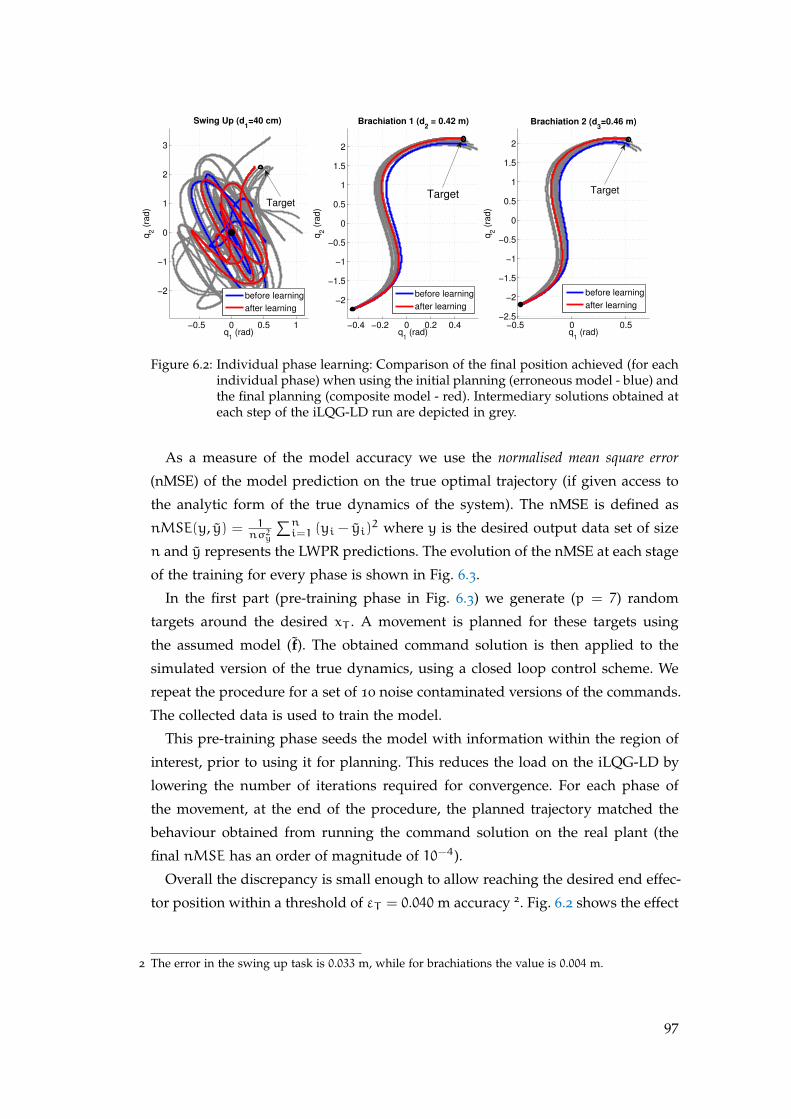
−0.5 0 0.5 1

−2

−1

0

1

2

3

q1 (rad)

q2 (

rad

)

Swing Up (d1=40 cm)

before learning

after learning

Target

−0.4 −0.2 0 0.2 0.4

−2

−1.5

−1

−0.5

0

0.5

1

1.5

2

q1 (rad)

q2 (

rad

)

Brachiation 1 (d2 = 0.42 m)

before learning

after learning

Target

−0.5 0 0.5−2.5

−2

−1.5

−1

−0.5

0

0.5

1

1.5

2

q1 (rad)

q2 (

rad

)

Brachiation 2 (d3=0.46 m)

before learning

after learning

Target

Figure 6.2: Individual phase learning: Comparison of the final position achieved (for eachindividual phase) when using the initial planning (erroneous model - blue) andthe final planning (composite model - red). Intermediary solutions obtained ateach step of the iLQG-LD run are depicted in grey.

As a measure of the model accuracy we use the normalised mean square error

(nMSE) of the model prediction on the true optimal trajectory (if given access to

the analytic form of the true dynamics of the system). The nMSE is defined as

nMSE(y, y) = 1nσ2y

∑ni=1 (yi − yi)

2 where y is the desired output data set of size

n and y represents the LWPR predictions. The evolution of the nMSE at each stage

of the training for every phase is shown in Fig. 6.3.

In the first part (pre-training phase in Fig. 6.3) we generate (p = 7) random

targets around the desired xT . A movement is planned for these targets using

the assumed model (f). The obtained command solution is then applied to the

simulated version of the true dynamics, using a closed loop control scheme. We

repeat the procedure for a set of 10 noise contaminated versions of the commands.

The collected data is used to train the model.

This pre-training phase seeds the model with information within the region of

interest, prior to using it for planning. This reduces the load on the iLQG-LD by

lowering the number of iterations required for convergence. For each phase of

the movement, at the end of the procedure, the planned trajectory matched the

behaviour obtained from running the command solution on the real plant (the

final nMSE has an order of magnitude of 10−4).

Overall the discrepancy is small enough to allow reaching the desired end effec-

tor position within a threshold of εT = 0.040m accuracy 2. Fig. 6.2 shows the effect

2 The error in the swing up task is 0.033 m, while for brachiations the value is 0.004 m.

97

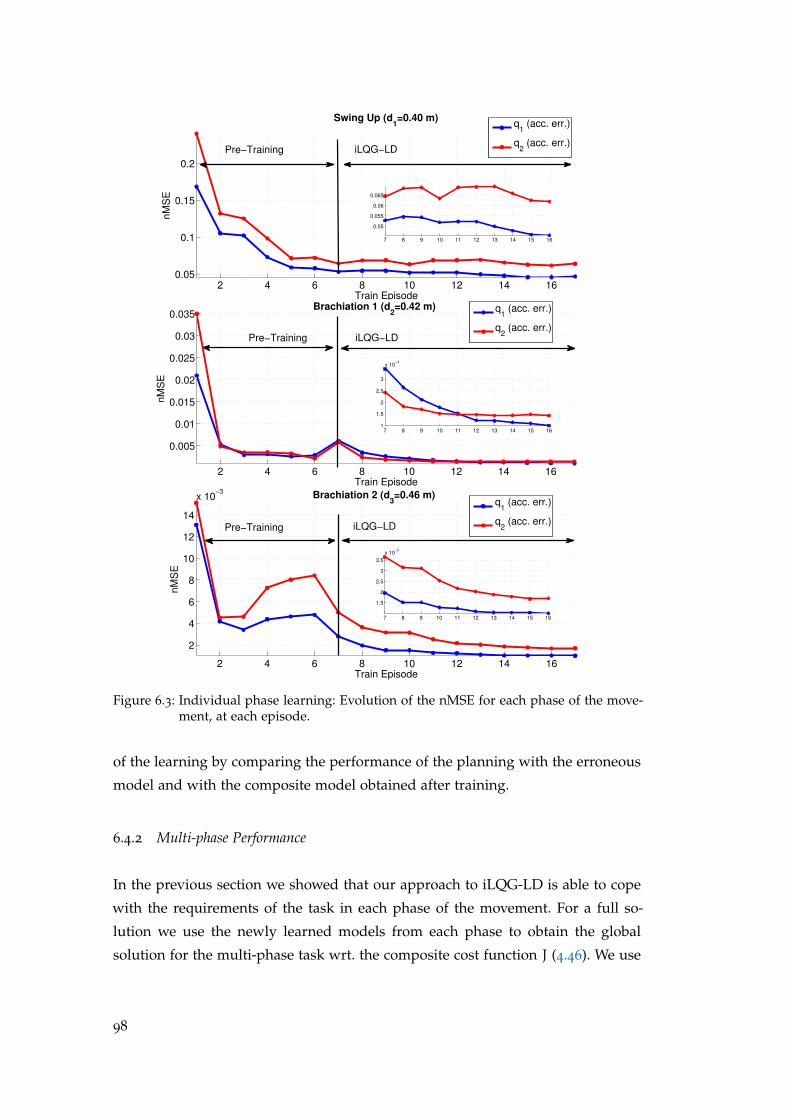
2 4 6 8 10 12 14 160.05

0.1

0.15

0.2

Train Episode

nM

SE

Swing Up (d1=0.40 m)

q1 (acc. err.)

q2 (acc. err.)

Pre−Training iLQG−LD

7 8 9 10 11 12 13 14 15 16

0.05

0.055

0.06

0.065

2 4 6 8 10 12 14 16

0.005

0.01

0.015

0.02

0.025

0.03

0.035

nM

SE


Train Episode

q1 (acc. err.)

q2 (acc. err.)

iLQG−LDPre−Training

7 8 9 10 11 12 13 14 15 161

1.5

2

2.5

3

x 10−3

2 4 6 8 10 12 14 16

2

4

6

8

10

12

14

x 10−3

nM

SE


Train Episode

q1 (acc. err.)

q2 (acc. err.)


7 8 9 10 11 12 13 14 15 16

1.5

2

2.5

3

3.5

x 10−3

Figure 6.3: Individual phase learning: Evolution of the nMSE for each phase of the move-ment, at each episode.

of the learning by comparing the performance of the planning with the erroneous

model and with the composite model obtained after training.

6.4.2 Multi-phase Performance

In the previous section we showed that our approach to iLQG-LD is able to cope

with the requirements of the task in each phase of the movement. For a full so-

lution we use the newly learned models from each phase to obtain the global

solution for the multi-phase task wrt. the composite cost function J (4.46). We use

98

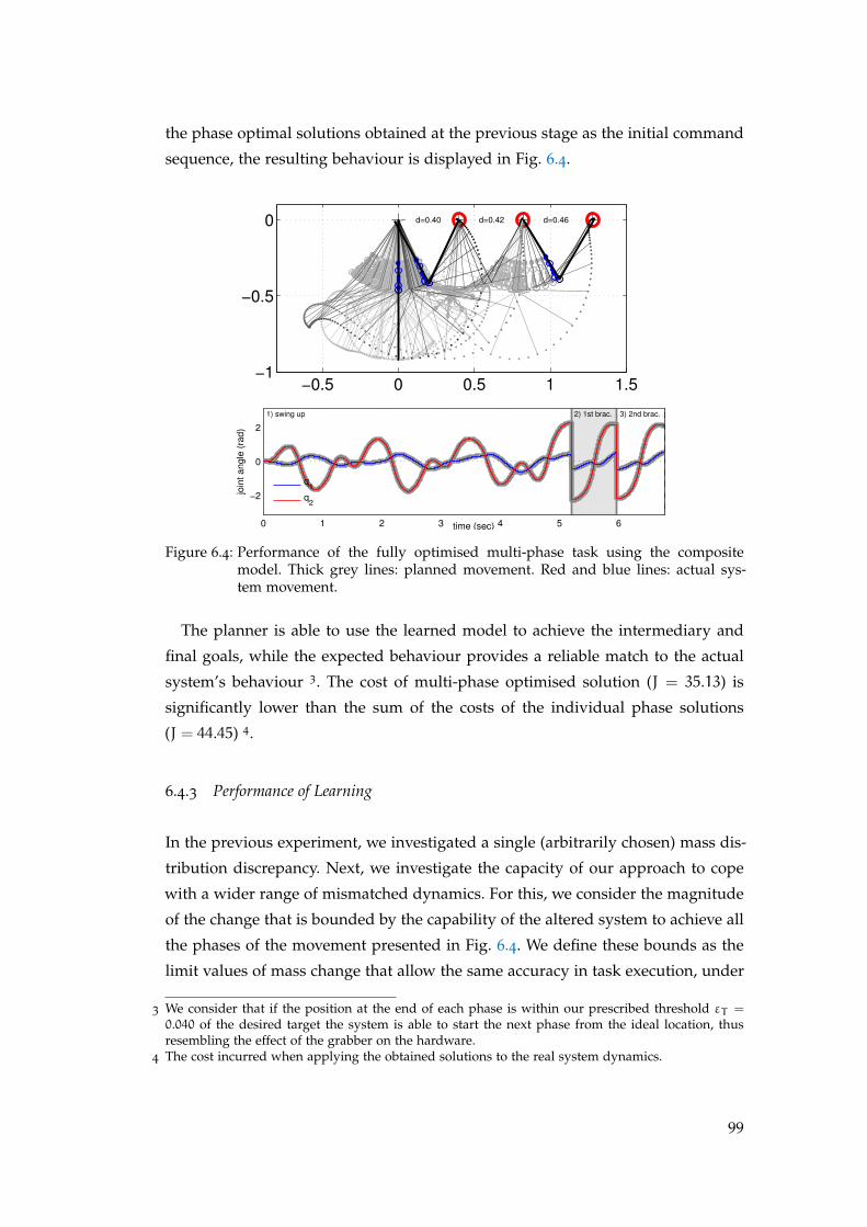
the phase optimal solutions obtained at the previous stage as the initial command

sequence, the resulting behaviour is displayed in Fig. 6.4.

−0.5 0 0.5 1 1.5−1

−0.5

0 d=0.40 d=0.42 d=0.46

0 1 2 3 4 5 6

−2

0

2

time (sec)

join

t an

gle

(ra

d)

1) swing up 2) 1st brac. 3) 2nd brac.

q1

q2

Figure 6.4: Performance of the fully optimised multi-phase task using the compositemodel. Thick grey lines: planned movement. Red and blue lines: actual sys-tem movement.

The planner is able to use the learned model to achieve the intermediary and

final goals, while the expected behaviour provides a reliable match to the actual

system’s behaviour 3. The cost of multi-phase optimised solution (J = 35.13) is

significantly lower than the sum of the costs of the individual phase solutions

(J = 44.45) 4.

6.4.3 Performance of Learning

In the previous experiment, we investigated a single (arbitrarily chosen) mass dis-

tribution discrepancy. Next, we investigate the capacity of our approach to cope

with a wider range of mismatched dynamics. For this, we consider the magnitude

of the change that is bounded by the capability of the altered system to achieve all

the phases of the movement presented in Fig. 6.4. We define these bounds as the

limit values of mass change that allow the same accuracy in task execution, under

3 We consider that if the position at the end of each phase is within our prescribed threshold εT =0.040 of the desired target the system is able to start the next phase from the ideal location, thusresembling the effect of the grabber on the hardware.

4 The cost incurred when applying the obtained solutions to the real system dynamics.

99

the same cost function (4.46). The corresponding values for these limits, found

empirically, are −0.200 kg and +0.300 kg, respectively 5.

We apply our framework to the scenarios where the mass has been altered

to these boundary values and demonstrate the result on just one of the phases,

namely the first brachiation move, to study the relative effects.

Fig. 6.5 (a) shows the effect of the alteration introduced, when executing the

commands resulting from the initial planning (using the erroneous model). After

training and re-planning the model starts approximating the true behaviour of the

system, such that in less than 10 iLQG-LD episodes, the system is once again able

to reach the desired target, as depicted in Fig. 6.5 (b) and 6.5 (c).

−0.4 −0.2 0 0.2 0.4−2.5

−2

−1.5

−1

−0.5

0

0.5

1

1.5

2

2.5

q1 (rad)

q2 (

rad)

mmin

morig

mmax

−0.5 0 0.5

−2

−1.5

−1

−0.5

0

0.5

1

1.5

2

q1 (rad)

q2 (

rad

)

mmin

= morig

− 0.2 kg

before learning

after learning

−0.4 −0.2 0 0.2 0.4−2.5

−2

−1.5

−1

−0.5

0

0.5

1

1.5

2

2.5

q1 (rad)

q2 (

rad

)

mmax

= morig

+ 0.3 kg

before learning

after learning

a b c

Figure 6.5: (a): Effect of the discrepancy introduced by the limit values on the mass modu-lation (blue lines). The behaviour when the model match is correct is depictedfor comparison (green line). (b) - (c): Comparison of the final position achieved(for each individual phase) when using the initial planning (erroneous model- blue) and the final planning (composite model - red). Intermediary solutionsobtained at each step of the iLQG-LD run are depicted in grey. Results for theboundary value discrepancies on the mass distribution.

6.5 impedance discrepancy

In the previous section we introduced a model discrepancy by changing the mass

(and mass distribution) on one the links (i.e. the mass of the true model is smaller

by 150 g (located at the joint) on link i = 1). We showed that our online adaptation

5 We note that in our experiments, we assume that modulating the mass distribution does not affectthe motor dynamics – this represents a simplified scenario. In the real hardware, the speed of themotor dynamics (4.7) is indeed a function of the overall load distribution.

100

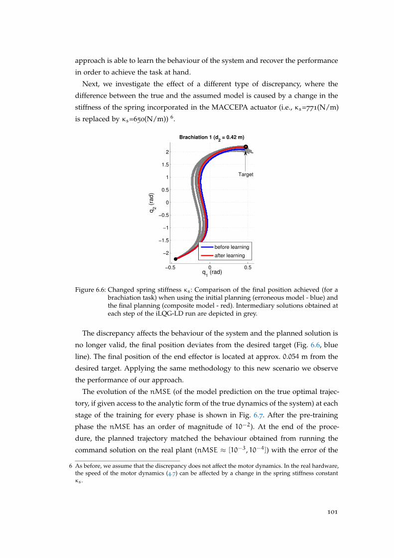
approach is able to learn the behaviour of the system and recover the performance

in order to achieve the task at hand.

Next, we investigate the effect of a different type of discrepancy, where the

difference between the true and the assumed model is caused by a change in the

stiffness of the spring incorporated in the MACCEPA actuator (i.e., κs=771(N/m)

is replaced by κs=650(N/m)) 6.

−0.5 0 0.5

−2

−1.5

−1

−0.5

0

0.5

1

1.5

2

q1 (rad)

q2 (

rad)

Brachiation 1 (d2 = 0.42 m)

before learning

after learning

Target

Figure 6.6: Changed spring stiffness κs: Comparison of the final position achieved (for abrachiation task) when using the initial planning (erroneous model - blue) andthe final planning (composite model - red). Intermediary solutions obtained ateach step of the iLQG-LD run are depicted in grey.

The discrepancy affects the behaviour of the system and the planned solution is

no longer valid, the final position deviates from the desired target (Fig. 6.6, blue

line). The final position of the end effector is located at approx. 0.054 m from the

desired target. Applying the same methodology to this new scenario we observe

the performance of our approach.

The evolution of the nMSE (of the model prediction on the true optimal trajec-

tory, if given access to the analytic form of the true dynamics of the system) at each

stage of the training for every phase is shown in Fig. 6.7. After the pre-training

phase the nMSE has an order of magnitude of 10−2). At the end of the proce-

dure, the planned trajectory matched the behaviour obtained from running the

command solution on the real plant (nMSE ≈ [10−3, 10−4]) with the error of the

6 As before, we assume that the discrepancy does not affect the motor dynamics. In the real hardware,the speed of the motor dynamics (4.7) can be affected by a change in the spring stiffness constantκs.

101

final position for the end effector after training 0.008 m. Fig. 6.6 shows the effect

of the learning by comparing the performance of the planning with the erroneous

model and with the composite model obtained after training.

2 4 6 8 10 12 14 16

0.005

0.01

0.015

0.02

0.025

Train Episode

nM

SE

q1 (acc. err.)

q2 (acc. err.)


Figure 6.7: Changed spring stiffness κs: Evolution of the nMSE at each episode

The results obtained in this investigation suggest that the approach can be em-

ployed for several types of discrepancies, caused by a variety of changes in the

system’s structure.

6.6 transfer learning

In the investigation so far we build a model for each specific task of the multi-

phase movement by collecting and training it on data near the domain of each task.

This approach can be time consuming, especially for systems with large DOFs and

it scales with the number of tasks introduced. A more efficient approach will use a

singular (general model) and allow the knowledge gained in the context of previous

tasks to be reused in improving performance on a new task.

6.6.1 General Background on Transfer Learning

The concept of transferring knowledge between different tasks is not novel. In

transfer learning knowledge from previous task(s) (source task(s)) is applied to a

new task (target task) in order to facilitate learning in the new context (compared

to the scenario of learning for the new task in isolation). Transfer learning has

been studied in the context of machine learning [Pan and Yang, 2010; Torrey and

Shavlik, 2009] for classification, regression and clustering problems. In the field

of robotics most transfer learning work has focused on reinforcement learning

assignments [Barrett et al., 2010; Thrun and Mitchell, 1995].

102

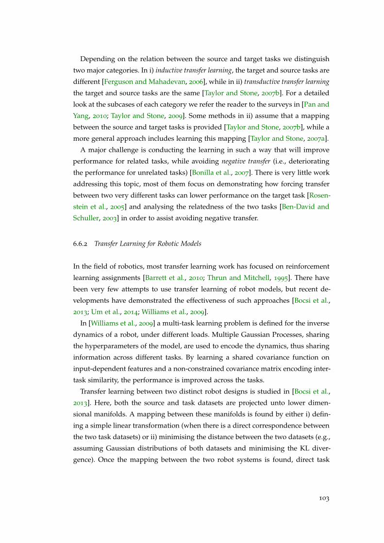
Depending on the relation between the source and target tasks we distinguish

two major categories. In i) inductive transfer learning, the target and source tasks are

different [Ferguson and Mahadevan, 2006], while in ii) transductive transfer learning

the target and source tasks are the same [Taylor and Stone, 2007b]. For a detailed

look at the subcases of each category we refer the reader to the surveys in [Pan and

Yang, 2010; Taylor and Stone, 2009]. Some methods in ii) assume that a mapping

between the source and target tasks is provided [Taylor and Stone, 2007b], while a

more general approach includes learning this mapping [Taylor and Stone, 2007a].

A major challenge is conducting the learning in such a way that will improve

performance for related tasks, while avoiding negative transfer (i.e., deteriorating

the performance for unrelated tasks) [Bonilla et al., 2007]. There is very little work

addressing this topic, most of them focus on demonstrating how forcing transfer

between two very different tasks can lower performance on the target task [Rosen-

stein et al., 2005] and analysing the relatedness of the two tasks [Ben-David and

Schuller, 2003] in order to assist avoiding negative transfer.

6.6.2 Transfer Learning for Robotic Models

In the field of robotics, most transfer learning work has focused on reinforcement

learning assignments [Barrett et al., 2010; Thrun and Mitchell, 1995]. There have

been very few attempts to use transfer learning of robot models, but recent de-

velopments have demonstrated the effectiveness of such approaches [Bocsi et al.,

2013; Um et al., 2014; Williams et al., 2009].

In [Williams et al., 2009] a multi-task learning problem is defined for the inverse

dynamics of a robot, under different loads. Multiple Gaussian Processes, sharing

the hyperparameters of the model, are used to encode the dynamics, thus sharing

information across different tasks. By learning a shared covariance function on

input-dependent features and a non-constrained covariance matrix encoding inter-

task similarity, the performance is improved across the tasks.

Transfer learning between two distinct robot designs is studied in [Bocsi et al.,

2013]. Here, both the source and task datasets are projected unto lower dimen-

sional manifolds. A mapping between these manifolds is found by either i) defin-

ing a simple linear transformation (when there is a direct correspondence between

the two task datasets) or ii) minimising the distance between the two datasets (e.g.,

assuming Gaussian distributions of both datasets and minimising the KL diver-

gence). Once the mapping between the two robot systems is found, direct task

103

transfer is possible. Using previously available information is shown to improve

the learning of forward kinematics.

In [Um et al., 2014] an alternative for task-to-task transfer learning is provided,

whereby a model is learned for each joint independently, instead of a whole body

model. This differs from a multi-task approach since the focus is not improving

performance across all tasks, but rather focusing on the current target task. The

method uses the modular Newton-Euler formulation of the dynamics to separate

the data relevant to each joint. A Gaussian Process regression is then used for each

joint to learn the model of the error between an assumed rigid body dynamics

model and the true system behaviour.

6.6.3 Transfer Learning : Forward Dynamics of Brachiation System

In the previous section we introduced the topic of transfer learning. We showed

that, in spite of a limited amount of research addressing robot models in this con-

text, the available results show the potential benefits of using previous knowledge

in building the model of the system within the context of a new task.

In this section we perform an investigation into transfer learning in the context

of our multi-phase movement task. We use the brachiation system to analyse the

effect of using knowledge from a previously available task on the performance

within the current task for the LWPR based model.

Subsequently, we compare the results obtained for the multi-phase scenario in

Sec. 6.4.2, with the resulting behaviour on the same task using a single unified

model of the dynamics, instead of individual ones for each phase.

a Task-to-task Transfer

For the first transfer of knowledge investigation we define the source task as the

swing-up motion and the target task as the final brachiation (i.e., the third phase of

the multi-phase task described). In this scenario we know empirically that the two

tasks share a segment of the domain space. We use the model learned during the

source task, instead of training a new model just on the data from the brachiation

task.

In the LWPR learning we set the forgetting factor variables (i.e., initial and final

forgetting factors, and the annealing constant for adjusting the forgetting factor) to

minimise information loss. Thus, we aim to reduce the effect of negative transfer

in the inverse direction. By adding new information, the performance of the pre-

104

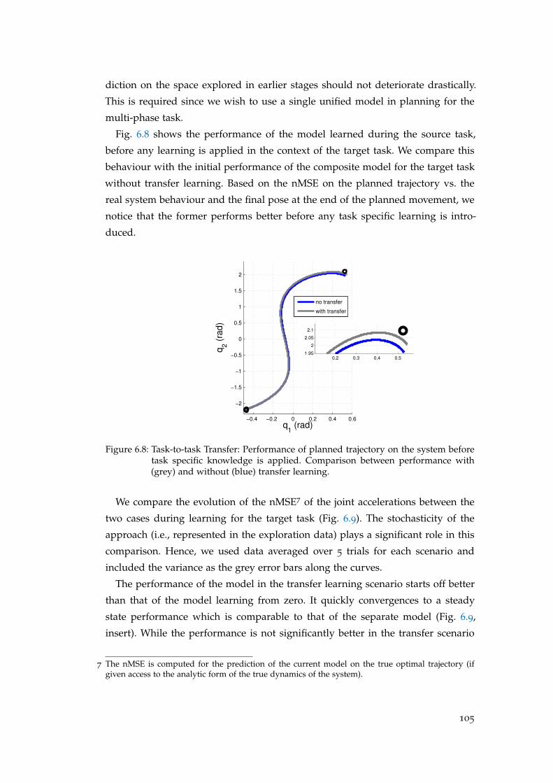
diction on the space explored in earlier stages should not deteriorate drastically.

This is required since we wish to use a single unified model in planning for the

multi-phase task.

Fig. 6.8 shows the performance of the model learned during the source task,

before any learning is applied in the context of the target task. We compare this

behaviour with the initial performance of the composite model for the target task

without transfer learning. Based on the nMSE on the planned trajectory vs. the

real system behaviour and the final pose at the end of the planned movement, we

notice that the former performs better before any task specific learning is intro-

duced.

−0.4 −0.2 0 0.2 0.4 0.6

−2

−1.5

−1

−0.5

0

0.5

1

1.5

2

q1 (rad)

q2 (

rad)

no transfer

with transfer

0.2 0.3 0.4 0.5

1.95

2

2.05

2.1

Figure 6.8: Task-to-task Transfer: Performance of planned trajectory on the system beforetask specific knowledge is applied. Comparison between performance with(grey) and without (blue) transfer learning.

We compare the evolution of the nMSE7 of the joint accelerations between the

two cases during learning for the target task (Fig. 6.9). The stochasticity of the

approach (i.e., represented in the exploration data) plays a significant role in this

comparison. Hence, we used data averaged over 5 trials for each scenario and

included the variance as the grey error bars along the curves.

The performance of the model in the transfer learning scenario starts off better

than that of the model learning from zero. It quickly convergences to a steady

state performance which is comparable to that of the separate model (Fig. 6.9,

insert). While the performance is not significantly better in the transfer scenario

7 The nMSE is computed for the prediction of the current model on the true optimal trajectory (ifgiven access to the analytic form of the true dynamics of the system).

105

2 4 6 8 10 12 14 16

Train Episode

0

0.005

0.01

0.015

0.02

0.025

0.03

0.035

0.04

0.045

0.05

nM

SE

q1 (acc. err.) NO TRANSFER


q1 (acc. err.) WITH TRANSFER


iLQG-LDPre-Training

Figure 6.9: Task-to-task Transfer: Evolution of the nMSE at each episode. Comparison be-tween performance with and without transfer learning. The results are aver-aged over 5 trials in each scenarios. The variance is included in the grey errorbars along the curves.

we observe that the convergence to a lower nMSE level can be faster (e.g., episodes

#8 : #10, Fig. 6.9). If the task permits, a more relaxed accuracy threshold, a transfer

learning approach may lower the time spent in reaching the solution.

b Inverted Model

Having investigated task-to-task transfer within the previous experiments, we now

turn our attention to transfer learning where the target task is the first brachiation

movement (i.e., the second phase of the multi-phase task described). The source

tasks are the previously explored phases. We note than in this case the source

tasks both use the same handhold configuration, while the target task is using the

alternative configuration.

We compare the evolution of the nMSE on the joint accelerations between the

two cases during learning for the target task (Fig. 6.10). As in the previous investi-

gation, the results presented are averaged over 5 trials for each scenario with the

variance represented by the grey error bars along the curves.

The overall performance of the model in the transfer learning scenario is compa-

rable that of the model learning from zero. The small improvement of the average

performance of the model in the transfer learning scenario, including the asymp-

totic performance (Fig. 6.10, insert), can be justified by the stochastic nature of the

106

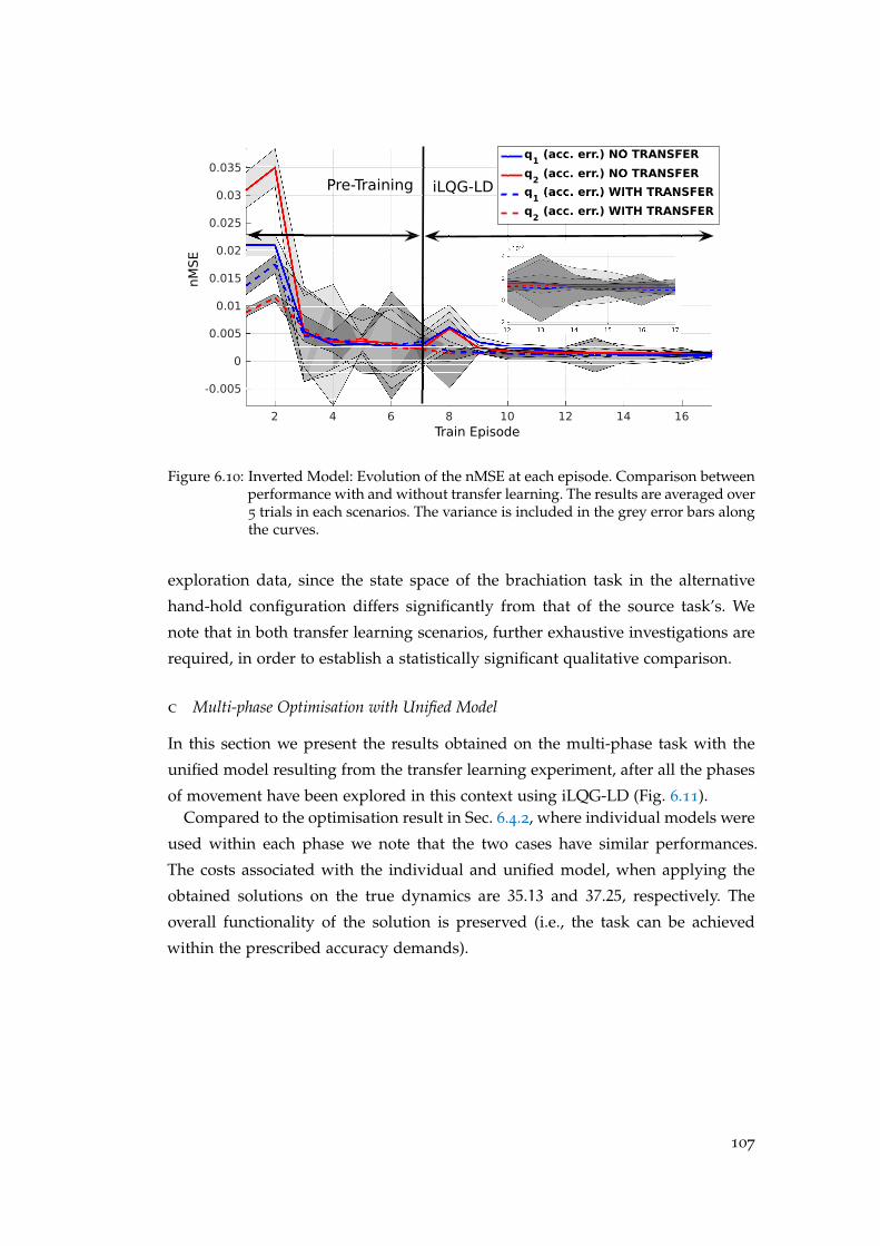
2 4 6 8 10 12 14 16

Train Episode

-0.005

0

0.005

0.01

0.015

0.02

0.025

0.03

0.035

nM

SE





iLQG-LDPre-Training

Figure 6.10: Inverted Model: Evolution of the nMSE at each episode. Comparison betweenperformance with and without transfer learning. The results are averaged over5 trials in each scenarios. The variance is included in the grey error bars alongthe curves.

exploration data, since the state space of the brachiation task in the alternative

hand-hold configuration differs significantly from that of the source task’s. We

note that in both transfer learning scenarios, further exhaustive investigations are

required, in order to establish a statistically significant qualitative comparison.

c Multi-phase Optimisation with Unified Model

In this section we present the results obtained on the multi-phase task with the

unified model resulting from the transfer learning experiment, after all the phases

of movement have been explored in this context using iLQG-LD (Fig. 6.11).Compared to the optimisation result in Sec. 6.4.2, where individual models were

used within each phase we note that the two cases have similar performances.

The costs associated with the individual and unified model, when applying the

obtained solutions on the true dynamics are 35.13 and 37.25, respectively. The

overall functionality of the solution is preserved (i.e., the task can be achieved

within the prescribed accuracy demands).

107

−0.5 0 0.5 1 1.5−1

−0.8

−0.6

−0.4

−0.2

0 d=0.40 d=0.42 d=0.46

optimized robot movement

0 1 2 3 4 5 6

−2

0

2

time (sec)

join

t a

ng

le (

rad

)

joint angles

1) swing up 2) 1st brac. 3) 2nd brac.

q1

q2

Figure 6.11: Performance of the fully optimised multi-phase task using the compositemodel. Thick grey lines: planned movement. Red and blue lines: actual systemmovement.

6.7 hardware experiments : individual phase learning for a brachi-

ation robot

In this section we perform a hardware validation of the simulation results obtained

in Sec. 6.4. We deploy the developed strategy, once the mass distribution discrep-

ancy has been introduced, in order to learn the new behaviour of the system and

recover the task performance.

In the hardware experiment set-up we only have access to readings from two

IMU units attached to each link, a potentiometer mounted on the main joint and

the internal potentiometers of the actuating motors8. The former are fairly accurate

and, with adequate filtering, provide reliable readings for estimating the positions

and velocities of the robot links. The motors’ internal potentiometers however, suf-

fer from high noise; with filtering, their readings can be used as an estimation

of the motor position, but they are too unreliable for deriving the motor accel-

8 For details please see Sec. 4.9.

108

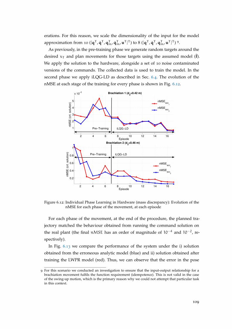
erations. For this reason, we scale the dimensionality of the input for the model

approximation from 10 ([qT , qT , qTm, qTm, uT ]T ) to 8 ([qT , qT , qTm, uT ]T ) 9.

As previously, in the pre-training phase we generate random targets around the

desired xT and plan movements for those targets using the assumed model (f).

We apply the solution to the hardware, alongside a set of 10 noise contaminated

versions of the commands. The collected data is used to train the model. In the

second phase we apply iLQG-LD as described in Sec. 6.4. The evolution of the

nMSE at each stage of the training for every phase is shown in Fig. 6.12.

2 4 6 8 10 12 14 16

1

2

3

4

5

x 10−3

Episode

nM

SE

(crt

. so

lutio

n)


nMSEacc

1

nMSEacc

2


2 4 6 8 10 12 14 16

0.2

0.4

0.6

0.8

1

Episode

nM

SE

(crt

. so

lutio

n)


nMSEacc

1

nMSEacc

2


Figure 6.12: Individual Phase Learning in Hardware (mass discrepancy): Evolution of thenMSE for each phase of the movement, at each episode

For each phase of the movement, at the end of the procedure, the planned tra-

jectory matched the behaviour obtained from running the command solution on

the real plant (the final nMSE has an order of magnitude of 10−4 and 10−2, re-

spectively).

In Fig. 6.13 we compare the performance of the system under the i) solution

obtained from the erroneous analytic model (blue) and ii) solution obtained after

training the LWPR model (red). Thus, we can observe that the error in the pose

9 For this scenario we conducted an investigation to ensure that the input-output relationship for abrachiation movement fulfils the function requirement (idempotence). This is not valid in the caseof the swing-up motion, which is the primary reason why we could not attempt that particular taskin this context.

109

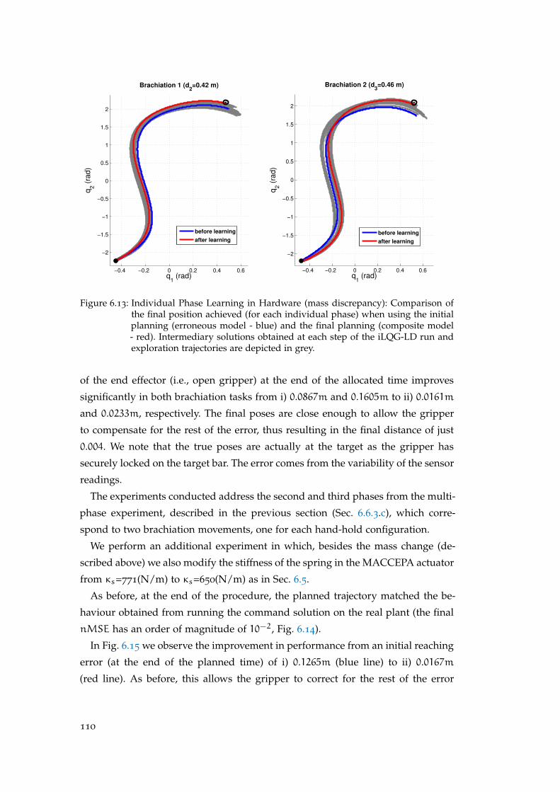
−0.4 −0.2 0 0.2 0.4 0.6

−2

−1.5

−1

−0.5

0

0.5

1

1.5

2

q1 (rad)

q2 (

rad)


before learning

after learning

−0.4 −0.2 0 0.2 0.4 0.6

−2

−1.5

−1

−0.5

0

0.5

1

1.5

2

q1 (rad)

q2 (

rad)


before learning

after learning

Figure 6.13: Individual Phase Learning in Hardware (mass discrepancy): Comparison ofthe final position achieved (for each individual phase) when using the initialplanning (erroneous model - blue) and the final planning (composite model- red). Intermediary solutions obtained at each step of the iLQG-LD run andexploration trajectories are depicted in grey.

of the end effector (i.e., open gripper) at the end of the allocated time improves

significantly in both brachiation tasks from i) 0.0867m and 0.1605m to ii) 0.0161m

and 0.0233m, respectively. The final poses are close enough to allow the gripper

to compensate for the rest of the error, thus resulting in the final distance of just

0.004. We note that the true poses are actually at the target as the gripper has

securely locked on the target bar. The error comes from the variability of the sensor

readings.

The experiments conducted address the second and third phases from the multi-

phase experiment, described in the previous section (Sec. 6.6.3.c), which corre-

spond to two brachiation movements, one for each hand-hold configuration.

We perform an additional experiment in which, besides the mass change (de-

scribed above) we also modify the stiffness of the spring in the MACCEPA actuator

from κs=771(N/m) to κs=650(N/m) as in Sec. 6.5.

As before, at the end of the procedure, the planned trajectory matched the be-

haviour obtained from running the command solution on the real plant (the final

nMSE has an order of magnitude of 10−2, Fig. 6.14).

In Fig. 6.15 we observe the improvement in performance from an initial reaching

error (at the end of the planned time) of i) 0.1265m (blue line) to ii) 0.0167m

(red line). As before, this allows the gripper to correct for the rest of the error

110

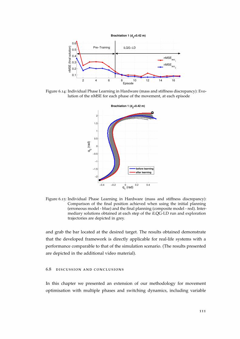
2 4 6 8 10 12 14 16

0.1

0.2

0.3

0.4

0.5

0.6

Episode

nM

SE

(fin

al so

lutio

n)


nMSEacc

1

nMSEacc

2


Figure 6.14: Individual Phase Learning in Hardware (mass and stiffness discrepancy): Evo-lution of the nMSE for each phase of the movement, at each episode

−0.4 −0.2 0 0.2 0.4

−2

−1.5

−1

−0.5

0

0.5

1

1.5

2

q1 (rad)

q2 (

rad)


before learning

after learning

Figure 6.15: Individual Phase Learning in Hardware (mass and stiffness discrepancy):Comparison of the final position achieved when using the initial planning(erroneous model - blue) and the final planning (composite model - red). Inter-mediary solutions obtained at each step of the iLQG-LD run and explorationtrajectories are depicted in grey.

and grab the bar located at the desired target. The results obtained demonstrate

that the developed framework is directly applicable for real-life systems with a

performance comparable to that of the simulation scenario. (The results presented

are depicted in the additional video material).


In this chapter we presented an extension of our methodology for movement

optimisation with multiple phases and switching dynamics, including variable

111

impedance actuators. We broaden the approach by incorporating adaptive learn-

ing, which allows for adjustments to the dynamics model, based on changes oc-

curred to the system’s behaviour, or when the behaviour cannot be fully captured

by a rigid body dynamics formulation.

The method employed (in the form of the LWPR algorithm) is particularly suited

for certain regression situations, such as non-linear function learning, with the re-

quirement of incremental learning. However, since this method is limited to ap-

proximating smooth enough functions we restrict the range of the discrepancies

introduced in our experiments accordingly. At the same time, in the case of the

brachiation system, the impact map is impervious to changes in the phase dy-

namics. This is not always true, for example, in the case of the hopper system it

depends on the inertia of the system. For such systems, a change in the model

parameters would affect not only the phase dynamics, but also the instantaneous

impact map, requiring a relearning of both behaviours.

Within our investigation, we showed that the augmented developed methodol-

ogy can be successfully applied in the case of underactuated systems, such as the

brachiation system. We provided results for a range of model discrepancies, in

both numerical simulations and real hardware experiments. Future work aims to

extend the presented investigate by covering a wider range of discrepancies and

dynamics, as mentioned above.

112

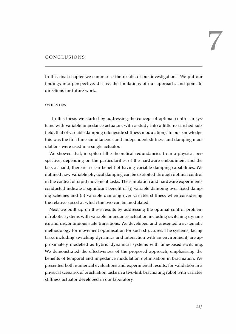
7C O N C L U S I O N S

In this final chapter we summarise the results of our investigations. We put our

findings into perspective, discuss the limitations of our approach, and point to

directions for future work.

overview

In this thesis we started by addressing the concept of optimal control in sys-

tems with variable impedance actuators with a study into a little researched sub-

field, that of variable damping (alongside stiffness modulation). To our knowledge

this was the first time simultaneous and independent stiffness and damping mod-

ulations were used in a single actuator.

We showed that, in spite of the theoretical redundancies from a physical per-

spective, depending on the particularities of the hardware embodiment and the

task at hand, there is a clear benefit of having variable damping capabilities. We

outlined how variable physical damping can be exploited through optimal control

in the context of rapid movement tasks. The simulation and hardware experiments

conducted indicate a significant benefit of (i) variable damping over fixed damp-

ing schemes and (ii) variable damping over variable stiffness when considering

the relative speed at which the two can be modulated.

Next we built up on these results by addressing the optimal control problem

of robotic systems with variable impedance actuation including switching dynam-

ics and discontinuous state transitions. We developed and presented a systematic

methodology for movement optimisation for such structures. The systems, facing

tasks including switching dynamics and interaction with an environment, are ap-

proximately modelled as hybrid dynamical systems with time-based switching.

We demonstrated the effectiveness of the proposed approach, emphasising the

benefits of temporal and impedance modulation optimisation in brachiation. We

presented both numerical evaluations and experimental results, for validation in a

physical scenario, of brachiation tasks in a two-link brachiating robot with variable

stiffness actuator developed in our laboratory.

113

We then extended the evaluation of our proposed approach to a monopod hop-

per system. This constitutes a significantly more challenging platform in terms of

contacts (i.e., more complex impact map) and individual phase dynamics (i.e., exis-

tence of a flight phase). With an appropriate choice of the composite cost function

to encode the task, we demonstrated the effectiveness of the proposed approach

on the hopper system and showcased the robustness of the optimal feedback con-

troller for a continuous hopping task.

Next, we extended our approach by incorporating adaptive learning, which al-

lows for adjustments to the dynamics model, based on changes occurred to the

system’s behaviour, or when the behaviour cannot be fully capture by a rigid

body dynamics formulation. We showed that the developed methodology can be

successfully applied in the case of underactuated systems, such as the brachiation

platform for a range of discrepancies, in both numerical simulations and in real

hardware experiments.

future work

The focus of our investigation into variable damping was on a relatively sim-

ple task for a single link system. We have not addressed the role of damping in

multi-link variable impedance control, nor have we explored the relative bene-

fits of using variable damping versus variable stiffness in the context of energy-

optimal behaviour. Future work on these aspects could reveal how the benefits of

variable damping capabilities relate to the complexity of the system. This could

potentially aid the design process of robotic systems (actuators could be equipped

with different impedance capabilities depending on the scope of the system being

developed).

Similarly, we applied our methodology for optimal control of robotic systems

with variable impedance actuation including switching dynamics and discontinu-

ous state transitions on two realistic systems. We demonstrated the benefit of si-

multaneous temporal and variable stiffness for a variety of tasks in numerical sim-

ulations and hardware implementation of a brachiating robot with VSA. In future

work, we would like to apply this approach to more complex locomotion systems,

such as bipedal or quadrupedal robotics systems with impedance modulation ca-

pabilities. As the current framework assumes a predefined phase sequence, this

would require the development of a method for determining the best sequence for

a given task, for systems where there are multiple candidates.

114

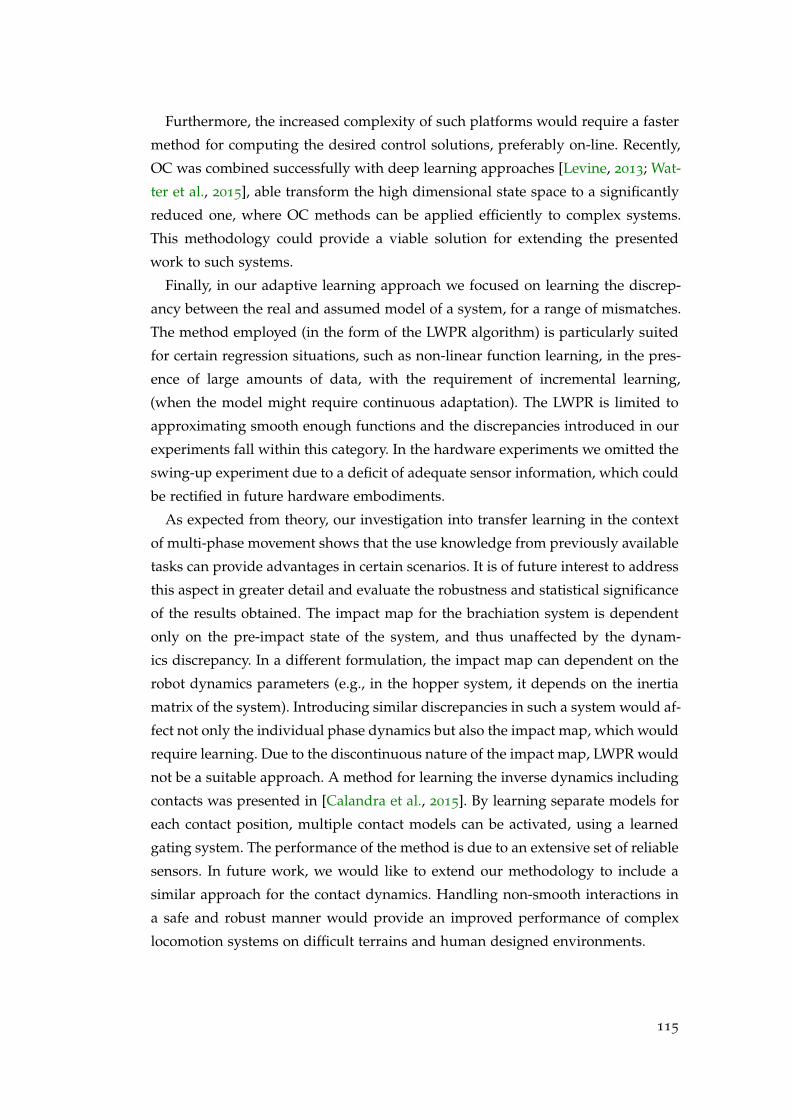
Furthermore, the increased complexity of such platforms would require a faster

method for computing the desired control solutions, preferably on-line. Recently,

OC was combined successfully with deep learning approaches [Levine, 2013; Wat-

ter et al., 2015], able transform the high dimensional state space to a significantly

reduced one, where OC methods can be applied efficiently to complex systems.

This methodology could provide a viable solution for extending the presented

work to such systems.

Finally, in our adaptive learning approach we focused on learning the discrep-

ancy between the real and assumed model of a system, for a range of mismatches.

The method employed (in the form of the LWPR algorithm) is particularly suited

for certain regression situations, such as non-linear function learning, in the pres-

ence of large amounts of data, with the requirement of incremental learning,

(when the model might require continuous adaptation). The LWPR is limited to

approximating smooth enough functions and the discrepancies introduced in our

experiments fall within this category. In the hardware experiments we omitted the

swing-up experiment due to a deficit of adequate sensor information, which could

be rectified in future hardware embodiments.

As expected from theory, our investigation into transfer learning in the context

of multi-phase movement shows that the use knowledge from previously available

tasks can provide advantages in certain scenarios. It is of future interest to address

this aspect in greater detail and evaluate the robustness and statistical significance

of the results obtained. The impact map for the brachiation system is dependent

only on the pre-impact state of the system, and thus unaffected by the dynam-

ics discrepancy. In a different formulation, the impact map can dependent on the

robot dynamics parameters (e.g., in the hopper system, it depends on the inertia

matrix of the system). Introducing similar discrepancies in such a system would af-

fect not only the individual phase dynamics but also the impact map, which would

require learning. Due to the discontinuous nature of the impact map, LWPR would

not be a suitable approach. A method for learning the inverse dynamics including

contacts was presented in [Calandra et al., 2015]. By learning separate models for

each contact position, multiple contact models can be activated, using a learned

gating system. The performance of the method is due to an extensive set of reliable

sensors. In future work, we would like to extend our methodology to include a

similar approach for the contact dynamics. Handling non-smooth interactions in

a safe and robust manner would provide an improved performance of complex

locomotion systems on difficult terrains and human designed environments.

115

Part I

A P P E N D I X

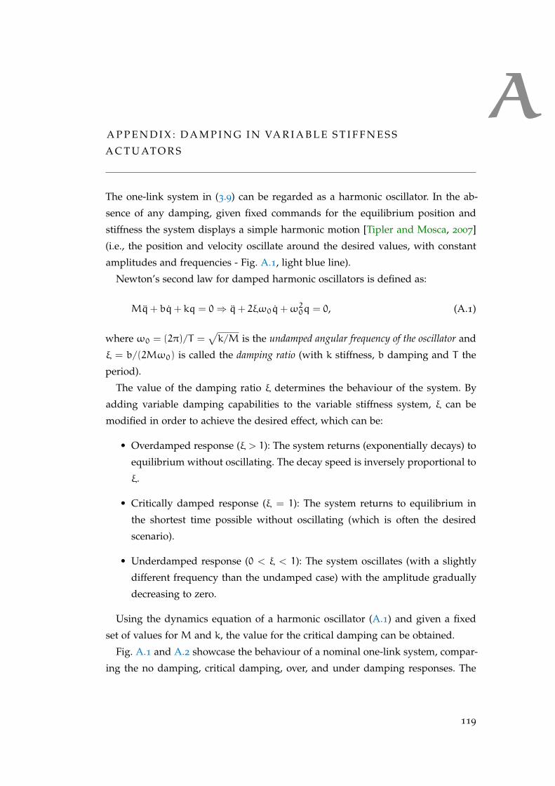
AA P P E N D I X : D A M P I N G I N VA R I A B L E S T I F F N E S S

A C T U AT O R S

The one-link system in (3.9) can be regarded as a harmonic oscillator. In the ab-

sence of any damping, given fixed commands for the equilibrium position and

stiffness the system displays a simple harmonic motion [Tipler and Mosca, 2007]

(i.e., the position and velocity oscillate around the desired values, with constant

amplitudes and frequencies - Fig. A.1, light blue line).

Newton’s second law for damped harmonic oscillators is defined as:

Mq+ bq+ kq = 0⇒ q+ 2ξω0q+ω20q = 0, (A.1)

where ω0 = (2π)/T =√k/M is the undamped angular frequency of the oscillator and

ξ = b/(2Mω0) is called the damping ratio (with k stiffness, b damping and T the

period).

The value of the damping ratio ξ determines the behaviour of the system. By

adding variable damping capabilities to the variable stiffness system, ξ can be

modified in order to achieve the desired effect, which can be:

• Overdamped response (ξ > 1): The system returns (exponentially decays) to

equilibrium without oscillating. The decay speed is inversely proportional to

ξ.

• Critically damped response (ξ = 1): The system returns to equilibrium in

the shortest time possible without oscillating (which is often the desired

scenario).

• Underdamped response (0 < ξ < 1): The system oscillates (with a slightly

different frequency than the undamped case) with the amplitude gradually

decreasing to zero.

Using the dynamics equation of a harmonic oscillator (A.1) and given a fixed

set of values for M and k, the value for the critical damping can be obtained.

Fig. A.1 and A.2 showcase the behaviour of a nominal one-link system, compar-

ing the no damping, critical damping, over, and under damping responses. The

119

0 0.2 0.4 0.6 0.8 1 1.2 1.4 1.6 1.8 2−0.2

0

0.2

0.4

0.6

0.8

1

1.2

time t (sec)

Po

sitio

n q

critical

under (min)

over(max)

no damping

Figure A.1: Nominal one-link system. Comparison of position between no damping, criti-cal damping, over and under damping.

0 0.2 0.4 0.6 0.8 1 1.2 1.4 1.6 1.8 2−8

−6

−4

−2

0

2

4

6

8

time t (sec)

critical

Ve

locity

q

under (min)

over (max)

no damping

Figure A.2: Nominal one-link system. Comparison of velocity between no damping, criti-cal damping, over and under damping.

values for the parameters of the system were selected (mainly for visualisation

purpose) as T = 0.125sec and k = 0.9633Nm/rad. The limit minimum and max-

imum value of the damping command (corresponding to the under- and over-

damped limits) were chosen with respect to the value of the critical damping

(bξ=1 = 0.1533Nmsec/rad) such that the effects are observable.

120

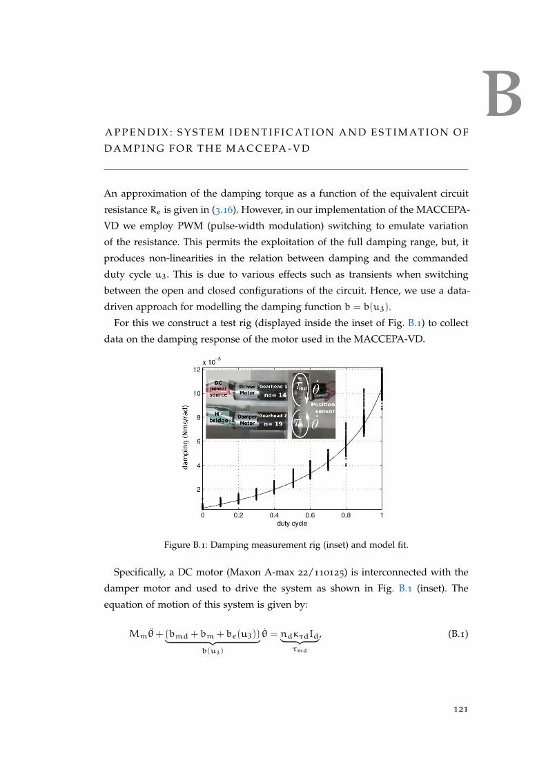
BA P P E N D I X : S Y S T E M I D E N T I F I C AT I O N A N D E S T I M AT I O N O F

D A M P I N G F O R T H E M A C C E PA - V D

An approximation of the damping torque as a function of the equivalent circuit

resistance Re is given in (3.16). However, in our implementation of the MACCEPA-

VD we employ PWM (pulse-width modulation) switching to emulate variation

of the resistance. This permits the exploitation of the full damping range, but, it

produces non-linearities in the relation between damping and the commanded

duty cycle u3. This is due to various effects such as transients when switching

between the open and closed configurations of the circuit. Hence, we use a data-

driven approach for modelling the damping function b = b(u3).

For this we construct a test rig (displayed inside the inset of Fig. B.1) to collect

data on the damping response of the motor used in the MACCEPA-VD.

Figure B.1: Damping measurement rig (inset) and model fit.

Specifically, a DC motor (Maxon A-max 22/110125) is interconnected with the

damper motor and used to drive the system as shown in Fig. B.1 (inset). The

equation of motion of this system is given by:

Mmθ+ (bmd + bm + be(u3))︸︷︷︸b(u3)

θ = ndκτdId︸︷︷︸τmd

, (B.1)

121

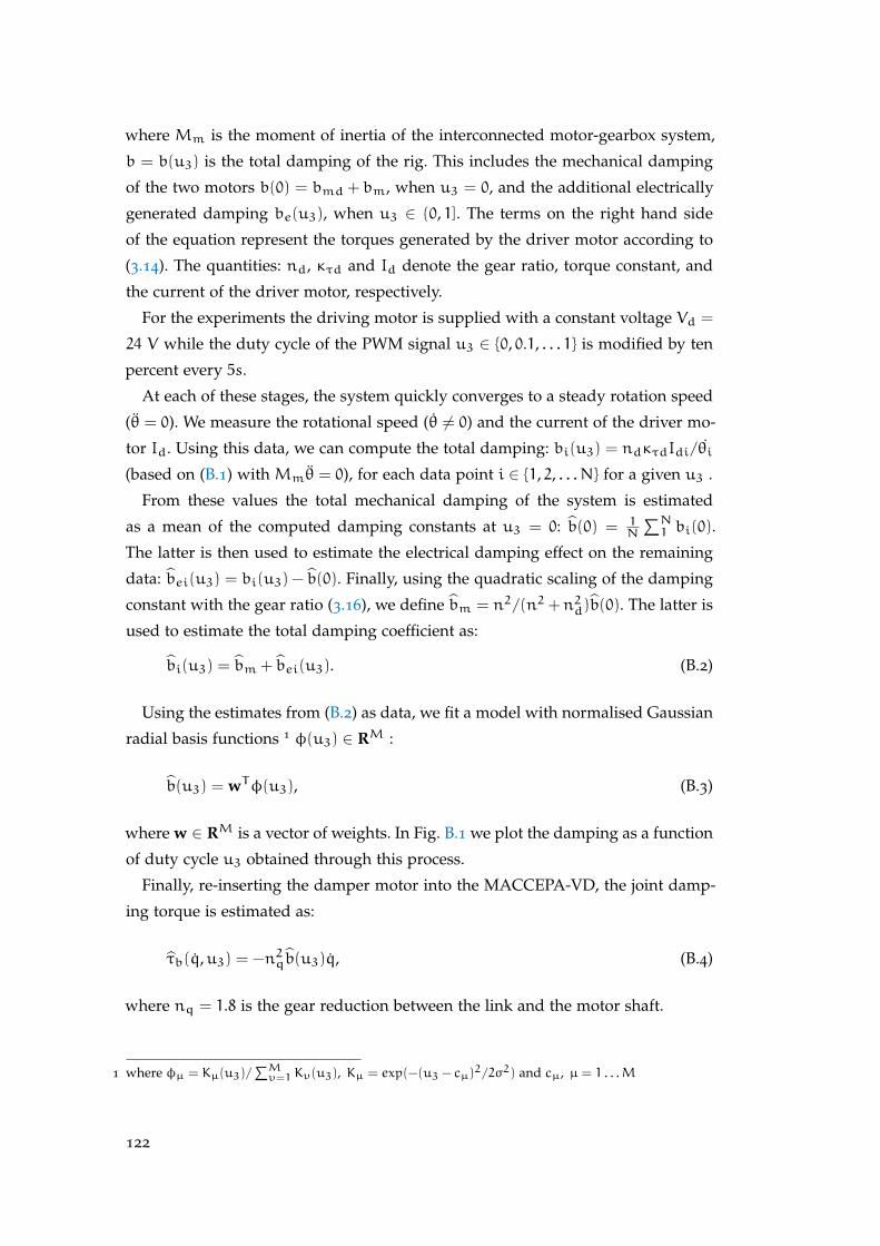
where Mm is the moment of inertia of the interconnected motor-gearbox system,

b = b(u3) is the total damping of the rig. This includes the mechanical damping

of the two motors b(0) = bmd + bm, when u3 = 0, and the additional electrically

generated damping be(u3), when u3 ∈ (0, 1]. The terms on the right hand side

of the equation represent the torques generated by the driver motor according to

(3.14). The quantities: nd, κτd and Id denote the gear ratio, torque constant, and

the current of the driver motor, respectively.

For the experiments the driving motor is supplied with a constant voltage Vd =

24 V while the duty cycle of the PWM signal u3 ∈ 0, 0.1, . . . 1 is modified by ten

percent every 5s.

At each of these stages, the system quickly converges to a steady rotation speed

(θ = 0). We measure the rotational speed (θ 6= 0) and the current of the driver mo-

tor Id. Using this data, we can compute the total damping: bi(u3) = ndκτdIdi/θi(based on (B.1) with Mmθ = 0), for each data point i ∈ 1, 2, . . . N for a given u3 .

From these values the total mechanical damping of the system is estimated

as a mean of the computed damping constants at u3 = 0: b(0) = 1N

∑N1 bi(0).

The latter is then used to estimate the electrical damping effect on the remaining

data: bei(u3) = bi(u3) − b(0). Finally, using the quadratic scaling of the damping

constant with the gear ratio (3.16), we define bm = n2/(n2+n2d)b(0). The latter is

used to estimate the total damping coefficient as:

bi(u3) = bm + bei(u3). (B.2)

Using the estimates from (B.2) as data, we fit a model with normalised Gaussian

radial basis functions 1 φ(u3) ∈ RM :

b(u3) = wTφ(u3), (B.3)

where w ∈ RM is a vector of weights. In Fig. B.1 we plot the damping as a function

of duty cycle u3 obtained through this process.

Finally, re-inserting the damper motor into the MACCEPA-VD, the joint damp-

ing torque is estimated as:

τb(q,u3) = −n2qb(u3)q, (B.4)

where nq = 1.8 is the gear reduction between the link and the motor shaft.

1 where φµ = Kµ(u3)/∑Mυ=1 Kυ(u3), Kµ = exp(−(u3 − cµ)

2/2σ2) and cµ, µ = 1 . . .M

122

CA P P E N D I X : D E S I G N A N D S E L E C T I O N O F T H E C O S T

F U N C T I O N F O R T H E B R A C H I AT I O N TA S K

In this appendix we provide a brief investigation conducted by our collaborator, Dr. Nakan-

ishi, into the possible options in defining a viable cost function for the brachiation task

addressed in Sec. 4.7.3.

In OC, the usual approach is to encode an abstract representation of the task

using a cost function. The design of the cost function is one of the most important

and difficult parts for a successful application of the OC framework. For simple

task and plant dynamics, an intuitive choice (typically a quadratic cost in the

state and control as in an LQR setting) would suffice1. For a highly dynamic task

and complex plant dynamics, this becomes increasingly difficult and finding an

appropriate choice of the cost terms which best encode the task remains an open

issue.

In this section, we explore additional candidates for the cost function, in the

context of the brachiation task described in Sec. 4.7.3. Alongside the cost function

in (4.42), we consider the following prospective running cost functions r = r(x, u):

• quadratic cost in the control command (servo motor position command):

r = uTRu, (C.1)

• quadratic cost in the joint torque. The main term is the cost associated with

the joint torque τ and uTR1u is added for regularisation (small R1):

r = uTR1u + R2τ2. (C.2)

Fig. C.1 shows the results obtained using the running cost (C.1) with R =

diag1, 1. The computed optimal movement duration is T = 0.604 (sec). Fig. C.2

shows the results using the running cost (C.2) with R1 = diag10−4, 10−4 and

R2 = 100. The obtained optimal movement duration is T = 0.620s. In both of these

two cases, the same terminal cost parameters are used as in (4.42).

1 The adjustment of the weights would still be required.

123

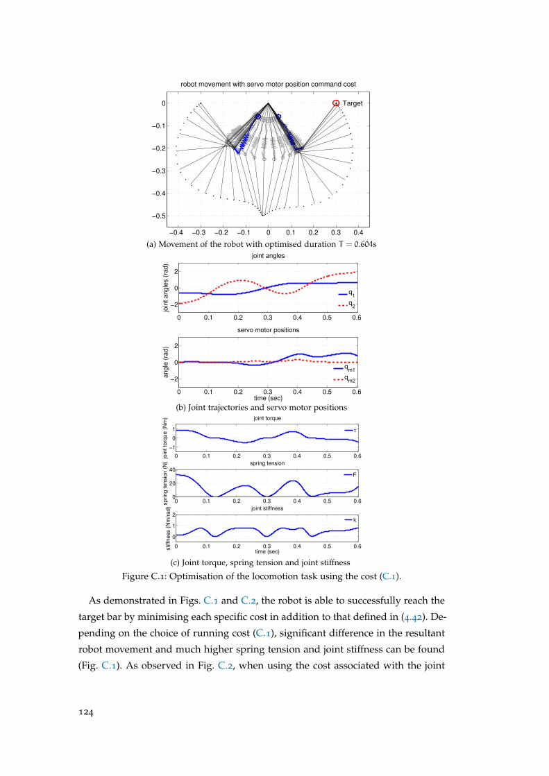
−0.4 −0.3 −0.2 −0.1 0 0.1 0.2 0.3 0.4

−0.5

−0.4

−0.3

−0.2

−0.1

0 Target

robot movement with servo motor position command cost

(a) Movement of the robot with optimised duration T = 0.604s

0 0.1 0.2 0.3 0.4 0.5 0.6

−2

0

2

join

t a

ng

les (

rad

)

joint angles

q1

q2

0 0.1 0.2 0.3 0.4 0.5 0.6

−2

0

2

time (sec)

an

gle

(ra

d)


qm1

qm2


0 0.1 0.2 0.3 0.4 0.5 0.6

−1

0

1

join

t to

rqu

e (

Nm

) joint torque

τ

0 0.1 0.2 0.3 0.4 0.5 0.60

20

40

sp

rin

g t

en

sio

n (

N) spring tension

F

0 0.1 0.2 0.3 0.4 0.5 0.6

0

1

2

time (sec)

stiff

ne

ss (

Nm

/ra

d) joint stiffness

k


Figure C.1: Optimisation of the locomotion task using the cost (C.1).

As demonstrated in Figs. C.1 and C.2, the robot is able to successfully reach the

target bar by minimising each specific cost in addition to that defined in (4.42). De-

pending on the choice of running cost (C.1), significant difference in the resultant

robot movement and much higher spring tension and joint stiffness can be found

(Fig. C.1). As observed in Fig. C.2, when using the cost associated with the joint

124

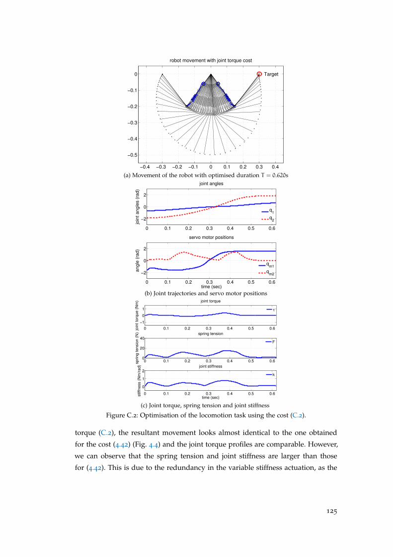
−0.4 −0.3 −0.2 −0.1 0 0.1 0.2 0.3 0.4

−0.5

−0.4

−0.3

−0.2

−0.1

0 Target

robot movement with joint torque cost

(a) Movement of the robot with optimised duration T = 0.620s

0 0.1 0.2 0.3 0.4 0.5 0.6

−2

0

2

join

t angle

s (

rad)

joint angles

q1

q2

0 0.1 0.2 0.3 0.4 0.5 0.6

−2

0

2

time (sec)

angle

(ra

d)


qm1

qm2


0 0.1 0.2 0.3 0.4 0.5 0.6

−1

0

1

join

t to

rqu

e (

Nm

) joint torque

τ

0 0.1 0.2 0.3 0.4 0.5 0.60

20

40

sp

rin

g t

en

sio

n (

N) spring tension

F

0 0.1 0.2 0.3 0.4 0.5 0.6

0

1

2

time (sec)

stiff

ne

ss (

Nm

/ra

d) joint stiffness

k


Figure C.2: Optimisation of the locomotion task using the cost (C.2).

torque (C.2), the resultant movement looks almost identical to the one obtained

for the cost (4.42) (Fig. 4.4) and the joint torque profiles are comparable. However,

we can observe that the spring tension and joint stiffness are larger than those

for (4.42). This is due to the redundancy in the variable stiffness actuation, as the

125

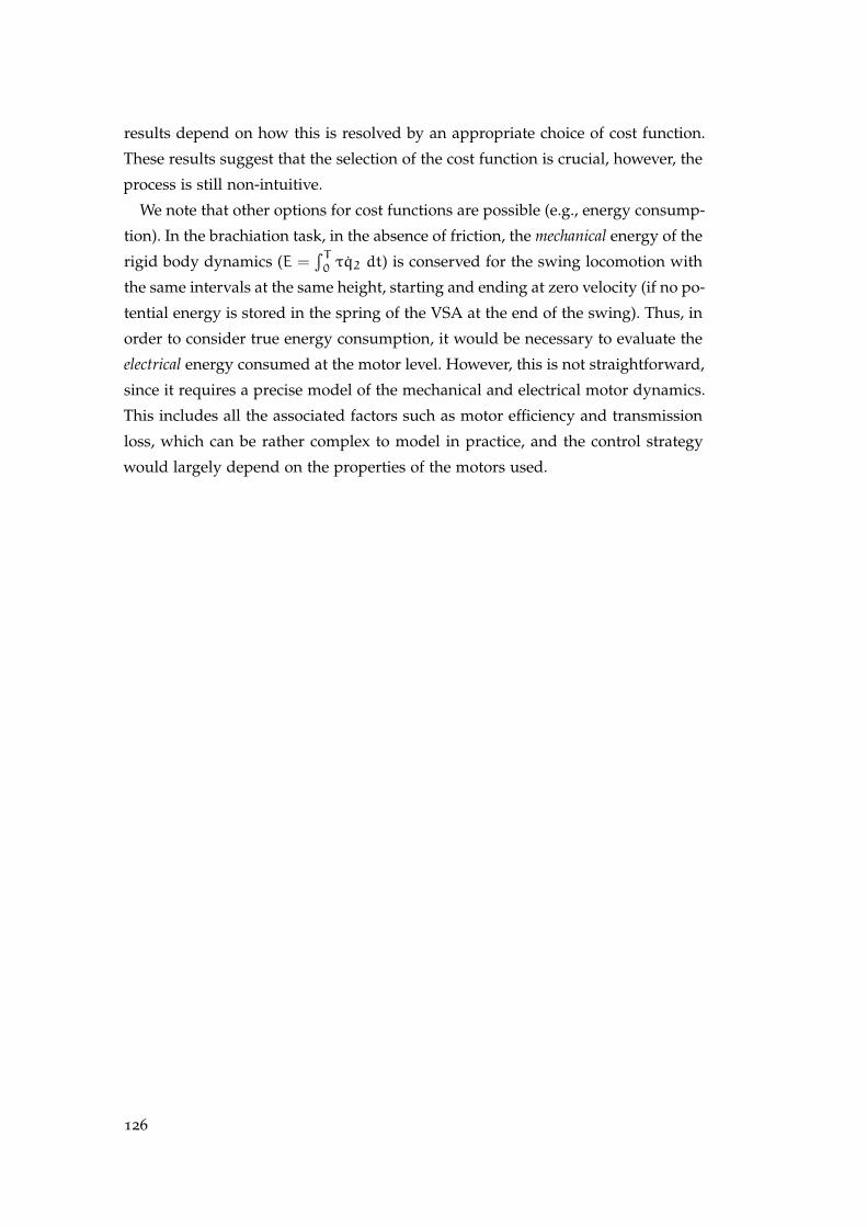
results depend on how this is resolved by an appropriate choice of cost function.

These results suggest that the selection of the cost function is crucial, however, the

process is still non-intuitive.

We note that other options for cost functions are possible (e.g., energy consump-

tion). In the brachiation task, in the absence of friction, the mechanical energy of the

rigid body dynamics (E =∫T0 τq2 dt) is conserved for the swing locomotion with

the same intervals at the same height, starting and ending at zero velocity (if no po-

tential energy is stored in the spring of the VSA at the end of the swing). Thus, in

order to consider true energy consumption, it would be necessary to evaluate the

electrical energy consumed at the motor level. However, this is not straightforward,

since it requires a precise model of the mechanical and electrical motor dynamics.

This includes all the associated factors such as motor efficiency and transmission

loss, which can be rather complex to model in practice, and the control strategy

would largely depend on the properties of the motors used.

126

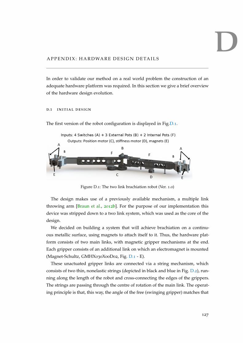
DA P P E N D I X : H A R D WA R E D E S I G N D E TA I L S

In order to validate our method on a real world problem the construction of an

adequate hardware platform was required. In this section we give a brief overview

of the hardware design evolution.

d.1 initial design

The first version of the robot configuration is displayed in Fig.D.1.

Figure D.1: The two link brachiation robot (Ver. 1.0)

The design makes use of a previously available mechanism, a multiple link

throwing arm [Braun et al., 2012b]. For the purpose of our implementation this

device was stripped down to a two link system, which was used as the core of the

design.

We decided on building a system that will achieve brachiation on a continu-

ous metallic surface, using magnets to attach itself to it. Thus, the hardware plat-

form consists of two main links, with magnetic gripper mechanisms at the end.

Each gripper consists of an additional link on which an electromagnet is mounted

(Magnet-Schultz, GMHX030X00D02, Fig. D.1 - E).

These unactuated gripper links are connected via a string mechanism, which

consists of two thin, nonelastic strings (depicted in black and blue in Fig. D.2), run-

ning along the length of the robot and cross-connecting the edges of the grippers.

The strings are passing through the centre of rotation of the main link. The operat-

ing principle is that, this way, the angle of the free (swinging gripper) matches that

127

of the holding (fixed gripper). At the moment of contact the magnet is aligned with

the brachiation surface, thus achieving a successful hold. Two switches mounted

on each side of the magnet, along the brachiation direction (Fig. D.1 - A), provide

additional information about the gripper’s position and help the tuning of the pas-

sive mechanism. One of the limitations of this design is that brachiation is limited

to same level surfaces.

Figure D.2: Depiction of the passive string mechanism, devised to ensure surface align-ment at surface contact.

The two main links form an actuated joint that uses the mechanically adjustable

series elastic actuators (MACCEPA) introduced in [Ham et al., 2007]. The MAC-

CEPA actuator is designed to give simultaneous equilibrium position and joint

stiffness control through use of two independently controlled servomotors.

The original design from [Braun et al., 2012b] was modified by upgrading the

servos to the high speed HITEC HSR-7940TH model. The upgrade was dictated

by the inability of the old motors to cope with the new load in successfully achiev-

ing a brachiation movement. The joint angles (including the unactuated links) are

measured using by rotary potentiometers (Alps RDC503013A), which can cover

an effective variable range of 320. Information on the motor positions is given by

direct access to the internal potentiometers of the servo motors.

The first implementation suffered from very low performance. The main issue

encountered was that the mechanism required a perfect magnet-to-surface align-

ment at the point of contact, in order to operate successfully. A large discrepancy

between the planned final position and the achieved one was observed, caused

by a sliding behaviour of the gripper on the metallic surface towards the end of

128

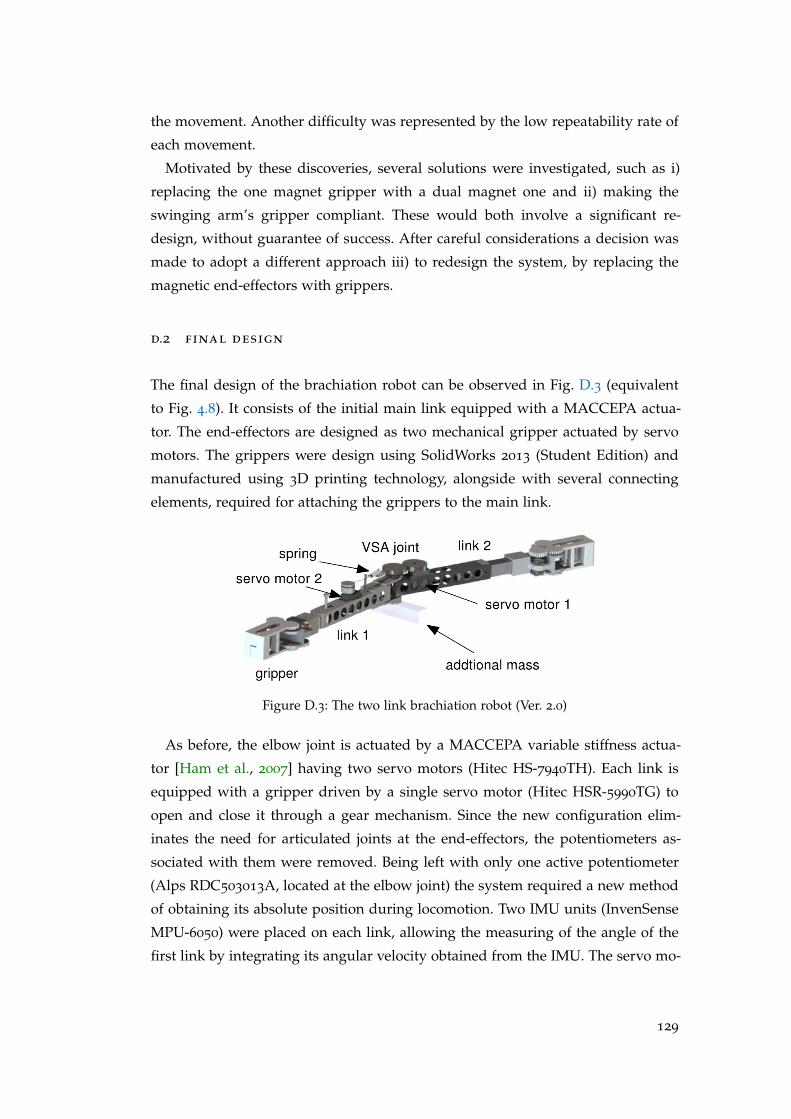
the movement. Another difficulty was represented by the low repeatability rate of

each movement.

Motivated by these discoveries, several solutions were investigated, such as i)

replacing the one magnet gripper with a dual magnet one and ii) making the

swinging arm’s gripper compliant. These would both involve a significant re-

design, without guarantee of success. After careful considerations a decision was

made to adopt a different approach iii) to redesign the system, by replacing the

magnetic end-effectors with grippers.

d.2 final design

The final design of the brachiation robot can be observed in Fig. D.3 (equivalent

to Fig. 4.8). It consists of the initial main link equipped with a MACCEPA actua-

tor. The end-effectors are designed as two mechanical gripper actuated by servo

motors. The grippers were design using SolidWorks 2013 (Student Edition) and

manufactured using 3D printing technology, alongside with several connecting

elements, required for attaching the grippers to the main link.

Figure D.3: The two link brachiation robot (Ver. 2.0)

As before, the elbow joint is actuated by a MACCEPA variable stiffness actua-

tor [Ham et al., 2007] having two servo motors (Hitec HS-7940TH). Each link is

equipped with a gripper driven by a single servo motor (Hitec HSR-5990TG) to

open and close it through a gear mechanism. Since the new configuration elim-

inates the need for articulated joints at the end-effectors, the potentiometers as-

sociated with them were removed. Being left with only one active potentiometer

(Alps RDC503013A, located at the elbow joint) the system required a new method

of obtaining its absolute position during locomotion. Two IMU units (InvenSense

MPU-6050) were placed on each link, allowing the measuring of the angle of the

first link by integrating its angular velocity obtained from the IMU. The servo mo-

129

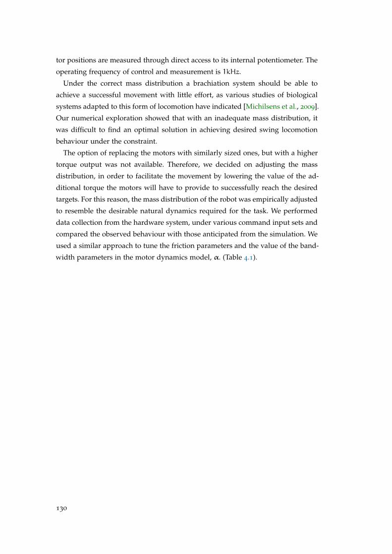
tor positions are measured through direct access to its internal potentiometer. The

operating frequency of control and measurement is 1kHz.

Under the correct mass distribution a brachiation system should be able to

achieve a successful movement with little effort, as various studies of biological

systems adapted to this form of locomotion have indicated [Michilsens et al., 2009].

Our numerical exploration showed that with an inadequate mass distribution, it

was difficult to find an optimal solution in achieving desired swing locomotion

behaviour under the constraint.

The option of replacing the motors with similarly sized ones, but with a higher

torque output was not available. Therefore, we decided on adjusting the mass

distribution, in order to facilitate the movement by lowering the value of the ad-

ditional torque the motors will have to provide to successfully reach the desired

targets. For this reason, the mass distribution of the robot was empirically adjusted

to resemble the desirable natural dynamics required for the task. We performed

data collection from the hardware system, under various command input sets and

compared the observed behaviour with those anticipated from the simulation. We

used a similar approach to tune the friction parameters and the value of the band-

width parameters in the motor dynamics model, α. (Table 4.1).

130

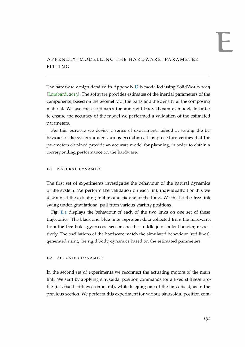
EA P P E N D I X : M O D E L L I N G T H E H A R D WA R E : PA R A M E T E R

F I T T I N G

The hardware design detailed in Appendix D is modelled using SolidWorks 2013

[Lombard, 2013]. The software provides estimates of the inertial parameters of the

components, based on the geometry of the parts and the density of the composing

material. We use these estimates for our rigid body dynamics model. In order

to ensure the accuracy of the model we performed a validation of the estimated

parameters.

For this purpose we devise a series of experiments aimed at testing the be-

haviour of the system under various excitations. This procedure verifies that the

parameters obtained provide an accurate model for planning, in order to obtain a

corresponding performance on the hardware.

e.1 natural dynamics

The first set of experiments investigates the behaviour of the natural dynamics

of the system. We perform the validation on each link individually. For this we

disconnect the actuating motors and fix one of the links. We the let the free link

swing under gravitational pull from various starting positions.

Fig. E.1 displays the behaviour of each of the two links on one set of these

trajectories. The black and blue lines represent data collected from the hardware,

from the free link’s gyroscope sensor and the middle joint potentiometer, respec-

tively. The oscillations of the hardware match the simulated behaviour (red lines),

generated using the rigid body dynamics based on the estimated parameters.

e.2 actuated dynamics

In the second set of experiments we reconnect the actuating motors of the main

link. We start by applying sinusoidal position commands for a fixed stiffness pro-

file (i.e., fixed stiffness command), while keeping one of the links fixed, as in the

previous section. We perform this experiment for various sinusoidal position com-

131

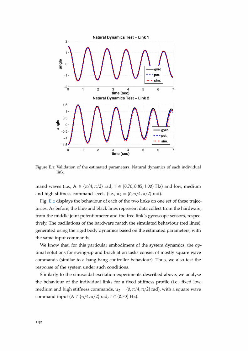
0 1 2 3 4 5 6 7−2

−1

0

1

2

time (sec)

an

gle

Natural Dynamics Test − Link 1

gyro

pot.

sim.

0 1 2 3 4 5 6 7

−1.5

−1

−0.5

0

0.5

1

1.5

time (sec)

an

gle

Natural Dynamics Test − Link 2

gyro

pot.

sim.

Figure E.1: Validation of the estimated parameters. Natural dynamics of each individuallink.

mand waves (i.e., A ∈ π/4,π/2 rad, f ∈ 0.70, 0.85, 1.00 Hz) and low, medium

and high stiffness command levels (i.e., u2 = 0,π/4,π/2 rad).

Fig. E.2 displays the behaviour of each of the two links on one set of these trajec-

tories. As before, the blue and black lines represent data collect from the hardware,

from the middle joint potentiometer and the free link’s gyroscope sensors, respec-

tively. The oscillations of the hardware match the simulated behaviour (red lines),

generated using the rigid body dynamics based on the estimated parameters, with

the same input commands.

We know that, for this particular embodiment of the system dynamics, the op-

timal solutions for swing-up and brachiation tasks consist of mostly square wave

commands (similar to a bang-bang controller behaviour). Thus, we also test the

response of the system under such conditions.

Similarly to the sinusoidal excitation experiments described above, we analyse

the behaviour of the individual links for a fixed stiffness profile (i.e., fixed low,

medium and high stiffness commands, u2 = 0,π/4,π/2 rad), with a square wave

command input (A ∈ π/4,π/2 rad, f ∈ 0.70 Hz).

132

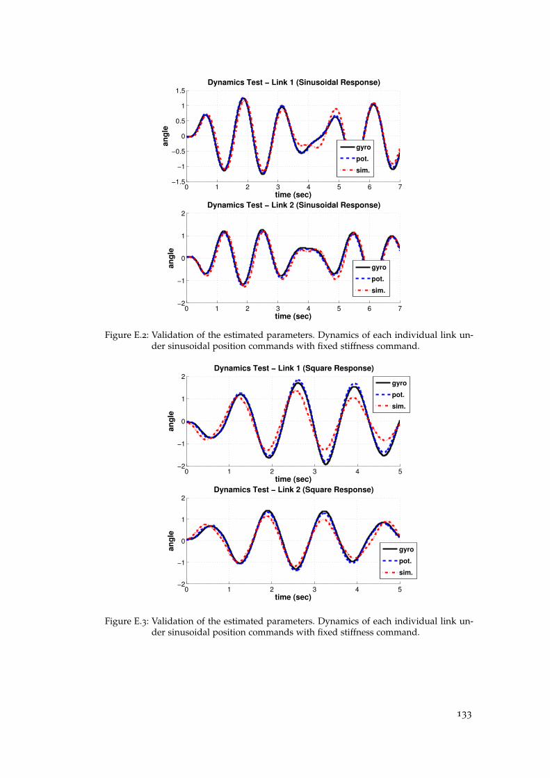
0 1 2 3 4 5 6 7−1.5

−1

−0.5

0

0.5

1

1.5

time (sec)

an

gle

Dynamics Test − Link 1 (Sinusoidal Response)

gyro

pot.

sim.

0 1 2 3 4 5 6 7−2

−1

0

1

2

time (sec)

an

gle

Dynamics Test − Link 2 (Sinusoidal Response)

gyro

pot.

sim.

Figure E.2: Validation of the estimated parameters. Dynamics of each individual link un-der sinusoidal position commands with fixed stiffness command.

0 1 2 3 4 5−2

−1

0

1

2

time (sec)

an

gle

Dynamics Test − Link 1 (Square Response)

gyro

pot.

sim.

0 1 2 3 4 5−2

−1

0

1

2

time (sec)

an

gle

Dynamics Test − Link 2 (Square Response)

gyro

pot.

sim.

Figure E.3: Validation of the estimated parameters. Dynamics of each individual link un-der sinusoidal position commands with fixed stiffness command.

133

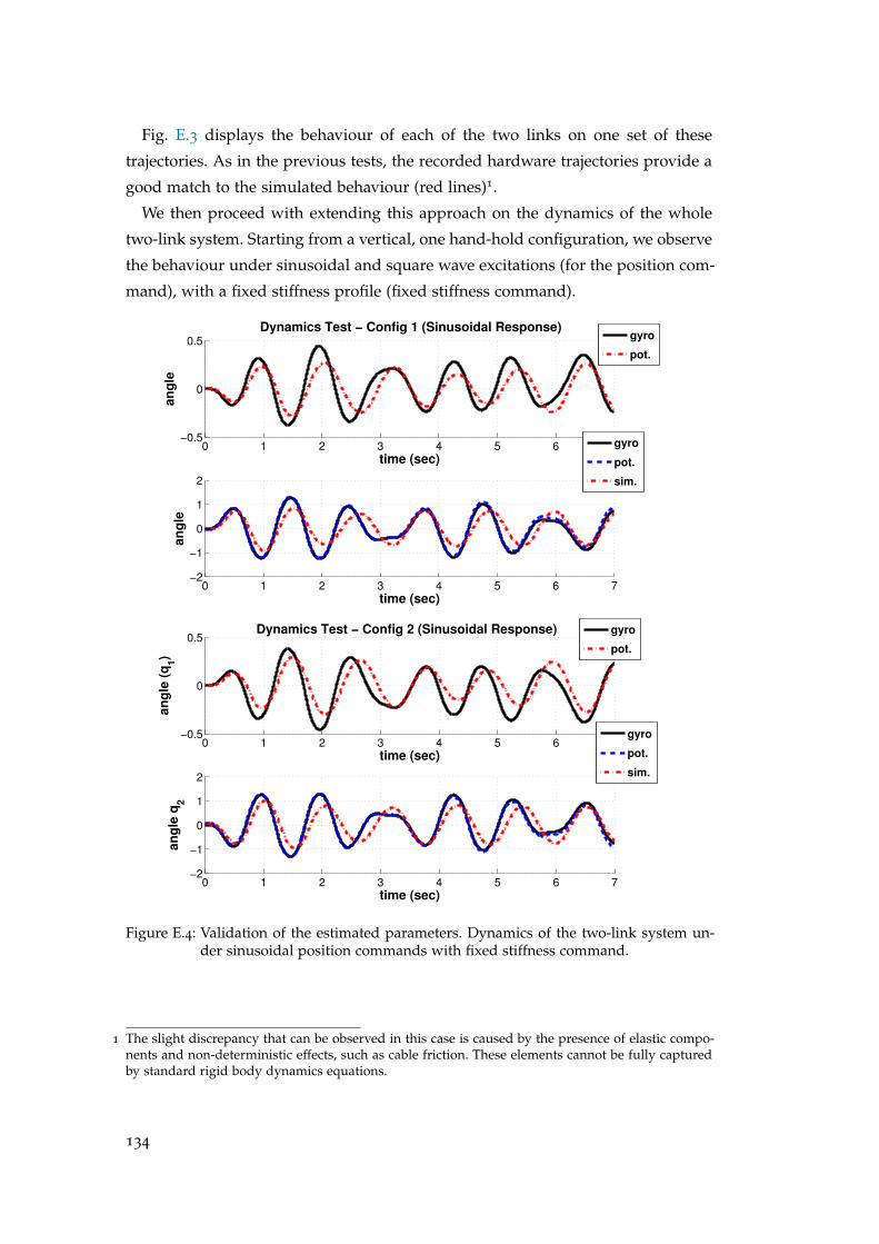
Fig. E.3 displays the behaviour of each of the two links on one set of these

trajectories. As in the previous tests, the recorded hardware trajectories provide a

good match to the simulated behaviour (red lines)1.

We then proceed with extending this approach on the dynamics of the whole

two-link system. Starting from a vertical, one hand-hold configuration, we observe

the behaviour under sinusoidal and square wave excitations (for the position com-

mand), with a fixed stiffness profile (fixed stiffness command).

0 1 2 3 4 5 6 7−0.5

0

0.5

time (sec)

an

gle

Dynamics Test − Config 1 (Sinusoidal Response)

gyro

pot.

0 1 2 3 4 5 6 7−2

−1

0

1

2

time (sec)

an

gle

gyro

pot.

sim.

0 1 2 3 4 5 6 7−0.5

0

0.5

time (sec)

an

gle

(q

1)

Dynamics Test − Config 2 (Sinusoidal Response)

gyro

pot.

0 1 2 3 4 5 6 7−2

−1

0

1

2

time (sec)

an

gle

q2

gyro

pot.

sim.

Figure E.4: Validation of the estimated parameters. Dynamics of the two-link system un-der sinusoidal position commands with fixed stiffness command.

1 The slight discrepancy that can be observed in this case is caused by the presence of elastic compo-nents and non-deterministic effects, such as cable friction. These elements cannot be fully capturedby standard rigid body dynamics equations.

134

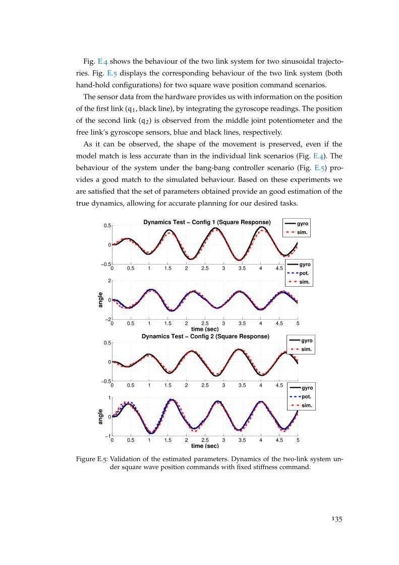
Fig. E.4 shows the behaviour of the two link system for two sinusoidal trajecto-

ries. Fig. E.5 displays the corresponding behaviour of the two link system (both

hand-hold configurations) for two square wave position command scenarios.

The sensor data from the hardware provides us with information on the position

of the first link (q1, black line), by integrating the gyroscope readings. The position

of the second link (q2) is observed from the middle joint potentiometer and the

free link’s gyroscope sensors, blue and black lines, respectively.

As it can be observed, the shape of the movement is preserved, even if the

model match is less accurate than in the individual link scenarios (Fig. E.4). The

behaviour of the system under the bang-bang controller scenario (Fig. E.5) pro-

vides a good match to the simulated behaviour. Based on these experiments we

are satisfied that the set of parameters obtained provide an good estimation of the

true dynamics, allowing for accurate planning for our desired tasks.

0 0.5 1 1.5 2 2.5 3 3.5 4 4.5 5−0.5

0

0.5Dynamics Test − Config 1 (Square Response)

gyro

sim.

0 0.5 1 1.5 2 2.5 3 3.5 4 4.5 5−2

0

2

time (sec)

an

gle

gyro

pot.

sim.

0 0.5 1 1.5 2 2.5 3 3.5 4 4.5 5−0.5

0

0.5

Dynamics Test − Config 2 (Square Response)

gyro

sim.

0 0.5 1 1.5 2 2.5 3 3.5 4 4.5 5−1

0

1

time (sec)

an

gle

gyro

pot.

sim.

Figure E.5: Validation of the estimated parameters. Dynamics of the two-link system un-der square wave position commands with fixed stiffness command.

135

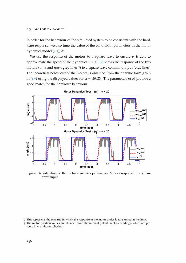
e.3 motor dynamics

In order for the behaviour of the simulated system to be consistent with the hard-

ware response, we also tune the value of the bandwidth parameters in the motor

dynamics model (4.7), α.

We use the response of the motors to a square wave to ensure α is able to

approximate the speed of the dynamics 2. Fig. E.6 shows the response of the two

motors (qm1 and qm2, grey lines 3) to a square wave command input (blue lines).

The theoretical behaviour of the motors is obtained from the analytic form given

in (4.7) using the displayed values for α = [20, 25]. The parameters used provide a

good match for the hardware behaviour.

0 0.5 1 1.5 2 2.5 3 3.5 4 4.5 5−2

−1

0

1

2

time (sec)

an

gle

(ra

d)

Motor Dynamics Test − (u1) − α = 20

qmPOS

HW

qmPOS

SIM

uPOS

HW

0 0.5 1 1.5 2 2.5 3 3.5 4 4.5 5

0

0.5

1

1.5

time (sec)

an

gle

(ra

d)

Motor Dynamics Test − (u2) − α = 25

qmK HW

qmK SIM

uK HW

Figure E.6: Validation of the motor dynamics parameters. Motors response to a squarewave input.

2 This represents the scenario in which the response of the motor under load is tested at the limit.3 The motor position values are obtained from the internal potentiometers’ readings, which are pre-

sented here without filtering.

136

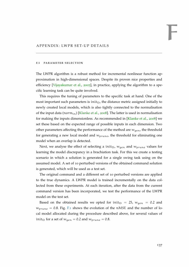
FA P P E N D I X : LW P R S E T- U P D E TA I L S

f.1 parameter selection

The LWPR algorithm is a robust method for incremental nonlinear function ap-

proximation in high-dimensional spaces. Despite its proven nice properties and

efficiency [Vijayakumar et al., 2005], in practice, applying the algorithm to a spe-

cific learning task can be quite involved.

This requires the tuning of parameters to the specific task at hand. One of the

most important such parameters is initD, the distance metric assigned initially to

newly created local models, which is also tightly connected to the normalisation

of the input data (normin) [Klanke et al., 2008]. The latter is used in normalisation

for making the inputs dimensionless. As recommended in [Klanke et al., 2008] we

set these based on the expected range of possible inputs in each dimension. Two

other parameters affecting the performance of the method are wgen, the threshold

for generating a new local model and wprune, the threshold for eliminating one

model when an overlap is detected.

Next, we analyse the effect of selecting a initD, wgen and wprune values for

learning the model discrepancy in a brachiation task. For this we create a testing

scenario in which a solution is generated for a single swing task using on the

assumed model. A set of 10 perturbed versions of the obtained command solution

is generated, which will be used as a test set.

The original command and a different set of 10 perturbed versions are applied

to the true dynamics. A LWPR model is trained incrementally on the data col-

lected from these experiments. At each iteration, after the data from the current

command version has been incorporated, we test the performance of the LWPR

model on the test set.

Based on the obtained results we opted for initD = 25, wgen = 0.2 and

wprune = 0.8. Fig. F.1 shows the evolution of the nMSE and the number of lo-

cal model allocated during the procedure described above, for several values of

initD for a set of wgen = 0.2 and wprune = 0.8.

137

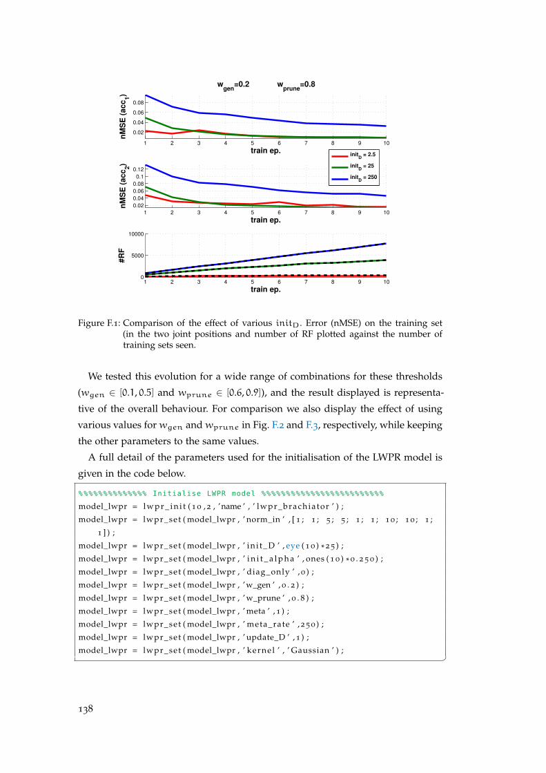
1 2 3 4 5 6 7 8 9 10

0.02

0.04

0.06

0.08

nM

SE

(a

cc

1)

train ep.

wgen

=0.2 wprune

=0.8

1 2 3 4 5 6 7 8 9 10

0.02

0.04

0.06

0.08

0.1

0.12

nM

SE

(a

cc

2)

train ep.

1 2 3 4 5 6 7 8 9 100

5000

10000

#R

F

train ep.

initD

= 2.5

initD

= 25

initD

= 250

Figure F.1: Comparison of the effect of various initD. Error (nMSE) on the training set(in the two joint positions and number of RF plotted against the number oftraining sets seen.

We tested this evolution for a wide range of combinations for these thresholds

(wgen ∈ [0.1, 0.5] and wprune ∈ [0.6, 0.9]), and the result displayed is representa-

tive of the overall behaviour. For comparison we also display the effect of using

various values forwgen andwprune in Fig. F.2 and F.3, respectively, while keeping

the other parameters to the same values.

A full detail of the parameters used for the initialisation of the LWPR model is

given in the code below.

%%%%%%%%%%%%%% Initialise LWPR model %%%%%%%%%%%%%%%%%%%%%%%%%

model_lwpr = l w p r _ i n i t ( 1 0 , 2 , ’name ’ , ’ lwpr_brachiator ’ ) ;

model_lwpr = lwpr_set ( model_lwpr , ’ norm_in ’ , [ 1 ; 1 ; 5 ; 5 ; 1 ; 1 ; 1 0 ; 1 0 ; 1 ;

1 ] ) ;

model_lwpr = lwpr_set ( model_lwpr , ’ in i t_D ’ , eye ( 1 0 ) * 2 5 ) ;

model_lwpr = lwpr_set ( model_lwpr , ’ i n i t _ a l p h a ’ , ones ( 1 0 ) * 0 . 2 5 0 ) ;

model_lwpr = lwpr_set ( model_lwpr , ’ diag_only ’ , 0 ) ;

model_lwpr = lwpr_set ( model_lwpr , ’w_gen ’ , 0 . 2 ) ;

model_lwpr = lwpr_set ( model_lwpr , ’ w_prune ’ , 0 . 8 ) ;

model_lwpr = lwpr_set ( model_lwpr , ’ meta ’ , 1 ) ;

model_lwpr = lwpr_set ( model_lwpr , ’ meta_rate ’ , 2 5 0 ) ;

model_lwpr = lwpr_set ( model_lwpr , ’ update_D ’ , 1 ) ;

model_lwpr = lwpr_set ( model_lwpr , ’ kernel ’ , ’ Gaussian ’ ) ;

138

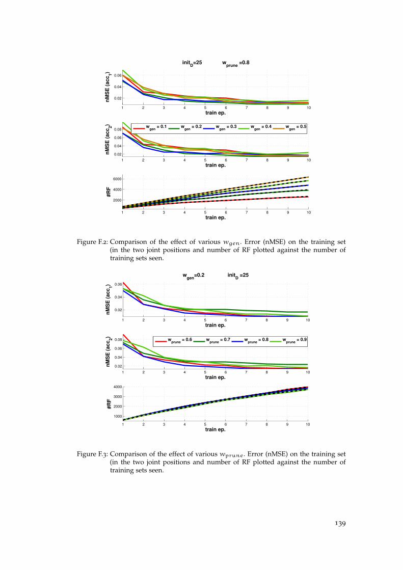
1 2 3 4 5 6 7 8 9 10

0.02

0.04

0.06

nM

SE

(a

cc

1)

train ep.

initD

=25 wprune

=0.8

1 2 3 4 5 6 7 8 9 10

0.02

0.04

0.06

0.08

nM

SE

(a

cc

2)

train ep.

1 2 3 4 5 6 7 8 9 10

2000

4000

6000

#R

F

train ep.

wgen

= 0.1 wgen

= 0.2 wgen

= 0.3 wgen

= 0.4 wgen

= 0.5

Figure F.2: Comparison of the effect of various wgen. Error (nMSE) on the training set(in the two joint positions and number of RF plotted against the number oftraining sets seen.

1 2 3 4 5 6 7 8 9 10

0.02

0.04

0.06

nM

SE

(a

cc

1)

train ep.

wgen

=0.2 initD

=25

1 2 3 4 5 6 7 8 9 10

0.02

0.04

0.06

0.08

nM

SE

(a

cc

2)

train ep.

1 2 3 4 5 6 7 8 9 10

1000

2000

3000

4000

#R

F

train ep.

wprune

= 0.6 wprune

= 0.7 wprune

= 0.8 wprune

= 0.9

Figure F.3: Comparison of the effect of various wprune. Error (nMSE) on the training set(in the two joint positions and number of RF plotted against the number oftraining sets seen.

139

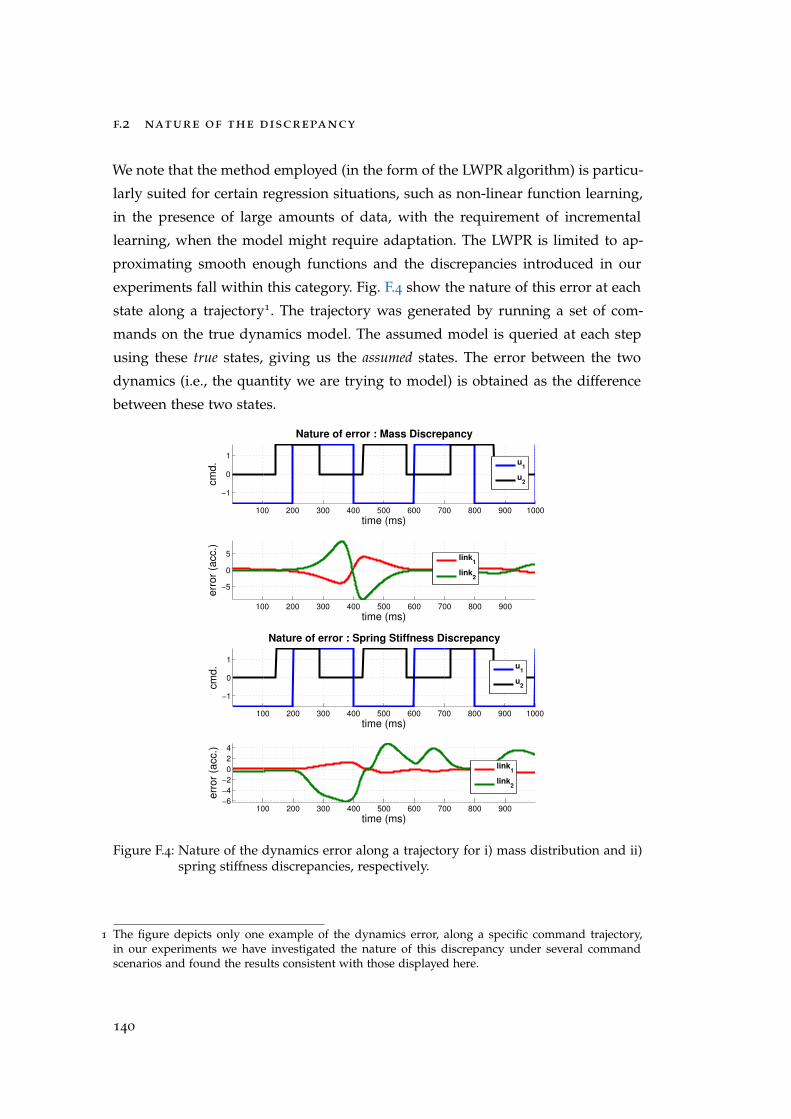
f.2 nature of the discrepancy

We note that the method employed (in the form of the LWPR algorithm) is particu-

larly suited for certain regression situations, such as non-linear function learning,

in the presence of large amounts of data, with the requirement of incremental

learning, when the model might require adaptation. The LWPR is limited to ap-

proximating smooth enough functions and the discrepancies introduced in our

experiments fall within this category. Fig. F.4 show the nature of this error at each

state along a trajectory1. The trajectory was generated by running a set of com-

mands on the true dynamics model. The assumed model is queried at each step

using these true states, giving us the assumed states. The error between the two

dynamics (i.e., the quantity we are trying to model) is obtained as the difference

between these two states.

100 200 300 400 500 600 700 800 900

−5

0

5

time (ms)

err

or

(acc.)

link1

link2

100 200 300 400 500 600 700 800 900 1000

−1

0

1

time (ms)

cm

d.

Nature of error : Mass Discrepancy

u1

u2

100 200 300 400 500 600 700 800 900−6

−4

−2

0

2

4

time (ms)

err

or

(acc.)

link1

link2

100 200 300 400 500 600 700 800 900 1000

−1

0

1

time (ms)

cm

d.

Nature of error : Spring Stiffness Discrepancy

u1

u2

Figure F.4: Nature of the dynamics error along a trajectory for i) mass distribution and ii)spring stiffness discrepancies, respectively.

1 The figure depicts only one example of the dynamics error, along a specific command trajectory,in our experiments we have investigated the nature of this discrepancy under several commandscenarios and found the results consistent with those displayed here.

140

B I B L I O G R A P H Y

Ahmadi, M. and Buehler, M. (1997). Stable control of a simulated one-legged

running robot with hip and leg compliance. IEEE Transactions on Robotics and

Automation, 13(1):96–104. (Cited on pages 75, 77, and 80.)

Akawaza, K., Aldridge, J., Steeves, J., and Stein, R. (1982). Modulation of stretch

reflexes during locomotion in the mesencephalic cat. Journal of Physiolosy,

329(1):553–567. (Cited on page 60.)

Anderson, R. and Spong, M. (1988). Hybrid impedance control of robotic manip-

ulators. Robotics and Automation, IEEE Journal of, 4(5):549–556. (Cited on pages 2

and 26.)

Athans, M., editor (1971). Special issue on the linear-quadratic-gaussian estimation and

control problem, volume 16. IEEE Transactions on Automated Control. (Cited on

page 13.)

Atkeson, C. G. (2007). Randomly sampling actions in dynamic programming. In

Proceedings of the 2007 IEEE Symposium on Approximate Dynamic Programming and

Reinforcement Learning (ADPRL 2007), pages 185–192. (Cited on page 13.)

Atkeson, C. G., An, C. H., and Hollerbach, J. M. (1986). Estimation of inertial

parameters of manipulator loads and links. The Int. Jour. of Rob. Research, 5.

(Cited on pages 5 and 86.)

Atkeson, C. G., Moore, A. W., and Schaal, S. (1997). Locally weighted learning

for control. Artificial Intelligence Review, 11(1-5):75–113. (Cited on pages 86, 88,

and 94.)

Atkeson, C. G. and Morimoto, J. (2002). Nonparametric representation of policies

and value functions: A trajectory-based approach. (Cited on page 87.)

Barrett, S., Taylor, M. E., and Stone, P. (2010). Transfer learning for reinforcement

learning on a physical robot. In Ninth International Conference on Autonomous

Agents and Multiagent Systems-Adaptive Learning Agents Workshop (AAMAS-ALA).

Citeseer. (Cited on pages 102 and 103.)

141

Bathe, K. and Bouzinov, P. (1997). On the constraint function method for contact

problems. Computers & Structures, 64(5):1069–1085. (Cited on page 45.)

Bätz, G., Mettin, U., Schmidts, A., Scheint, M., Wollherr, D., and Shiriaev, A. S.

(2010). Ball dribbling with an underactuated continuous-time control phase:

Theory & experiments. In IEEE/RSJ International Conference on Intelligent Robots

and Systems, pages 2890–2895. (Cited on pages 3 and 45.)

Bellman, R. and Kalaba, R. E. (1965). Dynamic programming and modern control

theory. Academic Press New York. (Cited on page 11.)

Ben-David, S. and Schuller, R. (2003). Exploiting task relatedness for multiple task

learning. In Learning Theory and Kernel Machines, pages 567–580. Springer. (Cited

on page 103.)

Bennett, D. J., Hollerbach, J. M., Xu, Y., and Hunter, I. W. (1992). Time-varying

stiffness of human elbow joint during cyclic voluntary movement. Experimental

Brain Research, 88:433–442. (Cited on page 60.)

Bilodeau, G. and Papadopoulos, E. (1998). A model-based impedance control

scheme for high-performance hydraulic joints. In Intelligent Robots and Systems,

1998. Proceedings., 1998 IEEE/RSJ International Conference on, volume 2, pages

1308–1313. IEEE. (Cited on page 22.)

Bischoff, R., Kurth, J., Schreiber, G., Koeppe, R., Albu-Schäffer, A., Beyer, A.,

Eiberger, O., Haddadin, S., Stemmer, A., Grunwald, G., et al. (2010). The kuka-

dlr lightweight robot arm-a new reference platform for robotics research and

manufacturing. In Robotics (ISR), 2010 41st international symposium on and 2010

6th German conference on robotics (ROBOTIK), pages 1–8. VDE. (Cited on page 22.)

Blaya, J., Herr, H., et al. (2004). Adaptive control of a variable-impedance ankle-

foot orthosis to assist drop-foot gait. Neural Systems and Rehabilitation Engineer-

ing, IEEE Transactions on, 12(1):24–31. (Cited on page 4.)

Bocsi, B., Csató, L., and Peters, J. (2013). Alignment-based transfer learning for

robot models. In Neural Networks (IJCNN), The 2013 International Joint Conference

on, pages 1–7. IEEE. (Cited on page 103.)

Bonilla, E. V., Chai, K. M., and Williams, C. (2007). Multi-task gaussian process

prediction. In Advances in neural information processing systems, pages 153–160.

(Cited on page 103.)

142

Brach, R. (2007). Mechanical Impact Dynamics: Rigid Body Collisions. Raymond M.

Brach. (Cited on page 44.)

Branicky, M. S., Borkar, V. S., and Mitter, S. K. (1998). A unified framework for

hybrid control: Model and optimal control theory. IEEE Transactions on Automatic

Control, 43(1):31–45. (Cited on page 46.)

Braun, D., Howard, M., and Vijayakumar, S. (2012a). Optimal variable stiffness

control: formulation and application to explosive movement tasks. Autonomous

Robots, 33(3):237–253. (Cited on pages 25, 52, 65, and 70.)

Braun, D. J., Howard, M., and Vijayakumar, S. (2012b). Exploiting variable stiffness

in explosive movement tasks. Robotics: Science and Systems VII, page 25. (Cited

on pages 2, 27, 127, and 128.)

Bryson, A. E. and Ho, Y.-C. (1975). Applied Optimal Control. Taylor & Francis. (Cited

on page 10.)

Burdet, E., Osu, R., Franklin, D., Milner, T., and Kawato, M. (2001). The central

nervous system stabilizes unstable dynamics by learning optimal impedance.

Nature, 414(6862):446–449. (Cited on page 1.)

Buss, M., Glocker, M., Hardt, M., von Stryk, O., Bulirsch, R., and Schmidt, G. (2002).

Nonlinear hybrid dynamical systems: Modeling, optimal control, and applica-

tions. In Engell, S., Frehse, G., and Schnieder, E., editors, Lecture Notes in Control

and Information Science, pages 311–335. Springer. (Cited on page 47.)

Calandra, R., Ivaldi, S., Deisenroth, M., Rueckert, E., and Peters, J. (2015). Learning

inverse dynamics models with contacts. In Proc. IEEE Int. Conf. on Robotics and

Automation (ICRA). (Cited on page 115.)

Caldwell, T. M. and Murphey, T. D. (2011a). Single integration optimization of

linear time-varying switched systems. In American Control Conference, pages

2024–2030. (Cited on page 50.)

Caldwell, T. M. and Murphey, T. D. (2011b). Switching mode generation and

optimal estimation with application to skid-steering. Automatica, 47(1):50–64.


Camacho, E. F. and Alba, C. B. (2013). Model predictive control. Springer Science &

Business Media. (Cited on page 47.)

143

Catalano, M. G., Grioli, G., Garabini, M., Bonomo, F., Mancini, M., Tsagarakis, N.,

and Bicchi, A. (2011). Vsa-cubebot: A modular variable stiffness platform for

multiple degrees of freedom robots. In Robotics and Automation (ICRA), 2011

IEEE International Conference on, pages 5090–5095. IEEE. (Cited on page 3.)

Cho, H., Warnecke, H., and Gweon, D. (1987). Robotic assembly: a synthesizing

overview. Robotica, 5(02):153–165. (Cited on page 2.)

Collins, S., Ruina, A., Tedrake, R., and Wisse, M. (2005). Efficient bipedal robots

based on passive-dynamic walkers. Science, 307(5712):1082–1085. (Cited on

page 48.)

D’Août, K. and Vereecke, E. E. (2011). Primate locomotion: Linking field and laboratory

research. Springer Science & Business Media. (Cited on page 4.)

Deguet, A., Joukhadar, A., and Laugier, C. (1998). A collision model for deformable

bodies. In Intelligent Robots and Systems, 1998. Proceedings., 1998 IEEE/RSJ Inter-

national Conference on, volume 1, pages 636–641. IEEE. (Cited on page 44.)

Dumont, G., Huzmezan, M., et al. (2002). Concepts, methods and techniques in

adaptive control. In American Control Conference, 2002. Proceedings of the 2002,

volume 2, pages 1137–1150. IEEE. (Cited on page 91.)

Dyer, P. and McReynolds, S. R. (1970). The computation and theory of optimal control.

Academic Press, New York. (Cited on pages 10 and 15.)

Egerstedt, M., Wardi, Y., and Delmotte, F. (2003). Optimal control of switching

times in switched dynamical systems. In IEEE Conference on Decision and Control,

volume 3, pages 2138–2143. (Cited on page 50.)

Eimerl, S. and DeVore, I. (1966). The Primates. TIME-LIFE BOOKS. (Cited on

page 49.)

Erez, T., Tassa, Y., and Todorov, E. (2011). Infinite-horizon model predictive control

for periodic tasks with contacts. In Robotics: Science and Systems (RSS). (Cited on

page 47.)

Faisal, A., Selen, L., and Wolpert, D. (2008). Noise in the nervous system. Nature

Reviews Neuroscience, 9(4):292–303. (Cited on pages 1 and 14.)

Farahani, K., Mofid, M., and Vafai, A. (2000). A solution method for general

contact–impact problems. Computer methods in applied mechanics and engineering,

187(1):69–77. (Cited on page 45.)

144

Ferguson, K. and Mahadevan, S. (2006). Proto-transfer learning in markov de-

cision processes using spectral methods. Computer Science Department Faculty

Publication Series, page 151. (Cited on page 103.)

François, C. and Samson, C. (1998). A new approach to the control of the planar

one-legged hopper. The International Journal of Robotics Research, 17(11):1150–1166.

(Cited on page 76.)

Franklin, D., Liaw, G., Milner, T., Osu, R., Burdet, E., and Kawato, M. (2007). End-

point stiffness of the arm is directionally tuned to instability in the environment.

The Journal of neuroscience, 27(29):7705–7716. (Cited on page 1.)

Garabini, M., Passaglia, A., Belo, F., Salaris, P., and Bicchi, A. (2011). Optimality

principles in variable stiffness control: The VSA hammer. In IEEE/RSJ Interna-

tional Conference on Intelligent Robots and Systems, pages 3770–3775. (Cited on

page 27.)

Gautier, M. and Khalil, W. (1992). Exciting trajectories for the identification of

base inertial parameters of robots. The International journal of robotics research,

11(4):362–375. (Cited on page 89.)

Gilardi, G. and Sharf, I. (2002). Literature survey of contact dynamics modelling.

Mechanism and Machine Theory, 37(10):1213 – 1239. (Cited on pages 44 and 45.)

Gomes, M. and Ruina, A. (2005). A five-link 2D brachiating ape model with

life-like zero-energy-cost motions. Journal of Theoretical Biology, 237(3):265–278.


Goris, K., Saldien, J., Vanderborght, B., and Lefeber, D. (2011). Mechanical design

of the huggable robot probo. International Journal of Humanoid Robotics, 8(03):481–

511. (Cited on page 3.)

Gregorio, P., Ahmadi, M., and Buehler, M. (1997). Design, control, and energetics

of an electrically actuated legged robot. Systems, Man, and Cybernetics, Part B:

Cybernetics, IEEE Transactions on, 27(4):626–634. (Cited on page 75.)

Grizzle, J. W., Abba, G., and Plestan, F. (2001). Asymptotically stable walking for

biped robots: Analysis via systems with impulse effects. IEEE Transactions on

Automatic Control, 46(1):51–64. (Cited on pages 3, 45, and 78.)

145

Groothuis, S. S., Rusticelli, G., Zucchelli, A., Stramigioli, S., and Carloni, R. (2012).

The vsaut-ii: A novel rotational variable stiffness actuator. In Robotics and Au-

tomation (ICRA), 2012 IEEE International Conference on, pages 3355–3360. IEEE.

(Cited on page 2.)

Guglielmino, E., Stammers, C. W., Edge, K. A., Sireteanu, T., and Stancioiu, D.

(2005). Damp-by-wire: Magnetorheological vs friction dampers. In 16th IFAC

World Congress. (Cited on page 31.)

Ham, R., Sugar, T., Vanderborght, B., Hollander, K., and Lefeber, D. (2009). Com-

pliant actuator designs. Robotics Automation Magazine, IEEE, 16(3):81 –94. (Cited

on page 21.)

Ham, R. V., Vanderborght, B., Damme, M. V., Verrelst, B., and Lefeber, D. (2007).

MACCEPA, the mechanically adjustable compliance and controllable equilib-

rium position actuator: Design and implementation in a biped robot. Robotics &

Autonomous Sys., 55(10):761–768. (Cited on pages 23, 25, 29, 94, 128, and 129.)

Herbort, O., Butz, M. V., and Pedersen, G. (2010). The sure_reach model for motor

learning and control of a redundant arm: from modeling human behavior to

applications in robotics. In From motor learning to interaction learning in robots,

pages 85–106. Springer. (Cited on page 86.)

Hogan, N. (1984). Impedance control: An approach to manipulation. In American

Control Conference, 1984, pages 304–313. IEEE. (Cited on page 2.)

Howard, M., Braun, D. J., and Vijayakumar, S. (2011). Constraint-based equilib-

rium and stiffness control of variable stiffness actuators. In Robotics and Automa-

tion (ICRA), 2011 IEEE International Conference on, pages 5554–5560. IEEE. (Cited

on page 25.)

Howard, M., Mitrovic, D., and Vijayakumar, S. (2010). Transferring impedance

control strategies between heterogeneous systems via apprenticeship learning.

In Humanoid Robots (Humanoids), 2010 10th IEEE-RAS International Conference on,

pages 98 –105. (Cited on pages 2 and 27.)

Hurst, J., Chestnutt, J., and Rizzi, A. (2004). An actuator with mechanically ad-

justable series compliance. Robotics Institute, Carnegie Mellon University, Pitts-

burgh, PA. (Cited on page 22.)

146

Hyon, S. and Emura, T. (2002). Quasi-periodic gaits of passive one-legged hop-

per. In Intelligent Robots and Systems, 2002. IEEE/RSJ International Conference on,

volume 3, pages 2625–2630. IEEE. (Cited on page 76.)

Hyon, S. and Emura, T. (2004). Energy-preserving control of a passive one-legged

running robot. Advanced Robotics, 18(4):357–381. (Cited on pages 76, 78, 79,

and 80.)

Jacobson, D. H. and Mayne, D. Q. (1970). Differential dynamic programming. Elsevier.

(Cited on page 15.)

Kajima, H., Doi, M., Hasegawa, Y., and Fukuda, T. (2004). A study on a brachia-

tion controller for a multi-locomotion robot—realization of smooth, continuous

brachiation. Advanced Robotics, 18(10):1025–1038. (Cited on page 4.)

Kalakrishnan, M., Buchli, J., Pastor, P., and Schaal, S. (2009). Learning locomotion

over rough terrain using terrain templates. In IEEE/RSJ Intl. Conf. on Intelligent

Robots and Systems (IROS 2009). (Cited on page 86.)

Kalman, R. E. et al. (1960). Contributions to the theory of optimal control. Bol. Soc.

Mat. Mexicana, 5(2):102–119. (Cited on page 12.)

Karssen, J. and Wisse, M. (2011). Running with improved disturbance rejec-

tion by using non-linear leg springs. International Journal of Robotics Research,

30(13):1585–15956. (Cited on page 48.)

Khalil, W. and Dombre, É. (2004). Modeling, identification & control of robots. Kogan

Page Science paper edition. Kogan Page Science. (Cited on pages 5 and 86.)

Klanke, S., Vijayakumar, S., and Schaal, S. (2008). A library for locally weighted

projection regression. The Journal of Machine Learning Research, 9:623–626. (Cited

on page 137.)

Kulchenko, P. and Todorov, E. (2011). First-exit model predictive control of fast

discontinuous dynamics: Application to ball bouncing. In Robotics and Automa-


on page 47.)

Laffranchi, M., Tsagarakis, N. G., and Caldwell, D. G. (2010). A variable physical

damping actuator (vpda) for compliant robotic joints. In Robotics and Automation

(ICRA), 2010 IEEE International Conference on, pages 1668–1674. IEEE. (Cited on

pages 31 and 41.)

147

Laffranchi, M., Tsagarakis, N. G., and Caldwell, D. G. (2013). Analysis and devel-

opment of a semiactive damper for compliant actuation systems. Mechatronics,

IEEE/ASME Transactions on, 18(2):744–753. (Cited on page 31.)

Levine, S. (2013). Exploring deep and recurrent architectures for optimal control.

arXiv preprint arXiv:1311.1761. (Cited on page 115.)

Li, W. and Todorov, E. (2004). Iterative linear quadratic regulator design for non-

linear biological movement systems. In ICINCO (1), pages 222–229. (Cited on

pages 14, 15, and 17.)

Li, W. and Todorov, E. (2007). Iterative linearization methods for approximately

optimal control and estimation of non-linear stochastic system. International

Journal of Control, 80(9):1439–1453. (Cited on pages 50 and 53.)

Lombard, M. (2013). Solidworks 2013 bible. John Wiley & Sons. (Cited on page 131.)

Long, A., Murphey, T., and Lynch, K. (2011). Optimal motion planning for a class

of hybrid dynamical systems with impacts. In Robotics and Automation (ICRA),

2011 IEEE International Conference on, pages 4220–4226. IEEE. (Cited on pages 3,

45, 46, and 47.)

Loughlin, C., Albu-Schäffer, A., Haddadin, S., Ott, C., Stemmer, A., Wimböck, T.,

and Hirzinger, G. (2007). The dlr lightweight robot: design and control con-

cepts for robots in human environments. Industrial Robot: an international journal,

34(5):376–385. (Cited on pages 22 and 43.)

Luca, A. D. and Oriolo, G. (2002). Trajectory planning and control for planar robots

with passive last joint. International Journal of Robotics Research, 21(5-6):575–590.

(Cited on page 49.)

Lunze, J., Lamnabhi-Lagarrigue, F., et al. (2009). Handbook of hybrid systems control:

theory, tools, applications. Cambridge University Press. (Cited on page 46.)

Lynch, K. M., Shiroma, N., Arai, H., and Tanie, K. (2000). Collision-free trajectory

planning for a 3-DOF robot with a passive joint. International Journal of Robotics

Research, 19(12):1171–1184. (Cited on page 49.)

Mazumdar, A. and Asada, H. H. (2010). An underactuated, magnetic-foot robot

for steel bridge inspection. Journal of Mechanisms and Robotics, 2(3):031007. (Cited

on page 4.)

148

McCallion, H., Johnson, G., and Pham, D. (1979). A compliant device for inserting

a peg in a hole. Industrial Robot: An International Journal, 6(2):81–87. (Cited on

pages 1 and 3.)

McGeer, T. (1990). Passive dynamic walking. The International Journal of Robotics

Research, 9(2):62–82. (Cited on page 76.)

McGinnis, P. (2005). Biomechanics of Sport and Exercise. Human Kinetics. (Cited on

page 44.)

Meghdari, A., Lavasani, S. M. H., Norouzi, M., and Mousavi, M. S. R. (2013). Min-

imum control effort trajectory planning and tracking of the CEDRA brachiation

robot. Robotica, 31(7):1119–1129. (Cited on page 49.)

Mehling, J. S., Colgate, J. E., Peshkin, M., et al. (2005). Increasing the impedance

range of a haptic display by adding electrical damping. In Eurohaptics Conference,

2005 and Symposium on Haptic Interfaces for Virtual Environment and Teleoperator

Systems, 2005. World Haptics 2005. First Joint, pages 257–262. IEEE. (Cited on

page 28.)

Meriam, J. and Kraige, L. (2012). Engineering Mechanics: Dynamics. Engineering

Mechanics. Wiley. (Cited on page 44.)

Michilsens, F., Vereecke, E. E., D’Août, K., and Aerts, P. (2009). Functional anatomy

of the gibbon forelimb: adaptations to a brachiating lifestyle. Journal of anatomy,

215(3):335–354. (Cited on pages 4 and 130.)

Mitrovic, D. (2010). Stochastic Optimal Control with Learned Dynamics Models. PhD

thesis, The University of Edinburgh. (Cited on pages 83 and 91.)

Mitrovic, D., Klanke, S., Haith, A., and Vijayakumar, S. (2009). A theory of

impedance control based on internal model uncertainty. In ESF Int. Workshop

on Computational Principles of Sensorimotor Learning. (Cited on pages 2 and 27.)

Mitrovic, D., Klanke, S., Howard, M., and Vijayakumar, S. (2010a). Exploiting

sensorimotor stochasticity for learning control of variable impedance actuators.


pages 536–541. IEEE. (Cited on pages 1, 5, and 86.)

Mitrovic, D., Klanke, S., Howard, M., and Vijayakumar, S. (2010b). Exploiting

sensorimotor stochasticity for learning control of variable impedance actuators.

149


pages 536–541. IEEE. (Cited on pages 22 and 25.)

Mitrovic, D., Klanke, S., Osu, R., Kawato, M., and Vijayakumar, S. (2010c). A

computational model of limb impedance control based on principles of internal

model uncertainty. PLoS ONE, 5:10. (Cited on pages 2 and 27.)

Mitrovic, D., Klanke, S., and Vijayakumar, S. (2008). Optimal control with adaptive

internal dynamics models. (Cited on page 87.)

Mitrovic, D., Klanke, S., and Vijayakumar, S. (2010d). Adaptive optimal feedback

control with learned internal dynamics models. From Motor Learning to Interac-

tion Learning in Robots, pages 65–84. (Cited on pages 86, 87, 88, and 91.)

Morimoto, J. and Atkeson, C. (2003). Minimax differential dynamic programming:

An application to robust biped walking. (Cited on page 47.)

Nakamura, Y. and Hanafusa, H. (1987). Optimal redundancy control of robot

manipulators. The International Journal of Robotics Research, 6(1):32–42. (Cited on

page 27.)

Nakamura, Y., Suzuki, T., and Koinuma, M. (1997). Nonlinear behavior and con-

trol of a nonholonomic free-joint manipulator. IEEE Transactions on Robotics and

Automation, 13(6):853–862. (Cited on page 49.)

Nakanishi, J., Farrell, J. A., and Schaal, S. (2005). Composite adaptive control with

locally weighted statistical learning. Neural Networks, 18(1):71–90. (Cited on

pages 5, 86, and 90.)

Nakanishi, J., Fukuda, T., and Koditschek, D. (2000). A brachiating robot controller.

IEEE Transactions on Robotics and Automation, 16(2):109–123. (Cited on page 49.)

Nakanishi, J., Radulescu, A., and Vijayakumar, S. (2013). Spatio-temporal optimiza-

tion of multi-phase movements: Dealing with contacts and switching dynamics.

In IEEE/RSJ Intl. Conf. on Intelligent Robots and Systems (IROS 2013). (Cited on

page 8.)

Nakanishi, J., Rawlik, K., and Vijayakumar, S. (2011). Stiffness and temporal op-

timization in periodic movements: An optimal control approach. In Intelligent

Robots and Systems (IROS), 2011 IEEE/RSJ International Conference on, pages 718–

724. IEEE. (Cited on pages 3, 4, 27, 49, 56, 73, and 78.)

150

Nakanishi, J. and Schaal, S. (2004). Feedback error learning and nonlinear adaptive

control. Neural Networks, 17(10):1453–1465. (Cited on page 87.)

Nakanishi, J. and Vijayakumar, S. (2013). Exploiting passive dynamics with vari-

able stiffness actuation in robot brachiation. Robotics, page 305. (Cited on

pages 27 and 56.)

Narendra, K. S. and Annaswamy, A. M. (1987). Persistent excitation in adaptive

systems. International Journal of Control, 45(1):127–160. (Cited on page 89.)

Narendra, K. S. and Annaswamy, A. M. (2012). Stable adaptive systems. Courier

Corporation. (Cited on page 91.)

Nguyen-Tuong, D. and Peters, J. (2010a). Using model knowledge for learning

inverse dynamics. In Robotics and Automation (ICRA), 2010 IEEE International

Conference on, pages 2677–2682. IEEE. (Cited on page 90.)

Nguyen-Tuong, D. and Peters, J. (2011). Model learning for robot control: a survey.

Cognitive processing, 12(4):319–340. (Cited on pages 5, 86, 87, 89, and 90.)

Nguyen-Tuong, D. and Peters, J. R. (2010b). Incremental sparsification for real-

time online model learning. In International Conference on Artificial Intelligence

and Statistics, pages 557–564. (Cited on page 90.)

Nguyen-Tuong, D., Seeger, M., and Peters, J. (2009). Model learning with local

gaussian process regression. Advanced Robotics, 23(15):2015–2034. (Cited on

page 86.)

Okada, M., Nakamura, Y., and Ban, S. (2001). Design of programmable passive

compliance shoulder mechanism. In Robotics and Automation, 2001. Proceedings

2001 ICRA. IEEE International Conference on, volume 1, pages 348–353. IEEE.

(Cited on page 22.)

Palli, G., Melchiorri, C., and Luca, A. D. (2008). On the feedback linearization of

robots with variable joint stiffness. In IEEE International Conference on Robotics

and Automation, pages 1753–1759. (Cited on page 61.)

Pan, S. J. and Yang, Q. (2010). A survey on transfer learning. Knowledge and Data

Engineering, IEEE Transactions on, 22(10):1345–1359. (Cited on pages 102 and 103.)

Petit, F., Chalon, M., Friedl, W., Grebenstein, M., Albu-Schäffer, A., and Hirzinger,

G. (2010). Bidirectional antagonistic variable stiffness actuation: Analysis, design

151

& implementation. In Robotics and Automation (ICRA), 2010 IEEE International

Conference on, pages 4189–4196. IEEE. (Cited on page 2.)

Petkos, G., Toussaint, M., and Vijayakumar, S. (2006). Learning multiple models

of non-linear dynamics for control under varying contexts. In Artificial Neural

Networks–ICANN 2006, pages 898–907. Springer. (Cited on page 90.)

Piccoli, B. (1998). Hybrid systems and optimal control. In Decision and Control,

1998. Proceedings of the 37th IEEE Conference on, volume 1, pages 13–18. IEEE.

(Cited on page 46.)

Polak, E. (2012). Optimization: Algorithms and Consistent Approximations. Applied

Mathematical Sciences. Springer New York. (Cited on page 12.)

Posa, M., Cantu, C., and Tedrake, R. (2014). A direct method for trajectory opti-

mization of rigid bodies through contact. International Journal of Robotics Research,

33(1):69–81. (Cited on page 47.)

Radford, N. A., Strawser, P., Hambuchen, K., Mehling, J. S., Verdeyen, W. K.,

Donnan, A. S., Holley, J., Sanchez, J., Nguyen, V., Bridgwater, L., et al. (2015).

Valkyrie: Nasa’s first bipedal humanoid robot. Journal of Field Robotics, 32(3):397–

419. (Cited on page 43.)

Radulescu, A., Howard, M., Braun, D. J., and Vijayakumar, S. (2012). Exploiting

variable physical damping in rapid movement tasks. In Advanced Intelligent

Mechatronics (AIM), 2012 IEEE/ASME International Conference on, pages 141–148.

IEEE. (Cited on pages 8 and 28.)

Radulescu, A., Nakanishi, J., and Vijayakumar, S. (2016). Optimal control of multi-

phase movements with learned dynamics. In Man–Machine Interactions 4, pages

61–76. Springer. (Cited on page 8.)

Raibert, M. and Tello, E. (1986). Legged robots that balance. IEEE Expert, 1(4):89–89.

(Cited on page 75.)

Rasmussen, C. E. (2006). Gaussian processes for machine learning. (Cited on

page 89.)

Rawlik, K., Toussaint, M., and Vijayakumar, S. (2010). An approximate inference

approach to temporal optimization in optimal control. In Lafferty, J., Williams,

152

C. K. I., Shawe-Taylor, J., Zemel, R., and Culotta, A., editors, Advances in Neu-

ral Information Processing Systems 23, pages 2011–2019. MIT Press. (Cited on

page 55.)

Rawlik, K. C. (2013). On probabilistic inference approaches to stochastic optimal

control. (Cited on page 47.)

Rocha, J. and Sequeira, J. (2004). The development of a robotic system for mainte-

nance and inspection of power lines. power, 3(2):3. (Cited on page 4.)

Rosa Jr., N., Barber, A., Gregg, R. D., and Lynch, K. M. (2012). Stable open-loop

brachiation on a vertical wall. In IEEE International Conference on Robotics and

Automation, pages 1193–1199. (Cited on pages 3, 4, 45, 49, and 78.)

Rosenstein, M. T., Marx, Z., Kaelbling, L. P., and Dietterich, T. G. (2005). To transfer

or not to transfer. In NIPS 2005 Workshop on Inductive Transfer: 10 Years Later,

volume 2, page 7. (Cited on page 103.)

Ross, I. (2009). A Primer on Pontryagin’s Principle in Optimal Control. Collegiate

Publishers. (Cited on page 10.)

Routh, E. J. et al. (1960). Dynamics of a system of rigid bodies. Dover New York.

(Cited on page 44.)

Saito, F., Fukuda, T., and Arai, F. (1994). Swing and locomotion control for a

two-link brachiation robot. Control Systems, IEEE, 14(1):5–12. (Cited on pages 4

and 49.)

Sato, A. and Buehler, M. (2004). A planar hopping robot with one actuator: de-

sign, simulation, and experimental results. In Intelligent Robots and Systems,

2004.(IROS 2004). Proceedings. 2004 IEEE/RSJ International Conference on, vol-

ume 4, pages 3540–3545. IEEE. (Cited on pages 75 and 76.)

Schaal, S. and Atkeson, C. G. (1998). Constructive incremental learning from only

local information. Neural Computation, 10(8):2047–2084. (Cited on page 88.)

Schaal, S., Atkeson, C. G., and Vijayakumar, S. (2002). Scalable techniques

from nonparametric statistics for real time robot learning. Applied Intelligence,

17(1):49–60. (Cited on page 86.)

Schiavi, R., Grioli, G., Sen, S., and Bicchi, A. (2008). Vsa-ii: a novel prototype of

variable stiffness actuator for safe and performing robots interacting with hu-

153

mans. In Robotics and Automation, 2008. ICRA 2008. IEEE International Conference

on, pages 2171–2176. IEEE. (Cited on page 2.)

Sciavicco, L. and Villani, L. (2009). Robotics:modelling, planning&control. Springer.


Shadmehr, R. (1990). Learning virtual equilibrium trajectories for control of a robot

arm. Neural Computation, 2(4):436–446. (Cited on page 61.)

Shaikh, M. S. and Caines, P. E. (2007). On the hybrid optimal control problem:

Theory and algorithms. IEEE Transactions on Automatic Control, 52(9):1587–1603.

(Cited on page 46.)

Siciliano, B. and Khatib, O. (2008). Springer Handbook of Robotics. Springer. (Cited

on pages 5, 24, and 85.)

Sigaud, O., Salaün, C., and Padois, V. (2011). On-line regression algorithms for

learning mechanical models of robots: a survey. Rob. and Auton. Sys., 59. (Cited

on pages 5 and 86.)

Spong, M. W. (1987). Modeling and control of elastic joint robots. Transactions

of ASME, Journal of Dynamic Systems, Measurement, and Control, 109(6):310–319.

(Cited on page 61.)

Spong, M. W. (1995). The swing up control problem for the acrobot. IEEE Control

Systems Magazine, 15(1):49–55. (Cited on page 49.)

Sreenath, K., Park, H., Poulakakis, I., and Grizzle, J. (2011). A compliant hybrid

zero dynamics controller for stable, efficient and fast bipedal walking on mabel.

The International Journal of Robotics Research, 30(9):1170–1193. (Cited on page 48.)

Srikanth, M., Vasudevan, H., and Muniyandi, M. (2008). DC motor damping:

A strategy to increase passive stiffness of haptic devices. In Ferre, M., editor,

Haptics: Perception, Devices and Scenarios, volume 5024 of LNCS, pages 53–62.

Springer. (Cited on page 28.)

Stengel, R. (1994). Optimal Control and Estimation. Dover. (Cited on page 10.)

Stramigioli, S., van Oort, G., and Dertien, E. C. (2008). A concept for a new en-

ergy efficient actuator. In Proc., IEEE/ASME International Conference on Advanced

Intelligent Mechatronics (AIM’08), pages 671–675. (Cited on pages 3, 48, and 50.)

154

Stronge, W. (1991). Unraveling paradoxical theories for rigid body collisions. Jour-

nal of Applied Mechanics, 58(4):1049–1055. (Cited on page 44.)

Sussmann, H. J. (1999). A maximum principle for hybrid optimal control problems.

In Conference on Decision and Control, pages 425–430. (Cited on page 46.)

Sweet, L. M. and Good, M. C. (1985). Redefinition of the robot motion-control

problem. Control Systems Magazine, IEEE, 5(3):18–25. (Cited on page 1.)

Swevers, J., Ganseman, C., Tükel, D. B., De Schutter, J., and Van Brussel, H. (1997).

Optimal robot excitation and identification. Robotics and Automation, IEEE Trans-

actions on, 13(5):730–740. (Cited on page 89.)

Tassa, Y., Erez, T., and Todorov, E. (2012). Synthesis and stabilization of complex

behaviors through online trajectory optimization. In IEEE/RSJ International Con-

ference on Intelligent Robots and Systems, pages 2144–2151. (Cited on page 47.)

Taylor, M. E. and Stone, P. (2007a). Cross-domain transfer for reinforcement learn-

ing. In Proceedings of the 24th international conference on Machine learning, pages

879–886. ACM. (Cited on page 103.)

Taylor, M. E. and Stone, P. (2007b). Representation transfer for reinforcement learn-

ing. In AAAI 2007 Fall Symposium on Computational Approaches to Representation

Change during Learning and Development. (Cited on page 103.)

Taylor, M. E. and Stone, P. (2009). Transfer learning for reinforcement learning

domains: A survey. The Journal of Machine Learning Research, 10:1633–1685. (Cited

on page 103.)

Tenenbaum, J. B., De Silva, V., and Langford, J. C. (2000). A global geometric

framework for nonlinear dimensionality reduction. Science, 290(5500):2319–2323.

(Cited on page 90.)

Thompson, C. and Raibert, M. (1990). Passive dynamic running. In Experimental

Robotics I, pages 74–83. Springer. (Cited on page 75.)

Thrun, S. and Mitchell, T. M. (1995). Lifelong robot learning. Springer. (Cited on

pages 90, 102, and 103.)

Ting, J.-A., Kalakrishnan, M., Vijayakumar, S., and Schaal, S. (2009). Bayesian ker-

nel shaping for learning control. In Advances in NIPS, pages 1673–1680. (Cited

on page 86.)

155

Tipler, P. A. and Mosca, G. (2007). Physics for scientists and engineers. Macmillan.

(Cited on page 119.)

Todorov, E. (2006). Optimal control theory. In Bayesian Brain: Probabilistic Ap-

proaches to neural Coding, pages 269–298. MIT Press Cambridge, MA. (Cited on

page 10.)

Todorov, E. and Li, W. (2003). Optimal control methods suitable for biomechanical

systems. In Engineering in Medicine and Biology Society, 2003. Proceedings of the

25th Annual International Conference of the IEEE, volume 2, pages 1758–1761. IEEE.

(Cited on page 15.)

Todorov, E. and Li, W. (2005). A generalized iterative lqg method for locally-

optimal feedback control of constrained nonlinear stochastic systems. In Ameri-

can Control Conference, 2005. Proceedings of the 2005, pages 300–306. IEEE. (Cited

on pages 14, 15, and 18.)

Torrey, L. and Shavlik, J. (2009). Transfer learning. Handbook of Research on Machine

Learning Applications and Trends: Algorithms, Methods, and Techniques, 1:242. (Cited

on page 102.)

Toussaint, K., Pouliot, N., and Montambault, S. (2009). Transmission line main-

tenance robots capable of crossing obstacles: State-of-the-art review and chal-

lenges ahead. Journal of Field Robotics, 26(5):477–499. (Cited on page 4.)

Toussaint, M. and Vijayakumar, S. (2005). Learning discontinuities with products-

of-sigmoids for switching between local models. In Proceedings of the 22nd inter-

national conference on Machine Learning, pages 904–911. ACM. (Cited on page 89.)

Tsumugiwa, T., Yokogawa, R., and Hara, K. (2002). Variable impedance control

with virtual stiffness for human-robot cooperative peg-in-hole task. In Intelligent

Robots and Systems, 2002. IEEE/RSJ International Conference on, volume 2, pages

1075–1081. IEEE. (Cited on page 3.)

Um, T. T., Park, M. S., and Park, J.-M. (2014). Independent joint learning: A novel

task-to-task transfer learning scheme for robot models. In Robotics and Automa-


on pages 103 and 104.)

Unsal, M., Niezrecki, C., and Crane III, C. (2004). Two semi-active approaches

for vibration isolation: piezoelectric friction damper and magnetorheological

156

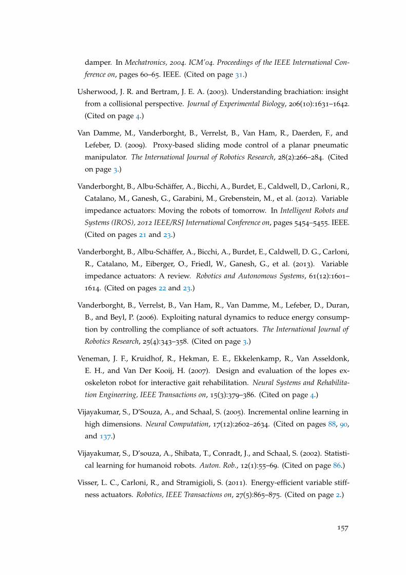
damper. In Mechatronics, 2004. ICM’04. Proceedings of the IEEE International Con-

ference on, pages 60–65. IEEE. (Cited on page 31.)

Usherwood, J. R. and Bertram, J. E. A. (2003). Understanding brachiation: insight

from a collisional perspective. Journal of Experimental Biology, 206(10):1631–1642.

(Cited on page 4.)

Van Damme, M., Vanderborght, B., Verrelst, B., Van Ham, R., Daerden, F., and

Lefeber, D. (2009). Proxy-based sliding mode control of a planar pneumatic

manipulator. The International Journal of Robotics Research, 28(2):266–284. (Cited

on page 3.)

Vanderborght, B., Albu-Schäffer, A., Bicchi, A., Burdet, E., Caldwell, D., Carloni, R.,

Catalano, M., Ganesh, G., Garabini, M., Grebenstein, M., et al. (2012). Variable

impedance actuators: Moving the robots of tomorrow. In Intelligent Robots and

Systems (IROS), 2012 IEEE/RSJ International Conference on, pages 5454–5455. IEEE.


Vanderborght, B., Albu-Schäffer, A., Bicchi, A., Burdet, E., Caldwell, D. G., Carloni,

R., Catalano, M., Eiberger, O., Friedl, W., Ganesh, G., et al. (2013). Variable

impedance actuators: A review. Robotics and Autonomous Systems, 61(12):1601–

1614. (Cited on pages 22 and 23.)

Vanderborght, B., Verrelst, B., Van Ham, R., Van Damme, M., Lefeber, D., Duran,

B., and Beyl, P. (2006). Exploiting natural dynamics to reduce energy consump-

tion by controlling the compliance of soft actuators. The International Journal of

Robotics Research, 25(4):343–358. (Cited on page 3.)

Veneman, J. F., Kruidhof, R., Hekman, E. E., Ekkelenkamp, R., Van Asseldonk,

E. H., and Van Der Kooij, H. (2007). Design and evaluation of the lopes ex-

oskeleton robot for interactive gait rehabilitation. Neural Systems and Rehabilita-

tion Engineering, IEEE Transactions on, 15(3):379–386. (Cited on page 4.)

Vijayakumar, S., D’Souza, A., and Schaal, S. (2005). Incremental online learning in

high dimensions. Neural Computation, 17(12):2602–2634. (Cited on pages 88, 90,

and 137.)

Vijayakumar, S., D’souza, A., Shibata, T., Conradt, J., and Schaal, S. (2002). Statisti-

cal learning for humanoid robots. Auton. Rob., 12(1):55–69. (Cited on page 86.)

Visser, L. C., Carloni, R., and Stramigioli, S. (2011). Energy-efficient variable stiff-

ness actuators. Robotics, IEEE Transactions on, 27(5):865–875. (Cited on page 2.)

157

Vitiello, N., Lenzi, T., McIntyre, J., Roccella, S., Cattin, E., Vecchi, F., and Carrozza,

M. C. (2008). Characterization of the neurarm bio-inspired joint position and

stiffness open loop controller. In Biomedical Robotics and Biomechatronics, 2008.

BioRob 2008. 2nd IEEE RAS & EMBS International Conference on, pages 138–143.

IEEE. (Cited on page 2.)

Vukobratovic, M. K. and Potkonjak, V. (1999). Dynamics of contact tasks in

robotics. part i: general model of robot interacting with environment. Mecha-

nism and machine theory, 34(6):923–942. (Cited on page 44.)

Wada, T., Ishikawa, M., Kitayoshi, R., Maruta, I., and Sugie, T. (2009). Practical

modeling and system identification of r/c servo motors. In Control Applica-

tions,(CCA) & Intelligent Control,(ISIC), 2009 IEEE, pages 1378–1383. IEEE. (Cited

on page 37.)

Wang, Y. and Mason, M. T. (1992). Two-dimensional rigid-body collisions with

friction. Journal of Applied Mechanics, 59(3):635–642. (Cited on page 44.)

Watter, M., Springenberg, J., Boedecker, J., and Riedmiller, M. (2015). Embed to

control: A locally linear latent dynamics model for control from raw images. In

Advances in Neural Information Processing Systems, pages 2728–2736. (Cited on

page 115.)

Whittaker, E. T. (1970). A treatise on the analytical dynamics of particles and rigid bodies:

with an introduction to the problem of three bodies. CUP Archive. (Cited on page 44.)

Williams, C., Klanke, S., Vijayakumar, S., and Chai, K. M. (2009). Multi-task gaus-

sian process learning of robot inverse dynamics. In Advances in Neural Informa-

tion Processing Systems, pages 265–272. (Cited on page 103.)

Xu, X. and Antsaklis, P. J. (2002). An approach to general switched linear quadratic

optimal control problems with state jumps. In International Symposium on Math-

ematical Theory of Networks and Systems. (Cited on page 46.)

Xu, X. and Antsaklis, P. J. (2003a). Quadratic optimal control problems for hybrid

linear autonomous systems with state jumps. In American Control Conference,

pages 3393–3398. (Cited on page 46.)

Xu, X. and Antsaklis, P. J. (2003b). Results and perspectives on computational

methods for optimal control of switched systems. In Maler, O. and Pnueli, A.,

editors, International Workshop on Hybrid Systems: Computation and Control, pages

540–555. Springer. (Cited on pages 47 and 51.)

158

Xu, X. and Antsaklis, P. J. (2004). Optimal control of switched systems based

on parameterization of the switching instants. IEEE Transactions on Automatic

Control, 49(1):2–16. (Cited on pages 50 and 74.)

Yang, C., Ganesh, G., Haddadin, S., Parusel, S., Albu-Schäeffer, A., and Burdet, E.

(2011). Human-like adaptation of force and impedance in stable and unstable

interactions. Robotics, IEEE Transactions on, 27(5):918–930. (Cited on page 3.)

Zinn, M., Khatib, O., Roth, B., and Salisbury, J. (2004). Playing it safe [human-

friendly robots]. Robotics & Automation Magazine, IEEE, 11(2):12–21. (Cited on

pages 21 and 22.)

159

radulescu2016.pdf - edinburgh research archive

Documents