This thesis has been submitted in fulfilment of the requirements for a postgraduate degree

(e.g. PhD, MPhil, DClinPsychol) at the University of Edinburgh. Please note the following

terms and conditions of use:

This work is protected by copyright and other intellectual property rights, which are

retained by the thesis author, unless otherwise stated.

A copy can be downloaded for personal non-commercial research or study, without

prior permission or charge.

This thesis cannot be reproduced or quoted extensively from without first obtaining

permission in writing from the author.

The content must not be changed in any way or sold commercially in any format or

medium without the formal permission of the author.

When referring to this work, full bibliographic details including the author, title,

awarding institution and date of the thesis must be given.

MAPPING THE ECONOMIC

POTENTIAL OF WAVE ENERGY:

GRID-CONNECTED AND OFF-GRID

SYSTEMS

A thesis submitted in partial ful�lment of the requirements for the award of anEngineering Doctorate

Ciaran FrostThe University of Exeter

August 2018

In memory of Louis Gillespie.

IDCORE

This thesis is submitted in partial ful�lment of the requirements for the award of

an Engineering Doctorate, jointly awarded by the University of Edinburgh, the

University of Exeter and the University of Strathclyde. The work presented has

been conducted under the industrial supervision of Albatern Ltd. as a project

within the Industrial Doctoral Centre for O�shore Renewable Energy (IDCORE).

i

Abstract

In recent times there has been a surge in renewable energy investment, as costs

fall and the full danger of global warming is realised by policymakers. As well as

more established industries, like wind and solar power, there is also high interest

in pre-commercial technologies with signi�cant potential. Wave energy �ts into

this category and has a number of advantages that make it a subject of ongoing

research and industrial activity. An energy dense resource, it is easier to forecast

than wind and �ts the seasonal demand pro�le well. A global capacity of the order

of hundreds of gigawatts has been estimated, with a particularly strong resource

in the UK.

Despite these characteristics the industry has yet to reach a commercial level.

No company has been able to demonstrate consistent energy production at a cost

e�ective rate. Viable project locations must balance an energetic resource with

conditions that allow devices to be accessed for maintenance, while also trying to

minimise system costs. While utility scale farms are seen as the long term future

for the technology, o�-grid hybrid systems could supply cheaper and dispatchable

energy at local levels. This market, while smaller, is made up of more costly forms

of energy so provides a better entry market. Conventional economic analyses for

both types of systems tend to be performed for single locations at a time. While

useful for benchmarking the technology, these methods are of limited use for site

scoping as energy production and costs can show large variation over relatively

short distances (<10 km).

This research thesis describes a geospatial economic model that has been cre-

ated to address the above issues. It was developed in collaboration with Albatern,

a wave energy developer, who provided their expertise and helped to guide the

research activities. The targeted application was to allow economic assessment

of Albatern's �WaveNET� device, either as a power station for grid connection or

an o�-grid hybrid solution for aquaculture applications. The model has a number

of aspects that are of signi�cant interest to the industry. These include compu-

tational model design and geographic calculation of energy production, costs and

Levelised Cost of Energy (LCOE). The spatial approach is valuable as a whole

area can be evaluated at a time, indicating deployment locations particularly suit-

able for the technology at hand. Sensitivity analysis is also easily carried out, to

build understanding of the cost drivers at speci�c locations.

The theory underpinning the model and its implementation is described. It

ii

is then demonstrated with two representative case studies: considering grid-

connected and o�-grid WaveNET device demonstrators on the West Coast of

Scotland. The results show the strengths of the approach as a way of identifying

economically viable hotspots and the main cost drivers. For the grid-connected

case, examining an area of 150 by 250 km, the model was able to identify a sig-

ni�cant LCOE hotspot between the Isle of Skye and the Outer Hebrides. The

potential for the device to power a �sh farm, when combined with a battery bank

and diesel generator, was then analysed. Two regions were examined and real

�sh farm locations considered. The output results allow easy comparison between

the two system types, emphasising the advantages of investigating both to inform

business activity.

iii

Acknowledgements

Overall I greatly enjoyed this research, and feel like I have learnt a lot. I could

not have done it without the help of many di�erent people.

Firstly I want to thank my lead academic supervisor, Prof. Lars Johanning

from the University of Exeter. He has been very supportive throughout, especially

over the last year, and his wisdom has been invaluable. I would also like to

thank my other academic supervisors, Dr. Ewen Macpherson and Dr. Phil Sayer.

Their input was especially helpful in the early and mid stages of the project, and

helped shape the structure of the thesis and direction of the work. Prof. David

Ingram, the Programme Director of IDCORE, should also be thanked for his

support and for playing such a key role in the IDCORE doctoral training centre.

My thanks also extends to Energy Technologies Institute (ETI) and the RCUK

Energy Programme for funding IDCORE (Grant Number EP/J500847/1).

Secondly I want to thank my old colleagues of Albatern. David Findlay, my

Industrial Supervisor, played a pivotal role in guiding the model direction and

research focus. Other key �gures were David Campbell, Vivien Mavel and Danny

McLaughlin, although everybody there imparted wisdom to me at some stage.

My thanks also extends to my current employers at BVG Associates, who have

given me the �exibility to get the thesis completed.

I also want to thank my fellow IDCORE colleagues: Steve Allsop, Enrico

Anderlini, Leah Barker-Ewart, Claire Canning, Rob Clayton, George Crossley,

Stephanie Mann, Scott McKirdy, Donald Noble, Simon Reynolds, Sunny Shah,

Marco Sepulveda Gutierrez and Siobhan Vaughan. I could not have hoped for a

better group of people to have gone on this journey with, and have enjoyed the

fun that we have had over the last �ve years.

I would like to thank my friends and family. My parents, Richard and Mar-

guerite Frost, have been extremely supportive, helping me with proof reading and

sending me microwavable rice and dark chocolate to help cope with the writing!

My girlfriend, Stephanie Lawrie, has also been extremely supportive by listening

to my thesis-related issues and helping to proof read. My sisters, Aileen Frost and

Louise Spencer, were also extremely helpful in this regard.

This has been a big part of my life, and I look forward to the next adventures

in the exciting world of renewable energy.

iv

Declaration

I declare that this thesis was composed by myself, that the work contained herein

is my own except where explicitly stated otherwise in the text, and that this work

has not been submitted for any other degree or professional quali�cation except

as speci�ed.

Parts of the work outlined in this thesis have been published:

• C. Frost, D. Findlay, E. Macpherson, P. Sayer, and L. Johanning, A model

to map levelised cost of energy for wave energy projects, Ocean Engineering,

vol. 149, pp. 438-451, 2018.

• C. Frost, D. Findlay, E. Macpherson, P. Sayer, and L. Johanning, Mapping

Economic Performance of Wave Energy in Proceedings of Renew2016, 2016.

• C. Frost, D. Findlay, E. Macpherson, P. Sayer, and L. Johanning, �Global

market potential for small scale wave energy.� Presentation at the Interna-

tional Conference on Ocean Energy (ICOE), Edinburgh, 2015.

Ciaran Frost

26th of April, 2019

v

vi

Contents

1 Introduction 1

1.1 Motivation . . . . . . . . . . . . . . . . . . . . . . . . . . . . . . . 1

1.1.1 Economic modelling: a research priority . . . . . . . . . . 1

1.2 Industrial Partnership . . . . . . . . . . . . . . . . . . . . . . . . 3

1.2.1 IDCORE . . . . . . . . . . . . . . . . . . . . . . . . . . . 3

1.2.2 Albatern Ltd. . . . . . . . . . . . . . . . . . . . . . . . . . 3

1.3 Research Aim and Objectives . . . . . . . . . . . . . . . . . . . . 4

1.4 Contribution to Knowledge . . . . . . . . . . . . . . . . . . . . . . 6

1.5 Method Statement . . . . . . . . . . . . . . . . . . . . . . . . . . 7

2 Research Context and Literature Review 9

2.1 Wave Energy . . . . . . . . . . . . . . . . . . . . . . . . . . . . . 9

2.1.1 Anatomy of a wave energy system . . . . . . . . . . . . . . 10

2.1.2 Small scale wave energy . . . . . . . . . . . . . . . . . . . 14

2.2 Market Context . . . . . . . . . . . . . . . . . . . . . . . . . . . . 16

2.3 Elements of a Wave Energy Economic Study . . . . . . . . . . . . 18

2.3.1 Levelised cost of energy . . . . . . . . . . . . . . . . . . . 19

2.3.2 Energy analysis . . . . . . . . . . . . . . . . . . . . . . . . 21

2.3.3 Cost analysis . . . . . . . . . . . . . . . . . . . . . . . . . 22

2.4 Previous Research . . . . . . . . . . . . . . . . . . . . . . . . . . . 25

2.4.1 Economic evaluation . . . . . . . . . . . . . . . . . . . . . 26

2.4.2 Spatial economic analysis . . . . . . . . . . . . . . . . . . 38

vii

2.4.3 Other models . . . . . . . . . . . . . . . . . . . . . . . . . 50

2.5 Hybrid Energy systems . . . . . . . . . . . . . . . . . . . . . . . . 52

2.5.1 Features of a hybrid energy system . . . . . . . . . . . . . 52

2.5.2 Hybrid system modelling . . . . . . . . . . . . . . . . . . . 55

2.5.3 Application to aquaculture . . . . . . . . . . . . . . . . . . 56

2.5.4 Hybrid system research examples: aquaculture and wave

energy . . . . . . . . . . . . . . . . . . . . . . . . . . . . . 60

2.5.5 Summary . . . . . . . . . . . . . . . . . . . . . . . . . . . 62

3 The Computational Model: Structure and Implementation 63

3.1 Overall Calculation Procedure . . . . . . . . . . . . . . . . . . . . 63

3.2 Module Structure . . . . . . . . . . . . . . . . . . . . . . . . . . . 66

3.3 Data Types . . . . . . . . . . . . . . . . . . . . . . . . . . . . . . 70

3.4 Base Classes Module . . . . . . . . . . . . . . . . . . . . . . . . . 72

3.4.1 The Base class . . . . . . . . . . . . . . . . . . . . . . . . 73

3.4.2 Costs . . . . . . . . . . . . . . . . . . . . . . . . . . . . . . 73

3.4.3 Cost items . . . . . . . . . . . . . . . . . . . . . . . . . . . 74

3.4.4 Analysis results . . . . . . . . . . . . . . . . . . . . . . . . 76

3.4.5 Analysis classes . . . . . . . . . . . . . . . . . . . . . . . . 77

3.4.6 Geographic classes . . . . . . . . . . . . . . . . . . . . . . 79

3.4.7 The Fuel class . . . . . . . . . . . . . . . . . . . . . . . . . 80

3.5 Wave Site Module . . . . . . . . . . . . . . . . . . . . . . . . . . . 81

3.5.1 The spatial domain . . . . . . . . . . . . . . . . . . . . . . 82

3.5.2 Point locations . . . . . . . . . . . . . . . . . . . . . . . . 86

3.6 Wave Device Module . . . . . . . . . . . . . . . . . . . . . . . . . 89

3.6.1 The power matrix . . . . . . . . . . . . . . . . . . . . . . . 89

3.6.2 The wave device . . . . . . . . . . . . . . . . . . . . . . . 92

3.6.3 Wave energy projects . . . . . . . . . . . . . . . . . . . . . 96

3.6.4 Energy calculation . . . . . . . . . . . . . . . . . . . . . . 97

viii

3.7 Operations and Maintenance Module . . . . . . . . . . . . . . . . 100

3.7.1 Vessels . . . . . . . . . . . . . . . . . . . . . . . . . . . . . 100

3.7.2 Ports . . . . . . . . . . . . . . . . . . . . . . . . . . . . . . 103

3.7.3 The Operation class . . . . . . . . . . . . . . . . . . . . . 104

3.7.4 Marine operations . . . . . . . . . . . . . . . . . . . . . . . 105

3.7.5 Maintenance at port . . . . . . . . . . . . . . . . . . . . . 115

3.7.6 Operation schedule . . . . . . . . . . . . . . . . . . . . . . 116

3.7.7 Assigning operations to items . . . . . . . . . . . . . . . . 118

3.8 Export Cable Module . . . . . . . . . . . . . . . . . . . . . . . . . 119

3.8.1 Export cable . . . . . . . . . . . . . . . . . . . . . . . . . 119

3.8.2 Export cable installation . . . . . . . . . . . . . . . . . . . 122

3.9 Mooring System Module . . . . . . . . . . . . . . . . . . . . . . . 125

3.9.1 Theory . . . . . . . . . . . . . . . . . . . . . . . . . . . . . 125

3.9.2 Anchors and lines . . . . . . . . . . . . . . . . . . . . . . . 127

3.9.3 Mooring systems . . . . . . . . . . . . . . . . . . . . . . . 130

3.10 Constraints Module . . . . . . . . . . . . . . . . . . . . . . . . . . 134

3.11 Limitations and Assumptions Summary . . . . . . . . . . . . . . . 137

4 The O�-grid System Sub-Model 141

4.1 Overview . . . . . . . . . . . . . . . . . . . . . . . . . . . . . . . . 141

4.2 O�-grid System Analysis . . . . . . . . . . . . . . . . . . . . . . . 145

4.2.1 The o�-grid project class . . . . . . . . . . . . . . . . . . . 145

4.2.2 Algorithm overview . . . . . . . . . . . . . . . . . . . . . . 146

4.2.3 The o�-grid analysis class . . . . . . . . . . . . . . . . . . 148

4.2.4 Energy balancing algorithm implementation . . . . . . . . 149

4.2.5 Calculating LCOE . . . . . . . . . . . . . . . . . . . . . . 151

4.2.6 Extension to spatial modelling . . . . . . . . . . . . . . . . 152

4.3 Load Pro�le . . . . . . . . . . . . . . . . . . . . . . . . . . . . . . 153

4.4 Energy Sources and Converters . . . . . . . . . . . . . . . . . . . 155

ix

4.4.1 Diesel generator . . . . . . . . . . . . . . . . . . . . . . . . 159

4.4.2 Hybrid wave device . . . . . . . . . . . . . . . . . . . . . . 162

4.4.3 Batteries . . . . . . . . . . . . . . . . . . . . . . . . . . . . 163

4.5 Limitations and Assumptions Summary . . . . . . . . . . . . . . . 170

5 Grid-connected Wave Energy Systems 173

5.1 Case Study Location and Metocean Data . . . . . . . . . . . . . . 173

5.2 Baseline Scenario: Early Demonstrator . . . . . . . . . . . . . . . 175

5.2.1 Input data . . . . . . . . . . . . . . . . . . . . . . . . . . . 175

5.2.2 Model execution . . . . . . . . . . . . . . . . . . . . . . . 184

5.2.3 Results . . . . . . . . . . . . . . . . . . . . . . . . . . . . . 184

5.3 Sensitivity Analysis . . . . . . . . . . . . . . . . . . . . . . . . . . 193

5.3.1 Energy considerations . . . . . . . . . . . . . . . . . . . . 193

5.3.2 Operational considerations . . . . . . . . . . . . . . . . . . 197

5.3.3 Other considerations . . . . . . . . . . . . . . . . . . . . . 201

5.3.4 Optimistic combination of sensitivities . . . . . . . . . . . 206

5.3.5 Summary . . . . . . . . . . . . . . . . . . . . . . . . . . . 207

6 O�-grid Wave Energy Systems for Aquaculture 211

6.1 Case Study Locations . . . . . . . . . . . . . . . . . . . . . . . . . 211

6.2 O�-grid Baseline Scenario . . . . . . . . . . . . . . . . . . . . . . 212

6.2.1 Input data . . . . . . . . . . . . . . . . . . . . . . . . . . . 212

6.2.2 Model execution . . . . . . . . . . . . . . . . . . . . . . . 219

6.2.3 Results . . . . . . . . . . . . . . . . . . . . . . . . . . . . . 220

6.3 Sensitivities . . . . . . . . . . . . . . . . . . . . . . . . . . . . . . 226

6.3.1 Battery quantity . . . . . . . . . . . . . . . . . . . . . . . 227

6.3.2 Diesel price . . . . . . . . . . . . . . . . . . . . . . . . . . 228

6.3.3 Battery lifetime . . . . . . . . . . . . . . . . . . . . . . . . 229

6.3.4 1-Hex array size . . . . . . . . . . . . . . . . . . . . . . . . 230

x

7 Discussion 233

7.1 Model Summary . . . . . . . . . . . . . . . . . . . . . . . . . . . 233

7.1.1 Grid-connected array . . . . . . . . . . . . . . . . . . . . . 234

7.1.2 O�-grid array for aquaculture . . . . . . . . . . . . . . . . 239

7.1.3 Computational performance . . . . . . . . . . . . . . . . . 242

7.2 Areas for Further Improvement . . . . . . . . . . . . . . . . . . . 244

7.2.1 Overall model . . . . . . . . . . . . . . . . . . . . . . . . . 244

7.2.2 O�-grid module . . . . . . . . . . . . . . . . . . . . . . . . 248

8 Concluding Remarks 251

8.1 Summary and Achievements . . . . . . . . . . . . . . . . . . . . . 251

8.2 Recommendations for Future Work . . . . . . . . . . . . . . . . . 252

References 254

Appendices 276

A Programming Terminology 277

Appendices . . . . . . . . . . . . . . . . . . . . . . . . . . . . . . . . . 277

A.1 Python . . . . . . . . . . . . . . . . . . . . . . . . . . . . . . . . . 277

A.2 Object-Orientated Programming . . . . . . . . . . . . . . . . . . . 277

A.3 UML Diagrams . . . . . . . . . . . . . . . . . . . . . . . . . . . . 278

B Supporting Python Modules 281

B.1 GIS Utilities . . . . . . . . . . . . . . . . . . . . . . . . . . . . . . 281

B.2 MongoDB Utilities . . . . . . . . . . . . . . . . . . . . . . . . . . 282

B.3 Path Finding . . . . . . . . . . . . . . . . . . . . . . . . . . . . . 283

B.4 Time Series Manipulation . . . . . . . . . . . . . . . . . . . . . . 284

B.5 Extra Utilities . . . . . . . . . . . . . . . . . . . . . . . . . . . . . 285

C Grid-connected Case Study Con�guration Files 287

C.1 File Structure . . . . . . . . . . . . . . . . . . . . . . . . . . . . . 288

xi

C.2 Con�guration Files . . . . . . . . . . . . . . . . . . . . . . . . . . 289

A Project and Site . . . . . . . . . . . . . . . . . . . . . . . . 289

B Device . . . . . . . . . . . . . . . . . . . . . . . . . . . . . 290

C Export Cable . . . . . . . . . . . . . . . . . . . . . . . . . 292

D Mooring System . . . . . . . . . . . . . . . . . . . . . . . . 293

E Operations and Maintenance . . . . . . . . . . . . . . . . . 295

D Sample Results 307

E O�-grid Case Study Component Datasheets 313

List of Figures

1.1 The Albatern WaveNET device concept . . . . . . . . . . . . . . . 5

1.2 Photographs of the Albatern Series-6 WaveNET system . . . . . . 5

1.3 Future WaveNET Squid concepts . . . . . . . . . . . . . . . . . . 5

1.4 Historical device deployments and milestones related to the

WaveNET Series-6 concept . . . . . . . . . . . . . . . . . . . . . . 6

1.5 Structure of the thesis and relationships between the chapters . . 8

2.1 Main components of a wave energy system as de�ned by DNV . . 11

2.2 The �ve main stages that make up a wave energy project lifecycle 13

2.3 Evolution of wind turbine rotor diameter . . . . . . . . . . . . . . 15

2.4 The ratio of o�-grid to grid-connected solar PV system deployment

from 1993 to 2012 . . . . . . . . . . . . . . . . . . . . . . . . . . . 16

2.5 Electricity mix in Europe for 2017, by source . . . . . . . . . . . . 17

2.6 LCOE in 2017 compared to 2010 for seven renewable energy sources. 18

2.7 Example of a power matrix . . . . . . . . . . . . . . . . . . . . . . 21

2.8 Examples of wind and solar hybrid system con�gurations . . . . . 54

2.9 Historic pre-tax diesel price in the UK. . . . . . . . . . . . . . . . 55

2.10 The six stages of the salmon farming production cycle . . . . . . . 58

2.11 Interactions of a �sh farm cage with the environment . . . . . . . 59

3.1 Overall model calculation �ow chart . . . . . . . . . . . . . . . . . 65

3.2 The main input data and processes associated with the model cal-

culations . . . . . . . . . . . . . . . . . . . . . . . . . . . . . . . . 67

3.3 Structure of the modules within the model . . . . . . . . . . . . . 69

xiii

3.4 UML diagram of the base_classes module . . . . . . . . . . . . 72

3.5 UML diagram of the wave_site . . . . . . . . . . . . . . . . . . . 81

3.6 Example of how the three site domains are de�ned . . . . . . . . . 85

3.7 UML diagram of the wave_device module . . . . . . . . . . . . . 90

3.8 Example of how power matrix values can be modi�ed . . . . . . . 92

3.9 Example of the composite relationship between a wave device and

array of devices . . . . . . . . . . . . . . . . . . . . . . . . . . . . 95

3.10 Flow chart outlining the energy analysis procedure . . . . . . . . 98

3.11 Example of options to project energy timeseries forward in time . 99

3.12 UML diagram for the operations_and_maintenance module . . 101

3.13 De�ning port on data grid example . . . . . . . . . . . . . . . . . 104

3.14 Example of maximum task time raster output. . . . . . . . . . . . 115

3.15 UML diagram for the export cable module . . . . . . . . . . . . . 119

3.16 UML diagram of the mooring_system . . . . . . . . . . . . . . . 126

3.17 Catenary geometry used within the mooring_system . . . . . . . 133

3.18 Plan view of the Albatern WaveNET mooring system . . . . . . . 133

3.19 Demonstration of how contraints are applied in practice . . . . . . 136

4.1 Typical hybrid energy system con�guration . . . . . . . . . . . . . 143

4.2 UML diagram for the o�-grid module . . . . . . . . . . . . . . . . 144

4.3 UML diagram for the o�-grid project class . . . . . . . . . . . . . 145

4.4 Flow diagram demonstrating the energy balacing algorithm . . . . 147

4.5 Example of a diesel generator fuel consumption curve . . . . . . . 160

4.6 Kinetic battery model analogy . . . . . . . . . . . . . . . . . . . . 166

4.7 Example of a battery capacity curve . . . . . . . . . . . . . . . . 169

5.1 The location and extent of the domain that was used for the case

study analyses . . . . . . . . . . . . . . . . . . . . . . . . . . . . . 174

5.2 Mean Hs and Tp for the ten year caset study metocean dataset . . 174

5.3 Power matrix for Albatern's 3-Hex Series-6 Device . . . . . . . . . 177

xiv

5.4 Locations of the ten ports chosen for the case study . . . . . . . . 181

5.5 The energy production of the device over its lifetime for the baseline

scenario . . . . . . . . . . . . . . . . . . . . . . . . . . . . . . . . 185

5.6 NPC values for the main project elements for the baseline scenario 186

5.7 NPC values for the main cost types for the baseline scenario . . . 187

5.8 Planned O&M costs by task for the baseline scenario . . . . . . . 189

5.9 LCOE across the domain for the baseline scenario. . . . . . . . . . 190

5.10 Deployment constraints applied to the baseline scenario . . . . . . 192

5.11 The change in LCOE from the baseline after applying three di�er-

ent cut-in Hs limits . . . . . . . . . . . . . . . . . . . . . . . . . . 194

5.12 The change in LCOE from the baseline after applying three di�er-

ent cut-out Hs limits . . . . . . . . . . . . . . . . . . . . . . . . . 195

5.13 The optimum PTO quantity across the domain and the associated

reduction in LCOE compared to the baseline scenario . . . . . . . 196

5.14 The change in LCOE from the baseline scenario for di�erent com-

binations of task duration and Hs threshold . . . . . . . . . . . . 198

5.15 Absolute LCOE for the most optimistic and pessimistic combina-

tions of task duration and Hs threshold . . . . . . . . . . . . . . . 199

5.16 Impact on baseline LCOE of using Albatern's workboat for device

installation and operations . . . . . . . . . . . . . . . . . . . . . . 200

5.17 The absolute planned OPEX and the change in LCOE from the

baseline scenario for the four single intervention scenarios . . . . . 202

5.18 The absolute LCOE considering a single annual intervention in July 203

5.19 The impact of three di�erent discount rates on the baseline LCOE 203

5.20 Change in LCOE from the baseline scenario for six di�erent device

CAPEX values considered . . . . . . . . . . . . . . . . . . . . . . 205

5.21 The change in LCOE from the baseline for the three new cable

CAPEX values considered . . . . . . . . . . . . . . . . . . . . . . 206

5.22 The absolute LCOE of the optimistic scenario, applying four sen-

sitivities, and change in LCOE from the baseline . . . . . . . . . . 207

5.23 The lowest LCOE calculated for all of the simulated sensitivites,

relative to the baseline scenario, ranked from lowest LCOE to highest.208

xv

6.1 The two locations considered for the o�-grid case study . . . . . . 212

6.2 The mean daily energy consumed by the feeding system at Gorsten

�sh farm for each month from January 2015 to December 2016 . . 214

6.3 Cumulative probability distribution for the Gorsten �sh farm load

pro�le . . . . . . . . . . . . . . . . . . . . . . . . . . . . . . . . . 214

6.4 Load pro�le recorded at Gorsten �sh farm for four months repre-

sentative of the main stages of the �sh growth cycle . . . . . . . . 216

6.5 Average daily load pro�le for the four months shown in Figure 6.4. 216

6.6 The energy provided to the load from the three hybrid system com-

ponents in the o�-grid baseline scenario . . . . . . . . . . . . . . . 221

6.7 The excess energy dumped by the WEC for the o�-grid baseline

scenario . . . . . . . . . . . . . . . . . . . . . . . . . . . . . . . . 221

6.8 Net present cost of the main system components for the o�-grid

baseline scenario . . . . . . . . . . . . . . . . . . . . . . . . . . . 222

6.9 Net present cost by cost type for the o�-grid baseline scenario . . 223

6.10 LCOE for the baseline hybrid system . . . . . . . . . . . . . . . . 224

6.11 Comparison between the baseline, optimistic and conventional

diesel-only systems . . . . . . . . . . . . . . . . . . . . . . . . . . 225

6.12 Hybrid system LCOE and change from the baseline for the opti-

mistic device . . . . . . . . . . . . . . . . . . . . . . . . . . . . . . 225

6.13 Change in LCOE due to di�erent numbers of battery strings . . . 227

6.14 Change in LCOE for di�erent diesel prices . . . . . . . . . . . . . 228

6.15 LCOE against diesel price for the conventional diesel system and

the lowest LCOE points in the North Uist and Minch areas . . . . 229

6.16 Change in LCOE for di�erent battery lifetimes . . . . . . . . . . . 230

6.17 Plan view of the 1-Hex array layout compared to a single Squid . 231

6.18 Power matrix for Albatern's 1-Hex Series-6 Device . . . . . . . . . 231

6.19 Absolute LCOE and change in LCOE from the 3-Hex baseline to

the smaller 1-Hex array . . . . . . . . . . . . . . . . . . . . . . . . 232

6.20 LCOE breakdown for the 1-Hex device at the two regions, com-

pared to the conventional diesel system . . . . . . . . . . . . . . . 232

xvi

7.1 Selected LCOE results from the grid-connected case study at �ve

locations . . . . . . . . . . . . . . . . . . . . . . . . . . . . . . . . 237

7.2 LCOE vs distance to shore for the baseline grid-connected case study238

7.3 Reduction in overall diesel consumption for the 3-Hex and 1-Hex

hybrid systems compared to the conventional diesel-only case . . . 240

7.4 LCOE vs distance to shore and LCOE vs useful energy produced

for the grid-connected and o�grid baseline case studies . . . . . . 242

7.5 Computation time for the grid-connected case study over di�erent

domain sizes . . . . . . . . . . . . . . . . . . . . . . . . . . . . . . 243

7.6 Computation time for the o�-grid case study over di�erent domain

sizes . . . . . . . . . . . . . . . . . . . . . . . . . . . . . . . . . . 243

7.7 Demonstration of pathing problems due to data resolution: the

Sound of Mull example . . . . . . . . . . . . . . . . . . . . . . . . 245

C.1 Example of how con�guration �les are organised within the direc-

tory structure . . . . . . . . . . . . . . . . . . . . . . . . . . . . . 288

D.1 Examples of categorised cost map outputs from the grid-connected

baseline scenario . . . . . . . . . . . . . . . . . . . . . . . . . . . 308

D.2 Costs for the mooring installation task from the grid-connected

baseline scenario . . . . . . . . . . . . . . . . . . . . . . . . . . . 309

D.3 Costs for the cable installation task from the grid-connected base-

line scenario . . . . . . . . . . . . . . . . . . . . . . . . . . . . . . 310

D.4 Weather window durations for the mooring inspection task from

the grid-connected baseline scenario . . . . . . . . . . . . . . . . . 311

xvii

xviii

List of Tables

3.1 The eight di�erent modules that make up the overall model . . . 68

3.4 Examples of constraint classes . . . . . . . . . . . . . . . . . . . . 134

3.5 The most signi�cant assumptions and limitations in the main model138

4.1 The combinations of energy sources that can be simulated by the

o�-grid model . . . . . . . . . . . . . . . . . . . . . . . . . . . . . 142

4.2 Data extracted from the energy balacing algorithm . . . . . . . . 151

4.4 Example capacity data for a battery (the Trojan T-105) . . . . . 168

4.5 O�-grid module main assumptions and limitations . . . . . . . . . 171

5.1 Current costs for the Series-6 Squid and 3-Hex array . . . . . . . 176

5.2 Mooring system components that were considered for the analysis 178

5.3 Vessels that were considered to carry out the operations in the

baseline scenario . . . . . . . . . . . . . . . . . . . . . . . . . . . 179

5.4 Additional costs for export cable installation equipment . . . . . . 180

5.5 The installation task properties that were considered for the case

study baseline scenario . . . . . . . . . . . . . . . . . . . . . . . . 180

5.6 The planned O&M task properties that were considered for the case

study baseline scenario . . . . . . . . . . . . . . . . . . . . . . . . 182

5.7 The constraints on device deployment that were considered . . . . 183

5.8 The nine sensitivities that were used for more detailed examination

of the spatial variations . . . . . . . . . . . . . . . . . . . . . . . . 193

5.9 The lower and higher Hs thresholds and task durations considered

for the Hs and task timescales sensitivity . . . . . . . . . . . . . . 197

xix

5.10 Modelling properties set for the vessel owned by Albatern . . . . . 199

5.11 The six di�erent array CAPEX costs that were examined as a sen-

sitivity . . . . . . . . . . . . . . . . . . . . . . . . . . . . . . . . . 204

5.12 The rankings of the 42 di�erent simulations that were carried out 209

6.1 Properties of the diesel generator considered for the o�-grid case

study . . . . . . . . . . . . . . . . . . . . . . . . . . . . . . . . . . 217

6.2 Properties of the battery that was considered for the o�-grid case

study . . . . . . . . . . . . . . . . . . . . . . . . . . . . . . . . . . 218

6.3 Properties of the battery bank considered for the o�-grid case study 219

6.4 Properties of the charge controller considered for the o�-grid case

study . . . . . . . . . . . . . . . . . . . . . . . . . . . . . . . . . . 219

6.5 The four sensitivities that were exmained in more detail for the

o�-grid case study . . . . . . . . . . . . . . . . . . . . . . . . . . . 226

6.6 The properties of the four battery bank sizes that were examined

as a sensitivity . . . . . . . . . . . . . . . . . . . . . . . . . . . . 227

xx

Nomenclature

Acronyms

BOEM Bureau of Ocean Energy Management

CAPEX Capital expenditure

CfD Contract for di�erence

COE Cost of energy

DECEX Decommissioning expenditure

EIA Environmental impact assessment

EMEC European Wave Energy Centre

EngD Engineering Doctorate

FMEA Failure mode and e�ects analysis

GIS Geographic information system

GUI Graphical user interface

IDCORE Industrial Doctoral Centre for O�shore Renewable Energy

LCOE Levelised cost of energy

MPA Marine protected area

NPC Net present cost

O&M Operations and maintenance

OOP Object-orientated programming

OPEX Operational expenditure

xxi

PTO Power take-o�

PV Photovoltaic

R&D Research and development

RHIB Rigid-hulled in�atable boat

ROC Renewable obligation certi�cate

SARF Scottish Aquaculture Research Forum

SOC State of charge

SPA Special protected area

TRL Technology readiness level

UML Uni�ed modeling language

WEC Wave energy converter

WSM Weighted sum method

Greek Symbols

∆t Length of time step for o�-grid simulation

η Total device e�ciency

ηi Input power conversion e�ciency (battery)

ηo Output power conversion e�ciency

ηrt Round trip e�ciency of battery

ρmaterial Density of mooring line material

ρseawater Density of seawater

τac Average window length for a speci�c access signi�cant wave height

Roman Symbols

b Scale parameter (3-parameter Weibull distribution)

c Capacity fraction that holds available charge (kinetic battery model con-

stant)

xxii

Ccharter Total vessel charter cost for a marine operation

Cfuel Total vessel fuel cost for a marine operation

Cns Total non-spatial cost for a marine operation

Cop total Total cost for a marine operation

Copl Non-spatial costs de�ned within MarineOperation class instance

Cport Total non-spatial costs de�ned within Port class instance

Cstandby Total vessel standby cost for a marine operation

CTMaP Total cost for maintenance at port operation in a given month

cc Vessel charter cost per day

cd Vessel demobilisation cost per day

cf Cost of vessel fuel per litre

cm Vessel mobilisation cost per day

cs Vessel standby cost per day

CT Total count of sea states in given time period

Cv Total vessel cost for a marine operation for a given month

CHs>HbCount of sea states with Hs above bin edge Hb

Dch Mooring chain diameter

dport Distance from port to site

Dm Number of days in a given month

Ed Energy desired by the load at a given time step

Emax, in Maximum energy that can be put into energy source (battery) in a given

time step

Emax, out Maximum energy that can be produced by an energy source

Emin, in Minimum energy that an energy source must supply

EOG,m Monthly �useful� energy produced by the o�-grid system (used to satisfy

energy demand)

xxiii

EOG Total �useful� energy produced by the o�-grid system (used to satisfy energy

demand)

Eout Energy produced by an energy source at a given time step

F Fuel consumed by vessel for given number of hours

fL Mooring line length multiplier (Line class)

h Displacement of mooring line fairlead from the seabed

Hac Threshold signi�cant wave height for a given marine operation

Hcut-in Cut-in signi�cant wave height

Hcut-out Cut-out signi�cant wave height

Hs Signi�cant wave height of sea state

Ic, max Maximum battery charge current

Id, max Maximum battery discharge current

k Rate constant (kinetic battery model)

k Shape parameter (3-parameter Weibull distribution)

L�nal Final mooring line length as calculated by the Line class

lmin Mooring line length (minimum potential length)

mdry Mooring line dry mass per metre

Nac Number of days that site can be accessed in a given time period for a given

signi�cant wave height

Nrt Number of round trips to/from site

Pi,j Device power for power matrix element (i, j)

Pmax, in Maximum power that can �ow into energy source (battery)

Pmax, out Maximum power that energy source can generate (before losses)

Pmax Maximum output power speci�ed for device (grid-connected)

Pmin, in Minimum power that an energy source must generate

xxiv

Prated Rated power

Ph Probability of exceeding given signi�cant wave height (exceedance proba-

bility)

Pmi,jModi�ed device power for power matrix element (i, j)

q Initial battery capacity at start of o�-grid simulation time step

q0 Nominal battery capacity

qmax maximum capacity of the battery (kinetic battery model constant)

qmin Minimum battery capacity allowed

r Discount rate

Rmin Diesel generator minimum load ratio

Rtravel Fuel consumption rate when vessel is travelling

Rwork Fuel consumption rate when vessel is working

Smin Minimum battery state of charge allowed

T Mooring line tension tangential to mooring line

t Time period

tfrom Time to travel from site

tMaP Total time for maintenance at port operation

Tmax Mooring line maximum resultant tension

tresting Total time resting between multiple trips to site for a given operation

tsite Total time spent on site carrying out an operation

ttask,d Total time spent carrying out a marine operation (in days)

ttask Total time spent carrying out a marine operation (in hours)

tto Time to travel to site

ttravel Time that vessel spends travelling for a given operation

twaiting Total time waiting for suitable weather window to carry out operation

xxv

twork Time that vessel spends working for a given operation

td Number of days to demobilise vessel

TE Energy period of sea state

TH Horizontal mooring line tension

tm Number of days to mobilise vessel

Tp Peak period of sea state

TZ Vertical mooring line force at the fairlead

V Battery voltage

vav Average vessel speed considering journey to and from site

vfrom Average vessel speed from site

vto Average vessel speed to site

w Mooring line submerged weight per unit length

X Horizontal displacement of mooring line

X0 Location parameter (3-parameter Weibull distribution)

Xac Length of weather window required for a given operation

xxvi

1Introduction

1.1 Motivation

All over the world, policymakers are seeing the importance of supporting the

renewable energy industry. The e�ects of climate change are being seen and

the danger is apparent in people's minds. This, combined with the plummeting

costs of renewable energy technologies, means that the transition to a low carbon

society is not only a necessity, but also contains a number of lucrative business

opportunities. The wider industry is indeed growing and building momentum, as

more and more organisations are divesting from fossil fuels.

Within the UK electricity sector, the brunt of development has come from

the wind, solar and bioenergy industries. Along with hydro these generation

technologies provided 26.6% of electricity generation in the �rst quarter of 2017 [1].

However, despite some progress, there is much work to be done in securing a low

carbon future. One example that demonstrates this concerns the EU renewable

energy directive, which targets 20% of energy from renewable sources across its

member states by 2020 [2]. While several countries have exceeded their targets [3],

the UK is lagging behind and is predicted to miss its 2020 target of 15% [4,5].

1.1.1 Economic modelling: a research priority

Despite the resource size and potential advantages, wave energy as a concept

is still in its infancy. The industry is currently in a pre-commercial, research and

development (R&D) stage, with no company selling devices to produce energy or

1

turning over pro�ts from selling electricity directly. The main reasons for this start

at the technical challenge. The marine environment is a harsh one, especially in

the high energy locations that are traditionally thought of as best suited for wave

energy extraction. While the o�shore wind industry has learnt from the onshore

wind and oil and gas industries, (marine structures in the case of the latter), wave

energy does not have a similar precursor. Tidal stream energy, once thought of

at a similar stage to wave energy [6], has pulled ahead as it can take advantage

of decades of learning in the wind energy industry due to similarities in the rotor

design. To design a device capable of not only surviving but also generating

suitable amounts of electricity in the marine environment is a di�cult task. The

industry is yet to converge on a speci�c device concept in the way that other

industries have (for example the horizontal axis turbine in the wind industry)

which makes developing industry standards di�cult, although there have been

attempts (for example [7, 8]).

While the technical challenge is clearly an overriding factor, dedicated compu-

tational tools are also a high priority for the industry. To make the transition to

a viable commercial industry the main economic drivers need to be understood

and quanti�ed. Numerical modelling provides an invaluable, low cost way to de-

termine these drivers by assessing the performance, costs and economic potential

of a speci�c technology. These metrics are of great interest to multiple parties.

For developers, it allows them to benchmark the progress of their technology and

make informed design decisions in order to create the optimum energy capture

system for a given project. It also allows them to see which project aspects incur

the highest costs, informing future R&D activity. Additionally it will be easier

for a developer to unlock further funding if they can demonstrate that they are

actively working towards a market ready product, improving investor con�dence

and helping to inform future business direction (for example aiding market re-

search). For investors, such modelling work can help to determine if a concept

is worth investing in and can quantify the level of risk. For policymakers, vital

insight can be gained into how the industry is progressing and the areas where

public funding would deliver the best value.

Such an economic model has been developed for this thesis, designed to en-

courage the advancement of the wave energy industry. While there have been

other models used in the literature, this research has a number of unique aspects

that are of signi�cant interest to the industry, including geographic calculation

of energy production, costs, and Levelised Cost of Energy (LCOE) for both grid

and o�-grid systems. This spatial approach is particularly valuable as it allows

2

the most suitable sites for projects to be determined, indicating the locations and

markets that would best suit the technology at hand. It also bridges the gap

between the technical and non-technical aspects of the wave energy system. Con-

senting and Environmental Impact Assessment (EIA) are signi�cant factors for

wave energy, over which there is a lack of clarity over the processes that must be

undertaken by the developer [9]. These will be location speci�c as they will be

dependent on local environmental issues. Knowledge of the most suitable wave

energy deployment locations would help policymakers choose suitable demonstra-

tion zones and streamline the consenting processes required for projects in those

areas.

1.2 Industrial Partnership

1.2.1 IDCORE

This research was conducted to satisfy the requirements of an Engineering

Doctorate (EngD). The EngD has been carried out at the Industrial Doctoral

Centre for O�shore Renewable Energy (IDCORE). IDCORE is a doctoral training

centre that is operated by a consortium of partners: The University of Edinburgh,

the University of Exeter, the University of Strathclyde, the Scottish Association

of Marine Science (SAMS) and HR Wallingford.

1.2.2 Albatern Ltd.

The industrial partner and sponsor for the research project was Albatern Ltd,

a wave energy developer. Albatern are based in Roslin, just outside Edinburgh,

and are currently developing the WaveNET device. This is an array based concept,

made up of modular units known as �Squids�. A central theme of the device is

that that arbitrary numbers of these modules can be combined together to suit

the desired application, with the quantity and array con�guration optimised to

minimise LCOE. The system can o�er redundancy through utilising many Squids;

individual units can be removed and swapped out for maintenance, leaving behind

a fully functional array.

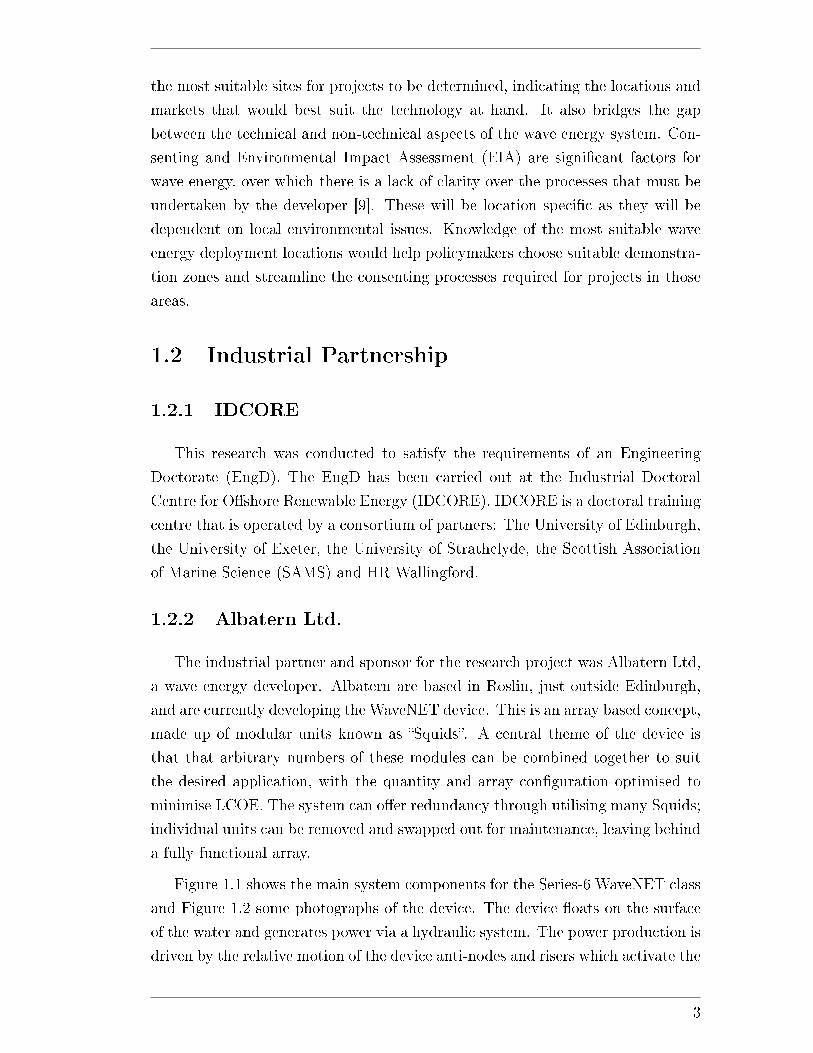
Figure 1.1 shows the main system components for the Series-6 WaveNET class

and Figure 1.2 some photographs of the device. The device �oats on the surface

of the water and generates power via a hydraulic system. The power production is

driven by the relative motion of the device anti-nodes and risers which activate the

3

pumping modules, pumping hydraulic �uid through a hydraulic motor/generator.

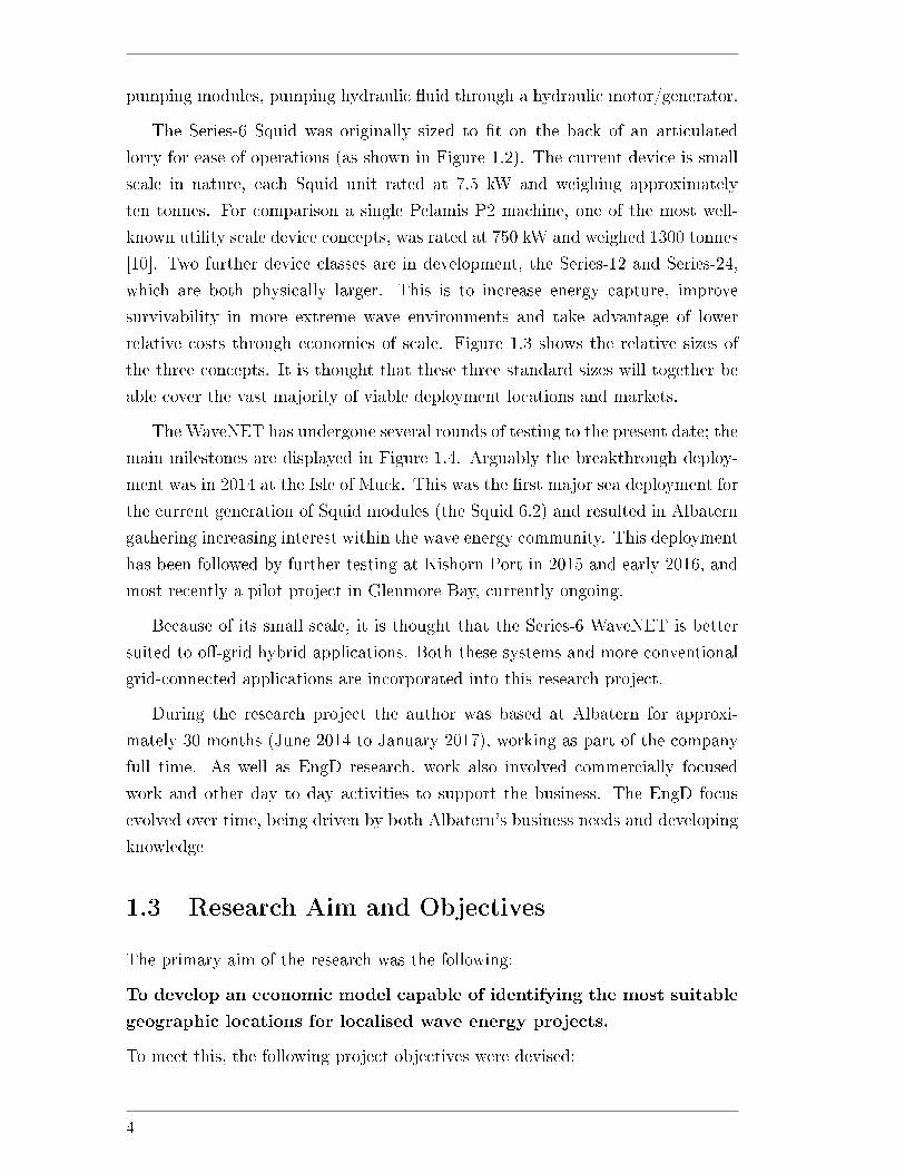
The Series-6 Squid was originally sized to �t on the back of an articulated

lorry for ease of operations (as shown in Figure 1.2). The current device is small

scale in nature, each Squid unit rated at 7.5 kW and weighing approximately

ten tonnes. For comparison a single Pelamis P2 machine, one of the most well-

known utility scale device concepts, was rated at 750 kW and weighed 1300 tonnes

[10]. Two further device classes are in development, the Series-12 and Series-24,

which are both physically larger. This is to increase energy capture, improve

survivability in more extreme wave environments and take advantage of lower

relative costs through economies of scale. Figure 1.3 shows the relative sizes of

the three concepts. It is thought that these three standard sizes will together be

able cover the vast majority of viable deployment locations and markets.

The WaveNET has undergone several rounds of testing to the present date; the

main milestones are displayed in Figure 1.4. Arguably the breakthrough deploy-

ment was in 2014 at the Isle of Muck. This was the �rst major sea deployment for

the current generation of Squid modules (the Squid 6.2) and resulted in Albatern

gathering increasing interest within the wave energy community. This deployment

has been followed by further testing at Kishorn Port in 2015 and early 2016, and

most recently a pilot project in Glenmore Bay, currently ongoing.

Because of its small scale, it is thought that the Series-6 WaveNET is better

suited to o�-grid hybrid applications. Both these systems and more conventional

grid-connected applications are incorporated into this research project.

During the research project the author was based at Albatern for approxi-

mately 30 months (June 2014 to January 2017), working as part of the company

full time. As well as EngD research, work also involved commercially focused

work and other day to day activities to support the business. The EngD focus

evolved over time, being driven by both Albatern's business needs and developing

knowledge

1.3 Research Aim and Objectives

The primary aim of the research was the following:

To develop an economic model capable of identifying the most suitable

geographic locations for localised wave energy projects.

To meet this, the following project objectives were devised:

4

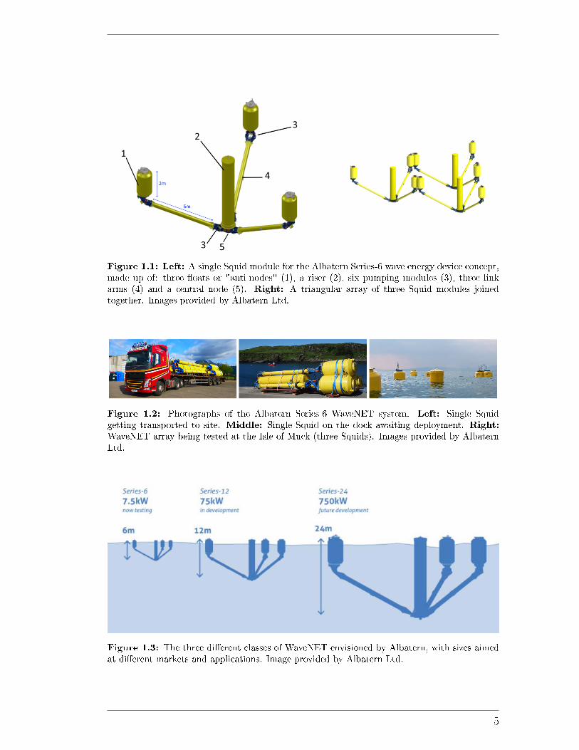
Figure 1.1: Left: A single Squid module for the Albatern Series-6 wave energy device concept,made up of: three �oats or "anti-nodes" (1), a riser (2), six pumping modules (3), three linkarms (4) and a central node (5). Right: A triangular array of three Squid modules joinedtogether. Images provided by Albatern Ltd.

Figure 1.2: Photographs of the Albatern Series-6 WaveNET system. Left: Single Squidgetting transported to site. Middle: Single Squid on the dock awaiting deployment. Right:WaveNET array being tested at the Isle of Muck (three Squids). Images provided by AlbaternLtd.

Figure 1.3: The three di�erent classes of WaveNET envisioned by Albatern, with sizes aimedat di�erent markets and applications. Image provided by Albatern Ltd.

5

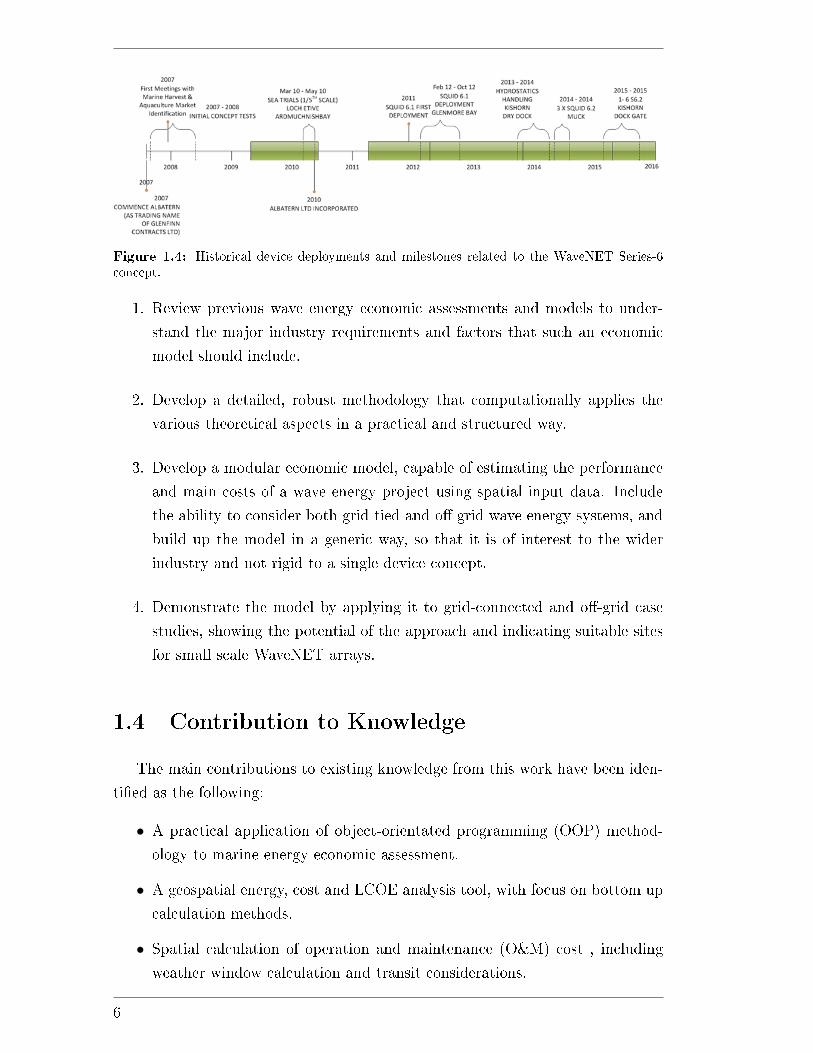
Figure 1.4: Historical device deployments and milestones related to the WaveNET Series-6concept.

1. Review previous wave energy economic assessments and models to under-

stand the major industry requirements and factors that such an economic

model should include.

2. Develop a detailed, robust methodology that computationally applies the

various theoretical aspects in a practical and structured way.

3. Develop a modular economic model, capable of estimating the performance

and main costs of a wave energy project using spatial input data. Include

the ability to consider both grid tied and o�-grid wave energy systems, and

build up the model in a generic way, so that it is of interest to the wider

industry and not rigid to a single device concept.

4. Demonstrate the model by applying it to grid-connected and o�-grid case

studies, showing the potential of the approach and indicating suitable sites

for small scale WaveNET arrays.

1.4 Contribution to Knowledge

The main contributions to existing knowledge from this work have been iden-

ti�ed as the following:

• A practical application of object-orientated programming (OOP) method-

ology to marine energy economic assessment.

• A geospatial energy, cost and LCOE analysis tool, with focus on bottom up

calculation methods.

• Spatial calculation of operation and maintenance (O&M) cost , including

weather window calculation and transit considerations.

6

• Development and application of a hybrid energy �power balancing� algo-

rithm to an o�-grid system with wave energy input, to calculate LCOE of

the system.

• Spatial hybrid LCOE analysis tool, designed to allow promising locations

for o�-grid wave systems to be determined.

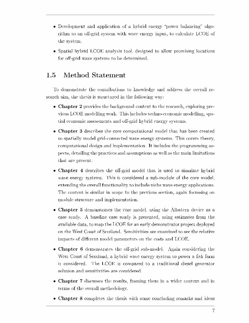
1.5 Method Statement

To demonstrate the contributions to knowledge and address the overall re-

search aim, the thesis is structured in the following way:

• Chapter 2 provides the background context to the research, exploring pre-

vious LCOE modelling work. This includes techno-economic modelling, spa-

tial economic assessments and o�-grid hybrid energy systems.

• Chapter 3 describes the core computational model that has been created

to spatially model grid-connected wave energy systems. This covers theory,

computational design and implementation. It includes the programming as-

pects, detailing the practices and assumptions as well as the main limitations

that are present.

• Chapter 4 describes the o�-grid model that is used to simulate hybrid

wave energy systems. This is considered a sub-module of the core model,

extending the overall functionality to include niche wave energy applications.

The content is similar in scope to the previous section, again focussing on

module structure and implementation.

• Chapter 5 demonstrates the core model, using the Albatern device as a

case study. A baseline case study is presented, using estimates from the

available data, to map the LCOE for an early demonstrator project deployed

on the West Coast of Scotland. Sensitivities are examined to see the relative

impacts of di�erent model parameters on the costs and LCOE.

• Chapter 6 demonstrates the o�-grid sub-model. Again considering the

West Coast of Scotland, a hybrid wave energy system to power a �sh farm

is considered. The LCOE is compared to a traditional diesel generator

solution and sensitivities are considered.

• Chapter 7 discusses the results, framing them in a wider context and in

terms of the overall methodology.

• Chapter 8 completes the thesis with some concluding remarks and ideas

7

Figure 1.5: The structure of the thesis, with chapters working left to right. Blue arrowsrepresent the �ow of knowledge in the thesis. Circles denote the two chapters which describethe key modelling theory and implementation.

for future work.

This structure is represented pictorially in Figure 1.5. The chapters propagate

left to right, the arrows denoting the �ow of knowledge through the thesis. For

example, the themes within the o�-grid model theory section are guided by both

the background context from Chapter Two and the previous modelling theory

from Chapter Three.

8

2Research Context and Literature

Review

2.1 Wave Energy

Wave energy is a form of renewable energy which allows the kinetic energy of

sea waves to be captured and converted into electricity. It is predominantly a third

hand form of solar energy: the di�erential heating of the Earth's surface creates

winds which transfer energy to the water surface [11]. While there are many

device concepts at present, energy is typically produced by a device through a

prime mover that is perturbed by the wave motion. While the concept of wave

energy has existed for some time, with the �rst patent being �led as early as

1799 [12], the �rst o�shore device to be grid-connected only occurred as recently

as 2004 [13]. Since then there have been various demonstrators tested in the

water, but no commercial projects.

One of the early wave energy pioneers was Yoshio Masuda. Working in Japan

in the 1940s he developed a wave-powered navigation buoy which worked by forc-

ing air through a turbine [14]. This is the same principle which modern oscillating

water column concepts use. In Europe, the �rst serious wave energy funding pro-

gramme was set up in the UK in the 1970s. This came as a result of the 1973

oil crisis, which saw the oil price dramatically rise, and the early work of Stephen

Salter, whose nodding duck concept and 1974 publication in the journal Nature

attracted attention in the scienti�c community [15, 16]. The UK government,

with the aim of limiting the reliance on oil, supplied funding through an R&D

9

programme known as the Wave Energy Program [17]. This ran from the mid

1970s to the early 1980s, after which almost all funding was cut. This was due

to the oil prices stabilising and the unrealistic, politically motivated, expectations

of the government for wave energy, who did not see it as cost competitive as

�rst anticipated [18]. After 1982, almost all government funding ceased until the

1990s, when interest was reignited by an increased awareness of climate change

and the need to reduce CO2 emissions. New policy was introduced, for example

by the European Commission in 1991 who included wave energy in their R&D

funding programme [14], and the UK government who introduced a small scale

R&D programme of their own in 1999 [18].

As a concept wave energy has a number of advantages that would make it a

useful contributor to electricity demand. Because the resource has a high energy

density, output is more predictable than wind energy and solar energy, being less

prone to temporal �uctuations and easier to forecast [19]. The resource is also

not restricted by the diurnal cycle like solar, and follows seasonal demand much

better: with more energetic waves in the stormier winter months where electricity

demand is higher. Wave also has a number of environmental advantages compared

to o�shore wind and tidal stream. Generally it is thought that wave devices

would be less risk to sea birds [20], as they tend to be on or below the water

surface without a rotor, although collisions from diving birds would be possible

[20, 21]. The visual and noise impacts are also lower, which could mean a more

straightforward and cheaper consenting process. There are also potential positive

environmental impacts not unique to wave, including habitat enhancement and the

potential for environmental protected zones directly in the vicinity of the devices,

although more research needs carried out to quantity the impacts [21,22]. Lastly,

wave energy could o�er advantages to existing o�shore energy systems; combined

o�shore wind and wave are commonly considered. Such systems could reduce

costs (for example in the transmission network [23] or mooring system [24]), o�er

more consistent power with less variability [25] and the wave devices could o�er

some protection from challenging wave conditions to improve accessibility [26,27].

2.1.1 Anatomy of a wave energy system

Unlike wind energy, wave energy is two dimensional, with reliance on both

the wave height and the wave period. This, combined with the fact that there

are six potential degrees of freedom for a body in the marine environment, means

that there are many di�erent ways that wave energy can be extracted. While the

wind industry has overwhelmingly converged on a single design, the horizontal

10

axis wind turbine, the wave resource is more complex and hence many di�erent

approaches to energy capture still exist.

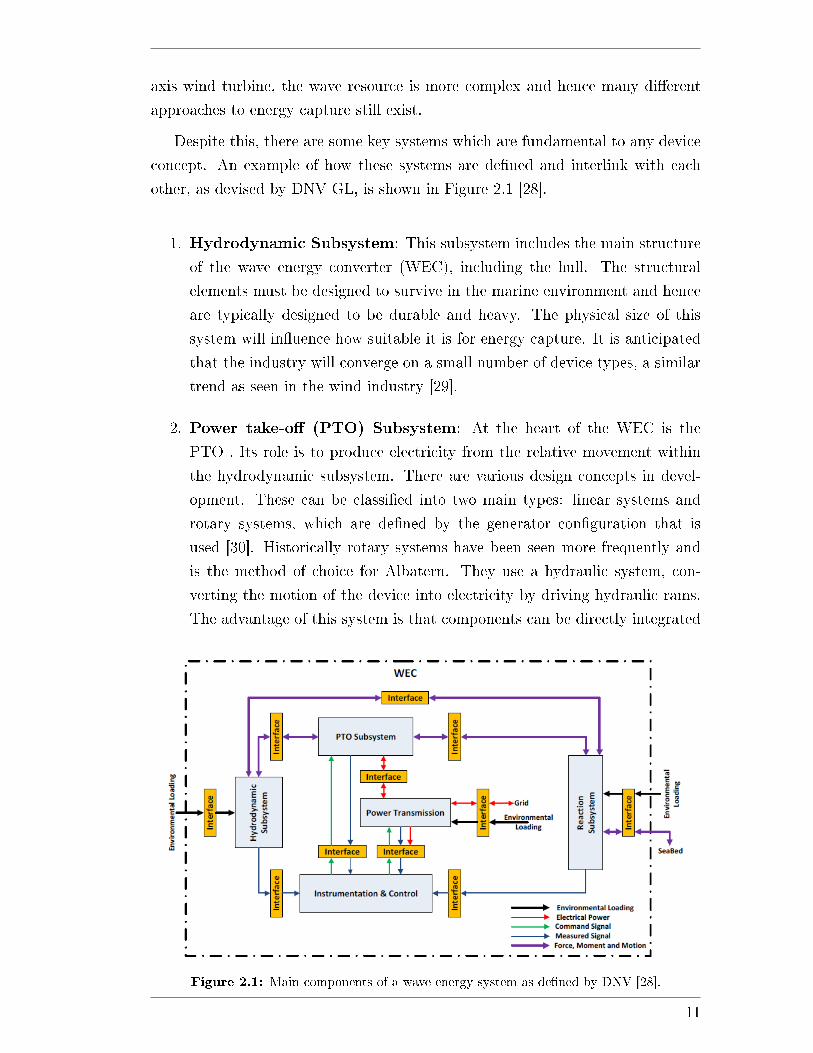
Despite this, there are some key systems which are fundamental to any device

concept. An example of how these systems are de�ned and interlink with each

other, as devised by DNV GL, is shown in Figure 2.1 [28].

1. Hydrodynamic Subsystem: This subsystem includes the main structure

of the wave energy converter (WEC), including the hull. The structural

elements must be designed to survive in the marine environment and hence

are typically designed to be durable and heavy. The physical size of this

system will in�uence how suitable it is for energy capture. It is anticipated

that the industry will converge on a small number of device types, a similar

trend as seen in the wind industry [29].

2. Power take-o� (PTO) Subsystem: At the heart of the WEC is the

PTO . Its role is to produce electricity from the relative movement within

the hydrodynamic subsystem. There are various design concepts in devel-

opment. These can be classi�ed into two main types: linear systems and

rotary systems, which are de�ned by the generator con�guration that is

used [30]. Historically rotary systems have been seen more frequently and

is the method of choice for Albatern. They use a hydraulic system, con-

verting the motion of the device into electricity by driving hydraulic rams.

The advantage of this system is that components can be directly integrated

Figure 2.1: Main components of a wave energy system as de�ned by DNV [28].

11

to provide short term energy storage and passively smooth out the output

power, for example high pressure accumulators. As they use common, o�

the shelf components [31], costs tend to be lower and supply chain issues are

reduced. By contrast the linear PTO system is generally regarded as more

e�cient and requires less maintenance than hydraulic systems [31], thus is

well suited for systems where accessing the PTO is more challenging (for

example structures �xed to the seabed).

3. Power Transmission: Once power is produced it must be routed to shore.

Multiple WEC units will be installed together in farms and connected with

inter-array cables. In some cases, particularly for larger farms that are

further from shore, an o�shore substation might be required to boost the

voltage and hence reduce electrical losses in transmission. As these platforms

can be very costly many developers will avoid them in early farms, instead

combining the inter-array cables within a junction box �xed to the seabed.

The power is then sent to shore using an export cable. These tend to be AC

cables, matching the electricity type produced by the PTO generators.

For the Albatern device there are some notable di�erences to the conven-

tional approach. As all of the Squid units are directly linked together there

is no need for array cabling, and the junction box can be housed within one

of the Anti Node �oats. Additionally, recti�cation is also carried out within

the PTO system: converting the voltage to 1 kV DC. This means that the

export cable is a cheaper two-core DC rather than an AC cable.

4. Reaction Subsystem: This subsystem consists of the mooring system,

and is designed to keep the device on station. It is an important element,

as failure would be hugely costly in both �nancial and political terms. The

speci�cs of the system again vary depending on the device concept, as well as

the seabed conditions. For many device types, such as point absorbers, the

system provides a reference point on the seabed for the device's movement.

It is the movement of the device relative to this �xed point which drives the

energy production. An alternative type of device is �self referencing�, where

energy is produced from the relative motion between elements of the WEC.

The Albatern WaveNET is an example of this.

For the mooring system the main cost drivers are the anchors and any

mooring lines required to connect to the device. These costs are typically

considered to make up 10-20% of the WEC capital cost [32]. For catenary

mooring lines, often the length is considered to be 3-5 times the water depth

12

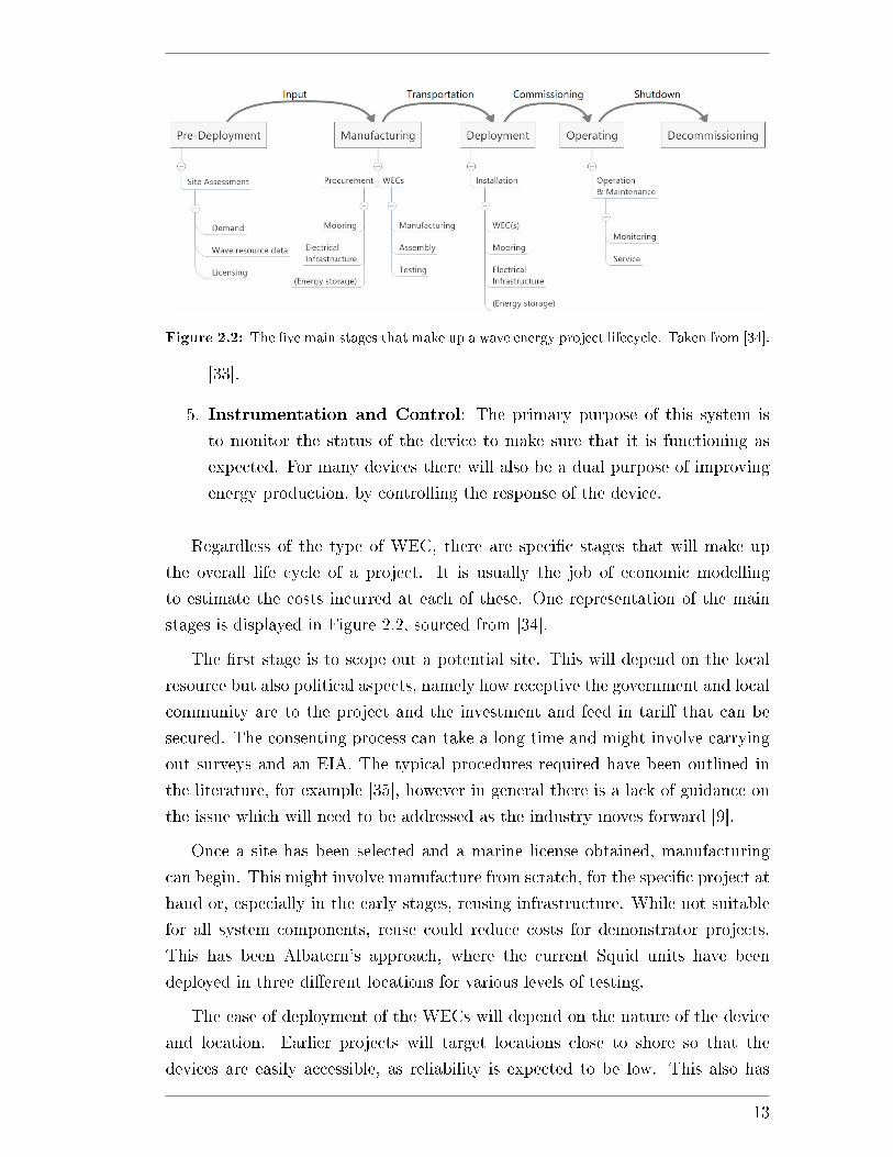
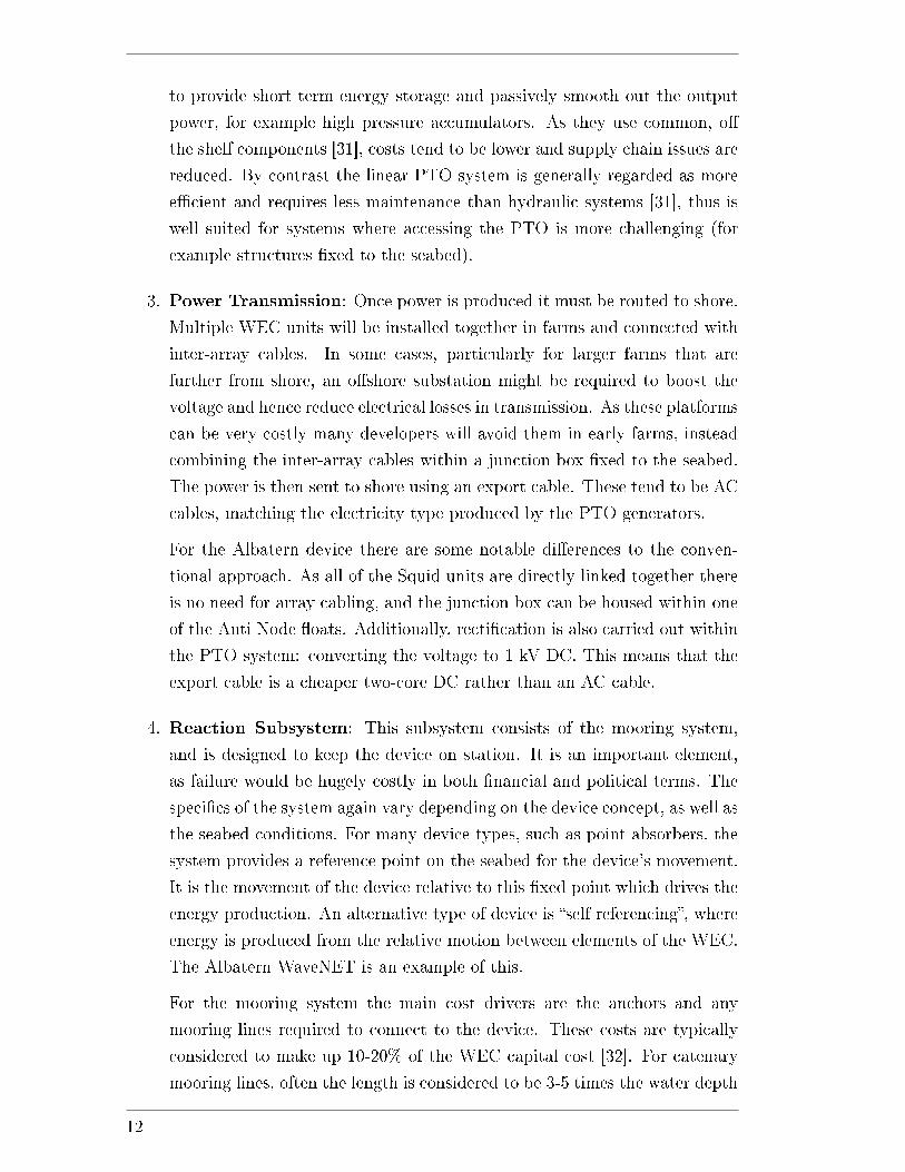
Figure 2.2: The �ve main stages that make up a wave energy project lifecycle. Taken from [34].

[33].

5. Instrumentation and Control: The primary purpose of this system is

to monitor the status of the device to make sure that it is functioning as

expected. For many devices there will also be a dual purpose of improving

energy production, by controlling the response of the device.

Regardless of the type of WEC, there are speci�c stages that will make up

the overall life cycle of a project. It is usually the job of economic modelling

to estimate the costs incurred at each of these. One representation of the main

stages is displayed in Figure 2.2, sourced from [34].

The �rst stage is to scope out a potential site. This will depend on the local

resource but also political aspects, namely how receptive the government and local

community are to the project and the investment and feed in tari� that can be

secured. The consenting process can take a long time and might involve carrying

out surveys and an EIA. The typical procedures required have been outlined in

the literature, for example [35], however in general there is a lack of guidance on

the issue which will need to be addressed as the industry moves forward [9].

Once a site has been selected and a marine license obtained, manufacturing

can begin. This might involve manufacture from scratch, for the speci�c project at

hand or, especially in the early stages, reusing infrastructure. While not suitable

for all system components, reuse could reduce costs for demonstrator projects.

This has been Albatern's approach, where the current Squid units have been

deployed in three di�erent locations for various levels of testing.

The ease of deployment of the WECs will depend on the nature of the device

and location. Earlier projects will target locations close to shore so that the

devices are easily accessible, as reliability is expected to be low. This also has

13

the advantage of keeping export cable costs low, a key cost driver particularly

for smaller scale projects. Other environmental factors, for example strong tidal

currents and rocky bathymetry will make installation more challenging [36] and

might require the use of more expensive vessels.

After the WEC farm has been installed it will begin its operational life. The

devices will require monitoring and maintenance, to increase the energy generated

and maximise the revenue. Maintenance will be a combination of minor servicing

carried out on site and more signi�cant activities which will require bringing the

devices back to port and carrying out work on land. At the end of the project the

devices are then brought back to port and decommissioned. Resources might be

kept for future projects, salvaged for income or scrapped.

2.1.2 Small scale wave energy

As well as larger, utility scale systems, wave energy also has signi�cant po-

tential at smaller scales. A so called �twin-track� development strategy, �nancial

support for both large and small scale concepts, is an advantageous approach

for the industry as it facilitates both deploying signi�cant capacity and a rapid

learning approach [37]. Smaller devices will lack the power producing potential

of larger ones and cannot take advantage of the same economies of scale. It does

mean, however, that the absolute costs will be much lower for early stage projects.

This equates to lower �nancial risk for an investor, the lower costs also allowing

fast innovation through learning, for example by being able to turnover multiple

device iterations for a given monetary input. This approach of taking advantage

of �learning-by-doing� has been seen historically for the onshore wind industry, as

demonstrated in Figure 2.3. It shows the historical evolution of rotor diameter in

the onshore wind industry, with commercial breakthroughs initially occurring for

smaller devices [38].

For wave energy, a learning-by-doing approach is best suited for small scale

devices to allow rapid expansion and demonstrate proof of concept [37]. It is a

suitable strategy to promote early stage growth in the industry and build investor

con�dence. The best way to apply this kind of learning is through deploying

devices in the water, gaining knowledge through the processes of operating and

maintaining the devices. As this can be costly it does present problems for early

TRL level concepts. It is for this reason that some instead promote a �learning-by-

research� approach [39], whereby companies utilise research tools like tank testing

and numerical modelling to lower costs and reduce risks before going into the

14

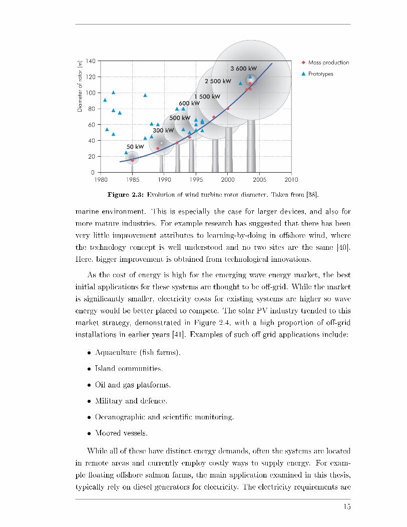
Figure 2.3: Evolution of wind turbine rotor diameter. Taken from [38].

marine environment. This is especially the case for larger devices, and also for

more mature industries. For example research has suggested that there has been

very little improvement attributes to learning-by-doing in o�shore wind, where

the technology concept is well understood and no two sites are the same [40].

Here, bigger improvement is obtained from technological innovations.

As the cost of energy is high for the emerging wave energy market, the best

initial applications for these systems are thought to be o�-grid. While the market

is signi�cantly smaller, electricity costs for existing systems are higher so wave

energy would be better placed to compete. The solar PV industry trended to this

market strategy, demonstrated in Figure 2.4, with a high proportion of o�-grid

installations in earlier years [41]. Examples of such o�-grid applications include:

• Aquaculture (�sh farms).

• Island communities.

• Oil and gas platforms.

• Military and defence.

• Oceanographic and scienti�c monitoring.

• Moored vessels.

While all of these have distinct energy demands, often the systems are located

in remote areas and currently employ costly ways to supply energy. For exam-

ple �oating o�shore salmon farms, the main application examined in this thesis,

typically rely on diesel generators for electricity. The electricity requirements are

15

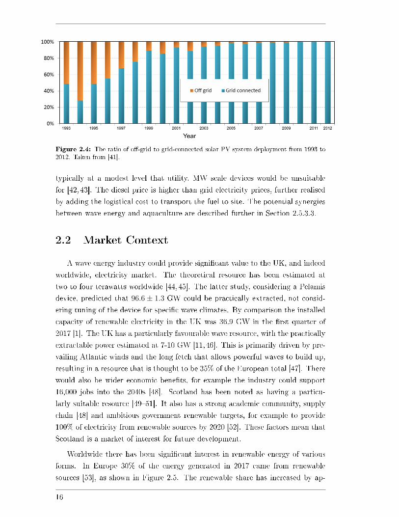
Figure 2.4: The ratio of o�-grid to grid-connected solar PV system deployment from 1993 to2012. Taken from [41].

typically at a modest level that utility, MW scale devices would be unsuitable

for [42, 43]. The diesel price is higher than grid electricity prices, further realised

by adding the logistical cost to transport the fuel to site. The potential synergies

between wave energy and aquaculture are described further in Section 2.5.3.3.

2.2 Market Context

A wave energy industry could provide signi�cant value to the UK, and indeed

worldwide, electricity market. The theoretical resource has been estimated at

two to four terawatts worldwide [44, 45]. The latter study, considering a Pelamis

device, predicted that 96.6 ± 1.3 GW could be practically extracted, not consid-

ering tuning of the device for speci�c wave climates. By comparison the installed

capacity of renewable electricity in the UK was 36.9 GW in the �rst quarter of

2017 [1]. The UK has a particularly favourable wave resource, with the practically

extractable power estimated at 7-10 GW [11,46]. This is primarily driven by pre-

vailing Atlantic winds and the long fetch that allows powerful waves to build up,

resulting in a resource that is thought to be 35% of the European total [47]. There

would also be wider economic bene�ts, for example the industry could support

16,000 jobs into the 2040s [48]. Scotland has been noted as having a particu-

larly suitable resource [49�51]. It also has a strong academic community, supply

chain [48] and ambitious government renewable targets, for example to provide

100% of electricity from renewable sources by 2020 [52]. These factors mean that

Scotland is a market of interest for future development.

Worldwide there has been signi�cant interest in renewable energy of various

forms. In Europe 30% of the energy generated in 2017 came from renewable

sources [53], as shown in Figure 2.5. The renewable share has increased by ap-

16

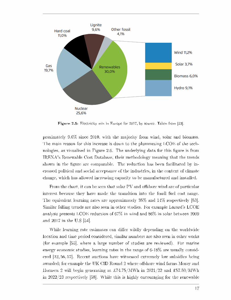
Figure 2.5: Electricity mix in Europe for 2017, by source. Taken from [53].

proximately 9.6% since 2010, with the majority from wind, solar and biomass.

The main reason for this increase is down to the plummeting LCOE of the tech-

nologies, as visualised in Figure 2.6. The underlying data for this �gure is from

IRENA's Renewable Cost Database, their methodology meaning that the trends

shown in the �gure are comparable. The reduction has been facilitated by in-

creased political and social acceptance of the industries, in the context of climate

change, which has allowed increasing capacity to be manufactured and installed.

From the chart, it can be seen that solar PV and o�shore wind are of particular

interest because they have made the transition into the fossil fuel cost range.

The equivalent learning rates are approximately 35% and 14% respectively [53].

Similar falling trends are also seen in other studies. For example Lazard's LCOE

analysis presents LCOE reduction of 67% in wind and 86% in solar between 2009

and 2017 in the U.S [54].

While learning rate estimates can di�er wildly depending on the worldwide

location and time period considered, similar numbers are also seen in other works

(for example [55], where a large number of studies are reviewed). For marine

energy economic studies, learning rates in the range of 6-18% are usually consid-

ered [32, 56, 57]. Recent auctions have witnessed extremely low subsidies being

awarded; for example the UK CfD Round 2 where o�shore wind farms Moray and

Hornsea 2 will begin generating at ¿74.75/MWh in 2021/22 and ¿57.50/MWh

in 2022/23 respectively [58]. While this is highly encouraging for the renewable

17

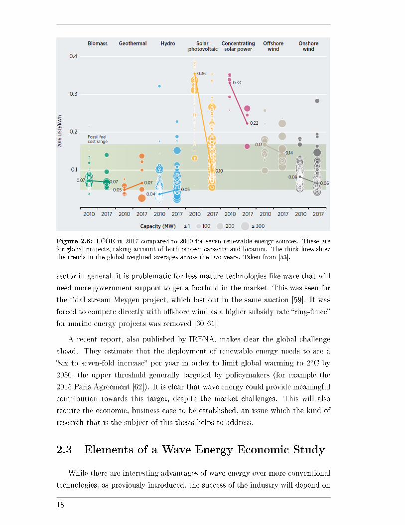
Figure 2.6: LCOE in 2017 compared to 2010 for seven renewable energy sources. These arefor global projects, taking account of both project capacity and location. The thick lines showthe trends in the global weighted averages across the two years. Taken from [53].

sector in general, it is problematic for less mature technologies like wave that will

need more government support to get a foothold in the market. This was seen for

the tidal stream Meygen project, which lost out in the same auction [59]. It was

forced to compete directly with o�shore wind as a higher subsidy rate �ring-fence�

for marine energy projects was removed [60,61].

A recent report, also published by IRENA, makes clear the global challenge

ahead. They estimate that the deployment of renewable energy needs to see a

�six to seven-fold increase� per year in order to limit global warming to 2◦C by

2050, the upper threshold generally targeted by policymakers (for example the

2015 Paris Agreement [62]). It is clear that wave energy could provide meaningful

contribution towards this target, despite the market challenges. This will also

require the economic, business case to be established, an issue which the kind of

research that is the subject of this thesis helps to address.

2.3 Elements of a Wave Energy Economic Study

While there are interesting advantages of wave energy over more conventional

technologies, as previously introduced, the success of the industry will depend on

18

its ability to deliver at a competitive price. Understanding the performance and

costs of a project are a crucial step towards building a commercial wave energy

industry.

Estimating the economic potential of any energy technology should include a

number of di�erent aspects. Many of these are technology and project speci�c, and

some can be problematic for wave energy due to limited operational experience

and data availability. At the typical level, two criteria are required:

1. The total energy produced, and

2. The total cost.

This section describes the main themes which are included within these.

2.3.1 Levelised cost of energy

In the energy industry, the most common way to assess market potential is by

calculating the LCOE. LCOE is de�ned as:

�The constant price at which electricity would have to be sold for the production

facility to break even over its lifetime, assuming it operates at full capacity.� [63]

Mathematically this is expressed as:

LCOE =CPV

EPV

, (2.1)

where CPV is the total cost incurred over the project lifetime and EPV the total

energy produced over the project lifetime. These are discounted to present values.

Discounted costs are known as Net Present Costs (NPC). Discounting is a process

commonly used in �nance that involves reducing the values of cash �ows that

occur in the future by multiplying them by a time dependent factor, the discount

factor. This is done to re�ect the �time preference� of money: namely that cash

in the present is worth more than the same value in the future, as it is subject

to less uncertainty and could be invested sooner. The approach is also applied to

energy with a similar logic: as it is more valuable in the present. The discount

factor, D is expressed as:

D(t) =1

(1 + r)t, (2.2)

which is a function of the time period (commonly the year) the cash �ow occurs

in, t, and the discount rate r. This is a percentage that essentially represents

19

the level of risk in the project. It should re�ect the market value of equity and

debt [64]. There is a degree of subjectivity in its selection as it will depend on

the return that an investor would hope to get. For wave energy the value chosen

is typically in the range 5%-15% [26], depending on the commissioning date and

technology maturity assumed for the project. More mature, commercial projects

will have lower perceived risk and hence command lower discount rates [65, 66].

Considering D, Equation 2.1 can be expressed as a sum of the discounted cost and

energy contributions for each discrete project period (C(t) and E(t) respectively):

LCOE =

n∑t=0

C(t)/(1 + r)t

n∑t=0

E(t)/(1 + r)t. (2.3)

It should be noted that the above equation assumes that the same discount rate

is applied to every cost. In reality, di�erent aspects of the project can be funded

in di�erent ways, with some investors willing to take more risk than others. This

can be modelled by applying di�erent discount rates for di�erent elements of the

project. One approach that is sometimes seen is using di�erent discount rates for

the capital costs and operational costs.

The calculation can be performed both in nominal (with in�ation) or real

(without in�ation) terms by selecting an appropriate discount rate [67]. The

main costs that are usually considered are introduced in the next section.

The main advantage of using LCOE as a metric is its simplicity, as it is well

understood and used by developers, investors and policymakers alike. It also

allows direct comparison between di�erent sources of electricity to be easily made

and the main cost drivers to be identi�ed. Moreover, by incorporating the present

value of the variables it allows risk to be introduced into the analysis.

LCOE does have drawbacks. It does not include revenue, which can vary

depending on the business model chosen and could have a large impact on the po-

tential of a given project. This is especially true for more established technologies

like wind, which is moving to a zero subsidy market. In this context, where the

relative costs are low, energy price and quality is a more signi�cant consideration.

For example, more dispatchable system types that can be switched on quickly to

follow demand, may command a higher price in the market and thus would be

more valuable to an investor in reality. For early stage wave technologies this

also limits the application to business strategy. For example, competing business

20

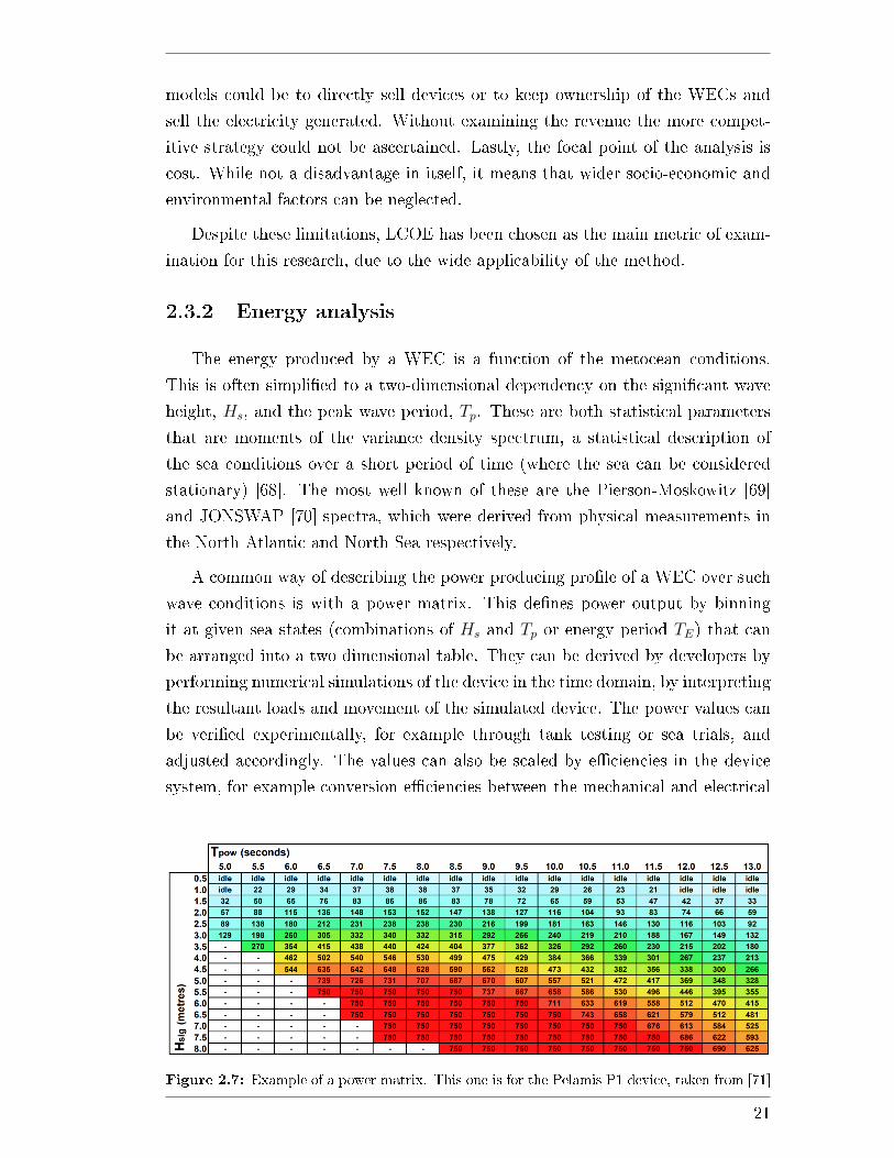
models could be to directly sell devices or to keep ownership of the WECs and

sell the electricity generated. Without examining the revenue the more compet-

itive strategy could not be ascertained. Lastly, the focal point of the analysis is

cost. While not a disadvantage in itself, it means that wider socio-economic and

environmental factors can be neglected.

Despite these limitations, LCOE has been chosen as the main metric of exam-

ination for this research, due to the wide applicability of the method.

2.3.2 Energy analysis

The energy produced by a WEC is a function of the metocean conditions.

This is often simpli�ed to a two-dimensional dependency on the signi�cant wave

height, Hs, and the peak wave period, Tp. These are both statistical parameters

that are moments of the variance density spectrum, a statistical description of

the sea conditions over a short period of time (where the sea can be considered

stationary) [68]. The most well known of these are the Pierson-Moskowitz [69]

and JONSWAP [70] spectra, which were derived from physical measurements in

the North Atlantic and North Sea respectively.

A common way of describing the power producing pro�le of a WEC over such

wave conditions is with a power matrix. This de�nes power output by binning

it at given sea states (combinations of Hs and Tp or energy period TE) that can

be arranged into a two dimensional table. They can be derived by developers by

performing numerical simulations of the device in the time domain, by interpreting

the resultant loads and movement of the simulated device. The power values can

be veri�ed experimentally, for example through tank testing or sea trials, and

adjusted accordingly. The values can also be scaled by e�ciencies in the device

system, for example conversion e�ciencies between the mechanical and electrical

Figure 2.7: Example of a power matrix. This one is for the Pelamis P1 device, taken from [71]

21

system. An example of a power matrix is shown in Figure 2.7.

Given a time-series of wave elevation, a time-series of power can be obtained by

using a power matrix as a lookup table, interpolating the metocean data at each

time step. This interpolation is required when the metocean values of interest

are given to a higher resolution than the power matrix bins (lying between the

discrete sea state values that the numerical models have been run at). Another

way that this can be achieved is by binning the input metocean data to the same

resolution as the power matrix and directly multiplying the two. The timeseries

interpolation is the superior method, however, as considering discrete metocean

bins can introduce rounding errors [72].

The energy produced can then be obtained by summing the resulting over

the time series, and can be discounted as described in Section 2.3.1 to form the

denominator of the LCOE calculation.

2.3.3 Cost analysis

Costs are typically categorised into three types: capital expenditure (CAPEX),

operational expenditure (OPEX) and decommissioning (DECEX) [73].

CAPEX items are those that are required to set-up a given project. They

are often assumed to occur in year zero of the project (for example [57]), and

as a result are not discounted, although this is not always the case (for example

[74]). Installation of the wave energy device also falls under CAPEX, although

is sometimes regarded within a separate category. Other examples of CAPEX

include the cost to purchase the WECs, the mooring system and the export cable.

The development cost is also an item of CAPEX. This is the cost associated

with site surveys and obtaining a marine license, required to legally deploy the

device. This cost is often very small, only a few percent, so is often assumed to

be negligible

DECEX is the cost to uninstall and remove the system from the water at the

end of the project. As there has been very limited decommissioning experience in

the wave sector, it is often assumed to be equal to a percentage of the initial cost

(for example [75]). As the costs occur very far into the future, they are heavily

discounted. Components will also be salvaged, meaning that there will be some

positive cash�ow. Because of these factors this cost is typically assumed to be

very low, for example estimated at 0.26% of the LCOE in [26], and sometimes

will not be considered at all (for example [29,74,76]).

22

2.3.3.1 Operating expenditure

OPEX are the costs that are incurred during the operational lifetime of the

WEC farm. These include both planned and unplanned O&M, and ongoing costs

like labour and insurance. Because maintenance costs will depend on the state of

the WECs and environmental factors, they have a time dependency that makes

them more challenging to model.

For o�shore wind, OPEX accounts for roughly 25% of the total project ex-

penditure [77, 78]. Wave energy costs are expected to be higher than this, for

example as considered in [32], due to lack of operating experience and reduced

reliability from devices being deployed in more extreme environments. The aim

would be to avoid winter for carrying out O&M, as accessibility is more di�cult

and there would be a greater loss of revenue from missing out on higher energy

conditions [33].

A marine operation is a task that must be performed on the WEC out at sea.

This could include deploying the WEC, accessing it to carry out maintenance or

towing it back to port for maintenance on land. To carry out a marine operation

the sea conditions must be suitable. If the conditions are too extreme, with high

wave heights, wave periods or wind speeds, then the task cannot be carried out.

This is due to safety concerns or technical limitations, for example a vessel is not

stable enough to use certain equipment. The most in�uential factors are wave

height and wave period, with wind speed also a factor if cranes are required [79].

These kind of extreme conditions are also linked to reliability. If the device

is subjected to higher loads from the environment then this can cause failures in

the device, possibly resulting in loss of energy production (known as downtime).

Examples of failures include extreme snatch loads in mooring systems and end stop

issues in PTOs, whereby a high force can cause a hydraulic cylinder to abruptly

reach the end of its stroke [80]. Thus, in more energetic wave climates devices can

be both more di�cult to access and require more regular access for maintenance.

An early step towards understanding reliability for a particular technology is

to undertake a Failure Mode and E�ects Analysis (FMEA). This is undertaken by

a developer, built up from device performance data, with the aim of documenting,

quantifying and ranking by risk all of the potential failures that could occur in

the system during operation. This analysis was undertaken for the Albatern

device in 2017 by Kenny et al. [81]. Due to the poor data resolution the authors

were unable to derive mean time to failure values, which can used to calculate

availability [82]. They noted that relatively high occurrences of electrical and

23

instrumentation issues coincided with each new deployment of the Squids, hence

could be attributed to the adoption of new innovations. They also anticipated

that reliability will improve over time as �teething issues and design faults are

addressed� [81].

Availability is de�ned as the proportion of time that the WEC is able to

produce power. Availability is reduced by failures in devices, as well as planned

downtime for scheduled maintenance. Quoted availabilities for onshore wind and

o�shore wind are 96.2% and 94.5% respectively [83]. There are limited data

available for wave, due to the lack of commercial projects, but availability is

generally regarded as being less than 90% [84] and as low as 60% for early stage

technology in particularly energetic regions [65].

A weather window is a sustained period of time where conditions are suitable

for the WEC to be accessed at sea. They are de�ned in terms of the maximum

weather limits that the operation can be carried out in. These thresholds can be

increased in di�erent ways, for example using more stable vessels or simplifying

O&M procedures. The length of the window that is required must be long enough

to allow the desired operation to be carried out. Longer operations at sea will

require longer weather windows. Usually maintenance will be carried out in the

summer months, where possible, when the devices are easier to access [76]. For

higher energy sites, generally more suitable for wave energy, there will be more

waiting time for suitable windows [85]. In these waiting periods the vessel and

crew will be on standby. For a chartered vessel this time will incur a fee; thus

weather window analysis and waiting time estimation is an important part of the

LCOE calculation.

There are two main ways that waiting time can be estimated: using frequency

based methods or time based methods. Both of these require the maximum envi-

ronmental limits to be de�ned, in which the operation could be carried out. Time

based methods require a time series of the environmental quantities, typically the

wind speed, Hs and Tp. Starting from an initial time step, the environmental

data at each subsequent step are checked to see whether the maximum limits are

exceeded. Consecutive time steps of non-exceedance form weather windows, of

which those that are greater than the time required for the operation, can be

identi�ed. Because these methods often require large quantities of data, Markov

chain methods can be used to create representative time series for a site [10].

This is achieved by using a transformation matrix, created from existing data,

that allows the next sea state to be randomly generated from the current one.

24

Frequency based methods do not require such a detailed knowledge of the time

series. Joint occurrence matrices, de�ning the frequency and probability of sea

states occurring in particular bins of Hs and Tp, are used. This means that, when

considering a speci�c time interval, the ordering of sea states within the interval

is not important: the waiting time is calculated statistically. First formulated by

Kuwashima and Hogben [86] the method is also described in [87] and [88].

Time series based methods are regarded as being more accurate and also allow

multiple environmental limits to be simultaneously considered [79,87]. Anastasiou

and Tsekos compared a Markov chain method with Kuwashima and Hogben's

frequency based method, �nding that their method provided a better �t to the

observed data [89]. However in general the methods are more complex and a large

quantity of time series data are required. Because the economic model developed

for this research project is spatial in nature, with calculations needing to repeated

over hundreds or thousands of time series, a frequency based approach was chosen

to reduce run time and allow for smaller datasets of less than ten years. It can

give a useful indication as to the most suitable time period for deployment, for

example the month where the waiting time for operations will be minimised.

2.4 Previous Research

Understanding the previous research on the topic of wave energy economic

assessments was important to this research project. This is so that the key

methodologies and cost drivers could be determined and factored into the model

framework created.

As computational power has increased, so has the capability of numerical

modelling. The accessibility and usability of modelling tools means that they

are readily available and of increasing interest both in an academic setting and

within industry. Because wave energy lacks maturity the research topic is broad,

and there has been signi�cant work within the LCOE modelling theme. There is

a strong need for research, with particular emphasis on bridging the gap between

academic research and commercial application. The current status of wave energy,

as well as high uncertainty over its future potential, means that there are numerous

unanswered questions. The aim of this section is to introduce the literature that

has been published on the research subject of wave energy economic modelling, so

as to frame the wider context of this work and acknowledge the variety of research

which it aims to contribute towards.

25

2.4.1 Economic evaluation

As economic modelling is such a broad subject area, with many underlying

themes, there is a selection of material available. As wave energy has only recently

generated interest again, the majority of relevant studies can be found in the 2000s.

One of the early pioneers in the �eld was Tom Thorpe. In 1999, Thorpe

published a technical report for the UK government entitled: "A Brief Review of

Wave Energy" [90]. It gives economic assessments of several of the most developed

technologies at the time, including the Limpet and Salter's Duck, and also covers

other aspects like environmental e�ects. The aim was to identify projects with

the best potential for future government funding and development. At 200 pages,

the methodology and cost breakdowns are detailed and consistent between the

di�erent technologies to allow direct comparison. For most of the devices, both

LCOE and IRR are provided and the author highlights the high uncertainty in

the calculations and the need for future research.

A limitation of the report is that it is very optimistic in nature. For example

the majority of the devices are found to have LCOE of under 10 p/kWh, with some

approaching 5 p/kWh. Based on these, wave power would be comparable with

fossil fuels and almost certainly a commercial market by now. Thorpe does state

that these costs are estimated based on the �predicted performances� of the devices

and that there is �considerable uncertainty� with some of the cost estimates. As

very few of these devices had actually been designed at full sea scale and deployed

for any length of time, CAPEX and OPEX were based on proportional estimates

and were potentially subject to bias from the companies who were keen to secure

funding for their devices (indeed Thorpe states that �the inputs to the assessment

are based on data provided by the teams working on these devices� and �it has not

been possible to validate these data independently�). Nevertheless, the report was

successful in applying simple and well understood economic evaluation methods

to wave technology, paving the way for future work.

Into the early 2000s, interest in wave energy continued to grow. The creation of

the European Wave Energy Centre (EMEC) in 2003 and the rise of the companies

Pelamis and Aquabuoy were notable events [91], demonstrating that people were

thinking more seriously about wave energy as a viable business opportunity. The

need to assess the economics of the technology became more apparent: to help

fuel industry growth, improve understanding and encourage investment.

An example of this wider interest, outside of the purely academic environment,

26

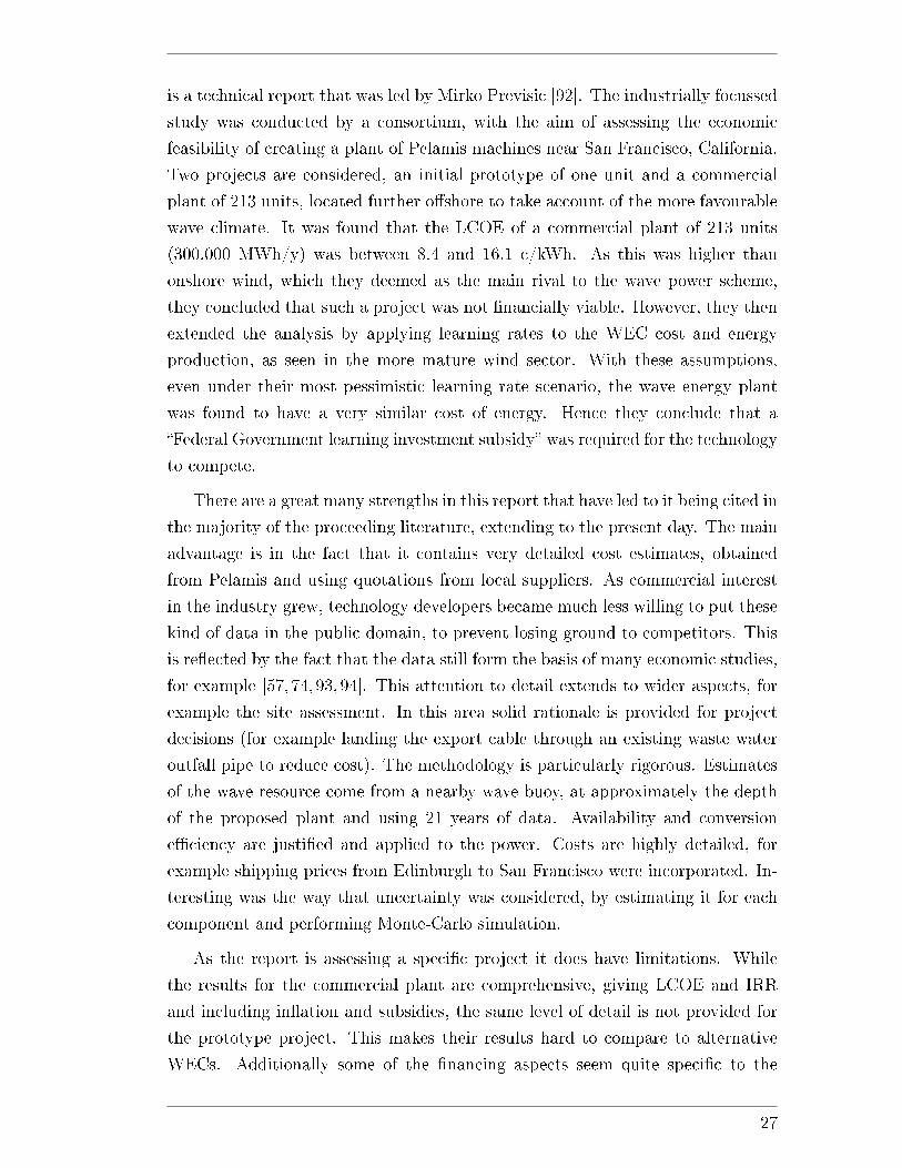
is a technical report that was led by Mirko Previsic [92]. The industrially focussed

study was conducted by a consortium, with the aim of assessing the economic

feasibility of creating a plant of Pelamis machines near San Francisco, California.

Two projects are considered, an initial prototype of one unit and a commercial

plant of 213 units, located further o�shore to take account of the more favourable

wave climate. It was found that the LCOE of a commercial plant of 213 units

(300,000 MWh/y) was between 8.4 and 16.1 c/kWh. As this was higher than

onshore wind, which they deemed as the main rival to the wave power scheme,

they concluded that such a project was not �nancially viable. However, they then

extended the analysis by applying learning rates to the WEC cost and energy

production, as seen in the more mature wind sector. With these assumptions,

even under their most pessimistic learning rate scenario, the wave energy plant

was found to have a very similar cost of energy. Hence they conclude that a

�Federal Government learning investment subsidy� was required for the technology

to compete.

There are a great many strengths in this report that have led to it being cited in

the majority of the proceeding literature, extending to the present day. The main

advantage is in the fact that it contains very detailed cost estimates, obtained

from Pelamis and using quotations from local suppliers. As commercial interest

in the industry grew, technology developers became much less willing to put these

kind of data in the public domain, to prevent losing ground to competitors. This

is re�ected by the fact that the data still form the basis of many economic studies,

for example [57, 74, 93, 94]. This attention to detail extends to wider aspects, for

example the site assessment. In this area solid rationale is provided for project

decisions (for example landing the export cable through an existing waste water

outfall pipe to reduce cost). The methodology is particularly rigorous. Estimates

of the wave resource come from a nearby wave buoy, at approximately the depth

of the proposed plant and using 21 years of data. Availability and conversion

e�ciency are justi�ed and applied to the power. Costs are highly detailed, for

example shipping prices from Edinburgh to San Francisco were incorporated. In-

teresting was the way that uncertainty was considered, by estimating it for each

component and performing Monte-Carlo simulation.

As the report is assessing a speci�c project it does have limitations. While

the results for the commercial plant are comprehensive, giving LCOE and IRR

and including in�ation and subsidies, the same level of detail is not provided for

the prototype project. This makes their results hard to compare to alternative

WECs. Additionally some of the �nancing aspects seem quite speci�c to the

27

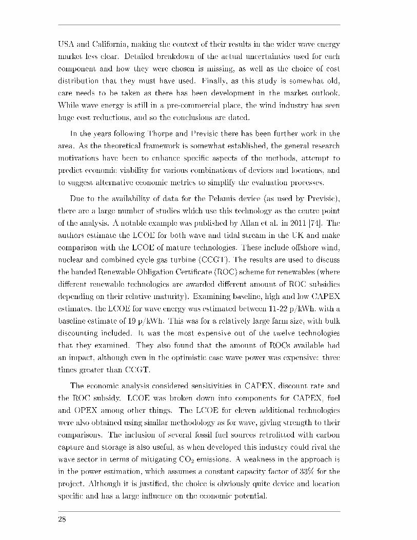
USA and California, making the context of their results in the wider wave energy

market less clear. Detailed breakdown of the actual uncertainties used for each

component and how they were chosen is missing, as well as the choice of cost

distribution that they must have used. Finally, as this study is somewhat old,

care needs to be taken as there has been development in the market outlook.

While wave energy is still in a pre-commercial place, the wind industry has seen

huge cost reductions, and so the conclusions are dated.

In the years following Thorpe and Previsic there has been further work in the

area. As the theoretical framework is somewhat established, the general research

motivations have been to enhance speci�c aspects of the methods, attempt to

predict economic viability for various combinations of devices and locations, and

to suggest alternative economic metrics to simplify the evaluation processes.

Due to the availability of data for the Pelamis device (as used by Previsic),

there are a large number of studies which use this technology as the centre point

of the analysis. A notable example was published by Allan et al. in 2011 [74]. The

authors estimate the LCOE for both wave and tidal stream in the UK and make

comparison with the LCOE of mature technologies. These include o�shore wind,

nuclear and combined cycle gas turbine (CCGT). The results are used to discuss

the banded Renewable Obligation Certi�cate (ROC) scheme for renewables (where

di�erent renewable technologies are awarded di�erent amount of ROC subsidies

depending on their relative maturity). Examining baseline, high and low CAPEX

estimates, the LCOE for wave energy was estimated between 11-22 p/kWh, with a

baseline estimate of 19 p/kWh. This was for a relatively large farm size, with bulk

discounting included. It was the most expensive out of the twelve technologies

that they examined. They also found that the amount of ROCs available had

an impact, although even in the optimistic case wave power was expensive: three

times greater than CCGT.

The economic analysis considered sensitivities in CAPEX, discount rate and

the ROC subsidy. LCOE was broken down into components for CAPEX, fuel

and OPEX among other things. The LCOE for eleven additional technologies

were also obtained using similar methodology as for wave, giving strength to their

comparisons. The inclusion of several fossil fuel sources retro�tted with carbon

capture and storage is also useful, as when developed this industry could rival the

wave sector in terms of mitigating CO2 emissions. A weakness in the approach is

in the power estimation, which assumes a constant capacity factor of 33% for the

project. Although it is justi�ed, the choice is obviously quite device and location

speci�c and has a large in�uence on the economic potential.

28

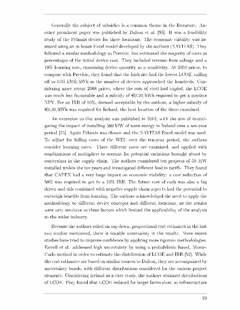
Generally the subject of subsidies is a common theme in the literature. An-

other prominent paper was published by Dalton et al. [93]. It was a feasibility

study of the Pelamis device for three locations. The economic viability was as-

sessed using an in house Excel model developed by the authors (NAVITAS). They

followed a similar methodology to Previsic, but estimated the majority of costs as

percentages of the initial device cost. They included revenue from salvage and a

10% learning rate, examining device quantity as a sensitivity. At 2004 prices, to

compare with Previsic, they found that the Irish site had the lowest LCOE, tailing

o� to 0.05 EUR/kWh as the number of devices approached the hundreds. Con-

sidering more recent 2008 prices, where the cost of steel had tripled, the LCOE

was much less favourable and a subsidy of e0.20/kWh required to get a positive

NPV. For an IRR of 10%, deemed acceptable by the authors, a higher subsidy of

e0.30/kWh was required for Ireland, the best location of the three examined.

An extension to this analysis was published in 2012, with the aim of investi-

gating the impact of installing 500 MW of wave energy in Ireland over a ten-year

period [75]. Again Pelamis was chosen and the NAVITAS Excel model was used.

To adjust for falling costs of the WEC over the ten-year period, the authors

consider learning rates. Three di�erent rates are examined, and applied with

combinations of multipliers to account for potential variations brought about by

constraints in the supply chain. The authors considered ten projects of 50 MW

installed within the ten years and investigated di�erent feed in tari�s. They found

that CAPEX had a very large impact on economic viability: a cost reduction of

50% was required to get to a 10% IRR. The future cost of cash was also a big

driver and this combined with negative supply chain aspects had the potential to

outweigh bene�ts from learning. The authors acknowledged the need to apply the

methodology to di�erent device concepts and di�erent locations, as the results

were very sensitive to these factors which limited the applicability of the analysis

to the wider industry.

Because the authors relied on top down, proportional cost estimates in the last

two studies mentioned, there is notable uncertainty in the results. More recent

studies have tried to improve con�dence by applying more rigorous methodologies.

Farrell et al. addressed high uncertainty by using a probabilistic based, Monte-

Carlo method in order to estimate the distribution of LCOE and IRR [57]. While

the cost estimates are based on similar sources to Dalton, they are accompanied by

uncertainty bands, with di�erent distributions considered for the various project

elements. Considering Ireland as a case study, the authors obtained distributions

of LCOE. They found that LCOE reduced for larger farms sizes, as infrastructure

29

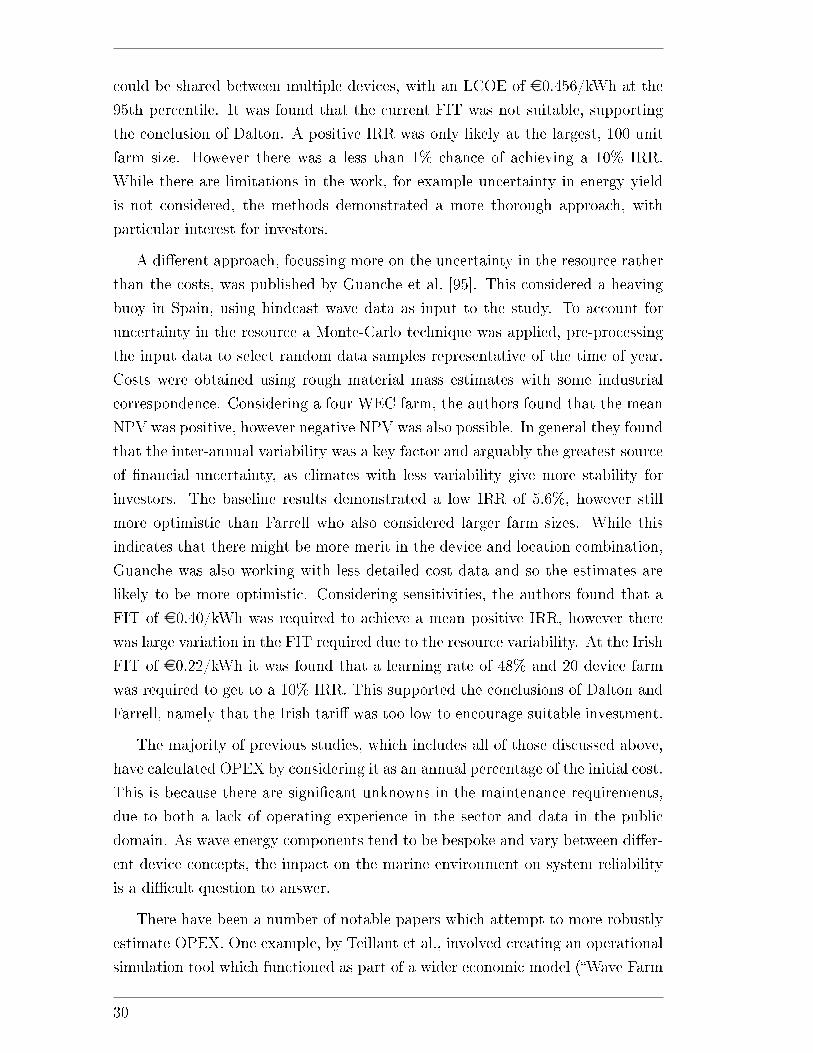
could be shared between multiple devices, with an LCOE of e0.456/kWh at the

95th percentile. It was found that the current FIT was not suitable, supporting

the conclusion of Dalton. A positive IRR was only likely at the largest, 100 unit

farm size. However there was a less than 1% chance of achieving a 10% IRR.

While there are limitations in the work, for example uncertainty in energy yield

is not considered, the methods demonstrated a more thorough approach, with

particular interest for investors.

A di�erent approach, focussing more on the uncertainty in the resource rather

than the costs, was published by Guanche et al. [95]. This considered a heaving

buoy in Spain, using hindcast wave data as input to the study. To account for

uncertainty in the resource a Monte-Carlo technique was applied, pre-processing

the input data to select random data samples representative of the time of year.

Costs were obtained using rough material mass estimates with some industrial

correspondence. Considering a four WEC farm, the authors found that the mean

NPV was positive, however negative NPV was also possible. In general they found

that the inter-annual variability was a key factor and arguably the greatest source

of �nancial uncertainty, as climates with less variability give more stability for

investors. The baseline results demonstrated a low IRR of 5.6%, however still

more optimistic than Farrell who also considered larger farm sizes. While this

indicates that there might be more merit in the device and location combination,

Guanche was also working with less detailed cost data and so the estimates are

likely to be more optimistic. Considering sensitivities, the authors found that a

FIT of e0.40/kWh was required to achieve a mean positive IRR, however there

was large variation in the FIT required due to the resource variability. At the Irish

FIT of e0.22/kWh it was found that a learning rate of 48% and 20 device farm

was required to get to a 10% IRR. This supported the conclusions of Dalton and

Farrell, namely that the Irish tari� was too low to encourage suitable investment.

The majority of previous studies, which includes all of those discussed above,

have calculated OPEX by considering it as an annual percentage of the initial cost.

This is because there are signi�cant unknowns in the maintenance requirements,

due to both a lack of operating experience in the sector and data in the public

domain. As wave energy components tend to be bespoke and vary between di�er-

ent device concepts, the impact on the marine environment on system reliability

is a di�cult question to answer.

There have been a number of notable papers which attempt to more robustly

estimate OPEX. One example, by Teillant et al., involved creating an operational

simulation tool which functioned as part of a wider economic model (�Wave Farm

30

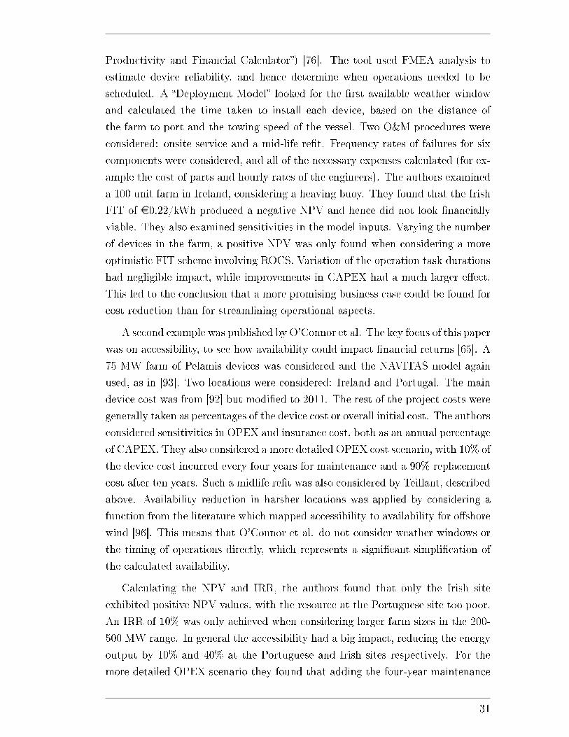
Productivity and Financial Calculator�) [76]. The tool used FMEA analysis to

estimate device reliability, and hence determine when operations needed to be

scheduled. A �Deployment Model� looked for the �rst available weather window

and calculated the time taken to install each device, based on the distance of

the farm to port and the towing speed of the vessel. Two O&M procedures were

considered: onsite service and a mid-life re�t. Frequency rates of failures for six

components were considered, and all of the necessary expenses calculated (for ex-

ample the cost of parts and hourly rates of the engineers). The authors examined

a 100 unit farm in Ireland, considering a heaving buoy. They found that the Irish

FIT of e0.22/kWh produced a negative NPV and hence did not look �nancially

viable. They also examined sensitivities in the model inputs. Varying the number

of devices in the farm, a positive NPV was only found when considering a more

optimistic FIT scheme involving ROCS. Variation of the operation task durations

had negligible impact, while improvements in CAPEX had a much larger e�ect.

This led to the conclusion that a more promising business case could be found for

cost reduction than for streamlining operational aspects.

A second example was published by O'Connor et al. The key focus of this paper

was on accessibility, to see how availability could impact �nancial returns [65]. A

75 MW farm of Pelamis devices was considered and the NAVITAS model again

used, as in [93]. Two locations were considered: Ireland and Portugal. The main

device cost was from [92] but modi�ed to 2011. The rest of the project costs were

generally taken as percentages of the device cost or overall initial cost. The authors

considered sensitivities in OPEX and insurance cost, both as an annual percentage

of CAPEX. They also considered a more detailed OPEX cost scenario, with 10% of

the device cost incurred every four years for maintenance and a 90% replacement

cost after ten years. Such a midlife re�t was also considered by Teillant, described

above. Availability reduction in harsher locations was applied by considering a

function from the literature which mapped accessibility to availability for o�shore

wind [96]. This means that O'Connor et al. do not consider weather windows or

the timing of operations directly, which represents a signi�cant simpli�cation of

the calculated availability.

Calculating the NPV and IRR, the authors found that only the Irish site

exhibited positive NPV values, with the resource at the Portuguese site too poor.

An IRR of 10% was only achieved when considering larger farm sizes in the 200-

500 MW range. In general the accessibility had a big impact, reducing the energy

output by 10% and 40% at the Portuguese and Irish sites respectively. For the

more detailed OPEX scenario they found that adding the four-year maintenance

31

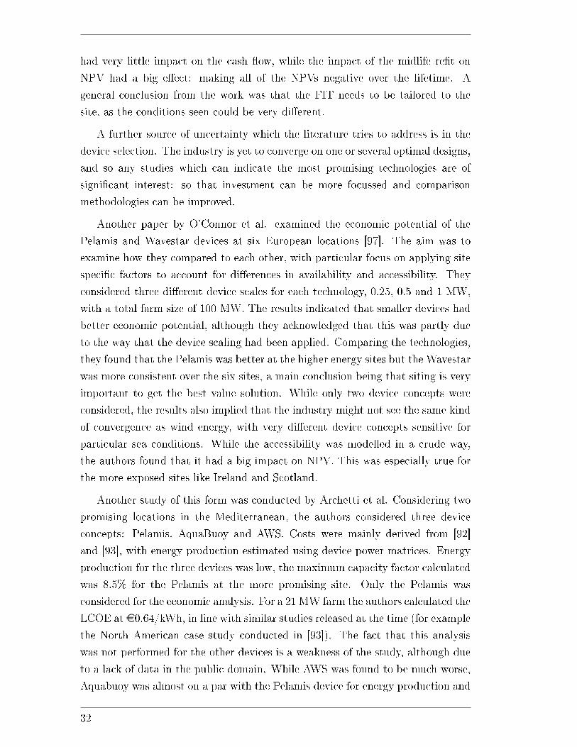
had very little impact on the cash �ow, while the impact of the midlife re�t on

NPV had a big e�ect: making all of the NPVs negative over the lifetime. A

general conclusion from the work was that the FIT needs to be tailored to the

site, as the conditions seen could be very di�erent.

A further source of uncertainty which the literature tries to address is in the

device selection. The industry is yet to converge on one or several optimal designs,

and so any studies which can indicate the most promising technologies are of

signi�cant interest: so that investment can be more focussed and comparison

methodologies can be improved.

Another paper by O'Connor et al. examined the economic potential of the

Pelamis and Wavestar devices at six European locations [97]. The aim was to

examine how they compared to each other, with particular focus on applying site

speci�c factors to account for di�erences in availability and accessibility. They

considered three di�erent device scales for each technology, 0.25, 0.5 and 1 MW,

with a total farm size of 100 MW. The results indicated that smaller devices had

better economic potential, although they acknowledged that this was partly due

to the way that the device scaling had been applied. Comparing the technologies,

they found that the Pelamis was better at the higher energy sites but the Wavestar

was more consistent over the six sites, a main conclusion being that siting is very

important to get the best value solution. While only two device concepts were

considered, the results also implied that the industry might not see the same kind

of convergence as wind energy, with very di�erent device concepts sensitive for

particular sea conditions. While the accessibility was modelled in a crude way,

the authors found that it had a big impact on NPV. This was especially true for

the more exposed sites like Ireland and Scotland.

Another study of this form was conducted by Archetti et al. Considering two

promising locations in the Mediterranean, the authors considered three device

concepts: Pelamis, AquaBuoy and AWS. Costs were mainly derived from [92]

and [93], with energy production estimated using device power matrices. Energy

production for the three devices was low, the maximum capacity factor calculated

was 8.5% for the Pelamis at the more promising site. Only the Pelamis was

considered for the economic analysis. For a 21 MW farm the authors calculated the

LCOE at e0.64/kWh, in line with similar studies released at the time (for example

the North American case study conducted in [93]). The fact that this analysis

was not performed for the other devices is a weakness of the study, although due

to a lack of data in the public domain. While AWS was found to be much worse,

Aquabuoy was almost on a par with the Pelamis device for energy production and

32

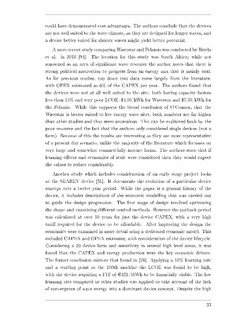
could have demonstrated cost advantages. The authors conclude that the devices

are not well suited to the wave climate, as they are designed for longer waves, and

a device better suited for shorter waves might yield better potential.

A more recent study comparingWavestar and Pelamis was conducted by Biyela

et al. in 2016 [94]. The location for this study was South Africa; while not

renowned as an area of signi�cant wave resource the author notes that there is

strong political motivation to progress from an energy mix that is mainly coal.

As for previous studies, top down cost data come largely from the literature,

with OPEX estimated as 6% of the CAPEX per year. The authors found that

the devices were not at all well suited to the site: both having capacity factors

less than 15% and very poor LCOE, $4.50/kWh for Wavestar and $7.50/kWh for

the Pelamis. While this supports the broad conclusion of O'Connor, that the

Wavestar is better suited to low energy wave sites, both numbers are far higher

than other studies and thus seem anomalous. This can be explained both by the

poor resource and the fact that the authors only considered single devices (not a

farm). Because of this the results are interesting as they are more representative

of a present day scenario, unlike the majority of the literature which focusses on

very large and somewhat commercially mature farms. The authors state that if

learning e�ects and economies of scale were considered then they would expect

the values to reduce considerably.

Another study which includes consideration of an early stage project looks

at the SEAREV device [31]. It documents the evolution of a particular device

concept over a twelve year period. While the paper is a general history of the

device, it includes descriptions of the economic modelling that was carried out

to guide the design progression. The �rst stage of design involved optimising

the shape and examining di�erent control methods. However the payback period

was calculated at over 50 years for just the device CAPEX, with a very high

tari� required for the device to be a�ordable. After improving the design the

economics were examined in more detail using a dedicated economic model. This

included CAPEX and OPEX estimates, with consideration of the device lifecycle.

Considering a 20 device farm and sensitivity in several high level areas, it was

found that the CAPEX and energy production were the key economic drivers.

The former conclusion mirrors that found in [76]. Applying a 10% learning rate

and a starting point at the 100th machine the LCOE was found to be high,

with the device requiring a FIT of e421/MWh to be �nancially viable. The low

learning rate compared to other studies was applied to take account of the lack

of convergence of wave energy into a dominant device concept. Despite the high

33

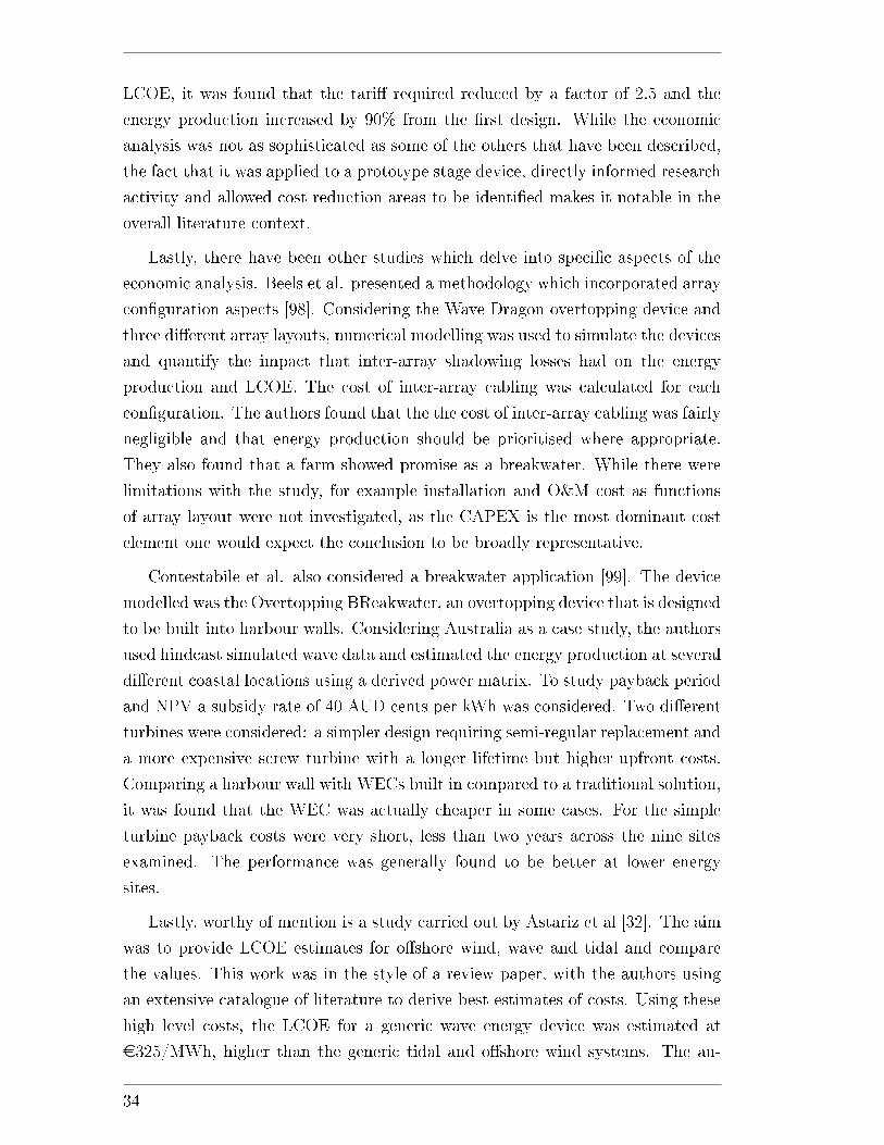
LCOE, it was found that the tari� required reduced by a factor of 2.5 and the

energy production increased by 90% from the �rst design. While the economic

analysis was not as sophisticated as some of the others that have been described,

the fact that it was applied to a prototype stage device, directly informed research

activity and allowed cost reduction areas to be identi�ed makes it notable in the

overall literature context.

Lastly, there have been other studies which delve into speci�c aspects of the

economic analysis. Beels et al. presented a methodology which incorporated array

con�guration aspects [98]. Considering the Wave Dragon overtopping device and

three di�erent array layouts, numerical modelling was used to simulate the devices

and quantify the impact that inter-array shadowing losses had on the energy

production and LCOE. The cost of inter-array cabling was calculated for each

con�guration. The authors found that the the cost of inter-array cabling was fairly

negligible and that energy production should be prioritised where appropriate.

They also found that a farm showed promise as a breakwater. While there were

limitations with the study, for example installation and O&M cost as functions

of array layout were not investigated, as the CAPEX is the most dominant cost

element one would expect the conclusion to be broadly representative.

Contestabile et al. also considered a breakwater application [99]. The device

modelled was the Overtopping BReakwater, an overtopping device that is designed

to be built into harbour walls. Considering Australia as a case study, the authors

used hindcast simulated wave data and estimated the energy production at several

di�erent coastal locations using a derived power matrix. To study payback period

and NPV a subsidy rate of 40 AUD cents per kWh was considered. Two di�erent

turbines were considered: a simpler design requiring semi-regular replacement and

a more expensive screw turbine with a longer lifetime but higher upfront costs.

Comparing a harbour wall with WECs built in compared to a traditional solution,

it was found that the WEC was actually cheaper in some cases. For the simple

turbine payback costs were very short, less than two years across the nine sites

examined. The performance was generally found to be better at lower energy

sites.

Lastly, worthy of mention is a study carried out by Astariz et al [32]. The aim

was to provide LCOE estimates for o�shore wind, wave and tidal and compare

the values. This work was in the style of a review paper, with the authors using

an extensive catalogue of literature to derive best estimates of costs. Using these

high level costs, the LCOE for a generic wave energy device was estimated at

e325/MWh, higher than the generic tidal and o�shore wind systems. The au-

34

thors quoted that 20-50% capacity factors are used in the literature, however it

was not explicitly stated which was chosen to get to the LCOE. As the LCOE is

very sensitive to the energy, and will be highly site speci�c, the value chosen would

have been of interest. Additionally, due to the large number of di�erent device

concepts available, the notion of a generic device has limited usefulness. The au-

thors also discuss the impact of externalities on LCOE. These are socio-economic

factors which have an indirect impact on the cost of energy. Examples include job

creation, security of supply and CO2 emissions. Including these factors made the

wave energy system much more competitive, halving the LCOE di�erence with

conventional forms of energy generation. The authors also advocated combined

wind and wave systems as a way to reduce the costs of both systems, by sharing

project infrastructure.

2.4.1.1 Alternative methodologies

One of the main disadvantages of conventional economic analyses like LCOE

or NPV are the amounts of input data required in order to formulate an accu-

rate representation. To mitigate this problem there have been several studies

published which propose alternative methodologies. While these can have advan-

tages, for example being faster to compute or reducing bias [33], they are generally

considered to be inferior as they include higher uncertainty.

An older example, published in 2004 by Stallard et al., studied a selection of

point absorber concepts with the aim of investigating how the energy production

and cost of energy varied at eight di�erent UK locations [33]. A data envelopment

analysis (DEA) was used, a technique that allowed di�erent design decisions to

be analysed with the aim of maximising energy output (or �technical e�cacy�)

by minimising a selection of inputs. The advantage of this method is that it

is not sensitive to the input units and allows both physical (e.g. installation

time) and non-physical parameters (e.g. jobs created) to be incorporated. The

authors considered four di�erent types of point absorbers, de�ned by their control

system. One was based on the Waveswing device and used a real power matrix.

Considering seven weighted independent inputs, including the quantity of devices,

inter-array cable length and device failure probability, the DEA method aimed to

minimise them while maximising energy outputs for each device. The results

were ranked, to get to 100MW of rated capacity while minimising maintenance

expense. The results found that the unrealistic, ideal point absorber was the

only one to reach the required technical e�ciency. The passive and tuned devices

performed better at medium energy than the maximum energy sites, indicating

35

the location speci�c nature of the technology. Di�erent sensitivities, e.g. O&M

and transmission cost, had the e�ect of improving the outlook at di�erent sites.

This was particularly apparent for lower energy site, where the technical e�cacy

saw marked improvement when O&M was considered.

An advantage of the method is that it is independent of �expert costs�, useful

when wanting an unbiased outlook. However, when costs are well known and un-

derstood, it adds another layer of complexity and hence has not seen widespread

usage in the literature. While the author considers relatively simple input vari-

ables, the method is more di�cult to scale to large problems with many variables

to be incorporated.

There have also been studies which aim to indirectly estimate LCOE by us-

ing simpli�ed methods. One of these, published by Okamoto et al., attempted

to create an index to estimate LCOE from WEC design parameters [100]. The

motivation for the methodology came from a need to quickly assess di�erent sites

and device options in order to predict combinations with the best economic poten-

tial. A generic heaving buoy device is considered with a power matrix obtained

from frequency domain simulations. The device width and generator capacity

were incrementally varied, both with energy and cost implications, and an index

created taking both factors into account. This was then compared to the LCOE,

calculated using a more traditional method. They found that the index better

matched the LCOE for lower energy sites and smaller farms, with the index not

properly scaling for larger farm sizes. While broadly similar trends were seen, the

index lacked the resolution of the traditional LCOE method.

Two further studies which have discussed using alternative metrics to estimate

LCOE are [101] and [102]. The former created numerical models of eight di�erent

wave converter concepts and examined three design metrics: the absorbed energy

per mass, per km2 of footprint and per root mean square of PTO force. The aim

was to see how these varied across the device classes; as all of the metrics relate

to physical parameters of the device they could be linked to cost. While full cost

analysis is not conducted, the resulted showed that there was surprisingly little

variation between the devices. This was despite the fact that the absorbed energy

saw a high variation. This provided a typical target metric that an early TRL

level device should be aiming for, however the low variation also implied that such

a metric is not well suited for estimating economic potential.

The second study presented a methodology to optimise sizing of a WEC, con-

sidering both LCOE and other metrics. A point absorber was considered, the

36

technology being developed by CorPower. From an initial power matrix, power

matrices for several di�erent sizes of devices were obtained, from 25 kW to 2 MW,

by using Froude scaling (similar to [97]). Costs were also scaled depending on the

nature of the subsystem. Five sites across Europe were considered, with costs ob-

tained from correspondence with CorPower and other economic parameters chosen

according to the literature. Two di�erent O&M schemes were considered: high

level based on a percentage of CAPEX and a more detailed estimate based on the

life cycle of the device. This latter strategy included one major repair every two

years. The authors discovered that the annual energy production was higher for

smaller devices, a similar result to [97] and due to the way the power matrix scal-

ing was performed. Due to learning discount applied to multiple devices, the best

LCOE was found for the smallest size of device when considering the simpli�ed

O&M. Considering the more detailed O&M strategy, which scaled the O&M more

accurately with increasing device quantity at lower ratings, the authors found that

the larger devices were better. However this considered the same size vessel for

all device scales, in reality larger vessels would be required for the larger devices

which would incur greater cost. Accessibility and weather windows were also not

considered.

The authors also examined the CorPower device with respect to the metrics

that were detailed in [101], including discussion on how closely they followed the

trends in LCOE. While the trend with LCOE for most of them was unclear, the

Average Climate Capture Width per Characteristic Capital Expenditure (ACE)

metric as advocated by the Wave Energy Prize showed the most promise as it

had a clear functional form for the technology over all �ve sites. Despite this,

no analysis was conducted considering other devices. As the purpose of such a

metric is for early TRL level, comparison how it fares across devices is crucial and

unclear.

In a di�erent study, de Andres et al. considered a reversed LCOE calculation

[29]. This method starts with a target LCOE. The energy and cost components

that are required to get to the LCOE can then be derived. The bene�t of the

method is that it gives the technology developer an idea of the costs that they

should be targeting to reach the LCOE, hence allowing research activity and

relevant supply chain aspects to be focussed on. The authors considered �ve

types of devices and a target LCOE of 15 p/kWh, as identi�ed in the literature.

From a target array capacity, an AEP was calculated for a farm. The costs were

then derived in order to get to the LCOE, calculated considering typical cost

breakdowns as seen in the literature. Categories with higher costs were considered

37

more restrictive, with less �exibility to get to the LCOE. Comparing with o�shore

wind, the authors found that the wave devices showed much greater variation in

CAPEX, supporting the notion that the technology is in a less mature stage and

yet to converge on a concept. Comparing the cost categories it was found that,

while some costs were not too far away from �oating o�shore wind expectations

(for example the mooring system), the majority of categories were far away from

the trends seen in o�shore wind. This was partly driven by the relatively high

OPEX calculated. While the overall method is interesting, it is really only useful

to technology developers. Moreover, the cost breakdowns seen in the future would

vary signi�cantly between device concepts and are not necessarily relevant to the

devices in the present, which are largely in the prototype stage.

2.4.2 Spatial economic analysis

What the studies from Section 2.4.1 have in common is that they all only

consider a single or a small selection of locations to conduct the analyses. While

this is suitable for getting a general feel of the economic potential, it is not so useful

to a developer as metocean conditions can show large variation over relatively

small areas. Additionally there will be a balance between energy and cost which

is not so apparent when only considering single locations at a time. For example

locations further from shore will typically be in more exposed locations, bene�ting

from higher energy waves which can improve yield. However this also means that

accessing the devices for maintenance will be more di�cult, increasing downtime

and OPEX. It also means that transmission costs will be higher, as a longer export

cable is required. Analysing multiple locations at a time means that it is easier

to identify any sweet spots that arise because of speci�cs of the WEC design.

While spatial analysis methods do have limitations, requiring large amount

of data and relying on spatial approximations that may not always hold in re-

ality, they are very useful for initial site screening. As all devices will be better

suited for some locations than others, the ability to perform economic evaluations

over multiple locations allows the best sites for the technology to be determined.

These will not necessarily be in the highest energy locations [45, 99]. For exam-

ple, for early stage devices this might involve leaving the most promising sites

for future, more technically advanced devices that can fully utilise the economic

potential [33]. This methodology could be advantageous to developers, investors

and policymakers, and as a result has garnered interest in the literature.

38

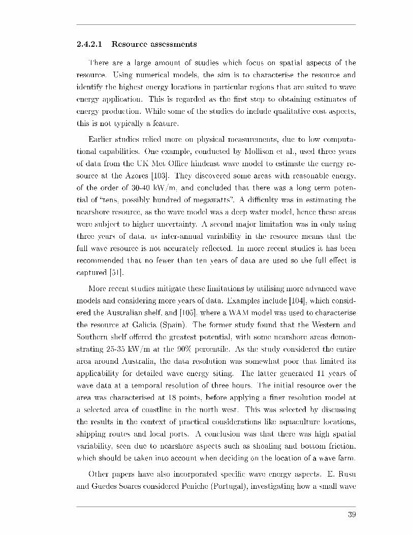
2.4.2.1 Resource assessments

There are a large amount of studies which focus on spatial aspects of the

resource. Using numerical models, the aim is to characterise the resource and

identify the highest energy locations in particular regions that are suited to wave

energy application. This is regarded as the �rst step to obtaining estimates of

energy production. While some of the studies do include qualitative cost aspects,

this is not typically a feature.

Earlier studies relied more on physical measurements, due to low computa-

tional capabilities. One example, conducted by Mollison et al., used three years

of data from the UK Met O�ce hindcast wave model to estimate the energy re-

source at the Azores [103]. They discovered some areas with reasonable energy,

of the order of 30-40 kW/m, and concluded that there was a long term poten-

tial of �tens, possibly hundred of megawatts�. A di�culty was in estimating the

nearshore resource, as the wave model was a deep water model, hence these areas

were subject to higher uncertainty. A second major limitation was in only using

three years of data, as inter-annual variability in the resource means that the

full wave resource is not accurately re�ected. In more recent studies it has been

recommended that no fewer than ten years of data are used so the full e�ect is

captured [51].

More recent studies mitigate these limitations by utilising more advanced wave

models and considering more years of data. Examples include [104], which consid-

ered the Australian shelf, and [105], where a WAM model was used to characterise

the resource at Galicia (Spain). The former study found that the Western and

Southern shelf o�ered the greatest potential, with some nearshore areas demon-

strating 25-35 kW/m at the 90% percentile. As the study considered the entire

area around Australia, the data resolution was somewhat poor that limited its

applicability for detailed wave energy siting. The latter generated 11 years of

wave data at a temporal resolution of three hours. The initial resource over the

area was characterised at 18 points, before applying a �ner resolution model at

a selected area of coastline in the north west. This was selected by discussing

the results in the context of practical considerations like aquaculture locations,

shipping routes and local ports. A conclusion was that there was high spatial

variability, seen due to nearshore aspects such as shoaling and bottom friction,

which should be taken into account when deciding on the location of a wave farm.

Other papers have also incorporated speci�c wave energy aspects. E. Rusu

and Guedes Soares considered Peniche (Portugal), investigating how a small wave

39

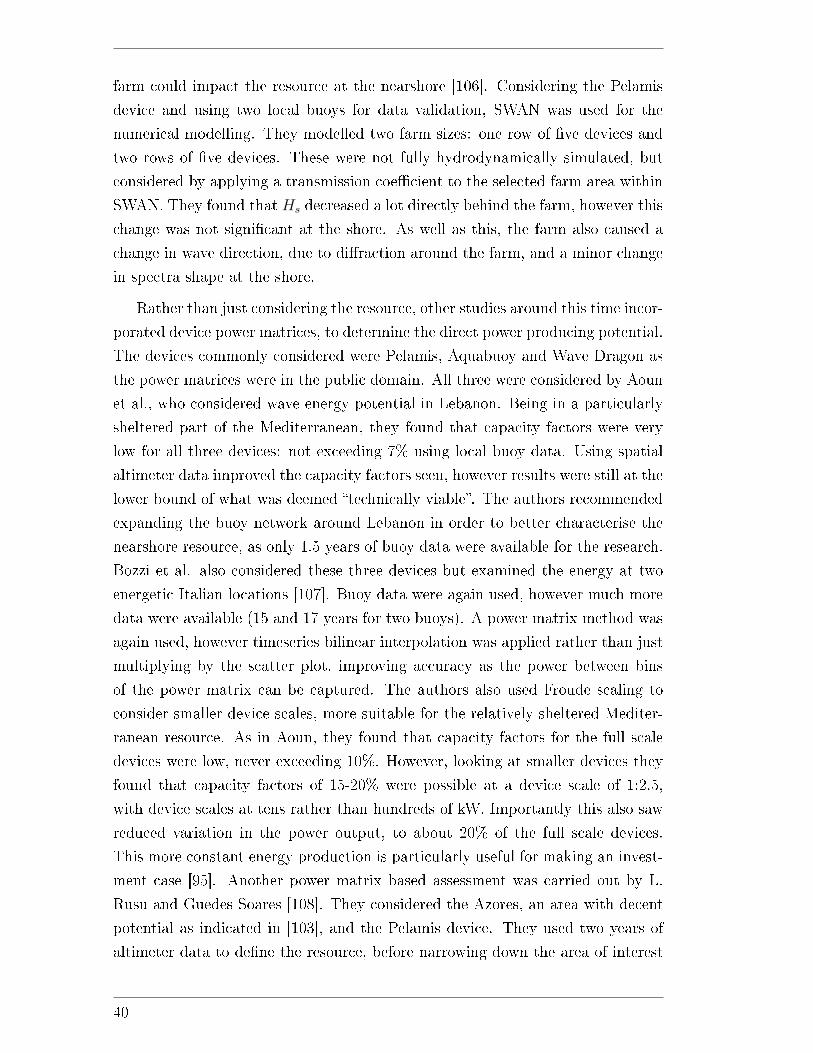
farm could impact the resource at the nearshore [106]. Considering the Pelamis

device and using two local buoys for data validation, SWAN was used for the

numerical modelling. They modelled two farm sizes: one row of �ve devices and

two rows of �ve devices. These were not fully hydrodynamically simulated, but

considered by applying a transmission coe�cient to the selected farm area within

SWAN. They found that Hs decreased a lot directly behind the farm, however this

change was not signi�cant at the shore. As well as this, the farm also caused a

change in wave direction, due to di�raction around the farm, and a minor change

in spectra shape at the shore.

Rather than just considering the resource, other studies around this time incor-

porated device power matrices, to determine the direct power producing potential.

The devices commonly considered were Pelamis, Aquabuoy and Wave Dragon as

the power matrices were in the public domain. All three were considered by Aoun

et al., who considered wave energy potential in Lebanon. Being in a particularly

sheltered part of the Mediterranean, they found that capacity factors were very

low for all three devices: not exceeding 7% using local buoy data. Using spatial

altimeter data improved the capacity factors seen, however results were still at the

lower bound of what was deemed �technically viable�. The authors recommended

expanding the buoy network around Lebanon in order to better characterise the

nearshore resource, as only 1.5 years of buoy data were available for the research.

Bozzi et al. also considered these three devices but examined the energy at two

energetic Italian locations [107]. Buoy data were again used, however much more

data were available (15 and 17 years for two buoys). A power matrix method was

again used, however timeseries bilinear interpolation was applied rather than just

multiplying by the scatter plot, improving accuracy as the power between bins

of the power matrix can be captured. The authors also used Froude scaling to

consider smaller device scales, more suitable for the relatively sheltered Mediter-

ranean resource. As in Aoun, they found that capacity factors for the full scale

devices were low, never exceeding 10%. However, looking at smaller devices they

found that capacity factors of 15-20% were possible at a device scale of 1:2.5,

with device scales at tens rather than hundreds of kW. Importantly this also saw

reduced variation in the power output, to about 20% of the full scale devices.

This more constant energy production is particularly useful for making an invest-

ment case [95]. Another power matrix based assessment was carried out by L.

Rusu and Guedes Soares [108]. They considered the Azores, an area with decent

potential as indicated in [103], and the Pelamis device. They used two years of

altimeter data to de�ne the resource, before narrowing down the area of interest

40

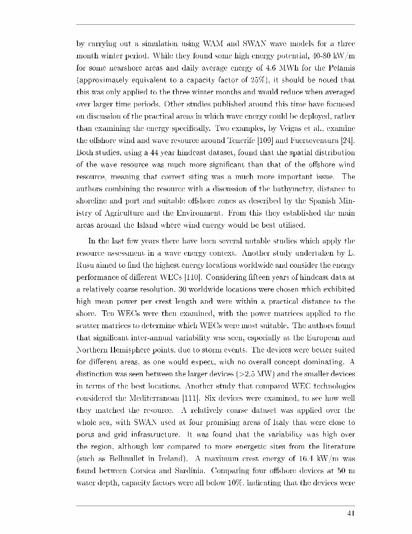
by carrying out a simulation using WAM and SWAN wave models for a three

month winter period. While they found some high energy potential, 40-80 kW/m

for some nearshore areas and daily average energy of 4.6 MWh for the Pelamis

(approximately equivalent to a capacity factor of 25%), it should be noted that

this was only applied to the three winter months and would reduce when averaged

over larger time periods. Other studies published around this time have focussed

on discussion of the practical areas in which wave energy could be deployed, rather

than examining the energy speci�cally. Two examples, by Veigas et al., examine

the o�shore wind and wave resource around Tenerife [109] and Fuerteventura [24].

Both studies, using a 44 year hindcast dataset, found that the spatial distribution

of the wave resource was much more signi�cant than that of the o�shore wind

resource, meaning that correct siting was a much more important issue. The

authors combining the resource with a discussion of the bathymetry, distance to

shoreline and port and suitable o�shore zones as described by the Spanish Min-

istry of Agriculture and the Environment. From this they established the main

areas around the Island where wind energy would be best utilised.

In the last few years there have been several notable studies which apply the

resource assessment in a wave energy context. Another study undertaken by L.

Rusu aimed to �nd the highest energy locations worldwide and consider the energy

performance of di�erent WECs [110]. Considering �fteen years of hindcast data at

a relatively coarse resolution, 30 worldwide locations were chosen which exhibited

high mean power per crest length and were within a practical distance to the

shore. Ten WECs were then examined, with the power matrices applied to the

scatter matrices to determine which WECs were most suitable. The authors found

that signi�cant inter-annual variability was seen, especially at the European and

Northern Hemisphere points, due to storm events. The devices were better suited

for di�erent areas, as one would expect, with no overall concept dominating. A

distinction was seen between the larger devices (>2.5 MW) and the smaller devices

in terms of the best locations. Another study that compared WEC technologies

considered the Mediterranean [111]. Six devices were examined, to see how well

they matched the resource. A relatively coarse dataset was applied over the

whole sea, with SWAN used at four promising areas of Italy that were close to

ports and grid infrastructure. It was found that the variability was high over

the region, although low compared to more energetic sites from the literature

(such as Bellmullet in Ireland). A maximum crest energy of 16.4 kW/m was

found between Corsica and Sardinia. Comparing four o�shore devices at 50 m

water depth, capacity factors were all below 10%, indicating that the devices were

41

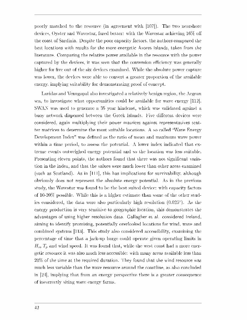
poorly matched to the resource (in agreement with [107]). The two nearshore

devices, Oyster and Wavestar, fared better: with the Wavestar achieving 16% o�

the coast of Sardinia. Despite the poor capacity factors, the authors compared the

best locations with results for the more energetic Azores Islands, taken from the

literature. Comparing the relative power available in the resource with the power

captured by the devices, it was seen that the conversion e�ciency was generally

higher for �ve out of the six devices examined. While the absolute power capture

was lower, the devices were able to convert a greater proportion of the available

energy, implying suitability for demonstrating proof of concept.

Lavidas and Venugopal also investigated a relatively benign region, the Aegean

sea, to investigate what opportunities could be available for wave energy [112].

SWAN was used to generate a 35 year hindcast, which was validated against a

buoy network dispersed between the Greek Islands. Five di�erent devices were

considered, again multiplying their power matrices against representatives scat-

ter matrices to determine the most suitable locations. A so called �Wave Energy

Development Index� was de�ned as the ratio of mean and maximum wave power

within a time period, to assess the potential. A lower index indicated that ex-

treme events outweighed energy potential and so the location was less suitable.

Presenting eleven points, the authors found that there was not signi�cant varia-

tion in the index, and that the values were much lower than other areas examined

(such as Scotland). As in [111], this has implications for survivability, although

obviously does not represent the absolute energy potential. As in the previous

study, the Wavestar was found to be the best suited device: with capacity factors

of 10-20% possible. While this is a higher estimate than some of the other stud-

ies considered, the data were also particularly high resolution (0.025◦). As the

energy production is very sensitive to geographic location, this demonstrates the

advantages of using higher resolution data. Gallagher et al. considered Ireland,

aiming to identify promising, potentially overlooked locations for wind, wave and

combined systems [113]. This study also considered accessibility, examining the

percentage of time that a jack-up barge could operate given operating limits in

Hs, Tp and wind speed. It was found that, while the west coast had a more ener-

getic resource it was also much less accessible: with many areas available less than

20% of the time at the required duration. They found that the wind resource was

much less variable than the wave resource around the coastline, as also concluded

in [24], implying that from an energy perspective there is a greater consequence

of incorrectly siting wave energy farms.

42

2.4.2.2 Multi-criteria studies

Multi-criteria analyses can be thought of as the next step on from resource

assessments as they combine the wider technical, economic and social aspects. The

methods are used to aid decision making, by maximising bene�ts and minimising

costs of a technology to arrive at an optimal solution for the issue being examined

[114]. This involves a scoring methodology: weighting and ranking the relevant

aspects which are then combined into a �nal metric. As the literature is extensive,

this section focusses on studies that are directly concerned with wave energy. As

siting is such a key issue, as demonstrated in Section 2.4.2.1, typically the analyses

are conducted using GIS software and incorporate geospatial aspects.

As the ranking aspect is arbitrary in nature, attempting to quantify factors

which are usually more qualitative in nature, caution must be exercised in the

results [115]. This is especially the case with wave energy, where there are still

signi�cant unknowns. To attempt to mitigate these e�ects the scoring is usually

conducted through collaborating with experts in the industry (e.g. [115�117]) and

sensitivity analysis of the scoring is carried out (e.g. [117�119]).

In the wave energy context, there are two general stages that are carried out

for the analysis:

1. Exclude any areas where deployment of wave energy is not deemed possible,

for example due to very low energy or overlap with heavily used sea areas.

2. Rank any issues that are more subjective in nature (for example distance to

ports or grid infrastructure) and combine these to arrive at an overall index.

The way that the spatial factor are ranked and combined depends on the

method chosen, descriptions of these can be found in [114] and [120]. One of

the more common methods is the weighted sum method (WSM). This involves

combining each individual judging criteria with an arbitrary weighting factor and

summing the contributions. The �nal criteria is typically normalised to a value

between 0 and 1. Because of the simplicity it has been considered several times

in the literature.

Galparsoro et al. considered the Basque continental shelf [121]. They exam-

ined seventeen criteria, covering commonly considered aspects like water depth

and distance to port and lesser known e�ects like sediment transport and bathing

zones. A very high resolution grid of 20 m was considered for the criteria, with

coarser layers re-sampled to match the resolution (for example the energy re-

source). Some exclusion zones were applied, for example covering 500 m around

43

harbours to allow access. The results found that one particular stretch exhibited

strong potential. Higher indices were generally in shallower waters and were found

not to greatly coincide with environmental protection areas. However the authors

do note the limitations in the method, particularly regarding aspects like �shing

and recreational use of the sea where data are limited.

A paper published by the Bureau of Ocean Energy Management (BOEM),

based in the USA, applied WSM to the coastline of Oregon [116]. Eight di�erent

criteria were selected, including the energy in the resource, distance to port, seabed

geology, water depth and distance to grid infrastructure; these were weighted

through engagement with 21 wave energy stakeholders. Three di�erent WEC

classes were considered: nearshore, mid and o�shore devices. The only di�erence

between these was the water depth constraint considered, a large simpli�cation

being that the WEC energy was characterised by the resource energy rather than

device power production estimates. The results found that a very small number

of sites, less than 1%, were suitable for the nearshore technology, driven by the

poor resource. A more recent study by Flocard et al. performed a WSM analysis

considering the south Australian coast [117]. This was more detailed than the

BOEM study, with eighteen criteria incorporated. This included all of those from

the BOEM study, as well as extreme wave conditions, protected environmental

areas, �sheries and areas for military activity. Sites deemed unfeasible, with

average Hs less than 1 m, were �ltered out of the analysis before performing

the multi criteria aggregation. Using a high resolution SWAN model to create

the metocean data, the authors found a best resource of about 30 kW/m at the

100 m depth contour, in agreement with other studies (e.g. [104]). Applying the

di�erent criteria, the best area was determined to be South of Portland. Minimal

variation for this area was found when applying sensitivity analysis to the criteria

weightings, indicating the resilience of the method. As in the BOEM study,

the WEC power production was not directly incorporated, and criteria such as

extreme wave height and seabed geology would be very device speci�c and so

might have the adverse e�ect of driving attention away from areas suitable for

speci�c device concepts.

Another recent paper, by Cradden et al., considered a large area of encom-

passing most of Northern Europe [122]. They examined two combined wind and

wave platforms, using a GIS focussed approach which included development of

a tool as part of the EU funded MARINA Platform project. For the resource

data, ten years of hindcast data were used at a 0.05◦ spatial resolution. Plug-in

tools were created for QGIS software which included a GUI (Graphical User In-

44

terface) and PostgresSQL database to store the data layers. Exclusions included

wind speed, MPAs and a relatively high energy density of 20-30 kW, depending

on the platform. Unlike other studies an exclusion was also applied to depth for

cable installation; 250 m was applied although it was indicated that 100 m was

more commonly considered by industry. The results found that the North West

of Europe looked particularly promising, especially Scotland and Ireland. This

was largely based on the energy, suitable water depth and distances to port. Five

points were examined in more detail, considering speci�c ports and weather win-

dows to the sites. The accessibility was not considered over the full domain, which

would have a great impact at many of the more exposed locations [113].

Two �nal studies that presented more limited WSM methodologies were [123],

which introduced the methodology for a region in the South of France and [124]

who considered Morocco. The former considered very similar criteria to BOEM,

while also considering several exclusion criteria. Considering o�shore devices,

some of the best areas were found relatively far from the coast, at 50 km and

greater. As costs would be high at these relatively large distances, it indicates

that the results are potentially biased towards energy production and do not re�ect

the economic picture. The main focus of the latter study is in resource assessment.

A 44 year hindcast was used, created using a WAM model, at a relatively coarse

spatial resolution of 0.25 degrees. Along the Atlantic facing coast, the 23 nearest

points to shore were considered for the analysis (varying between �ve and 52 km

from shore). Relatively high resource was seen over the central stretch of coastline

of 25-30 kW/m. Only �ve criteria were considered for the multi criteria analysis

including water depth, distance to shore and resource energy as seen previously.

Unlike previous studies, they considered power output from two WECs, the Wave

Dragon and Pelamis, which were obtained from the power matrices. Despite only

considering two physical criteria to represent the site, it was enough to rule out

the most promising energy producing site which was located at a very large 500

m water depth.

Another common multi-criteria approach is Analytical Hierarchy Process

(AHP). The weightings of n di�erent criteria are considered in a pairwise manner,

de�ned by a n by n square matrix [114,125]. A matrix of normalised weightings is

calculated by dividing each matrix element by its column sum, the relative weight-

ings for each criteria then derived by computing the average for each row [119].

The method can be assessed by computing an �inconsistency index�, a key ad-

vantage of the method as it allows the robustness of the pairwise values to be

judged [114].

45

Vasilou et al. applied the AHP method to combined wave and wind sys-

tems in the Aegean sea, to determine the most suitable locations [119]. The

method was implemented in GIS, and made use of a GIS database. Areas ex-

cluded from the analysis included those designated for military exercise areas, oil

and gas exploration, areas already designated for o�shore renewables and marine

protected areas. In the case of the latter, the authors assumed that any areas

within Natura2000 sites were unfeasible. Additionally, areas with wave resource

below 5 kW/m were excluded, a lower threshold than that considered in [122].

Eight criteria were chosen for the AHP analysis, covering the main aspects with

the exception of actual device power (as also seen in previous studies). Twelve

suitable areas were identi�ed and examined with AHP, with the waters to the east

of Crete found to be particularly suitable. Sensitivity in the weighting parameters

was examined, with the authors �nding that, while the suitability values for the

sites changes, the order did not. However the new values were not included, so it

is unclear the extent to which they were actually varied.

Two further studies using AHP for spatial assessment are [125] and [115].

The former considered Tasmania, combining AHP with the Technique for Order

Preference by Similarity to Ideal Solution (TOPSIS) method, which de�nes the

best solution as that which is furthest from the ideal negative solution and closest

to the ideal positive solution [114]. Ten factors were chosen for the analysis, areas

that were �ltered out included those which coincided with aquaculture areas and

commercial shipping areas. The south coast was generally deemed to be the

most suitable location, however the results were somewhat sensitive depending on

whether the ocean features (e.g. energy and bathymetry) or marine user features

were selected as dominant. The second study was applied at two selected points,

one in the UK and one in Jamaica, rather than over a domain using GIS. An

arti�cial neural network was used to assess and predict the relationships between

the input criteria and the output suitability index, to identify the key drivers.

Ten input criteria were considered, with the most important found to be the

wind speed and site characteristics. Interestingly wave energy was not directly

considered, as in the majority of previous studies: instead the wave height and

distances between waves were considered which makes the results less clear in

an energy context. The shipping density and water depth were two relatively

insigni�cant factors, the latter also at odds with other studies where this is given

higher weighting (for example it was the third highest factor in [119] and had a

big in�uence in [124]).

Lastly, there have been other studies which have applied the methodology in

46

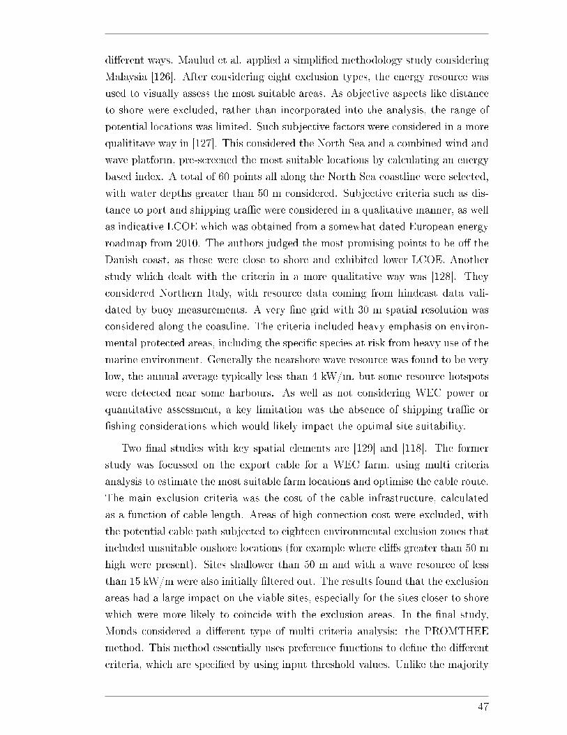
di�erent ways. Maulud et al. applied a simpli�ed methodology study considering

Malaysia [126]. After considering eight exclusion types, the energy resource was

used to visually assess the most suitable areas. As objective aspects like distance

to shore were excluded, rather than incorporated into the analysis, the range of

potential locations was limited. Such subjective factors were considered in a more

qualititave way in [127]. This considered the North Sea and a combined wind and

wave platform, pre-screened the most suitable locations by calculating an energy

based index. A total of 60 points all along the North Sea coastline were selected,

with water depths greater than 50 m considered. Subjective criteria such as dis-

tance to port and shipping tra�c were considered in a qualitative manner, as well

as indicative LCOE which was obtained from a somewhat dated European energy

roadmap from 2010. The authors judged the most promising points to be o� the

Danish coast, as these were close to shore and exhibited lower LCOE. Another

study which dealt with the criteria in a more qualitative way was [128]. They

considered Northern Italy, with resource data coming from hindcast data vali-

dated by buoy measurements. A very �ne grid with 30 m spatial resolution was

considered along the coastline. The criteria included heavy emphasis on environ-

mental protected areas, including the speci�c species at risk from heavy use of the

marine environment. Generally the nearshore wave resource was found to be very

low, the annual average typically less than 4 kW/m, but some resource hotspots

were detected near some harbours. As well as not considering WEC power or

quantitative assessment, a key limitation was the absence of shipping tra�c or

�shing considerations which would likely impact the optimal site suitability.

Two �nal studies with key spatial elements are [129] and [118]. The former

study was focussed on the export cable for a WEC farm, using multi criteria

analysis to estimate the most suitable farm locations and optimise the cable route.

The main exclusion criteria was the cost of the cable infrastructure, calculated

as a function of cable length. Areas of high connection cost were excluded, with

the potential cable path subjected to eighteen environmental exclusion zones that

included unsuitable onshore locations (for example where cli�s greater than 50 m

high were present). Sites shallower than 50 m and with a wave resource of less

than 15 kW/m were also initially �ltered out. The results found that the exclusion

areas had a large impact on the viable sites, especially for the sites closer to shore

which were more likely to coincide with the exclusion areas. In the �nal study,

Monds considered a di�erent type of multi criteria analysis: the PROMTHEE

method. This method essentially uses preference functions to de�ne the di�erent

criteria, which are speci�ed by using input threshold values. Unlike the majority

47

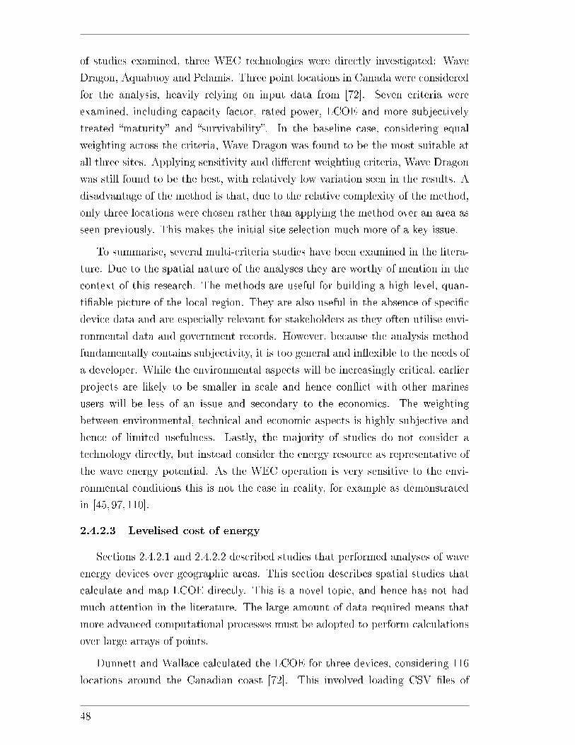
of studies examined, three WEC technologies were directly investigated: Wave

Dragon, Aquabuoy and Pelamis. Three point locations in Canada were considered

for the analysis, heavily relying on input data from [72]. Seven criteria were

examined, including capacity factor, rated power, LCOE and more subjectively

treated �maturity� and �survivability�. In the baseline case, considering equal

weighting across the criteria, Wave Dragon was found to be the most suitable at

all three sites. Applying sensitivity and di�erent weighting criteria, Wave Dragon

was still found to be the best, with relatively low variation seen in the results. A

disadvantage of the method is that, due to the relative complexity of the method,

only three locations were chosen rather than applying the method over an area as

seen previously. This makes the initial site selection much more of a key issue.

To summarise, several multi-criteria studies have been examined in the litera-

ture. Due to the spatial nature of the analyses they are worthy of mention in the

context of this research. The methods are useful for building a high level, quan-

ti�able picture of the local region. They are also useful in the absence of speci�c

device data and are especially relevant for stakeholders as they often utilise envi-

ronmental data and government records. However, because the analysis method

fundamentally contains subjectivity, it is too general and in�exible to the needs of

a developer. While the environmental aspects will be increasingly critical, earlier

projects are likely to be smaller in scale and hence con�ict with other marines

users will be less of an issue and secondary to the economics. The weighting

between environmental, technical and economic aspects is highly subjective and

hence of limited usefulness. Lastly, the majority of studies do not consider a

technology directly, but instead consider the energy resource as representative of

the wave energy potential. As the WEC operation is very sensitive to the envi-

ronmental conditions this is not the case in reality, for example as demonstrated

in [45,97,110].

2.4.2.3 Levelised cost of energy

Sections 2.4.2.1 and 2.4.2.2 described studies that performed analyses of wave

energy devices over geographic areas. This section describes spatial studies that

calculate and map LCOE directly. This is a novel topic, and hence has not had

much attention in the literature. The large amount of data required means that

more advanced computational processes must be adopted to perform calculations

over large arrays of points.

Dunnett and Wallace calculated the LCOE for three devices, considering 116

locations around the Canadian coast [72]. This involved loading CSV �les of

48

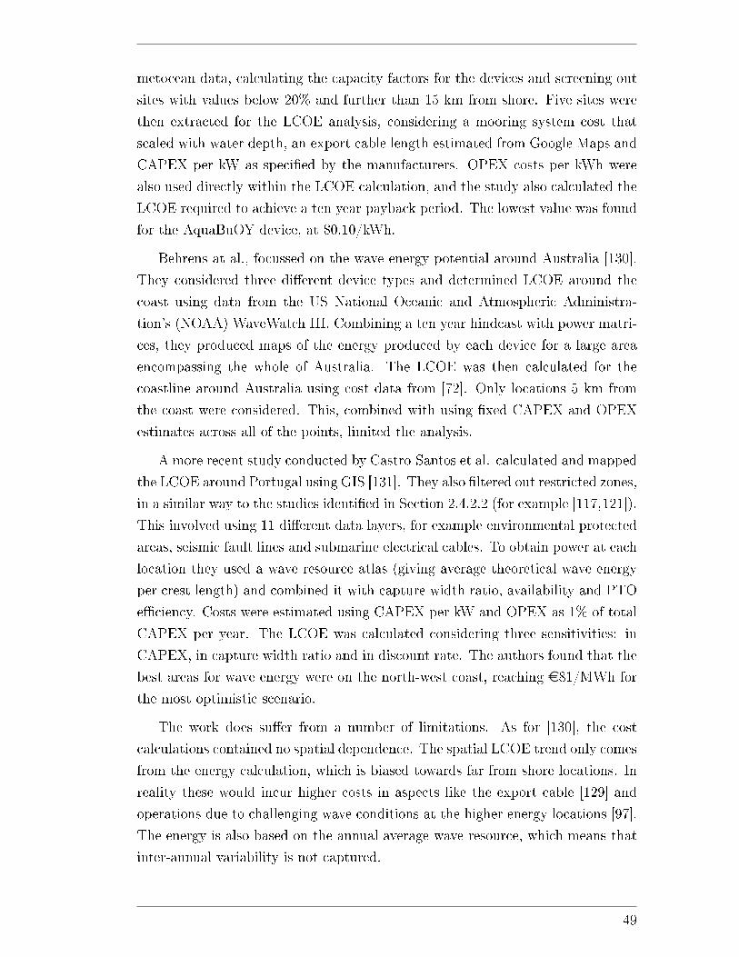
metocean data, calculating the capacity factors for the devices and screening out

sites with values below 20% and further than 15 km from shore. Five sites were

then extracted for the LCOE analysis, considering a mooring system cost that

scaled with water depth, an export cable length estimated from Google Maps and

CAPEX per kW as speci�ed by the manufacturers. OPEX costs per kWh were

also used directly within the LCOE calculation, and the study also calculated the

LCOE required to achieve a ten year payback period. The lowest value was found

for the AquaBuOY device, at $0.10/kWh.

Behrens at al., focussed on the wave energy potential around Australia [130].

They considered three di�erent device types and determined LCOE around the

coast using data from the US National Oceanic and Atmospheric Administra-

tion's (NOAA) WaveWatch III. Combining a ten year hindcast with power matri-

ces, they produced maps of the energy produced by each device for a large area

encompassing the whole of Australia. The LCOE was then calculated for the

coastline around Australia using cost data from [72]. Only locations 5 km from

the coast were considered. This, combined with using �xed CAPEX and OPEX

estimates across all of the points, limited the analysis.

A more recent study conducted by Castro-Santos et al. calculated and mapped

the LCOE around Portugal using GIS [131]. They also �ltered out restricted zones,

in a similar way to the studies identi�ed in Section 2.4.2.2 (for example [117,121]).

This involved using 11 di�erent data layers, for example environmental protected

areas, seismic fault lines and submarine electrical cables. To obtain power at each

location they used a wave resource atlas (giving average theoretical wave energy

per crest length) and combined it with capture width ratio, availability and PTO

e�ciency. Costs were estimated using CAPEX per kW and OPEX as 1% of total

CAPEX per year. The LCOE was calculated considering three sensitivities: in

CAPEX, in capture width ratio and in discount rate. The authors found that the

best areas for wave energy were on the north-west coast, reaching e81/MWh for

the most optimistic scenario.

The work does su�er from a number of limitations. As for [130], the cost

calculations contained no spatial dependence. The spatial LCOE trend only comes

from the energy calculation, which is biased towards far from shore locations. In

reality these would incur higher costs in aspects like the export cable [129] and

operations due to challenging wave conditions at the higher energy locations [97].

The energy is also based on the annual average wave resource, which means that

inter-annual variability is not captured.

49

There have been other studies focussing on di�erent areas. The Carbon Trust

published a report in 2012 detailing as a wave energy resource study [46]. This

also included a map of LCOE, derived by modelling empirical costs curves for

the mooring system, export cable, vessel transit and availability. The mooring

system was a function of water depth, while the other three were linear with

distance to shore. Guanche et al. published a global analysis of O&M costs

[132]. This used a global hindcast and time domain method to predict weather

window occurrence. These were used to estimate global O&M costs for device

corrective maintenance, using a Monte-Carlo technique to randomise the time

periods for maintenance. Almost 1,200 points were considered along country

coastlines. The authors calculated OPEX of e0.01-0.06/kWh, with the highest in

Chile and Australia.

There have been spatial LCOE studies carried out for other marine renewables.

Vazquez and Iglesias developed a MatLAB based spatial model for analysing tidal

stream projects [133]. They considered CAPEX only, deriving rotor cost from ro-

tor diameter, export cable cost from the distance to shore, and using an empirical

relationship to express foundation cost (including installation) as a function of

water depth. Sites were categorised in three ways: viable sites up to 21 p/kWh,

future sites between 21-42 p/kWh and sites that are not economic, above 42

p/kWh. They also compared their results to a standard case, which assumes the

same cost over the whole area and is only based on the power. Two points which

look identical in this second study are found to be an order of magnitude di�erent

using their new approach (14 p/kWh vs 100 p/kWh), demonstrating the power of

the spatial cost approach.

Cavazzi and Dutton examined o�shore wind around the UK [134]. They cre-

ated a GIS tool which included empirical spatial cost calculations for foundation,

transmission, OPEX, installation. These were linked to factors like distances to

port, cable length, vessel costs and associated timescales. They also included ex-

clusions, and created maps for the di�erent spatial elements. Sensitivity analysis

was performed across the geographic domain for six parameters to see how they

in�uenced the �nal results, as a way of including uncertainty.

2.4.3 Other models

In terms of economic modelling software, there are several commercial level

tools that are in various stages of development:

• WaveFarmer: This software was created by DNV and is part of a wider suit

50

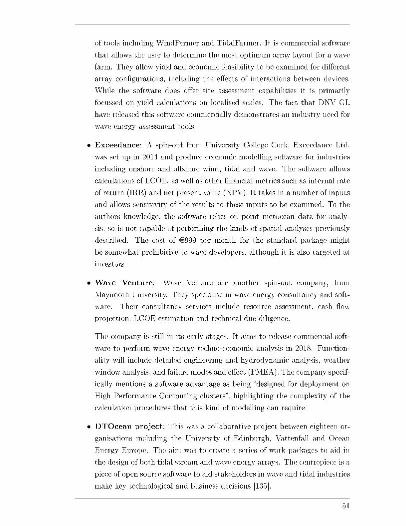
of tools including WindFarmer and TidalFarmer. It is commercial software

that allows the user to determine the most optimum array layout for a wave

farm. They allow yield and economic feasibility to be examined for di�erent

array con�gurations, including the e�ects of interactions between devices.

While the software does o�er site assessment capabilities it is primarily

focussed on yield calculations on localised scales. The fact that DNV GL

have released this software commercially demonstrates an industry need for

wave energy assessment tools.

• Exceedance: A spin-out from University College Cork, Exceedance Ltd.

was set up in 2014 and produce economic modelling software for industries

including onshore and o�shore wind, tidal and wave. The software allows

calculations of LCOE, as well as other �nancial metrics such as internal rate

of return (IRR) and net present value (NPV). It takes in a number of inputs

and allows sensitivity of the results to these inputs to be examined. To the

authors knowledge, the software relies on point metocean data for analy-

sis, so is not capable of performing the kinds of spatial analyses previously

described. The cost of e999 per month for the standard package might

be somewhat prohibitive to wave developers, although it is also targeted at

investors.

• Wave Venture: Wave Venture are another spin-out company, from

Maynooth University. They specialise in wave energy consultancy and soft-

ware. Their consultancy services include resource assessment, cash �ow

projection, LCOE estimation and technical due diligence.

The company is still in its early stages. It aims to release commercial soft-

ware to perform wave energy techno-economic analysis in 2018. Function-

ality will include detailed engineering and hydrodynamic analysis, weather

window analysis, and failure modes and e�ect (FMEA). The company specif-

ically mentions a software advantage as being �designed for deployment on

High Performance Computing clusters�, highlighting the complexity of the

calculation procedures that this kind of modelling can require.

• DTOcean project: This was a collaborative project between eighteen or-

ganisations including the University of Edinburgh, Vattenfall and Ocean

Energy Europe. The aim was to create a series of work packages to aid in

the design of both tidal stream and wave energy arrays. The centrepiece is a

piece of open source software to aid stakeholders in wave and tidal industries

make key technological and business decisions [135].

51

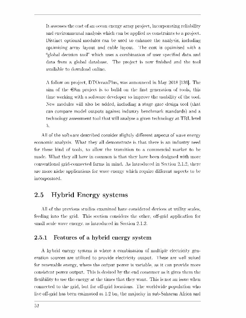
It assesses the cost of an ocean energy array project, incorporating reliability

and environmental analysis which can be applied as constraints to a project.

Distinct optional modules can be used to enhance the analysis, including

optimising array layout and cable layout. The cost is optimised with a

�global decision tool� which uses a combination of user speci�ed data and

data from a global database. The project is now �nished and the tool

available to download online.

A follow on project, DTOceanPlus, was announced in May 2018 [136]. The

aim of the e8m project is to build on the �rst generation of tools, this

time working with a software developer to improve the usability of the tool.

New modules will also be added, including a stage gate design tool (that

can compare model outputs against industry benchmark standards) and a

technology assessment tool that will analyse a given technology at TRL level

5.

All of the software described consider slightly di�erent aspects of wave energy

economic analysis. What they all demonstrate is that there is an industry need

for these kind of tools, to allow the transition to a commercial market to be

made. What they all have in common is that they have been designed with more

conventional grid-connected farms in mind. As introduced in Section 2.1.2, there

are more niche applications for wave energy which require di�erent aspects to be

incorporated.

2.5 Hybrid Energy systems

All of the previous studies examined have considered devices at utility scales,

feeding into the grid. This section considers the other, o�-grid application for

small scale wave energy, as introduced in Section 2.1.2.

2.5.1 Features of a hybrid energy system

A hybrid energy system is where a combination of multiple electricity gen-

eration sources are utilised to provide electricity output. These are well suited

for renewable energy, where the output power is variable, as it can provide more

consistent power output. This is desired by the end consumer as it gives them the

�exibility to use the energy at the times that they want. This is not an issue when

connected to the grid, but for o�-grid locations. The worldwide population who

live o�-grid has been estimated at 1.2 bn, the majority in sub-Saharan Africa and

52

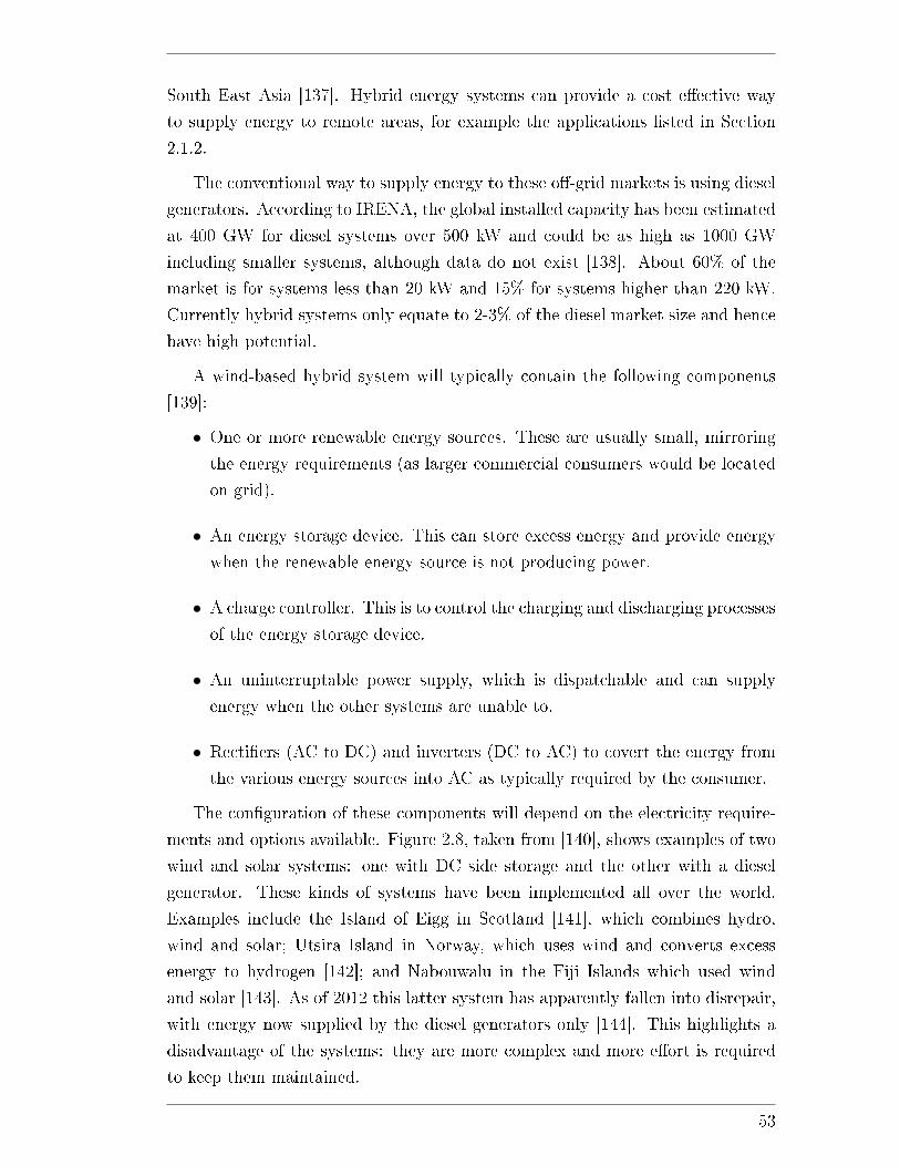
South East Asia [137]. Hybrid energy systems can provide a cost e�ective way

to supply energy to remote areas, for example the applications listed in Section

2.1.2.

The conventional way to supply energy to these o�-grid markets is using diesel

generators. According to IRENA, the global installed capacity has been estimated

at 400 GW for diesel systems over 500 kW and could be as high as 1000 GW

including smaller systems, although data do not exist [138]. About 60% of the

market is for systems less than 20 kW and 15% for systems higher than 220 kW.

Currently hybrid systems only equate to 2-3% of the diesel market size and hence

have high potential.

A wind-based hybrid system will typically contain the following components

[139]:

• One or more renewable energy sources. These are usually small, mirroring

the energy requirements (as larger commercial consumers would be located

on-grid).

• An energy storage device. This can store excess energy and provide energy

when the renewable energy source is not producing power.

• A charge controller. This is to control the charging and discharging processes

of the energy storage device.

• An uninterruptable power supply, which is dispatchable and can supply

energy when the other systems are unable to.

• Recti�ers (AC to DC) and inverters (DC to AC) to covert the energy from

the various energy sources into AC as typically required by the consumer.

The con�guration of these components will depend on the electricity require-

ments and options available. Figure 2.8, taken from [140], shows examples of two

wind and solar systems: one with DC side storage and the other with a diesel

generator. These kinds of systems have been implemented all over the world.

Examples include the Island of Eigg in Scotland [141], which combines hydro,

wind and solar; Utsira Island in Norway, which uses wind and converts excess

energy to hydrogen [142]; and Nabouwalu in the Fiji Islands which used wind

and solar [143]. As of 2012 this latter system has apparently fallen into disrepair,

with energy now supplied by the diesel generators only [144]. This highlights a

disadvantage of the systems: they are more complex and more e�ort is required

to keep them maintained.

53

Figure 2.8: Examples of wind and solar hybrid system con�gurations. Taken from [140].

2.5.1.1 Energy storage

There are various storage options suitable for hybrid systems including bat-

teries, �ywheels and hydrogen fuel cells. Battery storage has many advantages.

Batteries are portable, easy to scale to system size and provide instant response

to the energy system [145]. The most common option is lead acid batteries [139],

as they are a mature technology and especially cost e�ective [146, 147]. As of

2018 they have the largest global market share in terms of both sales value and

storage capacity [145]. Other types of batteries, for example lithium ion and �ow

batteries, can also be used. However these are more expensive, especially at the

larger scales required for use in an energy system.

There are two main types of lead-acid batteries: �ooded (FLA) and valve-

regulated (VRLA). FLA batteries contain a liquid electrolyte that need regularly

replenished. They also release hydrogen gas during charging and so the storage

location needs actively ventilated [148]. VRLA batteries contain a solid electrolyte

and are sealed. While the costs are higher and lifetimes typically shorter, they

only need passive ventilation and require less maintenance [145].

The lifetime of a battery will vary depending on the type and how it is used,

but is typically in the range of 4-7 years [149,150]. Deep discharges of the battery

will reduce the lifetime, as will higher operating temperatures. Some batteries are

specially designed for deep cycle applications, which means that they can regularly

be discharged by 80% of their capacity with a reduced impact on lifetime. The

charge going in and out of the batteries must be carefully regulated, to protect

them from damage. The charge controller monitors the battery charge to ensure

that the state of change does not drop too low.

2.5.1.2 Diesel generators

Regardless of the scale of the renewable energy systems and battery bank,

almost all systems will need a backup power option to supply power when the need

is critical. This role is served with a diesel generator [140]. The major advantages

54

Figure 2.9: Historic pre-tax diesel price in the UK. Taken from [153].

of using diesel generators are cost and convenience, and for this reason they are

the most common way to provide power for o�-grid markets.

Diesel generators typically run at e�ciencies of 30-35% [146] and have a lifetime

of 20,000 hours [151,152]. They are subject to �uctuating diesel price, subject to

geopolitical factors and outside the control of the consumer. Examples of this long

term variation are shown in Figure 2.9 for the UK from 1990-2014 [153]. They

are noisy and pollute the local environment. These issues mean that the general

aim of the hybrid system is to minimise the reliance on the generator, but in a

cost e�ective way.

2.5.2 Hybrid system modelling

It is important to be able to model the performance of a hybrid system, to

judge whether it would be bene�cial for the proposed application and ensure that

it is properly designed. The systems are more complex to model than just a

single energy source [154], as the energy provided is obtained from a combination

of the systems. These have di�erent operational modes that depend on the load

requirement and energy available [139].

There are various software options available to simulate hybrid energy systems,

for example nineteen are described in [154]. These can be classi�ed into four

types [155]: pre-feasibility, for high level economic analysis and rough sizing of

components; sizing, to optimise the components used; simulation, which perform

in depth simulations using detailed system parameters; and open architecture,

where the user can specify their own control algorithms.

The Hybrid Optimization Model for Electric Renewables (HOMER) is an ex-

55

ample of this software [156,157]. First developed in 1993, this is the most widely

used software [154], claiming over 100,000 users in 192 countries [158]. It is numer-

ously used in research, recent examples include [159�162]. HOMER takes both

technical and economic input parameters and simulates the system by balancing

the power produced with the electricity demands over a series of timesteps. It

should be noted that HOMER does not perform full analysis of the electrical sys-

tem, (for example simulating currents and voltages) but deals with the average

energy produced over discrete time-steps. The energy inputs from the various

sources are optimised to minimise the total NPC. Sensitivity analysis can also be

performed by modifying the system components (for example considering di�erent

generator models or costs).

HOMER is a powerful tool, underpinned by years of research, and is generally

regarded as being sophisticated and realistic [158]. There are two key issues with

the model which motivate this research. The �rst is that it does not support

wave energy. The second is that, as a commercial tool, the software is di�cult

to integrate into other tools used by industry. The user is reliant on the control

systems and optimisation process as speci�ed by HOMER.

2.5.3 Application to aquaculture

2.5.3.1 The aquaculture market

The main market that Albatern are pursuing for their technology is the Aqua-

culture sector. Aquaculture is the process of farming aquatic organisms for human

consumption. The industry is well established and expected to grow into the fu-

ture due to pressure on food supply from overpopulation. In 2007 it provided 43%

of aquatic animal food for humans and in 2008 was worth $98.5 billion, produc-

ing 52.5 million tonnes of produce [163]. The largest world market is Asia, which

made up 89% of the volume and 79% of the value. The two main facilities suitable

for wave energy development are coastal ponds/tanks and o�shore cages. This is

because they are located closest to the resource and are often o�-grid, relying on

diesel generators and fuel imports for power.

Scotland is renowned for its aquaculture industry. In 2017 the gross value

added (GVA) of the sector was ¿620 m [164]. The majority of this, ¿540 m, was in

the salmon farming trade. This �sh also account for 95% of the �n�sh produced.

From 2005 to 2015 the amount of salmon produced per annum increased from

130,000 to 170,000 tonnes, a 30% increase. This is smaller than Norway and

China, the leading producers, who produced 1.3 m tonnes and 600,000 tonnes

56

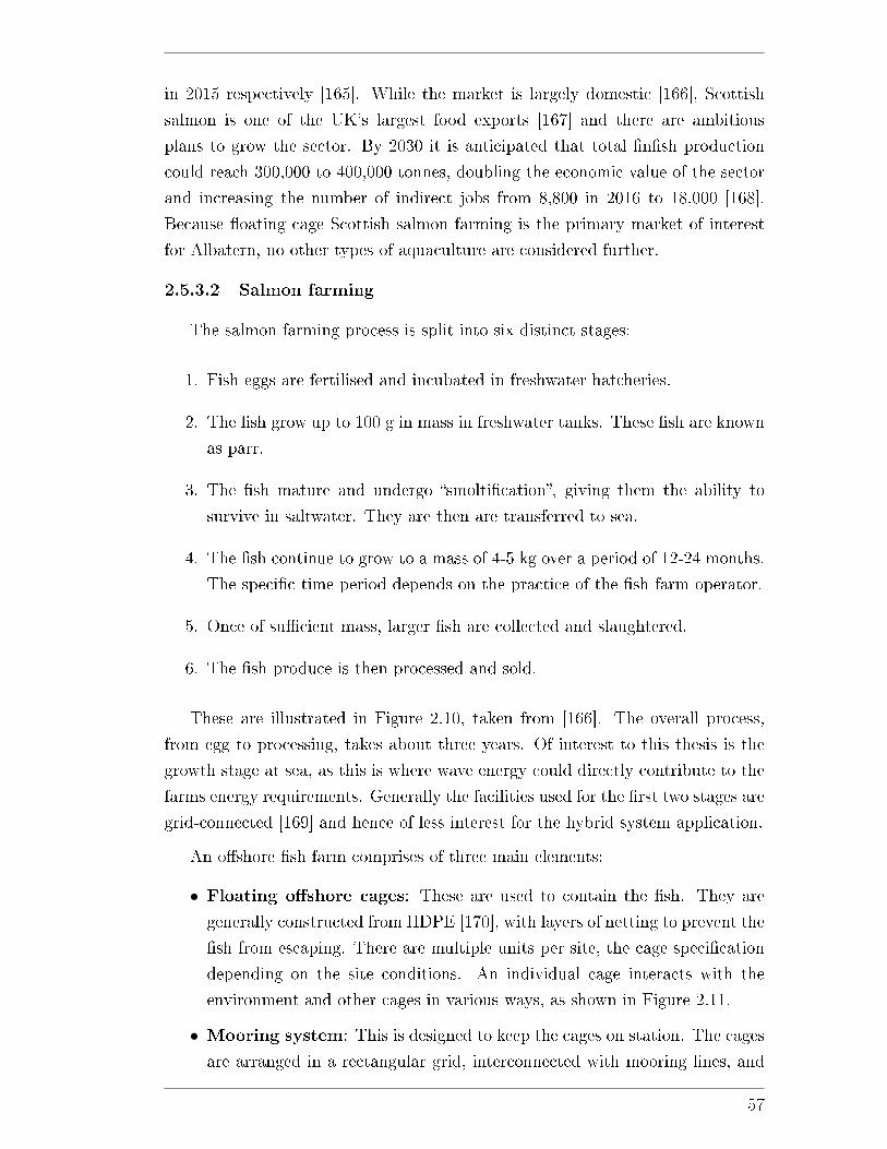
in 2015 respectively [165]. While the market is largely domestic [166], Scottish

salmon is one of the UK's largest food exports [167] and there are ambitious

plans to grow the sector. By 2030 it is anticipated that total �n�sh production

could reach 300,000 to 400,000 tonnes, doubling the economic value of the sector

and increasing the number of indirect jobs from 8,800 in 2016 to 18,000 [168].

Because �oating cage Scottish salmon farming is the primary market of interest

for Albatern, no other types of aquaculture are considered further.

2.5.3.2 Salmon farming

The salmon farming process is split into six distinct stages:

1. Fish eggs are fertilised and incubated in freshwater hatcheries.

2. The �sh grow up to 100 g in mass in freshwater tanks. These �sh are known

as parr.

3. The �sh mature and undergo �smolti�cation�, giving them the ability to

survive in saltwater. They are then are transferred to sea.

4. The �sh continue to grow to a mass of 4-5 kg over a period of 12-24 months.

The speci�c time period depends on the practice of the �sh farm operator.

5. Once of su�cient mass, larger �sh are collected and slaughtered.

6. The �sh produce is then processed and sold.

These are illustrated in Figure 2.10, taken from [166]. The overall process,

from egg to processing, takes about three years. Of interest to this thesis is the

growth stage at sea, as this is where wave energy could directly contribute to the

farms energy requirements. Generally the facilities used for the �rst two stages are

grid-connected [169] and hence of less interest for the hybrid system application.

An o�shore �sh farm comprises of three main elements:

• Floating o�shore cages: These are used to contain the �sh. They are

generally constructed from HDPE [170], with layers of netting to prevent the

�sh from escaping. There are multiple units per site, the cage speci�cation

depending on the site conditions. An individual cage interacts with the

environment and other cages in various ways, as shown in Figure 2.11.

• Mooring system: This is designed to keep the cages on station. The cages

are arranged in a rectangular grid, interconnected with mooring lines, and

57

Figure 2.10: The six stages of the salmon farming production cycle. Taken from [166].

anchored to the seabed at multiple points using drag embedment or gravity

anchors [170]. The number and strength of the lines will depend on the site

conditions.

• Feed system: There are various ways that the �sh can be fed. A common

option is a feed blower (or cannon), which blows high volumes of feed from a

hopper into the cages [169]. This can be automated. Larger or more modern

sites might instead use a feed barge: a dedicated vessel which houses the

necessary feed. This serves as a centralised store, often with lines which

run to the individual cages [170]. These systems can be costly, and are less

suitable for more exposed locations [170].

There are many factors that need to be considered at this stage. The most

signi�cant cost to the �sh farm operator is in �sh feed, which makes up 50-75%

of the total production cost [166, 170]. Minimising the feed requirement not only

58

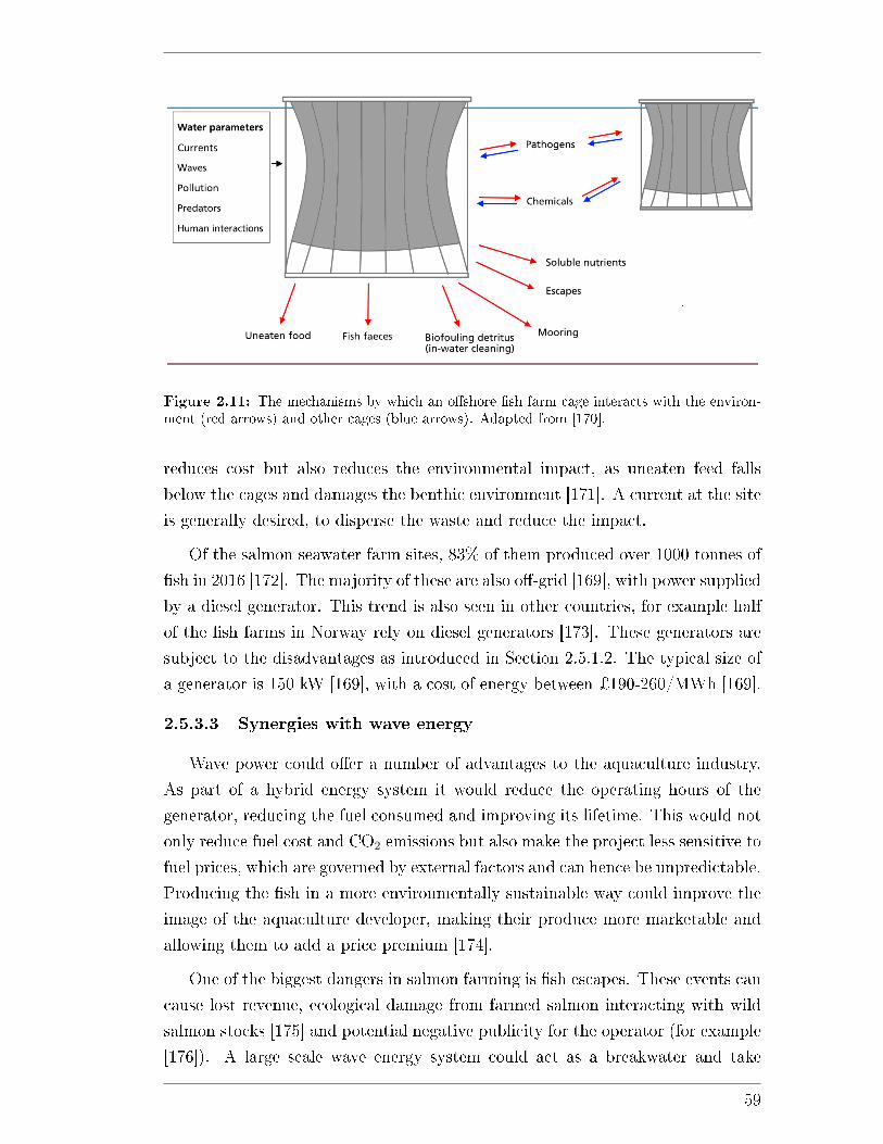
Figure 2.11: The mechanisms by which an o�shore �sh farm cage interacts with the environ-ment (red arrows) and other cages (blue arrows). Adapted from [170].

reduces cost but also reduces the environmental impact, as uneaten feed falls

below the cages and damages the benthic environment [171]. A current at the site

is generally desired, to disperse the waste and reduce the impact.

Of the salmon seawater farm sites, 83% of them produced over 1000 tonnes of

�sh in 2016 [172]. The majority of these are also o�-grid [169], with power supplied

by a diesel generator. This trend is also seen in other countries, for example half

of the �sh farms in Norway rely on diesel generators [173]. These generators are

subject to the disadvantages as introduced in Section 2.5.1.2. The typical size of

a generator is 150 kW [169], with a cost of energy between ¿190-260/MWh [169].

2.5.3.3 Synergies with wave energy

Wave power could o�er a number of advantages to the aquaculture industry.

As part of a hybrid energy system it would reduce the operating hours of the

generator, reducing the fuel consumed and improving its lifetime. This would not

only reduce fuel cost and CO2 emissions but also make the project less sensitive to

fuel prices, which are governed by external factors and can hence be unpredictable.

Producing the �sh in a more environmentally sustainable way could improve the

image of the aquaculture developer, making their produce more marketable and

allowing them to add a price premium [174].

One of the biggest dangers in salmon farming is �sh escapes. These events can

cause lost revenue, ecological damage from farmed salmon interacting with wild

salmon stocks [175] and potential negative publicity for the operator (for example

[176]). A large scale wave energy system could act as a breakwater and take

59

signi�cant energy out of the sea, reducing the damage to nets and moorings. Such

damage does occur. For example in 2015 16,000 salmon, worth approximately

¿250,000 escaped from a farm operated by Marine Harvest due to storm damage

[177].

Generally the industry in the EU is trending towards more exposed farm lo-

cations, a requirement to meet 2030 industry targets [178, 179]. These sites have

better water circulation that mitigates environmental impacts, improves �sh wel-

fare and results in a better quality product [170]. This could also bene�t WECs,

the more energetic resource leading to better energy capture.

There are similarities in the types of components that are required, especially

for small scale WECs. This includes the mooring systems and the vessels required

for manoeuvring around site. If the wave industry could access these items at a

cost reduction then it could bene�t both industries. There is also the possibility

that small wave devices could be directly connected into the �sh farm mooring

system, again saving cost, although this would require detailed feasibility analysis

[169].

Lastly, there are numerous lower power ancillary applications that a small scale

WEC would be well suited for. Any excess energy could be used for non critical,

low power applications like sensors, underwater cameras, net cleaning robots or

heating site o�ce space [42]. There are also more novel applications, such as

equipment to remove sea lice from the �sh (for example [180] or [181]). This is of

particular interest as sea lice, parasites that prey on salmon, are a major concern

for �sh farm operators and their prevention is a priority going forward [168]. As

farms move to more exposed locations, more automated systems are required to

counteract reduced accessibility issues [170].

2.5.4 Hybrid system research examples: aquaculture and

wave energy

Using a hybrid energy system to power a �sh farm is not a new idea. However it

is one which has been seldom examined in the literature, even without considering

wave energy.

A study by the Scottish Aquaculture Research Forum (SARF) examined the

di�erent renewable energy options that could suit an aquaculture site [169].

Largely a qualitative approach, they identi�ed salmon farming as especially suit-

able, with more passive types of �sh farming such as for shell�sh generally unsuit-

60

able due to the very low energy requirements. They identi�ed wave energy as an

option with �possible suitability�, with the main barrier in the short term being

a high LCOE. From this, they concluded that small scale wave would be unlikely

to be suitable, although just compared an LCOE number from the literature and

did not carry out a full economic evaluation.

Syse carried out a more in depth study, also comparing di�erent renewable

sources [173]. A quantitative analysis was carried out for a wind-solar-diesel sys-

tem at an o�-grid aquaculture site, using HOMER. The energy demand was es-

timated from visiting a �sh farm and noting the components used; this included

domestic usage and assumed a period of one year, with variability applied on a

daily and timestep basis. The hybrid system was found to have a lower NPC than

the diesel only system. A renewable only system was also examined, however this

was found to be uneconomic with a LCOE of ¿0.81/kWh compared to ¿0.491 for

the conventional diesel system. The author did consider wave energy at the start

of the project, however again excluded it as an option due to higher LCOE, which

was not quanti�ed, and lack of data regarding OPEX.

Botne Sandberg et al. investigated both technical and non-technical factors

critical to the viability of wave energy to power luxury resorts and small utilities.

It included an LCOE analysis. A point absorber, currently being developed by

CorPower, was used for the analysis. Considering an availability of 90% and using

a device power matrix, an array of 1-4 WECs was found to be able to supply 7.5-

22% of a hotels energy demand, although the time dependence of this was not

accounted for in the calculations. The LCOE of a wave-battery system was found

to be e240-430/MWh, with a battery lifetime of ten years assumed.

There have been other studies examining various lower power applications in

the aquaculture industry. Erwin et al. used HOMER to examine hybrid biomass

and wind systems for a shrimp pond in Indonesia [182]. They found that a renew-

able option was feasible for the small system (with peak energy demand of about

15 kWh). Prasetyaningsari et al. considered a solar powered aeration system

for an onshore �sh pond, again with a lower energy requirements (2kWh per day

average). Both of these studies demonstrate the applicability of hybrid energy

systems to aquaculture, however are too small to be of interest for wave energy

at Albatern's scale.

61

2.5.5 Summary

Despite references to wave energy for hybrid system applications, there has

been very little research in quantitatively examining them. A key reason for this

is the complexity of modelling required, lack of data and the fact that it is too

niche to have caught the attention of large software developers like HOMER En-

ergy. This thesis aims to contribute to knowledge in this area by describing a

model capable of performing such hybrid system analysis. Because it calculates

LCOE it is highly desirable for early stage feasibility analysis. Moreover it in-

corporates spatial analysis methodology, as described in Section 2.4.2. To the

authors knowledge this kind of analysis has never been carried out before in the

literature.

62

3The Computational Model:

Structure and Implementation

In order to perform the in-depth calculations required to assess the economic

potential of a wave energy project, a dedicated computational model has been

created. Because there is a large variety of both input data required and output

data generated, a key part of this research has been concerned with designing the

model in an organised, �exible way. Emphasis has been placed on modularity of

the underlying code, to make the model easy to interpret, adapt and expand into

the future.

This section begins with an overview of the overall model structure and the

calculation which is being performed. This is followed by a summary of the input

data required and more detailed descriptions of each of the various sub-modules,

including how they are organised and the functionality that they contribute.

As well as the code used directly in the model, more generic modules have been

designed to aid with particular processes. Descriptions of these can be found in

Appendix B.

3.1 Overall Calculation Procedure

While the model has the ability to analyse di�erent wave energy systems and

probe a large number of system sensitivities, in all cases the overall computational

procedure follows an identical logic. This is made up of well de�ned, ordered

calculation stages which are interspersed with several key decisions which dictate

63

the elements of the model that need to be utilised. A high level �ow diagram

describing this calculation sequence from start to �nish is shown in Figure 3.1.

Programmatically this is executed by a top level function, spatial_analysis,

which calls sub-functions to achieve each process in the chain. This analysis is

contained within a distinct module, spatial_analyses.py. It contains all of the

top level functions and scripts that de�ne the overall calculation process.

First the input data, stored in con�guration �les, are loaded into the model

environment. This includes metocean data, a device power matrix and costs, as

well as optional system components like an export cable and mooring system.

The model is fully coded using the Python (2.7) programming language [183].

This decision was taken for multiple reasons: the relative ease of use, high level of

support available and the fact it is free to use. A further advantage of Python is

that it is very well suited for OOP [184]. OOP is a popular software development

approach, based around the idea that real world objects can be categorised and

represented programatically using a distinct data type, or class. OOP was applied

to this project to keep the underlying code modular and �exible, providing consis-

tency and making it easy to modify speci�c parts of the model without worrying

about impacting the rest of the code. Basic de�nitions of the Python terminology

used in this section can be found in Appendix A.1.

After loading the data, a default discount rate of zero is set if not speci�ed in

the con�guration �le. The function can then follow two di�erent paths, depending

on the application for the wave energy system. The more typical grid-connected

analysis, the subject of this chapter, follows the high level methods previously

outlined in Section 2.3. The o�-grid analysis obtains a wave energy time series

for each point in turn, using this as an input to an energy balancing algorithm.

This employs a specially created o�-grid analysis module, similar in principle to

HOMER software (as introduced in Section 2.5.2). It requires additional system

components to be speci�ed; these, along with the other facets of the o�-grid

module, are discussed in Chapter 4. Whichever application is considered, the key

output is the total energy produced by the device. This is the denominator in the

LCOE calculation, Equation 2.1 from Section 2.3.1. If the time series data do not

cover the lifetime of the system that is being modelling (for example ten years of

data but a WEC lifetime of 20 years) then the calculated energy can be projected

forwards in time to cover the full lifetime.

Next the costs analysis is undertaken for every system component. The speci�c

calculations, discussed within the proceeding sections, depend on the nature of

the component but all create the same output: discounted cash �ows which are

64

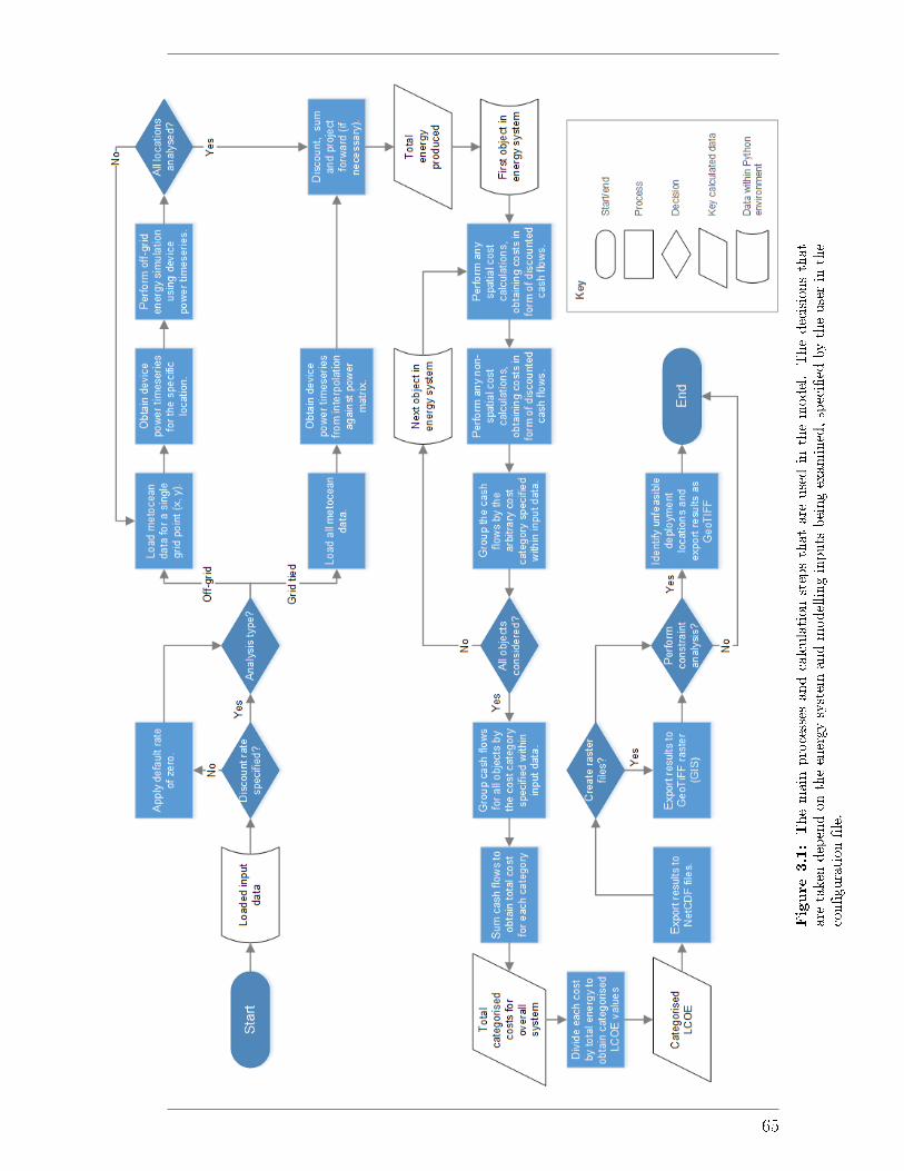
Figure3.1:Themain

processes

andcalculationstepsthatare

usedin

themodel.Thedecisionsthat

are

taken

dependontheenergy

system

andmodellinginputs

beingexamined,speci�ed

bytheuserin

the

con�guration�le.

65

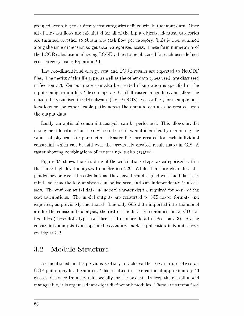
grouped according to arbitrary cost categories de�ned within the input data. Once

all of the cash �ows are calculated for all of the input objects, identical categories

are summed together to obtain one cash �ow per category. This is then summed

along the time dimension to get total categorised costs. These form numerators of

the LCOE calculation, allowing LCOE values to be obtained for each user-de�ned

cost category using Equation 2.1.

The two-dimensional energy, cost and LCOE results are exported to NetCDF

�les. The merits of this �le type, as well as the other data types used, are discussed

in Section 3.3. Output maps can also be created if an option is speci�ed in the

input con�guration �le. These maps are GeoTi� raster image �les and allow the

data to be visualised in GIS software (e.g. ArcGIS). Vector �les, for example port

locations or the export cable paths across the domain, can also be created from

the output data.

Lastly, an optional constraint analysis can be performed. This allows invalid

deployment locations for the device to be de�ned and identi�ed by examining the

values of physical site parameters. Raster �les are created for each individual

constraint which can be laid over the previously created result maps in GIS. A

raster showing combinations of constraints is also created.

Figure 3.2 shows the structure of the calculations steps, as categorised within

the three high level analyses from Section 2.3. While there are clear data de-

pendencies between the calculations, they have been designed with modularity in

mind: so that the key analyses can be isolated and run independently if neces-

sary. The environmental data includes the water depth, required for some of the

cost calculations. The model outputs are converted to GIS raster formats and

exported, as previously mentioned. The only GIS data imported into the model

are for the constraints analysis, the rest of the data are contained in NetCDF or

text �les (these data types are discussed in more detail in Section 3.3). As the

constraints analysis is an optional, secondary model application it is not shown

on Figure 3.2.

3.2 Module Structure

As mentioned in the previous section, to achieve the research objectives an

OOP philosophy has been used. This resulted in the creation of approximately 40

classes, designed from scratch specially for the project. To keep the overall model

manageable, it is organised into eight distinct sub modules. These are summarised

66

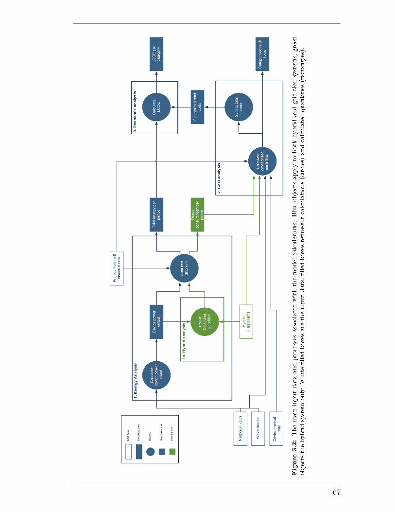
Figure3.2:Themain

inputdata

andprocesses

associatedwiththemodel

calculations.

Blueobjectsapply

toboth

hybridandgrid-tiedsystem

s,green

objectsthehybridsystem

only.White�lled

boxes

are

theinputdata,�lled

boxes

representcalculations(circles)andcalculatedquantities

(rectangles).

67

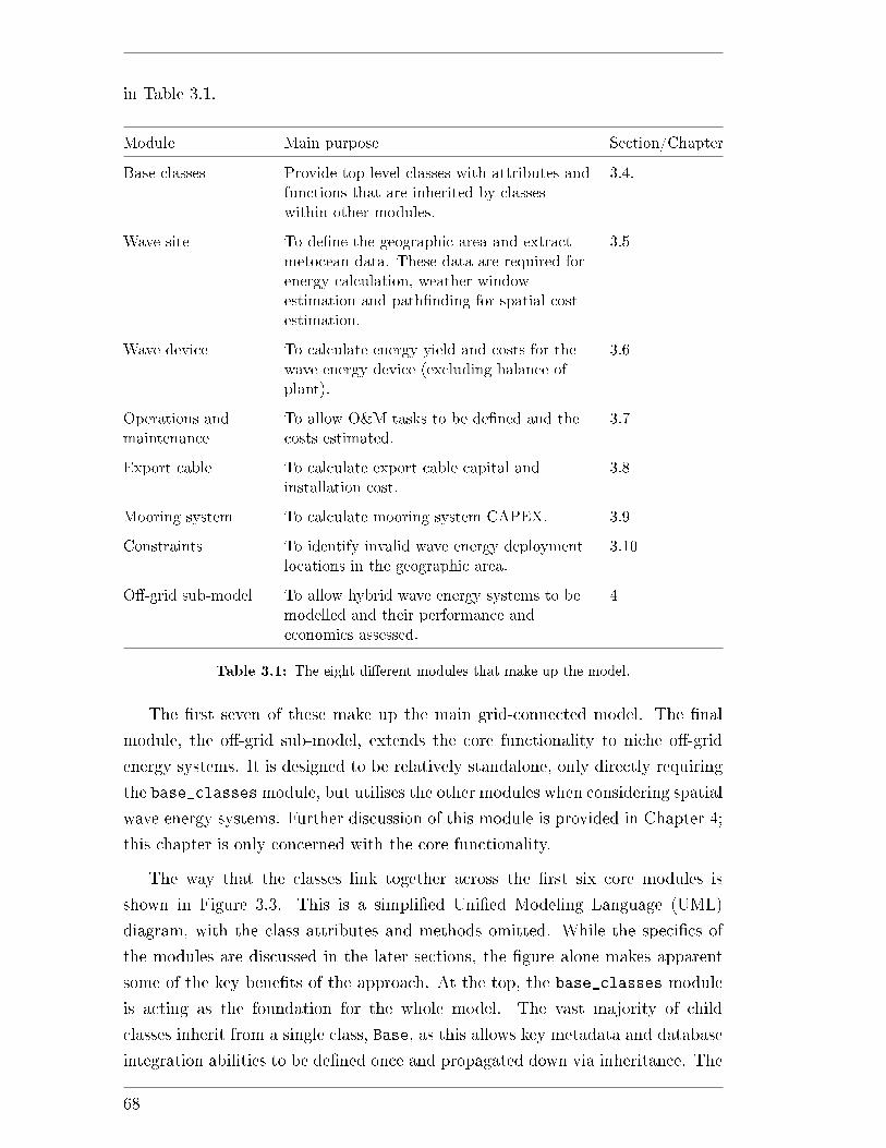
in Table 3.1.

Module Main purpose Section/Chapter

Base classes Provide top level classes with attributes andfunctions that are inherited by classeswithin other modules.

3.4.

Wave site To de�ne the geographic area and extractmetocean data. These data are required forenergy calculation, weather windowestimation and path�nding for spatial costestimation.

3.5

Wave device To calculate energy yield and costs for thewave energy device (excluding balance ofplant).

3.6

Operations andmaintenance

To allow O&M tasks to be de�ned and thecosts estimated.

3.7

Export cable To calculate export cable capital andinstallation cost.

3.8

Mooring system To calculate mooring system CAPEX. 3.9

Constraints To identify invalid wave energy deploymentlocations in the geographic area.

3.10

O�-grid sub-model To allow hybrid wave energy systems to bemodelled and their performance andeconomics assessed.

4

Table 3.1: The eight di�erent modules that make up the model.

The �rst seven of these make up the main grid-connected model. The �nal

module, the o�-grid sub-model, extends the core functionality to niche o�-grid

energy systems. It is designed to be relatively standalone, only directly requiring

the base_classesmodule, but utilises the other modules when considering spatial

wave energy systems. Further discussion of this module is provided in Chapter 4;

this chapter is only concerned with the core functionality.

The way that the classes link together across the �rst six core modules is

shown in Figure 3.3. This is a simpli�ed Uni�ed Modeling Language (UML)

diagram, with the class attributes and methods omitted. While the speci�cs of

the modules are discussed in the later sections, the �gure alone makes apparent

some of the key bene�ts of the approach. At the top, the base_classes module

is acting as the foundation for the whole model. The vast majority of child

classes inherit from a single class, Base, as this allows key metadata and database

integration abilities to be de�ned once and propagated down via inheritance. The

68

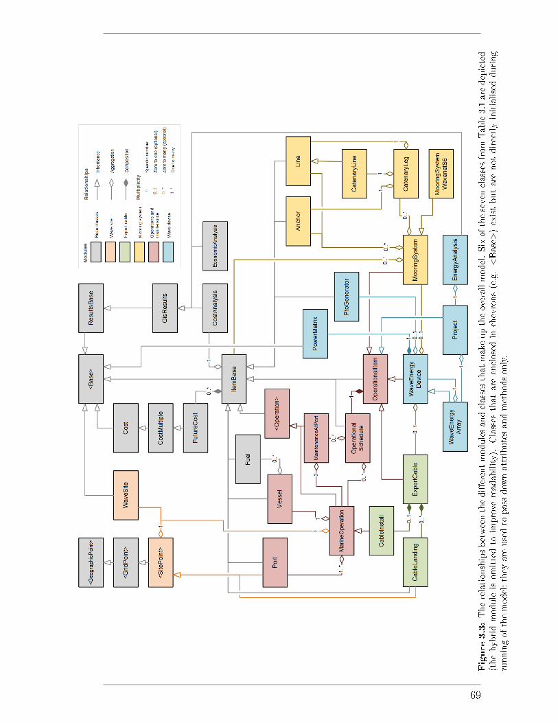
Figure3.3:Therelationshipsbetweenthedi�erentmodulesandclasses

thatmakeuptheoverallmodel.Sixoftheseven

classes

from

Table3.1are

depicted

(thehybridmodule

isomittedto

improve

readability).

Classes

thatare

enclosedin

chevrons(e.g.<Base>)existbutare

notdirectlyinitialisedduring

runningofthemodel;they

are

usedto

pass

dow

nattributesandmethodsonly.

69

ItemBase class is arguably the most important in the model, de�ning any cost

item and allowing combinations of cost components to be easily calculated under

a uniform methodology. The WaveEnergyDevice class represents the culmination

of the various di�erent system components: the export cable, mooring system and

operational activities.

It is worth noting that these modules occupy very speci�c spaces within the

overall structure, with very few interdependencies between them. This is particu-

larly advantageous as it allows new functionality to be easily added with little to

no modi�cation of existing modules required. Version control is also straightfor-

ward, as each module can be tracked separately. Care has been taken to limit the

usage of multiple inheritance, as this can be a source of bugs as the complexity of

the class hierarchy increases [185].

The constraints module is not included in the diagram. This is because the

classes are more abstract in nature and do not represent physical aspects of the

wave energy project.

To complement Figure 3.3, more detailed UML diagrams for each module

are presented in the relevant sections. Each is used to guide the �ow of text

within the section, and hence should be used by the reader as a reference to the

attribute and function names and descriptions that are presented. Descriptions

of the terminology used in the UML diagrams can be found in Appendix A.3.

3.3 Data Types

There are various types of input data that are required. Metocean data,

namely Hs and Tp, are stored as NetCDF (.nc) �les [186]. Because the data

required by the spatial model are three-dimensional (time by latitude by longi-

tude), these �le types are advantageous as they allow di�erent portions of the

data to be easily queried and loaded separately. This is useful when analysing

smaller datasets, so that the necessary data can be easily extracted from the full

dataset without incurring the memory issues from having to load all the data.

Within a NetCDF �le multiple data variables can be stored and de�ned over the

same dimensions. Speci�c portions of data can be easily queried using Python

packages like Pandas or xarray [187]. The data can also be chunked, either when

creating the �le (using a tool like nccopy) or upon reading (using xarray). This

essentially allows the data to be loaded in bite-size chunks, rather than in one go,

which is much less memory intensive.

70

Class instances that represent physical objects, for example devices and export

cables, are stored in text (.txt) �les. These �les are two column, with attribute

names on the left and the attribute values on the right, separated by a tab de-

limiter. The attributes can point to further text �le paths, de�ning other class

instances. The �les are read with a specially created function, which iterates

down through the directory tree and creates a class instance in Python from the

attributes speci�ed in the �le. This way of storing objects is useful, as it is rel-

atively simple for the user and does not require the use of any further software

or python packages. It also allows class instances to easily be nested inside each

other, and the attributes are straightforward to modify on the �y. Examples of

these text �les can be found in Appendix C.

An alternative method that was examined was using a datebase. The ad-

vantage is that it enforces organisation and allows the data to be easily queried.

NoSQL was considered rather than the more conventional SQL database approach.

This is because NoSQl has no constraints on structure, allowing di�erent types of

data to be stored together. Setting up a SQL database requires good knowledge

of the schema and more preparation upfront to avoid future issues associated with

large quantities of data [188]. Having no limitations on schema would be useful

for this type of research as the object classes and functionality has evolved on an

iterative basis, and hence there is no need to constantly re-evaluate the database

design. The speci�c NoSQL software considered was MongoDB. This is because

it has good integration with Python, lots of support available (including tutorials

and a free online course) and can be downloaded free of charge. While a more

elegant solution, the text �le storage method ended up being used. This was for

two reasons: project time constraints and because the learning curve associated

with using databases would make the model harder to use for other people within

the sponsoring company.

Lastly, some input data sources are stored as GIS �les. This mainly applies

to constraint layers: layers which limit the potential deployment locations of the

wave energy device. Storing these data as GIS �les allows them to be externally

visualised in GIS software (for example ArcGIS) as well as loaded into Python to

use in analyses. These constraint layers are discussed in more detail in Section

3.10.

71

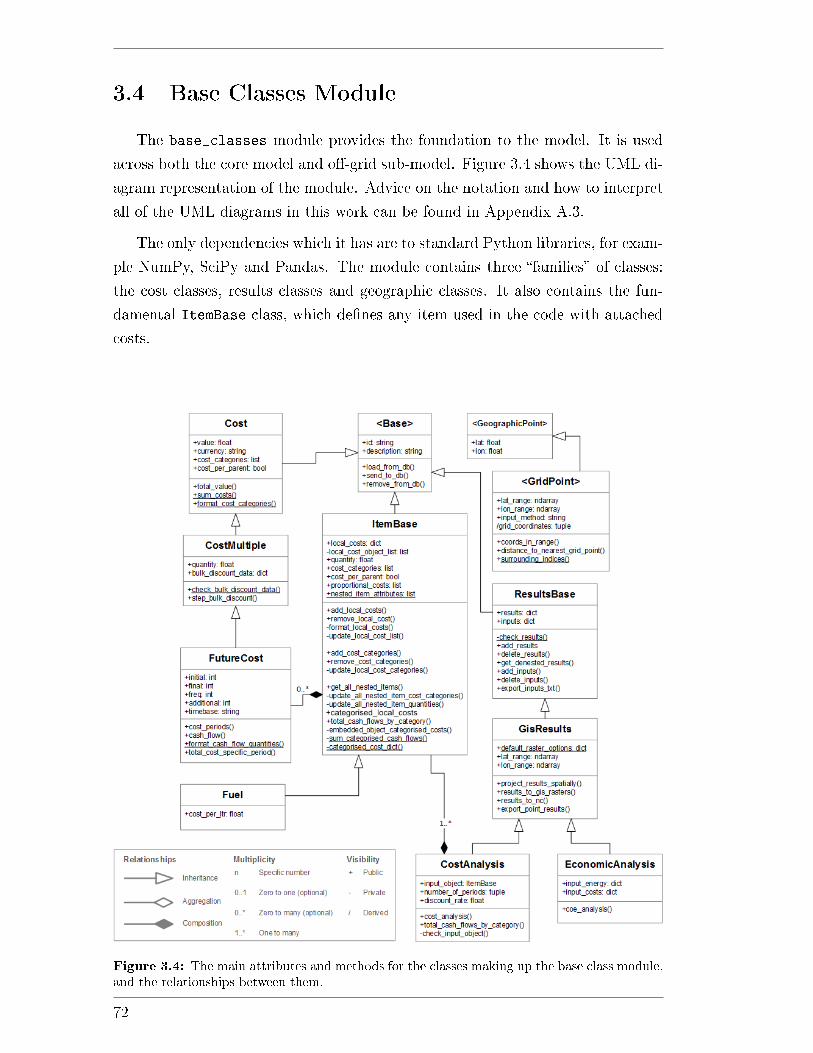
3.4 Base Classes Module

The base_classes module provides the foundation to the model. It is used

across both the core model and o�-grid sub-model. Figure 3.4 shows the UML di-

agram representation of the module. Advice on the notation and how to interpret

all of the UML diagrams in this work can be found in Appendix A.3.

The only dependencies which it has are to standard Python libraries, for exam-

ple NumPy, SciPy and Pandas. The module contains three �families� of classes:

the cost classes, results classes and geographic classes. It also contains the fun-

damental ItemBase class, which de�nes any item used in the code with attached

costs.

Figure 3.4: The main attributes and methods for the classes making up the base class module,and the relationships between them.

72

3.4.1 The Base class

The Base class serves as a parent class to every class that represents a physical

object. Objects have an _id attribute, an id tag that allows the object to be

identi�ed and, in theory, stored as a unique database entry. This can either be

speci�ed by the user or automatically created using the MongoDB ObjectId class.

The class also has methods for exporting the current object to or from a MongoDB

database, although these are not used in the implementation described and are

included for completeness. As well as an id, base class objects also contain a

description and comments attribute that can hold basic information.

All of the base class attributes can be exported to a csv �le, using the instance

method export_attributes. This allows the user to view the attributes outside

of the Python environment, and is particularly useful for documenting the inputs

going into the model. Within the method, the user can choose speci�c attributes

to export by name and/or by data type. Additionally, the user can decide whether

to export the attributes of nested objects. These objects are class instances them-

selves, typically incorporated into the instance within speci�c attributes. An

example is the wave device class (WaveDevice), which includes an export cable

attribute. This attribute is an instance of another class, ExportCable, and is

embedded within the device instance.

3.4.2 Costs

These classes were created to allow the model to properly handle costs. Be-

cause there are a large variety of objects that have costs associated with them, a

base cost class allows the uniform treatment of costs across the model.

The base cost class, Cost, represents a single cost. Its attributes include the

cost value itself, the currency of the cost and description and comments, as in

Base. A method in_currency allows the cost to be represented in a di�erent

currency, using the third party Python package CurrencyConverter [189]. This

is useful when aggregating costs that are provided in di�erent currencies. A key

attribute to aggregate multiple costs is the cost_categories attribute. This is

essentially a list of tags, representing the categories that the cost �ts into. These

are designated arbitrarily. Examples could include �device CAPEX�, �mooring

system� or something lower level like �delivery cost�. All of the costs that fall

under a certain category can be grouped together for cost analysis, and hence

di�erent costs easily compared (see Section 3.4.3).

73

The CostMultiple class builds on this by introducing a quantity attribute, to

de�ne times when a cost is incurred multiple times. The bulk_discount_data

attribute allows bulk discount factors to be applied to the items, occurring after

discrete quantities. This is speci�ed as a dictionary, for example {0.8: 10,

0.6: 20} would indicate that the cost value falls to 80% of the original cost

after ten items and to 60% after 20 items. The total cost value, calculated using

the total_value function, is hence the cost value multiplied by the quantity, with

any bulk discount factored in.

The FutureCost class represents costs that are incurred in the future. Costs

are de�ned not only with a value, but with attributes that allow the future time

periods where the cost occurs to be de�ned. The initial and final attributes

are integer values de�ning the �rst and last time period where the cost is incurred.

The freq attribute sets the frequency of the cost. For example, a frequency of

two tells the class that the cost is incurred every second time period from the

start period to the end period. The additional attribute allows any additional

periods not covered by the frequency attribute to be speci�ed. The time period

de�nition can be speci�ed to either an annual or monthly base. This is only

relevant if a discount rate has been speci�ed for calculating the �nal cost, to

ensure that the costs are appropriately discounted into the future (see Section

2.3.1 for a description of discounting). Linking the base cost with a time element

means that capital costs and operational costs are properly discounted and can

be distinguished. Capital costs are assumed to occur in time period 0.

3.4.3 Cost items

The ItemBase class is one of the most important in the model. It is used

to represent objects that have one or many costs associated with them. It is a

parent class to many objects and provides methods which allows costs to be easily

grouped and summed according to their cost category attributes.

At the heart of the class is the local_costs property. This is where all of the

individual costs related to the object are stored, each converted into a FutureCost

instance upon input using the method format_local_costs. The actual property

is a dictionary made up of these cost instances, with each key de�ned by the cost's

_id attribute. Using a dictionary makes it easy to remove speci�c cost items and

prevents identical costs from being accidentally duplicated within the ItemBase

instance. Methods to add or remove individual local costs are coded into the class,

improving usability when working within Python.

74

Like the cost classes previously discussed, the class also has quantity and

cost_categories attributes which work in the same way as previously described.

They are both implemented by composition, via a private embedded Cost in-

stance. This allows only these attributes to be copied from the Cost instance

without requiring an unrealistic inheritance relationship. The quantity is multi-

plied by the constituent cash �ow totals to obtain an overall cash �ow for the

instance as as whole.

At a local level, this is achieved using the method categorised_local_costs.

The method iterates through the local costs and obtains a cash �ow for each cost

instance, based on an input number of time periods and discount rate. As the

total_value method of the cost classes is used, it means present values and any

bulk cost reductions are automatically included. The totals are then multiplied

by the instance quantity, if the cost_per_parent attribute of the cost is set

to True (otherwise the assumption is made that the cost is only incurred once

despite the quantity of ItemBase). The cash �ows are then linked to their cost

categories using a dictionary. The cost_categories de�ned at the ItemBase

level are automatically added to the individual cost instances at the beginning of

the cost calculation. This follows the logic that the embedded cost items can be

considered part of the wider system.

More useful than calculating cash �ows for the costs within local_costs

is the ability to calculate cash �ows for all of the embedded cost objects con-

tained within the instance. The method _embedded_object_categorised_costs

does this by examining all of the instance's attributes, searching for other in-

stances of ItemBase. This process is achieved by a specially coded algorithm,

get_nested_instances, which is contained within the extra utilities library (in-

troduced in Appendix B). Any additional ItemBase instances that are found are

saved into an output dictionary and appended to the loop, the algorithm working

down through all of the embedded objects recursively until all ItemBase instances

are identi�ed. As these items are found, the higher level quantities and cost cat-

egories are �ltered down to them to ensure the correct item quantities are used.

One �nal point is that the _embedded_object_categorised_costs searching

algorithm also �nds instances contained in lists, by searching each list entry in

turn. This allows multiple ItemBase instances to be grouped together within

a single attribute, preventing class hierarchies from getting too complex. The

method is not compatible with ItemBase instances contained in dictionaries. This

decision was made because the dictionary data type is typically used for larger data

within the model (e.g. graphs from path �nding algorithms) which would greatly

75

slow down the code. The dictionary exclusion does not apply to the local_costs

attribute, this achieved using the local_cost_list private attribute. This is

updated automatically and contains identical data to the local_costs dictionary.

As a list type it can be found by the algorithm.

After the embedded CostItem instances are found, the

categorised_local_costs method is run on each one. In the most basic

case this just performs as previously introduced, although some child classes

modify this method to perform other calculations that are required. For example,

the ExportCable class version of the method contains an initial stage which

calculates the cable length prior to cost calculation.

The _embedded_object_categorised_costs method is private, not meant

to be directly used. The whole cost aggregation process described above is

achieved with the total_cash_flows_by_category method. This internally

runs the aforementioned function, combining this with the private functions

sum_categorised_cash_flows and categorised_cost_dict to format the out-

put in a more user friendly way.

The �nal thing that this function does is create any proportional costs de�ned

by the user with the proportional_costs attribute. These costs are di�erent

to local costs because, rather than absolute values, they are de�ned in terms

of speci�c cost categories. They are still instances of FutureCost but with an

additional attribute, the master_category. Once all of the cost category totals

categories are obtained, all of the proportional costs enclosed in the top level item

are extracted. For each, the cost category which matches the master category

�eld is identi�ed and the proportional cost value obtained by multiplying the cost

category total by the proportional cost's user-de�ned value �eld. Because the

proportional cost is an instance of FutureCost, time values can also be assigned

to them. This is useful when considering high level costs that are incurred at

regular intervals; A common example in the literature is expressing O&M cost as

an annual proportional of CAPEX (for example [57, 93])

3.4.4 Analysis results

Output results of any kind can be stored together using the ResultsBase

class. The data type of each result element can be anything, although two-

dimensional numeric NumPy arrays are most commonly used for spatial data.

They are grouped together as a dictionary within the results attribute and meth-

ods are de�ned to add and remove speci�c results using the underlying dictionary

76

keys. These keys can be used to de�ne the name of the result and are linked to

the output data �le names. The attribute also supports nested dictionaries, al-

lowing a way of creating sub result groups. The get_denested_results function

reduces this multilevel dictionary to a single level by joining the keys together.

This is desired as it means that unique output �le names can be created from the

data within a single results instance. It should be noted that ResultsBase is an

abstract class, hence does not contain methods to export the data. Instead, data

export is left to child classes where the data types will be more speci�c. Lastly,

the inputs attribute is also a dictionary to accompany the results set. This is

implemented so that the inputs used to generate the results are remembered. As

most of these inputs are typically strings or single numbers (as the more complex

inputs can be linked to speci�c class instances) they are suitable for storing in a

simple text �le. This is done with the export_inputs_txt method.

Locational results are stored within a GisResults instance. This class adds

methods to export results to NetCDF �les and GeoTi� raster images. Each pixel

in these images represents a location in the domain. To create the raster, func-

tions from a separate module, gis_utilities, are imported. This module is

summarised in Appendix B.1.

The results contained in this class are typically two-dimensional arrays which

de�ne some quantity over a geographic domain of latitudes and longitudes. This

means that the class requires knowledge of the geographic system so that the

locations of results are correctly interpreted. The attributes lat_range and

lon_range are included for this purpose; they are Python lists which together

de�ne the (x, y) pixel locations. Single numbers can also be mixed into the results

dictionary; typically these de�ne parameters that are static across the geographic

domain (for example cost aspects which will be the same regardless of location).

The function project_results_spatially takes the values and, using NumPy

array methods, projects the number across the whole range: so that it is the same

shape as the spatial domain

3.4.5 Analysis classes

The aim of these classes is to group functions and class methods together that

de�ne speci�c spatial calculations. Uniting di�erent aspects of the code in this

way improves usability, providing functionality which would otherwise be di�cult

without an in depth understanding of the inner module workings. While the model

functionality could also be achieved using functions instead of classes, the class

77

based approach o�ers a convenient way of grouping di�erent functions under a

unifying concept. For example, the economic analysis class could include distinct

methods to perform LCOE, IRR and NPV analyses. These could be calculated

independently, but grouping them enforces consistency in the input and output

data by design.

Within the overall model there are four analysis classes: CostAnalysis

and EconomicAnalysis, within this module; EnergyAnalysis, within the

wave_device; and OffGridAnalysis, within the o�-grid module.

Both CostAnalysis and EconomicAnalysis inherit from GisResults and are

designed to obtain spatial costs and spatial LCOE. They are contained in this

module because they are relevant to both the hybrid and non-hybrid system con�g-

urations. CostAnalysis calculates total costs and output cash �ow from an input

instance of ItemBase. This instance is embedded within the input_object at-

tribute. The total number of periods to consider for the analysis (months or years)

and discount rate are also required. The main class function, cost_analysis, uses

the total_cash_flows_by_category method, as de�ned in Section 3.4.3, to ob-

tain both categorised cash �ows and total costs for the input object. These results

are saved within the results attribute, and can hence be exported as NetCDF

�les or GIS rasters when paired with the necessary spatial dimensions.

The EconomicAnalysis class takes in energy data and cost data as input, the

latter as can be created from a cost analysis. From these data, cost of energy is

simply obtained by dividing each of the costs by the energy. This class does not

apply discounting for the COE analysis, assuming that the input data have already

been discounted. This is advantageous as it makes the class �exible and generic

in nature, not �xed to data of any particular type. It also means, however, that

a degree of care must be taken to ensure that the energy and cost input data are

both de�ned according to the same discount rate and project lifetime assumptions.

The output of coe_analysis is COE (LCOE if discounting is applied) for each

input cost. Using spatial results as inputs allows total COE to be calculated

across the domain and the results exported to GIS rasters. It should be noted

that only LCOE analysis is coded within the class. This decision was taken due

to the research project time constraints, with the sponsoring company instead

prioritising di�erent model aspects.

78

3.4.6 Geographic classes

Single spatial points that are used within the analysis, namely ports and ca-

ble landing points, derive their geographic properties from two base classes. The

purpose of these classes is to provide a framework that allows any single location,

de�ned by a latitude and longitude, to be de�ned. This uniform way of represent-

ing locations is useful as it allows core attributes and functionality to be present,

regardless of the point's place in the overall model.

The �rst class, GeographicPoint, simply de�nes a pair of coordinates. It is

initialised with a longitude and a latitude value, which must be given in decimal

degrees. A method export_as_vector uses functions from the aforementioned

gis_utilities module to create a vector layer of the point which can be viewed

in GIS software.

Functionality is added to this class with the child class GridPoint. This class

provides the link between a single point, as described by its parent class, and an

array or �grid� of points which is the level that the desired analyses are performed

over. As well as coordinates, this class also takes in latitude and longitude dimen-

sions in the form of one dimensional NumPy arrays or lists. The user can choose

to input the coordinates in the form of indices using the input_method attribute,

in this case the coordinates are selected from the input dimensions. This is par-

ticularly useful for debugging, to ensure that valid coordinates are always chosen

regardless of the input dimensions.

This class has several methods which are useful for the physical object child

classes. The point coordinates can be checked against the latitude-longitude grid

to see if the point lies within the input dimensions, using the coords_in_range

method. This check is required because if the point lies outside the grid then

path�nding analysis cannot be safely conducted. In addition, the class pro-

vides methods to determine where the point lies in relation to the grid. The

surrounding_indices static method returns the nearest grid points to the input

coordinates, with distances calculated using the haversine equation. These neigh-

bouring points are required for path�nding, discussed in more detail in Section

3.5.2. Lastly, using similar methods the grid_coordinates for the grid point

instance can be obtained. These are the coordinates of the nearest grid point to

the input coordinates, and are useful to know as they can be substituted for the

input coordinates in child class path�nding methods to ensure that a solution can

be found.

79

3.4.7 The Fuel class

This base class is used to describe a combustible fuel source. Inheriting from

ItemBase, it is used to de�ne vessel fuel in the operations_and_maintenance

module and fuel consumed by a diesel generator in the o�-grid sub-model.

The class is designed so that fuel cost can be easily considered within the

economic analyses. It is a simple class, inheriting most of its behaviours from

ItemBase. The main addition is the cost_per_ltr property, which de�nes the

cost paid per litre of fuel. As this is a cost, the data are stored as a FutureCost

instance within the local_costs attribute. As a cost instance, cost_per_ltr

has a quantity attribute of its own. This is where the quantity of fuel that is

consumed is de�ned, when calculated by other classes.

80

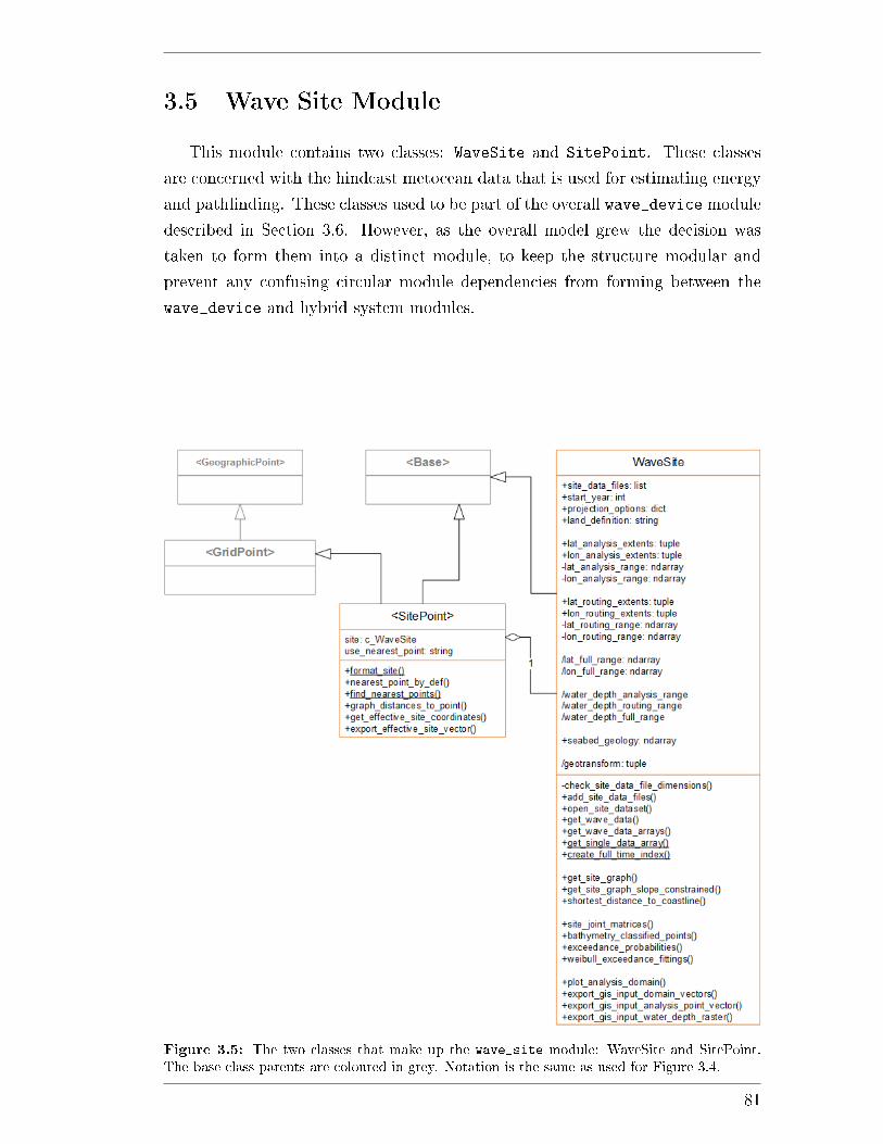
3.5 Wave Site Module

This module contains two classes: WaveSite and SitePoint. These classes

are concerned with the hindcast metocean data that is used for estimating energy

and path�nding. These classes used to be part of the overall wave_device module

described in Section 3.6. However, as the overall model grew the decision was

taken to form them into a distinct module, to keep the structure modular and

prevent any confusing circular module dependencies from forming between the

wave_device and hybrid system modules.

Figure 3.5: The two classes that make up the wave_site module: WaveSite and SitePoint.The base class parents are coloured in grey. Notation is the same as used for Figure 3.4.

81

3.5.1 The spatial domain

The class WaveSite is one of the most important in the model. It is a represen-

tation of a physical geographic area, over which is de�ned some gridded hindcast

metocean data. Its main purpose is to facilitate the easy import and handling of

the metocean data into the model for analysis.

The actual metocean data are stored within NetCDF (.nc) �les, prior to be-

ing loaded into Python. For an instance of the class, the directories where the

NetCDF �les are stored must be de�ned within the site_data_files property.

For convenience, entries can be added with the add_site_data_files method.

Typically each year of hindcast data is stored within its own NetCDF �le, a good

balance between convenience and memory1. Either a single string is speci�ed,

de�ning a single �le, or a list de�ning multiple �les. Each list entry can either be

a string or a dictionary containing the string accompanied by two further keys:

a `time range' key to allow a speci�c time range in the �le to be isolated and

a `rank' key that controls the ordering that the data �les are loaded in. This

latter functionality was provided to allow the user to mix and match data �les,

for example one could combine the most low energy months from a series of data

�les to examine a pessimistic energy scenario. By default the whole time range

is chosen, and the rank set to one more than the previous highest. Within the

property setter a function also checks that all of the �les are de�ned over the same

spatial range and at the same resolution, and returns an error if this is not the

case.

The NetCDF �les are three-dimensional, containing time series of Hs and Tpspeci�ed over latitude and longitude dimensions. The default geographic area

de�ned by the area is known as the �full domain�. The extents of this domain are

extracted using the open_site_dataset method, which opens a single �le within

the site_data_files attribute; by default this is the �le with the lowest rank

although the user can specify a rank to open a certain �le. Usually the user will

not be interested in the whole geographic area, as it will include many unsuit-

able locations and the more points that are included the slower the subsequent

analyses will take to run. To avoid this issue, data extraction can be limited

to a speci�c rectangular subset of the full domain. This is known as the �anal-

ysis domain� and can be speci�ed using the analysis_extent attributes. The

analysis range can be de�ned either in terms of coordinates, the format of the

1A single �le containing all of the data would be preferential but there would be signi�cantmemory overheads when accessing the data, even after chunking.

82

Purpose: To extract metocean data in a form suitable for spatial analyses.Required: A WaveSite instance (de�ned as self below) with site data �les de�ned.Returns: Metocean data variables, that can be projected and used to estimate devicepower and weather windows.

def get_wave_data(self)

# Get the spatial domain

lat_range = self.lat_analysis_range

lon_range = self.lon_analysis_range

nc_filepaths = self.site_data_files

nc_filepaths_sorted = sort_data_files(nc_filepaths) # Sort the data

files according to rank key.

D_files =[] # Pre-allocate list of arrays.

for file_dict in sorted_data_files:

# Open the dataset.

filepath = file_dict['path']

ds = open_dataset(filepath)

time_range = ds['time_range']

ds_subset = ds.sel(time_range, lat_range, lon_range) # Set the data

extents.

ds_subset_no_leap = remove_leap_day(ds_subset) # Remove leap day

from subset.

D_files.append(ds_subset_no_leap)

D_wave = concatenate(D_files) # Combine the data from each file.

start_year = self.start_year

t_i = create_full_time_index(D_wave, start_year) # Create a new time

index.

D_wave['time'] = t_i # Assign the time index.

return D_wave

Algorithm 3.2: Extract metocean data, de�ned within external NetCDF �les.

dimensions in the �le, or in terms of the indices in the array. This latter func-

tionality is useful for debugging. Two functions analysis_extent_coordinates

and analysis_extent_indices return the analysis domain extents in terms of

coordinates or indices, again primarily for debugging purposes. If analysis extents

are not de�ned then the analysis domain defaults to the full domain.

With the data �les and the spatial domain de�ned, the user can extract the

actual data. This is achieved using the get_wave_data instance method. This is

used twice: to get both Hs and Tp variables. The procedure for this method is

shown in Algorithm 3.2.

First the analysis domain extents are obtained in terms of coordinates, and

the site data �le strings are sorted according to the rank key. A for loop iterates

83

through the dictionary entries that de�ne each �le: opening the dataset, select-

ing the dimension ranges and removing the leap day. A list, D_files, stores

the intermediate datasets which are then concatenated together into a single

dataset, D_wave. Lastly a new time index is created for the dataset, t_i, us-

ing the start_year attribute of the WaveSite instance. This allows the user to

normalise the data to a starting year and is required so that the data are de�ned

over a constant period of time (as gaps could otherwise occur from mixing and

matching input data �les).

It should be noted that the data has not been directly loaded into memory.

The output dataset, created using the xarray Python module, e�ectively serves

as a link to the data in memory. This can then be loaded for analysis by looping

over the array, as typically the dataset will be too large to load in one go.

The fundamental use of the metocean data is to calculate the energy produced

by the device. This part of the model is introduced in Section 3.6. The second

major use of the metocean data is for path�nding, to allow distances and spatial

costs to be estimated. The variable that is used for this is the bathymetry. As

several wave models require the use of bathymetry data, such as SWAN, this is

easy to package with the output metocean time series results. The model relies on

the user saving the bathymetry data as a variable within every metocean NetCDF

�le using a prede�ned variable name. The open_site_dataset method is used to

get the bathymetry data; because all of the �les will contain the same bathymetry

any of the �les can be used. A private method, _set_water_depth_full_range

is initiated within the site_data_files property setter to e�ectively set the

bathymetry data automatically. The method loads the bathymetry data from the

�le and assigns them to the attribute water_depth_full_range. The data are

contained within a ConstraintData class to allow water depth based constraints

to be considered; this is discussed in more detail in Section 3.10.

With the bathymetry data contained within the WaveSite class instance,

path�nding graphs can be created from the data. The data are a two-dimensional

array: water depth in metres as a function of latitude and longitude. Points that

coincide with points on land are denoted by NaN values. These serve as obstacles

and can be identi�ed using simple inequality statements. The get_site_graph

method is used to create the graph. This uses methods from an external module

created specially for path�nding, path_finding, details of which can be found

in Appendix B.3. The graph itself is a dictionary which maps each point to its

nearest neighbours. By default a third domain is used to create the graph, the

�routing domain�. The reason for this is so that points outside of the analysis

84

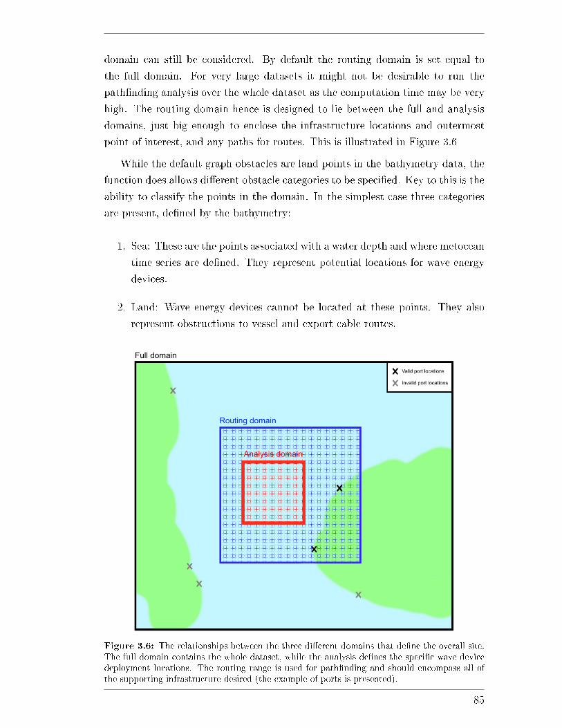
domain can still be considered. By default the routing domain is set equal to

the full domain. For very large datasets it might not be desirable to run the

path�nding analysis over the whole dataset as the computation time may be very

high. The routing domain hence is designed to lie between the full and analysis

domains, just big enough to enclose the infrastructure locations and outermost

point of interest, and any paths for routes. This is illustrated in Figure 3.6

While the default graph obstacles are land points in the bathymetry data, the

function does allows di�erent obstacle categories to be speci�ed. Key to this is the

ability to classify the points in the domain. In the simplest case three categories

are present, de�ned by the bathymetry:

1. Sea: These are the points associated with a water depth and where metocean

time series are de�ned. They represent potential locations for wave energy

devices.

2. Land: Wave energy devices cannot be located at these points. They also

represent obstructions to vessel and export cable routes.

Figure 3.6: The relationships between the three di�erent domains that de�ne the overall site.The full domain contains the whole dataset, while the analysis de�nes the speci�c wave devicedeployment locations. The routing range is used for path�nding and should encompass all ofthe supporting infrastructure desired (the example of ports is presented).

85

3. Coastline: These are land points that are nearest to the sea. They are

determined by iterating through the land points are looking for any that

have at least one sea neighbour.

These point classi�cations are stored in a global dictionary within the module,

allowing them to be easily used for di�erent path�nding applications and added

to. The ways that the point de�nitions are used to facilitate graph creation and

path�nding are discussed more in the next section.

3.5.2 Point locations

Within the model there are a number of objects which represent single geo-

graphic points in the domain, namely ports and cable landing points. It is useful

for these to have access to the parameters that de�ne the overall site (contained

within a WaveSite instance) so that they can use the underlying data for path�nd-

ing and distance calculation. As the nature of the path�nding calculation is the

same for these di�erent elements, it follows that they should be grouped by a

parent class.

The site point class, SitePoint, inherits from both GridPoint, discussed in

Section 3.4.6 and the Base class. It takes advantage of multiple inheritance.

Inheriting from GridPoint allows the point coordinates to be de�ned, and existing

methods utilised in order to constrain the coordinates to the speci�ed site grid,

where appropriate.

At initialisation, the coordinates de�ning the point location are de�ned. As

well as these, the user de�nes a site property; this is formatted upon input to

ensure that it is an instance of WaveSite and to try and convert it it is not.

The site_range attribute is a string which must correspond to the potential

range options that can be selected within WaveSite (namely the analysis range,

full range or routing range). This allows the point's grid ranges to be set to

the coordinate ranges of the site. Using only the analysis range will decrease

computation time, however often points outside the direct analysis range are of

interest so the routing range is the typical range that is chosen.

3.5.2.1 Calculating distances

The main reason for the class is to provide a framework for calculat-

ing distances from a single point to all of the analysis points in the do-

main, de�ned by the analysis extents of the input site. The instance method

graph_distances_to_point makes this possible through the following process:

86

1. Get the e�ective point coordinates: While any coordinates within the

site extents are technically valid for path�nding, sometimes it is necessary to

use coordinates which explicitly lie on the site domain grid. This is because

the input point needs at least one neighbour that is not an obstruction,

or else it is blocked in and cannot link up with the other graph nodes. A

common example is sheltered ports at coarser grid resolutions; the real world

coordinates might have no sea neighbours and hence vessel paths cannot be

resolved.

To use the nearest coordinates on the grid, the use_nearest_coordinates

property is speci�ed. This is a string which must match one of the

bathymetry categories introduced in Section 3.5.1. In this case, the co-

ordinates used as the starting point for the path�nding (the �e�ective coor-

dinates�) are those nearest to the input coordinates of the desired category.

2. Check that the coordinates are in the analysis range: The user-

de�ned coordinates must lie within the graphing range of the site, otherwise

the point's position relative to the site cannot be determined. If this condi-

tion is not met then a custom error is returned.

3. Get the site graph: The graph is obtained from the embedded site in-

stance using its get_site_graph method.

4. Add the e�ective coordinates to the graph: If the e�ective coordi-

nates are not contained within the graph then they must be added to allow

path�nding. This is necessary when the user has arbitrarily de�ned coor-

dinates not on the grid. This point is added by �nding the nearest grid

coordinates surrounding the point. These are stored as neighbours if they

match existing nodes in the graph, or else it is assumed that they are ob-

stacles. The e�ective coordinates and its neighbours are then added to the

graph dictionary in an identical format to the rest of the graph.

If the coordinates are already present in the graph, perhaps due to using

the use_nearest property, then this stage is skipped.

5. Perform the path�nding: Using the e�ective coordinates as the starting

point, the path�nding operation can be performed by applying Dijkstra's

algorithm to the modi�ed site graph. Two dictionaries are returned, with

the analysis coordinates as keys. The �rst contains the distances from the

analysis point to the e�ective point, which is converted into a NumPy array

by comparing the coordinates values with the embedded site analysis ranges

87

and getting the corresponding indices. The second dictionary stores the

successful paths, pairing each analysis point with its predecessor along the

resolved path.

With the distances to the analysis points obtained, spatial costs can be derived.

These processes are discussed in the proceeding sections. One �nal comment on

the site_point class is that both the input and e�ective coordinates can be

exported as vector point layers, for visualisation in GIS.

The functions have also been extended to consider multiple input points. The

static method find_nearest_points performs Dijkstra's algorithm for each in

turn, using a for loop. Each loop obtains an array of distances, which are then

compared at the end, and the NumPy package used to �nd the minimums.

88

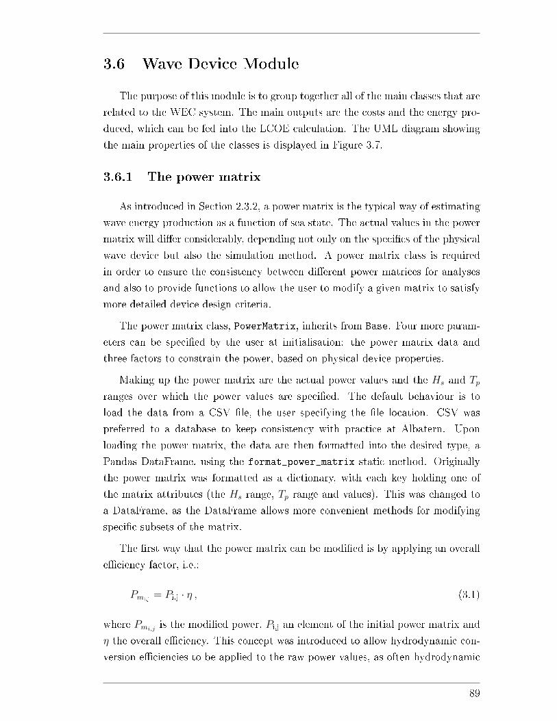
3.6 Wave Device Module

The purpose of this module is to group together all of the main classes that are

related to the WEC system. The main outputs are the costs and the energy pro-

duced, which can be fed into the LCOE calculation. The UML diagram showing

the main properties of the classes is displayed in Figure 3.7.

3.6.1 The power matrix

As introduced in Section 2.3.2, a power matrix is the typical way of estimating

wave energy production as a function of sea state. The actual values in the power

matrix will di�er considerably, depending not only on the speci�cs of the physical

wave device but also the simulation method. A power matrix class is required

in order to ensure the consistency between di�erent power matrices for analyses

and also to provide functions to allow the user to modify a given matrix to satisfy

more detailed device design criteria.

The power matrix class, PowerMatrix, inherits from Base. Four more param-

eters can be speci�ed by the user at initialisation: the power matrix data and

three factors to constrain the power, based on physical device properties.

Making up the power matrix are the actual power values and the Hs and Tpranges over which the power values are speci�ed. The default behaviour is to

load the data from a CSV �le, the user specifying the �le location. CSV was

preferred to a database to keep consistency with practice at Albatern. Upon

loading the power matrix, the data are then formatted into the desired type, a

Pandas DataFrame, using the format_power_matrix static method. Originally

the power matrix was formatted as a dictionary, with each key holding one of

the matrix attributes (the Hs range, Tp range and values). This was changed to

a DataFrame, as the DataFrame allows more convenient methods for modifying

speci�c subsets of the matrix.

The �rst way that the power matrix can be modi�ed is by applying an overall

e�ciency factor, i.e.:

Pmi,j= Pi,j · η , (3.1)

where Pmi,jis the modi�ed power, Pi,j an element of the initial power matrix and

η the overall e�ciency. This concept was introduced to allow hydrodynamic con-

version e�ciencies to be applied to the raw power values, as often hydrodynamic

89

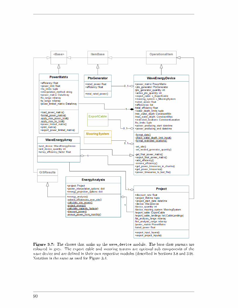
Figure 3.7: The classes that make up the wave_device module. The base class parents arecoloured in grey. The export cable and mooring system are optional sub components of thewave device and are de�ned in their own respective modules (described in Sections 3.8 and 3.9).Notation is the same as used for Figure 3.4.

90

simulations are performed under somewhat idealised conditions. In this case, the

device will be unable to capture all of this energy in reality as there are losses in

the mechanical system. Programatically the factor is a property of PowerMatrix,

so that only valid values can be set (between 0 and 1). This approach is mimicked

for other e�ciencies also de�ned in the model (for example for the device and

PTO generator classes described in the proceeding sections).

Secondly a maximum power limit can be applied to the power matrix data.

This is useful when considering a speci�c PTO generator, which will only be

able to extract power up to its rated value. If a power matrix value exceeds the

maximum speci�ed then it is curtailed and set to the maximum:

Pmi,j= min {Pi,j, Pmax} . (3.2)

The condition applies the maximum power, Pmax, in an element-wise manner to

the whole power matrix.

The last way that the values can be modi�ed is by de�ning the range of Hs

over which power can be extracted. This is achieved by de�ning power extraction

limits: cut-in and cut-out Hs values. For matrix values outside of these limits

(Hcut-in and Hcut-out), the power output is set to zero:

Pmi,j=

0 if Hsi≤Hcut-in ∨Hsi≥Hcut-out

Pi,j otherwise .(3.3)

Hence, putting the three expressions together leads to the overall modi�cation

being applied:

Pmi,j=

0 if Hsi < Hcut-in ∨Hsi > Hcut-out

min {Pi,j · η, Pmax} otherwise .(3.4)

The unmodi�ed input power matrix values are permanently stored within the

class instance. This means that the e�ciency values can be easily changed when

working within Python, safe in the knowledge that they are always being applied

to the original input data. The method power_limited_matrix returns a copy of

the power matrix with the power constraints applied; this is the matrix used for

estimation of the energy yield (the implementation of this calculation is discussed

in Section 3.6.2). Figure 3.8 gives an example of how the factors a�ect the values

in practice.

There is one �nal attribute that in�uences the energy calculation: the

91

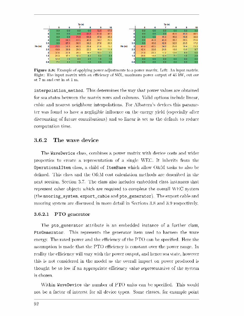
Figure 3.8: Example of applying power adjustments to a power matrix. Left: An input matrix.Right: The input matrix with an e�ciency of 85%, maximum power output of 45 kW, cut-outat 7 m and cut-in at 1 m.

interpolation_method. This determines the way that power values are obtained

for sea states between the matrix rows and columns. Valid options include linear,

cubic and nearest neighbour interpolations. For Albatern's devices this parame-

ter was found to have a negligible in�uence on the energy yield (especially after

discounting of future contributions) and so linear is set as the default to reduce

computation time.

3.6.2 The wave device

The WaveDevice class, combines a power matrix with device costs and wider

properties to create a representation of a single WEC. It inherits from the

OperationalItem class, a child of ItemBase which allow O&M tasks to also be

de�ned. This class and the O&M cost calculation methods are described in the

next section, Section 3.7. The class also includes embedded class instances that

represent other objects which are required to complete the overall WEC system

(the mooring_system, export_cable and pto_generator). The export cable and

mooring system are discussed in more detail in Sections 3.8 and 3.9 respectively.

3.6.2.1 PTO generator

The pto_generator attribute is an embedded instance of a further class,

PtoGenerator. This represents the generator item used to harness the wave

energy. The rated power and the e�ciency of the PTO can be speci�ed. Here the

assumption is made that the PTO e�ciency is constant over the power range. In

reality the e�ciency will vary with the power output, and hence sea state, however

this is not considered in the model as the overall impact on power produced is

thought be to low if an appropriate e�ciency value representative of the system

is chosen.

Within WaveDevice the number of PTO units can be speci�ed. This would

not be a factor of interest for all device types. Some classes, for example point

92

absorbers, might only contain one generator per device. The Albatern WaveNET

is capable of supporting up to three generators per Squid (one in each anti-node)

and for an array could contain extra units for redundancy. The two relevant

class attributes are pto_generator_quantity, which is a handle to the quantity

attribute of the embedded PTO object, and active_pto_quantity. This latter

number determines the device rated power; it is the number of PTOs that produce

power and must be less than the total PTO quantity. Lastly, sometimes a higher

level approach is desired without needing to think about the speci�cs of PTO

units. This can be achieved by de�ning the rated power attribute directly within

WaveDevice, which overrides the rated power calculated for the PtoGenerator

instance. This is useful for sensitivity studies, so that arbitrary rated powers can

be easily considered without needing to delve into the embedded object.

3.6.2.2 Energy production

To calculate energy production, the device requires two key attributes: a

power matrix and a site instance. Both of these are embedded objects, within

the power_matrix and site attributes, the reason so that the relevant meth-

ods can be easily exploited. Other optional attributes that can be speci�ed are

the start and end times for the power production (power_producing_start and

power_producing_end) and any power conversion e�ciencies in the PTO sys-

tem. An arbitrary number of e�ciency values can be speci�ed (optionally they

can be accompanied by strings describing the nature of the value, e.g. �hydraulic

losses�). Values can also be designated as �pre� or �post� generator depending on

where in the conversion process they occur. Values occurring before the genera-

tor are multiplied into to the power matrix e�ciency value, to be applied before

the power matrix is constrained by rated power. Post values are applied after the

power matrix is created, representing losses between the generator and connection

point.

The �rst step towards getting to energy is to obtain a power time se-

ries. This process is achieved using the instance method get_power_time

series_in_chunks. First, Hs and Tp time series are required. These can be

obtained from the embedded site instance for the time period of interest using

the methods described in Section 3.5.1. Once these are obtained, the data are

chunked according to the time axis. If the input metocean time series gets large,

the model will experience memory issues if it tries to load it all into memory at

once. This can range from large lag to completely crashing the running model.

The function allows the data to be chunked by year or by month, year is the

93

default as this has been su�cient for the examined datasets.

A for loop iterates through the chunks, loading each in turn and interpolat-

ing the sea state values against the power matrix. The interpolation is handled

by a separate function, get_power_time_series, to keep the code modular and

function length manageable. This takes in the Hs and Tp chunks, interpolates the

values against the constrained power matrix from the embedded power matrix

object to obtain the power time series. Device-level e�ciencies are applied to the

matrix prior to interpolation. Various NumPy operations are utilised here to re-

format the input arrays into the desired shape. The interpolation itself is achieved

using the griddata function from the SciPy interpolation package. While there are

alternative function options (notably the interp2 function from the same module),

griddata was found to be computationally quicker. The interpolation method that

is used is extracted from the power matrix's interpolation_method attribute.

Once the data are obtained they are reshaped into a new array to match the

dimensions of the original input data. If any of the array elements in the meto-

cean data are NaN then these are set to NaN in the power array too. Lastly a

new DataArray is created, linking the power values with the time and geographic

dimensions.

Once the power time series is obtained for the chunk then any time steps that

occur before the power producing start time or after the power producing end are

set to zero. For the resulting array there are two options available, speci�ed by the

user with the boolean variable sum_to_base. In the default True case, the power

values are summed for the chunk along the time axis to obtain a two-dimensional

energy. For example, a monthly chunk will lead to an array of monthly energy

production. Alternatively, no summation will take place and a power pro�le will

be returned. This latter functionality is more suitable for smaller datasets where

the power time series could �t comfortably in memory. Its main use is to obtain

a time series to be used as an input for the o�-grid sub-model; this application is

discussed more in Section 4.4.2.

The monthly energy time series can also be projected into the future, re-

quired when the project lifetime exceeds the amount of metocean data available.

This process is achieved within the overall analysis by using another class, the

EnergyAnalysis class, which is discussed in Section 3.6.4.

3.6.2.3 Calculating costs

Because the class inherits from ItemBase, local costs can be de�ned and calcu-

lated in the way described in Section 3.4.3. Device cost categories and quantities

94

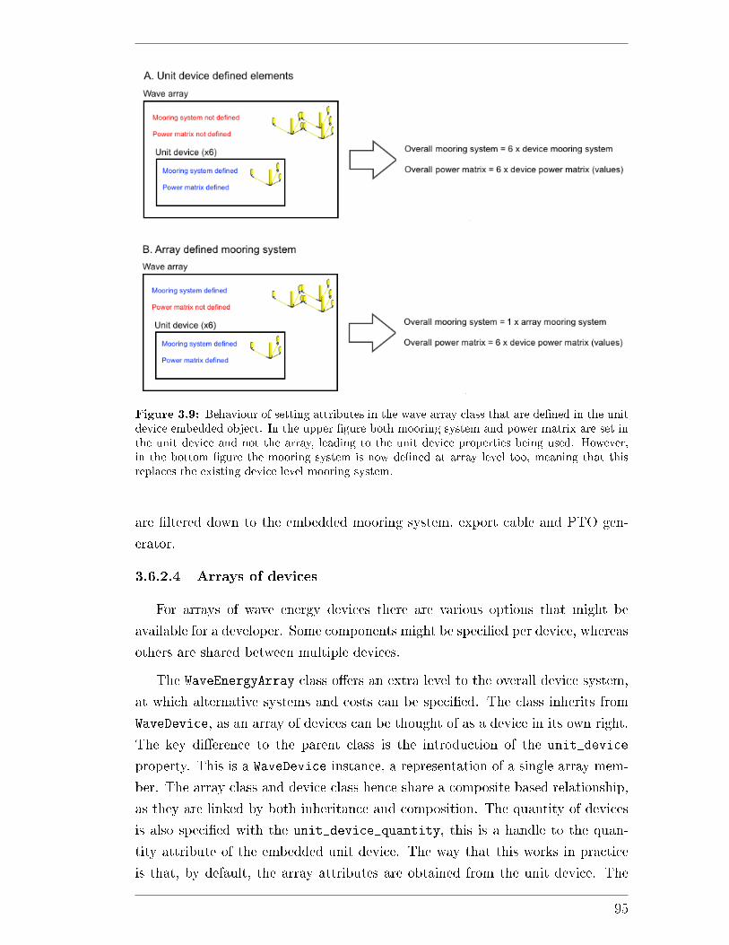
Figure 3.9: Behaviour of setting attributes in the wave array class that are de�ned in the unitdevice embedded object. In the upper �gure both mooring system and power matrix are set inthe unit device and not the array, leading to the unit device properties being used. However,in the bottom �gure the mooring system is now de�ned at array level too, meaning that thisreplaces the existing device level mooring system.

are �ltered down to the embedded mooring system, export cable and PTO gen-

erator.

3.6.2.4 Arrays of devices

For arrays of wave energy devices there are various options that might be

available for a developer. Some components might be speci�ed per device, whereas

others are shared between multiple devices.

The WaveEnergyArray class o�ers an extra level to the overall device system,

at which alternative systems and costs can be speci�ed. The class inherits from

WaveDevice, as an array of devices can be thought of as a device in its own right.

The key di�erence to the parent class is the introduction of the unit_device

property. This is a WaveDevice instance, a representation of a single array mem-

ber. The array class and device class hence share a composite based relationship,

as they are linked by both inheritance and composition. The quantity of devices

is also speci�ed with the unit_device_quantity, this is a handle to the quan-

tity attribute of the embedded unit device. The way that this works in practice

is that, by default, the array attributes are obtained from the unit device. The

95

exception to this are array level local costs, which are considered in addition to

any local costs within the unit device. With the unit quantity speci�ed, the pa-

rameters are equal to the unit device parameters multiplied by the number of

devices. For a single parameter, this behaviour is changed if it is explicitly set on

the array instance level. In this case the model uses the array level parameter, as

demonstrated in Figure 3.9. The properties that can be set at array level are the

mooring system, power matrix, export cable, rated power and generator quantity.

This array level is of particular signi�cance to Albatern because the device

modules are directly connected. They share a mooring system which reduces

costs, but also the power capture per unit has been shown to increase for smaller

arrays. This is because the characteristic length of the unit increases, improving

the power capture across a range of sea states. The result is a di�erent power

matrix that represents the whole array.

A limitation with considering the power calculation on the unit device level is

that it assumes that all devices are exposed to the same input metocean data at a

given location. In reality, particularly for a large and spread out farm, the devices

will see di�erent wave conditions which will result in more smoothed out power.

There are ways around this, for example by specifying an overall power matrix

at the array level with an assumption about smoothing built in. As the Albatern

device is very small relative to the metocean grid resolutions examined previously

this has not been an issue, but should be noted for larger devices, farms or smaller

data resolutions

3.6.2.5 Constraints

The physical properties of the wave device or array will have an in�uence on

the potential areas that it can be deployed in. The model allows constraints to

deployment to be examined and plotted in GIS. Within the device itself there are

two constraints built in: water depth limits and restricted locations. These, as

well as a description of how the overall analysis is carried out, are described in

Section 3.10.

3.6.3 Wave energy projects

The purpose of the Project class is to represent the entire grid-connected

wave energy project. It is essentially a container for the various objects that are

required to form estimates of energy, cost and LCOE. Keeping all of these elements

together in this way is bene�cial, as it gives a convenient way to de�ne and load

96

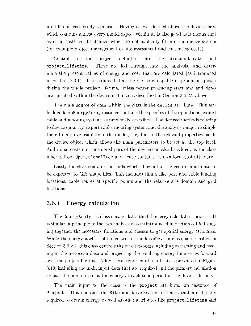
up di�erent case study scenarios. Having a level de�ned above the device class,

which contains almost every model aspect within it, is also good as it means that

external costs can be de�ned which do not explicitly �t into the device system

(for example project management or site assessment and consenting costs).

Central to the project de�nition are the discount_rate and

project_lifetime. These are fed through into the analysis, and deter-

mine the present values of energy and cost that are calculated (as introduced

in Section 2.3.1). It is assumed that the device is capable of producing power

during the whole project lifetime, unless power producing start and end dates

are speci�ed within the device instance as described in Section 3.6.2.2 above.

The main source of data within the class is the device attribute. This em-

bedded WaveEnergyArray instance contains the speci�cs of the operations, export

cable and mooring system, as previously described. The derived methods relating

to device quantity, export cable, mooring system and the analysis range are simple

there to improve usability of the model, they link to the relevant properties inside

the device object which allows the main parameters to be set at the top level.

Additional costs not considered part of the device can also be added, as the class

inherits from OperationalItem and hence contains its own local cost attribute.

Lastly the class contains methods which allow all of the vector input data to

be exported to GIS shape �les. This includes things like port and cable landing

locations, cable routes at speci�c points and the relative site domain and grid

locations.

3.6.4 Energy calculation

The EnergyAnalysis class encapsulates the full energy calculation process. It

is similar in principle to the two analysis classes introduced in Section 3.4.5, bring-

ing together the necessary functions and classes to get spatial energy estimates.

While the energy itself is obtained within the WaveDevice class, as described in

Section 3.6.2.2, this class controls the whole process including extracting and feed-

ing in the metocean data and projecting the resulting energy time series forward

over the project lifetime. A high level representation of this is presented in Figure

3.10, including the main input data that are required and the primary calculation

steps. The �nal output is the energy at each time period of the device lifetime.

The main input to the class is the project attribute, an instance of

Project. This contains the Site and WaveDevice instances that are directly

required to obtain energy, as well as other attributes like project_lifetime and

97

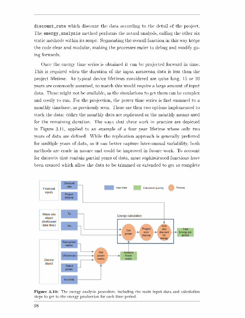
discount_rate which discount the data according to the detail of the project.

The energy_analysis method performs the actual analysis, calling the other six

static methods within its scope. Segmenting the overall function in this way keeps

the code clear and modular, making the processes easier to debug and modify go-

ing forwards.

Once the energy time series is obtained it can be projected forward in time.

This is required when the duration of the input metocean data is less than the

project lifetime. As typical device lifetimes considered are quite long, 15 or 20

years are commonly assumed, to match this would require a large amount of input

data. These might not be available, as the simulations to get them can be complex

and costly to run. For the projection, the power time series is �rst summed to a

monthly timebase, as previously seen. There are then two options implemented to

stack the data: either the monthly data are replicated or the monthly means used

for the remaining duration. The ways that these work in practice are depicted

in Figure 3.11, applied to an example of a four year lifetime where only two

years of data are de�ned. While the replication approach is generally preferred

for multiple years of data, as it can better capture inter-annual variability, both

methods are crude in nature and could be improved in future work. To account

for datasets that contain partial years of data, more sophisticated functions have

been created which allow the data to be trimmed or extended to get to complete

Figure 3.10: The energy analysis procedure, including the main input data and calculationsteps to get to the energy production for each time period.

98

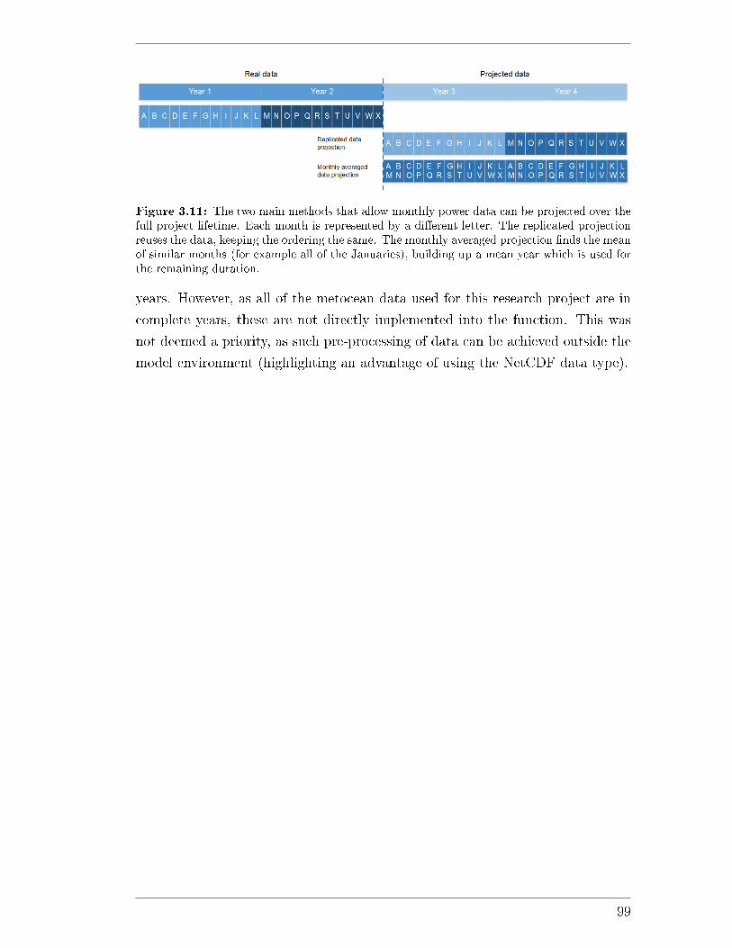
Figure 3.11: The two main methods that allow monthly power data can be projected over thefull project lifetime. Each month is represented by a di�erent letter. The replicated projectionreuses the data, keeping the ordering the same. The monthly averaged projection �nds the meanof similar months (for example all of the Januaries), building up a mean year which is used forthe remaining duration.

years. However, as all of the metocean data used for this research project are in

complete years, these are not directly implemented into the function. This was

not deemed a priority, as such pre-processing of data can be achieved outside the

model environment (highlighting an advantage of using the NetCDF data type).

99

3.7 Operations and Maintenance Module

The aim of this module is to allow the timescales and costs that are associated

with speci�c O&M activities to be calculated. These could include things like

installing the mooring system or recovering the devices to carry out scheduled

maintenance. The classes that have been created to facilitate this are displayed

in Figure 3.12. The module is only directly linked to two other modules: the

base_classes and wave_site (previously described in Sections 3.4 and 3.5). The

ItemBase class is required for cost calculations. Two classes from wave_site

are required: SitePoint to de�ne ports and WaveSite to de�ne the grid and

wave climate necessary for the calculations. The main O&M cost calculation is

performed within the MarineOperation class, the other classes providing input

data and methods to extend the functionality and improve usability.

It should be noted that the O&M module only supports planned operations.

Unplanned operations, required to �x WECs, are not directly supported. If the

time periods where failures occur were known then the MarineOperation class

could be used, however the model o�ers no way to calculate these. This and other

limitations of the research are presented and discussed in Section 3.11.

This section continues with a discussion of each class, detailing how each has

been structured and how they �t into the overall cost calculation.

3.7.1 Vessels

The vessel is an important consideration for any marine operation, to ensure

that it can be carried out in a safe and cost e�ective way. The properties of the

vessel will have a signi�cant impact on how well O&M tasks can be performed

and the weather windows that are required. Within the model the physical vessels

are represented by the Vessel class, containing a number of attributes that are

important for the cost calculation performed within MarineOperation.

As for previous classes, Vessel inherits from ItemBase. This means that local

costs can be de�ned, for example the cost required to �t equipment onto the vessel

to carry out its duties. These are one-o� costs (unless cost periods are speci�ed by

the user); costs that recur for each operation must be de�ned within the overall

charter rate.

This charter rate, charter_cost, is one of four unique cost attributes that

can be de�ned, the others being standby_cost, mob_cost (mobilisation cost)

100

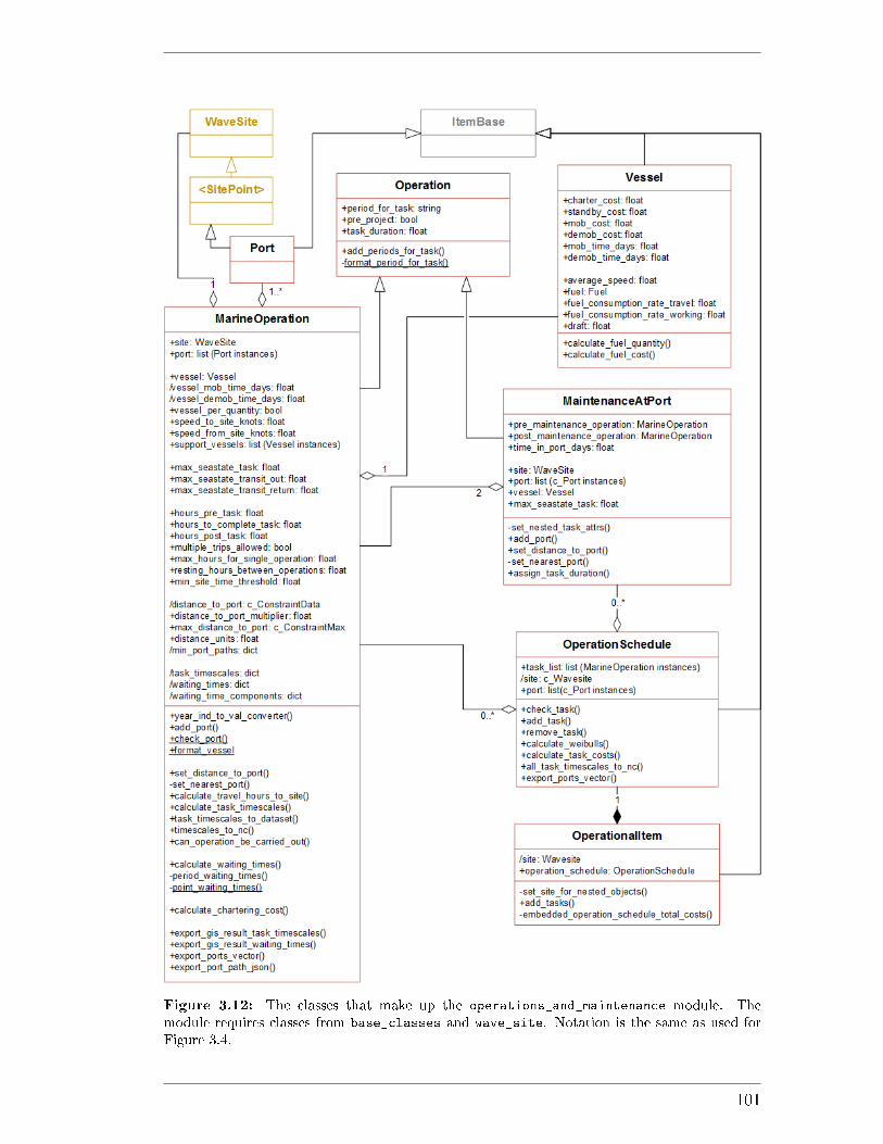
Figure 3.12: The classes that make up the operations_and_maintenance module. Themodule requires classes from base_classes and wave_site. Notation is the same as used forFigure 3.4.

101

and demob_cost (demobilisation cost). They are all properties, formatted prior

to being set using the add_local_costs method from the ItemBase parent class.

This means that they are stored within the instance's local costs attribute, so

that they can be included in the cost category aggregation as described in Section

3.4.3. They are all speci�ed in units of days. Longer term options, for example

monthly or annual charter, can also be de�ned but would be speci�ed as recurring

local costs.

The charter and standby costs are important as they are multiplied by

task timescales calculated within the MarineOperation class to obtain charter

cost estimates. This di�ers to the the mobilisation and demobilisation costs,

where the times are speci�ed within the vessel directly (mob_time_days and

demob_time_days) and are considered to apply equally across the whole domain.

While spatially varying numbers could be estimated using path�nding algorithms

over a global dataset, it would be a largely trivial improvement in functionality as

better estimates could be supplied by vessel hire companies themselves (for given

ports).

The average_speed attribute de�nes how quickly the vessel can travel to

site. This also feeds into the calculated charter time, discussed in Section 3.7.4.

The fuel consumed by the vessel while performing its duties is split into two

components: fuel_consumption_rate_travel for the fuel used while travelling

and fuel_consumption_rate_working for the fuel used while working. The lat-

ter attribute could include aspects like vessel station keeping, vessel movement

around the site and the fuel required to operate any on-board machinery. The

fuel quantity consumed for a given number of hours, F , can be calculated with

the calculate_fuel_quantity method. This takes the travel and working times,

ttravel and twork, and multiplies by the relevant fuel consumption rate directly:

F = Rtravelttravel +Rworktwork . (3.5)

Using this and the fuel attribute, an instance of Fuel, the fuel cost can be

calculated using the calculate_fuel_cost method. The calculated fuel quan-

tity is assigned to the quantity attribute of the fuel instance's cost_per_ltr

attribute, ensuring that the categorised costs propagate through. To provide �ex-

ibility the fuel and two fuel consumption rate attributes are optional. Within the

MarineOperation class the fuel consumption will only be calculated if both are

speci�ed. This allows fuel cost to be ignored if not of interest or if it is considered

within the overall charter cost.

102

The �nal attribute for the vessel class is the draft. This is the physical length

of the vessel below the waterline, and e�ectively de�nes the minimum water depth

that the vessel can traverse on its journey to site. This is considered when creating

graphs from the ports to the sites.

3.7.2 Ports

The port is the second main element associated with the operation. This

representation of the physical port is where the operation vessel (or vessels) is

harboured, and assumed to contain the main workshop where onshore repairs are

carried out. As di�erent port instances can be speci�ed for di�erent tasks, dis-

tinction can be made between a major port for installation activities and smaller

operations ports which might be set up closer to the device deployment site.

The Port class, inherits from the SitePoint class from the wave_site module

and the ItemBase class from the base_classesmodule. This multiple inheritance

is required so that local costs can be de�ned for the port (for example workshop

rental and equipment hire fees) and path �nding algorithms can be used to de-

termine distances to the sites using methods de�ned in SitePoint (introduced in

Section 3.5.2.1).

The only modi�cation to the port child class is in the

graph_distances_to_point method. If the port is in a particularly shel-

tered location, the parent method might fail as the neighbouring grid points are

land and there is no path to the wider graph. This occurs as a consequence of

the data resolution. To avoid this problem the method is contained within a

try/except block. If a path cannot be found, a graphing error is returned and

the nearest coastline point will be considered as the port location instead. This

process is demonstrated in Figure 3.13, considering Stornaway Port and some

sample site data. The actual location of Stornaway port is isolated in relation

to the domain, surrounded by points in the domain that are de�ned as land.

Because the four nearest neighbours are land, routes to the sea points cannot be

resolved. Hence, in this circumstance the port class uses the nearest coastline

point for any pathing analysis, a point which is linked to the wider dataset by the

bottom left most sea point. For the example this is only 1.4 km away from the

original point, a negligible distance in terms of both time and fuel consumption.

Something to note is that this reassignment of the port location is only necessary

if the data resolution is not su�cient. If higher resolution data are used then this

issue would not arise.

103

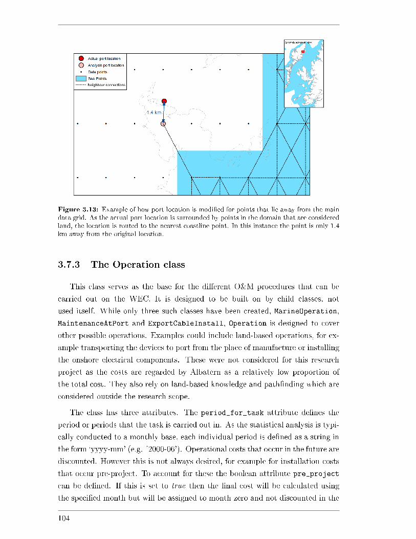
Figure 3.13: Example of how port location is modi�ed for points that lie away from the maindata grid. As the actual port location is surrounded by points in the domain that are consideredland, the location is routed to the nearest coastline point. In this instance the point is only 1.4km away from the original location.

3.7.3 The Operation class

This class serves as the base for the di�erent O&M procedures that can be

carried out on the WEC. It is designed to be built on by child classes, not

used itself. While only three such classes have been created, MarineOperation,

MaintenanceAtPort and ExportCableInstall, Operation is designed to cover

other possible operations. Examples could include land-based operations, for ex-

ample transporting the devices to port from the place of manufacture or installing

the onshore electrical components. These were not considered for this research

project as the costs are regarded by Albatern as a relatively low proportion of

the total cost. They also rely on land-based knowledge and path�nding which are

considered outside the research scope.

The class has three attributes. The period_for_task attribute de�nes the

period or periods that the task is carried out in. As the statistical analysis is typi-

cally conducted to a monthly base, each individual period is de�ned as a string in

the form `yyyy-mm' (e.g. '2000-06'). Operational costs that occur in the future are

discounted. However this is not always desired, for example for installation costs

that occur pre-project. To account for these the boolean attribute pre_project

can be de�ned. If this is set to true then the �nal cost will be calculated using

the speci�ed month but will be assigned to month zero and not discounted in the

104

subsequent cash �ow analysis. The two class methods, add_periods_for_task

and format_period_for_task, give a convenient way to add new periods into an

initialised class instance and ensure that the data formatting is consistent.

The task_duration is the total time to complete the operation. Is it a dic-

tionary, with a value de�ned for each time period that the task occurs in. For the

Operation class it is just a placeholder, but is used in the child classes.

3.7.4 Marine operations

The MarineOperation class is the most important in the module, as it contains

the attributes and methods that are used to calculate the timescales and hence

costs associated with speci�c tasks. It de�nes a single operation that involves

making a trip out to site, made up of the following stages:

1. A vessel waits in port for a suitable weather window to carry out the task

(in standby).

2. The vessel travels to the site.

3. Some operation is carried out on site.

4. The vessel returns to the original port.

Tasks that involve maintenance in port require two trips out to site: recovery

and redeployment of a device. These are modelled using the MaintenanceAtPort

class, which builds on the methods presented in this section and is described in

Section 3.7.5.

The spatial aspect of the class is in calculation of the vessel standby and charter

costs, generally regarded as major components of the overall operation cost. As

it inherits from ItemBase, additional costs can be added as local costs. Examples

could include costs of spare parts or project management overheads.

To calculate the spatial costs, �rst the timescales associated with the task are

calculated. For each analysis point in the domain this is the time to travel to and

from the point, and the time to wait for a suitable weather window to perform the

operation. From these, the charter costs are calculated by multiplying the task

time required by the vessel charter rate and the waiting time by the vessel standby

rate. These processes are achieved using methods within MarineOperation and

are discussed in more detail in Sections 3.7.4.3 to 3.7.4.5.

105

3.7.4.1 Key attributes

There are �ve compulsory attributes that must be speci�ed to obtain spatial

cost estimates for the task:

• The site of interest (a WaveSite instance).

• A vessel to carry out the operation (a Vessel instance).

• One or more port options, where the operation starts and �nishes (Port

instances).

• The time to complete the task.

• The time period (or periods) when the operation is carried out.

The site is used for two purposes: to determine the distances from the port to

the sites and to provide the metocean data for weather window estimation. The

relevant methods are coded within the WaveSite class (see Section 3.5.1). The

distances are stored within the distance_to_port attribute.

While only a single vessel is used to compute the task timescales, multiple

ports can be speci�ed using a list of Port instances. This is to preserve the

model applicability over large areas, by allowing ports to be de�ned for localised

regions of the domain. The model e�ectively optimises the task port by dis-

tance, for a given point choosing the closest port for the cost analysis using the

find_nearest_points static method described in Section 3.5.2.1. Future be-

haviour could be to optimise by cost instead, as di�erent ports will charge dif-

ferent rates for usage, however this is not deemed a key feature (and would be

straightforward to achieve by comparing output results for single ports) so has

not been considered for this research.

At site, the time to complete the task is de�ned by three attributes:

1. The time on site required to set up any equipment prior to commencing

work (hours_pre_task).

2. The time to carry out the actual task (hours_to_complete_task).

3. The time that it takes to prepare the vessel for travel back to port

(hours_post_task)

While the pre and post times could be incorporated into the overall task com-

pletion time, they are kept separate to allow for greater �exibility. This is espe-

cially useful for the export cable installation class, ExportCable, where the task

106

time is spatially dependent but the pre and post task times generally would not

be. This class is discussed in Section 3.8.2.

The waiting time for weather windows is calculated using the max_sea

state_task. As this calculation is the slowest part of the code it is not a com-

pulsory element, however is recommended to get an overall re�ection of the site

speci�c metocean conditions.

The attribute de�nes the maximum sea state that the operation can be per-

formed in. For real operations there are many factors that would be taken into

account, including wave period and wind speed. However, the weather window

analysis for this model only considers signi�cant wave height as a metric. This de-

cision was taken because it is usually regarded as the most signi�cant factor [85,87]

and the thresholds are better understood (in Albatern's case the wind speed and

period thresholds have not been quanti�ed and would be largely hypothetical).

Any locations where the weather window required exceeds the time available in

the month are �ltered out of the analysis, as it is physically impossible to perform

the necessary operation. This is carried out when calculating the costs, and is

discussed more in Section 3.7.4.5.

The task_timescales and waiting_times attributes store the results of the

timescale calculations. They are dictionary types, and hence the data can be

easily exported to NetCDF or raster �les.

3.7.4.2 Other attributes

As well as those described above, there are also minor attributes that in�uence

how the task timescales and costs are calculated.

In the default case the vessel instance's average_speed is used to compute

the timescales. Di�erent speeds can also be speci�ed with speed_to_site_knots

and speed_from_site_knots. These are required when the vessel speed might

be limited, for example when towing a device to site, and also have implications

for operation waiting time calculation.

The vessel_per_quantity attribute has implications for multiple operations

de�ned within a single MarineOperation class instance. This is set through the

quantity attribute, inherited from ItemBase. Multiple operations in a single

time period could mean one of two things:

1. One vessel is used for all the operations.

2. Each operation is carried out by its own vessel.

107

While the options are assumed to have the same cost associated with them, there

is a di�erence in the time available for the operation. Using the example of six

identical operations in the month of January, one vessel would have 31 days to

complete all six tasks. Alternatively, six vessels would each have 31 days to do

one task, a more relaxed deadline. This in�uences which points are excluded at

the cost calculation stage and also the mobilisation costs (as this is incurred for

each vessel assumed).

As well as the main vessel, support vessels can also be de�ned by specifying a

list of Vessel instances. These represent smaller vessels like Rigid-Hulled In�at-

able Boats (RHIB) that are chartered to assist the task at hand. They are treated

di�erently to the main vessel. Timescales are not calculated for these vessels, they

use those calculated for the main vessel. For example if the main vessel is found

to require two days of charter and three days of waiting then the support vessel

will also assume these times, using its own cost rates to obtain overall costs.

There are two further sea state thresholds that are optional. The max_sea

state_transit_out and max_sea state_transit_return attributes allow Hs

thresholds to be set for transit to and from site. The main application for this is

for operations where the wave device is towed to site, as this will require calmer

conditions. Following the methodology of Walker [88], weather window analysis

is performed for each component separately and the results summed. Results are

stored in the waiting_times_components attribute. More information on these

is provided in Section 3.7.4.4.

There are several attributes that control how the task timescales are calculated.

The max_hours_for_single_operation quantity de�nes the maximum number

of hours that are available to carry out the task, including travel to and from

the site. If the task cannot be completed in this time (excluding waiting time)

then there are two di�erent options. The multiple_trips_allowed attribute

determines whether or not the operation can be carried out over multiple trips. If

False then the task must be carried out in a single journey; it cannot be carried

out if the time required for the task exceeds the maximum number of hours. If

True then the task can, in theory, be carried out all over the domain (subject

to waiting time), although might require multiple round trips. In this case, the

time that elapses between arriving back at port and heading back out to the site

can be set with the resting_hours_between_operations attribute which adds

to the charter time that is required. Finally, the min_site_time_threshold

attribute can be speci�ed to screen out sites at more extreme distances. Without

this attribute, for longer multiple trip operations the issue arises where valid

108

sites furthest from the port would require very large numbers of round trips to

complete the task, as once the vessel has travelled it has very little time to actually

complete the task at hand. Such situations are both unrealistic and increase the

computation time. The attribute screens out these sites when calculating the

task timescales: if the time available for the task after travelling is less than the

attribute then it is �ltered out.

Lastly, there are two attributes which concern the port distances stored within

distance_to_port. The distance_to_port_multiplier attribute is a modi�-

cation factor that is applied to the calculated distances prior to the calculation of

task timescales. This can be used to account for uncertainty in the distances cal-

culated but is set to a value of one by default. The second is a distance constraint,

max_distance_to_port. This can be assigned to the operation class which allows

points that are too far away to be easily identi�ed and �ltered out in GIS (see

Section 3.10 for a description of constraints).

3.7.4.3 Calculating task timescales

As previously stated, the calculations that underpin the cost analyses re-

quire calculating the timescales associated with distinct tasks. The main cost

drivers incorporate a time dependence, i.e. vessels are commonly chartered

on a daily rate, which allows cost estimates to be built up. The method

calculate_task_timescales is used to calculate these timescales, with the ex-

ception of weather window waiting time that is described in the next section.

For a particular operation, the total time required to carry out the task at a

particular point (x, y) is expressed as:

ttask(x, y) = ttravel(x, y) + tsite + twaiting(x, y) + tresting . (3.6)

Here ttravel is the total time to travel to and from the point, tsite is the time spent

on site carrying out the task and twaiting is the average time spent waiting for a

suitable weather window. tresting is the time resting between operations if multiple

trips to site are required. All quantities are considered in units of hours.

The travel time is estimated by calculating the time to get to and from site,

tto and tfrom and multiplying by the number of round trips needed until the task

is completed, Nrt :

ttravel(x, y) = Nrt [tto(x, y) + tfrom(x, y)] . (3.7)

109

The parameter Nrt depends on the number of hours that are available for a single

operation. In the default case, the variables tto and tfrom are calculated by mul-

tiplying the distance from a speci�ed port, dport, by the average transit speed of

the vessel that is carrying out the task, vav :

tto(x, y) = tfrom(x, y) = vavdport(x, y) . (3.8)

As the vessel speed is the same in both directions they are considered equal. Al-

ternatively, if the speed_to_site_knots or speed_from_site_knots attributes

are de�ned, vto and vfrom, then the timescales are calculated as:

tto(x, y) = vtodport(x, y) (3.9)

tfrom(x, y) = vfromdport(x, y) . (3.10)

The port distances are calculated using the set_nearest_port method, which

runs Dijkstra's algorithm on the site instance with the port locations as starting

locations (as described in Section 3.5.2.1).

As the time on site required to carry out the operation, tsite, is de�ned directly,

it is independent of location in the current model. This could be made spatially

dependent in future to account for the fact that operations may take longer in

more exposed locations, where conditions could be more challenging.

Within the class, the task timescale results are stored together as a dictionary

within the task_timescales attribute. This includes the following components:

• The travel hours to site.

• The total hours on site.

• The total hours travelling.

• The number of round trips.

• The total hours required for the operation, excluding waiting time.

• The window lengths that are required at each location, for each trip required

to site.

The window lengths are used to calculate the waiting time for each individual trip

required out to site. This procedure is discussed in the next section.

110

3.7.4.4 Calculating waiting time

To calculate waiting times the model incorporates the frequency based ap-

proach of Kuwashima and Hogben [86], as introduced in Section 2.3.3.1. This

process �rst involves creating a joint occurrence matrix for every point in the anal-

ysis domain for every month of interest (as de�ned within the period_for_task

attribute). For each ascending Hs bin with edge value Hb, the probability that a

given sea state will exceed the bin, Ph, is calculated as:

Ph(Hb) =CHs>Hb

(Hb)

CT, (3.11)

where CHs>Hbis the number of recorded sea states in the matrix above the bin

and CT is the total number of sea states in the time period. Ph is known as the

exceedance probability and can also be approximated by a 3-parameter Weibull

distribution for a given threshold signi�cant wave height, Hac :

Ph(H > Hac) = exp

(−(Hac −X0

b

)k). (3.12)

The parameters k, b and X0 are the shape, scale and location parameters respec-

tively. From initial values (by default k = 1.5, b = 1.5 and X0 = min(Hs)− 0.05),

they are then adjusted to get as good a �t to the raw distribution as possible

(Equation 3.11). This is done using using an iterative least squares method from

the SciPy statistical Python package.

Once they are obtained, the average window length at a particular Hac can be

found:

τac(Hac) =1− Ph(Hac)

Ph(Hac)· A

[− ln(Ph(Hac))]β, (3.13)

where the constants A and β are functions of a separate factor γ, calculated from

the Weibull parameters:

A =35√γ

(3.14)

β = 0.6γ0.287 (3.15)

γ = k +1.8X0

(H̄ −X0)(3.16)

H̄ = bΓ

(1 +

1

k

)+X0 . (3.17)

111

Given these quantities, the probability that wave conditions less than the thresh-

old will persist for at least a desired duration Xac can be calculated:

Pt(Xi > Xac) = exp (−Cac(Xi)αac) , (3.18)

where:

Cac =

[Γ

(1 +

1

αac

)]αac

(3.19)

αac = 0.267γ

(Hac

H̄

)−0.4

. (3.20)

The value Xac can be thought of as the length of weather window required, which

is calculated using the calculate_task_timescales method from the above sec-

tion.

The overall probability of a weather window occurring in the time period

conforming to both the Hs threshold and duration required is equal to:

P (T > τac) = Ph(H > Hac) · Pt(Xi > Xac) . (3.21)

Hence, the number of days that the site can be accessed in the time period, Nac,

and the average number of days required to wait for a suitable weather window,

twaiting, can be determined by also considering the total duration of the time

period in days, Dm:

Nac = Dm · P (T > τac) (3.22)

twaiting =

Dm−NacτacNac

twaiting ≤ Dm

Dm twaiting > Dm

(3.23)

Of these quantities twaiting is the main output of interest, as it represents the

average time that the vessel will be on standby to carry out the operation within

the month. The number of waiting days cannot exceed that available in the

month; in this case twaiting is set to D, with these locations �ltered out of the

analysis in the cost calculation step.

The above formulae are coded into the class within the

calculate_waiting_times method. The joint occurrence matrices are created

for each time period and analysis location using the site_joint_matrices

method of the embedded Site instance. Next the Weibull �tting parameters

are calculated as above. From these, the waiting time for each time period and

112

point are found by calling the private functions period_waiting_times and

point_waiting_times.

If Hs thresholds are speci�ed for the transit to and from site, max_sea

state_transit_out and max_sea state_transit_return, then the above pro-

cess is repeated for each of these. This gives three components of the waiting

time. The resulting waiting times are then added to that for the task itself to

get the total waiting time, as recommended in [88]. For the transit operations

the metocean conditions at the site are used to estimate the weather window,

assumed representative of the journey to site as a whole.

The total waiting times for each time period are stored together in the

waiting_times attribute. This is a dictionary: each key being a di�erent time

period and each corresponding value a NumPy array of the waiting times. For

locations where multiple trips to site are required to carry out the operation in

a given time period, the waiting times are calculated for each trip required and

summed to get a total waiting time.

The three waiting time components are stored within the

waiting_times_components attribute. This is so the �nal results can be

dissected and the most in�uential factor determined.

3.7.4.5 Calculating task costs

Once the task timescales are obtained, the vessel charter costs are calculated.

The method calculate_chartering_cost carries out this step and also calls

the other two calculations automatically if no timescales have been set (i.e. the

task_timescales attribute is None). The standby cost for the operation in a

given month m is calculated by multiplying the waiting time (rounded down to

the nearest day) by the vessel standby cost per day cs:

Cstandby(m,x, y) = cstwaiting(m,x, y) . (3.24)

The working charter cost is equal to the vessel charter cost cc multiplied by the

time that the vessel is working (i.e. the sum of ttravel and tsite):

Ccharter(x, y) = cc [ttravel(x, y) + tsite] . (3.25)

The total fuel cost is calculated from the transit and working contributions:

Cfuel(x, y) =B∑b=1

cf [Rt(b)ttravel(x, y) +Rwork(b)tsite] . (3.26)

113

Here cf is the fuel cost per litre. For each vessel b involved in the operation (the

main vessel and any supporting vessels), the fuel consumption is calculated using

the relevant timescales, where Rtravel and Rwork are the fuel consumption rate

attributes for travelling and working respectively.

Both Ccharter and Cfuel are spatially dependent, however are assumed to be

the same for each operation time period. This means that the cost associated

with vessel hire in a given month is equal to:

Cm(m,x, y) = Cstandby(m,x, y) + Ccharter(x, y) + Cfuel(x, y) (3.27)

Cv(m,x, y) =

Cm(m,x, y) ttask,d(m,x, y) ≤ Dm(m)

inf ttask,d(m,x, y) > Dm(m), (3.28)

where ttask,d(m,x, y) is the total time that the vessel is required in the month,

in days, as de�ned in Equation 3.6. If the total time exceeds that available in

the month then the operation cannot physically occur, and is assigned a value of

Inf. This value can be detected in the GIS raster outputs, so these regions can be

easily identi�ed.

For operations carried out over multiple periods it is useful to be able to

see, for a given point, the time period where the maximum task times occur.

This is because particularly stormy months might signi�cantly shrink the size

of the domain. The maximum task times over the periods are calculated within

calculate_chartering_cost, as well as the speci�c time periods where the max-

imums occur. These can then be visualised in GIS, as demonstrated in Figure 3.14.

In this example the time periods (19, 3) and (10, 3) incur the longest time penal-

ties to the west of Lewis and Harris. From this information these months could be

manually substituted for other months to see if the domain could be made larger.

The monthly vessel totals are then summed and added to any non spatial costs

Cns to obtain the total cost for all of the months speci�ed:

Cop total(x, y) = Cns +

mT∑m=m0

Cv(m,x, y) . (3.29)

Examples of non spatial costs include vessel mobilisation and demobilisation costs,

cm and cd respectively, any local costs of the MarineOperation instance (Copl) and

any local costs of the port instance (Cport):

Cns = cmtm + cdtd + Copl + Cport . (3.30)

114

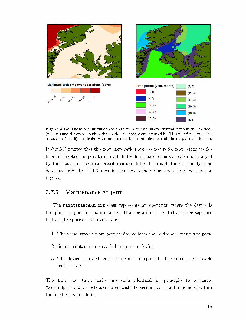
Figure 3.14: The maximum time to perform an example task over several di�erent time periods(in days) and the corresponding time period that these are incurred in. This functionality makesit easier to identify particularly stormy time periods that might curtail the output data domain.

It should be noted that this cost aggregation process occurs for cost categories de-

�ned at the MarineOperation level. Individual cost elements are also be grouped

by their cost_categories attributes and �ltered through the cost analysis as

described in Section 3.4.3, meaning that every individual operational cost can be

tracked.

3.7.5 Maintenance at port

The MaintenanceAtPort class represents an operation where the device is

brought into port for maintenance. The operation is treated as three separate

tasks and requires two trips to site:

1. The vessel travels from port to site, collects the device and returns to port.

2. Some maintenance is carried out on the device.

3. The device is towed back to site and redeployed. The vessel then travels

back to port.

The �rst and third tasks are each identical in principle to a single

MarineOperation. Costs associated with the second task can be included within

the local costs attribute.

115

To model the three tasks, the class contains three unique attributes. The

pre_maintenance_operation and post_maintenance_operation attributes de-

�ne tasks 1 and 3 above. These are MarineOperation instances, taking advantage

of all the existing class functionality.

The time_in_port_days attribute, tport de�nes how long the port mainte-

nance takes. This is used to apply the operation time constraint. As for the

MarineOperation class, the maintenance at port must be carried out in a single

month. The total time to carry out the operation is:

tMaP = ttask1 + tport + ttask2 . (3.31)

As for the MarineOperation class, the total time to carry out the three tasks,

tMaP, cannot physically exceed the time available in the month. This means that

the total cost in a given month, CTMaP is calculated as:

J(m,x, y) = Ctask1(m,x, y) + Clocal(m) + Ctask2(m,x, y) (3.32)

CTMaP(m,x, y) =

J(m,x, y) tMaP(m,x, y) ≤ Dm(m)

inf tMaP(m,x, y) > Dm(m) ,(3.33)

where Ctask1 is the cost of the operation to site, Clocal the class instance's local

costs, including port maintenance costs, and Ctask2 is the cost of redeploying the

device at site.

To achieve the cost calculation, the inherited categorised_local_costs class

method is modi�ed, calling the categorised_local_costs method for the two

embedded MarineOperation classes and then applying the time constraint as

described above. The four remaining class attributes, as shown in the UML,

are included for convenience (site, port, vessel and max_sea state_task).

They can be set at the class level and are then assigned to the two embedded

MarineOperation classes at runtime with the _set_nested_task_attrs private

method. This is also the case for the period_for_task and pre_project at-

tributes inherited from Operation.

3.7.6 Operation schedule

When considering larger arrays or more complex operational tasks it is not

practical to have to de�ne the inputs for each individual task, especially where in-

put quantities like the vessel or port are shared among multiple tasks. In addition,

repeating the task timescale calculations among similar tasks can greatly increase

116

the computation time. The OperationSchedule class is essentially a group of

tasks and has been developed to mitigate these problems.

The most important attribute of this class is task_list, a list contain-

ing all of the task instances. Tasks can be instances of MarineOperation,

MaintenanceAtPort or other instances of OperationSchedule, this latter ability

allowing schedules to be easily combined. Tasks can be added or removed from

the list using dedicated instance methods (add_task and remove_task), which

can be useful when scripting or debugging within Python. The real advantage

in storing multiple tasks together is that certain operation attributes can be de-

�ned in the schedule which are then applied to all of the task_list members at

calculation runtime. These attributes are:

• The site.

• The vessel.

• The port.

• The time period that the operations take place in.

It is mandatory that the same site (WaveSite instance) is de�ned for every task.

The schedule class gives a convenient way of ensuring that this is the case, using

the private method _assign_site_to_tasks which is initiated upon setting the

site property. The other three attributes do not have to be the same across

multiple task instances but commonly might be. Examples of these scenarios

could include a group of installation tasks that occur in the same time period or

a single operational port from which all tasks are carried out from.

For a single operation, calculating the Weibull parameters is a particularly

time consuming part of the task timescale calculation process. For tasks that

are carried out within the same time period it does not make sense to perform

these calculations multiple times. The calculate_weibulls method reduces the

computation time in these situations. The time period for each task within

task_list is extracted into a list, with any duplicated entries removed. The

function then iterates through these time periods, obtaining the joint matrices

and Weibull parameters as described in Section 3.7.4.3. A dictionary of the form

{< period >:< weibulls >} allows the parameters to be matched to the corre-

sponding tasks prior to calculating the waiting times.

The calculate_task_costs method gives a straightforward way to calculate

all of the task costs: looping through each task and performing the calculations

described in Sections 3.7.4.3 to 3.7.4.5.

117

3.7.7 Assigning operations to items

The operational item class, OperationalItem, combines the important

ItemBase class with an operation schedule instance to de�ne a cost object which

has some operational tasks associated with it.

As a child of ItemBase it inherits all of the methods related to embedded cost

calculation. The main di�erence is that there are two new inputs to be speci�ed

at initialisation: a site attribute and an operation_schedule attribute. Both

of these must be instances of the respective classes. Setting the site property for

the operational item will automatically set it for the embedded operation schedule

too.

To prevent double counting of task costs, the get_embedded_costs method

is modi�ed. Because the categorised_local_costs method of the operation

schedule calculates task costs, the risk is that the default function would get

the task (and task embedded object) costs twice. To mitigate this problem, the

function uses the following process:

1. The usual local and embedded cash �ows within the operational item object

are calculated and extracted (as in Section 3.4.3), but with the the embedded

operation schedule and operation items omitted.

2. The operation schedule's embedded costs are obtained with the pri-

vate method embedded_operation_schedule_total_costs. This uses the

methods described in Section 3.7.4 and 3.7.6 to obtain cash �ows for all of

the operational tasks speci�ed. The function makes sure to only get oper-

ation schedule or operation embedded instances, to prevent items from the

last step being included again.

3. Both sets of cash �ow outputs are combined to get all of the embedded

costs. This means that the overall categorised cash �ows can be obtained

as previously described in Section 3.4.3.

118

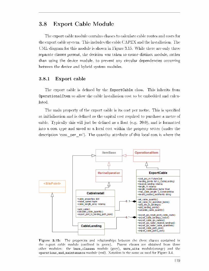
3.8 Export Cable Module

The export cable module contains classes to calculate cable routes and costs for

the export cable system. This includes the cable CAPEX and the installation. The

UML diagram for this module is shown in Figure 3.15. While there are only three

separate classes present, the decision was taken to create distinct module, rather

than using the device module, to prevent any circular dependencies occurring

between the device and hybrid system modules.

3.8.1 Export cable

The export cable is de�ned by the ExportCable class. This inherits from

OperationalItem to allow the cable installation cost to be embedded and calcu-

lated.

The main property of the export cable is its cost per metre. This is speci�ed

at initialisation and is de�ned as the capital cost required to purchase a metre of

cable. Typically this will just be de�ned as a �oat (e.g. 20.0), and is formatted

into a cost type and saved as a local cost within the property setter (under the

description `cost_per_m'). The quantity attribute of this local cost is where the

Figure 3.15: The properties and relationships between the three classes contained inthe export cable module (outlined in green). Parent classes are obtained from threeother modules: the base_classes module (grey), wave_site module(orange) and theoperations_and_maintenance module (red). Notation is the same as used for Figure 3.4.

119

actual length of cable is stored and used for calculation. This is not set but rather

calculated from the site and cable landing properties.

Cable landing points on shore are de�ned within the attribute

landing_points. There are two options for landing points. If no points

are speci�ed (i.e. the landing point attribute is set to None) then the model

will assume that the cable travels the shortest distance to shore for each site

analysis point. This approach is seen in the literature (for example [133]) and

gives a useful way of assessing site viability in the absence of more detailed

information. The alternative is to explicitly state the coordinates of potential

landing locations. In reality this will depend on factors such as geology and

topography along the coastline and, in the case of grid-connected systems, the

distance to potential grid connection points.

The suitable landing points are input as a list of coordinates (in decimal de-

grees). The landing points property then iterates through these, converting each

into an instance of the LandingPoint class. This class inherits from both the

ItemBase and SitePoint classes (from Sections 3.4 and 3.5.2 respectively). This

is so that the distances from the landing point to the analysis points can be cal-

culated and so that, if the user desires, di�erent costs can be applied to di�erent

landing points.

The cable lengths are calculated using the instance method

calculate_cable_quantity. This considers the analysis domain points

from the embedded site attribute. When speci�c cable landing points are

speci�ed the function is almost identical to the distances to port calculation,

using the distance calculation framework introduced in Section 3.5.2.1. This

really highlights the bene�ts of using an object-orientated approach for such a

model: inheritance means that code only needs to be written once and can be

used for similar applications, making it easier to understand and debug. Using

the find_nearest_points static method for all of the cable landings results

in an array of distances, from each analysis point to its nearest cable landing.

Something to bear in mind is that the function optimises for distance, not for

cost. In reality it is possible that a further away cable landing might require

more cable but be easier to excavate and connect to, leading to a lower cost.

This kind of cost optimisation is of interest for future work but is not considered

for this work.

If the shortest distance to coastline is desired then an alternative function is

employed. This function, shortest_distance_to_coastline is coded within the

120

site instance and was brie�y introduced in Section 3.5.1. Originally it was located

within the ExportCable class, however was shifted to the Site class as it only

uses underlying site data and could, in theory, be extended for other applications.

The �rst step is to identify all of the inland points in the routing range, i.e. points

that are land but not coastline (do not have a sea point neighbour). These points

serve as the obstacles. A graph containing the sea and coastline points is created

using the get_site_graph methods, as described in Section 3.5.2.1. All of the

nodes in the graph are then classi�ed according to if they are sea or coastline.

From the analysis nodes the valid sea points are identi�ed. The algorithm then

iterates through these points, carrying out Dijkstra's algorithm for each in turn.

This modi�ed version of the algorithm �nishes when it encounters a coastline

point: the �rst point that it �nds is the nearest coastline point in the routing

domain. The distance value and path are then extracted as for the path�nding

methods described previously.

The main output of interest is the array of cable distances, one for each analysis

point. Points in the analysis domain that are land are automatically screened out

and assigned values of NaN. The distances, the calculated cable quantities, are

stored within a new attribute: length_m. This is not used directly for the cost

per metre quantity. Instead, it is �rst combined with an arbitrary modi�cation

factor, length_modification_factor. The purpose of this factor is to allow

cable length to be easily adjusted or examined as a sensitivity. As the path�nding

algorithm calculates the shortest path, this also allows contingency to be added

to the cable lengths to account for divergence from this path on the sea bed. The

factor is multiplied by the calculated length to obtain an e�ective length. This is

the value used as the cost per metre quantity and is set automatically whenever

the length modi�cation factor or length_m are set by calling a function within

the property setters.

As well as cable distances, the other outputs to the algorithm are the cable

paths (stored within a dictionary as described previously) and, when considering

speci�c landing points, an array showing which landing point is nearest for each

analysis point.

All three of the outputs can be exported as raster �les for visualisation in GIS,

using instance methods within the class. A multi-point vector layer showing the

landing locations can also be exported.

Lastly, there are two constraints associated with the cable class. The �rst is

maximum cable length; analysis points which require cables over a certain length

121

can e�ectively be screened out of the analysis. This is useful if only nearshore

sites are to be considered, or if a particular cable needs to be used but must

not exceed a certain length to keep losses within a desired limit. The second

constraint is seabed geology. Invalid seabed geologies can be speci�ed as input

to the class (these must match up with the de�nitions within the site's seabed

geology attribute). This is considered as a constraint in the traditional sense

(i.e. a device cannot deploy where the geology is invalid) and is also input as an

obstacle into the path�nding function. This latter process is achieved by de�ning

the geology as a new point classi�cation, adding to the default bathymetry based

classi�cations described in Section 3.5.1. It means that cables will route around

unsuitable geologies. The main purpose for this is if the cable is being trenched.

Cheaper cable ploughs will not be suitable for rocky seabed types, and so these

locations can be considered as obstacles to the path�nding (in the same way that

land is).

3.8.2 Export cable installation

The export cable installation class, ExportCableInstall, inherits from the

MarineOperation class but with changes to re�ect the nature of the operation.

While the standard operations are assumed to occur at a single point in the

domain, for example installing the mooring system, the export cable is di�erent

because it must be installed over a number of locations.

The class contains two additional properties that must be speci�ed to per-

form the necessary calculations: export_cable and install_speed. The

export_cable is simply a ExportCable class instance, or a dictionary of

ExportCable attributes that is used to initialise an export cable instance. De�ni-

tion of the export cable is required as this is where the cable distance and pathing

calculation is conducted (see Section 3.8.1). The install speed is used to esti-

mate the length of the weather window required for the whole cable installation

procedure. The default units are metres per hour. Di�erent units can be spec-

i�ed by the user by inputting a tuple of the form (<install speed value>,

<units>).

The costs are estimated using a similar procedure, but modi�ed methods, from

the standard MarineOperation class. A simpli�ed representation of the function

to obtain the timescales that feed into the cost calculation is shown in Algorithm

3.3.

First the export cable lengths are calculated at every location in the analysis

122

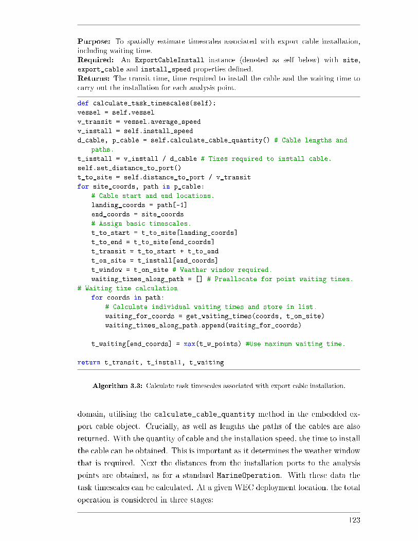
Purpose: To spatially estimate timescales associated with export cable installation,including waiting time.Required: An ExportCableInstall instance (denoted as self below) with site,export_cable and install_speed properties de�ned.Returns: The transit time, time required to install the cable and the waiting time tocarry out the installation for each analysis point.

def calculate_task_timescales(self):

vessel = self.vessel

v_transit = vessel.average_speed

v_install = self.install_speed

d_cable, p_cable = self.calculate_cable_quantity() # Cable lengths and

paths.

t_install = v_install / d_cable # Times required to install cable.

self.set_distance_to_port()

t_to_site = self.distance_to_port / v_transit

for site_coords, path in p_cable:

# Cable start and end locations.

landing_coords = path[-1]

end_coords = site_coords

# Assign basic timescales.

t_to_start = t_to_site[landing_coords]

t_to_end = t_to_site[end_coords]

t_transit = t_to_start + t_to_end

t_on_site = t_install[end_coords]

t_window = t_on_site # Weather window required.

waiting_times_along_path = [] # Preallocate for point waiting times.

# Waiting time calculation

for coords in path:

# Calculate individual waiting times and store in list.

waiting_for_coords = get_waiting_times(coords, t_on_site)

waiting_times_along_path.append(waiting_for_coords)

t_waiting[end_coords] = max(t_w_points) #Use maximum waiting time.

return t_transit, t_install, t_waiting

Algorithm 3.3: Calculate task timescales associated with export cable installation.

domain, utilising the calculate_cable_quantity method in the embedded ex-

port cable object. Crucially, as well as lengths the paths of the cables are also

returned. With the quantity of cable and the installation speed, the time to install

the cable can be obtained. This is important as it determines the weather window

that is required. Next the distances from the installation ports to the analysis

points are obtained, as for a standard MarineOperation. With these data the

task timescales can be calculated. At a given WEC deployment location, the total

operation is considered in three stages:

123

1. The vessel travels from port to the cable landing point that is associated

with the location. The port nearest to the landing point is assumed.

2. The vessel begins the installation. Using the export cable path dictionary

as a reference, the vessel travels from the landing point to the deployment

location.

3. The vessel completes the installation, and travels from the deployment lo-

cation back to port.

Whereas in the standard marine operation the time to and from the site are

assumed to be the same, this is not the case for the cable installation. The time

to the site is represented by the �rst part of the operation and the time back the

third part. The second part is the hours on site; this is calculated rather than

being speci�ed by the user, as in the standard case. This is equivalent to the

window length required for the operation.

There is a possibility that two di�erent ports will be used for the operation,

as the port nearest to the cable landing is assumed for the �rst part of the op-

eration and the port nearest to the deployment location for the �nal part. As

the installation is a single operation, with the vessel returned to the operator

upon completion of the task, the discrepancy between initial and �nal port is

not deemed to be a signi�cant issue and will only have a minor in�uence on the

charter time.

Once the task timescales are calculated the waiting time can be estimated. The

main assumption underpinning this is that the export cable must be installed in a

single operation. This is the typical approach for small to medium projects from

Albatern's experience, and was corroborated from correspondence with Leaske

Marine, a marine contractor who specialise in vessel charter. The waiting time is

calculated for every point along the path, using the standard methodology from

Section 3.7.4.4, using the metocean data at that point along with the window

length. The total waiting time is then set to the maximum value that was cal-

culated along the path. Essentially, this assumes that the metocean conditions

along the whole path are equal to the most extreme conditions seen along the

route. This is a somewhat pessimistic approach, as for particularly long routes

the vessel would see calmer conditions at certain stages of the installation, for

example when very close to shore.

With the task timescales and the waiting times, the cost for the operation can

be calculated as for a standard marine operation.

124

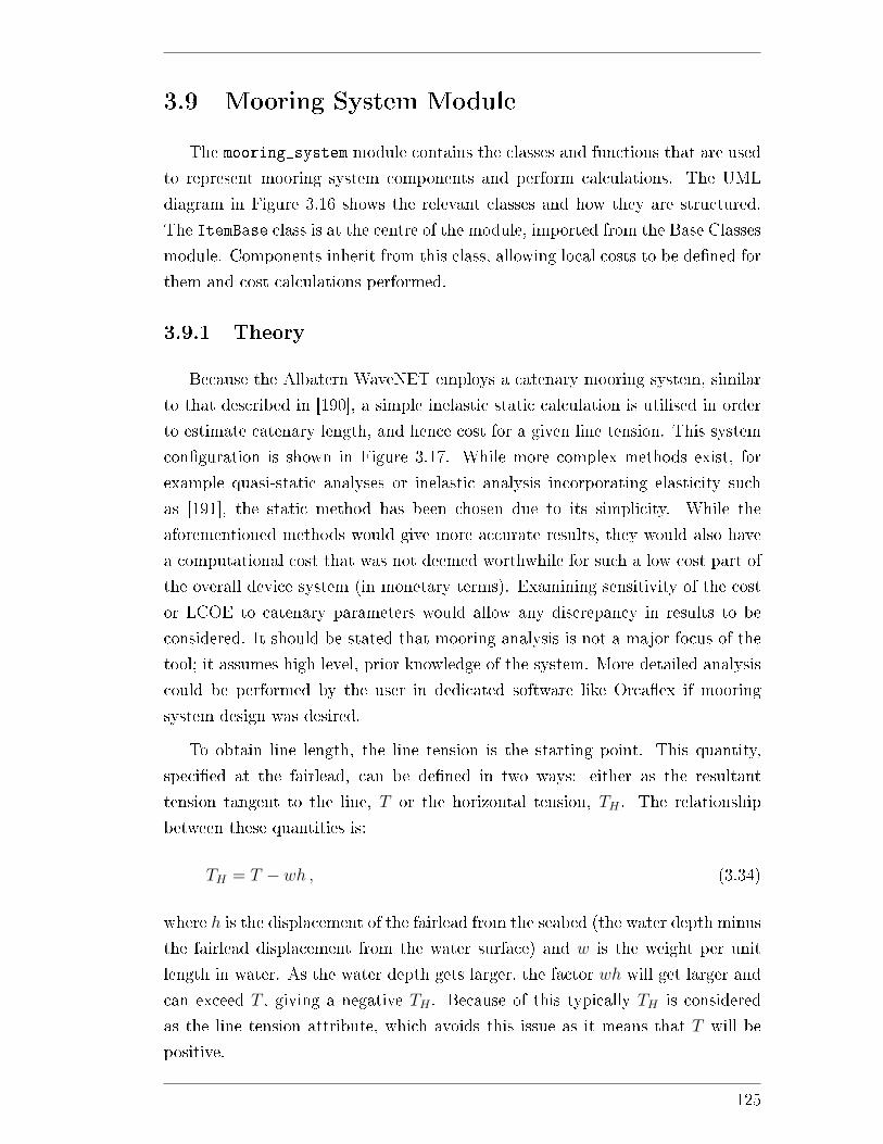
3.9 Mooring System Module

The mooring_system module contains the classes and functions that are used

to represent mooring system components and perform calculations. The UML

diagram in Figure 3.16 shows the relevant classes and how they are structured.

The ItemBase class is at the centre of the module, imported from the Base Classes

module. Components inherit from this class, allowing local costs to be de�ned for

them and cost calculations performed.

3.9.1 Theory

Because the Albatern WaveNET employs a catenary mooring system, similar

to that described in [190], a simple inelastic static calculation is utilised in order

to estimate catenary length, and hence cost for a given line tension. This system

con�guration is shown in Figure 3.17. While more complex methods exist, for

example quasi-static analyses or inelastic analysis incorporating elasticity such

as [191], the static method has been chosen due to its simplicity. While the

aforementioned methods would give more accurate results, they would also have

a computational cost that was not deemed worthwhile for such a low cost part of

the overall device system (in monetary terms). Examining sensitivity of the cost

or LCOE to catenary parameters would allow any discrepancy in results to be

considered. It should be stated that mooring analysis is not a major focus of the

tool; it assumes high level, prior knowledge of the system. More detailed analysis

could be performed by the user in dedicated software like Orca�ex if mooring

system design was desired.

To obtain line length, the line tension is the starting point. This quantity,

speci�ed at the fairlead, can be de�ned in two ways: either as the resultant

tension tangent to the line, T or the horizontal tension, TH . The relationship

between these quantities is:

TH = T − wh , (3.34)

where h is the displacement of the fairlead from the seabed (the water depth minus

the fairlead displacement from the water surface) and w is the weight per unit

length in water. As the water depth gets larger, the factor wh will get larger and

can exceed T , giving a negative TH . Because of this typically TH is considered

as the line tension attribute, which avoids this issue as it means that T will be

positive.

125

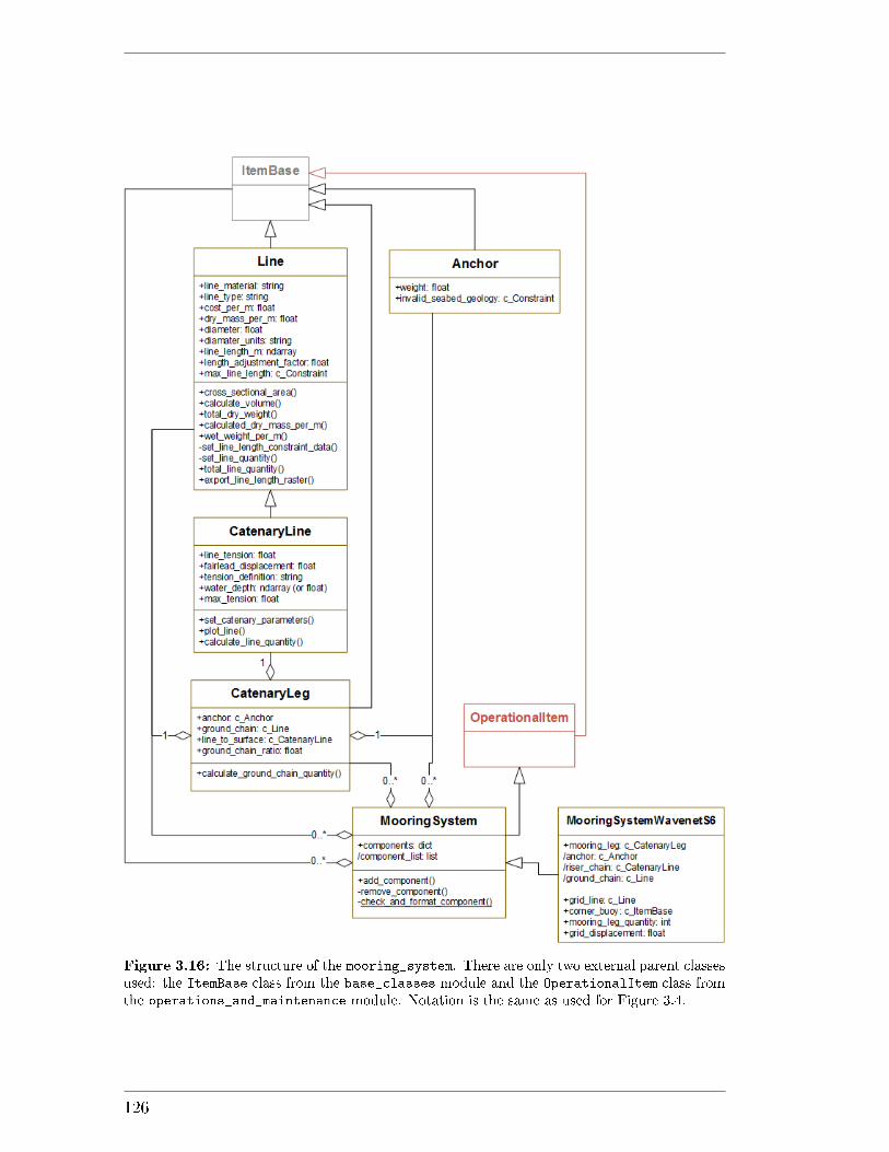
Figure 3.16: The structure of the mooring_system. There are only two external parent classesused: the ItemBase class from the base_classes module and the OperationalItem class fromthe operations_and_maintenance module. Notation is the same as used for Figure 3.4.

126

Given a maximum resultant tension Tmax, the line length, lmin can be found:

lmin = h

(2Tmax

wh− 1

) 12

. (3.35)

This length represents the minimum potential length of the line and is what is

used for the line quantity, and hence cost, calculations. In addition to lmin two

further output quantities can be calculated: the horizontal displacement of the

line, X, and the vertical fairlead force, Tz:

X =THw

sinh−1

(wlmin

TH

)(3.36)

TZ = wlmin . (3.37)

3.9.2 Anchors and lines

For the purposes of the model, the mooring system is considered to be made

up of two main types of components: the anchor and any lines. These form the

building blocks of the subsequent mooring system classes. The anchor is a simple

child of ItemBase. It contains a weight attribute, which can help inform the

user about the suitability of the installation vessels that are being considered. In

the model, the only impact that the anchor type would have would be on costs,

which the user has to de�ne. For example, the anchor instance could be a drag

embedment anchor or a gravity anchor; the anchor speci�cs are not factored into

the mooring system analysis or design.

Mooring lines are instances of the Line class, which also inherits from

ItemBase. The line is de�ned by seven main attributes:

• The line length.

• A length adjustment factor.

• The cost per metre of line.

• The line material.

• The dry mass per metre.

• The diameter of the line.

• The line type (for example studless chain, wire or rope).

The line length can be de�ned by the user, but is more typically calculated

within the model to obtain a cost dependency based on the water depth. Total

127

cost of the line is calculated by multiplying the line length by the cost per metre

attribute and adding any local costs. The cost per metre is a cost instance, stored

within the local cost attribute. This is similar in principle to the ExportCable

class. The �nal line length, used for the cost calculation, is stored within the

quantity attribute of the cost instance. This is not set directly, but is the product

of the line length attribute, L and the length adjustment factor fL:

L�nal = LminfL . (3.38)

It is set when either the line length or line adjustment factor is varied, using a

private method. The length adjustment factor is a contingency factor of sorts,

arbitrarily set by the user to take account of uncertainty in the length. This could

provide a mechanism for Monte-Carlo analysis, allowing di�erent lengths to be

considered without changing the underlying input data.

The line material, dry mass per metre, line diameter and line type are used

to calculate the submerged weight of the line in water, required to estimate the

line length for catenary lines. Including these parameters in the class could also

be useful for estimating breaking loads in the line, although this is not a consid-

eration in the current model. The line material is de�ned by a separate class,

Material, denoted as an aggregation in the UML. This class is primarily de�ned

by a density attribute that the user must specify in units of kg/m3. A method,

seawater_density_factor, calculates the ratio of the material density to that

of seawater. This allows the submerged weight for that material to be deter-

mined. If a dry mass per metre is speci�ed, mdry, then this is used to calculate

the submerged weight:

w = mdryF , (3.39)

where F is the submerged density factor:

F = 1− ρseawaterρmaterial

. (3.40)

If the user does not specify a dry mass per metre then the class will at-

tempt to calculate it, using an external function contained in the module (the

calculate_dry_mass_per_m function). This provides a default value which is

useful if the user is lacking speci�c data for the line. The formula to calculate the

mass depends on the type of line, speci�ed by the line_type attribute. For chains,

128

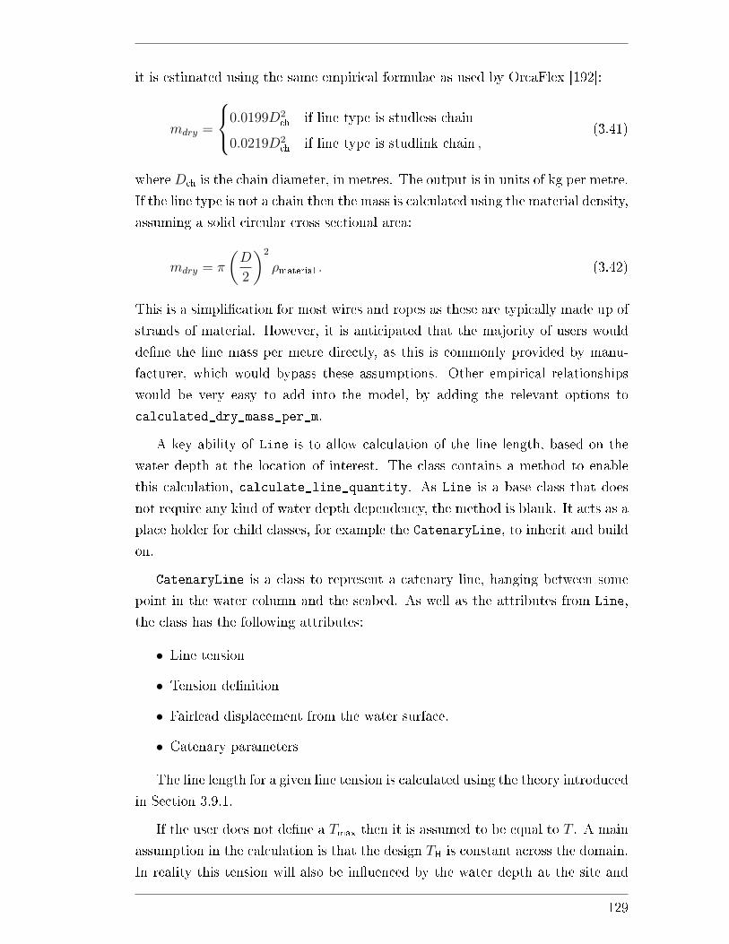
it is estimated using the same empirical formulae as used by OrcaFlex [192]:

mdry =

0.0199D2ch if line type is studless chain

0.0219D2ch if line type is studlink chain ,

(3.41)

where Dch is the chain diameter, in metres. The output is in units of kg per metre.

If the line type is not a chain then the mass is calculated using the material density,

assuming a solid circular cross sectional area:

mdry = π

(D

2

)2

ρmaterial . (3.42)

This is a simpli�cation for most wires and ropes as these are typically made up of

strands of material. However, it is anticipated that the majority of users would

de�ne the line mass per metre directly, as this is commonly provided by manu-

facturer, which would bypass these assumptions. Other empirical relationships

would be very easy to add into the model, by adding the relevant options to

calculated_dry_mass_per_m.

A key ability of Line is to allow calculation of the line length, based on the

water depth at the location of interest. The class contains a method to enable

this calculation, calculate_line_quantity. As Line is a base class that does

not require any kind of water depth dependency, the method is blank. It acts as a

place holder for child classes, for example the CatenaryLine, to inherit and build

on.

CatenaryLine is a class to represent a catenary line, hanging between some

point in the water column and the seabed. As well as the attributes from Line,

the class has the following attributes:

• Line tension

• Tension de�nition

• Fairlead displacement from the water surface.

• Catenary parameters

The line length for a given line tension is calculated using the theory introduced

in Section 3.9.1.

If the user does not de�ne a Tmax then it is assumed to be equal to T . A main

assumption in the calculation is that the design TH is constant across the domain.

In reality this tension will also be in�uenced by the water depth at the site and

129

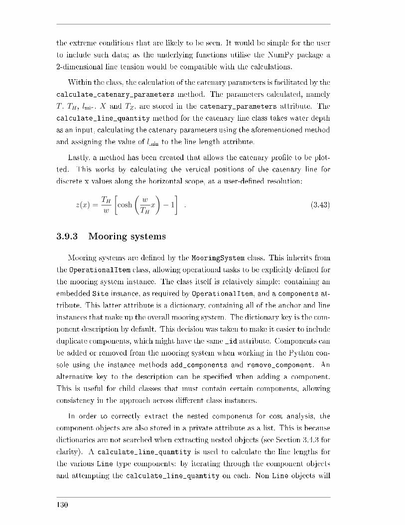
the extreme conditions that are likely to be seen. It would be simple for the user

to include such data; as the underlying functions utilise the NumPy package a

2-dimensional line tension would be compatible with the calculations.

Within the class, the calculation of the catenary parameters is facilitated by the

calculate_catenary_parameters method. The parameters calculated, namely

T , TH , lmin, X and TZ , are stored in the catenary_parameters attribute. The

calculate_line_quantity method for the catenary line class takes water depth

as an input, calculating the catenary parameters using the aforementioned method

and assigning the value of lmin to the line length attribute.

Lastly, a method has been created that allows the catenary pro�le to be plot-

ted. This works by calculating the vertical positions of the catenary line for

discrete x values along the horizontal scope, at a user-de�ned resolution:

z(x) =THw

[cosh

(w

THx

)− 1

]. (3.43)

3.9.3 Mooring systems

Mooring systems are de�ned by the MooringSystem class. This inherits from

the OperationalItem class, allowing operational tasks to be explicitly de�ned for

the mooring system instance. The class itself is relatively simple: containing an

embedded Site instance, as required by OperationalItem, and a components at-

tribute. This latter attribute is a dictionary, containing all of the anchor and line

instances that make up the overall mooring system. The dictionary key is the com-

ponent description by default. This decision was taken to make it easier to include

duplicate components, which might have the same _id attribute. Components can

be added or removed from the mooring system when working in the Python con-

sole using the instance methods add_components and remove_component. An

alternative key to the description can be speci�ed when adding a component.

This is useful for child classes that must contain certain components, allowing

consistency in the approach across di�erent class instances.

In order to correctly extract the nested components for cost analysis, the

component objects are also stored in a private attribute as a list. This is because

dictionaries are not searched when extracting nested objects (see Section 3.4.3 for

clarity). A calculate_line_quantity is used to calculate the line lengths for

the various Line type components: by iterating through the component objects

and attempting the calculate_line_quantity on each. Non Line objects will

130

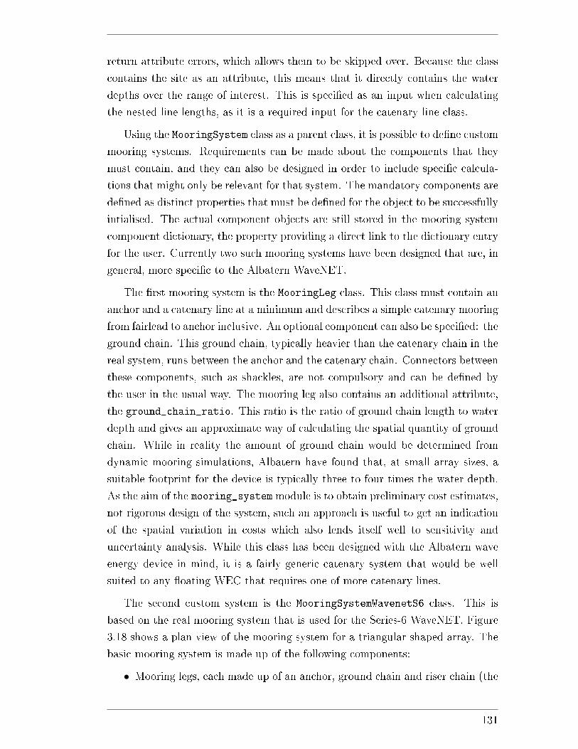
return attribute errors, which allows them to be skipped over. Because the class

contains the site as an attribute, this means that it directly contains the water

depths over the range of interest. This is speci�ed as an input when calculating

the nested line lengths, as it is a required input for the catenary line class.

Using the MooringSystem class as a parent class, it is possible to de�ne custom

mooring systems. Requirements can be made about the components that they

must contain, and they can also be designed in order to include speci�c calcula-

tions that might only be relevant for that system. The mandatory components are

de�ned as distinct properties that must be de�ned for the object to be successfully

intialised. The actual component objects are still stored in the mooring system

component dictionary, the property providing a direct link to the dictionary entry

for the user. Currently two such mooring systems have been designed that are, in

general, more speci�c to the Albatern WaveNET.

The �rst mooring system is the MooringLeg class. This class must contain an

anchor and a catenary line at a minimum and describes a simple catenary mooring

from fairlead to anchor inclusive. An optional component can also be speci�ed: the

ground chain. This ground chain, typically heavier than the catenary chain in the

real system, runs between the anchor and the catenary chain. Connectors between

these components, such as shackles, are not compulsory and can be de�ned by

the user in the usual way. The mooring leg also contains an additional attribute,

the ground_chain_ratio. This ratio is the ratio of ground chain length to water

depth and gives an approximate way of calculating the spatial quantity of ground

chain. While in reality the amount of ground chain would be determined from

dynamic mooring simulations, Albatern have found that, at small array sizes, a

suitable footprint for the device is typically three to four times the water depth.

As the aim of the mooring_system module is to obtain preliminary cost estimates,

not rigorous design of the system, such an approach is useful to get an indication

of the spatial variation in costs which also lends itself well to sensitivity and

uncertainty analysis. While this class has been designed with the Albatern wave

energy device in mind, it is a fairly generic catenary system that would be well

suited to any �oating WEC that requires one of more catenary lines.

The second custom system is the MooringSystemWavenetS6 class. This is

based on the real mooring system that is used for the Series-6 WaveNET. Figure

3.18 shows a plan view of the mooring system for a triangular shaped array. The

basic mooring system is made up of the following components:

• Mooring legs, each made up of an anchor, ground chain and riser chain (the

131

catenary line to the surface) as previously described.

• Corner buoys, used to support the mooring grid.

• A mooring grid. This connects the array to the mooring legs and is posi-

tioned below the water surface.

Other low cost components such as shackles and intermediate grid lines can be

added as additional components. The mooring grid is typically made from rope,

with the length a function of the array size and shape. This should be speci�ed

by the user as an input, although could be approximated for given con�gurations

in future work (because of the low cost nature of the component this calculation

is neglected here). The properties of the mooring leg, for example the speci�c

components and the ground chain ratio can be set within the class itself, properties

providing a direct link to the embedded leg properties.

3.9.3.1 Calculation procedure

The process to calculate the spatial costs associated with a particular mooring

system is as follows:

1. De�ne the system: The desired mooring system is de�ned in a class con-

�guration text �le. This includes specifying all of the components, which can

be done either directly in the con�guration �le or by providing a database

query or �le path to the necessary class text �le (see Section 3.3). The path

of the site NetCDF �le is also required to calculate water depth dependent

costs and any operational costs that are speci�ed.

2. Load the system: The con�guration �le is read and the class instance

created.

3. Calculate quantities (line lengths): The calculate_line_quantity

method is executed for each component (any non line components are auto-

matically skipped). If the site attribute is de�ned, the water depth for the

analysis range (water_depth_analysis_range) is used to calculate spa-

tial quantities with water depth dependence, primarily catenary lines and

ground chain.

4. Calculate costs: Categorised costs and cash �ows are calculated for the

whole system, including the embedded component instances, using the em-

bedded cost method as previously described.

132

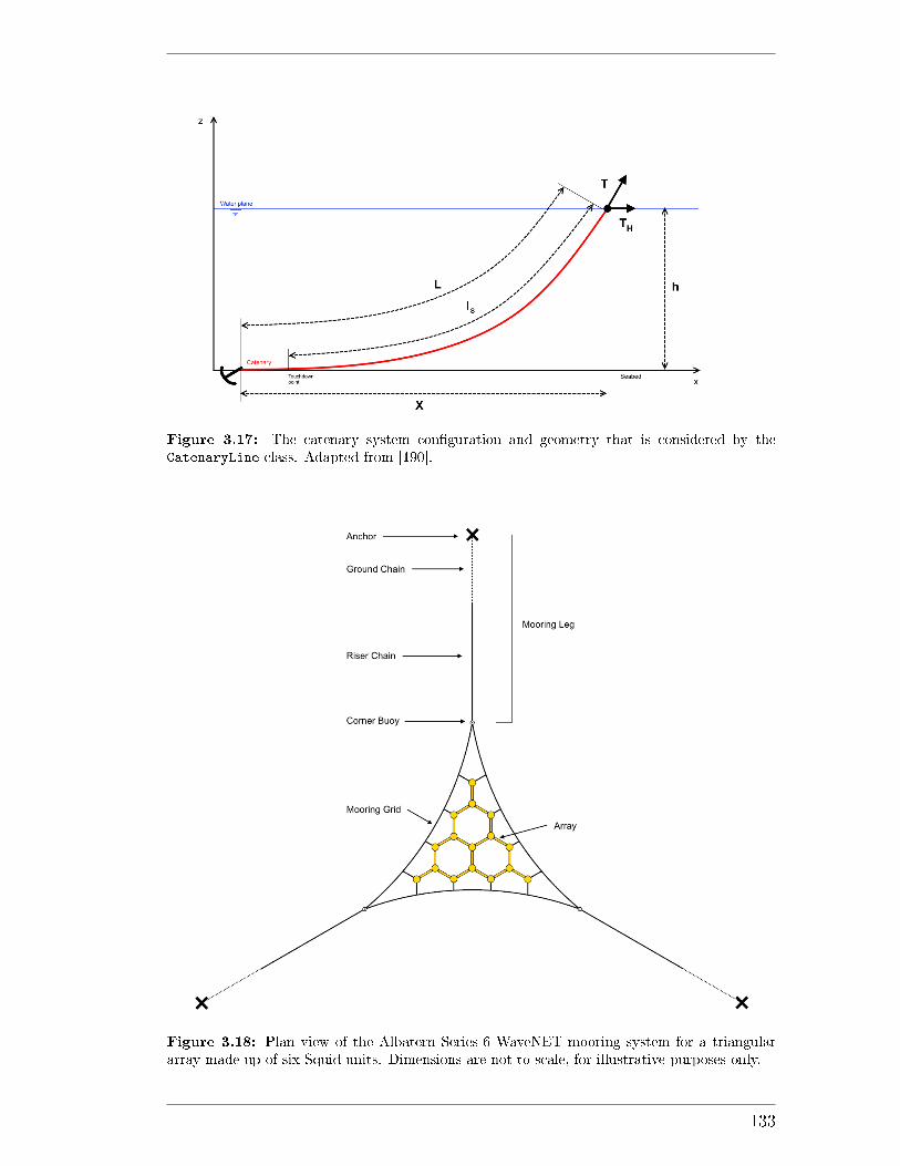
Figure 3.17: The catenary system con�guration and geometry that is considered by theCatenaryLine class. Adapted from [190].

Figure 3.18: Plan view of the Albatern Series-6 WaveNET mooring system for a triangulararray made up of six Squid units. Dimensions are not to scale, for illustrative purposes only.

133

3.10 Constraints Module

In the context of the model, constraints are de�ned as conditions that limit

the potential deployment locations for the wave energy device. These factors are

important to consider, as not including them can give unrealistic expectations of

device performance and deployment capability. They help to narrow down the

data domain to only suitable areas, saving time and helping the model user to

build up an accurate picture of the opportunities and limitations of the device

design.

To include an individual constraint in the model, two pieces of information are

required:

1. The condition (typically an inequality) used to de�ne the constraint.

2. The data that the condition is applied to.

The module de�nes constraints as classes, with several di�erent options existing.

These constraint classes, inheriting from a base class to provide a uniform struc-

ture, each e�ectively de�ne a di�erent conditional statement that is applied to

the input data. Data values that meet the conditional can be masked, and hence

excluded from the output data. The modi�ed data can also be exported as a

raster �le, so the invalid data locations can be seen in the context of the data

domain. Table 3.4 shows examples of some of the conditions that can be applied

to arrays of data.

Class Name E�ect Example of Usage

ConstraintMin Exclude values below aspeci�ed value

Exclude shallow water depths.

ConstraintMax Exclude values above aspeci�ed value

Exclude locations too far fromshore.

ConstraintLocation Exclude values at speci�cgeographic locations

Exclude locations that fallwithin protected areas.

Table 3.4: Examples of the constraint classes, and hence conditions, that can be applied todi�erent data arrays used by the model.

Within the model itself, the constraints are contained within attributes of

the higher level objects that they are being applied to, for example the wave

energy device. All of the constraint instances contain a special attribute, the

constraint_variable attribute, which is a string. This allows the constraint

instance to be linked to the data which is it applied to, by matching this string to

134

the description attribute of the data. All of the data arrays that are required by

constraints, such as the 2D array of water depths across the domain, are stored

as instances of a unique class, the ConstraintData class. This is a simple class,

inheriting from Base but with an additional attribute to store the data. The

purpose of this di�erent class for the data is so that references to the instances

can be easily obtained using with the Base instances attribute (see Section 3.4.1).

The desired outputs of the constraints analysis are individual raster layers,

presenting the invalid locations calculated for each constraint, and an overall

raster containing all of the constraints. These can be used as overlay layers for

the output results from the model analysis, and formatted within GIS software

to the wishes of the user. For the overall raster, each constraint is assigned a

di�erent pixel value which allows them all to be identi�ed. At some locations,

multiple constraints can apply. For example, a point could have a water depth of

less than 30 m and also be located within the boundary of a Marine Protected

Area (MPA). For such combinations of constraints, new pixel values are created

and assigned.

Figure 3.19 gives an example of how the constraint layer data can be visualised

in GIS, considering an area in the Inner Hebrides, to the South of the Isle of Rum.

Four project constraints were speci�ed, with the data and export cable landing

location arbitrarily chosen to demonstrate the output capabilities:

• Water depth must be greater than 30 m.

• Water depth must be less than 150 m.

• Cable length must be less than 5 km.

• Locations within Special Protected Areas (SPA) are not valid for deploy-

ment.

The main map, in the top right, shows the combined constraints. The four

input constraints yield �ve unique categories of constraint over the region when

combinations of constraints are taken into account (for example, the purple area

signi�es locations that both lie in the SPA and where the cable is too long).

The locational data used to de�ne a constraint are speci�ed in a GIS �le. This

could be a vector �le, where restricted areas are de�ned by polygon features, or

a raster �le, where restricted areas will depend on pixel values. Some constraints

are instead de�ned by calculated quantities within the model.

135

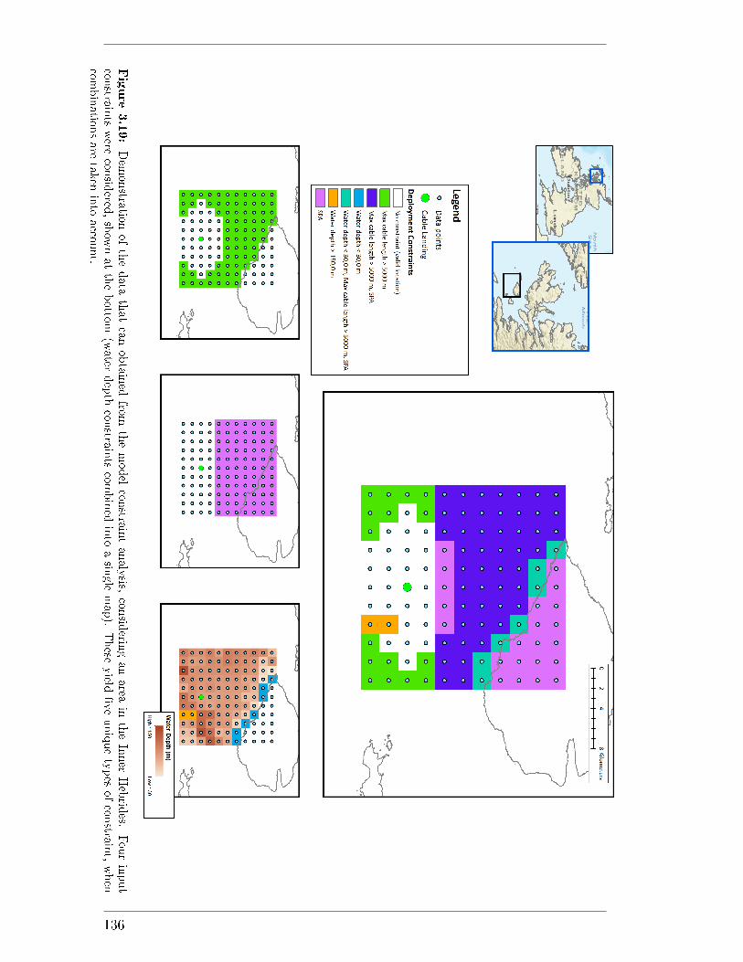
Figure3.19:Dem

onstra

tionofthedata

thatcanobtained

from

themodel

constra

intanalysis,

consid

eringanarea

intheInner

Hebrid

es.Fourinput

constra

ints

were

consid

ered,show

natthebotto

m(water

depth

constra

ints

combined

into

asin

glemap).

These

yield

�ve

uniquetypes

ofconstra

int,when

combinatio

nsare

taken

into

acco

unt.

136

3.11 Limitations and Assumptions Summary

As has been demonstrated by the material presented so far, there are a large

number of factors that in�uence the economic viability of a wave energy project.

Due to the time constraints associated with this project it was not feasible to

include every aspect in the research. The key functionality of the model was

driven by the wishes of the industrial sponsor, primarily centred on the theme of

spatial mapping. The future for the model, designed and created completely from

scratch, is to follow an iterative process and be built upon over time. Eventually

it is hoped that it can form a key part of Albatern's project scoping, development

and business strategy.

The main limitations and assumptions that are present in the model are sum-

marised in Table 3.5. These vary from missing functionality to limitations in the

modelling approach. The table also provides some justi�cation as to why the

identi�ed areas were not covered in the detail described.

Arguably the most signi�cant omission is regarding unplanned O&M. As

stated in the introduction of Section 3.7, while unplanned operations could be

de�ned if the months that they occur in are known, the model o�ers no way to

directly simulate these. This could be done by using Monte Carlo based analy-

sis to simulate component failures, allowing the timing of the failures, and hence

timings of operations, to be derived. Following this, the associated costs could

be calculated as described within the relevant subsections of Section 3.7. The

decision to leave out this cost aspect was due to the scope of this project relative

to other R&D activities within the sponsoring company. As reliability was the

research focus of another doctoral research engineer, the decision was made to

keep the work packages distinct but keep open the possibility of a uni�ed model

for the future.

Rather than leaving out unplanned O&M it can be modelled as a proportional

cost (Section 3.4.3), equal to a �xed percentage of the total CAPEX per year.

While this is an inferior treatment of the cost, the method is an approach used

numerous times in the literature (for example [57, 65, 99]) and is hence deemed

suitable to complete the overall wave device cost picture.

A related feature missing from the model is downtime calculation for opera-

tional tasks (planned or unplanned), which will impact availability. To include

this would require feeding the time series of energy production from the device

directly into the cost calculation. There was not time in the project to accomplish

137

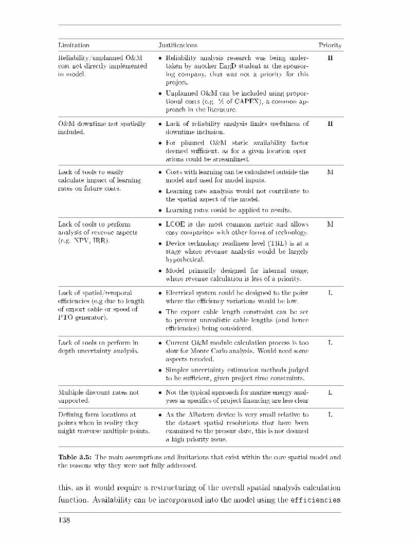
Limitation Justi�cations Priority

Reliability/unplanned O&Mcost not directly implementedin model.

• Reliability analysis research was being under-taken by another EngD student at the sponsor-ing company, thus was not a priority for thisproject.

• Unplanned O&M can be included using propor-tional costs (e.g. % of CAPEX), a common ap-proach in the literature.

H

O&M downtime not spatiallyincluded.

• Lack of reliability analysis limits usefulness ofdowntime inclusion.

• For planned O&M static availability factordeemed su�cient, as for a given location oper-ations could be streamlined.

H

Lack of tools to easilycalculate impact of learningrates on future costs.

• Costs with learning can be calculated outside themodel and used for model inputs.

• Learning rate analysis would not contribute tothe spatial aspect of the model.

• Learning rates could be applied to results.

M

Lack of tools to performanalysis of revenue aspects(e.g. NPV, IRR).

• LCOE is the most common metric and allowseasy comparison with other forms of technology.

• Device technology readiness level (TRL) is at astage where revenue analysis would be largelyhypothetical.

• Model primarily designed for internal usage,where revenue calculation is less of a priority.

M

Lack of spatial/temporale�ciencies (e.g due to lengthof export cable or speed ofPTO generator).

• Electrical system could be designed to the pointwhere the e�ciency variations would be low.

• The export cable length constraint can be setto prevent unrealistic cable lengths (and hencee�ciencies) being considered.

L

Lack of tools to perform indepth uncertainty analysis.

• Current O&M module calculation process is tooslow for Monte Carlo analysis. Would need someaspects recoded.

• Simpler uncertainty estimation methods judgedto be su�cient, given project time constraints.

L

Multiple discount rates notsupported.

• Not the typical approach for marine energy anal-yses as speci�cs of project �nancing are less clear

L

De�ning farm locations atpoints when in reality theymight traverse multiple points.

• As the Albatern device is very small relative tothe dataset spatial resolutions that have beenexamined to the present date, this is not deemeda high priority issue.

L

Table 3.5: The main assumptions and limitations that exist within the core spatial model andthe reasons why they were not fully addressed.

this, as it would require a restructuring of the overall spatial analysis calculation

function. Availability can be incorporated into the model using the efficiencies

138

attribute of the wave device, although this applies the value over the whole spa-

tial domain. In the absence of detailed reliability and downtime estimation this is

considered a suitable approach, especially when examining more localised regions

as the variation in the parameter will be reduced.

Two omitted analysis types analyses that are sometimes seen in the literature

are revenue based analyses (for example NPV and IRR) and learning rate analysis

to examine future LCOE potential. The latter of these can be applied manually,

by selecting input data with learning cost reduction built into the values. This is

demonstrated in the case study in Chapter 5. While the ability to do this within

the model itself would improve usability, it was not regarded as a research priority.

This was because it was not judged to �t so well into the spatial analysis theme.

The �nal four limitations are more minor. The �rst two, electrical e�ciencies

and uncertainty, can be partially achieved by the model and mitigated by careful

selection of input data, but more sophisticated modelling approaches are desired

for future work. Uncertainty analysis is less of a concern over time, as better data

are collected from real projects.

Multiple discount rates, the ability to set di�erent discount rates for di�erent

costs, would be a useful addition to the model. It would be possible by de�n-

ing the discount rate as an attribute of the ItemBase class rather than at the

Project level. It is not deemed a key limitation as using a single discount rate

is overwhelmingly the accepted method in the marine energy context (for exam-

ple [57, 92,93,95]).

The �nal point concerns data resolution. For larger devices and �ne metocean

data resolutions the model may not give an accurate representation of a farm: as

the farm is considered at a single point. As the Albatern device is very small this is

not an issue for the current model application. Even for large devices, where array

footprint is comparable to the data resolution, the analysis can still give valuable

information on siting at a �rst pass. This could be followed by lower level, bottom

up modelling at more localised regions where aspects like array layout could be

explicitly taken into account.

139

140

4The O�-grid System Sub-Model

This chapter describes the module that is used for analysing o�-grid wave

energy systems. As this is a more niche wave energy application it is considered

as a distinct entity, a sub-model of the core grid-connected model as described in

Chapter 3.

Given an electricity demand time series (or load pro�le) and an arbitrary

selection of energy sources, the aim of the module is to determine the useful energy

input and time dependent costs. This is achieved by simulating the energy �ow

in the o�-grid system in the time domain, using an algorithm which attempts to

balance the energy production and demand. This involves calculating the energy

contributions that are required to meet the demand at each time step. This

allows cost contributions over the system lifetime to be determined, that can then

be �ltered into a wider cost analysis using the methods from Chapter 3.

4.1 Overview

Three di�erent types of energy sources have been coded into the model: a

WEC, battery bank and diesel generator, represented by Python classes. The

component combinations that can be theoretically examined are listed in Table

4.1, along with justi�cation of which have been presented in the case studies for

this body of work.

Of the six system types, two are considered. Because the Albatern device

considered in this thesis is so small, the systems would struggle to economically

support the �sh farm loads, even with storage. To put this into context: a load of

141

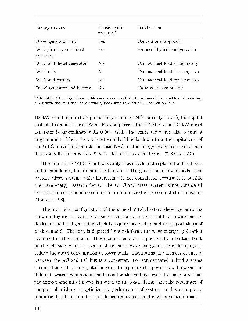
Energy sources Considered inresearch?

Justi�cation

Diesel generator only Yes Conventional approach

WEC, battery and dieselgenerator

Yes Proposed hybrid con�guration

WEC and diesel generator No Cannot meet load economically

WEC only No Cannot meet load for array size

WEC and battery No Cannot meet load for array size

Diesel generator and battery No No wave energy present

Table 4.1: The o�-grid renewable energy systems that the sub-model is capable of simulating,along with the ones that have actually been simulated for this research project.

100 kW would require 67 Squid units (assuming a 20% capacity factor), the capital

cost of this alone is over ¿5m. For comparison the CAPEX of a 160 kW diesel

generator is approximately ¿20,000. While the generator would also require a

large amount of fuel, the total cost would still be far lower than the capital cost of

the WEC units (for example the total NPC for the energy system of a Norwegian

diesel-only �sh farm with a 20 year lifetime was estimated at ¿838k in [173]).

The aim of the WEC is not to supply these loads and replace the diesel gen-

erator completely, but to ease the burden on the generator at lower loads. The

battery/diesel system, while interesting, is not considered because it is outside

the wave energy research focus. The WEC and diesel system is not considered

as it was found to be uneconomic from unpublished work conducted in-house for

Albatern [193].

The high level con�guration of the typical WEC/battery/diesel generator is

shown in Figure 4.1. On the AC side it consists of an electrical load, a wave energy

device and a diesel generator which is required as backup and to support times of

peak demand. The load is depicted by a �sh farm, the wave energy application

examined in this research. These components are supported by a battery bank

on the DC side, which is used to store excess wave energy and provide energy to

reduce the diesel consumption at lower loads. Facilitating the transfer of energy

between the AC and DC bus is a converter. For sophisticated hybrid systems

a controller will be integrated into it, to regulate the power �ow between the

di�erent system components and monitor the voltage levels to make sure that

the correct amount of power is routed to the load. These can take advantage of

complex algorithms to optimise the performance of system, in this example to

minimise diesel consumption and hence reduce cost and environmental impact.

142

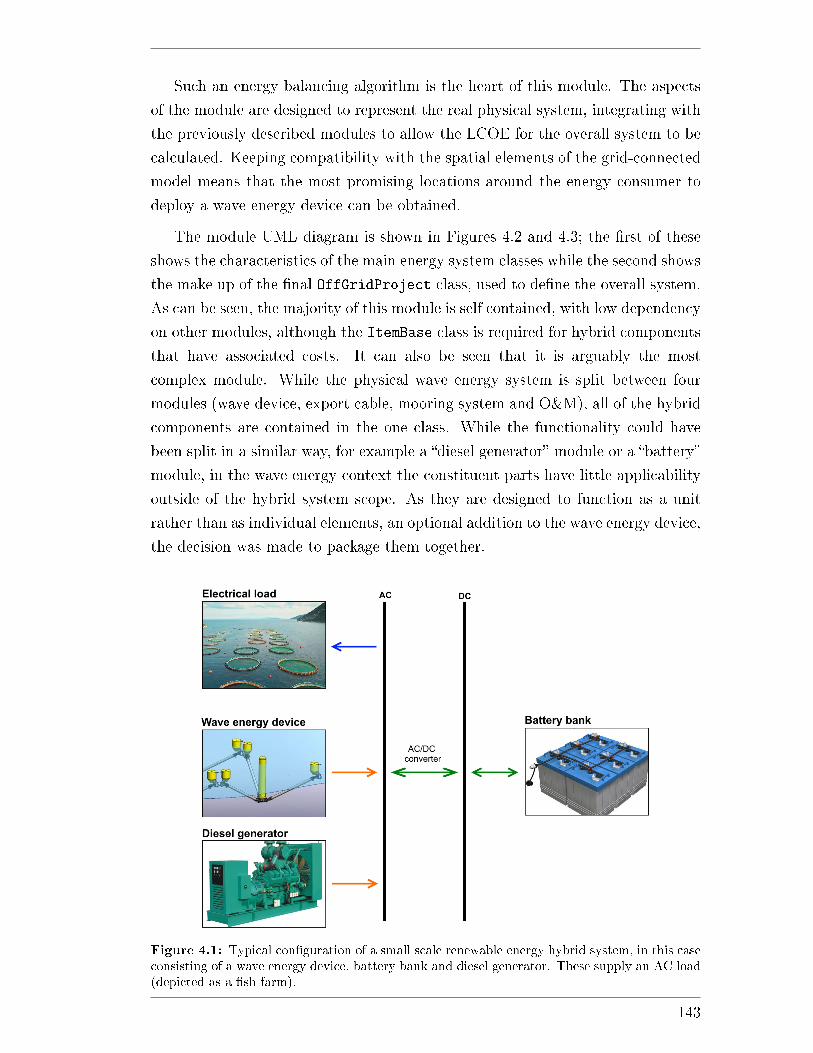
Such an energy balancing algorithm is the heart of this module. The aspects

of the module are designed to represent the real physical system, integrating with

the previously described modules to allow the LCOE for the overall system to be

calculated. Keeping compatibility with the spatial elements of the grid-connected

model means that the most promising locations around the energy consumer to

deploy a wave energy device can be obtained.

The module UML diagram is shown in Figures 4.2 and 4.3; the �rst of these

shows the characteristics of the main energy system classes while the second shows

the make up of the �nal OffGridProject class, used to de�ne the overall system.

As can be seen, the majority of this module is self contained, with low dependency

on other modules, although the ItemBase class is required for hybrid components

that have associated costs. It can also be seen that it is arguably the most

complex module. While the physical wave energy system is split between four

modules (wave device, export cable, mooring system and O&M), all of the hybrid

components are contained in the one class. While the functionality could have

been split in a similar way, for example a �diesel generator� module or a �battery�

module, in the wave energy context the constituent parts have little applicability

outside of the hybrid system scope. As they are designed to function as a unit

rather than as individual elements, an optional addition to the wave energy device,

the decision was made to package them together.

Figure 4.1: Typical con�guration of a small scale renewable energy hybrid system, in this caseconsisting of a wave energy device, battery bank and diesel generator. These supply an AC load(depicted as a �sh farm).

143

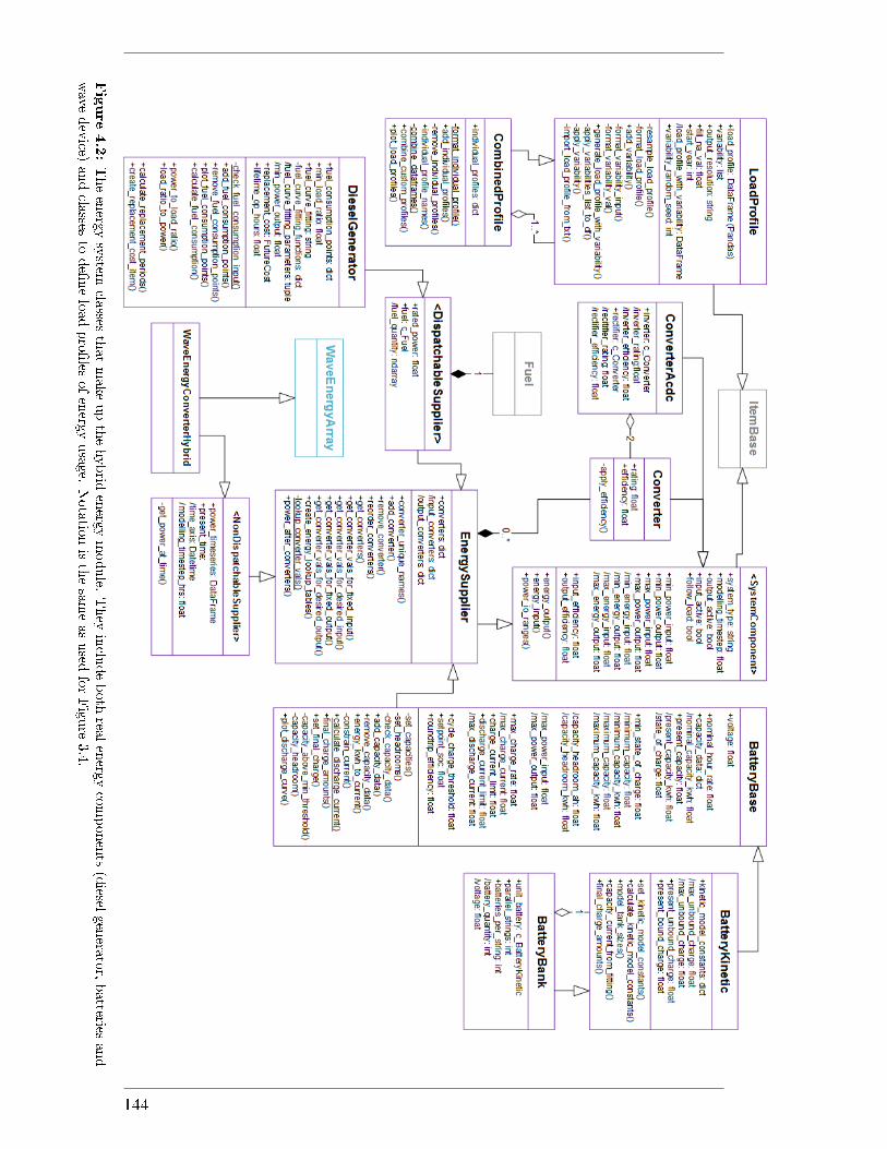
Figure4.2:Theenerg

ysystem

classes

thatmake

upthehybrid

energ

ymodule.

They

inclu

deboth

realenerg

ycomponents

(diesel

genera

tor,batteries

and

wavedevice)

andcla

ssesto

de�neloadpro�les

ofenerg

yusage.

Notatio

nisthesameasused

forFigure

3.4.

144

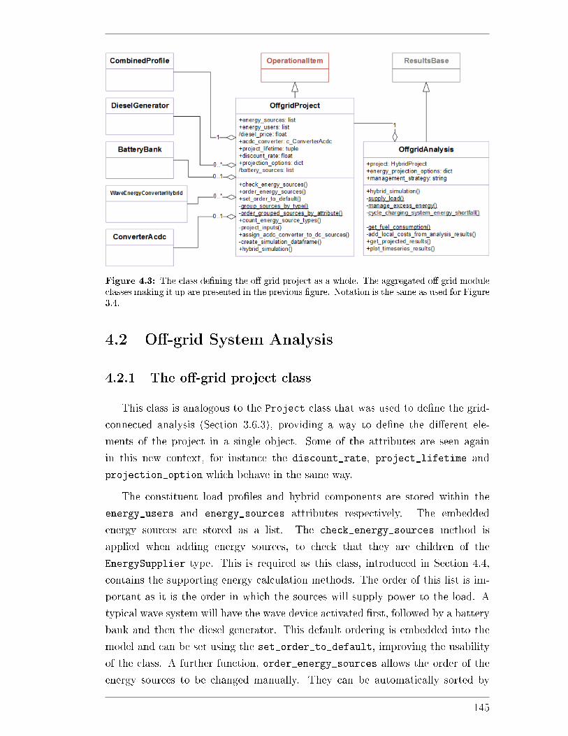
Figure 4.3: The class de�ning the o�-grid project as a whole. The aggregated o�-grid moduleclasses making it up are presented in the previous �gure. Notation is the same as used for Figure3.4.

4.2 O�-grid System Analysis

4.2.1 The o�-grid project class

This class is analogous to the Project class that was used to de�ne the grid-

connected analysis (Section 3.6.3), providing a way to de�ne the di�erent ele-

ments of the project in a single object. Some of the attributes are seen again

in this new context, for instance the discount_rate, project_lifetime and

projection_option which behave in the same way.

The constituent load pro�les and hybrid components are stored within the

energy_users and energy_sources attributes respectively. The embedded

energy sources are stored as a list. The check_energy_sources method is

applied when adding energy sources, to check that they are children of the

EnergySupplier type. This is required as this class, introduced in Section 4.4,

contains the supporting energy calculation methods. The order of this list is im-

portant as it is the order in which the sources will supply power to the load. A

typical wave system will have the wave device activated �rst, followed by a battery

bank and then the diesel generator. This default ordering is embedded into the

model and can be set using the set_order_to_default, improving the usability

of the class. A further function, order_energy_sources allows the order of the

energy sources to be changed manually. They can be automatically sorted by

145

class type and/or size, this latter ability useful when considering multiple objects

of the same type. For example two generators could be put into the system: a

smaller one and a larger one, the larger one only used if the smaller one fails to

meet the necessary demand.

The diesel_price attribute gives a way of setting the fuel price for all of

the embedded diesel generators at the same time, by iterating through the energy

sources list. This is useful as it prevents the user from having to set this parameter

for multiple objects, which could lead to errors. The acdc_converter is required

to link any DC components to the load and components on the AC side.

4.2.2 Algorithm overview

Once the project is fully de�ned a hybrid system simulation can be executed.

This is carried out by using another class: OffGridAnalysis. The class itself

is similar in application to those previously described (Sections 3.4.5 and 3.6.4)

and serves as a convenient structure to group the various algorithm sub functions

together. While not directly spatial in nature, it also inherits from GisResults

(described in Section 3.4.4) which forces consistency in the output data that are

generated.

The overarching methodology employed is a hybrid energy balancing algo-

rithm, similar in principle to those found in the literature and commercial soft-

ware (the main example being HOMER [156]). The requirements are an input

load pro�le, de�ned over a number of discrete time steps, and a selection of energy

sources; both of these are embedded within the o�-grid project. Essentially the

algorithm loops through the load, at each time step seeing if each energy source in

turn can supply the full load. If it cannot then the responsibility falls to the next

energy source in line to make up the shortfall. Costs can be deduced from the

results, the primary one being the fuel cost consumed by any diesel generators.

An example of the �ow of logic for the algorithm that has been created is shown

in Figure 4.4. This is for a wave/battery/diesel generator system, the same as

depicted in Figure 4.1.

The �rst phase of operation is to attempt to supply the load with the energy

from the wave energy device. If this is possible then any excess energy is routed to

the battery bank and the simulation continues to the next time step. Conversely,

if there is energy required after the WEC input then the battery bank attempts

to supply the remaining load. In this example the energy that can be supplied by

the battery bank is constrained by two conditions. First the capacity must not

146

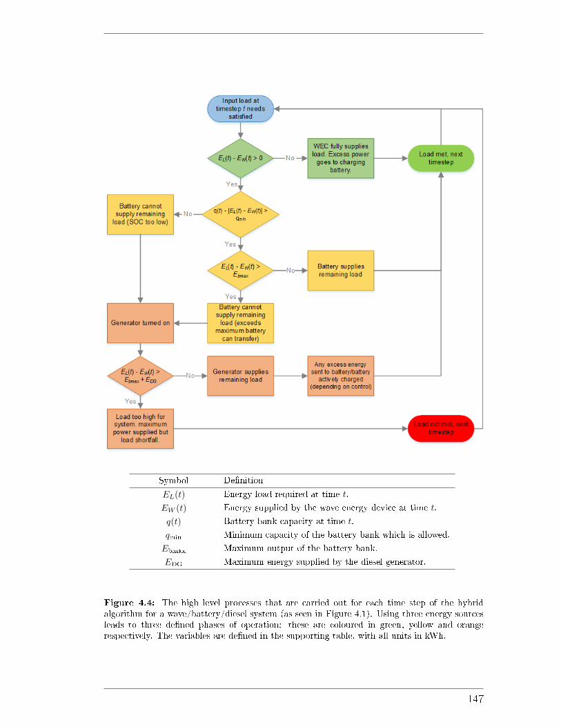
Symbol De�nition

EL(t) Energy load required at time t.

EW (t) Energy supplied by the wave energy device at time t.

q(t) Battery bank capacity at time t.

qmin Minimum capacity of the battery bank which is allowed.

Ebmax Maximum output of the battery bank.

EDG Maximum energy supplied by the diesel generator.

Figure 4.4: The high level processes that are carried out for each time step of the hybridalgorithm for a wave/battery/diesel system (as seen in Figure 4.1). Using three energy sourcesleads to three de�ned phases of operation: these are coloured in green, yellow and orangerespectively. The variables are de�ned in the supporting table, with all units in kWh.

147

drop below a threshold state of charge, arbitrarily de�ned by the user. Second,

the energy is limited by the absolute capacity and, for the kinetic battery model,

the charging history of the battery. These aspects are discussed in more detail in

Section 4.4.3, where the battery classes are described. If the battery bank cannot

supply the load then it falls to the diesel generator. If the generator is properly

sized for the application, with rated power exceeding the peak demand, then the

load will always be met. Depending on the battery bank state of charge and the

input parameters for the simulation, the generator may be operated at a higher

load than necessary to recharge the battery. Once the algorithm has worked

through all of the time steps then the simulation is completed. For each energy

component the input and output power values at each time are obtained. These

can then be summed for each month to get seasonal trends and can subsequently

be projected forward in time using the same methods as previously described in

Section 3.6.4.

It should be noted that Figure 4.4 describes the algorithm for just one potential

con�guration. Di�erent systems can be examined by varying the types and order

of the energy sources and by specifying di�erent inputs to guide the overall process.

4.2.3 The o�-grid analysis class

Together OffGridProject and the hybrid algorithm work to de�ne the hy-

brid system and run the simulation. In a similar way to the conventional

EnergyAnalysis (Section 3.6.4) the hybrid project is directly embedded within

the analysis so that all of the objects needed for the simulation can be easily ac-

cessed. While the hybrid analysis can be thought of as a type of energy analysis

the classes are not linked to each other, for example through inheritance. This

decision was taken for two reasons: �rst to reduce the dependencies between the

modules and allow the o�-grid module to function in a standalone way, and second

because the hybrid algorithm is applied in a non-spatial way. The algorithm uses

single time series, the application to spatial modelling achieved using a higher

level function. This is described in Section 4.2.6.

As well as the project, the only other inputs de�ned directly at the class

level are the projection options, as in EnergyAnalysis, and a new parameter:

management_strategy. Directly following the logic used in HOMER commercial

software [156], two di�erent control strategies have been implemented: load follow-

ing and cycle charging. The di�erence between these concerns the diesel generator

behaviour. In the load following case it will only supply the load required and will

148

not produce any excess energy to recharge any battery bank present; the battery

bank is only charged by the wave energy device. In the cycle charging case, when

the battery state of charge falls below a certain level the generator will operate

at a level exceeding the peak load and charge the battery.

4.2.4 Energy balancing algorithm implementation

The method hybrid_simulation executes the hybrid simulation. Programat-

ically this is made up of the following stages:

1. Copies are made of the energy sources, to prevent any time dependent pa-

rameters from being overwritten. This is particularly important when ap-

plying the algorithm spatially to ensure that the same initial conditions are

used each time (the spatial process is described in more detail in Section

4.2.6).

2. The initial capacities of any battery banks are set. The capacity depends

on the number of batteries in the bank and the discharge current pro�le of

the battery (discussed further in Section 4.4.3).

3. The output data structure is created, using the

create_simulation_dataframe private method within the project.

This is a Pandas DataFrame, with each column representing a time

dependent property of the simulation. The columns that are created for

each system component are summarised in Table 4.2. The unique _id

attribute of the component is assigned to the column names, so that the

object can be linked to the output data after the simulation has completed.

4. The analysis load pro�le is obtained: this is the load pro�le as de�ned by the

user but modi�ed to include any time based variability factors (see Section

4.3).

5. The algorithm then begins to iterate through the time steps using a for loop:

(a) The duration of the current time step is calculated by �nding the time

di�erence with the next time step.

(b) The supply_load private method in the OffGridAnalysis class is

called, to determine which energy sources are required to meet the

load.

This method iterates through the energy sources in order, until a so-

lution is obtained. For each it calculates the energy which could be

149

supplied to the load, taking account of the length of time, any con-

straints on power output and power reduction due to any converters

between the energy source and the load. After each stage the reduced

load is calculated. Once the load is fully satis�ed this part of the

simulation is complete.

If any battery banks have supplied load then their capacities are recal-

culated. If the SOC is below the cycle charging threshold (arbitrarily

de�ned for the battery, see Section 4.4.3) then the battery bank is

�turned o��, �agging up to the simulation that the system must create

more excess power on the next simulation run.

(c) The manage_excess_energy function then routes any excess energy

to the battery banks. For a WEC, this is simply that left over from

supplying the load (assuming that the WEC is �rst in the list of energy

sources).

For the diesel generator, excess energy can only be created for the

cycle_charging strategy. In this case, the maximum amount of energy

that can be put into the battery bank in the present time step is back

calculated within the battery bank class. The diesel generator will

then attempt to supply this. If the resulting bank capacity exceeds a

setpoint state of charge, again an arbitrary attribute of the battery,

then the battery will be �turned on� again and can supply energy to

the system as before. If not, the battery remains in an o� state and

the excess energy requirement is carried over to the next time step.

(d) At the end of the time step all of the results are saved into the respective

columns of the preallocated results DataFrame.

6. Once all of the time steps are complete the simulation is �nished. For any

diesel generators the fuel consumption is calculated by using the output

energy pro�le and input parameters de�ned within the class. New columns

in the DataFrame are created to store these data.

7. Finally the output results are projected over the speci�ed

project_lifetime de�ned within the OffGridProject instance, as

previously described. The resulting data are then restructured into a

dictionary and saved within the OffGridAnalysis instance.

150

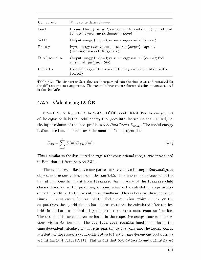
Component Time series data columns

Load Required load (required); energy sent to load (input); unmet load(unmet), excess energy dumped (dump)

WEC Output energy (output); excess energy created (excess)

Battery Input energy (input); output energy (output); capacity(capacity); state of charge (soc)

Diesel generator Output energy (output); excess energy created (excess); fuelconsumed (fuel_quantity)

Converter Incident energy into converter (input); energy out of converter(output)

Table 4.2: The time series data that are incorporated into the simulation and extracted forthe di�erent system components. The names in brackets are shortened column names as usedin the simulation.

4.2.5 Calculating LCOE

From the monthly results the system LCOE is calculated. For the energy part

of the equation it is the useful energy that goes into the system that is used, i.e.

the input column of the load pro�le in the DataFrame EOG,m. The useful energy

is discounted and summed over the months of the project, i.e.:

EOG =n∑

m=1

D(m)EOG,m(m) . (4.1)

This is similar to the discounted energy in the conventional case, as was introduced

in Equation 2.1 from Section 2.3.1.

The system cash �ows are categorised and calculated using a CostAnalysis

object, as previously described in Section 3.4.5. This is possible because all of the

hybrid components inherit from ItemBase. As for some of the ItemBase child

classes described in the preceding sections, some extra calculation steps are re-

quired in addition to the parent class ItemBase. This is because there are some

time dependent costs, for example the fuel consumption, which depend on the

output from the hybrid simulation. These costs can be calculated after the hy-

brid simulation has �nished using the calculate_item_cost_results function.

The details of these costs can be found in the respective energy sources sub sec-

tions within Section 4.4. The set_item_cost_results function performs the

time dependent calculations and reassigns the results back into the local_costs

attribute of the respective embedded objects (as the time dependent cost outputs

are instances of FutureCost). This means that cost categories and quantities are

151

properly �ltered down to the costs from the parent objects.

4.2.6 Extension to spatial modelling

As previously explained, the hybrid algorithm is only performed for a single

input time series. Extending the analyses over multiple points is achieved within

the overall spatial_analyses module that was introduced in Section 3.1. The

analysis is carried out using a dedicated function, spatial_hybrid_simulation.

All that this requires is an instance of OffGridAnalysis, as this contains all of

the necessary spatial data within the embedded wave energy device instance. The

spatial functionality that is being provided stems from this object, namely the

three-dimensional metocean data. As the load, battery bank and diesel generator

do not depend on this resource, the spatial modelling only applies to systems that

contain a WEC.

Algorithm 4.3 describes the main calculation steps for the spatial algorithm.

First the hybrid analysis object is copied so that the original object is kept un-

modi�ed. From the site attribute the metocean data are extracted, as seen

previously within the EnergyAnalysis class. Then the function iterates through

the energy sources, creating a power time series for each instance of WaveDevice

using the class methods described in Section 3.6.4. The data are stored in a

dictionary, linking the _id of the object to the three-dimensional Pandas data

structure. This part of the algorithm is coded in a fairly generic way, so that it

could be applied to other time dependent energy classes in the future (as long as

they contain a get_power_time_series function. Also any energy lookup tables

are created within the energy sources; these speed up the algorithm when chains

of converts are speci�ed for individual sources (described further in Section 4.4).

Once the initial data are set up, the spatial for loop is executed. Looping

through each latitude and longitude, the power time series data are extracted

for each time dependent energy source in the dictionary and stored within the

object. A temporary copy of the hybrid analysis is made and the hybrid simulation

is run, as described in Section 4.2.4. The projected results are stored in the

result dictionary, each key representing the latitude/longitude dimension indices.

Once all of the points have been analysed, each result can be restructured into

a NumPy array into the position de�ned by these keys. This fairly standard

process is represented by the combine_results function within Algorithm 4.3,

not explicitly included to make the algorithm easier to follow.

The time dependent cost results are dealt with in a similar way. At

152

each loop the costs are set within the relevant class instance using the

set_cost_results_to_items. The amended cost items are then stored within a

separate dictionary, again keeping the link to the spatial indices with the dictio-

nary key. These are then formed into three-dimensional FutureCost items which

are stored within the source object's local_costs attribute. As above, the full

details of this are not displayed in Algorithm 4.3. Using the cost class allows the

values to be picked up by the cash �ow algorithm within ItemBase as described

in Section 3.4.3. As before the cost analysis can be achieved using the dedicated

CostAnalysis class, using the o�-grid project as the input object, and from this

the LCOE determined.

4.3 Load Pro�le

A new component required for the hybrid analysis is a load pro�le. While

the conventional analysis assumes that all energy is exported into the grid, to be

dealt with by the network operator, the hybrid system has a speci�c, time step

by time step local energy demand. It is the overall system objective to meet this

demand, by balancing the di�erent energy sources available at that time. The

LoadProfile class allows the energy demand to be de�ned at every time step.

The actual load pro�le time series is represented by a Pandas DataFrame

embedded within the load_profile attribute. The DataFrame class is used as it

contains in-built methods for advanced indexing, grouping and resampling of data.

The load pro�le time series data are typically stored in text �les and loaded into

the model, using the import_load_profile_from_txt attribute. Text �les were

chosen as the default because they are easy to work with, match the data type

used previously at the sponsoring company and match the load pro�le data type

used by HOMER, allowing data to be reused and analysis methods compared.

The �les are arranged into two columns: the �rst containing the time dimension

and the second the accompanying power requirements.

Within the class, random variability can also be added to load pro�les. This

allows natural, systematic variations in the data to be applied and the uncertainty

associated with the load pro�le to be incorporated into the analysis, opening up

the potential for Monte Carlo analysis or similar. Multiple variabilities can be

de�ned and are stored as a list within the variability attribute. Each individual

variability is de�ned as a tuple within the list: containing the time base over

which unique random values are applied (e.g. hourly, three-hourly, daily) and the

variability proportion. The value is chosen so that the load values in each time

153

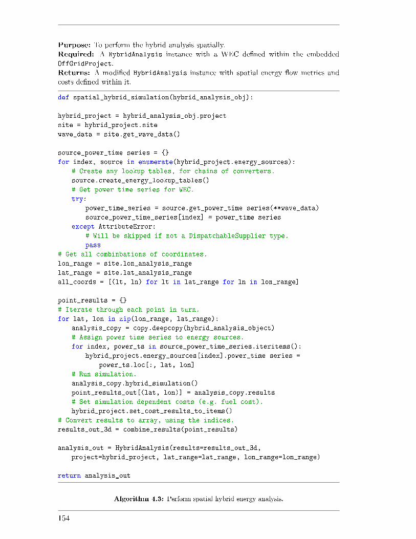
Purpose: To perform the hybrid analysis spatially.Required: A HybridAnalysis instance with a WEC de�ned within the embeddedOffGridProject.Returns: A modi�ed HybridAnalysis instance with spatial energy �ow metrics andcosts de�ned within it.

def spatial_hybrid_simulation(hybrid_analysis_obj):

hybrid_project = hybrid_analysis_obj.project

site = hybrid_project.site

wave_data = site.get_wave_data()

source_power_time series = {}

for index, source in enumerate(hybrid_project.energy_sources):

# Create any lookup tables, for chains of converters.

source.create_energy_lookup_tables()

# Get power time series for WEC.

try:

power_time_series = source.get_power_time series(**wave_data)

source_power_time_series[index] = power_time series

except AttributeError:

# Will be skipped if not a DispatchableSupplier type.

pass

# Get all combinbations of coordinates.

lon_range = site.lon_analysis_range

lat_range = site.lat_analysis_range

all_coords = [(lt, ln) for lt in lat_range for ln in lon_range]

point_results = {}

# Iterate through each point in turn.

for lat, lon in zip(lon_range, lat_range):

analysis_copy = copy.deepcopy(hybrid_analysis_object)

# Assign power time series to energy sources.

for index, power_ts in source_power_time_series.iteritems():

hybrid_project.energy_sources[index].power_time series =

power_ts.loc[:, lat, lon]

# Run simulation.

analysis_copy.hybrid_simulation()

point_results_out[(lat, lon)] = analysis_copy.results

# Set simulation dependent costs (e.g. fuel cost).

hybrid_project.set_cost_results_to_items()

# Convert results to array, using the indices.

results_out_3d = combine_results(point_results)

analysis_out = HybridAnalysis(results=results_out_3d,

project=hybrid_project, lat_range=lat_range, lon_range=lon_range)

return analysis_out

Algorithm 4.3: Perform spatial hybrid energy analysis.

154

group are modi�ed by plus or minus the load value. For example, for a load value

of 10 and variability of 0.2 the modi�ed load value will be between 10± 2.

The variability_random_seed attribute allows the seed to be chosen for

generating the random numbers, so di�erent scenarios can be run for the same

random variabilities. The actual output load pro�le from the class is the de-

rived attribute load_profile_with_variability. This applies the method

generate_load_profile_with_variability to the input load pro�le. The two

private methods below this in the hybrid UML (Figure 4.2) are just used to apply

the variabilities. The �nal load pro�le with variability attribute can then be prop-

agated into any subsequent hybrid system simulations. If the output_resolution

is speci�ed then the output load pro�le will be resampled to a new time base. This

step is carried on in a straightforward manner, using the inbuilt resample method

of Pandas.

The second load pro�le based class, CombinedProfile, contains multiple

LoadProfile instances and provides a way to combine then into a single pro-

�le. This is useful for situations where the overall energy demand can be clearly

compartmentalised into distinct, independent components. For a �sh farm energy

system, two examples might be the feed system (active during the morning and

early afternoon) and underwater lighting (which might be active 24 hours per day

during winter months).

In a similar way to WaveDevice and WaveArray from Section 3.6.2, the load

pro�le classes are linked by a composite relationship: as a combined load pro-

�le can also be thought of as a load pro�le in its own right. To generate the

combined load pro�le the class resamples all of the constituent load pro�les,

with any variabilities applied, to the same time base, de�ned by the inherited

output_resolution attribute. As a child of LoadProfile, variabilities can also

be de�ned at the combined pro�le level. These are then applied, the output load

pro�le consistent in type to that generated by the parent class.

4.4 Energy Sources and Converters

All of the system components that de�ne the hybrid system and are used di-

rectly in the algorithm inherit from a common class: SystemComponent. This

includes diesel generators, batteries and the wave energy converter. While the

nature of the energy provided by these objects di�ers, the parent class contains

attributes and methods that are applicable to all of them, and provides the nec-

155

essary blueprint for creating components compatible with the hybrid algorithm.

For a given system component, four generic attributes dictate the upper and

lower limits of power transfer, in units of kW:

• The maximum power that can be output (max_power_output).

• The minimum power that must be output (min_power_output).

• The maximum power that can be input (max_power_input).

• The minimum power that must be input (min_power_input).

The convention is for output to be positive and input negative. In some cases

the values are constants, indirectly set by the user (for example the maximum

power output of the diesel generator is set equal to its rated power). For other

classes, the values will vary in time and will essentially be reassigned for each time

step of the simulation; includes the battery where the energy output depends on

the battery capacity at that time step. The input_active and output_active

attributes allow the component to be turned on and o� within the simulation. This

is primarily used for the battery class to allow it to build up charge over multiple

simulation time steps without being expected to supply load. This functionality

could be extended to other components, to allow them to be forced on or o�

at speci�c periods in time, however this is not a fundamental feature and so is

considered as future work.

The modelling_time step attribute is the length of the algorithm time step

in hours. It is set within the hybrid simulation, and allows the extents of en-

ergy output and input to be determined through multiplication with the above

attributes. For example, the maximum energy output that is possible, Emax, out,

is given by:

Emax, out = Pmax, out ×∆t× ηo , (4.2)

where Pmax, out is the maximum power output attribute, ∆t the

modelling_time_step attribute and ηo is the output_efficiency attribute.

The energy_output and energy_input methods calculate the actual energy

values that can be obtained, given the values that are desired. They are

calculated by limiting the energy to the energy ranges:

Eout(t) =

Emin, in, if Ed < Emin, in

Ed(t), if Emin, in ≤ Ed ≤ Emax, out

Emax, out, if Ed > Emax, out ,

(4.3)

156

where Ed is the energy that is desired from the energy supplier by the load. Similar

equations are speci�ed for energy input considering the power input limits; this

includes an input_efficiency attribute. Both this and the output e�ciency

are considered to be inherent properties of the physical component, although

might not be relevant for all child classes. The energy output and input functions

are used at each time step of the hybrid algorithm, to see how a given system

component interacts with the energy �ow.

As for the e�ciency attributes, the decision was taken to have both energy

input and output contained within the same object, even when input is not rele-

vant (for example, in the case of the diesel generator). This ensures that all of the

objects look identical to the energy balancing algorithm previously introduced.

While there are a small number of potential components that can be considered,

enforcing this typing and coding the objects in this generic fashion means that

additional energy sources, for example wind turbines or solar PV, could be easily

introduced in the future.

The EnergySupplier class represents objects that produce power and can

supply energy to reduce the load requirements. The main distinction between

this class and its parent is the introduction of the converters attribute. This is

added to account for any physical electrical power converters that are required to

obtain the necessary energy form. Examples could include transformers, recti�ers

and inverters. By essentially considering the converter and energy source as one

system, while not a true representation of the physical system, means that the

impact on the �nal energy due to losses in the converter are straightforward to

apply internally.

Individual converters are de�ned by the Converter class. This adds the

rating attribute to the SystemComponent parent, which acts as an upper

limit to power output. The efficiency attribute is directly linked to the

output_efficiency attribute inherited from the parent class. The class also

contains a modi�ed energy_output method. This allows two potential variations

of energy output to be obtained: the output for a desired output value (post

e�ciency) and the output where the output value is �xed (pre e�ciency). For

example, considering a 20 kW converter with e�ciency of 90%, the output power

could be de�ned in the following ways:

• 15 kW is desired from the converter. The maximum power output is 18 kW

(20× 0.9) so Eout = 15 kW.

• A �xed power of 15 kW is send to the converter from a component further

157

up the chain. The input power cannot be modi�ed, and so the output power

is Eout = 15× 0.9 = 13.5 kW.

The approach chosen depends on the level of control that the system has on

the power �ow. For example, wave energy converter output is non-dispatchable

and so a converter for this system would use a �xed approach. Conversely, the

hybrid system can provide feedback into a diesel generator so has control over the

generator power to obtain a certain amount of energy. Here a converter's energy

output would use the desired method, to back-calculate the generator power.

Within the EnergySupplier class, multiple converters can be chained and

stored within the converters attribute as entries in an ordered dictionary type.

The dictionary key is set to the converter's _id. As well as the converter the di-

rection of the converter must be speci�ed, i.e. whether it applies to output power,

input power or both directions. For multiple converters, due to the rating param-

eter the order of the converters in the system is important. For example a low

rating converter at the beginning of the chain would limit the power �owing into

subsequent converters, acting as a power bottleneck. The converters can hence

be reordered, using reorder_converters which creates a new ordered dictionary

based on the key order speci�ed.

The modi�ed energy values due to the converters can be obtained using four

methods:

• get_converter_vals_for_fixed_input

• get_converter_vals_for_fixed_output

• get_converter_vals_for_desired_input

• get_converter_vals_for_desired_input

These methods essentially supersede the energy_output and energy_input

functions, giving breakdowns of the energy �ow across the converter components.

For each function, an algorithm cycles through each converter in the chain of

converters in turn. It calculates the resolved power, constraining by rating and

multiplying by e�ciency as described above, and sends this though to the next

converter. Each function outputs the input and output power for every converter

in the chain for the initial power value speci�ed. The �xed functions start at the

beginning of the converter chain, whereas the desired functions perform a similar

calculation but considering a reversed chain which starts at the desired value.

For longer chains of converters this process can increase the hybrid algorithm

calculation time if it needs to be done at every time step. The solution for this

158

is the create_energy_lookup_tables function. This calculates the energy input

and output at discrete energy values, storing the resulting functions within the

object so that the energy can be looked up rather than needing to be calculated.

While all of the child energy sources inherit from EnergySupplier, the main

distinction between them is how they de�ne and calculate their power limits. The

next sections describe the components and the properties that they have which

facilitate these considerations.

4.4.1 Diesel generator

For the majority of hybrid energy applications a conventional energy source

will be required in some form to ensure that energy can be supplied at crucial

times. For smaller hybrid systems, like the �sh farms that are the subject of this

research, a diesel generator is the primary source of energy. The main output

of the diesel generator class in the model context is the fuel quantity that must

be consumed by the generator to supply the necessary energy to the required

load. This allows fuel cost to be calculated. As fuel cost is one of the biggest

components of a conventional o�-grid energy system, it is vital to quantify this

number and see how the introduction of renewable energy can reduce it.

The diesel generator functionality has been split up into two classes:

DispatchableSupplier and DieselGenerator. The DispatchableSupplier

class is to represent energy sources which run o� a fuel source, and hence can

be turned on and o� at will when the energy user desires. The base Fuel class

is reused for the fuel in this context, as described in Section 3.4.7 and previously

used for the vessel fuel in Section 3.7.1. This is to provide a uniform framework

for fuel cost de�nition and calculation. The fuel quantity is denoted as a derived

attribute in the hybrid system UML as it can be set at the dispatchable supplier

level using a dedicated method.

The DieselGenerator class inherits from DispatchableSupplier. It is the

sole child; the classes were separated to allow dispatchable sources to be easily

added to the model in the future if desired. As well as costs and rated power

(inherited from the parent classes) the class is also de�ned by its fuel consumption

properties. On diesel generator data sheets, it is common for the manufacturer

to quote the amount of fuel that is consumed when the generator is providing

di�erent levels of power, typically in units of litres or gallons per hour of operation.

An example of these data is shown in Figure 4.5.

The DieselGenerator class stores these data as a dictionary within the

159

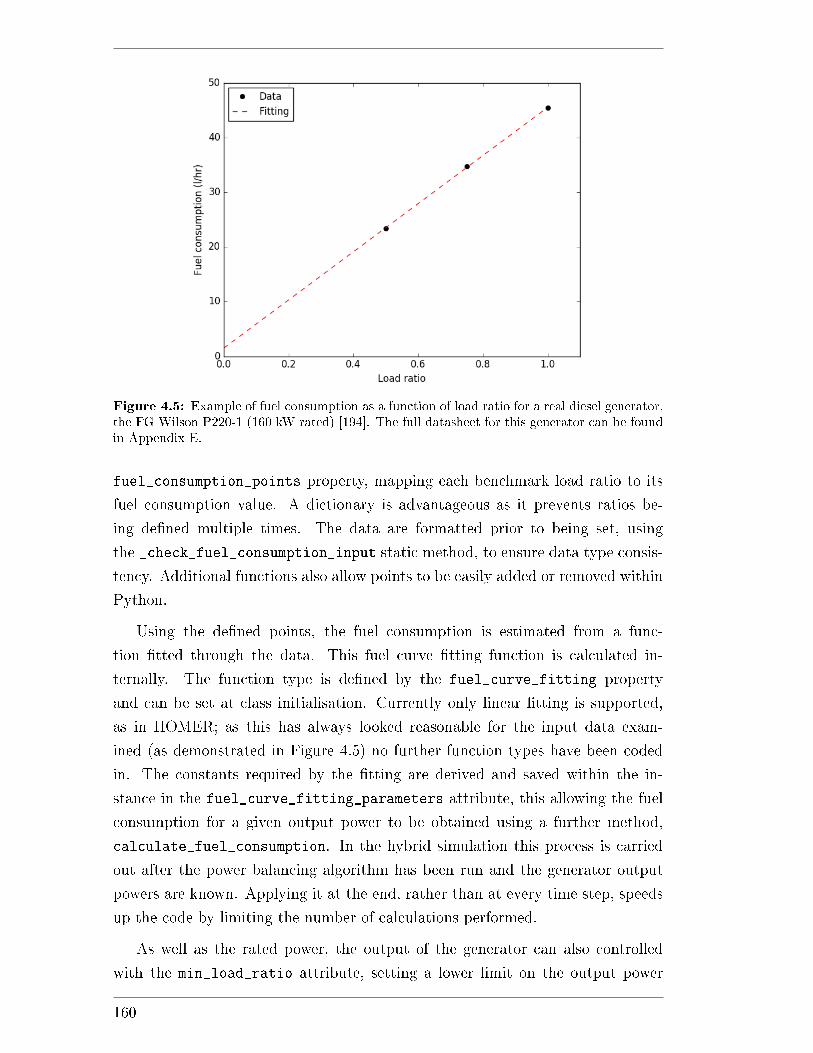
Figure 4.5: Example of fuel consumption as a function of load ratio for a real diesel generator,the FG Wilson P220-1 (160 kW rated) [194]. The full datasheet for this generator can be foundin Appendix E.

fuel_consumption_points property, mapping each benchmark load ratio to its

fuel consumption value. A dictionary is advantageous as it prevents ratios be-

ing de�ned multiple times. The data are formatted prior to being set, using

the _check_fuel_consumption_input static method, to ensure data type consis-

tency. Additional functions also allow points to be easily added or removed within

Python.

Using the de�ned points, the fuel consumption is estimated from a func-

tion �tted through the data. This fuel curve �tting function is calculated in-

ternally. The function type is de�ned by the fuel_curve_fitting property

and can be set at class initialisation. Currently only linear �tting is supported,

as in HOMER; as this has always looked reasonable for the input data exam-

ined (as demonstrated in Figure 4.5) no further function types have been coded

in. The constants required by the �tting are derived and saved within the in-

stance in the fuel_curve_fitting_parameters attribute, this allowing the fuel

consumption for a given output power to be obtained using a further method,

calculate_fuel_consumption. In the hybrid simulation this process is carried

out after the power balancing algorithm has been run and the generator output

powers are known. Applying it at the end, rather than at every time step, speeds

up the code by limiting the number of calculations performed.

As well as the rated power, the output of the generator can also controlled

with the min_load_ratio attribute, setting a lower limit on the output power

160

can be produced. This feature, also used in HOMER, copies a real generator

management strategy that might be followed in situations where the generator is

oversized for the application. Some generators will have minimum loads speci�ed

by the manufacturer. At other times it might be desirable to prevent damage to

the generator, for example to limit �wet stacking� (where fuel is not completely

combusted and hence can clog up and reduce the lifetime of the generator). In

reality, a minimum load could be applied by connecting the generator to a bank

of resistors to dissipate power. The attribute is represented as a proportion of

the rated power, de�ned as a �oat between 0 and 1, and overwrites the inherited

min_power_output property:

Pmin, in = Prated ×Rmin , (4.4)

where Rmin is the minimum load ratio and Prated the generator rated power.

Lastly, in addition to any local costs, a dedicated replacement cost can be

set. This is represented by the replacement_cost attribute. This can be used

in combination with the generator lifetime, de�ned in units of hours within the

attribute lifetime_op_hours, to calculate the cost periods that the generator

needs to be replaced in.

The method calculate_replacement_periods takes in a time series of gen-

erator operating hours, either as a NumPy array or Pandas DataFrame. This is

the number of hours that the generator is operating per time period and works

irrespective of the time units (although monthly data is used in the main hybrid

algorithm to keep consistency with the other components of the cash �ow anal-

ysis which tend to consider a month base). The function iterates through the

array, calculating the cumulative sum of the operating hours. The time period

where replacement is needed is found when the hours exceed the lifetime. In this

case the cumulative sum is reset (starting from the time remaining in the period)

and the index of the period is stored. This algorithm continues until it has iter-

ated through the whole array, the output being a list containing periods where

generator replacement is required.

With knowledge of these replacement periods, a new cost instance represent-

ing the replacement can be created. This process is achieved using the method

create_replacement_cost_item. After getting the replacement periods above,

the method creates a new FutureCost instance: with a value set to that speci�ed

in the replacement_cost and cost periods de�ned as in the periods (see Section

3.4.2 for a description on how these are speci�ed). This output instance can then

161

be assigned to any object as a local cost and �ltered into the cash �ow analysis

using any cost_categories de�ned within the generator replacement cost.

4.4.2 Hybrid wave device

To incorporate wave energy devices into the algorithm, a class is required which

combines the EnergySource class characteristics with the wave device classes de-

�ned in Section 3.6.2. It is assumed that, while not all of the grid tied project costs

will apply, the nature of the device structure itself will remain the same. The hy-

brid wave energy device class, WaveEnergyConverterHybrid hence inherits from

both the wave_device module's WaveEnergyArray class and the EnergySource

class, through the intermediate NonDispatchableSupplier.

The class NonDispatchableSupplier is the opposite of the dispatchable sup-

plier class from Section 4.4.1. It is a representation of intermittent renew-

able energy sources, which generate power according to physical resource and

hence contribute to the load at will. Whereas the latter class can be simply

de�ned by constant minimum and maximum power limits over all time steps,

NonDispatchableSupplier instances have limits which �uctuate according to

the power output at the desired time.

The key attribute for this class is power_time_series. This power pro�le is a

Pandas DataFrame (as used for previous time series), the time dimension allowing

the power value at a speci�c time to be easily queried. The time_axis property

is directly derived from this embedded DataFrame.

To obtain the energy output for a particular time step in the hybrid power

balancing algorithm, �rst the instance attribute present_time is set to the same

time as the current time step of the hybrid algorithm; this is the start time of

power production. The end time of power production is equal to the start time

plus the length of the modelling_time step attribute (this is set from the load

pro�le time dimension as described in Section 4.3).

If both start time and end time are de�ned in the power time series (i.e. the

load pro�le and power time series are de�ned over the same time dimension) then

the energy is just obtained by multiplying the power at the start time step by the

time di�erence. Computationally this is the fastest method. If the power time

series dimension is di�erent then the energy is calculated by looking at the power

values between the start and end time, calculating the energy for each portion of

the time series in turn. This functionality is useful as it means that the power

can be provided at a di�erent time dimension, however it is also slower to execute

162

as there are more calculations required to resolve the energy factors between the

time displacements.

In this class there is no distinction between maximum and minimum energy

output: the energy is always de�ned by the relevant portion of the time series,

which is then modi�ed to account for any embedded converters.

The WaveEnergyConverterHybrid class contains no additional methods, only

using those inherited from its two parents. To prepare the wave device object for

the hybrid analysis, the power_time_series attribute needs to be set. This is

done within the overall spatial analysis function (described in Section 3.1). The

modular nature of the code makes any modi�cations to the embedded items within

the wave device easy to de�ne, without needing to de�ne the whole system again.

For a �sh farm system, this might include specifying a cable landing point to the

feed barge location and reduced mooring costs due to being able to share some of

the �sh farm infrastructure.

4.4.3 Batteries

The energy storage is a crucial part of the wave energy hybrid system, both re-

ducing the amount of excess energy produced when the wave energy input exceeds

the load and picking up any shortfall to reduce diesel consumption.

There are three classes that have been created to model battery systems.

These all inherit from EnergySupplier, allowing power input and output limits

to be de�ned and set at each simulation time step set. The �rst two classes,

BatteryBase and KineticBattery are representations of individual batteries.

The third, BatteryBank, represents a bank of batteries, with the batteries con-

nected in series and parallel. This is the class that is most commonly used as it

allows larger amount of energy to be stored.

4.4.3.1 Battery base class

The class BatteryBase represents a very basic battery. While it can be used

in the model, the main purpose of the class is to de�ne fundamental battery

parameters, serving as a foundation for more complex battery child classes (for

example the KineticBattery described in Section 4.4.3.2). Whereas in a real

battery the maximum amount of energy that can be input or output will depend on

the charging history of the battery, in this system the limits are de�ned arbitrarily

by the user.

As for the energy sources previously introduced, this class seeks to determine

163

the power limits, and hence energy, that the battery can contribute towards the

load pro�le in a given time step. To achieve this the class has three key properties:

• The battery capacity (the nominal_capacity_kwh attribute). This de�nes

the nameplate energy that is stored in the battery.

• The maximum current that is applied to charge the battery (calculated using

the max_charge_current function).

• The maximum discharging current that is applied to get energy out of the

battery (calculated using the max_discharge_current function).

Whereas the diesel generator and hybrid wave energy converter classes are

only concerned with energy production, the battery system also must be able to

calculate the maximum energy that can be put into it.

At a given time step, the power limits are calculated using the voltage at-

tribute, V , and respective charge current limit:

Pmax, in = V Ic, max (4.5)

Pmax, out = V Id, max , (4.6)

where Ic, max is the maximum charge current and Id, max the maximum discharge

current. The voltage is a fundamental property of the battery and for the simu-

lation is assumed to be �xed. The o�-grid model is not designed to be a detailed

electrical design tool, instead framing the simulation from an economic perspec-

tive, and so a higher level energy focussed approach can be justi�ed (mirroring

commercially available tools, e.g. HOMER).

For BatteryBase the maximum discharge current is set arbitrarily using the

discharge_current_limit attribute. In reality, and for more realistic battery

models, this is an internal property of the battery and would be calculated. The

maximum output energy is limited by both this attribute and the battery capac-

ity, which is constrained by the the minimum state of charge. This attribute,

min_state_of_charge, is introduced in real system controllers to prevent the

battery from experiencing deep charging cycles, as this can shorten their lifes-

pan [195]. Considering these aspects, as there is no minimum energy output, the

energy output that can be achieved at time step t can be expressed as:

Emax, out(t) =

Ed(t) if q(t)− Ed(t) > qmin

∆tPmax, out otherwise ,(4.7)

164

where ∆t is the length of time, q(t) is the initial battery capacity and qmin the

minimum allowed capacity, the product of the nominal battery capacity q0 and

the minimum state of charge Smin :

qmin = q0 × Smin . (4.8)

There is a second lower threshold, cycle_charge_threshold, which was intro-

duced in Section 4.2.4. This is only relevant in the context of the �cycle charge�

management strategy. If the battery SOC drops below this percentage then the

battery output is disabled (the output_active attribute set to false). This

means that the battery can only accept energy, until the capacity exceeds the

setpoint_soc threshold (at this point it can operate as an energy source once

more).

The maximum energy that the battery can receive is considered in a similar

manner to the output. It is constrained by an upper limit, the maximum capacity

of the battery qmax :

Emax, in(t) =

Ei(t) if q(t) + Ei(t) > qmax

∆tPmax, in otherwise ,(4.9)

where Ei(t) is the energy that is trying to be put into the battery. For

BatteryBase the maximum battery capacity is set equal to the nominal capacity

(typically the capacity at the 20 hour discharge rate), although it is calculated for

the KineticBattery child class.

Putting the above equations together means that the battery capacity can

never exceed the maximum or fall below the minimum state of charge. The

private methods capacity_above_min_threshold and capacity_headroom cal-

culate the limits on energy extraction for the present_capacity of the battery.

This attribute de�nes the capacity of the battery at the present time being con-

sidered, and is set at each time step within the o�-grid simulation so that the

battery capacity is updated and monitored throughout the simulation. This is

achieved using the set_final_charge method. This takes in a desired current

and constrains it to the maximum that is allowed, by converting the current to

power and hence energy (using the modelling_time step attribute) and using

the above inequalities. This energy is then added to the present_capacity, per-

manently modifying it. The function is compatible with both input and output

currents, applying the sign convention introduced in Section 4.4. The battery can

be reset to its initial, fully charged state, by using the set_initial_capacities

165

Figure 4.6: The two tank analogy, which is used as the basis of the kinetic battery model.The battery is essentially split into two halves: the right �available charge side� which containscharge which is immediately available to the system, and the left �bound charge� side. Thisenergy is only available after it has propagated to the right tank. Diagram based on [196].

method, which simply reassigns the nominal_capacity value to the present ca-

pacity attribute. It should be noted that all of the quantities concerned with

capacity are de�ned within the class twice: in units of AH and kWh. While AH

is the standard unit, kWh is the unit considered for the load pro�le and so is the

default output in the hybrid simulation. Conversion to kWh is easily achieved by

the following:

q[kWh] =q[AH]V

1000. (4.10)

Lastly, the input and output e�ciencies of this class are de�ned by the

roundtrip_efficiency. Mimicking the approach taken in HOMER, this assumes

that the same e�ciency is applied in each direction:

ηo = ηi =√ηrt , (4.11)

where ηrt is the round trip e�ciency.

4.4.3.2 Kinetic battery

The KineticBattery class builds on BatteryBase class by providing more

realistic estimates of the energy input and output. While these are essentially

de�ned by the user for the base class and only constrained by the state of charge,

within KineticBattery the values are also dependent on the time history of the

battery.

The main theory and calculations behind the battery model can be found

in [196]. The underlying principle, displayed in Figure 4.6, is that the battery

166

is modelled by two connected tanks. The �available charge� side contains energy

which is immediately available to the system, and also initially holds energy put

into the battery. The �bound charge� side contains energy which is not available

to the system in the immediate term. This energy must be transferred into the

available tank before it can be used; this has the e�ect of limiting the amount

of energy that the battery can provide or take in. The relative head di�erence

between the tanks, h1−h2 impacts the energy that can be transferred, the theoret-

ical basis meaning that charging regime more closely follows that of a real battery.

If the battery capacity is low then it will charge more quickly (bulk charging),

levelling o� as the head reduces and the battery reaches its maximum capacity.

To �nd the maximum power that can be transferred Equations 4.5 and 4.6 can

be used, however this time the current values are calculated:

Id,max =kq1,0e

−k∆t + q0kc(1− e−k∆t)

1− e−k∆t + c(k∆t− 1 + e−k∆t)(4.12)

Ic,max =−kcqmax + kq1,0e

−k∆t + q0kc(1− e−k∆t)

1− e−k∆t + c(k∆t− 1 + e−k∆t). (4.13)

Here q1,0 and q0 are the initial capacities in the available tank and the battery

as a whole and ∆t is the length of the time step, as before. There are also three

constants present: k, c and qmax. These are referred to as the kinetic model

constants and are based on the physical properties of the battery. The �rst two

essentially de�ne the ratio of the two tanks and the rate that charge can be

transferred between the tanks. The third, qmax, is the maximum charge as seen

previously, and with c de�nes the size of the two tanks:

q1, max = cqmax (4.14)

q2, max = (1− c)qmax . (4.15)

While for BatteryBase qmax was set equal to the nominal capacity, for this class

it is calculated (along with the other two constants) by using battery discharge

capacity data. This process is described in [196]. These constants only need to

be calculated once, at the beginning of the simulation.

To integrate all of the new theory and calculations required, the class con-

tains a number of additional attributes to its parent. The actual kinetic model

equations are de�ned in a separate module, kinetic_battery_model.py, to keep

the theory separate from the implementation. First, to set up the battery the

kinetic model constants need to be calculated. This can be achieved using the

167

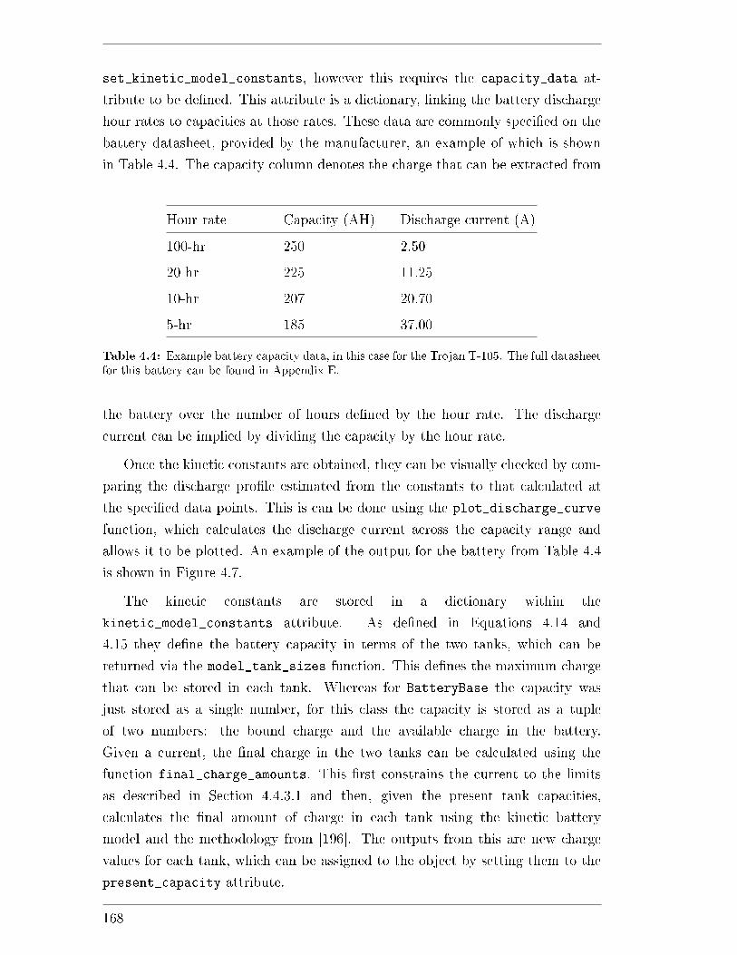
set_kinetic_model_constants, however this requires the capacity_data at-

tribute to be de�ned. This attribute is a dictionary, linking the battery discharge

hour rates to capacities at those rates. These data are commonly speci�ed on the

battery datasheet, provided by the manufacturer, an example of which is shown

in Table 4.4. The capacity column denotes the charge that can be extracted from

Hour rate Capacity (AH) Discharge current (A)

100-hr 250 2.50

20-hr 225 11.25

10-hr 207 20.70

5-hr 185 37.00

Table 4.4: Example battery capacity data, in this case for the Trojan T-105. The full datasheetfor this battery can be found in Appendix E.

the battery over the number of hours de�ned by the hour rate. The discharge

current can be implied by dividing the capacity by the hour rate.

Once the kinetic constants are obtained, they can be visually checked by com-

paring the discharge pro�le estimated from the constants to that calculated at

the speci�ed data points. This is can be done using the plot_discharge_curve

function, which calculates the discharge current across the capacity range and

allows it to be plotted. An example of the output for the battery from Table 4.4

is shown in Figure 4.7.

The kinetic constants are stored in a dictionary within the

kinetic_model_constants attribute. As de�ned in Equations 4.14 and

4.15 they de�ne the battery capacity in terms of the two tanks, which can be

returned via the model_tank_sizes function. This de�nes the maximum charge

that can be stored in each tank. Whereas for BatteryBase the capacity was

just stored as a single number, for this class the capacity is stored as a tuple

of two numbers: the bound charge and the available charge in the battery.

Given a current, the �nal charge in the two tanks can be calculated using the

function final_charge_amounts. This �rst constrains the current to the limits

as described in Section 4.4.3.1 and then, given the present tank capacities,

calculates the �nal amount of charge in each tank using the kinetic battery

model and the methodology from [196]. The outputs from this are new charge

values for each tank, which can be assigned to the object by setting them to the

present_capacity attribute.

168

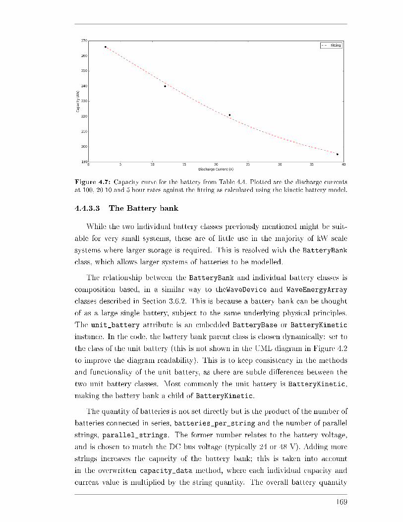
Figure 4.7: Capacity curve for the battery from Table 4.4. Plotted are the discharge currentsat 100, 20 10 and 5 hour rates against the �tting as calculated using the kinetic battery model.

4.4.3.3 The Battery bank

While the two individual battery classes previously mentioned might be suit-

able for very small systems, these are of little use in the majority of kW scale

systems where larger storage is required. This is resolved with the BatteryBank

class, which allows larger systems of batteries to be modelled.

The relationship between the BatteryBank and individual battery classes is

composition based, in a similar way to theWaveDevice and WaveEnergyArray

classes described in Section 3.6.2. This is because a battery bank can be thought

of as a large single battery, subject to the same underlying physical principles.

The unit_battery attribute is an embedded BatteryBase or BatteryKinetic

instance. In the code, the battery bank parent class is chosen dynamically: set to

the class of the unit battery (this is not shown in the UML diagram in Figure 4.2

to improve the diagram readability). This is to keep consistency in the methods

and functionality of the unit battery, as there are subtle di�erences between the

two unit battery classes. Most commonly the unit battery is BatteryKinetic,

making the battery bank a child of BatteryKinetic.

The quantity of batteries is not set directly but is the product of the number of

batteries connected in series, batteries_per_string and the number of parallel

strings, parallel_strings. The former number relates to the battery voltage,

and is chosen to match the DC bus voltage (typically 24 or 48 V). Adding more

strings increases the capacity of the battery bank; this is taken into account

in the overwritten capacity_data method, where each individual capacity and

current value is multiplied by the string quantity. The overall battery quantity

169

is calculated and set to the unit battery's quantity property, ensuring that the

correct quantity is used for the cost analysis. As the battery bank inherits from

ItemBase, additional costs can also be set at the battery bank level, within the

local_costs attribute. This means that costs that are independent of the battery

model only need to be de�ned once, allowing di�erent battery models to be easy

swapped in and out. Examples could be the cost to inspect or install the battery

bank.

4.5 Limitations and Assumptions Summary

This section highlights the main limitations and assumptions that are present

in the o�-grid sub-model. These are presented in Table 4.5. While the main

functionality draws from the commercial HOMER software, not all of the de-

sired features could be implemented due to the time constraints of the project.

The most signi�cant limitations concern the battery. While the kinetic battery

approach does provide some realism to the battery model, the model does not

include calculation of the battery lifetime or account for degradation of the bat-

tery capacity over time or due to operating temperature. As the former aspect is

linked to the energy �ow through the battery, a geospatial property when paired

with a WEC, it means that the battery bank cost calculated in the model is

always static over the spatial domain. This means that the spatial cost pro�le

will not re�ect reality. The main reason why they were not included was due to

the time constraints of the project; there is nothing in the model implementation

that would prevent them from being added in future. As the relative cost of the

battery bank is low relative to the typical WEC and fuel costs it is not thought

that these missing aspects will have much impact on the �nal LCOE. Also, with

careful system design and examining background literature, the battery life could

be estimated and replacement included using a FutureCost local cost with a re-

curring time component (see Section 3.4.2). This process is carried out in Chapter

6 for the o�-grid case study sensitivity analysis.

The second main limitation compared to the literature is that the algorithm

does not optimise for cost. If implemented, this would allow energy sources to

provide variable energy and operate �out of turn�, to minimise the overall system

cost. While this is sometimes seen, for example in HOMER and [158], it was

considered too complex for this project. There are more signi�cant factors which

impact cost, for example the WEC costs, which can be examined and are su�cient

for such easy stage feasibility. Cost optimisation of the algorithm would likely to

170

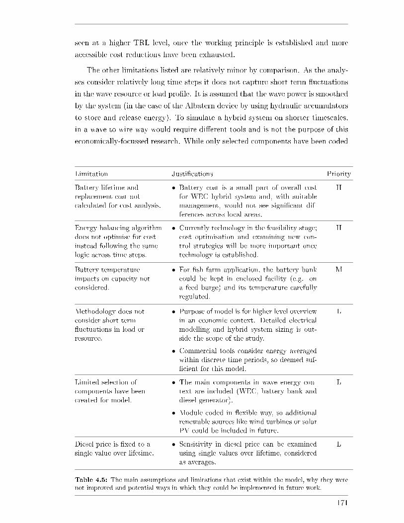
seen at a higher TRL level, once the working principle is established and more

accessible cost reductions have been exhausted.

The other limitations listed are relatively minor by comparison. As the analy-

ses consider relatively long time steps it does not capture short term �uctuations

in the wave resource or load pro�le. It is assumed that the wave power is smoothed

by the system (in the case of the Albatern device by using hydraulic accumulators

to store and release energy). To simulate a hybrid system on shorter timescales,

in a wave to wire way would require di�erent tools and is not the purpose of this

economically-focussed research. While only selected components have been coded

Limitation Justi�cations Priority

Battery lifetime andreplacement cost notcalculated for cost analysis.

• Battery cost is a small part of overall costfor WEC hybrid system and, with suitablemanagement, would not see signi�cant dif-ferences across local areas.

H

Energy balancing algorithmdoes not optimise for costinstead following the samelogic across time steps.

• Currently technology in the feasibility stage;cost optimisation and examining new con-trol strategies will be more important oncetechnology is established.

H

Battery temperatureimpacts on capacity notconsidered.

• For �sh farm application, the battery bankcould be kept in enclosed facility (e.g. ona feed barge) and its temperature carefullyregulated.

M

Methodology does notconsider short term�uctuations in load orresource.

• Purpose of model is for higher level overviewin an economic context. Detailed electricalmodelling and hybrid system sizing is out-side the scope of the study.

• Commercial tools consider energy averagedwithin discrete time periods, so deemed suf-�cient for this model.

L

Limited selection ofcomponents have beencreated for model.

• The main components in wave energy con-text are included (WEC, battery bank anddiesel generator).

• Module coded in �exible way, so additionalrenewable sources like wind turbines or solarPV could be included in future.

L

Diesel price is �xed to asingle value over lifetime.

• Sensitivity in diesel price can be examinedusing single values over lifetime, consideredas averages.

L

Table 4.5: The main assumptions and limitations that exist within the model, why they werenot improved and potential ways in which they could be implemented in future work.

171

into the sub-model, they capture the options available for a small wave energy hy-

brid system which is the purpose of this study. Fundamentally, the modular nature

of the code means that new energy sources could be easily created. For example

wind turbines or solar PV classes could inherit from the DispatchableSupplier

class and would only require a power time series in order to slot directly into the

algorithm. The last point, while a limitation, can be incorporated by viewing the

diesel price as a discounted lifetime average and conducting sensitivity analysis

on the price value.

172

5Grid-connected Wave Energy

Systems

The section presents a case study to demonstrate the model capabilities and

how it can be used in practice. A grid connected wave energy system is considered,

as in the majority of previous literature. First a baseline analysis is described,

considering a speci�c WaveNET array, which serves as a reference point for pro-

ceeding analyses. Henceforth this is known as the baseline scenario. The input

data are described and justi�ed, and the immediate results are discussed. Some

sensitivities are then examined, looking at the impact of speci�c parameters on

the overall baseline scenario LCOE. Several of these are combined to form an

Optimistic Scenario to show how the model can be used to evaluate modi�ed

systems.

All of the data in the con�guration �les that were used to run the baseline

scenario can be found in Appendix C.

5.1 Case Study Location and Metocean Data

The metocean dataset that was used for the case studies covers an area o� the

west coast of Scotland. This area, shown in Figure 5.1, is a rectangle encompassing

both the Inner and Outer Hebrides and lies in the range 56.2 to 58.6◦N latitude

and -7.6 to -5.2◦E longitude. The spatial resolution of the data is 1/60◦ (one arc-

minute); this equates to a domain of 145 by 157 points (latitude by longitude).

The metocean data were provided by Albatern, having been previously pur-

173

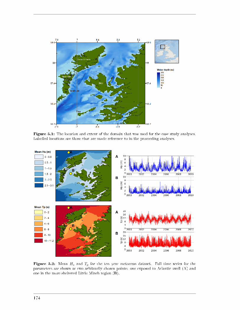
Figure 5.1: The location and extent of the domain that was used for the case study analyses.Labelled locations are those that are made reference to in the proceeding analyses.

Figure 5.2: Mean Hs and Tp for the ten year metocean dataset. Full time series for theparameters are shown at two arbitrarily chosen points: one exposed to Atlantic swell (A) andone in the more sheltered Little Minch region (B).

174

chased from Metocean Solutions Ltd. Metocean Solutions is a New Zealand based

consultancy who create and distribute metocean data, among other services [197].

The data consist of ten NetCDF �les, each made up of a single year of simulated

hindcast data, from 2000 to 2009. Included parameters are gridded Hs and Tp, at

a temporal resolution of 3 hours, and the water depths that were used to generate

the data. The data were created by Metocean Solutions in-house, using SWAN,

and validated by them internally using historical buoy data. Figure 5.2 shows the

mean Hs and Tp over the ten years of data, as well as time series data at two

arbitrarily chosen points.

The west of the domain is dominated by energetic swell waves with a long

Atlantic fetch. The mean Hs exceeds 3 m over much of this region, with mean

swells up to 11.2 s. As the waves move round the Outer Hebrides a signi�cant

amount of this energy is dissipated. Point B in the Little Minch shows similar

seasonal trends to the exposed point A but with a much lower mean Hs of 1.1

m. The peak period is also lower, with a more noisy signal that has a higher

contribution from locally wind driven waves.

5.2 Baseline Scenario: Early Demonstrator

The baseline scenario is based on best estimates for the current Albatern

WaveNET in the present day. As the TRL of the device is behind market matu-

rity (6-7), this represents an early stage demonstrator project. From this starting

point, the sensitivity analysis conducted in Section 5.3 aims to demonstrate the

model functionality by investigating the key cost drivers for the technology se-

lected.

5.2.1 Input data

5.2.1.1 The device

The baseline scenario considers a small Series-6 WaveNET deployed in the

area described in Section 5.1. The array is made up of six Squids arranged in a

triangular formation; this is known as a �3-Hex� array. Costs for the devices were

obtained from Albatern, with a high level breakdown shown in Table 5.1. The

most expensive item is the Anti Node, both per Squid and for the total array. As

well as these CAPEX, an insurance cost was included. This proportional cost was

set equal to 1% of the total project CAPEX, incurred annually. This value was

provided by Albatern, consistent with values quoted to them.

175

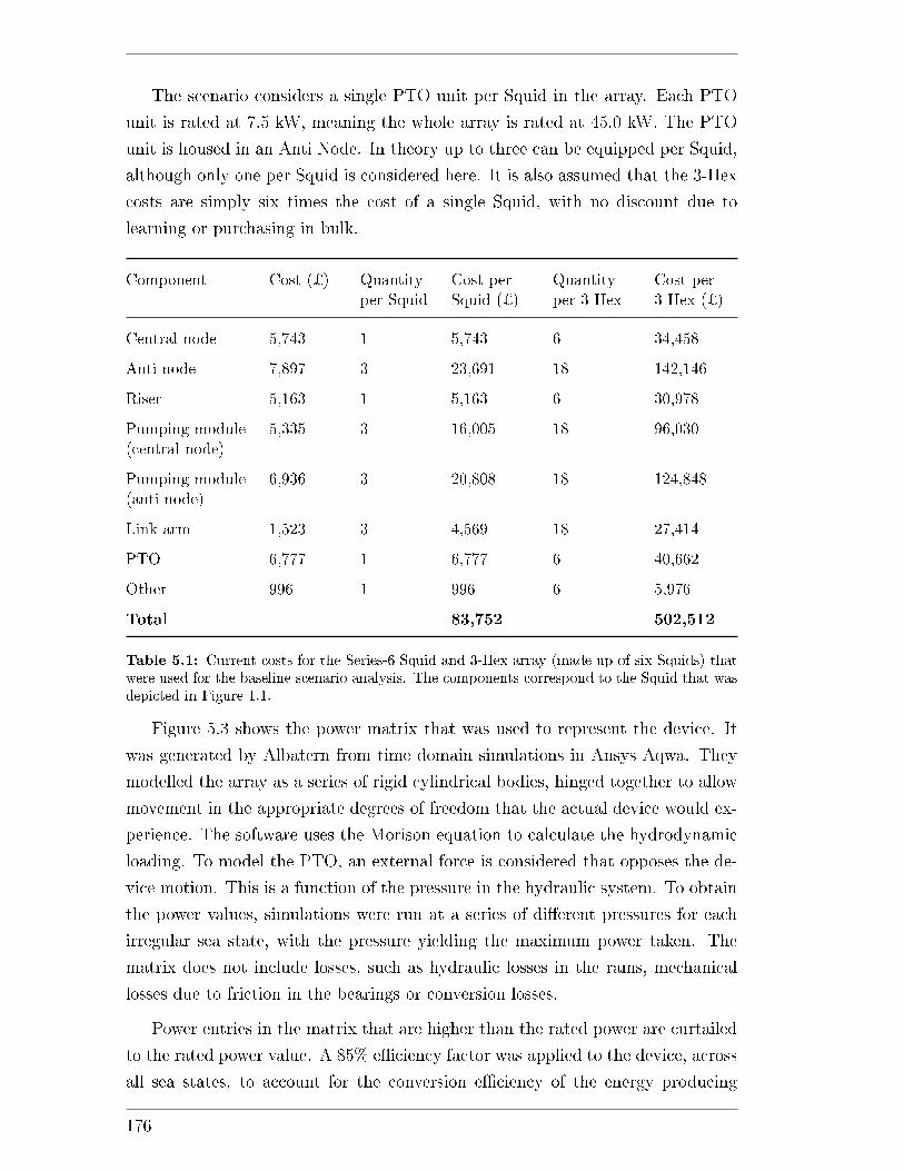
The scenario considers a single PTO unit per Squid in the array. Each PTO

unit is rated at 7.5 kW, meaning the whole array is rated at 45.0 kW. The PTO

unit is housed in an Anti Node. In theory up to three can be equipped per Squid,

although only one per Squid is considered here. It is also assumed that the 3-Hex

costs are simply six times the cost of a single Squid, with no discount due to

learning or purchasing in bulk.

Component Cost (¿) Quantityper Squid

Cost perSquid (¿)

Quantityper 3-Hex

Cost per3-Hex (¿)

Central node 5,743 1 5,743 6 34,458

Anti-node 7,897 3 23,691 18 142,146

Riser 5,163 1 5,163 6 30,978

Pumping module(central node)

5,335 3 16,005 18 96,030

Pumping module(anti node)

6,936 3 20,808 18 124,848

Link arm 1,523 3 4,569 18 27,414

PTO 6,777 1 6,777 6 40,662

Other 996 1 996 6 5,976

Total 83,752 502,512

Table 5.1: Current costs for the Series-6 Squid and 3-Hex array (made up of six Squids) thatwere used for the baseline scenario analysis. The components correspond to the Squid that wasdepicted in Figure 1.1.

Figure 5.3 shows the power matrix that was used to represent the device. It

was generated by Albatern from time domain simulations in Ansys Aqwa. They

modelled the array as a series of rigid cylindrical bodies, hinged together to allow

movement in the appropriate degrees of freedom that the actual device would ex-

perience. The software uses the Morison equation to calculate the hydrodynamic

loading. To model the PTO, an external force is considered that opposes the de-

vice motion. This is a function of the pressure in the hydraulic system. To obtain

the power values, simulations were run at a series of di�erent pressures for each

irregular sea state, with the pressure yielding the maximum power taken. The

matrix does not include losses, such as hydraulic losses in the rams, mechanical

losses due to friction in the bearings or conversion losses.

Power entries in the matrix that are higher than the rated power are curtailed

to the rated power value. A 85% e�ciency factor was applied to the device, across

all sea states, to account for the conversion e�ciency of the energy producing

176

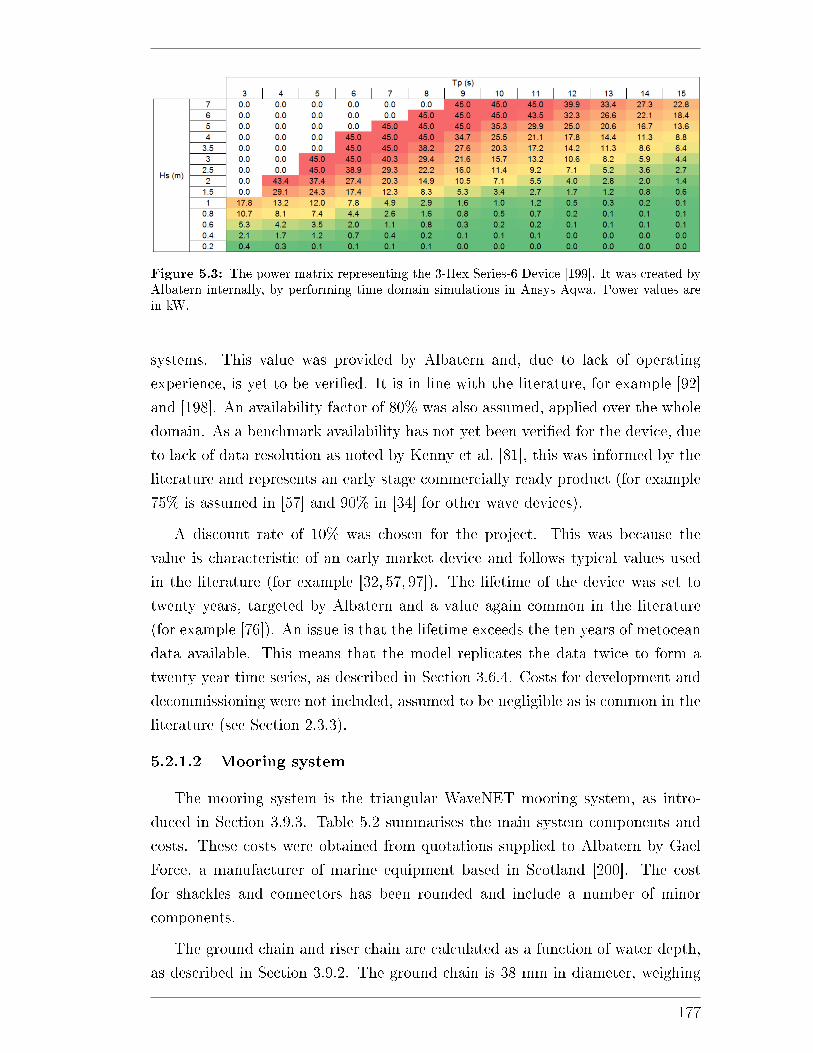
Figure 5.3: The power matrix representing the 3-Hex Series-6 Device [199]. It was created byAlbatern internally, by performing time domain simulations in Ansys Aqwa. Power values arein kW.

systems. This value was provided by Albatern and, due to lack of operating

experience, is yet to be veri�ed. It is in line with the literature, for example [92]

and [198]. An availability factor of 80% was also assumed, applied over the whole

domain. As a benchmark availability has not yet been veri�ed for the device, due

to lack of data resolution as noted by Kenny et al. [81], this was informed by the

literature and represents an early stage commercially ready product (for example

75% is assumed in [57] and 90% in [34] for other wave devices).

A discount rate of 10% was chosen for the project. This was because the

value is characteristic of an early market device and follows typical values used

in the literature (for example [32, 57, 97]). The lifetime of the device was set to

twenty years, targeted by Albatern and a value again common in the literature

(for example [76]). An issue is that the lifetime exceeds the ten years of metocean

data available. This means that the model replicates the data twice to form a

twenty year time series, as described in Section 3.6.4. Costs for development and

decommissioning were not included, assumed to be negligible as is common in the

literature (see Section 2.3.3).

5.2.1.2 Mooring system

The mooring system is the triangular WaveNET mooring system, as intro-

duced in Section 3.9.3. Table 5.2 summarises the main system components and

costs. These costs were obtained from quotations supplied to Albatern by Gael

Force, a manufacturer of marine equipment based in Scotland [200]. The cost

for shackles and connectors has been rounded and include a number of minor

components.

The ground chain and riser chain are calculated as a function of water depth,

as described in Section 3.9.2. The ground chain is 38 mm in diameter, weighing

177

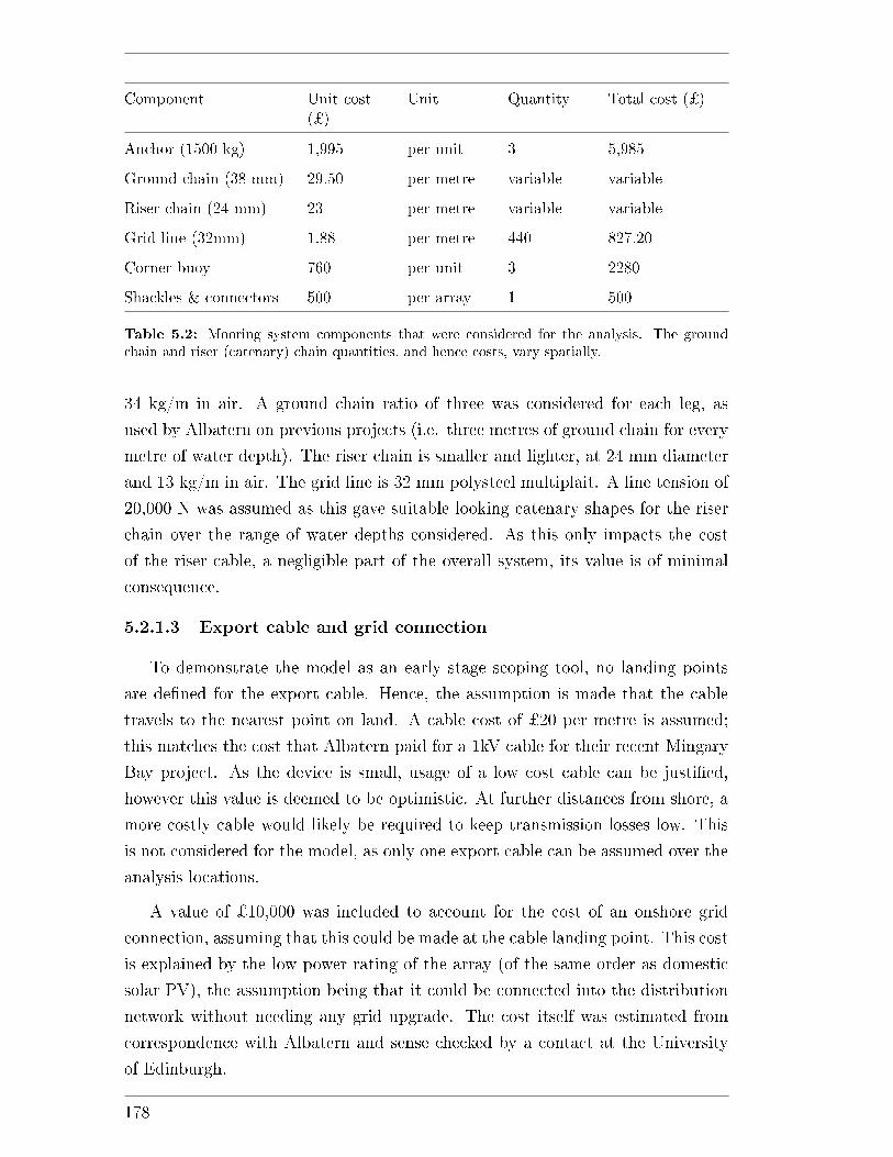
Component Unit cost(¿)

Unit Quantity Total cost (¿)

Anchor (1500 kg) 1,995 per unit 3 5,985

Ground chain (38 mm) 29.50 per metre variable variable

Riser chain (24 mm) 23 per metre variable variable

Grid line (32mm) 1.88 per metre 440 827.20

Corner buoy 760 per unit 3 2280

Shackles & connectors 500 per array 1 500

Table 5.2: Mooring system components that were considered for the analysis. The groundchain and riser (catenary) chain quantities, and hence costs, vary spatially.

34 kg/m in air. A ground chain ratio of three was considered for each leg, as

used by Albatern on previous projects (i.e. three metres of ground chain for every

metre of water depth). The riser chain is smaller and lighter, at 24 mm diameter

and 13 kg/m in air. The grid line is 32 mm polysteel multiplait. A line tension of

20,000 N was assumed as this gave suitable looking catenary shapes for the riser

chain over the range of water depths considered. As this only impacts the cost

of the riser cable, a negligible part of the overall system, its value is of minimal

consequence.

5.2.1.3 Export cable and grid connection

To demonstrate the model as an early stage scoping tool, no landing points

are de�ned for the export cable. Hence, the assumption is made that the cable

travels to the nearest point on land. A cable cost of ¿20 per metre is assumed;

this matches the cost that Albatern paid for a 1kV cable for their recent Mingary

Bay project. As the device is small, usage of a low cost cable can be justi�ed,

however this value is deemed to be optimistic. At further distances from shore, a

more costly cable would likely be required to keep transmission losses low. This

is not considered for the model, as only one export cable can be assumed over the

analysis locations.

A value of ¿10,000 was included to account for the cost of an onshore grid

connection, assuming that this could be made at the cable landing point. This cost

is explained by the low power rating of the array (of the same order as domestic

solar PV), the assumption being that it could be connected into the distribution

network without needing any grid upgrade. The cost itself was estimated from

correspondence with Albatern and sense checked by a contact at the University

of Edinburgh.

178

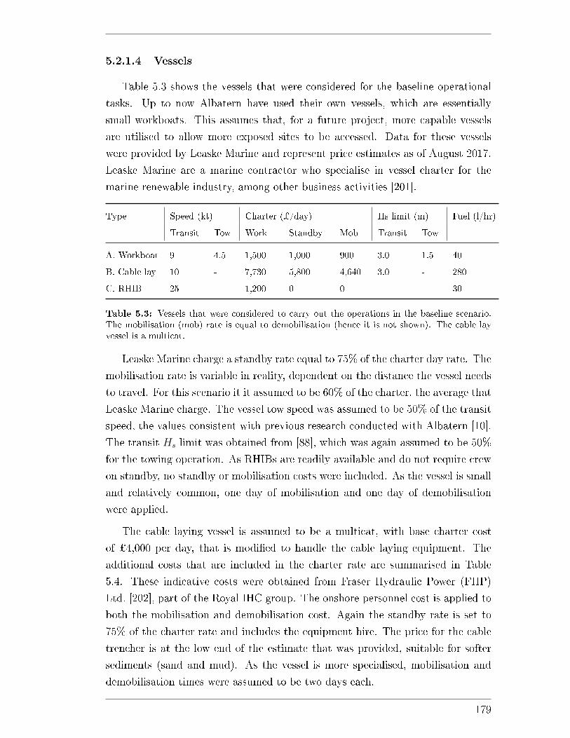
5.2.1.4 Vessels

Table 5.3 shows the vessels that were considered for the baseline operational

tasks. Up to now Albatern have used their own vessels, which are essentially

small workboats. This assumes that, for a future project, more capable vessels

are utilised to allow more exposed sites to be accessed. Data for these vessels

were provided by Leaske Marine and represent price estimates as of August 2017.

Leaske Marine are a marine contractor who specialise in vessel charter for the

marine renewable industry, among other business activities [201].

Type Speed (kt) Charter (¿/day) Hs limit (m) Fuel (l/hr)

Transit Tow Work Standby Mob Transit Tow

A. Workboat 9 4.5 1,500 1,000 900 3.0 1.5 40

B. Cable lay 10 - 7,730 5,800 4,640 3.0 - 280

C. RHIB 25 - 1,200 0 0 - - 30

Table 5.3: Vessels that were considered to carry out the operations in the baseline scenario.The mobilisation (mob) rate is equal to demobilisation (hence it is not shown). The cable layvessel is a multicat.

Leaske Marine charge a standby rate equal to 75% of the charter day rate. The

mobilisation rate is variable in reality, dependent on the distance the vessel needs

to travel. For this scenario it it assumed to be 60% of the charter, the average that

Leaske Marine charge. The vessel tow speed was assumed to be 50% of the transit

speed, the values consistent with previous research conducted with Albatern [10].

The transit Hs limit was obtained from [88], which was again assumed to be 50%

for the towing operation. As RHIBs are readily available and do not require crew

on standby, no standby or mobilisation costs were included. As the vessel is small

and relatively common, one day of mobilisation and one day of demobilisation

were applied.

The cable laying vessel is assumed to be a multicat, with base charter cost

of ¿4,000 per day, that is modi�ed to handle the cable laying equipment. The

additional costs that are included in the charter rate are summarised in Table

5.4. These indicative costs were obtained from Fraser Hydraulic Power (FHP)

Ltd. [202], part of the Royal IHC group. The onshore personnel cost is applied to

both the mobilisation and demobilisation cost. Again the standby rate is set to

75% of the charter rate and includes the equipment hire. The price for the cable

trencher is at the low end of the estimate that was provided, suitable for softer

sediments (sand and mud). As the vessel is more specialised, mobilisation and

demobilisation times were assumed to be two days each.

179

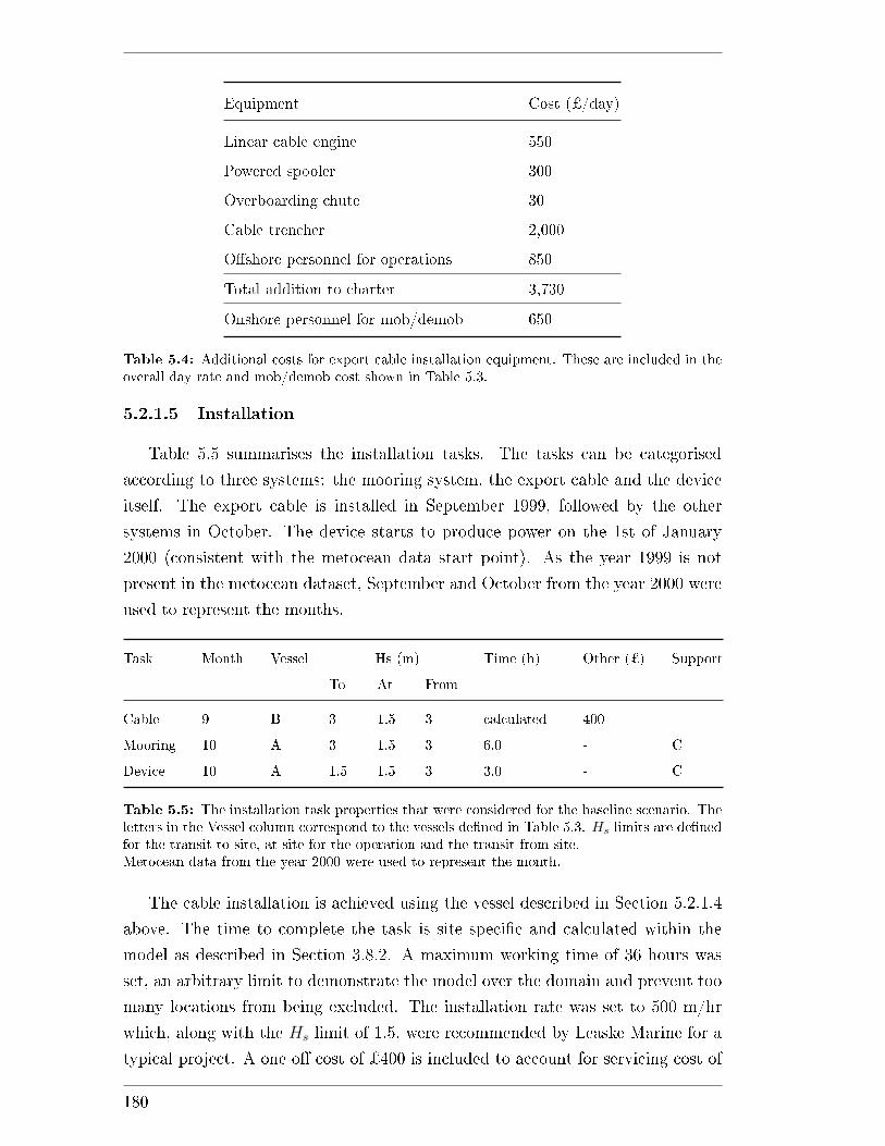
Equipment Cost (¿/day)

Linear cable engine 550

Powered spooler 300

Overboarding chute 30

Cable trencher 2,000

O�shore personnel for operations 850

Total addition to charter 3,730

Onshore personnel for mob/demob 650

Table 5.4: Additional costs for export cable installation equipment. These are included in theoverall day rate and mob/demob cost shown in Table 5.3.

5.2.1.5 Installation

Table 5.5 summarises the installation tasks. The tasks can be categorised

according to three systems: the mooring system, the export cable and the device

itself. The export cable is installed in September 1999, followed by the other

systems in October. The device starts to produce power on the 1st of January

2000 (consistent with the metocean data start point). As the year 1999 is not

present in the metocean dataset, September and October from the year 2000 were

used to represent the months.

Task Month Vessel Hs (m) Time (h) Other (¿) Support

To At From

Cable 9 B 3 1.5 3 calculated 400 -

Mooring 10 A 3 1.5 3 6.0 - C

Device 10 A 1.5 1.5 3 3.0 - C

Table 5.5: The installation task properties that were considered for the baseline scenario. Theletters in the Vessel column correspond to the vessels de�ned in Table 5.3. Hs limits are de�nedfor the transit to site, at site for the operation and the transit from site.Metocean data from the year 2000 were used to represent the month.

The cable installation is achieved using the vessel described in Section 5.2.1.4

above. The time to complete the task is site speci�c and calculated within the

model as described in Section 3.8.2. A maximum working time of 36 hours was

set, an arbitrary limit to demonstrate the model over the domain and prevent too

many locations from being excluded. The installation rate was set to 500 m/hr

which, along with the Hs limit of 1.5, were recommended by Leaske Marine for a

typical project. A one o� cost of ¿400 is included to account for servicing cost of

180

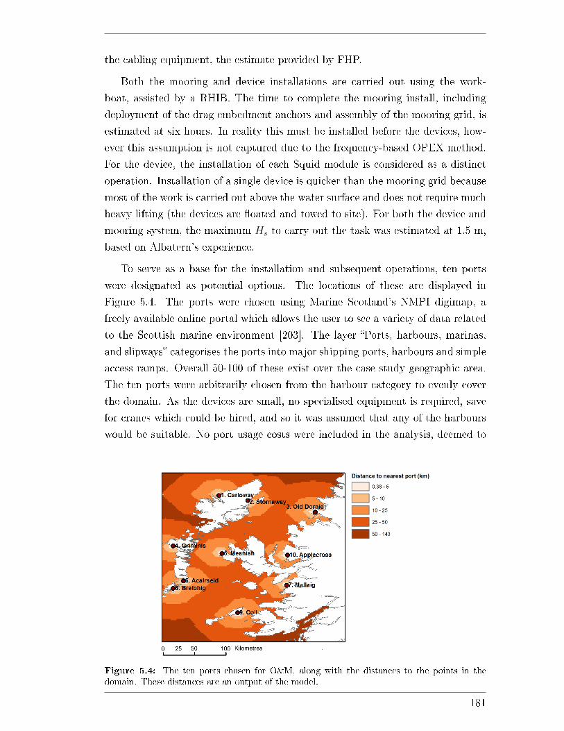
the cabling equipment, the estimate provided by FHP.

Both the mooring and device installations are carried out using the work-

boat, assisted by a RHIB. The time to complete the mooring install, including

deployment of the drag embedment anchors and assembly of the mooring grid, is

estimated at six hours. In reality this must be installed before the devices, how-

ever this assumption is not captured due to the frequency-based OPEX method.

For the device, the installation of each Squid module is considered as a distinct

operation. Installation of a single device is quicker than the mooring grid because

most of the work is carried out above the water surface and does not require much

heavy lifting (the devices are �oated and towed to site). For both the device and

mooring system, the maximum Hs to carry out the task was estimated at 1.5 m,

based on Albatern's experience.

To serve as a base for the installation and subsequent operations, ten ports

were designated as potential options. The locations of these are displayed in

Figure 5.4. The ports were chosen using Marine Scotland's NMPI digimap, a

freely available online portal which allows the user to see a variety of data related

to the Scottish marine environment [203]. The layer �Ports, harbours, marinas,

and slipways� categorises the ports into major shipping ports, harbours and simple

access ramps. Overall 50-100 of these exist over the case study geographic area.

The ten ports were arbitrarily chosen from the harbour category to evenly cover

the domain. As the devices are small, no specialised equipment is required, save

for cranes which could be hired, and so it was assumed that any of the harbours

would be suitable. No port usage costs were included in the analysis, deemed to

Figure 5.4: The ten ports chosen for O&M, along with the distances to the points in thedomain. These distances are an output of the model.

181

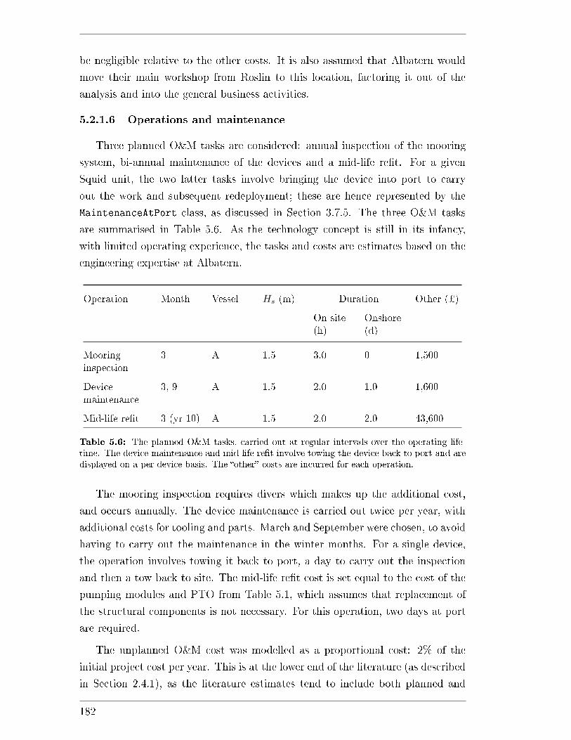
be negligible relative to the other costs. It is also assumed that Albatern would

move their main workshop from Roslin to this location, factoring it out of the

analysis and into the general business activities.

5.2.1.6 Operations and maintenance

Three planned O&M tasks are considered: annual inspection of the mooring

system, bi-annual maintenance of the devices and a mid-life re�t. For a given

Squid unit, the two latter tasks involve bringing the device into port to carry

out the work and subsequent redeployment; these are hence represented by the

MaintenanceAtPort class, as discussed in Section 3.7.5. The three O&M tasks

are summarised in Table 5.6. As the technology concept is still in its infancy,

with limited operating experience, the tasks and costs are estimates based on the

engineering expertise at Albatern.

Operation Month Vessel Hs (m) Duration Other (¿)

On site(h)

Onshore(d)

Mooringinspection

3 A 1.5 3.0 0 1,500

Devicemaintenance

3, 9 A 1.5 2.0 1.0 1,600

Mid-life re�t 3 (yr 10) A 1.5 2.0 2.0 43,600

Table 5.6: The planned O&M tasks, carried out at regular intervals over the operating life-time. The device maintenance and mid-life re�t involve towing the device back to port and aredisplayed on a per device basis. The �other� costs are incurred for each operation.

The mooring inspection requires divers which makes up the additional cost,

and occurs annually. The device maintenance is carried out twice per year, with

additional costs for tooling and parts. March and September were chosen, to avoid

having to carry out the maintenance in the winter months. For a single device,

the operation involves towing it back to port, a day to carry out the inspection

and then a tow back to site. The mid-life re�t cost is set equal to the cost of the

pumping modules and PTO from Table 5.1, which assumes that replacement of

the structural components is not necessary. For this operation, two days at port

are required.

The unplanned O&M cost was modelled as a proportional cost: 2% of the

initial project cost per year. This is at the lower end of the literature (as described

in Section 2.4.1), as the literature estimates tend to include both planned and

182

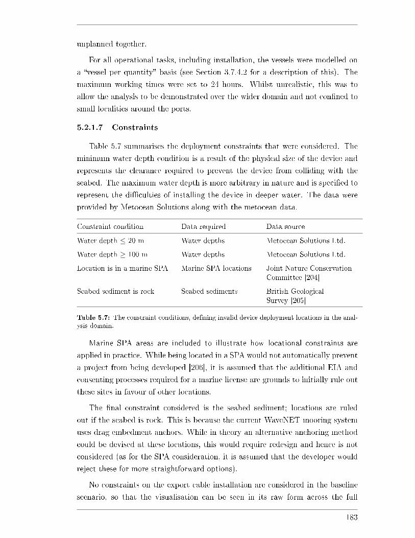
unplanned together.

For all operational tasks, including installation, the vessels were modelled on

a �vessel per quantity� basis (see Section 3.7.4.2 for a description of this). The

maximum working times were set to 24 hours. Whilst unrealistic, this was to

allow the analysis to be demonstrated over the wider domain and not con�ned to

small localities around the ports.

5.2.1.7 Constraints

Table 5.7 summarises the deployment constraints that were considered. The

minimum water depth condition is a result of the physical size of the device and

represents the clearance required to prevent the device from colliding with the

seabed. The maximum water depth is more arbitrary in nature and is speci�ed to

represent the di�culties of installing the device in deeper water. The data were

provided by Metocean Solutions along with the metocean data.

Constraint condition Data required Data source

Water depth ≤ 20 m Water depths Metocean Solutions Ltd.

Water depth ≥ 100 m Water depths Metocean Solutions Ltd.

Location is in a marine SPA Marine SPA locations Joint Nature ConservationCommittee [204]

Seabed sediment is rock Seabed sediments British GeologicalSurvey [205]

Table 5.7: The constraint conditions, de�ning invalid device deployment locations in the anal-ysis domain.

Marine SPA areas are included to illustrate how locational constraints are

applied in practice. While being located in a SPA would not automatically prevent

a project from being developed [206], it is assumed that the additional EIA and

consenting processes required for a marine license are grounds to initially rule out

these sites in favour of other locations.

The �nal constraint considered is the seabed sediment; locations are ruled

out if the seabed is rock. This is because the current WaveNET mooring system

uses drag embedment anchors. While in theory an alternative anchoring method

could be devised at these locations, this would require redesign and hence is not

considered (as for the SPA consideration, it is assumed that the developer would

reject these for more straightforward options).

No constraints on the export cable installation are considered in the baseline

scenario, so that the visualisation can be seen in its raw form across the full

183

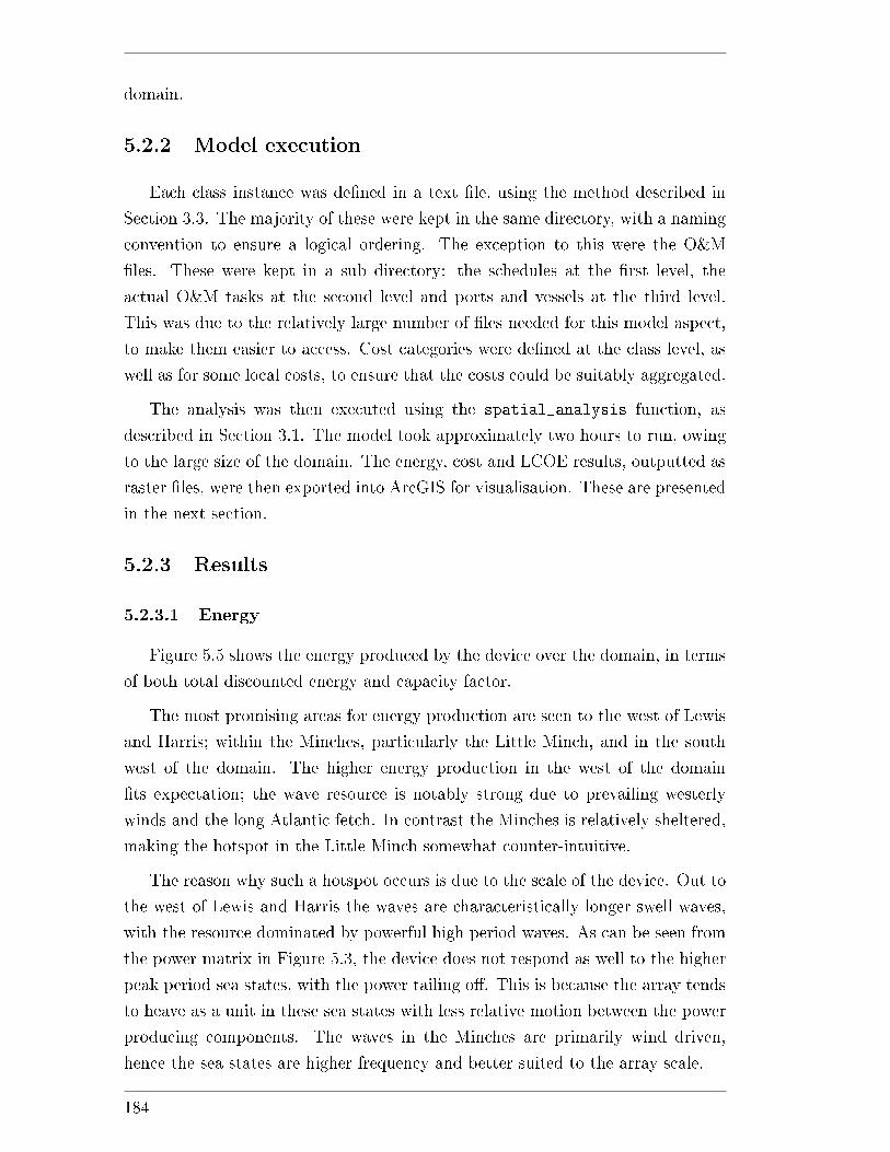
domain.

5.2.2 Model execution

Each class instance was de�ned in a text �le, using the method described in

Section 3.3. The majority of these were kept in the same directory, with a naming

convention to ensure a logical ordering. The exception to this were the O&M

�les. These were kept in a sub directory: the schedules at the �rst level, the

actual O&M tasks at the second level and ports and vessels at the third level.

This was due to the relatively large number of �les needed for this model aspect,

to make them easier to access. Cost categories were de�ned at the class level, as

well as for some local costs, to ensure that the costs could be suitably aggregated.

The analysis was then executed using the spatial_analysis function, as

described in Section 3.1. The model took approximately two hours to run, owing

to the large size of the domain. The energy, cost and LCOE results, outputted as

raster �les, were then exported into ArcGIS for visualisation. These are presented

in the next section.

5.2.3 Results

5.2.3.1 Energy

Figure 5.5 shows the energy produced by the device over the domain, in terms

of both total discounted energy and capacity factor.

The most promising areas for energy production are seen to the west of Lewis

and Harris; within the Minches, particularly the Little Minch, and in the south

west of the domain. The higher energy production in the west of the domain

�ts expectation; the wave resource is notably strong due to prevailing westerly

winds and the long Atlantic fetch. In contrast the Minches is relatively sheltered,

making the hotspot in the Little Minch somewhat counter-intuitive.

The reason why such a hotspot occurs is due to the scale of the device. Out to

the west of Lewis and Harris the waves are characteristically longer swell waves,

with the resource dominated by powerful high period waves. As can be seen from

the power matrix in Figure 5.3, the device does not respond as well to the higher

peak period sea states, with the power tailing o�. This is because the array tends

to heave as a unit in these sea states with less relative motion between the power

producing components. The waves in the Minches are primarily wind driven,

hence the sea states are higher frequency and better suited to the array scale.

184

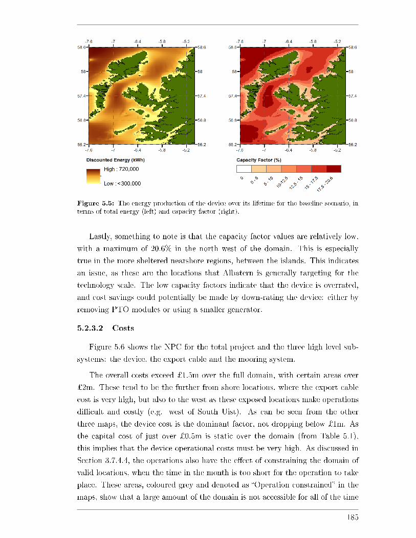
Figure 5.5: The energy production of the device over its lifetime for the baseline scenario, interms of total energy (left) and capacity factor (right).

Lastly, something to note is that the capacity factor values are relatively low,

with a maximum of 20.6% in the north west of the domain. This is especially

true in the more sheltered nearshore regions, between the islands. This indicates

an issue, as these are the locations that Albatern is generally targeting for the

technology scale. The low capacity factors indicate that the device is overrated,

and cost savings could potentially be made by down-rating the device: either by

removing PTO modules or using a smaller generator.

5.2.3.2 Costs

Figure 5.6 shows the NPC for the total project and the three high level sub-

systems: the device, the export cable and the mooring system.

The overall costs exceed ¿1.5m over the full domain, with certain areas over

¿2m. These tend to be the further from shore locations, where the export cable

cost is very high, but also to the west as these exposed locations make operations

di�cult and costly (e.g. west of South Uist). As can be seen from the other

three maps, the device cost is the dominant factor, not dropping below ¿1m. As

the capital cost of just over ¿0.5m is static over the domain (from Table 5.1),

this implies that the device operational costs must be very high. As discussed in

Section 3.7.4.4, the operations also have the e�ect of constraining the domain of

valid locations, when the time in the month is too short for the operation to take

place. These areas, coloured grey and denoted as �Operation constrained� in the

maps, show that a large amount of the domain is not accessible for all of the time

185

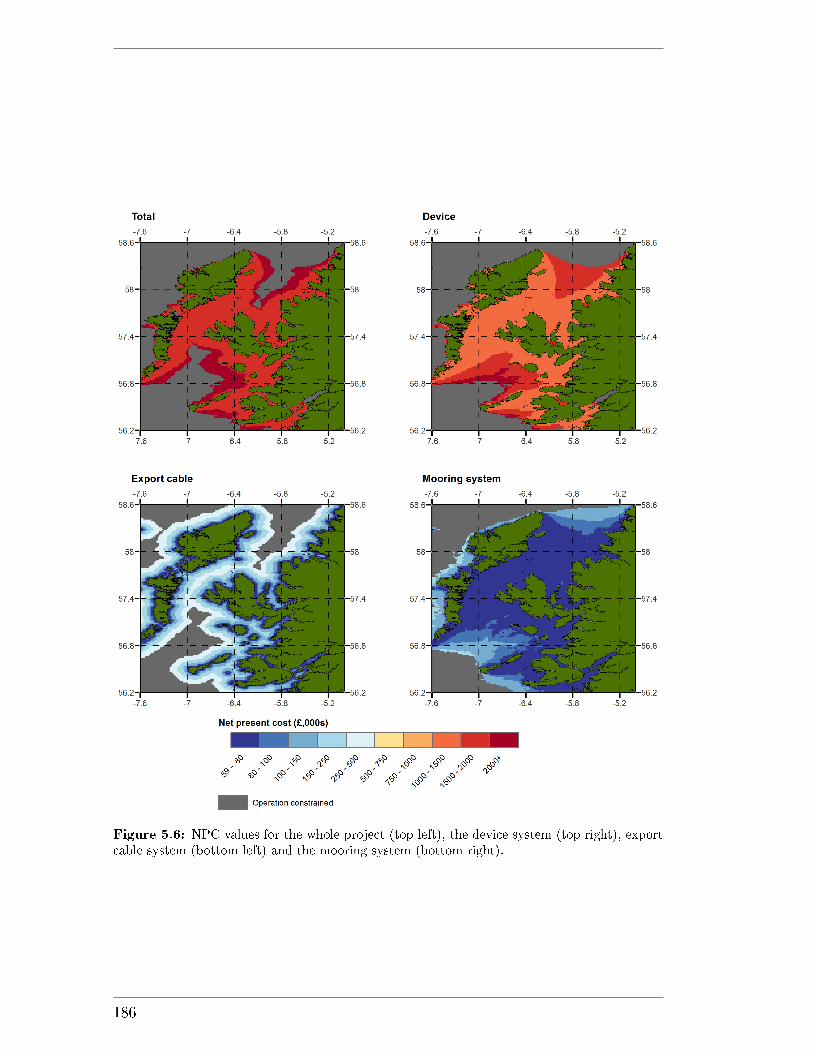
Figure 5.6: NPC values for the whole project (top left), the device system (top right), exportcable system (bottom left) and the mooring system (bottom right).

186

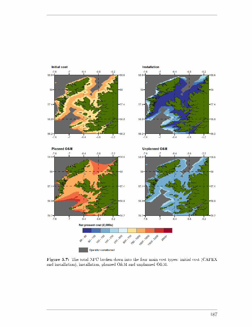
Figure 5.7: The total NPC broken down into the four main cost types: initial cost (CAPEXand installation), installation, planned O&M and unplanned O&M.

187

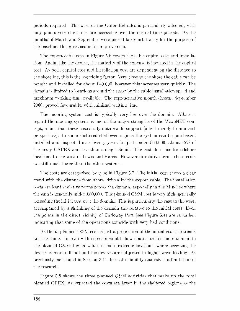
periods required. The west of the Outer Hebrides is particularly a�ected, with

only points very close to shore accessible over the desired time periods. As the

months of March and September were picked fairly arbitrarily for the purpose of

the baseline, this gives scope for improvement.

The export cable cost in Figure 5.6 covers the cable capital cost and installa-

tion. Again, like the device, the majority of the expense is incurred in the capital

cost. As both capital cost and installation cost are dependent on the distance to

the shoreline, this is the overriding factor. Very close to the shore the cable can be

bought and installed for about ¿40,000, however this increases very quickly. The

domain is limited to locations around the coast by the cable installation speed and

maximum working time available. The representative month chosen, September

2000, proved favourable, with minimal waiting time.

The mooring system cost is typically very low over the domain. Albatern

regard the mooring system as one of the major strengths of the WaveNET con-

cept, a fact that these case study data would support (albeit merely from a cost

perspective). In some sheltered shallower regions the system can be purchased,

installed and inspected over twenty years for just under ¿60,000, about 12% of

the array CAPEX and less than a single Squid. The cost does rise for o�shore

locations to the west of Lewis and Harris. However in relative terms these costs

are still much lower than the other systems.

The costs are categorised by type in Figure 5.7. The initial cost shows a clear

trend with the distance from shore, driven by the export cable. The installation

costs are low in relative terms across the domain, especially in the Minches where

the sum is generally under ¿80,000. The planned O&M cost is very high, generally

exceeding the initial cost over the domain. This is particularly the case to the west,

accompanied by a shrinking of the domain size relative to the initial costs. Even

the points in the direct vicinity of Carloway Port (see Figure 5.4) are curtailed,

indicating that some of the operations coincide with very bad conditions.

As the unplanned O&M cost is just a proportion of the initial cost the trends

are the same. In reality these costs would show spatial trends more similar to

the planned O&M: higher values in more extreme locations, where accessing the

devices is more di�cult and the devices are subjected to higher wave loading. As

previously mentioned in Section 3.11, lack of reliability analysis is a limitation of

the research.

Figure 5.8 shows the three planned O&M activities that make up the total

planned OPEX. As expected the costs are lower in the sheltered regions as the

188

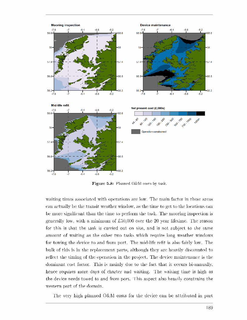
Figure 5.8: Planned O&M costs by task.

waiting times associated with operations are low. The main factor in these areas

can actually be the transit weather window, as the time to get to the locations can

be more signi�cant than the time to perform the task. The mooring inspection is

generally low, with a minimum of ¿50,000 over the 20 year lifetime. The reason

for this is that the task is carried out on site, and is not subject to the same

amount of waiting as the other two tasks which require long weather windows

for towing the device to and from port. The mid-life re�t is also fairly low. The

bulk of this is in the replacement parts, although they are heavily discounted to

re�ect the timing of the operation in the project. The device maintenance is the

dominant cost factor. This is mainly due to the fact that it occurs bi-annually,

hence requires more days of charter and waiting. The waiting time is high as

the device needs towed to and from port. This aspect also heavily constrains the

western part of the domain.

The very high planned O&M costs for the device can be attributed in part

189

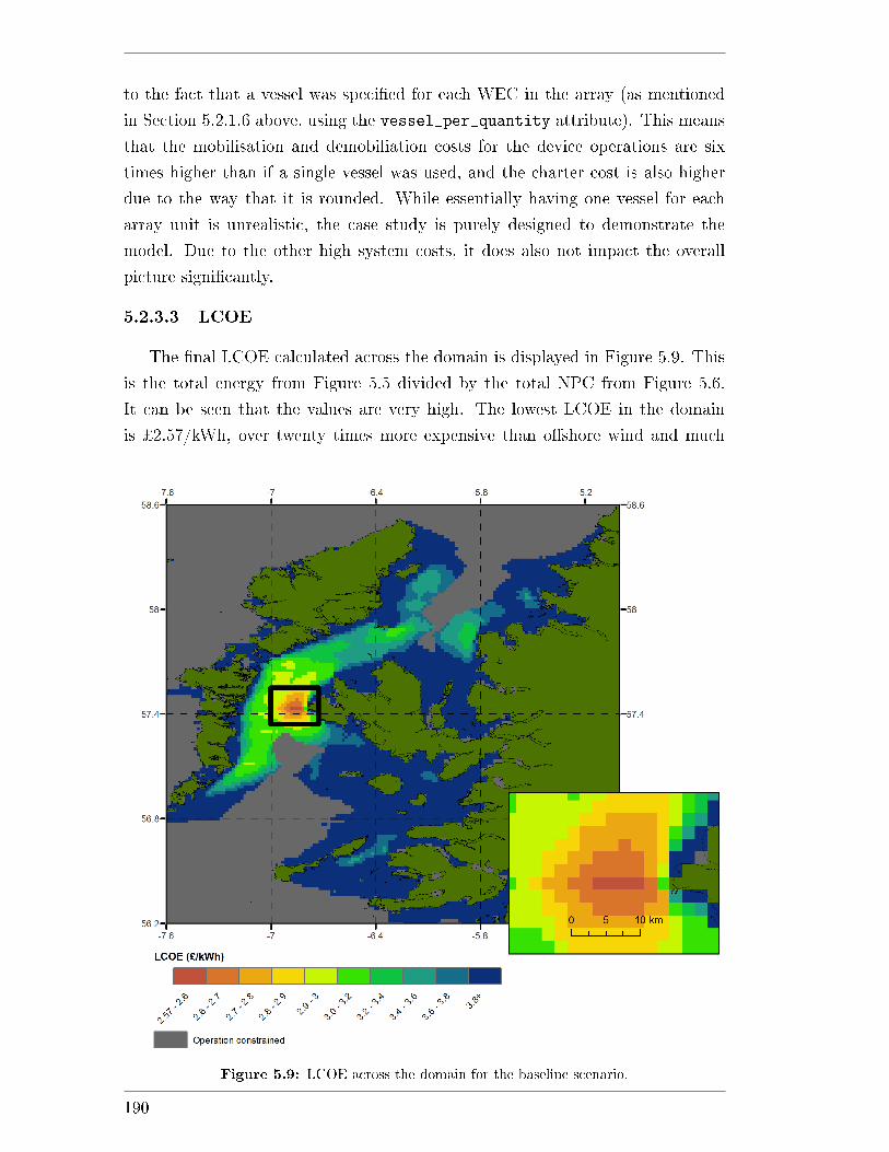
to the fact that a vessel was speci�ed for each WEC in the array (as mentioned

in Section 5.2.1.6 above, using the vessel_per_quantity attribute). This means

that the mobilisation and demobiliation costs for the device operations are six

times higher than if a single vessel was used, and the charter cost is also higher

due to the way that it is rounded. While essentially having one vessel for each

array unit is unrealistic, the case study is purely designed to demonstrate the

model. Due to the other high system costs, it does also not impact the overall

picture signi�cantly.

5.2.3.3 LCOE

The �nal LCOE calculated across the domain is displayed in Figure 5.9. This

is the total energy from Figure 5.5 divided by the total NPC from Figure 5.6.

It can be seen that the values are very high. The lowest LCOE in the domain

is ¿2.57/kWh, over twenty times more expensive than o�shore wind and much

Figure 5.9: LCOE across the domain for the baseline scenario.

190

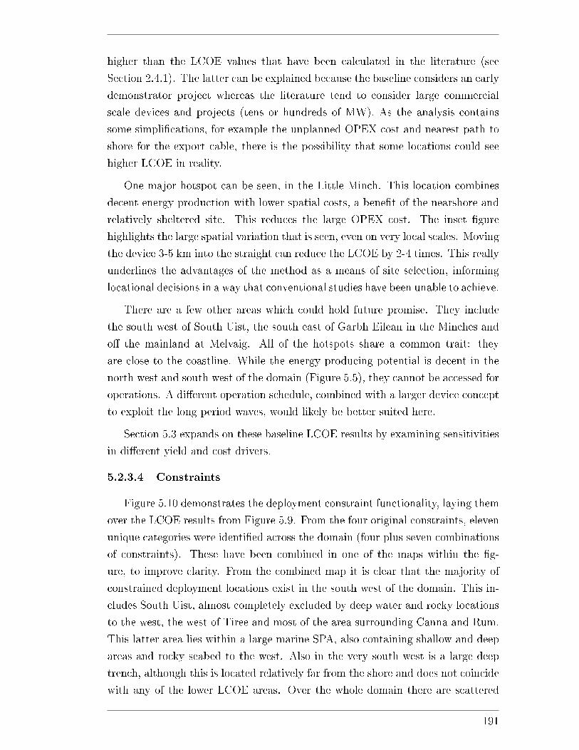
higher than the LCOE values that have been calculated in the literature (see

Section 2.4.1). The latter can be explained because the baseline considers an early

demonstrator project whereas the literature tend to consider large commercial

scale devices and projects (tens or hundreds of MW). As the analysis contains

some simpli�cations, for example the unplanned OPEX cost and nearest path to

shore for the export cable, there is the possibility that some locations could see

higher LCOE in reality.

One major hotspot can be seen, in the Little Minch. This location combines

decent energy production with lower spatial costs, a bene�t of the nearshore and

relatively sheltered site. This reduces the large OPEX cost. The inset �gure

highlights the large spatial variation that is seen, even on very local scales. Moving

the device 3-5 km into the straight can reduce the LCOE by 2-4 times. This really

underlines the advantages of the method as a means of site selection, informing

locational decisions in a way that conventional studies have been unable to achieve.

There are a few other areas which could hold future promise. They include

the south west of South Uist, the south east of Garbh Eilean in the Minches and

o� the mainland at Melvaig. All of the hotspots share a common trait: they

are close to the coastline. While the energy producing potential is decent in the

north west and south west of the domain (Figure 5.5), they cannot be accessed for

operations. A di�erent operation schedule, combined with a larger device concept

to exploit the long period waves, would likely be better suited here.

Section 5.3 expands on these baseline LCOE results by examining sensitivities

in di�erent yield and cost drivers.

5.2.3.4 Constraints

Figure 5.10 demonstrates the deployment constraint functionality, laying them

over the LCOE results from Figure 5.9. From the four original constraints, eleven

unique categories were identi�ed across the domain (four plus seven combinations

of constraints). These have been combined in one of the maps within the �g-

ure, to improve clarity. From the combined map it is clear that the majority of

constrained deployment locations exist in the south west of the domain. This in-

cludes South Uist, almost completely excluded by deep water and rocky locations

to the west, the west of Tiree and most of the area surrounding Canna and Rum.

This latter area lies within a large marine SPA, also containing shallow and deep

areas and rocky seabed to the west. Also in the very south west is a large deep

trench, although this is located relatively far from the shore and does not coincide

with any of the lower LCOE areas. Over the whole domain there are scattered

191

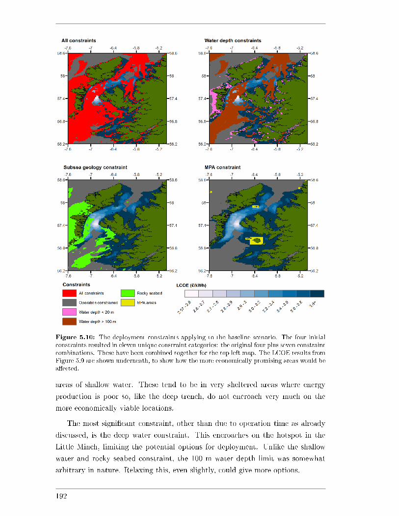
Figure 5.10: The deployment constraints applying to the baseline scenario. The four initialconstraints resulted in eleven unique constraint categories: the original four plus seven constraintcombinations. These have been combined together for the top left map. The LCOE results fromFigure 5.9 are shown underneath, to show how the more economically promising areas would bea�ected.

areas of shallow water. These tend to be in very sheltered areas where energy

production is poor so, like the deep trench, do not encroach very much on the

more economically viable locations.

The most signi�cant constraint, other than due to operation time as already

discussed, is the deep water constraint. This encroaches on the hotspot in the

Little Minch, limiting the potential options for deployment. Unlike the shallow

water and rocky seabed constraint, the 100 m water depth limit was somewhat

arbitrary in nature. Relaxing this, even slightly, could give more options.

192

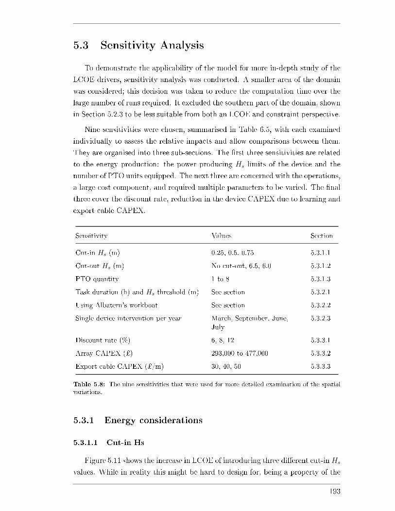
5.3 Sensitivity Analysis

To demonstrate the applicability of the model for more in-depth study of the

LCOE drivers, sensitivity analysis was conducted. A smaller area of the domain

was considered; this decision was taken to reduce the computation time over the

large number of runs required. It excluded the southern part of the domain, shown

in Section 5.2.3 to be less suitable from both an LCOE and constraint perspective.

Nine sensitivities were chosen, summarised in Table 6.5, with each examined

individually to assess the relative impacts and allow comparisons between them.

They are organised into three sub-sections. The �rst three sensitivities are related

to the energy production: the power producing Hs limits of the device and the

number of PTO units equipped. The next three are concerned with the operations,

a large cost component, and required multiple parameters to be varied. The �nal

three cover the discount rate, reduction in the device CAPEX due to learning and

export cable CAPEX.

Sensitivity Values Section

Cut-in Hs (m) 0.25, 0.5, 0.75 5.3.1.1

Cut-out Hs (m) No cut-out, 6.5, 6.0 5.3.1.2

PTO quantity 1 to 8 5.3.1.3

Task duration (h) and Hs threshold (m) See section 5.3.2.1

Using Albatern's workboat See section 5.3.2.2

Single device intervention per year March, September, June,July

5.3.2.3

Discount rate (%) 6, 8, 12 5.3.3.1

Array CAPEX (¿) 293,000 to 477,000 5.3.3.2

Export cable CAPEX (¿/m) 30, 40, 50 5.3.3.3

Table 5.8: The nine sensitivities that were used for more detailed examination of the spatialvariations.

5.3.1 Energy considerations

5.3.1.1 Cut-in Hs

Figure 5.11 shows the increase in LCOE of introducing three di�erent cut-inHs

values. While in reality this might be hard to design for, being a property of the

193

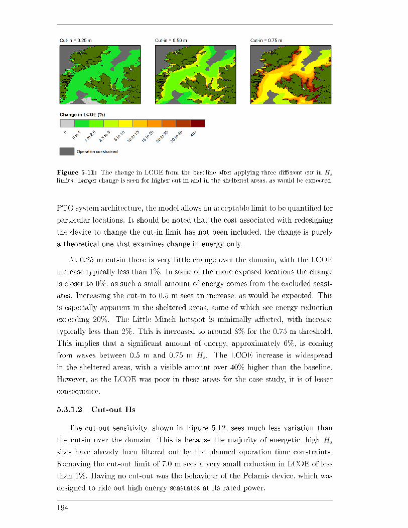
Figure 5.11: The change in LCOE from the baseline after applying three di�erent cut-in Hs

limits. Larger change is seen for higher cut-in and in the sheltered areas, as would be expected.

PTO system architecture, the model allows an acceptable limit to be quanti�ed for

particular locations. It should be noted that the cost associated with redesigning

the device to change the cut-in limit has not been included, the change is purely

a theoretical one that examines change in energy only.

At 0.25 m cut-in there is very little change over the domain, with the LCOE

increase typically less than 1%. In some of the more exposed locations the change

is closer to 0%, as such a small amount of energy comes from the excluded seast-

ates. Increasing the cut-in to 0.5 m sees an increase, as would be expected. This

is especially apparent in the sheltered areas, some of which see energy reduction

exceeding 20%. The Little Minch hotspot is minimally a�ected, with increase

typically less than 2%. This is increased to around 8% for the 0.75 m threshold.

This implies that a signi�cant amount of energy, approximately 6%, is coming

from waves between 0.5 m and 0.75 m Hs. The LCOE increase is widespread

in the sheltered areas, with a visible amount over 40% higher than the baseline.

However, as the LCOE was poor in these areas for the case study, it is of lesser

consequence.

5.3.1.2 Cut-out Hs

The cut-out sensitivity, shown in Figure 5.12, sees much less variation than

the cut-in over the domain. This is because the majority of energetic, high Hs

sites have already been �ltered out by the planned operation time constraints.

Removing the cut-out limit of 7.0 m sees a very small reduction in LCOE of less

than 1%. Having no cut-out was the behaviour of the Pelamis device, which was

designed to ride out high energy seastates at its rated power.

194

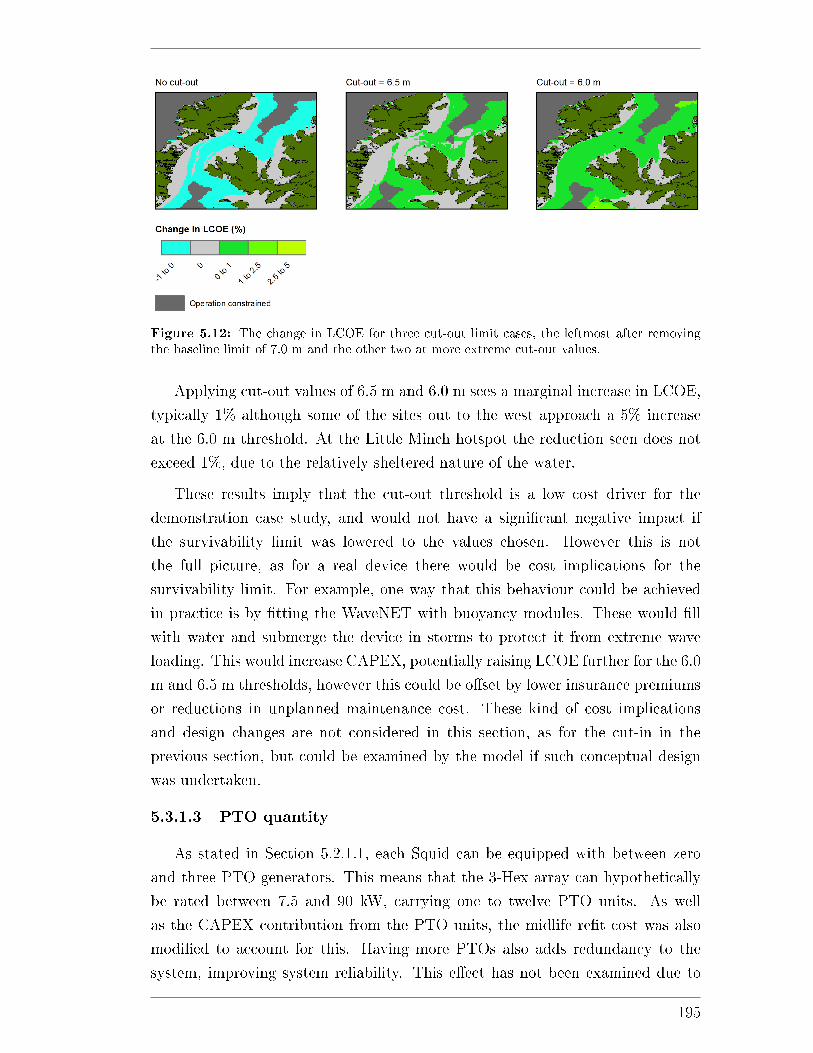
Figure 5.12: The change in LCOE for three cut-out limit cases, the leftmost after removingthe baseline limit of 7.0 m and the other two at more extreme cut-out values.

Applying cut-out values of 6.5 m and 6.0 m sees a marginal increase in LCOE,

typically 1% although some of the sites out to the west approach a 5% increase

at the 6.0 m threshold. At the Little Minch hotspot the reduction seen does not

exceed 1%, due to the relatively sheltered nature of the water.

These results imply that the cut-out threshold is a low cost driver for the

demonstration case study, and would not have a signi�cant negative impact if

the survivability limit was lowered to the values chosen. However this is not

the full picture, as for a real device there would be cost implications for the

survivability limit. For example, one way that this behaviour could be achieved

in practice is by �tting the WaveNET with buoyancy modules. These would �ll

with water and submerge the device in storms to protect it from extreme wave

loading. This would increase CAPEX, potentially raising LCOE further for the 6.0

m and 6.5 m thresholds, however this could be o�set by lower insurance premiums

or reductions in unplanned maintenance cost. These kind of cost implications

and design changes are not considered in this section, as for the cut-in in the

previous section, but could be examined by the model if such conceptual design

was undertaken.

5.3.1.3 PTO quantity

As stated in Section 5.2.1.1, each Squid can be equipped with between zero

and three PTO generators. This means that the 3-Hex array can hypothetically

be rated between 7.5 and 90 kW, carrying one to twelve PTO units. As well

as the CAPEX contribution from the PTO units, the midlife re�t cost was also

modi�ed to account for this. Having more PTOs also adds redundancy to the

system, improving system reliability. This e�ect has not been examined due to

195

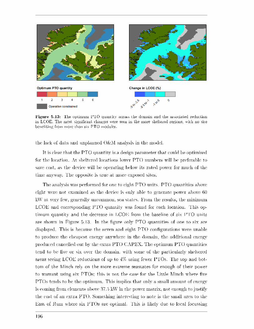
Figure 5.13: The optimum PTO quantity across the domain and the associated reductionin LCOE. The most signi�cant changes were seen in the more sheltered regions, with no sitebene�ting from more than six PTO modules.

the lack of data and unplanned O&M analysis in the model.

It is clear that the PTO quantity is a design parameter that could be optimised

for the location. At sheltered locations lower PTO numbers will be preferable to

save cost, as the device will be operating below its rated power for much of the

time anyway. The opposite is true at more exposed sites.

The analysis was performed for one to eight PTO units. PTO quantities above

eight were not examined as the device is only able to generate power above 60

kW at very few, generally uncommon, sea states. From the results, the minimum

LCOE and corresponding PTO quantity was found for each location. This op-

timum quantity and the decrease in LCOE from the baseline of six PTO units

are shown in Figure 5.13. In the �gure only PTO quantities of one to six are

displayed. This is because the seven and eight PTO con�gurations were unable

to produce the cheapest energy anywhere in the domain, the additional energy

produced cancelled out by the extra PTO CAPEX. The optimum PTO quantities

tend to be �ve or six over the domain, with some of the particularly sheltered

areas seeing LCOE reductions of up to 4% using fewer PTOs. The top and bot-

tom of the Minch rely on the more extreme seastates for enough of their power

to warrant using six PTOs; this is not the case for the Little Minch where �ve

PTOs tends to be the optimum. This implies that only a small amount of energy

is coming from elements above 37.5 kW in the power matrix, not enough to justify

the cost of an extra PTO. Something interesting to note is the small area to the

East of Rum where six PTOs are optimal. This is likely due to local focussing

196

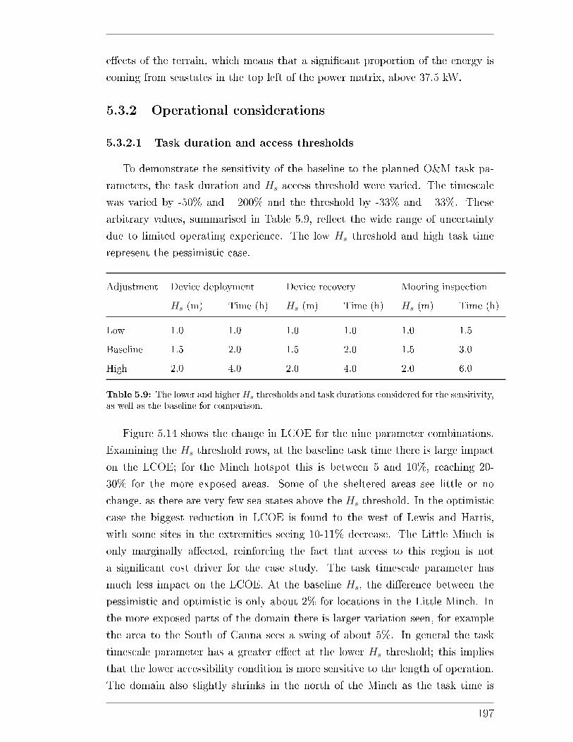
e�ects of the terrain, which means that a signi�cant proportion of the energy is

coming from seastates in the top left of the power matrix, above 37.5 kW.

5.3.2 Operational considerations

5.3.2.1 Task duration and access thresholds

To demonstrate the sensitivity of the baseline to the planned O&M task pa-

rameters, the task duration and Hs access threshold were varied. The timescale

was varied by -50% and +200% and the threshold by -33% and +33%. These

arbitrary values, summarised in Table 5.9, re�ect the wide range of uncertainty

due to limited operating experience. The low Hs threshold and high task time

represent the pessimistic case.

Adjustment Device deployment Device recovery Mooring inspection

Hs (m) Time (h) Hs (m) Time (h) Hs (m) Time (h)

Low 1.0 1.0 1.0 1.0 1.0 1.5

Baseline 1.5 2.0 1.5 2.0 1.5 3.0

High 2.0 4.0 2.0 4.0 2.0 6.0

Table 5.9: The lower and higherHs thresholds and task durations considered for the sensitivity,as well as the baseline for comparison.

Figure 5.14 shows the change in LCOE for the nine parameter combinations.

Examining the Hs threshold rows, at the baseline task time there is large impact

on the LCOE; for the Minch hotspot this is between 5 and 10%, reaching 20-

30% for the more exposed areas. Some of the sheltered areas see little or no

change, as there are very few sea states above the Hs threshold. In the optimistic

case the biggest reduction in LCOE is found to the west of Lewis and Harris,

with some sites in the extremities seeing 10-11% decrease. The Little Minch is

only marginally a�ected, reinforcing the fact that access to this region is not

a signi�cant cost driver for the case study. The task timescale parameter has

much less impact on the LCOE. At the baseline Hs, the di�erence between the

pessimistic and optimistic is only about 2% for locations in the Little Minch. In

the more exposed parts of the domain there is larger variation seen, for example

the area to the South of Canna sees a swing of about 5%. In general the task

timescale parameter has a greater e�ect at the lower Hs threshold; this implies

that the lower accessibility condition is more sensitive to the length of operation.

The domain also slightly shrinks in the north of the Minch as the task time is

197

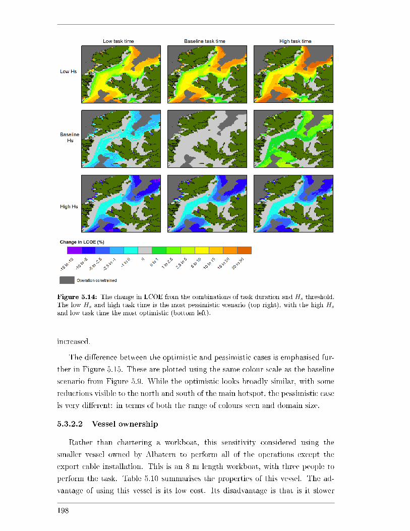
Figure 5.14: The change in LCOE from the combinations of task duration and Hs threshold.The low Hs and high task time is the most pessimistic scenario (top right), with the high Hs

and low task time the most optimistic (bottom left).

increased.

The di�erence between the optimistic and pessimistic cases is emphasised fur-

ther in Figure 5.15. These are plotted using the same colour scale as the baseline

scenario from Figure 5.9. While the optimistic looks broadly similar, with some

reductions visible to the north and south of the main hotspot, the pessimistic case

is very di�erent: in terms of both the range of colours seen and domain size.

5.3.2.2 Vessel ownership

Rather than chartering a workboat, this sensitivity considered using the

smaller vessel owned by Albatern to perform all of the operations except the

export cable installation. This is an 8 m length workboat, with three people to

perform the task. Table 5.10 summarises the properties of this vessel. The ad-

vantage of using this vessel is its low cost. Its disadvantage is that is it slower

198

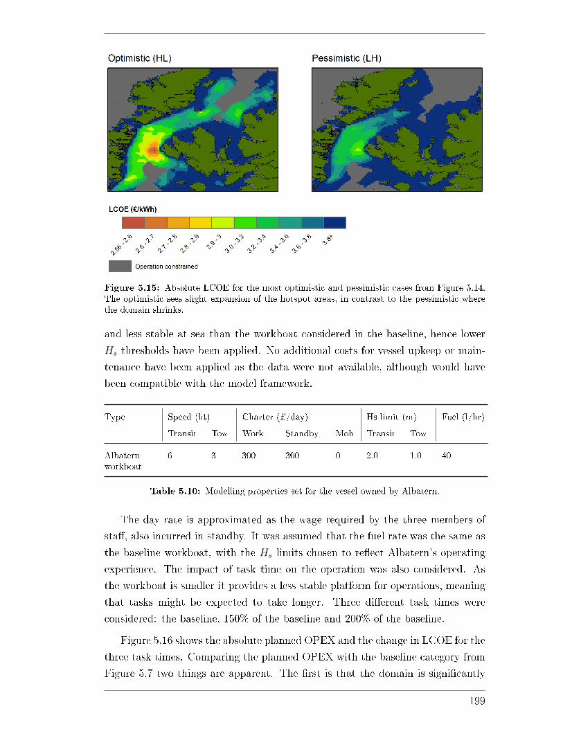
Figure 5.15: Absolute LCOE for the most optimistic and pessimistic cases from Figure 5.14.The optimistic sees slight expansion of the hotspot areas, in contrast to the pessimistic wherethe domain shrinks.

and less stable at sea than the workboat considered in the baseline, hence lower

Hs thresholds have been applied. No additional costs for vessel upkeep or main-

tenance have been applied as the data were not available, although would have

been compatible with the model framework.

Type Speed (kt) Charter (¿/day) Hs limit (m) Fuel (l/hr)

Transit Tow Work Standby Mob Transit Tow

Albaternworkboat

6 3 300 300 0 2.0 1.0 40

Table 5.10: Modelling properties set for the vessel owned by Albatern.

The day rate is approximated as the wage required by the three members of

sta�, also incurred in standby. It was assumed that the fuel rate was the same as

the baseline workboat, with the Hs limits chosen to re�ect Albatern's operating

experience. The impact of task time on the operation was also considered. As

the workboat is smaller it provides a less stable platform for operations, meaning

that tasks might be expected to take longer. Three di�erent task times were

considered: the baseline, 150% of the baseline and 200% of the baseline.

Figure 5.16 shows the absolute planned OPEX and the change in LCOE for the

three task times. Comparing the planned OPEX with the baseline category from

Figure 5.7 two things are apparent. The �rst is that the domain is signi�cantly

199

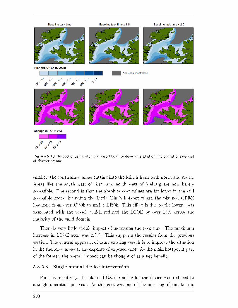
Figure 5.16: Impact of using Albatern's workboat for device installation and operations insteadof chartering one.

smaller, the constrained areas cutting into the Minch from both north and south.

Areas like the south west of Rum and north west of Melvaig are now barely

accessible. The second is that the absolute cost values are far lower in the still

accessible areas, including the Little Minch hotspot where the planned OPEX

has gone from over ¿750k to under ¿450k. This e�ect is due to the lower costs

associated with the vessel, which reduced the LCOE by over 15% across the

majority of the valid domain.

There is very little visible impact of increasing the task time. The maximum

increase in LCOE seen was 2.3%. This supports the results from the previous

section. The general approach of using existing vessels is to improve the situation

in the sheltered areas at the expense of exposed ones. As the main hotspot is part

of the former, the overall impact can be thought of as a net bene�t.

5.3.2.3 Single annual device intervention

For this sensitivity, the planned O&M routine for the device was reduced to

a single operation per year. As this cost was one of the most signi�cant factors

200

for the baseline (see Section 5.2.3.2), this is the kind of hypothetical improvement

which could be inferred from using the model.

Four di�erent months were examined: March and September, as used previ-

ously, and June and July. To keep consistency within the maintenance schedule,

the mooring inspection and midlife re�t operations were also scheduled to the

same month.

Figure 5.17 shows the total planned OPEX and the change in LCOE from

the baseline for each month. Looking at the March and September results, now

decoupled from the baseline, it is apparent that the March operation was the larger

contributor to cost. The magnitude of LCOE reduction is lower than September

and less variable over the domain. The September intervention sees larger LCOE

reduction, especially near the fringes of the domain. The planned OPEX cost

shows that it is also less constrained to the west and the top right. However this

bene�t is not seen in the �nal LCOE results, largely due to the constraining e�ect

from the installation (as can be seen from the shape of the installation component

in Figure 5.6).

The June and July intervention months see signi�cantly lower planned OPEX

costs to the west of Lewis and Harris as would be expected. The full domain

is also accessible. For the planned OPEX the lighter areas coincide with the

port locations, again as expected due to the shorter weather window required for

transit and lower vessel fuel costs over the lifetime. In the Little Minch there is

marginal di�erence between the September, July and June cases. September is

slightly better around the hotspot location, driven by fewer waiting days.

To get an appreciation of the change in LCOE and domain size, the absolute

LCOE for July is displayed in Figure 5.18. The domain is slightly larger out to

the west in this case, now constrained by the installation activities. While there

is a green band out to the west of Lewis and Harris, the LCOE is still relatively

high compared to the Minch.

5.3.3 Other considerations

5.3.3.1 Discount rate

The sensitivity of the baseline LCOE to discount rate was explored by exam-

ining three additional values: 6%, 8% and 12%. The lower values would typically

be reserved for more mature technologies (as noted in Section 2.3.1) and so are

included purely on a hypothetical basis.

201

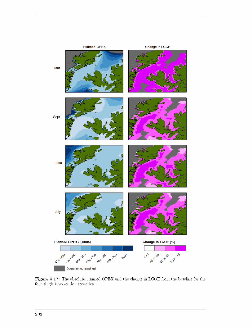
Figure 5.17: The absolute planned OPEX and the change in LCOE from the baseline for thefour single intervention scenarios.

202

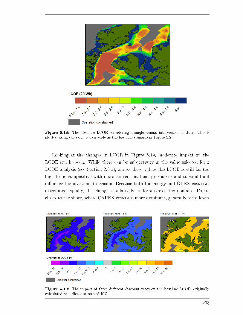
Figure 5.18: The absolute LCOE considering a single annual intervention in July. This isplotted using the same colour scale as the baseline scenario in Figure 5.9.

Looking at the changes in LCOE in Figure 5.19, moderate impact on the

LCOE can be seen. While there can be subjectivity in the value selected for a

LCOE analysis (see Section 2.3.1), across these values the LCOE is still far too

high to be competitive with more conventional energy sources and so would not

in�uence the investment decision. Because both the energy and OPEX costs are

discounted equally, the change is relatively uniform across the domain. Points

closer to the shore, where CAPEX costs are more dominant, generally see a lower

Figure 5.19: The impact of three di�erent discount rates on the baseline LCOE, originallycalculated at a discount rate of 10%.

203

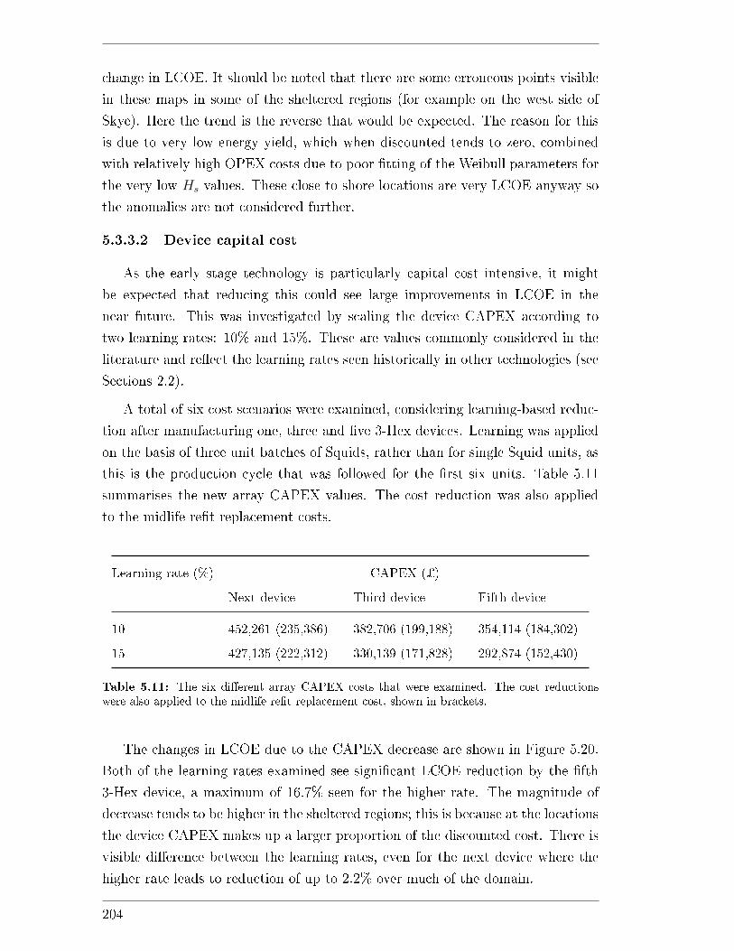
change in LCOE. It should be noted that there are some erroneous points visible

in these maps in some of the sheltered regions (for example on the west side of

Skye). Here the trend is the reverse that would be expected. The reason for this

is due to very low energy yield, which when discounted tends to zero, combined

with relatively high OPEX costs due to poor �tting of the Weibull parameters for

the very low Hs values. These close to shore locations are very LCOE anyway so

the anomalies are not considered further.

5.3.3.2 Device capital cost

As the early stage technology is particularly capital cost intensive, it might

be expected that reducing this could see large improvements in LCOE in the

near future. This was investigated by scaling the device CAPEX according to

two learning rates: 10% and 15%. These are values commonly considered in the

literature and re�ect the learning rates seen historically in other technologies (see

Sections 2.2).

A total of six cost scenarios were examined, considering learning-based reduc-

tion after manufacturing one, three and �ve 3-Hex devices. Learning was applied

on the basis of three unit batches of Squids, rather than for single Squid units, as

this is the production cycle that was followed for the �rst six units. Table 5.11

summarises the new array CAPEX values. The cost reduction was also applied

to the midlife re�t replacement costs.

Learning rate (%) CAPEX (¿)

Next device Third device Fifth device

10 452,261 (235,386) 382,706 (199,188) 354,114 (184,302)

15 427,135 (222,312) 330,139 (171,828) 292,874 (152,430)

Table 5.11: The six di�erent array CAPEX costs that were examined. The cost reductionswere also applied to the midlife re�t replacement cost, shown in brackets.

The changes in LCOE due to the CAPEX decrease are shown in Figure 5.20.

Both of the learning rates examined see signi�cant LCOE reduction by the �fth

3-Hex device, a maximum of 16.7% seen for the higher rate. The magnitude of

decrease tends to be higher in the sheltered regions; this is because at the locations

the device CAPEX makes up a larger proportion of the discounted cost. There is

visible di�erence between the learning rates, even for the next device where the

higher rate leads to reduction of up to 2.2% over much of the domain.

204

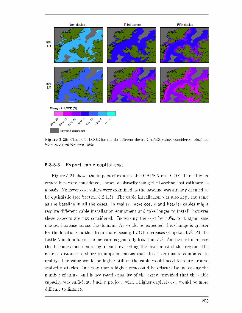
Figure 5.20: Change in LCOE for the six di�erent device CAPEX values considered, obtainedfrom applying learning rates.

5.3.3.3 Export cable capital cost

Figure 5.21 shows the impact of export cable CAPEX on LCOE. Three higher

cost values were considered, chosen arbitrarily using the baseline cost estimate as

a basis. No lower cost values were examined as the baseline was already deemed to

be optimistic (see Section 5.2.1.3). The cable installation was also kept the same

as the baseline in all the cases. In reality, more costly and heavier cables might

require di�erent cable installation equipment and take longer to install, however

these aspects are not considered. Increasing the cost by 50%, to ¿30/m, sees

modest increase across the domain. As would be expected this change is greater

for the locations further from shore, seeing LCOE increases of up to 10%. At the

Little Minch hotspot the increase is generally less than 5%. As the cost increases

this becomes much more signi�cant, exceeding 10% over most of this region. The

nearest distance to shore assumption means that this is optimistic compared to

reality. The value would be higher still as the cable would need to route around

seabed obstacles. One way that a higher cost could be o�set is by increasing the

number of units, and hence rated capacity of the array, provided that the cable

capacity was su�cient. Such a project, with a higher capital cost, would be more

di�cult to �nance.

205

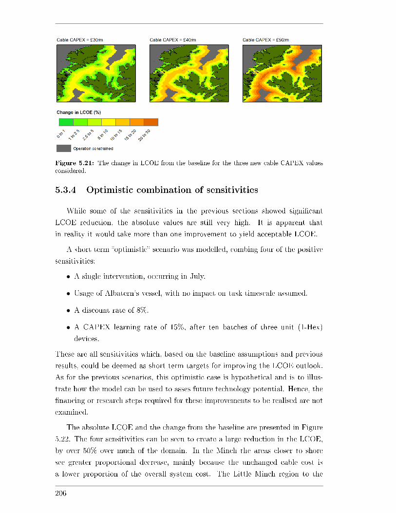
Figure 5.21: The change in LCOE from the baseline for the three new cable CAPEX valuesconsidered.

5.3.4 Optimistic combination of sensitivities

While some of the sensitivities in the previous sections showed signi�cant

LCOE reduction, the absolute values are still very high. It is apparent that

in reality it would take more than one improvement to yield acceptable LCOE.

A short term �optimistic� scenario was modelled, combing four of the positive

sensitivities:

• A single intervention, occurring in July.

• Usage of Albatern's vessel, with no impact on task timescale assumed.

• A discount rate of 8%.

• A CAPEX learning rate of 15%, after ten batches of three unit (1-Hex)

devices.

These are all sensitivities which, based on the baseline assumptions and previous

results, could be deemed as short term targets for improving the LCOE outlook.

As for the previous scenarios, this optimistic case is hypothetical and is to illus-

trate how the model can be used to asses future technology potential. Hence, the

�nancing or research steps required for these improvements to be realised are not

examined.

The absolute LCOE and the change from the baseline are presented in Figure

5.22. The four sensitivities can be seen to create a large reduction in the LCOE,

by over 50% over much of the domain. In the Minch the areas closer to shore

see greater proportional decrease, mainly because the unchanged cable cost is

a lower proportion of the overall system cost. The Little Minch region to the

206

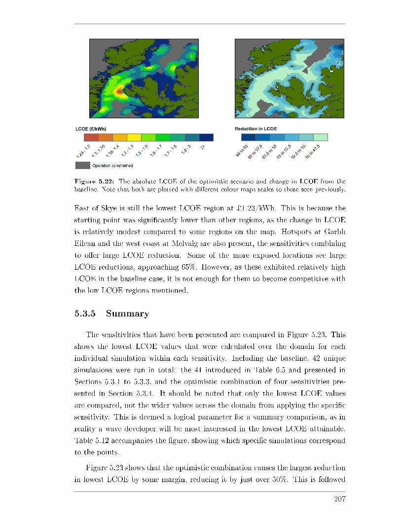
Figure 5.22: The absolute LCOE of the optimistic scenario and change in LCOE from thebaseline. Note that both are plotted with di�erent colour maps scales to those seen previously.

East of Skye is still the lowest LCOE region at ¿1.23/kWh. This is because the

starting point was signi�cantly lower than other regions, as the change in LCOE

is relatively modest compared to some regions on the map. Hotspots at Garbh

Eilean and the west coast at Melvaig are also present, the sensitivities combining

to o�er large LCOE reduction. Some of the more exposed locations see large

LCOE reductions, approaching 65%. However, as these exhibited relatively high

LCOE in the baseline case, it is not enough for them to become competitive with

the low LCOE regions mentioned.

5.3.5 Summary

The sensitivities that have been presented are compared in Figure 5.23. This

shows the lowest LCOE values that were calculated over the domain for each

individual simulation within each sensitivity. Including the baseline, 42 unique

simulations were run in total: the 41 introduced in Table 6.5 and presented in

Sections 5.3.1 to 5.3.3, and the optimistic combination of four sensitivities pre-

sented in Section 5.3.4. It should be noted that only the lowest LCOE values

are compared, not the wider values across the domain from applying the speci�c

sensitivity. This is deemed a logical parameter for a summary comparison, as in

reality a wave developer will be most interested in the lowest LCOE attainable.

Table 5.12 accompanies the �gure, showing which speci�c simulations correspond

to the points.

Figure 5.23 shows that the optimistic combination causes the largest reduction

in lowest LCOE by some margin, reducing it by just over 50%. This is followed

207

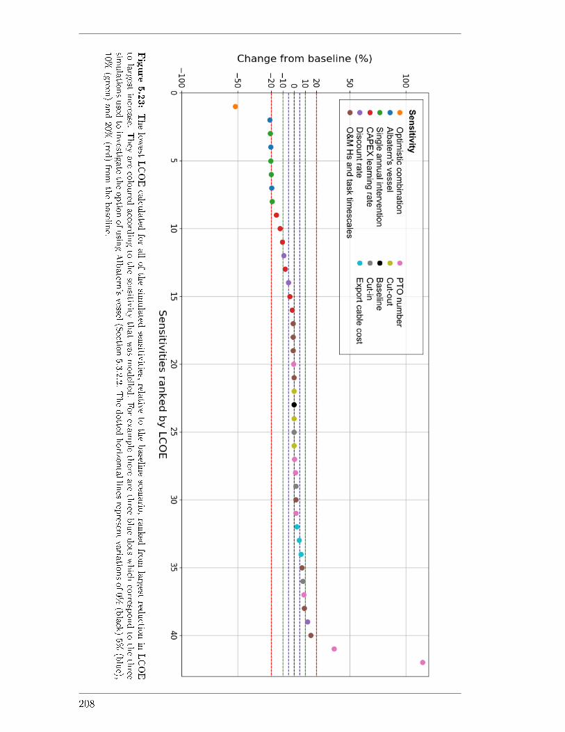
Figure5.23:Thelow

estLCOEcalcu

lated

forallofthesim

ulated

sensitiv

ities,rela

tiveto

thebaselin

escen

ario

,ranked

from

largest

reductio

nin

LCOE

tolargest

increa

se.They

are

coloured

acco

rdingto

thesen

sitivity

thatwasmodelled

.Forexamplethere

are

three

bluedots

which

corresp

ondto

thethree

simulatio

nsused

toinvestig

ate

theoptio

nofusin

gAlbatern

'svessel

(Sectio

n5.3.2.2.Thedotted

horizo

ntallin

esrep

resentvaria

tionsof0%

(black)5%

(blue),

10%

(green

)and20%

(red)fro

mthebaselin

e.

208

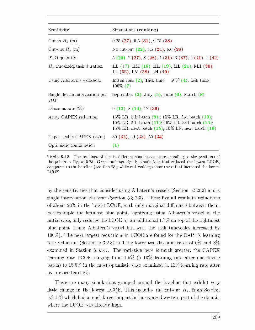
Sensitivity Simulations (ranking)

Cut-in Hs (m) 0.25 (27), 0.5 (31), 0.75 (38)

Cut-out Hs (m) No cut-out (22), 6.5 (24), 6.0 (26)

PTO quantity 5 (20), 7 (27), 8 (28), 4 (31), 3 (37), 2 (41), 1 (42)

Hs threshold/task duration HL (17), HM (18), HH (19), ML (21), MH (30),LL (35), LM (38), LH (40)

Using Albatern's workboat Initial case (2), Task time + 50% (4), task time +100% (7)

Single device intervention peryear

September (3), July (5), June (6), March (8)

Discount rate (%) 6 (12), 8 (14), 12 (39)

Array CAPEX reduction 15% LR, 5th batch (9) ; 15% LR, 3rd batch (10);10% LR, 5th batch (11); 10% LR, 3rd batch (13);15% LR, next batch (15); 10% LR, next batch (16)

Export cable CAPEX (¿/m) 30 (32), 40 (33), 50 (34)

Optimistic combination (1)

Table 5.12: The rankings of the 42 di�erent simulations, corresponding to the positions ofthe points in Figure 5.23. Green rankings signify simulations that reduced the lowest LCOE,compared to the baseline (position 23), while red rankings show those that increased the lowestLCOE.

by the sensitivities that consider using Albatern's vessels (Section 5.3.2.2) and a

single intervention per year (Section 5.3.2.3). These �ve all result in reductions

of about 20% in the lowest LCOE, with only marginal di�erence between them.

For example the leftmost blue point, signifying using Albatern's vessel in the

initial case, only reduces the LCOE by an additional 1.7% on top of the rightmost

blue point (using Albatern's vessel but with the task timescales increased by

100%). The next largest reductions in LCOE are found for the CAPEX learning

rate reduction (Section 5.3.2.3) and the lower two discount rates of 6% and 8%

examined in Section 5.3.3.1. The variation here is much greater, the CAPEX

learning rate LCOE ranging from 1.5% (a 10% learning rate after one device

batch) to 15.5% in the most optimistic case examined (a 15% learning rate after

�ve device batches).

There are many simulations grouped around the baseline that exhibit very

little change in the lowest LCOE. This includes the cut-out Hs, from Section

5.3.1.2) which had a much larger impact in the exposed western part of the domain

where the LCOE was already high.

209

There are some sensitivities that had a notable negative e�ect on LCOE. The

largest are from equipping the array with low numbers of PTOs (Section 5.3.1.3);

the two rightmost pink points show the increase in lowest LCOE with one PTO

module (115%) and two PTO modules (36%). As illustrated in Figure 5.13 these

PTO quantities did reduce the LCOE in some very sheltered parts of the domain.

However they increased the LCOE in the most cost-competitive Little Minch

region. Increasing the Hs thresholds also resulted in signi�cant increase in the

lowest LCOE as shown by the rightmost three brown points

210

6O�-grid Wave Energy Systems for

Aquaculture

This chapter presents a case study of the o�-grid sub-module as described

in Chapter 4. The aim is to demonstrate the model functionality, showing the

strengths of the methodology and how it can be applied in practice. It combines

the baseline WaveNET system from the previous chapter with hybrid system

components, with the aim of supplying power to a �sh farm. This is compared to

the conventional, diesel generator only case. Sensitivity analysis is also performed

to show how the model can guide project decisions.

6.1 Case Study Locations

For the case study two areas were considered: a site to the north east of North

Uist and a site to the west of Skye. These are shown in Figure 6.1. They were cho-

sen because they contain active �sh farms and coincided with lower LCOE values

from the previous analyses in Chapter 5. The �sh farm locations were down-

loaded from the Scotland's Aquaculture website [207]. The �ve farms enclosed in

the analysis domains are active �n�sh sites.

The same ten years of hindcast metocean data were used as described in Sec-

tion 5.1. Each analysis domain is approximately ten by twelve kilometres, contain-

ing 30 site data points. These areas are signi�cantly smaller than those considered

for the grid-connected case study, due to the longer computation time associated

with the energy balancing algorithm. One iteration of this algorithm at a single

211

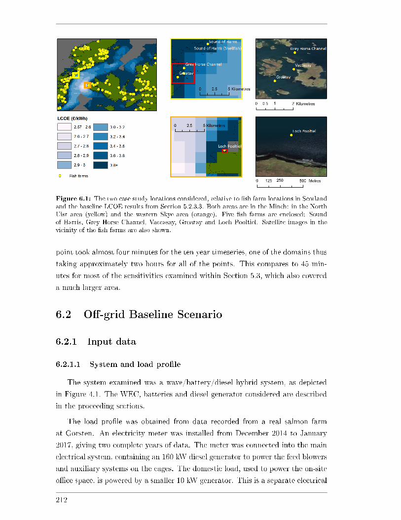
Figure 6.1: The two case study locations considered, relative to �sh farm locations in Scotlandand the baseline LCOE results from Section 5.2.3.3. Both areas are in the Minch: in the NorthUist area (yellow) and the western Skye area (orange). Five �sh farms are enclosed: Soundof Harris, Grey Horse Channel, Vaccasay, Groatay and Loch Pooltiel. Satellite images in thevicinity of the �sh farms are also shown.

point took almost four minutes for the ten year timeseries, one of the domains thus

taking approximately two hours for all of the points. This compares to 45 min-

utes for most of the sensitivities examined within Section 5.3, which also covered

a much larger area.

6.2 O�-grid Baseline Scenario

6.2.1 Input data

6.2.1.1 System and load pro�le

The system examined was a wave/battery/diesel hybrid system, as depicted

in Figure 4.1. The WEC, batteries and diesel generator considered are described

in the proceeding sections.

The load pro�le was obtained from data recorded from a real salmon farm

at Gorsten. An electricity meter was installed from December 2014 to January

2017, giving two complete years of data. The meter was connected into the main

electrical system, containing an 160 kW diesel generator to power the feed blowers

and auxiliary systems on the cages. The domestic load, used to power the on-site

o�ce space, is powered by a smaller 10 kW generator. This is a separate electrical

212

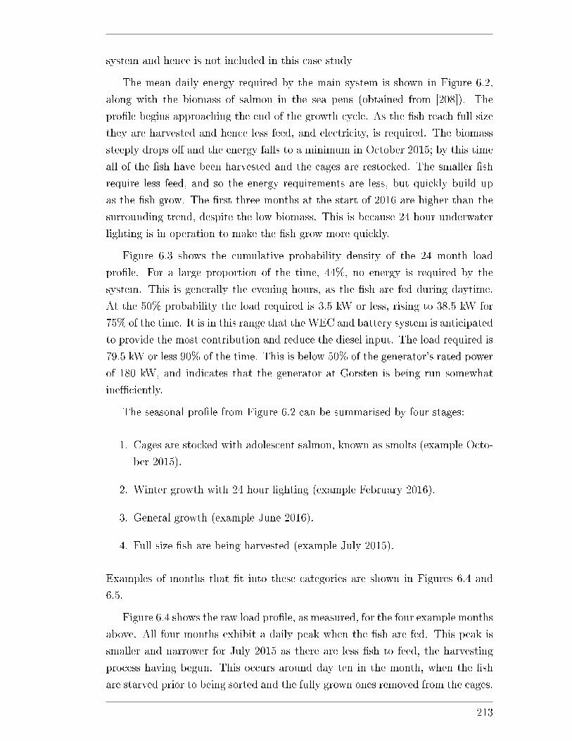
system and hence is not included in this case study

The mean daily energy required by the main system is shown in Figure 6.2,

along with the biomass of salmon in the sea pens (obtained from [208]). The

pro�le begins approaching the end of the growth cycle. As the �sh reach full size

they are harvested and hence less feed, and electricity, is required. The biomass

steeply drops o� and the energy falls to a minimum in October 2015; by this time

all of the �sh have been harvested and the cages are restocked. The smaller �sh

require less feed, and so the energy requirements are less, but quickly build up

as the �sh grow. The �rst three months at the start of 2016 are higher than the

surrounding trend, despite the low biomass. This is because 24 hour underwater

lighting is in operation to make the �sh grow more quickly.

Figure 6.3 shows the cumulative probability density of the 24 month load

pro�le. For a large proportion of the time, 44%, no energy is required by the

system. This is generally the evening hours, as the �sh are fed during daytime.

At the 50% probability the load required is 3.5 kW or less, rising to 38.5 kW for

75% of the time. It is in this range that the WEC and battery system is anticipated

to provide the most contribution and reduce the diesel input. The load required is

79.5 kW or less 90% of the time. This is below 50% of the generator's rated power

of 180 kW, and indicates that the generator at Gorsten is being run somewhat

ine�ciently.

The seasonal pro�le from Figure 6.2 can be summarised by four stages:

1. Cages are stocked with adolescent salmon, known as smolts (example Octo-

ber 2015).

2. Winter growth with 24 hour lighting (example February 2016).

3. General growth (example June 2016).

4. Full size �sh are being harvested (example July 2015).

Examples of months that �t into these categories are shown in Figures 6.4 and

6.5.

Figure 6.4 shows the raw load pro�le, as measured, for the four example months

above. All four months exhibit a daily peak when the �sh are fed. This peak is

smaller and narrower for July 2015 as there are less �sh to feed, the harvesting

process having begun. This occurs around day ten in the month, when the �sh

are starved prior to being sorted and the fully grown ones removed from the cages.

213

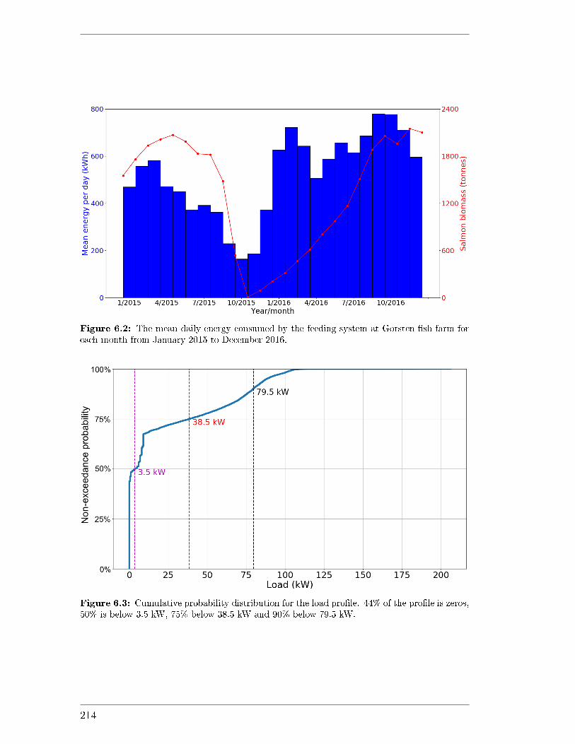
Figure 6.2: The mean daily energy consumed by the feeding system at Gorsten �sh farm foreach month from January 2015 to December 2016.

Figure 6.3: Cumulative probability distribution for the load pro�le. 44% of the pro�le is zeros,50% is below 3.5 kW, 75% below 38.5 kW and 90% below 79.5 kW.

214

This harvesting day is at a regular time in the month, as demonstrated by the

October pro�le. The last of the adult �sh are removed and the cages restocked

with smaller �sh, that only require a small amount of feed. This restocking process

is achieved over a number of months. By February 2016, the �sh are being fed a

substantial amount of feed, and growth lighting is operating 24 hours a day over

much of the month. This lighting is no longer being used by June 2016, the load

pro�le taking on a much more regular form.

The daily average pro�les for the four months are shown in Figure 6.5. Here

the shorter July pro�le can be seen, as well as the much lower demand in October.

The February pro�le is higher outside the feeding hours because of the growth

lighting.

The biomass data from Figure 6.2 indicates that the lifecycle is slightly shorter

than 24 months in reality, as the start and end points of the 24 month pro�le do

not match up. To examine a shorter time interval would have meant a somewhat

irregular seasonal pattern, which would have been di�cult to project over a 20

year lifetime. Hence, the full 24 month pro�le was chosen in this study as an

approximation of the real cyclical behaviour. This pro�le was duplicated �ve

times to give a ten year pro�le, this consistent with the amount of metocean data

available. No fallowing period between cycles is included, as this was not seen

over the 24 month pro�le. After running the algorithm for ten years, the monthly

results are duplicated to cover the 20 year lifetime (as described in Section 3.6.2.2.

No distinction is made between the �ve �sh farms with regard to energy re-

quirements. In reality, each farm will consume a di�erent amount of energy de-

pending on how it is operated (for example some farms might use more feed, some

will use more underwater lighting, etc.). These data were not available so the load

pro�le from Gorsten as described above was assumed for all of the farms.

6.2.1.2 Wave energy device

The wave energy device is the same that was chosen for the grid-connected

case study from Chapter 5, described in Section 5.2. Valid export cable landing

points are assumed to be at the exact �sh farm coordinates, as shown in Figure

6.1. Here the cable connects into the hybrid system on the AC side, located close

to the diesel generator either onshore or on a feed barge.

6.2.1.3 Diesel generator

Table 6.1 shows the properties of the diesel generator. This is not a backup

generator and is actively designed to meet the peak load, due to the scale of the

215

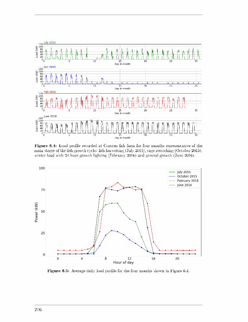
Figure 6.4: Load pro�le recorded at Gorsten �sh farm for four months representative of themain stages of the �sh growth cycle: �sh harvesting (July 2015), cage restocking (October 2015),winter load with 24 hour growth lighting (February 2016) and general growth (June 2016).

Figure 6.5: Average daily load pro�le for the four months shown in Figure 6.4.

216

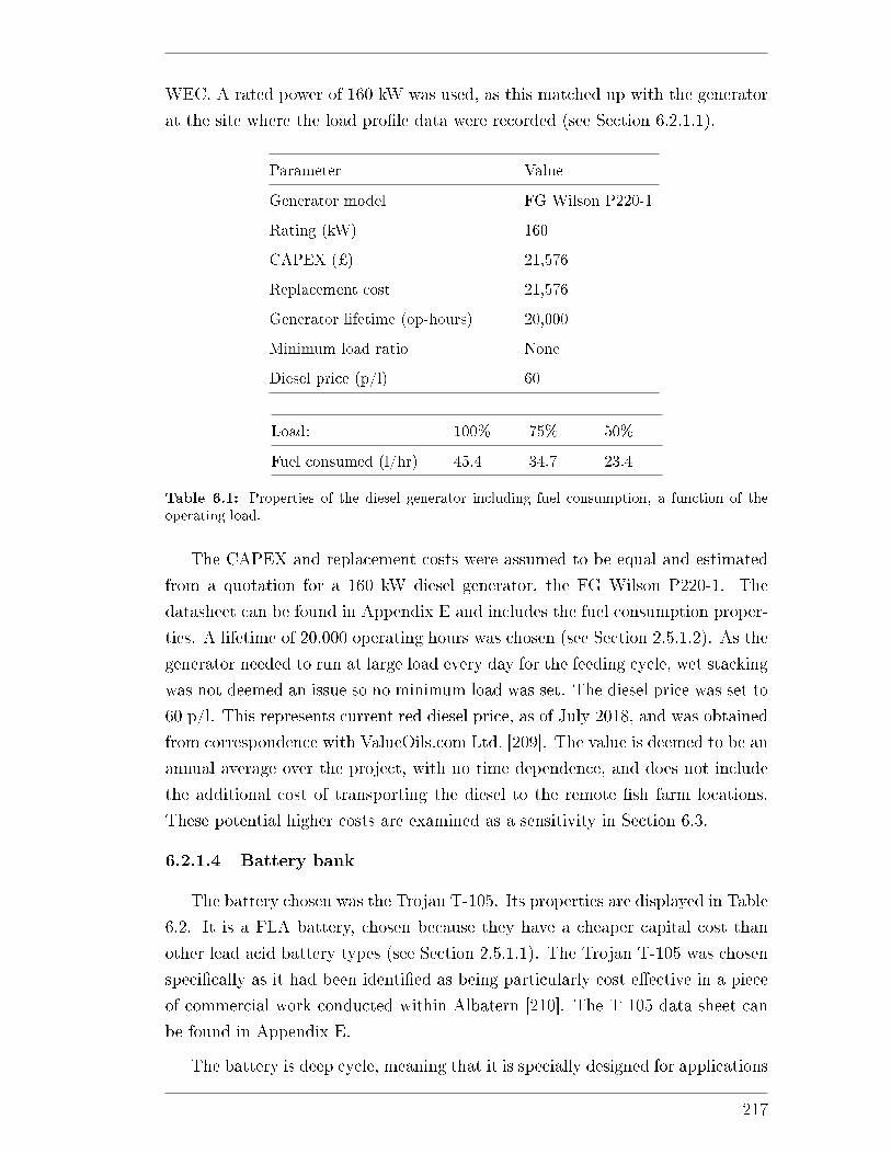
WEC. A rated power of 160 kW was used, as this matched up with the generator

at the site where the load pro�le data were recorded (see Section 6.2.1.1).

Parameter Value

Generator model FG Wilson P220-1

Rating (kW) 160

CAPEX (¿) 21,576

Replacement cost 21,576

Generator lifetime (op-hours) 20,000

Minimum load ratio None

Diesel price (p/l) 60

Load: 100% 75% 50%

Fuel consumed (l/hr) 45.4 34.7 23.4

Table 6.1: Properties of the diesel generator including fuel consumption, a function of theoperating load.

The CAPEX and replacement costs were assumed to be equal and estimated

from a quotation for a 160 kW diesel generator, the FG Wilson P220-1. The

datasheet can be found in Appendix E and includes the fuel consumption proper-

ties. A lifetime of 20,000 operating hours was chosen (see Section 2.5.1.2). As the

generator needed to run at large load every day for the feeding cycle, wet stacking

was not deemed an issue so no minimum load was set. The diesel price was set to

60 p/l. This represents current red diesel price, as of July 2018, and was obtained

from correspondence with ValueOils.com Ltd. [209]. The value is deemed to be an

annual average over the project, with no time dependence, and does not include

the additional cost of transporting the diesel to the remote �sh farm locations.

These potential higher costs are examined as a sensitivity in Section 6.3.

6.2.1.4 Battery bank

The battery chosen was the Trojan T-105. Its properties are displayed in Table

6.2. It is a FLA battery, chosen because they have a cheaper capital cost than

other lead acid battery types (see Section 2.5.1.1). The Trojan T-105 was chosen

speci�cally as it had been identi�ed as being particularly cost e�ective in a piece

of commercial work conducted within Albatern [210]. The T-105 data sheet can

be found in Appendix E.

The battery is deep cycle, meaning that it is specially designed for applications

217

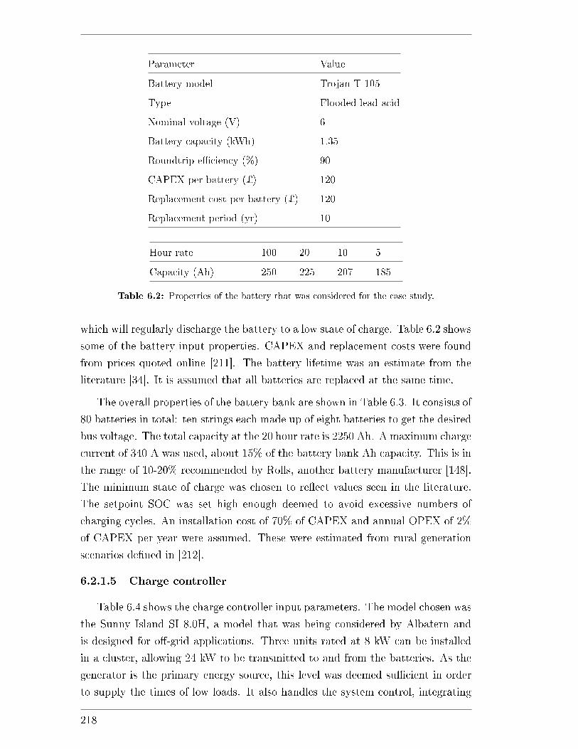
Parameter Value

Battery model Trojan T-105

Type Flooded lead-acid

Nominal voltage (V) 6

Battery capacity (kWh) 1.35

Roundtrip e�ciency (%) 90

CAPEX per battery (¿) 120

Replacement cost per battery (¿) 120

Replacement period (yr) 10

Hour rate 100 20 10 5

Capacity (Ah) 250 225 207 185

Table 6.2: Properties of the battery that was considered for the case study.

which will regularly discharge the battery to a low state of charge. Table 6.2 shows

some of the battery input properties. CAPEX and replacement costs were found

from prices quoted online [211]. The battery lifetime was an estimate from the

literature [34]. It is assumed that all batteries are replaced at the same time.

The overall properties of the battery bank are shown in Table 6.3. It consists of

80 batteries in total: ten strings each made up of eight batteries to get the desired

bus voltage. The total capacity at the 20 hour rate is 2250 Ah. A maximum charge

current of 340 A was used, about 15% of the battery bank Ah capacity. This is in

the range of 10-20% recommended by Rolls, another battery manufacturer [148].

The minimum state of charge was chosen to re�ect values seen in the literature.

The setpoint SOC was set high enough deemed to avoid excessive numbers of

charging cycles. An installation cost of 70% of CAPEX and annual OPEX of 2%

of CAPEX per year were assumed. These were estimated from rural generation

scenarios de�ned in [212].

6.2.1.5 Charge controller

Table 6.4 shows the charge controller input parameters. The model chosen was

the Sunny Island SI 8.0H, a model that was being considered by Albatern and

is designed for o�-grid applications. Three units rated at 8 kW can be installed

in a cluster, allowing 24 kW to be transmitted to and from the batteries. As the

generator is the primary energy source, this level was deemed su�cient in order

to supply the times of low loads. It also handles the system control, integrating

218

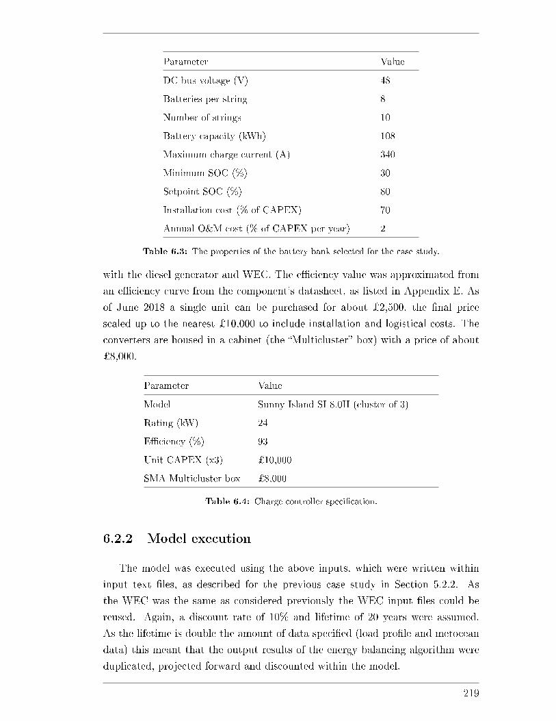
Parameter Value

DC bus voltage (V) 48

Batteries per string 8

Number of strings 10

Battery capacity (kWh) 108

Maximum charge current (A) 340

Minimum SOC (%) 30

Setpoint SOC (%) 80

Installation cost (% of CAPEX) 70

Annual O&M cost (% of CAPEX per year) 2

Table 6.3: The properties of the battery bank selected for the case study.

with the diesel generator and WEC. The e�ciency value was approximated from

an e�ciency curve from the component's datasheet, as listed in Appendix E. As

of June 2018 a single unit can be purchased for about ¿2,500, the �nal price

scaled up to the nearest ¿10,000 to include installation and logistical costs. The

converters are housed in a cabinet (the �Multicluster� box) with a price of about

¿8,000.

Parameter Value

Model Sunny Island SI 8.0H (cluster of 3)

Rating (kW) 24

E�ciency (%) 93

Unit CAPEX (x3) ¿10,000

SMA Multicluster box ¿8,000

Table 6.4: Charge controller speci�cation.

6.2.2 Model execution

The model was executed using the above inputs, which were written within

input text �les, as described for the previous case study in Section 5.2.2. As

the WEC was the same as considered previously the WEC input �les could be

reused. Again, a discount rate of 10% and lifetime of 20 years were assumed.

As the lifetime is double the amount of data speci�ed (load pro�le and metocean

data) this meant that the output results of the energy balancing algorithm were

duplicated, projected forward and discounted within the model.

219

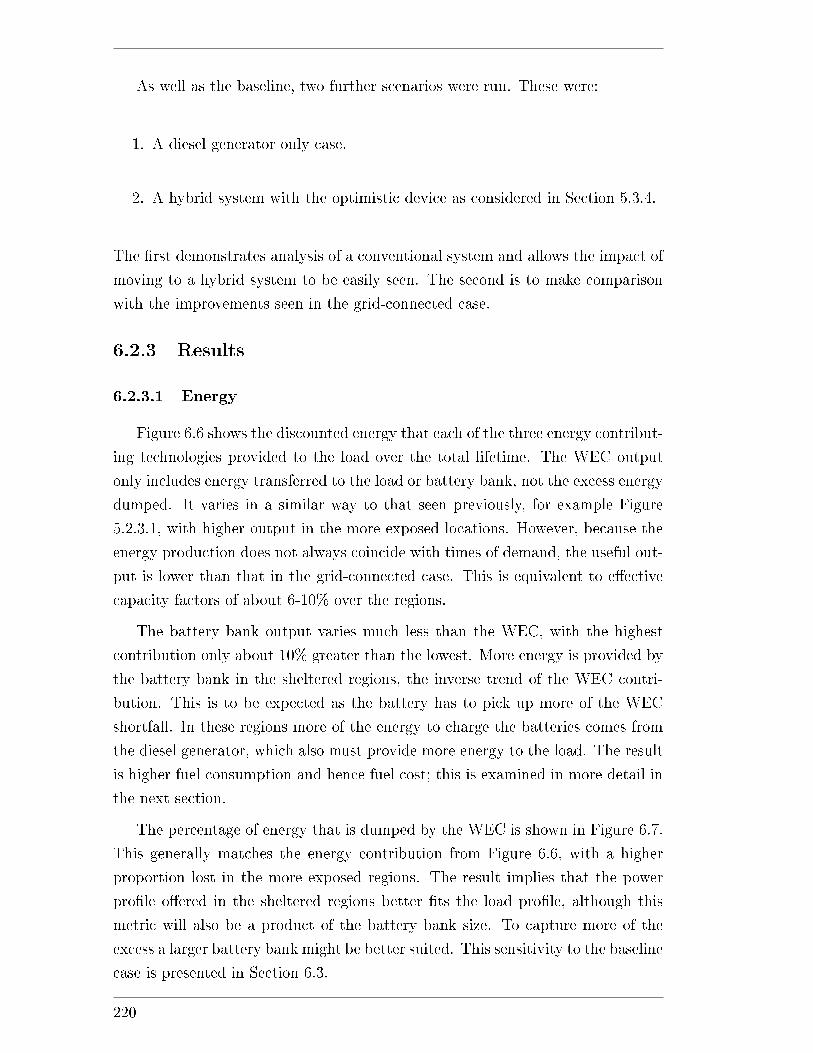
As well as the baseline, two further scenarios were run. These were:

1. A diesel generator only case.

2. A hybrid system with the optimistic device as considered in Section 5.3.4.

The �rst demonstrates analysis of a conventional system and allows the impact of

moving to a hybrid system to be easily seen. The second is to make comparison

with the improvements seen in the grid-connected case.

6.2.3 Results

6.2.3.1 Energy

Figure 6.6 shows the discounted energy that each of the three energy contribut-

ing technologies provided to the load over the total lifetime. The WEC output

only includes energy transferred to the load or battery bank, not the excess energy

dumped. It varies in a similar way to that seen previously, for example Figure

5.2.3.1, with higher output in the more exposed locations. However, because the

energy production does not always coincide with times of demand, the useful out-

put is lower than that in the grid-connected case. This is equivalent to e�ective

capacity factors of about 6-10% over the regions.

The battery bank output varies much less than the WEC, with the highest

contribution only about 10% greater than the lowest. More energy is provided by

the battery bank in the sheltered regions, the inverse trend of the WEC contri-

bution. This is to be expected as the battery has to pick up more of the WEC

shortfall. In these regions more of the energy to charge the batteries comes from

the diesel generator, which also must provide more energy to the load. The result

is higher fuel consumption and hence fuel cost; this is examined in more detail in

the next section.

The percentage of energy that is dumped by the WEC is shown in Figure 6.7.

This generally matches the energy contribution from Figure 6.6, with a higher

proportion lost in the more exposed regions. The result implies that the power

pro�le o�ered in the sheltered regions better �ts the load pro�le, although this

metric will also be a product of the battery bank size. To capture more of the

excess a larger battery bank might be better suited. This sensitivity to the baseline

case is presented in Section 6.3.

220

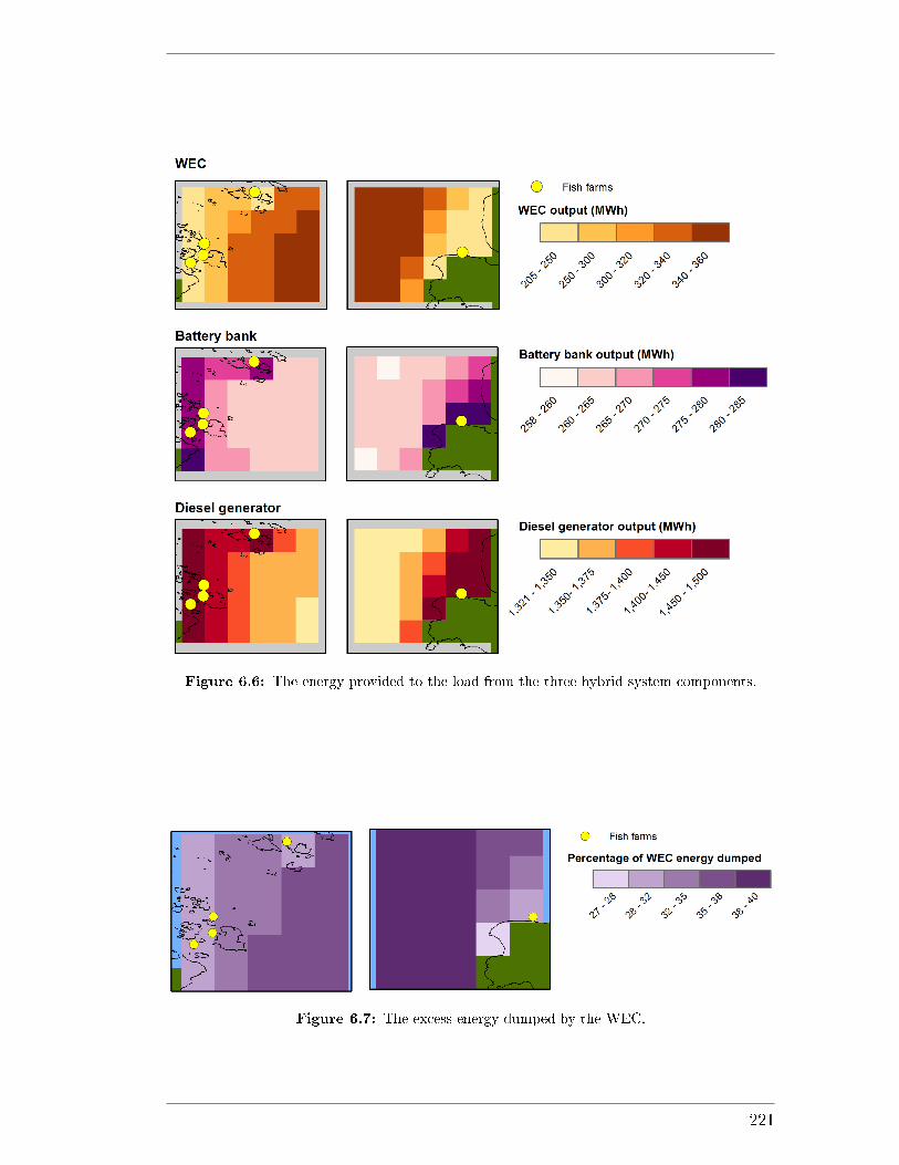
Figure 6.6: The energy provided to the load from the three hybrid system components.

Figure 6.7: The excess energy dumped by the WEC.

221

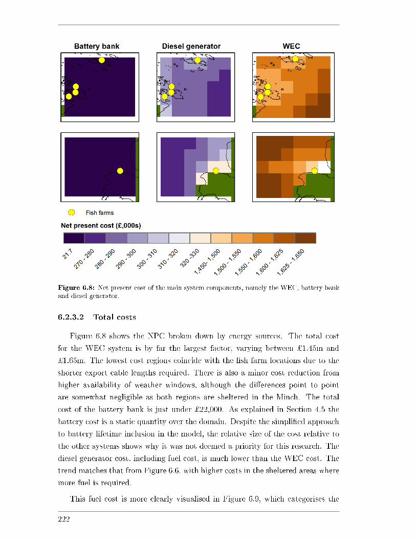
Figure 6.8: Net present cost of the main system components, namely the WEC, battery bankand diesel generator.

6.2.3.2 Total costs

Figure 6.8 shows the NPC broken down by energy sources. The total cost

for the WEC system is by far the largest factor, varying between ¿1.45m and

¿1.65m. The lowest cost regions coincide with the �sh farm locations due to the

shorter export cable lengths required. There is also a minor cost reduction from

higher availability of weather windows, although the di�erences point to point

are somewhat negligible as both regions are sheltered in the Minch. The total

cost of the battery bank is just under ¿22,000. As explained in Section 4.5 the

battery cost is a static quantity over the domain. Despite the simpli�ed approach

to battery lifetime inclusion in the model, the relative size of the cost relative to

the other systems shows why it was not deemed a priority for this research. The

diesel generator cost, including fuel cost, is much lower than the WEC cost. The

trend matches that from Figure 6.6, with higher costs in the sheltered areas where

more fuel is required.

This fuel cost is more clearly visualised in Figure 6.9, which categorises the

222

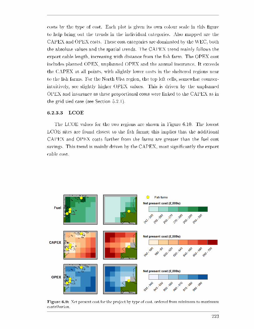
costs by the type of cost. Each plot is given its own colour scale in this �gure

to help bring out the trends in the individual categories. Also mapped are the

CAPEX and OPEX costs. These cost categories are dominated by the WEC, both

the absolute values and the spatial trends. The CAPEX trend mainly follows the

export cable length, increasing with distance from the �sh farm. The OPEX cost

includes planned OPEX, unplanned OPEX and the annual insurance. It exceeds

the CAPEX at all points, with slightly lower costs in the sheltered regions near

to the �sh farms. For the North Uist region, the top left cells, somewhat counter-

intuitively, see slightly higher OPEX values. This is driven by the unplanned

OPEX and insurance as these proportional costs were linked to the CAPEX as in

the grid tied case (see Section 5.2.1).

6.2.3.3 LCOE

The LCOE values for the two regions are shown in Figure 6.10. The lowest

LCOE sites are found closest to the �sh farms; this implies that the additional

CAPEX and OPEX costs further from the farms are greater than the fuel cost

savings. This trend is mainly driven by the CAPEX, most signi�cantly the export

cable cost.

Figure 6.9: Net present cost for the project by type of cost, ordered from minimum to maximumcontribution.

223

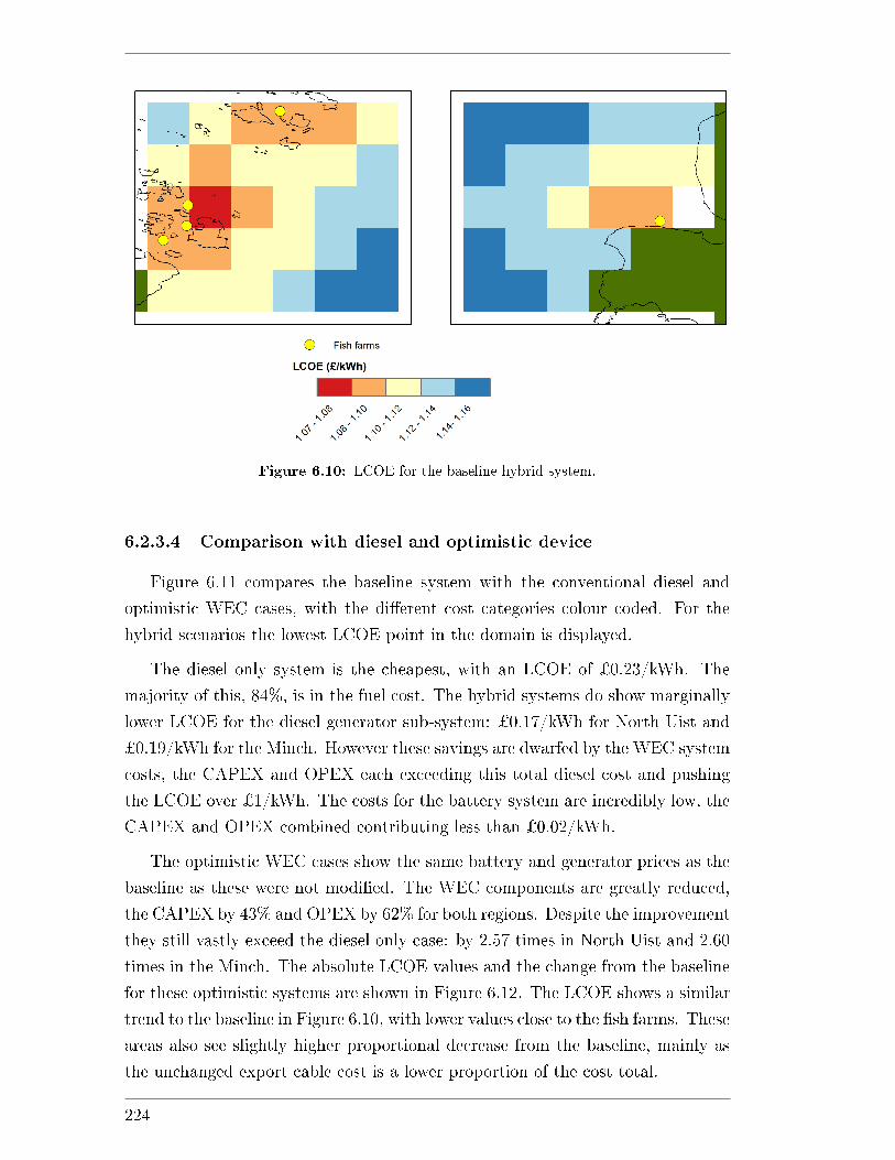
Figure 6.10: LCOE for the baseline hybrid system.

6.2.3.4 Comparison with diesel and optimistic device

Figure 6.11 compares the baseline system with the conventional diesel and

optimistic WEC cases, with the di�erent cost categories colour coded. For the

hybrid scenarios the lowest LCOE point in the domain is displayed.

The diesel only system is the cheapest, with an LCOE of ¿0.23/kWh. The

majority of this, 84%, is in the fuel cost. The hybrid systems do show marginally

lower LCOE for the diesel generator sub-system: ¿0.17/kWh for North Uist and

¿0.19/kWh for the Minch. However these savings are dwarfed by the WEC system

costs, the CAPEX and OPEX each exceeding this total diesel cost and pushing

the LCOE over ¿1/kWh. The costs for the battery system are incredibly low, the

CAPEX and OPEX combined contributing less than ¿0.02/kWh.

The optimistic WEC cases show the same battery and generator prices as the

baseline as these were not modi�ed. The WEC components are greatly reduced,

the CAPEX by 43% and OPEX by 62% for both regions. Despite the improvement

they still vastly exceed the diesel only case: by 2.57 times in North Uist and 2.60

times in the Minch. The absolute LCOE values and the change from the baseline

for these optimistic systems are shown in Figure 6.12. The LCOE shows a similar

trend to the baseline in Figure 6.10, with lower values close to the �sh farms. These

areas also see slightly higher proportional decrease from the baseline, mainly as

the unchanged export cable cost is a lower proportion of the cost total.

224

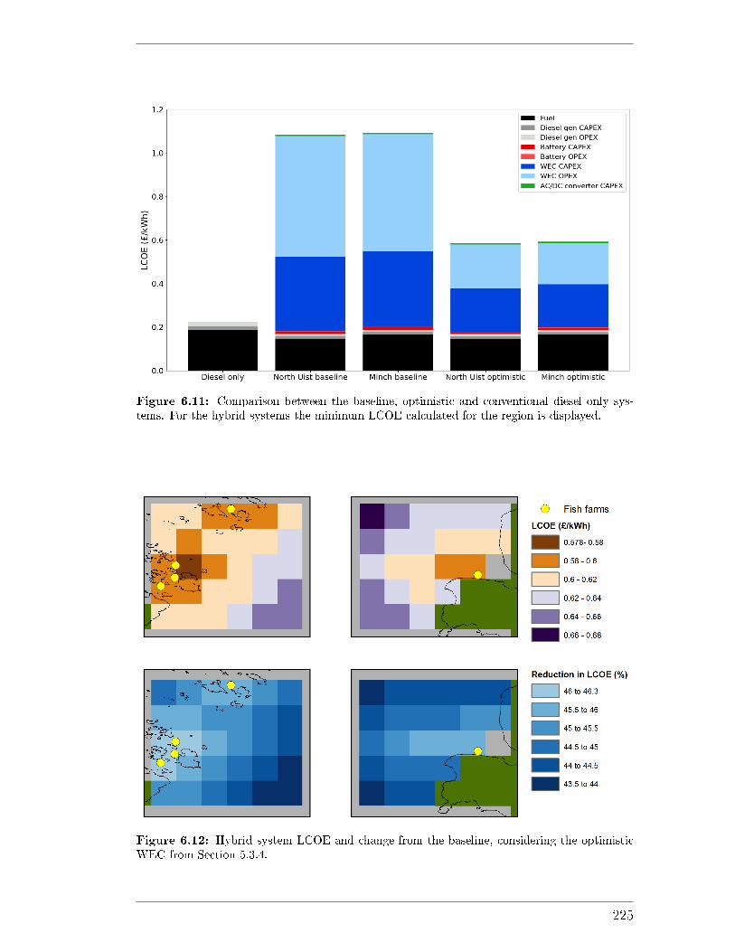
Figure 6.11: Comparison between the baseline, optimistic and conventional diesel only sys-tems. For the hybrid systems the minimum LCOE calculated for the region is displayed.

Figure 6.12: Hybrid system LCOE and change from the baseline, considering the optimisticWEC from Section 5.3.4.

225

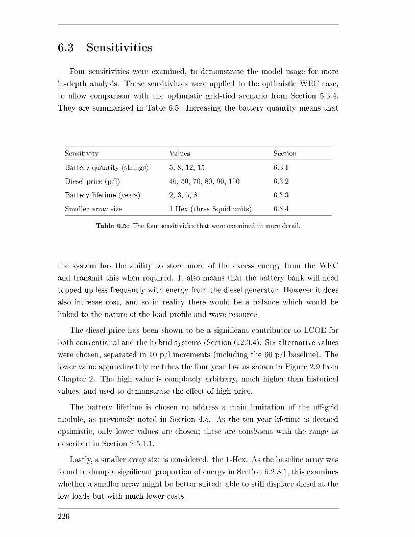
6.3 Sensitivities

Four sensitivities were examined, to demonstrate the model usage for more

in-depth analysis. These sensitivities were applied to the optimistic WEC case,

to allow comparison with the optimistic grid-tied scenario from Section 5.3.4.

They are summarised in Table 6.5. Increasing the battery quantity means that

Sensitivity Values Section

Battery quantity (strings) 5, 8, 12, 15 6.3.1

Diesel price (p/l) 40, 50, 70, 80, 90, 100 6.3.2

Battery lifetime (years) 2, 3, 5, 8 6.3.3

Smaller array size 1-Hex (three Squid units) 6.3.4

Table 6.5: The four sensitivities that were examined in more detail.

the system has the ability to store more of the excess energy from the WEC

and transmit this when required. It also means that the battery bank will need

topped up less frequently with energy from the diesel generator. However it does

also increase cost, and so in reality there would be a balance which would be

linked to the nature of the load pro�le and wave resource.

The diesel price has been shown to be a signi�cant contributor to LCOE for

both conventional and the hybrid systems (Section 6.2.3.4). Six alternative values

were chosen, separated in 10 p/l increments (including the 60 p/l baseline). The

lower value approximately matches the four year low as shown in Figure 2.9 from

Chapter 2. The high value is completely arbitrary, much higher than historical

values, and used to demonstrate the e�ect of high price.

The battery lifetime is chosen to address a main limitation of the o�-grid

module, as previously noted in Section 4.5. As the ten year lifetime is deemed

optimistic, only lower values are chosen; these are consistent with the range as

described in Section 2.5.1.1.

Lastly, a smaller array size is considered: the 1-Hex. As the baseline array was

found to dump a signi�cant proportion of energy in Section 6.2.3.1, this examines

whether a smaller array might be better suited: able to still displace diesel at the

low loads but with much lower costs.

226

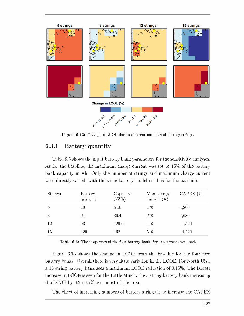
Figure 6.13: Change in LCOE due to di�erent numbers of battery strings.

6.3.1 Battery quantity

Table 6.6 shows the input battery bank parameters for the sensitivity analyses.

As for the baseline, the maximum charge current was set to 15% of the battery

bank capacity in Ah. Only the number of strings and maximum charge current

were directly varied, with the same battery model used as for the baseline.

Strings Batteryquantity

Capacity(kWh)

Max chargecurrent (A)

CAPEX (¿)

5 40 54.0 170 4,800

8 64 86.4 270 7,680

12 96 129.6 410 11,520

15 120 162 510 14,420

Table 6.6: The properties of the four battery bank sizes that were examined.

Figure 6.13 shows the change in LCOE from the baseline for the four new

battery banks. Overall there is very little variation in the LCOE. For North Uist,

a 15 string battery bank sees a maximum LCOE reduction of 0.15%. The largest

increase in LCOE is seen for the Little Minch, the 5 string battery bank increasing

the LCOE by 0.25-0.5% over most of the area.

The e�ect of increasing numbers of battery strings is to increase the CAPEX

227

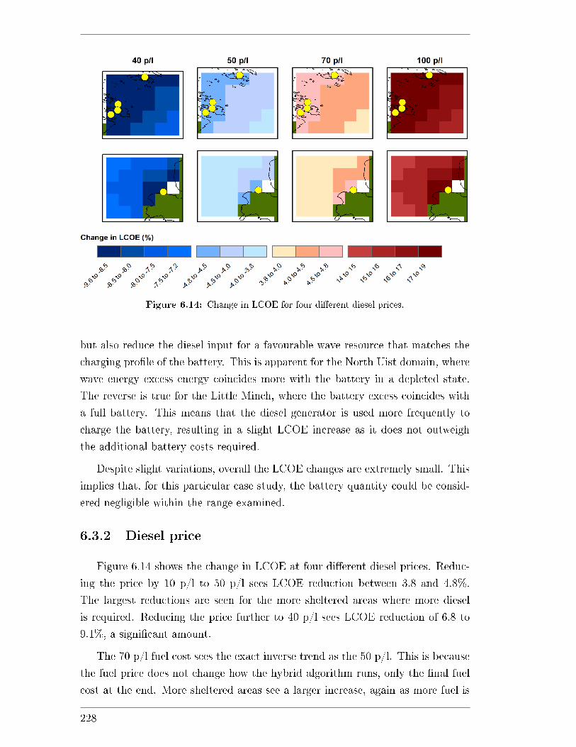
Figure 6.14: Change in LCOE for four di�erent diesel prices.

but also reduce the diesel input for a favourable wave resource that matches the

charging pro�le of the battery. This is apparent for the North Uist domain, where

wave energy excess energy coincides more with the battery in a depleted state.

The reverse is true for the Little Minch, where the battery excess coincides with

a full battery. This means that the diesel generator is used more frequently to

charge the battery, resulting in a slight LCOE increase as it does not outweigh

the additional battery costs required.

Despite slight variations, overall the LCOE changes are extremely small. This

implies that, for this particular case study, the battery quantity could be consid-

ered negligible within the range examined.

6.3.2 Diesel price

Figure 6.14 shows the change in LCOE at four di�erent diesel prices. Reduc-

ing the price by 10 p/l to 50 p/l sees LCOE reduction between 3.8 and 4.8%.

The largest reductions are seen for the more sheltered areas where more diesel

is required. Reducing the price further to 40 p/l sees LCOE reduction of 6.8 to

9.1%, a signi�cant amount.

The 70 p/l fuel cost sees the exact inverse trend as the 50 p/l. This is because

the fuel price does not change how the hybrid algorithm runs, only the �nal fuel

cost at the end. More sheltered areas see a larger increase, again as more fuel is

228

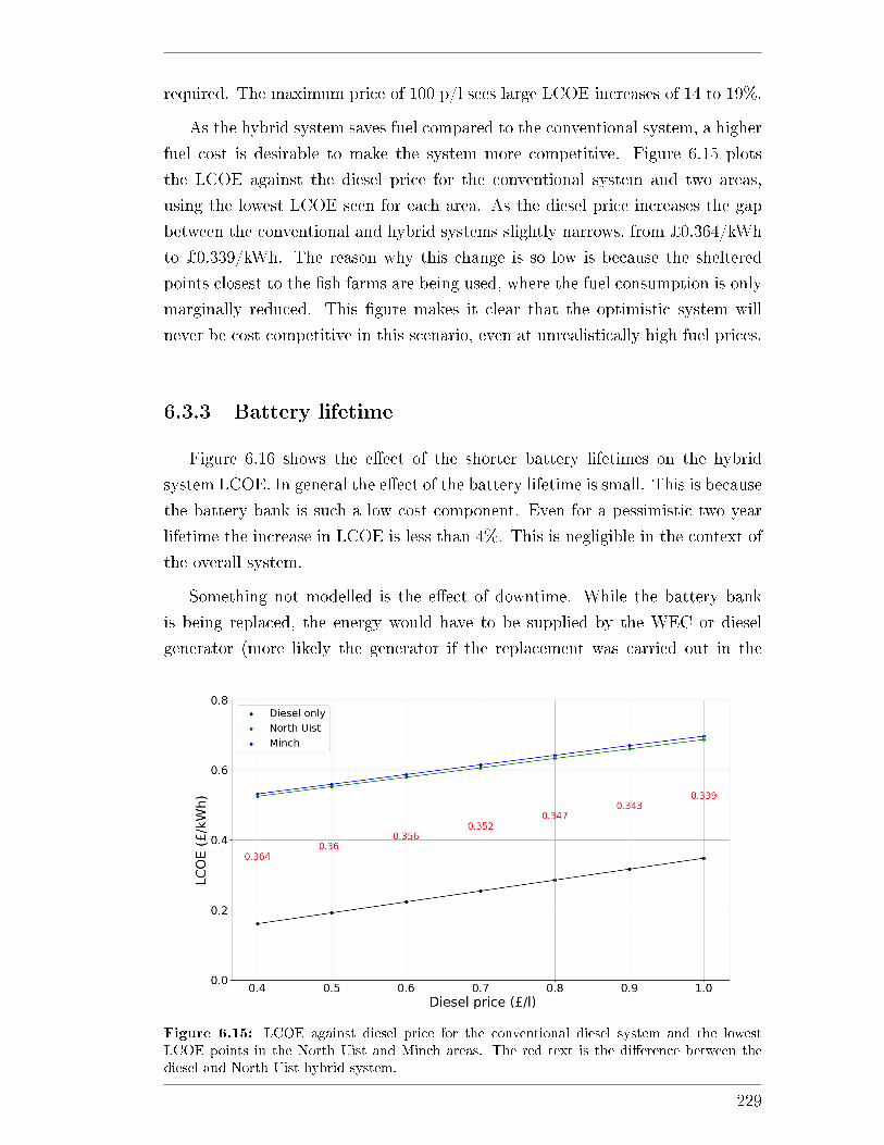
required. The maximum price of 100 p/l sees large LCOE increases of 14 to 19%.

As the hybrid system saves fuel compared to the conventional system, a higher

fuel cost is desirable to make the system more competitive. Figure 6.15 plots

the LCOE against the diesel price for the conventional system and two areas,

using the lowest LCOE seen for each area. As the diesel price increases the gap

between the conventional and hybrid systems slightly narrows, from ¿0.364/kWh

to ¿0.339/kWh. The reason why this change is so low is because the sheltered

points closest to the �sh farms are being used, where the fuel consumption is only

marginally reduced. This �gure makes it clear that the optimistic system will

never be cost competitive in this scenario, even at unrealistically high fuel prices.

6.3.3 Battery lifetime

Figure 6.16 shows the e�ect of the shorter battery lifetimes on the hybrid

system LCOE. In general the e�ect of the battery lifetime is small. This is because

the battery bank is such a low cost component. Even for a pessimistic two year

lifetime the increase in LCOE is less than 4%. This is negligible in the context of

the overall system.

Something not modelled is the e�ect of downtime. While the battery bank

is being replaced, the energy would have to be supplied by the WEC or diesel

generator (more likely the generator if the replacement was carried out in the

Figure 6.15: LCOE against diesel price for the conventional diesel system and the lowestLCOE points in the North Uist and Minch areas. The red text is the di�erence between thediesel and North Uist hybrid system.

229

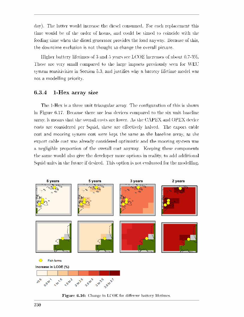
day). The latter would increase the diesel consumed. For each replacement this

time would be of the order of hours, and could be timed to coincide with the

feeding time when the diesel generator provides the load anyway. Because of this,

the downtime exclusion is not thought to change the overall picture.

Higher battery lifetimes of 3 and 5 years see LCOE increases of about 0.7-3%.

These are very small compared to the large impacts previously seen for WEC

system sensitivities in Section 5.3, and justi�es why a battery lifetime model was

not a modelling priority.

6.3.4 1-Hex array size

The 1-Hex is a three unit triangular array. The con�guration of this is shown

in Figure 6.17. Because there are less devices compared to the six unit baseline

array, it means that the overall costs are lower. As the CAPEX and OPEX device

costs are considered per Squid, these are e�ectively halved. The export cable

cost and mooring system cost were kept the same as the baseline array, as the

export cable cost was already considered optimistic and the mooring system was

a negligible proportion of the overall cost anyway. Keeping these components

the same would also give the developer more options in reality, to add additional

Squid units in the future if desired. This option is not evaluated for the modelling.

Figure 6.16: Change in LCOE for di�erent battery lifetimes.

230

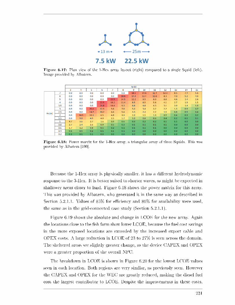
Figure 6.17: Plan view of the 1-Hex array layout (right) compared to a single Squid (left).Image provided by Albatern.

Figure 6.18: Power matrix for the 1-Hex array, a triangular array of three Squids. This wasprovided by Albatern [199]..

Because the 1-Hex array is physically smaller, it has a di�erent hydrodynamic

response to the 3-Hex. It is better suited to shorter waves, as might be expected in

shallower areas closer to land. Figure 6.18 shows the power matrix for this array.

This was provided by Albatern, who generated it in the same way as described in

Section 5.2.1.1. Values of 85% for e�ciency and 80% for availability were used,

the same as in the grid-connected case study (Section 5.2.1.1).

Figure 6.19 shows the absolute and change in LCOE for the new array. Again

the locations close to the �sh farm show lower LCOE, because the fuel cost savings

in the more exposed locations are exceeded by the increased export cable and

OPEX costs. A large reduction in LCOE of 23 to 27% is seen across the domain.

The sheltered areas see slightly greater change, as the device CAPEX and OPEX

were a greater proportion of the overall NPC.

The breakdown in LCOE is shown in Figure 6.20 for the lowest LCOE values

seen in each location. Both regions are very similar, as previously seen. However

the CAPEX and OPEX for the WEC are greatly reduced, making the diesel fuel

cost the largest contributor to LCOE. Despite the improvements in these costs,

231

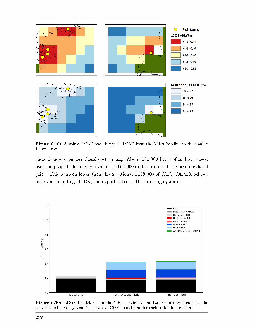
Figure 6.19: Absolute LCOE and change in LCOE from the 3-Hex baseline to the smaller1-Hex array.

there is now even less diesel cost saving. About 100,000 litres of fuel are saved

over the project lifetime, equivalent to ¿60,000 undiscounted at the baseline diesel

price. This is much lower than the additional ¿158,000 of WEC CAPEX added,

not even including OPEX, the export cable or the mooring system.

Figure 6.20: LCOE breakdown for the 1-Hex device at the two regions, compared to theconventional diesel system. The lowest LCOE point found for each region is presented.

232

7Discussion

This chapter discusses the performance of the spatial LCOE model as a tool

to identify promising locations for wave energy projects. This is framed in the

context of the case study results from Chapters 5 and 6, which were used to

demonstrate the model functionality and outputs. It includes re�ection on both

the key capabilities and the areas which would require further improvement to

extend its potential.

7.1 Model Summary

An overall assessment of the model should examine two areas:

1. The calculations that are being performed to derive energy, costs and LCOE.

2. The computational structure of the model and how this bene�ts usability

and performance.

The �rst assessment is necessary to ensure that the model is functioning correctly

and providing trustworthy estimates of performance and spatial trends. The sec-

ond assessment is vitally important to allow the calculations to be checked, bugs

to be identi�ed and corrected, runtime to be reduced and to make it possible to

expand the model into the future.

233

7.1.1 Grid-connected array

7.1.1.1 Cost analysis

The cost calculations cover a number of di�erent areas. The model allows a

high degree of �exibility in the costs that are speci�ed and how they are cate-

gorised. This is made possible by the ItemBase class, the most important class

for these calculations. It provides a blueprint for any item that has costs associ-

ated with it. The local_costs attribute means that single and recurring costs

are easy to de�ne and are automatically discounted to present values. Multiple

and arbitrary cost categories can be de�ned for ItemBase instances or single cost

elements which, along with their quantities, are recursively �ltered down to nested

items and aggregated. The advantage of this approach was seen in Section 5.2.3.2,

where cost results were presented both by type (e.g. CAPEX and OPEX) and by

system (e.g. device, export cable). Being able to de�ne proportional costs relative

to category totals is another useful feature of the model. This was demonstrated

in the case study for two recurring costs: the insurance cost and the unplanned

OPEX cost. While not a replacement for a dedicated unplanned O&M module,

the latter demonstrated how the model can be used to make higher level estimates

to account for missing data or functionality.

For the case study results in Section 5.2.3.2, the model allowed the relative

proportions of the costs to be easily visualised and compared. From the costs by

system results in Figure 5.6, the device cost could be clearly identi�ed as the most

signi�cant factor. The smaller costs are also useful to inform business strategy.

For example the spatial trends in the total costs are largely driven by the export

cable cost behaviour, and so quantifying this for di�erent system designs is shown

to be a priority for the company. The mooring system cost is very low, the model

is thus able to advise cost reduction and optimisation focus away from this system.

A similar case is seen for the installation cost in Figure 5.7, which is insignif-

icant compared to the initial cost and O&M. Being able to visualise the spatial

trends in OPEX is extremely powerful and a key contribution to knowledge from

the research. De�ning each operation with its own cost category means that the

output costs for each are automatically isolated, as shown in Figure 5.8. Again

these results can clearly indicate the dominant cost factors, for this case study

the device maintenance cost. One might have expected the mid-life re�t cost to

be more signi�cant due to the high replacement cost involved. The model shows

that this is not the case, however, due to the high discounting by project year ten.

234

Overall the OPEX analysis works well, with the three main parts of the cal-

culation appropriately ordered (calculation of task timescales, waiting times and

then vessel costs). The calculation is potentially on the pessimistic side, as the

metocean conditions at each point are also used for estimation of transit waiting

time. The waiting time has a large impact on the viability of projects at exposed

locations, and the methods could be adjusted and improved over time to match

the physical reality. The model's ability to automatically constrain the domain

size, to exclude points where operations cannot take place, is a useful feature.

The path�nding abilities coded into the WaveSite class are invaluable for

the spatial costs. Keeping this benchmark, embedded within all the cost items,

ensures consistency in the calculations. Keeping the relevant path�nding code

in a standalone package (the �path�nding� module, described in Appendix B.3)

also means that the functionality is easy to adapt in the future. The locations of

ports and export cable landing points in the domain were also demonstrated as

in�uential factors in Figures 5.17 and 6.9 respectively (the latter for the hybrid

system). While not included due to lack of data, costs can also be assigned to these

points which can provide a �ner level of detail in the resulting cost calculations.

7.1.1.2 Energy analysis

The classes used for the power interpolation, WaveDevice and PowerMatrix are

intuitively structured and conveniently combined with the metocean data within

the EnergyAnalysis class. The WaveEnergyArray class gives the �exibility to

specify a di�erent power matrix at the array level. While this power matrix

modi�cation is somewhat unique to the Albatern interconnected array concept, it

is optional and calculating power using power matrices at the device level is also

a feature.

The maps in Figure 5.5 show two di�erent measures of the energy production

performance. They also show the power of plotting in GIS, as the data visu-

alisation can be fully customised in a straightforward way. To the west of the

domain the results were as expected, with energy production increasing further

from shore. The sheltered areas between the islands saw very low capacity factors,

typically less then 10%. The hotspot in the Little Minch was of particular inter-

est. Because of the multi-dimensional nature of the power production it is more

di�cult to judge where the best locations will be, especially when confronted with

a full timeseries. Being able to map energy production is extremely powerful, and

brings attention to areas that would otherwise not be seen.

The modi�cations that can be applied to the speci�ed power matrix in the

235

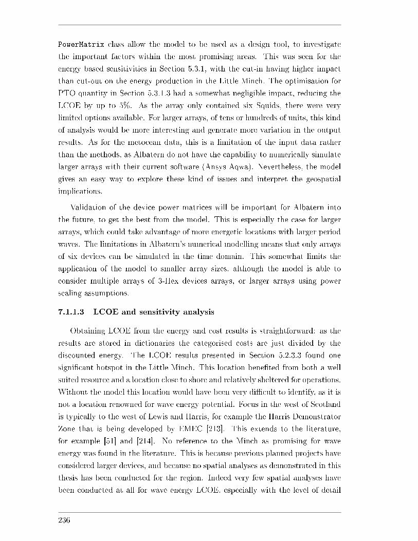
PowerMatrix class allow the model to be used as a design tool, to investigate

the important factors within the most promising areas. This was seen for the

energy based sensitivities in Section 5.3.1, with the cut-in having higher impact

than cut-out on the energy production in the Little Minch. The optimisation for

PTO quantity in Section 5.3.1.3 had a somewhat negligible impact, reducing the

LCOE by up to 5%. As the array only contained six Squids, there were very

limited options available. For larger arrays, of tens or hundreds of units, this kind

of analysis would be more interesting and generate more variation in the output

results. As for the metocean data, this is a limitation of the input data rather

than the methods, as Albatern do not have the capability to numerically simulate

larger arrays with their current software (Ansys Aqwa). Nevertheless, the model

gives an easy way to explore these kind of issues and interpret the geospatial

implications.

Validation of the device power matrices will be important for Albatern into

the future, to get the best from the model. This is especially the case for larger

arrays, which could take advantage of more energetic locations with larger period

waves. The limitations in Albatern's numerical modelling means that only arrays

of six devices can be simulated in the time domain. This somewhat limits the

application of the model to smaller array sizes, although the model is able to

consider multiple arrays of 3-Hex devices arrays, or larger arrays using power

scaling assumptions.

7.1.1.3 LCOE and sensitivity analysis

Obtaining LCOE from the energy and cost results is straightforward: as the

results are stored in dictionaries the categorised costs are just divided by the

discounted energy. The LCOE results presented in Section 5.2.3.3 found one

signi�cant hotspot in the Little Minch. This location bene�ted from both a well

suited resource and a location close to shore and relatively sheltered for operations.

Without the model this location would have been very di�cult to identify, as it is

not a location renowned for wave energy potential. Focus in the west of Scotland

is typically to the west of Lewis and Harris, for example the Harris Demonstrator

Zone that is being developed by EMEC [213]. This extends to the literature,

for example [51] and [214]. No reference to the Minch as promising for wave

energy was found in the literature. This is because previous planned projects have

considered larger devices, and because no spatial analyses as demonstrated in this

thesis has been conducted for the region. Indeed very few spatial analyses have

been conducted at all for wave energy LCOE, especially with the level of detail

236

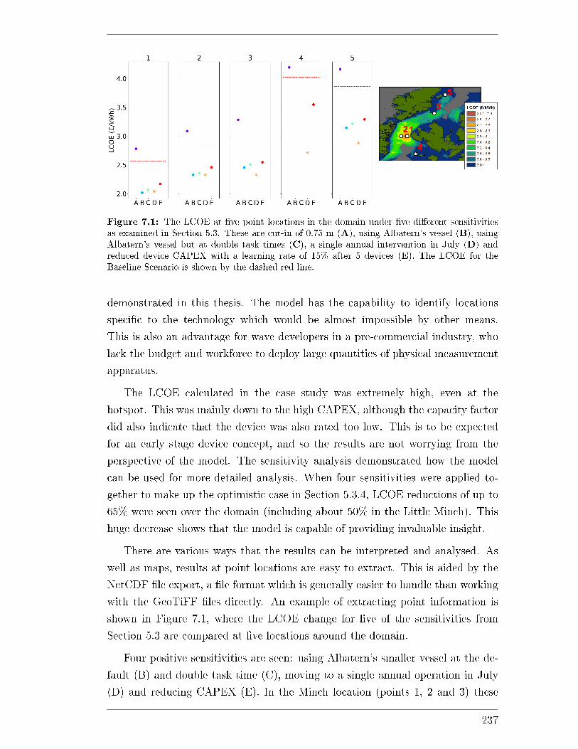
Figure 7.1: The LCOE at �ve point locations in the domain under �ve di�erent sensitivitiesas examined in Section 5.3. These are cut-in of 0.75 m (A), using Albatern's vessel (B), usingAlbatern's vessel but at double task times (C), a single annual intervention in July (D) andreduced device CAPEX with a learning rate of 15% after 5 devices (E). The LCOE for theBaseline Scenario is shown by the dashed red line.

demonstrated in this thesis. The model has the capability to identify locations

speci�c to the technology which would be almost impossible by other means.

This is also an advantage for wave developers in a pre-commercial industry, who

lack the budget and workforce to deploy large quantities of physical measurement

apparatus.

The LCOE calculated in the case study was extremely high, even at the

hotspot. This was mainly down to the high CAPEX, although the capacity factor

did also indicate that the device was also rated too low. This is to be expected

for an early stage device concept, and so the results are not worrying from the

perspective of the model. The sensitivity analysis demonstrated how the model

can be used for more detailed analysis. When four sensitivities were applied to-

gether to make up the optimistic case in Section 5.3.4, LCOE reductions of up to

65% were seen over the domain (including about 50% in the Little Minch). This

huge decrease shows that the model is capable of providing invaluable insight.

There are various ways that the results can be interpreted and analysed. As

well as maps, results at point locations are easy to extract. This is aided by the

NetCDF �le export, a �le format which is generally easier to handle than working

with the GeoTiFF �les directly. An example of extracting point information is

shown in Figure 7.1, where the LCOE change for �ve of the sensitivities from

Section 5.3 are compared at �ve locations around the domain.

Four positive sensitivities are seen: using Albatern's smaller vessel at the de-

fault (B) and double task time (C), moving to a single annual operation in July

(D) and reducing CAPEX (E). In the Minch location (points 1, 2 and 3) these

237

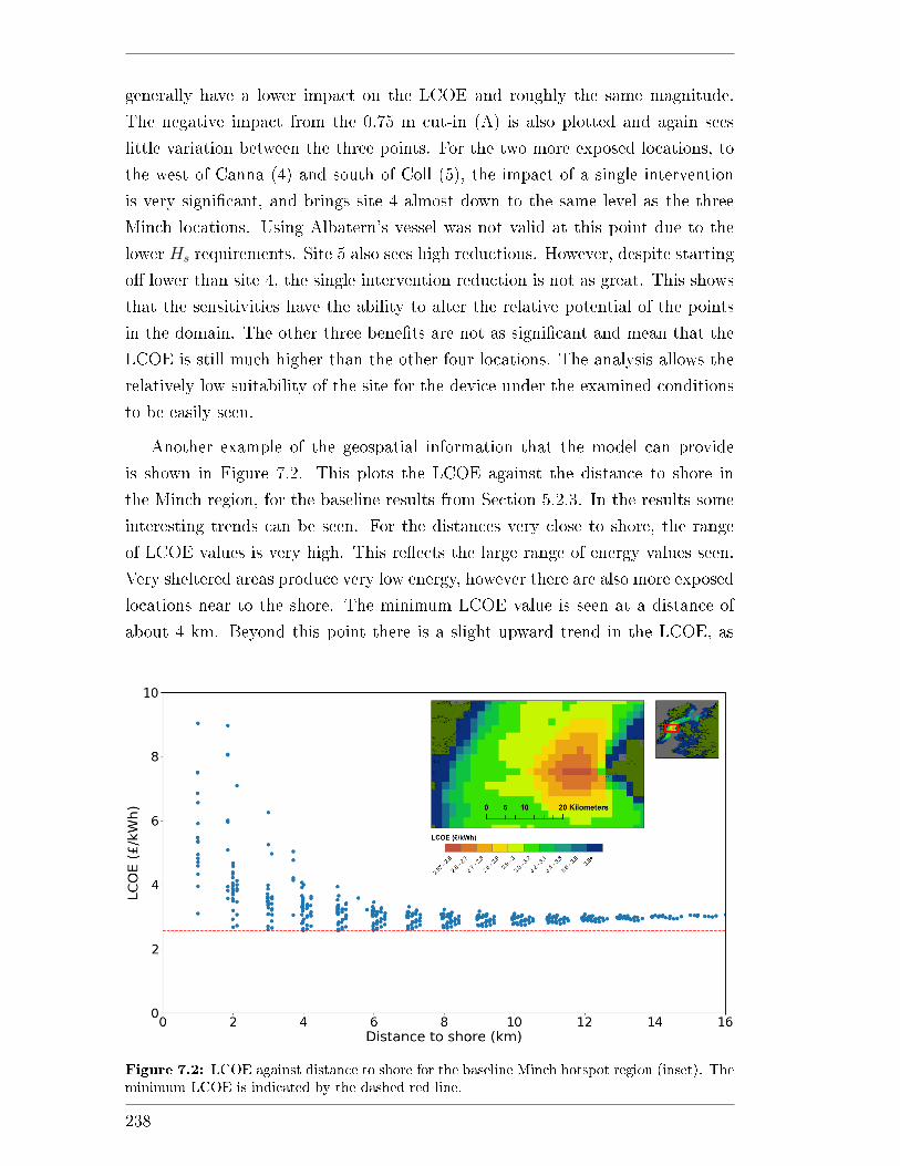
generally have a lower impact on the LCOE and roughly the same magnitude.

The negative impact from the 0.75 m cut-in (A) is also plotted and again sees

little variation between the three points. For the two more exposed locations, to

the west of Canna (4) and south of Coll (5), the impact of a single intervention

is very signi�cant, and brings site 4 almost down to the same level as the three

Minch locations. Using Albatern's vessel was not valid at this point due to the

lower Hs requirements. Site 5 also sees high reductions. However, despite starting

o� lower than site 4, the single intervention reduction is not as great. This shows

that the sensitivities have the ability to alter the relative potential of the points

in the domain. The other three bene�ts are not as signi�cant and mean that the

LCOE is still much higher than the other four locations. The analysis allows the

relatively low suitability of the site for the device under the examined conditions

to be easily seen.

Another example of the geospatial information that the model can provide

is shown in Figure 7.2. This plots the LCOE against the distance to shore in

the Minch region, for the baseline results from Section 5.2.3. In the results some

interesting trends can be seen. For the distances very close to shore, the range

of LCOE values is very high. This re�ects the large range of energy values seen.

Very sheltered areas produce very low energy, however there are also more exposed

locations near to the shore. The minimum LCOE value is seen at a distance of

about 4 km. Beyond this point there is a slight upward trend in the LCOE, as

Figure 7.2: LCOE against distance to shore for the baseline Minch hotspot region (inset). Theminimum LCOE is indicated by the dashed red line.

238

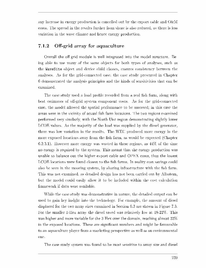
any increase in energy production is cancelled out by the export cable and O&M

costs. The spread in the results further from shore is also reduced, as there is less

variation in the wave climate and hence energy production.

7.1.2 O�-grid array for aquaculture

Overall the o�-grid module is well integrated into the model structure. Be-

ing able to use many of the same objects for both types of analyses, such as

the WaveSite object and device child classes, ensures consistency between the

analyses. As for the grid-connected case, the case study presented in Chapter

6 demonstrated the analysis principles and the kinds of sensitivities that can be

examined.

The case study used a load pro�le recorded from a real �sh farm, along with

best estimates of o�-grid system component costs. As for the grid-connected

case, the model allowed the spatial performance to be assessed; in this case the

areas were in the vicinity of actual �sh farm locations. The two regions examined

performed very similarly, with the North Uist region demonstrating slightly lower

LCOE values. As the majority of the load was supplied by the diesel generator,

there was low variation in the results. The WEC produced more energy in the

more exposed locations away from the �sh farm, as would be expected (Chapter

6.2.3.1). However more energy was wasted in these regions, as 44% of the time

no energy is required by the system. This meant that the energy production was

unable to balance out the higher export cable and OPEX costs, thus the lowest

LCOE locations were found closest to the �sh farms. In reality cost savings could

also be seen in the mooring system, by sharing infrastructure with the �sh farm.

This was not examined, as detailed design has not been carried out by Albatern,

but the model could easily allow it to be included within the cost calculation

framework if data were available.

While the case study was demonstrative in nature, the detailed output can be

used to gain key insight into the technology. For example, the amount of diesel

displaced for the two array sizes examined in Section 6.3 are shown in Figure 7.3.

For the smaller 1-Hex array the diesel saved was relatively low at 18-22%. This

was higher and more variable for the 3-Hex over the domain, reaching almost 33%

in the exposed locations. These are signi�cant numbers and might be favourable

to an aquaculture player from a marketing perspective as well as an environmental

one.

The case study system was found to be most sensitive to array size and diesel

239

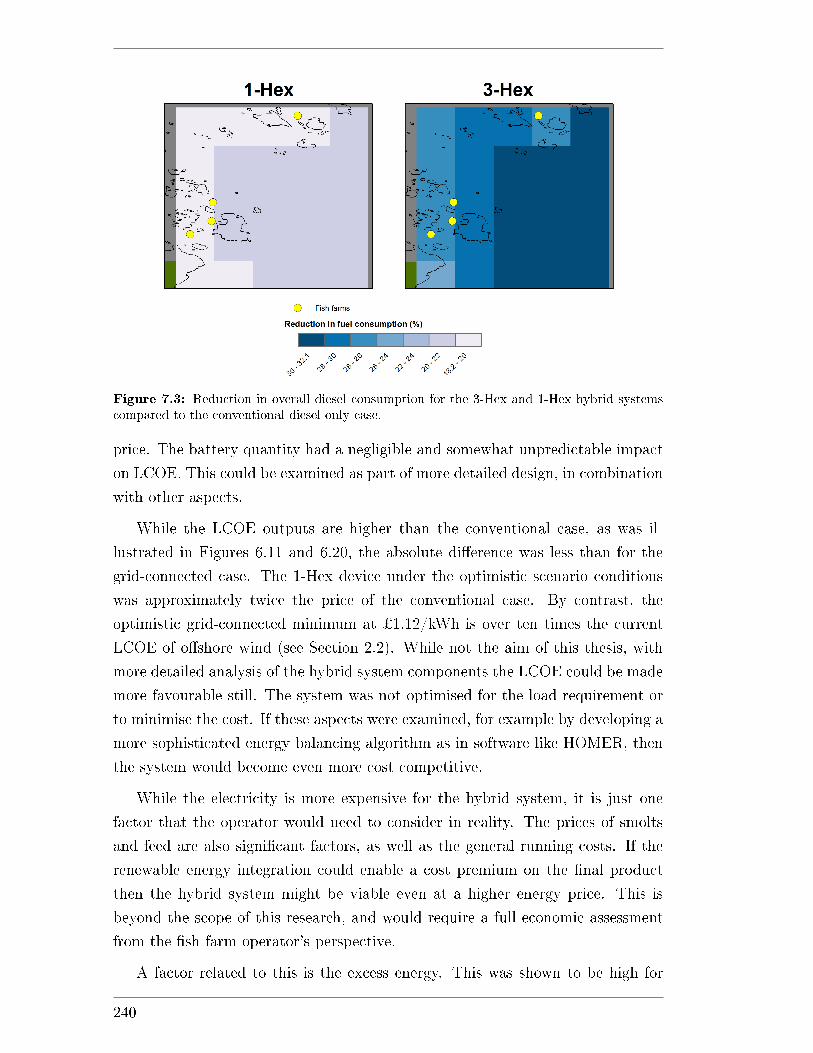
Figure 7.3: Reduction in overall diesel consumption for the 3-Hex and 1-Hex hybrid systemscompared to the conventional diesel-only case.

price. The battery quantity had a negligible and somewhat unpredictable impact

on LCOE. This could be examined as part of more detailed design, in combination

with other aspects.

While the LCOE outputs are higher than the conventional case, as was il-

lustrated in Figures 6.11 and 6.20, the absolute di�erence was less than for the

grid-connected case. The 1-Hex device under the optimistic scenario conditions

was approximately twice the price of the conventional case. By contrast, the

optimistic grid-connected minimum at ¿1.12/kWh is over ten times the current

LCOE of o�shore wind (see Section 2.2). While not the aim of this thesis, with

more detailed analysis of the hybrid system components the LCOE could be made

more favourable still. The system was not optimised for the load requirement or

to minimise the cost. If these aspects were examined, for example by developing a

more sophisticated energy balancing algorithm as in software like HOMER, then

the system would become even more cost competitive.

While the electricity is more expensive for the hybrid system, it is just one

factor that the operator would need to consider in reality. The prices of smolts

and feed are also signi�cant factors, as well as the general running costs. If the

renewable energy integration could enable a cost premium on the �nal product

then the hybrid system might be viable even at a higher energy price. This is

beyond the scope of this research, and would require a full economic assessment

from the �sh farm operator's perspective.

A factor related to this is the excess energy. This was shown to be high for

240

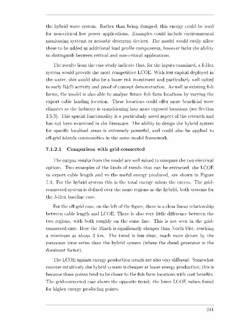
the hybrid wave system. Rather than being dumped, this energy could be used

for non-critical low power applications. Examples could include environmental

monitoring systems or acoustic deterrent devices. The model would easily allow

these to be added as additional load pro�le components, however lacks the ability

to distinguish between critical and non-critical applications.

The results from the case study indicate that, for the inputs examined, a 1-Hex

system would provide the most competitive LCOE. With less capital deployed in

the water, this would also be a lower risk investment and particularly well suited

to early R&D activity and proof of concept demonstration. As well as existing �sh

farms, the model is also able to analyse future �sh farm locations by varying the

export cable landing location. These locations could o�er more bene�cial wave

climates as the industry is transitioning into more exposed locations (see Section

2.5.3). This spatial functionality is a particularly novel aspect of the research and

has not been examined in the literature. The ability to design the hybrid system

for speci�c localised areas is extremely powerful, and could also be applied to

o�-grid islands communities in the same model framework.

7.1.2.1 Comparison with grid-connected

The output results from the model are well suited to compare the two electrical

options. Two examples of the kinds of trends that can be extracted, the LCOE

vs export cable length and vs the useful energy produced, are shown in Figure

7.4. For the hybrid system this is the total energy minus the excess. The grid-

connected system is de�ned over the same regions as the hybrid, both systems for

the 3-Hex baseline case.

For the o�-grid case, on the left of the �gure, there is a clear linear relationship

between cable length and LCOE. There is also very little di�erence between the

two regions, with both roughly on the same line. This is not seen in the grid-

connected case. Here the Minch is signi�cantly cheaper than North Uist, reaching

a minimum at about 3 km. The trend is less clear, much more driven by the

metocean time series than the hybrid system (where the diesel generator is the

dominant factor).

The LCOE against energy production trends are also very di�erent. Somewhat

counter-intuitively the hybrid system is cheaper at lower energy production; this is

because these points tend to be closer to the �sh farm locations with cost bene�ts.

The grid-connected case shows the opposite trend: the lower LCOE values found

for higher energy producing points.

241

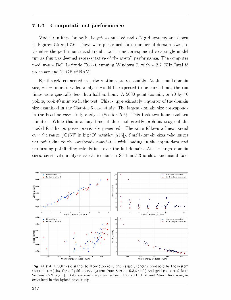
7.1.3 Computational performance

Model runtimes for both the grid-connected and o�-grid systems are shown

in Figures 7.5 and 7.6. These were performed for a number of domain sizes, to

visualise the performance and trend. Each time corresponded to a single model

run as this was deemed representative of the overall performance. The computer

used was a Dell Latitude E6330, running Windows 7, with a 2.7 GHz Intel i5

processor and 12 GB of RAM.

For the grid-connected case the runtimes are reasonable. At the small domain

size, where more detailed analysis would be expected to be carried out, the run

times were generally less than half an hour. A 5000 point domain, or 70 by 70

points, took 40 minutes in the test. This is approximately a quarter of the domain

size examined in the Chapter 5 case study. The largest domain size corresponds

to the baseline case study analysis (Section 5.2). This took two hours and ten

minutes. While this is a long time, it does not greatly prohibit usage of the

model for the purposes previously presented. The time follows a linear trend

over the range (�O(N)� in big `O' notation [215]). Small domain sizes take longer

per point due to the overheads associated with loading in the input data and

performing path�nding calculations over the full domain. At the larger domain

sizes, sensitivity analysis as carried out in Section 5.3 is slow and could take

Figure 7.4: LCOE vs distance to shore (top row) and vs useful energy produced by the system(bottom row) for the o�-grid energy system from Section 6.2.3 (left) and grid-connected fromSection 5.2.3 (right). Both systems are presented over the North Uist and Minch locations, asexamined in the hybrid case study.

242

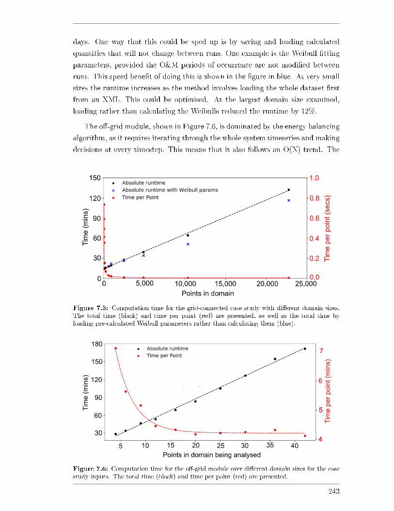
days. One way that this could be sped up is by saving and loading calculated

quantities that will not change between runs. One example is the Weibull �tting

parameters, provided the O&M periods of occurrence are not modi�ed between

runs. This speed bene�t of doing this is shown in the �gure in blue. At very small

sizes the runtime increases as the method involves loading the whole dataset �rst

from an XML. This could be optimised. At the largest domain size examined,

loading rather than calculating the Weibulls reduced the runtime by 12%.

The o�-grid module, shown in Figure 7.6, is dominated by the energy balancing

algorithm, as it requires iterating through the whole system timeseries and making

decisions at every timestep. This means that it also follows an O(N) trend. The

Figure 7.5: Computation time for the grid-connected case study with di�erent domain sizes.The total time (black) and time per point (red) are presented, as well as the total time byloading pre-calculated Weibull parameters rather than calculating them (blue).

Figure 7.6: Computation time for the o�-grid module over di�erent domain sizes for the casestudy inputs. The total time (black) and time per point (red) are presented.

243

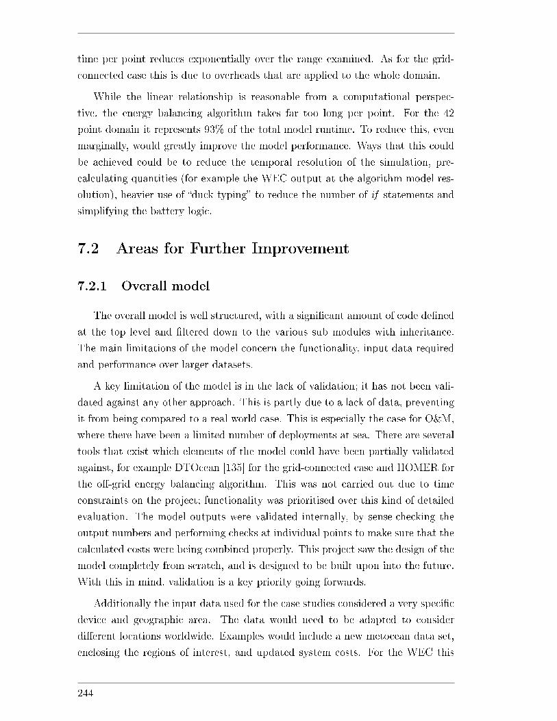
time per point reduces exponentially over the range examined. As for the grid-

connected case this is due to overheads that are applied to the whole domain.

While the linear relationship is reasonable from a computational perspec-

tive, the energy balancing algorithm takes far too long per point. For the 42

point domain it represents 93% of the total model runtime. To reduce this, even

marginally, would greatly improve the model performance. Ways that this could

be achieved could be to reduce the temporal resolution of the simulation, pre-

calculating quantities (for example the WEC output at the algorithm model res-

olution), heavier use of �duck typing� to reduce the number of if statements and

simplifying the battery logic.

7.2 Areas for Further Improvement

7.2.1 Overall model

The overall model is well structured, with a signi�cant amount of code de�ned

at the top level and �ltered down to the various sub modules with inheritance.

The main limitations of the model concern the functionality, input data required

and performance over larger datasets.

A key limitation of the model is in the lack of validation; it has not been vali-

dated against any other approach. This is partly due to a lack of data, preventing

it from being compared to a real world case. This is especially the case for O&M,

where there have been a limited number of deployments at sea. There are several

tools that exist which elements of the model could have been partially validated

against, for example DTOcean [135] for the grid-connected case and HOMER for

the o�-grid energy balancing algorithm. This was not carried out due to time

constraints on the project; functionality was prioritised over this kind of detailed

evaluation. The model outputs were validated internally, by sense-checking the

output numbers and performing checks at individual points to make sure that the

calculated costs were being combined properly. This project saw the design of the

model completely from scratch, and is designed to be built upon into the future.

With this in mind, validation is a key priority going forwards.

Additionally the input data used for the case studies considered a very speci�c

device and geographic area. The data would need to be adapted to consider

di�erent locations worldwide. Examples would include a new metocean data set,

enclosing the regions of interest, and updated system costs. For the WEC this

244

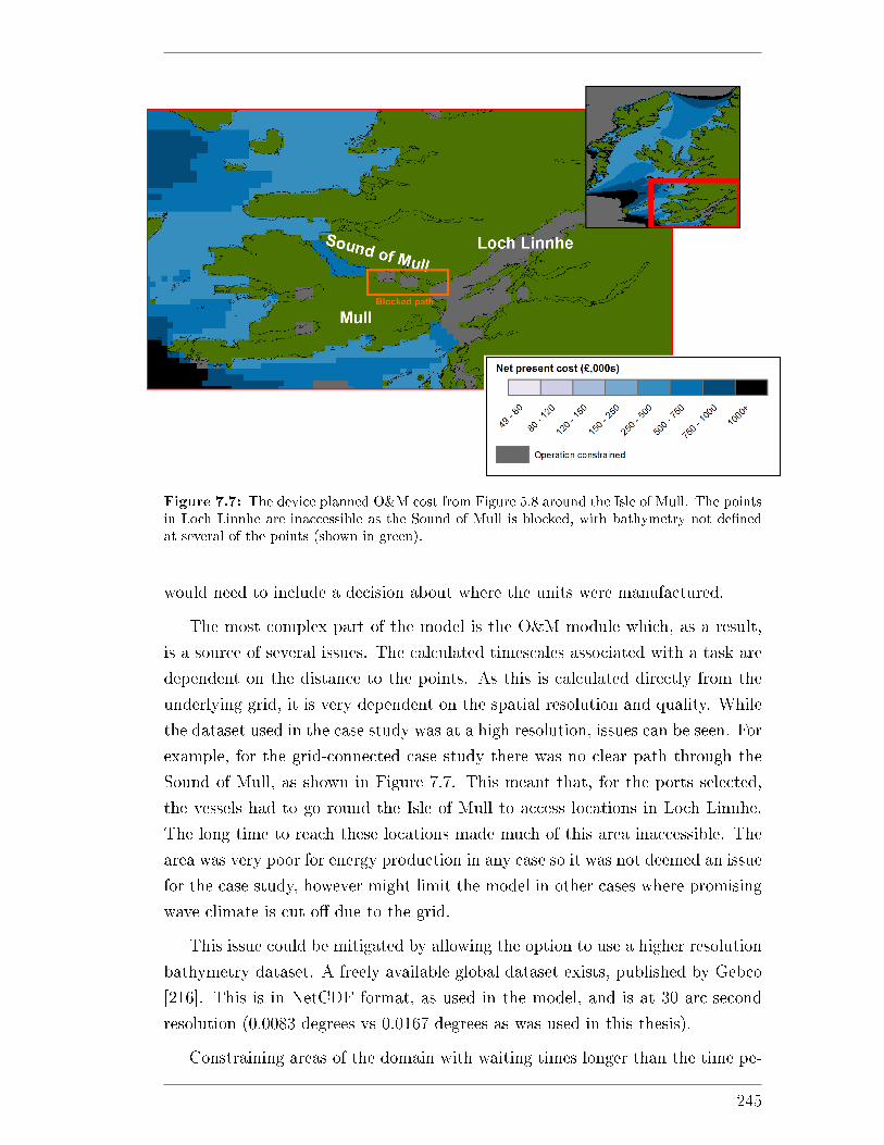
Figure 7.7: The device planned O&M cost from Figure 5.8 around the Isle of Mull. The pointsin Loch Linnhe are inaccessible as the Sound of Mull is blocked, with bathymetry not de�nedat several of the points (shown in green).

would need to include a decision about where the units were manufactured.

The most complex part of the model is the O&M module which, as a result,

is a source of several issues. The calculated timescales associated with a task are

dependent on the distance to the points. As this is calculated directly from the

underlying grid, it is very dependent on the spatial resolution and quality. While

the dataset used in the case study was at a high resolution, issues can be seen. For

example, for the grid-connected case study there was no clear path through the

Sound of Mull, as shown in Figure 7.7. This meant that, for the ports selected,

the vessels had to go round the Isle of Mull to access locations in Loch Linnhe.

The long time to reach these locations made much of this area inaccessible. The

area was very poor for energy production in any case so it was not deemed an issue

for the case study, however might limit the model in other cases where promising

wave climate is cut o� due to the grid.

This issue could be mitigated by allowing the option to use a higher resolution

bathymetry dataset. A freely available global dataset exists, published by Gebco

[216]. This is in NetCDF format, as used in the model, and is at 30 arc-second

resolution (0.0083 degrees vs 0.0167 degrees as was used in this thesis).

Constraining areas of the domain with waiting times longer than the time pe-

245

riod also introduces issues. It means that one extreme month can make large areas

appear unviable. A monthly period was coded into the model by default to allow

for easier cost discounting. Allowing longer, user de�ned, time periods by default

would allow this issue to be circumvented. In addition, a useful feature would

be a standalone metocean analysis class (much in the form of the CostAnalysis

and EnergyAnalysis classes as introduced in Section 3.4.5). This could allow

the metocean conditions to be examined prior to executing the model. Output

of monthly exceedance statistics would mean that suitable months could be dis-

covered and assigned to the relevant tasks, or optimal solutions chosen from a

number of input options.

The weather window analysis is also limited by only including Hs. Other

parameters like wind speed and Tp would also be considered in reality and would

require a time-series based methodology. The model also assumes a constant

vessel charter cost. In reality this will �uctuate with the seasons, with lower

rates obtainable in winter as there is less vessel demand [217]. This could bene�t

sheltered areas like the Minch and make winter operations appear more viable.

While e�orts have been made to keep the model and its guiding principles

generic, the variation between di�erent device concepts is signi�cant. Larger

devices would require more consideration of logistics and port related issues, in-

cluding having enough space on land to carry out repairs. With more signi�cant

energy being exported to the grid there is also the issue of grid stability. The

amount that the developer pays for this will depend on the farm size, local envi-

ronment and government policy [218]. The assumption that the device can feed

into the distribution network is not realistic above 20 MW. As larger farms are

likely to be more cost competitive, this would need to be addressed to apply the

model to situations further in the future.

Also of more relevance to larger scale farms are more complex economic calcu-

lations. While LCOE is the most common metric, it is of less interest to investors.

The potential return for commercially ready technologies will depend on the sub-

sidy available, and could be calculated from the output energy pro�le. For the

Albatern concept this is more relevant for the hybrid system. A PPA would need

to be struck with the �sh farm operator above the LCOE for a return to be made.

This detail is lacking, and needs expanded for the geospatial and time-dependent

trends to inform the business reality.

Lastly, there are other types of analyses that are absent from the model and

would help to provide con�dence in the results. Unplanned O&M has previously

246

been mentioned and would be particularly useful for assessing the trade o� be-

tween cost and survivability over the spatial domain. The mooring module is

simplistic, and would bene�t from being extended from a cost-based analysis to a

more robust design tool. This was not a priority of the research as the Albatern

mooring cost is low (as demonstrated in Section 5.2.3.2). Being able to assess the

environmental loading on the mooring system, for example through quasi-static

methods, would allow extreme wave climates to be factored in as a cost premium

or constraint. These kind of cost functions could be de�ned with a generic spa-

tial formulation and built upon the existing cost methods. This would allow the

model parameters to be tuned to conditions seen in the real world, for example

the impact of water depth on installation time.

7.2.1.1 Model Usability

The recursive setting of cost categories and quantities works well. However it

is not the most transparent process. Particularly at the lower cost levels, where

multiple items are embedded, keeping track of these categories can be di�cult. A

function to visualise the hierarchical item relationship would help to reduce user

error and improve the overall model function.

In general, the usability is also hampered by the con�guration text �le method.

While this is convenient and makes the process more widely accessible, it means

that many di�erent �les need to be being de�ned and errors can be di�cult to

track. Rather than this, a fully integrated database would improve the analysis

process: ensuring consistency in the input objects and reducing error. A GUI

could serve as the model front end, to allow the model to be better understood

by users less familiar with Python.

There are also other input data that can be hard to generate. One example is

the hybrid module load pro�le. As there is likely to be a degree of regularity in the

pro�le, Python scripts to generate this from various recurring components would

save time and allow di�erent systems to be more easily and quickly examined.

A particularly time consuming part of the process is in formatting the out-

put raster �les. Depending on the cost categories speci�ed there can be large

numbers of these �les, which are then cumbersome to format within ArcGIS. In-

tegration with QGIS using the PyQGIS Python package would allow maps to be

automatically formatted according to de�ned options [219].

247

7.2.2 O�-grid module

As this module also uses the objects and methods de�ning the wave energy

system, it is subject to the limitations as in Section 7.2.1 above. In addition to

these, the main issue with the o�-grid module is the slow runtime, as identi�ed in

Section 7.1.3, which prohibits sensitivity analysis over larger areas. The impacts

of sensitivities are also harder to predict, as was seen for the battery quantity

sensitivity in Section 6.3.1, which means that it can take a long time to obtain the

necessary results. As the methodology is based on that seen in the literature and

HOMER, commercially used software, it is fairly robust. However the algorithm

logic is split across a number of functions within the HybridProject class and

would be di�cult to modify for more complex system behaviour.

For getting a higher level spatial estimate of LCOE the module works well,

however it is less suitable for detailed hybrid system design due to the prohibitive

runtime. For this kind of work, the model would bene�t from an optimisation

based approach, as achieved in HOMER. Being able to specify di�erent con�gu-

ration options and determine the most suitable would limit the runtime and allow

the various combinations to be considered together. This would be interesting to

apply spatially, to see the progression of the design for di�erent site conditions.

There are a number of open source Python packages that could be utilised, for

example scipy.

Another limitation concerns the available functionality. While suitable for the

aquaculture markets Albatern is examining, the range of electrical components

is limited for larger scale applications. Examples of these could include island

communities which might also contain wind turbines or solar PV. The model is also

limited in the storage options available, with only lead acid batteries supported.

Di�erent battery models, for example lithium ion or �ow batteries, might be

better options in reality and would require di�erent governing equations. The

weight and space constraints of the battery bank are also not included in the

model. For larger numbers of batteries this could restrict the usage in certain

locations, for example on a feed barge.

The module is also relatively in�exible when it comes to diesel price. Using

a �xed fuel price over the project duration is not realistic; being able to vary

this would allow future trends to be examined but with more emphasis on the

present day situation. While the uncertainty can be examined by looking at the

extreme cases, as was demonstrated in Section 6.3.2, more realistic cases will also

be sensitive to the time variation in the resource which a static price does not

248

capture. Being able to link the price to speci�c locations in the domain would

also make the model able to account for price premiums at particularly remote

locations.

249

250

8Concluding Remarks

8.1 Summary and Achievements

The aim of this research was �To develop an economic model capable of iden-

tifying the most suitable geographic locations for localised wave energy projects.�

To meet this aim, a sophisticated and detailed computational model has been

created. It has been structured using the OOP programming principle, making

it modular, scalable, and hence adaptable into the future. This is especially

important from the industrial perspective, as it gives Albatern the ability to mould

the tool to suit their technology development and commercial requirements.

The research has been broad in focus, the modelling covering a substantial

number of aspects. These included energy production estimation from metocean

timeseries, manipulation of 2D power matrices, application of path�nding algo-

rithms, spatial weather window estimation and spatial application of a hybrid

system energy balancing algorithm. Eight modules were created, with the inter-

dependencies clearly mapped out and minimised to allow the various calculations

to function in isolation. While there are limitations, most notably lack of reliabil-

ity based unplanned OPEX calculation and the associated downtime, the model

o�ers alternative ways to incorporate these, albeit in a less robust way. The prin-

ciples de�ned in the base_classes module give the user the �exibility to specify

any number of costs, the time periods that they occur in and categorise them in

an arbitrary way. In an industry like wave energy, where there are a great many

di�erent device concepts made up of di�erent subsystems, this is valuable.

251

The spatial calculation aspects were a key research need, to help Albatern

identify promising locations for their technology and the associated LCOE drivers.

These drivers have been shown to vary signi�cantly in the spatial domain, espe-

cially for the grid-connected case which was focussed on a larger area. A key

example was using Albatern's vessel for the planned O&M procedures, which sig-

ni�cantly reduced the number of viable sites to the west of Lewis and Harris but

reduced the LCOE by 20-30% in the Little Minch. Being able to apply the cal-

culations over large areas is a huge bene�t, with the results easy to visualise and

examine further in GIS software.

The o�-grid energy simulation was a particularly novel aspect of the research,

in particular the application over the spatial domain within the main model frame-

work. This is a market of primary interest of Albatern and thus was a key mod-

elling priority. The model allows easy comparison between the o�-grid and grid-

connected cases. It also allows sensitivity analysis to be easily conducted, by

manipulating the input con�guration �les. While the case studies were hypo-

thetical, they were deemed to be based on the best data available and indicated

signi�cantly more promising LCOE for the hybrid system. There is clearly a case

that can be made for pursuing these markets, at least initially until the technology

can be proved at a lower cost utility scale.

Both models have been designed with the Albatern device concept in mind.

Despite this there are very few, if any, aspects of the model which would not be

applicable to other device concepts, or the industry as a whole. The future of wave

energy will depend on its ability to optimise performance and reduce costs. This

research has presented a model with the capabilities to inform these areas, which

will encourage investment in the sector and allow locations and target markets to

be established.

8.2 Recommendations for Future Work

The main recommendations for future work are to add in additional model

functionality and improve the overall usability.

Unplanned OPEX could be incorporated by creating a class to represent com-

ponents liable to failures. Multiple failure modes and the associated probabilities

could be stored within class attributes. A Monte-Carlo based class method could

estimate the times of component failures using an input of timestamps. The time

periods, corresponding to the times when vessels need to be mobilised, could then

252

be used as in the existing MarineOperation class as the period_for_task at-

tribute. Alternatively a time domain O&M methodology could be integrated, as

opposed to the current frequency domain method, which would allow more sophis-

ticated task scheduling to be modelled (for example as seen in [10] or the DTOcean

project). This would be built up as an alternative, rather than directly replacing

the existing methods, to give more options to the user as both approaches have

advantages and disadvantages (as discussed in Section 2.3.3.1).

The Monte-Carlo functionality could also serve a dual purpose: to integrate

probabilistic uncertainty analysis. The variables to apply this analysis could easily

be marked by a new class type, with attributes to specify the type of distribution

and the constants de�ning it. A new function could run the model for a speci�ed

number of iterations, generating new values for the distribution-de�ned variables

for each model run. The resulting energy, cost and LCOE values could be anal-

ysed spatially. This would allow standard deviation and uncertainty limits to be

determined, as well as con�dence levels like the P50 and P90 (as achieved in [57].

This type of analysis would be of particular interest to investors, and give more

con�dence in the �nal results.

The main barrier to incorporating such uncertainty analysis is computational

performance rather than the implementation, which would be straightforward ow-

ing to the structured code development. A run of 1000 iterations is typical for

such an analysis. For the grid-connected sensitivity analysis from Section 5.3 this

would take 45,000 minutes (assuming 45 minutes per run) or approximately one

month. This is not feasible, and so di�erent options would need to be exam-

ined. These could include applying parallel computing methods, gaining super

computer access, speeding up the existing code and pre-calculating quantities like

the energy output and task timescales and varying these rather than the model

inputs. Making the model faster to run is of wider interest beyond this additional

functionality, and all of these options should be explored.

The o�-grid module would particularly bene�t from computational perfor-

mance improvements. Other improvements to the module would be to add to

the functionality. Adding in renewable technologies like wind turbines and solar

would allow larger hybrid systems to be considered, for example to power island

communities. These aspects would also broaden the appeal of the model beyond

wave energy and provide wave developers with insight on how to compete in the

wider marketplace. Di�erent strategies of dealing with excess energy production

from the WEC would also be a good addition. The case study result from Sec-

tion 6.2.3.1 found that a large proportion of energy was dumped, so incorporating

253

applications for this would help identify additional markets. This could include

desalination, hydrogen production (Power to gas) or displacing energy to heat of-

�ces on site in the winter. As well as new capabilities, the existing module could

be improved by introducing multi-parameter optimisation of the physical system.

This could include aspects like WEC array size, battery quantity and diesel gener-

ator size. It would allow the model to be used for more detailed system design and

come to more informed choices about the maximum potential for the technology.

For both grid-connected and o�-grid functions, the extension beyond LCOE

to other �nancial metrics would enhance the tool. Including the revenue from

feed in tari�s or power purchase agreements means that payback time, NPV and

IRR could be calculated. These metrics are of particular interest to investors so

would improve the model's prospect as a commercial tool to attract funding for

the technology.

A key priority going forward should also be in data validation and veri�cation

of the theoretical elements. The absence of these elements is a notable limitation of

the research project, and mainly due to a lack of available data. This is especially

true for O&M, as limited deployments at sea have taken place and developers are

apprehensive of sharing data and losing commercial advantage. As an internal

tool developed for Albatern, the model can be re�ned over time by examining

the performance and spatial costs against what is seen in the �eld. Applying the

model to larger device sizes and di�erent areas of the world will be particularly

bene�cial and would open up new possibilities for the company.

Lastly, the usability of the overall model is an area of interest. Full database

integration would provide consistency to the modelling, improve performance,

reduce user error and ensure that data is responsibly archived. This could be more

closely integrated with GIS software, making output maps quicker to format and

statistical geospatial analysis more straightforward. The modular nature of the

code could also be better utilised. Commonly used sub-module functionality could

be grouped into dedicated scripts or tools to make analyses more straightforward,

much like the analysis classes described in Section 3.4.5. Examples could include

an export cable design tool or O&M simulation tool, which would make it easier

and faster to focus on speci�c elements in isolation.

254

References

[1] Energy Trends June 2017, Technical report, Department for Business, En-

ergy & Industrial Strategy (BEIS), 2017.

[2] Parliment and Council of European Union, Directive 2009/28/EC of the

European Parliament and of the Council on the Production of the use of

Energy from Renewable Sources, 2009.

http://data.europa.eu/eli/dir/2009/28/oj, accessed 23/04/18.

[3] Eurostat, Share of renewables in energy consumption in the EU still on the

rise to almost 17% in 2015, 2017.

http://ec.europa.eu/eurostat/documents/2995521/7905983/8-

14032017-BP-EN.pdf/af8b4671-fb2a-477b-b7cf-d9a28cb8beea.

[4] House of Commons Energy and Climate Change Committee, 2020 renew-

able heat and transport targets, 2016.

https://publications.parliament.uk/pa/cm201617/cmselect/

cmenergy/173/17302.htm.

[5] R. Harrabin, Renewable energy: UK expected to miss 2020 targets, 2016.

http://www.bbc.co.uk/news/science-environment-36710290.

[6] House of Commons Innovation, Universities, Science and Skills Committee,

Renewable electricity generation technologies: �fth report of session 2007-08

(Volume 2) 2008.

[7] L. Quesnel, J. Rabe, M. Brommundt, and F. Vorpahl, Task 3.4 Report:

State of the art of design tools and standards for o�shore renewable energy

conversion systems, Technical report, O�-shore Renewable Energy Conver-

sion platforms � Coordination Action (ORECCA) project, 2011.

[8] J. Sandström, J. Gri�ths, and T. Svensson, Review of standards on relia-

bility for ocean energy and relation to VMEA, Technical report, Reliability

in a Sea of Risk (RiaSoR) project, 2016.

255

[9] A. O'Hagan, C. Huertas, J. O'Callaghan, and D. Greaves, Wave energy in

Europe: Views on experiences and progress to date, International Journal

of Marine Energy, vol. 14, pp. 180�197, 2016.

[10] A. Gray, Modelling Operations and Maintenance Strategies for Wave Energy

Arrays. PhD thesis, The Industrial Doctoral Centre for O�shore Renewable

Energy (IDCORE), 2017.

[11] D. Mackay, Sustainable Energy - Without The Hot Air. UIT Cambridge,

2008.

[12] D. Ross, Power From Sea Waves. Oxford University Press, 1995.

[13] S. Kishore, L. Snyder, and P. Pradhan, Electricity from Ocean Wave Energy:

Technologies, Opportunities and Challenges, IEEE Smartgrid Newsletter,

February 2013.

[14] A. F. O. Falcao, Wave Energy Utilisation: A Review of the Technologies,

Renewable and Sustainable Energy Reviews, vol. 14, pp. 899�918, 2010.

[15] S. Salter, Wave Power, Nature, vol. 249, pp. 720�724, 1974.

[16] J. C. Wilson, A history of the UK renewable energy programme, 1974-88:

some social, political, and economic aspects. PhD thesis, University of Glas-

gow, 2012.

[17] C. Grove-Palmer, Wave Energy in the United Kingdom: A Review of the

Programme June 1975-March 1982 in Proceedings of 2nd International Sym-

posium on Wave Energy Utilization, 1982.

[18] A. Mukora, H. Je�rey, M. Winskel, and M. Mueller, Wave Energy Tech-

nology Development Review in the UK: Application of the Learning Curve

Concept, 1970-1999 pp. 1036�1042, 2008.

[19] G. Reikard, B. Robertson, and J.-R. Bidlot, Combining wave energy with

wind and solar: Short-term forecasting, Renewable Energy, vol. 81, pp. 442�

456, 2015.

[20] R. W. Furness, H. M. Wade, A. M. C. Robbins, and E. A. Masden, Assessing

the sensitivity of seabird populations to adverse e�ects from tidal stream

turbines and wave energy devices, ICES Journal of Marine Science, vol. 69,

pp. 1466�1479, 2012.

256

[21] W. J. Grecian, R. Inger, M. J. Attrill, S. Bearhop, B. J. Godley, M. J.

Witt, and S. C. Votier, Potential impacts of wave-powered marine renewable

energy installations on marine birds, The International Journal of Avian

Science, vol. 152, pp. 683�697, 2010.

[22] M. Ashley, S. Mangi, and L. Rodwell, The potential of o�shore wind farms

to act as marine protected areas � A systematic review of current evidence,

Marine Policy, vol. 45, pp. 301�309, 2014.

[23] E. D. Stoutenburg and M. Z. Jacobson, Reducing O�shore Transmission

Requirements by Combining O�shore Wind and Wave Farms, IEEE Journal

of Oceanic Engineering, vol. 36, pp. 552�561, 2011.

[24] M. Veigas and G. Iglesias, A Hybrid Wave-Wind O�shore Farm for an Is-

land, International Journal of Green Energy, vol. 12, pp. 570�576, 2015.

[25] E. D. Stoutenburg, N. Jenkins, and M. Z. Jacobson, Power output vari-

ations of co-located o�shore wind turbines and wave energy converters in

California, Renewable Energy, vol. 35, pp. 2781�2791, 2010.

[26] S. Astariz and G. Iglesias, Enhancing wave energy competitiveness through

co-Located wind and wave energy farms. a review on the shadow e�ect,

Energies, vol. 8, pp. 7344�7366, 2015.

[27] J. Abanades, D. Greaves, and G. Iglesias, Coastal defence through wave

farms, Coastal Engineering, vol. 91, pp. 299�307, 2014.

[28] B. Hamedni, C. B. Ferreira, and M. Cocho, Generic WEC system breakdown

(Deliverable D5.1) 2014. Structural design of wave energy devices (SDWED)

project.

[29] A. de Andres, E. Medina-Lopez, D. Crooks, O. Roberts, and H. Je�rey, On

the reversed LCOE calculation: Design constraints for wave energy com-

mercialization, International Journal of Marine Energy, vol. 18, pp. 88�108,

2017.

[30] E. Ozkop and I. H. Altas, Control, power and electrical components in wave

energy conversion systems: A review of the technologies, Renewable and

Sustainable Energy Reviews, vol. 67, pp. 106�115, 2017.

[31] J. Cordonnier, F. Gorintin, A. D. Cagny, A. H. Clement, and A. Babarit,

SEAREV: Case study of the development of a wave energy converter, Re-

newable Energy, vol. 80, pp. 40�52, 2015.

257

[32] S. Astariz, A. Vazquez, and G. Iglesias, Evaluation and comparison of the

levelized cost of tidal, wave, and o�shore wind energy, Journal of Renewable

and Sustainable Energy, vol. 7, 053112, 2015.

[33] T. Stallard, R. Rothschild, and G. A. Aggidis, A comparative approach

to the economic modelling of a large-scale wave power scheme, European

Journal of Operational Research, vol. 185, pp. 884�898, 2008.

[34] A. B. Sandberg, E. Klementsen, G. Muller, A. de Andres, and J. Maillet,

Critical factors in�uencing viability of wave energy converters in o�-grid

luxury resorts and small utilities, Sustainability, vol. 8, p. 1274., 2016.

[35] L. Margheritini, A. Hansen, and P. Frigaard, A Method for EIA Scoping of

Wave Energy Converters: Based on Classi�cation of the used Technology,

Environmental Impact Assessment Review, vol. 32, no. 1, pp. 33�44, 2012.

[36] S. Viz, C. Adnitt, R. Staniland, J. Everard, A. Sleigh, R. Cappell, S. Mc-

Nulty, M. Budd, I. Bonnon, and J. Carey, Review of cabling techniques and

environmental e�ects applicable to the o�shore wind farm industry, Tech-

nical report, Department for Business, Enterprise and Regulatory Reform

(BERR), 2008.

[37] R. Bucher and I. Bryden, Overcoming the marine energy pre-pro�t phase:

What classi�es the game-changing �array-scale success�?, International

Journal of Marine Energy, vol. 13, pp. 180�192, 2016.

[38] Energy technology perspectives: strategies and scenarios to 2050, Technical

report, International Energy Agency (IEA), 2006.

[39] M. Winskel, N. Markusson, H. Je�rey, S. Jablonski, C. Candelise, D. Ward,

and P. Howarth, Technology Change and Energy Systems: Learning Path-

ways for Future Sources of Energy, Technical report, Draft paper for UK

Energy Research Centre research programme on Energy Technology Learn-

ing Rates and Learning E�ects, 2008.

[40] D. E. Dismukes and G. B. Upton, Economies of scale, learning e�ects and

o�shore wind development costs, Renewable Energy, vol. 83, pp. 61�66, 2015.

[41] Trends 2013 in photovoltaic applications, Technical report IEA-PVPS T1-

23:2013, International Energy Agency (IEA), 2013.

258

[42] M. Menicou and V. Vassiliou, Prospective energy needs in Mediterranean

o�shore aquaculture: Renewable and sustainable energy solutions, Renew-

able and Sustainable Energy Reviews, vol. 14, pp. 3084�3091, 2010.

[43] A. Vögler and V. Venugopal, Wave data analysis for a semi-sheltered site in

the Inner Hebrides of Scotland suitable for small scale WEC development,

Ocean Engineering, vol. 126, pp. 374�383, 2016.

[44] G. Mørk, S. Barstow, A. Kabuth, and M. T. Pontes, Assessing The Global

Wave Energy Potential in Proceedings of OMAE2010, 2010.

[45] K. Gunn and C. Stock-Williams, Quantifying the Global Wave Power Re-

source, Renewable Energy, vol. 44, pp. 296�304, 2012.

[46] R. Boud, UK Wave Resource Study, Technical report, The Carbon Trust,

2012.

[47] House of Commons Energy and Climate Change Committee, Low Carbon

Technologies in a Green Economy: Fourth Report of Session 2009-10 2009.

[48] The Carbon Trust, Focus for success: A new approach to commercialising

low carbon technologies, Technical report, The Carbon Trust, 2009.

[49] M. T. Pontes, Assessing the European wave energy resource, J. O�shore

Mech. Arct. Eng, vol. 120, pp. 226�231, 1998.

[50] UK Wave and Tidal Key Resource Areas Project, Technical report, The

Crown Estate, 2012.

[51] G. Lavidas, V. Venugopal, and D. Friedrich, Wave energy extraction in

Scotland through an improved nearshore wave atlas, International Journal

of Marine Energy, vol. 17, pp. 64�83, 2017.

[52] 2020 Routemap for Renewable Energy in Scotland, Technical report, The

Scottish Government, 2012.

[53] A. Ilas, P. Ralon, A. Rodriguez, and M. Taylor, Renewable Power Gen-

eration Costs in 2017, Technical report, International Renewable Energy

Agency (IRENA), 2018.

[54] Lazard's levelised cost of energy analysis - version 11.0, Technical report,

Lazard, 2017.

259

[55] E. S. Rubin, I. M. Azevedo, P. Jaramillo, and S. Yeh, A review of learning

rates for electricity supply technologies, Energy Policy, vol. 86, pp. 198�218,

2015.

[56] A. MacGillivray, H. Je�rey, M. reduction for marine analysis, Technological

Forecasting & Social Change, vol. 87, pp. 108�124, 2014.

[57] N. Farrell, C. O. Donoghue, and K. Morrissey, Quantifying the uncertainty

of wave energy conversion device cost for policy appraisal: an Irish case

study, Energy Policy, vol. 78, pp. 62�77, 2015.

[58] Renewable UK, O�shore wind prices tumble in record breaking auction

results - cheaper than nuclear and gas, 2017.

http://www.renewableuk.com/news/362971/Offshore-wind-prices-

tumble-in-record-breaking-auction-results--cheaper-than-

nuclear-and-gas-.htm, accessed 20/04/18.

[59] P. Gourley, Tidal power �rm Atlantis hits out at funding `travesty', 2017.

https://www.scotsman.com/news/tidal-power-firm-atlantis-hits-

out-at-funding-travesty-1-4557371, accessed 20/04/18.

[60] ReNews, PTEC slams missing minima, 2017.

http://renews.biz/104867/ptec-slams-missing-minima/, accessed

20/04/18.

[61] J. Murray, Atlantis warns UK must ensure marine energy prospects not

swept away by o�shore wind cost revolution, 2017.

https://www.businessgreen.com/bg/analysis/3017049/atlantis-

warns-uk-must-ensure-marine-energy-prospects-not-swept-away-

by-offshore-wind-cost-revolution, accessed 20/04/18.

[62] Parliment and Council of European Union, The Paris Protocol - a blueprint

for tackling global climate change beyond 2020, 2015.

http://eur-lex.europa.eu/legal-content/EN/TXT/?qid=

1425546396765&uri=COM:2015:81:FIN, accessed 23/04/18.

[63] G. Heal, The Economics of Renewable Energy, Technical report NBER

Working Paper No. 15081, National Bureau of Economic Research (NBER),

2009.

[64] A. Myhr, C. Bjerkseter, A. Ågotnes, and T. A. Nygaard, Levelised cost of

energy for o�shore �oating wind turbines in a life cycle perspective, Renew-

able Energy, vol. 66, pp. 714�728, 2014.

260

[65] M. O'Connor, T. Lewis, and G. Dalton, Operational expenditure costs for

wave energy projects and impacts on �nancial returns, Renewable Energy,

vol. 50, pp. 1119�1131, 2013.

[66] Ocean Energy: Cost of Energy and Cost Reduction Opportunities, Technical

report, Strategic Initiative for Ocean Energy (SI OCEAN), 2013.

[67] S. B. Darling, F. You, T. Veselka, and A. Velosa, Assumptions and the

levelized cost of energy for photovoltaics, Energy & Environmental Science,

vol. 4, pp. 3133�3139, 2011.

[68] L. H. Holthuijsen, Waves in Oceanic and Coastal Waters. Cambridge, UK:

Cambridge University Press, 2007.

[69] J. P. Pierson and L. Moskowitz, A Proposed Spectral Form for Fully De-

veloped Wind Seas Based on the Similarity Theory of S.A.Kitaigorodskii,

Journal of Geophysical Research, vol. 69, pp. 5181�5190, 2016.

[70] K. Hasselmann, T. P. Barnett, E. Bouws, H. Carlson, D. E. Cartwright,

K. Enke, J. A Ewing, H. Gienapp, D. E. Hasselmann, P. Kruseman, A. Meer-

burg, P. Muller, D. Olbers, K. Richter, W. Sell, and H. Walden, Measure-

ments of wind-wave growth and swell decay during the Joint North Sea

Wave Project (JONSWAP), vol. 8, pp. 1�95, 01 1973.

[71] PELAMIS WEC - CONCLUSION OF PRIMARY R&D, Technical report

ETSU V/06/00181/REP, Department of Trade and Industry (DTI), 2003.

[72] D. Dunnett and J. S. Wallace, Electricity generation from wave power in

Canada, Renewable Energy, vol. 34, pp. 179�195, 2009.

[73] A. Pecher and J. P. Kofoed, eds., Handbook of Ocean Wave Energy. Springer

Open, 2017.

[74] G. Allan, M. Gilmartin, P. McGregor, and K. Swales, Levelised costs of wave

and tidal energy in the UK: cost competitiveness and the importance of

"banded" renewables obligation certi�cates, Energy Policy, vol. 39, pp. 23�

39, 2011.

[75] G. Dalton, R. Alcorn, and T. Lewis, A 10 year installation program for wave

energy in Ireland: A case study sensitivity analysis on �nancial returns,

Renewable Energy, vol. 40, pp. 80�89, 2012.

261

[76] B. Teillant, R. Costello, J. Weber, and J. Ringwood, Productivity and eco-

nomic assessment of wave energy projects through operational simulations,

Renewable Energy, vol. 48, pp. 220�230, 2012.

[77] A. Karyotakis and R. Bucknall, Planned intervention as a maintenance and

repair strategy for o�shore wind turbines, Journal of Marine Engineering

& Technology, vol. 9, pp. 27�35, 2010.

[78] C. Röckmann, S. Lagerveld, and J. Stavenuiter, Operation and Maintenance

Costs of O�shore Wind Farms and Potential Multi-use Platforms in the

Dutch North Sea, pp. 97�113. Cham: Springer International Publishing,

2017.

[79] M. O'Connor, D. Bourke, T. Curtin, T. Lewis, and G. Dalton, Weather win-

dows analysis incorporating wave height, wave period, wind speed and tidal

current with relevance to deployment and maintenance of marine renewables

in Proceedings of the 4th International conference on Ocean Energy (ICOE),

2012.

[80] B. Drew, A. R. Plummer, and M. N. Sahinkaya, A review of wave energy

converter technology, Proceedings of the Institution of Mechanical Engineers,

Part A: Journal of Power and Energy, vol. 223, no. 8, pp. 887�902, 2009.

[81] C. Kenny, D. Findlay, P. Thies, J. Shek, and I. Lazakis, Lessons Learned

from 3 Years of Failure: Validating an FMEA with Historical Failure Data

in Proceedings of the 12th European Wave and Tidal Energy Conference

(EWTEC 2017), 2017.

[82] P. R. Thies, J. Flinn, and G. H. Smith, Is it a showstopper? Reliability as-

sessment and criticality analysis for Wave Energy Converters in Proceedings

of the 8th European Wave and Tidal Energy Conference (EWTEC 2009),

2017.

[83] A. Ilas, P. Ralon, A. Rodriguez, and M. Taylor, System Performance, Avail-

ability and Reliability Trend Analysis � SPARTA 2017/18 Portfolio Review,

Technical report, SPARTA, 2018.

[84] S. Astariz and G. Iglesias, The economics of wave energy: A review, Renew-

able and Sustainable Energy Reviews, vol. 45, pp. 397�408, 2015.

[85] M. O'Connor, T. Lewis, and G. Dalton, Weather window analysis of Irish

west coast wave data with relevance to operations & maintenance of marine

renewables, Renewable Energy, vol. 52, pp. 57�66, 2013.

262

[86] S. Kuwashima and N. Hogben, The estimation of wave height and

wind speed persistence statistics from cumulative probability distributions,

Coastal Engineering, vol. 9, pp. 563�590, 1986.

[87] T. Stallard, J. Dhedin, S. Saviot, and C. Noguera, Deliverables D7.4.1 and

D7.4.2: Procedures for Estimating Site Accessibility and Appraisal of Im-

plications of Site Accessibility, Technical report, Equimar, 2010.

[88] R. T. Walker, J. van Nieuwkoop-McCall, L. Johanning, and R. J. Parkinson,

Calculating weather windows: Application to transit, installation and the

implications on deployment success, Ocean Engineering, vol. 68, pp. 88�101,

2013.

[89] K. Anastasiou and C. Tsekos, Persistence statistics of marine environmental

parameters from Markov theory, Part 1: analysis in discrete time, Applied

Ocean Research, vol. 18, no. 4, pp. 187�199, 1996.

[90] T. W. Thorpe, A Brief Review of Wave Energy, Technical report, UK De-

partment of Trade and Industry, 1999.

[91] The World Energy Council, World Energy Resources: Marine Energy 2016,

Technical report, The World Energy Council, 2016.

[92] M. Previsic, System level design, performance and costs for San Francisco

California Pelamis o�shore wave power plant, Technical report, EPRI, 2004.

[93] G. Dalton, R. Alcorn, and T. Lewis, Case study feasibility of the Pelamis

wave energy converter in Ireland, Portugal and North America, Renewable

Energy, vol. 35, pp. 443�455, 2010.

[94] S. Biyela and W. Cronje, Techno-Economic Analysis Framework for Wave

Energy Conversion Schemes under South African Conditions: Modeling and

Simulations in Proceedings of World Academy of Science, Engineering and

Technology, 2016.

[95] R. Guanche, A. D. de Andres, P. D. Simal, C. Vidal, and I. J. Losada,

Uncertainty analysis of wave energy farms �nancial indicators, Renewable

Energy, vol. 68, pp. 570�580, 2014.

[96] G. J. W. van Bussel and M. B. Zaaijer, Reliability, availability and mainte-

nance aspects of large-scale o�shore wind farms, a concepts study in Marine

Renewable Energies Conference, 2001.

263

[97] M. O'Connor, T. Lewis, and G. Dalton, Techno-economic performance of

the Pelamis P1 and Wavestar at di�erent ratings and various locations in

Europe, Renewable Energy, vol. 50, pp. 889�900, 2013.

[98] C. Beels, P. Troch, J. P. Kofoed, P. Frigaard, J. V. Kringelum, P. C. Kro-

mann, M. H. Donovan, J. D. Rouck, and G. D. Backer, A methodology

for production and cost assessment of a farm of wave energy converters,

Renewable Energy, vol. 36, pp. 3402�3416, 2011.

[99] P. Contestabile, E. D. Lauro, M. Buccino, and D. Vicinanza, Economic

Assessment of Overtopping BReakwater for Energy Conversion (OBREC):

A Case Study in Western Australia, Sustainability, vol. 9, p. 1., 2016.

[100] T. Okamoto, Y. Fukaya, and Y. Higo, Validation of the index to deter-

mine design parameters of a WEC for cost optimisation of a wave farm in

Proceedings of OMAE2015, 2015.

[101] A. Babarit, J. Hals, M. J. Muliawan, A. Kurniawan, T. Moan, and

J. Krokstad, Numerical benchmarking study of a selection of wave energy

converters, Renewable Energy, vol. 41, pp. 44�63, 2012.

[102] A. de Andres, E. Medina-Lopez, D. Crooks, O. Roberts, and H. Je�rey,

Techno-economic related metrics for a wave energy converters feasibility

assessment, Sustainability, vol. 8, p. 1109., 2016.

[103] D. Mollison and M. Pontes, Assessing the Portuguese wave-power resource,

Energy, vol. 17, no. 3, pp. 255�268, 1992.

[104] M. G. Hughes and A. D. Heap, National-scale wave energy resource as-

sessment for Australia, Renewable Energy, vol. 35, no. 8, pp. 1783 � 1791,

2010.

[105] G. Iglesias, M. López, R. Carballo, A. Castro, J. Fraguela, and P. Frigaard,

Wave energy potential in Galicia (NW Spain), Renewable Energy, vol. 34,

no. 11, pp. 2323�2333, 2009.

[106] E. Rusu and C. G. Soares, Coastal impact induced by a Pelamis wave farm

operating in the Portuguese nearshore, Renewable Energy, vol. 58, pp. 34�

49, 2013.

[107] S. Bozzi, R. Archetti, and G. Passoni, Wave electricity production in Italian

o�shore: A preliminary investigation, Renewable Energy, vol. 62, pp. 407�

416, 2014.

264

[108] L. Rusu and C. G. Soares, Wave energy assessments in the Azores islands,

Renewable Energy, vol. 45, pp. 183 � 196, 2012.

[109] M. Veigas and G. Iglesias, Wave and o�shore wind potential for the island of

Tenerife, Energy Conversion and Management, vol. 76, pp. 738�745, 2013.

[110] L. Rusu and F. Onea, The performance of some state-of-the-art wave energy

converters in locations with the worldwide highest wave power, Renewable

and Sustainable Energy Reviews, vol. 75, pp. 1348�1362, 2017.

[111] V. Vannucchi and L. Cappietti, Wave Energy Assessment and Performance

Estimation of State of the Art Wave Energy Converters in Italian Hotspots,

Sustainability, vol. 8, no. 12, 2016.

[112] G. Lavidas and V. Venugopal, A 35 year high-resolution wave atlas for

nearshore energy production and economics at the Aegean Sea, Renewable

Energy, vol. 103, pp. 401�417, 2017.

[113] S. Gallagher, R. Tiron, E. Whelan, E. Gleeson, F. Dias, and R. McGrath,

The nearshore wind and wave energy potential of Ireland: A high resolu-

tion assessment of availability and accessibility, Renewable Energy, vol. 88,

pp. 494�516, 2016.

[114] S. Pohekar and M. Ramachandran, Application of multi-criteria decision

making to sustainable energy planning - A review, Renewable and Sustain-

able Energy Reviews, vol. 8, pp. 365�381, 2004.

[115] S. Ghosh, T. Chakraborty, S. Saha, M. Majumder, and M. Pal, Development

of the location suitability index for wave energy production by ANN and

MCDM techniques, Renewable and Sustainable Energy Reviews, vol. 59,

pp. 1017�1028, 2016.

[116] O�shore Wind and Wave Energy Feasibility Mapping for the Outer Con-

tinental Shelf o� the State of Oregon, Technical report BOEM 2014-658,

Bureau of Ocean Energy Management (BOEM), 2014.

[117] F. Flocard, D. Ierodiaconou, and I. R. Coghlan, Multi-criteria evaluation of

wave energy projects on the south-east Australian coast, Renewable Energy,

vol. 99, pp. 80�94, 2016.

[118] J. R. Monds, Multicriteria Decision Analysis for Wave Power Technology in

Canada, Journal of Energy Resources Technology, vol. 136, 021201-021201-

8, 2013.

265

[119] M. Vasileiou, E. Loukogeorgaki, and D. G. Vagiona, GIS-based multi-criteria

decision analysis for site selection of hybrid o�shore wind and wave en-

ergy systems in Greece, Renewable and Sustainable Energy Reviews, vol. 73,

pp. 745�757, 2017.

[120] J.-J. Wang, Y.-Y. Jing, C.-F. Zhang, and J.-H. Zhao, Review on multi-

criteria decision analysis aid in sustainable energy decision-making, Renew-

able and Sustainable Energy Reviews, vol. 13, pp. 2263�2278, 2009.

[121] I. Galparsoro, P. Liria, I. Legorburu, J. Bald, G. Chust, P. Ruiz-Minguela,

G. Pérez, J. Marqués, Y. Torre-Enciso, M. González, and Ángel Borja, A

marine spatial planning approach to select suitable areas for installing wave

energy converters (WECs), on the Basque continental shelf (Bay of Biscay),

Coastal Management, vol. 40, no. 1, pp. 1�19, 2012.

[122] L. Cradden, C. Kalogeri, I. M. Barrios, G. Galanis, D. Ingram, and G. Kal-

los, Multi-criteria site selection for o�shore renewable energy platforms, Re-

newable Energy, vol. 87, pp. 791�806, 2016.

[123] A. Martinez, Z. B. Mustapha, R. Campbell, and T. Bouragba, A multi-

criteria methodology to select the best wave energy sites in World Congress

on Sustainable Technologies (WCST), 2016.

[124] J. Sierra, C. Martín, C. Mösso, M. Mestres, and R. Jebbad, Wave energy

potential along the Atlantic coast of Morocco, Renewable Energy, vol. 96,

pp. 20�32, 2016.

[125] P. Le, A. Fischer, I. Penesis, and R. Rahimi, Aggregating GIS and MCDM

to Optimize Wave Energy Converters Location in Tasmania, Australia,

Soft Computing Applications for Renewable Energy and Energy E�ciency,

pp. 141�164, 2015.

[126] K. N. A. Mauluda, W. H. M. W. Mohtara, and O. A. Karima, Spatial Multi

Criteria Analysis For the Determination of Areas with High Potential Wave

Energy, Jurnal Teknologi (Sciences & Engineering), vol. 65, pp. 113�120,

2013.

[127] S. Astariz and G. Iglesias, The collocation feasibility index � A method

for selecting sites for co-located wave and wind farms, Renewable Energy,

vol. 103, pp. 811�824, 2017.

266

[128] F. P. de Mendoza, S. Bonamano, G. Stella, M. Giovacchini, D. Capizzi,

F. Fraticelli, S. Muratore, C. Burgio, S. Scanu, M. A. Peviani, and M. Mar-

celli, Where is the best site for wave energy exploitation? Case study along

the coast of northern Latium (Italy), J Coast Conserv, vol. 20, pp. 13�29,

2016.

[129] R. Prest, T. Daniell, and B. Ostendorf, Using GIS to evaluate the impact

of exclusion zones on the connection cost of wave energy to the electricity

grid, Energy Policy, vol. 35, pp. 4516�4528, 2007.

[130] S. Behrens, J. Hayward, M. Hemer, and P. Osman, Assessing the wave

energy converter potential for Australian coastal regions, Renewable Energy,

vol. 43, pp. 210�217, 2012.

[131] L. Castro-Santos, G. P. Garcia, A. Estanqueiro, and P. A. Justino, The

Levelized Cost of Energy (LCOE) of wave energy using GIS based analysis:

The case study of Portugal, Electrical Power and Energy Systems, vol. 65,

pp. 21�25, 2015.

[132] R. Guanche, A. de Andres, I. J. Losada, C. Vidal, and I. J. Losada, A global

analysis of the operation and maintenance role on the placing of wave energy

farms, Energy Conversion and Management, vol. 106, pp. 440�456, 2015.

[133] A. Vazquez and G. Iglesias, Capital costs in tidal stream energy projects -

a spatial approach, Energy, vol. 107, pp. 215�226, 2016.

[134] S. Cavazzi and A. G. Dutton, An O�shore Wind Energy Geographic Infor-

mation System (OWE-GIS) for assessment of the UK's o�shore wind energy

potential, Renewable Energy, vol. 87, pp. 212�228, 2016.

[135] DTOcean, DTOcean User Manual, 10 2016.

[136] �Advanced design tools for ocean energy systems innovation, development

and deployment (dtoceanplus).� https://cordis.europa.eu/project/

rcn/214811_en.html. Accessed 28/08/18.

[137] The World Energy Council, O�-grid Solar Market Trends 2016, Technical

report, World Bank Group, 2016.

[138] R. Kempener, O. L. d'Ortigue, D. Saygin, J. Skeer, S. Vinci, and D. Gie-

len, O�-grid renewable energy systems: status and methodological issues,

Technical report, IRENA, 2015.

267

[139] J. K. Kaldellis, Overview of stand-alone and hybrid wind energy systems,

pp. 3�28. Woodhead Publishing, 2010.

[140] U. Datta, A. Kalam, and J. Shi, Hybrid PV-wind renewable energy sources

for microgrid application: an overview, pp. 1�22. Woodhead Publishing,

2018.

[141] Z. Chmiel and S. C. Bhattacharyya, Analysis of o�-grid electricity system at

Isle of Eigg (Scotland): Lessons for developing countries, Renewable Energy,

vol. 81, pp. 578�588, 2015.

[142] H. Aki, Independent hybrid renewable energy systems: Example applica-

tions around the world in Proceedings of IEEE PES General Meeting, 2010.

[143] Y. Bhikabhai, Hybrid power systems and their potential in the paci�c is-

lands, Technical report SOPAC Miscellaneous Report 406, SOPAC Com-

munity Lifelines Programme, 2005.

[144] S. Lal and A. Raturi, Techno-economic analysis of a hybrid mini-grid sys-

tem for Fiji islands, International Journal of Energy and Environmental

Engineering, vol. 3, no. 1, p. 10, 2012.

[145] G. J. May, A. Davidson, and B. Monahov, Lead batteries for utility energy

storage: A review, Journal of Energy Storage, vol. 15, pp. 145�157, 2018.

[146] S. P. Ayeng'o, T. Schirmer, K.-P. Kairies, H. Axelsen, and D. U. Sauer,

Comparison of o�-grid power supply systems using lead-acid and lithium-

ion batteries, Solar Energy, vol. 162, pp. 140�152, 2018.

[147] N.-K. C. Nair and N. Garimella, Battery energy storage systems: Assess-

ment for small-scale renewable energy integration, Energy and Buildings,

vol. 42, pp. 2124�2130, 2010.

[148] Rolls Battery Engineering, BATTERY USER MANUAL, 3 2017. ver.5.

[149] J. K. Kaldellis, Feasibility assessment for stand-alone and hybrid wind en-

ergy systems, pp. 102�161. Woodhead Publishing, 2010.

[150] P. Butler, J. Dunleavey, M. Farber-DeAnda, and P. Moseley, Performance

of valve-regulated lead-acid batteries in real-world stationary applications -

Utility installations, Journal of Power Sources, vol. 96, pp. 94�101, 2001.

268

[151] Fuelling Development: Energy Technologies for Developing Countries, OTA-

E-516t, Technical report, U.S. Congress, O�ce of Technology Assessment,

1992.

[152] V. Nelson, Wind Energy: Renewable Energy and the Environment. CRC

Press, Florida, 2014.

[153] P. Bolton, Petrol and diesel prices, Technical report, DECC, House of Com-

mons Library, 2014.

[154] S. Sinha and S.S.Chandel, Review of software tools for hybrid renewable en-

ergy systems, Renewable and Sustainable Energy Reviews, vol. 32, pp. 192�

205, 2014.

[155] D. Turcotte and F. Sheri�, Photovoltaic Hybrid System Sizing and Simula-

tion Tools: Status and Needs in Proceedings of PV Horizon: Workshop on

Photovoltaic Hybrid Systems, 2001.

[156] T. Lambert, P. Gilman, and P. Lilenthal, Micropower system modelling

with HOMER in Integration of alternative sources of energy (F. Farret and

M. Simões, eds.), ch. 15, pp. 379�418, Wiley-IEEE Press, 2006.

[157] HOMER Energy, �Homer energy.�

https://www.homerenergy.com/, accessed 27/08/2018.

[158] E. Hittinger, T. Wiley, J. Kluza, and J. Whitacre, Evaluating the value of

batteries in microgrid electricity systems using an improved Energy Systems

Model, Energy Conversion and Management, vol. 89, pp. 458�472, 2015.

[159] P. O. Oviroh and T.-C. Jen, The Energy Cost Analysis of Hybrid Systems

and Diesel Generators in Powering Selected Base Transceiver Station Loca-

tions in Nigeria, Energies, vol. 11, p. 687, 2018.

[160] A. C. Duman and Önder Güler, Techno-economic analysis of o�-grid

PV/wind/fuel cell hybrid system combinations with a comparison of reg-

ularly and seasonally occupied households, Sustainable Cities and Society,

vol. 42, pp. 107�126, 2018.

[161] L. M.Halabi, S. Mekhilef, L. Olatomiwa, and J. Hazelton, Performance anal-

ysis of hybrid PV/diesel/battery system using HOMER: A case study Sabah,

Malaysia, Energy Conversion and Management, vol. 144, pp. 322�339, 2018.

269

[162] R. Rajbongshi, D. Borgohain, and S. Mahapatra, Optimization of PV-

biomass-diesel and grid base hybrid energy systems for rural electri�cation

by using HOMER, vol. 126, pp. 461�474, 2017.

[163] J. Bostock, B. McAndrew, R. Richards, K. Jauncey, T. Telfer, K. Lorenzen,

D. Little, L. Ross, N. Handisyde, I. Gatward, and R. Corner, Aquaculture:

global status and trends, Phil. Trans. R. Soc. B, vol. 365, p. 2897�2912,

2010.

[164] The value of aquaculture to Scotland, Technical report, Highlands and Is-

lands Enterprise (HIE), 2017.

[165] W. Kenyon and D. Davies, Salmon Farming in Scotland, Technical report

SB 18-12 rev, The Scottish Parliament, 2018.

[166] Salmon Farming Industry Handbook 2015, Technical report, Marine Har-

vest, 2015.

[167] Scottish Government, �Record levels of salmon and whisky exports.�

https://news.gov.scot/news/record-levels-of-salmon-and-

whisky-exports, accessed 19/08/2018.

[168] Aquaculture Growth to 2030, Technical report, Scotland Food & Drink,

2016.

[169] Renewable power generation on aquaculture sites, Technical report ETSU

V/06/00181/REP, Scottish Aquaculture Research Forum (SARF), 2014.

[170] F. Cardia and A. Lovatelli, Aquaculture operations in �oating HDPE cages:

a �eld handbook. FAO, 2015.

[171] M. Ballester-Moltó, P. Sanchez-Jerez, J. Cerezo-Valverde, and F. Aguado-

Giménez, Particulate waste out�ow from �sh-farming cages. How much is

uneaten feed?, Marine Pollution Bulletin, vol. 119, pp. 23�30, 2017.

[172] L. A. Munro and I. S. Wallace, Scottish Fish Farm Production Survey 2016,

Technical report, Marine Scotland Science, 2017.

[173] H. L. Syse, Investigating O�-Grid Energy Solutions for the Salmon Farming

Industry, 2016.

[174] D. Whitmarsh and P. Wattage, Public Attitudes Towards the Environ-

mental Impact of Salmon Aquaculture in Scotland, European Environment,

vol. 16, pp. 108�121, 2006.

270

[175] A. M. Walker, M. C. Beveridge, W. Crozier, N. . Maoiléidigh, and N. Mil-

ner, Monitoring the incidence of escaped farmed Atlantic salmon, Salmo

salar L., in rivers and �sheries of the United Kingdom and Ireland: cur-

rent progress and recommendations for future programmes, ICES Journal

of Marine Science, vol. 63, pp. 1201�1210, 2006.

[176] �Fish farm loses 155,000 salmon as a result of extreme weather.�

http://www.bbc.co.uk/news/uk-scotland-north-east-orkney-

shetland-26459825. Accessed 27/07/2017.

[177] �16,000 salmon escape argyll �sh farm after storms.� http:

//www.scotsman.com/news/16-000-salmon-escape-argyll-fish-

farm-after-storms-1-3803325. Accessed 27/07/2017.

[178] K. Black and A. Hughes, Future of the Sea: Trends in Aquaculture, Techni-

cal report NBER Working Paper No. 15081, Government O�ce for Science,

2017.

[179] J. Bostock, A. Lane, C. Hough, and K. Yamamoto, An assessment of the

economic contribution of EU aquaculture production and the in�uence of

policies for its sustainable development, Aquacult Int, vol. 24, p. 699�733,

2016.

[180] Steinsvik, �Thermolicer.�

https://www.steinsvik.no/en/products/e/seaculture/fish-

health/thermolicer, accessed 20/08/2018.

[181] M. Dumiak, �Lice-hunting underwater drone protects salmon with lasers.�

https://spectrum.ieee.org/semiconductors/optoelectronics/

licehunting-underwater-drone-protects-salmon-with-lasers, ac-

cessed accessed 20/08/2018.

[182] E. Erwin, T. P. Soemardi, A. Surjosatyo, J. Nugroho, K. Nugraha, and

S. Wiyono, Design optimization of hybrid biomass and wind turbine for

minapolitan cluster in Domas, Serang, Banten, Indonesia in IOP Conference

Series: Earth and Environmental Science, Indonesia, 2018.

[183] Python Software Foundation, �The Python Language Reference.� Available

at http://www.python.org.

[184] M. Lutz, Learning Python: Powerful Object-Oriented Programming.

O'Reilly Media, 2013.

271

[185] S. Mount, J. Shuttleworth, and R. Winder, Python for Rookies. England:

Cengage Learning EMEA, 2008.

[186] Unidata, �The netcdf user's guide.�

http://www.unidata.ucar.edu/software/netcdf/docs/user_guide.

html, accessed 19/09/2017.

[187] �N-d labeled arrays and datasets in python.�

http://xarray.pydata.org/en/stable/index.html, accessed

19/09/2017.

[188] N. Marz and J. Warren, Big Data: Principles and best practices of scalable

realtime data systems. Manning Publications, 2015.

[189] A. Prengère, �Currencyconverter 0.13.2.�

https://pypi.python.org/pypi/CurrencyConverter, accessed 28/01/18.

[190] O. M. Faltinsen, Sea Loads on Ships and O�shore Structures. Cambridge,

UK: Cambridge University Press, 1990.

[191] A. Pecher, A. Foglia, and J. P. Kofoed, Comparison and Sensitivity Inves-

tigations of a CALM and SALM Type Mooring System for Wave Energy

Converters, J. Mar. Sci. Eng., vol. 2, pp. 93�122, 2014.

[192] �Orca�ex documentation; chain: Mechanical properties.� https://www.

orcina.com/SoftwareProducts/OrcaFlex/Documentation/. Accessed

07/07/17.

[193] C. Frost, �Examining the economic potential of hybrid energy systems for

�sh farms.� unpublished, 2016.

[194] FG Wilson, P220-3.

http://bellspowersolutions.co.uk/sites/solutions/files/

products//P220-3.pdf, accessed 20/02/2018.

[195] A. Jossen, Battery management in Valve-Regulated Lead�Acid Batteries

(P. T. Moseley, J. Garche, C. Parker, and D. Rand, eds.), ch. 8, pp. 207�240,

Elsevier, 2004.

[196] J. F. Manwell and J. G. McGowan, Lead acid battery model for hybrid

energy systems, Solar Energy, vol. 50, pp. 399�405, 1993.

[197] Metocean Solutions Ltd.

http://www.metocean.co.nz/, accessed 15/08/2017.

272

[198] PELAMIS WEC - CONCLUSION OF PRIMARY R&D: FINAL REPORT,

Technical report ETSU V/06/00181/REP, Energy Technology Support Unit

(ETSU), 2002.

[199] Albatern Ltd., Albatern Series 6 power matrix. 2015. Data received from

Albatern, unpublished.

[200] Gael Force Group, �Gael force group.�

http://www.gaelforcegroup.co.uk/, accessed 06/09/2017.

[201] Leaske Marine Ltd.

http://www.leaskmarine.com, accessed 16/08/2017.

[202] Fraser Hydraulic Power Ltd.

http://www.fhpltd.co.uk, accessed 06/05/2018.

[203] Marine Scotland, �Maps nmpi.�

https://marinescotland.atkinsgeospatial.com/nmpi/, accessed

12/05/2017.

[204] Joint Nature Conservation Committee, Marine SPAs 2009.

http://jncc.defra.gov.uk/page-1414, accessed 05/09/2017.

[205] British Geological Survey, �BGS bedrock and super�cial geology (WFS

service).�

http://ogc.bgs.ac.uk/cgi-bin/BGS_Bedrock_and_Superficial_

Geology/ows?service=WFS&request=GetCapabilities&, accessed

05/09/2017.

[206] D. Latinopoulos and K. Kechagia, A GIS-based multi-criteria evaluation for

wind farm site selection. A regional scale application in Greece, Renewable

Energy, vol. 78, pp. 550�560, 2015.

[207] Aquaculture site details, 2018.

http://aquaculture.scotland.gov.uk/data/site_details.aspx.

[208] Monthly Biomass & Treatment Reports: Gorsten, 2018.

http://aquaculture.scotland.gov.uk/data/fish_farms_monthly_

biomass_and_treatment_reports.aspx?sepa_site_id=GORS1&

ctl00_ctl00_ContentPlaceHolder1_ContentPlaceHolder2_ctl00_

gvResultsChangePage=10_15, Accessed 27/07/18.

273

[209] ValueOils.com.

https://www.valueoils.com/, accessed 23/07/2018.

[210] C. Frost, Economic Feasibility of Integrating a Hybrid Diesel/Battery Sys-

tem into the Domestic Electrical Circuit at Gorsten Fish Farm, Technical

report, Albatern Ltd., 2014. unpublished.

[211] �T-105 trojan battery deep cycle.� https://www.tayna.co.uk/T-105-

Trojan-Battery-Deep-Cycle-T105-P7253.html. Accessed 28/05/2018.

[212] J. Kurtz, G. Saur, S. Sprik, and C. Ainscough, Backup Power Cost of Own-

ership Analysis and Incumbent Technology Comparison, Technical report,

National Renewable Energy Laboratory (NREL), 2014.

[213] �Press release: Emec to take on new development sites in scotland,.�

http://www.emec.org.uk/press-release-emec-to-take-on-new-

development-sites-in-scotland/. Accessed 29/07/18.

[214] S. P. Neill, A. Vögler, A. J. Goward-Brown, S. Baston, M. J. Lewis, P. A.

Gillibrand, S. Waldman, and D. K. Woolf, The wave and tidal resource of

Scotland, Renewable Energy, vol. 114, pp. 3�17, 2017.

[215] ISRD Group, Data structures using C. New Delhi, India: McGraw-Hill,

2012.

[216] General Bathymetric Chart of the Oceans (GEBCO), �Gebco 30

arc-second grid.� https://www.gebco.net/data_and_products/gridded_

bathymetry_data/gebco_30_second_grid/. Accessed 15/08/17.

[217] I. Dinwoodie, D. McMillan, M. Revie, I. Lazakis, and Y. Dalgic, Develop-

ment of a Combined Operational and Strategic Decision Support Model for

O�shore Wind, Energy Procedia, vol. 35, pp. 157�166, 2013.

[218] D. O'Sullivan and G. Dalton, Challenges in the Grid Connection of Wave

Energy Devices in Proceedings of EWTEC2009, 2009.

[219] QGIS, �Pyqgis developer cookbook.� https://docs.qgis.org/2.14/en/

docs/pyqgis_developer_cookbook/. Accessed 13/08/18.

[220] C. Garrard, Geoprocessing with Python. Shelter Island, NY: Manning Pub-

lications, 2016.

274

[221] D. Eppstein, �Dijkstra's algorithm for shortest paths.�

https://www.ics.uci.edu/~eppstein/161/python/dijkstra.py/,

accessed 15/12/2017.

275

276

AProgramming Terminology

A.1 Python

This section describes some common Python terminology that is used in the

thesis.

• Module: An individual �le containing some Python code.

• Package: A collection of modules that together form a complete unit. The

model examined in this work is an example of a package.

• String: A data type de�ning some text. e.g. programming = �fun�

• Float: A data type de�ning numeric data. e.g. task_length = 10.5

• List: A data type that contains an ordered group of variables.

e.g. cute_cats = [`Billy', `Chuckles', 13.7]

• Dictionary (dict): An unordered data type that maps one variable onto

another.

e.g. losses = {`hydraulic': 0.03, `mechanical': 0.05,

`electrical': 0.01}

A.2 Object-Orientated Programming

In OOP, data variables and the functions that use them can be grouped to-

gether in the code into single structures. This is relevant when the variables are

related, and together describe some kind of singular entity. In programming terms

277

this is known as a class. It is e�ectively a blueprint, used to create di�erent ob-

jects (or instances) that are de�ned by variables of di�erent values. Variables

and functions common to a class are known as class attributes and class methods

respectively.

Classes can be used to represent real, physical objects in code. For example

a �car� class might contain attributes like manufacturer, model, engine size and

colour. A key advantage of using OOP is the principle of inheritance. This is

the idea that a hierarchy of classes can exist, whereby a class instance can be a

member of several di�erent class categories. Higher level attributes and functions

can be passed down from the super class (�parent�) to the subclass (�child�), so

that all of the classes share some common variables and methods. This has the

advantage that code is only written in a single place, improving organisation and

meaning that modi�cations to code only need to be made once.

A.3 UML Diagrams

UML diagrams are used to visually represent the hierarchy of classes within

an OOP framework. In this thesis, three relationships between the classes are

represented:

• Inheritance: All of the attributes and methods de�ned for a parent class

are passed down to the child, as the child is e�ectively a sub-type of the

parent. For example the MarineOperation class is a type of Operation.

• Aggregation: The parent class contains the child class and the child class

can exist independently. The MarineOperation class contains a Vessel,

but the vessel is also an entity in its own right.

• Composition: The parent class contains the child class, however the child

class cannot exist outside the parent. For example the ExportCable class

contains landing points (CableLanding class instances), however cable land-

ing points do not make physical sense without a cable.

For aggregation and composition, the amount of child classes that exist in the

parent are de�ned with the multiplicity de�nitions:

• n: A speci�c number are always contained, e.g. 2.

• 0..1: Zero or one can be contained, i.e a parent does not have to contain

the child.

• 0..*: Any number can be contained, including zero.

278

• 1..*: At least one child must be contained in the parent.

Lastly, the UML diagram shows the visibility of the attributes within each

class:

• Public: The attribute can be freely set by the user.

• Private: The attribute cannot be seen or directly set by the user, instead

used within the inner class workings.

• Derived: The attribute is not set by the user but is derived or calculated

within the class. It is visible to the user.

279

280

BSupporting Python Modules

This section describes the external modules that are required by the model.

These have been coded from scratch, and provide classes and functions to assist

in the structuring and operation of the model. They are not solely concerned with

the research theme and could, in theory, be applied to other types of projects.

B.1 GIS Utilities

The gis_utilities module contains the functions that are used to create

and manipulate GIS data. This is required to both import the spatial inputs and

results from the model and to extract GIS data from existing �les to include in

the analysis. The foundation of this module are the gdal and ogr packages. They

are open source and provide the framework for manipulating raster and vector

�les respectively. The functions are built upon the classes within these modules,

each focussing on a speci�c task and coded in a more readable manner. Much of

the code has been created using Garrard as a reference [220].

The �rst half of the module is concerned with vector data. Functions have been

coded to allow di�erent types of shape geometries to be created, including single

points, multipoints and polygons. These are typically used to export map layers

showing the locations of the geographic input data: examples include the data

points being analysed, the full size of the data domain and export cable landing

point locations. Fields can be added to these features, providing information and

identi�cation, which can be viewed in GIS software. In addition, functions also

allow the reading of vector data. This is most useful when exporting geographic

data (polygon layers) from external sources into the model in order to create

281

constraint layers, which are described in Section 3.10. After loading the data into

Python, individual coordinates can be cross-referenced against the polygons to

determine if they intersect, allowing discrete locations to be categorised.

The functions supporting raster data make up the second half of the module.

Like the vector functions, the primary application of these functions is to read

and write raster GIS data. Because the hindcast wave data used for the model

energy estimation is discrete, time series data given at speci�c locations, the

majority of the GIS data created by the model is raster data. Important to the

correct visualisation of the raster data is the geotransform. This is an attribute

of the underlying gdal raster data class, and de�nes the transformation of the 2D

array representing the data to geographic coordinates. By storing the top left

pixel position, the resolution in each direction and any rotation angles, the data

contained in each raster pixel can be mapped to a geographic position, after also

considering the projection. As for the vector functions, attribute tables can be

created and added to the data. Raster data imported into Python can not only

be read, but also re-sampled. This is desired when the input data of interest is at

a di�erent resolution to the hindcast wave data, and allows values to be generated

at speci�ed locations not present in the original data.

B.2 MongoDB Utilities

This module was designed to allow MongoDB NoSQL databases to be devel-

oped as part of the model. This functionality was desired by Albatern as part

of an internal shift towards using a centralised database to keep track of costings

and bill of materials. The long term vision is that the model will pull out up to

date device costs and feed back into the future design process. The module itself

contains some basic classes and functions for performing database queries within

Python as well as updating existing databases with new data. It was created using

the pymongo module, created by MongoDB Inc. to assist Python developers.

Two classes were created. The MongoDaemon class allows Python to access the

server containing the databases. This is typically achieved using a con�guration

text �le. The second class is a direct representation of a database, MongoDatabase.

This inherits from the pymongo DataBase class, but with additional functions to

carry out some common procedures (for example querying and saving items to

the database).

The functions within the module use the classes to perform basic operations,

282

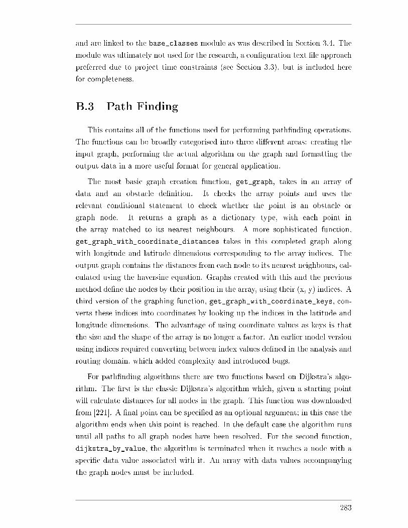
and are linked to the base_classes module as was described in Section 3.4. The

module was ultimately not used for the research, a con�guration text �le approach

preferred due to project time constraints (see Section 3.3), but is included here

for completeness.

B.3 Path Finding

This contains all of the functions used for performing path�nding operations.

The functions can be broadly categorised into three di�erent areas: creating the

input graph, performing the actual algorithm on the graph and formatting the

output data in a more useful format for general application.

The most basic graph creation function, get_graph, takes in an array of

data and an obstacle de�nition. It checks the array points and uses the

relevant conditional statement to check whether the point is an obstacle or

graph node. It returns a graph as a dictionary type, with each point in

the array matched to its nearest neighbours. A more sophisticated function,

get_graph_with_coordinate_distances takes in this completed graph along

with longitude and latitude dimensions corresponding to the array indices. The

output graph contains the distances from each node to its nearest neighbours, cal-

culated using the haversine equation. Graphs created with this and the previous

method de�ne the nodes by their position in the array, using their (x, y) indices. A

third version of the graphing function, get_graph_with_coordinate_keys, con-

verts these indices into coordinates by looking up the indices in the latitude and

longitude dimensions. The advantage of using coordinate values as keys is that

the size and the shape of the array is no longer a factor. An earlier model version

using indices required converting between index values de�ned in the analysis and

routing domain, which added complexity and introduced bugs.

For path�nding algorithms there are two functions based on Dijkstra's algo-

rithm. The �rst is the classic Dijkstra's algorithm which, given a starting point

will calculate distances for all nodes in the graph. This function was downloaded

from [221]. A �nal point can be speci�ed as an optional argument; in this case the

algorithm ends when this point is reached. In the default case the algorithm runs

until all paths to all graph nodes have been resolved. For the second function,

dijkstra_by_value, the algorithm is terminated when it reaches a node with a

speci�c data value associated with it. An array with data values accompanying

the graph nodes must be included.

283

The Dijkstra algorithm-based functions return outputs, path distances and

the predecessor in the path, in the form of dictionaries, with each node presented

by a key in the dictionary. The distances_to_np_array function converts the

distances dictionary to an array, allowing it to be easily visualised (for example

converted to a raster). Lastly, the full paths from the start point to each node

can be extracted using another function. This more readable format can be easily

stored within a json �le, and vectors for individual paths created using the GIS

Utilities module described in Section B.1.

B.4 Time Series Manipulation

The purpose of this module is to provide functions to allow time series data to

be easily created and modi�ed. It makes use of the Pandas module, in particular

the DataFrame class, which allows data to be easily grouped along speci�c dimen-

sions. Because of this the DataFrame class tends to be the default type used for

time series data within the overall model.

Because the three dimensional data arrays (time, latitude and longitude dimen-

sions) can get very large, it is often necessary to group the data along the time di-

mension, where they can be easily summed or averaged. This is also advantageous

as it allows an easily way to examine seasonal trends in the data (for example the

power produced by a wave energy device). The function group_values_by_time

builds on methods in DataFrame and allows input time series to be grouped ac-

cording to a time index (for example by month or year).

A key functionality is the ability to project time series data forward in time.

This is required when there is only limited input data to work with (for ex-

ample metocean data or load pro�le data) and is achieved using the function

format_and_project_timeseries. This utilises a number of other functions

coded in the module. Given an input DataFrame and total periods desired, the

function will replicate the DataFrame forward, after grouping the data by the time

base desired. For incomplete time series, the time series can either be trimmed

back or extended forward to a suitable time base prior to replication. This is to

ensure that the time periods are consistent with the time index, capturing the

seasonal pro�le. An issue with the data projection is that it simply copies pre-

existing data. This means that a projected time series will not see the full inter

annual variability that would exist in reality. For larger datasets this is not a

signi�cant issue. To handle smaller datasets better, an improvement would be to

derive future months based on the data supplied, for example by �tting monthly

284

normal distributions to the data and using the resulting function to predict future

trends. Another option would be to use Markov chains to predict future metocean

sea states. This is noted as future work.

B.5 Extra Utilities

Contained within this module are miscellaneous functions which would be

suitable for Python applications outside of this research project. They include

functions to format and manipulate di�erent object types, conversion functions

and functions to read di�erent �le formats into Python, among other things.

285

286

CGrid-connected Case Study

Con�guration Files

287

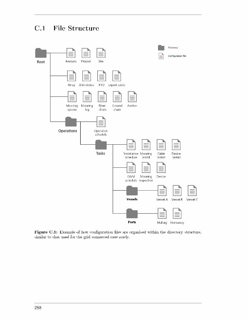
C.1 File Structure

Figure C.1: Example of how con�guration �les are organised within the directory structure,similar to that used for the grid connected case study.

288

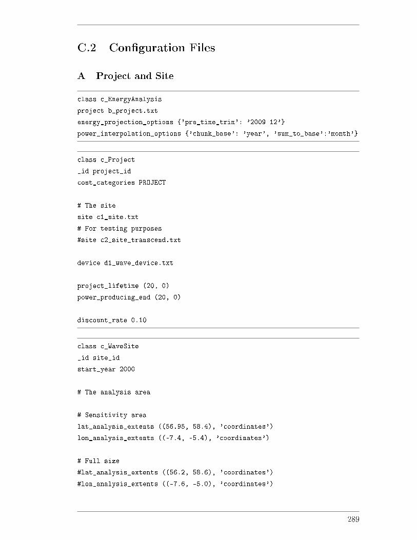
C.2 Con�guration Files

A Project and Site

class c_EnergyAnalysis

project b_project.txt

energy_projection_options {'pre_time_trim': '2009-12'}

power_interpolation_options {'chunk_base': 'year', 'sum_to_base':'month'}

class c_Project

_id project_id

cost_categories PROJECT

# The site

site c1_site.txt

# For testing purposes

#site c2_site_transcend.txt

device d1_wave_device.txt

project_lifetime (20, 0)

power_producing_end (20, 0)

discount_rate 0.10

class c_WaveSite

_id site_id

start_year 2000

# The analysis area

# Sensitivity area

lat_analysis_extents ((56.95, 58.4), 'coordinates')

lon_analysis_extents ((-7.4, -5.4), 'coordinates')

# Full size

#lat_analysis_extents ((56.2, 58.6), 'coordinates')

#lon_analysis_extents ((-7.6, -5.0), 'coordinates')

289

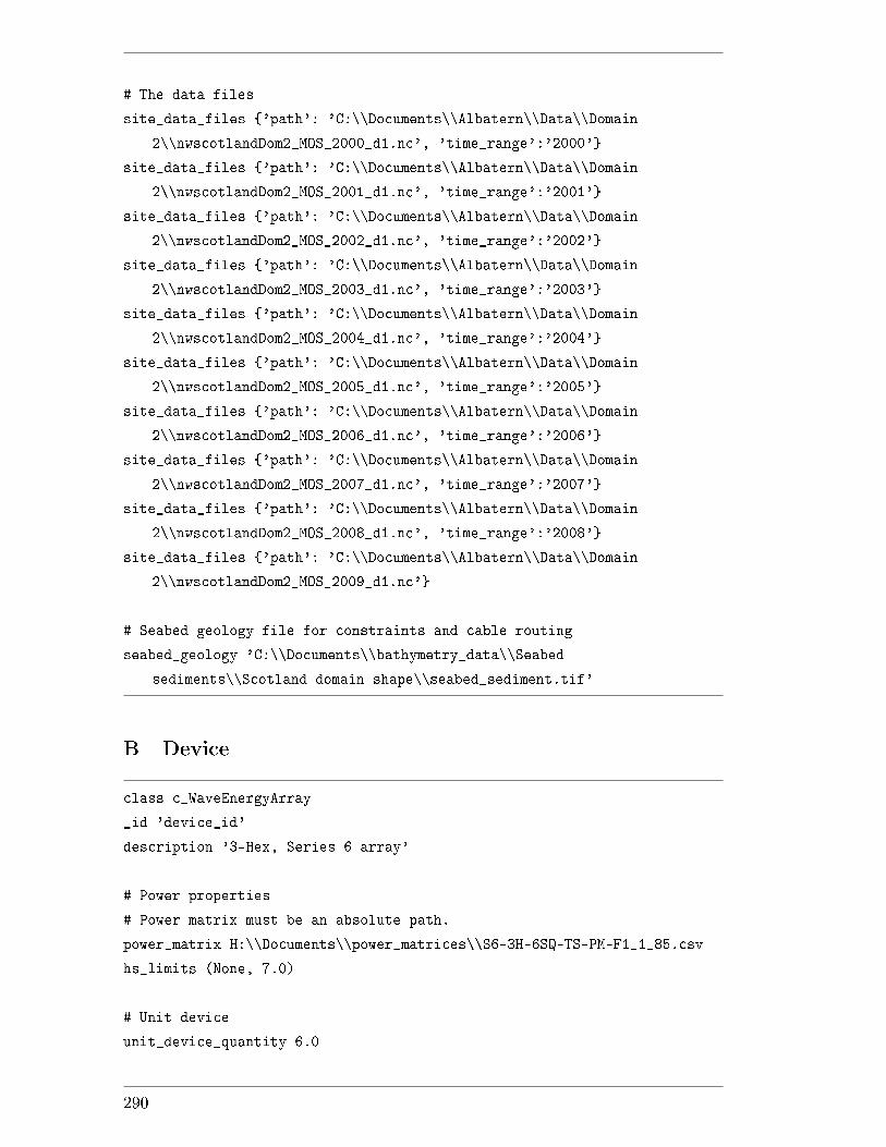
# The data files

site_data_files {'path': 'C:\\Documents\\Albatern\\Data\\Domain

2\\nwscotlandDom2_MOS_2000_d1.nc', 'time_range':'2000'}

site_data_files {'path': 'C:\\Documents\\Albatern\\Data\\Domain

2\\nwscotlandDom2_MOS_2001_d1.nc', 'time_range':'2001'}

site_data_files {'path': 'C:\\Documents\\Albatern\\Data\\Domain

2\\nwscotlandDom2_MOS_2002_d1.nc', 'time_range':'2002'}

site_data_files {'path': 'C:\\Documents\\Albatern\\Data\\Domain

2\\nwscotlandDom2_MOS_2003_d1.nc', 'time_range':'2003'}

site_data_files {'path': 'C:\\Documents\\Albatern\\Data\\Domain

2\\nwscotlandDom2_MOS_2004_d1.nc', 'time_range':'2004'}

site_data_files {'path': 'C:\\Documents\\Albatern\\Data\\Domain

2\\nwscotlandDom2_MOS_2005_d1.nc', 'time_range':'2005'}

site_data_files {'path': 'C:\\Documents\\Albatern\\Data\\Domain

2\\nwscotlandDom2_MOS_2006_d1.nc', 'time_range':'2006'}

site_data_files {'path': 'C:\\Documents\\Albatern\\Data\\Domain

2\\nwscotlandDom2_MOS_2007_d1.nc', 'time_range':'2007'}

site_data_files {'path': 'C:\\Documents\\Albatern\\Data\\Domain

2\\nwscotlandDom2_MOS_2008_d1.nc', 'time_range':'2008'}

site_data_files {'path': 'C:\\Documents\\Albatern\\Data\\Domain

2\\nwscotlandDom2_MOS_2009_d1.nc'}

# Seabed geology file for constraints and cable routing

seabed_geology 'C:\\Documents\\bathymetry_data\\Seabed

sediments\\Scotland domain shape\\seabed_sediment.tif'

B Device

class c_WaveEnergyArray

_id 'device_id'

description '3-Hex, Series 6 array'

# Power properties

# Power matrix must be an absolute path.

power_matrix H:\\Documents\\power_matrices\\S6-3H-6SQ-TS-PM-F1_1_85.csv

hs_limits (None, 7.0)

# Unit device

unit_device_quantity 6.0

290

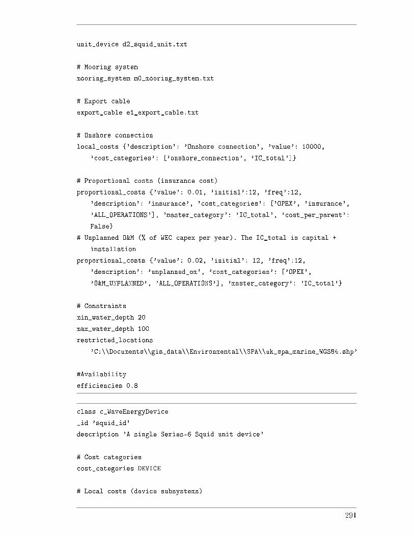
unit_device d2_squid_unit.txt

# Mooring system

mooring_system m0_mooring_system.txt

# Export cable

export_cable e1_export_cable.txt

# Onshore connection

local_costs {'description': 'Onshore connection', 'value': 10000,

'cost_categories': ['onshore_connection', 'IC_total']}

# Proportional costs (insurance cost)

proportional_costs {'value': 0.01, 'initial':12, 'freq':12,

'description': 'insurance', 'cost_categories': ['OPEX', 'insurance',

'ALL_OPERATIONS'], 'master_category': 'IC_total', 'cost_per_parent':

False}

# Unplanned O&M (% of WEC capex per year). The IC_total is capital +

installation

proportional_costs {'value': 0.02, 'initial': 12, 'freq':12,

'description': 'unplanned_om', 'cost_categories': ['OPEX',

'O&M_UNPLANNED', 'ALL_OPERATIONS'], 'master_category': 'IC_total'}

# Constraints

min_water_depth 20

max_water_depth 100

restricted_locations

'C:\\Documents\\gis_data\\Environmental\\SPA\\uk_spa_marine_WGS84.shp'

#Availability

efficiencies 0.8

class c_WaveEnergyDevice

_id 'squid_id'

description 'A single Series-6 Squid unit device'

# Cost categories

cost_categories DEVICE

# Local costs (device subsystems)

291

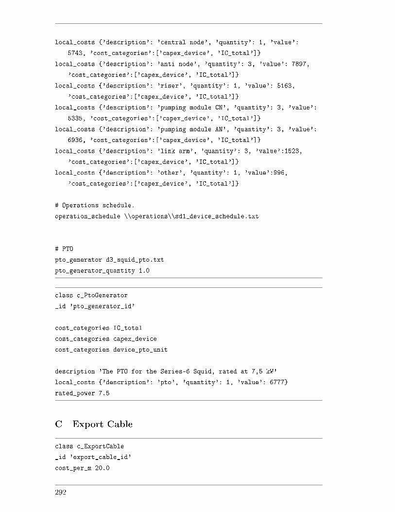
local_costs {'description': 'central node', 'quantity': 1, 'value':

5743, 'cost_categories':['capex_device', 'IC_total']}

local_costs {'description': 'anti node', 'quantity': 3, 'value': 7897,

'cost_categories':['capex_device', 'IC_total']}

local_costs {'description': 'riser', 'quantity': 1, 'value': 5163,

'cost_categories':['capex_device', 'IC_total']}

local_costs {'description': 'pumping module CN', 'quantity': 3, 'value':

5335, 'cost_categories':['capex_device', 'IC_total']}

local_costs {'description': 'pumping module AN', 'quantity': 3, 'value':

6936, 'cost_categories':['capex_device', 'IC_total']}

local_costs {'description': 'link arm', 'quantity': 3, 'value':1523,

'cost_categories':['capex_device', 'IC_total']}

local_costs {'description': 'other', 'quantity': 1, 'value':996,

'cost_categories':['capex_device', 'IC_total']}

# Operations schedule.

operation_schedule \\operations\\sd1_device_schedule.txt

# PTO

pto_generator d3_squid_pto.txt

pto_generator_quantity 1.0

class c_PtoGenerator

_id 'pto_generator_id'

cost_categories IC_total

cost_categories capex_device

cost_categories device_pto_unit

description 'The PTO for the Series-6 Squid, rated at 7,5 kW'

local_costs {'description': 'pto', 'quantity': 1, 'value': 6777}

rated_power 7.5

C Export Cable

class c_ExportCable

_id 'export_cable_id'

cost_per_m 20.0

292

# Cost categories

cost_categories EXPORT_CABLE

cost_categories IC_total

cost_categories capex_export_cable

# Operational tasks

operation_schedule \\operations\\tasks\\ti3c_cable_install.txt

# Do for sensitivity, not here.

maximum_depth_for_install None

invalid_seabed_sediments None

#max_cable_length 8000

D Mooring System

class c_MooringSystemWavenetS6

_id mooring_system_id

description 'WEC mooring system'

# Cost categories

cost_categories MOORING_SYSTEM

# Operation schedule

operation_schedule \\operations\\sm1_mooring_schedule.txt

# Mooring system components

mooring_leg m4_mooring_leg.txt

grid_line {'cost_per_m': 1.88, 'line_material': 'basic_nylon',

'cost_categories': ['IC_total', 'capex_mooring_system'],

'line_length_m': 220, 'quantity':2}

corner_buoy {'local_costs': {'description': 'unit', 'value':760},

'cost_categories': ['IC_total', 'capex_mooring_system']}

local_costs {'description': 'Connectors and shackles', 'value': 500,

'cost_categories': ['IC_total', 'capex_mooring_system']}

# Other inputs

grid_displacement 5.0

293

class c_Anchor

_id anchor_id

description 'Mooring system anchor'

#cost_categories 'mooring_anchor'

local_costs {'description': 'unit', 'value': 1995.0}

weight 1500.0

invalid_seabed_geology 5

class c_Line

_id ground_chain_id

description 'Mooring system ground chain'

#cost_categories 'mooring_ground_chain'

cost_per_m 29.5

# From

http://www.sotra.net/products/tables/weight-for-studlink-anchor-chain

dry_mass_per_m 34.0

line_material basic_steel

diameter 38

class c_CatenaryLine

_id riser_chain_id

description 'Mooring system riser chain'

#cost_categories 'mooring_riser_chain'

cost_per_m 23.0

# From

http://www.sotra.net/products/tables/weight-for-studlink-anchor-chain

dry_mass_per_m 13.0

line_tension 20000

line_material basic_steel

diameter 24

class c_CatenaryLeg

_id mooring_leg_id

description 'Mooring system leg'

cost_categories IC_total

cost_categories capex_mooring_system

#cost_categories 'mooring_leg'

294

anchor m1_anchor.txt

ground_chain m2_ground_chain.txt

line_to_surface m3_line_to_surface.txt

ground_chain_ratio 3

E Operations and Maintenance

E.1 Operation Schedules

class c_OperationSchedule

description device_op_schedule_id

cost_categories ALL_OPERATIONS

# The device operational tasks

task_list tasks\\ti2d_device_install.txt

task_list tasks\\to2d_device_port_service.txt

task_list tasks\\to3d_midlife_refit.txt

# The ports

port tasks\\ports\\p1_port_stornaway.txt

port tasks\\ports\\p2_port_mallaig.txt

port tasks\\ports\\p3_port_carloway.txt

port tasks\\ports\\p4_port_griminis.txt

port tasks\\ports\\p5_port_breibhig.txt

port tasks\\ports\\p6_port_acairseid.txt

port tasks\\ports\\p7_port_meanish.txt

port tasks\\ports\\p8_port_coll.txt

port tasks\\ports\\p9_port_old_dornie.txt

port tasks\\ports\\p10_port_applecross.txt

class c_OperationSchedule

_id o&m_schedule_moorings

description Operation schedule for the mooring system

# Cost categories

cost_categories ALL_OPERATIONS

295

# List of tasks

task_list \\tasks\\ti1m_mooring_install.txt

task_list \\tasks\\to1m_mooring_inspection.txt

port tasks\\ports\\p1_port_stornaway.txt

port tasks\\ports\\p2_port_mallaig.txt

port tasks\\ports\\p3_port_carloway.txt

port tasks\\ports\\p4_port_griminis.txt

port tasks\\ports\\p5_port_breibhig.txt

port tasks\\ports\\p6_port_acairseid.txt

port tasks\\ports\\p7_port_meanish.txt

port tasks\\ports\\p8_port_coll.txt

port tasks\\ports\\p9_port_old_dornie.txt

port tasks\\ports\\p10_port_applecross.txt

E.2 Tasks

class c_MarineOperation

_id inst_mooring_id

description Mooring system install

cost_categories INSTALLATION

cost_categories installation_mooring_system

cost_categories IC_total

# Pre project as installation activity

pre_project True

vessel \\vessels\\v1_workboat.txt

vessel_per_quantity True

vessel_mob_time_days 1

vessel_demob_time_days 1

support_vessels \\vessels\\v2_rhib.txt

hours_to_complete_task 6

max_seastate_transit_out 3.0

max_seastate_task 1.5

296

max_seastate_transit_return 3.0

period_for_task '2000-10'

# Scheduling timescale inputs

multiple_trips_allowed False

max_hours_for_single_operation 24

resting_hours_between_operations 0

min_site_time_threshold 1.0

sleep_on_vessel False

class c_MarineOperation

_id inst_device_id

description Squid_install

cost_categories INSTALLATION

cost_categories installation_device

cost_categories IC_total

# Pre project as installation activity

pre_project True

vessel \\vessels\\v1_workboat.txt

vessel_per_quantity True

vessel_mob_time_days 1.0

vessel_demob_time_days 1.0

support_vessels \\vessels\\v2_rhib.txt

speed_to_site_knots 4.5

speed_from_site_knots None

hours_to_complete_task 3

max_seastate_transit_out 1.5

max_seastate_task 1.5

max_seastate_transit_return 3.0

period_for_task '2000-10'

297

# Scheduling timescale inputs

multiple_trips_allowed False

max_hours_for_single_operation 24

resting_hours_between_operations 0

min_site_time_threshold 1.0

sleep_on_vessel False

class c_ExportCableInstall

_id inst_cable_id

description Cable install

# Cost categories

cost_categories INSTALLATION

cost_categories ALL_OPERATIONS

cost_categories installation_cable

cost_categories IC_total

invalid_cost_categories capex_export_cable

# Pre project as installation activity

pre_project True

vessel \\vessels\\v4_multicat_cable_lay_vessel.txt

vessel_mob_time_days 2

vessel_demob_time_days 2

install_speed (500, 'metre/hour')

max_seastate_transit_out 3.0

max_seastate_task 1.5

max_seastate_transit_return 3.0

period_for_task '2000-09'

local_costs {'description': 'rig servicing', 'value': 400,

'cost_categories': 'installation_cable_rig_servicing'}

# Timescale properties

298

max_hours_for_single_operation 36

multiple_trips_allowed False

min_site_time_threshold 1.0

port ports\\p1_port_stornaway.txt

port ports\\p2_port_mallaig.txt

port ports\\p3_port_carloway.txt

port ports\\p4_port_griminis.txt

port ports\\p5_port_breibhig.txt

port ports\\p6_port_acairseid.txt

port ports\\p7_port_meanish.txt

port ports\\p8_port_coll.txt

port ports\\p9_port_old_dornie.txt

port ports\\p10_port_applecross.txt

class c_MarineOperation

_id mooring_inspection_id

description Mooring inspection at site

cost_categories OPEX

cost_categories O&M_PLANNED

cost_categories o&m_mooring_inspection

vessel \\vessels\\v1_workboat.txt

vessel_per_quantity True

vessel_mob_time_days 1

vessel_demob_time_days 1

hours_to_complete_task 3

max_seastate_transit_out 3.0

max_seastate_task 1.5

max_seastate_transit_return 3.0

period_for_task ['2001-03', '2002-03', '2003-03', '2004-03', '2005-03',

'2006-03', '2007-03', '2008-03', '2009-03', '2010-03', '2011-03',

'2012-03', '2013-03', '2014-03', '2015-03', '2016-03', '2017-03',

'2018-03', '2019-03']

299

local_costs {'description': 'inspection', 'value': 1500, 'initial': 15,

'freq': 12}

# Scheduling timescale inputs

multiple_trips_allowed False

max_hours_for_single_operation 24

resting_hours_between_operations 0

min_site_time_threshold 1.0

sleep_on_vessel False

class c_MaintenanceAtPort

_id device_service_in_port_id

description device service in port

cost_categories OPEX

cost_categories O&M_PLANNED

cost_categories o&m_device_routine_service

vessel \\vessels\\v1_workboat.txt

vessel_per_quantity True

pre_maintenance_operation toAd_recover_device_from_site.txt

time_in_port_days 1.0

post_maintenance_operation toBd_deploy_device_at_site.txt

period_for_task ['2000-03', '2000-09', '2001-3','2001-9',

'2002-3','2002-9','2003-3','2003-9', '2004-3', '2004-9', '2005-3',

'2005-9', '2006-3', '2006-9', '2007-3', '2007-9', '2008-3',

'2008-9', '2009-3', '2009-9', '2010-9', '2011-3', '2011-9',

'2012-3', '2012-9', '2013-3', '2013-9', '2014-3', '2014-9',

'2015-3', '2015-9', '2016-3', '2016-9', '2017-3', '2017-9',

'2018-3', '2018-9', '2019-3', '2019-9', '2020-3', '2020-9']

# Pre mid life refit

local_costs {'description':'parts', 'value': 800, 'initial':3, 'freq':6,

'final':120}

local_costs {'description':'other', 'value': 600, 'initial':3, 'freq':6,

'final':120}

local_costs {'description':'inspection', 'value': 200, 'initial':3,

'freq':6, 'final':120}

300

# Post midlife refit

local_costs {'description':'parts2', 'value': 800, 'initial':129,

'freq':6}

local_costs {'description':'other2', 'value': 600, 'initial':129,

'freq':6}

local_costs {'description':'inspection2', 'value': 200, 'initial':129,

'freq':6}

class c_MaintenanceAtPort

_id midlife_refit_id

description midlife refit in port

cost_categories OPEX

cost_categories O&M_PLANNED

cost_categories o&m_midlife_refit

vessel \\vessels\\v1_workboat.txt

vessel_per_quantity True

pre_maintenance_operation toAd_recover_device_from_site.txt

time_in_port_days 2.0

post_maintenance_operation toBd_deploy_device_at_site.txt

period_for_task ['2010-03']

local_costs {'initial': 123, 'description': 'pumping modules',

'quantity': 3, 'value': 12271}

local_costs {'initial': 123, 'description': 'pto', 'quantity': 1,

'value': 6777}

class c_MarineOperation

_id device_service_rtn_id

description device_service_rtn

vessel \\vessels\\v1_workboat.txt

# Assume occurs per 6 devices

vessel_mob_time_days 0.0

vessel_demob_time_days 1.0

301

max_seastate_transit_out 3.0

max_seastate_task 1.5

max_seastate_transit_return 1.5

speed_to_site_knots None

speed_from_site_knots 4.5

hours_to_complete_task 2

# Scheduling timescale inputs

multiple_trips_allowed False

max_hours_for_single_operation 24

resting_hours_between_operations 0

min_site_time_threshold 1.0

sleep_on_vessel False

class c_MarineOperation

_id device_service_out_id

description device_service_out

vessel \\vessels\\v1_workboat.txt

# Assume occurs per 6 devices

vessel_mob_time_days 1.0

vessel_demob_time_days 0.0

max_seastate_transit_out 1.5

max_seastate_task 1.5

max_seastate_transit_return 3.0

speed_to_site_knots 4.5

speed_from_site_knots None

hours_to_complete_task 2

# Scheduling timescale inputs

multiple_trips_allowed False

max_hours_for_single_operation 24

resting_hours_between_operations 0

302

min_site_time_threshold 1.0

sleep_on_vessel False

E.3 Vessels

class c_Fuel

cost_categories vessel_fuel_cost

cost_per_ltr 0.60

class c_Vessel

_id workboat_vessel_id

description Workboat for smaller operations; Suitable for Series 6

cost_categories vessel_workboat

charter_cost 1500

standby_cost 1000

mob_cost 900

demob_cost 900

average_speed 9

speed_units 'knot'

fuel_consumption_rate_travel 40.0

fuel f0_vessel_fuel.txt

comments 'Based on Leaske Marine's MV Uskmoor

http://www.leaskmarine.com/vessels/mv-uskmoor'

class c_Vessel

_id rhib_vessel_id

description Support vessel

cost_categories vessel_rhib

charter_cost 1200

standby_cost 0

mob_cost 0

demob_cost 0

303

mob_time_days 0

demob_time_days 0

average_speed 25

speed_units 'knot'

fuel_consumption_rate_travel 30.0

fuel f0_vessel_fuel.txt

comments 'Based on Leaske Marine's MV Explorer

http://www.leaskmarine.com/vessels/mv-explorer'

class c_Vessel

_id cable_multicat_vessel_id

description Cable lay vessel

cost_categories vessel_cable_lay_multicat

charter_cost 7700

standby_cost 5800

mob_cost 4600

demob_cost 4600

average_speed 10

speed_units 'knot'

fuel_consumption_rate_travel 280.0

fuel_consumption_rate_working 70

fuel f0_vessel_fuel.txt

comments 'Based on Leaske Marine's MV Uskmoor

http://www.leaskmarine.com/vessels/mv-uskmoor'

E.4 Ports

class c_Port

lat 58.20692587839467

lon -6.382697603124509

description Stornaway port

#cost_categories port

#local_costs {'description': 'Port Hire', 'value':1000}

304

class c_Port

lat 57.00521880549277

lon -5.827369554384538

description Mallaig port

#cost_categories port

#local_costs {'description': 'Port Hire', 'value':2000}

class c_Port

lat 58.279

lon -6.791

description Carloway port

#cost_categories port

#local_costs {'description': 'Port Hire', 'value':2000}

class c_Port

lat 58.20692587839467

lon -6.382697603124509

description Stornaway port

#cost_categories port

#local_costs {'description': 'Port Hire', 'value':1000}

class c_Port

lat 57.564

lon -7.439

description Griminis port

#cost_categories port

#local_costs {'description': 'Port Hire', 'value':2000}

class c_Port

lat 56.96

lon -7.441

description Breibhig port

#cost_categories port

#local_costs {'description': 'Port Hire', 'value':2000}

class c_Port

lat 57.068

305

lon -7.294

description Acairseid port

#cost_categories port

#local_costs {'description': 'Port Hire', 'value':2000}

class c_Port

lat 57.456

lon -6.746

description Meanish port

#cost_categories port

#local_costs {'description': 'Port Hire', 'value':2000}

class c_Port

lat 56.615

lon -6.522

description Coll port

#cost_categories port

#local_costs {'description': 'Port Hire', 'value':2000}

class c_Port

lat 58.044

lon -5.421

description Old Dornie port

#cost_categories port

#local_costs {'description': 'Port Hire', 'value':2000}

class c_Port

lat 57.434

lon -5.814

description Applecross port

#cost_categories port

#local_costs {'description': 'Port Hire', 'value':2000}

306

DSample Results

307

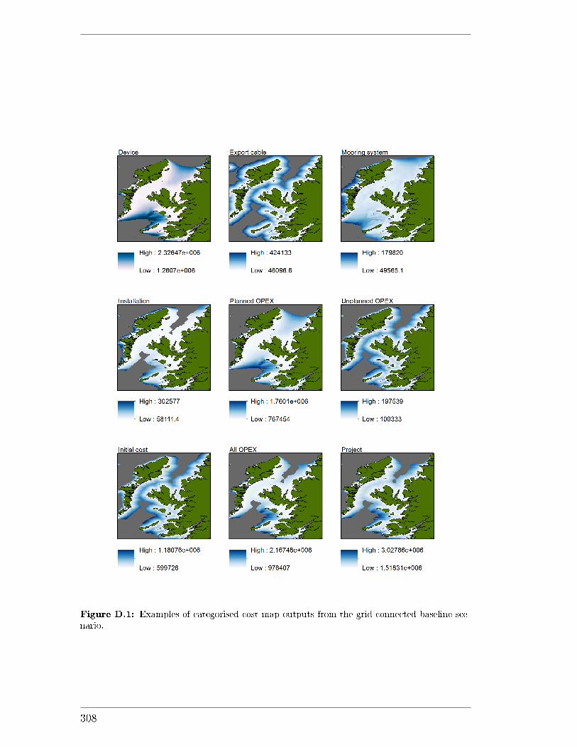
Figure D.1: Examples of categorised cost map outputs from the grid-connected baseline sce-nario.

308

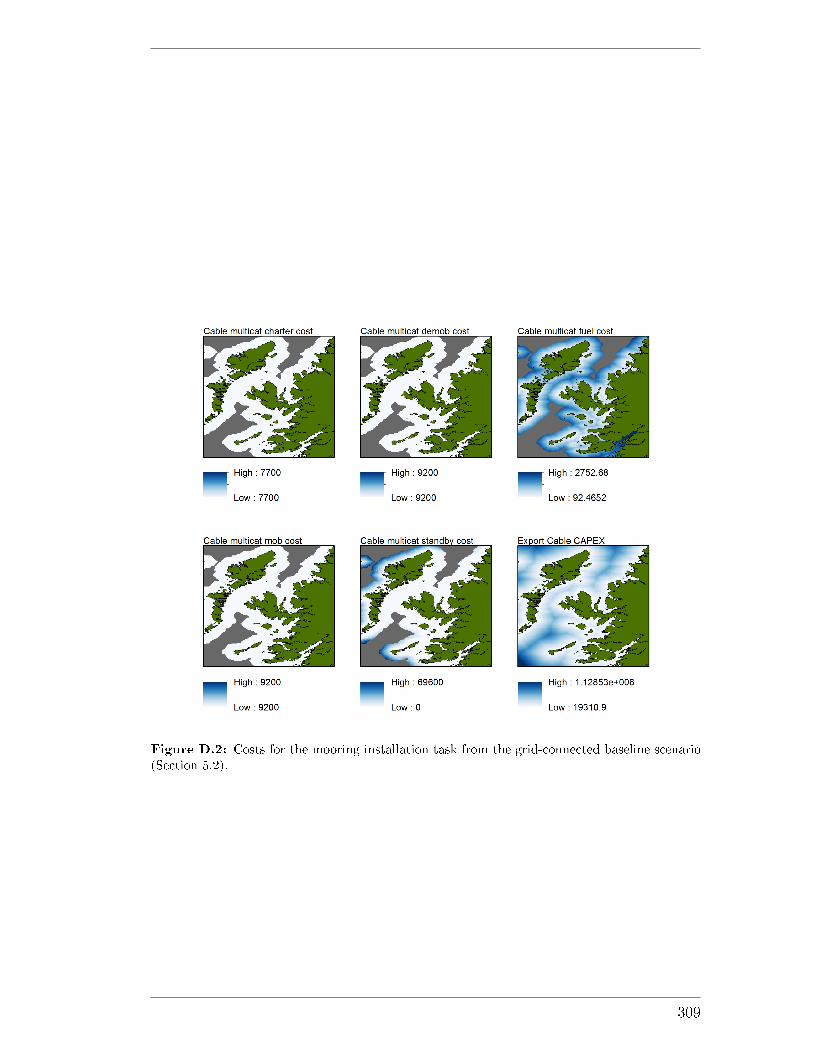
Figure D.2: Costs for the mooring installation task from the grid-connected baseline scenario(Section 5.2).

309

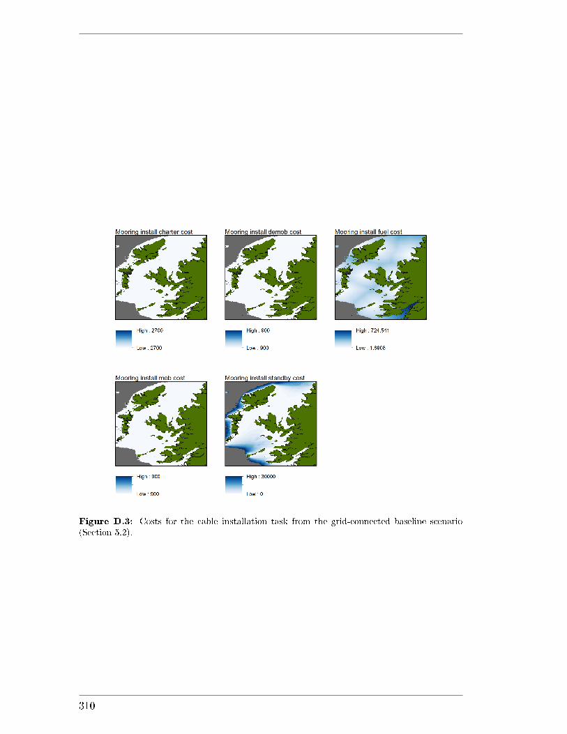
Figure D.3: Costs for the cable installation task from the grid-connected baseline scenario(Section 5.2).

310

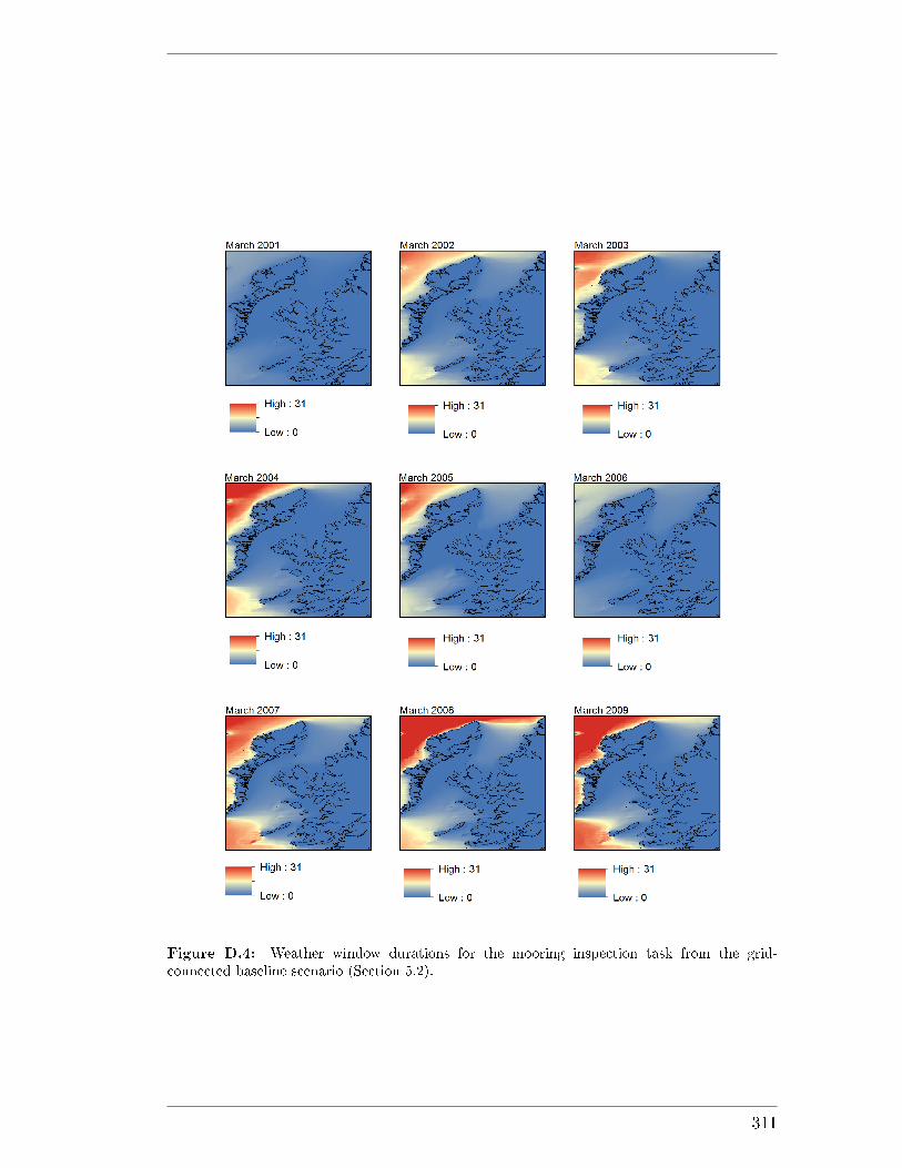
Figure D.4: Weather window durations for the mooring inspection task from the grid-connected baseline scenario (Section 5.2).

311

312

EO�-grid Case Study Component

Datasheets

313

Prime Rating These ratings are applicable for supplying continuous electrical power(at variable load) in lieu of commercially purchased power. There is nolimitation to the annual hours of operation and this model can supply 10% overload power for 1 hour in 12 hours.

Standby Rating These ratings are applicable for supplying continuous electrical power (atvariable load) in the event of a utility power failure. No overload ispermitted on these ratings. The alternator on this model is peakcontinuous rated (as defined in ISO 8528-3).

Standard Reference Conditions Note: Standard reference conditions 25°C (77°F) Air Inlet Temp, 100m(328 ft) A.S.L. 30% relative humidity.Fuel consumption data at full load with diesel fuel with specific gravity of0.85 and conforming to BS2869: 1998, Class A2.

FG Wilson has manufacturing facilities in the following locations:Northern Ireland • Brazil • China • India • USAWith headquarters in Northern Ireland, FG Wilson operates through a Global Dealer Network.

Output Ratings Ratings and Performance Data

Leroy Somer

Generating Set Model Prime Standby Engine Make & Model:

Alternator manufactured for FG Wilson by:

Alternator Model:

Control Panel:

Circuit Breaker Type:

Engine Speed: RPM

Base Frame:

zH 06zH 05:ycneuqerF

Fuel Tank Capacity: litres (US gal)

Dimensions and Weights

Length (L)mm (in)

Width (W)mm (in)

Height (H)mm (in)

Drykg (lb)

Wetkg (lb)

Dry = With Lube Oil Wet = With Lube Oil and Coolant

Ratings in accordance with ISO 8528, ISO 3046, IEC 60034, BS5000 and NEMA MG-1/22. Generating set pictured may include optional accessories.

www.FGWilson.com

//

//

Fuel Consumption: l/hr (US gal/hr)

(100% Load) - Prime

Ratings at power factor.

Image for illustration purposes only.

- Standby

Available Options

FG Wilson offer a range of optional features to tailor our generating sets to meet your power needs. Options include:

Upgrade to CE Certification

A wide range of Sound Attenuated Enclosures

A variety of generating set control and synchronising panels

Additional alarms and shutdowns

A selection of exhaust silencer noise levels

For further information on all of the standard and optional features accompanying this product please contact your local Dealer or visit: www.FGWilson.com

Heavy Duty Fabricated Steel

Perkins 1106A-70TAG4

LL5014F

380-415V,50Hz 200.0 kVA 160.0 kW 220.0 kVA 176.0 kW

----

P220-1

3 Pole MCCB

-1500

418 (110.4)

-45.4 (12.0)

-49.5 (13.1)

2500 (98.4) 1320 (52.0) 1626 (64.0) 1731 (3816) 1758 (3876)

0.8 DCP-10

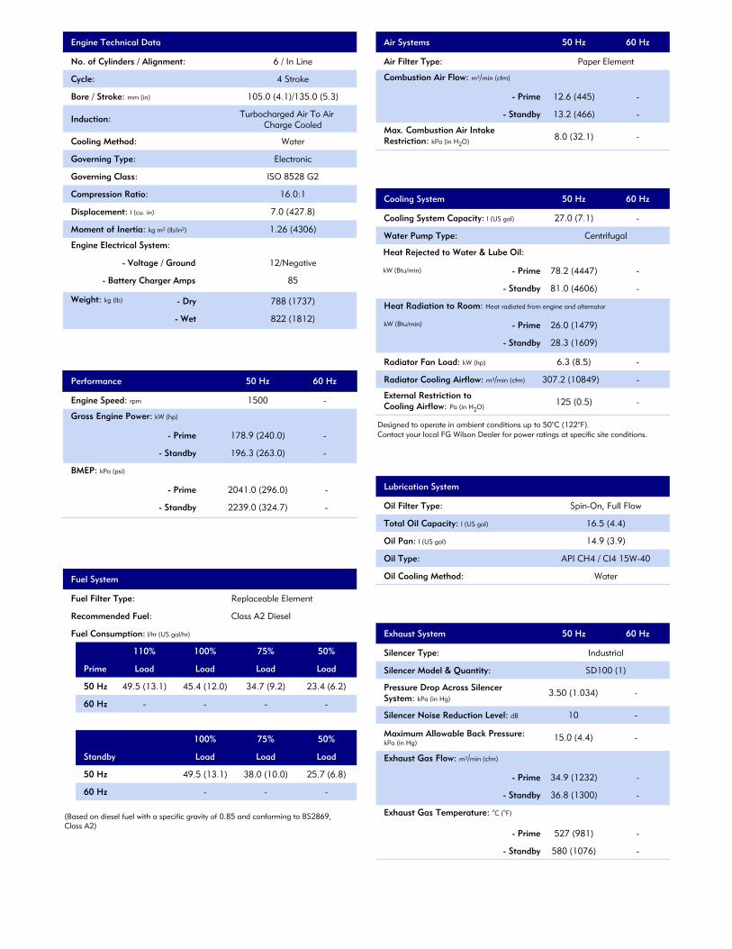
Exhaust System

Silencer Type:

Silencer Model & Quantity:

Pressure Drop Across Silencer System: kPa (in Hg)

Silencer Noise Reduction Level: dB

Maximum Allowable Back Pressure: kPa (in Hg)

Exhaust Gas Flow: m³/min (cfm)

Exhaust Gas Temperature: °C (°F)

60 Hz50 Hz

- Prime

- Standby

- Prime

- Standby

Lubrication System

Oil Filter Type:

Total Oil Capacity: l (US gal)

Oil Pan: l (US gal)

Oil Type:

Oil Cooling Method:

Cooling System

Cooling System Capacity: l (US gal)

Water Pump Type:

Heat Rejected to Water & Lube Oil:

kW (Btu/min)

Heat Radiation to Room: Heat radiated from engine and alternator

kW (Btu/min)

Radiator Fan Load: kW (hp)

Radiator Cooling Airflow: m³/min (cfm)

External Restriction to Cooling Airflow: Pa (in H2O)

Designed to operate in ambient conditions up to 50°C (122°F).Contact your local FG Wilson Dealer for power ratings at specific site conditions.

60 Hz50 Hz

- Prime

- Standby

- Prime

- Standby

smetsyS riAataD lacinhceT enignE

No. of Cylinders / Alignment:

Cycle:

Bore / Stroke: mm (in)

Induction:

Engine Speed: rpm

Performance

Gross Engine Power: kW (hp)

BMEP: kPa (psi)

Fuel System

Fuel Filter Type:

Recommended Fuel:

Fuel Consumption: l/hr (US gal/hr)

Prime

50 Hz

60 Hz

110% 100% 75% 50%

Load Load Load Load

60 Hz

50 Hz

Standby Load Load Load

50%75%100%

(Based on diesel fuel with a specific gravity of 0.85 and conforming to BS2869, Class A2)

Air Filter Type:

Combustion Air Flow: m³/min (cfm)

Max. Combustion Air IntakeRestriction: kPa (in H2O)

60 Hz50 Hz

Cooling Method:

Governing Type:

Governing Class:

Compression Ratio:

Displacement: l (cu. in)

Moment of Inertia: kg m² (lb/in²)

Engine Electrical System:

Weight: kg (lb)

60 Hz50 Hz

- Standby

- Prime

- Standby

- Prime

- Standby

- Prime

- Dry

- Wet

- Voltage / Ground

- Battery Charger Amps

-527 (981)

-580 (1076)

-34.9 (1232)

-36.8 (1300)

-15.0 (4.4)

-10

-3.50 (1.034)

SD100 (1)

Industrial

Water

14.9 (3.9)

16.5 (4.4)

Spin-On, Full Flow

API CH4 / CI4 15W-40

-27.0 (7.1)

Centrifugal

-

-

78.2 (4447)

81.0 (4606)

26.0 (1479)

28.3 (1609)

-6.3 (8.5)

-307.2 (10849)

-125 (0.5)1500 -

Class A2 Diesel

Replaceable Element

6 / In Line

4 Stroke

105.0 (4.1)/135.0 (5.3)

Turbocharged Air To AirCharge Cooled

Water

ISO 8528 G2

Electronic

16.0:1

7.0 (427.8)

1.26 (4306)

12/Negative

85

788 (1737)

822 (1812)

2041.0 (296.0) -

-2239.0 (324.7)

-

-

178.9 (240.0)

196.3 (263.0)

----

23.4 (6.2)34.7 (9.2)45.4 (12.0)49.5 (13.1)

-

25.7 (6.8)

-

38.0 (10.0)

-

49.5 (13.1)

Paper Element

-12.6 (445)

-13.2 (466)

-8.0 (32.1)

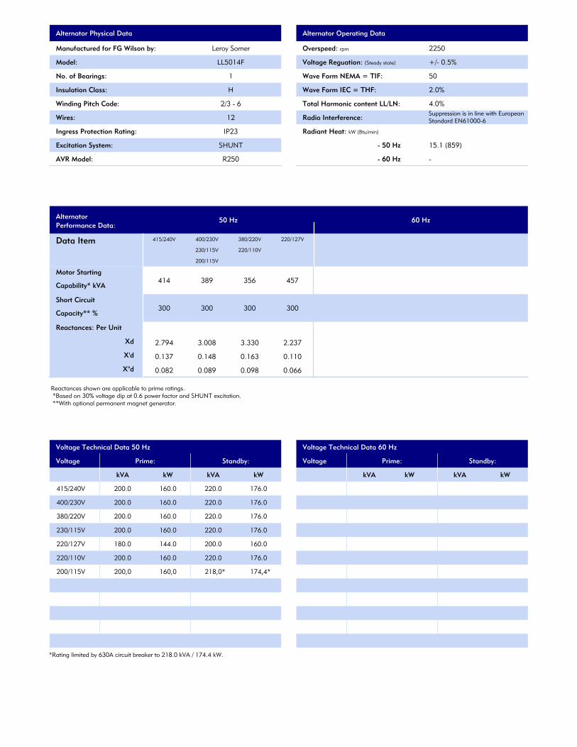
Alternator Physical Data

Manufactured for FG Wilson by:

Model:

No. of Bearings:

Insulation Class:

Winding Pitch Code:

Wires:

Ingress Protection Rating:

Excitation System:

AVR Model:

Overspeed: rpm

Voltage Reguation: (Steady state)

Wave Form NEMA = TIF:

Wave Form IEC = THF:

Total Harmonic content LL/LN:

Radio Interference:

Radiant Heat: kW (Btu/min)

- 50 Hz

- 60 Hz

Voltage Technical Data 50 Hz

Voltage Prime: Standby:

kVA kW kVA kW

AlternatorPerformance Data:

Data Item

Motor Starting

Capability* kVA

Short Circuit

Capacity** %

Reactances: Per Unit

Xd

X'd

X"d

Reactances shown are applicable to prime ratings. *Based on 30% voltage dip at 0.6 power factor and SHUNT excitation. **With optional permanent magnet generator.

Leroy Somer

Suppression is in line with European Standard EN61000-6

Voltage Technical Data 60 Hz

Voltage Prime: Standby:

kVA kW kVA kW

60 Hz50 Hz

Alternator Operating Data

0.671V042/514 220.0160.0200.0

0.671V032/004 220.0160.0200.0

0.671V511/032 220.0160.0200.0

0.061V721/022 200.0144.0180.0

0.671V011/022 220.0160.0200.0

160.0 0.6710.002 220.0380/220V

003003 300300

2.2373.3303.0082.794

0.1100.1630.1480.137

0.0660.0980.0890.082

457356389414

R250

SHUNT

IP23

12

2/3 - 6

H

1

LL5014F

-

15.1 (859)

4.0%

2.0%

50

+/- 0.5%

2250

415/240V

200/115V

230/115V

400/230V

220/110V

380/220V 220/127V

*Rating limited by 630A circuit breaker to 218.0 kVA / 174.4 kW.

,4.4*71V511/002 218,0*160,0200,0

TRJN_T-105_D

S_0315Page 1 of 2

CHARGING INSTRUCTIONSCHARGER VOLTAGE SETTINGS (AT 77°F/25°C)

System Voltage 6V 12V 24V 36V 48V

Absorption Charge 7.40 14.8 29.6 44.4 59.2

Float Charge 6.60 13.2 26.4 39.6 52.8

Equalize Charge 7.75 15.5 31.0 46.5 62.0

Do not install or charge batteries in a sealed or non-ventilated compartment. Constant under or overcharging will damage the battery and shorten its life as with any battery.

MODEL: T-105 with Bayonet Cap

VOLTAGE: 6

DIMENSIONS: Inches (mm)

BATTERY: Flooded/wet lead-acid battery

COLOR: Maroon (case/cover)

MATERIAL: Polypropylene

WATERING SYSTEM: HydroLink™ Watering System

TERMINAL CONFIGURATIONS

PRODUCT SPECIFICATIONSBCI

GROUP SIZE

TYPE CAPACITY A Minutes CAPACITY B Amp-Hours (AH) ENERGY

(kWh) TERMINAL Type E

DIMENSIONS C Inches (mm) WEIGHT lbs. (kg)

@25 Amps @75 Amps 5-Hr Rate 10-Hr Rate 20-Hr Rate 100-Hr Rate 100-Hr Rate Length Width Height D

6 VOLT DEEP CYCLE BATTERY - with T2 TECHNOLOGY™GC2 T-105 447 115 185 207 225 250 1.50 1, 2, 3, 4 10.30 (262) 7.11 (181) 11.07 (281) 62 (28)

1 ELPT Embedded Low Profile Terminal

Terminal Height Inches (mm)1.22 (31)

Torque Values in-lb (Nm)95 – 105 (11 - 12)

Bolt Size5/16"

2 EHPT Embedded High Profile Terminal

Terminal Height Inches (mm)1.50 (38)

Torque Values in-lb (Nm)95 – 105 (11 - 12)

Bolt Size5/16"

3 EAPT Embedded Automotive Post Terminal

Terminal Height Inches (mm).95 (24)

Torque Values in-lb (Nm)50 – 70 (5.6 - 7.9)

4 EUT Embedded Universal Terminal

Terminal Height Inches (mm)1.10 (28)

Torque Values in-lb (Nm)95 – 105 (11 - 12)

Bolt5/16"

CHARGING TEMPERATURE COMPENSATION.028 VPC for every 10°F (5.55°C) above or below 77°F (25°C) (add .028 VPC for every 10°F (5.55°C) below 77°F and subtract .028 VPC for every 10°C above 77°F).

OPERATIONAL DATAOperating Temperature Self Discharge

-4°F to 113°F (-20°C to +45°C). At temperatures below 32°F (0°C) maintain a state of charge greater than 60%.

5 – 15% per month depending on storage temperature conditions.

T-105 DATA SHEET

A. The number of minutes a battery can deliver when discharged at a constant rate at 80°F (27°C) and maintain a voltage above 1.75 V/cell. Capacities are based on peak performance.B. The amount of amp-hours (AH) a battery can deliver when discharged at a constant rate at 80°F (27°C) and 86°F (30°C) for the 5-Hour rate and maintain a voltage above 1.75 V/cell. Capacities are based on

peak performance.C. Dimensions are based on nominal size. Dimensions may vary depending on type of handle or terminal.D. Dimensions taken from bottom of the battery to the highest point on the battery. Heights may vary depending on type of terminal.E. Terminal images are representative only.Trojan’s battery testing procedures adhere to both BCI and IEC test standards.

TRJN_T-105_D

S_0315

For a Trojan Master Distributor near you, call 800.423.6569 or + 1.562.236.3000 or visit www.trojanbattery.com12380 Clark Street, Santa Fe Springs, CA 90670 • USA

Trojan batteries are available worldwide through Trojan’s Master Distributor Network.We offer outstanding technical support, provided by full-time application engineers.

Page 2 of 2© 2015 Trojan Battery Company. All rights reserved. Trojan Battery Company is not liable for damages that may result from any information provided in or omitted from this

publication, under any circumstances. Trojan Battery Company reserves the right to make adjustments to this publication at any time, without notices or obligation.Please check the Trojan Battery website (www.trojanBattery.com) for the most up-to-date information.

BATTERY DIMENSIONS (shown with EHPT)

TROJAN T-105 PERFORMANCE PERCENT CAPACITY VS. TEMPERATURE

Estimation Purposes Only

1

10

100

1000

10 100 1000 10000 100000

Dis

char

ge C

urre

nt (a

mps

)

Time (min)60%40%20%0% 80% 100% 120%

140

120

100

80

60

40

20

-20

-40

50

60

40

30

20

10

-10

-20

-30

-40

0

0

T-105 DATA SHEET

7.13

10.74

.47

6.97

10.30

10.18

9.69

SI6.

0H-1

1 / S

I8.0

H-11

SUNNY ISLAND 6.0H / 8.0H for off-grID AppLIcAtIoNS

Easy to use•OptiUse:fastinstallationand commissioning,simplifiedoperation•OptiBat:stateofchargecalculation

keepsyouinformedatalltimes

robust•IP54:optimalprotectionfrom dustandhumidity•OptiCool:greatertemperature range

flexible•Forsystemsfrom3to300kW•Precisedesign•SupportsMulticlusterTechnology

•OptiPower:secureoperationinanysituation

SUNNY ISLAND 6.0H / 8.0H Simple. Robust. Flexible.Moredurablethanitspredecessors:ThenewSunnyIslandimpresseswithitshighprotectionclassandwidetemperaturerange.Moisture,dustandtemperaturefluctuationswon’timpairitsoperation,evenafter20years.ThankstoOptiCool,there’snoneedtocompromisewhenitcomestooverloadcapacityandeconomicviability.Andthere’smore:OptiPower,theintelligentloadandenergymanagementsystem,ensuresoperationevenincriticalsituations.OptiUsemakesinstallation,commission-inganddailyuseeasierthaneverwithautomaticrotaryfielddetection,anoptimizedquickconfigurationguideandintuitiveoperation.AndtheintelligentOptiBatbatterymanagementsystemautomaticallycontrolsthemostimportantcharginganddischargingprocedures,whichextendstheservicelifeofsensitiveenergystorage.SunnyIslandisatrulycomprehensivepack-ageforaworry-free,reliableandself-sufficientelectricitysupply.

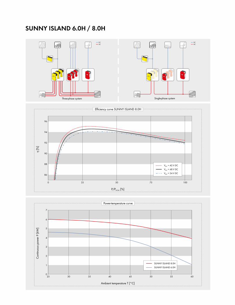
SUNNY ISLAND 6.0H / 8.0H

Three-phasesystem Single-phasesystem

Sunny Island 6.0H

Sunny Island 8.0H

230V/202V...253V50Hz/45Hz...65Hz

4600W6000W/6800W/11000W

3700W20A/120A<4%/-1...+1

230V/172.5V...264.5V50Hz/40Hz...70Hz

50A11500W

48V/41V...63V110A

90A/103AFLA,VRLA/100Ah...10000AhIUoUchargeprocedurewithauto-maticfullchargeandequalization

charge.

96%<26W/<4W

●/●–/–●/●

III

467mmx612mmx242mm63kg

-25°C...+60°CI

3K6IP54

ExternalviaSRC-20/2●/●–/●

●/●/●●/●●/●

www.SMA-Solar.com●

○/○○/○

○○/○

SI6.0H-11

230V/202V...253V50Hz/45Hz...65Hz

6000W8000W/9100W/11000W

5430W26A/120A<4%/-1...+1

230V/172.5V...264.5V50Hz/40Hz...70Hz

50A11500W

48V/41V...63V140A

115A/136AFLA,VRLA/100Ah...10000Ah

IUoUchargeprocedurewithautomaticfullchargeandequalizationcharge

96%<26W/<4W

●/●–/–●/●

III

467mmx612mmx242mm63kg

-25°C...+60°CI

3K6IP54

ExternalviaSRC-20/2●/●–/●

●/●/●●/●●/●

www.SMA-Solar.com●

○/○○/○

○○/○

SI8.0H-11

Ac output (loads / stand-alone grid)Ratedgridvoltage/ACvoltagerangeRatedfrequency/frequencyrange(adjustable)Ratedpower(forUnom/fnom/25°C/cosϕ=1)ACpowerat25°Cfor30min/5min/3secACpowerat45°CRatedcurrent/maximumoutputcurrent(peak)THDoutputvoltage/powerfactorwithratedpowerAc input (pV array, grid or Mc box)Ratedinputvoltage/ACinputvoltagerangeRatedinputfrequency/allowableinputfrequencyrangeMaximumACinputcurrentMaximumACinputpowerBattery Dc inputRatedinputvoltage/DCvoltagerangeMaximumbatterychargingcurrentRatedDCchargingcurrent/DCdischargingcurrentBatterytype/batterycapacity(range)Chargecontrol

Efficiency / self-consumptionMaximumefficiencySelf-consumptionwithoutload/standbyProtective devices (equipment)ACshort-circuit/ACoverloadDCreversepolarityprotection/DCfuseOvertemperature/batterydeepdischargeOvervoltagecategoryasperIEC60664-1general dataDimensions(widthxheightxdepth)PriorityOperatingtemperaturerangeProtectionclassaccordingtoIEC62103ClimaticcategoryaccordingtoIEC60721DegreeofprotectionaccordingtoIEC60529Features / functionOperationanddisplay/multifunctionrelayThree-phasesystems/parallelconnectionIntegratedbypass/multiclusteroperationStateofchargecalculation/fullcharge/equalizationchargeIntegratedsoftstart/generatorsupportBatterytemperaturesensor/datacablesCertificatesandapprovalsWarranty:5yearsAccessoryBatterycable/batteryfuseInterfaceSI-COMSMA(RS485)/SI-SYSCAN(Multicluster)Extendedgeneratorstart“GenMan”Load-sheddingcontactor/batterycurrentmeasurement

Typedesignation

●Standardfeatures○Optionalfeatures—NotavailableDataatnominalconditions

Technical data

Multicluster-Boxes for suNNY islAND 5048M

c-Bo

x-6.

3 / M

c-Bo

x-12

.3 /

Mc-

Box-

36.3

Simila

r to

figur

e

Flexible• Three different power ranges

from 30 kW to 300 kW• Different generators,

PV and load magnitudes

reliable• Automatic bypass for the

generator• Active Anti-Islanding• Reverse current monitoring

Durable• High protection class IP65• 5-year SMA warranty

simple• Integrated AC distribution for

Sunny Island, generator, PV• Integrated load-shedding

contactor

Multicluster Boxes for suNNY islAND 5048 For Easy Set-Up of Stand-Alone and Hybrid SystemsThe Multicluster Boxes for Sunny Island 5048 enable the formation of off-grid and hybrid systems with a capacity of between 30 and 300 kW. As the main AC distribution for the connection of generators and to supply loads of up to 300 kW, between two and 12 three-phase clusters, each consisting of three Sunny Island inverters, can be connected in parallel using the Multi-cluster Box. To simplify installation, all Multicluster Boxes are completely wired and fitted at the factory and have a main connector for PV plants or wind turbine systems. All communication cables required for the installation are included in the delivery.

Multicluster Boxes for suNNY islAND 5048

GeneralPhase numberNominal AC voltageAC voltage range

Nominal AC frequency / rangeReliable grid configurationDimensions (W / H / D)Assembly typeWeightterminals for sunny islandMaximum number of devicesNominal AC power / nominal AC current at 25 °CNominal AC power / nominal AC current at 45 °CAC power (25 °C, 30 minutes)AC power (25 °C, 1 minute)Fusesload connectionNumberNominal AC power (25 °C, unlimited)Nominal AC current (25 °C)FusesPV plant connectionNumberNominal AC power (25 °C, unlimited)Nominal AC current (25 °C)FusesGenerator connectionNumberNominal AC power (25 °C, unlimited)Nominal AC current (25 °C)FusesFeaturesWarranty (5 / 10 / 15 / 20 / 25 years)CertificatesAmbient conditionsAmbient temperatureDegree of protection (according to IEC 60529)HumidityAccessoriesCommunication linesMulticluster Piggy-Back

● Standard features ○ Optional — Not availableType designation

3-phase230 V (L, N), 400 V (L1, L2)

172.5 V – 265 V 300 V – 433 V

50 Hz / 40 Hz … 70 HzTN

760 / 760 / 210 mmSuspended

60 kg

630 kW / 3 x 44 A24 kW / 3 x 35 A

40 kW50 kW

Miniature circuit-breaker C 32A

1 (3-phase)55 kW

3 x 80 ALV / HRC (size 00)

1 (3-phase)55 kW

3 x 80 A—

1 (3-phase)55 kW

3 x 80 ALV / HRC (size 00)

● / ○ / ○ / ○ / ○CE

-25 °C … +50 °CIP65

0 % … 100 %

●○

MC-BOx-6.3

3-phase230 V (L, N), 400 V (L1, L2)

172.5 V – 265 V 300 V – 433 V

50 Hz / 40 Hz … 70 HzTN

1000 / 1400 / 300 mmStanding on base

140 kg

1260 kW / 3 x 87 A48 kW / 3 x 70 A

80 kW100 kW

Miniature circuit-breaker C 32A

1 (3-phase)110 kW

3 x 160 ALV / HRC (size 00)

1 (3-phase)110 kW

3 x 160 A—

1 (3-phase)110 kW

3 x 160 ALV / HRC (size 00)

● / ○ / ○ / ○ / ○CE

-25 °C … +50 °CIP65

0 % … 100 %

●○

MC-BOx-12.3

technical Data suNNY islAND 5048Multicluster Box 6

suNNY islAND 5048Multicluster Box 12

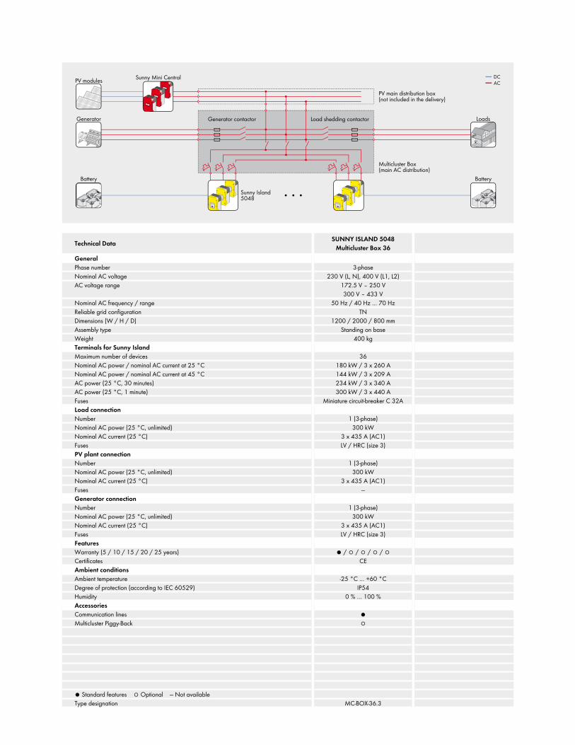
GeneralPhase numberNominal AC voltageAC voltage range

Nominal AC frequency / rangeReliable grid configurationDimensions (W / H / D)Assembly typeWeightterminals for sunny islandMaximum number of devicesNominal AC power / nominal AC current at 25 °CNominal AC power / nominal AC current at 45 °CAC power (25 °C, 30 minutes)AC power (25 °C, 1 minute)Fusesload connectionNumberNominal AC power (25 °C, unlimited)Nominal AC current (25 °C)FusesPV plant connectionNumberNominal AC power (25 °C, unlimited)Nominal AC current (25 °C)FusesGenerator connectionNumberNominal AC power (25 °C, unlimited)Nominal AC current (25 °C)FusesFeaturesWarranty (5 / 10 / 15 / 20 / 25 years)CertificatesAmbient conditionsAmbient temperatureDegree of protection (according to IEC 60529)HumidityAccessoriesCommunication linesMulticluster Piggy-Back

● Standard features ○ Optional — Not availableType designation

3-phase230 V (L, N), 400 V (L1, L2)

172.5 V – 250 V 300 V – 433 V

50 Hz / 40 Hz … 70 HzTN

1200 / 2000 / 800 mmStanding on base

400 kg

36180 kW / 3 x 260 A144 kW / 3 x 209 A234 kW / 3 x 340 A300 kW / 3 x 440 A

Miniature circuit-breaker C 32A

1 (3-phase)300 kW

3 x 435 A (AC1)LV / HRC (size 3)

1 (3-phase)300 kW

3 x 435 A (AC1)—

1 (3-phase)300 kW

3 x 435 A (AC1)LV / HRC (size 3)

● / ○ / ○ / ○ / ○CE

-25 °C … +60 °CIP54

0 % … 100 %

●○

MC-BOx-36.3

technical Data suNNY islAND 5048Multicluster Box 36