trehan1989.pdf - edinburgh research archive

This thesis has been submitted in fulfilment of the requirements for a postgraduate degree

(e.g. PhD, MPhil, DClinPsychol) at the University of Edinburgh. Please note the following

terms and conditions of use:

• This work is protected by copyright and other intellectual property rights, which are

retained by the thesis author, unless otherwise stated.

• A copy can be downloaded for personal non-commercial research or study, without

prior permission or charge.

• This thesis cannot be reproduced or quoted extensively from without first obtaining

permission in writing from the author.

• The content must not be changed in any way or sold commercially in any format or

medium without the formal permission of the author.

• When referring to this work, full bibliographic details including the author, title,

awarding institution and date of the thesis must be given.

An investigation of

design and execution alternatives

for the

Committed Choice Non-Deterministic

Logic languages

Rajiv Trehan

Ph.D.

Department of Artificial Intelligence

University of Edinburgh

1989

Abstract

The general area of developing, applying and studying new and parallel models

of computation is motivated by a need to overcome the limits of current Von

Neumann based architectures. A key area of research in understanding how new

technology can be applied to Al problem solving is through using logic languages.

Logic programming languages provide a procedural interpretation for sentences of

first order logic, mainly using a class of sentence called Horn clauses. Horn clauses

are open to a wide variety of parallel evaluation models, giving possible speed-ups

and alternative parallel models of execution.

The research in this thesis is concerned with investigating one class of parallel

logic language known as Committed Choice Non-Deterministic languages. The in-

vestigation considers the inherent parallel behaviour of Al programs implemented

in the CCND languages and the effect of various alternatives open to language

implementors and designers. This is achieved by considering how various Al pro-

gramming techniques map to alternative language designs and the behaviour of

these Al programs on alternative implementations of these languages.

The aim of this work is to investigate how Al programming techniques are

affected (qualitatively and quantitatively) by particular language features. The

qualitative evaluation is a consideration of how Al programs can be mapped to

the various CCND languages. The applications considered are general search

algorithms (which focuses on the committed choice nature of the languages); chart

parsing (which focuses on the differences between safe and unsafe languages);

and meta-level inference (which focuses on the difference between deep and flat

languages). The quantitative evaluation considers the inherent parallel behaviour

of the resulting programs and the effect of possible implementation alternatives

on this inherent behaviour. To carry out this quantitative evaluation we have

implemented a system which improves on the current interpreter based evaluation

systems. The new system has an improved model of execution and allows several

i

Acknowledgements

To my supervisors, Paul Wilk and Chris Mellish, I offer my thanks and apprecia-

tion. Their guidance, insight and understanding of the area has helped to mould

and motivate this work.

Thanks also go to: Robert Scott for his comments and discussion on much

of this work; Richard Tobin for his miracle 'C' programming (over a weekend he

implemented a garbage collector for Edinburgh Prolog); Gail Anderson, Richard

Baker, Eleanor Bradley, Andrew Hamilton, Bert Hutchings, Roberto Desimone,

Tim Duncan, Jan Newmarch, Henry Pinto, Brian Ross and Peter Ross for provid-

ing a stimulating and enjoyable environment in which to work.

This work was possible due to funding from Science and Engineering Research

Council - in the form of a studentship and the computing resources made avail-

able by the Artificial Intelligence Applications Institute and the Department of

Artificial Intelligence.

Finally, my warmest appreciation goes to my family and friends.

ill

Meejoo

iv

Table of Contents

1. Introduction 1

1.1 Thesis outline . . . . . . . . . . . . . . . . . . . . . . . . . . . . . . 3

I Committed Choice Non-Deterministic languages 5

Preface 6

2. The Languages 7

2.1 Overview . . . . . . . . . . . . . . . . . . . . . . . . . . . . . . . . . 7

2.2 Logic as a programming language . . . . . . . . . . . . . . . . . . . 8

2.2.1 Syntax of Horn clauses . . . . . . . . . . . . . . . . . . . . . 8

2.2.2 Semantics of Horn clauses . . . . . . . . . . . . . . . . . . . 9

2.2.3 Prolog . . . . . . . . . . . . . . . . . . . . . . . . . . . . . . 11

2.3 Parallelism in logic programming . . . . . . . . . . . . . . . . . . . 12

2.3.1 All-solutions AND-parallelism . . . . . . . . . . . . . . . . . 12

2.3.2 OR-parallelism . . . . . . . . . . . . . . . . . . . . . . . . . 14

2.3.3 Restricted AND-parallelism . . . . . . . . . . . . . . . . . . 14

2.3.4 Streamed AND-parallelism . . . . . . . . . . . . . . . . . . . 15

2.3.5 Implicit/Explicit parallel languages . . . . . . . . . . . . . . 17

2.4 Committed Choice Non-Deterministic languages . . . . . . . . . . . 19

2.4.1 Syntax of guarded horn clauses . . . . . . . . . . . . . . . . 19

2.4.2 Semantics of guarded horn clauses . . . . . . . . . . . . . . . 20

2.4.3 Concurrent Prolog (CP) . . . . . . . . . . . . . . . . . . . . 21

2.4.4 Parlog . . . . . . . . . . . . . . . . . . . . . . . . . . . . . . 23

v

2.4.5 Guarded Horn Clauses (GHC) . . . . . . . . . . . . . . . . . 26

2.4.6 An example of a CCND program, and its evaluation . . . . . 27

2.5 Classifications . . . . . . . . . . . . . . . . . . . . . . . . . . . . . . 34

2.5.1 Safe/Unsafe . . . . . . . . . . . . . . . . . . . . . . . . . . . 34

2.5.2 Deep/Flat . . . . . . . . . . . . . . . . . . . . . . . . . . . . 35

2.6 Implementations . . . . . . . . . . . . . . . . . . . . . . . . . . . . 35

2.6.1 Interpreters . . . . . . . . . . . . . . . . . . . . . . . . . . . 36

2.6.2 Abstract machine emulators . . . . . . . . . . . . . . . . . . 43

2.6.3 Multi-processor implementations . . . . . . . . . . . . . . . 44

2.7 Summary . . . . . . . . . . . . . . . . . . . . . . . . . . . . . . . . 45

II An evaluation system 46

Preface 47

3. Interpreters for evaluation 48

3.1 Overview . . . . . . . . . . . . . . . . . . . . . . . . . . . . . . . . . 48

3.2 Current evaluation systems . . . . . . . . . . . . . . . . . . . . . . . 49

3.3 Current measurements and their limitations . . . . . . . . . . . . . 53

3.3.1 Cycles . . . . . . . . . . . . . . . . . . . . . . . . . . . . . . 53

3.3.2 Reductions . . . . . . . . . . . . . . . . . . . . . . . . . . . 55

3.3.3 Suspensions . . . . . . . . . . . . . . . . . . . . . . . . . . . 56

3.4 Requirements of an improved model . . . . . . . . . . . . . . . . . . 57

3.5 Idealisations in our improved model . . . . . . . . . . . . . . . . . . 59

3.5.1 AND-parallel idealisations . . . . . . . . . . . . . . . . . . . 59

3.5.2 Guard evaluation idealisations . . . . . . . . . . . . . . . . . 60

3.5.3 OR-parallel idealisations . . . . . . . . . . . . . . . . . . . . 61

3.5.4 System call idealisations . . . . . . . . . . . . . . . . . . . . 61

3.6 Development of our improved model . . . . . . . . . . . . . . .. . 62

3.6.1 Suspension/Failure . . . . . . . . . . . . . . . . . . . . . . . 62

3.6.2 Depth (cycles) .. .... . .. .... .. .. . .. .. .. .. 67

vi

3.6.3 AND-parallelism . . . . . .. . . . . .. . . . . . . . . . .. 71

3.6.4 OR-parallelism .. . . . . . .. . . . .. . . . .. .. . . .. 73

3.6.5 Features of our improved model . . . . . . . . . . . . . . . . 75

3.7 Summary . . . . . . . . . . . . . . . . . . . . . . . . . . . . . . . . 76

4. New evaluation parameters and example evaluations 77

4.1 Overview . . . . . . . . . . . . . . . . . . . . . . . . . . . . . . . . . 77

4.2 Basis for new parameters . . . . . . . . . . . . . . . . . . . . . . . . 78

4.2.1 Pruning OR-branches . . . . . . . . . . . . . . . . . . . . . . 79

4.2.2 Suspension mechanisms . . . . . . . . . . . . . . . . . . . . 80

4.2.3 Scheduling policy . . . . . . . . . . . . . . . . . . . . . . . . 81

4.3 Proposed profiling parameters . . . . . . . . . . . . . . . . . . . . . 81

4.3.1 Busy waiting, non-pruning, goal suspension . . . . . . . . . 83

4.3.2 Non-busy waiting, pruning, clause suspension . . . . . . . . 85

4.3.3 Depth of evaluation . . . . . . . . . . . . . . . . . . . . . . . 86

4.3.4 Minimum reductions . . . . . . . . . . . . . . . . . . . . . . 87

4.4 Profile tool . . . . . . .. . . . . . . . .. . . . . .. . . . . . . . . 88

4.5 Example executions and measurements . . . . . . . . . . . . . . . . 91

4.5.1 List member check . . . . . . . . . . . . . . . . . . . . . . . 92

4.5.2 Parallel list member checks . . . . . . . . . . . . . . . . . . . 94

4.5.3 Quick-sort . . . . . . . . . . . . . . . . . . . . . . . . . . . . 98

4.5.4 Iso-tree . . . . . . . . . . . . . . . . . . . . . . . . . . . . . 106

4.5.5 Prime number generation by sifting . . . . . . . . . . . . . . 111

4.6 Limitations of the new measurements . . . . . . . . . . . . . . . . . 116

4.7 Summary . . . . . . . . . . . . . . . . . . . . . . . . . . . . . . . . 119

III Example AI programs and their evaluation 120

Preface 121

vii

5. Search - committed choice 123

5.1 Overview . . . . . . . . . . . . . . . . . . . . . . . . . . . . . . . . . 123

5.2 Search . . . . . . . . . . . . . . . . . . . . . . . . . . . . . . . . . . 124

5.2.1 Don't care non-determinism . . . . . . . . . . . . . . . . . . 124

5.2.2 Don't know non-determinism . . . . . . . . . . . . . . . . . . 125

5.2.3 Generate and test non-determinism . . . . . . . . . . . . . . 127

5.2.4 Summary . . . . . . . . . . . . . . . . . . . . . . . . . . . . 129

5.3 Continuation based compilation . . . . . . . . . . . . . . . . . . . . 132

5.4 Stream based compilation . . . . . . . . . . . . . . . . . . . . . . . 135

5.5 Layered Streams . . . . . . . . . . . . . . . . . . . . . . . . . . . . 138

5.6 Previous analysis . . . . . . . . . . . . . . . . . . . . . . . . . . . . 142

5.7 Results and new analysis . . . . . . . . . . . . . . . . . . . . . . . . 143

5.8 Synopsis of analysis . . . . . . . . . . . . . . . . . . . . . . . . . . . 154

5.9 Summary . . . . . . . . . . . . . . . . . . . . . . . . . . . . . . . . 156

6. Shared data structures - safe/unsafe 157

6.1 Overview . . . . . . . . . . . . . . . . . . . . . . . . . . . . . . . . 157

6.2 Shared Data . . . . . . . . . . . . . . . . . . . . . . . . . . . . . . . 159

6.3 Support for Shared Data Structures . . . . . . . . . . . . . . . . . . 161

6.3.1 Unsafe . . . . . .. . .. . . ... . .. . .. . .. .. . . . 162

6.3.2 Safe . .. . . .. . . .. .. . . . . . . .. .. .. . .. . .. 163

6.3.3 Safe+System Streams . . . . . . . . . . . . . . . . . . . . 166

6.4 Chart Parsing: an overview . . . . . . . . . . . . . . . . . . . . . . 169

6.4.1 Sequential chart parsing . . . . . . . . . . . . . . . . . . . . 169

6.4.2 Parallel chart parser . . . . . . . . . . . . . . . . . . . . . . 170

6.5 Parallel Chart Parsers for the CCND languages . . . . . . . . . . . 171

6.5.1 Unsafe Chart Parser . . . . . . . . . . . . . . . . . . . . . . 171

6.5.2 Safe Chart Parser . . . . . . . . . . . . . . . . . . . . . . . 173

6.5.3 Safe+System Streams Chart Parser . . . . . . . . . . . . 175

6.6 Results and analysis . . . . . . . . . . . . . . . . . . . . . . . . . . 176


6.8 Summary . . . . . . . . . . . . . . . . . . . . . . . . . . . . . . . . 194

viii

7. Meta-level inference - deep/flat 195

7.1 Overview . . . . . . . . . . . . . . . . . . . . . . . . . . . . . . . . . 195

7.2 PRESS ..................................196 7.2.1 Prolog . .. .. .. ... .. . . .. .. .. . . .. .. . . .. 197

7.3 Using deep guards . . . . . . . . . . . . . . . . . . . . . . . . . . . 198

7.4 Using flat guards . . . . . . . . . . . . . . . . . . . . . . . . . . . . 201

7.4.1 Guard continuation - mutual exclusion semaphore . . . . . . 201

7.4.2 If-then-else . .... . . .. . .. . . .. . . . . .. . .. .. 203

7.4.3 Rewriting . . . . . . . . . . . . . . . . . . . . . . . . . . . . 204

7.4.4 Guard continuation - monitor goal . . . . . . . . . . . . . . 205

7.5 Programs evaluated . . . . . . . . . . . . . . . . . . . . . . . . . . . 209

7.6 Previous analysis . . . . . . . . . . . . . . . . . . . . . . . . . . . . 211

7.7 Results and new analysis . . . . . . . . . . . . . . . . . . . . . . . . 213


7.9 Summary . . . . . . . . . . . . . . . . . . . . . . . . . . . . . . . . 232

8. Conclusions 234

8.1 Overall Contribution of the Thesis . . . . . . . . . . . . . . . . . . 234

8.1.1 Inherent parallelism . . . . . . . . . . . . . . . . . . . . . . . 235

8.1.2 Search - committed choice . . . . . . . . . . . . . . . . . . . 236

8.1.3 Shared data structures - safe/unsafe . . . . . . . . . . . . . . 237

8.1.4 Meta-level inference - deep/flat . . . . . . . . . . . . . . . . 240

8.1.5 Summary of Contribution . . . . . . . . . . . . . . . . . . . 241

8.2 Research assumptions . . . . . . . . . . . . . . . . . . . . . . . . . . 243

8.2.1 The evaluation system . . . . . . . . . . . . . . . . . . . . . 243

8.2.2 The applications . . . . . . . . . . . . . . . . . . . . . . . . 245

8.2.3 The evaluations . . . . . . . . . . . . . . . . . . . . . . . . . 245

8.2.4 The approach . . . . . . . . . . . . . . . . . . . . . . . . . . 246

8.3 Future work . . . . . . . . . . . . . . . . . . . . . . . . . . . . . . . 247

References 249

ix

N Appendices 262

A. Effect of alternative execution models 263

A.1 Busy waiting, non-pruning, goal suspension . . . . . . . . . . . . . . 263

A.2 Busy waiting, non-pruning, clause suspension . . . . . . . . . . . . 265

A.3 Busy waiting, pruning, goal suspension . . . . . . . . . . . . . . . . 267

A.4 Busy waiting, pruning, clause suspension . . . . . . . . . . . . . . . 268

A.5 Non-busy waiting, non-pruning, goal suspension . . . . . . . . . . . 269

A.6 Non-busy waiting, non-pruning, clause suspension . . . . . . . . . . 270

A.7 Non-busy waiting, pruning, goal suspension . . . . . . . . . . . . . 271

A.8 Non-busy waiting, pruning, clause suspension . . . . . . . . . . . . 272

x

List of Figures

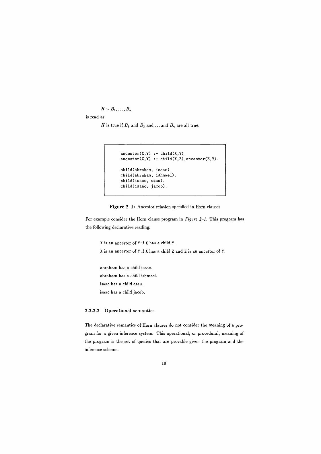
2-1 Ancestor relation specified in Horn clauses . . . . . . . . . . . . . . 10

2-2 A simple Horn clause program . . . . . . . . . . . . . . . . . . . . . 13

2-3 Searching down two lists in parallel . . . . . . . . . . . . . . . . . . 15

2-4 An example of Streamed AND-parallelism . . . . . . . . . . . . 16

2-5 Possible use of the "." and ";" operators in Parlog . . . . . . . . . 24

2-6 Quick-sort program in Concurrent Prolog . . . . . . . . . . . . . . . 28

2-7 Quick-sort program in Parlog . . . . . . . . . . . . . . . . . . . . . 29

2-8 Quick-sort program in GHC . . . . . . . . . . . . . . . . . . . . . . 30

2-9 An interpreter for Prolog in Prolog . . . . . . . . . . . . . . . . . . 36

2-10 An interpreter for counting resolutions in Prolog . . . . . . . . . . . 38

2-11 An interpreter for counting procedure calls in Prolog . . . . . . . . 39

2-12 An interpreter for breadth-first evaluation of Horn clauses . . . . . 40

2-13 Execution of imperative languages . . . . . . . . . . . . . . . . . . . 43

2-14 Execution of logic languages . . . . . . . . . . . . . . . . . . . . . . 43

3-1 A basic Parlog interpreter in Prolog . . . . . . . . . . . . . . . . . . 51

3-2 Mode based unification for PARLOG in Prolog . . . . . . . . . . . 52

3-3 Member check in Parlog . . . . . . . . . . . . . . . . . . . . . . . . 54

3-4 Simple example program for suspensions . . . . . . . . . . . . . . . 54

3-5 Two argument call for a suspend/fail Parlog interpreter . . . . . . . 63

3-6 A suspend/fail Parlog interpreter in Prolog . . . . . . . . . . . . . . 64

3-7 Mode based unification for suspend/fail PARLOG interpreter . . . 65

3-8 Simple clause selection for suspend/fail PARLOG interpreter . . . . 67

3-9 Two argument top-level cycle counting Parlog interpreter . . . . . . 68

xi

3-10 Three argument call for Parlog in Prolog . . . . . . . . . . . . . . . 69

3-11 Parlog interpreter with a bindings and commitments queue . . . . . 72

3-12 Binding/commitments processing for Parlog interpreter . . . . . . . 73

3-13 Modelling parallel clause selection in a interpreter . . . . . . . . . . 74

4-1 Parallel member test in Parlog . . . . . . . . . . . . . . . . . . . . . 82

4-2 An example of an interactive profile tool to analyse program execution 91

4-3 Schematic of member/2 evaluation on the original Parlog interpreter 92

4-4 Schematic of member/2 evaluation on our new system . . . . . . . . 93

4-5 List member check reductions . . . . . . . . . . . . . . . . . . . . 94

4-6 Schematic of one ither/4 evaluation on the original Parlog interpreter 95

4-7 Schematic of oneither/4 evaluation on our new system . . . . . . . 96

4-8 Parallel list member check (pruned and non-pruned reductions) . 97

4-9 Quick-sorting an ordered list (goal and clause suspensions) . . . . 100

4-10 Quick-sorting an ordered list (busy and non-busy suspensions) . . 101

4-11 Quick-sorting an ordered list (reductions and suspensions) . . . 102

4-12 Quick-sorting an unordered list (goal and clause suspensions) . . . 103

4-13 Quick-sorting an unordered list (busy and non-busy suspensions) 104

4-14 Quick-sorting an unordered list (reductions and suspensions) . . 105

4-15 Isomorphism algorithm expressed in a CCND language (Parlog) . . 106

4-16 Iso-tree examples . . . . . . . . . . . . . . . . . . . . . . . . . . . . 107

4-17 Iso-tree evaluation example 1 (reductions) . . . . . . . . . . . . . 108



4-20 Prime number generation by sifting . . . . . . . . . . . . . . . . . . 111

4-21 Prime numbers up to 50 (busy and non-busy suspensions) . . . . 112

4-22 Prime numbers up to 500 (busy and non-busy suspensions) . . . . 113

5-1 Unordered combination of two lists in Horn clauses . . . . . . . . . 125

5-2 Isomorphic tree program expressed in Horn clauses . . . . . . . . . 126

5-3 Isomorphism algorithm expressed in a CCND language (Parlog) . . 127

xii

5-4 Generate and test algorithm expressed in Horn clauses . . . . . . . 128

5-5 Generate and test algorithm nearly implemented in Parlog . . . . . 129

5-6 4-queens problem in Horn clauses . . . . . . . . . . . . . . . . . . . 131

5-7 Mode analysis of sel/2 . . . . . . . . . . . . . . . . . . . . . . . . . 132

5-8 Normal form of sel/2 . . . . . . . . . . . . . . . . . . . . . . . . . 132

5-9 sel/2 - translated using Continuation based compilation . . . . . . 133

5-10 4-queens implemented using Continuation based compilation . . . . 134

5-11 sel/2 - translated using Stream based compilation . . . . . . . . . 136

5-12 4-queens implemented using Stream based compilation . . . . . . . 137

5-13 4-queens implemented using Layered Streams . . . . . . . . . . . . 139

5-14 Profile of 6-queens using Continuation based compilation . . . . . . 144

5-15 Profile of 6-queens using Stream based compilation . . . . . . . . . 145

5-16 Profile of 6-queens using Stream based compilation . . . . . . . . . 146

5-17 Profile of 6-queens using Layered Streams . . . . . . . . . . . . . . 147



6-1 Use of merge processes to support multiple writers to a stream . . . 160

6-2 Predicate to merge two streams into one . . . . . . . . . . . . . . . 161

6-3 An unsafe predicate to add an element to an ordered binary tree . 162

6-4 Manager process for a binary tree . . . . . . . . . . . . . . . . . . . 164

6-5 A perpetual process which generates a stream of random integers . 165

6-6 A perpetual process which uses proposed stream primitives . . . . . 167

6-7 Unsafe predicate to support an AET based on a stream . . . . . . 172

6-8 Top-down activation process for an unsafe language . . . . . . . . . 172

6-9 Safe predicate to support a manager for an AET based on a stream 174

6-10 Top-down activation process for a safe language . . . . . . . . . . . 174

6-11 Top-down activation process making use of system streams . . . . 175

6-12 Profile of a top-down unsafe chart parser . . . . . . . . . . . . . . 178



xiii

6-15 Profile of a top-down safe chart parser . . . . . . . . . . . . . . .



6-18 Profile of a top-down safe+system streams chart parser . . . .



6-21 Profile of a bottom-up unsafe chart parser . . . . . . . . . . . . .

6-22 Profile of a bottom-up safe chart parser . . . . . . . . . . . . . .

6-23 Profile of a bottom-up safe+system streams chart parser . . .

. 179

. 180

. 180

. 181

. 181

. 182

. 182

. 183

. 183

7-1 Meta-level of PRESS in Prolog . .. .. .. .. .. .. .. .. .. . 198

7-2 Meta-level of PRESS using deep guards . . . . . . . . . . . . . . . 200

7-3 Meta-level of PRESS using flat guards-mutual exclusion variable . . 202

7-4 parse/3 using deep guards . . . . . . . . . . . . . . . . . . . . . . 203

7-5 Flattened clauses of parse/3 . . . . . . . . . . . . . . . . . . . . . 204

7-6 remove-duplicates/2 using deep guards . . . . . . . . . . . . . . 205

7-7 remove-duplicates/2 using flat guards . . . . . . . . . . . . . . . 206

7-8 Meta-level of PRESS using flat guards-monitor goal (nonterminating)207

7-9 Meta-level of PRESS using flat guards-monitor goal (terminating) . 208

7-10 Profile of PRESS1 using deep guards . . . . . . . . . .

7-11 Profile of PRESS1 using (non-terminating) flat guards

7-12 Profile of PRESS1 using (terminating) flat guards . . .

7-13 Profile of PRESS2 using deep guards . . . . . . . . . .



7-16 Profile of PRESS3 using deep guards . . .. .. . . . .



. . . . . . . 214

. . . . . . . 215

. . . . . . . 215

. . . . . . . 216

. . . . . . . 216

. . . . . . . 217

. .. .. .. 217

. . . . . . . 218

. . . . . . . 218

xiv

List of Tables

4-1 Predicted results for example query . . . . . . . . . . . . . . . . . . 83

4-2 Example of degree of OR-parallelism . . . . . . . . . . . . . . . . . 88

4-3 Summary of previous measurements for example programs . . . . . 114

4-4 Summary of new reduction parameters for example programs . . . . 114

4-5 Summary of new suspension parameters for example programs . . . 115

4-6 Results collected for example query . . . . . . . . . . . . . . . . . . 118

5-1 Summary of previous measurements for All-solutions programs . . . 142

5-2 Summary of reduction parameters for All-solutions programs . . . . 143

5-3 Summary of suspension parameters for All-solutions programs . . . 143

5-4 Comparison of previous and new reduction measures . . . . . . . . 144

5-5 Comparing previous and new suspension measures . . . . . . . . . . 147

5-6 Comparing previous and new measures for average parallelism . . . 148

5-7 Degree of OR-parallelism for All-solutions programs . . . . . . . . . 150

5-8 Maximum reductions in a given cycle for All-solutions programs . . 150

5-9 Maximum suspensions in a given cycle for All-solutions Programs . 151

5-10 Goal/Clause suspension ratios for All-solutions programs . . . . . 151

5-11 Busy/Non-busy suspension ratios for All-solutions programs . . . 153

6-1 Summary of reduction parameters for the various chart parsers . . . 177

6-2 Summary of suspension parameters for the various chart parsers . . 177

6-3 Degree of OR-parallelism for the various chart parsers . . . . . . . . 184

6-4 Maximum reductions in a given cycle for the various chart parsers . 185

6-5 Maximum suspensions in a given cycle for the various chart parsers 186

xv

6-6 Clause/Goal suspension ratios for the various chart parsers . . . . 186

6-7 Busy/Non-busy suspension ratios for the various chart parsers . . 188

6-8 Average parallelism for the various chart parsers . . . . . . . . . . . 190

7-1 Summary of our reconstructed previous measurements for Parallel PRESSes .................................211

7-2 Summary of reduction parameters for Parallel PRESSes . . . . . . . 213

7-3 Summary of suspension parameters for Parallel PRESSes . . . . . . 214

7-4 Comparing previous and new reduction measures . . . . . . . . . . 219

7-5 Comparing previous and new suspension measures . . . . . . . . . . 220

7-6 Comparing previous and new measures for average parallelism . . . 221

7-7 Comparing pruned and non-pruned reductions for DeepPAR- PRESS ..................................223

7-8 Comparing reductions: deep non-pruning and flat-nonterm . . . . 224

7-9 Comparing reductions: deep pruning and flat terminating . . . . . 225

7-10 Comparing suspensions: deep non-pruning and flat-nonterm . . . . 225

7-11 Comparing suspensions: deep pruning and flat terminating . . . . 225

7-12 Degree of OR-parallelism for Parallel PRESSes . . . . . . . . . . . . 226

7-13 Maximum reductions in a given cycle for Parallel PRESSes . . . . . 227

7-14 Maximum suspensions in a given cycle for Parallel PRESSes . . . . 228

7-15 Clause/Goal suspension ratios for Parallel PRESSes . . . . . . . . 229

7-16 Busy/Non-busy suspension ratios for Parallel PRESSes . . . . . . 230

xvi

Chapter 1

Introduction

Artificial Intelligence (AI) by its nature is a multi-disciplined field bringing to-

gether subject areas such as Philosophy; Natural Language; Vision; Robotics;

Logic; Computer Science; Engineering and Physics. The main tool of the Artifi-

cial Intelligence researcher has been the digital computer, enabling theory to be

put into practice.

Currently most digital computers are based on the Von Neumann architecture;

a single central processing unit with a small amount of memory and a large amount

of separate memory (which holds the data and the program). The limits of such

computers are widely recognised: the speed of a signal in a wire; the physical

limits of integration; heat dissipation and memory accessing.

The development of new architectures with several processing and memory

units and new models of computation promises to alleviate some of these limita-

tions. There are two clear implications for Artificial Intelligence: increased exe-

cution speed and more natural decomposition of applications. An improvement

in execution speed results in models and applications being tested that would not

have been feasible on previous generations of computers, e.g. the use of AI in

embedded real-time systems, which are time critical. More natural decomposition

may be possible as many problems are parallel rather than sequential and so are

better thought of in terms of a parallel rather than a sequential framework. For

1

example, being able to parse a string and build a semantic structure as well as

refer to a world model in an incremental fashion requires control over how these

parts execute and interlink. Implementing such a model in a sequential frame-

work requires the programmer to consider how to mimic the parallel execution

and control required. This adds an additional level of conceptual complexity to

the problem when realising the solution as a program.

A key area of research in understanding how this new technology can be

applied to Al problem solving is through using logic languages. The Japanese

Fifth Generation Computer Systems (FGCS) project uses logic programming as

the link between information processing and parallel architectures [Uchida 82].

Logic programming languages provide a procedural interpretation for sentences

of first order logic, mainly using a class of sentence called Horn clauses. The

first and most widely used of the family of Horn clause based languages is Prolog

[Clocksin & Mellish 81], [Sterling & Shapiro 86]. Prolog currently provides a se-

quential means of evaluating Horn clause based programs. This sequential search

efficiently realised in a stack based implementation [Warren 83] gives in excess of

100,000 Logical inferences per second (Lips). However, Horn clauses are open to

a wide variety of parallel evaluation models, giving possible speed-ups and alter-

native parallel models of execution.

The research in this thesis is concerned with investigating one class of paral-

lel logic language known as Committed Choice Non-Deterministic (CCND) lan-

guages. The investigation considers the inherent parallel behaviour of Al programs

implemented in the CCND languages and the effect of various alternatives open

to language implementors and designers. This is achieved by considering how

various AI programming techniques map to alternative language designs and the

behaviour of these Al programs on alternative implementations of these languages.

The aim of this work is to evaluate some of the design and execution alterna-

tives open in the development of these languages, in the light of Al requirements.

While choices have been made as to the direction that the languages should take,

2

the choices to date appear to be motivated by implementation or historical reason-

ing rather than a rational study of how the alternatives will affect the use of these

languages and realisable parallelism. This work is a study of alternative language

designs and execution models.

1.1 Thesis outline

The thesis is structured into three main parts:

In part 1 we provide a review of the field of parallel logic programming.

In part 2 we develop an evaluation system for the CCND languages.

In part 3 we evaluate three distinct classes of AI program.

The chapter structure is as follows:

Chapter 2 serves as an introduction to sequential and parallel logic program-

ming, in particular the CCND languages, introducing basic concepts and technol-

ogy. The chapter also considers how the languages are modelled by interpretation

and how these interpretation systems can be instrumented.

Chapter 3 considers how the inherent parallelism available in the evaluation

of programs implemented in the CCND languages can be measured. The chap-

ter initially highlights the limitations of current evaluation systems and then in-

crementally develops an improved model for obtaining measures of the inherent

parallelism.

Chapter 4 considers some of the alternatives open to language implementors.

We also propose some new evaluation parameters that reflect the expected be-

haviour of programs in the alternative models of execution. Finally, we develop a

profiling tool, which is described by considering some simple programs.

3

Chapter 5 is the first of the evaluation chapters. In this chapter we consider

the behaviour of the various techniques for offering exhaustive search in the CCND

languages, namely: Continuation based compilation; Stream based compilation;

and Layered Streams. The techniques considered have been evaluated before and

so we are able to compare our new evaluation with this previous evaluation.

Chapter 6 evaluates how shared data structures can be supported in the CCND

languages. The main feature being investigated here is the differences between

using safe and unsafe languages. The question of how shared data structures

are supported in the CCND languages is an important one for Al. Several current

AI paradigms which require several different forms of expertise, like blackboard

systems, require a common communication medium which each expert can see and

update. The various CCND languages require different programming techniques

to support shared data structures, so this evaluation also serves to highlight and

compare the differing language features. We use a well known natural language

processing technique known as chart parsing as an application which makes use

of shared data.

Chapter 7 focuses on another variation in the possible styles of CCND lan-

guage being proposed, namely: the difference in using deep and flat languages.

The first style of language appears to be more expressive, or at least more high

level, whilst the second, a subset of the first, is more likely to be efficiently imple-

mented. One solution to this problem is to develop algorithms using the complete

languages and then translate them to the executable subset. However, there are

several alternative translations that can be employed. We use a program, known

as PRESS - PRolog Equation Solving System, which naturally maps to the full

CCND languages to evaluate and compare the behaviour of programs implemented

using the complete language and the alternative translations to the more efficiently

implementable subset.

Finally, in chapter 8 we draw some conclusions on our work, comment on the

research assumptions and highlight some areas of future work.

4

Part I

Committed Choice

Non-Deterministic languages

5

Preface

This part of the thesis is a review of the field. The review consists of one chapter

with three main focuses:

to show how logic can be used as a programming language and how programs

specified in logic are open to both sequential and parallel evaluation models;

to introduce a class of parallel logic programming language, known as Com-

mitted Choice Non-Deterministic languages, which we intend to evaluate in

this thesis; and

to consider the implementations of these languages for evaluation purposes,

in particular via interpretation, as this is the method employed in the eval-

uation system we develop.

6

Chapter 2

The Languages

2.1 Overview

This chapter is a review of the field of parallel logic programming. The review aims

to show how logic can be used as a programming language; how logic programs can

be evaluated in a sequential or parallel fashion; the parallel computation model

employed for the Committed Choice Non-Deterministic (CCND) languages (the

class of language evaluated in this thesis); the execution of these CCND languages

via interpretation (as this is the technique employed in our evaluation system).

Section 2.2 considers how logic can be used as a programming language and

how such logic programs are open to a sequential evaluation model.

Section 2.3 considers several parallel execution models that can be employed

in the evaluation of logic based programs.

Section 2.4 introduces the three main CCND languages, namely Concurrent

Prolog, Parlog and Guarded Horn Clauses.

Section 2.5 presents two general classifications of the language features of these

CCND languages. The classifications are used in our evaluation of how various AI

programming techniques map to these languages.

7

Section 2.6 reviews current implementations of these languages, in particular

the execution of these languages using interpreters which is how we implement our

evaluation system.

2.2 Logic as a programming language

Logic provides a language of formal description. The earliest logic was syllogis-

tic logic which was the main tool of philosophers and logicians up to the nine-

teenth century. The limitations of syllogistic logic were addressed by the advent

of propositional logic, followed by a more general logic known as predicate

logic. The automated proofs of problems stated in both propositional logic

and predicate logic have been of considerable interest. Consideration of efficient

automated proof procedures has resulted in a subset of predicate logic known

as Horn clauses being adopted as one of the main logic languages for automated

proofs. The automated proof of a logical specification allows us to consider logic

as a programming language.

2.2.1 Syntax of Horn clauses

A Horn clause program is a finite set of clauses of the form:

H :- B1,...,B,, (n > 0)

H is known as the clause head and Bl,... , B,, is known as the clause body.

The clause head is an atom of the form:

R(al,... , ak) (k > 0)

R is the relation, or predicate, name and a1,... , ak are the arguments. The

relation is said to be of arity k. Each of the elements of the clause body, B1, ... , B,,

are literals. These literals are either atoms or negated atoms, of the form:

8

-'R(al,...,ak) (k> 0)

Each argument is either a variable, a constant or a structure; these are

collectively known as terms. The convention used in this thesis is that variables

will be unquoted alphanumerics beginning with an upper-case letter, e.g. X, Foo

and BaZ12. Structures are of the form:

F(tl,... , t=) (i > 1)

where F is known as the functor and t1, ... , t, are known as the arguments, which

are also terms, e.g. foo(a,b,c), bazl2(X,Y) and foo(a,bazl2(X,Y)). Constants

are either numbers, alphanumerics beginning with a lower-case letter or a term

containing no variables.

Lists are one of the most common types of structure used in Horn clause

programs. Lists have a reserved functor, namely ".", e.g. . (a, . (b, . (c,nil)) ) is a three element list. For convenience, lists also have a more readable syntax.

This syntax is based around a list being viewed as the first element of the list (the

head), say h, and the rest of the list (the tail), say t. So a list could be denoted

as [h It]. Using this syntax the above list becomes El 1 [2 I E31 [1111. This is still

further simplified to [1 , 2 , 3] .

A general query in a Horn clauses language has the following form:

.- C1,C2,...,Cn

each of the Ci is called a goal.

2.2.2 Semantics of Horn clauses

2.2.2.1 Declarative semantics

A Horn clause program has a declarative reading based on each of its clauses.

Each clause:

9

H :- B1,...,B,,

is read as:

H is true if B, and B2 and ... and B,, are all true.

ancestor(X,Y) :- child(X,Y).

ancestor(X,Y) :- child(X,Z),ancestor(Z,Y).

child(abraham, isaac). child(abraham, ishmael). child(isaac, esau). child(isaac, jacob).

Figure 2-1: Ancestor relation specified in Horn clauses

For example consider the Horn clause program in Figure 2-1. This program has

the following declarative reading:

X is an ancestor of Y if X has a child Y.

X is an ancestor of Y if X has a child Z and Z is an ancestor of Y.

abraham has a child isaac.

abraham has a child ishmael.

isaac has a child esau.

isaac has a child jacob.

2.2.2.2 Operational semantics

The declarative semantics of Horn clauses do not consider the meaning of a pro-

gram for a given inference system. This operational, or procedural, meaning of

the program is the set of queries that are provable given the program and the

inference scheme.

10

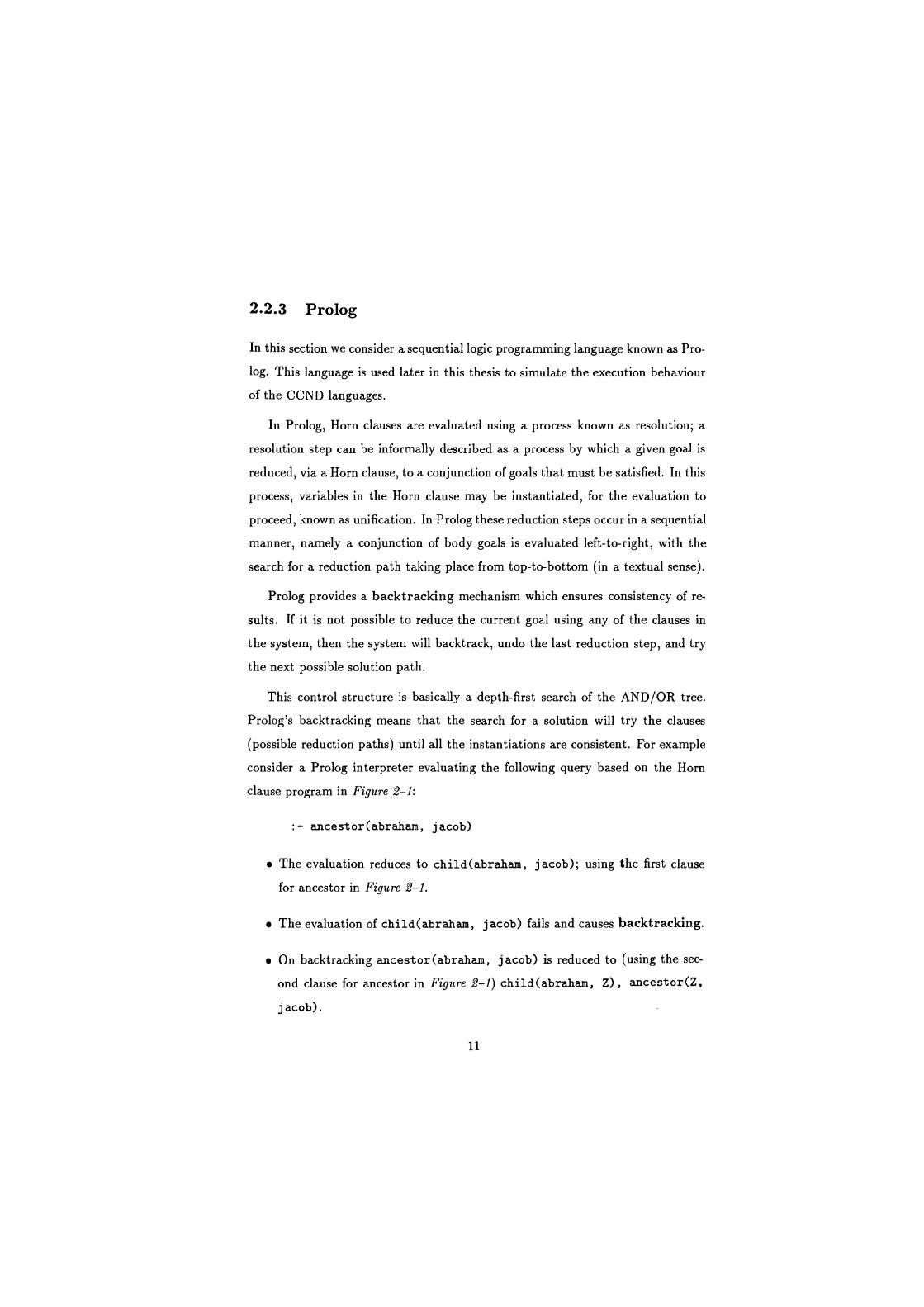
2.2.3 Prolog

In this section we consider a sequential logic programming language known as Pro-

log. This language is used later in this thesis to simulate the execution behaviour

of the CCND languages.

In Prolog, Horn clauses are evaluated using a process known as resolution; a

resolution step can be informally described as a process by which a given goal is

reduced, via a Horn clause, to a conjunction of goals that must be satisfied. In this

process, variables in the Horn clause may be instantiated, for the evaluation to

proceed, known as unification. In Prolog these reduction steps occur in a sequential

manner, namely a conjunction of body goals is evaluated left-to-right, with the

search for a reduction path taking place from top-to-bottom (in a textual sense).

Prolog provides a backtracking mechanism which ensures consistency of re-

sults. If it is not possible to reduce the current goal using any of the clauses in

the system, then the system will backtrack, undo the last reduction step, and try

the next possible solution path.

This control structure is basically a depth-first search of the AND/OR tree.

Prolog's backtracking means that the search for a solution will try the clauses

(possible reduction paths) until all the instantiations are consistent. For example

consider a Prolog interpreter evaluating the following query based on the Horn

clause program in Figure 2-1:

:- ancestor(abraham, jacob)

The evaluation reduces to child(abraham, jacob); using the first clause

for ancestor in Figure 2-1.

The evaluation of child(abraham, Jacob) fails and causes backtracking.

On backtracking ancestor(abraham, jacob) is reduced to (using the sec-

ond clause for ancestor in Figure 2-1) child(abraham, z) , ancestor(Z,

j acob).

11

Prolog evaluates the goals in a left-to-right order, first child(abraham, Z)

and then ancestor(Z, jacob).

The child(abraham, Z) goal can be reduced (using the 1st clause for child)

to true. In the process Z is instantiated to isaac.

The second goal ancestor(isaac, jacob) is now attempted. This goal is

true.

So, ancestor(abraham, jacob) is true.

2.3 Parallelism in logic programming

Horn clauses are open to many forms of evaluation, in that there are many ways

that the statements making up a logical system can be applied to proving a query.

Often several resolution steps can be applied in parallel. There are four main

approaches to parallel application of Horn clause statements to proving a query:

All-solutions AND-parallelism;

OR-parallelism;

Restricted AND-parallelism; and

Streamed AND-parallelism.

2.3.1 All-solutions AND-parallelism

All-solutions AND-parallelism involves the parallel evaluation of a conjunction

of goals, hence the use of the phrase AND-parallelism. However, the conjunction

is being solved for all possible solutions (that is all the alternative bindings),

12

hence the use of the phrase All-solutions. This has resulted in the term All-

solutions AND-parallelism. It is intended that all solutions to the query should

be obtained in about the same time as it takes to obtain one solution. There

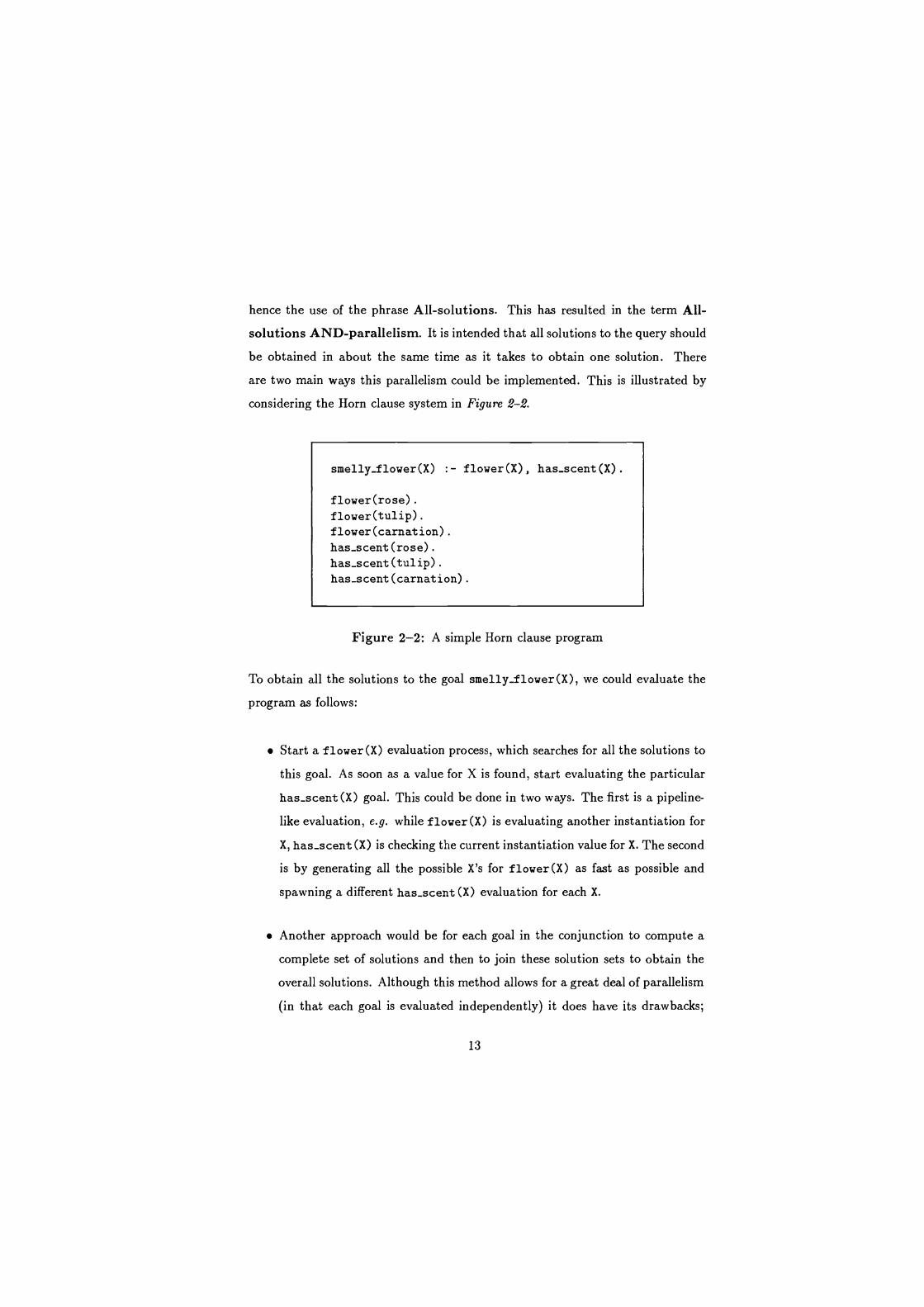
are two main ways this parallelism could be implemented. This is illustrated by

considering the Horn clause system in Figure 2-2.

smelly_flower(X) :- flower(X), has_scent(X).

flower(rose). flower(tulip). flower(carnation). has-scent (rose) .

has_scent (tulip). has-scent (carnation) .

Figure 2-2: A simple Horn clause program

To obtain all the solutions to the goal smelly_flower (X), we could evaluate the

program as follows:

Start a flower(X) evaluation process, which searches for all the solutions to

this goal. As soon as a value for X is found, start evaluating the particular

has-scent (X) goal. This could be done in two ways. The first is a pipeline-

like evaluation, e.g. while flower(X) is evaluating another instantiation for

X, has-scent (X) is checking the current instantiation value for X. The second

is by generating all the possible X's for flower(X) as fast as possible and

spawning a different has-scent (X) evaluation for each X.

Another approach would be for each goal in the conjunction to compute a

complete set of solutions and then to join these solution sets to obtain the

overall solutions. Although this method allows for a great deal of parallelism

(in that each goal is evaluated independently) it does have its drawbacks;

13

letting each of the goals in the conjunction produce a complete set of solu-

tions without control may lead to a large amount of space being used for

intermediate results. Depending on the type of problem the intersection

could result in a small set of solutions.

2.3.2 OR-parallelism

If we again consider the example Horn clause system in Figure 2-2, then the

following query:

:- flower(X).

would be true if X was tulip OR rose OR carnation. These solutions are the

OR-solutions to the query posed.

Basically OR-parallelism is the search for a solution via each of the clauses

(OR-alternatives) for a given predicate in parallel. Using this form of parallelism

will lead to a more complete search than that of Prolog as all the OR-branches can

be investigated in parallel. In Prolog if we have a clause in the search tree that

never terminates then the OR-branches that are to be searched after this branch

will never be tried. Another point to note is that because we are dealing with

the parallel search of clauses the evaluation of the clauses will be independent and

hence fairly easy to implement.

2.3.3 Restricted AND-parallelism

The general parallel evaluation of a conjunction of goals may be complex, as

the goals may share variables. These variables must have consistent bindings

and so the evaluation of these goals cannot be totally independent. However,

in Restricted AND-parallelism only goals which do not share variables are

evaluated in parallel. This restriction makes this form of parallelism fairly easy

14

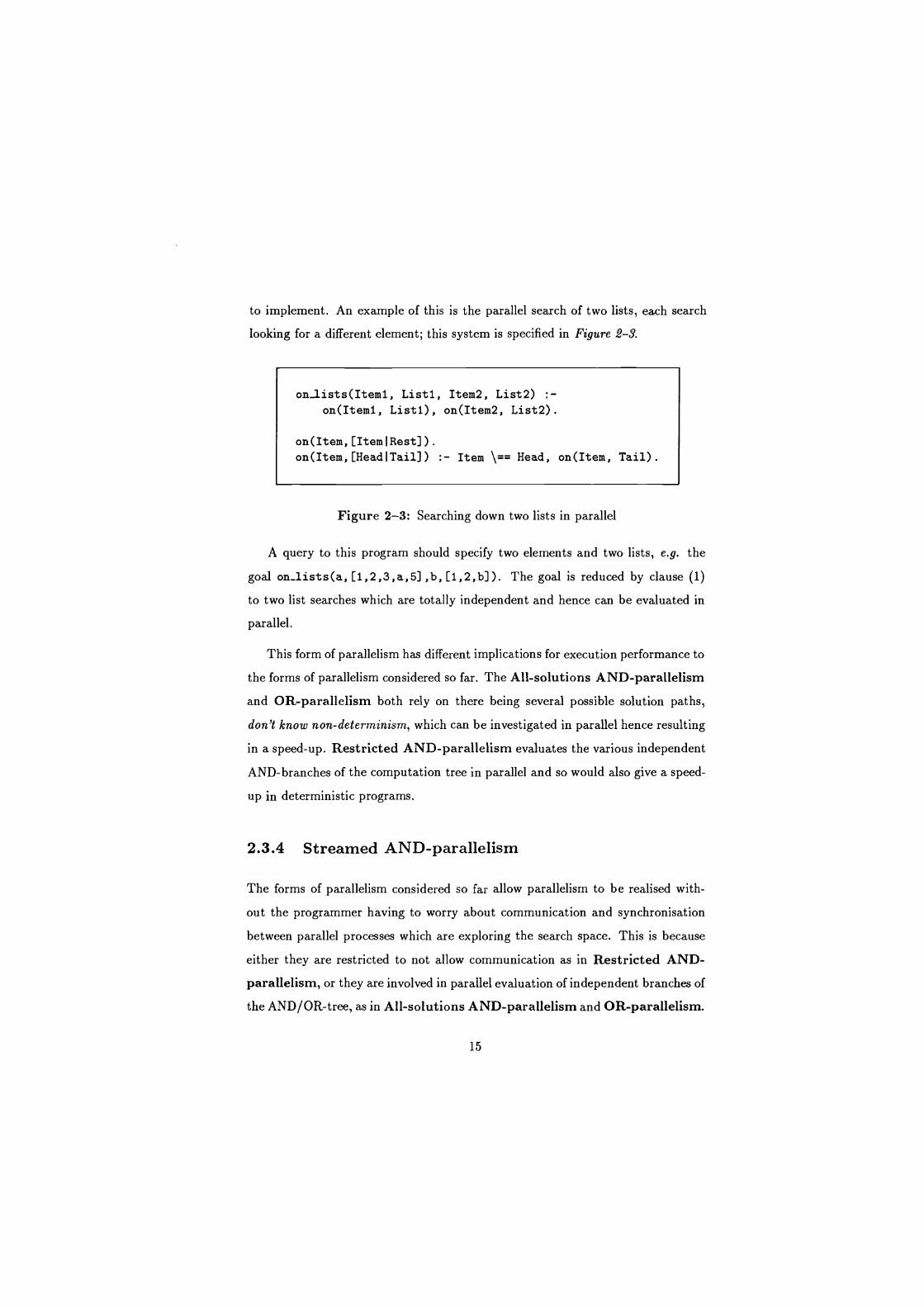
to implement. An example of this is the parallel search of two lists, each search

looking for a different element; this system is specified in Figure 2-3.

on 1ists(Iteml, Listl, Item2, List2) :- on(Iteml, Listi), on(Item2, List2).

on(Item,[ItemiRest]). on(Item,[HeadlTail]) :- Item \== Head, on(Item, Tail).

Figure 2-3: Searching down two lists in parallel

A query to this program should specify two elements and two lists, e.g. the

goal on_lists(a, [1,2,3,a,5] ,b, [1,2,b] ). The goal is reduced by clause (1)

to two list searches which are totally independent and hence can be evaluated in

parallel.

This form of parallelism has different implications for execution performance to

the forms of parallelism considered so far. The All-solutions AND-parallelism

and OR-parallelism both rely on there being several possible solution paths,

don't know non-determinism, which can be investigated in parallel hence resulting

in a speed-up. Restricted AND-parallelism evaluates the various independent

AND-branches of the computation tree in parallel and so would also give a speed-

up in deterministic programs.

2.3.4 Streamed AND-parallelism

The forms of parallelism considered so far allow parallelism to be realised with-

out the programmer having to worry about communication and synchronisation

between parallel processes which are exploring the search space. This is because

either they are restricted to not allow communication as in Restricted AND-

parallelism, or they are involved in parallel evaluation of independent branches of

the AND/OR-tree, as in All-solutions AND-parallelism and OR-parallelism.

15

In Streamed AND-parallelism we have a conjunction of goals to evaluate,

hence the AND-parallelism. These goals share variables which can act as a

means of communications between goals. If the evaluation of one goal binds a

variable, the evaluation of the other goals that share the newly bound variable can

use the binding. By incrementally binding a shared variable (i.e. binding it to

a structure containing a message and a new shared variable), processes can view

shared variables as communication streams, hence the term Streamed AND-

parallelism.

This form of parallelism can be realised in producer/consumer programs. The

producer goal incrementally binds some shared variable, the consumer goal is

evaluated in parallel with this producer and incrementally consumes the bindings.

This is evident in the case where a list is being produced using a recursive pro-

cedure and this list can be consumed incrementally using a recursive procedure;

on each recursion the consumer processes the next element on the list. Figure

2-4 is a example of a producer/consumer Horn clause program which can exploit

Streamed AND-parallelism.

producer(Current, List) :- List = [CurrentIRest], Next is Current + 1, producer(Next, Rest).

consumer([Head(Rest]) :- process(Head), consumer(Rest).

process(Item) :- write(Item).

:- producer(1, List),consumer(List).

Figure 2-4: An example of Streamed AND-parallelism

The producer builds up a list of integers. Starting with 1 this list is built-up in-

crementally by a perpetual producer process. The consumer takes the first integer

16

from the list, processes it and consumes the rest of the list. The consumer given

in Figure 2-4 simply writes the next integer to the screen. Note that the expected

behaviour of this consumer is that it should not reduce until the shared variable

is instantiated to a list, that is its evaluation should be suspended until it can

reduce with the required operational effect. Similarly, the process/1 goal should

suspend until the head of the list is instantiated to give the required behaviour.

So in offering this form of parallelism, issues of communication, synchronisation

and suspension must be considered.

The issue of insuring consistent binding in a model of AND-parallelism and

shared variables can be addressed in two ways. Either all the goals are evaluated

in parallel and parallel backtracking takes place if bindings become inconsistent or

only one goal can bind a shared variable (the producer) and the other goals that

share this variable are required to suspend until they can be evaluated without

binding the variable. The first approach is a fully parallel evaluation of the AND-

OR tree, while the second approach forms the basis of the CCND languages.

Streamed AND-parallelism may become Restricted AND-parallelism

if the shared variables become fully bound; making the goals independent.

2.3.5 Implicit/ Explicit parallel languages

Implicit parallel languages attempt to offer the forms of parallelism previously dis-

cussed without the programmer being aware of the parallel execution. The idea

is to speed up the execution of current Prolog programs (for instance) by using

parallel evaluation. However, the parallel evaluation of Prolog programs may be

limited in the degree of parallelism that can be obtained, in that these programs

may rely on the (sequential) operational semantics of the Prolog interpreter. An-

other problem is that Streamed AND-parallelism may be difficult to exploit

as current sequential logic programs do not obviously exploit such a model of

computation. So, parallelism is restricted to All-solutions AND-parallelism,

Restricted AND-parallelism and OR-parallelism. Of these forms of paral-

17

lelism, OR-parallelism looks the most promising evaluation model for obtaining

a speed-up. All-solutions AND-parallelism only applies if an exhaustive search

is required. Restricted AND-parallelism can only be used if the conjunctive

goals are independent.

In explicit parallel languages the programmer has to address the issue of con-

trolling the parallel evaluation, e.g. the parallel search of clauses and the synchro-

nisation of the Streamed AND-parallelism. The justification for this language

design is that the programmer usually knows the forms of parallelism that exist

in the problem domain, and hence is best able to implement the parallelism ex-

plicitly. Also, by adding Streamed AND-parallelism to the current procedural

interpretation of Horn clauses, it may be possible to implement algorithms that

cannot currently be implemented in Prolog.

This explicit control of parallelism can be achieved in two ways. Firstly, by the

addition of parallel search operators to Prolog which indicate those parts of the

computation that will be unaffected by a parallel operational model. Secondly,

by the addition of a controlling semantics to restrict a fully parallel evaluation of

the AND/OR-tree for the purposes of control and synchronisation. This second

approach can be seen as the basis of the Committed Choice Non-Deterministic

logic languages. These languages derive their name from the use of a commitment

operator (similar to Dijkstra's guarded command [Dijkstra 75]) which is used to

control the parallel evaluation of the OR-alternatives while allowing the exploita-

tion of Streamed AND-parallelism. The major variation between the CCND

languages lies in their means of synchronisation of bindings of shared variables.

18

2.4 Committed Choice Non-Deterministic lan-

guages

2.4.1 Syntax of guarded horn clauses

A Committed Choice Non-Deterministic (CCND) program is a finite set of guarded

horn clauses of the form:

R(al,...,ak) :- G1,...,Gn : Bi,..., Bm (n,m > 0)

The different CCND languages adopt various names for the various components of

the guarded horn clause. We use the following terminology for all the languages:

R(al, ... , ak) is a head goal;

R is its functor, or predicate name;

k is the number of arguments (referred to as the predicate arity);

G1, ... , Gn form the guarded goals;

":" is known as the commit operator;

B1,.. . , Bm are known as the body goals.

where the Gs and Bs are literals.

The commit operator generalises and cleans the cut of sequential Prolog; the

cut is used to control and reduce the search of OR-branches in Prolog. The

commit operator forms the means of pruning OR-branches in a parallel search.

A general query in the CCND languages has the following form:

.- C1, C2, ... , Cn

19

2.4.2 Semantics of guarded horn clauses

2.4.2.1 Declarative semantics

A guarded horn clause program has a similar declarative reading to Horn clause

based programs (see section 2.2.2).

Each clause:

H :- G1,...,G, : B1i...,Bm

is read as:

H is true if G, and .. and G,, and B, and ... and B, are all true.

2.4.2.2 Operational semantics

As with Horn clauses the declarative semantics of guarded horn clauses does not

consider the meaning of a program for a given inference system. This operational,

or procedural, meaning of the program is the set of goals that are provable given

the program and the inference scheme.

In the CCND model the general feature of the evaluation of a conjunction of goals

is as follows. A given goal in the conjunction Ci is evaluated by unifying the

goal with the clauses in the system. Those clauses whose heads successfully unify

are now possible solution paths for this goal. The guarded goals for the possible

solution paths are then evaluated, this evaluation can take place in parallel. The

first guarded system to terminate successfully causes the evaluation committing to

the body goals of the given clause. These body goals are essentially added to the

original conjunction for evaluation. This is known as a reduction. On commitment

to a given clause the other OR-guard evaluations can be discarded.

In the CCND languages concurrency is achieved by reducing several goals in

parallel; Streamed AND-parallelism. The issue of insuring consistent bindings

of shared variables is addressed by only allowing a variable to be bound once. This

20

requires some means of indicating that some goals should not be allowed to bind

shared variables while others may. This requirement can be achieved in two ways:

the evaluation of some goal which should not bind a variable can only be

instigated when the given variable becomes bound;

the evaluation of goals that should not bind a variable can be suspended

when they require the given variable to be bound.

The CCND languages adopt the second approach of suspending evaluations on

undesired bindings. The CCND languages differ in their means of specifying and

insuring which goals can be evaluated and which should suspend.

The following sub-sections consider the three main CCND languages, Con-

current Prolog, Parlog and Guarded Horn Clauses. This is followed by an

example evaluation which highlights the difference in the synchronisation models

they employ.

2.4.3 Concurrent Prolog (CP)

2.4.3.1 History and background

Concurrent Prolog (CP), proposed by Shapiro [Shapiro 83], was initially designed

to offer both Streamed AND-parallelism and some OR-parallelism (in the

evaluation of the guarded goals). Due to implementation problems [Ueda 85a]

several restricted versions of the language have been proposed.

Flat Concurrent Prolog, FCP, [Mierowsky et al 85], here guarded goals are

restricted to system predicates.

Safe Concurrent Prolog, SCP, [Codish 85], Codish introduces output anno-

tations into Concurrent Prolog. A clause is safe if all output instantiations

are made through variables declared as output.

21

Dual Concurrent Prolog, DCP, [Levy 86b] Levy also introduces output an-

notation into Concurrent Prolog. The resulting language is claimed to be a

simple extension of Guarded Horn Clauses, [Ueda 85b] which is complemen-

tary or Dual to Concurrent Prolog.

2.4.3.2 Basic concept

In Concurrent Prolog, communication is achieved by shared variables and syn-

chronisation by declaring certain occurrences of these shared variables as read

only. The evaluation of a goal will suspend if it attempts to bind a read only

variable. Any instantiation made during the evaluation of the guarded goals is

made in a local binding environment which is unified with the global environment

at the time of trying to commit to a given clause.

2.4.3.3 Syntax of CP

Concurrent Prolog adds two syntactic constructs to that of the guarded horn

clause.

The read only annotation of variables, "?". Any occurrence of a variable

in a clause can be read only annotated.

The "otherwise" guarded goal.

2.4.3.4 Operational semantics of CP

The synchronisation mechanism for instantiating shared variables in a conjunction

takes place through the read only annotation of variables. Any evaluation that

tries to instantiate a read only variable must suspend evaluation until the unifica-

tion can take place without causing the given instantiation. The issue of several

guards instantiating a global variable is addressed by making local copies of the

22

instantiations to the global environment. Once a guard terminates successfully,

several operations take place as follows:

Local copies of instantiations are unified with those in the calling process,

i.e. passing back instantiations made in the guard.

If the unification is successful the other parallel guards for this evaluation

are terminated, or ignored.

The calling process is reduced to the body goals of the clause that was

committed to.

The guarded goals for a given clause can be evaluated in AND-parallel and

once commitment takes place the body goals can also be reduced in AND-parallel.

There is one remaining semantic addition to the language called the otherwise

goal. This goal can appear as the first goal in the guard of a CP clause. The

operational semantics for clauses are that predicates with an otherwise goal in

their guard will not be evaluated until all the other clauses for this predicate have

failed.

2.4.4 Parlog


Parlog [Gregory 85], [Gregory 87] is a descendant of the Relational Language

[Clark & Gregory 81]. The major difference between PARLOG and the Relational

Language is that the mode constraints are relaxed in the former, to allow weak

arguments. A weak argument of a goal is one in which an input argument con-

tains variables which may be instantiated by evaluation of the goal; hence allowing

a form of two way communication (back communication).

23

2.4.4.2 Basic concepts

Synchronisation is achieved by declaring the inputs and outputs to every clause in

the system. A goal can only attempt to be reduced by a clause if the arguments

declared as input can be unified with the head of the clause without causing any

instantiations in the goal being evaluated and if the output arguments are not

instantiated. If head unification attempts to cause any instantiations of input

arguments that clause evaluation is suspended.

2.4.4.3 Syntax of Parlog

Parlog adds three types of syntactic constructs to guarded horn clauses.

Mode declarations take the form:

mode A(ml...... mk).

where A is the predicate name and each of the mi's of the mode is either ?, or

, optionally preceded by an identifier, which has no semantic significance.

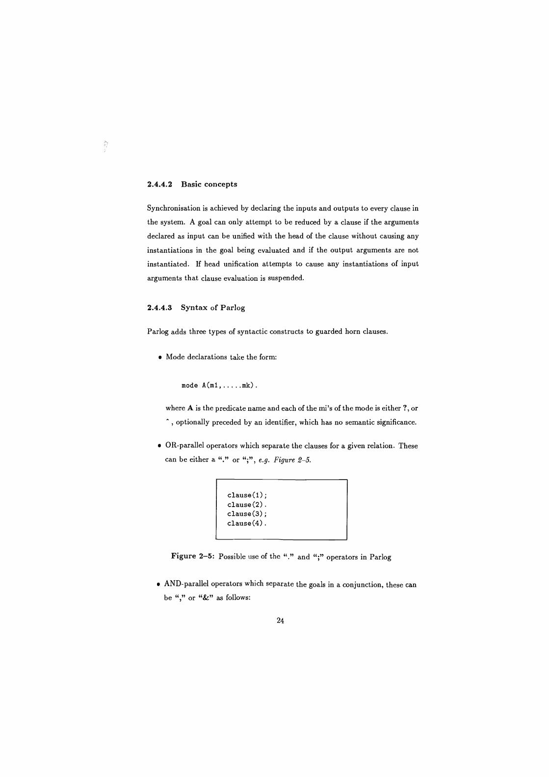
OR-parallel operators which separate the clauses for a given relation. These

can be either a "." or ";", e.g. Figure 2-5.

clause(1); clause (2) clause (3) clause (4)

Figure 2-5: Possible use of the "." and ";" operators in Parlog

AND-parallel operators which separate the goals in a conjunction, these can

be "," or "&" as follows:

24

(C1,C2) OR (Cl & C2)

where C1 and C2 are both conjunctions of goals.

2.4.4.4 Operational semantics of Parlog

The mode declarations serve to synchronise the binding of shared variables in

Parlog. A "?" in the mode declaration means that this argument of a goal cannot

be instantiated on head unification or guard evaluation of a possible clause. If

the head unification would result in an output instantiation the evaluation of the

particular clause is suspended. " " in the mode declaration specifies the output

arguments from the predicate, which will be output unified when a given clause is

committed to.

Note that the input restriction means that there is no need for local guard

environments. Guard evaluations suspend if they require an output instantiation

to be made. The mode declarations can be used by the compiler to translate

programs into a form with explicit unification and suspension tests, known as

kernel Parlog [Gregory 87].

The operators "." and ";" which separate clauses for a given predicate serve

to control the OR-parallel search:

Clauses separated by the "." can be tried in parallel.

Clauses separated by ";" are evaluated sequentially, i.e. the clause after the

";" can only be tried if the one before fails.

If we consider the example in Figure 2-5, the clauses are tried as follows: clause(1)

is evaluated, if it fails clause(2) and clause(3) are evaluated in parallel. If the first

three clauses fail, clause(4) is tried.

The "," and the "&" separators for conjunctive goals serve to control the

degree of parallelism in the evaluation of the conjunction:

25

(Cl , C2) means that C1 and C2 would be evaluated in parallel.

(Cl & C2) means that C2 is to be evaluated only when C1 has successfully

terminated.

2.4.5 Guarded Horn Clauses (GHC)


Guarded Horn Clauses (GHC), was intended to form the basis of a Kernel Lan-

guage for the Japanese Fifth Generation Parallel Inference Machines. GHC was

proposed by Kazunori Ueda in 1985 [Ueda 85b]. A restricted version of GHC has

been proposed based on the AND-parallel subset of the language and with the

restriction of system goals in the guard. This is known as Flat Guarded Horn

Clauses (FGHC).

2.4.5.2 Basic concepts

GHC adopts a unique approach to the problem of offering Streamed AND-

parallelism. In GHC synchronisation is achieved by giving special significance to

the semantics of the commit operator. The basic idea is that no output instantia-

tions can occur until the evaluation has committed to a given clause. If the system

tries to instantiate a variable in the goal being executed before commitment, the

evaluation suspends. By adopting this form of synchronisation, the part of the

clause before the commit operator just forms a test for input instantiation.

2.4.5.3 Syntax of GHC

GHC adds one new syntactic constructs to guarded horn clauses, the "otherwise"

guarded goal.

26

2.4.5.4 Operational semantics of GHC

GHC adopts only one synchronisation rule for Streamed AND-parallelism,

that is no instantiations may be passed to the calling goal in the passive part

of the clauses - the head unification and the guarded evaluation. So output in-

stantiations can only occur after commitment to a given OR-branch. There is one

remaining semantic addition to the language, the otherwise goal. This construct

has been borrowed from CP and has the same purpose and operational semantics

as in CP.

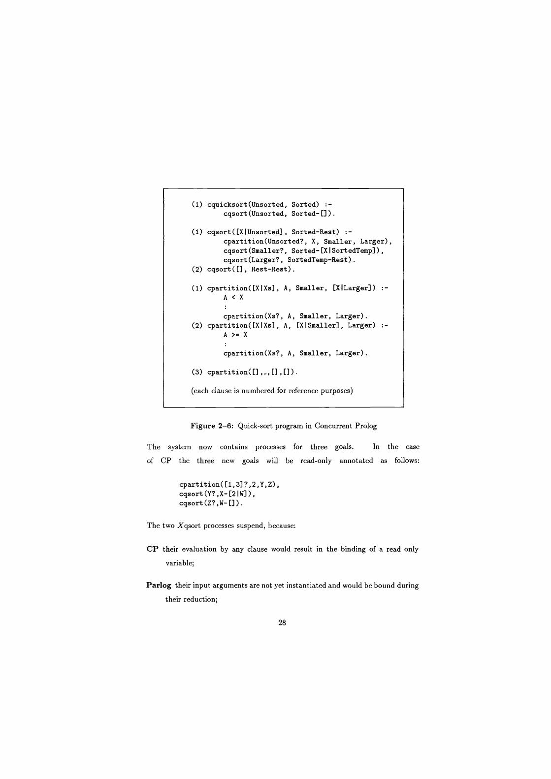
2.4.6 An example of a CCND program, and its evaluation

In this section we consider a simple example program, quick-sort, to highlight

the different suspension mechanisms proposed for the CCND languages. This

example was first commented on for CP in [Shapiro 1983]. Figures 2-6, 2-7

and 2-8 respectively provide the CP, Parlog and GHC versions of the quick-sort

program.

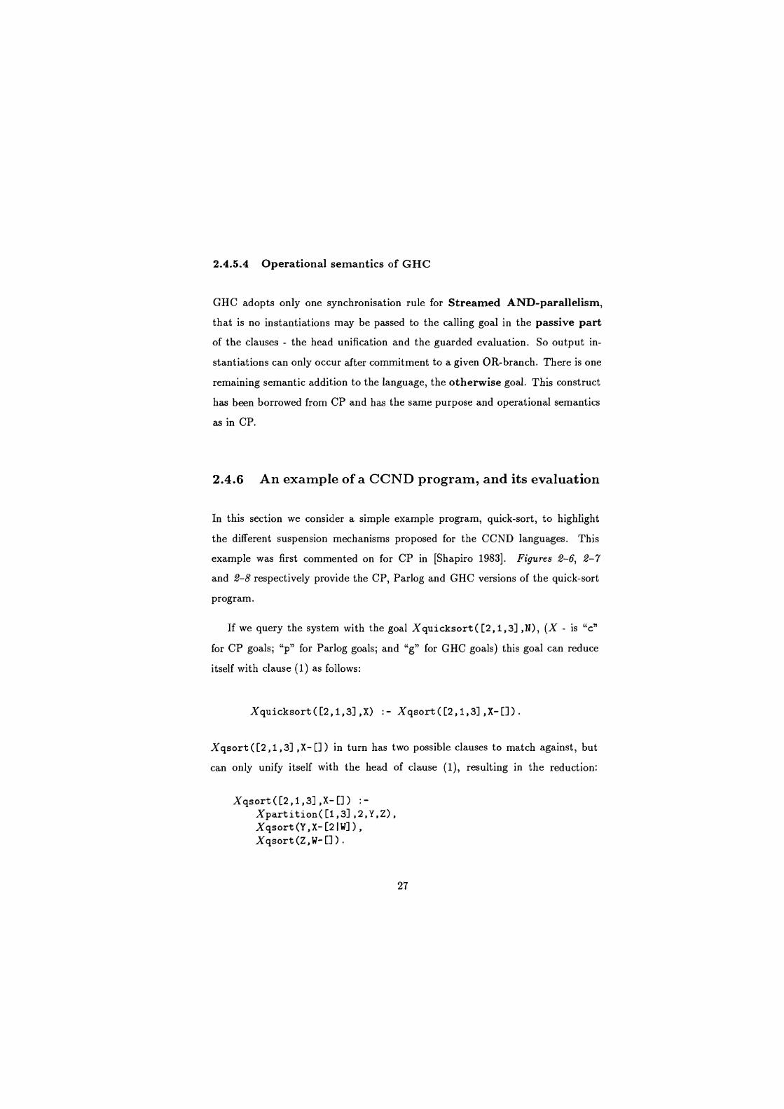
If we query the system with the goal Xquicksort([2,1,3] ,N), (X - is "c"

for CP goals; "p" for Parlog goals; and "g" for GHC goals) this goal can reduce

itself with clause (1) as follows:

Xquicksort([2,1,3],X) :- Xgsort([2,1,3],X-[]).

Xqsort ([2 ,1, 3] , X- [] ) in turn has two possible clauses to match against, but

can only unify itself with the head of clause (1), resulting in the reduction:

Xgsort([2,1,3],X-[]) :- Xpartition([1, 31,2, Y, Z), Xgsort(Y,X-[21W]), Xqsort (Z , W- []) .

27

(1) cquicksort(Unsorted, Sorted) :-

cqsort(Unsorted, Sorted-[D.

(1) cgsort([XlUnsorted], Sorted-Rest) :- cpartition(Unsorted?, X, Smaller, Larger), cqsort(Smaller?, Sorted- [X I SortedTemp]) ,

cqsort(Larger?, SortedTemp-Rest). (2) cqsort([], Rest-Rest).

(1) cpartition([XIXs], A, Smaller, [XILarger]) :- A < X

cpartition(Xs?, A, Smaller, Larger). (2) cpartition([XIXs], A, [XISmaller], Larger) :-

A>=X

cpartition(Xs?, A, Smaller, Larger).

(3) cpartition([] ,_, [] , []) .

(each clause is numbered for reference purposes)

Figure 2-6: Quick-sort program in Concurrent Prolog

The system now contains processes for three goals. In the case

of CP the three new goals will be read-only annotated as follows:

cpartition([1,3]?,2,Y,Z), cgsort(Y?, X- [21 W]) ,

cgsort (Z?, W- []) .

The two Xqsort processes suspend, because:

CP their evaluation by any clause would result in the binding of a read only

variable;

Parlog their input arguments are not yet instantiated and would be bound during

their reduction;

28

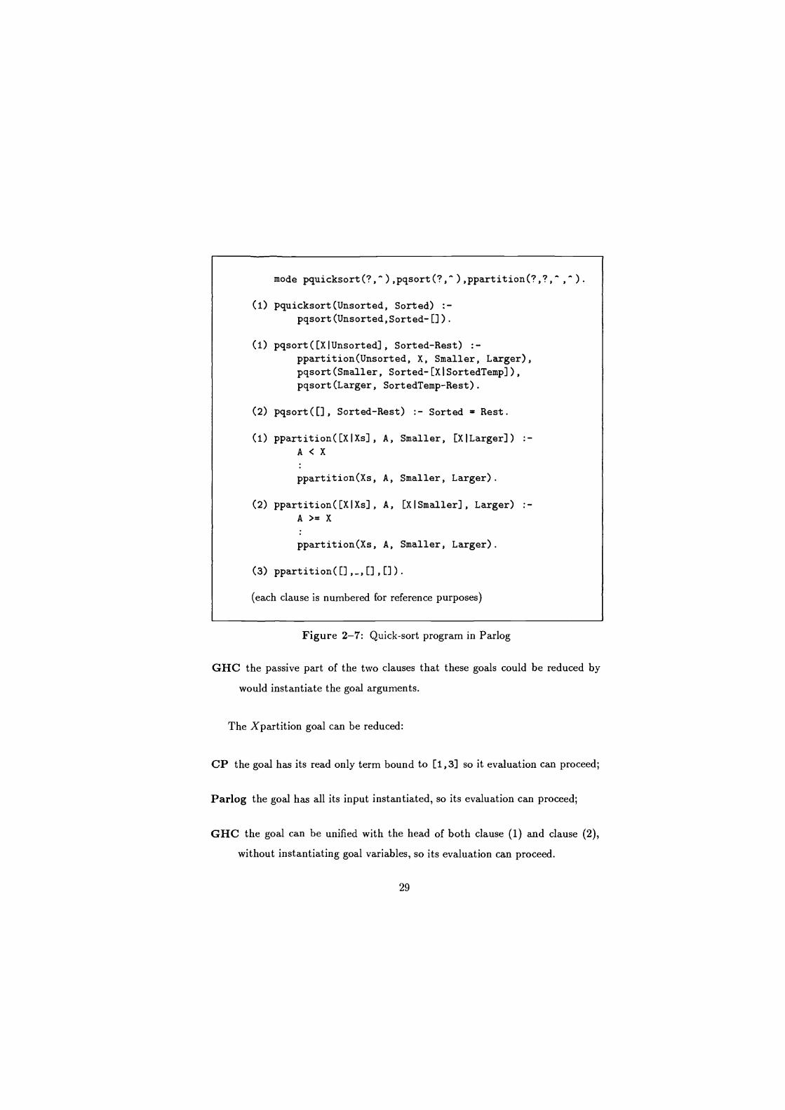
mode pquicksort(?,"),pgsort(?,-),ppartit ion(?,?,

(1) pquicksort(Unsorted, Sorted) :-

pgsort(Unsorted,Sorted-[]).

(1) pgsort([XlUnsorted], Sorted-Rest) :- ppartition(Unsorted, X, Smaller, Larger), pqsort(Smaller, Sorted-[XISortedTemp]),

pqsort(Larger, SortedTemp-Rest).

(2) pqsort([], Sorted-Rest) :- Sorted = Rest.

(1) ppartition([XIXs], A, Smaller, [XILarger]) :- A < X

ppartition(Xs, A, Smaller, Larger).

(2) ppartition([XIXs], A, [XiSmaller], Larger) :- A>=X

ppartition(Xs, A, Smaller, Larger).

(3) ppartition([],_, [] , []) .


Figure 2-7: Quick-sort program in Parlog

GHC the passive part of the two clauses that these goals could be reduced by

would instantiate the goal arguments.

The Xpartition goal can be reduced:

CP the goal has its read only term bound to [1,3] so it evaluation can proceed;

Parlog the goal has all its input instantiated, so its evaluation can proceed;

GHC the goal can be unified with the head of both clause (1) and clause (2),

without instantiating goal variables, so its evaluation can proceed.

29

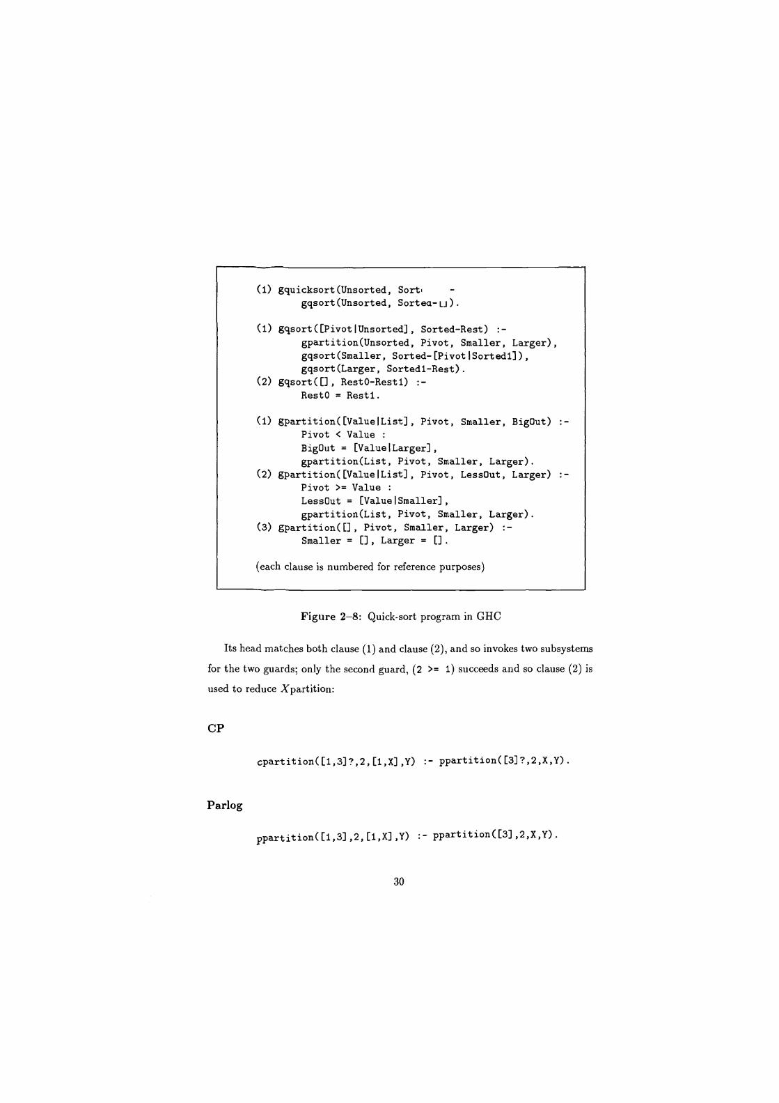
(1) gquicksort(Unsorted, Sorti - gqsort(Unsorted, Sortea- U).

(1) ggsort([PivotlUnsorted], Sorted-Rest) :- gpartition(Unsorted, Pivot, Smaller, Larger), gqsort(Smaller, Sorted-[PivotlSortedl]), gqsort(Larger, Sortedl-Rest).

(2) gqsort([], RestO-Restl) :- RestO = Restl.

(1) gpartition([ValuelList], Pivot, Smaller, BigOut) :- Pivot < Value :

BigOut = [Value{Larger], gpartition(List, Pivot, Smaller, Larger).

(2) gpartition([ValuelList], Pivot, LessOut, Larger) :- Pivot >= Value :

LessOut = [ValuelSmaller], gpartition(List, Pivot, Smaller, Larger).

(3) gpartition([], Pivot, Smaller, Larger) Smaller = [1, Larger = D.


Figure 2-8: Quick-sort program in GHC

Its head matches both clause (1) and clause (2), and so invokes two subsystems

for the two guards; only the second guard, (2 >= 1) succeeds and so clause (2) is

used to reduce Xpartition:

CP

cpartition([1,3]?,2,[1,X],Y) :- ppartition([3]?,2,X,Y).

Parlog

ppartition([1,3],2,[1,X],Y) :- ppartition([3],2,X,Y).

30

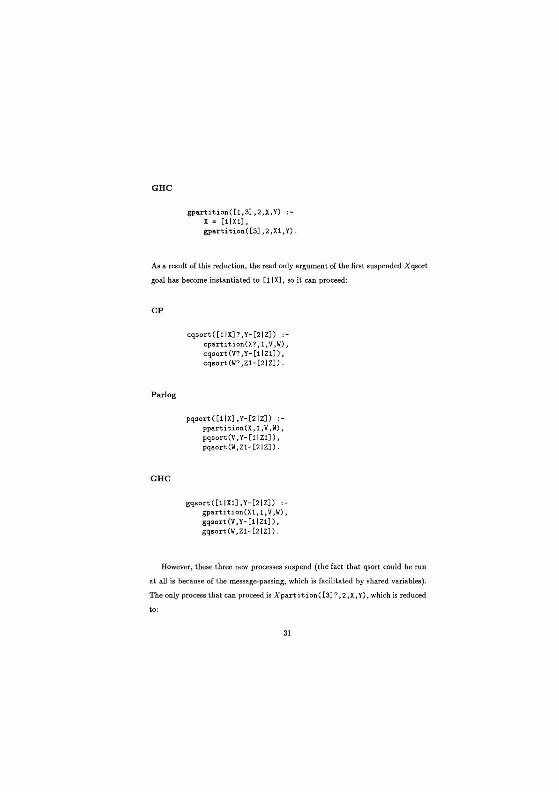
GHC

gpartition([1,3],2,X,Y) :-

X = [1 IX1] ,

gpartition([3],2,X1,Y).

As a result of this reduction, the read only argument of the first suspended Xqsort

goal has become instantiated to [I I X] , so it can proceed:

CP

cgsort([1IX]?,Y-[21Z]) :- cpartition(X?,1,V,W), cqsort (V? , Y- [1 I Z 1]) ,

cqsort(W?,Z1-[21Z]).

Parlog

pgsort([1IX],Y-[21Z]) :- ppartition(X,1,V,W), pqsort(V,Y-[1IZ1]), pgsort(W,Z1-[21Z]).

GHC

ggsort([1IX1],Y-[21Z]) :- gpartition(X1,1,V,W), gqsort(V,Y-[1IZ1]),

ggsort(W,Z1-[21Z]).

However, these three new processes suspend (the fact that qsort could be run

at all is because of the message-passing, which is facilitated by shared variables).

The only process that can proceed is Xpartition([3]?,2,X,Y), which is reduced

to:

31

CP

cpartition([3]?,2,X,[31W]) cpartition([]?,2,X,W).

Parlog

ppartition([3],2,X,[31W]) :- ppartition([],2,X,W).

GHC

gpartition([3],2,X,Y) :- Y=[31W], gpartition([],2,X,W).

As a result of this reduction, the first argument of the second Xqsort goal becomes

instantiated, so its evaluation can proceed:

CP

cgsort([3IX]?,Y-[I) :- cpartition(X?,3,U,V), cgsort(U?,Y-[31Y1]),

cgsort(V?,Y1-[]).

Parlog

pgsort([31X],Y-[I) :-

ppartition(X,3,U,V),

pgsort(U,Y-[31Y1]),

pgsort(V,Y1-[]).

GHC

ggsort([31X],Y-[D

gpartition(X,3,U,V),

ggsort(U,Y-[31y11),

ggsort(V,Y1-[]).

32

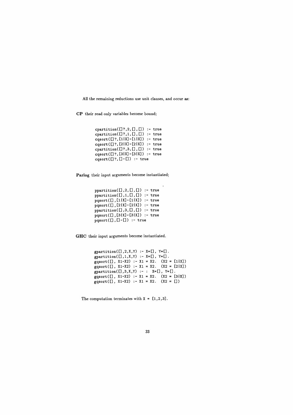
All the remaining reductions use unit clauses, and occur as:

CP their read only variables become bound;

cpartition([]?,2,[],[]) :- true cpartition([]?,1,[],[]) :- true cgsort([]?, [1IX]-[1IX]) :- true cgsort ([] ?, [21X]-[21X]) : - true cpartition([]?,3,[],[]) :- true cgsort ([] ? , [31X]-[31X]) : - true cgsort ([] ?, [] - []) :- true

Parlog their input arguments become instantiated;

ppartition([],2,[],[]) :- true ppartition([],1,[],[]) :- true pgsort([],[1IX]-[11X]) true pgsort ([] , [21X] - [2 I X]) : - true ppartition([],3,[],[]) true pgsort ([] , [3 I X] - [3 1 X]) true pgsort ([] , [] - []) :- true

GHC their input arguments become instantiated.

gpartition([],2,X,Y) gpartition([],1,X,Y) gqsort([], X1-X2) X1

gqsort ([] , X1-X2) : - X1

X=[],

X=11,

Y=[].

Y=[] .

= X2. (X2 = [11X]) = X2. (X2 = [2 I X] )

gpartition([],3,X,Y) :- : X=[], Y=[].

ggsort ([] , X1-X2) : - X1 = X2. (X2 = [31X]) gqsort([], X1-X2) :- X1 = X2. (X2 = [])

The computation terminates with X = [1,2,3].

33

2.5 Classifications

Although the CCND languages and their subsets adopt different synchronisation

mechanisms the languages possess some similar features. Algorithms and program-

ming techniques that make use of a given feature of a language will be portable to

other languages with similar features. In our evaluation of the CCND languages

for AI (part 3 of this thesis) we consider how some well known AI programming

paradigms map to languages with different features. We then examine the execu-

tion behaviour of programs which make use of the different language features.

Two main groupings of the language features are widely recognised, these are

detailed below. The Al applications considered later in this thesis highlight the

differences between the languages in these two groups.

2.5.1 Safe/Unsafe

A clause is defined to be safe if and only if for any goal the evaluation of the head

unification and guarded goals never instantiate a variable appearing in the goal to

a non-variable term [Clark & Gregory 84]. This definition has been expanded by

[Takeuchi & Furukawa 86] as follows:

for any goal the evaluation of the head and guarded goals never instantiate

a variable appearing in the goal to a non-variable;

each clause in the program is safe;

as a result, any program written in the language is safe;

The design of Parlog is supposed to exclude any programs which would violate

the safety condition. It is proposed that the legality of programs could be checked

at compile time. However, current attempts at performing this analysis exclude

34

possible legal programs [Gregory 87]. GHC is a safe language, in fact the suspen-

sion rule of GHC is based on guard safety. If a clause requires a goal variable to

be instantiated in the guard the evaluation of that clause suspends. Concurrent

Prolog is unsafe; goal variables are allowed to be instantiated by the evaluation

of the guard. On commitment these bindings are unified with the global copies of

the variables. The use of local environments results in difficulties in implementing

Concurrent Prolog [Ueda 85a].

2.5.2 Deep/Flat

A program which only has system goals in the guards is said to be flat

[Mierowsky et al 85] [Foster & Taylor 87]. This results in a simple language which

still offers Streamed AND-parallelism; as the guarded evaluations are simple.

This reduces the complexity of implementing the languages. Moreover, it should

be possible to compile the full language into its flat subset. [Gregory 87] discusses

how OR-parallel evaluation can be compiled to AND-parallel evaluation by us-

ing a controlled metacall. [Codish 85] provides a source to source transformation

technique which does not require the introduction of a new language primitive.

2.6 Implementations

The development of the CCND languages has taken the following path. Firstly

interpreters were implemented in Prolog [Shapiro 83], [Pinto 86]. These were

followed by compilers where the target language was Prolog [Gregory 84],

[Ueda & Chikayama 85]. Subsequently, compilers were produced where the

target language was an abstract machine, which is emulated by a 'C' program

[Foster et al 86]. Enough is now generally understood about the operational se-

mantics of the languages to be able to consider implementation on a parallel archi-

tecture [Crammond 88]. Although interpreters allow the synchronisation mecha-

35

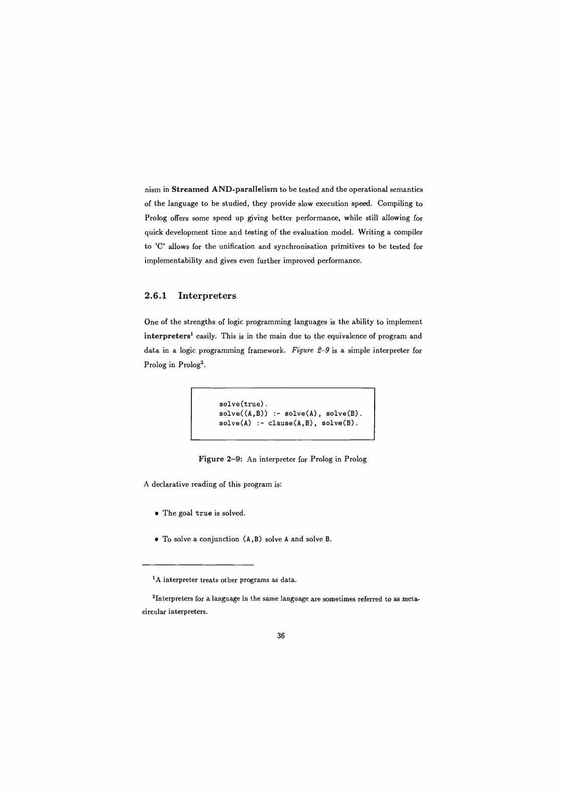
nism in Streamed AND-parallelism to be tested and the operational semantics

of the language to be studied, they provide slow execution speed. Compiling to

Prolog offers some speed up giving better performance, while still allowing for

quick development time and testing of the evaluation model. Writing a compiler

to 'C' allows for the unification and synchronisation primitives to be tested for

implement ability and gives even further improved performance.

2.6.1 Interpreters

One of the strengths of logic programming languages is the ability to implement

interpreters' easily. This is in the main due to the equivalence of program and

data in a logic programming framework. Figure 2-9 is a simple interpreter for

Prolog in Prolog2.

solve(true).

solve((A,B)) :- solve(A), solve(B). solve(A) :- clause(A,B), solve(B).

Figure 2-9: An interpreter for Prolog in Prolog

A declarative reading of this program is:

The goal true is solved.

To solve a conjunction (A,B) solve A and solve B.

'A interpreter treats other programs as data.

2Interpreters for a language in the same language are sometimes referred to as meta-

circular interpreters.

36

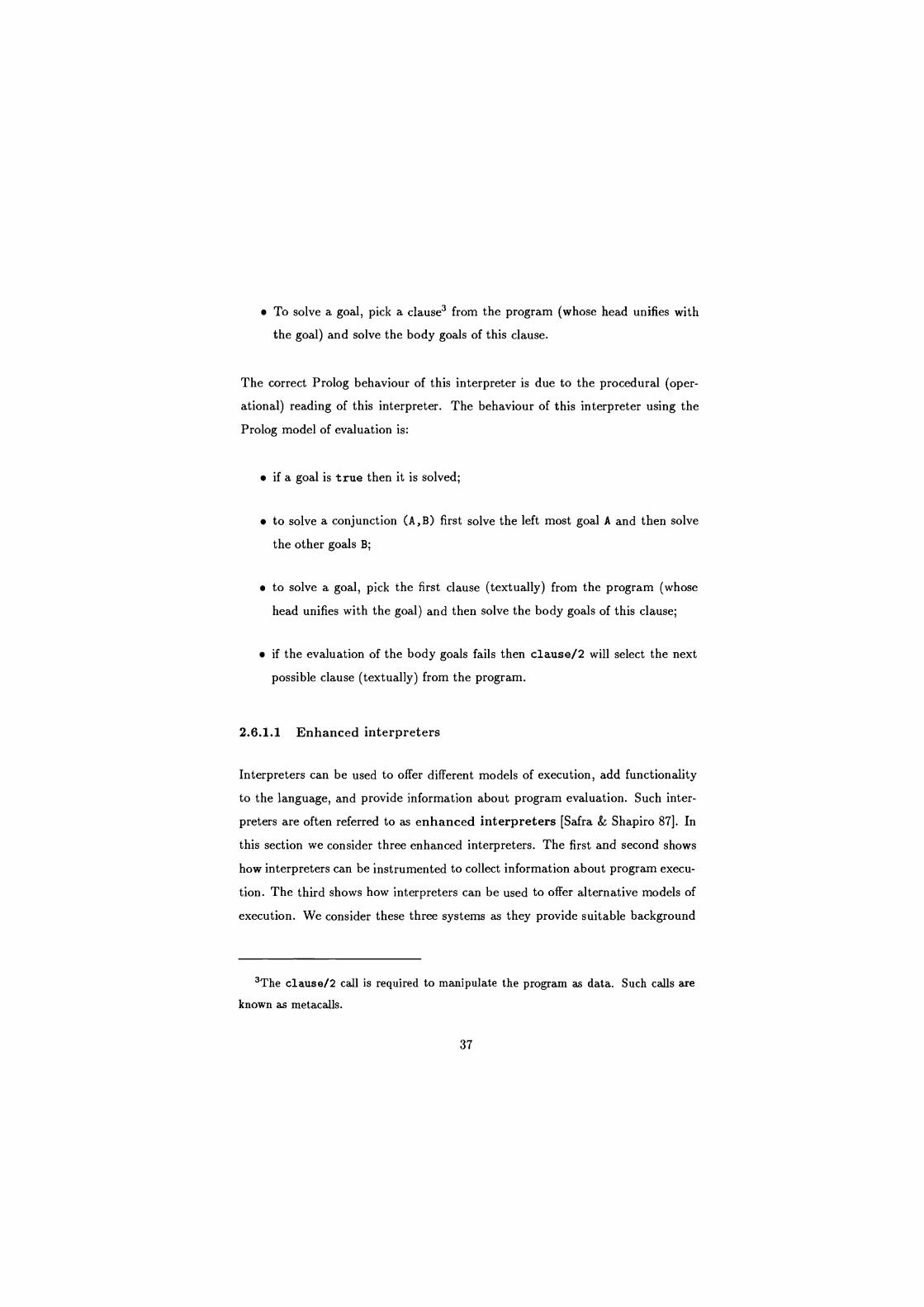
To solve a goal, pick a clause3 from the program (whose head unifies with

the goal) and solve the body goals of this clause.

The correct Prolog behaviour of this interpreter is due to the procedural (oper-

ational) reading of this interpreter. The behaviour of this interpreter using the

Prolog model of evaluation is:

if a goal is true then it is solved;

to solve a conjunction (A,B) first solve the left most goal A and then solve

the other goals B;

to solve a goal, pick the first clause (textually) from the program (whose

head unifies with the goal) and then solve the body goals of this clause;

if the evaluation of the body goals fails then clause/2 will select the next

possible clause (textually) from the program.

2.6.1.1 Enhanced interpreters

Interpreters can be used to offer different models of execution, add functionality

to the language, and provide information about program evaluation. Such inter-

preters are often referred to as enhanced interpreters [Safra & Shapiro 87]. In

this section we consider three enhanced interpreters. The first and second shows

how interpreters can be instrumented to collect information about program execu-

tion. The third shows how interpreters can be used to offer alternative models of

execution. We consider these three systems as they provide suitable background

3The clause/2 call is required to manipulate the program as data. Such calls are

known as metacalls.

37

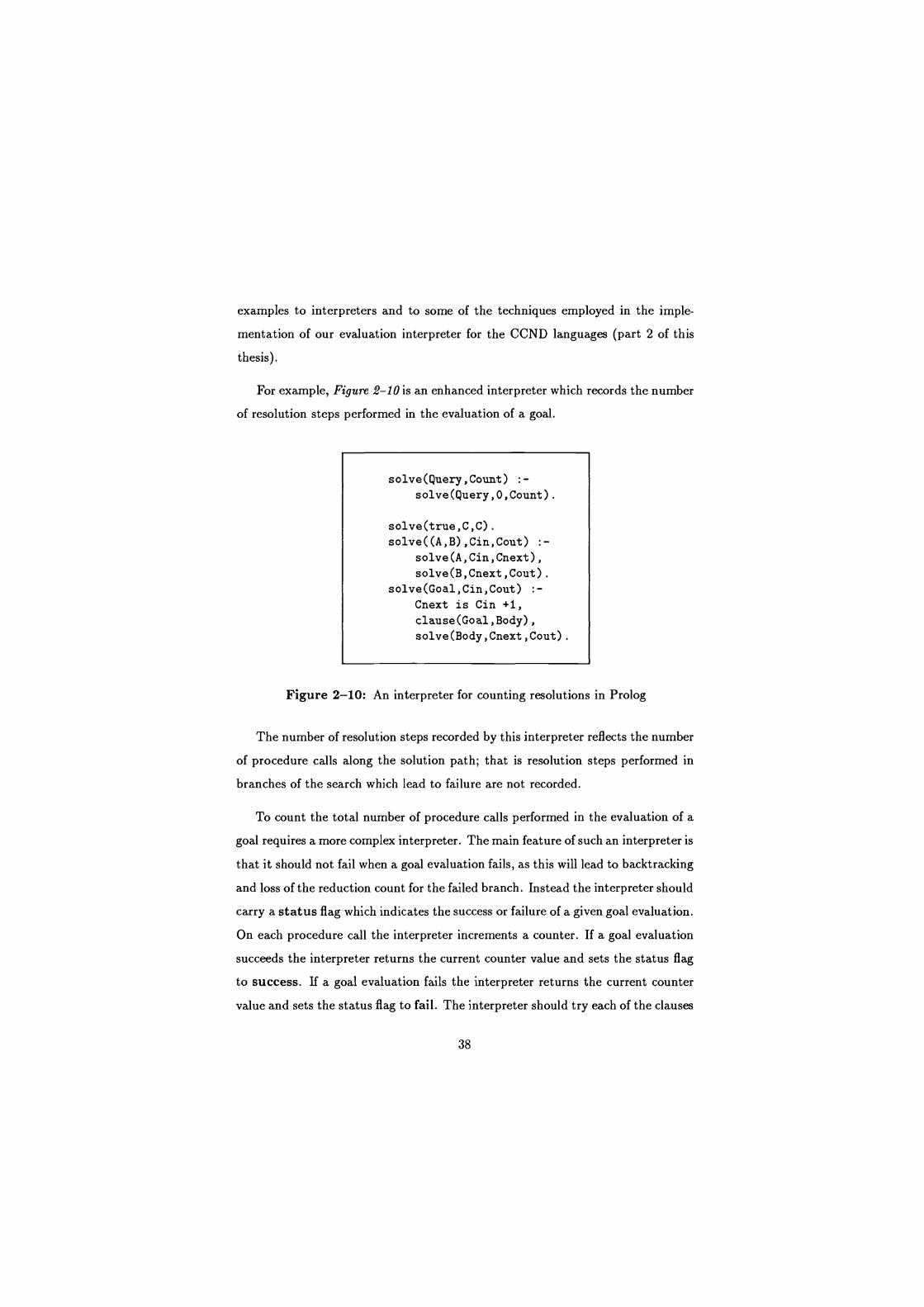
examples to interpreters and to some of the techniques employed in the imple-

mentation of our evaluation interpreter for the CCND languages (part 2 of this

thesis).

For example, Figure 2-10 is an enhanced interpreter which records the number

of resolution steps performed in the evaluation of a goal.

solve(Query,Count) :-

solve(Query,0,Count).

solve(true,C,C).

solve((A,B),Cin,Cout) :-

solve(A,Cin,Cnext),

solve(B,Cnext,Cout).

solve(Goal,Cin,Cout) :-

Cnext is Cin +1,

clause(Goal,Body),

solve(Body,Cnext,Cout).

Figure 2-10: An interpreter for counting resolutions in Prolog

The number of resolution steps recorded by this interpreter reflects the number

of procedure calls along the solution path; that is resolution steps performed in

branches of the search which lead to failure are not recorded.

To count the total number of procedure calls performed in the evaluation of a

goal requires a more complex interpreter. The main feature of such an interpreter is

that it should not fail when a goal evaluation fails, as this will lead to backtracking

and loss of the reduction count for the failed branch. Instead the interpreter should

carry a status flag which indicates the success or failure of a given goal evaluation.

On each procedure call the interpreter increments a counter. If a goal evaluation

succeeds the interpreter returns the current counter value and sets the status flag

to success. If a goal evaluation fails the interpreter returns the current counter

value and sets the status flag to fail. The interpreter should try each of the clauses

38

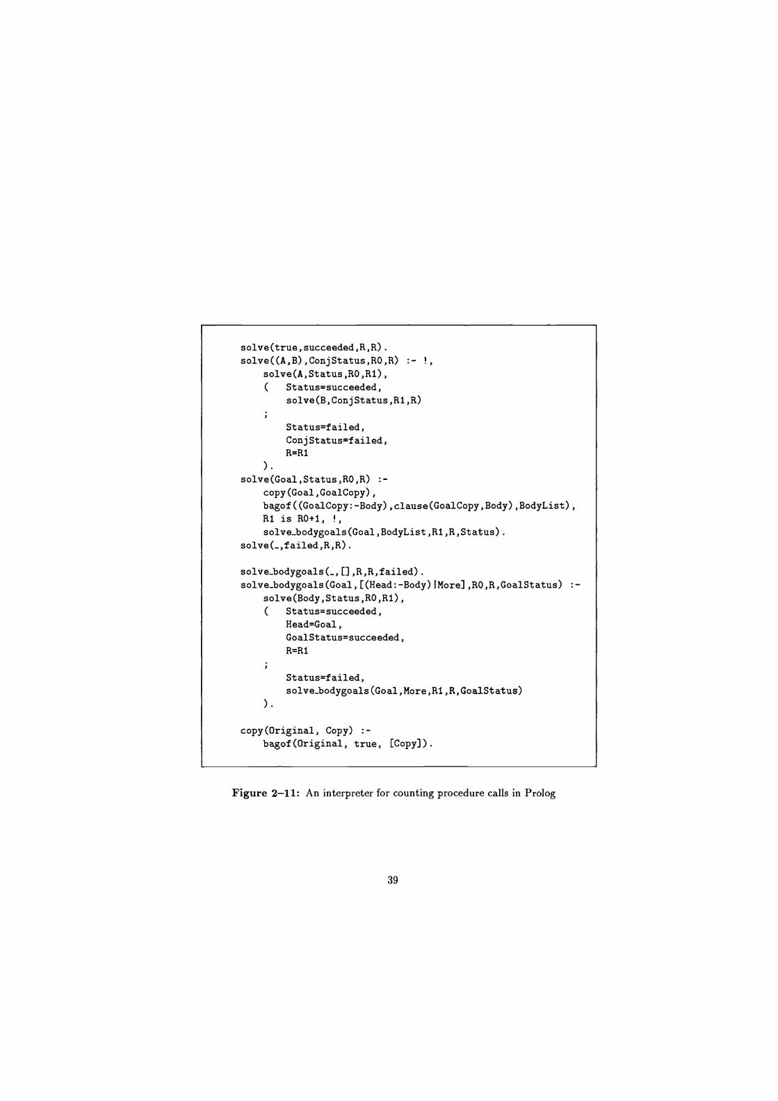
solve(true,succeeded,R,R). solve((A,B),ConjStatus,RO,R) :- !,

solve(A,Status,R0,R1), ( Status=succeeded,

solve(B,ConjStatus,R1,R)

Status=failed, ConjStatus=f ailed,

R=R1 ) solve(Goal,Status,RO,R) :-

copy(Goal,GoalCopy),

bagof((GoalCopy:-Body),clause(GoalCopy,Body),BodyList), R1 is RO+1, !, solve_bodygoals(Goal,BodyList,R1,R,Status) .

solve(_,failed,R,R).

solve_bodygoals(_, [] ,R,R,failed) .

solve_bodygoals(Goal,[(Head:-Body)IMorel, RO,R,GoalStatus) :- solve(Body,Status,R0,R1), ( Status=succeeded,

Head=Goal, GoalStatus=succeeded, R=R1

Status=failed, solve bodygoals(Goal,More,R1,R,GoalStatus)

copy(Original, Copy) :- bagof(Original, true, [Copy]).

Figure 2-11: An interpreter for counting procedure calls in Prolog

39

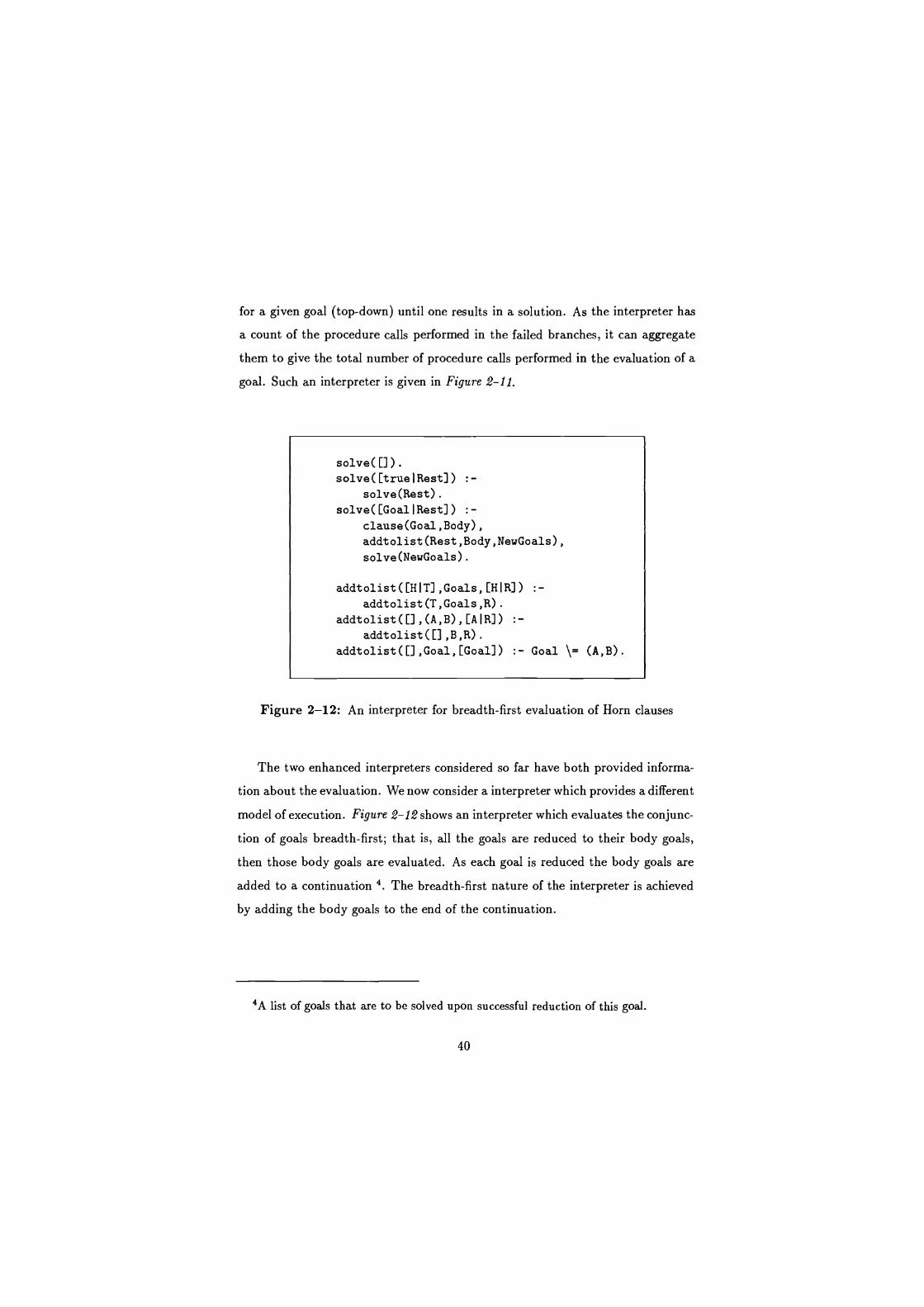
for a given goal (top-down) until one results in a solution. As the interpreter has

a count of the procedure calls performed in the failed branches, it can aggregate

them to give the total number of procedure calls performed in the evaluation of a

goal. Such an interpreter is given in Figure 2-11.

solve([]). solve([truelRest]) :-

solve(Rest). solve([GoallRest]) :-

clause(Goal,Body), addtolist(Rest,Body,NewGoals), solve(NewGoals).

addtolist([HIT],Goals,[HIR]) :- addtolist(T,Goals,R).

addtolist([],(A,B),[AIR]) :- addtolist([],B,R).

addtolist([],Goal,[Goal]) :- Goal \= (A,B).

Figure 2-12: An interpreter for breadth-first evaluation of Horn clauses

The two enhanced interpreters considered so far have both provided informa-

tion about the evaluation. We now consider a interpreter which provides a different

model of execution. Figure 2-12 shows an interpreter which evaluates the conjunc-

tion of goals breadth-first; that is, all the goals are reduced to their body goals,

then those body goals are evaluated. As each goal is reduced the body goals are

added to a continuation 4. The breadth-first nature of the interpreter is achieved

by adding the body goals to the end of the continuation.

4A list of goals that are to be solved upon successful reduction of this goal.

40

2.6.1.2 Interpreters for the CCND languages

When Shapiro first proposed Concurrent Prolog [Shapiro 83] [Shapiro 87a] he also

presented a interpreter in Prolog for the new language. The interpreter maintains

a queue (continuation) of Concurrent Prolog goals and a status flag.

To solve a query, the interpreter schedules the goals in the queue which also

contains a cycle marker (used to indicate when all the goals have been attempted),

and sets a status flag to deadlock. It then operates on each of the goals in the

queue, dequeueing a goal, reducing it, and scheduling the body goals (according

to the scheduling policy). If a goal reduction suspends, or fails to be reduced, the

goal is placed at the end of the queue. The top level of the interpreter has the

following procedural reading:

If the queue only contains a cycle marker, then the interpreter terminates

successfully.

If each goal in the queue has been attempted and the status flag is deadlock,

then the interpreter fails.

If each goal in the queue has been attempted and the status flag is

nodeadlock, then re-enqueue the cycle marker, set the status flag to

deadlock and continue solving the remaining goals.

If the dequeued goal is a system call, evaluate it and then solve the remaining

goals in the queue.

To reduce a Concurrent Prolog goal, the interpreter sequentially picks a

guarded clause whose head unifies with the goal (according to Concurrent

Prolog's unification algorithm). It then attempts to solve the guarded goals

for this clause (by recursively calling itself). If the interpreter finds a clause

(by backtracking) which satisfies such requirements, then the body goals for

the clause are scheduled for evaluation.

41

The scheduling policy used in the interpreter for the goals is breadth-first,

that is the body goals are scheduled at the back-end of the goal queue. However,

because the guarded goals are evaluated by recursively calling the interpreter,

the evaluation of the OR-goals is not breadth-first. The guarded clause selec-

tion, which involves using Concurrent Prolog's read-only unification, is given in

[Shapiro 83].

Shapiro also proposed three profiling parameters, cycles, reductions and sus-

pensions, which provide information about the evaluation.

Cycles

The cycles parameter attempts to measure the length of the breadth-first

execution. A cycle corresponds to attempting to reduce all the goals in the

system once in parallel.

Reductions

This parameter aims to give a measure of the work involved in solving a

query. The parameter attempts to measure the number of inference steps

performed by the system. In [Shapiro 83] an inference step is considered to

be a commitment to a clause.

Suspensions

This parameter attempts to count the number of suspended evaluations in

the evaluation of a query. The number of suspensions is however dependent

on when suspended evaluations are rescheduled. When an evaluation sus-

pends in Shapiro's interpreter it is immediately rescheduled for evaluation;

this is known as busy waiting. This rescheduled evaluation may resuspend

and so will count as two or more suspensions.

The cycles, reductions and suspensions have become the standard pa-

rameters used when comparing applications and programming techniques

[Okumura & Matsumoto 87], [Sterling & Codish 87].

42

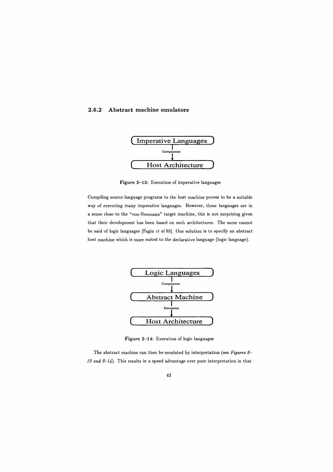
2.6.2 Abstract machine emulators

Compilation

Host Architecture

Figure 2-13: Execution of imperative languages

Compiling source language programs to the host machine proves to be a suitable

way of executing many imperative languages. However, these languages are in

a sense close to the "von-Neumann" target machine, this is not surprising given

that their development has been based on such architectures. The same cannot

be said of logic languages [Fagin et al 85]. One solution is to specify an abstract

host machine which is more suited to the declarative language (logic language).

Logic Languages Compilation

Abstract Machine Emulation

Host Architecture

Figure 2-14: Execution of logic languages

The abstract machine can then be emulated by interpretation (see Figures 2-

13 and 2-14). This results in a speed advantage over pure interpretation in that

43

much of the run-time overheads of unification and flow of control can be compiled

away. Over pure compilation it results in a space advantage, in that the abstract

machine is more closely tailored to the logic language and so a more (direct)

efficient mapping exists.

A number of abstract machines have been proposed for logic languages, the

most well known being [Warren 77a] [Warren 77b] [Warren 83] who proposed

an abstract machine for Prolog. This notion of abstract machine emulation

has also been applied to concurrent/ parallel logic languages, the many different

types of parallelism (see section 2.3) giving rise to a whole host of different ab-

stract machines [Foster et al 86] [Houri & Shapiro 87] [Kimura & Chikayama 87]

[Shapiro 87b] [Warren 87] [Crammond 88].

2.6.3 Multi-processor implementations

The Concurrent Logic Languages are amenable to parallel execution; in fact, this

has been one of the driving forces in their development. The work on multi-

processor realisations of these languages is split into two main areas.

The first area of work is on the implementation of these languages on shared

memory multi-processors, like the Sequent SymmetryTM, [DeGroot 84]

[Crammond 85] [Hausman et al 87] [Warren 87] [Westphal et al 87]

[Crammond 88] [Sato & Goto 88]. With shared memory implementation,

global binding schemes can be implemented directly, i.e. each processor

manipulates the same data areas.

The second area of work is on the implementation of these languages on dis-

tributed memory multi-processors, like the Intel iPSC HypercubeTM, [Ali 86]

[Conery 87] [Taylor et al 87]. With a distributed memory implementation

either data areas are stored on one processor, or distributed binding and

unification schemes are required. This makes distributed implementations

more complex.

44

2.7 Summary

In this chapter the following have been presented and discussed:

How logic can be used as a programming language, in particular via Horn

clauses and the sequential evaluation model of Prolog.

The various forms of parallel evaluation of programs specified in Horn

clauses, namely OR-parallelism, Restricted AND-parallelism, All-Solutions

AND-parallelism and Streamed AND-parallelism.

The Committed Choice Non-Deterministic (CCND) model of execution. The

synchronisation mechanisms for the three main CCND languages, Concur-

rent Prolog, Parlog and Guarded Horn Clauses, are highlighted using an

example sort program.

The CCND languages are then classified in two ways: safe/unsafe and

deep/flat. In the evaluation of the CCND languages for Al (part 3 of this

thesis) we consider how some well known Al programming paradigms map

to languages with different features.

Finally we review current implementations of these languages, in particular

the modelling of the execution of these languages by enhanced interpreters.

45

Part II

An evaluation system

46

Preface

In this part of the thesis we develop our evaluation system for the CCND languages.

The system developed aims to measure the inherent parallelism available in the

execution of programs implemented in the CCND languages and the effects of

alternative implementation possibilities on this inherent behaviour.

The first chapter in this part, chapter 3 has three main focuses:

the limitations of current evaluation systems;

the requirements of an improved model of execution on which we can collect

information about the inherent behaviour of programs; and

the incremental design and development of an interpreter which provides the

basis of our new evaluation system.

The second chapter in this part, chapter 4 also has three main focuses:

the possible implementation alternatives open to language implementors,

which form the basis of a set of evaluation parameters;

how we collect these evaluation parameters; and

the theoretical behaviour of some example programs and the behaviour in-

dicated using our evaluation system and proposed evaluation parameters.

47

Chapter 3

Interpreters for evaluation

3.1 Overview

This chapter considers the inherent parallelism available in the evaluation of pro-

grams implemented in the CCND languages. A measure of the inherent parallelism

has several uses: it gives a theoretical measure of parallelism against which partic-

ular implementations can be gauged; and it provides information for programmers

on the relative merits of various programming techniques.

For typical Computer Science application areas, such as matrix multiplication,

it is often possible to obtain theoretical measures for the inherent parallelism.

However, for Al type problems the parallelism depends on several factors, such as

data structures (knowledge representation), inference mechanisms and irregular

search spaces. The irregular nature of Al problems makes a theoretical measure of

parallelism difficult. Another approach to obtaining measures of inherent paral-

lelism for both regular and irregular problems is to simulate the given computation

on an infinite processor model. The simulated processor utilisation then gives a

measure of the inherent parallelism.

It is this second approach we adopt in this work. To obtain a measure of

the inherent parallelism available in program execution we adopt a breadth-first

48

execution model assuming an unlimited number of processors. The evaluation

system developed is used in the following chapters to consider some of the execution

alternatives open to language implementors.

Section 3.2 considers some current evaluation systems for the CCND languages.

The focus is on interpretation systems as these are generally used when evaluating

and comparing programming techniques and applications.

Section 3.3 considers the current parameters that are collected during program

execution and discusses their limitations as a way of measuring inherent paral-

lelism.

Section 3.4 considers the requirements of an execution system which will allow

us to more accurately obtain a measure of the inherent parallelism.

In section 3.5 we give an overview of the idealisations we assume in our execu-

tion model.

Finally, in section 3.6 we incrementally develop an interpreter which offers

an improved AND/OR-parallel evaluation model which allows us to measure the

inherent parallelism available in the execution of a program more accurately.

3.2 Current evaluation systems

The first implementations of the CCND languages consisted of interpreters on top

of Prolog [Shapiro 83] [Gregory 84] [Tanaka et al 86] [Pinto 86], these were instru-

mented to record simple parameters, namely cycles, suspensions and reduc-

tions (see section 2.6.1.2). To measure the inherent parallelism of programs these

interpreters use a breadth-first evaluation model. Subsequently, compilers to Pro-

log were produced. The compiled code could also include mechanisms for collect-

ing cycles, suspensions and reductions [Gregory 84] [Ueda & Chikayama 85]

[Saraswat 87a]. These compilers to Prolog could be viewed as partial evaluators

of the original interpreters [Safra & Shapiro 87]. More recently, these languages

49

have been implemented via abstract machine emulators realised in 'C' (see sec-

tion 2.6.2) [Foster et al 86] [Levy 86a] [Chikayama & Kimura 87], giving a speed-

up over the original interpreters and compilers. However, for efficiency reasons

these systems tend not to be instrumented, as in [Foster et al 86). So, the eval-

uation of programming techniques and applications tends to be carried out on

interpreters [Sterling & Codish 87] [Okumura & Matsumoto 871. Although these

interpreters claim to execute the object code (CCND program) breadth-first (see

section 2.6.1.2), hence collecting information about inherent parallelism, the actual

evaluation models used make several approximations, as follows:

the AND-parallel goals are represented as a list of goals to be evaluated;

as each goal is reduced, the resulting body goals are added to the goal list

and any appropriate bindings are made;

variable bindings are produced in the order that the goals are evaluated;

guarded goals are evaluated as a single reduction which incur no cycle over-

heads;

the interpreters make no distinction between suspension and failure of

guarded goals;

the interpreters model OR-parallelism by backtracking through alternative

clauses;

the first textual clause in a predicate whose guarded goals succeed is com-

mitted to.

50

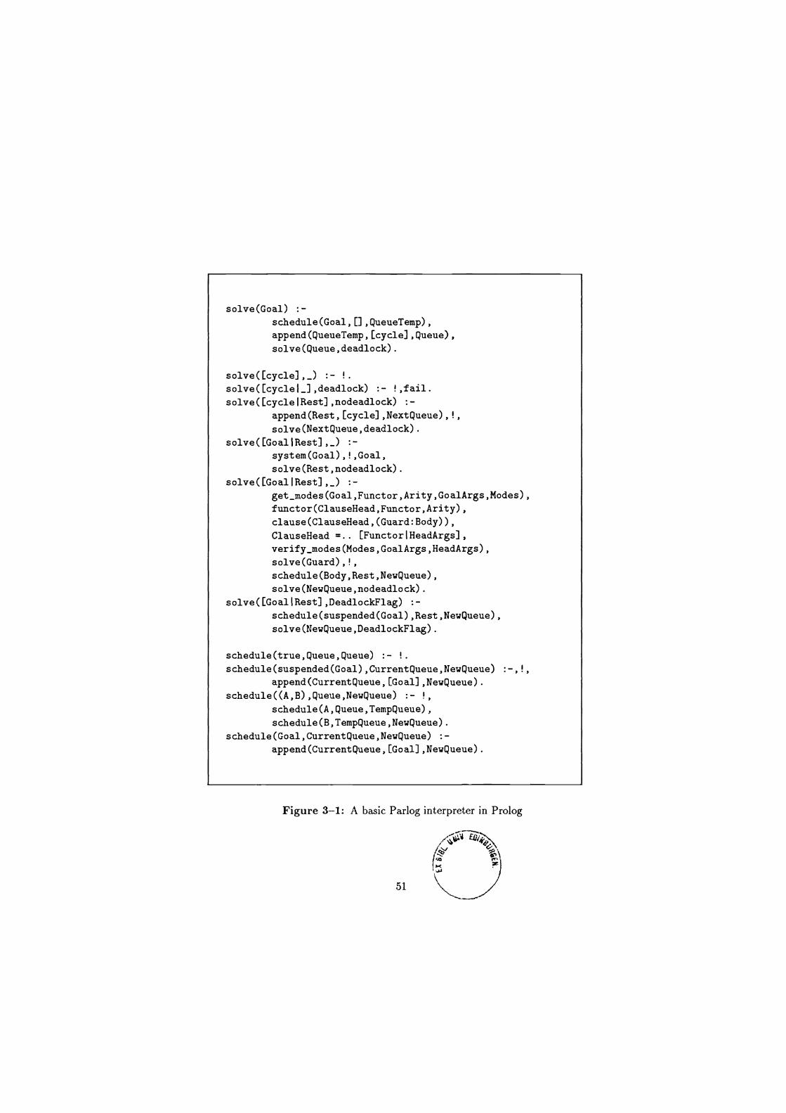
solve(Goal) :- schedule(Goal,[],QueueTemp), append(QueueTemp,[cycle],Queue), solve(Queue,deadlock).

solve([cycle],_) :- !.

solve([cyclel_],deadlock) :- !,fail. solve([cyclelRest],nodeadlock) :-

append(Rest,[cycle],NextQueue),!, solve(NextQueue,deadlock).

solve([GoallRest],_) :- system(Goal),!,Goal, solve(Rest,nodeadlock).

solve([GoallRest],_) :- get_modes(Goal,Functor,Arity,GoalArgs,Modes), functor(ClauseHead,Functor,Arity), clause(ClauseHead,(Guard:Body)), ClauseHead =.. [FunctorlHeadArgs], verify modes(Modes,GoalArgs,HeadArgs), solve(Guard),!, schedule(Body,Rest,NewQueue), solve(NewQueue,nodeadlock).

solve([GoallRest],DeadlockFlag) :- schedule(suspended(Goal),Rest,NewQueue), solve(NewQueue,DeadlockFlag).

schedule(true,Queue,Queue) :- !. schedule(suspended(Goal),CurrentQueue,NewQueue) :-,!,

append(CurrentQueue,[Goal],NewQueue). schedule((A,B),Queue,NewQueue) :- !,

schedule(A,Queue,TempQueue), schedule(B,TempQueue,NewQueue).

schedule(Goal,CurrentQueue,NewQueue) :- append(CurrentQueue,[Goal],NewQueue).

Figure 3-1: A basic Parlog interpreter in Prolog

51

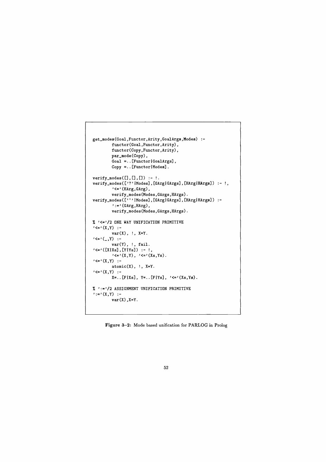
get_modes(Goal,Functor,Arity,GoalArgs,Modes) :- functor(Goal,Functor,Arity),

functor(Copy,Functor,Arity),

par_mode(Copy),

Goal =..[FunctorlGoalArgs], Copy =..[FunctorlModes].

verify_modes ([] , [] , []) :- !. verify_modes(['?'IModes],[GArgIGArgs],[HArgIHArgs]) :-

'<='(HArg,GArg), verify_modes(Modes,GArgs,HArgs).

verify_modes(['"'IModes],[GArgIGArgs],[HArgtHArgs]) :- ':='(GArg,HArg), verify-modes(Modes,GArgs,HArgs)-

% '<='/2 ONE WAY UNIFICATION PRIMITIVE

var(X), !, X=Y.

var(Y), ! , fail. '<='([X{Xs],[YIYs]) :- !,

'<='(X,Y), '<='(Xs,Ys).

atomic(X), !, X=Y.

X=..[FIXs], Y=..[FIYs], '<='(Xs,Ys).

'/, ':='/2 ASSIGNMENT UNIFICATION PRIMITIVE ':='(X,Y) :-

var(X),X=Y.

I ,

Figure 3-2: Mode based unification for PARLOG in Prolog

52

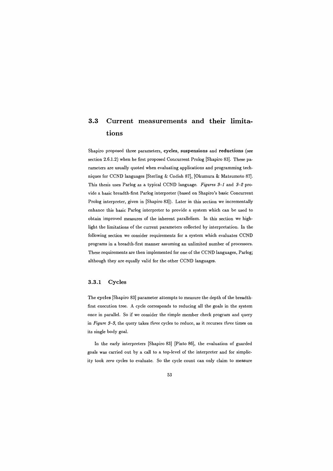
3.3 Current measurements and their limita-

tions

Shapiro proposed three parameters, cycles, suspensions and reductions (see

section 2.6.1.2) when he first proposed Concurrent Prolog [Shapiro 83]. These pa-

rameters are usually quoted when evaluating applications and programming tech-

niques for CCND languages [Sterling & Codish 87], [Okumura & Matsumoto 87].

This thesis uses Parlog as a typical CCND language. Figures 3-1 and 3-2 pro-

vide a basic breadth-first Parlog interpreter (based on Shapiro's basic Concurrent

Prolog interpreter, given in [Shapiro 83]). Later in this section we incrementally

enhance this basic Parlog interpreter to provide a system which can be used to

obtain improved measures of the inherent parallelism. In this section we high-

light the limitations of the current parameters collected by interpretation. In the

following section we consider requirements for a system which evaluates CCND

programs in a breadth-first manner assuming an unlimited number of processors.

These requirements are then implemented for one of the CCND languages, Parlog;

although they are equally valid for the other CCND languages.

3.3.1 Cycles

The cycles [Shapiro 83] parameter attempts to measure the depth of the breadth-

first execution tree. A cycle corresponds to reducing all the goals in the system

once in parallel. So if we consider the simple member check program and query

in Figure 3-3, the query takes three cycles to reduce, as it recurses three times on

its single body goal.

In the early interpreters [Shapiro 83] [Pinto 86], the evaluation of guarded

goals was carried out by a call to a top-level of the interpreter and for simplic-

ity took zero cycles to evaluate. So the cycle count can only claim to measure

53

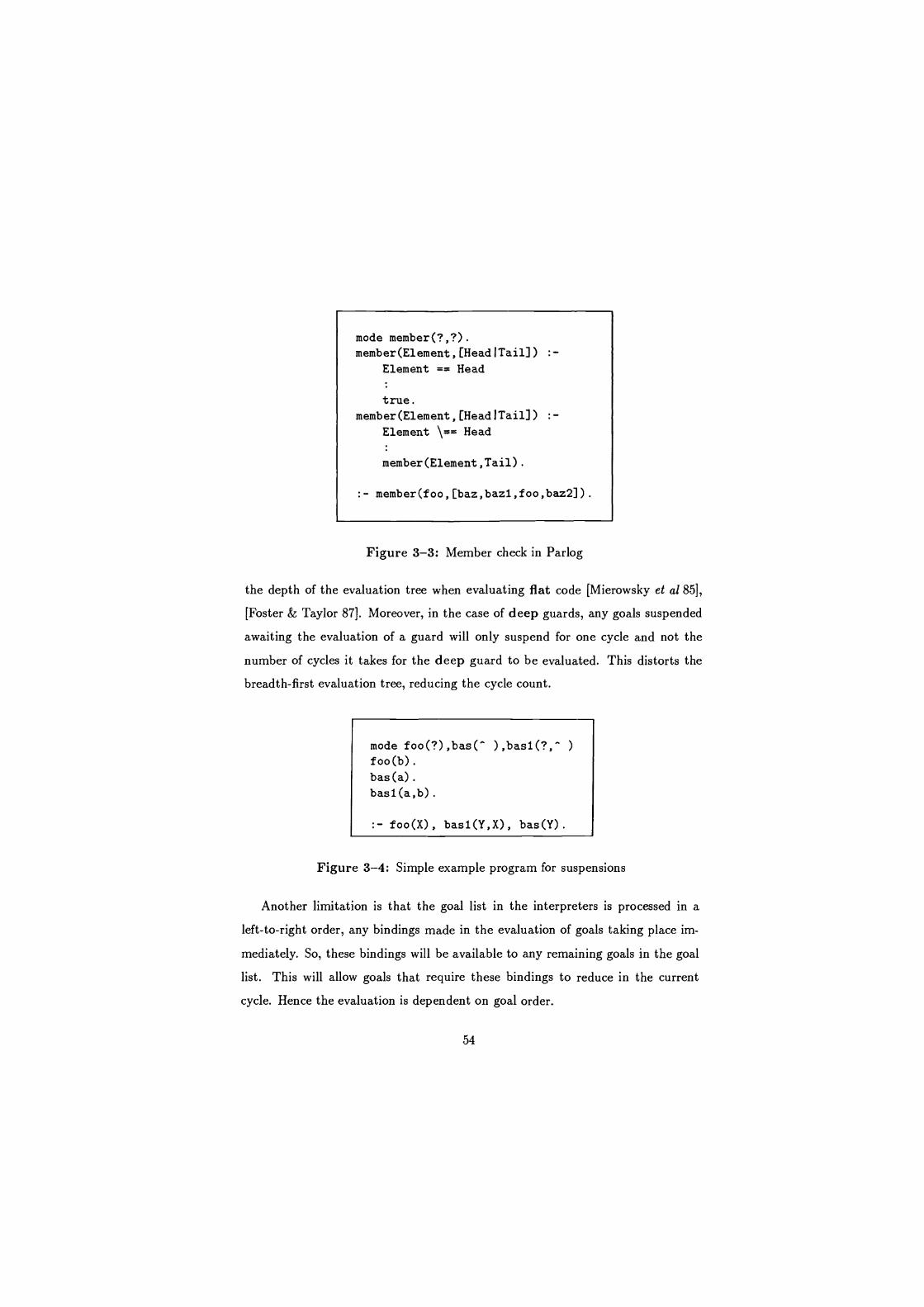
mode member(?,?). member(Element,[HeadITail])

Element == Head

true. member(Element,[HeadiTail]) :-

Element \== Head

member(Element,Tail).

:- member(foo,[baz,bazl,foo,baz2]).

Figure 3-3: Member check in Parlog

the depth of the evaluation tree when evaluating flat code [Mierowsky et al 85],

[Foster & Taylor 87]. Moreover, in the case of deep guards, any goals suspended

awaiting the evaluation of a guard will only suspend for one cycle and not the

number of cycles it takes for the deep guard to be evaluated. This distorts the

breadth-first evaluation tree, reducing the cycle count.

mode foo(?),bas(" ),bast(?,"

foo (b) .

bas (a) .

basl(a,b).

:- foo(X), basl(Y,X), bas(Y).

Figure 3-4: Simple example program for suspensions

Another limitation is that the goal list in the interpreters is processed in a

left-to-right order, any bindings made in the evaluation of goals taking place im-

mediately. So, these bindings will be available to any remaining goals in the goal

list. This will allow goals that require these bindings to reduce in the current

cycle. Hence the evaluation is dependent on goal order.

54

If we consider the program in Figure 3-4, then by changing the order of the

query to be:

:- bas(Y),bas1(Y,X) ,foo(X) .

the existing interpreters will give a cycle count of one, whereas the previous query

(Figure 3-4) resulted in a cycle count of three. Previously the goal evaluation order

resulted in the goals foo(X) and bas1(Y,X) suspending in the first cycle and the

goal foo(X) suspending in the second cycle. However, now the goal evaluation

order and the order in which the bindings are produced are the same. So, all the

goals are able to reduce to true in one cycle. In an AND-parallel evaluation, the

cycle count should be three, as follows: in the evaluation of the first cycle both

foo (X) and basl (Y, X) will suspend; in the second cycle foo (X) will suspend and

in the last cycle all the goals will evaluate to true.

3.3.2 Reductions

This parameter attempts to measure the reductions performed by the system in

solving a query, which indicates the number of parallel goal evaluations that can

take place. For the example query in Figure 3-3, the number of reductions mea-

sured by Shapiro's interpreter is three; where each commitment counts as a re-

duction. The evaluation of system calls, supported by calls to the underlying

Prolog, are not counted as reductions. However, these system calls do contribute

to the overall work done in evaluating programs. By ignoring their contribution

the comparison of programming techniques which make use of system primitives is

meaningless or at best misleading. If we also consider the successful system calls

as reductions, then the evaluation will now perform six reductions (three more

because of system guards) 1.

'It may be the case that some system calls like == should not be counted as a reduction

as they are simple, and could be compiled to be part of the head unification. However,

55

Another limitation is that current interpreters try evaluating the alternatives

for a given predicate top-down, committing to the first clause whose guarded

goals succeed. So reductions can only be counted for the clauses that have been

attempted. Hence the reduction count depends on the order of the clauses. In a

parallel OR-evaluation model the set of guarded goals for the clauses whose head

unified successfully should be evaluated in parallel, the evaluation committing to

the first clause whose guard succeeds.

Finally if a goal fails, then in the current interpreters it is rescheduled and

may be re-attempted (the failed goal will be re-evaluated if the computation goes

on for further cycles before the whole computation deadlocks). The re-evaluation

of failed goals may introduce erroneous statistics into the reduction count (that

is if reductions are performed in a deep guard evaluation before failure, these

reductions will be repeated when the goal is re-evaluated).

3.3.3 Suspensions

This parameter attempts to count the number of suspended evaluations in the

evaluation of a query. The number of suspensions may be dependent on when

suspended evaluations are rescheduled. When an evaluation suspends in the ex-

isting interpreters they are immediately rescheduled for evaluation; this is known

as busy waiting. For example, the query in Figure 3-4 will undergo three reduc-

tions in three cycles, and incur three suspensions, assuming that the interpreter is

evaluating the query breadth-first. However, a non-busy waiting strategy could

have been used 2. Using an ideal non-busy waiting strategy each suspended

as a general principle system calls should be counted as reductions as they contribute

to the overall work done.

2The suspended goals could be hooked (or tagged) to the variables that they are sus-

pended on so that they can be reactivated when sufficient variables become instantiated.

56

goal will be suspended once. So, the example query in Figure 3-4 will incur two

suspensions.

Another point to note is that current interpreters process the goals from left-

to-right, allowing any bindings that result to be made available to the remaining

goals to be processed in the current cycle. This may allow a goal to reduce in the

current cycle which would suspend if the goals were evaluated in a different order.

Finally, as failed goals are rescheduled they may introduce erroneous statistics

into the suspension count as failed goals will add to the suspension counts.

3.4 Requirements of an improved model

Many of the limitations and inaccuracies of the statistics generated by current

interpreter implementations are due to the execution mechanisms employed to

model these languages. The collection of more meaningful statistics requires the

development of an improved implementation. Such an implementation would have

to exhibit the following features:

The implementation must distinguish between suspension and failure of an

evaluation of a goal. Goal evaluations can either:

The implementation must more accurately measure the depth of the evalu-

ation tree:

- the depth of the evaluation tree must account for the use of deep

guards;

57

- the depth of the evaluation tree should not be dependent on goal or

clause order;

- the depth of the tree should account for producer-consumer type algo-

rithms. That is, a consumer should suspend for as many cycles as it

takes the producer to generate the message. This is particularly rele-

vant in the case of deep guarded producers, where consumer processes

should suspend for the duration of the producers guard evaluation.

The implementation should model parallel AND-parallelism:

each of the goals in the conjunction should appear to be evaluated in

parallel;

each AND-parallel goal should be reduced once in each cycle. The

reduction may take place in the guarded evaluation in the case of deep

guards;

the simulated reduction of each goal in a given cycle should be inde-

pendent of the actual order in which the goals are processed.

The implementation should model parallel OR-parallelism:

- each of the clauses that a goal could use to reduce should appear to be

explored in parallel;

- in a parallel evaluation a goal should commit to the first clause whose

guard successfully terminates;

- the evaluation of a goal suspends if no committable clause exists and at

least one clause evaluation suspends (not suspend or fail as in current

interpreters).

In the following subsection we consider the idealisations made in the design of

our improved execution model. Then taking each of the requirements above we

incrementally develop an improved interpreter. The interpreter developed aims

58

to provide a fully parallel model of program execution with which we can col-

lect meaningful statistics. Using an interpreter allows us to collect coarse grained

information like number of commitments or size of suspension queues. These

coarse parameters are similar to the coarse grained parameters, like logical in-

ferences [Wilk 83], collected for sequential logic programming languages (Pro-

log) and to the currently accepted evaluation parameters used for the CCND

languages [Shapiro 83] [Sterling & Codish 87] [Okumura & Matsumoto 87]. How-

ever, it does not easily allow us to measure fine detail like the cost of the commit-

ment operation.

The dynamic cost of various operations and the reference characteristics of

CCND languages would require the instrumentation of a suitable and representa-

tive abstract machine, like [Crammond 88] for Parlog. The emulator for such an

abstract machine can then be used to collect information about data and instruc-

tion referencing, in the same vein as [Tick 87]. This approach was not feasible for

this work because there was no representative abstract machine for the entire class

of CCND languages available for instrumentation.

3.5 Idealisations in our improved model

3.5.1 AND-parallel idealisations

In Shapiro's interpreter the goal list is processed in a left-to-right order, any bind-

ings made in the evaluation of goals take place immediately. So, these bindings

will be available to any remaining goals in the goal list. Hence the evaluation is

dependent on goal order.

A fully accurate model would be able to determine exactly when a goal makes

a binding, how long it would take for this binding to reach another goal and

whether this would be in time for the goal to use it. Such a model would be

heavily implementation dependent and its results would not transfer easily to

59

other implementations. Clearly the inherent parallelism should not be dependent

on goal order. Instead we make the assumption that, in a cycle, a goal can only

use bindings available to it at the start of the cycle. Such a model may not display

all the parallelism that could be achieved in a given implementation, but at least

it gives a measure which is not dependent on how the goals are ordered.

3.5.2 Guard evaluation idealisations

Shapiro's model assumed, that in a cycle, a goal can be head unified with the

clauses in the system, the guarded goals could be evaluated, and the body goals

committed to. This model assumed that guard evaluations take zero cycles, so no

contribution of the guard evaluations are seen in the overall depth measure of the

evaluation. Shapiro's depth measure (cycles count) only records the depth of the

commitments of the goals at the top-level of the AND/OR-tree. Only in the case

where all guards are all flat does this measure give an indication the depth of the

evaluation tree.

We propose two alternative models for incorporating the effect of the guard

evaluation into the overall evaluation. The first assumes that in a cycle, a goal

can be head unified with a clause and the guarded goal evaluation instigated. The

body goals will be committed to at a depth of 1+(the depth of the guarded

evaluation). Note that this model assumes that guarded system goals (flat

guards) will evaluate in 1 cycle. The second assumes that in a cycle, a goal can

be head unified with a clause and either the guarded evaluation instigated or a

system guard evaluated. Commitment to the body goals occurs at 1+(the depth

of the guarded evaluation) for deep guards and in the next cycle for flat

guards. Note that this model assumes that system goals incur no cycle costs.

We adopt the second model as this model has a similar notion of depth to the

previous implementations when executing flat guarded programs.

60

It should be noted that most cycle based models for obtaining a measure of the

depth of the evaluation tree will be prone to giving distorted results, in that they

will tend to associate fixed costs with the various components of the evaluation, like

head unification, system call evaluation and commitment. Although an elaborate

model of cost could be developed, these costs would tend to be implementation

dependent. Moreover, such a model is unlikely to give a radically different view of

the general features of the evaluation compared with a fixed cost model.

3.5.3 OR-parallel idealisations

The model of inherent OR-parallelism requires the evaluation to commit to the

clause whose first guard successfully terminates. In our system the duration of

a guard evaluation is approximated by the depth of its evaluation tree. So the

evaluation should commit to the guard with the shallowest evaluation tree.

3.5.4 System call idealisations

The evaluation of system calls contributes to the overall work done in the evalu-

ation of a goal. We assume the evaluation of a system call counts as a reduction.

It may be the case that some system calls like == should not be counted as a

reduction as they are simple, and could be compiled to be part of the head uni-

fication. As a general principle system calls should be counted as reductions as

they contribute to the overall work done.

In suspending the evaluation of a system call we assume it behaves like a

goal with one clause. Later in this thesis (section 4.2.2), we consider alternative

suspension mechanisms and this idealisation will reflect the fact that there should

be no performance difference in which suspension mechanism is employed for such

calls.

61

3.6 Development of our improved model

We could implement the required improved execution model by an abstract ma-

chine emulated in 'C' (see section 2.6.2). The abstract machine could then be

instrumented to dump, rather than dynamically collect information (as this will

reduce the speed of the system) about program evaluation. Alternatively, we could

implement an improved interpreter which could either dynamically collect statis-

tics like the previous evaluation interpreters or dump information about the pro-

gram evaluation as in the 'C' emulator. We have chosen to implement an improved

interpreter which will then be used to dump profiling data about the program ex-

ecution. This dump data is post analysed. Adopting a interpreter rather than a

'C' based emulator allows us to rapidly prototype our system [Sterling & Beer 86],

however the trade-off is that our system executes orders (at least 2) of magnitude

slower than a comparable 'C' version.

In this section we take each of the requirements for an improved evaluation

system given in section 3.4 and incrementally design and develop an improved

interpreter.

3.6.1 Suspension/ Failure

Providing a interpreter which can distinguish between suspension and failure re-

quires several improvements to the basic interpreter, given in Figure 3-1. The

basic interpreter returned only two states nodeadlock or deadlock/failed in-

dicated by the interpreter succeeding or failing. To indicate three possible termi-

nation states, nodeadlock, deadlock or failed, requires an additional argument

which indicates the final state of the computation. This results in a two argument

(top-level) interpreter, as given in Figure 3-5.

62

solve(Goal,StatusOut) :- schedule(Goal,[],QueueTemp), append(QueueTemp,[cycle],Queue), solve(Queue,deadlock,StatusOut).

Figure 3-5: Two argument call for a suspend/fail Parlog interpreter

The next stage is for each of the clauses in the original interpreter, Figure 3-1,

to support this extra argument. The resulting interpreter is given in Figure 3-6.

This interpreter has the following procedural reading:

If the goal list only contains a cycle marker, the evaluation has terminated

successfully, so set the output status flag to nodeadlock.

If each goal in the goal list has been attempted and the current status flag

is deadlock, then set the output status flag to deadlock.

If each goal in the goal list has been attempted and the status flag is

nodeadlock, then re-enqueue the cycle marker, set the status flag to

deadlock and pass the output status flag onto the next cycle of the solver.

If the dequeued goal is a system call and can be evaluated (that is if the goal

is sufficiently bound to allow it to be evaluated), evaluate it using Prolog's

built in metacall (call/1). If the evaluation fails then the output status

flag is set to failed; if the evaluation succeeds then continue evaluating the

goal list; and if the goal is not sufficiently bound to be evaluated suspend

the goal and then continue evaluating the goal list.

Checking if a goal is sufficiently bound can be simply achieved by a call such

as:

eval(_ is Y) :- numbervars(Y,1,1).

63

solve([cycle],_,nodeadlock) :- !. solve([cyclel_],deadlock,deadlock) :- !. solve([cyclelRest],nodeadlock,StatusOut) :- !,

append(Rest,[cycle],NextQueue), solve(NextQueue,deadlock,StatusOut).

solve([GoallRest],StatusIn,StatusOut) :- system(Goal), (eval(Goal) ->

(call(Goal) -> solve(Rest,nondeadlock,StatusOut) StatusOut = fail) ;

schedule(suspend(Goal),Rest,NextQueue), solve(NextQueue,Statusln,StatusOut)).

solve([GoallRest],Statusln,StatusOut) :- get_modes(Goal,Functor,Arity,GoalArgs,Modes), functor(ClauseHead,Functor,Arity), bagof(

(StatusGuard, (ClauseHead :- (Guard:Body))), Functor"HeadArgs"GoalArgs"StatusHU" ( clause(ClauseHead,(Guard:Body)), ClauseHead =.. [FunctorlHeadArgs], verifymodes(Modes,GoalArgs,HeadArgs,StatusHU), (StatusHU == nodeadlock ->

solve(Guard,StatusGuard) StatusGuard = StatusHU)),

Guardlnfo), (pick_commitment(Guardlnfo,(Goal :- (Guard:CommitBody))) ->

schedule(CommitBody,Rest,NewQueue),!, solve(NewQueue,nodeadlock,StatusOut);

suspended(Guardlnfo) -> schedule(suspended(Goal),Rest,NewQueue),!, solve(NewQueue,Statusln,StatusOut);

StatusOut = failed).

Figure 3-6: A suspend/fail Parlog interpreter in Prolog

64

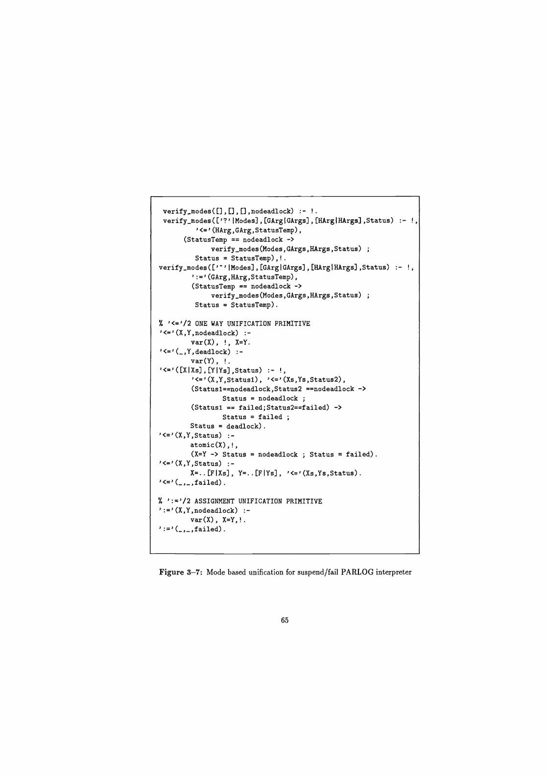
verify_modes ([] , [] , ,nodeadlock) :- !. verifymodes ([' ?' I Modes] , [GArg (GArgs] , [HArg I HArgs] ,Status)

'<='(HArg,GArg,StatusTemp), (StatusTemp == nodeadlock ->

verify modes(Modes,GArgs,HArgs,Status) Status = StatusTemp),!.

verify_modes(['"IlModes],[GArgIGArgs],[HArgIHArgs],Status) :- !, ':='(GArg,HArg,StatusTemp), (StatusTemp == nodeadlock ->

verifymodes(Modes,GArgs,HArgs,Status) Status = StatusTemp).

'<='/2 ONE WAY UNIFICATION PRIMITIVE '<='(X,Y,nodeadlock) :-

var(X), !, X=Y.

'<='(_,Y,deadlock) .- var(Y), !.

'<='([XIXs],[YIYs],Status) :- !, '<='(X,Y,Statusl), '<='(Xs,Ys,Status2), (Statusl==nodeadlock,Status2 ==nodeadlock ->

Status = nodeadlock ;

(Statusi == failed;Status2==f ailed) -> Status = failed

Status = deadlock). '<='(X,Y,Status) :-

atomic(X),!, (X=Y -> Status = nodeadlock ; Status = failed).

'<='(X,Y,Status) :- X=..[FIXs], Y=..[FIYs], '<='(Xs,Ys,Status).

,<=,(-,-,failed).

% ':='/2 ASSIGNMENT UNIFICATION PRIMITIVE

':='(X,Y,nodeadlock) :- var(X), X=Y,!.

':='(_,_,failed).

Figure 3-7: Mode based unification for suspend/fail PARLOG interpreter

65

which indicates that the is/2 system call can be evaluated if its second

argument contains no variables.

Before considering the procedural interpretation of the clause that processes

Parlog goals we should consider some of the required extensions and how they may

be achieved. The reduction/suspension/failure of a Parlog process requires

several extensions.

- The head unification of a goal with some clause head may suspend, succeed

or fail. This requires an extension to the mode based unification given in

Figure 3-2, which is used by the basic interpreter. The new mode based

unification should indicate the state of the unification; again this is achieved

using an additional argument. The resulting mode based unification is given

in Figure 3-7.

Suspending a goal evaluation requires that no clause is committable and at

least one clause evaluation suspends. Failing a goal evaluation requires that

no clause is committable and no clause has suspended. These requirements

mean that each clause has to be attempted and the status of each guard

evaluation collected. This is achieved using a Prolog bagof/3 metacall.

Once a set of clause evaluation statuses are known, picking a committable

clause, or testing if the goal evaluation has suspended, or testing if the

goal evaluation has failed is a relatively simple task. The code for picking

a committable clause or testing if the goal evaluation suspends is given in

Figure 3-8.

Now we can consider the procedural interpretation of the clause used to reduce

a Parlog process.

Firstly, obtain the mode declarations for the dequeued Parlog goal. Secondly,

for each clause (using a bagof/3) head unify the goal and the clause head.

If the unification succeeds then evaluate the guard. The state of each clause

66

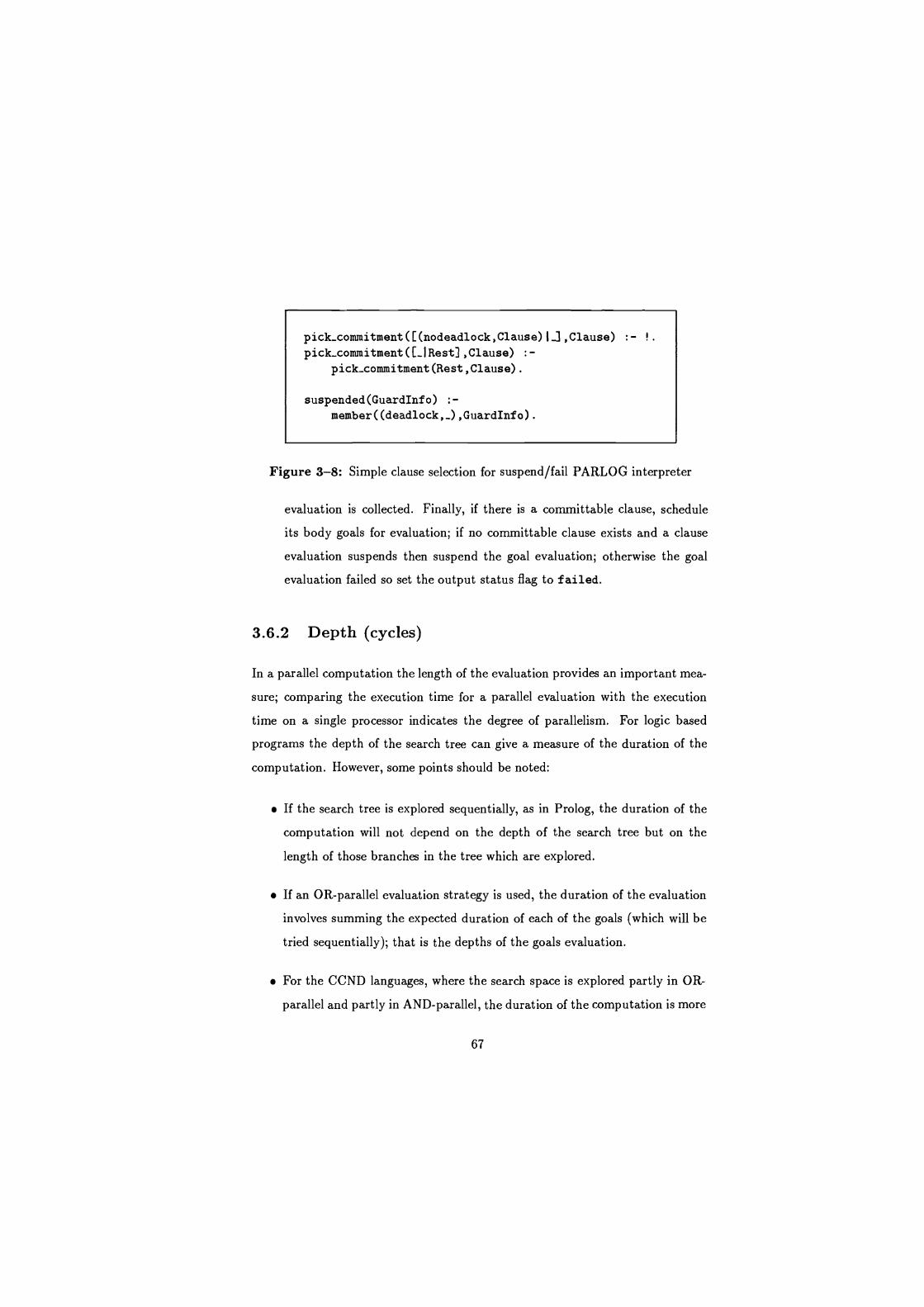
pick_conunitment([(nodeadlock,Clause)L],Clause) :- !

pick-commitment ([_IRest] ,Clause) :-

pick-commitment (Rest, Clause).

suspended(GuardInfo) :-

member((deadlock,_),GuardInfo).

Figure 3-8: Simple clause selection for suspend/fail PARLOG interpreter

evaluation is collected. Finally, if there is a committable clause, schedule

its body goals for evaluation; if no committable clause exists and a clause

evaluation suspends then suspend the goal evaluation; otherwise the goal

evaluation failed so set the output status flag to failed.

3.6.2 Depth (cycles)

In a parallel computation the length of the evaluation provides an important mea-

sure; comparing the execution time for a parallel evaluation with the execution

time on a single processor indicates the degree of parallelism. For logic based

programs the depth of the search tree can give a measure of the duration of the

computation. However, some points should be noted:

If the search tree is explored sequentially, as in Prolog, the duration of the

computation will not depend on the depth of the search tree but on the

length of those branches in the tree which are explored.

If an OR-parallel evaluation strategy is used, the duration of the evaluation

involves summing the expected duration of each of the goals (which will be

tried sequentially); that is the depths of the goals evaluation.

For the CCND languages, where the search space is explored partly in OR-

parallel and partly in AND-parallel, the duration of the computation is more

67

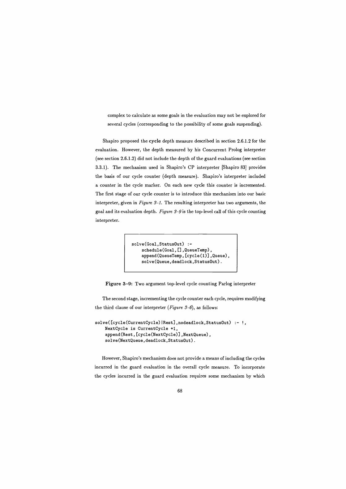
complex to calculate as some goals in the evaluation may not be explored for

several cycles (corresponding to the possibility of some goals suspending).

Shapiro proposed the cycle depth measure described in section 2.6.1.2 for the

evaluation. However, the depth measured by his Concurrent Prolog interpreter

(see section 2.6.1.2) did not include the depth of the guard evaluations (see section

3.3.1). The mechanism used in Shapiro's CP interpreter [Shapiro 83] provides

the basis of our cycle counter (depth measure). Shapiro's interpreter included

a counter in the cycle marker. On each new cycle this counter is incremented.

The first stage of our cycle counter is to introduce this mechanism into our basic

interpreter, given in Figure 3-1. The resulting interpreter has two arguments, the

goal and its evaluation depth. Figure 3-9 is the top-level call of this cycle counting

interpreter.

solve(Goal,StatusOut) :-

schedule(Goal,[],QueueTemp),

append(QueueTemp,[cycle(1)],Queue),

solve(Queue,deadlock,Status0ut).

Figure 3-9: Two argument top-level cycle counting Parlog interpreter

The second stage, incrementing the cycle counter each cycle, requires modifying

the third clause of our interpreter (Figure 3-6), as follows:

solve([cycle(CurrentCycle) IRest],nodeadlock,Status0ut) :- !

NextCycle is CurrentCycle +1,

append(Rest,[cycle(NextCycle)],NextQueue),

solve(NextQueue,deadlock,StatusOut).

However, Shapiro's mechanism does not provide a means of including the cycles

incurred in the guard evaluation in the overall cycle measure. To incorporate

the cycles incurred in the guard evaluation requires some mechanism by which

68

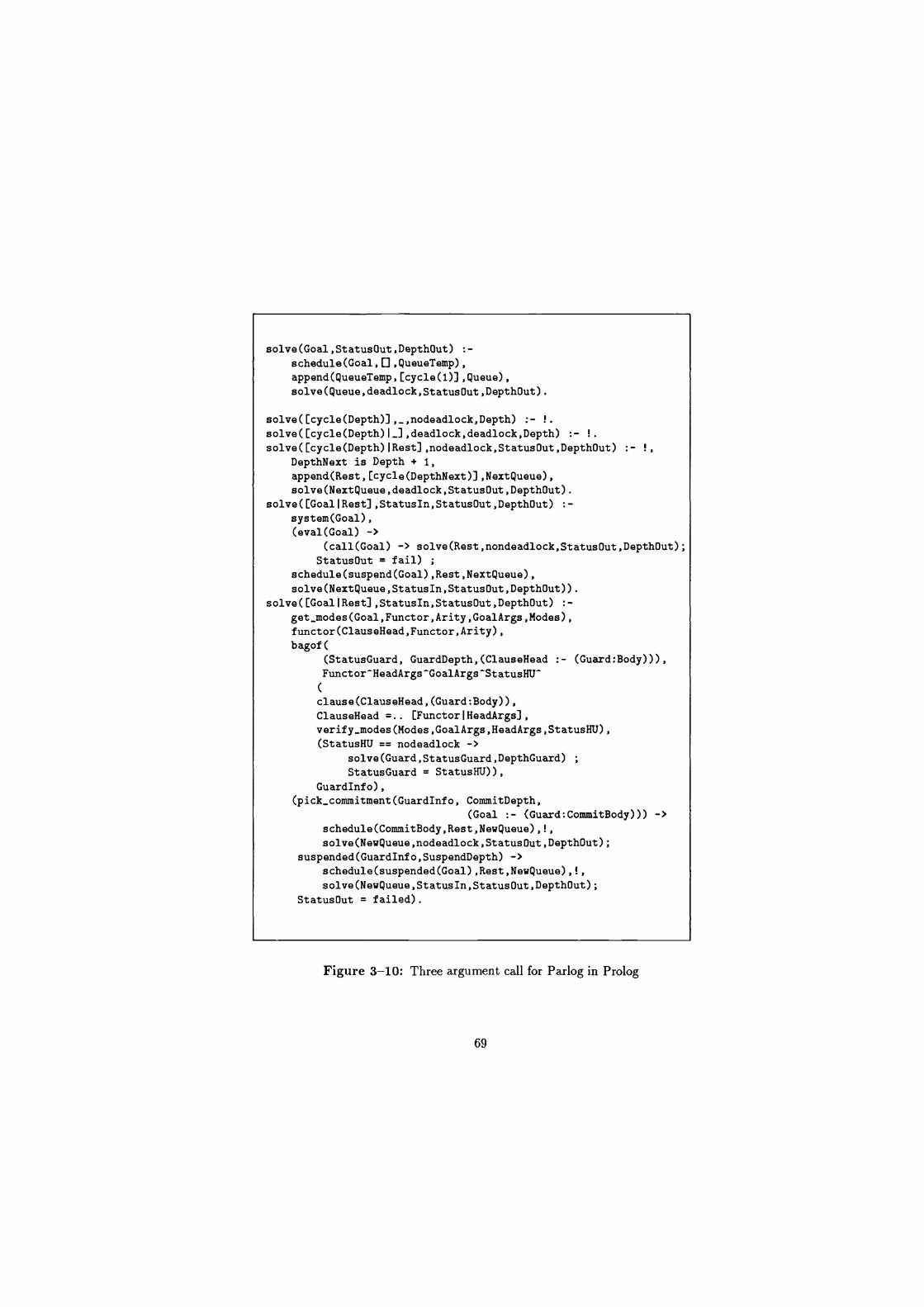
solve(Goal,StatusOut,DepthOut) :- schedule(Goal,[],QueueTemp), append(QueueTemp,[cycle(1)],Queue), solve(queue,deadlock,StatusOut,DepthOut).

solve([cycle(Depth)],_,nodeadlock,Depth) :- !. solve([cycle(Depth)I_],deadlock,deadlock,Depth) !. solve([cycle(Depth)IRest],nodeadlock,StatusOut,DepthOut)

DepthNext is Depth + 1, append(Rest,[cycle(DepthNext)],NextQueue), solve(NextQueue,deadlock,StatusOut,DepthOut).

solve([GoallRest],StatusIn,StatusOut,DepthOut) :- system(Goal),

(eval(Goal) -> (call(Goal) -> solve(Rest,nondeadlock,StatusOut,DepthOut);

StatusOut = fail) ;

schedule(suspend(Goal),Rest,NextQueue), solve(NextQueue,StatusIn,StatusOut,DepthOut)).

solve([GoallRest],StatusIn,StatusOut,DepthOut) :- get modes(Goal,Functor,Arity,GoalArgs,Modes), functor(ClauseHead,Functor,Arity),

bagof( (StatusGuard, GuardDepth,(ClauseHead :- (Guard:Body))), Functor-HeadArgs-GoalArgs-StatusHU-

clause(ClauseHead,(Guard:Body)), ClauseHead =.. [FunctorlHeadArgs], verify_modes(Modes,GoalArgs,HeadArgs,StatusHU), (StatusHU == nodeadlock ->

solve(Guard,StatusGuard,DepthGuard) StatusGuard = StatusHU)),

Guardlnfo),

(pick_commitment(Guardlnfo, CommitDepth, (Goal :- (Guard:CommitBody))) ->

schedule(CommitBody,Rest,NewQueue),!, solve(Newqueue,nodeadlock,StatusOut,DepthOut);

suspended(Guardlnfo,SuspendDepth) -> schedule(suspended(Goal),Rest,NewQueue),!, solve(Newqueue,Statusln,StatusOut,DepthOut);


Figure 3-10: Three argument call for Parlog in Prolog

69

the depth of a guard evaluation is returned. This is achieved by having a three

argument call. The first argument is the goal conjunction to be evaluated, the

second argument is the final status of the evaluation and the third is the depth of

the evaluation. Figure 3-10 provides such a three argument interpreter.

We can now develop a mechanism by which the cycles incurred in the guard

evaluation can contribute to the overall cycle (depth) measure. The actual

mechanism developed forms the means by which we also model inherent AND-

parallelism, and is covered in the next section.

70

3.6.3 AND-parallelism

As stated earlier (see section 3.3.1) current interpreters evaluate the process

queue left-to-right and any bindings made by the evaluation of goals in the queue

take place immediately. So these bindings will be available to any remaining goals

in the goal list. This will allow goals that require these bindings to reduce in the

current cycle. Hence the evaluation is dependent on goal order. We make the

assumption that, in a cycle, a goal can only use bindings available to it at the

start of the cycle (see section 3.5).

To offer such a model requires the addition of a binding list in which the

bindings produced are maintained until the appropriate cycle. In the case of deep

guards this mechanism can also be employed to account for the cycles performed

in the guard evaluation. As well as having a binding list we maintain a commit

list, this commit list contains a set of 'body goal'/'depth counter' pairs. The

depth counter indicates when the body goals would have been committed to if the

guard evaluation took place in parallel with other body goal evaluations. We have

combined both the lists (bindings and goals) into one list. The new list contains

wtc/3-(wait to commit) structures. Such a structure contains a relative depth

counter (the depth of the guard evaluation), the goal that was evaluated and the

clause that is to be committed to. The output bindings are made by unifying the

goal and the head of the committed clause when the appropriate cycle is reached.

Implementing this functionality in our interpreter requires an additional argu-

ment, a wait to commit list, in the main loop of our interpreter. The resulting

'When carrying out the guard evaluation a copy of the goal is used to select the

committable clause, hence the bindings that result are maintained in the committed

clause and only exported when the goal and the clause head are unified. Using this

mechanism the binding list becomes semi-implicit, in that no real binding list need be

maintained. This method is suitable for safe languages, like Parlog.

71

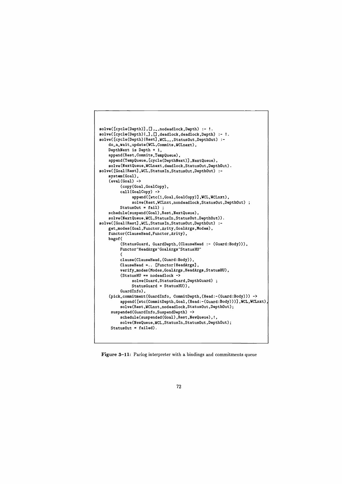
solve([cycle(Depth)],[],_,nodeadlock,Depth) :- !.

solve([cycle(Depth){_],[],deadlock,deadlock,Depth) :- !.

solve([cycle(Depth)IRest],WCL,_,StatusOut,DepthOut) :-

do_a_wait_update(WCL,Commits,WCLnext),

DepthNext is Depth + 1,

append(Rest,Commits,TempQueue),

append(TempQueue,[cycle(DepthNext)],NextQueue),

solve(NextQueue,WCLnext,deadlock,StatusOut,DepthOut).

solve([GoallRest],WCL,StatusIn,StatusOut,DepthOut) :-

system(Goal),

(eval(Goal) ->

(copy(Goal,GoalCopy),

call(GoalCopy) ->

append([wtc(1,Goal,GoalCopy)],WCL,WCLnxt),

solve(Rest,WCLnxt,nondeadlock,StatusOut,DepthOut) StatusOut = fail) ;

schedule(suspend(Goal),Rest,NextQueue),

solve(NextQueue,WCL,StatusIn,StatusOut,DepthOut)).

solve([GoallRest],WCL,StatusIn,StatusOut,DepthOut) :-

get_modes(Goal,Functor,Arity,GoalArgs,Modes), functor(ClauseHead,Functor,Arity),

bagof( (StatusGuard, GuardDepth,(ClauseHead :- (Guard:Body))),

Functor"HeadArgs"GoalArgs"StatusHU"

clause(ClauseHead,(Guard:Body)), ClauseHead =.. [FunctorlHeadArgs], verify_modes(Modes,GoalArgs,HeadArgs,StatusHU), (StatusHU == nodeadlock ->

solve(Guard,StatusGuard,DepthGuard) StatusGuard = StatusHU)),

Guardlnfo), (pick_commitment(Guardlnfo, CommitDepth,(Head:-(Guard:Body))) ->

append([wtc(CommitDepth,Goal,(Head:-(Guard:Body)))],WCL,WCLnxt), solve(Rest,WCLnxt,nodeadlock,StatusOut,DepthOut);

suspended(Guardlnfo,SuspendDepth) -> schedule(suspended(Goal),Rest,NewQueue),!, solve(NewQueue,WCL,Statusln,StatusOut,DepthOut);


Figure 3-11: Parlog interpreter with a bindings and commitments queue

72

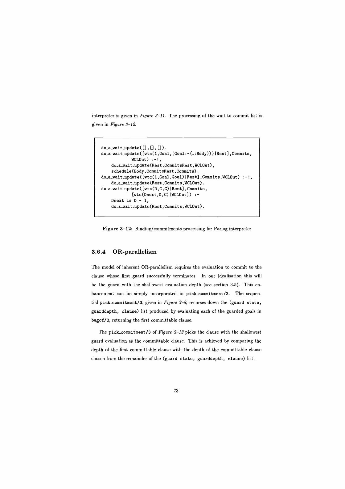
interpreter is given in Figure 3-11. The processing of the wait to commit list is

given in Figure 3-12.

do_a_wait update([] , [] , []) .

do_a_wait_update([wtc(1,Goal, (Goal:-(_:Body)))IRest],Commits, WCLOut) :-!,

do_a_wait_update(Rest,Commit sRest,WCLOut), schedule(Body,CommitsRest,Commits).

do_a_wait_update([wtc(1,Goal, Goal) I Rest], Commits, WCLOut) :-!, do_a_wait_update(Rest,Commits, WCLOut).

do_a_wait_update([wtc(D,G,C)IRest],Commits, [wtc(Dnext,G,C)JWCLOut]) :-

Dnext is D - 1, do_a_wait_update(Rest,Commits, WCLOut).

Figure 3-12: Binding/commitments processing for Parlog interpreter

3.6.4 OR-parallelism

The model of inherent OR-parallelism requires the evaluation to commit to the

clause whose first guard successfully terminates. In our idealisation this will

be the guard with the shallowest evaluation depth (see section 3.5). This en-

hancement can be simply incorporated in pick-commitment/3. The sequen-

tial pick-commitment/3, given in Figure 3-8, recurses down the (guard state,

guarddepth, clause) list produced by evaluating each of the guarded goals in

bagof/3, returning the first committable clause.

The pick-commitment/3 of Figure 3-13 picks the clause with the shallowest

guard evaluation as the committable clause. This is achieved by comparing the

depth of the first committable clause with the depth of the committable clause

chosen from the remainder of the (guard state, guarddepth, clause) list.

73

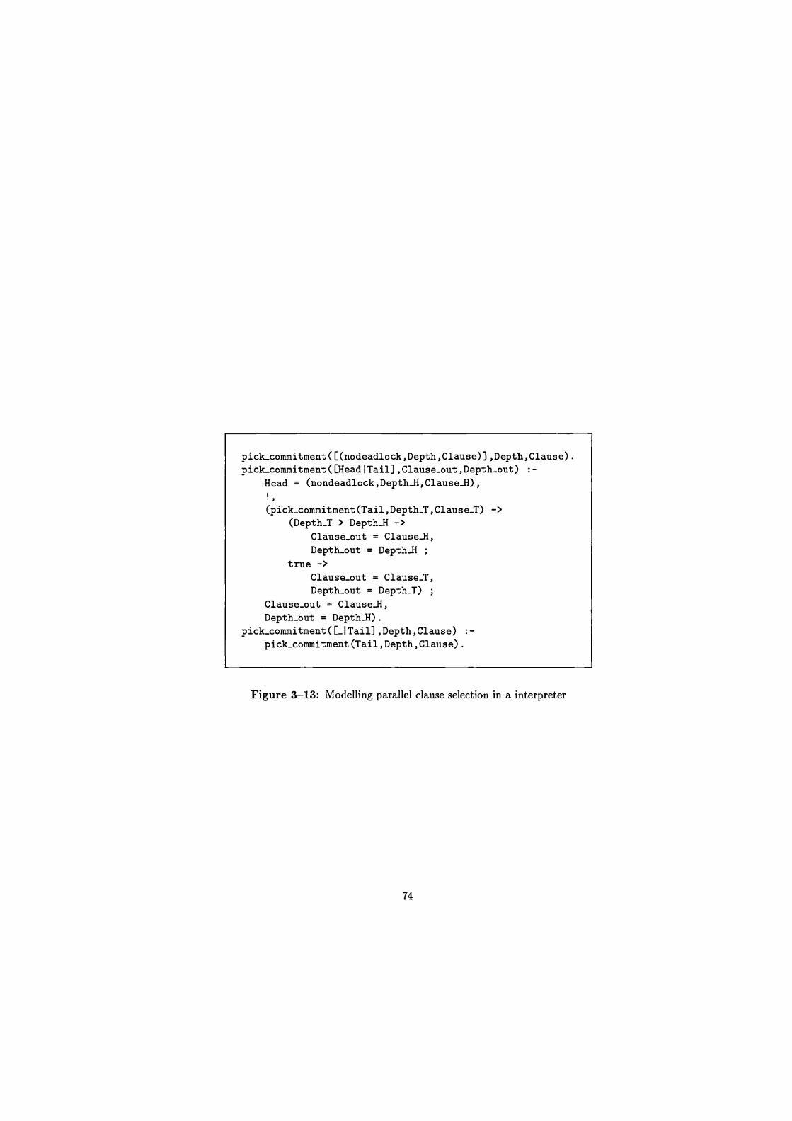
pick_commitment([(nodeadlock,Depth,Clause)],Depth,Clause).

pick_commitment([HeadITail] ,Clause-out ,Dept h_out) :-

Head = (nondeadlock,Depthii,Clause-H),

,

(pick_commitment(Tail,Depth-T, Clause_T) -> (Depth_T > Depthii ->

Clause-out = Clause-H,

Depth-out = Depthii

true ->

Clause-out = Clause T, Depth-out = Depth T)

Clause-out = Clause-H,

Depth-out = Depth-H).

pick-commitment ([_ITail] , Depth, Clause) :- pick_commitment(Tail,Depth, Clause).

Figure 3-13: Modelling parallel clause selection in a interpreter

74

3.6.5 Features of our improved model

The features of our interpreter are as follows:

both AND and OR-parallelism are modelled;

each of the guarded goals for a given predicate are tried and relevant statistics

collected;

the statistics from the evaluation of the guarded goal are used to pick the

solution path (currently this is the shallowest successful guard, i.e. the first

guard that would have succeeded in a breadth-first execution);

the goals that form the goal list each undergo one reduction in a cycle; any

bindings made as the goal list is processed occur only when all the goals have

been attempted;

the evaluation of a system goal which makes a call to the underlying Prolog

system is counted as one reduction;

bindings made using calls to the underlying Prolog system are made only

when all the goals have been attempted;

the interpreter makes a distinction between suspension and failure;

although guard evaluations are carried out to completion in one go, the

commitment of a goal to a given clause is prevented for the number of cycles

the guard took to evaluate; and

the suspension of all the guarded goals causes suspension of the goal being

evaluated.

75

3.7 Summary


Why a measure of the inherent parallelism is useful.

How we can obtain a measure of the inherent parallelism by simulating the

execution of the evaluation on an unlimited number of processors.

The current models of execution and what they provide in terms of evaluation

metrics.

The currently quoted metrics (cycles, reductions and suspensions) and

their limitations.

The requirements of an improved model of execution, which would be used

to collect information about the inherent parallelism.

The idealisations we assume in our execution model.

The incremental design and implementation of an improved interpreter which

forms the basis of our new evaluation system.

76

Chapter 4

New evaluation parameters and example evaluations

4.1 Overview

The current interpreters used for evaluation are limited in two respects:

their model of breadth-first execution of these languages contains several

major deviations from a fully parallel execution;

the evaluation parameters used (cycles, reductions and suspensions) give

no indication of various alternatives open to the language implementors.

In chapter 3, we considered limitations in the execution model provided by

the current interpreters and then developed a new interpreter which allows us to

obtain improved measures of the inherent parallelism in a program.

In this chapter we consider the second limitation of the current evaluation sys-

tems; the parameters collected. Current parameters give no indication as to how

the program would have behaved under alternative models of execution. For exam-

ple, on commitment to one clause the other guard evaluations could be terminated

or ignored.

77

Section 4.2 considers some possible execution alternatives open to language

implementors. This provides the basis for a set of parameters which can be used

to indicate the relative merits of these alternatives. These are presented in Section

4.3.

In section 4.4 we present a tool developed to profile the various proposed pa-

rameters over time (cycles). Later in this thesis we use this profiling tool to

consider the execution behaviour of several AI programs.

Section 4.5 presents measurements of our parameters for one CCND language,

Parlog. An evaluation using these parameters is given for a small set of simple

example programs and the results analysed. The nature of these examples allows

us to consider the theoretical behaviour of these programs compared with the

behaviour predicted by our evaluation system.

Finally, section 4.6 considers some of the limitations of our evaluation system.

4.2 Basis for new parameters

Apart from having inaccuracies in measuring the inherent parallel behaviour of

programs introduced through limitations in the execution model, the parameters

proposed by Shapiro (cycles, suspensions and reductions) do not give any

indication of the effects that alternative implementation models may have had.

Currently the models of execution being adopted for the CCND languages are

settling down to a subset of the possible models. For example, the languages

are being restricted to flat guards or only allowing the clauses to be investigated

sequentially. In general the subset being adopted as standard is being governed

by implementation issues rather than application requirements. This work aims

to present an applications viewpoint of the possible direction that the CCND

implementors may take. To this end we have considered how applications would

78

behave on various alternative executions and hence provide some applications

rationale for the implementation alternatives.

The execution alternatives considered are relevant to the complete CCND lan-

guage rather than any given subset and represent extremes in the implementation

options, for instance the alternatives for scheduling are busy and non-busy wait-

ing. Our results for busy waiting, an implementation option which many think

is not appropriate, indicates that for Layered Streams this could be a suitable im-

plementation option (see section 5). In the following subsections we consider some

of these alternatives. The new parameters we propose aim to provide information

about the relative merits of these different alternatives.

4.2.1 Pruning OR-branches

The parallel evaluation of a goal invokes several guarded systems, one for each

clause that the goal successfully head unifies with. The evaluation commits to the

first clause whose guarded system successfully terminates. On commitment, the

other guarded systems invoked by the goal evaluation can be terminated or ig-

nored. Terminating the alternative clauses (pruning) requires the system to stop

the computation being carried out in the alternative branches. This may prevent

these branches carrying out needless computation. However, if the guarded goals

for a given predicate are balanced, that is evaluated in the same time, then prun-

ing the OR-search will not prevent any computation in the alternative guards.

Ignoring the other alternative clauses (non-pruning) when a goal commits, re-

quires the system to disregard any commitment requests from the other alterna-

tives should their guarded systems also terminate successfully. This assumes that

guard evaluations terminate and certainly do not diverge. This may save some

computation (in sending a terminate message to the other guard evaluation) if the

guards are balanced or in cases where only one clause can be committed to.

Even if pruning the clauses reduces some theoretical computation it may be

worth attempting only if the amount of work saved is comparable to the expected

79

overheads of terminating the other clause evaluations. This will depend on the

architecture and implementation.

Pruning clauses is likely to be most beneficial for programming techniques

and applications that employ an uneven guarded computation. Such programs

in the main will employ deep guards [Gregory 87]. However, it should be noted

that even flat guards may benefit from pruning. This will occur when some of

the (flat) guards have data dependencies which result in them taking longer to

evaluate than other guards, or if some guards make use of costly system predicates

while others do not. However, most programs with flat guards are likely to have

an even guard evaluation.

4.2.2 Suspension mechanisms

A goal evaluation suspends if there is no committable clause and at least one of the

guard evaluations or head unifications suspends. Suspending the evaluation can

be achieved in several ways, the two extremes being goal suspension and clause

suspension. Goal suspension involves suspending the parent goal of a computation

when each of the clauses it could reduce by suspend. Note that this parent goal

may actually be the guarded goal of some other evaluation.

Alternatively each of the clauses (guarded computations and head unifications)

could be suspended, which is known as clause suspension. Here the current state

of each clause evaluation is saved. As there may be recursive guard evaluations

invoked, clause suspension may result in a tree of suspended evaluations, rep-

resenting the guard call structure. The trade-off between these two extremes is

basically a space-time consideration. Suspending a goal requires less space than

suspending the evaluation of each of the clauses. However, if some computation is

performed in the evaluation of the guarded goals before the evaluation suspends

then this computation will be lost, and repeated, if the goal is suspended.

80

In our system we treat system calls as goals with one clause. This is because we

assume the two suspension mechanism alternatives should not portray a difference

for system calls (see section 3.5).

4.2.3 Scheduling policy

Another choice is how and when suspended evaluations are re-scheduled. When

an evaluation suspends it could be tagged to the variables which are required and

unbound and re-scheduled when they become bound, this is known as non-busy

waiting. It should be noted that some predicates, like merge/3, only suspend on

one variable whereas others, like equals/2, require both arguments to be bound.

The other extreme would be to immediately reschedule the suspended evaluation,

known as busy waiting.

Employing a non-busy waiting suspension mechanism is appropriate if sus-

pended evaluations remain suspended for several cycles, for example in generating

primes numbers by sifting [Gregory 87] most of the filter processes will be sus-

pended most of the time. Employing a busy waiting suspension mechanism is

appropriate if suspended goals are only likely to be suspended for a short period,

as with Layered Streams [Okumura & Matsumoto 87] (see chapter 5).

4.3 Proposed profiling parameters

The profiling parameters we propose aim to reflect the effect of the various op-

tions available in pruning OR-branches, alternative suspension mechanisms and

alternative scheduling polices. The basic parameters are still suspensions and

reductions. However, these are given for the various combinations of the execu-

tion alternatives considered. Two additional parameters are also considered, the

depth of the evaluation and the minimum reductions. So the basic top-level

parameters put forward are suspensions and reductions using:

81

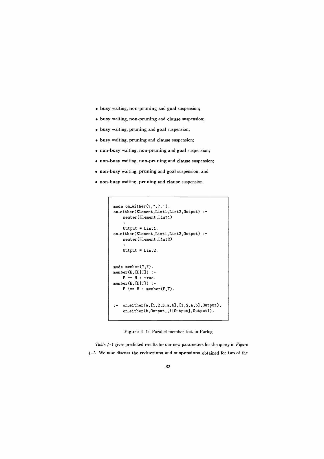
busy waiting, non-pruning and goal suspension;

busy waiting, non-pruning and clause suspension;

busy waiting, pruning and goal suspension;

busy waiting, pruning and clause suspension;

non-busy waiting, non-pruning and goal suspension;

non-busy waiting, non-pruning and clause suspension;

non-busy waiting, pruning and goal suspension; and

non-busy waiting, pruning and clause suspension.

mode on_either(?,?,?,").

on_either(Element,Listl,List2,Output) :-

member(Element,Listl)

Output = Listi.

on_either(Element,Listl,List2,Output) :-

member(Element,List2)

Output = List2.

mode member(?,?). member(E,[HIT]) :-

E == H : true.

member(E,[HIT]) :-

E \== H : member(E,T).

on_either(a,[1,2,3,a,b],[1,2,a,b],Output), on-either (b, Output, [11 Output]. Output 1) .

Figure 4-1: Parallel member test in Parlog

Table 4-1 gives predicted results for our new parameters for the query in Figure

,4-1. We now discuss the reductions and suspensions obtained for two of the

82

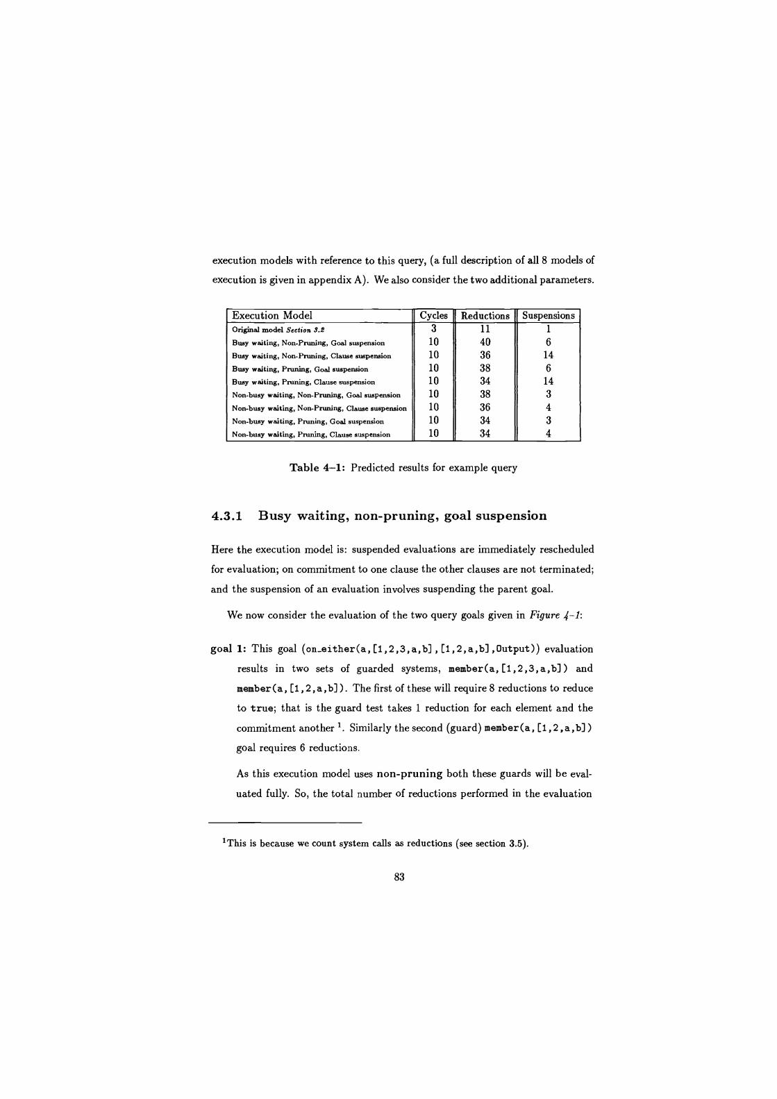
execution models with reference to this query, (a full description of all 8 models of

execution is given in appendix A). We also consider the two additional parameters.

Execution Model Cycles Reductions Suspensions Original model Section 3.2 3 11 1

Busy waiting, Non-Pruning, Goal suspension 10 40 6

Busy waiting, Non-Pruning, Clause suspension 10 36 14

Busy waiting, Pruning, Goal suspension 10 38 6

Busy waiting, Pruning, Clause suspension 10 34 14 Non-busy waiting, Non-Pruning, Goal suspension 10 38 3

Non-busy waiting, Non-Pruning, Clause suspension 10 36 4 Non-busy waiting, Pruning, Goal suspension 10 34 3 Non-busy waiting, Pruning, Clause suspension

1

10 34 4

Table 4-1: Predicted results for example query

4.3.1 Busy waiting, non-pruning, goal suspension

Here the execution model is: suspended evaluations are immediately rescheduled

for evaluation; on commitment to one clause the other clauses are not terminated;

and the suspension of an evaluation involves suspending the parent goal.

We now consider the evaluation of the two query goals given in Figure 4-1:

goal 1: This goal (on_either(a, [1,2,3,a,b] , [1,2,a,b] ,Output)) evaluation

results in two sets of guarded systems, member (a, [ 1, 2 , 3 , a , b] ) and

member(a, [1 ,2,a,b]). The first of these will require 8 reductions to reduce

to true; that is the guard test takes 1 reduction for each element and the

commitment another 1. Similarly the second (guard) member (a, [1,2,a,b] )

goal requires 6 reductions.

As this execution model uses non-pruning both these guards will be eval-

uated fully. So, the total number of reductions performed in the evaluation

'This is because we count system calls as reductions (see section 3.5).

83

of this goal is 16 (8 in evaluating the first guard, 6 in the second guard, 1 for

the commitment to the body goals and finally 1 for the output unification).

The total number of cycles that this evaluation takes is 4. That is the

evaluation commits to the second, on-either/4, clause after 3 cycles and it

takes 1 cycle to carry out the output unification. So the binding made to

the shared variable "Output" will be seen by the other AND-parallel goals

in cycle 5.

goal 2: The second goal (on_either(b,Output, [11 Output] ,Outputl)) eval-

uation results in two sets of guarded goals, member(b,Output) and

member(b, El IOutput]). The first of these could be evaluated via two

clauses, however these both suspend on head unification. As we are us-

ing goal suspension the evaluation of the first guarded goal suspends. The

second (guard) is able to perform 2 reductions (the guard test and the com-

mitment to member (b, Output)). The resulting goal could be evaluated via

two clauses but both of these suspend on head unification. This results in

the suspension of the second guarded goal. Now both sets of guarded goals

have suspended the evaluation of the second query goal suspends, giving a

total of 3 goal suspensions and 2 reductions, the second query goal suspends

after 2 cycles.

Using busy waiting this top-level goal will be retried in cycle 3. In cycle 3

the variable "Output" will still be unbound, so the rescheduled evaluation

will perform the same 2 reductions and then suspend again. The goal will

next be tried in cycle 5.

In cycle 5 the shared variable "Output" will be bound, so the sec-

ond query goal becomes on_either(b, [1,2,a,b] , [1,1,2,a,b] ,Outputl).

This goal invokes two guarded systems, member (b, [1, 2 , a, b]) and

member(b,[1,1,2,a,b]). The first of these will require 8 reductions to

reduce to true. Similarly the second guard requires 10 reductions.

84

As the execution uses non-pruning both these guards will be evaluated

fully. Hence the final attempt at evaluating this goal results in 20 reductions

(8 in the first guard, 10 in the second, 1 for the commitment to the body

goals and finally 1 for the output unification). The total number of cycles

that this evaluation takes is 5. That is the evaluation commits to the first

clause after 4 cycles and it takes 1 cycle to carry out the output unification.

So, the evaluation of the query using this execution model takes: 10 cycles; 40

reductions (16 for the first goal, 4 for the second goal before suspension, and 20

for the final evaluation of the second goal); and 6 goal suspensions (1 suspension

for the first guarded goal, member(b,L), 1 suspension for the second guarded goal,

member(b, [1IL]) and 1 suspension for the query goal, these suspensions occur

twice because of the busy waiting).

4.3.2 Non-busy waiting, pruning, clause suspension

Here the execution model is: suspended evaluations are tagged to the variables

which must be bound before the evaluation can proceed; on commitment to one

clause the other clauses are not terminated; and the suspension of an evaluation

involves suspending the clauses.

We now consider the evaluation of the two query goals given in Figure 4-1:

goal 1: The evaluation of the first goal of the query will invoke two guarded

systems, member(a, [1,2,3,a,b]) and member(a, [1,2,a,b]). The first of

these requires 8 reductions to reduce to true, and evaluates in 4 cycles. The

second (guarded) goal requires 6 reductions and evaluates in 3 cycles.

This execution model uses pruning, so on commitment to the second clause

the system will be able to prevent 2 reductions being performed2 in the

2That is two reductions at best, ie. assuming that pruning can happen immediately.

85

evaluation of the first guard. Hence the total number of reductions performed

in the evaluation of this goal is 14 (6 in the first guard (when it is pruned),

6 in the second guard (when it commits), 1 for the commitment to the body

goals and finally 1 for the output unification). The binding of the variable

"Output" will be available to the other goals in cycle 5.

goal 2: The second goal will invoke two guarded systems, member(b,Output)

and member(b, [1 I Output] ). The first (guard) could be evaluated via two

clauses. However, both evaluations suspend on head unification. These sus-

pended clause evaluations are tagged to the variable "Output". The second

(guard) is able to perform 2 reductions (the guard test and the commit-

ment to member (b, Output)). This resulting goal could be evaluated via

two clauses but again both evaluations suspend on head unification. The

two suspended clause evaluations are again tagged to variable "Output".

In cycle 5 the shared variable "Output" will be bound, so the 4 suspended

clause evaluations will now be evaluated. These will reduce to true in 16

reductions. Hence the total number of reductions performed in the evalua-

tion of this goal is 20 (8 in the first guard, 10 in the second (2 before the

suspensions and 8 after the suspensions), 1 for the commitment to the body

goal and finally 1 for the output unification). No pruning can take place,

although the guards are different depths the evaluation of the deeper guard

(via second clause) is able to perform some evaluation while the first guard

is suspended.

So the evaluation of the query using this execution model takes: 10 cycles; 34

reductions (14 for the first goal and 20 for the second goal); and 4 suspensions.

4.3.3 Depth of evaluation

A measure of the average expected processor utilisation is a useful quantity in se-

lecting appropriate architectures or in estimating expected performance improve-

86

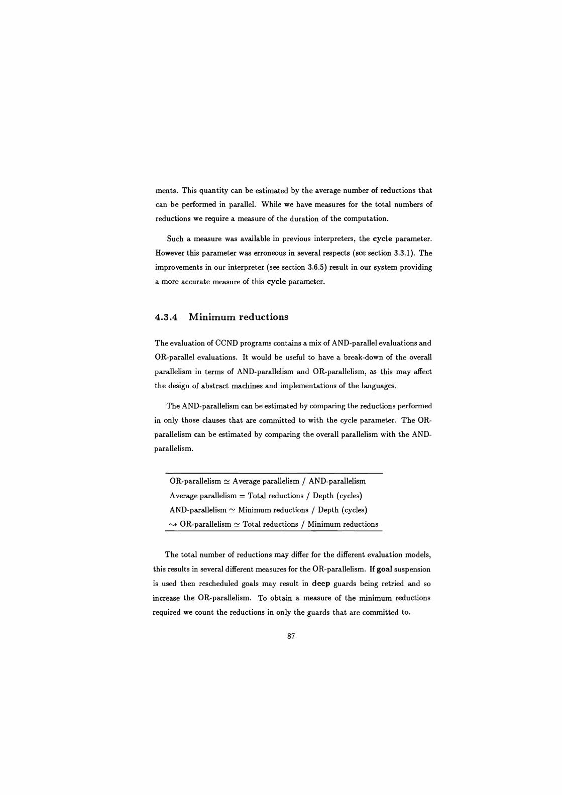
ments. This quantity can be estimated by the average number of reductions that

can be performed in parallel. While we have measures for the total numbers of

reductions we require a measure of the duration of the computation.

Such a measure was available in previous interpreters, the cycle parameter.

However this parameter was erroneous in several respects (see section 3.3.1). The

improvements in our interpreter (see section 3.6.5) result in our system providing

a more accurate measure of this cycle parameter.

4.3.4 Minimum reductions

The evaluation of CCND programs contains a mix of AND-parallel evaluations and

OR-parallel evaluations. It would be useful to have a break-down of the overall

parallelism in terms of AND-parallelism and OR-parallelism, as this may affect

the design of abstract machines and implementations of the languages.

The AND-parallelism can be estimated by comparing the reductions performed

in only those clauses that are committed to with the cycle parameter. The OR-

parallelism can be estimated by comparing the overall parallelism with the AND-

parallelism.

OR-parallelism Average parallelism / AND-parallelism

Average parallelism = Total reductions / Depth (cycles)

AND-parallelism Minimum reductions / Depth (cycles)

OR-parallelism N Total reductions / Minimum reductions

The total number of reductions may differ for the different evaluation models,

this results in several different measures for the OR-parallelism. If goal suspension

is used then rescheduled goals may result in deep guards being retried and so

increase the OR-parallelism. To obtain a measure of the minimum reductions

required we count the reductions in only the guards that are committed to.

87

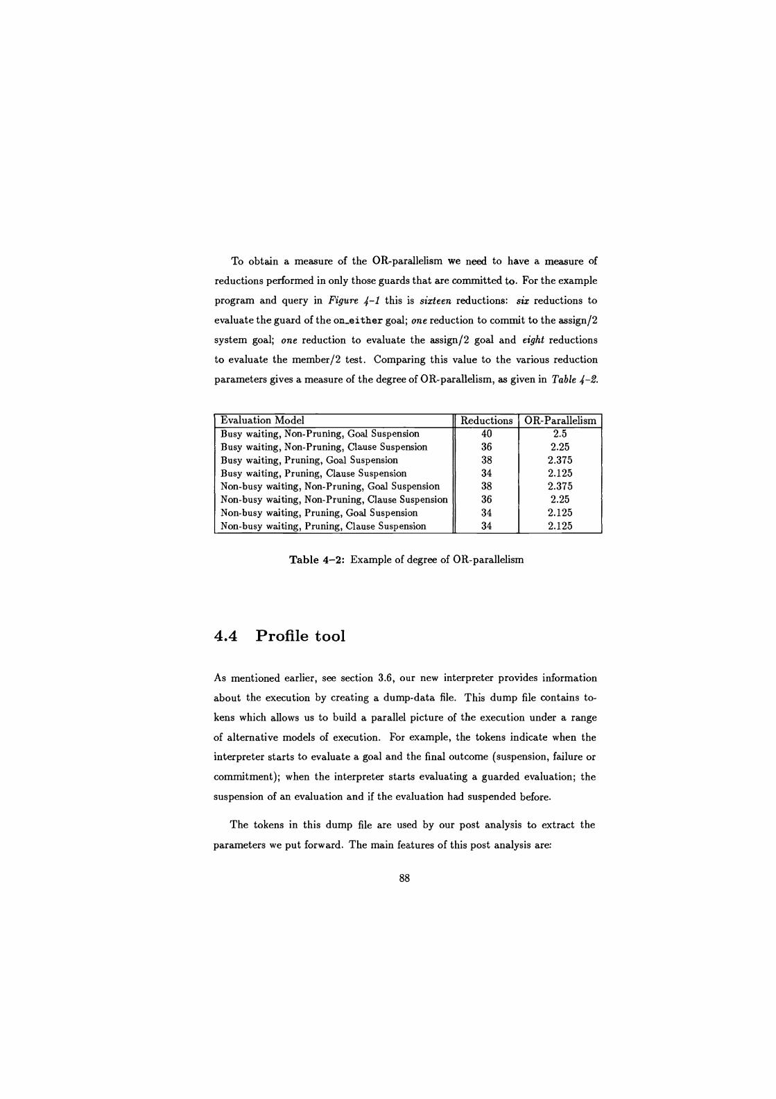
To obtain a measure of the OR-parallelism we need to have a measure of

reductions performed in only those guards that are committed to. For the example

program and query in Figure 4-1 this is sixteen reductions: six reductions to

evaluate the guard of the on-either goal; one reduction to commit to the assign/2

system goal; one reduction to evaluate the assign/2 goal and eight reductions

to evaluate the member/2 test. Comparing this value to the various reduction

parameters gives a measure of the degree of OR-parallelism, as given in Table 4-2.

Evaluation Model Reductions OR-Parallelism Busy waiting, Non-Pruning, Goal Suspension 40 2.5 Busy waiting, Non-Pruning, Clause Suspension 36 2.25 Busy waiting, Pruning, Goal Suspension 38 2.375 Busy waiting, Pruning, Clause Suspension 34 2.125 Non-busy waiting, Non-Pruning, Goal Suspension 38 2.375 Non-busy waiting, Non-Pruning, Clause Suspension 36 2.25 Non-busy waiting, Pruning, Goal Suspension 34 2.125 Non-busy waiting, Pruning, Clause Suspension 34 2.125

Table 4-2: Example of degree of OR-parallelism

4.4 Profile tool

As mentioned earlier, see section 3.6, our new interpreter provides information

about the execution by creating a dump-data file. This dump file contains to-

kens which allows us to build a parallel picture of the execution under a range

of alternative models of execution. For example, the tokens indicate when the

interpreter starts to evaluate a goal and the final outcome (suspension, failure or

commitment); when the interpreter starts evaluating a guarded evaluation; the

suspension of an evaluation and if the evaluation had suspended before.

The tokens in this dump file are used by our post analysis to extract the

parameters we put forward. The main features of this post analysis are:

88

The profiler maintains a cycle by cycle aggregate of each of the proposed pro-

file parameters. This provides us with a break down of the various profiling

parameters which can be used to give a dynamic picture of the execution.

Moreover this mechanism also provides the means by which we are able to

collect pruned/non-pruned, busy/non-busy and goal/clause data.

Profiling the guard data also maintains a cycle by cycle aggregate of each of

the parameters as collected in the guard evaluation.

On completing the profiling of some guard data the next token indicates that

the parent goal either commits, suspends or fails.

If the goal commits, the clause number and depth of the commitment

are also returned. This provides information which is used to prune

those profiling parameters which adopt a pruned execution model.

The pruned guard cycle by cycle profile is then combined (spliced) into

its parents cycle by cycle profile. Next, an additional reduction repre-

senting this commitment is added to each of the reduction parameters

at the depth at which the guarded evaluation committed. Finally, the

minimum reduction parameter from the guard evaluation is added

to the parents minimum reduction parameter, which is then incre-

mented by one (to reflect the commitment).

If the goal evaluation suspends for the first time the suspension param-

eters of the guarded goal evaluations are spliced into the parents profile.

An additional suspension is also added to all the goal suspension pa-

rameters at the depth at which the guard suspended.

- If the goal evaluation re-suspends (non-busy waiting) the busy sus-

pension parameters of the guarded goal evaluations are spliced into

the parents profile. An additional suspension is also added to the busy

waiting goal suspension parameters, at the depth at which the guarded

evaluation suspended.

89

- Head unifications only contribute to the clause suspension parameters.

The data produced by our analysis system gives a cycle by cycle break down of

the various proposed parameters. We have also implemented a profile tool which

executes under SUNVIEWTM. This tool allows us to see any, or several, profiling

parameters in graphical form. The tool also provides information on the totals of

the various parameters. The tool is best used in an interactive mode. However as

technical reports do not facilitate this usage we have included, where appropriate,

screendumps of this tool executing.

The dump file could be used to collect several other parameters. For example,

we count system calls as reductions, which we use as a measure of parallelism.

However the dump file contains different tokens for commitments and system call

evaluations and so different measures for the parallelism could be obtained. Sim-

ilarly, our current analysis assumes that pruning takes place immediately. How-

ever the dump file could be processed differently, allowing some number of cycles

before pruning is applied. This would reflect the possible delay in committing to

a clause and being able to terminate the evaluation of the other clauses.

Figure 4-2 contains an example screendump of our tool. The tool shows plots

of the number of reductions and suspensions (y-axis) in each cycle (x-axis). Such

plots can be given for any combination of suspension mechanism, scheduling

strategy and pruning option. The options selected are indicated by the toggle

buttons on the right hand side. The tool also presents information on the total

number of reductions and suspensions using a given execution model. These are

presented next to the toggle buttons for each option. Finally, the tool also contains

some more general information, like: the goal that was evaluated; the elapsed time

of the evaluation; and the minimum number of reductions required to evaluate the

goal, assuming the existence of an oracle to pick the correct clause.

90

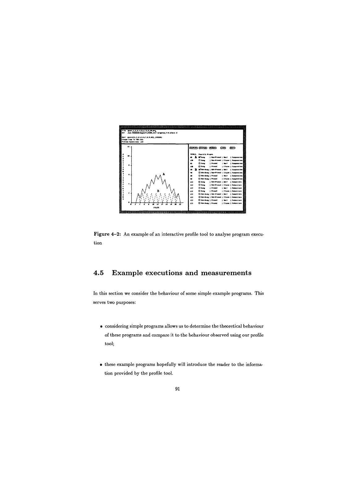
H /or.P MS25/.2y.2/./Cf1O.wl U.V.'.. 5../&p

S.., pe.IC*, 2,], w,5.E,2,0.9.15], 12SSS5) C. $ 21. 1. 75 M C .1- bdu.11- 122

I

I

In=

122 0 65ry 15 15..1 1S 14- M O lbw-Yny P _d C1u,.0 15rp+.f- s O' n-5wy 19-.d 1 5..1 150.pr.f0..I M O M n- I Mr1-Sl..1. I C1wM. 19usy...tam

in n

n. 55.5 10n.r5 C, 19Y.yem1- n B fir5eo-9up I N0.- i* Sd 15N1 $ Su.MM10M

as D 91 I y.fewe 150.1 15l.y.s,m+

6 A 22/Wry I ww*nawl 15.21 I S+Nw.fon. in O 5155 I x.+-wwe I C1w.. I fl.y.,r,er

9S7SC3 ...., bla trey...

122 0 Wry I M-P...d I CI_ I S.SUCa1an.

f22 0 Wry I M1w5 15wl I SMae.lall.

122 0 5e.-w.5 150.i5M. Seal 111.-aiw.0 122 0 W.5 .ur5 I CI.O.. 101-.fp,.

122 O 5M-55.y 15a.fwr0 I Cl-. I SMS.fa.. 122 0 Sew-S5, F-d 15 ) 15ews.l.w. 122 0 lbw-bus I p1 d I CI.SM I R. .+... {I

Figure 4-2: An example of an interactive profile tool to analyse program execu-

tion

4.5 Example executions and measurements

In this section we consider the behaviour of some simple example programs. This

serves two purposes:

considering simple programs allows us to determine the theoretical behaviour

of these programs and compare it to the behaviour observed using our profile

tool;

these example programs hopefully will introduce the reader to the informa-

tion provided by the profile tool.

91

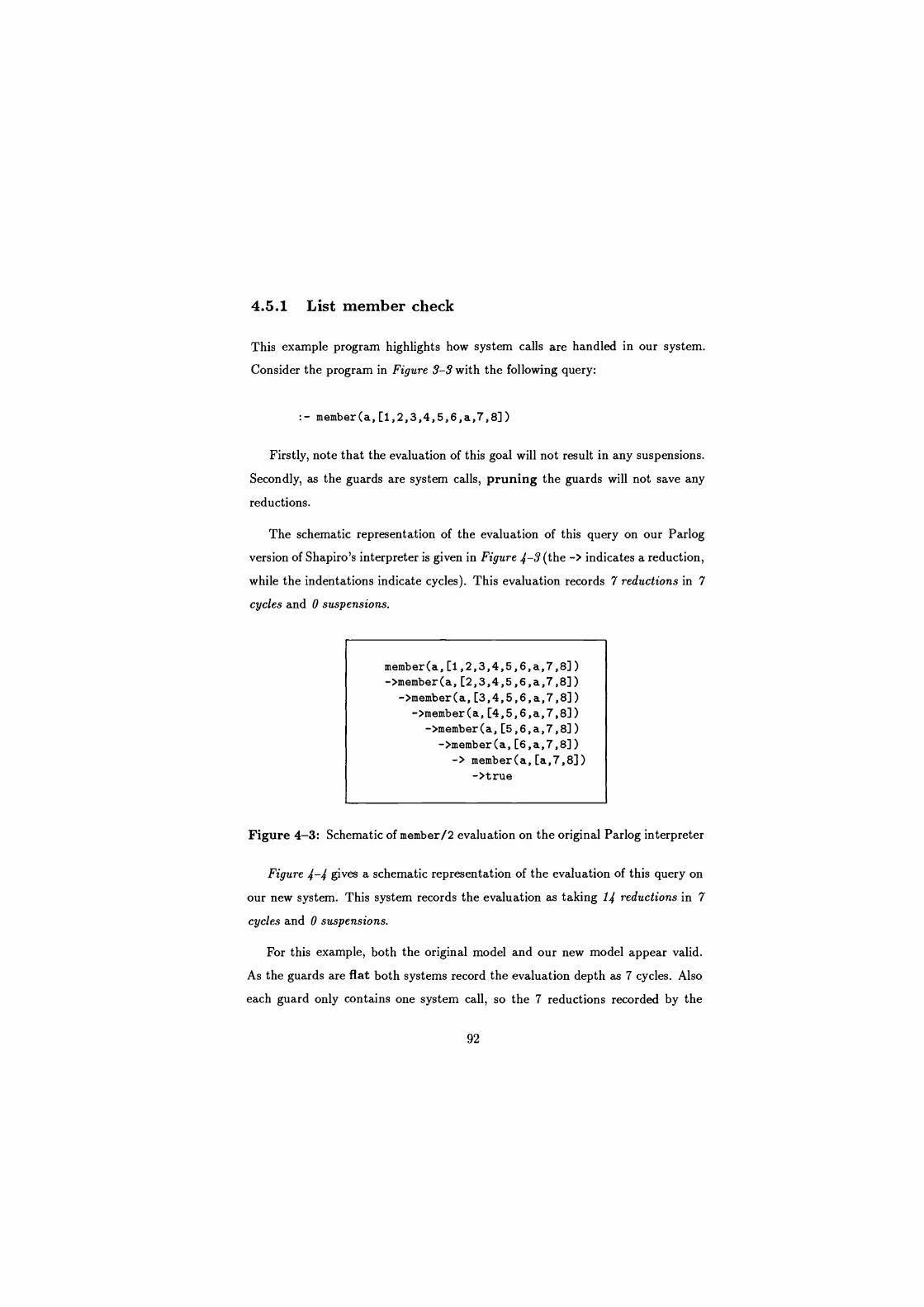
4.5.1 List member check

This example program highlights how system calls are handled in our system.

Consider the program in Figure 3-3 with the following query:

:- member(a,[1,2,3,4,5,6,a,7,8])

Firstly, note that the evaluation of this goal will not result in any suspensions.

Secondly, as the guards are system calls, pruning the guards will not save any

reductions.

The schematic representation of the evaluation of this query on our Parlog

version of Shapiro's interpreter is given in Figure 4-3 (the -> indicates a reduction,

while the indentations indicate cycles). This evaluation records 7 reductions in 7

cycles and 0 suspensions.

member(a,[1,2,3,4,5,6,a,7,8]) ->member(a,[2,3,4,5,6,a,7,8])

->member(a,[3,4,5,6,a,7,8]) ->member(a,[4,5,6,a,7,8])

->member(a,[5,6,a,7,8]) ->member(a,[6,a,7,8])

-> member(a,[a,7,8]) ->true

Figure 4-3: Schematic of member/2 evaluation on the original Parlog interpreter

Figure 4-4 gives a schematic representation of the evaluation of this query on

our new system. This system records the evaluation as taking L reductions in 7

cycles and 0 suspensions.

For this example, both the original model and our new model appear valid.

As the guards are flat both systems record the evaluation depth as 7 cycles. Also

each guard only contains one system call, so the 7 reductions recorded by the

92

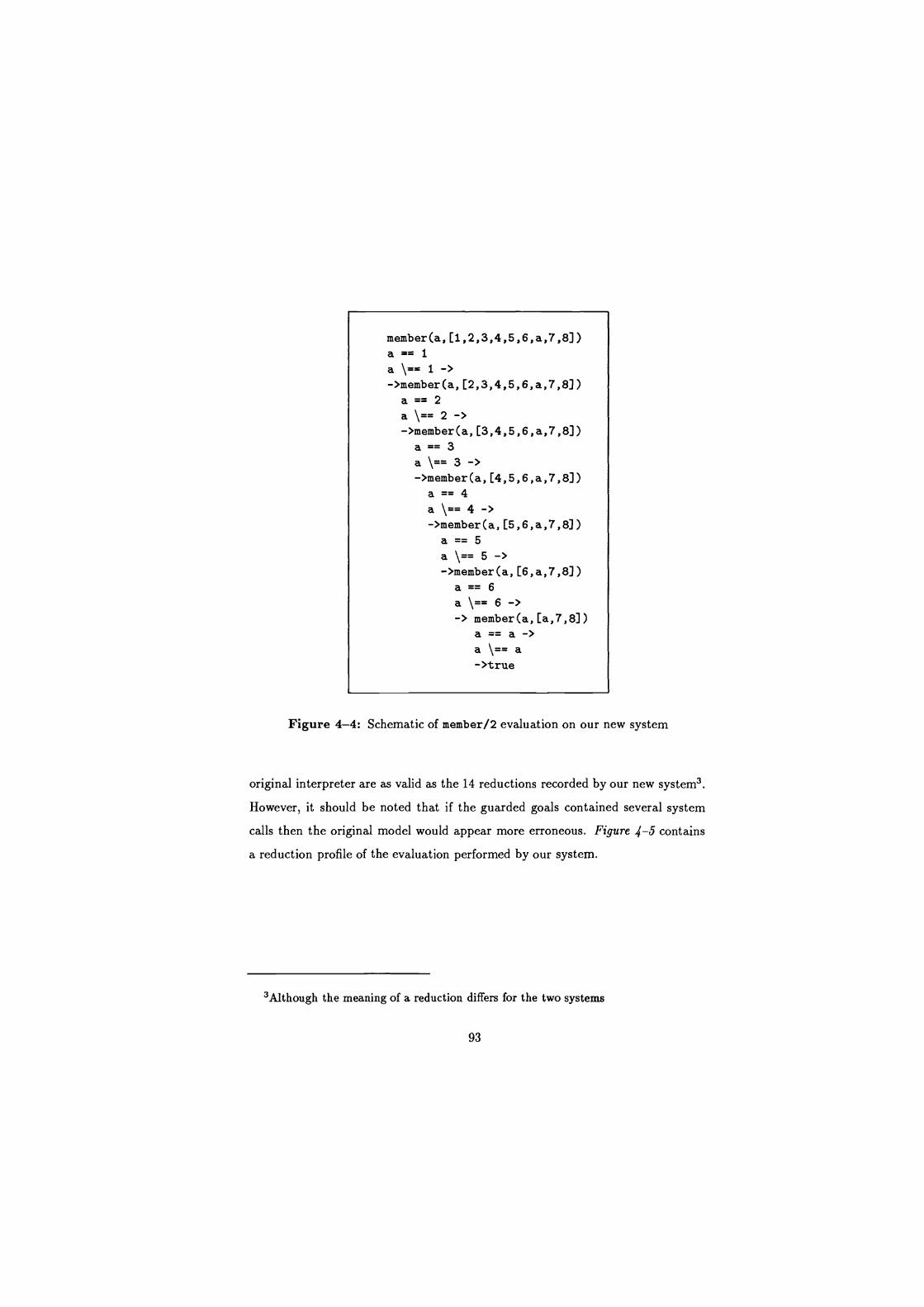
member(a,[1,2,3,4,5,6,a,7,8]) a == 1

a ->member(a,[2,3,4,5,6,a,7,8])

a == 2

a\==2-> ->member(a,[3,4,5,6,a,7,8])

a == 3

a \_= 3 -> ->member(a,[4,5,6,a,7,8])

a == 4

a\==4-> ->member(a,[5,6,a,7,8])

a == 5

a\=-5-> ->member(a,[6,a,7,8])

a == 6

a \== 6 -> -> member(a,[a,7,8])

a == a -> a \_= a

->true

Figure 4-4: Schematic of member/2 evaluation on our new system

original interpreter are as valid as the 14 reductions recorded by our new system3.

However, it should be noted that if the guarded goals contained several system

calls then the original model would appear more erroneous. Figure 4-5 contains

a reduction profile of the evaluation performed by our system.

3Although the meaning of a reduction differs for the two systems

93

TOTAL& .eu161. W.pt. 6YW.y I Men-P-ad I e1 W.pn.fam

e O , Wry I rrYnw 1 M.1 I W.,rnr.n. a W.y I rr,.l.r CS.-

N--ft- I 9e1 WYr^,- O N, I May-Rww. I Cl.... I Wp.iwt.n. O M..-W.y I kn... I ..1 W,q..hn. O Nan-Wry I .r,.us Ce.... 1 sty ,rm

1. EIW.y M..-hu.C 1 w1 I ...blo.. 1h O M I NOn-rruM. I C1.... I M.uc tl.M 1h Mwy I rr...r Twt M..uttf.A 1h O Way Irum. Citu.. I MCUt11w

1h O Men-i.a 1 Mwl-rru.w 1 0t1 M.w,etlar 1h 0 Maw-W.y I M..-MU... 1 Chins I W.uttles 1h O Man-rosy I .rvW I Twi I Mrotfa. 1h O M.,rW.Y 'rnM

1 Cit... I M.*aLIo...

Figure 4-5: List member check reductions

4.5.2 Parallel list member checks

In this example we consider how deep guards are handled in our system. Consider

the program in Figure 4-1 with the following query:

on_either(a,[1,2,3,4,5,6,7,8,9,a],[1,a],L)

The program checks to see if a given a term is on either of two lists. The two

lists are searched in parallel in the guards of two clauses. The first list that is

found to contain the given term is returned. Firstly, note that the evaluation of

the above query will not result in any suspensions. Secondly, as the guards are

deep and uneven, pruning the guards should save some reductions.

Figure 4-6 gives a schematic representation of the evaluation of the query

on our Parlog version of Shapiro's interpreter (the branches of the tree indicate

reductions while the depth indicates cycles). The evaluation commits to the first

94

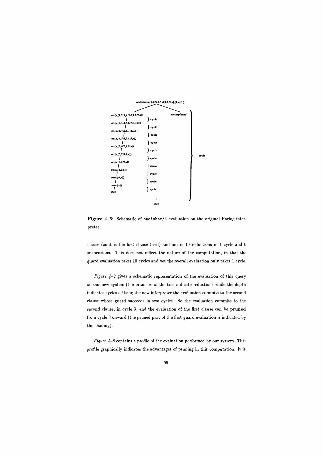
one3ther(a,[I,2.3,4,5,6,7.8,9.a1,[I.ald-)

on(a,[ I ,2.3,4,5,6,7.8.9,aJ)

on(a,[2,3.4,5.6,7,8,9.a])

on(a,13.4.5.6.7.8.9,al)

I on(a,[4,5,6,7.8,9.al)

on(a,[5,6,7,8,9,a1)

1

on(a,[6,7,8.9.a])

I on(a,[7,8,9.al)

I on(a,[8,9.al)

I on(a.[9.al)

I on(a,[a])

cycle

cycle

cycle

cycle

cycle

cycle

cycle

cycle

cycle

cycle

true

Hoot explore d

cycle

Figure 4-6: Schematic of oneither/4 evaluation on the original Parlog inter-

preter

clause (as it is the first clause tried) and incurs 10 reductions in 1 cycle and 0

suspensions. This does not reflect the nature of the computation, in that the

guard evaluation takes 10 cycles and yet the overall evaluation only takes 1 cycle.

Figure 4-7 gives a schematic representation of the evaluation of this query

on our new system (the branches of the tree indicate reductions while the depth

indicates cycles). Using the new interpreter the evaluation commits to the second

clause whose guard succeeds in two cycles. So the evaluation commits to the

second clause, in cycle 3, and the evaluation of the first clause can be pruned

from cycle 3 onward (the pruned part of the first guard evaluation is indicated by

the shading).

Figure 4-8 contains a profile of the evaluation performed by our system. This

profile graphically indicates the advantages of pruning in this computation. It is

95

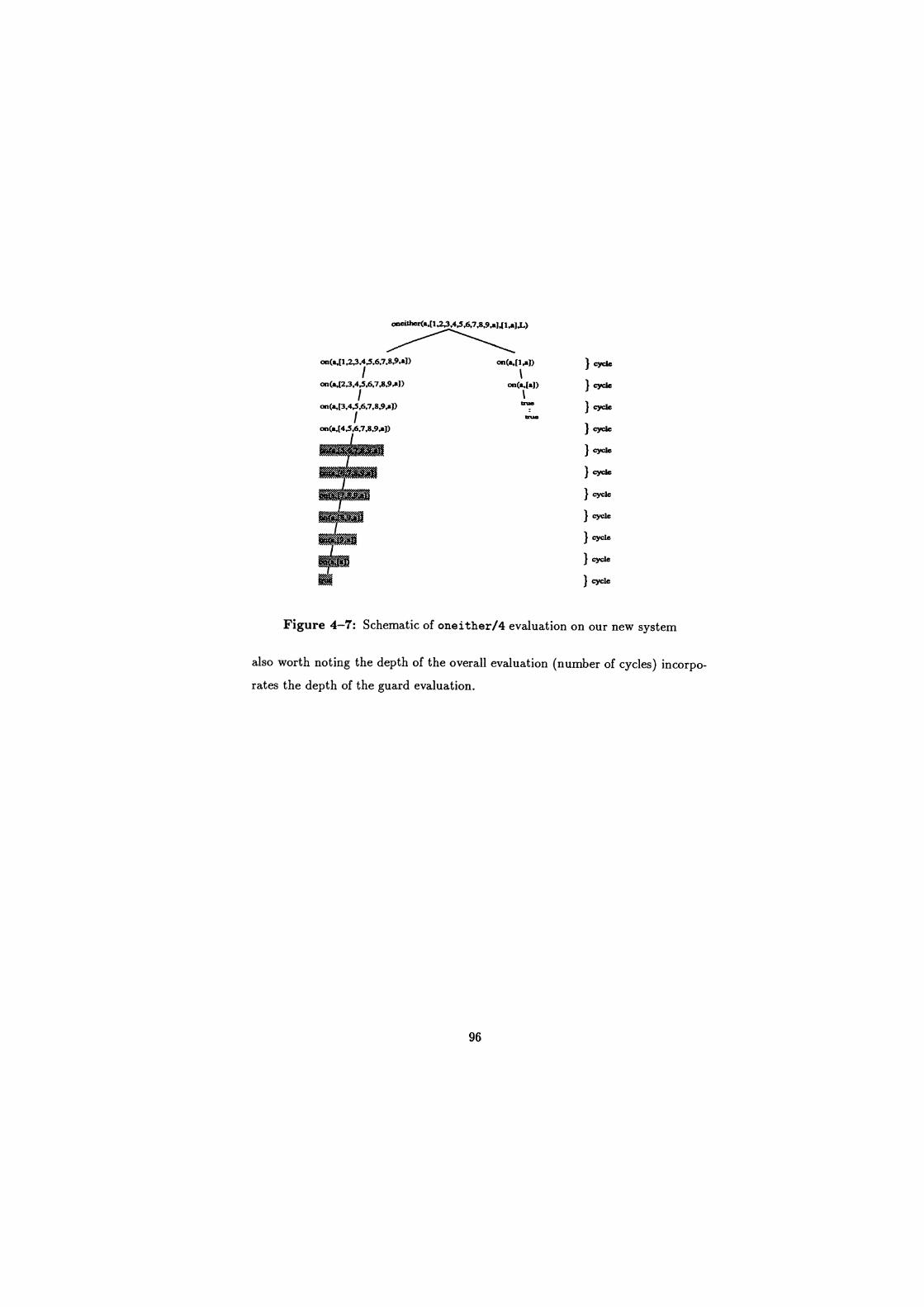
oncither(a,[1.2,3,4,5,6,7,8,9,a1.[1.aM)

on(a,[1,2,3,4,5,6,7,8.9.a1)

I on(a.[2,3,4.5.6.7,8.9.81)

I

on(a,[3.4.5.6.7.8.9.a1)

I

on(a,[4.5,6.7,8.9.a])

D

M

on(a,[1,al)

on(a,[al)

Figure 4-7: Schematic of oneither/4 evaluation on our new system

also worth noting the depth of the overall evaluation (number of cycles) incorpo-

rates the depth of the guard evaluation.

96

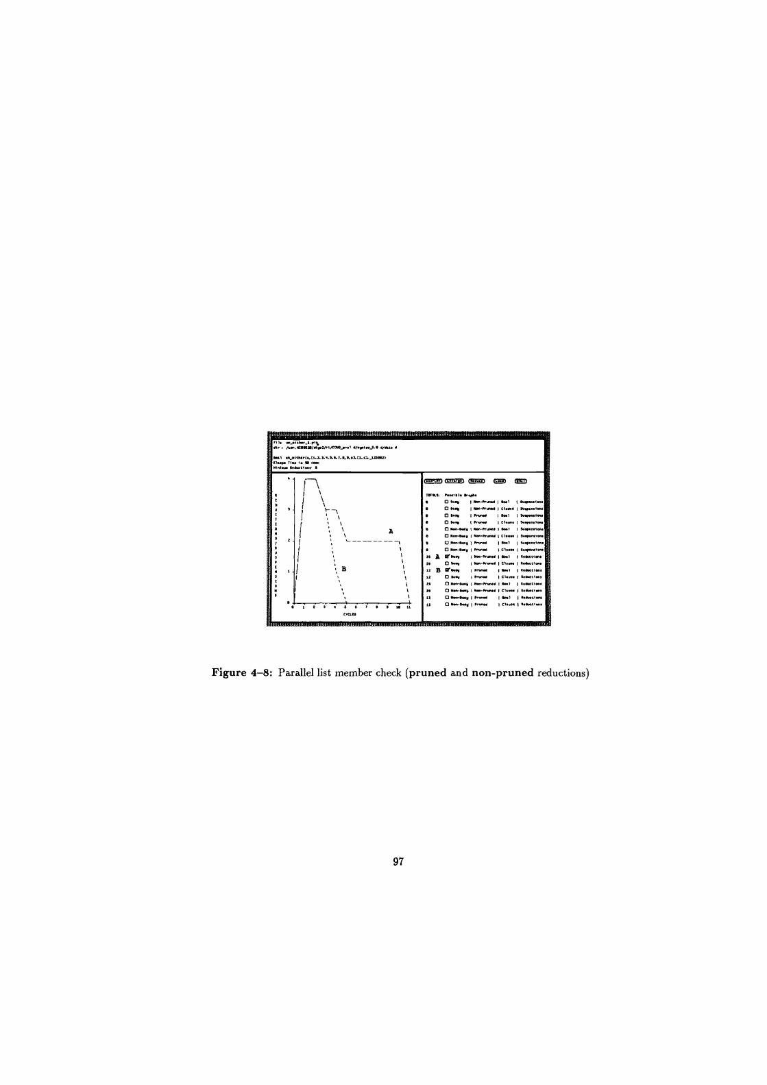
loll on61tMr(1, t1,2, 1,0,AAT,I.AU. C1, U, SSSee20 [l..p Tins 1. SB 0000 111.1.00 0.!..1100. 6

TOTALS. 200.001. 4.010 e 0 80.11 I wm-hurl 161.1 wpa.1100 e O 60.11 I Non-rrlme i ct.l.l I wp.n.lenl

.0011 12.1a I eat 1 110.0.011. e 0 a 0 60.11 t v..../ I cl0.. 1 wopndam e 0 Men-111 I Ma-hurl 1 ert I S p..1... 6 0 ya.-e0.y 1 yen-hurl I C1.0.. 111..00000.

e 0 yen-.100 1 Pr 16-1 wpn.1en. e 0 ya.e,ny 12.ww xe A tiny I wen-err./ I sat I lotto... 21 0 61ry I wan-ft-d I Cl.w. I b100110. 12 B tw.y 120110" I wt 11.101110.

12 0 wy 1 h I C1u0. 11/01111000

2e 0 ino e I 0.0-20-001 1 1.01 1 1.1.1100.

26 01000-000y 10180-hurl I Cl.... 11./0:11.0. 13 0 NO-81011 1 h.0./ I sat I Rmr11m1

12 0 1100-11111 I P8 111.1..1 8.e,e01en.

Figure 4-8: Parallel list member check (pruned and non-pruned reductions)

97

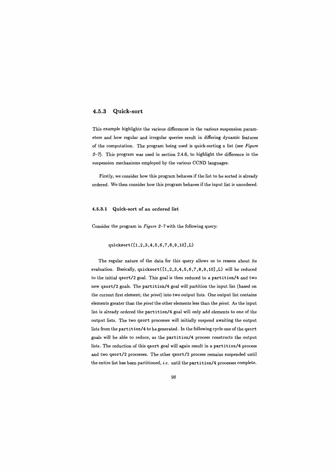
4.5.3 Quick-sort

This example highlights the various differences in the various suspension param-

eters and how regular and irregular queries result in differing dynamic features

of the computation. The program being used is quick-sorting a list (see Figure

2-7). This program was used in section 2.4.6, to highlight the difference in the

suspension mechanisms employed by the various CCND languages.

Firstly, we consider how this program behaves if the list to be sorted is already

ordered. We then consider how this program behaves if the input list is unordered.

4.5.3.1 Quick-sort of an ordered list


quicksort([1,2,3,4,5,6,7,8,9,10],L)

The regular nature of the data for this query allows us to reason about its

evaluation. Basically, quicksort([1,2,3,4,5,6,7,8,9,10],L) will be reduced

to the initial qsort/2 goal. This goal is then reduced to a partition/4 and two

new qsort/2 goals. The partition/4 goal will partition the input list (based on

the current first element; the pivot) into two output lists. One output list contains

elements greater than the pivot the other elements less than the pivot. As the input

list is already ordered the partition/4 goal will only add elements to one of the

output lists. The two qsort processes will initially suspend awaiting the output

lists from the partition/4 to be generated. In the following cycle one of the qsort

goals will be able to reduce, as the partition/4 process constructs the output

lists. The reduction of this qsort goal will again result in a partition/4 process

and two qsort/2 processes. The other qsort/2 process remains suspended until

the entire list has been partitioned, i.e. until the partition/4 processes complete.

98

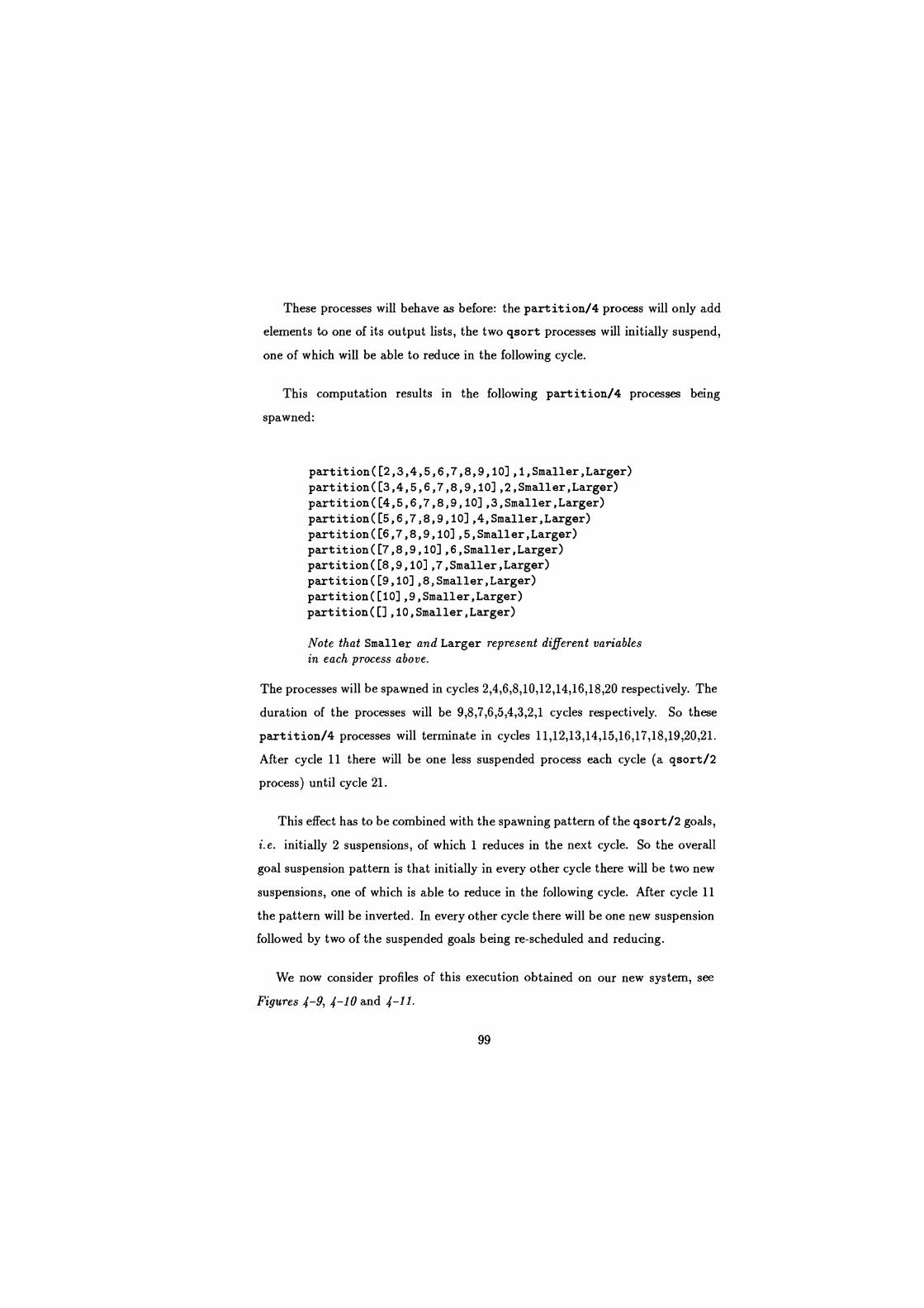
These processes will behave as before: the partition/4 process will only add

elements to one of its output lists, the two qsort processes will initially suspend,

one of which will be able to reduce in the following cycle.

This computation results in the following partition/4 processes being

spawned:

partition([2,3,4,5,6,7,8,9,10],1,Smaller,Larger) partition([3,4,5,6,7,8,9,10],2,Smaller,Larger) partition([4,5,6,7,8,9,10],3,Smaller,Larger) partition([5,6,7,8,9,10],4,Smaller,Larger) partition([6,7,8,9,10],5,Smaller,Larger) partition([7,8,9,10],6,Smaller,Larger) partition([8,9,10],7,Smaller,Larger) partition([9,10],8,Smaller,Larger) partition([10],9,Smaller,Larger) partition([],10,Smaller,Larger)

Note that Smaller and Larger represent different variables in each process above.

The processes will be spawned in cycles 2,4,6,8,10,12,14,16,18,20 respectively. The

duration of the processes will be 9,8,7,6,5,4,3,2,1 cycles respectively. So these

partition/4 processes will terminate in cycles 11,12,13,14,15,16,17,18,19,20,21.

After cycle 11 there will be one less suspended process each cycle (a qsort/2

process) until cycle 21.

This effect has to be combined with the spawning pattern of the qsort/2 goals,

i.e. initially 2 suspensions, of which 1 reduces in the next cycle. So the overall

goal suspension pattern is that initially in every other cycle there will be two new

suspensions, one of which is able to reduce in the following cycle. After cycle 11

the pattern will be inverted. In every other cycle there will be one new suspension

followed by two of the suspended goals being re-scheduled and reducing.

We now consider profiles of this execution obtained on our new system, see

Figures 4-9, 4-10 and 4-11.

99

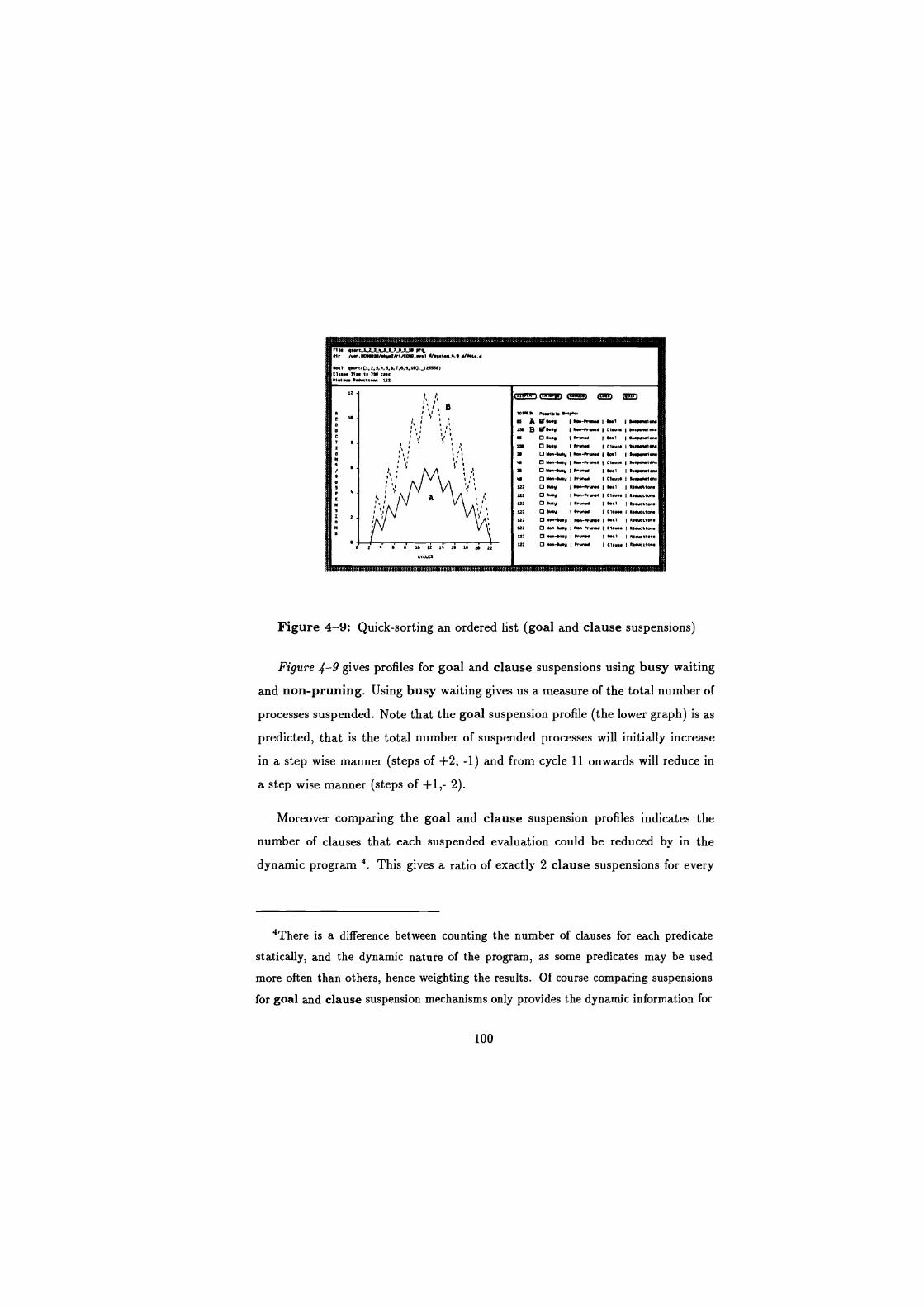
file K% Mr lw.Woe l+w2/rt/CM-O .I 4.wt"_e.q NwN.d

SOt1' g.. (C1.2. a. t.l.a7.a1.1p.-i1ASl2I tkIp. ll.e 1. l9S tilt RIM.M S.MCttsM 1.22

12 14 16 IS

CYCLES

22

ro1Rl! ....1Mle U.aM Sa fYe..y x..-ft. I Stet I gw tar 1SS $ wY I MM-huiH 1 Ctwt.

w 1 wtMntl-

SS O St.y P-ed 1 wit t..YM..I.N 1s 0 Wty 11?lnw 1 Cttwt a.tY.n.ltlu s O M.niwy 1 Men-Ruw. I Sots I Swwr/.t.r N O Man-1..

1 Min-.rows 1 Ci.wt I wlren.lM.

>r O N_ Seem I P1~ 1 8.1 1 Swpurlon. N O M -&'ty I hmrt I CI.... I SwMwl en.

122 O 511 I Mw.-hwt 1 ..t I ltt+utttan.

122 O w.y M.n-/-N 1 Cltu.. R..luctl.n. 122 O St.y I hunt. I Swt I bt.etl.n. 122 Q wW Sr.n.t I CI.- I Rer..lm. 122 O MM4Y.y I Men-.r1nH I Soo R..uttl M. 122 O M.n-w.y Men-ht.we I Cltw. I Retwt/tw 122 O N..-S..y I r.nw 1 Sett I Retuttltn. 122 0 M.n-Sney I h.nr I Cl... I Rt1..ttaw

Figure 4-9: Quick-sorting an ordered list (goal and clause suspensions)

Figure 4-9 gives profiles for goal and clause suspensions using busy waiting

and non-pruning. Using busy waiting gives us a measure of the total number of

processes suspended. Note that the goal suspension profile (the lower graph) is as

predicted, that is the total number of suspended processes will initially increase

in a step wise manner (steps of +2, -1) and from cycle 11 onwards will reduce in

a step wise manner (steps of +1,- 2).

Moreover comparing the goal and clause suspension profiles indicates the

number of clauses that each suspended evaluation could be reduced by in the

dynamic program 4. This gives a ratio of exactly 2 clause suspensions for every

4There is a difference between counting the number of clauses for each predicate

statically, and the dynamic nature of the program, as some predicates may be used

more often than others, hence weighting the results. Of course comparing suspensions

for goal and clause suspension mechanisms only provides the dynamic information for

100

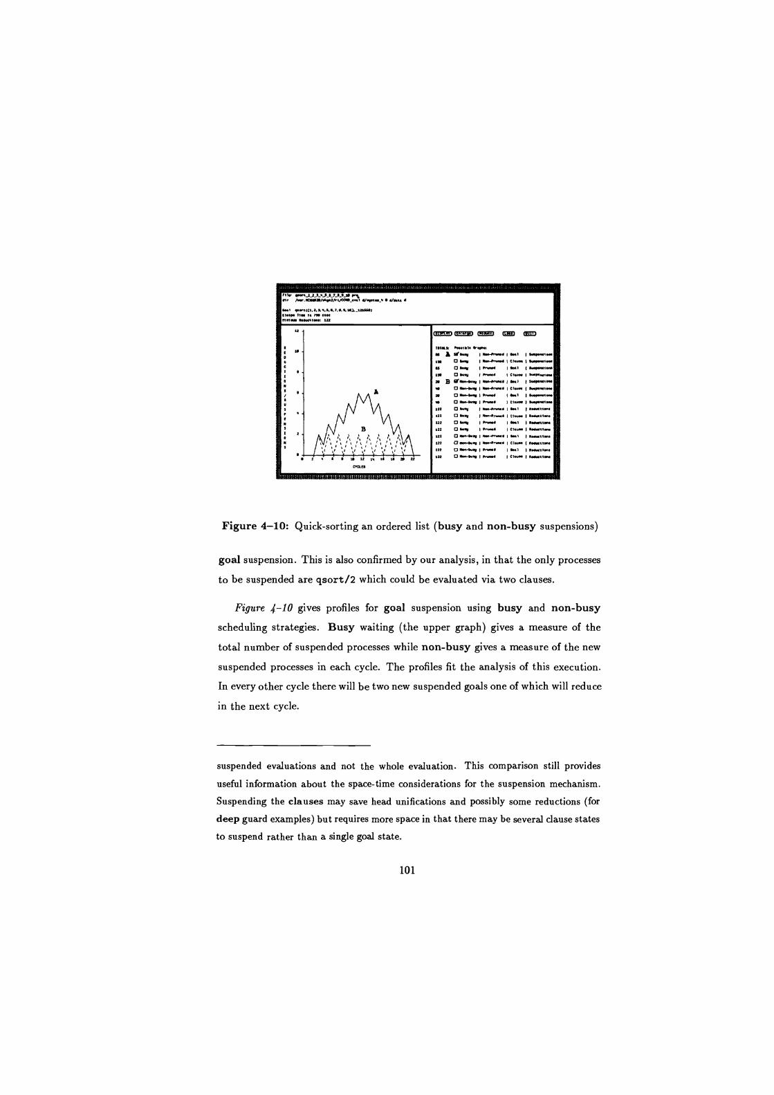
iem.m n...+.u tr.- s , ofwq Mw4.w4 wf I a,wr.,,.f«w .ee O M-II I MM-P-6 cf.ur firf-i-ff.r Y O w.e I hvfd I w1 w..wfa- 17e O wry I nn--A I elW.. I w.prlw M B irMen-eeW I M-IM--e w/ iweu-font

0 -M-" I M-.ftvw. I CI.w. I $-I -font s 0 Men-b" Pr-W wf I w.p.-fa. .e 0 Me.wy I a.." Cf.w. wpuf.fes

w.y I M.n+rw. I wf R. e11 1 1n 0 122 0 wp I MenIr--1 Clw.. 122 O.wy I i.v-A

1 wf I b..eN.n. .u 0 woe f nr..-6 I CI.f-. I efM-.f.m .z: o Mew-Wp IMen-Iron.. I wl I ewe.fem 1n anon-euw I Men-hw. I Cfaua I Msbcafau 122 0 M.n-wp Dr--e I e.el I e.fti,-.im in 0 Men-wy 1 rr--n efwf- e.q-.fen.

Figure 4-10: Quick-sorting an ordered list (busy and non-busy suspensions)

goal suspension. This is also confirmed by our analysis, in that the only processes

to be suspended are qsort/2 which could be evaluated via two clauses.

Figure 4-10 gives profiles for goal suspension using busy and non-busy

scheduling strategies. Busy waiting (the upper graph) gives a measure of the

total number of suspended processes while non-busy gives a measure of the new

suspended processes in each cycle. The profiles fit the analysis of this execution.

In every other cycle there will be two new suspended goals one of which will reduce

in the next cycle.

suspended evaluations and not the whole evaluation. This comparison still provides

useful information about the space-time considerations for the suspension mechanism.

Suspending the clauses may save head unifications and possibly some reductions (for

deep guard examples) but requires more space in that there may be several clause states

to suspend rather than a single goal state.

101

22

ieYN2x P.~. WW_ a A aw.Y 1 N.n-h'.avt tyl I wyw+rr is O wY INN.-e....t I Cl.- I wq.nf,w. a C w.N I rr....t tpl I w.,m+e.. 2r O S n,.... I Cluw. 1 f..p....+e.. a C N.o-Wy I Nsrh..rt I Ml I woyw,as rt O Naw wy I Ns.-fr,.W cl.w 12.wpwNan r O N..F4n I f.wrt 1 tyl I w.fw.,a.. a O Nw-w.y I f.v..t cl.w. I w+ww 222 B twy I N..-M..M 1 twl I w.uttlpN In C wry I Nr-flint I c1.W I nsw.ca,en

122 O w., I P .M 1 t..l 1 Mtu.t,.n 122 O w.11 I Hv.N I Cl.u.. ""41- 222 O Nat-!.y N..-M_ I w.l 1 Mdr.t.m. 222 0 Nw.t..5 Nu.-fwn.t I Cl.- 1 ..W.al.m 222 O Norv-w.y I h,...t I Ml I R"-&Ien. 122 C Nerw.y I fr.w.t I Cl.w. I eM.ta,M

Figure 4-11: Quick-sorting an ordered list (reductions and suspensions)

Finally we give a profile of the reductions in Figure 4-11. The number of

reductions increases by 1 each cycle, as new partition/4 processes are spawned

and reduced. After cycle 11 the partition/4 goals begin to succeed (terminate)

and the processes begin to collapse. At the peak there will be 10 partition/4 and 1 qsort process reducing in parallel.

4.5.3.2 Quick-sort of an unordered list

We now turn our attention to the behaviour of quicksort on an unordered list.


quicksort([4,6,2,9,5,5,1,10,3,7],L)

The irregular nature of the data for this query makes reasoning about its

evaluation difficult. However some global features can be predicted, namely:

z . s t 2s 22 2. 2t ft a 22

102

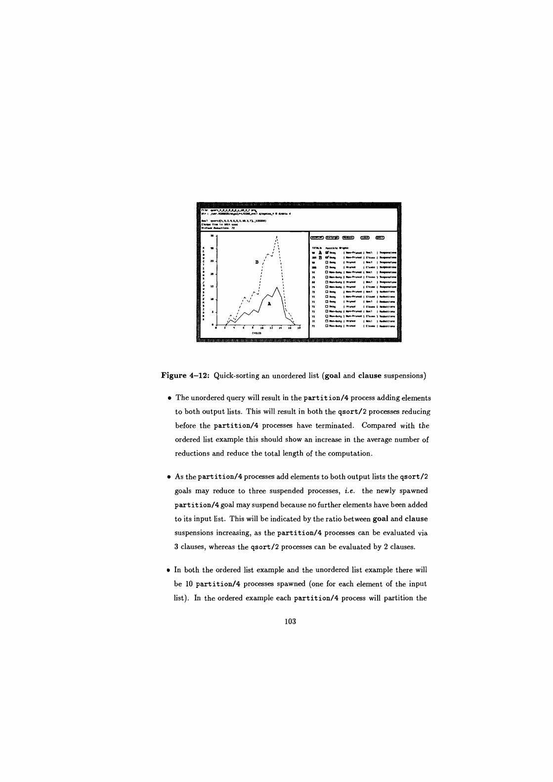
tf > q.ert-.J1JJ1aJJR-SJ P'% Mr I / RCR ./..y.t/rt/COm_... 1 VMtw _ d/Mt. d

M.f qwK/C' 3,Z , O.l.1. IS. Dr n1slip tl.q. H S t. 1RSY CsK Ift 1 . Me.tsiom. 7t

11 1

R ! 1

1 TOTM.! ..H.i. &WW

C / I A Bs I fwn-.rwe 1

Wl I svy.w- O 1d B feY.w.y I Mn-bore I C1.- 1 INr C

u B o .u.y 1 et..re 1 2-1 11wy.lrla.

T l tt6 0 fRl.y I rrurs I Cu.. I )D 51 O Mow-7Ww Mw-Pans 1 Wl 9."-* r

R 1

I I 71 O M.w-b.Y 1 M.w-h'In.e I Ct.w. 1 alyww.lw

/ I u 0 M-Nwy 1 .twe I ow I Ary.M1.M 1s >. 0 Msw-w.y wow 1 Cl.w. &www.f-

t /. 7Z 0 R.W I IMw-hu.t I Wl MtW t , 1t 0 fwwy 1 1.In.rwe I nw. I Mewt,.n. t L

M `t

A Tt 0 wy I fYOe,.e i Wl I R.beH an.

12 0 fw.y I ft-6 I ci. s. i MefMttM. = s a l` 72 0 Mew-OU.y I Nen-run.A I Wl I Maw[, W

M 72 O Men-W.y Mw-Mln.e I Cl.... 1 MAutttam t

72 0 Men-w.y run.e I 0.1 I Meuctten.

s : . t t 10 a 1. is 1a 1) 0 Men-W.Y 174ure I C1.W I R.lwt,em

[rats

Figure 4-12: Quick-sorting an unordered list (goal and clause suspensions)

The unordered query will result in the part it ion/4 process adding elements

to both output lists. This will result in both the qsort/2 processes reducing

before the partition/4 processes have terminated. Compared with the

ordered list example this should show an increase in the average number of

reductions and reduce the total length of the computation.

As the part ition/4 processes add elements to both output lists the qsort/2

goals may reduce to three suspended processes, i.e. the newly spawned

part it ion/4 goal may suspend because no further elements have been added

to its input list. This will be indicated by the ratio between goal and clause

suspensions increasing, as the partition/4 processes can be evaluated via

3 clauses, whereas the qsort/2 processes can be evaluated by 2 clauses.

In both the ordered list example and the unordered list example there will

be 10 partition/4 processes spawned (one for each element of the input

list). In the ordered example each partition/4 process will partition the

103

.tr Mr .,e.s/ryaz/re/Cae_.w, 4Nm_r a 01a. .

...1 e.ert(C642,446.i.iA471_uaitiq

MM.... e...ect... 72

a ,o,.i.a r..,61. r.c-a c ,e A or" I ««.+..-.. I .-., I e y M O wy I «a--+...... I t,...- I .-t -1- C

zs o w.y -.w. I m., I w.r.-n«-

a $ ,Mn w.e I Mn.wN 1 tq.t I wy.N.n. a " s 17 to w.y I «.. v w. I Ci.w. I &"-I ... 7v

33 93 N_" P-d 6.1 1

u » O m..-....a I P7-.... I CT.w. 1 wg.-,... $ s 72 13 %. 14-4--d I 6- 1 1

A 72 13 wte I «-P-... I c,..... I .w.t7.-. u n 17 ww I r...-. I .--t 1 ...uet,am 72 13 w.y I h..-s 1 ci.... I t.e-clam

S A 72 13 ft-" I «.--M.-.. 1 .-., 1 t.s-tt--.

. . \ 72 13 «...-w.V I «w.rv-. I Cite I Mb.f.-. B

`

# ao-,w.y I rr..-. I e-.1 1 Ma.-0a.

e 2 r e . Y 12 fr is i. 72 17 «.--.-.e I ..-m. I ON,. 1 .....ttt.-. CYCuc

Figure 4-13: Quick-sorting an unordered list (busy and non-busy suspensions)

remainder of the input list, i.e. the partition process with a pivot of 3 will

have to partition the remainder of the input list, namely [4,5,6,7,8,9, 101.

For the unordered example each partition/4 process will only have to par-

tition a subset of the remaining input list because the remaining input list

will be partitioned into two lists. So there will be less reductions performed

in the sorting of the unordered list example.

We now compare the data collected using our new profiling system with the

theoretical evaluation given above. Figure 4-12 gives profiles for goal and clause

suspensions using busy waiting and non-pruning. The first point to note is

that the ratio of goal to clause suspensions changes from 1:2 for the ordered

example, to 90:205 for the unordered example. From this we can conclude that

some partition/4 processes suspend. Furthermore, we can see that the overall

length of the computation has been reduced from 23 cycles (for qsorting an ordered

list) to 18 cycles for this example.

104

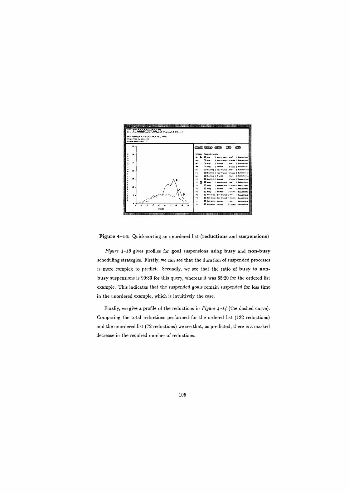
IdIfiU, "I" y.ort-Y-RA9-SS-L>8_9_7.prt1 die t /o.r.RCR9R2l/.RN.2/rt/cam ewe 0.9.04.-4.8 a/d.t..d

dool S9ortt[Y. 5.2.9. 5.9. 1.15..77.23955) El.we Ttr is 151Y else R1n101 Reduetlene 72

UNIUMIMM

I"_W_I MI MR-MI MUM am)

TOTReb Possible 9rephe

90 A if eSey Non-Pruned I boll 19uwen51on. 299 06-A INon-Pruned I el.W. 19uwens1ons

9o 0 Way I Pruned 16.1 19uwenslone

zBR 0 W.9 I Pruned I Ch.. 19uw.nrlon. 99 ibn-Buoy I Non-Pruned 9041 19uwen.lone

79 17 Noe-Wey 1 Non-Prun.d I el.W. 19uwsne1one

99 17 No,-Wey I Pruned 15041 19uepenelone

79 17 Non-6-9 I Prun.d 1 21.04. 19uwmelone 72 H ®'90.9 I Non-Prun.d 1 5041 I RadWtlon.

72 o easy I Non-Pruned I E1.We I Remetl one

72 bury Pruned 15041 I Reduetlans

72 O 5usy I Pruned I el-W. Reduction.

T 2 O Non-way Non-Pruned Goal ftdumi cot

72 O Nun-W" I Non-Pruned 121.We I Reductions

72 O Non-busy I Pruned 10041 R.duttlen.

72 O Non-5009 I Pruned 121.We Reduction

Figure 4-14: Quick-sorting an unordered list (reductions and suspensions)

Figure 4-13 gives profiles for goal suspensions using busy and non-busy

scheduling strategies. Firstly, we can see that the duration of suspended processes

is more complex to predict. Secondly, we see that the ratio of busy to non-

busy suspensions is 90:33 for this query, whereas it was 65:20 for the ordered list

example. This indicates that the suspended goals remain suspended for less time

in the unordered example, which is intuitively the case.

Finally, we give a profile of the reductions in Figure 4-1 (the dashed curve).

Comparing the total reductions performed for the ordered list (122 reductions)

and the unordered list (72 reductions) we see that, as predicted, there is a marked

decrease in the required number of reductions.

105

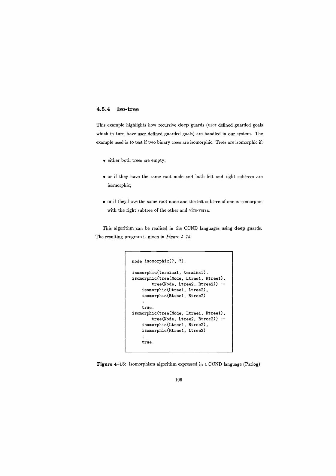
4.5.4 Iso-tree

This example highlights how recursive deep guards (user defined guarded goals

which in turn have user defined guarded goals) are handled in our system. The

example used is to test if two binary trees are isomorphic. Trees are isomorphic if:

either both trees are empty;

or if they have the same root node and both left and right subtrees are

isomorphic;

or if they have the same root node and the left subtree of one is isomorphic

with the right subtree of the other and vice-versa.

This algorithm can be realised in the CCND languages using deep guards.

The resulting program is given in Figure 4-15.

mode isomorphic(?, ?).

isomorphic(terminal, terminal). isomorphic(tree(Node, Ltreel, Rtreel),

tree(Node, Ltree2, Rtree2)) :- isomorphic(Ltreel, Ltree2), isomorphic(Rtreel, Rtree2)

true. isomorphic(tree(Node, Ltreel, Rtreel),

tree(Node, Ltree2, Rtree2)) :- isomorphic(Ltreel, Rtree2), isomorphic(Rtreel, Ltree2)

true.

Figure 4-15: Isomorphism algorithm expressed in a CCND language (Parlog)

106

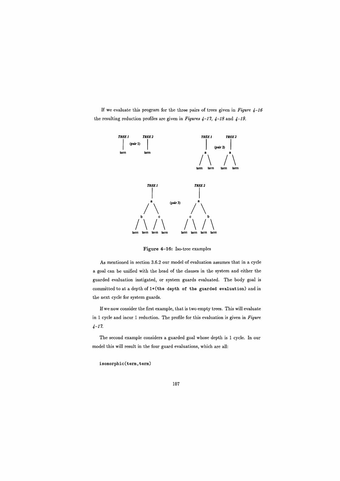
If we evaluate this program for the three pairs of trees given in Figure 4-16

the resulting reduction profiles are given in Figures 4-17, 4-18 and 4-19.

TREE 1 TREE 2 TREE 1

(pair 1) I I

term term a

(pair 2)

TREE 2

I

term term

TREE 1 TREE 2

a (pair 3) a

b c c b

term term term term term term term term

Figure 4-16: Iso-tree examples

a

term term

As mentioned in section 3.6.2 our model of evaluation assumes that in a cycle

a goal can be unified with the head of the clauses in the system and either the

guarded evaluation instigated, or system guards evaluated. The body goal is

committed to at a depth of 1+(the depth of the guarded evaluation) and in

the next cycle for system guards.

If we now consider the first example, that is two empty trees. This will evaluate

in 1 cycle and incur 1 reduction. The profile for this evaluation is given in Figure

4-17.

The second example considers a guarded goal whose depth is 1 cycle. In our

model this will result in the four guard evaluations, which are all:

isomorphic(term,term)

107

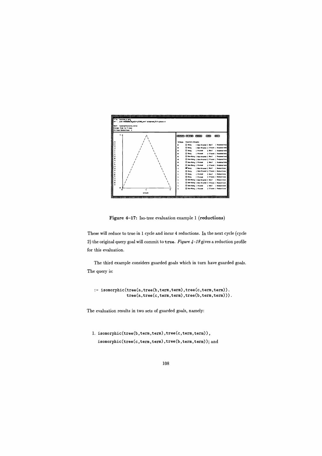
flit. 7totKt-1 pros dlr , /e.r RCeteIS/.ky.Y/rt/CON-tvtl d/tysttn_S D d/dttt a

Seal 1s..orymc(tere, tare)

E I..pt Ti. it 7 C..C Ri ni 01 Reunion. 1

Po0.1 elt Snpba

I Non-Pruned I bbl I au.ptn.lon.

1 t9fl ,.Nd I Ci.u.t I $u.pension

I pruned I ash 1 $OOPSne1onb

I pruned I Cisu.t I Su.ptMlont

1

CYCLES

O Non 4u. I Non-PruNd I tool I Ruopnrlane

O Mm-euty I Nen-Pruned I Cl.u.e I Su.pentlont

O Non-Puss Prune 00.1 Su.Ptne1000

O Non-Suty I Prune C1.0.0 au.pentlens

Srbu.y I Non-ftUMd 10091 I e.dulhlon.

O buts I Non-Pruned I Chute I Reduotlon.

O au .y Pruned I beel I R.dootlon.

O busy Prune I Cl.u.. I R.duotlon.

O Non-tu.y I Non-Preo.d I Do.1 I Rtductlon.

O 1000-bury I Non-Rnntd I Cl.u.. I Reduwtlon.

O Non-Duty Pruned 00.1 I Redutt/one

O Non-Posy I Prune I Cl.u.. I Reduotlone

IMMOMMOM

Figure 4-17: Iso-tree evaluation example 1 (reductions)

These will reduce to true in 1 cycle and incur 4 reductions. In the next cycle (cycle

2) the original query goal will commit to true. Figure 4-18gives a reduction profile

for this evaluation.

The third example considers guarded goals which in turn have guarded goals.

The query is:

isomorphic (tree (a,tree (b,term, term),tree (c,term,term)). tree (a,tree(c,term,term),tree (b,term,term))).

The evaluation results in two sets of guarded goals, namely:

1. isomorphic(tree(b,term,term),tree(c,term,term)),

isomorphic(tree(c,term,term),tree(b,term,term));and

108

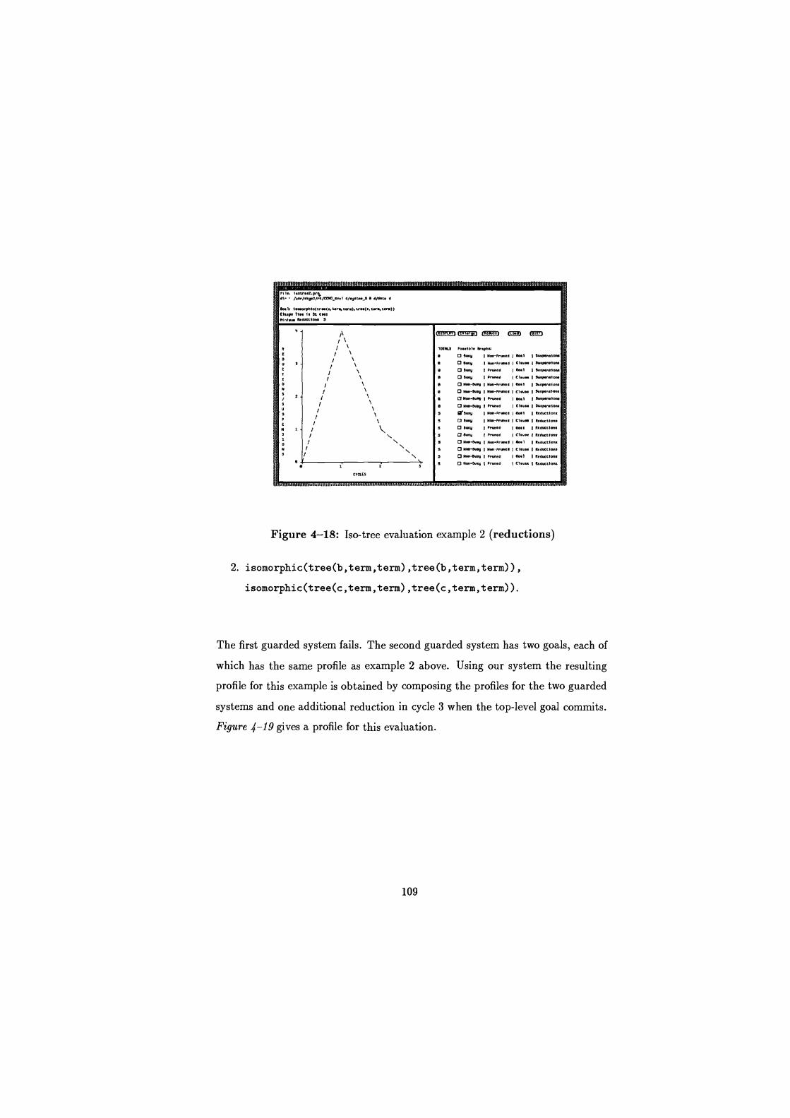
ftle. 1.OVe2.prg 01r hr/stys2/rt/Cdro_.t.1 d/ytto 3 0 0/000 a

0001, tOOrpMO(trs(.r 0ry.sr.)r tr(.r terq tsr.)) E1up. Ti0. 1. 311 tees ntnt.t R.daetiom 3

v

3

2

CYCLES

TOMB Possible arepl.

0 06- 3 I N00-Prunsd 10001 ) 00.pemlmw

0 Owy INon-Pruned I £10ua I Su.p.neion.

0 O 0005 I Pruned 10001 Scp.n.tos. 0 O 0005 I Pnnns 1 Cl.ur I Oo.Mn.iom

O Non-0o. I N.n-Pruned 100.1 I Supn.tom

O N.n-easy I Non-Pr-.d I Cl- 13up...is. Cl Non-0013 I Prisms! 10001 Ssepsn.tom

0 .011-0003 I Pruned Cl.0.4 130.9.0.101. 0'0005 I Non-Pruned 00.1 I R.MS:tton.

0005 I

.Non

-Pruned I Cl.... I Resnletlone

O BMW I Prw. 10.., I R.duct(.n.

O 0.o P-s: Cl- I R.duetton.

0 Non-00.5 I Non-Prui.d 40.1 R.s00t1On

O I Non-rrunsd I Cl.ut. I

s I

R.duion. O N--buy I Pad Son I

ution

0 Non-3003 I Pruned I Cl- I Rs3wtt.nc


2. isomorphic (tree (b,term,term),tree (b, term, term)),

isomorphic(tree(c,term,term),tree(c,term,term)).

I

The first guarded system fails. The second guarded system has two goals, each of

which has the same profile as example 2 above. Using our system the resulting

profile for this example is obtained by composing the profiles for the two guarded

systems and one additional reduction in cycle 3 when the top-level goal commits.

Figure 4-19 gives a profile for this evaluation.

109

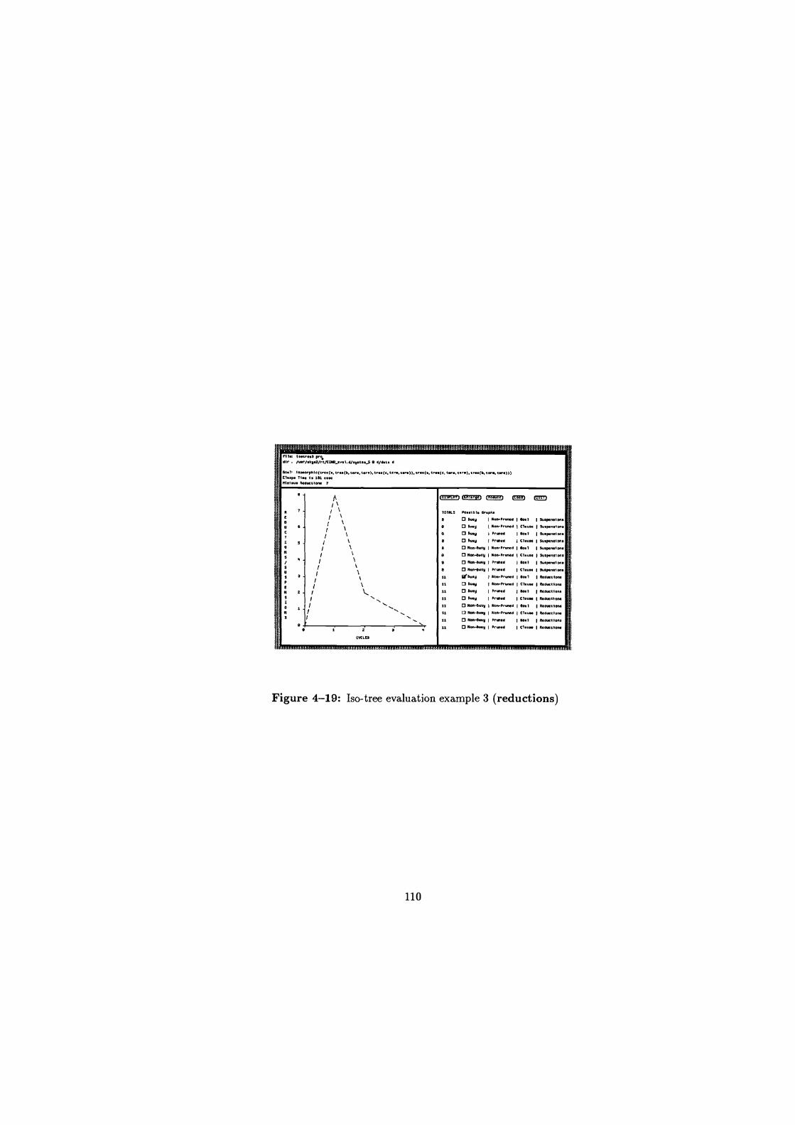
) 1CrJ t:dI1#L(II1111[IsLITS 71ruiiiiit rlld IIOWa.3 prey dlr / d/e .tt.r5 0 d/d.t, d

Possible Gr.pn.

O Goad I Mat-Pruned I Go.1 13uapenalons

O Go.y I Mat-pruned C1.uae 13uaponelata

O Guty pruned $0.1 1 3u.penel one

O Gu.y I .ruled CI... I suapamlbne

O Non-Gaeb I Nat-pruned I Go.1 13uapetelona

O N.-Gory Noo-pramed I Cie.. I suep.ta10n1

O Mon-Go.O I .rie,ed 10..1 13o.petel one

O 11.0-0010 I Pr,n.d I Cl.ua I taep.toioo. .rGueO I Non-Orated I $0.1 I Gtduatlona

0 Gu.y Not-Pr-d I cl.up 1 Mdaatiot.

Goal' Iee.erpMle(tne(.. tre.(b, tar., tar.), tr.e(e, r.)), tree(., tr.e(e, tea, t.ra),e ee/s, tee, tare))) t 01. op. Tin 1e 101

e Mtn1.u. Ged0atlon. I

2

CYCLe3

G

O way

O Gu.y

MMMErm

I Pruned

I probed

Oe.1 I Gaduetlon.

I Cl.ua. I Reducaom

O N-410 Noo-pra ed 100.1 I teouettona

Non-G-$ I No0-pruted Cl.uw I Gedootlone

O Men-00.$ I vru,.u 1 00.1 1 $Od000iOnl

O Non-aa.O I pruned I Cl- I Ged0atl0n.


110

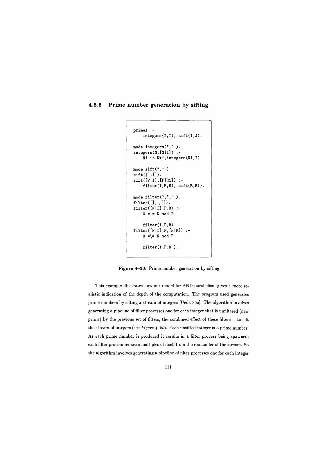
4.5.5 Prime number generation by sifting

primes :- integers(2,I), sift(I,J).

mode integers(?," ). integers(N,[NII]) :-

Ni is N+1,integers(N1,I).

mode sift(?," ). sift([],[]). sift([PII],[PIR1]) :-

filter(I,P,R), sift(R,R1).

mode filter(?,?," ) .

filter ([] , _, []) .

filter([NII],P,R) :- 0 =:= N mod P

filter(I,P,R).

filter([NII],P,[NIR]) :- 0 =\= N mod P

filter(I,P,R ).

Figure 4-20: Prime number generation by sifting

This example illustrates how our model for AND-parallelism gives a more re-

alistic indication of the depth of the computation. The program used generates

prime numbers by sifting a stream of integers [Ueda 86a]. The algorithm involves

generating a pipeline of filter processes one for each integer that is unfiltered (new

prime) by the previous set of filters, the combined effect of these filters is to sift

the stream of integers (see Figure 4-20). Each unsifted integer is a prime number.

As each prime number is produced it results in a filter process being spawned;

each filter process removes multiples of itself from the remainder of the stream. So

the algorithm involves generating a pipeline of filter processes one for each integer

111

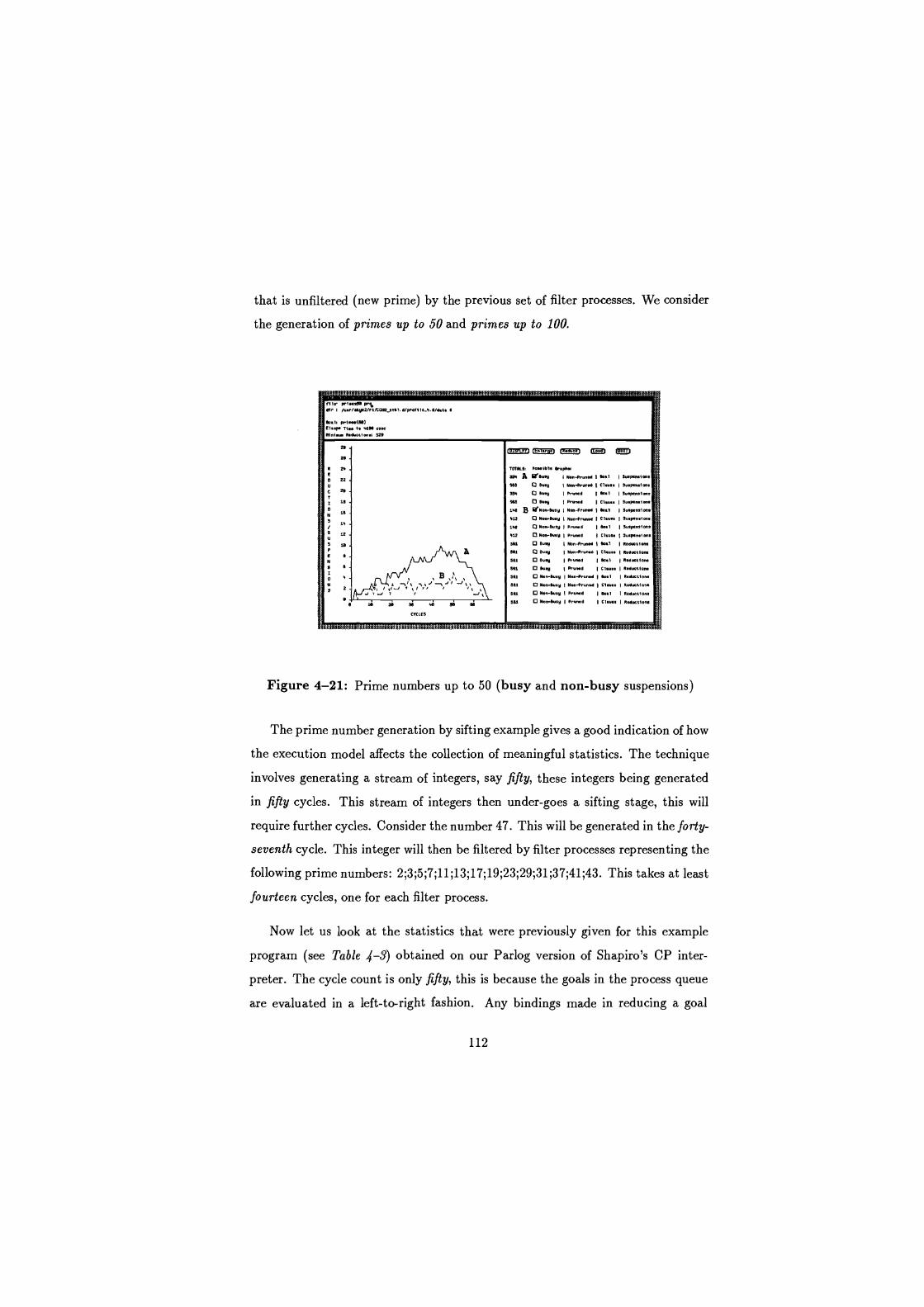
that is unfiltered (new prime) by the previous set of filter processes. We consider

the generation of primes up to 50 and primes up to 100.

s;autaax.zWI.a A

rile- pHss.Se Prod

Hr : NmHRys2/rtttCN6_sv.l. a/pr.mav. a/d.t. d

mau Pri... 5el Elaps Ti.e 1. 4651 era MMww Sed.01- 520

aisllaa,fALFrwE33:daal.iulk{. i.{.3aaSLzL&kb3 islaBFF,FIkkz{..L:E2FFFFZRS{{};g'

TO1RLSi Possible t.p6w 35. A fireury Non-Pron. Sssl I Suspensions

See Q Dory { Non-Pron. I Clause I Supnalon 3" Q guru I Pruned I m.l I Su.penelm

9U Q busy I Pruned I clause 15uPaniaoe 140 B WNOn-may I Non-Aroma, m.1 I Suspsnrione

412 Q Non-m.e I NomPrun. I Cl.,.. mPenim 140 Q Nan-may I Pruned I m.l 3u.P..I.. 412 Non-my Pruned Clause { 9u.pan.i me

561 Q Busy I Non-Pron. Seal I Reduction

661 Q Busy NomPrun. I Clause I Reduction

561 0 Bury I pruned S.1 I Reductiam

S61 Bury Prunsd I Clause I Reductions

561 0 N.n-may Nan-Prun. 11 .l I Reduction

S61 Non-m6 N.n-P-n.d Clause

561 0 Non-m.6 I Pruned 100.1 I Reduetlom

561 Q Non-may I Pruned I Clause I Reductions

Figure 4-21: Prime numbers up to 50 (busy and non-busy suspensions)

The prime number generation by sifting example gives a good indication of how

the execution model affects the collection of meaningful statistics. The technique

involves generating a stream of integers, say fifty, these integers being generated

in fifty cycles. This stream of integers then under-goes a sifting stage, this will

require further cycles. Consider the number 47. This will be generated in the forty-

seventh cycle. This integer will then be filtered by filter processes representing the

following prime numbers: 2;3;5;7;11;13;17;19;23;29;31;37;41;43. This takes at least

fourteen cycles, one for each filter process.

Now let us look at the statistics that were previously given for this example

program (see Table 4-3) obtained on our Parlog version of Shapiro's CP inter-

preter. The cycle count is only fifty, this is because the goals in the process queue

are evaluated in a left-to-right fashion. Any bindings made in reducing a goal

112

rTIve

IR11(IIIllA't41PEP®UD1

.p% M/et9s2/rt/.dID_66.1 d/et76Jr.71 le d/d.tt 9

) 59793 .tee

0Ts: 12339

TOTALS roesiele 67.Rlt 216a7 A W5.9 $9092 E7 5250

59092 0 5259

4579 B GfNeni25y

144" 0 Non-9us9

4575 0 N0.-9259

14436 0 Non-9259

12739 0 9259

I N.9-hv-d 190.1 13W557o55

I N-P-d I .leis. 130epWsia95M

I honed I C15509 13uspen910.e

I Non-hue-d 180.1 I 30spmslans

I Non-h--! I C1... 13utRm91an9 I hunts 160.1 13uytn.lane h:nM I C1... 13...9.1 one

I Noa- 1 0d 10941 1 ft-,-- 12739 0 5059 I N.9 p- 10160.9 I 6.d11541555

12759 0 9259 I er25.d 1 60.1 I 6.6055100.

91.

5 0 2" 235 3" C tL63

a

0

12739 06-0 I hunts .1.256 I Roduotiom

12739 0 N0.-50.9 N.n-ftumd 160.1 Reduet1555

12759 0 31en-9259 I 509 P, :ned I Clews 196009.1955

12739 0 N0.1-5259 I h--4 1 60.1 166605.1.55

12739 31.91-5255 h0.I.d I C1.256 15060.5io .

Figure 4-22: Prime numbers up to 500 (busy and non-busy suspensions)

occur immediately. So an integer that is produced in a given cycle is able to

propagate through the filter processes in the same cycle (the filter processes in the

queue are set-up in a left to right fashion). Our system gives 67 cycles to produce

the first 50 prime numbers (see Table 4-5). Fifty of these cycles can be attributed

to producing the 50 integers, fifteen of these can be attributed to propagating the

last integer through the fifteen filter processes and the remaining two are due to

spawning the first filter process and terminating the output of these integers. The

effect of accounting for the propagation of the integers through the filter processes

results in the number of suspended goals being higher. Other points that arise

are:

There is no difference between the various new reduction counts (see Table

4-4) for this program. The similarity in the reduction counts using goal

and clause suspensions indicate either there are no suspensions or that the

113

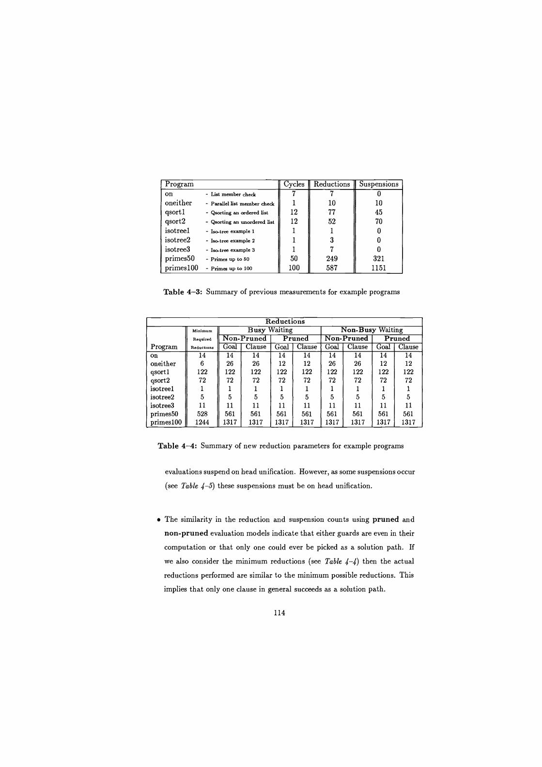
Program Cycles Reductions Suspensions on - List member check 7 7 0 onelther - Parallel list member check 1 10 10 qsortl - Qsorting an ordered list 12 77 45 qsort2 - Qsorting an unordered list 12 52 70

isotreel - Iso-tree example 1 1 1 0

isotree2 - Iso-tree example 2 1 3 0

isotree3 - Iso-tree example 3 1 7 0 primes50 - Primes up to 50 50 249 321 primes100 - Primes up to loo 100 587 1151

Table 4-3: Summary of previous measurements for example programs

Reductions Minimum Busy Waiting Non-Busy Waiting Required Non- Pruned Pruned Non- Pruned Pruned

Program Reductions Goal Clause Goal Clause Goal Clause Goal Clause on 14 14 14 14 14 14 14 14 14

oneither 6 26 26 12 12 26 26 12 12

gsortl 122 122 122 122 122 122 122 122 122

qsort2 72 72 72 72 72 72 72 72 72

isotreel 1 1 1 1 1 1 1 1 1

isotree2 5 5 5 5 5 5 5 5 5

isotree3 11 11 11 11 11 11 11 11 11

primes50 528 561 561 561 561 561 561 561 561

primeslOO 1244 1317 1317 1317 1317 1317 1317 1317 1317

Table 4-4: Summary of new reduction parameters for example programs

evaluations suspend on head unification. However, as some suspensions occur

(see Table 4-5) these suspensions must be on head unification.

The similarity in the reduction and suspension counts using pruned and

non-pruned evaluation models indicate that either guards are even in their

computation or that only one could ever be picked as a solution path. If

we also consider the minimum reductions (see Table 4-4) then the actual

reductions performed are similar to the minimum possible reductions. This

implies that only one clause in general succeeds as a solution path.

114

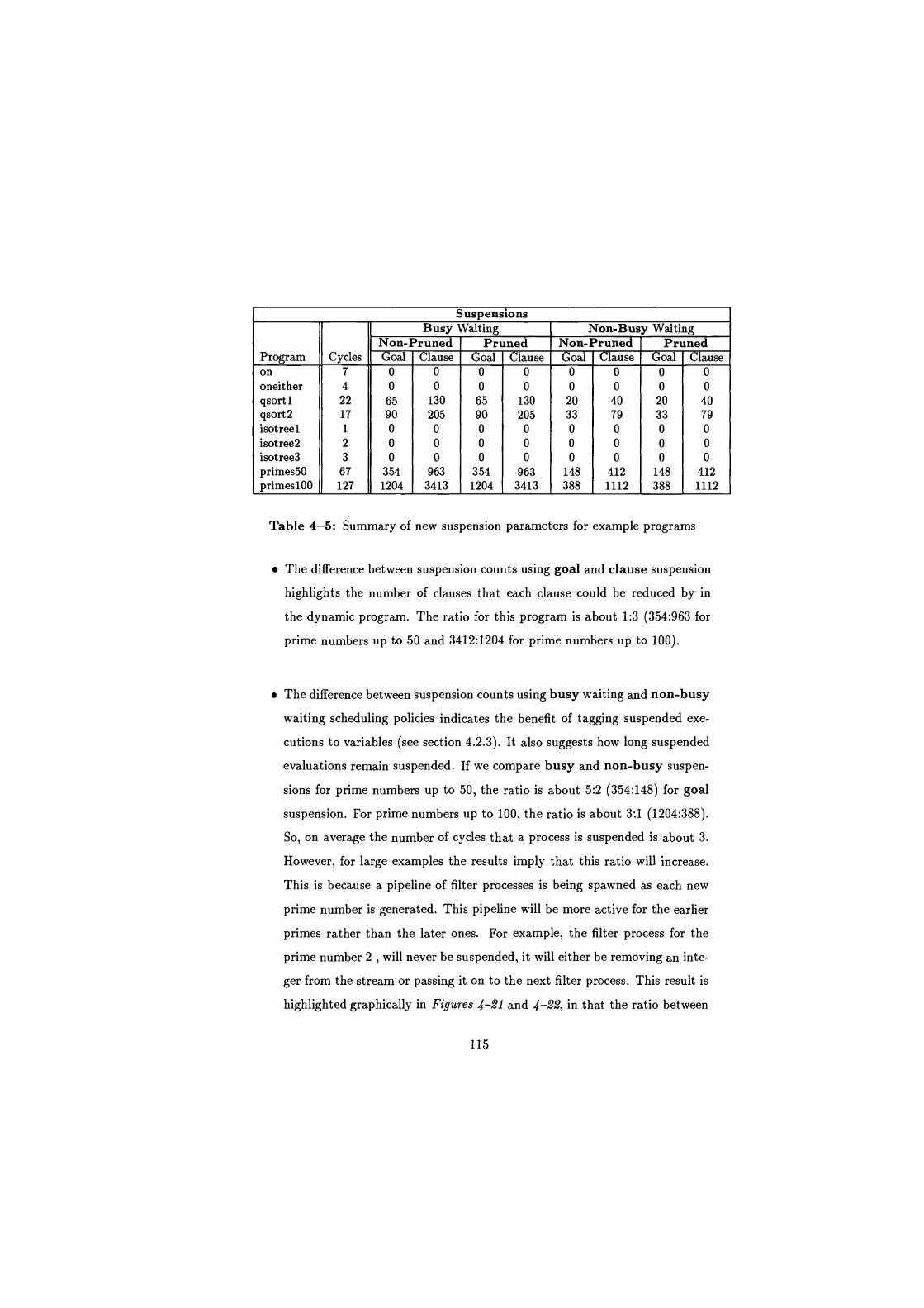
Suspensions Busy Waiting Non-Busy Waiting

Non-Pruned Pruned Non-Pruned Pruned Program Cycles Goal Clause Goal Clause Goal Clause Goal Clause on 7 0 0 0 0 0 0 0 0

oneither 4 0 0 0 0 0 0 0 0

gsortl 22 65 130 65 130 20 40 20 40

qsort2 17 90 205 90 205 33 79 33 79

isotreel 1 0 0 0 0 0 0 0 0

isotree2 2 0 0 0 0 0 0 0 0

isotree3 3 0 0 0 0 0 0 0 0

primes50 67 354 963 354 963 148 412 148 412

primesl00 127 1204 3413 1204 3413 388 1112 388 1112

Table 4-5: Summary of new suspension parameters for example programs

The difference between suspension counts using goal and clause suspension

highlights the number of clauses that each clause could be reduced by in

the dynamic program. The ratio for this program is about 1:3 (354:963 for

prime numbers up to 50 and 3412:1204 for prime numbers up to 100).

The difference between suspension counts using busy waiting and non-busy

waiting scheduling policies indicates the benefit of tagging suspended exe-

cutions to variables (see section 4.2.3). It also suggests how long suspended

evaluations remain suspended. If we compare busy and non-busy suspen-

sions for prime numbers up to 50, the ratio is about 5:2 (354:148) for goal

suspension. For prime numbers up to 100, the ratio is about 3:1 (1204:388).

So, on average the number of cycles that a process is suspended is about 3.

However, for large examples the results imply that this ratio will increase.

This is because a pipeline of filter processes is being spawned as each new

prime number is generated. This pipeline will be more active for the earlier

primes rather than the later ones. For example, the filter process for the

prime number 2 , will never be suspended, it will either be removing an inte-

ger from the stream or passing it on to the next filter process. This result is

highlighted graphically in Figures 4-21 and 4-22, in that the ratio between

115

two suspension graphs for busy (the large plot) and non-busy (the smaller

plot) suspensions increases with the number of primes being produced.

4.6 Limitations of the new measurements

The limitations of our new system can be classified in two ways. Those associated

with modelling the execution and the collection of our proposed parameters, and

those associated with information we do not collect. The second class of limitation

forms the basis of future possible evaluation systems, these are discussed in the

section on future work at the end of this thesis. Here we focus on the first class

of limitation - those with our evaluation model and the collection of our new

parameters:

Firstly, we adopt a fixed cost model (see section 3.6.2). In this model the var-

ious components of the evaluation, like head unification, have been assigned

fixed costs (in terms of cycles). However, the cost of the given operation may

depend on several factors, such as its complexity. It would be better to adopt

a functional cost model, where the cost of an operation is calculated based

on its complexity. Such a model would however require the costs of the var-

ious operations to be accurately quantified. The resulting cost model would

be difficult to construct without reference to an actual implementation.

Secondly, we make the assumption that, in a cycle, a goal can only use

bindings available to it at the start of the cycle. This is an improvement

over the current interpreters, in modelling the inherent parallelism. Current

interpreters process the goals in a given order, allowing bindings to be made

immediately and so possibly allowing subsequent goals that require these

bindings to reduce in the current cycle. This problem is compounded if deep

guards are employed. A fully accurate model would be able to determine

exactly when a goal makes a binding, how long it would take for this binding

116

to reach another goal and whether this would be in time for the goal to

use it in the current cycle. Such a model would be heavily implementation

dependent and its results would not transfer easily to other implementations.

Clearly the inherent parallelism should not be dependent on goal order. Our

model may not display all the parallelism that could be achieved in a given

implementation, but at least it gives a measure which is not dependent on

how the goals are ordered.

Finally, in our interpreter, if an evaluation suspends, the top-level goal being

evaluated is suspended. Unlike previous interpreters the suspension record

contains information (counters) about the duration of the guard evaluation

before the evaluation suspended. Although each goal record in the goal list

is processed each cycle the additional counters indicate whether this goal

would have been evaluated in a given execution model. Whilst this is an

improvement over the previous evaluation systems our new parameters may

be in error for certain classes of program.

Two related problems arise:

- There may be a problem in busy clause suspension profiles. Only

the bindings that are available at the beginning of a cycle are used in

the evaluation of a goal. However, if the guard has a deep consumer

then this guard may suspend, whereas in a parallel implementation the

bindings may become available as the deep guard is being evaluated.

- There may be a problem in pruning consumer guards. If a clause

suspension model is employed and the different consumer guards have

different data dependencies then it may be possible for one guard to

be processed further than another, before suspending. So, the depth to

which these guards will be evaluated may differ if clause suspension

is employed (as one guard can be processed while the other suspends).

Our interpreter actually employs goal suspensions, while some infor-

mation like the depth of the previous evaluation before suspension is

117

stored in the suspension record. The depth to which each of the various

guards was previously evaluated to is not stored and so this informa-

tion is lost. If pruning is employed then for such evaluation models

the results may be in error, as the evaluation depth may be in error.

The class of program affected by these two problems have consumer goals in

the guard (deep consumer guards) which suspend and the guard evaluations

suspend at different depths. An example of such a program and query is

given in Figure 4-1-

-Execution Model Cycles Reductions Suspensions

Original model Section 3.2 3 11 1

Busy waiting, Non-Pruning, Goal Suspension 10 40 6

Busy waiting, Non-Pruning, Clause Suspension 10 36 16

Busy waiting, Pruning, Goal Suspension 10 36 6

Busy waiting, Pruning, Clause Suspension 10 32 16

Non-busy waiting, Non-Pruning, Goal Suspension 10 38 3

Non-busy waiting, Non-Pruning, Clause Suspension 10 36 4

Non-busy waiting, Pruning, Goal Suspension 10 34 3

Non-busy waiting, Pruning, Clause Suspension 10 32 4

Table 4-6: Results collected for example query

The query has two goals. The second goal is a deep guarded consumer

and the first goal is a producer. Table 4-1 gives a summary of the pre-

dicted results of the evaluation of this query. Table 4-6 gives a summary

of the results obtained by our evaluation system. As expected our results

are slightly in error for the suspension parameters using busy waiting and

clause suspension and also for reductions using pruning.

118

4.7 Summary


The basis of the new profiling parameters we propose.

A detailed example execution which highlights the various new parameters.

How the new parameters are collected by post analysis of a dump file and

an example of a graphical tool developed for viewing profiles of the various

new parameters.

The use of this graphical tool to analyse the execution of several example

programs. These highlight several features of both the interpreter and our

proposed metrics.

The limitations of our evaluation system.

119

Part III

Example AI programs and their evaluation

120

Preface

In this part of the thesis we evaluate the execution behaviour of Al applica-

tions/programming techniques realised on the CCND languages. The selection

of the application areas was motivated by two requirements:

The applications should represent some common Al programming techniques

or paradigms.

The possible realisations (mappings) should highlight the use of particular

language features. The evaluation of the resulting programs then allows us

to compare the dynamic behaviour of the use of these features in our Al

applications.

This part of the thesis consists of three chapters, each focusing on a different

Al application and CCND language feature:

Chapter 5 considers how Al search based algorithms can be mapped to the

committed choice feature of the CCND languages. The qualitative evalua-

tion highlights the need for some techniques for translating general search

programs into all-solutions search programs. Three techniques for trans-

lating search programs on to the CCND computation model are then dis-

cussed, namely Continuation based compilation; Stream based compilation;

and Layered Streams. We then evaluate three all-solutions versions (obtained

using each of the translation techniques) of the n-queens problem.

Chapter 6 considers how multiple writers to shared data structures can be

supported in the CCND languages. The main feature being investigated

here is the difference between using safe and unsafe languages. Support for

shared data areas appears to be a important consideration for Al program-

ming. Several current Al applications/programming paradigms use a shared

121

area to allow independent experts to co-operate in the solving of a problem

e.g. blackboard type problem solvers and chart parsers. We consider how

chart parsing maps to safe and unsafe languages and to a language with

additional primitives to support shared streams. The three resulting chart

parsers are then evaluated.

Chapter 7 considers how an AI programming technique known as meta-level

inference maps to the CCND languages. The language feature being in-

vestigated here is the difference between using deep and flat languages.

Meta-level inference attempts to control the search at one level of the prob-

lem space (the object-level) by providing some general control rules (the

meta-level) to guide the search over the object level search. The application

evaluated is known as PRESS. We consider how the meta-level of PRESS

maps to deep guards and to flat guards using two techniques in supporting

the meta-level. The three resulting PRESS systems are then evaluated.

122

Chapter 5

Search - committed choice

5.1 Overview

This chapter considers how Al search based algorithms can be mapped to the com-

mitted choice feature of the CCND languages. Axioms specified in Horn clauses

can be viewed as a program if there is some theorem prover which can apply the

axioms to solving a query. The selection of which axioms to apply to solving a

given goal highlights several types of choice point (don't care; don't know; and

generate and test) that exists in the search space for the theorem prover. The

scope and applicability of a logic programming language is determined by how it

supports/caters for these various choice points.

This chapter first considers how various forms of non-determinism (don't care;

don't know; and generate and test) can be realised in the CCND framework. This

analysis highlights a class of search algorithms which cannot be supported di-

rectly (mapped) on the CCND computational model. We then consider various

techniques for offering exhaustive search in the CCND languages. The techniques

considered are Continuation based compilation, Stream based compilation and

Layered Streams.

123

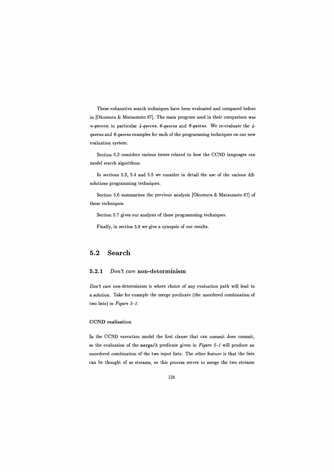
These exhaustive search techniques have been evaluated and compared before

in [Okumura & Matsumoto 87]. The main program used in their comparison was

n-queens; in particular 4-queens, 6-queens and 8-queens. We re-evaluate the 4-

queens and 6-queens examples for each of the programming techniques on our new

evaluation system.

Section 5.2 considers various issues related to how the CCND languages can

model search algorithms.

In sections 5.3, 5.4 and 5.5 we consider in detail the use of the various All-

solutions programming techniques.

Section 5.6 summarises the previous analysis [Okumura & Matsumoto 87] of

these techniques.

Section 5.7 gives our analysis of these programming techniques.

Finally, in section 5.8 we give a synopsis of our results.

5.2 Search

5.2.1 Don't care non-determinism

Don't care non-determinism is where choice of any evaluation path will lead to

a solution. Take for example the merge predicate (the unordered combination of

two lists) in Figure 5-1.

CCND realisation

In the CCND execution model the first clause that can commit does commit,

so the evaluation of the merge/3 predicate given in Figure 5-1 will produce an

unordered combination of the two input lists. The other feature is that the lists

can be thought of as streams, so this process serves to merge the two streams

124

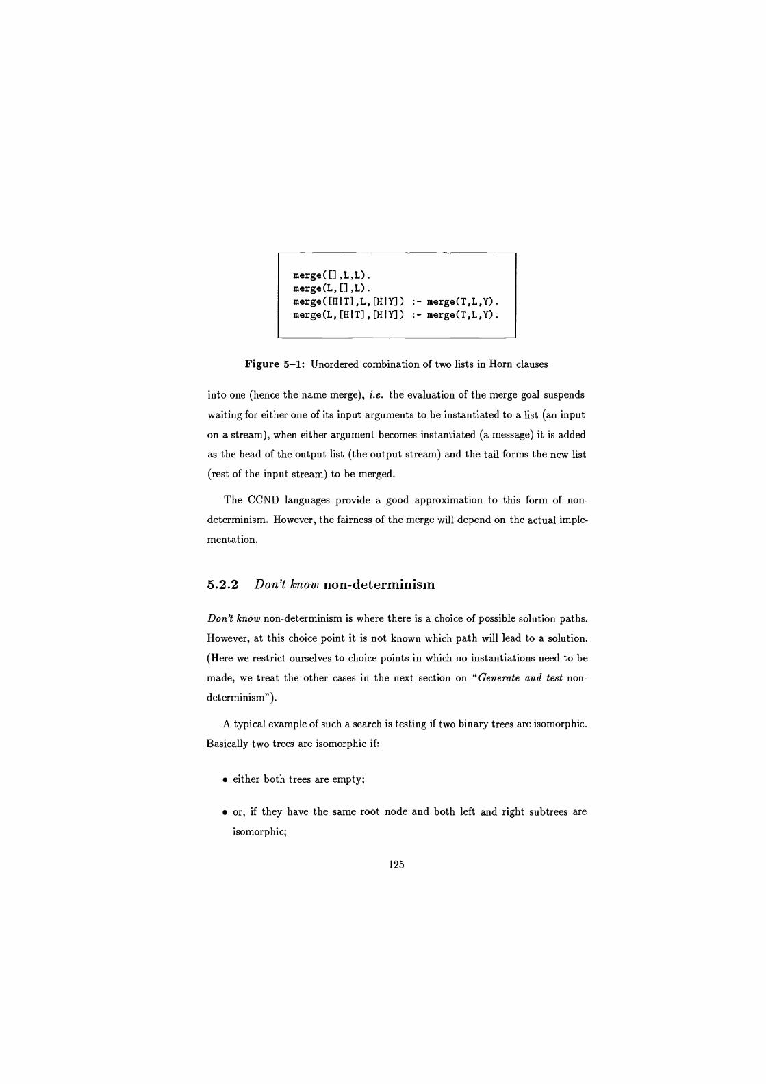
merge([],L,L).

merge(L, [] ,L) .

merge([HIT],L, [HIY]) :- merge(T,L,Y). merge(L, [HIT] , [HIY]) :- merge(T,L,Y).

Figure 5-1: Unordered combination of two lists in Horn clauses

into one (hence the name merge), i.e. the evaluation of the merge goal suspends

waiting for either one of its input arguments to be instantiated to a list (an input

on a stream), when either argument becomes instantiated (a message) it is added

as the head of the output list (the output stream) and the tail forms the new list

(rest of the input stream) to be merged.

The CCND languages provide a good approximation to this form of non-

determinism. However, the fairness of the merge will depend on the actual imple-

mentation.

5.2.2 Don't know non-determinism

Don't know non-determinism is where there is a choice of possible solution paths.

However, at this choice point it is not known which path will lead to a solution.

(Here we restrict ourselves to choice points in which no instantiations need to be

made, we treat the other cases in the next section on "Generate and test non-

determinism").

A typical example of such a search is testing if two binary trees are isomorphic.

Basically two trees are isomorphic if.

either both trees are empty;

or, if they have the same root node and both left and right subtrees are

isomorphic;

125

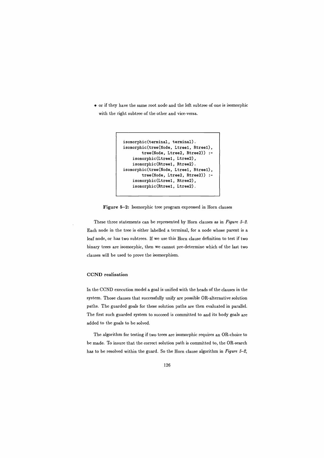
or if they have the same root node and the left subtree of one is isomorphic

with the right subtree of the other and vice-versa.


tree(Node, Ltree2, Rtree2)) :- isomorphic(Ltreel, Ltree2),

isomorphic(Rtreel, Rtree2). isomorphic(tree(Node, Ltreel, Rtreel),

tree(Node, Ltree2, Rtree2)) :- isomorphic(Ltreel, Rtree2), isomorphic(Rtreel, Ltree2).

Figure 5-2: Isomorphic tree program expressed in Horn clauses

These three statements can be represented by Horn clauses as in Figure 5-2.

Each node in the tree is either labelled a terminal, for a node whose parent is a

leaf node, or has two subtrees. If we use this Horn clause definition to test if two

binary trees are isomorphic, then we cannot pre-determine which of the last two

clauses will be used to prove the isomorphism.

CCND realisation

In the CCND execution model a goal is unified with the heads of the clauses in the

system. Those clauses that successfully unify are possible OR-alternative solution

paths. The guarded goals for these solution paths are then evaluated in parallel.

The first such guarded system to succeed is committed to and its body goals are

added to the goals to be solved.

The algorithm for testing if two trees are isomorphic requires an OR choice to

be made. To insure that the correct solution path is committed to, the OR-search

has to be resolved within the guard. So the Horn clause algorithm in Figure 5-2,

126

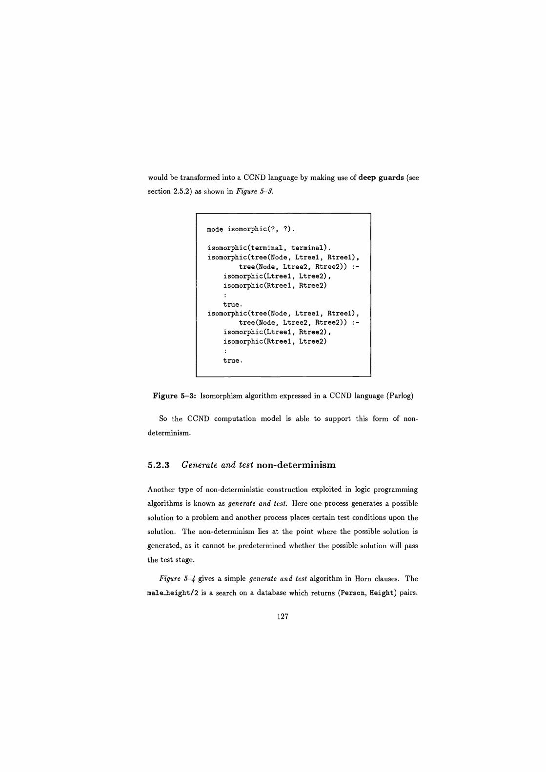
would be transformed into a CCND language by making use of deep guards (see

section 2.5.2) as shown in Figure 5-3.

mode isomorphic(?, ?).


tree(Node, Ltree2, Rtree2)) :- isomorphic(Ltreei, Ltree2), isomorphic(Rtreel, Rtree2)

true. isomorphic(tree(Node, Ltreel, Rtreel),

tree(Node, Ltree2, Rtree2)) :- isomorphic(Ltreei, Rtree2), isomorphic(Rtreel, Ltree2)

true.

Figure 5-3: Isomorphism algorithm expressed in a CCND language (Parlog)

So the CCND computation model is able to support this form of non-

determinism.

5.2.3 Generate and test non-determinism

Another type of non-deterministic construction exploited in logic programming

algorithms is known as generate and test. Here one process generates a possible

solution to a problem and another process places certain test conditions upon the

solution. The non-determinism lies at the point where the possible solution is

generated, as it cannot be predetermined whether the possible solution will pass

the test stage.

Figure 5-4 gives a simple generate and test algorithm in Horn clauses. The

male-height/2 is a search on a database which returns (Person, Height) pairs.

127

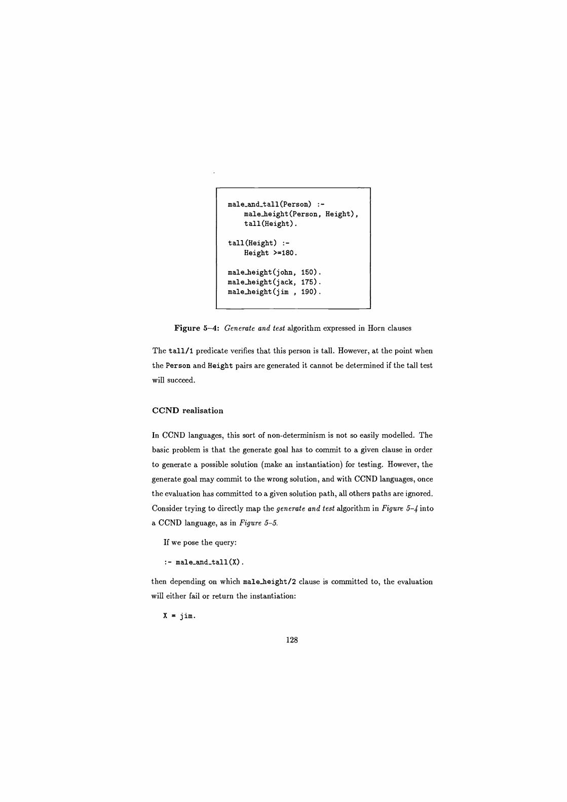
male_and_tall(Person) :- male-height (Person, Height), tall(Height).

tall(Height) :- Height >=180.

mal else ight (john , 150). male-height (jack, 175). male-height (j im , 190).

Figure 5-4: Generate and test algorithm expressed in Horn clauses

The tall/i predicate verifies that this person is tall. However, at the point when

the Person and Height pairs are generated it cannot be determined if the tall test

will succeed.

CCND realisation

In CCND languages, this sort of non-determinism is not so easily modelled. The

basic problem is that the generate goal has to commit to a given clause in order

to generate a possible solution (make an instantiation) for testing. However, the

generate goal may commit to the wrong solution, and with CCND languages, once

the evaluation has committed to a given solution path, all others paths are ignored.

Consider trying to directly map the generate and test algorithm in Figure 5-4 into

a CCND language, as in Figure 5-5.

If we pose the query:

:- male_and_tall(X).

then depending on which male-height/2 clause is committed to, the evaluation

will either fail or return the instantiation:

X = j im.

128

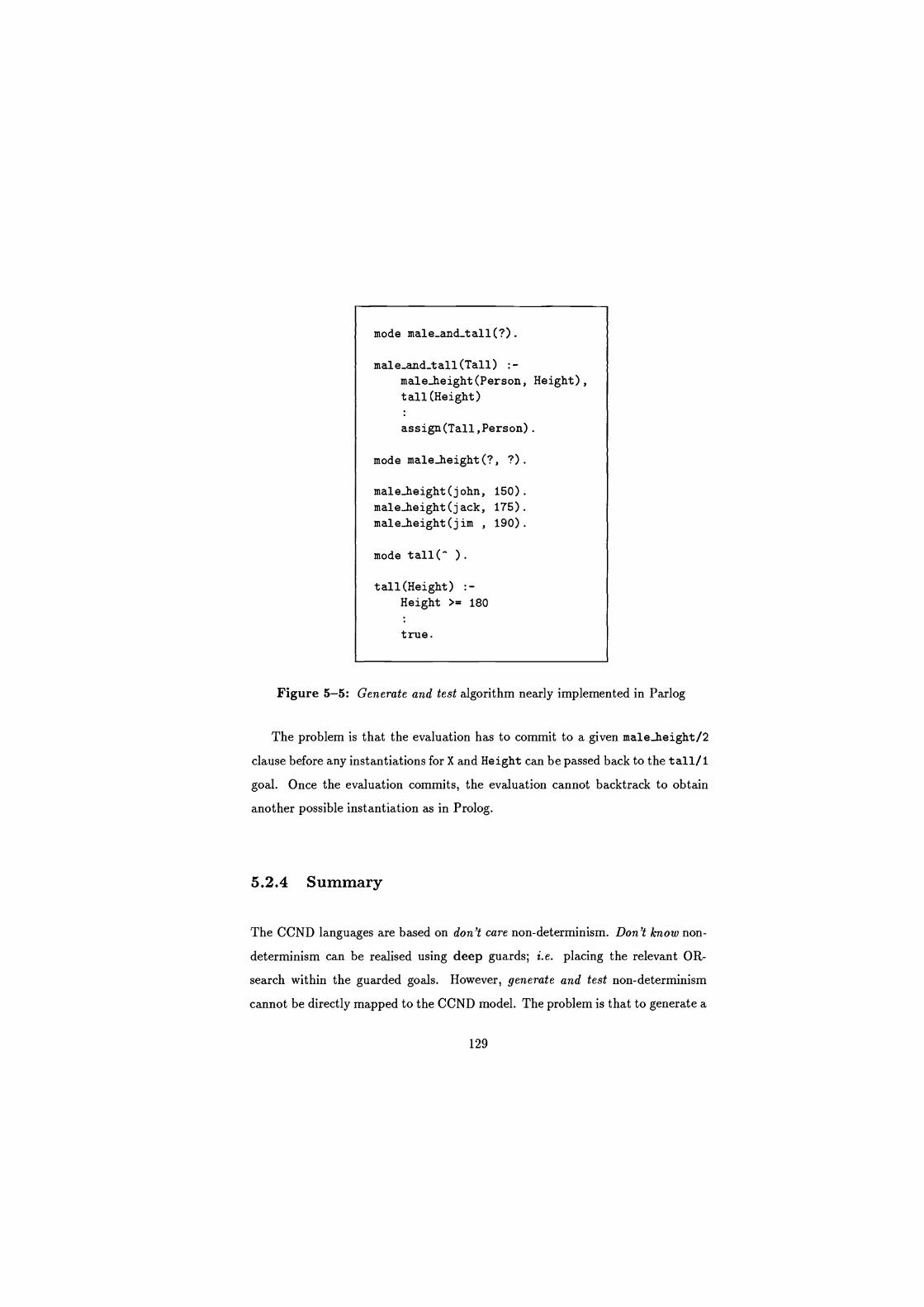
mode male-and-tall(?).

male_and_tall(Tall) :-

male-height (Person, Height), tall (Height)

assign(Tall,Person).

mode malelieight (?, ?).

malelieight (john, 150). malelieight (jack, M). malelieight (j im , 190).

mode tall(" ).

tall(Height) :-

Height >= 180

true.

Figure 5-5: Generate and test algorithm nearly implemented in Parlog

The problem is that the evaluation has to commit to a given male-height/2

clause before any instantiations for X and Height can be passed back to the tall/1 goal. Once the evaluation commits, the evaluation cannot backtrack to obtain

another possible instantiation as in Prolog.

5.2.4 Summary

The CCND languages are based on don't care non-determinism. Don't know non-

determinism can be realised using deep guards; i.e. placing the relevant OR-

search within the guarded goals. However, generate and test non-determinism

cannot be directly mapped to the CCND model. The problem is that to generate a

129

solution the evaluation has to commit to a given solution path. Once the evaluation

has committed, alternative bindings cannot be generated.

In [Trehan & Wilk 87] we consider various automated and manual methods

for offering full search in the CCND languages. The automatic methods are only

suitable for a restricted set of Horn clause programs. The basic restrictions are

that each predicate must be input and output moded and the input arguments

must be instantiated when a goal is to be evaluated and its output arguments

must be fully instantiated when the goal has been evaluated. This prevents the

use of Streamed And-Parallelism in the algorithm.

Three manual methods for addressing the generate and test problem have been

considered: restructuring the knowledge; selected use of all-solutions parallelism;

and Layered Streams. The first involves generating a set of possible solutions. This

is achieved by altering the data to insure that all possible solutions can be gener-

ated by a deterministic search. The second involves using an all-solutions search

mechanism at the generate choice points, to return a set of possible bindings. The

last provides a programming style suitable for solutions that are generated incre-

mentally and bottom-up, for example constructing sentences from words. Here,

the test goal is placed inside the generate goal.

In the following sub-sections we consider three of the techniques for translating

Horn clause programs into all-solutions search programs in more detail. The tech-

niques are applied to a simple search program for the 4-queens problem, (given in

Figure 5-6). Two of the techniques, Continuation based compilation and Stream

based compilation allow Horn clause programs to be automatically translated into

an all-solutions CCND program. The third technique is suitable for problems in

which the solution can be generated in an incremental and bottom-up manner.

130

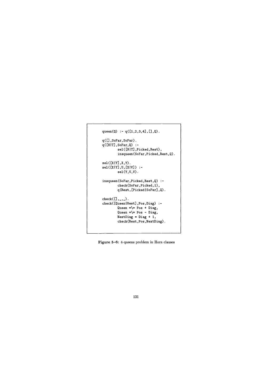
queen(Q) :- q( [1,2,3,4] , [] ,Q) .

q([],SoFar,SoFar). q([HIT],SoFar,Q) :-

sel([HIT],Picked,Rest), insqueen(SoFar,Picked,Rest,Q).

sel ([X IY] ,X,Y). se1([XIY],U,[XIV]) :-

sel(Y,U,V).

insqueen(SoFar,Picked,Rest,Q) :- check(SoFar,Picked,i), q(Rest,[PickedlSoFar],Q).

check([],_,_). check([QueenlRest],Pos,Diag) :-

Queen =\= Pos + Diag, Queen =\= Pos - Diag, NextDiag = Diag + 1, check(Rest,Pos,NextDiag).

Figure 5-6: 4-queens problem in Horn clauses

131

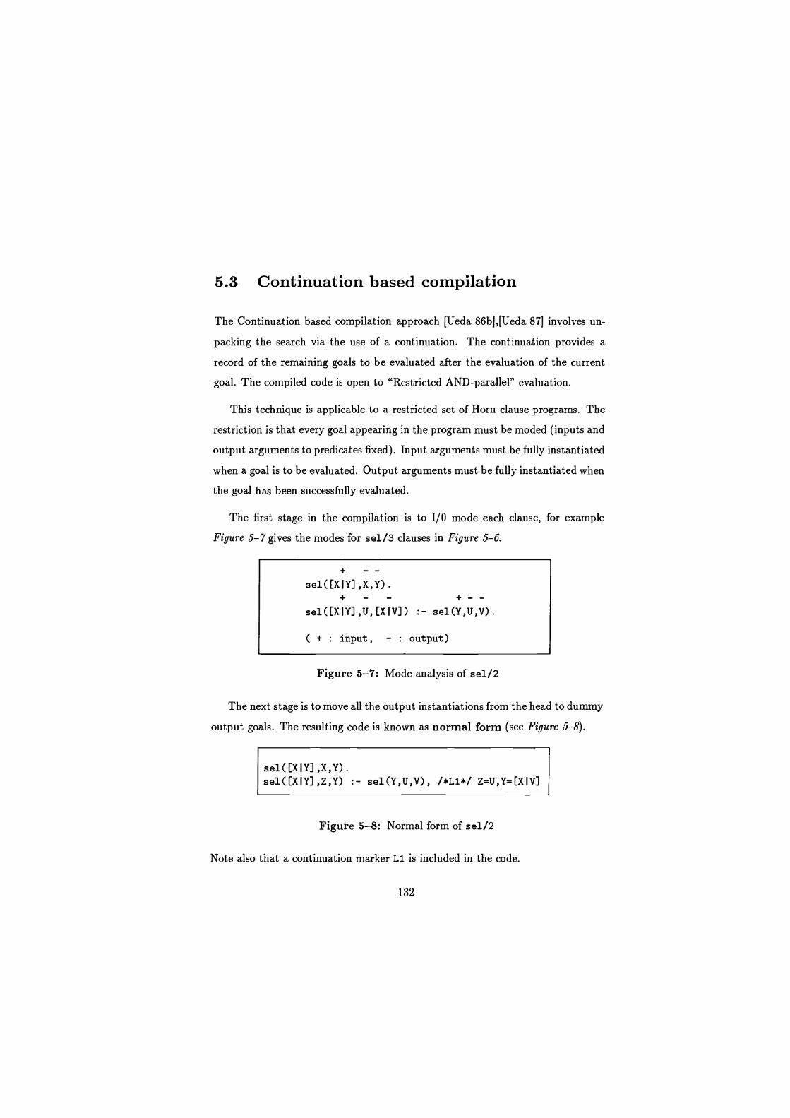
5.3 Continuation based compilation

The Continuation based compilation approach [Ueda 86b],[Ueda 87] involves un-

packing the search via the use of a continuation. The continuation provides a

record of the remaining goals to be evaluated after the evaluation of the current

goal. The compiled code is open to "Restricted AND-parallel" evaluation.

This technique is applicable to a restricted set of Horn clause programs. The

restriction is that every goal appearing in the program must be moded (inputs and

output arguments to predicates fixed). Input arguments must be fully instantiated

when a goal is to be evaluated. Output arguments must be fully instantiated when

the goal has been successfully evaluated.

The first stage in the compilation is to I/O mode each clause, for example

Figure 5-7 gives the modes for sel/3 clauses in Figure 5-6.

+ - - se1([XIY],X,Y) .

se1([XIY],U, [XIV]) :- se1(Y,U,V).

( + : input, - : output)

Figure 5-7: Mode analysis of sel/2

The next stage is to move all the output instantiations from the head to dummy

output goals. The resulting code is known as normal form (see Figure 5-8).

se1([XIY],X,Y). se1([XIY],Z,Y) :- se1(Y,U,V), /*L1*/ Z=U,Y=[XIV]

Figure 5-8: Normal form of sel/2

Note also that a continuation marker L1 is included in the code.

132

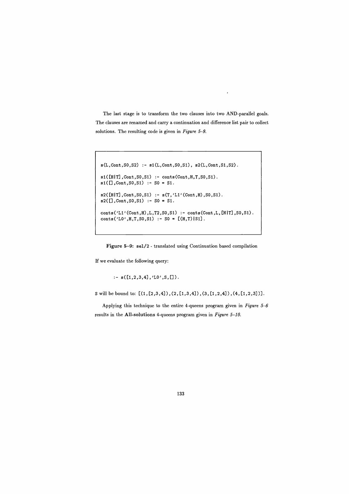
The last stage is to transform the two clauses into two AND-parallel goals.

The clauses are renamed and carry a continuation and difference list pair to collect

solutions. The resulting code is given in Figure 5-9.

s(L,Cont,SO,S2) :- s1(L,Cont,SO,S1), s2(L,Cont,S1,S2).

s1([HIT],Cont,SO,S1) :- conts(Cont,H,T,SO,S1). s1( ,Cont,SO,S1) :- So = S1.

s2([HIT],Cont,SO,S1) :- s(T,'L1'(Cont,H),SO,S1). s2([],Cont,SO,S1) :- SO = S1.

conts('L1'(Cont,H),L,T2,SO,S1) :- conts(Cont,L,[HIT],SO,S1). conts('LO',H,T,SO,S1) :- SO = [(H,T)IS1].

Figure 5-9: sel/2 - translated using Continuation based compilation

If we evaluate the following query:

:- s([1,2,3,4],'LO',S,[])

Swill be bound to: [(1, [2,3,4]) , (2, [1,3,4]) , (3, [1,2,4]) , (4, [1,2,3] )] .

Applying this technique to the entire 4-queens program given in Figure 5-6

results in the All-solutions 4-queens program given in Figure 5-10.

133

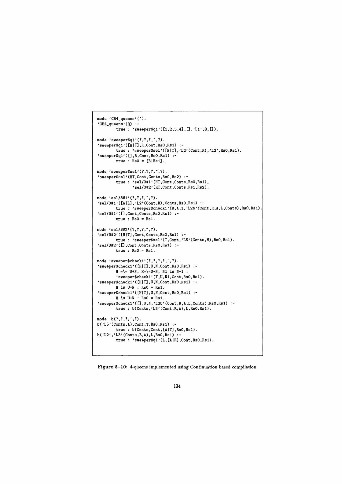
mode 'CB4_queens'("). 'CB4_queens'(Q) :-

true : 'sweeper$gi' ([1,2,3,4] , ,'L1' ,Q, ) . mode 'sweeper$gi'(?,?,?, ?).

'sweeper$gi'([HIT],R,Cont,RsO,Rsl) :- true : 'sweeper$sel'([H(T],'L2'(Cont,R),'L2',RsO,Rsl).

'sweeper$gl'([],R,Cont,RsO,Rsl) :- true : RsO = [RIRs1].

mode 'sweeper$sel'(?,?,?,",?).

'sweeper$sel'(HT,Cont,Conts,RsO,Rs2) :- true : 'sel/3#1'(HT,Cont,Conts,RsO,Rsl),

'sel/3#2'(HT,Cont,Conts,Rsl,Rs2).

mode 'sel/3#1'(?,?,?, ?).

'sel/3#1'([AIL],'L2'(Cont,R),Conts,RsO,Rsl) true : 'sweeper$checks'(R,A,1,'L2b'(Cont,R,A,L,Conts),RsO,Rsl).

'sel/3#1'( ,Cont,Conts,RsO,Rsl) :- true : RsO = Rsi.

mode 'sel/3#2'(?,?,?,",?). 'sel/3#2'([HIT],Cont,Conts,RsO,Rsl) :-

true : 'sweeper$sel'(T,Cont,'L5'(Conts,H),RsO,Rsl). 'sel/3#2'( ,Cont,Conts,RsO,Rsl) :-

true : RsO = Rsi.

mode 'sweeper$checki'(?,?,?,?,",?). 'sweeper$checkl'([HIT],U,N,Cont,RsO,Rsl) :-

H =\= U+N, H=\=U-N, N1 is N+1 :

'sweeper$checki'(T,U,N1,Cont,RsO,Rsl). 'sweeper$checki'([HIT],U,N,Cont,RsO,Rsl) :-

H is U+N : RsO = Rsi. 'sweeper$checki'([HIT],U,N,Cont,RsO,Rsl) :-

H is U-N : RsO = Rsi. 'sweeper$checks'([],U,N,'L2b'(Cont,R,A,L,Conts),RsO,Rsl) :-

true : b(Conts,'L3'(Cont,R,A),L,RsO,Rsl).

mode b(?,?,?,-,?).

b('L5'(Conts,A),Cont,T,RsO,Rs1) :- true : b(Conts,Cont,[AIT],RsO,Rs1).

b('L2','L3'(Conts,R,A),L,RsO,Rsl) :- true : 'sweeper$gi'(L,[AIR],Cont,RsO,Rsl).

Figure 5-10: 4-queens implemented using Continuation based compilation

134

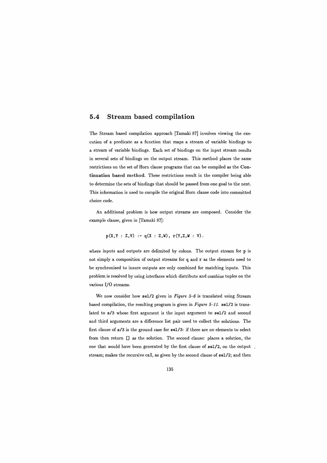
5.4 Stream based compilation

The Stream based compilation approach [Tamaki 87] involves viewing the exe-

cution of a predicate as a function that maps a stream of variable bindings to

a stream of variable bindings. Each set of bindings on the input stream results

in several sets of bindings on the output stream. This method places the same

restrictions on the set of Horn clause programs that can be compiled as the Con-

tinuation based method. These restrictions result in the compiler being able

to determine the sets of bindings that should be passed from one goal to the next.

This information is used to compile the original Horn clause code into committed

choice code.

An additional problem is how output streams are composed. Consider the

example clause, given in [Tamaki 87]:

p(X,Y : Z,V) :- q(X : Z,W), r(Y,Z,W : V).

where inputs and outputs are delimited by colons. The output stream for p is

not simply a composition of output streams for q and r as the elements need to

be synchronised to insure outputs are only combined for matching inputs. This

problem is resolved by using interfaces which distribute and combine tuples on the

various I/O streams.

We now consider how sel/2 given in Figure 5-6 is translated using Stream

based compilation, the resulting program is given in Figure 5-11. sel/2 is trans-

lated to s/3 whose first argument is the input argument to sel/2 and second

and third arguments are a difference list pair used to collect the solutions. The

first clause of s/3 is the ground case for sel/3: if there are no elements to select

from then return as the solution. The second clause: places a solution, the

one that would have been generated by the first clause of sel/2, on the output

stream; makes the recursive call, as given by the second clause of sel/2; and then

135

s([],SO,Si) :- So = S1.

s([HIT],SO,S2) :-

SO = [(H,T) IS1], s(T,UV,[]),

i(H,UV,S1,S2).

i(x,[(U,V)IUVs],SO,S2)

i(x,UVs,Si,s2),

so = [(u, [xIV]) IS1] .

i(x,[],SO,Si) :- SO = S1.

Figure 5-11: sel/2 - translated using Stream based compilation

combines the solution of the recursive call with the input argument to give the

remainder of the solution stream. The composing interface is given by i/4.

If we execute the following goal:

:- s([1,2,3,4],S,[]).

Swill be bound to: [(1, [2,3,4]) , (2, [1,3,4]) , (3, [1,2,4]) , (4, [1,2,3] )] .

Applying this technique to the entire 4-queens program given in Figure 5-6

results in the All-solutions 4-queens program given in Figure 5-12.

136

mode 'SB4_queens'("). 'SB4_queens'(Q) :- true : 'Qq'([1,2,3,4],[3,Q,[3).

mode 'Qq'(?,?, ?).

'Qq'([],Y,ZO,Z1) :- true : ZO = [YIZ1].

'Qq'(X,Y,ZO,Z1) :- X \= [] :

'Qsel'(X,UVs,[]), 'Ig21'(Y,UVs,ZO,Z1).

mode 'Qsel'(?,",?).

'Qsel'([],ZO,Z1) :- true : ZO = Z1.

'Qsel'([XIY],ZO,Z2) :- true : ZO = [(X,Y)IZ1],

'Qsel'(Y,UVs,[]),

'Isel2l'(X,UVs,Z1,Z2).

mode 'Ig21'(?,?,",?).

'Ig21'(Y,[(U,V)IUVs],ZO,Z2) :-

true : 'Qcheck'(Y,U,1,YY),

'Ig22'(V,[UIY],YY,ZO,Z1),

'Ig21'(Y,UVs,Z1,Z2).

'Ig21'(_,[],ZO,Z1) :- true : ZO = Z1.

mode 'Ig22'(?,?,?,",?).

'Ig22'(V,List,ok,ZO,Z1) :- true : 'Qq'(V,List,ZO,Z1).

'Ig22'(_,_,ng,ZO,Z1) :- true : ZO = Z1.

mode 'Ise121'(?,?,",?).

'Isel2l'(X,[(U,V)IUVs],ZO,Z2) :- true : ZO = [(U,[XIV])IZ1], 'Isel2l'(X,UVs,Z1,Z2).

'Isel2l'(_,[],ZO,Z1) :- true : ZO = Z1.

mode 'Qcheck'(?,?,?,").

'Qcheck'([QIR],P,N,Res) :- Q =\= P+N, Q=\= P-N : M is N+1, 'Qcheck'(R,P,M,Res).

'Qcheck'([QIR],P,N,Res) :- Q is P+N : Res = ng. 'Qcheck'([QIR],P,N,Res) :- Q is P-N : Res = ng. 'Qcheck'([],_,_,Res) :- true : Res = ok.

Figure 5-12: 4-queens implemented using Stream based compilation

137

5.5 Layered Streams

The Layered Streams approach [Okumura & Matsumoto 87] is a programming

paradigm for implementing search problems in the CCND languages. Using Lay-

ered Streams, solutions are generated in an incremental and bottom-up manner.

This gives rise to partial solutions (on each incrementation) which can be tested,

and so incorrect partial solutions can be eliminated before being fully generated.

The other feature of this programming technique is that the partial solutions are

represented in a layered data structure. This data structure provides the means

by which each further generation of the possible solutions can share the previous

bottom-up solutions. This allows for an efficient testing mechanism.

Figure 5-13 gives a Layered Streams solution to the 4-queens problem. Using

Layered Streams queens can be added to the board incrementally, on each incre-

mentation the new partial board solutions can be tested. The representation of the

board is a layered data structure which combines together the bottom-up gener-

ated partial solutions. The top-level call ' LS4_queens' (Q4) spawns four queen/2

processes, which are connected by streams. Each queen/2 process places another

queen on to the board and tests (or rather filters) out the previous bottom-up

partial solutions that are incompatible with this new queen.

The use of the layered data structure and testing of partial solutions is high-

lighted by considering the streams which connect the four queen/2 processes. The

first stream Q1 will be bound to:

[1*begin,2*begin,3*begin,4*begin]

This stream represents the position of the final queen whilst no other queens are

in place (as the solution is being generated bottom-up); the final queen can (for

now) be placed anywhere.

138

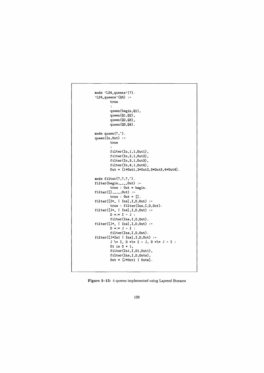
mode 'LS4_queens'(?). 'LS4_queens'(Q4) :-

true

queen(begin,Q1), queen(Q1,Q2), queen(Q2,Q3), queen(Q3,Q4).

mode queen(?,"). queen(In,Out) :-

true

filter(In,1,1,Outl), filter(In,2,1,Out2), filter(In,3,1,Out3), filter(In,4,1,Out4), Out = [1*Outl,2*Out2,3*Out3,4*Out4].

mode filter(?,?,?,").

filter(begin,_,_,Out) :- true : Out = begin.

filter([] ,_,_,Out) .- true : Out = [] .

filter([I*_ I Ins],I,D,Out) :- true : filter(Ins,I,D,Out).

filter([J*_ I Ins],I,D,Out) :- D=:=I-J .

filter(Ins,I,D,Out). filter([J*_ I Ins],I,D,Out) :-

D=:=J-I .

filter(Ins,I,D,Out). filter([)*Inl I Ins],I,D,Out) :-

J \= I, D =\= I - J, D=\= J- I D1 is D + 1, filter(InI,I,D1,Out1), filter(Ins,I,D,Outs), Out = [J*Outl I Outs].

Figure 5-13: 4-queens implemented using Layered Streams

139

The second stream Q2 will be bound to:

[1*[3*begin,4*begin], 2* [4*begin] ,

3* [1*begin] ,

4*[1*begin,2*begin]]

This represents that the last two queens can be in the following positions: the

second from last queen on position 1 and the last queen on position 3 or 4; the

second from last queen on position 2 and the last queen on position 4; the second

from last queen on position 3 and the last queen on position 1; the second from

last queen on position 4 and the last queen on position 1 or 2. This is obtained

from the partial solution for the last queen being filtered to remove incompatible

solutions with the previous queen position. Moreover this layered data structure

means that once a queen position is found to be incompatible with a bottom-up

generated partial solution all the sub-board positions are removed in one operation.

The third stream Q3 will be bound to:

[1* [3* [] , 4* [2*begin] ] , 2* [4* [1*begin] ] ,

3* [1* [4*begin] ] ,

4* [1 * [3*begin] , 2* [] ] ]

Finally the fourth stream Q4 will be bound to the complete solution:

[1*[3*[] ,4*[2*[]]], 2*[4*[1*[3*begin]]], 3* [1* [4* [2*begin] ] ] ,

4*[1*[3*[]],2*[]]]

This data structure has the following interpretation:

140

The first queen can be placed on position 1. The second queen can be placed

on position 3 or 4. If the second queen is placed on position 3 then no further

queens can be added. If the second queen is placed on position 4 then the

only place the next queen can be added is position 2. However, no further

queens can be added after this third queen.

The first queen can be placed on position 2. The only place for the second

queen is position 4. Similarly the third and fourth queens can only be placed

in positions 1 and 3 respectively. This is a complete solution.

The first queen can be placed on position 3. The only place for the second

queen is position 1. Similarly the third and fourth queens can only be placed

in positions 4 and 2 respectively. This is a complete solution.

The first queen can be placed on position 4. The second queen can be placed

on position 1 and 2. If the second queen is placed on position 1 then the

only place the next queen can be added is position 3. However, no further

queens can be added after this third queen. If the second queen is placed on

position 2 then no further queens can be added.

141

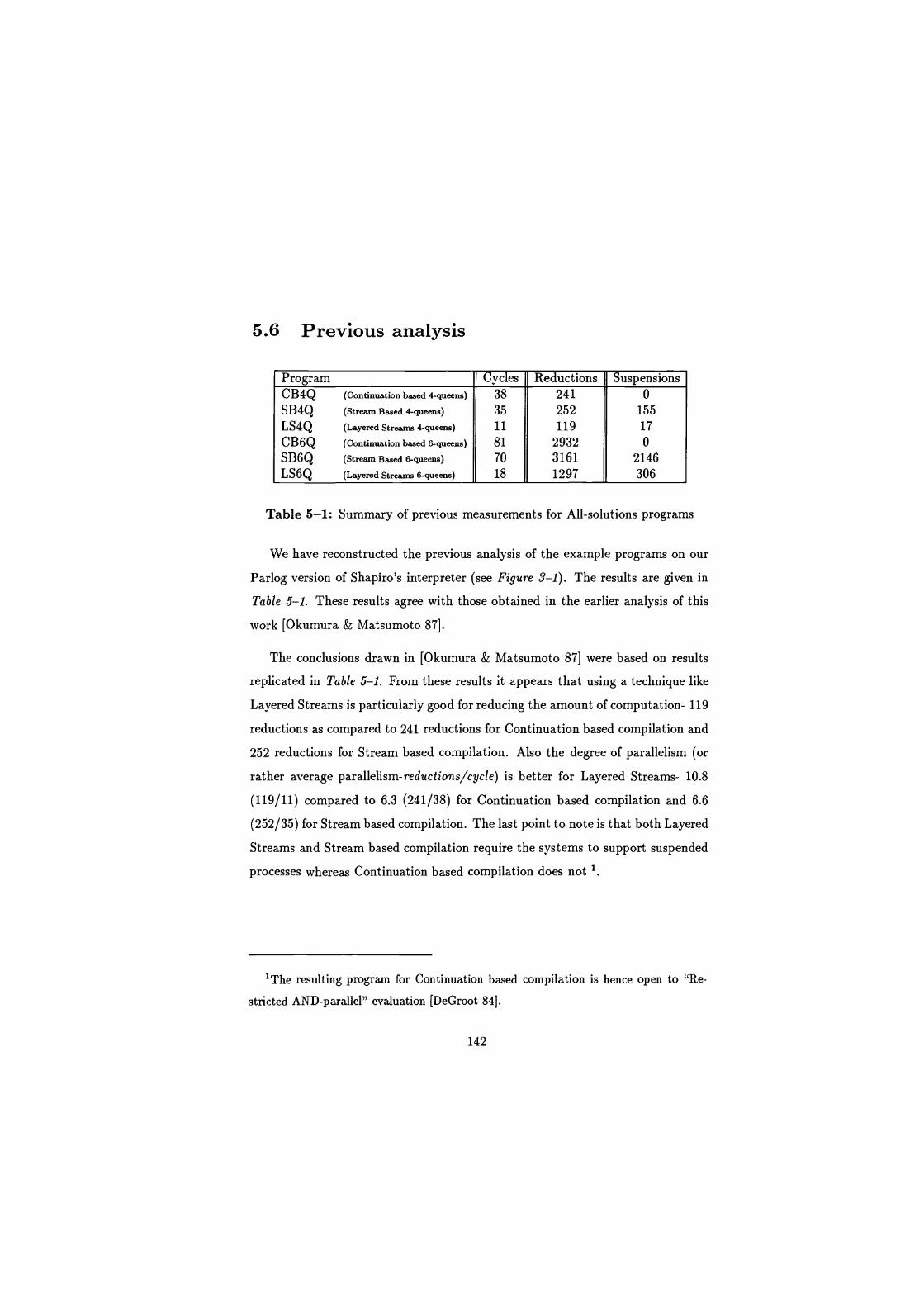
5.6 Previous analysis

Program Cycles Reductions Suspensions CB4Q (Continuation based 4-queens) 38 241 0

SB4Q (Stream Based 4-queens) 35 252 155

LS4Q (Layered Streams 4-queens) 11 119 17

CB6Q (Continuation based 6-queens) 81 2932 0

SB6Q (Stream Based 6-queens) 70 3161 2146 LS6Q (Layered Streams 6-queens) 18 1297 306

Table 5-1: Summary of previous measurements for All-solutions programs

We have reconstructed the previous analysis of the example programs on our

Parlog version of Shapiro's interpreter (see Figure 3-1). The results are given in

Table 5-1. These results agree with those obtained in the earlier analysis of this

work [Okumura & Matsumoto 87].

The conclusions drawn in [Okumura & Matsumoto 87] were based on results

replicated in Table 5-1. From these results it appears that using a technique like

Layered Streams is particularly good for reducing the amount of computation- 119

reductions as compared to 241 reductions for Continuation based compilation and

252 reductions for Stream based compilation. Also the degree of parallelism (or

rather average parallelism-reductions/cycle) is better for Layered Streams- 10.8

(119/11) compared to 6.3 (241/38) for Continuation based compilation and 6.6

(252/35) for Stream based compilation. The last point to note is that both Layered

Streams and Stream based compilation require the systems to support suspended

processes whereas Continuation based compilation does not '.

'The resulting program for Continuation based compilation is hence open to "Re-

stricted AND-parallel" evaluation [DeGroot 84].

142

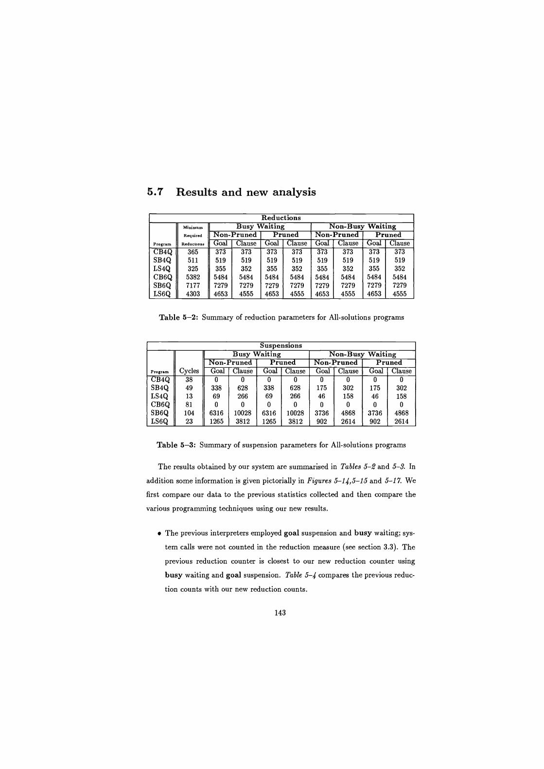
5.7 Results and new analysis

Reductions Minimum Busy Waiting N on-Busy Waiting Required Non- Pruned Pruned Non- Pruned Pruned

Program Reductions Goal Clause Goal Clause Goal Clause Goal Clause CB4Q 365 373 373 373 373 373 373 373 373 SB4Q 511 519 519 519 519 519 519 519 519

LS4Q 325 355 352 355 352 355 352 355 352

CB6Q 5382 5484 5484 5484 5484 5484 5484 5484 5484

SB6Q 7177 7279 7279 7279 7279 7279 7279 7279 7279 LS6Q 4303 4653 4555 4653 4555 4653 4555 4653 4555

Table 5-2: Summary of reduction parameters for All-solutions programs

Suspensions Busy Waiting Non-Bus y Waiting

Non-Pruned Pruned Non-Pruned Pruned Program Cycles Goal Clause Goal Clause Goal Clause Goal Clause CB4Q 38 0 0 0 0 0 0 0 0

SB4Q 49 338 628 338 628 175 302 175 302 LS4Q 13 69 266 69 266 46 158 46 158

CB6Q 81 0 0 0 0 0 0 0 0

SB6Q 104 6316 10028 6316 10028 3736 4868 3736 4868

LS6Q 23 1265 3812 1265 3812 902 2614 902 2614

Table 5-3: Summary of suspension parameters for All-solutions programs

The results obtained by our system are summarised in Tables 5-2 and 5-3. In

addition some information is given pictorially in Figures 5-14,5-15 and 5-17. We

first compare our data to the previous statistics collected and then compare the

various programming techniques using our new results.

The previous interpreters employed goal suspension and busy waiting; sys-

tem calls were not counted in the reduction measure (see section 3.3). The

previous reduction counter is closest to our new reduction counter using

busy waiting and goal suspension. Table 5-4 compares the previous reduc-

tion counts with our new reduction counts.

143

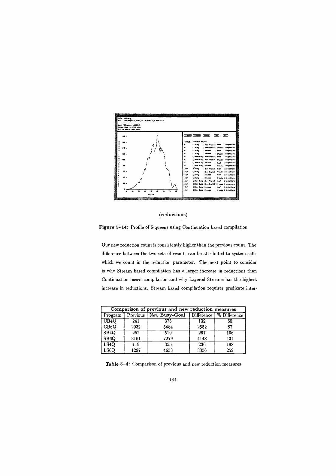
r11.m CSe0

1s /a.r/.Ry.2/rt/C0M_.v.1 d/p. fll._4 d/d.ts, a

60.1. C0._yu...1*L6Z5546) El.s TIPS i$,23738 ..s Ni n1.0. Rsdu1iww 3302

PEI

u 140

FE]

If, 20 10 40 50 00 70

CYCLES

INGURNBRIBBEEM

fr5ra7w-I MM am)

1S1RLd

e

5363

5403

8404

$404

6464

34" $404

000101. 0r.0hn

O Busy

O busy

O w.y O busy

O 000-w.y I 0101Pruud 160.1 I SY.P.n.ton.

O 000-Bug 1000-Proud I Cl.u.. I Suop001- Nen-wq I Pr-

-busy 1 hums Cl.... I Su.v.m1len.

bu.y I Mm-Prun.d 100.1 10101161100.

O buq I MmtPrumd 1 C1.u.. R.duOtim. p bu.y 1 Prurma0 I Be.1 I Rsuetl0n.

O 6u.y I P- I Claus. 10.5uttim. Nm-Busy I Nm-Pruned 100.1 11'.duotion.

Mm-Duty I won-Prm.d I Clw.a 10.01121100.

O Non-06.y Prm.e 100.1 I Rsdutim. p Non-wq I Pans I C1.u.. I R.duttlmt M

I Men-ftumd 16-1 130.0..100. I Man-Prun.d I Claus. I lu.idnaan. 1 Plums

1 oe.1 1 Su.0.0.ion.

sr1lI i Ci.u.. I Sup.n.4m.

tip _ .I:§';1,PItf9?jpEI:f,'.tla

(reductions)

Figure 5-14: Profile of 6-queens using Continuation based compilation

Our new reduction count is consistently higher than the previous count. The

difference between the two sets of results can be attributed to system calls

which we count in the reduction parameter. The next point to consider

is why Stream based compilation has a larger increase in reductions than

Continuation based compilation and why Layered Streams has the highest

increase in reductions. Stream based compilation requires predicate inter-

Comparison of previous and new reduction measures Program Previous New Busy-Goal Difference % Difference CB4Q CB6Q

241

2932 373

5484

132

2552 55

87

SB4Q SB6Q

252

3161

519 7279

267 4148

106

131

LS4Q LS6Q

119

1297

355

4653

236

3356

198

259

Table 5-4: Comparison of previous and new reduction measures

144

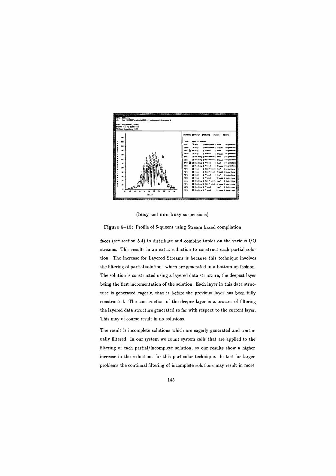
f11. 6610 P'% dlr Ner NC6010/ .2/rt/CCIOS_6..1 d/eyet._3 0 d/d.e. d

06.b e06_R ..n.(USSR) EluPC T1. 1. 6580 1 Mniw Reductions 7177

e 10 El 0 9s FD

rumcm

TOtRl.3. P..el old &60130.

6316 0 00.0 I Men-Prun./ I so.l 13usp0IIam 10020 0 e-.9 I N6n-Pr1M. I C1.u.. w.pcn.lom em. A Mrs-.9 Pun. 6.1 I Suspan.l on.

10826 0 0I. $ R" I C1.ua I Su.pen.lom

3736 0 Mon-Iu.9 1 Non-Pr-n. 10o0 I Su.pwelI

9868 0 0.n-6u.y I Men-P,.e,. I C1.u.. S0.pen.0n.

3736 B aloe-e-.9 Rvn.d 10661 I Su.pen.lon.

.ewe O Mon-.0 Prun. I C1.-.. 16u.p.n.lau 7279 O 0-.9 I NM-Pron. 19.(1 I R.duetlon.

7279 O 0-.0 I N6n44-. I CI.-.. R.-6tlen. 7270 00-.0 hun.d 166.1 I R.d.elons 7279 0 0000 I Pruned I Cl.u.. I R666611Ml.

7279 0 N6n-eu.9 I Non-P,a .d I eo.1 Red-otl we

7279 0 M6n-61.9 I Non-Pron. C1.u.. e.W.tlone 7279 0 Non-6u.9 I ft-4 100.1 I Reduetlon.

7279 0 N6n-6u.. I Prwwd I CI.u.. I It.-ti.. Ve SO 60

CYCLES

flYY£:P:FT::gYT:S'£

(busy and non-busy suspensions)

Figure 5-15: Profile of 6-queens using Stream based compilation

faces (see section 5.4) to distribute and combine tuples on the various I/O

streams. This results in an extra reduction to construct each partial solu-

tion. The increase for Layered Streams is because this technique involves

the filtering of partial solutions which are generated in a bottom-up fashion.

The solution is constructed using a layered data structure, the deepest layer

being the first incrementation of the solution. Each layer in this data struc-

ture is generated eagerly, that is before the previous layer has been fully

constructed. The construction of the deeper layer is a process of filtering

the layered data structure generated so far with respect to the current layer.

This may of course result in no solutions.

The result is incomplete solutions which are eagerly generated and contin-

ually filtered. In our system we count system calls that are applied to the

filtering of each partial/incomplete solution, so our results show a higher

increase in the reductions for this particular technique. In fact for larger

problems the continual filtering of incomplete solutions may result in more

145

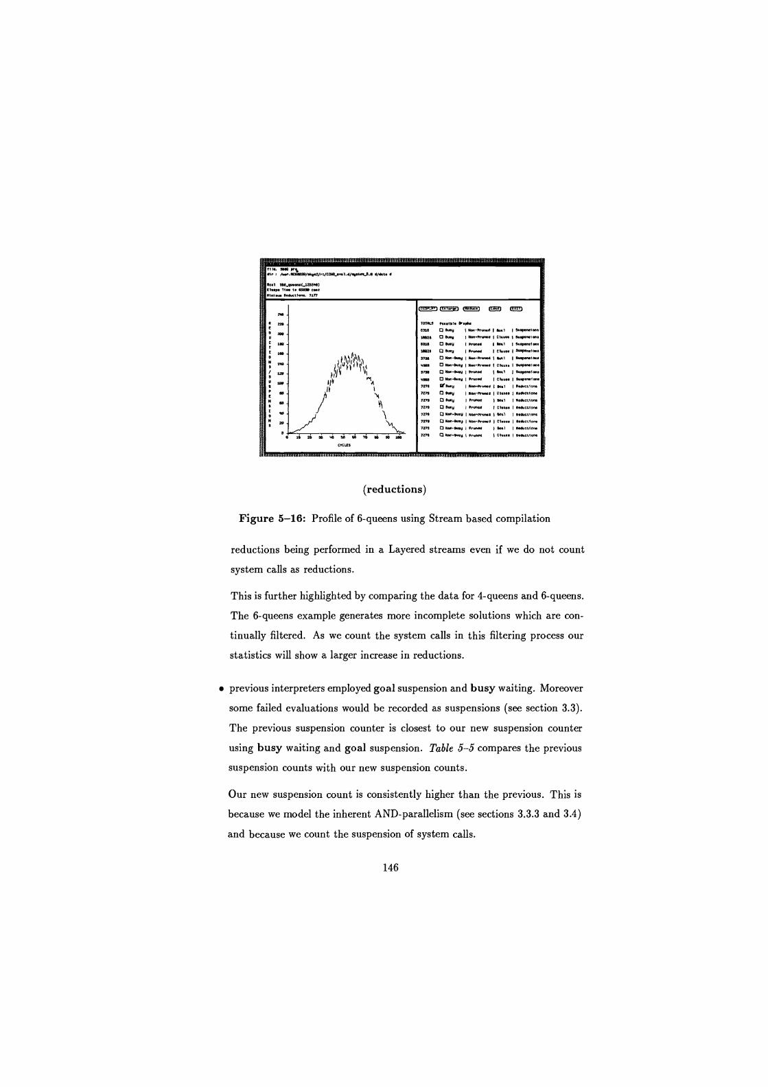
fill. 7N0 or% d1r i /u.nRCNe29/.My.2/rt/CCM0_-l.d/sUat"J.! d/date d

Goal 956_q ..ns(_125946) Rl..p. file i. NND cre M.- R.Aucttwa. 71fl

f01M9 P...lbl. er.ph. one Cl Duty I Non-frond 1 6o.1 I Bu.pamlon:

IM20 0 Bu.y I Non-Rrun.d 1 Cl- 19uµron.io .

one 0 Duly Prune Goal 19uq.n.l on.

1x20 O Bu.y orue 1 Cl... 19uspn.l ons

9790

4WD

9790

4000

7279

7279

7279

7279

7279

7279

7279

7249

0 Non-Bury I N--ft -l I to.1 19utp.nel on 0 Non-Duly Non-eruntd

Cl Non-S..y 19run.1

Mau.. 1 e..l

19up.-I 1 9ugn.lene

0 Nm-9u.0 Drun.d I Ci.u.. I eu.pen.l.n. GrDu.y I Non-erunRd I..l I R.ductlw.

0 Dory Non-p-d I Cwt. I R.duatom

Cl Duty Pruned Go.1 Reductta.

Cl Duly Pruned I C1.u.. R.ductiom

Cl N"-Wry I N.n-prun.d I %..1 NduN.n. 0 Non-Go.y I Non-Pruned I Clause Reduction.

O Non-Go.q orun" Go.1 I Reduction.

0 Non-bury P-ft I Cl.- R.ducNOns

(reductions)

Figure 5-16: Profile of 6-queens using Stream based compilation

reductions being performed in a Layered streams even if we do not count

system calls as reductions.

This is further highlighted by comparing the data for 4-queens and 6-queens.

The 6-queens example generates more incomplete solutions which are con-

tinually filtered. As we count the system calls in this filtering process our

statistics will show a larger increase in reductions.

previous interpreters employed goal suspension and busy waiting. Moreover

some failed evaluations would be recorded as suspensions (see section 3.3).

The previous suspension counter is closest to our new suspension counter

using busy waiting and goal suspension. Table 5-5 compares the previous

suspension counts with our new suspension counts.

Our new suspension count is consistently higher than the previous. This is

because we model the inherent AND-parallelism (see sections 3.3.3 and 3.4)

and because we count the suspension of system calls.

146

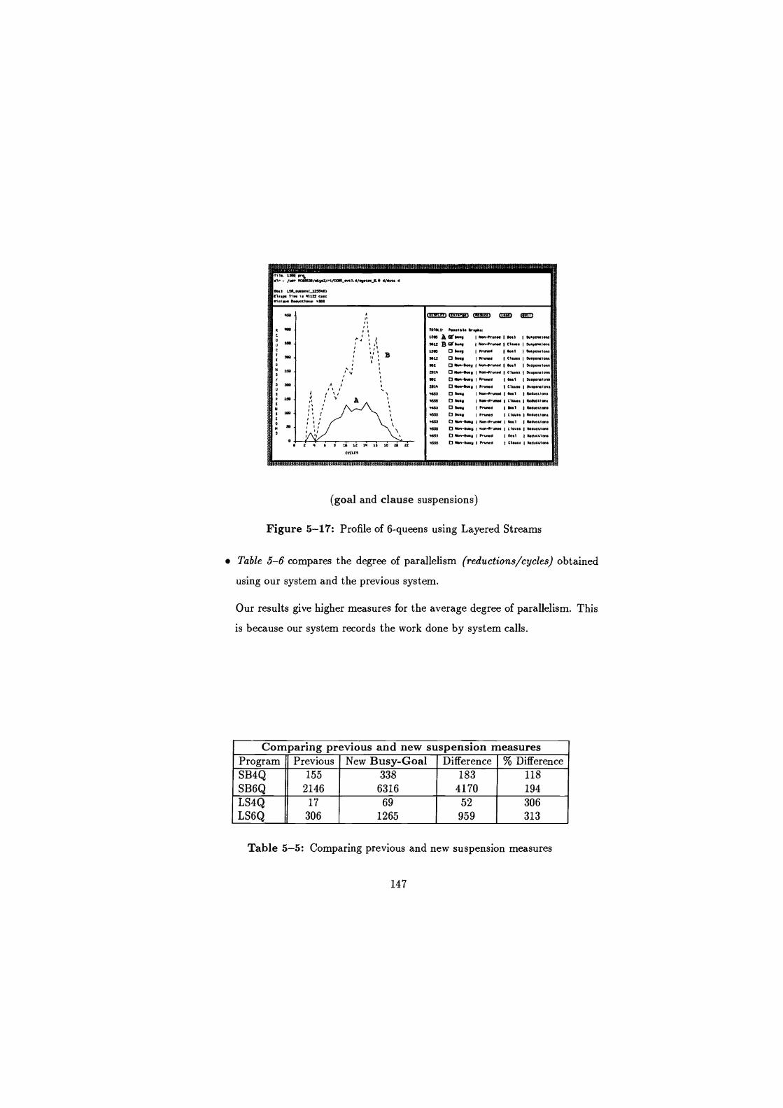
fi1.. L7ep PPrry

dir i /un NCdjelb/Mcy2/rt/CCW0-M1 d/y.u b S d/d.q d

PS.HSI. erph. I Non-Frond I earl I supcnsiom

I Non-' .'" I Clan I L.pwnion I P-d e..1 1 9aP.n.i.n. Prunnd I Cia.. 19u.pen.ian.

o Men-MNy 1 Nan-Pr.n.d 1 e..1 1 easp.n.i... o ftq.-Mny I Nom/run" I Cl... I eup.mion o Nan-S." Pruned

o NM-wy V-d

O Men-e.-u I Pruned I e.1 N.ddctian o Non-wy Pruned CI.... Neu.ti-.

O ..n-wy 1 N,n-prom. I c..... I Nda.ca.n. Il.w-wy 1 Non-Prdmd I M.1 I Nadwtians

o Sdey V-d I m.i 1 N.duott M. O wy I Pruned

I Cl".. 1 Mducttan

O Sdey Non-PrunN I eo.1 1 Mducttms

O wy N0.4, 0.0 I Cl- I baacti.n

(goal and clause suspensions)

Figure 5-17: Profile of 6-queens using Layered Streams

Table 5-6 compares the degree of parallelism (reductions/cycles) obtained

using our system and the previous system.

Our results give higher measures for the average degree of parallelism. This

is because our system records the work done by system calls.

Com paring previous and new suspension measures Program Previous New Busy-Goal Difference % Difference SB4Q SB6Q

155

2146

338 6316

183

4170 118

194

LS4Q LS6Q

17

306 69

1265

52

959 306

313

Table 5-5: Comparing previous and new suspension measures

147

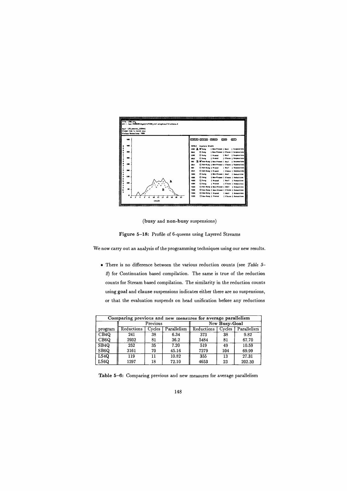
f91.: LSaq p0.%

011 /w1 520007/.k0.2/1t/C0.0_.gI 0/.0.0.0} 504.4 d

"0 E

S

N

0..1' La9_g0em(_32106) E1.0 0 1/N 1. 43122 ... Mnf... 0duotfmm 4909

2 4

0 n i 1

1 r v 1

6 a 10 12 14 1s 0 00CIE0

20 22

00104.5 P-..101. Y.PM 1x93 A fire-0 I N-0-9010.0 19o&1 I Ou.p.n.10n.

5922 0 W.0 Non-P-d 0100.. I Su000n.i-n.

1290 0 W.0 Paned I No.1 Su.p.n.fon.

5022 0 W.0 I P1vod I Cl- Su.p.n.Io0n

902 B fY N0n-300X N-n-P,0.d I So.1 I So.p.n./-n. 2054 0 000-00.0 i 000-0110.0 C1... I 3u.P.W.n. 902 0 000-00.0 I PrSn.d 110.1 susp.n.lon.

290 0 N-0.45.0 P.un.0 I Cl... SuIp.n./-n. 4NS] 0 10.0 I "_P0u0.d 14031 4.05.0005.

4696 0 Wry I X05-000.040 10100.. 14.0001100.

4X5] Q 41.0 101um0 100.1 *.d..100- 4S9 0 41.0 1000000 I Cl.u.. I R.d.tf0M 40.59 0 Non-41.0 I 005-0000.0 1 401 I Nodot.l.0. 450 0 Non-0u.0 1005-0000.0 I C10050 RMU..100

45.55 0 000-05330 Pruned 4041 0000000050

4333 0 Non-00.0 I P0-0 I C1.u.. I R.d..f0M

(busy and non-busy suspensions)


We now carry out an analysis of the programming techniques using our new results.

There is no difference between the various reduction counts (see Table 5-

2) for Continuation based compilation. The same is true of the reduction

counts for Stream based compilation. The similarity in the reduction counts

using goal and clause suspensions indicates either there are no suspensions,

or that the evaluation suspends on head unification before any reductions

Comparing previous and new measures for average parallelism Previous New Busy-Goal

program Reductions Cycles Parallelism Reductions Cycles Parallelism CB4Q CB6Q

241 2932

38 81

6.34 36.2

373 5484

38 81

9.82 67.70

SB4Q SB6Q

252

3161 35 70

7.20 45.16

519 7279

49 104

10.59 69.99

LS4Q LS6Q

119

1297 11

18

10.82 72.10

355 4653

13

23 27.31 202.30

Table 5-6: Comparing previous and new measures for average parallelism

148

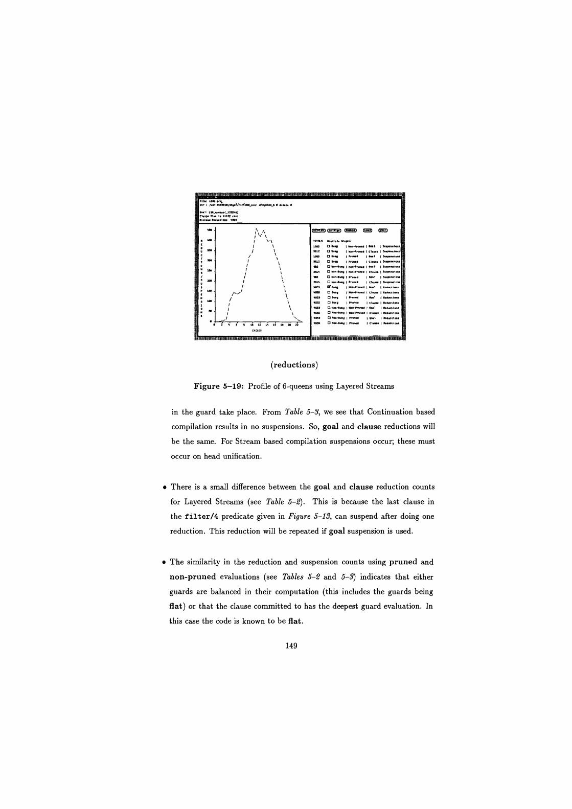
TOTALS

i1bs

3812

IM BMi

CM

M. 991

2M.

Ms

4859

45555

4699

4555

4699

4ss5

(reductions)

Pasiel. erspu:

O eu.u N.nirNKe I MI t wspealon. O w.u I Na-Pruae I C1s-. I wP.ai... O e V PruaB I ea1 I w.P...... O wry I Prune C1.-. wsMat.n. O Non-Bury I Na-rrvroe I eat I w.P...ion. o Men-e-u Nen-Prodid Cows I wtpenclan.

O No.-e-u I Prune I eal w.P.ai.n. O N.n-bw% I Prune I tl.w. Suq+n ion. teusu I Na-Prune I .al I ntsuettan.

O euse Nao-hun.B y C1... I Mauctias

I

O w.u Prune I eat Mlu.tion. O Busy I Pruned I Cl.-e I etdPCtias

Na-B-N N n-Prune Bal I Pesuctimt

O ft.-B-N I Man-Prima! I C1... A.N t/mr O Nonlu.u I wuae eat Nsauctla. O No-eue Prune C1.-. I Meuatia.


in the guard take place. From Table 5-3, we see that Continuation based

compilation results in no suspensions. So, goal and clause reductions will

be the same. For Stream based compilation suspensions occur; these must

occur on head unification.

There is a small difference between the goal and clause reduction counts

for Layered Streams (see Table 5-2). This is because the last clause in

the filter/4 predicate given in Figure 5-13, can suspend after doing one

reduction. This reduction will be repeated if goal suspension is used.

The similarity in the reduction and suspension counts using pruned and

non-pruned evaluations (see Tables 5-2 and 5-3) indicates that either

guards are balanced in their computation (this includes the guards being

flat) or that the clause committed to has the deepest guard evaluation. In

this case the code is known to be flat.

149

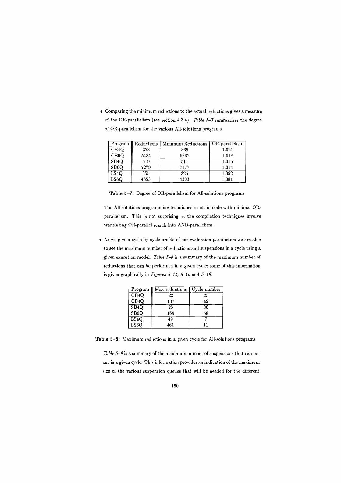
Comparing the minimum reductions to the actual reductions gives a measure

of the OR-parallelism (see section 4.3.4). Table 5-7 summarises the degree

of OR-parallelism for the various All-solutions programs.

Program Reductions Minimum Reductions OR-parallelism CB4Q 373 365 1.021

CB6Q 5484 5382 1.018 SB4Q 519 511 1.015 SB6Q 7279 7177 1.014 LS4Q 355 325 1.092 LS6Q 4653 4303 1.081

Table 5-7: Degree of OR-parallelism for All-solutions programs

The All-solutions programming techniques result in code with minimal OR-

parallelism. This is not surprising as the compilation techniques involve

translating OR-parallel search into AND-parallelism.

As we give a cycle by cycle profile of our evaluation parameters we are able

to see the maximum number of reductions and suspensions in a cycle using a

given execution model. Table 5-8 is a summary of the maximum number of

reductions that can be performed in a given cycle; some of this information

is given graphically in Figures 5-14, 5-16 and 5-19.

Program Max reductions Cycle number CB4Q 22 25

CB4Q 187 49

SB4Q 25 30

SB6Q 164 58

LS4Q 49 7

LS6Q 461 11

Table 5-8: Maximum reductions in a given cycle for All-solutions programs

Table 5-9 is a summary of the maximum number of suspensions that can oc-

cur in a given cycle. This information provides an indication of the maximum

size of the various suspension queues that will be needed for the different

150

suspension mechanisms and scheduling policies, given by the busy waiting

suspension parameters. It also indicates the maximum number of suspen-

sions that will occur in a cycle, given by the non-busy waiting suspension

parameters.

Maximum number of suspensions in a given cycle Busy Waiting Non-Bus y Waiting

Goal Clause Goal Clause Program Max Cycle Max Cycle Max Cycle Max Cycle SB4Q SB6Q

23 180

31 59

34 258

31

59

13

120

31

61

16

166

28 55

LS4Q LS6Q 1

16

1 141

8

14

72

460

3

14 1

14

1 115

8

14

72 364

3

14

Table 5-9: Maximum suspensions in a given cycle for All-solutions Programs

The difference between suspensions using goal and clause suspension mech-

anisms highlights the number of clauses that each goal could be reduced by

in the dynamic program (see section 4.5.3.1). Table 5-10 is a summary of

the ratio of clause to goal suspensions for Stream based compilation and

Layered Streams, using busy and non-busy waiting.

Busy Waiting Non-Busy Waiting Program Goal Clause Ratio Goal Clause Ratio SB4Q SB6Q

338

6316 628

10028

1.875 1.587

175

3736

302

4868 1.725

1.302

LS4Q LS6Q

69

1265

266

3812 3.855 3.013

46

902

158

2614

3.434 2.898

Table 5-10: Goal/Clause suspension ratios for All-solutions programs

Consider the results for Stream based compilation and the program given

in Figure 5-12. Most of the predicates in the program have two clauses

which can suspend for each goal. However, the last predicate ' Qcheck' /4

will result in four clause suspensions for each goal if its first input is not

bound and four clause suspensions and five goal suspensions if its first input

is partially bound; the first element on the list is unbound. This is because

151

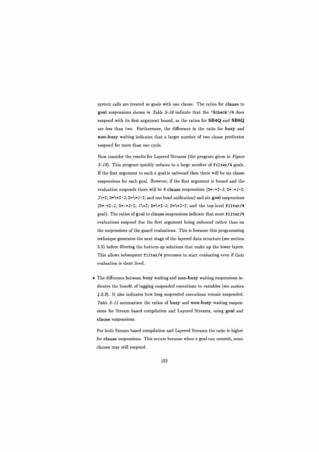
system calls are treated as goals with one clause. The ratios for clause to

goal suspensions shown in Table 5-10 indicate that the ' Qcheck' /4 does

suspend with its first argument bound, as the ratios for SB4Q and SB6Q

are less than two. Furthermore, the difference in the ratio for busy and

non-busy waiting indicates that a larger number of two clause predicates

suspend for more than one cycle.

Now consider the results for Layered Streams (the program given in Figure

5-13). This program quickly reduces to a large number of filter/4 goals.

If the first argument to such a goal is unbound then there will be six clause

suspensions for each goal. However, if the first argument is bound and the

evaluation suspends there will be 6 clause suspensions (D=:=I-J; D=:=.J-I;

J\=I; D=\=I-J; D=\=J-I; and one head unification) and six goal suspensions

(D=:=I-J; D=:=J-I; J\=I; D=\=I-J; D=\=J-I; and the top-level filter/4 goal). The ratios of goal to clause suspensions indicate that more filter/4 evaluations suspend due the first argument being unbound rather than on

the suspensions of the guard evaluations. This is because this programming

technique generates the next stage of the layered data structure (see section

5.5) before filtering the bottom-up solutions that make up the lower layers.

This allows subsequent filter/4 processes to start evaluating even if their

evaluation is short lived.

The difference between busy waiting and non-busy waiting suspensions in-

dicates the benefit of tagging suspended executions to variables (see section

4.2.2). It also indicates how long suspended executions remain suspended.

Table 5-11 summarises the ratios of busy and non-busy waiting suspen-

sions for Stream based compilation and Layered Streams, using goal and

clause suspensions.

For both Stream based compilation and Layered Streams the ratio is higher

for clause suspensions. This occurs because when a goal can commit, some

clauses may still suspend.

152

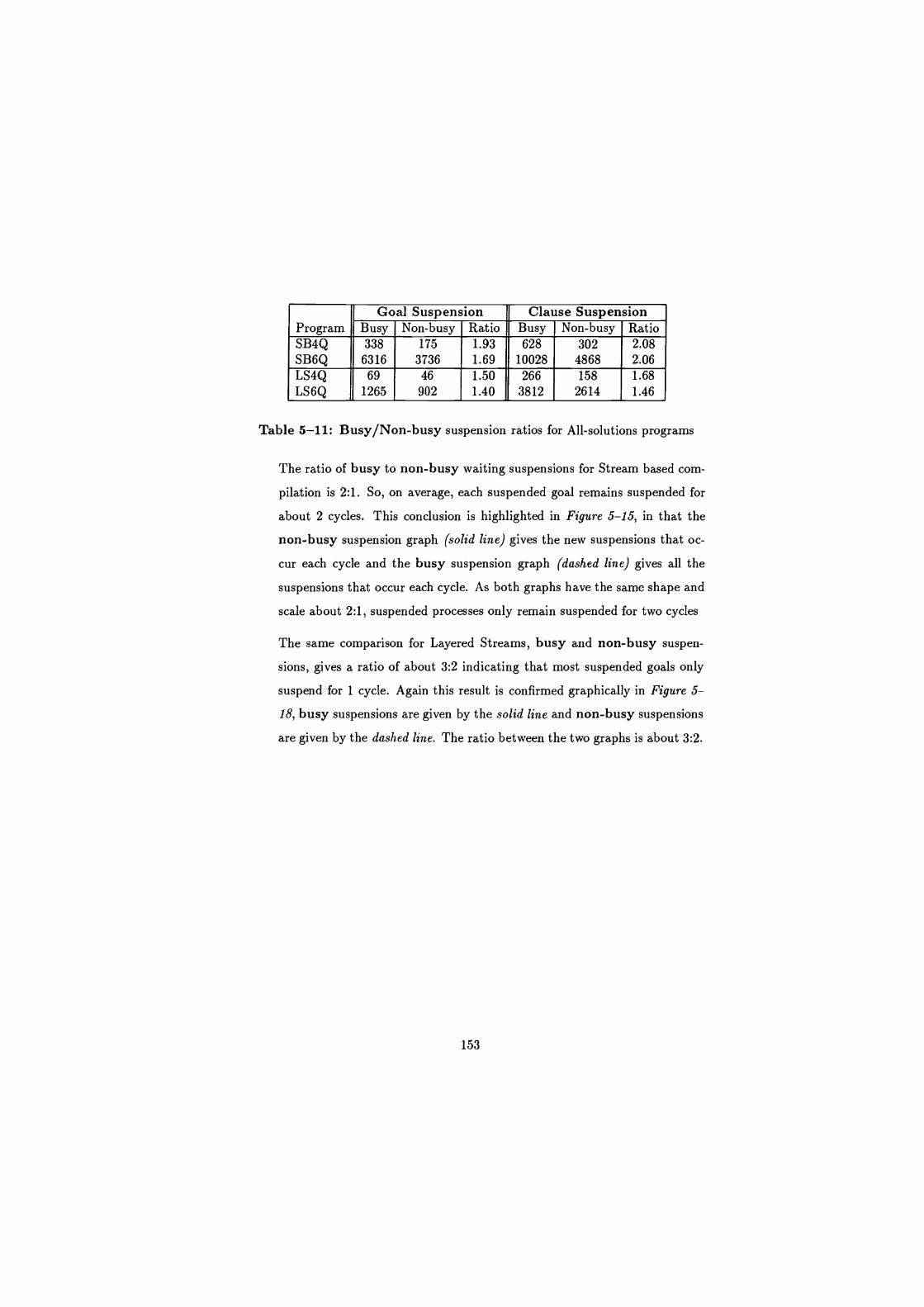
Goal Suspension Clause Suspension Program Busy Non-busy Ratio Busy Non-busy Ratio SB4Q SB6Q

338 6316

175

3736

1.93 1.69

628 10028

302 4868

2.08 2.06

LS4Q LS6Q

69

1265 46

902 1.50 1.40

266 1

3812 158

2614 1.68

1.46

Table 5-11: Busy/Non-busy suspension ratios for All-solutions programs

The ratio of busy to non-busy waiting suspensions for Stream based com-

pilation is 2:1. So, on average, each suspended goal remains suspended for

about 2 cycles. This conclusion is highlighted in Figure 5-15, in that the

non-busy suspension graph (solid line) gives the new suspensions that oc-

cur each cycle and the busy suspension graph (dashed line) gives all the

suspensions that occur each cycle. As both graphs have the same shape and

scale about 2:1, suspended processes only remain suspended for two cycles

The same comparison for Layered Streams, busy and non-busy suspen-

sions, gives a ratio of about 3:2 indicating that most suspended goals only

suspend for 1 cycle. Again this result is confirmed graphically in Figure 5-

18, busy suspensions are given by the solid line and non-busy suspensions

are given by the dashed line. The ratio between the two graphs is about 3:2.

153

5.8 Synopsis of analysis

In this section we consolidate some of the results given in our analysis.

The previous results for the All-solutions programming techniques indicate

that Layered Streams achieves the best results:

Cycles: Layered Streams requires about 1/4 of the cycles of Continuation

based compilation and about 1/3 the cycles of Stream based compila-

tion.

Reductions: Layered Streams requires half as many reductions as Contin-

uation based compilation or Stream based compilation.

Suspensions: Layered Streams incurs only about 1/8 of the suspensions

incurred by Stream based compilation. Continuation based compilation

incurs no suspensions.

Our new results give a slightly different picture:

Cycles: In terms of cycles, our new results are similar to the previous cy-

cle measures for Layered Streams and Continuation based compilation.

The cycles parameter indicates the duration of the computation, so if

all the parallelism could be exploited Layered Streams would indeed be

the best.

The results for Stream based compilation have increased. The increase

in cycles is due to our model of AND-parallelism, we assume only bind-

ings available at the start of a given cycle are available for each of the

goal evaluations and not those that are generated during the processing

of each goal. This causes some goals to suspend for additional cycles

and so increases the cycle count.

154

Viewed another way, the processing of goals in the previous interpreters

gave rise to goal data dependencies being satisfied as the goals were

processed. This reduced the measured depth of the evaluation tree.

Reductions: In terms of reductions, our new results are higher for each of

the All-solutions techniques. Although Layered Streams has a larger

increase in reductions than either of the other All-solutions program-

ming techniques we see that it is still the most parallel programming

technique (see Table 5-6). However, if the chosen architecture cannot

support all of the realisable parallelism then other factors like the over-

all amount of work become important considerations; that is the total

number of reductions. In which case Layered Streams and Continuation

based compilation would appear comparable.

Suspensions: In terms of suspensions, our new results are higher than

the previous suspension counts. This is because our model of AND-

parallelism does not allow goals to reduce on bindings generated in the

same cycle as their evaluation and because we count the suspension of

system calls as suspensions.

The suspension statistics for Layered Streams (see Table 5-11) indi-

cate that on average suspended evaluations suspend for about 1.5 cy-

cles. Given that there will be overheads in using non-busy suspensions

(tagging suspended computations) it may be the case that a busy sus-

pension mechanism is suitable for applications employing this search

technique.

None of these techniques make use of OR-parallelism (see Table 5-7). This is

not surprising as the compilation techniques involve translating OR-parallel

search into AND-parallelism.

155

5.9 Summary


How the CCND languages support various forms of non-deterministic search.

Several methods, automatic and manual, for addressing the limitations

of mapping generate and test non-determinism on to the CCND com-

putation model. The particular example program used was n-queens,

which has been evaluated using the previous evaluation system by

[Okumura & Matsumoto 87].

Our re-evaluation of the n-queens example for 4-queens and 6-queens, using

our basic Parlog interpreter, confirm the previous evaluation was carried out

on a similar system.

The results from the evaluation of the 4-queens and 6-queens on our new

evaluation system. The results differ in several respects to those obtained

on our basic Parlog interpreter. Our new analysis and results highlight how

our new evaluation gives a better picture of the program behaviour and

the relative merits of the various programming techniques. In particular, it

shows that Layered Streams is not as good as was previously supposed.

A consolidation of the results obtained using our system.

156

Chapter 6

Shared data structures - safe/unsafe

6.1 Overview

Support for shared data areas appears to be an important consideration for AI pro-

gramming. Several current AI applications/programming paradigms use a shared

area to allow independent experts/problem solvers to cooperate in the solving of

a problem, e.g. blackboard type problem solvers [Hayes-Roth 85] [Hayes-Roth 88]

[Corkill et al 88] and chart parsers [Earley 70], [Kay 73]. These systems could be

parallelised by having the problem solvers working in parallel.

It has been noted by several researchers [Shapiro 87c] that only CP derivatives,

like Flat Concurrent Prolog (FCP) [Mierowsky et al 85] can directly support sev-

eral processes with write access to shared data structures. By directly we mean

that the language provides the relevant synchronisation primitives to allow mul-

tiple writers. Such languages are known as unsafe (see section 2.5.1). Parlog

and GHC cannot directly support such shared data structures, they are known

as safe (see section 2.5.1). Shared data areas can be indirectly supported in safe

languages by a manager process which maintains the shared data structure, the

writer processes send update requests to this manager. The two particular appli-

157

cations/programming paradigms mentioned above have been reconstructed (par-

allelised) for Parlog (a safe language) in [Davison 87] and [Trehan & Wilk 88].

This chapter considers how multiple writers to shared data structures and

streams can be supported in the CCND languages. Initially two types of CCND

language are considered, safe and unsafe. We then consider a third language

in which streams and multiple writers are supported by system primitives. The

three language types, unsafe, safe and safe+system streams are examined by

considering how they support a shared binary tree with multiple writers. We go

on to consider how an Artificial Intelligence application which requires a shared

data structure, a chart parser, maps onto the various languages. Three resulting

chart parsers are described and then evaluated.

Section 6.2 considers how shared data structures are supported by the various

features of the CCND languages.

In section 6.3 we consider how shared data structures can be supported in the

three styles of language, unsafe, safe and safe+system streams.

Section 6.4 provides an overview of chart parsing.

Section 6.5 describes the chart parsers developed for comparing the three styles

of language.

In section 6.6 we evaluate the execution of these chart parsers.


158

6.2 Shared Data

The CCND languages provide an elegant means of inter-process communication.

Communication is achieved though a variable which is shared between the pro-

cesses that wish to communicate. If one process binds the variable another process

can consume the binding. These languages easily support one-to-many commu-

nication. That is one process binds a shared variable, which is shared by several

other consumer processes each of which consumes the binding. By incrementally

binding a shared variable, that is binding it to a structure containing a message

and a new variable, processes can use shared variables as communication streams.

The most common data structure used for this stream communication is a list,

the tail of which is incrementally bound to a message and a new variable.

It has been noted by several researchers [Shapiro 87c] that only CP deriva-

tives, like Flat Concurrent Prolog (FCP) [Mierowsky et al 85] can directly sup-

port many-to-one communication on a single variable. By directly we mean that

the language provides the relevant synchronisation primitives to allow multiple

writers. In the CP family of languages this is supported by allowing process eval-

uations to make bindings to variables within a local environment, the guard. On

commitment the system tries to unify the local bindings with the binding envi-

ronment of the parent process. This requires the commitment stage to be atomic

[Saraswat 87b], that is all bindings that would result by unifying local and parent

environments should be made in one step or not at all. Such languages are known

as unsafe, as the local bindings that are made are speculative until commitment

has taken place.

Parlog and GHC do not allow bindings of global variables to be made in the

guard. They are known as safe languages, so they avoid the problems associated

159

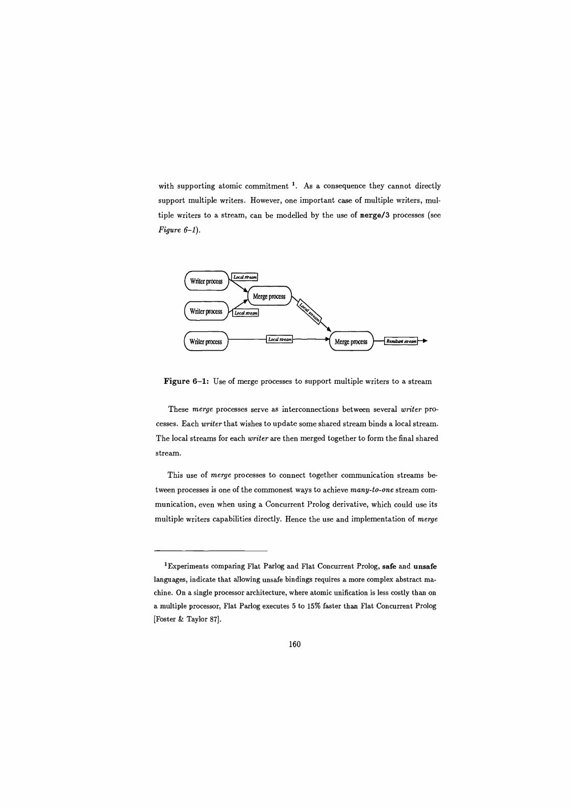
with supporting atomic commitment 1. As a consequence they cannot directly

support multiple writers. However, one important case of multiple writers, mul-

tiple writers to a stream, can be modelled by the use of merge/3 processes (see

Figure 6-1).

Figure 6-1: Use of merge processes to support multiple writers to a stream

These merge processes serve as interconnections between several writer pro-

cesses. Each writer that wishes to update some shared stream binds a local stream.

The local streams for each writer are then merged together to form the final shared

stream.

This use of merge processes to connect together communication streams be-

tween processes is one of the commonest ways to achieve many-to-one stream com-

munication, even when using a Concurrent Prolog derivative, which could use its

multiple writers capabilities directly. Hence the use and implementation of merge

'Experiments comparing Flat Parlog and Flat Concurrent Prolog, safe and unsafe

languages, indicate that allowing unsafe bindings requires a more complex abstract ma-

chine. On a single processor architecture, where atomic unification is less costly than on

a multiple processor, Flat Parlog executes 5 to 15% faster than Flat Concurrent Prolog

[Foster & Taylor 87].

160

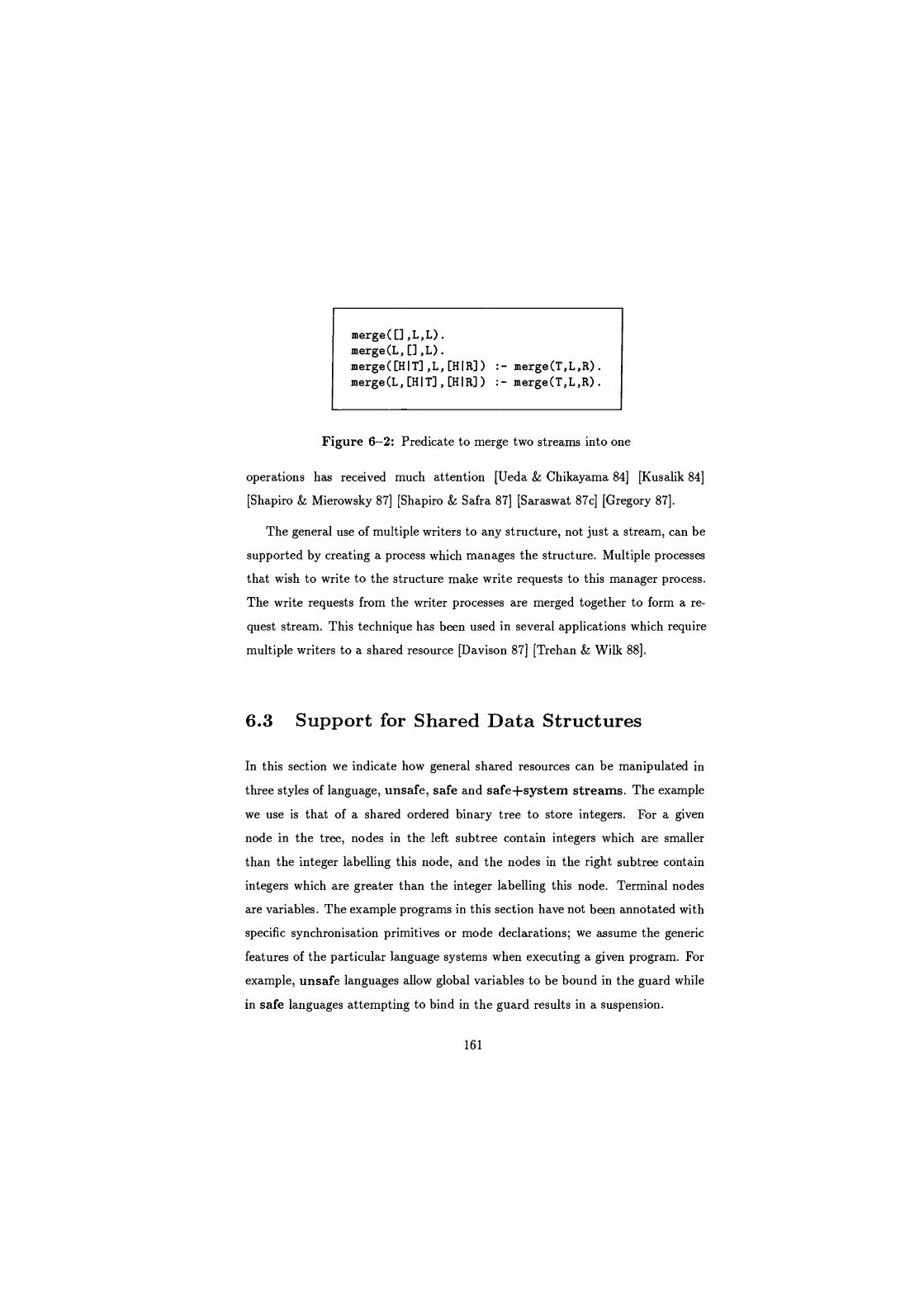
merge([],L,L).

merge (L,[],L). merge([HIT],L, [HIR]) :- merge(T,L,R). merge(L, [HIT] , [HIR]) :- merge(T,L,R).

Figure 6-2: Predicate to merge two streams into one

operations has received much attention [Ueda & Chikayama 84] [Kusalik 84]

[Shapiro & Mierowsky 87] [Shapiro & Safra 87] [Saraswat 87c] [Gregory 87].

The general use of multiple writers to any structure, not just a stream, can be

supported by creating a process which manages the structure. Multiple processes

that wish to write to the structure make write requests to this manager process.

The write requests from the writer processes are merged together to form a re-

quest stream. This technique has been used in several applications which require

multiple writers to a shared resource [Davison 87] [Trehan & Wilk 88].

6.3 Support for Shared Data Structures

In this section we indicate how general shared resources can be manipulated in

three styles of language, unsafe, safe and safe+system streams. The example

we use is that of a shared ordered binary tree to store integers. For a given

node in the tree, nodes in the left subtree contain integers which are smaller

than the integer labelling this node, and the nodes in the right subtree contain

integers which are greater than the integer labelling this node. Terminal nodes

are variables. The example programs in this section have not been annotated with

specific synchronisation primitives or mode declarations; we assume the generic

features of the particular language systems when executing a given program. For

example, unsafe languages allow global variables to be bound in the guard while

in safe languages attempting to bind in the guard results in a suspension.

161

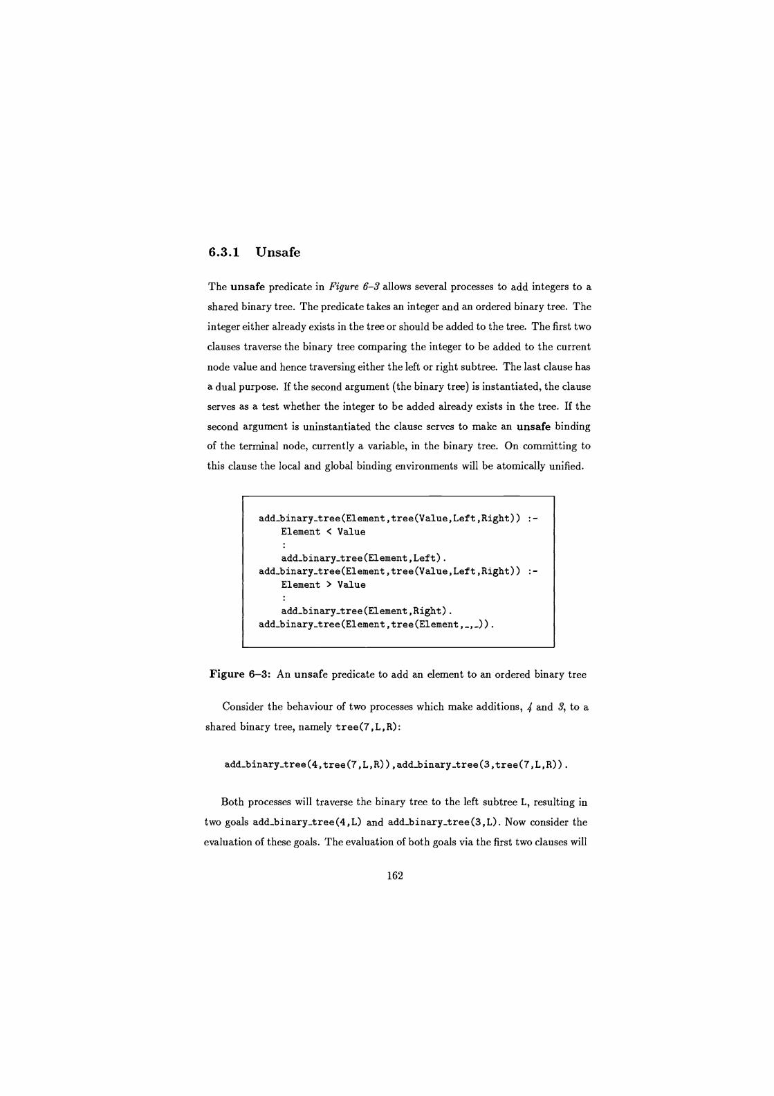
6.3.1 Unsafe

The unsafe predicate in Figure 6-3 allows several processes to add integers to a

shared binary tree. The predicate takes an integer and an ordered binary tree. The

integer either already exists in the tree or should be added to the tree. The first two

clauses traverse the binary tree comparing the integer to be added to the current

node value and hence traversing either the left or right subtree. The last clause has

a dual purpose. If the second argument (the binary tree) is instantiated, the clause

serves as a test whether the integer to be added already exists in the tree. If the

second argument is uninstantiated the clause serves to make an unsafe binding

of the terminal node, currently a variable, in the binary tree. On committing to

this clause the local and global binding environments will be atomically unified.

add-binary-tree (Element, tree (Value, Left, Right))

Element < Value

add_binary_tree (Element ,Left). add_binary_tree(Element,tree (Value, Left, Right)) :-

Element > Value

add-binary-tree (Element, Right) .

add-binary-tree (Element, tree (Element,_,_)).

Figure 6-3: An unsafe predicate to add an element to an ordered binary tree

Consider the behaviour of two processes which make additions, 4 and 3, to a

shared binary tree, namely tree(7,L,R):

add_binary_tree(4,tree(7,L,R)),add_binary_tree(3,tree(7,L,R)).

Both processes will traverse the binary tree to the left subtree L, resulting in

two goals add_binary_tree(4,L) and add_binary_tree(3,L). Now consider the

evaluation of these goals. The evaluation of both goals via the first two clauses will

162

suspend, as the guard evaluations Value > 3, Value < 3, Value > 4 and Value

< 4 suspend. Both will hence make speculative bindings of the parent variable

L via the last clause; the first binding L to tree(4,_,_); the second binding L

to tree (3, _, _) . The system will then on commitment try to make both local

bindings global. However, using atomic commitment one of the processes will

succeed and the other will fail. Say the second process succeeds, hence L will be

bound to tree (3, _, _) . Now the two suspended clauses for the first process can

be rescheduled for evaluation as Value is now bound to 3. This will result in the

evaluation committing to the second clause, as 4 > 3. Finally, this process will

bind the right subtree of the newly created node to tree (4,-,-). So, the final

state of the shared binary tree is:

tree (7,tree(3,_,tree(4,_,_)),_)

6.3.2 Safe

In a safe language the binary tree addition predicate in Figure 6-3 would suspend.

Safe languages do not permit the binding of global variables in the guard. In the

case where the last clause is used to add an element to a binary tree, rather than

test to see if an element already exists, the evaluation of the third clause would

suspend awaiting the second argument to be bound. The programmer could, of

course, transfer the output binding of the global variable to the body of the clause.

However, if the binding is transferred to the body, two processes could try to bind

the same variable to different terms. In this case one of the processes would fail.

The manipulation of a global data structure, like a global binary tree, by several

writer processes would have to be supported by a manager process, (perpetual

process [Shapiro & Takeuchi 83)). This manager is the only process which can

write to the shared data structure, hence resolving the problem of binding conflicts

that occurs with several processes writing to a shared resource. The processes that

163

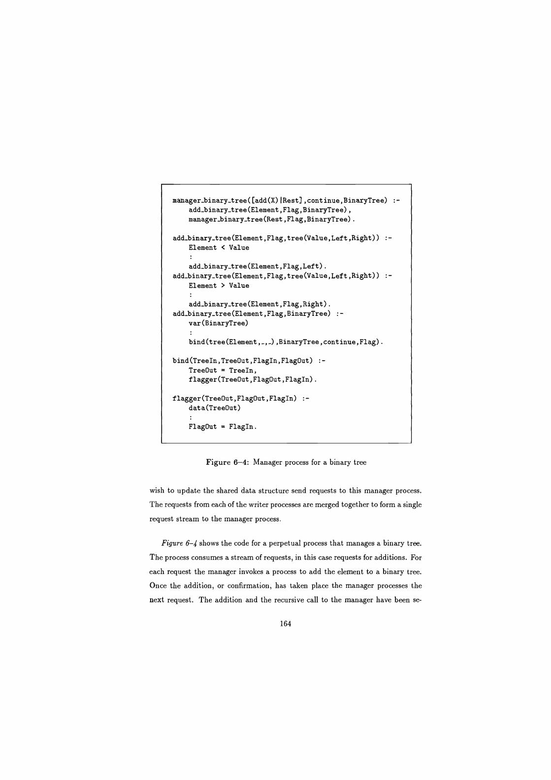
manager-binary-tree ([add(X)I Rest], continue,BinaryTree) :- add_binary_tree(Element,Flag, BinaryTree), manager-binary-tree (Rest,Flag,BinaryTree).

add_binary_tree(Element, Flag, tree (Value,Left, Right)) Element < Value

add_binary_tree(Element,Flag, Left).

:-

add_binary_tree(Element, Flag, tree (Value,Left, Right)) :-

Element > Value

add_binary_tree(Element,Flag, Right). add_binary_tree(Element,Flag, BinaryTree) :-

var(BinaryTree)

bind (tree (Element,_,_),BinaryTree, continue, Flag).

bind(TreeIn,TreeOut,FlagIn,FlagOut) :- TreeOut = Treeln, f lagger(TreeOut,FlagOut,FlagIn).

f lagger(TreeOut,FlagOut,FlagIn) :- data(TreeOut)

FlagOut = FlagIn.

Figure 6-4: Manager process for a binary tree

wish to update the shared data structure send requests to this manager process.

The requests from each of the writer processes are merged together to form a single

request stream to the manager process.

Figure 6-i$ shows the code for a perpetual process that manages a binary tree.

The process consumes a stream of requests, in this case requests for additions. For

each request the manager invokes a process to add the element to a binary tree.

Once the addition, or confirmation, has taken place the manager processes the

next request. The addition and the recursive call to the manager have been se-

164

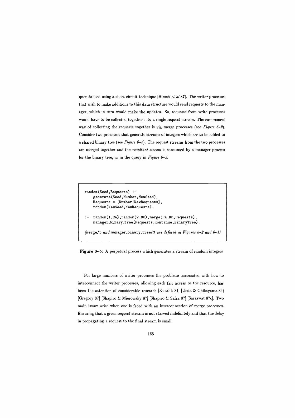
quentialised using a short circuit technique [Hirsch et al 87]. The writer processes

that wish to make additions to this data structure would send requests to the man-

ager, which in turn would make the updates. So, requests from write processes

would have to be collected together into a single request stream. The commonest

way of collecting the requests together is via merge processes (see Figure 6-2).

Consider two processes that generate streams of integers which are to be added to

a shared binary tree (see Figure 6-5). The request streams from the two processes

are merged together and the resultant stream is consumed by a manager process

for the binary tree, as in the query in Figure 6-5.

random(Seed,Requests) :- generate(Seed, Number,NewSeed), Requests = [NumberINewRequests], random(NewSeed,NewRequests).

random(1,Ra),random(2,Rb),merge(Ra,Rb,Requests), manager-binary-tree (Requests, continue, BinaryTree).

(merge/3 and manager-binary-tree/3 are defined in Figures 6-2 and 6-4)

Figure 6-5: A perpetual process which generates a stream of random integers

For large numbers of writer processes the problems associated with how to

interconnect the writer processes, allowing each fair access to the resource, has

been the attention of considerable research [Kusalik 84] [Ueda & Chikayama 84]

[Gregory 87] [Shapiro & Mierowsky 87] [Shapiro & Safra 87] [Saraswat 87c]. Two

main issues arise when one is faced with an interconnection of merge processes.

Ensuring that a given request stream is not starved indefinitely and that the delay

in propagating a request to the final stream is small.

165

6.3.3 Safe+System Streams

In the safe languages merge processes are the commonest way to support many-

to-one communication. Moreover the general manipulation of a shared data struc-

tures by multiple writers can be supported by using merge processes to combine

streams of write requests and manager processes to maintain the shared data struc-

ture. The general feature of both these uses of streams is to combine requests from

many sources to one final stream, the resultant stream.

Consider another view of this resultant stream, that is a list with a tail vari-

able to be instantiated. This view of the resultant stream was employed in

[Saraswat 87c] to mimic merging several streams together in constant time. Basi-

cally, processes that wish to write to the resultant stream could use the multiple

writers capabilities of unsafe languages. Each writer would have a copy of the

stream, additions to the stream taking place by a writer recursing down the stream

until it finds the tail variable which is then instantiated to a list containing the

required message and a new tail variable. For efficiency the writer could keep a

copy of the new tail variable for future additions. This technique would require n

process reductions, where n is the number of new elements that have been added

to the stream since the last addition. However, this approach is not applicable to

safe languages, as they do not support multiple writers.

The use of streams generally requires the use of merge processes to combine

these streams. While the use of merge processes is logically clear with respect to

the CCND computation model they may add heavy overheads in terms of creating

and managing large numbers of processes. This may degrade system performance.

An alternative option is for the system to support the use of streams more

directly [Itoh et al 87]. [Itoh et al 87] propose several stream manipulation prim-

itives for GHC, for creating a system supported stream, adding an element to a

stream, removing an element from a stream and merging streams. The most inter-

esting of these primitives is the merge operation. The merge primitive introduces

an indirect stream pointer cell which is shared by every producer and points to the

166

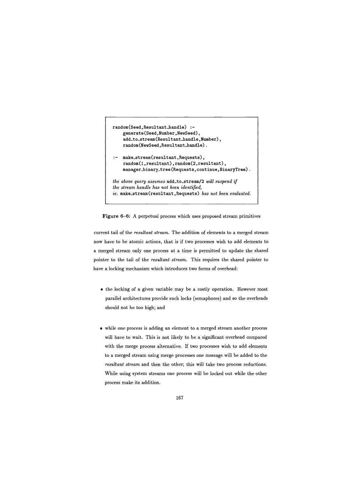
random(Seed,Resultant_handle) :-

generate(Seed,Number,NewSeed), add_to_stream(Result ant-handle, Number), random(NewSeed,Resultant_handle).

make-stream (resultant, Requests), random(1,resultant),random(2,resultant),

manager-binary-tree (Requests, continue, BinaryTree)

the above query assumes add-to-stream/2 will suspend if the stream handle has not been identified, ie. make-stream (resultant,Requests) has not been evaluated.

Figure 6-6: A perpetual process which uses proposed stream primitives

current tail of the resultant stream. The addition of elements to a merged stream

now have to be atomic actions, that is if two processes wish to add elements to

a merged stream only one process at a time is permitted to update the shared

pointer to the tail of the resultant stream. This requires the shared pointer to

have a locking mechanism which introduces two forms of overhead:

the locking of a given variable may be a costly operation. However most

parallel architectures provide such locks (semaphores) and so the overheads

should not be too high; and

while one process is adding an element to a merged stream another process

will have to wait. This is not likely to be a significant overhead compared

with the merge process alternative. If two processes wish to add elements

to a merged stream using merge processes one message will be added to the

resultant stream and then the other; this will take two process reductions.

While using system streams one process will be locked out while the other

process make its addition.

167

The results of [Itoh et al 87] show a significant improvement when using their

proposed primitives. This clearly indicates that the cost of manipulating streams

in the system is less than when under programmer control.

We consider similar extensions to our system, the basis for these extensions

being that the system could provide special primitives for multiple writers to a

resultant stream. The extended language we identify as safe+system streams.

This requires the system to know when a given stream, or variable, is a resultant

stream. The system can then keep track of the end of this stream via a pointer

to the tail variable. Additions to this stream would be supported by the system

which would automatically update the pointer. The additions to this resultant

stream would have to be atomic actions. The consumption of a resultant stream

by any process would proceed as normal, as it is still a stream.

Two primitives are introduced to support our notion of a resultant stream. The

first make_stream (STREAM_ID,STREAM) identifies a stream as a resultant stream.

The second add_to_stream(STREAM_ID,Element) directly adds an element to this

resultant stream. An additional primitive to close a resultant stream could also

be provided. Using these primitives the example predicate in Figure 6-5, is trans-

formed into Figure 6-6. A point to note is that the clarity of the program with

respects to the CCND computation model has been somewhat lost. This is because

the use of system streams means that streams are addressed by some global name

rather than as a local logical variable so predicates are not declarative. Future sys-

tems may be able to recognise the use of streams in predicates and automatically

support their use by system streams.

Our analysis of programs which use system streams compared with the two

other language types, unsafe and safe, indicates that while programs may be less

declarative if system streams are used the advantages in performance and sys-

tem predictability make this language extension an important addition for future

systems (see section 6.7).

168

6.4 Chart Parsing: an overview

In this section we present an overview of an Artificial Intelligence programming

technique known as chart parsing [Earley 70] [Kay 73]. The basis of chart pars-

ing is that duplicate attempts at parses of sub-phrases of a sentence, should be

prevented. Redundant parses occur because natural language is often ambiguous

(at least locally) and hence alternative parsing options must be frequently tried.

These alternative options may have common parts and it is wasteful to duplicate

these sub-parses. We now consider a sequential chart parsing algorithm and a

parallel extension.

6.4.1 Sequential chart parsing

Sequential chart parsing is achieved by keeping a record of all parses undertaken

in an Active Edge Table (AET), and a record of all sub-strings found, in the

Well Formed Sub-string Table (WFST). The AET and the WFST form the chart.

Ongoing parses are referred to as active edges and complete sub-strings are referred

to as inactive edges:

An example of the contents of an active edge is:

- searching for a Noun Phrase (NP);

- using the grammar rule a NP is a Determiner (Det), Noun (N);

- so far a Det has been found;

- the initial words being parsed are: "the man saw the woman";

- the remaining words to be parsed are: "man saw the woman".

An example of the contents of an inactive edge is:

- searching for a Noun Phrase (NP);

169

- using the grammar rule NP is a Det,N;

- we have found the Det and the N;

- the initial words being parsed are: "the man saw the woman";

- the remaining words to be parsed are: "saw the woman".

The AET is used by the parser to ensure that no repeat parsing attempts are

undertaken. The WFST is used by the parser to share the results of successful sub-

parses. The data structure used to represent the chart may be anything that allows

the parser to refer to it and update it, e.g. a database or partially instantiated

list.

The parser picks an active edge from the AET. The parser may further the

evaluation of the active edge using information in the WFST. Active edges and

inactive edges are combined under the fundamental rule [Thompson & Ritchie 84].

The resulting edges may be active (which will be added to the AET) or inactive

(which will be added to the WFST). Possible new active edges are also generated

using the grammar and an activation strategy. A bottom-up strategy constructs

possible new active edges based on the WFST (inactive edges). A top-down strat-

egy constructs possible new active edges based on the AET (active edges). Active

edges that are new are added to the AET. New active edges are those that do

not already exist in the AET. A description of sequential chart parsing, and an

implementation, can be found in [Thompson & Ritchie 84].

6.4.2 Parallel chart parser

There are many ways of adding parallel extensions to sequential chart parsers. The

parallelism occurs at a number of conceptual levels within a chart parser. Here, we

consider several processes which pick different active edges from the AET, process

them in parallel, and update the chart by adding any new active edges to the AET

and any sub-strings to the WFST. This approach requires that testing for a new

active edge and its addition to the AET be an atomic step. Without an atomic

170

step another process might add the proposed edge after the test and before the

update. Usually, this type of extension is supported by an atomic test and set

operation in the programming language. This approach is similar to that taken in

several chart parsers, for example [Grishman & Chitrao 88].

6.5 Parallel Chart Parsers for the CCND lan-

guages

In this section we focus on how the AET table of a parallel chart parser could be

implemented in the various languages.

6.5.1 Unsafe Chart Parser

In an unsafe language the shared data structure, the chart, can be directly sup-

ported. Given some possible new active edges the parser compares these proposed

new edges against the AET. Those edges that do not exist on the AET are added

to the AET. The predicate in Figure 6-7 supports an AET which is a stream. The

edges to be added are compared against each of the edges in the AET. If the head

of the AET and the edge to be added are the same the addition process succeeds

(not adding the edge to the AET). If the head of the AET and the edge to be

added are different the process recurses on the rest (tail) of the AET. If the AET

is a variable then this variable (tail) is bound, in the guard, to the new edge and

a new tail variable.

If the activation strategy is top-down, the process generating the possible new

active edges will consume the AET. For each active edge in the AET, the process

will examine the grammar to see if there are any grammar rules which can be

applied to further the evaluation of this edge. For each grammar rule a new

possible active edge is generated. Those active edges that are new are added to

171

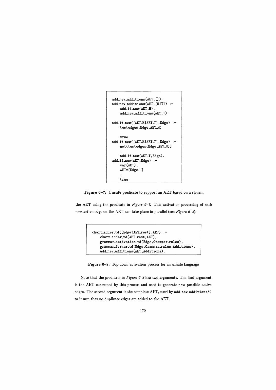
add_new_additions(AET,[]). add-new_additions (AET,[HIT]) :-

add_if-new (AET,H) , add-new_additions (AET,T).

add_if_new ( [AET. H I AET_T] , Edge) : - testedges(Edge,AETJi)

true. :- add-if -new ([AET.HIAET_T],Edge)

not(testedges(Edge,AET-i))

add-if -new (AET-T, Edge) add-if -new (AET, Edge) : -

var(AET), AET= [Edge I _]

true.

Figure 6-7: Unsafe predicate to support an AET based on a stream

the AET using the predicate in Figure 6-7. This activation processing of each

new active edge on the AET can take place in parallel (see Figure 6-8).

chart_adder_td([EdgeIAET_rest],AET) :- chart_adder_td(AET_rest,AET), grammar-act ivation-td (Edge,Grammar-rules), grammar_forker_td(Edge,Grammar_rules,Additions) ,

add-new_additions (AET,Additions) .

Figure 6-8: Top-down activation process for an unsafe language

Note that the predicate in Figure 6-8 has two arguments. The first argument

is the AET consumed by this process and used to generate new possible active

edges. The second argument is the complete AET, used by add-new-additions/2

to insure that no duplicate edges are added to the AET.

172

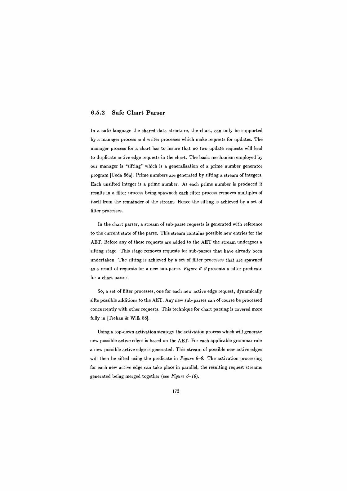
6.5.2 Safe Chart Parser

In a safe language the shared data structure, the chart, can only be supported

by a manager process and writer processes which make requests for updates. The

manager process for a chart has to insure that no two update requests will lead

to duplicate active edge requests in the chart. The basic mechanism employed by

our manager is "sifting" which is a generalisation of a prime number generator

program [Ueda 86a]. Prime numbers are generated by sifting a stream of integers.

Each unsifted integer is a prime number. As each prime number is produced it

results in a filter process being spawned; each filter process removes multiples of

itself from the remainder of the stream. Hence the sifting is achieved by a set of

filter processes.

In the chart parser, a stream of sub-parse requests is generated with reference

to the current state of the parse. This stream contains possible new entries for the

AET. Before any of these requests are added to the AET the stream undergoes a

sifting stage. This stage removes requests for sub-parses that have already been

undertaken. The sifting is achieved by a set of filter processes that are spawned

as a result of requests for a new sub-parse. Figure 6-9 presents a sifter predicate

for a chart parser.

So, a set of filter processes, one for each new active edge request, dynamically

sifts possible additions to the AET. Any new sub-parses can of course be processed

concurrently with other requests. This technique for chart parsing is covered more

fully in [Trehan & Wilk 88].

Using a top-down activation strategy the activation process which will generate

new possible active edges is based on the AET. For each applicable grammar rule

a new possible active edge is generated. This stream of possible new active edges

will then be sifted using the predicate in Figure 6-9. The activation processing

for each new active edge can take place in parallel, the resulting request streams

generated being merged together (see Figure 6-10).

173

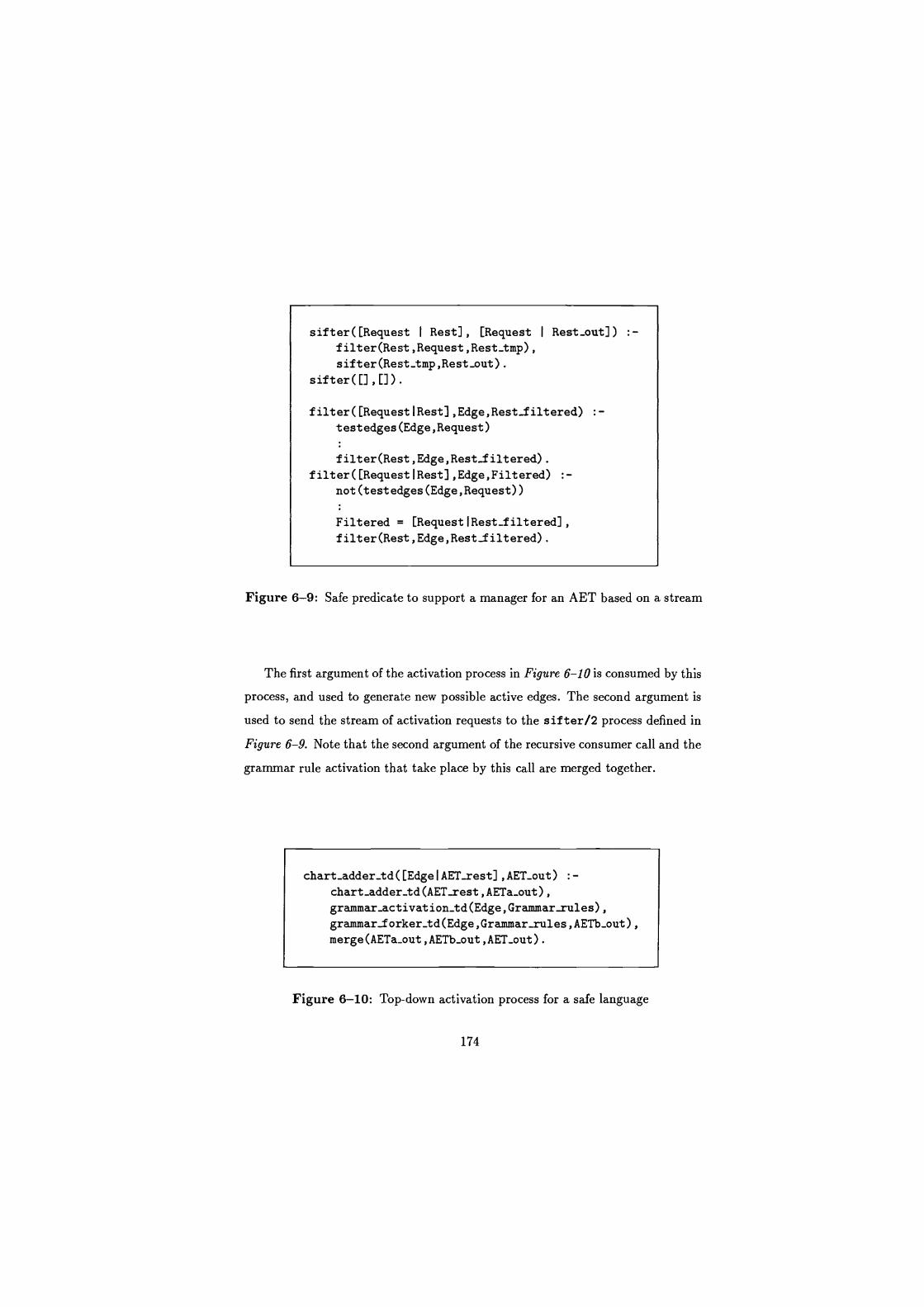
sifter([Request I Rest], [Request I Rest-out]) :- filter (Rest, Request, Rest_tmp), sifter (Rest-tmp,Rest-out)

sifter([] , []) .

filter( [Request IRest],Edge, Rest..filtered) :-

test edges(Edge,Request)

filter (Rest,Edge, Rest..filtered) .

filter([RequestlRest],Edge,Filtered) :-

not(test edges(Edge,Request))

Filtered = [Request IRest_filtered], filter(Rest,Edge,Rest filtered).

Figure 6-9: Safe predicate to support a manager for an AET based on a stream

The first argument of the activation process in Figure 6-10 is consumed by this

process, and used to generate new possible active edges. The second argument is

used to send the stream of activation requests to the sifter/2 process defined in

Figure 6-9. Note that the second argument of the recursive consumer call and the

grammar rule activation that take place by this call are merged together.

chart _adder_td([EdgeIAETxest],AET_out) :-

chart-adder-td (AET-rest, AETa_out) , grammar_activation-td (Edge,Grammar_rules), grammar_forker_td(Edge,Grammar-rules,AETh_out),

merge (AETa_out,AETb_out,AET_out).

Figure 6-10: Top-down activation process for a safe language

174

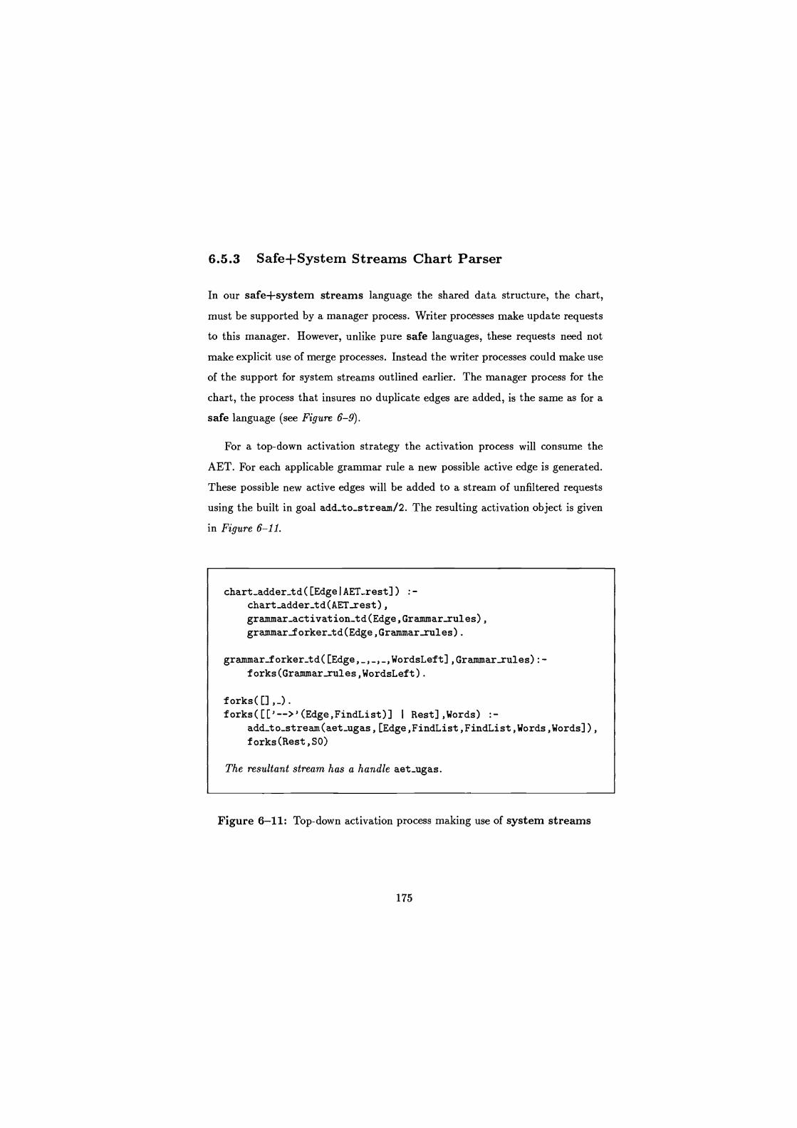
6.5.3 Safe+System Streams Chart Parser

In our safe+system streams language the shared data structure, the chart,

must be supported by a manager process. Writer processes make update requests

to this manager. However, unlike pure safe languages, these requests need not

make explicit use of merge processes. Instead the writer processes could make use

of the support for system streams outlined earlier. The manager process for the

chart, the process that insures no duplicate edges are added, is the same as for a

safe language (see Figure 6-9).

For a top-down activation strategy the activation process will consume the

AET. For each applicable grammar rule a new possible active edge is generated.

These possible new active edges will be added to a stream of unfiltered requests

using the built in goal add-to-stream/2. The resulting activation object is given

in Figure 6-11.

chart _adder_td([EdgeIAET_rest]) :- chart _adder_td(AETxest) , grammar-act ivation_td(Edge,Grammar_rules), grammar.Iorker_td(Edge,Grammar-rules) .

grammar_f orker_td ( [Edge, _, _, _, WordsLeft] , Grammar-rules) : - forks(Grammar_rules,WordsLeft) .

forks([] ,_) .

forks([['-->' (Edge,FindList)] I Rest],Words) :- add_to_stream (aet_ugas,[Edge,FindList,FindList,Words, Words]), forks(Rest,SO)

The resultant stream has a handle aet_ugas.

Figure 6-11: Top-down activation process making use of system streams

175

6.6 Results and analysis

As these parsers have not been analysed before and the safe+system streams exam-

ple cannot run on previous interpreters we do not carry out a comparative analysis

of our new system with the previous systems. To execute the three styles of lan-

guage on one system, Parlog, we have added some extensions to our evaluation

system.

unsafe predicates are declared by program annotation. The interpreter

delays the processing of any goals to be evaluated by such a predicate within

a cycle until all the safe goals have been processed. The unsafe goals are

then evaluated as in the previous interpreters (see section 2.6.1.2) which

handle the evaluation of unsafe predicates 2

The two stream manipulation system calls are also supported by extensions

to our system. Any stream calls are only processed at the end of a cycle. The

interpreter maintains a record of the streams declared as resultant stream and

is hence able to add elements to these streams as if they were atomic actions.

2Unsafe predicates are allowed to bind the input variables in the guard. In Shapiro's

original interpreter [Shapiro 83] these predicates did not cause any implementation dif-

ficulties as bindings were generated as the goals were processed. As this processing

was sequential there were no problems associated with supporting atomic commitment

required for unsafe bindings. In our system we have attempted to model parallel AND-

parallelism and to this end we have developed a model in which goal order does not

affect the overall computation; by allowing only bindings available at the beginning of a

cycle to be used by the goals (see section 3.6.3). To execute unsafe predicates we relax

this restriction but require that such predicates are evaluated at the end of a cycle and

only possess flat guards

176

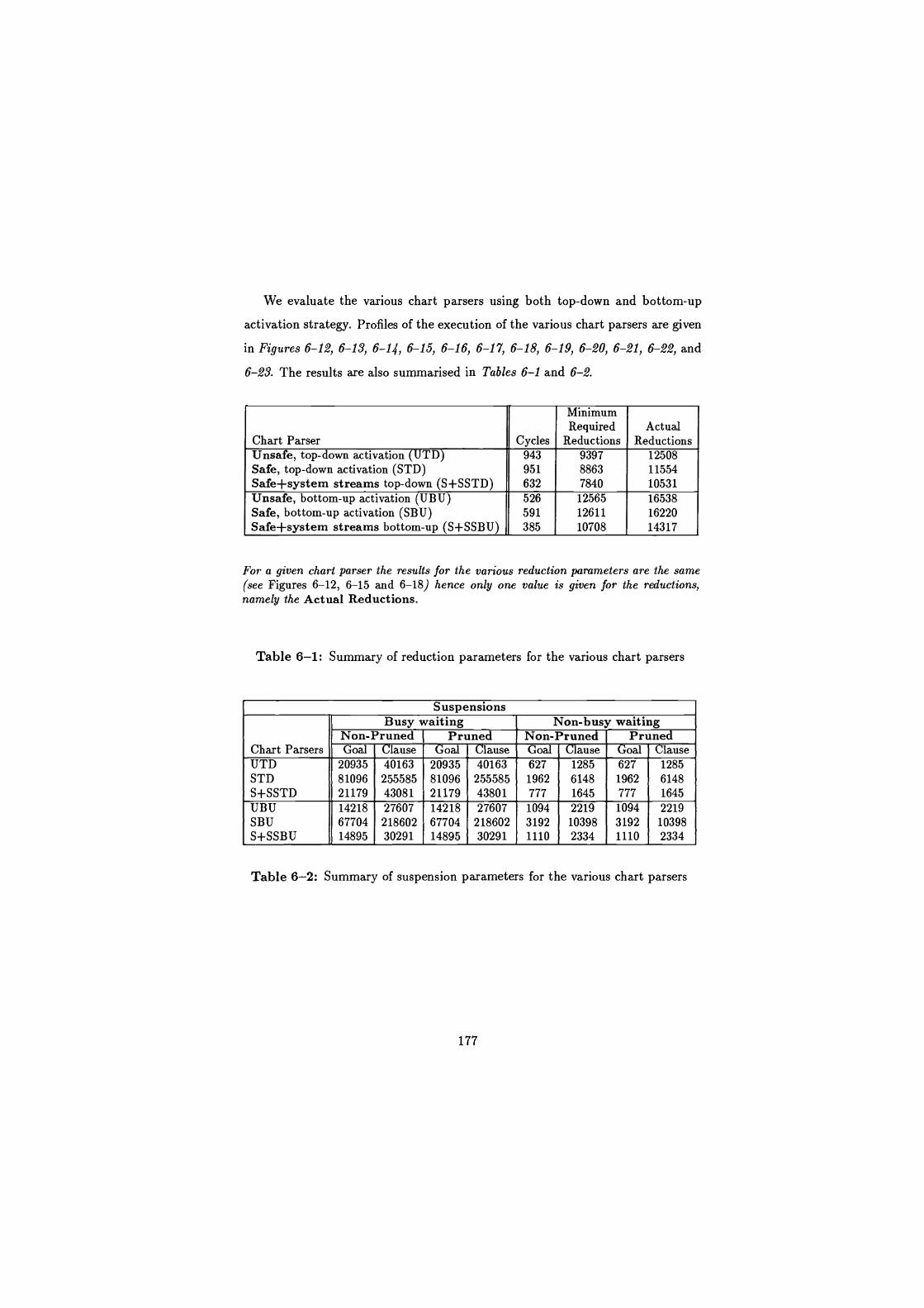
We evaluate the various chart parsers using both top-down and bottom-up

activation strategy. Profiles of the execution of the various chart parsers are given

in Figures 6-12, 6-13, 6-14, 6-15, 6-16, 6-17, 6-18, 6-19, 6-20, 6-21, 6-22, and

6-23. The results are also summarised in Tables 6-1 and 6-2.

Minimum Required Actual

Chart Parser Cycles Reductions Reductions Unsafe, top-down activation (UTD) 943 9397 12508 Safe, top-down activation (STD) 951 8863 11554 Safe+system streams top-down (S+SSTD) 632 7840 10531 Unsafe, bottom-up activation (UBU) 526 12565 16538 Safe, bottom-up activation (SBU) 591 12611 16220 Safe+system streams bottom-up (S+SSBU) 385 10708 14317

For a given chart parser the results for the various reduction parameters are the same (see Figures 6-12, 6-15 and 6-18) hence only one value is given for the reductions, namely the Actual Reductions.

Table 6-1: Summary of reduction parameters for the various chart parsers

Suspensions Busy waiting Non-bus y waiting

Non-Pruned Pruned Non-Pruned Pruned Chart Parsers Goal Clause Goal Clause -Goal Clause Goal Clause UTD 20935 40163 20935 40163 627 1285 627 1285

STD 81096 255585 81096 255585 1962 6148 1962 6148

S+SSTD 21179 43081 21179 43801 777 1645 777 1645

UBU 14218 27607 14218 27607 1094 2219 1094 2219 SBU 67704 218602 67704 218602 3192 10398 3192 10398

S+SSBU 14895 30291 14895 30291 1110 2334 1110 2334

Table 6-2: Summary of suspension parameters for the various chart parsers

177

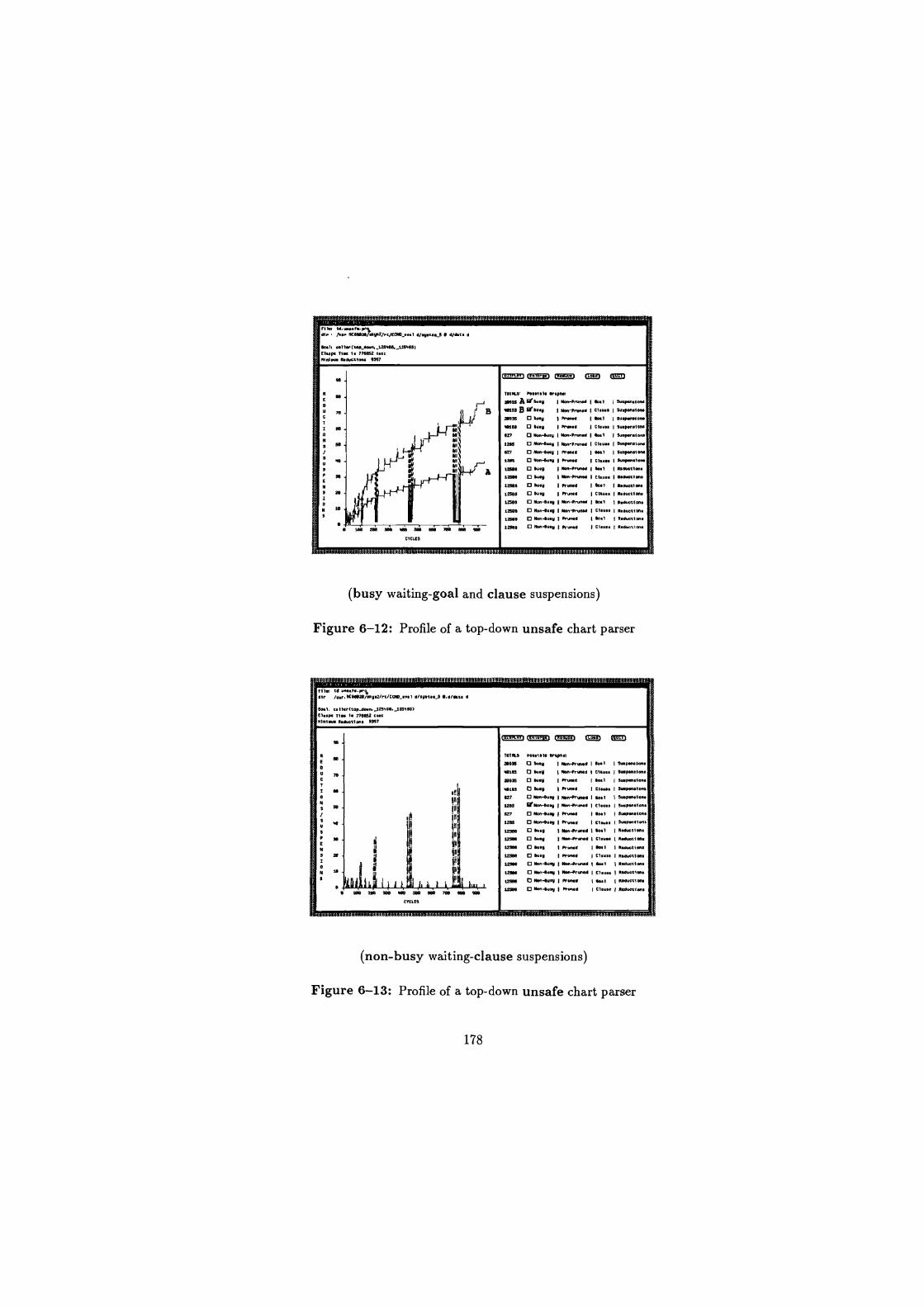
rf la ed un..r. PP yy elr /u.r MC$5129T .2/75/000_...1 4/.y.u.} 5 4/4.51 a

m

59 SN

AN

Sn

Sn

SN

145 0.5 515 455 351 50 755 555 951

CYCLES

N

03-0 I Prun.a 150.1 I /.46011.1.

D 5U.5 R0... I CItuu I R..uctl.l. D Non-0.. I N0n-57,150 150.1 1 8.4505101.

D N0n-OU.5 I Non-Pr0n.4 I C..... I R1.u5tlon1

D Non-OU.y I Prun.. 1 50.1 1

8..14510..

D Man-15.5 I R6.. I CLAUS. 1 1.4Oelm.

(busy waiting-goal and clause suspensions)

Figure 6-12: Profile of a top-down unsafe chart parser

"Inv fl Ia 54 65u0. F

/u.r NC51020//li511/rt/CCW wr1 4/.5.1,45 5 ./4.1, d

6W1. n llrr(tops*n.-t25.10.-507537 El. p. T1.. 1. 775552 ... Mlnf.w R.10.510n. 9597

5 5

D

ND

I l 1

590 09 CYCLES

709 051 900

T5l4IS' PC111b1. I*PMPt

7ssss 1,A

5eu.y I Non+r nw 110.1 I su*PM.lons

Wins B fif15.o Non-Pruned I C1.u.m I w.p.n.to.o moss D 15.5 I Pru0.4 I b.1 I su.p.n.lo0. .5155 0 15.5 I Run.. I Cl.... I su.P.n.f.n. SV 13 Non-015 11011-Pruned 1 b.l 1 !1.5.1,.100

I0. D Non-swy I Non-Pruned I Cl.u.. 13u.P-.b1,. 527 D Non-91511 I .r-5 15..1 1305µ1,1f 0i0

5255 D N00.4u.y 1 P.00.0 1 [1111. 10up.n.1.15 12551 D 51.5 I N.1,-570150 150.1 11.suttlon. 17351 D 1505 N0.-Pruned 15110.. I Redu011 0.5

5100

Toms srLphm

70959 D 15.5 I Nomlrum0 I S..1 S0.p.nsfon.

95555 4 15.11 { Non-run.. CI.u.. 1 swp.nSfan.

75975 D 1519 I Pro .d 150.1 130.5..110,.

451ss I, 01.5 Pr.N.. I Cl- 130.70101.0. 527 D 5 001.5 I Non-PruM. I IN.1 130.5.111.0. 7235 fl N.1,091.5 1.00-51.0. C..u.. I S0.pP.l.n. 027 0 X511215 I Prun.. 90.1 I M-p.n.lon. 5256 0 Non-5uq I R6m4 I C1.... I l.p.o.fon. 52385 D 15.9 1 Non-Prul.4 50.1 RNU *1... 72395 D 5505 115*n-pr00. I Cu1.. 16.4.05101,.

5250 D 1505 I Prun.. 18..1 1 0.4645100.

12359 0 S.0 I Pr1.N. 1

C1.uS. 15s.un1065 12951 0 Non2u.5 I N002n.0. 19151 1 8506[1101,.

12551 0 Non-4.05 111on-rm04 I CT.un fl"-I00 120. Q Non-99011 I Pr*MR %.l 16.410. a1.

$2751 0 NemW.6 I Ironed 101.11.. 16.404510..

(non-busy waiting-clause suspensions)


0

178

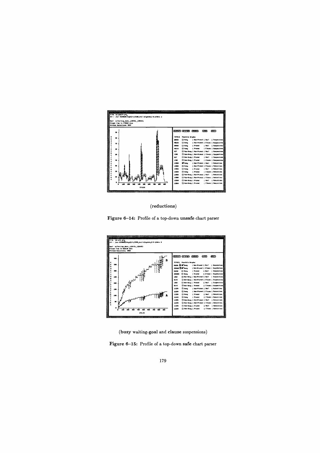
n 1. td .00..r. prod 0r : 100, MCNNO0/0.302/,./CC*l twi ./.y".0-5 0.3/MCs d

00.1 t.lt.r( cap_doln.}25.66. 123483) E10.p. 1130 t. 226052 ...0 0311.0. 30000150.00 1011

e too 2pe 0000 3000 sea 00100 )e8 OBa lee CYCLES

J1J333#=Ak PAOAAA.UM

(reductions)


00.1 C.ll.r(t.p_Mwi.15373.}25.50) E7. Spa Ti.. I. 000110 0000 MInI._ 801ue10.n0. 0001

mrwm (UMM am mm

1010L80 0...101. Or.p3N

2075 O wry I 000-0r000d 130a1 1500peo1a00

30U0 O 0003 I Nen-0,0000 Cl.... I -p00.1- 23100 0 3003 I hun01 1 00.1 1 w.p.0HOna

30101 0 easy I n3.1.d I Cl.... 150.300.100. 027 O N.n-6003 I N0.,-Oru00d 100.1 1 00070000000

1206 0 Nae-111.$ I man-#ron.d I Cl.... 1 500703.1000

522 O 300-Wry 130.+00 1 loot 1 0aspan0lpp

1206 O 30.0-00.3 h1.10d I Cl... 1500p0.10as

12506 fiireasy Non-Prd00d 160.1 I esduett00.

12580 O 0003 I Nas-0r0ood I Cl- 1 e.dastlsn.

12500 O 0003 10,0001 1 8011 1

O.Ouet10n.

12386 O 6003 I Peon. I C1.,.. I esauctl00.

12580 O Ne0-Gory No.-0rotd 1 toot I e.d olloo. 12350 El N.n-0..3 N0.-0r00.d I C1.... .3..050.. 12300 O 300-34ry 17,0001 1 30.1 1

800003103.

12508 a No.-w.9 I n.n01 I C1.-. I e.d0oclon.

T01KS 70..101. Or.p3N

61000 A W0u.3 1303-7r,0.d 160.1 100.7.0.0000

2666e6Br-rw3 1 Non-r000d 1 Cl.we I S..pln.1000

01030 13 w.3 1

prawd I Goal 10u"-.1030 256600 El w.y 130.300 C1100. 150.700.0000

1102 Cl N--Gory N..-300060 1 0001 15u4pen.i- 6130 0500-w.3 I Nnn-7,0000 I Clue. 15u.p.n.i000

1902 O 303-6..y pruned 130.1 13u.pen.1.oo

6140 O N.n-Wry 17,0000 C1.0.. w.p00.1o00

11551 D w.3 NOn-runsd I )301 15c0u3t10n0

us" O woo 1 Noe-7rNe

1."71 e7.0000.1 on.

11553 O wry p003.0 1017.00011000 sss53 0003 I pruned 1 0.ase 1 e.d001OOn.

11301 Npn-w.0 13.30,.00 I %.1 100duetla0e

1159. O N.0-w.0 Ndn-7,.0 3 I Cl.-. 15eduetlan.

11155 3.0-0000 I #0.000 100.1 15.Oucclan0

11593 N.0-wry I Or.Md Ci.oe a0d1Oel.n.


Figure 6-15: Profile of a top-down safe chart parser

179

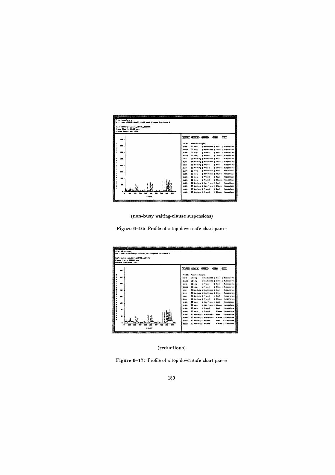
TOTALS. P...ibl. U.pb.: vim D w.y I NenArun.d I Goal I SwP.m,m. 2R%% 17 b.y I N.nirwted I 0.ua I %.""- son D wry I Prumd 1 45.1 15..0.-l en.

255%5 0I i I Printed I CI.u.. I bapanai

1962 0 N.n1..y 1 Nen-Pr.me 1 Owl I Su.p.mi m. 0140 W140n-I. "an-Prunes I Cl.... Su.P.m,... 1962 0 Non-Bwy I Prumd 150.1 I Swpemr m. 8145 D Nen-w.y I Prwwa 1 Clu.. I Su.P.n.1Pn.

1159 D buoy N-F-W 1 541 I N.du.t1an.

SISS. D W" I Non-rwiW I Claw. I R.duot,on.

1155 D was I Prumd I Real mdu.tlom lisp 0 bay Prumd I C1.u Rad-UM 1139. D Non- .y I NOnirund I Real RmdmtlM,a

11554 D N.n- .V 11bn-Pr1mee 1 Clause I Ridu.tlom

1t5$% D ften-buay I Prumd I RP.I I Redu.t,om

11591 D Non-b..y I Prumd Cl.... I Radu.tion.



r11. td ..r. PrOj dlr /d.r RCSS820/skye2/rt/CCND_.v.l d/.y.tu3 R d/data d

bo.1, nlter(tep_do.I.25473, 12SWb) Eleaps lift ,. 855110 mo IN n,Wd Redn L10n Rbd

TOTALS, Paatlbl. Graphs,

MB% D Swy Non-Pruwd I Roll I SutpenlPnl

2555.5 0 Sews I 110 -P , d I Cit... Suq.n/m MB% Q Ntey I P-d 110.1 I b.pem,m. 2SS%5 0 bwy Memd Clwn I Su.PSm,en.

1962 D Nee-butt' I Nbn-P. d Seal I Supam,ene

aM D Nen-way Non-Prue.d I Cl.... 1 Sutgmlmt S%2 D Nee-way I Mumd 1 6w1 1 9utP.ml6e+

Ri'b 0 Non-b.ay I P-d I Cl.u.. I Su.PSnH on IISS4 19 bwy Non-P--d 10001 Radmiiom

lisp D bwy I R. Prumd I Clause Raduet70m

1159. D bwy I Prined I ba.t I RWWII- 11554 D wy 15'.810 Cl.... I Red.tlam 11556 0 Non-win I N..-Prvmd 4-1 I Red-ti- 11654 D Nee-b.y Non-P-d I CI.UU I Red..I lisp D Nen-wet' Prumd I boat 1 Redbeclem

its" D N..-boy I Prumd Cl.... I A.&W am

(reductions)


180

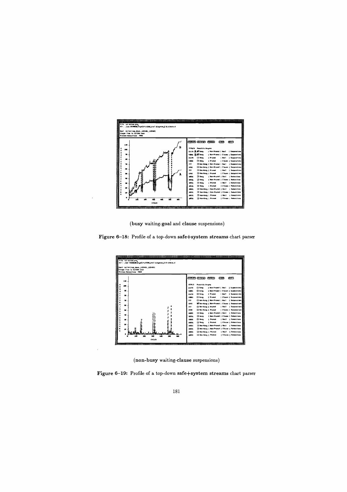
flit t0 sates. /f 011 /usr IIC4W2i/skyt2/rt/CCRD-.0.1 0/.5.00} 0 O/4000 t

R RIM.I T.I. 41TT

® 0 It

101Re51 P15151. teas,

21179 Air 615I 0o1-110.0 1051 510900.100.

43 e1 8 511sy I Non-Prune. I Clat.e 90tpensl0ns

21179 0 Otry I P t00d 190.1 I Swp.n.lon. .78ft 13 Wty I Mu1Nd I Clews I Swptnstans

777 011-81 1 I Non-Pruned 1 $0.1 I Su.90SHen.

1543 0 Nen-W.y I N--051900 I Cl- OwpOn.le0S

777 0 Non-0055 I PruntS 100.1 1 Swp.nsim.

15105 0 Men-Woy I Prune I C1". I Swp.n*lens

10051 O Owy I Nnn-Prw.O I goal R.du.tlo0.

10531 Wry Men-A'uMC I Cl.w. I Rad .te*" 10051 0 Owy PruntO 00.1 RNU.1100.

10531 0 0050 1 PrunM I Cl.0 1

R.5wt1,M

10551 0 Np-lu.y I NOrP0tftd 100.1 15,015.100.

10931 0 Non4u.S Non-Pruned 111.10. I RMUO.imr

10551 0 00,-4055 I Prunq 1 50.1 1 800010/50

10551 0 Non-0155 I Pr-ea I Cl.u.. I R.5wt1 o0.

M


Figure 6-18: Profile of a top-down safe+system streams chart parser

ri la OS 1trno.prq 5lr t /wr NCOMMhk5.2/rt/CC/IO_ev 1 5/pate.} 0 5/O...5

00.1: 001 1Sl(1ep_dl.n, 135005, 125503) (laps ilea 1. 217295 00.0 nlnitu. 50005.1090 7500

05531 0 10.5 I 500l-P-ad 15051 10005011M

777 0 X00-50.0 I RtnN 150.1 S0.pefMen*

15905 0 Non-0105 I Pr1n*d 1 C..u.. I W0p.0.lon.

15.5 0X05-Eo.S NPn-P-d I Cl.... I So.p.nslont

777 0 Non-W.y I N0 -Pru.N I $0.1 1 W.p.ONOn.

.M51 0 Sony PruMO I Cl... tu.p.0.io0. 21170 0 10.0 I P50505

1 50.1 1 9090n5I005

21179 0 Busy I Wm P-td 150.1 I Su.Pnns1P0.

.MOi 0 Busy I NPn-Pr5M2 I C1tt55 1509P9051/n5

101RW 0055151. Or.p1

0 W.y I Non-Prsoo O I Cl.... I R55-1n0.

0 5.55 1 05055 1 00.1 1 00550550.

13 Sun I pruned j Clause Re*5t1a0.

0 Non-5105 I N.ro-Pr0005 100.1 R.au.tlo0.

0 Nen-euog Na.-Pr1,Md Mute I Redu.55...

0 Non-ate5 1 Pr-td W.1 I R.a-%io0.

0 Non-5us5 I Pruned Cl... I R.005-le0.



181

31l. 00 .tree Pr air rwr Rc.eea/.tyez/rc/m96_0001 ar.yne. s d/d.te d

60.1 p ll.r(to_de."M125400._125409) M.P. Tie. 1. 211296 0000

01n1eue 000.0190. 7646

CYCUG

10050.0. Possible &&ph=

21179 13 00.9 I Nan-Prune I to.I I ].pennon. 430,01 0 W.9 I Non-Prune I C1.... 11up.n.1000

21179 13 6..9 I Pr.ed 15.1 190penelone

43001 0 Duty I Prang I t1.... 1 eupennan.

222 0 0e.-0099 I Nan-prune 160 0 I S.penoion.

1645 0 N.-0099 I Nen-prune I Cl.... I Wape 01000

777 0 Non-019 I Prune I toe 19.p.nnon9 1645 0 Non--y I Pramd I Cie... I W.p.nnen.

10511 00°W.y I 0100ir.000 00.1 1000001 en.

10031 0 00.9 I Non-prune Clw.. 110Arcti.n. 10511 0 wry I Prune. Gael I Reoucnan.

10031 0 0..y I Prune Cl..,. Red-ions 10531 0 Non-Gwy I N0.n-Prune 10001 10000001 one

10031 0 Non-0099 Non-Or.md Clw.. 1 leach one

10531 0 N..-O..y Pp.n.d tool 110..91-0 10531 0 Non-0w9 1000m0 Cl_. 10000.010.0.

t1w M

(reductions)


1.010.41 l l rile 0. .00090 pro,

.0602/rt/COq_e3.l.dhy9tN_s O.d/0.09 d

to0N o.11.rlbu00oe_p. 125400._128.60) EL .. T1e. 10 60196$ ca

dinI.09 e.daion.. 12505

fra-M GM)

TOTAL' Po.MPle rphe 14210 A WO..y Non-Proo00 1 0000 19.0p000Pne

2]662 B 1tou0y 1

Non-prvn.d I Clw.. 19u.p.mlone

14210 0 tu.y I pruned 190.1 19u.penlon0 27607 0 00.9 1 Pr.md I Cl... 1 00.p.mi.n. 1094 0 NOn-00.9 Non-PndNd I toe1 19wp-ion. 2219 0 Non-Way I Non-prams I Clw.. 1 3u0p.m1on0

50Nr 0 Non-W.y I Pruned 100.1 wepemlen. 2219 0 Non-00.9 I Prw.e I Clw0. I l..p.mlon. 16530 0 W.y I Non-Prunes 100.1 1.d.ettan0

1909$ 0 W.y 1 non-pr0000 1 Cl_.. 00d-lion. 1830 0 0u.y I Prumd 1 00.1 I Reu001on.

1393$ 0 a..% I Pr.md Cl.,.. 10d-lion. 10530 0 600-0009 I Non-Prunes 1601 I F.-lone 16000 0 Non-Way I Non-p_d I C1w.. 11.0.0.00.00

10536 0 N--Way Pruned I Peel 100duetion. 16990 0 Non-Way I P'..0 Chu.e 1100u00/an.

VIROMMOM


Figure 6-21: Profile of a bottom-up unsafe chart parser

182

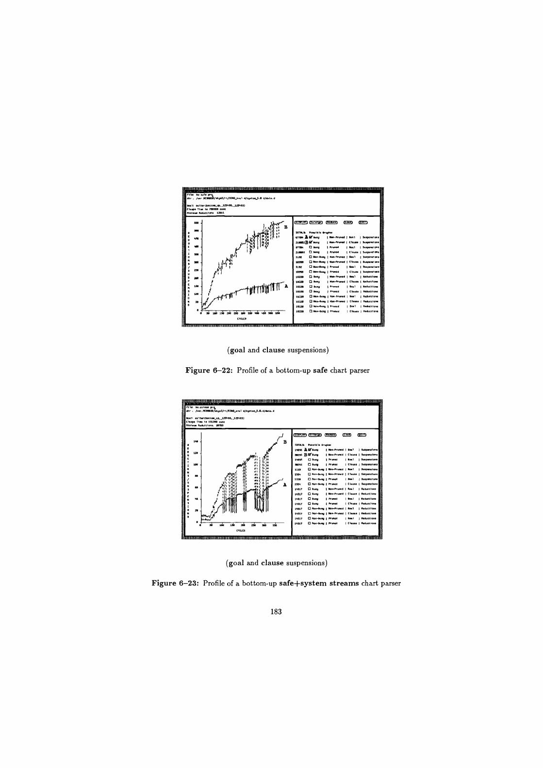
rll.: b safe pr0%

dlr . /uar NCOe070/.Lys2/n/CQ10 ..1 d/syst.s,3.0 d/d.te.d

bsi: alter feotto.!_up, }2a4w,,,,125403) flepe T1. Is 780960 COM

Mni.u. R.duCtt One 12611

TOTALS Posible 0..ph.

077y4 Afit Way I Nen-honed bs1 Wapenatws

21e802Bfir Wey I Nw-PrttMe I Clew. Wp.Mi we

e77e9 Way proved I Boat I wep.Miws

210802 way I Pruroa I Cisuu I Su.p.M1 w. O ft.-Wag I Ns,-Pruned I bet su.peMiw.

3e39e p lbn auy Nw-ProMe I Clue. WaPaMl we

3112 13 x80-easy I .rump I tidal I w.peroi w. log" Non-euay I proved Claus. I Suapamtwa

16220 13 Way I Non-pruned Seal RsduetiOM

3622e O Way I Non-pruned Cleats I Raduc7/aM

11220 Wee Pruned I Wel I R.ductic, la220 0 way I Pruned Claus. I baucti.M fe220 13 Non-busy NO.-Pruned I b.I dewetieM

16220 13 Non-euey I w-Pruned I Clause I RawotioM

16220 N0n-bury Pruned I Ooat ton 16220 Non-bury I Proved

1 Ciau.. I 1.d4CtlOM


Figure 6-22: Profile of a bottom-up safe chart parser

ELI:1:#$...d8$..x"i.1.$.$.1£aS3`:#.db.:tkbJ;#.$.E..kd#31C£.kl.i#.8.$A£z"11.1..$£.{.EkISB .b.i$#.#.t@:.

ftle: W. strew pr% dir . /uw.NC68020/s4.2/rt/CCNO_..I d/5 stu.O. d/d. . d

bel esllMfboeto up, tzsiee, 1L44tl) Elsape Tin 1s 191380 Case

RIM.- R.OUet/wt 107ee

frnTrr-vn ®ues

TOTRLU: P...tb We er.phn

133 Aeled.y I N Pruned I 1..l I Eupmiel w. ae291 BGr Busy I Non-Pruned Clause 16uspensIMS

1393 ewy I Pruned 8o.1 I bepwaiwa I Suspensiws Mel bury I pruned I Cl....

1110 0 N--Way I Non-Is'uMd I bet I fuepweiwe

234 Nen-Way Ma,t-PruMd Clause 3uapwa/wa

1110 Non-Wry I Pruned b.l S..psn./on.

234 0 N.n-Wsy I Proved I Cleu.e Suap-.1...

14317 easy Nv,-Pruned Owl bd.tiwa 14317 busy I Non-Pr m d I Clause I Red-tiwa

14917 0 Wsy I "-ad 0-1 st.ductl... 14317 0 busy Pruned I Cleu.s Reduostone

14317 0 N--W% I Nen-PryMd 10.1 I R.du.l.n. 1317 tepn-by Non-pruned C1.u.e Rsduotiw.

14317 0 Nw-Wry I Pruned 160.1 1 bWet.iw3

14317 Nen-Wey I Pruned I Clues I eaauoelOn.


I

Figure 6-23: Profile of a bottom-up safe+system streams chart parser

183

First we consider some general points raised by these profiles:

There is no difference between the various reduction counts for the unsafe

chart parsers (see Figure 6-14). The same is also true of the safe and

safe+system streams parsers (see Figures 6-17 and 6-20). The similarity

in the reduction counts, using goal and clause suspensions, indicates either

there are no suspensions or that the evaluation suspends on head unification

before any reductions in the guard take place. As there are suspensions for

each of these chart parsers the suspensions must occur on head unification.

The similarity in the suspension counts using pruned and non-pruned

evaluations indicates that either guards are even in their computation (this

includes the guards being flat) or that only one clause could ever be picked

as a solution path.

Comparing the minimum reductions to the actual reductions gives a measure

of the OR-parallelism (see section 4.3.4). Table 6-3 summarises the degree

of OR-parallelism for the various chart parsers and activation strategies.

Chart Parser Actual

Reductions Minimum

Reductions OR-parallelism UTD 12508 9397 1.33 STD 11554 8863 1.30 S+SSTD 10531 7840 1.34

UBU 16538 12565 1.32 SBU 16220 12611 1.29

S+SSBU 14317 10708 1.34

Table 6-3: Degree of OR-parallelism for the various chart parsers

The various chart parser do not exhibit much OR-parallelism. This is be-

cause the perpetual process view of Parlog which was employed in the design

of these chart parsers gives rise to predicates with simple guards. The most

complex guards in the systems check if two edges combine or if two edges

184

will result in the same activations. Also chart parsing computes all-solutions,

essentially replacing OR-parallelism by AND-parallelism.

Our profiles allow us to obtain an indication of the maximum number of

reductions and suspensions in a cycle. Table 6-4 summarises the maximum

number of reductions that can be performed in a given cycle, some of this

information is given graphically in Figures 6-13, 6-16 and 6-19.

Program Max reductions Cycle number UTD 95 757 STD 105 834 S+SSTD 107 497

UBU 154 374

SBU 145 458

S+SSBU 152 280

Table 6-4: Maximum reductions in a given cycle for the various chart parsers

Whilst we see that the maximum number of reductions is high, the profiles,

Figures 6-13, 6-16 and 6-19 show that these maxima are very narrow peaks.

This indicates that the maximum reductions in a cycle should not be taken

as a strong indication of the possible number of exploitable processes 3.

The main feature to note is the maximum parallelism occurs sooner for

the bottom-up activation strategy, indicating that activation model is more

parallel at the start.

Table 6-5 summarises the maximum number of suspensions that can occur

in a given cycle. Because of the nature of these chart parsing algorithms

31t can be argued that the average number of reductions over the whole computa-

tion is the only measure that reflects realistic processor requirements. However, some

computation may exhibit large amounts of parallelism for several cycles but still have

a low average utilisation. In these cases some weight should be given to the maximum

possible processor utilisation.

185

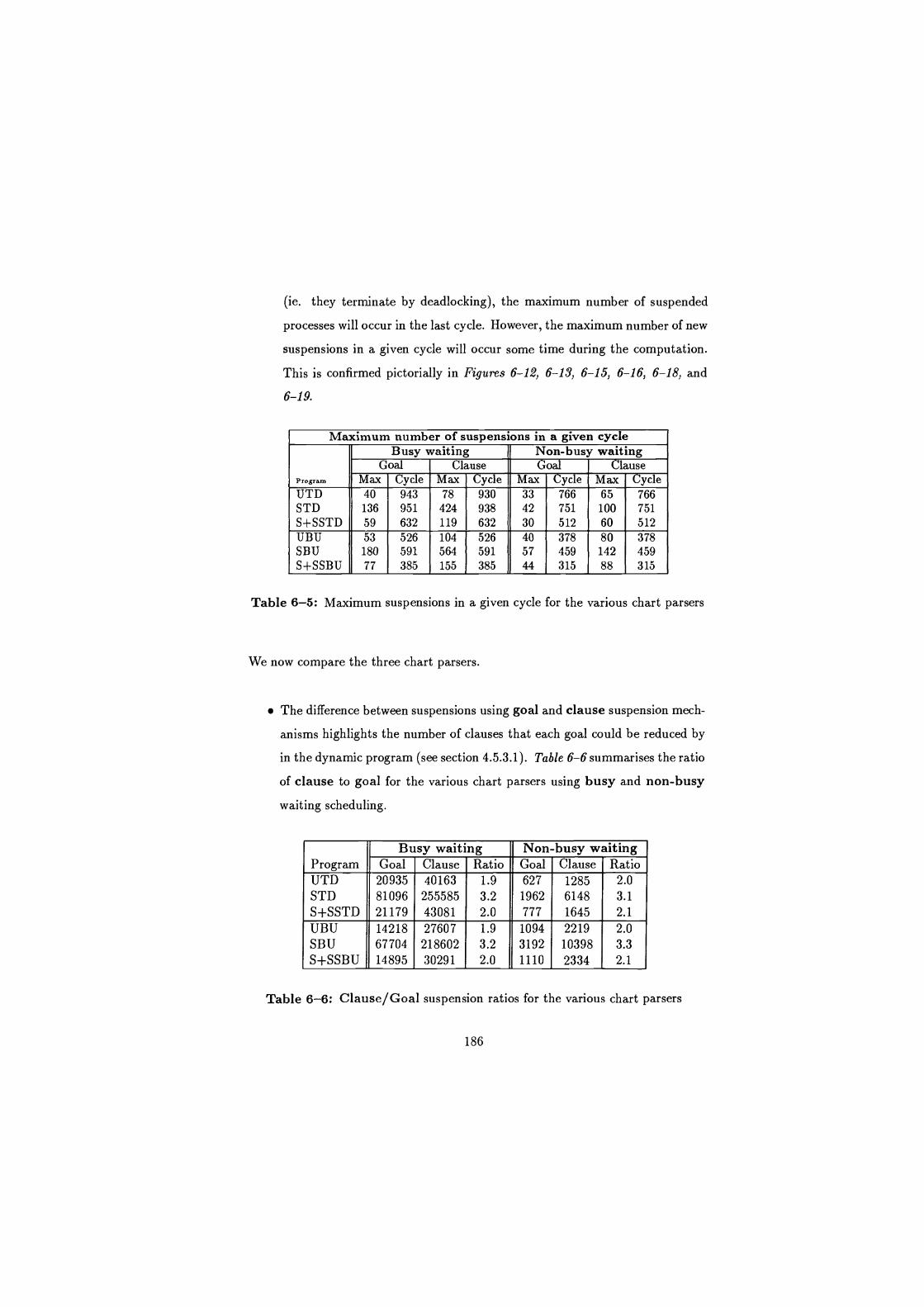
(ie. they terminate by deadlocking), the maximum number of suspended

processes will occur in the last cycle. However, the maximum number of new

suspensions in a given cycle will occur some time during the computation.

This is confirmed pictorially in Figures 6-12, 6-13, 6-15, 6-16, 6-18, and

6-19.

Maximum number of suspens ions in a given cycle Busy waiting Non-bus y waiting

Goal Clause Goal CI-ause Program Max Cycle Max Cycle Max Cycle Max -Cycle UTD 40 943 78 930 33 766 65 766 STD 136 951 424 938 42 751 100 751

S+SSTD 59 632 119 632 30 512 60 512 UBU 53 526 104 526 40 378 80 378 SBU 180 591 564 591 57 459 142 459 S+SSBU

1 1 77 385 155 385 44 315 88 315

Table 6-5: Maximum suspensions in a given cycle for the various chart parsers

We now compare the three chart parsers.



in the dynamic program (see section 4.5.3.1). Table 6-6 summarises the ratio

of clause to goal for the various chart parsers using busy and non-busy

waiting scheduling.

Busy waiting Non-busy waiting Program Goal Clause Ratio Goal Clause Ratio UTD 20935 40163 1.9 627 1285 2.0

STD 81096 255585 3.2 1962 6148 3.1

S+SSTD 21179 43081 2.0 777 1645 2.1

UBU 14218 27607 1.9 1094 2219 2.0

SBU 67704 218602 3.2 3192 10398 3.3

S+SSBU 14895 30291 2.0 1110 2334 2.1

Table 6-6: Clause/Goal suspension ratios for the various chart parsers

186

The similarity in busy and non-busy waiting ratios indicates that the dif-

ferent predicates (differing in number of clauses) suspend for similar numbers

of cycles. The similarity in the ratios for top-down and bottom-up activa-

tions indicates either that all the goals that suspend have similar numbers of

clauses or that the program's behaviour is independent of activation model.

In the various chart parsers most predicates have two clauses.

The ratio of suspensions using clause and goal suspension mechanisms is

largest for the safe chart parsers. This is due to merge/3 processes. In the

main these merge processes are suspended. Since each merge goal can reduce

via four clauses this increases the average suspension count.

The (non-busy) suspension parameter records the number of new sus-

pended processes that occur in each cycle. For the safe chart parser the

number of new goals suspended is 1962 (see Table 6-2) for the unsafe chart

parser the number is 627 and for the safe+system streams chart parser

the number is 777.

In the unsafe chart parser the main processes that suspend are those for

active edges. Updates to the shared data structure are achieved by directly

accessing the chart. In the safe+system streams chart parser there will

be suspended processes for active edges and some filter processes, which sift

the request stream. Messages are placed on the request stream using system

primitives. In the safe chart parser there will be suspended processes for

active edges, filter processes and a network of merge processes to combine

local request streams from each active edge process. For each active edge

187

their are two associated merge processes 4. This indicates that generally

both the filter processes and the network of merge processes are suspended.

Goal Suspension Clause Suspension Program Busy Non-busy Ratio Busy Non-busy Ratio UTD 20935 627 33.4 40163 1285 31.2 STD 81096 1962 41.3 255585 6148 41.6

S+SSTD 21179 777 27.3 43081 1645 26.2

UBU 14218 1094 13.0 27607 2219 12.4

SBU 67704 3192 21.2 218602 10398 21.0

S+SSBU 14895 1110 13.4 30291 2334 13.0

Table 6-7: Busy/Non-busy suspension ratios for the various chart parsers

The comparison of busy and non-busy suspensions (total suspensions with

new suspensions) indicates the benefit of tagging suspended executions to

variables (see section 4.2.2). Table 6-7 summarises the ratios of busy and

non-busy waiting suspensions for the various chart parsers using goal and

clause suspension mechanisms.

In chart parsing the generation of inactive edges can be delayed in two ways:

Firstly, delays in the creation of new active edges and their addition to the

AET, which construct the inactive edges. Secondly, in the addition of newly

formed inactive edges being added to the WFST (see section 6.5). The

interaction and effect of the alternative delays result in the behaviour of the

chart parsers being complex 5. From the results we can deduce:

4Merge processes are created by the active edge spawner, this process spawns one

active edge and two merge processes. That is the AET and WFST streams from the

spawned active edge are merged with AET and WFST streams from any active edge

processes that will be generated in the future.

51n the unsafe chart parser additions to the WFST take place using an unsafe pred-

icate which recurses down the WFST until it reaches the unbound tail which it then

188

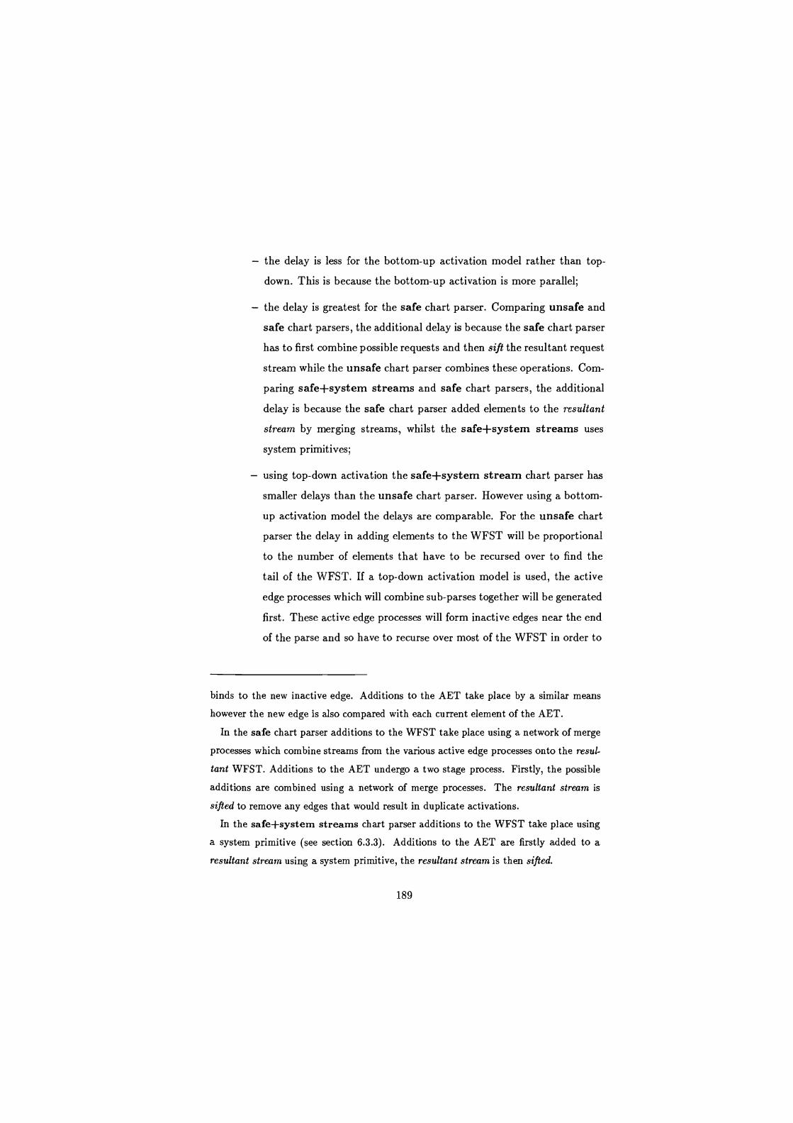
- the delay is less for the bottom-up activation model rather than top-

down. This is because the bottom-up activation is more parallel;

- the delay is greatest for the safe chart parser. Comparing unsafe and

safe chart parsers, the additional delay is because the safe chart parser

has to first combine possible requests and then sift the resultant request

stream while the unsafe chart parser combines these operations. Com-

paring safe+system streams and safe chart parsers, the additional

delay is because the safe chart parser added elements to the resultant

stream by merging streams, whilst the safe+system streams uses

system primitives;

- using top-down activation the safe+system stream chart parser has

smaller delays than the unsafe chart parser. However using a bottom-

up activation model the delays are comparable. For the unsafe chart

parser the delay in adding elements to the WFST will be proportional

to the number of elements that have to be recursed over to find the

tail of the WFST. If a top-down activation model is used, the active

edge processes which will combine sub-parses together will be generated

first. These active edge processes will form inactive edges near the end

of the parse and so have to recurse over most of the WFST in order to

binds to the new inactive edge. Additions to the AET take place by a similar means

however the new edge is also compared with each current element of the AET.

In the safe chart parser additions to the WFST take place using a network of merge

processes which combine streams from the various active edge processes onto the resul-

tant WFST. Additions to the AET undergo a two stage process. Firstly, the possible

additions are combined using a network of merge processes. The resultant stream is

sifted to remove any edges that would result in duplicate activations.

In the safe+system streams chart parser additions to the WFST take place using

a system primitive (see section 6.3.3). Additions to the AET are firstly added to a

resultant stream using a system primitive, the resultant stream is then sifted.

189

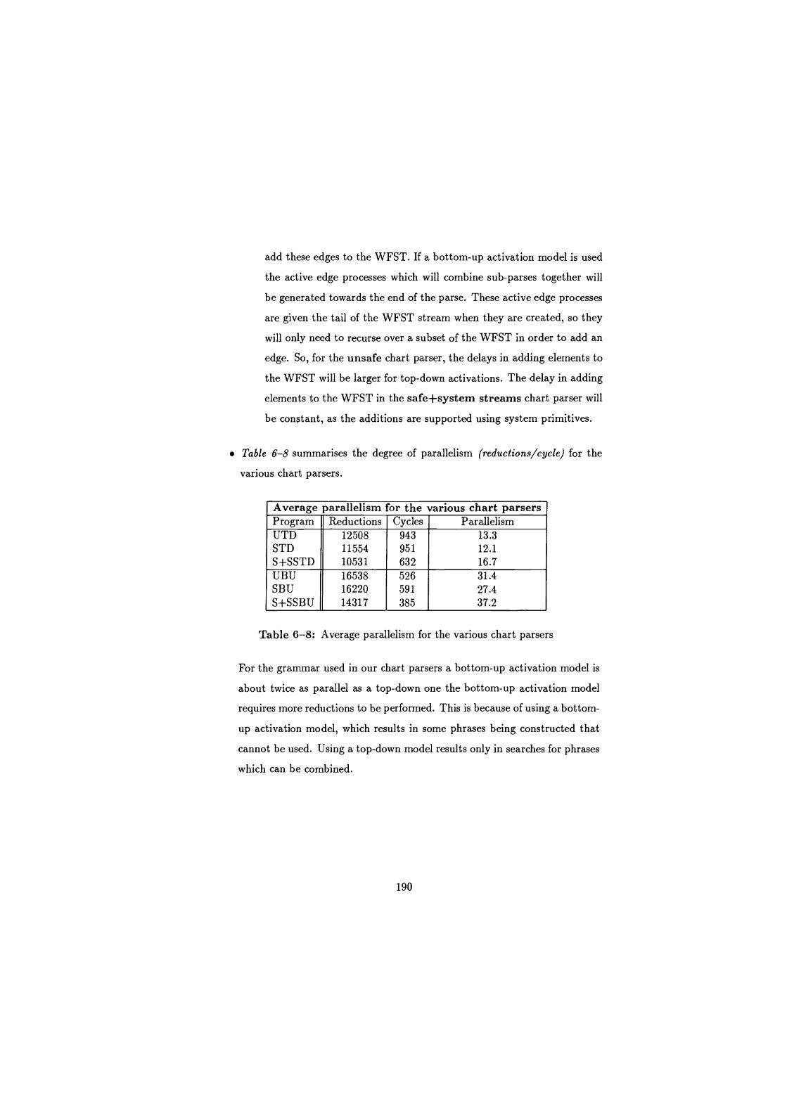
add these edges to the WFST. If a bottom-up activation model is used

the active edge processes which will combine sub-parses together will

be generated towards the end of the parse. These active edge processes

are given the tail of the WFST stream when they are created, so they

will only need to recurse over a subset of the WFST in order to add an

edge. So, for the unsafe chart parser, the delays in adding elements to

the WFST will be larger for top-down activations. The delay in adding

elements to the WFST in the safe+system streams chart parser will

be constant, as the additions are supported using system primitives.

Table 6-8 summarises the degree of parallelism (reductions/cycle) for the

various chart parsers.

Average parallelism for the various chart parsers Program Reductions Cycles Parallelism UTD 12508 943 13.3 STD 11554 951 12.1 S+SSTD 10531 632 16.7

UBU 16538 526 31.4 SBU 16220 591 27.4 S+SSBU 14317 385 37.2

Table 6-8: Average parallelism for the various chart parsers

For the grammar used in our chart parsers a bottom-up activation model is

about twice as parallel as a top-down one the bottom-up activation model

requires more reductions to be performed. This is because of using a bottom-

up activation model, which results in some phrases being constructed that

cannot be used. Using a top-down model results only in searches for phrases

which can be combined.

190



The various chart parsers do not exhibit much OR-parallelism. This is be-

cause the chart parsers are constructed as a collection of simple processes

which receive messages and based on these messages, send further messages.

The computation involved in processing incoming messages is simple, so the

guards are not too complex and hence there is little OR-parallelism.

The maximum number of suspended processes occur at the end of the com-

putation for all of the chart parsers, as they deadlock, although the maximum

number of new suspensions occur somewhere during the computation.

It was expected that the unsafe chart parser would be significantly better

than the safe chart parser, because of the differences in the support for

shared data structures. The actual results give the following conclusions:

Reductions: In terms of reductions, the safe and unsafe systems are very

similar. The combining of request streams using a network of merge

processes and the filtering of the resultant stream, requires a similar

number of reductions to recursing down the shared chart comparing

the possible new edge with the existing edges and eventually adding

the new edge to the tail of the shared data structure.

Suspensions: In terms of suspensions, the unsafe chart parser only has one

type of suspended process: that representing the active edge searches.

The safe chart parser has three types of suspended processes: those

representing the active edge searches; those representing the network of

merge processes; and those representing the pipeline of filter processes.

This is reflected in the results, in that there are about 4 times as many

suspensions for the safe chart parser as for the unsafe chart parser.

191

Cycles: In terms of cycles, the unsafe chart parser was marginally better

than the safe chart parser. Both chart parsers have the same activation

model and search space so the difference between the cycle counts is

due to different delays in making additions to the shared chart.

In the unsafe chart parser additions to the chart involve finding the tail

of the shared data structure, while in the safe chart parser additions

to the chart involve first merging streams of requests together and then

filtering the request stream.

If a top-down activation model is used, the active edge processes which

combine sub-parses together will be generated first. These active edge

processes will form inactive edges near the end of the parse. For the

unsafe chart parser this will involve recursing over most of the WFST in

order to add these edges to the WFST, whilst for the safe chart parser

the additions will involve the traversal of only a few merge processes (as

the active edge processes were generated early on in the parse). This is

a complex feature of the parsers which results in the actual difference

in cycles not being as high as first expected.

So the unsafe chart parser appears marginally better than the safe chart

parser. However, this margin is based mostly on the difference in suspended

processes. In an actual implementation if an efficient suspension mechanism

can be employed and the cost of atomic unification to support the unsafe

chart parser is accounted for, this margin may swing to the benefit of the

safe system.

The merge networks which connect together streams onto one single resultant

stream are mostly suspended. This is indicated by considering goal and

clause suspensions using busy and non-busy waiting.

We now turn our attention to the safe+system streams chart parser. This

system proves to be better than either the unsafe or safe chart parser.

192

Reductions: In terms of reductions, the safe+system streams preforms

about 10 % fewer reductions than either of the other two parsers. Com-

pared with the unsafe chart parser the difference occurs in processing

over the shared data structure to find the unbound tail. Compared with

the safe chart parser the difference occurs in supporting a network of

merge processes.

Suspensions: In terms of suspensions, the safe+system streams parser

has more suspensions than the unsafe parser. These are due to the

pipeline of filter processes. Compared with the safe chart parser the

safe+system streams chart parsers has about 1/4 of the suspensions

using busy waiting and about 1/3 of the suspensions using non-busy

waiting. This is due to the safe+system streams parser not support-

ing a network of (mostly suspended) merge processes.

Cycles: In terms of cycles, the safe+system streams shows about a 30%

reduction in the overall cycle count. This is due to the additions to the

resultant stream being supported by the system and so the delays asso-

ciated with the merge network are avoided in the case of the safe chart

parser. Compared with the unsafe chart parser the safe+system

streams parser gains because processing over the shared data struc-

ture to find the unbound tail can be avoided.

Finally, the safe+system streams chart parser exhibits the most paral-

lelism. This is because of improved accessing to the shared data structures.

Supporting streams in the system results in fewer reductions being performed

in data management and also fewer cycles for the overall computation.

193

6.8 Summary


How all the CCND languages easily and directly support one-to-many com-

munication by single writers to a shared variable.

Why only unsafe CCND languages are able to directly support many-to-one

communication.

How shared data structures can be supported in the other, safe, CCND

languages; by merging requests for updates to a manager process.

Possible stream manipulation extensions to safe languages which support

the combining of several streams onto one resultant stream. The extended

language is known as safe+system streams.

How an Al application, a chart parser, maps onto the three different lan-

guages: unsafe; safe; and safe+system streams.

The evaluation of the three resulting chart parsers using our profiling system

developed in Chapter 3. The results indicate that:

- there are significant overheads introduced by networks of merge pro-

cesses, in the safe languages;

- the unsafe languages also introduce some delays in supporting shared

streams, in that the tail of the shared stream has to be found;

- in terms of suspension overheads, available parallelism and total num-

ber of cycles required the safe+system streams chart parser is best,

highlighting the benefits of supporting multiple writers to a stream by

the system.

194

Chapter 7

Meta-level inference - deep/flat

7.1 Overview

This chapter considers how an AI programming technique known as meta-level

inference maps to the CCND languages. Meta-level inference attempts to control

the search at one level of the problem space (the object-level) by providing some

general control rules (the meta-level) to guide the search over the object level

search. The program evaluated is known as PRESS- PRolog Equation Solving

System, [Sterling et al 821. PRESS was originally implemented in Prolog, this

system was translated to Concurrent Prolog and FCP in [Sterling & Codish 85]

resulting in CONPRESS and FCPPRESS respectively.

In [Trehan 86] we reconstruct this translation for Concurrent Prolog, Parlog

and GHC, resulting in CONPRESS, PARPRESS and GHCPRESS. The transla-

tions were used to compare the synchronisation, expressiveness and programma-

bility of the various CCND languages.

In this chapter we consider the behaviour of DeepPARPRESS (which employs

deep guards) and two flattened versions known as F1atPARPRESS-term and

Flat PARP RES S-nonterm. The flat programs are derived from DeepPARPRESS

195

using some of the techniques employed in flattening CONPRESS to FCPPRESS

and some techniques covered in [Gregory 87].

The purpose of this chapter is to highlight improvements in our system as a

basis for collecting information about the inherent parallelism of programs with

deep guards; to provide an application which allows us to investigate the rela-

tionship between deep and flat guards; and to consider the effects of employing

termination techniques for flat guarded programs.

In section 7.2 we give a short review of PRESS and consider how the meta-level

of PRESS was originally represented in Prolog.

Section 7.3 considers the issues of translating PRESS to a CCND language

which supports deep guards.

Section 7.4 considers the method employed in flattening CONPRESS to FCP-

PRESS and how we have flattened PARPRESS.

In section 7.5 we present the programs and queries that we intend to evaluate.

Section 7.6 summarises the previous analysis [Sterling et al 82] of the execution

of the Parallel PRESSes.

In section 7.7 we first compare our results with those obtained in the previous

evaluation. We compare the behaviour of our three Parallel PRESSes.


7.2 PRESS

PRESS attempts to capture a theory of solving mathematics equations in terms of

axioms specified in Prolog. These axioms can then be executed to give an equation

solving system. The axioms of PRESS represent a control level which embodies a

meta-theory of solving mathematical equations. As such the top-level of PRESS is

196

termed the meta-level. The level of the search space that this meta-level controls

is termed the object-level.

The meta-level of PRESS is defined as a set of axioms which have two parts.

A precondition which determines the suitability of some method and the method

itself. In the following sections we consider how the meta-level of PRESS was

originally realised in Prolog. This is followed by considering how the meta-level

of PRESS can be realised in the CCND languages. We focus on the use of deep

guards to directly support the meta-level rules in CCND languages and how these

deep guards can be flattened.

7.2.1 Prolog

The axioms that make up the meta-level of PRESS are easily represented in an

executable form as Prolog clauses of the following form:

solve_equation(Equation,X,Solution) :-

precondition(Equation,X), solution-nethod(Equation,X,Solution).

The subset of PRESS we consider has meta-rules (axioms) which cater for

equations requiring the following types of solution methods:

factorisation;

isolation;

polynomial; and

homogenisation.

The meta-level axioms for PRESS are given in Figure 7-1. The main point

to note is that the meta-level rules will be investigated sequentially, according to

Prolog's evaluation model.

197

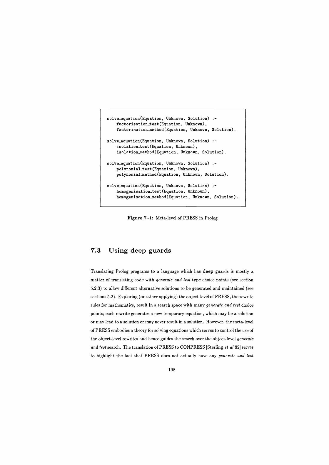
solve_equation(Equation, Unknown, Solution) :- factorisation test(Equation, Unknown), factorisation. nethod(Equation, Unknown, Solution).

solve_equation(Equation, Unknown, Solution) isolation-test (Equation, Unknown), isolation.method(Equation, Unknown, Solution).

solve_equation(Equation, Unknown, Solution) polynomial-test (Equation, Unknown), polynomial.method(Equation, Unknown, Solution).

solve_equation(Equation, Unknown, Solution) :- homogenisation_test(Equation, Unknown), homogenisationlnethod(Equation, Unknown, Solution).

Figure 7-1: Meta-level of PRESS in Prolog

7.3 Using deep guards

Translating Prolog programs to a language which has deep guards is mostly a

matter of translating code with generate and test type choice points (see section

5.2.3) to allow different alternative solutions to be generated and maintained (see

sections 5.2). Exploring (or rather applying) the object-level of PRESS, the rewrite

rules for mathematics, result in a search space with many generate and test choice

points; each rewrite generates a new temporary equation, which may be a solution

or may lead to a solution or may never result in a solution. However, the meta-level

of PRESS embodies a theory for solving equations which serves to control the use of

the object-level rewrites and hence guides the search over the object-level generate

and test search. The translation of PRESS to CONPRESS [Sterling et al 82] serves

to highlight the fact that PRESS does not actually have any generate and test

198

choice points; in that the translation essentially involves replacing Prolog's cut

operator for Concurrent Prolog's (Parlog's and GHC's) guard operator.

Consider the meta-level axioms of PRESS. The structure of the meta-rules

maps to the CCND languages in the following way. The tests for the suitability of

various solution methods becomes the guarded goals and the solution methods be-

come the body goals (which are committed to if the guards succeed), i.e. guarded

horn clauses of the following form:

solve_equation(Equation,X,Solution) :- precondition(Equation,X) : solution..method(Equation,X,Solution).

Now the meta-rules can be evaluated in parallel, and the first rule to evaluate

its guard completely is committed to. There are several points arising from this

evaluation model:

When the conditions are written the sequential evaluation of the conditions

(as in Prolog) cannot be assumed, i.e. the conditionK cannot assume the

negation of condition) to conditionK-1 being true. The only reason for

adopting knowledge of the control mechanism, like the negation of certain

goals, is performance. By knowing certain goals will have been attempted,

some computation may be prevented. In a parallel system, the evaluation

of the conditions occurs in parallel, and hence this particular efficiency as-

pect is no longer such a major consideration for the programmer. Instead

the conditions are made completely independent of textual order, i.e. they

introduce whatever explicit tests are required in each condition, even if it

means duplicating code.

Each condition must be strict enough to ensure that the action will produce

a solution because once a method is committed to there is no backtracking

to find another possible solution method. In Prolog, backtracking allows

the programmer to try another meta-rule, should the current one fail to

199

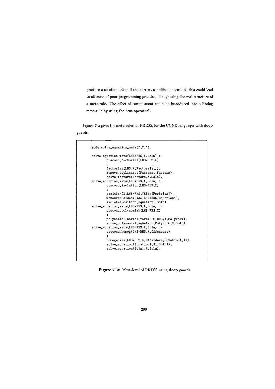
produce a solution. Even if the current condition succeeded, this could lead

to all sorts of poor programming practice, like ignoring the real structure of

a meta-rule. The effect of commitment could be introduced into a Prolog

meta-rule by using the "cut operator".

Figure 7-2 gives the meta-rules for PRESS, for the CCND languages with deep

guards.

mode solve_equation meta(?,?,").

solve_equation_meta(LHS=RHS,X,Soln) :- precond_factorial(LHS=RHS,X)

factorise(LHS,X,Factorsl\ ), remove_duplicates(Factorsl,Factors), solve_f actors(Factors,X,Soln).

solve_equation_meta(LHS=RHS,X,Soln) :- precond_ isolation(LHS=RHS,X)

position(X,LHS=RHS,[SidelPosition]), maneuver_sides(Side,LHS=RHS,Equationl), isolate(Position,Equationl,Soln).

solve_equation_meta(LHS=RHS,X,Soln) :- precond_polynomial(LHS=RHS, X)

polynomial_normal_form(LHS-RHS,X,PolyForm), solve_polynomial_equation(PolyForm,X,Soln).

solve_equation_meta(LHS=RHS,X,Soln) :- precond_homog(LHS=RHS,X,Offenders)

homogenize(LHS=RHS,X,Offenders,Equationl,X1), solve_equation(Equationl,Xl,Soln1), solve_equation(Soln1,X,Soln).

Figure 7-2: Meta-level of PRESS using deep guards

200

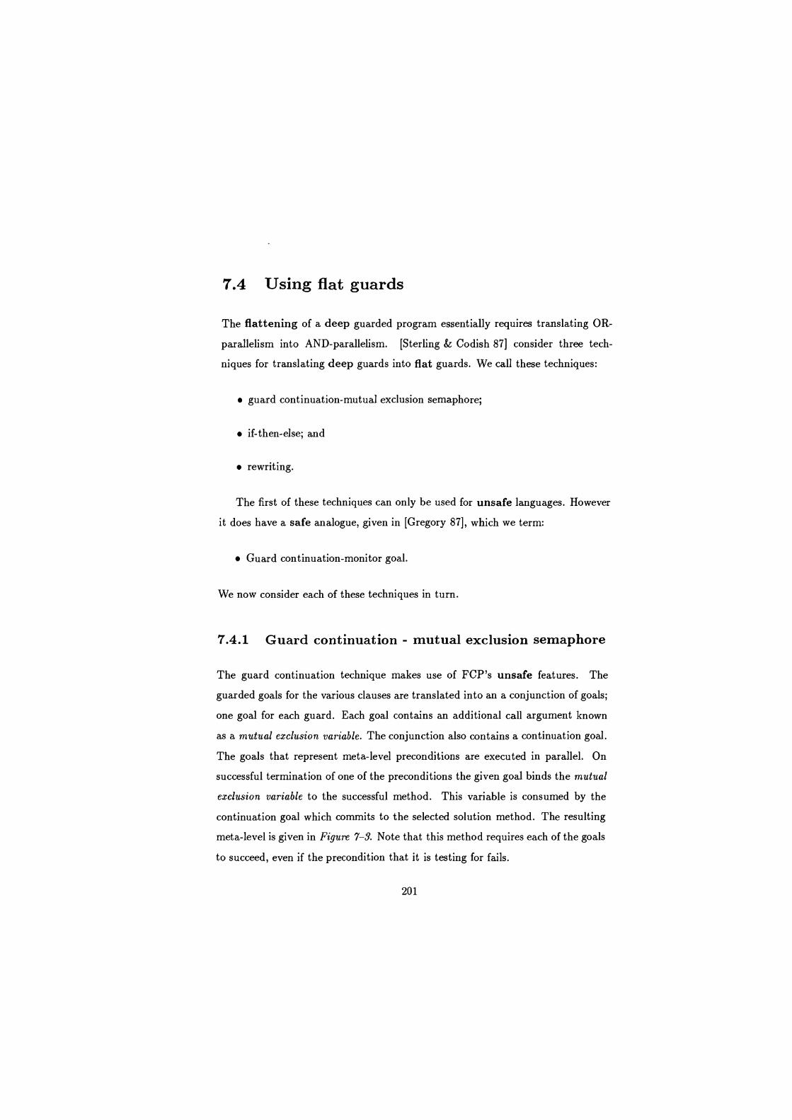
7.4 Using flat guards

The flattening of a deep guarded program essentially requires translating OR-

parallelism into AND-parallelism. [Sterling & Codish 87] consider three tech-

niques for translating deep guards into flat guards. We call these techniques:

guard continuation-mutual exclusion semaphore;

if-then-else; and

rewriting.

The first of these techniques can only be used for unsafe languages. However

it does have a safe analogue, given in [Gregory 87], which we term:

Guard continuation-monitor goal.

We now consider each of these techniques in turn.

7.4.1 Guard continuation - mutual exclusion semaphore

The guard continuation technique makes use of FCP's unsafe features. The

guarded goals for the various clauses are translated into an a conjunction of goals;

one goal for each guard. Each goal contains an additional call argument known

as a mutual exclusion variable. The conjunction also contains a continuation goal.

The goals that represent meta-level preconditions are executed in parallel. On

successful termination of one of the preconditions the given goal binds the mutual

exclusion variable to the successful method. This variable is consumed by the

continuation goal which commits to the selected solution method. The resulting

meta-level is given in Figure 7-3. Note that this method requires each of the goals

to succeed, even if the precondition that it is testing for fails.

201

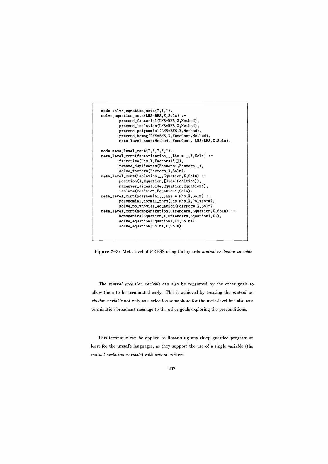
mode solve_equationmeta(?,?,"). solve_equationmeta(LHS=RHS,X,Soln) :-

precond_factorial(LHS=RHS,X,Method), precond_isolation(LHS=RHS,X,Method), precond_polynomial(LHS=RHS,X,Method), precond_homog(LHS=RHS,X,HomoCont,Method), meta_level_cont(Method, HomoCont, LHS=RHS,X,Soln).

mode meta_level_cont(?,?,?,?,").

meta_level_cont(f actorisation,_,Lhs = _,X,Soln) :- f actorise(Lhs,X,Factorsl\ ), remove_duplicates(Factorsl,Factors,_), solve_factors(Factors,X,Soln).

meta_level_cont(isolation,_,Equation,X,Soln) :- position(X,Equation,[SideIPosition]), maneuver_sides(Side,Equation,Equationl), isolate(Position,Equationl,Soln).

meta_level_cont(polynomial,_,Lhs = Rhs,X,Soln) polynomial_normal_form(Lhs-Rhs,X,PolyForm), solve_polynomial_equation(PolyForm,X,Soln).

meta_level_cont(homogenization,Offenders,Equation,X,Soln) :- homogenize(Equation,X,Offenders,Equationl,X1), solve_equation(Equationl,X1,Solnl), solve_equation(Soln1,X,Soln).

Figure 7-3: Meta-level of PRESS using flat guards-mutual exclusion variable

The mutual exclusion variable can also be consumed by the other goals to

allow them to be terminated early. This is achieved by treating the mutual ex-

clusion variable not only as a selection semaphore for the meta-level but also as a

termination broadcast message to the other goals exploring the preconditions.

This technique can be applied to flattening any deep guarded program at

least for the unsafe languages, as they support the use of a single variable (the

mutual exclusion variable) with several writers.

202

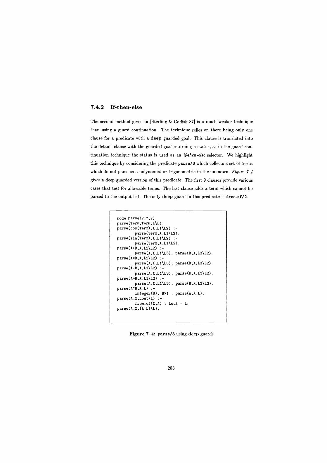
7.4.2 If-then-else

The second method given in [Sterling & Codish 871 is a much weaker technique

than using a guard continuation. The technique relies on there being only one

clause for a predicate with a deep guarded goal. This clause is translated into

the default clause with the guarded goal returning a status, as in the guard con-

tinuation technique the status is used as an if-then-else selector. We highlight

this technique by considering the predicate parse/3 which collects a set of terms

which do not parse as a polynomial or trigonometric in the unknown. Figure 7-

gives a deep guarded version of this predicate. The first 9 clauses provide various

cases that test for allowable terms. The last clause adds a term which cannot be

parsed to the output list. The only deep guard in this predicate is free_of/2.

mode parse(?,?,?). parse(Term,Term,L\L).

parse(cos(Term),X,L1\L2) :-

parse(Term,X,L1\L2).

parse(sin(Term),X,L1\L2) :-

parse(Term,X,L1\L2).

parse(A+B,X,L1\L2) :-

parse(A,X,L1\L3), parse(B,X,L3\L2).

parse(A*B,X,L1\L2) :-

parse(A,X,L1\L3), parse(B,X,L3\L2). parse(A-B,X,L1\L2) :-


parse(A=B,X,L1\L2) :-


parse(A"B,X,L) :-

integer(B), B>1 : parse(A,X,L).

parse(A,X,Lout\L) :-

free_of(X,A) : Lout = L; parse(A,X,[AIL]\L).

Figure 7-4: parse/3 using deep guards

203

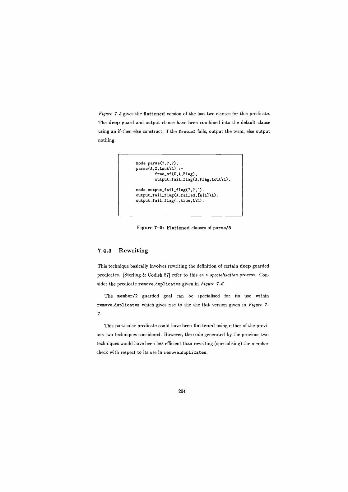
Figure 7-5 gives the flattened version of the last two clauses for this predicate.

The deep guard and output clause have been combined into the default clause

using an if-then-else construct; if the free-of fails, output the term, else output

nothing.

mode parse(?,?,?).

parse(A,X,Lout\L) :-

free_of (X,A,F1ag) ,

output_fail_flag(A,Flag,Lout\L).

mode output_fai1_f1ag(?,?,"). output_fail_flag(A,failed, [AIL] \L) .

output_fail_flag(_,true,L\L).

Figure 7-5: Flattened clauses of parse/3

7.4.3 Rewriting

This technique basically involves rewriting the definition of certain deep guarded

predicates. [Sterling & Codish 87] refer to this as a specialisation process. Con-

sider the predicate remove-duplicates given in Figure 7-6.

The member/2 guarded goal can be specialised for its use within

remove-duplicates which gives rise to the the flat version given in Figure 7-

7.

This particular predicate could have been flattened using either of the previ-

ous two techniques considered. However, the code generated by the previous two

techniques would have been less efficient than rewriting (specialising) the member

check with respect to its use in remove_duplicates.

204

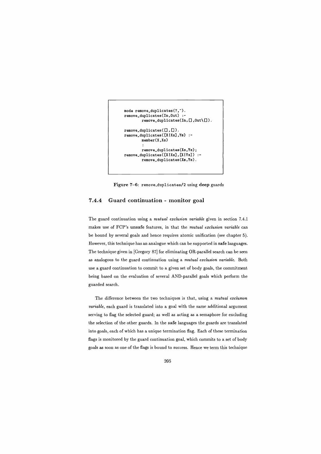
mode remove-duplicates(?,-). remove_duplicates(In,Out) :-

remove_duplicates(In, ,Outs ).

remove_duplicates(,[]). remove_duplicates([XIXs],Ys) :-

member(X,Xs)

remove_duplicates(Xs,Ys); remove_duplicates ([X I Xs] , [X I Ys]) : -

remove_duplicates(Xs,Ys).

Figure 7-6: remove-duplicates/2 using deep guards

7.4.4 Guard continuation - monitor goal

The guard continuation using a mutual exclusion variable given in section 7.4.1

makes use of FCP's unsafe features, in that the mutual exclusion variable can

be bound by several goals and hence requires atomic unification (see chapter 5).

However, this technique has an analogue which can be supported in safe languages.

The technique given in [Gregory 87] for eliminating OR-parallel search can be seen

as analogous to the guard continuation using a mutual exclusion variable. Both

use a guard continuation to commit to a given set of body goals, the commitment

being based on the evaluation of several AND-parallel goals which perform the

guarded search.

The difference between the two techniques is that, using a mutual exclusion

variable, each guard is translated into a goal with the same additional argument

serving to flag the selected guard; as well as acting as a semaphore for excluding

the selection of the other guards. In the safe languages the guards are translated

into goals, each of which has a unique termination flag. Each of these termination

flags is monitored by the guard continuation goal, which commits to a set of body

goals as soon as one of the flags is bound to success. Hence we term this technique

205

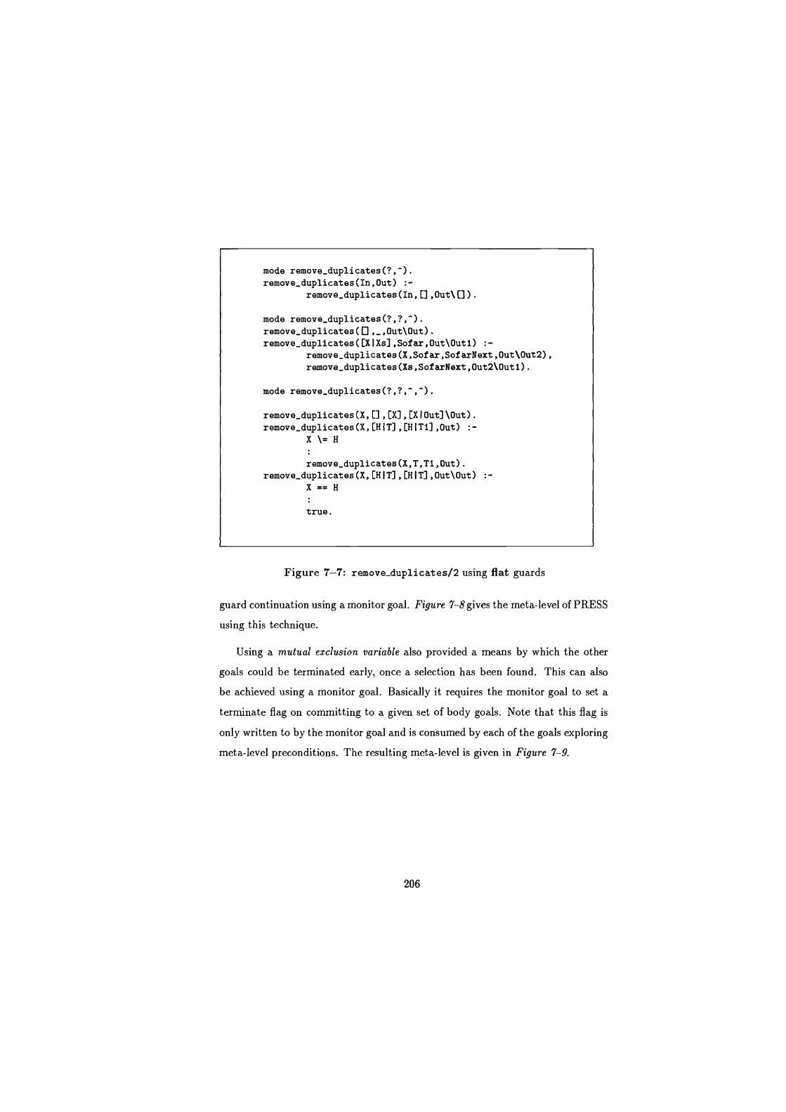
mode remove-duplicates(?,-). remove_duplicates(In,Out) :-

remove_duplicates(In,[],Out\ ) mode remove-duplicates(?,?,-).

remove_duplicates( ,_,Out\Out). remove_duplicates([XIXs],Sofar,Out\Outl) :-

remove_duplicates(X,Sofar,SofarNext,Out\Out2),

remove_duplicates(Xs,SofarNext,Out2\Out1).

mode remove_duplicates(?,?,",").

remove_duplicates (X, [] , [X] , [X I Out] \Out) .

remove_duplicates(X,[HIT],[HIT1],Out) :- X\=H

remove_duplicates(X,T,T1,Out). remove_duplicates(X,[HIT],[HIT],Out\Out) :-

X==H

true.

Figure 7-7: remove-duplicates/2 using flat guards

guard continuation using a monitor goal. Figure 7-8 gives the meta-level of PRESS

using this technique.

Using a mutual exclusion variable also provided a means by which the other

goals could be terminated early, once a selection has been found. This can also

be achieved using a monitor goal. Basically it requires the monitor goal to set a

terminate flag on committing to a given set of body goals. Note that this flag is

only written to by the monitor goal and is consumed by each of the goals exploring

meta-level preconditions. The resulting meta-level is given in Figure 7-9.

206

mode solve_equation_meta(?,?,").

solve_equation_meta(LHS=RHS,X,Soln) :- precond_f actorial(LHS=RHS,X,FactFlag), precond_isolation(LHS=RHS,X,IsoFlag), precond_polynomial(LHS=RHS,X,PolyFlag), precond_homog(LHS=RHS,X,HomoCont,HomoFlag), meta_level_cont(FactFlag,IsoFlag,PolyFlag,HomoFlag

HomoCont, LHS=RHS,X,Soln).

mode meta_level_cont(?,?,?,?,?,?,?,").

meta_level_cont(true,_,_,_,_,Lhs = _,X,Soln) .- f actorise(Lhs,X,Factorsl\ ), remove_duplicates(Factorsl,Factors,_), solve_f actors(Factors,X,Soln).

meta_level_cont(_,true,_,_,_,Equation,X,Soln) position(X,Equation,[SidelPosition]), maneuver_sides(Side,Equation,Equationl), isolate(Position,Equationl,Soln).

meta_level_cont(_,_,true,_,_,Lhs = RhS,X,Soln) :- polynomial.normal_form(Lhs-Rhs,X,PolyForm), solve.polynomial_equation(PolyForm,X,Soln).

meta_level_cont(_,_,_,true,Offenders,Equation,X,Soln) :- homogenize(Equation,X,Offenders,Equationl,X1), solve_equation(Equationl,X1,Solnl), solve_equation(Soln1,X,Soln).

Figure 7-8: Meta-level of PRESS using flat guards-monitor goal (nonterminat-

ing)

207

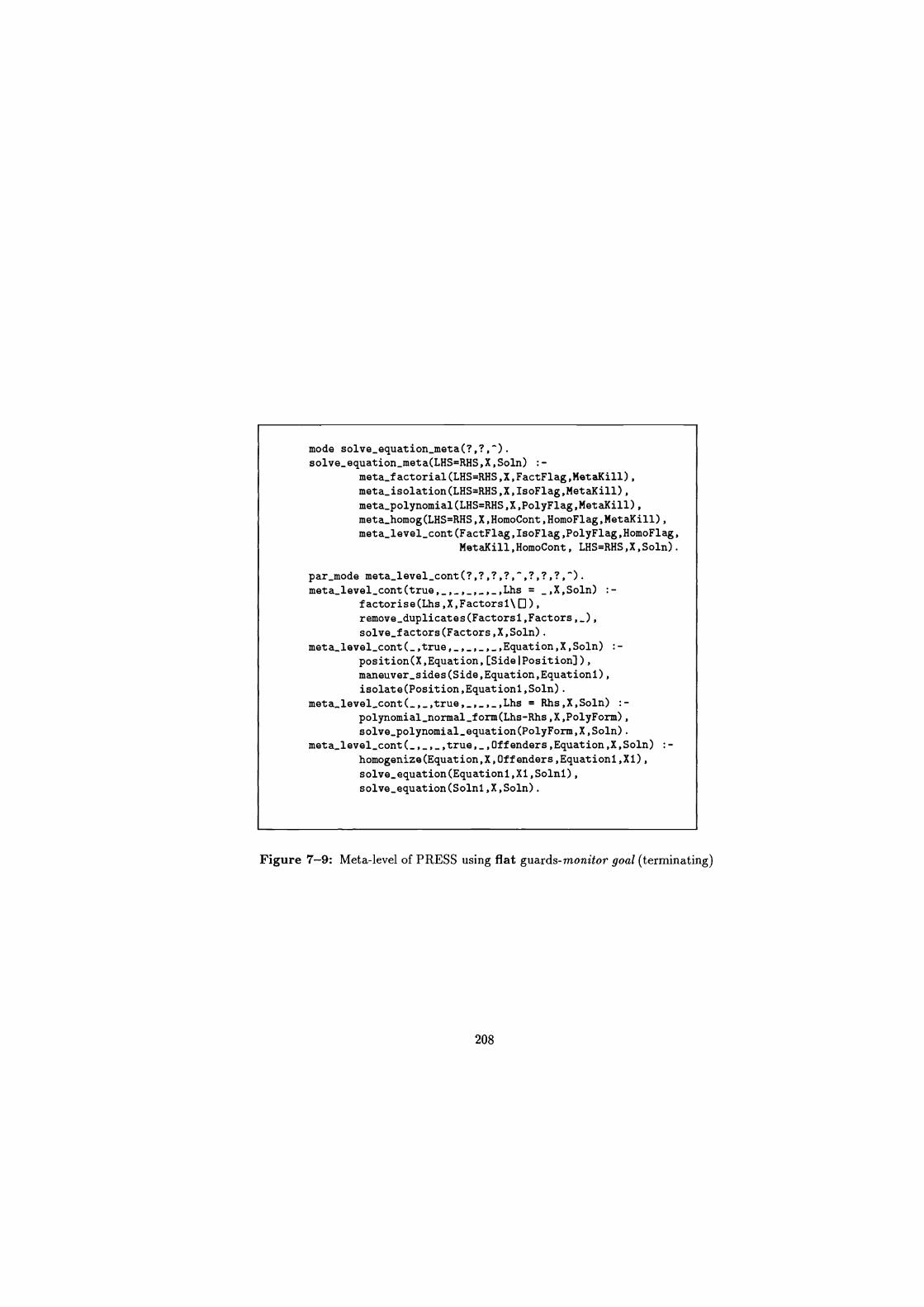
mode solve_equation_meta(?,?,"). solve_equation_meta(LHS=RHS,X,Soln)

meta_f actorial(LHS=RHS,X,FactFlag,MetaKill), meta_isolation(LHS=RHS,X,IsoFlag,MetaKill), meta_polynomial(LHS=RHS,X,PolyFlag,MetaKill), meta_homog(LHS=RHS,X,HomoCont,HomoFlag,MetaKill), meta_level_cont(FactFlag,IsoFlag,PolyFlag,HomoFlag,

MetaKill,HomoCont, LHS=RHS,X,Soln).

par mode meta_level_cont(?,?,?,?, ?,?,?,").

meta_level_cont(true,_,_,_,_,_,Lhs = _,X,Soln) .- factorise(Lhs,X,Factorsl\[]), remove_duplicates(Factorsl,Factors,_), solve_factors(Factors,X,Soln).

meta_level_cont(_,true,_,_,_,_,Equation,X,Soln) .- position(X,Equation,[SidelPosition]), maneuver_sides(Side,Equation,Equationl), isolate(Position,Equationl,Soln).

meta_level_cont(_,_,true,_,_,_,Lhs = Rhs,X,Soln) .- polynomial_normal_f orm(Lhs-Rhs,X,PolyForm), solve_polynomial_equation(PolyForm,X,Soln).

meta_level_cont(-,_,_,true,_,Offenders,Equation,X,Soln) :- homogenize(Equation,X,Offenders,Equationl,X1), solve_equation(Equationl,Xl,Soln1), solve_equation(Soln1,X,Soln).

Figure 7-9: Meta-level of PRESS using flat guards-monitor goal (terminating)

208

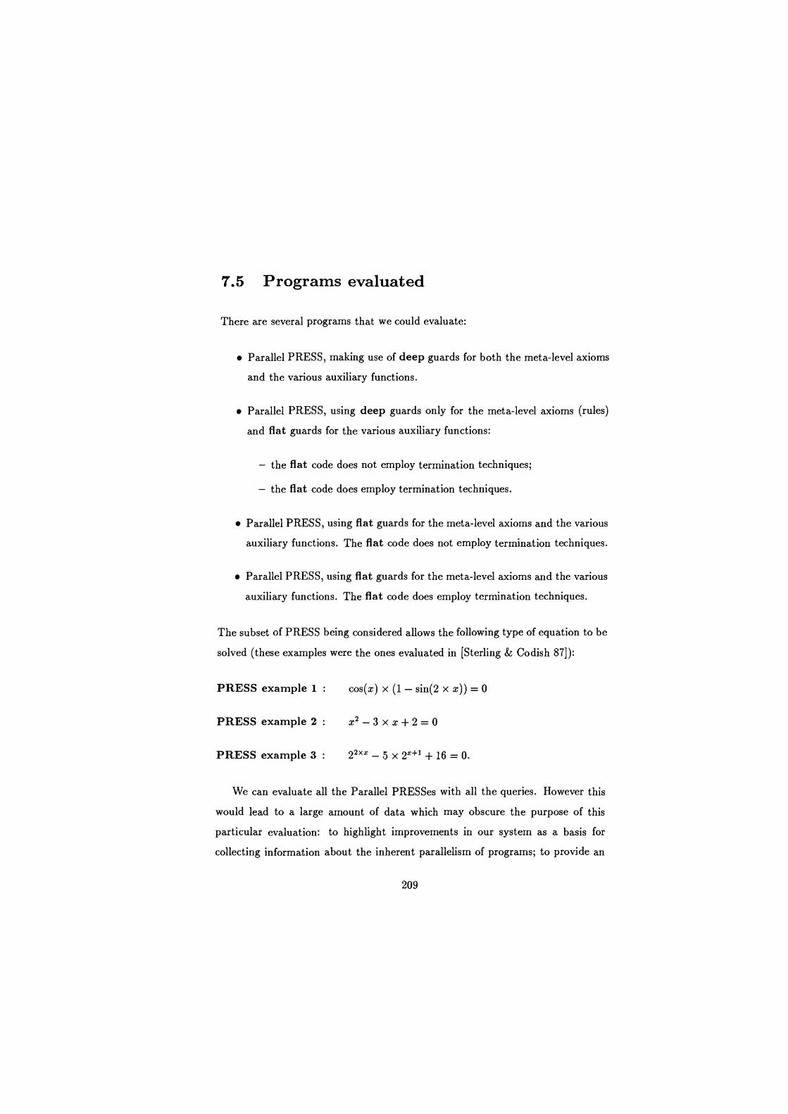
7.5 Programs evaluated

There are several programs that we could evaluate:

Parallel PRESS, making use of deep guards for both the meta-level axioms

and the various auxiliary functions.

Parallel PRESS, using deep guards only for the meta-level axioms (rules)

and flat guards for the various auxiliary functions:

- the flat code does not employ termination techniques;

- the flat code does employ termination techniques.

Parallel PRESS, using flat guards for the meta-level axioms and the various

auxiliary functions. The flat code does not employ termination techniques.

Parallel PRESS, using flat guards for the meta-level axioms and the various

auxiliary functions. The flat code does employ termination techniques.

The subset of PRESS being considered allows the following type of equation to be

solved (these examples were the ones evaluated in [Sterling & Codish 87]):

PRESS example 1 cos(x) x (1 - sin(2 x x)) = 0

PRESS example 2 x2 - 3 x x + 2 = 0

PRESS example 3 : 22xo - 5 x 20+1 + 16 = 0.

We can evaluate all the Parallel PRESSes with all the queries. However this

would lead to a large amount of data which may obscure the purpose of this

particular evaluation: to highlight improvements in our system as a basis for

collecting information about the inherent parallelism of programs; to provide an

209

application which allows us to investigate the relationship between deep and flat

guards; and to consider the effects of employing termination techniques for flat

guarded programs.

We have chosen to consider one aspect of PRESS and meta-level inference; how

the execution of the meta-level differs using deep and flat guards, where the

flat meta-levels may or may not employ termination techniques. The systems

evaluated are:

DeepPARPRESS : Parallel PRESS implemented in Parlog, employing deep

guards just for the meta-level axioms.

Flat PARPRESS-nonterm : Parallel PRESS implemented in Parlog, employing

flat guards. On successful termination of one of the preconditions (to a

meta-level axiom) the other preconditions are not terminated.

F1atPARPRESS-term : Parallel PRESS implemented in Parlog, employing


meta-level axiom) the other preconditions are terminated.

We evaluate these systems using the three example queries given above.

Using our basic Parlog interpreter (see Figure 3-1) we have reconstructed the

previous evaluation of these systems. Our raw results differ from those given in

[Sterling & Codish 871 due to using slightly different parallel implementations; we

only employ deep guards for the meta-level. However, the conclusions that can be

drawn from these results are the same as those drawn in [Sterling & Codish 87].

In the following sections we first briefly consider the conclusions that can be

drawn from the results obtained using the basic Parlog interpreter. We then

present the raw data obtained from our improved Parlog interpreter. The results

from the two interpreters are then briefly compared. We finally analyse the data

from our improved Parlog interpreter.

210

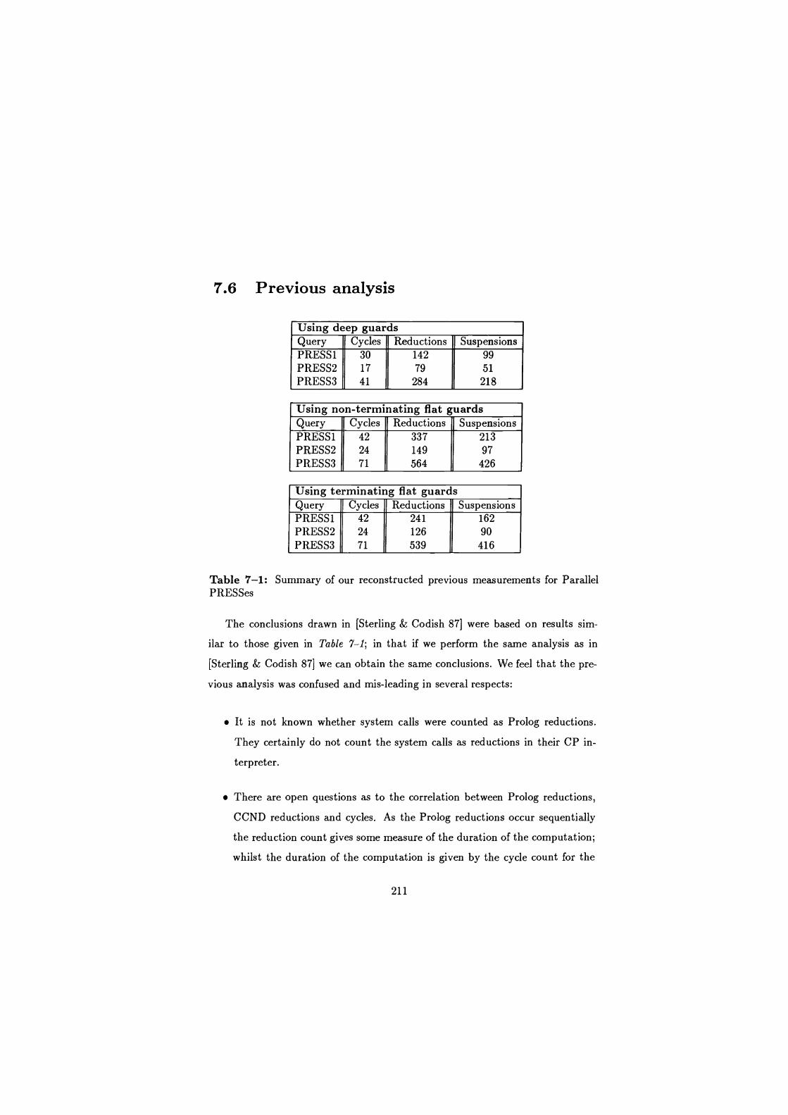
7.6 Previous analysis

Using deep guards Query Cycles Reductions Suspensions PRESS1 30 142 99 PRESS2 17 79 51 PRESS3 41 284 218

Using non-terminating flat guards Query Cycles Reductions Suspensions PRESS1 42 337 213 PRESS2 24 149 97 PRESS3 71 564 426

Using terminating flat guards Query Cycles Reductions Suspensions PRESS1 42 241 162 PRESS2 24 126 90 PRESS3 71 539 416

Table 7-1: Summary of our reconstructed previous measurements for Parallel PRESSes

The conclusions drawn in [Sterling & Codish 87] were based on results sim-

ilar to those given in Table 7-1; in that if we perform the same analysis as in

[Sterling & Codish 87] we can obtain the same conclusions. We feel that the pre-

vious analysis was confused and mis-leading in several respects:

It is not known whether system calls were counted as Prolog reductions.

They certainly do not count the system calls as reductions in their CP in-

terpreter.

There are open questions as to the correlation between Prolog reductions,

CCND reductions and cycles. As the Prolog reductions occur sequentially

the reduction count gives some measure of the duration of the computation;

whilst the duration of the computation is given by the cycle count for the

211

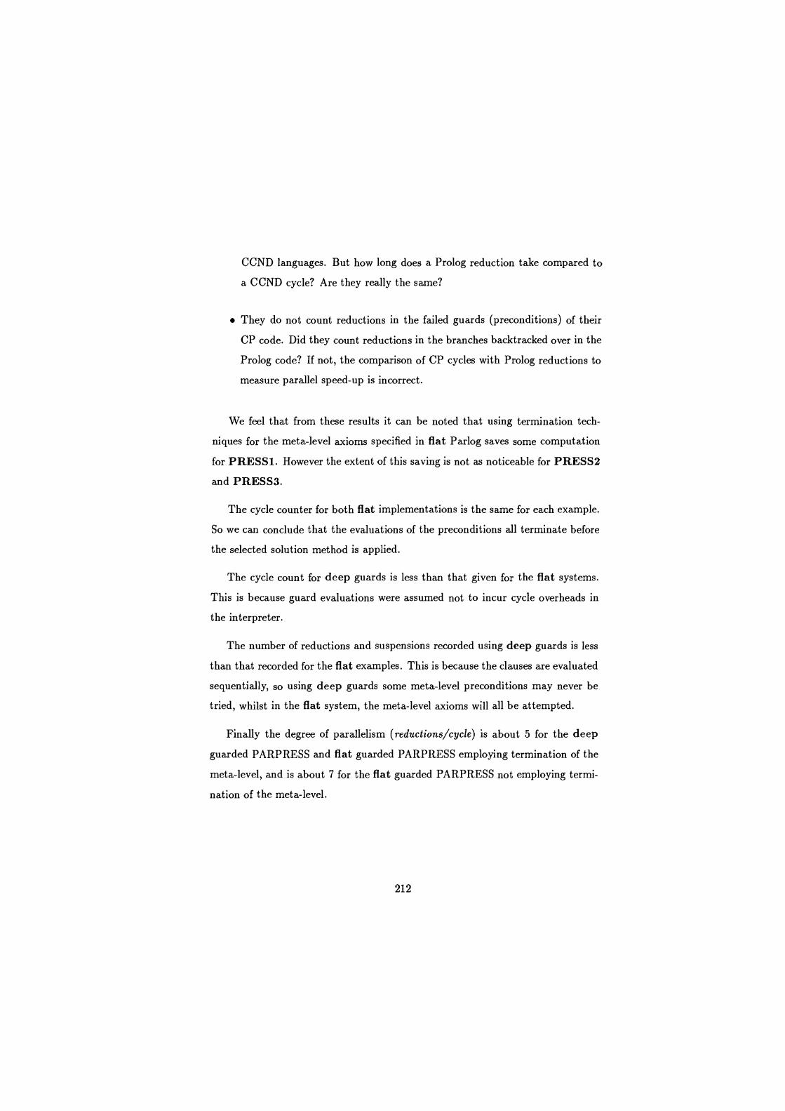
CCND languages. But how long does a Prolog reduction take compared to

a CCND cycle? Are they really the same?

They do not count reductions in the failed guards (preconditions) of their

CP code. Did they count reductions in the branches backtracked over in the

Prolog code? If not, the comparison of CP cycles with Prolog reductions to

measure parallel speed-up is incorrect.

We feel that from these results it can be noted that using termination tech-

niques for the meta-level axioms specified in flat Parlog saves some computation

for PRESSI. However the extent of this saving is not as noticeable for PRESS2

and PRESS3.

The cycle counter for both flat implementations is the same for each example.

So we can conclude that the evaluations of the preconditions all terminate before

the selected solution method is applied.

The cycle count for deep guards is less than that given for the flat systems.

This is because guard evaluations were assumed not to incur cycle overheads in

the interpreter.

The number of reductions and suspensions recorded using deep guards is less

than that recorded for the flat examples. This is because the clauses are evaluated

sequentially, so using deep guards some meta-level preconditions may never be

tried, whilst in the flat system, the meta-level axioms will all be attempted.

Finally the degree of parallelism (reductions/cycle) is about 5 for the deep

guarded PARPRESS and flat guarded PARPRESS employing termination of the

meta-level, and is about 7 for the flat guarded PARPRESS not employing termi-

nation of the meta-level.

212

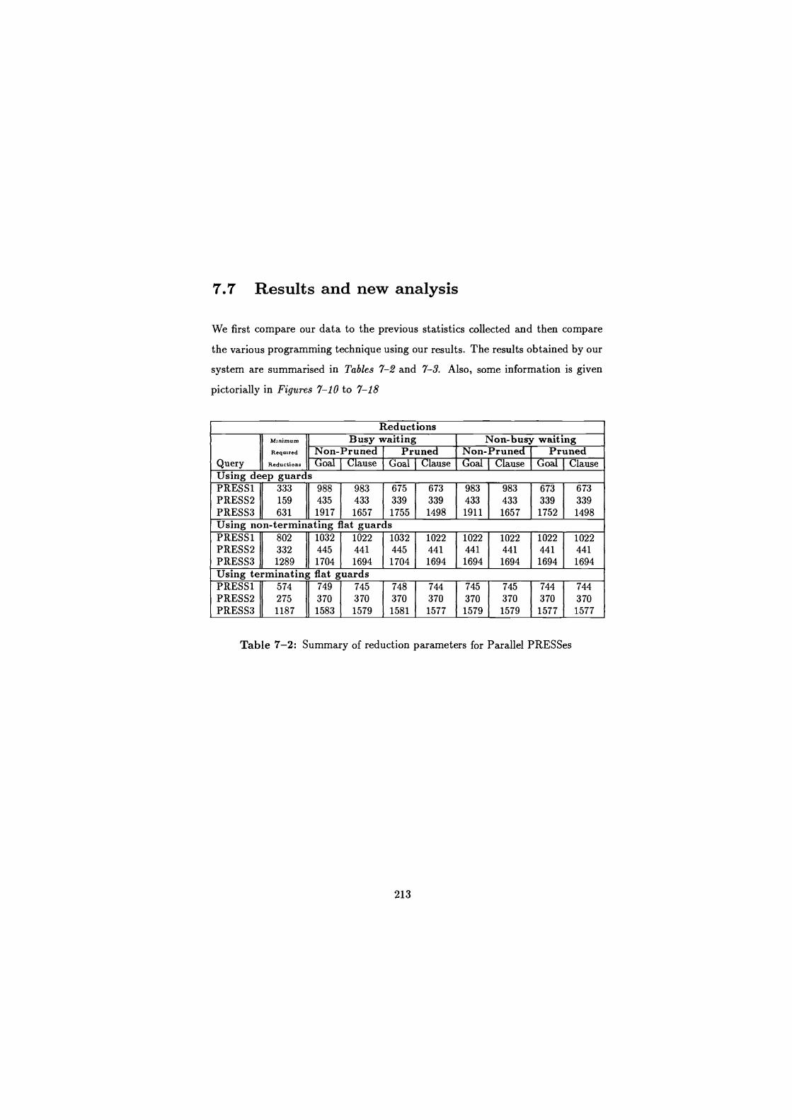
7.7 Results and new analysis

We first compare our data to the previous statistics collected and then compare

the various programming technique using our results. The results obtained by our

system are summarised in Tables 7-2 and 7-3. Also, some information is given

pictorially in Figures 7-10 to 7-18

Reductions Minimum Busy waiting Non-busy waiting Required Non-Pruned Pruned Non-Prune Pruned

Query Reductions Goal Clause Goal Clause o ause Goal Clause Using deep guard s

PRESS1 PRESS2 PRESS3

333 159

631

988 435 1917

983 433 1657

675 339 1755

673 339 1498

983 433 1911

983 433 1657

673 339 1752

673 339 1498

Using non-terminating flat guards PRESSI PRESS2 PRESS3

802 332 1289

1032 445 1704

1022 441 1694

1032 445 1704

1022 441 1694

1022 441 1694

1022 441 1694

1022 441

1694

1022 441 1694

Using terminatin g flat guards PRESS1 PRESS2 PRESS3

574 275 1187

749

370 1583

745 370 1579

748 370 1581

744 370 1577

745

370 1579

745 370 1579

744

370 1577

744

370 1577

Table 7-2: Summary of reduction parameters for Parallel PRESSes

213

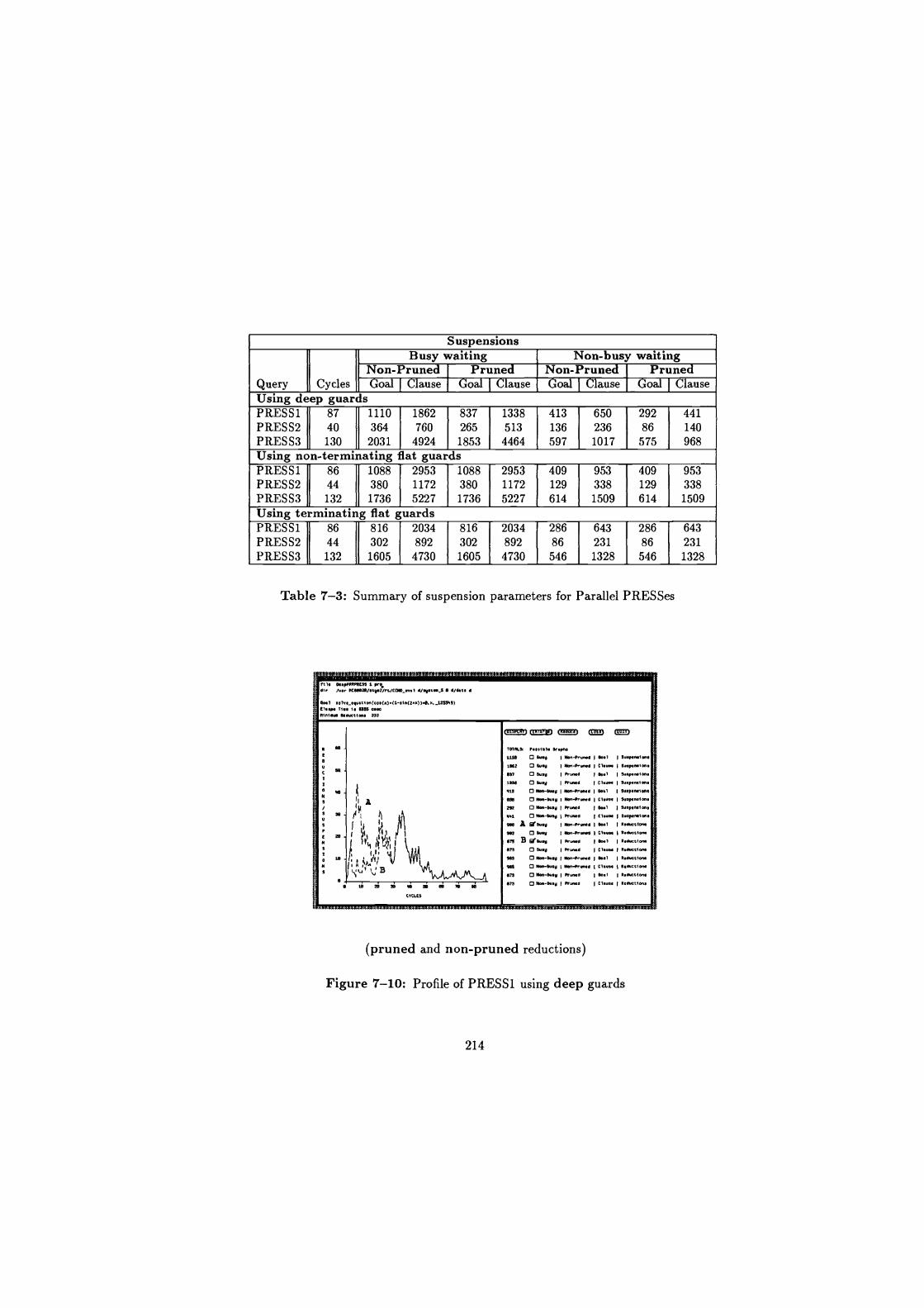
Suspensions Busy waiting Non-busy waiting

Non-Pruned Pruned Non-Prune Prune Query Cycles Goal Clause o Clause o ause Goal Clause Using deep guards PRESS1 PRESS2 PRESS3

87

40

130

1110

364

2031

1862

760

4924

837

265

1853

1338

513

4464

413

136

597

650

236

1017

292

86

575

441

140

968

Using non-terminating flat guards PRESS1 PRESS2 PRESS3

86

44

132

1088

380

1736

2953

1172

5227

1088

380

1736

2953

1172

5227

409

129

614

953

338

1509

409

129

614

953

338

1509

Using terminating flat guards PRESS1 PRESS2 PRESS3

86

44

132

816

302

1605

2034

892

4730

816

302

1605

2034

892

4730

286

86

546

643

231

1328

286

86

546

643

231

1328

Table 7-3: Summary of suspension parameters for Parallel PRESSes

I+1. 0.4NMtMESS 1 p.% d+r hr MCtle2!/.y2/rt/COID_rvel ./ty.ts ! e d/attv d

eo.1 .olve_ta..t+M(t0$(M).(1-.1n(2.M)).O.M._Z.2SA9)

E1..p. T+.. + SUS 0.ao Mn+... Md.tt+M. 979

TOIMLIC p..e+.l. tr.pn. 1110 0 W.y I NMir.Md I W.i a.ep.M+M.

1992 I I I NMM.d I C1.... 9n 0 W.9 I R.Md 1 0.0 1 W.p.M+M. 1990 0 W.y I .r.Md I V... I I..p.M+M. 119 0 Non-eu.y I ewn-PIun.a 19..1 I S..P.-MMt 058 NM-Wey I NM-honed I CIA.. I l..peM+M. 212 NM-W.y Pr. ed I N1 I l.ep.M1 M. 1.1 0 MM-w.y 1 .ewMd I CA- SWp.M+M.

910 A RrW.9 NM-prwrd I ew1 1 R.d.OitOM

9q 0 W.y NOn-P . d Ctwr 1 9dwt/MM 129 B IY9wy I ft~ 1 9w1 1 .d.OO+OM

STS 0 W.9 I pr.Md C1..r 1 Rsd.ct+oM

9I 0 NMn-W.y I 01M'p-d I MW I R.duteM 919 MM-W.y I NMtrgMd I Ctwss) R.wtt+MM

929 0 N.n-I, I .r.Md I W.1 I RMO.eNMM

973 0 NM-Wey pruned 1 Cl... I Red.oL+MM

CYCLES

(pruned and non-pruned reductions)

Figure 7-10: Profile of PRESS1 using deep guards

214

7111 F1.IPRRMEssJwd..,. t p.e dtr 1 m- NCNB7/t.s.urt/CUIO_.o.T d/.5.I.. 0 d/NU.d

Ee.u .oTO._.g.tlan(.00(.).(t-.tn(2..))l, r. it'81f) El.." T1.. I. 10773 0.00 Ntn1.1/ $.do.tlawt Ni

ISO .lIIrsPtw 0P0 t":! ® t"r in

R TOTf11A: 5.0.101. 1r.pM E !e 1000 O wry I Nen-Nrn.a 0r1 w.p.nsl- 5 xsss Cl 3.0411 11170-Muwd I c1.Pr 107P.MOr

es C Less E3 n0 I Pruwd 1 On, 1 S.Swsler

x 70 2163 0 I-v I Pr004d CT.... 13wP.,wlaro 0 400 0 Nr-00.0 W_-Pr. ,.d 111.1 I w.N..Imw W 00 300 Na14W.y 1 Nr-huw0 C1.7 w.Pnoom / 400 0 Nm-Wry I P-d 00.1 I S.."n for

es s 133 13 Wr-00ry prlwd I c1.ur I w.P.n.1or 6 9 N 1002 Ere." I Nr-Pr1n. aT 1 RNUet1w.

1002 0 Mw0 1 Nr-Prawd C1.ur E 10 N fest 400.0 I P__4 I dr1 R.FNt1ew

= m "5 II

L022 M sw5 Pron.. Must 1 R.dwttw.

0 1 1022 o Nat-key 1 Won-Pr d dw1 I R.duetlo

N 10 A 1012 0 004-00.5 I N1.P I CT.ar 1 R.dottlw. S Laxs 0 Nr-0404 I vruwa d.i I R.wt1..

e 14 as 1s 50 so 70 w YO 1022 0 000-0075 I Pr004d I C1.ur I amula tom

CYCLES


Figure 7-11: Profile of PRESS1 using (non-terminating) flat guards

M. F1.IM1RPOE33_1ir 1.p. dl. /u.. NC000m/.t92/rt/CD*_...1 d/.ptw S 0 d/MU d

[1..pd TIM 1. 0191 0.9e b.T, r1r_.p,.t1.n(oo.(.).(t-.ln(i..))l.., U3501)

M.,... RN.wt/040 374

TOTALS, P0r10TI 0npr, sis M 04.0 1 N.n-Prow! 1 0041 I Su.p.n.lon 2011 0 0070 I NS,.-Pr.P.d I Cl$0 I Wp.n.Iar 010 0 wry I Prawd 1 00.1 I w.p.n.lon. 2034 0 W15 I Pruw6 C1.ur I w.p.nslaN 200 0 N0n-MUV I Non-Pruned 1 0q1 I w.pen.low 003 0 0.0-M-0 I Non-Pron.d C1wr I w.p.n.lnw 206 E3 110-00040 1111,- 16..1 I w.psP.ldw 143 0 New-3000 Prw.d 1 Ci.u.. I Sump ...I.. As 'I0y Nen-P-od 1 0r1 1 0.d.t11.0. 743 0 0055 I Non-Iron. I CT.ur I R.d.tlon.

In

1 0

livk) Pry v v is i3 10 4e so 00 79 r

w

CYCLES

714 O soy PP.w. CT.or I R.dwiton. 710 Gr 04.0 1

Pr.wd 1 00.1 1 Reduttlon.

T3 0 N7..-Ors Nen-run. I loll I Rrductton.

751 0 Ilen-0045 511-5.00. C1e0. 10.dwtI.S 744 0 Ne.-sw0 I M'0P. I 8e.1 1 Rtauctlent

TN 0 yen-sury Rw.d I Ch.- (Rtduot10..


Figure 7-12: Profile of PRESS1 using (terminating) flat guards

215

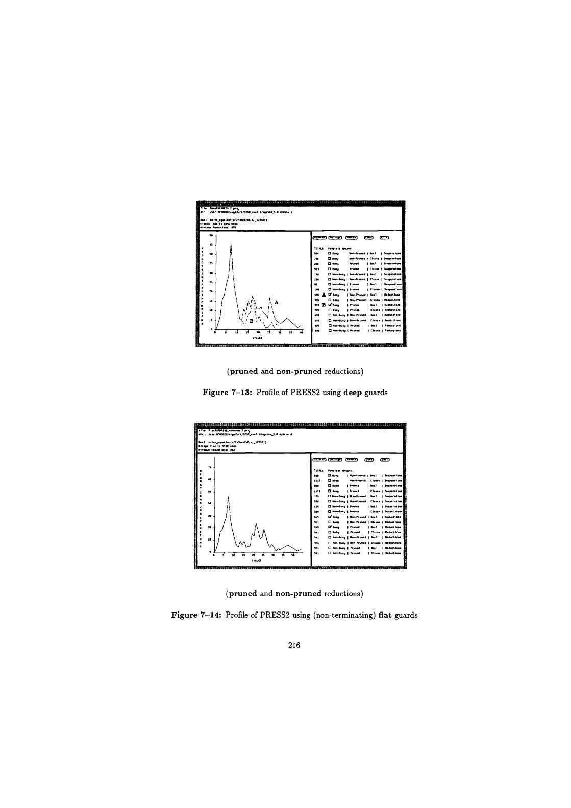
fl 1. MgPMVRE33 2 pro, 510 /u.r .[6.023/.kWI2/r0/CCW_.-I 6/.Y.C...3 0 0410 0

N

I 6701. sslvi_.11NC10..Co 2-Y6.2.6. K 125"11 El..p. TI.. I 13995 5..5 0195.40 0.6405150.. 133

50

90

"

30

25 , 3 Y 20

13

0 5 10 LS 20 25 = S5 "

T.IRL7: P1 61616 Yob. !64 0 6449 1 000-0405 166.1 I WIM.110n.

730 0 6409 1 0.11-05500

1 111411 154,.6.150

230 06-9 Prance 16551 I !-,.401550 !15 0 6449 I Pnn.O Cl... S.W.n.5on.

150 0 656-65.9 1650-Pr1M4 ( 6651 I 544,.0015 0

21. 0 650-W.y 1650-Pr.nN 1 Clog.. I S. M.-/50. 66 0 95.-W.y I .14110 115.1 I S.y.n.1.M 1V 0 M.-W.y ft-1 Cl... 1301,.5.1.0. 435 A 5t140y 1

656-0440 16611 101/5551550

on 0 656-0*69 I P14M6 1 5551 I 1.0t51514 4" 0 955-90.9 1455-0.505 I C. 15.90[515.5

535 0 Wty I P14506 I Cl.us. I R60u55la

4" 0 H4*464.9 I N55-10446 1 65.1 19.41.0-

437

B 0 5- 1456-01.4Y I [1.40. 11404.15.4

9" B 33.09 .04505 1 66.1 I 1.6.C51w

311 0 6.-65.9 P145p 101.4.. 10.000515.4

CYCLES



f11. PI.*RRP0E"_50o0.n 2 pry 6o- . /1100 6[33020/.ky.2/r5/CCNQ,.Y.1 0/,.C.1rS 0 0/0.5. 5

Boll 0515._.30.5(50(1023..21...125521) Eh..p. 1/x ,. 442. cue 6/51.011554011554* 332

1.

Iil

15TRL3 Ps.0611 M.p9.. 3.0 0 15.4. 1655-0.500 105.1 15.55.5.1400 1112 0 W, I Nm-Pr4nla I Cl... I Wlp.."_ ... 0 W W I Prw66

1 6.1 190.43077

1112 0 60, 10440 Cl.- 130.7.551550 129 0 900.4.9 1655-.055.6 .5.1 13417n.lo50 !!. 0 Nd.-5u.y 1655-104003 111.0.1 130.p00t/50 129 0 605-55.44 105506 6651 I W.Mn51.M

53. 0 905-6449 0440 11.51, I Wspe5M0M

445 g 6-y 16511-11045.0 115.1 I R.6-5150.

541 0 Wy 1955-1114 .6 I Cl.... 1 6.04451550

44! ®'W.(( 10446 166.1 1 1405115n.

441 0 6419 1055.6 111.406 1 9.0005155.

441 0 Na 4*..y I N.n-0-10 166.1 19.5011/00.

441 0 60o-&_U 1655-/05.06 111.401 11105501155.

441 0 950-M4y 151 406 15.1 1150451100 411 0 900-0-9 100...6 I Cl.w1 111.0001/en. 18 U 20 2S I SS 411

CYCLES



216

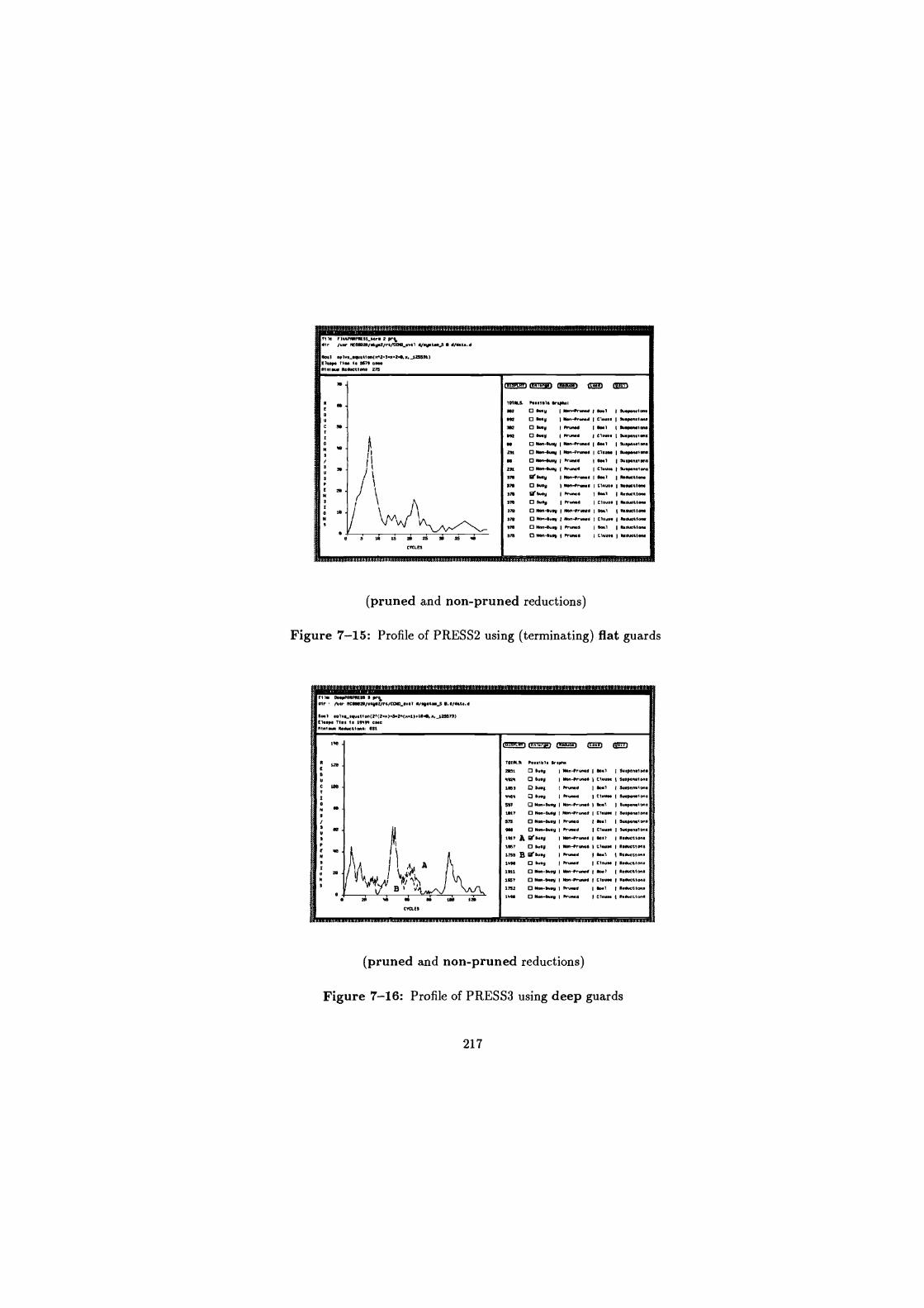
1115 111,PNIPI1E53_ttr 2 yr% s+r Iur ncesilm/.ty2/rt/COm_.r.l yry.*. 5 1/4u.5

E.01..1 e,lv._W.tia(S"2-a.,.2.Y..2551R) ry. TI.. I. 3579 cae

5137 W. 5e3O0tIa. 275

70 ® . ® O 5 10710.. P..1575 M.pll.s [ 662 17 W.y I N.Mrua. I .o.l au..a+Om y .a2 n Wy I N...+rae I n.u.. I Wp.n./a, C as 592 E3 1545 haN 1110.1 I W.p.a+ea [ a92 O 0.y hun.a ) Ct.un 1 03.5,75.7.0.

O a E3 N.0-u.y I M.0rOae I .at 13upe b+.0 N W a

' z30 [] N.04.u.y (Non-vr....e I Cl- I wa.nnen. SO 17 w.-Wp i ft-5 8a1 I W.Mbt1011.

a , 231 E3 Hen-....y Iw.N4 I Cl.... SWp.n+a.

a 1 a10 d W.y I Nmirun.a I Oat I R.ACt13N 5 371 O W. y t lbnruae I Clw.. I WOUlea /

SA 3W.y I /rwrs 1 6.1 O.JUrt1a.

$7O E3 W.y I hun.0 I Cl.... I S.e.Nti.O.

3 Ip 1 - 77. O Na.4u,y Non-pru75.. I aat 15aaaclea

N ,1

V`,/ )q N.n-G." Non-/ruaa C .w aMnt lws aNl O N.n-euay h I ur0 al I le.a.cttem

e s A u a6 zs s as SR O Na-Duty .runt, C,_.. I g0uetlea

CYCLES



11 E9 19

r+l.i 0..55508350 O POD 31r /u.r IC.M29/.xy.z/rt/CCNO_.wi q.y.ta} /../etc...

.0.1 .olvt_.qwt+.0(In(I.+.).S.I+(a.21.1Or. 0.X2875) El..pe TI.. 1. 1933. to Mn+0. 6Awt+ma sit

0

® MM

1015Lai P0..+ble unpin 2031 0 W.y NOn4run.a 190.1 1 3e.p.a1.0. 9929 W.y I Non-Haas I C1...a I Wtp.a+.0. 163 I] So.y 1 P-d 1 6.1 SOtpeala. 196, ...y h Cl.,.. 30.5.75.+.0.

597 N.0-WV I N.0-Prone ..751 1 Oosp.n.7.0.

1511 E3 Na-W.V f M.0-ruae I Cl.... I 3..p.a+.0. 573 N.0-Eu.y I huge 1 0..1 I Su.5.n./.0. 9.. Hen-0355 I Prune I Cl.ua I wtp.alat 1917 A 31'50.y 110.75-0755.0.0 33.1 115315c1055

167 W.y I NOe-PenS 1 Claw" I I.Iwtla. 3755 B 6Y W.y huge 110o7 15.mec/.0. S.N E3 Say s,-s0 I Cl.- 15.evtc.- 1301 E3 N.0-W,y I N.0-P,*n.e 1 ,a1 1 5 350 IOnt

167 E3 Piss-03.5 I 110-P,Oad I C1.Oa 15..0095.0. 1752 E3 Non-3v I pr.+a! 141 I I.a0clae 1105 N.0-03.5 I huge I Closes I O.M.et1.05

ffillsom



217

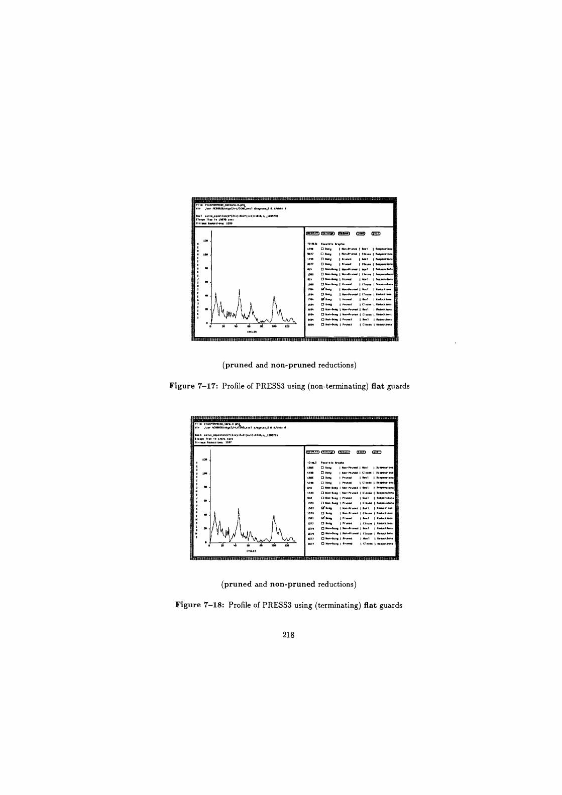
fl1. fa,xEsz artiascas.¢l uEE- Aunxctzs:vlLtsesxa"°&xzlxttifls&-115.,00>)e.exeitl., uui:i,l s...oebai

61r /.K 11[!6525/skyet/rt/COO v171 d/1774..' 0.d/bt& d

50.1 II7..qu.tl67(2^(2.^)S.2^(6.1).13.0.; 123614) [!17.617 TI.e I. 19070 en. finish. [NU.t/on.: 1231

F 1.11 SVNE/!-pmt.r..S.K%

In J

! 6 M

CYCL[S

TOTALS/ Pl..Ibl. M.P6s

1599 O NM-461 I PruMd CI.un 16.MKtlon.

153 13 Non-461 Non-Pru3d 150.1 I S.duot/m..

1511 O 360-461 1507, ~ I Cl.u.. 13N1761111.1

1691 0 333-51.9 10,136 I 8n1 1551.106167.

leer O Mh.y I N.7,-Prunq I Cl.... 15...11111..

6756 61.9 I PrUMd I So.1 I ..du6t/a.. 1699 O 1359 Pruned CI..... 510.1611691

173 fire1.y I Non-PruM6 I Swt 15.0,11 tlae

1770 0 519 I N6n-Pruned 1 e..t swpenn.77

$227 0 O.V I Non-PrunW I CI.... 151.3133161.

17,e O 51.9 I PrS67d 156171 !1.110.1.7,.

5227 13 S,h.y Prwd I Ci.... 51.P.m16n.

O. 13 317-W.y 130n-M 156.1 1016663111. 1509 0 Non-461 I Non-Prunes I CI.... 1 17.1131.70

h.9 0 36114171 Pr17,/.1 I 56.1 I W17110.10n.

1505 0 N66-461 I Pra..6 1 C1.1.. !1.673103



fi .'F-( 'Y-Si &adfize$$&L Lk. Ft11 1kfk LF EY.Q,Il.C 9II 4.4S'$4R445,(4311.L-1E {.1t153eaoi eeeooaevi,tii

dir /u. MC66920/.k9e2/rt/C6NO_7v.l d/.911.._5 0 d/d.u d

P1.tPM7P3E13 t.r..! KAS

56.9 ..IV._.q..1lo7,(2^(2.^)4.2^(^.1).10.6.^. 123373) [1..66 2151 I. 17371 6.66 317,1.1. Mdu.cl On.. 1107

TOTALS P0..191. 63ph1

1793 0 51 I Non-P-d 150.1 3u.pm/on. .770 o 461 1 607-Pru3d I Cl.u.. I S..Pon./ens

SOB! 13 611 I Pruned 10..1 I t1.111.e161.

9733 0 461 I Pru7,1d 1 C/.u.. I SI.Pennon.

5.6 13 Nat-1179 I N6n-Pruned I 4e.1 1 lu.P.1,1.7. Site 0 N1W1 1516^-Pruned I Cl- 146.6.7,./67

596 13 3111-01.9 I Pru119d 00.1 146.11n./.n1

1520 13 50747.9 I Pruned C1.ow lwpnalon. 15$! 61- ea1 1367,-Pr177d I 4W 1 5.61.1)0111

1579 13 461 I 51.6-Pruned ( (1.76. B.ductI6,

1901 or 461 I Pruned Swl 16.6,111)07.

1377 O 5099 I Pr77.4 I C16u" 13.5.1611711.

1579 C3 Non-4669 1306-Pruned I ew1 I Mw11111n.

1579 01.1111 N0-Pl T7 I C1.up 16.61.1/67,1

177 13 N.6-461 I Pru651 1 17.1 1 3.0111107,.

1377 13 N.n-W1 I Pr-51 C1..- 13.6,111166.



218

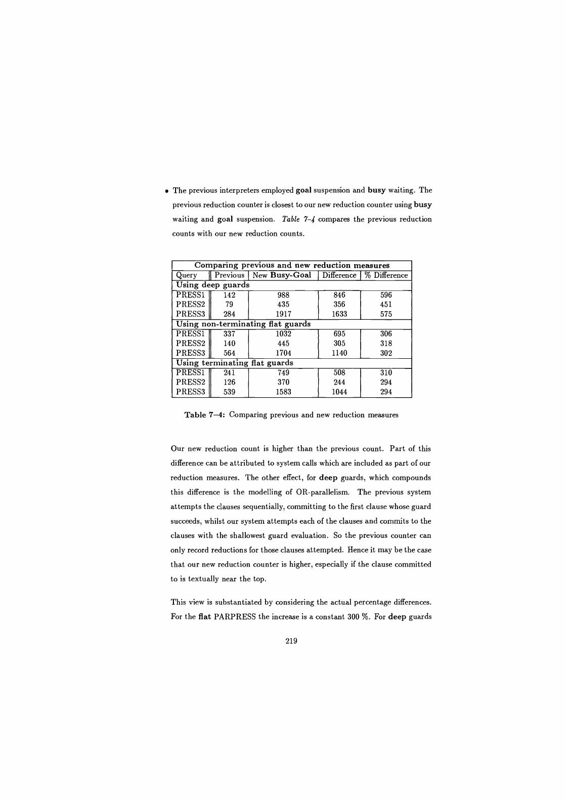
The previous interpreters employed goal suspension and busy waiting. The

previous reduction counter is closest to our new reduction counter using busy

waiting and goal suspension. Table 7-4 compares the previous reduction

counts with our new reduction counts.

Comparing previous and new reduction measures Query 1 1 Previous New Busy-Goal Difference % Difference Using deep guards PRESS 1 142 988 846 596 PRESS2 79

T 435 356 451

PRESS3 284 1917 1633 575 Using non-terminating flat guards PRESS1 337 1032 695 306 PRESS2 140 445 305 318 PRESS3 564 1704 1140 302 Using terminating flat guards PRESS1 241 749 508 310 PRESS2 126 370 244 294 PRESS3 539 1583 1044 294

Table 7-4: Comparing previous and new reduction measures

Our new reduction count is higher than the previous count. Part of this

difference can be attributed to system calls which are included as part of our

reduction measures. The other effect, for deep guards, which compounds

this difference is the modelling of OR-parallelism. The previous system

attempts the clauses sequentially, committing to the first clause whose guard

succeeds, whilst our system attempts each of the clauses and commits to the

clauses with the shallowest guard evaluation. So the previous counter can

only record reductions for those clauses attempted. Hence it may be the case

that our new reduction counter is higher, especially if the clause committed

to is textually near the top.

This view is substantiated by considering the actual percentage differences.

For the flat PARPRESS the increase is a constant 300 %. For deep guards

219

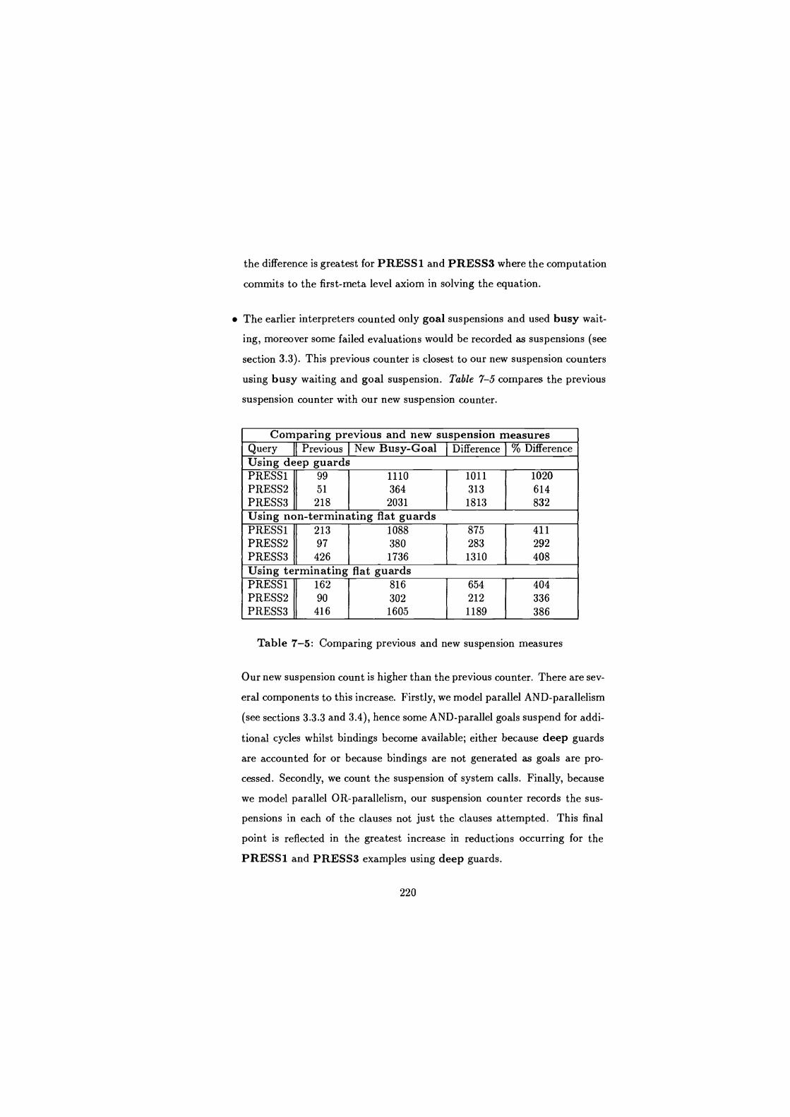
the difference is greatest for PRESS 1 and PRESS3 where the computation

commits to the first-meta level axiom in solving the equation.

The earlier interpreters counted only goal suspensions and used busy wait-

ing, moreover some failed evaluations would be recorded as suspensions (see

section 3.3). This previous counter is closest to our new suspension counters

using busy waiting and goal suspension. Table 7-5 compares the previous

suspension counter with our new suspension counter.

Comparing previous and new suspension measures Query 1 1 Previous New Busy-Goal Difference % Difference Using deep guards PRESS 1 99 1110 1011 1020 PRESS2 51 364 313 614 PRESS3 218 2031 1813 832

Using non-terminating flat guards PRESS1 213 1088 875 411

PRESS2 97 380 283 292

PRESS3 426 1736 1310 408

Using terminating flat guards PRESS1 162 816 654 404 PRESS2 90 302 212 336 PRESS3 416 1605 1189 386

Table 7-5: Comparing previous and new suspension measures

Our new suspension count is higher than the previous counter. There are sev-

eral components to this increase. Firstly, we model parallel AND-parallelism

(see sections 3.3.3 and 3.4), hence some AND-parallel goals suspend for addi-

tional cycles whilst bindings become available; either because deep guards

are accounted for or because bindings are not generated as goals are pro-

cessed. Secondly, we count the suspension of system calls. Finally, because

we model parallel OR-parallelism, our suspension counter records the sus-

pensions in each of the clauses not just the clauses attempted. This final

point is reflected in the greatest increase in reductions occurring for the

PRESS1 and PRESS3 examples using deep guards.

220

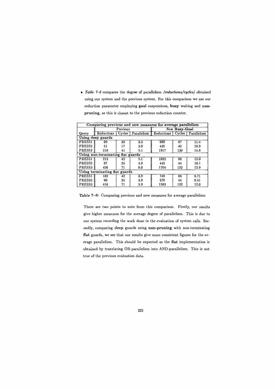
Table 7-6 compares the degree of parallelism (reductions/cycles obtained

using our system and the previous system. For this comparison we use our

reduction parameter employing goal suspensions, busy waiting and non-

pruning, as this is closest to the previous reduction counter.

Comparing previous and new measures for average parallelism

1 1

Previous 1 1

New Busy-Goal Query Reductions Cycles Parallelism Reductions Cycles Parallelism Using deep guards PRESS1 99 30 3.3 988 87 11.4 PRESS2 51 17 3.0 435 40 10.9 PRESS3 218 41 5.1 1917 130 14.8 Using non-terminating flat guards PRESS1 213 42 5.1 1032 86 12.0 PRESS2 97 24 4.0 445 44 10.1 PRESS 3 426 71 6.0 1704 132 12.9 Using terminating flat guard s

PRESS 1

162 42 3.9 749 86 8.71 PRESS2

1

90

1

24 3.8 370 44 8.41 PRESS 3 416 71 5.9 1583 132 12.0

Table 7-6: Comparing previous and new measures for average parallelism

There are two points to note from this comparison. Firstly, our results

give higher measures for the average degree of parallelism. This is due to

our system recording the work done in the evaluation of system calls. Sec-

ondly, comparing deep guards using non-pruning with non-terminating

flat guards, we see that our results give more consistent figures for the av-

erage parallelism. This should be expected as the flat implementation is

obtained by translating OR-parallelism into AND-parallelism. This is not

true of the previous evaluation data.

221

We now carry out an analysis, based on our new results, of the various Parallel

PARPRESS systems.

For the flat PARPRESSes there is little or no difference in the reduction

counts using goal and clause suspensions (see Table 7-2). As suspensions

do occur, we can conclude that these take place on head unification before

any reductions in the guard can be performed.

For the deep PARPRESS we see that there is a noticeable difference (see Ta-

ble 7-2) in reduction counts for the PRESS3 example using goal and clause

suspensions. To understand why there is a difference we must consider the

evaluation of this example. The PRESS3 example involves changing the

unknown of the equation; the equation in the new unknown is solved and

this solution is substituted back to give solutions to the original unknown.

In PRESS3 these three processes, change of unknown, solving for the new

unknown and substituting back and solving, take place in parallel. The pur-

pose in carrying out the three stages in parallel is that some precondition can

fail on partially complete equations, so changing the unknown and solving

the new equation may be more parallel. However, our results indicate that

the preconditions perform some reductions and then suspend. So, if goal

suspension is used these reductions will be repeated.

Furthermore, the difference between busy and non-busy waiting indicates

that these suspended meta-level preconditions only suspend once before they

can be evaluated; the differences in reduction parameters, using the busy

and non-busy waiting, is minimal.

For the flat PARPRESSes there is little or no difference between the reduc-

tion and suspension parameters using pruned and non-pruned evaluations.

On the other hand, for DeepPARPRESS, pruning saves some reductions

and suspensions. This is because pruning flat guards can only be of limited

benefit.

222

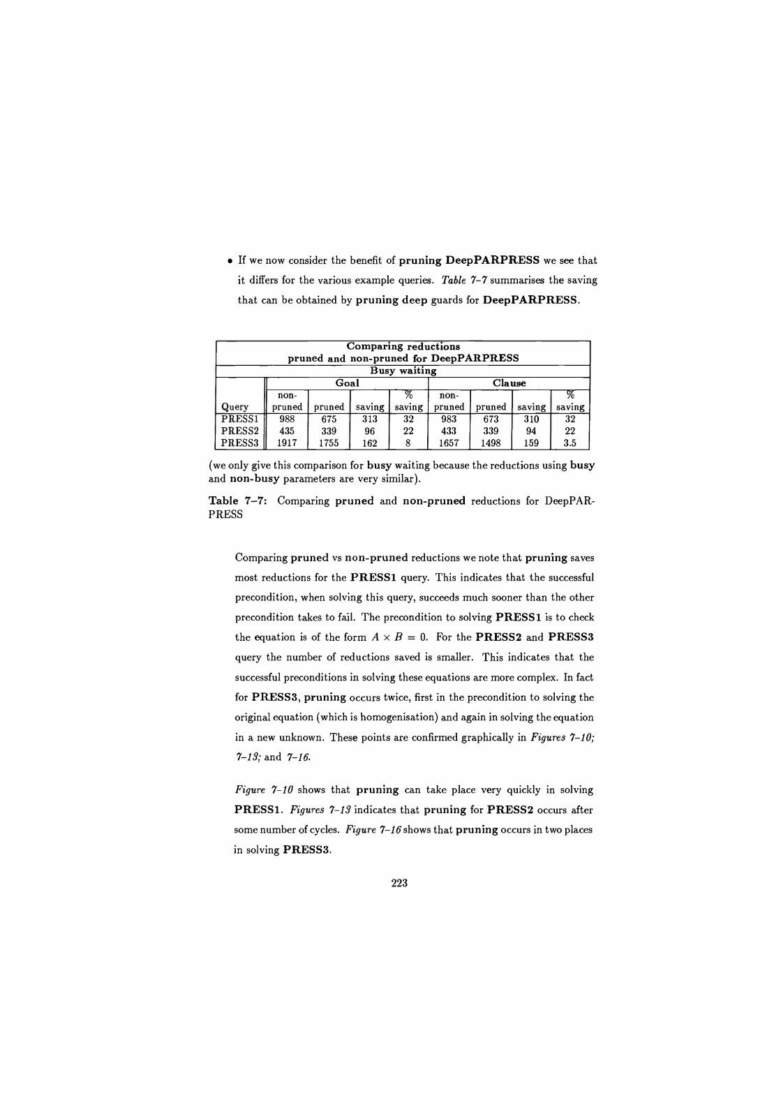
If we now consider the benefit of pruning DeepPARPRESS we see that

it differs for the various example queries. Table 7-7 summarises the saving

that can be obtained by pruning deep guards for DeepPARPRESS.

Comparing reductions pruned and non-pruned for DeepPARPRESS

Busy waiting Goal Clause

non- o non- o

Query pruned pruned saving saving pruned pruned saving saving PRESS1 988 675 313 32 983 673 310 32 PRESS2 435 339 96 22 433 339 94 22 PRESS3 1917 1755 162 8 1657 1498 159 3.5

(we only give this comparison for busy waiting because the reductions using busy and non-busy parameters are very similar).

Table 7-7: Comparing pruned and non-pruned reductions for DeepPAR- PRESS

Comparing pruned vs non-pruned reductions we note that pruning saves

most reductions for the PRESS1 query. This indicates that the successful

precondition, when solving this query, succeeds much sooner than the other

precondition takes to fail. The precondition to solving PRESS1 is to check

the equation is of the form A x B = 0. For the PRESS2 and PRESS3

query the number of reductions saved is smaller. This indicates that the

successful preconditions in solving these equations are more complex. In fact

for PRESS3, pruning occurs twice, first in the precondition to solving the

original equation (which is homogenisation) and again in solving the equation

in a new unknown. These points are confirmed graphically in Figures 7-10;

7 1 3; and 7-16.

Figure 7-10 shows that pruning can take place very quickly in solving

PRESS1. Figures 7-13 indicates that pruning for PRESS2 occurs after

some number of cycles. Figure 7-16 shows that pruning occurs in two places

in solving PRESS3.

223

Our profiling parameters should reflect the benefit of pruning or non-

pruning the computation. In terms of meta-level inference this reflects

the amount of computation that will be saved in fully evaluating the pre-

conditions once one succeeds. The two techniques employed in flattening

PARPRESS also aim to highlight the benefit of terminating or not termi-

nating the evaluation of the preconditions once one succeeds.

In fact our parameters using pruning for DeepPARPRESS, should

be similar to the parameters for F1atPARPRESS-term, and our pa-

rameters using non-pruning for DeepPARPRESS, should be similar

to the parameters for F1atPARPRESS-nonterm. Table 7-8 compares

the reduction parameters for DeepPARPRESS using non-pruning with

F1atPARPRESS-nonterm. Table 7-9 compares the reduction parame-

ters for DeepPARPRESS using pruning with F1atPARPRESS-term.

Both tables show a high correlation in the reduction counts for deep and

flat systems.

Comparing reductions DeepPARPRESS non-pruning VS Flat PARPRESS-nonterm

Busy waiting Non-busy waiting Goal Clause Goal Clause

Query deep flat deep flat deep flat deep flat PRESS1 PRESS2 PRESS3

988

435

1917

1032

445

1704

983

433

1657

1022

441

1694

983

433

1911

1022

441

1694

983

433

1657

1022

441

1694

Table 7-8: Comparing reductions: deep non-pruning and flat-nonterm

Table 7-10 compares the suspension parameters for DeepPARPRESS us-

ing non-pruning with F1atPARPRESS-nonterm and Table 7-11 com-

pares the suspension parameters for DeepPARPRESS using pruning with

F1atPARPRESS-term.

Both tables show a high correlation in the suspension counts using goal

suspensions. However, using clause suspension, the suspension count for

F1atPARPRESS-term is always higher than the counter for DeepPAR-

224

Comparing reductions DeepPARPRESS pruning VS FlatPARPRESS-term

Busy waiting Non-bus y waiting Goal Clause Goal Clause

Query deep flat deep flat deep flat deep at PRESS1 PRESS2 PRESS3

675

339

1755

749

370

1583

673

339

1498

743

370

1579

673

339

1752

745

370

1579

673

339

1498

744

370

1577

Table 7-9: Comparing reductions: deep pruning and flat terminating

Comparing suspensions DeepPARPRESS non-pruning VS F1atPARPRESS-nonterm



1110

364 2031

1088

380 1736

1862

760 4924

2957

1172

5227

413

136

597

409

126

614

650

236 1017

953

338 1509

Table 7-10: Comparing suspensions: deep non-pruning and flat-nonterm

PRESS. This is because each flat predicate called as part of the meta-level

precondition requires one extra clause to support the possible termination

message required for terminating the evaluation of the other preconditions'.

'This need not be true of Flat PARPRESS-nonterm as it does not terminate the

precondition evaluation. However, we use the same flat functions for both F1atPAR-

PRESSes and only send the terminate message in Flat PARPRESS-term.

Comparing suspensions DeepPARPRESS pruning VS Flat PARPRESS-term



837

265 1853

816

302 1605

1338

513 4464

2034

892 4730

292

89 575

286

86 546

441

140

968

643

231 1328

Table 7-11: Comparing suspensions: deep pruning and flat terminating

225

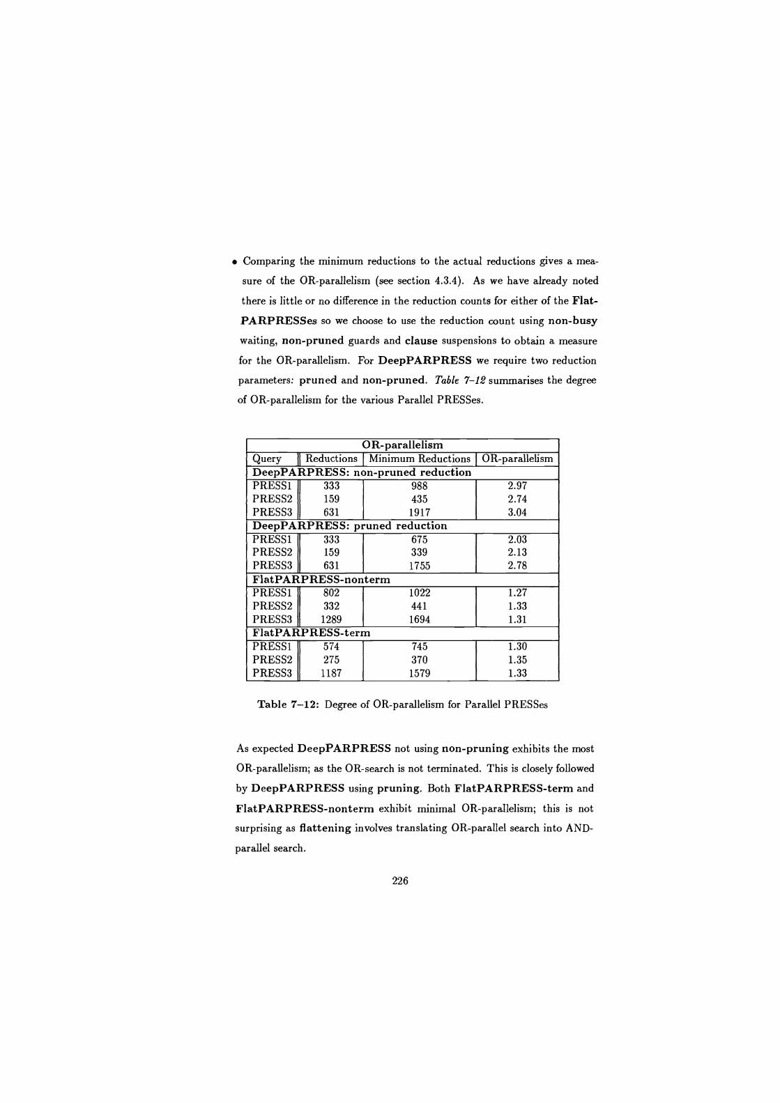
Comparing the minimum reductions to the actual reductions gives a mea-

sure of the OR-parallelism (see section 4.3.4). As we have already noted

there is little or no difference in the reduction counts for either of the Flat-

PARPRESSes so we choose to use the reduction count using non-busy

waiting, non-pruned guards and clause suspensions to obtain a measure

for the OR-parallelism. For DeepPARPRESS we require two reduction

parameters: pruned and non-pruned. Table 7-12 summarises the degree

of OR-parallelism for the various Parallel PRESSes.

OR-parallelism Query Reductions Minimum Reductions OR-parallelism DeepPARPRESS: non-pruned reduction PRESS1 333 988 2.97 PRESS2 159 435 2.74 PRESS3 631 1917 3.04 DeepPARPRESS: pruned reduction PRESS1 333 675 2.03 PRESS2 159 339 2.13 PRESS3 631 1755 2.78 F1atPARPRESS-nonterm PRESS1 802 1022 1.27 PRESS2 332 441 1.33 PRESS3 1289 1694 1.31 F1atPARPRESS-term PRESSI 574 745 1.30 PRESS2 275 370 1.35 PRESS3 1187 1579 1.33

Table 7-12: Degree of OR-parallelism for Parallel PRESSes

As expected DeepPARPRESS not using non-pruning exhibits the most

OR-parallelism; as the OR-search is not terminated. This is closely followed

by DeepPARPRESS using pruning. Both F1atPARPRESS-term and

F1atPARPRESS-nonterm exhibit minimal OR-parallelism; this is not

surprising as flattening involves translating OR-parallel search into AND-

parallel search.

226

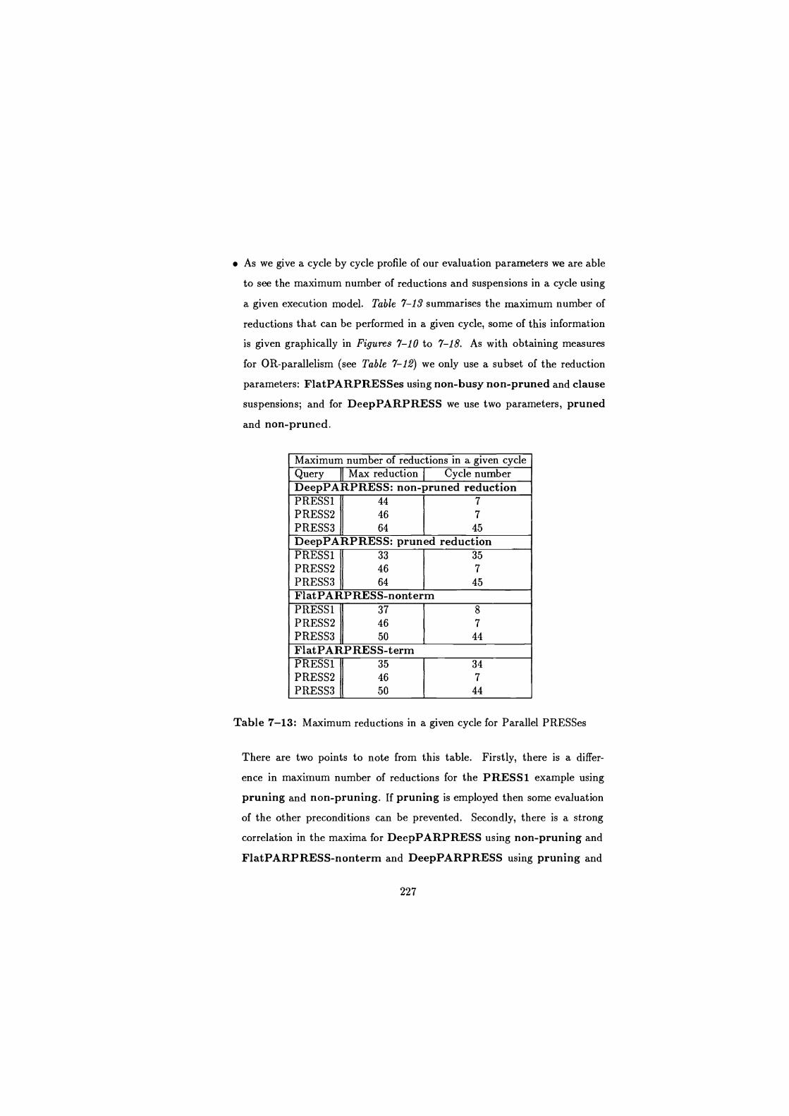
As we give a cycle by cycle profile of our evaluation parameters we are able

to see the maximum number of reductions and suspensions in a cycle using

a given execution model. Table 7-13 summarises the maximum number of

reductions that can be performed in a given cycle, some of this information

is given graphically in Figures 7-10 to 7-18. As with obtaining measures

for OR-parallelism (see Table 7-12) we only use a subset of the reduction

parameters: F1atPARPRESSes using non-busy non-pruned and clause

suspensions; and for DeepPARPRESS we use two parameters, pruned

and non-pruned.

Maximum number of reductions in a given cycle Query 1 1 Max reduction Cycle number DeepPARPRESS: non-pruned reduction PRESSI 44 7

PRESS2 46 7

PRESS3 64 45 DeepPARPRESS: pruned reduction PRESSI 33 35 PRESS2 46 7

PRESS3 64 45 Flat PARPRESS-nonterm PRESS1 37 8

PRESS2 46 7

PRESS3 50 44

Flat PARPRESS-term PRESSI 35 34 PRESS2 46 7

PRESS3 50 44

Table 7-13: Maximum reductions in a given cycle for Parallel PRESSes

There are two points to note from this table. Firstly, there is a differ-

ence in maximum number of reductions for the PRESSI example using

pruning and non-pruning. If pruning is employed then some evaluation

of the other preconditions can be prevented. Secondly, there is a strong

correlation in the maxima for DeepPARPRESS using non-pruning and

F1atPARPRESS-nonterm and DeepPARPRESS using pruning and

227

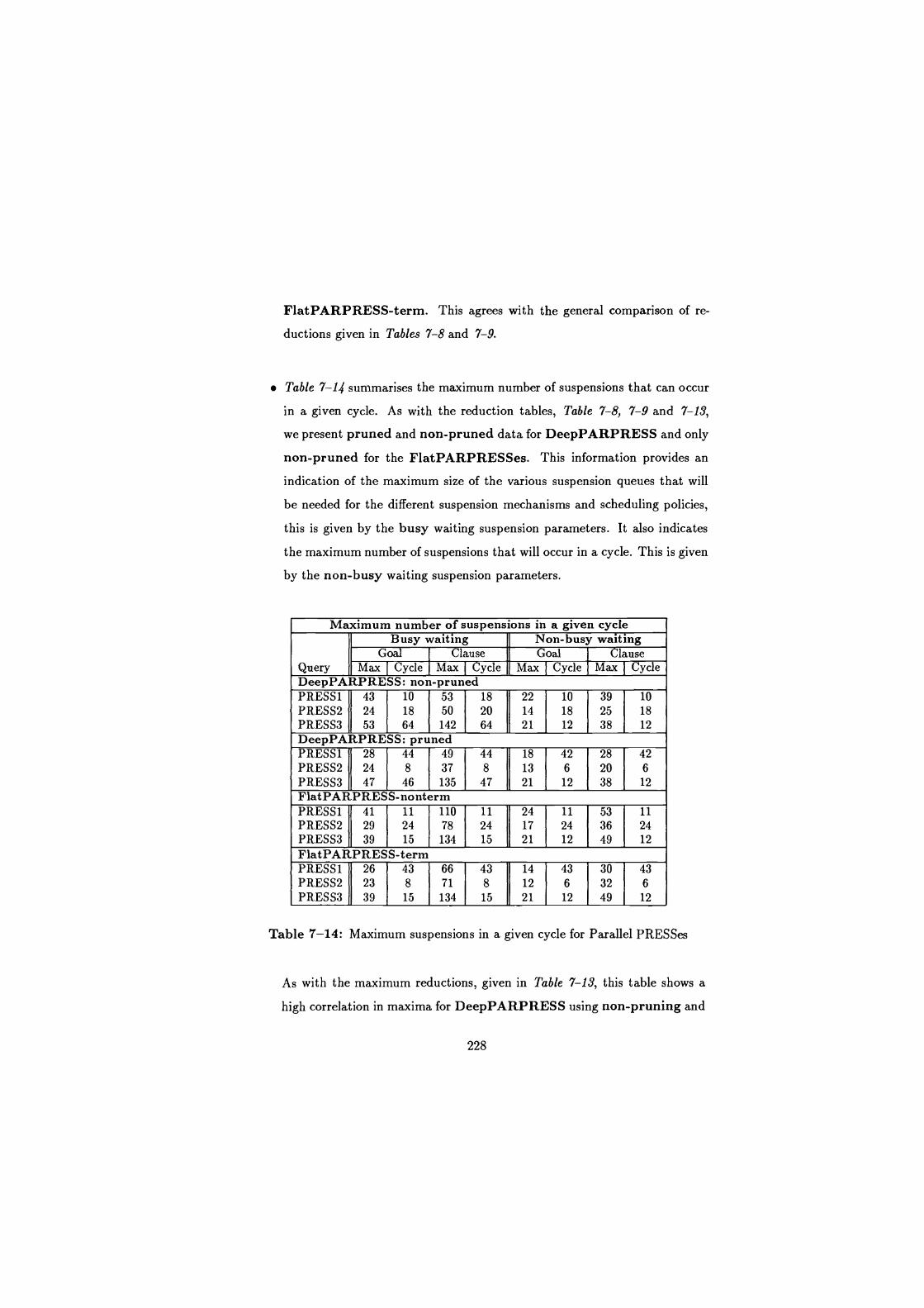
Flat PARP RES S-t erm. This agrees with the general comparison of re-

ductions given in Tables 7-8 and 7-9.

Table 7-14 summarises the maximum number of suspensions that can occur

in a given cycle. As with the reduction tables, Table 7-8, 7-9 and 7-13,

we present pruned and non-pruned data for DeepPARPRESS and only

non-pruned for the F1atPARPRESSes. This information provides an

indication of the maximum size of the various suspension queues that will

be needed for the different suspension mechanisms and scheduling policies,

this is given by the busy waiting suspension parameters. It also indicates

the maximum number of suspensions that will occur in a cycle. This is given

by the non-busy waiting suspension parameters.

Maximum number of suspensions in a given cycle Busy waiting Non-busy waiting

Goal Clause Goal Clause Query Max Cycle Max Cycle Max Cycle Max yc e DeepPA RPRESS: non-pruned PRESSI 43 10 53 18 22 10 39 10 PRESS2 24 18 50 20 14 18 25 18 PRESS3 53 64 142 64 21 12 38 12 DeepPA RPRESS: pruned PRESS1 28 44 49 44 18 42 28 42 PRESS2 24 8 37 8 13 6 20 6 PRESS3 47 46 135 47 21 12 38 12

F1atPARPRESS-nonterm PRESS1 41 11 110 11 24 11 53 11

PRESS2 29 24 78 24 17 24 36 24 PRESS3 39 15 134 15 21 12 49 12

F1atPARPRESS-term PRESS1 26 43 66 43 14 43 30 43

PRESS2 23 8 71 8 12 6 32 6 PRESS3 39 15 134 15 21 12 49 12

Table 7-14: Maximum suspensions in a given cycle for Parallel PRESSes

As with the maximum reductions, given in Table 7-13, this table shows a

high correlation in maxima for DeepPARPRESS using non-pruning and

228

F1atPARPRESS-nonterm and DeepPARPRESS using pruning and

F1atPARPRESS-term.



in the dynamic query (see section 4.5.3.1). Table 7-15 summarises the ratio

of clause to goal suspensions using busy and non-busy waiting schedul-

ing for DeepPARPRESS, using pruned and non-pruned models and

FIatPARPRESS-nonterm and FIatPARPRESS-term.

Busy waiting Non-busy waiting Query Goal Clause Ratio 1 1 Goal Clause Ratio DeepPARPRESS: non-pruned PRESS 1 1110 1862 1.68 413 650 1.57 PRESS2 364 760 2.09 136 236 1.74 PRESS3 2031 4924 2.42 597 1017 1.70

DeepPARPRESS: pruned PRESSI 837 1338 1.60 292 441 1.51 PRESS2 265 513 1.94 86 140 1.63

PRESS3 1853 4464 2.41 575 968 1.68

FIatPARPRESS-nonterm PRESS1 1088 2953 2.71 409 953 2.33 PRESS2 380 1172 3.08 129 338 2.60 PRESS3 1736 5227 3.01 614 1509 2.45 F1atPARPRESS-term PRESS1 819 2034 2.48 286 643 2.24 PRESS2 302 892 2.95 86 231 2.68 PRESS3 1605 4730 2.95 546 1328 2.43

Table 7-15: Clause/Goal suspension ratios for Parallel PRESSes

The only point to note is that the flattened code incurs a high clause to

goal suspension ratio. This is because additional clauses are required to sup-

port the termination of those goals in the conjunction, which are essentially

performing the guarded search.

The difference between busy waiting and non-busy waiting suspensions in-

dicates the benefit of tagging suspended executions to variables (see section

229

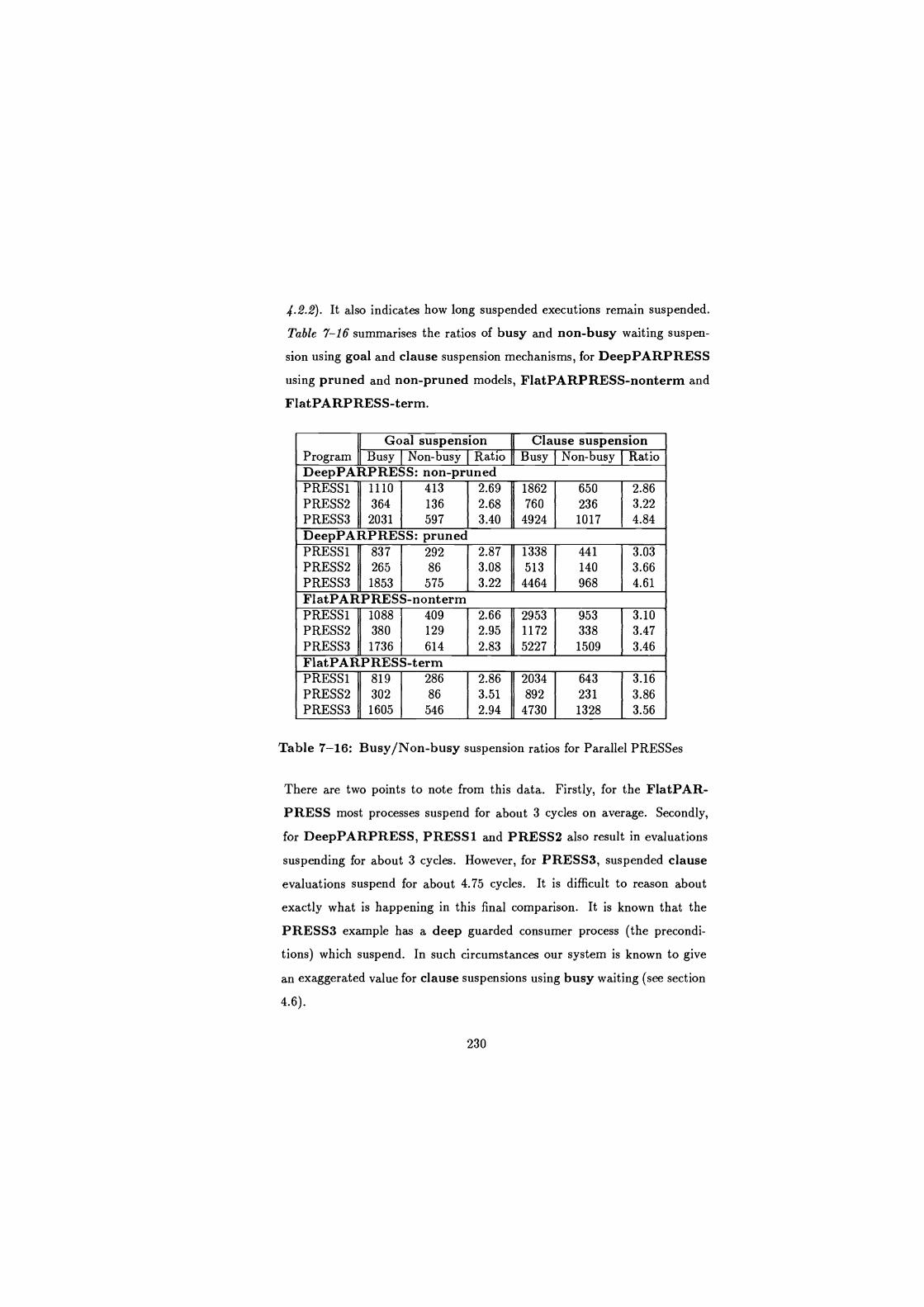
4.2.2). It also indicates how long suspended executions remain suspended.

Table 7-16 summarises the ratios of busy and non-busy waiting suspen-

sion using goal and clause suspension mechanisms, for DeepPARPRESS

using pruned and non-pruned models, FIatPARPRESS-nonterm and

FIatPARPRESS-term.

11 Goal suspension '

Clause suspension Program I l Busy Non-busy Ratio Busy Non-busy Ratio DeepPARPRESS: non-pruned PRESS1 1110 413 2.69 1862 650 2.86 PRESS2 364 136 2.68 760 236 3.22 PRESS3 2031 597 3.40 4924 1017 4.84

DeepPARPRESS: pruned PRESSI 837 292 2.87 1338 441 3.03 PRESS2 265 86 3.08 513 140 3.66 PRESS3 1853 575 3.22 4464 968 4.61

FIatPARPRESS-nonterm PRESS1 1088 409 2.66 2953 953 3.10 PRESS2 380 129 2.95 1172 338 3.47 PRESS3 1736 614 2.83 5227 1509 3.46 F1atPARPRESS-term PRESS1 819 286 2.86 2034 643 3.16

PRESS2 302 86 3.51 892 231 3.86 PRESS3 1605 546 2.94 4730 1328 3.56

Table 7-16: Busy/Non-busy suspension ratios for Parallel PRESSes

There are two points to note from this data. Firstly, for the FIatPAR-

PRESS most processes suspend for about 3 cycles on average. Secondly,

for DeepPARPRESS, PRESS1 and PRESS2 also result in evaluations

suspending for about 3 cycles. However, for PRESS3, suspended clause

evaluations suspend for about 4.75 cycles. It is difficult to reason about

exactly what is happening in this final comparison. It is known that the

PRESS3 example has a deep guarded consumer process (the precondi-

tions) which suspend. In such circumstances our system is known to give

an exaggerated value for clause suspensions using busy waiting (see section

4.6).

230



Our re-evaluation of the Parallel PRESS systems gives similar raw data to

that given in [Sterling & Codish 87). However, we feel that their analysis of

this data is mis-leading and incomplete. We re-analyse the raw data, the

basic cycle, reductions and suspensions. The evaluation is enhanced by

the fact that we consider flat implementations which employ termination

and do not employ termination of the meta-level precondition.

We then present our new measurements and perform an in depth analysis

of this data. Our new data indicates the benefits in using pruning if deep

guards are employed.

The data for the DeepPARPRESS evaluation strongly indicates the sav-

ing in both reductions and suspensions if the flat implementations employ

termination techniques.

The results also show that the overall parallelism remains unchanged for

deep and flat implementations. Whilst the contribution of AND and OR-

parallelism vary for the deep and flat implementations, the flat implemen-

tations have little or no OR-parallelism.

It is worth noting that our model for including the contribution of deep

guards into the overall evaluation appears reasonable, e.g. the overall cy-

cle measures for the evaluations are similar for the various Parallel PRESS

systems.

Using deep guards is more natural for the meta-level of PRESS where pre-

conditions for a given meta-rule become user defined guarded goals. In

231

flattening the meta-level of PRESS, or for that matter any code with deep

guards, various alternatives techniques can be applied. The simplest and

most basic is to translate each precondition, the guard, into an AND-goal. If

the precondition succeeds a continuation flag is set and the solution method

selected is committed to. An alternative and more complex translation is

to generate flat code which employs early termination. The evaluation of

the alternative meta-rule preconditions can be terminated as soon as one

precondition succeeds rather than being fully evaluated. This enhancement

is applicable if the amount of computation that can be prevented by early

termination is significant. This is where there is a dilemma - how do we

know how much computation can be saved if we do not translate the code

to both terminating and non-terminating flat code?

The use of the profiletool in this context is very informative. Our results

indicate that there is a very strong correlation between the results for the

deep guarded version when executing without pruning and the flat guarded

version not employing termination and the deep guarded version when ex-

ecuting with pruning and the flat guarded version employing termination.

So, by first implementing the more natural deep guarded version and then

using the profiletool we are able to select the most appropriate flattening

technique.

7.9 Summary


PRESS - a PRolog Equation Solving System and how it provides a set of

meta-level axioms for solving symbolic equation.

How the meta-level axioms of PRESS can be realised in terms of Prolog

clauses, known as meta-rules.

232

How these meta-rules can be directly mapped into CCND languages which

allow deep guards.

How the deep guarded version of PRESS can be flattened. The resulting

flat code can either terminate the evaluation of the other meta-rules should

one rule succeed or allow all the rules to execute to completion.

The re-evaluation of these Parallel PRESSes on both the basic evaluation

system and our new system. The results indicate that:

- our system provides a more accurate picture of the execution of the

parallel PRESSes;

- our system also allows us to consider the benefits of the various trans-

lation options between deep and flat code by analysing the behaviour

of the deep implementation;

- it is worth employing pruning in the implementation of the system to

evaluate PRESS using deep guards; and

- it is worth the programmer employing termination techniques in the

mapping of the meta-level of PRESS to flat guards.

233

Chapter 8

Conclusions

8.1 Overall Contribution of the Thesis

In this thesis, the following contributions are made to the task of understanding

and evaluating the execution behaviour of the CCND languages with regard to AI

applications:

We develop a model of execution which allows us to obtain measures for the

inherent parallelism available in the evaluation of CCND programs.

The evaluation system developed also allows us to observe the effects of vary-

ing several implementation parameters, such as the suspension mechanism,

the scheduling of suspended evaluations and the pruning (termination) of

competing guarded evaluations on commitment.

We then focus on three aspects of these languages - how they support search,

the benefits in using safe or unsafe languages and the benefits in using deep

or flat guards. These reflect questions about how these languages should be

used and implemented.

234

We test these aspects of the languages by choosing Al type applications

which we have implemented across the various language classifications.

These various systems are evaluated and the results analysed.

The study shows the significant improvement our evaluation system gives in

terms of both measuring the inherent features of the algorithm and under-

standing the dynamic behaviour of the execution.

Our analysis of Al applications highlights several interesting points relating

to the behaviour of programs which make use of given language features.

These points are summarised in the following sections.

8.1.1 Inherent parallelism

The CCND languages provide a model of computation which supports both lim-

ited OR-parallelism and concurrent goal evaluation. In this work we consider the

inherent parallelism that is available in the evaluation of programs implemented

in the CCND languages. A measure of the inherent parallelism provides a the-

oretical measure of the parallelism against which particular implementations can

be gauged. Without a theoretical measure it is difficult to consider the actual per-

formance improvements of various implementations. The inherent parallelism also

provides information for programmers on the relative merits of various program-

ming techniques regardless of the particular implementation. Finally a theoretical

model of the parallel execution of these languages allows implementors of the lan-

guages to consider the possible benefits of alternative implementation issues like

suspensions, pruning and scheduling.

To obtain a measure of the inherent parallelism available in program execution

we adopt a breadth-first execution model on an unlimited number of processors.

Previous systems used for evaluating and comparing programming techniques and

applications suffer from two main limitations. The first is that the parameters

quoted in the evaluations of a program do not reflect possible alternatives open

235

to language implementors, like scheduling policy. The second is that although

these interpreters claimed to execute the object code (CCND program) breadth-

first (hence allowing the inherent parallel features to be measured) the actual

evaluation models used make several approximations. This results in misleading

and distorted measurements.

In this work we have considered the measurements that should be collected

to capture the nature of a CCND computation. The new system comprises two

stages: an AND/OR-interpreter, which evaluates the program breadth-first pro-

ducing a dump file and an analyser program which reconstructs a parallel view of

the program execution. The statistics obtained are more accurate in two respects.

The first is in the modelling of a parallel AND/OR execution, this allows us to

measure the inherent parallel features of our algorithm. The second is in iden-

tifying the nature of the execution: pruned or non-pruned guard evaluations;

busy or non-busy waiting; and goal or clause suspension.

8.1.2 Search - committed choice

The CCND languages are committed choice, as such they cannot be used to di-

rectly implement general search algorithms. To carry out search in these languages

requires some means of translating the non-determinism in the search algorithm

into a deterministic algorithm.

We evaluate three models for translating search algorithms into deterministic

algorithms:

Continuation based compilation;

Stream based compilation; and

Layered streams.

These three techniques were chosen because they had already been evaluated on an

earlier evaluation system [Okumura & Matsumoto 87]. We revaluate the n-queens

236

example for 4-queens and 6-queens using our basic Parlog interpreter. The results

obtained agree with the previous evaluations.

We then re-evaluate the 4-queens and 6-queens on our new evaluation system.

The results given by our system differ in several respects to those obtained on our

basic Parlog interpreter. Our analysis of the results highlights how our evaluation

gives a picture of the program behaviour and the relative merits of the various

programming techniques.

Previous results for the all-solutions programming techniques indicated that

Layered Streams required only half the reductions that Continuation based com-

pilation required. Also the results highlighted the greater increase in the available

parallelism for large problems using Layered streams. This is due to solutions be-

ing generated bottom-up and hence large problems tend to have more parallelism

if explored bottom-up.

Our re-evaluation gives a slightly different picture. Layered Streams does re-

quire less reductions than Continuation based compilation but the difference is

only 5%. Layered streams also results in the continual exploration of incomplete

solutions, ie. incomplete solutions are continually tested against each incrementa-

tion in the generation of the solution. For larger problems this over generation may

result in more reductions being performed for Layered Streams. So, our results

show that Layered Streams is not as good as was previously supposed. However,

the overall number of cycles required for Layered Streams is considerably less

than for either of the other two methods, so this technique is the most inherently

parallel.

8.1.3 Shared data structures - safe/unsafe

The question of how shared data structures are supported in the CCND languages

is an important one for Al. Several current Al paradigms which require several

different forms of expertise, like blackboard systems, require a common communi-

237

cation medium which each expert can see and update. Also, parallelising existing

sequential algorithms often results in several solvers performing similar tasks on

different parts of the same data; this is particularly the case if the parallelisa-

tion involves replacing a sequential control mechanism like a scheduler for parallel

functioning solvers, as in parallelising a chart parser.

Whilst all the CCND languages and their subsets allow several processes to

read the same data structure; one-to-many communication, it has been noted

by several researchers that only unsafe languages directly support many-to-one

communication on a single variable; several writers to the same data. Whilst

the safe languages cannot directly support many-to-one type communication, one

important case of multiple writers, multiple writers to a stream, can be modelled

by the use of merge processes. Each writer that wishes to update some shared

stream, binds a local stream. The local streams for each writer are then merged

together to form the final shared stream.

The general use of multiple writers to any structure, not just a stream, can be

then indirectly supported by creating a process which manages the structure. Mul-

tiple processes that wish to write to the structure make write requests to this man-

ager process. The write requests from the writer processes are merged together to

form a request stream. This technique has been used in several applications which

require multiple writers to a shared resource [Davison 87] [Trehan & Wilk 88]. The

general feature of this use of streams is to combine requests from many sources to

one final stream, which we call the resultant stream.

System extensions to support resultant streams have been considered by us and

other researchers. If the system knows that a given variable, or list, is a resultant

stream it can keep a pointer to its tail, which can be used to add elements to this

stream in unit time. We consider two basic primitives: the first identifies a stream

as a resultant stream; the second directly adds an element to this resultant stream.

The stream addition primitive has to be atomic.

We have implemented several chart parsers using three styles of language: safe;

238

unsafe; and safe+system streams (where the resultant stream is supported by

the system). The chart parsers allow several processes which pick different active

edges from the AET (active edge table), process them in parallel, and update the

chart (records of the active edges undertakes and the parses found) by adding any

new active edges to the AET and any sub-strings to the WFST (parses found).

The approach requires that testing if an active edge is new and its addition to the

AET to be an atomic step. In an unsafe language the shared data structure, the

chart, can be directly supported. In a safe language the shared data structure,

the chart, can only be supported by a manager process and writer processes which

make requests for updates. The basic mechanism employed by the manager is

"sifting" which is a generalisation of a prime number generator program. In the

safe+system streams language the shared data structure, the chart, must also

be supported by a manager process. Writer processes make update requests to

this manager. However, unlike in a pure safe language, these requests need not

make explicit use of merge processes as streams are supported by the system.

Our evaluation of these chart parsers indicates that:

there are significant overheads introduced by networks of merge processes,

in the safe languages;

the unsafe languages also introduce some delays in supporting shared data,

in that the data structure has to be traversed to find the next free position,

in the case of shared streams the unbound tail;

the dynamic behaviour of the manipulation of shared data structures de-

pends on which processes access the data, when they access the data and

how often they access the data;

in the chart parsers the dynamic considerations result in the difference, in

terms of cycles, between unsafe and safe chart parsers not being as high as

first expected;

239

there are benefits from supporting multiple writers to a stream by the system,

in terms of suspension overheads, available parallelism and total number of

cycles required.

8.1.4 Meta-level inference - deep/flat

The question of whether guards should be deep (any user defined goals are allowed

in the guards) or flat (only system calls are allowed in the guards), is interesting

and controversial. Deep guards appear to be more expressive and flat guards

more efficiently implemented. One proposal to get the best from both worlds

is to write deep guarded code and then have this code translated to flat code

which is executed. In the translation from deep to flat code there are several

alternative models that can be employed. For example, should the flattened

code be correct or should it also mimic possible efficiency options open to deep

guarded evaluations, like that of pruning guarded evaluations on the commitment

to one clause.

To compare deep guards with flat guards and the possible effects of mimic-

ing pruning we consider the behaviour of a program implemented using several

different flavours of language. The application considered is known as PRESS - a

Prolog Equation Solving System. A subset of this system was initially translated to

Concurrent Prolog and FCP in [Sterling & Codish 87] the resulting system being

known as CONPRESS. We take their basic translation and reconstruct it for Par-

log, which results in PARPRESS. The translation to Parlog is essentially the same

as the translation to Concurrent Prolog. The translation of PARPRESS into flat

code required us to adopt slightly different translation techniques [Gregory 87].

As a result we have several Parallel PRESS systems which we could have

evaluated and we chose to consider one aspect of PRESS and meta-level inference.

This is how the execution of the meta-level differs using deep and flat guards,

where the flat meta-levels may or may not employ termination techniques. The

systems evaluated are:

240

DeepPARPRESS - Parallel PRESS implemented in Parlog, employing deep

guards just for the meta-level axioms;

F1atPARPRESS-nonterm - Parallel PRESS implemented in Parlog, employing


meta-level axiom) the other preconditions are not terminated.

F1atPARPRESS-term - Parallel PRESS implemented in Parlog, employing flat

guards. On successful termination of one of the preconditions (to a meta-

level axiom) the other preconditions are terminated.

Our new evaluation indicates the benefits in using pruning if deep guards

are employed. Moreover, the data for the DeepPARPRESS evaluation strongly

indicates the saving in both reductions and suspensions if the flat implementations

employ termination techniques.

The results also show that the overall parallelism remains unchanged for deep

and flat implementations. Whilst the contribution of AND and OR-parallelism

varies for the deep and flat implementations, the flat implementations have little

or no OR-parallelism.

Finally, it is worth noting that our model for including the contribution of

deep guards into the overall evaluation appears reasonable, e.g. the overall cycle

measures for the evaluations are similar for the various Parallel PRESS systems.

8.1.5 Summary of Contribution

In this section we summarise the contribution of this work. The main contribution

of this work can be classed in two ways. Firstly in the approach. This work aims to

present an applications viewpoint of the possible direction that the CCND imple-

mentors may take. To this end we have implemented an improved interpreter for

collecting more meaningful information; proposed and collect an improved set of

profiling parameters, which reflect the effect of alternative model of execution and

241

and developed several applications which allow us to compare language features.

Secondly the actual results of our evaluations. The three different application

areas and language features investigated in this work provide a large number of

interesting points for both users of these languages as well as language implemen-

tors. The following points aim to provide some general messages that result from

this work:

Language design and execution models has been governed by implementation

considerations. The resulting languages appear to have flat guards and

adopt non-busy waiting scheduling policy. There is still some discussion on

whether the languages should be safe or unsafe. Our work aims to place

some applications rationale for the design of language features and their

usage. Applications input is important because the classes of application

that language implementors aim to support and the models of execution

that they provide make not be those required by applications programmers.

For example, the results for our evaluation of Layered Streams indicates

that this programming technique could employ a busy waiting scheduling

policy. Busy waiting scheduling policy is easier to implement than non-

busy waiting. However, most implementations do not offer busy waiting

scheduling as it is assumed not to be applicable for real programs.

Other language features, or rather additions, being provided by implemen-

tors, like supporting streams in the system results in more efficient programs

because the heavy overhead in maintaining and using merge processes is al-

leviated. Our results indicate that while the programs that use systems

streams may be less declarative the programs tend to have more predictable

behaviours. Because the exact structure of the merge network, for safe

languages, or the manipulation of a shared data structure, for unsafe lan-

guages, is not an issue if additions to the shared streams are supported by

the system. So, the behaviour of an application is not dependent on how the

242

worker processes are interconnected by merge processes, but rather on the

global behaviour of the worker processes.

Finally, we note the use of tools, like our profiletool, can provide a great

deal of insight into the dynamic properties of an application program. Such

insight is useful if a programmer intends to modify or improve their program.

For example, deep guards are easier to use for certain algorithms. However,

implementations are unlikely to offer such language features. This will re-

quire translating to flat code, or using flat guards in the first place. There

are many alternative options in mimicking the partial search capabilities of

deep guards in a flat system. For example, the benefits of using a technique

which not only produce correct code but also allows the early termination

may be limited. Our profiletool provides such information without having

to translate to flat code.

8.2 Research assumptions

This work is limited to some extent by the idealisations made, a large number of

which give directions for future work. These come in several classes:

Those associated with the evaluation system.

Those associated with the applications chosen.

Those associated with our evaluations.

Those associated with this general approach.

8.2.1 The evaluation system

We adopt a fixed cost model, that is the various components of the evaluation,

like head unification, have been assigned fixed costs (in terms of cycles). However,

243

the actual costs of a given operation may depend on several factors, eg. the cost

of a head unification will depend on the number of arguments and the complexity

of these arguments. It would be better to adopt a functional cost model, where

the cost of an operation is calculated based on its complexity.

We assume that, in a cycle, a goal can only use bindings available to it at

the start of the cycle. This is an improvement over the previous interpreters,

in modelling the inherent parallelism, a fully accurate model would be able to

determine exactly when a goal makes a binding, how long it would take for this

binding to reach another goal and whether this would be in time for the goal to

use it in the current cycle.

Although we are able to vary several parameters in our evaluation system to

reflect different implementation alternatives we do not consider the effects of a

finite number of processors and the resulting scheduling issues like bounded depth

first-search. Our focus from the start has been to provide measures of the inherent

parallelism which we obtain by using an infinite processor model. Simulating the

evaluation on a finite processor model would have been relatively straightforward

for flat code, but is non-trivial for deep guarded evaluation.

There are several questions that our system is not designed to answer, for

example the following questions relating to memory usage:

the relative costs of the different suspension mechanisms (goal and clause);

the overhead in creating tag suspension lists to support non-busy waiting;

the different data types (temporary variables; streams, state holding, etc.)

and their frequency of occurrence.

We are sure there are countless other limitations in this method of obtaining

a measure of the inherent parallelism. However, we feel that there is a significant

improvement in our evaluation system over the original and currently widely used

evaluation systems.

244

8.2.2 The applications

In evaluating these languages for Al type processing we could only hope to open a

"can of worms" rather than answer all the questions relating to the behaviour of Al

programs and Concurrent Logic Languages. We have tried to motivate our choice

of applications and programming technique to answer questions which relate to the

design and possible implementation of these languages. However, such knowledge

really comes not from one set of example programs but from the analysis of many

programs which then allow the generic features to be distilled. We do not intend

to, or attempt to, provide a list of possible extensions to our existing applications

or propose other suitable applications which would either enhance or complicate

the conclusions we draw in this thesis.

8.2.3 The evaluations

The evaluations performed using the raw data extracted by our system tend to be

complex exercises. There are main two limitations we wish to note:

We do not give a step by step guide to the analysis of raw data. In our

evaluations we compare a given parameter with another to get a measure of

a particular property of the execution. For example, reductions and cycles

gives average parallelism. However, in some cases we perform an in depth

comparison, eg. comparing all the busy waiting parameters with all the

non-busy parameters and other times we do not, as we can see that there

is no difference in the individual counters. The outcome is that although we

are able to perform this analysis the skill has not been abstracted.

Secondly, we only compare total figures for given parameters rather than the

profile curves. It is possible to obtain measures of the correlation between

two curves or the scaling factor that will produce the best coefficient of

correlation. This is likely to be more conclusive than just comparing totals

and would be more akin to the interactive use of the profiletool.

245

8.2.4 The approach

Finally, we should also question this approach to evaluating these languages and in

particular the emphasis on AI applications and programming techniques. Several

questions spring to mind:

Are AI applications and programming techniques any different from conven-

tional programs as far as the CCND languages are concerned? If not, then

we could just analyse conventional programs, possibly even theoretically, and

then apply the results to executing all programs. There is no fixed answer

to this question, unless you have a vested interest in the outcome. We do

however feel that the demands made on current computer architecture and

languages by AI applications are a good indication that there are likely to

be differences between executing a CCND language as a conventional pro-

gramming language (e.g. for system programming) and as an AI language,

(e.g. to support co-operating problem solvers).

Does the inherent parallelism as measured by our system really provide

any useful information about the execution of the programs on real multi-

processor architectures? Again this question is difficult to answer. The only

justified statement we can make is that it appears to be an improvement over

the previous systems being used to compare the executions of applications

and programming techniques. We have carefully tried to mimic the execu-

tion of these languages on an infinite number of processors and we attempt

to consider different implementation alternatives.

Finally, the programs evaluated attempt to focus on given features of the

languages, providing a means to consider the benefits of these feature for

programmers and the possible implementation of these features for language

implementors. It could be claimed that the approach taken does neither, as

the programs were implemented to highlight the differences that we drew

conclusions about. It may have been more appropriate to just implement

246

and evaluate programs and only then draw conclusions on the effects of the

various features used in the programs and the resulting execution behaviour.

The problem with this approach is that it is not scientific, as the search space

of application areas is vast, and on drawing conclusions the classic "what if"

questions arises; that is "what if I had implemented this program like this"?

8.3 Future work

There are many directions for future work that are either extensions of our work

or should complement our work.

The evaluation could be enhanced by adopting a functional, rather than

fixed, cost model, although an elaborate model of cost would tend to be to

be implementation dependent.

Additional measures could be considered, for example memory usage for the

various suspension mechanisms.

The interpreter could be extended to consider the effects of a finite number

of processors and the resulting scheduling issues.

An extended evaluation tool could be implemented that performed the vari-

ous alternative analysis of the raw data and helped spot particular patterns

in the results.

Finally, further applications could be considered. This would eventually

allow more generic features of applications to be abstracted away from the

specific results that can only be obtained for a small number of applications.

The correlation of our results with measurements obtained from parallel

implementations.

247

The analysis of Al programs and languages is an important area if we are to

better support Al applications in terms of hardware and software.

248

Bibliography

[Ali 86]

[Chikayama & Kimura 87]

[Clark & Gregory 81]

K.A.M. Ali. OR-parallel Execution of Prolog on a

Multi-Sequential Machine. International Journal of

Parallel Programming, 15(3), June 1986.

T. Chikayama and Y. Kimura. Multiple Reference

Management in Flat GHC. In J. Lassez, editor,

Fourth international conference of Logic Program-

ming, pages 276-293, MIT Press, Melbourne, 1987.

K. L. Clark and S. Gregory. A Relational Language

for Parallel Programming. In Proceedings of ACM

Conference on Functional Programming Languages

and Computer Architectures, pages 171-178, 1981.

[Clark & Gregory 84] K. Clark and S. Gregory. Parallel Programming in

Logic. Technical Report DOC 84/4, Department of

Computing, Imperial College of Science and Tech-

nology, London, 1984.

[Clocksin & Mellish 81] W. Clocksin and C. Mellish. Programming in Prolog.

Springer-Verlag, 1981.

[Codish 85] M. Codish. Compiling OR-parallelism into AND-

parallelism. Unpublished M.Sc. thesis, Department

249

of Computer Science, Weizmann Institute of Science,

Israel, 1985.

[Conery 87] J.S. Conery. Binding Environments for Parallel

Logic Programs in Non-Shared Memory Processors.

In Proceedings of the IEEE 4th Symposium on Logic

Programming, pages 457-467, San Fransisco, 1987.

[Corkill et al 88] D.D. Corkill, D.Q. Gallagher, and P.M. Johnson.

Achieving Fexibility, Efficiency, and Generality in

Blackboard Architecutes. In A. H. Bond and L.

Gasser, editors, Distributed Artificial Intelliegence,

chapter 7, pages 541-546, Maorgan Kaumann Pub-

lishers, 1988.

[Crammond 85] J. Crammond. A Comaprative Study of Unification

Algorithms for OR-parallel Execution of Logic Lan-

guages. In Proceedings of the IEEE International

Conference on Parallel Processing, pages 131-138,

1985.

[Crammond 88] J. Crammond. Implementation of Committed

Choice Logic Languages on Shared Memory Multi-

processors. Unpublished PhD thesis, Department

of Computer Science, Heriot-Watt, Edinburgh, May

1988.

[Davison 87] A. Davison. Blackboard systems in Parlog. Techni-

cal Report PAR 87/8, Department of Computing,

Imperial College, London, 1987.

[DeGroot 84] D. DeGroot. Restricted And-parallelism. In H.

Aiso, editor, Proceedings of the International Con-

250

ference on Fifth Generation Computer Systems,

pages 471-478, North-Holland, Tokyo, Japan, 1984.

[Dijkstra 75]

[Earley 70]

E.W. Dijkstra. Guarded commands, nondetermi-

nacy and formal derivation of programs. Commu-

nications ACM, 18(8):453-457, 1975.

J. Earley. An Efficient Context Free Parsing Algo-

rithm. Communications of the Association for Com-

puting Machinery, 13(2), 1970.

[Fagin et al 85] B. Fagin, Y.N. Patt, V. Srini, and A.M. Despain.

Compiling Prolog into Microcode: A Case Study Us-

ing the NCR/32000. In Proceedings of the 8th An-

nual Workshop on Microprogramming, pages 79-88,

1985.

[Foster & Taylor 87] I. T. Foster and S. Taylor. Flat Parlog: a basis for

comparison. Technical Report DOC 87/5, Depart-

ment of Computing, Imperial College of Science and

Technology, London, 1987.

[Foster et al 86] I. Foster, S. Gregory, G. Ringwood, and K. Satoh. A

Sequential Implementation of Parlog. In E. Shapiro,

editor, Third International Conference on Logic Pro-

gramming, pages 149-156, Springer-Verlag, London,

1986.

[Gregory 84] How to use Parlog (C-Prolog version). Department

of Computer Science, Imperial College of Science

and Technology, London, 1984.

251

[Gregory 85]

[Gregory 87]

[Grishman & Chitrao 88]

[Hausman et al 87]

[Hayes-Roth 85]

S. Gregory. Design, Application and Implementation

of a Parallel Logic Programming Language. Unpub-

lished PhD thesis, Department of Computer Science,

Imperial College of Science and Technology, London,

1985.

S. Gregory. Parallel Logic Programming in Parlog.

Addison-Wesley, 1987.

R. Grishman and M. Chitrao. Evaluation of a Par-

allel Chart Parser. In Second Conference on Applied

Natural Language Processing, pages 71-76, Associa-

tion for Computer Linguistics, Austin, Texas, 1988.

B. Hausman, A. Ciepielewski, and S. Haridi. OR-

parallel Prolog Made Efficient on Shared Memory

Multiprocessors. In Proceedings of the IEEE 4th

Symposium on Logic Programming, 1987.

B. Hayes-Roth. A Blackboard Architecture for

Control. Artificial Intelligence, 26(3):251-321, July

1985.

[Hayes-Roth 88] B. Hayes-Roth. A Blackborad Architecture for

Control. In A. H. Bond and L. Gasser, edi-

tors, Distributed Artificial Intelliegence, chapter 7,

pages 505-540, Maorgan Kaumann Publishers, 1988.

[Hirsch et al 87] M. Hirsch, W. Silverman, and E. Shapiro. Compu-

tation Control and Protection in the Logix System.

In E. Shapiro, editor, Concurrent Prolog: Collected

Papers, chapter 20, pages 28-45, MIT Press, 1987.

Volume 2.

252

[Houri & Shapiro 87] A. Houri and E. Shapiro. A Sequential Abstract

Machine for Flat Concurrent Prolog. In E. Shapiro,

editor, Concurrent Prolog: Collected Papers, chap-

ter 38, pages 513-574, MIT Press, 1987. Volume

2.

[Itoh et al 87] N. Itoh, E. Kuno, and T. Oohara. Efficient Stream

Processing in GHC and its Evaluation on a Parallel

Inference Machine. Technical Report TR-323, In-

stitute For New Generation Computer Technology,

Tokyo, November 1987.

[Kay 73] M. Kay. The MIND system. In R. Rustin, editor,

Natural Language Processing, pages 155-188, New

York: Algorithmics Press, 1973.

[Kimura & Chikayama 87] Y. Kimura and T. Chikayama. An Abstract KL1

Machine and its Instruction Set. In 1987 Sympo-

sium on Logic Programming, pages 468-477, Com-

puter Society Press, San Francisco, California, 1987.

[Kusalik 84]

[Levy 86a]

A.J. Kusalik. Bounded-wait merge in Shapiro's

Concurrent Prolog. New Generation Computing,

1(2):157-169, 1984.

J. Levy. A GHC Abstract Machine and Instruc-

tion Set. In E. Shapiro, editor, Third International

Conference on Logic Programming, pages 157-171,

Springer-Verlag, London, 1986.

[Levy 86b] J. Levy. Dual Concurrent Prolog- A Complementary

Language to Concurrent Prolog. Technical Report,

253

Department of Computer Science, Weizmann Insti-

tute of Science, Israel, 1986.

[Mierowsky et al 85] C. Mierowsky, S. Taylor, E. Shapiro, J. Levy, and M.

Safra. The Design and Implementation of Flat Con-

current Prolog. Technical Report CS85-09, Weiz-

mann Institute of Science, Rehovot, Israel, 1985.

[Okumura & Matsumoto 87] A. Okumura and Y. Matsumoto. Parallel Program-

ming with Layered Streams. In Fourth Symposium

on Logic Programming, San Francisco, 1987.

[Pinto 86] H. Pinto. Implementing Meta-Interpreters and

Compilers for Parallel Logic Languages in Prolog.

Project Report PR-14, Artificial Intelligence Ap-

plications Institute, University of Edinburgh, Edin-

burgh, 1986.

[Safra & Shapiro 87] S. Safra and E. Shapiro. Meta-Interpreters for Real.

In E. Shapiro, editor, Concurrent Prolog: Collected

Papers, chapter 25, pages 166-179, MIT Press, 1987.

Volume 2.

[Saraswat 87a] V. A. Saraswat. Compiling CP(j,I,&) on top of

Prolog. Technical Report CMU-CS-87-174, Carnegie

Mellon, October 1987.

[Saraswat 87b] V. A. Saraswat. The concurrent logic programming

language CP: definition and operational semantics.

In SIGA CT-SIGPLAN Symposium on Principles of

Programming Languages, ACM, January 1987.

254

[Saraswat 87c] V.A. Saraswat. Merging Many Streams Efficiently:

The Importance of Atomic Commitment. In E.

Shapiro, editor, Concurrent Prolog: Collected Pa-

pers, chapter 16, pages 420-445, MIT Press, 1987.

Volume 1.

[Sato & Goto 88] M. Sato and A. Goto. Evaluation of the KL1 Parallel

System on a Shared Memory Multiprocessor. Tech-

nical report TR-349, Institute for New generation

Computer Technology, Japan, 1988.

[Shapiro & Mierowsky 87] E. Shapiro and C. Mierowsky. Fair, Biased, and

Self-Balancing Merge Operators: Their Specification

and Implementation in Concurrent Prolog. In E.



Volume 1.

[Shapiro & Safra 87] E. Shapiro and S. Safra. Multiway Merge with Con-

stant Delay in Concurrent Prolog. In E. Shapiro,



1.

[Shapiro & Takeuchi 83] E. Shapiro and A. Takeuchi. Object Oriented Pro-

gramming in Concurrent Prolog. New Generation

Computing, Vol. 1(No. 1):25-48, 1983.

[Shapiro 83] E. Shapiro. A Subset of Concurrent Prolog and

Its Interpreter. Research Paper TR-003, Institute

For New Generation Computer Technology, Tokyo,

1983.

255

[Shapiro 87a] E. Shapiro. A Subset of Concurrent Prolog and Its

Interpreter. In E. Shapiro, editor, Concurrent Pro-

log: Collected Papers, chapter 2, pages 27-84, MIT

Press, 1987.

[Shapiro 87b] E. Shapiro. An Or-Parallel Execution Algorithm for

Prolog and its FCP Implementation. In Jean-Louis

Lassez, editor, Proceedings of the Fourth Interna-

tional Conference on Logic Programming, pages 311-

338, MIT Press, 1987.

[Shapiro 87c] E. Shapiro, editor. Concurrent Prolog: Collected

Papers. MIT Press, 1987.

[Sterling & Beer 861 L. Sterling and R. D. Beer. Incremental Flavor-

Mixing of Meta-Interpreters for Expert System Con-

struction. In 1986 Symposium on Logic Program-

ming, Salt Lake City, Utah, pages 20-27, IEEE,

1986.

[Sterling & Codish 851 L. Sterling and M. Codish. PRESSing for Paral-

lelism: A Prolog Program Made Concurrent. Tech-

nical Report CS85-12, Dept. of Computer Science,

Weizmann Institute of Science, Israel, 1985.

[Sterling & Codish 87] L. Sterling and M. Codish. PRESSing for Paral-

lelism: A Prolog Program Made Concurrent. In E.



Volume 2.

[Sterling & Shapiro 86] L. Sterling and E. Shapiro. The Art of Prolog. MIT

Press, 1986.

256

[Sterling et al 82] L. Sterling, A. Bundy, L. Byrd, R. O'Keefe, and B.

Silver. Solving Symbolic Equations with Press. Re-

search Paper 171, Department of Artificial Intelli-

gence, University of Edinburgh, 1982.

[Takeuchi & Furukawa 86] A. Takeuchi and K. Furukawa. Parallel Logic

Programming Languages. In E. Shapiro, edi-

tor, Third international conference of Logic Pro-

gramming, pages 242-255, Springer-Verlag, London,

1986.

[Tamaki 87] H. Tamaki. Stream-based Compilation of Ground

I/O Prolog into Committed Choice Languages. In

J. Lassez, editor, Fourth international conference of

Logic Programming, pages 376-393, MIT Press, Mel-

bourne, 1987.

[Tanaka et al 86] J. Tanaka, K. Ueda, T. Miyazaki, A. Takeuchi,

Y. Matsumoto, and K. Furukawa. Guarded Horn

Clauses and Experiences with Parallel Logic Pro-

gramming. Technical Report TR-168, Institute


1986.

[Taylor et al 87] S. Taylor, S. Safra, and E. Shapiro. A Parallel Imple-

mentation of Flat Concurrent Prolog. In E. Shapiro,



2.

[Thompson & Ritchie 84] H. Thompson and G. Ritchie. Implementing Natural

Language Parsers. In T. O'Shea and M. Eisenstadt,

257

editors, Artificial Intelligence, Tools Techniques and

Applications, Harper and Row, 1984.

[Tick 87] E. Tick. Studies in Prolog Architectures. Unpub-

lished PhD thesis, Stanford University, 1987.

[Trehan & Wilk 87] R. Trehan and P. Wilk. Issues of Non-

Determinism in Prolog and the Committed Choice

Non-Deterministic Languages. Research Paper RP-

378, Department of Artificial Intelligence, University

of Edinburgh, 1987. Also: Artificial Intelligence Ap-

plications Institute, University of Edinburgh, AIAI-

TR-43. To appear in: Artificial Intelligence Review

Vol 4.

[Trehan & Wilk 88] R. Trehan and P. F. Wilk. A Parallel Chart

Parser for the Committed Choice Non-Deterministic

(CCND) Logic Languages. In R. Kowalski and

Bowen K. A., editors, Proceedings of the 5th In-

ternational Logic Programming Conference Seattle.,

pages 212-232, 1988. Artificial Intelligence Applica-

tions Institute, University of Edinburgh, AIAI-TR-

36. Also:Department of Artificial Intelligence, Uni-

versity of Edinburgh, Research Paper-RP-366.

[Trehan 86] R. Trehan. Parallelism in a Mathematical Equation

Solver (PRESS) a Comparison of Committed Choice

Non-Deterministic Logic Languages. Project Re-

port PR-13, Artificial Intelligence Applications In-

stitute, University of Edinburgh, Edinburgh, 1986.

258

[Uchida 82]

[Ueda & Chikayama 84]

S. Uchida. Toward a New Generation Computer

Architecture. Technical Report TR-001, Institute


1982. Also: VLSI Architecture, Prentice-Hall, 1984.

K. Ueda and T. Chikayama. Efficient stream/array

processing in logic programming languages. In Inter-

national Conference on Fifth Generation Computer

Systems, pages 317-326, Tokyo, 1984.

[Ueda & Chikayama 85] K. Ueda and T. Chikayama. Concurrent Prolog

Compiler on Top of Prolog. In Symposium on Logic

Programming, pages 119-126, IEEE Computer Soci-

ety, 1985. Also: New Generation Computing, Vol.

2, No. 4, pp 361-369.

[Ueda 85a]

[Ueda 85b]

[Ueda 86a]

K. Ueda. Concurrent Prolog Re-Examined. Tech-

nical Report TR-102, Institute For New Genera-

tion Computer Technology, Tokyo, 1985. Also:

Logic Programming '85, Lecture Notes in Computer

Science,Springer-Varlag (1986) pp 168-179.

K. Ueda. Guarded Horn Clauses. Technical Re-

port TR-103, Institute For New Generation Com-

puter Technology, Tokyo, 1985.

K. Ueda. Guarded Horn Clauses. Unpublished PhD

thesis, Department of Information Engineering, Uni-

versity of Tokyo, Tokyo, 1986.

[Ueda 86b] K. Ueda. Making Exhaustive Search Deterministic.

In E. Shapiro, editor, Third international conference

259

of Logic Programming, pages 270-282, Springer-

Verlag, London, 1986.

[Ueda 87] K. Ueda. Making Exhaustive Search Programs

Deterministic, Part II. In J. Lassez, editor,

Fourth international conference of Logic Program-

ming, pages 356-375, MIT Press, Melbourne, 1987.

[Warren 77a] D.H.D Warren. Compiling Logic Programs 1. Re-

search Paper RP-39, Department of Artificial Intel-

ligence, University of Edinburgh, 1977.

[Warren 77b] D.H.D Warren. Compiling Logic Programs 2. Re-

search Paper RP-40, Department of Artificial Intel-

ligence, University of Edinburgh, 1977.

[Warren 83] D.H.D. Warren. An Abstract Prolog Instruction Set.

Technical Note 309, SRI International, 1983.

[Warren 87] D.H.D. Warren. The SRI-Model for OR-parallel Ex-

ecution of Prolog-Abstract Design and Implementa-

tion. In Proceedings of the IEEE 4th Symposium

on Logic Programming, pages 92-101, San Fransisco,

1987.

[Westphal et al 87] H. Westphal, P. Robert, J. Chassin, and J. Syre.

The PEPSys Model: Combining Backtracking AND-

and OR-parallelism. In Proceedings of the IEEE 4th

Symposium on Logic Programming, pages 436-448,

San Fransisco, 1987.

260

[Wilk 83] P. F. Wilk. Prolog Benchmarking. Research Pa-

per 111, Department of Artificial Intelligence, Uni-

versity of Edinburgh, 1983.

261

Part IV

Appendices

262

Appendix A

Effect of alternative execution models

In this appendix we consider the alterntaive evaluations of the program and query

in figure i$-1.

A.1 Busy waiting, non-pruning, goal suspen-

sion


for evaluation; on commitment to one clause the other OR-clauses are not termi-

nated; and the suspension of an evaluation involves suspending the parent goal.

We now consider the evaluation of the two query goals given in figure 4-1:

goal 1: This goal (on_either(a, [1,2,3,a,b] , [1,2,a,b] ,Output)) evaluation

results in two sets of guarded systems, member(a, [1,2,3,a,b]) and

member (a, [1, 2, a, b]) . The first of these will require 8 reductions to reduce

to true; that is the guard test takes 1 reduction for each element and the

263

commitment another 1. Similarly the second (guard) member(a, [1,2,a,b] )

goal requires 6 reductions.

As this execution model uses non-pruning both these guards will be eval-

uated fully. So, the total number of reductions performed in the evaluation

of this goal is 16 (8 in evaluating the first guard, 6 in the second guard, 1 for

the commitment to the body goals and finally 1 for the output unification).

The total number of cycles that this evaluation takes is 4. That is the

evaluation commits to the second, on-either/4, clause after 3 cycles and it

takes 1 cycle to carry out the output unification. So the binding made to

the shared variable "Output" will be seen by the other AND-parallel goals

in cycle 5.

goal 2: The second goal (on_either(b,Output, [11 Output] ,Outputl)) eval-

uation results in two sets of guarded goals, member(b,Output) and

member(b, [11 Output] ). The first of these could be evaluated via two

clauses, however these both suspend on head unification. As we are us-

ing goal suspension the evaluation of the first guarded goal suspends. The

second (guard) is able to perform 2 reductions (the guard test and the com-

mitment to member(b,Output)). The resulting goal could be evaluated via

two clauses but both of these suspend on head unification. This results in

the suspension of the second guarded goal. Now both sets of guarded goals

have suspended the evaluation of the second query goal suspends, giving a

total of 3 goal suspensions and 2 reductions. The second query goal suspends

after 2 cycles.

Using busy waiting this top-level goal will be retried in cycle 3. In cycle 3

the variable "Output" will still be unbound, so the rescheduled evaluation

'This is because we count system calls as reductions, see section 3.5.

264

will perform the same 2 reductions and then suspend again. The goal will

next be tried in cycle 5.

In cycle 5 the shared variable "Output" will be bound, so the sec-

ond query goal becomes on_either(b, [1,2,a,b] , [1,1,2,a,b] ,Outputs).

This goal invokes two guarded systems, member (b , [1, 2 , a, b]) and

member(b,[1,1,2,a,b]). The first of these will require 8 reductions to

reduce to true. Similarly the second guard requires 10 reductions.

As the execution uses non-pruning both these guards will be evaluated

fully. Hence the final attempt at evaluating this goal results in 20 reductions

(8 in the first guard, 10 in the second, 1 for the commitment to the body goals

and finally 1 for the output unification). The total number of cycles that this

evaluation takes is 5. That is the evaluation commits to the first OR-clause

after 4 cycles and it takes 1 cycle to carry out the output unification.


reductions (16 for the first goal, 4 for the second goal before suspension, and 20

for the final evaluation of the second goal); 6 goal suspensions (1 suspension for

the first guarded goal, member (b , L) , 1 suspension for the second guarded goal,

member (b, [1IL]), and 1 suspension for the query goal, these suspensions occur

twice because of the busy waiting).

A.2 Busy waiting, non-pruning, clause suspen-

sion


for evaluation; on commitment to one clause the other OR-clauses are not termi-

nated; and the suspension of an evaluation involves suspending the clauses.


265

goal 1: The evaluation of this goal will be as given in section A.1, as this goal

evaluation incurs no suspensions and so an alternative suspension mechanism

makes no difference.

goal 2: The evaluation of the second goal results in two guarded systems,

member (b, Output) and member (b , [110utput]) . The first (guard) could

be evaluated via two clauses. Both clause evaluations suspend on head

unification. Using clause suspension and busy waiting these 2 suspended

evaluations will be attempted every cycle until cycle 5, when the variable

"Output" becomes bound; a total of 8 suspensions. The second (guard)

is able to perform 2 reductions (the guard test and the commitment to

member(b,Output)). The resulting goal could be evaluated via two clauses

but again both evaluations suspend on head unification. These two sus-

pended evaluations will also be tried every cycle until cycle 5, resulting in 6

suspensions.





suspension and 8 when the variable "Output" becomes bound), 1 for the

commitment to the body goal and finally 1 for the output unification). The

total number of cycles that this evaluation takes is 5.


reductions (16 for the first goal, and 20 for the second goal); 14 suspensions (8

for suspending the two clauses of the first guarded goal, 6 for suspending the two

clauses of the second guarded goal).

Note: that 4 reductions can be prevented by using clause rather than goal

suspension; although the suspension counts are the same the nature of the suspen-

266

sions are different. Clause suspension will incur some overheads in maintaining a

suspension tree, see section 4.2.2.

A.3 Busy waiting, pruning, goal suspension


for evaluation; on commitment to one clause the other OR-clauses are terminated;

and the suspension of an evaluation involves suspending the goal.


goal 1: The evaluation of the first goal of the query will invoke two guarded

systems member (a, [1,2,3,a,b]) and member (a, [1,2,a,b]). The first of

these requires 8 reductions to reduce to true, and evaluates in 4 cycles. The

second (guarded) goal requires 6 reductions and evaluates in 3 cycles.

This execution model uses pruning, so on commitment to the second clause

the system will be able to prevent 2 reductions being performed2 in the

evaluation of the first guard. Hence the total number of reductions performed

in the evaluation of this goal is 14 (6 in the first guard (when it is pruned),

6 in the second guard (when it commits), 1 for the commitment to the body

goals and finally 1 for the output unification). The binding of the variable

"Output" will be available to the other goals in cycle 5.

goal 2: The evaluation of the second goal results in the same number of suspen-

sions as the evaluation given in section A.1, as the pruning of OR-clauses

will not prevent any suspensions and both use busy waiting and goal sus-

pension.

2That is two reductions at best, ie. assuming that pruning can happen immediately.

267

In cycle 5 the shared variable "Output" will be bound, so the sus-

pended goal becomes on_either(b,[1,2,a,b],[1,1,2,a,b],Outputl). This goal results in two guarded systems, member(b,[1,2,a,b]) and

member (b , [ 1,1, 2 , a, b]) . The first of these will require 8 reductions to re-

duce to true which takes 4 cycles. Similarly the second (guard) goal requires

10 reductions which take 5 cycles.

As this execution model uses pruning, 2 reductions will be prevented in

the evaluation of the second guard. Hence the total number of reductions

performed in the evaluation of this goal is 18 (8 in the first guard (to commit),

8 in the second (before it is pruned), 1 for the commitment to the body goals

and finally 1 for the output unification).


reductions (16 for the first goal, 4 to suspend the second goal twice, and 18 for

the second goal); and 6 suspensions.

A.4 Busy waiting, pruning, clause suspension


for evaluation; on commitment to one clause the other OR-clauses are terminated;

and the suspension of an evaluation involves suspending the clauses.


goal 1: The evaluation of the first goal of the query will be the same as in section

A.3, as both execution models use pruning and the evaluation of this goal

incurs no suspensions.

goal 2: This goal will have the same suspension count as the evaluation in sec-

tion A.2, as pruning does not prevent any suspensions and both execution

models use busy waiting with clause suspension.

268


clause evaluations can now be evaluated. These evaluations reduce to true

in 16 reductions; no reductions will be preventable by pruning. So, the

total number of reductions performed in the evaluation of this goal is 20

(8 in the first guard, 10 in the second (2 before suspension and 8 after

suspension), 1 for the commitment to the body goal and finally 1 for the

output unification). The total number of cycles that this evaluation takes is

5. That is the evaluation commits to the first OR-clause after 4 cycles and

it takes 1 cycle to carry out the output unification.


reductions (14 for the first goal, 2 to suspend the second goal, and 18 to evaluate

the second goal); 14 suspensions.

A.5 Non-busy waiting, non-pruning, goal sus-

pension



clause the other OR-clauses are not terminated; and the suspension of an evalua-

tion involves suspending the goal.


goal 1: The evaluation of the first goal will be the same as in section A.1, as both

execution models use non-pruning and the evaluation of this goal involves

no suspensions.

goal 2: The evaluation of the second goal will initially be as in section A.1. How-

ever, once this top-level goal suspends it will not be rescheduled as in section

269

A.1 because we employ non-busy waiting. So this goal evaluation suspends

awaiting the variable "Output" to be bound. The initial suspension requires

3 suspensions and 2 reductions.

In cycle 5 the shared variable "Output" will be bound. So the suspended eval-

uation becomes on_either(b, [1,2,a,b] , [1,1,2,a,b] ,Outputl). This is

now rescheduled and will be evaluated as in section A.1. The total num-

ber of reductions performed in the evaluation of this goal, after "Output" is

bound, is 20 (8 in the first guard, 10 in the second, 1 for the commitment to

the body goals and finally 1 for the output unification).

So, the evaluation of the query using this execution model takes: 10 cycles;

38 reductions (16 for the first goal, 2 in suspending the second goal, and 20 for

evaluating the second goal); 3 goal suspensions.

A.6 Non-busy waiting, non-pruning, clause

suspension




tion involves suspending the clauses.


goal 1: The evaluation of the first goal will be the same as in section A.1.


and member(b, [11Output] ). The first (guard) could be evaluated via two



270


ment to member (b, Output)). This resulting goal could be evaluated via




clause evaluations will be rescheduled and evaluated. These will reduce to

true in 16 reductions. Hence the total number of reductions performed in

the evaluation of this goal is 20 (8 in the first guard, 10 in the second (2

before suspension and 8 after suspension), 1 for the commitment to the body

goal and finally 1 for the output unification).

As this execution model uses non-pruning all the reductions and suspensions

will be counted fully. Therefore the evaluation of the query using this execution

model takes: 10 cycles; 36 reductions (16 for the first goal, and 20 for the second

goal); 4 suspensions.

A.7 Non-busy waiting, pruning, goal suspen-

sion



clause the other OR-clauses are terminated; and the suspension of an evaluation

involves suspending the goal.



goal 2: The evaluation of the second goal will initially be as in section A.3. How-

ever, once this top-level goal suspends it will not be rescheduled as in section

271

A.3 because we employ non-busy waiting. So this goal evaluation suspends

awaiting the variable "Output" to be bound. The initial suspension requires

3 suspensions and 2 reductions.

In cycle 5 the shared variable "Output" will be bound. So the suspended

evaluation becomes on_either(b, [1,2,a,b] , [1,1,2,a,b] ,Output 1) this

is rescheduled. As no further suspensions occur this will be evaluated as in

section A.3. The total number of reductions performed in the evaluation

of this goal, after "Output" is bound, is 18 (8 in the first guard (when it

commits), 8 in the second guard (before it is pruned), 1 for the commitment

to the body goals and finally 1 for the output unification).


reductions (14 for the first goal, 2 before suspending the second goal, and 18 for

evaluating the second goal); 3 suspensions.

A.8 Non-busy waiting, pruning, clause suspen-

sion




tion involves suspending the clauses.




and member (b, [11 Output] ). The first (guard) could be evaluated via two

272




ment to member(b,Output)). This resulting goal could be evaluated via







suspensions and 8 after the suspensions), 1 for the commitment to the body

goal and finally 1 for the output unification). No pruning can take place,

although the guards are different depths the evaluation of the deeper guard

(via second clause) is able to perform some evaluation while the first guard

is suspended.

So the evaluation of the query using this execution model takes: 10 cycles; 34

reductions (14 for the first goal, and 20 for the second goal); 4 suspensions.

273

trehan1989.pdf - edinburgh research archive

Documents